image processing ii

Lecture #5 – Histograms – Lecture notes

Christoph Biskup / Michael Habeck

Lecture notes

Image Processing IIHistograms &Intensity transformations

Histograms are a basic tool in image processing and can be used for various purposes. Visual inspection of the histogram allows to analyze the overall image quality. Moreover, histograms are the basis for many image processing techniques. By using histograms an image can be quickly and automatically improved. Histograms can also help to distinguish an object from its background. In this way histograms can be the starting point of mid-level image processing algorithms such as segmentation.


Slide #2

HistogramsLearning objectives

This lecture will cover the following topics:• Generation of image histograms• Optimization of image acquisition• Intensity transformations used for image

enhancemento Brightness and contrast adjustmento Histogram equalizationo Histogram matching

… and this is also the plan for this lecture.

We will have first a look at the definition of a histogram and see how histograms are can be generated.

Then we will discuss how histograms can be used to optimize image acquisition. We will discuss what defines a good image in photography, and we will discuss what criteria must be met for scientific recordings. The criteria are not necessarily the same.

Then we will discuss about how images can be enhanced by simple intensity transformations. Intensity transformations map the intensities at one point to new intensities.

We will start with simple transformations such as brightness and contrast, which are implemented in many image viewers. We will try to understand what the sliders do in these programs, and what effect they have on the image histogram. Then we will try to write a program which optimizes brightness and contrast automatically.

Afterwards we will have a look and more advanced techniques such as histogram equalization and histogram matching. The advantage of these techniques is that they can by quickly and automatically applied to enhance images.

In the beginning we will restrict our discussion to grey level images. Techniques learned here can be easily expanded to color images, which we will discuss at the end of this lecture.


Slide #3

HistogramsGeneration of histograms

Fig. from: Pearson, Phil. Trans. R. Soc. Lond. A 1895 186, 343-414 (1895)

What is a histogram?

A histogram is a representation used to show the distribution of numerical data. It was first introduced by Karl Pearson. In this slide you see some of the figures of his original publication.

To construct a histogram, the first step is to divide the range of values of a measurement in appropriate “bins” or “buckets”, which are usually specified as consecutive (adjacent), non-overlapping intervals of a variable.

The next step is to count how many values fall into each interval. Then a rectangle is drawn over the bin with the height proportional to the number (or frequency) of cases in each bin.

A histogram may also be normalized to display "relative" frequencies. It then shows the proportion of cases that fall into each of several categories, with the sum of the heights equaling 1.


Slide #4

HistogramsGeneration of image histograms

An image histogram is a histogram that shows the distribution of gray levels in an image. To create a histogram for a digital image is easy. The bins represent the gray levels, and the x-axis spans the entire bit range of an image.

Thus, the class of the image determines the values represented on the x-axis. If the image class is binary, only two bins are used. If the class of the image is uint8, like in this image, the intensity histogram has 256 bins. If the class of the image is uint16 the intensity histogram has 65536 bins.

Now, all what we have to do, is to scan the image row by row and column by column, get the gray level for each pixel and increment the number of the respective bin.

To verify that no mistake was done during the histogram generation process, one can add up all values of all bins. This should yield the total number of pixels.

By looking at the histogram we can now get an impression of the intensity distribution at a glance. It shows us, how many pixels have a given gray level. The location of each bar corresponds to a gray level, the height of an bar corresponds to the number of pixels having the value.

The left side of the histogram represents the dark areas, the middle represents mid-tone values and the right hand side represents light areas.

Camera settings: F 8.0, 1/8, ISO400


Slide #5

5

HistogramsGeneration of image histograms in MATLAB

Syntax Description

MATLAB functions for generating histograms

[counts,edges] = histcounts(X,edges)

Sorts data into bins with the bin edges specified by the vector edges. Each bin includes the left edge, but does not include the right edge, except for the last bin which includes both edges.

counts =histc(X,binRange)

Counts the number of values in X that are within each specified bin range. The input binRange determines the endpoints for each bin. The output counts contains the number of elements from X in each bin.Note: Since histc has limited overall capabilities, its use in new code is discouraged.

Image processing toolbox functions

[counts,binLocations]=imhist(Img)

Calculates the histogram for the grayscale image Img. The imhist function returns the histogram counts in counts and the bin locations in binLocations. The number of bins in the histogram is determined by the image class.

See MATLAB help page for further information

Matlab has several commands that can be used to generate histograms.

histcounts is part of the MATLAB standard package. It replaces histc, which was used in older MATLAB versions. For histcounts the edges of the bins need to be specified. histcounts then calculates the number of data values that are within the specified range.

imhist comes with the image processing toolbox. It is especially programmed to display image histograms. Here, the number of bins does not need to be specified. It is automatically determined from the image class.


Slide #6

6

HistogramsPlotting histograms in MATLAB

Syntax Description Example

MATLAB functions for plotting bar graphs

h = bar(X,Y) Draws bars with the height Y at the locations specified by X.h.FaceColor = “black” or set(h,“FaceColor”,“black”) choses black as color for the bars.

h = stem(X,Y) Plots the data sequence Y as stems that extend from the baseline. The data values are indicated by circles terminating each stem.Other symbols can be chosen by setting the property Marker. The color is determined by the property “Color”. Also style of the stems and of the baseline can be changed.

h = stairs(X,Y) Draws a stairstep graph of the elements in Y at the locations specified by X.


Once a histogram has been calculated, one of MATLABs commands to generate bar charts can be used to display the data.

bar(X,Y) draws bars with the height Y at the locations specified by X. The color of the bars can be chosen by setting the property “FaceColor”.

stem(X,Y) plots the data as stems that extend from a baseline. The data values are indicated by circles terminating each stem. Other symbols can be chosen by setting the property “Marker.” The color is determined by the property “Color”. Also the style of the stem lines and of the baseline can be changed by setting the respective properties. Have a look at the MATLAB help page for more information.

stairs(X,Y) draws a stairstep graph.


Slide #7

7

HistogramsGenerating and plotting image histograms in MATLAB

Syntax Description

MATLAB functions for generating and plotting histograms

h = histogram(X,edges) Sorts X into bins with the bin edges specified by the vector edges and creates a histogram plot. Each bin includes the left edge, but does not include the right edge, except for the last bin which includes both edges.

hist(X,binRange) Counts the number of values in X that are within each specified bin range. The input binRange determines the endpoints for each bin. Note: Using hist in new code is not recommended.

Image processing toolbox functions

imhist(Img) imhist without output parameters calculates and plots the histogram for the grayscale image. If the input image is an indexed image, then the histogram shows the distribution of the pixel values above a colorbar of the colormap.


Matlab has also several commands that can be used to generate a histogram and create a plot in one step.

histogram is part of the MATLAB standard package. It has the same syntax as histcounts. Like with histcounts, the edges of the bins need to be specified. histogram then calculates the number of data values that are within the specified bin range. In addition to this it creates a histogram plot, whose appearance can be modified by setting the respective properties.

hist was part of older MATLAB versions. It should not be used anymore.

imhist calculates and plots a histogram for an image, when no output parameters are specified. In the case of indexed images the distribution of the pixel values is shown above a colorbar of the colormap.


Slide #8

Optimizing image acquisitionPerceived image quality of photographs

t = 20 ms

t = 250 ms

t = 125 ms

This slide gives an example, about how image histograms can be used to assess the image quality. In the series of images which you can see here, only the exposure time has been varied.

Which of the images has the better quality? Which image seems to provide a better view of the scene? Intensities in the upper left image have very little variations in grey levels. The image

appears to be too dark. The image in the center of the slide is crispier and conveys more detail. In contrast to this, intensities in the lower right image appear to be too bright.

When we rate the image by their quality, we might come to the conclusion that the image in the center is the best one, possibly followed by the one at the bottom and then by the one at the top. If this more or less subjective assessment holds, is something we will have to discuss later. Here, histograms can help us to better explore the different abundance of grey levels in an image.

Camera settings: A) F8.0, 1/50, ISO400, B) F8.0, 1/8, ISO400, C) F8.0, 1/4, ISO400


Slide #9

Optimizing image acquisitionUsing histograms to assess the image quality

t = 20 ms t = 250 mst = 125 ms

In this slide you can see the images of the previous slide together with their histograms:

Consider the first case. The image histogram is concentrated at low values and not spread over the entire dynamic range. As a result, the image is dark and has poor contrast.

In contrast to this, the image histogram is wide in the second case image and intensity values are well spread throughout the dynamic range of the image. As a result, the image is not too dark and not too bright and offers good contrast.

For the acquisition of the last image the exposure time was doubled. The histogram is concentrated at high values of the dynamic range, and accordingly the image appears to be too bright. Especially high intensity regions lack contrast.

Note, that doubling the exposure time means that all pixels that had previously an intensity equal to 128 or higher now reach a value of 256 or higher. But since 255 is the highest value a pixel of the class unit8 can have, all pixels having had previously intensities of 128 and higher will now have the gray value 255. This explains the enormous height of the bar belonging to the grey value of 255. As consequence, contrast in brighter pixels is lost. But not only the contrast, but all the information that previously distinguished pixels of different intensity is lost, too. Since all values are clipped to 255, we are not able to tell if the true intensity value was exactly 255 or higher. This means that we will have little possibilities to enhance the image quality. We will discuss this in detail later.

From these examples we can conclude that when similar grey levels occur in an image, the image quality seems to be degraded. When the entire dynamic range is exploited the image quality appears to be enhanced. In essence, the shape of the histogram is a good indicator showing if an image is too dark or too bright, and whether the image is likely to have poor or good contrast.

Camera settings: A) F8.0, 1/50, ISO400, B) F8.0, 1/8, ISO400 C) F8.0, 1/4, ISO400


Slide #10

Optimizing image acquisitionFactors affecting the brightness of photographs

Factors affecting the brightness of photographs:• Exposure time• ISO value• Aperture size• Illumination intensity

In a photograph the exposure time is not the only factor that affects the brightness of an image. Other important factors are the iso value, the size of the aperture and of course the intensity of the light used for illuminating the scene.

Let’s briefly discuss, how these parameters affect the brightness of an image.


Slide #11

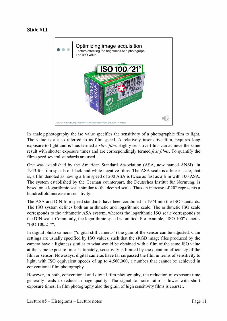
Optimizing image acquisitionFactors affecting the brightness of a photograph:The ISO value

Source: Wikipedia, https://commons.wikimedia.org/w/index.php?curid=37351557

In analog photography the iso value specifies the sensitivity of a photographic film to light. The value is a also referred to as film speed. A relatively insensitive film, requires long exposure to light and is thus termed a slow film. Highly sensitive films can achieve the same result with shorter exposure times and are correspondingly termed fast films. To quantify the film speed several standards are used.

One was established by the American Standard Association (ASA, now named ANSI) in 1943 for film speeds of black-and-white negative films. The ASA scale is a linear scale, that is, a film denoted as having a film speed of 200 ASA is twice as fast as a film with 100 ASA. The system established by the German counterpart, the Deutsches Institut für Normung, is based on a logarithmic scale similar to the decibel scale. Thus an increase of 20° represents a hundredfold increase in sensitivity.

The ASA and DIN film speed standards have been combined in 1974 into the ISO standards. The ISO system defines both an arithmetic and logarithmic scale. The arithmetic ISO scale corresponds to the arithmetic ASA system, whereas the logarithmic ISO scale corresponds to the DIN scale. Commonly, the logarithmic speed is omitted. For example, "ISO 100" denotes "ISO 100/21°“.

In digital photo cameras ("digital still cameras") the gain of the sensor can be adjusted. Gain settings are usually specified by ISO values, such that the sRGB image files produced by the camera have a lightness similar to what would be obtained with a film of the same ISO value at the same exposure time. Ultimately, sensitivity is limited by the quantum efficiency of the film or sensor. Nowasays, digital cameras have far surpassed the film in terms of sensitivity to light, with ISO equivalent speeds of up to 4,560,000, a number that cannot be achieved in conventional film photography.

However, in both, conventional and digital film photography, the reduction of exposure time generally leads to reduced image quality. The signal to noise ratio is lower with short exposure times. In film photography also the grain of high sensitivity films is coarser.


Slide #12

Optimizing image acquisitionFactors affecting the brightness of a photograph:The aperture size

Source: Wikipedia, https://commons.wikimedia.org/w/index.php?curid=78136658

The aperture stop of a photographic lens can be adjusted to control the amount of light reaching the film or image sensor. Typically, a smaller aperture will require longer exposure times to ensure sufficient light exposure. Vice versa, shorter exposure times will require a larger aperture.

Since the aperture and the focal length determine the cone angle of a bundle of rays that come to focus in the image plane, the lens aperture is usually specified as a f-number. The f-number is defined as the ratio of focal length to the effective aperture diameter.

A lens typically has a set of marked "f-stops" that the f-number can be set to. A lower f-number denotes a greater aperture opening which allows more light to reach the film or image sensor. The photography term "one f-stop" refers to a factor of √2 change in f-number, which in turn corresponds to a factor of 2 change in light intensity. Typical ranges of apertures used in photography are about f/2.8–f/22 covering six stops.

Reducing the aperture size also increases the depth of field. The depth of field describes the extent to which an object being closer or farther from the actual plane of focus appears to be in focus. In general, the smaller the aperture (the larger the f-number), the greater the depth of field. This is illustrated by the following slides.


Slide #13

Optimizing image acquisitionEffect of the aperture: F = 1/4

Here, the focus of the camera is on the plush toy in the foreground. With the aperture wide open, the titles of the books in the background cannot be read although the distance between the toy and the library is just about 20 cm. In the following images the aperture was closed to the next f-stop, and the exposure time was doubled to keep the amount of light collected by the image sensor constant.

As we close the aperture step by step, you will see that the depth of focus gradually increases.


Slide #14-15

Optimizing image acquisitionEffect of the aperture: F = 1/5.6



Slide #16-17




Slide #18

Optimizing image acquisitionFactors affecting the brightness of photographs

Factors affecting the brightness of photographs:• Exposure time• ISO value• Aperture size• Illumination intensity

As consequence, when getting a picture a photographer has several options to ensure that the entire dynamic range of an image is exploited.

The easiest way would be to delegate the task of finding a good compromise between all the parameters to the camera. When the user choses the “automatic” mode the camera tries to optimize exposure time, ISO-value and aperture size.

The manual mode, however, opens better possibilities to adapt the parameters to the scene. When objects in a scene are moving, then the exposure time must be kept short to prevent that moving objects are blurred. In this case, the photographer might open the aperture to collect as much light as possible. Also, the gain (ISO value) will be adjusted such that the entire bit range is exploited. In cameras this mode is called time-priority or time-value (TV) mode.

When objects in a scene are not moving, a good idea is to choose the aperture first, so that the desired depth of field can be chosen. Then only exposure time and gain must be set. In cameras this mode is called aperture priority or aperture-value (AV) mode. With the aperture set, it would be, in principle, desirable to choose a long exposure time and a low gain to get a better the signal-to-noise ratio. But, also in this case there are limits. Camera shakes occurring during long exposure times might blur the image, especially when no tripod is used.


Slide #19

19

Optimizing image acquisitionHistograms of microscopy images

In principle similar rules apply when microscopic images are concerned that just aim at showing structural details. However, when we want to retrieve quantitative information from an image, we must pay attention that gray scale values do not exceed the dynamic range.

Pixels having intensities that match the highest possible value of the bit range, which is 255 in case of 8-bit images or 65535 in case of 16-bit images will have to be excluded from the analysis. If a pixel has this value, there is no possibility to find out, if a measurement yielded exactly this or a higher value, because values exceeding the bit-range would have been clipped.


Slide #20

Optimizing image acquisitionFactors affecting the brightness of microscopy images

Factors affecting the intensity of an epifluorescence micrograph:• Illumination intensity• Acquisition time• Gain of the camera• Digital gain

Factors affecting the intensity of a confocal laser scanning micrograph• Illumination intensity, i.e. laser intensity• Pixel dwell time, i.e. scan speed • Photomultiplier gain• Digital gain

When it comes to optimizing the intensity of an image obtained in an epifluorescence microscope, illumination intensity, acquisition time and gain of the camera can be adjusted. In principle, the ideal microscope setup would be sensitive enough to acquire superior images from weakly fluorescent specimens, while simultaneously being fast enough to record all dynamic processes. In addition, the system would have sufficient resolution to capture the finest specimen detail. Unfortunately, optimizing one of these criteria is only accomplished at the expense of the others.

The relatively high light intensities and long exposure times that are typically employed in recording images of fixed cells and tissues must be strictly avoided when working with living cells. In virtually all cases, live-cell microscopy represents a compromise between achieving the best possible image quality and preserving the health of the cells.

The same applies for measurements on the stage of a laser scanning microscope. Also here a good compromise has to be found between the laser intensity used to excite the sample, the exposure time of a pixel, which in this case is determined by the scan speed and the gain of the photomultiplier. Details about how to adjust these parameters will be discussed in the course of Biological Microscopy (Module S3.1) in the next semester.


Slide #21

21

Intensity transformationsDefinition

General form of intensity transformation functions:

, ,

where , is the input image,, is the output image,

is an operator on f defined over a specified neighborhood of point ,

Special form of intensity transformation for histogram operations:

where denotes the intensity in point (x,y) of the input image,denotes the intensity in the same point (x,y) of the output image,is an operator on f acting only on point ,

So much for optimizing image acquisition. Now let’s discuss, how we can optimize acquired images for display.

Here, the emphasis is indeed on display. In science we should always leave the data we get out of an experiment untouched.

This means that we keep the original dataset for a quantitative analysis, while all manipulations, which we discuss in the following, are done on a copy of the dataset. Another way to optimize the display is to use colormaps (see Lecture #4)

To optimize grey level values for display we have to use so-called intensity transformation functions. In general, intensity transfer functions transform intensities of an input image (in this equation f) to an output image (in this equation g). The operator T acts on the neighborhood of a pixel, but can also operate on a set of images.

For histogram operations, however, we only need the simplest form in which the value of one pixel is mapped to a new value. Here, the output at one point depends only on the intensity at the same point.


Slide #22

22

Intensity transformationsDefinition

Intensity transformation for histogram operations:

where denotes the intensity in

point (x,y) of the input image,denotes the intensity in the same point (x,y) of the output image,is an operator on f acting only on point ,

Fig. from: Gonzales, Woods, Eddins, Digital Image Processing using MATLAB, 2nd ed, Gatesmark (2009), p.85.

This graph shows, how it works:

On the x-axis we have the grey-level values of the image we want to process. In case of an image of the class uint8 it will be a grey level value between 0 and 255. This number is now passed through this look-up table to produce another number between 0 and 255, which drives the output display. This means, stored grey level values are transferred into displayed brightness.

Here, we will use intensity transformations to improve the appearance of images. But in the same way, the output of the hardware is controlled. One example is the gamma correction curve of monitors. We will discuss these curves later. But now let’s focus on image enhancement and let’s see what we can achieve by adjusting brightness and contrast of an image.


Slide #23

23

Adjusting brightness & contrastIncreasing the brightness

+75 +75

What do brightness and contrast mean? Let’s to this aim start with one of the images we discussed already. This image was very dark and accordingly the histogram was concentrated on the left part at lower grey level values. Increasing the “brightness” means to increase the grey level values. Thus, all what we need to do is just to add some offset to each pixel. In this example I added 75 twice.

The images appear brighter. Adding 75 improved the image a little bit. However, adding twice 75 makes the image too bright. All images lack contrast, especially the one generated by adding 150.

After adding 75 once the histogram preserves its shape and is just shifted towards higher values. When 75 is added a second time, grey level values of some pixels exceed the bit range and are clipped to 255. This is why the peak at 255 is so high. It now comprises all pixels that had values between 105 and 255 of the original image.

Camera settings: F8.0, 1/50, ISO400


Slide #24

24

Adjusting brightness & contrastIncreasing the contrast (= gain)

x1.5 x1.5

Contrast is the difference in brightness that makes an object distinguishable from its surroundings. To increase the contrast between pixels, all what we need to do is to multiply the gray level values of all pixels by some factor. Multiplying the gray level values stretches the histogram. The resulting image becomes brighter and has more contrast.

If we chose 1.5 like in this example, gray level values do not exceed the bitrange. Multiplication with higher values has the consequence that some values are clipped although the contrast in important parts of the image is improved. Although the last image looks better than the second one, it has less information.



Slide #25

25

Adjusting brightness & contrastContrast stretching

,, ,

, ,,

where gray level value in the original image f

, , , range of interestmapped gray level value in the transformed image g

, , , range to which the intensities are mapped

General scaling transformation to map gray level values of the original image f to the transformed image g:

ImgOut = imadjust(ImgIn,[lowIn,highIn],[lowOut,highOut])

In MATLAB contrast stretching can be achieved with imadjust:

What we have done manually by toying around with some arbitrarily chosen values for brightness and contrast, is something we can also calculate. This technique is also called contrast stretching.

For example, if If,min and If,max define the intensity range of interest, a scaling transformation can be introduced to map the image intensity If of the input image f to the output image g with the range of I g,min to I g,max. This mapping is a liner stretch. Before stretching some offset value can be subtracted from the original values. This can be background or a range where no relevant objects occur. After stretching a new offset can be added, to increase the overall brightness.

If If,min is set to the lowest and If,max to the highest value in the original image, then some outliers might restrict the scaling range unnecessarily. Therefore, a good idea is to set the limit such that a given percentage of pixel values is saturated at black (= 0) and white (= 255) values.

In MATLAB contrast stretching can be done via implementing this equation or by using the function imadjust.


Slide #26

26

Adjusting brightness & contrastContrast stretching

contraststretching

This slide shows the result for the contrast stretching operation applied to our test image. Here, the lowest and highest input value have been chosen such that in the transformed image ~5% of the pixels are saturated at zero and ~5% of the pixels are saturated at 255.



Slide #27

27

Adjusting brightness & contrastPower law (gamma) transformations

, ,,

, ,,

where gray level value in the original image f

, , , range of interestmapped gray level value in the transformed image g

, , , range to which the intensities are mapped adjustable exponential factor (> 0)

General scaling transformation to map gray level values of the original image f to the transformed image g:

Instead of using a linear factor for mapping input values to output values the input value can be raised to the power gamma. The effect is shown in the next slide.


Slide #28

28

Adjusting brightness & contrastPower law (gamma) transformations

In MATLAB also power law transformations can be done with imadjust:

ImgOut = imadjust(ImgIn,[lowIn,highIn],[lowOut,highOut],gamma)

gamma specifies the shape of the curve that maps the intensity values :

gamma specifies the shape of the curve that maps the intensity values of the input image to the output image:

If gamma is one, mapping is linear as we discussed it before. If gamma is less than 1, the mapping is weighted toward higher (brighter) output values as

compared to the linear case. The resulting image appears brighter. If gamma is greater than 1, the mapping is weighted toward lower (darker) output values as

compared to the linear case. The resulting image appears darker.

The MATLAB function imadjust also allows to do power law transformations. gamma can be specified as additional parameter.


Slide #29

29

HistogramsContrast stretching in MATLAB

Syntax Description

ImgOut = imadjust(ImgIn) Maps the intensity values in the input image ImgIn to new values in the output ImgOut. By default, imadjust saturates the bottom 1% and the top 1% of all pixel values.

ImgOut = imadjust(ImgIn, [lowIn,highIn], [lowOut,highOut])

Maps intensity values in ImgIn to new values in ImgOut such that values between lowIn and highIn map to values between lowOut and highOut. Values below lowIn and above highIn are clipped. This means, values below lowInmap to lowOut, and those above highIn map to highOut.Note: All limits are specified as values between 0 and 1 , independently of the class of ImgIn.

ImgOut = imadjust(ImgIn, [lowIn,highIn], [lowOut,highOut],gamma)

Maps intensity values in ImgIn to new values in ImgOut, where gamma specifies the shape of the curve describing the relationship between the values in ImgIn and ImgOut.

LowHigh= stretchlim(Img,Tol)

Computes the lower and upper limits that can be used for contrast stretching. Tol specifies the percentage of pixels that are allowed to saturate at the bottom and at the top. The default is 1%. Limits are returned in LowHigh.


This slide summarizes what we have discussed before. ImgOut = Imadjust(ImgIn) maps the intensity values in the input image ImgIn to

new values in the output image ImgOut. By default, imadjust saturates the bottom 1% and the top 1% of all pixel values. This operation increases the contrast of the output image and is a good tool to have a quick view at an contrast enhanced image.

ImgOut = imadjust(Img[lowIn,highIn],[lowOut,highOut]) maps values of the input range to the output range. Values below lowIn and above highIn are clipped. This means, values below lowIn map to lowOut, and those above highIn map to highOut. Note: All limits are specified as values between 0 and 1 , independently of the class of ImgIn. If, for example, ImgIn is of class uint8, imadjust multiplies the values supplied by 255 to determine the actual values to use. Using the empty matrix ([ ]) for the input range [lowIn highIn] or for the output range [lowOut highOut] results in the default values [0 1] . If highOut is less than lowOut, the output intensity is reversed.

imadjust can accept an additional argument that specifies the gamma correction factor. gamma specifies the shape of the curve that maps the intensity values in ImgIn to create ImgOut. If gamma is less than 1, the mapping is weighted toward higher (brighter) output values. If gamma is greater than 1, the mapping is weighted toward lower (darker) output values. If it is omitted from the function argument, gamma defaults to 1 (linear mapping).

stretchlim (Img,Tol) computes the lower and upper limits that can be used for contrast stretching. Tol specifies the percentage of pixels that are allowed to saturate at the bottom and at the top. The default is 1%. Limits are returned in LowHigh.


Slide #30

30

Adjusting brightness & contrastThe test image

Fig. from: Smith, The Scientist and Engineer's Guide to Digital Signal Processing, California Technical Publishing (1997), p.389

By adjusting brightness and contrast we can also highlight details of an image.

To demonstrate this we have to create a good test image, like the one shown on this slide.

The background of the test image is filled with random noise, uniformly distributed between 0 (= black) and 255 (= white). The slide contains three square boxes having pixel values of 75, 150 and 225. Each square contains two triangles with pixel values only slightly different from their surrounding squares. The contrast is so low that the triangles can hardly be distinguished from the surroundings squares.

In brief, our test object has dark, medium and bright objects with low contrast details. Let us now try to better emphasize these differences by adjusting brightness and contrast.


Slide #31

31

Adjusting brightness & contrastAdjusting the brightness (= offset)


= 0

= 1

= 1

= 1

= -100

= +100

Output = (Input + B) x C

A) In the first example brightness and contrast are set at the normal level, as indicated by the B and C slide bars at the left side of the image. This means brightness (i.e. the offset) is at 0 and contrast (i.e. gain) is 1. Under these conditions the intensity transform function does nothing. Output values for display equal the input values.

B/C) The second and third example show the effect of changing the brightness. Increasing the brightness shifts the intensity transform function to the left, while decreasing the brightness shifts it to the right.

Increasing the brightness makes every pixel in the image appear brighter. Conversely, decreasing the brightness makes every pixel in the image appear darker.

These changes can improve the visibility of excessively dark or light areas in the image, but will saturate the image if taken too far. For example, all of the pixels in the right square of the second example are saturated at 255 and displayed with full intensity. The opposite effect is shown in the third case, where all of the pixels in the left square have the intensity 0 and are displayed as black. Since all the pixels in these regions have the same value, the triangles are completely wiped out.

Note also that none of the triangles in the second and third case are easier to see than in the original image. Changing the brightness provides little (if any) help in distinguishing low contrast objects from their surroundings.


Slide #32

32

Adjusting brightness & contrastAdjusting the contrast (= slope)



= 4

= -46

= 16

= -142

D) Figure d shows the display optimized to view pixel values around the gray scale value 75. This is done by turning up the contrast, resulting in increasing the slope of the intensity transform function (from 1 to 4). For example, the stored pixel values of 71 and 75 become 100 and 116 in the display, making the contrast a factor of four greater. The price for this increased contrast is that only pixel values between 46 and 109 are within the bit range for display. Pixel values from 0 to 45 are saturated at black, and pixel values 110 to 255 are saturated at white. The increased contrast allows the triangles in the left square to be seen, at the cost of saturating the middle and right squares.

E) Figure e takes the effect of increasing the contrast even further, resulting in only 16 of the possible 256 stored levels being displayed as nonsaturated. The brightness was also decreased so that the 16 usable levels are centered around 150. The details in the center square are now very visible. However, almost everything else in the image is saturated. For example, look at the noise in the background. There are very few pixels with an intermediate gray shade; almost every pixel is either pure black or pure white.

This technique of using high contrast to view only a few gray levels is sometimes called a grayscale stretch. The contrast adjustment is a way of zooming in on a smaller range of pixel values. The brightness control centers the zoomed section on the pixel values of interest.

Most digital imaging systems allow the brightness and contrast to be adjusted in just this manner and often provide a graphical display of the output transform. In contrast to this, the brightness and contrast controls on television and video monitors are analog circuits and may operate differently. For example, the contrast control of a monitor may adjust the gain of the analog signal, while the brightness control might add or subtract a DC offset. Programs that mimic this behavior multiply input value and contrast first and then add the offset.


The moral is, don't be surprised if different image viewer programs work differently and do not respond in the way you think they should.

Slide #33

34

Adjusting brightness & contrastAdjusting the contrast (= slope)



= 4

= -46

= 16

= -142

F) The last image is different from the rest. Rather than having a slope in the curve over one range of input values, it has a slope in two ranges. This allows the display to simultaneously show the triangles in both the left and the right square. Of course, this results in saturation of the pixel values that are not near these gray scale levels. Notice that the slide bars for contrast and brightness are not shown in this figure. This display is beyond what brightness and contrast adjustments can provide.

Taking this approach further results in a powerful technique for improving the appearance of images: the histogram equalization. The idea is to increase the contrast at pixel values of interest, at the expense of the pixel values we do not care about. The more relevant the value, the greater its contrast is made in the displayed image. Here, relevance is determined by the frequency of the respective gray scale values.


Slide #34

35

Histogram equalizationOverview

This slide gives us an overview about how histogram equalization works. Let’s start with the original underexposed image, which we obtained at the beginning of this lecture. From this image we can get the histogram in which pixel frequencies are concentrated at the left side at low gray-level values. Starting with a gray-level value of 0 the task is now to calculate the value of the next gray level, taking into account that the increase to the next level is weighted by the number of pixels having this intensity.

To this aim we need to normalize the histogram, so that the total area is 1.

Then each bar corresponds to the relative increase in gray levels on a gray scale ranging from 0 to 255. Thus, by multiplying the relative frequency with 255 we get the absolute increase in gray levels the respective pixels should have in the new image.

If we carry out this procedure step by step we end up with this contrast enhanced picture which looks amazingly good.

But, let’s do this step by step for the first gray level values.



Slide #35

36

Histogram equalizationStep by step

0.1

1.6

6.8

9.7

8.07.3

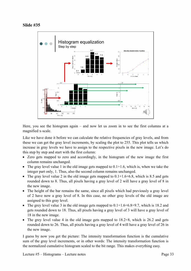
Here, you see the histogram again – and now let us zoom in to see the first columns at a magnified x-scale.

Like we have done it before we can calculate the relative frequencies of gray levels, and from these we can get the gray level increments, by scaling the plot to 255. This plot tells us which increase in gray levels we have to assign to the respective pixels in the new image. Let’s do this step by step and start with the first column: Zero gets mapped to zero and accordingly, in the histogram of the new image the first

column remains unchanged. The gray level value 1 in the old image gets mapped to 0.1+1.6, which is, when we take the

integer part only, 1. Thus, also the second column remains unchanged. The gray level value 2 in the old image gets mapped to 0.1+1.6+6.8, which is 8.5 and gets

rounded down to 8. Thus, all pixels having a gray level of 2 will have a gray level of 8 in the new image.

The height of the bar remains the same, since all pixels which had previously a gray level of 2 have now a gray level of 8. In this case, no other gray levels of the old image are assigned to this gray level.

The grey level value 3 in the old image gets mapped to 0.1+1.6+6.8+9.7, which is 18.2 and gets rounded down to 18. Thus, all pixels having a gray level of 3 will have a gray level of 18 in the new image.

The grey level value 4 in the old image gets mapped to 18.2+8, which is 26.2 and gets rounded down to 26. Thus, all pixels having a gray level of 4 will have a gray level of 26 in the new image.

I guess by now you get the picture: The intensity transformation function is the cumulative sum of the gray level increments, or in other words: The intensity transformation function is the normalized cumulative histogram scaled to the bit range. This makes everything easy.


Slide #36

37


histogramequalization

All what we have to do, is to calculate the cumulative histogram and scale it to the bit range. This yields the intensity transform function for histogram equalization. When we now use this look up table, we get the contrast enhanced picture. The improvement is evident.

Histogram equalization modifies the values of pixels so that the number of pixels at each gray level will be approximately the same. This is probably not so evident from this histogram, since we have at low gray levels high peaks interspaced with gray levels which are zero, since no gray level value of the old picture was mapped to them.

But when we average pixel frequencies intensities, …



Slide #37

38



… or just take a bigger bin size, we see that on average the number of pixels at each gray level will be approximately the same in the histogram of the new image. This is why this process is called histogram equalization.

Generally this operation tends to enhance the image contrast and improves the appearance. Since it can be performed without any input, it is a good mechanism for automatic image enhancement.

Let’s explore the effect of this algorithm further on all of the pictures we got previously.



Slide #38

39



The second picture we got had already a good quality. The image had good contrast and the histogram was well spread over the entire bit range.

Here, the algorithm can do little to better equalize the histogram. Accordingly, input values are mapped to approximately the same output values – and the resulting image and its histogram look very similar to the originals.

Camaera settings (Image B) F8.0, 1/8 s, ISO400


Slide #39

40



Now, let’s have a look at the last image we got. This image was overexposed. Many pixels are saturated at white. Accordingly, a peak at 255 dominates the gray level histogram.

Histogram equalization can only improve the histogram at non saturating gray levels - and accordingly the overall image quality can only be marginally improved.

Camera settings (Image C): F8.0, 1/4 s, ISO400


Slide #40

Histogram equalizationComparison of the results

t = 20 ms t = 250 mst = 125 ms

This slide summarizes the results. Here, you see in the upper row all images we obtained previously.

The lower row shows the result of the histogram equalization. All images look astonishingly good. If we look at some details, however, we will find out that some pixels are still overexposed. Thus, when taking a photograph it is a good idea to underexpose the photo a little bit, since we can later improve its appearance.

Intensity information gets lost when pixel saturate. In photographs this might not matter too much. But, saturation is something we should avoid in any case for a measurement. If pixels have the maximum value of the bit range, we have no way to tell, if exactly this value was measured, or if a value exceeded the bit range and was clipped to the maximum of the bit range. If a measurement looks too dim at the first sight, this should not matter too much. By using the algorithms we discussed so far, we can easily improve its appearance.

Note, that all the algorithms we discussed, serve to improve the image display only. Brightness adjustment shifts the offset, so that the difference between different pixels remains the same. In offset corrected images enhancing the contrast does not affect the ratio of pixel intensities. Histogram equalization, however, redistributes gray scale levels. After histogram equalization, intensities cannot be put in relation to each other.

Camera settings: A) F8.0, 1/50, ISO400, B) F8.0, 1/8, ISO400, C) F8.0, 1/4, ISO400


Slide #42

42

Histogram equalization & matchingHistogram equalization & matching in MATLAB

Syntax Description

ImgOut = histeq(ImgIn) transforms the grayscale image ImgIn to a grayscale image with ImgOut with the same number of discrete gray levels. A roughly equal number of pixels is mapped to each of the levels in ImgOut, so that the histogram of ImgOut is approximately flat.

ImgOut = histeq(ImgIn,n) transforms the grayscale image ImgIn to a grayscale image with ImgOut with n discrete gray levels. A roughly equal number of pixels is mapped to each of the levels in ImgOut, so that the histogram of ImgOut is approximately flat. The histogram of ImgOut is flatter when n is much smaller than the number of discrete levels in ImgIn

ImgOut= histeq(ImgIn,HistIn)

transforms the grayscale image ImgIn so that the histogram of the output grayscale image ImgOut matches approximately the target histogram HistIn.

[ImgOut,T] = histeq(ImgIn) returns the transformation function T that maps gray levels in the image ImgIn to gray levels in ImgOut.


In MATLAB histeq can be used to enhance the contrast using histogram equalization

If no other parameter except for the input image is specified, the output image has the same number of gray levels like the input image. The number of desired gray levels can be specified as additional parameter. In both cases gray levels are assigned such, that a roughly equal number of pixels is mapped to each of the levels.

histeq can also used for histogram matching. In this case the histogram, which should serve as a template, has to be passed to the function.

If desired, the intensity transfer function used for histogram equalization can be transferred back together with the contrast enhanced image.

image processing ii

Documents