fractal based image and video processing
TRANSCRIPT

1
Dott. Ing. Giulio Soro
Fractal based image and video processing
PhD. Thesis
UNIVERSITÀ DEGLI STUDI DI CAGLIARI FACOLTÀ DI INGEGNERIA
DIPARTIMENTO DI INGEGNERIA ELETTRICA ED ELETTRONICA
M ULTIMEDIA AND COMMUNICATION LABS

2

3
Contents
CONTENTS................................................................................................................................................................. 3
ACKNOWLEDGMENT ............................................................................................................................................ 5
FOREWORD............................................................................................................................................................... 6
INTRODUCTION....................................................................................................................................................... 7
CHAPTER I ................................................................................................................................................................ 9
I.1 ZOOMING TECNIQUES.................................................................................................................................. 9
I.2 SLOW MOTION TECNIQUES......................................................................................................................... 10
CHAPTER II ............................................................................................................................................................. 17
FRACTALS............................................................................................................................................................... 17
II.1 INTRODUCTION.......................................................................................................................................... 17
II.2 FRACTAL CODING ...................................................................................................................................... 20
II.3 ITERATED FUNCTION SYSTEMS FOR IMAGE ENCODING ............................................................................. 26
II.4 DECODING STAGE...................................................................................................................................... 29
II.5 FRACTAL ZOOM ......................................................................................................................................... 32
II.6 STATE OF THE ART FOR FRACTAL ZOOMING............................................................................................... 34
CHAPTER III ........................................................................................................................................................... 38
FRACTALS AND VIDEO SEQUENCES .............................................................................................................. 38
III.1 INTRODUCTION.......................................................................................................................................... 38
III.2 FRACTAL CODING OF VIDEO SIGNALS........................................................................................................ 40
III.3 SLOW MOTION WITH FRACTAL EXPANSION................................................................................................ 44
III.4 PERFORMANCE ANALYSIS AND COMPARISON........................................................................................... 57
CHAPTER IV............................................................................................................................................................ 63
FRACTALS AND COLOR IMAGE COMPRESSION ........................................................................................ 63
IV.1 INTRODUCTION.......................................................................................................................................... 63
IV.2 THE CIELAB COLOR SPACE....................................................................................................................... 65

4
IV.3 CLUSTERING.............................................................................................................................................. 70
IV.4 CLUSTERING PROCESS APPLIED TO FRACTAL ENCODING............................................................................ 73
IV.5 EARTH MOVER’S DISTANCE FOR IFS.......................................................................................................... 77
IV.6 EXPERIMENTAL RESULTS.......................................................................................................................... 81
CHAPTER V ............................................................................................................................................................. 84
CONCLUSIONS ....................................................................................................................................................... 84
APPENDIX A............................................................................................................................................................ 86
ALGORITMS FOR FRACTAL ENCODING ....................................................................................................... 86
INTRODUCTION....................................................................................................................................................... 86
BIDIMENSIONAL FRACTAL ENCODE......................................................................................................................... 87
BIDIMENSIONAL FRACTAL DECODER...................................................................................................................... 92
THREE-DIMENSIONAL FRACTAL CODEC................................................................................................................ 96
BIBLIOGRAPHY..................................................................................................................................................... 97

5
Acknowledgment
To Prof. D.D. Giusto and Dr. M. Murroni without
whom this work could not have been made, and to
all of my family and friends who supported me along
this part of life.
6
Foreword
This work is based on fractals. Since Barnsely demonstrated how to use these strange non-
linear functions to encode images and Jaquin developed an automated fractal image compression
algorithm, in just 14 years over 600 papers have appeared. This huge amount of study is due to
the immense world of possibilities fractals give to researchers.
Fractals founded place in several fields of study, not only compression of images or video
sequences or mathematics: economics, biology, geology, socials, and even politics.
The studies presented here, which derive from three years of research in this area, try to
focus on the extremely promising property of implicit interpolation fractals gave us.
Since images, or more in general signals, are managed with the powerful concept of function
instead of a collection of pixels, we can easily obtain interpolation between nodes of these
functions.
This assumption leads to discover some amazing advantages that fractal encoding has
compared to classical interpolation techniques.
7
Introduction
This work is divided in four chapters. The first chapter introduces the classical tecniques used to
interpolate pictures, videos or signals in general. The problems of these interpolators are studied and
confronted each other. The analisys of quality loss and errors introduced using the classical
approach are the motivation that pushed us to work on the field of fractal to improve the
interpolation quality.
Each of the following chapter focus on an aspect of fractal encoding and try to prove the
improvement made using that tecnique.
The chapter two introduces the fractal theory and the use of fractals for encoding and decoding
image. The decoding stage is extremely important because is at this stage that the actual zoom or
interpolation is performed.
Since the image is decomposed at encoding time into a set of mathematical functions and
correlations, at decoding time the interpolation is a mere multiplication by a scalar factor, i.e. a
really simple step.
The simplicity of this step actually leads to a lot of quality loss. In fact using just standard fractal
zoom leads to artifacts, blurring and a lot of other errors that masks the potentiality of the zoom.
To override these problems some we improved some existing tecniques and theories and our
work was repaid by a great quality enhancement.
Third chapter analizes the key problem of this work, which is the interpolation using fractals of
video sequences.
Since video sequences usually are huge amount of data, the analisys of video streams takes, even
with fast machines, hours of working and are extremely complex.
To decrease the complexity while preserving quality we developed a framework for encode
videos based on a combination of tecniques such wavelet decomposition, motion detection and

8
overlapping fractal encoding, prior to the interpolation phase, and then all the necessary operations
needed to recombine the stream(s) during the final zoom.
The last chapter introduces our recent study about metrics and a new way to use a non-standard
metric, known as EMD, to increase the quality of fractal encoding of color images.
Further study will be made on this last tecnique to test the validity of such interesting metric on
the video fractal encoding.
9
Chapter I
I.1 Zooming tecniques
Currently, oversampling is often needed in several fields. In aerial or satellite imaging zoom is
used in order to facilitate the image interpretation, or just to obtain a more comfortable visualization
environment,
Available software realizes zooms using often some classical interpolators, which we briefly
describe here.
These interpolators are particular oversamplers. An interpolator (or interpolation function) is a
function which is equal to another function for some given points (interpolation nodes) [1]. That is
the main differences between fractal oversamplers, described in the following sections, which do
not necessarily keep the original luminance values. Each interpolator used in this work is a
polynomial function.
The simplest oversampling is the Nearest-Neighbor Interpolation (N.N.I.). It consists in
duplicating the original pixel’s values. For example when zooming by a factor two, each original
pixel is duplicated four times. So the degree of the polynomial function of interpolation is zero.
In practice the most frequently used oversampling is the Linear Interpolation (L.I.). This
interpolator is based on a local hypothesis of luminance signal continuity and cylates by averaging
[1] a value at a subpixel position.
The last interpolator we used as a reference is a modified version of the cubic one, the Cubic
Convolution Interpolation (C.C.I) [3].
10
Nearest neighbor, linear and cubic convolution interpolators, which are approximation of the
firs, second and third orders respectively, are based on local continuity hypothesis of the luminance
signal and use a set of pixels located in a neighborhood (of resp. 1,4 and 16 pixels) around the
position to be interpolated.
I.2 Slow motion tecniques
Among all possible interactive applications, widely used in classic analogic video reproduction,
slow motion replay is one of the most expected to be extended to the digital formats.
Slow motion is a commercial feature of home video players, but also, a special effect used in the
video production field. Its aim is usually to represent a slower replica of a fast sequence, making
possible for the user to observe all the details of the scene which at regular speed could be lost.
In an analog framework, given a video sequence with a fixed frame ratef , the slow motion effect
is obtained reducing the frame rate to ff <' , so that a frame remains visible for a time proportional
to slow motion factor. This kind of slow motion, which does not involve any special technique, is
usually the method that analog video players, like VCR equipment for example, use.
At present commercial digital video players allow users to browse a video sequence frame by
frame or by chapter selection with prefixed indexes. Slow motion replay is classically achieved by
reducing the frame rate display, just like analog slow motion, or keeping the frame rate constant and
inserting within the sequence additional intermediate frames.
In a digital environment those frame can be generated by means of linear or cubic interpolation or
simply repeating copies of frames along the time.
Interpolation along frames derives from classical interpolation of pixels within an image, and can
be considered as oversampler. An interpolation (or an interpolating function) is a function which is
equal to another function in some particular points called interpolation nodes.
11
The simplest oversampling function is the Nearest Neighbour Interpolator (N.N.I). It consists in
duplicating the original pixels’ values. For example when zooming an image by a factor of 2
(zooming factor = 2X) each original pixel is duplicated four times.
The N.N.I. is the base for digital frame replica slow motion. Every single pixel is duplicated along
the time axis, of a factor equal to the desired slow motion factor.
One of the most frequently used interpolator in practice is the Linear Interpolator (L.I.). This
interpolator is based on a local hypothesis of luminance signal continuity and calculates, by
averaging, [2] a value at subpixel position. Another important interpolator, which we used as a
reference, is the Cubic Convolution Interpolation (C.C.I.)[3].
All of these interpolations, N.N.I, L.I. and C.C.I., are approximation of the first, second and third
orders respectively and are based on the concept of continuity of luminance signal of the pixels
located on the neighbourhood around the position to be interpolated.
Concerning the video domain, the concept of L.I. and C.C.I. can easily be extended considering
the values of pixel at the same position in adjacent frames as interpolating nodes.
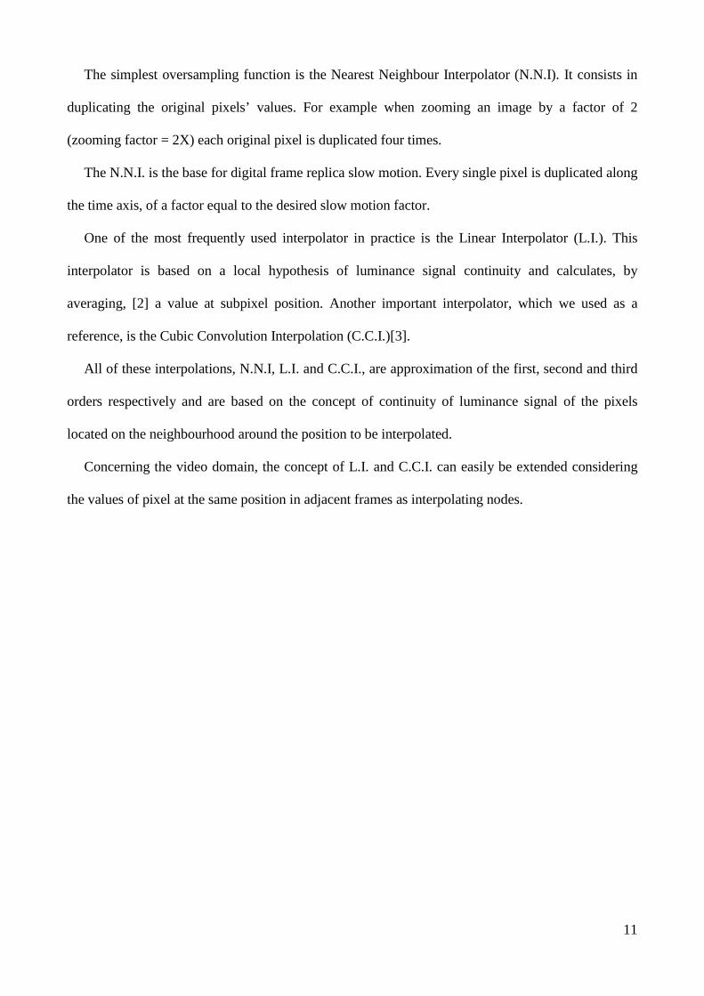
12
Fig. 1: Fading effect on interpolation
A major drawbacks of these approaches are that interpolation for slow motion replay yields to a
“fading” effect between frames, whereas frame replication creates a “jerky” distortion, both resulting
in low motion quality for the human visual system [26]. Similar issues arise in image plane if pixel
replication or interpolation is used to perform spatial zoom.
These factors decrease the visual quality of the slowed sequence and, especially the jerkiness is
considered by the Human Vision System (HVS) as an annoying distortion even for minor slow
motion factors.
Both the terms jerkiness and fading will be completely addressed later on this work when we will
introduce the quality metrics deployed by I.T.U [23] for the video quality assessment.
There are different kinds of interpolation that can be used for this purpose. In literature we found
examples of classical interpolators as linear, cubic functions or more sophisticated tecniques such as
splines or motion vector interpolation and motion compensation.
13
Some of those are used in this work as reference for quality measures, and could be found in the
quality assessment chapter.
An intuitive definition of jerkiness is given as the discontinuity along the temporal axis of objects
or group of pixels that move along the scene.
The Human Vision System (HVS) is particularly sensible to this kind of effects. This means that
the quality of a slowed sequence is deeply degraded if the overall jerkiness is not kept under control.
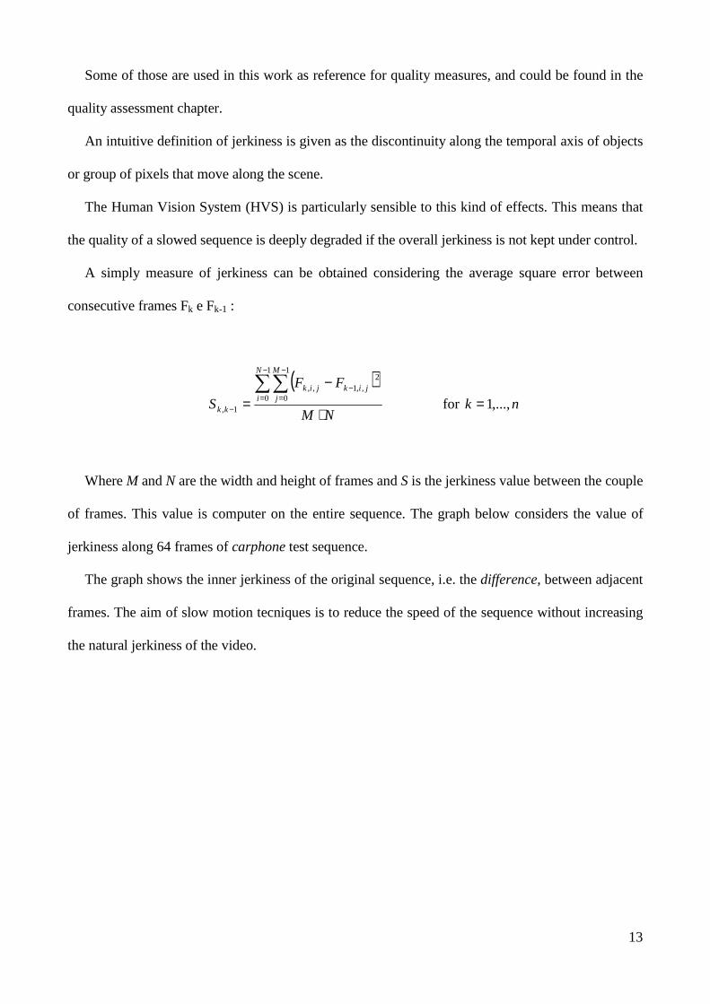
A simply measure of jerkiness can be obtained considering the average square error between
consecutive frames Fk e Fk-1 :
( )NM
FF
S
N
i
M
jjikjik
kk ⋅
−=∑∑
−
=
−
=−
−
1
0
1
0
2,,1,,
1, for nk ,...,1=
Where M and N are the width and height of frames and S is the jerkiness value between the couple
of frames. This value is computer on the entire sequence. The graph below considers the value of
jerkiness along 64 frames of carphone test sequence.
The graph shows the inner jerkiness of the original sequence, i.e. the difference, between adjacent
frames. The aim of slow motion tecniques is to reduce the speed of the sequence without increasing
the natural jerkiness of the video.
14
Jerkiness
0
20
40
60
80
100
120
140
1 4 7 10 13 16 19 22 25 28 31 34 37 40 43 46 49 52 55 58 61
frames
Jerk
ines
s
Fig. 2 Jerkiness values (RMS values) between frames of Carphone
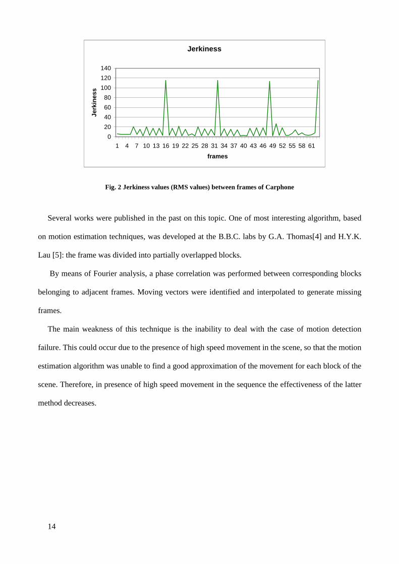
Several works were published in the past on this topic. One of most interesting algorithm, based
on motion estimation techniques, was developed at the B.B.C. labs by G.A. Thomas[4] and H.Y.K.
Lau [5]: the frame was divided into partially overlapped blocks.
By means of Fourier analysis, a phase correlation was performed between corresponding blocks
belonging to adjacent frames. Moving vectors were identified and interpolated to generate missing
frames.
The main weakness of this technique is the inability to deal with the case of motion detection
failure. This could occur due to the presence of high speed movement in the scene, so that the motion
estimation algorithm was unable to find a good approximation of the movement for each block of the
scene. Therefore, in presence of high speed movement in the sequence the effectiveness of the latter
method decreases.
15
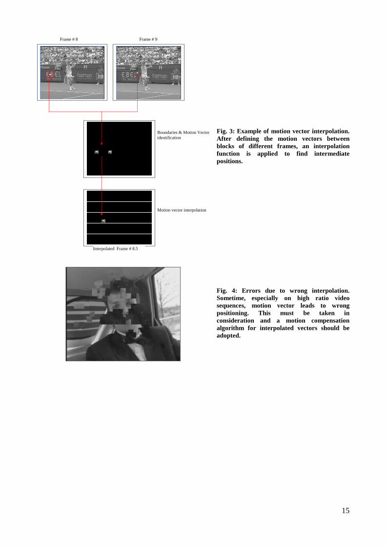
Frame # 8 Frame # 9
Boundaries & Motion Vectoridentification
Motion vector interpolation
Interpolated Frame # 8.5
Fig. 3: Example of motion vector interpolation. After defining the motion vectors between blocks of different frames, an interpolation function is applied to find intermediate positions.
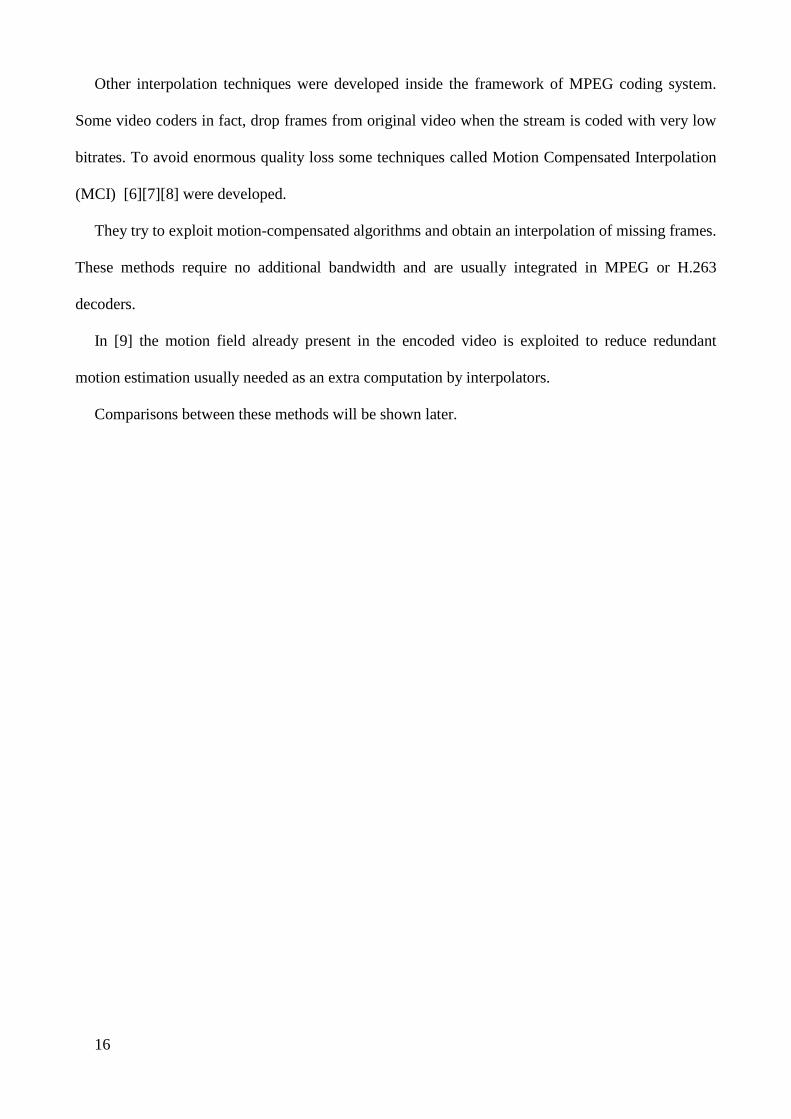
Fig. 4: Errors due to wrong interpolation. Sometime, especially on high ratio video sequences, motion vector leads to wrong positioning. This must be taken in consideration and a motion compensation algorithm for interpolated vectors should be adopted.
16
Other interpolation techniques were developed inside the framework of MPEG coding system.
Some video coders in fact, drop frames from original video when the stream is coded with very low
bitrates. To avoid enormous quality loss some techniques called Motion Compensated Interpolation
(MCI) [6][7][8] were developed.
They try to exploit motion-compensated algorithms and obtain an interpolation of missing frames.
These methods require no additional bandwidth and are usually integrated in MPEG or H.263
decoders.
In [9] the motion field already present in the encoded video is exploited to reduce redundant
motion estimation usually needed as an extra computation by interpolators.
Comparisons between these methods will be shown later.
17
Chapter II
Fractals
II.1 Introduction
The name fractal was invented by Mandelbrot [10] and derives from the latin word fractus,
which means broken in pieces.
In fact one of the most intuitive properties of this kind of objects is that can be thought as a lot of
similar parts that make the whole object. Also the name refers to the important mathematical quality
of this kind of functions: the dimension of fractals is not an integer value as the classical topological
dimension. Actually the dimension of a fractal should not be computed using original Euclidian
dimension TD but introducing a new concept of dimension called Hausdroff-Besicovitch dimension
[11].
Usually we think about fractals as complicated images and forms, perceiving them as static
objects. Besides the fact that usually fractal images are actually complicated images, this point of
view can hide the focal points of generations and evolution of fractal object, i.e. the dynamic
properties of fractals.
There are some different definitions of how an object can be considered a fractal or not.
These include the properties of self-similarity, fine resolution, dense objects and so on.
Among these, the one that mostly can describe the mathematical properties of fractal can be the
one that define a fractal by its dimension, based on the Hausdroff-Besicovitch definition.

18
In fact the mathematical definition of fractal that Mandelbrot introduces is of an object which its
Hausdroff-Besicovitch dimension FD is (not strictly) greater than its Euclidian dimension:
TF DD ≥
Instead, the most intuitive definition of fractal is of a figure, or better an object, composed by a
motif that repeats itself scaled or rotated at every resolution. This leads to a fractal as a dense and
fine function, as mentioned above.
Given that, a zoomed part of a fractal will always contain infinite points at every grade of
zooming factor. More, the position of this point is imposed by the motif pattern defined by the
equation that creates the fractal. This last point gives us the intuition on how important is the
evolution and the dynamic properties of a fractal.
The theory was defined mathematically by Mandelbrot in the XX century but the first step and
discoveries of these strange functions go back in time.
Classical pre-fractals (as they are called since the definition of fractal was not yet given) are the
ones invented by Cantor, Sierpinski and many others.
But the inner properties and use of fractals could be achieved only when the computational
power of computer appears.
Joined with the chaos theory, fractals could be then used to create models for many natural
events like clouds geometry, metereological events (Lorentz [12]), terrain and natural object’s
geometry, lighting distributions and so on.
In fact fractal geometry creates approximations of natural objects closer than approximations
created using the classical Euclidian geometry.

19
This will lead, as we will see later, to a better realism of zoomed images with fractals functions
compared to classical interpolators based on the Euclidian geometry.
Fractals also appeared to be a good mathematical framework for image and, as we will explain in
this work, video compression and processing exploiting the fact that those images have a lot of
inner redundancy.
A lot of works have been done to create image compressors like the famous JPEG and JPEG2K
as for video (MPEG1, MPEG2, MPEG4 and others..).
Fractal image compression born in the 80s of the XX century, mostly by studies leaded by
Barnsley [13], Jaquin [14] and Fisher[15].
As we will see on the following part of this work, a lot of properties besides compression can be
obtained using fractals for image and video coding instead of common techniques as the ones
mentioned above.
20
II.2 Fractal coding
Since fractals can be intended as collection of similar parts defined by a common motif (or
pattern) derived by some mathematical functions, the fractal encoding can be thought as the search
for this motif inside a natural image.
For being a fractal, an object F must satisfy some properties:
1. Self-similarity: F must be composed by copies of itself at different scale rate
2. Fine structure: F must have details at every resolution
3. Recursivity: the function Z from which F derives has to be recursively defined:
( )( )( ){ }...| fffZZF ==
4. Dimension: TF DD >
A classical example of how to create a fractal is by means of a simply algorithm that copies and
scales an initial image given as input. This algorithm, known as the Barnsley copy machine (or the
Multiple Reduction Copy Machine MRCM), takes an initial image 0µ and creates as output three
copies of it displaced on the vertexes of an equilateral triangle and reduced by a factor of13 .
After this step the output is taken as the new input for the algorithm and the process starts again.
If we call this functionτ ∆ , and ( )0τ µ∆ the result we obtain, the first step the output of the
algorithm leads to the image shown in Fig. 5.
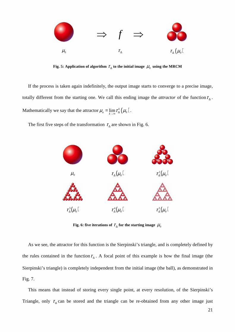
21
⇒⇒ f
0µ τ ∆ ( )0τ µ∆
Fig. 5: Application of algorithm τ ∆ to the initial image 0µ using the MRCM
If the process is taken again indefinitely, the output image starts to converge to a precise image,
totally different from the starting one. We call this ending image the attractor of the functionτ ∆ .
Mathematically we say that the attractor ( )0lim ka
kµ τ µ∆→∞
= .
The first five steps of the transformation τ ∆ are shown in Fig. 6.
0µ ( )0µτ ∆ ( )02 µτ ∆
( )03 µτ ∆ ( )0
4 µτ ∆ ( )05 µτ ∆
Fig. 6: five iterations of τ ∆ for the starting image 0µ
As we see, the attractor for this function is the Sierpinski’s triangle, and is completely defined by
the rules contained in the functionτ ∆ . A focal point of this example is how the final image (the
Sierpinski’s triangle) is completely independent from the initial image (the ball), as demonstrated in
Fig. 7.
This means that instead of storing every single point, at every resolution, of the Sierpinski’s
Triangle, only τ ∆ can be stored and the triangle can be re-obtained from any other image just
22
applying the τ ∆ to it. This last sentence gives some hints about the relation that can exist with
fractals and compression.
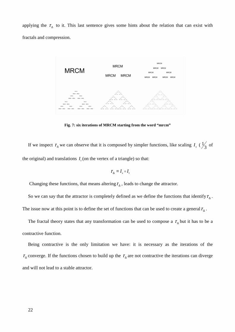
Fig. 7: six iterations of MRCM starting from the word “mrcm”
If we inspect τ ∆ we can observe that it is composed by simpler functions, like scaling sI ( 13 of
the original) and translations tI (on the vertex of a triangle) so that:
s tI Iτ ∆ = o
Changing these functions, that means alteringτ ∆ , leads to change the attractor.
So we can say that the attractor is completely defined as we define the functions that identifyτ ∆ .
The issue now at this point is to define the set of functions that can be used to create a generalτ ∆ .
The fractal theory states that any transformation can be used to compose a τ ∆ but it has to be a
contractive function.
Being contractive is the only limitation we have: it is necessary as the iterations of the
τ ∆ converge. If the functions chosen to build up the τ ∆ are not contractive the iterations can diverge
and will not lead to a stable attractor.
23
Mathematically a transformation τ is said to be contractive if, given a distance metric d
and 10: ≤≤ℜ∈ ss , we prove that:
( ) ( )( ) ( ) Cbabadsbad ∈∀⋅≤ , ;,,ττ
With C being the space of points we consider.
Back to the example shown above, the contractivity s is assured by the scaling factor 13 of sI (can
be proved that the contractivity of a translation tI is 1s = ).
The number of functions that respect the property defined is huge, so for our purposes we can
limit our functions to a class, called affine transforms, that is enough for create a sufficient sets of
attractors.
An affine transform is a bijective transform that maps a point ( )1 2, ,..., n nP x x x ∈ℜ onto a point
( )'1 2, ,..., n nP y y y ∈ℜ so that Y AX B= + with , nA B ∈ℜ and det( ) 0A ≠ .
Usually in literature the class of affine functions used to build up fractals, for image compression
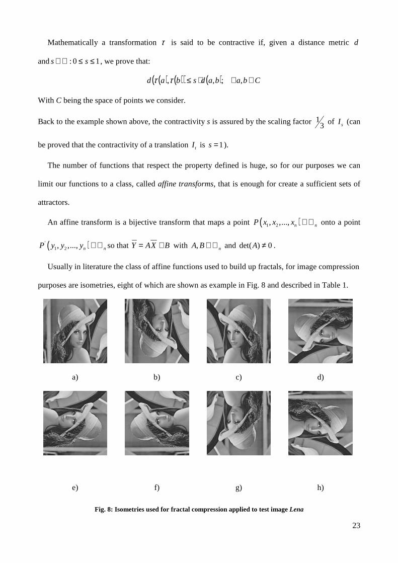
purposes are isometries, eight of which are shown as example in Fig. 8 and described in Table 1.
a) b) c) d)
e) f) g) h)
Fig. 8: Isometries used for fractal compression applied to test image Lena
24
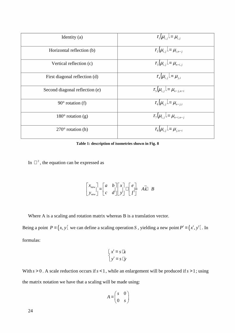
Identity (a) ( ) jiji ,,1 µµτ =
Horizontal reflection (b) ( ) jniji −= ,,2 µµτ
Vertical reflection (c) ( ) jinji ,,3 −= µµτ
First diagonal reflection (d) ( ) ijji ,,4 µµτ =
Second diagonal reflection (e) ( ) injnji −−= ,,5 µµτ
90° rotation (f) ( ) ijnji ,,6 −= µµτ
180° rotation (g) ( ) jninji −−= ,,7 µµτ
270° rotation (h) ( ) injji −= ,,8 µµτ
Table 1: description of isometries shown in Fig. 8
In 2ℜ , the equation can be expressed as
new
new
x a b x eAx B
y c d y f
= + = +
Where A is a scaling and rotation matrix whereas B is a translation vector.
Being a point ( ),P x y= we can define a scaling operationS , yielding a new point ( ),P x y′ ′ ′= . In
formulas:
x s x
y s y
′ = ⋅ ′ = ⋅
With 0s > . A scale reduction occurs if 1s < , while an enlargement will be produced if1s > ; using
the matrix notation we have that a scaling will be made using:
0
0
sA
s
=

25
Next, a rotation R is applied to ( ),P x y′ ′ ′= yielding ( ),P x y′′ ′′ ′′=
cos sin
sin cos
x x y
y x y
θ θθ θ
′′ ′ ′= ⋅ − ⋅ ′′ ′ ′= ⋅ + ⋅
The rotation is counter-clockwise, rotating the object of an angle equals to teta. The matrix notation
is:
cos sin
sin cosA
θ θθ θ
− =
Finally a translation T of P′′ can be obtained using a displacement( ),x yT T :
x
y
x x T
y y T
′′′ ′′= + ′′′ ′′= +
That is a translation vector:
x
y
TB
T ∂
=
26
II.3 Iterated Function Systems for Image Encoding
The technique that leads fractal theory to image compression for general purposes derives from
the concept of Iterated Function Systems (I.F.S.) [13]. As mentioned before, IFS are fractals
generated by means of affine transforms.
To code an image using fractal, the IFS method is posed backward.
Given the image µ that we want to code, we state that this image µ is the attractor of some
transformation τ generated by combinations of elementary functions taken by the affine set
described above (i.e.: isometries, scaling factors…).
The issue is to find these functions so that applied to any arbitrary image 0µ for k → ∞
iterations ( )0kτ µ converge to the given initial imageµ . This is called the inverse problem.
The theory, proven by Barnsley, states that if we assure that the functions used are contractive
the solution of the problem exists (collage theorem), and the final image is actually composed by
tiny copies of the initial image.
The Barnsley method of encoding an image is not actually applicable. We can instead use a sub-
part of the method, discovered by Jaquin, using what is called Partitioned Iterated Function
Systems.
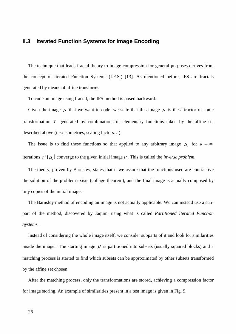
Instead of considering the whole image itself, we consider subparts of it and look for similarities
inside the image. The starting image µ is partitioned into subsets (usually squared blocks) and a
matching process is started to find which subsets can be approximated by other subsets transformed
by the affine set chosen.
After the matching process, only the transformations are stored, achieving a compression factor
for image storing. An example of similarities present in a test image is given in Fig. 9.
27
Fig. 9: some similarities in test image Lena
The set of transform stored is used at the decoding stage. These transforms are applied to an
initial image 0µ , usually blank, and iterated for n steps depending, as we will see, on PSNR ratio.
This encoding method is a lossy technique. In fact the matching process is not perfect and also
iterations will not go forever.
Basically, fractal coding of an image consists in building a code τ (i.e.: a particular
transformation) such that, if µ is the original image, then ( )µ τ µ≈ , that is, µ is approximately
self-transforming underτ .
The Collage Theorem states that if τ is a contractive transformation, µ is approximately the
attractor ofτ , that is ( )0lim kk µµ τ→∞≈ for the some initial image0µ .
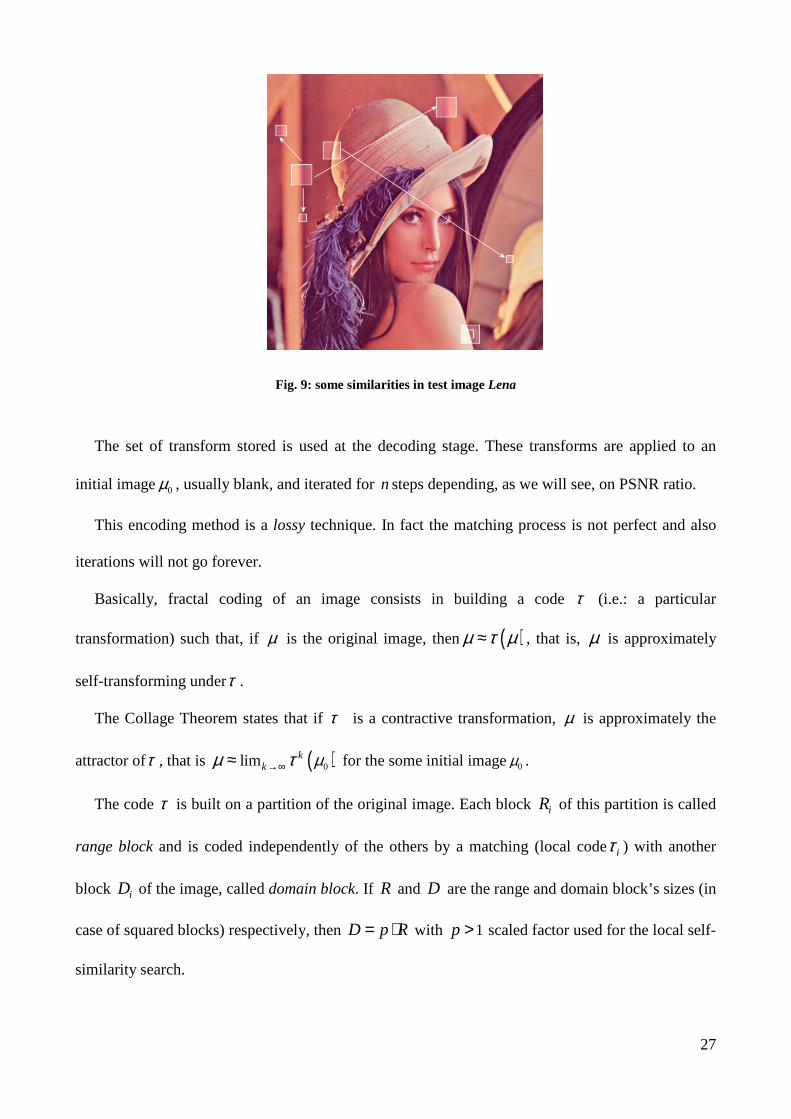
The code τ is built on a partition of the original image. Each block iR of this partition is called
range block and is coded independently of the others by a matching (local codeiτ ) with another
block iD of the image, called domain block. If R and D are the range and domain block’s sizes (in
case of squared blocks) respectively, then D p R= ⋅ with 1p > scaled factor used for the local self-
similarity search.
28
Classical iτ transforms are isometries (i.e.: rotations flip, etc.) and massive transform (i.e.,
contrast scaling and grey shifting).
If L is the number of range blocks, the fractal code of the initial image is then
( ) 1
L
orig iiµ ττ
==U
Where :i i iD Rτ → and ,i i i i pM I rτ = o o with ( )i i iM x a x b= ⋅ + an affine operator with a scale
ia and a shift ib on the luminance pixel, iI a transformation selected from eight discrete isometries
and ,i pr a reduction by a factor p using an averaging.
In other words, the task of the fractal encoder is to find for each range block a larger domain
block such that, after an opportune transformation, this constitutes a good approximation of the
present range block. An example is shown in Fig. 10
Fig. 10: Example of domain to range block mapping for Lena
29
The fractal code for the original image is a collection of so extracted local codes. This
approach implemented by Jaquin gives a representation of the image as composed by copies of
parts of the image itself. The classical fractal decoding stage consists in an iterated process starting
from an arbitrary initial image0µ . In fact, if τ is a contractive transformation theτ 's attractor
( )0τ µ∞ gives an approximation of the original image µ independently from the initial image.
II.4 Decoding stage
At decoding, starting from any 0µ initial image, the fractal code is reversely applied: 0µ is
partitioned in the same number of range and domain blocks of the encoded image.
For every 0iµ range block, the corresponding iτ coded for the i -esim range block of the
original image is applied.
This means that the right domain block of 0µ is taken, the right isometry in applied and then
mapped to the range block.
This process is made for every range block of0µ . The output ( )10τ µ , made of the collage of
the entire range block transformed, is then used back as the input of the algorithm and the process
starts again.
After n iterations the image ( )0nτ µ converges to a close representation of the original
image.
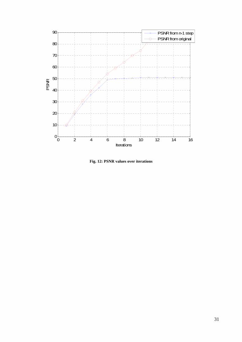
Usually the n iterations are chosen using PSNR threshold. When the PSNR difference
between ( )10
nτ µ− and ( )0nτ µ is less than 0.1 dB iterations are stopped.
30
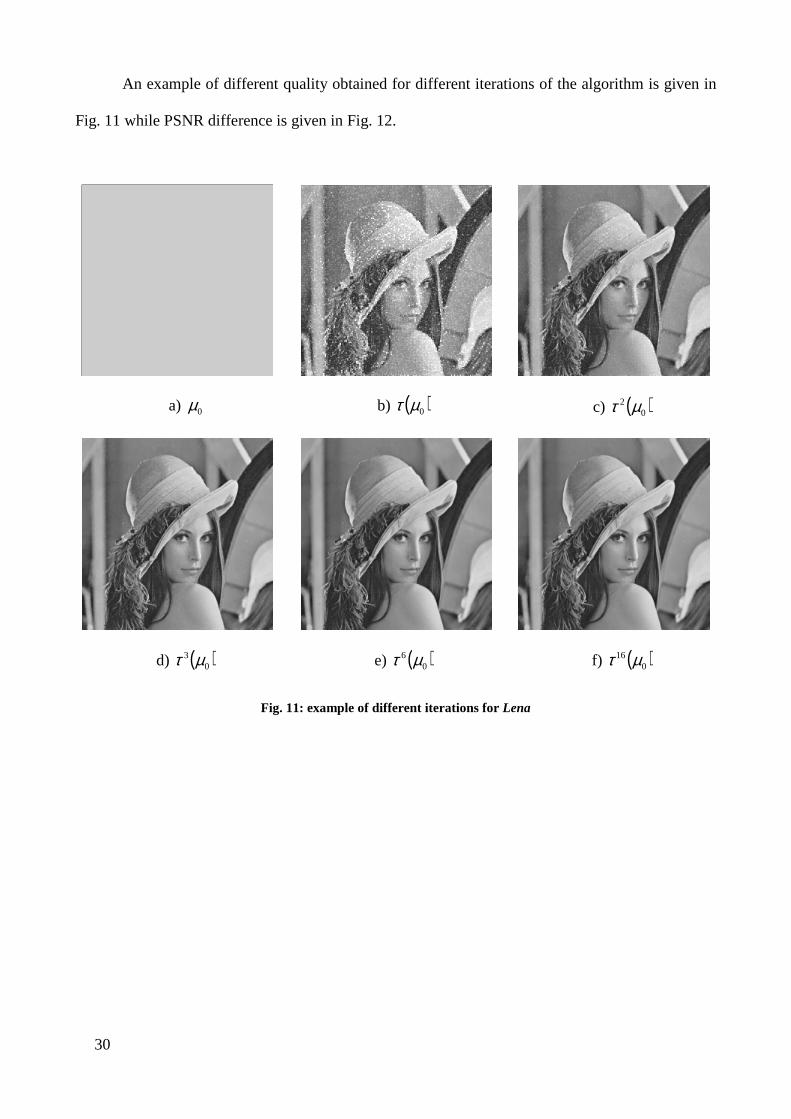
An example of different quality obtained for different iterations of the algorithm is given in
Fig. 11 while PSNR difference is given in Fig. 12.
a) 0µ b) ( )0µτ c) ( )02 µτ
d) ( )03 µτ e) ( )0
6 µτ f) ( )016 µτ
Fig. 11: example of different iterations for Lena
31
0 2 4 6 8 10 12 14 160
10
20
30
40
50
60
70
80
90
Iterations
PS
NR
PSNR from n-1 step
PSNR from original
Fig. 12: PSNR values over iterations
32
II.5 Fractal zoom
One of the most important features of fractal encoding is hidden into its mathematical
representation.
Since the image fractally coded can be thought as a mathematical function, given by the
collection of τ of every block, i.e. ( ) 1
L
orig iiµ ττ
==U , and these are isometries, we can obtain
easily a larger scale of the original image.
In fact, if Y AX B= + is a chosen isometry that maps the point nX ∈ℜ to nY ∈ℜ we can obtain a
zoom simply by a scalar multiplication so that
zoomedY s AX s B= ⋅ + ⋅
With s being the zoom factor.
Pratically the fractal code extracted from the original image has itself everything necessary to
obtain a zoomed replica of the image.
Usually this property is called implicit interpolation, because no explicit formulas are used to
obtain interpolation between pixel, and all the information required is taken during encoding time.
To use this property of fractals with our technique, based on P.I.F.S. encoding, we decode the
image using range blocks and domain blocks greater than the ones used on encoding stage.
More, the fractal code itself does not give any information about the range or domain block size
used during the encoding, so we can apply the same fractal code to different sizes of blocks.
If for example we star encoding an image with range blocks of size n n× pixels but during the
encoding we apply the extracted fractal code to range blocks of sizem m× , withm n> , we obtain a
zoom factor ofm n .
33
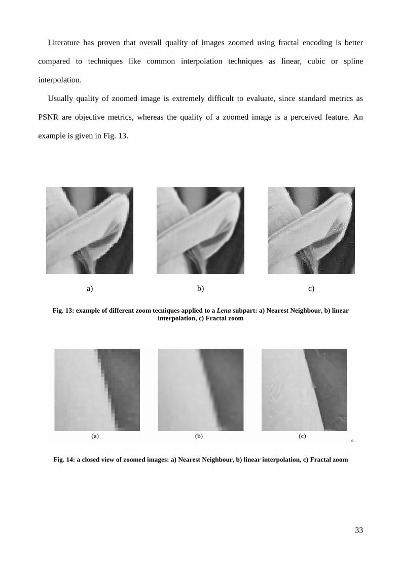
Literature has proven that overall quality of images zoomed using fractal encoding is better
compared to techniques like common interpolation techniques as linear, cubic or spline
interpolation.
Usually quality of zoomed image is extremely difficult to evaluate, since standard metrics as
PSNR are objective metrics, whereas the quality of a zoomed image is a perceived feature. An
example is given in Fig. 13.
a)
b)
c)
Fig. 13: example of different zoom tecniques applied to a Lena subpart: a) Nearest Neighbour, b) linear interpolation, c) Fractal zoom
Fig. 14: a closed view of zoomed images: a) Nearest Neighbour, b) linear interpolation, c) Fractal zoom
34
II.6 State of the art for fractal zooming
The main problem of fractal zoom is that for big zooming factor, blockness distortion decreases
the overall quality of the output image.
This is due to the fact that fractal encoding as described above involve a block partition exactly
at the first stage of the process.
These artefacts are responsible of high frequencies on the decoded image that were not present in
the original image.
A method that improves the quality of the fractal zoom was developed by Reusen [18] and
Polidori [25].
Since the inner problem is partitioning into range blocks, the blockness effect can avoided just
using an overlapped range block partitioning (O.R.B).
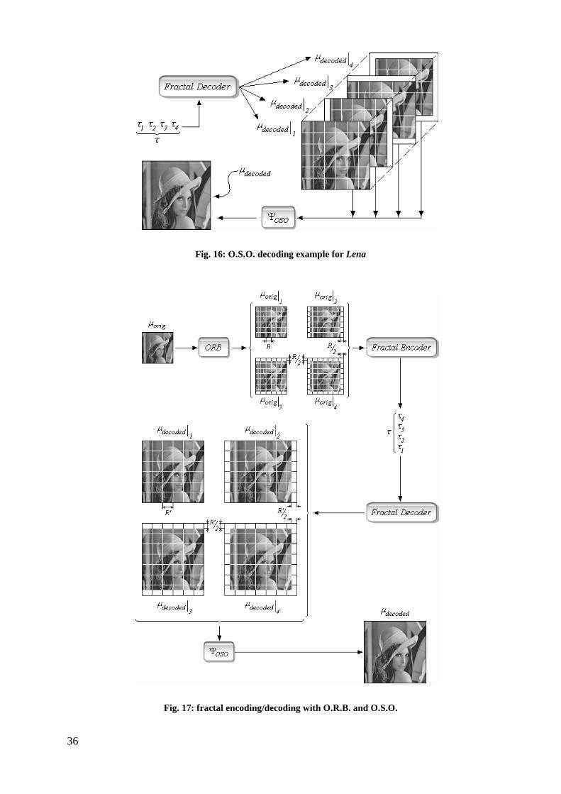
The original image is partitioned in four different ways so that range blocks of a partition overlap
the other partitions’ range blocks.
The classical method was intended by means of range blocks of size R and domain blocks of
sizeD p R= ⋅ . This means that a range block is distant R from another one. Given the original
image µ to be encoded, we can identify four other partitions considering different parts ofµ :
• 1
µ is the originalµ ;
• 2
µ is obtained taking off two strips of pixels 2R wide at the left and at the right of µ ;
• 3
µ is obtained taking off two strips of pixels 2R wide at the top and at the bottom of µ ;
• 4
µ Is obtained taking off four strips of pixels 2R wide both at the left and at the right and
at the top and at the bottom ofµ .

35
Every , 1,..., 4i
iµ = is then again partitioned using blocks of sizeR .
This method assures us that every range block of the original partition is covered several times with
the blocks of the other three partitions. An example of these four partitions is shown in Fig. 15.
1µ
2µ
3µ
4µ
Fig. 15: different partitions for Lena
These four partitions are than coded independently. This leads to four different fractal
codes1
τ ,2
τ 3
τ and 4
τ for one initial image µ so that the global fractal code is ∑=
=4
1ii
ττ 1.
At decoding time every i
τ will be used to obtain a target image( )iiτ µ .
The four target images then are melted together to obtain the final image using a filtering
operator OSOΨ . Usually this O.S.O. (Ordered Square Overlapping) operator is a classical median
filter.
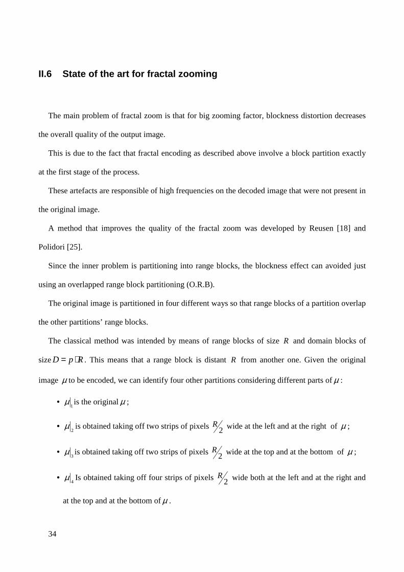
The decoding stage with O.S.O. filtering and zoom expansion is shown in Fig. 16 while the
complete process is shown in Fig. 17.
1 Here the operator ∑ is intended as a concatenation of fractal codes.
36
Fig. 16: O.S.O. decoding example for Lena
Fig. 17: fractal encoding/decoding with O.R.B. and O.S.O.

37
This technique improves greatly the quality of zoomed images with the fractal method.
The overall gain of quality using fractal theory for zooming is good. Usually the quality gap
between classical interpolators as linear, bicubic or splines and fractal zoom increases in favour of
the latter when high zoom factor are used.
The table below shows different PSNR values for zoom for different techniques and zoom
factors.
38
Chapter III
Fractals and video sequences
III.1 Introduction
This chapter describes the work done to extend the classic theory of fractal encoding and fractal
interpolation from the image field to the video sequence area.
The purpose of this research was intended to extend fractal interpolation to cover the problem of
slow motion of video sequence.
The enormous amount of data in a sequence leads to problems like complexity reduction and
algorithm optimizations. This chapter will introduce the wavelet transform of signals and how its
use, joined with some other technique, gave us the possibility of overwhelming the issues described
above.
Slow motion is a special effect used also in the television broadcasting production field. It is a
filmmaking technique in which the action on screen is slower than normal. Already consolidated as a
feature within analog TV production studios, today slow motion is likely to be extended to the
Digital Video Broadcasting (DVB) technology. At present, slow motion is performed during the pre-
production stage by means of fast-shuttered cameras able to capture the scene at a frame rate higher
than the standard rate that is 25 Frame/sec for PAL/SECAM systems and 30 Frame/sec for NTSC
systems. Slow motion is achieved by filming at a speed faster than the standard rate and then
projecting the film at the standard speed. In this case an optical zoom is executed and the slow
motion factor achievable is limited to shutter speed and fixed during the pre-production stage. In a
39
digital video production higher slow motion factors can be achieved by means of video post
processing techniques aiming at enhancing the performance of the fast-shuttered cameras by
inserting intermediate frames within the captured sequence. This process is normally referred as
digital zoom. Intermediate frames can be a replica of the previous frame, or can be generated by
means of interpolation. In the latter case, either linear or cubic spline functions can be used. Both
frame replication and interpolation have some drawbacks: interpolation for slow motion replay bears
to vanishing effects, as well as frame replication yields to jerky motion, both resulting in low
perceived quality to human vision system. An original solution to these problems based on motion
detection techniques was proposed at the BBC labs by G.A. Thomas [4] and H.Y.K. Lau [5] the
frames were divided into partially overlapped blocks; by means of Fourier analysis, a phase
correlation was performed between corresponding blocks belonging to adjacent frames. Moving
vectors were identified and interpolated to generate missing frames. The main weakness of this
technique was the inability to deal with the case of motion detection failure. This could occur due to
the presence of high speed movement in the scene, so that the motion estimation algorithm was
unable to find a good approximation of the movement for each block of the scene. Therefore, in
presence of high speed movement within the sequence, the effectiveness of the method significantly
decreased. In this work, we propose an alternative post processing scheme which combines the
properties of expansion, given by fractal representation of a video sequence, with motion detection
techniques and wavelet subband analysis to overcome the limitations of the state of the art solutions.
In literature, fractals on image applications were proposed to achieve data compression exploiting
self-similarity inside natural images.
But the potentiality of fractals is not limited to compression. The properties of fractal coding
allow expanding a multi-dimensional signal (e.g., image and video sequences) along its dimensions.
One of the major weaknesses of the fractal representation of a signal is the high computational
complexity of the encoding process. The computational load, and so the processing time, increases
for signals of higher dimension (1D, 2D, 3D…).
40
This is due to the fact that the main idea of fractal encoding is to look for similarities of blocks
using affine transforms, therefore a best match algorithm leads to a great time consuming process for
multi-dimensional data sets. Several methods have been proposed in literature to speed up the fractal
coding process [16]. A class of proposed solutions is based on wavelet subband analysis. Due to their
orthogonal and localization properties, wavelets are well suited (and extensively adopted) for
subband data analysis and processing.
The proposed algorithm exploits these features performing the fractal coding of each subband
with particular attention to the frequency distribution of the coefficients. To further reduce the high
computational cost of fractal encoding, active scene detection is used so as to perform fractal coding
only in high information areas (moving areas). As suggested in [18], to improve overall visual
quality overlapped block coding and post process filtering, extended to the three dimensional case,
are used.
Results show that with the proposed approach the quality achieved is higher if compared to the
state of the art techniques.
III.2 Fractal coding of video signals
The theory described in Chapter II for encoding an image by means of fractals, can be extended
straightforward to video signals.
In fact, a video signals can be thought as a ordered collection of images, called now frames, that
give information about changes along time.
There are different ways of how to encode video using fractals.
We can think of the frames as an independent stream of data and encode them independently.
So if a video sequence is composed by n frames:
1
n
ii
S µ=
=U Eq. 1
41
We can obtain the encoded stream just searching for appropriate transformations iτ on every
single frame, so that the output video is:
( )01
'n
ii
S τ µ=
=U Eq. 2
'n
S S→∞→
Being 0µ an initial arbitrary frame. Coding a video sequence in this way does not introduce
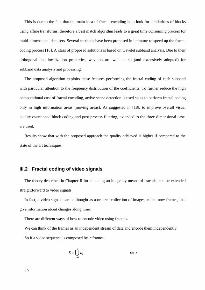
anything new, besides is not capable of reduce the redundancy between frames which in a video
sequence is extremely high (Fig. 18),. In fact most of the frames are correlated each other along time.
Fig. 18: correlation along time in test sequence “mobile”
42
To exploit these redundancy, another technique can be used to encode fractally a video. For
every frame 1i + the domain blocks are searched using the frame i as the searching pool.
The video sequence is first analyzed to find which frames are highly correlated each other. We
used a MSE ratio to divide the sequence into group of pictures (GOP) and then use the first frame as
a domain pool for the rest of the GOP frames.
Being the GOP composed by p frames, we can encode a sub-sequence stating:
( )01
'p
m ii
S τ µ=
=U
1:i iD Rτ →
The complete sequence will be 1
' 't
jm
S S=
=U where t the overall amount of GOPs is.
Every frame in the packet is partitioned in range blocks, and a transformation of a domain block
obtained by the first frame of the packet is chosen to be the best approximation of every range block
on the current frame.
At decoding time the process is inverted and starting from a blank frame, all of the others frame
of a packet are reconstructed using the transformation set obtained during the encoding stage.
Even if this method is able to find some of the correlations that exist between frames of a
sequence, does not represent an actual extension of the two-dimensional fractal encoding described
in the previous chapter. To extend that technique a full three-dimensional approach must be used.
The direct extension of the two-dimensional fractal encoding is to consider the sequence of
frames, i.e. the overall sequence, as a three-dimensional object with the third axis represented by the
timing.
43
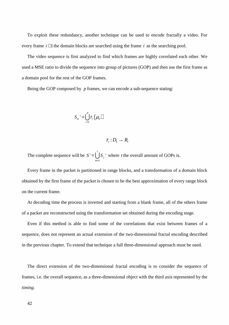
In fractal video coding using the three-dimensional extension range and domain blocks become
three dimensional objects: range and domain cubes. The process is straight-forward: the video
sequence is partitioned into range and domain cubes, and for every range cube a transformed
domain cube is searched to minimize the error measure and to be the best approximation of it.
Fig. 19: example of identification of range cube in test sequence “coastguard”
Fig. 20: three dimensional matching process
Since now we work in a three-dimensional space, the number of isometries and affine
transformation increase, and a great effort should be made to find some method to speed up the
process. This subject will be the focal point of the next section using, as we will see, wavelets
decomposition and motion detection.
44
III.3 Slow motion with fractal expansion
As for image encoding, fractals have some peculiarities when applied on video signals. We
saw in chapter 2 that a fractal code extracted from an image can be decoded with a zoom factor.
This quality pushed our study towards the possibility of “zooming” an entire video sequence or a
subpart of it.
The problem relies on understanding what an “expansion” of a video signal really means.
Considering the video sequence as a three dimensional object, being X and Y the image plane and T
the time axis, we can see that an expansion on the image plane leads to a classical zooming of a
frame while the expansion along the time axis increase the “length” of the sequence, meaning that
we “add” frames to the sequence.
Keeping the frame rate constant the result is that the sequence is “slowed” down by a factor
equal to the expansion factor (i.e. the “zooming” factor).
This means that a fractal expansion applied to a video sequence leads to an “implicit” interpolation
between frames and to a “slow motion” effect.
This effect is widely used in commercial devices or as a special FX for media production.
As for image zooming using fractal we prove that the quality of this expansion along time is
better than other classical method as polynomial interpolation, spline and motion vector
interpolation.
More, since all the information about zooming are kept inside the fractal code, we can obtain
several zooming factor during the decoding stage without complicated computation or algorithms.
In fact, as for images, a fractal zoom consist mathematically just in a scalar multiplication.
Depending on which fractal encoding technique is used, we can have different ways of
expand a sequence using fractals.

45
One of the methods consists in considering the slices of a sequence along different planes.
Considering a sequence of P frames of sizeN M× , we have these series of slices (Fig. 21):
• P image planes XY of size N M×
• M slices XT of size N P×
• N slices YT of size M P×
Fig. 21: slices of a video sequence: a) image plane; b) XT; c) YT
Fig. 22: example of slice (YT) expansion along time axis only
Those slices can be encoded as separate images. Once the slices are encoded a decoding
stage with a zooming factor k is applied (Fig. 22). This zooming factor can be applied only along a
certain direction (e.g.: the time axis) depending on the fact the final zoom will be only a slow
motion or a frame zoom too.
The zoomed slices are then joined together to form the expanded version of the sequence.
The joining function (Fig. Fig. 23) we used between the different expanded slices is a simple
average value between the pixels on the same position:
( ) ( ) ( ) ( ), , ,' , ,
3XT YT XY
j i pF i p F j p F i jF i j p
+ += Eq. 3
46
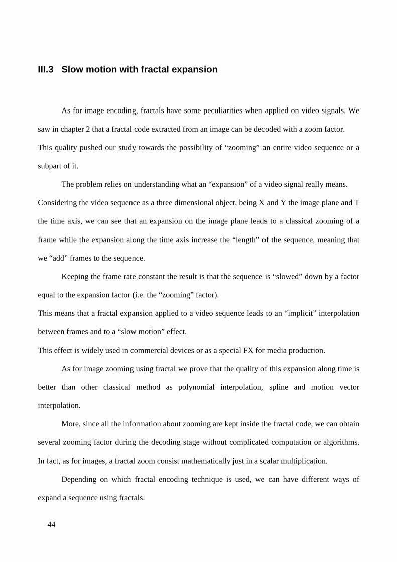
Where:
• 'F is the expanded sequence.
• ( ),nZWF l m is the point with coordinates ( ),l m of the n -esim element of the series of slices
along { }, ,ZW XY XT YT∈
And1 j N≤ ≤ , 1 i M≤ ≤ , 1 p P≤ ≤ .
Fig. 23: expansion using slices
Fig. 24: Sketch of the fractal expansion method using slices
47
This method leads to good quality for expanded video sequences2 but has a lot of
redundancy: in fact most of the information on slices on a plane is highly correlated with
information on other planes.
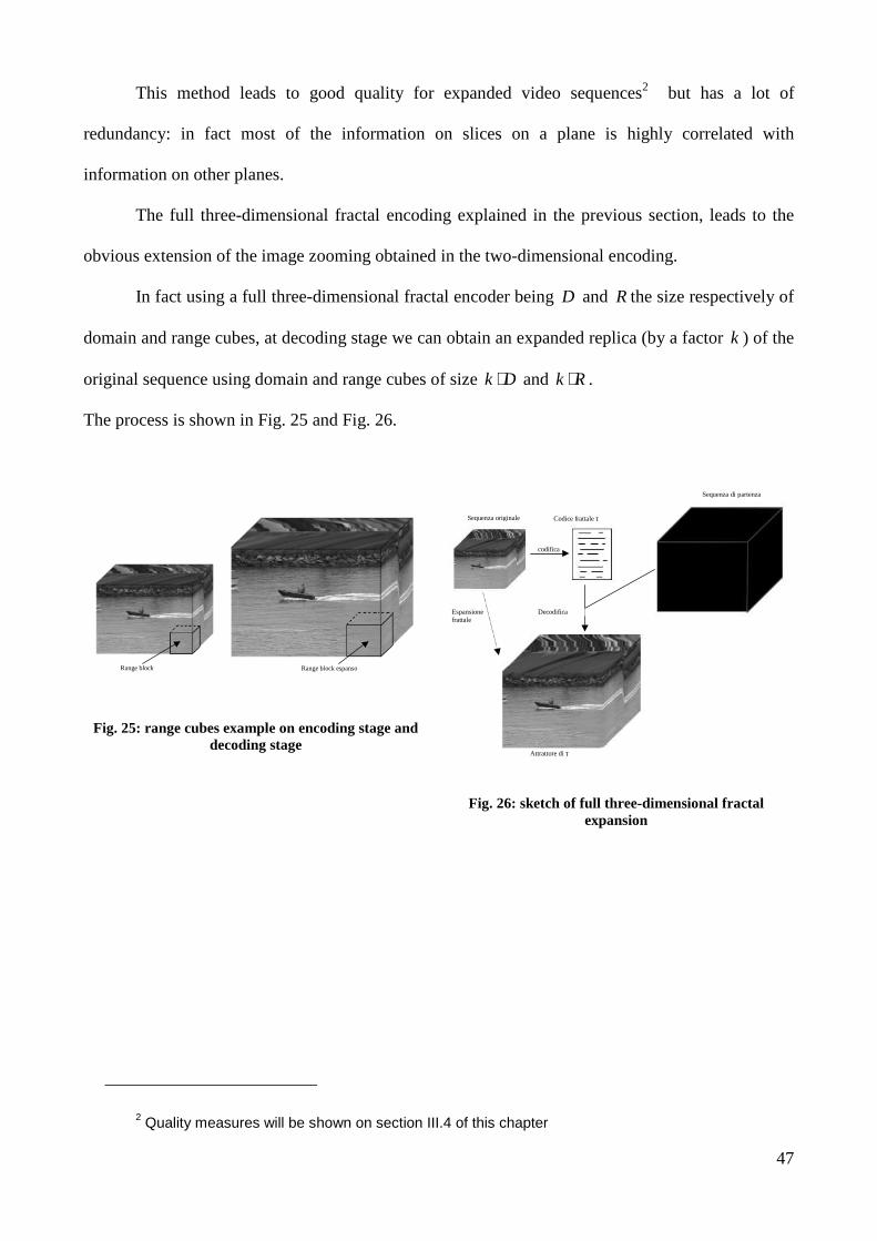
The full three-dimensional fractal encoding explained in the previous section, leads to the
obvious extension of the image zooming obtained in the two-dimensional encoding.
In fact using a full three-dimensional fractal encoder being D and R the size respectively of
domain and range cubes, at decoding stage we can obtain an expanded replica (by a factor k ) of the
original sequence using domain and range cubes of size k D⋅ and k R⋅ .
The process is shown in Fig. 25 and Fig. 26.
Range block Range block espanso
Fig. 25: range cubes example on encoding stage and decoding stage
Sequenza originale Codice frattale τ
Espansione frattale
Sequenza di partenza
Attrattore di τ
Decodifica
codifica
Fig. 26: sketch of full three-dimensional fractal expansion
2 Quality measures will be shown on section III.4 of this chapter
48
Using the full three-dimensional encoding and expansion to obtain zoomed replicas of sequence
leads to some problems. We can divide these problems in two main groups:
- Visual quality loss
- Computational cost
We developed some techniques to overcome both of these issues.
III.3.A Visual quality improving techniques
Using fractal zoom leads to blockness distortion during the decoding step along both the
time and spatial dimensions (image plane). This problem derives from partitioning the original
sequence into non overlapping range cubes during the encoding process. When high zoom (i.e.
above 8x factor) is performed these artefacts become visible and the overall visual quality
decreases.
Even if the origin of this distortion is the same, the effects are different on image plane and time
axis.
While on the image plane the effect is the appearance of artefacts on the frame, along the time
axis of a “slow motion” sequence the blockness produce an annoying effect known in literature as
“jerky motion”.
This jerky motion results in rapid and not natural movements of blocks (i.e.: range blocks in our
case) or entire frames along the scene of a video sequence.
We saw in the previous chapter how the problem of blockness distortion could be solved using
the O.R.B. and O.S.O. technique for the image zooming using fractals.
49
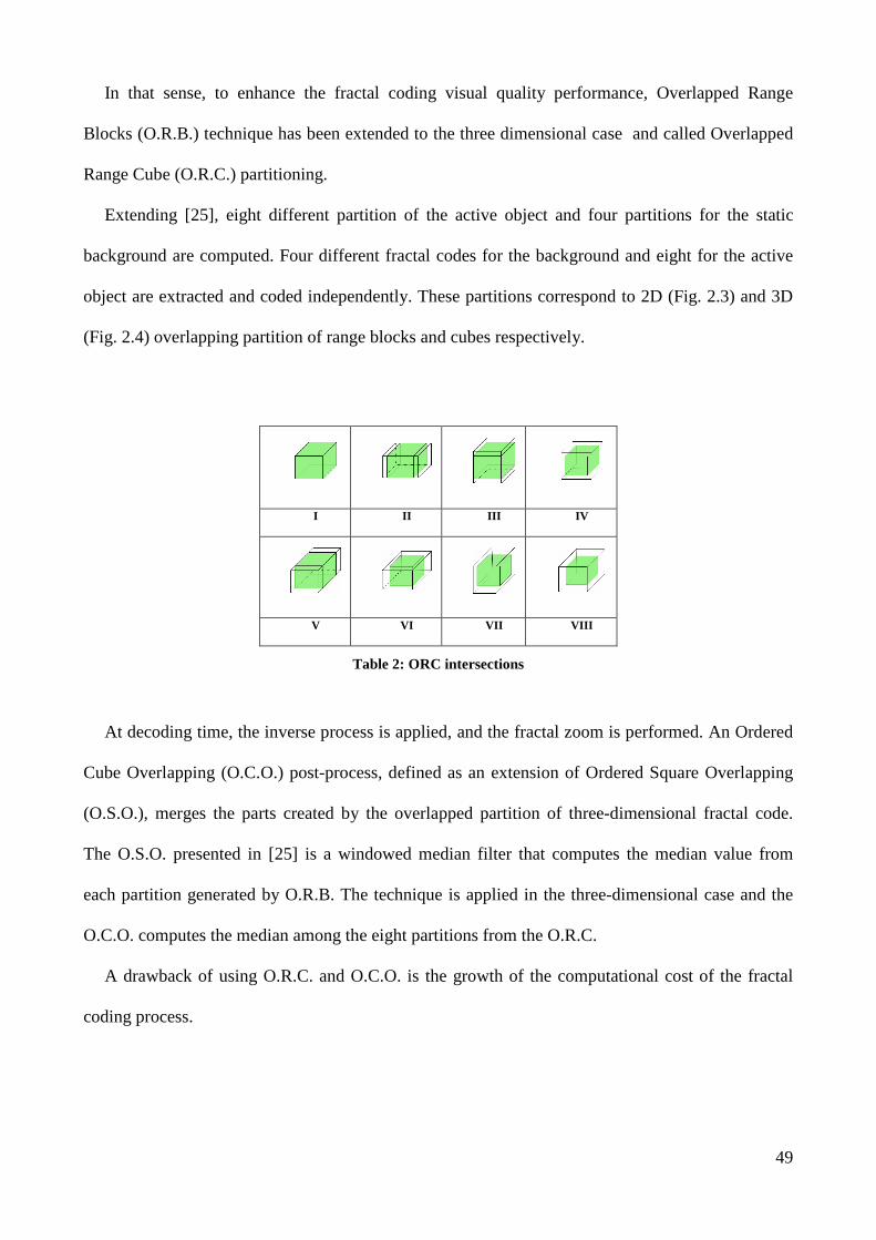
In that sense, to enhance the fractal coding visual quality performance, Overlapped Range
Blocks (O.R.B.) technique has been extended to the three dimensional case and called Overlapped
Range Cube (O.R.C.) partitioning.
Extending [25], eight different partition of the active object and four partitions for the static
background are computed. Four different fractal codes for the background and eight for the active
object are extracted and coded independently. These partitions correspond to 2D (Fig. 2.3) and 3D
(Fig. 2.4) overlapping partition of range blocks and cubes respectively.
I II III IV
V VI VII VIII
Table 2: ORC intersections
At decoding time, the inverse process is applied, and the fractal zoom is performed. An Ordered
Cube Overlapping (O.C.O.) post-process, defined as an extension of Ordered Square Overlapping
(O.S.O.), merges the parts created by the overlapped partition of three-dimensional fractal code.
The O.S.O. presented in [25] is a windowed median filter that computes the median value from
each partition generated by O.R.B. The technique is applied in the three-dimensional case and the
O.C.O. computes the median among the eight partitions from the O.R.C.
A drawback of using O.R.C. and O.C.O. is the growth of the computational cost of the fractal
coding process.
50
III.3.B Computational cost reduction
The increasing amount of process time derives not only for the bigger number of isometries but
also because of the enormous dimension of the matching space.
In fact a video sequence is usually composed by thousand of frames, and the partitions of range
and domain cubes contain a huge amount of items.
For sake of explanation if we have a CIF video sequence3 composed by 1024 frames
(approximately 20 sec. of video @50Hz), using a non-overlapping (to simplify the computation)
partition of domain cubes of size 4x4x4 and range cubes of size 2x2x2, this leads to:
- 1.640.448 Domain Cubes
- 13.123.584 Range Cubes
Using a close set of 16 isometries on the three-dimensional space, without considering massive
transforms, we have 151.640.448 13.123.584 16 2,7 10× × ⋅� as the upper limit of matches’ amount.
This number leads to the pratical impossibility of using a raw fractal encoding of a whole
sequence, which usually is larger than a CIF frame and longer than just 20 seconds.
To limit the number of matches we decided first to use the same approach defined above, and
frames are grouped into packets that are going to be treated as single units. The packet size is
chosen according to the temporal activity within the sequence, so that bigger sizes can be selected
for slowly changing scenes without a significant time processing increase. This due to the fact that
using a threshold to identify one of the combination of domain and transformation that leads to a
close representation of a range block, slowly changing scenes usually have a big percentage of exact
copies of blocks in the same position (or in the neighbour of the searching area) along time.
Packets are selected considering the temporal variance of the sequence, estimated by means of
the Minimum Square Error (MSE) metric between frames:
3 The size of a CIF (Common Interchange Format) frame is 352x288 pixels
51
( ), ,
1 1 2
0 0( , )i j i j
N Mh h k
i j
F F
MSE h kM N
− −+
= =
−=
⋅
∑∑ Eq. 4
[ ], 1,2,...h k n∈
where ,p
i jF is the pixel ( ),i j of the frame and, p is the frame position within the sequence, M N⋅
the frame size and n the number of frames of the entire sequence.
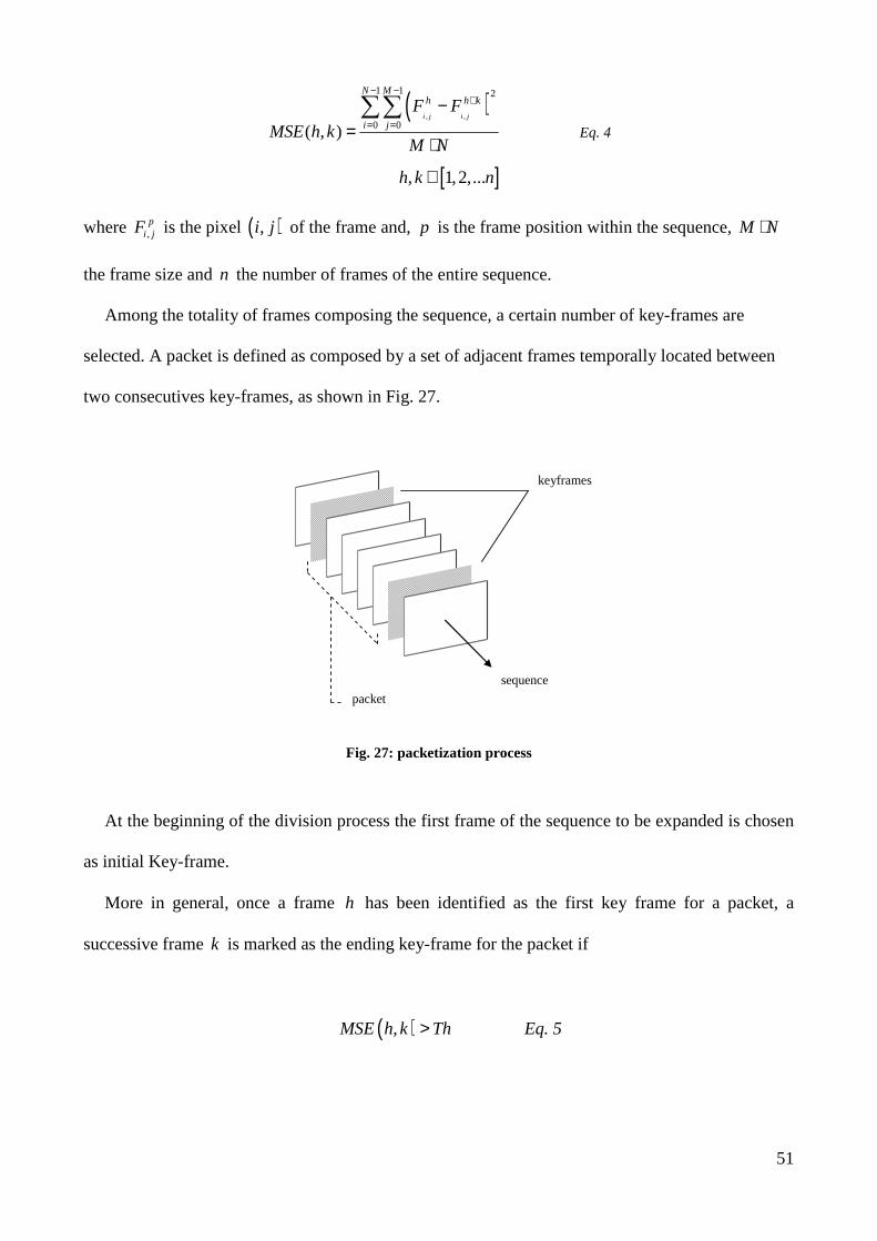
Among the totality of frames composing the sequence, a certain number of key-frames are
selected. A packet is defined as composed by a set of adjacent frames temporally located between
two consecutives key-frames, as shown in Fig. 27.
packet
keyframes
sequence
Fig. 27: packetization process
At the beginning of the division process the first frame of the sequence to be expanded is chosen
as initial Key-frame.
More in general, once a frame h has been identified as the first key frame for a packet, a
successive frame k is marked as the ending key-frame for the packet if
( ),MSE h k Th> Eq. 5
52
where Th is a threshold selected so that
( )1,
2
MSE nTh = Eq. 6
In other words, for each packet the temporal variance must be lower than the 50% of the
temporal variance of the whole sequence. Equation Eq. 6 assures at least a two packet
subdivision of the sequence to be expanded.
According to Eq. 5 and Eq. 6, each packet can be composed by a variable number of
frames. At the end of the packetization process, each packet is considered for coding as a single
unit: in this manner the computational load and, thus, the time consumed for the coding are
significantly reduced.
However, this packet based coding leads to discontinuity problems when the sequence is
zoomed, if each packet is independently coded. In fact, since the expansion is applied within each
packet, the successive packet merging process generates a temporal discontinuity between adjacent
“zoomed” packets.
To solve this problem, each packet is coded using the motion information of the previous packet
as a boundary condition. Owing to this, the presence of a buffer is necessary to assure the process
being causal.
A more general constraint is that the packet sizes must be a multiple ofR , size of the range
block, and not smaller thanD, size of the domain block. This guarantees the packet being
partitioned into range and domain blocks, and not into portions of them.
An example of right and wrong packetization is shown in Fig. 28.
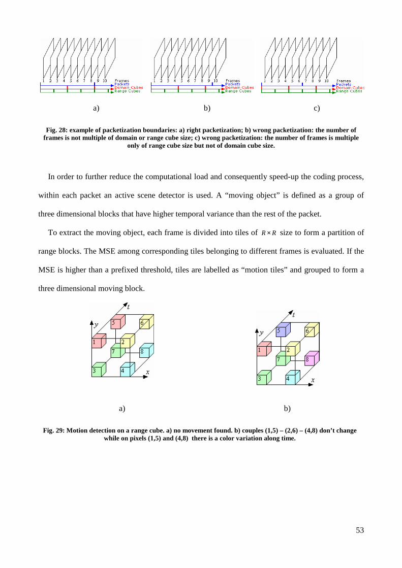
53
a) b) c)
Fig. 28: example of packetization boundaries: a) right packetization; b) wrong packetization: the number of frames is not multiple of domain or range cube size; c) wrong packetization: the number of frames is multiple
only of range cube size but not of domain cube size.
In order to further reduce the computational load and consequently speed-up the coding process,
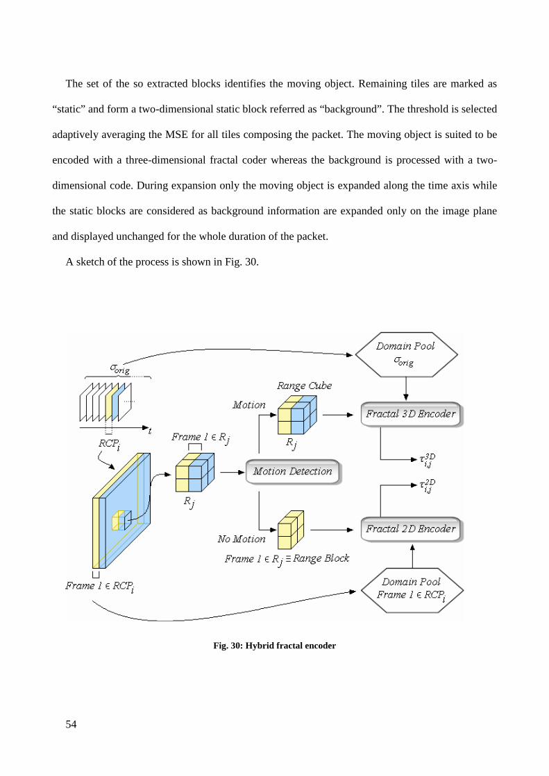
within each packet an active scene detector is used. A “moving object” is defined as a group of
three dimensional blocks that have higher temporal variance than the rest of the packet.
To extract the moving object, each frame is divided into tiles of RR × size to form a partition of
range blocks. The MSE among corresponding tiles belonging to different frames is evaluated. If the
MSE is higher than a prefixed threshold, tiles are labelled as “motion tiles” and grouped to form a
three dimensional moving block.
a) b)
Fig. 29: Motion detection on a range cube. a) no movement found. b) couples (1,5) – (2,6) – (4,8) don’t change while on pixels (1,5) and (4,8) there is a color variation along time.
54
The set of the so extracted blocks identifies the moving object. Remaining tiles are marked as
“static” and form a two-dimensional static block referred as “background”. The threshold is selected
adaptively averaging the MSE for all tiles composing the packet. The moving object is suited to be
encoded with a three-dimensional fractal coder whereas the background is processed with a two-
dimensional code. During expansion only the moving object is expanded along the time axis while
the static blocks are considered as background information are expanded only on the image plane
and displayed unchanged for the whole duration of the packet.
A sketch of the process is shown in Fig. 30.
Fig. 30: Hybrid fractal encoder
55
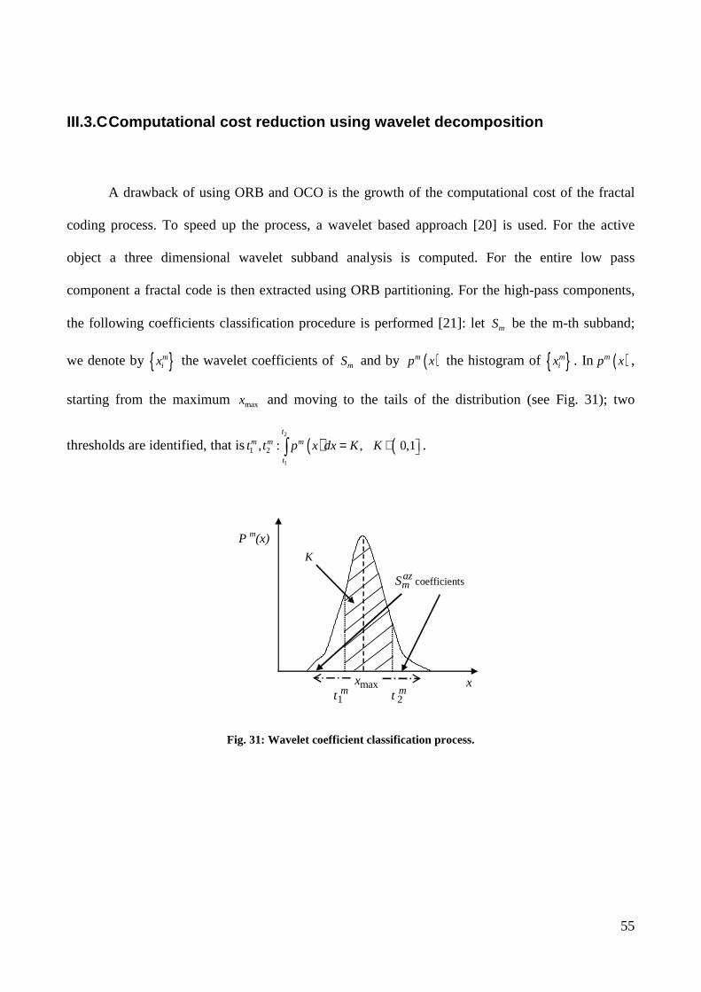
III.3.C Computational cost reduction using wavelet decomposition
A drawback of using ORB and OCO is the growth of the computational cost of the fractal
coding process. To speed up the process, a wavelet based approach [20] is used. For the active
object a three dimensional wavelet subband analysis is computed. For the entire low pass
component a fractal code is then extracted using ORB partitioning. For the high-pass components,
the following coefficients classification procedure is performed [21]: let mS be the m-th subband;
we denote by { }mix the wavelet coefficients of mS and by ( )mp x the histogram of { }m
ix . In ( )mp x ,
starting from the maximum maxx and moving to the tails of the distribution (see Fig. 31); two
thresholds are identified, that is ( ) (2
1
1 2, : , 0,1t
m m m
t
t t p x dx K K = ∈∫ .
P m(x)
mt1 mt 2
x
azmS coefficients
maxx
K
Fig. 31: Wavelet coefficient classification process.
56
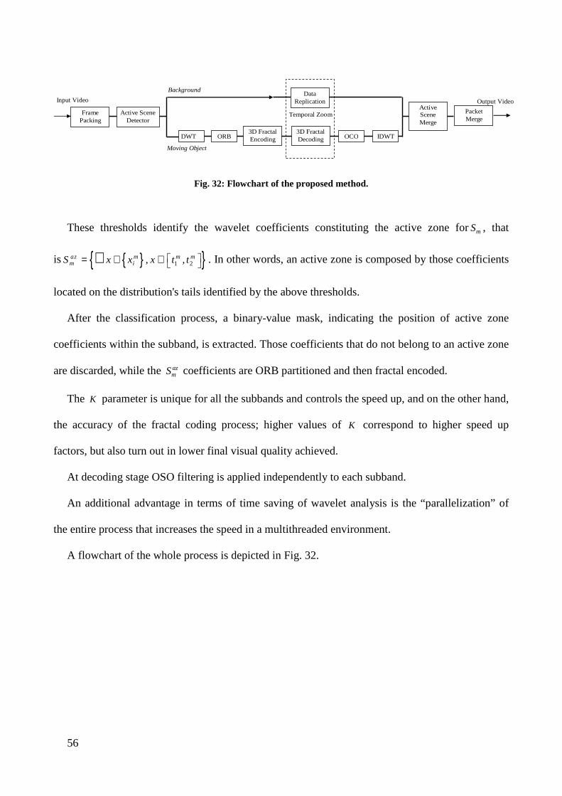
Frame Packing
Active Scene Detector
Active Scene Merge
Packet Merge
DWT 3D Fractal Encoding
3D Fractal Decoding IDWT ORB OCO
Moving Object
Background
Input Video Output Video Data
Replication
Temporal Zoom
Fig. 32: Flowchart of the proposed method.
These thresholds identify the wavelet coefficients constituting the active zone formS , that
is { }{ }1 2, ,az m m mm iS x x x t t
= ∈ ∉∀ . In other words, an active zone is composed by those coefficients
located on the distribution's tails identified by the above thresholds.
After the classification process, a binary-value mask, indicating the position of active zone
coefficients within the subband, is extracted. Those coefficients that do not belong to an active zone
are discarded, while the azmS coefficients are ORB partitioned and then fractal encoded.
The K parameter is unique for all the subbands and controls the speed up, and on the other hand,
the accuracy of the fractal coding process; higher values of K correspond to higher speed up
factors, but also turn out in lower final visual quality achieved.
At decoding stage OSO filtering is applied independently to each subband.
An additional advantage in terms of time saving of wavelet analysis is the “parallelization” of
the entire process that increases the speed in a multithreaded environment.
A flowchart of the whole process is depicted in Fig. 32.
57
III.4 Performance Analysis and Comparison
We tested ([26]) the effectiveness of the proposed method by comparing the result achieved to
those obtained, under the same constraint (i.e., equal slow motion factors) by frame replication and
classical interpolation techniques.
Test sequences were Silent, Miss America, Stefan, Carphone, Coastguard and Mobile in CIF
format. In a framework of broadcasting digital TV, to measure the quality achieved we refer to the
video quality assessment described on [22] and formalized in [23]. As to this, the perception of
continuous motion by human vision faculties is a manifestation of complex functions,
representative of the characteristics of the eye and brain.
When presented with a sequence of images at a suitably frequent update rate, the brain
interpolates intermediate images, and the observer subjectively appears to see continuous motion
that in reality does not exist. In a video display, jerkiness is defined as the perception, by human
vision faculties, of originally continuous motion as a sequence of distinct "snapshots” [23]. Usually,
jerkiness occurs when the position of a moving object within the video scene is not updated rapidly
enough.
This can be a primary index of a poor performance for a slow motion algorithm. More in
general, the total error generated by an incorrect coding of a moving object on a video sequence is
representative of spatial distortion and incorrect positioning of the object. In [23] a class of full
reference quality metrics to measure end–to–end video performance features and parameters was
presented.
In particular, [23] defines a framework for measuring such parameters that are sensitive to
distortions introduced by the coder, the digital channel, or the decoder. Ref. [23] is based on a
special model, called the Gradient Model. Main concept of the model is the quantification of
distortions using spatial and temporal gradients, or slopes, of the input and output video sequences.
58
These gradients represent instantaneous changes in the pixel value over time and space. We can
classify gradients into three different types that have proven to be useful for video quality
measurement:
• The spatial information in the horizontal direction hSI
• The spatial information in the vertical direction vSI
• The temporal informationTI .
Features, or specific characteristics associated with individual video frames, are extracted in
quantity from the spatial and temporal information. The extracted features quantify fundamental
perceptual attributes of the video signals such as spatial and temporal detail. A scalar feature is a
single quantity of information, evaluated per video frame.
The ITU recommendation [23] divides the scalar features into two main groups: based on
statistics of spatial gradients in the vicinity of image pixels and based on the statistics of temporal
changes to the image pixels.
The former features are indicators of the amount and type of spatial information, or edges, in the
video scene, whereas the latter are indicators of the amount and type of temporal information, or
motion, in the video scene from one frame to the next. Spatial and temporal gradients are useful
because they produce measures of the amount of perceptual information, or change in the video
scene.
Surprisingly parameters based on scalar features (i.e., a single quantity of information per video
frame) have produced significant good correlation to subjective quality measurement (producing
coefficients of correlation to subjective mean opinion score from 0.85 to 0.95) [22].
This demonstrates that the amount of reference information that is required from the video input
to perform meaningful quality measurements is much less than the entire video frame.
59
A complete description of all the features and parameters in [23] is beyond the scope of this
work.
In the following a brief summary of the above feature will be given, a mathematical
determination of the above features is provided in [23]:
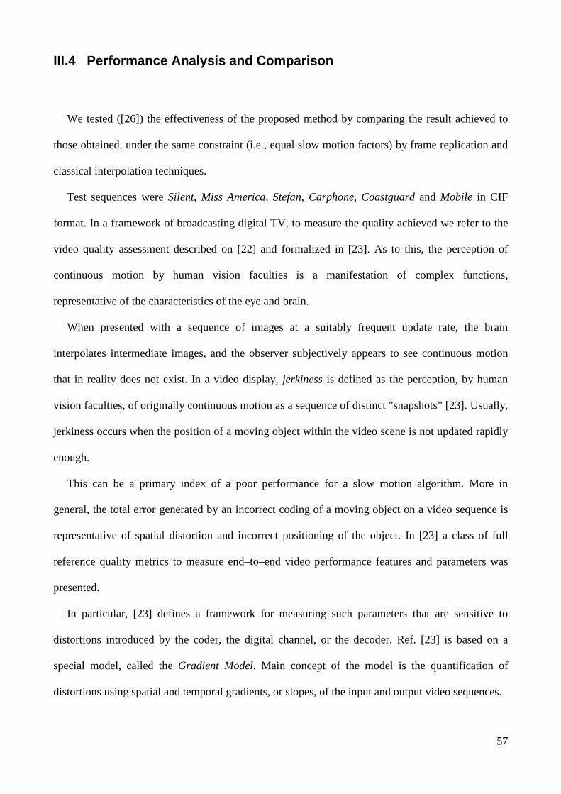
Blurring: A global distortion over the entire image, characterized by reduced sharpness of edges
and spatial detail.
The [23] defines a Lost Edge Energy Parameter for measuring the blurring-effect, which causes
a loss of edge sharpness and a loss of fine details in the output image. This loss is easily perceptible
by comparing the Spatial Information (SI) of the output image with the SI of the input image.
The lost edge energy parameter compares the edge energy of the input image with the edge
energy of the output image to quantify how much edge energy has been lost.
0%
5%
10%
15%
20%
25%
30%
2x 4x 8x
Slow Motion Factor
Blu
rrin
g
Fractal Expansion Frame replica Frame Interpolation
Fig. 33: Measured blurring for “Silent” sequence.
0%
10%
20%
30%
40%
50%
60%
70%
80%
90%
2x 4x 8x
Slow Motion Factor
Tili
ng
Fractal Expansion Frame Replica Frame Interpolation
Fig. 34: Measured tiling for “Silent” sequence..
0%
5%
10%
15%
20%
25%
30%
35%
40%
2x 4x 8x
Slow Motion Factor
Err
or B
lock
Fractal Expansion Frame Replica Frame Interpolation
Fig. 35: Measured error blocks for “Silent” sequence.
0%
10%
20%
30%
40%
50%
60%
2x 4x 8x
Slow Motion Factor
Jerk
ines
s
Fractal Expansion Frame Replica Frame Interpolation
Fig. 36: Measured jerkiness for “Silent” sequence.
60
Tiling: Distortion of the image characterised by the appearance of an underlying block encoding
structure. The [23] paper defines a HV to non-HV edge energy difference parameter for quantifying
the tiling impairment.
In contrast to blurring which results in lost edge energy, tiling creates false horizontal and
vertical edges. By examining the spatial information (SI) as a function of angle, the tiling effects
can be separated from the blurring effects.
Error Block: A form of block distortion where one or more blocks in the image bear no
resemblance to the current or previous scene and often contrast greatly with adjacent blocks.
Reference [23] defines an Added Motion Energy Parameter for detecting and quantifying the
perceptual effects of error blocks.
The sudden occurrence of error blocks produces a relatively large amount of added temporal
information. So the Added Motion Energy Parameter compares the temporal information (TI) of
successive input frames to the TI of the corresponding output frames.
Jerkiness: Motion that was originally smooth and continuous is perceived as a series of distinct
snapshots. Reference [23] paper defines a Lost Motion Energy and Percent Repeated Frames
Parameter for measuring the jerkiness impairment. The percent repeated frames parameter counts
the percentage of TI samples that are repeated, whereas the average lost motion energy parameter
integrates the fraction of lost motion (i.e., sums the vertical distances from the input samples to the
corresponding repeated output samples, where these distances are normalised by the input before
summing).
To extract the performance metrics we deployed the Video Quality Metric (VQM) software
developed by the ITS-Video Quality Research project [24] and compliant with [23]. All tests
performed on the different test sequences produced similar outcomes that have been proven to be
dependent to the natural temporal activity of the sequences.
61
Therefore, for the shake of concision, we reported here only a subset of results that were relevant
to the Silent and Mobile sequences. The Silent sequence presents a limited temporal activity
compared to Mobile.
We considered 64 frames for the sequence Silent at 15 frame/s rate and 128 frames for the
sequence Mobile at 30 frame/s rate, both corresponding to approximately 4 seconds of the video
scene. Fig. 33 to Fig. 40 show the results of the above mentioned features for the proposed method,
the frame replica and the spline cubic interpolation techniques, in case of 2x, 4x and 8x slow motion
factors. A general overview of the outcomes shows the advantage in using the proposed technique
for higher slow motion factors. An in-depth analysis of the results demonstrates the sensitivity of
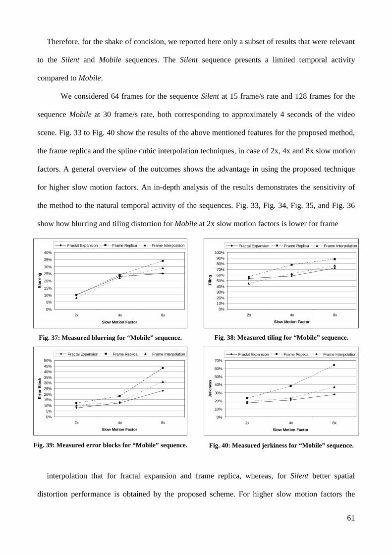
the method to the natural temporal activity of the sequences. Fig. 33, Fig. 34, Fig. 35, and Fig. 36
show how blurring and tiling distortion for Mobile at 2x slow motion factors is lower for frame
0%
5%
10%
15%
20%
25%
30%
35%
40%
2x 4x 8x
Slow Motion Factor
Blu
rrin
g
Fractal Expansion Frame Replica Frame Interpolation
Fig. 37: Measured blurring for “Mobile” sequence.
0%
10%20%
30%40%
50%
60%70%
80%90%
100%
2x 4x 8x
Slow Motion Factor
Tilin
g
Fractal Expansion Frame Replica Frame Interpolation
Fig. 38: Measured tiling for “Mobile” sequence.
0%
5%10%
15%20%
25%
30%35%
40%45%
50%
2x 4x 8x
Slow Motion Factor
Err
or B
lock
Fractal Expansion Frame Replica Frame Interpolation
Fig. 39: Measured error blocks for “Mobile” sequence.
0%
10%
20%
30%
40%
50%
60%
70%
2x 4x 8x
Slow Motion Factor
Jerk
ines
s
Fractal Expansion Frame Replica Frame Interpolation
Fig. 40: Measured jerkiness for “Mobile” sequence.
interpolation that for fractal expansion and frame replica, whereas, for Silent better spatial
distortion performance is obtained by the proposed scheme. For higher slow motion factors the
62
predominance of the proposed method is more evident and is due to the joint use of motion
estimation and ORB/OSO fractal coding that allows mitigating the presence of spatial artifacts.
Fig. 35 shows how for Silent the error block feature measured for the proposed system is
considerably lower than for frame replica and interpolation for high slow motion factors, whereas is
comparable for 2x temporal expansion.
For Mobile (Fig. 37) the error block is comparable for 2x and 4x slow motion factors for fractal
zooming and interpolation and only for higher slow motion factors the prevalence of the proposed
system is noticeable.
This outcome is mainly due to the intrinsic block-based nature of fractal coding that, in presence
of high temporal activity within the scene, reduces the efficacy of the proposed approach.
The results shown in Fig. 36 and Fig. 40 are relevant to jerkiness and confirm the above
statement: the effectiveness of the proposed method for this feature is evident for Mobile (Fig. 40)
only for 8x slow motion factor.
For lower temporal expansions the proposed scheme achieves performance comparable to
classical interpolation technique.
For Silent the predominance of fractal expansion in terms of jerkiness is evident for slow motion
factors higher than 2x.
The use of a combined motion and subband analysis during the fractal coding and again the
smoothing properties of the OSO filtering allow the method achieving high performance in terms of
fluent motion flow during the presentation in slow motion of video sequences.
63
Chapter IV
Fractals and color image compression
IV.1 Introduction
This chapter proposes a fractal coding technique based on Iterated Function Systems (IFS) to
encode color image signals. IFS aim to exploit the redundancy given by the self-similarity always
contained in natural images.
Exhaustive studies have been conducted on ISF applied to grey level image coding but, on the
other hand, even if fractal coding of color images has been investigated, still remain an open issue.
The need for color image compression is gaining importance in recent time due to large scale
multimedia applications.
Conventional fractal compression schemes can easily be extended to color image compression
as a color image is usually represented in multichannels such as Red, Green and Blue (RGB)
components.
Thus each channel in color image can be compressed as a grey-level image. Hurtgen, Mols and
Simon proposed a fractal transform coding of color images in [27]
This kind of encoding lacks the possibility of considering similarities between the three color
planes, thus not achieving a good compression ratio neither a fair population on the domain pool
needed to obtain a high quality interpolation for zooming purposes.
To exploit the spectral redundancy in RGB components, the root mean square error (RMS)
measure in gray-scale space can be extended to 3-dimensional color space for fractal-based color
64
image coding [28]. Experimental results show that a 1.5 compression ratio improvement can be
obtained using vector distortion measure in fractal coding with fixed image partition as compared to
separate fractal coding in RGB images.
However, since RGB space is not perceptually uniform, we decided to use another color space,
called CIE-L*a*b*.
Also RMS metrics, as deeply discussed on the other chapters, demonstred to not be a good
quality measure, so we introduced a different metric never use for fractal encoding purpouses,
called Earth Mover’s Distance Metric.
We then will propose a novel approach for coding color images based on the joint use of the Lab
color space and Earth Mover’s Distance (EMD) measure [30]
EMD has been suitably deployed for color image retrieval applications and can be thought as a
vector metric that combines spatial and color information to resolve similarities among color
images. This definition clearly gave us some hints on how this metric was extremely suitable for
fractal encoding, which is, after all, a search of similarities among parts of an image.
In this work we implement a fractal coding approach that relies on EMD for finding self-
similarities within color images represented in the Lab color space and later we show some results
of this technique.
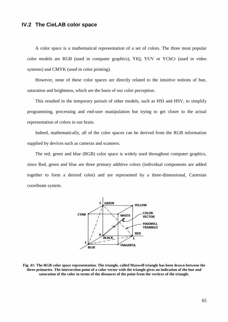
65
IV.2 The CieLAB color space
A color space is a mathematical representation of a set of colors. The three most popular
color models are RGB (used in computer graphics), YIQ, YUV or YCbCr (used in video
systems) and CMYK (used in color printing).
However, none of these color spaces are directly related to the intuitive notions of hue,
saturation and brightness, which are the basis of our color perception.
This resulted in the temporary pursuit of other models, such as HSI and HSV, to simplify
programming, processing and end-user manipulation but trying to get closer to the actual
representation of colors in our brain.
Indeed, mathematically, all of the color spaces can be derived from the RGB information
supplied by devices such as cameras and scanners.
The red, green and blue (RGB) color space is widely used throughout computer graphics,
since Red, green and blue are three primary additive colors (individual components are added
together to form a desired color) and are represented by a three-dimensional, Cartesian
coordinate system.
Fig. 41: The RGB color space representation. The triangle, called Maxwell triangle has been drawn between the three primaries. The intersection point of a color vector with the triangle gives an indication of the hue and
saturation of the color in terms of the distances of the point from the vertices of the triangle.
66
The RGB color space is the most prevalent choice for computer graphics because color
displays use red, green and blue to create the desired color. Therefore, the choice of the RGB
color space simplifies the architecture and design of the system.
Also, in a system that is designed using the RGB color space can take advantage of a large
number of existing software routines, since this color space has been around for a number of
years.
However, RGB is not very efficient when dealing with “real-world” images. All three RGB
components need to be of equal band width to generate any color within the RGB color cube.
The result of this is a frame buffer that has the same pixel depth and display resolution for each
RGB component.
Also, processing an image in the RGB color space is usually not the most efficient method.
For example, to modify the intensity or color of a given pixel, the three RGB values must be read
from the frame buffer, the intensity or color calculated, the desired modifications performed and
the new RGB values calculated and written back to the frame buffer. If the system had access to
an image stored directly in the intensity and color format, the processing steps would be faster.
For these and other reasons, many video standards decided to use luminancy and two color
difference signals. The most common systems are the YUV and YCbCr color spaces.
The YUV color space is used by the PAL (Phase Alternation Line), NTSC (National
Television System Committee), and SECAM (Sequentiel Couleur Avec Mémoire) composite
color video standards. The black-white system used only luminancy (Y) information;
This system was ideated mainly for backward compatibility with old monocromatic
television, since U and V where easily be discarded by old equipment.
Color receivers decoded the additional color information to display a color picture. The
equations that describe the direct transformation RGB � YUV are:
67
0.299 0.587 0.114
0.147 0.289 0.436 0.492( )
0.615 0.515 0.100 0.877( )
Y R G B
U R G B B Y
V R G B R Y
= + += − + + = −= − − = −
and for the inverse transformation:
UYB
VUYG
VYR
032.2
581.0395.0
140.1
+=−−=
+=
For digital RGB values with a range of 0-255, Y has a range of 0-255, U a range of 0 to ±112
and V a range of 0 to ±157.
As the RGB color space, the YUV space is not uniform concerning the HVS.
A system is said to be not uniform if a little perturbation of a value is perceived linearly
along the possible variation of that value. This means that a color space is perceptually uniform
if a distance from a color a and another color b a c= + ∆ will be perceived as constant
independently from a orb . Using a non perceptually uniform space as RGB has the drawback
that the Human Vision System will be affected by computer measures for digital video
processing, since the distance from RGB value will not be uniform in respect of the HVS.
Starting from these considerations, the Commission Internationale d’Eclairage (CIE) defined
a uniform color model, called L*a*b* that represents all the color humans is able to resolve.
Danciu and Hart [29]presented a comparative study of fractal color image compression in
the L*a*b* color space with that of Jacquin's iterated transform technique for 3-dimensional
color. It has been shown that the use of uniform color space yield compressed images to have
less noticeable color distortion than other methods.
68
Since there are three types of color photoreceptor cone cells in the retina, each with a
different spectral response curve, all colors can be completely described by three numbers,
corresponding to the outputs of the cone cells.
The CIE workgroup then defined XYZ tristimulus values, where all visible colors can be
represented using only positive values of X, Y and Z.
For applications where it is important to be able to measure differences between colors in a
way that matches perceptual similarity as good as possible the perceptually uniform color spaces
find their best field of use.
The CIE-L*a*b* (CIE-Lab) color space was designed such that the perceived differences
between single, nearby colors correspond to the Euclidean distance of the color coordinates.
The (nonlinear) conversions from RGB to CIE-Lab are given by:
,200
,500
,
3.903
008856.016116
950227.0119193.0019334.0
072169.0715160.0212671.0
180423.0357580.0412453.0
*
*
3
1
*
−
=
−
=
>−
=
⋅
=
nn
nn
n
nn
Z
Zf
Y
Yfb
Y
Yf
X
Xfa
otherwiseY
Y
Y
Yif
Y
Y
L
B
G
R
Z
Y
X
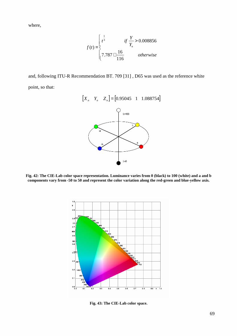
69
where,
1
3 0.008856( )
167.787
116
n
Yt if
Yf t
otherwise
>
= +
and, following ITU-R Recommendation BT. 709 [31] , D65 was used as the reference white
point, so that:
[ ] [ ]088754.1195045.0=nnn ZYX
Fig. 42: The CIE-Lab color space representation. Luminance varies from 0 (black) to 100 (white) and a and b components vary from -50 to 50 and represent the color variation along the red-green and blue-yellow axis.
Fig. 43: The CIE-Lab color space.
70
IV.3 Clustering
An image block signature is a set of features extracted by means of a clustering process.
The Clustering tecnique is a branch of Image (or data) segmentation field. A segmentation of an
image entails the division or separation of the image into regions of similar attribute. The most
basic attribute for segmentation is image luminance amplitude for a monochrome image and color
components for a color image. Image edges and texture are also useful attributes for segmentation.
Clustering aiming at partitioning the image block in a set of sub regions, (i.e., clusters) formed by
pixels gathered according to some distance rule, which is the “segmentation” similar attribute. To
each cluster is associated a feature representative of the cluster.
The clustering segmentation concept is simple but usually computationally intensive.
Considering a vector [ ]1 2, , ,T
Nx x x x= L of measurements at each pixel coordinate (j,k) of the
image. The measurements could be point multispectral values, point color components and derived
color components or neighborhood feature measurements. Is the measurement set is to be effective
for image segmentation, data collected at various pixels within a segment of common attribute
should be similar. That is, the data should be tightly clustered in an N-dimensional measurement
space. If this condition holds, the segmenter design task becomes one of subdividing the N-
dimensional measurement space into mutually exclusive compartments, each of which envelops
typical data clusters for each image segment. Fig. 44 illustrates the concept for two features. In the
segmentation process, if a measurement vector for a pixel falls within a measurement space
compartment, the pixel is assigned the segment name or label of that compartment.
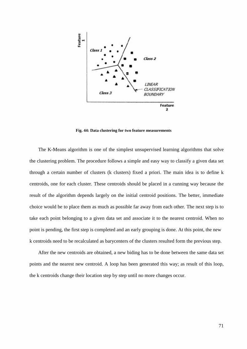
71
Fig. 44: Data clustering for two feature measurements
The K-Means algorithm is one of the simplest unsupervised learning algorithms that solve
the clustering problem. The procedure follows a simple and easy way to classify a given data set
through a certain number of clusters (k clusters) fixed a priori. The main idea is to define k
centroids, one for each cluster. These centroids should be placed in a cunning way because the
result of the algorithm depends largely on the initial centroid positions. The better, immediate
choice would be to place them as much as possible far away from each other. The next step is to
take each point belonging to a given data set and associate it to the nearest centroid. When no
point is pending, the first step is completed and an early grouping is done. At this point, the new
k centroids need to be recalculated as barycenters of the clusters resulted form the previous step.
After the new centroids are obtained, a new biding has to be done between the same data set
points and the nearest new centroid. A loop has been generated this way; as result of this loop,
the k centroids change their location step by step until no more changes occur.

72
The aim of the algorithm is that of minimizing an objective function, such as a squared error
function:
2( )
1 1
,k n
ji j
j i
J x c= =
= −∑∑
where 2( )j
i jx c− is a chosen distance measure between a data point ( )jix and the cluster centre
jc and is an indication of the distance of the n data points from their respective cluster centres.
The algorithm can be synthesised as follows:
1. Place K points into the space represented by the objects that are being clustered. These
points represent initial group centroids.
2. Assign each object to the group that has the closest centroid.
3. When all objects have been assigned, recalculate the values of the K centroids.
4. Repeat Steps 2 and 3 until the centroids no longer change. This produces a separation of
the objects into groups from which the metric to be minimized can be calculated.
73
IV.4 Clustering process applied to fractal encoding
The aim of our study was pratically to use clustering tecniques as hint on similarities between
range and domain blocks.
Instead of using one-to-one pixel distance of transformed domain, we wanted to compute
distance, i.e. similarity, of blocks using a higher level concept.
To apply clustering to fractal encoding we also needed two other steps: find a way to catalog
clusters on domain and range blocks, and an effective way to compute the distance between these
objects.
While the second problem is addressed in the next chapter, we define here the concept of the
“signature” of an image.
After the clustering properties we use the information gained to create a “signature” of blocks,
and compare them each other to find the best approximation of transformed domains for every
range block, as usual in the fractal encoding.
Formally, given an image block C of sizen , we define its signature as { }1
( ) ( , )T
j j jS C c w
== , with
T number of clusters, jw weight and jc centroid (i.e., the representative element) of the clusterj .
We have now to measure the distance among pixels both in the spatial and color domains. As to
the spatial domain, for every pixel { } 1
ni i
y=
we limit the search area to a circle centered in iy with
radius r. The length of r is computed considering the medium spatial distance between iy and the
initial distribution of centroids.
The initial set of 12 centroids for a 8 8× size image block is shown in Fig. 45 while an example
of circle bounded search is given in image Fig. 46.

74
Fig. 45: Initial displacement of centroids.
Fig. 46: Circle containing centroids that can be identifyed by element (5,4)
The color distance is also upper bounded by the resolution of the HVS in the uniform color
L*a*b* space (HVSres), that is the minimum distance in the L*a*b* color space that allows the
HVS discriminating two different colors.
Formally, we define the distance between the generic pixel iy and a centroid jc as:
2 2
1
* * *
( ) ( ) ( )
1( ) 1;
( ) 1
i j s i j c i j
Ti jspatial
s i j i jspatial
j
i jL a b
c i jres
y c y c y c
y cy c r y c
r T
y cy c
HVS
=
, = , + ,
−, = < = −
−, = <
∑
d dis dis
dis
dis
(1)
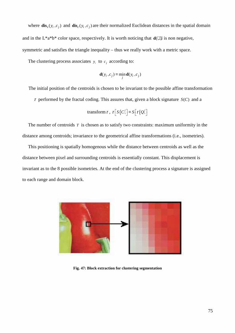
75
where ( )s i jy c,dis and ( )c i jy c,dis are their normalized Euclidean distances in the spatial domain
and in the L*a*b* color space, respectively. It is worth noticing that ( )⋅,⋅d is non negative,
symmetric and satisfies the triangle inequality – thus we really work with a metric space.
The clustering process associates iy to jc according to:
( ) min ( )i j i jj
y c y c, = ,d d
The initial position of the centroids is chosen to be invariant to the possible affine transformation
τ performed by the fractal coding. This assures that, given a block signature ( )S C and a
transformτ , ( ) ( )S C S Qτ τ =
The number of centroids T is chosen as to satisfy two constraints: maximum uniformity in the
distance among centroids; invariance to the geometrical affine transformations (i.e., isometries).
This positioning is spatially homogenous while the distance between centroids as well as the
distance between pixel and surrounding centroids is essentially constant. This displacement is
invariant as to the 8 possible isometries. At the end of the clustering process a signature is assigned
to each range and domain block.
Fig. 47: Block extraction for clustering segmentation
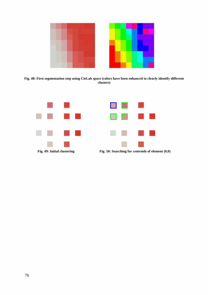
76
Fig. 48: First segmentation step using CieLab space (colors have been enhanced to clearly identify different clusters)
Fig. 49: Initial clustering Fig. 50: Searching for centroids of element (0,0)
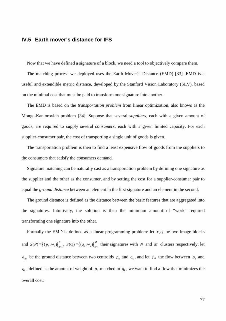
77
IV.5 Earth mover’s distance for IFS
Now that we have defined a signature of a block, we need a tool to objectively compare them.
The matching process we deployed uses the Earth Mover’s Distance (EMD) [33] .EMD is a
useful and extendible metric distance, developed by the Stanford Vision Laboratory (SLV), based
on the minimal cost that must be paid to transform one signature into another.
The EMD is based on the transportation problem from linear optimization, also knows as the
Monge-Kantorovich problem [34]. Suppose that several suppliers, each with a given amount of
goods, are required to supply several consumers, each with a given limited capacity. For each
supplier-consumer pair, the cost of transporting a single unit of goods is given.
The transportation problem is then to find a least expensive flow of goods from the suppliers to
the consumers that satisfy the consumers demand.
Signature matching can be naturally cast as a transportation problem by defining one signature as
the supplier and the other as the consumer, and by setting the cost for a supplier-consumer pair to
equal the ground distance between an element in the first signature and an element in the second.
The ground distance is defined as the distance between the basic features that are aggregated into
the signatures. Intuitively, the solution is then the minimum amount of “work" required
transforming one signature into the other.
Formally the EMD is defined as a linear programming problem: let ,P Q be two image blocks
and { } 1( ) ( , )
N
h h hS P p w
== , { } 1
( ) ( , )M
k k kS Q q w
== their signatures with N and M clusters respectively; let
hkd be the ground distance between two centroids hp and kq , and let hkf the flow between hp and
kq , defined as the amount of weight of hp matched to kq , we want to find a flow that minimizes the
overall cost:
78
( ) ( )1 1
WORKN M
hk hk hkh k
S P S Q f d f= =
, , = ⋅∑∑
with the following constraints:
1
1
1 1 1 1
0 1 1
1
1
min
hkM
hk hkN
hk kh
N M N M
hk h kh k h k
f h N k M
f w h N
f w k M
f w w
=
=
= = = =
≥ ≤ ≤ , ≤ ≤
≤ ≤ ≤
≤ ≤ ≤
= ,
∑
∑
∑∑ ∑ ∑
(1)
The first constraint assures for unidirectional supplies transportation from ( )S P to ( )S Q . With
the second we limit the amount of supplies that can be sent by the clusters in ( )S P to their weights.
The third constraint allows the clusters in ( )S Q to receive no more supplies than their weights,
while the last constraint forces to move as much supplies as possible.
We call this amount the total flow. Once the transportation problem is solved, and we have found
the optimal flow hkf , the EMD is defined as the work normalized by the total flow:
1 1
1 1
EMD[ ( ) ( )]
N M
hk hkh k
N M
hkh k
d f
S P S Q
f
= =
= =
⋅, =
∑∑
∑∑ (2)
The normalization is needed when the two signatures have different total weight, to avoid giving
more importance to smaller signatures. In general, the ground distance hkd can be any distance and
will be chosen according to the problem at hand.
79
We need then to define a ground distance that matches our purposes. For the extraction of range
and domain blocks signatures we deploy a clustering process based on a metric distance as defined
in eq. (1).
Such a distance was a Euclidean based metric able to compare pixels and centroids both in the
spatial color domains. The comparison is restricted in the spatial domain byr , which is the medium
spatial distance between pixels and the initial distribution of centroids.
In the color space the search is limited to the centroids that differ less than the resolution of the
human visual system (i.e., the HVSres). To define the ground distancehkd , we use a similar, but
slight different approach. Although we still keep the boundary for the color component, and we use
the HVSres value to normalize the Euclidean metric, we do not have elements to limit the search
area in the spatial domain.
Therefore, in the spatial domain, we do not set any constraint; we just normalize the distance
component to the maximum measured Euclidean distance between centroids. Moreover, in a
matching process based on signatures as above defined, to the success of the search, the importance
of the spatial component is not the same as the relevance the color component. In fact, in two image
blocks having a similar color distribution, the color position can be very different and this can lead
to a weak best match algorithm. As to the above considerations, we propose the following measure
for the ground distance:
2 2( ) (1 ) ( )
, 0 1s chk h k h kd p q p qλ λ
λ λ
= , + − ,∈ < <
dis dis
� (3)
where ( )s ⋅,⋅dis and ( )c ⋅,⋅dis are the same as in eq. (1), but for the former, here,
,max h k spatialh k
r p q= − . In fact, the parameter λ in eq. (3) weights the importance given to the color
distance respect to the spatial distance and it is chosen as to maximize the quality in the
80
reconstructed image. It is worth remarking that also hkd , as well as ( )⋅,⋅d of eq. (2), is non-negative,
symmetric and satisfies the triangle inequality, hence it is a true metric.
To extract the fractal code, IFS look for similarities between range and domain blocks by
comparing their signatures. IFS work with contractive transformations reducing the size of the
domain blocks to the one of the range blocks.
Therefore, the matching process compares signatures of same total weight. In this case, since the
ground distance hkd is a true metric, also the EMD as to eq. (2) defines a metric space. Moreover, it
can be shown that in this particular case,
1
1
EMD[ ( ) ( )]
1
1
pq
N
h hh
N
k kk
p k
S P S Q d
p w pw
q w qw
w w w
=
=
, <
=
=
= =
∑
∑ (4)
where w is the total weight of the two signatures and ,p q their average centroids. In other
words, the ground distance between the average centroids of two signatures of same total weight is
a lower bound for the EMD between the two signatures.
This property is used by the IFS process to reduce the complexity of the similarities search
algorithm. Using the EMD for the IFS best matching search has several advantages. In fact,
comparing summary information of image blocks extracted by a clustering process leads to an
increased robustness of the search process to the offset errors. This is not true for the pixel based
RMS approach. Moreover, it is less sensitive to quantization errors due to the intrinsic “averaging”
nature of the clustering process.
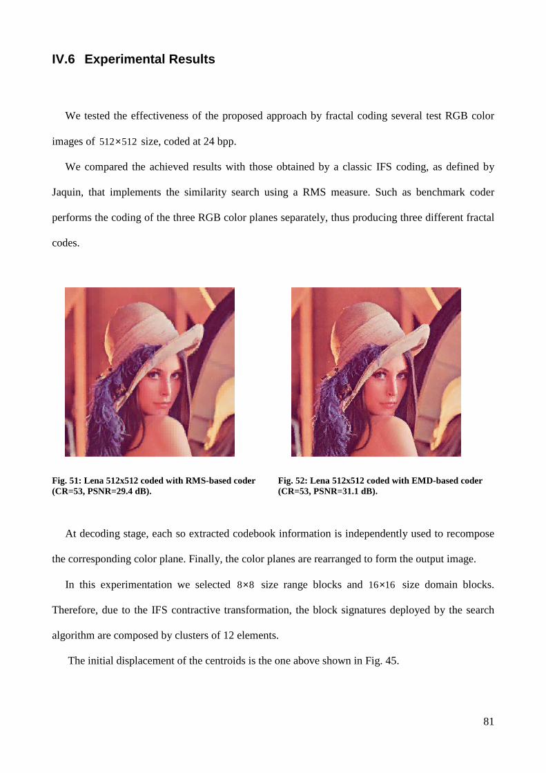
81
IV.6 Experimental Results
We tested the effectiveness of the proposed approach by fractal coding several test RGB color
images of 512 512× size, coded at 24 bpp.
We compared the achieved results with those obtained by a classic IFS coding, as defined by
Jaquin, that implements the similarity search using a RMS measure. Such as benchmark coder
performs the coding of the three RGB color planes separately, thus producing three different fractal
codes.
Fig. 51: Lena 512x512 coded with RMS-based coder (CR=53, PSNR=29.4 dB).
Fig. 52: Lena 512x512 coded with EMD-based coder (CR=53, PSNR=31.1 dB).
At decoding stage, each so extracted codebook information is independently used to recompose
the corresponding color plane. Finally, the color planes are rearranged to form the output image.
In this experimentation we selected 8 8× size range blocks and 16 16× size domain blocks.
Therefore, due to the IFS contractive transformation, the block signatures deployed by the search
algorithm are composed by clusters of 12 elements.
The initial displacement of the centroids is the one above shown in Fig. 45.
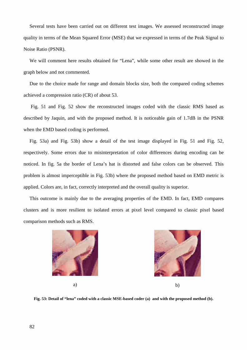
82
Several tests have been carried out on different test images. We assessed reconstructed image
quality in terms of the Mean Squared Error (MSE) that we expressed in terms of the Peak Signal to
Noise Ratio (PSNR).
We will comment here results obtained for “Lena”, while some other result are showed in the
graph below and not commented.
Due to the choice made for range and domain blocks size, both the compared coding schemes
achieved a compression ratio (CR) of about 53.
Fig. 51 and Fig. 52 show the reconstructed images coded with the classic RMS based as
described by Jaquin, and with the proposed method. It is noticeable gain of 1.7dB in the PSNR
when the EMD based coding is performed.
Fig. 53a) and Fig. 53b) show a detail of the test image displayed in Fig. 51 and Fig. 52,
respectively. Some errors due to misinterpretation of color differences during encoding can be
noticed. In fig. 5a the border of Lena’s hat is distorted and false colors can be observed. This
problem is almost imperceptible in Fig. 53b) where the proposed method based on EMD metric is
applied. Colors are, in fact, correctly interpreted and the overall quality is superior.
This outcome is mainly due to the averaging properties of the EMD. In fact, EMD compares
clusters and is more resilient to isolated errors at pixel level compared to classic pixel based
comparison methods such as RMS.
a)
b)
Fig. 53: Detail of “lena” coded with a classic MSE-based coder (a) and with the proposed method (b).
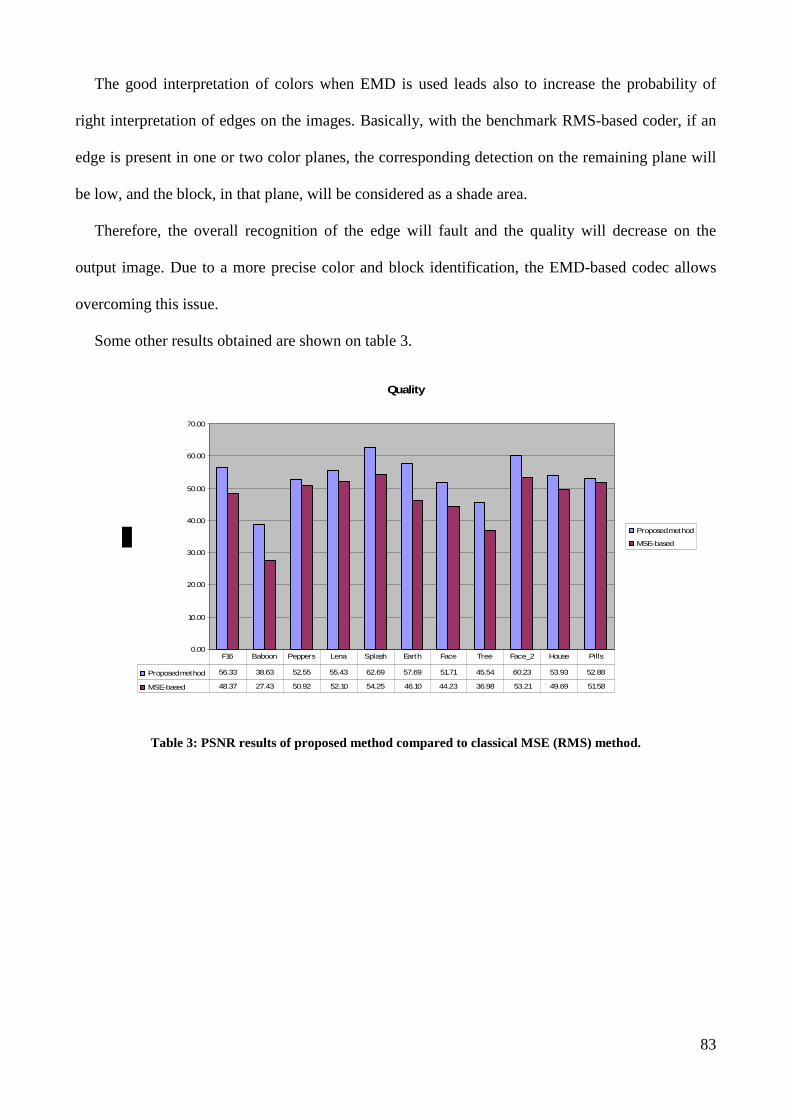
83
The good interpretation of colors when EMD is used leads also to increase the probability of
right interpretation of edges on the images. Basically, with the benchmark RMS-based coder, if an
edge is present in one or two color planes, the corresponding detection on the remaining plane will
be low, and the block, in that plane, will be considered as a shade area.
Therefore, the overall recognition of the edge will fault and the quality will decrease on the
output image. Due to a more precise color and block identification, the EMD-based codec allows
overcoming this issue.
Some other results obtained are shown on table 3.
Quality
0.00
10.00
20.00
30.00
40.00
50.00
60.00
70.00
Proposed method
MSE-based
Proposed method 56.33 38.63 52.55 55.43 62.69 57.69 51.71 45.54 60.23 53.93 52.88
MSE-based 48.37 27.43 50.92 52.10 54.25 46.10 44.23 36.98 53.21 49.69 51.58
F16 Baboon Peppers Lena Splash Earth Face Tree Face_2 House Pills
Table 3: PSNR results of proposed method compared to classical MSE (RMS) method.

84
Chapter V
Conclusions
In this work we proposed two different way of using fractal on different fields, image and
videos, but with a lot of points in common.
Fractal theory is a powerful tool we have not only for compressing these signals, but because it
opens a wide range of interesting features.
The possibility of using fractal coding more on the “decoding” side, i.e. after a video or an
image is downloaded, demonstrated how this tecnique is extremely good to interpolating data
available and obtain zoom, slow motion sequences or frame rate conversions.
There are two main innovations we made on the way of encode signals using fractals.
The first one, related to video sequences, is the joint use of several instruments that made
possible obtain high quality versions of interpolated sequences. The combination of fractal with
wavelet decomposition and moving estimation was successfull, and push us to continue
exploring this path.
A great problem when considering interpolated replicas of data is how to measure the
quality. The problem is in a certain way a philosophical issue since we want to measure how
good is data we obtain compared to data we do not have before.
Some escamotages as first subsample video sequences and after the decoding obtain a full
scale video to be compared with the original one, are, as we said just escamotages, especially
when using objective measures as RMS, that made a low level simple computation between
pixel values instead of measuring the overall high level quality as our brain make.
In this scenario we adopted brand new metrics as the ITU-R BT-1683 [23] metric, which
gave us a more powerful amount of measures that can address our needs.

85
The other main innovation we made was in the encoding of images.
By always focusing on high level quality and our aim (using fractals to interpolate data), we
introduced a different approach on the usual way of fractally encode images.
The use of Earth Mover’s Distance on fractal encoding is original, and the joint use of EMD
with clustering and signature extraction made possible to obtain good results for color images.
As we said at the beginning of this work, fractals have innumerable way of use. The results
obtained in our research demonstrated that a lot of innovation can still be done in this field.
In fact future works can include the use of EMD and clustering also on encoding video
sequences, while instead the use of ORB and OSO can be used for enhance the quality of an
EMD encoded image.
Also all of these tecniques reveal interesting applications on the audio and music field as for
example frame rate conversion or as digital audio effects.
We, in fact, will pursuit this aim and continue to explore the amazing world of fractals.
86
Appendix A
Algorithms for fractal encoding
Introduction
In charter 2 we saw the principles and concepts that lead to apply fractal theory to the image and
video processing fields.
In this appendix we will see the implementation we made for a fractal encoder and decoder,
based on the concepts we developed in the thesis.
We will discuss an algorithmic point of view instead of an actual implementation, like in C or
Java, since it is more general and more intuitive.
The entire actual framework made for this study was entirely developed in ANSI C, and some
parts of the algorithms we will discuss here will contain same of this code.
.
87
Bidimensional fractal encode
The two-dimensional fractal encoder works on gray-level images, or with one layer of color
decomposition. To encode a color image, it should be decomposed in three color layer
decomposition as separated RGB or YIQ layers.
Every image will be partitioned in squared domain and range blocks. We assume that:
• Range blocks have a constant size equal to R
• Domain blocks have a constant size equal to D, which is two times the size of a range
block.
• The Domain Pool is a “Non Overlapped Domain Block”
The last restriction will be removed in a second evolution of the coder, in order to exploit the
ORB and ORC method for zooming images.
Given a starting image origµ the encoder process will be:
for ever Range Block iR on the partition obtained from the starting image origµ :
1) extract l’i-esim Range Block iR ;
2) find the fractal transform of this block;
3) save the fractal code iτ
end
The core of the fractal encoder is the second step, since the first and the last steps are simply
memory access:
88
2.a) from the input Range Block iR compute its luminance iRl and its contrast
iRc
2.b) compute iR with the norm of the Range Block using the luminance and the contrast.
For every Domain Block jD inside the Domain Pool:
2.c) subsample jD to match Range Block’s size
2.d) compute its luminance iDl and its contrast
iDc
2.e) compute jD with the norm of jD using iDl and
iDc
For every isometry k from the isometry set:
2.f) compute the k-esim isometry kjD starting from jD
2.g) compute the error between iR and kjD
2.h) if the error is a local minimum, save iτ composed by information on isometry and
domain used.
end “isometry” loop
end “Domain Block” loop
Now we will take a closer look on each of these points:
2.a) The luminance iRl and the contrast
iRc del of the range block iR is computed the
following way : • Luminance
iRl is the minimum value of luminance among all pixels that composeiR :
( )[ ]yxplii R
RyRx
R ,min11
≤≤≤≤
=
where ( )yxpiR , is a generic pixel of iR whereas R is the size of the Range Block

89
• Contrast iRc is obtained by the overall sum of pixels inside the Range iR . Before the
addition, the previous luminance iRl is subtracted to every pixel’s value.
( )[ ]∑∑= =
−=R
y
R
xRRR
iiilyxpc
1 1
,
2.b) The normalization iR of the range block iR is obtained:
1) From the pixels that belong to the Range Block iR , the luminance iRl is
subtracted (luminance shift) 2) Every pixel is then divided by the contrast
iRc (contrast scaling)
a) b) c) d)
Fig. 54: An example of normalization: a) the range block; b) a three-dimensional representation of the range block; c) luminance shift; d) contrast.
We can explain the overall process using the given range block as an example.
10 7
5 4
It is easy to notice that 4=iRl . To obtain the contrast we subtract the luminance value to
every pixel, and then we sum all the pixels together:
( ) ( ) ( ) ( ) 10444547410 =−+−+−+−=iRc
90
2.c) The generic domain block jD is subsampled by a factor of two (as we stated as a
condition) to have the same dimension of the range block iR
2.d) The same procedure of 2.a) is now executed on jD
2.e) The same procedure of 2.b) is now executed on jD
2.f) A k isometry is chosen
Identity ( ) jiji ,,1 µµτ =
Horizontal reflection ( ) jniji −= ,,2 µµτ
Vertical reflection ( ) jinji ,,3 −= µµτ
First diagonal reflection ( ) ijji ,,4 µµτ =
Second diagonal reflection ( ) injnji −−= ,,5 µµτ
90° counter-clockwise rotation ( ) ijnji ,,6 −= µµτ
180° counter-clockwise rotation ( ) jninji −−= ,,7 µµτ
270° counter-clockwise rotation ( ) injji −= ,,8 µµτ
Allowed isometries
2.g) To compare ranges and transformed domain we need a metric. As a first approximation we
can use the simple MSE between pixels of iR and kjD :
( ) ( ) ( )∑∑= =
−
⋅=
R
y
R
xDRkji yxpyxp
RRDRMSE
kji1 1
2
,,1
,
2.h) Finally the fractal code iτ of the Range Block iR is obtained considering:
• The coordinates ( )jj DD yx , that identify the Domain Block jD (founded as in 2.g that
minimize the MSE error measure) on the encoding image.
• The isometry k that minimize the error measure.
• Luminance iRl ,
jDl and the contrast ratio:
91
i
i
D
Ri c
cc =
All these steps are mandatory, to obtain an efficient matching between Range Blocks iR and all
the isometries of the subsampled Domain BlockjD . This can be proved with a simple example.
Given the following Range Block and Domain Block (the Domain Block is already subsampled to
match the Range Block size):
iR jD
10 7 19 13
5 4 9 7
We can notice that they seem completely different from each other for every isometry applied
to jD .
The luminances of the blocks are: 4=iRl and 7=
jDl . As stated in 2.b.1 we can subtract the
luminance to their respective blocks:
iRi lR − jDj lD −
6 3 12 6
1 0 2 0
4=iRl 7=
jDl
Now we can compute the contrast of the blocks and apply the ratio as in 2.h:
92
( )i
i
R
Ri
c
lR −
( )j
j
D
Dj
c
lD −
0.6 0.3 0.6 0.3
0.1 0 0.1 0
4=iRl 7=
jDl
10=iRc 20=
jDc
As we can see now, the initials blocks that seemed different are now identical.
All the operations made are reversible.
Bidimensional Fractal Decoder
Once we have the fractal code τ computed with the method described above, we can reobtain a
fractal approximation of its initial attractor (the initial image) origµ . We assume that:
• Range Blocks have a constant size of RR ⋅= β'
• Domain Blocks have a constant size 'D which is two times the size of the Range Blocks
• The starting image of the decoding process0µ has a size that is β times the size of the
initial encoded imageorigµ .
The factor β is the zooming factor used at the decoding stage to obtain variable different sizes
of decode image.
93
Given the fractal code τ and a starting image 0µ the decoding stage is composed by the
following steps:
1) for m<α iterations
2) for every iτ of τ
3) read from iτ the domain block coordinates ( )jj DD yx ,
4) extract the Domain Block jD situated at the position ( )jj DD yx ⋅⋅ ββ , of mµ
5) Compute a subsample approximationsub
jD of jD to match the size of iR
6) apply the k isometry extracted from iτ to sub
jD obtaining sub
kjD
7) extract iRl ,
jDl and ic from iτ
8) apply luminance values and contrast to sub
kjD obtaining decodediR
9) write decodediR on 1mµ +
End iτ loop
End iteration loop
The previous steps mean:
1) This loop cycles the whole decoding procedure α times: this is the cycle that generate the
sequence of images that will converge toward the attractor ( origµ or an expanded version of
it)
2) This loop decode all the iτ fractal transform related to the Range Block iR
3) Reads from iτ the coordinates ( )jj DD yx , of Domain Block jD . This domain is the best
transformed domain that the encoder found in the original image origµ for iR
4) Since all the image is zoomed by a factorβ , all the coordinates must be shifted of the same
amount.
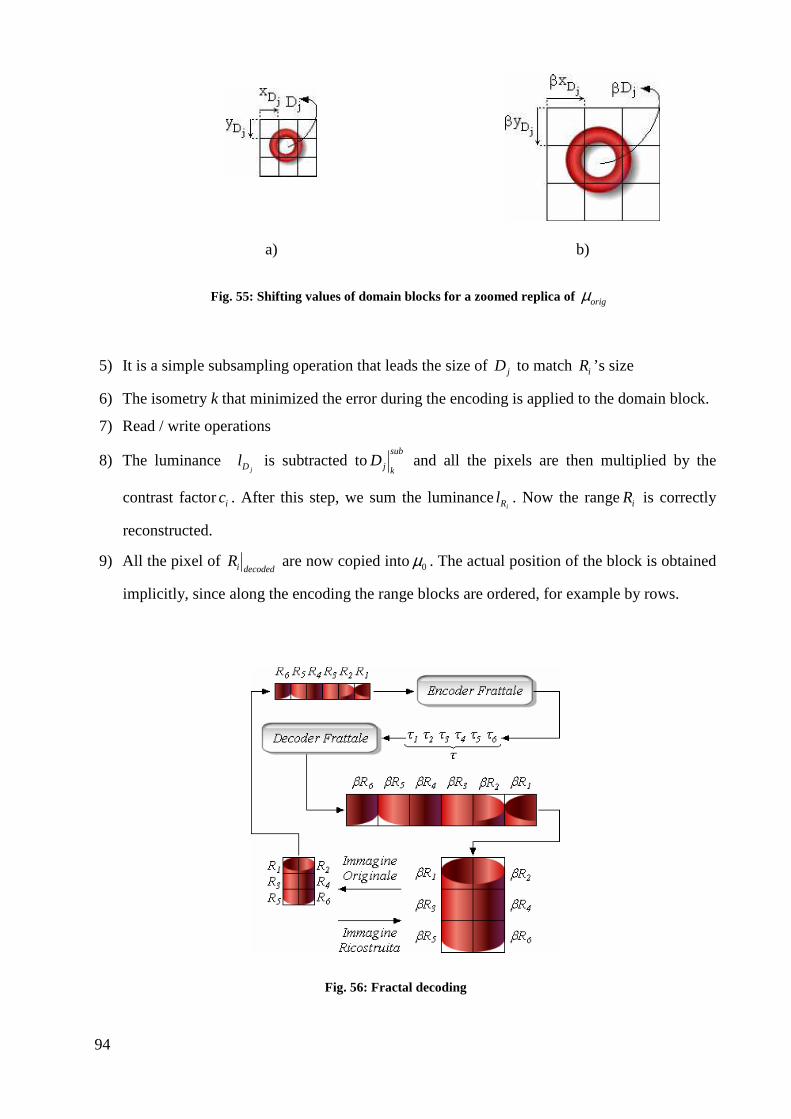
94
a) b)
Fig. 55: Shifting values of domain blocks for a zoomed replica of origµ
5) It is a simple subsampling operation that leads the size of jD to match iR ’s size
6) The isometry k that minimized the error during the encoding is applied to the domain block.
7) Read / write operations
8) The luminance jDl is subtracted to
sub
kjD and all the pixels are then multiplied by the
contrast factoric . After this step, we sum the luminanceiRl . Now the range iR is correctly
reconstructed.
9) All the pixel of decodediR are now copied into0µ . The actual position of the block is obtained
implicitly, since along the encoding the range blocks are ordered, for example by rows.
Fig. 56: Fractal decoding
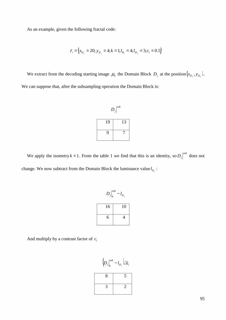
95
As an example, given the following fractal code:
{ }5.0;3;4;1;4;20 ======= iDRDDi cllkyxjijj
τ
We extract from the decoding starting image 0µ the Domain Block jD at the position( )jj DD yx , .
We can suppose that, after the subsampling operation the Domain Block is:
sub
jD
19 13
9 7
We apply the isometry 1=k . From the table 1 we find that this is an identity, sosub
jD does not
change. We now subtract from the Domain Block the luminance valuejDl :
jD
sub
kj lD −
16 10
6 4
And multiply by a contrast factor of ic
( ) iD
sub
kj clDj
⋅−
8 5
3 2
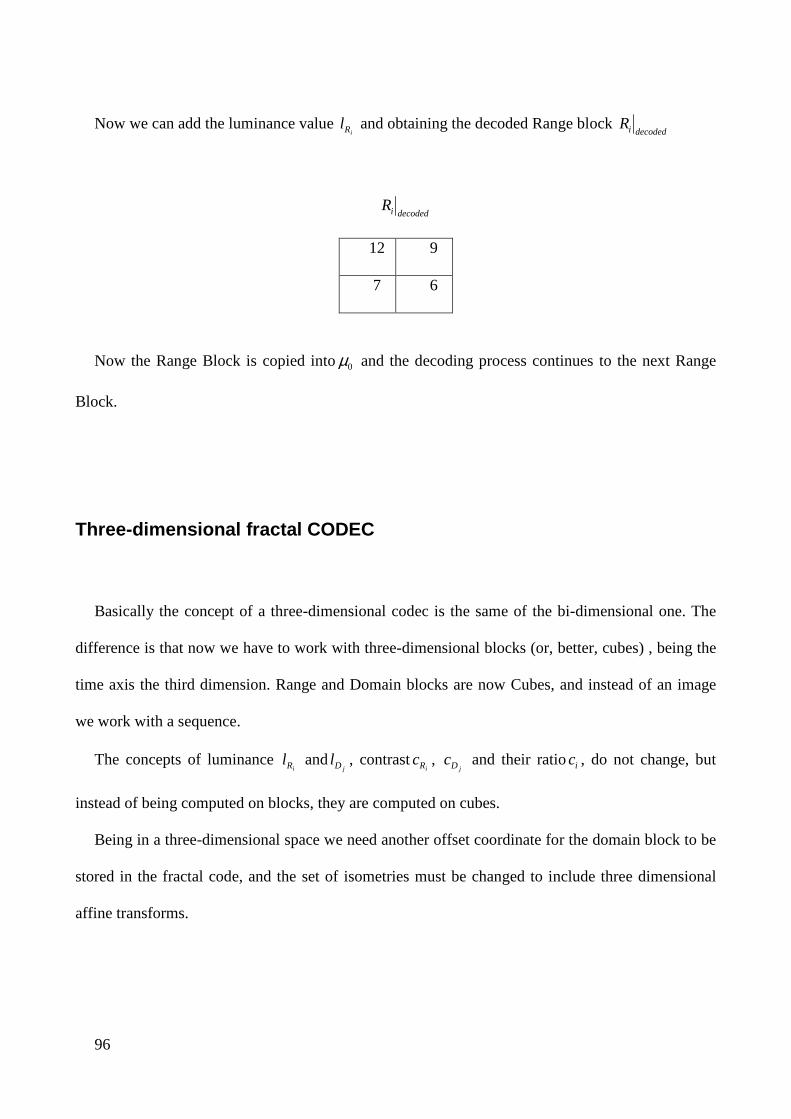
96
Now we can add the luminance value iRl and obtaining the decoded Range block
decodediR
decodediR
12 9
7 6
Now the Range Block is copied into0µ and the decoding process continues to the next Range
Block.
Three-dimensional fractal CODEC
Basically the concept of a three-dimensional codec is the same of the bi-dimensional one. The
difference is that now we have to work with three-dimensional blocks (or, better, cubes) , being the
time axis the third dimension. Range and Domain blocks are now Cubes, and instead of an image
we work with a sequence.
The concepts of luminance iRl and
jDl , contrastiRc ,
jDc and their ratioic , do not change, but
instead of being computed on blocks, they are computed on cubes.
Being in a three-dimensional space we need another offset coordinate for the domain block to be
stored in the fractal code, and the set of isometries must be changed to include three dimensional
affine transforms.
97
Bibliography
[1] R. H. Bartels, J. C. Beatty, and B. A. Barsky, "Hermite and Cubic Spline Interpolation." Ch.
3 in An Introduction to Splines for Use in Computer Graphics and Geometric Modelling.
San Francisco, CA: Morgan Kaufmann, pp. 9-17, 1998.
[2] L.Polidori and J. Chorowicz, “Comparison of Bilinear and Brownian Interpolation for
Digital Elevation Models,” USPRS Journal of Photogrammetry and Remote Sensing, No.48
pp. 18-23. 1993
[3] R.G. Keys, “Cubic Convolution Interpolation for Digital Image Processing,” IEEE trans on
ASSP, No. 29, pag 11153-1160, 1981
[4] G.A. Thomas, “Distorting the time axis: motion compensated image processing in the
studio,” IBC’88 IEE Conference Publication no 293, pp. 256-259.
[5] G.A. Thomas and H.Y.K. Lau, “Generation of high quality slow motion replay using motion
compensation,” Conference Proceeding, IBC September 90, pp. 121-125.
[6] T. Chen, “Adaptive temporal interpolation using bidirectional motion estimation and
compensation”, IEEE International Conference of Image Processing 2002, pp.313-316.
[7] K. Hilman, H.-W. Park, and Y.-M. Kim, “Using motion compensated frame-rate conversion
for the correction of 3:2 pulldown artifacts in video sequences,” IEEE Trans. on CSVT, Vol.
10, No. 6, pp. 869-877, Sep. 2000.
[8] Al-Mualla, M.E.,“Motion field interpolation for frame rate conversion”, IEEE International
Symposium on Circuits and Systems 2003, pp. II 652 -655.
[9] C.W. Tang, O.C. Au, “Comparison between block-based and pixelbased temporal
interpolation for video coding”, IEEE Int. Sym. On Circuits & Systems, Vol. 4, pp.122-125,
May 1998.
[10] B. Mandelbrot, “The Fractal geometry of nature”, Freeman & Co, S. Francisco, 1982.
[11] F. Hausdorff, “Dimension und äu ßeres ma ß”, Math. Ann. 79, 157-179, 1918.
[12] E. N. Lorentz, “The local structure of a chaotic attractor in four dimensions”, Physica 13D,
90-104, 1984.
[13] S. Barnsley and M.F. Demko, “Iterated function systems and the global construction of
fractal,” Proc. Royal Soc. London, A399, pp. 243-275, 1985.
[14] A.E. Jaquin, “Image coding based on a fractal theory of iterated contractive image
trasformation,” IEEE Trans. on Image Processing, vol. 1, no. 1, pp. 18-30, Jan. 1992.

98
[15] Y. Fisher, and R. D. Boss, and E. W. Jacobs, “Fractal image compression: image and text
compression”, Kluwer Academic Publishers, Norwell MA, 1992.
[16] M. Polvere, and M. Nappi, “Speed-Up in Fractal Image Coding: Comparison of Methods,”
IEEE Trans. on Image Processing, vol. 9, no. 6, pp. 1002-1009, Sept. 2000.
[17] S. Mallat, “A theory for multiresolution signal decomposition: The wavelet representation,”
IEEE Trans. Pattern Analysis and Machine Intelligence,1989, vol. 11, pp. 674-693.
[18] E Reusens, “Overlapped Adaptive Partitioning for Image Coding Based on Theory of
Iterated Function Systems,” Proc. IEEE ICASSP, vol 5, pp 569-572, Adelaide, Australia,
1994.
[19] K.U. Barthel and T. Voye, “Three-Dimensional Fractal Video Coding,” Proc. IEEE ICIP-95,
vol 3, pp. 260-263, Washington, D.C., 1995.
[20] K.U. Barthel, T. Voye and G. Ruhl “Combining Wavelet and Fractal Coding for 3-D Video
Coding,” Proc. IEEE ICIP-96, vol. I, pp 181-185, Lausanne, 1996.
[21] M. Ancis and D.D. Giusto, “Image data compression by adaptive vector quantization of
classified wavelet coefficients,” Proc. IEEE PACRIM Conference, pp. 330-333, Victoria,
Canada, 1997.
[22] S. Wolf, “Measuring the End–to–End Performance of Digital Video Systems”, IEEE Trans.
on Broadcasting, vol. 43, no. 3, pp. 320–328, Sept. 1997
[23] ITU-R Recommendation BT.1683, “Objective perceptual video quality measurement
techniques for standard definition digital broadcast television in the presence of a full
reference”, International Telecommunication Union, Geneva, Switzerland, 2004.
[24] Video Quality Research project, http://www.its.bldrdoc.gov/n3/video/Default.htm.
[25] E. Polidori, J.-L. Dugelay, “Zooming using Iterated Function Systems,” NATO ASI
Conference on Fractal Image Encoding and Analysis, Trondheim, July 1995.
[26] D. D. Giusto, M Murroni and G. Soro “Slow Motion Replay of Video Sequences using
Fractal Zooming,” IEEE Trans. on Consumer Electronics, vol. 51, Issue 1,pp.103−111,
February 2005.
[27] B. Hurtgen, P. Mols. and S.F. Simon, “Fractal transformation coding of color images,”
Visual Comunication and Image Processing, SPIE Proceeding, 1994.
[28] Y. Zhang and L.M. Po. “Fractal color image compression using vector distortion measure,”
International Conference on Image Processing. vol. 3, October 1995.
[29] I. M. Danciu and J. C. Hart, “Fractal color compression in the L*a*b* uniform color space,”
Data Compression Conference, March 1998.
99
[30] Y. Rubner, L. J. Guibas and C. Tomasi, “The earth mover’s distance as a metric for image
retrivial”, Technical Report STAN-CS-TN-98-86, Stanford Computer Science Department,
Sept. 1998.
[31] Recommendation ITU-R BT.709-5, “Parameter values for the HDTV standards for
production and international programme exchange” ,1990, 1994,1995, 1998, 2000, 2002.
[32] J. B. MacQueen: "Some Methods for classification and Analysis of Multivariate
Observations, Proceedings of 5-th Berkeley Symposium on Mathematical Statistics and
Probability", Berkeley, University of California Press, 1:281-297, 1967
[33] S. Cohen and L. Guibasm, “The Earth Mover's Distance under transformation sets,”
International Conference on Computer Vision. Vol. 2, pp. 1076 – 1083, Sept. 1999.
[34] S. T. Rachev. “The Monge-Kantorovich mass transference problem and its stochastic
applications,”. Theory of Probability and its Applications, XXIX(4), pp. 647−676, 1984.