identification of arx and ararx models in the presence of input and output noises

European Journal of Control (2010)3:242–255# 2010 EUCADOI:10.3166/EJC.16.242–255

Identification of ARX and ARARX Models in the Presence of Input

and Output Noises

Roberto Diversi�, Roberto Guidorzi��, Umberto Soverini��

Dipartimento di Elettronica, Informatica e Sistemistica. Università di Bologna, Viale del Risorgimento 2, 40136 Bologna, Italy

ARX (AutoRegressive models with eXogenous vari-

ables) are the simplest models within the equation error

family but are endowed with many practical advantages

concerning both their estimation and their predictive

use since their optimal predictors are always stable.

Similar considerations can be repeated for ARARX

models where the equation error is described by an AR

process instead of a white noise. The ARX and ARARX

schemes can be enhanced by introducing the assumption

of the presence of additive white noise on the input and

output observations. These schemes, that will be

denoted as ‘‘ARX þ noise’’ and ‘‘ARARX þ noise’’,

can be seen as errors-in-variables models where both

measurement errors and process disturbances are taken

into account. This paper analyzes the problem of

identifying ARX þ noise and ARARX þ noise models.

The proposed identification algorithms are derived on

the basis of the procedures developed for the solution of

the dynamic Frisch scheme. The paper reports also

Monte Carlo simulations that confirm the effectiveness

of the proposed procedures.

Keywords: System identification, Errors-in-variables

models, ARX models, ARARX models, Dynamic

Frisch scheme

1. Introduction

The identification of dynamic processes can rely on

many families of possible models, describing different

stochastic environments, as well as on different

selection criteria within a specified class of models.

The choice of model families and criteria is often

based more on the planned use of the model rather

than on the adherence of the associated stochastic

contexts to real ones because real processes are in

general more complex than the representations used

for their description.

Equation error models describe a very useful cat-

egory of models because of their wide applicability in

prediction and control [8]. ARX models constitute the

simplest way of representing a dynamic process driven

by an input in presence of uncertainties. In fact, these

models describe the observed output of the process as

the sum of a regression on previous input and output

observations and of a white process that describes the

equation error [9, 12, 16]. This stochastic context, as

well as that of all other equation error models, does

not make explicit assumptions on the origin of the

misfit between the observations and the process

output. It is, however, possible to interpret ARX

models as shown in Fig. 1, i.e. to consider a deter-

ministic part of the process driven by the observed

input u0ðtÞ and characterized, in the scalar case, by a

transfer function Gðz�1Þ ¼ Bðz�1Þ=Aðz�1Þ; the outputy0ðtÞ of this part is not accessible. The stochastic

part of the system, driven by a remote white

�Correspondence to: R. Diversi, E-mail: [email protected]��E-mail: [email protected]��E-mail: [email protected]

Received 5 March 2009; Accepted 14 September 2009Recommended by A. Karimi, L. Ljung

process eðtÞ, is characterized by the transfer function

Fðz�1Þ ¼ 1=Aðz�1Þ and its output is a colored noise

vðtÞ. The observed output is then �yðtÞ ¼ y0ðtÞ þ vðtÞ[9]. In this interpretation, the input is considered as

exactly known and the output as corrupted by an

additive noise whose spectrum is determined by the

poles of the system.

Despite the great simplicity of this scheme, ARX

models have many advantages like the possibility of

performing asymptotically unbiased estimates of their

parameters by means of least squares and the absence

of stability problems in optimal predictors [12]. These

advantages and also the possibility of approximating

other more complex equation error models like

ARMAX ones with high order ARX models have

determined their wide range of applications.

A more complex stochastic environment can be

obtained by describing the equation error by means

of MA or AR processes obtaining ARMAX and

ARARX models (Fig. 2). These models can be more

realistic in some applications; ARMAX models

however do not share the computational advantages

of ARX models and their optimal predictors can be

affected by stability problems. ARARX models, on

the contrary, can be estimated by means of simpler

approaches and their optimal predictors are always

stable since, like ARX ones, describe the expected

value of future outputs by means of the sum of twoMA

processes driven by past input and output observa-

tions. Moreover ARARX models can approximate, at

any desired degree, the family of ARMAX models [9,

16] and this property leads to the use of ARARX

processes also in model reduction [17, 20].

In many practical contexts it is however unrealistic

to assume the existence of exact measurements; quite

often the observation errors have an additive nature

and can be described as white noise. It is thus possible

to enhance the ARX and ARARX schemes by intro-

ducing the assumption of the presence of additive

white noise on the input and output observations.

These schemes (see Figures 3 and 4), that can be

denoted as ‘‘ARXþnoise’’ and ‘‘ARARXþnoise’’,

allow thus taking into account both measurement

errors and process disturbances. This feature is par-

ticularly useful in fault diagnosis and filtering pro-

blems. Note that ARXþnoise models are also denoted

as ‘‘dynamic shock-error models’’ in the econometrics

literature [7, 11].

These models belong to the Errors-In-Variables

(EIV) family and a consistent estimation of their

parameters can no longer be obtained by means of

least squares [14, 21, 22]. Possible identification

approaches could be the joint output [13] and the

maximum likelihood ones [7]. These methods,

however, require representing the noise-free input

u0ðtÞ by means of an ARMA model and rely on time-

consuming numerical procedures whose accuracy

strongly depends on the initial parameter estimates.

The simplest approach that can be adopted is the

instrumental variable one [13]. Despite their compu-

tational efficiency, the accuracy of IV methods is often

poor, since they require the estimation of high-lag

auto and cross covariances [13, 15].

This paper, that completes the results reported in [3]

and [4], proposes a new approach for identifying

ARXþnoise and ARARXþnoise processes. By taking

into account the specific structure of noisy ARX and

ARARX models, that are characterized by three dis-

tinct sources of noise, their identification is mapped

into the identification of EIV models in the Frisch

scheme context. In particular, the dynamic EIV

problem considered in [2] is first extended to the

ARXþnoise case, then, an identification procedure

that takes advantage of the properties of both the

Frisch scheme and the high-order Yule–Walker

equations is developed. The identification of ARA-

RXþnoise models is solved by means of a three–step

procedure. The first step concerns the identification of

an auxiliary high-order ARXþnoise model while the

second and third steps are based on the properties of

polynomials with common factors and can be per-

formed by means of simple least-squares algorithms.

Fig. 1. Interpretation of ARX models. Fig. 2. Interpretation of ARARX models.

Identification of ‘‘ARX þ Noise’’ Models 243

The good performance of the proposed identification

procedures is confirmed by some Monte Carlo simu-

lations.

The paper is organized as follows. Section 2 con-

tains a statement of the problem while Section 3

describes the asymptotic properties of ARXþnoise

processes. Section 4 describes the proposed identi-

fication procedure for ARXþnoise processes and

Section 5 describes the identification of ARA-

RXþnoise processes. Section 6 reports the results

obtained in Monte Carlo simulations and some con-

cluding remarks are finally reported in Section 7.

2. Statement of the Problem

Let us consider the linear ARX model described by

the difference equation

Aðq�1Þ�yðtÞ ¼ Bðq�1Þu0ðtÞ þ eðtÞ; ð1Þ

where u0ðtÞ is the input, �yðtÞ the output and eðtÞ theequation error while Aðq�1Þ;Bðq�1Þ are polynomials

in the backward shift operator q�1

Aðq�1Þ ¼ 1þ a1q�1 þ . . .þ anq

�n ð2Þ

Bðq�1Þ ¼ b0 þ b1q�1 þ . . .þ bnq

�n: ð3Þ

It is assumed that u0ðtÞ and �yðtÞ are corrupted by the

additive noises ~uðtÞ and ~yðtÞ so that the available

measures uðtÞ; yðtÞ are given (see Figure 3) by

uðtÞ ¼ u0ðtÞ þ ~uðtÞ ð4Þ

yðtÞ ¼ �yðtÞ þ ~yðtÞ: ð5Þ

The ARXþnoise model (1)–(5) can be interpreted as

an errors-in-variables model where:

� the true system, whose input and output are u0ðtÞand y0ðtÞ, is described by the difference equation

Aðq�1Þy0ðtÞ ¼ Bðq�1Þu0ðtÞ; ð6Þ

� the noise-free input u0ðtÞ is affected by the meas-

urement error ~uðtÞ;� the noise-free output y0ðtÞ is affected by two noise

contributions, a measurement error ~yðtÞ and a pro-

cess disturbance vðtÞ given by

vðtÞ ¼1

Aðq�1ÞeðtÞ: ð7Þ

In fact, relation (5) can be rewritten as

yðtÞ ¼ �yðtÞ þ ~yðtÞ ¼ y0ðtÞ þ vðtÞ þ ~yðtÞ: ð8Þ

The following assumptions are introduced.

A1. The dynamic system (6) is asymptotically stable, i.e. AðzÞ has all zeros outside the unite circle.

A2. AðzÞ and BðzÞ do not share any common factor.A3. The order n of the system is assumed as a priori

known.A4. The true input u0ðtÞ can be either a zero-mean

ergodic process or a quasi–stationary bounded

deterministic signal, i.e. such that the limit

limN!1

1

N

XNt¼1

u0ðtÞu0ðt� �Þ ð9Þ

exists 8� [12]. Moreover, u0ðtÞ is considered as per-

sistently exciting of sufficiently high order.A5. eðtÞ, ~uðtÞ and ~yðtÞ are zero-mean white processes

with unknown variances �2�e , ~�2�u and ~�2�

y , respect-

ively.

Fig. 3. Structure of ARXþnoise models.

Fig. 4. Structure of ARARX+noise models.

244 R. Diversi et al.

A6. eðtÞ, ~uðtÞ and ~yðtÞ are mutually uncorrelated and

uncorrelated with the noise-free input u0ðtÞ.

The problem to be solved can be stated as follows.

Problem 1. Given a set of noisy input–output obser-

vations uð1Þ; . . . ; uðNÞ; yð1Þ; . . . ; yðNÞ, determine an

estimate of the coefficients akðk ¼ 1; . . . ; nÞ,bkðk ¼ 0; . . . ; nÞ, and of the variances �2�

e , ~�2�u , ~�2�

y .

Remark 1: It is well known that EIV models may not

be uniquely identifiable when only the second order

statistics are considered, see [1]. Note that the

ARXþnoise model (1)–(5) belongs to the class of EIV

models considered in [1]. In fact, from (8)

yðtÞ ¼Bðq�1Þ

Aðq�1Þu0ðtÞ þ

1

Aðq�1ÞeðtÞ þ ~yðtÞ

¼Bðq�1Þ

Aðq�1Þu0ðtÞ þ eyðtÞ; ð10Þ

where eyðtÞ is an additive disturbance that, by using the

spectral factorization theorem [16], can be uniquely

represented as the ARMA model

eyðtÞ ¼Cðq�1Þ

Aðq�1Þ"ðtÞ; ð11Þ

where the stable polynomial Cðq�1Þ of degree n and the

variance �2�" of the white process "ðtÞ are given by

�2�" Cðq�1ÞCðqÞ ¼ ~�2�

y Aðq�1ÞAðqÞ þ �2�e : ð12Þ

3. Asymptotic Properties of Noisy ARX

Models

By introducing the vectors

�’0ðtÞ ¼ ½��yðtÞ . . .� �yðt� nÞ u0ðtÞ . . . u0ðt� nÞ�T

ð13Þ

’ðtÞ ¼ ½�yðtÞ . . .� yðt� nÞ uðtÞ . . . uðt� nÞ�T

¼~½�’T

y ðtÞ’Tu ðtÞ�

T ð14Þ

~’ðtÞ ¼ ½�~yðtÞ . . .� ~yðt� nÞ ~uðtÞ . . . ~uðt� nÞ�T ð15Þ

’eðtÞ ¼ ½eðtÞ 0 . . . 0|fflffl{zfflffl}2nþ1

�T; ð16Þ

and the parameter vector

�� ¼ ½1 a1 � � � an b0 � � � bn�T ¼ ½1 ��0

T�T; ð17Þ

the model (1)–(5) can be written in the form

�’T0 ðtÞ þ ’T

e ðtÞ� �

�� ¼ 0; ð18Þ

’ðtÞ ¼ �’0ðtÞ þ ~’ðtÞ: ð19Þ

Let us now define the covariance matrix

�� ¼ E

��’0ðtÞ þ ’eðtÞ

� ��’0ðtÞ þ ’eðtÞ

�T�; ð20Þ

where E ½�� denotes the expectation operator. Because

of (18), it is possible to write the set of 2nþ 2 relations

�� ¼ 0: ð21Þ

Since E½�yðtÞeðtÞ� ¼ �2�e it is also easy to show that

�� ¼ E½�’0ðtÞ�’T0 ðtÞ� � diag½�2�

e 0 � � � 0|fflffl{zfflffl}2nþ1

�: ð22Þ

From (19) and assumptions A5 and A6 it follows

that

� ¼ E½’ðtÞ’TðtÞ� ¼ E½�’0ðtÞ�’T0 ðtÞ� þ E½~’ðtÞ~’TðtÞ�;

ð23Þ

where

E½~’ðtÞ~’TðtÞ� ¼~�2�y Inþ1 0

0 ~�2�u Inþ1

� �: ð24Þ

By combining (22) and (23) it is easy to obtain the

relation

� ¼ ��þ ~��; ð25Þ

where

~�� ¼

~�2�y þ �2�

e 0

~�2�y In

0 ~�2�u Inþ1

24

35: ð26Þ

The positive definite covariancematrix of the noisy data

� can thus be decomposed into the sum of a positive

semidefinite singular matrix ��, whose kernel defines the

true parameter vector, and of a diagonal matrix ~��.

Consider now the problem of determining the

family of all non–negative definite diagonal matrices~� of the type

~� ¼ diag½~�2y þ �2

e ~�2y � � � ~�

2y|fflfflfflffl{zfflfflfflffl}

n

~�2u � � � ~�

2u|fflfflfflffl{zfflfflfflffl}

nþ1

� ð27Þ

such that

�� ~� � 0; min eigð�� ~�Þ ¼ 0: ð28Þ


This problem, which is similar to the algebraic and

dynamic errors–in–variables problems considered

in [2], consists in determining the set of points P ¼ð~�2

u; ~�2y; �

2eÞ belonging to the first orthant of R 3 satis-

fying (27) and (28), i.e. leading to positive semidefinite

matrices ��ðPÞ ¼ �� ~�ðPÞ with one eigenvalue equal

to zero. This set will be described by the following

results.

Lemma 1: The maximal value of �2e compatible with

(28) is given by

�2emax ¼

detð�Þ

detð�0Þ; ð29Þ

where �0 is obtained from � by deleting its first row

and column.

Proof: Partition � as follows

� ¼�2y �T

� �0

� �; ð30Þ

where �2y is a scalar, so that

��ðPÞ ¼ �� ~�ðPÞ ¼�2y � �2e � ~�2

y �T

� �0 � ~�0ðPÞ

� �;

ð31Þ

with ~�0ðPÞ ¼ diag½~�2y � � � ~�


n

~�2u � � � ~�


nþ1

�. The maximal

admissible value of �2e such that detð��ðPÞÞ ¼ 0 is

obtained in correspondence of ~�2u ¼ ~�2

y ¼ 0. In this case,

detð��ðPÞÞ ¼ detð�0Þð�2y � �2

emax � �T�0�1�Þ ¼ 0

ð32Þ

is satisfied when

�2emax

¼ �2y � �T�0�1� ¼

detð�Þ

detð�0Þ; ð33Þ

where the last equality follows immediately from

detð�Þ ¼ detð�0Þð�2y � �T�0�1�Þ: ð34Þ

Remark 2: The point P ¼ ð0; 0; �2emaxÞ leads to the least

squares solution of Problem 1 since when ~�2u ¼ ~�2

y ¼ 0

equations (1)–(5) describe an ARX model.

Theorem 1: Consider the following partition of �

� ¼�yy �yu

�Tyu �uu

� �; ð35Þ

where the meaning of the blocks follows from (14) and

(23). For every fixed �2e satisfying the condition

0 � �2e < �2

emax ð36Þ

the set of points P ¼ ð~�2u; ~�

2y; �

2eÞ compatible with (28)

is defined by a curve whose intersections with the

planes ~�2y ¼ 0 and ~�2

u ¼ 0 are given by

~�2Mu ¼ min eig �uu � �T

yuð�yy � �eÞ�1�yu

ð37Þ

~�2My ¼ min eig �yy � �e � �yu�

�1uu �

Tyu

; ð38Þ

where �e ¼ diag½�2e 0 � � � 0|fflffl{zfflffl}

n

�.

Proof: Because of partition (35), the matrix ��ðPÞ ¼�� ~�ðPÞ can be partitioned as

��ðPÞ ¼�yy � �e � ~�2

yInþ1 �yu

�Tyu �uu � ~�2

uInþ1

" #:

ð39Þ

If ~�2y ¼ 0 it follows that

detð��ðPÞÞ ¼ detð�yy � �eÞdetð�uu � ~�2uInþ1

��Tyuð�yy � �eÞ

�1�yuÞ; ð40Þ

where condition (36) assures the positive definiteness

of �yy � �e (see Lemma 1). To satisfy condition (28),

the least eigenvalue of ��ðPÞmust be equal to zero and

this holds in correspondence of ~�2u ¼ ~�2M

u given by

(37). Of course ~�2Mu > 0 if and only if

�uu � �Tyuð�yy � �eÞ

�1�yu > 0; ð41Þ

which is equivalent to the condition

�yy � �e �yu

�Tyu �uu

� �> 0; ð42Þ

that is guaranteed by (36) and Lemma 1. In a similar

way it is then possible to prove (38) starting from

relation

detð��ðPÞÞ ¼ detð�uuÞdetð�yy � �e � ~�2yInþ1

��yu��1uu �

TyuÞ; ð43Þ

that holds when ~�2u ¼ 0. The remaining part of the

curve can be characterized by using similar con-

siderations. In fact, for a value ~�2u ¼ k~�2M

u ; ð0 � k < 1Þof the input noise variance given by a fraction of the

maximum admissible value (37), it holds (see (39))


detð��ðPÞÞ ¼ detð�uu � ~�2uInþ1Þ

det �yy � �e � ~�2yInþ1 � �yuð�uu � ~�2

uInþ1Þ�1�T

yu

;

ð44Þ

so that the corresponding value ~�2y is given by

~�2y ¼ min eig �yy � �e � �yuð�uu � ~�2uInþ1Þ

�1�T

yu

:

ð45Þ

The matrix �uu � ~�2uInþ1 is, of course, positive definite

since ~�2u < ~�2M

u . Alternatively, it is possible to consider

a generic value ~�2y ¼ k~�2M

y ; ð0 � k < 1Þ of the output

noise variance, given by a fraction of the maximum

admissible value (38). In this case, since detð��ðPÞÞ canalso be expressed as

detð��ðPÞÞ ¼ detð�yy � �e � ~�2yInþ1Þ

det �uu � ~�2uInþ1 � �T

yuð�yy � �e � ~�2yInþ1Þ

�1�yu

;

ð46Þ

the corresponding value ~�2u is given by

~�2u ¼ min eig �uu � ~�2

uInþ1

��T

yuð�yy � �e � ~�2yInþ1Þ

�1�yuÞ: ð47Þ

The previous results can be summarized as follows.

Theorem 2: The set of all diagonal matrices of type (27)

satisfying condition (28) defines the points P ¼ð~�2

u; ~�2y; �

2eÞ of a surface S ð�Þ belonging to the first

orthant of the noise space R3. Every point P of S ð�Þ

can be associated with a coefficient vector �ðPÞ satis-

fying the relation

��ðPÞ�ðPÞ ¼ 0; ð48Þ

where

��ðPÞ ¼ �� diag½~�2y þ �2

e ~�2y � � � ~�


n

~�2u � � � ~�


nþ1

�

ð49Þ

�ðPÞ ¼ 1 a1ðPÞ � � � anðPÞ b0ðPÞ � � � bnðPÞ½ �T: ð50Þ

Note that �ðPÞ is a normalized basis (first coefficient

equal to one) of kerð��ðPÞÞ. Fig. 5 shows a typical

shape of S ð�Þ. Relations (21) and (25) lead easily to

the following important corollary.

Corollary 1: The point P� ¼ ð~�2�u ; ~�2�

y ; �2�e Þ, associated

with the true variances of ~uðtÞ, ~yðtÞ and eðtÞ belongs to

S ð�Þ and the coefficient vector �ðP�Þ is characterizedby the true parameters, i.e. �ðP�Þ ¼ ��. In this asymp-

totic context Problem 1 consists thus in finding, by

means of a suitable selection criterion, the point P� on

S ð�Þ.

4. Identification of Noisy ARX Models

This section describes a selection criterion based

on the properties of high-order Yule–Walker equa-

tions. This criterion will be used in the solution of

Problem 1.

Define the � 1ð� � 1Þ vectors

’�u0ðtÞ ¼ ½u0ðt� n� 1Þ . . . u0ðt� n� �Þ�T ð51Þ

’�uðtÞ ¼ ½uðt� n� 1Þ . . . uðt� n� �Þ�T ð52Þ

’�~uðtÞ ¼ ½~uðt� n� 1Þ . . . ~uðt� n� �Þ�T; ð53Þ

that, because of (4), satisfy the condition

’�uðtÞ ¼ ’�

u0ðtÞ þ ’�

~uðtÞ: ð54Þ

Define also the covariance matrix

�� ¼ E½’�uðtÞ’

TðtÞ�: ð55Þ

Because of (54) and assumptions A5–A6, we have

�� ¼ E½’�u0ðtÞ�’T

0 ðtÞ� ¼ E½’�u0ðtÞð�’0ðtÞ þ ’eðtÞÞ

T�;

ð56Þ

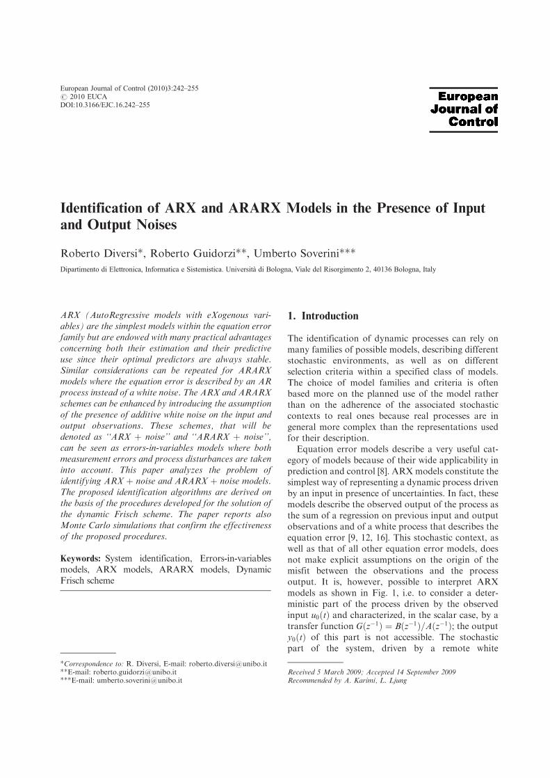
Fig. 5. Typical shape of S ð�Þ.


so that from (18)

�� ¼ 0: ð57Þ

Relation (57) constitutes a set of high-order Yule–

Walker equations that could be directly used to obtain

the parameter vector ��. In this paper, these equations

are used jointly with the results of Theorem 2 and

Corollary 1 in order to solve Problem 1. In fact, on the

basis of the above considerations, the search for the

point P� on S ð�Þ can be performed by minimizing the

cost function

JðPÞ ¼ k��ðPÞk22 ¼ �TðPÞð��ÞT��ðPÞ;

P 2 S ð�Þ; ð58Þ

that exhibits the following properties

(i) JðPÞ � 0

(ii) JðP�Þ ¼ 0.

In practice, since only a finite number N of data is

available, the matrices � and �� must be replaced by

the sample estimates

� ¼1

N� n� �

Xt¼N

t¼nþ�þ1

’ðtÞ’TðtÞ; ð59Þ

�� ¼1

N� n� �

Xt¼N

t¼nþ�þ1

’�uðtÞ’

TðtÞ: ð60Þ

It is still possible to define a locus of possible solutions

S ð�Þ satisfying condition (28). In this case P� 62 S ð�Þand the minimum of the cost function JðPÞ will be nolonger equal to zero. However, because of the ergo-

dicity assumption we have

limN!1

� ¼ �; limN!1

�� ¼ ��; a:s: ð61Þ

so that

S ð�Þ!N!1

S ð�Þ a:s: ð62Þ

and the cost function JðPÞ will satisfy, asymptotically,

conditions i) and ii).

The implementation of the identification procedure

can take advantage of a different parameterization of

S ð�Þ that allows to associate a solution of (28) with

every straight line departing from the origin and lying

in the first orthant of R3. This parameterization,

introduced in [10], is described by the next theorem.

Theorem 3: Let � ¼ ð�1; �2; �3Þ be a generic point of the

first orthant of R 3 and r the straight line from the origin

through �. Its intersection with S ð�Þ is the point P ¼ð~�2

u; ~�2y; �

2eÞ given by

~�2u ¼

�1�M

; ~�2y ¼

�2�M

; �2e ¼

�3�M

; ð63Þ

where

�M ¼ max eig ��1diag½�2 þ �3 �2 � � � �2|fflfflfflffl{zfflfflfflffl}n

�1 � � � �1|fflfflfflffl{zfflfflfflffl}nþ1

�

0@

1A:

ð64Þ

Proof: Since both � and P belong to r there exists a

scalar � such that � ¼ �P. Moreover, the entries of P

must satisfy the conditions

�� ~�ðPÞ � 0; min eigð�� ~�ðPÞÞ ¼ 0; ð65Þ

where

~�ðPÞ ¼ diag½~�2y þ �2

e ~�2y � � � ~�


n

~�2u � � � ~�


nþ1

�: ð66Þ

The second condition implies that

detð�� ~�ðPÞÞ ¼ det ��1

�~��

� �¼ 0; ð67Þ

where

~�� ¼ diag½�2 þ �3 �2 � � � �2|fflfflfflffl{zfflfflfflffl}n

�1 � � � �1|fflfflfflffl{zfflfflfflffl}nþ1

� ð68Þ

or, equivalently

det��1det I2nþ2 �1

��1 ~��

� �¼ 0: ð69Þ

The scalar � satisfying (69) is thus given by

� ¼ max eigð��1 ~��Þ: ð70Þ

The previous considerations allow to formulate the

following algorithm.

Algorithm 1.

1. Compute, on the basis of the available observa-

tions the sample estimates � and �� by using (59)

and (60).

2. Start from a generic direction r belonging to the

first orthant of R 3.


3. Compute, by means of (63)–(64), the intersection

P ¼ ð~�2u; ~�

2y; �

2eÞ between r and S ð�Þ.

4. Compute ��ðPÞ and �ðPÞ by means of the relations

��ðPÞ ¼ �� diag½~�2y þ �2

e ~�2y � � � ~�


n

~�2u � � � ~�


nþ1

�

��ðPÞ�ðPÞ ¼ 0;

and normalize the first entry of �ðPÞ to 1.

5. Compute the cost function

JðPÞ ¼ k��ðPÞk22: ð71Þ

6. Move to a new direction r�r corresponding to a

decrease of JðPÞ.7. Repeat steps 3–6 until the point P ¼ ð ~�2

u; ~�2y; �

2eÞ

associated with the minimum of JðPÞ is found.8. The estimates of the model coefficients and of the

noise variances are given by �ðPÞ and ~�2u; ~�

2y; �

2e .

Remark 3: Possible variations of the proposed proced-

ure can rely on the choice of different instrument vec-

tors, such as

’�yðtÞ ¼ ½yðt� n� 1Þ : : : yðt� n� �Þ�T ð72Þ

’�uyðtÞ ¼ ½yðt� n� 1Þ : : : yðt� n� �Þ uðt� n� 1Þ

: : : uðt� n� �Þ�T: ð73Þ

Both choices satisfy (57).

Remark 4: As already mentioned, an estimation of ��

can be directly obtained from equations (57). In fact, by

partitioning �� as follows

�� ¼ r R�;�

ð74Þ

where r is a column and using (17), it is possible to

compute the estimate

�IV0 ¼ � RTR� ��1

RTr: ð75Þ

This approach can be viewed as an instrumental

variable (IV) method that uses delayed inputs as

instruments [13, 14]. Note that, if � � 2nþ 1, the

consistency of the IV estimator is guaranteed when R

has full rank. It is possible to show that, under

Assumption A2, this is a persistence of excitation like

condition on the noise-free input u0ðtÞ [16, 18]. Note

that the above conclusion holds also when the input

noise is finitely auto-correlated and the output noise is

arbitrarily auto-correlated [18]. Even if it is not pos-

sible to guarantee the consistency of (75) for every

input signal most inputs satisfy the aforementioned

‘‘persistence of excitation’’ condition (see the discus-

sion on generic consistency in [16]). Anyway, it is

important to note that, since R can be estimated from

the data, its rank can be tested [18].

IV approaches are simpler from the computational

point of view but can lead to a poor estimation

accuracy [15] as shown also in Section 6.Moreover, no

estimations of �2�e , ~�2�

u and ~�2�y are obtained.

Remark 5: If the variances ~�2�u , ~�2�

y and �2�e are known

up to the same scalar factor, the identification problem

can be solved by means of the Koopmans-Levin (KL)

method [6], that leads to the same solution as the total

least squares approach [23]. It can be easily shown

that this solution belongs to the set S ð�Þ. For

this purpose, assume that ~�� ¼ �� ~�, where ~� ¼diag½3; 2In; 1Inþ1� is known. The KL solution is

obtained by computing the minimum value of � satis-

fying the relation

ð�� ~�Þ� ¼ 0; ð76Þ

which is given by

� ¼ min eig �ð~�Þ�1

; ð77Þ

or, equivalently

1

�¼ max eig ��1 ~�

� �: ð78Þ

Relation (78) is indeed preferable since it yields the

solution also when ~� is singular. Since � satisfies the

condition

�� ~� � 0; min eigð�� ~�Þ ¼ 0; ð79Þ

the KL solution belongs to S ð�Þ. By comparing (63),

(64) with (78) if follows that the KL solution

can be obtained by applying Theorem 3 with

� ¼ ð1; 2; 3 � 2Þ. Asymptotically, since � ! � it

follows that � ! ��.

5. Identification of Noisy ARARX Models

This section shows how the proposed ARXþnoise

identification method can be used also for identifying

ARARXþnoise models. With reference to Fig. 4,

consider an ARARXmodel described by the equation

Aðq�1Þ�yðtÞ ¼ Bðq�1Þu0ðtÞ þeðtÞ

Dðq�1Þ; ð80Þ


where

Aðq�1Þ ¼ 1þ a1q�1 þ : : : þ anq

�n ð81Þ

Bðq�1Þ ¼ b0 þ b1q�1 þ : : : þ bnq

�n ð82Þ

Dðq�1Þ ¼ 1þ d1q�1 þ : : : þ dndq

�nd : ð83Þ

Again it is assumed that u0ðtÞ and �yðtÞ are corrupted

by the additive noises ~uðtÞ and ~yðtÞ so that the avail-

able measures uðtÞ; yðtÞ are given by (4) and (5). The

whole system can still be viewed as in (6)–(8). The

only difference concerns the colored noise vðtÞ whichis now given by

vðtÞ ¼1

Aðq�1ÞDðq�1ÞeðtÞ: ð84Þ

In this case, however, the set of process disturbances

that can be modelled is wider. In fact, since a moving

average process driven by white noise can be

approximated by an autoregessive process of suitably

high order [5, 12, 16], vðtÞ can approximate a generic

ARMA modelCðq�1ÞAðq�1Þ

eðtÞ. As a consequence, ARARX

models can approximate ARMAX structures.

In addition to A1-A6, consider the following

assumptions.

A7. DðzÞ has all zeros outside the unit circle.A8. The order nd is a priori known.

The identification of ARARXþnoise models can

thus be defined as follows.

Problem 2. Estimate the coefficients akðk ¼ 1; . . . ; nÞ,bkðk ¼ 0; . . . ; nÞ, dkðk ¼ 1; . . . ; ndÞ and the noise var-

iances �2�e , ~�2�

u , ~�2�y on the basis of a sequence of input–

output observations uð1Þ; . . . ; uðNÞ, yð1Þ; . . . ; yðNÞ.By defining the polynomials of degree �n ¼ nþ nd

�Aðq�1Þ ¼ Aðq�1ÞDðq�1Þ ð85Þ

�Bðq�1Þ ¼ Bðq�1ÞDðq�1Þ; ð86Þ

with coefficients

�Aðq�1Þ ¼ 1þ 1q�1 þ . . .þ �nq

��n ð87Þ

�Bðq�1Þ ¼ �0 þ �1q�1 þ . . .þ ��nq

��n; ð88Þ

it is possible to rewrite (80) as

�Aðq�1Þ�yðtÞ ¼ �Bðq�1Þu0ðtÞ þ eðtÞ; ð89Þ

i.e. as an �n-order ARX process. This model can

be written in the vector form (18) and (19) by repla-

cing n with �n in (13)–(16) and �� with the parameter

vector

#� ¼ 1 1 � � ��n�0 � � ��n½ �T: ð90Þ

The ARX model (89) and the noise variances �2�e ;

~�2�u ; ~�2�

y can thus be identified by means of

Algorithm 1.

Once that an estimate # of #� has been obtained,

the coefficients of Aðq�1Þ, Bðq�1Þ and Dðq�1Þ can be

estimated by taking into account the properties

of polynomials with common factors. For this

purpose, multiply (85) byBðq�1Þ and (86) byAðq�1Þ toobtain

�Aðq�1ÞBðq�1Þ � �Bðq�1ÞAðq�1Þ ¼ 0: ð91Þ

This expression can also be written in the matrix form

ST��0 ¼ 0; ð92Þ

where S is the ð2nþ 2Þ ð�nþ nþ 1Þ Sylvester

matrix

S ¼

�0 �1 : : : ��n 0 : : : 0

0 �0 �1 : : : ��n : : : 0

..

. . .. . .

. . .. ..

.

0 : : : 0 �0 �1 : : : ��n

�1 �1 : : : ��n 0 : : : 0

0 �1 �1 . . . ��n : : : 0

..

. . .. . .

. . .. ..

.

0 : : : 0 �1 �1 : : : ��n

26666666666664

37777777777775:

ð93Þ

By partitioning ST as

ST ¼ ½mM�; ð94Þ

where m is the first column of ST and taking into

account (17) it follows that [19]

mþM��0 ¼ 0: ð95Þ

An estimate of ��0 can thus be computed as

�0 ¼ � MTM� ��1

MTm; ð96Þ

where M and m are constructed with the entries of #.Since relations (85) and (86) can be jointly written in

the matrix form

#� ¼ G�D; ð97Þ


where

and

�D ¼ 1d1 � � � dn½ �T; ð99Þ

the coefficients of Dðq�1Þ can finally be estimated as

follows

�D ¼ GTG� ��1

GT#; ð100Þ

where G is constructed with the entries of �0.The whole ARARXþnoise identification procedure

can be summarized as follows.

Algorithm 2.

1. Estimate the high–order ARX model (89) and the

variances �2�e , ~�2�

u , ~�2�y by means of Algorithm 1.

Let # be the estimate of #�.

2. Construct, with the entries of #, the vector m and

the matrix M as in (93) and (94) and compute an

estimate �0 of ��0 by means of (96).

3. Construct, with the entries of �0, the matrix G with

structure (98) and compute an estimate of Dðq�1Þby means of (100).

6. Numerical Results

This section shows the performance of the proposed

ARXþnoise and ARARXþnoise identification tech-

niques by means of numerical simulations.

6.1. Example 1

The behavior of Algorithm 1 has been tested on

sequences generatedby the followingmodelofordern ¼ 2

Aðq�1Þ ¼ 1� 0:5q�1 þ 0:3q�2

Bðq�1Þ ¼ 1:2� 0:7q�1 � 0:3q�2:

The noise–free input u0ðtÞ is a pseudo random binary

sequence of unit variance and length N ¼ 1000 while

the variances of the process, input and output noises

are given by

�2�e ¼ 0:2; ~�2�u ¼ 0:1; ~�2�

y ¼ 0:3:

These values correspond to signal to noise ratios on

the input and output of SNRI ¼ 12dB and

SNRO � 2dB, where

SNRI ¼ 20 log10

ffiffiffiffiffiffiffiffiffiffiffiffiffiffiffiffiE½u20ðtÞ�

E½~u2ðtÞ�

s¼ 20 log10

ffiffiffiffiffiffiffiffiffiffiffiffiffiffiffiffiE½u20ðtÞ�

~�2�u

s

SNRO ¼ 20 log10

ffiffiffiffiffiffiffiffiffiffiffiffiffiffiffiffiffiffiffiffiffiffiffiffiffiffiffiffiffiffiffiE½y20ðtÞ�

E½v2ðtÞ þ ~y2ðtÞ�

s

¼ 20 log10

ffiffiffiffiffiffiffiffiffiffiffiffiffiffiffiffiffiffiffiffiffiffiffiffiffiffiffiffiffiffiffiE½y20ðtÞ�

ðE½v2ðtÞ� þ ~�2�y Þ

s�

The ARX models have been identified by using both

Algorithm 1 and the IV estimator (75). The user–chosen

parameter � has been set to 5 forAlgorithm 1while three

different values � ¼ 5; � ¼ 10; � ¼ 20 have been tested

for the IV approach. A Monte Carlo simulation of 100

independent runs has been performed. Each run is

characterized bydifferent gaussianwhite noise sequences

eð�Þ; ~uð�Þ; ~yð�Þ. The results are summarized in Tables 1

and 2 that report the true values of parameters and

variances, themeans of their estimates and the associated

standard deviations. The estimate accuracy obtained

with Algorithm 1 is very good for both parameters and

noise variances. It is worth to stress that the use of larger

values of � does not lead to significative improvements.

The IV estimator gives very poor estimates for � ¼ 5. To

obtain satisfactory results it is necessary to use large

values of � and this reduces the computational advan-

tages associated with the IV approach. Moreover, the

choice of � becomes a critical issue.

The good selectivity of the cost function (71) is

shown in Figures 6 and 7, which refer to a typical run

of the Monte Carlo simulation. Figure 6 reports the

values of JðPÞ versus ~�2y for a fixed value of �2e .

In particular, this figure refers to the value �2e ¼ �2

e .

Fig. 7 reports, for every fixed value of �2e

(0 � �2e < �2

emax) the minimum Jemin of JðPÞ.

6.2. Example 2

In this section the performance of Algorithm 1 is

compared to that of the joint output (JO) approach

G ¼

1 a1 : : : an 0 : : : 0

0 1 a1 : : : an : : : 0

..

. . .. . .

. . .. ..

.

0 : : : 0 1 a1 : : : an

b0 : : : bn 0 : : : 0

0 b0 : : : bn : : : 0

..

. . .. . .

. ...

0 : : : 0 b0 : : : bn

26664

37775T

; ð98Þ


[13]. For this purpose, consider the following model of

order n ¼ 2

Aðq�1Þ ¼ 1� 1:5q�1 þ 0:7q�2

Bðq�1Þ ¼ q�1 þ 0:5q�2:

The noise–free input u0ðtÞ is the ARMA process

u0ðtÞ ¼1

1� 0:9q�1wðtÞ;

where wðtÞ is a zero mean gaussian white noise with

unit variance. The noises eðtÞ; ~uðtÞ; ~yðtÞ are gaussian

white noise sequences with variances �2�e ¼ 4, ~�2�u ¼ 1

and ~�2�y ¼ 2. The methods have been compared by

considering the following number of samples:

N ¼ 250; 500; 1000; 1500; 2000. For each value of N a

Monte Carlo simulations of 100 independent runs

has been performed by setting � ¼ 5 for Algorithm 1.

The normalized root mean square error

NRMSE ¼1

k��0ðiÞk

ffiffiffiffiffiffiffiffiffiffiffiffiffiffiffiffiffiffiffiffiffiffiffiffiffiffiffiffiffiffiffiffiffiffiffiffiffiffiffiffiffiffiffiffiffi1

M

XMi¼1

k�kðiÞ � ��0ðiÞk2

vuut ;

ð101Þ

has been used as performance index of the estimation,

where �kðiÞ denotes the estimate of the i-th element of

��0 obtained in the k-th run of the Monte Carlo

simulation while M is the number of runs (100 in this

case). The results have been reported in Fig. 8.

To compare the computational load of Algorithm 1

and of the JO approach, Table 3 reports the mean

values (in seconds) of the CPU time requested to carry

out a single run of the Monte Carlo simulations. Even

though this value cannot be considered as a precise

measure of the computational efficiency of the con-

sidered methods, it provides the correct order of

magnitude.

As it can be observed, the proposed procedure

represents a good trade-off between estimation

Table 1. True and estimated values of the coefficients ofAðq�1Þ and Bðq�1Þ. A Monte Carlo simulation of 100 runs has beenperformed with N ¼ 1000

a1 a2 b0 b1 b2

true �0:5 0:3 1:2 �0:7 �0:3Alg: 1 ð� ¼ 5Þ �0:4949 0:0453 0:2944 0:0401 1:1956 0:0408 �0:6932 0:0721 �0:3051 0:0664IV ð� ¼ 5Þ �0:4590 0:2381 0:3166 0:2514 1:3281 4:4367 �0:1814 4:5380 �0:3752 2:4048IV ð� ¼ 10Þ �0:4982 0:0486 0:2909 0:0493 1:1433 0:3758 �0:7049 0:3898 �0:3665 0:5235IV ð� ¼ 20Þ �0:4909 0:0481 0:2916 0:0407 1:1212 0:2480 �0:6596 0:2871 �0:2959 0:2999

Table 2. True and estimated values of the variances of ~uðtÞ, ~yðtÞ and eðtÞ. A Monte Carlo simulation of 100 runs has beenperformed with N ¼ 1000

~�2�u ~�2�y �2�

e

true 0:1 0:3 0:2Alg: 1 ð� ¼ 5Þ 0:0955 0:0326 0:2961 0:0485 0:2061 0:0555

Fig. 6. Typical shape of JðPÞ versus ~�2y for a fixed admissible valueof �2

e .

Fig. 7. Minimum values of JðPÞ for every fixed value of �2e suchthat 0 � �2e < �2emax.


Fig. 8. Normalized root mean square errors of the estimated system parameters versus the number of samples: Algorithm 1 (solid), jointoutput approach (dashed). For every value of N a Monte Carlo simulation of 100 runs has been performed.

Table 3. Mean values (in seconds) of the CPU time requested to carry out a single run of the Monte Carlo simulations. Forevery value of N a Monte Carlo simulation of 100 runs has been performed

N 250 500 1000 1500 2000Alg:1 0:1151 0:0859 0:0855 0:0881 0:1264JO 2:6485 1:9285 2:1436 2:6041 3:8437

Table 4. True and estimated values of the coefficients of Aðq�1Þ, Bðq�1Þ and Dðq�1Þ. A Monte Carlo simulation of 100 runshas been performed with N ¼ 1000

a1 a2 b1 b2 d1

true �0:5 0:06 1 �0:7 0:95Alg: 2 ð� ¼ 7Þ �0:5086 0:0554 0:0561 0:0290 0:9961 0:0396 �0:7099 0:0858 0:9461 0:0305IV ð� ¼ 7Þ �0:4062 0:8771 0:0694 0:2289 0:9028 0:9211 �0:5657 1:0762 0:3566 0:8454IV ð� ¼ 20Þ �0:3914 0:1673 0:0699 0:0862 0:9381 0:1201 �0:5667 0:2348 0:7014 0:2350IV ð� ¼ 35Þ �0:4235 0:1094 0:0690 0:0597 0:9288 0:0837 �0:5688 0:1574 0:7717 0:1491

Table 5. True and estimated values of the variances of ~uðtÞ, ~yðtÞ and eðtÞ. A Monte Carlo simulation of 100 runs has beenperformed with N ¼ 1000

~�2�u ~�2�y �2�

e

true 0:06 0:02 0:1Alg: 2 ð� ¼ 7Þ 0:0549 0:0344 0:0200 0:0079 0:1025 0:0562


accuracy and computational efficiency. It is worth to

remember that the JO approach, that is based on a

prediction error method, may fail to give good results

if the initial parameter estimate is poor. Moreover, it

requires to model the noiseless input as an ARMA

process.

6.3. Example 3

The effectiveness of Algorithm 2 has been tested by

means of numerical simulations performed on the

following ARARX model, already used in [20]

Aðq�1Þ ¼ 1� 0:5q�1 þ 0:06q�2

Bðq�1Þ ¼ q�1 � 0:7q�2

Dðq�1Þ ¼ 1þ 0:95q�1:

The noise–free input is a pseudo random binary

sequence with unit variance and length N ¼ 1000

while the noises eðtÞ; ~uðtÞ; ~yðtÞ are gaussian white

noise sequences with variances �2�e ¼ 0:1, ~�2�

u ¼ 0:06and ~�2�

y ¼ 0:02. These values correspond to signal to

noise ratios on the input and output of SNRI �12dB and SNRO � 4dB. The ARARX models have

been identified by using both Algorithm 2 and the IV

estimator. A Monte Carlo simulation of 100 inde-

pendent runs has been performed by setting � ¼ 7 for

Algorithm 2 while the values � ¼ 7; � ¼ 20; � ¼ 35

have been considered for the IV approach. Every run

is characterized by different gaussian white noise

sequences eð�Þ; ~uð�Þ; ~yð�Þ. The results are summarized

in Tables 4 and 5 that report the true values of

parameters and variances, the means of their esti-

mates and the associated standard deviations. The

obtained results confirm the observations reported

in Subsection 6.1

7. Conclusions

This paper has considered an extension of traditional

ARX and ARARX processes by introducing the

assumption of additive white noise on the input and

output observations. Identification procedures for

these new ARXþnoise and ARARXþnoise models

have been developed on the basis of the properties of

the solution locus of the dynamic Frisch scheme and

high-order Yule-Walker equations.

The performance of the proposed procedures has

been tested by means of Monte Carlo simulations

and has been compared with those of other EIV

identification methods. On the basis of the obtained

results, it can be observed that the new algorithms are

characterized by a good trade-off between estimation

accuracy and computational efficiency.

References

1. Aguero JC, Goodwin GC. Identifiability of errorsin variables dynamic systems. Automatica 2008; 44:371–382

2. Beghelli S, Guidorzi R, Soverini U. The Frisch schemein dynamic system identification. Automatica 1990; 26:171–176

3. Diversi R, Guidorzi R, Soverini U. Identification ofARX models with noisy input and output. In: Proceed-ings of the 9th European Control Conference, Kos,Greece, 2007, pp. 4073–4078

4. Diversi R, Guidorzi R, Soverini U. Identification ofARARX models in presence of additive noise. In:Proceedings of the 17th IFAC World Congress, Seoul,Korea, 2008, pp. 432–437

5. Durbin J. Efficient estimation of parameters in moving-average models. Biometrika 1959; 46: 306–316

6. Fernando KV, Nicholson H. Identification of linearsystems with input and output noise: the Koopmans–Levin method. IEE Proc 1985; 132: 30–36

7. Ghosh D. Maximum likelihood estimation of thedynamic shock-error model. J Econ 1989; 41: 121–143

8. Goodwin GC, Sin KS.Adaptive Filtering, Prediction andControl. Prentice-Hall, Englewood Cliffs, NJ, 1984

9. Guidorzi R. Multivariable System Identification: FromObservations to Models. Bononia University Press,Bologna, Italy, 2003

10. Guidorzi R, Pierantoni M. A new parametrization ofFrisch scheme solutions. In: Proceedings of the 12thInternational Conference on Systems Science, Wroclaw,Poland, 1995, pp. 114–120

11. Krishnamurthy V. On-line estimation of dynamicshock-error models based on the Kullback–Leiblerinformation measure. IEEE Trans Autom Control1994; 39: 1129–1135

12. Ljung L. System Identification – Theory for the User.Prentice-Hall, Englewood Cliffs, NJ, 1999

13. Soderstrom T. Identification of stochastic linearsystems in presence of input noise. Automatica 1981;17: 713–725

14. Soderstrom T. Errors-in-Variables methods in systemidentification. Automatica 2007; 43: 939–958

15. Soderstrom T, Soverini U, Mahata K. Perspectives onerrors-in-variables estimation for dynamic systems.Signal Proc 2002; 82: 1139–1154

16. Soderstrom T, Stoica P. System Identification. Prentice-Hall, Cambridge, UK, 1989

17. Soderstrom T, Stoica P, Friedlander B. An indirectprediction error method for system identification.Automatica 1991; 27: 183–188

18. Stoica P, Cedervall M, Eriksson T. Combined instru-mental variable and subspace fitting approach toparameter estimation of noisy input–output systems.IEEE Trans Signal Proc 1995; 43: 2386–2397

19. Stoica P, Soderstrom T. Common factor detection andestimation. Automatica 1997; 33: 985–989


20. Tjarnstrom F, Ljung L. Variance properties of atwo–step ARX estimation procedure. Eur J Control2003; 9: 422–430

21. Van Huffel S (ed.). Recent Advances in Total LeastSquares Techniques and Errors-in-Variables Modelling.SIAM, Philadelphia, PA, 1997.

22. Van Huffel S, Lemmerling P (eds.). Total Least SquaresTechniques and Errors-in-Variables Modelling: Analysis,

Algorithms and Applications. Kluwer Academic Publish-ers, Dordrecht, The Netherlands, 2002

23. Van Huffel S, Vandewalle J. Comparison of total leastsquares and instrumental variable methods for para-meter estimation of transfer function models. Int JControl 1989; 50: 1039–1056


identification of arx and ararx models in the presence of input and output noises

Documents