characterization of errors and noises in mems inertial
TRANSCRIPT

Departament de Teoria del Senyali Comunicacions
Master of Science Thesis
Characterization of Errors and Noises in
MEMS Inertial Sensors Using Allan
Variance Method
by
Leslie Barreda Pupo
Supervisors: Josep Maria Mirats Tur,
Maria Concepcion Santos Blanco
Barcelona, 2016


To my beloved husband for his support, to my mother for be there for me.

Contents
Contents i
1 Introduction 3
1.1 Motivation . . . . . . . . . . . . . . . . . . . . . . . . . . . . . . . . . . . . . . . . . 3
1.2 Aim of the Thesis . . . . . . . . . . . . . . . . . . . . . . . . . . . . . . . . . . . . . 4
1.3 A Thesis overview . . . . . . . . . . . . . . . . . . . . . . . . . . . . . . . . . . . . . 5
2 Inertial Sensors: Gyroscopes and Accelerometers 7
2.1 Introduction . . . . . . . . . . . . . . . . . . . . . . . . . . . . . . . . . . . . . . . . . 7
2.2 Mechanical sensors . . . . . . . . . . . . . . . . . . . . . . . . . . . . . . . . . . . . . 7
2.2.1 Mechanical gyros . . . . . . . . . . . . . . . . . . . . . . . . . . . . . . . . . . 7
2.2.2 Mechanical accelerometers . . . . . . . . . . . . . . . . . . . . . . . . . . . . . 9
2.3 Sensors based in optical technologies . . . . . . . . . . . . . . . . . . . . . . . . . . . 11
2.3.1 Optical gyroscopes . . . . . . . . . . . . . . . . . . . . . . . . . . . . . . . . 11
2.3.2 Other optical technologies for gyros . . . . . . . . . . . . . . . . . . . . . . . 14
2.3.3 Optical accelerometers . . . . . . . . . . . . . . . . . . . . . . . . . . . . . . . 15
2.4 Micro Electro-Mechanical System Sensors . . . . . . . . . . . . . . . . . . . . . . . . 17
2.4.1 Introduction . . . . . . . . . . . . . . . . . . . . . . . . . . . . . . . . . . . . 17
2.4.2 MEMS gyros technology . . . . . . . . . . . . . . . . . . . . . . . . . . . . . . 18
2.4.3 MEMS accelerometer technology . . . . . . . . . . . . . . . . . . . . . . . . . 19
2.5 Inertial sensor error and noise characteristics . . . . . . . . . . . . . . . . . . . . . . 20
2.5.1 Introduction . . . . . . . . . . . . . . . . . . . . . . . . . . . . . . . . . . . . 20
2.5.2 Constant bias error . . . . . . . . . . . . . . . . . . . . . . . . . . . . . . . . . 21
2.5.3 Bias instability . . . . . . . . . . . . . . . . . . . . . . . . . . . . . . . . . . . 21
2.5.4 Angle random walk/velocity random walk . . . . . . . . . . . . . . . . . . . . 21
2.5.5 Quantization noise . . . . . . . . . . . . . . . . . . . . . . . . . . . . . . . . . 22
2.5.6 Rate random walk . . . . . . . . . . . . . . . . . . . . . . . . . . . . . . . . . 22
2.5.7 Rate ramp . . . . . . . . . . . . . . . . . . . . . . . . . . . . . . . . . . . . . 23
2.5.8 Sinusoidal noise . . . . . . . . . . . . . . . . . . . . . . . . . . . . . . . . . . . 23
2.6 Inertial sensor trends . . . . . . . . . . . . . . . . . . . . . . . . . . . . . . . . . . . . 23
3 Allan Variance method and denoising 25
3.1 Introduction . . . . . . . . . . . . . . . . . . . . . . . . . . . . . . . . . . . . . . . . . 25
3.2 Allan variance method overview . . . . . . . . . . . . . . . . . . . . . . . . . . . . . . 25
3.3 Allan variance principles . . . . . . . . . . . . . . . . . . . . . . . . . . . . . . . . . . 26
i
ii CONTENTS
3.3.1 Estimation accuracy of the Allan Variance . . . . . . . . . . . . . . . . . . . . 28
3.4 Allan variance analysis of the inertial sensor’s noise sources . . . . . . . . . . . . . . 29
3.4.1 AVAR analysis of Bias Instability . . . . . . . . . . . . . . . . . . . . . . . . 29
3.4.2 AVAR analysis of ARW/VRW noise . . . . . . . . . . . . . . . . . . . . . . . 29
3.4.3 AVAR analysis of Quantization noise . . . . . . . . . . . . . . . . . . . . . . 29
3.4.4 AVAR analysis of Rate Random Walk noise . . . . . . . . . . . . . . . . . . 30
3.4.5 AVAR analysis of Rate Ramp noise . . . . . . . . . . . . . . . . . . . . . . . 31
3.4.6 AVAR analysis of Sinusoidal noise . . . . . . . . . . . . . . . . . . . . . . . . 31
3.4.7 Combined effects of the noises . . . . . . . . . . . . . . . . . . . . . . . . . . . 32
3.5 Discrete wavelet transform for denoising . . . . . . . . . . . . . . . . . . . . . . . . . 32
4 Test and Results 35
4.1 Introduction . . . . . . . . . . . . . . . . . . . . . . . . . . . . . . . . . . . . . . . . . 35
4.2 Data acquisition and experimental setup . . . . . . . . . . . . . . . . . . . . . . . . . 35
4.2.1 Data preprocessing . . . . . . . . . . . . . . . . . . . . . . . . . . . . . . . . . 37
4.3 AVAR implementation . . . . . . . . . . . . . . . . . . . . . . . . . . . . . . . . . . . 38
4.3.1 Noise analysis . . . . . . . . . . . . . . . . . . . . . . . . . . . . . . . . . . . . 41
4.4 Denoising . . . . . . . . . . . . . . . . . . . . . . . . . . . . . . . . . . . . . . . . . . 45
4.4.1 Wavelet denoising . . . . . . . . . . . . . . . . . . . . . . . . . . . . . . . . . 45
4.4.2 Median filter denoising . . . . . . . . . . . . . . . . . . . . . . . . . . . . . . . 46
5 Conclusions 51
List of Figures 53
List of Tables 55
Bibliography 57
A IMU 3DM-GX3 -25 datasheet 63
B Matlab code 67
Acknowledgements
I would like to thank my supervisors Josep Maria Mirats Tur and Maria Concepcion Santos Blanco
for their continuous support, encouragement, guidance and advice during the Master period. I also
would like to express my sincere gratitude to Diego Garcia for his contributions, kind assistance
and friendship.
1

Chapter 1
Introduction
1.1 Motivation
Navigation systems have an important role in the history of mankind and will continue to do so in
the future. They are required to provide information of a position of a moving object with respect
to a well known reference frame. Several forms of navigation have been used since long time ago.
Travellers used to follow a map and determine his position by observing roads, rivers, mountains,
etc. Navigators used to determine his position by stablishing a fixed star as a reference frame,
usually referred to as inertial reference frame [1].
From the basic ways of traveling until modern unmanned vehicles, the navigation systems
may be clasified as: pilotage, where the navigator identifies landmarks and infers from these the
position and the orientation; dead reckoning, where the navigator knows the vessel initial position
and orientation, and the estimated position and orientation is thereafter inferred from the motion
of the vessel, i.e. heading and speed; celestial navigation, which relies on the navigator ability to
use known celestial objects (e.g. sun, moon, planets, stars) and knowledge of the movements of
the Earth to estimate the current position and orientation; radio navigation, which relies on radio
frequency sources with known locations (e.g. global navigation satellite systems or radio beacons);
inertial navigation, which relies on the navigator to know the vessel initial position, velocity and
attitude, and inferring the estimated position and orientation from measuring the linear acceleration
and angular velocity of the system, estimating the position relative to the initial point.
In the modern days, Inertial Navigation Systems (INS) have an increasing wide range of appli-
cations covering navigation of cars, ships, aircrafts, spacecrafts,etc [2]. INS have also applications
in the militar industry as can be tactical and strategic missiles. There are also applications in the
field of robotics and in the survey of underground pipelines [3]. Different methods and technolo-
gies have been developed, improved and evolved, enabling increasing levels of accuracy in their
measurements [1]. Eventhougth the basic principles of INS do not change from one application to
another, the accuracy of the inertial sensors and the precision of the associated computation that
should be carried out, varies dramatically over the range of applications [4].
The operation of INS are based in the classical mechanical laws of Newton, who established
that a moving object will have an acceleration if an external force is applyed over it, changing its
uniform straight movement. Measuring this acceleration, doing some mathematical operations, it
is possible to obtain the velocity and position of the object. The device capable of measure the
acceleration is known as accelerometer [5].
3

4 CHAPTER 1. INTRODUCTION
Among other components, an INS have three acceleremoters which measure the acceleration
in a single direction, each one measuring in one axis, and three gyroscopes which measure the
deviation of the direcction pointed by the accelerometers, sensing the rotational motion of a body
respect the orientation of accelerometers at all times [6] [7].
When the three accelerometers and gyroscopes are used to determine the position, this process
is calle inertial navigation, and the unit where all these sensors are embeeded are called Inertial
Measurement Unit (IMU).
IMUs have expanded from their traditional military usage and are now finding wider application
in industrial segments. With their more compact form factors, lower power requirements, higher
stability, and better accuracy, today’s IMUs give designers flexibility when they are creating inertial
sensing and control applications. To select the proper IMUs, it’s important to understand how their
specifications (and error sources) can affect positioning, velocity, and orientation.
An important disadvantage of the inertial sensors are the significant errors which are present
in measurements. The IMU measurements are usually corrupted by different types of error sources
such as sensor noises, scale factor and bias variations with temperature, etc. By integrating the IMU
measurements in the navigation algorithm, these errors will be accumulated, leading to significant
drift in the position and velocity outputs. The inertial sensor errors lie in two parts: deterministic
and stochastic.
The deterministic part includes error due to the constant bias, axis non orthogonality, axis
misalignement, which are removed from measurements by the corresponding calibration techniques.
The stochastic part contains random errors, usually called noises, that can not be removed from
measurements and should be modeled as stochastic processes. The same error models can be used
for inertial navigation and for stabilization applications.
Several methods have been developed to model the stochastic noise of the inertial sensors, as
can be the Adaptive Kalman Filter [8] [9], frequency domain approaching using spectral density
[10], as well as variance techniques where the most known and used is the Allan Variance method
[11] [12] [13].
Once the noises are identified and their values known, to remove the noise effect in the mea-
surements at the post-processing stage of the signal, a noise removal technique is applied [14]. The
process of noise removal is generally referred to as signal denoising or simply denoising, where
smoothing filters are applied, such as the well known technique named Wavelet denoising [15]. In
this way, the position of an IMU can be determined in a more accurate way.
To select the proper IMU for an application, the sensor’s parameters to be taken into account
for a specific purpose are the accuracy, reliability, repeatability, weigth/size and cost. Once the
proper gyro is selected, its error source must be understood and characterized by the development
of a suitable error model, and afterwards a signal denoising technique should be applied to obtain
the more accurate posible position of a vehicle where the IMU is embeeded.
1.2 Aim of the Thesis
The aim of this work is to develop a simple and effective tool that can be used, in an accurate way, to
characterize and quantify the types and values of the noises affecting any gyros and accelerometers
that we need to use or compare, depending on the application we want to develop. Hence, once
the error and noise parameters are known, they can be used to correct and improve the estimated
position.
To have previously identified the errors or noises values on the sensors’ outputs will serve us for
correcting, or taking into account, in the final obtained position.

1.3. A THESIS OVERVIEW 5
For that purpose, in this work several aspects of the inertial sensors will be studied in order
to have a complete overview of the existing technologies, the principle of functioning of gyros and
accelerometers, advantages and disadvantages and suitability depending on the application, future
trends, and so on. More focus will be put on the study of the MEMS technology for its suitability
for industrial applications and its good cost/performance relation, as these will be the features
needed for the applications we will be developing.
A deeper study will be carried out for the noise and error terms affecting gyroscopes and acce-
lerometers as well as their characterization. From previous and basics findings the Allan Variance
method has been identified to be a powerful and straightforward method for error and noise cha-
racterization in inertial sensors. Therefore, a deep study of the concepts, methodology, equations
of the Allan Variance method will be performed.
A practical implementation of the method using the IMU 3DM-GX3-25 in an experimental setup
will serve us to test the Allan variance methodology. For the tests several datasets will be collected.
An Allan Variance toolbox will be implemented in the Matlab environment in order to process the
data gathered by the sensors, and it will serve as the tool for gyroscopes and accelerometers analysis.
After the identification and characterization of the noises terms present in our sensor, a process of
denoising will be needed. In that sense, some digital signal filters as the Wavelet Transform and the
Median Filter, will be studied. The Discrete Wavelet Transform and the Median Filter will be also
implemented in the Matlab code in order to evaluate if the previously detected noises are removed
or at least their values are reduced. As a summary, the work will be addressing the following:
• Study of inertial gyroscopes and accelerometers.
• Theorical analysis of the Allan Variance method.
• Practical implementation of the Allan Variance and analysis of the experimental results.
1.3 A Thesis overview
The thesis is organized in the following manner: Chapter 2 deals with the inertial sensors (gyro-
scopes and acceleremoters), their basic principles, different types and technologies. Also the type
of errors inherent to gyros and accelerometers are described.
In Chapter 3, the Allan variance method, that will be used to model the stochastic noise of the
experimental inertial sensors, is reviewed and its principles analyzed. The main error sources and
noises, involved in inertial sensors measurements, are reviewed. Moreover, denoising techniques, as
the Wavelet method and median filtering, are detailed and used to reduce the noise.
Chapter 4 is devoted to the experimental tests carried out to model stochastic noises in an IMU
with Allan variance method, and the results obtained are analyzed. Once characterize and sense
the errors affecting the experimental sensors, the Wavelet denoising method is applied in order to
correct and remove the error components of the signal. Results of the denoising are analyzed.
Finally, in Chapter 5 the conclusions of this work are presented.

Chapter 2
Inertial Sensors: Gyroscopes and
Accelerometers
2.1 Introduction
Inertial sensors comprise accelerometers and gyroscopes, commonly abbreviated to gyros. An
accelerometer measures specific acceleration and a gyroscope measures angular rate, both without
an external reference.
Gyros and accelerometers are key for INS. Historically, gyros have been used in many applica-
tions due to their capacity to sense the angle turned and the angular rate of turn over a defined
axis of a structure. An earliest convencional gyros consisted in a rotating wheel mounted in two
gimbals that can rotate in the three coordinate axes, and related parts able to measure the angle
rate changes about the coordinate system.
Recent designs involve sensing mechanisms based in physic phenomena such as vibrating quartz
and silicon, optical and micro electro mechanical techniques.
This chapter describes the basic principles of gyros and accelerometer technology, analyzes
the different types of sensors, and reviews the error sources. Section 2.2 deals with conventional
mechanical sensors outlining the most relevant types. Sections 2.3 and 2.4 deal with optical and
micro electro mechanical (MEMS) sensors, respectively, the different types and technologies, and the
main highlights of each technology. Section 2.5 gives an overview of the main error sources involved
in inertial sensor measurements, their different types, quantification and the overall contribution
of each one to the final result. Finally, section 2.6 deals about the current and future trends in the
inertial sensor developments.
2.2 Mechanical sensors
2.2.1 Mechanical gyros
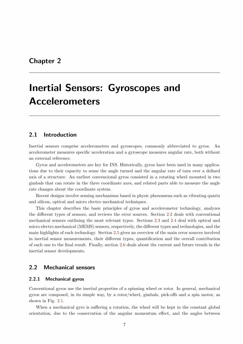
Conventional gyros use the inertial properties of a spinning wheel or rotor. In general, mechanical
gyros are composed, in its simple way, by a rotor/wheel, gimbals, pick-offs and a spin motor, as
shown in Fig. 2.1.
When a mechanical gyro is suffering a rotation, the wheel will be kept in the constant global
orientation, due to the conservation of the angular momentum effect, and the angles between
7

8 CHAPTER 2. INERTIAL SENSORS: GYROSCOPES AND ACCELEROMETERS
Figure 2.1: A conventional mechanical gyroscope [1].
adjacent gimbals can be read using the angles pick-off [4] [16]. Within the mechanical gyroscope
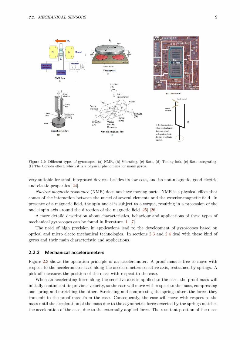
classes, we can find the rate-integrating, the tuned rotor, the flex, the rate, the vibratory, the tuning
fork, the quartz, the silicon and the nuclear magnetic resonance sensors. Many of these devices are
shown in Fig. 2.2.
Rate-integrating gyros has been used in different applications including navigation systems in
aircraft, ships and guided weapons. Unfortunately, this sensor is sensitive to linear and angular
accelerations, causing errors in measurements. Temperature changes modify the characteristic of
the magnetic materials within the sensors. It was fully developed and used in strapdown systems
in many types of vehicles [17].
The tuned rotor gyro have found similar applications as the rate-integrating gyros, and also
share the same error sources [18].
The flex gyro operates in similar manner to the tuned rotor gyro, and was developed in the
middle of the 1970s. Errors in measurement come from the same sources as the tuned gyro, and
have very similar applications [1].
The rate sensors has lower accuracy than the rate-integrating and the tuned rotor gyroscopes
accuracies, thus, it is not very useful for navigation applications [7] [19].
Vibratory gyros has a vibrating element has taken different shapes such as string, a rod, a
tuning fork, a beam and hemispherical dome. The limitations of vibratory gyros lie in having high
drift rates, sensitivity to environmental effects, etc. Within their applications of these gyros, the
providing of feedback for stabilisation or angular position measurements, are the most common [20]
[21].
The tuning fork sensor has two vibrational elements mounted in parallel on a base. When the
structures are excited to vibrate in opposite, the resultant effect is similar to the motion of tuning
fork elements [22].
The quartz rate sensor bases its operation in the tuning fork principles, and can have several
rate sensitivities. These devices are micromachined and are the cutting edge of MEMS technology
[23].
The silicon sensor, as manufactured with silicon material, has a lot of properties which make it
2.2. MECHANICAL SENSORS 9
Figure 2.2: Different types of gyroscopes, (a) NMR, (b) Vibrating, (c) Rate, (d) Tuning fork, (e) Rate integrating.(f) The Coriolis effect, which it is a physical phenomena for many gyros.
very suitable for small integrated devices, besides its low cost, and its non-magnetic, good electric
and elastic properties [24].
Nuclear magnetic resonance (NMR) does not have moving parts. NMR is a physical effect that
comes of the interaction between the nuclei of several elements and the exterior magnetic field. In
presence of a magnetic field, the spin nuclei is subject to a torque, resulting in a precession of the
nuclei spin axis around the direction of the magnetic field [25] [26].
A more detaild description about characteristics, behaviour and applications of these types of
mechanical gyroscopes can be found in literature [1] [7].
The need of high precision in applications lead to the development of gyroscopes based on
optical and micro electo mechanical technologies. In sections 2.3 and 2.4 deal with these kind of
gyros and their main characteristic and applications.
2.2.2 Mechanical accelerometers
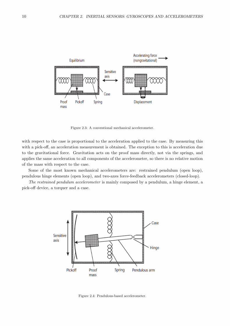
Figure 2.3 shows the operation principle of an acceleremoter. A proof mass is free to move with
respect to the accelerometer case along the accelerometers sensitive axis, restrained by springs. A
pick-off measures the position of the mass with respect to the case.
When an accelerating force along the sensitive axis is applied to the case, the proof mass will
initially continue at its previous velocity, so the case will move with respect to the mass, compressing
one spring and stretching the other. Stretching and compressing the springs alters the forces they
transmit to the proof mass from the case. Consequently, the case will move with respect to the
mass until the acceleration of the mass due to the asymmetric forces exerted by the springs matches
the acceleration of the case, due to the externally applied force. The resultant position of the mass
10 CHAPTER 2. INERTIAL SENSORS: GYROSCOPES AND ACCELEROMETERS
Figure 2.3: A conventional mechanical accelerometer.
with respect to the case is proportional to the acceleration applied to the case. By measuring this
with a pick-off, an acceleration measurement is obtained. The exception to this is acceleration due
to the gravitational force. Gravitation acts on the proof mass directly, not via the springs, and
applies the same acceleration to all components of the accelerometer, so there is no relative motion
of the mass with respect to the case.
Some of the most known mechanical accelerometers are: restrained pendulum (open loop),
pendulous hinge elements (open loop), and two-axes force-feedback accelerometers (closed-loop).
The restrained pendulum accelerometer is mainly composed by a pendulum, a hinge element, a
pick-off device, a torquer and a case.
Figure 2.4: Pendulous-based accelerometer.
2.3. SENSORS BASED IN OPTICAL TECHNOLOGIES 11
The deviation of the pendulum produced by an acceleration is sensed by the pick-off device,
which in the most simple cases is directly measured from the displacement, but generally this kind
of device operates with an electronic re-balance loop to feed the signal back in the pick-off to the
torquer. The current in the torquer is proportional to the applied acceleration [1] [27].
The hinge element of a pendulous accelerometer is the component that enables the mass to
move in a plane normal to the hinge axis. The two basic types of hinge elements are flexures and
pivots, having several variations of each form.
In the flexure hinges, a low mechanical hysteresis material to minimize undesirable spring torque
errors, is used. The main advantage of this type of flexure hinges is its very low static friction
offering almost infinite resolution and low threshold. In the downside these devices have a very
significant temperature dependent bias requiring calibration and compensation for must accurate
applications.
The pivot hinges supports the pendulum between two spring synthetic jewel assemblies. This
type provides a very small temperature dependent bias characteristics, but wearing the pivots in
very discordant environment can be a serious problem [6].
The two-axes force-feedback accelerometer has many applications such as inertial navigation
systems in ships. This sensor has a pendulum which freely swings about two orthogonal axes. It
is restrained to its “null” position by electrical coils working in a permanent magnetic field. The
principle of operation is identical the previous described sensors having a performance similar to
the higher grade single axis devices [6].
2.3 Sensors based in optical technologies
2.3.1 Optical gyroscopes
The optical gyros use the properties of electromagnetic radiations, usually visible and infrared
wavelengths, to sense the rotation. Therefore, it is possible to consider electromagnetic radiations
as the inertial element of these sensors.
The principle behind this kind of gyros is the Sagnac effect [28], reported in 1913. When the
light travels in opposite directions around an enclosed ring, differences come out in the optical
length of the two paths when the ring is rotated around an axis orthogonal to the plane containing
the ring.
The developments of these sensors are more recent than the mechanical gyros. The performance
range of optical gyros is similar to that covered by mechanical sensors, but they offer several
advantages over the mechanical gyros, such as [1]
• wide dynamic range
• instant start-up
• digital output
• independent of some enviromental conditions (accelerartion, vibration)
• high rate capability
• easy self-test
• system design flexibility
12 CHAPTER 2. INERTIAL SENSORS: GYROSCOPES AND ACCELEROMETERS
• extended running life
The principle of operation of optical gyros rely on the detection of an effective path length
difference between two counter-propagating beams in a closed path, which arises with the presence
of the turn rate applied around an axis perpendicular to the plane containing the optical paths.
The transit time, which is the time the light beam employs to travel a complete round of the ring
path, is identical for both beams when the ring is stationary [1].
When the ring is rotated with an angular velocity Ω, the transit of each beam change. Generally,
the light travelling with the direction of rotation must travel further than when the interferometer
is stationary [29]. The opposite will happen with the light beam travelling against the direction of
rotation. The resultant beam at the output experiments a relative phase shift proportional to the
undergoing rotation rate, due to the beams require different times to complete a trip around the
rotating path.
Fiber Optic Gyros (FOG) and Ring Laser Gyros (RLG) [4] [30] provide performance degrees
for applications oriented to higher precision as torpedos, air/land/sea navegation, geo-referencing
mapping, surface and under surface surveying and navigation.
Ring Laser Gyroscopes
Ring Laser Gyroscopes (RLG) are based in the Sagnac effect, as explained in the previous section.
Research had led to very low bias devices, with tyical path length in the order of 300 mm, but
some investigation groups have developed devices of 50 mm.
The difference between the RLG and the FOG relies in the fact that in the RLGs the beams
are addressed in a closed path employing mirrors instead of fibers. The principle of operation relies
on a laser acting as an optical frequency oscilator using three or more mirrors to form a continous
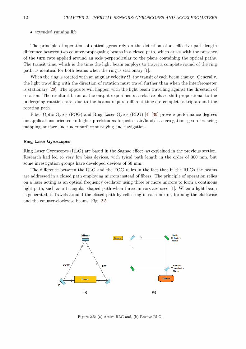
light path, such as a triangular shaped path when three mirrors are used [1]. When a light beam
is generated, it travels around the closed path by reflecting in each mirror, forming the clockwise
and the counter-clockwise beams, Fig. 2.5.
(a) (b)
Figure 2.5: (a) Active RLG and, (b) Passive RLG.

2.3. SENSORS BASED IN OPTICAL TECHNOLOGIES 13
RLG highlights by the method employed to overcome or reduce the lock-in effect, which occurs
at low rotational rate, when both laser beams cease to oscillate at different frequencies causing the
absence of ouput signal. The lock-in is eliminate by introducing a mechanical dither, a magneto-
optic biasing or by the use of multiple optical frequencies [1].
The RLGs are well established today in the market of medium and high performance. This kind
of gyroscope provides lot of advantages over mechanical gyros as high sensitivity and stability, quick
start up, insensitivity to acceleration and inmunity to most enviromental effects. In the downside,
as limitations, it can be pointed the restricted manufacturing of the exact ring cavity dimensions
and the precision mirror, which also requires a very demanding clean room enviroment, which
makes this option not suitable for low or economic performance applications. Other drawbacks are
the size/weight, as well as the the high power requirements needed to supply the lasing media.
Fiber optic gyroscopes
Fiber optic gyros (FOG) consist in a long fiber optic coil, and use the light interference to measure
the angular velocity by detecting the phase difference between the two beams passing the path in
opposite directions, working as a Sagnac interferometer. In its simpler form, the light coming form
a source is divided in two counter-propagating beams which are combined after the path length.
An interference pattern is formed and the resultant intesity is detected by a photodetector. When
the sensor is rotated, a path difference appears for the propagating beams, causing a change in the
amplitude pattern, which is detected by the photodetector.
At present there are two classes of FOGs, the Interferometric FOG (IFOG) and the Resonant
FOG (RFOG). The latter, the RFOG, has received less attention to date, and even it seems to
offer better potential accuracy, is the less mature technology [31].
RFOG requires a narrowband light source and relies on an optical cavity which is formed by a
optic fiber tuned, fostering a single frequency to propagate. If a rotation is applied, the frequency
changes. The fiber resonator is formed by a few coils of fiber and a beam splitter; two input ports
place the beams which are produced by the same coherent source, Fig 2.6.
Figure 2.6: Resonant fiber optic gyroscope scheme [31].
14 CHAPTER 2. INERTIAL SENSORS: GYROSCOPES AND ACCELEROMETERS
In IFOGs devices, the Sagnac effect generates an optical phase difference between two counter-
propagating waves in a rotating fiber coil, which is an indirect measurement of the rotation rate Ω.
Longer coils increase the sensitivity, but at the same time they are more sensitive to temperature
variation and vibration.
IFOGs can operate with two main configurations: open loop and closed loop. In the open loop
configuration, the angular rate information is obtained directly through the output electrical signal.
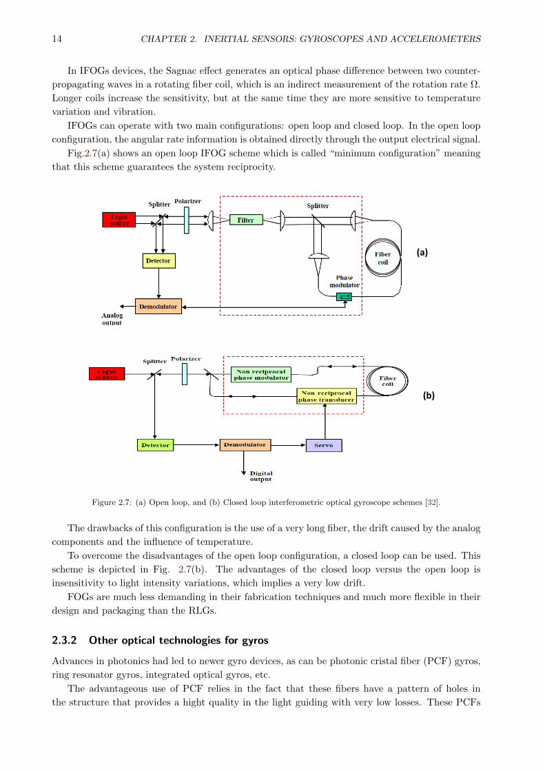
Fig.2.7(a) shows an open loop IFOG scheme which is called “minimum configuration” meaning
that this scheme guarantees the system reciprocity.
(a)
(b)
Figure 2.7: (a) Open loop, and (b) Closed loop interferometric optical gyroscope schemes [32].
The drawbacks of this configuration is the use of a very long fiber, the drift caused by the analog
components and the influence of temperature.
To overcome the disadvantages of the open loop configuration, a closed loop can be used. This
scheme is depicted in Fig. 2.7(b). The advantages of the closed loop versus the open loop is
insensitivity to light intensity variations, which implies a very low drift.
FOGs are much less demanding in their fabrication techniques and much more flexible in their
design and packaging than the RLGs.
2.3.2 Other optical technologies for gyros
Advances in photonics had led to newer gyro devices, as can be photonic cristal fiber (PCF) gyros,
ring resonator gyros, integrated optical gyros, etc.
The advantageous use of PCF relies in the fact that these fibers have a pattern of holes in
the structure that provides a hight quality in the light guiding with very low losses. These PCFs
2.3. SENSORS BASED IN OPTICAL TECHNOLOGIES 15
gives very tight optical mode confinement making possible single mode propagation over many
wavelengths, so tighter coils can be produced which translates in smaller packages. Also dispersion
compensation can be embeeded in these fibers, reducing the spectral distortion on the performance
of the sensor.
The ring resonator gyroscope has a ring formed by an optical waveguide with typical ring
diameters of 50 mm. This type of sensor is known as micro-optic gyroscope (MOG), and when the
problems associated to scattering and coupling can be overcome in these devices, the gyroscope on
a ”chip” can become a reality, along with all the advantages of optical sensors [33].
Developments of integrated optical gyroscope are considered highly desirable, as a ”gyroscope
on a chip” approach. The sensing element relies on an optical waveguide with the light travelling
in opposite directions. These devices are built on a wafer and combine electromechanical processes
and integrated optical fabrication. This type of sensing offers significant reduction in size in the
order of 20 compared with conventional gyros, besides a power consumption reduction by a factor
of 5. The fabrication of these devices are quite challenging nowaday, but many effort are addressed
in this direction.
2.3.3 Optical accelerometers
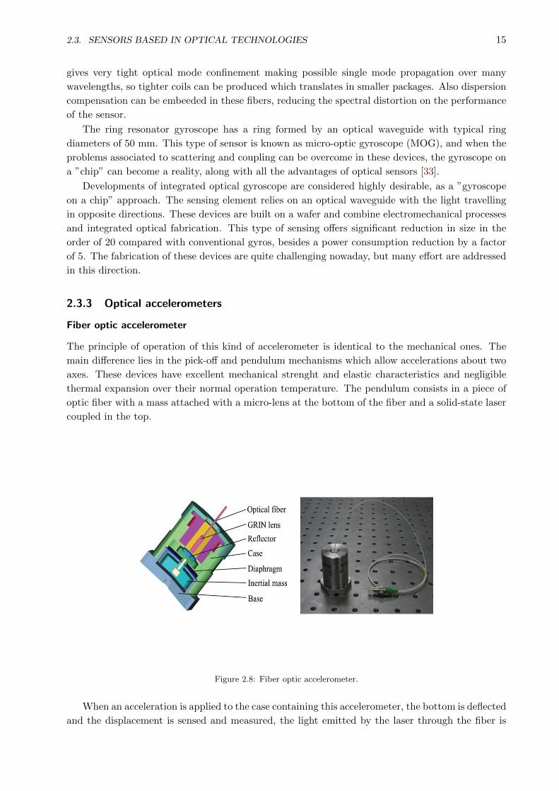
Fiber optic accelerometer
The principle of operation of this kind of accelerometer is identical to the mechanical ones. The
main difference lies in the pick-off and pendulum mechanisms which allow accelerations about two
axes. These devices have excellent mechanical strenght and elastic characteristics and negligible
thermal expansion over their normal operation temperature. The pendulum consists in a piece of
optic fiber with a mass attached with a micro-lens at the bottom of the fiber and a solid-state laser
coupled in the top.
Figure 2.8: Fiber optic accelerometer.
When an acceleration is applied to the case containing this accelerometer, the bottom is deflected
and the displacement is sensed and measured, the light emitted by the laser through the fiber is

16 CHAPTER 2. INERTIAL SENSORS: GYROSCOPES AND ACCELEROMETERS
focused on to two-dimensional photo-sensitive array, e.g. a charge coupled imaging device (CCID)
which can provide x and y coordinates of the displacement. Currently, the accuracy is limited by
the pixel density of the CCID [1] [34] [35].
Mach-Zehnder interferometric accelerometer
A Mach Zehnder interferometer can use one or two optical fibers attached to a mass [36]. When an
acceleration is applied, the optical fiber experiments a small change in length which is proporcional
to the acceleration, and this change can be detected by interferometric techniques. Using two fibers
allows to form an arm an the use of nulling techniques enables greater sensitivities [1] [37].
Figure 2.9: Mach Zehnder interferometric accelerometer.
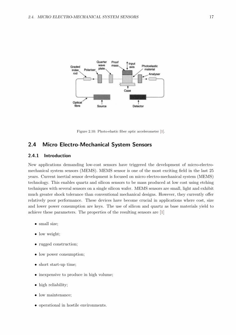
Photo-elastic optic accelerometer
This tye of sensor is the target of lot of research nowaday. In this type of device the sensitive
element is a birefringent material. The polarised light is launched into the birefringent material
trough a fiber, and when an acceleration is applied to the photo-elastic material the light changes
proportionally to the acceleration and measured by a detector, as shown in Figure 2.10.
Bragg grating fiber accelerometer
Several research centers have developed accelerometers based in Bragg gratings [38]. The principal
wavelenght of the Bragg grating is set by its characteristic but ib can be changed with the changes
in temperature, strain and pressure on the grating. Therefore, when an acceleration is applied, the
grating wavelenght changes proportionally to the acceleration and can be detected using a fiber
interferometric. Still the performance of such device is not clearly established, but initial research
has shown good sensitivities.
2.4. MICRO ELECTRO-MECHANICAL SYSTEM SENSORS 17
Figure 2.10: Photo-elastic fiber optic accelerometer [1].
2.4 Micro Electro-Mechanical System Sensors
2.4.1 Introduction
New applications demanding low-cost sensors have triggered the development of micro-electro-
mechanical system sensors (MEMS). MEMS sensor is one of the most exciting field in the last 25
years. Current inertial sensor development is focused on micro electro-mechanical system (MEMS)
technology. This enables quartz and silicon sensors to be mass produced at low cost using etching
techniques with several sensors on a single silicon wafer. MEMS sensors are small, light and exhibit
much greater shock tolerance than conventional mechanical designs. However, they currently offer
relatively poor performance. These devices have become crucial in applications where cost, size
and lower power consumption are keys. The use of silicon and quartz as base materials yield to
achieve these parameters. The properties of the resulting sensors are [1]
• small size;
• low weight;
• rugged construction;
• low power consumption;
• short start-up time;
• inexpensive to produce in high volume;
• high reliability;
• low maintenance;
• operational in hostile environments.

18 CHAPTER 2. INERTIAL SENSORS: GYROSCOPES AND ACCELEROMETERS
These features provide to the engineers a design flexibility beyond any technology preceeding
these developments. Therefore, many applications, both commercial and militar, have been prolife-
rated in the last years. The drawbacks lie on critical performance parameters as the angle random
walk, which is very important in stabilization and positioning systems; they also have bigger bias
instability, which degradates the navegation and stabilization/positioning solutions.
Despite these limitations, MEMS sensors approaching sensitivities of 1/h are expected to
become reality in the next few years. Consequently, the inertial sensor technology researches have
been focused almost exclusively in the development and improvement of MEMS devices.
Nowadays, MEMS are tipically used in consumer and industrial applications as digital came-
ras, smartphones, videogame controllers, automotive purposes, AHRS miniaturization, inteligent
ammunition, robotics, etc [16].
2.4.2 MEMS gyros technology
MEMS gyros are non-rotatory devices and use the Coriolis effect on a vibrating mass(es) to detect
angular rotation. Thus, these sensors detect the force acting over a mass which is subject to a lineal
vibratory motion in a frame of reference, and is rotating about an axis perpendicular to axis of the
linear motion. The resultant force, the Coriolis force, acts in a direction which is perpendicular to
both axes, the vibratory and the axis around the rotation is applied [39].
The MEMS gyros available can be classified as follows: vibrating beams, tuning fork, vibrating
shells and vibrating plates [32]. The operating principle is the same for all of them. The tuning
fork configuration, is shown in Fig. 2.11. In this case, two masses oscilate and move in opposite
directions. When an angular velocity is applied, the Coriolis force to act each mass in opposite
direction resulting in a capacitance change, which is proportional to the angular velocity and it is
converted in an output voltage for analog devices or LSBs for digital ones. When a linear velocity
is applied, both masses move in the same direction, and no capacitance difference is detected, thus,
MEMS gyros are not sensitive to linear acceleration [40].
Figure 2.11: MEMS gyroscope with tuning fork configuration [40].
Vibrating structures have been sucessfully used to detect turn rates. These structures have the

2.4. MICRO ELECTRO-MECHANICAL SYSTEM SENSORS 19
advantage to keep the drive and sense vibrational energy in a single plane, but suffer a relatively
low vibrating mass and therefore, exhibit a low-scale factor.
A new approach to MEMS is the micro-opto electromechanical systems (MOEMS). This tech-
nology offers a true solid-state sensor with an optical readout, overcoming the lack of the MEMS
performance for measuring small displacements [1].
2.4.3 MEMS accelerometer technology
As in the case of gyros, the use of silicon to manufacture accelerometers is well established. MEMS
accelerometers can be divided in two classes taking into account the way the acceleration is sensed:
• the displacement of a mass sustained by a hinge or a flexure in the presence of an acceleration.
• the change of frequency of a vibrating element caused by the change in tension as a result of
an acceleration.
Several types of MEMS acceleremoters are available in the market, as the pendulous mass,
resonant, tunneling and electrostatically levitate MEMS acceleremoters.
Pendulous mass MEMS accelerometer has the advantage its versatility of packaging, allowing
planar mounting of the device. This type of sensor has found many applications in the militar
industry, such as guide-munitions applications [41]. Figure 2.12 shows an in-plane pendulous MEMS
acceleremoter. Acceleration is measured by detecting the change in capacitance across the sensing
element, being more sensitive in the horizontal plane than in the orthogonal direction [1].
Figure 2.12: MEMS pendulous accelerometer.
Resonant MEMS accelerometers can sense acceleration acting in the planar and the perpendi-
cular axes of the accelerometer, which can measure acceleration as the result of the change of the
resonant frequency of beam oscillators under inertial loading of a mass instead of a displacement’s
measurement. Silicon and quartz have been used to manufacture these sensors [42].
Tunneling MEMS accelerometers offer enhancements over the previous analized devices, offe-
ring better resolution, higher bandwidth and small packaging. They are based on bulk silicon

20 CHAPTER 2. INERTIAL SENSORS: GYROSCOPES AND ACCELEROMETERS
Figure 2.13: MEMS resonant accelerometer.
micromachining, normally incorporating boron etch-stop wafer processes. Some of the main phy-
sical components in a tunneling accelerometer include a proof-mass, a tunneling tip and a counter
electrode [43].
Figure 2.14: Tunneling MEMS accelerometer.
2.5 Inertial sensor error and noise characteristics
2.5.1 Introduction
This section will show a review of the most common errors and noises in gyroscopes and accelero-
meters and their effects on the integrated output signal. The predominant error and noise sources
are: constant bias error, bias instability, angle random walk (gyros) and velocity random walk
(accelerometer), quantization, rate angle walk, rate ramp and sinusoidal component.
2.5. INERTIAL SENSOR ERROR AND NOISE CHARACTERISTICS 21
2.5.2 Constant bias error
The sensor bias is the average output of the device over a specified time measured in specific
operation conditions which have no correlation with the sensor rotation (gyros) or input acceleration
(accelerometer). The bias is typically expressed in degree per hour (/h) or radian per second
(rad/s) for gyros, and in meter per second squared (m/s2 or g). The bias generally consists in
two parts: one deterministic part called bias offset and a random part. The bias offset, which is
the offset in the measurement provided by the inertial sensor can be determined by calibration [12]
[44]. The random part is a stochastic process and refers to the rate at which the error in an inertial
sensor accumulates with time.
2.5.3 Bias instability
Additionally, there are two characteristics used to described the sensor bias: the bias asymmetry,
which is the difference between the bias for positive and negative inputs; and the bias instability,
which is the random variation in the bias computed over a finite sample of time. This effect affects
both gyros and acceleremoters.
Usually, it is interesting to know how this error affects the orientation obtained through inte-
gration the rate gyro/accelerometer signal.
The rate power spectral density (PSD) associated with the bias instability, also known as 1/f
noise is
SΩ(f) =
(B2
2π
)1f f ≤ f0
0 f > f0
, (2.1)
where B is the bias instability coefficient and f0 is the 3dB cutoff frequency.
2.5.4 Angle random walk/velocity random walk
An angular/velocity rate sensor measures the rotation/displacement rate over its sensitive axis.
The sensor output signal is perturbed by a type of thermo-mechanical noise fluctuating in a bigger
rate than the sample rate of the sensor, called angle/velocity random walk (ARW/VRW). The
ARW/VRW is a noise specification given in units of /√h for gyros, andm/s/
√h for accelerometers,
which is directly applicable to the computation of the angle/velocity. As consequence, the samples
obtained are disturbed by a white noise, which is a sequence of uncorrelated random variables and
mean zero.
ARW/VRW describes the average deviation or the error that will occur when the signal is
integrated. This error increases with the integration time, and provides a fundamental limitation
to any angle/velocity measurement based only on integration of a rate [45].
For instance, an ARW = 0.1/√h means that after 1 hour the angle deviation is 0.1; after 2
hours working, ARW = 0.1/√h ·√
2 ≈ 0.14.
As mentioned, this term of noise is characterized by a white noise spectra on the gyro rate
output, which is a random noise with a constant power spectral density (PSD) independent of
frequency.
The associated PSD is given by [13]
SΩ(f) = Q2, (2.2)
where Q is the angle randow walk coefficient expressed in /h/√Hz, describing the output noise
as a function of the sensor bandwidth.
22 CHAPTER 2. INERTIAL SENSORS: GYROSCOPES AND ACCELEROMETERS
Generally, the manufacturers quote noise specifications in different ways: an ARW/VRW, a
PSD or FFT noise density and with one or three σ variation in the output sensor. Estimating the
ARW/VRW given these parameters, is well stablished in the IEEE Std. 952-1997 C.1.1 In the case
of ARW
ARW (/√h) =
1
60
√PSD[(/h)2/Hz], (2.3)
ARW (/√h) =
1
60FFT (/h/
√Hz)), (2.4)
ARW (/√h) =
1
60σ(/h)
1√BW (Hz)
, (2.5)
where σ is the standard deviation of the signal and BW is the effective bandwidth of the sensor
in Hz.
2.5.5 Quantization noise
This noise is introduced into an analogic signal as the result of encoding it into a digital signal. This
is caused by the differences between the real amplitudes of the points sampled and the analog-digital
converter resolution .
The angle PSD is given as (IEEE 952 1997)
Sθ(f) = TQ2
sin2(πfT )
(πfT )2
≈ TQ2, (2.6)
for f << 12T ; Q is the quatization noise coefficient and T is the sample interval.
The theoretical limit for Q is S/√
12, where S is the sensor-scaling coefficient for tests with
uniform and fixed sample times [46] [44]. The rate PSD is related to the angle PSD through the
expression
SΩ(2πf) = (2πf)2Sθ(2πf). (2.7)
Therefore,
SΩ(f) =4Q2
Tsin2(πfT ) ≈ (2πf)2TQ2, (2.8)
for f < 12T .
2.5.6 Rate random walk
This is an error of unknown origin, with a rate PSD associated (IEEE 952 1997)
SΩ(f) = (K
2π)2 1
f2, (2.9)
where K is the rate random walk coefficient.
2.6. INERTIAL SENSOR TRENDS 23
2.5.7 Rate ramp
For long but finite time spans, this error is more a deterministic error than a random noise. The
rate ramp is defined as (IEEE 952 1997)
Ω = Rt, (2.10)
where R is the rate ramp coefficient.
The rate PSD associated with this noise is
SΩ(f) =R2
(2πf)3. (2.11)
2.5.8 Sinusoidal noise
This noise is characterized by s number of different frequencies. A representation of the PSD, which
contains a single frequency is given by (IEEE 951 1997)
SΩ(f) =1
2Ω2
0[δ(f − f0) + δ(f + f0)], (2.12)
where Ω0 is the amplitude, f0 is the frequency and δ(x) is the Dirac delta function.
Several frequencies sinusoidal errors can be represented by a sum of terms with equation 2.12
with their frequency and amplitude, respectively.
2.6 Inertial sensor trends
As shown in this Chapter, there are many sensor types and technologies, which are used to detect
or measure an angular motion, in case of gyros, and acceleration in the case of accelerometer. A
great effort has been put to develop the so called ”sensor on a chip”. New technologies used in the
industry, as robotics, hold this effort. Several sensors show an undesired sensitivity under certain
environments, thus, the goal of researchers involved in this field, has been to reduce these sensi-
tivities. Generally, a significant amount of precision engineering and high technology is needed to
produce a functional device. At short-mid term, despite the advances in optical devices, applica-
tions needing very high performance (10−4 − 10−5/h) are still addresed to mechanical sensors. To
mid-range performance requiring a high stabilitaty factor, optical sensors are a good choice.
For MEMS devices a continous improvements are required, it means, special care in the material
uniformity, robust vacuum packaging and tuning in frequency to compensate the sensor drift. Also,
a low noise and low drift electronic circuitry are needed.
In log-term, MEMS sensors will improve and will find a niche in high performance applications.
MEMS and integrated optic devices also will dominate in the low and medium performance range,
while optical will dominate when a high factor of stability is needed. For this, optical MEMS
(MOEMS) sensors are under development since several years ago, but their design is very difficult
due to their small dimensions [47]. Also, integrated optic versions of inertial sensors with the target
of a very small size and low cost are currently investigated [48].

Chapter 3
Allan Variance method and denoising
3.1 Introduction
Within the noise analysis methods, the PSD and Allan variance methods have been adopted as
preferred means of analysis in the inertial systems community for having more general application
on stochastic models (IEEE Std 952-1997).
The frequency-domain approach for modeling noise by using PSD to estimate the transfer
functions is straightforward but difficult to understand for nonsystem analysts. In the other hand,
Allan variance is simple to compute and relatively simple to interpret and understand as well as
accurate enough in modeling noises.
Since a low-cost INS (MEMS grade) presents error sources with short-term (high-frequency)
and long-term (low-frequency) components, we introduce wavelet denosing and averaging filter.
Wavelet is specially powerful removing high frequency components. Wavelet de-noising has been
used in similar works, because of its great effectiveness removing high-frequency noises, as it is
shown in [49][50][51].
This Chapter is focused in the Allan variance method, and in the Wavelet transform which will
be described in the next sections.
3.2 Allan variance method overview
The Allan Variance (AVAR) method was proposed by David Allan in 1966 as a simply variance
analysis method, and it was widely adopted for the characterization of phase and frequency insta-
bility of precision oscillators [11]. In 1998, the IEEE standard introduced the AVAR as a noise
identification method for linear accelerometer analysis (IEEE Std1293-1998).
The AVAR method was first applied to MEMS device noise identification by Hou and El-Sheimy
in 2003 [12].
AVAR is a time domain analysis technique originally designed for characterizing noise and
stability in clock systems, and it is an accepted IEEE standard for gyro specifications [11]. The
technique can be applied to any signal to determine the character of the underlying noise processes,
and can be applied to analyse the error characteristics of any precision measurement instruments
[46].
It is a method of representing root mean square (RMS) random drift error as a function of
average time, and can be used to determine the character of the underlying random processes
25
26 CHAPTER 3. ALLAN VARIANCE METHOD AND DENOISING
that give rise to the data noise. By performing certain operations on the entire length of data,
it is employed to characterize various types of noise terms in the inertial sensor data [52]. Its
value, however, depends upon the degree of understanding of the physics of the instrument. The
uncertainty in the data is assumed to be generated by noise sources of specific character. The key
attribute of the method is that it allows for a finer, easier characterization and identification of
error sources and their contribution to the overall noise statistics.
In the next section, the relationship between the AVAR and the noise PSD is established. Using
this relationship, the behavior of the characteristic curve for a number of prominent noise terms
can be determined.
3.3 Allan variance principles
AVAR is based in the method of cluster analysis. The data flux is divided in clusters of a specific
length. Given N consecutive data points, each one having a sample time t0. Forming a group of n
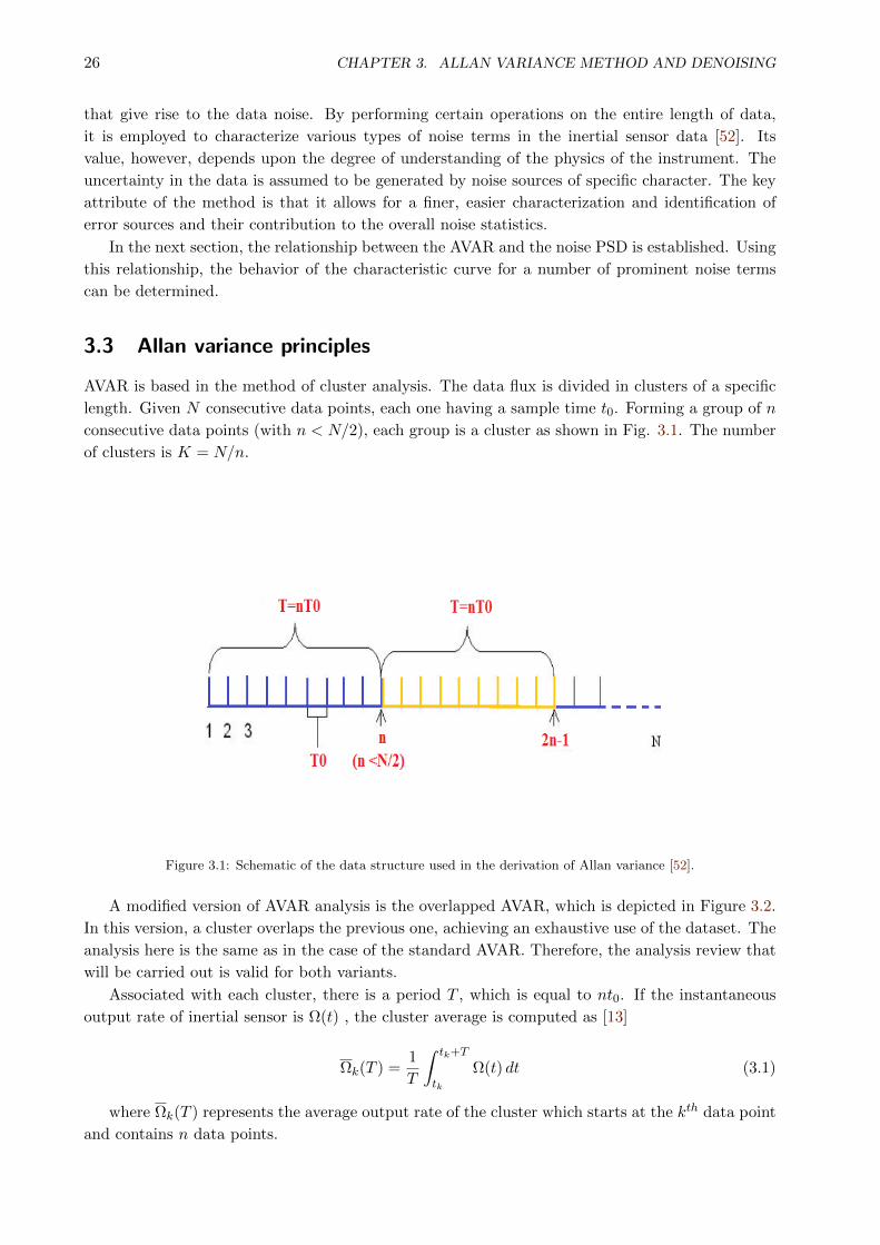
consecutive data points (with n < N/2), each group is a cluster as shown in Fig. 3.1. The number
of clusters is K = N/n.
Figure 3.1: Schematic of the data structure used in the derivation of Allan variance [52].
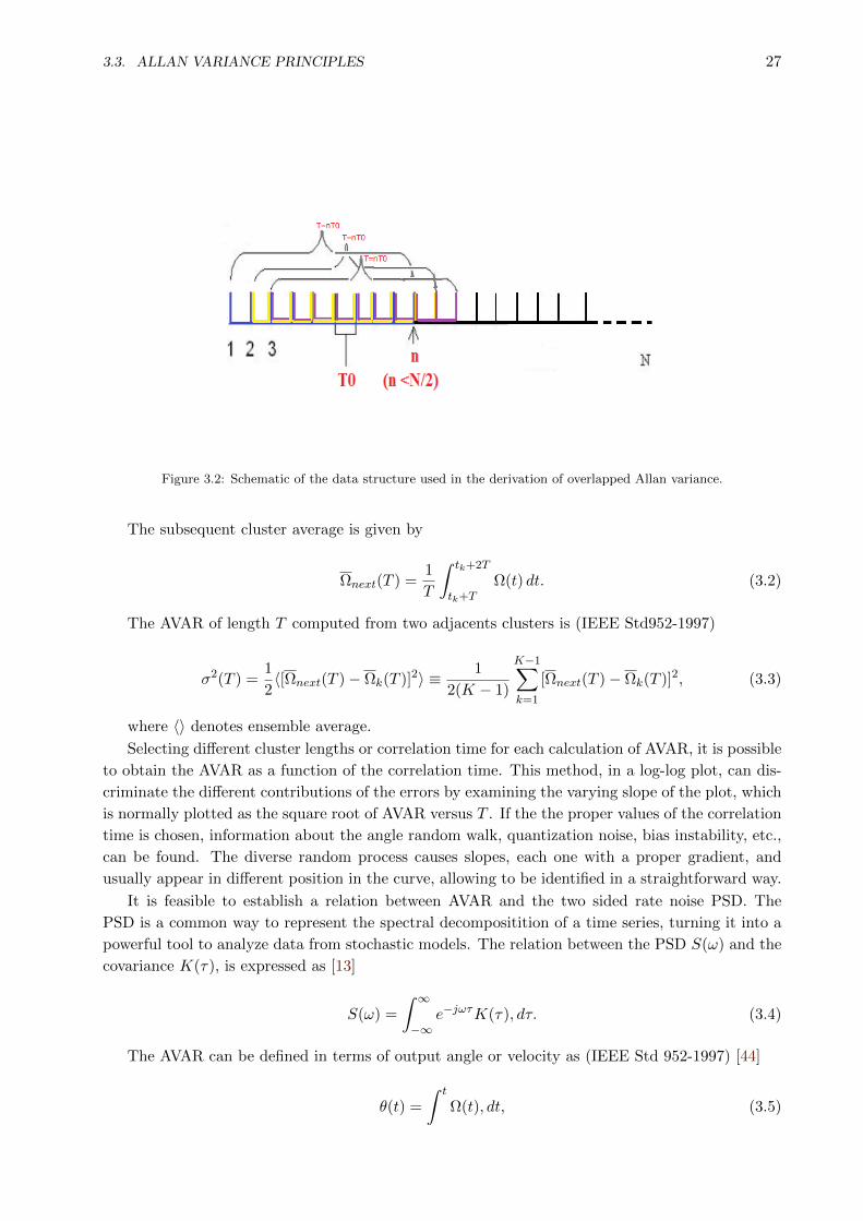
A modified version of AVAR analysis is the overlapped AVAR, which is depicted in Figure 3.2.
In this version, a cluster overlaps the previous one, achieving an exhaustive use of the dataset. The
analysis here is the same as in the case of the standard AVAR. Therefore, the analysis review that
will be carried out is valid for both variants.
Associated with each cluster, there is a period T , which is equal to nt0. If the instantaneous
output rate of inertial sensor is Ω(t) , the cluster average is computed as [13]
Ωk(T ) =1
T
∫ tk+T
tk
Ω(t) dt (3.1)
where Ωk(T ) represents the average output rate of the cluster which starts at the kth data point
and contains n data points.
3.3. ALLAN VARIANCE PRINCIPLES 27
Figure 3.2: Schematic of the data structure used in the derivation of overlapped Allan variance.
The subsequent cluster average is given by
Ωnext(T ) =1
T
∫ tk+2T
tk+TΩ(t) dt. (3.2)
The AVAR of length T computed from two adjacents clusters is (IEEE Std952-1997)
σ2(T ) =1
2〈[Ωnext(T )− Ωk(T )]2〉 ≡ 1
2(K − 1)
K−1∑k=1
[Ωnext(T )− Ωk(T )]2, (3.3)
where 〈〉 denotes ensemble average.
Selecting different cluster lengths or correlation time for each calculation of AVAR, it is possible
to obtain the AVAR as a function of the correlation time. This method, in a log-log plot, can dis-
criminate the different contributions of the errors by examining the varying slope of the plot, which
is normally plotted as the square root of AVAR versus T . If the the proper values of the correlation
time is chosen, information about the angle random walk, quantization noise, bias instability, etc.,
can be found. The diverse random process causes slopes, each one with a proper gradient, and
usually appear in different position in the curve, allowing to be identified in a straightforward way.
It is feasible to establish a relation between AVAR and the two sided rate noise PSD. The
PSD is a common way to represent the spectral decompositition of a time series, turning it into a
powerful tool to analyze data from stochastic models. The relation between the PSD S(ω) and the
covariance K(τ), is expressed as [13]
S(ω) =
∫ ∞−∞
e−jωτK(τ), dτ. (3.4)
The AVAR can be defined in terms of output angle or velocity as (IEEE Std 952-1997) [44]
θ(t) =
∫ t
Ω(t), dt, (3.5)

28 CHAPTER 3. ALLAN VARIANCE METHOD AND DENOISING
where the lower limit of the integral is not especified as only angle or velocity differences are
employed in the definitions.
The angle or velocity measures are done in discrete times given by t = kt0, k = 1, 2, 3..., N .
The notation is simplified as θk = θ(kt0). The cluster averages can be rewritten as
Ωk(T ) =θk+n − θk
T, (3.6)
and
Ωnext(T ) =θk+2n − θk+n
T. (3.7)
Therefore the AVAR can be found as
σ2(T ) =1
2T 2(K − 1)
K−1∑k=1
(θk+2n − 2θk+n + θk)2. (3.8)
The equivalent relation between the AVAR and the PSD is given by the expression [46] [13]
σ2(T ) = 4
∫ ∞0
df · SΩ(f)sin4(πfT )
(πfT )2, (3.9)
where SΩ(f) is the PSD of the Ω(T ) process, which is assumed to be stationary in time.
Equation 3.9 is the focal point of the Allan variance method. This equation will be used
to calculate the Allan variance from the rate noise PSD. The PSD of any physically meaningful
random process can be substituted in the integral, and an expression for the Allan variance σ2(T )
as a function of cluster length is identified. Conversely, since σ2(T ) is a measurable quantity, a
log-log plot of σ(T ) versus T provides a direct indication of the type of random process existing in
the inertial sensor data. The corresponding Allan variance of a stochastic process may be uniquely
derived from its PSD [44].
As explained in this section, AVAR is a very attractive method to sort the error components in
the gyro output by their own slopes in the log-log plot.
3.3.1 Estimation accuracy of the Allan Variance
A finite number of clusters can be generated from any finite set of data. Allan variance of any
noise term is estimated using the total number of clusters of a given length that can be created.
Estimation accuracy of the Allan variance for a given τ , on the other hand, depends on the number
of independent clusters within the data set (IEEE 952 1997).
The accuracy in the estimation of√AV AR (RAVAR) increases with the number of clusters.
Generally, the σ percentage of error of the computation for K clusters, while computing σ(τ) is
[46]
σ(%error) =100√
2(K − 1). (3.10)
The number of clusters K is given by N/n where N is the length of the data set, and n is the
number of points contained in a cluster. The estimation errors in the regions of short (long) τ are
small (large) as the number of independent clusters in these regions is large (small). This equation
can be used to design a test to observe a particular noise of certain characteristics to within a given
accuracy, as explained in (IEEE 952 1997).
3.4. ALLAN VARIANCE ANALYSIS OF THE INERTIAL SENSOR’S NOISE SOURCES 29
3.4 Allan variance analysis of the inertial sensor’s noise sources
3.4.1 AVAR analysis of Bias Instability
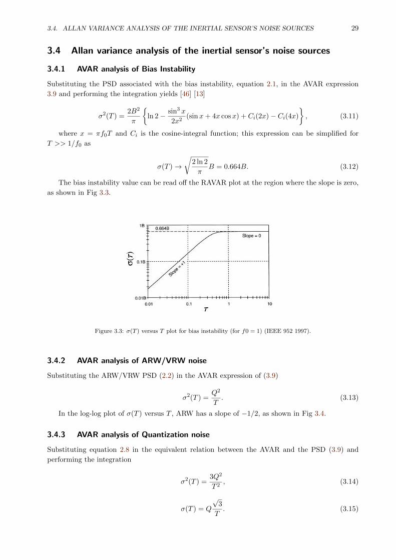
Substituting the PSD associated with the bias instability, equation 2.1, in the AVAR expression
3.9 and performing the integration yields [46] [13]
σ2(T ) =2B2
π
ln 2− sin3 x
2x2(sinx+ 4x cosx) + Ci(2x)− Ci(4x)
, (3.11)
where x = πf0T and Ci is the cosine-integral function; this expression can be simplified for
T >> 1/f0 as
σ(T )→√
2 ln 2
πB = 0.664B. (3.12)
The bias instability value can be read off the RAVAR plot at the region where the slope is zero,
as shown in Fig 3.3.
Figure 3.3: σ(T ) versus T plot for bias instability (for f0 = 1) (IEEE 952 1997).
3.4.2 AVAR analysis of ARW/VRW noise
Substituting the ARW/VRW PSD (2.2) in the AVAR expression of (3.9)
σ2(T ) =Q2
T. (3.13)
In the log-log plot of σ(T ) versus T , ARW has a slope of −1/2, as shown in Fig 3.4.
3.4.3 AVAR analysis of Quantization noise
Substituting equation 2.8 in the equivalent relation between the AVAR and the PSD (3.9) and
performing the integration
σ2(T ) =3Q2
T 2, (3.14)
σ(T ) = Q
√3
T. (3.15)

30 CHAPTER 3. ALLAN VARIANCE METHOD AND DENOISING
Figure 3.4: σ(T ) versus T plot for ARW/VRW noise (IEEE 952 1997).
Therefore, the quantization noise is represented by a slope of −1 in the log-log plot. The noise
magnitude can be read in the slope line at T =√
3.
Figure 3.5: σ(T ) versus T plot for quantization noise (IEEE 952 1997).
3.4.4 AVAR analysis of Rate Random Walk noise
Substituting the expression of the rate random walk PSD (2.9) in the equation 3.9, and performing
the integration
σ2(T ) =K2T
3, (3.16)
thus
σ(T ) = KT
3. (3.17)
Therefore, this noise is represented by a slope of 12 on a log-log plot of σ(T ) versus T . The
magnitude of this noise can be read in this slope line at T = 3. The unit of K is usually given in/h2/
√Hz.
3.4. ALLAN VARIANCE ANALYSIS OF THE INERTIAL SENSOR’S NOISE SOURCES 31
Figure 3.6: σ(T ) versus T plot for rate random walk noise (IEEE 952 1997).
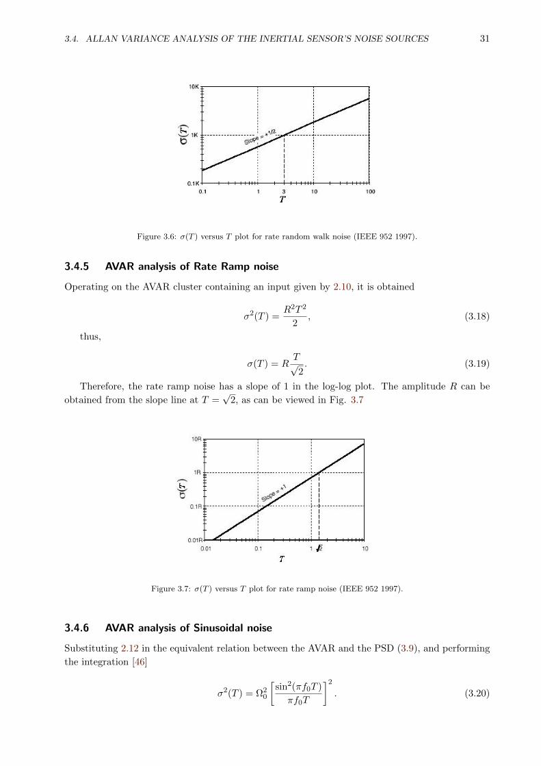
3.4.5 AVAR analysis of Rate Ramp noise
Operating on the AVAR cluster containing an input given by 2.10, it is obtained
σ2(T ) =R2T 2
2, (3.18)
thus,
σ(T ) = RT√2. (3.19)
Therefore, the rate ramp noise has a slope of 1 in the log-log plot. The amplitude R can be
obtained from the slope line at T =√
2, as can be viewed in Fig. 3.7
Figure 3.7: σ(T ) versus T plot for rate ramp noise (IEEE 952 1997).
3.4.6 AVAR analysis of Sinusoidal noise
Substituting 2.12 in the equivalent relation between the AVAR and the PSD (3.9), and performing
the integration [46]
σ2(T ) = Ω20
[sin2(πf0T )
πf0T
]2
. (3.20)

32 CHAPTER 3. ALLAN VARIANCE METHOD AND DENOISING
The AVAR of a sinusoid, when it is plotted in the log-log curve, indicates a sinusoidal behaviour
with attenuate consecutive peaks at the slope of −1. The observation of this noise is difficult due to
the fact that the peaks fall off rapidly and can be masked by higher order peaks of other frequencies
[44].
Figure 3.8: σ(T ) versus T plot for sinusoidal noise (IEEE 952 1997).
3.4.7 Combined effects of the noises
Generally, a number of error components are present in the data, depending of the device and on
the enviroment in which the data is measured. If the noise sources are statistically independent ,
the computed AVAR is the sum of the square of each error as
σ2total = σ2
quant. + σ2ARW + σ2
biasInst + σ2sin + σ2
RRW + .. (3.21)
A typical AVAR plot looks like Fig.3.9, where the noise terms appear in different regions of T ,
which allow and easy identification of the random process existing in the data. A certain amount
of error can be found in the curve due to the uncertainty of the AVAR measures [46] [44].
The error percentage in the estimation of σ(T ), with clusters containing M data points from
N points data set, is given by [44]
σ =1√
2(NM − 1)(3.22)
3.5 Discrete wavelet transform for denoising
Wavelet analysis is a powerful method for decomposing and representing signals which has been
used in a wide range of fields. Similar to the Fourier transform, wavelet can be used to analyze
a time domain signal and transform it in frequencies components, based on analyzing a signal
through signal windowing but with variable window size. Discrete wavelet transform (DWT) are
used for discrete time signals [53].
Wavelets have been found to be a powerful tool for removing noise from a variety of signals
(denoising). To use this method, it is not necessary to know the nature of the signal, and allows
discontinuities and spatial variation of the signal.
3.5. DISCRETE WAVELET TRANSFORM FOR DENOISING 33
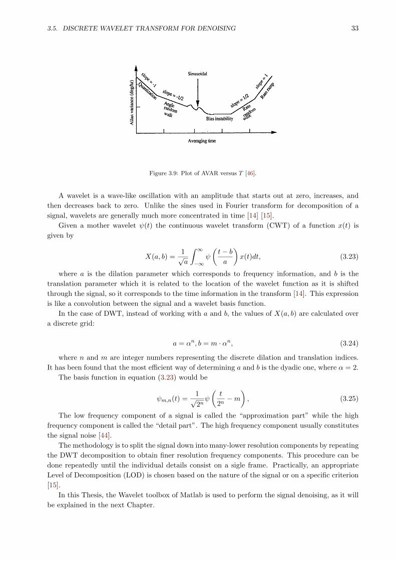
Figure 3.9: Plot of AVAR versus T [46].
A wavelet is a wave-like oscillation with an amplitude that starts out at zero, increases, and
then decreases back to zero. Unlike the sines used in Fourier transform for decomposition of a
signal, wavelets are generally much more concentrated in time [14] [15].
Given a mother wavelet ψ(t) the continuous wavelet transform (CWT) of a function x(t) is
given by
X(a, b) =1√a
∫ ∞−∞
ψ
(t− ba
)x(t)dt, (3.23)
where a is the dilation parameter which corresponds to frequency information, and b is the
translation parameter which it is related to the location of the wavelet function as it is shifted
through the signal, so it corresponds to the time information in the transform [14]. This expression
is like a convolution between the signal and a wavelet basis function.
In the case of DWT, instead of working with a and b, the values of X(a, b) are calculated over
a discrete grid:
a = αn, b = m · αn, (3.24)
where n and m are integer numbers representing the discrete dilation and translation indices.
It has been found that the most efficient way of determining a and b is the dyadic one, where α = 2.
The basis function in equation (3.23) would be
ψm,n(t) =1√2nψ
(t
2n−m
), (3.25)
The low frequency component of a signal is called the “approximation part” while the high
frequency component is called the “detail part”. The high frequency component usually constitutes
the signal noise [44].
The methodology is to split the signal down into many-lower resolution components by repeating
the DWT decomposition to obtain finer resolution frequency components. This procedure can be
done repeatedly until the individual details consist on a sigle frame. Practically, an appropriate
Level of Decomposition (LOD) is chosen based on the nature of the signal or on a specific criterion
[15].
In this Thesis, the Wavelet toolbox of Matlab is used to perform the signal denoising, as it will
be explained in the next Chapter.

Chapter 4
Test and Results
4.1 Introduction
This Chapter is devoted to the practical implementation of the overlapped AVAR method to char-
acterize the different types and magnitudes of error terms existing in the IMU 3DM-GX3-25, which
is composed by three gyroscopes and three accelerometers, together with other components. Once
the AVAR is performed, a process of denoising, using the Wavelets Transform and Median Filter,
is carried out.
To collect and to analyze the data for characterizing the noises, an experimental setup was
assembled to gather static sensors readings. Three datasets with different duration, 9.5, 1, and 3.5
hours, were collected.
The AVAR method was coded in Matlab, and the Allan deviation plots were constructed for
gyros and accelerometers for the different datasets. From the inspection and processing of the
obtained characteristic curves, the magnitude and the type of the errors affecting our sensor, were
determined and the quality of the sensor evaluated. After that, a process of denoising by using the
Wavelets Transform and Median Filter were performed taking advantages of the Wavelet Toolbox
of Matlab.
The next sections show the performed tests and the analysis of the obtained results.
4.2 Data acquisition and experimental setup
For the data acquisition, an experimental setup was held in a customized desk at room temperature
for several days. The experimental setup involved: an IMU model 3DM-GX3 -25, a laptop model
Dell XPS M1330 with operating systems Ubuntu 14.04, and a C++ driver to extract the data from
the sensor.
The IMU 3DM-GX3 -25 is a high-performance, miniature Attitude Heading Reference System
(AHRS) using MEMS sensor technology. It combines a triaxial accelerometer, a triaxial gyro, a
triaxial magnetometer, temperature sensors, and an on-board processor, running a sophisticated
sensor fusion algorithm to provide static and dynamic orientation and inertial measurements. (the
datasheet of the device is provided in Appendix A).
The laptop is a 64-bits Dell XPS M1330 with CPU Intel Core 2 Duo T5250 at 1.5 GHz with
Data Bus Speed of 667 MHz.
The test layout and the used equipments are shown in Figure 4.1.
35

36 CHAPTER 4. TEST AND RESULTS
Figure 4.1: Experimental setup for the data acquisition.
As shown in Figure 4.1, the IMU was anchored to a vessel which was put inside a container
with water to prevent the IMU to be sensitive to vibrations and other kind of environmental noise
that could be added to the measured signals.
Three datasets with 9.5, 1, and 3 hours of gyros and accelerometers measurements were recorded,
saved and exported to *.txt files. An example of the format of the output files is shown in Figure
4.2.
Figure 4.2: Example of the format data recorded by the IMU.
In the files, the first three columns corresponds to the readings of the three accelerometers:
accelerations in X,Y,Z axes expressed in gravities (g); the following three columns are the three

4.2. DATA ACQUISITION AND EXPERIMENTAL SETUP 37
gyros measurements: rotation rates about its sensitive axes X,Y,Z expressed in radians per second
(rad/s), and the last column corresponds to the time stamp in nanoseconds from 1970.
As the AVAR calculations and the error terms are expressed in m/s2 for accelerations and
degrees for the gyros, conversions of units from radians to degrees were carried out over all gyros
data samples (degrees = rad ∗ 180/pi) and from g to m/s2 (1g = 9.8m/s2) for all accelerometer
data samples.
An example raw data reading has been plotted and it is shown in Figure 4.3. Analyzing the
data, and because of the static positioning of the sensor, one may expect, ideally, a zero reading
of angular rates and accelerations, except in the case of the accelerometer that is aligned with the
gravity force, which is expected to have a nearly constant acceleration from gravity. In our case is
the Z axis as it can be noticed in Figure 4.3.
The X,Y,Z gyro outputs are centered at zero value, but in the case of the X and Y accelerometers,
their outputs are a bit off of zero, at 1.52 and −0.80 m/s2, respectively. Probably the accelerometers
are at a slight tilt with respect to the vector of Earth’s gravity and they are therefore feeling a bit
of the pull.
(a) (b)
Figure 4.3: (a) Gyros raw data, and (b)Accelerometers raw data for the three axes.
With the IMU at rest, the outputs should be zero, but there is always noise added on. The
output might have a bias value, but it can be measured and subtract it out.
As shown in Figure 4.3, sometimes the noise takes the output above zero, and sometimes below,
obtaining a range of values within a relatively thin spread. Noise is often thought of as the short-
term variation in the output, such as the peak-to-peak output variation or the standard deviation
of the output while the sensor is at rest. An issue in inertial sensors, that can be seen in a more
accentuated way in the Y axis accelerometer, is the noise accumulated over the time.
4.2.1 Data preprocessing
As the Allan methodology involves calculations of variances, standard deviation and so on, a
preprocessing of the data to prevent it from outliers causing false errors, was performed on all
datasets that were used in the experiments.
A statistical outlier is an observation point distant from the rest of the observations, this may
be due to variability in the measurement or it may indicate experimental errors.
38 CHAPTER 4. TEST AND RESULTS
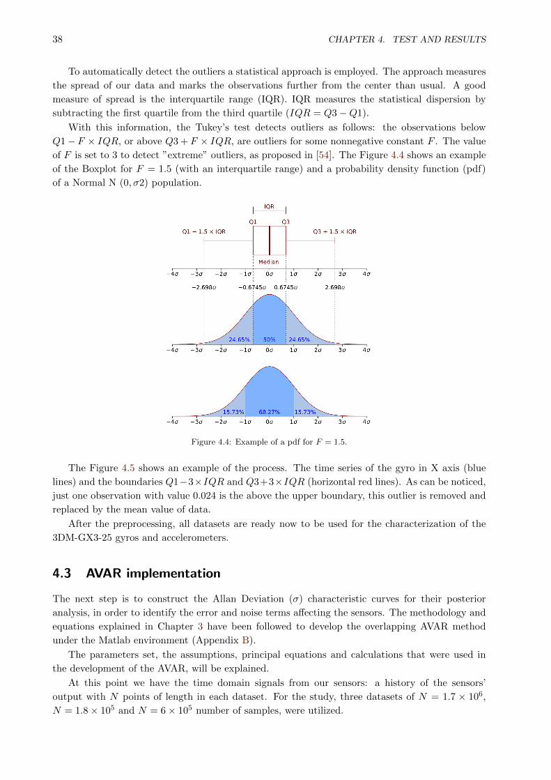
To automatically detect the outliers a statistical approach is employed. The approach measures
the spread of our data and marks the observations further from the center than usual. A good
measure of spread is the interquartile range (IQR). IQR measures the statistical dispersion by
subtracting the first quartile from the third quartile (IQR = Q3−Q1).
With this information, the Tukey’s test detects outliers as follows: the observations below
Q1− F × IQR, or above Q3 + F × IQR, are outliers for some nonnegative constant F . The value
of F is set to 3 to detect ”extreme” outliers, as proposed in [54]. The Figure 4.4 shows an example
of the Boxplot for F = 1.5 (with an interquartile range) and a probability density function (pdf)
of a Normal N (0, σ2) population.
Figure 4.4: Example of a pdf for F = 1.5.
The Figure 4.5 shows an example of the process. The time series of the gyro in X axis (blue
lines) and the boundaries Q1−3×IQR and Q3+3×IQR (horizontal red lines). As can be noticed,
just one observation with value 0.024 is the above the upper boundary, this outlier is removed and
replaced by the mean value of data.
After the preprocessing, all datasets are ready now to be used for the characterization of the
3DM-GX3-25 gyros and accelerometers.
4.3 AVAR implementation
The next step is to construct the Allan Deviation (σ) characteristic curves for their posterior
analysis, in order to identify the error and noise terms affecting the sensors. The methodology and
equations explained in Chapter 3 have been followed to develop the overlapping AVAR method
under the Matlab environment (Appendix B).
The parameters set, the assumptions, principal equations and calculations that were used in
the development of the AVAR, will be explained.
At this point we have the time domain signals from our sensors: a history of the sensors’
output with N points of length in each dataset. For the study, three datasets of N = 1.7 × 10⁶,
N = 1.8× 10⁵ and N = 6× 10⁵ number of samples, were utilized.

4.3. AVAR IMPLEMENTATION 39
×10 5
0 2 4 6 8 10 12 14 16 18-0.02
-0.015
-0.01
-0.005
0
0.005
0.01
0.015
0.02
0.025Gyroscope X axis
raw data+-3*IQR boundaries
Figure 4.5: Example of data outliers removal.
From the number of samples and the time stamps provided by the sensors, the sampling rate
τ0 = 0.01s and sample frequency f = 100 Hz, were estimated.
The next step was to set the averaging factor m. As the value of m can be chosen arbitrarily
fulfilling the condition m < (N − 1)/2, a vector of log spaced numbers between 1 and (N −1)/2 values, was created. In this way, the averaging time or cluster time τ , is a vector with
logarithmically spaced values, with τ = m ∗ τ0. The overlapping method to take the clusters
is chosen to make maximum use of the dataset because it forms all possible overlapping sample
clusters. The computation of the AVAR in terms of averages of output samples over each cluster
was performed according to the equation 3.8, which is rewritten here as
σ2(τ) =1
2τ2(N − 2m)
N−2m∑k=1
(θk+2m − 2θk+m + θk)2. (4.1)
where N is the total number of samples, m is the averaging factor, τ = m ∗ τ0 is the averaging
time, and k is a set of discrete values varying from 1 to N − 2m.
For each τ value, the AVAR (σ2) is calculated. From the square roots of AVAR values, the
Allan Deviation (σ) value for each particular value of τ , is obtained. Iterations of the steps for the
different and multiple values of τ provides us of the σ for each τ defined.
With σ(τ) values we are able to construct the Allan Deviation curve by plotting all the σ(τ)
versus τ on a log-log plot.
Next figures show the obtained Allan standard deviation curves versus cluster time correspond-
ing to one dataset (N = 1.7× 10⁶), analyzed for the three axes gyros and the three axes accelero-
meters of the 3DM-GX3-25.
In the curves, the noises which oscillate quickly are found along the region with decreasing
slopes due to the fact that in this part of the curves are the small cluster time frames, so the noise
varies in less samples. In the regions of increasing slopes, the noise which oscillates over longer
time frames begins to influence bigger groups of averaged data.
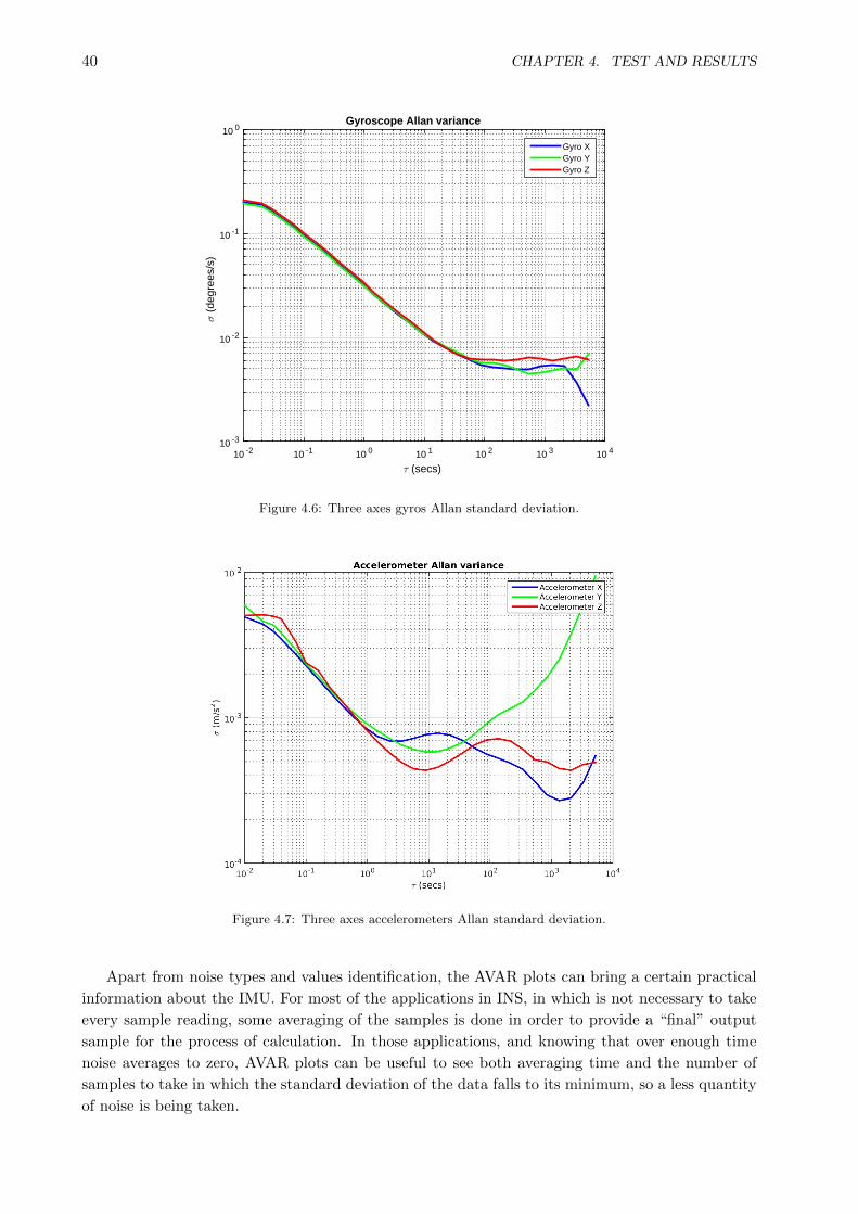
40 CHAPTER 4. TEST AND RESULTS
τ (secs)10 -2 10 -1 10 0 10 1 10 2 10 3 10 4
σ (
degr
ees/
s)
10 -3
10 -2
10 -1
10 0Gyroscope Allan variance
Gyro XGyro YGyro Z
Figure 4.6: Three axes gyros Allan standard deviation.
Figure 4.7: Three axes accelerometers Allan standard deviation.
Apart from noise types and values identification, the AVAR plots can bring a certain practical
information about the IMU. For most of the applications in INS, in which is not necessary to take
every sample reading, some averaging of the samples is done in order to provide a “final” output
sample for the process of calculation. In those applications, and knowing that over enough time
noise averages to zero, AVAR plots can be useful to see both averaging time and the number of
samples to take in which the standard deviation of the data falls to its minimum, so a less quantity
of noise is being taken.

4.3. AVAR IMPLEMENTATION 41
As AVAR uses a log-log plot, it will give more weight to smaller numbers than larger numbers
accentuating changes in the point of change that it will be the minimum group size in time and
number o samples before the standard deviation start raising again.
4.3.1 Noise analysis
As stated in Chapter 3, from the inspection of some regions in the curves accomplishing some AVAR
conditions, we are able to determine the different types and magnitude of noise terms existing in
our sensors. Allan results are related to the five basic gyro-accelerometer noises: ARW/VRW, rate
random walk, bias instability, quantization noise, and rate ramp.
As the majority of the noise terms are found by evaluating the slopes in specific regions in the
curves, a process of finding the slopes were done by using the equation of a line, linear regression
and derivatives, taking as a boundary points the τ vector values of the analyzed regions. The
allowed error margin in the finding of the slopes were set from 0.01 to 0.015 in the Matlab code
(Appendix B).
Gyros analysis
The two types of noise terms detected in the three axes gyros were the ARW and Bias Instability
(BI). The other types of basic noise terms were not detected to be affecting the gyros.
Figure 4.8 shows an example of how to obtain the ARW and BI coefficients from the AVAR
result in a log-log plot for X-axis gyro.
τ (secs)10 -2 10 -1 10 0 10 1 10 2 10 3 10 4
σ (
degr
ees/
s)
10 -3
10 -2
10 -1
10 0Gyroscope Allan variance
Gyro X
Figure 4.8: X axis gyro result.
In the region of the curve with slope −0.5 that intersects in τ = 100s (1 second), the ARW
value will be the corresponding σ at this point. A straight dashed line with slope of −0.5 was fitted
to the curve for a better visualization of the interception point. The ARW is expressed in /√s.
Since the estimation of ARW is based on short cluster times, the number of independent clusters
is large and the quality of estimation is good. Using equation 3.10, with K = 100 for all datasets
since this noise is always found at 1 second, the percentage of error will only depends on the length
of the datasets, the bigger datasets are the lower would be the estimation of error (more accuracy).
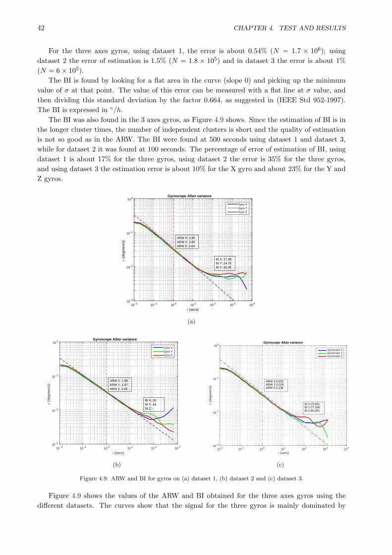
42 CHAPTER 4. TEST AND RESULTS
For the three axes gyros, using dataset 1, the error is about 0.54% (N = 1.7 × 10⁶); using
dataset 2 the error of estimation is 1.5% (N = 1.8 × 10⁵) and in dataset 3 the error is about 1%
(N = 6× 10⁵).
The BI is found by looking for a flat area in the curve (slope 0) and picking up the minimum
value of σ at that point. The value of this error can be measured with a flat line at σ value, and
then dividing this standard deviation by the factor 0.664, as suggested in (IEEE Std 952-1997).
The BI is expressed in /h.
The BI was also found in the 3 axes gyros, as Figure 4.9 shows. Since the estimation of BI is in
the longer cluster times, the number of independent clusters is short and the quality of estimation
is not so good as in the ARW. The BI were found at 500 seconds using dataset 1 and dataset 3,
while for dataset 2 it was found at 100 seconds. The percentage of error of estimation of BI, using
dataset 1 is about 17% for the three gyros, using dataset 2 the error is 35% for the three gyros,
and using dataset 3 the estimation error is about 10% for the X gyro and about 23% for the Y and
Z gyros.
τ (secs)10 -2 10 -1 10 0 10 1 10 2 10 3 10 4
σ (
degr
ees/
s)
10 -3
10 -2
10 -1
10 0Gyroscope Allan variance
Gyro XGyro YGyro Z
ARW X: 1.95ARW Y: 1.93ARW Z: 2.03
BI X: 27.48BI Y: 24.75BI Z: 33.28
(a)
τ (secs)10 -2 10 -1 10 0 10 1 10 2 10 3
σ (
degr
ees/
s)
10 -3
10 -2
10 -1
10 0Gyroscope Allan variance
Gyro XGyro YGyro Z
ARW X: 1.98ARW Y: 1.97ARW Z: 2.05
BI X: 30BI Y: 44BI Z: -
(b)
10 -2 10 -1 100 101 102 103 104
τ (secs)
10 -3
10 -2
10 -1
100
σ (
degr
ees/
s)
Gyroscope Allan variance
Gyroscope XGyroscope YGyroscope Z
BI X:25.651BI Y:27.336BI Z:40.261
ARW X:2.031ARW Y:2.029ARW Z:2.138
(c)
Figure 4.9: ARW and BI for gyros on (a) dataset 1, (b) dataset 2 and (c) dataset 3.
Figure 4.9 shows the values of the ARW and BI obtained for the three axes gyros using the
different datasets. The curves show that the signal for the three gyros is mainly dominated by
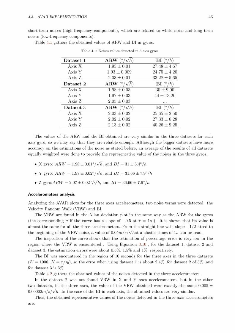
4.3. AVAR IMPLEMENTATION 43
short-term noises (high-frequency components), which are related to white noise and long term
noises (low-frequency components).
Table 4.1 gathers the obtained values of ARW and BI in gyros.
Table 4.1: Noises values detected in 3 axis gyros.
Dataset 1 ARW (/√h) BI (/h)
Axis X 1.95± 0.01 27.48± 4.67Axis Y 1.93± 0.009 24.75± 4.20Axis Z 2.03± 0.01 33.28± 5.65
Dataset 2 ARW (/√h) BI (/h)
Axis X 1.98± 0.03 30± 9.00Axis Y 1.97± 0.03 44± 13.20Axis Z 2.05± 0.03 ...
Dataset 3 ARW (/√h) BI (/h)
Axis X 2.03± 0.02 25.65± 2.50Axis Y 2.02± 0.02 27.33± 6.28Axis Z 2.13± 0.02 40.26± 9.25
The values of the ARW and the BI obtained are very similar in the three datasets for each
axis gyro, so we may say that they are reliable enough. Although the bigger datasets have more
accuracy on the estimations of the noise as stated before, an average of the results of all datasets
equally weighted were done to provide the representative value of the noises in the three gyros.
• X gyro: ARW = 1.98± 0.01/√h, and BI = 31± 5.4/h.
• Y gyro: ARW = 1.97± 0.02/√h, and BI = 31.66± 7.9/h
• Z gyro:ARW = 2.07± 0.02/√h, and BI = 36.66± 7.6/h
Accelerometers analysis
Analyzing the AVAR plots for the three axes accelerometers, two noise terms were detected: the
Velocity Random Walk (VRW) and BI.
The VRW are found in the Allan deviation plot in the same way as the ARW for the gyros
(the corresponding σ if the curve has a slope of −0.5 at τ = 1s ). It is shown that its value is
almost the same for all the three accelerometers. From the straight line with slope −1/2 fitted to
the beginning of the VRW noise, a value of 0.05m/s/√hat a cluster times of 1s can be read.
The inspection of the curve shows that the estimation of percentage error is very low in the
region where the VRW is encountered . Using Equation 3.10 , for the dataset 1, dataset 2 and
dataset 3, the estimation errors were about 0.5%, 1.5% and 1%, respectively.
The BI was encountered in the region of 10 seconds for the three axes in the three datasets
(K = 1000, K = τ/τ0), so the error when using dataset 1 is about 2.4%, for dataset 2 of 5%, and
for dataset 3 is 3%.
Table 4.2 gathers the obtained values of the noises detected in the three accelerometers.
In the dataset 2 was not found VRW in X and Y axes accelerometers, but in the other
two datasets, in the three axes, the value of the VRW obtained were exactly the same 0.005 ±0.00002m/s/
√h. In the case of the BI in each axis, the obtained values are very similar.
Thus, the obtained representative values of the noises detected in the three axis accelerometers
are:

44 CHAPTER 4. TEST AND RESULTS
τ (secs)10 -2 10 -1 10 0 10 1 10 2 10 3 10 4
σ (
m/s
2)
10 -4
10 -3
10 -2Accelerometer Allan variance
Accelerometer XAccelerometer YAccelerometer Z
BI X:1.507BI Y:3.251BI Z:2.486
VRW X:0.051VRW Y:0.055VRW Z:0.050
(a)
τ (secs)10 -2 10 -1 10 0 10 1 10 2 10 3
σ (
m/s
2)
10 -4
10 -3
10 -2Accelerometer Allan variance
Accelerometer XAccelerometer YAccelerometer Z
BI X:2.871BI Y:3.871BI Z:2.443
VRW X:-VRW Y:-VRW Z:0.049
(b)
τ (secs)10 -2 10 -1 10 0 10 1 10 2 10 3 10 4
σ (
m/s
2)
10 -4
10 -3
10 -2Accelerometer Allan variance
Accelerometer XAccelerometer YAccelerometer Z
BI X:1.507BI Y:3.251BI Z:2.486
VRW X:0.051VRW Y:0.055VRW Z:0.050
(c)
Figure 4.10: VRW and BI for accelerometers on (a) dataset 1, (b) dataset 2 and (c) dataset 3.
Table 4.2: Noises values detected in 3 axis accelerometers.
Dataset 1 VRW (m/s/√h) BI (m/s/h)
Axis X 0.005± 0.00002 1.50± 0.03Axis Y 0.005± 0.00002 3.25± 0.07Axis Z 0.005± 0.00002 2.48± 0.05
Dataset 2 VRW (m/s/√h) BI (m/s/h)
Axis X ... 2.87± 0.15Axis Y ... 3.87± 0.20Axis Z 0.005± 0.00007 2.44± 0.12
Dataset 3 VRW (m/s/√h) BI (m/s/h)
Axis X 0.005± 0.00005 2.57± 0.07Axis Y 0.006± 0.00006 3.54± 0.10Axis Z 0.005± 0.00005 2.53± 0.07
• X accelerometer: V RW = 0.005± 0.00003m/s/√h, and BI = 2.31± 0.08m/s/h.
• Y accelerometer: V RW = 0.005± 0.00003m/s/√h, and BI = 3.55± 0.12m/s/h.

4.4. DENOISING 45
• Z accelerometer: V RW = 0.005± 0.00003m/s/√h, and BI = 2.48± 0.08m/s/h.
At this point we have characterized the types and values of the noises affecting our gyros
and accelerometers using the AVAR method. The obtained values have been compared with the
obtained in [10] in which the IMU 3DM-GX3-25 was also utilized for a comparison between different
error modeling of MEMS using AVAR and PSD. The values are very similar, so we can conclude
that the methodology followed and the AVAR method are well suited for noise characterization.
4.4 Denoising
Once we have the knowledge about the noise types and values that are present in our sensor, the
next step is to try to remove or reduce the affecting noise trough a denoising process. In digital
signal processing there are different methods of noise reduction on a signal. The methods selected
and applied in this work are the Discrete Wavelet Transform (DWT) and the Median Filter. Next
sections show the obtained results of applying these two methods to the datasets. Both filters were
applied to the data, and subsequently, processed with the AVAR algorithm in order to evaluate if
the previously detected noises were removed or at least if their values has been reduced.
4.4.1 Wavelet denoising
The wavelet denoising process were performed using the Matlab Wavelet Toolbox. The Level of
Decomposition (LoD) for the DWT and the wavelet family has been selected after the analysis of the
reconstructed signal when applying different test values and parameters. In [55], some exhaustive
procedures to select an optimal LoD, are explained.
From the several wavelet families two of them, Haar and Symlet8, were tested. Figure 4.11
shows how they return different reconstructed signals after filtering, and how the LoD impacts
directly on the reconstruction wavelet.
Figure 4.11 depicts the AVAR standard deviation versus cluster times (τ) for the X-axis acce-
lerometer after applying wavelet denoising with 4 , 8 and 12 LoD using Haar and Symlet8.
10 -2 10 -1 100 101 102 103
τ (secs)
10 -4
10 -3
10 -2
σ (
m/s
2)
Allan variance after wavelet denoising (Haar)
Decomposition level=4Decomposition level=8Decomposition level=12
(a)
10 -2 10 -1 100 101 102 103
τ (secs)
10 -4
10 -3
10 -2
σ (
m/s
2)
Allan variance after wavelet denoising (Symlet 8)
Decomposition level=4Decomposition level=8Decomposition level=12
(b)
Figure 4.11: X-axis accelerometer if IMU 3DM-GX-25 after applying wavelet denoising with 4, 8 and 12 levels ofdecomposition (a) A-Haar , (b) Symlet8.
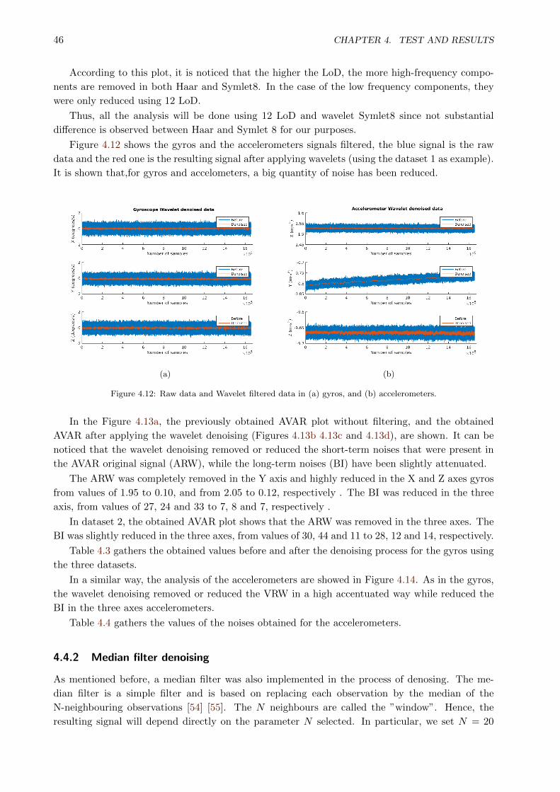
46 CHAPTER 4. TEST AND RESULTS
According to this plot, it is noticed that the higher the LoD, the more high-frequency compo-
nents are removed in both Haar and Symlet8. In the case of the low frequency components, they
were only reduced using 12 LoD.
Thus, all the analysis will be done using 12 LoD and wavelet Symlet8 since not substantial
difference is observed between Haar and Symlet 8 for our purposes.
Figure 4.12 shows the gyros and the accelerometers signals filtered, the blue signal is the raw
data and the red one is the resulting signal after applying wavelets (using the dataset 1 as example).
It is shown that,for gyros and accelometers, a big quantity of noise has been reduced.
(a) (b)
Figure 4.12: Raw data and Wavelet filtered data in (a) gyros, and (b) accelerometers.
In the Figure 4.13a, the previously obtained AVAR plot without filtering, and the obtained
AVAR after applying the wavelet denoising (Figures 4.13b 4.13c and 4.13d), are shown. It can be
noticed that the wavelet denoising removed or reduced the short-term noises that were present in
the AVAR original signal (ARW), while the long-term noises (BI) have been slightly attenuated.
The ARW was completely removed in the Y axis and highly reduced in the X and Z axes gyros
from values of 1.95 to 0.10, and from 2.05 to 0.12, respectively . The BI was reduced in the three
axis, from values of 27, 24 and 33 to 7, 8 and 7, respectively .
In dataset 2, the obtained AVAR plot shows that the ARW was removed in the three axes. The
BI was slightly reduced in the three axes, from values of 30, 44 and 11 to 28, 12 and 14, respectively.
Table 4.3 gathers the obtained values before and after the denoising process for the gyros using
the three datasets.
In a similar way, the analysis of the accelerometers are showed in Figure 4.14. As in the gyros,
the wavelet denoising removed or reduced the VRW in a high accentuated way while reduced the
BI in the three axes accelerometers.
Table 4.4 gathers the values of the noises obtained for the accelerometers.
4.4.2 Median filter denoising
As mentioned before, a median filter was also implemented in the process of denosing. The me-
dian filter is a simple filter and is based on replacing each observation by the median of the
N-neighbouring observations [54] [55]. The N neighbours are called the ”window”. Hence, the
resulting signal will depend directly on the parameter N selected. In particular, we set N = 20

4.4. DENOISING 47
τ (secs)10 -2 10 -1 10 0 10 1 10 2 10 3 10 4
σ (
degr
ees/
s)
10 -3
10 -2
10 -1
10 0Gyroscope Allan variance
Gyro XGyro YGyro Z
ARW X: 1.95ARW Y: 1.93ARW Z: 2.03
BI X: 27.48BI Y: 24.75BI Z: 33.28
(a)
τ (secs)10 -2 10 -1 10 0 10 1 10 2 10 3 10 4
σ (
degr
ees/
s)
10 -5
10 -4
10 -3
10 -2
10 -1
10 0Gyroscope (wavelet) Allan variance
Gyroscope XGyroscope YGyroscope Z
BI X:6.918BI Y:8.199BI Z:7.219
ARW X:0.101ARW Y:-ARW Z:0.121
(b)
τ (secs)10 -2 10 -1 10 0 10 1 10 2 10 3
σ (
degr
ees/
s)
10 -4
10 -3
10 -2
10 -1
10 0Gyroscope (wavelet) Allan variance
Gyroscope XGyroscope YGyroscope Z
BI X:28.973BI Y:12.339BI Z:14.791
(c)
τ (secs)10 -2 10 -1 10 0 10 1 10 2 10 3 10 4
σ (
degr
ees/
s)
10 -6
10 -5
10 -4
10 -3
10 -2Gyroscope (wavelet) Allan variance
Gyroscope XGyroscope YGyroscope Z
ARW X:0.003ARW Y:-ARW Z:0.003
BI X:0.445BI Y:0.180BI Z:0.163
(d)
Figure 4.13: Three axes gyros AVAR analysis, (a) dataset 1 without filtering (comparison purposes), (b) dataset 1filtered with wavelets , (c) dataset 2 filtered with wavelets, (d) dataset 3 filtered with wavelets.
Table 4.3: Noises values detected in 3 axis gyros with and without Wavelet denoising.
Dataset 1 ARW) ARW (denoised) BI BI (denoised)
(/√h) (/
√h) (/h) (/h)
Axis X 1.95± 0.01 0.10 27.48± 4.67 6.91Axis Y 1.93± 0.009 ... 24.75± 4.20 8.19Axis Z 2.03± 0.01 0.12 33.28± 5.65 7.21
Dataset 2 ARW ARW (denoised) BI BI (denoised)
(/√h) (/
√h) (/h) (/h)
Axis X 1.98± 0.03 0 30± 9.00 28.97Axis Y 1.97± 0.03 0 44± 13.20 12.33Axis Z 2.05± 0.03 0 ... ...
Dataset 3 ARW ARW (denoised) BI BI (denoised)
(/√h) (/
√h) (/h) (/h)
Axis X 2.03± 0.02 0.15 25.65± 2.50 25.49Axis Y 2.02± 0.02 0 27.33± 6.28 10.32Axis Z 2.13± 0.02 0.14 40.26± 9.25 9.35

48 CHAPTER 4. TEST AND RESULTS
τ (secs)10 -2 10 -1 10 0 10 1 10 2 10 3 10 4
σ (
m/s
2)
10 -4
10 -3
10 -2Accelerometer Allan variance
Accelerometer XAccelerometer YAccelerometer Z
BI X:1.507BI Y:3.251BI Z:2.486
VRW X:0.051VRW Y:0.055VRW Z:0.050
(a)
τ (secs)10 -2 10 -1 10 0 10 1 10 2 10 3 10 4
σ (
m/s
2)
10 -7
10 -6
10 -5
10 -4
10 -3
10 -2Accelerometer (wavelet) Allan variance
Accelerometer XAccelerometer YAccelerometer Z
BI X:0.366BI Y:0.181BI Z:2.502
RRW X:-RRW Y:-134.118RRW Z:-
(b)
τ (secs)10 -2 10 -1 10 0 10 1 10 2 10 3
σ (
m/s
2)
10 -6
10 -5
10 -4
10 -3
10 -2Accelerometer (wavelet) Allan variance
Accelerometer XAccelerometer YAccelerometer ZBI X:0.732
BI Y:0.821BI Z:0.572
RRW X:-129.087RRW Y:-142.014RRW Z:-168.890
(c)
τ (secs)10 -2 10 -1 10 0 10 1 10 2 10 3 10 4
σ (
m/s
2)
10 -6
10 -5
10 -4
10 -3
10 -2
10 -1Accelerometer (wavelet) Allan variance
Accelerometer XAccelerometer YAccelerometer ZVRW X:-
VRW Y:0.015VRW Z:-
BI X:0.576BI Y:-BI Z:0.451
RRW X:-133.637RRW Y:-152.322RRW Z:-
(d)
Figure 4.14: Three axes accelerometers AVAR analysis, (a) dataset 1 without filtering (comparison purposes), (b)dataset 1 filtered with wavelets , (c) dataset 2 filtered with wavelets, (d) dataset 3 filtered with wavelets.
Table 4.4: Noises values detected in 3 axis acceleremoter with and without Wavelet denoising.
Dataset 1 VRW) VRW (denoised) BI BI (denoised)
(m/s/√h) (m/s/
√h) (m/s/h) (m/s/h)
Axis X 0.005± 0.00002 0 1.50± 0.03 0.36Axis Y 0.005± 0.00002 0 3.25± 0.07 0.18Axis Z 0.005± 0.00002 0 2.48± 0.05 2.50
Dataset 2 VRW VRW (denoised) BI BI (denoised)
(m/s/√h) (m/s/
√h) (m/s/h) (m/s/h)
Axis X ... ... 2.87± 0.15 0.73Axis Y ... ... 3.87± 0.20 0.82Axis Z 0.005± 0.00007 0 2.44± 0.12 0.57
Dataset 3 VRW VRW (denoised) BI BI (denoised)
(m/s/√h) (m/s/
√h) (m/s/h) (m/s/h)
Axis X 0.005± 0.00005 0 2.57± 0.07 0.57Axis Y 0.006± 0.00006 0.015 3.54± 0.10 0Axis Z 0.005± 0.00005 0 2.53± 0.07 0.45
4.4. DENOISING 49
for the results presented in this work, as it was the maximum value that the PC performace could
afford.
As can be notice from Figure 4.15, analyzing the filtered signal, not too much noise were removed
comparing with the wavelet filtering.
(a) (b)
(c) (d)
Figure 4.15: (a) dataset 1 gyros noise filtered with Median Filter, (b) dataset 1 gyros noises filtered with Wavelets, (c)dataset 1 accelerometers noises filtered with Median Filter, (d) dataset 1 accelerometers noises filtered with Wavelets.
Figure 4.16 shows the AVAR plots for the gyros and accelerometers filtered with the Median
Filter using dataset 1. The ARW in the gyros were not attenuated, on the contrary, the values are
a little bit higher or almost the same. The values of the BI are also almost the same before and
after filtering. In the accelerometers, the VRW was removed in the X and Y axes, and in the Z
axis the value before and after filtering was the same 0.05m/s/√
(h). The BI in the accelerometers
increase a little bit its value.
Using dataset 2 and dataset 3, the obtained results are very similar to the stated before.
Next tables gather the obtained values using all datasets.

50 CHAPTER 4. TEST AND RESULTS
τ (secs)10 -2 10 -1 10 0 10 1 10 2 10 3 10 4
σ (
degr
ees/
s)
10 -4
10 -3
10 -2
10 -1
10 0Gyroscope (filtered) Allan variance
Gyroscope XGyroscope YGyroscope Z
BI X:27.340BI Y:27.318BI Z:33.609
ARW X:2.034ARW Y:2.006ARW Z:2.123
(a)
τ (secs)10 -2 10 -1 10 0 10 1 10 2 10 3 10 4
σ (
m/s
2)
10 -5
10 -4
10 -3
10 -2Accelerometer (filtered) Allan variance
Accelerometer XAccelerometer YAccelerometer Z
VRW X:-VRW Y:-VRW Z:0.053
BI X:3.985BI Y:3.311BI Z:2.503
(b)
Figure 4.16: (a) dataset 1 gyros noises filtered with Median Filter, (b) dataset 1 accelerometers noises filtered withMedian Filter.
Table 4.5: Noises values detected in 3 axis gyros with and without Median Filter denoising.
Dataset 1 ARW) ARW (Median Filter) BI BI (Median Filter)
(/√h) (/
√h) (/h) (/h)
Axis X 1.95± 0.01 2.03 27.48± 4.67 27.34Axis Y 1.93± 0.009 2.00 24.75± 4.20 27.31Axis Z 2.03± 0.01 2.12 33.28± 5.65 33.60
Dataset 2 ARW ARW (Median Filter) BI BI (Median Filter)
(/√h) (/
√h) (/h) (/h)
Axis X 1.98± 0.03 2.04 30± 9.00 30.80Axis Y 1.97± 0.03 2.05 44± 13.20 18.62Axis Z 2.05± 0.03 2.15 ... ...
Dataset 3 ARW ARW (Median Filter) BI BI (Median Filter)
(/√h) (/
√h) (/h) (/h)
Axis X 2.03± 0.02 2.08 25.65± 2.50 31.35Axis Y 2.02± 0.02 2.10 27.33± 6.28 27.88Axis Z 2.13± 0.02 2.21 40.26± 9.25 40.52
Table 4.6: Noises values detected in 3 axis acceleremoter with and without Median Filter denoising.
Dataset 1 VRW) VRW (Median Filter) BI BI (Median Filter)
(m/s/√h) (m/s/
√h) (m/s/h) (m/s/h)
Axis X 0.005± 0.00002 0 1.50± 0.03 3.98Axis Y 0.005± 0.00002 0 3.25± 0.07 3.31Axis Z 0.005± 0.00002 0.05 2.48± 0.05 2.50
Dataset 2 VRW VRW (Median Filter) BI BI (Median Filter)
(m/s/√h) (m/s/
√h) (m/s/h) (m/s/h)
Axis X ... ... 2.87± 0.15 2.87Axis Y ... ... 3.87± 0.20 4.02Axis Z 0.005± 0.00007 0.05 2.44± 0.12 2.49
Dataset 3 VRW VRW (Median Filter) BI BI (Median Filter)
(m/s/√h) (m/s/
√h) (m/s/h) (m/s/h)
Axis X 0.005± 0.00005 0 2.57± 0.07 2.56Axis Y 0.006± 0.00006 0 3.54± 0.10 3.97Axis Z 0.005± 0.00005 0.05 2.53± 0.07 2.64
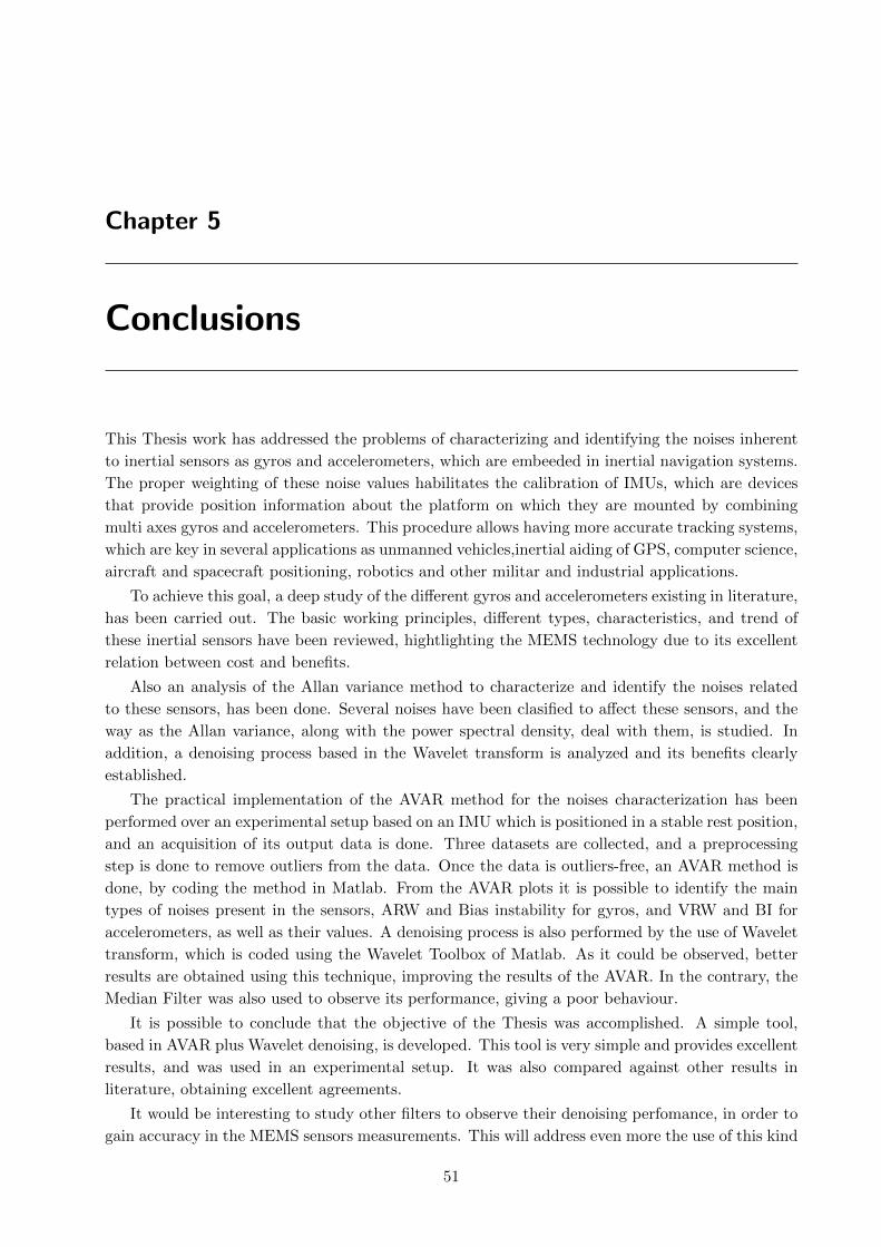
Chapter 5
Conclusions
This Thesis work has addressed the problems of characterizing and identifying the noises inherent
to inertial sensors as gyros and accelerometers, which are embeeded in inertial navigation systems.
The proper weighting of these noise values habilitates the calibration of IMUs, which are devices
that provide position information about the platform on which they are mounted by combining
multi axes gyros and accelerometers. This procedure allows having more accurate tracking systems,
which are key in several applications as unmanned vehicles,inertial aiding of GPS, computer science,
aircraft and spacecraft positioning, robotics and other militar and industrial applications.
To achieve this goal, a deep study of the different gyros and accelerometers existing in literature,
has been carried out. The basic working principles, different types, characteristics, and trend of
these inertial sensors have been reviewed, hightlighting the MEMS technology due to its excellent
relation between cost and benefits.
Also an analysis of the Allan variance method to characterize and identify the noises related
to these sensors, has been done. Several noises have been clasified to affect these sensors, and the
way as the Allan variance, along with the power spectral density, deal with them, is studied. In
addition, a denoising process based in the Wavelet transform is analyzed and its benefits clearly
established.
The practical implementation of the AVAR method for the noises characterization has been
performed over an experimental setup based on an IMU which is positioned in a stable rest position,
and an acquisition of its output data is done. Three datasets are collected, and a preprocessing
step is done to remove outliers from the data. Once the data is outliers-free, an AVAR method is
done, by coding the method in Matlab. From the AVAR plots it is possible to identify the main
types of noises present in the sensors, ARW and Bias instability for gyros, and VRW and BI for
accelerometers, as well as their values. A denoising process is also performed by the use of Wavelet
transform, which is coded using the Wavelet Toolbox of Matlab. As it could be observed, better
results are obtained using this technique, improving the results of the AVAR. In the contrary, the
Median Filter was also used to observe its performance, giving a poor behaviour.
It is possible to conclude that the objective of the Thesis was accomplished. A simple tool,
based in AVAR plus Wavelet denoising, is developed. This tool is very simple and provides excellent
results, and was used in an experimental setup. It was also compared against other results in
literature, obtaining excellent agreements.
It would be interesting to study other filters to observe their denoising perfomance, in order to
gain accuracy in the MEMS sensors measurements. This will address even more the use of this kind
51

52 CHAPTER 5. CONCLUSIONS
of sensors in high accuracy applications. This, along with their compact form, easy integration,
and their low costs, will turn the IMU MEMS based technology in the dominant one in the future.
List of Figures
2.1 A conventional mechanical gyroscope [1]. . . . . . . . . . . . . . . . . . . . . . . . . . . 8
2.2 Different types of gyroscopes, (a) NMR, (b) Vibrating, (c) Rate, (d) Tuning fork, (e)
Rate integrating. (f) The Coriolis effect, which it is a physical phenomena for many
gyros. . . . . . . . . . . . . . . . . . . . . . . . . . . . . . . . . . . . . . . . . . . . . . . 9
2.3 A conventional mechanical accelerometer. . . . . . . . . . . . . . . . . . . . . . . . . . . 10
2.4 Pendulous-based accelerometer. . . . . . . . . . . . . . . . . . . . . . . . . . . . . . . . . 10
2.5 (a) Active RLG and, (b) Passive RLG. . . . . . . . . . . . . . . . . . . . . . . . . . . . . 12
2.6 Resonant fiber optic gyroscope scheme [31]. . . . . . . . . . . . . . . . . . . . . . . . . . 13
2.7 (a) Open loop, and (b) Closed loop interferometric optical gyroscope schemes [32]. . . . 14
2.8 Fiber optic accelerometer. . . . . . . . . . . . . . . . . . . . . . . . . . . . . . . . . . . . 15
2.9 Mach Zehnder interferometric accelerometer. . . . . . . . . . . . . . . . . . . . . . . . . 16
2.10 Photo-elastic fiber optic accelerometer [1]. . . . . . . . . . . . . . . . . . . . . . . . . . . 17
2.11 MEMS gyroscope with tuning fork configuration [40]. . . . . . . . . . . . . . . . . . . . 18
2.12 MEMS pendulous accelerometer. . . . . . . . . . . . . . . . . . . . . . . . . . . . . . . . 19
2.13 MEMS resonant accelerometer. . . . . . . . . . . . . . . . . . . . . . . . . . . . . . . . . 20
2.14 Tunneling MEMS accelerometer. . . . . . . . . . . . . . . . . . . . . . . . . . . . . . . . 20
3.1 Schematic of the data structure used in the derivation of Allan variance [52]. . . . . . . 26
3.2 Schematic of the data structure used in the derivation of overlapped Allan variance. . . 27
3.3 σ(T ) versus T plot for bias instability (for f0 = 1) (IEEE 952 1997). . . . . . . . . . . . 29
3.4 σ(T ) versus T plot for ARW/VRW noise (IEEE 952 1997). . . . . . . . . . . . . . . . . 30
3.5 σ(T ) versus T plot for quantization noise (IEEE 952 1997). . . . . . . . . . . . . . . . . 30
3.6 σ(T ) versus T plot for rate random walk noise (IEEE 952 1997). . . . . . . . . . . . . . 31
3.7 σ(T ) versus T plot for rate ramp noise (IEEE 952 1997). . . . . . . . . . . . . . . . . . . 31
3.8 σ(T ) versus T plot for sinusoidal noise (IEEE 952 1997). . . . . . . . . . . . . . . . . . . 32
3.9 Plot of AVAR versus T [46]. . . . . . . . . . . . . . . . . . . . . . . . . . . . . . . . . . . 33
4.1 Experimental setup for the data acquisition. . . . . . . . . . . . . . . . . . . . . . . . . . 36
4.2 Example of the format data recorded by the IMU. . . . . . . . . . . . . . . . . . . . . . 36
4.3 (a) Gyros raw data, and (b)Accelerometers raw data for the three axes. . . . . . . . . . 37
4.4 Example of a pdf for F = 1.5. . . . . . . . . . . . . . . . . . . . . . . . . . . . . . . . . . 38
4.5 Example of data outliers removal. . . . . . . . . . . . . . . . . . . . . . . . . . . . . . . . 39
4.6 Three axes gyros Allan standard deviation. . . . . . . . . . . . . . . . . . . . . . . . . . 40
4.7 Three axes accelerometers Allan standard deviation. . . . . . . . . . . . . . . . . . . . . 40
4.8 X axis gyro result. . . . . . . . . . . . . . . . . . . . . . . . . . . . . . . . . . . . . . . . 41
53

54 LIST OF FIGURES
4.9 ARW and BI for gyros on (a) dataset 1, (b) dataset 2 and (c) dataset 3. . . . . . . . . . 42
4.10 VRW and BI for accelerometers on (a) dataset 1, (b) dataset 2 and (c) dataset 3. . . . . 44
4.11 X-axis accelerometer if IMU 3DM-GX-25 after applying wavelet denoising with 4, 8 and
12 levels of decomposition (a) A-Haar , (b) Symlet8. . . . . . . . . . . . . . . . . . . . . 45
4.12 Raw data and Wavelet filtered data in (a) gyros, and (b) accelerometers. . . . . . . . . . 46
4.13 Three axes gyros AVAR analysis, (a) dataset 1 without filtering (comparison purposes),
(b) dataset 1 filtered with wavelets , (c) dataset 2 filtered with wavelets, (d) dataset 3
filtered with wavelets. . . . . . . . . . . . . . . . . . . . . . . . . . . . . . . . . . . . . . 47
4.14 Three axes accelerometers AVAR analysis, (a) dataset 1 without filtering (comparison
purposes), (b) dataset 1 filtered with wavelets , (c) dataset 2 filtered with wavelets, (d)
dataset 3 filtered with wavelets. . . . . . . . . . . . . . . . . . . . . . . . . . . . . . . . . 48
4.15 (a) dataset 1 gyros noise filtered with Median Filter, (b) dataset 1 gyros noises fil-
tered with Wavelets, (c) dataset 1 accelerometers noises filtered with Median Filter, (d)
dataset 1 accelerometers noises filtered with Wavelets. . . . . . . . . . . . . . . . . . . . 49
4.16 (a) dataset 1 gyros noises filtered with Median Filter, (b) dataset 1 accelerometers noises
filtered with Median Filter. . . . . . . . . . . . . . . . . . . . . . . . . . . . . . . . . . . 50
List of Tables
4.1 Noises values detected in 3 axis gyros. . . . . . . . . . . . . . . . . . . . . . . . . . . . . 43
4.2 Noises values detected in 3 axis accelerometers. . . . . . . . . . . . . . . . . . . . . . . . 44
4.3 Noises values detected in 3 axis gyros with and without Wavelet denoising. . . . . . . . 47
4.4 Noises values detected in 3 axis acceleremoter with and without Wavelet denoising. . . . 48
4.5 Noises values detected in 3 axis gyros with and without Median Filter denoising. . . . . 50
4.6 Noises values detected in 3 axis acceleremoter with and without Median Filter denoising. 50
55


Bibliography
[1] D. H. Titterton and J. L. Weston, Strapdown Inertial Navigation Technology. The Institution of
Electrical Engineers, 2004. [cited at p. 3, 8, 9, 11, 12, 13, 16, 17, 19, 53]
[2] O. J. Woodman, “An introduction to inertial navigation,” University of Cambridge, UCAM-CL-TR-696,
ISSN 1476-2986, Tech. Rep., 2007. [cited at p. 3]
[3] O. Duran, K. Althoefer, and l. D. Seneviratne, “State of the art in sensor technologies for sewer inspec-
tion,” IEEE Sensors Journal, Vol. 2, No. 2, pp. 73-81,, 2002. [cited at p. 3]
[4] “Guide to comparing gyro and IMU technologies micro-electro-mechanical systems and fiber optic gy-
ros,” KVH Industries, Tech. Rep., 2014. [cited at p. 3, 8, 12]
[5] C. Aszkler, Acceleration, Shock and Vibration Sensors, J. S. Wilson, Ed. Sensor Technology Handbook,
Elsevier, 2005. [cited at p. 3]
[6] A. Lawrence, Modern Inertial Technology: Navigation, Guidance, and Control. Springer, 1993.
[cited at p. 4, 11]
[7] P. H. Savet, Gyroscopes: theory and design. MacGraw-Hill, 1961. [cited at p. 4, 8, 9]
[8] R. G. Brown, Introduction to Random Signal Analysis and Kalman Filtering, I. John Wiley & Sons,
Ed., 1983. [cited at p. 4]
[9] S. M. Grewal and A. P. Andrews, Kalman Filtering Theory and Practice, P. Hall., Ed. Uppe r Saddle
River, NJ USA, 1993. [cited at p. 4]
[10] A. Quinchia, G. Falco, E. Falleti, F. Dovis, and C. Ferrer, “A comparison between different error
modeling of MEMS applied to GPS/INS integrated systems,” Sensors, pp. 9549-9588, 2013. [cited at p. 4,
45]
[11] D. Allan, “Statistics of atomic frequency standards,” Proceedings of the IEEE , Vol. 54 , Is. 2, pp.
221-230, 1966. [cited at p. 4, 25]
[12] H. Hou and N. El-Sheimy, “Inertial sensors errors modelling using Allan Variance,” Proceedings of ION
GNSS 2003, 2003. [cited at p. 4, 21, 25]
[13] N. El-Sheimy, H. Haiying, and N. Xiaoji, “Analysis and modeling of inertial sensors using Allan vari-
ance,” IEEE Transactions on Instrumentation and Measurement, Vol. 57, No. 1, 2008. [cited at p. 4, 21,
26, 27, 28, 29]
[14] R. Cohen, “Signal denoising using wavelets,” Department of Electrical Engineering Technion, Israel
Institute of Technology, Tech. Rep., 2012. [cited at p. 4, 33]
[15] T. Park, “An introduction to wavelets and wavelet de-noising,” Lancaster University, Tech. Rep., 2011.
[cited at p. 4, 33]
57
58 BIBLIOGRAPHY
[16] S. Merlo, M. Norgia, and S. Donati, Handbook of Fibre Optic Sensing Technology, Chapter 16: Fiber
Giroscope Principles. John Wiley & Sons Ltd, 2000. [cited at p. 8, 18]
[17] “Rate integrating gyroscope (RIG) . the RIG, revisited (Part I),” US Dynamics Corp, Tech. Rep., 2007.
[cited at p. 8]
[18] R. J. G. Craig, “Theory of operation of an elastically supported tuned gyroscope,” IEEE Transactions
on Aerospace and Electronic System, AES-8 (3), pp. 280-297, 1972. [cited at p. 8]
[19] A. Trusov, A. Schofield, and A. Shkel, “Micromachined rate gyroscope architecture with ultra-high
quality factor and improved mode ordering,” Sens. Actuators A: Phys. , pp. 2634, 2010. [cited at p. 8]
[20] B. Johnson and I. M. Longden, “Vibrating structure gyroscopes and their applications,” in DGON
Proceedings, Gyro Technology Symposium, Stuttgart, 1994. [cited at p. 8]
[21] A. . M. Shkel, “Type I and type iI micromachined vibratory gyroscopes,” in Proc. IEEE/ION Position
Locat. Navigat. Symp. , San Diego, CA, pp. 586-593,, 2006. [cited at p. 8]
[22] A. A. Trusov, I. P. Prikhodko, S. A. Zotov, and A. M. Shkel, “Low-dissipation silicon tuning fork
gyroscopes for rate and whole angle measurements,” IEEE Sensors Journal, Vol. 11, No. 11, pp. 2763-
2770, 2011. [cited at p. 8]
[23] L. Xie, X. Wu, S. Li, H. Wang, J. Su, and P. Dong, “A Z-Axis quartz cross-fork micromachined gyroscope
based on shear stress detection,” Sensors, Vol.10, pp. 1573-1588,, 2010. [cited at p. 8]
[24] A. Trusov, I. Prikhodko, S. Zotov, A. Schofield, and A. Shkel, “Ultra high Q silicon gyroscopes with
interchangeable rate and whole angle modes of operation,” in Proc. IEEE Sensors Conf. , Waikoloa,
pp. 864867,, 2010. [cited at p. 9]
[25] F. A. Karwacki, “Nuclear magnetic resonance gyro development,” in Navigation Journal of the Institute
of Navigation, 27 (1), 1980. [cited at p. 9]
[26] E. Kanegsburg, “A nuclear magnetic resonance (NMR) gyroscope with optical magnetometer detection,”
in SPIE 157, Laser Inertial Rotation Sensors, 73, 1978. [cited at p. 9]
[27] T. J. Kaiser and M. G. Allen, “A micromachined pendulous oscillating gyroscopic accelerometer,”
in Solid-State Sensor and Actuator Workshop Hilton Head Island, South Carolina, USA., 2000.
[cited at p. 11]
[28] G. Sagnac, “L’ ether lumineux demonstre par l’effet du vent relatif d’ether dans un interferometre en
rotation uniforme,” Comptes Rendus de l’Academie des Sciences, 157, p. 708, 1913. [cited at p. 11]
[29] P. R. Aywarya, S. S. Pournami, and R. Nambiar, “A survey on ring laser gyroscope technology,”
International Journal of Computer Applications, Vol. 116, No. 2, 2015. [cited at p. 12]
[30] V. Sahu, S. Kumar, and R. Kumar, “Laser and fiber-optic gyro: The satus and tendencies of devel-
opments,” International Journal of Innovative Research in Technology, Vol. 1, Iss. 6, pp. 1618-1622,
2014. [cited at p. 12]
[31] A. Kersey, “Fiber optic gyroscope technology,” Optics News, pp. 12-19, 1989. [cited at p. 13, 53]
[32] M. N. Armenise, C. Ciminelli, F. Dell’Olio, and V. M. N. Passaro, Advances in Gyroscopes Technologies.
Springer, 2010. [cited at p. 14, 18, 53]
[33] W. Bernard, R. Englert, R. Fangmeier, E. Froning, K. Langner, and K. Schwarz, “Waveguide ring
resonators in glass for optical gyros,” in DGON Proceedings, Gyro Technology Symposium, Stuttgart,
1986. [cited at p. 15]
[34] D. L. D. Uttamchandani and B. Culshaw, “A micromachined silicon accelerometer with fiber optic inte-
gration.” In Proc. SPIE Integrated Optics and Microstructures, vol. 1793, pp. 2733, 1992. [cited at p. 16]
BIBLIOGRAPHY 59
[35] J. M. et al., “Fiber-optic accelerometer using silicon micromachined techniques,” Sensors and Actuators
A, vol. 46-47, pp. 470-473,, 1995. [cited at p. 16]
[36] K. P. Zetie, S. F. Adams, and R. M. Tocknell, “How does a machzehnder interferometer work?” Phys.
Educ. 35 (1), pp. 46-48, 2000. [cited at p. 16]
[37] W. B. Spillman, Fiber Optic Sensors: An Introduction for Engineers and Scientists, Chapter 10, E. Udd,
Ed. Wiley, 2011. [cited at p. 16]
[38] K. Hill, Y. Fujii, D. C. Johnson, and B. S. Kawasaki, “Photosensitivity in optical fiber waveguides:
Application to reflection fiber fabrication,” Appl. Phys. Lett. 32 (10): pp. 647, 1978. [cited at p. 16]
[39] D. Lynch, “Coriolis vibratory gyros,” in Proc. Symp. Gyro Technol. , Stuttgart, pp. 1.0-1.14,, 1998.
[cited at p. 18]
[40] J. Esfandyari, R. D. Nuccio, and G. Xu, “Introduction to MEMS gyroscopes,” STMicroelectronics,
Tech. Rep., 2010. [cited at p. 18, 53]
[41] A. M. Lestev and M. V. Fedorov, “Vibration-induced error of a pendulous MEMS accelerometer,”
Gyroscopy and Navigation, Vol. 3, Iss. 1, pp 47-50, 2012. [cited at p. 19]
[42] O. R. H. et. al., “Post-CMOS-compatible aluminum nitride resonant MEMS accelerometers,” Journal
of Microelectromechanical Systems, Vol. 18, No. 3, pp. 671-678, 2009. [cited at p. 19]
[43] C. H. Liu and T. W. Kenny, “A high-precision, wide-bandwidth micromachined tunneling accelerome-
ter,” Journal of Microelectromechanical Systems, Vol. 10, No. 3, pp. 425-433, 2001. [cited at p. 20]
[44] H. Haiying, “Modeling inertial sensors errors using Allan variance,” Ph.D. dissertation, University of
Calgary, (URL: http://www.geomatics.ucalgary.ca/links/GradTheses.html), 2004. [cited at p. 21, 22, 27,
28, 32, 33]
[45] W. Stockwell, “Angle random walk,” Crossbow Technology, Inc., Tech. Rep., 2000. [cited at p. 21]
[46] C. N. Lawrence, “On the application of Allan variance method for ring laser gyro performance charac-
terization,” Lawrence Livermore National Laboratory, Tech. Rep., 1993. [cited at p. 22, 25, 28, 29, 31, 32,
33, 53]
[47] J. R. Gilbert, “Exploring design spaces for optical MEMS devices,” in Advanced Applications of Lasers
in Materials Processing, IEEE/LEOS Summer Top. Meet., 5-9, pp. 54 55, 1996. [cited at p. 23]
[48] N. El-Sheimy and X. Niu, “The promise of MEMS to the navigation community,” Inside GNSS, pp.
4656., 2007. [cited at p. 23]
[49] N. El-Sheimy, S. Nassar, and A. Noureldin, “Wavelet de-noising for imu alignment,” IEEE Aerosp.
Electron. Syst. Vol. 19, pp. 3239., 2004. [cited at p. 25]
[50] J. Skaloud, A. M. Bruton, and K. P. Schwarz, “Detection and filtering of short-term (1/f ) noise in
nertial sensors,” NAVIGATION: Journal of The Institute of Navigation, Vol. 46, No 2, Summer 1999,
pp. 97-107, 1999. [cited at p. 25]
[51] N. El-Sheimy, S. Nassar, K. P. Schwarz, and A. Noureldin, “Modeling inertial sensor errors using
autoregressive (AR) models,” Navigation, Vo. 51, Iss. 4, pp. 259268, 2004. [cited at p. 25]
[52] M. Marinov and Z. Petrov, “Allan variance analysis on error characters of low-cost MEMS accelerometer
MMA8451Q,” in International Conference of Scientific Paper AFASES 2014, 2014. [cited at p. 26, 53]
[53] R. Cohen, “Signal denoising using wavelets,” Department of Electrical Engineering Technion, Israel
Institute of Technology, Tech. Rep., 2012. [cited at p. 32]
[54] W. K. Pratt, Digital Image Processing, N. 4th Ed. Hoboken, Ed. John Wiley & Sons, 2007. [cited at p. 38,
46]
[55] S. W. Smith, The Scientist & Engineer’s Guide to Digital Signal Processing, 1st Ed. California Techni-
cal Pub, Ed., 1997. [cited at p. 45, 46]


Appendices
61

Appendix A
IMU 3DM-GX3 -25 datasheet
63

LORD PRODUCT DATASHEET
The 3DM-GX3® -25 is a high-performance, miniature AttitudeHeading Reference System (AHRS), utilizing MEMS sensortechnology. It combines a triaxial accelerometer, triaxial gyro, triaxialmagnetometer, temperature sensors, and an on-board processorrunning a sophisticated sensor fusion algorithm to provide static anddynamic orientation, and inertial measurements.
System OverviewThe 3DM-GX3® -25 offers a range of fully calibrated inertialmeasurements including acceleration, angular rate, magnetic field,deltaTheta and deltaVelocity vectors. It can also output computedorientation estimates including Euler angles (pitch, roll, and heading(yaw)), rotation matrix and quaternion. All quantities are fullytemperature compensated and are mathematically aligned to anorthogonal coordinate system. The angular rate quantities are furthercorrected for g-sensitivity and scale factor non-linearity to third order.The 3DM-GX3® -25 architecture has been carefully designed tosubstantially eliminate common sources of error such as hysteresisinduced by temperature changes and sensitivity to supply voltagevariations. Gyro drift is eliminated in AHRS mode by referencingmagnetic North and Earth’s gravity and compensating for gyro bias.On-board coning and sculling compensation allows for use of lowerdata output rates while maintaining performance of a fast internal
3DM-GX3 -25Miniature Attitude Heading Reference System
Features & BenefitsBest in Class
precise attitude estimations high-speed sample rate & flexible data outputs high performance under vibration and high g
Easiest to Use smallest, lightest industrial AHRS available simple integration supported by SDK and comprehensive API
Cost Effective reduced cost and rapid time to market for customer’s applications aggressive volume discount schedule
ApplicationsAccurate guidance, orientation and positioning under dynamic conditions such as:
Inertial Aiding of GPSUnmanned Vehicle NavigationPlatform Stabilization, Artificial HorizonAntenna and Camera PointingHealth and Usage Monitoring of VehiclesReconnaissance, Surveillance, and Target AcquisitionRobotic ControlPersonnel Tracking
®
sampling rate. For those users, integrators or OEMs who develop their own orientation and navigation applications, the 3DM-GX3® -25 is shipped with a complete Data Communications Protocol guide that provides access to the powerful LORD MicroStrain® Inertial Packet Protocol (MIP). Applications of your own design can readily be devel-oped in any coding language and on any computing platform including microprocessors. The 3DM-GX3® -25 is initially sold as a starter kit consisting of an AHRS+GPS module, RS-232 or USB communication and power cable, software CD, user manual and quick start guide.
triaxial mags
triaxial accels
5 temperature sensors
EEPROM calibration data
user settable parameters
triaxial gyros
USB 2.0RS-232
AHRS MCU
sensor signal conditioners
multiplexer
16 bit A/D
9002 9002
64 APPENDIX A. IMU 3DM-GX3 -25 DATASHEET

459 Hurricane Lane,Suite 102Williston, VT 05495 USAwww.microstrain.com
ph: 800-449-3878fax: [email protected]
LORD CorporationMicroStrain® Sensing Systems
3DM-GX3 -25 Miniature Attitude Heading Reference System®
Senror Specifications Accels Gyros Mags
Measurement range ±5 g ±300°/sec ±2.5 Gauss
Non-linearity ±0.1 % fs ±0.03 % fs ±0.4 % fs
In-run bias stability ±0.04 mg 18°/hr —
Initial bias error ±0.002 g ±0.25°/sec ±0.003 Gauss
Scale factor stability ±0.05 % ±0.05 % ±0.1 %
Noise density 80 µg/√Hz 0.03°/sec/√Hz 100 µGauss/√Hz
Alignment error ±0.05° ±0.05° ±0.05°
User adjustable bandwidth 225 Hz max 440 Hz max 230 Hz max
Sampling rate 30 kHz 30 kHz 7.5 kHz max
Options
Accelerometer range ±1.7 g, ±16 g, ±50 g
Gyroscope range ±50°/sec, ±600°/sec, ±1200°/sec
AHRS SpecificationsAttitude and Heading
Attitude heading range 360° about all 3 axes
Accelerometer range ±5g standard
Gyroscope range ±300°/sec standard
Static accuracy ±0.5° pitch, roll, heading typical for static test conditions
Dynamic accuracy ±2.0° pitch, roll, heading for dynamic (cyclic) test conditions andfor arbitrary angles
Long term drift eliminated by complimentary filter architecture
Repeatability 0.2°
Resolution <0.1°
Data output rate up to 1000 Hz
Filtering sensors sampled at 30 kHz, digitally filtered (user adjustable )and scaled into physical units; coning and sculling integralscomputed at 1 kHz
Output modes acceleration, angular rate, and magnetic fielddeltaTheta, deltaVelocity, Euler angles, quaternion, rotationmatrix
General
A/D resolution 16 bits SAR oversampled to 17 bits
Interface options USB 2.0 or RS232
Baud rate 115,200 bps to 921,600 bps
Power supply voltage +3.2 to +16 volts DC
Power consumption 80 mA @ 5 volts with USB
Connector micro-DB9
Operating temperature -40° C to +70° C
Dimensions 44 mm x 24 mm x 11 mm - excluding mounting tabs, widthacross tabs 37 mm
Weight 18 grams
ROHS compliant
Shock limit 500 g
Software utility CD in starter kit (XP/Vista/Win7/Win8 compatible)
Software development kit (SDK) complete data communications protocol and sample code
Specifications
8400-0033 rev. 003 Patent Pending
Copyright © 2014 LORD CorporationStrain Wizard®, DEMOD-DC®, DVRT®, DVRT-Link™, WSDA®, HS-Link®, TC-Link®, G-Link®,V-Link®, SG-Link®, ENV-Link™, Watt-Link™, Shock-Link™, LXRS®, Node Commander®,SensorCloud™, Live Connect™, MathEngine®, EH-Link®, 3DM®, FAS-A®,3DM-GX3®, 3DM-DH®, 3DM-DH3™, MicroStrain®, and Little Sensors, Big Ideas.®are trademarks of LORD Corporation.Specifications are subject to change without notice.
65

Appendix B
Matlab code
Main.m
1 g l o b a l ou tput d i r
2 s a v e f i g u r e s=true ;
3 f i l ename=’ . . / data / GyroData 23 10 2015 15 52 34 te s t4 . txt ’ ; g y r o u n i t s =
’ rad/ s ’ ; a c c u n i t s=’ g ’ ;
4 data range =2∗10ˆ5:6 .32∗10ˆ5; %remove i n i t i a l and f i n a l pe r tu rba t i on s
5 h e a d e r l i n e s =6;
6 [ f1 , f i l e b a s e n a m e ] = f i l e p a r t s ( f i l ename ) ;
7 output d i r =[ ’ r e s u l t s ’ , f i l e b a s e n a m e ] ;
8 mkdir ( ou tput d i r ) ;
9 output d i r =[ output d i r , f i l e s e p ] ;
10 t e s t i m p o r t=importdata ( f i l ename , ’ , ’ , h e a d e r l i n e s ) ; %Read data txt ;
s eparated by comma ; 6 header l i n e s ;
11 dataVector=t e s t i m p o r t . data ;
12 i f ˜ e x i s t ( ’ data range ’ , ’ var ’ )
13 data range =1: l ength ( dataVector ( : , 1 ) ) ;
14 end
15 XYZ Aceler ( : , 1 )=dataVector ( data range , 1 ) ;
16 XYZ Aceler ( : , 2 )=dataVector ( data range , 2 ) ;
17 XYZ Aceler ( : , 3 )=dataVector ( data range , 3 ) ;
18 XYZ Gyro ( : , 1 )=dataVector ( data range , 4 ) ;
19 XYZ Gyro ( : , 2 )=dataVector ( data range , 5 ) ;
20 XYZ Gyro ( : , 3 )=dataVector ( data range , 6 ) ;
21 time stamp ( : , 1 )=dataVector ( : , 7 ) ;
22 %% Convert un i t s
23 i f strcmp ( gyro un i t s , ’ rad ’ )
24 XYZ Gyro=XYZ Gyro∗180/ p i ; %rad to deg
25 g y r o u n i t s = ’ degree s / s ’ ;
26 end
27 i f strcmp ( acc un i t s , ’ g ’ )
28 XYZ Aceler=XYZ Aceler ∗ 9 . 8 ; %g to m/ s
67
68 APPENDIX B. MATLAB CODE
29 a c c u n i t s = ’m/ s ˆ2 ’ ;
30 end
31 %% Pre−proce s s data
32 [ XYZ Gyro processed , t ime vector , sampl ing f requency ]= preproce s s (XYZ Gyro
, time stamp , ’ Gyroscope ’ , s a v e f i g u r e s ) ;
33 [ XYZ Aceler processed , t ime vector , sampl ing f requency ]= preproce s s (
XYZ Aceler , time stamp , ’ Acce lerometer ’ , s a v e f i g u r e s ) ;
34 %% Noise a n a l y s i s
35 pts =100;
36 g y r o a l l a n c o e f f i c i e n t s = n o i s e a n a l y s i s ( XYZ Gyro processed , t ime vector
, sampl ing frequency , pts , ’ Gyroscope Allan var iance ’ , ’ degree s / s ’ ,
s a v e f i g u r e s ) ;
37 a c c e l a l l a n c o e f f i c i e n t s = n o i s e a n a l y s i s ( XYZ Aceler processed ,
t ime vector , sampl ing frequency , pts , ’ Acce lerometer Al lan var iance ’ , ’m
/ s ˆ2 ’ , s a v e f i g u r e s ) ;
38 %% Denois ing
39 wave l e t decomp leve l =12;
40 m e d i a n f i l t e r n = 20 ;%round ( 1 . 5/ (1/ sampl ing f requency ) ) ;
41 [ XYZ Gyro f i l t e r deno i sed , XYZ Gyro wavelet denoised ,
XYZ Gyro KF denoised ] = deno i s i ng ( XYZ Gyro processed ,1/
sampl ing frequency , m e d i a n f i l t e r n , wave l e t decomp leve l ) ;
42 %f i l t e r i n i t i a l median peak
43 XYZ Gyro f i l t e r deno i s ed = XYZ Gyro f i l t e r deno i s ed ( 3 : end , : ) ;
44 [ XYZ Ace l e r f i l t e r deno i s ed , XYZ Aceler wavelet denoised ,
XYZ Aceler KF denoised ] = deno i s i ng ( XYZ Aceler processed ,1/
sampl ing frequency , m e d i a n f i l t e r n , wave l e t decomp leve l ) ;
45 %f i l t e r i n i t i a l peaks
46 X Y Z A c e l e r f i l t e r d e n o i s e d = X Y Z A c e l e r f i l t e r d e n o i s e d ( 3 : end , : ) ;
47 %% Post Noise a n a l y s i s
48 pts =100;
49 g y r o a l l a n c o e f f i c i e n t s d e n o i s e d = n o i s e a n a l y s i s (
XYZ Gyro f i l t e r deno i sed , t ime vector , sampl ing frequency , pts , ’
Gyroscope ( f i l t e r e d ) Allan var iance ’ , ’ degree s / s ’ , s a v e f i g u r e s ,
x l im gyro , y l im gyro ) ;
50 a c c e l a l l a n c o e f f i c i e n t s d e n o i s e d = n o i s e a n a l y s i s (
XYZ Ace l e r f i l t e r deno i s ed , t ime vector , sampl ing frequency , pts , ’
Acce lerometer ( f i l t e r e d ) Allan var iance ’ , ’m/ s ˆ2 ’ , s a v e f i g u r e s ,
x l im acc , y l im acc ) ;
51 s a v e a l l a n r e s u l t s ( g y r o a l l a n c o e f f i c i e n t s ,
g y r o a l l a n c o e f f i c i e n t s d e n o i s e d , ’ G y r o s c o p e a l l a n r e s u l t s ’ ) ;
52 s a v e a l l a n r e s u l t s ( a c c e l a l l a n c o e f f i c i e n t s ,
a c c e l a l l a n c o e f f i c i e n t s d e n o i s e d , ’ A c c e l e r o m e t e r a l l a n r e s u l t s ’ ) ;
53 g y r o a l l a n c o e f f i c i e n t s w a v e l e t d e n o i s e d = n o i s e a n a l y s i s (
XYZ Gyro wavelet denoised , t ime vector , sampl ing frequency , pts , ’
Gyroscope ( wavelet ) Al lan var iance ’ , ’ degree s / s ’ , s a v e f i g u r e s ,
x l im gyro , y l im gyro ) ;
54 a c c e l a l l a n c o e f f i c i e n t s w a v e l e t d e n o i s e d = n o i s e a n a l y s i s (
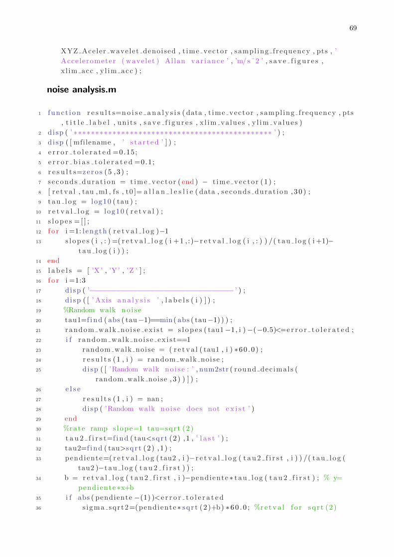
69
XYZ Aceler wavelet denoised , t ime vector , sampl ing frequency , pts , ’
Acce lerometer ( wavelet ) Al lan var iance ’ , ’m/ s ˆ2 ’ , s a v e f i g u r e s ,
x l im acc , y l im acc ) ;
noise analysis.m
1 f unc t i on r e s u l t s=n o i s e a n a l y s i s ( data , t ime vector , sampl ing frequency , pts
, t i t l e l a b e l , un i t s , s a v e f i g u r e s , x l im va lues , y l im va lue s )
2 di sp ( ’ ∗∗∗∗∗∗∗∗∗∗∗∗∗∗∗∗∗∗∗∗∗∗∗∗∗∗∗∗∗∗∗∗∗∗∗∗∗∗∗∗∗∗∗∗∗∗ ’ ) ;
3 di sp ( [ mfilename , ’ s t a r t e d ’ ] ) ;
4 e r r o r t o l e r a t e d =0.15;
5 e r r o r b i a s t o l e r a t e d =0.1 ;
6 r e s u l t s=ze ro s (5 , 3 ) ;
7 s e conds dura t i on = t ime vec to r ( end ) − t ime vec to r (1 ) ;
8 [ r e tva l , tau ,m1, f s , t0 ]= a l l a n l e s l i e ( data , seconds durat ion , 3 0 ) ;
9 t a u l o g = log10 ( tau ) ;
10 r e t v a l l o g = log10 ( r e t v a l ) ;
11 s l o p e s = [ ] ;
12 f o r i =1: l ength ( r e t v a l l o g )−1
13 s l o p e s ( i , : ) =( r e t v a l l o g ( i +1 , : )−r e t v a l l o g ( i , : ) ) /( t a u l o g ( i +1)−t a u l o g ( i ) ) ;
14 end
15 l a b e l s = [ ’X ’ , ’Y ’ , ’Z ’ ] ;
16 f o r i =1:3
17 di sp ( ’−−−−−−−−−−−−−−−−−−−−−−−−−−−−−−−−− ’ ) ;
18 di sp ( [ ’ Axis a n a l y s i s ’ , l a b e l s ( i ) ] ) ;
19 %Random walk no i s e
20 tau1=f i n d ( abs ( tau−1)==min ( abs ( tau−1) ) ) ;
21 random wa lk no i s e ex i s t = s l o p e s ( tau1−1, i )−(−0.5)<=e r r o r t o l e r a t e d ;
22 i f r andom wa lk no i s e ex i s t==1
23 random walk noise = ( r e t v a l ( tau1 , i ) ∗60 .0 ) ;
24 r e s u l t s (1 , i ) = random walk noise ;
25 di sp ( [ ’Random walk no i s e : ’ , num2str ( round dec imals (
random walk noise , 3 ) ) ] ) ;
26 e l s e
27 r e s u l t s (1 , i ) = nan ;
28 di sp ( ’Random walk no i s e does not e x i s t ’ )
29 end
30 %rate ramp s l ope=1 tau=s q r t (2 )
31 t a u 2 f i r s t=f i n d ( tau<s q r t (2 ) ,1 , ’ l a s t ’ ) ;
32 tau2=f i n d ( tau>s q r t (2 ) ,1 ) ;
33 pendiente=( r e t v a l l o g ( tau2 , i )−r e t v a l l o g ( t a u 2 f i r s t , i ) ) /( t a u l o g (
tau2 )−t a u l o g ( t a u 2 f i r s t ) ) ;
34 b = r e t v a l l o g ( t a u 2 f i r s t , i )−pendiente ∗ t a u l o g ( t a u 2 f i r s t ) ; % y=
pendiente ∗x+b
35 i f abs ( pendiente −(1) )<e r r o r t o l e r a t e d
36 s i gma sqr t2=(pendiente ∗ s q r t (2 )+b) ∗6 0 . 0 ; %r e t v a l f o r s q r t (2 )

70 APPENDIX B. MATLAB CODE
37 di sp ( [ ’ Rate ramp no i s e : ’ , num2str ( round dec imals ( s igma sqrt2 , 3 ) )
] ) ;
38 r e s u l t s (2 , i )=s igma sqr t2 ;
39 e l s e
40 di sp ( ’ Rate ramp no i s e does not e x i s t ’ )
41 r e s u l t s (2 , i )=nan ;
42 end
43 %quant i za t i on no i s e s l ope=−1 tau=s q r t (3 )
44 i f abs ( pendiente −(−1) )<e r r o r t o l e r a t e d
45 s i gma sqr t3=(pendiente ∗ s q r t (3 )+b) ∗6 0 . 0 ; %r e t v a l f o r s q r t (3 )
46 di sp ( [ ’ Quant izat ion no i s e : ’ , num2str ( round dec imals ( s igma sqrt3
, 3 ) ) ] ) ;
47 r e s u l t s (3 , i ) = s igma sqr t3 ;
48 e l s e
49 di sp ( ’ Quant izat ion no i s e does not e x i s t ’ )
50 r e s u l t s (3 , i ) = nan ;
51 end
52 %rate random walk s l ope =0.5 tau=3
53 t a u 3 f i r s t=f i n d ( tau<3 ,1 , ’ l a s t ’ ) ;
54 tau3 end=f i n d ( tau>3 ,1) ;
55 pendiente=( r e t v a l l o g ( tau3 end , i )−r e t v a l l o g ( t a u 3 f i r s t , i ) ) /(
t a u l o g ( tau3 end )−t a u l o g ( t a u 3 f i r s t ) ) ;
56 b = r e t v a l l o g ( tau3 end , i )−pendiente ∗ t a u l o g ( tau3 end ) ;
57 i f abs ( pendiente −(0 .5) )<e r r o r t o l e r a t e d
58 s igma 3=(pendiente∗3+b) ∗6 0 . 0 ; %r e t v a l f o r 3
59 di sp ( [ ’ Rate random walk no i s e : ’ , num2str ( s igma 3 ) ] ) ;
60 r e s u l t s (4 , i ) = sigma 3 ;
61 e l s e
62 di sp ( ’ Rate random walk no i s e does not e x i s t ’ )
63 r e s u l t s (4 , i ) = nan ;
64 end
65 %bia s i n s t a b i l i t y
66 i d x s l o p e 0 = abs ( s l o p e s ( : , i ) )<e r r o r b i a s t o l e r a t e d ;
67 b i a s i n s t a b i l i t y =(min ( r e t v a l ( idx s l ope0 , i ) ) /0 .644) ∗3600 ;
68 %b i a s i n s t a b i l i t y =(min ( r e t v a l ( : , i ) ) /0 .644) ∗3600 ;
69 i f ˜ isempty ( b i a s i n s t a b i l i t y )
70 di sp ( [ ’ Bias i n s t a b i l i t y : ’ , num2str ( round dec imals (
b i a s i n s t a b i l i t y , 3 ) ) , ’ dps/h ’ ] ) ;
71 e l s e
72 b i a s i n s t a b i l i t y=nan ;
73 di sp ( ’ Bias i n s t a b i l i t y does not e x i s t ’ ) ;
74 end
75 r e s u l t s (5 , i ) = b i a s i n s t a b i l i t y ;
76 end
77 di sp ( [ mfilename , ’ f i n i s h e d ’ ] ) ;
78 di sp ( ’ ∗∗∗∗∗∗∗∗∗∗∗∗∗∗∗∗∗∗∗∗∗∗∗∗∗∗∗∗∗∗∗∗∗∗∗∗∗∗∗∗∗∗∗∗∗∗ ’ ) ;
79 end
71
allan leslie.m
1 f unc t i on [ sigma ,T,m1, f s , t0 ]= a l l a n l e s l i e ( XYZ vector , seconds , pts )
2 [N,M] = s i z e ( XYZ vector ) ;
3 f s= c e i l (N/ seconds ) ; % sampling f requency in Hertz
4 n = 2 . ˆ ( 0 : f l o o r ( log2 ( (N−1)/2) ) ) ’ ; % determine l a r g e s t bin s i z e
5 maxN = n( end ) ;
6 endLogInc = log10 (maxN) ;
7 m = unique ( c e i l ( l og space (0 , endLogInc , pts ) ) ) ’ ; % c r e a t e l og spaced
vec to r average f a c t o r
8 m1 = unique ( c e i l ( l og space (0 , endLogInc , pts ) ) ) ’ ; %t e s t
9 t0 = 1/ f s ; % t0 = sample i n t e r v a l the sample per iod
10 T = m∗ t0 ; % T = length o f time f o r each c l u s t e r
11 sigma2 = ze ro s ( l ength (T) ,M) ; % array o f dimensions ( c l u s t e r pe r i od s ) X
(# v a r i a b l e s )
12 f o r j =1:M
13 theta ( : , j ) = cumsum( XYZ vector ( : , j ) ) ∗ t0 ; % i n t e g r a t i o n o f samples
over time to obta in output ang le ?
14 f o r i =1: l ength (m) % loop over the var i ous c l u s t e r s i z e s
15 f o r k=1:N−2∗m( i ) % implements the summation in the AV equat ion
16 sigma2 ( i , j ) = sigma2 ( i , j ) + ( theta ( k+2∗m( i ) , j ) − 2∗ theta ( k+
m( i ) , j ) + theta (k , j ) ) . ˆ 2 ;
17 end
18 end
19 sigma22 ( : , j ) = sigma2 ( : , j ) . / repmat ( (2∗T. ˆ 2 . ∗ (N−2∗m) ) ,1 , 1 ) ;
20 sigma ( : , j ) = s q r t ( sigma22 ( : , j ) ) ;
21 end
22 end
remove outliers.m
1 f unc t i on data=r e m o v e o u t l i e r s ( data , t i t l e l a b e l , s a v e f i g u r e s )
2 g l o b a l ou tput d i r
3 i q r d a t a=i q r ( data ) ;
4 q u a r t i l e 1=q u a n t i l e ( data , 0 . 2 5 ) ;
5 q u a r t i l e 3=q u a n t i l e ( data , 0 . 7 5 ) ;
6 lower bound=q u a r t i l e 1 −3∗ i q r d a t a ;
7 upper bound=q u a r t i l e 3 +3∗ i q r d a t a ;
8 f i g u r e ;
9 p lo t ( data ) ;
10 t i t l e ( t i t l e l a b e l ) ;
11 h l i n e = r e f l i n e ( [ 0 lower bound ] ) ;
12 h l i n e . Color = ’ r ’ ;
13 h l i n e 2 = r e f l i n e ( [ 0 upper bound ] ) ;
14 h l i n e 2 . Color = ’ r ’ ;
15 l egend ( ’ raw data ’ , ’+−3∗IQR boundar ies ’ , ’ Locat ion ’ , ’ bes t ’ )
16 %detec t them

72 APPENDIX B. MATLAB CODE
17 i d x o u t l i e r s u p p e r=data>upper bound ;
18 i d x o u t l i e r s l o w e r=data<lower bound ;
19 %remove them
20 data ( i d x o u t l i e r s u p p e r | i d x o u t l i e r s l o w e r )=median ( data ) ;
21 i f s a v e f i g u r e s
22 s a v e f i g ( [ output d i r , t i t l e l a b e l , ’ . f i g ’ ] )
23 pr in t ( [ output d i r , t i t l e l a b e l , ’ . eps ’ ] , ’−depsc ’ )
24 pr in t ( [ output d i r , t i t l e l a b e l , ’ . png ’ ] , ’−dpng ’ )
25 end
26 end
preprocess.m
1 f unc t i on [ data , t ime vector , sampl ing f requency ]= preproce s s ( data ,
t ime vector , t i t l e l a b e l , s a v e f i g u r e s )
2 di sp ( ’ ∗∗∗∗∗∗∗∗∗∗∗∗∗∗∗∗∗∗∗∗∗∗∗∗∗∗∗∗∗∗∗∗∗∗∗∗∗∗∗∗∗∗∗∗∗∗ ’ ) ;
3 di sp ( [ mfilename , ’ s t a r t e d ’ ] ) ;
4 %Remove o u t l i e r s
5 data ( : , 1 )=r e m o v e o u t l i e r s ( data ( : , 1 ) , [ t i t l e l a b e l , ’ X a x i s ’ ] ,
s a v e f i g u r e s ) ;
6 data ( : , 2 )=r e m o v e o u t l i e r s ( data ( : , 2 ) , [ t i t l e l a b e l , ’ Y a x i s ’ ] ,
s a v e f i g u r e s ) ;
7 data ( : , 3 )=r e m o v e o u t l i e r s ( data ( : , 3 ) , [ t i t l e l a b e l , ’ Z a x i s ’ ] ,
s a v e f i g u r e s ) ;
8 %Regu la r i z e time sampling
9 %I d e n t i f y sampling time and frequency
10 nanoseconds= t ime vec to r ( end )− t ime vec to r (1 ) ; % time in nanoseconds o f
the ho le data s e t
11 seconds= nanoseconds /10ˆ9 ; % conver s i on seconds
12 nHours=seconds /3600 ; % hours f o r i f i t i s neccesary and to have idea
13 t ime stamp seconds=(t ime vector−t ime vec to r (1 ) ) /1 e9 ;
14 d i f f t im e s ta m p=d i f f ( t ime stamp seconds ) ;
15 %histogram of sampling t imes with width=min ( sampling t imes )
16 %histograma=h i s t c ( d i f f t ime s tamp , 0 : min ( d i f f t im e s ta m p ) : max(
d i f f t im e s ta m p ) +1) ;
17 sampl ing t ime=round ( median ( d i f f t im e s ta m p ) ∗1000) /1000 ;%f l o o r ( f i n d (
histograma==max( histograma ) ) ∗min ( d i f f t im e s ta m p ) ∗100) /100 ;
18 sampl ing f requency=1/sampl ing t ime ;
19 t ime vec to r =0: sampl ing t ime : sampl ing t ime ∗( l ength ( data ( : , 1 ) )−1) ;
20 di sp ( [ mfilename , ’ f i n i s h e d ’ ] ) ;
21 di sp ( ’ ∗∗∗∗∗∗∗∗∗∗∗∗∗∗∗∗∗∗∗∗∗∗∗∗∗∗∗∗∗∗∗∗∗∗∗∗∗∗∗∗∗∗∗∗∗∗ ’ ) ;
22 end
denoising.m
1 % Denois ing
2 f unc t i on [ f i l t d a t a d e n o i s e d , wave l e t data deno i s ed , k f d a t d e n o i s e d ] =
73
deno i s i ng ( data vector , sampling t ime , m e d i a n f i l t e r n ,
wave l e t decomp leve l )
3 di sp ( ’ ∗∗∗∗∗∗∗∗∗∗∗∗∗∗∗∗∗∗∗∗∗∗∗∗∗∗∗∗∗∗∗∗∗∗∗∗∗∗∗∗∗∗∗∗∗∗ ’ ) ;
4 di sp ( [ mfilename , ’ s t a r t e d ’ ] ) ;
5 [m, n ] = s i z e ( da ta vec to r ) ;
6 sampl ing f requency = 1/ sampl ing t ime ;
7 f o r i =1:n
8 data = data vec to r ( : , i ) ;
9 %% F i l t e r i n g
10 f i l t d a t a d e n o i s e d ( : , i )=med f i l t 1 ( data , m e d i a n f i l t e r n ) ;
11 %% Fast f o u r i e r trans form
12 f f t v a l u e s = f f t ( data ) ;
13 L=length ( data ) ;
14 %Compute the two−s ided spectrum P2 . Then compute the s i n g l e−s ided
spectrum P1 based on P2 and the even−valued s i g n a l l ength L .
15 P2 = abs ( f f t v a l u e s /L) ;
16 P1 = P2 ( 1 : L/2+1) ;
17 P1 ( 2 : end−1) = 2∗P1 ( 2 : end−1) ;
18 %Def ine the f requency domain f and p lo t the s i n g l e−s ided amplitude
spectrum P1 .
19 %The ampl itudes are not exac t l y at 0 . 7 and 1 , as expected , because
o f the added no i s e .
20 %On average , l onge r s i g n a l s produce b e t t e r f requency approximations
.
21 f = sampl ing f requency ∗ ( 0 : ( L/2) ) /L ;
22 f i g u r e ;
23 p lo t ( f , P1)
24 t i t l e ( ’ S ing le−Sided Amplitude Spectrum of X( t ) ’ )
25 x l a b e l ( ’ f (Hz) ’ )
26 y l a b e l ( ’ |P1( f ) | ’ )
27 %Get the mean value and c a l c u l a t e a th r e sho ld :
28 mean value = mean( abs ( f f t v a l u e s ) ) ;
29 th r e sho ld = 1.1∗mean value ; % Fine−tune t h i s
30 %Remove everyth ing that ’ s below the th re sho ld (we assume that i t
cor responds to no i s e ) :
31 f f t v a l u e s = f f t ( data ) ;
32 %Remove everyth ing that ’ s below the th re sho ld (we assume that i t
cor responds to no i s e ) :
33 f f t v a l u e s ( abs ( f f t v a l u e s ) < th r e sho ld ) = 0 ;
34 %Get the f i l t e r e d data :
35 f f t d a t a d e n o i s e d ( : , i ) = i f f t ( f f t v a l u e s ) ;
36 %% Wavelet decomposit ion .
37 [ c , l ] = wavedec ( data , wave le t decomp leve l , ’ sym8 ’ ) ;
38 % thre sho ld the decomposit ion s t r u c t u r e [ c , l ] .
39 wave l e t da ta deno i s ed ( : , i ) = wden( c , l , ’ minimaxi ’ , ’ s ’ , ’ s l n ’ ,
wave le t decomp leve l , ’ sym8 ’ ) ;
40 end

74 APPENDIX B. MATLAB CODE
41 di sp ( [ mfilename , ’ f i n i s h e d ’ ] ) ;
42 di sp ( ’ ∗∗∗∗∗∗∗∗∗∗∗∗∗∗∗∗∗∗∗∗∗∗∗∗∗∗∗∗∗∗∗∗∗∗∗∗∗∗∗∗∗∗∗∗∗∗ ’ ) ;
43 end
plot allan variance.m
1 f unc t i on p l o t a l l a n v a r i a n c e ( sigma ,T, t i t l e l a b e l , un i t s , s a v e f i g u r e s ,
x l im va lues , y l im va lues , a l l a n v a l u e s )
2 g l o b a l ou tput d i r
3 ind=f i n d ( t i t l e l a b e l==’ ’ ) ;
4 main labe l = t i t l e l a b e l ( 1 : ind (1 )−1) ;
5 x=sigma ( : , 1 ) ;
6 y=sigma ( : , 2 ) ;
7 z=sigma ( : , 3 ) ;
8 f i g u r e ;
9 l o g l o g (T, x , ’b ’ , ’ LineWidth ’ , 2 ) ;
10 t i t l e ( t i t l e l a b e l ) ;
11 hold on ;
12 l o g l o g (T, y , ’ g ’ , ’ LineWidth ’ , 2 ) ;
13 l o g l o g (T, z , ’ r ’ , ’ LineWidth ’ , 2 ) ;
14 l egend ( [ main labe l , ’ X ’ ] , [ main labe l , ’ Y ’ ] , [ main labe l , ’ Z ’ ] ) ;
15 x l a b e l ( ’ \ tau ( s e c s ) ’ ) ;
16 y l a b e l ( [ ’ \ sigma ( ’ , un i t s , ’ ) ’ ] )
17 s e t ( gca , ’ XMinorGrid ’ , ’On ’ ) ;
18 s e t ( gca , ’ XGrid ’ , ’On ’ ) ;
19 s e t ( gca , ’ YMinorGrid ’ , ’On ’ ) ;
20 s e t ( gca , ’ YGrid ’ , ’On ’ ) ;
21 s e t ( gca , ’ MinorGridAlpha ’ , 0 . 9 5 )
22 % plo t l i n e s with m=−0−5 f o r random walk no i s e
23 l x=log10 ( x ) ;
24 l y=log10 ( y ) ;
25 l z=log10 ( z ) ;
26 l t=log10 (T) ;
27 xo=f i n d ( abs ( l t ) <0.1 ,1) ;
28 bx=lx ( xo )−0.5∗ l t ( xo ) ;
29 by=ly ( xo )−0.5∗ l t ( xo ) ;
30 bz=l z ( xo )−0.5∗ l t ( xo ) ;
31 y x f i t =−0.5∗ l t+bx ;
32 y y f i t =−0.5∗ l t+by ;
33 y z f i t =−0.5∗ l t+bz ;
34 l o g l o g (T, 1 0 . ˆ y x f i t , ’b−− ’ ) ;
35 l o g l o g (T, 1 0 . ˆ y y f i t , ’ g−− ’ ) ;
36 l o g l o g (T, 1 0 . ˆ y z f i t , ’ r−− ’ ) ;
37 i f ˜ isempty ( x l im va lue s ) && ˜ isempty ( y l im va lue s )
38 y l i m c u r r e n t v a l u e s=get ( gca , ’YLim ’ ) ;
39 y l im va lue s = [ min ( y l i m c u r r e n t v a l u e s (1 ) , y l im va lue s (1 ) ) , max(
y l i m c u r r e n t v a l u e s (2 ) , y l im va lue s (2 ) ) ] ;
75
40 xlim ( x l im va lue s ) ;
41 ylim ( y l im va lue s ) ;
42 e l s e
43 xlim ( [ 1 0 ˆ round ( min ( l t ) ) ,10ˆ c e i l (max( l t ) ) ] ) ;
44 ylim ( [ 1 0 ˆ f l o o r ( min ( [ l x ; l y ; l z ] ) ) ,10ˆ c e i l (max ( [ l x ; l y ; l z ] ) ) ] ) ;
45 end
46 % plo t red dotted v e r t i c a l l i n e in tau=10ˆ0
47 SP=1;
48 l i n e ( [ SP SP ] , get ( gca , ’YLim ’ ) , ’ Color ’ , [ 1 0 0 ] , ’ L ineSty l e ’ , ’−− ’ )
49 i f strcmp ( main labe l , ’ Gyroscope ’ )
50 n o i s e l a b e l s = ’ARW’ , ’RR’ , ’QN’ , ’RRW’ , ’ BI ’ ;
51 e l s e
52 n o i s e l a b e l s = ’VRW’ , ’RR’ , ’QN’ , ’RRW’ , ’ BI ’ ;
53 end
54 f o r i =1:5
55 i f ˜ a l l ( i snan ( a l l a n v a l u e s ( i , : ) ) )
56 t = annotat ion ( ’ textbox ’ ) ;
57 t . S t r ing = s p r i n t f ( ’%s X:%.3 f \n%s Y:%.3 f \n%s Z:%.3 f ’ ,
n o i s e l a b e l s i , a l l a n v a l u e s ( i , 1 ) , n o i s e l a b e l s i ,
a l l a n v a l u e s ( i , 2 ) , n o i s e l a b e l s i , a l l a n v a l u e s ( i , 3 ) ) ;
58 t po s = t . Pos i t i on ;
59 t po s (1 ) = 0 . 5 ;
60 t po s (2 ) = 0 . 5 ;
61 t . Po s i t i on = t pos ;
62 end
63 end
64 i f s a v e f i g u r e s
65 s a v e f i g ( [ output d i r , t i t l e l a b e l , ’ . f i g ’ ] )
66 pr in t ( [ output d i r , t i t l e l a b e l , ’ . eps ’ ] , ’−depsc ’ )
67 pr in t ( [ output d i r , t i t l e l a b e l , ’ . png ’ ] , ’−dpng ’ )
68 end
69 end
save allan results.m
1 f unc t i on s a v e a l l a n r e s u l t s ( a l l a n c o e f , a l l a n c o e f d e n o i s e d , t i t l e f i l e )
2 g l o b a l ou tput d i r
3 [m, n ] = s i z e ( a l l a n c o e f ) ;
4 f i l e I D = fopen ( [ output d i r , t i t l e f i l e , ’ . csv ’ ] , ’w ’ , ’ n ’ , ’ ISO−8859−1 ’ ) ;
5 f p r i n t f ( f i l e I D , ’ ,X,Y, Z ,X ( deno i sed ) ,Y ( deno i sed ) ,Z ( deno i sed ) \n ’ ) ;
6 n o i s e l a b e l s = ’Random walk ’ , ’ Rate ramp ’ , ’ Quant izat ion no i s e ’ , ’ Rate
random walk ’ , ’ Bias i n s t a b i l i t y ’ ;
7 f o r i =1:m
8 n o i s e l a b e l=n o i s e l a b e l s i ;
9 f p r i n t f ( f i l e I D , ’%s ,%f ,%f ,%f ,%f ,%f ,% f \n ’ , n o i s e l a b e l , a l l a n c o e f ( i , 1 )
, a l l a n c o e f ( i , 2 ) , a l l a n c o e f ( i , 3 ) , a l l a n c o e f d e n o i s e d ( i , 1 ) ,
a l l a n c o e f d e n o i s e d ( i , 2 ) , a l l a n c o e f d e n o i s e d ( i , 3 ) ) ;

76 APPENDIX B. MATLAB CODE
10 end
11 f c l o s e ( f i l e I D ) ;
Acronyms
INS Inertial Navigation System
IMU Inertial Measurement Unit
MEMS Micro Electromechanical Systems
NMR Nuclear Magnetic Resonance
FOG Fiber Optic Gyro
RLG Ring Lasers Gyro
IFOG Interferometric Fiber Optic Gyro
RFOG Resonant Fiber Optic Gyro
PCF Photonic Crystal Fiber
MOG Micro Optic Gyro
CCID Charge Coupled Imaging Device
MOEMS Micro-Opto Electromechanical Systems
BRW Bias Random Walk
PSD Power Spectral Density
ARW Angle Random Walk
VRW Velocity Random Walk
FFT Fast Fourier Transform
IEEE Institute of Electrical and Electronic Engineers
AVAR Allan Variance
RMS Root Means Square
RAVAR Root Allan Variance
DWT Discrete Wavelet Transform
CWT Continous Wavelet Transform
LOD Level of Decomposition
AHRS Attitude Heading Reference System
IQR Interquartile Range
pdf probability density function
77