hydrological and soil erosion modeling using swat model

HAL Id: tel-03178705https://hal.archives-ouvertes.fr/tel-03178705v2

Submitted on 24 Mar 2021

HAL is a multi-disciplinary open accessarchive for the deposit and dissemination of sci-entific research documents, whether they are pub-lished or not. The documents may come fromteaching and research institutions in France orabroad, or from public or private research centers.

L’archive ouverte pluridisciplinaire HAL, estdestinée au dépôt et à la diffusion de documentsscientifiques de niveau recherche, publiés ou non,émanant des établissements d’enseignement et derecherche français ou étrangers, des laboratoirespublics ou privés.

Hydrological and soil erosion modeling using SWATmodel and Pedotransfert Functions: a case study of

Settat-Ben Ahmed watersheds, MoroccoYassine Bouslihim

To cite this version:Yassine Bouslihim. Hydrological and soil erosion modeling using SWAT model and PedotransfertFunctions: a case study of Settat-Ben Ahmed watersheds, Morocco. Hydrology. Université HassanIer Settat (Maroc), 2020. English. �tel-03178705v2�

https://hal.archives-ouvertes.fr/tel-03178705v2

https://hal.archives-ouvertes.fr

Hassan First University

Faculty of Sciences and Technologies

Settat

Doctoral thesis

Presented by

Yassine BOUSLIHIM

Specialty: Geosciences, Hydrology and Geomatics

Host laboratory: Physico-Chemistry of Processes and Materials

Research team : Geosciences & Environment

Hydrological and soil erosion modeling using SWAT model and

Pedotransfert Functions: a case study of Settat-Ben Ahmed

watersheds, Morocco

Publicly defended on 07/22/2020 in front of the jury composed of:

Pr. Fouad AMRAOUI

Pr. Abdellah LAKHOUILI

Pr. Noureddine LAFTOUHI

Pr. Ahmed BARAKAT

Pr. Khadija ABOUMARIA

Pr. Namira ELAMRANI PAAZA

Pr. Aicha ROCHDI

FS Ain Chok, Hassan II University, Casablanca

FST, Hassan Fisrt University, Settat

FS Semlalia, Cadi Ayyad University, Marrakech

FST, Sultan Moulay Slimane University, Béni –Mellal

FST, Abdelmalek Essaadi University, Tanger



President

Reporter

Reporter

Reporter

Examiner

Co-thesis director

Thesis director

II

ABSTRACT

Data availability problems for hydrological and soil studies are undoubtedly a critical constraint for all

scientists around the world. This was also our challenge in this thesis, where the study area is poorly documented and

devoid of any hydrological study. The first part of this thesis report was devoted to the execution and applicability

of the Soil and Water Assessment Tool (SWAT) model to predict runoff and to assess soil erosion rate in three

watersheds belonged to Settat - Ben Ahmed region, namely Tamedroust (642.42 km2), Mazer (179.2 km2) and El

Himer (177.7 km2). A semi-arid climate and irregular rainfall also characterize this zone. SWAT model inputs were

collected and extracted from different sources and simulations were carried out over eight years (January 1995 –

December 2002). For soil data, seventy-seven samples were sampled from 0-40 cm depth and analyzed to obtain

different soil parameters such as texture, organic matter (OM), soil aggregate stability, pH and electrical conductivity

(EC). This soil database (TAMED-SOIL) was compared with the Harmonized World Soil Database (HWSD) to

analyze the effects of soil data quality on the SWAT model performance and hydrologic process Tamedroust

watershed. Before calibration, results showed a considerable variability and a significant effect of the soil

characteristics on the different components of the hydrological cycle. After the calibration period, both soil databases

improved the model performance in terms of streamflow, with values of R2 and NSE (Nash-Sutcliffe Efficiency)

between 0.64 and 0.65. Model validation was acceptable and similar for both databases with R2 and NSE values of

0.76 and 0.57, respectively. The results also show that all sub-watersheds of Tamedroust present a weak soil erosion

rate for both soil databases.

Using the regionalization method between Mazer (gauged watershed) and El Himer (ungauged watershed),

SWAT model results showed a good correlation between observed and simulated streamflow with an NSE of 0.65

and 0.89, and with R2 of 0.75 and 0.95 for calibration and validation, respectively. The fitted values for the most

sensitive parameters obtained at the Mazer watershed are transferred to the El Himer watershed to estimate

streamflow and erosion. The results showed that all studied sub-watersheds present a weak rate of soil erosion.

The last part of this thesis report focuses on the comparison of the capabilities of Multiple Linear Regression

(MLR) and a machine learning technique (Random Forest (RF)) to predict soil aggregate stability (SAS) index from

Pedotransfer Functions (PTFs) using different sets of input variables (soil properties and remote sensing parameters).

The results obtained were satisfactory for both models. However, the sample size must be increased to ensure more

excellent uniformity to predict the SAS index better. Thus, the PTFs developed in this study can be used worldwide

as a basis for predicting the soil aggregate stability in another area with the same climatic and edaphic characteristics.

Keywords: SWAT model, hydrological modeling, soil erosion, Pedotransfer Functions, soil aggregate stability,

multiple linear regression, random forest, Machine learning, Settat-Ben Ahmed plateau watersheds,

Morocco.

III

RÉSUMÉ

Les problèmes de disponibilité des données pour les études hydrologiques et pédologiques constituent sans

aucun doute une contrainte critique pour tous les scientifiques du monde entier. C’était également notre défi dans

cette thèse où la zone d’étude est mal documentée et dépourvue de toute étude hydrologique. Cette zone est également

caractérisée par un climat semi-aride et des précipitations irrégulières. La première partie de ce travail a été consacrée

à l'exécution et à l'applicabilité du modèle SWAT (Soil and Water Assessment Tool) pour estimer le ruissellement et

le taux d'érosion du sol dans les trois bassins versants (BV) de la région de Settat-Ben Ahmed, à savoir Tamedroust

(642.42 km2), Mazer (179.2 km2) et El Himer (177.7 km2). Les données du modèle SWAT ont été collectées de

différentes sources et les simulations ont été effectuées sur huit années (janvier 1995 - décembre 2002). Pour les

données du sol, une base de données TAMED-SOIL de soixante-dix-sept échantillons ont été prélevés à une

profondeur de 0-40 cm et analysés afin d’obtenir les différents paramètres du sol tel que la texture, la matière

organique (MO), la stabilité structurale des agrégats, le pH et la conductivité électrique (CE). L’effet de la qualité de

données du sol sur les performances de simulation du modèle SWAT a été testé en utilisant deux bases de données

différentes, TAMED-SOIL et Harmonized World Soil Database (HWSD) sur le BV Tamedroust. Les résultats avant

calibration ont montré une variabilité considérable et un effet significatif des caractéristiques du sol sur les différentes

composantes du cycle hydrologique. Après la calibration, les deux bases de données du sol ont amélioré les

performances du modèle en matière de débit, avec des valeurs de R2 et NSE (Nash-Sutcliffe Efficiency) entre 0,64

et 0,65. La validation du modèle est acceptable et similaire pour les deux bases de données avec des valeurs de R2 et

NSE de 0,76 et 0,57, respectivement. Les résultats montrent également que tous les sous-bassins de Tamedroust

présentent un faible taux d'érosion pour les deux bases de données du sol.

En utilisant la méthode de régionalisation entre les BVs Mazer (jaugé) et El Himer (non jaugé). Les résultats

du modèle ont montré une bonne corrélation entre le débit observé et simulé avec un NSE de 0,65 et 0,89, et avec un

R2 de 0,75 et 0,95 pour la calibration et la validation, respectivement. Les valeurs ajustées des paramètres les plus

sensibles obtenues dans le BV Mazer sont transférées au bassin versant El Himer pour estimer le débit et le taux

d'érosion. Les résultats ont montré que tous les sous-bassins versants étudiés présentent un faible taux d'érosion.

La dernière partie de ce rapport de thèse concerne la comparaison des capacités de la Régression Linéaire

Multiple (MLR) et de la technique d'apprentissage automatique Random Forest (RF) pour prédire l'indice de stabilité

structurale des agrégats (SAS) à partir des Fonctions de Pédotransfert (PTFs) utilisant différents ensembles de

variables d'entrée (propriétés du sol et paramètres de télédétection). Les résultats obtenus sont satisfaisants pour les

deux modèles. Cependant, la taille de l'échantillon doit être augmentée pour assurer une plus grande uniformité

d'échantillonnage afin de mieux prédire la SAS. Les PTFs ainsi développés dans cette étude pourraient être utilisés

ailleurs pour prédire la stabilité structurale des agrégats sous les mêmes caractéristiques climatiques et édaphiques.

Mots Clés: Modèle SWAT, modélisation hydrologique, érosion du sol, fonctions de pédotransfert, stabilité

structurale des agrégats, Régression Linéaire Multiple, Random Forest, apprentissage automatique,

bassins versants du plateau de Settat-Ben Ahmed, Maroc.

IV

ملخص

لشيئ الذي يشكل عائقا ايعاني أغلب الباحثين والمتخصصين في العلوم المتعلقة بالماء والتربة في العالم من شح المعلومات والبيانات،

رولوجية كافية هرالطبيعية بشكل كبير. يتمثل تحدي هذه األطروحة في غياب دراسات هيدأماماهم من أجل الحصول على نتائج تحاكي الضوا

Soilار تطبيق أداة للمنطقة المدروسة و التي تتميز بمناخ شبه جاف وأمطار غير منتظمة. يقدم الجزء األول من هذه األطروحة محاولة اختب

and Water Assessment Tool (SWATلتوقع جريان الماء ع ) لتالث الى السطح، وتقدير معدل انجراف التربة في األحواض المائية

179.2 كلم مربع، باإلضافة لحوض "مازر" بمساحة 642.42بن أحمد"، حيث نجد حوض "تامدروست" بمساحة -التابعة لمنطقة "سطات

ة المحاكاة مصادر مختلفة، كما تمت عملي من عدةSWAT تم جمع و استخراج بيانات نموذج .مربع كلم 177.7كلم و " لحيمر " بمساحة

ينة بعمق يتراوح (. بالنسبة للبيانات الخاصة بالتربة، تم جمع سبعة و سبعين ع2002ودجنبر 1995على مدى ثماني سنوات )ما بين يناير

التربة و ضةر الكلي وحموسنتيميتر، وتمت دراستها لقياس عدة معامالت مختلفة مثل الملمس والمادة العضوية واالستقرا 40و 0بين

( لدراسة تأثير HWSDبقاعدة بيانات التربة العالمية )(TAMED-SOIL) الُموِصلية الكهربائية. تمت مقارنة قاعدة بيانات التربة السابقة

رة النموذج والتصرف الهيدرولوجي بالحوض المائي"تامدروست". أظهرت النتائج قبل معاي SWATجودة بيانات التربة على نتائج نموذج

قاعدتي التربة من وجود تباين و تأثير كبيرين لخصائص التربة على مختلف مكونات الدورة الهيدرولوجية. بعد عملية المعايرة، حسنت كلتا

fe Sutclif-NSE (Nashو معامل 2Rلمعامل االرتباط 0.65و 0.64أداء النموذج من حيث التدفق المائي، مع قيم محصورة بين

)cyEfficien 2عامل ارتباط م. يمكن اعتبار نتائج التحقق من فعالية النموذج مقبولة و متشابهة بالنسبة لكلتا قاعدتي البيانات، معR بقيمة

. كما أظهرت النتائج نسبا ضعيفة لمعدل انجراف التربة لقاعدتي البيانات المتعلقة بالتربة.NSEلمعامل 0.57و 0.76

ظهرت أليمي بين حوض "مازر" )بيانات الجريان مسجلة( وحوض الحيمر )بيانات غير مسجلة(، باستخدام طريقة التقارب االق

محصور بين ومعامل ترابط 0.89و 0.65محصور بين NSEالنتائج وجود ترابط جيد بين الجريان المائي المقاس و المحاكى، مع معامل

دراسة جريان لاألكثر حساسية من حوض "مازر" الى حوض "لحيمر"، وذلك لفترة المعايرة والتحقق. تم نقل قيم اإلعدادات 0.95و 0.75

عية التي تمت دراستها.أظهرت النتائج نسبا ضعيفا لمعدل إنجراف التربة بالنسبة لجميع األحواض المائية الفر الماء و نسبة انجراف التربة.

Multiple Linear)تعمال االنحدار الخطي المتعددفي الجزء األخير من هذه األطروحة تم التركيز على مقارنة إمكانية إس

Regression (MLR)) وواحدة من تقنيات تعلم اآللة(Random Forest (RF)) شتقاقات اباالستقرار الكلي للتربة عن طريق ،للتنبؤ

ت باستعمال مجموعة من المتغيرات )خصائص التربة و إعدادا Pedotransfer Functions (PTFs)"دوال نقل إعدادات التربة"

المصدر لضمان اتساق االستشعار عن بعد(. النتائج كانت مقبولة لكال النموذجين. رغم ذلك، يجب زيادة حجم قاعدة البيانات، اآلتية من نفس

الت التربة" المطورة ا أيضا من استخدام "دوال نقل معامالعينات ، الشيئ الذي سيساعد على التنبؤ بمعامل استقرار التربة الكلي. وسيمكنن

صائص التربة.خخالل هذه الدراسة في جميع بقاع العالم للتنبؤ بمعامل استقرار التربة في منطقة أخرى لها نفس الخصائص المناخية و

قرار التربة، اإلنحدار ات التربة، معامل إست، النمذجة الهيرولوجية، إنجراف التربة، دوال نقل إعدادSWAT وذجنم الكلمات المفتاحية:

المغرب.-األحواض المائية لهضبة سطات بن أحمد ,التعلم االلي، Random Forestالخطي المتعدد،

V

ACKNOWLEDGMENTS

I will first thank the Almighty God for giving me the ability and strength to start and finish this Ph.D.

research.

I would like to express my profound gratitude to my supervisors, Pr. Aicha Rochdi and Pr Namira El

Amrani Paaza, for their guidance, advice, encouragement, and support thought this study. I really feel

honored to have had the opportunity to work on my thesis under their supervision.

I also thank the Faculty of Science and Technology of Settat and The Hassan First University for

providing the necessary material resources to the successful completion of this Ph.D. research.

I am especially thankful to Dr. Lorena Liuzzo of the Faculty of Engineering and Architecture, Kore

University of Enna, for here helpful assistance on the model's technical issues.

A pleasure to express my appreciation to those who shared their knowledge and time during the thesis

process: Pr. Miftah Abdelhalim, Soufiane Taia, Lahcen H'ssaini, Hakim Lhajouj and Pr Aniss Moumen.

I also would like to thank those who helped me with fieldwork and laboratory analyses: Samir Ait

M’barek, Fath ElKhair Elmaataoui, Ibrahim Elyaakoubi and Elkhalil Akabli.

I am also thankful to my friends for their encouragement during this study.

Last but not least, I thank my family and my fiancée for their patience, kindness, and support. I could

not have done it without them.

I thank the support of all the people whose help made this thesis possible.

VI

TABLE OF CONTENTS

ABSTRACT ............................................................................................................................................................... II

RÉSUMÉ ................................................................................................................................................................... III

IV........................................................................................................................................................................... ملخص

ACKNOWLEDGMENTS ......................................................................................................................................... V

TABLE OF CONTENTS .........................................................................................................................................VI

LIST OF TABLES ....................................................................................................................................................IX

LIST OF FIGURES ................................................................................................................................................... X

LIST OF PICTURES ...............................................................................................................................................XI

ABBREVIATIONS ...................................................................................................................................................XI

INTRODUCTION ...................................................................................................................................................... 1

I. General background and objectives .................................................................................................................. 1

II. Thesis outline .................................................................................................................................................... 2

CHAPTER 1: LITERATURE REVIEW ................................................................................................................. 4

I. Rainfall-Runoff Models .................................................................................................................................... 4

1. A short review of rainfall-runoff models ...................................................................................................... 4

2. Hydrological model types and classification ................................................................................................ 6

II. Overview of soil erosion................................................................................................................................... 7

1. Generality ..................................................................................................................................................... 7

2. Soil Erosion Process ................................................................................................................................... 10

3. Soil erosion estimation ............................................................................................................................... 11

III. Hydrological modeling in ungauged and gauged watersheds .................................................................... 13

IV. Pedotransfer functions ................................................................................................................................ 15

V. Overview of SWAT model ............................................................................................................................. 17

1. Model processes ......................................................................................................................................... 18

2. A brief comparison with other models ....................................................................................................... 20

3. Application of SWAT model in Moroccan watersheds .............................................................................. 21

CHAPTER 2: STUDY AREA ................................................................................................................................. 25

I. Overview of the study area ............................................................................................................................. 25

1. General context ........................................................................................................................................... 25

2. Chaouia plain .............................................................................................................................................. 28

II. Descriptions of Settat Ben-Ahmed plateau watersheds .................................................................................. 29

1. Morphological characteristics ..................................................................................................................... 30

2. Climate ....................................................................................................................................................... 32

3. Geology ...................................................................................................................................................... 34

VII

4. Land use ...................................................................................................................................................... 38

5. Soil map ...................................................................................................................................................... 39

CHAPTER 3: EFFECT OF SOIL DATA QUALITY ON SWAT MODEL ....................................................... 42

I. Introduction .................................................................................................................................................... 42

II. Soil sampling and analysis ............................................................................................................................. 43

1. Collection and Preparation of Soil Samples ............................................................................................... 44

2. Soil Laboratory Analysis ............................................................................................................................ 44

III. Methods ...................................................................................................................................................... 46

IV. Defining SWAT hydrologic response units ................................................................................................ 50

V. Model Sensitivity Analysis, Calibration and Validation ................................................................................ 50

VI. Results: ....................................................................................................................................................... 51

1. Modeling results before calibration ............................................................................................................ 51

2. Modeling results after calibration ............................................................................................................... 54

3. Soil erosion results in Tamedroust watershed ............................................................................................ 57

VII. Discussion ................................................................................................................................................... 58

VIII. Conclusion .................................................................................................................................................. 59

CHAPTER 4: ESTIMATION OF RUNOFF AND SOIL EROSION AT MAZER AND EL HIMER

WATERSHEDS ........................................................................................................................................................ 60

I. Introduction .................................................................................................................................................... 60

II. Methods .......................................................................................................................................................... 60

III. Simulation information ............................................................................................................................... 61

IV. Results: ....................................................................................................................................................... 62

1. Comparison of watershed characteristics ................................................................................................... 62

2. Sensitivity analysis results .......................................................................................................................... 63

3. Calibration and validation of SWAT model ............................................................................................... 63

4. Soil erosion results and identification of the critical sub-watersheds ......................................................... 64

V. Conclusion ...................................................................................................................................................... 68

CHAPTER 5: SOIL AGGREGATE STABILITY PREDICTION USING MULTIPLE LINEAR

REGRESSION AND RANDOM FOREST ............................................................................................................ 69

I. Introduction .................................................................................................................................................... 69

II. Modeling approaches and data sets ................................................................................................................ 70

III. Evaluation of prediction accuracy .............................................................................................................. 73

IV. Results: ....................................................................................................................................................... 73

1. Descriptive statistics of soil properties ....................................................................................................... 73

2. Multiple linear regression model performance ........................................................................................... 79

3. Random Forest performance ...................................................................................................................... 82

4. Spatial prediction of MWD ........................................................................................................................ 83

VIII

V. Comparison between MLR and RF ................................................................................................................ 87

VI. Conclusion .................................................................................................................................................. 88

CONCLUSIONS AND RECOMMENDATIONS ................................................................................................. 89

I. Conclusions .................................................................................................................................................... 89

II. Limitations of the study and recommendations .............................................................................................. 90

REFERENCES ......................................................................................................................................................... 92

APPENDICES......................................................................................................................................................... 115

IX

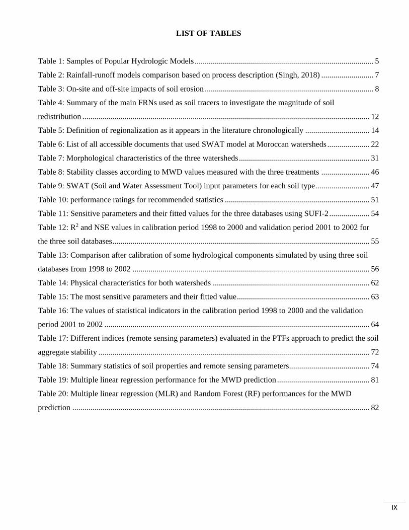
LIST OF TABLES

Table 1: Samples of Popular Hydrologic Models ......................................................................................... 5

Table 2: Rainfall-runoff models comparison based on process description (Singh, 2018) .......................... 7

Table 3: On-site and off-site impacts of soil erosion .................................................................................... 8

Table 4: Summary of the main FRNs used as soil tracers to investigate the magnitude of soil

redistribution ............................................................................................................................................... 12

Table 5: Definition of regionalization as it appears in the literature chronologically ................................ 14

Table 6: List of all accessible documents that used SWAT model at Moroccan watersheds ..................... 22

Table 7: Morphological characteristics of the three watersheds ................................................................. 31

Table 8: Stability classes according to MWD values measured with the three treatments ........................ 46

Table 9: SWAT (Soil and Water Assessment Tool) input parameters for each soil type........................... 47

Table 10: performance ratings for recommended statistics ........................................................................ 51

Table 11: Sensitive parameters and their fitted values for the three databases using SUFI-2 .................... 54

Table 12: R2 and NSE values in calibration period 1998 to 2000 and validation period 2001 to 2002 for

the three soil databases ................................................................................................................................ 55

Table 13: Comparison after calibration of some hydrological components simulated by using three soil

databases from 1998 to 2002 ...................................................................................................................... 56

Table 14: Physical characteristics for both watersheds .............................................................................. 62

Table 15: The most sensitive parameters and their fitted value .................................................................. 63

Table 16: The values of statistical indicators in the calibration period 1998 to 2000 and the validation

period 2001 to 2002 .................................................................................................................................... 64

Table 17: Different indices (remote sensing parameters) evaluated in the PTFs approach to predict the soil

aggregate stability ....................................................................................................................................... 72

Table 18: Summary statistics of soil properties and remote sensing parameters ........................................ 74

Table 19: Multiple linear regression performance for the MWD prediction .............................................. 81

Table 20: Multiple linear regression (MLR) and Random Forest (RF) performances for the MWD

prediction .................................................................................................................................................... 82

X

LIST OF FIGURES

Figure 1: Four-stage for erosion process ..................................................................................................... 10

Figure 2: A scheme for developing Pedotransfer Functions (McBratney et al., 2002) .............................. 16

Figure 3: Schematic representation of the hydrologic cycle in SWAT model (Neitsch et al., 2011) ......... 18

Figure 4: Different components of routing in SWAT model (Neitsch et al., 2011) ................................... 20

Figure 5: Water stress in the Mediterranean basin ...................................................................................... 25

Figure 6: Geographic distribution of Moroccan Watershed Basin Agencies ............................................. 27

Figure 7: Geographic map of Bouregreg and Chaouia watershed basin (ABHBC, 2009) ......................... 27

Figure 8: Distribution of aquifers in Bouregreg and Chaouia (ABHBC, 2009) ......................................... 29

Figure 9: Localization of the three watersheds (Tamedroust, Mazer and El Himer) .................................. 30

Figure 10: The monthly average rainfall evolution for each station ........................................................... 33

Figure 11: Average annual rainfall series for each station .......................................................................... 33

Figure 12: Average annual rainfall for the three stations ............................................................................ 34

Figure 13: Geological and structural Map of Settat-Ben Ahmed plateau ................................................... 35

Figure 14: Stratigraphic logs of the three areas, a: Phosphate plateau, b: intermediate area, c: Berrechid

plain ............................................................................................................................................................. 37

Figure 15: Dynamic function in the transition area .................................................................................... 38

Figure 16: Land use map and statistic class distribution of the three watersheds ...................................... 39

Figure 17: Soil map of Mazer and El Himer watersheds ............................................................................ 40

Figure 18: Soil map of Tamedroust watershed (El Oumri et al., 1995) ...................................................... 40

Figure 19: Location of the sampling points ................................................................................................ 43

Figure 20: Tamedroust watershed soil maps on (a) HWSD-2L map (b) TAMED-SOIL map ................... 48

Figure 21: Methodological flowchart ......................................................................................................... 49

Figure 22: Comparison before calibration of observed and simulated monthly streamflow using HWSD-

2L and TAMED-SOIL databases ................................................................................................................ 52

Figure 23: Comparison of hydrological components simulated by using the two different soil databases

TAMED-SOIL and HWSD-2L (before calibration) ................................................................................... 53

Figure 24: Comparison before calibration between simulated monthly streamflow using the three soil

databases ..................................................................................................................................................... 53

Figure 25: Scatter plot of simulated versus observed streamflow for the calibration (1998-2000) and the

validation (2001-2002) periods for the three databases .............................................................................. 55

Figure 26: The spatial distribution of Soil Water content by using a) TAMED-SOIL, b) HWSD-1L and c)

HWSD-2L databases from 1998 to 2002 .................................................................................................... 57

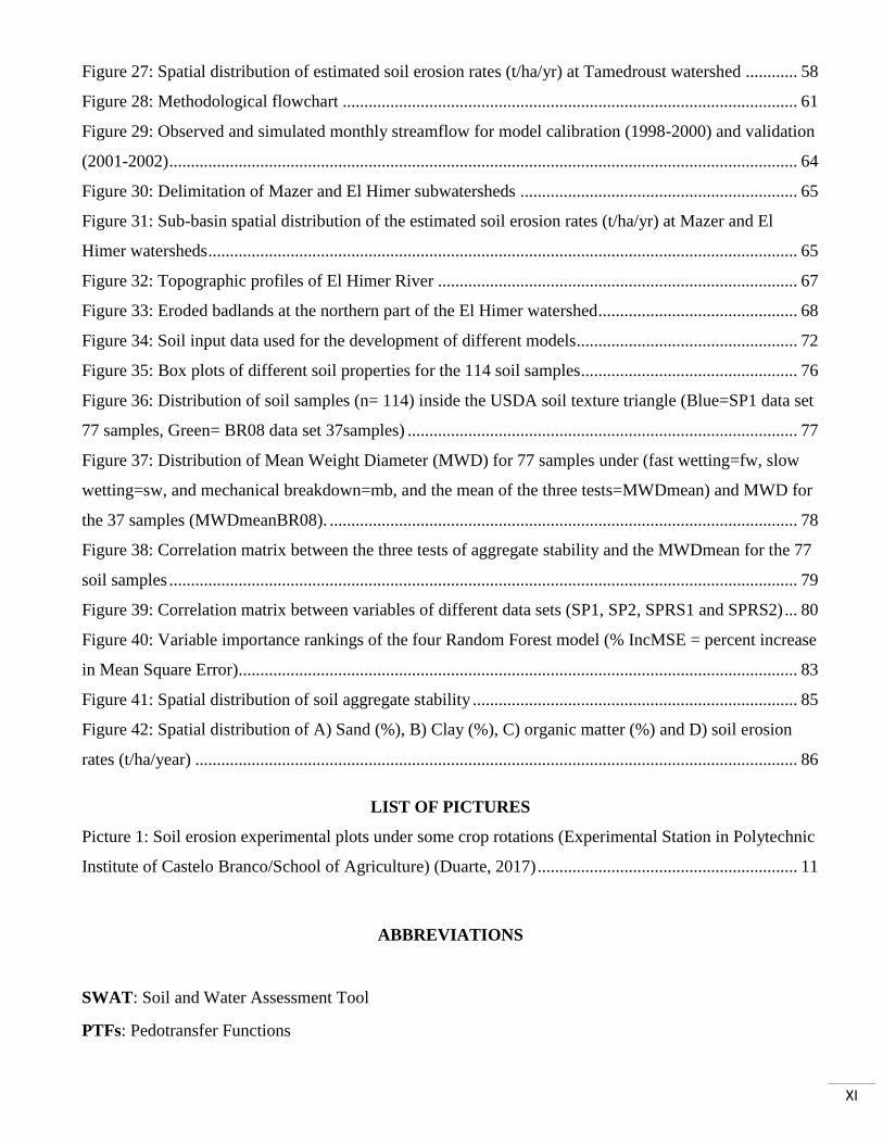
XI

Figure 27: Spatial distribution of estimated soil erosion rates (t/ha/yr) at Tamedroust watershed ............ 58

Figure 28: Methodological flowchart ......................................................................................................... 61

Figure 29: Observed and simulated monthly streamflow for model calibration (1998-2000) and validation

(2001-2002) ................................................................................................................................................. 64

Figure 30: Delimitation of Mazer and El Himer subwatersheds ................................................................ 65

Figure 31: Sub-basin spatial distribution of the estimated soil erosion rates (t/ha/yr) at Mazer and El

Himer watersheds ........................................................................................................................................ 65

Figure 32: Topographic profiles of El Himer River ................................................................................... 67

Figure 33: Eroded badlands at the northern part of the El Himer watershed .............................................. 68

Figure 34: Soil input data used for the development of different models ................................................... 72

Figure 35: Box plots of different soil properties for the 114 soil samples .................................................. 76

Figure 36: Distribution of soil samples (n= 114) inside the USDA soil texture triangle (Blue=SP1 data set

77 samples, Green= BR08 data set 37samples) .......................................................................................... 77

Figure 37: Distribution of Mean Weight Diameter (MWD) for 77 samples under (fast wetting=fw, slow

wetting=sw, and mechanical breakdown=mb, and the mean of the three tests=MWDmean) and MWD for

the 37 samples (MWDmeanBR08). ............................................................................................................ 78

Figure 38: Correlation matrix between the three tests of aggregate stability and the MWDmean for the 77

soil samples ................................................................................................................................................. 79

Figure 39: Correlation matrix between variables of different data sets (SP1, SP2, SPRS1 and SPRS2) ... 80

Figure 40: Variable importance rankings of the four Random Forest model (% IncMSE = percent increase

in Mean Square Error)................................................................................................................................. 83

Figure 41: Spatial distribution of soil aggregate stability ........................................................................... 85

Figure 42: Spatial distribution of A) Sand (%), B) Clay (%), C) organic matter (%) and D) soil erosion

rates (t/ha/year) ........................................................................................................................................... 86

LIST OF PICTURES

Picture 1: Soil erosion experimental plots under some crop rotations (Experimental Station in Polytechnic

Institute of Castelo Branco/School of Agriculture) (Duarte, 2017) ............................................................ 11

ABBREVIATIONS

SWAT: Soil and Water Assessment Tool

PTFs: Pedotransfer Functions

XII

MLR: Multiple linear regression

RF: Random forest

SAS: Soil aggregate stability

MWD: Mean weight diameter

NSE: Nash–Sutcliffe Efficiency

OM: Organic matter

BD: Bulk density

AWC: Available water capacity

EC: Electrical conductivity

ET: Evapotranspiration

WYLD: Water yield

LAI: Leaf Area Index

EVI: Enhanced Vegetation Index

GSI: Grain Size Index

SAVI: Soil Adjusted Vegetation Index

GVI: Green Vegetation Index

BI: Brightness Index

RI: Redness Index

SI: Salinity Index

NDWI: Normalized Difference Water Index

MSI: Moisture Stress Index

RVI: Ratio Vegetation Index

DVI: Difference Vegetation Index

NDVI: Normalized Difference Vegetation Index

TNDVI: Transformed Normalized Difference Vegetation Index

1

INTRODUCTION

I. General background and objectives

Sustainable management of soil and water resources at the watershed level requires effective

planning based on appropriate scientific studies and using rainfall-runoff models with various inputs

from different sources. Therefore, many environmental problems, such as quantification of soil

erosion and flow prediction, are simulated to ensure a good understanding and to propose adequate

solutions.

In principle, hydrological models should be calibrated to be used (Gupta et al., 1998). Thus,

properly calibrated and validated hydrologic models provide extremely powerful water assessment

tools to estimate streamflow when combined with good data sets. This aim could be achieved by

ensuring a large amount of data, especially when using a highly parameterized model such as the Soil

and Water Assessment Tool (SWAT) model. This requires time for setting up and needs different

inputs (for example, meteorological and hydrological data, land use, soil map, soil parameters and

slope). Also, the large number of parameters included in the equations requires specific knowledge

for the calibration (Abdelwahab et al., 2018). Wherefore, considerable difficulties are cropping up

when applying models in watersheds with conditions of insufficient or unavailable data.

Many watersheds worldwide suffer from a lack of data regardless of their nature, making the

hydrological modelers' work more complicated. However, that opens new perspectives to researchers

and academics who want to find adequate solutions or better ways to overcome the challenges related

to data availability. This can be viewed as one of the novelties of this thesis. Besides, soil plays a

crucial role in the hydrological cycle; it captures and stores water, making it available for absorption

by crops, and thus minimizing surface evaporation and maximizing water use efficiency and

productivity (Gibbon, 2012).

Collecting and preparing soil data is a tedious, expensive and time-consuming task, especially

when it involves some complex parameters to measure. In these conditions, researchers are forced to

find alternative solutions, like some techniques to estimate soil properties from easily measurable soil

parameters (Gunarathna et al., 2019), a practice is commonly known as "Pedotransfer Function

(PTFs)". It can be defined as predictive functions of certain soil properties from others easily,

routinely, or cheaply measured. The most readily available data comes from soil surveys, such as

field morphology, texture, structure, and pH (Odeh and McBratney, 2005). That can be considered

2

again as one of the advantages or novelties of this study, knowing that these methods have not been

used before in Morocco.

The first part of this Ph.D. thesis can be considered as an attempt to test the execution and

applicability of the SWAT model in predicting runoff and estimate soil erosion rate in a region that

has long been considered as the granary of Morocco, which suffers for some decades from the fall of

the cereals yields, the main regional production. The results of this study can help scientists, decision-

makers and all those involved in the environmental field to define all areas that require intervention

to reduce the impact of soil erosion. The calibrated and validated model in the selected watersheds

could give help in this purpose by testing different best management practices (BMPs) that are

integrated into the SWAT model. In addition, the model may also be used in futures studies to analyze

the impacts of climate change effect on water resources, soil erosion and land use.

On the other hand, soil aggregate stability analysis can be considered a time-consuming method, as

we need to deal with different tests and repetitions. For this reason, the last part of this thesis focuses

on the comparison of the capabilities of Multiple Linear Regression (MLR) and a machine learning

technique (Random Forest (RF)) to derive Pedotransfer Functions (PTFs) between different sets of

input variables (soil properties and remote sensing data) and soil aggregate stability (SAS) index, as

one of the essential factors in soil conservation and maintenance of soil environmental functions.

This study can be considered as the first initiative to use a machine-learning algorithm to build PTFs

in Morocco. It can help researchers and responsible laboratories provide more soil data and encourage

rational management for human, material and financial resources. Knowing that machine learning

techniques can handle large data sets. Finally, the developed PTFs in this study could be used

worldwide as a basis for predicting soil aggregate stability in another area with the same climatic and

edaphic characteristics, using another collection of soil samples.

II. Thesis outline

This report starts with an introduction to the subject of this research.

In chapter 1, a literature review describes the rainfall-runoff models, their types, and their

classification. We also describe the erosion and soil loss processes, the factors affecting them, their

on-site and off-site effects, and an overview of methods to estimate soil erosion. Various

regionalization approaches and the ungauged watershed concept are also described, and an overview

of Pedotransfer Functions and SWAT model.

3

In chapter 2, an overview of the study area and all watersheds characteristics such as

morphology, climate, geology, pedology, and land use are described.

Chapter 3 examines the effect of the soil data quality on the SWAT model with, at first, a

general presentation of soil sampling as well as the methods used to measure all different soil

parameters. We also describe the methodology followed to setup the SWAT model and the results

obtained in the two phases (before and after calibration). In the end, we presented the results of soil

erosion in the Tamedroust watershed.

Chapter 4 discusses the SWAT model's use and the regionalization method to estimate runoff

and soil erosion at Mazer and El Himer watersheds. In this chapter, we have presented the

methodology adopted and the results obtained.

Chapter 5 focuses on comparing MLR and RF methods to predict soil aggregate stability and

the significance of the variables included in both models. We have presented all the data used as input

data and the scenarios proposed for the comparison. A statistical comparison of the data and the two

models' performance were detailed in the results part, with a comparison between the two models.

The last part presents the general conclusions and limits of this research and provides

recommendations and outlooks for further studies.

4

CHAPTER 1: LITERATURE REVIEW

I. Rainfall-Runoff Models

1. A short review of rainfall-runoff models

According to Shoemaker et al. (2005), the term ‘model’ denotes a set of equations or algorithms

that are used to simulate the behavior of the physical system. It is also used to refer to the available

computer software tools that automate the calculation of equations or a combination of equations

representing the system. There was a time 160 years ago when the first hydrologists used limited data

and some basic computational methods to estimate possible flows from a rainfall event. Moreover,

all credit goes to the Irish engineer Thomas James Mulvaney (1822–1892), who created the first

rainfall-runoff model published in 1851. The model was a single easy equation that used rainfall

intensity (�̅�) drainage area (A) and a runoff coefficient (C) to determine the peak discharge (𝑄𝑝) in a

drainage basin, but it succeeds in illustrating most of the issues that have since made life difficult for

hydrological modelers (Beven, 2012). The equation is as follows:

𝑄𝑝=𝐶𝐴�̅�

Thus, this model reflects how discharges are expected to increase with area and rainfall intensity

rationally. That is why it has become known as the Rational Method. It is not as sophisticated as the

Soil Conservation Service–Curve Number (SCS-CN) method (USDA, 1986). Still, it is the most

commonly used method for sizing sewer systems, design a bridge or culvert capable of carrying the

estimated peak discharge.

Since the computer revolution, hydrological modeling has made a huge leap forward, which gives

birth to a new branch of hydrology, called digital or numerical hydrology (Singh, 2018). That allows

hydrological modelers to handle a large amount of data at the same time, and that made possible the

integration of different hydrologic cycle components and the simulation of the entire watershed.

The available literature suggests that the Stanford Watershed Model developed by Crawford and

Linsley (1966) was probably the first attempt to model virtually the entire hydrologic cycle. It is

followed by countless watershed models developed worldwide in the coming decades, such as HEC

1, developed in 1967 at the Hydrologic Engineering Center in Davis, the Hydrologic Simulation

Program in Fortran (HSPF) developed in the early 1960s as the Stanford Watershed Model and Soil

and Water Assessment Tool (SWAT) (Arnold et al., 1998).

5

The progress in watershed modeling has been affected by developments in GIS and remote

sensing technologies. GIS development has offered hydrologists with additional capacity to reduce

computation times, handle and explore big databases that describe heterogeneity in soil surface

features, and improve model results display (Daniel et al., 2011). Many of these models are described

in (Singh, 1995; Singh and Frevert, 2002). The list created by Singh and Woolhiser (2002) and

presented in Table 1 shows a hydrological models sample from around the world in chronological

order. This list was modified to keep the most popular models and to add some new ones.

Table 1: Samples of Popular Hydrologic Models

Model name/acronym Author(s) (year) Remarks

Stanford Watershed Model

(SWM)/Hydrologic Simulation

Package-Fortran IV (HSPF)

(Crawford and Linsley,

1966)

(Bicknell et al., 1996)

Continuous, dynamic event or a

steady-state simulator of hydrologic

and hydraulic and water quality

processes

Physically Based Runoff Production

Model (TOPMODEL)

(Beven and Kirkby,

1979, 1976)

Physically-based, distributed, a

continuous hydrologic simulation

model

Chemicals, Runoff, and Erosion from

Agricultural Management Systems

(CREAMS)

(Knisel, 1980) Process-oriented, lumped parameter,

agricultural runoff and water quality

model

Hydrologic Engineering Center—

Hydrologic Modeling System (HEC-

HMS)

(Feldman, 1981) Physically-based, semi-distributed,

event-based, runoff model

Areal Non-point Source Watershed

Environment Response Simulation

(ANSWERS)

(Beasley et al., 1980)

(Bouraoui et al., 2002)

Event-based or continuous, lumped

parameter runoff and sediment yield

simulation model

Erosion Productivity Impact Calculator

(EPIC) Model

(Williams, 1989) Process-oriented, lumped-parameter,

continuous water quantity and quality

simulation model

Agricultural Non-Point Source Model

(AGNPS)

(Young et al., 1995,

1989)

Distributed parameter, event-based,

water quantity and quality simulation

model

Kinematic Runoff and Erosion Model

(KINEROS)

(Smith et al., 1995;

Woolhiser et al., 1989)

Physically-based, semi-distributed,

event-based, runoff and water quality

simulation model

6

Groundwater Loading Effects of

Agricultural Management Systems

(GLEAMS)

(Knisel, 1993) Process-oriented, lumped parameter,

event-based water quantity and quality

simulation model

Soil Water Assessment Tool (SWAT) (Arnold et al., 1998) Distributed, a conceptual and

continuous simulation model

2. Hydrological model types and classification

In general terms, the watershed models are of different types because they have been developed

for different uses and purposes. Nevertheless, many of them share some structural similarities

because their underlying assumptions are similar, and some others are distinctly different (Singh and

Frevert, 2002).

Previous literature reviews have outlined several ways to classify hydrological models according to

a wide range of characteristics (Devia et al., 2015). The hydrological modelers have classified the

rainfall-runoff models into different groups. Lumped and distributed models based on the model

parameters as a function of space and time, and deterministic and stochastic models based on the

other criteria.

According to Devia et al. (2015), the deterministic model will give the same output for a single input

value set. Whereas in stochastic models, different values of output can be produced for a single set

of inputs. Lumped models, or what we call “global models”, treat the watershed as a single unit,

where spatial variability is disregarded. Hence, the outputs are generated, taking no account of the

spatial variability of processes, inputs, boundary conditions, and geometric system characteristics

(Singh, 1995). In comparison, a distributed model makes predictions by dividing the entire watershed

into small units (square cells or triangulated irregular networks) so that the parameters, inputs, and

outputs can vary spatially (Moradkhani and Sorooshian, 2008). Semi-distributed models have been

suggested to combine the advantages of both types of spatial representation. These models can,

therefore, represent the essential features of a watershed while at the same time requiring fewer data

and lower computational costs than distributed models (Orellana et al., 2008).

Depending on the time factor, different scales are used: event-based and continuous models. The first

one estimates flow only for specific periods, while continuous models simulate processes over long

periods.

We can find other classification, for example, Singh (1995) has classified hydrological models into

three groups, based on the area, those of small catchments (up to 100 km2), medium-size watersheds

7

(100-1000 km2), and large watershed (higher than 1000 km2). However, this classification is arbitrary

and not conceptual, and more ideally, the classification might be based on homogeneity. Another

classification is static and dynamic models based on time factors. The static model excludes time,

while the dynamic model includes time.

Depending on simulated physical processes, hydrological models can be classified into three

categories: empirical, conceptual and physically-based models. The model algorithms are describing

these processes and the model's data dependence (Saavedra, 2005).

Empirical (black box) models are developed from experiments or observed input-output relationships

without describing the behavior caused by individual processes. The limitation of applying empirical

models at the watershed level is the stationary assumption, which assumes that underlying conditions

do not change during the simulation period (Kandel et al., 2004). Conceptual models (grey box) are

intermediate to empirical models and physically-based models, and they generally consider physical

laws but in high simplified form. Physically-based, also called process-based (white box) models, are

described in terms of critical governing laws associated with the hydrological cycle, and they have a

logical structure similar to the real system being modeled (Muleta, 2004). The following table shows

the main characteristics of the three models.

Table 2: Rainfall-runoff models comparison based on process description (Singh, 2018)

Empirical model Conceptual model Physically-based model

Data based or metric or

black-box model

Parametric or grey box

model

Mechanistic or white box

model

Involve mathematical

equations, derive value from

available time series

Based on modeling of

reservoirs and include semi-

empirical equations with a

physical basis

Based on spatial distribution,

Evaluation of parameters

describing physical

characteristics

Little consideration of

features and processes of the

system

Parameters are derived from

field data and calibration.

Require data about the initial

state of model and

morphology of catchment

High predictive power, low

explanatory depth

Simple and can be easily

implemented in computer

code

Complex model. Require

human expertise and

computation capability

Cannot be generated to other

catchments

Require large hydrological

and meteorological data

Suffer from scale-related

problems

ANN, unit hydrograph HBV model, TOPMODEL MIKE-SHE model, SWAT

II. Overview of soil erosion

1. Generality

Population growth problem leads to an increased demand for food and cropland caused wasteful

exploitation of the forest, soil and water resources. Soil and land resources are a cause of concern,

8

particularly in countries where significant incomes are based on agricultural products (Semmahasak

and Philosophy, 2014).

Erosion damages are not restricted to cultivated soils, but they also affect water quality and are

responsible for sediment transport, creating a direct effect on reservoir storage and water resources

availability (Le Bissonnais et al., 2002). Soil erosion by water is the most prevalent form of soil

degradation worldwide (Oldeman et al., 2017). It should be noted that it can take up to 200 years

(depending on site characteristics) to form only 1 cm of soil (Verheijen et al., 2009), knowing that a

moderate storm can erode it quickly in just a few minutes. The most widely used definition of soil

erosion is given by Bosco et al. (2009): “Soil erosion is the wearing away of the land surface by

physical forces such as rainfall, flowing water, wind, ice, temperature change, gravity or other natural

or anthropogenic agents that abrade, detach and remove soil or geological material from one point on

the earth’s surface to be deposited elsewhere”. Soil erosion is a natural process that human activities

can exacerbate”.

In this sense, two types of erosion can be distinguished: geological erosion (natural) and accelerated

erosion (human-induced). The first one results from many interacting factors such as tectonic uplift,

earthquakes, weathering, chemical decomposition and the long-term action of water, wind, gravity,

and ice that produce some enormous erosional scars over long periods. The second one, human

activities, may wholly or partly cause accelerated erosion. Their effects may be subtle and may start

slowly but can result in rapid and dramatic morphological changes, sediment production, and

deposition with time once critical geomorphic stability thresholds are exceeded (MacArthur et al.,

2008). Moreover, soil erosion consequences can be divided into two groups, as shown in table 3.

Table 3: On-site and off-site impacts of soil erosion

On-site impacts Off-site impacts

- Loss of organic matter and nutrients,

- Soil structure degradation,

- Plant uprooting,

- Reduction of available soil moisture.

- Infrastructure burial,

- Changes in watercourses forms and obstructs

drainage networks that increase the risk of

flooding and shorten the life of reservoirs,

- Eutrophication of water bodies,

- Degradation of water quality.

It is noteworthy that soil erosion is not a problem confined to specific countries but is a

particularly severe problem worldwide. The damages can cause significant economic losses. In the

9

European Union, more than 5 Mg/ha/yr of soil was lost from 12.7% of arable lands. Those 140×103

km2 (more than the surface of Greece) of potentially eroded areas could jeopardize more than 12

billion Euros of arable production annually, and around 970 million tons of soil are potentially lost

each year because of water erosion (Panagos et al., 2016). In the United States, erosion is responsible

for the loss of an average of 30 t/ha/yr, about eight times greater than the rate of soil formation in the

human lifetime (Ghabbour et al., 2017). In his study sponsored by the Food and Agriculture

Organization of the United Nations (FAO), the United Nations Development Programme (UNDP)

and the United Nations Environment Programme (UNEP), Nkonya et al. (2011) revealed a loss of at

least US$10 billion annually because of land degradation in South Asian countries. Also, 31 million

hectares were strongly degraded, and 63 million hectares moderately degraded. The worst country

affected was Iran, with 94% of agricultural land degraded, followed by Bangladesh, Pakistan, Sri

Lanka, Afghanistan, Nepal, India, and Bhutan with percentages of 75%, 61%, 44%, 33%, 26%, 25%,

and 10%, respectively.

In Morocco, several studies were carried out to investigate this phenomenon, and their results

are detailed in the following paragraphs. Generally speaking and according to a report published by

the FAO (Hudson, 1990), up to 40% of the total Moroccan land area was affected by soil erosion,

with a total annual soil loss corresponding to 100 million tons, which leads to a reduction by 50 Mm3

of water storage capacity in reservoirs per year.

More specifically, in Morocco, Benmansour et al. (2013) found that soil losses are generally between

12 t/ha/yr and 14 t/ha/yr (depending on the method used) and exceed these rates in some areas of the

Rif and pre-Rif areas, which can be considered as the most affected by water erosion in all country.

These values reach 70 t/ha/yr, which could be regarded as the highest soil erosion levels recorded in

the Northern part of Morocco using the Cs-137 technique. In another study, the soil erosion rates

were evaluated using the Cs-137 and Be-7 techniques in three regions, Marchouch, Harchane and

Oued Mellah, located in Rabat, Tétouan and Casablanca, respectively. The values obtained ranged

from 8 to 58 t/ha/yr, mostly found in the upslope part of the fields (Benmansour et al., 2016).

In the Oued El Makhazine watershed (Northwestern Morocco), which covers an area of 2414 km2,

Belasri and Lakhouili (2016) estimate the soil erosion risk using the Universal Soil Loss Equation

(USLE). Results show that this watershed is exposed to a very high erosion risk, with a max value of

95 t/ha/yr, accounted for more than 60% of the total area. Using the same method, Khali Issa et al.

(2016) tried to evaluate the risk of soil erosion in the Kalaya Watershed (Northwestern Morocco)

with an area of 3837 ha. The resulting map of soil losses shows an average erosion rate of 34.74

10

t/ha/yr, with a very high erosion above 120 t/ha/yr, which does not exceed 3.5% of the total watershed

area.

Using the revised version of USLE (RUSLE) (more detail in the following subsection) and GIS,

Moussebbih et al. (2019) assessed soil erosion within the Bouregreg river watershed (drainage area

of 3956 km2). Results show that the average value of a RUSLE for the whole Bouregreg river

watershed was 13.81 t/ha/yr. On another small watershed (occupying an area of 199.9 Km2) in the

Western Rif, Northern Morocco, Ouallali et al. (2016) used the same method to characterize the

watershed vulnerability. The synthetic map obtained depicts an annual average soil loss rate of about

25.77 t/ha/yr.

Moreover, to predict potential soil erosion losses and sediment yield by using the SWAT model, two

studies were conducted at the N′fis basin in the High Atlas of Morocco (Markhi et al., 2019) and

Kalaya watershed in Northern Morocco (Briak et al., 2016). In the first watershed, which covers 1704

km2, results show a maximum sediment yield exceeding 1000 t/ha/yr with an average of 131 t/ha/yr.

While in the second, the quantity of sediment supplied by the various space units of the watershed

varies between 20 and 120 t/ha/yr, with an average rate of around 55 t/ha/yr.

2. Soil Erosion Process

Derpsch et al. (1991) provide a simple and satisfactory explanation of the soil erosion process

by dividing the whole process into four phases (Figure 1), which could be detailed, as follows:

Figure 1: Four-stage for erosion process

11

(A) The contact of raindrops with the bare soil surface. (B) Raindrop impact on the ground surface

detaches particles, leading to clogging soil pores and sealing its surface (C). (D) Soil particles

are transported by flowing water and deposited when the runoff velocity is reduced.

A study conducted by Meyer and Mannering (1967) indicated that raindrops provide an impact

energy equivalent to 20 tons of TNT to an acre of soil in one year. Moreover, when the soil is covered

with living plants or protected with mulch, this soil cover absorbs the energy of falling raindrops and

impedes soil pores' clogging. As a result, rainwater flows gently to the soil surface, where it infiltrates

into the soil that is porous and undisturbed (Derpsch, 2004).

3. Soil erosion estimation

In the literature consulted, many methods could be used to estimate soil erosion. In this part,

we propose a simple division into three main categories. Without forgetting that the distinction

between methods is not sharp and, therefore, can be somewhat subjective.

The first group (experimental methods) allows measuring soil loss directly on a selected area by

installing monitoring tools such as erosion pins or experimental plots (picture 1). Unfortunately, using

erosion plots, e.g., would require an excessive investment and long-term monitoring programs,

limiting the applicability of these approaches to develop an integrated strategy of land and water

management (Fournier, 2011).

Picture 1: Soil erosion experimental plots under some crop rotations (Experimental Station in Polytechnic

Institute of Castelo Branco/School of Agriculture) (Duarte, 2017)

12

Development and refinement of alternative approaches like fallout radionuclides (FRNs) have

been developed to overcome some of the limitations of the traditional methods. The FRNs are a cost-

effective tool that is useful in studying soil redistribution due to erosion within the landscape from

plot to basin-scale (Maina et al., 2018). In a recent study, Mabit et al. (2018) cited the major FRNs

used as soil erosion tracers (table 4), including anthropogenic radionuclides such as the medium-lived

cesium-137 (137Cs) and the long-lived isotopes of plutonium (239+240Pu), originating from atmospheric

nuclear weapon tests and nuclear power plant accidents, and natural radionuclides such as the

medium lived geogenic lead‐210 (210Pbex) and short‐lived cosmogenic beryllium‐7 (7Be). However,

many factors such as stream water geochemistry, organic matter and particle-size sorting can affect

sediment tracing results, making interpretation difficult (Foster, 2000; Fu et al., 2006).

Table 4: Summary of the main FRNs used as soil tracers to investigate the magnitude of soil redistribution

(adapted from Mabit et al., (2008)

FRN Origin Half-life Required analytical

facility Scale of application

137Cs Anthropogenic 30.2 years GS Plot to large

watershed

239+240Pu Anthropogenic

24,110 years

(239Pu) and 6,561

years (240Pu)

ICP‐MS, AS, AMS Field

210Pb Natural geogenic 22.8 years GSa, LSC, ASb Plot to watershed

7Be Natural geogenic 53.3 days GS Plot to field

Note. FRN = fallout radionuclide; GS = gamma spectroscopy; LSC = liquid scintillation counting; ICP‐MS

= inductively coupled plasma mass spectrometry; AS = alpha spectrometry; AMS = accelerator mass

spectrometry. aGS requiring a broad energy range high purity germanium gamma detector; bAS indirect measurement

through 210Po.

The third approach regroups all soil erosion models of various complexity (empirical,

conceptual and physics-based) who have received much attention in the last forty years (Fu et al.,

2010; Merritt et al., 2003). Consequently, several models can be found in the literature, such as:

Empirical formulas:

The Universal Soil Loss Equation (USLE) (Wichmeier and Smith, 1978; Wischmeier, 1965)

is a commonly-used hillslope-erosion model developed in the 1950s for application on

agricultural land in the eastern U.S. The outputs of USLE are annually-averaged and single-

13

sized. The USLE has been modified in the last few decades, and its modifications include the

Revised Universal Soil Loss Equation (RUSLE) and the Modified Universal Soil Loss

Equation (MUSLE). According to Kirkby (1985), the mean weakness of the USLE is that it

estimates erosion by combining and multiplying together values of factors expressing rainfall,

soil, slope, land cover and conservation practice. In reality, erosion cannot be represented in

this simplistic way.

To provide a better representation of erosion processes, scientists around the world have concentrated

on developing more physically-based erosion models such as:

EPIC (Erosion-Productivity Impact Calculator) was developed to determine the relationship

between erosion and soil productivity throughout the U.S. EPIC continuously simulates the

processes involved simultaneously and realistically, using a daily time step and readily

available inputs (Williams, 1989).

The Water Erosion Prediction Project (WEPP) is a physics-based model that estimates soil

loss and sediment yields from hillslope erosion at hillslope or small catchment scales. WEPP

was initially designed for application in agricultural areas and has also been used to estimate

erosion from forest roads. WEPP is a spatially-distributed, daily-continuous model that

produces annual-averaged and multiple-sized outputs (Nearing et al., 1989).

The Kinematic Runoff and Erosion Model (KINEROS) is a dynamic, event-based runoff and

erosion model developed by the Agricultural Research Service, U.S. Department of

Agriculture, for typically small-scale applications (Woolhiser et al., 1989).

The European Soil Erosion Model (EUROSEM) is a dynamic distributed model that simulates

sediment transport, erosion, and deposition. EUROSEM has been developed with Financial

support of European commission research founds in the period (1986-2010) with the

contribution of many European soil scientists (Morgan et al., 1998).

III. Hydrological modeling in ungauged and gauged watersheds

Modeling ungauged watershed is a challenge for hydrologists around the world. In order to

overcome this challenge, many researchers have tried to develop and test methods for Predictions in

Ungauged Basins (PUB). Plus that, the International Association of Hydrological Sciences (IAHS)

established a ‘Decade on (PUB): 2003-2012’ to provide more efficient and effective solutions to that

problem (Sivapalan et al., 2003). The idea behind this initiative is to encourage a paradigm shift in

14

the methods used to predict several variables such as runoff, sediment and water-quality, away from

traditional methods reliant on statistical analysis and calibrated models. Towards new techniques

which are based primarily on improved understandings and representations of physical processes

within and around the hydrological cycle. Many works have been done in this period (2003-2012).

Several achievements were reported in the review paper by Hrachowitz et al. (2013) and emphasized

the challenges ahead for the hydrological sciences community.

For gauged watersheds, runoff is commonly estimated using a calibrated rainfall-runoff model and

streamflow data. However, numerous watersheds worldwide are ungauged or poorly gauged

(Sivapalan et al., 2003; Young, 2006). Therefore, hydrological models cannot directly be applied in

watersheds where observed runoff data are unavailable for model calibration.

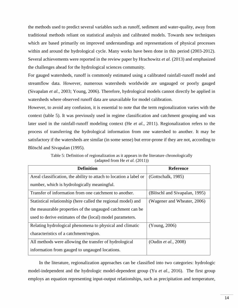
However, to avoid any confusion, it is essential to note that the term regionalization varies with the

context (table 5). It was previously used in regime classification and catchment grouping and was

later used in the rainfall-runoff modeling context (He et al., 2011). Regionalization refers to the

process of transferring the hydrological information from one watershed to another. It may be

satisfactory if the watersheds are similar (in some sense) but error-prone if they are not, according to

Blöschl and Sivapalan (1995).

Table 5: Definition of regionalization as it appears in the literature chronologically

(adapted from He et al. (2011))

Definition Reference

Areal classification, the ability to attach to location a label or

number, which is hydrologically meaningful.

(Gottschalk, 1985)

Transfer of information from one catchment to another. (Blöschl and Sivapalan, 1995)

Statistical relationship (here called the regional model) and

the measurable properties of the ungauged catchment can be

used to derive estimates of the (local) model parameters.

(Wagener and Wheater, 2006)

Relating hydrological phenomena to physical and climatic

characteristics of a catchment/region.

(Young, 2006)

All methods were allowing the transfer of hydrological

information from gauged to ungauged locations.

(Oudin et al., 2008)

In the literature, regionalization approaches can be classified into two categories: hydrologic

model-independent and the hydrologic model-dependent group (Yu et al., 2016). The first group

employs an equation representing input-output relationships, such as precipitation and temperature,

15

as inputs and flows as output. The second group methods transfer model parameters from calibrated

basins to ungauged basins using hydrological models to estimate flow in ungauged basins. According

to several studies (Merz and Blöschl, 2004; Oudin et al., 2008; Parajka et al., 2013; Samuel et al.,

2011; Young, 2006; Yu et al., 2016), the most popular regionalization approaches are the regression

approach, spatial proximity and physical proximity. The regression-based approach consists of

developing construct relationships between optimized model parameters and catchment

characteristics such as soil, vegetation, climate and topography using regression equations. Therefore,

the model parameters in ungauged catchments are estimated by multiple regression equations with

several catchment characteristics. The second method is the spatial proximity approach. Its concept

is to transfer the model parameter sets based upon a spatial distance technique, i.e., an interpolation

technique, a function of the geographic location. The most popular interpolation technique in this

context is kriging. The last is the physical similarity approach, based on transferring hydrological

model parameters from gauged to ungauged basins according to the similarity of their physical

attributes.

IV. Pedotransfer functions

Estimating soil properties from other more easily measurable soil properties has been a

challenge in soil science from its early beginning (Van Looy et al., 2017). The first estimation

equations date back to the beginning of the twentieth century. Pedotransfer Functions (PTFs) were

coined by Bouma (1989) to translate data we have into what we need. The concept of PTFs has long

been applied to estimate soil properties that are difficult to determine. Many soil science agencies

have their own unofficial ‘rule of thumb’ for estimating difficult-to-measure soil parameters

(McBratney et al., 2002). Probably because of the particular difficulty, cost of measurement, and

availability of large databases. The most comprehensive research in developing PTFs have been for

the estimation of water retention. The first attempt to use such predictions came from the study of

Briggs and McLane (1907), which was later refined by Briggs and Shantz (1912). Although most

PTFs have been developed to predict soil hydraulic properties. However, they are not restricted to

hydraulic properties. PTFs for estimating soil physical, mechanical, chemical and biological

properties have also been developed.

According to McBratney et al. (2002), the development of a new PTF requires the answer to the

question: ‘‘Under what circumstances might one wish to develop a new PTF?’’. The answers to this

question could be: I have a model, and it needs certain parameters. Do I have them? Do I need PTFs?

16

Figure 2 illustrates a proposed scheme by McBratney et al. (2002), where one might wish to perform

the following steps:

Literasearch

Database compilation: search for an existing or create a new database.

Figure 2: A scheme for developing Pedotransfer Functions (McBratney et al., 2002)

During the last few decades, regression approaches have been successfully used to develop

PTFs (Gunarathna et al., 2019). Applying statistical regression techniques to predict soil properties

that are difficult to measure requires deciding which properties are to be used as predictors and which

regression equation to use. Those decisions are not straightforward, especially when the databases

contain many potential predictors and the relationships between soil properties may be different in

different parts of the databases (Pachepsky and Schaap, 2004). The data mining and exploration

methods introduce algorithms that automate predictor and equation selections.

Modern data mining techniques are becoming more common in the development of PTFs, and they

require no previous knowledge to work well. Data mining methods are good at finding hidden

structures in the data, so all available information can be used in producing more accurate predictions.

They are usually based on an input-output black box system, where soil properties are fed to the

model as an input, and the model analyses the data and returns the predicted response. This approach

17

makes the resulting models difficult to interpret compared to the more classical methods. Data mining

techniques that are commonly used for PTFs development are artificial neural networks, support

vector machines, k-nearest neighbor-type algorithms, regression-/classification trees, and more

sophisticated techniques based on regression-/classification trees, like bagging, random forest and

boosted random forest. Van Looy et al. (2017), McBratney et al. (2002), and Pachepsky and Schaap

(2004) explain the different PTF development methods in more detail.

Currently, many PTFs are being developed to predict certain soil properties all around the world,

especially for parameters that are difficult and time-consuming to measure, such as soil carbon

(Keskin et al., 2019), bulk density (Souza et al., 2016), soil water content (Santra et al., 2018),

hydraulic conductivity (Zhao et al., 2016), soil phosphorus (Valadares et al., 2017), soil nitrogen

(Dessureault-Rompré et al., 2015) and total silicon concentrations (Landre et al., 2018). On the other

hand, a very few studies have been done to assess the feasibility of using PTFs (regression or machine

learning methods) for predicting soil aggregate stability (Annabi et al., 2017; Besalatpour et al., 2013;

Marashi et al., 2017; De Melo et al., 2018). Following this research, we have detected that the

Random Forest method has never been used before predicting soil aggregate stability. Based on our

literature review research, no study was found concerning the use of PTFs methods to estimate soil

parameters in Morocco.

Developing new PTFs is an arduous task, so it is sensible to utilize functions that have already been

developed. However, commonsensical a given PTFs should not be extrapolated beyond the

geomorphic region or soil type from which it was developed. Most current research focuses only on

developing new functions for different areas or a group of soil types. Little effort has been made to

integrate all the available functions into a system that can tell us which function is the most suitable

for a particular soil type (McBratney et al., 2002).

V. Overview of SWAT model

SWAT is a semi-distributed, process-based river basin model, developed by Arnold et al.

(1998) on behalf of the US Department for Agriculture (USDA) to predict the impact of land

management practices on water, sediment, and agricultural chemical yields in large complex

watersheds with a variety of soils, land use, and management conditions (Neitsch et al., 2011).

Watershed is divided into multiple sub-basins based on topography. Then each sub-basin is

further conceptually divided into several Hydrologic Response Units (HRUs), which have a unique

combination of soil, land use and slope (Worqlul et al., 2018).

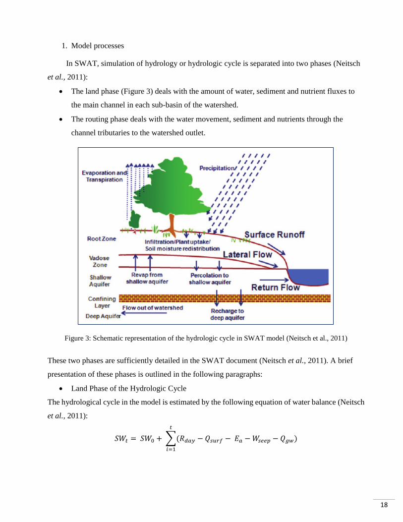
18

1. Model processes

In SWAT, simulation of hydrology or hydrologic cycle is separated into two phases (Neitsch

et al., 2011):

The land phase (Figure 3) deals with the amount of water, sediment and nutrient fluxes to

the main channel in each sub-basin of the watershed.

The routing phase deals with the water movement, sediment and nutrients through the

channel tributaries to the watershed outlet.

Figure 3: Schematic representation of the hydrologic cycle in SWAT model (Neitsch et al., 2011)

These two phases are sufficiently detailed in the SWAT document (Neitsch et al., 2011). A brief

presentation of these phases is outlined in the following paragraphs:

Land Phase of the Hydrologic Cycle

The hydrological cycle in the model is estimated by the following equation of water balance (Neitsch

et al., 2011):

𝑆𝑊𝑡 = 𝑆𝑊0 + ∑(𝑅𝑑𝑎𝑦 − 𝑄𝑠𝑢𝑟𝑓 − 𝐸𝑎 − 𝑊𝑠𝑒𝑒𝑝 − 𝑄𝑔𝑤)

𝑡

𝑖=1

19

Where SW is the soil water content, t is the time in days, and Rday, Qsurf, Ea, Wseep and Qgw are,

respectively, daily amounts of precipitation, surface runoff, evapotranspiration, water entering the

vadose zone from the soil profile, and return flow (all units are in mm).

SWAT comprises two methods for the estimation of surface runoff: (i) The Soil Conservation Service

(SCS) Curve Number (CN) method (Neitsch et al., 2011; SCS national engineering handbook, 1972).

This method is only available at a daily time step, daily and a sub-hourly time step and (ii) the Green

and Ampt infiltration method (Green and Ampt, 1911; Neitsch et al., 2011) can be used. The

percolation through each soil layer is predicted using storage routing techniques combined with the

crack-flow model.

The predicted evapotranspiration (PET) is estimated in SWAT using three options; Priestley–Taylor

(Priestley and Taylor 1972), Penman-Monteith (Monteith, 1965) and Hargreaves (Hargreaves and

Samani, 1985). The three PET methods included in SWAT vary in the number of required inputs.

The Penman-Monteith method requires solar radiation, air temperature, relative humidity and wind

speed. The Priestley-Taylor method requires the same parameters except for wind speed, while the

Hargreaves method requires air temperature only.

Erosion and sediment yield in SWAT are estimated at each HRU with the Modified Universal Soil

Loss Equation (MUSLE) (Williams, 1975), which is a modified version of the Universal Soil Loss

Equation (USLE) (Wischmeier, 1965). MUSLE and USLE methods have the same structure, except

that the rainfall energy factor was replaced by the runoff factor in the MUSLE method (Blaszczynski,

2003; Kaffas et al., 2018).

The sediment yield in the model is estimated by the following equation of MUSLE (Williams, 1975)

as:

𝑠𝑒𝑑 = 11.8 ∙ (𝑄𝑠𝑢𝑟𝑓 + 𝑞𝑝𝑒𝑎𝑘 + 𝑎𝑟𝑒𝑎ℎ𝑟𝑢)0.56

∙ 𝐾𝑈𝑆𝐿𝐸 ∙ 𝐶𝑈𝑆𝐿𝐸 ∙ 𝑃𝑈𝑆𝐿𝐸 ∙ 𝐿𝑆𝑈𝑆𝐿𝐸 ∙ 𝐶𝐹𝑅𝐺

Where sed is the sediment yield on a given day (t), and Qsurf, qpeak, areahru, KUSLE, CUSLE, PUSLE, LSUSLE

and CFRG are respectively, runoff volume (mm/ha), peak runoff rate (m3/s), area of Hydrologic

Response Unit (ha), USLE soil erodibiliy factor [0.013 t m2 h/ (m3 - t cm)], USLE cover and

management factor, USLE support practice factor, USLE topographic factor and the coarse fragment

factor.

Routing Phase of the Hydrologic Cycle

The command structure used to route the loadings of water, sediment and nutrient to the main

channel through the watershed’s stream network is similar to that of the Hydrological Model

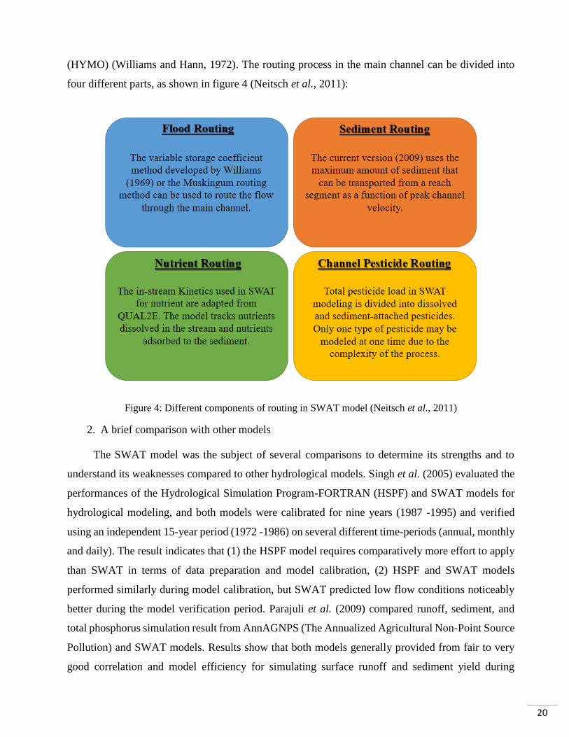
20

(HYMO) (Williams and Hann, 1972). The routing process in the main channel can be divided into

four different parts, as shown in figure 4 (Neitsch et al., 2011):

Figure 4: Different components of routing in SWAT model (Neitsch et al., 2011)

2. A brief comparison with other models

The SWAT model was the subject of several comparisons to determine its strengths and to

understand its weaknesses compared to other hydrological models. Singh et al. (2005) evaluated the

performances of the Hydrological Simulation Program-FORTRAN (HSPF) and SWAT models for

hydrological modeling, and both models were calibrated for nine years (1987 -1995) and verified

using an independent 15-year period (1972 -1986) on several different time-periods (annual, monthly

and daily). The result indicates that (1) the HSPF model requires comparatively more effort to apply

than SWAT in terms of data preparation and model calibration, (2) HSPF and SWAT models

performed similarly during model calibration, but SWAT predicted low flow conditions noticeably

better during the model verification period. Parajuli et al. (2009) compared runoff, sediment, and

total phosphorus simulation result from AnnAGNPS (The Annualized Agricultural Non-Point Source

Pollution) and SWAT models. Results show that both models generally provided from fair to very

good correlation and model efficiency for simulating surface runoff and sediment yield during

21

calibration and validation. They determined that SWAT be the most appropriate model for this

watershed-based on calibration and validation results. In another study, Abdelwahab et al. (2018)

used the same models (SWAT and AnnAGNPS) in studying hydrology and sediment load in a

Mediterranean watershed. This study indicates that SWAT requires time for the setting up and needs

a large data set. On the other side, the AnnAGNPS input preparation is user-friendly; hence, if

streamflow and sediment load are required to be simulated at a monthly time scale, the AnnAGNPS

could be the right choice. In the study conducted by Ahmadi et al. (2019), three models (SWAT,

Artificial neural networks (ANN) and Identification of unit Hydrographs and Component flow from

Rainfall, Evaporation and Streamflow data (IHACRES)) were used on a daily, monthly and annual

basis in the Kan watershed (Iran). The results showed that the performance of the three considered

models is generally suitable for rainfall-runoff process simulation. However, the ANN model showed

a better performance for daily, monthly, and annual flow simulations than the other two models. Also,

the performance of the SWAT model was better than the IHACRES model.

3. Application of SWAT model in Moroccan watersheds

SWAT model succeeded in approving its capabilities for application in different climates and

conditions around the world. The model is widely used to study many issues such as hydrological

modeling, erosion, climate change and water quality at various spatial and temporal scales in the

United States and Europe, as well as in Asia and Africa (Tuppad et al., 2011).

In this part, we collected all documents carried out to date, using the SWAT model at Moroccan

watersheds. Table 6 summarizes a list of all accessible documents. This list includes research papers,

thesis, books, chapter books, reports and peer-reviewed articles published in conference proceedings.

However, inaccessible documents (thesis or administrative reports) and studies in the form of the

"abstract" are excluded from this list. Generally, we found 24 publications, most of them published

in the last three years. Most studies were conducted at the Sebou basin, with a total of 10 studies, and

only 6 studies in the Loukkous, 4 studies in Oum Er-Rbia, three studies in Bouregreg and Chaouia

and one single study in Tensift. Whereas no studies were found in other basins, or they are not

available on the internet.

22

Table 6: List of all accessible documents that used SWAT model at Moroccan watersheds

Authors/year Title Type Journal/Publisher/University or Institution

(Chaponniere,

2005)

Fonctionnement hydrologique d'un bassin versant

montagneux semi-aride : cas du bassin versant du

Rehraya (Haut Atlas marocain)

Thesis Institut National Agronomique de Paris

Grignon

(Chaponniere and

Smakhtin, 2006)

A review of climate change scenarios and preliminary

rainfall trend analysis in The Oum Er-Rbia Basin,

Morocco.

Book International Water Management Institute/Book

(Chaponnière et

al., 2008)

Understanding hydrological processes with scarce data

in a mountain environment Research paper

Hydrological Processes: An International

Journal

(Fadil et al.,

2011)

Hydrologic modeling of the Bouregreg watershed

(Morocco) using GIS and SWAT model Research paper Journal of Geographic Information System

(Terink et al.,

2011)

Impacts of Land Management Options in the Sebou

Basin: Using the Soil and Water Assessment Tool -

SWAT

Report ISRIC/ Green Water Credits Report Morocco

(Droogers et al.,

2011)

Green Water Management Options in the Sebou Basin:

Analysing the Costs and Benefits using WEAP Report ISRIC/ Green Water Credits Report M2b

(Fadil et al.,

2013)

Comparaison de deux modèles hydrologiques sur une

zone pilote du bassin versant de Bouregreg Conference paper

Proceedings of the 1 st International Congress

on GIS & Land Management, Casablanca,

Morocco. Travaux de l’Institut Scientifique,

Rabat, série Géologie & Géographie physique

(Kharchaf et al.,

2013)

The Contribution of the Geospatial Information to the

Hydrological Modelling of a Watershed with

Reservoirs: Case of Low Oum Er Rbiaa Basin

(Morocco)

Research paper Journal of Geographic Information System

23


(Briak et al.,

2016)

Assessing sediment yield in Kalaya gauged watershed

(Northern Morocco) using GIS and SWAT model. Research paper

International Soil and Water Conservation

Research

(Bouslihim et al.,

2016)

Hydrologic modeling using SWAT and GIS,

application to subwatershed Bab-Merzouka (Sebou,

Morocco).

Research paper Journal of Geographic Information System

(Brouziyne et al.,

2017b)

SWAT manual calibration and parameters sensitivity

analysis in a semi-arid watershed in North-western

Morocco

Research paper Arabian Journal Of Geosciences

(Brouziyne et al.,

2017a)

Water balance modeling under climate change impact

in a Mediterranean watershed. Case of R’dom, morocco Book section ECOLOGY, PLANNING

(Semlali et al.,

2017)

SWAT model for hydrological modeling of Oued Laou

Watershed (Morocco) Research paper

ARPN Journal of Engineering and Applied

Sciences

(Khalid, 2018) Hydrological modeling of the Mikkés watershed

(Morocco) using ARCSWAT model Research paper Sustainable Water Resources Management

(Brouziyne et al.,

2018a)

SWAT streamflow modeling for hydrological

components’ understanding within an agro-sylvo-

pastoral watershed in Morocco

Research paper Journal of Materials and Environmental

Sciences

(Brouziyne et al.,

2018b)

Modeling sustainable adaptation strategies toward

climate-smart agriculture in a Mediterranean watershed

under projected climate change scenarios

Research paper Agricultural Systems

(Briak et al.,

2019)

Use of a calibrated SWAT model to evaluate the effects

of agricultural BMPs on sediments of the Kalaya river

basin (North of Morocco)

Research paper International Soil and Water Conservation

Research

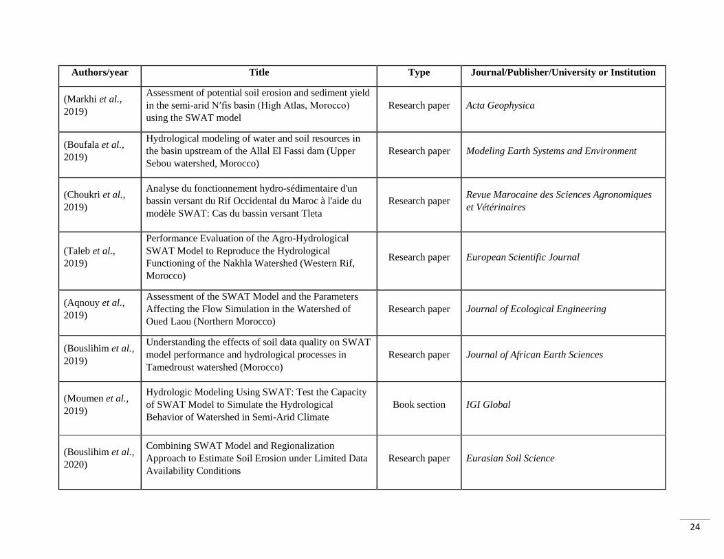
24


(Markhi et al.,

2019)

Assessment of potential soil erosion and sediment yield

in the semi-arid N′fis basin (High Atlas, Morocco)

using the SWAT model

Research paper Acta Geophysica

(Boufala et al.,

2019)

Hydrological modeling of water and soil resources in

the basin upstream of the Allal El Fassi dam (Upper

Sebou watershed, Morocco)

Research paper Modeling Earth Systems and Environment

(Choukri et al.,

2019)

Analyse du fonctionnement hydro-sédimentaire d'un

bassin versant du Rif Occidental du Maroc à l'aide du

modèle SWAT: Cas du bassin versant Tleta

Research paper Revue Marocaine des Sciences Agronomiques

et Vétérinaires

(Taleb et al.,

2019)

Performance Evaluation of the Agro-Hydrological

SWAT Model to Reproduce the Hydrological

Functioning of the Nakhla Watershed (Western Rif,

Morocco)

Research paper European Scientific Journal

(Aqnouy et al.,

2019)

Assessment of the SWAT Model and the Parameters

Affecting the Flow Simulation in the Watershed of

Oued Laou (Northern Morocco)

Research paper Journal of Ecological Engineering

(Bouslihim et al.,

2019)

Understanding the effects of soil data quality on SWAT

model performance and hydrological processes in

Tamedroust watershed (Morocco)

Research paper Journal of African Earth Sciences

(Moumen et al.,

2019)

Hydrologic Modeling Using SWAT: Test the Capacity

of SWAT Model to Simulate the Hydrological

Behavior of Watershed in Semi-Arid Climate

Book section IGI Global

(Bouslihim et al.,

2020)

Combining SWAT Model and Regionalization

Approach to Estimate Soil Erosion under Limited Data

Availability Conditions

Research paper Eurasian Soil Science

25

CHAPTER 2: STUDY AREA

I. Overview of the study area

1. General context

The climate problem represents a major global issue nowadays for humanity. Challenging to

tackle, mainly the consequences of this phenomenon are manifold, irreversible, and beyond the

response capacity of both ecosystems and humans, which may be permanently altered or destroyed.

According to the latest report of the World Resources Institute (WRI) published on August 6, 2019

(Hofste et al., 2019), twelve out of the 17 most water-stressed countries are in the Middle East and

North Africa (MENA). The region is hot and dry, so the water supply is low to begin with, but growing

demands have pushed countries further into extreme stress. The map conducted by (WRI) shows that

Morocco is also affected and categorized as a highly stressed country, taking 22nd out of 164 countries

(Figure 5).

Figure 5: Water stress in the Mediterranean basin

(source: wri.org/aqueduct, viewed on 23/08/2019)

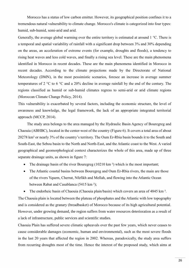
26

Morocco has a status of low carbon emitter. However, its geographical position confines it to a

tremendous natural vulnerability to climate change. Morocco's climate is categorized into four types:

humid, sub-humid, semi-arid and arid.

Generally, the average global warming over the entire territory is estimated at around 1 °C. There is

a temporal and spatial variability of rainfall with a significant drop between 3% and 30% depending

on the areas, an acceleration of extreme events (for example, droughts and floods), a tendency to

rising heat waves and less cold waves, and finally a rising sea level. These are the main phenomena

identified in Morocco in recent decades. These are the main phenomena identified in Morocco in

recent decades. According to the climate projections made by the Directorate of National

Meteorology (DMN), in the most pessimistic scenarios, foresee an increase in average summer

temperatures of 2 °C to 6 °C and a 20% decline in average rainfall by the end of the century. The

regions classified as humid or sub-humid climates regress to semi-arid or arid climate regions

(Moroccan Climate Change Policy, 2014).

This vulnerability is exacerbated by several factors, including the economic structure, the level of

awareness and knowledge, the legal framework, the lack of an appropriate integrated territorial

approach (MCCP, 2014).

The study area belongs to the area managed by the Hydraulic Basin Agency of Bouregreg and

Chaouia (ABHBC), located in the center-west of the country (Figure 6). It covers a total area of about

20278 km² or nearly 3% of the country’s territory. The Oum Er-Rbia basin bounds it to the South and

South-East, the Sebou basin to the North and North-East, and the Atlantic coast to the West. A varied

geographical and geomorphological context characterizes the whole of this area, made up of three

separate drainage units, as shown in figure 7:

The drainage basin of the river Bouregreg (10210 km ²) which is the most important;

The Atlantic coastal basins between Bouregreg and Oum Er-Rbia rivers, the main are those

of the rivers Yquem, Cherrat, Nfefikh and Mellah, and flowing into the Atlantic Ocean

between Rabat and Casablanca (5415 km ²);

The endorheic basin of Chaouia (Chaouia plain/basin) which covers an area of 4845 km ².

The Chaouia plain is located between the plateau of phosphates and the Atlantic with low topography

and is considered as the granary (breadbasket) of Morocco because of its high agricultural potential.

However, under growing demand, the region suffers from water resources deterioration as a result of

a lack of infrastructure, public services and scientific studies.

Chaouia Plain has suffered severe climatic upheavals over the past few years, which never ceases to

cause considerable damages (economic, human and environmental), such as the most severe floods

in the last 20 years that affected the region in 2002. Whereas, paradoxically, the study area suffers

from recurring droughts most of the time. Hence the interest of the proposed study, which aims at

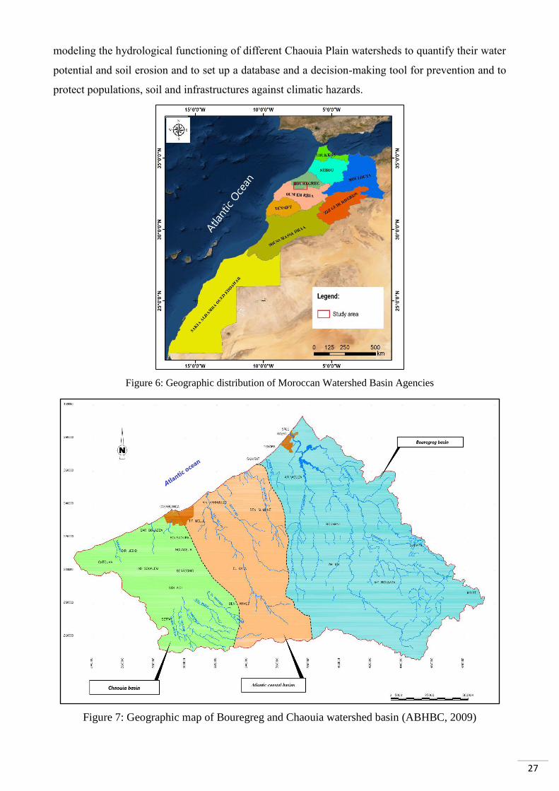
27

modeling the hydrological functioning of different Chaouia Plain watersheds to quantify their water

potential and soil erosion and to set up a database and a decision-making tool for prevention and to

protect populations, soil and infrastructures against climatic hazards.

Figure 6: Geographic distribution of Moroccan Watershed Basin Agencies

Figure 7: Geographic map of Bouregreg and Chaouia watershed basin (ABHBC, 2009)

28

2. Chaouia plain

Based on some natural characteristics, Chaouia plain can be divided into two parts:

(1) The plain of Low Chaouia, also known as Berrechid plain, which characterized by the

predominance of dark and fertile soils (Tirs) and

(2) High Chaouia, which is also known as Settat-Ben Ahmed Plateau. The Chaouia plain is

characterized by a vast limestone plateau and shallow calcimagnetic soils with reduced land fertility.

2.1.Climatic context

Generally, rainfall slightly decreases with the latitude and increases with altitude, from the

South to the North and from the coast towards the interior of the country. The climate is considered

arid to semi-arid and characterized by irregular rainfall with a total precipitation average of about 280

to 320 mm per year (El Assaoui, 2017). This average decreases towards the South of Morocco, where

the climate becomes arid. This area experienced severe drought in recent decades. Furthermore,

temperatures are strongly influenced by hot currents in dry periods, especially in Settat - Ben Ahmed

Plateau, where they can reach 40 °C during the summer (July-August), with a mean annual

temperature of around 17°C (El Assaoui, 2017)

2.2.Land use

Shallow calcimagnetic soils cover a large area, and they are characterized by average

productivity. However, tirs soils are most widespread in the valleys. This type of soil is mainly

characterized by its high productivity and its deep black color with 30 to 60% clay (Tanji and Taleb,

1994). The perennial water resources of this zone consist of the discontinuous Cenomanian aquifer.

This aquifer often presents several superimposed water levels that are drained by the Tamdroust River,

which gives rise to some resurgences such as Ain Settat, Ain Nzhar, Ain Zouirka, Ain Zoukerch, Ain

Beida and Ain Sania, which are used for the irrigation of small agricultural perimeters (ABHBC,

2009).

The main activity is based on traditional rainfed farming and livestock, with some localized

irrigation systems in the valleys when water resources are available. The natural vegetation is limited

to some reforestation of eucalyptus and a few trees around the rangelands. Rainfed farming is mainly

based on cereal cultivation with a regional distribution controlled by two major factors, soil type and

climate (Taleb and Maillet, 1994). Rainfed farming yields are uncertain and relatively low due to

irregular inter and intra-annual distribution of rainfall and the predominance of shallow soils.

2.3.Groundwater resources

The ABHBC acting area is characterized by the absence of any geological bases likely to create

large water aquifers. Nearly 85% of the total area is composed of lands with a poor rainwater storage

ability; its texture and structure do not encourage infiltration and groundwater accumulation. The

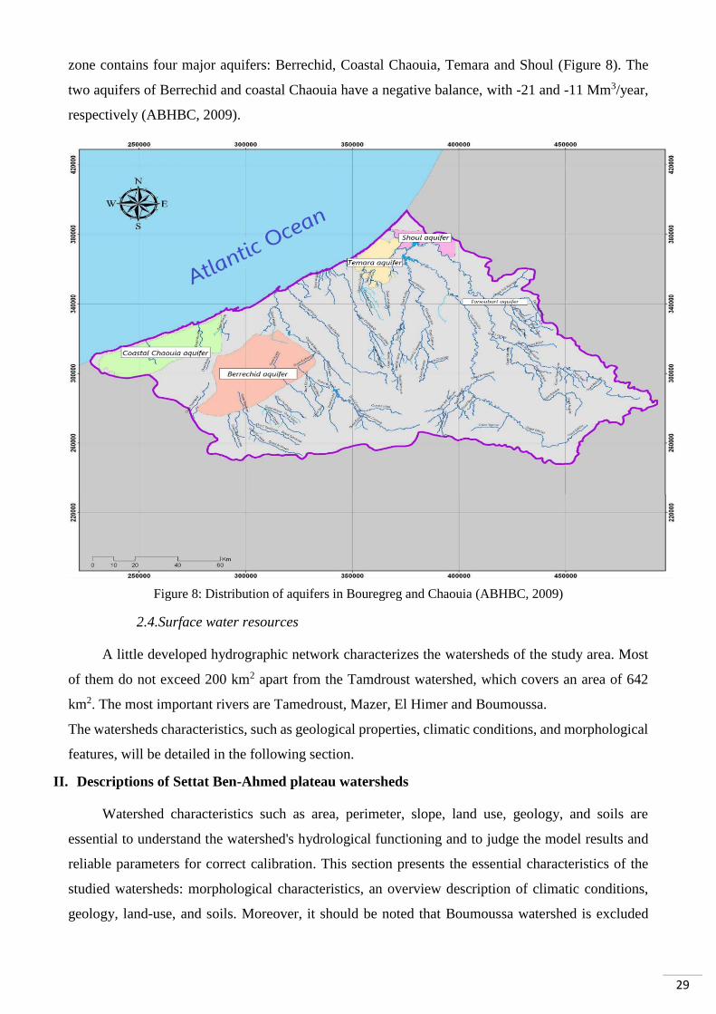
29

zone contains four major aquifers: Berrechid, Coastal Chaouia, Temara and Shoul (Figure 8). The

two aquifers of Berrechid and coastal Chaouia have a negative balance, with -21 and -11 Mm3/year,

respectively (ABHBC, 2009).

Figure 8: Distribution of aquifers in Bouregreg and Chaouia (ABHBC, 2009)

2.4.Surface water resources

A little developed hydrographic network characterizes the watersheds of the study area. Most

of them do not exceed 200 km2 apart from the Tamdroust watershed, which covers an area of 642

km2. The most important rivers are Tamedroust, Mazer, El Himer and Boumoussa.

The watersheds characteristics, such as geological properties, climatic conditions, and morphological

features, will be detailed in the following section.

II. Descriptions of Settat Ben-Ahmed plateau watersheds

Watershed characteristics such as area, perimeter, slope, land use, geology, and soils are

essential to understand the watershed's hydrological functioning and to judge the model results and

reliable parameters for correct calibration. This section presents the essential characteristics of the

studied watersheds: morphological characteristics, an overview description of climatic conditions,

geology, land-use, and soils. Moreover, it should be noted that Boumoussa watershed is excluded

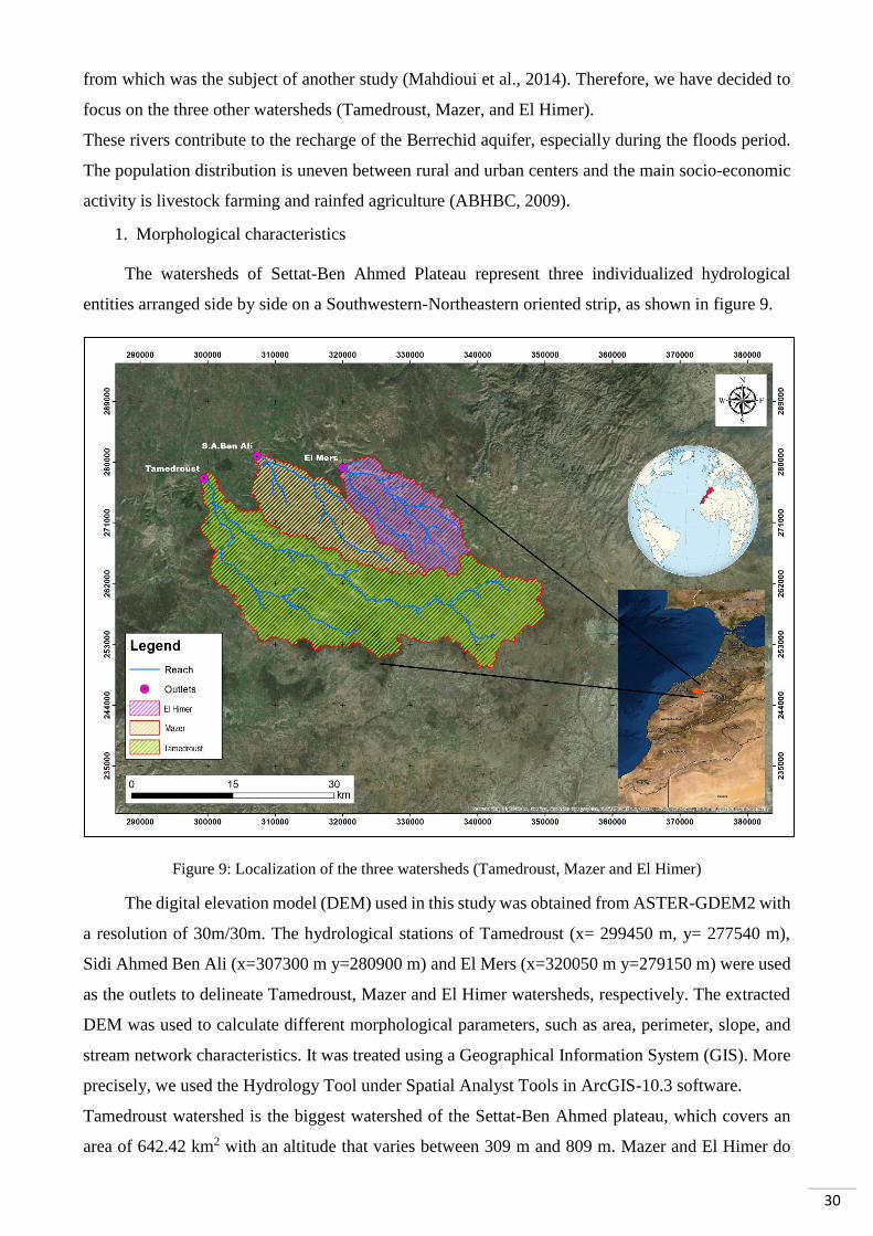
30

from which was the subject of another study (Mahdioui et al., 2014). Therefore, we have decided to

focus on the three other watersheds (Tamedroust, Mazer, and El Himer).

These rivers contribute to the recharge of the Berrechid aquifer, especially during the floods period.

The population distribution is uneven between rural and urban centers and the main socio-economic

activity is livestock farming and rainfed agriculture (ABHBC, 2009).

1. Morphological characteristics

The watersheds of Settat-Ben Ahmed Plateau represent three individualized hydrological

entities arranged side by side on a Southwestern-Northeastern oriented strip, as shown in figure 9.

Figure 9: Localization of the three watersheds (Tamedroust, Mazer and El Himer)

The digital elevation model (DEM) used in this study was obtained from ASTER-GDEM2 with

a resolution of 30m/30m. The hydrological stations of Tamedroust (x= 299450 m, y= 277540 m),

Sidi Ahmed Ben Ali (x=307300 m y=280900 m) and El Mers (x=320050 m y=279150 m) were used

as the outlets to delineate Tamedroust, Mazer and El Himer watersheds, respectively. The extracted

DEM was used to calculate different morphological parameters, such as area, perimeter, slope, and

stream network characteristics. It was treated using a Geographical Information System (GIS). More

precisely, we used the Hydrology Tool under Spatial Analyst Tools in ArcGIS-10.3 software.

Tamedroust watershed is the biggest watershed of the Settat-Ben Ahmed plateau, which covers an

area of 642.42 km2 with an altitude that varies between 309 m and 809 m. Mazer and El Himer do

31

not exceed 200 km², with an area of 179.2 km2 and 177.7 km2, respectively. Their altitudes varied

between 332 m and 785 m. Watershed length is 54 km, 32 km and 27 km for Tamedroust, Mazer and

El Himer, respectively, with a very gentle slope for the three watersheds. Table 7 summarizes all

calculated parameters.

Table 7: Morphological characteristics of the three watersheds

Watershed Tamedroust Mazer El Himer

Hydrological station (outlet) Tamedroust Sidi Ahmed Ben

Ali El Mers

Area (Km²) 642.42 179.2 177.7

Perimeter (Km) 268.7 84 70

Watershed length (Km) 54 32 27

Maximum altitude (m) 809 758 785

Minimum altitude (m) 309 332 451

Mean altitude (m) 638.9 578.26 656.54

Stream order 5 3 3

Slope (%) 0.93 1.33 1.24

Length of the equivalent rectangle

(Km) 130.47 37.55 29.18

Width f the equivalent rectangle

(Km) 4.92 4.77 6.09

Gravelius compacite index 2.99 1.76 1.48

Outlet X (m) 299 450 307 300 320 050

Y (m) 277 540 280 900 279 150

The stream order was derived using the Strahler method (Strahler, 1957). This method is

straightforward; its principle is the following: all of the smallest, unbranched tributaries are

designated order 1. Two first-order streams join, a second-order segment is formed; where two

second-order segments join, a third-order segment is formed, and so on (Fitzpatrick et al., 1998). In

the Tamedroust watershed, the stream is distributed up to the 5th order. For Mazer and El Himer

watersheds, the stream order is equal to the 3rd order.

Gravelius compactness index (compactness coefficient) is used to express the relationship of a

hydrologic basin to that of a circular basin having the same area as the hydrologic basin. A circular

basin is the most susceptible from a drainage point of view because it will yield the shortest time of

concentration before peak flow occurs in the basin (Nooka Ratnam et al., 2005). Gravelius

compactness index can be calculated using the following equation:

𝐾𝐺 =𝑃

2. √𝜋. 𝐴≈ 0.28.

𝑃

𝐴

Where KG is Gravelius compactness index; P is the watershed perimeter (km) and A is the

watershed area (Km2).

32

The obtained KG values for the three watersheds vary between 1.48 and 2.99, which shows that all

the watersheds are elongated. As mentioned above, an elongated shape favors low peak flows due

to high concentration time.

2. Climate

Data source

Daily rainfall and runoff time series were collected from the Hydraulic Basin Agency of

Bouregreg and Chaouia (ABHBC) for the three meteorological stations (Tamedroust, Sidi Ahmed

Ben Ali and El Mers) over a long period, with a lack of runoff data, extends from a few days to several

years, especially at El Mers station for 16 years (1988-2003). Such a lack of runoff data could hamper

the model calibration at the El Himer watershed. However, to overcome these limitations, one of the

regionalization methods can be used in this case (see section III in chapter 1).

The other meteorological parameters, such as temperature (max/min), wind speed, relative humidity

and solar radiation, were obtained from the National Centers for Environmental Prediction (NCEP)

Climate Forecast System Reanalysis (CFSR). NCEP-CFSR data are available globally for each hour

since 1979 at a 38-km resolution (Fuka et al., 2014). This data was used to set-up the SWAT model

in the three watersheds.

Monthly/Annual rainfall

To understand the climatic conditions of the study area, we analyzed a long series of

precipitation over 38 years (1974-2012). The monthly average rainfall histogram presented in (Figure

10) indicates that the precipitation is highly variable for each month for the three stations. The rainy

period extends from October to April, and the rainiest months are December and January, with values

of 53.1 mm and 48.7 mm, respectively. In addition, from May to September, rainfall decreases and

becomes increasingly scarce or non-existent during July and August.

33

Figure 10: The monthly average rainfall evolution for each station

The analysis of the annual average rainfall series for the three stations (Figure 11) allowed us

to detect some outlier values such as those of Tamedroust (1989) and Sidi Ahmed Ben Ali (2002,

2003 and 2004) stations. The average calculated at each station in these years is different from that

calculated at the other stations. A significant difference can be observed between the values of the

three stations (Figure 11 & appendix A).

Figure 11: Average annual rainfall series for each station

We examined the daily rainfall data in an attempt to understand this difference. Through this

process, we have noted the absence of specific data during the years mentioned earlier. It is probably

due to the interruption of rain gauge measurement after the last flood of 2002. This hypothesis finds

support in the report published by the ABHBC (ABHBC, 2009), where the rainfall data used was

0,0

10,0

20,0

30,0

40,0

50,0

60,0

1 2 3 4 5 6 7 8 9 10 11 12

Month

Average rainfall Tamedroust Average rainfall Sidi M. Ben Ali Average rainfall El Mers

0,0

100,0

200,0

300,0

400,0

500,0

600,0

700,0

800,0

900,0

1972 1976 1980 1984 1988 1992 1996 2000 2004 2008 2012 2016

Month

Rainfall Tamedroust Rainfall Sidi M. Ben Ali Rainfall El Mers

34

only from Sep1972 to Aug 2002. However, more confusing is that some other studies such as (El

Assaoui, 2017) and (El Gasmi et al., 2014a) have exceeded this period in calculating the monthly and

annual average rainfall with no indication of the missing data during these years (2002, 2003 and

2004). They calculate the missing data using one of the statistical methods to extend the duration of

the available data.

In this study, we decided to neglect the years where data are missing and we used only the data

provided by the ABHBC without making any changes to reduce the uncertainty during hydrological

modeling.

Based on the comparison of the annual average rainfall (for the period 1975-2001), the station with

the low altitude receives a lower amount of precipitation than those registered in other stations. These

results show that rainfall in this region is mainly influenced by elevation (relief) or continentality

effect. This was confirmed by subsequent studies such as (Driouech, 2010; Knippertz et al., 2003)

have shown that the climatic variability of the central region of Morocco is organized according to

three main components: altitude (relief), seasonality and latitude/longitude, and proximity to the

ocean.

As shown in figure 12, the average annual rainfall overall stations range from 134.8 mm to 699.3

mm, and it also shows significant variability between years (1975-2001), in which many dry periods

occurred (1975, 1981-1988, 1990, 1992-1995 and 1998-2001). These periods are interspersed with

wet periods of shorter cycles.

Figure 12: Average annual rainfall for the three stations

3. Geology

As already mentioned, the studied watersheds are located in the Settat Ben Ahmed Plateau, part

of the phosphate plateau. This sub-tabular set has a double-dip to the South-East and North-West

0,0

100,0

200,0

300,0

400,0

500,0

600,0

700,0

800,0

1970 1975 1980 1985 1990 1995 2000 2005

Average Average annual rainfall

35

(Carpentier, 1950 in El Gasmi et al., 2014b), covered by Cretaceous deposits which are straddling

two domains (Central Morocco and the Rehamna) with complex and polyphasic Hercynian structure

(Michard et al., 2008) (Figure 13).

Figure 13: Geological and structural Map of Settat-Ben Ahmed plateau (adapted from El Gasmi et al. (2014b))

The Tamdroust watershed outlet is located in the southeast of the Berrechid plain, which is considered

a natural extension of the studied area to the North and North-West, which forms part of the Triassic

basin of Berrechid-El Gara-Ben Slimane (an integral part of the Western Meseta).

Stratigraphically, the Continental Jurassic series consists of red clay layers that are not found

elsewhere and located in the Ouled-Saïd region to the West and South-West of Settat (Gigout, 1954

in El Gasmi et al., 2014b). As a result, the subhorizontal and transgressive limestones of the Infra-

Cenomanian and Cenomanian are found in discordance on the plateau's Paleozoic basement (Figure

14a). At the same time, the red Triassic clays in association with basalts of the Berrechid plain with

a thickness varying from 20 and 400 m are located in the North-East part of the study area, more

precisely between the two communes Ben Ahmed and Jamaa Riah (Figure 14c) (Michard, 1976;

Termier. H & Termier. G, 1951 in El Gasmi et al., 2014b).

36

The lithofacies of the Infra-cénomanien plateau are represented by 10 to 60 m of multicolored marls,

red sandstone and gypsum, unconformably on the Trias or the Primary (Archambault et al., 1975).

They result from several Cretaceous marine pulsations.

The Cenomanian deposits are represented by alternating gypseous marl and yellow marl-limestones

(Archambault et al., 1975) (Figures 13-14b). The Cenomanian is widely distributed on the Settat-

Ben Ahmed plateau. The presence of some fractures in the Cenomanian formations reduces runoff,

resulting in a high coefficient of infiltration and the groundwater in the limestone of the Cenomanian

aquifer have three types of flow: the recharge of underlying aquifers, the lateral feeding of

groundwater and underflow of different rivers and sources (El Gasmi et al., 2014b).

The Turonian is formed by very thick limestone and marl facies, forming a cracked slab characteristic

of the phosphate plateau (Salvan, 1954 in El Gasmi et al., 2014b) (Figures 13-14a). At the end of the

Cretaceous period (Senonian), the reduction of marine influences is expressed by the dominance of

marls and sandstone to marls and limestone facies characteristic of confined coastal environments

(Salvan, 1954). The phosphate series of Oulad Abdoun basin begins in the Maastrichtian by

phosphate deposits that are relatively very marly and end at the Lutetian by a limestone slab (Zerouali

et al., 2018) called the upper Eocene "Thersity slab" characterized by its resistance to erosion (Boujo,

1976; Choubert and Salvan, 1949)

The Quaternary is mostly located in the Berrechid plain and the valley of the El Himer and

Tamedroust Rivers (Termier. H & Termier. G, 1951 in El Gasmi et al., 2014b) (Figures 13-14c). The

base of this period series is formed by a more or less conglomeratic level, which surmounted by loamy

red clays with pebbles and gravel (El Mansouri, 1993).

From a structural point of view, known or mapped fractures can be grouped into two systems

(Figure 15) (El Gasmi et al., 2014b):

The first system with two faults directions. The first one (directed NNE-SSW) is parallel to

the well-known Hercynian directions (FWM: Flexure West Mesetian, FOTJ: Fault Oued

Touijjine and FM: Mediouna Fault). The second has a NE-SW direction. Both directions

would be a component of the West Mesetian Shear Zone (WMSZ).

The second system is sub-equatorial with an NW-SE direction, where the Settat fault (SF),

the most important, borders the south transition zone.

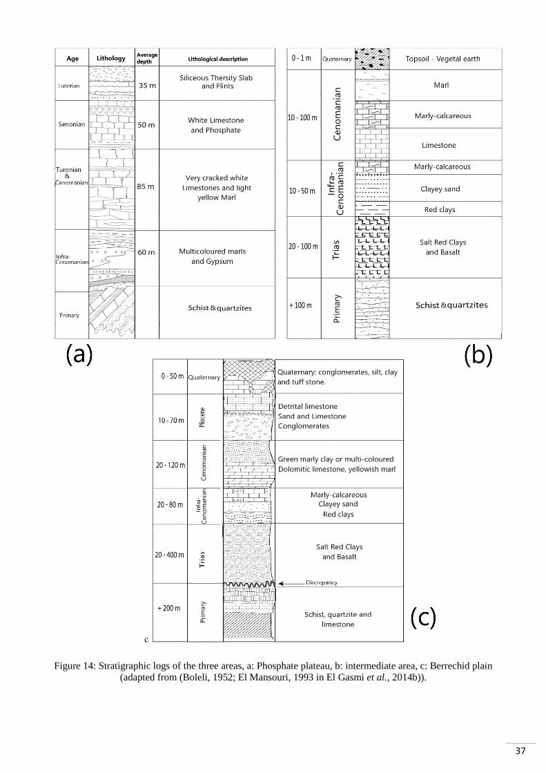
37

Figure 14: Stratigraphic logs of the three areas, a: Phosphate plateau, b: intermediate area, c: Berrechid plain (adapted from (Boleli, 1952; El Mansouri, 1993 in El Gasmi et al., 2014b)).

38

Figure 15: Dynamic function in the transition area

(adapted from El Gasmi et al. (2014b)).

4. Land use

The land use map was extracted from a Landsat-8 Operational Land Imager (OLI)/Thermal

Infrared Sensor (TIRS) satellite image (Acquisition date: 06-APR-14, Path: 202, Row: 37), with:

band 1-Coastal Aerosol (0.435-0.451 µm/30 m), band 2-Blue (0.452-0.512 µm /30 m), band 3-Green

(0.533-0.590 µm/30 m), band 4-Red (0.636-0.673 µm/30 m), band 5-NIR (0.851-0.879 µm/30 m),

band 6-SWIR1 (1.566-1.651 µm/30 m), band 7-SWIR2 (2.107-2.294 µm/30 m), band 8-Pan (0.503-

0.676 µm/15 m), band 9-Cirrus (1.363-1.384 µm/30 m), band 10-TIR1 (10.60-11.19 µm/100m) and

band 11-TIR2 (11.50-12.51 µm/100 m). This image was processed by the supervised classification

method in ArcGIS software with a confirmation by field observations. Figure 16 shows the spatial

distribution of different land-use classes over the whole area.

Generally, the area of the three watersheds is poorly covered with vegetation. The bare soil occupies

the most prominent part, with 80% and 85% in the three watersheds. Water represents only a small

part; it does not even exceed 0.01% of the total area. The other types occupied the remaining area

with percentages not exceeding 10% and varied between 4.86-8.62%, 2.9-4.53% and 4.12-11.42%

for urban, agriculture and pasture, respectively, as shown in figure 16.

39

Figure 16: Land use map and statistic class distribution of the three watersheds

5. Soil map

The Watershed area is covered by two soil maps with a different scale. The first soil map was obtained

from the pedological study produced by the Ministry of Agriculture and the Hassan II Agricultural and

Veterinary Institute (IAV) in 1985 at the scale of 1/100000 (Figure 17). This map covers the area of Mazer

and El Himer and a small part of the Tamedroust watershed. For the entire Tamedroust watershed, we used a

second map with a scale of 1:500000 realized by INRA-Morocco (National Institute for Agronomic Research),

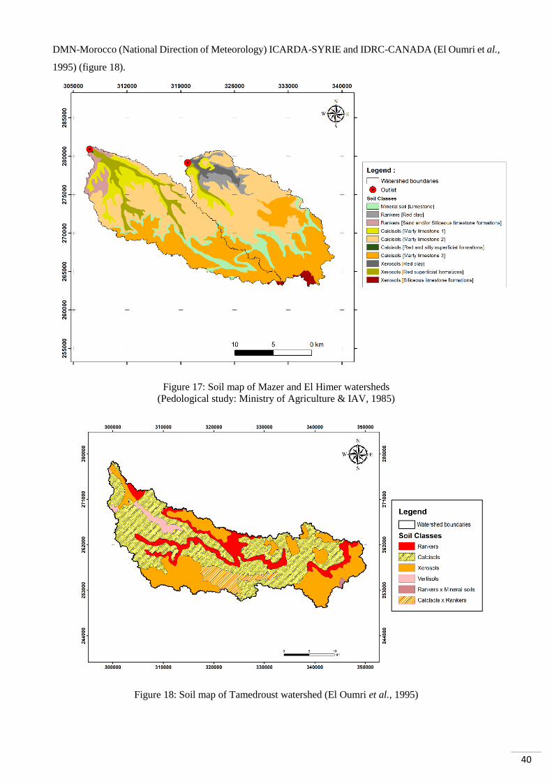
40

DMN-Morocco (National Direction of Meteorology) ICARDA-SYRIE and IDRC-CANADA (El Oumri et al.,

1995) (figure 18).

Figure 17: Soil map of Mazer and El Himer watersheds

(Pedological study: Ministry of Agriculture & IAV, 1985)

Figure 18: Soil map of Tamedroust watershed (El Oumri et al., 1995)

41

From figures 17 and 18, it can be seen that the Calcisols occupy the largest surface area, with values of 49.39%,

76.5% and 78.84% for Tamedroust, Mazer and El Himer, respectively. We can notice that Rankers and

Xerosols (Red Clay) are limited explicitly in the El Himer watershed downstream.

The soil map of the Tamedroust watershed was compared with another map from the FAO database to study

the effect of soil data quality on SWAT model performance and hydrological processes (Bouslihim et al.,

2019). The methodology adopted was presented in the next chapter.

42

CHAPTER 3: EFFECT OF SOIL DATA QUALITY ON SWAT MODEL

I. Introduction

Different studies have examined the effects of different soil characteristics input data on

hydrological processes using SWAT or other hydrological models. Levick et al. (2004) found that

the runoff using State Soil Geographic (STATSGO) soils was generally higher than those simulated

with Soil Survey Geographic (SSURGO). Geza and McCray (2008) compared the effect of SSURGO

(highest spatial resolution) and STATSGO (lowest spatial resolution) soil databases in streamflow

and water quality predictions. Results showed that, before calibration, SSURGO overpredicted the

total streamflow compared to STATSGO. However, less stream loading in sediment and sediment-

attached nutrients components after calibration results suggest a better estimation by SSURGO than

STATSGO, since Nash–Sutcliffe Efficiency (NSE) value was 0.70 and 0.61 for SSURGO and

STATSGO, respectively. Mukundan et al. (2010) evaluated the effect of STATSGO and SSURGO

soil databases of streamflow and sediment in the North Fork Broad River (182 km2). Results show

that the model predictions of flow and sediment by the two models were similar, and the differences

were statistically insignificant. Ye et al. (2011) analyzed soil data's impact with two different spatial

resolutions in a large humid watershed of Xinjiang River (15 535 km2) and found that soil data

resolution affects soil water storage. The finer resolution produced a higher monthly soil water storage

simulation than a lower resolution but does not significantly reduce streamflow simulation. In a small

watershed of Turkey Creek (126 km2), Zhao (2016) tested the effect of two soil data sets, FAO (world

reference base) and GSCC (the Genetic Soil Classification of China). Results show that both soil data

sets improved the model performance after model calibration in terms of discharge, but soil water

content (SW) is more sensitive to soil properties. Worqlul et al. (2018) evaluated the effects of soil

characteristics on SWAT runoff and water balance in paired-watersheds in the Upper Blue Nile Basin.

The study indicated that the SWAT model captured the observed flow very well for both calibration

and validation periods.

Most of these previous studies focused on comparing open source databases available online

(STATSGO and SSURGO) or at different national organizations such as GSCC that cover a little part

of the world. Due to the non-availability of these data in many regions with severe soil data

availability limitations, modelers have been forced to create their databases. Adding that spatial

information of soil physical properties is costly, requires numerous soil observations and laboratory

analysis, which makes the preparation of the SWAT input database a very long and tedious task.

In Morocco, input data effect on hydrological modeling quality has been poorly studied and

most of the studies focused on applying the SWAT model without verifying the effect of input data.

This study was conducted to understand the effect of soil data on the hydrological behavior in

an understudied watershed, in which most research was aimed at shallow aquifer located in the

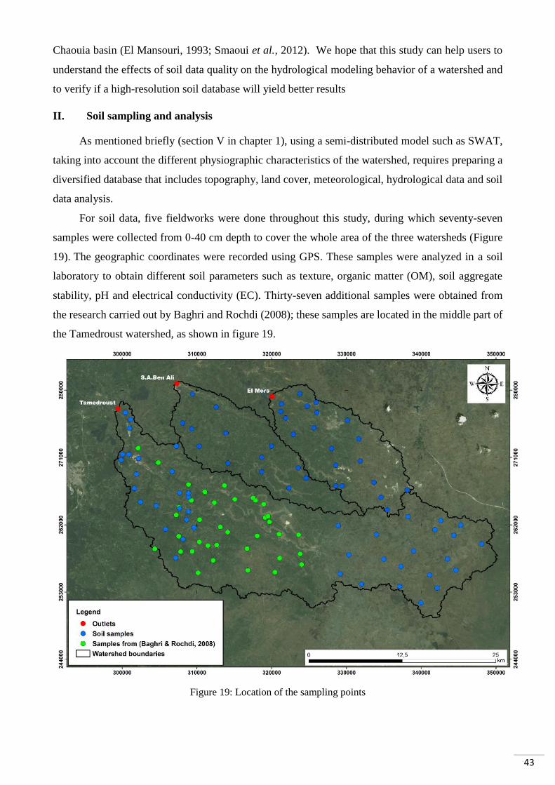
43

Chaouia basin (El Mansouri, 1993; Smaoui et al., 2012). We hope that this study can help users to

understand the effects of soil data quality on the hydrological modeling behavior of a watershed and

to verify if a high-resolution soil database will yield better results

II. Soil sampling and analysis

As mentioned briefly (section V in chapter 1), using a semi-distributed model such as SWAT,

taking into account the different physiographic characteristics of the watershed, requires preparing a

diversified database that includes topography, land cover, meteorological, hydrological data and soil

data analysis.

For soil data, five fieldworks were done throughout this study, during which seventy-seven

samples were collected from 0-40 cm depth to cover the whole area of the three watersheds (Figure

19). The geographic coordinates were recorded using GPS. These samples were analyzed in a soil

laboratory to obtain different soil parameters such as texture, organic matter (OM), soil aggregate

stability, pH and electrical conductivity (EC). Thirty-seven additional samples were obtained from

the research carried out by Baghri and Rochdi (2008); these samples are located in the middle part of

the Tamedroust watershed, as shown in figure 19.

Figure 19: Location of the sampling points

44

1. Collection and Preparation of Soil Samples

Sampling fieldwork was planned, using soils maps that have already been prepared in chapter

2(section II), topographic maps, Google Earth and ArcGIS program. These preliminary studies are

essential to choosing the best accessible location in the field.

It should be noted that some selected sites were be changed during the fieldwork when they are not

accessible (private property or extensive human activities).

Two types of sampling were carried out:

The first type is a disturbed soil sample. This type does not conserve the in situ properties of the soil

during the collection process. Disturbed soil samples were taken using a hand auger to collect a

sample from the top layer of a uniformed color (between 20 and 40 cm). Soil sampling standards have

been respected, such as cleaning the surface and utensils and the use of hermetic bags during transport.

Typically about two kilograms of soil were taken from several points in a plastic container, and then

the soil was mixed several times to ensure its homogeneity (Proce, 1997). After that, one kilogram

was taken inside a plastic bag; the sampling date and soil number were marked on each bag.

Soil samples are dried at 70 °C in the oven. The dried soil was ground using mortar and pestle, sieved

through a 2 mm mesh and mixed by hand. All samples are prepared in the laboratory before

calculating several parameters such as texture, organic carbon, pH and electrical conductivity.

The second type is the undisturbed soil sample, which is taken out for testing the physical properties

in the laboratory without disturbing its structure. In this study, these undisturbed soil samples were

used to determine the soil bulk density using the Kopecki cylinders with a calibrated volume of 100

cm3. During sampling, the cylinders were pressed parallel to the surface at a 15cm depth (Šušnjar et

al., 2006).

2. Soil Laboratory Analysis

All soil analyses were carried out at Hydrology and Soils Laboratory at the Faculty of Science

and Technology, Hassan First University, Settat, Morocco, following the standard operating

procedures.

Soil bulk density

Measurement of soil bulk density (the mass of a unit volume of dry soil) is required for the

determination of compactness (as a measure of soil structure) for calculating soil pore space (as an

indicator of aeration status and water content) (Baruah and Barthakur, 1998). Soil bulk density was

determined from the undisturbed core sampling method after drying the soil samples in an oven at

105°C to constant weights. It is determined by dividing the mass of dry soil with the volume of the

soil in its natural condition (Šušnjar et al., 2006), the following equation can calculate it:

45

𝐵𝐷 = (𝑚𝑆 𝑉⁄ ) 𝑖𝑛 𝑔 𝑐𝑚3⁄

Where BD is soil bulk density, mS is the mass of dried soil and V is the cylinder volume.

Soil texture

Soil texture was determined with the Sedimentation-Pipette method (NFX31–107) (Standard

French method). At first, we remove organic matter from all soils by using hydrogen peroxide. The

finest particles (clay and silt) were determined with the Robinson pipette method. The sand fraction

was separated via sieving at 50 µm. This method is considered an exact and precise method; however,

it is time-consuming and not very suitable for routine analyses (Beretta et al., 2014). In this study,

the time needed for total organic matter destruction was very long, especially for soils with high

organic matter content. However, despite these time constraints, this method is widely used in several

international studies, such as in Calvaruso et al. (2017), Kirchen et al. (2017) and Roulier et al.

(2018).

Soil pH and electrical conductivity

Soil pH was measured in water (pH water) and potassium chloride solution (pH in KCl) with a

soil/water ratio of 1:2 and 1:5 for mineral and organic soil, respectively (NF ISO 10390) using the

Hanna pH meter. The electrical conductivity was determined according to (ISO 11265) in soil/water

(1:2) suspension with a conductivity meter.

Soil organic matter

Organic matter is one of the essential soil constituents because it affects several physical and

chemical properties of soil.

Soil carbon was determined by the Walkley and Black procedure (Walkley and Black, 1934). This

method is based on the oxidation of organic carbon by potassium dichromate (K2Cr2O7) in the

presence of sulfuric acid (H2SO4). The percentage of soil organic matter was obtained by multiplying

percent soil organic carbon by a factor of 1.724 following the assumption that organic matter is

composed of 58% of carbon (Sleutel et al., 2007). However, only a percentage of the soil organic

carbon is recovered when using this method because the temperature obtained by the H2SO4 dilution

(approximately 120°C) is not sufficient to oxidize all the soil organic compounds (Walkley, 1947).

Calcium carbonate

Carbonate content (expressed as calcium carbonate) was measured by a volumetric method with

a Bernard Calcimeter according to the French standard NF ISO 10693, with an analytical precision

of ±0.2% CaCO3 (Baudin et al., 2010). This method consists of acidifying soil using a dilute

hydrochloric acid solution (37%) in a closed flask. The volume of CO2 released was measured using

the Bernard Calcimeter, a graduate tube filled with 200 mL of water, and was compared to the volume

46

of CO2 produced by pure CaCO3 under the same temperature and pressure conditions (Caria et al.,

2011). In this test, the assessment of effervescence is essential to estimate the quantity of calcium

carbonate to take the right amount of soil for each test.

Aggregate stability

Aggregate stability was measured using the standardized method ISO/FDIS 10930 (2012),

which is noted in Le Bissonnais (2016). This method borrows from several existing methods (Yoder,

1936), (Henin, 1958), (Grieve, 1980), (Kemper and Rosenau, 1986), (Matkin and Smart, 1987), (Le

Bissonnais, 1988), (Le Bissonnais, 1989), (Le Bissonnais and Le Souder, 1995) and (Le Bissonnais,

2016), in order to apply to an extensive range of soils and conditions.

The air-dried soil was sieved of 5-mm mesh, and the 3–5 mm aggregates were selected for the three

treatments: fast wetting, slow wetting and mechanical breakdown by shaking after pre-wetting.

Before the three treatments, aggregates were dried in the oven at 40 °C for 24 hours so that they are

at a constant matric potential. The aggregate stability for each treatment was expressed by the mean

weight diameter (MWD), which is the sum of the mass fraction of soil remaining on each sieve after

sieving multiplied by the mean aperture of the adjacent mesh (the experimental protocol is presented

in appendix B). According to Le Bissonnais (2016), the calculated MWDs values were used to

classify our soils into five classes (table 8). This classification can be applied to each treatment and

is related to the climatic conditions that correspond to the treatment.

Table 8: Stability classes according to MWD values measured with the three treatments

Class MWD value/mm stability

1 < 0.4 Very unstable

2 0.4 – 0.8 Unstable

3 0.8 – 1.3 Medium

4 1.3 – 2.0 Stable

5 > 2.0 Very stable

III. Methods

Hydrological modeling remains an indispensable tool for water resources research to

understand the watershed functioning and manage water supplies effectively. The study of a semi-

arid watershed's hydrologic functioning is a real challenge in the lack of reliable and regular data. In

this work, we propose (1) to evaluate the performance of SWAT on the Tamedroust watershed under

extremely contrasted climatic conditions during the period 1998-2002 and (2) to test the effects of

the soil resolution data on the watershed response.

To achieve these purposes, the SWAT model was calibrated and validated at Tamedroust watershed

using two soil database:

47

(i) HWSD-2L (two layers), a low-resolution soil database with three soil types obtained from the

Harmonized World Soil Database produced by FAO and (ii) TAMED-SOIL (one layer), a refined

database with eleven soil types, performed from field measurements and laboratory analysis.

The first is a global database developed by the Food and Agriculture Organization of the United

Nations (FAO), the International Institute for Applied Systems Analysis (IIASA), and the Institute of

Soil Science, Chinese Academy of Science. This database contains 16000 map units with two

different soil layers (0 - 30 cm and 30 - 100 cm deep) (Nachtergaele et al., 2010). Most of the soil

data requested by the SWAT model were directly obtained from this database (sequence number,

drainage class, organic carbon and soil texture data), using other sources to complete it. Table 9 lists

all parameters with the sources and/or methods used to calculate them. We call this data HWSD-2L,

where 2L means two layers (Figure 20a). The second database, TAMED-SOIL, is the result of

extensive research conducted by our research group (Bouslihim et al., 2019), based on the schematic

soil map with a scale of 1:50,0000 realized by INRA-Morocco (National Institute for Agronomic

Research), DMN-Morocco (National Direction of Meteorology) ICARDA-SYRIE and IDRC-

CANADA (El Oumri et al., 1995) (chapter 2- section II).

All soil types are reclassified by their texture and represented spatially, as shown in figure 20b using

ArcGIS. For example, the calcimagnesian soil is classified into three groups: silty in the upstream

portion of the watershed, silty-clay in the middle and clayey in the downstream part of the watershed.

Table 9: SWAT (Soil and Water Assessment Tool) input parameters for each soil type

Parameter

Description

Unit

Source

HWSD-2L TAMED-SOIL

SOL-Z Depth from soil surface

to bottom of layer

mm HWSD database Soil analysis

SOL_BD Moist bulk density g·cm-3 equations (Saxton and Rawls, 2006)

SOL_AWC Available water capacity

of the soil layer

mm H2O·mm-1 sol equations (Saxton and Rawls, 2006)

SOL_K Saturated hydraulic

conductivity

mm·Hr-1 equations (Saxton and Rawls, 2006)

SOL_CBN Organic carbon content % of soil weight HWSD database Soil analysis

SOL_CLAY Clay content % of soil weight HWSD database Soil analysis

SOL_SILT Silt content % of soil weight HWSD database Soil analysis

SOL_SAND Sand content % of soil weight HWSD database Soil analysis

ROCK Rock fragment content % of total weight HWSD database Soil analysis

SAL_ALB Moist soil albedo _ Landsat-8 image

USLE_K USLE equation soil

erodibility (K) factor

0.013 metric ton m2 hr/

(m3 -metric ton cm)

(Neitsch et al., 2011; Williams, 1995)

equations

SOL_EC Electrical conductivity dS·m-1 HWSD database Soil analysis

48

Figure 20: Tamedroust watershed soil maps on (a) HWSD-2L map (b) TAMED-SOIL map

Other SWAT soil parameters such as SOL_BD (moist bulk density), SOL_AWC (available

water capacity), and SOL_K (saturated hydraulic conductivity) were estimated using Saxton and

Rawls's (2006) equations. USLE_K (USLE equation soil erodibility K factor) was calculated using

the equations described by Neitsch et al. (2011) and Williams (1995). The moist soil albedo

(SOL_ALB) was extracted for each soil by using the Landsat-8 satellite image and compared with

49

some results from (Hinse et al., 1989). The soil depth was verified in situ and supplemented by

previous geological studies of the region (El Bouqdaoui, 1995). The FAO Penman-Monteith method

(Monteith, 1965) was used to predict the rate of total evaporation and transpiration from the Earth's

surface using commonly measured weather data.

The data used to set up the SWAT model (DEM, land use and metrological and hydrological data)

have already been presented previously in chapter 2. All this data and their sources can be found in

figure 21, which also summarizes the methodological approach adopted in this study. The general

idea is to set up the SWAT model using different soil databases, keeping the same other data (DEM,

land use and metrological data).

Figure 21: Methodological flowchart

50

IV. Defining SWAT hydrologic response units

Hydrologic response units (HRUs) were created using land use, slope and soil. Several choices

are available for creating these HRUs through the SWAT model, focusing either on dominant HRUs

or on given minimum limits for each input. In our case, we tried to show the effect of soil on

hydrological modeling, for that 0% was chosen as a minimum percentage of soil class over the

watershed area to integrate the maximum information related to the soil, and 5% as the minimum

percentage of land use and slope.

Comparing the two soil databases used in this work (Figure 20), the soil map resolution affects the

number of Hydrological Response Units (HRUs). The high number of soil types in TAMED-SOIL

increases the combinations between soil, land use and slope. The number of HRUs created by

TAMED-SOIL is very high compared to HWSD-2L soil data (421 against 164).

V. Model Sensitivity Analysis, Calibration and Validation

The simulation was divided into three periods: 3 years (January 1995 to December 1997) for

model initialization (warm-up), 3 years (from January 1998 to December 2000) for calibration and 2

years (from January 2001 to December 2002) for validation.

Sensitivity analysis aims to identify the key parameters that affect model performance and play

essential roles in model parameterization (Song et al., 2015). Thus, it is possible to reduce the number

of parameters to be included in the calibration, reducing the efforts required in calibration and

increasing the probability of converging towards a powerful combination (Arnold et al., 2012).

The p-value and t-stat were used to evaluate the significance of the relative sensitivity. A larger

absolute t-stat means a higher sensitivity and, a p-value close to zero represents higher significance

(Abbaspour, 2011).

The coefficient of determination (R2, Eq. (3)) (Krause et al., 2005) and Nash–Sutcliffe Efficiency

(NSE, Eq.(4)) (Nash and Sutcliffe, 1970) were used to evaluate the accuracy of calibration and

validation.

The R2 values vary from zero to one; a closer value to one represents a perfect correlation, while zero

indicates no correlation. NSE values can range between negative infinity and one (Moriasi et al.,

2007). The closer the NSE value to one, the better is the estimation of the streamflow by the model

(Geza and McCray, 2008).

𝑅2 = [𝑛 ∑ 𝑄𝑜𝑏𝑠(𝑖)𝑄𝑠𝑖𝑚(𝑖)−(∑𝑄𝑜𝑏𝑠(𝑖))(∑𝑄𝑠𝑖𝑚(𝑖))

√[𝑛(∑𝑄𝑜𝑏𝑠(𝑖)2)−(∑𝑄𝑜𝑏𝑠(𝑖)

2)] [𝑛(∑𝑄𝑠𝑖𝑚(𝑖)2)−(∑𝑄𝑠𝑖𝑚(𝑖)

2)]

]

2

Eq.3

𝑁𝑆𝐸 = 1 − ∑ (𝑄𝑜𝑏𝑠(𝑖)

𝑛𝑖=1 − 𝑄𝑠𝑖𝑚(𝑖))2

∑ (𝑄𝑜𝑏𝑠(𝑖)𝑛𝑖=1 − �̅�𝑜𝑏𝑠(𝑖))2

Eq.4

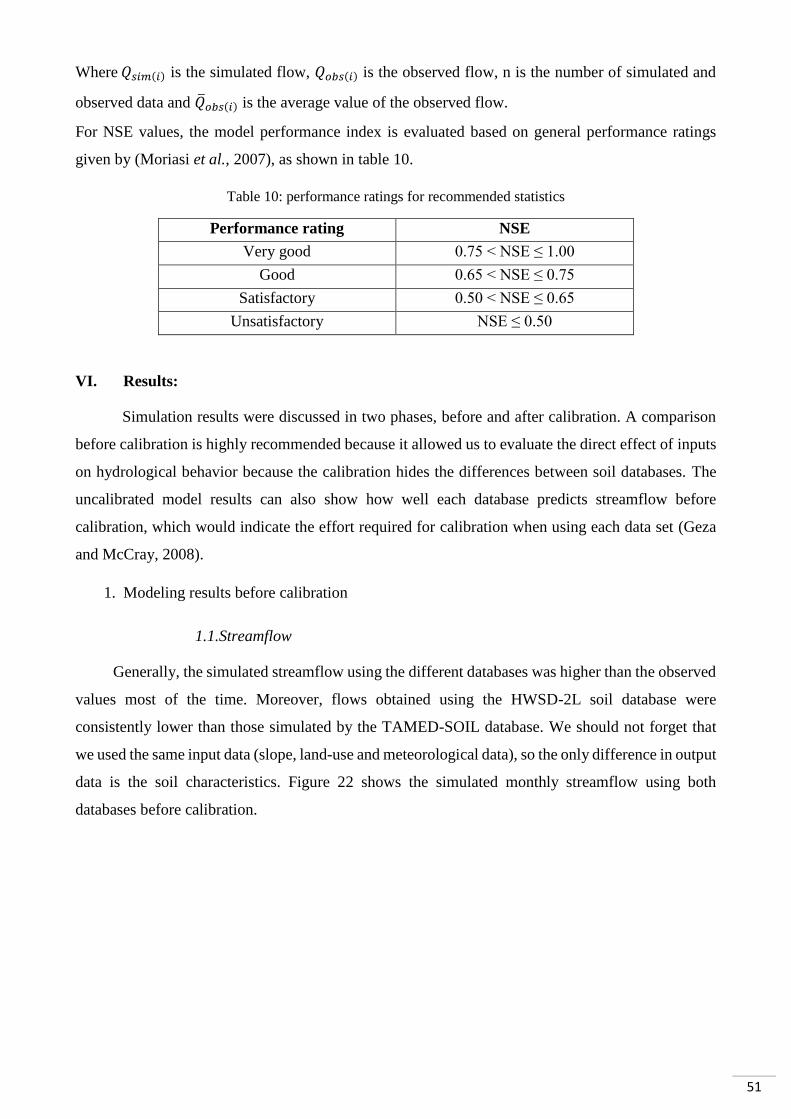
51

Where 𝑄𝑠𝑖𝑚(𝑖) is the simulated flow, 𝑄𝑜𝑏𝑠(𝑖) is the observed flow, n is the number of simulated and

observed data and �̅�𝑜𝑏𝑠(𝑖) is the average value of the observed flow.

For NSE values, the model performance index is evaluated based on general performance ratings

given by (Moriasi et al., 2007), as shown in table 10.

Table 10: performance ratings for recommended statistics

Performance rating NSE

Very good 0.75 < NSE ≤ 1.00

Good 0.65 < NSE ≤ 0.75

Satisfactory 0.50 < NSE ≤ 0.65

Unsatisfactory NSE ≤ 0.50

VI. Results:

Simulation results were discussed in two phases, before and after calibration. A comparison

before calibration is highly recommended because it allowed us to evaluate the direct effect of inputs

on hydrological behavior because the calibration hides the differences between soil databases. The

uncalibrated model results can also show how well each database predicts streamflow before

calibration, which would indicate the effort required for calibration when using each data set (Geza

and McCray, 2008).

1. Modeling results before calibration

1.1.Streamflow

Generally, the simulated streamflow using the different databases was higher than the observed

values most of the time. Moreover, flows obtained using the HWSD-2L soil database were

consistently lower than those simulated by the TAMED-SOIL database. We should not forget that

we used the same input data (slope, land-use and meteorological data), so the only difference in output

data is the soil characteristics. Figure 22 shows the simulated monthly streamflow using both

databases before calibration.

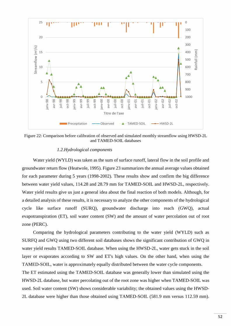
52

Figure 22: Comparison before calibration of observed and simulated monthly streamflow using HWSD-2L

and TAMED-SOIL databases

1.2.Hydrological components

Water yield (WYLD) was taken as the sum of surface runoff, lateral flow in the soil profile and

groundwater return flow (Heatwole, 1995). Figure 23 summarizes the annual average values obtained

for each parameter during 5 years (1998-2002). These results show and confirm the big difference

between water yield values, 114.28 and 28.79 mm for TAMED-SOIL and HWSD-2L, respectively.

Water yield results give us just a general idea about the final reaction of both models. Although, for

a detailed analysis of these results, it is necessary to analyze the other components of the hydrological

cycle like surface runoff (SURQ), groundwater discharge into reach (GWQ), actual

evapotranspiration (ET), soil water content (SW) and the amount of water percolation out of root

zone (PERC).

Comparing the hydrological parameters contributing to the water yield (WYLD) such as

SURFQ and GWQ using two different soil databases shows the significant contribution of GWQ in

water yield results TAMED-SOIL database. When using the HWSD-2L, water gets stuck in the soil

layer or evaporates according to SW and ET's high values. On the other hand, when using the

TAMED-SOIL, water is approximately equally distributed between the water cycle components.

The ET estimated using the TAMED-SOIL database was generally lower than simulated using the

HWSD-2L database, but water percolating out of the root zone was higher when TAMED-SOIL was

used. Soil water content (SW) shows considerable variability; the obtained values using the HWSD-

2L database were higher than those obtained using TAMED-SOIL (581.9 mm versus 112.59 mm).

0

100

200

300

400

500

600

700

800

900

10000

5

10

15

20

25

jan

v-9

8

avr-

98

juil-

98

oct

-98

jan

v-9

9

avr-

99

juil-

99

oct

-99

jan

v-0

0

avr-

00

juil-

00

oct

-00

jan

v-0

1

avr-

01

juil-

01

oct

-01

jan

v-0

2

avr-

02

juil-

02

oct

-02

Rai

nfa

ll (m

m)

Stre

amfl

ow

(m

³/s)

Titre de l'axe

Precepitation Observed TAMED-SOIL HWSD-2L

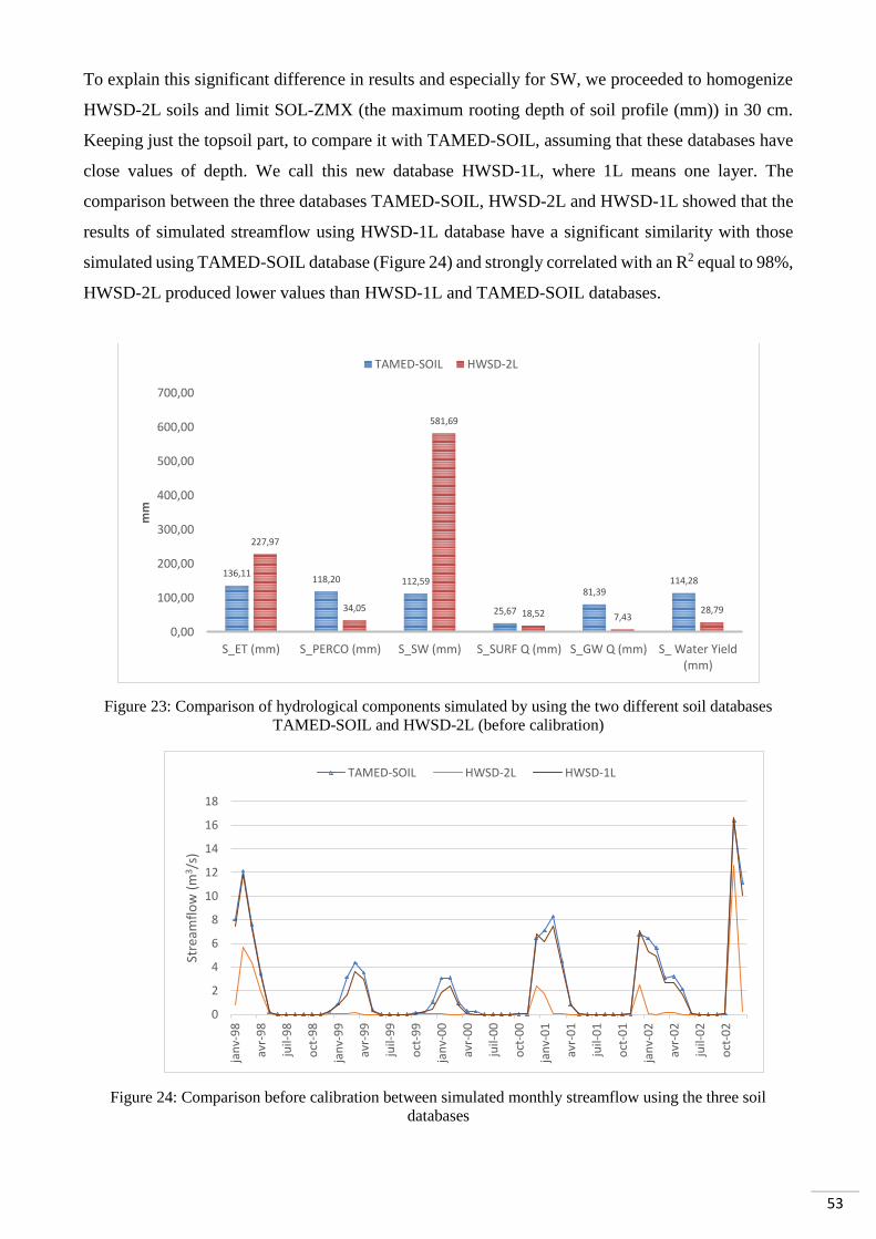
53

To explain this significant difference in results and especially for SW, we proceeded to homogenize

HWSD-2L soils and limit SOL-ZMX (the maximum rooting depth of soil profile (mm)) in 30 cm.

Keeping just the topsoil part, to compare it with TAMED-SOIL, assuming that these databases have

close values of depth. We call this new database HWSD-1L, where 1L means one layer. The

comparison between the three databases TAMED-SOIL, HWSD-2L and HWSD-1L showed that the

results of simulated streamflow using HWSD-1L database have a significant similarity with those

simulated using TAMED-SOIL database (Figure 24) and strongly correlated with an R2 equal to 98%,

HWSD-2L produced lower values than HWSD-1L and TAMED-SOIL databases.

Figure 23: Comparison of hydrological components simulated by using the two different soil databases

TAMED-SOIL and HWSD-2L (before calibration)

Figure 24: Comparison before calibration between simulated monthly streamflow using the three soil

databases

136,11118,20 112,59

25,67

81,39114,28

227,97

34,05

581,69

18,52 7,4328,79

0,00

100,00

200,00

300,00

400,00

500,00

600,00

700,00

S_ET (mm) S_PERCO (mm) S_SW (mm) S_SURF Q (mm) S_GW Q (mm) S_ Water Yield(mm)

mm

TAMED-SOIL HWSD-2L

0

2

4

6

8

10

12

14

16

18

jan

v-9

8

avr-

98

juil-

98

oct

-98

jan

v-9

9

avr-

99

juil-

99

oct

-99

jan

v-0

0

avr-

00

juil-

00

oct

-00

jan

v-0

1

avr-

01

juil-

01

oct

-01

jan

v-0

2

avr-

02

juil-

02

oct

-02

Stre

amfl

ow

(m

3/s

)

TAMED-SOIL HWSD-2L HWSD-1L

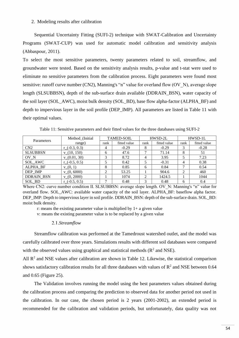
54

2. Modeling results after calibration

Sequential Uncertainty Fitting (SUFI-2) technique with SWAT-Calibration and Uncertainty

Programs (SWAT-CUP) was used for automatic model calibration and sensitivity analysis

(Abbaspour, 2011).

To select the most sensitive parameters, twenty parameters related to soil, streamflow, and

groundwater were tested. Based on the sensitivity analysis results, p-value and t-stat were used to

eliminate no sensitive parameters from the calibration process. Eight parameters were found most

sensitive: runoff curve number (CN2), Manning's “n” value for overland flow (OV_N), average slope

length (SLSUBBSN), depth of the sub-surface drain available (DDRAIN_BSN), water capacity of

the soil layer (SOL_AWC), moist bulk density (SOL_BD), base flow alpha-factor (ALPHA_BF) and

depth to impervious layer in the soil profile (DEP_IMP). All parameters are listed in Table 11 with

their optimal values.

Table 11: Sensitive parameters and their fitted values for the three databases using SUFI-2

Parameters Method_(Initial

range)

TAMED-SOIL HWSD-2L HWSD-1L

rank fitted value rank fitted value rank fitted value

CN2 r_(-0.3, 0.3) 4 -0.29 8 -0.29 3 -0.28

SLSUBBSN v_(10, 150) 6 47.6 7 71.14 8 51

OV_N v_(0.01, 30) 3 8.72 4 3.95 5 7.23

SOL_AWC r_(-0.5, 0.5) 5 0.42 5 -0.31 4 0.38

ALPHA_BF v_(0, 1) 8 0.85 6 0.84 7 0.54

DEP_IMP v_(0, 6000) 2 53.25 1 904.6 2 460

DDRAIN_BSN v_(0, 2000) 1 1074 2 1424.5 1 1044

SOL_BD r_(-0.5, 0.5) 7 0.48 3 0.48 6 0.4

Where CN2: curve number condition II. SLSUBBSN: average slope length. OV_N: Manning's “n” value for

overland flow. SOL_AWC: available water capacity of the soil layer. ALPHA_BF: baseflow alpha factor.

DEP_IMP: Depth to impervious layer in soil profile. DDRAIN_BSN: depth of the sub-surface drain. SOL_BD:

moist bulk density.

r: means the existing parameter value is multiplied by 1+ a given value

v: means the existing parameter value is to be replaced by a given value

Streamflow

Streamflow calibration was performed at the Tamedroust watershed outlet, and the model was

carefully calibrated over three years. Simulations results with different soil databases were compared

with the observed values using graphical and statistical methods (R2 and NSE).

All R2 and NSE values after calibration are shown in Table 12. Likewise, the statistical comparison

shows satisfactory calibration results for all three databases with values of R2 and NSE between 0.64

and 0.65 (Figure 25).

The Validation involves running the model using the best parameters values obtained during

the calibration process and comparing the prediction to observed data for another period not used in

the calibration. In our case, the chosen period is 2 years (2001-2002), an extended period is

recommended for the calibration and validation periods, but unfortunately, data quality was not

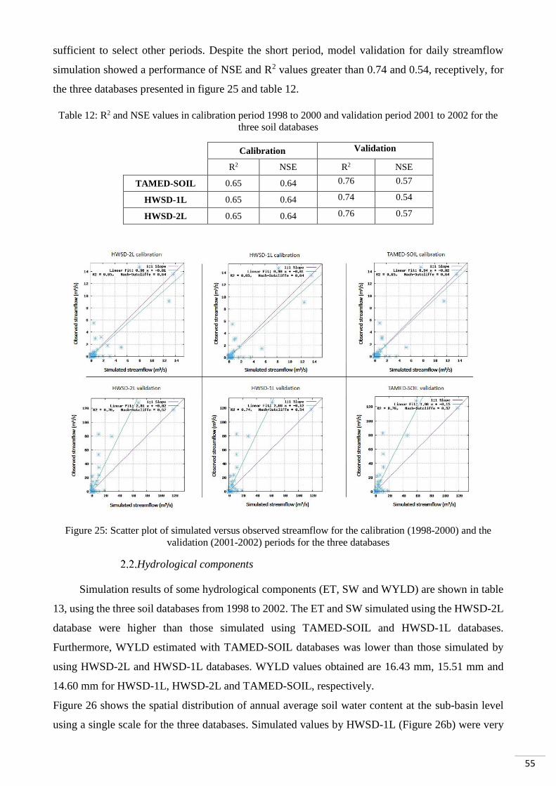
55

sufficient to select other periods. Despite the short period, model validation for daily streamflow

simulation showed a performance of NSE and R2 values greater than 0.74 and 0.54, receptively, for

the three databases presented in figure 25 and table 12.

Table 12: R2 and NSE values in calibration period 1998 to 2000 and validation period 2001 to 2002 for the

three soil databases

Calibration Validation

R2 NSE R2 NSE

TAMED-SOIL 0.65 0.64 0.76 0.57

HWSD-1L 0.65 0.64 0.74 0.54

HWSD-2L 0.65 0.64 0.76 0.57

Figure 25: Scatter plot of simulated versus observed streamflow for the calibration (1998-2000) and the

validation (2001-2002) periods for the three databases

Hydrological components

Simulation results of some hydrological components (ET, SW and WYLD) are shown in table

13, using the three soil databases from 1998 to 2002. The ET and SW simulated using the HWSD-2L

database were higher than those simulated using TAMED-SOIL and HWSD-1L databases.

Furthermore, WYLD estimated with TAMED-SOIL databases was lower than those simulated by

using HWSD-2L and HWSD-1L databases. WYLD values obtained are 16.43 mm, 15.51 mm and

14.60 mm for HWSD-1L, HWSD-2L and TAMED-SOIL, respectively.

Figure 26 shows the spatial distribution of annual average soil water content at the sub-basin level

using a single scale for the three databases. Simulated values by HWSD-1L (Figure 26b) were very

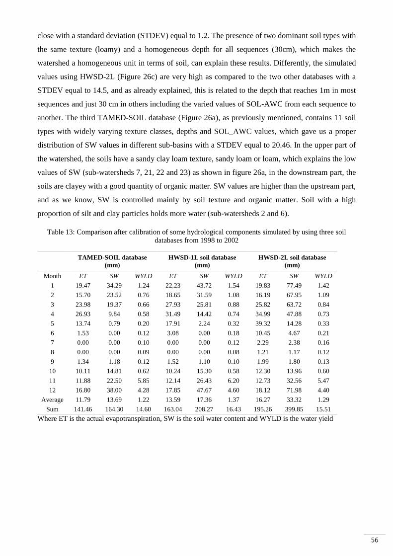
56

close with a standard deviation (STDEV) equal to 1.2. The presence of two dominant soil types with

the same texture (loamy) and a homogeneous depth for all sequences (30cm), which makes the

watershed a homogeneous unit in terms of soil, can explain these results. Differently, the simulated

values using HWSD-2L (Figure 26c) are very high as compared to the two other databases with a

STDEV equal to 14.5, and as already explained, this is related to the depth that reaches 1m in most

sequences and just 30 cm in others including the varied values of SOL-AWC from each sequence to

another. The third TAMED-SOIL database (Figure 26a), as previously mentioned, contains 11 soil

types with widely varying texture classes, depths and SOL_AWC values, which gave us a proper

distribution of SW values in different sub-basins with a STDEV equal to 20.46. In the upper part of

the watershed, the soils have a sandy clay loam texture, sandy loam or loam, which explains the low

values of SW (sub-watersheds 7, 21, 22 and 23) as shown in figure 26a, in the downstream part, the

soils are clayey with a good quantity of organic matter. SW values are higher than the upstream part,

and as we know, SW is controlled mainly by soil texture and organic matter. Soil with a high

proportion of silt and clay particles holds more water (sub-watersheds 2 and 6).

Table 13: Comparison after calibration of some hydrological components simulated by using three soil

databases from 1998 to 2002

TAMED-SOIL database

(mm)

HWSD-1L soil database

(mm)

HWSD-2L soil database

(mm)

Month ET SW WYLD ET SW WYLD ET SW WYLD

1 19.47 34.29 1.24 22.23 43.72 1.54 19.83 77.49 1.42

2 15.70 23.52 0.76 18.65 31.59 1.08 16.19 67.95 1.09

3 23.98 19.37 0.66 27.93 25.81 0.88 25.82 63.72 0.84

4 26.93 9.84 0.58 31.49 14.42 0.74 34.99 47.88 0.73

5 13.74 0.79 0.20 17.91 2.24 0.32 39.32 14.28 0.33

6 1.53 0.00 0.12 3.08 0.00 0.18 10.45 4.67 0.21

7 0.00 0.00 0.10 0.00 0.00 0.12 2.29 2.38 0.16

8 0.00 0.00 0.09 0.00 0.00 0.08 1.21 1.17 0.12

9 1.34 1.18 0.12 1.52 1.10 0.10 1.99 1.80 0.13

10 10.11 14.81 0.62 10.24 15.30 0.58 12.30 13.96 0.60

11 11.88 22.50 5.85 12.14 26.43 6.20 12.73 32.56 5.47

12 16.80 38.00 4.28 17.85 47.67 4.60 18.12 71.98 4.40

Average 11.79 13.69 1.22 13.59 17.36 1.37 16.27 33.32 1.29

Sum 141.46 164.30 14.60 163.04 208.27 16.43 195.26 399.85 15.51

Where ET is the actual evapotranspiration, SW is the soil water content and WYLD is the water yield

57

Figure 26: The spatial distribution of Soil Water content by using a) TAMED-SOIL, b) HWSD-1L and c)

HWSD-2L databases from 1998 to 2002

3. Soil erosion results in Tamedroust watershed

Tamedroust watershed was divided into 23 sub-watersheds, ranging from 2.86 km2 to 78.23

km2 for sub-watersheds 12 and 6. After the calibration and validation processes, the model was

executed for 5 years (1998-2002) to estimate the soil erosion in each sub-watershed for both databases

(TAMED-SOIL and HWSD-2L). The average annual values recorded of sediment yield at the

Tamedroust outlet were 645.27 and 657.55 tons/year for TAMED-SOIL and HWSD-2L, respectively.

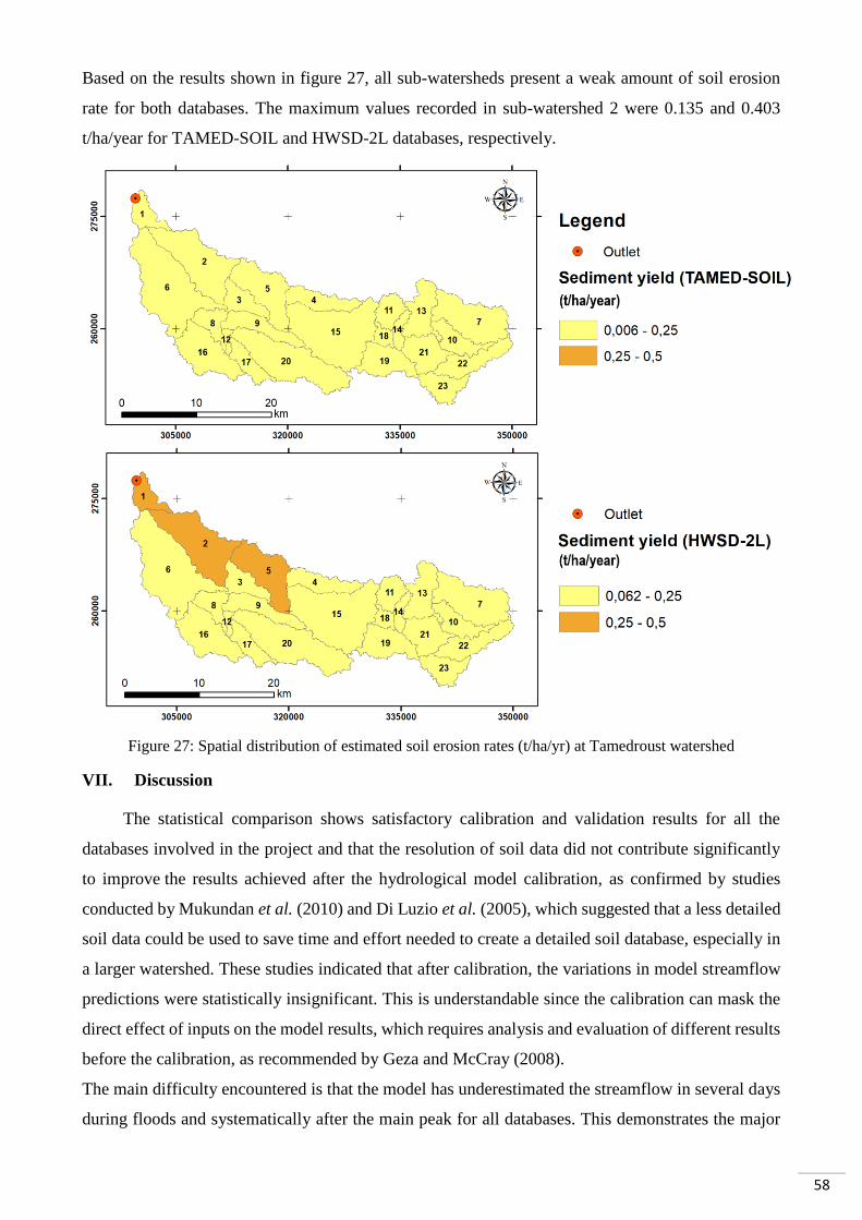
58

Based on the results shown in figure 27, all sub-watersheds present a weak amount of soil erosion

rate for both databases. The maximum values recorded in sub-watershed 2 were 0.135 and 0.403

t/ha/year for TAMED-SOIL and HWSD-2L databases, respectively.

Figure 27: Spatial distribution of estimated soil erosion rates (t/ha/yr) at Tamedroust watershed

VII. Discussion

The statistical comparison shows satisfactory calibration and validation results for all the

databases involved in the project and that the resolution of soil data did not contribute significantly

to improve the results achieved after the hydrological model calibration, as confirmed by studies

conducted by Mukundan et al. (2010) and Di Luzio et al. (2005), which suggested that a less detailed

soil data could be used to save time and effort needed to create a detailed soil database, especially in

a larger watershed. These studies indicated that after calibration, the variations in model streamflow

predictions were statistically insignificant. This is understandable since the calibration can mask the

direct effect of inputs on the model results, which requires analysis and evaluation of different results

before the calibration, as recommended by Geza and McCray (2008).

The main difficulty encountered is that the model has underestimated the streamflow in several days

during floods and systematically after the main peak for all databases. This demonstrates the major

59

limitation for the runoff modeling in arid and semi-arid regions (Beven, 2011; Pilgrim et al., 1988;

Wheater et al., 2007). In such meteorological conditions, with limited data availability and poor

spatial distribution of measurement stations, this was an additional challenge that was overcome with

good reliability (Näschen et al., 2018; Tuo et al., 2016).

Several studies have shown that soil characteristics such as soil depth, hydrological group, and

hydraulic conductivity can influence hydrological cycle components in the watershed (Geroy et al.,

2011; Mohanty and Mousli, 2000; Wang and Melesse, 2006). However, in our case, it has been noted

that the soil water content (SW) has the most significant variation between all water cycle

components. These results are consistent with other studies such as Ye et al. (2011) and Zhao (2016).

Specifically, in our case, the HWSD-2L soil database contains two soil layers for each soil type (0-

300 mm and 300-1000 mm for topsoil and subsoil, respectively), with a maximum rooting depth of

soil profile (SOL_ZMX) being equal to 1 m. On the other hand, the SOL_ZMX values of the

dominant soils of the TAMED-SOIL database are between 300 and 450 mm.

This significant difference in soil depth may be the most plausible explanation for higher SW values

observed in the HWSD-L2 soil database, which affects all the other components of the hydrological

cycle. The clear difference between SOL_AWC values in the two databases can be considered one of

the main factors responsible. An increase in SOL_ AWC allows the soil to retain more water and

decreases the streamflow (Opere and Okello, 2011).

VIII. Conclusion

This article presents the performance of the SWAT model using two different soil databases

to evaluate the effect of soil data quality on the hydrological behavior and water balance analysis in

a semi-arid watershed. The comparison between the two soil databases was made before and after

calibration. Results indicated that the quality and the resolution of the soil map affect the number of

HRUs because the high number of soil types increases the combinations between different soil, land

use and slope. The soil depth affects the various components of the hydrological cycle such as SW

and GWQ and directly affects WYLD. The fine soil resolution produces higher WYLD values than

the lower resolution (114.28 and 28.79mm for TAMED-SOIL and HWSD-2L, respectively). The

statistical comparison shows satisfactory calibration results and validation for all soil databases

(TAMED-SOIL, HWSD-1L and HWSD-2L). A significant variation has been observed in the other

parameters such as SW, WYLD and ET, as mentioned in the results section. We can, therefore,

conclude that the model can give good results after streamflow calibration, but it does not mean that

the other components are well simulated. Using a detailed soil map or the modification of some

parameters, depth, for example, can influence all the results. Consequently, before each project,

researchers need to select the appropriate resolution of each input data taking into account the results

and the expected objectives.

60

CHAPTER 4: ESTIMATION OF RUNOFF AND SOIL EROSION AT MAZER

AND EL HIMER WATERSHEDS

I. Introduction

According to the literature, many watersheds worldwide suffer from a lack of data regardless

of their nature, making the hydrologic modelers' work more complicated. However, that opens new

perspectives to researchers and academics who want to find adequate solutions or better ways to

overcome the challenges related to data availability. Watersheds with insufficient or no flow data are

classified as poorly gauged or ungauged watersheds, respectively (Razavi and Coulibaly, 2013),

making it difficult for hydrologists to apply any hydrological model in such circumstances. The lack

of streamflow data used for calibrating model parameters is the main challenge with rainfall-runoff

modeling in ungauged catchments (Blöschl, 2006). Therefore, to make a realistic and valid hydrologic

modeling, flow and meteorological data are necessary over a temporary long enough period.

Data availability in hydrological modeling has been the subject of several studies in the past, with

various solutions proposed. It is the recommendation of most of the scientific studies quoted that in

ungauged catchments, model parameters have to be estimated from other sources of information

(Arsenault and Brissette, 2014; Bárdossy, 2007; Bates, 1994; Beck et al., 2016; Blöschl, 2006;

Blöschl et al., 2013; Blöschl and Sivapalan, 1995; He et al., 2011; Hrachowitz et al., 2013; Merz et

al., 2006; Merz and Blöschl, 2004; Oudin et al., 2008; Parajka et al., 2013; Razavi and Coulibaly,

2013; Samuel et al., 2011; Young, 2006). The method consists of gathering the model parameters

from hydrologically similar catchments (Merz et al., 2006). The process of transferring parameters

from gauged to ungauged watersheds is generally referred to as regionalization (Blöschl and

Sivapalan, 1995). See also chapter 1 (section III).

II. Methods

Hydrological modeling and soil erosion estimation using the SWAT model requires several

input data such as topography, soil, land cover, and meteorological data. For model calibration and

validation, flow data are required. This procedure is impossible in the case of an ungauged watershed.

Therefore, to solve this problem, the hydrological model’s parameters and data of a gauged watershed

considered "similar" can be transferred to an ungauged watershed (Bárdossy, 2007). This method is

called regionalization.

The physical proximity approach was selected in the current study. The concept of this approach is

to transfer hydrological model parameters from the gauged watershed (Mazer) to the ungauged

watershed (El Himer) according to the similarity of their physical attributes, the rationale being that

watersheds with similar attributes should behave similarly (Oudin et al., 2008).

Based on the previous information, the following steps must be respected:

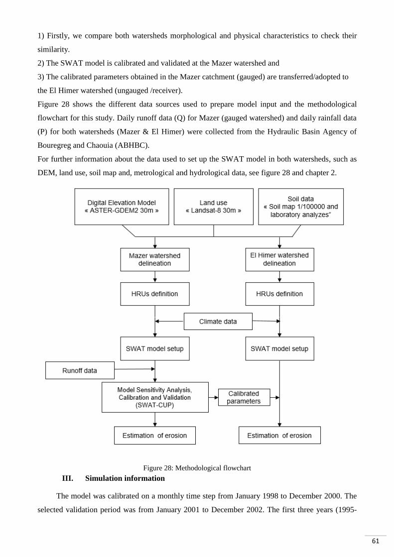
61

1) Firstly, we compare both watersheds morphological and physical characteristics to check their

similarity.

2) The SWAT model is calibrated and validated at the Mazer watershed and

3) The calibrated parameters obtained in the Mazer catchment (gauged) are transferred/adopted to

the El Himer watershed (ungauged /receiver).

Figure 28 shows the different data sources used to prepare model input and the methodological

flowchart for this study. Daily runoff data (Q) for Mazer (gauged watershed) and daily rainfall data

(P) for both watersheds (Mazer & El Himer) were collected from the Hydraulic Basin Agency of

Bouregreg and Chaouia (ABHBC).

For further information about the data used to set up the SWAT model in both watersheds, such as

DEM, land use, soil map and, metrological and hydrological data, see figure 28 and chapter 2.

Figure 28: Methodological flowchart

III. Simulation information

The model was calibrated on a monthly time step from January 1998 to December 2000. The

selected validation period was from January 2001 to December 2002. The first three years (1995-

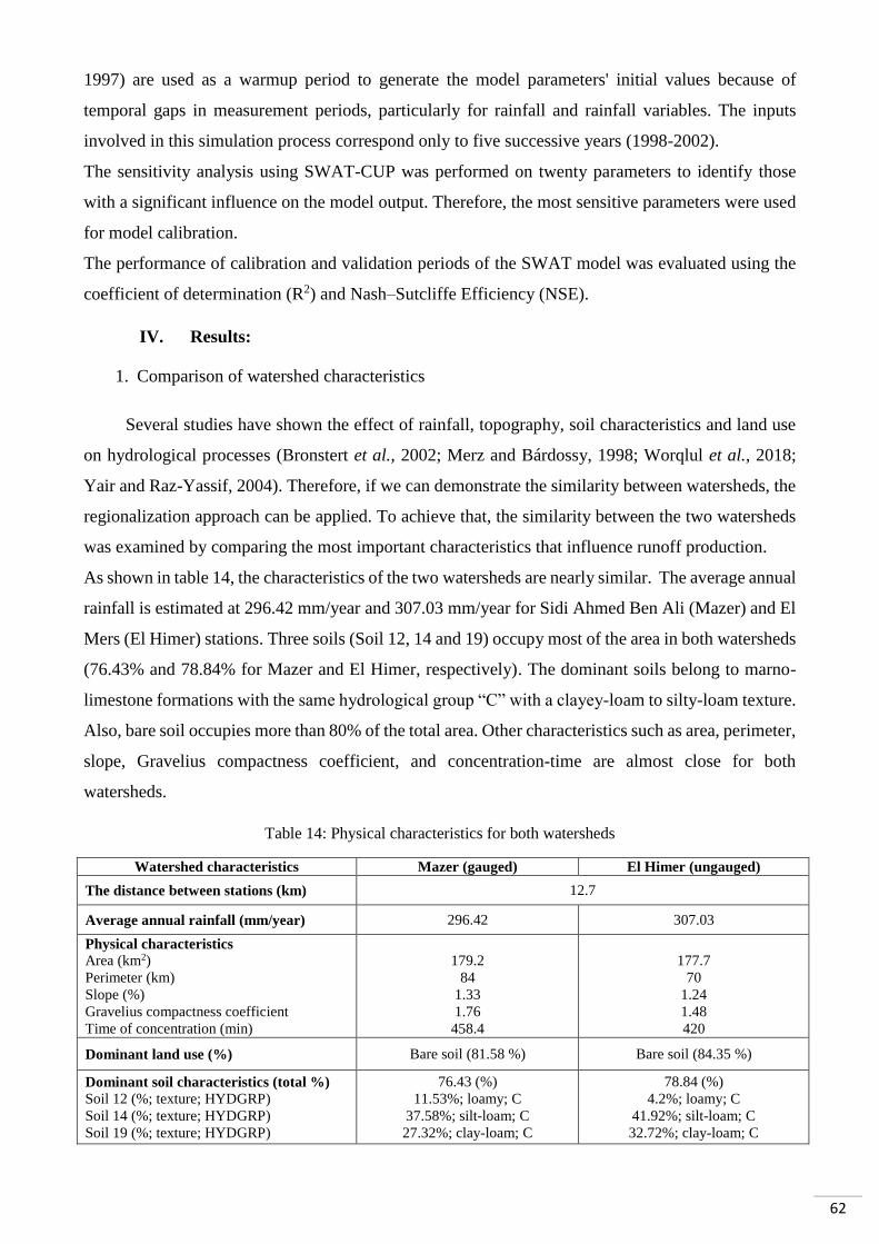
62

1997) are used as a warmup period to generate the model parameters' initial values because of

temporal gaps in measurement periods, particularly for rainfall and rainfall variables. The inputs

involved in this simulation process correspond only to five successive years (1998-2002).

The sensitivity analysis using SWAT-CUP was performed on twenty parameters to identify those

with a significant influence on the model output. Therefore, the most sensitive parameters were used

for model calibration.

The performance of calibration and validation periods of the SWAT model was evaluated using the

coefficient of determination (R2) and Nash–Sutcliffe Efficiency (NSE).

IV. Results:

1. Comparison of watershed characteristics

Several studies have shown the effect of rainfall, topography, soil characteristics and land use

on hydrological processes (Bronstert et al., 2002; Merz and Bárdossy, 1998; Worqlul et al., 2018;

Yair and Raz-Yassif, 2004). Therefore, if we can demonstrate the similarity between watersheds, the

regionalization approach can be applied. To achieve that, the similarity between the two watersheds

was examined by comparing the most important characteristics that influence runoff production.

As shown in table 14, the characteristics of the two watersheds are nearly similar. The average annual

rainfall is estimated at 296.42 mm/year and 307.03 mm/year for Sidi Ahmed Ben Ali (Mazer) and El

Mers (El Himer) stations. Three soils (Soil 12, 14 and 19) occupy most of the area in both watersheds

(76.43% and 78.84% for Mazer and El Himer, respectively). The dominant soils belong to marno-

limestone formations with the same hydrological group “C” with a clayey-loam to silty-loam texture.

Also, bare soil occupies more than 80% of the total area. Other characteristics such as area, perimeter,

slope, Gravelius compactness coefficient, and concentration-time are almost close for both

watersheds.

Table 14: Physical characteristics for both watersheds

Watershed characteristics Mazer (gauged) El Himer (ungauged)

The distance between stations (km) 12.7

Average annual rainfall (mm/year) 296.42 307.03

Physical characteristics

Area (km2)

Perimeter (km)

Slope (%)

Gravelius compactness coefficient

Time of concentration (min)

179.2

84

1.33

1.76

458.4

177.7

70

1.24

1.48

420

Dominant land use (%) Bare soil (81.58 %) Bare soil (84.35 %)

Dominant soil characteristics (total %)

Soil 12 (%; texture; HYDGRP)



76.43 (%)

11.53%; loamy; C

37.58%; silt-loam; C

27.32%; clay-loam; C

78.84 (%)

4.2%; loamy; C

41.92%; silt-loam; C

32.72%; clay-loam; C

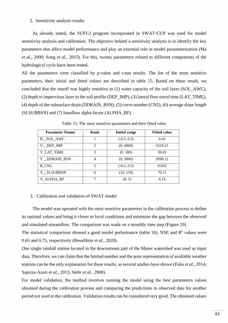
63

2. Sensitivity analysis results

As already stated, the SUFI-2 program incorporated in SWAT-CUP was used for model

sensitivity analysis and calibration. The objective behind a sensitivity analysis is to identify the key

parameters that affect model performance and play an essential role in model parameterization (Ma

et al., 2000; Song et al., 2015). For this, twenty parameters related to different components of the

hydrological cycle have been tested.

All the parameters were classified by p-value and t-stat results. The list of the most sensitive

parameters, their initial and fitted values are described in table 15. Based on these result, we

concluded that the runoff was highly sensitive to (1) water capacity of the soil layer (SOL_AWC),

(2) depth to impervious layer in the soil profile (DEP_IMP), (3) lateral flow travel time (LAT_TIME),

(4) depth of the subsurface drain (DDRAIN_BSN), (5) curve number (CN2), (6) average slope length

(SLSUBBSN) and (7) baseflow alpha-factor (ALPHA_BF).

Table 15: The most sensitive parameters and their fitted value

Parameter Names Rank Initial range Fitted value

R__SOL_AWC 1 (-0.5, 0.5) 0.45

V__DEP_IMP 2 (0, 6000) 3319.25

V_LAT_TIME 3 (0, 180) 59.03

V__DDRAIN_BSN 4 (0, 3000) 2090.12

R_CN2 5 (-0.5, 0.5) 0.016

V__SLSUBBSN 6 (10, 150) 76.11

V_ALPHA_BF 7 (0, 1) 0.14

3. Calibration and validation of SWAT model

The model was operated with the most sensitive parameters in the calibration process to define

its optimal values and bring it closer to local conditions and minimize the gap between the observed

and simulated streamflow. The comparison was made on a monthly time step (Figure 29).

The statistical comparison showed a good model performance (table 16). NSE and R2 values were

0.65 and 0.75, respectively (Bouslihim et al., 2020).

One single rainfall station located in the downstream part of the Mazer watershed was used as input

data. Therefore, we can claim that the limited number and the poor representation of available weather

stations can be the only explanation for these results, as several studies have shown (Fuka et al., 2014;

Sapriza-Azuri et al., 2015; Stehr et al., 2008).

For model validation, the method involves running the model using the best parameters values

obtained during the calibration process and comparing the predictions to observed data for another

period not used in the calibration. Validation results can be considered very good. The obtained values

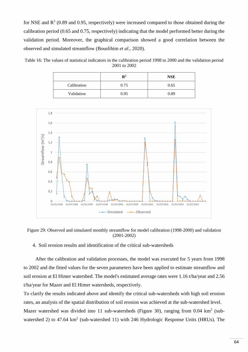
64

for NSE and R2 (0.89 and 0.95, respectively) were increased compared to those obtained during the

calibration period (0.65 and 0.75, respectively) indicating that the model performed better during the

validation period. Moreover, the graphical comparison showed a good correlation between the

observed and simulated streamflow (Bouslihim et al., 2020).

Table 16: The values of statistical indicators in the calibration period 1998 to 2000 and the validation period

2001 to 2002

R2 NSE

Calibration 0.75 0.65

Validation 0.95 0.89

Figure 29: Observed and simulated monthly streamflow for model calibration (1998-2000) and validation

(2001-2002)

4. Soil erosion results and identification of the critical sub-watersheds

After the calibration and validation processes, the model was executed for 5 years from 1998

to 2002 and the fitted values for the seven parameters have been applied to estimate streamflow and

soil erosion at El Himer watershed. The model's estimated average rates were 1.16 t/ha/year and 2.56

t/ha/year for Mazer and El Himer watersheds, respectively.

To clarify the results indicated above and identify the critical sub-watersheds with high soil erosion

rates, an analysis of the spatial distribution of soil erosion was achieved at the sub-watershed level.

Mazer watershed was divided into 11 sub-watersheds (Figure 30), ranging from 0.04 km2 (sub-

watershed 2) to 47.64 km2 (sub-watershed 11) with 246 Hydrologic Response Units (HRUs). The

0

0,2

0,4

0,6

0,8

1

1,2

1,4

1,6

1,8

01/01/1998 01/07/1998 01/01/1999 01/07/1999 01/01/2000 01/07/2000 01/01/2001 01/07/2001 01/01/2002 01/07/2002

Stre

amfl

ow

(m

3 /s)

Simulated Observed

65

same figure shows the El Himer watershed subdivision, with a total of 315 HRUs and 23 sub-

watersheds ranging from 0.14 km2 (sub-watershed 4) to 36.22 km2 (sub-watershed 22).

Figure 30: Delimitation of Mazer and El Himer subwatersheds

Results show that all studied sub-watersheds present a weak amount of soil erosion rate, with a

maximum of 5.20 t/ha/year for the sub-basin 6 (Figure 31), which cover only 6.51 % of the total area

of the El Himer watershed (Bouslihim et al., 2020).

Figure 31: Sub-basin spatial distribution of the estimated soil erosion rates (t/ha/yr) at Mazer and El Himer

watersheds

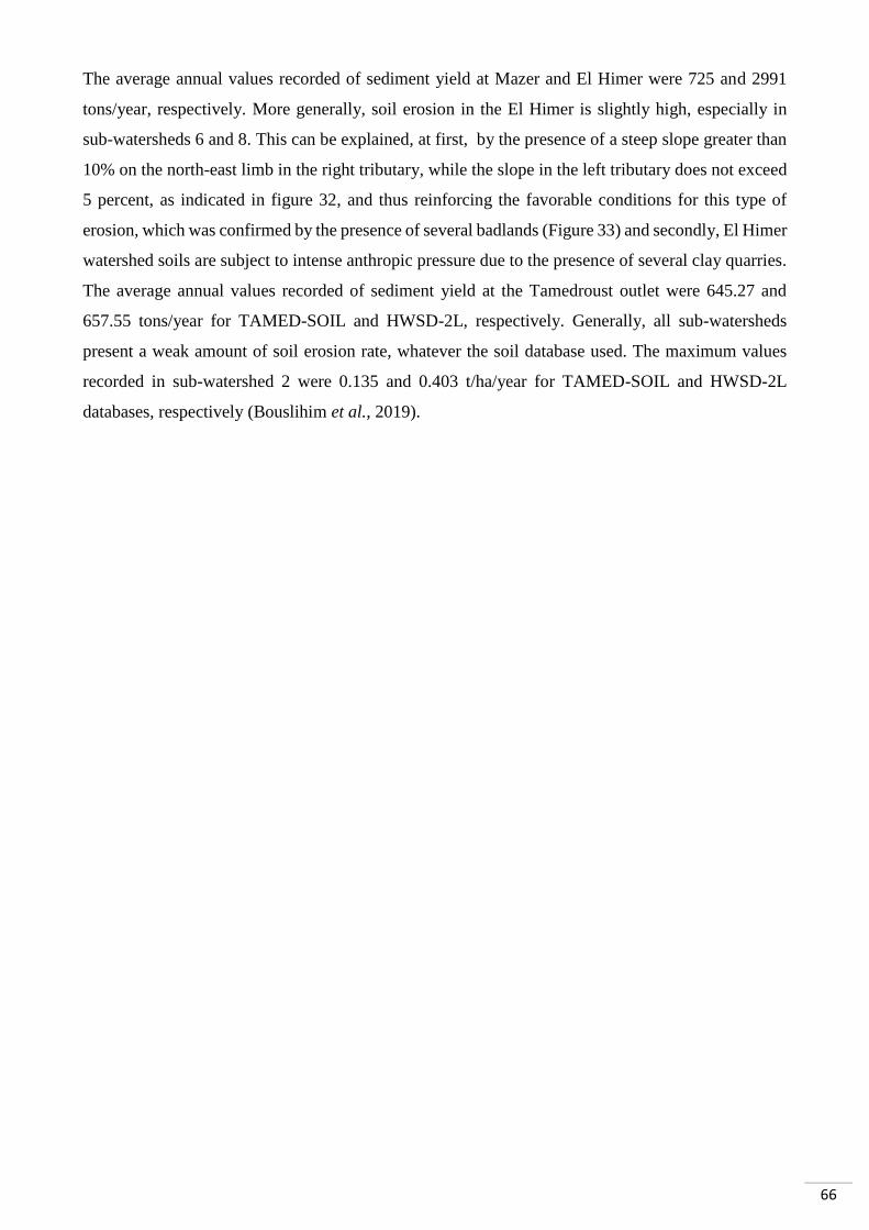
66

The average annual values recorded of sediment yield at Mazer and El Himer were 725 and 2991

tons/year, respectively. More generally, soil erosion in the El Himer is slightly high, especially in

sub-watersheds 6 and 8. This can be explained, at first, by the presence of a steep slope greater than

10% on the north-east limb in the right tributary, while the slope in the left tributary does not exceed

5 percent, as indicated in figure 32, and thus reinforcing the favorable conditions for this type of

erosion, which was confirmed by the presence of several badlands (Figure 33) and secondly, El Himer

watershed soils are subject to intense anthropic pressure due to the presence of several clay quarries.

The average annual values recorded of sediment yield at the Tamedroust outlet were 645.27 and

657.55 tons/year for TAMED-SOIL and HWSD-2L, respectively. Generally, all sub-watersheds

present a weak amount of soil erosion rate, whatever the soil database used. The maximum values

recorded in sub-watershed 2 were 0.135 and 0.403 t/ha/year for TAMED-SOIL and HWSD-2L

databases, respectively (Bouslihim et al., 2019).

67

Figure 32: Topographic profiles of El Himer River

68

Figure 33: Eroded badlands at the northern part of the El Himer watershed

V. Conclusion

The application of a hydrological simulation model under conditions of limited data availability

is a tremendous challenge for hydrologists and modelers, especially in the case of using a hydrological

model such as SWAT, which requires a large number of input data that takes time and resources. The

presence of a neighboring/gauged watershed (Mazer) has been an advantage in this study as it allowed

us to compare its similarity with the ungauged watershed (El Himer). This comparison showed us

that the most physical attributes that influence runoff production are almost close for both watersheds,

which allowed us to apply regionalization methods by transferring hydrological model parameters

from the gauged watershed (Mazer) to the ungauged watershed (El Himer).

This process has been done by using the SWAT model at Mazer watershed, which has shown

a good model performance with an NSE of 0.65, 0.89 and with R2 of 0.75, 0.95 for calibration and

validation, respectively. After this, the fitted values for all sensitive parameters have been used to

estimate the streamflow and soil erosion at the ungauged watershed (El Himer). The results showed

that all studied subwatersheds present a weak soil erosion rate, except for numbers 6 and 8, with a

high erosion rate compared to other subwatersheds. Generally, soil erosion in the El Himer watershed

is slightly elevated due to the presence of a steep slope in the northern part of the area. Therefore,

despite the low erosion rate, it is highly recommended that the calibrated model in both watersheds

and the achieved results can be used to choose the best management practices for managing soil and

for determining proper land use and soil conservation measures at both watersheds.

69

CHAPTER 5: SOIL AGGREGATE STABILITY PREDICTION USING

MULTIPLE LINEAR REGRESSION AND RANDOM FOREST

I. Introduction

Soil is a natural resource of public interest that is under increasing environmental pressure and,

therefore, must be sustainably managed for the benefit of future generations. This management cannot

be reached without a proper understanding of the different soil characteristics and properties.

Aggregate stability is one of the essential factors in soil conservation and maintenance of its

environmental functions (Hanke and Dick, 2017), it affects water (Kunhikrishnan et al., 2012), and

store and stabilize organic carbon (Kodešová et al., 2008). Furthermore, an increase in soil structural

stability can directly increase the resistance against erosive agents and compaction (Chaplot and

Cooper, 2015). Stable soil aggregates form a stable soil structure, allowing optimum movement and

storage of gases, water and nutrients (Gliński et al., 2011). All this information could confirm that

soil aggregate stability may be a useful indicator for monitoring soil quality (Chaplot and Cooper,

2015).

Soil aggregate stability can be measured with many different methods, which have been the subject

of several reviews (Amezketa, 1999; Le Bissonnais, 2016; Nimmo and Perkins, 2002). According to

Jastrow and Miller (1991), this diversification of measurement methods can be explained by three

reasons: (1) the existence of different mechanisms that produce destabilization, (2) the different scales

at which stability can be determined, and (3) methodological reasons.

More recently, the most common method used for aggregate stability measurement is Le Bissonnais's

method, which has become established as the standard approach to determine the soil's aggregate

stability. This method has been adopted as the international standard with the award of the (ISO/FDIS

10930, 2012). Despite the consensus on this measurement methodology, it remains difficult to apply

routinely since it is very time-consuming. Indeed, one needs to deal with three different tests,

including fast wetting (FW), slow wetting (SW) and mechanical breakdown (WS), repeated three

times for each analysis, and a large quantity of ethanol would be necessary for this method (Le

Bissonnais, 2016). Generally, it is a common problem for all other soil properties, especially when

talking about a large surface and large samples to be analyzed.

To overcome this problem, scientists have searched for alternative solutions. Therefore, Pedotransfer

Functions (PTFs) have appeared to be the best solution. These approaches are used to estimate soil

properties by easily measurable soil parameters (Gunarathna et al., 2019). It can also be defined as

predictive functions of certain soil properties from others easily, routinely, or cheaply measured

properties. The most readily available data come from soil surveys, such as field morphology, texture,

structure, and pH (Odeh and McBratney, 2005).

70

During the last few decades, regression methods have been widely used to develop PTFs worldwide.

Recently, machine learning methods have been deployed in PTFs development, such as the K-Nearest

Neighbor (KNN) (Mihalikova et al., 2014), Cubist (Kuhn et al., 2013), Artificial Neural Networks

(ANN) (D'Emilio et al., 2018), and Random Forests (RF) approaches (Dharumarajan et al., 2017).

Despite those frequent applications, machine learning approaches remain hardly used to develop

PTFs.

The possibility of using PTFs methods to estimate the different soil parameters has been widely

studied all around the world, especially for parameters that are difficult and time-consuming to

measure, such as soil carbon (Keskin et al., 2019), bulk density (Souza et al., 2016), soil water content

(Santra et al., 2018), hydraulic conductivity (Zhao et al., 2016), soil phosphorus (Valadares et al.,

2017), soil nitrogen (Dessureault-Rompré et al., 2015) and total silicon concentrations (Landre et al.,

2018). On the other hand, very few studies have been done to assess the feasibility of using PTFs

(regression or machine learning methods) for predicting soil aggregate stability (Annabi et al., 2017;

Besalatpour et al., 2013; Marashi et al., 2017; Melo et al., 2018). Following this research, we have

seen that the Random Forest method has never been used before predicting the soil aggregate stability.

Based on our literature review, no study was found concerning the use of PTFs methods to estimate

soil parameters in Morocco.

The objectives of this study were to compare the capabilities of Multiple Linear Regression (MLR)

and Random Forest (RF) to derive PTFs between soil aggregate stability and different sets of input

variables. The developed PTFs can be used as a basis to predict the soil aggregate stability in this

region and to avoid waste of time and money deployed for analyses.

II. Modeling approaches and data sets

For comparative assessment, two different methods were used to analyze the feasibility of using

the PTFs techniques to predict the soil aggregate stability from routinely measured soil properties and

remote sensing indices.

Multiple Linear Regression (Bottenberg and Ward, 1963) is a prediction method and a widely

known modeling technique. Linear Regression establishes a relationship between the dependent

variable (y) and one or more independent variables (x) using a best fit straight line. It is represented

by the following equation (Marashi et al., 2017):

𝑦 = 𝑏0 + 𝑏1𝑥𝑖,1 + 𝑏2𝑥𝑖,2 + ⋯ + 𝑏𝑘𝑥𝑖,𝑘 + 𝑒𝑖

Where yi is the dependent variable, b0 is a constant (the intercept), xi,k is an independent variable, bk

is the vector of regression coefficients called slope, and ei represents residuals not explained by the

model.

71

The second model used in this study is the Random Forest; it is a flexible and easy to use

machine learning algorithm that developed mainly to overcome the single regression tree limitations

(Breiman, 2001). During the model's construction, many regression trees are grown with randomly

selected combinations of input variables which gives many different results and the final prediction

is achieved through voting (Anysz et al., 2020). In this way, the model will be more robust to outliers

and noise than a single regression tree. Prediction is based on a whole set of regression trees, while

the results of all individual trees are averaged, or weighted average is calculated (Van Looy et al.,

2017). Random Forest modeling can improve predictions made by classification and regression trees

(Breiman, 2001). Two important parameters in RF method are the number of trees (ntree) and the

number of variables available for selection in each split (mtry) (Houborg and McCabe, 2018). The

model was performed using the Statistical Package for Social Sciences (SPSS) software (version

25.0).

As already mentioned in section II - chapter 3, a total of 77 soil samples (0-40 cm depth) over

the majority of the study area's surface were collected and analyzed for soil aggregate stability and

other physicochemical properties. Thirty-seven additional samples were obtained from Baghri and

Rochdi's (2008) study to expand our database; these samples are located in the middle part of the

Tamedroust watershed, as shown in Fig. 3. The soil aggregate stability data obtained from this study

were analyzed with a different method. For this reason, we have compared four different data sets

(SP1, SP2, SPRS1 and SPRS2) to verify and avoid any influence of Baghri and Rochdi's (2008) data.

Figure 34 illustrates how the data was packaged to form the four sets.

The first set (denoted as SP1) consisted of soil properties alone for the first 77 soil samples.

The second set (denoted as SP2) included all soil samples (77+37)

The third set (denoted as SPRS1) combines soil properties and remote sensing indices for the

first 77 soil.

The fourth set (denoted as SPRS2) included all soil samples (77+37) and all other remote

sensing indices.

Cation Exchange Capacity (CEC) was obtained from the International Soil Reference and

Information Centre (ISRIC) database (Batjes et al., 2017) and Available Water Capacity (AWC) was

estimated using (Saxton and Rawls, 2006) equations. All remote sensing parameters were extracted

generally from the imagery satellite Landsat-8 Operational Land Imager (OLI)/Thermal Infrared

Sensor (TIRS) (Acquisition date: 14-APR-17, Patch: 202, Row: 37) using remote sensing techniques.

Their description and calculation formulae for determination are presented in table 17.

MLR and RF models were performed using R software.

72

Figure 34: Soil input data used for the development of different models

Table 17: Different indices (remote sensing parameters) evaluated in the PTFs approach to predict the soil

aggregate stability

Index Description Equation Reference

LAI Leaf Area Index 3.618 ∗ 𝐸𝑉𝐼 − 0.118 Boegh et al., 2002

EVI Enhanced

Vegetation Index 2.5 ∗ (

𝜌𝑃𝐼𝑅 − 𝜌𝑅𝜌𝑃𝐼𝑅 + 𝐶1𝜌𝑅 − 𝐶2𝜌𝐵 + 𝐿⁄ )

[C1 = 6, C2 = 7.5, L = 1]

Huete et al., 1999

GSI Grain Size Index 𝐺𝑆𝐼 =(𝑅 − 𝐵)

(𝑅 + 𝐵 + 𝐺)⁄ Xiao et al., 2006

SAVI Soil Adjusted

Vegetation Index

𝜌𝑃𝐼𝑅 − 𝜌𝑅𝜌𝑃𝐼𝑅 + 𝜌𝑅 + 0.5⁄ ∗ (1.5) Huete, 1988

GVI Green Vegetation

Index

(−0.2848 ∗ 𝜌𝑎𝑒𝑟𝑜) + (−0.2435 ∗ 𝜌𝐵) +(−0.5436 ∗ 𝜌𝐺) + (−0.7243 ∗ 𝜌𝑅) +

(−0.0840 ∗ 𝜌𝑀𝐼𝑅1) + (−0.1800 ∗ 𝜌𝑀𝐼𝑅2)

Kauth, 1976

BI Brightness Index √𝜌𝐺2 + 𝜌𝑅2 Khan et al., 2005

RI Redness Index 𝜌𝑅2

𝜌𝐺3⁄ Pouget et al.,

1991

SI Salinity Index √𝜌𝐺 ∗ 𝜌𝑅 Dehni and

Lounis, 2012

NDWI Normalized

Difference Water

Index

𝜌𝑃𝐼𝑅 − 𝜌𝑀𝐼𝑅𝜌𝑃𝐼𝑅 − 𝜌𝑀𝐼𝑅⁄ Gao, 1996

73

MSI Moisture Stress

Index

𝜌𝑀𝐼𝑅𝜌𝑃𝐼𝑅⁄ Hunt and Rock,

1989

RVI Ratio Vegetation

Index

𝜌𝑃𝐼𝑅𝜌𝑅⁄ Kriegler et al.,

1969

DVI Difference

Vegetation Index 𝜌𝑃𝐼𝑅 − 𝜌𝑅 Bacour et al.,

2006

NDVI Normalized

Difference

Vegetation Index

𝜌𝑃𝐼𝑅 − 𝜌𝑅𝜌𝑃𝐼𝑅 + 𝜌𝑅⁄ Rouse et al., 1973

TNDVI Transformed

Normalized

Difference

Vegetation Index

√0.5 + ((𝜌𝑁𝐼𝑅 − 𝜌𝑅)

(𝜌𝑁𝐼𝑅 + 𝜌𝑅)⁄ ) Bannari et al.,

2002

III. Evaluation of prediction accuracy

The MLR and RF models' performance was evaluated using a 10-fold cross-validation

procedure that involved comparisons between the predicted and observed MWD values. Cross-

validation provides a modeling structure for dividing several calibrations and validation sets, which

guarantees that each sample can be assigned to the validation at least once. The greatest advantage of

this method is that it runs reliably and is unbiased for small sample set (Y. Hong et al., 2020). The

created PTFs were also assessed based on the differences between the observed and predicted MWD,

using two parameters, the coefficient of determination (R2) and the root mean square error (RMSE).

Thus, we applied the model performance classification criteria defined by Li et al. (2016) as values

of R2 < 0.5 (unacceptable prediction capacity), 0.5 ≤ R2 <0.75 (acceptable prediction capacity), and

R2 ≥ 0.75 (good prediction capacity), to evaluate model performance based on R2.

𝑅𝑀𝑆𝐸 = √∑ [𝑂𝑖𝑛𝑖=1 − 𝑃𝑖]²

𝑛⁄

𝑅2 = 1 −∑ (𝑂𝑖 − 𝑃𝑖)

2𝑛𝑖=1

∑ (𝑂𝑖 − �̅�)2𝑛𝑖=1

where Oi, Pi and O ̅are the observed, predicted and mean Oi value at site i, respectively, and n is the

number of samples.

IV. Results:

1. Descriptive statistics of soil properties

Statistical analysis was performed on the whole data set (n=114 samples) for different soil

properties (pH, OM, clay, silt, sand, BD, CEC and AWC) and remote sensing indices (LAI, GSI, EVI,

SAVI, GVI, BI, RI, SI, NDWI, MSI, RVI, DVI, NDVI and TNDVI).

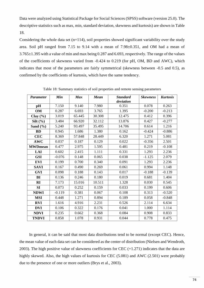
74

Data were analyzed using Statistical Package for Social Sciences (SPSS) software (version 25.0). The

descriptive statistics such as max, min, standard deviation, skewness and kurtosis) are shown in Table

18.

Considering the whole data set (n=114), soil properties showed significant variability over the study

area. Soil pH ranged from 7.15 to 9.14 with a mean of 7.98±0.351, and OM had a mean of

3.765±1.395 with a value of min and max being 0.287 and 6.693, respectively. The range of the values

of the coefficients of skewness varied from -0.424 to 0.219 (for pH, OM, BD and AWC), which

indicates that most of the parameters are fairly symmetrical (skewness between -0.5 and 0.5), as

confirmed by the coefficients of kurtosis, which have the same tendency.

Table 18: Summary statistics of soil properties and remote sensing parameters

Parameter Min Max Mean Standard

deviation

Skewness Kurtosis

pH 7.150 9.140 7.980 0.351 0.078 0.263

OM 0.287 6.693 3.765 1.395 -0.200 -0.213

Clay (%) 3.019 65.445 30.308 12.475 0.412 0.396

Silt (%) 3.484 66.920 32.112 13.876 0.427 -0.277

Sand (%) 5.240 93.497 35.495 14.706 0.614 1.216

BD 0.945 1.686 1.380 0.162 -0.424 -0.886

CEC 8.369 57.848 28.449 6.320 1.271 5.081

AWC 0.037 0.187 0.129 0.022 -0.356 2.501

MWDmean 0.477 2.975 1.595 0.481 0.219 -0.108

LAI 0.602 2.415 1.111 0.331 1.293 2.236

GSI -0.076 0.148 0.065 0.038 -1.125 2.079

EVI 0.199 0.700 0.340 0.091 1.293 2.236

SAVI 0.167 0.490 0.269 0.061 0.994 1.148

GVI 0.098 0.188 0.143 0.017 -0.188 -0.139

BI 0.136 0.246 0.180 0.019 0.681 1.404

RI 7.173 15.016 10.511 1.328 0.030 0.545

SI 0.073 0.252 0.159 0.033 0.199 0.606

NDWI -0.119 0.381 0.067 0.108 0.313 -0.520

MSI 0.448 1.271 0.894 0.189 0.058 -0.848

RVI 1.616 4.916 2.231 0.526 2.114 6.634

DVI 0.106 0.322 0.176 0.041 1.000 1.114

NDVI 0.235 0.662 0.368 0.084 0.908 0.833

TNDVI 0.858 1.078 0.931 0.044 0.778 0.475

In general, it can be said that most data distributions tend to be normal (except CEC). Hence,

the mean value of each data set can be considered as the center of distribution (Nielsen and Wendroth,

2003). The high positive value of skewness coefficients for CEC (+1.271) indicates that the data are

highly skewed. Also, the high values of kurtosis for CEC (5.081) and AWC (2.501) were probably

due to the presence of one or more outliers (Brys et al., 2003).

75

As can be noted in the box plots of all parameters (Figure 35), several values can be identified as

outliers, especially at CEC and AWC, confirming earlier kurtosis results.

Clay fraction ranged from 3.019 to 65.445, with a mean and standard deviation of 30.308 and 12.475,

respectively. Silt fraction ranged from 3.484 to 66.92, with a mean and standard deviation of 32.112

and 13.876, respectively. Sand fraction ranged from 5.24 to 93.497, with a mean and standard

deviation of 35.495 and 14.706, respectively.

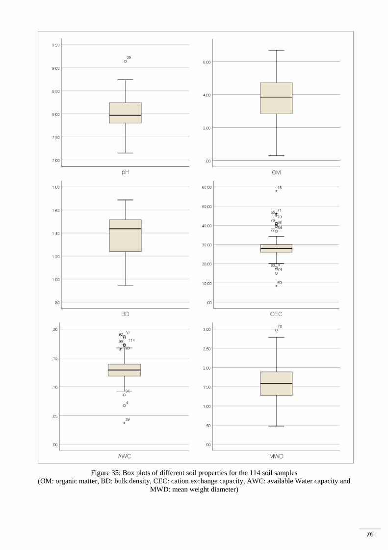
76

Figure 35: Box plots of different soil properties for the 114 soil samples

(OM: organic matter, BD: bulk density, CEC: cation exchange capacity, AWC: available Water capacity and

MWD: mean weight diameter)

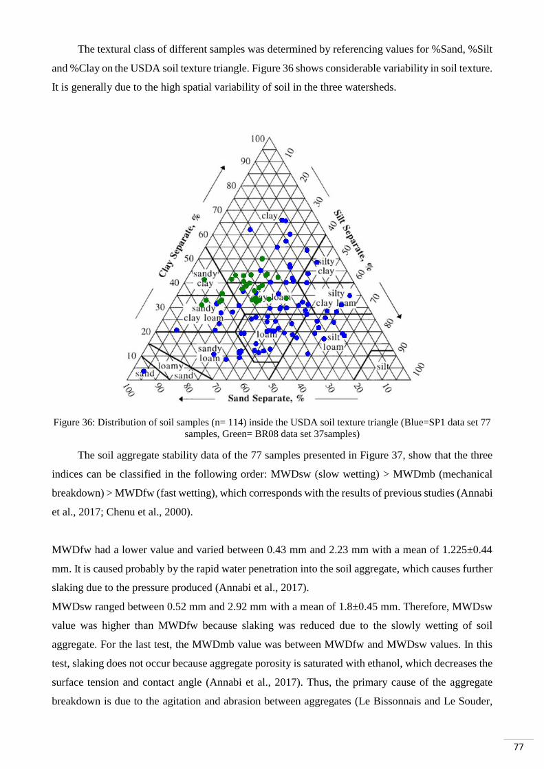
77

The textural class of different samples was determined by referencing values for %Sand, %Silt

and %Clay on the USDA soil texture triangle. Figure 36 shows considerable variability in soil texture.

It is generally due to the high spatial variability of soil in the three watersheds.

Figure 36: Distribution of soil samples (n= 114) inside the USDA soil texture triangle (Blue=SP1 data set 77

samples, Green= BR08 data set 37samples)

The soil aggregate stability data of the 77 samples presented in Figure 37, show that the three

indices can be classified in the following order: MWDsw (slow wetting) > MWDmb (mechanical

breakdown) > MWDfw (fast wetting), which corresponds with the results of previous studies (Annabi

et al., 2017; Chenu et al., 2000).

MWDfw had a lower value and varied between 0.43 mm and 2.23 mm with a mean of 1.225±0.44

mm. It is caused probably by the rapid water penetration into the soil aggregate, which causes further

slaking due to the pressure produced (Annabi et al., 2017).

MWDsw ranged between 0.52 mm and 2.92 mm with a mean of 1.8±0.45 mm. Therefore, MWDsw

value was higher than MWDfw because slaking was reduced due to the slowly wetting of soil

aggregate. For the last test, the MWDmb value was between MWDfw and MWDsw values. In this

test, slaking does not occur because aggregate porosity is saturated with ethanol, which decreases the

surface tension and contact angle (Annabi et al., 2017). Thus, the primary cause of the aggregate

breakdown is due to the agitation and abrasion between aggregates (Le Bissonnais and Le Souder,

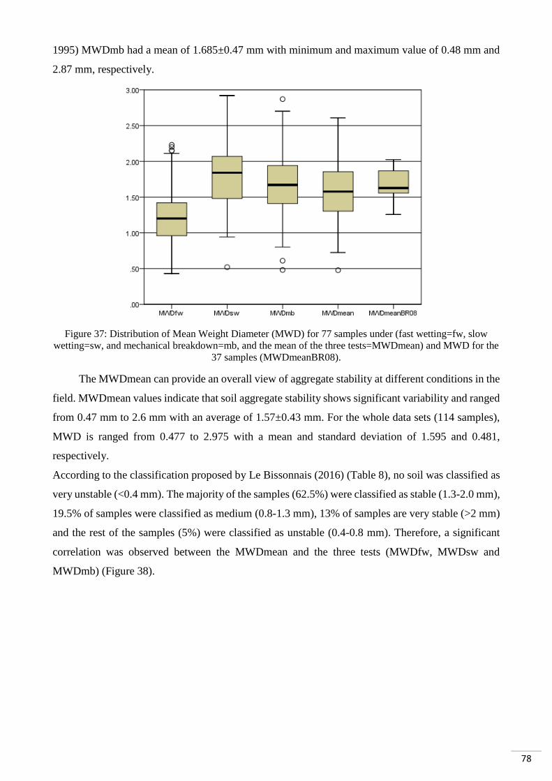
78

1995) MWDmb had a mean of 1.685±0.47 mm with minimum and maximum value of 0.48 mm and

2.87 mm, respectively.

Figure 37: Distribution of Mean Weight Diameter (MWD) for 77 samples under (fast wetting=fw, slow

wetting=sw, and mechanical breakdown=mb, and the mean of the three tests=MWDmean) and MWD for the

37 samples (MWDmeanBR08).

The MWDmean can provide an overall view of aggregate stability at different conditions in the

field. MWDmean values indicate that soil aggregate stability shows significant variability and ranged

from 0.47 mm to 2.6 mm with an average of 1.57±0.43 mm. For the whole data sets (114 samples),

MWD is ranged from 0.477 to 2.975 with a mean and standard deviation of 1.595 and 0.481,

respectively.

According to the classification proposed by Le Bissonnais (2016) (Table 8), no soil was classified as

very unstable (<0.4 mm). The majority of the samples (62.5%) were classified as stable (1.3-2.0 mm),

19.5% of samples were classified as medium (0.8-1.3 mm), 13% of samples are very stable (>2 mm)

and the rest of the samples (5%) were classified as unstable (0.4-0.8 mm). Therefore, a significant

correlation was observed between the MWDmean and the three tests (MWDfw, MWDsw and

MWDmb) (Figure 38).

79

Figure 38: Correlation matrix between the three tests of aggregate stability and the MWDmean for the 77 soil

samples

(**) Significant at the level of 0.01

2. Multiple linear regression model performance

A high correlation between variables may influence the achievement of th+e expected results for the

MLR. This is referred to as multicollinearity (between more than two variables) or collinearity

(between two variables) (Kumari, 2008), which can cause unstable estimates of regression

coefficients in linear and logistic regression models, incorrect variance estimates for the coefficients

of those parameters in regression models, and some difficulties in the numerical calculations involved

in fitting the regression model (Dohoo et al., 1997). Multicollinearity occurs in a data set due to the

correlation between the predictors. Models derived from such data without a check on

multicollinearity may lead to erroneous system analysis (Garg and Tai, 2013). This problem can be

avoided by selecting the appropriate predictors from the data set and eliminate the variables that could

affect the model results.

For this reason, the correlation was checked using the matrix of Pearson's between all independent

variables of the four data sets (Figure 39). All correlations matrices were performed using the corrplot

package in R (Wei et al., 2017).

For SP1 data set, sand and AWC were excluded from the list of input variables because of

multicollinearity between clay/silt and sand, and the collinearity between silt and AWC.

For SP2 data set, the same variables detected in the SP1 data set were eliminated (sand and AWC),

with the addition of BD because of collinearity with silt.

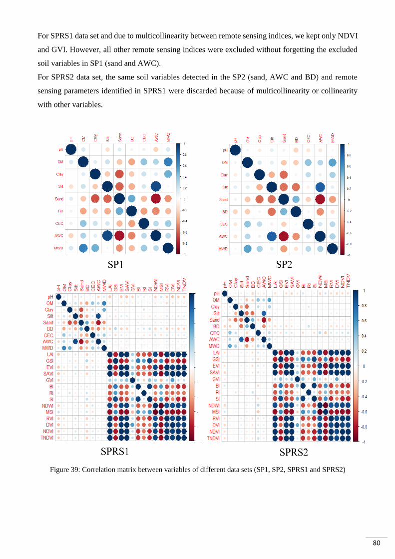
80

For SPRS1 data set and due to multicollinearity between remote sensing indices, we kept only NDVI

and GVI. However, all other remote sensing indices were excluded without forgetting the excluded

soil variables in SP1 (sand and AWC).

For SPRS2 data set, the same soil variables detected in the SP2 (sand, AWC and BD) and remote

sensing parameters identified in SPRS1 were discarded because of multicollinearity or collinearity

with other variables.

Figure 39: Correlation matrix between variables of different data sets (SP1, SP2, SPRS1 and SPRS2)

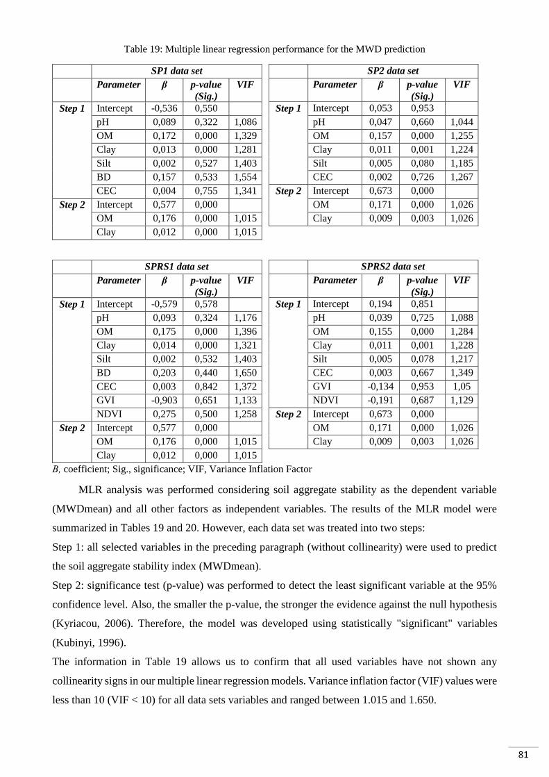
81

Table 19: Multiple linear regression performance for the MWD prediction

SP2 data set

Parameter β p-value

(Sig.)

VIF

Step 1 Intercept 0,053 0,953

pH 0,047 0,660 1,044

OM 0,157 0,000 1,255

Clay 0,011 0,001 1,224

Silt 0,005 0,080 1,185

CEC 0,002 0,726 1,267


OM 0,171 0,000 1,026

Clay 0,009 0,003 1,026

SPRS2 data set


(Sig.)

VIF


pH 0,039 0,725 1,088

OM 0,155 0,000 1,284

Clay 0,011 0,001 1,228

Silt 0,005 0,078 1,217

CEC 0,003 0,667 1,349

GVI -0,134 0,953 1,05

NDVI -0,191 0,687 1,129


OM 0,171 0,000 1,026

Clay 0,009 0,003 1,026

Β, coefficient; Sig., significance; VIF, Variance Inflation Factor

MLR analysis was performed considering soil aggregate stability as the dependent variable

(MWDmean) and all other factors as independent variables. The results of the MLR model were

summarized in Tables 19 and 20. However, each data set was treated into two steps:

Step 1: all selected variables in the preceding paragraph (without collinearity) were used to predict

the soil aggregate stability index (MWDmean).

Step 2: significance test (p-value) was performed to detect the least significant variable at the 95%

confidence level. Also, the smaller the p-value, the stronger the evidence against the null hypothesis

(Kyriacou, 2006). Therefore, the model was developed using statistically "significant" variables

(Kubinyi, 1996).

The information in Table 19 allows us to confirm that all used variables have not shown any

collinearity signs in our multiple linear regression models. Variance inflation factor (VIF) values were

less than 10 (VIF < 10) for all data sets variables and ranged between 1.015 and 1.650.

SP1 data set Parameter β p-value

(Sig.)

VIF

Step 1 Intercept -0,536 0,550

pH 0,089 0,322 1,086

OM 0,172 0,000 1,329

Clay 0,013 0,000 1,281

Silt 0,002 0,527 1,403

BD 0,157 0,533 1,554

CEC 0,004 0,755 1,341


OM 0,176 0,000 1,015

Clay 0,012 0,000 1,015

SPRS1 data set


(Sig.)

VIF

Step 1 Intercept -0,579 0,578

pH 0,093 0,324 1,176

OM 0,175 0,000 1,396

Clay 0,014 0,000 1,321

Silt 0,002 0,532 1,403

BD 0,203 0,440 1,650

CEC 0,003 0,842 1,372

GVI -0,903 0,651 1,133

NDVI 0,275 0,500 1,258


OM 0,176 0,000 1,015

Clay 0,012 0,000 1,015

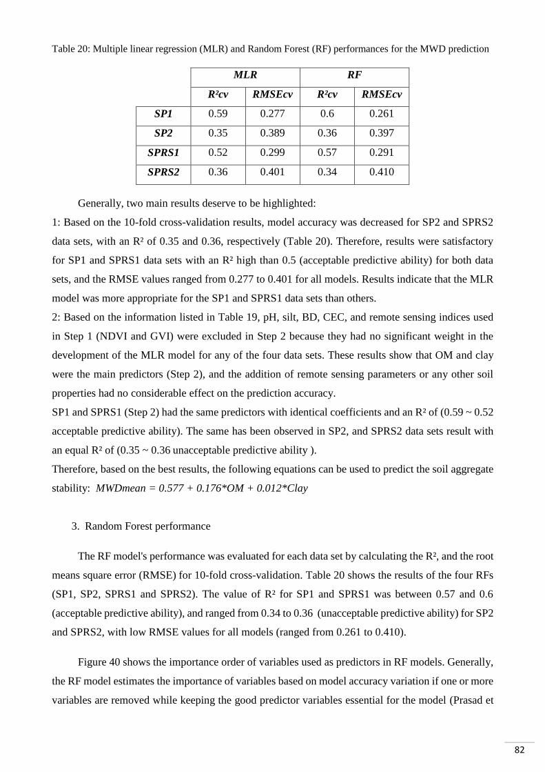
82

Table 20: Multiple linear regression (MLR) and Random Forest (RF) performances for the MWD prediction

Generally, two main results deserve to be highlighted:

1: Based on the 10-fold cross-validation results, model accuracy was decreased for SP2 and SPRS2

data sets, with an R² of 0.35 and 0.36, respectively (Table 20). Therefore, results were satisfactory

for SP1 and SPRS1 data sets with an R² high than 0.5 (acceptable predictive ability) for both data

sets, and the RMSE values ranged from 0.277 to 0.401 for all models. Results indicate that the MLR

model was more appropriate for the SP1 and SPRS1 data sets than others.

2: Based on the information listed in Table 19, pH, silt, BD, CEC, and remote sensing indices used

in Step 1 (NDVI and GVI) were excluded in Step 2 because they had no significant weight in the

development of the MLR model for any of the four data sets. These results show that OM and clay

were the main predictors (Step 2), and the addition of remote sensing parameters or any other soil

properties had no considerable effect on the prediction accuracy.

SP1 and SPRS1 (Step 2) had the same predictors with identical coefficients and an R² of (0.59 ~ 0.52

acceptable predictive ability). The same has been observed in SP2, and SPRS2 data sets result with

an equal R² of (0.35 ~ 0.36 unacceptable predictive ability ).

Therefore, based on the best results, the following equations can be used to predict the soil aggregate

stability: MWDmean = 0.577 + 0.176*OM + 0.012*Clay

3. Random Forest performance

The RF model's performance was evaluated for each data set by calculating the R², and the root

means square error (RMSE) for 10-fold cross-validation. Table 20 shows the results of the four RFs

(SP1, SP2, SPRS1 and SPRS2). The value of R² for SP1 and SPRS1 was between 0.57 and 0.6

(acceptable predictive ability), and ranged from 0.34 to 0.36 (unacceptable predictive ability) for SP2

and SPRS2, with low RMSE values for all models (ranged from 0.261 to 0.410).

Figure 40 shows the importance order of variables used as predictors in RF models. Generally,

the RF model estimates the importance of variables based on model accuracy variation if one or more

variables are removed while keeping the good predictor variables essential for the model (Prasad et

MLR RF

R²cv RMSEcv R²cv RMSEcv

SP1 0.59 0.277 0.6 0.261

SP2 0.35 0.389 0.36 0.397

SPRS1 0.52 0.299 0.57 0.291

SPRS2 0.36 0.401 0.34 0.410

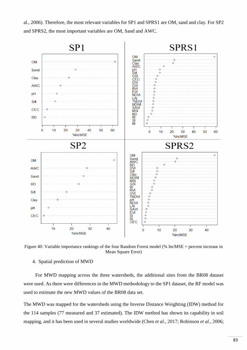
83

al., 2006). Therefore, the most relevant variables for SP1 and SPRS1 are OM, sand and clay. For SP2

and SPRS2, the most important variables are OM, Sand and AWC.

Figure 40: Variable importance rankings of the four Random Forest model (% IncMSE = percent increase in

Mean Square Error)

4. Spatial prediction of MWD

For MWD mapping across the three watersheds, the additional sites from the BR08 dataset

were used. As there were differences in the MWD methodology to the SP1 dataset, the RF model was

used to estimate the new MWD values of the BR08 data set.

The MWD was mapped for the watersheds using the Inverse Distance Weighting (IDW) method for

the 114 samples (77 measured and 37 estimated). The IDW method has shown its capability in soil

mapping, and it has been used in several studies worldwide (Chen et al., 2017; Robinson et al., 2006;

84

Zhang et al., 2011). The values inferred at non-sampled areas by IDW are estimated using a linear

combination of values at the sampled places, weighted by an inverse function of the distance from

the point of interest to the sample points (Silva et al., 2017). The weights (λi) are expressed in the

following equation:

𝜆𝑖 =

1

𝑑𝑖𝑝

∑1

𝑑𝑖𝑝

𝑛𝑖=1

⁄

Where di is the distance between two points, p is a power parameter, and n represents the number of

sampled points used for the estimation. Concerning the created map (Figure 41), the lowest RMSE

value (0.289) was obtained using a p = 1.5 with a number of neighbors between 10 and 15.

The generated map (Figure 41) using the IDW method shows that the "stable soil" category occupies

most of the study area, a small area of the "medium soil" located in the southeastern portion of the

study area and the existence of very stable soils in the west part.

These results can be explained by returning to the geological features, soil maps and the different soil

characteristics. The presence of medium stable soil in the southeastern part can be explained firstly

by the geological nature of this part due to the presence of Lutetian formations in the form of siliceous

earth; secondly, the presence of shallow soils (Rankers) and Xerosols, which are generally

characterized by low levels of organic matter (Figure 42-C). Also, soil analysis results indicate the

presence of small or medium quantities of organic matter and a significant presence of sand (between

40 and 60% or higher) (Figure 42-A).

The presence of Vertisols and quaternary formations in the western part of the Tamedroust watershed,

plus the existence of a gentle slope in the same area, can help provide a favorable context for the

development of clayey soils rich in organic matter (Figure 42 B & C). This proposition can explain

the existence of very stable soils in this part with a significant percentage of clay (between 40 and

60%) and very high rates of organic matter.

The study results confirm the significant role of organic matter and clay in soils' structural

stability (Amezketa, 1999; Annabi et al., 2017; Chaney and Swift, 1984; Chenu et al., 2000; Kavdir

et al., 2004). Other studies have shown that some parameters, such as soil microorganisms and their

activities and cations (Ca2+ and Fe2+, among others), are also involved in soil aggregation and

stabilization (Lynch and Bragg, 1985; Wuddivira and Camps-Roach, 2007).

In general, these results confirm the low soil erosion rates obtained from the SWAT model in

the three watersheds (chapters 3 & 4 and figure 42-D). That is mainly due to several factors, the most

important of which are: (i) soil properties so that the stable soil occupies most of the study area with

85

a significant percentage of OM and clay, (ii) the low slop values of all watersheds except for the north

part of El Himer watershed, which was explained before (results section in chapter 4 and Bouslihim

et al., 2020), and (iii) the scarcity of precipitation as one of the main factors of the soil erosion process,

especially in arid and semi-arid regions.

Figure 41: Spatial distribution of soil aggregate stability

86

Figure 42: Spatial distribution of A) Sand (%), B) Clay (%), C) organic matter (%) and D) soil erosion rates (t/ha/year)

87

V. Comparison between MLR and RF

Both the MLR and RF methods were acceptable in predicting soil aggregate stability (MWDmean)

based on soil properties (SP1) with or without other remote sensing parameters (SPRS1). However,

combining this data with the supplementary data (SP2 and SPRS2) decreases the model performance.

These results may be explained by variations in data properties, considering that SP1 and BR08 data

sets do not have the same source and do not show the same properties and relations between variables,

which can be the principal cause of these results. Unlike the significant correlation between

MWDmean, Clay and OM of the SP1 data set (77 samples), Pearson's correlation values between

variables for the other 37 samples are not significant, with a value of 0.283 between MWD and OM,

and -0.264 between MWD and clay, which may reduce MLR model performance.

Thus far, few studies have used the MLR method to predict soil aggregate stability (MWDmean), and

none have used Random Forest. Overall, results obtained in this study using MLR to predict

MWDmean were lower than those of Marashi et al. (2017). They evaluate the capabilities of MLR

and ANNs (in the East of Azerbaijan) for estimating the MWD from two different data sets, routine

soil properties (P1) and combination of routine soil properties and fractal dimension of aggregates

(P2) data sets (n= 85 samples). The obtained values of R2 for the MLR model were 0.78 and 0.90 for

P1 and P2, respectively. These results also show that the ANN model was more accurate than the

MLR model. Besalatpour et al. (2013) used four different models: inference system (ANFIS),

generalized linear model (GLM), ANNs and MLR to predict the MWDmean in a highly mountainous

watershed in Iran (n= 160 samples), and found lower values than in the current study. The results

obtained for the MLR model ranged from 0.07 and 0.18 for three different sets (soil data, vegetation

and topographic data, and the combination between the three covariates). In the same way, Asadi and

Bagheri (2010) tried to predict soil aggregate stability with ANNs and MLR models (n= 100 samples)

in Iran. The obtained R2 values for the MLR model ranged from 0.15 to 0.39, which is lower compared

to the results obtained in the current study.

The RF method showed varying results when it was used to predict different soil properties. In a study

in Denmark, Pouladi et al. (2019) compared the performance of four machine learning techniques

(kriging, Cubist, Random Forest and regression-kriging) to predict soil organic matter using different

environmental predictors for 285 soil samples. The value obtained of Varex for the RF technique was

0.89, with an RMSE of 4.2. In another study in South India, (Dharumarajan et al., 2017) used the RF

technique (116 samples) to predict three soil properties and reported lower Varex values for organic

carbon (0.23) and pH (0.3) and a satisfactory value for electrical conductivity (0.62). Chagas et al.

(2016) evaluated the efficiency of using remote sensing data based on MLR and RF to predict the

sand, silt and clay contents for 399 samples. They reported similar results between the two methods,

88

with satisfactory results for sand (0.47 to 0.51) and clay (0.48 to 0.49) and lower values for silt (0.08

to 0.2). These previous studies show that the results of the RF are varied and related to many factors

such as the size of the data set, the scale of variation, and also the relations between dependent and

independent variables, which may be the same reason for the results achieved during this current

study.

According to the literature, one of the main advantages of the RF model is that it estimates the relative

importance of each variable in the model, unlike MLR, which keeps only the highly correlated

variables due to the stepwise selection. On the other hand, the RF avoids removing predictive

variables that may be important to prediction, even if correlations exist between them (collinearity)

(Akpa et al., 2014; Cutler et al., 2007).

VI. Conclusion

We tested two completely different models (MLR and RF) to predict soil aggregate stability, which

can be considered an essential indicator for monitoring soil quality, but that requires considerable

time and effort. Therefore, the development of models was performed using several soil paraméters

and remote sensing indices. Overall, both models have performed acceptably in predicting soil

aggregate stability (MWDmean) based on soil properties, with or without other remote sensing

indices. However, the combination of SP1 and BR08 decreases both model performances, which was

maybe explained by variations in soil data properties for both data sets. Thus, the addition of remote

sensing indices to soil properties does not improve results. One cannot yet judge the best model based

on these results. Therefore, the sample size from the same source must be increased to ensure more

excellent uniformity of sampling and analysis, which could help create a better recognized and

understood process of predicting soil aggregate stability. Finally, the lack of some previous research

studies limited the possibility to discuss some of the results of this manuscript. However, the results

obtained in this study are generally satisfactory.

89

CONCLUSIONS AND RECOMMENDATIONS

I. Conclusions

For this Ph.D. thesis, three main objectives have been developed. The first aim was to suggest

some alternative sources for different necessary parameters to set up the SWAT model and analyze

the effect of soil data on the SWAT model performance and hydrological process. The second aim

was to estimate the soil erosion rate at the three watersheds of Settat-Ben Ahmed plateau, knowing

that one of them is ungauged (El Himer). The third aim was to predict soil aggregate stability as one

of the most important soil properties and its direct relation with other parameters. We compared two

approaches (MLR and RF) using soil properties from two sources and remote sensing parameters for

this last object.

Specific conclusions are summarized below related to the results of the different parts of this study:

i) The SWAT model was performed using two different soil databases to evaluate the effect of

soil data quality on the hydrological behavior and water balance in Tamedroust watershed. The

comparison between the two soil databases was made before and after calibration. Results indicated

that the quality and the resolution of the soil map affect the number of HRUs because a high number

of soil types increase the combinations between soil, land use and slope. Soil depth affects the

various components of the hydrological cycle, such as SW and GWQ and directly affects WYLD.

The statistical comparison shows satisfactory calibration results and validation for all soil databases

(TAMED-SOIL, HWSD-1L and HWSD-2L). A significant variation has been seen in the other

parameters, such as SW, WYLD and ET, as mentioned in chapter 4. We can, therefore, conclude

that the model can give good results after streamflow calibration. Using a detailed soil map or the

modification of some parameters (depth, for example) can influence all the results.

ii) Applying a hydrological model under conditions of limited data availability is a tremendous

challenge for hydrologists and modelers, especially when a hydrological model such as SWAT was

used, which requires a large number of input data.

The presence of a neighboring/gauged watershed (Mazer) has been an advantage in this study as it

allowed us to compare its similarity with the ungauged watershed (El Himer). The most physical

attributes that influence runoff production are almost close for both watersheds, allowing us to apply

the regionalization method by transferring hydrological model parameters from the gauged

watershed (Mazer) to the ungauged watershed (El Himer).

This process has been done by using the SWAT model at Mazer watershed, which has shown a good

model performance during the calibration and validation phases with a NSE of 0.65, 0.89 and with

90

R2 of 0.75, 0.95 for calibration and validation, respectively. After this, the fitted values for all

sensitive parameters have been used to generate the flow and estimate soil erosion at the ungauged

watershed (El Himer).

The results showed that all studied sub-watersheds (Mazer and El Himer) present a weak amount of

soil erosion rate, except for subwatershed 6 and 8 with a high sediment rate compared to other sub-

watersheds. Generally, soil erosion in the El Himer watershed is slightly high due to the presence

of a steep slope in the northern part. Therefore, despite the low erosion rate, it is highly

recommended that the generated model in both watersheds and the achieved results can be used to

choose the best management practices for managing soil and for determining suitable land use and

soil conservation measures at both watersheds.

iii) This study's literature review showed that machine learning methods had not been applied

before to predict any soil parameters in the Moroccan context. Besides, no research has been done

to predict soil aggregate stability using the Random Forest method worldwide.

In this research, we compare MLR and RF's performance to predict MWDmean as an index of soil

aggregate stability using different input data sets. The results achieved were satisfactory for both

models when our soil data set was used (SP1). On the other hand, the combination of the SP1 data

set and the supplementary data set (BR08) decreases both model performances, which was explained

by variations in soil data properties for both data sets. Thus, the addition of remote sensing

parameters to soil properties does not improve results. One cannot yet judge the best model based

on these results. Therefore, the sample size from the same source must be increased to ensure more

uniformity, which could improve the expected results.

II. Limitations of the study and recommendations

As already mentioned several times, hydrologic modeling is always a complicated issue under

limited data availability, especially when using a highly parameterized model like the SWAT model.

The combination of these two factors can only yield questionable results. Among the limitation of

this research, the most significant was the inadequacy of runoff data and the poor spatial distribution

of rainfall stations and also the absence of all auxiliary data such as temperature, wind speed, relative

humidity, and solar radiation. It should also be noted that the lack of soil data forces researchers to

use some alternative data, which can affect all hydrological process results, as this study

demonstrated.

It is important to have sufficient samples to ensure good results in predicting soil aggregate

stability or any other soil parameters. Also, the lack of some previous studies limited the possibility

to discuss the results relative to aggregate soil stability.

91

This study contributes to understanding soil data quality's effect on hydrological modeling

performance and encourages researchers to work on data-scare regions. It also opens up new

prospects for using machine learning in the soil field to reduce the effort required to obtain some

parameters. It also opens the way to analyze the impacts of climate change on water resources, erosion

rates, and agriculture.

Recommendations for future research include (i) more monitoring field data, (ii) install more

weather stations to monitor climatic parameters (rainfall, temperature, wind speed, solar radiation,

and evapotranspiration) to model water resource components in the watershed accurately, (iii)

monitor sediment rate in each watershed to be able to calibrate and validate the model with suspended

matter and (iv) try to reduce the erosion rate in the area by testing the different best management

practices (BMPs).

92

REFERENCES

Abbaspour, K. C. (2011). SWAT-CUP4: SWAT calibration and uncertainty programs–a user manual.

Swiss Federal Institute of Aquatic Science and Technology, Eawag, 106.

Abdelwahab, O. M. M., Ricci, G. F., De Girolamo, A. M., & Gentile, F. (2018). Modelling soil erosion

in a Mediterranean watershed: Comparison between SWAT and AnnAGNPS models.

Environmental research, 166, 363-376. doi:10.1016/j.envres.2018.06.029.

ABHBC. (2009). Strategic Plan for Integrated Management of Bouregreg and Chaouia Basin Water

Resources. Mission I. Assessment of water resources and aquatic ecosystems.

Ahmadi, M., Moeini, A., Ahmadi, H., Motamedvaziri, B., & Zehtabiyan, G. R. (2019). Comparison

of the performance of SWAT, IHACRES and artificial neural networks models in rainfall-

runoff simulation (case study: Kan watershed, Iran). Physics and Chemistry of the Earth,

Parts A/B/C, 111, 65-77. doi:10.1016/j.pce.2019.05.002.

Akpa, S. I., Odeh, I. O., Bishop, T. F., & Hartemink, A. E. (2014). Digital mapping of soil particle-

size fractions for Nigeria. Soil Science Society of America Journal, 78(6), 1953-

1966.doi:10.2136/sssaj2014.05.0202.

Amézketa, E. (1999). Soil Aggregate Stability: A Review. Journal of Sustainable Agriculture, 14(2-

3), 83–151. doi: 10.1300/j064v14n02_08

Annabi, M., Raclot, D., Bahri, H., Bailly, J. S., Gomez, C., & Bissonnais, Y. L. (2017). Spatial

variability of soil aggregate stability at the scale of an agricultural region in Tunisia.

Catena, 153, 157–167. doi: 10.1016/j.catena.2017.02.010

Anysz, H., Brzozowski, Ł., Kretowicz, W., & Narloch, P. (2020). Feature Importance of Stabilised

Rammed Earth Components Affecting the Compressive Strength Calculated with

Explainable Artificial Intelligence Tools. Materials, 13(10), 2317

Aqnouy, M., El Messari, J. E. S., Ismail, H., Bouadila, A., Moreno Navarro, J. G., Loubna, B., &

Mansour, M. R. A. (2019). Assessment of the SWAT Model and the Parameters Affecting

the Flow Simulation in the Watershed of Oued Laou (Northern Morocco). Journal of

Ecological Engineering, 20(4), 104–113. doi:10.12911/22998993102794.

Archambault C., Combe M. & Ruchard J.P. (1975). Le plateau des phosphates : ressources en eau.

Notes et Mémoires du Service. Géologique du Maroc, 231, 239–258.

Arnold, J. G., Moriasi, D. N., Gassman, P. W., Abbaspour, K. C., White, M. J., Srinivasan, R. &

Kannan, N. (2012). SWAT: Model use, calibration, and validation. Transactions of the

ASABE, 55(4), 1491-1508.

93

Arnold, J. G., Srinivasan, R., Muttiah, R. S., & Williams, J. R. (1998). Large area hydrologic modeling

and assessment part I: model development 1. JAWRA Journal of the American Water

Resources Association, 34(1), 73-89.

Arsenault, R., & Brissette, F. P. (2014). Continuous streamflow prediction in ungauged basins: The

effects of equifinality and parameter set selection on uncertainty in regionalization

approaches. Water Resources Research, 50(7), 6135–6153. doi: 10.1002/2013wr014898

Asadi, H., & Bagheri, F. (2010). Comparison of regression pedotransfer functions and artificial neural

networks for soil aggregate stability simulation. World Applied Sciences Journal, 8(9),

1065-1072.

Bacour, C., Bréon, F.-M., & Maignan, F. (2006). Normalization of the directional effects in NOAA–

AVHRR reflectance measurements for an improved monitoring of vegetation cycles.

Remote Sensing of Environment, 102(3-4), 402–413. doi: 10.1016/j.rse.2006.03.006

Baghri M., & Rochdi A. (2008). Soil aggregate stability under two rainfall modes. In EUROSOIL

2008, Book of Abstracts (p. 347). BOKU Vienna, Austria.

Bannari, A., Asalhi, H., & Teillet, P. (2002). Transformed difference vegetation index (TDVI) for

vegetation cover mapping. IEEE International Geoscience and Remote Sensing

Symposium. doi: 10.1109/igarss.2002.1026867

Bárdossy, A. (2007). Calibration of hydrological model parameters for ungauged catchments.

Hydrology and Earth System Sciences, 11(2), 703–710. doi: 10.5194/hess-11-703-2007

Baruah, T. C., & Barthakur, H. P. (1997). A Text Book of Soil Analysis. 1st Published. New Delhi.

Bates, B. C. (1994). Regionalisation of hydrologic data: a review. Cooperative Research Centre for

Catchment Hydrology.

Batjes, N. H., Ribeiro, E., Oostrum, A. V., Leenaars, J., Hengl, T., & Jesus, J. M. D. (2017). WoSIS:

providing standardised soil profile data for the world. Earth System Science Data, 9(1), 1–

14. doi: 10.5194/essd-9-1-2017

Baudin, F., Disnar, J.-R., Martinez, P., & Dennielou, B. (2010). Distribution of the organic matter in

the channel-levees systems of the Congo mud-rich deep-sea fan (West Africa). Implication

for deep offshore petroleum source rocks and global carbon cycle. Marine and Petroleum

Geology, 27(5), 995–1010. doi: 10.1016/j.marpetgeo.2010.02.006

Beasley, D. B., Huggins, L. F., & Monke, E. J. (1980). ANSWERS: A Model for Watershed Planning.

Transactions of the ASAE, 23(4), 0938–0944. doi: 10.13031/2013.34692

Beck, H. E., van Dijk, A. I., De Roo, A., Miralles, D. G., McVicar, T. R., Schellekens, J., & Bruijnzeel,

L. A. (2016). Global‐scale regionalization of hydrologic model parameters. Water

Resources Research, 52(5), 3599-3622. doi:10.1002/2015WR018247.

94

Belasri, A., & Lakhouili, A. (2016). Estimation of Soil Erosion Risk Using the Universal Soil Loss

Equation (USLE) and Geo-Information Technology in Oued El Makhazine Watershed,

Morocco. Journal of Geographic Information System, 08(01), 98–107. doi:

10.4236/jgis.2016.81010

Benmansour, M., Mabit, L., Moussadek, R., Yassin, M., Nouira, A., Zouagui, A., & Hajib, S. (2016).

Effectiveness of soil conservation strategies on erosion in Morocco. In EGU General

Assembly Conference Abstracts, 18.

Benmansour, M., Mabit, L., Nouira, A., Moussadek, R., Bouksirate, H., Duchemin, M., & Benkdad,

A. (2013). Assessment of soil erosion and deposition rates in a Moroccan agricultural field

using fallout 137Cs and 210Pbex. Journal of environmental radioactivity, 115, 97-106.

Beretta, A. N., Silbermann, A. V., Paladino, L., Torres, D., Bassahun, D., Musselli, R., & García-

Lamohte, A. (2014). Soil texture analyses using a hydrometer: modification of the

Bouyoucos method. Ciencia e Investigación Agraria, 41(2), 25–26. doi: 10.4067/s0718-

16202014000200013

Besalatpour, A., Ayoubi, S., Hajabbasi, M., Mosaddeghi, M., & Schulin, R. (2013). Estimating wet

soil aggregate stability from easily available properties in a highly mountainous watershed.


Beven, K. J. (2011). Rainfall-runoff modelling: the primer. John Wiley & Sons.

doi:10.1002/9781119951001.

Beven, K. J., & Kirkby, M. J. (1976). Toward a simple physicallybased variable contributing area of

catchment hydrology, 154.

Beven, K. J., & Kirkby, M. J. (1979). A physically based, variable contributing area model of basin

hydrology. Hydrological Sciences Bulletin, 24(1), 43–69. doi:

10.1080/02626667909491834

Bicknell, B. R., Imhoff, J. C., Kittle Jr, J. L., Donigian Jr, A. S., & Johanson, R. C. (1996).

Hydrological simulation program-FORTRAN. User's manual for release 11. US EPA.

Blaszczynski, J. (2003). Estimating watershed runoff and sediment yield using a GIS interface to

curve number and MUSLE models. Bureau of Land Management Resource Notes, 66.

Blöschl, G. (2005). Rainfall-Runoff Modeling of Ungauged Catchments. Encyclopedia of

Hydrological Sciences. doi: 10.1002/0470848944.hsa140

Blöschl, G., & Sivapalan, M. (1995). Scale issues in hydrological modelling: A review. Hydrological

Processes, 9(3-4), 251–290. doi: 10.1002/hyp.3360090305

Blöschl, G., Sivapalan, M., Wagener, T., Savenije, H., & Viglione, A. (Eds.). (2013). Runoff

prediction in ungauged basins: synthesis across processes, places and scales. Cambridge

95

University Press.

Boegh, E., Soegaard, H., Broge, N., Hasager, C., Jensen, N., Schelde, K., & Thomsen, A. (2002).

Airborne multispectral data for quantifying leaf area index, nitrogen concentration, and

photosynthetic efficiency in agriculture. Remote Sensing of Environment, 81(2-3), 179–

193. doi: 10.1016/s0034-4257(01)00342-x

Boleli, E. (1952). Plateau des phosphates ‘’hydrogéologie du Maroc’’. Notes et Mémoires du Service.

Géologique du Maroc, 77, 197-204.

Bosco, C., rusco, E., Montanarella, L., & Panagos, P. (2009). Soil erosion in the Alpine area: risk

assessment and climate change. Studi Trentini di scienze naturali, 85, 117-123.

Bottenberg, R. A., & Ward, J. H. (1963). Applied multiple linear regression (Vol. 63, No. 6). 6570th

Personnel Research Laboratory, Aerospace Medical Division, Air Force Systems

Command, Lackland Air Force Base.

Boufala, M. H., Hmaidi, A. E., Chadli, K., Essahlaoui, A., Ouali, A. E., & Taia, S. (2019).

Hydrological modeling of water and soil resources in the basin upstream of the Allal El

Fassi dam (Upper Sebou watershed, Morocco). Modeling Earth Systems and Environment,

5(4), 1163–1177. doi: 10.1007/s40808-019-00621-y

Boujo, A. (1976). Contribution à l'étude géologique du gisement de phosphate crétacé-éocène des

Ganntour (Maroc occidental) 43(1). Persée-Portail des revues scientifiques en SHS.

Bouma, J. (1989). Using soil survey data for quantitative land evaluation. In Advances in soil

science (pp. 177-213). Springer, New York, NY.

Bouraoui, F., Braud, I., & Dillaha, T. A. (2002). ANSWERS: A nonpoint-source pollution model for

water, sediment, and nutrient losses. Chapter 22 in Mathematical Models of Small

Watershed Hydrology and Applications, 833-882. VP Singh and DK Frevert, eds.

Highlands Ranch, Colo. Water Resources Publications, LLC, Highlands Ranch, CO.

Bouslihim, Y., Kacimi, I., Brirhet, H., Khatati, M., Rochdi, A., El Amrani-Paaza, N., Miftah, A., &

Yaslo, Z. (2016). Hydrologic Modeling Using SWAT and GIS, Application to

Subwatershed Bab-Merzouka (Sebou, Morocco). Journal of Geographic Information

System, 08(01), 20–27. doi: 10.4236/jgis.2016.81002

Bouslihim, Y., Rochdi, A.,El Amrani-Paaza, N., & Liuzzo, L. (2019). Understanding the effects of

soil data quality on SWAT model performance and hydrological processes in Tamedroust

watershed (Morocco). Journal of African Earth Sciences, 160, 103616. doi:

10.1016/j.jafrearsci.2019.103616

Bouslihim, Y., Rochdi, A., El Amrani-Paaza,N. (2020). Combining SWAT Model and

Regionalization Approach to Estimate Soil Erosion under Limited Data Availability

96

Conditions. Eurasian Soil Sc. 53, 1280–1292. https://doi.org/10.1134/S1064229320090021

Breiman, L. (2001). Random forests. Machine learning, 45(1), 5-32.

Briak, H., Moussadek, R., Aboumaria, K., & Mrabet, R. (2016). Assessing sediment yield in Kalaya

gauged watershed (Northern Morocco) using GIS and SWAT model. International Soil and

Water Conservation Research, 4(3), 177–185. doi: 10.1016/j.iswcr.2016.08.002

Briak, H., Mrabet, R., Moussadek, R., & Aboumaria, K. (2019). Use of a calibrated SWAT model to

evaluate the effects of agricultural BMPs on sediments of the Kalaya river basin (North of

Morocco). International Soil and Water Conservation Research, 7(2), 176–183. doi:

10.1016/j.iswcr.2019.02.002

Briggs, L. J., & McLane, J. W. (1907). The moisture equivalents of soils (No. 45). US Government

Printing Office.

Briggs, L. J., & Shantz, H. L. (1912). The wilting coefficient for different plants: and its indirect

determination (No. 230). US Government Printing Office.

Bronstert, A., Niehoff, D., & Bürger, G. (2002). Effects of climate and land-use change on storm

runoff generation: present knowledge and modelling capabilities. Hydrological Processes,

16(2), 509–529. doi: 10.1002/hyp.326

Brouziyne, Y., Abouabdillah, A., & Benaabidate, L. (2017a). Water balance modeling under climate

change impact in a mediterranean watershed. Case of r’dom, morocco. Ecology, Planning,

307.

Brouziyne, Y., Abouabdillah, A., Bouabid, R., & Benaabidate, L. (2018a). SWAT streamflow

modeling for hydrological components’ understanding within an agro - sylvo - pastoral

watershed in Morocco. Journal of Materials and Environmental Sciences, 9(1), 128–138.

doi: 10.26872/jmes.2018.9.1.16

Brouziyne, Y., Abouabdillah, A., Bouabid, R., Benaabidate, L., & Oueslati, O. (2017b). SWAT

manual calibration and parameters sensitivity analysis in a semi-arid watershed in North-

western Morocco. Arabian Journal of Geosciences, 10(19). doi: 10.1007/s12517-017-

3220-9

Brouziyne, Y., Abouabdillah, A., Hirich, A., Bouabid, R., Zaaboul, R., & Benaabidate, L. (2018b).

Modeling sustainable adaptation strategies toward a climate-smart agriculture in a

Mediterranean watershed under projected climate change scenarios. Agricultural Systems,

162, 154–163. doi: 10.1016/j.agsy.2018.01.024

Brys, G., Hubert, M., & Struyf, A. (2003). A Comparison of Some New Measures of Skewness.

Developments in Robust Statistics, 98–113. doi: 10.1007/978-3-642-57338-5_8

Calvaruso, C., Kirchen, G., Saint-André, L., Redon, P.-O., & Turpault, M.-P. (2017). Relationship

97

between soil nutritive resources and the growth and mineral nutrition of a beech ( Fagus

sylvatica ) stand along a soil sequence. Catena, 155, 156–169. doi:

10.1016/j.catena.2017.03.013

Caria, G., Arrouays, D., Dubromel, E., Jolivet, C., Ratié, C., Bernoux, M., & Grinand, C. (2011).

Black carbon estimation in French calcareous soils using chemo-thermal oxidation method.

Soil Use and Management. doi: 10.1111/j.1475-2743.2011.00349.x

Carpentier, A. (1950). Flore sénonienne de Sidi Hajaj. Notes et Mémoires du Service Géologique du

Maroc, 76, 149-154.

Chagas, C. D. S., Junior, W. D. C., Bhering, S. B., & Filho, B. C. (2016). Spatial prediction of soil

surface texture in a semiarid region using random forest and multiple linear regressions.


Chaney, K., & Swift, R. S. (1984). The influence of organic matter on aggregate stability in some

British soils. Journal of Soil science, 35(2), 223-230.

Chaplot, V., & Cooper, M. (2015). Soil aggregate stability to predict organic carbon outputs from

soils. Geoderma, 243-244, 205–213. doi: 10.1016/j.geoderma.2014.12.013

Chaponniere, A. (2005). Fonctionnement hydrologique d’un bassin versant montagneux semi aride.

Cas du bassin versant du Rehraya (Haut Atlas marocain). These, Institut National

Agronomique de Paris Grignon.

Chaponniere, A., & Smakhtin, V. (2006). A review of climate change scenarios and preliminary

rainfall trend analysis in The Oum er Rbia Basin, Morocco, 110. IWMI.

Chaponnière, A., Boulet, G., Chehbouni, A., & Aresmouk, M. (2008). Understanding hydrological

processes with scarce data in a mountain environment. Hydrological Processes, 22(12),

1908–1921. doi: 10.1002/hyp.6775

Chen, H., Fan, L., Wu, W., & Liu, H. B. (2017). Comparison of spatial interpolation methods for soil

moisture and its application for monitoring drought. Environmental monitoring and

assessment, 189(10), 525.

Chenu, C., Bissonnais, Y. L., & Arrouays, D. (2000). Organic Matter Influence on Clay Wettability

and Soil Aggregate Stability. Soil Science Society of America Journal, 64(4), 1479–1486.

doi: 10.2136/sssaj2000.6441479x

Choubert, G., & Salvan, H. (1949). Essai sur la paléogéographie du Sénonien au Maroc. Notes et

Mémoires du Service Géologique du Maroc, 74, 13-50.

Choukri, F., Chikhaoui, M., Naimi, M., Pepin, Y., & Raclot, D. (2019). Analyse du fonctionnement

hydro-sédimentaire d'un bassin versant du Rif Occidental du Maroc à l'aide du modèle

SWAT: Cas du bassin versant Tleta. Revue Marocaine des Sciences Agronomiques et

98

Vétérinaires, 7(2).

Crawford, H.H. & Linsley, R.K. (1966). Digital Simulation in Hydrology: Stanford Watershed Model

IV. Technical Report No. 39, Department of Civil and Environmental Engineering,

Stanford University, Stanford.

Cutler, D. R., Edwards Jr, T. C., Beard, K. H., Cutler, A., Hess, K. T., Gibson, J., & Lawler, J. J.

(2007). Random forests for classification in ecology. Ecology, 88(11), 2783-2792.

doi:10.1890/07-0539.1.

D’Emilio, A., Aiello, R., Consoli, S., Vanella, D., & Iovino, M. (2018). Artificial Neural Networks

for Predicting the Water Retention Curve of Sicilian Agricultural Soils. Water, 10(10),

1431. doi: 10.3390/w10101431

Daniel, E. B., Camp, J. V., LeBoeuf, E. J., Penrod, J. R., Abkowitz, M. D., & Dobbins, J. P. (2011).

Watershed modeling using GIS technology: A critical review. Journal of Spatial

Hydrology, 10(2), 13–28.

Dehni, A., & Lounis, M. (2012). Remote Sensing Techniques for Salt Affected Soil Mapping:

Application to the Oran Region of Algeria. Procedia Engineering, 33, 188–198. doi:

10.1016/j.proeng.2012.01.1193

Derpsch, R. (2004). Understanding the process of water infiltration. No-till on the Plains Inc.

Recuperado de: http://www. rolf-derpsch.com.

Derpsch, R., Roth, C., Sidiras, N., & Köpke, U. (1991). Controle da erosão no Paraná, Brasil:

Sistemas de cobertura do solo, plantio direto e preparo conservacionista do solo.

Dessureault-Rompré, J., Zebarth, B. J., Burton, D. L., & Georgallas, A. (2015). Predicting soil

nitrogen supply from soil properties. Canadian Journal of Soil Science, 95(1), 63–75. doi:

10.4141/cjss-2014-057

Devia, G. K., Ganasri, B., & Dwarakish, G. (2015). A Review on Hydrological Models. Aquatic

Procedia, 4, 1001–1007. doi: 10.1016/j.aqpro.2015.02.126

Dharumarajan, S., Hegde, R., & Singh, S. (2017). Spatial prediction of major soil properties using

Random Forest techniques - A case study in semi-arid tropics of South India. Geoderma

Regional, 10, 154–162. doi: 10.1016/j.geodrs.2017.07.005

Dirksen, C. (1999). Soil physics measurements. Catena Verlag.

Dohoo, I., Ducrot, C., Fourichon, C., Donald, A., & Hurnik, D. (1997). An overview of techniques

for dealing with large numbers of independent variables in epidemiologic studies.

Preventive Veterinary Medicine, 29(3), 221–239. doi: 10.1016/s0167-5877(96)01074-4

Driouech, F. (2010). Distribution des précipitations hivernales sur le Maroc dans le cadre d'un

changement climatique: descente d'échelle et incertitudes (Doctoral dissertation, INPT).

99

Droogers, P., Terink, W., Hunink, J. E., Kauffman, J. H., & van Lynden, G. W. J. (2011). Green Water

Management Options in the Sebou Basin: Analysing the Costs and Benefits using

WEAP. Green Water Credits Report M2b.

Duarte, A. C. (2017). Vulnerability of Soil and Water in Mediterranean Agro-Forestry

Systems. Mediterranean Identities: Environment, Society, Culture, 241.

El Assaoui N. (2017). Contribution à l’étude méthodologique de l’impact des changements

climatiques sur les ressources en eaux souterraines: cas de la nappe de Berrechid. Univ.

Hassan II, Maroc.

El Bouqdaoui, K. (1995). Etude géologique et géotechnique de la ville de Settat. Cartographie

géotechnique et substances utiles de la province de Settat, Doctorat 3e cycle, Univ. Med

V. Maroc.

El Gasmi, H., El Mansouri, B., & Tammal, M. (2014a). Surface flows in the plate of Settat-Ben

Ahmed and the plain of Berrechid: Endoreic hydrography. International Journal of

Innovation and Scientific Research, 9, 40–53.

El Gasmi, H., Mridekh, A., El Mansouri, B., Tammal, M., & El bouhaddiouI, M. (2014b). Apport des

données géophysiques et géologiques à la mise en évidence de nouveaux éléments

structuraux associés à la flexure de Settat (Maroc central) Contribution of geophysical and

geological data for the identification of new structural elements related to the Settat flexure

(central Morocco). Bulletin de l’Institut Scientifique, Rabat, 36, 00-00.

El Mansouri, B. (1993). Structure et modélisation quantitative de l'aquifère de Berrechid (Maroc):

Validation par l'approche géostatistique (Doctoral dissertation, Lille 1).

El Oumri, El Mourid, Ambri, El Ouali, Gobel et Jmyi. (1995). Carte des sols de la zone test clé Projet

“Caracterisation agro-ecologique”Atelier sur la caracterisation agroecologique.

Fadil A, Rhinane H, Kaoukaya A. et Kharchaf Y. (2013). Comparaison de deux modèles

hydrologiques sur une zone pilote du bassin versant de Bouregreg. Proceedings of the 1 st

International Congress on GIS & Land Management (p. 33), Casablanca, Morocco.

Travaux de l’Institut Scientifique, série Géologie & Géographie physique.

Fadil, A., Rhinane, H., Kaoukaya, A., Kharchaf, Y., & Bachir, O. A. (2011). Hydrologic Modeling of

the Bouregreg Watershed (Morocco) Using GIS and SWAT Model. Journal of Geographic

Information System, 03(04), 279–289. doi: 10.4236/jgis.2011.34024

Feldman, A. D. (1981). HEC models for water resources system simulation: theory and experience.

In Advances in hydroscience, 12, 297-423. Elsevier.

Fitzpatrick, F. A. (1998). Revised methods for characterizing stream habitat in the National Water-

Quality Assessment Program, 98. US Department of the Interior, US Geological Survey.

100

Foster, I. L., & Lees, J. A. (2000). Tracers in geomorphology: theory and applications in tracing fine

particulate sediments. In Tracers in geomorphology, 3-20.

Fournier, A. J. (2011). Soil Erosion: Causes, Processes, and Effects. Nova Science Publishers.

Fu, B., Field, J. B., & Newham, L. T. (2006). Tracing the source of sediment in Australian coastal

catchments. In Regolith, 100-104.

Fu, B., Newham, L. T., & Ramos-Scharrón, C. (2010). A review of surface erosion and sediment

delivery models for unsealed roads. Environmental Modelling & Software, 25(1), 1–14.

doi: 10.1016/j.envsoft.2009.07.013

Fuka, D. R., Walter, M. T., Macalister, C., Degaetano, A. T., Steenhuis, T. S., & Easton, Z. M. (2013).

Using the Climate Forecast System Reanalysis as weather input data for watershed models.

Hydrological Processes, 28(22), 5613–5623. doi: 10.1002/hyp.10073

Gao, B.-C. (1996). NDWI—A normalized difference water index for remote sensing of vegetation

liquid water from space. Remote Sensing of Environment, 58(3), 257–266. doi:

10.1016/s0034-4257(96)00067-3

Garg, A., & Tai, K. (2013). Comparison of statistical and machine learning methods in modelling of

data with multicollinearity. International Journal of Modelling, Identification and Control,

18(4), 295. doi: 10.1504/ijmic.2013.053535

Geroy, I., Gribb, M., Marshall, H., Chandler, D., Benner, S., & Mcnamara, J. (2011). Aspect

influences on soil water retention and storage. Hydrological Processes, 25(25), 3836–3842.

doi: 10.1002/hyp.8281

Geza, M., & Mccray, J. E. (2008). Effects of soil data resolution on SWAT model stream flow and

water quality predictions. Journal of Environmental Management, 88(3), 393–406. doi:

10.1016/j.jenvman.2007.03.016

Ghabbour, E. A., Davies, G., Misiewicz, T., Alami, R. A., Askounis, E. M., Cuozzo, N. P., & Shade,

J. (2017). National comparison of the total and sequestered organic matter contents of

conventional and organic farm soils. In Advances in Agronomy, 146, 1-35.

doi:10.1016/bs.agron.2017.07.003.

Gibbon, D. (2011). Save and Grow: A Policymakers Guide to the Sustainable Intensification of

Smallholder Crop Production. Rome, Italy: Food and Agriculture Organization of the

United Nations (2011), pp. 112, US$45.00. ISBN 978-92-5-106871-7. Experimental

Agriculture, 48(1), 154–154. doi: 10.1017/s0014479711001049

Gliñski, J., Gliñski, J., Horabik, J., & Lipiec, J. (2011). Agrophysical objects (soils, plants, agricultural

products, and food). Encyclopedia of Agrophysics (Eds J. Gliñski, J. Horabik, J. Lipiec),

Springer Press, Dordrecht-Heidelberg-London-New York.

101

Gottschalk, L. (1985). Hydrological regionalization of Sweden. Hydrological Sciences Journal,

30(1), 65–83. doi: 10.1080/02626668509490972

Green, W. H., & Ampt, G. A. (1911). Studies on Soil Phyics. The Journal of Agricultural Science,

4(1), 1–24. doi: 10.1017/s0021859600001441

Grieve, I. (1980). The magnitude and significance of soil structural stability declines under cereal

cropping. Catena, 7(1), 79–85. doi: 10.1016/s0341-8162(80)80005-1

Gunarathna, M., Sakai, K., Nakandakari, T., Momii, K., & Kumari, M. (2019). Machine Learning

Approaches to Develop Pedotransfer Functions for Tropical Sri Lankan

Soils. Water, 11(9), 1940. doi: 10.3390/w11091940

Gupta, H. V., Sorooshian, S., & Yapo, P. O. (1998). Toward improved calibration of hydrologic

models: Multiple and noncommensurable measures of information. Water Resources

Research, 34(4), 751–763. doi: 10.1029/97wr03495

Hanke, D., & Dick, D. P. (2017). Aggregate Stability in Soil with Humic and Histic Horizons in a

Toposequence under Araucaria Forest. Revista Brasileira De Ciência Do Solo, 41(0). doi:

10.1590/18069657rbcs20160369

Hong, Y.; Chen, S.; Chen, Y.; Linderman, M.; Mouazen, A.M.; Liu, Y.; Guo, L.; Yu, L.; Liu, Y.;

Cheng, H. 2020. Comparing laboratory and airborne hyperspectral data for the estimation and

mapping of topsoil organic carbon: Feature selection coupled with random forest. Soil Tillage Res,

199, 104589

Hargreaves, G. H., & Samani, Z. A. (1985). Reference Crop Evapotranspiration from Temperature.

Applied Engineering in Agriculture, 1(2), 96–99. doi: 10.13031/2013.26773

He, Y., Bárdossy, A., & Zehe, E. (2011). A review of regionalisation for continuous streamflow

simulation. Hydrology and Earth System Sciences, 15(11), 3539–3553. doi: 10.5194/hess-

15-3539-2011

Heatwole, C. D. (1995). Water Quality Modeling: Proceedings of the International Symposium, April

2-5, 1995, Hyatt Hotel Orlando, Florida. American Society of Agricultural Engineers.

Henin, S. (1958). Méthode pour l'étude de la stabilité structurale des sols. Ann. Agron., 9, 73-92.

Hinse, M., Gwyn, Q. H., Bonn, F., Merzouk, A., & Badraoui, M. (1989). Réflectance spectrale des

sols de Settat (Chaouia, Maroc).

Hofste, R., Kuzma, S., Walker, S., Sutanudjaja, E., Bierkens, M., Kujiper, M., & Rodríguez, S. (2019).

Aqueduct 3.0: Updated Decision-Relevant Global Water Risk Indicators. Technical Note

https://www. wri. org/publication/aqueduct-30 (World Resources Institute, 2019).

Houborg, R., & McCabe, M. F. (2018). A hybrid training approach for leaf area index estimation via

Cubist and random forests machine-learning. ISPRS Journal of Photogrammetry and

102

Remote Sensing, 135, 173-188.

Hrachowitz, M., Savenije, H., Blöschl, G., Mcdonnell, J., Sivapalan, M., Pomeroy, J., & Cudennec,

C. (2013). A decade of Predictions in Ungauged Basins (PUB)—a review. Hydrological

Sciences Journal, 58(6), 1198–1255. doi: 10.1080/02626667.2013.803183

Hudson, N. W. (1990). Conservation des sols et des eaux dans les zones semi-arides (Vol. 57). Food

& Agriculture Org.

Huete, A. (1988). Huete, AR A soil-adjusted vegetation index (SAVI). Remote Sensing of

Environment. Remote sensing of environment, 25, 295-309.

Huete, A. R., Justice, C. O., & Van Leeuwen, W. J. D. (1999). MODIS vegetation index (MOD 13).

Version 3. Algorithm theoretical basis document. Greenbelt MD NASA Goddard Space

Flight Cent, Greenbelt, MD, USA, 7.

Hunink, J. E., Immerzeel, W. W., Droogers, P., Kauffman, J. H., & van Lynden, G. (2011). Impacts

of land management options in the Upper Tana, Kenya, using the Soil and Water

Assessment Tool—SWAT. Green Water Credits Report, 10.

Hunt Jr, E. R., & Rock, B. N. (1989). Detection of changes in leaf water content using near-and

middle-infrared reflectances. Remote sensing of environment, 30(1), 43-54.

Institut géographique national (France), & Gigout, M. (1954). Carte géologique de la Méséta entre

Mechra Benâbbou et Safi:(Abda, Doukkala et Massif des Rehamna). Service Géologique

du Maroc.

Jastrow, J. D., & Miller, R. M. (1991). Methods for assessing the effects of biota on soil

structure. Agriculture, Ecosystems & Environment, 34(1-4), 279-303.

Kaffas, K., Hrissanthou, V., & Sevastas, S. (2018). Modeling hydromorphological processes in a

mountainous basin using a composite mathematical model and ArcSWAT. Catena, 162,

108–129. doi: 10.1016/j.catena.2017.11.017

Kandel, D. D., Western, A. W., Grayson, R. B., & Turral, H. N. (2004). Process parameterization and

temporal scaling in surface runoff and erosion modelling. Hydrological Processes, 18(8),

1423–1446. doi: 10.1002/hyp.1421

Kauth, R. J., & Thomas, G. S. (1976). The tasselled cap--a graphic description of the spectral-temporal

development of agricultural crops as seen by Landsat. In LARS symposia (p. 159).

Kavdir, Y., Özcan, H., Ekinci, H., YÜKSEL, O., & YİĞİNİ, Y. (2004). The influence of clay content,

organic carbon and land use types on soil aggregate stability and tensile strength. Turkish

Journal of Agriculture and Forestry, 28(3), 155-162.

Kemper, W. D., & Rosenau, R. C. (1986). Aggregate stability and size distribution. Methods of Soil

Analysis: Part 1 Physical and Mineralogical Methods, 5, 425-442.

103

Keskin, H., Grunwald, S., & Harris, W. G. (2019). Digital mapping of soil carbon fractions with

machine learning. Geoderma, 339, 40–58. doi: 10.1016/j.geoderma.2018.12.037

Khali Issa, L., Ben Hamman, K. L. H., Raissouni, A., & El Arrim, A. (2016). Quantitative Mapping

of Soil Erosion Risk Using GIS/USLE Approach at the Kalaya Watershed (North Western

Morocco). J Mater Environ Sci, 7(8), 2778-2795.

Khalid, C. (2017). Hydrological modeling of the Mikkés watershed (Morocco) using ARCSWAT

model. Sustainable Water Resources Management, 4(1), 105–115. doi: 10.1007/s40899-

017-0145-0

Khan, N. M., Rastoskuev, V. V., Sato, Y., & Shiozawa, S. (2005). Assessment of hydrosaline land

degradation by using a simple approach of remote sensing indicators. Agricultural Water

Management, 77(1-3), 96–109. doi: 10.1016/j.agwat.2004.09.038

Kharchaf, Y., Rhinane, H., Kaoukaya, A., & Fadil, A. (2013). The Contribution of the Geospatial

Information to the Hydrological Modelling of a Watershed with Reservoirs: Case of Low

Oum Er Rbiaa Basin (Morocco). Journal of Geographic Information System, 05(03), 258–

268. doi: 10.4236/jgis.2013.53025

Kirchen, G., Calvaruso, C., Granier, A., Redon, P.-O., Heijden, G. V. D., Bréda, N., & Turpault, M.-

P. (2017). Local soil type variability controls the water budget and stand productivity in a

beech forest. Forest Ecology and Management, 390, 89–103. doi:

10.1016/j.foreco.2016.12.024

Kirkby, M. J. (1985). Hillslope hydrology. Hydrological Forecasting, John Wiley and Sons, New

York.

Knippertz, P., Christoph, M., & Speth, P. (2003). Long-term precipitation variability in Morocco and

the link to the large-scale circulation in recent and future climates. Meteorology and

Atmospheric Physics, 83(1-2), 67–88. doi: 10.1007/s00703-002-0561-y

Knisel, W. G. (1980). CREAMS: A field scale model for chemicals, runoff, and erosion from

agricultural management systems (No. 26). Department of Agriculture, Science and

Education Administration.

Knisel, W. G. (1993). GLEAMS: Groundwater Loading Effects of Agricultural Management Systems:

Version 2.10 (No. 5). University of Georgia Coastal Plain Experiment Station, Bio. & Ag.

Engineering.

Kodešová, R., Kočárek, M., Kodeš, V., Šimůnek, J., & Kozák, J. (2008). Impact of soil

micromorphological features on water flow and herbicide transport in soils. Vadose Zone

Journal, 7(2), 798-809.

Krause, P., Boyle, D. P., & Bäse, F. (2005). Comparison of different efficiency criteria for

104

hydrological model assessment. Advances in Geosciences, 5, 89–97. doi: 10.5194/adgeo-

5-89-2005

Kriegler, F. J., Malila, W. A., Nalepka, R. F., & Richardson, W. (1969). Preprocessing

transformations and their effects on multispectral recognition. In Remote Sensing of

Environment, VI, p. 97-131.

Kubinyi, H. (1996). Evolutionary variable selection in regression and PLS analyses. Journal of

Chemometrics, 10(2), 119-133.

Kuhn, M., Weston, S., Keefer, C., Coulter, N., & Quinlan, R. (2013). Cubist: Rule-and Instance-Based

Regression Modeling. R package version 0.0. 15.

Kumari, S. S. (2008). Multicollinearity: Estimation and elimination. Journal of Contemporary

research in Management, 3(1), 87-95.

Kunhikrishnan, A., Bolan, N. S., Müller, K., Laurenson, S., Naidu, R., & Kim, W. I. (2012). The

influence of wastewater irrigation on the transformation and bioavailability of heavy metal

(loid) s in soil. Advances in Agronomy (Vol. 115, pp. 215-297). Academic Press.

Kyriacou, D. N. (2016). The enduring evolution of the p value. Jama, 315(11), 1113-1115.

Landré, A., Saby, N., Barthès, B., Ratié, C., Guerin, A., Etayo, A., & Cornu, S. (2018). Prediction of

total silicon concentrations in French soils using pedotransfer functions from mid-infrared

spectrum and pedological attributes.Geoderma, 331, 70–80. doi:

10.1016/j.geoderma.2018.06.007

Lane, L. J. (1989). USDA-Water Erosion Prediction Project: hillslope profile model

documentation (No. 2). USDA-ARS, National Soil Erosion Research Laboratory.

Le Bissonnais, Y. (2016). Aggregate stability and assessment of soil crustability and erodibility: I.

Theory and methodology. European Journal of Soil Science, 67(1), 11–21. doi:

10.1111/ejss.4_12311

Le Bissonnais, Y. (1988). Analyse des mecanismes de desagregation et de la mobilisation des

particles de terre sous l'action des pluies. These de Doctorat, Universite d'Orleans.

Le Bissonnais, Y. (1989). Analyse des processus de microfissuration des agrégats à l'humectation.

Science du sol, 27(2), 187-199.

Le Bissonnais, Y., & Le Souder, C. (1995). Mesurer la stabilité structurale des sols pour évaluer leur

sensibilité à la battance et à l’érosion. Etude et Gestion des sols, 2(1), 43-56.

Le Bissonnais, Y., Montier, C., Jamagne, M., Daroussin, J., & King, D. (2002). Mapping erosion risk

for cultivated soil in France. Catena, 46(2-3), 207-220.

Levick, L. R., Semmens, D. J., Guertin, D. P., Burns, I. S., Scott, S. N., Unkrich, C. L., & Goodrich,

D. C. (2004). Adding global soils data to the automated geospatial watershed assessment

105

tool (AGWA). In Proceedings of the 2nd International Symposium on Transboundary

Waters Management.

Li, L., Lu, J., Wang, S., Ma, Y., Wei, Q., Li, X., Cong, R., Ren, T., 2016. Methods for estimating leaf

nitrogen concentration of winter oilseed rape (Brassica napus L.) using in situ leaf spectroscopy. Ind.

Crop. Prod. 91, 194–204.

Luzio, M. D., Arnold, J. G., & Srinivasan, R. (2005). Effect of GIS data quality on small watershed

stream flow and sediment simulations. Hydrological Processes, 19(3), 629–650. doi:

10.1002/hyp.5612

Lynch, J. M., & Bragg, E. (1985). Microorganisms and soil aggregate stability. In Advances in soil

science (pp. 133-171). Springer, New York, NY.

Ma, L., Ii, J. C. A., Ahuja, L. R., Shaffer, M. J., Hanson, J. D., & Rojas, K. W. (2000). Root Zone

Water Quality Model Sensitivity Analysis Using Monte Carlo Simulation. Transactions of

the ASAE, 43(4), 883–895. doi: 10.13031/2013.2984

Mabit, L., Benmansour, M., & Walling, D. E. (2008). Comparative advantages and limitations of the

fallout radionuclides 137Cs, 210Pbex and 7Be for assessing soil erosion and

sedimentation. Journal of environmental radioactivity, 99(12), 1799-1807.

Mabit, L., Bernard, C., Lee Zhi Yi, A., Fulajtar, E., Dercon, G., Zaman, M., & Heng, L. (2018).

Promoting the use of isotopic techniques to combat soil erosion: An overview of the key

role played by the SWMCN Subprogramme of the Joint FAO/IAEA Division over the last

20 years. Land Degradation & Development, 29(9), 3077-3091. doi:10.1002/ldr.3016.

Macarthur, R. C., Neill, C., Hall, B. R., Galay, V. J., & Shvidchenko, A. B. (2008). Overview of

Sedimentation Engineering. Sedimentation Engineering, 1–20. doi:

10.1061/9780784408148.ch01

Mahdioui, L., Chalrhami, H., Allali, H., Naja, J., & Bakkali, A. (2014). Spatial modeling and

assessment of soil loss of watershed oued Bou Moussa, High Chaouia, Cettat, Morocco.

International Journal of Latest Research in Science and Technology, 3, 18–21.

Maina, C. W., Sang, J. K., Mutua, B. M., & Raude, J. M. (2018). A review of radiometric analysis on

soil erosion and deposition studies in Africa. Geochronometria, 45(1), 10–19. doi:

10.1515/geochr-2015-0085

Marashi, M., Torkashvand, A. M., Ahmadi, A., & Esfandyari, M. (2017). Estimation of soil aggregate

stability indices using artificial neural network and multiple linear regression

models. Spanish Journal of Soil Science, 7(2). doi:10.3232/SJSS.2017.V7.N2.04

Markhi, A., Laftouhi, N., Grusson, Y., & Soulaimani, A. (2019). Assessment of potential soil erosion

and sediment yield in the semi-arid N′fis basin (High Atlas, Morocco) using the SWAT

106

model. Acta Geophysica, 67(1), 263–272. doi: 10.1007/s11600-019-00251-z

Matkin, E. A., & Smart, P. (1987). A comparison of tests of soil structural stability. Journal of Soil

Science, 38(1), 123-135.

Mcbratney, A. B., Minasny, B., Cattle, S. R., & Vervoort, R. (2002). From pedotransfer functions to

soil inference systems. Geoderma, 109(1-2), 41–73. doi: 10.1016/s0016-7061(02)00139-8

MCCP (Morocco developed its National Climate Change Policy). (2014). Ministry Delegate of the

Minister of Energy, Mines, Water and Environment, In charge of Environment.

Melo, T. R. D., Machado, W., Oliveira, J. F. D., & Filho, J. T. (2018). Predicting aggregate stability

index in ferralsols. Soil Use and Management, 34(4), 545–553. doi: 10.1111/sum.12453

Merritt, W., Letcher, R., & Jakeman, A. (2003). A review of erosion and sediment transport

models. Environmental Modelling & Software, 18(8-9), 761–799. doi: 10.1016/s1364-

8152(03)00078-1

Merz, B., & Bárdossy, A. (1998). Effects of spatial variability on the rainfall runoff process in a small

loess catchment. Journal of Hydrology, 212-213, 304–317. doi: 10.1016/s0022-

1694(98)00213-3

Merz, R., & Blöschl, G. (2004). Regionalisation of catchment model parameters. Journal of

Hydrology, 287(1-4), 95–123. doi: 10.1016/j.jhydrol.2003.09.028

Merz, R., Blöschl, G., & Parajka, J. D. (2006). Regionalization methods in rainfall-runoff modelling

using large catchment samples. IAHS publication, 307, 117.

Meyer, L. D., & Mannering, J. V. (1967). Tillage and land modification for water erosion control.

In Amer. Soc. Agric. Eng. Tillage for Greater Crop Production Conference. Proc, 58-62.

Michard A. (1976). Eléments de Géologie Marocaine. Notes et Mémoires du Service Géologique,

252-399.

Michard, A., Saddiqi, O., Chalouan, A., & de Lamotte, D. F. (Eds.). (2008). Continental evolution:

The geology of Morocco: Structure, stratigraphy, and tectonics of the Africa-Atlantic-

Mediterranean triple junction (Vol. 116). Springer.

Miháliková, M., Matula, S., & Doležal, F. (2014). Application of k-Nearest code to the improvement

of class pedotransfer functions and countrywide Field Capacity and Wilting Point

maps. Soil and Water Research, 9(No. 1), 1–8. doi: 10.17221/44/2013-swr

Mohanty, B. P., & Mousli, Z. (2000). Saturated hydraulic conductivity and soil water retention

properties across a soil-slope transition. Water Resources Research, 36(11), 3311–3324.

doi: 10.1029/2000wr900216

Monteith, J. L. (1965). Evaporation and environment. In Symposia of the society for experimental

biology (Vol. 19, pp. 205-234). Cambridge University Press (CUP) Cambridge.

107

Moradkhani, H., & Sorooshian, S. (2009). General Review of Rainfall-Runoff Modeling: Model

Calibration, Data Assimilation, and Uncertainty Analysis. Water Science and Technology

Library Hydrological Modelling and the Water Cycle, 1–24. doi: 10.1007/978-3-540-

77843-1_1

Moriasi, D. N., Arnold, J. G., Liew, M. W. V., Bingner, R. L., Harmel, R. D., & Veith, T. L. (2007).

Model Evaluation Guidelines for Systematic Quantification of Accuracy in Watershed

Simulations. Transactions of the ASABE, 50(3), 885–900. doi: 10.13031/2013.23153

Moumen, Z., Nabih, S., Elhassnaoui, I., & Lahrach, A. (2020). Hydrologic Modeling Using

SWAT. Advances in Environmental Engineering and Green Technologies Decision

Support Methods for Assessing Flood Risk and Vulnerability, 162–198. doi: 10.4018/978-

1-5225-9771-1.ch008

Moussebbih, A., Souissi, M., Larabi, A., & Faouzi, M. (2019). Modeling and Mapping of the Water

Erosion Risk using Gis / Rusle Approach in the Bouregreg River Watershed. International

Journal of Mechanical and Production Engineering Research and Development, 9(3),

1605–1618. doi: 10.24247/ijmperdjun2019169

Mukundan, R., Radcliffe, D., & Risse, L. (2010). Spatial resolution of soil data and channel erosion

effects on SWAT model predictions of flow and sediment. Journal of Soil and Water

Conservation, 65(2), 92–104. doi: 10.2489/jswc.65.2.92

Muleta, M. K. (2004). A decision support system for the management of non-point source pollution

from watersheds.

Nachtergaele, F., van Velthuizen, H., Verelst, L., Batjes, N. H., Dijkshoorn, K., van Engelen, V. W.

P., & Montanarela, L. (2010). The harmonized world soil database. Proceedings of the 19th

World Congress of Soil Science, Soil Solutions for a Changing World, Brisbane, Australia,

1-6 August 2010, 34-37.

Näschen, K., Diekkrüger, B., Leemhuis, C., Steinbach, S., Seregina, L., Thonfeld, F., & Linden, R.

V. D. (2018). Hydrological Modeling in Data-Scarce Catchments: The Kilombero

Floodplain in Tanzania. Water, 10(5), 599. doi: 10.3390/w10050599

Nash, J., & Sutcliffe, J. (1970). River flow forecasting through conceptual models part I — A

discussion of principles. Journal of Hydrology, 10(3), 282–290. doi: 10.1016/0022-

1694(70)90255-6

Neitsch, S. L., Arnold, J. G., Kiniry, J. R., & Williams, J. R. (2011). Soil and water assessment tool

theoretical documentation version 2009. Texas Water Resources Institute.

Nielsen, D. R., & Wendroth, O. (2003). Spatial and temporal statistics: sampling field soils and their

vegetation. Catena Verlag.

108

Nimmo, J. R., & Perkins, K. S. (2002). 2.6 Aggregate stability and size distribution. Methods of soil

analysis: part 4 physical methods, 5, 317-328.

Nkonya, E., Gerber, N., Baumgartner, P., von Braun, J., De Pinto, A., Graw, V., & Walter, T. (2011).

The economics of desertification, land degradation, and drought toward an integrated

global assessment. ZEF‐Discussion Papers on Development Policy, 150.

Odeh, I., & Mcbratney, A. (2005). Pedometrics. Encyclopedia of Soils in the Environment, 166–175.

doi: 10.1016/b0-12-348530-4/00020-5

Oldeman, L. R., Hakkeling, R. T. A., & Sombroek, W. G. (2017). World map of the status of human-

induced soil degradation: an explanatory note. International Soil Reference and

Information Centre.

Opere, A. O., & Okello, B. N. (2011). Hydrologic analysis for river Nyando using SWAT. Hydrology

and Earth System Sciences Discussions, 8(1), 1765-1797.

Orellana, B., Pechlivanidis, I. G., McIntyre, N., Wheater, H. S., & Wagener, T. (2008). A toolbox for

the identification of parsimonious semi-distributed rainfall-runoff models: Application to

the Upper Lee catchment. Proc IEMSs 4th Biennial Meeting - Int Congress on

Environmental Modelling and Software: Integrating Sciences and Information Technology

for Environmental Assessment and Decision Making, IEMSs 2008

Ouallali, A., Moukhchane, M., Aassoumi, H., Berrad, F., & Dakir, I. (2016). Evaluation and mapping

of water erosion rates in the watershed of the Arbaa Ayacha River(Western Rif, Northern

Morocco). Bulletin de l’Institut Scientifique, Rabat, (38), 65-79.

Oudin, L., Andréassian, V., Perrin, C., Michel, C., & Moine, N. L. (2008). Spatial proximity, physical

similarity, regression and ungaged catchments: A comparison of regionalization

approaches based on 913 French catchments. Water Resources Research, 44(3). doi:

10.1029/2007wr006240

Pachepsky, Y. A., & Schaap, M. G. (2004). Data mining and exploration techniques. Developments

in soil science, 30, 21-32.

Panagos, P., Imeson, A., Meusburger, K., Borrelli, P., Poesen, J., & Alewell, C. (2016). Soil

Conservation in Europe: Wish or Reality? Land Degradation & Development, 27(6), 1547–

1551. doi: 10.1002/ldr.2538

Parajka, J., Viglione, A., Rogger, M., Salinas, J. L., Sivapalan, M., & Blöschl, G. (2013). Comparative

assessment of predictions in ungauged basins – Part 1: Runoff-hydrograph

studies. Hydrology and Earth System Sciences, 17(5), 1783–1795. doi: 10.5194/hess-17-

1783-2013

Parajuli, P. B., Nelson, N. O., Frees, L. D., & Mankin, K. R. (2009). Comparison of AnnAGNPS and

109

SWAT model simulation results in USDA-CEAP agricultural watersheds in south-central

Kansas. Hydrological Processes, 23(5), 748–763. doi: 10.1002/hyp.7174

Pilgrim, D. H., Chapman, T. G., & Doran, D. G. (1988). Problems of rainfall-runoff modelling in arid

and semiarid regions. Hydrological Sciences Journal, 33(4), 379-400.

Pouget, M., Madeira, J., Le Floch, E., & Kamal, S. (1990). Caracteristiques spectrales des surfaces

sableuses de la region cotiere nord-ouest de l'Egypte: application aux donnees satellitaires

SPOT. Journées de télédétection, 2e, Bondy, France, 1990, 27-38.

Pouladi, N., Møller, A. B., Tabatabai, S., & Greve, M. H. (2019). Mapping soil organic matter

contents at field level with Cubist, Random Forest and kriging. Geoderma, 342, 85–92. doi:

10.1016/j.geoderma.2019.02.019

Prasad, A. M., Iverson, L. R., & Liaw, A. (2006). Newer Classification and Regression Tree

Techniques: Bagging and Random Forests for Ecological Prediction. Ecosystems, 9(2),

181–199. doi: 10.1007/s10021-005-0054-1

Priestley, C. H. B., & Taylor, R. J. (1972). On the assessment of surface heat flux and evaporation

using large-scale parameters. Monthly weather review, 100(2), 81-92.

Proce, G. (1997). Soil Sampling.

Quinton, J. N., Morgan, R. P. C., Smith, R. E., Govers, G., Poesen, J. W. A., Auerswald, K., & Torri,

D. (1998). The EUROSEM model.

Ratnam, K. N., Srivastava, Y. K., Rao, V. V., Amminedu, E., & Murthy, K. S. R. (2005). Check dam

positioning by prioritization of micro-watersheds using SYI model and morphometric

analysis — Remote sensing and GIS perspective. Journal of the Indian Society of Remote

Sensing, 33(1), 25–38. doi: 10.1007/bf02989988

Razavi, T., & Coulibaly, P. (2013). Streamflow Prediction in Ungauged Basins: Review of

Regionalization Methods. Journal of Hydrologic Engineering, 18(8), 958–975.

Robinson, T. P., & Metternicht, G. (2006). Testing the performance of spatial interpolation techniques

for mapping soil properties. Computers and electronics in agriculture, 50(2), 97-108.

Roulier, M., Bueno, M., Thiry, Y., Coppin, F., Redon, P.-O., Hécho, I. L., & Pannier, F. (2018). Iodine

distribution and cycling in a beech (Fagus sylvatica) temperate forest. Science of The Total

Environment, 645, 431–440. doi: 10.1016/j.scitotenv.2018.07.039

Rouse, J. W., Haas, R. H., Schell, J. A., & Deering, D. W. (1974). Monitoring vegetation systems in

the Great Plains with ERTS. NASA special publication, 351, 309.

Saavedra, C. (2005). Estimating spatial patterns of soil erosion and deposition of the Andean region

using geo-information techniques: a case study in Cochabamba, Bolivia.

Salvan, H. (1954). Les invertébrés fossiles des phosphates Marocains: paléontologie. Typographie

110

firmin-Didot.

Samuel, J., Coulibaly, P., & Metcalfe, R. A. (2011). Estimation of Continuous Streamflow in Ontario

Ungauged Basins: Comparison of Regionalization Methods. Journal of Hydrologic

Engineering, 16(5), 447–459. doi: 10.1061/(asce)he.1943-5584.0000338

Santra, P., Kumar, M., Kumawat, R. N., Painuli, D. K., Hati, K. M., Heuvelink, G. B. M., & Batjes,

N. H. (2018). Pedotransfer functions to estimate soil water content at field capacity and

permanent wilting point in hot Arid Western India. Journal of Earth System

Science, 127(3). doi: 10.1007/s12040-018-0937-0

Sapriza-Azuri, G., Jódar, J., Navarro, V., Slooten, L. J., Carrera, J., & Gupta, H. V. (2015). Impacts

of rainfall spatial variability on hydrogeological response. Water Resources

Research, 51(2), 1300–1314. doi: 10.1002/2014wr016168

Saxton, K. E., & Rawls, W. J. (2006). Soil Water Characteristic Estimates by Texture and Organic

Matter for Hydrologic Solutions. Soil Science Society of America Journal, 70(5), 1569–

1578. doi: 10.2136/sssaj2005.0117

SCS (Soil Conservation Servic). (1972). Hydrology. Sect. 4. National Engineering Handbook. United

States Department of Agriculture, Beltsville, MD.

Semlali, I., Ouadif, L., Baba, K., Akhssas, A., & Bahi, L. (2017). SWAT model for hydrological

modelling of Oued Laou Watershed (Morocco). ARPN J. Eng. Appl. Sci, 12(23), 6933.

Semmahasak, S. (2014). Soil erosion and sediment yield in tropical mountainous watershed of

northwest Thailand: the spatial risk assessments under land use and rainfall

changes (Doctoral dissertation, University of Birmingham).

Shoemaker, L., Dai, T., Koenig, J., & Hantush, M. (2005). TMDL model evaluation and research

needs. Cincinnati (OH: National Risk Management Research Laboratory, US

Environmental Protection Agency.

Silva, S. H. G., Teixeira, A. F. D. S., Menezes, M. D. D., Guilherme, L. R. G., Moreira, F. M. D. S.,

& Curi, N. (2017). Multiple linear regression and random forest to predict and map soil

properties using data from portable X-ray fluorescence spectrometer (pXRF). Ciência e

Agrotecnologia, 41(6), 648-664.

Singh, J., Knapp, H. V., Arnold, J. G., & Demissie, M. (2005). Hydrological modeling of the Iroquois

river watershed using HSPF and SWAT 1. JAWRA Journal of the American Water

Resources Association, 41(2), 343-360. doi:10.1111/j.1752-1688.2005.tb03740.x

Singh, V. P. (1995). Computer models of watershed hydrology. Rev.

Singh, V. P. (2018). Hydrologic modeling: progress and future directions. Geoscience Letters, 5(1),

1-18. doi:10.1186/s40562-018-0113-z

111

Singh, V. P., & Frevert, D. K. (Eds.). (2002). Mathematical models of small watershed hydrology and

applications. Water Resources Publication.

Singh, V. P., & Woolhiser, D. A. (2002). Mathematical modeling of watershed hydrology. Journal of

hydrologic engineering, 7(4), 270-292.

Sivapalan, M., Takeuchi, K., Franks, S. W., Gupta, V. K., Karambiri, H., Lakshmi, V., & Oki, T.

(2003). IAHS Decade on Predictions in Ungauged Basins (PUB), 2003–2012: Shaping an

exciting future for the hydrological sciences. Hydrological sciences journal, 48(6), 857-

880. doi:10.1623/hysj.48.6.857.51421.

Sleutel, S., De Neve, S., Singier, B., & Hofman, G. (2007). Quantification of organic carbon in soils:

a comparison of methodologies and assessment of the carbon content of organic

matter. Communications in Soil Science and Plant Analysis, 38(19-20), 2647-2657.

Smaoui, H., Zouhri, L., Ouahsine, A., & Carlier, E. (2012). Modelling of groundwater flow in

heterogeneous porous media by finite element method. Hydrological Processes, 26(4),

558-569. doi:10.1002/hyp.8156.

Smith, R. E., Goodrich, D. C., & Quinton, J. N. (1995). Dynamic, distributed simulation of watershed

erosion: the KINEROS2 and EUROSEM models. Journal of Soil and Water

Conservation, 50(5), 517-520.

Song, X., Zhang, J., Zhan, C., Xuan, Y., Ye, M., & Xu, C. (2015). Global sensitivity analysis in

hydrological modeling: Review of concepts, methods, theoretical framework, and

applications. Journal of hydrology, 523, 739-757.

Souza, E. D., Fernandes Filho, E. I., Schaefer, C. E. G. R., Batjes, N. H., Santos, G. R. D., & Pontes,

L. M. (2016). Pedotransfer functions to estimate bulk density from soil properties and

environmental covariates: Rio Doce basin. Scientia agricola, 73(6), 525-534.

Stehr, A., Debels, P., Romero, F., & Alcayaga, H. (2008). Hydrological modelling with SWAT under

conditions of limited data availability: evaluation of results from a Chilean case

study. Hydrological Sciences Journal, 53(3), 588–601. doi: 10.1623/hysj.53.3.588

Strahler, A. N. (1957). Quantitative analysis of watershed geomorphology. Eos, Transactions

American Geophysical Union, 38(6), 913-920. doi:10.1029/TR038i006p00913.

Šušnjar, M., Horvat, D., & Šešelj, J. (2006). Soil compaction in timber skidding in winter

conditions. Croatian Journal of Forest Engineering: Journal for Theory and Application

of Forestry Engineering, 27(1), 3-15.

Taleb, A., & Maillet, J. (1994). Mauvaises herbes des céréales de la Chaouia (Maroc). I. Aspect

floristique. Weed research, 34(5), 345-352.

Taleb, R. B., Naimi, P. M., Chikhaoui, P. M., Raclot, D., & Sabir, P. M. (2019). Evaluation Des

112

Performances Du Modele Agro-Hydrologique SWAT à Reproduire Le Fonctionnement

Hydrologique Du Bassin Versant Nakhla (Rif occidental, Maroc). European Scientific

Journal ESJ 2019,15. doi:10.19044/esj.2019.v15n5p311.

Tanji, A., & Taleb, A. (1994). [Tirs soils weeds in Chaouia].[French]. Awamia.

Termier, H. (1951). Stratigraphie et Paléobiologie des Terrains Primaires de Benhamed (Chaouia

sud, Maroc). Fortin-Moullot.

Tuo, Y., Duan, Z., Disse, M., & Chiogna, G. (2016). Evaluation of precipitation input for SWAT

modeling in Alpine catchment: A case study in the Adige river basin (Italy). Science of the

total environment, 573, 66-82.

Tuppad, P., Douglas-Mankin, K. R., Lee, T., Srinivasan, R., & Arnold, J. G. (2011). Soil and Water

Assessment Tool (SWAT) hydrologic/water quality model: Extended capability and wider

adoption. Transactions of the ASABE, 54(5), 1677-1684.

USDA, S. (1986). Urban hydrology for small watersheds. Technical release, 55, 2-6.

Valadares, S. V., Cropper, W. P., Lima Neves, J. C., Leite, H. G., Barros, N. F., & Gerber, S. (2017).

Pedotransfer functions to estimate parameters for soil phosphorus models. Soil Science

Society of America Journal, 81(1), 210-213.

Van Looy, K., Bouma, J., Herbst, M., Koestel, J., Minasny, B., Mishra, U., & Schaap, M. G. (2017).

Pedotransfer functions in Earth system science: Challenges and perspectives. Reviews of

Geophysics, 55(4), 1199-1256. doi:10.1002/2017RG000581.

Verheijen, F., Jones, R., Rickson, R., & Smith, C. (2009). Tolerable versus actual soil erosion rates

in Europe. Earth-Science Reviews, 94(1-4), 23-38. doi:10.1016/j.earscirev.2009.02.003.

Wagener, T., & Wheater, H. S. (2006). Parameter estimation and regionalization for continuous

rainfall-runoff models including uncertainty. Journal of hydrology, 320(1-2), 132-154.

doi:10.1016/j.jhydrol.2005.07.015.

Walkley, A. (1947). A critical examination of a rapid method for determining organic carbon in

soils—effect of variations in digestion conditions and of inorganic soil constituents. Soil

science, 63(4), 251-264. doi:10.1097/00010694-194704000-00001.

Walkley, A., & Black, I. A. (1934). An examination of the Degtjareff method for determining soil

organic matter, and a proposed modification of the chromic acid titration method. Soil

science, 37(1), 29-38. doi:10.1097/00010694-193401000-00003.

Wang, X., & Melesse, A. M. (2006). Effects Of Statsgo And Ssurgo As Inputs On Swat Models

Snowmelt Simulation1. JAWRA Journal of the American Water Resources

Association, 42(5), 1217–1236. doi: 10.1111/j.1752-1688.2006.tb05296.x

Wei, T., Simko, V., Levy, M., Xie, Y., Jin, Y., & Zemla, J. (2017). Package ‘corrplot’. Statistician, 56,

113

316-324.

Wheater, H., Sorooshian, S., & Sharma, K. D. (Eds.). (2007). Hydrological modelling in arid and

semi-arid areas. Cambridge University Press.

Williams, J. R. (1975). Sediment routing for agricultural watersheds 1. JAWRA Journal of the

American Water Resources Association, 11(5), 965-974.

Williams, J. R. (1989). EPIC: The erosion-productivity impact calculator.

Williams, J. R. (1995). The EPIC model. Computer models of watershed hydrology, 909-1000.

Williams, J. R., & Hann, R. W. (1972). Hymo, A problem‐oriented computer language for building

hydrologic models. Water Resources Research, 8(1), 79-86.

doi:10.1029/WR008i001p00079.

Wischmeier, W. H., & Smith, D. D. (1965). Predicting rainfall-erosion losses from cropland east of

the Rocky Mountains: Guide for selection of practices for soil and water conservation (No.

282). US Department of Agriculture.

Wischmeier, W. H., & Smith, D. D. (1978). Predicting rainfall erosion losses: a guide to conservation

planning (No. 537). Department of Agriculture, Science and Education Administration.

Woolhiser, D. A. (1989). KINEROS, a kinematic runoff and erosion model. Documentation and Use

Manual.

Worqlul, A. W., Ayana, E. K., Yen, H., Jeong, J., Macalister, C., Taylor, R., & Steenhuis, T. S. (2018).

Evaluating hydrologic responses to soil characteristics using SWAT model in a paired-

watersheds in the Upper Blue Nile Basin. Catena, 163, 332–341. doi:

10.1016/j.catena.2017.12.040

Wuddivira, M. N., & Camps‐Roach, G. (2007). Effects of organic matter and calcium on soil

structural stability. European Journal of Soil Science, 58(3), 722-727.

Xiao, J., Shen, Y., Tateishi, R., & Bayaer, W. (2006). Development of topsoil grain size index for

monitoring desertification in arid land using remote sensing. International Journal of

Remote Sensing, 27(12), 2411-2422. doi:10.1080/01431160600554363.

Yair, A., & Raz-Yassif, N. (2004). Hydrological processes in a small arid catchment: scale effects of

rainfall and slope length. Geomorphology, 61(1-2), 155–169. doi:

10.1016/j.geomorph.2003.12.003

Ye, X., Zhang, Q., & Viney, N. R. (2011). The effect of soil data resolution on hydrological processes

modelling in a large humid watershed. Hydrological processes, 25(1), 130-140.

Yoder, R. E. (1936). A direct method of aggregate analysis of soils and a study of the physical nature

of erosion losses 1. Agronomy Journal, 28(5), 337-351.

114

Young, A. R. (2006). Stream flow simulation within UK ungauged catchments using a daily rainfall-

runoff model. Journal of Hydrology, 320(1-2), 155–172. doi:

10.1016/j.jhydrol.2005.07.017

Young, R. A., Onstad, C. A., Bosch, D. D., & Anderson, W. P. (1989). AGNPS: A nonpoint-source

pollution model for evaluating agricultural watersheds. Journal of soil and water

conservation, 44(2), 168-173.

Young, R. A., Onstad, C. A., Bosch, D. D., & Anderson, W. P. (1995). AGNPS: An Agricultural

Non-Point Source pollution model: In Computer Model of Watersheds Hydrology edited

by Singh VP (Highlands Ranch, CO.

Yu, R., Zhang, Y., Zhang, X., & Liu, T. (2016). Research progress on regionalization methods of

runoff prediction in non-station basins [J] .Journal of Hydraulic Engineering, 47 (12):

1528-1539. doi:10.13243/j.cnki.slxb.20160069.

Zerouali, E., Wafik, A., Najine, A., Radouani, F., Didi, S., & Alaoui, M. (2018). Application of

Geophysics for the Detection of Derangement of Phosphate Layers in the Oulad Abdoun

Basin in Morocco. European Scientific Journal, ESJ, 14(7).

doi:10.19044/esj.2018.v14n30p7.

Zhang, C., Tang, Y., Xu, X., & Kiely, G. (2011). Towards spatial geochemical modelling: Use of

geographically weighted regression for mapping soil organic carbon contents in Ireland.

Applied Geochemistry, 26(7), 1239-1248.

Zhao, A. (2016). Effect of different soil data on hydrological process modeling in Weihe River basin

of Northwest China. Arabian Journal of Geosciences, 9(15), 664.

Zhao, C., Shao, M. A., Jia, X., Nasir, M., & Zhang, C. (2016). Using pedotransfer functions to

estimate soil hydraulic conductivity in the Loess Plateau of China. Catena, 143, 1-6.

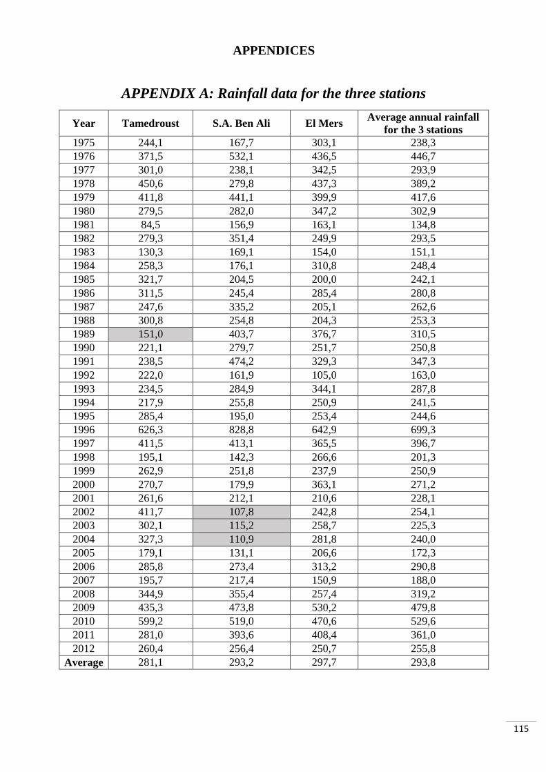
115

APPENDICES

APPENDIX A: Rainfall data for the three stations

Year Tamedroust S.A. Ben Ali El Mers Average annual rainfall

for the 3 stations

1975 244,1 167,7 303,1 238,3

1976 371,5 532,1 436,5 446,7

1977 301,0 238,1 342,5 293,9

1978 450,6 279,8 437,3 389,2

1979 411,8 441,1 399,9 417,6

1980 279,5 282,0 347,2 302,9

1981 84,5 156,9 163,1 134,8

1982 279,3 351,4 249,9 293,5

1983 130,3 169,1 154,0 151,1

1984 258,3 176,1 310,8 248,4

1985 321,7 204,5 200,0 242,1

1986 311,5 245,4 285,4 280,8

1987 247,6 335,2 205,1 262,6

1988 300,8 254,8 204,3 253,3

1989 151,0 403,7 376,7 310,5

1990 221,1 279,7 251,7 250,8

1991 238,5 474,2 329,3 347,3

1992 222,0 161,9 105,0 163,0

1993 234,5 284,9 344,1 287,8

1994 217,9 255,8 250,9 241,5

1995 285,4 195,0 253,4 244,6

1996 626,3 828,8 642,9 699,3

1997 411,5 413,1 365,5 396,7

1998 195,1 142,3 266,6 201,3

1999 262,9 251,8 237,9 250,9

2000 270,7 179,9 363,1 271,2

2001 261,6 212,1 210,6 228,1

2002 411,7 107,8 242,8 254,1

2003 302,1 115,2 258,7 225,3

2004 327,3 110,9 281,8 240,0

2005 179,1 131,1 206,6 172,3

2006 285,8 273,4 313,2 290,8

2007 195,7 217,4 150,9 188,0

2008 344,9 355,4 257,4 319,2

2009 435,3 473,8 530,2 479,8

2010 599,2 519,0 470,6 529,6

2011 281,0 393,6 408,4 361,0

2012 260,4 256,4 250,7 255,8

Average 281,1 293,2 297,7 293,8

116

APPENDIX B: Measurement of soil aggregates stability

The proposed method by Le Bissonnais (2016) borrows from several existing methods, in order to be

applicable to a large range of soils and conditions. Three treatments were selected to form the whole

test.

Preparation of the sample

Particular attention must be paid to the field sampling. Because of seasonal variations in aggregate

stability, it is wise to take all the samples at the same time of the year and to avoid critical conditions

such as freezing, very wet soil and exceptionally hot and dry periods.

Samples should be carried to the laboratory in rigid boxes and immediately air dried. Large clods may

be broken by hand as they dry when they are at the optimal moisture content. The air-dried material

is then forced through a sieve of 5-mm mesh, and the 3–5-mm aggregates are selected for the tests.

Just before the treatment, aggregates are put in the oven at 40 °C for 24 hours so that they are at a

constant matric potential. Aggregates are then ready for the three treatments.

Treatment 1: fast wetting

Immersion of aggregates in water is the simplest way to check their stability. It may be recommended

as a simple, rapid and qualitative field test. Although often criticized because it emphasizes the slaking

compared to others, it appears in almost all the methods. It is a good way to compare the behaviour

of a large range of soils on rapid wetting (heavy rain storms in summer).

The following treatment is proposed.

1. 5 g of calibrated aggregates are gently immersed in a 250 cm3 beaker filled with 50 cm3 of

deionized water for 10minutes;

2. the water is then sucked off with a pipette;

3. the soil material is transferred to a 50-μm sieve previously immersed in ethanol for the measurement

of fragment size distribution.

Treatment 2: slow wetting

Slow wetting with controlled tension corresponds to a field condition of wetting under gentle rain. It

is less destructive than fast wetting and may allow a better discrimination between unstable soils. The

method is as follows.

117

1. 5 g of calibrated aggregates are put on a filter paper for 30 minutes

2. aggregates are then transferred to a 50-μm sieve previously immersed in ethanol for the

measurement of fragment size distribution.

Treatment 3: mechanical breakdown

The objective of pre-wetting is to test the wet mechanical cohesion of aggregates independently of

slaking. Air must therefore be removed from the aggregates before the energy is applied. This can be

done either by rewetting under vacuum or by rewetting with a nonpolar liquid and then exchanging

with water. Ethanol was found to be very effective for this purpose.

1. 5 g of calibrated aggregates are gently immersed in a 250 cm3 beaker filled with 50 cm3 of ethanol

for 10minutes;

2. the ethanol is then sucked off with a pipette;

3. the soil material is transferred in a 250 cm3 Erlenmeyer flask filled with 50 cm3 of deionized water;

the water content is then adjusted to 200 cm3;

4. the Erlenmeyer flask is corked and agitated end over end 20 times;

5. it is left for 30 minutes for sedimentation of coarse fragments;

6. excess water is then sucked off with a pipette;

7. the remaining mixture of soil and water is transferred to a 50 μm sieve previously immersed in

ethanol for the measurement of fragment size distribution.

Fragment size distribution measurement

The objective of this part of the test is to measure the result of the breakdown occurring for the

treatments with the minimum of additional breakdown. The measurement is divided into two

operations: wet-sieving with a 50 μm sieve in ethanol, and dry-sieving of six fragment size fractions.

First, the 50-μm sieve previously immersed in ethanol which contains the soil material after the

treatments is gently moved five times to separate fragments <50 μm from those >50 μm. Ethanol

should be used for wet sieving because it reduces additional breakdown even though large volumes

of ethanol are needed. The ethanol can be recycled by filtering. If a large amount of ethanol is not

available the sieving may be done in water (in this case, little additional breakdown generally occurs),

but the remaining >50 μm fraction must be re-immersed in a small amount of ethanol before oven-

drying and dry-sieving, to avoid recementing fragments and particles during drying.

Second, the >50 μm fraction is collected from the 50 μm sieve, oven-dried and gently dry-sieved by

hand on a column of six sieves: 2000, 1000, 500, 200, 100 and 50 μm (mechanical sieving would be

more difficult to control and would lead to further breakdown). The mass percentage of each size

118

fraction is then calculated; the fraction <50 μm is the difference between initial mass and the sum of

the six other fractions. The aggregate stability for each breakdown mechanism is expressed by the

resulting fragment size distribution (FSD) in seven classes or by calculation of the mean weight

diameter (MWD), which is the sum of the mass fraction of soil remaining on each sieve after sieving

multiplied by the mean aperture of the adjacent mesh. Calculated MWDs range between 25 μm and

3.5 mm using the set of six sieves, using the following equation:

MWD = (average between 2 sieves [% weighted particles retained on the sieve])/100

= (3,5 [% > 2 mm]) + (1,5 [% 1 mm à 2 mm]) + (0,75 [% 0,5 mm à 1 mm]) + (0,35 [%

0,2 mm à 0,5 mm]) + (0,15 [% 0,1 mm à 0,2 mm]) + (0,075 [% 0,05 mm à 0,1 mm]) + (0,02 [% < 0,05 mm])/100

hydrological and soil erosion modeling using swat model

Documents