ACL-05

Workshop on Software

Proceedings of the Workshop

30 June 2005University of Michigan

Ann Arbor, Michigan, USA

Production and Manufacturing byOmnipress Inc.Post Office Box 7214Madison, WI 53707-7214

c©2005 The Association for Computational Linguistics

Order copies of this and other ACL proceedings from:

Association for Computational Linguistics (ACL)75 Paterson Street, Suite 9New Brunswick, NJ 08901USATel: +1-732-342-9100Fax: +1-732-342-9339acl@aclweb.org

ii

Introduction

Welcome to the ACL Workshop on Software, the first of its kind. It is intended as a venue for discussingand comparing the implementation of software and algorithms used in Natural Language and SpeechProcessing. The goal is to bring together researchers, software developers, teachers, and students witha common interest in the implementation of NLP applications, and to allow useful implementationtechniques and “tricks of the trade” to be discussed in detail and disseminated widely.

We received 13 submissions, of which 8 were selected for presentation and inclusion in the proceedings,after a careful review process. Because the number of reviewers exceeded the number of submissions,each submission received more than four reviews on average, while the workload per reviewer wasless than three papers on average. This being the workshop on software, the initial assignment ofreviews was performed algorithmically using the Ford–Fulkerson max-flow algorithm, while takinginto account individual reviewer preferences. The reviewers did an admirable job dealing with a diverseset of submissions, for which they deserve the thanks of the community.

The papers presented in this workshop deal with many different aspects of NLP software: Carpenterdescribes a scalable implementation of high-order character language models; Clegg & Shepherd takethree existing parsers that were trained on business news text and perform a comparative evaluation ona corpus of biomedical journal papers; Cohen-Sygal & Wintner have implemented a compiler whichtranslates between the description languages of two different finite state toolboxes; Foster has designeda generation module for a dialogue system which can ship out text without having to wait for theplanning phase to finish; Koller & Thater describe the intelligent design of increasingly powerfulconstraint solvers; Newman proposes a uniform formalism for representing the output of parsers foreasy inspection and comparison; Tron, Gyepesi, Halacsy, Kornai, Nemeth & Varga have implementeda generic library for analyzing orthographic words; and White discusses the design of a generationcomponent which flexibly incorporates language models in a syntactic surface realizer.

The workshop proceedings are being made available in electronic form only. Not only does this savecosts, but it also allows the distribution of additional software and resources that could not be included inprinted proceedings. A number of authors have included the software described in their papers directlyon the proceedings CD. As always, the latest versions of the included software can be found on theInternet or by contacting the individual authors.

I would like to thank the reviewers and authors once again for their hard work and look forward to anexciting workshop.

Martin JanscheColumbia University, New York

iii

Organizer:

Martin Jansche, Columbia University (USA)

Program Committee:

Cyril Allauzen, AT&T (USA)Jason Baldridge, University of Edinburgh (UK)Srinivas Bangalore, AT&T (USA)Frederic Bechet, Universite d’Avignon (France)Tilman Becker, DFKI (Germany)Steven Bird, University of Melbourne (Australia)Antal van den Bosch, Universiteit van Tilburg (Netherlands)Bob Carpenter, Alias-i (USA)Nizar Habash, Columbia University (USA)Benoit Lavoie, CoGenTex and Universite du Quebec a Montreal (Canada)Alexis Nasr, Universite Paris 7 (France)Hermann Ney, RWTH Aachen (Germany)Stephan Oepen, CSLI (USA)Owen Rambow, Columbia University (USA)Brian Roark, OGI/OHSU (USA)Richard Sproat, University of Illinois (USA)Nathan Vaillette, Universitat Tubingen (Germany)Michael White, University of Edinburgh (UK)

Additional Reviewers:

Oliver Bender, RWTH Aachen (Germany)Evgeny Matusov, RWTH Aachen (Germany)David Vilar, RWTH Aachen (Germany)

v

Table of Contents

TextTree Construction for Parser and Treebank DevelopmentPaula S. Newman . . . . . . . . . . . . . . . . . . . . . . . . . . . . . . . . . . . . . . . . . . . . . . . . . . . . . . . . . . . . . . . . . . . . . . .1

Evaluating and Integrating Treebank Parsers on a Biomedical CorpusAndrew B. Clegg and Adrian J. Shepherd . . . . . . . . . . . . . . . . . . . . . . . . . . . . . . . . . . . . . . . . . . . . . . . .14

Interleaved Preparation and Output in the COMIC Fission ModuleMary Ellen Foster . . . . . . . . . . . . . . . . . . . . . . . . . . . . . . . . . . . . . . . . . . . . . . . . . . . . . . . . . . . . . . . . . . . . .34

Designing an Extensible API for Integrating Language Modeling and RealizationMichael White . . . . . . . . . . . . . . . . . . . . . . . . . . . . . . . . . . . . . . . . . . . . . . . . . . . . . . . . . . . . . . . . . . . . . . . .47

The Evolution of Dominance Constraint SolversAlexander Koller and Stefan Thater . . . . . . . . . . . . . . . . . . . . . . . . . . . . . . . . . . . . . . . . . . . . . . . . . . . . .65

Hunmorph: Open Source Word AnalysisViktor Tron, Gyorgy Gyepesi, Peter Halacsy, Andras Kornai, Laszlo Nemeth and Daniel Varga77

Scaling High-Order Character Language Models to GigabytesBob Carpenter. . . . . . . . . . . . . . . . . . . . . . . . . . . . . . . . . . . . . . . . . . . . . . . . . . . . . . . . . . . . . . . . . . . . . . . . .86

XFST2FSA: Comparing Two Finite-State ToolboxesYael Cohen-Sygal and Shuly Wintner . . . . . . . . . . . . . . . . . . . . . . . . . . . . . . . . . . . . . . . . . . . . . . . . . . .100

vii

Workshop Program

Thursday, June 30, 2005

9:25–9:30 Opening Remarks

Session 1: Parsing

9:30–10:00 TextTree Construction for Parser and Treebank DevelopmentPaula S. Newman

10:00–10:30 Evaluating and Integrating Treebank Parsers on a Biomedical CorpusAndrew B. Clegg and Adrian J. Shepherd

10:30–11:00 Break

Session 2: Generation and Semantics

11:00–11:30 Interleaved Preparation and Output in the COMIC Fission ModuleMary Ellen Foster

11:30–12:00 Designing an Extensible API for Integrating Language Modeling and RealizationMichael White

12:00–12:30 The Evolution of Dominance Constraint SolversAlexander Koller and Stefan Thater

12:30–2:00 Lunch

Session 3: Morphology and Language Modeling

2:00–2:30 Hunmorph: Open Source Word AnalysisViktor Tron, Gyorgy Gyepesi, Peter Halacsy, Andras Kornai, Laszlo Nemeth andDaniel Varga

2:30–3:00 Scaling High-Order Character Language Models to GigabytesBob Carpenter

3:00–3:30 XFST2FSA: Comparing Two Finite-State ToolboxesYael Cohen-Sygal and Shuly Wintner

ix

Proceedings of the ACL 2005 Workshop on Software, pages 1–13,Ann Arbor, June 2005.c©2005 Association for Computational Linguistics

TextTree Construction for Parser and Treebank Development

Paula S. Newman newmanp@acm.org

Abstract

TextTrees, introduced in (Newman, 2005), are skeletal representations formed by systematically converting parser output trees into unlabeled indented strings with minimal bracketing. Files of TextTrees can be read rapidly to evaluate the results of parsing long documents, and are easily edited to allow limited-cost treebank development. This paper reviews the TextTree concept, and then describes the implementation of the almost parser- and grammar-independent TextTree generator, as well as auxiliary methods for producing parser review files and inputs to bracket scoring tools. The results of some limited experiments in TextTree usage are also provided.

1 Introduction

The TextTree representation was developed to support a limited-resource effort to build a new hybrid English parser1. When the parser reached significant apparent coverage, in terms of numbers of sentences receiving some parse, the need arose to quickly assess the quality of the parses produced, for purposes of detecting coverage gaps, refining analyses, and measurement. But this was hampered by the use of a detailed parser output representation.

The two most common parser-output displays of constituent structure are: (a) multi-line labeled and bracketed strings, with indentation indicating dominance, and (b) 2-dimensional trees. While these displays are indispensable in grammar development, they cannot be scanned quickly. Labels and brackets interfere with reading. And,

1 The hybrid combines the chunker part of the fast, robust XIP parser (Aït-Mokhtar et al., 2002) with an ATN-style parser operating primarily on the chunks.

although relatively flat 2D node + edge trees for short sentences can be grasped at a glance, for long sentences this property must be compromised.

In contrast, for languages with a relatively fixed word order, and a tendency to post-modification, TextTrees capture the dependencies found by a parser in a natural, almost self-explanatory way. For example:

They must have a clear delineation of [roles, missions, and authority].

Indented elements are usually right-hand post-modifiers or subordinates of the lexical head of the nearest preceding less-indented line. Brackets are generally used only to delimit coordinations (by [...]), nested clauses (by {…}), and identified multi-words (by |…|).

Reading a TextTree for a correct parse is similar to reading ordinary text, but reading a TextTree for an incorrect parse is jarring. For example, the following TextTree for a 33-word sentence exposes several errors made by the hybrid parser: But by |September 2001|, the executive branch of [the U.S. government, the Congress, the news media, and the American public] had received clear warning that {Islamist terrorists meant to kill Americans in high numbers}.

1

TextTrees can be embedded in bulk parser output files with arbitrary surrounding information. Figure 1 shows an excerpt from such a file, containing the TextTree-form results of parsing the roughly 500-sentence "Executive Summary" of the 9/11 Commission Report (2004) by the hybrid parser, with more detailed results for each sentence accessible via links. (Note: the links in Figure 1 are greyed to indicate that they are not operational in the illustration.)

Such files can also be edited efficiently to produce limited-function treebanks, because the needed modifications are easy to identify, labels are unnecessary, and little attention to bracketing is required. Edited and unedited TextTree files can then be mapped into files containing fully bracketed strings (although bracketed differently

than the original parse trees), and compared by bracket scoring methods derived from Black et al (1991).

Section 2 below examines the problems presented by detailed parse trees for late-stage parser development activities in more detail. Section 3 describes the inputs to and outputs from the TextTree generator, and Section 4 the generator implementation. Section 5 discusses the use of the TextTree generator in producing TextTree files for parser output review and TextTreebank construction, and the use of TextTreebanks in parser measurement. The results of some limited experiments in TextTree file use are provided in Section 6. Section 7 discusses related work and Section 8 explores some directions for further exploitation of TextTrees.

6 (3) We have come together with a unity of purpose because our nation demands it. best more chunks

We have come together with a unity of purpose because {our nation demands it}.

7 (15) September 11 , 2001 , was a day of unprecedented shock and suffering in the history of the United States . best more chunks |September 11 , 2001|, was a day of [unprecedented shock and suffering] in the history of the United States.

8 (1) The nation was unprepared . best more chunks The nation was unprepared.

Figure 1. A TextTree file excerpt

2

Figure 2. An LFG c-structure

2 Problems of Detailed Parse Trees

This section examines the readability problems posed by conventional parse tree representations, and their implications for parser development activities.

As noted above, parse trees are usually displayed using either 2-dimensional trees or fully bracketed strings. Two dimensional trees are intended to provide a clear understanding of structure. Yet because of the level of detail involved in many grammars, and the problem of dealing with long sentences, they often fail in this regard. Figure 2 illustrates an LFG c-structure, reproduced from King et al. (2000), for the 7 word sentence "Mary sees the girl with the telescope." Similar structures would be obtained from parsers using other popular grammatical paradigms. The amount of detail created by the deep category nesting makes it difficult to grasp the structure by casual inspection, and the tree in this case is actually wider than the sentence.

Grammar-specific transformations have been used in the LKB system to simplify displays (Oepen et al., 2002). But there are no truly satisfactory approaches for dealing with the problem of tree width, that is, for presenting 2D

trees so as to provide an "at-a-glance" appreciation of structure for sentences longer than 25 words, which are very prevalent.2 The methods currently in use or suggested either obscure the structure or require additional actions by the reader. Allowing trees to be as wide as the sentences requires horizontal scrolling. Collapsing some subtrees into single nodes (wrapping represented token sequences under those nodes) requires repeated expansions to view the entire parse. Using more of the display space by overlapping subtrees vertically interferes with comprehension because it obscures dominance and sequence. In Figure 2, for example, the period at the end of the sequence is the second constituent at the top. For a longer sentence, a coordinated constituent might be placed here as well. Such unpredictable arrangements impede reading, because the reader does not know where to look

2 Casual records of parser results for many English

non-fiction documents suggest an average of about 20 words per sentence, with a standard deviation of about 11.

3

S (NP-SBJ Stokely) (VP says (SBAR 0 (S (NP-SBJ stores) (VP revive (NP (NP specials) (PP like (NP (NP three cans) (PP of (NP peas)) (PP for (NP 99 cents )))))))))

Figure 3. A Penn Treebank Tree

The other conventional parse tree representation is as a fully-bracketed string, usually including category labels and, for display purposes, using indentation to indicate dominance. Figure 3 shows such a tree, drawn from a Penn Treebank annotation guide (Bies et al., 1995), shown with somewhat narrower indentation than the original. Even though the tree is in the relatively flat form developed for use by annotators, the brackets, labels, and depth of nesting combine to prohibit rapid scanning.

However, it should be noted that this format is the source of the TextTree concept. Because by eliminating labels, null elements, and most brackets, and further flattening, the more readable TextTree form emerges: Stokely says {stores revive specials like three cans of peas for 99 cents}

2.1 Implications

The conventional parse tree representations discussed above can be a bottleneck in parser development, most importantly in checking parser accuracy with respect to current focus areas and in extending coverage to new genres or domains. For these purposes, one would like to review the results of analyzing collections of relatively long (100+ sentence) documents. But unless this can be done quickly, a parser developer or grammar writer is tempted to rely on statistics with respect to the number of

sentences given a parse, and declare victory if a high rate of parsing is reported.

Another approach to assessing parser quality is to rely on treebank-based bracket scoring measures, if treebanks are available in the particular genre. This can also can be a pitfall, as bracket scores tend to be unconsciously interpreted as measures of full-sentence parse correctness, which they are not.

On the other hand, treebank-based measurements can play a useful secondary role in evaluating parser development progress and in comparing parsers. But if insufficient treebanked material is available for the relevant domains and/or genres, a custom treebank must be developed. This process generally consists of two phases: (a) a bootstrapping phase in which an existing parser is applied to the corpus to produce either a single ''best'' tree, or multiple alternative trees, for each sentence, and then (b) a second phase in which annotators approve or edit a given parse tree, select among alternative trees, or manually create a full parse tree when no parse exists. All of the second phase alternatives are difficult given conventional parse-tree representations. For example, experiments by Marcus et al. (1993) associated with the Penn Treebank indicated that for the first annotation pass ''At an average rate of 750 words per hour, a team of five part-time annotators …'', i.e., a bit more than a page of this text per hour. Aids to selecting among alternative 2D trees can be given in the form of differentiating features (Oepen et al., 2002), but their effectiveness in helping to select among large trees differing in attachment choices is not clear.

Another activity impeded by conventional parse tree representations is regression testing. As a grammar increases in size, it is advisable to frequently re-apply the grammar to a large test corpus to determine whether recent changes have had negative effects on accuracy. While the existence of differences in output can be detected by automatic means, one would like to assess the differences by quickly comparing the divergent parses, which is difficult to do using detailed parse displays for long sentences.

Finally, an activity that is rarely discussed but is becoming increasingly important is providing comprehensible parser demonstrations. A syntactic parser is not an end-in-itself, but a

4

building block in larger NLP research and development efforts. The criteria for selecting a parser for a project include both the kind of information provided by the parser and parser accuracy. However, current parser output representations are not geared to allowing potential users to quickly assess accuracy with respect to document types of interest.

3 The TextTree Generator: Externals

TextTrees are generated by an essentially grammar-independent processor from a combination of

(a) parser output trees that have been put into a standard form that retains the grammar-specific category labels and constituents, but whose details conform to the requirements of a parser-independent tool interface, and,

(b) a set of grammar-specific <category, directive> pairs, e.g., "<ROOT, Align>". Each pair specifies a default formatting for constituents in the category, specifically whether their sub-constituents are to be aligned vertically, or concatenated relative to a marked point, with subsequent children indented. These defaults are used in the absence of overriding factors such as coordination.

The directives used are very simple ones, because the simpler the formatting rules, the more likely it is that outputs can be accurately checked for correctness, and edited conveniently

It is assumed that the parser output either includes conventional parse trees, or that such trees can be derived from the output. This assumption covers many grammatical approaches, such as CG, HPSG, LFG, and TAG.

The logical configuration implied by these inputs is shown in Figure 4. It includes a parser-specific adaptor to convert parser-output trees into a standard form. The adaptor need not be very large; for the hybrid parser it consists of about 75 lines of Java code.

The subsections below discuss the standard ParseTree form, the directives that have been identified to date and their formatting effects, and the treatment of coordination.

3.1 Standard ParseTrees

A standard ParseTree consists of recursively

Figure 4: Logical Configuration.

nested subtrees, each representing a constituent C, and each indicating: � A grammar-specific category label for C. � Whether C should be considered the head of

its immediately containing constituent P for formatting purposes. Generally, this is the case if C is, or dominates, the lexical head of P, but might differ from that to obtain some desired formatting effects. As heads are identified by most parsers, this marker can usually be set by parser-specific rules embedded in the adaptor.

� Whether C is a coord_dom, that is, whether it immediately dominates the participants in a coordination.

� If C is a leaf, the associated token, and � (optionally) whether C is a multi-word.

3.2 Formatting Directives

To generate TextTrees for a particular grammar, a <category, directive> pair is provided for each category that will appear in a ParseTree for the grammar. The directive specifies how to format the children of constituents in the category in the absence of lengthy coordinations.

The definitions of the directives make use of one additional locator for a constituent, its real_head. While we generally want the directives to format constituents relative to their lexical heads, in some grammars, those heads are deeply nested. For example, a tree for an NP might be generated by rules such as:

NPz => DET NPy NPy => ADJ* NPx NPx => NOUN PP*

5

where each of the underscored terms are heads, but the real_head of NPz is the head NOUN of NPx. More generally, the real_head of a constituent C is the first constituent found by following the head-marked descendants of C downward until either (a) a leaf or headless constituent is reached, or (b) a post-modified head-marked constituent is found.

Using this definition, the current formatting directives are as follows:

Align: Align specifies that all children of the constituent are vertically aligned. Thus, for example, a directive <ROOT, Align>, would cause a constituent generated by a rule ''ROOT => NP, VP'' to be formatted as:

formatted NP formatted VP

ConcatHead: ConcatHead concatenates the tokens of a constituent (with separating blanks) up to and including its real_head (as defined above), and indents and aligns the post-modifiers of the real_head. For example, given the directive ''<NP, ConcatHead>'', a constituent produced by the rules:

NPz => PreMod* NPx NPx => NOUN PostMods*

would be formatted as: All-words-in-PreMod* NOUN

Formatted PostMod1 Formatted PostMod2

ConcatCompHead: ConcatCompHead concatenates everything up to and including the real_head, and concatenates with that the results of a ConcatHead of the first post-modifier of the real_head (if any).

This directive is motivated by rules such as ''PP => P NP'', where the desired formatting groups the head with words up to and including the lexical head of the single complement, e.g., of the man in the moon

ConcatSimpleComp: ConcatSimpleComp concatenates material up to and including the real_head and, if first post-modifying constituent is a simple token, concatenates that as well, and then aligns and indents any further post-modifiers of the real_head. It thus formats noun phrases for languages that routinely use simple adjective post-modifiers. For example (Sp.):

La casa blanca que ...

ConcatPreHead: This directive concatenates material, if any, before the real_head, and then if such material exists, increases the indent level. It then aligns the following component. The directive is intended for formatting clauses that begin with subordinating conjunctions, complementizers, or relative pronouns, where the grammar has identified the following sentential component as the head, but it is more readable to indent that head under the initial constituent. In practice, in such cases it is easier to just alter the head marker within the adaptor.

3.3 Treatment of Coordination

The directives listed in the previous subsection are defaults that specify the handling of categories in the absence of coordination. A set of coordinated constituents are always indicated by surrounding square brackets ([ ]). If the coordination occurs within a requested concatenation, then if the width of coordination is less than a predesignated size, the non-token constituents of the coordination are bracketed, as in:

[{Old men} and women] in the park.

However, if the width of the coordination exceeds that size, the concatenation is converted to an alignment to avoid line wrap, for example, He gave sizeable donations to [the church, the school, and the new museum of art.]

4 TextTree Generator: Implementation

TextTrees are produced in two steps. First, a ParseTree is processed to form one or more InternalTextTrees (ITTs), which are then mapped into an external TextTree. Most of the work is accomplished in the first step; the use of a second step allows the first to focus on logical structure, independent of many details of indentation, linebreaks, and punctuation.

We begin by describing ITTs and their relationship to external TextTrees, to motivate

6

the description of ITT formation. We then describe the mapping from ParseTrees to ITTs.

4.1 Transforming ITTs to Strings

Figure 5 shows a simple ITT and its associated external TextTree. The node labels of an ITT are called the "headparts" of their associated subtrees. Headparts may be null, simple strings, or references to other ITTs.

If the headpart of a subtree is null, like that of the outermost subtree of Figure 5, the external TextTrees for its children are aligned vertically at the current level of indentation. Also, if the subtree is not outermost, the aligned sequence is bracketed.

However, if the headpart of a subtree is a simple string, as in the other subtrees of Figure 5 ITT, that string is printed at the current level of indentation, and the external TextTrees for its children, if any, are aligned vertically at the next level of indentation.

The headpart of a subtree may also reference another ITT, as illustrated in Figure 6. Such a reference headpart signals the bracketed inclusion of the referenced tree, which has a null headpart, at the current indentation level. This permits the entire referenced tree to be post-modified. The brackets used depend on a feature associated with the referenced tree, and are either [ ], if the referenced tree represents a coordination, or { } otherwise.

Pseudo-code for the ITT2String function that produces external TextTrees from ITTs is shown in Figure 7. The code omits the treatment of non-bracketing punctuation; in general, care is taken to prefix or suffix punctuation to tokens appropriately. 4.2 Transforming ParseTrees to ITTs

To transform ParseTrees into ITTs, subtrees are processed recursively top-down using the function BuildITT of Figure 8. Its arguments

are an input subtree p, and a directive override, which may be null. It returns an ITT for p.

BuildITT sets the operational directive d as either the override argument, if that is non-null, or to the default directive for the category of p.

Then, if d is ''Align'', the result ITT has a null headpart and, if p is a coord_dom, the isCoord property of the ITT is set. The children of the result ITT are the ITTs of p's children.

However, if d specifies that an initial sequence of p is to be concatenated, BuildITT uses the recursive function Catenate (Figure 9) to obtain the initial sequence if possible.

However, a simple transformation

to TextTrees of parse trees

However,a simple transformation

of parse treesto TextTrees

can expeditethese activities.

can expedite

these activities

Figure 5: Simple InternalTextTree.

However, a simple transformation ����T1

these activities

T1 (coord)

significantly simplifies

and generally expedites

However,a simple transformation[significantly simplifiesandgenerally expedites]

these activities.

Figure 6: ITT with long coordination

7

Figure 7. The ITT2String Function Figure 9. The Catenate Function

Figure 8. The BuildITT Function

Function ITT2String(ITT s, String indent) returns String // indent is a string of blanks, eol is end-of-line Set ls to null If s has a null headpart, set nextIndent to indent + 1 blank (adds space for [ or { bracket ) Otherwise set nextIndent to indent + N blanks, where N is the constant indent increment If s has a headpart reference set nextIndent to nextIndent + 1 blank

If s has children, set ls to the lines produced by ITT2String (ci, nextIndent) for each child ci of s

If s has a headpart string hs Return the concatenation of indent, hs, eol, ls Else if s has a headpart reference to an ITT s2 Return the concatenation of ITT2String(s2, indent), ls Else (s has a null headpart ) Remove initial & trailing whitespace from ls If s is a coordination, set pfx to [ and sfx to ] Else set pfx to {and sfx to } Return the concatenation of nextIndent – 1 blank, pfx, ls, sfx, eol

Function Catenate (ParseTree p, ParseTree r) returns <Code, String> 1. Set result = null, code = incomplete. If p is a leaf, result = the token of p. 2. for each child ci of p, while code ≠ complete: If ci = r, set code = complete. Set <ccode, cstring> to result of Catenate(ci, r) If (ccode = failed) return <failed, null> If p is a coord_dom & cstring not 1 word // indicate coordinated within concat Suffix ''{cstring}'' to result. Otherwise suffix ''cstring'' to result If ccode = complete, set code = complete 3. Finally, If p = r, set code = complete. if p is a coord_dom and the length of result > LONG_CONST, return <failed, null>. Else if p is a coord_dom Return <code, ''[result]''> Else if p is a multi-word, return <code, ''|result|''> Otherwise return <code, result>

Function BuildITT(ParseTree p, Directive override) returns ITT Set d to override if non-null, otherwise to the default category directive for p. 1. If p is a leaf or a multiword:

- return an ITT whose headline concatenates the tokens spanned by p, and which has no children. If p is a multiword, bracket the headline by |.

2. Else if d is Align return an ITT with a null headpart, and children built by invoking BuildITT(ci, null) for each child ci of p. If p is a coord_dom, indicate that the ITT isCoord.

3. Otherwise concatenate: a) Find the nested subtree s that contains the rightmost element r to be concatenated according to d. b) Set the pair <ccode, cstring> to the result of Catenate (p, r). c) If ccode ≠ ''failed'', return ITT with headpart = cstring, and children formed by BuildITT(ci, null) for each child ci of s after r. . d) Otherwise return a directive-dependent tree aligning the contained coordination, for example: For ConcatHead: i. Let p’ be like p but without the right siblings of the real_head of p ii. Return an ITT with headpart referencing the results of BuildITT (p’, Align) and with children obtained from BuildITT(ci, null) for each right sibling ci of the real_head of p For ConcatCompHead: Return an ITT obtained by invoking BuildITT(p, ConcatHead)

8

Catenate takes two arguments: a ParseTree p whose initial sequence is to be concatenated, and a ParseTree r, beyond which the concatenation is to stop, based on the particular directive involved. It returns a pair <Code, String>. The Code indicates if the concatenation succeeded, failed, or is incomplete. If the concatenation succeeded, BuildITT creates an ITT with a headpart string containing the concatenated sequence, and children consisting of ITTs of the right-hand siblings of r.

Complex aspects of BuildITT and Catenate relate to coordinations within to-be-concatenated extents. The desired effect is to include short coordinations within the concatenation, while bracketing its boundaries and non-leaf components, e.g. '' [{Old men} and women]'', but aligning the elements of longer coordinations.

So if Catenate (in step 3) determines that the string resulting from a coordination is very long, it directly or indirectly returns an indicator to BuildITT that the concatenation failed. BuildITT (step 3d) then returns an ITT structured so that the sub-constituents that were to be concatenated are eventually shown as aligned, using different methods dependent on the directive d.

For example, if d is ConcatHead or ConcatSimpleComp, the result ITT contains:

a) a headpart reference to an ITT built by BuildITT(p’,Align) , where p’ is like p but without the right-hand siblings of its real_head, and

b) children consisting of the ITTs for those right-hand siblings, if any.

5 TextTree Files and TextTreebanks

Previous sections focused on the production of individual TextTrees by the TextTree generator. This section considers some uses of the generator and auxiliary methods within parser development.

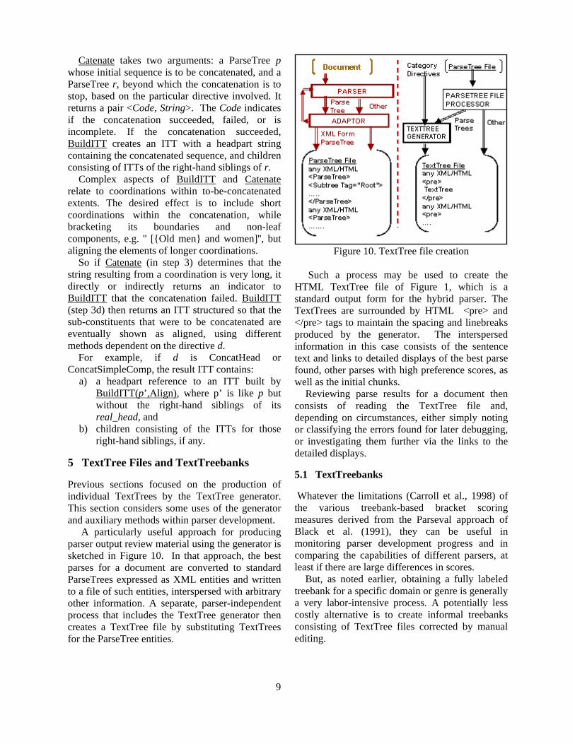
A particularly useful approach for producing parser output review material using the generator is sketched in Figure 10. In that approach, the best parses for a document are converted to standard ParseTrees expressed as XML entities and written to a file of such entities, interspersed with arbitrary other information. A separate, parser-independent process that includes the TextTree generator then creates a TextTree file by substituting TextTrees for the ParseTree entities.

Figure 10. TextTree file creation

Such a process may be used to create the

HTML TextTree file of Figure 1, which is a standard output form for the hybrid parser. The TextTrees are surrounded by HTML <pre> and </pre> tags to maintain the spacing and linebreaks produced by the generator. The interspersed information in this case consists of the sentence text and links to detailed displays of the best parse found, other parses with high preference scores, as well as the initial chunks.

Reviewing parse results for a document then consists of reading the TextTree file and, depending on circumstances, either simply noting or classifying the errors found for later debugging, or investigating them further via the links to the detailed displays.

5.1 TextTreebanks

Whatever the limitations (Carroll et al., 1998) of the various treebank-based bracket scoring measures derived from the Parseval approach of Black et al. (1991), they can be useful in monitoring parser development progress and in comparing the capabilities of different parsers, at least if there are large differences in scores.

But, as noted earlier, obtaining a fully labeled treebank for a specific domain or genre is generally a very labor-intensive process. A potentially less costly alternative is to create informal treebanks consisting of TextTree files corrected by manual editing.

9

Both corrected and uncorrected TextTree files can be converted to files consisting of fully-bracketed strings by a simple script that considers only the contained TextTrees. The script brackets the TextTrees so as to retain the explicit brackets, and to add brackets around each subtree, i.e., around each sequence of a line and the lines, if any, indented beneath it, directly or indirectly.

For example, a full bracketing of the TextTree of Figure 5 would be:

{However,} {a simple transformation {of parse trees} {to text trees}} {can expedite {these activities}}

The actual bracketed strings produced by the script are ones acceptable as input to the EVALB bracket scoring program (Sekine and Collins, 1997) with all brackets expressed as parentheses, and brackets added around words (apparently required but subsequently discarded by the program). Also, most punctuation is removed, to avoid spurious token differences. Then bracketed files deriving from noncorrected and corrected TextTree files can be submited to EVALB to obtain a bracket score.

Lest this approach be dismissed as overly sketchy, we note that the resulting brackets are similar to those resulting from a proposal by Ringger et al. (2004) for neutralizing differences between parser outputs and treebanks by bracketing maximal head projections, plus some additional mechanisms to further minimize brackets.

5.2 Preventing Bracketing Errors

To avoid bracketing errors resulting from imprecise spacing in manually edited trees, the TextTree indentations used are relatively wide. With indentations of five spaces, it is likely that an imprecisely positioned line will be placed closer to the desired level of indentation, so that an intelligent guess can be made as to the intent. For example, in:

Line a Line b Line c Line e??

the misplaced Line e begins at a point closer to the beginning of Line a than Line b. It is then reasonable to guess that Line e is sibling to Line a.

6 Experiments

This section describes two limited experiments to assess the efficiency of reviewing parser outputs for accuracy using TextTrees. One of the experiments also measures the efficiency of TextTreebank creation

6.1 First Experiment

The document used in the first experiment was the roughly 500-sentence "Executive Summary" of the 9/11 Commission Report (2004). After parsing by the hybrid parser, the expected TextTree file, excerpted in Figure 1, was created, reproducing each sentence and, for parsed sentences, the TextTree string for the best parse obtained, and a links to the detailed two-dimensional tree representation.

Of the 503 sentences, averaging 20 words in length, 93% received a parse. However, reviewing the TextTree file revealed that at least 191 of the 470 parsed sentences were not parsed correctly, indicating an actual parser accuracy for the document of at most 55%.

Reviewing the TextTrees required 92 minutes, giving a review rate of 6170 words per hour, including checking detailed parses for sentences where errors might have lain in the TextTree formatting.

That review rate can be compared to the results of Marcus et al. (1993) for post-annotation proofreading of relatively flat, indented, but fully labelled and bracketed trees. Those results indicated that:

"... experienced annotators can proofread previously corrected material at very high speeds. A parsed subcorpus …was recently proofread at an average speed of approximately 4,000 words per annotator per hour. At this rate…, annotators are able to find and correct gross errors in parsing, but do not have time to check, for example, whether they agree with all prepositional phrase attachments." While the two tasks are not exactly comparable,

if we assume that little or no editing was required

10

in proofreading, the ballpark improvement of 50% is encouraging.

6.2 Second Experiment

For the second experiment, we used the CB01 file3 of the Brown Corpus (Francis and Kucera, 1964), and reviewed both the TextTree file and then, separately, the detailed 2D parse trees also produced.

While the parser reported that 91 of the 103 sentences, or 88%, received a parse, the review of the TextTree file determined that at most only 50 sentences, or 48.5%, received a fully correct parse. The review of the detailed parse trees revealed three additional errors.

The comparison of review times was less decisive in this experiment, with the rate for the TextTree review being 5733 words per hour, and that for the detailed 2D representation 4410 words per hour.

However, there were non-quantifiable differences in the reviews. One difference was that the TextTree review was a fairly relaxed exercise, while the review of the 2D representations was done with a conscious attempt at speed, and was quite stressful—not something one would like to repeat. Another difference was that scanning the TextTree file provided a far better cumulative sense of the kinds of problems presented by the document/genre, which might be further exploited by a more interactive format (e.g., using HTML forms) allowing users to classify erroneous parses by error type.

The experiment was then extended to check the extent to which TextTree files could efficiently edited for purposes of limited-function treebank creation.

For this purpose, to minimize typing when a sentence had no complete parse, the TextTree file included the list of chunks identified by the XIP parser. A similar strategy could be used with parsers that, when no complete parse is found, return an unrelated sequence of adjacent constituent parses. This is done by some statistical and finite-state-based parsers, as well as by parsers employing the "fitted parse" method of Jensen et al. (1983) or the "fragment parse" method described by Riezler et al. (2002).

3 With part-of-speech tags removed

Editing the TextTrees for the 104 sentences, with an average sentence length of 21 words, required 83 minutes, giving a rate of 1518 words per hour. This might be compared with the average of 750 words per hour for the initial annotation of parses in the Penn Treebank experiment (Marcus et al., 1993) mentioned earlier.

After the TextTreebank was created, the bracketing script described in section 5.1 was applied both to the original TextTree file and to the TextTreebank, and the results were submitted to the EVALB program, which reported a bracketing recall of 71%, a bracketing precision of 84%, and an average crossing bracket count of 1.15.4 Two sentences were not processed because of token mismatches. As expected, these scores were much higher than the percentage of sentences correctly parsed.

7 Related Work

Most natural language parsers include some provision for displaying their outputs, including parse tree representations, and/or other material, such as head-dependent relationships, feature structures, etc. These displays are generally intended for deep review of parse results, and thus attempt to maximize information content

Work on reducing review effort usually takes place in the context of developing treebanks by selection among, and/or manual correction of, parser outputs. In this area, the most relevant work may be the experiments of Marcus et al. (1993) using bracketed, indented trees. They found that annotator efficiency required eliminating many detailed brackets and category labels from the parser outputs presented. Other approaches rest, in whole or in part, on selecting among alternative two dimensional parse trees, such as the distinguishing-feature-augmented approach of Oepen et al. (2002), discussed in Section 2. As discussed in that section, however, two-dimensional tree displays are problematical for large trees, and it is not clear to what extent distinguishing feature information can expedite selecting among attachment choices.

4 Sentences not receiving complete parses were submitted to EVALB without any brackets, contributing zero counts to the total # of correct constituents recalled.

11

Other related work deals with reducing measured differences between parser outputs and treebanks due solely to grammar style. As discussed in section 5, the bracketed material used in treebank-based measurement by Ringger et al. (2004) is similar to the bracketed material that would result from systematically bracketing TextTrees.

Finally, work by Walker (2001), intended not for parser/grammar development, but to facilitate reading and improve retention, produces text formats that bear some similarity to TextTrees, but are more closely attuned to spoken phrasing than syntactic form. The method uses complex segmentation and indentation strategies generally based on a combination of punctuation and closed-class words. 8 Directions for Further Development

We have described an implemented method for presenting parser outputs permitting fast visual inspection of the results of parsing long documents, as well as efficient editing to create informal treebanks. Although, because of their flattened, skeletal nature, TextTrees can hide some parser errors, we strongly believe, based on extended usage, that the convenience of reviewing TextTree files can contribute significantly to parser development efforts.

However, TextTrees are best suited to languages tending to a fixed word order and post-modification. To improve results for languages and language aspects that do not fall into this category, TextTrees might be augmented with highlighting and color to indicate syntactic functions. One way this could be done in a parser- and grammar-independent way is by adding a string-valued representation feature to the standard ParseTrees, and an additional set of directives to map the feature values to representation alternatives. For example, a subtree might be annotated with the feature Rep = "subject", and the additional directives might include <"subject", "blue">. Experimentation is needed to determine the usability of this approach.

Another topic to explore is the use of TextTrees in the creation of corpora annotated by deeper syntactic or semantic information. Because such information is generally expressed in forms that are even less readable than parse trees, a useful

bootstrapping practice is to allow annotators to approve, or select among, parser output trees connected with the deeper information (King et al., 2003). TextTrees might be used to facilitate this process, with annotators either (a) interactively selecting among alternative TextTrees or, because there may be many alternatives, (b) editing a TextTree file containing at most one parse for each sentence (possibly chosen arbitrarily) and using the result for offline selection. Also, a parser used in the bootstrapping might refer to bracketed TextTreebanks to avoid pruning away elements of correct parses at intermediate points in parsing.

A third direction for further work is in extending the TextTree approach to deal with outputs of dependency-based parsers that do not produce constituent trees. While this should be a natural extension, an alternative system of features and directives would seem to be needed.

Acknowledgements

The author is indebted to Tracy Holloway King, John Sowa, and the anonymous reviewers for their very helpful comments and suggestions on earlier versions of this paper.

References Salah Aït-Mokhtar, Jean-Pierre Chanod, and

Claude Roux. 2002. Robustness beyond shallowness: incremental deep parsing, Natural Language Engineering 8:121-144 Cambridge University Press.

Ann Bies, Mark Ferguson, Karen Katz, and Robert

MacIntyre. 1995. Bracketing Guidelines for the Treebank II Style Penn Treebank Project.

E. Black, S. Abney, D. Flickinger, C. Gdaniec, R.

Grishman, P. Harrison, D. Hindle, R. Ingria, F. Jelinek, J. Klavans, M. Liberman, M. Marcus, S. Roukos, B Santorini, and T. Strzalkowski. 1991. A procedure for quantitatively comparing the syntactic coverage of english grammars. In Proc 1991 DARPA Speech and Natural Language Workshop. 306-311.

John Carroll, Ted Briscoe, and Antonio SanFillipo.

1998. Parser Evaluation: a Survey and a New Proposal. In Rubio et al., editors, Proc First

12

International Conference on Language Resources and Evaluation, Granada, Spain, 447-454.

W. Nelson Francis and Henry Kucera. 1964, 1971,

1979. Brown Corpus Manual. Available at http://helmer.aksis.uib.no/icame/brown/bcm.html Corpus available at http://nltk.sourceforge.net

Karen Jensen, George Heidorn, Lance A. Miller,

Yael Ravin. 1983. Parse fitting and prose fixing: getting a hold on ill-formedness. Computational Linguistics 9(3-4):147-160.

Tracy H. King, Stefanie Dipper, Anette Frank,

Jonas Kuhn, and John Maxwell. 2000. Ambiguity management in grammar writing. In Erhard Hinrichs, Detmar Meurers, and Shuly Wintner, editors, Proc ESSLLI Workshop on Linguistic Theory and Grammar Implementation, 5-19, Birmingham, UK.

Tracy H. King, Richard Crouch, Stefan Riezler,

Mary Dalrymple, and Ronald M. Kaplan. 2003. The PARC 700 Dependency Bank, Proc. 4th International Workshop on Linguistically Interpreted Corpora, at the 10th Conf of the European Chapter of the ACL, Budapest.

Mitchell P. Marcus, Mary Ann Marcinkiewicz, and

Beatrice Santorini. 1993. Building a Large Annotated Corpus of English: The Penn Treebank, Computational Linguistics 19(2):313-330.

Paula S. Newman. 2005. Abstract: TextTrees in

Grammar Development. Workshop on Grammar Engineering of the 2005 Scandinavian

Conference on Linguistics (SCL). Available at http://www.hf.ntnu.no/scl/grammar_engineering

9/11 Commission. 2004. Final Report of the National Commission on Terrorist Attacks upon the United States, Executive Summary. Available at http://www.gpoaccess.gov/911

Stephan Oepen, Dan Flickinger, Kristina Toutanova, and Christopher Manning. 2002. LinGO Redwoods: A Rich and Dynamic Treebank for HPSG, Proc Workshop on Treebanks and Linguistic Theories (TLT02), Sozopol, Bulgaria

Stephan Riezler, Tracy H. King, Ronald M. Kaplan, Richard Crouch, John T. Maxwell, and Mark Johnson. 2002. Parsing the Wall Street Journal using a Lexical-Functional Grammar and Discriminative Estimation Techniques. Proc 40th Annual Meeting of the Assoc. for Computational Linguistics (ACL), Philadelphia, 271-278.

Eric K. Ringger, Robert C. Moore, Lucy Vanderwende, Hisam Suzuki and Eugene Charniak. 2004. Using the Penn Treebank to Evaluate Non-Treebank Parsers, Proc 2004 Language Resources and Evaluation Conference (LREC), Lisbon, Portugal.

Satoshi Sekine and Michael Collins. 1997. EvalB. Available at http://nlp.cs.nyu.edu/evalb

Randall C. Walker. 2001. Method and Apparatus for Displaying Text Based Upon Attributes Found Within the Text, U.S. Patent 6279017.

13

Proceedings of the ACL 2005 Workshop on Software, pages 14–33,Ann Arbor, June 2005.c©2005 Association for Computational Linguistics

Evaluating and Integrating Treebank Parsers on a Biomedical Corpus

Andrew B. Clegg and Adrian J. ShepherdSchool of Crystallography

Birkbeck CollegeUniversity of London

London WC1E 7HX, UK{a.clegg,a.shepherd}@mail.cryst.bbk.ac.uk

Abstract

It is not cleara priori how well parserstrained on the Penn Treebank will parsesignificantly different corpora withoutretraining. We carried out a compet-itive evaluation of three leading tree-bank parsers on an annotated corpusfrom the human molecular biology do-main, and on an extract from the PennTreebank for comparison, performing adetailed analysis of the kinds of errorseach parser made, along with a quan-titative comparison of syntax usage be-tween the two corpora. Our results sug-gest that these tools are becoming some-what over-specialised on their trainingdomain at the expense of portability, butalso indicate that some of the errors en-countered are of doubtful importance forinformation extraction tasks.

Furthermore, our inital experimentswith unsupervised parse combinationtechniques showed that integrating theoutput of several parsers can amelioratesome of the performance problems theyencounter on unfamiliar text, providingaccuracy and coverage improvements,and a novel measure of trustworthiness.

Supplementary materials are availableat http://textmining.cryst.bbk.ac.uk/acl05/.

1 Introduction

The availability of large-scale syntactically-annotated corpora in general, and the Penn Tree-bank1 (PTB;Marcus et al., 1994) in particular, hasenabled the field of stochastic parsing to advancerapidly over the course of the last 10-15 years.However, the newspaper English which makes upthe bulk of the PTB is only one of many dis-tinct genres of writing in the Anglophone world,and certainly not the only domain where poten-tial natural-language processing (NLP) applica-tions exist that would benefit from robust and re-liable syntactic analysis. Due to the massive glutof published literature, the biomedical sciences ingeneral, and molecular biology in particular, con-stitute one such domain, and indeed much atten-tion has been focused recently on NLP in this area(Shatkay and Feldman, 2003; Cohen and Hunter,2004).

Unfortunately, annotated corpora of a largeenough size to retrain stochastic parsers on do notexist in this domain, and are unlikely to for sometime. This is partially due to the same differencesof vocabulary and usage that set biomedical En-glish apart from theWall Street Journalin the firstplace; these differences necessitate the input ofboth biological and linguistic knowledge on bio-logical corpus annotation projects (Kulick et al.,2004), and thus require a wider variety of annota-tor skills than general-English projects. For exam-ple,5′ (pronounced “five-prime”) is an adjective inmolecular biology, butp53 is a noun;amino acid

1http://www.cis.upenn.edu/~treebank/

14

is an adjective-noun sequence2 butcadmium chlo-ride is a pair of nouns. These tagging decisionswould be hard to make correctly without biologi-cal background knowledge, as would the preposi-tional phrase attachment decisions inFigure 1.

Although it is intuitively apparent that thereare differences between newspaper English andbiomedical English, and that these differencesare quantifiable enough for biomedical writingto be characterised as a sublanguage of En-glish (Friedman et al., 2002), the performance ofconventionally-trained parsers on data from thisdomain is to a large extent an open question.Nonetheless, papers have begun to appear whichemploy treebank parsers on biomedical text, es-sentially untested (Xiao et al., 2005). Recently,however, the GENIA project (Kim et al., 2003)and the Mining the Bibliome project (Kulick et al.,2004) have begun producing small draft corpora ofbiomedical journal paper abstracts with PTB-stylesyntactic bracketing, as well as named-entity andpart-of-speech (POS) tags. These are not currentlyon a scale appropriate for retraining parsers (com-pare the∼50,000 words in the GENIA Treebankto the∼1,000,000 in the PTB; but see alsoSec-tion 7.2) but can provide a sound basis for empiri-cal performance evaluation and analysis. A collec-tion of methods for performing such an analysis,along with several interesting results and an inves-tigation into techniques for narrowing the perfor-mance gap, is presented here.

1.1 Motivation

We undertook this project with the intention ofaddressing several questions. Firstly, in order todeploy existing parsing technologies in a bioin-formatics setting, the biomedical NLP commu-nity needs a comprehensive assessment of perfor-mance – which parser(s) to choose, what accuracyeach should be expected to achieve etc., along withinformation about the different situations in whicheach parser can be expected to perform well orpoorly. Secondly, assuming there is a performancedeficit, can any simple steps be taken to mitigateit? Thirdly, what engineering issues arise from the

2According to some annotators at least; others tagaminoas a noun, although one would not speak of*an amino, *someamino or *several aminos.

idiosyncracies of biomedical text?The differences discovered in the behaviour of

each parser, either between domains or betweendifferent software versions on the same domain,will also be of interest to those in the computa-tional linguistics community who are involved inparser design. These values will give a compara-tive index of the flexibility of each parsing modelon being presented with out-of-domain data, andmay help parser developers to detect signs of over-training or, analogously, ‘over-design’ for one nar-row genre of English. It is hoped that our findingscan assist those better equipped than ourselves inproperly investigating these phenomena, and thatour analysis of the problems encountered can shednew light on the thorny problem of parser evalua-tion.

Finally, several questions arise from the use ofmultiple parsers on the same corpus that are ofboth theoretical and practical interest. Does agree-ment between several parsers indicate that a sen-tence has been parsed correctly, or do they tend tomake the same mistakes? How best can the outputof an ensemble of parsers be integrated, in orderto boost performance above that of the best sin-gle member? And what additional information canbe gleaned from comparing the opinions of sev-eral parsers that can help make sense of unfamiliartext?

2 Evaluation methodologies

We initially chose to rate the parsers in our as-sessment by several different means which canbe grouped into two broad classes: constituent-and lineage-based. WhileSampson and Babarczy(2003) showed that there is a limited degree of cor-relation between the per-sentence scores assignedby the two methods, they are independent enoughthat a fuller picture of parser competence can bebuilt up by combining them and thus sidestep-ping the drawbacks of either approach. However,overall performance scores designed for competi-tively evaluating parsers do not provide much in-sight into the aetiology of errors and anomalies, sowe developed a third approach based on produc-tion rules that enabled us to mine the megabytesof syntactic data for enlightening results more ef-

15

a. [ This protein ] [ binds the DNA [ by the TATA box [ on its minor groove. ]2 ]1 ]

b. [ This protein ] [ binds the DNA [ by the TATA box ]1 [ at its C-terminal domain. ]2 ]

Figure 1: These two sentences are biologically clear but syntactically ambiguous. Only the knowledgethat the C-terminal domain is part of a protein, whereas the TATA box and minor groove are parts ofDNA, allows a human to interpret them correctly, by attaching the prepositional phrases 1 and 2 at theright level.

fectively. All the Perl scoring routines we wroteare available from ourwebsite.

2.1 Constituent-based assessment

Most evaluations of parser performance are basedupon three primary measures: labelled constituentprecision and recall, and number of crossingbrackets per sentence. Calculation of these scoresfor each sentence is straightforward. Each con-stituent in a candidate parse is treated as a tu-ple 〈lbound,LABEL, rbound〉, wherelbound andrbound are the indices of the first and last wordscovered by the constituent. Precision is the pro-portion of candidate constituents that are correctand is calculated as follows:

P =# true positives

# true positives + # false positives

Recall is the proportion of constituents from thegold standard that are in the candidate parse:

R=# true positives

# true positives + # false negatives

The crossing brackets score is reached by count-ing the number of constituents in the candidateparse that overlap with at least one constituent inthe gold standard, in such a way that one is not asubsequence of the other.

Although this scoring system is in wide use, itis not without its drawbacks. Most obviously, itgives no credit for partial matches, for examplewhen a constituent in one parse covers most ofthe same words as the other but is truncated or ex-tended at one or both ends. Indeed, one can imag-ine situations where a long constituent is truncatedat one end and extended at the other compared tothe gold standard; this would incur a penalty un-der each of the above metrics even though some

or even most of the words in the constituent werecorrectly categorised. One can of course suggestmodifications for these measures designed to ac-count for particular situations like these, althoughnot without losing some of their elegance. Thesame is true for label mismatches, where a con-stituent’s boundaries are correct but its category iswrong.

More fundamentally, it could be argued that bytaking as it were horizontal slices through the syn-tax tree, these measures lose important informa-tion about the ability of a parser to recreate thegross grammatical structure of a sentence. Theheight of a given constituent in the tree, and thedetails of its ancestors and descendants, are notdirectly taken into account, and it is surely thecase that these broader phenomena are at least asimportant as the extents of individual constituentsin affecting meaning. However, constituent-basedmeasures are not without specific advantages too.These include the ease with which they can be bro-ken down into scores per label to give an impres-sion of a parser’s performance on particular kindsof constituent, and the straightforward messagethey deliver about whether a badly-performingparser is tending to over-generate (low precision),under-generate (low recall) or mis-generate (highcrossing brackets).

2.2 Lineage-based assessment

In contrast to this horizontal-slice philosophy,Sampson and Babarczy(2003) advocate a verti-cal view of the syntax tree. By walking up thetree structure from the immediate parent of a givenword until the top node is reached, and addingeach label encountered to the end of a list, a ‘lin-eage’ representing the word’s ancestry can be re-trieved. Boundary symbols are inserted into this

16

lineage before the highest constituent that beginson the word, and after the highest constituent thatends on the word, if such conditions apply; this al-lows potential ambiguities to be avoided, so thatthe tree as a whole has one and only one corre-sponding set of ‘lineage strings’ (seeFigure 2).

Using dynamic programming, a Levenshteinedit distance can be calculated between eachword’s lineage strings in the candidate parse andthe gold standard, by determining the smallestnumber of symbol insertions, deletions and substi-tutions required to transform one of the strings intothe other. The leaf-ancestor (LA) metric, a simi-larity score ranging between 0 (total parse failure)and 1 (exact match), is then calculated by takinginto account the lengths of the two lineages:

LA = 1− dist(lineage1, lineage2)len(lineage1)+ len(lineage2)

The per-word score can then be averaged over asentence or a whole corpus in order to arrive at anoverall performance indicator. Besides avoidingsome of the limitations of constituent-based eval-uation discussed above, one major advantage ofthis approach is that it can provide a word-by-wordmeasure of parser performance, and thus draw at-tention easily to those regions of a sentence whichhave proved problematic (seeSection 6.2for anexample). The algorithm can be made more sen-sitive to near-matches between phrasal categoriesby tuning the cost incurred for a substitution be-tween similar labels, e.g. those for ‘singular noun’and ‘proper noun’, rather than adhering to the uni-form edit cost dictated by the standard Levenshteinscheme. In order to avoid over-complicating thisstudy, however, we chose to keep the standardpenalty of 1 for each insertion, deletion or substi-tution.

One drawback to leaf-ancestor evaluation is thatalthough it scores each word (sentence, corpus)between 0 and 1, and these scores are presentedhere as percentages for readability, it is mislead-ing to think of them as percentages of correctnessin the same way that one would regard constituentprecision and recall. Indeed, the very fact thatit results in a single score means that it revealsless at first glance about the broad classes of er-rors that a parser is making than precision, recall

and crossing brackets do. Another possible objec-tion is that since an error high in the tree will af-fect many words, the system implicitly gives mostweight to the correct determination of those fea-tures of a sentence which are furthest from be-ing directly observable. One might argue, how-ever, that since a high-level attachment error cangrossly perturb the structure of the tree and thusthe interpretation of the sentence, this is a perfectlyvalid approach; it is certainly complementary tothe uniform scoring scheme described in the previ-ous section, where every mistake is weighted iden-tically.

2.3 Production-based assessment

In order to properly characterise the kinds of errorsthat occurred in each parse, and to help elucidatethe differences between multiple corpora and be-tween each parser’s behaviour on each corpus, wedeveloped an additional scoring process based onproduction rules. A production rule is a syntacticoperation that maps from a parent constituent in asyntax tree to a list of daughter constituents and/orPOS tags, of the general form:

LABELp→ LABEL1 . . .LABELn

For example, the rule that maps from the top-most constituent inFigure 2to its daughters wouldbe S → NP VP. A production is the applicationof a production rule at a particular location in thesentence, and can be expressed as:

LABELp(lbound, rbound)→ LABEL1 . . .LABELn

Production precision and recall can be calcu-lated as in a normal labelled constituent-based as-sessment, except that a proposed production is atrue positive if and only if there exists a productionin the gold standard with the same parent label andboundaries, and the same daughter labels in thesame order. (The respective widths of the daughterconstituents, where applicable, are not taken intoaccount, only their labels and order; any errors ofwidth in the daughters are detected when they aretested as parents themselves.)

Furthermore, as an aid to the detection and anal-ysis of systematic errors, we developed a heuristic

17

S

NP

NN

TCF-1

NN

mRNA

VP

VBD

was

VP

VBN

expressed

ADVP

RB

uniquely

PP

IN

in

NP

NN

T

NNS

lymphocytes

Figure 2: Skipping the POS tag, the lineage string foruniquely is: [ ADVP ] VP VP S . The left andright boundary markers record the fact that theADVP constituent both starts and ends with this word.

for finding the closest-matching candidate produc-tionsPRODc1 . . .PRODcm in a parse, in each casewhere a productionPRODg in the gold standard isnot exactly matched in the parse.

1. First, the heuristic looks for productions withcorrect boundaries and parent labels, but in-correct daughters. The corresponding pro-duction rules are returned.

2. Failing that, it looks for productions withcorrect boundaries and daughters, preservingthe order of the daughters, but with incorrectparent labels. The corresponding productionrules are returned.

3. Failing that, it looks for productions with cor-rect boundaries but incorrect parent labelsand daughters. The corresponding produc-tion rules are returned.

4. Failing that, it looks for all extensions andtruncations of the production (boundary mod-ifications such that there is at least one wordfrom PRODg still covered) with correct par-ent and daughter labels and daughter order,keeping only those that are closest in width toPRODg (minimum number of extensions andtruncations). The meta-rulesEXT ALLMATCHand/orTRUNC ALLMATCH as appropriate arereturned.

5. Failing that, it looks for all extensionsand truncations of the production wherethe parent label is correct but the daugh-ters are incorrect, keeping only thosethat are closest in width toPRODg. Themeta-rules EXT PARENTMATCH and/orTRUNC PARENTMATCH are returned.

6. If no matches are found in any of theseclasses, a null result is returned.

Note that in some cases,m production rules ofthe same class may be returned, for example whenthe closest matches in the parse are two produc-tions with the correct parent label, one of which isone word longer thanPRODg, and one of whichis one word shorter. It is also conceivable thatmultiple productions with the same parent or samedaughters could occupy the same location in thesentence without branching, although it seems un-likely that this would occur apart from in patho-logically bad parses. In any ambiguous cases, noattempt is made to decided which is the ‘real’ clos-est match; allmmatches are returned, but they aredownweighted so that each counts as 1/m of anerror when error frequencies are calculated. In nocircumstances are matches from different classesreturned.

The design of this procedure reflects our re-quirements for a tool to facilitate the diagnosis and

18

summarisation of parse errors. We wanted to beable to answer questions like “given that parserA has a low recall forNP → NN NN productions,what syntactic structures is it generating in theirplace? Why might this be so? And what effectmight these errors have on the interpretation of thesentence?” Accordingly, as the heuristic casts thenet further and further to find the closest matchfor a productionPRODg, the classes to which itassigns errors become broader and broader. Anymatch at stages 1–3 is not simply recorded as asubstitution error, but a substitution for aparticu-lar incorrect production rule. However, matches atstages 4 and 5 do not make a distinction betweendifferent magnitudes of truncation and extension,and at stage 5 the information about the daugh-ters of incorrect productions is discarded. This al-lowed us to identify broad trends in the data evenwhere the correspondences between the gold stan-dard and the parses were weak, yet nonethelessrecover detailed substitution information akin toconfusion matrices where possible.

Similar principles guided the decision not toconsider extensions and truncations with differentparent labels as potential loose matches, in order toavoid uninformative matches to productions else-where in the syntax tree. In practice, the matchesreturned by the heuristic accounted for almost allof the significant systematic errors suffered by theparsers (seeSection 6) – null matches were in-frequent enough in general that their presence inlarger numbers on certain production rules was it-self useful from an explanatory point of view.

2.4 Alternative approaches

Several other proposed solutions to the evalua-tion problem exist, and it is an ongoing and con-tinually challenging field of research. Suggestedprotocols based on grammatical or dependencyrelations (Crouch et al., 2002), head projection(Ringger et al., 2004), alternative edit distancemetrics (Roark, 2002) and various other schemeshave been suggested. Many of these alterna-tive methodologies, however, suffer from one ormore disadvantages, such as specificity to one par-ticular grammatical formalism (e.g. head-drivenphrase structure grammar) or one class of parser(e.g. partial parsers), or a requirement for a spe-

cific manually-prepared evaluation corpus in anon-treebank format. In addition, none of themdeliver the richness of information supplied byproduction-based assessment, particularly in com-bination with the other methods outlined above.

3 Comparing the corpora

The gold standard data for our experiments wasdrawn from the GENIA Treebank3, a beta-stagecorpus of 200 abstracts drawn randomly fromthe MEDLINE database4 with the search terms“human”, “blood cell” and “transcription factor”.These abstracts have been annotated with POStags, named entity classes and boundaries5, andsyntax trees which broadly follow the conventionsof the PTB. Some manual editing was requiredto correct annotation errors and remove sentenceswith uncorrectable errors, leaving 1757 sentences(45406 tokens) in the gold standard. All errorswere reported to the GENIA group.

For comparison purposes, we used the standardset-aside test set from the PTB, section 23. Thisconsists of 56684 words in 2416 sentences.

To gain insight into the differences between thetwo corpora, we ran several tests of the grammati-cal composition of each. For consistency with theparser evaluation results, we stripped the follow-ing punctuation tokens from the corpora beforegathering these statistics: period, comma, semi-colon, colon, and double-quotes (whether theywere expressed as a single double-quotes charac-ter, or pairs of opening or closing single-quotes).We also removed any super-syntactic informationsuch as grammatical function suffixes, pruned anytree branches that did not contain textual termi-nals (e.g. traces), and deleted any duplicatedconstituents – that is, constituents with only onedaughter that has the same label.

3.1 Sentence length and complexity

Having performed these pre-processing steps, wecounted the distributions of sentence lengths (in

3http://www-tsujii.is.s.u-tokyo.ac.jp/GENIA/topics/Corpus/GTB.html

4http://www.pubmed.org/5The named entity annotations are supplied in a separate

file which was discarded.

19

words) and sentence complexities, using the num-ber of constituents, not counting POS tags, asa simple measure of complexity – although ofcourse one can imagine various other ways togauge complexity (mean tree depth, maximumtree depth, constituents per word etc.). The resultsare shown inFigure 3, and reveal an unexpectedlevel of correlation. Apart from a few sparse in-stances at the right-hand tails of the two GENIAdistributions, and a single-constituent spike on thePTB complexity distribution (due to one-phraseheadings likeSTOCK REPORT.), the two corporahave broadly similar distributions of word countand constituent count. The PTB has slightly moremass on the short end of the length scale, butGENIA does not have a corresponding number oflonger sentences. This ran contrary to our initialintuition that newspaper English would tend to becomposed predominantly of shorter and simplersentences than biological English.

3.2 Constituent and production rule usage

Next, we counted the frequency with which eachconstituent label appears in each corpus. The re-sults are shown inFigure 4. The distributions arereasonably similar between the two corpora, withthe most obvious difference being that GENIAuses noun phrases more often, by just over six per-centage points. This may reflect the fact that muchof the text in GENIA describes interactions be-tween multiple biological entities at the molecularand cellular levels; conjunction phrases are threetimes as frequent in GENIA too, although this isnot obvious from the chart as the numbers are solow in each corpus.

One surprising result is revealed by lookingat Table 1 which shows production rule usageacross the corpora. Although GENIA uses slightlymore productions per sentence on average, it usesmarginally fewerdistinct production rulesper sen-tence, and considerably fewer overall – 62% of thenumber of rules used in the PTB, despite being73% of the size in sentences. These figures, alongwith the significantly different rankings and fre-quencies of the actual rules themselves (Table 2),demonstrate that there are important syntactic dif-ferences between the corpora, despite the simi-larities in length, complexity and constituent us-

age. Such differences are invisible to conventionalconstituent-based analysis.

The comparative lack of syntactic diversity inGENIA may seem counter-intuitive, since biolog-ical language seems at first glance dense and dif-ficult. However, it must be remembered that thetext in GENIA consists only of abstracts, whichare tailored to the purpose of communicating afew salient points in a short passage, and tendto be composed in a somewhat formulaic man-ner. They are written in a very restricted regis-ter, compared to the range of registers that maybe present in one issue of a newspaper – news ar-ticles, lifestyle features, opinion pieces, financialreports and letters will be delivered in very dif-ferent voices. Also, some of the apparent com-plexity of biomedical texts is illusory, stemmingfrom the unfamiliar vocabulary, and furthermore,a distinction must be made between syntactic andsemantic complexity. Consider a phrase likeiron-sulphur cluster assembly transcription factor, thename of a family of DNA-binding proteins, whichis a semantically-complex concept expressed in asyntactically-simple form – essentially just a se-ries of nouns.

4 Evaluating the parsers

The parsers chosen for this evaluation were thosedescribed originally inCollins (1999), Charniak(1999) andBikel (2002). These were selected be-cause they are up-to-date (having last been up-dated in 2002, 2003 and 2004 respectively), highlyregarded by the computational linguistics com-munity, and importantly, free to use and modifyfor academic research. Since part of our moti-vation was to detect signs of over-specialisationon the PTB, we assessed the current (0.9.9) andprevious (0.9.8) versions of the Bikel parser in-dividually. The current version was invokedwith the newbikel.properties settings file,which enables parameter pruning (Bikel, 2004),whereas the previous version used the originalcollins.properties settings which were de-signed to emulate the Collins parser model 2 (seebelow). The same approach was attempted withthe Charniak parser, but the latest version (re-leased February 2005) suffered from fatal errors

20

� � � � � � � � � � � � � � � � � � � � � � � � � � � � � ��

� �

� �

� �

� �

� �

� �

� �

� �

�

� � �

� � �� � �

�� �

�� � �� �� � � � �� � �� � �� ��

!"#$"# %"%&'#$

� � � � � � � � � � � � � � � � � ��

� �

� �

� �

� �

� �

� �

� �

� �

�

� � �

� � �

� � �� � �

�� �

�� �� � � �� � � �� � �� � � � � � �� �

��� �� !�!"#�

Figure 3: Sentence length and complexity distributions, GENIA vs. PTB.

21

��� � �

�� � ��� �� � �

�� ��� �� �

���

� � ��� �� �

� � ���

� � � �

�� ��� �

� �� �

� �� �

� � � � ��

� � � �� �� �

�� � ��� � �

� � �� � � �� � � �� � � �� � � ��

�� � �� ��

�� �� � ! �" � #$ �% & � ' ( )

Figure 4: Constituent usages, GENIA vs. PTB.

GENIA PTBNum. productions used in corpus78831 (44.87/sent.) 96694 (40.02/sent.)Num. distinct production rules 1364 (5.47/sentence) 2184 (5.55/sent.)

Table 1: Production and production rule usage in the two corpora.

on GENIA which could not be diagnosed in timefor publication. Earlier versions of the Collinsparser are not available; however, the distributioncomes with three language models of increasingsophistication which were treated initially as dis-tinct parsers.

Tweaking of parser options was kept to a min-imum, aside from trivial changes to allow forunexpectedly long words, long or complex sen-tences (e.g. default memory/time limits), and dif-fering standards of tokenisation and punctuation,although a considerable degree of pre- and post-processing by Perl scripts was also necessary tobring these into line. More detailed tuning wouldhave massively increased the number of variablesunder consideration, given the number of compile-

time constants and run-time parameters availableto the programs; furthermore, it is probably safeto assume that each author distributes his softwarewith an optimal or near-optimal configuration, atleast for in-domain data.

4.1 Part-of-speech tagging

The Collins parser requires pre-tagged input, andalthough the Bikel parser can take untagged in-put, the author recommends the use of a dedicatedPOS tagger. For this reason, we pre-processedGENIA with MedPost (Smith et al., 2004), a spe-cialised biomedical POS tagger that was devel-oped and trained on MEDLINE abstracts. Thesupplied gold-standard POS tags were discardedas using them would not provide a realistic ap-

22

Top-25 production rules in GENIA (left) and PTB (right)Freq. Rule Rank Freq. Rule6.36 PP→ IN NP 1 4.80 PP→ IN NP3.32 NP→ NN 2 2.95 S→ NP VP3.13 NP→ NP PP 3 2.26 NP→ NP PP2.17 S→ NP VP 4 2.15 TOP→ S2.03 TOP→ S 5 1.86 NP→ DT NN1.23 NP→ DT NN 6 1.43 S→ VP0.89 NP→ NN NN 7 1.08 NP→ PRP0.85 NP→ NP CC NP 8 0.92 ADVP→ RB0.82 S→ VP 9 0.91 NP→ NNP0.76 VP→ VBN PP 10 0.83 NP→ NNS0.74 ADVP→ RB 11 0.81 VP→ TO VP0.70 NP→ DT JJ NN 12 0.78 NP→ NN0.66 NP→ NNS 13 0.74 NP→ NNP NNP0.58 NP→ JJ NNS 14 0.63 SBAR→ IN S0.53 NP→ JJ NN 15 0.62 NP→ DT JJ NN0.51 SBAR→ IN S 16 0.60 NP→ NP NP0.51 PP→ TO NP 17 0.57 SBAR→ S0.49 NP→ DT NN NN 18 0.50 VP→ VB NP0.48 NP→ NP PRN 19 0.48 NP→ NP SBAR0.48 ADJP→ JJ 20 0.47 VP→ MD VP0.47 NP→ NP PP PP 21 0.46 NP→ JJ NNS0.47 PRN→ ( NP ) 22 0.41 SBAR→ WHNP S0.45 NP→ NN NNS 23 0.40 PP→ TO NP0.44 NP→ NP VP 24 0.33 VP→ VBD SBAR0.40 VP→ VBD VP 25 0.32 NP→ NP CC NP

Table 2: The most common production rules in the two corpora, in order, with the frequency of occur-rence of each. Notice that several rules are much more common in one corpus than the other, such asVP→ TO VP, which is the 11th most common rule in the PTB but doesn’t make it into GENIA’s list.

proximation of the kinds of scenario where parsingsoftware would be deployed on unseen text. Med-Post was found to tag GENIA with 93% accuracy.

Likewise, although the Charniak parser assignsPOS tags itself and was developed and trainedwithout exposure to a biological vocabulary, it wasallowed to compete on its own terms against theother two parsers each in conjunction with Med-Post. Although this may seem slightly unfair, to dootherwise would not reflect real-life usage scenar-ios. The parser tagged GENIA with an accuracyof 85%.

The PTB extract used was included pre-processed with the MXPOST tagger (Ratnaparkhi,1996) as part of the Collins parser distribution; the

supplied tagging scored 97% accuracy. The Char-niak parser re-tagged this corpus with 96% accu-racy.

4.2 Initial performance comparison

Having parsed each corpus with each parser, theoutput was post-processed into a standardisedXML format. The same pruning operations per-formed on the original corpora (seeSection 3)were repeated where necessary. TOP nodes (S1nodes in the case of the Charniak parser) wereremoved from all files as these remain constantacross every sentence.NAC and NX labels werereplaced byNP labels in the parses of GENIA asthe GENIA annotators useNP labels where thesewould occur. We then performed lineage- and

23

Raw scores on GENIA (1757 sentences)Parser LA score Precision Recall F-measure % perfect % failureBikel 0.9.8 91.12 81.33 77.43 79.33 14.29 0.06Bikel 0.9.9 65.30 81.68 55.75 66.27 11.21 25.04Charniak 89.91 77.12 76.05 76.58 12.81 0.00Collins 1 88.74 79.06 73.87 76.38 13.15 0.68Collins 2 87.85 81.30 74.49 77.75 14.00 1.42Collins 3 86.33 81.57 73.28 77.20 14.00 2.28

Raw scores on PTB (2416 sentences)Parser LA score Precision Recall F-measure % perfect % failureBikel 0.9.8 94.45 88.09 88.13 88.11 33.44 0.04Bikel 0.9.9 80.11 88.03 74.61 80.76 29.80 12.75Charniak 94.36 88.09 88.28 88.18 35.06 0.00Collins 1 94.17 86.80 86.70 86.75 31.13 0.00Collins 2 94.36 87.29 87.20 87.24 33.49 0.04Collins 3 94.25 87.28 87.10 87.19 33.11 0.08

Table 3: Initial performance comparison.

constituent-based scoring runs using our own Perlscripts.

The results of this experiment are summarisedin Table 3, showing both the scores on bothGENIA and the PTB. The LA score given is themean of the leaf-ancestor scores for all the wordsin the corpus, and the precision and recall scoresare taken over the entire set of constituents in thecorpus. Initially, these measures were calculatedper sentence, and then averaged across each cor-pus, but the presence of pathologically short sen-tences such asEnergy. gives an unrepresenta-tive boost to per-sentence averages. (Interestingly,many published papers do not make clear whetherthe results they present are per-sentence averagesor corpus-wide scores.)

‘Mean X’ is simply the average number ofcrossing brackets per sentence. ‘F-measure’ (vanRijsbergen, 1979) is the harmonic mean of preci-sion and recall; it is a balanced score that penalisesalgorithms which favour one to the detriment ofthe other, and is calculated as follows:

F =2×P×R

P+R

4.3 Parse failures

Since most of the parsers suffered from a consid-erable number of parse failures in GENIA – sen-tences where no parse could be obtained –Table 4

shows recalculated scores based on evaluation ofsuccessfully-parsed sentences only. Conflating theperformance drops caused by poorly parsed sen-tences with those caused by total failures gives aninaccurate picture of parser behaviour. In order todetermine if there was any pattern to these fail-ures, we plotted the number of parse failures foreach parser against sentence length and sentencecomplexity (seeFigure 5). These charts revealedsome interesting trends.

There is a known problem with the Collins mod-els 2 and 3 failing on two sentences in the PTBsection 23 due to complexity, but this problemis exacerbated in GENIA, with even the simplermodel 1 failing on a number of sentences, one ofwhich was only 24 words long plus punctuation.

Overall, however, the failures do tend to clusteraround the right-hand tails of the sentence lengthand constituent count distributions. Discountingsuch sentences, the three models do show a con-sistent monotonic increase in precision, recall andLA score from the simplest to the most complex,accompanied by a decrease in the number of cross-ing brackets per sentence. Interestingly, theseintervals are much more pronounced on GENIAthan on the PTB, where the performance seems tolevel off between models 2 and 3. Difficult sen-tences aside, then, it appears that the advanced fea-

24

� � � � � � � � � � � � � � � � � � � � � � � � � � � � � ��

�

� �

� �

� �

� �

� �

� �

� �

� �

� �

� �

� �

� �

� �

� �

� �

� �

�

� �� � ��

�� �� � �� � �

�� � ����� �� � � � � �

�� � � �� � � �� � � � � ��� � � �� � � �� � � � � ��� � � �� � � �� � � � � �� � � � � � � � �

� � � � � � � � � �� � � ! � "

#$%&$%'$'()%&

� � � � � � � � � � � � � � � � � ��

�

� �

� �

� �

� �

� �

� �

� �

� �

� �

� �

� �

� �

� �

� �

� �

� �

�

� �� � ��

�� �� � �� � �

�� � ����� �� � �� � �

�� � � �� � � �� � �� � ��� � � �� � � � � � �� � ��� � � �� � � �� � �� � �� � � � � � � � �

�� � � � � �� � �� � � � � � � �

��� ��!�!"#�

Figure 5: Parse failures on GENIA vs. sentence length and complexity for each parser.25

Scores on GENIA, successfully-parsed sentences onlyParser LA score Precision Recall F-measure Mean X # parsedBikel 0.9.8 91.15 81.33 77.46 79.35 2.06 1756Bikel 0.9.9 91.17 81.68 77.04 79.29 1.89 1317Charniak 89.91 77.12 76.05 76.58 2.42 1757Collins 1 90.53 79.06 75.35 77.16 2.29 1745Collins 2 91.21 81.30 77.24 79.22 2.01 1732Collins 3 91.32 81.57 77.42 79.44 1.95 1717

Scores on PTB, successfully-parsed sentences onlyParser LA score Precision Recall F-measure Mean X # parsedBikel 0.9.8 94.53 88.09 88.20 88.15 1.07 2415Bikel 0.9.9 94.52 88.03 88.07 88.05 1.04 2108Charniak 94.36 88.09 88.28 88.18 1.08 2416Collins 1 94.17 86.80 86.70 86.75 1.23 2416Collins 2 94.45 87.29 87.28 87.28 1.19 2415Collins 3 94.44 87.28 87.27 87.28 1.18 2414

Table 4: Performance scores, discounting all parse failures. Scores for the Charniak parser, and Collinsmodel 1 on the PTB, are shown again for comparison, although they did not fail on any sentences.

tures of models 2 and 3 are actually more valuableon this unfamiliar corpus than on the original de-velopment domain – provided that they do not tripthe parser up completely.

While Bikel 0.9.8’s failures are relatively fewand tend to occur more often in longer and morecomplex sentences, like those of the Collins mod-els, the distributions inFigure 5for Bikel 0.9.9follow the shapes of the distributions remarkablyaccurately. In other words, the length or complex-ity of a sentence does not seem to be a major in-fluence on the ability of Bikel 0.9.9 to parse it.Undoubtedly, there is something more subtle inthe composition of these sentences that confusesBikel’s updated algorithm, although we could notdiscern any pattern by eye. Perhaps this problemcould be diagnosed by monitoring the parser ina Java debugger or modifying it to produce moreverbose output, but such an examination is beyondthe scope of this work.

Although version 0.9.9 fails on far fewer sen-tences in the PTB than in GENIA, it still suffersfrom two orders of magnitude more failures thanany other parser on the same corpus. These re-sults suggest that the author’s claim that parame-ter pruning results in “no loss of accuracy” (Bikel,2004) can only be taken seriously when the test set

has been cleaned of all unparseable sentences; thisimpression is reinforced by the fact that the preci-sion and recall scores reported by the author agreequite closely with our results on the PTB once theparse failures have been removed.

5 Combining the parsers

Given the poorer results of these parsers onGENIA than on the PTB, and the comparativelack of annotated data in this domain, it is im-portant to consider ways in which performancecan be enhanced without recourse to supervisedtraining methods. Various experimental tech-niques exist for reducing or eliminating the needfor labelled training data, particularly in the pres-ence of several diverse parsers (or more generally,classifiers). These include active learning (Os-borne and Baldridge, 2004), bagging and boost-ing (Henderson, 1999) and co-training (Steedmanet al., 2003). In addition to these ‘knowledge-poor’ techniques, one can easily imagine domain-specific ‘knowledge-rich’ techniques that employexisting biological data sources and NLP meth-ods in order to select, modify, or constrain parses(seeSection 7.2). For this preliminary investi-gation, however, we concentrated on knowledge-poor methods originating in work on parsing the

26

PTB which could exploit the availability of multi-ple parsers whilst requiring no time-consuming re-training processes or integration with external re-sources. Perl implementations of the algorithmsdiscussed below can be downloaded from ourwebsite.

5.1 Fallback cascades

In the Collins parser instructions, the author sug-gests stacking the three models in decreasing orderof sophistication (3→ 2→ 1), and for each sen-tence, falling back to the next less sophisticatedmodel each time a more sophisticated one fails toobtain a parse. The principle behind this is that themore complex a model is, the more often it willfail, but the better the results will be when it doesreturn a parse. We implemented this system forthe Collins models, and also for the Bikel parser,starting with version 0.9.9 and falling back to 0.9.8on failure. Since the Charniak parser did not sufferany failures, we added it to each of these cascadesas a last-resort level, to fill any remaining gaps.

As expected, the results for each cascade(Table 5) were comparable to their componentparsers’ scores on successfully-parsed sentences(Table 4), except with 100% coverage of the cor-pus. In each of the following parser integrationmethods, we used these fallback cascades to rep-resent the Bikel and Collins parsers, rather thanany of their individual parser models. The Bikelcascade was used as a baseline against which totest the results of each method for statistical sig-nificance, using a two-tailed dependent t-test overpaired scores.

5.2 Constituent voting

Henderson(1999) reports good results when us-ing a simple parse integration method called con-stituent voting, where a hybrid parse is producedby taking votes from all the parsers in an ensem-ble. Essentially, all the constituents proposed bythe parsers are pooled, and each one is added tothe hybrid parse if more than half of the parsersin the ensemble agree on it. The assumption be-hind this concept is that the mistakes made by theparsers are reasonably independently distributed –if different kinds of errors beset the parsers, andat different times, then a majority vote will tend to

converge on the correct set of constituents.We implemented a three-way majority vote en-

semble between the Collins and Bikel cascadesand the Charniak parser; the results are shown inTable 6. The most notable gain was in precision,as one would hope from an algorithm designedto screen out minority parsing decisions, but thescores also illustrate an interesting phenomenon.Although the ensemble took the lead on all theconstituent-based performance indicators, it per-formed poorly on LA score. This demonstratesan important point about parser scoring metrics –that an algorithm designed to boost one measure ofquality can do so without necessarily raising per-formance according to a different yardstick.

Part of the reason for this discrepancy may bea quirk of the constituent voting algorithm thatconstituent-based precision and recall scores glossover. The trees it produces are not guaranteedto be well-formed under the grammars of any ofthe members of the ensemble; if, for example,the parsers cannot reach consensus about the exactboundaries of a verb phrase, a sentence without aVP constituent will be produced, leading to someunusual attachments at a higher level. Unlike theconstituent-based approach, LA scoring tends tofavour parses that are accurate at the upper lev-els of the tree, so an increase in precision and re-call without a corresponding increase in LA scorewould be consistent with this kind of oddity.

5.3 Parse selection

An alternative approach to integrating the out-puts of a parser ensemble is whole parse selectionon a per-sentence basis, which has the potentialadded advantage over hybridisation methods likeconstituent voting that the gaps in trees describedabove cannot occur. The most obvious way toguess the best candidate parse for a sentence is toassume that the true parse lies close to the centroidof all the candidates in parse space, and then, usingsome similarity or distance measure between thecandidates, pick the candidate that is most similarto (or least distant from) all the other parses.

We implemented three parse switchers, twobased on constituent overlap, and one based on lin-eage similarity between pairs of parses. Similarityand distance switching (Henderson, 1999) take the

27

Ensemble scores on GENIA, all sentences parsed successfullyEnsemble LA score Precision Recall F-measure Mean X % perfectCollins-Charniak fallback 90.74 80.51 76.44 78.42 2.16 14.00Bikel-Charniak fallback 91.08 81.31 76.96 79.08 2.05 14.11

Table 5: Ensemble scores on GENIA for Collins(3, 2, 1)→Charniak and Bikel(0.9.9, 0.9.8)→Charniakfallback cascades.

Ensemble scores on GENIA, all sentences parsed successfullyAlgorithm LA score Precision Recall F-measure Mean X % perfectMajority vote ensemble 90.21 83.41 77.50 80.35 1.71 14.68

Table 6: Ensemble scores on GENIA for parse combination by majority constituent voting.

number of constituents that each parse has in com-mon, and the number that are proposed by eitherone but not both parsers, as measures of similar-ity and distance respectively. Levenshtein switch-ing, a novel method, uses the sentence-mean LAscores between parses as the similarity measure.In all methods, the parse with the maximum totalpairwise similarity (minimum total pairwise dis-tance) to the set of rival parses for a sentence ischosen. In no case were POS tags taken into ac-count when calculating similarity, as they wouldhave made the Collins and Bikel parsers artificiallysimilar.

The results of these experiments are shown inTable 7. All three methods achieved compara-ble improvements overall, with the similarity anddistance switching routines favouring recall andprecision respectively (both differences significantat p < 0.0001). Note however that the winningLA score for Levenshtein switching is not a sta-tistically significant improvement over the otherswitching methods.

6 Error analysis

All of the parser integration methods discussedabove make the assumption that the parsersin an ensemble will suffer from independently-distributed errors, to a greater or lesser extent.Simple fallback cascades rely on their individualmembers failing on different sentences, but themore sophisticated methods inSection 5.2andSection 5.3are all ultimately based on the princi-ple that agreement between parsers indicates con-vergence on the true parse. Although the perfor-

mance gains we achieved with such methods arestatistically significant, they are nonetheless some-what unimpressive compared to the 30% reductionof recall errors and 6% reduction of precision er-rors reported for the best ensemble techniques inHenderson and Brill(1999) on the PTB.

This led us to suspect that the parsers in the en-sembles were making similar kinds of errors onGENIA, perhaps not across the board, but cer-tainly often enough that consensus methods pickincorrect constituents, and centroid methods con-verge on incorrect parses, with a significant fre-quency. To investigate this phenomenon, andmore generally to tease apart the reasons for eachparser’s performance drop on GENIA, we mea-sured the precision and recall for each parser oneach production rule over GENIA and the PTB.We then gathered the 25 most common productionrules in GENIA and compared the scores achievedby each parser on each rule to the same rule inPTB, thus drawing attention to parser-specific is-sues and more widespread systematic errors. Wealso collected closest-match data on each missedproduction in GENIA, for each parser, and calcu-lated substitution frequencies for each productionrule. This enabled us to identify both the sourcesof performance problems, and to a certain extenttheir causes and connotations. These data tableshave been omitted for space reasons, since the dis-cussion below covers the important lessons learntfrom them, but they are available as supplemen-tary materials on ourwebsite.

28

Ensemble scores on GENIA, all sentences parsed successfullyAlgorithm LA score Precision Recall F-measure Mean X % perfectSimilarity switching 91.34 81.73 78.01 79.83 1.97 14.85Distance switching 91.35 82.10 77.72 79.85 1.92 15.08Levenshtein switching 91.39 81.83 77.51 79.61 1.95 14.74

Table 7: Ensemble scores on GENIA for parse selection by three centroid-distance algorithms

6.1 Bikel parser errors

Despite the similar overall LA score and F-measure for the two versions on parseable sen-tences only, there are signs that the differencesbetween them run deeper than failure rates. Thenewer version’s higher precision and lower cross-ing brackets per sentences, along with lower re-call, indicates that it is generating slightly moreconservatively than the older version, on GENIAat least; these scores are much closer on the PTB.Also, the production rule scores show one unex-pected phenomenon – the older version is actu-ally considerably better at labelling noun phrasesof the form( NP ) as parenthetical expressionsin GENIA (F = 81.07) than in PTB (F = 61.29),as are the Collins and Charniak parsers, while thenewer version is much worse at this task in GENIA(F = 42.36). On closer inspection, however, 84%of the occurrences ofPRN → ( NP )mislabelledby the newer version are instead marked asPRN→ ( NN ) productions of the same width – inother words, an intermediateNP constituent cov-ering just a single noun has in these cases beenremoved, and the noun ‘promoted’ to a directdaughter of thePRN constituent. Although thisdemonstrates a difference in the modelling of nounphrases between the two versions, it is unlikelythat such a difference would alter the meaning ofa sentence. Furthermore, it must be noted thatPRN→ ( NP ) is much more common in GENIAthan in PTB, so the improvements achieved by theother parsers may be partially accidental; even ifthey simply assumed that every phrase in paren-theses is a noun phrase, they would do better onthis production in GENIA as a result.

6.2 Charniak parser errors

The Charniak parser goes from state-of-the-art onPTB to comparatively poor on GENIA. It ranks

lowest in both LA score and F-measure when onlysuccessfully parsed sentences are taken into ac-count, and still only achieves mediocre perfor-mance when the other parsers’ scores cover failedsentences too, despite not failing on any sentencesitself. This discrepancy can be explained by a lackof biomedical vocabulary available to its built-inPOS tagger. Although it tags GENIA with an ac-curacy of 85% across all word classes, it achievesonly 63% on theNN (singular/mass noun) class.This is the most numerous single class in GENIA,and that which many domain-specific single-wordterms and components of multi-word phrases be-long to.

The knock-on syntactic effects of this disabilitycan be traced in the leaf-ancestor metrics, wherethe parser scores an impressive mean of 91.50 forcorrectly-tagged words, compared to just 80.71for incorrectly-tagged words. A similar effect canbe seen in the statistics for productions withNNtags on the right hand side.NP → NN and NP→ NN NN are identified with respective recallsof only 33% and 19% in GENIA, for example,as opposed to 90% and 82% in the PTB. Morethan 40% of mislabelledNP → NN productionsin GENIA were identified instead asNP → NNP(proper noun) orNP → NNS (plural noun) pro-ductions by the parser, and the implications ofthese mistakes for information extraction tasks donot seem great, especially since the majority ofsingle-word noun phrases of particular interest inthis domain are likely to be genes, proteins etc.that can be tagged independently by a dedicatednamed-entity recognizer. The story is differentfor mislabelledNP → NN NN productions, where29% are mistaken forNP → JJ NN productions,a substitution that one can imagine causing greatersemantic confusion. On the other hand, the Char-niak parser goes from being the worst at identify-

29

ing ADVP → RB productions (single-word adverbphrases) on the PTB (F = 87.68) to being the bestat this task on GENIA (F = 87.06).

Accuracy issues notwithstanding, Charniak’s isstill the most robust of all the parsers, failingon none of the supplied sentences in either cor-pus. This may reflect a strategy of ’making-do’when an exact parse cannot be derived; it de-ployed more general-purposesFRAG (fragment)and X (unknown/unparseable) constituents com-bined than any other parser, and even a handfulof INTJ (interjection) phrases that no other parserused in GENIA. Of course, such productions arenot always correct – there are actually no inter-jections in GENIA – but from an information ex-traction point of view, a rough parse may be betterthan no parse at all, especially if the inclusion ofsuch inexact labels can be reflected in a reducedlevel of confidence or trustworthiness for the sen-tence.

6.3 Collins parser errors

We noted inSection 4.2that the Collins mod-els achieved successively better performance onGENIA once parse failures were discounted. Con-sidering individual production rules, however, thetrends are not so clear-cut. There are rules that dofollow this overall pattern, such asS → NP VP,which model 3 actually assigns more effectivelyon GENIA (F = 88.98) than it does on the PTB(F = 88.79). However, there are several commonproductions where model 3’s accuracy degradesmore than model 2’s, most of which begin withNP→ .... Most of these are found in the PTB moreeffectively by model 3 than model 2, which sug-gests over-fitting; these specific increases in per-formance have apparently come at the expense ofportability. Note, however, the caveat regardingnoun phrases below.

6.4 Common trends

In addition to these parser-specific observations,there are various phenomena that are common toall or most of the parsers. Due to slight differ-ences in the annotation of co-ordinated structuresbetween the GENIA and PTB guidelines, the cor-rect generation of noun-phrase conjunctions (NP→ NP CC NP) proved much harder on GENIA,

with all parsers having problems with identifica-tion of the boundaries of the conjunction in thetext, and often with correct labelling of the con-stituents involved too. Cases where eachNP isa single word were handled relatively well, withthe essentially equivalentNN CC NN constructionoften being proposed instead, but more complexcases caused widespread difficulty.

More surprisingly, the labelling of single-wordnoun and adjective phrases (NP → NN andAJDP→ JJ), both of which are significantly more fre-quent in GENIA, seemed challenging across theboard. The most commonly-occurring error in-volved subsumption by a wider constituent withthe same label, apart from the errors of vocabularyfor the Charniak parser as described above. How-ever, for correctly-tagged adjectives and nouns,there are many situations where this will not makeany difference to the sense of a sentence. For ex-ample, in a production likeNP → DT JJ NN, theadjective still has its modificatory effect on thenoun without needing to be placed within anADJPphrase of its own, and the noun is entirely capableof acting as the head of the phrase without beingnested within anNP sub-phrase.

Similar effects occurred frequently with longerphrases containing nouns, such asNP → DT NNor NP → NN NN, where the most common errorswere also subsumptions by wider noun phrases.Although the GENIA annotators warn that ”whennoun phrase consists with sequence of nouns[sic] ,the internal structure is not neccessarily shown,”6

which must account for some of the noun handlingproblems, such subsumptions suggest that the op-posite may be occurring too – that there are caseswhere the parsers are failing to generate internalstructure within noun phrases.

Prepositions were involved in many of the prob-lematic cases, both on the left-hand and right-handsides of productions, and understandably so. Thedisambiguation of prepositional attachment is acontinuing problem in parser design, and meth-ods that take into account lexical dependencies be-tween head words will be less effective when thewords in question are out-of-domain and thus un-

6http://www-tsujii.is.s.u-tokyo.ac.jp/~genia/topics/Corpus/manual-for-bracketing.html

30

seen in training. The productionNP → NP PPPP is a good example. The most common errorfor all parsers was to produceNP → NP PP at thesame span of words in the sentence, indicating thatone of the prepositional phrases is frequently at-tached at the wrong level. The second most com-mon error was to substitute a shorterNP, suggest-ing that one or both of thePPs were excluded.Such errors are potentially of more serious seman-tic importance than differences of opinion abouthow to mark up the internal structure of noun-onlyphrases.

7 Discussion

Although the performance gains achieved by ourparser integration methods are statistically signif-icant, and illustrative of some important pointsabout parser behaviour and syntactic evaluationmethodologies, it is doubtful that the results aregood enough to justify deploying these techniqueson large amounts of text, at least in their currentform. The small increases in accuracy are prob-ably outweighed by the additional computationalcosts. The fallback cascades provided the sameprotection from parse failure, with better perfor-mance than the widest-coverage parser alone, andin a production system most sentences would onlyneed to be parsed by the first parser in the cascade.

However, the parser integration idea as a wholeis not without its merits; we determined that an or-acle picking the best sentences on GENIA wouldachieve an LA score of 93.56, so there is still roomfor improvement if the algorithms can be madesmarter. Although our analysis of the parsers’mistakes on GENIA indicated that the ideal ofindependently-distributed errors which underpinsthese integration methods does not hold true, thevery fact that we can analyse their behaviour pat-terns in such detail suggests that a sufficientlywell-designed ensemble could in principle learnthe circumstances under which each parser couldbe trusted on a given corpus.

Furthermore, there are additional ways in whichan ensemble might assist with practical NLP is-sues. While analysing the data from the parse se-lection algorithms, we discovered that the centroiddistances for thewinning parses, scaled by sen-

tence size where necessary, correlate fairly well(|r| ≈ 0.5) with those parses’ true LA scores and F-measures (seeSection 7.2). We developed a sim-ilar measurement for constituent voting based onthe level of consensus among the ensemble mem-bers – the number of constituents winning a ma-jority vote divided by the number of distinct can-didate constituents – which showed a comparabledegree of correlation. This provides an answerto our initial question about the extent to whichparser agreement signals parse correctness. Pre-sumably the major limiting factor on these corre-lations is the presence of widespread systematicerrors like those described inSection 6.4.

7.1 Engineering issues

As noted previously, the Charniak parser takes rawtext and performs tokenisation and POS tagginginternally. While this may seem like an advanta-geous convenience, in practice it is the source ofconsiderable extra work, besides being the causeof avoidable parse errors. The tokenisation stan-dards encoded by Charniak did not match those as-sumed by either the GENIA corpus, or indeed thePTB extract, although problems were much morewidespread in the GENIA. Words containing em-bedded punctuation were frequently split into mul-tiple tokens, so these word-internal symbols hadto be converted into textual placeholders beforeparsing and converted back afterwards. The some-what idiosyncratic conventions of the GENIA cor-pus did not help (differentiation/activation beingtagged as one token for example) but the fact thatsimilar issues occurred on the newspaper corpus(e.g. withUS$ or 81-year-old ) suggests that mak-ing assumptions about the ‘correct’ way to to-kenise text is a bad policy in any domain.

Even when working on in-domain data, it seemslike a bad design decision to assume the parser willbe able to match the performance of a state-of-the-art POS tagger on unseen text. The Bikel parsercan operate in either mode, which is a much moreflexible policy. In all fairness, however, it wouldprobably be fairly trivial for an interested C++ de-veloper to bypass the Charniak parser’s tokeniserand tagger and recompile it.

A different kind of engineering issue is that ofcomputation time. Parsing is a slow process in any

31

case, and ensemble methods compound this prob-lem. However, parsing is a canonically easy taskto perform in parallel, since (at this level of under-standing at least) each sentence has no dependen-cies on the previous, so even the parse integrationstep can be split across multiple pipelines. We in-tend to run pilot studies on the scalability of paral-lel distributed parsing techniques, both on an IBMBlade Center cluster running Beowulf Linux, anda heterogeneous network of Windows PCs in theirspare hours, in order to determine the feasibilityand comparative attractiveness of each approach.

7.2 Future work

We mentioned above that there is a significant cor-relation between the distance of a winning parsefrom the centroid and its accuracy compared tothe gold standard. In an IE or other text min-ing scenario, one could use these values as esti-mators of trustworthiness for each parse – empir-ical measures indicating how reliable to considerit. We would like to explore this idea further, as itcan provide an extra level of understanding whichis missing from many IE techniques, and couldbe easily employed in the ranking of extracted‘facts’ or the resolution of contradictions. SinceLA scores can be calculated per word or per anyarbitrary region of the sentence, the potential evenfor rating the trustworthiness of different clausesor relationships individually cannot be ignored.

We have been experimenting with training aneural network to pick the best parse for a sentencebased only on the pairwise Levenshtein distancesbetween the candidate parses, in the hope that itcan learn what decision to make based on patternsof agreement between the parsers, rather than justpicking the parse which is most similar to all theothers as the current methods do. So far, however,it has been unable to exceed the performance ofthe unsupervised methods, which suggests that ad-ditional features may need to be considered.

A complementary approach to parse integra-tion would be to merge the PTB with an anno-tated biomedical corpus and retrain a parser fromscratch. This proposition appears more attractivein the light of the production rule frequency differ-ences between GENIA and the PTB, and will be-come more effective as the GENIA treebank grows

and the Mining the Bibliome project begins post-ing official releases. In the meantime, we have be-gun investigating the potential for using biologicalnamed-entity and ontological-class information tohelp rule out unlikely parses, for example in caseswhere an entity name is bisected by a constituentboundary.

Acknowledgements

This work was funded by the Biotechnologyand Biological Sciences Research Council andAstraZeneca PLC. We would like to thank thereviewers for their insights and suggestions, andMark McLauchlan for his help with prepositions.

References

Daniel M. Bikel. 2002. Design of a multi-lingual,parallel-processing statistical parsing engine. InProceedings of the Human Language Technol-ogy Conference 2002 (HLT2002). San Diego.

Daniel M. Bikel. 2004. A distributional analysisof a lexicalized statistical parsing model. InProceedings of the 2004 Conference on Empir-ical Methods in Natural Language Processing(EMNLP 2004). ACL, Barcelona.

Eugene Charniak. 1999. A maximum-entropy-inspired parser. Technical report, Brown Uni-versity.

Kevin B. Cohen and Lawrence Hunter. 2004. Nat-ural language processing and systems biology.In Werner Dubitzky and Francisco Azuaje, ed-itors, Artificial Intelligence Methods and Toolsfor Systems Biology. Springer Verlag, Heidel-berg.

Michael Collins. 1999. Head-Driven StatisticalModels for Natural Language Parsing. PhD,University of Pennsylvania.

Richard Crouch, Ronald Kaplan, Tracy King, andStefan Riezler. 2002. A comparison of evalu-ation metrics for a broad coverage parser. InProceedings of the LREC-2002 workshop “Be-yond PARSEVAL: Towards Improved Evalua-tion Measures for Parsing Systems”. Las Pal-mas, Spain.

Carol Friedman, Pauline Kra, and Andrey Rzhet-sky. 2002. Two biomedical sublanguages: a de-

32

scription based on the theories of Zellig Harris.Journal of Biomedical Informatics, 35(4):222–235.

John C. Henderson. 1999.Exploiting Diversity forNatural Language Parsing. PhD, Johns Hop-kins University.

John C. Henderson and Eric Brill. 1999. Ex-ploiting diversity in natural language process-ing: Combining parsers. InProceedings ofthe Fourth Conference on Empirical Methodsin Natural Language Processing (EMNLP99).University of Maryland.

Jin-Dong Kim, Tomoko Ohta, Yuka Tateisi, andJun’ichi Tsujii. 2003. GENIA corpus – a se-mantically annotated corpus for bio-textmining.Bioinformatics, 19(Suppl. 1):i180–i182.

Seth Kulick, Ann Bies, Mark Liberman, MarkMandel, Ryan McDonald, Martha Palmer, An-drew Schein, Lyle Ungar, Scott Winters, andPete White. 2004. Integrated annotation forbiomedical information extraction. In LynetteHirschman and James Pustejovsky, editors,HLT-NAACL 2004 Workshop: BioLINK 2004,Linking Biological Literature, Ontologies andDatabases, pages 61–68. Association for Com-putational Linguistics, Boston, Massachusetts,USA.

Mitchell P. Marcus, Beatrice Santorini, andMary Ann Marcinkiewicz. 1994. Buildinga large annotated corpus of English: ThePenn Treebank. Computational Linguistics,19(2):313–330.

Miles Osborne and Jason Baldridge. 2004.Ensemble-based active learning for parse selec-tion. In Daniel Marcu Susan Dumais and SalimRoukos, editors,HLT-NAACL 2004: Main Pro-ceedings, pages 89–96. Association for Com-putational Linguistics, Boston, Massachusetts,USA.

Adwait Ratnaparkhi. 1996. A maximum entropypart-of-speech tagger. InProceedings of theEmpirical Methods in Natural Language Pro-cessing Conference. University of Pennsylva-nia.

Eric Ringger, Robert C. Moore, Eugene Char-niak, Lucy Vanderwende, and Hisami Suzuki.

2004. Using the Penn Treebank to evaluate non-treebank parsers. InProceedings of 4th Interna-tional Conference on Language Resource andEvaluation (LREC2004), volume IV. ELDA.

Brian Roark. 2002. Evaluating parser accuracy us-ing edit distance. InProceedings of the LREC-2002 workshop “Beyond PARSEVAL: TowardsImproved Evaluation Measures for Parsing Sys-tems”. Las Palmas, Spain.

Geoffrey Sampson and Anna Babarczy. 2003. Atest of the leaf-ancestor metric for parse accu-racy. Journal of Natural Language Engineer-ing, 9(4):365–380.

Hagit Shatkay and Ronen Feldman. 2003. Miningthe biomedical literature in the genomic era: Anoverview. Journal of Computational Biology,10(6):821–856.

Larry H. Smith, Thomas Rindflesch, and W. JohnWilbur. 2004. MedPost: a part-of-speechtagger for biomedical text. Bioinformatics,20(14):2320–2321.

Mark Steedman, Steven Baker, Stephen Clark, JayCrim, Julia Hockenmaier, Rebecca Hwa, MilesOsborne, Paul Ruhlen, and Anoop Sarkar. 2003.CLSP WS-02 final report: Semi-supervisedtraining for statistical parsing. Technical report,Johns Hopkins University.

Cornelis J. van Rijsbergen. 1979.Information Re-trieval, 2nd edition. Butterworths, London.

Juan Xiao, Jian Su, GuoDong Zhou, andChewLim Tan. 2005. Protein-protein interac-tion: A supervised learning approach. InPro-ceedings of the First International Symposiumon Semantic Mining in Biomedicine. Hinxton,UK.

33

Proceedings of the ACL 2005 Workshop on Software, pages 34–46,Ann Arbor, June 2005.c©2005 Association for Computational Linguistics

Interleaved Preparation and Outputin the COMIC Fission Module

Mary Ellen FosterInstitute for Communicating and Collaborative Systems

School of Informatics, University of Edinburgh2 Buccleuch Place, Edinburgh EH8 9LW United Kingdom

M.E.Foster@ed.ac.uk

Abstract

We give a technical description of thefission module of the COMIC mul-timodal dialogue system, which bothplans the multimodal content of the sys-tem turns and controls the execution ofthose plans. We emphasise the parts ofthe implementation that allow the sys-tem to begin producing output as soon aspossible by preparing and outputting thecontent in parallel. We also demonstratehow the module was designed to ensurerobustness and configurability, and de-scribe how the module has performedsuccessfully as part of the overall sys-tem. Finally, we discuss how the tech-niques used in this module can be ap-plied to other similar dialogue systems.

1 Introduction

In a multimodal dialogue system, even minor de-lays in processing at each stage can add up to pro-duce a system that produces an overall sluggishimpression. It is therefore critical that the outputsystem avoid as much as possible adding any de-lays of its own to the sequence; there should be aslittle time as possible between the dialogue man-ager’s selection of the content of the next turn andthe start of that turn’s output. When the output in-corporates temporal modalities such as speech, itis possible to take advantage of this by planninglater parts of the turn even as the earlier parts are

being played. This means that the initial parts ofthe output can be produced more quickly, and anydelay in preparing the later parts is partly or en-tirely eliminated. The net effect is that the over-all perceived delay in the output is much shorterthan if the whole turn had been prepared beforeany output was produced.

In this paper, we give a technical description ofthe output system of the COMIC multimodal dia-logue system, which is designed to allow exactlythis interleaving of preparation and output. Thepaper is arranged as follows. InSection 2, webegin with a general overview of multimodal di-alogue systems, concentrating on the design de-cisions that affect how output is specified andproduced. InSection 3, we then describe theCOMIC multimodal dialogue system and showhow it addresses each of the relevant design de-cisions. Next, inSection 4, we describe howthe segments of an output plan are represented inCOMIC, and how those segments are prepared andexecuted in parallel. InSection 5, we discuss twoaspects of the module implementation that are rel-evant to its role within the overall COMIC system:the techniques that were used to ensure the robust-ness of the fission module, and how it can be con-figured to support a variety of requirements. InSection 6, we then assess the practical impact ofthe parallel processing on the overall system re-sponsiveness, and show that the output speed hasa perceptible effect on the overall user experienceswith the system. Finally, inSection 7, we outlinethe aspects of the COMIC output system that areapplicable to similar systems.

34

ASR

Pen

...

Fusion Dialoguemanager

Speech

Animation

...

Fission

Dialogue anddomain knowledge

Input modules Output modules

User

Figure 1: High-level architecture of a typical multimodal dialogue system

2 Output in Multimodal DialogueSystems

Most multimodal dialogue systems use the basichigh-level architecture shown inFigure 1. Inputfrom the user is analysed by one or more input-processing modules, each of which deals with anindividual input channel; depending on the ap-plication, the input channels may include speechrecognition, pen-gesture or handwriting recogni-tion, or information from visual sensors, for ex-ample. The messages from the various sources arethen combined by a fusion module, which resolvesany cross-modal references and produces a com-bined representation of the user input. This com-bined representation is sent to the dialogue man-ager, which uses a set of domain and dialogueknowledge sources to process the user input, in-teract with the underlying application if necessary,and specify the content to be output by the sys-tem in response. The output specification is sent tothe fission module, which creates a presentation tomeet the specification, using a combination of theavailable output channels. Again, depending onthe application, a variety of output channels maybe used; typical channels are synthesised speech,on-screen displays, or behaviour specifications foran animated agent or a robot.

This general structure is typical across mul-timodal dialogue systems; however, there are anumber of design decisions that must be madewhen implementing a specific system. As this pa-

per concentrates on the output components high-lighted inFigure 1, we will discuss the design de-cisions that have a particular impact on those partsof the dialogue system: the domain of the applica-tion, the output modalities, the turn-taking proto-col, and the division of labour among the modules.We will use as examples the the WITAS (Lemonet al., 2002), MATCH (Walker et al., 2002), andSmartKom (Wahlster, 2005) systems.

The domain of the system and the interactionsthat it is intended to support both have an influ-ence on the type of output that is to be gener-ated. Many systems are designed primarily to sup-port information exploration and presentation, andconcentrate on effectively communicating the nec-essary information to the user. SmartKom andMATCH both fall into this category: SmartKomdeals with movie and television listings, whileMATCH works in the domain of restaurant rec-ommendations. In a system such as WITAS,which incorporates real-time control of a robot he-licopter, very different output must be generatedto communicate the current state and goals of therobot to the user.

The choice of output modalities also affects theoutput system—different combinations of modali-ties require different types of temporal and spatialcoordination, and different methods of allocatingthe content across the channels. Most multimodaldialogue systems use synthesised speech as an out-put modality, often in combination with lip-synch

35

and other behaviours of an animated agent (e.g.,MATCH, SmartKom). Various types of visualoutput are also often employed, including inter-active maps (MATCH, WITAS), textual informa-tion presentations (SmartKom, MATCH), or im-ages from visual sensors (WITAS). Some systemsalso dynamically adapt the output channels basedon changing constraints; for example, SmartKomchooses a spoken presentation over a visual one inan eyes-busy situation.

Another factor that has an effect on the designof the output components is the turn-taking proto-col selected by the system. Some systems—suchas WITAS—supportbarge-in (Strom and Seneff,2000); that is, the user may interrupt the systemoutput at any time. Allowing the user to inter-rupt can permit a more intuitive interaction withthe system; however, supporting barge-in createsmany technical complications. For example, it iscrucial that the output system be prepared to stopat any point, and that any parts of the system thattrack the dialogue history be made aware of howmuch of the intended content was actually pro-duced. For simplicity, many systems—includingSmartKom—instead use half-duplex turn-taking:when the system is producing output, the inputmodules are not active. This sort of system is tech-nically more straightforward to implement, but re-quires that the user be given very clear signals asto when the system is and is not paying attention totheir input. MATCH uses a click-to-talk interface,where the user presses a button on the interfaceto indicate that they want to speak; it is not clearwhether the system supports barge-in.

The division of labour across the modules alsodiffers among implemented systems. First of all,not all systems actually incorporate a separatecomponent that could be labelledfission: for ex-ample, in WITAS, the dialogue manager itself alsoaddresses the tasks of presentation planning andcoordination. The components of the typical nat-ural language generation “pipeline” (Reiter andDale, 2000) may be split across the modules in avariety of ways. When it comes to content selec-tion, for instance, in MATCH the dialogue man-ager specifies the content at a high level, while thetext planner selects and structures the actual factsto include in the presentation; in WITAS, on the

other hand, the specific content is selected by thedialogue manager. The tasks of text planning andsentence planning may be addressed by variouscombinations of the fission module and any text-generation modules involved—SmartKom createsthe text in a separate generation module, whilein MATCH text and sentence planning is moretightly integrated with content selection.

Coordination across multiple output channels isalso implemented in various ways. If the only pre-sentation modality is an animated agent, in manycases the generated text is sent directly to theagent, which then communicates privately withthe speech synthesiser to ensure synchronisation.This “visual text-to-speech” configuration is thedefault behaviour of the Greta (de Rosis et al.,2003) and RUTH (DeCarlo et al., 2004) animatedpresentation agents, for instance. However, if thebehaviour of the agent must be coordinated withother forms of output, it is necessary that the be-haviour of all synchronised modules be coordi-nated centrally. How this is accomplished in prac-tice depends on the capabilities of selected speechsynthesiser that is used. In SmartKom, for exam-ple, the presentation planner pre-synthesises thespeech and uses the schedule returned by the syn-thesiser to create the full multimodal schedule; inMATCH, on the other hand, the speech synthe-siser sends progress messages as it plays its out-put, which are used to control the output in theother modalities at run time.

3 The COMIC Dialogue System

COMIC1 (COnversational Multimodal Interac-tion with Computers) is an EU IST 5th frame-work project combining fundamental research onhuman-human dialogues with advanced technol-ogy development for multimodal conversationalsystems. The COMIC multimodal dialogue sys-tem adds a dialogue interface to a CAD-like ap-plication used in sales situations to help clientsredesign their bathrooms. The input to COMICconsists of speech, pen gestures, and handwriting;turn-taking is strictly half-duplex, with no barge-inor click-to-talk. The output combines the follow-ing modalities:

1http://www.hcrc.ed.ac.uk/comic/

36

“ [Nod] Okay. [Choose design] [Look at screen]THIS design[circling gesture]is CLAS-SIC. It uses tiles from VILLEROY AND BOCH’s CENTURY ESPRIT series. There areFLORAL MOTIFS andGEOMETRIC SHAPESon theDECORATIVE tiles.”

Figure 2: COMIC interface and sample output

• Synthesised speech, created using theOpenCCG surface realiser (White, 2005a;b)and synthesised by a custom Festival 2 voice(Clark et al., 2004) with support for APMLprosodic markup (de Carolis et al., 2004).

• Facial expressions and gaze shifts of a talkinghead (Breidt et al., 2003).

• Direct commands to the design application.

• Deictic gestures at objects on the applicationscreen, using a simulated mouse pointer.

Figure 2shows the COMIC interface and a typicaloutput turn, including commands for all modali-ties; the small capitals indicate pitch accents in thespeech, with corresponding facial emphasis.

The specifications from the COMIC dialoguemanager are high-level and modality-independent;for example, the specification of the output shownin Figure 2 would indicate that system shouldshow a particular set of tiles on the screen, andshould give a detailed description of those tiles.When the fission module receives input from thedialogue manager, it selects and structures mul-timodal content to create an output plan, us-ing a combination of scripted and dynamically-generated output segments. The fission moduleaddresses the tasks of low-level content selec-tion, text planning, and sentence planning; sur-face realisation of the sentence plans is done by

the OpenCCG realiser. The fission module alsocontrols the output of the planned presentation bysending appropriate messages to the output mod-ules including the text realiser, speech synthesiser,talking head, and bathroom-design GUI. Coordi-nation across the modalities is implemented usinga technique similar to that used in SmartKom: thesynthesised speech is prepared in advance, and thetiming information from the synthesiser is used tocreate the schedule for the other modalities.

The plan for an output turn in COMIC is rep-resented in a tree structure; for example,Figure 3shows part of the plan for the output inFigure 2.A plan tree like this is created from the top down,with the children created left-to-right at each level,and is executed in the same order. The planningand execution processes for a turn are started to-gether and run in parallel, which makes it possibleto begin producing output as soon as possible andto continue planning while output is active. In thefollowing section, we describe the set of classesand algorithms that make this interleaved prepara-tion and execution possible.

The COMIC fission module is implemented in acombination of Java and XSLT. The current mod-ule consists of 18 000 lines of Java code in 88source files, and just over 9000 lines of XSLT tem-plates. In the diagrams and algorithm descriptionsthat follow, some non-essential details are omittedfor simplicity.

37

Turn

Choose design Describe design

“This designis classic.”

“It uses tilesfrom ...”

[...]

Look at screenAcknowledge

Nod “Okay.”

Figure 3: Output plan

4 Representing an Output Plan

Each node in a output-plan tree such as that shownin Figure 3 is represented by an instance of theSegment class. The structure of this abstract classis shown inFigure 4; the fields and methods de-fined in this class control the preparation and out-put of the corresponding segment of the plan tree,and allow preparation and output to proceed inparallel.

Each Segment instance stores a reference to itsparent in the tree, and defines the following threemethods:

• plan() Begins preparing the output.

• execute() Produces the prepared output.

• reportDone() Indicates to the Segment’sparent that its output has been completed.

plan() and execute() are abstract methods ofthe Segment class; the concrete implementationsof these methods on the subclasses of Segmentare described later in this section. Each Segmentalso has the following Boolean flags that controlits processing; all are initially false.

• ready This flag is set internally once the Seg-ment has finished all of its preparation and isready to be output.

• skip This flag is set internally if the Segmentencounters a problem during its planning, andindicates that the Segment should be skippedwhen the time comes to produce output.

Segment# parent : Sequence# ready : boolean# skip : boolean# active : boolean+ plan()+ execute()# reportDone()

Figure 4: Structure of the Segment class

• active This flag is set externally by the Seg-ment’s parent, and indicates that this Seg-ment should produce its output as soon as itis ready.

The activity diagram inFigure 5 shows howthese flags and methods are used during the prepa-ration and output of a Segment. Note that aSegment may send asynchronous queries to othermodules as part of its planning. When such aquery is sent, the Segment sets its internal stateand exits itsplan() method; when the responseis received, preparation continues from the laststate reached. Since planning and execution pro-ceed in parallel across the tree, and the planningprocess may be interrupted to wait for responsesfrom other modules, theready andactive flagsmay be set in either order on a particular Seg-ment. Once both of these flags have been set, theexecute() method is called automatically. If bothskip andactive are set, the Segment instead au-tomatically callsreportDone() without ever ex-

38

plan()

Set activeSet ready Set skip

execute()

reportDone()

Called by parent

Called by parent

Callsparent.childIsDone()

Success Error

Communicateswith other modules

Figure 5: Segment preparation and output

39

Segment

# p

are

nt

: S

eq

uence

# r

ead

y :

boole

an

# a

ctiv

e :

boole

an

# s

kip :

boole

an

+ plan()

+ execute()

# r

eport

Done()

Sequence

# c

hild

ren :

Lis

t<S

egm

ent>

# c

ur

: in

t

+ e

xecu

te()

+ c

hild

IsD

one()

BallisticSegment

+ p

lan()

+ e

xecu

te()

StandaloneAvatarC

ommand

+ e

xecu

te()

+ h

and

lePoolM

ess

ag

e()

StandaloneAvatarC

ommand

+ e

xecu

te()

+ h

and

lePoolM

ess

ag

e()

Sentence

+ e

xecu

te()

+ h

and

lePoolM

ess

ag

e()

ScriptedSentence

+ p

lan()

- se

nd

Speech

Mess

ag

e()

PlannedSentence

+ p

lan()

- se

nd

Realis

erM

ess

ag

e()

PlannedSequence

+ h

and

lePoolM

ess

ag

e()

Turn

+ p

lan()

+ h

and

lePoolM

ess

ag

e()

TurnSequence

+ a

dd

Turn

()+

pla

n()

+ c

hild

IsD

one()

ScriptedSequence

+ p

lan()

AskSee

# p

ropN

am

e :

Str

ing

# p

ropV

al :

Str

ing

+ p

lan()

Describe

# o

bjID

s :

List

<S

trin

g>

# r

eq

uest

ed

Feats

: L

ist<

Str

ing

>#

um

Resp

onse

: U

MR

ankin

gs

# d

eta

iled

: b

oole

an

# p

ropV

al :

Str

ing

+ p

lan()

Figure 6: Segment class hierarchy

40

ecuting; this allows Segments with errors to beskipped without affecting the output of the rest ofthe turn.

The full class hierarchy under Segment is shownin Figure 6. There are three main top-level sub-classes of Segment, which differ primarily basedon how they implementexecute():

Sequence An ordered sequence of Segments. Itis executed by activating each child in turn.

BallisticSegment A single command whose du-ration is determined by the module producing theoutput. It is executed by sending a message to theappropriate module and waiting for that module toreport back that it has finished.

Sentence A single sentence, incorporating coor-dinated output in all modalities. Its schedule iscomputed in advance, as part of the planning pro-cess; it is executed by sending a “go” command tothe appropriate output modules.

In the remainder of this section, we discuss eachof these classes and its subclasses in more detail.

4.1 Sequence

All internal nodes in a presentation-plan tree(coloured blue inFigure 3) are instances of sometype of Sequence. A Sequence stores a list of childSegments, which it plans and activates in order,along with a pointer to the currently active Seg-ment.Figure 7shows the pseudocode for the mainmethods of a typical Sequence.

Note that a Sequence calls sets itsready flag assoon as all of its necessary child Segments havebeen created, and only then begins callingplan()on them. This allows the Sequence’sexecute()method to be called as soon as possible, whichis critical to allowing the fission module to beginproducing output from the tree before the full treehas been created.

When execute() is called on a Sequence, itcallsactivate() on the first child in its list. Allsubsequent children are activated by calls to thechildIsDone() method, which is called by eachchild as part of itsreportDone() method after itsexecution is completed. Note that this ensures thatthe children of a Sequence will always be executedin the proper order, even if they are prepared out of

public void plan() {// Create child Segments

cur = 0;ready = true ;

for ( Segment seg: children ) {seg.plan();

}}

public void execute() {children.get( 0 ).activate();

}

public void childIsDone() {cur++;if ( cur >= children.size() ) {

reportDone();} else {

children.get( cur ).activate();}

}

Figure 7: Pseudocode for Sequence methods

order. Once all of the Sequence’s children have re-ported that they are done, the Sequence itself callsreportDone().

The main subclasses of Sequence, and their rel-evant features, are as follows:

TurnSequence The singleton class that is theparent of all Turns. It is always active, and newchildren can be added to its list at any time.

Turn Corresponds to a single message from thedialogue manager; the root of the output plan inFigure 3 is a Turn. Itsplan() implementationcreates a Segment corresponding to each dialogueact from the dialogue manager; in some cases, theTurn adds additional children not directly speci-fied by the DAM, such as the verbal acknowledge-ment and the gaze shift inFigure 3.

ScriptedSequence A sequence of canned outputsegments stored as an XSLT template. A Scripted-Sequence is used anywhere in the dialogue wheredynamically-generated content is not necessary;for example, instructions to the user and acknowl-edgements such as the leftmost subtree inFigure 3are stored as ScriptedSequences.

PlannedSequence In contrast to a ScriptedSe-quence, a PlannedSequence creates its children

41

dynamically depending on the dialogue context.The principal type of PlannedSequence is a de-scription of one or more tile designs, such as thatshown inFigure 2. To create the content of sucha description, the fission module uses informationfrom the system ontology, the dialogue history,and the model of user preferences to select andstructure the facts about the selected design andto create the sequence of sentences to realise thatcontent. This process is described in detail in (Fos-ter and White, 2004; 2005).

4.2 BallisticSegment

A BallisticSegment is a single command for a sin-gle output module, where the output module is al-lowed to choose the duration at execution time.In Figure 3, the orangeNod, Choose design, andLook at screennodes are examples of BallisticSeg-ments. In itsplan() method, a BallisticSegmenttransforms its input specification into an appropri-ate message for the target output module. Whenexecute() is called, the BallisticSegment sendsthe transformed command to the output moduleand waits for that module to report back that it isdone; it callsreportDone() when it receives thatacknowledgement.

4.3 Sentence

The Sentence class represents a single sentence,combining synthesised speech, lip-synch com-mands for the talking head, and possible coordi-nated behaviours on the other multimodal chan-nels. The timing of a sentence is based on thetiming of the synthesised speech; all multimodalbehaviours are scheduled to coincide with partic-ular words in the text. Unlike a BallisticSegment,which allows the output module to determine theduration at execution time, a Sentence must pre-pare its schedule in advance to ensure that outputis coordinated across all of the channels. InFig-ure 3, all of the green leaf nodes containing textare instances of Sentence.

There are two types of Sentences: ScriptedSen-tences and PlannedSentences. A ScriptedSentenceis generally created as part of a ScriptedSequence,and is based on pre-written text that is sent directlyto the speech synthesiser, along with any neces-sary multimodal behaviours. A PlannedSentence

forms part of a PlannedSequence, and is based onlogical forms for the OpenCCG realiser (White,2005a;b). The logical forms may contain multiplepossibilities for both the text and the multimodalbehaviours; the OpenCCG realiser uses statisticallanguage models to make a final choice of the ac-tual content of the sentence.

The first step in preparing either type of Sen-tence is to send the text to the speech synthe-siser (Figure 8(a)). For a ScriptedSentence, thecanned text is sent directly to the speech synthe-siser; for a PlannedSentence, the logical forms aresent to the realiser, which then creates the textand sends it to the synthesiser. In either case, thespeech-synthesiser input also includes marks at allpoints where multimodal output is intended. Thespeech synthesiser prepares and stores the wave-form based on the input text, and returns timing in-formation for the words and phonemes, along withthe timing of any multimodal coordination marks.

The fission module uses the returned timinginformation to create the final schedule for allmodalities. It then sends the animation schedule(lip-synch commands, along with any coordinatedexpression or gaze behaviours) to the talking-headmodule so that it can prepare its animation in ad-vance (Figure 8(b)). Once the talking-head mod-ule has prepared the animation for a turn, it returnsa “ready” message. The design application doesnot need its schedule in advance, so once the re-sponse is received from the talking head, the Sen-tence has finished its preparation and is able to setits ready flag.

When a Sentence is executed by its parent,it selects a desired start time slightly in the fu-ture and sends two messages, as shown inFig-ure 8(c). First, it sends a “go” message withthe selected starting time to the speech-synthesisand talking-head modules; these modules thenplay the prepared output for that turn at the giventime. The Sentence also sends the concrete sched-ule for any coordinated gesture commands to thebathroom-design application at this point. Af-ter sending its messages, the Sentence waits untilthe scheduled duration has elapsed, and then callsreportDone().

42

Fission

Realiser

Synthesiser

Talking head

Design application

Logicalforms

Generated text

Canned text

Timing

(a) Preparing the speech

Fission

Realiser

Synthesiser

Talking head

Design application

Phonemes, motions

“Ready”

(b) Preparing the animation

Fission

Realiser

Synthesiser

Talking head

Design application

Start time

Gestureschedule

(c) Producing the output

Figure 8: Planning and executing a Sentence

43

5 Robustness and Configurability

In the preceding section, we gave a description ofthe data structures and methods that are used whenpreparing and executing and output plan. In thissection, we describe two other aspects of the mod-ule that are important to its functioning as part ofthe overall dialogue system: its ability to detectand deal with errors in its processing, and the var-ious configurations in which it can be run.

5.1 Error Detection and Recovery

Since barge-in is not implemented in COMIC, thefission module plays an important role in turn-taking for the whole COMIC system: it is themodule that informs the input components whenthe system output is finished, so that they are ableto process the next user input. The fission mod-ule therefore incorporates several measures to en-sure that it is able to detect and recover from un-expected events during its processing, so that thedialogue is able to continue even if there are errorsin some parts of the output.

Most input from external modules is validatedagainst XML schemas to ensure that it is well-formed, and any messages that fail to validate arenot processed further. As well, all queries to exter-nal modules are sent with configurable time-outs,and any Segment that is expecting a response to aquery is also prepared to deal with a time-out.

If a problem occurs while preparing any Seg-ment for output—either due to an error in internalprocessing, or because of an issue with some ex-ternal module—that Segment immediately sets itsskip flag and stops the preparation process. Asdescribed inSection 4, any Segments with this flagset are then skipped at execution time. This en-sures that processing is able to continue as muchas possible despite the errors, and that the fissionmodule is still able to produce output from theparts of an output plan unaffected by the problemsand to perform its necessary turn-taking functions.

5.2 Configurability

The COMIC fission module can be run in sev-eral different configurations, to meet a variety ofevaluation, demonstration, and development situa-tions. The fission module can be configured not to

wait for “ready” and “done” responses from eitheror both of the talking-head and design-applicationmodules; the fission module simply proceeds withthe rest of its processing as if the required responsehad been received. This allows the whole COMICsystem to be run without those output modules en-abled. This is useful during development of otherparts of the system, and for running demos andevaluation experiments where not all of the outputchannels are used. The module also has a num-ber of other configuration options to control fac-tors such as query time-outs and the method of se-lecting multimodal coarticulations.

As well, the fission module has the ability togenerate multiple alternative versions of a singleturn, using different user models, dialogue-historysettings, or multimodal planning techniques; thisis useful both as a testing tool and as part of a sys-tem demonstration. The module can also store allof the generated output to a script, and to play backthe scripted output at a later time using a subset ofthe full system. This allows alternative versionsof the system output to be directly compared inuser evaluation studies such as (Foster, 2004; Fos-ter and White, 2005).

6 Output Speed

In the final version of the COMIC system, the av-erage time2 that the speech synthesiser takes toprepare the waveform for a sentence is 1.9 sec-onds, while the average synthesised length of asentence is 2.7 seconds. This means that, on aver-age, each sentence takes long enough to play thatthe next sentence is ready as soon as it is needed;and even when this is not the case, the delay be-tween sentences is still greatly reduced by the par-allel planning process.

The importance of beginning output as soon aspossible was demonstrated by a user evaluation ofan interim version of COMIC (White et al., 2005).Subjects in that study used the full COMIC sys-tem in one of two configurations: an “expressive”condition, where the talking head used all of theexpressions it was capable of, or a “zombie” con-dition where all of the behaviours of the head weredisabled except for lip-synch. One effect of this

2On a Pentium 4 1.6GHz computer.

44

difference was that the system gave a consistentlyearlier response in the expressive condition—a fa-cial response was produced an average of 1.4 sec-onds after the dialogue-manager message, whilespoken input did not begin for nearly 4 seconds.Although that version of the system was very slow,the subjects in the expressive condition were sig-nificantly less likely to mention the overall slow-ness than the subjects in the zombie condition.

After this interim evaluation, effort was put intofurther reducing the delay in the final system. Forexample, we now store the waveforms for ac-knowledgements and other frequently-used textspre-synthesised in the speech module instead ofsending them to Festival, and other internal pro-cessing bottlenecks were eliminated. Using thesame computers as the interim evaluation, the fis-sion delay for initial output is under 0.5 seconds inthe final system.

7 Conclusions

The COMIC fission module is able to prepare andcontrol the output of multimodal turns. It preparesand executes its plans in parallel, which allows itto begin producing output as soon as possible andto continue with preparing later parts of the pre-sentation while executing earlier parts. It is ableto produce output coordinated and synchronisedacross multiple modalities, to detect and recoverfrom a variety of errors during its processing, andto be run in a number of different configurationsto support testing, demonstrations, and evaluationexperiments. The parallel planning process is ableto make a significant reduction in the time taken toproduce output, which has a perceptible effect onuser satisfaction with the overall system.

Some aspects of the fission module are specificto the design of the COMIC dialogue system; forexample, the module performs content-selectionand sentence-planning tasks that in other systemsmight be addressed by a dialogue manager or text-generation module. Also, aspects of the commu-nication with the output modules are tailored tothe particular modules involved: the fission mod-ule makes use of features of the OpenCCG realiser

to help choose the content of many of its turns, andthe implementation of the design application is ob-viously COMIC-specific.

However, the general technique of interleavingpreparation and execution, using the time whilethe system is playing earlier parts of a turn toprepare the later parts, is easily applicable to anysystem that produces temporal output, as long asthe same module is responsible for preparing andexecuting the output. There is nothing COMIC-specific about the design of the Segment class orits immediate sub-classes.

As well, the method of coordinating distributedmultimodal behaviour with the speech timing(Section 4.3) is a general one. Although the cur-rent implementation relies on the output modulesto respect the schedules that they are given—withno adaptation at run time—in practice the coordi-nation in COMIC has been generally successful,providing that three conditions are met. First, theselected starting time must be far enough in the fu-ture that it can be received and processed by eachmodule in time. Second, the clocks on all comput-ers involved in running the system must be syn-chronised precisely. Finally, the processing loadon each computer must be low enough that timerevents do not get delayed or pre-empted.

Since the COMIC system does not supportbarge-in, the current fission module always pro-duces the full presentation that is planned, bar-ring processing errors. However, since the mod-ule produces its output incrementally, it would bestraightforward to extend the processing to allowexecution to be interrupted after any Segment, andto know how much of the planned output was ac-tually produced.

Acknowledgements

Many thanks to Peter Poller, Tilman Becker, andespecially Michael White for helpful advice onand discussions about the implementation of theCOMIC fission module, and to the anonymous re-viewers for their comments on the initial versionof this paper. This work was supported by theCOMIC project (IST-2001-32311).

45

References

M. Breidt, C. Wallraven, D.W. Cunningham, andH.H. Bulthoff. 2003. Facial animation based on3d scans and motion capture. In Neill Campbell,editor,SIGGRAPH 03 Sketches & Applications.ACM Press.

R.A.J. Clark, K. Richmond, and S. King. 2004.Festival 2 – build your own general purpose unitselection speech synthesiser. InProceedings,5th ISCA workshop on speech synthesis.

B. de Carolis, C. Pelachaud, I. Poggi, andM. Steedman. 2004. APML, a mark-up lan-guage for believable behaviour generation. InH. Prendinger, editor,Life-like Characters,Tools, Affective Functions and Applications,pages 65–85. Springer.

F. de Rosis, C. Pelachaud, I. Poggi, V. Carofiglio,and B. De Carolis. 2003. From Greta’s mindto her face: modelling the dynamics of affectivestates in a conversational embodied agent.In-ternational Journal of Human-Computer Stud-ies, 59(1–2):81–118.

D. DeCarlo, M. Stone, C. Revilla, and J.J. Ven-ditti. 2004. Specifying and animating facialsignals for discourse in embodied conversa-tional agents.Computer Animation and VirtualWorlds, 15(1):27–38.

M.E. Foster. 2004. User evaluation of generateddeictic gestures in the T24 demonstrator. Publicdeliverable 6.5, COMIC project.

M.E. Foster and M. White. 2004. Techniquesfor text planning with XSLT. InProceedings,NLPXML-2004.

M.E. Foster and M. White. 2005. Assessing theimpact of adaptive generation in the COMIC

multimodal dialogue system. InProceedings,IJCAI 2005 Workshop on Knowledge and Rea-soning in Practical Dialogue systems.

O. Lemon, A. Gruenstein, and S. Peters. 2002.Collaborative activities and multi-tasking in di-alogue systems.Traitement Automatique desLangues (TAL), 43(2):131–154.

E Reiter and R Dale. 2000.Building Natural Lan-guage Generation Systems. Cambridge Univer-sity Press.

N. Strom and S. Seneff. 2000. Intelligent barge-in in conversational systems. InProceedings,ICSLP-2000, volume 2, pages 652–655.

W. Wahlster, editor. 2005. SmartKom: Foun-dations of Multimodal Dialogue Systems.Springer. In press.

M.A. Walker, S. Whittaker, A. Stent, P. Maloor,J.D. Moore, M. Johnston, and G. Vasireddy.2002. Speech-plans: Generating evaluative re-sponses in spoken dialogue. InProceedings,INLG 2002.

M. White. 2005a. Designing an extensible APIfor integrating language modeling and realiza-tion. In Proceedings, ACL 2005 Workshop onSoftware.

M. White. 2005b. Efficient realization of co-ordinate structures in Combinatory CategorialGrammar.Research on Language and Compu-tation. To appear.

M. White, M.E. Foster, J. Oberlander, andA. Brown. 2005. Using facial feedback toenhance turn-taking in a multimodal dialoguesystem. InProceedings, HCI International2005 Thematic Session on Universal Access inHuman-Computer Interaction.

46

Proceedings of the ACL 2005 Workshop on Software, pages 47–64,Ann Arbor, June 2005.c©2005 Association for Computational Linguistics

Designing an Extensible API forIntegrating Language Modeling and Realization

Michael WhiteSchool of Informatics

University of EdinburghEdinburgh EH8 9LW, UK

http://www.iccs.informatics.ed.ac.uk/~mwhite/

Abstract

We present an extensible API for inte-grating language modeling and realiza-tion, describing its design and efficientimplementation in the OpenCCG sur-face realizer. With OpenCCG, languagemodels may be used to select realiza-tions with preferred word orders, pro-mote alignment with a conversationalpartner, avoid repetitive language use,and increase the speed of the best-firstanytime search. The API enables a vari-ety of n-gram models to be easily com-bined and used in conjunction with ap-propriate edge pruning strategies. Then-gram models may be of any order,operate in reverse (“right-to-left”), andselectively replace certain words withtheir semantic classes. Factored lan-guage models with generalized backoffmay also be employed, over words rep-resented as bundles of factors such asform, pitch accent, stem, part of speech,supertag, and semantic class.

1 Introduction

The OpenCCG1 realizer (White and Baldridge,2003; White, 2004a; White, 2004c) is an opensource surface realizer for Steedman’s (2000a;2000b) Combinatory Categorial Grammar (CCG).It is designed to be the first practical, reusable re-alizer for CCG, and includes implementations of

1http://openccg.sourceforge.net

CCG’s unique accounts of coordination and infor-mation structure–based prosody.

Like other surface realizers, the OpenCCG re-alizer takes as input a logical form specifying thepropositional meaning of a sentence, and returnsone or more surface strings that express this mean-ing according to the lexicon and grammar. A dis-tinguishing feature of OpenCCG is that it imple-ments a hybrid symbolic-statistical chart realiza-tion algorithm that combines (1) a theoreticallygrounded approach to syntax and semantic com-position, with (2) the use of integrated languagemodels for making choices among the optionsleft open by the grammar (thereby reducing theneed for hand-crafted rules). In contrast, previouschart realizers (Kay, 1996; Shemtov, 1997; Car-roll et al., 1999; Moore, 2002) have not includeda statistical component, while previous statisti-cal realizers (Knight and Hatzivassiloglou, 1995;Langkilde, 2000; Bangalore and Rambow, 2000;Langkilde-Geary, 2002; Oh and Rudnicky, 2002;Ratnaparkhi, 2002) have employed less generalapproaches to semantic representation and com-position, and have not typically made use of fine-grained logical forms that include specificationsof such information structural notions as theme,rheme and focus.

In this paper, we present OpenCCG’s extensi-ble API (application programming interface) forintegrating language modeling and realization, de-scribing its design and efficient implementation inJava. With OpenCCG, language models may beused to select realizations with preferred word or-ders (White, 2004c), promote alignment with aconversational partner (Brockmann et al., 2005),and avoid repetitive language use. In addition,

47

by integrating language model scoring into thesearch, it also becomes possible to use more accu-rate models to improve realization times, when therealizer is run in anytime mode (White, 2004b).

To allow language models to be combinedin flexible ways—as well as to enable researchon how to best combine language modeling andrealization—OpenCCG’s design includes inter-faces that allow user-defined functions to be usedfor scoring partial realizations and for pruninglow-scoring ones during the search. The designalso includes classes for supporting a range oflanguage models and typical ways of combiningthem. As we shall see, experience to date indi-cates that the benefits of employing a highly gen-eralized approach to scoring and pruning can beenjoyed with little or no loss of performance.

The rest of this paper is organized as follows.Section 2 gives an overview of the realizer archi-tecture, highlighting the role of the interfaces forplugging in custom scoring and pruning functions,and illustrating how n-gram scoring affects accu-racy and speed. Sections 3 and 4 present Open-CCG’s classes for defining scoring and pruningfunctions, respectively, giving examples of theirusage. Finally, Section 5 summarizes the designand concludes with a discussion of future work.

2 Realizer Overview

The UML class diagram in Figure 1 shows thehigh-level architecture of the OpenCCG realizer;sample Java code for using the realizer appears inFigure 2. A realizer instance is constructed witha reference to a CCG grammar (which supportsboth parsing and realization). The grammar’s lex-icon has methods for looking up lexical items viatheir surface forms (for parsing), or via the prin-cipal predicates or relations in their semantics (forrealization). A grammar also has a set of hierar-chically organized atomic types, which can serveas the values of features in the syntactic categories,or as ontological sorts for the discourse referentsin the logical forms (LFs).

Lexical lookup yields lexical signs. A sign pairsa list of words with a category, which itself pairsa syntactic category with a logical form. Lexicalsigns are combined into derived signs using the

rules in the grammar’s rule group. Derived signsmaintain a derivation history, and their word listsshare structure with the word lists of their inputsigns.

As mentioned in the introduction, for general-ity, the realizer makes use of a configurable signscorer and pruning strategy. A sign scorer imple-ments a function that returns a number between0 and 1 for an input sign. For example, a stan-dard trigram language model can be used to im-plement a sign scorer, by returning the probabilityof a sign’s words as its score. A pruning strat-egy implements a method for determining whichedges to prune during the realizer’s search. Theinput to the method is a ranked list of edges forsigns that have equivalent categories (but differentwords); grouping edges in this way ensures thatpruning cannot “break” the realizer, i.e. prevent itfrom finding some grammatical derivation whenone exists. By default, an N-best pruning strategyis employed, which keeps the N highest scoring in-put edges, pruning the rest (where N is determinedby the current preference settings).

The realization algorithm is implemented by therealize method. As in the chart realizers citedearlier, the algorithm makes use of a chart andan agenda to perform a bottom-up dynamic pro-gramming search for signs whose LFs completelycover the elementary predications in the input log-ical form. See Figure 9 (Section 3.1) for a real-ization trace; the algorithm’s details and a workedexample appear in (White, 2004a; White, 2004c).Therealize method returns the edge for the bestrealization of the input LF, as determined by thesign scorer. After a realization request, the N-bestcomplete edges—or more generally, all the edgesfor complete realizations that survived pruning—are also available from the chart.

The search for complete realizations proceedsin one of two modes, anytime and two-stage(packing/unpacking). In the anytime mode, a best-first search is performed with a configurable timelimit (which may be a limit on how long to lookfor a better realization, after the first complete oneis found). With this mode, the scores assigned bythe sign scorer determine the order of the edgeson the agenda, and thus have an impact on realiza-tion speed. In the two-stage mode, a packed forest

48

Realizer +timeLimitMS: int

+Realizer(grammar: Grammar) +realize(lf: LF): Edge +getChart( ): Chart

Grammar

Chart

+bestEdge: Edge

+bestEdges( ): List<Edge>

«interface»

SignScorer

+score(sign: Sign, complete: boolean): double

«interface»

PruningStrategy

+pruneEdges(edges: List<Edge>): List<Edge>

Lexicon

+getSignsFromWord(...): Set<Sign> +getSignsFromPred(...): Set<Sign> +getSignsFromRel(...): Set<Sign>

RuleGroup

+applyRules(...): List<Sign>

Types

Edge

+score: double +completeness: double

Sign

«interface»

Category

+getLF( ): LF

Word DerivationHistory

A realizer for a CCG grammar makes use of a configurable sign scorer and pruning strategy. The realize method takes a logical form (LF) as input and returns the edge for the best realization of that LF.

After a realization request, the N−best edges are also available from the chart.

The lexico−grammar and signs are the same for parsing and realization.

*

1..n 0..2

Figure 1: High-level architecture of the OpenCCG realizer

49

// load grammar , instantiate realizerURL grammarURL = ...;Grammar grammar = new Grammar(grammarURL );Realizer realizer = new Realizer(grammar );

// configure realizer with trigram backoff model// and 10-best pruning strategyrealizer.signScorer = new StandardNgramModel (3, "lm.3bo");realizer.pruningStrategy = new NBestPruningStrategy (10);

// ... then , for each request:

// get LF from input XMLDocument inputDoc = ...;LF lf = realizer.getLfFromDoc(inputDoc );

// realize LF and get output words in XMLEdge bestEdge = realizer.realize(lf);Document outputDoc = bestEdge.sign.getWordsInXml ();

// return output... outputDoc ...;

Figure 2: Example realizer usage

of all possible realizations is created in the firststage; then in the second stage, the packed repre-sentation is unpacked in bottom-up fashion, withscores assigned to the edge for each sign as it isunpacked, much as in (Langkilde, 2000). In bothmodes, the pruning strategy is invoked to deter-mine whether to keep or prune newly constructededges. For single-best output, the anytime modecan provide signficant time savings by cutting offthe search early; see (White, 2004c) for discus-sion. For N-best output—especially when a com-plete search (up to the edges that survive the prun-ing strategy) is desirable—the two-stage mode canbe more efficient.

To illustrate how n-gram scoring can guide thebest-first anytime search towards preferred real-izations and reduce realization times, we repro-duce in Table 1 and Figures 3 through 5 the cross-validation tests reported in (White, 2004b). Inthese tests, we measured the realizer’s accuracyand speed, under a variety of configurations, onthe regression test suites for two small but linguis-tically rich grammars: the English grammar forthe COMIC2 dialogue system—the core of whichis shared with the FLIGHTS system (Moore et al.,2004)—and the Worldcup grammar discussed in

2http://www.hcrc.ed.ac.uk/comic/

(Baldridge, 2002). Table 1 gives the sizes of thetest suites. Using these two test suites, we timedhow long it took on a 2.2 GHz Linux PC to realizeeach logical form under each realizer configura-tion. To measure accuracy, we counted the num-ber of times the best scoring realization exactlymatched the target, and also computed a modifiedversion of the Bleu n-gram precision metric (Pap-ineni et al., 2001) employed in machine translationevaluation, using 1- to 4-grams, with the longern-grams given more weight (cf. Section 3.4). Torank candidate realizations, we used standard n-gram backoff models of orders 2 through 6, withsemantic class replacement, as described in Sec-tion 3.1. For smoothing, we used Ristad’s nat-ural discounting (Ristad, 1995), a parameter-freemethod that seems to work well with relativelysmall amounts of data.

To gauge how the amount of training data af-fects performance, we ran cross-validation testswith increasing numbers of folds, with 25 as themaximum number of folds. We also compared therealization results using the n-gram scorers withtwo baselines and one topline (oracle method).The first baseline assigns all strings a uniformscore of zero, and adds new edges to the end of theagenda, corresponding to breadth-first search. The

50

LF/target Unique uppairs to SC Mean Min Max Mean Min Max

COMIC 549 219 13.1 6 34 8.4 2 20Worldcup 276 138 9.2 4 18 6.8 3 13

Input nodesLength

Table 1: Test suite sizes.

Folds Baseline 1 Baseline 2 N2 N3 N4 N5 N6 Topline1.04 459.464 370.889 460.454 450.548 450.843 458.592 460.228 147.8181.1 459.464 370.889 406.743 365.058 360.705 370.678 372.869 147.8181.2 459.464 370.889 366.007 305.226 306.098 314.825 308.131 147.818

1.33 459.464 370.889 349.035 279.426 266.956 274.539 275.559 147.8181.5 459.464 370.889 342.078 272.148 256.851 260.654 262.124 147.818

2 459.464 370.889 320.536 238.563 217.597 222.8 221.709 147.8183 459.464 370.889 311.634 234.106 210.492 211.816 212.674 147.8185 459.464 370.889 307.725 225.306 202.372 203.661 201.568 147.818

10 459.464 370.889 302.233 223.579 199.632 200.148 198.929 147.81825 459.464 370.889 302.286 220.612 197.918 199.415 196.361 147.818

COMIC: First

0

100

200

300

400

500

1.04 1.1 1.2 1.33 1.5 2 3 5 10 25

Num Folds

Tim

e (m

s)

Baseline 1Baseline 2N2N3N4N5N6Topline

Folds Baseline 1 Baseline 2 N2 N3 N4 N5 N6 Topline1.04 151.819 115.243 159.754 156.134 158.022 160.493 160.38 49.1271.1 151.819 115.243 158.638 152.946 154.062 155.007 154.71 49.1271.2 151.819 115.243 145.496 130.123 131.138 130.167 131.674 49.127

1.33 151.819 115.243 138.312 119.837 119.029 119.754 119.815 49.1271.5 151.819 115.243 136.243 121.29 120.185 120.757 121.083 49.127

2 151.819 115.243 128.822 102.221 98.844 97.772 97.54 49.1273 151.819 115.243 124.475 97.652 92.931 92.373 93.493 49.1275 151.819 115.243 122.656 94.051 90.649 89.957 90.627 49.127

10 151.819 115.243 125.087 92.471 88.446 87.96 88.928 49.12725 151.819 115.243 121.076 92.623 88.043 86.149 87.293 49.127

Worldcup: First

0

40

80

120

160

200

1.04 1.1 1.2 1.33 1.5 2 3 5 10 25

Num Folds

Tim

e (m

s)

Baseline 1Baseline 2N2N3N4N5N6Topline

Figure 3: Mean time (in ms.) until first realization is found using n-grams of different orders and Ristad’snatural discounting (N), for cross-validation tests with increasing numbers of folds.

Folds Baseline 1 Baseline 2 N2 N3 N4 N5 N6 Topline1.04 241 41 524 512 513 513 513 5491.1 241 41 493 477 469 469 469 5491.2 241 41 542 542 542 542 542 549

1.33 241 41 538 541 541 541 541 5491.5 241 41 548 542 542 542 542 549

2 241 41 549 547 547 547 547 5493 241 41 549 548 548 548 548 5495 241 41 549 548 548 548 548 549

10 241 41 549 548 548 548 548 54925 241 41 549 548 548 548 548 549

COMIC: Exact

0

100

200

300

400

500

600

1.04 1.1 1.2 1.33 1.5 2 3 5 10 25

Num Folds

Tim

e (m

s)

Baseline 1Baseline 2N2N3N4N5N6Topline

Folds Baseline 1 Baseline 2 N2 N3 N4 N5 N6 Topline1.04 86 70 112 114 114 114 114 2761.1 86 70 148 156 154 157 157 2761.2 86 70 177 173 174 180 177 276

1.33 86 70 187 198 199 203 201 2761.5 86 70 200 210 211 211 213 276

2 86 70 210 227 225 231 232 2763 86 70 221 239 238 242 245 2765 86 70 222 245 241 244 247 276

10 86 70 224 242 235 246 246 27625 86 70 228 248 238 250 252 276

Worldcup: Exact

0

50

100

150

200

250

300

1.04 1.1 1.2 1.33 1.5 2 3 5 10 25

Num Folds

Tim

e (m

s)

Baseline 1Baseline 2N2N3N4N5N6Topline

Figure 4: Number of realizations exactly matching target using n-grams of different orders.

Folds Baseline 1 Baseline 2 N2 N3 N4 N5 N6 Topline1.04 0.754 0.379 0.974 0.963 0.963 0.963 0.963 11.1 0.754 0.379 0.967 0.953 0.942 0.942 0.942 11.2 0.754 0.379 0.996 0.996 0.996 0.996 0.996 1

1.33 0.754 0.379 0.992 0.995 0.995 0.995 0.995 11.5 0.754 0.379 1 0.996 0.996 0.996 0.996 1

2 0.754 0.379 1 0.999 0.999 0.999 0.999 13 0.754 0.379 1 0.999 0.999 0.999 0.999 15 0.754 0.379 1 0.999 0.999 0.999 0.999 1

10 0.754 0.379 1 0.999 0.999 0.999 0.999 125 0.754 0.379 1 0.999 0.999 0.999 0.999 1

COMIC: Score

0

0.2

0.4

0.6

0.8

1

1.04 1.1 1.2 1.33 1.5 2 3 5 10 25

Num Folds

Tim

e (m

s)

Baseline 1Baseline 2N2N3N4N5N6Topline

Folds Baseline 1 Baseline 2 N2 N3 N4 N5 N6 Topline1.04 0.6 0.538 0.646 0.658 0.656 0.656 0.656 11.1 0.6 0.538 0.766 0.767 0.764 0.768 0.768 11.2 0.6 0.538 0.806 0.794 0.8 0.804 0.803 1

1.33 0.6 0.538 0.833 0.849 0.852 0.859 0.856 11.5 0.6 0.538 0.87 0.877 0.873 0.873 0.877 1

2 0.6 0.538 0.875 0.888 0.886 0.894 0.895 13 0.6 0.538 0.901 0.923 0.92 0.924 0.924 15 0.6 0.538 0.9 0.93 0.925 0.927 0.931 1

10 0.6 0.538 0.905 0.93 0.915 0.928 0.922 125 0.6 0.538 0.915 0.938 0.917 0.932 0.935 1

Worldcup: Score

0

0.2

0.4

0.6

0.8

1

1.04 1.1 1.2 1.33 1.5 2 3 5 10 25

Num Folds

Tim

e (m

s)

Baseline 1Baseline 2N2N3N4N5N6Topline

Figure 5: Modified BLEU scores using n-grams of different orders.

51

second baseline uses the same scorer, but adds newedges at the front of the agenda, corresponding todepth-first search. The topline uses the modifiedBleu score, computing n-gram precision againstjust the target string. With this setup, Figures 3-5 show how initial realization times decrease andaccuracy increases when longer n-grams are em-ployed. Figure 3 shows that trigrams offer a sub-stantial speedup over bigrams, while n-grams oforders 4-6 offer a small further improvement. Fig-ures 4 and 5 show that with the COMIC test suite,all n-gram orders work well, while with the World-cup test suite, n-grams of orders 3-6 offer someimprovement over bigrams.

To conclude this section, we note that togetherwith OpenCCG’s other efficiency methods, n-gram scoring has helped to achieve realizationtimes adequate for interactive use in both theCOMIC and FLIGHTS dialogue systems, alongwith very high quality. Estimates indicate thatn-gram scoring typically accounts for only 2-5%of the time until the best realization is found,while it can more than double realization speed byaccurately guiding the best-first anytime search.This experience suggests that more complex scor-ing models can more than pay for themselves,efficiency-wise, if they yield significantly more ac-curate preference orders on edges.

3 Classes for Scoring Signs

The classes for implementing sign scorers appearin Figure 6. In the diagram, classes for n-gramscoring appear towards the bottom, while classesfor combining scorers appear on the left, and theclass for avoiding repetition appears on the right.

3.1 Standard N-gram Models

The StandardNgramModel class can load stan-dard n-gram backoff models for scoring, as shownearlier in Figure 2. Such models can be con-structed with the SRILM toolkit (Stolcke, 2002),which we have found to be very useful; in princi-ple, other toolkits could be used instead, as long astheir output could be converted into the same fileformats. Since the SRILM toolkit has more re-strictive licensing conditions than those of Open-CCG’s LGPL license, OpenCCG includes its own

classes for scoring with n-gram models, in order toavoid any necessary runtime dependencies on theSRILM toolkit.

The n-gram tables are efficiently stored in a triedata structure (as in the SRILM toolkit), therebyavoiding any arbitrary limit on the n-gram order.To save memory and speed up equality tests, eachstring is interned (replaced with a canonical in-stance) at load time, which accomplishes the samepurpose as replacing the strings with integers, butwithout the need to maintain a separate mappingfrom integers back to strings. For better gener-alization, certain words may be dynamically re-placed with the names of their semantic classeswhen looking up n-gram probabilities. Words areassigned to semantic classes in the lexicon, and thesemantic classes to use in this way may be config-ured at the grammar level. Note that (Oh and Rud-nicky, 2002) and (Ratnaparkhi, 2002) make simi-lar use of semantic classes in n-gram scoring, bydeferring the instantiation of classes (such asde-parture city) until the end of the generation pro-cess; our approach accomplishes the same goal ina slightly more flexible way, in that it also allowsthe specific word to be examined by other scoringmodels, if desired.

As discussed in (White, 2004c), with dialoguesystems like COMIC n-gram models can do anexcellent job of placing underconstrained adjec-tival and adverbial modifiers—as well as bound-ary tones—without resorting to the more com-plex methods investigated for adjective ordering in(Shaw and Hatzivassiloglou, 1999; Malouf, 2000).For instance, in examples like those in (1), theycorrectly select the preferred positions forhereandalso (as well as for the boundary tones), with re-spect to the verbal head and sister dependents:

(1) a. HereL+H∗ LH% we have a design inthe classicH∗ style LL% .

b. ThisL+H∗ design LH% hereL+H∗ LH%is alsoH∗ classic LL% .

We have also found that it can be useful touse reverse (or “right-to-left”) models, as they canhelp to place adverbs likethough, as in (2):

(2) The tiles are alsoH∗ from the JazzH∗ seriesthough LL% .

52

«interface»

SignScorer

+score(sign: Sign, complete: boolean): double +nullScorer: SignScorer

SignScorerInterpolation

#weights: double[ ]

SignScorerProduct RepetitionScorer

+penalty: double +updateContext(sign: Sign) +resetContext( ) +ageContext( )

Returns zero for all signs, thereby providing no distinguishing information.

NgramScorer #order: int #reverse: boolean #useSemClasses: boolean #wordsToScore: List<Word> #prepareToScoreWords( ) #score( ): double #logProbFromNgram(i: int, order: int): float

«interface»

NgramFilter

+filterOut(words: List<Word>): boolean

AAnFilter

+addException(w1: String, w2: String)

LinearNgramScorerCombo

#weights: double[ ]

#logProbFromNgram(i: int, order: int): float

Returns a score that is linear in log space with the number of repeated items times the penalty.

StandardNgramModel

+StandardNgramModel(order: int, filename:String) #prepareToScoreWords( ) #logProbFromNgram(i: int, order: int): float

NgramPrecisionModel

+NgramPrecisionModel(targets: String[ ], order: int) #prepareToScoreWords( ) #score( ): double

FactoredNgramModel

+FactoredNgramModel(child: String, parents: String[ ], filename: String) #prepareToScoreWords( ) #logProbFromNgram(i: int, order: int): float

FactoredNgramModelFamily

+FactoredNgramModelFamily(filename: String) #prepareToScoreWords( ) #logProbFromNgram(i: int, order: int): float

Utility classes for combining scorers multiplicatively or via linear interpolation.

Utility class for interpolating n−gram models at the word level.

N−gram models can be of any order, can reverse the words, and can replace certain words with their semantic classes.

Returns a modified version of the BLEU score used in MT evaluation.

Filters bigrams with the wrong choice of a or an given the initial letter of the following word, with configurable exceptions.

Factored n−gram models return the probability of the child factor of the current word given a sequence of parent factors. Multiple models can be organized into families.

2..n

*2..n

1..n

Figure 6: Classes for scoring signs

53

In principle, the forward and reverse probabilitiesshould be the same—as they are both derived viathe chain rule from the same joint probability ofthe words in the sequence—but we have found thatwith sparse data the estimates can differ substan-tially. In particular, sincethoughtypically appearsat the end of a variety of clauses, its right contextis much more predictable than its left context, andthus reverse models yield more accurate estimatesof its likelihood of appearing clause-finally. To il-lustrate, Figures 7 and 8 show the forward and re-verse trigram probabilities for two competing real-izations of (2) in a 2-fold cross-validation test (i.e.with models trained on the half of the test suitenot including this example). With the forward tri-gram model, sincethoughhas not been observedfollowing series, and sinceseriesis a frequentlyoccurring word, the penalty for backing off to theunigram probability forthough is high, and thusthe probability is quite low. The medial placement(following alsoH∗) also yields a low probability,but not as low as the clause-final one, and thusthe forward model ends up preferring the medialplacement, which is quite awkward. By contrast,the reverse model yields a very clear preferencefor the clause-final position ofthough, and for thisreason interpolating the forward and reverse mod-els (see Section 3.3) also yields the desired prefer-ence order.

Figure 9 shows a trace of realizing (2) with suchan interpolated model. In the trace, the interpo-lated model is loaded by the classMyEvenScorer.The input LF appears at the top. It is flattenedinto a list of elementary predications, so that cov-erage of these predications can be tracked using bitvectors. The LF chunks ensure that the subtreesunderh1 ands1 are realized as independent sub-problems; cf. (White, 2004a) for discussion. Theedges produced by lexical lookup and instantiationappear next, under the headingInitial Edges,with only the edges foralsoH∗ andthoughshownin the figure. For each edge, the coverage percent-age and score (here a probability) appear first, fol-lowed by the word(s) and the coverage vector, thenthe syntactic category (with features suppressed),and finally any active LF chunks. The edges addedto the chart appear (unsorted) under the headingAll Edges. As this trace shows, in the best-first

search, high probability phrases such asthe tilesare alsoH∗ can be added to the chart before low-frequency words such asthough have even leftthe agenda. The first complete realization, cor-responding to (2), also turns out to be the bestone here. As noted in the figure, complete realiza-tions are scored with sentence delimiters, which—by changing the contexts of the initial and finalwords—can result in a complete realization hav-ing a higher probability than its input partial real-izations (see next section for discussion). One wayto achieve more monotonic scores—and thus moreefficient search, in principle—could be to includesentence delimiters in the grammar; we leave thisquestion for future work.

3.2 N-gram Scorers

TheStandardNgramModel class is implementedas a subclass of the base classNgramScorer.All NgramScorer instances may have any num-ber of NgramFilter instances, whosefilter-Out methods are invoked prior to n-gram scoring;if any of these methods return true, a score of zerois immediately returned. TheAAnFilter providesone concrete implementation of theNgramFilterinterface, and returns true if it finds a bigram con-sisting ofa followed by a vowel-inital word, oranfollowed by a consonant-initial word, subject to aconfigurable set of exceptions that can be culledfrom bigram counts. We have found that such n-gram filters can be more efficient, and more reli-able, than relying on n-gram scores alone; in par-ticular, with a/an, since the unigram probabilityfor a tends to be much higher than that ofan, withunseen words beginning with a vowel, there maynot be a clear preference for the bigram beginningwith an.

The base classNgramScorer implements thebulk of thescore method, using an abstractlog-ProbFromNgrammethod for subclass-specific cal-culation of the log probabilities (with backoff) forindividual n-grams. Thescore method also in-vokes theprepareToScoreWords method, in or-der to allow for subclass-specific pre-processingof the words in the given sign. WithStandard-NgramModel, this method is used to extract theword forms or semantic classes into a list of stringsto score. It also appends any pitch accents to the

54

the tiles are also_H* from the SERIES_H* series though LL% .p( the | <s> ) = [2gram] 0.0999418 [ -1.00025 ]p( tiles | the ...) = [3gram] 0.781102 [ -0.107292 ]p( are | tiles ...) = [3gram] 0.484184 [ -0.31499 ]p( also_H* | are ...) = [3gram] 0.255259 [ -0.593018 ]p( from | also_H* ...) = [3gram] 0.0649038 [ -1.18773 ]p( the | from ...) = [3gram] 0.5 [ -0.30103 ]p( SERIES_H* | the ...) = [3gram] 0.713421 [ -0.146654 ]p( series | SERIES_H* ...) = [3gram] 0.486827 [ -0.312626 ]p( though | series ...) = [1gram] 1.58885e-06 [ -5.79892 ]p( LL% | though ...) = [2gram] 0.416667 [ -0.380211 ]p( . | LL% ...) = [3gram] 0.75 [ -0.124939 ]p( </s> | . ...) = [3gram] 0.999977 [ -1.00831e-05 ]

1 sentences, 11 words, 0 OOVs0 zeroprobs, logprob= -10.2677 ppl= 7.17198 ppl1= 8.57876

the tiles are also_H* though from the SERIES_H* series LL% .p( the | <s> ) = [2gram] 0.0999418 [ -1.00025 ]p( tiles | the ...) = [3gram] 0.781102 [ -0.107292 ]p( are | tiles ...) = [3gram] 0.484184 [ -0.31499 ]p( also_H* | are ...) = [3gram] 0.255259 [ -0.593018 ]p( though | also_H* ...) = [1gram] 1.11549e-05 [ -4.95254 ]p( from | though ...) = [1gram] 0.00805451 [ -2.09396 ]p( the | from ...) = [2gram] 0.509864 [ -0.292545 ]p( SERIES_H* | the ...) = [3gram] 0.713421 [ -0.146654 ]p( series | SERIES_H* ...) = [3gram] 0.486827 [ -0.312626 ]p( LL% | series ...) = [3gram] 0.997543 [ -0.00106838 ]p( . | LL% ...) = [3gram] 0.733867 [ -0.134383 ]p( </s> | . ...) = [3gram] 0.999977 [ -1.00831e-05 ]

1 sentences, 11 words, 0 OOVs0 zeroprobs, logprob= -9.94934 ppl= 6.74701 ppl1= 8.02574

Figure 7: Forward probabilities for two placements ofthough(COMIC test suite, 2-fold cross validation)

55

the tiles are also_H* from the SERIES_H* series though LL% .p( . | <s> ) = [2gram] 0.842366 [ -0.0744994 ]p( LL% | . ...) = [3gram] 0.99653 [ -0.00150975 ]p( though | LL% ...) = [3gram] 0.00677446 [ -2.16913 ]p( series | though ...) = [1gram] 0.00410806 [ -2.38636 ]p( SERIES_H* | series ...) = [2gram] 0.733867 [ -0.134383 ]p( the | SERIES_H* ...) = [3gram] 0.744485 [ -0.128144 ]p( from | the ...) = [3gram] 0.765013 [ -0.116331 ]p( also_H* | from ...) = [3gram] 0.0216188 [ -1.66517 ]p( are | also_H* ...) = [3gram] 0.5 [ -0.30103 ]p( tiles | are ...) = [3gram] 0.432079 [ -0.364437 ]p( the | tiles ...) = [3gram] 0.9462 [ -0.0240173 ]p( </s> | the ...) = [3gram] 0.618626 [ -0.208572 ]

1 sentences, 11 words, 0 OOVs0 zeroprobs, logprob= -7.57358 ppl= 4.27692 ppl1= 4.88098

the tiles are also_H* though from the SERIES_H* series LL% .p( . | <s> ) = [2gram] 0.842366 [ -0.0744994 ]p( LL% | . ...) = [3gram] 0.99653 [ -0.00150975 ]p( series | LL% ...) = [3gram] 0.0948425 [ -1.023 ]p( SERIES_H* | series ...) = [3gram] 0.733867 [ -0.134383 ]p( the | SERIES_H* ...) = [3gram] 0.744485 [ -0.128144 ]p( from | the ...) = [3gram] 0.765013 [ -0.116331 ]p( though | from ...) = [1gram] 3.50735e-08 [ -7.45502 ]p( also_H* | though ...) = [1gram] 0.00784775 [ -2.10525 ]p( are | also_H* ...) = [2gram] 0.2291 [ -0.639975 ]p( tiles | are ...) = [3gram] 0.432079 [ -0.364437 ]p( the | tiles ...) = [3gram] 0.9462 [ -0.0240173 ]p( </s> | the ...) = [3gram] 0.618626 [ -0.208572 ]

1 sentences, 11 words, 0 OOVs0 zeroprobs, logprob= -12.2751 ppl= 10.5421 ppl1= 13.0594

Figure 8: Reverse probabilities for two placements ofthough(COMIC test suite, 2-fold cross validation)

56

Input LF:

@b1:state(be ^ <info>rh ^ <mood>dcl ^ <tense>pres ^ <owner>s ^ <kon>- ^

<Arg>(t1:phys-obj ^ tile ^ <det>the ^ <num>pl ^ <info>rh ^ <owner>s ^ <kon>-) ^

<Prop>(h1:proposition ^ has-rel ^ <info>rh ^ <owner>s ^ <kon>- ^

<Of>t1:phys-obj ^

<Source>(s1:abstraction ^ series ^ <det>the ^ <num>sg ^ <info>rh ^ <owner>s ^ <kon>- ^

<HasProp>(j1:series ^ Jazz ^ <kon>+ ^ <info>rh ^ <owner>s))) ^

<HasProp>(a1:proposition ^ also ^ <kon>+ ^ <info>rh ^ <owner>s) ^

<HasProp>(t2:proposition ^ though ^ <info>rh ^ <owner>s ^ <kon>-))

Instantiating scorer from class: MyEvenScorer

Preds:

ep[0]: @a1:proposition(also)

ep[1]: @a1:proposition(<info>rh)

ep[2]: @a1:proposition(<kon>+)

ep[3]: @a1:proposition(<owner>s)

ep[4]: @b1:state(be)

ep[5]: @b1:state(<info>rh)

...

LF chunks:

chunk[0]: {14, 15, 16, 17, 18, 19, 20, 21, 22, 23, 24, 25, 26, 27, 28, 29, 30}

chunk[1]: {20, 21, 22, 23, 24, 25, 26, 27, 28, 29, 30}

Initial Edges:

{0.12} [0.011] also_H* {0, 1, 2, 3, 12} :- s\.s

{0.12} [0.011] also_H* {0, 1, 2, 3, 12} :- s\np/^(s\np)

{0.12} [0.011] also_H* {0, 1, 2, 3, 12} :- s/^s

...

{0.12} [6E-4] though {13, 37, 38, 39, 40} :- s\np/^(s\np)

{0.12} [6E-4] though {13, 37, 38, 39, 40} :- s\.s

{0.12} [6E-4] though {13, 37, 38, 39, 40} :- s/^s

...

Uninstantiated Semantically Null Edges:

{0.00} [0.073] LL% {} :- s$1\*(s$1)

{0.00} [0.011] L {} :- s$1\*(s$1)

All Edges:

{0.02} [0.059] . {7} :- sent\*s

{0.02} [0.059] . {7} :- sent\*(s\np)

{0.02} [0.052] the {25} :- np/^n < 0 1 >

{0.02} [0.052] the {32} :- np/^n

{0.12} [0.032] tiles {31, 33, 34, 35, 36} :- n

{0.02} [0.018] from {19} :- n\n/<np < 0 >

{0.15} [0.018] from {14, 15, 16, 17, 18, 19} :- s\!np/<np < 0 >

{0.17} [0.017] is {4, 5, 6, 8, 9, 10, 11} :- s\np/(s\!np)

...

{0.15} [0.009] the tiles {31, 32, 33, 34, 35, 36} :- np

{0.15} [0.009] the tiles {31, 32, 33, 34, 35, 36} :- s/@i(s\@inp)

{0.15} [0.009] the tiles {31, 32, 33, 34, 35, 36} :- s$1\@i(s$1/@inp)

...

{0.44} [0.001] the tiles are also_H* {0, 1, 2, 3, 4, 5, 6, 8, 9, 10, 11, 12, 31, 32, 33, 34, 35, 36} :- s/(s\!np)

...

{0.12} [6E-4] though {13, 37, 38, 39, 40} :- s\np/^(s\np)

{0.12} [6E-4] though {13, 37, 38, 39, 40} :- s\.s

{0.12} [6E-4] though {13, 37, 38, 39, 40} :- s/^s

...

{0.85} [1.32E-5] the tiles are also_H* from the Jazz_H* series {...} :- s

{0.85} [1.32E-5] the tiles are also_H* from the Jazz_H* series LL% {...} :- s

...

{0.24} [2.64E-6] also_H* though {0, 1, 2, 3, 12, 13, 37, 38, 39, 40} :- s\np/^(s\np)

{0.24} [2.64E-6] also_H* though {0, 1, 2, 3, 12, 13, 37, 38, 39, 40} :- s\.s

...

{0.88} [5.44E-8] the tiles are from the Jazz_H* series though LL% . {...} :- sent

...

{0.85} [4.85E-8] the tiles are from the Jazz_H* series also_H* {...} :- s

...

{0.88} [3.14E-9] the tiles also_H* are from the Jazz_H* series LL% . {...} :- sent

...

{0.98} [2.96E-9] the tiles are also_H* from the Jazz_H* series though {...} :- s

...

{0.98} [1.51E-9] the tiles are also_H* from the Jazz_H* series though LL% {...} :- s

{1.00} [1.34E-8] the tiles are also_H* from the Jazz_H* series though LL% . {...} :- sent

****** first complete realization; scored with <s> and </s> tags ******

...

{0.24} [1.44E-9] also_H* though L {...} :- s\np/^(s\np)

...

{0.56} [2E-10] though the tiles are also_H* LL% {...} :- s/(s\!np)

...

Complete Edges (sorted):

{1.00} [1.34E-8] the tiles are also_H* from the Jazz_H* series though LL% . {...} :- sent

{1.00} [1.33E-8] the tiles are also_H* from the Jazz_H* series LL% though LL% . {...} :- sent

...

Figure 9: Realizer trace for example (2) with interpolated model

57

word forms or semantic classes, effectively treat-ing them as integral parts of the words.

Since the realizer builds up partial realizationsbottom-up rather than left-to-right, it only addsstart of sentence (and end of sentence) tags withcomplete realizations. As a consequence, thewords with less than a fulln−1 words of historyare scored with appropriate sub-models. For ex-ample, the first word of a phrase is scored witha unigram sub-model, without imposing backoffpenalties.

Another consequence of bottom-up realizationis that both the left- and right-contexts may changewhen forming new signs from a given input sign.Consequently, it is often not possible (even in prin-ciple) to use the score of an input sign directly incomputing the score of a new result sign. If onecould make assumptions about how the score of aninput sign has been computed—e.g., by a bigrammodel—one could determine the score of the re-sult sign from the scores of the input signs togetherwith an adjustment for the word(s) whose contexthas changed. However, our general approach tosign scoring precludes making such assumptions.Nevertheless, it is still possible to improve the effi-ciency of n-gram scoring by caching the log prob-ability of a sign’s words, and then looking up thatlog probability when the sign is used as the firstinput sign in creating a new combined sign—thusretaining the same left context—and only recom-puting the log probabilities for the words of any in-put signs past the first one. (With reverse models,the sign must be the last sign in the combination.)In principle, the derivation history could be con-sulted further to narrow down the words whose n-gram probabilities must be recomputed to the min-imum possible, thoughNgramScorer only imple-ments a single-step lookup at present.3 Finally,note that a JavaWeakHashMap is used to imple-ment the cache, in order to avoid an undesirablebuildup of entries across realization requests.

3.3 Interpolation

Scoring models may be linearly interpolated intwo ways. Sign scorers of any variety may be

3Informal experiments indicate that caching log probabil-ities in this way can yield an overall reduction in best-firstrealization times of 2-3% on average.

combined using theSignScorerInterpolationclass. For example, Figure 10 shows how forwardand reverse n-gram models may be interpolated.

With n-gram models of the same direction, it isalso possible to linearly interpolate models at theword level, using theLinearNgramScorerComboclass. Word-level interpolation makes it easier touse cache models created with maximum likeli-hood estimation, as word-level interpolation witha base model avoids problems with zero probabil-ities in the cache model. As discussed in (Brock-mann et al., 2005), cache models can be used topromote alignment with a conversational partner,by constructing a cache model from the bigramsin the partner’s previous turn, and interpolating itwith a base model.4 Figure 11 shows one way tocreate such an interpolated model.

3.4 N-gram Precision Models

TheNgramPrecisionModel subclass ofNgram-Scorer computes a modified version of the Bleuscore used in MT evaluation (Papineni et al.,2001). Its constructor takes as input an array oftarget strings—from which it extracts the n-gramsequences to use in computing the n-gram preci-sion score—and the desired order. Unlike withthe Bleu score, rank order centroid weights (ratherthan the geometric mean) are used to combinescores of different orders, which avoids problemswith scoring partial realizations which have no n-gram matches of the target order. For simplicity,the score also does not include the Bleu score’sbells and whistles to make cheating on length dif-ficult.

We have found n-gram precision models to bevery useful for regression testing the grammar, asan n-gram precision model created just from thetarget string nearly always leads the realizer tochoose that exact string as its preferred realiza-tion. Such models can also be useful for evaluatingthe success of different scoring models in a cross-validation setup, though with high quality output,manual inspection is usually necessary to deter-mine the importance of any differences between

4At present, such cache models must be constructed witha call to the SRILM toolkit; it would not be difficult to addOpenCCG support for constructing them though, since thesemodels do not require smoothing.

58

// configure realizer with 4-gram forward and reverse backoff models ,// interpolated with equal weightNgramScorer forwardModel = new StandardNgramModel (4, "lm.4bo");NgramScorer reverseModel = new StandardNgramModel (4, "lm -r.4bo");reverseModel.setReverse(true);realizer.signScorer = new SignScorerInterpolation(

new SignScorer [] { forwardModel , reverseModel });

Figure 10: Example interpolated n-gram model

// configure realizer with 4-gram backoff base model ,// interpolated at the word level with a bigram maximum -likelihood// cache model , with more weight given to the base modelNgramScorer baseModel = new StandardNgramModel (4, "lm.4bo");NgramScorer cacheModel = new StandardNgramModel (2, "lm -cache.mle");realizer.signScorer = new LinearNgramScorerCombo(

new SignScorer [] { baseModel , cacheModel },new double [] { 0.6, 0.4 }

);

Figure 11: Example word-level interpolation of a cache model

the preferred realization and the target string.

3.5 Factored Language Models

A factored language model (Bilmes and Kirch-hoff, 2003) is a new kind of language model thattreats words as bundles of factors. To supportscoring with such models, OpenCCG representswords as objects with a surface form, pitch accent,stem, part of speech, supertag, and semantic class.Words may also have any number of further at-tributes, such as associated gesture classes, in or-der to handle in a general way elements like pitchaccents that are “coarticulated” with words.

To represent words efficiently, and to speed upequality tests, all attribute values are interned, andtheWord objects themselves are interned via a fac-tory method. Note that in Java, it is straightfor-ward to intern objects other than strings by em-ploying a WeakHashMap to map from an objectkey to a weak reference to itself as the canonicalinstance. (Using a weak reference avoids accu-mulating interned objects that would otherwise begarbage collected.)

With the SRILM toolkit, factored languagemodels can be constructed that supportgeneral-ized parallel backoff: that is, backoff order isnot restricted to just dropping the most temporally

distant word first, but rather may be specified asa path through the set of contextual parent vari-ables; additionally, parallel backoff paths may bespecified, with the possibility of combining thesepaths dynamically in various ways. In OpenCCG,theFactoredNgramModel class supports scoringwith factored language models that employ gen-eralized backoff, though parallel backoff is notyet supported, as it remains somewhat unclearwhether the added complexity of parallel backoffis worth the implementation effort. Typically, sev-eral related factored language models are specifiedin a single file and loaded by aFactoredNgram-ModelFamily, which can multiplicatively scoremodels for different child variables, and includedifferent sub-models for the same child variable.

To illustrate, let us consider a simplified versionof the factored language model family used in theCOMIC realizer. This model computes the proba-bility of the current word given the preceding onesaccording to the formula shown in (3), where aword consists of the factors word (W), pitch accent(A), gesture class (GC), and gesture instance (GI),plus the other standard factors which the model ig-nores:

59

(3)P(〈W,A,GC,GI〉 | 〈W,A,GC,GI〉−1 . . .)≈

P(W |W−1W−2A−1A−2)×P(GC|W)×P(GI |GC)

In (3), the probability of the current word is ap-proximated by the probability of the current wordform given the preceding two word forms and pre-ceding two pitch accents, multiplied by the proba-bility of the current gesture class given the currentword form, and by the probability of the currentgesture instance given the current gesture class.Note that in the COMIC grammar, the choice ofpitch accent is entirely rule governed, so the cur-rent pitch accent is not scored separately in themodel. However, the preceding pitch accents aretaken into account in predicting the current wordform, as perplexity experiments have suggestedthat they do provide additional information be-yond that provided by the previous word forms.

The specification file for this model appears inFigure 12. The format of the file is a restrictedform of the files used by the SRILM toolkit tobuild factored language models. The file specifiesfour models, where the first, third and fourth mod-els correspond to those in (3). With the first model,since the previous words are typically more infor-mative than the previous pitch accents, the backofforder specifies that the most distant accent,A(-2),should be dropped first, followed by the previousaccent,A(-1), then the most distant word,W(-2),and finally the previous word,W(-1). The sec-ond model is considered a sub-model of the first—since it likewise predicts the current word—to beused when there is only one word of context avail-able (i.e. with bigrams). Note that when scoringa bigram, the second model will take the previouspitch accent into account, whereas the first modelwould not. For documentation of the file format asit is used in the SRILM toolkit, see (Kirchhoff etal., 2002).

Like StandardNgramModel, the Factored-NgramModel class stores its n-gram tables in a triedata structure, except that it stores an interned fac-tor key (i.e. a factor name and value pair, or just astring, in the case of the word form) at each node,rather than a simple string. During scoring, thelogProbFromNgram method determines the logprobability (with backoff) of a given n-gram by

extracting the appropriate sequence of factor keys,and using them to compute the log probability aswith standard n-gram models. TheFactored-NgramModelFamily class computes log probabil-ities by delegating to its component factored n-gram models (choosing appropriate sub-models,when appropriate) and summing the results.

3.6 Avoiding Repetition

While cache models appear to be a promising av-enue to promote lexical and syntactic alignmentwith a conversational partner, a different mech-anism appears to be called for to avoid “self-alignment”—that is, to avoid the repetitive use ofwords and phrases. As a means to experimentwith avoiding repetition, OpenCCG includes theRepetitionScorer class. This class makes useof a configurable penalty plus a set of methods fordynamically managing the context. It returns ascore of 10−cr×p, wherecr is the count of repeateditems, andp is the penalty. Note that this formulareturns 1 if there are no repeated items, and returnsa score that is linear in log space with the numberof repeated items otherwise.

A repetition scorer can be combined multiplica-tively with an n-gram model, in order to discountrealizations that repeat items from the recent con-text. Figure 13 shows such a combination, to-gether with the operations for updating the con-text. By default, open class stems are the consid-ered the relevant items over which to count rep-etitions, though this behavior can be specializedby subclassingRepetitionScorer and overrid-ing theupdateItems method. Note that in count-ing repetitions, full counts are given to items in theprevious words or recent context, while fractionalcounts are given to older items; the exact detailsmay likewise be changed in a subclass, by over-riding therepeatedItems method.

4 Pruning Strategies

The classes for defining edge pruning strategiesappear in Figure 14. As mentioned in Section 2,an N-best pruning strategy is employed by default,where N is determined by the current preferencesettings. It is also possible to define custom strate-gies. To support the definition of a certain kind

60

## Simplified COMIC realizer FLM spec file

## Trigram Word model based on previous words and accents, dropping accents first,## with bigram sub-model;## Unigram Gesture Class model based on current word; and## Unigram Gesture Instance model based on current gesture class

4

## 3gram with AW : 4 W(-1) W(-2) A(-1) A(-2) w_w1w2a1a2.count w_w1w2a1a2.lm 5

W1,W2,A1,A2 A2 ndiscount gtmin 1W1,W2,A1 A1 ndiscount gtmin 1W1,W2 W2 ndiscount gtmin 1W1 W1 ndiscount gtmin 10 0 ndiscount gtmin 1

## bigram with AW : 2 W(-1) A(-1) w_w1a1.count w_w1a1.lm 3

W1,A1 A1 ndiscount gtmin 1W1 W1 ndiscount gtmin 10 0 ndiscount gtmin 1

## Gesture class depends on current wordGC : 1 W(0) gc_w0.count gc_w0.lm 2

W0 W0 ndiscount gtmin 10 0 ndiscount gtmin 1

## Gesture instance depends only on classGI : 1 GC(0) gi_gc0.count gi_gc0.lm 2

GC0 GC0 ndiscount gtmin 10 0

Figure 12: Example factored language model family specification

// set up n-gram scorer and repetition scorerString lmfile = "ngrams/combined.flm";boolean semClasses = true;NgramScorer ngramScorer = new FactoredNgramModelFamily(lmfile , semClasses );ngramScorer.addFilter(new AAnFilter ());RepetitionScorer repetitionScorer = new RepetitionScorer ();

// combine n-gram scorer with repetition scorerrealizer.signScorer = new SignScorerProduct(

new SignScorer [] { ngramScorer , repetitionScorer });

// ... then , after each realization request ,Edge bestEdge = realizer.realize(lf);

// ... update repetition context for next realization:repetitionScorer.ageContext ();repetitionScorer.updateContext(bestEdge.getSign ());

Figure 13: Example combination of an n-gram scorer and a repetition scorer

61

of custom strategy, the abstract classDiversity-PruningStrategy provides an N-best pruningstrategy that promotes diversity in the edges thatare kept, according to the equivalence relationestablished by the abstractnotCompellingly-Different method. In particular, in order to de-termine which edges to keep, a diversity pruningstrategy clusters the edges into a ranked list ofequivalence classes, which are sequentially sam-pled until the limit N is reached. If thesingle-BestPerGroup flag is set, then a maximum of oneedge per equivalence class is retained.

As an example, the COMIC realizer’s diversitypruning strategy appears in Figure 15. The ideabehind this strategy is to avoid having the N-bestlists become full of signs whose words differ onlyin the exact gesture instance associated with oneor more of the words. With this strategy, if twosigns differ in just this way, the edge for the lower-scoring sign will be considered “not compellinglydifferent” and pruned from the N-best list, mak-ing way for other edges whose signs exhibit moreinteresting differences.

OpenCCG also provides a concrete subclassof DiversityPruningStrategy namedNgram-DiversityPruningStrategy, which general-izes the approach to pruning described in (Langk-ilde, 2000). With this class, two signs are consid-ered not compellingly different if they share thesamen−1 initial and final words, wheren is then-gram order. When one is interested in single-best output, an n-gram diversity pruning strategycan increase efficiency while guaranteeing no lossin quality—as long as the reduction in the searchspace outweighs the extra time necessary to checkfor the same initial and final words—since anywords in between an input sign’sn−1 initial andfinal ones cannot affect the n-gram score of anew sign formed from the input sign. However,when N-best outputs are desired, or when repeti-tion scoring is employed, it is less clear whetherit makes sense to use an n-gram diversity pruningstrategy; for this reason, a simple N-best strategyremains the default option.

5 Conclusions and Future Work

In this paper, we have presented OpenCCG’s ex-tensible API for efficiently integrating languagemodeling and realization, in order to select realiza-tions with preferred word orders, promote align-ment with a conversational partner, avoid repeti-tive language use, and increase the speed of thebest-first anytime search. As we have shown,the design enables a variety of n-gram modelsto be easily combined and used in conjunctionwith appropriate edge pruning strategies. The n-gram models may be of any order, operate in re-verse (“right-to-left”), and selectively replace cer-tain words with their semantic classes. Factoredlanguage models with generalized backoff mayalso be employed, over words represented as bun-dles of factors such as form, pitch accent, stem,part of speech, supertag, and semantic class.

In future work, we plan to further explorehow to best employ factored language models; inparticular, inspired by (Bangalore and Rambow,2000), we plan to examine whether factored lan-guage models using supertags can provide an ef-fective way to combine syntactic and lexical prob-abilities. We also plan to implement the capabil-ity to useone-of alternations in the input logicalforms (Foster and White, 2004), in order to moreefficiently defer lexical choice decisions to the lan-guage models.

Acknowledgements

Thanks to Jason Baldridge, Carsten Brockmann,Mary Ellen Foster, Philipp Koehn, Geert-Jan Krui-jff, Johanna Moore, Jon Oberlander, Miles Os-borne, Mark Steedman, Sebastian Varges and theanonymous reviewers for helpful discussion.

62

«interface»

PruningStrategy

+pruneEdges(edges: List<Edge>): List<Edge>

NBestPruningStrategy

#CAT_PRUNE_VAL: int

DiversityPruningStrategy

+singleBestPerGroup: boolean

+notCompellinglyDifferent(sign1: Sign, sign2: Sign): boolean

NgramDiversityPruningStrategy

#order: int

+notCompellinglyDifferent(sign1: Sign, sign2: Sign): boolean

Returns the edges pruned from the given ones, which always have equivalent categories and are sorted by score.

Keeps only the n−best edges.

Prunes edges that are not compellingly different.

Defines edges to be not compellingly different when the n−1 initial and final words are the same (where n is the order).

Figure 14: Classes for defining pruning strategies

// configure realizer with gesture diversity prunerrealizer.pruningStrategy = new DiversityPruningStrategy () {

/*** Returns true iff the given signs are not compellingly different;* in particular , returns true iff the words differ only in their* gesture instances. */

public boolean notCompellinglyDifferent(Sign sign1 , Sign sign2) {

List words1 = sign1.getWords (); List words2 = sign2.getWords ();if (words1.size() != words2.size ()) return false;for (int i = 0; i < words1.size (); i++) {

Word w1 = (Word) words1.get(i); Word w2 = (Word) words2.get(i);if (w1 == w2) continue;if (w1.getForm () != w2.getForm ()) return false;if (w1.getPitchAccent () != w2.getPitchAccent ()) return false;if (w1.getVal("GC") != w2.getVal("GC")) return false;// nb: assuming that they differ in the val of GI at this point

}return true;

}};

Figure 15: Example diversity pruning strategy

63

References

Jason Baldridge. 2002.Lexically Specified Deriva-tional Control in Combinatory Categorial Gram-mar. Ph.D. thesis, School of Informatics, Universityof Edinburgh.

Srinivas Bangalore and Owen Rambow. 2000. Ex-ploiting a probabilistic hierarchical model for gen-eration. InProc. COLING-00.

Jeff Bilmes and Katrin Kirchhoff. 2003. Factored lan-guage models and general parallelized backoff. InProc. HLT-03.

Carsten Brockmann, Amy Isard, Jon Oberlander, andMichael White. 2005. Variable alignment in affec-tive dialogue. InProc. UM-05 Workshop on Affec-tive Dialogue Systems. To appear.

John Carroll, Ann Copestake, Dan Flickinger, and Vic-tor Poznanski. 1999. An efficient chart generatorfor (semi-) lexicalist grammars. InProc. EWNLG-99.

Mary Ellen Foster and Michael White. 2004. Tech-niques for Text Planning with XSLT. InProc. 4thNLPXML Workshop.

Martin Kay. 1996. Chart generation. InProc. ACL-96.

Katrin Kirchhoff, Jeff Bilmes, Sourin Das, Nico-lae Duta, Melissa Egan, Gang Ji, Feng He, JohnHenderson, Daben Liu, Mohamed Noamany, PatSchone, Richard Schwartz, and Dimitra Vergyri.2002. Novel Approaches to Arabic Speech Recogni-tion: Report from the 2002 Johns-Hopkins SummerWorkshop.

Kevin Knight and Vasileios Hatzivassiloglou. 1995.Two-level, many-paths generation. InProc. ACL-95.

Irene Langkilde-Geary. 2002. An empirical verifi-cation of coverage and correctness for a general-purpose sentence generator. InProc. INLG-02.

Irene Langkilde. 2000. Forest-based statistical sen-tence generation. InProc. NAACL-00.

Robert Malouf. 2000. The order of prenominal adjec-tives in natural language generation. InProc. ACL-00.

Johanna Moore, Mary Ellen Foster, Oliver Lemon, andMichael White. 2004. Generating tailored, com-parative descriptions in spoken dialogue. InProc.FLAIRS-04.

Robert C. Moore. 2002. A complete, efficientsentence-realization algorithm for unification gram-mar. InProc. INLG-02.

Alice H. Oh and Alexander I. Rudnicky. 2002.Stochastic natural language generation for spokendialog systems. Computer, Speech & Language,16(3/4):387–407.

Kishore Papineni, Salim Roukos, Todd Ward, and Wei-Jing Zhu. 2001. Bleu: a Method for AutomaticEvaluation of Machine Translation. Technical Re-port RC22176, IBM.

Adwait Ratnaparkhi. 2002. Trainable approaches tosurface natural language generation and their appli-cation to conversational dialog systems.Computer,Speech & Language, 16(3/4):435–455.

Eric S. Ristad. 1995. A Natural Law of Succession.Technical Report CS-TR-495-95, Princeton Univ.

James Shaw and Vasileios Hatzivassiloglou. 1999. Or-dering among premodifiers. InProc. ACL-99.

Hadar Shemtov. 1997.Ambiguity Management in Nat-ural Language Generation. Ph.D. thesis, StanfordUniversity.

Mark Steedman. 2000a. Information structure andthe syntax-phonology interface.Linguistic Inquiry,31(4):649–689.

Mark Steedman. 2000b.The Syntactic Process. MITPress.

Andreas Stolcke. 2002. SRILM — An extensible lan-guage modeling toolkit. InProc. ICSLP-02.

Michael White and Jason Baldridge. 2003. AdaptingChart Realization to CCG. InProc. EWNLG-03.

Michael White. 2004a. Efficient Realization of Coor-dinate Structures in Combinatory Categorial Gram-mar. Research on Language and Computation. Toappear.

Michael White. 2004b. Experiments with multimodaloutput in human-machine interaction. IST ProjectCOMIC Public Deliverable 7.4.

Michael White. 2004c. Reining in CCG Chart Real-ization. InProc. INLG-04.

64

Proceedings of the ACL 2005 Workshop on Software, pages 65–76,Ann Arbor, June 2005.c©2005 Association for Computational Linguistics

The evolution of dominance constraint solvers

Alexander Koller and Stefan ThaterDept. of Computational Linguistics

Saarland University, Saarbrücken, Germany{koller,stth}@coli.uni-sb.de

Abstract

We describe the evolution of solversfor dominance constraints, a formalismused in underspecified semantics, andpresent a new graph-based solver usingcharts. An evaluation on real-world datashows that each solver (including thenew one) is significantly faster than itspredecessors. We believe that our strat-egy of successively tailoring a powerfulformalism to the actual inputs is moregenerally applicable.

1 Introduction

In many areas of computational linguistics, there isa tension between a need for powerful formalismsand the desire for efficient processing. Expressiveformalisms are useful because they allow us tospecify linguistic facts at the right level of abstrac-tion, and in a way that supports the creation andmaintenance of large language resources. On theother hand, by choosing a more powerful formal-ism, we typically run the risk that our processingtasks (say, parsing or inference) can no longer beperformed efficiently.

One way to address this tension is to switch tosimpler formalisms. This makes processing moreefficient, but sacrifices the benefits of expressiveformalisms in terms of modelling. Another com-mon strategy is to simply use the powerful for-malisms anyway. This sometimes works prettywell in practice, but a system built in this way can-not give any runtime guarantees, and may becomeslow for certain inputs unpredictably.

In this paper, we advocate a third option: Use ageneral, powerful formalism, analyse what makesit complex and what inputs actually occur in prac-tice, and then find a restricted fragment of the for-malism that supports all practical inputs and canbe processed efficiently. We demonstrate this ap-proach by describing the evolution of solvers fordominance constraints(Egg et al., 2001), a certainformalism used for the underspecified descrip-tion of scope ambiguities in computational seman-tics. General dominance constraints have an NP-complete satisfiability problem, butnormal dom-inance constraints, which subsume all constraintsthat are used in practice, have linear-time satisfia-bility and can be solved extremely efficiently.

We describe a sequence of four solvers, rang-ing from a purely logic-based saturation algorithm(Koller et al., 1998) over a solver based on con-straint programming (Duchier and Niehren, 2000)to efficient solvers based on graph algorithms(Bodirsky et al., 2004). The first three solvers havebeen described in the literature before, but we alsopresent a new variant of the graph solver that usescaching to obtain a considerable speedup. Finallywe present a new evaluation that compares all foursolvers with each other and with a different under-specification solver from the LKB grammar devel-opment system (Copestake and Flickinger, 2000).

The paper is structured as follows. We will firstsketch the problem that our algorithms solve (Sec-tion 2). Then we present the solvers (Section 3)and conclude with the evaluation (Section 4).

2 The Problem

The problem we use to illustrate the progress to-wards efficient solvers is that of enumerating all

65

readings of anunderspecified description. Under-specification is a technique for dealing with thecombinatorial problems associated with quantifierscope ambiguities, certain semantic ambiguitiesthat occur in sentences such as the following:

(1) Every student reads a book.

This sentence has two different readings. Read-ing (2) expresses that each student reads a possiblydifferent book, while reading (3) claims that thereis a single book which is read by every student.

(2) ∀x.student(x)→ (∃y.book(y)∧ read(x,y))

(3) ∃y.book(y)∧ (∀x.student(x)→ read(x,y))

The number of readings can grow exponen-tially in the number of quantifiers and otherscope-bearing operators occuring in the sentence.A particularly extreme example is the follow-ing sentence from the Rondane Treebank, whichthe English Resource Grammar (Copestake andFlickinger, 2000) claims to have about 2.4 trillionreadings.

(4) Myrdal is the mountain terminus of the Flåmrail line (or Flåmsbana) which makes its waydown the lovely Flåm Valley (Flåmsdalen) toits sea-level terminus at Flåm.(Rondane 650)

Of course, this huge number of readings resultsnot only from genuine meaning differences, butfrom the (quite reasonable) decision of the ERGdevelopers to uniformly treat all noun phrases, in-cluding proper names and definites, as quantifiers.But a system that builds upon such a grammar stillhas to deal with these readings in some way.

The key idea of underspecification is now to notenumerate all these semantic readings from a syn-tactic analysis during or after parsing, but to derivefrom the syntactic analysis a single, compactun-derspecified description. The individual readingscan beenumeratedfrom the description if they areneeded, and this enumeration process should beefficient; but it is also possible to eliminate read-ings that are infelicitous given knowledge aboutthe world or the context on the level of underspec-ified descriptions.

∀x→

studx

∃y∧

booky yx

read

∀x

∃y

→

studx

∧

booky

yxread

Figure 1: Trees for the readings (2) and (3).

∀x ∃y→

studx

∧

booky

yxread

X1 : ∀x(X2) ∧X2 :→(X3,X4) ∧X5 : stud(X6) ∧X6 : x∧. . .X4 /∗ X7 ∧X7 : read(X8,X9) ∧X8 : x ∧X9 : y

Figure 2: A dominance constraint (right) and itsgraphical representation (left); the solutions of theconstraint are the two trees in Fig. 1.

Dominance constraints. The particular under-specification formalism whose enumeration prob-lem we consider in this paper is the formalismof dominance constraints(Egg et al., 2001). Thebasic idea behind using dominance constraints inunderspecification is that the semantic representa-tions (2) and (3) can be considered astrees(seeFig. 1). Then a set of semantic representations canbe characterised as the set of models of a formulain the following language:

ϕ ::= X: f (X1, . . . ,Xn) | X /∗ Y | X 6= Y | ϕ∧ϕ

The labelling atom X: f (X1, . . . ,Xn) expressesthat the node in the tree which is denoted by thevariableX has the labelf , and its children are de-noted by the variablesX1 to Xn. Dominance atomsX /∗Y say that there is a path (of length 0 or more)from the node denoted byX to the node denotedby Y; and inequality atoms X6= Y require thatXandY denote different nodes.

Dominance constraintsϕ can be drawn infor-mally as graphs, as shown in Fig. 2. Each nodeof the graph stands for a variable; node labels andsolid edges stand for labelling atoms; and the dot-ted edges represent dominance atoms. The con-straint represented by the drawing in Fig. 2 issat-isfiedby both trees shown in Fig. 1. Thus we can

66

use it as an underspecified description represent-ing these two readings.

The two obvious processing problems con-nected to dominance constraints aresatisfiability(is there a model that satisfies the constraint?)and enumeration(compute all models of a con-straint). Because every satisfiable dominance con-straint technically has an infinite number of mod-els, the algorithms below solve the enumerationproblem by computingsolved formsof the con-straint, which are finite characterisations of infinitemodel sets.

3 The Solvers

We present four different solvers for dominanceconstraints. As we go along, we analyse whatmakes dominance constraint solving hard, andwhat characterises the constraints that occur inpractice.

3.1 A saturation algorithm

The first dominance constraint solver (Koller et al.,1998; Duchier and Niehren, 2000) is an algorithmthat operates directly on the constraint as a logicalformula. It is asaturation algorithm, which suc-cessively enriches the constraint usingsaturationrules. The algorithm terminates if it either derivesa contradiction (marked by the special atomfalse),or if no rule can contribute any new atoms. In thefirst case, it claims that the constraint is unsatisfi-able; in the second case, it reports the end result ofthe computation as asolved formand claims thatit is satisfiable.

The saturation rules in the solver try to matchtheir preconditions to the constraint, and if theydo match, add their conclusions to the constraint.For example, the following rules express that dom-inance is a transitive relation, and that trees haveno cycles:

X /∗ Y∧Y /∗ Z → X /∗ ZX: f (. . . ,Y, . . .)∧Y /∗ X → false

Some rules have disjunctive right-hand sides; ifthey are applicable, they perform a case distinctionand add one of the disjuncts. One example is theChoice Rule, which looks as follows:

X /∗ Z∧Y /∗ Z → X /∗ Y∨Y /∗ X

This rule checks for the presence of two variablesX andY that are known to both dominate the samevariable Z. Because models must be trees, thismeans thatX andY must dominate each other insome order; but we can’t know yet whether it isXorY that dominates the other one. Hence the solvertries both choices. This makes it possible to derivemultiple solved forms (one for each reading of thesentence), such as the two different trees in Fig. 1.

It can be shown that a dominance constraint issatisfiable iff it is not possible to derivefalsefromit using the rules in the algorithm. In addition, ev-ery model of the original constraint satisfies ex-actly one solved form. So the saturation algorithmcan indeed be used to solve dominance constraints.However, even checking satisfiability takes nonde-terministic polynomial time. Because all choicesin the distribution rule applications have to bechecked, a deterministic program will take expo-nential time to check satisfiability in the worstcase.

Indeed, satisfiability of dominance constraintsis an NP-complete problem (Koller et al., 1998),and hence it is likely that any solver for dominanceconstraints will take exponential worst-case run-time. At first sight, it seems that we have falleninto the expressivity trap: We have a formalismthat allows us to model scope underspecificationvery cleanly, but actually computing with this for-malism is expensive.

3.2 Reduction to Set Constraints

In reaction to this NP-completeness result,Duchier and Niehren (2000) applied techniquesfromconstraint programmingto the problem in or-der to get a more efficient solver. Constraint pro-gramming (Apt, 2003) is a standard approach tosolving NP-complete combinatorial problems. Inthis paradigm, a problem is modelled as a for-mula in a logical constraint language. The pro-gram searches for values for the variables in theformula that satisfy the formula. In order to reducethe size of the search space, it performs cheap de-terministic inferences that exclude some values ofthe variables(propagation), and only after prop-agation can supply no further information it per-forms a non-deterministic case distinction(distri-bution).

67

Sidex

EqxUpx

Downx

Figure 3: The four node sets

Duchier and Niehren solved dominance con-straints by encoding them asfinite set constraints.Finite set constraints (Müller and Müller, 1997)are formulas that talk about relations between(terms that denote) finite sets of integers, suchas inclusionX ⊆ Y or equalityX = Y. Efficientsolvers for set constraints are available, e.g. as partof the Mozart/Oz programming system (Oz Devel-opment Team, 2004).

Reduction to set constraints. The basic ideaunderlying the reduction is that a tree can be rep-resented by specifying for each nodev of this treewhich nodes are dominated byv, which ones dom-inate v, which ones are equal tov (i.e. just v it-self), and which ones are “disjoint” fromv (Fig. 3).These four node sets are a partition of the nodes inthe tree.

Now the solver introduces for each variableXin a dominance constraintϕ four variablesEqX,UpX, DownX, SideX for the sets of node variablesthat denote nodes in the respective region of thetree, relative toX. The atoms inϕ are translatedinto constraints on these variables. For instance, adominance atomX /∗ Y is translated into

UpX ⊆ UpY∧DownY ⊆ DownX ∧SideX ⊆ SideY

This constraint encodes that all variables whosedenotation dominates the denotation ofX (UpX)must also dominate the denotation ofY (UpY), andthe analogous statements for the dominated anddisjoint variables.

In addition, the constraint program contains var-ious redundant constraints that improve propaga-tion. Now the search for solutions consists in find-ing satisfying assignments to the set variables. Theresult is a search tree as shown in Fig. 4: Theblue circles represent case distinctions, whereaseach green diamond represents a solution of theset constraint (and therefore, a solved form of

Figure 4: Search tree for constraint 42 from theRondane Treebank.

the dominance constraint). Interestingly, all leavesof the search tree in Fig. 4 are solution nodes;the search never runs into inconsistent constraints.This seems to happen systematically when solvingany constraints that come from underspecification.

3.3 A graph-based solver

This behaviour of the set-constraint solver is ex-tremely surprising: The key characteristic of anNP-complete problem is that the search tree mustnecessarily contain failed nodes on some inputs.The fact that the solver never runs into failure is astrong indication that there is a fragment of domi-nance constraints that contains all constraints thatare used in practice, and that the solver automat-ically exploits this fragment. This begs the ques-tion: What is this fragment, and can we developeven faster solvers that are specialised to it?

One such fragment is the fragment ofnormaldominance constraints (Althaus et al., 2003). Themost important restriction that a normal domi-nance constraintϕ must satisfy is that it isoverlap-free: Wheneverϕ contains two labelling atomsX: f (. . .) and Y:g(. . .) (where f and g may beequal), it must also contain an inequality atomX 6= Y. As a consequence, no two labelled vari-ables in a normal constraint may be mapped to thesame node. This is acceptable or even desirable inunderspecification: We are not interested in solu-tions of the constraint in Fig. 2 in which the quan-tifier representations overlap. On the other hand,the NP-completeness proof in (Koller et al., 1998)is no longer applicable to overlap-free constraints.Hence normal dominance constraints are a frag-ment that is sufficient from a modelling perspec-tive, and possibly admits polynomial-time solvers.

Indeed, it can be shown that the satisfiabilityproblem of normal dominance constraints can be

68

g

f

a b

g

a b

g

f

a b

Figure 5: An example computation of the graphsolver.

decided in linear time (Thiel, 2004), and the lin-ear algorithm can be used to enumerateN solvedforms of a constraint of sizen in timeO(n2N). Wenow present the simplerO(n2N) enumeration al-gorithm by Bodirsky et al. (2004).1 Note thatNmay still be exponential inn.

Dominance Graphs. The crucial insight under-lying the fast solvers for normal dominance con-straints is that such constraints can be seen asdom-inance graphs, and can be processed using graphalgorithms. Dominance graphs are directed graphswith two kinds of edges:tree edgesanddominanceedges. The graph without the dominance edgesmust be a forest; the trees of this forest are calledthe fragmentsof the graph. In addition, the dom-inance edges must go fromholes(i.e., unlabelledleaves) of fragments toroots of other fragments.For instance, we can view the graph in Fig. 2,which we introduced as an informal notation fora dominance constraint, directly as a dominancegraph with three fragments and two (dotted) dom-inance edges.

A dominance graphG which is a forest is calledin solved form. We say thatG′ is asolved form ofa graphG iff G′ is in solved form,G andG′ con-tain the same tree edges, and the reachability rela-tion of G′ extends that ofG. Using this definition,it is possible to define a mapping between normaldominance constraints and dominance graphs suchthat the solved forms of the graph can serve assolved forms of the constraint – i.e., we can reduceconstraint solving to graph solving.

By way of example, consider Fig. 5. The dom-inance graph on the left is not in solved form, be-cause it contains nodes with more than one incom-

1The original paper defines the algorithm forweaklynor-mal dominance constraints, a slight generalisation.

GRAPH-SOLVER(G′)1 if G′ is already in solved form2 then return G’3 free← FREE-FRAGMENTS(G′)4 if free= /05 then fail6 chooseF ∈ free7 G1, . . . ,Gk←WCCS(G′−F)8 for eachGi ∈G1, . . . ,Gk

9 do Si ← GRAPH-SOLVER(Gi)10 S← AttachS1, . . . ,Sk underF11 return S

Figure 6: The graph solver.

ing dominance edge. By contrast, the other twodominance graphs are in solved form. Because thegraph on the right has the same tree edges as theone on the left and extends its reachability relation,it is also a solved form of the left-hand graph.

The algorithm. The graph-based enumerationalgorithm is a recursive procedure that succes-sively splits a dominance graph into smaller parts,solves them recursively, and combines them intocomplete solved forms. In each step, the algo-rithm identifies thefree fragmentsof the domi-nance (sub-)graph. A fragment is free if it has noincoming dominance edges, and all of its holes arein different biconnected components of the undi-rected version of the dominance graph. It can beshown (Bodirsky et al., 2004) that if a graphG hasany solved form andF is a free fragment ofG,thenG has a solved form in whichF is at the root.

The exact algorithm is shown in Fig. 6. It com-putes the free fragments of a sub-dominance graphG′ in line 3. Then it chooses one of the free frag-ments, removes it from the graph, and calls itselfrecursively on the weakly connected componentsG1, . . . ,Gk of the resulting graph. Each recursivecall will compute a solved formSi of the con-nected componentGi . Now for eachGi there isexactly one holehi of F that is connected to somenode inGi by a dominance edge. We can obtain asolved form forG′ by combiningF and all theSi

with dominance edges fromhi to the root ofSi foreachi.

69

g

f

a b

Figure 7: An unsolvable dominance graph.

The algorithm is written as a nondeterministicprocedure which makes a nondeterministic choicein line 6, and can fail in line 5. We can turn it into adeterministic algorithm by considering the nonde-terministic choices as case distinctions in a searchtree, as in Fig. 4. However, if the input graphGis solvable, we know that every single leaf of thesearch tree must correspond to a (different) solvedform, because for every free fragment that can bechosen in line 6, there is a solved form that has thisfragment as its root. Conversely, ifG is unsolv-able, every single branch of the search tree willrun into failure, because it would claim the exis-tence of a solved form otherwise. So the algorithmdecides solvability in polynomial time.

An example computation of GRAPH-SOLVER

is shown in Fig. 5. The input graph is shown onthe left. It contains exactly one free fragmentF ;this is the fragment whose root is labelled withf . (The single-node fragments both have incom-ing dominance edges, and the two holes of thefragment with labelg are in the same biconnectedcomponent.) So the algorithm removesF from thegraph, resulting in the graph in the middle. Thisgraph is in solved form (it is a tree), so we are fin-ished. Finally the algorithm builds a solved formfor the whole graph by plugging the solved formin the middle into the single hole ofF ; the result isshown on the right. By contrast, the graph in Fig. 7has no solved forms. The solver will recognise thisimmediately, because none of the fragments is free(they either have incoming dominance edges, ortheir holes are biconnected).

3.4 A graph solver with charts

The graph solver is a great step forward towardsefficient constraint solving, and towards an under-standing of why (normal) dominance constraintscan be solved efficiently. But it wastes time whenit is called multiple times for the same subgraph,

f1 f2 f3 f4

a5 a6 a7

h1 h21 h22 h31 h32 h41 2 3 4

5 6 7

Figure 8: The chain of length 4.

{1,2,3,4,5,6,7} : 〈1,h1 7→ {2,3,4,5,6,7}〉〈2,h21 7→ {1,5},h22 7→ {3,4,6,7}〉〈3,h31 7→ {1,2,5,6},h32 7→ {4,7}〉〈4,h4 7→ {1,2,3,5,6,7}〉

{2,3,4,5,6,7} : 〈2,h21 7→ {5},h22 7→ {3,4,6,7}〉〈3,h31 7→ {2,5,6},h32 7→ {4,7}〉〈4,h4 7→ {2,3,5,6,7}〉

{1,2,3,5,6,7} : 〈1,h1 7→ {2,3,5,6,7}〉〈2,h21 7→ {1,5},h22 7→ {3,6,7}〉〈3,h31 7→ {1,2,5,6},h32 7→ {7}〉

{2,3,5,6,7} : 〈2,h21 7→ {5},h22 7→ {3,6,7}〉〈3,h31 7→ {2,5,6},h32 7→ {7}〉

. . . . . .

Figure 9: A part of the chart computed for the con-straint in Fig. 8.

because it will solve it anew each time. In solv-ing, for instance, the graph shown in Fig. 8, itwill solve the subgraph consisting of the fragments{2,3,5,6,7} twice, because it can pick the frag-ments 1 and 4 in either order.

We will now present a previously unpublishedoptimisation for the solver that uses caching to al-leviate this problem. The data structure we use forcaching (we call it “chart” below because of itsobvious parallels to charts in parsing) assigns eachsubgraph of the original graph a set ofsplits. Splitsencode the splittings of the graph into weakly con-nected components that take place when a freefragment is removed. Formally, a split for the sub-graphG′ consists of a reference to a fragmentFthat is free inG′ and a partial function that mapssome nodes ofF to subgraphs ofG′. A split is de-termined uniquely byG′ andF .

Consider, by way of example, Fig. 9, which dis-plays a part of the chart that we want to computefor the constraint in Fig. 8. In the entire graphG(represented by the set{1, . . . ,7} of fragments),the fragments 1, 2, 3, and 4 are free. As a conse-quence, the chart contains a split for each of thesefour fragments. If we remove fragment 1 fromG,we end up with a weakly connected graphG1 con-taining the fragments{2, . . . ,7}. There is a dom-

70

GRAPH-SOLVER-CHART(G′)1 if there is an entry forG′ in the chart2 then return true3 free← FREE-FRAGMENTS(G′)4 if free= /05 then return false6 if G′ contains only one fragment7 then return true89 for eachF ∈ free

10 do split← SPLIT(G′,F)11 for eachS∈WCCS(G′−F)12 do if GRAPH-SOLVER-CHART(S) = false13 then return false14 add(G′,split) to the chart15 return true

Figure 10: The graph solver with charts

inance edge from the holeh1 into G1, so oncewe have a solved form ofG1, we will have toplug it into h1 to get a solved form ofG; there-fore G1 is assigned toh1 in the split. On the otherhand, if we remove fragment 2 fromG, G is splitinto two weakly connected components{1,5} and{3,4,6,7}, whose solved forms must be pluggedinto h21 andh22 respectively.

We can compute a chart like this using the algo-rithm shown in Fig. 10. This recursive algorithmgets some subgraphG′ of the original graphG asits first argument. It returnstrue if G′ is solvable,andfalse if it isn’t. If an entry for its argumentG′

was already computed and recorded in the chart,the procedure returns immediately. Otherwise, itcomputes the free fragments ofG′. If there are nofree fragments,G was unsolvable, and thus the al-gorithm returnsfalse; on the other hand, ifG′ onlycontains one fragment, it is solved and we can im-mediately returntrue.

If none of these special cases apply, the algo-rithm iterates over all free fragmentsF of G′ andcomputes the (unique) split that placesF at theroot of the solved forms. If all weakly connectedcomponents represented in the split are solvable, itrecords the split as valid forG′, and returnstrue.

If the algorithm returns with valuetrue, thechart will be filled with splits for all subgraphs of

G that the GRAPH-SOLVER algorithm would havevisited. It is also guaranteed that every split in thechart is used in a solved form of the graph. Ex-tracting the actual solved forms from the chart isstraightforward, and can be done essentially likefor parse charts of context-free grammar.

Runtime analysis. The chart computed by thechart solver for a dominance graph withnnodes andm edges can grow to at mostO(n ·wcsg(G)) entries, where wcsg(G) is the number ofweakly connected subgraphs ofG: All subgraphsfor which GRAPH-SOLVER-CHART is called areweakly connected, and for each such subgraphthere can be at mostn different splits. Because arecursive call returns immediately if its argumentis already present in the chart, this means that atmostO(n·wcsg(G)) calls spend more than the ex-pected constant time that it takes to look upG′ inthe chart. Each of these calls needs timeO(m+n),the cost of computing the free fragments.

As a consequence, the total time that GRAPH-SOLVER-CHART takes to fill the chart isO(n(n+m)wcsg(G)). Applied to a dominanceconstraintwith k atoms, the runtime isO(k2wcsg(G)). Onthe other hand, ifG hasN solved forms, it takestime O(N) to extract these solved forms from thechart. This is a significant improvement over theO(n(n + m)N) time that GRAPH-SOLVER takesto enumerate all solved forms. A particularly dra-matic case is that ofchains– graphs with a zig-zagshape ofn upper andn−1 lower fragments suchas in Fig. 8, which occur frequently as part of un-derspecified descriptions. A chain has onlyO(n2)weakly connected subgraphs andO(n) edges, sothe chart can be filled in timeO(n4), despite thefact that the chain has1n+1

(2nn

)solved forms (this is

then-th Catalan number, which grows faster thann!). The worst case for the chart size is shown inFig. 11. If such a graph hasn upper fragments,it hasO(2n) weakly connected subgraphs, so thechart-filling phase takes timeO(n22n). But this isstill dominated by theN = n! solved forms thatthis graph has.

4 Evaluation

We conclude this paper with a comparative run-time evaluation of the presented dominance con-

71

g f h

a

i

Figure 11: A worst-case graph for the chart solver.

constraints max. solved formsRondane 961 ?Nets 879 2.4·1012

Nets< 106 solved forms 852 997920Solver solvable max. solved formsSaturation (§3.1) 757 10030Set constraints (§3.2) 841 557472Graph (§3.3) 850 768254Chart (§3.4) 852 997920LKB 682 17760All 682 7742

Figure 12: Sizes of the data sets.

straint solvers. To put the results into context, wealso compare the runtimes with a solver for Min-imal Recursion Semantics (MRS) (Copestake etal., 2004), a different formalism for scope under-specification.

Resources. As our test set we use constraints ex-tracted from the Rondane treebank, which is dis-tributed as part of the English Resource Grammar(Copestake and Flickinger, 2000). The treebankcontains syntactic annotations for sentences fromthe tourism domain such as (4) above, togetherwith corresponding semantic representations.

The semantics is represented using MRS de-scriptions, which we convert into normal domi-nance constraints using the translation specified byNiehren and Thater (2003). The translation is re-stricted to MRS constraints having certain struc-tural properties (callednets). The treebank con-tains 961 MRS constrains, 879 of which are nets.

For the runtime evaluation, we restricted thetest set to the 852 nets with less than one mil-lion solved forms. The distribution of these con-straints over the different constraint sizes (i.e.number of fragments) is shown in Fig. 15. Wesolved them using implementations of the pre-sented dominance constraint solvers, as well aswith the MRS solver in the LKB system (Copes-take and Flickinger, 2000).

Runtimes. As Fig. 12 shows, the chart solveris the only solver that could solve all constraintsin the test set; all other solvers ran into memorylimitations on some inputs.2 The increased com-plexity of constraints that each solver can handle(given as the maximum number of solved forms ofa solvable constraint) is a first indication that therepeated analysis and improvement of dominanceconstraint solvers described earlier was successful.

Fig. 13 displays the result of the runtime com-parison, taking into account only those 682 con-straints that all solvers could solve. For each con-straint size (counted in number of fragments), thegraph shows the mean quotient of the time to enu-merate all solved forms by the number of solvedforms, averaged over all constraints of this size.Note that the vertical axis is logarithmic, and thatthe runtimes of the LKB and the chart solver forconstraints up to size 6 are too small for accuratemeasurement.

The figure shows that each new generation ofdominance constraint solvers improves the perfor-mance by an order of magnitude. Another differ-ence is in the slopes of the graphs. While the sat-uration solver takes increasingly more time persolved form as the constraint grows, the set con-straint and graph solvers remain mostly constantfor larger constraints, and the line for the chartsolver even goes down. This demonstrates an im-proved management of the combinatorial explo-sion. It is also interesting that the line of the set-constraint solver is almost parallel to that of thegraph solver, which means that the solver reallydoes exploit a polynomial fragment on real-worlddata.

The LKB solver performs very well for smallerconstraints (which make up about half of the dataset): Except for the chart algorithm introduced inthis paper, it outperforms all other solvers. Forlarger constraints, however, the LKB solver getsvery slow. What isn’t visible in this graph is thatthe LKB solver also exhibits a dramatically highervariation in runtimes for constraints of the samesize, compared to the dominance solvers. We be-lieve this is because the LKB solver has been op-timised by hand to deal with certain classes of in-

2On a 1.2 GHz PC with 2 GB memory.

72

puts, but at its core is still an uncontrolled expo-nential algorithm.

We should note that the chart-based solver isimplemented in C++, while the other dominancesolvers are implemented in Oz, and the MRSsolver is implemented in Common Lisp. This ac-counts for some constant factor in the runtime, butshouldn’t affect the differences in slope and vari-ability.

Effect of the chart. Because the chart solver isespecially efficient if the chart remains small, wehave compared how the number of solved formsand the chart size (i.e. number of splits) grow withthe constraint size (Fig. 14). The graph shows thatthe chart size grows much more slowly than thenumber of solved forms, which supports our intu-ition that the runtime of the chart solver is asymp-totically less than that of the graph solver by a sig-nificant margin. The chart for the most ambigu-ous sentence in the treebank (sentence (4) above)contains 74.960 splits. It can be computed in lessthan ten seconds. By comparison, enumerating allsolved forms of the constraint would take about ayear on a modern PC. Even determining the num-ber of solved forms of this constraint is only pos-sible based on the chart.

5 Conclusion

In this paper we described the evolution of solversfor dominance constraints, a logical formalismused for the underspecified processing of scopeambiguities. We also presented a new solver,which caches the intermediate results of a graphsolver in a chart. An empirical evaluation showsthat each solver is significantly faster than the pre-vious one, and that the new chart-based solveris the fastest underspecification solver availabletoday. It is available online athttp://utool.sourceforge.net.

Each new solver was based on an analysis of themain sources of inefficiency in the previous solver,as well as an increasingly good understanding ofthe input data. The main breakthrough was the re-alisation that normal dominance constraints havepolynomial satisfiability and can be solved usinggraph algorithms. We believe that this strategy ofstarting with a clean, powerful formalism and then

successively searching for a fragment that con-tains all practically relevant inputs and excludesthe pathologically hard cases is applicable to otherproblems in computational linguistics as well.

However, it is clear that the concept of “all prac-tically relevant inputs” is a moving target. In thispaper, we have equated it with “all inputs that canbe generated by a specific large-scale grammar”,but new grammars or different linguistic theoriesmay generate underspecified descriptions that nolonger fall into the efficient fragments. In our case,it is hard to imagine what dominance constraintused in scope underspecification wouldn’t be nor-mal, and we have strong intuitions that all use-ful constraints must be nets, but it is definitely aninteresting question how our algorithms could beadapted to, say, the alternative scope theory advo-cated by Joshi et al. (2003).

An immediate line of future research is to ex-plore uses of the chart data structure that go be-yond pure caching. The general aim of underspec-ification is not to simply enumerate all readingsof a sentence, but to use the underspecified de-scription as a platform on which readings that aretheoretically possible, but infelicitous in the actualcontext, can be eliminated. The chart may proveto be an interesting platform for such operations,which combines advantages of the underspecifieddescription (size) and the readings themselves (ex-plicitness).

Acknowledgements. The work has been fundedby the DFG in the Collaborative Research Cen-tre 378Ressource-Adaptive Cognitive Processes,project MI 2 (CHORUS).

We would like to thank Joachim Niehren andDenys Duchier for the extremely fruitful col-laboration on dominance constraint solving, AnnCopestake and Dan Flickinger for helpful discus-sions about the ERG and the LKB solver, and ourreviewers for their comments. The primary imple-mentors of the various earlier constraint solverswere Katrin Erk and Sebastian Padó (§3.1), DenysDuchier (§3.2), and Sebastian Miele (§3.3).

73

References

Ernst Althaus, Denys Duchier, Alexander Koller, KurtMehlhorn, Joachim Niehren, and Sven Thiel. 2003.An efficient graph algorithm for dominance con-straints.Journal of Algorithms, 48:194–219.

Krzysztof R. Apt. 2003.Principles of Constraint Pro-gramming. Cambridge University Press.

Manuel Bodirsky, Denys Duchier, Joachim Niehren,and Sebastian Miele. 2004. An efficient algorithmfor weakly normal dominance constraints. InACM-SIAM Symposium on Discrete Algorithms. The ACMPress.

Ann Copestake and Dan Flickinger. 2000. Anopen-source grammar development environmentand broad-coverage english grammar using HPSG.In Conference on Language Resources and Evalua-tion. The LKB system is available athttp://www.delph-in.net/lkb/.

Ann Copestake, Dan Flickinger, Carl Pollard, and IvanSag. 2004. Minimal recursion semantics: An intro-duction.Journal of Language and Computation. Toappear.

Denys Duchier and Joachim Niehren. 2000. Domi-nance constraints with set operators. InProceed-ings of the First International Conference on Com-putational Logic, number 1861 in Lecture Notes inComputer Science, pages 326–341. Springer-Verlag,Berlin.

Markus Egg, Alexander Koller, and Joachim Niehren.2001. The Constraint Language for Lambda Struc-tures. Logic, Language, and Information, 10:457–485.

Aravind Joshi, Laura Kallmeyer, and Maribel Romero.2003. Flexible composition in LTAG, quantifierscope and inverse linking. In Harry Bunt, Ielkavan der Sluis, and Roser Morante, editors,Proceed-ings of the Fifth International Workshop on Compu-tational Semantics, pages 179–194, Tilburg.

Alexander Koller, Joachim Niehren, and Ralf Treinen.1998. Dominance constraints: Algorithms and com-plexity. In Proceedings of LACL, pages 106–125. Appeared in 2001 as volume 2014 of LNAI,Springer Verlag.

Tobias Müller and Martin Müller. 1997. Finite set con-straints in Oz. In François Bry, Burkhard Freitag,and Dietmar Seipel, editors,13. Workshop LogischeProgrammierung, pages 104–115, Technische Uni-versität München.

Joachim Niehren and Stefan Thater. 2003. Bridg-ing the gap between underspecification formalisms:

Minimal recursion semantics as dominance con-straints. InProceedings of the 41st Annual Meetingof the Association for Computational Linguistics.

Oz Development Team. 2004. The Mozart Pro-gramming System. Web pages.http://www.mozart-oz.org.

Sven Thiel. 2004. Efficient Algorithms for Con-straint Propagation and for Processing Tree De-scriptions. Ph.D. thesis, Department of ComputerScience, Saarland University.

74

0.01

0.1

1

10

100

1000

0 2 4 6 8 10 12 14 16 18 20 22

Runtime per solution (in ms)

Size of the constraint

"Section-3.1""Section-3.2""Section-3.3""Section-3.4"

"MRS"

Figure 13: Average runtimes per solved form, for each constraint size (number of fragments).

1

10

100

1000

10000

0 2 4 6 8 10 12 14 16 18 20 22

Number of solutions/Size of the chart

Size of the constraint

"chart-size""solved-forms"

Figure 14: Average size of the chart compared to the average number of solved forms, for each constraintsize. Notice that the measurements are based upon the same set of constraints as in Fig. 13, whichcontains very few constraints of size 20 or more.

75

0

10

20

30

40

50

60

70

0 5 10 15 20 25 30 35 40

"rondane-nets""rondane-test-set"

Figure 15: Distribution of the constraints in Rondane over the different constraint sizes. The solid line in-dicates the 852 nets with less than one million solved forms; the dashed line indicates the 682 constraintsthat all solvers could solve.

76

Proceedings of the ACL 2005 Workshop on Software, pages 77–85,Ann Arbor, June 2005.c©2005 Association for Computational Linguistics

Hunmorph: open source word analysis

Viktor TronIGK, U of Edinburgh

2 Buccleuch PlaceEH8 9LW Edinburghv.tron@ed.ac.uk

Gyorgy GyepesiK-PRO Ltd.

H-2092 BudakesziVillam u. 6.

ggyepesi@kpro.hu

Peter HalacsyCentre of Media Research and Education

Stoczek u. 2H-1111 Budapesthp@mokk.bme.hu

Andras KornaiMetaCarta Inc.

350 Massachusetts AvenueCambridge MA 02139andras@kornai.com

Laszlo NemethCMRE

Stoczek u. 2H-1111 Budapest

nemeth@mokk.bme.hu

Daniel VargaCMRE

Stoczek u. 2H-1111 Budapest

daniel@mokk.bme.hu

Abstract

Common tasks involving orthographicwords include spellchecking, stemming,morphological analysis, and morpho-logical synthesis. To enable signifi-cant reuse of the language-specific re-sources across all such tasks, we haveextended the functionality of the opensource spellchecker MySpell, yield-ing a generic word analysis library, theruntime layer of the hunmorph toolkit.We added an offline resource manage-ment component, hunlex, which com-plements the efficiency of our runtimelayer with a high-level description lan-guage and a configurable precompiler.

0 Introduction

Word-level analysis and synthesis problems rangefrom strict recognition and approximate matchingto full morphological analysis and generation. Ourtechnology is predicated on the observation thatall of these problems are, when viewed algorith-mically, very similar: the central problem is todynamically analyze complex structures derivedfrom some lexicon of base forms. Viewing wordanalysis routines as a unified problem means shar-ing the same codebase for a wider range of tasks, adesign goal carried out by finding the parameterswhich optimize each of the analysis modes inde-pendently of the language-specific resources.

The C/C++ runtime layer of our toolkit, calledhunmorph, was developed by extending the code-base of MySpell, a reimplementation of the well-known Ispell spellchecker. Our technology, likethe Ispell family of spellcheckers it descendsfrom, enforces a strict separation between thelanguage-specific resources (known as dictionaryand affix files), and the runtime environment,which is independent of the target natural lan-guage.

Figure 1: Architecture

Compiling accurate wide coverage machine-readable dictionaries and coding the morphologyof a language can be an extremely labor-intensivetask, so the benefit expected from reusing thelanguage-specific input database across tasks canhardly be overestimated. To facilitate this resourcesharing and to enable systematic task-dependentoptimizations from a central lexical knowledgebase, we designed and implemented a powerful of-fline layer we call hunlex. Hunlex offers an easy

77

to use general framework for describing the lexi-con and morphology of any language. Using thisdescription it can generate the language-specificaff/dic resources, optimized for the task at hand.The architecture of our toolkit is depicted in Fig-ure 1. Our toolkit is released under a permissiveLGPL-style license and can be freely downloadedfrom mokk.bme.hu/resources/hunmorph.

The rest of this paper is organized as follows.Section 1 is about the runtime layer of our toolkit.We discuss the algorithmic extensions and imple-mentational enhancements in the C/C++ runtimelayer over MySpell, and also describe the newlycreated Java port jmorph. Section 2 gives anoverview of the offline layer hunlex. In Section 3we consider the free open source software alterna-tives and offer our conclusions.

1 The runtime layer

Our development is a prime example of codereuse, which gives open source software devel-opment most of its power. Our codebase is adirect descendant of MySpell, a thread-safe C++spell-checking library by Kevin Hendricks, whichdescends from Ispell Peterson (1980), which inturn goes back to Ralph Gorin’s spell (1971),making it probably the oldest piece of linguisticsoftware that is still in active use and development(see fmg-www.cs.ucla.edu/fmg-members/geoff/ispell.html).

The key operation supported by this codebase isaffix stripping. Affix rules are specified in a staticresource (the aff file) by a sequence of conditions,an append string, and a strip string: for example,in the rule forming the plural of body the stripstring would be y, and the affix string would beies. The rules are reverse applied to complex inputwordforms: after the append string is stripped andthe edge conditions are checked, a pseudo-stem ishypothesized by appending the strip string to thestem which is then looked up in the base dictio-nary (which is the other static resource, called thedic file).

Lexical entries (base forms) are all associatedwith sets of affix flags, and affix flags in turn areassociated to sets of affix rules. If the hypothe-sized base is found in the dictionary after the re-

verse application of an affix rule, the algorithmchecks whether its flags contain the one that theaffix rule is assigned to. This is a straight table-driven approach, where affix flags can be inter-preted directly as lexical features that license en-tire subparts of morphological paradigms. To pickapplicable affix rules efficiently, MySpell uses afast indexing technique to check affixation condi-tions.

In theory, affix-rules should only specify gen-uine prefixes and suffixes to be stripped before lex-ical lookup. But in practice, for languages withrich morphology, the affix stripping mechanism is(ab)used to strip complex clusters of affix morphsin a single step. For instance, in Hungarian, dueto productive combinations of derivational and in-flectional affixation, a single nominal base canyield up to a million word forms. To treat allthese combinations as affix clusters, legacy ispellresources for Hungarian required so many com-bined affix rule entries that its resource file sizeswere not manageable.

To solve this problem we extended the affixstripping technique to a multistep method: afterstripping an affix cluster in step i, the resultingpseudo-stem can be stripped of affix clusters instep i + 1. Restrictions of rule application arechecked with the help of flags associated to affixesanalogously to lexical entries: this only requireda minor modification of the data structure codingaffix entries and a recursive call for affix stripping.By cross-checking flags of prefixes on the suffix(as opposed to the stem only), simultaneous pre-fixation and suffixation can be made interdepen-dent, extending the functionality to describe cir-cumfixes like German participle ge+t, or Hungar-ian superlative leg+bb, and in general provide thecorrect handling of prefix-suffix dependencies likeEnglish undrinkable (cf. *undrink), see Nemethet al. (2004) for more details.

Due to productive compounding in a lot of lan-guages, proper handling of composite bases is afeature indispensable for achieving wide coverage.Ispell incorporates the possibility of specifyinglexical restrictions on compounding implementedas switches in the base dictionary. However, thealgorithm allows any affixed form of the bases thathas the relevant switch to be a potential member

78

of a compound, which proves not to be restrictiveenough. We have improved on this by the intro-duction of position-sensitive compounding. Thismeans that lexical features can specify whethera base or affix can occur as leftmost, rightmostor middle constituent in compounds and whetherthey can only appear in compounds. Since thesefeatures can also be specified on affixes, this pro-vides a welcome solution to a number of resid-ual problems hitherto problematic for open-sourcespellcheckers. In some Germanic languages, ’fo-gemorphemes’, morphemes which serve linkingcompound constituents can now be handled easilyby allowing position specific compound licensingon the foge-affixes. Another important example isthe German common noun: although it is capital-ized in isolation, lowercase variants should be ac-cepted when the noun is a compound constituent.By handling lowercasing as a prefix with the com-pound flag enabled, this phenomenon can be han-dled in the resource file without resort to languagespecific knowledge hard-wired in the code-base.

1.1 From spellchecking to morphologicalanalysis

We now turn to the extensions of the MySpellalgorithm that were required to equip hunmorphwith stemming and morphological analysis func-tionality. The core engine was extended with anoptional output handling interface that can processarbitrary string tags associated with the affix-rulesread from the resources. Once this is done, sim-ply outputting the stem found at the stage of dic-tionary lookup already yields a stemmer. In mul-tistep affix stripping, registering output informa-tion associated with the rules that apply rendersthe system capable of morphological analysis orother word annotation tasks. Thus the processingof output tags becomes a mode-dependent param-eter that can be:

• switched off (spell-checking)

• turned on only for tag lookup in the dictio-nary (simple stemming)

• turned on fully to register tags with all rule-applications (morphological analysis)

The single most important algorithmic aspect thatdistinguishes the recognition task from analysisis the handling of ambiguous structures. In theoriginal MySpell design, identical bases are con-flated and once their switch-set licensing affixesare merged, there is no way to tell them apart.The correct handling of homonyms is crucial formorphological analysis, since base ambiguitiescan sometimes be resolved by the affixes. In-terestingly, our improvement made it possible torule out homonymous bases with incorrect simul-taneous prefixing and suffixing such as Englishout+number+’s. Earlier these could be handledonly by lexical pregeneration of relevant forms orduplication of affixes.

Most importantly, ambiguity arises in relationto the number of analyses output by the system.While with spell-checking the algorithm can ter-minate after the first analysis found, performingan exhaustive search for all alternative analyses isa reasonable requirement in morphological analy-sis mode as well as in some stemming tasks. Thusthe exploration of the search space also becomesan active parameter in our enhanced implementa-tion of the algorithm:

• search until the first correct analysis

• search restricted multiple analyses (e.g., dis-abling compounds)

• search all alternative analyses

Search until the first analysis is a functionality forrecognizers used for spell-checking and stemmingfor accelerated document indexing. Preemptionof potential compound analyses by existing lexi-cal bases serves as a general way of filtering outspurious ambiguities when a reduction is requiredin the space of alternative analyses. In these cases,frequent compounds which trick the analyzer canbe precompiled to the lexicon. Finally, there is apossibility to give back a full set of possible anal-yses. This output then can be passed to a taggerthat disambiguates among the candidate analyses.Parameters can be used that guide the search (suchas ’do lexical lookup first at all stages’ or ’strip theshortest affix first’), which yield candidate rank-ings without the use of numerical weights or statis-

79

tics. These rankings can be used as disambigua-tion heuristics based on a general idea of blocking(e.g., Times would block an analysis of time+s).All further parametrization is managed offline bythe resource compiler layer, see Section 2.

1.2 Reimplementing the runtime layer

In our efforts to gear up the MySpell codebaseto a fully functional word analysis library we suc-cessfully identified various resource-related, algo-rithmic and implementational bottlenecks of theaffix-rule based technology. With these lessonslearned, a new project has been launched in or-der to provide an even more flexible and efficientopen source runtime layer. A principled object-oriented refactorization of the same basic algo-rithm described above has already been imple-mented in Java. This port, called jmorph also usesthe aff/dic resource formats.

In jmorph, various algorithmic options guidingthe search (shortest/longest matching affix) canbe controlled for each individual rule. The im-plementation keeps track of affix and compoundmatches checking conditions only once for a givensubstring and caching partial results. As a conse-quence, it ends up being measurably faster thanthe C++ implementation with the same resources.

The main loop of jmorph is driven by config-uring consumers, i.e., objects which monitor therecursive step that is running. For example theanalysis of the form beszedesek ’talkative.PLUR’begins by inspecting the global configuration ofthe analysis: this initial consumer specifies howmany analyses, and what kind, need to be found.In Step 1, the initial consumer finds the rule thatstrips ek with stem beszedes, builds a consumerthat can apply this rule to the output of the analy-sis returned by the next consumer, and launchesthe next step with this consumer and stem. InStep 2, this consumer finds the rule stripping eswith stem beszed, which is found in the lexicon.beszed is not just a string, it is a complete lexi-cal object which lists the rules that can apply toit and all the homonyms. The consumer creates anew analysis that reflects that beszedes is formedfrom beszed by suffixing es (a suffix object), andpasses this back to its parent consumer, which ver-ifies whether the ek suffixation rule is applicable.

If not, the Step 1 consumer requests further anal-yses from the Step 2 consumer. If, however, theanswer is positive, the Step 1 consumer returns itsanalysis to the Step 0 (initial) consumer, which de-cides whether further analyses are needed.

In terms of functionality, there are a number ofdifferences between the Java and the C++ variants.jmorph records the full parse tree of rule appli-cations. By offering various ways of serializingthis data structure, it allows for more structuredinformation in the outputs than would be possibleby simple concatenation of the tag chunks asso-ciated with the rules. Class-based restrictions oncompounding is implemented and will eventuallysupersede the overgeneralizing position-based re-strictions that the C++ variant and our resourcescurrently use.

Two major additional features of jmorph areits capability of morphological synthesis as wellas acting as a guesser (hypothesizing lemmas).Synthesis is implemented by forward applicationof affix rules starting with the base. Rules haveto be indexed by their tag chunks for the search,so synthesis introduces the non-trivial problem ofchunking the input tag string. This is currently im-plemented by plug-ins for individual tag systems,however, this should ideally be precompiled off-line since the space of possible tags is limited.

2 Resource development and offlineprecompilation

Due to the backward compatibility of the runtimelayer with MySpell-style resources, our softwarecan be used as a spellchecker and simplistic stem-mer for some 50 languages for which MySpellresources are available, see lingucomponent.openoffice.org/spell dic.html.

For languages with complex morphology, com-piling and maintaining these resources is a painfulundertaking. Without using a unified frameworkfor morphological description and a principledmethod of precompilation, resource developers forhighly agglutinative languages like Hungarian (seemagyarispell.sourceforge.net) have to re-sort to a maze of scripts to maintain and precom-pile aff and dic files. This problem is intolerablymagnified once morphological tags or additional

80

lexicographic information are to be entered in or-der to provide resources for the analysis routinesof our runtime layer.

The offline layer of our toolkit seeks to remedythis by offering a high-level description languagein which grammar developers can specify rule-based morphologies and lexicons (somewhat inthe spirit of lexc Beesley and Karttunen (2003),the frontend to Xerox’s Finite State Toolkit). Thispromises rapid resource development which canthen be used in various tasks. Once primary re-sources are created, hunlex, the offline precom-piler can generate aff and dic resources op-timized for the runtime layer based on variouscompile-time configurations.

Figure 2 illustrates the description languagewith a fragment of English morphology describ-ing plural formation. Individual rules are sepa-rated by commas. The syntax of the rule descrip-tions organized around the notion of informationblocks. Blocks are introduced by keywords (likeIF:) and allow the encoding of various propertiesof a rule (or a lexical entry), among others speci-fying affixation (+es), substitution, character trun-cation before affixation (CLIP: 1), regular ex-pression matches (MATCH: [^o]o), positive andnegative lexical feature conditions on application(IF: f-v_altern), feature inheritance, output(continuation) references (OUT: PL_POSS), out-put tags (TAG: "[PLUR]").

One can specify the rules that can be applied tothe output of a rule and also one can specify appli-cation conditions on the input to the rule. Thesetwo possibilities allow for many different stylesof morphological description: one based on in-put feature constraints, one based on continuationclasses (paradigm indexes), and any combinationbetween these two extremes. On top of this, reg-ular expression matches on the input can also beused as conditions on rule application.

Affixation rules “grouped together” here underPLUR can be thought of as allomorphic rules of theplural morpheme. Practically, this allows informa-tion about the morpheme shared among variants(e.g., morphological tag, recursion level, someoutput information) to be abstracted in a pream-ble which then serves as a default for the individ-ual rules. Most importantly, the grouping of rules

PLTAG: "[PLUR]"OUT: PL_POSS

# house -> houses, +s MATCH: [^shoxy] IF: regular# kiss -> kisses, +es MATCH: [^c]s IF: regular# ...# ethics, + MATCH: cs IF: regular# body -> bodies <C> is a regexp macro, +ies MATCH: <C>y CLIP:1 IF: regular# zloty -> zlotys, +s MATCH: <C>y IF: y-ys# macro -> macros, +s MATCH: [^o]o IF: regular# potato -> potatoes, +es MATCH: [^o]o IF: o-oes# wife -> wives, +ves MATCH: fe CLIP: 2 IF: f-ves# leaf -> leaves, +ves MATCH: f CLIP: 1 IF: f-ves;

Figure 2: hunlex grammar fragment

into morphemes serves to index those rules whichcan be referenced in output conditions, For exam-ple, in the above the plural morpheme specifiesthat the plural possessive rules can be applied toits output (OUT: PL_POSS). This design makes itpossible to handle some morphosyntactic dimen-sions (part of speech) very cleanly separated fromthe conditions regulating the choice of allomorphs,since the latter can be taken care of by input fea-ture checking and pattern matching conditions ofrules. The lexicon has the same syntax as thegrammar only that morphemes stand for lemmasand variant rules within the morpheme correspondto stem allomorphs.

Rules with zero affix morph can be used asfilters that decorate their inputs with featuresbased on their orthographic shape or other featurespresent. This architecture enables one to let onlyexceptions specify certain features in the lexiconwhile regular words left unspecified are assigneda default feature by the filters (see PL_FILTER in

81

REGEXP: C [bcdfgklmnprstvwxyz];

DEFINE: NOUT: SG PL_FILTERTAG: NOUN

;

PL_FILTEROUT:

PLFILTER:

f-vesy-yso-oesregular

, DEFAULT:regular

;

Figure 3: Macros and filters in hunlex

Figure 3) potentially conditioned the same way asany rule application. Feature inheritance is fullysupported, that is, filters for particular dimensionsof features (such as the plural filter in Figure 3)can be written as independent units. This designmakes it possible to engineer sophisticated filterchains decorating lexical items with various fea-tures relevant for their morphological behavior.With this at hand, extending the lexicon with a reg-ular lexeme just boils down to specifying its baseand part of speech. On the other hand, indepen-dent sets of filter rules make feature assignmentstransparent and maintainable.

In order to support concise and maintainablegrammars, the description language also allows(potentially recursive) macros to abbreviate arbi-trary sets of blocks or regular expressions, illus-trated in Figure 3.

The resource compiler hunlex is a stand-alone program written in OCaml which comeswith a command-line as well as a Makefile astoplevel control interface. The internal workingsof hunlex are as follows.

As the morphological grammar is parsed by theprecompiler, rule objects are created. A block isread and parsed into functions which each trans-

form the ‘affix-rule’ data-structure by enriching itsinternal representation according to the semanticcontent of the block. At the end of each unit,the empty rule is passed to the composition ofblock functions to result in a specific rule. Thanksto OCaml’s flexibility of function abstraction andcomposition, this design makes it easy to imple-ment macros of arbitrary blocks directly as func-tions. When the grammar is parsed, rules are ar-ranged in a directed (possibly cyclic) graph withedges representing possible rule applications asgiven by the output specifications.

Precompilation proceeds by performing a re-cursive closure on this graph starting from lexi-cal nodes. Rules are indexed by ’levels’ and con-tiguous rule-nodes that are on the same level aremerged along the edges if constraints on rule ap-plication (feature and match conditions, etc.) aresatisfied. These precompiled affix-clusters andcomplex lexical items are to be placed in the affand dic file, respectively.

Instead of affix merging, closure between rulesa and b on different levels causes the affix clus-ters in the closure of b to be registered as rules ina hash and their indexes recorded on a. After theentire lexicon is read, these index sets registeredon rules are considered. The affix cluster rules tobe output into the affix file are arranged into max-imal subsets such that if two output affix clusterrules a and b are in the same set, then every itemor affix to which a can be applied, b can also beapplied. These sets of affix clusters correspond topartial paradigms which each full paradigm eitherincludes or is disjoint with. The resulting sets ofoutput rules are assigned to a flag and items ref-erencing them will specify the appropriate com-bination of flags in the output dic and aff file.Since equivalent affix cluster rules are conflated,the compiled resources are always optimal in thefollowing three ways.

First, the affix file is redundancy free: no two af-fix rules have the same form. With hand-coded af-fix files this can almost never be guaranteed sinceone is always inclined to group affix rules by lin-guistically motivated paradigms thereby possiblyduplicating entries. A redundancy-free set of affixrules will enhance performance by minimizing thesearch space for affixes. Note that conflation of

82

identical rules by the runtime layer is not possiblewithout reindexing the flags which would be verycomputationally intensive if done at runtime.

Second, given the redundancy free affix-set,maximizing homogeneous rulesets assigned to aflag minimizes the number of flags used. Since theinternal representation of flags depends on theirnumber, this has the practical advantage of reduc-ing memory requirements for the runtime layer.

Third, identity of output affix rules is calculatedrelative to mode and configuration settings, there-fore identical morphs with different morphologi-cal tags will be conflated for recognizers (spell-checking) where ambiguity is irrelevant, while foranalysis it can be kept apart. This is impossibleto achieve without a precompilation stage. Notethat finite state transducer-based systems performessentially the same type of optimizations, elimi-nating symbol redundancy when two symbols be-have the same in every rule, and eliminating stateredundancy when two states have the exact samecontinuations.

Though the bulk of the knowledge used byspellcheckers, by stemmers, and by morphologi-cal analysis and generation tools is shared (howaffixes combine with stems, what words allowcompounding), the ideal resources for these var-ious tasks differ to some extent. Spellcheck-ers are meant to help one to conform to ortho-graphic norms and therefore should be error sen-sitive, stemmers and morphological analyzers areexpected to be more robust and error tolerant espe-cially towards common violations of standard use.Although this seems at first to justify the individ-ual efforts one has to invest in tailoring one’s re-sources to the task at hand, most of the resourcespecifics are systematic, and therefore allow forautomatic fine-tuning from a central knowledgebase. Configuration within hunlex allows thespecification of various features, among others:

• selection of registers and degree of normativ-ity based on usage qualifiers in the database(allows for boosting robustness for analysisor stick to normativity for synthesis and spell-checking)

• flexible selection of output information:

choice of tagset for different encodings, sup-port for sense indexes

• arbitrary selection of morphemes

• setting levels of morphemes (grouping ofmorphs that are precompiled as a cluster tobe stripped with one rule application by theruntime layer)

• fine-tuning which morphemes are strippedduring stemming

• arbitrary selection of morphophonologicalfeatures that are to be observed or ignored(allows for enhancing robustness by e.g., tol-erating non-standard regularizations)

The input description language allows for arbi-trary attributes (ones encoding part of speech, ori-gin, register, etc.) to be specified in the descrip-tion. Since any set of attributes can be selected tobe compiled into the runtime resources, it takesno more than precompiling the central databasewith the appropriate configuration for the runtimeanalyzer to be used as an arbitrary word annota-tion tool, e.g., style annotator or part of speechtagger. We also provide an implementation of afeature-tree based tag language which we success-fully used for the description of Hungarian mor-phology.

If the resources are created for some filteringtask, say, extracting (possibly inflected) propernouns in a text, resource optimization describedabove can save considerable amounts of time com-pared to full analysis followed by post-processing.While the relevant portion of the dictionary mightbe easily filtered therefore speeding up lookup, tai-loring a corresponding redundancy-free affix filewould be a hopeless enterprise without the pre-compiler.

As we mentioned, our offline layer can be con-figured to cluster any or no sets of affixes togetheron various levels, and therefore resources can beoptimized for either memory use (affix by affixstripping) or speed (generally toward one levelstripping). This is a major advantage given po-tential applications as diverse as spellchecking onthe word processor of an old 386 at one end, and

83

industrial scale stemming on terabytes of web con-tent for IR at the other.

In sum, our offline layer allows for the princi-pled maintenance of a central resource, saving theredundant effort that would otherwise have to beinvested in encoding very similar knowledge in atask-specific manner for each word level analysistask.

3 Conclusion

The importance of word level analysis can hardlybe questioned: spellcheckers reach the extremelywide audience of all word processor users, stem-mers are used in a variety of areas ranging frominformation retrieval to statistical machine transla-tion, and for non-isolating languages morpholog-ical analysis is the initial phase of every naturallanguage processing pipeline.

Over the past decades, two closely intertwinedmethods emerged to handle word analysis tasks,affix stripping and finite state transducers (FSTs).Since both technologies can provide industrialstrength solutions for most tasks, when it comesto choice of actual software and its practical use,the differences that have the greatest impact arenot lodged in the algorithmic core. Rather, twoother factors play a role: the ease with which onecan integrate the software into applications and theinfrastructure offered to translate the knowledge ofthe grammarian to efficient and maintainable com-putational blocks.

To be sure, in an end-to-end machine learningparadigm, the mundane differences between howthe systems interact with the human grammari-ans would not matter. But as long as the gram-mars are written and maintained by humans, an of-fline framework providing a high-level language tospecify morphologies and supporting configurableprecompilation that allows for resource sharingacross word-analysis tasks addresses a major bot-tleneck in resource creation and management.

The Xerox Finite State Toolkit provides com-prehensive high-level support for morphologyand lexicon development (Beesley and Karttunen,2003). These descriptions are compiled into mini-mal deterministic FST-s, which give excellent run-time performance and can also be extended to

error-tolerant analysis for spellchecking Oflazer(1996). Nonetheless, XFST is not free software,and as long as the work is not driven by aca-demic curiosity alone, the LGPL-style license ofour toolkit, explicitly permitting reuse for com-mercial purposes as well, can already decide thechoice.

There are other free open source ana-lyzer technologies, either stand-alone an-alyzers such as the Stuttgart Finite StateToolkit (SFST, available only under theGPL, see www.ims.uni-stuttgart.de/projekte/gramotron/SOFTWARE/SFST.html,Smid et al. (2004)) or as part of a power-ful integrated NLP platform such as In-tex/NooJ (freely available for academic re-search to individuals affiliated with a universityonly, see intex.univ-fcomte.fr; a clonecalled Unitex is available under LGPL, seewww-igm.univ-mlv.fr/~unitex.) Unfortu-nately, NooJ has its limitations when it comesto implementing complex morphologies (Vajdaet al., 2004) and SFST provides no high-leveloffline component for grammar description andconfigurable resource creation.

We believe that the liberal license policy and thepowerful offline layer contributed equally to thehuge interest that our project generated, in spiteof its relative novelty. MySpell was not just ourchoice: it is also the spell-checking library incor-porated into OpenOffice.org, a free open-sourceoffice suite with an ever wider circle of users. TheHungarian build of OpenOffice is already runningour C++ runtime library, but OpenOffice is nowconsidering to completely replace MySpell withour code. This would open up the possibility ofintroducing morphological analysis capabilities inthe program, which in turn could serve as the firststep towards enhanced grammar checking and hy-phenation.

Though in-depth grammars and lexica are avail-able for nearly as many languages in FST-based frameworks (InXight Corporation’s Lin-guistX platform supports 31 languages), very lit-tle of this material is available for grammar hack-ing or open source dictionary development. In ad-dition to permissive license and easy to integrateinfrastructure, the fact that the hunmorph routines

84

are backward compatible with already existing andfreely available spellchecking resources for some50 languages goes a long way toward explainingits rapid spread.

For Hungarian, hunlex already serves as thedevelopment framework for the MORPHDB projectwhich merges three independently developed lex-ical databases by critically unifying their contentsand supplying it with a comprehensive morpho-logical grammar. It also provided a frameworkfor our English morphology project that used theXTAG morphological database for English (seeftp.cis.upenn.edu/pub/xtag/morph-1.5,Karp et al. (1992)). A project describing themorphology of the Beas dialect of Romani withhunlex is also under way.

The hunlex resource precompiler is not archi-tecturally bound to the aff/dic format used byour toolkit, and we are investigating the possibilityof generating FST resources with it. This woulddecouple the offline layer of our toolkit from thedetails of the runtime technology, and would be animportant step towards a unified open source so-lution for method-independent resource develop-ment for word analysis software.

Acknowledgements

The development of hunmorph and hunlex is fi-nancially supported by the Hungarian Ministryof Informatics and Telecommunications and byMATAV Telecom Co., and is led by the Centrefor Media Research and Education at the BudapestUniversity of Technology. We would like to thankthe anonymous reviewers of the ACL SoftwareWorkshop for their valuable comments on this pa-per.

Availability

Due to the confligting needs of Unix, Windows,and MacOs users, the packaging/build environ-ment for our software has not yet been final-ized. However, a version of our tools, andsome of the major language resources that havebeen created using these tools, are available atmokk.bme.hu/resouces.

References

Kenneth R. Beesley and Lauri Karttunen. 2003.Finite State Morphology. CSLI Publications.

Daniel Karp, Yves Schabes, Martin Zaidel, andDania Egedi. 1992. A freely available wide cov-erage morphological analyzer for english. InProceedings of the 14th International Confer-ence on Computational Linguistics (COLING-92) Nantes, France.

Laszlo Nemeth, Viktor Tron, Peter Halacsy,Andras Kornai, Andras Rung, and Istvan Sza-kadat. 2004. Leveraging the open-source is-pell codebase for minority language analysis.In Proceedings of SALTMIL 2004. EuropeanLanguage Resources Association. URL http://www.lrec-conf.org/lrec2004.

Kemal Oflazer. 1996. Error-tolerant finite-staterecognition with applications to morphologicalanalysis and spelling correction. ComputationalLinguistics, 22(1):73–89.

James Lyle Peterson. 1980. Computer programsfor spelling correction: an experiment in pro-gram design, volume 96 of Lecture Notes inComputer Science. Springer.

Helmut Smid, Arne Fitschen, and Ulrich Heid.2004. SMOR: A German computational mor-phology covering derivation, composition, andinflection. In Proceedings of the IVth Interna-tional Conference on Language Resources andEvaluation (LREC 2004), pages 1263–1266.

Peter Vajda, Viktor Nagy, and Emılia Dancsecs.2004. A Ragozasi szotartol a NooJ morfologiaimoduljaig [from a morphological dictionary toa morphological module for NooJ]. In 2nd Hun-garian Computational Linguistics Conference,pages 183–190.

85

Proceedings of the ACL 2005 Workshop on Software, pages 86–99,Ann Arbor, June 2005.c©2005 Association for Computational Linguistics

Scaling High-Order Character Language Models to Gigabytes

Bob CarpenterAlias-i, Inc.

181 North 11th St.,#401, Brooklyn, NY 11211carp@colloquial.com

Abstract

We describe the implementation steps re-quired to scale high-order character lan-guage models to gigabytes of trainingdata without pruning. Our online modelsbuild character-level PAT trie structures onthe fly using heavily data-unfolded imple-mentations of an mutable daughter mapswith a long integer count interface. Ter-minal nodes are shared. Character 8-gramtraining runs at 200,000 characters persecond and allows online tuning of hy-perparameters. Our compiled models pre-compute all probability estimates for ob-served n-grams and all interpolation pa-rameters, along with suffix pointers tospeedup context computations from pro-portional to n-gram length to a constant.The result is compiled models that arelarger than the training models, but exe-cute at 2 million characters per second ona desktop PC. Cross-entropy on held-outdata shows these models to be state of theart in terms of performance.

1 Introduction

Charactern-gram language models have been ap-plied to just about every problem amenable to sta-tistical language modeling. The implementationwe describe here has been integrated as the sourcemodel in a general noisy-channel decoder (with ap-plications to spelling correction, tokenization and

case normalization) and the class models for sta-tistical classification (with applications includingspam filtering, topic categorization, sentiment analy-sis and word-sense disambiguation). In addition tothese human language tasks,n-grams are also popu-lar as estimators for entropy-based compression andsource models for cryptography. (Teahan, 2000)and (Peng, 2003) contain excellent overviews ofcharacter-level models and their application from acompression and HMM perspective, respectively.

Our hypothesis was that language-model smooth-ing would behave very much like the classifiers ex-plored in (Banko and Brill, 2001), in that more datatrumps better estimation technique. We managedto show that the better of the interpolation mod-els used in (Chen and Goodman, 1996), namelyDirichlet smoothing with or without update exclu-sion, Witten-Bell smoothing with or without updateexclusion, and absolute discounting with update ex-clusion converged for 8-grams after 1 billion charac-ters to cross entropies of 1.43+/-0.01. The absolutediscounting with update exclusion is what Chen andGoodman refer to as the Kneser-Ney method, andit was the clear winner in their evaluation. Theyonly tested non-parametric Witten-Bell with a sub-optimal hyperparameter setting (1.0, just as in Wit-ten and Bell’s original implementation). After a bil-lion characters, roughly 95 percent of the characterswere being estimated from their highest-order (7)context. The two best models, parametric Witten-Bell and absolute discounting with update exclu-sion (aka Kneser-Ney), were even closer in cross-entropy, and depending on the precise sample (wekept rolling samples as described below), and after a

86

million or so characters, the differences even at thehigher variance 12-grams were typically in the +/-0.01 range. With a roughly 2.0 bit/character devi-ation, a 10,000 character sample, which is the sizewe used, leads to a 2σ (95.45%) confidence intervalof +/-0.02, and the conclusion that the differencesbetween these systems was insignificant.

Unlike in the token-based setting, we are not op-timistic about the possibility of improving these re-sults dramatically by clustering character contexts.The lower-order models are very well trained withexisting quantities of data and do a good job ofthis kind of smoothing. We do believe that train-ing hyperparameters for different model orders in-dependently might improve cross-entropy fraction-ally; we found that training them hierarchically,as in (Samuelsson, 1996), actually increased cross-entropy. We believe this is a direct correlate of theeffectiveness of update exclusion; the lower-ordermodels do not need to be the best possible modelsof those orders, but need to provide good estimateswhen heavily weighted, as in smoothing. The globaloptimization allows a single setting to balance theseattributes, but optimizing each dimension individu-ally should do even better. But with the number ofestimates taking place at the highest possible orders,we do not believe the amount of smoothing will havethat large an impact overall.

These experiments had a practical goal — weneeded to choose a language modeling implemen-tation for LingPipe and we didn’t want to take thestandard Swiss Army Knife approach because mostof our users are not interested in running experi-ments on language modeling, but rather using lan-guage models in applications such as informationretrieval, classification, or clustering. These appli-cations have actually been shown to perform betteron the basis of character language models than to-ken models ((Peng, 2003)). In addition, character-level models require no decisions about tokeniza-tion, token normalization and subtoken modeling (asin (Klein et al., 2003)).

We chose to include the Witten-Bell method inour language modeling API because it is derivedfrom full corpus counts, which we also use for col-location and relative frequency statistics within andacross corpora, and thus the overall implementationeffort was simpler. For just language modeling, an

update exclusion implementation of Kneser-Ney isno more complicated than Witten-Bell.

In this paper, we describe the implementation de-tails behind storing the model counts, how we sam-ple the training character stream to provide low-cost,online leave-one-out style hyperparameter estima-tion, and how we compile the models and evaluatethem over text inputs to achieve linear performancethat is nearly independent ofn-gram length. We alsodescribe some of the design patterns used at the in-terface level for training and execution. As far aswe know, the online leave-one-out analysis is novel,though there are epoch-based precursors in the com-pression literature.

As far as we know, no one has built a charac-ter language model implementation that will comeclose to the one presented here in terms of scala-bility. This is largely because they have not beendesigned for the task rather than any fundamentallimitation. In fact, we take the main contributionof this paper to be a presentation of simple datasharing and data unfolding techniques that wouldalso apply to token-level language models. Beforestarting our presentation, we’ll review some of thelimitations of existing systems. For a start, noneof the systems of which we are aware can scale to64-bit values for counts, which is necessary for thesize models we are considering without pruning orcount scaling. It’s simply easier to find 4 billion in-stances of a character than of a token. In fact, thecompression models typically use 16 bits for storingcounts and then just scale downward when neces-sary, thus not even trying to store a full set of countsfor even modest corpora. The standard implemen-tations of character models in the compression liter-ature represent ordinary trie nodes as arrays, whichis hugely wasteful for large sparse implementations;they represent PAT-trie nodes as pointers into theoriginal text plus counts, which works well for longn-gram lengths (32) over small data sets (1 MB) butdoes not scale well for reasonablen-gram lengths (8-12) over larger data sets (100MB-1GB). The stan-dard token-level language models used to restrictattention to 64K tokens and thus require 16-bit to-ken representatives per node just as our character-based approach; with the advent of large vocabu-lary speech recognition, they now typically use 32-bits per node just to represent the token. Arrays of

87

daughter nodes and lack of sharing of low-count ter-minal nodes were the biggest space hogs in our ex-periments, and as far as we know, none of the stan-dard approaches take the immutable data unfoldingapproach we adopt to eliminate this overhead. Thuswe would like to stress again that existing character-level compression and token-level language model-ing systems were simply not designed for handlinglarge character-level models.

We would also like to point out that the stan-dard finite state machine implementations of lan-guage models do not save any space over the trie-based implementations, typically only approximatesmoothing using backoff rather than interpolation,and further suffer from a huge space explosion whendeterminized. The main advantage of finite state ap-proaches is at the interface level in that they workwell with hand-written constraints and can interfaceon either side of a given modeling problem. Forinstance, typical language models implemented astrivial finite state transducers interface neatly withtriphone acoustic models on the one side and withsyntactic grammars on the other. When placed inthat context, the constraints from the grammar canoften create an overall win in space after composi-tion.

2 Online Character Language Models

For generality, we use the 16-bit subset of unicode asprovided by Java 1.4.2 to represent characters. Thispresents an additional scaling problem compared toASCII or Latin1, which fit in 7 and 8 bits.

Formally, if Char is a set of characters, alanguagemodelis defined to be a mappingP from the setChar

∗

of character sequences into non-negative real num-bers. Aprocesslanguage model is normalized oversequences of lengthn: ∑X∈Char

∗,|X|=nP(X) = 1.0.We also implement bounded language models whichnormalize over all sequences, but their implementa-tion is close enough to the process models that wedo not discuss them further here. The basic inter-faces are provided in Figure 1 (with names short-ened to preserve space). Note that the process andsequence distribution is represented through markerinterfaces, whereas the cross-cutting dynamic lan-guage models support training and compilation, aswell as the estimation inherited from the language

interface LM {double log2Prob(char[] cs,

int start, int end);}interface ProcessLM extends LM {}interface SequenceLM extends LM {}interface DynamicLM extends LM {

double train(char[] cs,int start, int end);

void compile(ObjectOutput out)throws IOException;

}

Figure 1: Language Model Interface

model interface.We now turn to the statistics behind character-

level langauge models. The chain rule factorsP(x0, . . . ,xk−1) = ∏i<k P(xi |x0, . . . ,xi−1). An n-gram language model estimates a character usingonly the lastn− 1 symbols, P(xk|x0, . . . ,xk−1) =P(xk|xk−n+1, . . . ,xk−1); we follow convention in de-noting generic estimators byP.

The maximum likelihood estimator forn-gramsis derived from frequency counts for sequenceXand symbolc, PML(c|X) = count(Xc)/extCount(X),wherecount(X) is the number of times the sequenceX was observed in the training data andextCount(X)is the number of single-symbol extensions ofXobserved:extCount(X) = ∑c∈Char count(Xc). Whentraining over one or more short samples, the dis-parity betweencount(X) and extCount(X) can belarge: forabracadabra, count(a) = 5, count(bra) =2, extCount(a) = 4, andextCount(bra) = 1.

We actually provide two implementations of lan-guage models as part of LingPipe. For languagemodels as random processes, there is no padding.They correspond to normalizing over sequences of agiven length in that the sum of probabilities for char-acter sequences of lengthk will sum to 1.0. Witha model that inserts begin-of-sequence and end-of-sequence characters and estimates only the end-of-sequence character, normalization is over all strings.Statistically, these are very different models. Inpractice, they are only going to be distinguishableif the boundaries are very significant and the to-tal string length is relatively small. For instance,they are not going to make much difference in esti-mating probabilities of abstracts of 1000 characters,

88

even though the start and ends are significant (e.g.capitals versus punctuation being preferred at be-ginning and end of abstracts) because cross-entropywill be dominated by the other 1000 characters. Onthe other hand, for modeling words, for instanceas a smoothing step for token-level part-of-speech,named-entity or language models, the begin/end ofa word will be significant, representing capitaliza-tion, prefixes and suffixes in a language. In fact, thislatter motivation is why we provide padded models.It is straightforward to implement the padded mod-els on top of the process models, which is why wediscuss the process models here. But note that wedo not pad all the way to maximumn-gram length,as that would bias the begin/end statistics for shortwords.

We use linear interpolation to form a mixturemodel of all orders of maximum likelihood es-timates down to the uniform estimatePU(c) =1/|Char|. The interpolation ratioλ (dX) ranges be-tween 0 and 1 depending on the contextdX.

P(c|dX) = λ (dX)PML(c|dX)

+ (1−λ (dX))P(c|X)

P(c) = λ ()PML(c)

+ (1−λ ())(1/|Char|)

The Witten-Bell estimator computed the interpo-lation parameterλ (X) using only overall trainingcounts. The best performing model that we evalu-ated is parameterized Witten-Bell interpolation withhyperparameterK, for which the interpolation ratiois defined to be:

λ (X) =extCount(X)

extCount(X)+K · numExts(X)

We takenumExts(X) = |{c|count(Xc) > 0}| to be thenumber of different symbols observed following thesequenceX in the training data. The original Witten-Bell estimator setK = 1. We optimize the hyperpa-rameterK online (see the next section).

3 Online Models and HyperparameterEstimation

A language model isonline if it can be estimatedfrom symbols as they arrive. An advantage of onlinemodels is that they are easy to use for adaptation to

0

2

4

6

8

10

12

14

16

18

100000 1e+006 1e+007 1e+008

Opt

imal

Hyp

erpa

ram

eter

Set

ting

Amount of Data (characters)

2-gram4-gram8-gram

12-gram

Figure 2: Optimal Hyperparameter Settings forWitten-Bell

documents or styles, hence their inclusion in com-mercial dictation packages such as DragonDictateand ViaVoice. Another advantage is that they areeasy to integrate into tag-a-little/learn-a-little sys-tems such as MITRE’s Alembic Workbench.

With online models, we are able to estimate hy-perparameters using an online form of leave-one-outanalysis (Ney et al., 1995). This can be performedin a number of ways as long as the model efficientlyestimates likelihoods given a set of hyperparametersettings. We opted for the simplest technique wecould muster to find the right settings. This wasmade easier because we only have a single hyperpa-rameter whose behavior is fairly flat around the op-timal setting and because the optimal setting didn’tchange quickly with increasing data. The optimalsettings are shown in Figure 2. Also note that the op-timal value is rarely at 1 except for very low-ordern-grams. To save the complexity of maintaining an in-terval around the best estimate do do true hill climb-ing, we simply kept rolling averages of values log-arithmically spaced from 1/4 to 32. We also imple-mented a training method that kept track of the last10,000 character estimates (made before the charac-ters were used for training, of course). We used a cir-cular queue for this data structure because its size isfixed and it allowed a constant time insert of the lastrecorded value. We used one circular queue for eachhyperparameter setting, thus storing around 5MB orso worth of samples. These samples can be usedto provide an estimate of the best hyperparameter

89

at any given point in the algorithm’s execution. Weused this explicit method rather than the much lesscostly rolling average method so that results wouldbe easier to report. We actually believe just keep-ing a rolling average of measured cross-entropies ononline held-out samples is sufficient.

We also sampled the character stream rather thanestimating each character before training. With a gi-gabyte of characters, we only needed to sample 1in 100,000 characters to find enough data for esti-mates. At this rate, online hyperparameter estimatedid not measurably affect training time, which wasdominated by simply constructing the trie.

We only estimated a single hyperparameter ratherthan one for each order to avoid having to solve amultivariate estimation problem; although we cancollect the data online, we would either have to im-plement an EM-like solution or spend a lot time perestimate iterating to find optimal parameters. Thismay be worthwhile for cases where less data is avail-able. As the training data increased, the sensitivity totraining parameters decreased. Counterintuitively,we found that recursively estimating each order fromlow to high, as implemented in (Samuelsson, 1996),actually increased entropy considerably. Clearly theestimator is using the fact that lower-order estimatesshould not necessarily be optimal for use on theirown. This is a running theme of the discountingmethods of smoothing such as absolute discountingor Kneser-Ney.

Rather than computing each estimate for hyperpa-rameter andn-gram length separately, we first gatherthe counts for each suffix and each context and thenumber of outcomes for that context. This is the ex-pensive step, as it require looking up counts in thetrie structure. Extension counts require a loop overall the daughters of a context node in the trie be-cause we did not have enough space to store them onnodes. With all of these counts, then-gram etimatesfor eachn and each hyperparameter setting can becomputed from shortest to longest, with the lowerorder estimates contributing the smoothed estimatefor the next higher order.

4 Substring Counters

Our n-gram language models derive estimates fromcounts of substrings of lengthn or less in the training

interface Node {Node increment(char[] cs,

int start, int end);long count(char[] cs,

int start, int end);long extCount(char[] cs,

int start, int end);int numExts(char[] cs,

int start, int end);Node prune(long minCount);

}

Figure 3: Trie Node Interface

corpus. Our counter implementation was the trick-iest component to scale as it essentially holds thestatistics derived from the training data. It containsstatistics sufficient to implement all of the estimatorsdefined above. The only non-trivial case is Kneser-Ney, which is typically implemented using the tech-nique known in the compression literature as “up-date exclusion” (Moffat, 1990). Under update ex-clusion, if a count “abc” is updated and the context“ab” was known, then counts for “a” and “ab” areexcluded from the update process. We actually com-pute these counts from the total counts by noting thatthe update exclusion count is equal to the number ofunique characters found following a shorter context.That is, the count for “ab” for smoothing is equal tothe number of characters “x” such that “xab” has anon-zero count, because these are the situations inwhich the count of “ab” is not excluded. This is notan efficient way to implement update exclusion, butmerely an expedient so we could share implementa-tions for experimental purposes. Straight update ex-clusion is actually more efficient to implement thanfull counts, but we wanted the full set of charactersubstring counts for other purposes, as well as lan-guage modeling.

Our implementation relies heavily on a data un-folded object-oriented implementation of Patriciatries. Unlike the standard suffix tree algorithms forconstructing this trie for all substrings as in (Clearyand Teahan, 1997), we limit the length and makecopies of characters rather than pointing back intothe original source. This is more space efficient thanthe suffix-tree approach for our data set sizes andn-gram lengths.

The basic node interface is as shown in Figure 3.Note that the interface is in terms of long integer val-

90

ues. This was necessary to avoid integer overflow inour root count when data size exceeded 2 GB andour 1-gram counts when data sizes exceeded 5 or6GB. A widely used alternative used for compres-sion is to just scale all the counts by dividing bytwo (and typically pruning those that go to zero);this allows PPM to use 8-bit counters at the cost ofarithmetic precision ((Moffat, 1990)). We eschewpruning because we also use the counts to find sig-nificant collocations. Although most collocation andsignificance statistics are not affected by global scal-ing, cross-entropy suffers tremendously if scaling isdone globally rather than only on the nodes that needit.

Next note that the interface is defined in termsof indexed character slices. This obviates a hugeamount of otherwise unnecessary object creationand garbage collection. It is simply not efficientenough, even with the newer generational garbagecollectors, to create strings or even lighter charactersequences where needed on the heap; slice indicescan be maintained in local variables.

Theincrement method increments the count foreach prefix of the specified character slice. Thecount method returns the count of a given charactersequence,extensionCount the count of all one-character extensions,numExtensions the numberof extensions. Theextensions method returnsall the observed extensions of a character sequence,which is useful for enumerating over all the nodes inthe trie.

Global pruning is implemented, but was not nec-essary for our scalability experiments. Itis neces-sary for compilation; we could not compile modelsnearly as large as those kept online. Just the sizeof the floating point numbers (two per node for es-timate and interpolation) lead to 8 bytes per node.In just about every study every undertaken, includ-ing our informal ones, unpruned models have out-performed pruned ones. Unfortunately, applicationswill typically not have a gigabyte of memory avail-able for models. The best performing models for agiven size are those trained on as much data avail-able and pruned to the specified size. Our prun-ing is simply a minimum count approach, becausethe other methods have not been shown to improvemuch on this baseline.

Finally, note that both the increment and prune

ArrayDtrNode B, S, I, L

OneDtrNode B, S, I, L

Node

AbstractNode

DtrNode PatNode

TerminalNode B, S, I, L

TwoDtrNode B, S, I, L

ThreeDtrNode B, S, I, L

Pat1Node 1, 2, 3, B, S, I, L

Pat2Node 1, 2, 3, B, S, I, L

Pat3Node 1, 2, 3, B, S, I, L

Pat4Node 1, 2, 3, B, S, I, L

PatArrayNode 1, 2, 3, B, S, I, L

Figure 4: Unfolded Trie Classes

methods return nodes themselves. This is to sup-port the key implementation technique for scalabil-ity – replacing immutable objects during increments.Rather than having a fixed mutable node representa-tion, nodes can return results that are essentially re-placements for themselves. For instance, there is animplementation ofNode that provides a count as abyte (8 bits) and a single daughter. If that class getsincremented above the byte range, it returns a nodewith a short-based counter (16 bits) and a daughterthat’s the result of incrementing the daughter. If theclass gets incremented for a different daughter path,then it returns a two-daughter implementation. Ofcourse, both of these can happen, with a new daugh-ter that pushes counts beyond the byte range. Thisstrategy may be familiar to readers with experiencein Prolog (O’Keefe, 1990) or Lisp (Norvig, 1991),where many standard algorithms are implementedthis way.

A diagram of the implementations ofNode is pro-vided in Figure 4. At the top of the diagram is theNode interface itself. The other boxes all representabstract classes, with the top class,AbstractNode,forming an abstract adapter for most of the utilitymethods inNode (which were not listed in the inter-face).

The abstract subclassDtrNode is used for nodeswith zero or more daughters. It requires its exten-sions to return parallel arrays of daughters and char-acters and counts from which it implements all theupdate methods at a generic level.

91

abstract class TwoDtrNodeextends DtrNode {

final char mC1; final Node mDtr1final char mC2; final node mDtr2;

TwoDtrNode(char c1, Node dtr1,char c2, Node dtr2,

mC1 = c1; mDtr1 = dtr1;mC2 = c2; mDtr2 = dtr2;

}

Node getDtr(char c) {return c == mC1

? mDaughter1: ( c == mC2

? mDaughter2: null );

}

[] chars() {return new char[] { mC1, mC2 };

}

Node[] dtrs() {return new Node[] { mDaughter1,

mDaughter2 };}

int numDtrs() { return 2; }}

Figure 5: Two Daughter Node Implementation

The subclassTerminalNode is used for nodeswith no daughters. Its implementation is particu-larly simple because the extension count, the num-ber of extensions and the count for any non-emptysequence starting at this node are zero. The nodeswith non-empty daughters are not much more com-plex. For instance, the two-daughter node abstractclass is shown in Figure 5.

All daughter nodes come with four concrete im-plementations, based on the size of storage allocatedfor counts:byte (8 bits),short (16 bits),int (32bits), orlong (64 bits). The space savings from onlyallocating bytes or shorts is huge. These concreteimplementations do nothing more than return theirown counts as long values. For instance, theshort

implementation of three-daughter nodes is shown inFigure 6. Note that because these nodes are not pub-lic, the factory can be guaranteed to only call theconstructor with a count that can be cast to a shortvalue and stored.

Increments are performed by the superclass

final class ThreeDtrNodeShortextends ThreeDtrNode {

final short mCount;

ThreeDtrNodeShort(char c1, Node dtr1,char c2, Node dtr2,char c3, Node dtr3,long count) {

super(c1,dtr1,c2,dtr2,c3,dtr3);mCount = (short) count;

}

long count() { return mCount; }}

Figure 6: Three Daughter Short Node

and will call constructors of the appropriatesize. The increment method as defined inAbstractDtrNode is given in Figure 7. Thismethod increments all the suffixes of a string.

The first line just increments the local node if thearray slice is empty; this involves taking its charac-ters, its daughters and calling the factory with oneplus its count to generate a new node. This gener-ates a new immutable node. If the first character inthe slice is an existing daughter, then the daughter isincremented and the result is used to increment theentire node. Note the assignment todtrs[k] afterthe increment; this is to deal with the immutability.The majority of the code is just dealing with the casewhere a new daughter needs to be inserted. Of spe-cial note here is the factory instance called on theremaining slice; this will create a PAT node. Thisappears prohibitively expensive, but we refactored tothis approach from a binary-tree based method withalmost no noticeable hit in speed; most of the arraysstabilize after very few characters and the resizingsof big arrays later on is quite rare. We even replacedthe root node implementation which was formerlya map because it was not providing a measurablespeed boost.

Once the daughter characters and daughters aremarshalled, the factory calls the appropriate con-structor based on the number of the character anddaughters. The factory then just calls the appropri-ately sized constructor as shown in Figure 8.

Unlike other nodes, low count terminal nodes arestored in an array and reused. Thus if the result ofan increment is within the cache bound, the stored

92

Node increment(char[] cs,int start, int end) {

// empty slice; incr this nodeif (start == end)return NodeFactory

.createNode(chars(),dtrs(),count()+1l);

char[] dtrCs = chars();// search for dtrint k = Arrays.binarySearch(dtrCs,

cs[start]);Node[] dtrs = dtrs();if (k >= 0) { // found dtrdtrs[k] = dtrs[k]

.increment(cs,start+1,end);return NodeFactory

.createNode(dtrCs,dtrs,count()+1l);

}// insert new dtrchar[] newCs = new char[dtrs.length+1];Node[] newDtrs = new Node[dtrs.length+1];int i = 0;for (; i < dtrs.length

&& dtrCs[i] < cs[start];++i) {

newCs[i] = dtrCs[i];newDtrs[i] = dtrs[i];

}newCs[i] = cs[start];newDtrs[i] = NodeFactory

.createNode(cs,start+1,end,1);

for (; i < dtrCs.length; ++i) {newCs[i+1] = dtrCs[i];newDtrs[i+1] = dtrs[i];

}return NodeFactory

.createNode(newCs,newDtrs,count()+1l);

}

Figure 7: Increment inAbstractDtrNode

version is returned. Because terminal nodes are im-mutable, this does not cause problems with consis-tency. In practice, terminal nodes are far and awaythe most common type of node, and the greatest sav-ing in space came from carefully coding terminalnodes.

The abstract classPatNode implements a so-called “Patricia” trie node, which has a single chainof descendants each of which has the same count.There are four fixed-length implementations for theone, two, three and four daughter case. For theseimplementations, the daughter characters are storedin member variables. For the array implementa-tion, PatArrayNode, the daughter chain is stored

static Node createNode(char c, Node dtr,long n) {

if (n <= Byte.MAX_VALUE)return new OneDtrNodeByte(c,dtr,n);

if (n <= Short.MAX_VALUE)return new OneDtrNodeShort(c,dtr,n);

if (n <= Integer.MAX_VALUE)return new OneDtrNodeInt(c,dtr,n);

return new OneDtrNodeLong(c,dtr,n);}

Figure 8: One Daughter Factory Method

as an array. Like the generic daughter nodes, PATnodes contain implementations for byte, short, intand long counters. They also contain constant im-plementations for one, two and three counts. Wefound in profiling that the majority of PAT nodeshad counts below four. By providing constant imple-mentations, no memory at all is used for the counts(other than a single static component per class). Patnodes themselves are actually more common thatregular daughter nodes in high-order character tries,because most long contexts are deterministic. Asn-gram order increases, so does the proportion ofPAT nodes. Implementing increments for PAT nodesis only done once in the abstract classPatNode.Each PAT node implementation supplied an array ina standardized interface to the implementations inPatNode. That array is created as needed and onlylives long enough to carry out the required incrementor lookup. Java’s new generational garbage collectoris fairly efficient at dealing with garbage collectionfor short-lived objects such as the trie nodes.

5 Compilation

Our online models are tuned primarily for scalabil-ity, and secondarily for speed of substring counts.Even the simplest model, Witten-Bell, requires foreach context length that exists, summing over exten-sion counts and doing arithmetic including severaldivisions and multiplications per order a logarithmat the end. Thus straightforward estimation frommodels is unsuitable for static, high throughput ap-plications. Instead, models may be compiled to aless compact but more efficient static representation.

We number trie nodes breadth-first in unicode or-der beginning from the root and use this indexing forfour parallel arrays following (Whittaker and Raj,2001). The main difference is that we have not

93

char int float float intIdx Ctx C Suf logP log(1-λ ) Dtr

0 n/a n/a n/a n/a -0.63 11 a 0 -2.60 -0.41 62 b 0 -3.89 -0.58 93 c 0 -4.84 -0.32 104 d 0 -4.84 -0.32 115 r 0 -3.89 -0.58 126 a b 2 -2.51 -0.58 137 a c 3 -3.49 -0.32 148 a d 4 -3.49 -0.32 159 b r 5 -1.40 -0.58 16

10 c a 1 -1.59 -0.32 1711 d a 1 -1.59 -0.32 1812 r a 1 -1.17 -0.32 1913 ab r 9 -0.77 n/a n/a14 ac a 10 -1.10 n/a n/a15 ad a 11 -1.10 n/a n/a16 br a 12 -0.67 n/a n/a17 ca d 8 -1.88 n/a n/a18 da b 6 -1.55 n/a n/a19 ra c 7 -1.88 n/a n/a

Figure 9: Compiled Representation of 3-grams for“abracadabra”

coded to a fixedn-gram length, costing us a bit ofspace in general, and also that we included contextsuffix pointers, costing us more space but savinglookups for all suffixes during smoothing.

The arrays are (1) the character leading to thenode, (2) the log estimate of the last character in thepath of characters leading to this node given the pre-vious characters in the path, (3) the log of one mi-nus the interpolation parameter for the context rep-resented by the full path of characters leading to thisnode, (4) the index of the first daughter of the node,and (5) index of the suffix of this node. Note that thedaughters of a given node will be contiguous and inunicode order given the breadth-first nature of the in-dexing, ranging from the daughter index of the nodeto the daughter index of the next node.

We show the full set of parallel arrays for trigramcounts for the string “abracadabra” in Figure 9. Thefirst column is for the array index, and is not explic-itly represented. The second column, labeled “Ctx”,

is the context, and this is also not explicitly repre-sented. The remaining columns are explicitly repre-sented. The third column is for the character. Thefourth column is an integer backoff suffix pointer;for instance, in the row with index 13, the contextis “ab”, and the character is “r”, meaning it repre-sents “abr” in the trie. The suffix index is 9, whichis for “br”, the suffix of “abr”. The fifth and sixthcolumns are 32-bit floating point estimates, the fifthof log2P(r|ab), and the sixth is empty because thereis no context for “abr”, just an outcome. The valueof log2(1− λ (ab)) is found in the row indexed 6,and equal to -0.58. The seventh and final columnis the integer index of the first daughter of a givennode. The value of the daughter pointer for the fol-lowing node provides an upper bound. For instance,in the row index 1 for the string “a”, the daughter in-dex is 6, and the next row’s daughter index is 9, thusthe daughters of “a” fall between 6 and 8 inclusively— these are “ab”, “ac” and “ad” respectively. Notethat the daughter characters are always in alphabeti-cal order, allowing for a binary search for daughters.

For n-gram estimators, we need to computelogP(cn|c0 · · ·cn−1). We start with the longest se-quenceck, . . . ,cn−1 that exists in the trie. If binarysearch finds the outcomecn among the daughters ofthis node, we return its log probability estimate; thishappens in over 90 percent of estimates with rea-sonably sized training sets. If the outcome characteris not found, we continue with shorter and shortercontexts, adding log interpolation values from thecontext nodes until we find the result or reach theuniform estimate at the root, at which point we addits estimate and return it. For instance, the estimateof log2P(r|ab) = −0.77 can be read directly off therow indexed 13 in Figure 9. But log2P(a|ab) =−0.58+ log2P(a|b) =−0.58+−0.58+ log2P(a) =−0.58+−0.58+−2.60, requiring two interpolationsteps.

For implementation purposes, it is significant thatwe keep track of where we backed off from. Therow for “a”, where the final estimate was made, willbe the starting point for lookup next time. This isthe main property of the fast string algorithms — weknow that the context “ba” does not exist, so we donot need to go back to the root and start our searchall over again at the next character. The result isa linear bound on lookup time because each back-

94

off of n characters guarantees at leastn steps to getback to the same context length, thus there can’t bemore backoff steps than characters input. The mainbottleneck in run time is memory bandwidth due tocache misses.

The log estimates can be compressed using asmuch precision as needed (Whittaker and Raj,2001), or even reduced to integral values and integerarithmetic used for computing log estimates. We usefloats and full characters for simplicity and speed.

6 Corpora and Parsers

Our first corpus is 7 billion characters from theNewYork Timessection of the Linguistic Data Consor-tium’s Gigaword corpus. Only the body of docu-ments of type story were used. Paragraphs indi-cated by XML markup were begun with a singletab character. All newlines were converted to singlewhitepspaces, and all other data was left unmodi-fied. The data is problematic in at least two ways.First, the document set includes repeats of earlierdocuments. Language models provide a good wayof filtering these repeated documents out, but we didnot do so for our measurements because there werefew enough of them that it made little differenceand we wanted to simplify other comparative eval-uations. Second, the document set includes numer-ical list data with formatting such as stock marketreports. TheTimesdata uses 87 ASCII characters.

Our second corpus is the 5 billion charactersdrawn from abstracts in the United States’ NationalLibrary of Medicine’s 2004 MEDLINE baseline ci-tation set. Abstract truncation markers were re-moved. MEDLINE uses a larger character set of 161characters, primarily extending ASCII with diacrit-ics on names and Greek letters.

By comparison, (Banko and Brill, 2001) used onebillion tokens for a disambiguation task, (Brown etal., 1991) used 583 million tokens for a languagemodel task, and (Chen and Goodman, 1996) cleverlysampled from 250 million tokens to evaluate higher-order models by only training on sequences used inthe held-out and test sets.

Our implementation is based a generic text parserand text handler interface, much like a simplifiedversion of XML’s SAX content handler and XMLparser. A text parser is implemented for the various

data sets, including decompressing their zipped andgzipped forms and parsing their XML, SGML andtokenized form. A handler is then implemented thatadds data to the online models and polls the modelfor results intermittently for generating graphs.

7 Results

We used a 1.4GB Java heap (unfortunately, the max-imum allowable with Java on 32-bit Intel hardwarewithout taking drastic measures), which allowed usto train 6-grams on up to 7 billion characters withroom to spare. Roughly, 8-grams ran out of mem-ory at 1 billion characters, 12 grams at 100 millioncharacters, and 32 grams at 10 million characters.We did not experiment with pruning for this paper,though our API supports both thresholded and pdi-visive scaling pruning. Training the counters de-pends heavily on the length ofn-gram, with 5-gramstraining at 431,000 characters per second, 8-gramsat 204,000 char/s, 12-grams at 88,000 char/s and 32-grams at 46,000 char/s, including online hyperpara-meter estimation (using a $2000 PC running Win-dows XP and Sun’s 1.4.2 JDK, with a 3.0GHz Pen-tium 4, 2GB of ECC memory at 800MHz, and two10K SATA drives in RAID 0).

Our primary results are displayed in Figure 11and Figure 10, which plot sample cross-entropyrates against amount of text used to build the mod-els for variousn-gram lengths. Sample cross en-tropy is simply the average log (base 2) probabil-ity estimate per character. All entropies are re-ported for the best hyperparameter settings throughonline leave-one-out estimation for parameterizedWitten-Bell smoothing. Each data point in the plotuses the average entropy rate over a sample sizeof up to 10,000 for MEDLINE and 100,000 forthe Times, with the samples being drawn evenlyover the data arriving since the last plot point.For instance, the point plotted at 200,000 charac-ters for MEDLINE uses a sample of every 10thcharacter between character 100,000 and 200,000whereas the sample at 2,000,000,000 charactersuses every 100,000th character between characters1,000,000,000 and 2,000,000,000.

Like the Tipster data used by (Chen and Good-man, 1996), the immediately noticeable feature ofthe plots is the jaggedness early on, including some

95

0.8

1

1.2

1.4

1.6

1.8

2

2.2

2.4

2.6

2.8

3

10000 100000 1e+006 1e+007 1e+008 1e+009 1e+010

Sam

ple

Cro

ss-E

ntro

py R

ate

(bits

per

cha

ract

er)

Amount of Data (characters)

Entropy=1.495 Entropy=1.570

4-gram6-gram8-gram

12-gram16-gram

Figure 10:NY TimesSample Cross-Entropy Rates

1

1.5

2

2.5

3

3.5

4

100 1000 10000 100000 1e+006 1e+007 1e+008 1e+009 1e+010

Sam

ple

Cro

ss E

ntro

py R

ate

(bits

per

cha

ract

er)

Amount of Data (characters)

Entropy=1.36 Entropy=1.435

2-gram4-gram6-gram8-gram

12-gram

Figure 11: MEDLINE Sample Cross-Entropy Rates

ridiculously low cross-entropy rates reported for theTimes data. This is largely due to low trainingdata count, highn-gram models being very goodat matching repeated passages coupled with the factthat a 2000 word article repeated out of 10,000 sam-

ple characters provides quite a cross-entropy reduc-tion. For later data points, samples are sparser andthus less subject to variance.

For applications other than cross-entropy bake-offs, 5-grams to 8-grams seem to provide the right

96

2

3

4

5

6

7

8

100 1000 10000 100000 1e+006 1e+007 1e+008 1e+009 1e+010

Sam

ple

Var

ianc

e (s

quar

ed b

its p

er c

hara

cter

)

Amount of Data (characters)

2-gram4-gram8-gram

Figure 12: MEDLINE Sample Variances

compromise between accuracy and efficiency.

We were surprised that MEDLINE had lowern-gram entropy bounds than theTimes, especiallygiven the occurrence of duplication within theTimesdata (MEDLINE does not contain duplicates in thebaseline). The best MEDLINE operating point is in-dicated in the figure, with a sample cross-entropyrate of 1.36 for 12-grams trained on 100 millioncharacters of data; 8-gram entropy is 1.435 at nearly1 billion characters. The best performance for theTimes corpus was also for 12-grams at 100 mil-lion characters, but the sample cross-entropy was1.49; with 8-gram sample cross-entropy as low as1.570 at 1 billion characters. Although MEDLINEmay be full of jargon and mixed-case alphanumericacronyms, the way in which they are used is highlypredictable given enough training data. Data in theTimessuch as five and six digit stock reports, sportsscores, etc., seem to provide a challenge.

The per-character sample variances for 2-grams,4-grams and 8-grams for MEDLINE are given inFigure 12. We did not plot results for higher-ordern-grams, as their variance was almost identical tothat of 8-grams. Standard error is the square root ofvariance, or about 2.0 in the range of interest. With10,000 samples, variance should be 4/10,000, with

standard error the square root of this, or 0.02. Thisis in line with measurement variances found at thetail end of the plots, but not at the beginnings.

Most interestingly, it turned out that smoothingmethod did not matter oncen-grams were large, thusbringing the results of (Banko and Brill, 2001) tobear on those of (Chen and Goodman, 1996). Thecomparison for 12-grams and then for the tail ofmore data for 8-grams in Figures 13 and 14. Fig-ure 14 shows the smoothing methods for 8-grams onan order of magnitude more data.

Conclusions

We have shown that it is possible to use object ori-ented techniques to scale language model counts tovery high levels without pruning on relatively mod-est hardware. Even more space could be saved byunfolding characters to bytes (especially for tokenmodels). Different smoothing models tend to con-verge to each other after gigabytes of data, makingsmoothing much less critical.

Full source with unit tests, javadoc, and applica-tions is available from the LingPipe web site:

http://www.alias-i.com/lingpipe

97

1.4

1.6

1.8

2

2.2

2.4

100000 1e+006 1e+007 1e+008

Sam

ple

Cro

ss E

ntro

py R

ate

(bits

per

cha

ract

er)

Amount of Data (characters)

Absolute Discounting 12-gramDirichlet w. Update Exclusion 12-gram

Witten-Bell w. Update Exclusion 12-gramDirichlet 12-gram

Absolute Discounting w. Update Exclusion 12-gramWitten-Bell 12-gram

Figure 13: Comparison of Smoothing for 12-grams

1.42

1.44

1.46

1.48

1.5

1.52

1e+009 2e+008

Sam

ple

Cro

ss E

ntro

py R

ate

(bits

per

cha

ract

er)

Amount of Data (characters)

Absolute Discounting 8-gramDirichlet w. Update Exclusion 8-gram

Witten-Bell w. Update Exclusion 8-gramDirichlet 8-gram

Absolute Discounting w. Update Exclusion 8-gramWitten-Bell 8-gram

Figure 14: Comparison of Smoothing for 8-grams

References

Michele Banko and Eric Brill. 2001. Scaling to very verylarge corpora for natural language disambiguation. InProceedings of the 39th Meeting of the ACL.

Eric Brill and Robert C. Moore. 2000. An improved

error model for noisy channel spelling correction. InProceedings of the 38th Annual Meeting of the ACL.

Peter F. Brown, Stephen Della Pietra, Vincent J. DellaPietra, and Robert L. Mercer. 1991. Word-sense dis-ambiguation using statistical methods. pages 264–270.

98

Stanley F. Chen and Joshua Goodman. 1996. An empir-ical study of smoothing techniques for language mod-eling. In Proceedings of the 34th Annual Meeting ofthe ACL, pages 310–318.

John G. Cleary and William J. Teahan. 1997. Un-bounded length contexts for PPM.The ComputerJournal, 40(2/3):67–??

Thomas M. Cover and Joy A. Thomas. 1991.Elementsof Information Theory. John Wiley.

Frederick Jelinek and Robert L. Mercer. 1980. Inter-polated estimation of Markov source parameters fromsparse data. InProceedings of the Workshop on Pat-tern Recognition in Practice. North-Holland.

Dan Klein, Joseph Smarr, Huy Nguyen, and Christo-pher D. Manning. 2003. Named entity recognitionwith character-level models. InProceedings the 7thConNLL, pages 180–183.

Reinhard Kneser and Hermann Ney. 1995. Improvedbacking off for n-gram language modeling. InPro-ceedings of ICASSP, pages 181–184.

Kevin Knight and Vasileios Hatzivassiloglou. 1995.Two-level, many-paths generation. InProceedings ofthe 33rd Annual Meeting of the ACL.

Lucian Vlad Lita, Abe Ittycheriah, Salim Roukos, andNanda Kambhatla. 2003. tRuEcasIng. InProceed-ings of the 41st Annual Meeting of the ACL, pages152–159.

David J. C. MacKay and Linda C. Peto. 1995. A hier-archical Dirichlet language model.Natural LanguageEngineering, 1(3):1–19.

Alistair Moffat. 1990. Implementing the PPM data com-pression scheme.IEEE Transactions on Communica-tions, 38:1917–1921.

Hermann Ney, U. Essen, and Reinhard Kneser. 1995.On the estimation of ’small’ probabilities by leaving-one-out. IEEE Transactions on Pattern Analysis andMachine Intelligence, 17:1202–1212.

Peter Norvig. 1991.Paradigms of Artificial IntelligenceProgramming: Case Studies in Common Lisp. Mor-gan Kaufmann.

Richard O’Keefe. 1990.The Craft of Prolog. MIT Press.

Fuchun Peng. 2003.Building Probabilistic Models forLanguage Independent Text Classification. Ph.D. the-sis.

Gerasimos Potamianos and Frederick Jelinek. 1998. Astudy of n-gram and decision tree letter language mod-eling methods. Speech Communication, 24(3):171–192.

Christer Samuelsson. 1996. Handling sparse data by suc-cessive abstraction. InProceedings of COLING-96,Copenhagen.

William J. Teahan and John G. Cleary. 1996. The en-tropy of english using PPM-based models. InDataCompression Conference, pages 53–62.

William J. Teahan. 2000. Text classification and segmen-tation using minimum cross-entropy. InProceeding ofRIAO 2000.

Edward Whittaker and Bhiksha Raj. 2001. Quantization-based language model compression. InProceedings ofEurospeech 2001, pages 33–36.

ChengXiang Zhai and John Lafferty. 2004. A study ofsmoothing methods for language models applied to in-formation retrieval.ACM Transactions on InformationSystems, 2(2):179–214.

99

Proceedings of the ACL 2005 Workshop on Software, pages 100–117,Ann Arbor, June 2005.c©2005 Association for Computational Linguistics

XFST2FSA: Comparing Two Finite-State Toolboxes

Yael Cohen-SygalDepartment of Computer Science

University of Haifa�������������� ����������� ����� ����

Shuly WintnerDepartment of Computer Science

University of Haifa�������������� ����������� ����� ����

Abstract

This paper introduces xfst2fsa, a compilerwhich translates grammars expressed inthe syntax of the XFST finite-state tool-box to grammars in the language of theFSA Utilities package. Compilation toFSA facilitates the use of grammars de-veloped with the proprietary XFST tool-box on a publicly available platform. Thepaper describes the non-trivial issues ofthe compilation process, highlighting sev-eral shortcomings of some published algo-rithms, especially where replace rules areconcerned. The compiler augments FSAwith most of the operators supported byXFST. Furthermore, it provides a meansfor comparing the two systems on compa-rable grammars. The paper presents theresults of such a comparison.

1 IntroductionFinite-state technology is widely considered to bethe appropriate means for describing the phonolog-ical and morphological phenomena of natural lan-guages since the pioneering works of Koskenniemi(1983) and Kaplan and Kay (1994). Finite statetechnology has some important advantages, makingit most appealing for implementing natural languagemorphology. One can find it very hard, almost im-possible, to build the full automaton or transducerdescribing some morphological phenomena. Thisdifficulty arises from the fact that there are a greatnumber of morpho-phonological processes combin-ing together to create the full language. However, it

is usually very easy to build a finite state machineto describe a specific morphological phenomenon.The closure properties of regular languages makeit most convenient to implement each phenomenonindependently and combine them together. More-over, finite state techniques have the advantage ofbeing efficient in their time and space complexity,as the membership problem is solvable in time lin-ear in the length of the input. Furthermore, there areknown algorithms for minimizing and determinizingautomata and some restricted kinds of transducers.

Several finite state toolboxes (software packages)provide extended regular expression description lan-guages and compilers of the expressions to finitestate devices, automata and transducers (Karttunenet al., 1996; Beesley and Karttunen, 2003; Mohri,1996; van Noord and Gerdemann, 2001a; van No-ord and Gerdemann, 2001b). Such toolboxes typ-ically include a language for extended regular ex-pressions and a compiler from regular expressionsto finite-state devices (automata and transducers).These toolboxes also include efficient implementa-tions of several standard algorithms on finite statemachines, such as union, intersection, minimiza-tion, determinization etc. More importantly, theyalso implement special operators that are useful forlinguistic description, such as replacement (Kaplanand Kay, 1994; Mohri and Sproat, 1996; Karttunen,1997; Gerdemann and van Noord, 1999) or predi-cates over alphabet symbols (van Noord and Gerde-mann, 2001a; van Noord and Gerdemann, 2001b),and even operators for particular linguistic theoriessuch as Optimality Theory (Karttunen, 1998; Gerde-mann and van Noord, 2000). Unfortunately, thereare no standards for the syntax of extended regularexpression languages and switching from one tool-

100

box to another is a non-trivial task.This work focuses on two toolboxes, XFST

(Beesley and Karttunen, 2003) and FSA Utilities(van Noord, 2000). Both are powerful tools for spec-ifying and manipulating finite state machines (ac-ceptors and transducers) using extended regular ex-pression languages. In addition to the standard oper-ators, XFST also provides advanced operators suchas replacement, markup, and restriction (Karttunen,1995; Karttunen, 1996; Karttunen, 1997; Karttunenand Kempe, 1995), and advanced methods such ascompile-replace and flag-diacritics. FSA, on theother hand, supports weighted finite state machinesand provides visualization of finite state networks.In addition, FSA is built over Prolog, allowing theadditional usage of Prolog predicates. A first signifi-cant difference between the two packages is the widevariety of operators that XFST provides in compar-ison to FSA. However, FSA has the clear advantageof being a free, open source package, whereas XFSTis proprietary.

This paper describes xfst2fsa, a compiler whichtranslates XFST grammars to grammars in the lan-guage of the FSA Utilities package.1 There is astrong parallelism between the languages, but cer-tain constructs are harder to translate and requiremore innovation. In particular, all the replace op-erators that XFST provides do not exist in FSA andhad to be re-implemented. In this work we relateonly to the core of the finite state calculus – naıveautomata and transducers. We do not deal with ex-tended features such as the weighted networks ofFSA or with advanced methods such as Prolog ca-pabilities in FSA and compile replace and flag dia-critics in XFST.

The contribution of this work is manifold. Ourmain motivation is to facilitate the use of grammarsdeveloped with XFST on publicly available systems.Furthermore, this work gives a closer insight into thetheoretical algorithms which XFST is based on. Weshow that the algorithms published in the literatureare incomplete and require refinement in order to becorrect for all inputs. Moreover, our compiler en-riches FSA with implementations of several replacerules, thereby scaling up the system and improving

1The system and the source code are available for downloadfrom http://cl.haifa.ac.il/projects/fstfsa/index.shtml

its expressivity. Finally, this work offers an inves-tigation of two similar, but different systems: thecompiler facilitates a comparison of the two systemson very similar benchmarks.

2 The xfst2fsa compiler

Compilation of a given XFST grammar into anequivalent FSA code is done in two main stages:first, the XFST grammar is parsed, and a tree rep-resenting its syntax is created. Then, by traversingthe tree, the equivalent FSA grammar is generated.

In order to parse XFST grammars, a specifica-tion of the XFST syntax is required. Unfortunately,we were unable to obtain a formal specificationand we resorted to reconstructing it from availabledocumentation (Beesley and Karttunen, 2003).Thisturned out to be a minor inconvenience; a more ma-jor obstacle was the semantics of XFST expressions,especially those involving advanced operators suchas replace rules, markup and restriction. We exem-plify in this section some of these issues.

XFST operators can be divided into three groupswith respect to their FSA equivalence: those whichhave an equivalent operator in FSA, those which donot but can be easily constructed from basic FSA op-erators, and those whose constructions is more com-plicated. In what follows we refer to operators ofthe first two groups as basic operators. Figure 1 dis-plays a comparison table of some basic operators inXFST and FSA.2 For example, consider the XFSToperator ����� (“contains at most one”). This opera-tor is not provided by FSA but can be constructed as ���"!"#�$�%�&('�)+*�,��.-/�102-3�14�56-7�148!9�(��: . It is nowprovided by FSA in our publicly available packageof extended FSA operators. The same holds forXFST operators such as ��;/<.;�= (internally ignore),�.;�� (contains one) etc. As another example con-sider the XFST operator > (n-ary concatenation). Itdoes not have an equivalent operator in FSA, but itcan be simply constructed in FSA by explicitly ex-pressing the concatenation as many times as needed.Thus, the XFST regular expression ,@?�42ACB6>ED0 istranslated into the equivalent FSA regular expres-sion

?�4F-�,GBH-IBH-IB�0�: . Similar techniques are usedfor other basic XFST operators such as ��>KJL% (more

2The complete list of XFST operators and the way theywhere translated into FSA can be found in Appendix A.

101

than n concatenations of A), ��> %�-@M�: (n to k con-catenations of A) etc.

Another minor issue is the different operatorprecedence in XFST and FSA. This problem wassolved by bracketing each translated operator inXFST with ‘( )’ to force the correct precedence.

Special care is needed in order to deal with XFSToperators of the third group, e.g., all the replace,markup and restriction rules in XFST. These rulesdo not have any equivalents in FSA, and hence theonly way to use them in FSA is to implement themfrom scratch. This was done using the existingdocumentation (Karttunen, 1995; Karttunen, 1996;Karttunen, 1997; Karttunen and Kempe, 1995) onthe construction of these operators from the basicones. However, not all the operators are fully doc-umented and in some cases some innovation wasneeded. As an example, consider the XFST opera-tor �1N�O1!�= (obligatory, lower to upper, left to right,longest match replacement). To the best of ourknowledge, this operator is not documented. How-ever, by Karttunen (1995), the operator ��O1!�= (oblig-atory, lower to upper replacement ) is defined as,I=�!1J��10�;�# (where =�!J(� is the obligatory, upper tolower replacement of the language B by the lan-guage A). We then concluded that ��N�O!�= is con-structed as ,P=�N1!1J(�0�;�# (where ,I=�N�!1J��10 is the oblig-atory, upper to lower, left to right, longest match re-placement of the language B by the language A) andfrom Karttunen (1996) the construction of the oper-ator =�N�!J(� is known.

For some of the documented operators, we foundthat the published algorithms are erroneous insome special cases. Consider the replace operator��!J�=QAASRUTWV (conditional replacement of thelanguage A by the language B, in the context ofL on the left and R on the right side, where bothcontexts are on the upper side). In Karttunen (1997;1995), a detailed description of the construction ofthis operator is given. In addition, Karttunen (1997)discusses some boundary cases, such as the casein which the language A contains the empty string.We discovered that there are some cases which arenot discussed as boundary ones in Karttunen (1997)and for which the standard algorithm in Karttunen(1997; 1995) does not produce the expected resultby the definition of the operator denotation. Onesuch case is a rule of the form ��!J�=XAAYTZ� , where

A and B are some regular expressions denotinglanguages. This rule states that any member of thelanguage A on the upper side is replaced by allmembers of the language B on the lower side whenthe upper side member is not followed by the end ofthe string on which the rule operates. For example,the rule ?1!JLB[AAYTZ� is expected to generatethe automaton of Figure 2. However, a directimplementation of the algorithms of Karttunen(1997; 1995) always yields a network accepting theempty language, independently of the way A and Bare defined. Other ambiguous cases are discussed inVaillette (2004).

a

? \ b

a : b

aa : b

? \ b

Figure 2: Desired interpretation of the regular ex-pression a ]_^ b `a` ?

Furthermore, in some cases XFST produces net-works that are somewhat different from the onesin the literature: the relations (as sets) are equalbut the resulting automata (as graphs) are not iso-morphic. For example, consider the replace rule?1!JLBbAAdcWT9e . This expression is compiled byXFST to the automaton shown in Figure 3. Imple-menting this rule from basic operators as describedin Karttunen (1997; 1995), results in the automatonof Figure 4. Observe that in some cases multiple ac-cepting paths are obtained. This is probably a resultof adding ε-self-loops in order to deal correctly withε symbols, following Pereira and Riley (1997); themultiple paths can then be removed using filters. Weassume that the same solution is adopted by XFST.This solution requires direct access to the underly-ing network, and cannot be applied at the level ofthe regular expression language. Therefore, we didnot utilitize it in our implementation of replace rules.

To validate the construction of the compiler, onewould ideally want to check that the obtained FSA

102

XFST syntax FSA syntax Meaning��4 ��4 Kleene star�XAf= �2-/=�: union�9g9= �9g9= intersection�"!W= �"!W= A minus B��<�= #�$�%�&('�)+*��.-/=�5 A ignoring B�(� �(� containment���L� ���"!"#�$�%�&('�)+*�,I�.-/�10.-7�14�5h-i�4W!"����: maximum one containment�j= ,��2-/=�0 concatenation��>�% does not exist n-ary concatenation��;�k�;I= �9k9= crossproduct��;@&l;I= �m&j= composition*n��5 ��> optionality,o0 *p5 precedenceVq;�# #E%�r�)('s2*/V�5 or #E%�r�)�'�t�)F*uV�5 regular relation inverse

Figure 1: A comparison table of some simple classic operators in XFST and FSA

? \ a \ b \ d c

? \ b \ dc

? \ a \ b a : ba

c

d

Figure 3: Automaton created from the regular ex-pression a ]_^ b `a` c d by XFST

networks are equivalent to the XFST ones fromwhich they were generated. Unfortunately, this isonly possible for very small networks, since XFSTdoes not allow to print its networks, when they aresignificantly large. We could only test XFST net-works and their FSA images over test strings to vali-date the identity of the outputs. In addition to check-ing each operator by itself for several instances, wetested the compiler on a more comprehensive code,namely HAMSAH (Yona and Wintner, 2005), whichwas designed and implemented using XFST. Wesuccessfully converted the entire network into FSAwith the compiler. Exhaustive tests produced thesame outputs for both networks.

? \ a \ b \ d c

? \ b \ dc

? \ a \ b a : ba

c

d

a : ε

ε : b

Figure 4: Automaton created from the regular ex-pression a ]_^ b `a` c d by the published algorithm

3 Comparison of XFST and FSAA byproduct of the compiler is a full implementa-tion, in FSA, of a vast majority of XFST’s opera-tors.3 In addition to the contribution to FSA users,this also facilitates an effective comparison betweenthe two toolboxes on similar benchmarks. We nowdescribe the results of such a comparison, focusingon usability and performance.

3.1 Display of networksFSA displays networks in two possible formats: astext, by listing the network states and transitions,

3We implemented in FSA all the operators of XFST, exceptparallel conditional replace rules and some direct replacementand markup rules.

103

and through a graphical user interface. The GUI thatFSA employs is user friendly, allows many kindsof manipulations of the networks and significantlyhelps to the understanding of the networks, espe-cially when they are small. The viewing parame-ters can be scaled by the user, thus improving thevisualization possibilities. Moreover, networks canbe saved in many different formats including bi-nary (for fast loading and saving), text (allowing in-spection of the network without the necessity to useFSA) and postscript (for printing). FSA also enablesgeneration of C, C++, Java and Prolog code, imple-menting analysis with a network.

XFST, on the other hand, prints its networks onlyin text format, and even this is supported for smallnetworks only. Networks in XFST can be savedin binary format only, thus requiring the usage ofXFST in order to inspect the network. With respectto visual display and ease of use, therefore, FSA hasclear benefits over XFST.

3.2 PerformanceA true comparison of the two systems should com-pare two different grammars, each designed specifi-cally for one of the two toolboxes, yielding the samecomprehensive network. However, as such gram-mars are not available, we compared the two tool-boxes using a grammar designed and implementedin XFST and its conversion into FSA. Again we usedHAMSAH (Yona and Wintner, 2005) for this pur-pose. The Hebrew morphological analyzer is a largeXFST grammar: the complete network consists ofapproximately 2 million states and 2.2 million arcs.We also inspected two subnetworks: the Hebrew ad-jectives network (approximately 100,000 states and120,000 arcs) and the Hebrew nouns network (ap-proximately 700,000 states and 950,000 arcs). Eachof the networks was created by composing a seriesof rules over a large-scale lexicon. Since Hebrewmorphology is non-trivial, the final network is cre-ated by composing many intermediate complex reg-ular expressions (including many replace rules andcompositions). The grammars were compiled andexecuted on a 64-bit computer with 16Gb of mem-ory. The table in Figure 5 shows the differencesin compilation and analysis times and memory re-quirements between the two toolboxes. XFST per-formed immeasurably better than FSA. In particular,

we were unable to use the complete FSA network foranalysis, compared to analyzing 70 words per sec-ond with the full network in XFST. Another issuethat should be noticed is the difference in memoryrequirements.

4 Conclusions

We presented a compiler which translates XFSTgrammars to grammars in the language of the FSAUtilities package. This work allows a closer lookinto two of the most popular finite state toolboxes.Although FSA has the advantage of being a pub-licly available software, we discovered that it doesnot scale up as well as XFST. However, for the non-expert user or for teaching purposes, where moremodest networks are manipulated, FSA seems to bemore friendly, especially with regard to graphicalrepresentation of networks. With our new imple-mentation of replace rules in FSA, it seems that forsuch uses FSA is better. However, for larger sys-tems and when time performance is an issue, XFSTis preferable.

This work can be extended in several directions.Not all XFST operators are implemented in FSA.Some for lack of documentation and some simplyrequire more time for implementation. Thus, fur-ther work can be done to construct more opera-tors (see footnote 3). We believe that replace rulesstill hide boundary cases which require special treat-ment. More work is needed in order to locate suchcases. Furthermore, other finite state toolboxes ex-ist (Mohri, 1996) which present different operators.Extending the compiler to convert XFST grammarsinto those formalisms will provide opportunities forbetter comparison of different finite-state toolboxes.On a different course, an fsa2xfst compiler can beconstructed. Such a compiler will enable a reverseperformance comparison, i.e. using a larger networkfor FSA and making it operational in XFST. Noticethat in contrast to the xfst2fsa direction, this courseis rather trivial: FSA allows the user to save its net-works in a readable format (listing the network statesand arcs). Although XFST is not capable of read-ing any format but its own, Kleene (1954) presents asimple algorithm for generating from a given FSA aregular expression denoting it. Using this algorithm,an XFST regular expression denoting the network

104

FSA XFSTTime Memory Time Memory

complete network 13h 43m v 11G 27m 41s v 3GCompilation nouns network 2h 29m 11m 4s

adjectives network 14m 56s 8m 21scomplete network, 350 words not possible 5s

Analysis nouns network, 120 nouns 1h 50m 0.17sadjectives network, 50 adjectives 2m 34s 0.17s

Figure 5: Times and memory requirements

can be generated. The only disadvantage of such anapproach is that the resulting XFST expression willbe most cumbersome.

Acknowledgments

This research was supported by The Israel ScienceFoundation (grant no. 136/01). We are grateful toGertjan van Noord and Shlomo Yona for their help.

ReferencesKenneth R. Beesley and Lauri Karttunen. 2003. Finite-

State Morphology. CSLI Publications.

Dale Gerdemann and Gertjan van Noord. 1999. Trans-ducers from rewrite rules with backreferences. InNinth Conference of the European Chapter of the As-sociation for Computational Linguistics, pages 126–133, Bergen Norway.

Dale Gerdemann and Gertjan van Noord. 2000. Approx-imation and exactness in finite state optimality the-ory. In Proceedings of Sigphon Workshop on FiniteState Phonology (invited paper), pages 34–45, Luxem-bourg. http://xxx.lanl.gov/ps/cs.CL/0006038 or ROA-403-08100 at http://ruccs.rutgers.edu/roa.html.

Ronald M. Kaplan and Martin Kay. 1994. Regular mod-els of phonological rule systems. Computational Lin-guistics, 20(3):331–378, September.

Lauri Karttunen and Andre Kempe. 1995. The parallelreplacement operation in finite state calculus. Tech-nical Report 1995-021, Rank Xerox research centre –Grenoble laboratory.

Lauri Karttunen, Jean-Pierre Chanod, Gregory Grefen-stette, and Anne Schiller. 1996. Regular expressionsfor language engineering. Natural Language Engi-neering, 2(4):305–328.

Lauri Karttunen. 1995. The replace operator. In Pro-ceedings of the 33rd Annual Meeting of the Associa-tion for Computational Linguistics, pages 16–24.

Lauri Karttunen. 1996. Directed replacement. In Pro-ceedings of ACL’96, pages 108–115.

Lauri Karttunen. 1997. The replace operator. In Em-manuel Roche and Yves Schabes, editors, Finite-StateLanguage Processing, Language, Speech and Com-munication, chapter 4, pages 117–147. MIT Press,Cambridge, MA.

Lauri Karttunen. 1998. The proper treatment of Optimal-ity Theory in computational phonology. In Finite-statemethods in natural language processing, pages 1–12,Ankara, June.

S. C. Kleene. 1954. Representation of events in nervenets and finite automata. In C. E. Shannon and J. Mc-Carthy, editors, Automata Studies, pages 3–42. Prince-ton University Press.

Kimmo Koskenniemi. 1983. Two-Level Morphology: aGeneral Computational Model for Word-Form Recog-nition and Production. The Department of GeneralLinguistics, University of Helsinki.

Mehryar Mohri and Richard Sproat. 1996. An efficientcompiler for weighted rewrite rules. In Proceedings ofthe 34th Annual Meeting of the Association for Com-putational Linguistics, pages 231–238, Santa Cruz.

Mehryar Mohri. 1996. On some applications of finite-state automata theory to natural language processing.Natural Language Engineering, 2(1):61–80.

Fernando Pereira and Michael Riley. 1997. Speechrecognition by composition of weighted finite au-tomata. In Emmanuel Roche and Yves Schabes, ed-itors, Finite-State Language Processing, pages 431–453. MIT Press, Cambridge.

Nathan Vaillette. 2004. Logical Specification of Finite-State Transductions for Natural Language Processing.Ph.D. thesis, Ohio State University.

105

Gertjan van Noord and Dale Gerdemann. 2001a. An ex-tendible regular expression compiler for finite-state ap-proaches in natural language processing. In O. Boldtand H. Jurgensen, editors, Automata Implementation,number 2214 in Lecture Notes in Computer Science.Springer.

Gertjan van Noord and Dale Gerdemann. 2001b. Finitestate transducers with predicates and identity. Gram-mars, 4(3):263–286.

Gertjan van Noord, 2000. FSA6 Reference Manual.

Shlomo Yona and Shuly Wintner. 2005. A finite-state morphological grammar of hebrew. In Proceed-ings of the ACL-2005 Workshop on Computational Ap-proaches to Semitic Languages.

106

AppendixA A comparison table of XFST and FSA operatorsA.1 Symbols

XFST syntax FSA syntax Meaninga a single symbol a% w or “*” escape(*) or ’*’ escape literal symbolabc abc multi-character symbol? ? any symbol0 or x3y or z zEz z x{y epsilon symbol, the empty string|abcd } x a \ b \ c \ d y single character brace

A.2 Basic operatorsXFST syntax FSA syntax MeaningA w A w Kleene starA ~ A ~ iteration (Kleene plus)A ` B |

A \ B } unionA & B A & B intersectionA ] B A ] B A minus B�A x�� A y & ? term complement� A � A complementA � B ignore � A \ B � A ignoring BA ���� B ignore � A \ B ��] | xB \ ? w{y \ x ? w \ B yG} A ignoring internally B$A $A containment$ � A $A ] ignore �uxA \ A y \ ? wK� one containment$?A

|$A ] ignore �ux A \ A y \ ? wK� \ ? w�] $A } maximum one containment

A B xA \ B y concatenationAˆn n-ary concatenationAˆ|n \ k } n to k concatenations of A

Aˆ ^ n more than n concatenations of AAˆ � n less than n concatenations of AA � x � B A x B crossproductA � o � B A o B composition� A � Aˆ optionalitya : b a : b symbol pair[ ] ( ) order controlR � P�Q |

R \ � domain � Q ��] domain � R �u� o Q } upper-side priority unionR � p �Q |

R \ Q o � range � Q ��] range � R �u�n} lower-side priority unionR �3] u �Q � domain � R ��] domain � Q �u� o R upper-side minusR �3] l �Q R o � range � R ��] range � Q �u� lower-side minusA � B � $ xB \ A y A before BA ^ B � $ xA \ B y A after BA � r reverse � A � reverseR � u or R � 1 domain � R � upper language of the regular relation RR � l or R � 2 range � R � lower language of the regular relation RR � i invert � R � or inverse � R � regular relation inverse

107

A.3 RestrictionXFST restriction rules are not provided by FSA, nor did we implement them. Therefore, we only presenttheir syntax in XFST.

� A ��^ L R� A ��^ L1 R1 \ L2 R2 \ �u�u� \ Ln Rn

A.4 ReplacementXFST replace rules do not exist in FSA. We present implementation of most of them in FSA, based on(Karttunen, 1995; Karttunen, 1996; Karttunen, 1997; Karttunen and Kempe, 1995). XFST replace rules canbe divided into 4 groups:

1. Unconditional replace rules (one rule with no context).

2. Unconditional parallel replace rules (several rules with no context that are performed at the same time).

3. Conditional replace rules (one rule and one condition).

4. Conditional parallel replace rules (several rules and/or several contexts).

A.4.1 ]_^ (obligatory, upper to lower replacement)� XFST syntax: A ]�^ BMeaning: Unconditional replacement of the language A by the language B.Construction: [ xNO A xA � x � B y�yGw NO A] where NO A abbreviates � $ x A ]�xny�y .

� XFST syntax: A1 ]�^ B1 \ �u�u� \ An ]_^ Bn

Meaning: Unconditional parallel replacement of the language A1 by the language B1 and the languageA2 by the language B2 ... and the language An by the language Bn.Construction: x�x N R yKw N y where N denotes the language of strings that do not contain any A i:

N ��� $ x�x A1 `K�a�a�` An y�]�x�y�yand R stands for the relation that pairs every Ai with the corresponding Bi:

R �9x�x A1 � x � B1 y�`E�a�a�1`�xAn � x � Bn y�y.

� XFST syntax: A ]�^ B `a` L RMeaning: Conditional replacement of the language A by the language B. This is like the relationA ]�^ B except that any instance of A in the upper string corresponds to an instance of B in the lowerstring only when it is preceded by an instance of L and followed by an instance of R. Other instances ofA in the upper string remain unchanged. A, B, L, and R must all denote simple languages, not relations.The slant of the double bars indicates whether the precede/follow constraints refer to the instance of Ain the upper string or to its image in the lower string. In the `a` version, both contexts refer to the upperstring.Construction: InsertBrackets � o � ConstrainBrackets � o � Le f tContext � o � RightContext � o � Replace � o �RemoveBrackets where:

108

– Let � and ^ be two symbols not in Σ. The escape character % is used since � and ^ are savedsymbols in XFST.

– InsertBrackets �9x�x3y���] % �Q` % ^�yInserBrackets eliminates from the upper side language all context markers that appear on the lowerside.

– ConstrainBrackets �9x�� $ x% � % ^Hy�yConstrainBrackets denotes the language consisting of strings that do not contain ��^ anywhere.

– Le f tContext �9x��mx��9x��a�a� LEFT y�x��_�a�a� y�y & �9x�x��a�a� LEFT y��9x����a�a� y�y�yLeftContext denotes the language in which any instance of � is immediately preceded by LEFTand every LEFT is immediately followed by � , ignoring irrelevant brackets. x��a�a� LEFT y denotesx�x ? w L ��x% �Q` % ^Hy�yL]�x ? w % �qy�y , the language of all strings ending in L, ignoring all bracketsexcept for a final � . x��j�a�a� y denotes x% ��� % ^ ? w{y , the language of strings beginning with � ,ignoring the other bracket.

– RightContext �9x��jx�x��a�a�^Hyp�9xRIGHT �a�a� yEy & �9x��9x��a�a�(^Hy�x RIGHT �a�a� yLy�yRightContext denotes the language in which any instance of ^ is immediately followed by RIGHTand any RIGHT is immediately preceded by ^ , ignoring irrelevant brackets. xRIGHT �a�a� y denotesx�x R ��x% ��` % ^Hy ? wqy]�x% � ? w{y�y , the language of all strings beginning with R, ignoring allbrackets except for an initial ^ . x��a�a��^Hy denotes x ? w % ^8� % �Hy , the language of strings endingwith ^ , ignoring the other bracket.

– The definition of Replace divides into three cases:1. If A does not contain the empty string (epsilon) then

Replace �mx% � A ��x% �Q` % ^Hy % ^�]_^ % � B ��x% �Q` % ^Hy % ^HyThis is the unconditional replacement of � A ^ by � B ^ , ignoring irrelevant brackets.

2. If A is the empty string (i.e., A � ε) then

Replace �9x% ^ % ��]_^ % � B w % ^Hy3. If A contains the empty string but is not equal to it (i.e., contains other strings too) then

Replace �

x% � A ��x% ��` % ^Hy % ^X]�^ % � B ��x% ��` % ^Hy % ^Hy \ % ^ % ��]�^ % � B w % ^That is, the first two cases are performed in parallel.

– RemoveBrackets �Ux % ��` % ^�]W^�x�yy . RemoveBrackets denotes the relation that maps thestrings of the upper language to the same strings without any context markers.

� XFST syntax: A ]�^ B ��� L R

Meaning: Conditional replacement of the language A by the language B. This is like the relationA ]�^ B `a` L R except that the // variant requires the left context on the lower side of the replacementand the right context on the upper side.

Construction: InsertBrackets � o � ConstrainBrackets � o � RightContext � o � Replace � o � Le f tContext � o �RemoveBrackets where InsertBrackets, ConstrainBrackets, RightContext, Replace, LeftContext andRemoveBrackets are the same as above.

109

� XFST syntax: A ]�^ B���

L RMeaning: Conditional replacement of the language A by the language B. This is like the relationA ]�^ B `a` L R except that the

���variant requires the left context on the upper side of the replacement

and the right context on the lower side.Construction: InsertBrackets � o � ConstrainBrackets � o � Le f tContext � o � Replace � o � RightContext � o �RemoveBrackets where InsertBrackets, ConstrainBrackets, RightContext, Replace, LeftContext andRemoveBrackets are the same as above.

� XFST syntax: A ]�^ B� � L R

Meaning: Conditional replacement of the language A by the language B. This is like the relationA ]�^ B `a` L R except that in the

� � variant, both contexts refer to the lower string.Construction: InsertBrackets � o � ConstrainBrackets � o � Replace � o � Le f tContext � o � RightContext � o �RemoveBrackets where InsertBrackets, ConstrainBrackets, RightContext, Replace, LeftContext andRemoveBrackets are the same as above.

The rest of the obligatory upper to lower replace rules are conditional parallel replace rules that where notimplemented. An example of such a rule is A11 ]_^ B11 \ �u�u� \ A1n ]�^ B1n `a` L11 R11 \ �u�u� \ L1m R1m.

A.4.2 �/]_^�� (optional, upper to lower replacement)� XFST syntax: A �/]�^�� BConstruction: x�x ? w�xA � x � B y�yGw ? w2y .

� XFST syntax: A1 �/]_^�� B1 \ �u�u� \ An �/]_^�� Bn

Construction: x�x ? w R yGw ? w.y where R stands for the relation that pairs every Ai with the correspondingBi: R �9x�xA1 � x � B1 y�`E�a�a�1`LxAn � x � Bn y�y .

� XFST syntax: A �/]�^�� B `a` L R, A �/]_^�� B ��� L R, A �/]�^�� B ��� L R, A �/]_^�� B � � L RConstruction: The same as the construction for the corresponding rules with the operator ]9^ withthe difference that in the Replace stage, for each one of the three cases the obligatory upper to lowerreplace operator ]�^ is replaced by the optional upper to lower replace operator �/]�^�� .

The rest of the optional upper to lower replace rules are conditional parallel replace rules and were notimplemented.

A.4.3 �_] (obligatory, lower to upper replacement)� XFST syntax: A �_] BConstruction: xB ]_^ A yP� i

� XFST syntax: A1 �_] B1 \ �u�u� \ An ��] Bn

Construction: x B1 ]_^ A1 \ �u�u� \ Bn ]�^ An yP� i� XFST syntax: A �_] B `a` L R, A �_] B ��� L R, A �_] B

���L R, A �_] B

� � L RConstruction: The same as the construction for the corresponding rules with the operator ]9^ withthe difference that in the Replace stage, for each one of the three cases the obligatory upper to lowerreplace operator ]�^ is replaced by the operator �_] .

The rest of the obligatory lower to upper replace rules are conditional parallel replace rules and were notimplemented.

110

A.4.4 �/�_]�� (optional, lower to upper replacement)� XFST syntax: A �/��]�� BConstruction: xB �/]_^�� A yP� i

� XFST syntax: A1 �/�_]�� B1 \ �u�u� \ An �/�_]�� Bn

Construction: x B1 �/]_^�� A1 \ �u�u� \ Bn �/]_^�� An yP� i� XFST syntax: A �/��]�� B `a` L R, A �/�_]�� B ��� L R, A �/��]�� B ��� L R, A �/�_]�� B � � L R

Construction: The same as the construction for the corresponding rules with the operator ]9^ withthe difference that in the Replace stage, for each one of the three cases the obligatory upper to lowerreplace operator ]�^ is replaced by the operator �/�_]�� .

The rest of the optional lower to upper replace rules are conditional parallel replace rules and were notimplemented.

A.4.5 �_]_^ (obligatory, upper to lower, lower to upper replacement)� XFST syntax: A �_]�^ BConstruction: Let @ be a character not in Σ. We use the escape character % to precede @, since @ isa reserved character in XFST. Thus, A �_]_^ B is defined as

� $ x%@ y� o �

A ]�^ %@

� o �%@ �_] B

� o �� $ x%@ y

� XFST syntax: A1 �_]�^ B1 \ �u�u� \ An �_]�^ Bn

Construction: Let @1 \ �u�u� \ @n be characters not in Σ. We use the escape character % to precede each@i, since @ is a reserved character in XFST. Thus, A �_]_^ B is defined as

� $ x%@1 `��u�u�F` %@n y� o �

A1 ]�^ %@1 \ �u�u� \ An ]�^ %@n

� o �%@1 �_] B1 \ �u�u� \ %@n �_] Bn

� o �� $ x%@1 `��u�u�F` %@n y

The rest of the obligatory upper to lower and lower to upper replace rules are conditional replace rulesand they were not implemented.

111

A.4.6 �/�_]_^�� (optional, upper to lower, lower to upper replacement)� XFST syntax: A �/��]�^�� BConstruction: Let @ be a character not in Σ. We use the escape character % to precede @, since @ isa reserved character in XFST. Thus, A �/��]_^�� B is defined as

� $ x%@ y� o �

A �/]�^�� %@� o �

%@ �/�_]�� B� o �

� $ x%@ yThe rest of the optional upper to lower and lower to upper replace rules are conditional and parallel replace

rules and they were not implemented.

A.4.7 @ ]�^ (obligatory, upper to lower, left to right, longest match replacement)The following operations are the same as in section A.4.1, except that instead of ] ^ occurs @ ]_^ . As

]�^ represented an obligatory upper to lower replacement, @ ]�^ represents an obligatory upper to lowerleft to right longest match replacement. Instances of the language A on the upper side of the relation arereplaced selectively. The selection factors each upper language string uniquely into A and non-A substrings.The factoring is based on a left-to-right and longest match regimen. The starting locations are selected fromleft-to-right. If there are overlapping instances of A starting at the same location, only the longest one isreplaced by all strings of B.� XFST syntax: A@ ]�^ B

Construction: InitialMatch � o � Le f tToRight � o � LongestMatch � o � ReplacementWhere:

– Let ˆ \ � \ ^ be characters not in Σ. We use the escape character % to precede them since they arereserved characters in XFST.

– InitialMatch �� $ x %ˆ ` % �Q` % ^¡y

� o �x���� y�]_^ %ˆ `a` A

where x���� y�]Z^ LOW ER `a` LEFT RIGHT is a version of empty string replacement that al-lows only one application between any LEFT and RIGHT. The construction for x��+� yH]¢^LOWER `a` LEFT RIGHT is the same as for UPPER ]9^ LOW ER `a` LEFT RIGHT exceptthat Replace �9x% ^ % ��]_^ % � LOWER % ^Hy .

– Le f tToRight �x�� $ x%ˆ y�x%ˆ : % � UPPER z 0 : % ^�y�yGw�� $ x%ˆ y

� o �%ˆ ]_^Xx7y

where UPPER z �9x A ��x%ˆ y�]�x ? w %ˆ y�y112

– LongestMatch �_� $ x % �Xx UPPER z z & $ x% ^Hy�y�ywhere UPPER z z � A ��x% �Q` % ^Hyq]¢x ? w�x % �Q` % ^Hy�y

– Replacement � % ��� $ x% ^Hy % ^X]_^ B

The rest of the obligatory upper to lower left to right longest match replace rules are conditional andparallel replace rules and they were not implemented.

The following XFST operators were not implemented:

� @ ^ (obligatory, upper to lower, left to right, shortest match replacement)

� ]�^ @ (obligatory, upper to lower, right to left, longest match replacement)

� ^ @ right (obligatory, upper to lower, right to left, shortest match replacement)

A.5 MarkupMarkup rules take an input string and mark it by inserting some strings before and after it. XFST markuprules do not exist in FSA. We present the implementation of most of them in FSA, based on Karttunen(1996).

� XFST syntax: A ]�^ L �u�u� RMeaning: Markup. Instances of the language A on the upper side of the relation are selected formarkup. Each selected A string is marked by inserting all strings of L to its left and all strings of R toits right. The selected A strings themselves remain unchanged, along with the non-A segments.

Construction: A ]_^ L A R

� XFST syntax: A@ ]�^ L �u�u� RMeaning: Directed markup. Instances of the language A on the upper side of the relation are selectedfor markup under left-to-right, longest match regimen. Thus, the starting locations are selected fromleft-to-right. If there are overlapping instances of A starting at the same location, only the longest oneis replaced by all strings of B. Each selected A string is marked by inserting all strings of R to its leftand all strings of S to its right. The selected A strings themselves remain unchanged, along with thenon-A segments.

Construction: InitialMatch � o � Le f tToRight � o � LongestMatch � o � InsrtionWhere:

– Let ˆ \ � \ ^ be characters not in Σ. We use the escape character % to precede them since they arereserved characters in XFST.

– InitialMatch �� $ x %ˆ ` % �Q` % ^¡y

� o �x���� y�]_^ %ˆ `a` A

where x���� y�]Z^ LOW ER `a` LEFT RIGHT is a version of empty string replacement that al-lows only one application between any LEFT and RIGHT. The construction for x��+� yH]¢^LOWER `a` LEFT RIGHT is the same as for UPPER ]9^ LOW ER `a` LEFT RIGHT exceptthat Replace �9x% ^ % ��]_^ % � LOWER % ^Hy .

113

– Le f tToRight �x�� $ x%ˆ y�x%ˆ : % � UPPER z 0 : % ^�y�yGw�� $ x%ˆ y

� o �%ˆ ]_^Xx7y

where UPPER zE�9x A ��x%ˆ y�]�x ? w %ˆ y�y– LongestMatch �_� $ x % �Xx UPPER z z & $ x% ^Hy�y�y

where UPPER z zL� A ��x% �Q` % ^Hyq]¢x ? w�x % �Q` % ^Hy�y– Insrtion � % ��]_^ L \ % ^�]_^ R

The rest of the markup rules were not implemented since we could not obtain any documentation of theirconstructions. These operators are:

� XFST syntax: A@ ^ L �u�u� RMeaning: Directed markup. Instances of the language A on the upper side of the relation are selectedfor markup under left-to-right, shortest match regimen. Thus, the starting locations are selected fromleft-to-right. If there are overlapping instances of A starting at the same location, only the shortest oneis replaced by all strings of B. Each selected A string is marked by inserting all strings of R to its leftand all strings of S to its right. The selected A strings themselves remain unchanged, along with thenon-A segments.

� XFST syntax: A ]�^ @L �u�u� RMeaning: Directed markup. Instances of the language A on the upper side of the relation are selectedfor markup under right-to-left, longest match regimen. Thus, the starting locations are selected fromright-to-left. If there are overlapping instances of A starting at the same location, only the longest oneis replaced by all strings of B. Each selected A string is marked by inserting all strings of R to its leftand all strings of S to its right. The selected A strings themselves remain unchanged, along with thenon-A segments.

� XFST syntax: A ^ @L �u�u� RMeaning: Directed markup. Instances of the language A on the upper side of the relation are selectedfor markup under right-to-left, shortest match regimen. Thus, the starting locations are selected fromright-to-left. If there are overlapping instances of A starting at the same location, only the shortest oneis replaced by all strings of B. Each selected A string is marked by inserting all strings of R to its leftand all strings of S to its right. The selected A strings themselves remain unchanged, along with thenon-A segments.

A.6 Boundary symbol for restriction and replacementIn the restriction, �£^ , and conditional replacement, ]8^ \ �/]8^�� \ �8] \ �/��]�� \ �p]8^ \ �/�8]p^�� \ @ ]p^ \ @ ^\ ]_^ @ \ ^ @ expressions we can use a special boundary marker, � # � , to refer to the beginning or to the endof a string. In the left context, the boundary marker signals the beginning of the string; in the right contextit means the end of the string.

Construction: We do not deal with all the cases where the boundary symbol � # � can be used. We onlydeal with boundary cases contexts that are in one of the following forms (Le f tContext and RightContext areassumed not to contain � # � ):� � # � Le f tContext RightContext

114

� x�� # � Le f tContext y RightContext� x�� # � y Le f tContext RightContext� xax�� # � y Le f tContext y RightContext� Le f tContext RightContext � # �� Le f tContext xRightContext � # � y� Le f tContext RightContext x�� # � y� Le f tContext xRightContext x�� # � yay� � # � Le f tContext RightContext � # �� x�� # � Le f tContext y RightContext � # �� x�� # � y Le f tContext RightContext � # �� xax�� # � y Le f tContext y RightContext � # �� � # � Le f tContext xRightContext � # � y� x�� # � Le f tContext y xRightContext � # � y� x�� # � y Le f tContext xRightContext � # � y� xax�� # � y Le f tContext y xRightContext � # � y� � # � Le f tContext RightContext x�� # � y� x�� # � Le f tContext y RightContext x�� # � y� x�� # � y Le f tContext RightContext x�� # � y� xax�� # � y Le f tContext y RightContext x�� # � y� � # � Le f tContext xRightContext x�� # � yay� x�� # � Le f tContext y xRightContext x�� # � yay� x�� # � y Le f tContext xRightContext x�� # � yay� xax�� # � y Le f tContext y xRightContext x�� # � yayAs we do not deal with restriction rules we need to deal with boundary cases only in replace rules. The

replace rules were constructed from six stages: InsertBrackets, ConstrainBrackets, LeftContext, RightCon-text, Replace and RemoveBrackets. In boundary cases where the left context is in the beginning of a string,only the LeftContext stage is changed. The LeftContext stage was defined as

Le f tContext �9x��jx��9x��a�a� LEFT y�x����a�a� y�y & �jx(x��a�a� LEFT y8�jx����a�a� y(y�ywhere x��a�a� LEFT y denoted

x�x ? w L ��x% �Q` % ^Hy�y�]�x ? w % �qy�y115

and x��_�a�a� y denotedx% �¤� % ^ ? w{y

The definition of LeftContext is not changed but the definition of x��a�a� LEFT y is changed into

x�x L ��x% �[` % ^Hy�yL]�x ? w % �Hy�yIn boundary cases where the right context is at the end of a string, only the RightContext stage is changed.The RightContext stage was defined as

RightContext �9xE�jx�x��a�a�(^Hyp�9x RIGHT �a�a� yKy & �9x��9x��a�a�^Hy�xRIGHT �a�a� yLy�ywhere x RIGHT �a�a� y denoted

x�x R ��x% �Q` % ^Hy ? w2y�]�x% � ? w{y�yand x��a�a�^Hy denoted

x ? w % ^�� % �qyThe definition of RightContext is not changed but the definition of xRIGHT �a�a� y is changed into

x�x R ��x% �[` % ^Hy�yL]�x% � ? w{y�yIn boundary cases where both the right context and the left context are at the end and in the beginning ofa string respectively, both the RightContext and the LeftContext stages are changed as described above.The idea behind these changes is that the context part of replacement expression can be actually seen as? w LEFT RIGHT ? w and by simply eliminating one of the ? w in one of the ends we can relate to aboundary case. The definitions that were changed above did exactly that: eliminated the appropriate ? w foreach case. More complicated cases, for example a ]�^ b `a`�x�� # ��` a y should be dealt by conditional parallelreplacement. For example, a ]�^ b `a`Lx�� # �1` a y , should be interpreted as

a ]_^ b `a`Lx�� # � y \u\ a ]_^ b `a`�x a ySince we do not deal with conditional parallel replacement, we cannot deal with these cases.

A.7 Order of PrecedenceA.7.1 XFST

The following list defines the order of precedence of all XFST operators. Operators of same precedenceare evaluated from left to right, except the prefix operators �P� �

$ $? $ ��� that are evaluated from rightto left. The list begins with the operators of highest precedence, i.e., with the most tightly binding ones.Operators of same precedence are on the same line.

:� �

$ $? $ �~ w ˆ � 1 � 2 � u � l � i � r�concatenation^��` & ]�£^ ]�^ �/]_^��¥��]Q�/��]��Z�_]�^ �/�_]_^�� @ ]_^ @ ^ ]�^ @ ^ @� x ��� o �

116

A.7.2 FSAThe following list defines the order of precedence in FSA:

: ��a�~ w ˆ& ]o x xx! #

A.8 Advanced techniquesBoth XFST and FSA have advanced techniques that do no exist in the other toolbox. For XFST thesetechniques include Compile-Replace and Flag-Diacritics; for FSA these techniques include predicates andweighted networks.

117

Author Index

Carpenter, Bob,86Clegg, Andrew B.,14Cohen-Sygal, Yael,100

Foster, Mary Ellen,34

Gyepesi, Gyorgy,77

Halacsy, Peter,77

Koller, Alexander,65Kornai, Andras,77

Nemeth, Laszlo, 77Newman, Paula S.,1

Shepherd, Adrian J.,14

Thater, Stefan,65Tron, Viktor, 77

Varga, Daniel,77

White, Michael,47Wintner, Shuly,100

119