historical and modern seismotectonics of the indian plate with
TRANSCRIPT
Historical and Modern Seismotectonics of the Indian Plate with anEmphasis on its Western Boundary with the Eurasian Plate
by
W. M. Szeliga
B. S., University of Massachusetts, 2003
M. S., Central Washington University, 2005
A thesis submitted to the
Faculty of the Graduate School of the
University of Colorado in partial fulfillment
of the requirements for the degree of
Doctor of Philosophy
Department of Geological Sciences
2010
This thesis entitled:Historical and Modern Seismotectonics of the Indian Plate with an Emphasis on its Western Boundary
with the Eurasian Platewritten by W. M. Szeliga
has been approved for the Department of Geological Sciences
Roger Bilham
Peter Molnar
Date
The final copy of this thesis has been examined by the signatories, and we find that both the content andthe form meet acceptable presentation standards of scholarly work in the above mentioned discipline.
iii
Szeliga, W. M. (Ph. D., Geophysics)
Historical andModern Seismotectonics of the Indian Platewith an Emphasis on itsWestern Boundarywith
the Eurasian Plate
Thesis directed by Dr Roger Bilham
The western edge of the Indian plate is a transform plate boundary similar to the San Andreas
Fault in that it lies mostly on land, has a similar expected slip rate, accommodates restraining bends, and
contains segments that may slip aseismically by surface creep. Tectonic models of the western edge of
India must also account for the absence of significant seismic moment release in the past century along
the Chaman Fault, the transform boundary between Asia and India. I discuss modern and historical data
from India and Pakistan that provide new constraints on deformation within this 100–250 km wide plate
boundary. Geological andplate-closure estimates suggest sinistral slip of 19–35mm/yr since theOligocene
across the Chaman Fault system. Analysis of space-based geodetic data suggests a prevalence of shallow
locking depths and an upper limit of approximately 19.5 mm/yr of sinistral motion across the Chaman
Fault System south of Afghanistan. In the past century, the region between the Chaman Fault System and
the Indus Plain near Quetta, Pakistan, has experienced numerous earthquakes with a larger total moment
release than an equivalent length of the Himalaya in the same period, comparable to a single Mw 8.0.
Of this moment release, 90% has occurred more than 70 km east of the Chaman fault. In this region, GPS
data have captured slip partitioning across the plate boundary suggesting that long-term sinistral slip is
shared between the Chaman and Ghazaband fault systems. Additionally, a combination of GPS and InSAR
analysis of a pair of Mw 6.4 earthquakes NE of Quetta in 2008 suggests that they occurred on a parallel
pair of sinistral faults, rather than the dextral mechanism suggested by their NW-SE trending fault planes.
I find that “bookshelf faulting” occurs in a zone NE of Quetta that includes several previous instrumental
and historical earthquakes. This geodetic view of deformation in Pakistan differs from that derived from
the instrumental seismic record, but is consistent with the sparse historical record of earthquakes in the
past two millennia, and has important implications for assessment of seismic hazards in Pakistan.

Dedication
To My Family
v
Acknowledgements
The compilation of macroseismic intensity data presented in Chapter 2 was in part supported by a
library research grant from Munich Re and conducted by Stacey Martin. Analysis of macroseismic inten-
sity data performed in Chapters 2 and 3 was funded through National Science Foundation grant number
EAR-00004349. Material in Chapter 4 is based on research supported by the National Science Foundation
under grant number EAR-0229690. Research presented in Chapter 5 was funded by the National Science
Foundation under grants EAR-003449 and EAR-0739081. Research presented in Chapter 6 was supported
by the National Science Foundation under grant number EAR-0729081.
ERS and Envisat data were provided by the European Space Agency under a category-1 proposal
number 2757 and were processed using the JPL/Caltech software package ROI PAC. Original InSAR data
are copyright of the European Space Agency.
Occupation andmaintenance of continuous and campaignGlobal Positioning System (GPS) receivers
was performed byDinMohammadKakar of theUniversity of Baluchistan, Quetta, Pakistan and Sarosh Lodi
of the NED University, Karachi, Pakistan. GPS data were processed using the MIT GAMIT/GLOBK software
package.
Seismic waveform data presented in Chapter 6 was obtained from Global Seismic Network sta-
tions using Iris’s Wilbur II system (www.iris.edu/wilbur). Data from the Global Centroid Moment Tensor
Project (CMT) was retrieved from http://www.globalcmt.org. Monthly Hypocenter Data File (MHDF)
data were retrieved using SeismiQuery (www.iris.edu/dms/sq.htm). International Seismological Centre
(ISC) and Engdahl, van der Hilst and Buland (EHB) catalog data were retrieved from http://www.isc.
ac.uk. In addition, I would like to acknowledge the following seismic networks: the Alaska Regional Net-

vi
work, the Australian Seismological Centre, the CanadianNational SeismicNetwork, the Czech SeismicNet-
work, GEOSCOPE, GEOFON, the Global Telemetered Southern Hemisphere Network, the IRIS China Digital
Seismic Network, the IRIS/IDA Network, the IRIS/USGS Network, the Japan Meteorological Agency Seis-
mic Network, MEDNET, the Malaysian National Seismic Network, the Polish National Seismic Network,
the Portuguese National Seismic Network, and the Broadband Array in Taiwan for Seismology. Landsat
imagery was acquired using the US Geological Survey’s Earth Explorer (http://edcsns17.cr.usgs.gov/
EarthExplorer).
Figures 5.3 and 5.4 were provided by Dr. Daniel Schelling of Structural Geology LLC, Salt Lake City,
UT. Figure 3.9 was created using gnuplot (http://www.gnuplot.info), all other figures were created using
Generic Mapping Tools (Wessel and Smith, 1998). I would like to thank Dr. Robert McCaffery of Rensselaer
Polytechnic Institute for discussion on teleseismic data processing, Drs. Eric Fielding of the Jet Proplusion
Laboratory, Gareth Funning of the University of California, Riverside, Rowena Lohman of Cornell Univer-
sity and Tim Wright of the University of Leeds for discussion on InSAR processing techniques. I would
also like to thank Dr. Gareth Funning for providing software for InSAR inversion and Dr. Rowena Lohman
for providing software for InSAR data resampling. I would like to thank Dr. Daniel Schelling for providing
detailed geological and structural information about Baluchistan. For numerous interesting discussions
and reviews I am indebted to Karl Mueller and Andrew Meigs. Miriam Garcia’s SOARS/RECESS internship
during the Summer of 2006 was instrumental in preliminary modeling that led to the results discussed in
Chapter 5.
vii
Contents
Chapter
1 Introduction 1
1.1 The Indian Plate . . . . . . . . . . . . . . . . . . . . . . . . . . . . . . . . . . . . . . . . . 1
1.2 Geodetic and Seismic Observations . . . . . . . . . . . . . . . . . . . . . . . . . . . . . . . 1
1.3 Thesis Outline . . . . . . . . . . . . . . . . . . . . . . . . . . . . . . . . . . . . . . . . . . 3
2 A Catalog of Felt Intensity Data for 570 Earthquakes in India from 1636 to 2009 7
2.1 Introduction . . . . . . . . . . . . . . . . . . . . . . . . . . . . . . . . . . . . . . . . . . . 7
2.2 Intensity Scale . . . . . . . . . . . . . . . . . . . . . . . . . . . . . . . . . . . . . . . . . . 11
2.3 Reporting Consistency and Completeness . . . . . . . . . . . . . . . . . . . . . . . . . . . 12
2.4 Summary of Results . . . . . . . . . . . . . . . . . . . . . . . . . . . . . . . . . . . . . . . 13
2.5 Discussion . . . . . . . . . . . . . . . . . . . . . . . . . . . . . . . . . . . . . . . . . . . . 17
2.6 Conclusions . . . . . . . . . . . . . . . . . . . . . . . . . . . . . . . . . . . . . . . . . . . . 19
3 Intensity, Magnitude, Location and Attenuation in India for Felt Earthquakes since 1762 21
3.1 Introduction . . . . . . . . . . . . . . . . . . . . . . . . . . . . . . . . . . . . . . . . . . . 21
3.2 Data and Methods . . . . . . . . . . . . . . . . . . . . . . . . . . . . . . . . . . . . . . . . 22
3.3 Results . . . . . . . . . . . . . . . . . . . . . . . . . . . . . . . . . . . . . . . . . . . . . . 26
3.3.1 Comparisons with previous attenuation studies . . . . . . . . . . . . . . . . . . . 27
3.4 Estimation of Historical Epicenters and Magnitudes . . . . . . . . . . . . . . . . . . . . . 35
3.4.1 Epicentral Locations and Magnitudes of Historical Events . . . . . . . . . . . . . . 35
viii
3.4.2 Catalog completeness . . . . . . . . . . . . . . . . . . . . . . . . . . . . . . . . . . 38
3.5 Case Studies . . . . . . . . . . . . . . . . . . . . . . . . . . . . . . . . . . . . . . . . . . . 39
3.5.1 The 1803 Uttarakhand Himalaya Earthquake . . . . . . . . . . . . . . . . . . . . . 39
3.5.2 The 1819 Allah Bund Earthquake . . . . . . . . . . . . . . . . . . . . . . . . . . . . 41
3.5.3 The 1833 and 1866 Nepal Earthquakes . . . . . . . . . . . . . . . . . . . . . . . . . 45
3.5.4 The 2001 Bhuj Earthquake (Mw 7.6) . . . . . . . . . . . . . . . . . . . . . . . . . . 47
3.6 Discussion . . . . . . . . . . . . . . . . . . . . . . . . . . . . . . . . . . . . . . . . . . . . 51
3.7 Conclusions . . . . . . . . . . . . . . . . . . . . . . . . . . . . . . . . . . . . . . . . . . . . 52
4 Interseismic Strain Accumulation along the Western Boundary of the Indian Subcontinent 54
4.1 Introduction . . . . . . . . . . . . . . . . . . . . . . . . . . . . . . . . . . . . . . . . . . . 54
4.2 Tectonic Summary . . . . . . . . . . . . . . . . . . . . . . . . . . . . . . . . . . . . . . . . 54
4.3 Methods . . . . . . . . . . . . . . . . . . . . . . . . . . . . . . . . . . . . . . . . . . . . . 58
4.3.1 GPS . . . . . . . . . . . . . . . . . . . . . . . . . . . . . . . . . . . . . . . . . . . . 58
4.3.2 InSAR . . . . . . . . . . . . . . . . . . . . . . . . . . . . . . . . . . . . . . . . . . 58
4.4 Results . . . . . . . . . . . . . . . . . . . . . . . . . . . . . . . . . . . . . . . . . . . . . . 62
4.4.1 Ornach-Nal . . . . . . . . . . . . . . . . . . . . . . . . . . . . . . . . . . . . . . . 62
4.4.2 Chaman Fault near Chaman . . . . . . . . . . . . . . . . . . . . . . . . . . . . . . 64
4.4.3 Chaman Fault near Qalat . . . . . . . . . . . . . . . . . . . . . . . . . . . . . . . . 68
4.5 Discussion . . . . . . . . . . . . . . . . . . . . . . . . . . . . . . . . . . . . . . . . . . . . 71
4.6 Conclusions . . . . . . . . . . . . . . . . . . . . . . . . . . . . . . . . . . . . . . . . . . . . 74
5 Fold and thrust partitioning in a contracting fold belt: Insights from the 1931 Mach Earthquake in
Baluchistan 77
5.1 Introduction . . . . . . . . . . . . . . . . . . . . . . . . . . . . . . . . . . . . . . . . . . . 77
5.2 Structural setting of the Bolan Pass Region . . . . . . . . . . . . . . . . . . . . . . . . . . 80
5.3 GPS measurements of convergence and shear between the Asian and Indian Plates . . . . 83
5.4 Macroseismic location of the Mach earthquake . . . . . . . . . . . . . . . . . . . . . . . . 85
ix
5.5 Leveling data . . . . . . . . . . . . . . . . . . . . . . . . . . . . . . . . . . . . . . . . . . . 88
5.6 Discussion: the earthquake cycle in a ramp-flat-ramp system . . . . . . . . . . . . . . . . 90
5.7 Geodetic convergence, slip potential and renewal time . . . . . . . . . . . . . . . . . . . . 94
5.8 Sequential triggering of ruptures . . . . . . . . . . . . . . . . . . . . . . . . . . . . . . . . 96
5.9 Conclusions . . . . . . . . . . . . . . . . . . . . . . . . . . . . . . . . . . . . . . . . . . . . 98
6 Bookshelf Faulting in the 2008 Ziarat Earthquake Sequence, Northern Baluchistan 101
6.1 Introduction . . . . . . . . . . . . . . . . . . . . . . . . . . . . . . . . . . . . . . . . . . . 101
6.2 Tectonic Overview . . . . . . . . . . . . . . . . . . . . . . . . . . . . . . . . . . . . . . . . 106
6.3 Data and Methods . . . . . . . . . . . . . . . . . . . . . . . . . . . . . . . . . . . . . . . . 107
6.3.1 Double-difference Relocations . . . . . . . . . . . . . . . . . . . . . . . . . . . . . 107
6.3.2 Teleseismic Body-wave Modeling . . . . . . . . . . . . . . . . . . . . . . . . . . . 107
6.3.3 InSAR . . . . . . . . . . . . . . . . . . . . . . . . . . . . . . . . . . . . . . . . . . 108
6.3.4 GPS Data . . . . . . . . . . . . . . . . . . . . . . . . . . . . . . . . . . . . . . . . . 108
6.3.5 Macroseismic Observations . . . . . . . . . . . . . . . . . . . . . . . . . . . . . . . 110
6.4 Interpretational Procedure . . . . . . . . . . . . . . . . . . . . . . . . . . . . . . . . . . . 110
6.4.1 The 9 Dec. 2008 Aftershock . . . . . . . . . . . . . . . . . . . . . . . . . . . . . . . 115
6.4.2 28–29 Oct. Mainshocks . . . . . . . . . . . . . . . . . . . . . . . . . . . . . . . . . 117
6.4.3 16 Nov. 1993 Earthquake . . . . . . . . . . . . . . . . . . . . . . . . . . . . . . . . 123
6.5 Discussion . . . . . . . . . . . . . . . . . . . . . . . . . . . . . . . . . . . . . . . . . . . . 125
6.5.1 Historical Seismicity and Shear Zone Extent . . . . . . . . . . . . . . . . . . . . . 125
6.5.2 Shear Zone Seismic Productivity . . . . . . . . . . . . . . . . . . . . . . . . . . . . 127
6.5.3 Tectonic Analogues . . . . . . . . . . . . . . . . . . . . . . . . . . . . . . . . . . . 127
6.6 Conclusions . . . . . . . . . . . . . . . . . . . . . . . . . . . . . . . . . . . . . . . . . . . . 131
7 Conclusions 133
7.1 Summary . . . . . . . . . . . . . . . . . . . . . . . . . . . . . . . . . . . . . . . . . . . . . 133
7.2 Future Work . . . . . . . . . . . . . . . . . . . . . . . . . . . . . . . . . . . . . . . . . . . 138

x
Appendix
A EMS-98 Short Form 140
B List of Epicentral Locations for Historical Seismicity on the Indian Plate 142
Bibliography 151

xi
Tables
Table
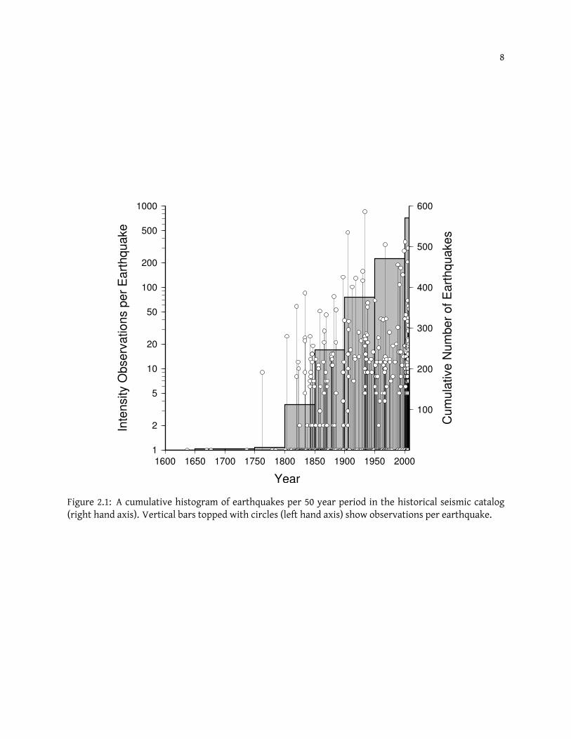
2.1 The first dozen earthquakes from the electronic supplement toMartin and Szeliga (2010) to
illustrate format. Columns Year, Month and Day refer to the date of an event in local time.
For earthquakes with more than seven intensity observations (column Number of Obser-
vations), the approximate epicentral location is listed (columns Longitude, Latitude). The
number of observations corresponds to the number of intensity reports listed in the elec-
tronic supplement to Martin and Szeliga (2010). A geographic region designator is defined
for some events (column Earthquake). This column serves as a reference column to groups
of intensity observations in Table 2.2 . . . . . . . . . . . . . . . . . . . . . . . . . . . . . . 9
2.2 The first 5 earthquakes of 570 from the electronic supplement toMartin and Szeliga (2010).
Columns Year, Month and Day refer to the date of an event in local time. Columns Longi-
tude and Latitude refer to the location of the intensity observation. Column EMS-98 lists
assessed EMS-98 intensities (Grunthal and Levret, 2001). The geographic location of each ob-
servation is listed in column Location. Column Earthquake serves to group observations
from the same earthquake and refers to the geographic location of each earthquake in Ta-
ble 2.1. Earthquakes with fewer than 2 observations are not assigned geographic locations. 9
2.3 Regression coefficients and anticipated mean return time in years for shaking at EMS-98
intensities V, VI and VII for the five largest cities in India. . . . . . . . . . . . . . . . . . . 17
3.1 Intensity attenuation relationship parameters for India, the Indian Craton and the Hi-
malaya. Columns a, b, c, and d refer to the variables in equation (3.1). . . . . . . . . . . . . 26
xii
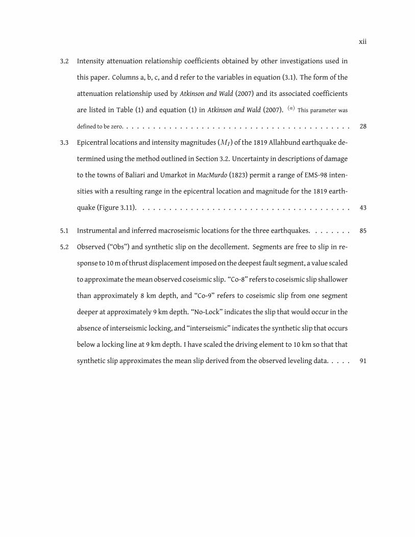
3.2 Intensity attenuation relationship coefficients obtained by other investigations used in
this paper. Columns a, b, c, and d refer to the variables in equation (3.1). The form of the
attenuation relationship used by Atkinson and Wald (2007) and its associated coefficients
are listed in Table (1) and equation (1) in Atkinson and Wald (2007). (a) This parameter was
defined to be zero. . . . . . . . . . . . . . . . . . . . . . . . . . . . . . . . . . . . . . . . . . . 28
3.3 Epicentral locations and intensity magnitudes (MI ) of the 1819 Allahbund earthquake de-
termined using the method outlined in Section 3.2. Uncertainty in descriptions of damage
to the towns of Baliari and Umarkot in MacMurdo (1823) permit a range of EMS-98 inten-
sities with a resulting range in the epicentral location and magnitude for the 1819 earth-
quake (Figure 3.11). . . . . . . . . . . . . . . . . . . . . . . . . . . . . . . . . . . . . . . . 43
5.1 Instrumental and inferred macroseismic locations for the three earthquakes. . . . . . . . 85
5.2 Observed (“Obs”) and synthetic slip on the decollement. Segments are free to slip in re-
sponse to 10mof thrust displacement imposed on the deepest fault segment, a value scaled
to approximate themean observed coseismic slip. “Co-8” refers to coseismic slip shallower
than approximately 8 km depth, and “Co-9” refers to coseismic slip from one segment
deeper at approximately 9 km depth. “No-Lock” indicates the slip that would occur in the
absence of interseismic locking, and “interseismic” indicates the synthetic slip that occurs
below a locking line at 9 km depth. I have scaled the driving element to 10 km so that that
synthetic slip approximates the mean slip derived from the observed leveling data. . . . . 91
xiii
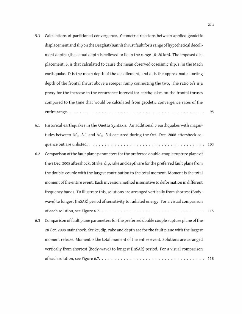
5.3 Calculations of partitioned convergence. Geometric relations between applied geodetic
displacement and slip on theDezghat/Bannh thrust fault for a range of hypothetical decoll-
ment depths (the actual depth is believed to lie in the range 18–20 km). The imposed dis-
placement, S, is that calculated to cause the mean observed coseismic slip, s, in the Mach
earthquake. D is the mean depth of the decollement, and d, is the approximate starting
depth of the frontal thrust above a steeper ramp connecting the two. The ratio S/s is a
proxy for the increase in the recurrence interval for earthquakes on the frontal thrusts
compared to the time that would be calculated from geodetic convergence rates of the
entire range. . . . . . . . . . . . . . . . . . . . . . . . . . . . . . . . . . . . . . . . . . . . 95
6.1 Historical earthquakes in the Quetta Syntaxis. An additional 5 earthquakes with magni-
tudes between Mw 5.1 and Mw 5.4 occurred during the Oct.–Dec. 2008 aftershock se-
quence but are unlisted. . . . . . . . . . . . . . . . . . . . . . . . . . . . . . . . . . . . . . 103
6.2 Comparison of the fault plane parameters for the preferred double-couple rupture plane of
the 9Dec. 2008 aftershock. Strike, dip, rake anddepth are for the preferred fault plane from
the double-couple with the largest contribution to the total moment. Moment is the total
moment of the entire event. Each inversionmethod is sensitive to deformation in different
frequency bands. To illustrate this, solutions are arranged vertically from shortest (Body-
wave) to longest (InSAR) period of sensitivity to radiated energy. For a visual comparison
of each solution, see Figure 6.7. . . . . . . . . . . . . . . . . . . . . . . . . . . . . . . . . . 115
6.3 Comparison of fault plane parameters for the preferred double couple rupture plane of the
28 Oct. 2008 mainshock. Strike, dip, rake and depth are for the fault plane with the largest
moment release. Moment is the total moment of the entire event. Solutions are arranged
vertically from shortest (Body-wave) to longest (InSAR) period. For a visual comparison
of each solution, see Figure 6.7. . . . . . . . . . . . . . . . . . . . . . . . . . . . . . . . . . 118
xiv
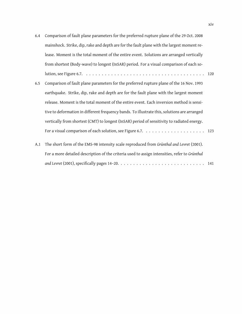
6.4 Comparison of fault plane parameters for the preferred rupture plane of the 29 Oct. 2008
mainshock. Strike, dip, rake and depth are for the fault plane with the largest moment re-
lease. Moment is the total moment of the entire event. Solutions are arranged vertically
from shortest (Body-wave) to longest (InSAR) period. For a visual comparison of each so-
lution, see Figure 6.7. . . . . . . . . . . . . . . . . . . . . . . . . . . . . . . . . . . . . . . 120
6.5 Comparison of fault plane parameters for the preferred rupture plane of the 16 Nov. 1993
earthquake. Strike, dip, rake and depth are for the fault plane with the largest moment
release. Moment is the total moment of the entire event. Each inversion method is sensi-
tive to deformation in different frequency bands. To illustrate this, solutions are arranged
vertically from shortest (CMT) to longest (InSAR) period of sensitivity to radiated energy.
For a visual comparison of each solution, see Figure 6.7. . . . . . . . . . . . . . . . . . . . 123
A.1 The short form of the EMS-98 intensity scale reproduced from Grunthal and Levret (2001).
For a more detailed description of the criteria used to assign intensities, refer to Grunthal
and Levret (2001), specifically pages 14–20. . . . . . . . . . . . . . . . . . . . . . . . . . . . 141
xv
Figures
Figure
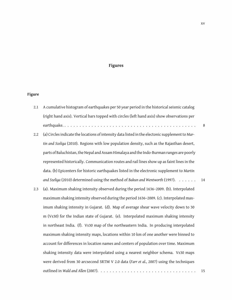
2.1 A cumulative histogram of earthquakes per 50 year period in the historical seismic catalog
(right hand axis). Vertical bars topped with circles (left hand axis) show observations per
earthquake. . . . . . . . . . . . . . . . . . . . . . . . . . . . . . . . . . . . . . . . . . . . . 8
2.2 (a) Circles indicate the locations of intensity data listed in the electonic supplement toMar-
tin and Szeliga (2010). Regions with low population density, such as the Rajasthan desert,
parts of Baluchistan, theNepal andAssamHimalaya and the Indo-Burman ranges are poorly
represented historically. Communication routes and rail lines show up as faint lines in the
data. (b) Epicenters for historic earthquakes listed in the electronic supplement to Martin
and Szeliga (2010) determined using the method of Bakun and Wentworth (1997). . . . . . . 14
2.3 (a). Maximum shaking intensity observed during the period 1636–2009. (b). Interpolated
maximum shaking intensity observed during the period 1636–2009. (c). Interpolatedmax-
imum shaking intensity in Gujarat. (d). Map of average shear wave velocity down to 30
m (Vs30) for the Indian state of Gujarat. (e). Interpolated maximum shaking intensity
in northeast India. (f). Vs30 map of the northeastern India. In producing interpolated
maximum shaking intensity maps, locations within 10 km of one another were binned to
account for differences in location names and centers of population over time. Maximum
shaking intensity data were interpolated using a nearest neighbor schema. Vs30 maps
were derived from 30 arcsecond SRTM V 2.0 data (Farr et al., 2007) using the techniques
outlined inWald and Allen (2007). . . . . . . . . . . . . . . . . . . . . . . . . . . . . . . . . 15
xvi
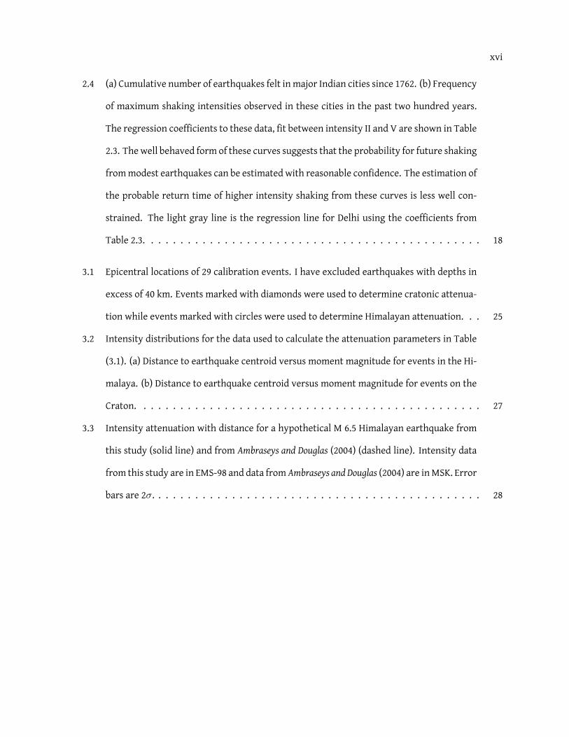
2.4 (a) Cumulative number of earthquakes felt inmajor Indian cities since 1762. (b) Frequency
of maximum shaking intensities observed in these cities in the past two hundred years.
The regression coefficients to these data, fit between intensity II and V are shown in Table
2.3. The well behaved form of these curves suggests that the probability for future shaking
frommodest earthquakes can be estimated with reasonable confidence. The estimation of
the probable return time of higher intensity shaking from these curves is less well con-
strained. The light gray line is the regression line for Delhi using the coefficients from
Table 2.3. . . . . . . . . . . . . . . . . . . . . . . . . . . . . . . . . . . . . . . . . . . . . . 18
3.1 Epicentral locations of 29 calibration events. I have excluded earthquakes with depths in
excess of 40 km. Events marked with diamonds were used to determine cratonic attenua-
tion while events marked with circles were used to determine Himalayan attenuation. . . 25
3.2 Intensity distributions for the data used to calculate the attenuation parameters in Table
(3.1). (a) Distance to earthquake centroid versus moment magnitude for events in the Hi-
malaya. (b) Distance to earthquake centroid versus moment magnitude for events on the
Craton. . . . . . . . . . . . . . . . . . . . . . . . . . . . . . . . . . . . . . . . . . . . . . . 27
3.3 Intensity attenuation with distance for a hypothetical M 6.5 Himalayan earthquake from
this study (solid line) and from Ambraseys and Douglas (2004) (dashed line). Intensity data
from this study are in EMS-98 and data from Ambraseys and Douglas (2004) are inMSK. Error
bars are 2σ. . . . . . . . . . . . . . . . . . . . . . . . . . . . . . . . . . . . . . . . . . . . . 28
xvii
3.4 Comparison of assessed intensities at 95 common locations from the catalog and Ambraseys
andDouglas (2004) for 3 earthquakes. For the histogram, thex-axis (top) corresponds to the
normalized frequency of the combined intensity differences. For individual earthquakes,
x-axis (bottom) corresponds to the assessed intensity value from the catalog. The y-axis
corresponds to the difference between the assessed intensities from the catalog and those
from Ambraseys and Douglas (2004) with negative values indicating that the intensity from
the catalog is lower than that listed in Ambraseys and Douglas (2004). For clarity, intensities
for the 1819 Allah Bund and 1833 Nepal earthquake have been artificially offset to the right
by 0.1 and 0.2 intensity units respectively. . . . . . . . . . . . . . . . . . . . . . . . . . . . 30
3.5 Intensity attenuation relationship between India from this study, the results of Bakun et al.
(2003) for easternNorth America, and the results ofAtkinson andWald (2007) for the Central
EasternUS (CEUS) for a hypotheticalM 6.5 earthquake. Indian intensity data are in EMS-98
while data from eastern North America are in MMI. Error bars are 2σ. . . . . . . . . . . . 32
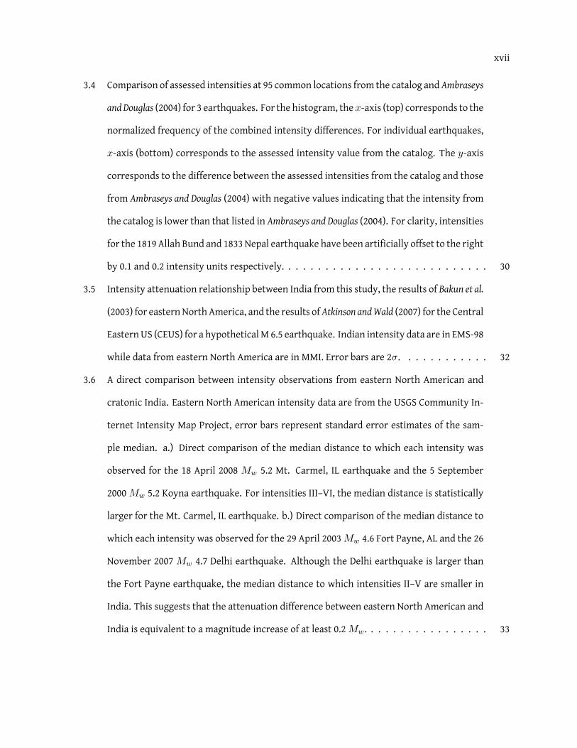
3.6 A direct comparison between intensity observations from eastern North American and
cratonic India. Eastern North American intensity data are from the USGS Community In-
ternet Intensity Map Project, error bars represent standard error estimates of the sam-
ple median. a.) Direct comparison of the median distance to which each intensity was
observed for the 18 April 2008 Mw 5.2 Mt. Carmel, IL earthquake and the 5 September
2000 Mw 5.2 Koyna earthquake. For intensities III–VI, the median distance is statistically
larger for the Mt. Carmel, IL earthquake. b.) Direct comparison of the median distance to
which each intensity was observed for the 29 April 2003Mw 4.6 Fort Payne, AL and the 26
November 2007 Mw 4.7 Delhi earthquake. Although the Delhi earthquake is larger than
the Fort Payne earthquake, the median distance to which intensities II–V are smaller in
India. This suggests that the attenuation difference between eastern North American and
India is equivalent to a magnitude increase of at least 0.2Mw. . . . . . . . . . . . . . . . . 33
xviii
3.7 Intensity attenuation relationship between the Himalaya from this study, the results of
Bakun andWentworth (1997) for California, and the results from Atkinson andWald (2007) for
California for a hypothetical M 6.5 earthquake. Indian intensity data are in EMS-98 while
data from California are in MMI. . . . . . . . . . . . . . . . . . . . . . . . . . . . . . . . . 34
3.8 Comparison of the epicentral misfit for instrumentally recorded earthquakes in the Koyna
region of India. On both figures, the arrowpoints from the instrumental epicenter towards
the intensity derived epicenter. (a) Epicentralmisfit in the Koyna region using the location
of the minimum of equation (3.2) as the epicentral estimate. (b) Epicentral misfit in the
Koyna region using the location of the minimum M from equation (3.2). . . . . . . . . . . 37
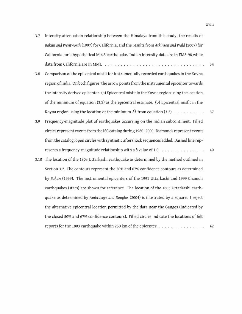
3.9 Frequency-magnitude plot of earthquakes occurring on the Indian subcontinent. Filled
circles represent events from the ISC catalog during 1980–2000. Diamonds represent events
from the catalog; open circleswith synthetic aftershock sequences added. Dashed line rep-
resents a frequency-magnitude relationship with a b value of 1.0 . . . . . . . . . . . . . . 40
3.10 The location of the 1803 Uttarkashi earthquake as determined by the method outlined in
Section 3.2. The contours represent the 50% and 67% confidence contours as determined
by Bakun (1999). The instrumental epicenters of the 1991 Uttarkashi and 1999 Chamoli
earthquakes (stars) are shown for reference. The location of the 1803 Uttarkashi earth-
quake as determined by Ambraseys and Douglas (2004) is illustrated by a square. I reject
the alternative epicentral location permitted by the data near the Ganges (indicated by
the closed 50% and 67% confidence contours). Filled circles indicate the locations of felt
reports for the 1803 earthquake within 250 km of the epicenter. . . . . . . . . . . . . . . . 42

xix
3.11 Possible locations for the 1819 Allahbund earthquake as determined by the method out-
lined in Section 3.2 (open arrows with calculated Mw). The parameters of these possible
locations are listed in Table 3.3. The location of the fault responsible for the 2001 Bhuj
Mw 7.6 earthquake (Schmidt and Burgmann, 2006) as well as the location of the Allah Bund
fault (Malik et al., 2001) are shown with barbs on the hanging wall. The location of the in-
ferred Island Belt Fault is shown with a dashed line (Malik et al., 2001). Contours represent
magnitudes from the epicentral location algorithm (Section 3.2) using the raw intensity
data; they indicate a minimum magnitude location in the Gulf of Kachchh. The locations
of Umarkot and Baliari are shown for reference. Filled circles represent felt intensity loca-
tions within 300 km of the epicenter and arrows indicate the change in epicentral location
due to changes outlined in Table 3.3. . . . . . . . . . . . . . . . . . . . . . . . . . . . . . . 44
3.12 The locations of the 1833 and 1866Nepal earthquakes as determined using themethod out-
lined in Section 3.2. The contours represent the 50% and 67% confidence regions obtained
using method described by Bakun (1999). The previous estimate of epicentral location for
the 1833 earthquake from Ambraseys and Douglas (2004) is represented by a square. Filled
circles indicate the locations of felt reports for the 1833 and 1866 earthquakes within 250
km of Kathmandu. . . . . . . . . . . . . . . . . . . . . . . . . . . . . . . . . . . . . . . . . 46
3.13 Intensity observations of the 2001 Bhuj Mw 7.6 earthquake compared to the attenuation
curve derived for cratonic India for an earthquake of Mw 7.6. Open circles represent ob-
served intensities, diamonds represent the median distance for each observed intensity
level. Dashed lines represent the 2-σ envelope of uncertainty in the intensity attenuation
model as a function of distance. . . . . . . . . . . . . . . . . . . . . . . . . . . . . . . . . . 48
xx
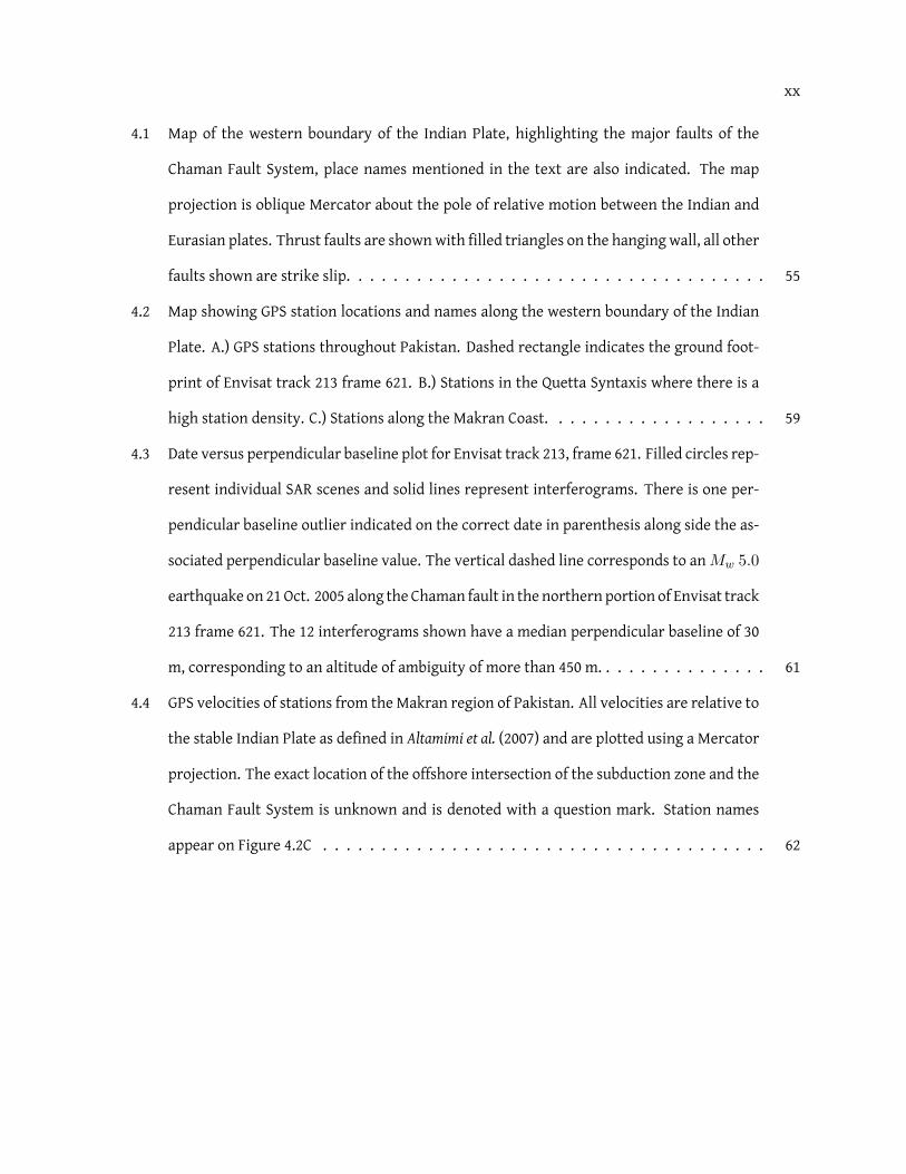
4.1 Map of the western boundary of the Indian Plate, highlighting the major faults of the
Chaman Fault System, place names mentioned in the text are also indicated. The map
projection is oblique Mercator about the pole of relative motion between the Indian and
Eurasian plates. Thrust faults are shownwith filled triangles on the hanging wall, all other
faults shown are strike slip. . . . . . . . . . . . . . . . . . . . . . . . . . . . . . . . . . . . 55
4.2 Map showing GPS station locations and names along the western boundary of the Indian
Plate. A.) GPS stations throughout Pakistan. Dashed rectangle indicates the ground foot-
print of Envisat track 213 frame 621. B.) Stations in the Quetta Syntaxis where there is a
high station density. C.) Stations along the Makran Coast. . . . . . . . . . . . . . . . . . . 59
4.3 Date versus perpendicular baseline plot for Envisat track 213, frame 621. Filled circles rep-
resent individual SAR scenes and solid lines represent interferograms. There is one per-
pendicular baseline outlier indicated on the correct date in parenthesis along side the as-
sociated perpendicular baseline value. The vertical dashed line corresponds to anMw 5.0
earthquake on 21Oct. 2005 along the Chaman fault in the northern portion of Envisat track
213 frame 621. The 12 interferograms shown have a median perpendicular baseline of 30
m, corresponding to an altitude of ambiguity of more than 450 m. . . . . . . . . . . . . . . 61
4.4 GPS velocities of stations from the Makran region of Pakistan. All velocities are relative to
the stable Indian Plate as defined in Altamimi et al. (2007) and are plotted using a Mercator
projection. The exact location of the offshore intersection of the subduction zone and the
Chaman Fault System is unknown and is denoted with a question mark. Station names
appear on Figure 4.2C . . . . . . . . . . . . . . . . . . . . . . . . . . . . . . . . . . . . . . 62
xxi
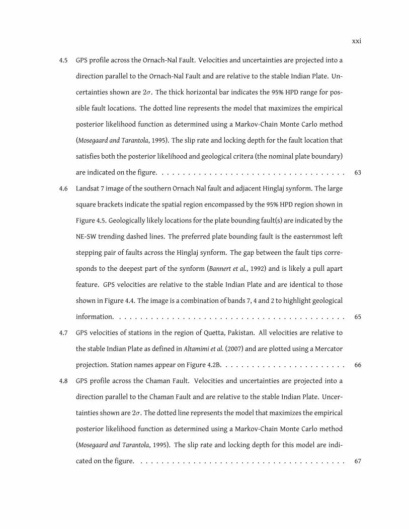
4.5 GPS profile across the Ornach-Nal Fault. Velocities and uncertainties are projected into a
direction parallel to the Ornach-Nal Fault and are relative to the stable Indian Plate. Un-
certainties shown are 2σ. The thick horizontal bar indicates the 95% HPD range for pos-
sible fault locations. The dotted line represents the model that maximizes the empirical
posterior likelihood function as determined using a Markov-Chain Monte Carlo method
(Mosegaard and Tarantola, 1995). The slip rate and locking depth for the fault location that
satisfies both the posterior likelihood and geological critera (the nominal plate boundary)
are indicated on the figure. . . . . . . . . . . . . . . . . . . . . . . . . . . . . . . . . . . . 63
4.6 Landsat 7 image of the southern Ornach Nal fault and adjacent Hinglaj synform. The large
square brackets indicate the spatial region encompassed by the 95% HPD region shown in
Figure 4.5. Geologically likely locations for the plate bounding fault(s) are indicated by the
NE-SW trending dashed lines. The preferred plate bounding fault is the easternmost left
stepping pair of faults across the Hinglaj synform. The gap between the fault tips corre-
sponds to the deepest part of the synform (Bannert et al., 1992) and is likely a pull apart
feature. GPS velocities are relative to the stable Indian Plate and are identical to those
shown in Figure 4.4. The image is a combination of bands 7, 4 and 2 to highlight geological
information. . . . . . . . . . . . . . . . . . . . . . . . . . . . . . . . . . . . . . . . . . . . 65
4.7 GPS velocities of stations in the region of Quetta, Pakistan. All velocities are relative to
the stable Indian Plate as defined in Altamimi et al. (2007) and are plotted using a Mercator
projection. Station names appear on Figure 4.2B. . . . . . . . . . . . . . . . . . . . . . . . 66
4.8 GPS profile across the Chaman Fault. Velocities and uncertainties are projected into a
direction parallel to the Chaman Fault and are relative to the stable Indian Plate. Uncer-
tainties shown are 2σ. The dotted line represents the model that maximizes the empirical
posterior likelihood function as determined using a Markov-Chain Monte Carlo method
(Mosegaard and Tarantola, 1995). The slip rate and locking depth for this model are indi-
cated on the figure. . . . . . . . . . . . . . . . . . . . . . . . . . . . . . . . . . . . . . . . 67
xxii
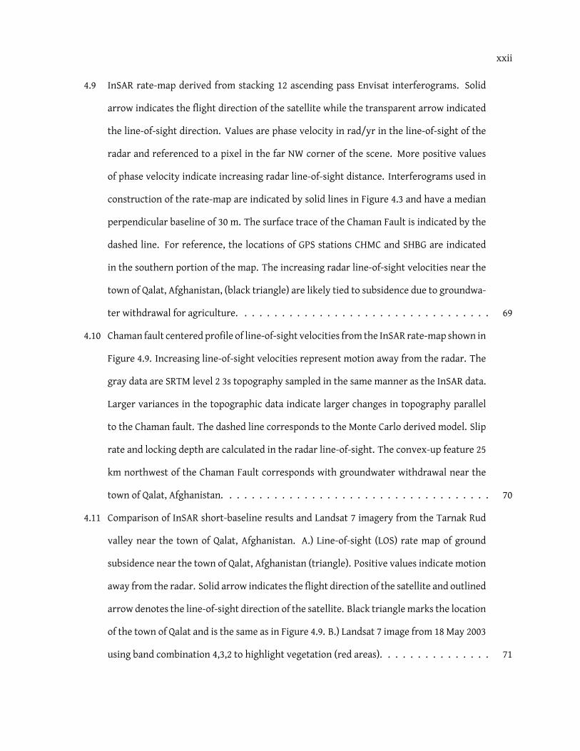
4.9 InSAR rate-map derived from stacking 12 ascending pass Envisat interferograms. Solid
arrow indicates the flight direction of the satellite while the transparent arrow indicated
the line-of-sight direction. Values are phase velocity in rad/yr in the line-of-sight of the
radar and referenced to a pixel in the far NW corner of the scene. More positive values
of phase velocity indicate increasing radar line-of-sight distance. Interferograms used in
construction of the rate-map are indicated by solid lines in Figure 4.3 and have a median
perpendicular baseline of 30 m. The surface trace of the Chaman Fault is indicated by the
dashed line. For reference, the locations of GPS stations CHMC and SHBG are indicated
in the southern portion of the map. The increasing radar line-of-sight velocities near the
town of Qalat, Afghanistan, (black triangle) are likely tied to subsidence due to groundwa-
ter withdrawal for agriculture. . . . . . . . . . . . . . . . . . . . . . . . . . . . . . . . . . 69
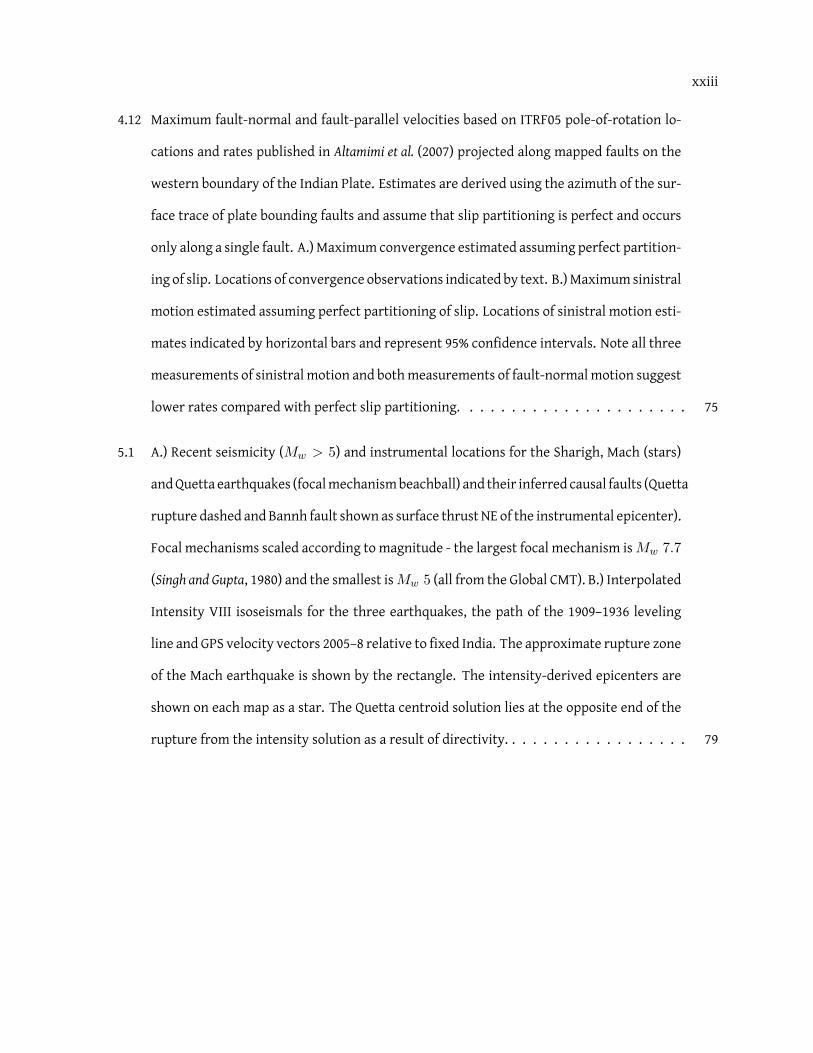
4.10 Chaman fault centered profile of line-of-sight velocities from the InSAR rate-map shown in
Figure 4.9. Increasing line-of-sight velocities represent motion away from the radar. The
gray data are SRTM level 2 3s topography sampled in the same manner as the InSAR data.
Larger variances in the topographic data indicate larger changes in topography parallel
to the Chaman fault. The dashed line corresponds to the Monte Carlo derived model. Slip
rate and locking depth are calculated in the radar line-of-sight. The convex-up feature 25
km northwest of the Chaman Fault corresponds with groundwater withdrawal near the
town of Qalat, Afghanistan. . . . . . . . . . . . . . . . . . . . . . . . . . . . . . . . . . . . 70
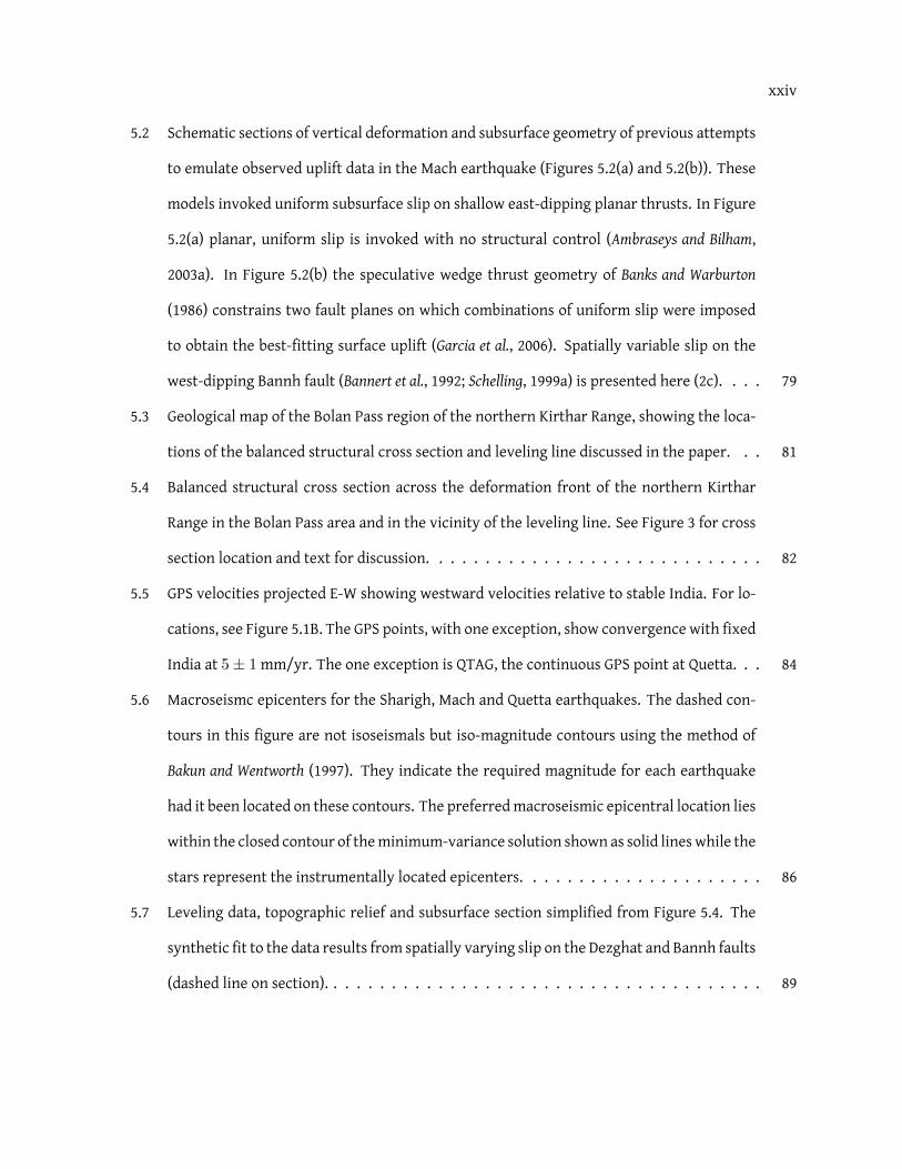
4.11 Comparison of InSAR short-baseline results and Landsat 7 imagery from the Tarnak Rud
valley near the town of Qalat, Afghanistan. A.) Line-of-sight (LOS) rate map of ground
subsidence near the town of Qalat, Afghanistan (triangle). Positive values indicate motion
away from the radar. Solid arrow indicates the flight direction of the satellite and outlined
arrow denotes the line-of-sight direction of the satellite. Black trianglemarks the location
of the town of Qalat and is the same as in Figure 4.9. B.) Landsat 7 image from 18 May 2003
using band combination 4,3,2 to highlight vegetation (red areas). . . . . . . . . . . . . . . 71
xxiii
4.12 Maximum fault-normal and fault-parallel velocities based on ITRF05 pole-of-rotation lo-
cations and rates published in Altamimi et al. (2007) projected along mapped faults on the
western boundary of the Indian Plate. Estimates are derived using the azimuth of the sur-
face trace of plate bounding faults and assume that slip partitioning is perfect and occurs
only along a single fault. A.) Maximum convergence estimated assuming perfect partition-
ing of slip. Locations of convergence observations indicated by text. B.)Maximum sinistral
motion estimated assuming perfect partitioning of slip. Locations of sinistral motion esti-
mates indicated by horizontal bars and represent 95% confidence intervals. Note all three
measurements of sinistral motion and bothmeasurements of fault-normalmotion suggest
lower rates compared with perfect slip partitioning. . . . . . . . . . . . . . . . . . . . . . 75
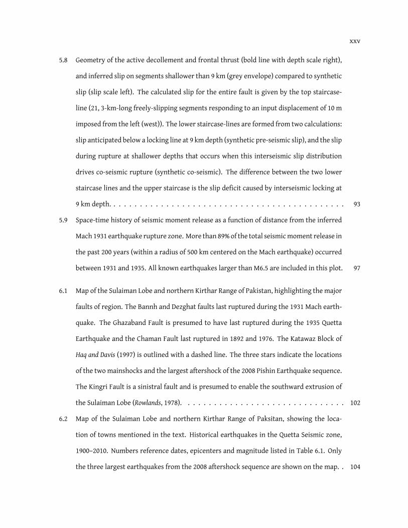
5.1 A.) Recent seismicity (Mw > 5) and instrumental locations for the Sharigh, Mach (stars)
andQuetta earthquakes (focalmechanismbeachball) and their inferred causal faults (Quetta
rupture dashed and Bannh fault shown as surface thrust NE of the instrumental epicenter).
Focal mechanisms scaled according to magnitude - the largest focal mechanism isMw 7.7
(Singh and Gupta, 1980) and the smallest isMw 5 (all from the Global CMT). B.) Interpolated
Intensity VIII isoseismals for the three earthquakes, the path of the 1909–1936 leveling
line and GPS velocity vectors 2005–8 relative to fixed India. The approximate rupture zone
of the Mach earthquake is shown by the rectangle. The intensity-derived epicenters are
shown on each map as a star. The Quetta centroid solution lies at the opposite end of the
rupture from the intensity solution as a result of directivity. . . . . . . . . . . . . . . . . . 79
xxiv
5.2 Schematic sections of vertical deformation and subsurface geometry of previous attempts
to emulate observed uplift data in the Mach earthquake (Figures 5.2(a) and 5.2(b)). These
models invoked uniform subsurface slip on shallow east-dipping planar thrusts. In Figure
5.2(a) planar, uniform slip is invoked with no structural control (Ambraseys and Bilham,
2003a). In Figure 5.2(b) the speculative wedge thrust geometry of Banks and Warburton
(1986) constrains two fault planes on which combinations of uniform slip were imposed
to obtain the best-fitting surface uplift (Garcia et al., 2006). Spatially variable slip on the
west-dipping Bannh fault (Bannert et al., 1992; Schelling, 1999a) is presented here (2c). . . . 79
5.3 Geological map of the Bolan Pass region of the northern Kirthar Range, showing the loca-
tions of the balanced structural cross section and leveling line discussed in the paper. . . 81
5.4 Balanced structural cross section across the deformation front of the northern Kirthar
Range in the Bolan Pass area and in the vicinity of the leveling line. See Figure 3 for cross
section location and text for discussion. . . . . . . . . . . . . . . . . . . . . . . . . . . . . 82
5.5 GPS velocities projected E-W showing westward velocities relative to stable India. For lo-
cations, see Figure 5.1B. The GPS points, with one exception, show convergence with fixed
India at 5± 1mm/yr. The one exception is QTAG, the continuous GPS point at Quetta. . . 84
5.6 Macroseismc epicenters for the Sharigh, Mach and Quetta earthquakes. The dashed con-
tours in this figure are not isoseismals but iso-magnitude contours using the method of
Bakun and Wentworth (1997). They indicate the required magnitude for each earthquake
had it been located on these contours. The preferredmacroseismic epicentral location lies
within the closed contour of theminimum-variance solution shown as solid lineswhile the
stars represent the instrumentally located epicenters. . . . . . . . . . . . . . . . . . . . . 86
5.7 Leveling data, topographic relief and subsurface section simplified from Figure 5.4. The
synthetic fit to the data results from spatially varying slip on the Dezghat and Bannh faults
(dashed line on section). . . . . . . . . . . . . . . . . . . . . . . . . . . . . . . . . . . . . . 89
xxv
5.8 Geometry of the active decollement and frontal thrust (bold line with depth scale right),
and inferred slip on segments shallower than 9 km (grey envelope) compared to synthetic
slip (slip scale left). The calculated slip for the entire fault is given by the top staircase-
line (21, 3-km-long freely-slipping segments responding to an input displacement of 10 m
imposed from the left (west)). The lower staircase-lines are formed from two calculations:
slip anticipated below a locking line at 9 km depth (synthetic pre-seismic slip), and the slip
during rupture at shallower depths that occurs when this interseismic slip distribution
drives co-seismic rupture (synthetic co-seismic). The difference between the two lower
staircase lines and the upper staircase is the slip deficit caused by interseismic locking at
9 km depth. . . . . . . . . . . . . . . . . . . . . . . . . . . . . . . . . . . . . . . . . . . . . 93
5.9 Space-time history of seismic moment release as a function of distance from the inferred
Mach 1931 earthquake rupture zone. More than 89%of the total seismicmoment release in
the past 200 years (within a radius of 500 km centered on the Mach earthquake) occurred
between 1931 and 1935. All known earthquakes larger than M6.5 are included in this plot. 97
6.1 Map of the Sulaiman Lobe and northern Kirthar Range of Pakistan, highlighting the major
faults of region. The Bannh and Dezghat faults last ruptured during the 1931 Mach earth-
quake. The Ghazaband Fault is presumed to have last ruptured during the 1935 Quetta
Earthquake and the Chaman Fault last ruptured in 1892 and 1976. The Katawaz Block of
Haq and Davis (1997) is outlined with a dashed line. The three stars indicate the locations
of the twomainshocks and the largest aftershock of the 2008 Pishin Earthquake sequence.
The Kingri Fault is a sinistral fault and is presumed to enable the southward extrusion of
the Sulaiman Lobe (Rowlands, 1978). . . . . . . . . . . . . . . . . . . . . . . . . . . . . . . 102
6.2 Map of the Sulaiman Lobe and northern Kirthar Range of Paksitan, showing the loca-
tion of towns mentioned in the text. Historical earthquakes in the Quetta Seismic zone,
1900–2010. Numbers reference dates, epicenters and magnitude listed in Table 6.1. Only
the three largest earthquakes from the 2008 aftershock sequence are shown on the map. . 104
xxvi
6.3 Spatially averaged GPS velocities with respect to the stable Indian Plate and centroid mo-
ment tensors from the Global CMT (Dziewonski et al., 1981) withMw > 5 since 1976. Filled
regions are compressional quadrants of the best-fitting double couple. Note the lack of
seismicitywithin the boundaries of the Katawaz Block (see Figure 6.1 for place names). Ve-
locities are calculated as the weighted spatial average of all regional GPS velocities within
a 30’ grid. The location of each velocity average is calculated as the mean of the locations
within each grid. . . . . . . . . . . . . . . . . . . . . . . . . . . . . . . . . . . . . . . . . . 105
6.4 Scene acquisition date versus perpendicular baseline for Envisat track 213 frames 585–621.
Circles represent Envisat Image Mode 6 SAR scenes while lines represent SAR interfer-
ograms. Scenes denoted by gray circles are heavily contaminated with topographically
correlated atmospheric signals and were not used. Solid black lines denote interfero-
grams used to invert for fault parameters. Solid gray lines denote coseismic interfero-
grams which were not used. Vertical dashed lines mark the times of the 28–29 Oct. 2008
mainshocks and 9 Dec. 2008 aftershock discussed in the text. . . . . . . . . . . . . . . . . 109

xxvii
6.5 Interseismic velocities, coseismic offsets and residuals for the 28–29 Oct. 2008 earthquakes
and the 9 Dec. 2008 earthquake. A.) Interseismic velocities relative to the stable Indian
Plate. Thick black lines without arrows represent regional faults (see Figure 6.1). B.) Co-
seismic offsets and C.) residuals from the 28–29 Oct. 2008 earthquake. Displacements for
stations KHST and SHRG are poorly defined due to low number of post-seismic observa-
tions. Stations ZART and CHTRwere established in 2009 and therefore have no pre-seismic
position measurements. Black lines represent the rupture planes determined from in-
version of InSAR data. D.) Coseismic displacements and E.) residuals for the 9 Dec. 2008
earthquake. The proximity of station KACH to the epicenter combined with fortunate
post-seismic occupation timing makes this the only station for which I am able to esti-
mate displacements. Black lines represent rupture determined from inversion of InSAR
data. The error ellipses represent formal uncertainties for the coseismic displacements
as measured from the time series for each station and certainly represent a best case sce-
nario. The residual displacements are calculated by removing the best-fitting coseismic
model determined from inversion of InSAR data. . . . . . . . . . . . . . . . . . . . . . . . 111
6.6 Epicentral locations for the 24 Aug. 1931 Sharigh earthquake and the 28 and 29 Oct. 2008
Ziarat earthquakes determined from shaking intensity data. Locations are determined
using the methodology outlined in Chapter 3. The contours represent the 50% and 67%
confidence contours for epicentral location calculated using parameters listed in Bakun
(1999). In each subfigure, filled circles indicate the locations of felt reports, the star in-
dicates the instrumentally determined epicenter and the center of the innermost con-
tour represents the preferredmacroseismic estimate of epicenter. Intensity data are from
Martin and Szeliga (2010). A.) Epicenter of the 24 Aug. 1931 Sharigh earthquake as deter-
mined frommacroseismic data. B.) Epicenter of the 28 Oct. 2008 earthquake as determined
from macroseismic data. C.) Epicenter of the 29 Oct. 2008 earthquake as determined from
macroseismic data. . . . . . . . . . . . . . . . . . . . . . . . . . . . . . . . . . . . . . . . . 112
xxviii
6.7 Graphical comparision of moment tensor solutions from inversion of teleseismic body-
wave data, the Global CMT (Dziewonski et al., 1981) and inversion of InSAR data. Each inver-
sion method is sensitive to deformation in different frequency bands. To illustrate this,
moment tensors are arranged, from left to right, in order of sensitivity to decreasing fre-
quencies (increasing periods) of radiated energy. In cases where more than one subevent
is inverted for, the moment tensor for the subevent with the largest contribution to the
total moment is shown. . . . . . . . . . . . . . . . . . . . . . . . . . . . . . . . . . . . . . 113
6.8 Envisat interferogram of scenes from 2 Dec. 2008 and 6 Jan. 2009. One fringe corresponds
to 28 mm of change in range. Solid arrow indicates the flight direction of the satellite
and outlined arrow denotes the look direction of the satellite. A.) Original interferogram.
B.) Preferred coseismic elastic dislocation model. C.) Interferogram with coseismic model
removed. Black line denotes the surface projectionof theup-dip edge of the fault identified
from inversion of A. . . . . . . . . . . . . . . . . . . . . . . . . . . . . . . . . . . . . . . . 114
6.9 Envisat interferogram of scenes from 6 May 2008 and 2 Dec. 2008. One fringe corresponds
to 28 mm of change in range. Solid arrow indicates the flight direction of the satellite and
outlined arrow denotes the look direction of the satellite. A.) Original interferogram. B.)
Preferred coseismic elastic dislocation model. C.) Interferogram with coseismic model re-
moved. Black lines denotes the surface projection of the up-dip edge of the fault identified
from inversion of A. . . . . . . . . . . . . . . . . . . . . . . . . . . . . . . . . . . . . . . . 114
xxix
6.10 Lower hemisphere projection of the moment tensors from the inversion of teleseismic
body-waves for the 9 Dec. 2008 aftershock. Fault plane information for each subevent are
listed in the header as event number, strike, dip, and rake in degrees, depth in km andmo-
ment inN-m. Seismic stationnames are printed vertically and to the left of eachwaveform.
Seismic station locations on the focal sphere are denoted by upper-case letters and corre-
spond to the letter indicated between the station name and the waveform trace. Upper
plot shows P-wave focal sphere and waveforms, while the lower plot shows SH-wave fo-
cal sphere and waveforms. Amplitudes have been normalized to highlight the agreement
between the data (solid line) and the synthetic waveforms (dashed line). The source-time
function along with the time scale for each waveform is shown beneath the P-wave data
for station KMBO. . . . . . . . . . . . . . . . . . . . . . . . . . . . . . . . . . . . . . . . . 116
6.11 Revised double-difference earthquake relocations for all events in the region during the
periods Feb. 1997–Mar. 1997 and Oct. 2008–Jan. 2009. Earthquakes during this time period
were relocated using phase data from the USGS monthly PDE using the double difference
method of Waldhauser and Ellsworth (2000). Double difference locations for the 9 Dec. 2008
Mw 5.7 aftershock were then compared with the location derived from inversion of the
interferogram in Figure 6.8 to obtain a shift parameter. Revised double difference epicen-
ters were then obtained by applying this shift parameter to all of the double differenced
earthquakes. . . . . . . . . . . . . . . . . . . . . . . . . . . . . . . . . . . . . . . . . . . . 118
xxx
6.12 Lower hemisphere projection of the moment tensors from the inversion of teleseismic
body-waves for the 28 Oct. 2008 aftershock. Fault plane information for each subevent
are listed in the header as event number, strike, dip, and rake in degrees, depth in km
and moment in N-m. Seismic station names are printed vertically and to the left of each
waveform. Seismic station locations on the focal sphere are denoted by upper-case letters
and correspond to the letter indicated between the station name and the waveform trace.
Upper plot shows P-wave focal sphere andwaveforms, while the lower plot shows SH-wave
focal sphere andwaveforms. Amplitudeshavebeennormalized tohighlight the agreement
between the data (solid line) and the synthetic waveforms (dashed line). The source-time
function along with the time scale for each waveform is shown beneath the P-wave data
for station RER. . . . . . . . . . . . . . . . . . . . . . . . . . . . . . . . . . . . . . . . . . . 119
6.13 Lower hemisphere projection of the moment tensors from the inversion of teleseismic
body-waves for the 29 Oct. 2008 aftershock. Fault plane information for each subevent
are listed in the header as event number, strike, dip, and rake in degrees, depth in km
and moment in N-m. Seismic station names are printed vertically and to the left of each
waveform. Seismic station locations on the focal sphere are denoted by upper-case letters
and correspond to the letter indicated between the station name and the waveform trace.
Upper plot shows P-wave focal sphere andwaveforms, while the lower plot shows SH-wave
focal sphere andwaveforms. Amplitudeshavebeennormalized tohighlight the agreement
between the data (solid line) and the synthetic waveforms (dashed line). The source-time
function along with the time scale for each waveform is shown beneath the P-wave data
for station DGAR. . . . . . . . . . . . . . . . . . . . . . . . . . . . . . . . . . . . . . . . . . 121
6.14 Photograph of the rupture zone of the 29 Oct. 2008 Ziarat Valley earthquake courtesy of
Din Mohammad Kakar. View looking south into the Kan Tangai (Stone Gorge) from the
village of Wam. No surface rupture was observed in the gorge, but numerous N-S trending
surface cracks were apparent along the roads and hill-slopes. . . . . . . . . . . . . . . . . 122

xxxi
6.15 ERS-1 interferogram of scenes from 13 Sep. 1993 and 22 Nov. 1993. One fringe corresponds
to 28mmof change in range. A.) Original interferogram. Black circle indicates the location
of anMb 4.2 that occurred on 30 Oct. 1993 along the northernmost trace of the Ghazaband
Fault. Solid arrow indicates the flight direction of the satellite and outlined arrow denotes
the look direction of the satellite. B.) Preferred coseismic elastic dislocation model. C.)
Interferogram with coseismic model removed. Black line denotes the surface projection
of the up-dip edge of the fault identified from inversion of A. . . . . . . . . . . . . . . . . 124
6.16 A map of Coulomb stress for a receiver fault with the same geometry as the down-dip
extension of the Deghat-Bannh thrust fault system (gray rectangle). Contours are 50 kPa.
A.) Thrust orientation for the 1931 Sharigh earthquake. B.) Dextral orientation for the 1931
Sharigh earthquake. C.) Sinistral orientation for the 1931 Sharigh earthquake. . . . . . . . 126
6.17 Landsat 7 image from 3 Apr. 2001. Black lines indicated mapped faults, and white lines in-
dicate the surface projection of faults that ruptured during the Oct.–Dec. 2008 earthquake
sequence. Questionmarks are placed to indicatewhere the fault extent is uncertain. Faults
shown with a dot-dash pattern are inferred from inspection of the Landsat image as pos-
sible locations for the 1931 Sharig earthquake. Dark colors along the northern edge of the
image correspond to exposedmafic and ultramafic rocks of theMuslimbagh ophiolite. Let-
ters indicate the location of cities and towns: Pishin (P), Quetta (Q), Sharigh (S), and Ziarat
(Z), star denotes the location of the photograph in Figure 6.14. This image is a combination
of Landsat bands 7, 4 and 2 to highlight differences in lithology. . . . . . . . . . . . . . . . 128
6.18 Idealized shear zone geometry, adapted from Sigmundsson et al. (1995). Black wedges rep-
resent stable boundaries to the shear zone, v is the shear velocity, L is the typical block
length, w is the typical block width, and τ is the rotation rate. . . . . . . . . . . . . . . . 129
xxxii
6.19 Moment release as a function of distance to the Quetta Syntaxis Shear Zone in fault lengths
(25 km). Gray circles indicate earthquakes occurring before 1900 for which moment has
been inferred. Shear zone location is indicated by the vertical dotted lines. Earthquake lo-
cations andmagnitudes are from the EHB Centennial Catalog (Engdahl and Villasenor, 2002),
historical earthquake locations (gray) are from Pakistan Meteorological Department and NOR-
SAR (2007). Note that, besides the lack of locations for aftershocks to the 1931 Sharigh
earthquake, the entire shear zone has ruptured in the past century. . . . . . . . . . . . . 130
7.1 Summarymapof interseismic deformation, as determinedusing space geodetic techniques,
across the western boundary of the Indian Plate. Interseismic deformation rate and fault
locking depth are indicated for three transects (black stippled rectangles) across the plate
boundary and one transect across the western edge of the Sulaiman Lobe (white stippled
rectangle). Thin black lines represent the location of major regional faults, thick black
lines represent the approximate location of fault segments known to have ruptured in
historical times. The years of select major historical earthquakes are shown near the seg-
ments believed to have ruptured. GPS velocities are shown in a Eurasian-Plate-fixed refer-
ence frame (Altamimi et al., 2007); the velocity of TURT is 29.96±0.42 mm/yr. Dark gray
vectors represent observed GPS velocities while light gray vectors represent velocities
predicted by motion about the pole of relative motion between the Indian Plate and the
Eurasian Plate. The map is an oblique Mercator projection about the pole of relative mo-
tion between the Indian and Eurasian Plates, thus points on the stable Indian Plate show
velocity vectors parallel to the lower edge of the figure. Thrust faults are shownwith black
triangles on the hanging wall, all other faults are strike-slip. Fault names are indicated in
Figure 4.1. . . . . . . . . . . . . . . . . . . . . . . . . . . . . . . . . . . . . . . . . . . . . 134
xxxiii
7.2 Seismicity and locations of historical fault rupture along the western boundary of the In-
dian Plate. The dashed line represents the boundary of the Katawaz Block (Chapter 4).
A.) Earthquake locations from 1964–2010 from the ISC catalog and moment tensors from
1976–2010 from the Global CMT Project. Filled segments of the moment tensors represent
the compressional quadrants for the best-fitting double-couple. B.) Approximate rupture
lengths for major historical strike-slip earthquakes. Rupture lengths were calculated us-
ing the relationships for strike-slip earthquakes listed in Wells and Coppersmith (1994) us-
ing published estimates of moment magnitude. The 375 km segment between the 1892
Chaman earthquake and the 1505 Kabul earthquake has no known major historical seis-
micity. The 1842 Jalalabad earthquake (Appendix B)was likely a thrust faulting earthquake
and is shown for completeness. . . . . . . . . . . . . . . . . . . . . . . . . . . . . . . . . . 137
Chapter 1
Introduction
1.1 The Indian Plate
The collision between the Indian Plate and the Eurasian Plate, which began during the early Ceno-
zoic Era (Molnar and Tapponnier, 1975), is responsible for some of the most significant relief on the planet.
Present day estimates of the convergence rate between these two plates using observations from perma-
nent and campaign Global Positioning System (GPS) stations are close to 38 mm/yr near Hyderbad, India
(Altamimi et al., 2007). Previous studies havemainly focussed on quantifying convergence across the north-
ern boundary between the Indian and Eurasian Plates (Jackson andMcKenzie, 1984; Treloar and Coward, 1991;
Bilham, 2004). Because the Indian Plate is rotating counter-clockwise relative to Eurasia, convergencewith
the Eurasian Plate decreases westwards of Hyderabad, India. The relative velocity along the transform
fault that separates India from Eurasia on the west has never before been measured directly and is the
subject of this Dissertation. This transform boundary includes numerous subsidiary faults and fold-belts
and is known as the Chaman Fault System (Wellman, 1966; Lawrence et al., 1992). The Chaman Fault itself
represents the westernmost tectonic structure in what is a 150–300 km wide belt of diffuse deformation
forming the western boundary between the Indian and Eurasian Plates.
1.2 Geodetic and Seismic Observations
In this thesis, I utilize various geodetic and seismological measurements to quantify and elucidate
tectonic processes along the western boundary of the Indian Plate. Each of these various measurement
techniques provides knowledge of different temporal and spatial aspects of the seismic cycle. In order
2
to examine patterns in seismicity over the longest temporal span, I use non-instrumental analysis tech-
niques, that consist of archival reports of shaking and destruction caused by large earthquakes. With
certain caveats, these macroseismic data may be analyzed to provide coarse resolution of epicentral loca-
tion and magnitude. For data in the past two decades, I use long-period ground velocity data in the form
of seismic waveforms. These waveforms, recorded at seismic stations with global coverage provide more
precise epicentral information thanmacroseismic data and also provide constraints on earthquake source
depth and possible fault rupture planes.
Geodetic data in the form of direct surface height measurements may be obtained using spirit-
leveling. These data, first collected on the Indian subcontinent during the late 19th century, provide
constraints on geoid height along a transect, and, when combined with prior observations, differential
heights. The effort involved in collecting spirit-leveling data with a high temporal resolution results in
infrequent reoccupation of benchmarks with detailed spatial coverage over limited areas (typically < 1
km transects). Differential heights from spirit-leveling provide excellent vertical resolution of coseismic
ground deformation along fortuitously placed survey lines.
Modern estimates of height are routinely measured along with high precision location estimates
using GPS receivers. When continuously operated from a permanent stable benchmark, relative positions
may be obtained to an accuracy of 2–5 mm horizontally and 6–15 mm in height (Segall and Davis, 1997).
While continuously operating GPS stations provide a vast improvement over spirit-leveling in the tem-
poral domain, they suffer in the spatial domain in being essentially point measurements and are often
separated by large distances (20–200 km).
Synthetic Aperature Radar (SAR) data provide dense spatial coverage at the expense of tempo-
ral resolution for geodetic applications. Interferometric SAR (InSAR), produced by differencing two SAR
scenes, provides information about the relative motion of the ground when the SAR scenes are obtained
at different times from similar vantage points. Deformation data obtained by any single InSAR image
provides spatially dense measurements of only one component of deformation, and can limit the capa-
bility of using InSAR alone to fully describe a deformation field (Burgmann et al., 2000). However, this
high spatial density of deformation information at low temporal sampling complements GPS positioning
3
data. Although it is possible to translatemeasured phase differences from an InSAR image tommprecision
line-of-sight measurements, the relationship between phasemeasurement and ground deformation is de-
pendent on the atmospheric conditions along the line-of-sight during the acquisition of each SAR scene
(Massonnet and Feigl, 1995). In Baluchistan, the arid climate and overall absence of vegetation provides
ideal conditions for InSAR analysis.
1.3 Thesis Outline
In Chapter 2, I begin by analyzing felt reports of seismic shaking across the Indian plate to deter-
mine the gross properties associated with the attenuation of ground shaking with distance. These data
are compared to results from previous studies on other tectonic plates to place the properties of the In-
dian Plate in a global context. With knowledge of the behavior of the attenuation of seismic waves as
observed through popular reporting, I then analyze a new and voluminous catalog of historical shaking
records from the Indian Plate (compiled bymy colleague S. Martin) to examine the limits of macroseismic
data on the derived quantities I seek, epicentral location and magnitude. In Chapter 2, I discuss historical
earthquakes on the Indian Plate and their felt reports. Eight thousand three hundred and thirty nine in-
tensity observations have been evaluated for earthquakes that occurred on the Indian subcontinent and
surrounding plate boundaries from the 17th century to the present. They characterize 570 earthquakes,
more than 90% of which occurred in the past two centuries. I summarize these data graphically in the
form of a spatially averaged intensity map for the subcontinent, a map that emphasizes the features of
many previously published earthquake hazard maps for the Indian plate, but which more faithfully de-
picts regional amplification and attenuation. I also estimate the probable return time for future damaging
shaking in five of India’s largest cities.
In Chapter 3, I utilize this catalog of intensity data to quantify uncertainties in the location andmag-
nitude of historical seismicity on the Indian subcontinent. This comprehensive, consistently interpreted
new catalog of felt intensities for India includes intensities for 570 earthquakes, of which, instrumental
magnitudes and locations are available for 100. I use the intensity values for 29 of these instrumentally
recorded events to develop new intensity versus attenuation relations for the Indian subcontinent and the
4
Himalayan region. I then use these relations to determine the locations and magnitudes of 234 historical
events using the method of Bakun and Wentworth (1997). For the remaining 336 events, intensity distribu-
tions are too sparse to determine magnitude or location. I evaluate magnitude and epicentral accuracy
of newly located events by comparing instrumentally-derived with intensity-derived locations for 29 cal-
ibration events for which more than 15 intensity observations are available. With few exceptions, most
intensity-derived locations lie within a fault length of the instrumentally determined location. For events
where the azimuthal distribution of intensities is limited, I conclude that the formal error bounds from
the regression of Bakun and Wentworth (1997) do not reflect the true uncertainties. Specifically, I also find
that the regression underestimates the uncertainties of the location andmagnitude of the 1819 Allah Bund
earthquake, for which a location has been inferred frommapped surface deformation. Comparing my in-
ferred attenuation relations to those developed for other regions, I find that attenuation for Himalayan
events is comparable to intensity attenuation observed in California (Bakun andWentworth, 1997), while in-
tensity attenuation for cratonic events is higher than intensity attenuation reported for central/eastern
North America (Bakun et al., 2003). Further, I present evidence that intensities of intraplate earthquakes
have a non-linear dependence on magnitude, such that attenuation relations based largely on small-to-
moderate earthquakes may significantly overestimate the magnitudes of historical earthquakes.
In Chapter 4, I discuss the strain accumulation rate along the western boundary of the Indian Plate
utilizing both InSAR and GPS measurements. The western boundary is defined by the Chaman Fault Sys-
tem, the on-land transform separating the Indian and Eurasian plates. From the Arabia/Eurasia/India
triple junction offshore of the Makran coast the Chaman Fault System passes north through Baluchistan
and trends NNE into Afghanistan before merging with the Himalayan arc in northern Afghanistan. Geo-
logical and plate closure estimates suggest sinistral slip across the Chaman Fault System of between 19 and
35mm/yr over the last 25 Ma. Along the southernmost on-land sections of the fault system near the town
of Las Bela, Pakistan, campaign GPSmeasurements indicate sinistral slip at a rate of nearly 15mm/yr with
a shallow locking depth. Farther north near the town of Chaman, Pakistan, campaign and continuous GPS
measurements indicate that the Chaman Fault is shallowly locked or possibly creeping at the surface at
a rate of 7.5 mm/yr. Immediately north of the town of Chaman, the trend of the Chaman Fault becomes
5
NNE-SSW and enters a transpressional bend. Estimates of interseismic strain accumulation rates from
InSAR analyses of this segment of the Chaman Fault indicate that the fault is also shallowly locked and
accumulating strain at a rate of 16.8 mm/yr. The modern prevalence of shallow locking depths along the
length of the Chaman Fault System between the Makran Coast and the Ghazni Province of Afghanistan
suggests that large strike-slip earthquakes (Mw > 7) typical of continental scale transform boundaries
are unlikely on the Chaman Fault.
With this understanding, I focus on a destructive sequence of earthquakes along thewestern bound-
ary between the Indian Plate and the Eurasian Plate during the 1930’s. This sequence began with a large
Mw 6.8 strike-slip earthquake in the Quetta Syntaxis shear zone and culminated in aMw > 7.5 strike-slip
event along one of the plate bounding faults killing > 35, 000 people in the city of Quetta, Pakistan. In
Chapter 5, I discuss one of these earthquakes, theMw 7.1Mach earthquake. Surface deformation associ-
ated with theMw 7.1 27 Aug. 1931 earthquake near Mach in Baluchistan is quantified from spirit-leveling
data and detailed structural sections of the region interpreted from seismic reflection data constrained
by numerous well logs. Mean slip on the west-dipping Dezghat-Bannh fault system amounted to 1.2 m
on a 42 km × 72 km thrust plane with slip locally attaining 3.2 m up-dip of an inferred locking line at
approximately 9 km depth. Slip also occurred at depths below the interseismic locking line. In contrast,
negligible slip occurred in the 4 km near the interseismic locking line. The absence of slip here in the
4 years following the earthquake suggests that elastic energy there must either dissipate slowly in the
interseismic cycle, or that a slip deficit remains, pending its release in a large future earthquake. Elastic
models of the earthquake cycle in this fold-and-thrust belt suggest that slip on the frontal thrust fault is
reduced by a factor of 2 to 8 compared to that anticipated from convergence of the hinterland, a partition-
ing process that is presumably responsible for thickening of the fold-and-thrust belt at the expense of slip
on the frontal thrust. Near the latitude of Quetta, campaign GPSmeasurements indicate that convergence
is approximately 5 mm/yr. Hence the minimum renewal time between earthquakes with 1.2 mmean dis-
placement should be as little as 240 years. However, when the partitioning of fold-belt-convergence to
frontal-thrust-slip is taken into account the minimum renewal time may exceed 2000 years.
Finally, in Chapter 6, I discuss a recent earthquake sequence whose deformation was observed us-
6
ing multiple space-based geodetic methods. In October 2008, two Mw 6.4 earthquakes occurred within
11 hours and 15 km of each other, 40 km NE of Quetta in northern Baluchistan, causing significant dam-
age throughout the Ziarat Valley. Initial interpretations suggested that the earthquakes had occurred on
contiguous segments of a shallow NW-SE trending dextral fault in spite of the absence of mapped faults
with this trend. A relocation of the mainshocks and aftershocks using a double-difference methodology
was confirmed using the surface deformation field of a large aftershock imaged by InSAR. The relocated
mainshocks were subsequently used to interpret InSAR imagery significantly decorrelated by landsliding
in the epicentral region, revealing that the two mainshocks had occurred on parallel NE-trending sinis-
tral faults. A reinterpretation of historical earthquakes near the 2008 earthquake sequence suggests that
“book-shelf” faulting extends to the NW and SE of the Ziarat valley and accommodates overall dextral
shear arising from the southward advance of the Sulaiman Lobe past the eastward advance of the north-
ern Kirthar ranges. Regional GPS data suggest that an effective dextral slip rate of approximately 17.0
mm/yr is accommodated by a previously unrecognized system of at least 5 approximately 25 km long,
NE-trending sinistral faults spaced approximately 15 km apart.
Chapter 2
A Catalog of Felt Intensity Data for 570 Earthquakes in India from 1636 to 2009
2.1 Introduction
Catalogs of historical Indian earthquakes occurring in the past 450 years contain errors in date,
location and magnitude, and list few intensity data in a form suited to numerical analysis. The following
account addresses this deficiency by presenting a unified analysis of intensity data assessed from accounts
of damage, or from felt perceptions of earthquakes. As such it omits some earthquakes for which no
intensity data are available. In contrast it includes several earthquakes missing from previous catalogs
. With few exceptions, the listing in based on original source materials archived in Indian and European
libraries, regional newspapers, private letters and diaries, and government reports. For earthquakes later
than 2000, eyewitness accounts provided via the World Wide Web or communicated in person have also
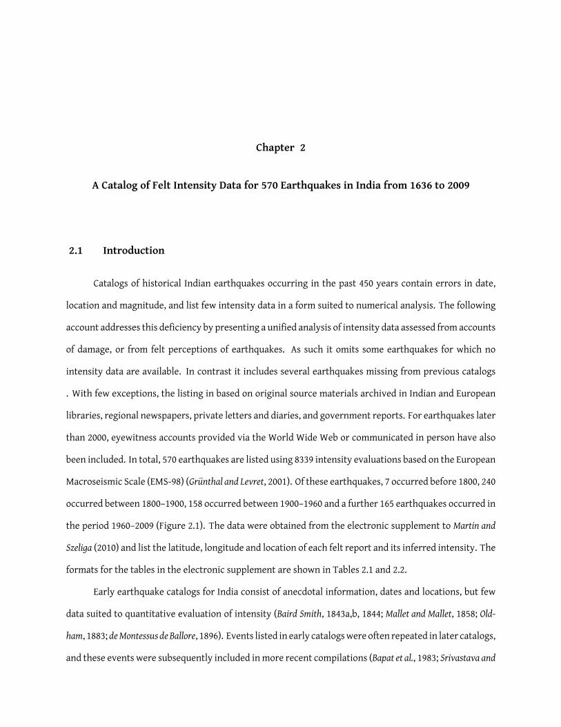
been included. In total, 570 earthquakes are listed using 8339 intensity evaluations based on the European
Macroseismic Scale (EMS-98) (Grunthal and Levret, 2001). Of these earthquakes, 7 occurred before 1800, 240
occurred between 1800–1900, 158 occurred between 1900–1960 and a further 165 earthquakes occurred in
the period 1960–2009 (Figure 2.1). The data were obtained from the electronic supplement to Martin and
Szeliga (2010) and list the latitude, longitude and location of each felt report and its inferred intensity. The
formats for the tables in the electronic supplement are shown in Tables 2.1 and 2.2.
Early earthquake catalogs for India consist of anecdotal information, dates and locations, but few
data suited to quantitative evaluation of intensity (Baird Smith, 1843a,b, 1844; Mallet and Mallet, 1858; Old-
ham, 1883; deMontessus deBallore, 1896). Events listed in early catalogswere often repeated in later catalogs,
and these events were subsequently included inmore recent compilations (Bapat et al., 1983; Srivastava and
8
100
200
300
400
500
600
Cum
ula
tive N
um
ber
of E
art
hquakes
1600 1650 1700 1750 1800 1850 1900 1950 2000
Year
1
2
5
10
20
50
100
200
500
1000
Inte
nsity O
bserv
ations p
er
Eart
hquake
Figure 2.1: A cumulative histogram of earthquakes per 50 year period in the historical seismic catalog(right hand axis). Vertical bars topped with circles (left hand axis) show observations per earthquake.
9
Table 2.1: The first dozen earthquakes from the electronic supplement toMartin and Szeliga (2010) to illus-trate format. Columns Year, Month and Day refer to the date of an event in local time. For earthquakeswith more than seven intensity observations (column Number of Observations), the approximate epi-central location is listed (columns Longitude, Latitude). The number of observations corresponds to thenumber of intensity reports listed in the electronic supplement toMartin and Szeliga (2010). A geographicregion designator is defined for some events (column Earthquake). This column serves as a referencecolumn to groups of intensity observations in Table 2.2
NumberDate Longitude Latitude of Earthquake
Observations1636-08-29 11669-06-23 11676-08-26 11736-03-24 11762-04-02 22.4 92.2 9 CHITTAGONG-17621779-??-?? 11784-12-?? 11800-10-19 11803-09-01 30.7 78.8 25 BARAHAT-18031808-06-04 11810-04-01 11810-05-13 1
Table 2.2: The first 5 earthquakes of 570 from the electronic supplement to Martin and Szeliga (2010).Columns Year, Month and Day refer to the date of an event in local time. Columns Longitude and Lati-tude refer to the location of the intensity observation. Column EMS-98 lists assessed EMS-98 intensities(Grunthal and Levret, 2001). The geographic location of each observation is listed in column Location. Col-umn Earthquake serves to group observations from the same earthquake and refers to the geographiclocation of each earthquake in Table 2.1. Earthquakes with fewer than 2 observations are not assignedgeographic locations.
Date Longitude Latitude EMS-98 Location Earthquake1636-08-29 72.81 21.19 3 Surat1669-06-23 74.79 34.08 5 Srinagar1676-08-26 86.94 21.48 4 Balasore1736-03-24 74.79 34.08 7 Srinagar1762-04-02 88.35 22.57 3 Calcutta CHITTAGONG-17621762-04-02 88.386 22.88 3 Chandernagore CHITTAGONG-17621762-04-02 91.838 22.342 5 Goyparah CHITTAGONG-17621762-04-02 91.665 22.552 6 Akulpoor-Bansbaria CHITTAGONG-17621762-04-02 91.773 22.297 6 Howla CHITTAGONG-17621762-04-02 91.826 22.349 7 Chittagong/Islamabad CHITTAGONG-17621762-04-02 92.101 22.133 7 Dahrampoor CHITTAGONG-17621762-04-02 92.065 22.168 7 Do Hazari CHITTAGONG-17621762-04-02 92.084 22.367 8 Bahngoo Changee CHITTAGONG-1762

10
Ramachandran, 1985; Ramachandran and Srivastava, 1991) supplemented by new earthquakes, and by newly
discovered archival information. Hence, these new catalogs include many erroneous entries from earlier
catalogs. The global Catalog of Significant Earthquakes by Dunbar et al. (1992) lists all these earthquakes
uncritically making it impossible to judge which accounts should be rejected. As Ambraseys (1971) noted,
the repetition of error is common to many catalogs of earthquakes that have not been evaluated from
primary source materials.
The present account includes data assessed from primary sources, or from sources that reproduce
the raw data from which intensity may be evaluated or verified (Martin and Szeliga, 2010, electronic sup-
plement). I emphasize that the list of the locations of Indian earthquakes in Martin and Szeliga (2010) is
subordinate to the listing of perceived and felt observations of intensity (electronic supplement toMartin
and Szeliga (2010)) because the determination of epicentral location is subject to interpretation. The tabu-
lated intensity data are quantified from reports at locations that are rarely at the epicenter. Therefore, the
location and magnitude of all pre-instrumental earthquakes in India derived from these data are uncer-
tain except in those rare locations where surface deformation has been recorded (e.g. 1819 Kachchh and
1897 Shillong). The entries are listed in chronological order. In Chapter 3 I calculate epicentral locations
for many of these earthquakes using the methods of Bakun and Wentworth (1997).
Beginning in the late 1800’s, the Geological Survey of India and other agencies compiled studies
of significant earthquakes. In many official government reports, a simplified description of the building
stock considered characteristic of a whole village is used (e.g. 1967 Koyna earthquake (Tandon and Chaud-
hury, 1968)). In some cases this generalized description of the building stock is classified into Types A, B
and C as defined in Grunthal and Levret (2001). However, many of these reports omit descriptions of shak-
ing experienced by people. From these government reports, descriptions of damage, in some instances
accompanied by photographs, were used to evaluate intensities. Of the 43 events from Ambraseys and Dou-
glas (2004) 28 have been re-evaluatedwhere it was possible to locate first-hand accounts or official reports.
None of the listed intensities have been repeated from maps or previously published listings. Where au-
thentic primary source materials are unavailable for a particular earthquake, those accounts have been
excluded from the final listing.
11
2.2 Intensity Scale
In previous studies, various intensity scales were used to evaluate earthquakes in India. Oldham
(1899) notes that early European scales listed inappropriate criteria for the assessment of acceleration-
related damage to indigenous structures, and for the 1897 Assam earthquake he chose to use his own
simplified scale rather than the thenprevalent Rossi-Forrel scale. Later studies of earthquakes adopted the
Modified Mercalli scale (e.g.Middlemiss, 1910) or the MSK-64 scale (Medvedev et al., 1965). Intensities in the
present study use the European Macroseismic Scale (EMS-98) (Grunthal and Levret, 2001, see also Appendix
A), a successor to the MSK-64 intensity scale. I note that MSK-64 listings of Ambraseys and Douglas (2004)
are numerically indistinguishable from the EMS-98 evaluations for those accounts I have compared. As in
Ambraseys andDouglas (2004) assessment of local intensities avoids observations based on, or contaminated
by, ground deformation, landslides, liquefaction, seismic seiches and surface faulting. Numerous accounts
that fall into these categories have thus been excluded from the catalog.
Many of the intensities evaluated lie in the intensity range II–V. These are differentiated from
sparse data as follows: reports that stated an earthquake was “barely felt” or “very slight” were assigned
intensity II while those that stated an earthquake was “slight” or “mild” were assigned intensity III. Re-
ports that spoke of tremulous motion, rumbling sounds, etc. were assigned intensity IV. Grade I damage
(Grunthal and Levret, 2001) to structures begins at intensity V with the appearance of structural cracks,
tiles and plaster being dislodged etc. Above intensity V, the following critera are used: Masonry damage
begins at intensity VI, and accounts of this level of damage often estimate the numbers of buildings af-
fected i.e. “a few”, “many”, or “most”, which together with human perceptions, permit us to distinguish
between intensities VI and VII. Photographs, if available, were used only to supplement intensity assign-
ment. I further note that photographic evidence is often biased towards the most damaged structures,
since undamaged structures are rarely photographed (Hough and Pande, 2007). Because of this known bias,
photographs were never used solely to determine intensities.

12
2.3 Reporting Consistency and Completeness
Earthquakes in India, as elsewhere, result in felt reports where the density of reporting is propor-
tional to the density of population. The number of felt reports is further dependent on the propensity
of a population to commit their perception of shaking or perceived damage to some form of permanent
record. Large urban centers contain a range of vulnerable structures, with people of different levels of
awareness, and the record of their perceptions depends much on the prevailing traditions of personal
diaries and responsibilities of the press and government offices to print these materials. Not only have
these reporting habits changed throughout the past few hundred year, but so have the style of buildings
and construction materials used to make these buildings.
Prior to the 18th century, reporting was sparse and mainly undertaken by official historians and
intellectuals. By the late 19th century the reporting of earthquakes by scattered colonial observers became
more verbose and eloquent. During the 20th century, seismologists began proactively collecting intensity
data and initiating studies of specific earthquakes. The mid 20th century is characterized by a decline in
the number of people writing and presenting personal diaries or sending notes to newspapers. Instead, we
must trust the record of professional reporters trained to gather and print information in the local and
national media. In the past decade the internet has given many people the opportunity to report their
perceptions rapidly. Specific blackouts in reporting have also occurred, such as during the Second World
War, when damage to some cities was classified.
Although reporting improves considerably after 1800, many areas are not represented well, even
at the present time. Thus, it is certain that uneveness in reporting prevails during the time spanned
by the catalog. This is partly because the density of people reporting earthquakes varies spatially, and
partly because public interest in reporting felt intensities has varied significantly with time. Many small
earthquakes may be noted by people but not recorded in news media or public reports. Thus I anticipate
that additional earthquakes and accounts of existing earthquakes will surface in future years that will
supplement the recorded observations listed.
I emphasize that the present catalog is not a complete list of all Indian earthquakes. I estimate that
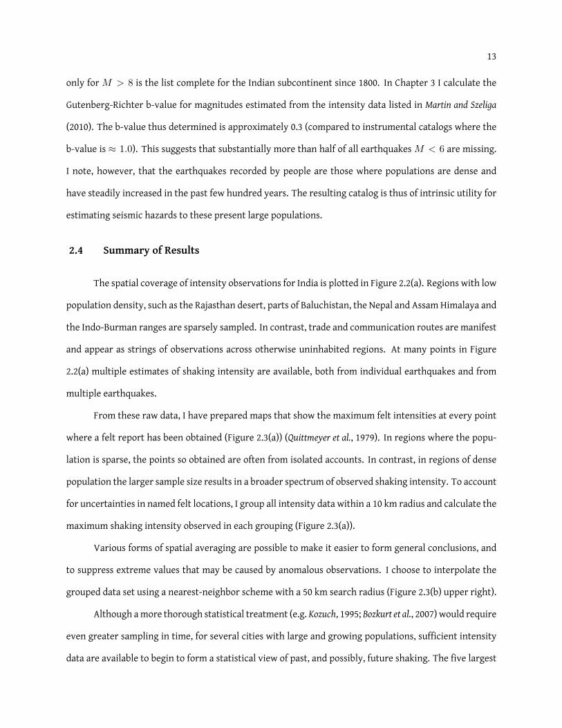
13
only for M > 8 is the list complete for the Indian subcontinent since 1800. In Chapter 3 I calculate the
Gutenberg-Richter b-value for magnitudes estimated from the intensity data listed in Martin and Szeliga
(2010). The b-value thus determined is approximately 0.3 (compared to instrumental catalogs where the
b-value is ≈ 1.0). This suggests that substantially more than half of all earthquakes M < 6 are missing.
I note, however, that the earthquakes recorded by people are those where populations are dense and
have steadily increased in the past few hundred years. The resulting catalog is thus of intrinsic utility for
estimating seismic hazards to these present large populations.
2.4 Summary of Results
The spatial coverage of intensity observations for India is plotted in Figure 2.2(a). Regions with low
population density, such as the Rajasthan desert, parts of Baluchistan, the Nepal and Assam Himalaya and
the Indo-Burman ranges are sparsely sampled. In contrast, trade and communication routes are manifest
and appear as strings of observations across otherwise uninhabited regions. At many points in Figure
2.2(a) multiple estimates of shaking intensity are available, both from individual earthquakes and from
multiple earthquakes.
From these raw data, I have prepared maps that show the maximum felt intensities at every point
where a felt report has been obtained (Figure 2.3(a)) (Quittmeyer et al., 1979). In regions where the popu-
lation is sparse, the points so obtained are often from isolated accounts. In contrast, in regions of dense
population the larger sample size results in a broader spectrum of observed shaking intensity. To account
for uncertainties in named felt locations, I group all intensity data within a 10 km radius and calculate the
maximum shaking intensity observed in each grouping (Figure 2.3(a)).
Various forms of spatial averaging are possible to make it easier to form general conclusions, and
to suppress extreme values that may be caused by anomalous observations. I choose to interpolate the
grouped data set using a nearest-neighbor scheme with a 50 km search radius (Figure 2.3(b) upper right).
Although amore thorough statistical treatment (e.g. Kozuch, 1995; Bozkurt et al., 2007) would require
even greater sampling in time, for several cities with large and growing populations, sufficient intensity
data are available to begin to form a statistical view of past, and possibly, future shaking. The five largest
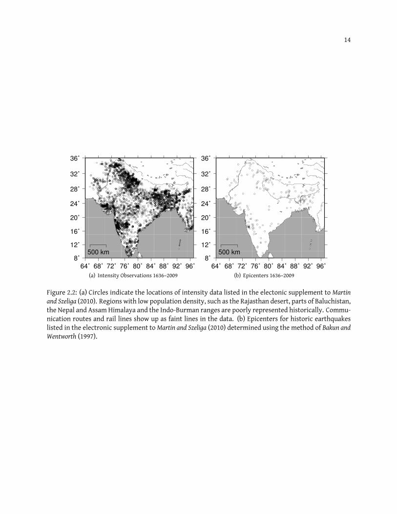
14
64˚ 68˚ 72˚ 76˚ 80˚ 84˚ 88˚ 92˚ 96˚
8˚
12˚
16˚
20˚
24˚
28˚
32˚
36˚
500 km
(a) Intensity Observations 1636–200964˚ 68˚ 72˚ 76˚ 80˚ 84˚ 88˚ 92˚ 96˚
8˚
12˚
16˚
20˚
24˚
28˚
32˚
36˚
500 km
(b) Epicenters 1636–2009
Figure 2.2: (a) Circles indicate the locations of intensity data listed in the electonic supplement to Martinand Szeliga (2010). Regions with low population density, such as the Rajasthan desert, parts of Baluchistan,the Nepal and Assam Himalaya and the Indo-Burman ranges are poorly represented historically. Commu-nication routes and rail lines show up as faint lines in the data. (b) Epicenters for historic earthquakeslisted in the electronic supplement toMartin and Szeliga (2010) determined using the method of Bakun andWentworth (1997).
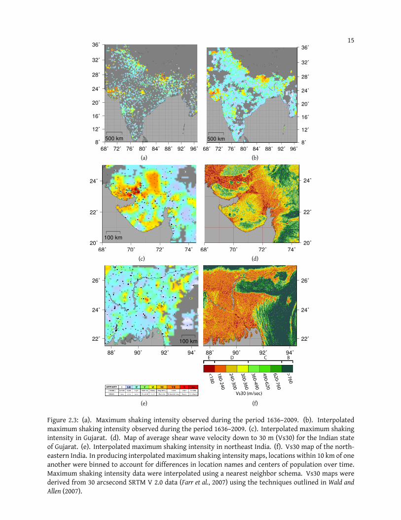
15
68˚ 72˚ 76˚ 80˚ 84˚ 88˚ 92˚ 96˚
8˚
12˚
16˚
20˚
24˚
28˚
32˚
36˚
500 km
(a)68˚ 72˚ 76˚ 80˚ 84˚ 88˚ 92˚ 96˚
8˚
12˚
16˚
20˚
24˚
28˚
32˚
36˚
500 km
(b)
68˚ 70˚ 72˚ 74˚
20˚
22˚
24˚
100 km
(c)68˚ 70˚ 72˚ 74˚
20˚
22˚
24˚
(d)
88˚ 90˚ 92˚ 94˚
22˚
24˚
26˚
100 km
(e)
88˚ 90˚ 92˚ 94˚
22˚
24˚
26˚
(f)
Figure 2.3: (a). Maximum shaking intensity observed during the period 1636–2009. (b). Interpolatedmaximum shaking intensity observed during the period 1636–2009. (c). Interpolated maximum shakingintensity in Gujarat. (d). Map of average shear wave velocity down to 30 m (Vs30) for the Indian stateof Gujarat. (e). Interpolated maximum shaking intensity in northeast India. (f). Vs30 map of the north-eastern India. In producing interpolated maximum shaking intensity maps, locations within 10 km of oneanother were binned to account for differences in location names and centers of population over time.Maximum shaking intensity data were interpolated using a nearest neighbor schema. Vs30 maps werederived from 30 arcsecond SRTM V 2.0 data (Farr et al., 2007) using the techniques outlined in Wald andAllen (2007).
16
modern cities in India, Mumbai, Delhi, Bangalore, Kolkata, and Chennai have been shaken numerous times
in the past 200 years by earthquakes. Figure 2.4(a) illustrates maximum shaking as a cumulative number
of observations per year experienced in each major city and Figure 2.4(b) shows the frequency of shaking
at different intensities. Figure 2.4(b) reveals well-behaved curves fromwhich it is possible to conclude the
probability for shaking in a given time window. Although the intensity data for these curves include both
infrequent large and distant earthquakes, and more frequent small but closer earthquakes, the return
times are probably reliable estimates of future shaking. That is, the infrequent larger earthquakes do not
substantially bias the statistics to shorter return times, because there are fewer of them.
The projection of the curves in Figure 2.4(b) to larger intensities than those recorded in the past
200 years in each city is possible, but the predictions are of uncertain reliability. The data in Figure 2.4(b)
follow a function of the form,
log(N) = a+ b(I − 2)
where N is the cumulative number of observations per year for each EMS-98 intensity value I , and a
and b are to be determined. The results of regressing the data to this function are shown in Table 2.3.
Certain of India’s largest cities report shaking (intensity II) more frequently than others. The “a” values
for Delhi and Kolkata are 50% greater than those for Chennai and Bangalore. This is partly due to their
tectonic setting, with cities that are far fromplate boundaries, like Bangalore, showing the longest interval
between shaking at any intensity. Cities closer to plate boundaries, like Delhi (The Himalaya) or Kolkata
(The Indo-Burman Ranges) show the shortest intervals between shaking at a given intensity. Intensity
V shaking in these cities occurs approximately every 15 years. Intensity VII shaking, where well-built
structures begin to show damage, has a forecast return time of approximately 30 years in major cities
such as Delhi and Kolkata, an interval of time comparable to the design life of most structures.
I recognize that the data in Figure 2.4(b) show evidence for incompleteness at both high and low
intensity values. The lowest EMS-98 intensity (I) is, in effect, a “not-felt” observation, and as such, is
expected to be underrepresented in any data set. The number of earthquakes observed in each city con-
sidered is constant over the past 200 years (Figure 2.4(a)). However, I know of no earthquake in India or
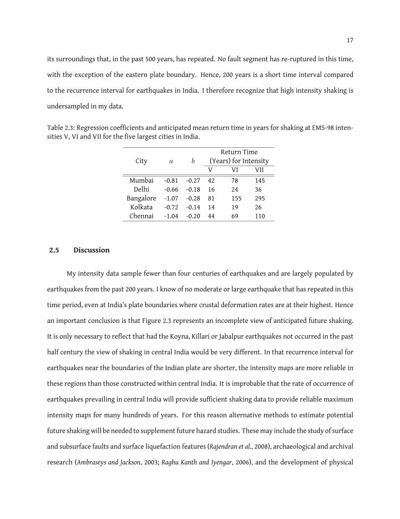
17
its surroundings that, in the past 500 years, has repeated. No fault segment has re-ruptured in this time,
with the exception of the eastern plate boundary. Hence, 200 years is a short time interval compared
to the recurrence interval for earthquakes in India. I therefore recognize that high intensity shaking is
undersampled in my data.
Table 2.3: Regression coefficients and anticipated mean return time in years for shaking at EMS-98 inten-sities V, VI and VII for the five largest cities in India.
Return TimeCity a b (Years) for Intensity
V VI VIIMumbai -0.81 -0.27 42 78 145Delhi -0.66 -0.18 16 24 36
Bangalore -1.07 -0.28 81 155 295Kolkata -0.72 -0.14 14 19 26Chennai -1.04 -0.20 44 69 110
2.5 Discussion
My intensity data sample fewer than four centuries of earthquakes and are largely populated by
earthquakes from the past 200 years. I know of no moderate or large earthquake that has repeated in this
time period, even at India’s plate boundaries where crustal deformation rates are at their highest. Hence
an important conclusion is that Figure 2.3 represents an incomplete view of anticipated future shaking.
It is only necessary to reflect that had the Koyna, Killari or Jabalpur earthquakes not occurred in the past
half century the view of shaking in central India would be very different. In that recurrence interval for
earthquakes near the boundaries of the Indian plate are shorter, the intensity maps are more reliable in
these regions than those constructed within central India. It is improbable that the rate of occurrence of
earthquakes prevailing in central India will provide sufficient shaking data to provide reliable maximum
intensity maps for many hundreds of years. For this reason alternative methods to estimate potential
future shakingwill be needed to supplement future hazard studies. Thesemay include the study of surface
and subsurface faults and surface liquefaction features (Rajendran et al., 2008), archaeological and archival
research (Ambraseys and Jackson, 2003; Raghu Kanth and Iyengar, 2006), and the development of physical
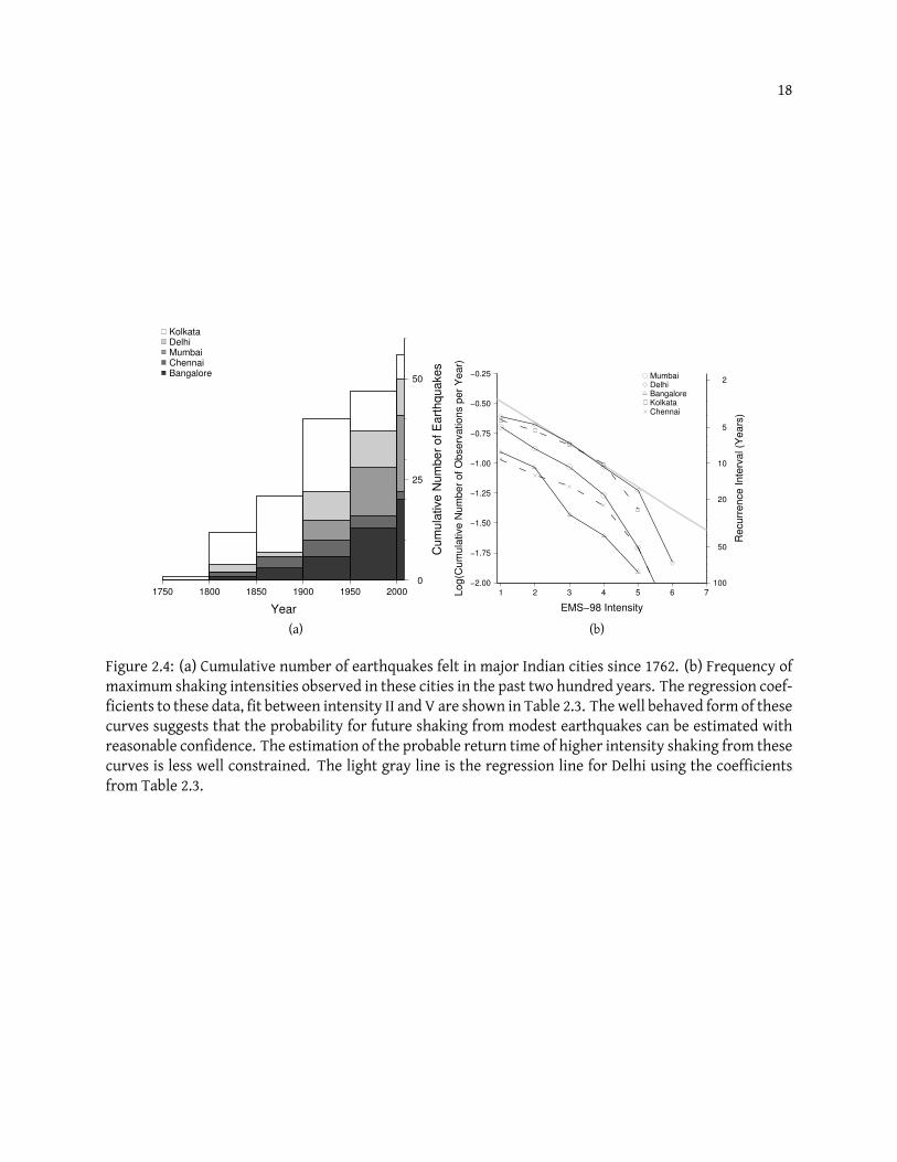
18
0
25
50
Cum
ula
tive N
um
ber
of E
art
hquakes
1750 1800 1850 1900 1950 2000
Year
KolkataDelhiMumbaiChennaiBangalore
(a)
−2.00
−1.75
−1.50
−1.25
−1.00
−0.75
−0.50
−0.25
Lo
g(C
um
ula
tive
Nu
mb
er
of
Ob
se
rva
tio
ns p
er
Ye
ar)
1 2 3 4 5 6 7
EMS−98 Intensity
2
5
10
20
50
100
Re
cu
rre
nce
In
terv
al (Y
ea
rs)
MumbaiDelhiBangaloreKolkataChennai
(b)
Figure 2.4: (a) Cumulative number of earthquakes felt in major Indian cities since 1762. (b) Frequency ofmaximum shaking intensities observed in these cities in the past two hundred years. The regression coef-ficients to these data, fit between intensity II and V are shown in Table 2.3. The well behaved form of thesecurves suggests that the probability for future shaking from modest earthquakes can be estimated withreasonable confidence. The estimation of the probable return time of higher intensity shaking from thesecurves is less well constrained. The light gray line is the regression line for Delhi using the coefficientsfrom Table 2.3.
19
models for characterizing stress caused by India’s collision with Asia (Bilham et al., 2003) .
I note that Figure 2.3(b) resembles many previously published seismic hazard maps of the Indian
subcontinent (e.g. from the Global Seismic Hazard Assessment Program http://www.seismo.ethz.ch/
GSHAP/). I caution however, that the maps presented here, based as they are on felt reports, or catalogs
of historical earthquakes, are maps of past shaking rather than future shaking. With this caveat Figure
2.3(b) is potentially superior to previous hazard maps of India in that it represents a spatial average of
intensities that includes the effects of local amplification or attenuation caused by surface properties but
excludes data such as reports of liquifaction and surface faulting. The averaging I impose on this all-India
scale smoothes the details of local amplification of most utility to hazard estimates. In some regions finer
zonation is possible from the data I provide in the electronic supplement toMartin and Szeliga (2010) (Fig-
ures 2.3(c) and 2.3(e)). Figures 2.3(d) and 2.3(f), show the estimated average shear-velocity to 30m derived
from the roughness of 30 arcsecond SRTM version 2.0 data (Farr et al., 2007) using the techniques outlined
inWald and Allen (2007). Thesemaps summarize seismic site conditions and are a proxy for ground-motion
amplification, which are partially reflected in my maximum shaking intensity maps.
2.6 Conclusions
I have used primary sources to assess 8339 macroseismic observations from 570 historical earth-
quakes occurring on the Indian subcontinent using the EMS-98 intensity scale. I have summarized these
data graphically and note similarities between maps of maximum felt intensity and previously published
seismic hazard maps.
Using the maximum observed intensity per earthquake, I have sufficient data to form conclusions
concerning the average time between strong shaking for five large Indian cities. My use of maximum
shaking intensity is biased towards regions in a city where amplification may occur, thus the intervals
between shaking at a given intensity are pessimistically short. The data are insufficiently dense to un-
dertake microzonation within each city. In Delhi and Kolkata, I find that the interval between potentially
damaging shaking (EMS-98 VII) is comparable to the design life of most structures, and should thus be
included in construction codes.

20
Chapter 3 analyses the data presented here in terms of their implications for attenuation of seis-
mic waves traversing the Indian craton and its plate boundaries. In this second article the location and
magnitude of the historical earthquakes discussed here are evaluated from relationships derived between
recent intensity observations and instrumental magnitudes.
Chapter 3
Intensity, Magnitude, Location and Attenuation in India for Felt Earthquakes since 1762
3.1 Introduction
Despite awritten history extendingmore than threemillennia the location andmagnitude of earth-
quakes in the Indian subcontinent and its surroundings prior to 1900 remain largely unquantified. The
catalog presented in Chapter 2 of 8339 felt reports of 570 earthquakes since 1636 permits this shortcoming
to be addressed. More than 98% of the earthquakes in this macroseismic catalog occurred after 1800, and
more than 50% since 1900. In this article I quantify attenuation versus distance relationships for India and
from these I determine the probable magnitudes and locations of earthquakes that occurred before the
instrumental catalog.
Previous studies have undertaken similar investigations using less complete data with variable and
uncertain quality. In 1996, Johnston used published intensity values to derive attenuation parameters for
the Indian subcontinent (Johnston, 1996). However, these intensity values were not consistently deter-
mined, and were biased by the inclusion of observations influenced by liquefaction and by inattention to
the effects of building fragility common to early reports. From these data, Johnston (1996) derived relations
between isoseismal area and earthquake magnitude.
More recently, a number of studies have carefully and systematically reinterpreted availablemacro-
seismic data for a number of important historical earthquakes. Ambraseys and Jackson (2003) present inten-
sity evaluations and approximate magnitudes for several early events in the Himalaya and southern Tibet
(1411, 1505, 1555, 1713, 1751, 1803 and 1806). Ambraseys (2004) assigns intensity values for a Bangladesh
earthquake in 1664 and discusses the location of an earthquake in Sindh in 1668. Ambraseys and Douglas
22
(2004) present re-evaluated intensities from 43 earthquakes in northern India and use inferred felt areas
to estimate attenuation.
Recent events, such as the 2001 Bhuj earthquake, have been the subject of extensive, traditional,
ground-based intensity surveying of damage andother effects (Pande andKayal, 2003). Additionally, Internet-
basedmethods (Wald et al., 1999a, Amateur Seismic Centre (http://www.asc-india.org)) have now begun
to yield objectively determined intensity distributions for moderate and large earthquakes through the
use of standardized questionnaires.
Recent efforts notwithstanding, systematically and carefully determined intensities have remained
lacking for bothmoderatehistorical earthquakes and formostmoderate and large instrumentally recorded
earthquakes in India. This new catalog of felt earthquakes and intensities, compiled from extant records
in colonial libraries and newspaper accounts provides a new, rich source of information for the past two
centuries. Intensity values in this catalog were assessed from the original sources using the European
Macroseismic Scale 1998 (EMS-98) (Grunthal and Levret, 2001). This new catalog includes 234 historical
earthquakes ranging in magnitude from 4 to 8.6, that I judge to have a sufficient number of intensity ob-
servations to permit the evaluation of their epicentral parameters. The results of these evaluations are
listed in electronic supplement.
This important new catalog provides the basis for determining intensity attenuation relations for
India and for determining locations and magnitudes for historical events for which sufficient macroseis-
mic information exists. I conclude my study by discussing examples of four earthquakes from the 19th
century.
3.2 Data and Methods
The intensity values from the catalog used to derive the attenuation relationships for this study
reveal significant scatter at all distances. Although some of this scatter is expected to result from impre-
cision in intensity assignments, (for example where structural fragility cannot be adequately assessed)
rich, objectively determined intensity distributions (e.g. Wald et al., 1999b; Atkinson and Wald, 2007) reveal
that intensities do vary substantially as a consequence of local site geology and other factors. Due to
23
unknown variations in the precise location of repeated observations, the calculation of meaningful site
corrections is not possible. Thus, I do not consider site corrections in this analysis.
Previous studies of intensity attenuation in the Indian subcontinent have used methods based on
the area contained within a contour of specific intensity (e.g. Johnston, 1996; Ambraseys and Douglas, 2004).
These methods assign epicentral locations and magnitudes based on the location of maximum shaking
and the areal extent of isoseismal contours. In this study, I use the method of Joyner and Boore (1993) to
derive intensity attenuation relationships for the Indian subcontinent empirically. The functional form
of the intensity attenuation relationship used in this study is as follows:
I = a+ bMw + cR+ d log(R) (3.1)
where R is the hypocentral distance, Mw is the moment magnitude and a, b, c and d are constants to be
determined. Equation (3.1) is derived by assuming that intensity is logarithmically proportional to the
energy density of a point source (Howell and Schultz, 1975). The cR and d log(R) terms are generally taken
to reflect intrinsic attenuation and geometrical spreading, respectively, although in practice these two
terms are difficult to resolve independently.
A one-stage maximum likelihood methodology is used to derive the intensity attenuation relation-
ship using 29 calibration events (Joyner and Boore, 1993). The calibration events consist of earthquakes
since 1950 withmore than 15 felt intensity reports (Figure 3.1). Although I give preference to earthquakes
with hypocenters in the Centennial catalog (Engdahl and Villasenor, 2002), I utilize other hypocentral cat-
alogs for more recent earthquakes. If an event is not listed in the Centennial Catalog, I use hypocen-
tral estimates from the Bulletin of the International Seismological Centre (ISC) and thereafter, the USGS
NEIC Monthly Hypocenter Data File (MHDF). Preferred moment magnitude estimates are from the Global
Centroid Moment Tensor Project. If an event is not listed in the Global CMT, I use moment magnitude
estimates from the Centennial Catalog, ISC, or the MHDF in decreasing order of preference (see Acknowl-
edgements). For five calibration events (4.1 < M < 5.3), only body wavemagnitude (mb) estimates were
available. Converting these body wave magnitudes to moment magnitudes using a published linear re-
lationship resulted in attenuation relationship coefficients that were statistically indistinguishable from

24
the uncorrected magnitudes. I therefore have chosen to retain the original body wave magnitudes during
inversion. For the largest event in the catalog, the 1950 Chayu earthquake in eastern Assam, I use the
hypocentral location and magnitude listed in Chen and Molnar (1977).
I first use a least squares approach to estimate parameters a–d in equation (3.1) using themagnitude
of all calibration earthquakes as well as the hypocentral distance to each observation. The least squares
inversion is weighted by a covariance matrix that includes off-diagonal terms that account for intra-
earthquake observational variance. The inversion is performed by inverting the normal equations with
the off-diagonal terms in the covariance matrix being determined using a maximum likelihood method-
ology.
Utilizing the attenuation relation derived from the methods outlined above, I then use the method
outlined in Bakun and Wentworth (1997) to determine epicenters and magnitudes. For each earthquake I
create a 5◦ × 5◦ grid of trial hypocenters centered on the instrumentally determined hypocenter with a
grid spacing of 5 arc-minutes. If no instrumental hypocenter is available, I use the geometrical centroid
of all of the intensity observations weighted by their EMS-98 value and a depth of 15 km. For each trial
hypocenter I calculate the slant distance to each intensity observation and solve equation (3.1) forMw. A
weightedmeasure of the dispersion of the magnitude estimates is then calculated at each grid point using
the following equation:
σ =
(∑i(Wi(Mi − M))2∑
iW2i
) 12
(3.2)
with,
Wi =
0.1 + cos( ∆iπ
(2)(150)) ∆i < 150 km
0.1 ∆i > 150 km,
where ∆i is the distance from the trial hypocenter to each intensity observation i, Mi is the magnitude
estimated from equation (3.1) for observation i and M is the mean magnitude at the trial epicenter. I
then choose the trial epicenter that minimizes equation (3.2) as the preferred epicentral estimate and
its associated M as the preferred magnitude estimate. In a scenario where all intensity observations are
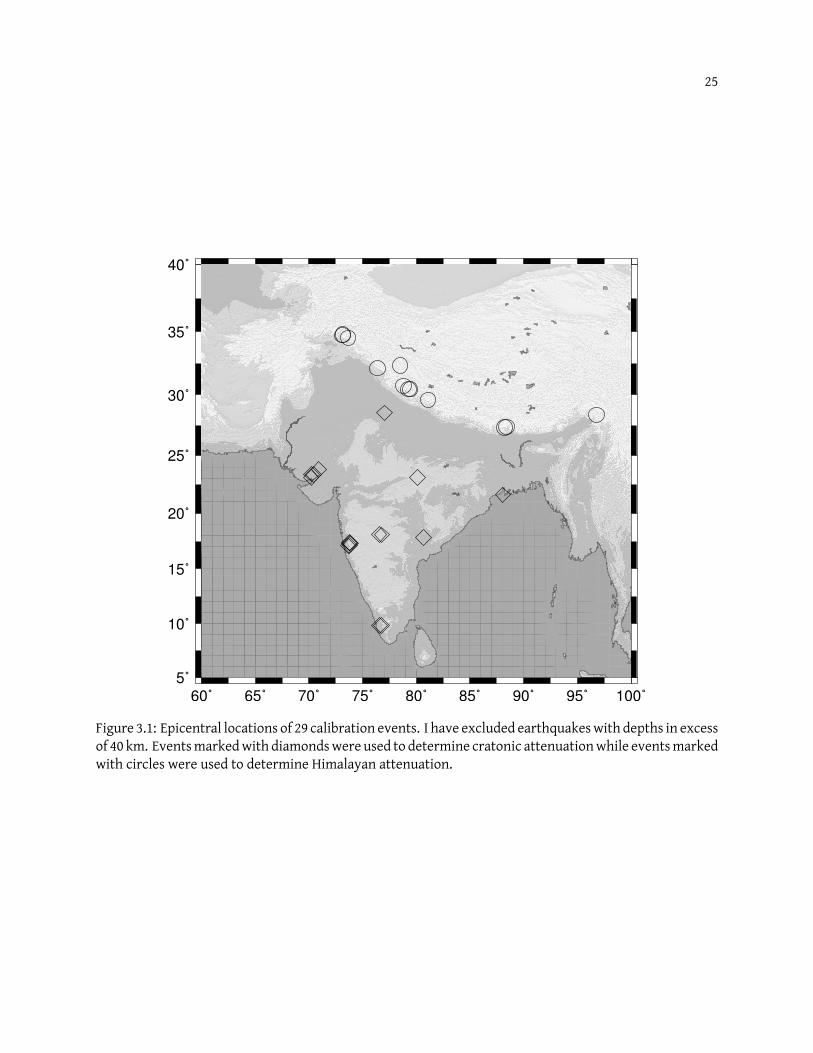
25
60˚ 65˚ 70˚ 75˚ 80˚ 85˚ 90˚ 95˚ 100˚
5˚
10˚
15˚
20˚
25˚
30˚
35˚
40˚
Figure 3.1: Epicentral locations of 29 calibration events. I have excluded earthquakeswith depths in excessof 40 km. Eventsmarkedwith diamondswere used to determine cratonic attenuationwhile eventsmarkedwith circles were used to determine Himalayan attenuation.
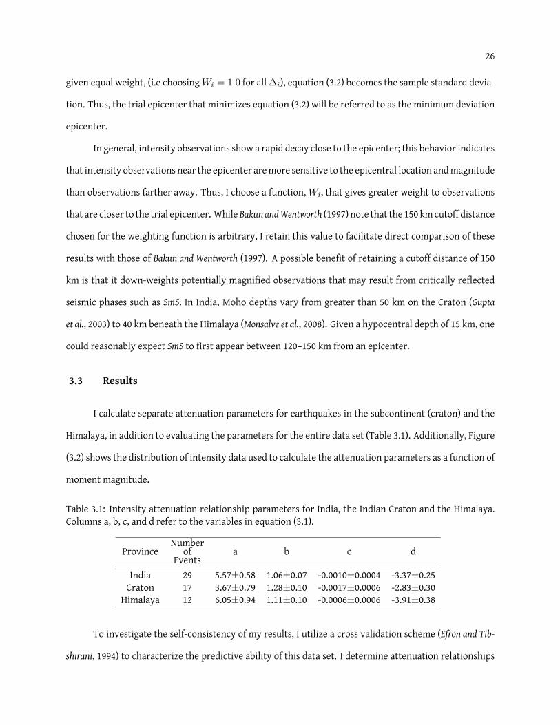
26
given equal weight, (i.e choosingWi = 1.0 for all∆i), equation (3.2) becomes the sample standard devia-
tion. Thus, the trial epicenter that minimizes equation (3.2) will be referred to as the minimum deviation
epicenter.
In general, intensity observations show a rapid decay close to the epicenter; this behavior indicates
that intensity observations near the epicenter aremore sensitive to the epicentral location andmagnitude
than observations farther away. Thus, I choose a function, Wi, that gives greater weight to observations
that are closer to the trial epicenter. While Bakun andWentworth (1997) note that the 150 kmcutoff distance
chosen for the weighting function is arbitrary, I retain this value to facilitate direct comparison of these
results with those of Bakun and Wentworth (1997). A possible benefit of retaining a cutoff distance of 150
km is that it down-weights potentially magnified observations that may result from critically reflected
seismic phases such as SmS. In India, Moho depths vary from greater than 50 km on the Craton (Gupta
et al., 2003) to 40 km beneath the Himalaya (Monsalve et al., 2008). Given a hypocentral depth of 15 km, one
could reasonably expect SmS to first appear between 120–150 km from an epicenter.
3.3 Results
I calculate separate attenuation parameters for earthquakes in the subcontinent (craton) and the
Himalaya, in addition to evaluating the parameters for the entire data set (Table 3.1). Additionally, Figure
(3.2) shows the distribution of intensity data used to calculate the attenuation parameters as a function of
moment magnitude.
Table 3.1: Intensity attenuation relationship parameters for India, the Indian Craton and the Himalaya.Columns a, b, c, and d refer to the variables in equation (3.1).
NumberProvince of a b c d
EventsIndia 29 5.57±0.58 1.06±0.07 -0.0010±0.0004 -3.37±0.25Craton 17 3.67±0.79 1.28±0.10 -0.0017±0.0006 -2.83±0.30
Himalaya 12 6.05±0.94 1.11±0.10 -0.0006±0.0006 -3.91±0.38
To investigate the self-consistency of my results, I utilize a cross validation scheme (Efron and Tib-
shirani, 1994) to characterize the predictive ability of this data set. I determine attenuation relationships
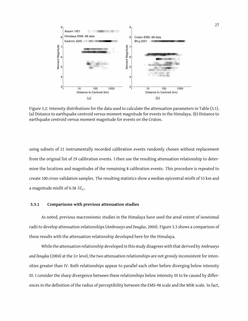
27
3
4
5
6
7
8
9
Mom
ent M
agnitude
1 10 100 1000
Distance to Centroid (km)
Assam 1951
Kashmir 2005
Himalaya EMS−98 data
(a)
3
4
5
6
7
8
9
Mom
ent M
agnitude
1 10 100 1000
Distance to Centroid (km)
Bhuj 2001
Craton EMS−98 data
(b)
Figure 3.2: Intensity distributions for the data used to calculate the attenuation parameters in Table (3.1).(a) Distance to earthquake centroid versus moment magnitude for events in the Himalaya. (b) Distance toearthquake centroid versus moment magnitude for events on the Craton.
using subsets of 21 instrumentally recorded calibration events randomly chosen without replacement
from the original list of 29 calibration events. I then use the resulting attenuation relationship to deter-
mine the locations and magnitudes of the remaining 8 calibration events. This procedure is repeated to
create 100 cross-validation samples. The resulting statistics show a median epicentral misfit of 53 km and
a magnitude misfit of 0.38Mw.
3.3.1 Comparisons with previous attenuation studies
As noted, previous macroseismic studies in the Himalaya have used the areal extent of isoseismal
radii to develop attenuation relationships (Ambraseys and Douglas, 2004). Figure 3.3 shows a comparison of
these results with the attenuation relationship developed here for the Himalaya.
While the attenuation relationship developed in this study disagreeswith that derived byAmbraseys
and Douglas (2004) at the 2σ level, the two attenuation relationships are not grossly inconsistent for inten-
sities greater than IV. Both relationships appear to parallel each other before diverging below intensity
III. I consider the sharp divergence between these relationships below intensity III to be caused by differ-
ences in the definition of the radius of perceptibility between the EMS-98 scale and the MSK scale. In fact,
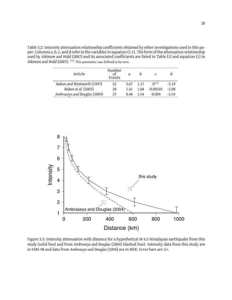
28
Table 3.2: Intensity attenuation relationship coefficients obtained by other investigations used in this pa-per. Columns a, b, c, and d refer to the variables in equation (3.1). The form of the attenuation relationshipused by Atkinson and Wald (2007) and its associated coefficients are listed in Table (1) and equation (1) inAtkinson and Wald (2007). (a) This parameter was defined to be zero.
NumberArticle of a b c d
EventsBakun and Wentworth (1997) 22 3.67 1.17 0(a) -3.19
Bakun et al. (2003) 28 1.41 1.68 -0.00345 -2.08Ambraseys and Douglas (2004) 23 0.46 1.54 -0.004 -2.54
1
2
3
4
5
6
7
8
Inte
nsity
0 200 400 600 800 1000
Distance (km)
this study
Ambraseys and Douglas (2004)
Figure 3.3: Intensity attenuation with distance for a hypothetical M 6.5 Himalayan earthquake from thisstudy (solid line) and from Ambraseys and Douglas (2004) (dashed line). Intensity data from this study arein EMS-98 and data from Ambraseys and Douglas (2004) are in MSK. Error bars are 2σ.
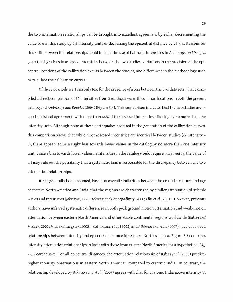
29
the two attenuation relationships can be brought into excellent agreement by either decrementing the
value of a in this study by 0.5 intensity units or decreasing the epicentral distance by 25 km. Reasons for
this shift between the relationships could include the use of half-unit intensities in Ambraseys and Douglas
(2004), a slight bias in assessed intensities between the two studies, variations in the precision of the epi-
central locations of the calibration events between the studies, and differences in the methodology used
to calculate the calibration curves.
Of these possibilities, I can only test for the presence of a bias between the two data sets. I have com-
piled a direct comparison of 95 intensities from 3 earthquakes with common locations in both the present
catalog and Ambraseys and Douglas (2004) (Figure 3.4). This comparison indicates that the two studies are in
good statistical agreement, with more than 88% of the assessed intensities differing by no more than one
intensity unit. Although none of these earthquakes are used in the generation of the calibration curves,
this comparison shows that while most assessed intensities are identical between studies (∆ Intensity =
0), there appears to be a slight bias towards lower values in the catalog by no more than one intensity
unit. Since a bias towards lower values in intensities in the catalog would require incrementing the value of
a I may rule out the possibility that a systematic bias is responsible for the discrepancy between the two
attenuation relationships.
It has generally been assumed, based on overall similarities between the crustal structure and age
of eastern North America and India, that the regions are characterized by similar attenuation of seismic
waves and intensities (Johnston, 1996; Talwani and Gangopadhyay, 2000; Ellis et al., 2001). However, previous
authors have inferred systematic differences in both peak ground motion attenuation and weak-motion
attenuation between eastern North America and other stable continental regions worldwide (Bakun and
McGarr, 2002;Miao and Langston, 2008). Both Bakun et al. (2003) and Atkinson andWald (2007) have developed
relationships between intensity and epicentral distance for eastern North America. Figure 3.5 compares
intensity attenuation relationships in India with those from eastern North America for a hypotheticalMw
= 6.5 earthquake. For all epicentral distances, the attenuation relationship of Bakun et al. (2003) predicts
higher intensity observations in eastern North American compared to cratonic India. In contrast, the
relationship developed by Atkinson and Wald (2007) agrees with that for cratonic India above intensity V,
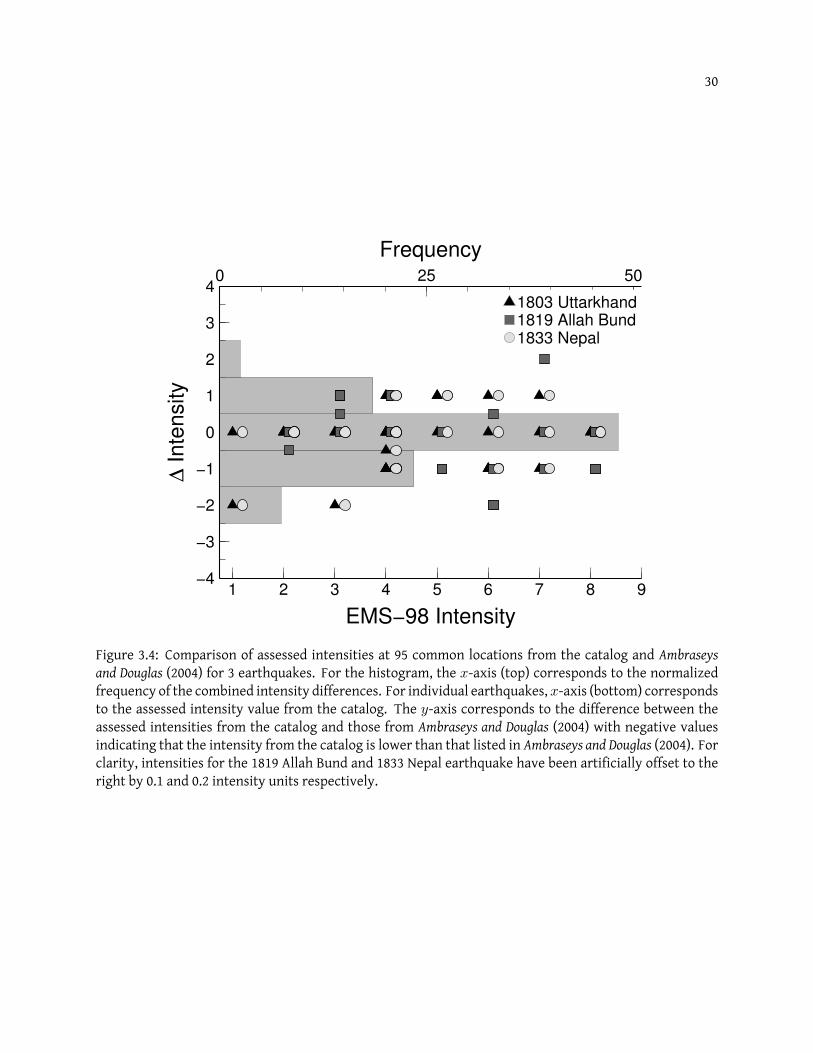
30
−4
−3
−2
−1
0
1
2
3
4
∆ Inte
nsity
1 2 3 4 5 6 7 8 9
EMS−98 Intensity
0 25 50
Frequency
1803 Uttarkhand1819 Allah Bund1833 Nepal
Figure 3.4: Comparison of assessed intensities at 95 common locations from the catalog and Ambraseysand Douglas (2004) for 3 earthquakes. For the histogram, the x-axis (top) corresponds to the normalizedfrequency of the combined intensity differences. For individual earthquakes, x-axis (bottom) correspondsto the assessed intensity value from the catalog. The y-axis corresponds to the difference between theassessed intensities from the catalog and those from Ambraseys and Douglas (2004) with negative valuesindicating that the intensity from the catalog is lower than that listed in Ambraseys and Douglas (2004). Forclarity, intensities for the 1819 Allah Bund and 1833 Nepal earthquake have been artificially offset to theright by 0.1 and 0.2 intensity units respectively.
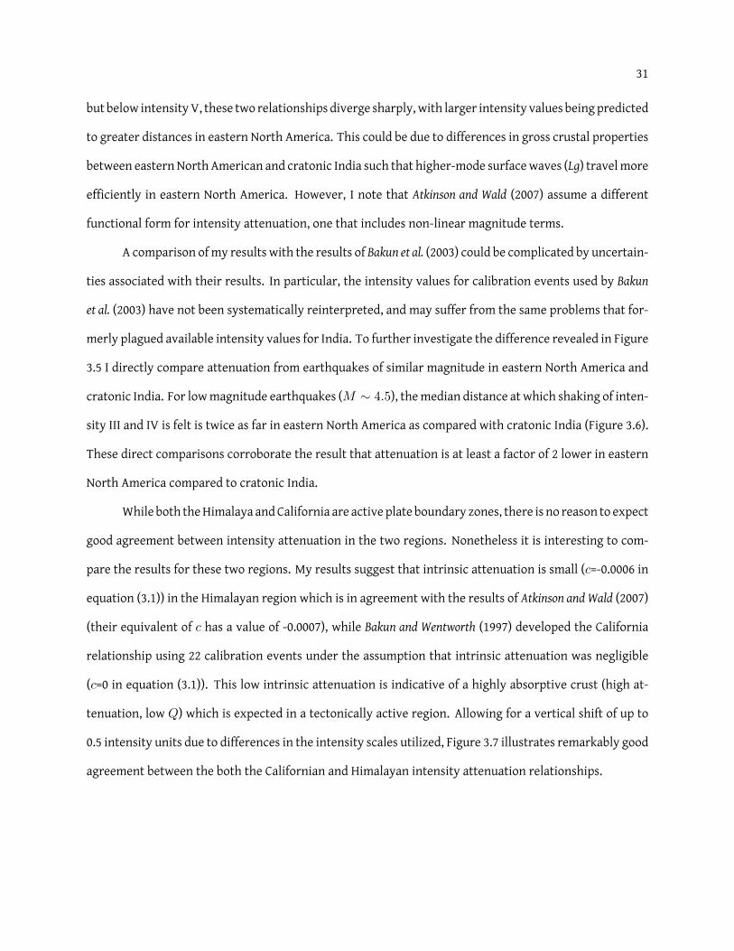
31
but below intensityV, these two relationships diverge sharply, with larger intensity values being predicted
to greater distances in eastern North America. This could be due to differences in gross crustal properties
between easternNorth American and cratonic India such that higher-mode surfacewaves (Lg) travelmore
efficiently in eastern North America. However, I note that Atkinson and Wald (2007) assume a different
functional form for intensity attenuation, one that includes non-linear magnitude terms.
A comparison ofmy results with the results of Bakun et al. (2003) could be complicated by uncertain-
ties associated with their results. In particular, the intensity values for calibration events used by Bakun
et al. (2003) have not been systematically reinterpreted, and may suffer from the same problems that for-
merly plagued available intensity values for India. To further investigate the difference revealed in Figure
3.5 I directly compare attenuation from earthquakes of similar magnitude in eastern North America and
cratonic India. For lowmagnitude earthquakes (M ∼ 4.5), themedian distance at which shaking of inten-
sity III and IV is felt is twice as far in eastern North America as compared with cratonic India (Figure 3.6).
These direct comparisons corroborate the result that attenuation is at least a factor of 2 lower in eastern
North America compared to cratonic India.
While both theHimalaya andCalifornia are active plate boundary zones, there is no reason to expect
good agreement between intensity attenuation in the two regions. Nonetheless it is interesting to com-
pare the results for these two regions. My results suggest that intrinsic attenuation is small (c=-0.0006 in
equation (3.1)) in the Himalayan region which is in agreement with the results of Atkinson and Wald (2007)
(their equivalent of c has a value of -0.0007), while Bakun and Wentworth (1997) developed the California
relationship using 22 calibration events under the assumption that intrinsic attenuation was negligible
(c=0 in equation (3.1)). This low intrinsic attenuation is indicative of a highly absorptive crust (high at-
tenuation, low Q) which is expected in a tectonically active region. Allowing for a vertical shift of up to
0.5 intensity units due to differences in the intensity scales utilized, Figure 3.7 illustrates remarkably good
agreement between the both the Californian and Himalayan intensity attenuation relationships.

32
1
2
3
4
5
6
7
8
9
10
Inte
nsity
0 200 400 600 800 1000 1200 1400
Distance (km)
this study
E. North America (Bakun et al. (2003))
CEUS (Atkinson and Wald (2007))
Figure 3.5: Intensity attenuation relationship between India from this study, the results of Bakun et al.(2003) for eastern North America, and the results of Atkinson and Wald (2007) for the Central Eastern US(CEUS) for a hypothetical M 6.5 earthquake. Indian intensity data are in EMS-98 while data from easternNorth America are in MMI. Error bars are 2σ.
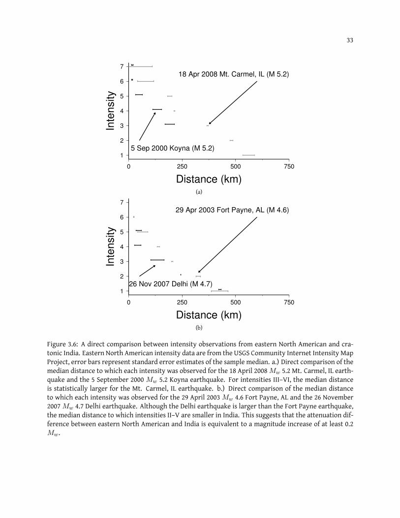
33
1
2
3
4
5
6
7
Inte
nsity
0 250 500 750
Distance (km)
5 Sep 2000 Koyna (M 5.2)
18 Apr 2008 Mt. Carmel, IL (M 5.2)
(a)
1
2
3
4
5
6
7
Inte
nsity
0 250 500 750
Distance (km)
26 Nov 2007 Delhi (M 4.7)
29 Apr 2003 Fort Payne, AL (M 4.6)
(b)
Figure 3.6: A direct comparison between intensity observations from eastern North American and cra-tonic India. Eastern North American intensity data are from the USGS Community Internet Intensity MapProject, error bars represent standard error estimates of the sample median. a.) Direct comparison of themedian distance to which each intensity was observed for the 18 April 2008Mw 5.2 Mt. Carmel, IL earth-quake and the 5 September 2000 Mw 5.2 Koyna earthquake. For intensities III–VI, the median distanceis statistically larger for the Mt. Carmel, IL earthquake. b.) Direct comparison of the median distanceto which each intensity was observed for the 29 April 2003 Mw 4.6 Fort Payne, AL and the 26 November2007 Mw 4.7 Delhi earthquake. Although the Delhi earthquake is larger than the Fort Payne earthquake,the median distance to which intensities II–V are smaller in India. This suggests that the attenuation dif-ference between eastern North American and India is equivalent to a magnitude increase of at least 0.2Mw.
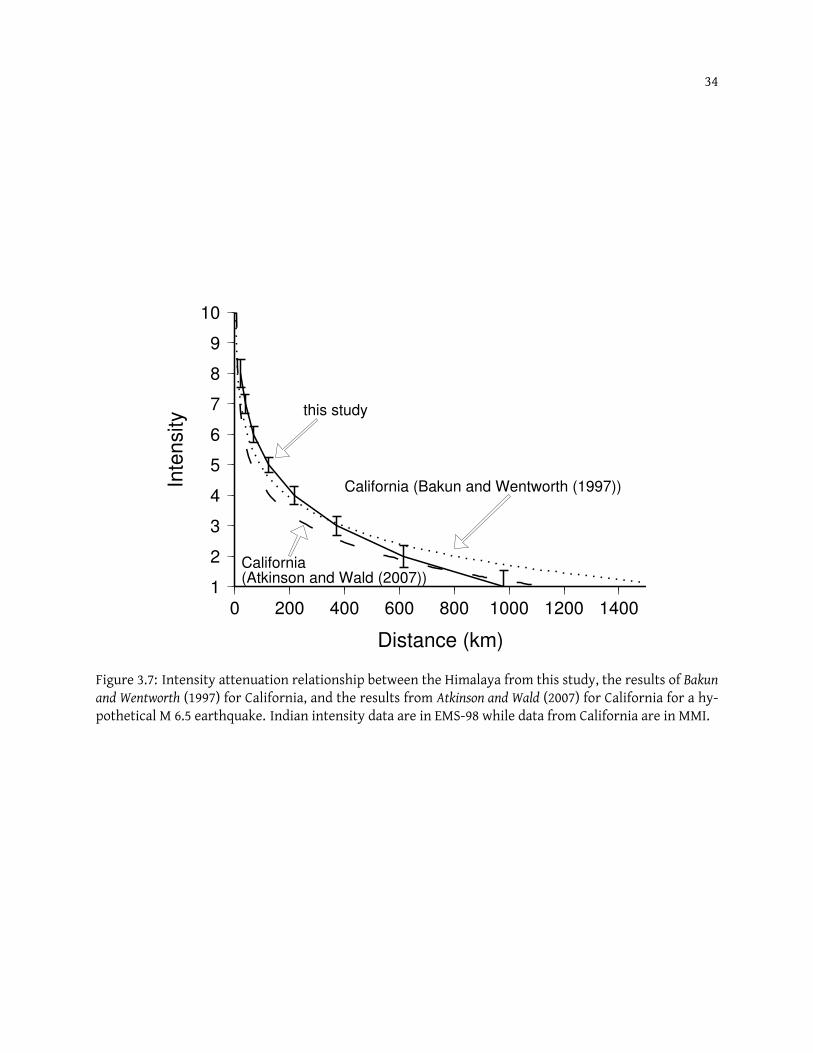
34
1
2
3
4
5
6
7
8
9
10
Inte
nsity
0 200 400 600 800 1000 1200 1400
Distance (km)
this study
California (Bakun and Wentworth (1997))
California(Atkinson and Wald (2007))
Figure 3.7: Intensity attenuation relationship between the Himalaya from this study, the results of Bakunand Wentworth (1997) for California, and the results from Atkinson and Wald (2007) for California for a hy-pothetical M 6.5 earthquake. Indian intensity data are in EMS-98 while data from California are in MMI.
35
3.4 Estimation of Historical Epicenters and Magnitudes
The precise locations of historical earthquakes in India and the Himalaya have important conse-
quences for recurrence interval studies as well as seismic hazard assessment. Using the intensity attenua-
tion relationships derived in the preceding section, I determine the locations andmagnitudes of historical
events, examine the uncertainties of epicentral locations and magnitudes, assess the completeness of the
catalog, and take a closer look at four historical earthquakes that have previously been interpreted as great
earthquakes. A list of the location andmagnitude of historical earthquakes calculated using data from the
the catalog appears in Appendix B. Finally, I use the intensity distribution for the 2001 Bhuj earthquake
to investigate what one would infer for this event, had it been known only from historical sources.
3.4.1 Epicentral Locations and Magnitudes of Historical Events
For earthquakes prior to 1890 the only information available to us for assessing the location and
magnitude of most historical earthquakes in India comes from felt intensity data. The exceptions are
for those earthquakes whose location can be constrained from independent observations such as tide
gauge data (e.g. the 1881CarNicobar earthquake (Ortiz andBilham, 2003)), documented surface rupture (e.g.
the June 1505 central Himalayan earthquake for which surface slip has been measured (D. Yule, personal
communication, 2007)), and obvious surface deformation, (e.g. the 1819 Allah Bund earthquake (Oldham,
1926) which caused local uplift and a large region of subsidence).
The catalog affords us the possibility of refining both the location and magnitude of many earth-
quakes in the historical record. Although the approach outlined in Section 3.2 offers a sophisticated
method to quantitatively evaluate a probable epicentral location and with it, a probable magnitude, I
have found that the Bakun andWentworth (1997) algorithm frequently chooses erroneous values where the
results can be compared with instrumental values. For 100 test earthquakes for which I have both inten-
sity data and an instrumental location and magnitude, the median location error is 120 km with a median
magnitude overprediction error ofMw 0.4.
The reason for the errors in location follows partly from a paucity of observations and their spatial
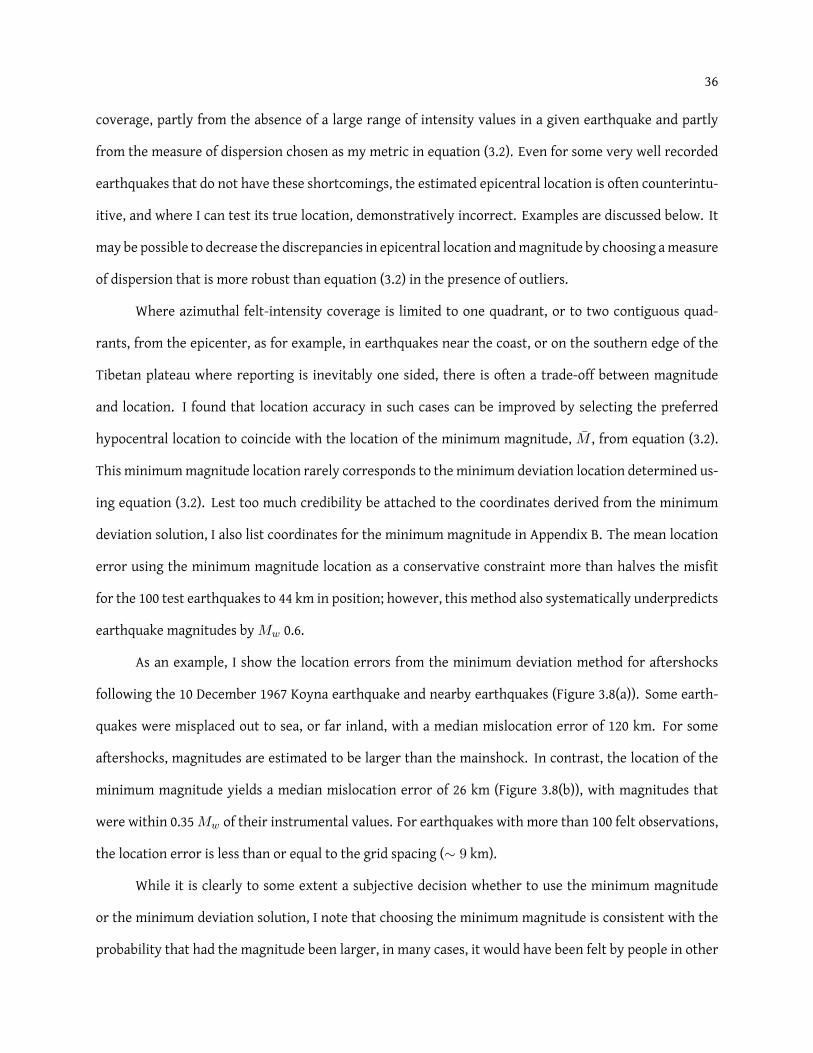
36
coverage, partly from the absence of a large range of intensity values in a given earthquake and partly
from the measure of dispersion chosen as my metric in equation (3.2). Even for some very well recorded
earthquakes that do not have these shortcomings, the estimated epicentral location is often counterintu-
itive, and where I can test its true location, demonstratively incorrect. Examples are discussed below. It
may be possible to decrease the discrepancies in epicentral location andmagnitude by choosing ameasure
of dispersion that is more robust than equation (3.2) in the presence of outliers.
Where azimuthal felt-intensity coverage is limited to one quadrant, or to two contiguous quad-
rants, from the epicenter, as for example, in earthquakes near the coast, or on the southern edge of the
Tibetan plateau where reporting is inevitably one sided, there is often a trade-off between magnitude
and location. I found that location accuracy in such cases can be improved by selecting the preferred
hypocentral location to coincide with the location of the minimum magnitude, M , from equation (3.2).
This minimummagnitude location rarely corresponds to the minimum deviation location determined us-
ing equation (3.2). Lest too much credibility be attached to the coordinates derived from the minimum
deviation solution, I also list coordinates for the minimum magnitude in Appendix B. The mean location
error using the minimum magnitude location as a conservative constraint more than halves the misfit
for the 100 test earthquakes to 44 km in position; however, this method also systematically underpredicts
earthquake magnitudes byMw 0.6.
As an example, I show the location errors from the minimum deviation method for aftershocks
following the 10 December 1967 Koyna earthquake and nearby earthquakes (Figure 3.8(a)). Some earth-
quakes were misplaced out to sea, or far inland, with a median mislocation error of 120 km. For some
aftershocks, magnitudes are estimated to be larger than the mainshock. In contrast, the location of the
minimum magnitude yields a median mislocation error of 26 km (Figure 3.8(b)), with magnitudes that
were within 0.35Mw of their instrumental values. For earthquakes with more than 100 felt observations,
the location error is less than or equal to the grid spacing (∼ 9 km).
While it is clearly to some extent a subjective decision whether to use the minimum magnitude
or the minimum deviation solution, I note that choosing the minimum magnitude is consistent with the
probability that had the magnitude been larger, in many cases, it would have been felt by people in other

37
73˚ 74˚ 75˚ 76˚ 77˚15˚00'
17˚30'
20˚00'
50 km
Thane
Koyna
Killari
Marathwada
(a) Minimum Deviation Method73˚ 74˚ 75˚ 76˚ 77˚
15˚00'
17˚30'
20˚00'
50 km
Thane
Koyna
Marathwada
(b) Minimum Magnitude Method
Figure 3.8: Comparison of the epicentral misfit for instrumentally recorded earthquakes in the Koynaregion of India. On both figures, the arrow points from the instrumental epicenter towards the intensityderived epicenter. (a) Epicentral misfit in the Koyna region using the location of theminimumof equation(3.2) as the epicentral estimate. (b) Epicentralmisfit in theKoyna regionusing the locationof theminimumM from equation (3.2).
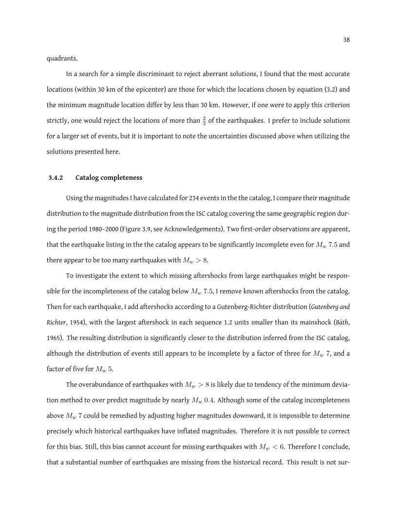
38
quadrants.
In a search for a simple discriminant to reject aberrant solutions, I found that the most accurate
locations (within 30 km of the epicenter) are those for which the locations chosen by equation (3.2) and
the minimum magnitude location differ by less than 30 km. However, if one were to apply this criterion
strictly, one would reject the locations of more than 23 of the earthquakes. I prefer to include solutions
for a larger set of events, but it is important to note the uncertainties discussed above when utilizing the
solutions presented here.
3.4.2 Catalog completeness
Using themagnitudes I have calculated for 234 events in the the catalog, I compare theirmagnitude
distribution to the magnitude distribution from the ISC catalog covering the same geographic region dur-
ing the period 1980–2000 (Figure 3.9, see Acknowledgements). Two first-order observations are apparent,
that the earthquake listing in the the catalog appears to be significantly incomplete even forMw 7.5 and
there appear to be too many earthquakes withMw > 8.
To investigate the extent to which missing aftershocks from large earthquakes might be respon-
sible for the incompleteness of the catalog below Mw 7.5, I remove known aftershocks from the catalog.
Then for each earthquake, I add aftershocks according to a Gutenberg-Richter distribution (Gutenberg and
Richter, 1954), with the largest aftershock in each sequence 1.2 units smaller than its mainshock (Bath,
1965). The resulting distribution is significantly closer to the distribution inferred from the ISC catalog,
although the distribution of events still appears to be incomplete by a factor of three for Mw 7, and a
factor of five forMw 5.
The overabundance of earthquakes withMw > 8 is likely due to tendency of the minimum devia-
tion method to over predict magnitude by nearly Mw 0.4. Although some of the catalog incompleteness
above Mw 7 could be remedied by adjusting higher magnitudes downward, it is impossible to determine
precisely which historical earthquakes have inflated magnitudes. Therefore it is not possible to correct
for this bias. Still, this bias cannot account for missing earthquakes with Mw < 6. Therefore I conclude,
that a substantial number of earthquakes are missing from the historical record. This result is not sur-
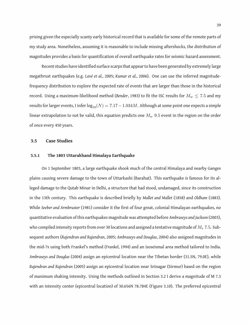
39
prising given the especially scanty early historical record that is available for some of the remote parts of
my study area. Nonetheless, assuming it is reasonable to include missing aftershocks, the distribution of
magnitudes provides a basis for quantification of overall earthquake rates for seismic hazard assessment.
Recent studies have identified surface scarps that appear to have been generated by extremely large
megathrust earthquakes (e.g. Lave et al., 2005; Kumar et al., 2006). One can use the inferred magnitude-
frequency distribution to explore the expected rate of events that are larger than those in the historical
record. Using a maximum-likelihood method (Bender, 1983) to fit the ISC results for Mw ≤ 7.5 and my
results for larger events, I infer log10(N) = 7.17− 1.034M . Although at some point one expects a simple
linear extrapolation to not be valid, this equation predicts one Mw 9.5 event in the region on the order
of once every 450 years.
3.5 Case Studies
3.5.1 The 1803 Uttarakhand Himalaya Earthquake
On 1 September 1803, a large earthquake shook much of the central Himalaya and nearby Ganges
plains causing severe damage to the town of Uttarkashi (Barahat). This earthquake is famous for its al-
leged damage to the Qutab Minar in Delhi, a structure that had stood, undamaged, since its construction
in the 13th century. This earthquake is described briefly by Mallet and Mallet (1858) and Oldham (1883).
While Seeber and Armbruster (1981) consider it the first of four great, colonial Himalayan earthquakes, no
quantitative evaluation of this earthquakesmagnitude was attempted before Ambraseys and Jackson (2003),
who compiled intensity reports fromover 30 locations and assigned a tentativemagnitude ofMs 7.5. Sub-
sequent authors (Rajendran and Rajendran, 2005; Ambraseys and Douglas, 2004) also assigned magnitudes in
the mid-7s using both Frankel’s method (Frankel, 1994) and an isoseismal area method tailored to India.
Ambraseys and Douglas (2004) assign an epicentral location near the Tibetan border (31.5N, 79.0E), while
Rajendran and Rajendran (2005) assign an epicentral location near Srinagar (Sirmur) based on the region
of maximum shaking intensity. Using the methods outlined in Section 3.2 I derive a magnitude of M 7.3
with an intensity center (epicentral location) of 30.656N 78.784E (Figure 3.10). The preferred epicentral
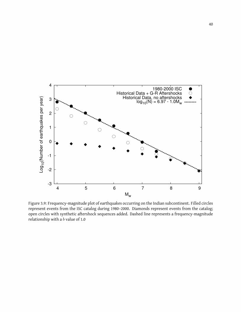
40
-3
-2
-1
0
1
2
3
4
4 5 6 7 8 9
Log
10(N
um
ber
of eart
hquakes p
er
year)
Mw
1980-2000 ISCHistorical Data + G-R Aftershocks
Historical Data, no aftershockslog10(N) = 6.97 - 1.0Mw
Figure 3.9: Frequency-magnitude plot of earthquakes occurring on the Indian subcontinent. Filled circlesrepresent events from the ISC catalog during 1980–2000. Diamonds represent events from the catalog;open circles with synthetic aftershock sequences added. Dashed line represents a frequency-magnituderelationship with a b value of 1.0
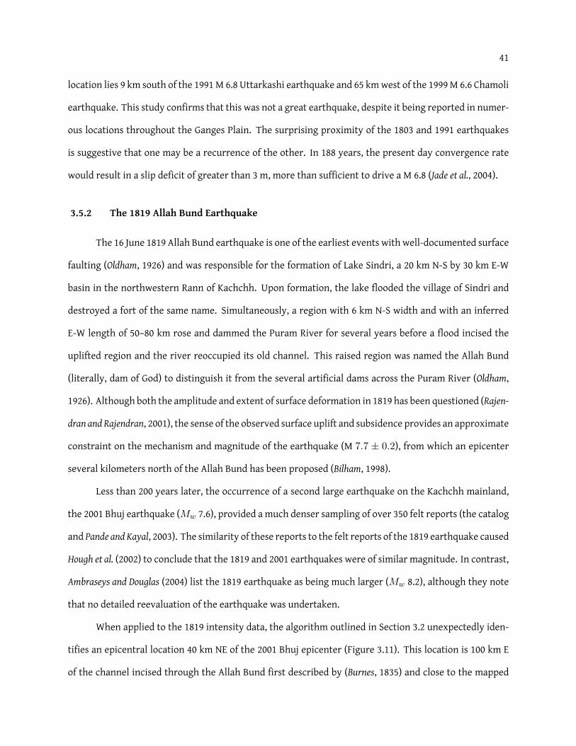
41
location lies 9 km south of the 1991M 6.8 Uttarkashi earthquake and 65 kmwest of the 1999M 6.6 Chamoli
earthquake. This study confirms that this was not a great earthquake, despite it being reported in numer-
ous locations throughout the Ganges Plain. The surprising proximity of the 1803 and 1991 earthquakes
is suggestive that one may be a recurrence of the other. In 188 years, the present day convergence rate
would result in a slip deficit of greater than 3 m, more than sufficient to drive a M 6.8 (Jade et al., 2004).
3.5.2 The 1819 Allah Bund Earthquake
The 16 June 1819 Allah Bund earthquake is one of the earliest events with well-documented surface
faulting (Oldham, 1926) and was responsible for the formation of Lake Sindri, a 20 km N-S by 30 km E-W
basin in the northwestern Rann of Kachchh. Upon formation, the lake flooded the village of Sindri and
destroyed a fort of the same name. Simultaneously, a region with 6 km N-S width and with an inferred
E-W length of 50–80 km rose and dammed the Puram River for several years before a flood incised the
uplifted region and the river reoccupied its old channel. This raised region was named the Allah Bund
(literally, dam of God) to distinguish it from the several artificial dams across the Puram River (Oldham,
1926). Although both the amplitude and extent of surface deformation in 1819 has been questioned (Rajen-
dran and Rajendran, 2001), the sense of the observed surface uplift and subsidence provides an approximate
constraint on the mechanism and magnitude of the earthquake (M 7.7 ± 0.2), from which an epicenter
several kilometers north of the Allah Bund has been proposed (Bilham, 1998).
Less than 200 years later, the occurrence of a second large earthquake on the Kachchh mainland,
the 2001 Bhuj earthquake (Mw 7.6), provided a much denser sampling of over 350 felt reports (the catalog
and Pande and Kayal, 2003). The similarity of these reports to the felt reports of the 1819 earthquake caused
Hough et al. (2002) to conclude that the 1819 and 2001 earthquakes were of similar magnitude. In contrast,
Ambraseys and Douglas (2004) list the 1819 earthquake as being much larger (Mw 8.2), although they note
that no detailed reevaluation of the earthquake was undertaken.
When applied to the 1819 intensity data, the algorithm outlined in Section 3.2 unexpectedly iden-
tifies an epicentral location 40 km NE of the 2001 Bhuj epicenter (Figure 3.11). This location is 100 km E
of the channel incised through the Allah Bund first described by (Burnes, 1835) and close to the mapped
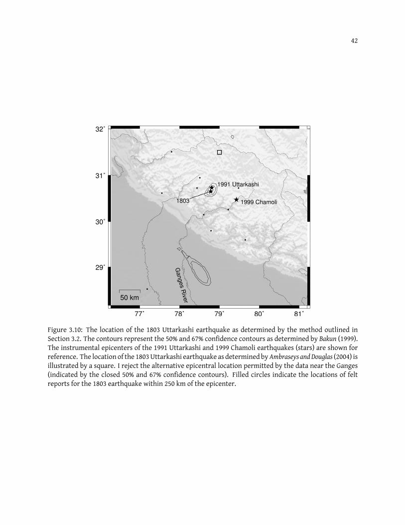
42
77˚ 78˚ 79˚ 80˚ 81˚
29˚
30˚
31˚
32˚
1803 1999 Chamoli
1991 Uttarkashi
Ganges R
iver50 km
Figure 3.10: The location of the 1803 Uttarkashi earthquake as determined by the method outlined inSection 3.2. The contours represent the 50% and 67% confidence contours as determined by Bakun (1999).The instrumental epicenters of the 1991 Uttarkashi and 1999 Chamoli earthquakes (stars) are shown forreference. The location of the 1803Uttarkashi earthquake as determined byAmbraseys andDouglas (2004) isillustrated by a square. I reject the alternative epicentral location permitted by the data near the Ganges(indicated by the closed 50% and 67% confidence contours). Filled circles indicate the locations of feltreports for the 1803 earthquake within 250 km of the epicenter.
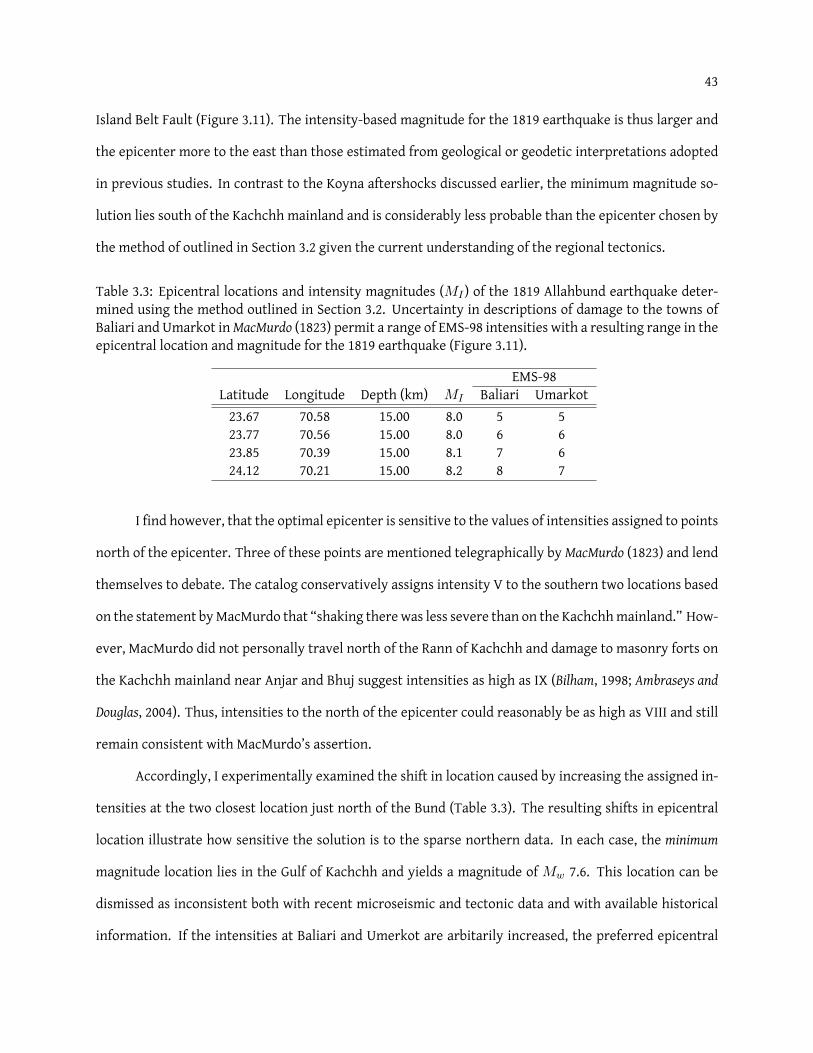
43
Island Belt Fault (Figure 3.11). The intensity-based magnitude for the 1819 earthquake is thus larger and
the epicenter more to the east than those estimated from geological or geodetic interpretations adopted
in previous studies. In contrast to the Koyna aftershocks discussed earlier, the minimum magnitude so-
lution lies south of the Kachchh mainland and is considerably less probable than the epicenter chosen by
the method of outlined in Section 3.2 given the current understanding of the regional tectonics.
Table 3.3: Epicentral locations and intensity magnitudes (MI ) of the 1819 Allahbund earthquake deter-mined using the method outlined in Section 3.2. Uncertainty in descriptions of damage to the towns ofBaliari and Umarkot inMacMurdo (1823) permit a range of EMS-98 intensities with a resulting range in theepicentral location and magnitude for the 1819 earthquake (Figure 3.11).
EMS-98Latitude Longitude Depth (km) MI Baliari Umarkot23.67 70.58 15.00 8.0 5 523.77 70.56 15.00 8.0 6 623.85 70.39 15.00 8.1 7 624.12 70.21 15.00 8.2 8 7
I find however, that the optimal epicenter is sensitive to the values of intensities assigned to points
north of the epicenter. Three of these points are mentioned telegraphically byMacMurdo (1823) and lend
themselves to debate. The catalog conservatively assigns intensity V to the southern two locations based
on the statement byMacMurdo that “shaking there was less severe than on the Kachchhmainland.” How-
ever, MacMurdo did not personally travel north of the Rann of Kachchh and damage to masonry forts on
the Kachchh mainland near Anjar and Bhuj suggest intensities as high as IX (Bilham, 1998; Ambraseys and
Douglas, 2004). Thus, intensities to the north of the epicenter could reasonably be as high as VIII and still
remain consistent with MacMurdo’s assertion.
Accordingly, I experimentally examined the shift in location caused by increasing the assigned in-
tensities at the two closest location just north of the Bund (Table 3.3). The resulting shifts in epicentral
location illustrate how sensitive the solution is to the sparse northern data. In each case, the minimum
magnitude location lies in the Gulf of Kachchh and yields a magnitude of Mw 7.6. This location can be
dismissed as inconsistent both with recent microseismic and tectonic data and with available historical
information. If the intensities at Baliari and Umerkot are arbitarily increased, the preferred epicentral
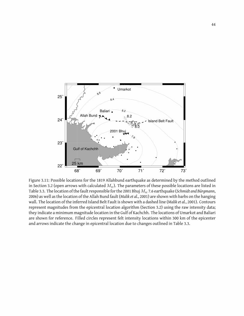
44
68˚ 69˚ 70˚ 71˚ 72˚ 73˚22˚
23˚
24˚
25˚
7.6
7.8
8
8.2
8.2
8.4
8.6
Allah Bund
Island Belt Fault
2001 Bhuj
8.08.0
8.1
8.2
Baliari
Umarkot
25 km
Gulf of Kachchh
Figure 3.11: Possible locations for the 1819 Allahbund earthquake as determined by the method outlinedin Section 3.2 (open arrows with calculatedMw). The parameters of these possible locations are listed inTable 3.3. The location of the fault responsible for the 2001 BhujMw 7.6 earthquake (Schmidt and Burgmann,2006) as well as the location of the Allah Bund fault (Malik et al., 2001) are shownwith barbs on the hangingwall. The location of the inferred Island Belt Fault is shownwith a dashed line (Malik et al., 2001). Contoursrepresent magnitudes from the epicentral location algorithm (Section 3.2) using the raw intensity data;they indicate aminimummagnitude location in the Gulf of Kachchh. The locations of Umarkot and Baliariare shown for reference. Filled circles represent felt intensity locations within 300 km of the epicenterand arrows indicate the change in epicentral location due to changes outlined in Table 3.3.
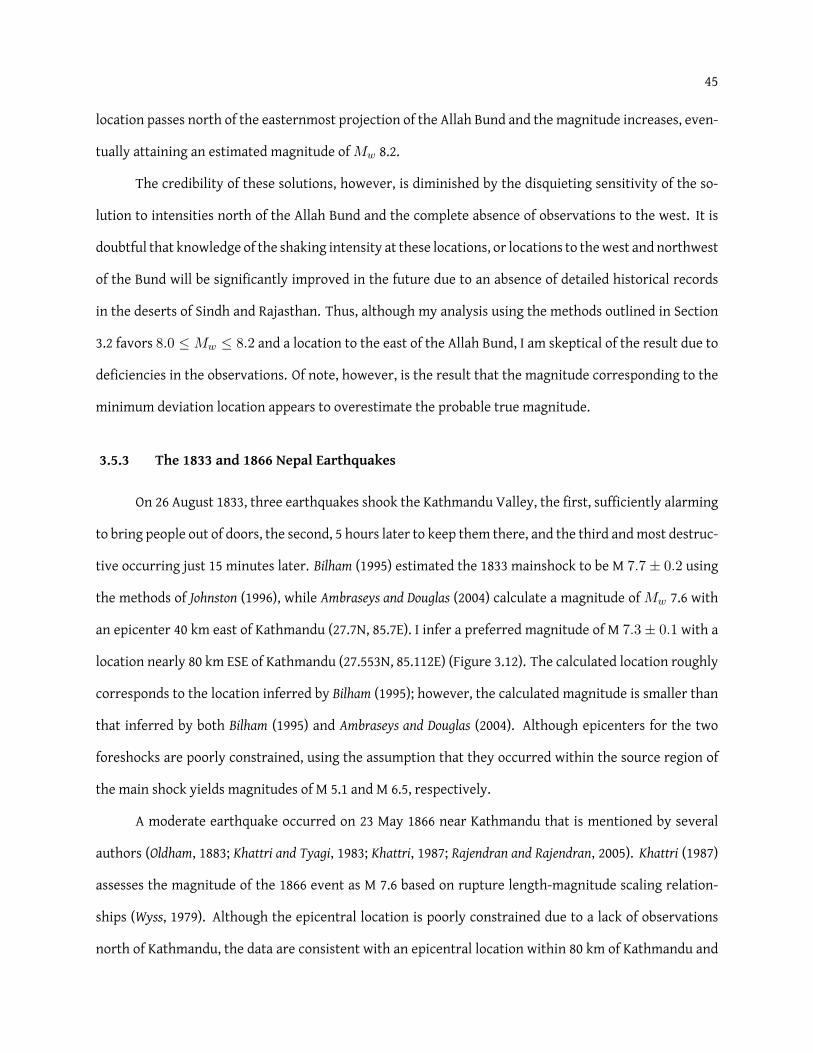
45
location passes north of the easternmost projection of the Allah Bund and the magnitude increases, even-
tually attaining an estimated magnitude ofMw 8.2.
The credibility of these solutions, however, is diminished by the disquieting sensitivity of the so-
lution to intensities north of the Allah Bund and the complete absence of observations to the west. It is
doubtful that knowledge of the shaking intensity at these locations, or locations to thewest and northwest
of the Bund will be significantly improved in the future due to an absence of detailed historical records
in the deserts of Sindh and Rajasthan. Thus, although my analysis using the methods outlined in Section
3.2 favors 8.0 ≤ Mw ≤ 8.2 and a location to the east of the Allah Bund, I am skeptical of the result due to
deficiencies in the observations. Of note, however, is the result that the magnitude corresponding to the
minimum deviation location appears to overestimate the probable true magnitude.
3.5.3 The 1833 and 1866 Nepal Earthquakes
On 26 August 1833, three earthquakes shook the Kathmandu Valley, the first, sufficiently alarming
to bring people out of doors, the second, 5 hours later to keep them there, and the third andmost destruc-
tive occurring just 15 minutes later. Bilham (1995) estimated the 1833 mainshock to be M 7.7± 0.2 using
the methods of Johnston (1996), while Ambraseys and Douglas (2004) calculate a magnitude of Mw 7.6 with
an epicenter 40 km east of Kathmandu (27.7N, 85.7E). I infer a preferred magnitude of M 7.3± 0.1 with a
location nearly 80 km ESE of Kathmandu (27.553N, 85.112E) (Figure 3.12). The calculated location roughly
corresponds to the location inferred by Bilham (1995); however, the calculated magnitude is smaller than
that inferred by both Bilham (1995) and Ambraseys and Douglas (2004). Although epicenters for the two
foreshocks are poorly constrained, using the assumption that they occurred within the source region of
the main shock yields magnitudes of M 5.1 and M 6.5, respectively.
A moderate earthquake occurred on 23 May 1866 near Kathmandu that is mentioned by several
authors (Oldham, 1883; Khattri and Tyagi, 1983; Khattri, 1987; Rajendran and Rajendran, 2005). Khattri (1987)
assesses the magnitude of the 1866 event as M 7.6 based on rupture length-magnitude scaling relation-
ships (Wyss, 1979). Although the epicentral location is poorly constrained due to a lack of observations
north of Kathmandu, the data are consistent with an epicentral location within 80 km of Kathmandu and
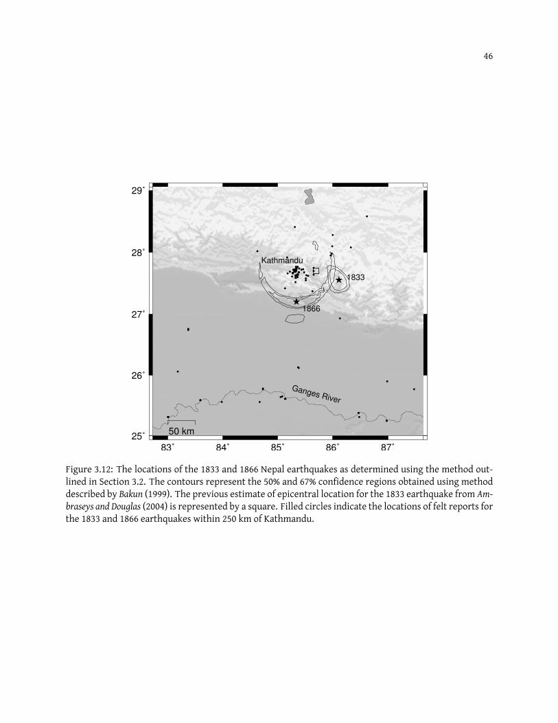
46
83˚ 84˚ 85˚ 86˚ 87˚25˚
26˚
27˚
28˚
29˚
1833
1866
Kathmandu
Ganges River
50 km
Figure 3.12: The locations of the 1833 and 1866 Nepal earthquakes as determined using the method out-lined in Section 3.2. The contours represent the 50% and 67% confidence regions obtained using methoddescribed by Bakun (1999). The previous estimate of epicentral location for the 1833 earthquake from Am-braseys and Douglas (2004) is represented by a square. Filled circles indicate the locations of felt reports forthe 1833 and 1866 earthquakes within 250 km of Kathmandu.
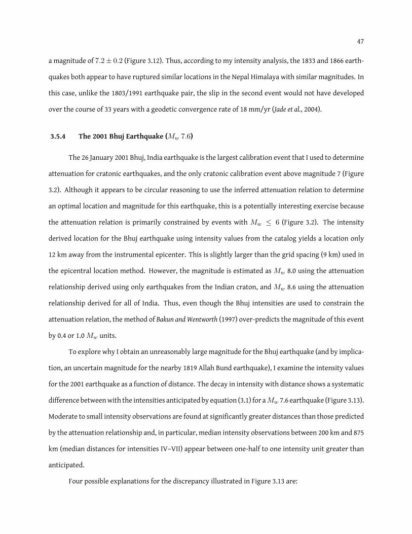
47
a magnitude of 7.2± 0.2 (Figure 3.12). Thus, according to my intensity analysis, the 1833 and 1866 earth-
quakes both appear to have ruptured similar locations in the Nepal Himalaya with similar magnitudes. In
this case, unlike the 1803/1991 earthquake pair, the slip in the second event would not have developed
over the course of 33 years with a geodetic convergence rate of 18 mm/yr (Jade et al., 2004).
3.5.4 The 2001 Bhuj Earthquake (Mw 7.6)
The 26 January 2001 Bhuj, India earthquake is the largest calibration event that I used to determine
attenuation for cratonic earthquakes, and the only cratonic calibration event above magnitude 7 (Figure
3.2). Although it appears to be circular reasoning to use the inferred attenuation relation to determine
an optimal location and magnitude for this earthquake, this is a potentially interesting exercise because
the attenuation relation is primarily constrained by events with Mw ≤ 6 (Figure 3.2). The intensity
derived location for the Bhuj earthquake using intensity values from the catalog yields a location only
12 km away from the instrumental epicenter. This is slightly larger than the grid spacing (9 km) used in
the epicentral location method. However, the magnitude is estimated as Mw 8.0 using the attenuation
relationship derived using only earthquakes from the Indian craton, and Mw 8.6 using the attenuation
relationship derived for all of India. Thus, even though the Bhuj intensities are used to constrain the
attenuation relation, the method of Bakun andWentworth (1997) over-predicts the magnitude of this event
by 0.4 or 1.0Mw units.
To explore why I obtain an unreasonably large magnitude for the Bhuj earthquake (and by implica-
tion, an uncertain magnitude for the nearby 1819 Allah Bund earthquake), I examine the intensity values
for the 2001 earthquake as a function of distance. The decay in intensity with distance shows a systematic
difference betweenwith the intensities anticipated by equation (3.1) for aMw 7.6 earthquake (Figure 3.13).
Moderate to small intensity observations are found at significantly greater distances than those predicted
by the attenuation relationship and, in particular, median intensity observations between 200 km and 875
km (median distances for intensities IV–VII) appear between one-half to one intensity unit greater than
anticipated.
Four possible explanations for the discrepancy illustrated in Figure 3.13 are:
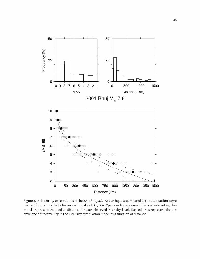
48
2
3
4
5
6
7
8
9
10
EM
S−
98
0 150 300 450 600 750 900 1050 1200 1350 1500
Distance (km)
2001 Bhuj Mw 7.6
0
25
50
Fre
quency (
%)
12345678910
MSK
0
25
50
0 500 1000 1500
Distance (km)
Figure 3.13: Intensity observations of the 2001 BhujMw 7.6 earthquake compared to the attenuation curvederived for cratonic India for an earthquake of Mw 7.6. Open circles represent observed intensities, dia-monds represent the median distance for each observed intensity level. Dashed lines represent the 2-σenvelope of uncertainty in the intensity attenuation model as a function of distance.
49
(1) That intensities for the Bhuj earthquake were systematically over-estimated.
(2) That there is, or can be, a non-linear dependence of intensities on magnitude for large earth-
quakes.
(3) That intensity observations at regional distances are amplified by the presence of higher-mode
surface (Lg) waves.
(4) That the intensity observations for the Bhuj earthquake indicate a high-Q in the Kachchh Basin.
I shall address each possibility in turn. First, I consider it unlikely that the intensities for the Bhuj
earthquake were systematically over-estimated. Most of the values for Bhuj in the catalog are, in fact,
systematically lower than the values inferred by Hough et al. (2002) whose intensity assignments were
based onmedia reports andhave been shown to be biased relative to those estimated fromdirect surveying
of damage (Hough and Pande, 2007).
Second, the functional form of equation (3.1) is identical to the functional form assumed for atten-
uation of peak ground acceleration (Evernden et al., 1973). Several studies have shown a good correspon-
dence between intensity and instrumentally determined ground motion measures (e.g.Wald et al., 1999b).
One might therefore reasonably expect equation (3.1) to be appropriate for characterizing intensity at-
tenuation for large events. Short of significant non-linearity associated with ground motions at sediment
sites, equation (3.1) appears to be appropriate for characterization of peak ground acceleration for large
and small earthquakes.
Third, when higher-mode surface wave trains develop and propagate in the continental crust, the
highest amplitude shaking typically has a long duration. It is thus reasonable, if not expected, that a pro-
longedLg wavetrain with a given peak acceleration will produce a higher perceived intensity observation
than groundmotions with the same peak acceleration and amuch shorter duration. Shaking durationwill
clearly be a potential factor for structural damage; it is self-evident that marginally perceptible shaking
is more likely to be felt if the strongest amplitudes are prolonged. Clearly, human perception of higher-
mode surface waves decreases with distance from the epicenter by a non-integer amount. Thus, a simple,
uniform adjustment of intensity observations to correct for amplification is not possible.
50
Lastly, I can consider the possibility that the intensity distribution reflects especially high-Q in the
Kachchh Basin. Bodin et al. (2004) calculate Q for the Kachchh Basin using aftershocks of the 2001 Bhuj
earthquake and note that their estimates are higher than estimates of Q in northern India calculated by
Singh et al. (1999). In contrast, in a regional study of Lg attenuation, Pasyanos et al. (2009) shows values
of Q in the Kachchh Basin to be closer to those measured in northern India (Singh et al., 1999). Addition-
ally, results in Mitra et al. (2006) indicate that estimates of Q from the 2001 Bhuj earthquake itself are
systematically higher than estimates from other regional events. To test the possibility that the attenua-
tion properties of the Kachchh Basin affect intensity observations and consequently inflate the calculated
magnitude of the 2001 Bhuj earthquake, I removed all intensity observations within 200 km of the Bhuj
epicenter and inverted for magnitude. The removal of all observations within 200 km of the epicenter
results in an increase in epicentral location uncertainty, but essentially no change in magnitude. This is
not surprising since equation (3.1) indicates that a change in magnitude will have a larger influence on
distant, lower intensity observations than near-source high intensity observations.
For large earthquakes, locations are well determinedwhere sufficient spatial coverage exists. How-
ever, the magnitudes of large events are not well determined using the method outlined in Section 3.2,
and requires consideration. As shown in Figure 3.13, the intensity values do not generally match the
intensities predicted by equation (3.1) for a Mw 7.6 earthquake between distances 200 km and 875 km
from the epicenter. In addition, the inferred intensity distribution includes moderate intensities to sig-
nificantly greater distances than the predicted distribution. The lowest felt intensities (II–III) similarly
extend farther than predicted. These results suggest that the formation of higher-mode surfaces waves
due to long shaking durations in a high-Q environment have amplified intensity observations at regional
distances. Simple correction of this amplification is not possible and these results moreover provide a
caution regarding the use of the Bakun and Wentworth (1997) method with an attenuation relation of the
form given by equation (3.1). In particular, if the attenuation relation is constrained largely or entirely by
small or moderate earthquakes, the magnitudes estimated for large historical earthquakes can be grossly
overestimated.
51
3.6 Discussion
The determination of the magnitudes of historical earthquakes is of interest since, were a com-
plete inventory of historical earthquakes available, I could subject a region to investigations of moment
release over space and time. Statistical tests assuming a Gutenberg-Richter distribution of magnitudes
show that I am missing 30% of the moderate earthquakes during the period for which most of data are
derived (1800–2000). Thus, while moment-release studies can be undertaken for the entire region, they
are doomed to be less reliable on a local scale, in particular for the relatively frequent 6.5 ≤ Mw ≤ 7.5
events that are typically important for controlling probabilistic hazard.
The caveat discussed in the previous section, that attenuation findings for small earthquakes do not
provide satisfactory predictions for the attenuation observed in the largest earthquakes and therefore
unsatisfactory magnitude predictions, is perceived to be a substantial problem in India, since it is for
these largest earthquakes that reliable magnitude information is most needed. It is possible that a similar
problem exists with the intensity relations established for North America.
Epicentral locations determined using the methods I describe show demonstrable scatter. One
question that arises in the determination of magnitude and epicentral location for early earthquakes is
what constitutes an acceptable determination of these parameters. If I am interested in establishing an
inventory of potentially active faults, I should presumably prefer locations that lie within one source di-
mension, e.g. a fault rupture length, of the earthquake. If I am interested in identifying segments of those
faults that remain unruptured, I require yet higher accuracy. It is clear from the analysis I present here
that few of the post-1950 solutions for earthquakes with Mw < 6 are within one fault length of the in-
strumental epicenter, and by implication I must assume that the same is true of the earthquakes earlier
in the catalog.
For many of the events in the catalog with poor intensity coverage, I do not attempt to determine
a location using quantitative methods. Yet even for these earthquakes I recognize that the approximate
location and its intensity data are of utility in seismic hazard studies. Chapter 2 utilizes this information
to map maximum shaking intensity encountered in a grid throughout India.
52
For larger earthquakes (7 < Mw < 8) where rupture lengths range from 30 km to 300 km I find, in
general, that the preferred location lies near or above the inferred rupture surface, but I note that even
for some very large earthquakes in the catalog the dimensions and location of the rupture zone remain
enigmatic (e.g Chittagong 1762 and Bihar-Nepal 1934).
For 100 earthquakes in the instrumental period (post 1950) for which I have both epicentral pa-
rameters and intensity data, I find that fewer than 30% of these earthquakes can be located to within one
fault length of the true epicenter using intensity data. The median mislocation location error using the
method of Bakun andWentworth (1997) exceeds 100 km. However, choosing the minimummagnitude loca-
tion instead of the minimum deviation location reduces the misfit by a factor of two. The reason for the
poor performance of the algorithm is partly due to the small number of observations available formany of
these earthquakes as well as the small dynamic range of the intensity observations for each earthquake. I
conclude that the algorithm cannot be expected to do better for historical earthquakes; locations accura-
cies are likely to be no better than 50 km. One disappointing result is that from the data alone, there seems
to be no reliable way to characterize the quality of each solution. In general, earthquakes with fewer than
10 locations gave consistently unreliable locations. I found that the least reliable solutions were those
where large differences were found between the minimum deviation location and the minimum magni-
tude location. The best locations were found to be those in which these two locations agreed to within 30
km, but this applies to fewer than 30% of the data.
3.7 Conclusions
Newly available intensity observations for India provide a wealth of material for evaluating the
location and magnitude of numerous earthquakes that have hitherto been amenable only to qualitative
analysis, and, in particular, permit us to assess attenuation throughout the subcontinent. I use attenua-
tion relation derived from modern (post 1950) earthquakes with well-determined instrumental locations
and the method of Bakun and Wentworth (1997) to estimate the optimal locations and magnitudes for 181
historical earthquakes, with case studies of large events in 1803, 1819, 1833, and 1866.
Of particular interest are the characteristic attenuation versus distance parameters for India. I
53
quantify attenuation for all Indian earthquakes, and separately for plate boundary events (Himalaya) and
cratonic events. I find that intensity attenuation in theHimalaya region is comparable to that in California,
while attenuation in cratonic India is significantly higher than attenuation in the central/eastern United
States.
One unexpected finding is that for the largest of the cratonic earthquakes (Bhuj 2001 and Allah
Bund 1819) my attenuation relation significantly overestimates the magnitudes estimated from instru-
mental and/or geological constraints. This results from shaking being felt more strongly out to greater
distances than expected bymy attenuation relationship. I suggest that thismay be a systematic effect that
is common to all attenuation models. The distant shaking from large earthquakes is simply not well char-
acterized by shaking from small earthquakes. I propose that the duration ofLg shaking at large distances
may be responsible for this effect.
My search for uncertainty criteria to describe location accuracy is unsatisfactory in that I have
found no objectivemethod, from the intensity data alone, to quantify the accuracy ofmy solutions. Where
more than 100 intensity values are available the solution is usually within 30 km of the true epicenter.
This criteria applies to only 16 events, less than 3% of the catalog. Where the minimum deviation and
minimum-magnitude solution are close, the calculated epicenter is usuallywithin 30 kmof the instrumen-
tal location, but even this condition applies to less than 30% of the instrumental catalog, and by extension,
to fewer than 177 of the 570 earthquakes in the entire catalog.
Themagnitudes of earthquakes in the instrumental periodwere notwell characterized by the Bakun
and Wentworth (1997) algorithm. This is perhaps not too surprising since the assigned magnitude for a
given attenuation depends on distance, which as summarized above shows a large range of mislocation
errors. Magnitudes were in general overestimated by a median mismatch of Mw 0.4 for the 100 earth-
quakes for which instrumental magnitudes were known. The median magnitude misfit using the mini-
mum magnitude location underpredicts the instrumental magnitude byMw 0.6. Again, this uncertainty
in magnitude suggests that historical earthquakes cannot be characterized to better thanMw ± 0.5 from
the historical data analyzed here.
Chapter 4
Interseismic Strain Accumulation along the Western Boundary of the IndianSubcontinent
4.1 Introduction
The Chaman Fault System is a major continental plate boundary transform zone separating the
Indian and Eurasian plates. South of the Afghanistan/Pakistan border, this fault system is composed of
three major left-lateral faults, the Chaman, the Ghazaband and the Ornach-Nal faults (Figure 4.1). The
Chaman Fault proper comprises themajority (860 km) of this 1250 km long transform zonewhich connects
the Makran subduction zone to the currently inactive right-lateral Herat Fault in northern Afghanistan. I
utilize two campaign GPS transects bounded on their East by continuous GPS stations located on the stable
Indian Plate to estimate the interseismic deformation rate along the Chaman Fault System. North of the
town of Chaman, Pakistan, I utilize nearly 4.5 years of InSAR data to produce a fault-centered transect of
interseismic deformation rate. In all three locations I examined, I find shallow locking depths. In regions
with shallow locking depths, large strike-slip earthquakes (Mw > 7) are unlikely due to the reduced
seismogenic thickness. However, large earthquakes have occurred in the past century in the ranges east
of the Chaman Fault both east and south of Quetta. The absence of GPS data south of the town of Chaman,
Pakistan hinders the ability to estimate interseismic deformation rates in this region.
4.2 Tectonic Summary
The Ornach-Nal fault is the southernmost on-land segment of the Chaman Fault System (Figure 4.1;
Zaigham (1991); Lawrence et al. (1992)). Running nearly 250 km north from the Makran Coast, the Ornach-
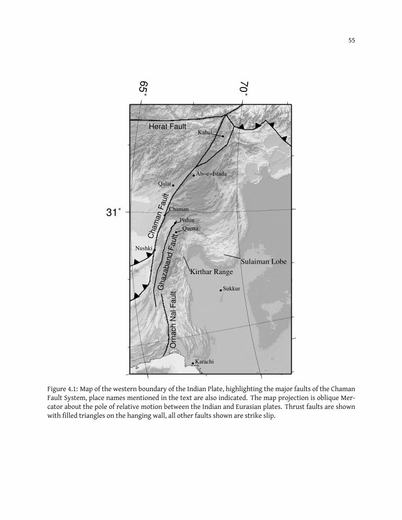
55
65˚
70˚
31˚
Orn
ach
Na
l F
au
lt
Ghazaband F
aultC
ham
an F
ault
Herat Fault
Quetta
Chaman
Pishin
Nushki
Sukkur
Karachi
Ab−e−Istada
Qalat
Kabul
Sulaiman Lobe
Kirthar Range
Figure 4.1: Map of the western boundary of the Indian Plate, highlighting the major faults of the ChamanFault System, place names mentioned in the text are also indicated. The map projection is oblique Mer-cator about the pole of relative motion between the Indian and Eurasian plates. Thrust faults are shownwith filled triangles on the hanging wall, all other faults shown are strike slip.
56
Nal Fault offsets primarily Cenozoicmudstones and shales (Snead, 1964; Zaigham, 1991; Lawrence et al., 1992).
The lack of detailed fieldmapping in this region, combinedwith themonotonyof themudstones and shales
have made estimates of the total offset across the Ornach-Nal fault impossible.
At the northern terminus of theOrnach-Nal fault, deformation likely stepswestward onto theGhaz-
aband Fault (Figure 4.1). Although no modern geodetic measurements exists across this segment of the
Chaman Fault System, the Ghazaband fault is a likely candidate for the source of the 1935 Quetta earth-
quake (∼ M 7.5) which caused surface cracking and extensive damage in the populated valleys south of
Quetta and approximately 15 km east of the Ghazaband Fault (Ramanathan and Mukherji, 1938; Engdahl and
Villasenor, 2002). The Ghazaband Fault parallels the Chaman fault northward to the town of Pishin where
it disappears into the southern end of the seismically quiet Katawaz Block (Haq and Davis, 1997).
South of the village of Nushki, Pakistan, the last of the arcuate thrust faults of the Makran merge
to form the N-S trending Chaman Fault (Figure 4.1). The Chaman Fault and Ghazaband Fault parallel each
other northwards to the latitude of the town of Chaman, Pakistan. Immediately north of the town of
Chaman, the fault veers NNE, enters Afghanistan and becomes the dominant fault in the Chaman Fault
System.
Lawrence et al. (1992) estimate the onset of faulting along the Chaman Fault System as Oligocene-
Miocene based on post-depositional offsets of the Eocene-Oligocene aged Khojak flysch. These displace-
ments suggest an average slip-rate of 19–24 mm/yr over the last 20–25 My. Similarly, correlation of
Pliocene volcanic units that straddle the fault north of Ab-e-Istada, Afghanistan, yields an average slip-rate
of 25–35 mm/yr over the last 2 My (Beun et al., 1979).
Kinematic and analogue modeling of the western boundary of the Indian plate indicates that pure
strike-slip motion is required along the Chaman fault with shortening being accommodated in the Su-
laiman Lobe and Kirthar ranges to the east of the Chaman fault (Haq and Davis, 1997; Bernard et al., 2000).
Estimates of modern plate motion indicate convergence of the Indian plate relative to Eurasia at a rate of
27 mm/yr at N7E near Sukkur, Pakistan (Altamimi et al., 2007). I estimate the amount of sinistral slip along
the Chaman Fault by noting that its strike between Chaman and Ab-e-Istada is approximately N34E, sug-
gesting approximately 24mm/yr of sinistralmotion and 12mm/yr of shortening are being accommodated
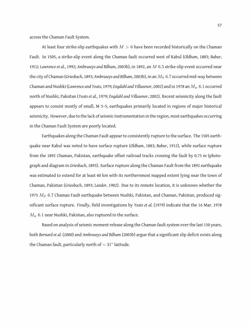
57
across the Chaman Fault System.
At least four strike-slip earthquakes with M > 6 have been recorded historically on the Chaman
Fault. In 1505, a strike-slip event along the Chaman fault occurred west of Kabul (Oldham, 1883; Babur,
1912; Lawrence et al., 1992; Ambraseys and Bilham, 2003b), in 1892, anM 6.5 strike-slip event occurred near
the city of Chaman (Griesbach, 1893; Ambraseys and Bilham, 2003b), in anMS 6.7 occurredmid-way between
Chaman andNushki (Lawrence and Yeats, 1979; Engdahl andVillasenor, 2002) and in 1978 anMw 6.1 occurred
north of Nushki, Paksitan (Yeats et al., 1979; Engdahl and Villasenor, 2002). Recent seismicity along the fault
appears to consist mostly of small, M 3–5, earthquakes primarily located in regions of major historical
seismicity. However, due to the lack of seismic instrumentation in the region, most earthquakes occurring
in the Chaman Fault System are poorly located.
Earthquakes along the Chaman Fault appear to consistently rupture to the surface. The 1505 earth-
quake near Kabul was noted to have surface rupture (Oldham, 1883; Babur, 1912), while surface rupture
from the 1892 Chaman, Pakistan, earthquake offset railroad tracks crossing the fault by 0.75 m (photo-
graph and diagram in Griesbach, 1893). Surface rupture along the Chaman Fault from the 1892 earthquake
was estimated to extend for at least 60 km with its northernmost mapped extent lying near the town of
Chaman, Pakistan (Griesbach, 1893; Landor, 1902). Due to its remote location, it is unknown whether the
1975 MS 6.7 Chaman Fault earthquake between Nushki, Pakistan, and Chaman, Pakistan, produced sig-
nificant surface rupture. Finally, field investigations by Yeats et al. (1979) indicate that the 16 Mar. 1978
Mw 6.1 near Nushki, Pakistan, also ruptured to the surface.
Based on analysis of seismicmoment release along the Chaman fault system over the last 150 years,
both Bernard et al. (2000) and Ambraseys and Bilham (2003b) argue that a significant slip deficit exists along
the Chaman fault, particularly north of∼ 31◦ latitude.

58
4.3 Methods
4.3.1 GPS
GPS measurements in Pakistan are historically of limited coverage and duration with no measure-
ments prior to 2001. Campaignmeasurements from 13 sites with locations predominantly north of Quetta
as well as 8 sites along the Makran coast and inland to Panjgur, Pakistan, have been measured at least
twice in the period 2006–2010 and compared to continuousmeasurementsmade in Karachi (KCHI), Sukkur
(SIBA), Peshawar (NCEG) and Quetta (QTAG and QTIT) (Figure 4.2).
The location of campaign GPS measurements across both the Chaman and Ornach-Nal faults are
constrained by the location of major roads to provide security and ease of access. The continuous points
in Pakistan are operated from flat-roofed concrete frame buildings and the campaign points aremeasured
on bipods set on stainless steel screws cemented into exposed rock. GPS observations were recorded with
Trimble NetRS, 5700 and R7 receivers using a 30 s sampling rate, and processed using an elevation cutoff
angle of 10◦. Campaign data have durations of 3–7 days from each site.
Daily data from all sites were processed along with data from at least 4 continuous stations in Pak-
istan and 10 regional IGS stations using GAMIT version 10.35 (King and Bock, 2002). These regional solutions
were then combined with global solutions from SOPAC (http://sopac.ucsd.edu) using GLOBK/GLORG
version 5.17 (Herring, 2002) to determine time series and velocities consistent with the ITRF2005 reference
frame. To achievemore realistic uncertainties, velocities were re-estimated using randomwalk noise esti-
mates obtained from iterative time series modeling. Final velocities were then transformed into an Indian
plate-fixed reference frame using pole-of-rotation parameters published in Altamimi et al. (2007).
4.3.2 InSAR
I acquired 27 ascending pass SAR scenes spanning nearly 4.5 years from track 213 frame 621 of the
European Space Agency’s Envisat satellite (Figure 4.2A, 4.3). A 90 meter resolution DEM was constructed
from SRTM version 2 data (Farr et al., 2007) and used to remove topographic fringes. Interferograms
were produced using the ROI PAC InSAR software package developed at the Jet Propulsion Laboratory
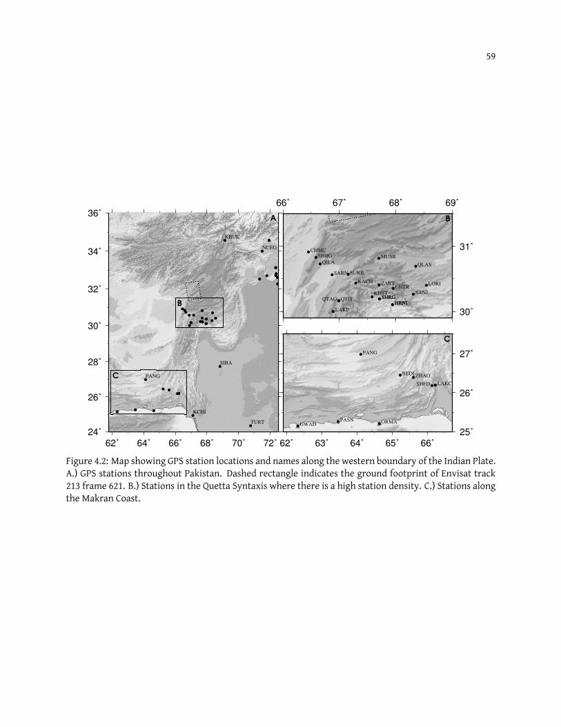
59
62˚ 64˚ 66˚ 68˚ 70˚ 72˚
24˚
26˚
28˚
30˚
32˚
34˚
36˚
NCEG
TURT
KBUL
SIBA
KCHI
PANG
A
B
C
62˚ 63˚ 64˚ 65˚ 66˚
25˚
26˚
27˚
ZHAOBEDI
ORMA
PANG
PASNGWAD
SHFD LAKC
C
66˚ 67˚ 68˚ 69˚
30˚
31˚
LORI
QLAS
SANJ
CHTR
HRNIHRNI
SHRGSHRG
ZART
MUSB
KACH
SURB
QTIT
LAKP
SARN
QILA
SHBGCHMC
KHST
QTAG
B
Figure 4.2: Map showing GPS station locations and names along the western boundary of the Indian Plate.A.) GPS stations throughout Pakistan. Dashed rectangle indicates the ground footprint of Envisat track213 frame 621. B.) Stations in the Quetta Syntaxis where there is a high station density. C.) Stations alongthe Makran Coast.
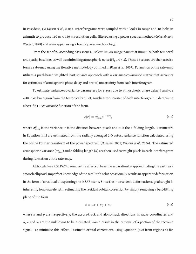
60
in Pasadena, CA (Rosen et al., 2004). Interferograms were sampled with 8 looks in range and 40 looks in
azimuth to produce 160 m× 160 m resolution cells, filtered using a power spectral method (Goldstein and
Werner, 1998) and unwrapped using a least squares methodology.
From the set of 27 ascending pass scenes, I select 12 SAR image pairs that minimize both temporal
and spatial baselines aswell asminimizing atmospheric noise (Figure 4.3). These 12 scenes are then used to
form a rate-map using the iterative methodology outlined in Biggs et al. (2007). Formation of the rate-map
utilizes a pixel-based weighted least squares approach with a variance-covariance matrix that accounts
for estimates of atmospheric phase delay and orbital uncertainty from each interferogram.
To estimate variance-covariance parameters for errors due to atmospheric phase delay, I analyze
a 48× 48 km region from the tectonically quiet, southeastern corner of each interferogram. I determine
a best-fit 1-D covariance function of the form,
c(r) = σ2atme(−αr), (4.1)
where σ2atm is the variance, r is the distance between pixels and α is the e-folding length. Parameters
in Equation (4.1) are estimated from the radially averaged 2-D autocovariance function calculated using
the cosine Fourier transform of the power spectrum (Hanssen, 2001; Parsons et al., 2006). The estimated
atmospheric variance (σ2atm) and e-folding length (α) are then used toweight pixels in each interferogram
during formation of the rate-map.
Although I use ROI PAC to remove the effects of baseline separation by approximating the earth as a
smooth ellipsoid, imperfect knowledge of the satellite’s orbit occasionally results in apparent deformation
in the form of a residual tilt spanning the InSAR scene. Since the interseismic deformation signal sought is
inherently long-wavelength, estimating the residual orbital correction by simply removing a best-fitting
plane of the form
z = ux+ vy + w, (4.2)
where x and y are, respectively, the across-track and along-track directions in radar coordinates and
u, v and w are the unknowns to be estimated, would result in the removal of a portion of the tectonic
signal. To minimize this effect, I estimate orbital corrections using Equation (4.2) from regions as far
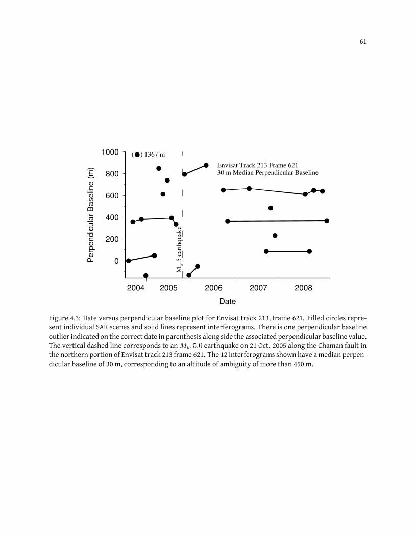
61
0
200
400
600
800
1000
Perp
endic
ula
r B
aselin
e (
m)
2004 2005 2006 2007 2008
Date
Envisat Track 213 Frame 62130 m Median Perpendicular Baseline
Mw
5 e
arth
qu
ake
( ) 1367 m
Figure 4.3: Date versus perpendicular baseline plot for Envisat track 213, frame 621. Filled circles repre-sent individual SAR scenes and solid lines represent interferograms. There is one perpendicular baselineoutlier indicated on the correct date in parenthesis along side the associated perpendicular baseline value.The vertical dashed line corresponds to anMw 5.0 earthquake on 21 Oct. 2005 along the Chaman fault inthe northern portion of Envisat track 213 frame 621. The 12 interferograms shown have amedian perpen-dicular baseline of 30 m, corresponding to an altitude of ambiguity of more than 450 m.
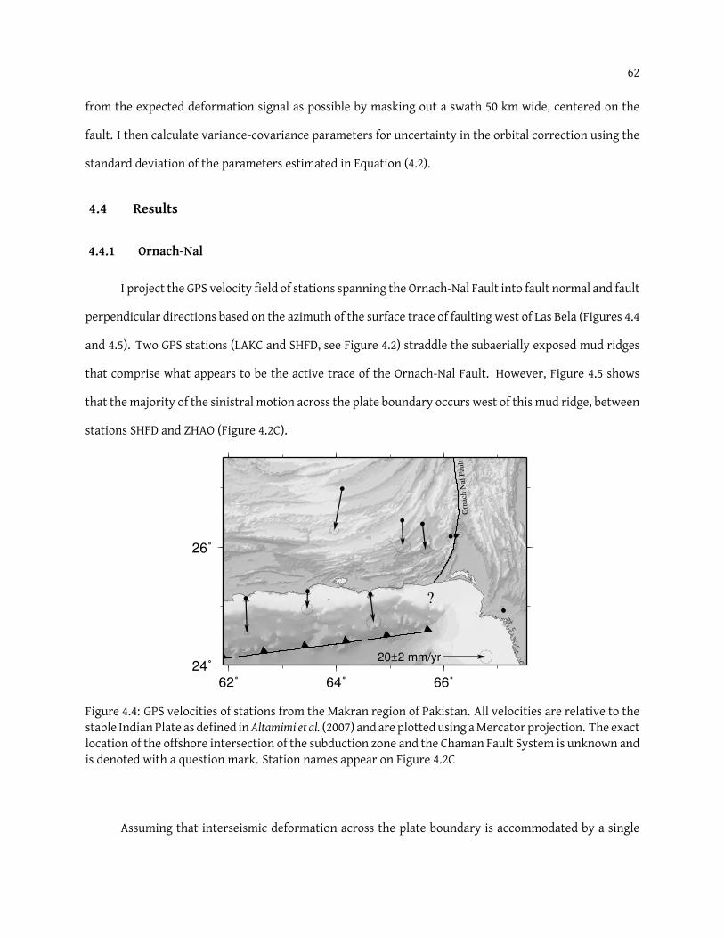
62
from the expected deformation signal as possible by masking out a swath 50 km wide, centered on the
fault. I then calculate variance-covariance parameters for uncertainty in the orbital correction using the
standard deviation of the parameters estimated in Equation (4.2).
4.4 Results
4.4.1 Ornach-Nal
I project the GPS velocity field of stations spanning the Ornach-Nal Fault into fault normal and fault
perpendicular directions based on the azimuth of the surface trace of faulting west of Las Bela (Figures 4.4
and 4.5). Two GPS stations (LAKC and SHFD, see Figure 4.2) straddle the subaerially exposed mud ridges
that comprise what appears to be the active trace of the Ornach-Nal Fault. However, Figure 4.5 shows
that themajority of the sinistral motion across the plate boundary occurs west of this mud ridge, between
stations SHFD and ZHAO (Figure 4.2C).
62˚ 64˚ 66˚24˚
26˚
20±2 mm/yr
Orn
ach N
al
Fault
?
Figure 4.4: GPS velocities of stations from the Makran region of Pakistan. All velocities are relative to thestable Indian Plate as defined inAltamimi et al. (2007) and are plotted using aMercator projection. The exactlocation of the offshore intersection of the subduction zone and the Chaman Fault System is unknown andis denoted with a question mark. Station names appear on Figure 4.2C
Assuming that interseismic deformation across the plate boundary is accommodated by a single
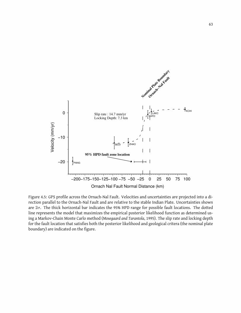
63
−20
−10
0
Velo
city (
mm
/yr)
−200−175−150−125−100 −75 −50 −25 0 25 50 75 100
Ornach Nal Fault Normal Distance (km)
Slip rate : 14.7 mm/yrLocking Depth: 7.3 km
Orn
ach−N
al F
ault
Nom
inal
Pla
te B
oundar
y
95% HPD fault zone location
PANG
BEDI ZHAO
SHFDLAKC
KCHI
Figure 4.5: GPS profile across the Ornach-Nal Fault. Velocities and uncertainties are projected into a di-rection parallel to the Ornach-Nal Fault and are relative to the stable Indian Plate. Uncertainties shownare 2σ. The thick horizontal bar indicates the 95% HPD range for possible fault locations. The dottedline represents the model that maximizes the empirical posterior likelihood function as determined us-ing a Markov-Chain Monte Carlo method (Mosegaard and Tarantola, 1995). The slip rate and locking depthfor the fault location that satisfies both the posterior likelihood and geological critera (the nominal plateboundary) are indicated on the figure.
64
fault with an unknown location, Markov-Chain Monte-Carlo (Mosegaard and Tarantola, 1995) analysis of
the velocity profile indicates that the data are most consistent with an interseismic deformation rate of
14.7mm/yr with a 95% Baysian High Posterior Density (95%HPD) region of 12.8–18.2mm/yr and a locking
depth of 7.4 kmwith awide 95%HPD of 1 km to 17.7 km. Similarly, estimation of the fault location suggests
that the plate boundary lies approximately 27 km west of the mud ridge originally thought to represent
the plate boundary (Figure 4.6). This fault location is associated with a 95%HPD region spanning nearly 35
km, indicating a large uncertainty. The majority of these locations lie beneath the large Hingjal synform
and are consistent with lineations extending north and south of the synform (Figure 4.6).
Previous authors have suggested that the mud ridges west of Las Bela are eruptive features (Jones,
1961; Bannert et al., 1992). Reanalysis of outcrop lithology by Delisle et al. (2002) as part of a systematic study
on mud volcanism in Pakistan indicates that the mud ridge (Figure 4.6) is actually an outcrop of Parkini
Mudstone, the source material erupted from mud volcanoes farther south and west of Las Bela, and not
part of an eruptive feature.
The velocity of the site at Panjgur, Pakistan, is nearly 82% of the expected ITRF2005 rate (Altamimi
et al., 2007). This observation combined with the low velocities of both SHFD and LAKC relative to the
stable Indian Plate suggests that the remaining plate boundary deformation occurs across faults on the
the Eurasian side of the plate boundary. It is also notable that the Ornach-Nal parallel velocity of the site
in Panjgur (PANG, Figures 4.2 and 4.5) is 7 mm/yr faster than the expected far-field velocity due solely to
slip on the Ornach-Nal fault. This disagreement is likely due to unmodeled convergence along the arcuate
faults that comprise the subaerial Makran forearc between Bedi and Panjgur, Pakistan. Examination of
fault normal motion indicates that there is little convergence across the Ornach-Nal Fault (< 2 mm/yr)
(Figure 4.4).
4.4.2 Chaman Fault near Chaman
I project the GPS velocity field of stations north of Quetta, Pakistan, onto a Chaman Fault perpen-
dicular profile and calculate both fault-parallel and fault-normal velocities (Figure 4.7 and 4.8). Due to
the location of the profile near the intersection of the northern Kirthar Range and the Sulaiman Lobe, the
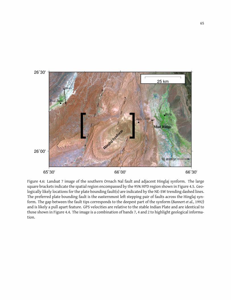
65
SHFD LAKC
ZHAO
10 mm/yr
Bela
Jhal Jhao
Hin
glaj
Syn
form ][
?
?
?
Mud Ridge
65˚30' 66˚00' 66˚30'
26˚00'
26˚30'
25 km
Figure 4.6: Landsat 7 image of the southern Ornach Nal fault and adjacent Hinglaj synform. The largesquare brackets indicate the spatial region encompassed by the 95% HPD region shown in Figure 4.5. Geo-logically likely locations for the plate bounding fault(s) are indicated by the NE-SW trending dashed lines.The preferred plate bounding fault is the easternmost left stepping pair of faults across the Hinglaj syn-form. The gap between the fault tips corresponds to the deepest part of the synform (Bannert et al., 1992)and is likely a pull apart feature. GPS velocities are relative to the stable Indian Plate and are identical tothose shown in Figure 4.4. The image is a combination of bands 7, 4 and 2 to highlight geological informa-tion.
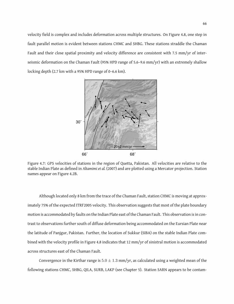
66
velocity field is complex and includes deformation across multiple structures. On Figure 4.8, one step in
fault parallel motion is evident between stations CHMC and SHBG. These stations straddle the Chaman
Fault and their close spatial proximity and velocity difference are consistent with 7.5 mm/yr of inter-
seismic deformation on the Chaman Fault (95% HPD range of 5.6–9.6 mm/yr) with an extremely shallow
locking depth (2.7 km with a 95% HPD range of 0–6.6 km).
66˚ 68˚
30˚
20±2 mm/yr
Ghazaband F
ault
Cham
an F
ault
Figure 4.7: GPS velocities of stations in the region of Quetta, Pakistan. All velocities are relative to thestable Indian Plate as defined in Altamimi et al. (2007) and are plotted using a Mercator projection. Stationnames appear on Figure 4.2B.
Although located only 8 km from the trace of the Chaman Fault, station CHMC is moving at approx-
imately 75% of the expected ITRF2005 velocity. This observation suggests that most of the plate boundary
motion is accommodated by faults on the Indian Plate east of the Chaman Fault. This observation is in con-
trast to observations further south of diffuse deformation being accommodated on the Eursian Plate near
the latitude of Panjgur, Pakistan. Further, the location of Sukkur (SIBA) on the stable Indian Plate com-
bined with the velocity profile in Figure 4.8 indicates that 12 mm/yr of sinistral motion is accommodated
across structures east of the Chaman Fault.
Convergence in the Kirthar range is 5.0 ± 1.3 mm/yr, as calculated using a weighted mean of the
following stations CHMC, SHBG, QILA, SURB, LAKP (see Chapter 5). Station SARN appears to be contam-

67
−20
−10
0
Ve
locity (
mm
/yr)
0 25 50 75
Chaman Fault Normal Distance (km)
Slip rate : 7.53 mm/yrLocking Depth: 2.68 km
Cham
an F
ault
Ghaz
aban
d F
ault
CHMC
QILA SARN
LAKP
SURB
KACH
SHBG
Figure 4.8: GPS profile across the Chaman Fault. Velocities and uncertainties are projected into a directionparallel to the Chaman Fault and are relative to the stable Indian Plate. Uncertainties shown are 2σ. Thedotted line represents themodel thatmaximizes the empirical posterior likelihood function as determinedusing aMarkov-ChainMonte Carlomethod (Mosegaard and Tarantola, 1995). The slip rate and locking depthfor this model are indicated on the figure.
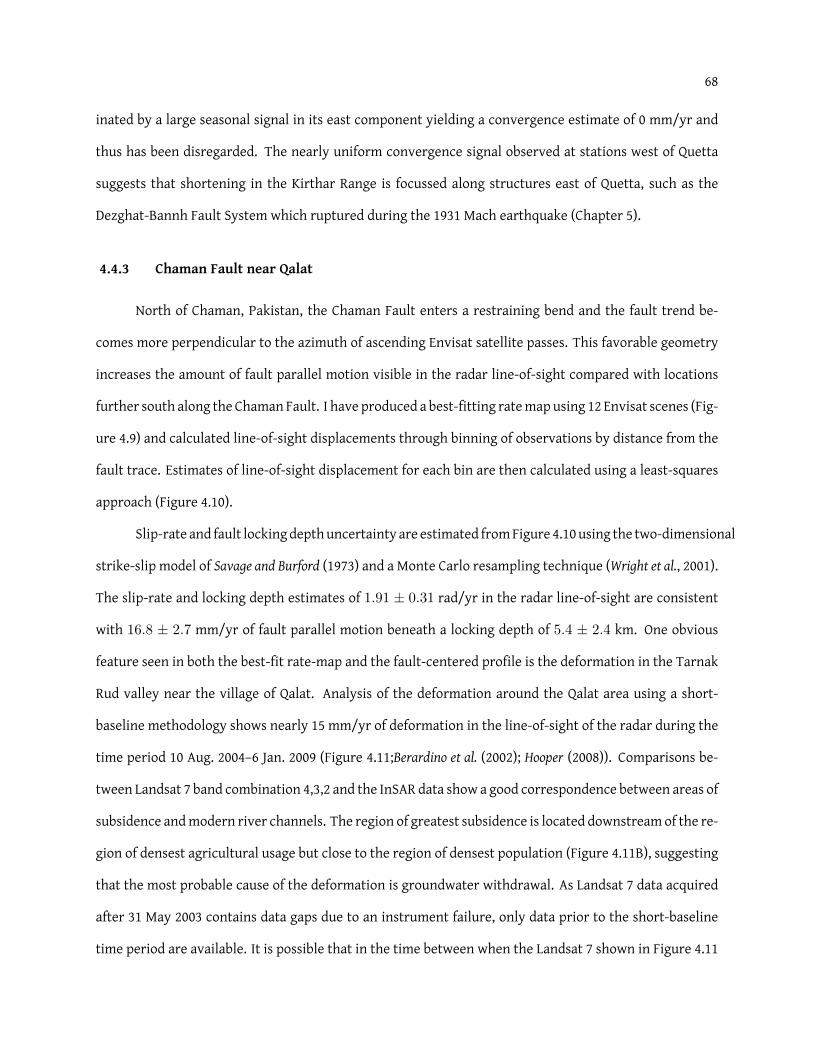
68
inated by a large seasonal signal in its east component yielding a convergence estimate of 0 mm/yr and
thus has been disregarded. The nearly uniform convergence signal observed at stations west of Quetta
suggests that shortening in the Kirthar Range is focussed along structures east of Quetta, such as the
Dezghat-Bannh Fault System which ruptured during the 1931 Mach earthquake (Chapter 5).
4.4.3 Chaman Fault near Qalat
North of Chaman, Pakistan, the Chaman Fault enters a restraining bend and the fault trend be-
comes more perpendicular to the azimuth of ascending Envisat satellite passes. This favorable geometry
increases the amount of fault parallel motion visible in the radar line-of-sight compared with locations
further south along the Chaman Fault. I have produced a best-fitting ratemap using 12 Envisat scenes (Fig-
ure 4.9) and calculated line-of-sight displacements through binning of observations by distance from the
fault trace. Estimates of line-of-sight displacement for each bin are then calculated using a least-squares
approach (Figure 4.10).
Slip-rate and fault lockingdepthuncertainty are estimated fromFigure 4.10 using the two-dimensional
strike-slip model of Savage and Burford (1973) and a Monte Carlo resampling technique (Wright et al., 2001).
The slip-rate and locking depth estimates of 1.91 ± 0.31 rad/yr in the radar line-of-sight are consistent
with 16.8 ± 2.7 mm/yr of fault parallel motion beneath a locking depth of 5.4 ± 2.4 km. One obvious
feature seen in both the best-fit rate-map and the fault-centered profile is the deformation in the Tarnak
Rud valley near the village of Qalat. Analysis of the deformation around the Qalat area using a short-
baseline methodology shows nearly 15 mm/yr of deformation in the line-of-sight of the radar during the
time period 10 Aug. 2004–6 Jan. 2009 (Figure 4.11;Berardino et al. (2002); Hooper (2008)). Comparisons be-
tween Landsat 7 band combination 4,3,2 and the InSAR data show a good correspondence between areas of
subsidence andmodern river channels. The region of greatest subsidence is located downstreamof the re-
gion of densest agricultural usage but close to the region of densest population (Figure 4.11B), suggesting
that the most probable cause of the deformation is groundwater withdrawal. As Landsat 7 data acquired
after 31 May 2003 contains data gaps due to an instrument failure, only data prior to the short-baseline
time period are available. It is possible that in the time between when the Landsat 7 shown in Figure 4.11
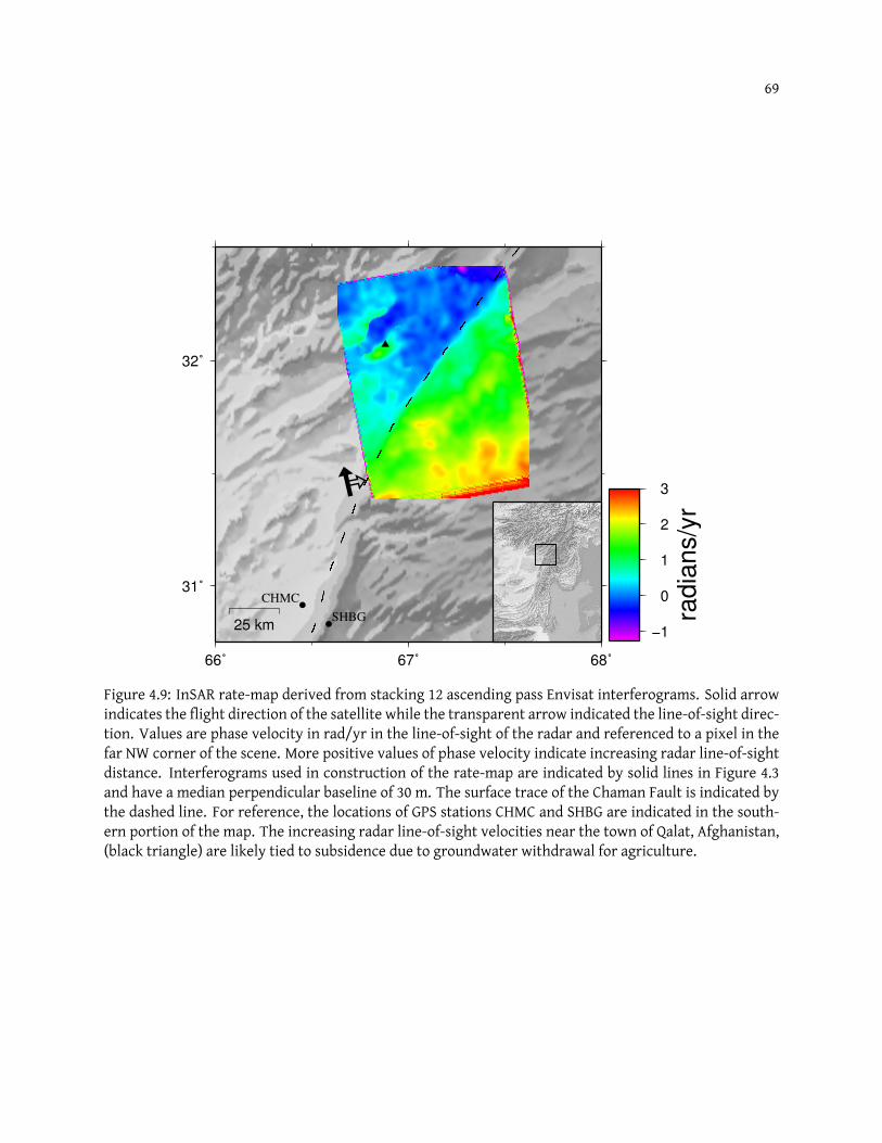
69
66˚ 67˚ 68˚
31˚
32˚
−1
0
1
2
3
radia
ns/y
r
CHMC
SHBG25 km
Figure 4.9: InSAR rate-map derived from stacking 12 ascending pass Envisat interferograms. Solid arrowindicates the flight direction of the satellite while the transparent arrow indicated the line-of-sight direc-tion. Values are phase velocity in rad/yr in the line-of-sight of the radar and referenced to a pixel in thefar NW corner of the scene. More positive values of phase velocity indicate increasing radar line-of-sightdistance. Interferograms used in construction of the rate-map are indicated by solid lines in Figure 4.3and have a median perpendicular baseline of 30 m. The surface trace of the Chaman Fault is indicated bythe dashed line. For reference, the locations of GPS stations CHMC and SHBG are indicated in the south-ern portion of the map. The increasing radar line-of-sight velocities near the town of Qalat, Afghanistan,(black triangle) are likely tied to subsidence due to groundwater withdrawal for agriculture.
70
−2
−1
0
1
2
Lin
e−
of−
Sig
ht V
elo
city (
radia
ns/y
r)
−30 −20 −10 0 10 20 30
Distance from Chaman Fault (km)
1000
2000
3000
4000
Ele
vation (
m)
Groundwater Withdrawal
NW SE
Slip rate : 1.91 rad/yrLocking Depth: 5.4 km
Figure 4.10: Chaman fault centered profile of line-of-sight velocities from the InSAR rate-map shown inFigure 4.9. Increasing line-of-sight velocities represent motion away from the radar. The gray data areSRTM level 2 3s topography sampled in the same manner as the InSAR data. Larger variances in the to-pographic data indicate larger changes in topography parallel to the Chaman fault. The dashed line cor-responds to the Monte Carlo derived model. Slip rate and locking depth are calculated in the radar line-of-sight. The convex-up feature 25 km northwest of the Chaman Fault corresponds with groundwaterwithdrawal near the town of Qalat, Afghanistan.
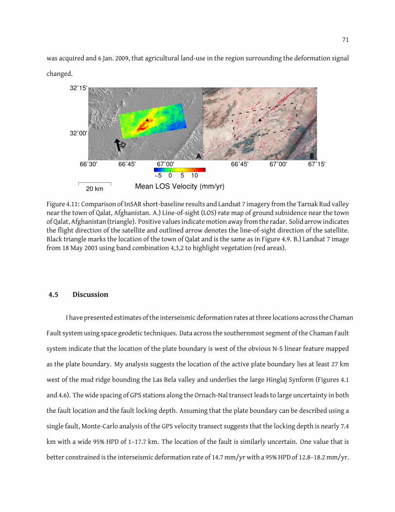
71
was acquired and 6 Jan. 2009, that agricultural land-use in the region surrounding the deformation signal
changed.
66˚30' 66˚45' 67˚00'
32˚00'
32˚15'
A
−5 0 5 10
Mean LOS Velocity (mm/yr)20 km
B
66˚45' 67˚00' 67˚15'
Figure 4.11: Comparison of InSAR short-baseline results and Landsat 7 imagery from the Tarnak Rud valleynear the town of Qalat, Afghanistan. A.) Line-of-sight (LOS) rate map of ground subsidence near the townofQalat, Afghanistan (triangle). Positive values indicatemotion away from the radar. Solid arrow indicatesthe flight direction of the satellite and outlined arrow denotes the line-of-sight direction of the satellite.Black triangle marks the location of the town of Qalat and is the same as in Figure 4.9. B.) Landsat 7 imagefrom 18 May 2003 using band combination 4,3,2 to highlight vegetation (red areas).
4.5 Discussion
I havepresented estimates of the interseismic deformation rates at three locations across theChaman
Fault system using space geodetic techniques. Data across the southernmost segment of the Chaman Fault
system indicate that the location of the plate boundary is west of the obvious N-S linear feature mapped
as the plate boundary. My analysis suggests the location of the active plate boundary lies at least 27 km
west of the mud ridge bounding the Las Bela valley and underlies the large Hinglaj Synform (Figures 4.1
and 4.6). Thewide spacing of GPS stations along the Ornach-Nal transect leads to large uncertainty in both
the fault location and the fault locking depth. Assuming that the plate boundary can be described using a
single fault, Monte-Carlo analysis of the GPS velocity transect suggests that the locking depth is nearly 7.4
km with a wide 95% HPD of 1–17.7 km. The location of the fault is similarly uncertain. One value that is
better constrained is the interseismic deformation rate of 14.7mm/yrwith a 95%HPD of 12.8–18.2mm/yr.
72
Analysis of Landsat 7 imagery (Figure 4.6) shows sinistral shearing in the eastern portions of the Hinglaj
synform. Constraining the fault location to the eastern Hinglaj synform, however, fails to significantly
lower the uncertainty in the locking depth and yields similar interseismic deformation rates. Additional
GPS measurements at locations between stations located in Jhal Jhao, Pakistan (ZHAO), and Lak Chuki,
Pakistan (SHFD), will be required to improve estimates of the locking depth and fault location.
Historically, the Ornach-Nal region has been seismically quiet (Zaigham, 1991; Lawrence et al., 1992);
evenMinchin (1907), in his “Gazateer of Las Bela”, notes that this region is not prone to earthquakes. Since
the 1950’s, the ISC catalog has bolstered this view, listing no seismicity near the Ornach-Nal Fault before
1972. During the 1970’s the increasing density of the global seismic network led to an increase in sensitivity
to small magnitude earthquakes, yet the ISC lists no earthquakes larger thanMb 4.9 near the Ornach-Nal
Fault during the period 1972–2010. The general absence of earthquakes combined with their low magni-
tudes and poor station coverage results in very poor depth estimates for these earthquakes. Although the
GPS station density is too low to provide an accurate constraint on the locking depth of the plate boundary
in the Ornach-Nal region, the low seismic productivity combined with the high interseismic deformation
rate shown by the GPS transect (14.7 mm/yr) suggests that the locking depth along the plate boundary is
shallow.
Modeling of Bouger gravity transects between Karachi and the Ornach-Nal Fault by Zaigham (1991)
suggest the presence of east-dipping subducted oceanic crust beneath the southern Kirthar Range. Al-
though depth estimates for earthquakes in the Ornach-Nal region are poor, the presences of sparse, deep
seismicity combined with the interpretation of an east-dipping crustal layer prompted Zaigham (1991)
to suggest on-going subduction of this crustal sliver, termed the Makran-Bela microplate. However, the
low eastward convergence velocity of stations LAKC and SHFD west of Las Bela and the southern Kirthar
Range (∼ 2mm/yr) suggests that subduction of this sliver has ceased. Although the low seismic produc-
tivity within southern Kirthar Range east of Las Bela further suggests that subduction of this sliver is not
ongoing, future GPS occupations between Las Bela and Hyderabad, Pakistan should confirm its cessation.
Farther north, near 31◦N at the town of Chaman, Pakistan (30.89N, 66.51E), I observe an interseis-
mic deformation rate of 7.5 mm/yr across the Chaman Fault. While this deformation rate is low compared
73
with geological estimates of 19–35 mm/yr, the velocity of station CHMC in Chaman, Pakistan relative to
the stable Indian Plate suggests that a total of 19.5 mm/yr of sinistral motion is accommodated by faults
between Chaman and Sukkur, Pakistan. The most likely candidate fault, the Ghazaband Fault, is also a
likely source for the 1935 Quetta earthquake based on relocated epicenters published in Engdahl and Vil-
lasenor (2002). Although the GPS transect crosses the Ghazaband Fault near the town of Pishin, it fails to
reveal any shear across it (Figure 4.8). The transect’s proximity to the Ghazaband Fault’s northern ter-
minus (< 10 km) could account for this observation. Transects further south across the Ghazaband Fault
could help to determine whether it plays a significant role in accommodating plate boundary motion.
The occurrence of the 1892 M 6.5 strike-slip earthquake at the town of Chaman also appears to
conflict with my estimate of a shallow locking depth and low interseismic slip rate along the Chaman
Fault. The description provided by Griesbach (1893) indicates that surface rupture from this earthquake
ran south of the point where the railroad crosses the fault (30.85N 66.52E) for some distance, but did not
extend much farther to the north of the railroad crossing. The transect across the Chaman Fault between
CHMC and SHBG lies 2 km north of this railroad crossing. It is possible that this segment of the Chaman
Fault behaves in a similar fashion to the Parkfield segment of the San Andreas Fault (Lienkaemper et al.,
2006), with the segment north of Chaman locked at depth and accumulating strain at a much higher rate
than the segment near the town of Chaman. If this is analogy holds true, transects across the Chaman
Fault north of the town of Chaman should show progressively deeper locking depths. Indeed, 75 km north
of the town of Chaman, my InSAR rate-map analysis suggests that the locking depth could be deeper than
at the town of Chaman (0–6.6 km near Chaman versus 3–7.8 km near Qalat, Figures 4.8 and 4.10).
Using cumulative seismic moment estimates, previous authors have noted a slip deficit along the
Chaman fault system at latitudes north of approximately 31◦N (Bernard et al., 2000; Ambraseys and Bilham,
2003b). While surface creep along the Chaman Fault has been suggested as an explanation for thismoment
deficit, the best-fit rate-map derived for the region of the Chaman Fault north of the town of Chaman
shows that the fault is not creeping at the surface (Figure 4.10). Given the observed interseismic defor-
mation rate of 16.8 ± 2.7 mm/yr, one would expect Mw 7.0 earthquakes every 60–90 years; this is not
the case as it is likely that the seismic catalog of this region is complete above M 6.5 since at least 1890
74
(Ambraseys and Bilham, 2003b), the absence of earthquakes withmagnitudesM > 7 in the historical record
suggests that the region of the Chaman Fault near Qalat may be due for a large earthquake. Further, this
observation suggests that the low Peak Ground Acceleration prediction for this region for the next 50
years presented in Pakistan Meteorological Department and NORSAR (2007) is too conservative.
In Figure 4.12, I compare the measurements and the maximum sinistral and fault-normal deforma-
tion estimates made from pole-of-rotation parameters published in Altamimi et al. (2007). Estimates along
each fault shown in Figure 4.12 assume that slip is perfectly partitioned across each fault. Since all three
estimates of sinistral motion and both estimates of convergence are lower than the expected velocities
calculated under the assumption of perfect slip partitioning, suggested in each measurement location,
both sinistral slip and convergence are accommodated across multiple structures. In the south, across the
Ornach-Nal Fault, the faults across the Hinglaj Synform appear to accommodate the majority of the sinis-
tral plate motion. Similarly, in the north, across the Chaman Fault near Qalat, Afghanistan, the Chaman
Fault appears to accommodate the majority of the sinistral plate motion. At the latitude of Chaman, Pak-
istan, however, the large deficit in sinistral deformation suggests that the majority of the sinistral plate
motion is accommodated across other faults in the Chaman Fault System.
4.6 Conclusions
I present interseismic deformation rates and locking depth estimates for three locations across
the Chaman Fault System using space geodetic techniques. Along the southern Chaman Fault System,
the Ornach-Nal fault represents the obvious plate bounding fault. Near the town of Las Bela, geodetic
measurements across the fault indicate that the plate boundary is actually located nearly 27 km west
of the Ornach-Nal Fault beneath the Hinglaj Synform. Assuming deformation is accommodated across
a single fault strand, strain is accumulating at a rate of 14.7 mm/yr and is locked to a depth of 7.5 km.
The absence of historical and modern seismicity suggests that significant off-fault deformation west of
the plate boundary must help dissipate accumulated strain. Farther north, at the latitude of Chaman,
Pakistan, the Chaman Fault appears to accommodate as little as 40% of the overall sinistral motion across
the plate boundary with the remaining deformation distributed across faults east of the plate boundary.
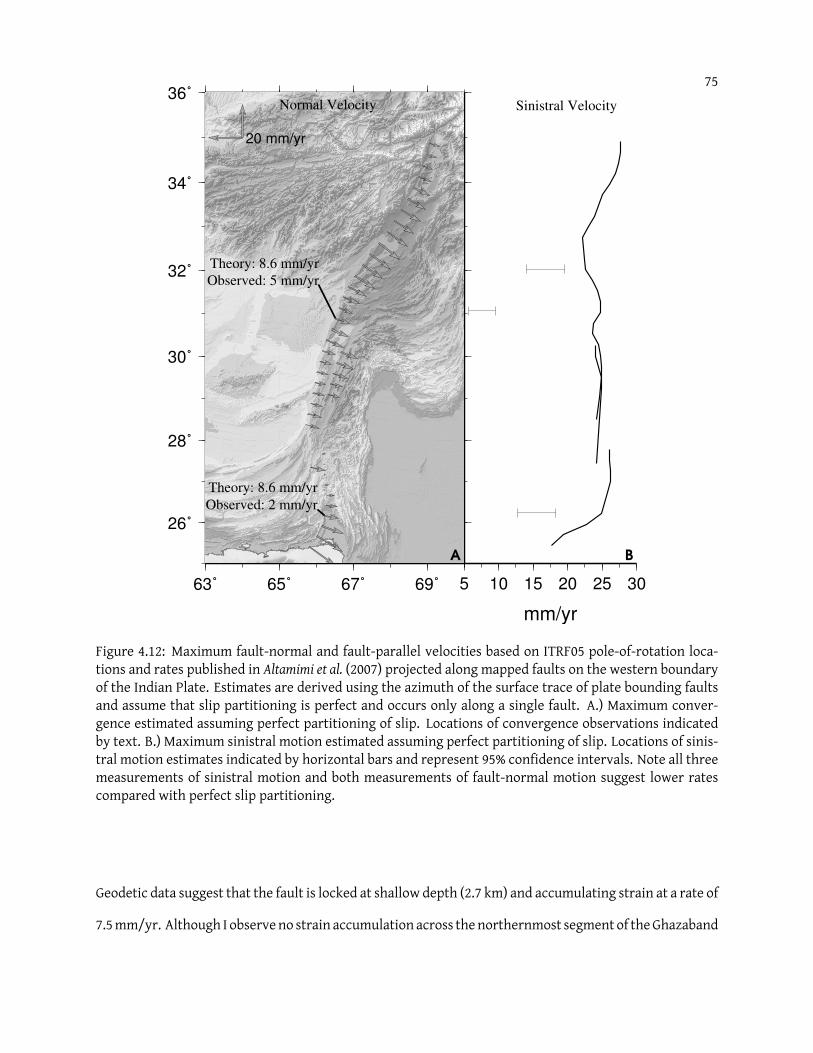
75
63˚ 65˚ 67˚ 69˚
26˚
28˚
30˚
32˚
34˚
36˚
Theory: 8.6 mm/yr
Observed: 2 mm/yr
Theory: 8.6 mm/yr
Observed: 5 mm/yr
20 mm/yr
A
Normal Velocity
5 10 15 20 25 30
mm/yr
Sinistral Velocity
B
Figure 4.12: Maximum fault-normal and fault-parallel velocities based on ITRF05 pole-of-rotation loca-tions and rates published in Altamimi et al. (2007) projected along mapped faults on the western boundaryof the Indian Plate. Estimates are derived using the azimuth of the surface trace of plate bounding faultsand assume that slip partitioning is perfect and occurs only along a single fault. A.) Maximum conver-gence estimated assuming perfect partitioning of slip. Locations of convergence observations indicatedby text. B.) Maximum sinistral motion estimated assuming perfect partitioning of slip. Locations of sinis-tral motion estimates indicated by horizontal bars and represent 95% confidence intervals. Note all threemeasurements of sinistral motion and both measurements of fault-normal motion suggest lower ratescompared with perfect slip partitioning.
Geodetic data suggest that the fault is locked at shallow depth (2.7 km) and accumulating strain at a rate of
7.5mm/yr. Although I observeno strain accumulation across thenorthernmost segment of theGhazaband
76
Fault, it is likely that this fault accommodates a large portion of the sinistral motion of the plate boundary
at latitudes south of Quetta, Pakistan. North of the town of Chaman, Pakistan, interseismic deformation
across the Chaman fault is consistent with 16.8 mm/yr of slip beneath a 5.4 km thick locked elastic lid.
Since there have been no recorded earthquakes Mw > 6.5 on this segment of the fault in the past 115
years, it is likely that this segment of the Chaman fault ruptures in earthquakes with magnitudes larger
thanMw 7 with a return interval of> 120 years.
Chapter 5
Fold and thrust partitioning in a contracting fold belt: Insights from the 1931 MachEarthquake in Baluchistan
5.1 Introduction
Between 1931 and 1935 threemajor earthquakes occurred between the Bolan Pass and Quetta in the
Baluchistan province of Pakistan. The first of these, an Mw 6.8 near Sharigh (21:35 UT 24 August 1931),
was followed 66 hours later by the Mach Mw 7.3 earthquake (15:27 UT 27 August). The third and largest
earthquake was the Mw 7.7 30 May 1935 earthquake, that destroyed 90% of Quetta and caused 35,000
deaths (Ambraseys and Bilham, 2003a). In that no similar magnitude earthquakes occurred in the three
decades before or after this sequence, it is very probable that static triggering of these nearby earthquakes
is responsible for their clustering in time.
All three earthquakes liewithin the 150-km-wide zone of deformation between theAsian and Indian
plates, a region bounded to thewest by the Chaman fault and to the east by the Indus plain (Bender andRaza,
1995) (Figure 5.1A). The strike-slip component of slip on the plate boundary is estimated to be 33 mm/yr
from global GPS closure estimates (Apel et al., 2006), and 31 mm/yr from paleomagnetic reconstructions of
the Indian Ocean sea floor (Molnar and Stock, 2009). Geological estimates of slip on the Chaman fault system
(Lawrence et al., 1992) indicate a slip rate of 19–24mm/year in the past 20Myr, and 25–35mm/yr for the past
2 Myr (Beun et al., 1979; Lawrence et al., 1992) suggesting that as much as one third of this shear signal may
be distributed in the fold belt. The plate boundary is regionally transpressive and from seismic-moment
release calculations in the past 200 years, and from the inferred obliquity of the plate boundary to the local
slip vector between India and Asia it has been estimated that strain partitioning results in convergence of

78
the fold belts of up to 13 ± 3 mm/yr (Ambraseys and Bilham, 2003a). This estimate is probably inflated by
the seismic productivity of the past century, which may be abnormally high if the earthquakes presently
under discussion are atypical of long term seismicity. A lower convergence rate is obtained from analog
and numerical modeling of the strain in the region (3–6 mm/yr NW/SE shortening - Haq and Davis, 1997;
Bernard et al., 2000), and this lower rate is consistent with preliminary GPS measurements north of Quetta
presented in this article.
Although triangulation data exist in the region, no remeasurements have been published (Am-
braseys and Bilham, 2003a). However, a first-order spirit leveling line, first measured in 1909 between
Sukkur and Chaman, was remeasured shortly after the 1935 Quetta earthquake (Wilson, 1938). Parts of the
line were raised 65 cm where they crossed the frontal thrusts of the northern Kirthar Range to the west
of Sibi, exceeding the combined errors in the survey by more than an order of magnitude. A preliminary
analysis of these data (Figure 5.2(a)) in the absence of geological constraints, concluded that the asymme-
try in the vertical deformation, if caused by planar slip, was caused by 1–1.2 m of slip on an east-dipping
blind thrust fault between 1 km depth and approximately 25 km depth (Ambraseys and Bilham, 2003a). The
fit between observed surface deformation and synthetic planar slip was appealing, but the asymmetry of
the uplift signal required a counterintuitive easterly dip to the frontal thrust. The description of a wedge-
thrust geometry with an east-dipping shallow ramp at this location in the literature, however, appeared
to confirm its presence (Banks and Warburton, 1986). Yet, when the surface deformation associated with
slip on the two faults of their triangle zone were examined in detail by Garcia et al. (2006), no combina-
tion of slip was found that resulted in an improved fit to the leveling data (Figure 5.2(b)). Models with
more complex geometries also failed to improve the fit. The two previous interpretations, based as they
were on limited structural information, may now be discarded due to the availability of seismic reflection
data from the Sibi and Mach areas, controlled by stratigraphic information from numerous boreholes.
I present structural interpretations in the next section that demonstrate that the frontal thrusts of the
Kirthar range west of Sibi indeed dip to the west (Bannert et al., 1992; Schelling, 1999a).
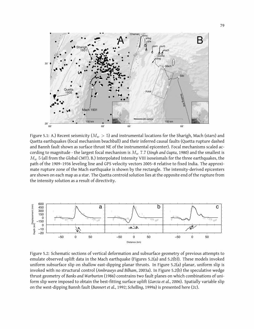
79
66˚ 68˚28˚
30˚
Sharigh1931
Quetta1935
Mach 1931
A
100 km
66˚ 68˚
leve
ling lin
e
chmc
qila
sarn surb
kach
qtag
shbg
20 mm/yr
Sibi
Quetta
Kalat
Mach
Chaman
B
100 km
Figure 5.1: A.) Recent seismicity (Mw > 5) and instrumental locations for the Sharigh, Mach (stars) andQuetta earthquakes (focal mechanism beachball) and their inferred causal faults (Quetta rupture dashedand Bannh fault shown as surface thrust NE of the instrumental epicenter). Focal mechanisms scaled ac-cording to magnitude - the largest focal mechanism is Mw 7.7 (Singh and Gupta, 1980) and the smallest isMw 5 (all from the Global CMT). B.) Interpolated Intensity VIII isoseismals for the three earthquakes, thepath of the 1909–1936 leveling line and GPS velocity vectors 2005–8 relative to fixed India. The approxi-mate rupture zone of the Mach earthquake is shown by the rectangle. The intensity-derived epicentersare shown on eachmap as a star. The Quetta centroid solution lies at the opposite end of the rupture fromthe intensity solution as a result of directivity.
Dis
plac
emen
t (m
m) a
Dep
th (k
m)
b
Distance (km)
c
Figure 5.2: Schematic sections of vertical deformation and subsurface geometry of previous attempts toemulate observed uplift data in the Mach earthquake (Figures 5.2(a) and 5.2(b)). These models invokeduniform subsurface slip on shallow east-dipping planar thrusts. In Figure 5.2(a) planar, uniform slip isinvoked with no structural control (Ambraseys and Bilham, 2003a). In Figure 5.2(b) the speculative wedgethrust geometry of Banks and Warburton (1986) constrains two fault planes on which combinations of uni-form slip were imposed to obtain the best-fitting surface uplift (Garcia et al., 2006). Spatially variable slipon the west-dipping Bannh fault (Bannert et al., 1992; Schelling, 1999a) is presented here (2c).
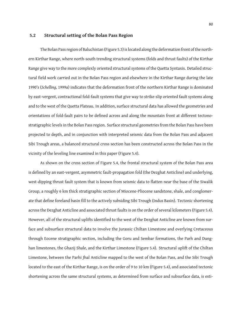
80
5.2 Structural setting of the Bolan Pass Region
TheBolanPass region of Baluchistan (Figure 5.3) is located along the deformation front of thenorth-
ern Kirthar Range, where north-south trending structural systems (folds and thrust faults) of the Kirthar
Range give way to the more complexly oriented structural systems of the Quetta Syntaxis. Detailed struc-
tural field work carried out in the Bolan Pass region and elsewhere in the Kirthar Range during the late
1990’s (Schelling, 1999a) indicates that the deformation front of the northern Kirthar Range is dominated
by east-vergent, contractional fold-fault systems that give way to strike-slip oriented fault systems along
and to the west of the Quetta Plateau. In addition, surface structural data has allowed the geometries and
orientations of fold-fault pairs to be defined across and along the mountain front at different tectono-
stratigraphic levels in the Bolan Pass region. Surface structural geometries from the Bolan Pass have been
projected to depth, and in conjunction with interpreted seismic data from the Bolan Pass and adjacent
Sibi Trough areas, a balanced structural cross section has been constructed across the Bolan Pass in the
vicinity of the leveling line examined in this paper (Figure 5.4).
As shown on the cross section of Figure 5.4, the frontal structural system of the Bolan Pass area
is defined by an east-vergent, asymmetric fault-propagation fold (the Dezghat Anticline) and underlying,
west-dipping thrust fault system that is known from seismic data to flatten near the base of the Siwalik
Group, a roughly 6 km thick stratigraphic section of Miocene-Pliocene sandstone, shale, and conglomer-
ate that define foreland basin fill to the actively subsiding Sibi Trough (Indus Basin). Tectonic shortening
across the Dezghat Anticline and associated thrust faults is on the order of several kilometers (Figure 5.4).
However, all of the structural uplifts identified to the west of the Dezghat Anticline are known from sur-
face and subsurface structural data to involve the Jurassic Chiltan Limestone and overlying Cretaceous
through Eocene stratigraphic section, including the Goru and Sembar formations, the Parh and Dung-
han limestones, the Ghazij Shale, and the Kirthar Limestone (Figure 5.4). Structural uplift of the Chiltan
Limestone, between the Parhi Jhal Anticline mapped to the west of the Bolan Pass, and the Sibi Trough
located to the east of the Kirthar Range, is on the order of 9 to 10 km (Figure 5.4), and associated tectonic
shortening across the same structural systems, as determined from surface and subsurface data, is esti-
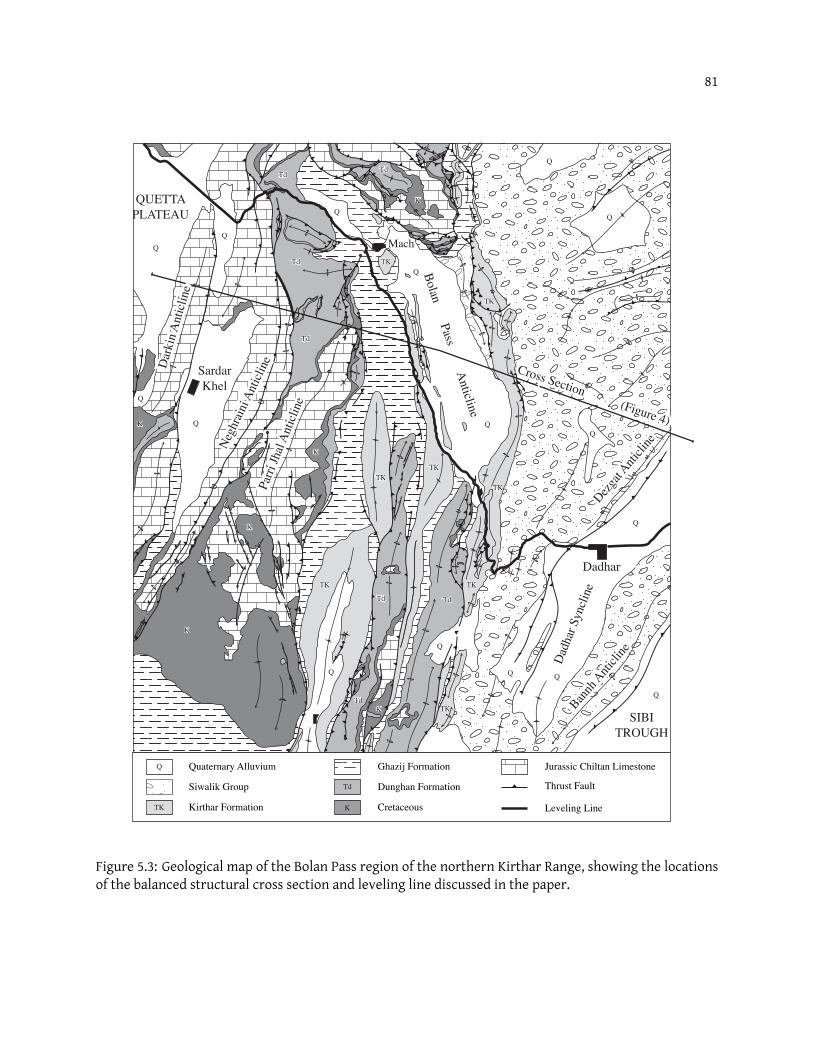
81
Bannh #1
Ghazij Formation
Dunghan FormationSiwalik Group
Quaternary Alluvium
Kirthar Formation Cretaceous
Jurassic Chiltan Limestone
Leveling Line
Thrust Fault
Q
TK
Td
K
TKTK
TKTKTKTK
TKTK
TKTK
TKTK
TKTK
TKTK
TdTd
TdTd
TdTd
TdTd
TdTd
TdTdTdTd
KK
KK
KK
KK
KK
KK
Cross Section (Figure 4)
Negh
rain
i Ant
iclin
eDar
kin
Ant
iclin
e
Parri
Jhal
Ant
iclin
e
Dezga
t Anti
cline
Bannh
Anti
cline
QUETTAPLATEAU
SardarKhel
Bolan Pass Anticline
Negh
rain
i Ant
iclin
eDar
kin
Ant
iclin
e
Parri
Jhal
Ant
iclin
e
Cross Section (Figure 4)
Mach
Dezga
t Anti
cline
Bannh
Anti
cline
SIBITROUGH
DadharD
adha
r Syn
clin
e
Figure 5.3: Geological map of the Bolan Pass region of the northern Kirthar Range, showing the locationsof the balanced structural cross section and leveling line discussed in the paper.
82
MSL
3 km
-5 km
-10 km
-15 km
3 km
MSL
-5 km
-10 km
-15 km
DEZGHATANTICLINE
BOLAN RIVERANTICLINE
PARRI JHALANTICLINE
QUETTAPLATEAU
KUMBRI NALASYNCLINE
Bolan River Valley
Pre-MZ
Pre-MZ
Pre-MZ Tg Td
K
Tg
J
Tdc
Tu TuTm Tm
TslTsl
T
J
J
T
TTdc
Cretaceous
Dunghan Fm.
K
Td
Upper Siwaliks
Dadhar Cglo.
Tu
Tdc Pre-MesozoicPre-MZKirthar Fm.
Ghazij Fm.
Tk
Tg
Chiltan Ls.
Triassic
J
TLower SiwaliksTsl
Tm Middle Siwalks
Figure 5.4: Balanced structural cross section across the deformation front of the northern Kirthar Rangein the Bolan Pass area and in the vicinity of the leveling line. See Figure 3 for cross section location andtext for discussion.
mated at approximately 15 km. This requires that thrust faults exposed at the surface and that involve
the Chiltan Limestone are relatively high-angle structural features, with measured, near surface dips of
roughly 60 degrees and estimated fault angles of 30 to 45 degrees at 10 to 20 km depth (Figure 5.4). In
addition, 9 to 10 kilometers of uplift across the combined Bolan Pass and Parhi Jhal Anticlines requires a
mid-crustal decollement surface at a depth of 18 to 20 kilometers beneath the Quetta Plateau, as indicated
on the cross section of Figure 5.4. This 18 to 20 km decollement depth is well below the projected, base-
Triassic stratigraphic level of known lithology from the Kirthar and nearby Sulaiman mountain ranges,
and therefore the lithology at the basal decollement level beneath the Quetta Plateau remains unknown,
and may actually be located in basement rocks.
Additional decollement surfaces of the Kirthar Range have been identifiedwithin the Eocene Ghazij
Shale, which separates the underlying, competent carbonates of the Chiltan-Dunghan limestones from
the overlying Kirthar Limestone and Siwalik Group (Figure 5.4). Significant deformation associated with
these Ghazij Shale decollement surfaces is restricted to an area above the sub-surface, frontal fault-ramp
identified beneath the Bolan Pass, where the underlying (basal) decollement surface to the Kirthar Range
climbs from a depth of 18 kilometers or more beneath the Parhi Jhal and Bolan Pass Anticlines to the up-
per, basal Siwalik Group decollement surface identified beneath the Dezghat Anticline at roughly 6 km
depth. Thrust faults originating within the Ghazij Shale result in short- (several hundred meter) wave-
length anticline-syncline pairs and the development of exposed back-thrust surfaces along the east-limb
83
of the Bolan River Anticline. These latter fold-fault systems have accommodated less than 1 km of tec-
tonic shortening, though as exposed structural systems in the Bolan Pass area there is little question that
thrust faults originating within the Ghazij Shale will affect surface deformation across the Bolan Pass area,
as indicated from the leveling data discussed in this paper.
5.3 GPS measurements of convergence and shear between the Asian and Indian Plates
GPS measurements in Pakistan are historically of limited coverage and duration. Campaign mea-
surements from six sites with locations between the town of Chaman, 30 km west of the Chaman fault,
and the town of Kach, approximately 70 km NE of Quetta, have been measured at least twice in the period
2006–2008, and compared to continuous measurements made in Karachi (not shown) and Quetta (qtag)
(Figure 5.1B). The continuous points in Pakistan are operated from flat-roofed concrete frame buildings
and the campaign points are measured on bipods set on stainless steel screws cemented into exposed
rock. GPS observations were recorded either with Trimble NetRS, 5700 or R7 receivers using a 30 second
sampling rate, and processed using an elevation cut-off angle of 10 degrees. Campaign data have dura-
tions of 3–7 days from each site. The daily data from these sites were processed along with data from 10
regional IGS stations using GAMIT version 10.34 (King and Bock, 2002). The regional solutions were then
combined with global solutions from SOPAC (ftp://garner.ucsd.edu/pub/hfiles) using GLOBK/GLORG
version 5.16 (Herring, 2002) to determine time series and velocities in the ITRF2005 reference frame. These
velocities were then transformed into an Indian Plate-fixed reference frame using pole of rotation param-
eters determined by Bettinelli et al. (2006).
The processed campaign GPS data are associated with formal uncertainties of ±3 mm/yr, and the
continuous data with uncertainties of ±1 mm/yr (Figure 5.5). Not shown on the figure are the velocity
vectors for Karachi and Nagar Parkar (north of the Bhuj 2001 earthquake) that move at approximately
the velocity of the Indian plate, suggesting that little deformation occurs across the Indus delta, or near
the Bhuj region. The SSW velocity of Quetta is anomalous relative to the points on the east-west transect
through Chaman due to intense groundwater withdrawl (S. Khan, Univ. Houston, personal communica-
tion 2010). The most easterly point on the traverse, Kach, is also anomalous in that it shows no conver-
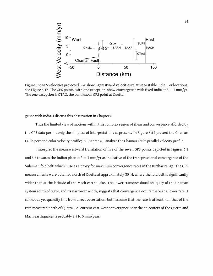
84
−5
0
5
10
West V
elo
city (
mm
/yr)
−50 0 50 100
Distance (km)
CHMC SHBG
QILA
SARN LAKP
SURB
QTAG
KACH
Chaman Fault
West East
Figure 5.5: GPS velocities projected E-W showingwestward velocities relative to stable India. For locations,see Figure 5.1B. The GPS points, with one exception, show convergence with fixed India at 5± 1mm/yr.The one exception is QTAG, the continuous GPS point at Quetta.
gence with India. I discuss this observation in Chapter 6
Thus the limited view of motions within this complex region of shear and convergence afforded by
the GPS data permit only the simplest of interpretations at present. In Figure 5.5 I present the Chaman
Fault-perpendicular velocity profile; in Chapter 4, I analyze the Chaman Fault-parallel velocity profile.
I interpret the mean westward translation of five of the seven GPS points depicted in Figures 5.1
and 5.5 towards the Indian plate at 5 ± 1 mm/yr as indicative of the transpressional convergence of the
Sulaiman fold belt, which I use as a proxy for maximum convergence rates in the Kirthar range. The GPS
measurements were obtained north of Quetta at approximately 30◦N, where the fold belt is significantly
wider than at the latitude of the Mach earthquake. The lower transpressional obliquity of the Chaman
system south of 30◦N, and its narrower width, suggests that convergence occurs there at a lower rate. I
cannot as yet quantify this from direct observation, but I assume that the rate is at least half that of the
rate measured north of Quetta, i.e. current east-west convergence near the epicenters of the Quetta and
Mach earthquakes is probably 2.5 to 5 mm/year.
85
5.4 Macroseismic location of the Mach earthquake
The Mach earthquake is named for the railway headquarters at Mach that were heavily damaged
in the earthquake (Ambraseys and Bilham, 2003a). The jail was destroyed and 400 prisoners were briefly at
large. Although no surface rupture was recorded, the parapets of a 140 m long approximately E-W bridge
converged 20 cmwithout being tilted. Numerous rock falls occurred at the time of the earthquake, raising
clouds of dust near Mach and the Bolan Pass to the SE.
Although instrumental locations and magnitudes are available for the 1931 and 1935 earthquakes
(Figure 5.1 and Table 5.1), additional knowledge of the extent and azimuth of their rupture zones can
be inferred from intensity data recorded for each event. The data are available in the form of damage
reports to structures near their epicenters, and from felt reports at larger distances. Previous analysis of
the intensity data for the Sharigh, Mach and Quetta earthquakes have interpolated isoseismal contours
for a range of intensities to determine the most probable location of their rupture zones. Banana-shaped
isoseismals drawn by West (1934) for the highest intensities are distorted by the uneven coverage of his
data. Ambraseys and Bilham (2003a) re-evaluated these data supplemented by additional observations and
concluded that the highest isoseismals for the second two earthquakes form north-elongated polygons
(Figure 5.1A). Insufficient data for the Sharigh earthquake were available to form definitive conclusions,
except that its epicentral location was close to the town of that name.
Table 5.1: Instrumental and inferred macroseismic locations for the three earthquakes.
Event Date Instrumental Mw Minimum Magnitude Mi Minimum VarianceEpicenter Epicenter Epicenter
Sharigh 24 Aug. 1931 31.1N 67.7E 6.8 29.87N 67.62E 5.9 30.12N 67.60EMach 27 Aug. 1931 29.9N 67.6E 7.3 29.55N 67.55E 7.2 29.22N 67.47EQuetta 30 May 1935 28.87N 66.4E 7.7 30.10N 66.92E 7.6 30.18N 66.92E
I have subjected these same observed intensities to a more rigorous analysis using the methods of
Bakun and Wentworth (1997). This approach does not contour isoseismals but instead contours the most
probable locations for the epicenter using a grid search and assumptions about attenuation of shaking in-
tensity with distance. The method uses recent earthquakes from elsewhere in the region for which loca-
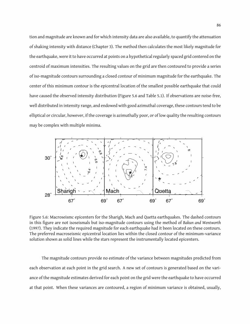
86
tion andmagnitude are known and for which intensity data are also available, to quantify the attenuation
of shaking intensity with distance (Chapter 3). The method then calculates the most likely magnitude for
the earthquake, were it to have occurred at points on a hypothetical regularly spaced grid centered on the
centroid of maximum intensities. The resulting values on the grid are then contoured to provide a series
of iso-magnitude contours surrounding a closed contour of minimummagnitude for the earthquake. The
center of this minimum contour is the epicentral location of the smallest possible earthquake that could
have caused the observed intensity distribution (Figure 5.6 and Table 5.1). If observations are noise-free,
well distributed in intensity range, and endowed with good azimuthal coverage, these contours tend to be
elliptical or circular, however, if the coverage is azimuthally poor, or of low quality the resulting contours
may be complex with multiple minima.
67˚ 69˚28˚
30˚
67˚ 69˚ 67˚ 69˚
6.4
6.66.8
6.8
Sharigh
7.2
7.4
Mach
7.8
8
Quetta
Figure 5.6: Macroseismc epicenters for the Sharigh, Mach and Quetta earthquakes. The dashed contoursin this figure are not isoseismals but iso-magnitude contours using the method of Bakun and Wentworth(1997). They indicate the required magnitude for each earthquake had it been located on these contours.The preferred macroseismic epicentral location lies within the closed contour of the minimum-variancesolution shown as solid lines while the stars represent the instrumentally located epicenters.
The magnitude contours provide no estimate of the variance between magnitudes predicted from
each observation at each point in the grid search. A new set of contours is generated based on the vari-
ance of the magnitude estimates derived for each point on the grid were the earthquake to have occurred
at that point. When these variances are contoured, a region of minimum variance is obtained, usually,
87
but not always, close to the minimum magnitude solution. For the three earthquakes in Baluchistan the
minimummagnitude locations are indeed close to their minimum variance locations, typical of an accept-
able macroseismic solution (Table 5.1). The minimum variance contours are assigned probabilities, with
the most probable location for the epicenter being the location of minimum variance. The intersection of
the minimum variance location with a contour of the iso-magnitude solution indicates the most probable
magnitude for the earthquake.
The solutions for all three earthquakes are listed inTable 5.1 and shown in Figure 5.6. The absence of
complexity to theminimummagnitude contours and their coincidencewith themarginallymore complex
minimum variance locations in each case is notable. The most probable location for the Mach epicenter
lies near the southern end of its rupture zone and near its instrumental location. I ignore the smallermini-
mum noted north of Sibi. In contrast, the location of the minimum variance epicenter for the 1935 Quetta
earthquake lies near Quetta, more than 130 km NNE of the instrumental location for the earthquake. I
assume that the high intensities reported from Quetta were enhanced by directivity in the direction of
rupture propagation (Singh and Gupta, 1980; Day et al., 2008). The minimum-variance epicentral location
for the Sharigh event is found to be approximately to the north of the Mach event, west of the epicentral
location inferred by earlier investigations, and in Chapter 6, I discuss candidate causal faults.
Using the constants derived in Bakun andWentworth (1997) for California I infer theMachmagnitude
to have beenMw 7.2 in good agreementwith the value ofMw 7.3 derived byAmbraseys and Bilham (2003a).
The inferred magnitude for the Sharigh event is significantly smaller, Mw 5.9 instead of 6.8, probably
the result of the sparse sampling of macroseismic data points for this event. The preferred location for
the Sharigh event lies to the west of previously inferred locations, but no causal fault can be identified
there from geological evidence or microseismicity. Recent CMT solutions (Dziewonski et al., 1999) in the
area (Figure 5.1A) indicate that the newly located Sharigh event lies in a transition region between NW-
SE directed compression in the Bolan Pass region and N-S compression to the north. Focal mechanisms
nearest to the epicenter of the Sharigh earthquake show a combination of NE dipping thrust faulting and
thrusting along N-S directed decollements.
88
5.5 Leveling data
The Sukkur-Quetta leveling line (Figures 5.1B and 5.7) was originally surveyed between 1909 and
1914with a benchmark spacing of 2–5 km (Wilson, 1938; Ambraseys and Bilham, 2003a). The leveling data are
associated with random errors that growwith the square root of the distance traversed (L km) as k√Lmm
where k = 0.65, a constant derived from circuit closure errors in India (Lenox-Conyngham, 1916). In addition,
a systematic height-dependent error is present in the data that is typically less than 1×10⁻⁶ of the height
above the starting point of the line in kilometers. The 65 cm of vertical deformation near the Bolan Pass
exceeds both systematic and random errors in the data by more than an order of magnitude. The leveling
bench marks were geo-referenced from 1”= 1 mile topographic sheets and have resulting uncertainties
of up to 30 m (listed in Ambraseys and Bilham, 2003a). I project these irregularly spaced leveling data at
N110◦E along a line perpendicular to the trend of folding in the Kirthar range (Figure 5.7).
No surface rupture was reported for the 1931 Mach earthquake, although it is possible that West’s
post seismic investigations did not include traverses across the frontal thrusts of the Kirthar range except
near Sibi (West, 1934). To proceed with the analysis of the leveling data, I assume that slip on one or
more of the mapped subsurface faults was responsible for the observed uplift. I digitized these subsurface
faults from the geological cross-sections, forming curved fault segments from a series of contiguous, 3-
km-wide, planar segments. I then permitted various combinations of contiguous segments to slip. Each
segment with non-zero slip contributes to the surface deformation field (Okada, 1992) and I searched for
smooth distributions of slip on contiguous segments that most precisely produced the observed surface
deformation. The analytical procedure I adopted was to shift the surface projection of the parameterized
faults relative to the leveling data, and invert for slip using the Green’s functions for each segment. By
minimizing the sum of squared residuals, I determined the optimal offset between the leveling data and
the modeled geometry.
The misfit between the parameterized faults and the projected leveling data is minimized with
slip on deep segments of the Dezgat Thrust with contiguous slip on segments of the Bannh Fault which
branches from it eastwards towards the surface (Figure 5.7). Maximum observed slip of 3.2 m occurs in
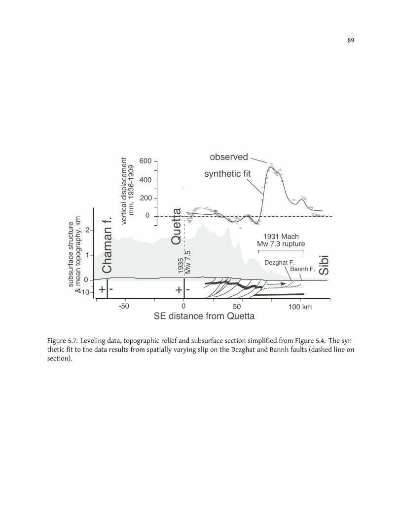
89
-50 0 50
verti
cal d
ispl
acem
ent
mm
, 193
6-19
09
Cha
man
f.
Que
tta
+ - + -subs
urfa
ce s
truct
ure
& m
ean
topo
grap
hy, k
m
1
2
0-10
100 km
Sibi
600
400
200
0
1931 Mach Mw 7.3 rupture
Mw
7.5
synthetic fit
observed
SE distance from Quetta
Dezghat F.Bannh F.
Figure 5.7: Leveling data, topographic relief and subsurface section simplified from Figure 5.4. The syn-thetic fit to the data results from spatially varying slip on the Dezghat and Bannh faults (dashed line onsection).
90
segments between 7 and 5 km depth, up-dip from an inferred interseismic locking line at 8 or 9 km depth,
where I observe minimum slip. The location of inferred interseismic locking is not constrained by ob-
servations of interseismic deformation, and hence there exists some uncertainty as to its true location.
However, in Section 5.6 I undertake additional numerical models that are consistent with this identifi-
cation. A deeper locking line would decrease the inferred along strike length of the Mach rupture. The
total width of the rupture above the 9-km-deep locking line is 42 km and themean slip is 1.2 m (Table 5.2).
Assuming a seismic moment of 1.1× 1027 dyne-cm, and that all the slip occurred seismically, the best-fit
slip distribution requires an along-strike rupture length of 72.2 km.
A broader region of uplift near Quetta (Figure 5.7) can be explained by invoking minor slip on an
uneven decollement or by invoking slip on one of several mapped listric faults near there, either before or
after the 1931 earthquakes. I note that the fit to these minor regions of uplift in the data are non-unique
since they are not constrained by well-defined subsurface geometry.
5.6 Discussion: the earthquake cycle in a ramp-flat-ramp system
The vertical displacement data fit in the foregoing section includes all deformation that occurred
between 1909 and 1936. Thus the data include not only co-seismic slip but possible post-seismic slip, if any
occurred. I show that this is likely with a series of elastic models that assume perfectly frictionless slip
below a locking line, and rupture at shallower depths (Figure 5.8). The models take the form of those de-
scribed by Feldl and Bilham (2006) inwhich a series of contiguous, frictionless boundary elements are driven
along a complex rupture surface in an uniform elastic half-space by a far-field displacement imposed at
depth. The geometry of this selected far-field driving condition is not critical to the models. Similar re-
sults are obtained by imposing regional contraction on the fault system, or imposed remote thrusting.
The boundary element computation calculates the amount of slip required on contiguous elements to
minimize stress in their vicinity.
The results from three calculations (Table 5.2 and Figure 5.8) illustrate models that emulate pre-
seismic, coseismic slip, and finally, slip assuming no interseismic locking below the region of coseismic
rupture (upper line). For the coseismic and preseismic slip calculations, the slip distribution is calculated
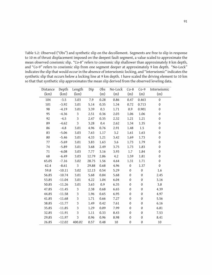
91
Table 5.2: Observed (“Obs”) and synthetic slip on the decollement. Segments are free to slip in responseto 10 m of thrust displacement imposed on the deepest fault segment, a value scaled to approximate themean observed coseismic slip. “Co-8” refers to coseismic slip shallower than approximately 8 km depth,and “Co-9” refers to coseismic slip from one segment deeper at approximately 9 km depth. “No-Lock”indicates the slip that would occur in the absence of interseismic locking, and “interseismic” indicates thesynthetic slip that occurs below a locking line at 9 km depth. I have scaled the driving element to 10 kmso that that synthetic slip approximates the mean slip derived from the observed leveling data.
Distance Depth Length Dip Obs No-Lock Co-8 Co-9 Interseismic(km) (km) (km) (m) (m) (m) (m) (m)104 -3.5 3.03 7.9 0.28 0.86 0.47 0.463 0101 -3.92 3.01 5.14 0.35 1.34 0.72 0.713 098 -4.19 3.01 3.39 0.3 1.71 0.9 0.901 095 -4.36 3 2.51 0.36 2.03 1.06 1.06 092 -4.5 3 2.47 0.35 2.32 1.21 1.21 089 -4.62 3 3.28 0.4 2.62 1.34 1.35 086 -4.8 3.01 4.96 0.76 2.91 1.48 1.5 083 -5.06 3.03 7.63 1.17 3.2 1.61 1.63 080 -5.46 3.01 4.33 1.21 3.42 1.69 1.73 077 -5.69 3.01 3.83 1.63 3.6 1.73 1.79 074 -5.89 3.01 3.68 2.49 3.75 1.73 1.83 071 -6.08 3.03 7.77 3.16 3.93 1.7 1.84 068 -6.49 3.03 12.79 2.86 4.2 1.59 1.81 0
65.05 -7.16 3.02 28.75 1.56 4.64 1.31 1.71 062.4 -8.61 3 29.88 0.68 4.96 0 1.37 059.8 -10.11 3.02 12.13 0.54 5.29 0 0 1.656.85 -10.74 3.01 5.68 0.84 5.68 0 0 2.4553.85 -11.04 3.01 4.22 1.04 6.04 0 0 3.1650.85 -11.26 3.01 3.63 0.9 6.35 0 0 3.847.85 -11.45 3 2.38 0.68 6.65 0 0 4.3944.85 -11.58 3 1.96 0.65 6.95 0 0 4.9741.85 -11.68 3 1.71 0.66 7.27 0 0 5.5638.85 -11.77 3 1.49 0.42 7.61 0 0 6.1635.85 -11.85 3 1.29 0.09 7.99 0 0 6.8132.85 -11.91 3 1.11 0.33 8.43 0 0 7.5329.85 -11.97 3 0.96 0.96 8.98 0 0 8.4126.85 -12.02 400.02 0.57 0.48 10 0 0 10
92
by assuming the decollement surface is frictionless and free to slip in response to 10 m of convergence
applied from the west, either for the entire fault surface (no-locking) or up to a locking line at 8 or 9 km
depth (pre-seismic). The coseismic calculation corresponds to seismic slip above the locking line, and the
input to this model is the static strain field developed from the preseismic slip distribution determined
from the interseismic slip calculation (Table 5.2).
The selection of a 10mdrivingdisplacement is arbitrary because the synthetic output scales linearly
with input. However, I note that this input value results in synthetic co-seismic slip that approximates
the coseismic slip inferred from the leveling data. The 10 m input condition corresponds to 2000 years of
convergence at 5mm/year. The selection of the locking line, the transition between downdip interseismic
creep and the locked seismogenic rupture zone, was investigated by running models with incrementally
increased locking depths and by examining the resulting slip distribution with that inferred from the lev-
eling data. The best fitting coseismic slip distribution occurs where interseismic locking occurred above 8
or 9 km depth. The coseismic slip distributions resulting from locking at each of the 8 km and 9 km depths
are listed in Table 5.2.
The spatial distributions of observed and synthetic co-seismic slip show similarities. Peak slip in
synthetic and observed data coincides in up-dip location but the ratio of peak slip to average slip is less in
the numerical experiments than observed in the Mach earthquake. Observed slip is twice the synthetic
slip at 6 km depth, and half the synthetic slip at 4.5 km depth. No simple changes in fault geometry, or
freely slipping width were able to emulate the localized maximum slip at 6 km depth.
The observed minimum in slip that occurs at the inferred locking line is of special interest. A sig-
nificant slip deficit (3 m) occurs here as a result of preseismic and postseismic pinning at the locking line.
The resulting slip deficit is analogous to the slip deficit that occurs between two contiguous strike-slip, or
normal faults that slip sequentially. Manighetti et al. (2005) suggests that the stresses generated by this slip
deficit are released in off-fault deformation through the creation of secondary faults and folding.
A paradox, however, arises in the thrust fault I am considering, for if the locking-line is pinned
over several earthquake cycles, the hanging wall cannot advance over the footwall. Thus although the
minimum slip in the model is confirmed by the 1909–1936 leveling data, slip may occur at the locking line

93
-12
-10
-8
-6
-4
-2
0
depth (km)
(no locking)
synthetic pre-seismic synthetic
co-seismic
observed co-seismic
locking line
rupturedecollement
8 1012
slippinned
driven element
imposed 10m slip
West East
Dezghat Fault Bannh F.
slip
def
icit
displa
ceme
t (m)
2
4
6
8
10
Figure 5.8: Geometry of the active decollement and frontal thrust (bold line with depth scale right), andinferred slip on segments shallower than 9 km (grey envelope) compared to synthetic slip (slip scale left).The calculated slip for the entire fault is given by the top staircase-line (21, 3-km-long freely-slippingsegments responding to an input displacement of 10m imposed from the left (west)). The lower staircase-lines are formed from two calculations: slip anticipated below a locking line at 9 km depth (syntheticpre-seismic slip), and the slip during rupture at shallower depths that occurs when this interseismic slipdistribution drives co-seismic rupture (synthetic co-seismic). The difference between the two lower stair-case lines and the upper staircase is the slip deficit caused by interseismic locking at 9 km depth.

94
at times not sampled by these data. Stress conditions for slip in the region (afterslip) aremost favorable for
this translation shortly after the earthquake before the shallow fault “heals”, yet a significant slip deficit
remains four years after the earthquake. Thus, if slip occurs here, it must do so over a period of many
decades after each earthquake.
Alternatively, if the locking line is truly locked for numerous earthquake cycles, the stored elastic
energy there must eventually be released in a much larger earthquake. The significant variability in slip I
see in the Mach earthquake could in fact be the result of the 1931 event being driven partly by elastic en-
ergy stored from a previous earthquake cycle. If this occurred it would suggest that previous earthquakes
terminated at a shallower locking line than that I infer for 1931. There is some evidence to suggest that
the Himalayamay exhibit similar enigmatic behavior, withmost decollement earthquakes associatedwith
3–7m of slip and no prominent surface rupture, but with infrequent earthquakes causing surface ruptures
with slip of as much as 24 m (Feldl and Bilham, 2006; Bilham and Szeliga, 2008).
I section 5.7 I discuss the implied discrepancy between the amount of convergence (approximately
10 m) required to drive 3 m of coseismic slip of the frontal thrust.
5.7 Geodetic convergence, slip potential and renewal time
In many paleoseismic estimates of earthquake recurrence interval, the renewal time for an earth-
quake is estimated from the strain rate applied to a fault, a number that is derived from the present-day
geodetic displacement rate measured in the region. Thus one might anticipate that a 3 mm/yr conver-
gence rate applied to a fold-and thrust-belt would permit earthquakes with 3 m of slip every thousand
years. The perfectly elastic frictionless calculation indicates that the renewal of the Mach earthquake us-
ing this approach would err by a factor of 8, because only one-eighth of the convergence is manifest as
slip on the frontal thrust (Table 5.3). The remaining convergence is presumably accommodated by folding
and thickening of the fold and thrust belt.
The effect occurs because the ramp separating the deepdecollement from the shallow frontal thrust
acts as a buttress to motion. The ratio of input displacement (geodetic convergence) to frontal fault slip
(measured coseismic slip) depends on the ratio of the depth of the decollement to the mean depth of the
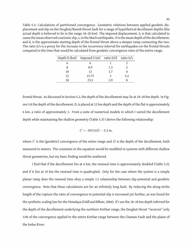
95Table 5.3: Calculations of partitioned convergence. Geometric relations between applied geodetic dis-placement and slip on the Dezghat/Bannh thrust fault for a range of hypothetical decollment depths (theactual depth is believed to lie in the range 18–20 km). The imposed displacement, S, is that calculated tocause themeanobserved coseismic slip, s, in theMach earthquake. D is themeandepth of the decollement,and d, is the approximate starting depth of the frontal thrust above a steeper ramp connecting the two.The ratio S/s is a proxy for the increase in the recurrence interval for earthquakes on the frontal thrustscompared to the time that would be calculated from geodetic convergence rates of the entire range.
Depth D (km) Imposed S (m) ratio D/d ratio S/s6 6 1 28 8.9 1.3 310 12 1.7 412 15.75 2 5.218 23.5 2.9 8
frontal thrust. As discussed in Section 5.2, the depth of the decollement may lie at 18–20 km depth. In Fig-
ure 5.8 the depth of the decollement, D, is placed at 12 km depth and the depth of the flat is approximately
6 km, a ratio of approximately 2. From a suite of numerical models in which I varied the decollement
depth while maintaining the shallow geometry (Table 5.3) I derive the following relationship:
C = .00154D − 3.2m,
where C is the (geodetic) convergence of the entire range and D is the depth of the decollement, both
measured in meters. The constants in the equation would be modified in systems with different shallow
thrust geometries, but my basic finding would be unaltered.
I find that if the decollement lies at 6 km, the renewal time is approximately doubled (Table 5.3),
and if it lies at 10 km the renewal time is quadrupled. Only for the case where the system is a simple
planar ramp does the renewal time obey a simple 1:1 relationship between slip-potential and geodetic
convergence. Note that these calculations are for an infinitely long fault. By reducing the along-strike
length of the rupture the ratio of convergence to potential slip is increased yet further, as was found for
the synthetic scaling law for the Himalaya (Feldl and Bilham, 2006). If I use the 18–20 km depth inferred for
the depth of the decollement underlying the northern Kirthar range, the Dezghat thrust “receives” only
12% of the convergence applied to the entire Kirthar range between the Chaman Fault and the plains of
the Indus River.
96
How can one explain this significant discrepancy? It would appear that the ramp acts as a buttress
to sedimentary layers driven from the west. Since convergence is not released as slip on the shallower
fault above and to the east of the ramp, it must be manifest as thickening of the sediment pile to the west.
The mean topography west of the ramp is 1.5 km higher than to the east of the ramp, and the seismic
section is shortened by approximately 15 km. East of the ramp the frontal Dezgat/Bannh fault system has
been shortened by less than 1 km.
5.8 Sequential triggering of ruptures
The three earthquakes are unusual in that most of the seismic moment release in the Baluchistan
region in the last 150 years occurred within the four years following the first of these earthquakes (Figure
5.9). The clustering of these three large Baluchistan earthquakes near 30◦N has a low probability of occur-
ring by chance; hence some form of triggering appears probable. The mechanisms of stress transfer are
currently speculative, especially for the first two events that occurred within 66 hours of each other. In
Chapter 6, I discuss possible mechanisms for the Sharigh earthquake by utilizing both its location within
the Quetta Syntaxis Shear Zone and its temporal relationship with the Mach earthquake. However, the
geometric relationship between the Mach and Quetta earthquakes renders a causal link substantially eas-
ier to comprehend. Rupture of the Dezgat thrust in the Mach earthquake reduced compressive east-west
stresses and acted, in a sense, to unclamp the fault-normal stress on the Quetta strike-slip fault 60 km to
the west. The instantaneous Coulomb failure change at Quetta is calculated to be 10 to 70 kPa, depending
on the nucleation depth of the Quetta earthquake, a stress change that ismore than sufficient to trigger an
earthquake (Stein et al., 1994). However, these instantaneous stress changes were apparently unimportant
because the earthquake was delayed bymore than three years. If the occurrence of the Quetta earthquake
less than 4 years after the Mach earthquake is not a coincidence, then some form of stress diffusion, or
viscous creep is required.
While poroelastic or viscoelastic processes in the body of the fold and thrust belt, or below it (Freed,
2005) are adequate to cause the observed delay, I consider here an alternative mechanism - viscous creep
on the decollement surface. The rate of propagation of the deformation front between Mach and Quetta,
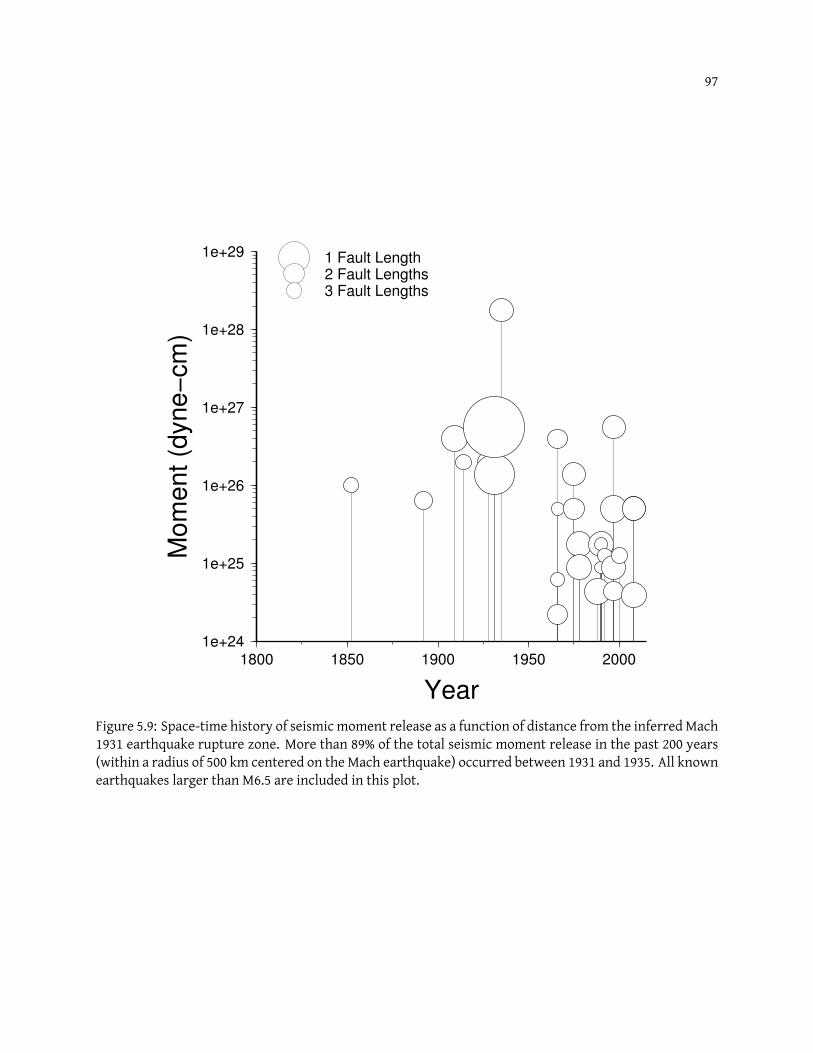
97
1e+24
1e+25
1e+26
1e+27
1e+28
1e+29
Mo
ment (d
yne−
cm
)
1800 1850 1900 1950 2000
Year
1 Fault Length2 Fault Lengths3 Fault Lengths
Figure 5.9: Space-time history of seismic moment release as a function of distance from the inferredMach1931 earthquake rupture zone. More than 89% of the total seismic moment release in the past 200 years(within a radius of 500 km centered on the Mach earthquake) occurred between 1931 and 1935. All knownearthquakes larger than M6.5 are included in this plot.

98
had it occurred linearly, is approximately 18 km/yr. I note that 4 years after the earthquake I infer afterslip
10 km below the locking line to have amounted to approximately 1 m, with approximately 0.5 m of slip 20
km below the locking line. If this decay rate continued linearly downdip towards the Quetta fault, the slip
on the decollementmay have amounted to 10-20 cmnear Quetta by 1935. The leveling data are insensitive
to slip on a planar, sub-horizontal surface, but the bulge in the data east of Quetta (Figure 5.7) suggests
that slip of some form occurred 40-50 km west from the Mach event. Slip may also have occurred prior
to the Mach event in the region between Quetta and Mach, manifest as vertical changes in the 1909-1936
leveling data. I cannot exclude the possibility that aseismic or weakly-seismic mobility of the structures
in the fold-belt prior to the earthquake sequence may have been responsible for all three events.
5.9 Conclusions
Precise leveling data and a fault model derived from detailed geological cross-sections, permit us
to calculate the slip distribution on the rupture surface of the 1931 Mach earthquake. I deduce that the
earthquake occurred on the 42 km wide (EW), 72 km long (NS) Dezghat/Bannh fault system west of Sibi.
The fault slipped in a reverse sense up to the east with maximum slip of 3.2 m and mean slip of 1.2 m.
Maximum slip coincides spatially with that predicted in elastic models driven by inferred interseismic
stresses, but themaximumslip is larger thanpredicted compared to themean slip of the fault. The leveling
data suggest that slip also occurred downdip of the rupture (approximately 1 m) either as afterslip or slip
in other events in the interval 1909–36.
A significant (3–5m) slip deficit remained near the interseismic locking line 4 years after the earth-
quake. This slip deficit may now, nearly 75 years later, have been reduced by aseismic processes sub-
sequent to the earthquake, or it may remain stored as elastic strain to drive future earthquakes. Two
mechanisms may act to prevent the accumulation of seismic deficit over multiple earthquake cycles. The
first is that slow, off-fault deformation, or pressure solution processes, act to reduce local stresses at the
locking line, and the second is that infrequent larger earthquakes mine an historically stored slip deficit,
accompanied by an incremental shift in the depth of the locking line. The first is testable in principle, in
that one could re-measure surviving points of the leveling line to determine whether the slip deficit re-
99
mains. In practice, current security issues in the region render this difficult. I favor, however, the second
mechanism: that stored elastic strain from one ormore previous earthquakesmay account for the 3.2m of
local slip observed updip from the inferred locking line in the 1931 earthquake. The local maximum slip is
easier to explain as an additional 1.5–2 m of slip inherited from strain un-released by former earthquakes,
than the alternative solution, that the slip in the earthquake should everywhere have been approximately
3 m in 1931 and that an approximately 2 m slip deficit remains on most of the fault.
In considering the details of theMach earthquake, I examined in numerical experiments the elastic
processes prevailing during the entire seismic cycle. I found that slip on a frontal thrust is always less than
the geodetic contraction rate of a fold and thrust belt, unless the frontal thrust consists of a planar fault.
In the case of a geometrically complex underlying thrust fault with variable dip, I find that partitioning
of slip to the frontal thrusts is reduced in proportion to the ratio of decollement-depth to shallow-thrust-
depth where these are separated by a ramp. This significant discrepancy between the geodetic loading
rate and the slip-potential of frontal faults of the fold belt is presumably responsible for thickening the
pile of sediments by folding and listric faulting. Partitioning in the Kirthar range, as elsewhere, results
in a significantly longer renewal time for earthquakes on the frontal fault of the range, than would be
derived from the geodetic convergence rate alone. Thus, although the weakly constrained 5 mm/yr GPS
convergence rate between Quetta and Sibi would result in a minimum renewal time for 1.2 m (average
slip) on a planar frontal thrust fault of 240 years, this study suggests that the presence of a decollement
at approximately 18 km depth would extend the recurrence interval for Mach-type earthquakes on the
Dezghat/Bannh fault system by a factor of 8, to approximately 2000 years.
Given that more than 90% of the seismic moment release in the region occurred between 1930 and
1935, I believe that sequential triggering of the three earthquakes occurred. The 1931 Sharigh earthquake
was clearly responsible for triggering the Mach earthquake 3 days later. The structural relationship be-
tween these two fault systems is discussed further in Chapter 6. In contrast, the “broadside” relation
between the Mach and Quetta rupture zones is consistent with an increase in Coulomb failure stress on
the Quetta fault at the time of the Mach earthquake. The 3.5 yr interval between the two earthquakes in-
dicates, however, that static stresses changes alone were insufficient to trigger the Quetta earthquake.

100
I hypothesize that the Mach earthquake reduced east-west stresses on the decollement/ramp system
that would have facilitated accelerated creep on the basal decollement beneath the Kirthar range. De-
formation between Mach and Quetta inferred from minor uplift and subsidence in the leveling data, are
consistent with strain changes accompanying decollement slip, although interpretation of these data are
non-unique.
Chapter 6
Bookshelf Faulting in the 2008 Ziarat Earthquake Sequence, Northern Baluchistan
6.1 Introduction
The Indian Plate is convergingwith the Eurasian Plate at a rate of 38mm/yr at the location ofHyder-
abad, India (Altamimi et al., 2007). Along the western boundary of the Indian Plate, this collision manifests
itself primarily as sinistral slip along the Chaman Fault System. Recent investigations of seismicity along
the Chaman Fault System in Baluchistan suggest that deformation is partitioned between sinistral motion
and range normal convergence (Chapters 5 and 4). In addition, recent geodetic estimates suggest that
overall sinistral rates are near the lower bound of geologic slip estimates (19.5 mm/yr, Chapter 4).
Some of this slip partitioning along the plate boundary manifests itself as diffuse deformation in
the Sulaiman Lobe, a southward verging salient produced by the northward translation of the semi-rigid
Katawaz block by the Chaman Fault System (Figure 6.1; Haq and Davis, 1997; Bernard et al., 2000). The south-
ward extrusion of the Sulaiman Lobe is accommodated along its eastern margin by the left-lateral Kingri
fault and related structures (Figure 6.1; Rowlands, 1978). Similarly, seismicity in the Quetta Syntaxis, along
the western margin of the Sulaiman Lobe, suggests the presence of a dextral feature analogous to the
Kingri fault, although there are no mapped faults with dextral offset in this region (Banks and Warburton,
1986; Bannert et al., 1992; Schelling, 1999b).
Seismicity in the Quetta Syntaxis occurs in a NW-SE oriented band approximately 25 km wide and
stretching 100 km from Pishin in the NW to near Harnai in the SE (Figure 6.2 and Table 6.1). Near the
town of Pishin, the southern end of the seismically quiet Katawaz Block marks one end of the seismic
zone, while to the SE, seismicity becomes more diffuse and focal mechanisms become dominantly thrust
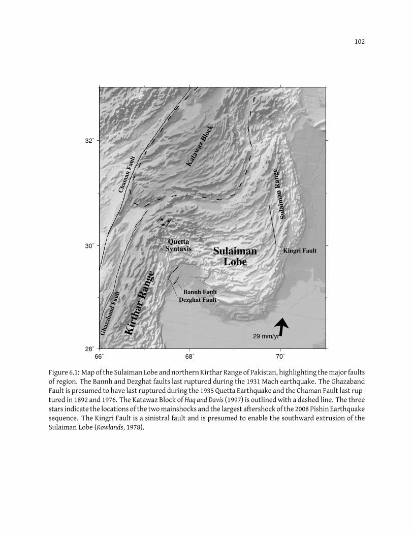
102
66˚ 68˚ 70˚28˚
30˚
32˚
Kat
awaz
Blo
ck
Gh
aza
ban
d F
au
ltC
ham
an
Fau
lt
Kingri Fault
Bannh Fault
Dezghat Fault
Kir
thar
Ran
ge
SulaimanLobe
QuettaSyntaxis
Su
laim
an
Ran
ge
29 mm/yr
Figure 6.1: Map of the Sulaiman Lobe andnorthernKirthar Range of Pakistan, highlighting themajor faultsof region. The Bannh and Dezghat faults last ruptured during the 1931 Mach earthquake. The GhazabandFault is presumed to have last ruptured during the 1935 Quetta Earthquake and the Chaman Fault last rup-tured in 1892 and 1976. The Katawaz Block of Haq and Davis (1997) is outlined with a dashed line. The threestars indicate the locations of the twomainshocks and the largest aftershock of the 2008 Pishin Earthquakesequence. The Kingri Fault is a sinistral fault and is presumed to enable the southward extrusion of theSulaiman Lobe (Rowlands, 1978).

103
faulting (Figure 6.3; Bernard et al., 2000). At least 4 earthquakes larger than Mw 6 have occurred in this
seismic belt in the past century (Table 6.1), the 1931 Mw 6.8 Sharigh earthquake (Chapter 5), the 1997
Mw 7.1Harnai earthquake (Khan, 1998; Bernard et al., 2000) and both 2008Mw 6.4 Ziarat earthquakes (this
Chapter). In addition, numerous moderate earthquakes (Mw > 5) have occurred in the region over the
past century (Figures 6.2 and 6.3). There is some indication that the epicenter of the 1909M ≈ 7 Kachhi
earthquake was close to the location of the 1997Mw 7.1 Harnai earthquake (Engdahl and Villasenor, 2002).
Table 6.1: Historical earthquakes in the Quetta Syntaxis. An additional 5 earthquakes with magnitudesbetweenMw 5.1 andMw 5.4 occurred during the Oct.–Dec. 2008 aftershock sequence but are unlisted.
Epicenter MagnitudeNumber Date Epicenter MagnitudeSource Source1 20 Oct. 1909 68.0E, 30.0N ISC 7.2 ISC2 24 Aug. 1931 67.7E, 30.2N ISC 6.8 ISC3 29 Sep. 1941 67.2E, 30.7N ISC 5.4 ISC4 16 Jun. 1976 67.2E, 30.7N ISC 5.1 ISC6 16 Nov. 1993 67.0891E, 30.8024N This Study 5.6 This Study7 27 Feb. 1997 67.9875E, 29.9932N This Study 7.2 ISC8 28 Oct. 2008 67.3825E, 30.5012N This Study 6.4 This Study9 29 Oct. 2008 67.5297E, 30.4659N This Study 6.4 This Study10 9 Dec. 2008 67.4416E, 30.4024N This Study 5.7 This Study
The identification of rupture planes for earthquakes in the Quetta Syntaxis has been hampered by
the mismatch between the expected dextral sense of deformation, the actual trend of mapped surface
structures and the ambiguity of fault planes from seismically determined moment tensors. Focal mecha-
nisms throughout theNW-SE trending seismic bandnorth of Quetta showdominantlyN-S trending P-axes,
consistent with the current day northward motion of the Indian plate relative to Eurasia (Figure 6.3; Al-
tamimi et al., 2007)). As one moves from NW to SE along this seismicity band, there is a continuous change
in mechanism from dominantly strike-slip in the NW to range-normal thrusting in the SE where mapped
fault orientations becomemore favorable to thrust fault activation (Bernard et al., 2000). Given the seismic
productivity of this region, little work has been done to understand how shear in the Quetta Syntaxis is
accommodated tectonically.
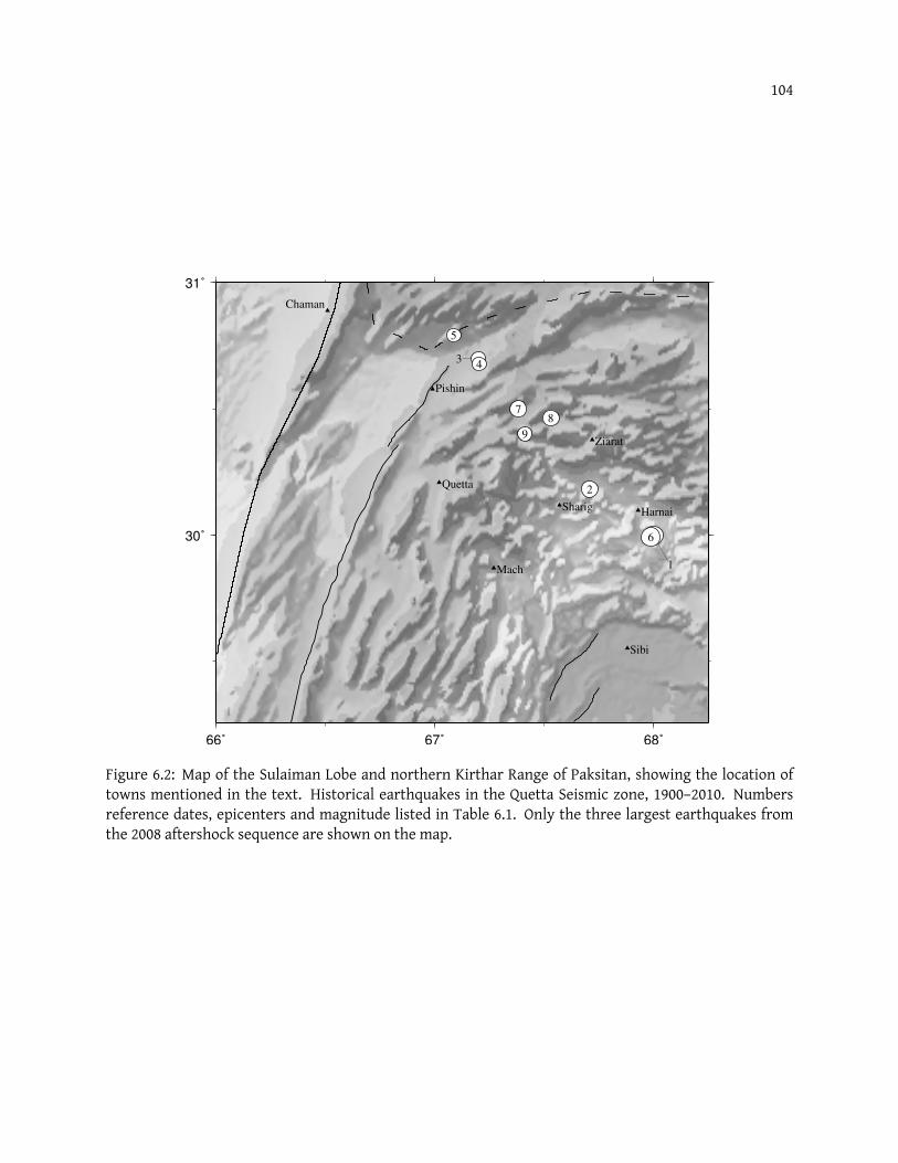
104
66˚ 67˚ 68˚
30˚
31˚
Quetta
Ziarat
Sharig
Mach
Sibi
Harnai
Chaman
Pishin
1
3
2
4
5
6
78
9
Figure 6.2: Map of the Sulaiman Lobe and northern Kirthar Range of Paksitan, showing the location oftowns mentioned in the text. Historical earthquakes in the Quetta Seismic zone, 1900–2010. Numbersreference dates, epicenters and magnitude listed in Table 6.1. Only the three largest earthquakes fromthe 2008 aftershock sequence are shown on the map.
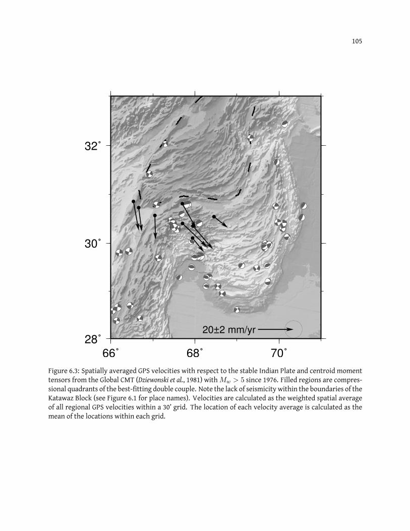
105
66˚ 68˚ 70˚28˚
30˚
32˚
20±2 mm/yr
Figure 6.3: Spatially averaged GPS velocities with respect to the stable Indian Plate and centroid momenttensors from the Global CMT (Dziewonski et al., 1981) withMw > 5 since 1976. Filled regions are compres-sional quadrants of the best-fitting double couple. Note the lack of seismicity within the boundaries of theKatawaz Block (see Figure 6.1 for place names). Velocities are calculated as the weighted spatial averageof all regional GPS velocities within a 30’ grid. The location of each velocity average is calculated as themean of the locations within each grid.
106
In this study, I focus on an earthquake sequence beginning in late Oct. 2008. At 2309 UTC on 28 Oct.
2008, an Mw 6.4 earthquake struck the region 40 km NE of Quetta. This earthquake was followed by a
similarly sized earthquake 11 hours later, 15 km SE of the first shock. The aftershock sequence from these
two earthquakes consisted of more than 50 earthquakes larger thanMw 4 with a total additional seismic
moment equivalent to Mw 6.0 and lasted until mid-December 2008. In the following account, the two
principal earthquakes in the sequence will both be referred to as mainshocks due to their approximately
equal magnitudes. When necessary, I will distinguish them by their date. I begin by analyzing teleseismic
body-wave data for the two mainshocks along with the largest aftershock. Because of the complexity of
the interferometric data spanning both mainshocks, I proceed by inverting interferometric data for the
Mw 5.7 aftershock of 9 Dec. 2008. I will then utilize the precise location information for this aftershock
provided by InSAR inversion to revise the double-difference relocations for the two mainshocks. These
revised mainshock locations along with the fault planes obtained from teleseismic body-wave inversion
are then used as starting parameters for an inversion of the complex coseismic mainshock interferogram.
I infer that this earthquake sequence involved sinistral faulting along NE-SW trending faults. This
interpretation, combined with the results of an inversion of InSAR data for anMw 5.6, 40 km to the NW of
the 2008 earthquake sequence, suggests that overall dextral shear in the Quetta Syntaxis is accommodated
along en-echelon NE-SW trending sinistral faults through “bookshelf faulting”.
6.2 Tectonic Overview
The lobate shape of the fold-and-thrust belts of western Pakistan have been a source of intrigue for
structural geologists for at least the past half-century (Jones, 1961; Rowlands, 1978; Quittmeyer et al., 1984;
Banks and Warburton, 1986; Humayon et al., 1991; Jadoon et al., 1993, 1994; Jadoon and Kurshid, 1996; Haq and
Davis, 1997; Bernard et al., 2000). Analogue and viscoelastic modeling of the margin demonstrates that the
lobate structure as well as the strike of both the Kirthar and Sulaiman Ranges can be attributed to the
translation of a semi-rigid block (the Katawaz block) northward along the eastern edge of the Chaman
Fault System (Haq and Davis, 1997; Bernard et al., 2000). Southward extrusion of the Sulaiman Lobe is ac-
commodated by simple strike-slip faulting on its eastern margin along faults such as the Kingri Fault (Fig-

107
ure 6.3; Rowlands, 1978). Along the western margin of the Sulaiman Lobe, the convergence velocities and
directions between the Sulaiman Lobe and the northern Kirthar Range suggest that dextral shear accom-
modates their differential shortening rates (Figure 6.3).
The Quetta Syntaxis is located at the transition between the fold-and-thrust belts of theN-S striking
Kirthar Range and the southward verging Sulaiman Lobe. The N-S strike of both the Kirthar Range and
the Sulaiman Range are nearly parallel to the northward velocity of the Indian Plate relative to Eurasia
(29 mm/yr at N7E, Figure 6.1; Altamimi et al., 2007). Proceeding east from the Kirthar Range, the trend of
mapped structures rotates to a nearly NW-SE azimuth at the apex of the Quetta Syntaxis and becomes
perpendicular to the India-Eurasia convergence direction before rotating back to a N-S orientation in the
Sulaiman Range (Figure 6.1). The intersection between the N-S trending Kirthar Range and the NW-SE
trending structures of the western Sulaiman Lobe, at the apex of the Quetta Syntaxis, coincides with the
most seismically active region of the western Indian Plate margin.
6.3 Data and Methods
6.3.1 Double-difference Relocations
I relocate both mainshocks of the 2008 Ziarat earthquake sequence along with its aftershock se-
quence through Jan. 2009 using P-wave phase data published in the monthly National Earthquake Infor-
mation Center Earthquake Data Records and a double-difference methodology (Waldhauser and Ellsworth,
2000). To increase the robustness of the relocations, I also include phase data from the nearby 1997Mw 7.1
Harnai earthquake along with its aftershock sequence through Apr. 1997.
6.3.2 Teleseismic Body-wave Modeling
Using IRIS’s WILBUR II (http://www.iris.edu/wilber), I obtained broad-band seismic data from
Global Seismic Network stations in the distance range 30–90◦ to avoid complexities from mantle triplica-
tions and the outer core. I then selected the best P and SHwaveformswith an emphasis on good azimuthal
coverage. Waveforms were low-passed filtered using a 3-pole Butterworth filter with a corner frequency
108
of 0.08 Hz and down-sampled to 0.5 s sample spacing. I then use the programMT5 (McCaffrey et al., 2000) to
simultaneously invert P and SHwaveforms for the best fitting double couple point source using aweighted
least-squares approach. I use a simple half-spacemodel for crustal structurewithwave speeds ofVP = 6.5
km/s and VS = 3.7 km/s and a density of ρ = 2.8 kg/m3. I use a mantle attenuation parameter (t∗) value
of 1 s for P-waves and 4 s for SH-waves.
6.3.3 InSAR
To study deformation related to the 2008 Ziarat earthquake sequence, I utilize 6 ascending pass SAR
scenes spanningNov. 2007–Jan. 2009 from the European Space Agency’s Envisat satellite (Figure 6.4), while
deformation from the 16 Nov. 1993 Pishin earthquake, was captured using 2 descending pass SAR scenes
spanning Sep. 1993–Nov. 1993 from the European Space Agency’s ERS-1 satellite (perpendicular baseline of
-22 m). Descending pass Envisat data covering the 2008 Ziarat earthquake sequence could not be used due
to temporal decorrelation over the coseismic region. A 90 m resolution Digital Elevation Model was con-
structed from Shuttle Radar Topography Mission version-2 data (Farr et al., 2007) to remove topographic
fringes. Interferograms were produced using the ROI PAC InSAR software package developed at the Jet
Propulsion Laboratory in Pasadena, CA (Rosen et al., 2004). Interferograms were sampled with 4 looks in
range and 20 looks in azimuth to produce 80 m × 80 m resolution cells, filtered using a power spectral
method (Goldstein and Werner, 1998) and unwrapped using a least squares methodology. Unwrapped in-
terferograms were then subsampled using a resolution-based methodology (Lohman and Simons, 2005) and
inverted for fault location and orientation using Powell’s conjugate gradient descent method with Monte
Carlo restarts (Powell, 1964; Clarke et al., 1997; Funning et al., 2007).
6.3.4 GPS Data
Continuous GPS measurements in the region of the Ziarat earthquake began in 2005 and have been
supplemented by campaign GPS measurements since 2007. Campaign measurements from 13 sites with
locations predominantly north of Quetta have been measured at least twice in the period 2007–2010 and
compared to continuous measurements made in Karachi (KCHI), Sukkur (SIBA), Peshawar (NCEG) and
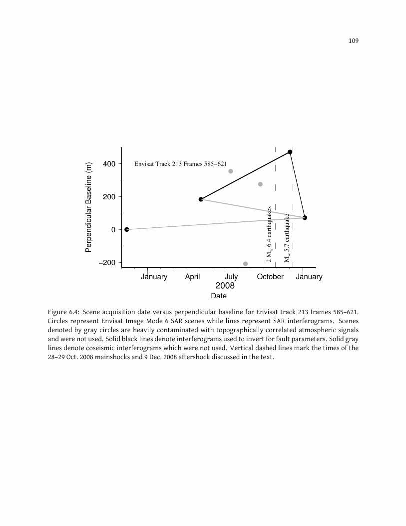
109
−200
0
200
400
Pe
rpe
nd
icu
lar
Ba
se
line
(m
)
January April July October January
2008Date
Envisat Track 213 Frames 585−621
2 M
w 6
.4 e
arth
quak
es
Mw
5.7
ear
thquak
e
Figure 6.4: Scene acquisition date versus perpendicular baseline for Envisat track 213 frames 585–621.Circles represent Envisat Image Mode 6 SAR scenes while lines represent SAR interferograms. Scenesdenoted by gray circles are heavily contaminated with topographically correlated atmospheric signalsand were not used. Solid black lines denote interferograms used to invert for fault parameters. Solid graylines denote coseismic interferograms which were not used. Vertical dashed lines mark the times of the28–29 Oct. 2008 mainshocks and 9 Dec. 2008 aftershock discussed in the text.
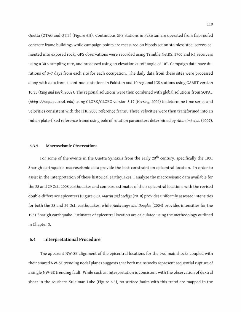
110
Quetta (QTAG and QTIT) (Figure 6.5). Continuous GPS stations in Pakistan are operated from flat-roofed
concrete frame buildings while campaign points are measured on bipods set on stainless steel screws ce-
mented into exposed rock. GPS observations were recorded using Trimble NetRS, 5700 and R7 receivers
using a 30 s sampling rate, and processed using an elevation cutoff angle of 10◦. Campaign data have du-
rations of 3–7 days from each site for each occupation. The daily data from these sites were processed
along with data from 4 continuous stations in Pakistan and 10 regional IGS stations using GAMIT version
10.35 (King and Bock, 2002). The regional solutions were then combined with global solutions from SOPAC
(http://sopac.ucsd.edu) using GLOBK/GLORG version 5.17 (Herring, 2002) to determine time series and
velocities consistent with the ITRF2005 reference frame. These velocities were then transformed into an
Indian plate-fixed reference frame using pole of rotation parameters determined by Altamimi et al. (2007).
6.3.5 Macroseismic Observations
For some of the events in the Quetta Syntaxis from the early 20th century, specifically the 1931
Sharigh earthquake, macroseismic data provide the best constraint on epicentral location. In order to
assist in the interpretation of these historical earthquakes, I analyze the macroseismic data available for
the 28 and 29 Oct. 2008 earthquakes and compare estimates of their epicentral locations with the revised
double-difference epicenters (Figure 6.6). Martin and Szeliga (2010) provides uniformly assessed intensities
for both the 28 and 29 Oct. earthquakes, while Ambraseys and Douglas (2004) provides intensities for the
1931 Sharigh earthquake. Estimates of epicentral location are calculated using the methodology outlined
in Chapter 3.
6.4 Interpretational Procedure
The apparent NW-SE alignment of the epicentral locations for the two mainshocks coupled with
their shared NW-SE trending nodal planes suggests that both mainshocks represent sequential rupture of
a single NW-SE trending fault. While such an interpretation is consistent with the observation of dextral
shear in the southern Sulaiman Lobe (Figure 6.3), no surface faults with this trend are mapped in the
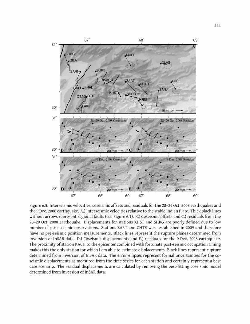
111
67˚ 68˚ 69˚
30˚
31˚
LORI
QLAS
SANJ
CHTR
HRNIHRNI
SHRGSHRG
ZART
MUSB
SURB
QTIT
KHAL
LAKP
QILA
SHBG
KACH
KHST
GULH
QTAG
SARN
10 mm/yr
A
30˚
31˚
30 mm
28−29 Oct. 2008 Coseismic
B
67˚ 68˚ 69˚
30˚
31˚
30 mm
9 Dec. 2008 Coseismic
D
30 mm
28−29 Oct. 2008 Residual
C
67˚ 68˚ 69˚
30 mm
9 Dec. 2008 Residual
E
Figure 6.5: Interseismic velocities, coseismic offsets and residuals for the 28–29 Oct. 2008 earthquakes andthe 9 Dec. 2008 earthquake. A.) Interseismic velocities relative to the stable Indian Plate. Thick black lineswithout arrows represent regional faults (see Figure 6.1). B.) Coseismic offsets and C.) residuals from the28–29 Oct. 2008 earthquake. Displacements for stations KHST and SHRG are poorly defined due to lownumber of post-seismic observations. Stations ZART and CHTR were established in 2009 and thereforehave no pre-seismic position measurements. Black lines represent the rupture planes determined frominversion of InSAR data. D.) Coseismic displacements and E.) residuals for the 9 Dec. 2008 earthquake.The proximity of station KACH to the epicenter combined with fortunate post-seismic occupation timingmakes this the only station for which I am able to estimate displacements. Black lines represent rupturedetermined from inversion of InSAR data. The error ellipses represent formal uncertainties for the co-seismic displacements as measured from the time series for each station and certainly represent a bestcase scenario. The residual displacements are calculated by removing the best-fitting coseismic modeldetermined from inversion of InSAR data.

112
66˚ 67˚ 68˚ 69˚
28˚
29˚
30˚
31˚
A
66˚ 67˚ 68˚ 69˚
B
66˚ 67˚ 68˚ 69˚
C
50 km
Figure 6.6: Epicentral locations for the 24 Aug. 1931 Sharigh earthquake and the 28 and 29 Oct. 2008 Ziaratearthquakes determined from shaking intensity data. Locations are determined using the methodologyoutlined in Chapter 3. The contours represent the 50%and 67%confidence contours for epicentral locationcalculated using parameters listed in Bakun (1999). In each subfigure, filled circles indicate the locations offelt reports, the star indicates the instrumentally determined epicenter and the center of the innermostcontour represents the preferred macroseismic estimate of epicenter. Intensity data are from Martin andSzeliga (2010). A.) Epicenter of the 24 Aug. 1931 Sharigh earthquake as determined from macroseismicdata. B.) Epicenter of the 28 Oct. 2008 earthquake as determined frommacroseismic data. C.) Epicenter ofthe 29 Oct. 2008 earthquake as determined from macroseismic data.
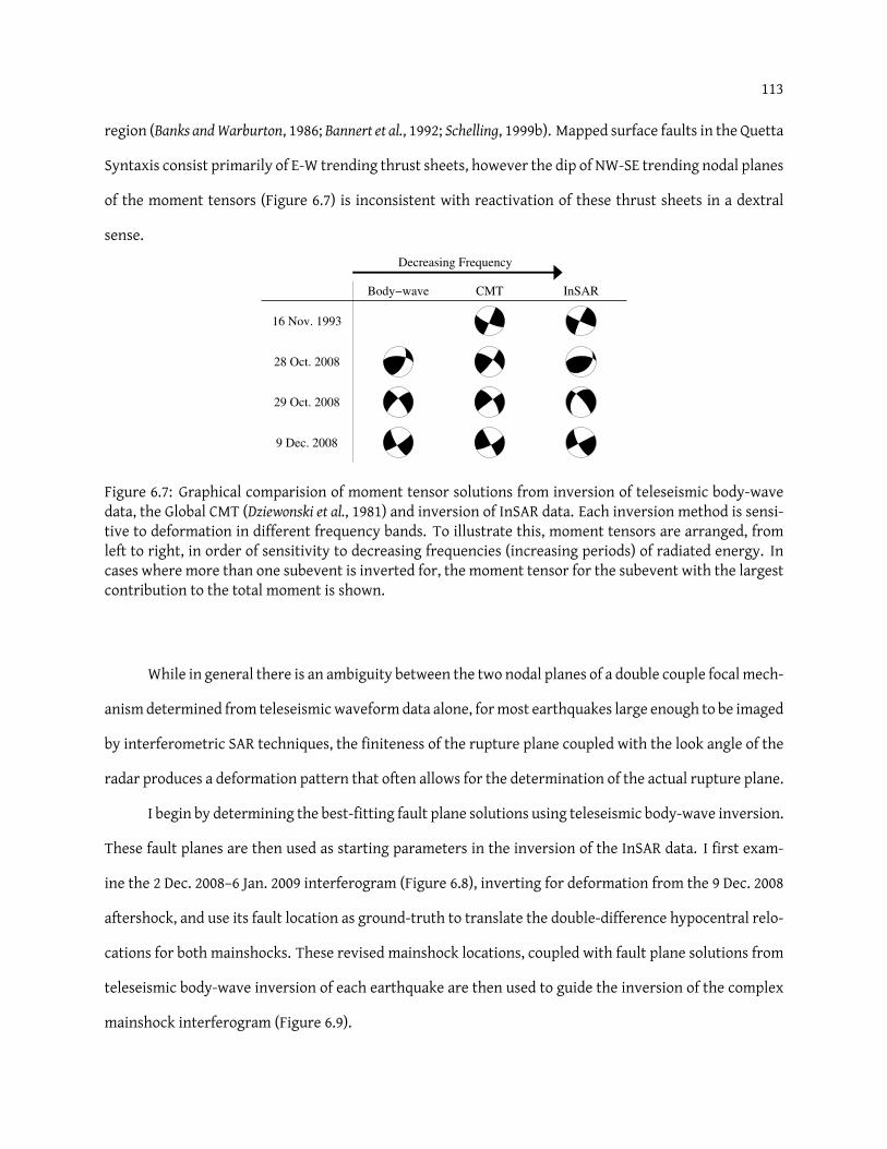
113
region (Banks andWarburton, 1986; Bannert et al., 1992; Schelling, 1999b). Mapped surface faults in the Quetta
Syntaxis consist primarily of E-W trending thrust sheets, however the dip of NW-SE trending nodal planes
of the moment tensors (Figure 6.7) is inconsistent with reactivation of these thrust sheets in a dextral
sense.
16 Nov. 1993
28 Oct. 2008
29 Oct. 2008
9 Dec. 2008
Body−wave CMT InSAR
Decreasing Frequency
Figure 6.7: Graphical comparision of moment tensor solutions from inversion of teleseismic body-wavedata, the Global CMT (Dziewonski et al., 1981) and inversion of InSAR data. Each inversion method is sensi-tive to deformation in different frequency bands. To illustrate this, moment tensors are arranged, fromleft to right, in order of sensitivity to decreasing frequencies (increasing periods) of radiated energy. Incases where more than one subevent is inverted for, the moment tensor for the subevent with the largestcontribution to the total moment is shown.
While in general there is an ambiguity between the two nodal planes of a double couple focal mech-
anism determined from teleseismicwaveformdata alone, formost earthquakes large enough to be imaged
by interferometric SAR techniques, the finiteness of the rupture plane coupled with the look angle of the
radar produces a deformation pattern that often allows for the determination of the actual rupture plane.
I begin by determining the best-fitting fault plane solutions using teleseismic body-wave inversion.
These fault planes are then used as starting parameters in the inversion of the InSAR data. I first exam-
ine the 2 Dec. 2008–6 Jan. 2009 interferogram (Figure 6.8), inverting for deformation from the 9 Dec. 2008
aftershock, and use its fault location as ground-truth to translate the double-difference hypocentral relo-
cations for both mainshocks. These revised mainshock locations, coupled with fault plane solutions from
teleseismic body-wave inversion of each earthquake are then used to guide the inversion of the complex
mainshock interferogram (Figure 6.9).
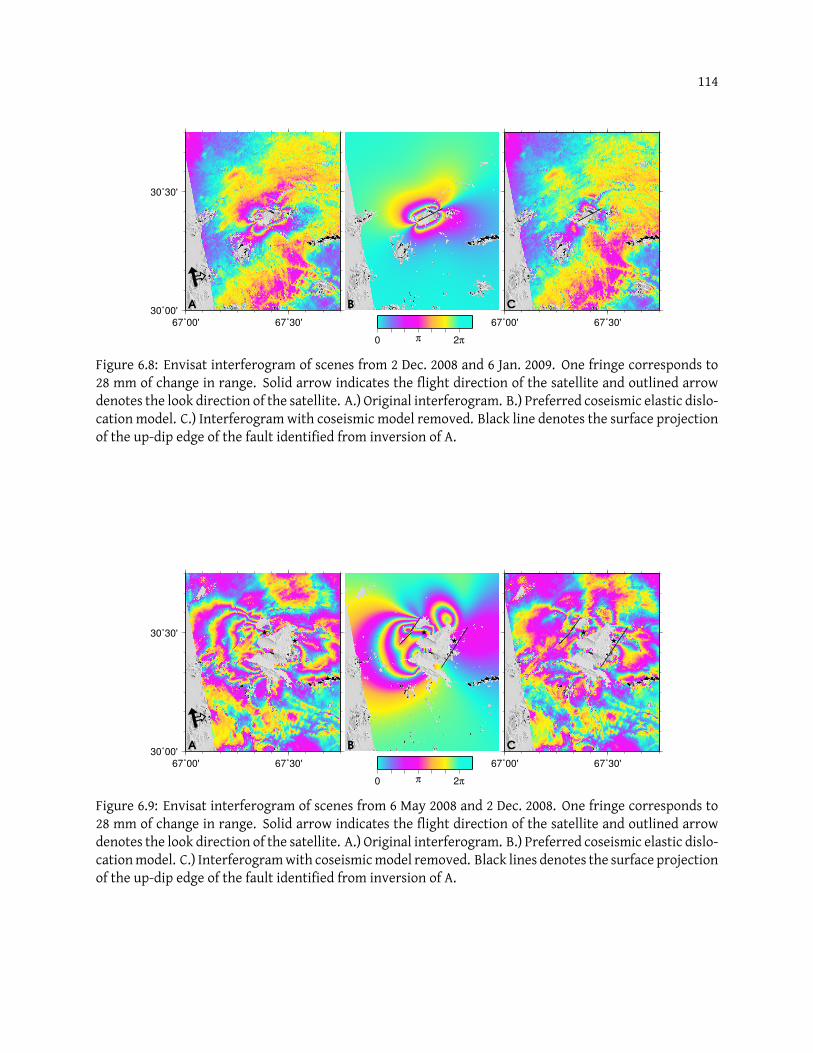
114
67˚00' 67˚30'
30˚00'
30˚30'
A B
67˚00' 67˚30'
C
0 π 2π
Figure 6.8: Envisat interferogram of scenes from 2 Dec. 2008 and 6 Jan. 2009. One fringe corresponds to28 mm of change in range. Solid arrow indicates the flight direction of the satellite and outlined arrowdenotes the look direction of the satellite. A.) Original interferogram. B.) Preferred coseismic elastic dislo-cation model. C.) Interferogramwith coseismic model removed. Black line denotes the surface projectionof the up-dip edge of the fault identified from inversion of A.
67˚00' 67˚30'
30˚00'
30˚30'
A B
67˚00' 67˚30'
C
0 π 2π
Figure 6.9: Envisat interferogram of scenes from 6 May 2008 and 2 Dec. 2008. One fringe corresponds to28 mm of change in range. Solid arrow indicates the flight direction of the satellite and outlined arrowdenotes the look direction of the satellite. A.) Original interferogram. B.) Preferred coseismic elastic dislo-cationmodel. C.) Interferogramwith coseismicmodel removed. Black lines denotes the surface projectionof the up-dip edge of the fault identified from inversion of A.
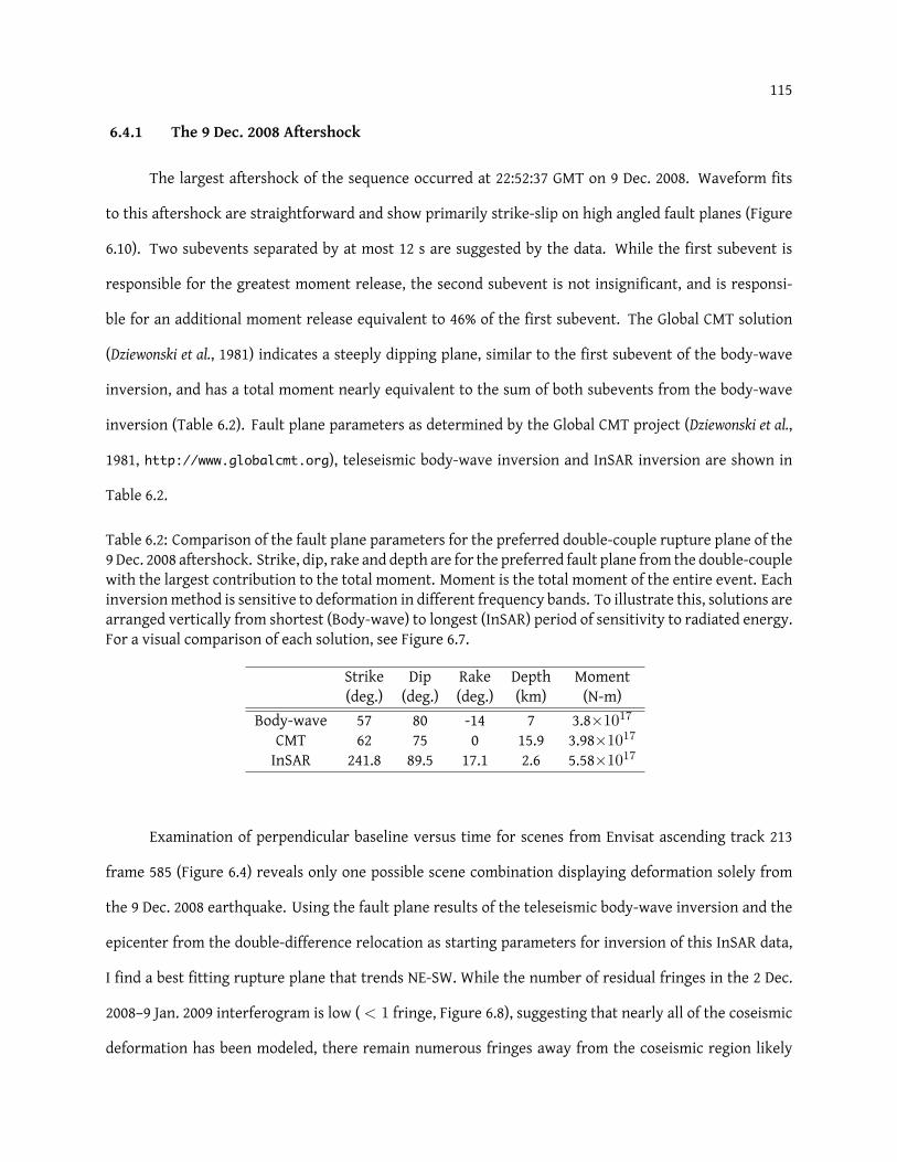
115
6.4.1 The 9 Dec. 2008 Aftershock
The largest aftershock of the sequence occurred at 22:52:37 GMT on 9 Dec. 2008. Waveform fits
to this aftershock are straightforward and show primarily strike-slip on high angled fault planes (Figure
6.10). Two subevents separated by at most 12 s are suggested by the data. While the first subevent is
responsible for the greatest moment release, the second subevent is not insignificant, and is responsi-
ble for an additional moment release equivalent to 46% of the first subevent. The Global CMT solution
(Dziewonski et al., 1981) indicates a steeply dipping plane, similar to the first subevent of the body-wave
inversion, and has a total moment nearly equivalent to the sum of both subevents from the body-wave
inversion (Table 6.2). Fault plane parameters as determined by the Global CMT project (Dziewonski et al.,
1981, http://www.globalcmt.org), teleseismic body-wave inversion and InSAR inversion are shown in
Table 6.2.
Table 6.2: Comparison of the fault plane parameters for the preferred double-couple rupture plane of the9 Dec. 2008 aftershock. Strike, dip, rake and depth are for the preferred fault plane from the double-couplewith the largest contribution to the total moment. Moment is the total moment of the entire event. Eachinversionmethod is sensitive to deformation in different frequency bands. To illustrate this, solutions arearranged vertically from shortest (Body-wave) to longest (InSAR) period of sensitivity to radiated energy.For a visual comparison of each solution, see Figure 6.7.
Strike Dip Rake Depth Moment(deg.) (deg.) (deg.) (km) (N-m)
Body-wave 57 80 -14 7 3.8×10¹⁷
CMT 62 75 0 15.9 3.98×10¹⁷
InSAR 241.8 89.5 17.1 2.6 5.58×10¹⁷
Examination of perpendicular baseline versus time for scenes from Envisat ascending track 213
frame 585 (Figure 6.4) reveals only one possible scene combination displaying deformation solely from
the 9 Dec. 2008 earthquake. Using the fault plane results of the teleseismic body-wave inversion and the
epicenter from the double-difference relocation as starting parameters for inversion of this InSAR data,
I find a best fitting rupture plane that trends NE-SW. While the number of residual fringes in the 2 Dec.
2008–9 Jan. 2009 interferogram is low (< 1 fringe, Figure 6.8), suggesting that nearly all of the coseismic
deformation has been modeled, there remain numerous fringes away from the coseismic region likely

116
0 60s
0 14s STF
A
TATO
A
B
NACB
B
C CHTO
CD
KKM
D
E
SBM
E
F
WR6
F
G
WR5
G
H
WR4
H
I
WC2
I
J
WR3
J
K
WRAB
K
L
WC1
L
M
KUM
M
N
KOM
N
O
PSI
O
P
KMBO
P
Q
TSUM
Q
RMBAR
RS
FURI
ST
IDI
T
U
TIP
U
V
TIR
V
A
YAK
A
B
ULN
B
C
YSS
C
D
ASAJ
D
E
NACB
E
FSSLB
FG
LBTB
G
H
KMBO
H
I
TSUM
I
J
MBAR
J
KFURI
K LDBIC
L
M
DIVS
M
9 Dec. 20081:57/80/346/7/2.614e172:185/62/22/10/1.193e17
Figure 6.10: Lower hemisphere projection of the moment tensors from the inversion of teleseismic body-waves for the 9 Dec. 2008 aftershock. Fault plane information for each subevent are listed in the header asevent number, strike, dip, and rake in degrees, depth in km and moment in N-m. Seismic station namesare printed vertically and to the left of each waveform. Seismic station locations on the focal sphere aredenoted by upper-case letters and correspond to the letter indicated between the station name and thewaveform trace. Upper plot shows P-wave focal sphere and waveforms, while the lower plot shows SH-wave focal sphere and waveforms. Amplitudes have been normalized to highlight the agreement betweenthe data (solid line) and the synthetic waveforms (dashed line). The source-time function along with thetime scale for each waveform is shown beneath the P-wave data for station KMBO.
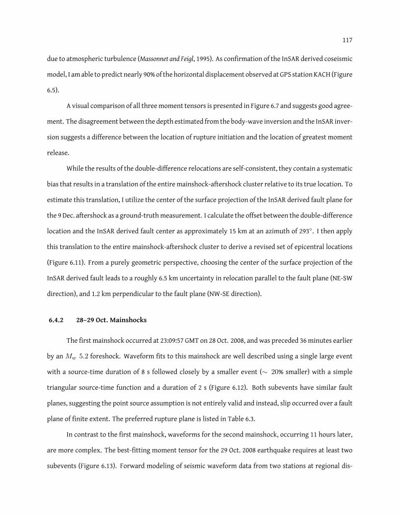
117
due to atmospheric turbulence (Massonnet and Feigl, 1995). As confirmation of the InSAR derived coseismic
model, I amable to predict nearly 90%of thehorizontal displacement observed at GPS stationKACH (Figure
6.5).
A visual comparison of all threemoment tensors is presented in Figure 6.7 and suggests good agree-
ment. The disagreement between the depth estimated from the body-wave inversion and the InSAR inver-
sion suggests a difference between the location of rupture initiation and the location of greatest moment
release.
While the results of the double-difference relocations are self-consistent, they contain a systematic
bias that results in a translation of the entiremainshock-aftershock cluster relative to its true location. To
estimate this translation, I utilize the center of the surface projection of the InSAR derived fault plane for
the 9 Dec. aftershock as a ground-truthmeasurement. I calculate the offset between the double-difference
location and the InSAR derived fault center as approximately 15 km at an azimuth of 293◦. I then apply
this translation to the entire mainshock-aftershock cluster to derive a revised set of epicentral locations
(Figure 6.11). From a purely geometric perspective, choosing the center of the surface projection of the
InSAR derived fault leads to a roughly 6.5 km uncertainty in relocation parallel to the fault plane (NE-SW
direction), and 1.2 km perpendicular to the fault plane (NW-SE direction).
6.4.2 28–29 Oct. Mainshocks
The first mainshock occurred at 23:09:57 GMT on 28 Oct. 2008, and was preceded 36minutes earlier
by an Mw 5.2 foreshock. Waveform fits to this mainshock are well described using a single large event
with a source-time duration of 8 s followed closely by a smaller event (∼ 20% smaller) with a simple
triangular source-time function and a duration of 2 s (Figure 6.12). Both subevents have similar fault
planes, suggesting the point source assumption is not entirely valid and instead, slip occurred over a fault
plane of finite extent. The preferred rupture plane is listed in Table 6.3.
In contrast to the first mainshock, waveforms for the second mainshock, occurring 11 hours later,
are more complex. The best-fitting moment tensor for the 29 Oct. 2008 earthquake requires at least two
subevents (Figure 6.13). Forward modeling of seismic waveform data from two stations at regional dis-
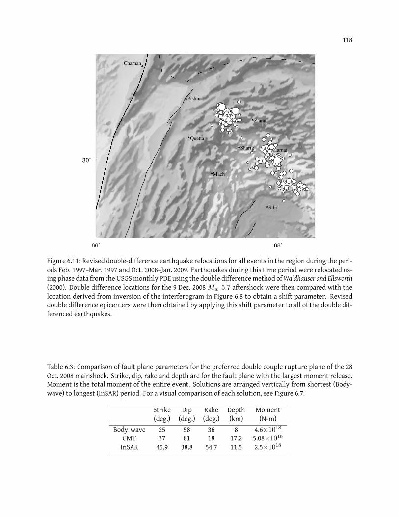
118
66˚ 68˚
30˚
Quetta
Ziarat
Sharig
Mach
Sibi
Harnai
Chaman
Pishin
Figure 6.11: Revised double-difference earthquake relocations for all events in the region during the peri-ods Feb. 1997–Mar. 1997 and Oct. 2008–Jan. 2009. Earthquakes during this time period were relocated us-ing phase data from the USGSmonthly PDE using the double differencemethod ofWaldhauser and Ellsworth(2000). Double difference locations for the 9 Dec. 2008 Mw 5.7 aftershock were then compared with thelocation derived from inversion of the interferogram in Figure 6.8 to obtain a shift parameter. Reviseddouble difference epicenters were then obtained by applying this shift parameter to all of the double dif-ferenced earthquakes.
Table 6.3: Comparison of fault plane parameters for the preferred double couple rupture plane of the 28Oct. 2008 mainshock. Strike, dip, rake and depth are for the fault plane with the largest moment release.Moment is the total moment of the entire event. Solutions are arranged vertically from shortest (Body-wave) to longest (InSAR) period. For a visual comparison of each solution, see Figure 6.7.
Strike Dip Rake Depth Moment(deg.) (deg.) (deg.) (km) (N-m)
Body-wave 25 58 36 8 4.6×10¹⁸
CMT 37 81 18 17.2 5.08×10¹⁸
InSAR 45.9 38.8 54.7 11.5 2.5×10¹⁸
119
0 60s
0 14s STF
A
SPBG
A
B
TLY
B
C
HIA
C
D
INCN
D
E
SSE
E
F
ENH
F
GNACB
GHTPUB
HI
KMI
I
J
PMG
J
K
SBM
K
L
IPM
L
M
DGAR
M
N
RER
N
O
MSEY
O
P
BOSA
P
Q
LBTB
Q
R
MBAR
R
S
FURI
S
TMSKU
T UDBIC
UV
WDD
V
W
CEL
W
X
VSL
X
Y
PAB
Y
Z
TUE
Z
[
GRFO
[
\
KBS
\
A
EYAK
A
B
YAK
B
C
MDJ
C
D
ERM
D
E COEN
EF
KSM
F
G
WRAB
G
H
IPM
H
I
FITZ
I
J
DGAR
J
K
FOMA
K
L
ABPO
L
M
BOSA
M
N
SUR
N
O
TSUM
O
P
MBAR
P
Q
VSL
Q
R
PVAQ
R
S
VTS
S
T
TIRR
T
U
SSB
U
V
BFO
V
28 Oct 20081:25/58/36/8/3.754e182:28/56/31/9/8.514e17
Figure 6.12: Lower hemisphere projection of the moment tensors from the inversion of teleseismic body-waves for the 28 Oct. 2008 aftershock. Fault plane information for each subevent are listed in the headeras event number, strike, dip, and rake in degrees, depth in km andmoment in N-m. Seismic station namesare printed vertically and to the left of each waveform. Seismic station locations on the focal sphere aredenoted by upper-case letters and correspond to the letter indicated between the station name and thewaveform trace. Upper plot shows P-wave focal sphere and waveforms, while the lower plot shows SH-wave focal sphere and waveforms. Amplitudes have been normalized to highlight the agreement betweenthe data (solid line) and the synthetic waveforms (dashed line). The source-time function along with thetime scale for each waveform is shown beneath the P-wave data for station RER.
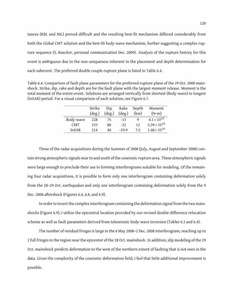
120
tances (KBL and NIL) proved difficult and the resulting best-fit mechanism differed considerably from
both the Global CMT solution and the best-fit body-wave mechanism, further suggesting a complex rup-
ture sequence (S. Roecker, personal communication Dec. 2009). Analysis of the rupture history for this
event is ambiguous due to the non-uniqueness inherent in the placement and depth determination for
each subevent. The preferred double couple rupture plane is listed in Table 6.4.
Table 6.4: Comparison of fault plane parameters for the preferred rupture plane of the 29 Oct. 2008 main-shock. Strike, dip, rake and depth are for the fault plane with the largest moment release. Moment is thetotal moment of the entire event. Solutions are arranged vertically from shortest (Body-wave) to longest(InSAR) period. For a visual comparison of each solution, see Figure 6.7.
Strike Dip Rake Depth Moment(deg.) (deg.) (deg.) (km) (N-m)
Body-wave 228 75 -13 9 4.1×10¹⁸
CMT 233 88 -22 12 5.39×10¹⁸
InSAR 214 40 -19.9 7.5 1.48×10¹⁸
Three of the radar acquisitions during the Summer of 2008 (July, August and September 2008) con-
tain strong atmospheric signals near to and south of the coseismic rupture area. These atmospheric signals
were large enough to preclude their use in forming interferograms suitable for modeling. Of the remain-
ing four radar acquisitions, it is possible to form only one interferogram containing deformation solely
from the 28–29 Oct. earthquakes and only one interferogram containing deformation solely from the 9
Dec. 2008 aftershock (Figures 6.4, 6.8, and 6.9).
In order to invert the complex interferogram containing the deformation signal from the twomain-
shocks (Figure 6.9), I utilize the epicentral location provided by our revised double-difference relocation
scheme as well as fault parameters derived from teleseismic body-wave inversion (Tables 6.3 and 6.4).
The number of residual fringes is large in the 6May 2008–2 Dec. 2008 interferogram, reaching up to
2 full fringes in the region near the epicenter of the 28 Oct. mainshock. In addition, slip modeling of the 29
Oct. mainshock predicts deformation to the west of the northern extent of faulting that is not seen in the
data. Given the complexity of the coseismic deformation field, I feel that little additional improvement is
possible.
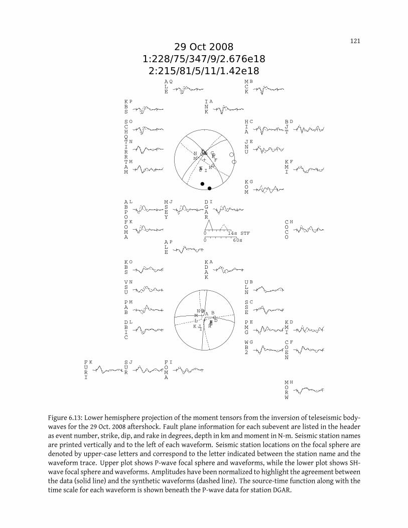
121
0 60s
0 14s STF
A
INK
A
B
MCK
B
C
HIA
C
D
BJT
D
E
JNU
E
F KMI
FG
KOM
G
H
COCO
H
I
DGAR
I
J
MSEY
J
K
FOMA
K
L
ABPO
L
MTAM
M
N
TIRR
N
O
SCHQ
O
P
KBS
P
Q
ALE
Q
A
KDAK
A
B
ULN
B
C
SSE
C
D KMI
DE PMG
EF
COEN
F
G
WB2
G
H
MORW
H
I
FOMA
I
J
SUR
J
K
FURI
K
LDBIC
LM
PAB
M
N
VSU
N
O
KBS
O
P
ALE
P
29 Oct 20081:228/75/347/9/2.676e18
2:215/81/5/11/1.42e18
Figure 6.13: Lower hemisphere projection of the moment tensors from the inversion of teleseismic body-waves for the 29 Oct. 2008 aftershock. Fault plane information for each subevent are listed in the headeras event number, strike, dip, and rake in degrees, depth in km andmoment in N-m. Seismic station namesare printed vertically and to the left of each waveform. Seismic station locations on the focal sphere aredenoted by upper-case letters and correspond to the letter indicated between the station name and thewaveform trace. Upper plot shows P-wave focal sphere and waveforms, while the lower plot shows SH-wave focal sphere and waveforms. Amplitudes have been normalized to highlight the agreement betweenthe data (solid line) and the synthetic waveforms (dashed line). The source-time function along with thetime scale for each waveform is shown beneath the P-wave data for station DGAR.
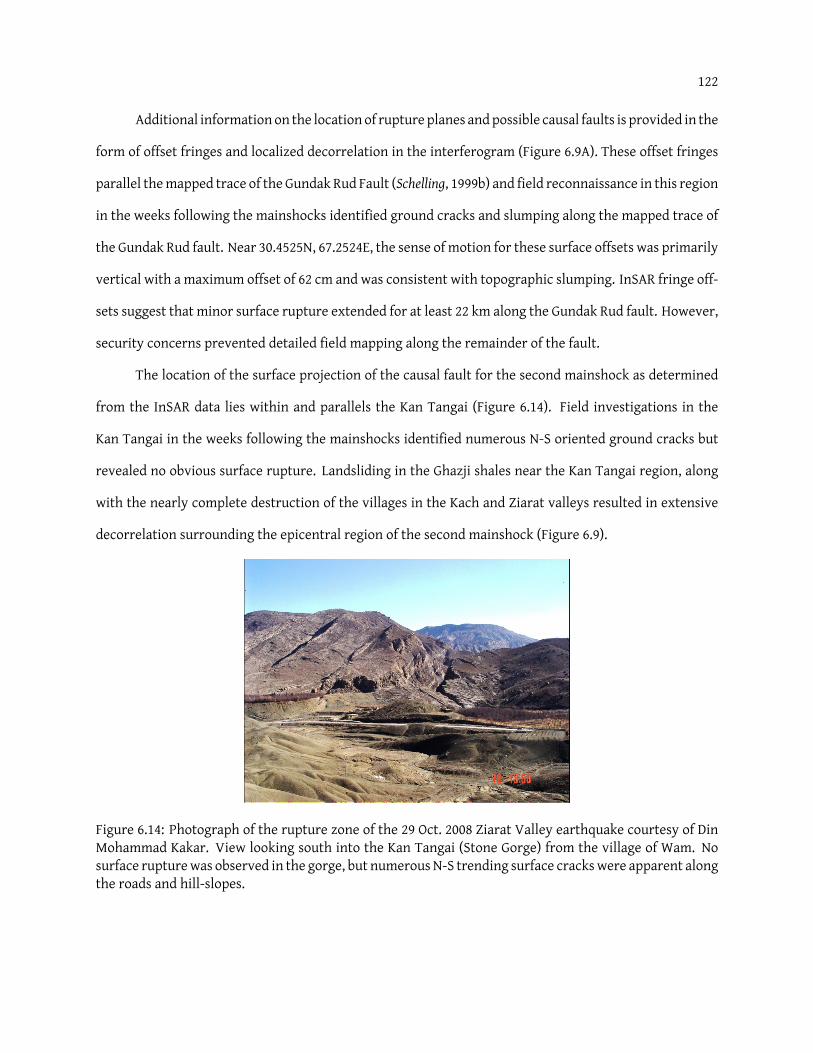
122
Additional information on the location of rupture planes andpossible causal faults is provided in the
form of offset fringes and localized decorrelation in the interferogram (Figure 6.9A). These offset fringes
parallel themapped trace of the Gundak Rud Fault (Schelling, 1999b) and field reconnaissance in this region
in the weeks following the mainshocks identified ground cracks and slumping along the mapped trace of
the Gundak Rud fault. Near 30.4525N, 67.2524E, the sense of motion for these surface offsets was primarily
vertical with a maximum offset of 62 cm and was consistent with topographic slumping. InSAR fringe off-
sets suggest that minor surface rupture extended for at least 22 km along the Gundak Rud fault. However,
security concerns prevented detailed field mapping along the remainder of the fault.
The location of the surface projection of the causal fault for the second mainshock as determined
from the InSAR data lies within and parallels the Kan Tangai (Figure 6.14). Field investigations in the
Kan Tangai in the weeks following the mainshocks identified numerous N-S oriented ground cracks but
revealed no obvious surface rupture. Landsliding in the Ghazji shales near the Kan Tangai region, along
with the nearly complete destruction of the villages in the Kach and Ziarat valleys resulted in extensive
decorrelation surrounding the epicentral region of the second mainshock (Figure 6.9).
Figure 6.14: Photograph of the rupture zone of the 29 Oct. 2008 Ziarat Valley earthquake courtesy of DinMohammad Kakar. View looking south into the Kan Tangai (Stone Gorge) from the village of Wam. Nosurface rupturewas observed in the gorge, but numerous N-S trending surface crackswere apparent alongthe roads and hill-slopes.
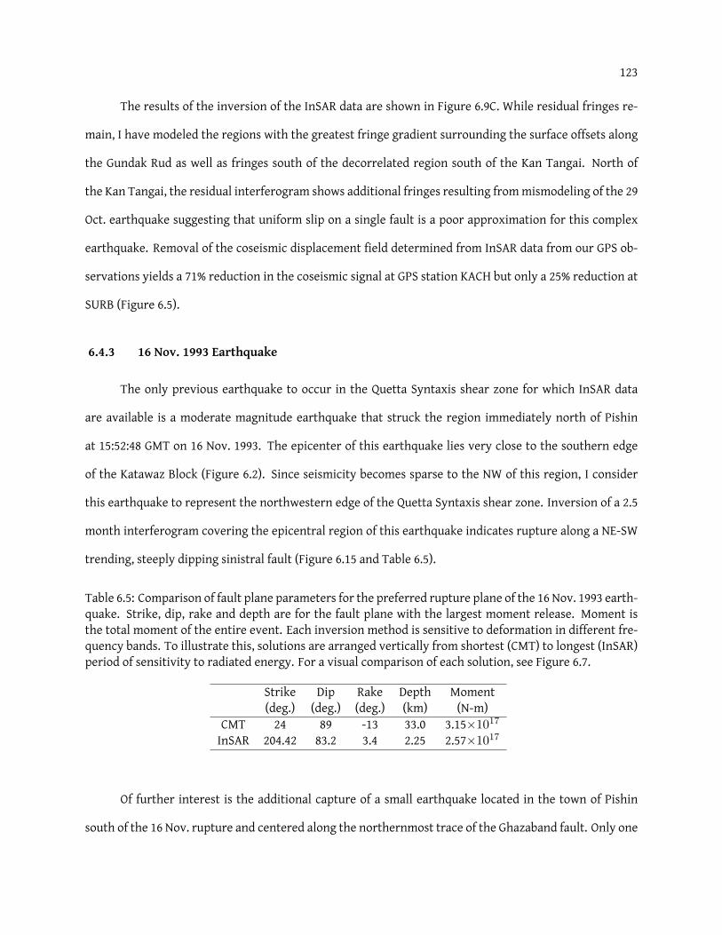
123
The results of the inversion of the InSAR data are shown in Figure 6.9C. While residual fringes re-
main, I have modeled the regions with the greatest fringe gradient surrounding the surface offsets along
the Gundak Rud as well as fringes south of the decorrelated region south of the Kan Tangai. North of
the Kan Tangai, the residual interferogram shows additional fringes resulting frommismodeling of the 29
Oct. earthquake suggesting that uniform slip on a single fault is a poor approximation for this complex
earthquake. Removal of the coseismic displacement field determined from InSAR data from our GPS ob-
servations yields a 71% reduction in the coseismic signal at GPS station KACH but only a 25% reduction at
SURB (Figure 6.5).
6.4.3 16 Nov. 1993 Earthquake
The only previous earthquake to occur in the Quetta Syntaxis shear zone for which InSAR data
are available is a moderate magnitude earthquake that struck the region immediately north of Pishin
at 15:52:48 GMT on 16 Nov. 1993. The epicenter of this earthquake lies very close to the southern edge
of the Katawaz Block (Figure 6.2). Since seismicity becomes sparse to the NW of this region, I consider
this earthquake to represent the northwestern edge of the Quetta Syntaxis shear zone. Inversion of a 2.5
month interferogram covering the epicentral region of this earthquake indicates rupture along a NE-SW
trending, steeply dipping sinistral fault (Figure 6.15 and Table 6.5).
Table 6.5: Comparison of fault plane parameters for the preferred rupture plane of the 16 Nov. 1993 earth-quake. Strike, dip, rake and depth are for the fault plane with the largest moment release. Moment isthe total moment of the entire event. Each inversion method is sensitive to deformation in different fre-quency bands. To illustrate this, solutions are arranged vertically from shortest (CMT) to longest (InSAR)period of sensitivity to radiated energy. For a visual comparison of each solution, see Figure 6.7.
Strike Dip Rake Depth Moment(deg.) (deg.) (deg.) (km) (N-m)
CMT 24 89 -13 33.0 3.15×10¹⁷
InSAR 204.42 83.2 3.4 2.25 2.57×10¹⁷
Of further interest is the additional capture of a small earthquake located in the town of Pishin
south of the 16 Nov. rupture and centered along the northernmost trace of the Ghazaband fault. Only one
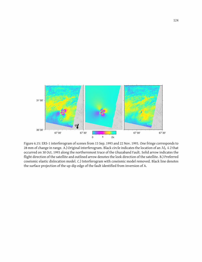
124
67˚00' 67˚30'
30˚30'
31˚00'
67˚00' 67˚30'
0 π 2π
Figure 6.15: ERS-1 interferogram of scenes from 13 Sep. 1993 and 22 Nov. 1993. One fringe corresponds to28mm of change in range. A.) Original interferogram. Black circle indicates the location of anMb 4.2 thatoccurred on 30 Oct. 1993 along the northernmost trace of the Ghazaband Fault. Solid arrow indicates theflight direction of the satellite and outlined arrow denotes the look direction of the satellite. B.) Preferredcoseismic elastic dislocation model. C.) Interferogram with coseismic model removed. Black line denotesthe surface projection of the up-dip edge of the fault identified from inversion of A.
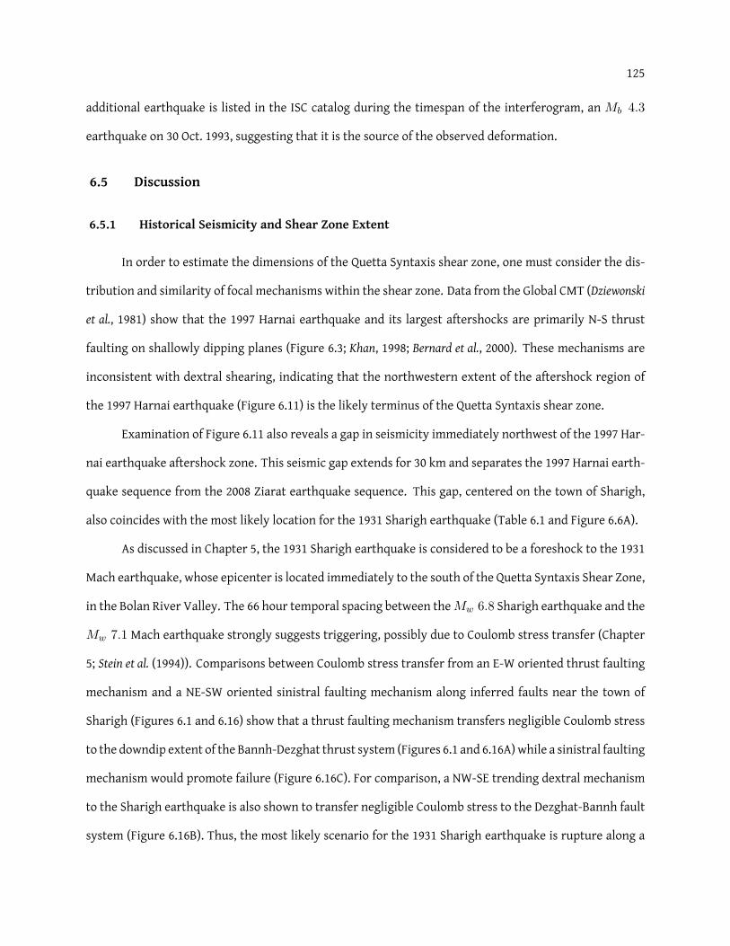
125
additional earthquake is listed in the ISC catalog during the timespan of the interferogram, an Mb 4.3
earthquake on 30 Oct. 1993, suggesting that it is the source of the observed deformation.
6.5 Discussion
6.5.1 Historical Seismicity and Shear Zone Extent
In order to estimate the dimensions of the Quetta Syntaxis shear zone, one must consider the dis-
tribution and similarity of focal mechanisms within the shear zone. Data from the Global CMT (Dziewonski
et al., 1981) show that the 1997 Harnai earthquake and its largest aftershocks are primarily N-S thrust
faulting on shallowly dipping planes (Figure 6.3; Khan, 1998; Bernard et al., 2000). These mechanisms are
inconsistent with dextral shearing, indicating that the northwestern extent of the aftershock region of
the 1997 Harnai earthquake (Figure 6.11) is the likely terminus of the Quetta Syntaxis shear zone.
Examination of Figure 6.11 also reveals a gap in seismicity immediately northwest of the 1997 Har-
nai earthquake aftershock zone. This seismic gap extends for 30 km and separates the 1997 Harnai earth-
quake sequence from the 2008 Ziarat earthquake sequence. This gap, centered on the town of Sharigh,
also coincides with the most likely location for the 1931 Sharigh earthquake (Table 6.1 and Figure 6.6A).
As discussed in Chapter 5, the 1931 Sharigh earthquake is considered to be a foreshock to the 1931
Mach earthquake, whose epicenter is located immediately to the south of the Quetta Syntaxis Shear Zone,
in the Bolan River Valley. The 66 hour temporal spacing between theMw 6.8 Sharigh earthquake and the
Mw 7.1 Mach earthquake strongly suggests triggering, possibly due to Coulomb stress transfer (Chapter
5; Stein et al. (1994)). Comparisons between Coulomb stress transfer from an E-W oriented thrust faulting
mechanism and a NE-SW oriented sinistral faulting mechanism along inferred faults near the town of
Sharigh (Figures 6.1 and 6.16) show that a thrust faulting mechanism transfers negligible Coulomb stress
to the downdip extent of the Bannh-Dezghat thrust system (Figures 6.1 and 6.16A)while a sinistral faulting
mechanism would promote failure (Figure 6.16C). For comparison, a NW-SE trending dextral mechanism
to the Sharigh earthquake is also shown to transfer negligible Coulomb stress to the Dezghat-Bannh fault
system (Figure 6.16B). Thus, the most likely scenario for the 1931 Sharigh earthquake is rupture along a
126
NE-SW trending sinistral fault. The location of this fault near the 1997 Harnai thrust faulting earthquakes
suggest that the Sharigh earthquake lies close to the southeastern extent of the Quetta Syntaxis shear
zone.
67˚ 68˚
29˚
30˚
−150−50
−50
50
50
150
A
67˚ 68˚
150
B
67˚ 68˚
−50
−50
50
C
Figure 6.16: Amapof Coulomb stress for a receiver faultwith the samegeometry as the down-dip extensionof the Deghat-Bannh thrust fault system (gray rectangle). Contours are 50 kPa. A.) Thrust orientationfor the 1931 Sharigh earthquake. B.) Dextral orientation for the 1931 Sharigh earthquake. C.) Sinistralorientation for the 1931 Sharigh earthquake.
The northeastern end of the shear zone terminates close to the southern edge of the seismically
quiet Katawaz Block (Figure 6.1; Haq and Davis (1997)). Near the southern end of the block, immediately
north of the town of Pishin, lies the epicentral location of the 16 Nov. 1993 earthquake (Figure 6.2). In-
version of InSAR data for this earthquake shows that it ruptured a NE-SW trending, steeply dipping fault
plane in a sinistral sense similar to earthquakes elsewhere in the shear zone. The location of this earth-
quake at the southern end of the seismically quiet Katawaz block suggests that this event represents the
northwestern extent of the Quetta Syntaxis shear zone.
Using the 1993 Pishin earthquake and the 1931 Sharigh earthquake to define the NW and SE extents
of the shear zone yields a shear zone length of 100 km (Figure 6.17). Although the subsurface rupture
length of the 1931 Sharigh earthquake is unknown, using relationships from Wells and Coppersmith (1994)
and a magnitude of Mw 6.8, I estimate its subsurface rupture length as ∼ 45km. Inversion of InSAR
data for the 28 and 29 Oct. 2008 earthquakes yields subsurface rupture lengths of approximately 22 km.
Similarly, inversion of the InSAR data recording the surface deformation of the 1993 Pishin earthquake
yields a subsurface rupture length of nearly 5 km. I begin with the assumption that faults in the shear
127
zone are of uniform length, and approximate the average subsurface rupture length as 25 km. Finally,
since all of the earthquakes in the shear zone occur in the shallow crust (Table 6.2, 6.3, 6.4, 6.5), I assume
a seismogenic thickness of 15 km.
6.5.2 Shear Zone Seismic Productivity
Given an estimate of the dextral shear rate across zone the from GPS measurements, I utilize the
idealized shear zone geometry to calculate the rate of slip on each fault (Figure 6.18, Ron et al. (1984);
Sigmundsson et al. (1995)). Projecting the spatially averaged GPS velocity field (Figure 6.3) into a shear
zone-parallel geometry yields a shear zone velocity of 17.0±2.0mm/yr relative to the stable Indian Plate.
Using equations relating block rotation rates to overall shear zone velocity derived in Sigmundsson et al.
(1995), I calculate a block rotation rate of 6.8× 10⁻⁷± 0.8× 10⁻⁷rad/yr, which corresponds to a slip rate
of 9.7± 1.1mm/yr on the block-bounding faults.
Assuming the inferred slip rate and fault lengths are uniform along the shear zone, I calculate a
geometric moment of 1.8× 10⁷ ± 0.2× 10⁷ m3/yr, or roughly 10Mw 6.4 earthquakes per century. This
value is comparable to the observed geometric moment of 1.0× 10⁷ m3/yr calculated from the EHB and
ISC catalogs for the past century (Table 6.1) over this same region, suggesting that the entire shear zone
has ruptured during the past century (Figure 6.19).
6.5.3 Tectonic Analogues
The southward motion of the Sulaiman Lobe relative to the stable Indian Plate, and the eastward
verging Kirthar range requires dextral shear in the Quetta Syntaxis (Figure 6.3). The absence of a promi-
nent dextral surface fault suggests that the observed dextral motion must be accommodated along con-
jugate structures. Our findings that the 1931 Sharigh earthquake, 1993 Pishin earthquake and both main-
shocks of the 2008 Ziarat earthquake sequence occurred on parallel NE/SW faults, indicates that dextral
shear is not confined to a single NW-SE trending fault. This accommodation of shear via conjugate struc-
tures is called “bookshelf faulting” and has been observed in locations as varied as the Afar, the Dead Sea,
southern California, Nicaragua and the South Iceland Seismic Zone (SISZ) (Ron et al., 1984; Garfunkel andRon,
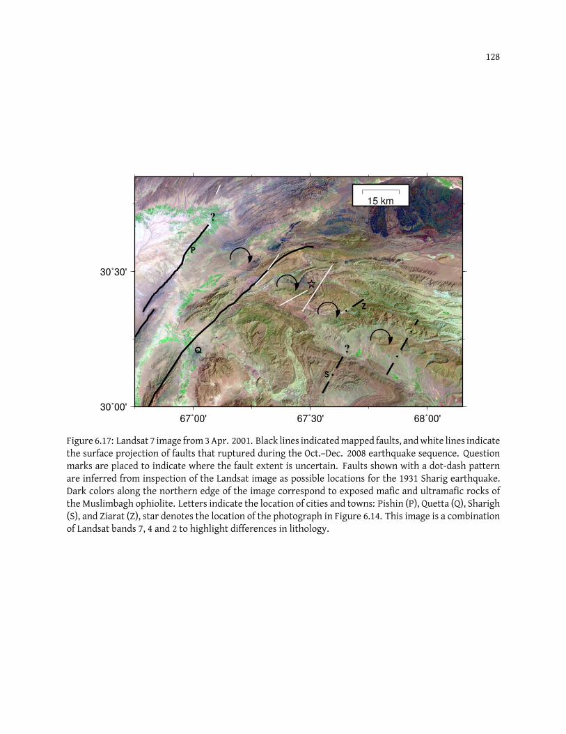
128
?
?
Q
S
Z
P
67˚00' 67˚30' 68˚00'
30˚00'
30˚30'
15 km
Figure 6.17: Landsat 7 image from3Apr. 2001. Black lines indicatedmapped faults, andwhite lines indicatethe surface projection of faults that ruptured during the Oct.–Dec. 2008 earthquake sequence. Questionmarks are placed to indicate where the fault extent is uncertain. Faults shown with a dot-dash patternare inferred from inspection of the Landsat image as possible locations for the 1931 Sharig earthquake.Dark colors along the northern edge of the image correspond to exposed mafic and ultramafic rocks ofthe Muslimbagh ophiolite. Letters indicate the location of cities and towns: Pishin (P), Quetta (Q), Sharigh(S), and Ziarat (Z), star denotes the location of the photograph in Figure 6.14. This image is a combinationof Landsat bands 7, 4 and 2 to highlight differences in lithology.
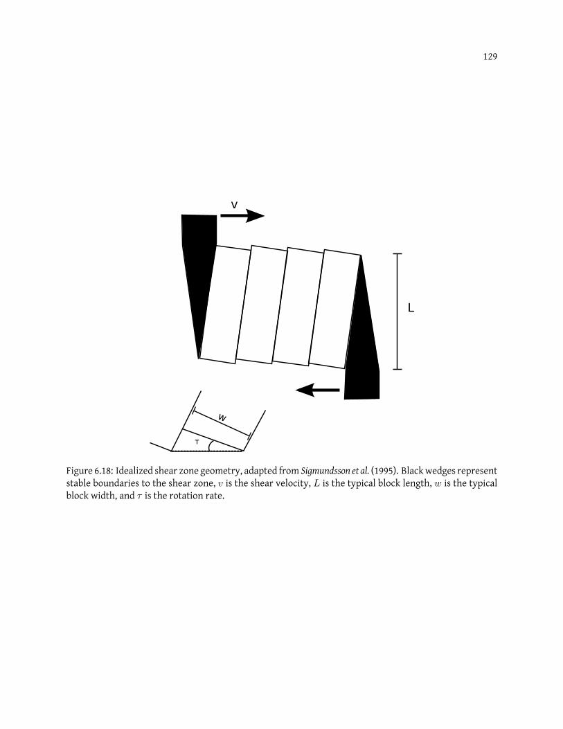
129
w
v
L
τ
Figure 6.18: Idealized shear zone geometry, adapted from Sigmundsson et al. (1995). Blackwedges representstable boundaries to the shear zone, v is the shear velocity, L is the typical block length, w is the typicalblock width, and τ is the rotation rate.
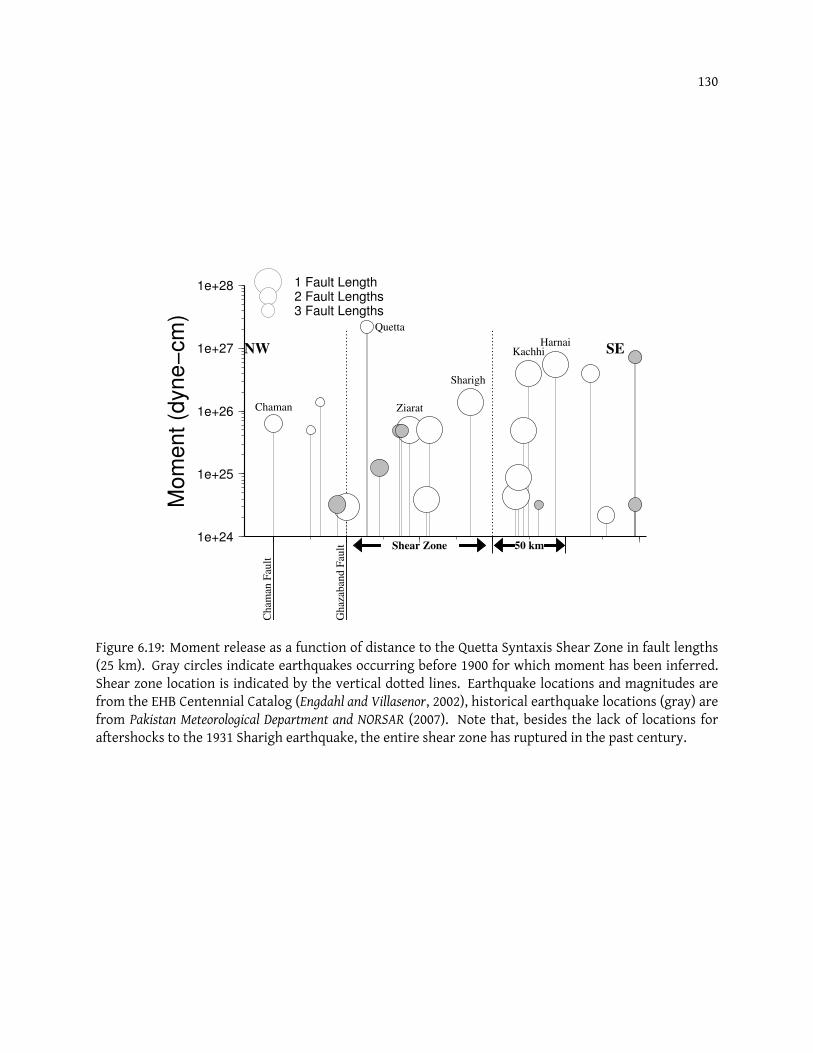
130
1e+24
1e+25
1e+26
1e+27
1e+28
Mom
ent (d
yne−
cm
)
Chaman
Kachhi
Sharigh
Quetta
Harnai
Ziarat
NW SE
1 Fault Length2 Fault Lengths3 Fault Lengths
Cham
an F
ault
Gh
azab
and
Fau
lt Shear Zone 50 km
Figure 6.19: Moment release as a function of distance to the Quetta Syntaxis Shear Zone in fault lengths(25 km). Gray circles indicate earthquakes occurring before 1900 for which moment has been inferred.Shear zone location is indicated by the vertical dotted lines. Earthquake locations and magnitudes arefrom the EHB Centennial Catalog (Engdahl and Villasenor, 2002), historical earthquake locations (gray) arefrom Pakistan Meteorological Department and NORSAR (2007). Note that, besides the lack of locations foraftershocks to the 1931 Sharigh earthquake, the entire shear zone has ruptured in the past century.
131
1985; McKenzie and Jackson, 1986; Nicholson et al., 1986; La Femina et al., 2002; Sigmundsson, 2006). In the Afar
and the SISZ, bookshelf faulting occurs in relatively young and thin volcanic crust through the formation
of new faults, while in southern California, and Nicaragua, pre-existing structures with trends which are
conjugate to the modern axis of maximum compression are reactivated. This utilization of pre-existing
structures to accommodate overall dextral shear via conjugate sinistral faults presents a mechanically
efficient means of shearing a region (Garfunkel and Ron, 1985).
In the Quetta Syntaxis Shear Zone, the trend of the faults bounding each block varies little from
the trend of the major strike-slip faults immediately to their west (the Ghazaband and Chaman Faults,
Figure 6.17). This similarity in strike suggests that not only is the dextral shear being accommodated by
pre-existing structures, but that little clockwise rotation has occurred in this shear zone and therefore,
the onset of dextral deformation is geologically recent. That the onset of dextral deformation is recent
is in accord with the analog models of Haq and Davis (1997) that suggest the total amount of shortening
across the Sulaiman Lobe is small and that northward translation of the Katawaz Block began late in the
collision between the Indian and Eurasian Plates.
In the Dead Sea region, the age and extent of bookshelf faulting has been investigated using pa-
leomagnetically determined block rotations (Ron et al., 1984). Although no paleomagnetic measurements
exist for the western Sulaiman Lobe, a similar approach could provide an age estimate for the onset of
deformation as well as an estimate of total deformation across the Quetta Syntaxis Shear Zone.
6.6 Conclusions
The Sulaiman Lobe is a southward verging salient formed by the confined translation of a relatively
rigid Katawaz block northward by the Chaman Fault System. The overall southwardmotion of this salient
relative to a stable Indian Plate is accommodated along its eastern margin by sinistral strike-slip faulting
along structures such as the Kingri Fault. Along the western margin, overall dextral shear between the
northern Kirthar Range and the Sulaiman Lobe is accommodated by clockwise rotation of small (25 km
× 15 km) blocks through sinistral motion on NE-SW oriented block-bounding faults. The trends of these
block-bounding faults nearly parallel the strike of the Chaman Fault and likely represent reactivated faults

132
that once aided the translation of the Katawaz Block. The similarity between the strike of the block-
bounding faults and the strike of major regional faults suggests that this shear zone has experienced little
overall rotation and is therefore a young feature. Finally, the similarity between the geometric moment
release in this shear zone calculated using kinematic and seismological data suggests that the entire shear
zone has ruptured over the past century.
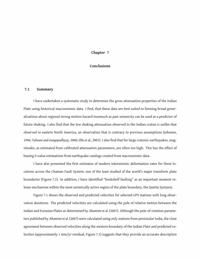
Chapter 7
Conclusions
7.1 Summary
I have undertaken a systematic study to determine the gross attenuation properties of the Indian
Plate using historical macroseismic data. I find, that these data are best suited to forming broad gener-
alizations about regional strong motion hazard insomuch as past seismicity can be used as a predictor of
future shaking. I also find that the low shaking attenuation observed in the Indian craton is unlike that
observed in eastern North America, an observation that is contrary to previous assumptions (Johnston,
1996; Talwani and Gangopadhyay, 2000; Ellis et al., 2001). I also find that for large cratonic earthquakes, mag-
nitudes, as estimated from calibrated attenuation parameters, are often too high. This has the effect of
biasing b-value estimations from earthquake catalogs created from macroseismic data.
I have also presented the first estimates of modern interseismic deformation rates for three lo-
cations across the Chaman Fault System, one of the least studied of the world’s major transform plate
boundaries (Figure 7.1). In addition, I have identified “bookshelf faulting” as an important moment re-
lease mechanism within the most seismically active region of the plate boundary, the Quetta Syntaxis.
Figure 7.1 shows the observed and predicted velocities for selected GPS stations with long obser-
vation durations. The predicted velocities are calculated using the pole of relative motion between the
Indian and Eurasian Plates as determined by Altamimi et al. (2007). Although the pole-of-rotation parame-
ters published by Altamimi et al. (2007) were calculated using only stations from peninsular India, the close
agreement between observed velocities along the western boundary of the Indian Plate and predicted ve-
locities (approximately 1 mm/yr residual, Figure 7.1) suggests that they provide an accurate description
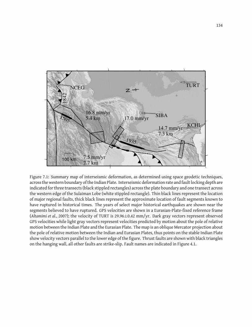
134
16.8 mm/yr5.4 km 17.0 mm/yr
7.5 mm/yr2.7 km
14.7 mm/yr7.3 km
1505
18
42
1935
SIBA
KCHI
TURTNCEG
100 km
N
Figure 7.1: Summary map of interseismic deformation, as determined using space geodetic techniques,across thewestern boundary of the Indian Plate. Interseismic deformation rate and fault locking depth areindicated for three transects (black stippled rectangles) across the plate boundary and one transect acrossthe western edge of the Sulaiman Lobe (white stippled rectangle). Thin black lines represent the locationof major regional faults, thick black lines represent the approximate location of fault segments known tohave ruptured in historical times. The years of select major historical earthquakes are shown near thesegments believed to have ruptured. GPS velocities are shown in a Eurasian-Plate-fixed reference frame(Altamimi et al., 2007); the velocity of TURT is 29.96±0.42 mm/yr. Dark gray vectors represent observedGPS velocities while light gray vectors represent velocities predicted by motion about the pole of relativemotion between the Indian Plate and the Eurasian Plate. Themap is an obliqueMercator projection aboutthe pole of relative motion between the Indian and Eurasian Plates, thus points on the stable Indian Plateshow velocity vectors parallel to the lower edge of the figure. Thrust faults are shownwith black triangleson the hanging wall, all other faults are strike-slip. Fault names are indicated in Figure 4.1.
135
of themotion of the entire stable Indian Plate. Not shown in Figure 7.1 is the velocity of GPS station CHMC,
which lies within the deforming region of the plate boundary and has a small velocity relative to stable
Eurasia (approximately 6 mm/yr, see Figure 4.7).
Interseismic deformation rates across the southernmost fault in the Chaman Fault System, the
Ornach-Nal Fault, demonstrate that the obvious mud ridge west of Bela, Pakistan, is not the location of
the modern plate boundary (Figure 4.6). Instead, GPS data suggests that an unmapped fault or faults be-
neath the Hinglaj synform, west of Bela, Pakistan, are accommodating a total of 14.7 mm/yr (12.8-18.2
mm/yr 95% HPD) of interseismic deformation. This velocity indicates that the shear localized here is ap-
proximately 60% of the theoretical shear at this point on the plate boundary (Figure 4.12). The absence
of historical and modern seismicity in this region coupled with the observation of relative motion with
respect to the Indian Plate indicates that deformation must be either distributed across multiple struc-
tures, each with low deformation rates, or is manifest as surface creep. The low rates of relative motion
between the Indian Plate and sites east of the Hinglaj synform also suggests that nearly all of the diffuse
deformation associated with the plate boundary must occur west of the Hinglaj synform, on the Eurasian
Plate. This hypothesis is further supported by the observation that the westernmost GPS station on the
transect across the Ornach-Nal Fault, PANG , shows that an additional 7.4 mm/yr of fault-parallel motion
must be accommodated across the arcuate faults comprising the subaerial Makran accretionary wedge
(Figure 4.5).
Further north, at the latitude of Chaman, Pakistan, I observe the Chaman Fault to be accommo-
dating only 40% of the 19.5 mm/yr of observed relative motion with the Indian Plate. The occurrence
of the 1892 Chaman Fault earthquake, immediately south of the present day GPS transect, indicates that
the fault is seismogenic at this latitude. In addition, the shallow locking depth derived from modeling of
the GPS transect (Figure 4.8) allows for the possibility that the Chaman Fault is creeping at the surface.
This shallow locking depth, coupled with observations of seismogenic behavior (the 1892 Chaman Fault
earthquake), suggests that this segment of the Chaman Fault displays a transitional behavior between a
locked segment south of Chaman, Pakistan, and a creeping segment near the GPS transect; a behavior
similar to that observed along the Parkfield segment of the San Andreas Fault (Harris and Segall, 1987). The
136
similarity between the velocity observed at GPS station CHMC and the expected velocity in the ITRF05
reference frame (Altamimi et al., 2007) suggests that diffuse plate boundary deformationmust occur east of
the Chaman Fault. This observation is in accordance with the pattern of regional seismicity (Figure 7.2).
North of Chaman, Pakistan, the Chaman Fault veers northeastward and enters a transpressional
bend. Along the southernmost 100 km of this fault segment, the observation of interseismic deformation
rates of nearly 17 mm/yr suggests that 75% of the plate boundary deformation is accommodated by the
Chaman Fault (Figure 4.12B). Previous authors had explained the historical absence of significant seismic
moment release along this fault segment by appealing to surface creep. However, the gentle gradient
seen in the surface deformation field in Figure 4.10 precludes surface creep. This absence of fault creep
coupled with an interseismic deformation rate of nearly 17 mm/yr suggests that the Chaman Fault north
of Chaman, Pakistan, releases stored strain through seismic rupture. Additionally, the relatively low rate
of seismicity along this segment during the past 50 years (Figure 7.2) suggests that nearly 375 km of the
Chaman Fault, between Chaman, Pakistan, and Kabul, Afghanistan, represents a major seismic gap. Were
this segment to rupture in one earthquake, it could release the equivalent of an Mw > 7.6. This pos-
sibility is not accounted for in modern analyses of regional seismic hazard (Giardini et al., 1999; Pakistan
Meteorological Department and NORSAR, 2007).
The region east of the Chaman Fault near Chaman, Pakistan, accommodates the remaining 60% of
the plate boundary shear. At this latitude, the width of the deforming region of the plate boundary as
highlighted by seismicity is 150–300 km (Figure 7.2A). The exceptional seismic productivity of this region
during the 20th century relative to theChamanFault Systemproper, alongwith its complex structural style
has made this region the focus of numerous geological studies during the past half century. The complex
interplay between seismicity in theQuetta Syntaxis Shear Zone and the fold-and-thrust belts of theKirthar
Range is exemplified by the 1931 Sharigh-Mach earthquake sequence. The subsequent occurrence of the
Mw 7.7 1935 Quetta earthquake only 60 km further west adds to this complexity. I have shown, that both
seismic and macroseismic estimates of the epicentral location of the Sharigh earthquake place it within
the Quetta Syntaxis Shear Zone. Given this epicentral location, the faulting mechanism most consistent
with a stress triggering relationship to the Mach earthquake is NE-SW trending sinistral faulting.
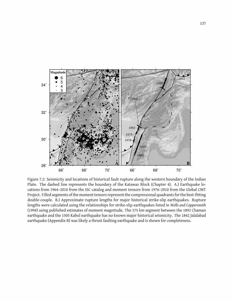
137
66˚ 68˚ 70˚
28˚
30˚
32˚
34˚
Magnitude
6
5
4
3
A
66˚ 68˚ 70˚
1505
1842
1892
1935
1975
1978
1990
]
[
375 km
B
Figure 7.2: Seismicity and locations of historical fault rupture along the western boundary of the IndianPlate. The dashed line represents the boundary of the Katawaz Block (Chapter 4). A.) Earthquake lo-cations from 1964–2010 from the ISC catalog and moment tensors from 1976–2010 from the Global CMTProject. Filled segments of themoment tensors represent the compressional quadrants for the best-fittingdouble-couple. B.) Approximate rupture lengths for major historical strike-slip earthquakes. Rupturelengths were calculated using the relationships for strike-slip earthquakes listed in Wells and Coppersmith(1994) using published estimates of moment magnitude. The 375 km segment between the 1892 Chamanearthquake and the 1505 Kabul earthquake has no known major historical seismicity. The 1842 Jalalabadearthquake (Appendix B) was likely a thrust faulting earthquake and is shown for completeness.

138
Detailed examination of subsequent earthquakes in the Quetta Syntaxis Shear Zone, most notably
the 2008 Ziarat earthquake sequence, also indicate NE-SW trending sinistral motion. The observation
of earthquakes in this shear zone using seismic and space geodetic techniques has helped identify it as a
region of “bookshelf faulting”, similar to that found in the SanAndreas-San Jacinto fault zone aswell as the
South Iceland Seismic Zone, and Afar (Nicholson et al., 1986; Tapponnier et al., 1990; Sigmundsson et al., 1995).
Comparisons between observed seismicity throughout the shear zone over the past century combined
with calculations of a geometry-based moment budget suggests that the entire shear zone has ruptured
in the past century. The ability for this shear zone to nucleate earthquakes withMw > 6.8 combinedwith
its complete rupture during the past century suggests that this remains a region of high seismic hazard.
7.2 Future Work
The relative absence of seismotectonic analyses of the Chaman Fault System compared to otherma-
jor transform systems around the globe leavesmany fundamental questions unanswered. The harsh land-
scape and difficult security situation that sometimes exists in the region can make even basic fieldwork
difficult. Yet, the ideal natural laboratory afforded by the Chaman Fault System makes it an important
location to test hypotheses based on other transform boundaries.
The difficulty in accessing this region suggests that further research using remote sensing tech-
niques are likely to be most successful. With the soon to be ubiquitous availability of high precision, low
cost InSAR data, many locations along the Chaman Fault System will become desirable targets for study
due to the arid climate and general lack of vegetation. Although fault azimuths in southern Chaman Fault
System, in general, are incompatible with current InSAR orbits, the likelihood that faults crossing the
Hinglaj Synform are creeping at the surface make them inviting targets.
Although the southern Chaman Fault System accommodates nearly 15 mm/yr of interseismic de-
formation, modern seismic data and historical reports suggest that, at least during the past 150 years,
earthquakes are not a common occurrence along this boundary (Minchin, 1907). There remains the possi-
bility that large earthquakes, unrecorded bywritten history, have occurred in this region. The presence of
long-lived Hindu temples in the Hinglaj area could be subjected to archeological and paleoseismic studies
139
in an effort to extend the seismic record for this region to longer timescales.
Current seismotectonic hazard analysis of western Pakistan and eastern Afghanistan suggest that
most populated region along the western Indian Plate boundary to expected to experience damaging
ground accelerations in the next 50 years is Quetta, Pakistan (Giardini et al., 1999; Pakistan Meteorological
Department and NORSAR, 2007). While seismicity from the Quetta Syntaxis Shear Zone, located 30 km to
the NE, does present a threat to the city, a repeat of the Mw 7.7 1935 Quetta earthquake would be catas-
trophic. The current absence of significant seismicity along the Ghazaband Fault, the presumed source of
the 1935 Quetta earthquake, suggests that this fault could currently be accumulating strain (Figure 7.2).
However, the absence of a geodetically determined slip rate across the Ghazaband Fault, SE of Quetta pro-
hibits estimations of the strain accumulation rate, and therefore, the recurrence interval, for rupture of
this fault.
One additional benefit to increasing the spatial resolution of geodetic measurements across the
Ghazaband Fault SE of Quetta would be the resulting increase in the accuracy of convergence estimates
across the Kirthar Range. Previous geodetic studies in this region focused primarily on leveling, helping
to capture the vertical deformation caused by the 1931Mach earthquake. Triangulation across the Kirthar
Range by the Survey of India during the beginning of the 20th was performed, however, the data are not
publicly available.

Appendix A
EMS-98 Short Form

141
Table A.1: The short form of the EMS-98 intensity scale reproduced from Grunthal and Levret (2001). Fora more detailed description of the criteria used to assign intensities, refer to Grunthal and Levret (2001),specifically pages 14–20.
EMS Definition Description of typical observed effectsintensity (abstracted)
I Not felt Not felt.II Scarcely felt Felt only by very few individual people at rest in houses.III Weak Felt indoors by a few people. People at rest feel a swaying or light
trembling.IV Largely Felt indoors by many people, outdoors by very few. A few people are
observed awakened. Windows, doors and dishes rattle.V Strong Felt indoors by most, outdoors by few. Many sleeping people awake, a few
are frightened. Buildings tremble throughout.Hanging objects swing considerably. Small objects are shifted. Doors andwindows swing open or shut.
VI Slightly Many people are frightened and run outdoors. Some objects fall. Manydamaging houses suffer slight non-structural damage like hair-line cracks and fall of
small pieces of plaster.VII Damaging Most people are frightened and run outdoors. Furniture is shifted and
objects fall from shelves in large numbers. Many well built ordinaryparts buildings suffer moderate damage: small cracks in walls, fall of plaster,of chimneys fall down; older buildings may show large cracks in walls andfailure of fill-in walls.
VIII Heavily Many people find it difficult to stand. Many houses have large cracks indamaging walls. A few well built ordinary buildings show serious failure of walls,
while weak older structures may collapse.IX Destructive General panic. Many weak constructions collapse. Even well built ordinary
buildings show very heavy damage: serious failure of walls and partialstructural failure.
X Very Many ordinary well built buildings collapse.destructive
XI Devastating Most ordinary well built buildings collapse, even some with goodearthquake resistant design are destroyed.
XII Completely Almost all buildings are destroyed.devastating
Appendix B
List of Epicentral Locations for Historical Seismicity on the Indian Plate
This appendix contains one table (Table B.1) providing a summary of earthquake epicenters for
each event in the catalog for which we were able to calculate an epicenter using the methods outlined in
Chapter 3. For each earthquake, the following information is listed: column Date refers to the date of an
earthquake in the local time. A location and magnitude derived using both the minimum deviation and
minimum magnitude epicentral location methodologies described in Chapter 3 are also listed. Column
Earthquake Name provides a geographic region descriptor that links each earthquakes to the tables in the
electronic supplement toMartin and Szeliga (2010).
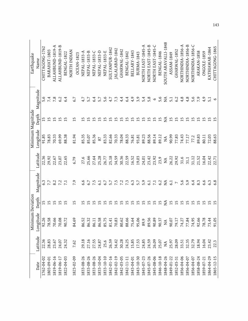
143Minim
umDe
viation
Minim
umMag
nitude
Earthq
uake
Date
Latit
ude
Long
itude
Depth
Mag
nitude
Latit
ude
Long
itude
Depth
Mag
nitude
Name
1762
-04-02
22.36
92.26
156.3
22.36
91.85
155.6
CHITTA
GONG
-176
218
03-09-01
28.83
78.58
157.7
29.92
78.83
157.4
BARA
HAT-
1803
1819
-06-16
23.67
70.66
158.2
22.67
70.33
157.8
ALLA
HBUN
D-18
19-A
1819
-06-17
24.07
70.08
157.2
23.07
69.99
156.2
ALLA
HBUN
D-18
19-B
1822
-04-03
24.32
90.72
157.1
22.65
88.38
156.4
BENG
AL-182
2NO
RTHIN
DIAN
1823
-02-09
7.62
84.69
157.9
6.79
81.94
156.7
OCEA
N-18
2318
33-08-26
29.18
86.52
156.6
27.6
85.35
154.7
NEPA
L-18
33-A
1833
-08-26
27.16
86.32
156.7
25.66
85.07
155.7
NEPA
L-18
33-B
1833
-08-26
27.55
86.11
157.5
27.64
85.36
156.4
NEPA
L-18
33-C
1833
-10-04
24.87
86.58
156.1
25.28
8715
5.7NE
PAL-18
33-D
1833
-10-10
25.6
85.75
156.7
26.77
83.33
155.6
NEPA
L-18
33-E
1842
-01-16
26.59
81.41
155.7
25.18
82.66
154.7
SULT
ANPU
R-18
4218
42-02-19
34.42
70.83
157.5
34.59
70.33
157.3
JALA
LABA
D-18
4218
42-03-05
30.28
80.62
157.2
30.36
78.04
154.4
GHAR
WAL
-184
218
42-11-11
24.25
88.66
157.3
22.59
88.33
156.4
BENG
AL-184
218
43-04-01
15.85
75.64
156.3
16.52
76.81
154.9
BELL
ARY-
1843
1843
-10-30
17.53
95.06
155.7
19.03
93.81
153.9
BURM
A-18
4318
45-07-23
24.85
89.9
155.9
24.01
89.23
155.4
NORT
HEA
ST-184
5-A
1845
-07-26
24.59
89.56
156.1
23.42
88.56
155.8
NORT
HEA
ST-184
5-B
1845
-08-06
26.09
90.89
157.1
23.92
89.14
156
NORT
HEA
ST-184
5-C
1846
-10-18
25.07
90.37
156.2
23.9
89.12
155.6
BENG
AL-184
618
48-04-26
NANA
NANA
NANA
NANA
SOUT
HAR
AVAL
LI-184
818
49-01-22
25.97
90.07
156.1
26.22
90.99
155.1
ASSA
M-184
918
52-03-31
28.09
79.17
157
29.92
77.83
156.2
GHAR
WAL
-185
218
56-04-06
33.51
74.27
155.6
31.6
74.43
154.8
NORT
HIND
IA-185
6-A
1856
-04-07
32.35
77.84
155.9
31.1
77.17
154.8
NORT
HIND
IA-185
6-B
1856
-04-07
32.79
74.95
156.4
31.12
77.2
155.6
NORT
HIND
IA-185
6-C
1858
-08-24
18.94
92.66
158.3
21.52
89.83
157.9
ARAK
AN-185
818
59-07-21
16.04
78.78
156.6
16.04
80.11
154.9
ONGO
LE-185
918
64-04-29
23.42
73.44
156.3
22.42
72.03
155.1
KATH
IAWAR
-186
418
65-12-15
22.3
91.05
156.8
22.71
88.63
156
CHITTA
GONG
-186
5

144Minim
umDe
viation
Minim
umMag
nitude
Earthq
uake
Date
Latit
ude
Long
itude
Depth
Mag
nitude
Latit
ude
Long
itude
Depth
Mag
nitude
Name
1865
-12-31
16.53
75.11
155.7
17.61
75.86
154.9
KARN
ATAK
A-18
6518
66-05-23
27.12
85.26
157.4
25.62
85.09
156.8
NEPA
L-18
6618
68-06-30
24.45
90.83
155.6
24.45
88.91
154.1
NORT
HEA
ST-186
818
68-07-31
22.6
85.47
155.5
23.68
86.81
154.5
JAMSH
EDPU
R-18
6818
69-01-10
24.05
93.33
158.3
25.55
91.83
157.6
CACH
AR-186
918
70-10-28
26.14
66.84
155.4
27.56
68.17
153.8
BALO
CHISTA
N-18
7018
71-01-31
23.04
73.58
156
21.13
7315
4.4SO
UTHGU
JARA
T-18
7118
78-02-05
25.95
92.3
154.8
26.12
91.72
154.5
NORT
HEA
ST-187
8-A
1878
-02-05
25.8
92.35
154.5
26.14
91.76
154.2
NORT
HEA
ST-187
8-B
1878
-03-02
34.13
74.43
157.4
33.97
72.09
156.4
HAZA
RA-187
818
78-04-29
27.65
91.48
155.2
26.57
93.98
154
NORT
HEA
ST-187
8-C
1878
-07-02
27.64
92.8
154.5
26.39
92.72
153.2
NORT
HEA
ST-187
8-D
1879
-01-03
27.88
93.81
155.5
26.8
94.23
154.4
NORT
HEA
ST-187
9-A
1879
-10-08
25.05
90.96
155.2
25.63
91.87
154.3
NORT
HEA
ST-187
9-B
1880
-06-30
25.64
93.44
155.7
26.22
91.85
155.3
NORT
HEA
ST-188
0CA
RNI
COBA
R18
81-12-31
7.17
89.6
159.3
987
.7715
8.9ISLA
ND-188
118
85-05-30
34.54
74.68
156.6
34.12
74.51
156
KASH
MIR-188
518
85-07-14
24.91
89.43
157.1
24.16
88.26
156.9
BENG
AL-188
5-A
1885
-07-14
25.68
88.91
155.1
24.43
89.66
154.4
BENG
AL-188
5-B
1897
-06-12
25.13
90.07
158.4
24.88
89.07
158.3
ASSA
M-189
7-A
1897
-06-22
24.35
88.34
156.1
25.85
89.42
155.7
ASSA
M-189
7-B
1898
-09-30
25.16
91.34
155.4
25.58
91.84
154.8
ASSA
M-189
819
00-02-08
11.03
76.58
156.4
11.37
76.83
156
COIM
BATO
RE-190
019
05-04-02
15.42
80.44
155.8
15.51
80.03
155
ONGO
LE-190
519
05-04-05
32.58
76.83
157.8
30.83
76.92
157.5
KANG
RA-190
5-A
1905
-06-13
32.05
78.36
155.6
31.13
77.2
154.2
KANG
RA-190
6-B
1905
-07-21
32.96
76.7
156.4
32.04
76.29
156
KANG
RA-190
6-C
1906
-02-28
31.73
75.36
156.9
31.14
77.2
156.2
BASH
AHR-
1906
1906
-05-20
29.68
76.56
155.9
30.35
78.06
154.9
KANG
RA-190
6-A
1906
-09-29
22.78
86.73
155.9
22.78
88.31
154.3
BENG
AL-190
619
09-10-20
28.83
68.08
05.7
29.33
67.83
05.3
KACH
HI-190
9
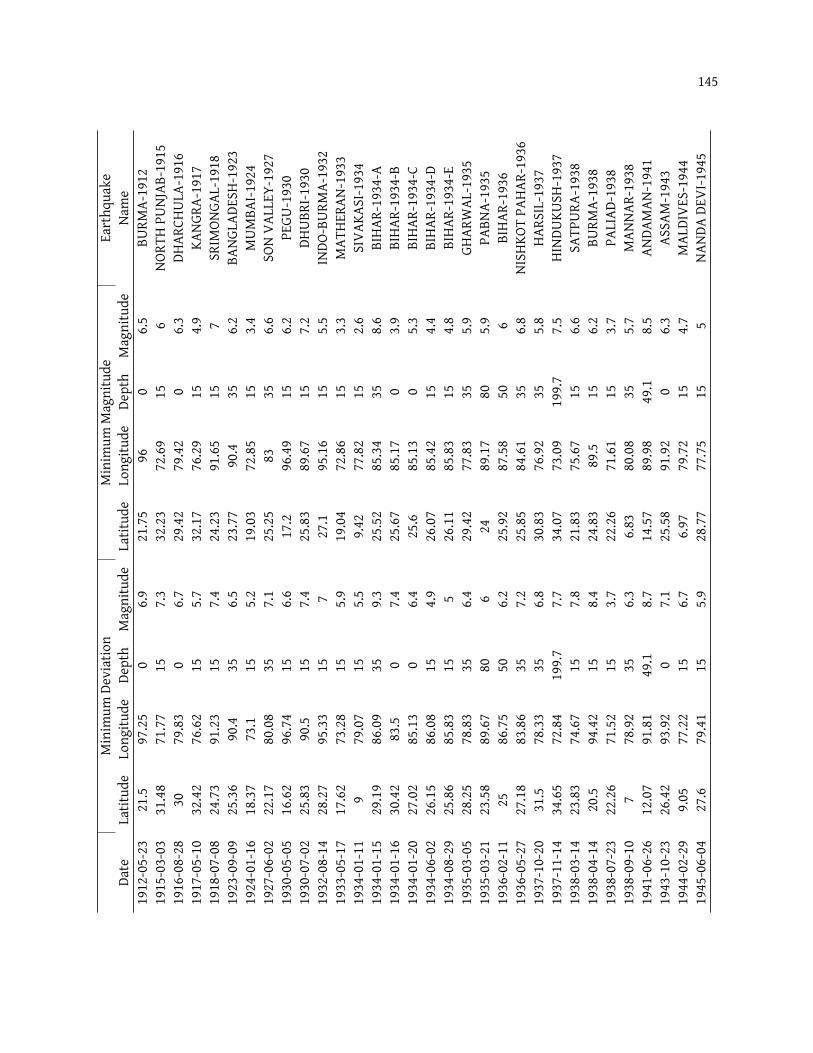
145Minim
umDe
viation
Minim
umMag
nitude
Earthq
uake
Date
Latit
ude
Long
itude
Depth
Mag
nitude
Latit
ude
Long
itude
Depth
Mag
nitude
Name
1912
-05-23
21.5
97.25
06.9
21.75
960
6.5BU
RMA-
1912
1915
-03-03
31.48
71.77
157.3
32.23
72.69
156
NORT
HPU
NJAB
-191
519
16-08-28
3079
.830
6.729
.4279
.420
6.3DH
ARCH
ULA-
1916
1917
-05-10
32.42
76.62
155.7
32.17
76.29
154.9
KANG
RA-191
719
18-07-08
24.73
91.23
157.4
24.23
91.65
157
SRIM
ONGA
L-19
1819
23-09-09
25.36
90.4
356.5
23.77
90.4
356.2
BANG
LADE
SH-192
319
24-01-16
18.37
73.1
155.2
19.03
72.85
153.4
MUM
BAI-1
924
1927
-06-02
22.17
80.08
357.1
25.25
8335
6.6SO
NVA
LLEY
-192
719
30-05-05
16.62
96.74
156.6
17.2
96.49
156.2
PEGU
-193
019
30-07-02
25.83
90.5
157.4
25.83
89.67
157.2
DHUB
RI-193
019
32-08-14
28.27
95.33
157
27.1
95.16
155.5
INDO
-BUR
MA-
1932
1933
-05-17
17.62
73.28
155.9
19.04
72.86
153.3
MAT
HERA
N-19
3319
34-01-11
979
.0715
5.59.4
277
.8215
2.6SIVA
KASI-193
419
34-01-15
29.19
86.09
359.3
25.52
85.34
358.6
BIHA
R-19
34-A
1934
-01-16
30.42
83.5
07.4
25.67
85.17
03.9
BIHA
R-19
34-B
1934
-01-20
27.02
85.13
06.4
25.6
85.13
05.3
BIHA
R-19
34-C
1934
-06-02
26.15
86.08
154.9
26.07
85.42
154.4
BIHA
R-19
34-D
1934
-08-29
25.86
85.83
155
26.11
85.83
154.8
BIHA
R-19
34-E
1935
-03-05
28.25
78.83
356.4
29.42
77.83
355.9
GHAR
WAL
-193
519
35-03-21
23.58
89.67
806
2489
.1780
5.9PA
BNA-
1935
1936
-02-11
2586
.7550
6.225
.9287
.5850
6BIHA
R-19
3619
36-05-27
27.18
83.86
357.2
25.85
84.61
356.8
NISH
KOTPA
HAR-
1936
1937
-10-20
31.5
78.33
356.8
30.83
76.92
355.8
HARS
IL-193
719
37-11-14
34.65
72.84
199.7
7.734
.0773
.0919
9.77.5
HIND
UKUS
H-19
3719
38-03-14
23.83
74.67
157.8
21.83
75.67
156.6
SATP
URA-
1938
1938
-04-14
20.5
94.42
158.4
24.83
89.5
156.2
BURM
A-19
3819
38-07-23
22.26
71.52
153.7
22.26
71.61
153.7
PALIAD
-193
819
38-09-10
778
.9235
6.36.8
380
.0835
5.7MAN
NAR-
1938
1941
-06-26
12.07
91.81
49.1
8.714
.5789
.9849
.18.5
ANDA
MAN
-194
119
43-10-23
26.42
93.92
07.1
25.58
91.92
06.3
ASSA
M-194
319
44-02-29
9.05
77.22
156.7
6.97
79.72
154.7
MAL
DIVE
S-19
4419
45-06-04
27.6
79.41
155.9
28.77
77.75
155
NAND
ADE
VI-194
5
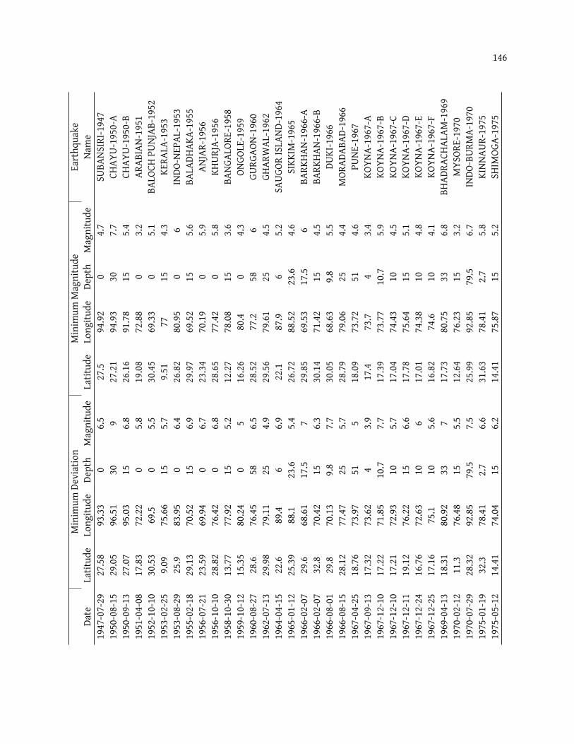
146Minim
umDe
viation
Minim
umMag
nitude
Earthq
uake
Date
Latit
ude
Long
itude
Depth
Mag
nitude
Latit
ude
Long
itude
Depth
Mag
nitude
Name
1947
-07-29
27.58
93.33
06.5
27.5
94.92
04.7
SUBA
NSIRI-1
947
1950
-08-15
29.05
96.51
309
27.21
94.93
307.7
CHAY
U-19
50-A
1950
-09-13
27.07
95.03
156.8
26.16
91.78
155.4
CHAY
U-19
50-B
1951
-04-08
17.83
72.22
05.8
19.08
72.88
03.2
ARAB
IAN-
1951
1952
-10-10
30.53
69.5
05.5
30.45
69.33
05.1
BALO
CHPU
NJAB
-195
219
53-02-25
9.09
75.66
155.7
9.51
7715
4.3KE
RALA
-195
319
53-08-29
25.9
83.95
06.4
26.82
80.95
06
INDO
-NEP
AL-195
319
55-02-18
29.13
70.52
156.9
29.97
69.52
155.6
BALA
DHAK
A-19
5519
56-07-21
23.59
69.94
06.7
23.34
70.19
05.9
ANJA
R-19
5619
56-10-10
28.82
76.42
06.8
28.65
77.42
05.8
KHUR
JA-195
619
58-10-30
13.77
77.92
155.2
12.27
78.08
153.6
BANG
ALOR
E-19
5819
59-10-12
15.35
80.24
05
16.26
80.4
04.3
ONGO
LE-195
919
60-08-27
28.6
76.45
586.5
28.52
77.2
586
GURG
AON-
1960
1962
-07-13
29.98
79.11
254.9
29.56
79.61
254.5
GHAR
WAL
-196
219
64-04-15
22.6
89.4
66.9
22.1
87.9
65.2
SAUG
ORISLA
ND-196
419
65-01-12
25.39
88.1
23.6
5.426
.7288
.5223
.64.6
SIKK
IM-196
519
66-02-07
29.6
68.61
17.5
729
.8569
.5317
.56
BARK
HAN-
1966
-A19
66-02-07
32.8
70.42
156.3
30.14
71.42
154.5
BARK
HAN-
1966
-B19
66-08-01
29.8
70.13
9.87.7
30.05
68.63
9.85.5
DUKI-196
619
66-08-15
28.12
77.47
255.7
28.79
79.06
254.4
MOR
ADAB
AD-196
619
67-04-25
18.76
73.97
515
18.09
73.72
514.6
PUNE
-196
719
67-09-13
17.32
73.62
43.9
17.4
73.7
43.4
KOYN
A-19
67-A
1967
-12-10
17.22
71.85
10.7
7.717
.3973
.7710
.75.9
KOYN
A-19
67-B
1967
-12-10
17.21
72.93
105.7
17.04
74.43
104.5
KOYN
A-19
67-C
1967
-12-11
19.12
76.22
156.6
17.78
75.64
155.1
KOYN
A-19
67-D
1967
-12-24
16.76
72.63
106
17.01
74.38
104.8
KOYN
A-19
67-E
1967
-12-25
17.16
75.1
105.6
16.82
74.6
104.1
KOYN
A-19
67-F
1969
-04-13
18.31
80.92
337
17.73
80.75
336.8
BHAD
RACH
ALAM
-196
919
70-02-12
11.3
76.48
155.5
12.64
76.23
153.2
MYS
ORE-19
7019
70-07-29
28.32
92.85
79.5
7.525
.9992
.8579
.56.7
INDO
-BUR
MA-
1970
1975
-01-19
32.3
78.41
2.76.6
31.63
78.41
2.75.8
KINN
AUR-
1975
1975
-05-12
14.41
74.04
156.2
14.41
75.87
155.2
SHIM
OGA-
1975
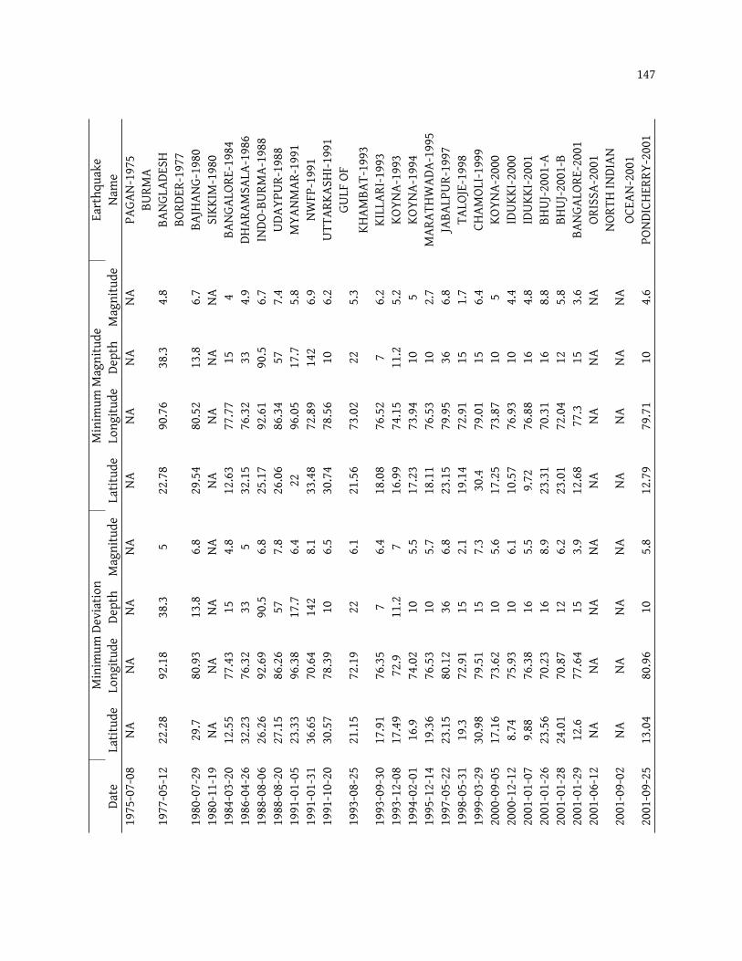
147Minim
umDe
viation
Minim
umMag
nitude
Earthq
uake
Date
Latit
ude
Long
itude
Depth
Mag
nitude
Latit
ude
Long
itude
Depth
Mag
nitude
Name
1975
-07-08
NANA
NANA
NANA
NANA
PAGA
N-19
75BU
RMA
1977
-05-12
22.28
92.18
38.3
522
.7890
.7638
.34.8
BANG
LADE
SHBO
RDER
-197
719
80-07-29
29.7
80.93
13.8
6.829
.5480
.5213
.86.7
BAJH
ANG-
1980
1980
-11-19
NANA
NANA
NANA
NANA
SIKK
IM-198
019
84-03-20
12.55
77.43
154.8
12.63
77.77
154
BANG
ALOR
E-19
8419
86-04-26
32.23
76.32
335
32.15
76.32
334.9
DHAR
AMSA
LA-198
619
88-08-06
26.26
92.69
90.5
6.825
.1792
.6190
.56.7
INDO
-BUR
MA-
1988
1988
-08-20
27.15
86.26
577.8
26.06
86.34
577.4
UDAY
PUR-
1988
1991
-01-05
23.33
96.38
17.7
6.422
96.05
17.7
5.8MYA
NMAR
-199
119
91-01-31
36.65
70.64
142
8.133
.4872
.8914
26.9
NWFP
-199
119
91-10-20
30.57
78.39
106.5
30.74
78.56
106.2
UTTA
RKAS
HI-199
1GU
LFOF
1993
-08-25
21.15
72.19
226.1
21.56
73.02
225.3
KHAM
BAT-
1993
1993
-09-30
17.91
76.35
76.4
18.08
76.52
76.2
KILL
ARI-1
993
1993
-12-08
17.49
72.9
11.2
716
.9974
.1511
.25.2
KOYN
A-19
9319
94-02-01
16.9
74.02
105.5
17.23
73.94
105
KOYN
A-19
9419
95-12-14
19.36
76.53
105.7
18.11
76.53
102.7
MAR
ATHW
ADA-
1995
1997
-05-22
23.15
80.12
366.8
23.15
79.95
366.8
JABA
LPUR
-199
719
98-05-31
19.3
72.91
152.1
19.14
72.91
151.7
TALO
JE-199
819
99-03-29
30.98
79.51
157.3
30.4
79.01
156.4
CHAM
OLI-1
999
2000
-09-05
17.16
73.62
105.6
17.25
73.87
105
KOYN
A-20
0020
00-12-12
8.74
75.93
106.1
10.57
76.93
104.4
IDUK
KI-200
020
01-01-07
9.88
76.38
165.5
9.72
76.88
164.8
IDUK
KI-200
120
01-01-26
23.56
70.23
168.9
23.31
70.31
168.8
BHUJ
-200
1-A
2001
-01-28
24.01
70.87
126.2
23.01
72.04
125.8
BHUJ
-200
1-B
2001
-01-29
12.6
77.64
153.9
12.68
77.3
153.6
BANG
ALOR
E-20
0120
01-06-12
NANA
NANA
NANA
NANA
ORISSA
-200
1NO
RTHIN
DIAN
2001
-09-02
NANA
NANA
NANA
NANA
OCEA
N-20
0120
01-09-25
13.04
80.96
105.8
12.79
79.71
104.6
POND
ICHE
RRY-
2001
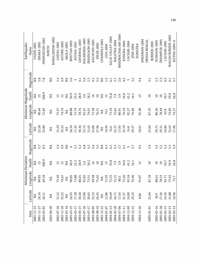
148Minim
umDe
viation
Minim
umMag
nitude
Earthq
uake
Date
Latit
ude
Long
itude
Depth
Mag
nitude
Latit
ude
Long
itude
Depth
Mag
nitude
Name
2001
-11-15
NANA
NANA
NANA
NANA
VASH
I-200
120
01-11-27
24.16
89.03
155.7
23.58
90.44
153.8
DHAK
A-20
0120
02-03-03
36.11
69.18
208.9
8.533
.8672
.8520
8.97.8
HIND
UKUS
H-20
02NO
RTH
2002
-06-20
NANA
NANA
NANA
NANA
BANG
LADE
SH-200
220
02-07-10
15.12
75.49
152.4
15.29
75.57
152.2
GADA
G-20
0220
02-11-20
35.52
74.67
134.9
35.52
74.76
134.9
ASTO
RE-200
220
03-03-10
NANA
NANA
NANA
NANA
AKOL
A-20
0320
03-03-25
26.93
90.05
50.9
626
.3488
.8850
.95.6
BHUT
AN-200
320
03-03-27
17.18
73.88
25.5
3.117
.4373
.7925
.53
KOYN
A-20
0320
03-05-27
30.44
80.01
28.9
5.230
.3678
.7628
.94.1
GHAR
WAL
-200
320
03-07-26
23.06
92.83
2.66.8
22.72
92.41
2.65.4
KOLA
BONI
A-20
0320
03-07-27
20.63
73.51
18.2
4.321
.6374
.0118
.22.3
DHAD
GAON
-200
320
03-08-05
23.15
69.58
165.6
23.06
72.58
164.2
KACH
CHH-
2003
2003
-08-10
26.55
75.65
105.5
27.96
76.31
103.5
SIKA
R-20
0320
03-12-22
NANA
NANA
NANA
NANA
CHAN
DOLI-200
320
04-01-07
12.86
71.93
156.3
14.95
74.1
151.5
GOA-
2004
2004
-02-14
34.69
73.25
35.8
6.134
.673
.3435
.86.1
ALLA
IVAL
LEY-
2004
2004
-02-20
26.71
72.21
7.95.3
25.37
72.62
7.93.7
BALO
TRA-
2004
2004
-07-06
17.65
80.5
3.93.7
17.65
80.91
3.92.6
BHAD
RACH
ALAM
-200
420
04-11-11
31.27
75.26
34.6
6.132
.1976
.3434
.64.2
KANG
RA-200
420
04-12-09
24.89
92.54
41.2
524
.892
.3741
.25
CACH
AR-200
420
04-12-22
29.32
76.46
16.1
3.729
.5776
.4616
.13.2
JIND-
2004
SUMAT
RA20
04-12-26
8.86
91.07
159.5
10.61
92.48
159.4
ANDA
MAN
-200
4OR
ISSA
BENG
AL20
05-01-01
21.64
87.18
103.4
21.64
87.35
103.1
BORD
ER-200
520
05-01-16
30.9
80.61
105.5
29.73
80.36
102.3
KUMAO
N-20
0520
05-01-30
27.56
78.53
105.1
29.31
78.44
102.3
DHAM
PUR-
2005
2005
-02-15
24.36
92.71
10.7
5.224
.8692
.810
.74.5
CACH
AR-200
520
05-02-15
31.88
73.43
59.9
5.331
.6374
.8559
.94.1
WAG
AHBO
RDER
-200
520
05-03-14
16.96
73.7
26.8
5.917
.9674
.3726
.85.7
KOYN
A-20
05-A
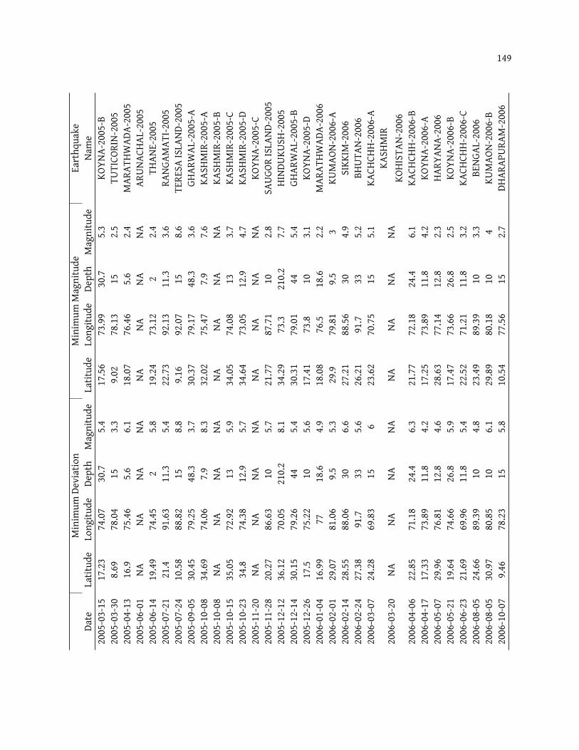
149Minim
umDe
viation
Minim
umMag
nitude
Earthq
uake
Date
Latit
ude
Long
itude
Depth
Mag
nitude
Latit
ude
Long
itude
Depth
Mag
nitude
Name
2005
-03-15
17.23
74.07
30.7
5.417
.5673
.9930
.75.3
KOYN
A-20
05-B
2005
-03-30
8.69
78.04
153.3
9.02
78.13
152.5
TUTICO
RIN-
2005
2005
-04-13
16.9
75.46
5.66.1
18.07
76.46
5.62.4
MAR
ATHW
ADA-
2005
2005
-06-01
NANA
NANA
NANA
NANA
ARUN
ACHA
L-20
0520
05-06-14
19.49
74.45
25.8
19.24
73.12
22.4
THAN
E-20
0520
05-07-21
21.4
91.63
11.3
5.422
.7392
.1311
.33.6
RANG
AMAT
I-200
520
05-07-24
10.58
88.82
158.8
9.16
92.07
158.6
TERE
SAISLA
ND-200
520
05-09-05
30.45
79.25
48.3
3.730
.3779
.1748
.33.6
GHAR
WAL
-200
5-A
2005
-10-08
34.69
74.06
7.98.3
32.02
75.47
7.97.6
KASH
MIR-200
5-A
2005
-10-08
NANA
NANA
NANA
NANA
KASH
MIR-200
5-B
2005
-10-15
35.05
72.92
135.9
34.05
74.08
133.7
KASH
MIR-200
5-C
2005
-10-23
34.8
74.38
12.9
5.734
.6473
.0512
.94.7
KASH
MIR-200
5-D
2005
-11-20
NANA
NANA
NANA
NANA
KOYN
A-20
05-C
2005
-11-28
20.27
86.63
105.7
21.77
87.71
102.8
SAUG
ORISLA
ND-200
520
05-12-12
36.12
70.05
210.2
8.134
.2973
.321
0.27.7
HIND
UKUS
H-20
0520
05-12-14
30.15
79.26
445.4
30.31
79.01
445.4
GHAR
WAL
-200
5-B
2005
-12-26
17.5
75.22
105.6
17.41
73.8
103.1
KOYN
A-20
05-D
2006
-01-04
16.99
7718
.64.9
18.08
76.5
18.6
2.2MAR
ATHW
ADA-
2006
2006
-02-01
29.07
81.06
9.55.3
29.9
79.81
9.53
KUMAO
N-20
06-A
2006
-02-14
28.55
88.06
306.6
27.21
88.56
304.9
SIKK
IM-200
620
06-02-24
27.38
91.7
335.6
26.21
91.7
335.2
BHUT
AN-200
620
06-03-07
24.28
69.83
156
23.62
70.75
155.1
KACH
CHH-
2006
-AKA
SHMIR
2006
-03-20
NANA
NANA
NANA
NANA
KOHI
STAN
-200
620
06-04-06
22.85
71.18
24.4
6.321
.7772
.1824
.46.1
KACH
CHH-
2006
-B20
06-04-17
17.33
73.89
11.8
4.217
.2573
.8911
.84.2
KOYN
A-20
06-A
2006
-05-07
29.96
76.81
12.8
4.628
.6377
.1412
.82.3
HARY
ANA-
2006
2006
-05-21
19.64
74.66
26.8
5.917
.4773
.6626
.82.5
KOYN
A-20
06-B
2006
-06-23
21.69
69.96
11.8
5.422
.5271
.2111
.83.2
KACH
CHH-
2006
-C20
06-08-05
24.66
89.39
104.8
23.49
89.39
103.3
BENG
AL-200
620
06-08-05
30.97
80.85
106.1
29.89
80.18
104
KUMAO
N-20
06-B
2006
-10-07
9.46
78.23
155.8
10.54
77.56
152.7
DHAR
APUR
AM-200
6
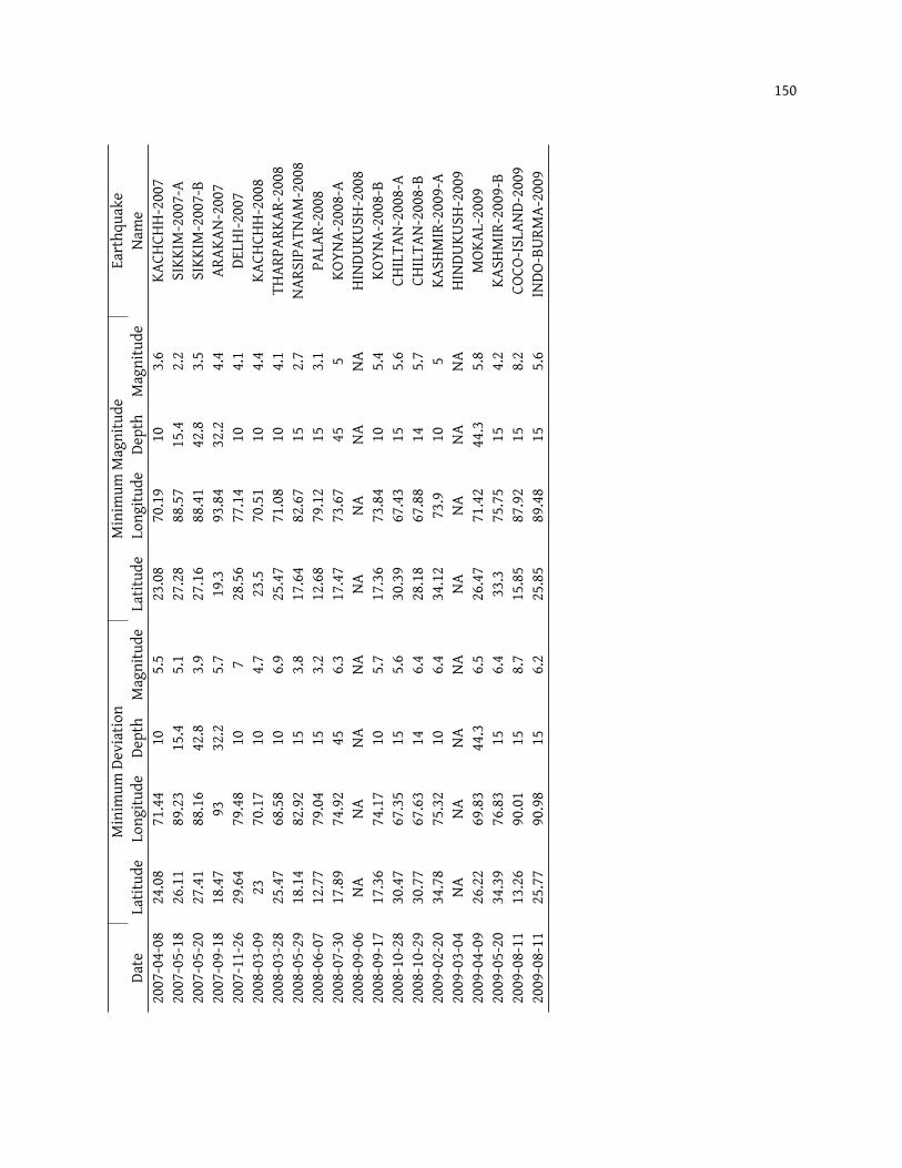
150Minim
umDe
viation
Minim
umMag
nitude
Earthq
uake
Date
Latit
ude
Long
itude
Depth
Mag
nitude
Latit
ude
Long
itude
Depth
Mag
nitude
Name
2007
-04-08
24.08
71.44
105.5
23.08
70.19
103.6
KACH
CHH-
2007
2007
-05-18
26.11
89.23
15.4
5.127
.2888
.5715
.42.2
SIKK
IM-200
7-A
2007
-05-20
27.41
88.16
42.8
3.927
.1688
.4142
.83.5
SIKK
IM-200
7-B
2007
-09-18
18.47
9332
.25.7
19.3
93.84
32.2
4.4AR
AKAN
-200
720
07-11-26
29.64
79.48
107
28.56
77.14
104.1
DELH
I-200
720
08-03-09
2370
.1710
4.723
.570
.5110
4.4KA
CHCH
H-20
0820
08-03-28
25.47
68.58
106.9
25.47
71.08
104.1
THAR
PARK
AR-200
820
08-05-29
18.14
82.92
153.8
17.64
82.67
152.7
NARS
IPAT
NAM-200
820
08-06-07
12.77
79.04
153.2
12.68
79.12
153.1
PALA
R-20
0820
08-07-30
17.89
74.92
456.3
17.47
73.67
455
KOYN
A-20
08-A
2008
-09-06
NANA
NANA
NANA
NANA
HIND
UKUS
H-20
0820
08-09-17
17.36
74.17
105.7
17.36
73.84
105.4
KOYN
A-20
08-B
2008
-10-28
30.47
67.35
155.6
30.39
67.43
155.6
CHILTA
N-20
08-A
2008
-10-29
30.77
67.63
146.4
28.18
67.88
145.7
CHILTA
N-20
08-B
2009
-02-20
34.78
75.32
106.4
34.12
73.9
105
KASH
MIR-200
9-A
2009
-03-04
NANA
NANA
NANA
NANA
HIND
UKUS
H-20
0920
09-04-09
26.22
69.83
44.3
6.526
.4771
.4244
.35.8
MOK
AL-200
920
09-05-20
34.39
76.83
156.4
33.3
75.75
154.2
KASH
MIR-200
9-B
2009
-08-11
13.26
90.01
158.7
15.85
87.92
158.2
COCO
-ISLA
ND-200
920
09-08-11
25.77
90.98
156.2
25.85
89.48
155.6
INDO
-BUR
MA-
2009
Bibliography
Altamimi, Z., X. Collilieux, J. Legrand, B. Garayt, and C. Boucher (2007), ITRF2005: A new release of the In-ternational Terrestrial Reference Frame based on time series of station positions and Earth OrientationParameters, J. Geophys. Res., 112, B09401, doi:10.1029/2007JB004949.
Ambraseys, N. (1971), Value of historical records of earthquakes, Nature, 232, 375–379.
Ambraseys, N. (2004), Three little known early earthquake in India, Curr. Sci. India, 86(4), 506–508.
Ambraseys, N., and R. Bilham (2003a), Earthquakes and associated deformation in northern Baluchistan,Bull. Seismol. Soc. Am., 93(4), 1573–1605.
Ambraseys, N., and R. Bilham (2003b), Earthquakes in Afghanistan, Seism. Res. Lett., 74(2), 107–123.
Ambraseys, N., and J. J. Douglas (2004), Magnitude calibration of north Indian earthquakes, Geophys. J. Int.,159, 165–206, doi:10.1111/j.1365-246X.2004.02323.x.
Ambraseys, N., and D. Jackson (2003), A note on early earthquakes in northern India and southern Tibet,Curr. Sci. India, 84(4), 570–582.
Apel, E., R. Burgmann, P. Bannerjee, and B. Nagarajan (2006), Geodetically constrained Indian Platemotionand implications for plate boundary deformation, Eos Trans. Am. Geophys. Union, 85(52).
Atkinson, G. M., and D. J. Wald (2007), “Did You Feel It?” intensity data: A surprisingly good measure ofearthquake ground motion, Seism. Res. Lett., 78(3), 362–368.
Babur, Z.-e.-d. M. (1912), The Babur-nama in English, Steven Austin and Sons, Hertford, translated by Bev-eredge, A. S.
Baird Smith, R. (1843a), Memoir of Indian earthquakes - part I, Journal of the Asiatic Society of Bengal, 12(136),257–293.
Baird Smith, R. (1843b), Memoir of Indian earthquakes - part II, Journal of the Asiatic Society of Bengal, 12(144),1029–1056.
Baird Smith, R. (1844), Memoir of Indian earthquakes - part III, Journal of the Asiatic Society of Bengal, 12(156),964–983.
Bakun, W. H. (1999), Erratum: Estimating earthquake location andmagnitude from seismic intensity data,Bull. Seismol. Soc. Am.
152
Bakun, W. H., and A. McGarr (2002), Differences in attenuation among the stable continental regions, Geo-phys. Res. Lett., 29(23), 2121, doi:10.1029/2002GL015457.
Bakun, W. H., and C. M. Wentworth (1997), Estimating earthquake location and magnitude from seismicintensity data, Bull. Seismol. Soc. Am., 87(6), 1502–1521.
Bakun,W. H., A. C. Johnston, andM. G. Hopper (2003), Estimating locations andmagnitudes of earthquakesin eastern North America from Modified Mercalli intensities, Bull. Seismol. Soc. Am., 93(1), 190–202.
Banks, C. J., and J.Warburton (1986), ’Passive-roof’ duplex geometry in the frontal structures of the Kirtharand Sulaiman mountain belts, Pakistan, J. Struct. Geol., 8(3/4), 229–237.
Bannert, D., A. Cheema, A. Ahmed, and U. Schaffer (1992), The structural development of theWestern FoldBelt, Pakistan, Geol. Jahrb., 80, 3–60.
Bapat, A., R. C. Kulkarni, and S. K. Guha (1983), Catalogue of earthquakes in India and neighborhood - fromhistorical period up to 1979, Indian Society of Earthquake Technology, Roorkee.
Bath, M. (1965), Lateral inhomogeneities of the upper mantle, Tectonophysics, 2(6), 483–514.
Bender, B. (1983), Maximum likelihood estimation of b values for magnitude grouped data, Bull. Seismol.Soc. Am., 73(3), 831–851.
Bender, F. K., and H. A. Raza (Eds.) (1995), Geology of Pakistan, Gebruder Borntraeger.
Berardino, P., R. Lanari, and E. Sansosti (2002), A new algorithm for surface deformationmonitoring basedon small baseline differential SAR interferograms, IEEE T. Geosci. Remote, 40(11), 2375–2383.
Bernard, M., B. Shen-Tu, W. E. Holt, and D. M. Davis (2000), Kinematics of active deformation in the Su-laiman lobe and range, Pakistan, J. Geophys. Res., 105(6), 13,253–13,279.
Bettinelli, P., J.-P. Avouac, M. Flouzat, F. Jouanne, L. Bollinger, P. Willis, and G. R. Chitrakar (2006), Platemotion of India and interseismic strain in the Nepal Himalaya from GPS and DORIS measurements, J.Geodesy, 80, 567–589, doi:10.1007/s00190-006-0030-3.
Beun, N., P. Bordet, and J.-P. Carbonnel (1979), Premieres donnees quantitatives relatives au coulissage dudecrochement de Chaman (Afghanistan du Sud-Est), C. R. Acad. Sc. Paris, 288, 931–934.
Biggs, J., T. J. Wright, L. Zhong, and B. Parsons (2007), Multi-interferogram method for measuring inter-seismic deformation: Denali fault, Alaska, Geophys. J. Int., 170, 1165–1179, doi:10.1111/j.1365-246X.2007.03415.x.
Bilham, R. (1995), Location and magnitude of the 1833 Nepal earthquake and its relation to the rupturezones of contiguous Great Himalayan eartquakes, Curr. Sci. India, 69(2), 101–128.
Bilham, R. (1998), Slip parameters for the Rann of Kachchh, India, 16 june 1819, earthquake, quantifiedfrom contemporary accounts, in Coastal Tectonics, Special Publications, vol. 146, edited by I. S. Stewart andC. Vita-Finzi, pp. 295–319, Geolocial Society, London.
Bilham, R. (2004), Earthquakes in India and the Himalaya: tectonics, geodesy and history, Annals of Geo-physics, 47, 839–858.
153
Bilham, R., and W. Szeliga (2008), Interaction between the Himalaya and the flexed Indian Plate — spatialfluctuations in seismic hazard in India in the past millenium?, in 2008 Seismic Engineering Conference com-memorating the 1908 Messina and Reggio Calabria earthquake, vol. 1020, edited by A. Santini and N. Moraci,pp. 224–231, American Institute of Physics.
Bilham, R., R. Bendick, and K. Wallace (2003), Flexure of the Indian plate and intraplate earthquakes, Proc.Indian Acad. Sci., 112(3), 315–329.
Bodin, P., L. Malagnini, and A. Akinci (2004), Ground-motion scaling in the Kachchh Basin, India, deducedfrom aftershocks of the 2001Mw 7.6 Bhuj earthquake, Bull. Seismol. Soc. Am., 94(5), 1658–1669.
Bozkurt, S. B., R. S. Stein, and S. Toda (2007), Forecasting probabilistic seismic shaking for greater Tokyofrom 400 years of intensity observations, Earthq. Spectra, 23(3), 525–546.
Burgmann, R., P. A. Rosen, and E. Fielding (2000), Synthetic aperature radar interferometry to measureEarth’s surface topography and its deformation, Ann. Rev. Earth Planet. Sci., 28, 169–209.
Burnes, A. (1835), A memoir on the eastern branch of the River Indus giving an account of the alterationsproduced by it by an earthquake in 1819, also a theory of the Runn, and some conjectures on the routeof Alexander the Great, drawn up in the years 1827–1828, Royal Asiatic Society, 3, 550–588.
Chen, W.-P., and P. Molnar (1977), Seismic moments of major earthquakes and the average rate of slip incentral Asia, J. Geophys. Res., 82(20), 2945–2969.
Clarke, P. J., D. Paradisses, P. C. England, B. Parsons, H. Billiris, G. Veis, and J.-C. Ruegg (1997), Geodeticinvestigation of the 13 May Kozani — Grevena (Greece) earthquake, Geophys. Res. Lett., 24(6), 707–710.
Day, S. M., S. H. Gonzalez, R. Anooshehpoor, and J. N. Brune (2008), Scale-model and numerical simulationsof near-fault seismic directivity, Bull. Seismol. Soc. Am., 98(3), 1186–1206.
de Montessus de Ballore, M. F. (1896), Seismic phenomena in the British Empire, Quarterly Journal of theGeological Society, 52, 651–668.
Delisle, G., U. von Rad, H. Andruleit, C. H. von Daniels, A. B. Tabrez, and A. Inam (2002), Active mud volca-noes on- and offshore eastern Makran, Pakistan, Int. J. Earth Sci., 91, 93–110, doi:10.1007/s005310100203.
Dunbar, P. K., P. A. Lockridge, and L. S. Whiteside (1992), Catalog of significant earthquakes, includingquantitative casualties and damage, Report SE-49, National Oceanic and Atmospheric Adminstration, Na-tional Environment Satellite Data and Information Service, National Geophysical Data Center.
Dziewonski, A.M., T.-A. Chou, and J. H.Woodhouse (1981), Determination of earthquake source parametersfrom waveform data for studies of global and regional seismicity, J. Geophys. Res., 86(4), 2825–2852.
Dziewonski, A. M., G. Ekstrom, and N. N. Maternovskaya (1999), Centroid-moment tensor solutions forOctober-December, 1998, Phys. Earth Planet. In., 115(1), 1–16.
Efron, B., and R. J. Tibshirani (1994), An introduction to the bootstrap, Chapman & Hall/CRC.
Ellis, M., J. Gomberg, and E. Schweig (2001), Indian earthquake may serve as analog for NewMadrid earth-quakes, Eos Trans. Am. Geophys. Union, 82(32), 345–347.
154
Engdahl, E. R., andA. Villasenor (2002), Global seismicity: 1900–1999, in International Handbook of Earthquakeand Engineering Seismology, vol. A, edited by W. H. K. Lee, H. Kanamori, P. C. Jennings, and C. Kisslinger,chap. 41, pp. 665–690, Academic Press.
Evernden, J. F., R. R. Hibbard, and J. F. Schneider (1973), Interpretation of seismic intensity data, Bull.Seismol. Soc. Am., 63(2), 399–422.
Farr, T. G., P. A. Rosen, E. Caro, R. E. Crippen, R. Duren, S. Hensley, M. Kobrick, M. Paller, E. Rodriguez,L. Roth, D. Seal, S. Schaffer, J. Shimada, J. Umland, M. Werner, M. Oskin, D. Burbank, and D. Alsdorf(2007), The shuttle radar topography mission, Rev. Geophys., 45, RG2004, doi:10.1029/2005RG000183.
Feldl, N., and R. Bilham (2006), Great Himalayan earthquakes and the Tibetian plateau,Nature, 444, 165–170,doi:10.1038/nature05199.
Frankel, A. D. (1994), Implications of felt area-magnitude relations for earthquake scaling and the averagefrequency of perceptible ground motion, Bull. Seismol. Soc. Am., 84(2), 462–465.
Freed, A. M. (2005), Earthquake triggering by static, dynamic, and postseismic stress transfer, Ann. Rev.Earth Planet. Sci., 33, 335–367, doi:10.1146/annurev.earth.33.092203.122505.
Funning, G. J., B. Parsons, and T. J. Wright (2007), Fault slip in the 1997 Manyi, Tibet earthquake fromlinear elastic modelling of InSAR displacements, Geophys. J. Int., 169, 988–1008, doi:10.1111/j.1365-246X.2006.03318.x.
Garcia, M. E., W. Szeliga, and R. Bilham (2006), Modeling vertical deformation associated with the 1931Mach earthquake, Pakistan, Eos Trans. Am. Geophys. Union, 87(52).
Garfunkel, Z., and H. Ron (1985), Block rotation and deformation by strike-slip faults 2. the properties of atype of macroscopic discontinuous deformation, J. Geophys. Res., 90(10), 8589–8602.
Giardini, D., G. Grunthal, K. M. Shedlock, and P. Zhang (1999), The GSHAP Global Seismic Hazard Map,Annali Di Geofisica, 42(6), 1225–1230.
Goldstein, R. M., and C. L. Werner (1998), Radar interferogram filtering for geophysical applications, Geo-phys. Res. Lett., 25(21), 4035–4038.
Griesbach, C. L. (1893), Notes on the earthquake in Baluchistan on the 20th December 1892, Records of theGeological Survey of India, 26(2), 57–61.
Grunthal, G., and A. Levret (Eds.) (2001), EuropeanMacroseismic Scale 1998 (EMS-98), Cahiers du Centre Europeende Geodynamique et de Seismologie, vol. 15, Joseph Beffort, Helfent-Bertrange, Luxembourg.
Gupta, S., S. S. Rai, K. S. Prakasam, D. Srinagesh, B. K. Bansal, R. K. Chadha, K. Priestley, andV. K. Gaur (2003),The nature of the crust in southern India: Implications for Precambrian crustal evolution, Geophys. Res.Lett., 30(8), 1419, doi:10.1029/2002GL016770.
Gutenberg, B., and C. F. Richter (1954), The Seismicity of the Earth and associated Phenomena, Princeton Uni-versity Press, Princeton, NJ.
Hanssen, R. F. (2001), Radar interferometry: Data interpretation and error analysis, Remote Sensing and DigitalImage Processing, vol. 2, Kluwer Academic Publishers, Dordrecht.
155
Haq, S. S. B., and D. M. Davis (1997), Oblique convergence and the lobate mountain belts of western Pak-istan, Geology, 25(1), 23–26.
Harris, R. A., and P. Segall (1987), Detection of a locked zone at depth on the parkfield, california, segmentof the san andreas fault, J. Geophys. Res., 92(8), 7945–7962, united States American Geophysical Union0885-3401 Serial.
Herring, T. A. (2002), GLOBK: Global Kalman filter VLBI and GPS analysis program, Technical report, Dep. ofEarth Atmos. and Planet. Sci. Mass. Inst. of Technol., Cambridge, Mass.
Hooper, A. (2008), Amulti-temporal InSARmethod incorporating both persistent scatterer and small base-line approaches, Geophys. Res. Lett., 35, L16302, doi:10.1029/2008GL034654.
Hough, S. E., and P. Pande (2007), Quantifying the media bias in intensity surveys: Lessons from the 2001Bhuj, India, earthquake, Bull. Seismol. Soc. Am., 97(2), 638–645, doi:10.1785/0120060072.
Hough, S. E., S. Martin, R. Bilham, and G. M. Atkinson (2002), The 26 January 2001M7.6 Bhuj, India, earth-quake obserevd and predicted ground motion, Bull. Seismol. Soc. Am., 92(6), 2061–2079.
Howell, B. F., and T. R. Schultz (1975), Attenuation of modified Mercalli intensity with distance from theepicenter, Bull. Seismol. Soc. Am., 65(3), 651–665.
Humayon, M., R. Lillie, and R. Lawrence (1991), Structural interpretation of the eastern Sulaiman foldbeltand foredeep, Pakistan, Tectonics, 10(2), 299–324.
Jackson, J., and D. McKenzie (1984), Active tectonics of the Alpine-Himalayan Belt between Turkey andPakistan, Geophy. J. R. astr. Soc., 77(1), 185–264.
Jade, S., B. C. Bhatt, Z. Yang, R. Bendick, V. K. Gaur, P. Molnar, M. B. Anand, and D. Kumar (2004), GPS mea-surments form the Ladakh Himalaya, India: Preliminary tests of plate-like or continuous deformationin Tibet, Geol. Soc. Am. Bull., 116(11/12), 1385–1391, doi:10.1130/B25357.1.
Jadoon, I. A. K., and A. Kurshid (1996), Gravity and tectonic models across the Sulaiman fold belt and theChaman fault zone in western Pakistan and eastern Afghanistan, Tectonophysics, 254, 89–109.
Jadoon, I. A. K., R. D. Lawrence, and R. Lillie (1993), Evolution of foreland structures: an example fromthe Sulaiman thrust lobe of Pakistan, southwest of the Himalayas, in Himalayan Tectonics, edited by P. J.Treloar and M. P. Searle, no. 74 in Special Publications, pp. 589–602, Geolocial Society, London, London,UK, doi:10.1144/GSL.SP.1993.074.01.39.
Jadoon, I. A. K., R. D. Lawrence, and R. J. Lillie (1994), Seismic data, geometry, evolution, and shorteningin the active Sulaiman fold-and-thrust belt of Pakistan, southwest of the Himalayas, AAPG Bull., 78(5),758–774.
Johnston, A. C. (1996), Seismic moment assessment of earthquakes in stable continental regions — II. his-torical seismicity, Geophys. J. Int., 125(3), 639–678.
Jones, A. (Ed.) (1961), Reconnaissance Geology of part of West Pakistan, a Columbo Plan cooperative project, Hunt-ing Survey Report, Government of Pakistan, Oshawa.
Joyner, W. B., and D. M. Boore (1993), Methods for regression analysis of strong-motion data, Bull. Seismol.Soc. Am., 83(2), 469–487.
156
Khan, K. (1998), Determination of focal mechanisms and hypocenters for the mainshock and aftershocksof the 1997 Quetta earthquake in Pakistan, Individual Studies by Participants to the International Institute ofSeismology and Earthquake Engineering, 34, 131–139.
Khattri, K. N. (1987), Great earthquakes, seismicity gaps and potential for earthquake disaster along theHimalayan plate boundary, Tectonophysics, 138, 79–92.
Khattri, K. N., and A. K. Tyagi (1983), Seismicity patterns in the Himalayan plate boundary and identifica-tion of the areas of high seismic potential, Tectonophysics, 96, 281–297.
King, R. W., and Y. Bock (2002), Documentation for the GAMIT GPS analysis software, Technical report, Dep.of Earth Atmos. and Planet. Sci. Mass. Inst. of Technol., Cambridge, Mass.
Kozuch, M. J. (1995), Earthquake hazard analysis of Venezuela using site specific attenuation, Ph.D. thesis,University of Colorado.
Kumar, S., S. G. Wesnousky, T. K. Rockwell, R. W. Briggs, V. C. Thakur, and R. Jayangondaperumal (2006),Paleoseismic evidence of great surface rupture earthquakes along the Indian Himalaya, J. Geophys. Res.,111, B03304.
La Femina, P. C., T. H. Dixon, andW. Strauch (2002), Bookshelf faulting inNicaragua, Geology, 30(8), 751–754.
Landor, A. H. S. (1902), Across coveted lands or a Journey from Flushing (Holland) to Calcutta Overland, Macmillanand Co., London.
Lave, J., D. Yule, S. Sopkota, K. Basant, C. Madden, M. Attal, and R. Pandey (2005), Evidence for a GreatMedieval earthquake (∼1100 A.D.) in the central Himalayas, Nepal, Science, 307, 1302–1305.
Lawrence, R. D., and R. S. Yeats (1979), Geological reconnaissance of the Chaman Fault in Pakistan, inGeodynamics of Pakistan, edited by A. Farah and K. A. DeJong, Geological Survey of Pakistan, Quetta.
Lawrence, R. D., S. H. Khan, and T. Nakata (1992), Chaman Fault, Pakistan-Afghanistan, Annales Tectonicae,6, 196–223.
Lenox-Conyngham, G. P. (1916), Leveling of precision in India, Addendum, Heights of bench marks, vol. Sheet 39,Survey of India, Dehra Dun, India.
Lienkaemper, J. J., B. Baker, and F. S. McFarland (2006), Surface slip associated with the 2004 Parkfield,California, earthquake measured with alinement arrays, Bull. Seismol. Soc. Am., 96(4), 239–249, doi:10.1785/0120050806.
Lohman, R. B., and M. Simons (2005), Some thoughts on the use of InSAR data to constrain models ofsurface deformation: Noise structure and data downsampling, Geochem. Geophys. Geosyst., 6(1), Q01007,doi:10.1029/2004GC000841.
MacMurdo, J. (1823), Papers relating to the earthquake which occurred in India in 1819, Literary Society ofBombay Transactions, 3, 90–116.
Malik, J. N., T. Nakata, H. Sato, T. Imaizumi, T. Yoshioka, G. Philip, A. K. Mahajan, and R. V. Karanth (2001),January 26, 2001, the Republic Day (Bhuj) earthquake of Kachchh and active faults, Gujarat, westernIndia, Journal of Active Fault Research, Japan, 20, 112–126.
157
Mallet, R., and J. W. Mallet (1858), The earthquake catalogue of the British Association with the discussion, curves,and maps, etc., Transactions of the British Association for the advancement of science, 1852 to 1858,Taylor and Francis, London.
Manighetti, I., M. Campillo, C. Sammis, P. M. Mai, and G. King (2005), Evidence for self-similar, triangularslip distributions on earthquakes: Implications for earthquake and fault mechanics, J. Geophys. Res., 110,B05302, doi:10.1029/2004JB003174.
Martin, S., and W. Szeliga (2010), A catalog of felt intensity data for 589 earthquakes in India from1636–2009, Bull. Seismol. Soc. Am., 100(2), 562–569, doi:10.1785/0120080328.
Massonnet, D., and K. Feigl (1995), Discrimination of geophysical phenomena in satellite radar interfero-grams, Geophys. Res. Lett., 22(12), 1537–1540.
McCaffrey, R., G. A. Abers, and P. C. Zwick (2000), Inversion of teleseismic body waves, in Digital Seismo-gram Analysis and waveform inversion, IASPEI Software Library, vol. 3, edited by W. H. K. Lee, InternationalAssociation of Seismology and Physics of the Earth’s Interior.
McKenzie, D., and J. Jackson (1986), A blockmodel of distributed deformation by faulting, J. Geol. Soc. London,143, 349–353.
Medvedev, S. V., W. Sponheuer, and V. Karnik (1965), Seismic intensity scale versionMSK 1964, Moscow, Akad.Nauk SSSR Geofiz. Kom., Moscow.
Miao, Q., and C. A. Langston (2008), Comparative study of distance attenuation in Central United Statesand Western India, Seism. Res. Lett., 79(3), 446–456.
Middlemiss, C. S. (1910), The Kangra earthquake of 4th April 1905, Memoirs of the Geological Survey of India,38.
Minchin, C. F. (Ed.) (1907), The Gazatteer of Las Bela, District Gazatteer series of Baluchistan, vol. 8, The TimesPress, Bombay.
Mitra, S., K. F. Priestley, V. K. Gaur, and S. S. Rai (2006), Frequency-dependentLg attenuation in the Indianplatform, Bull. Seismol. Soc. Am., 96(6), 2449–2456, doi:10.1785/0120050152.
Molnar, P., and J. M. Stock (2009), Slowing of India’s convergence with Eurasia since 20 Ma and its impli-cations for Tibetan mantle dynamics, Tectonics, 28, TC3001, doi:10.1029/2008TC002271.
Molnar, P., and P. Tapponnier (1975), Cenozoic tectonics of Asia: Effects of a continental collision, Science,189(4201), 419–426.
Monsalve, G., A. F. Sheehan, C. Rowe, and S. Rajaure (2008), Seismic structure of the crust and uppermantlebeneath the Himalayas: Evidence for eclogitization of lower crustal rocks in the Indian Plate, J. Geophys.Res., 113, B08315, doi:10.1029/2007JB005424.
Mosegaard, K., and A. Tarantola (1995), Monte Carlo sampling of solutions to inverse problems, J. Geophys.Res., 100(7), 12,431–12,447.
Nicholson, C., L. Seeber, and P. Williams (1986), Seismic evidence for conjugate slip and block rotationwithin the San Andreas fault system, southern California, Tectonics, 5(4), 629–648.
158
Okada, Y. (1992), Internal deformation due to shear and tensile faults in a half-space, Bull. Seismol. Soc. Am.,82(2), 1018–1040.
Oldham, R. D. (1899), Report of the Great Earthquake of 12th June 1897, Memoirs of the Geological Survey ofIndia, 29.
Oldham, R. D. (1926), The Cutch (Kachh) earthquake of 16th June 1819 with a revision of the great earth-quake of 12th June 1897, Memoirs of the Geological Survey of India, 46, 71–177.
Oldham, T. (1883), A catalogue of Indian earthquakes from the earliest time to the end of A.D. 1869,Memoirsof the Geological Survey of India, 29, 163–215.
Ortiz, M., and R. Bilham (2003), Source area and rupture parameters of the 31 December 1881 Mw = 7.9Car Nicobar earthquake estimated from tsunamis recorded in the Bay of Bengal, J. Geophys. Res., 108(4),2215, doi:10.1029/2002JB001941.
Pakistan Meteorological Department, and NORSAR (2007), Seismic hazard analysis and zonation for Pak-istan, Azad Jammu and Kashmir, Tech. rep., Pakistan Meteorological Department.
Pande, P., and J. R. Kayal (Eds.) (2003), Kutch (Bhuj) earthquake 26 January 2001, no. 76 in Special Publications,Geological Survey of India, Kolkata.
Parsons, B., T. J. Wright, P. Rowe, J. Andrews, J. Jackson, R. Walker, M. Khatib, M. Talebian, E. Bergman,and E. R. Engdahl (2006), The 1994 Sefidabeh (eastern Iran) earthquake revisited: new evidence fromsatellite radar interferometry and carbonate dating about the growth of an active fold above a blindthrust fault, Geophys. J. Int., 164, 202–217, doi:10.1111/j.1365-246X.2005.02655.x.
Pasyanos, M. E., E. M. Matzel, W. R. Walter, and A. J. Rodgers (2009), Broad-band Lg attenuation modellingin the Middle East, Geophys. J. Int., 177(3), 1166–1176, doi:10.1111/j.1365-246X.2009.04128.x.
Powell, M. J. D. (1964), An efficient method for finding the minimum of a function of several variableswithout calculating derivatives, Comput. J., 7(2), 152–162.
Quittmeyer, R., A. Farah, and K. H. Jacob (1979), The seismicity of Pakistan and its relation to surface faults,inGeodynamics of Pakistan, edited byA. Farah andK. A. DeJong, pp. 271–284, Geological Survey of Pakistan.
Quittmeyer, R., A. L. Kafka, and J. G. Armbruster (1984), Focal mechanisms and depths of earthquakes incentral Pakistan: a tectonic interpretation, J. Geophys. Res., 89, doi:10.1029/JB089iB04p02459.
Raghu Kanth, S. T. G., and R. N. Iyengar (2006), Seismic hazard estimation for Mumbai city, Curr. Sci. India,91(11), 1486–1494.
Rajendran, C. P., and K. Rajendran (2001), Characteristics of deformation and past seismicity associatedwith the 1819 Kutch earthquake, northwestern India, Bull. Seismol. Soc. Am., 91(3), 407–426.
Rajendran, C. P., and K. Rajendran (2005), The status of central seismic gap: a perspective based on thespatial and temporal aspects of the large Himalayan earthquakes, Tectonophysics, 395, 19–39.
Rajendran, C. P., K. Rajendran,M. Thakkar, andB. Goyal (2008), Assessing theprevious activity at the sourcezone of the 2001 Bhuj earthquake based on the near-source and distant paleoseismological indicators,J. Geophys. Res., 113, B05311, doi:10.1029/2006JB004845.
159
Ramachandran, K., and L. S. Srivastava (1991), New catalogue of felt Indian earthquakes during 1901–1971,Mausam, 42(2), 171–182.
Ramanathan, K. R., and S.M.Mukherji (1938), A seismological study of the Baluchistan (Quetta) earthquakeof May 31, 1935, Records of the Geological Survey of India, 73(4), 483–513.
Ron, H., R. Freund, and Z. Garfunkel (1984), Block rotation by strike-slip faulting: structural and paleo-magnetic evidence, J. Geophys. Res., 89(7), 6256–6270.
Rosen, P. A., S. Hensley, G. Peltzer, and M. Simons (2004), Updated Repeat Orbit Interferometry packagereleased, Eos Trans. Am. Geophys. Union, 85(5), 35.
Rowlands, D. (1978), The structure and seismicity of a portion of the southern Sulaiman Range, Pakistan,Tectonophysics, 51, 41–56.
Savage, J. C., and R. O. Burford (1973), Geodetic determination of relative platemotion in central California,J. Geophys. Res., 78(5), 832–845.
Schelling, D. (1999a), Structural geology of the Bolan block, western Pakistan, EGI Technical Report 5-20885-99, Energy and Geoscience Institute, University of Utah, Salt Lake City, Utah.
Schelling, D. (1999b), Geological map of the Bolan Block and Quetta Syntaxis regions, EGI Technical Report5-20885-99, Energy and Geoscience Institute, University of Utah, Salt Lake City, Utah.
Schmidt, D. A., and R. Burgmann (2006), InSAR constraints on the source parameters of the 2001 Bhujearthquake, Geophys. Res. Lett., 33, L02315, doi:10.1029/2005GL025109.
Seeber, L., and J. G. Armbruster (1981), Great detachment earthquakes along the Himalayan arc and long-term forecasting., in Earthquake Prediction — An International Review,Maurice Ewing Series, vol. 4, edited byD. W. Simpson and P. G. Richards, pp. 259–277, American Geophysical Union.
Segall, P., and J. L. Davis (1997), GPS applications for geodynamics and earthquake studies, Ann. Rev. EarthPlanet. Sci., 25, 301–336.
Sigmundsson, F. (2006), Iceland Geodynamics Crustal Deformation and Divergent Plate Tectonics, chap. 7, p. 232,Springer Praxis Books, Springer Berlin Heidelberg, doi:10.1007/3-540-37666-6.
Sigmundsson, F., P. Einarsson, R. Bilham, and E. Sturkell (1995), Rift-transform kinematics in south Ice-land: deformation from global positioning system measurements, 1986 to 1992, J. Geophys. Res., 100(4),6235–6248.
Singh, D. D., and H. K. Gupta (1980), Source dynamics of two great earthquakes of the Indian subcontinent:the Bihar-Nepal earthquake of January 15, 1934 and the Quetta earthquake of May 30, 1935, Bull. Seismol.Soc. Am., 70(3), 757–773.
Singh, S. K., R. S. Dattatrayam, and H. K. Gupta (1999), A spectral analysis of the 21 May 1997, Jabalpur,India, earthquake (Mw = 5.8) and estimation of ground motion from future earthquakes in the Indianshield region, Bull. Seismol. Soc. Am., 89(6), 1620–1630.
Snead, R. E. (1964), Active mud volcanoes of Baluchistan, west Pakistan, Geogr. Rev., 54(4), 546–560.
Srivastava, H. N., and K. Ramachandran (1985), New catalogue of earthquakes for peninsular India during1839–1900, Mausam, 36(3), 351–358.
160
Stein, R. S., G. C. P. King, and J. Lin (1994), Stress triggering of the 1994 Mw = 6.7 Northridge, California,earthquake by its predecessors, Science, 265(5177), 1432–1435.
Talwani, P., and A. Gangopadhyay (2000), Schematic model for intraplate earthquakes, Eos Trans. Am. Geo-phys. Union, 81(48), S21C–10.
Tandon, A. N., and H. M. Chaudhury (1968), Koyna earthquake of December, 1967, Sci. Rep 59, India Meteo-rol. Dept.
Tapponnier, P., R. Armijo, I. Manighetti, and V. Courtillot (1990), Bookshelf faulting and horizontal blockrotations between overlapping rifts in southern Afar, Geophys. Res. Lett., 17(1), 1–4.
Treloar, P. J., and M. P. Coward (1991), Indian plate motion and shape: constraints on the geometry of theHimalayan orogen, Tectonophysics, 191, 189–198.
Wald, D. J., and T. I. Allen (2007), Topographic slope as a proxy for seismic site conditions and amplification,Bull. Seismol. Soc. Am., 97(5), 1379–1395, doi:10.1785/0120060267%20.
Wald, D. J., V. Quitoriano, L. Dengler, and J. Dewey (1999a), Utilization of the Internet for rapid communityintensity maps, Seism. Res. Lett., 70(6), 680–697.
Wald, D. J., V. Quitoriano, T. H. Heaton, and H. Kanamori (1999b), Relationships between peak groundacceleration, peak ground velocity, and Modified Mercalli Intensity in California, Earthq. Spectra, 15(3),557–564.
Waldhauser, F., and W. L. Ellsworth (2000), A double-difference earthquake location algorithm: Methodand application to the northern Hayward Fault, California, Bull. Seismol. Soc. Am., 90(6), 1353–1368.
Wellman, H. W. (1966), Active wrench faults of Iran, Afghanistan and Pakistan, Geol. Rundsch., 55(3),716–735, doi:10.1007/BF02029650.
Wells, D. L., and K. J. Coppersmith (1994), New empirical relationships among magnitude, rupture length,rupture width, rupture area, and surface displacement, Bull. Seismol. Soc. Am., 84(4), 974–1002.
Wessel, P., and W. H. F. Smith (1998), New improved version of Generic Mapping Tools released, Eos Trans.Am. Geophys. Union, 79, 579.
West, W. D. (1934), The Baluchistan earthquakes of August 25th and 27th, 1931, Memoirs of the GeologicalSurvey of India, 67, 82.
Wilson, C. A. (1938), Leveling operations, Technical Report 1937, Survey of India, Dehra Dun, India.
Wright, T. J., B. Parsons, and E. Fielding (2001), Measurement of interseismic strain accumulation acrossthe North Anatolian Fault by satellite radar interferomety, Geophys. Res. Lett., 28(10), 2117–2120.
Wyss, M. (1979), Estimating maximum expectable magnitude of earthquakes from fault dimensions, Geol-ogy, 7(7), 336–340.
Yeats, R. S., R. D. Lawrence, S. Jamil-ud din, and S. H. Khan (1979), Surface effects of the 16 March 1978earthquake, Pakistan-Afghanistan border, in Geodynamics of Pakistan, edited byA. Farah andK. A. DeJong,Geological Survey of Pakistan, Quetta.
Zaigham, N. A. (1991), Bela ophiolites and associated mineralization in southern part of axial-belt of Pak-istan, Ph.D. thesis, University of Karachi.