high‐resolution topography and anthropogenic feature extraction: testing geomorphometric...

HYDROLOGICAL PROCESSESHydrol. Process. 28, 2046–2061 (2014)Published online 12 March 2013 in Wiley Online Library(wileyonlinelibrary.com) DOI: 10.1002/hyp.9727

High-resolution topography and anthropogenic featureextraction: testing geomorphometric parameters in floodplains

Giulia Sofia, Giancarlo Dalla Fontana and Paolo Tarolli*Department of Land, Environment, Agriculture and Forestry, University of Padova, Agripolis, viale dell’Università 16, 35020 Legnaro (PD), Italy

*CAg16,E-m

Co

Abstract:

In floodplains, anthropogenic features such as levees or road scarps, control and influence flows. An up-to-date and accurate digitaldata about these features are deeply needed for irrigation and flood mitigation purposes. Nowadays, LiDAR Digital TerrainModels (DTMs) covering large areas are available for public authorities, and there is a widespread interest in the application ofsuch models for the automatic or semiautomatic recognition of features. The automatic recognition of levees and road scarps fromthese models can offer a quick and accurate method to improve topographic databases for large-scale applications. In mountainouscontexts, geomorphometric indicators derived from DTMs have been proven to be reliable for feasible applications, and the use ofstatistical operators as thresholds showed a high reliability to identify features. The goal of this research is to test if similarapproaches can be feasible also in floodplains. Three different parameters are tested at different scales on LiDAR DTM. Theboxplot is applied to identify an objective threshold for feature extraction, and a filtering procedure is proposed to improve thequality of the extractions. This analysis, in line with other works for different environments, underlined (1) how statisticalparameters can offer an objective threshold to identify features with varying shapes, size and height; (2) that the effectiveness oftopographic parameters to identify anthropogenic features is related to the dimension of the investigated areas. The analysis alsoshowed that the shape of the investigated area has not much influence on the quality of the results. While the effectiveness ofresidual topography had already been proven, the proposed study underlined how the use of entropy can anyway provide goodextractions, with an overall quality comparable to the one offered by residual topography, and with the only limitation that theextracted features are slightly wider than the investigated one. Copyright © 2013 John Wiley & Sons, Ltd.

KEY WORDS LiDAR; anthropogenic feature; floodplains; high-resolution topography; DTM; surface morphology

Received 13 April 2012; Accepted 11 January 2013

INTRODUCTION

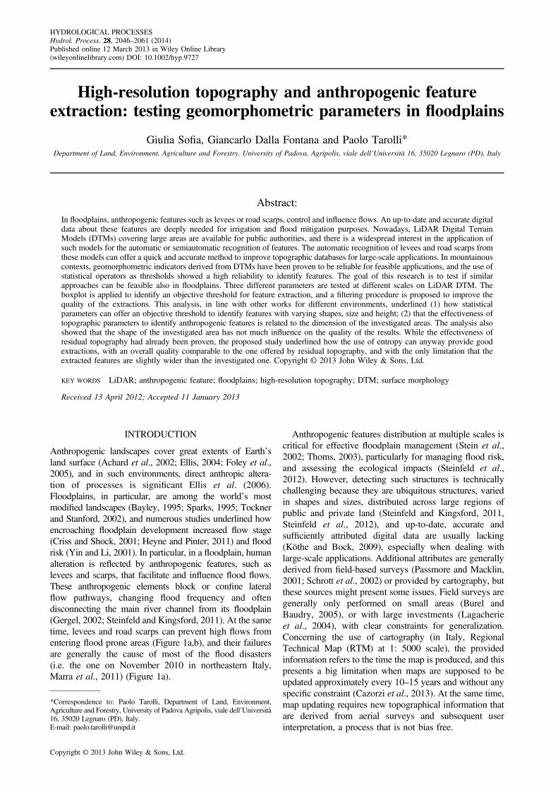
Anthropogenic landscapes cover great extents of Earth’sland surface (Achard et al., 2002; Ellis, 2004; Foley et al.,2005), and in such environments, direct anthropic altera-tion of processes is significant Ellis et al. (2006).Floodplains, in particular, are among the world’s mostmodified landscapes (Bayley, 1995; Sparks, 1995; Tocknerand Stanford, 2002), and numerous studies underlined howencroaching floodplain development increased flow stage(Criss and Shock, 2001; Heyne and Pinter, 2011) and floodrisk (Yin and Li, 2001). In particular, in a floodplain, humanalteration is reflected by anthropogenic features, such aslevees and scarps, that facilitate and influence flood flows.These anthropogenic elements block or confine lateralflow pathways, changing flood frequency and oftendisconnecting the main river channel from its floodplain(Gergel, 2002; Steinfeld and Kingsford, 2011). At the sametime, levees and road scarps can prevent high flows fromentering flood prone areas (Figure 1a,b), and their failuresare generally the cause of most of the flood disasters(i.e. the one on November 2010 in northeastern Italy,Marra et al., 2011) (Figure 1a).

orrespondence to: Paolo Tarolli, Department of Land, Environment,riculture and Forestry, University of Padova Agripolis, viale dell’Università35020 Legnaro (PD), Italy.ail: [email protected]

pyright © 2013 John Wiley & Sons, Ltd.

Anthropogenic features distribution at multiple scales iscritical for effective floodplain management (Stein et al.,2002; Thoms, 2003), particularly for managing flood risk,and assessing the ecological impacts (Steinfeld et al.,2012). However, detecting such structures is technicallychallenging because they are ubiquitous structures, variedin shapes and sizes, distributed across large regions ofpublic and private land (Steinfeld and Kingsford, 2011,Steinfeld et al., 2012), and up-to-date, accurate andsufficiently attributed digital data are usually lacking(Köthe and Bock, 2009), especially when dealing withlarge-scale applications. Additional attributes are generallyderived from field-based surveys (Passmore and Macklin,2001; Schrott et al., 2002) or provided by cartography, butthese sources might present some issues. Field surveys aregenerally only performed on small areas (Burel andBaudry, 2005), or with large investments (Lagacherieet al., 2004), with clear constraints for generalization.Concerning the use of cartography (in Italy, RegionalTechnical Map (RTM) at 1: 5000 scale), the providedinformation refers to the time the map is produced, and thispresents a big limitation when maps are supposed to beupdated approximately every 10–15 years and without anyspecific constraint (Cazorzi et al., 2013). At the same time,map updating requires new topographical information thatare derived from aerial surveys and subsequent userinterpretation, a process that is not bias free.

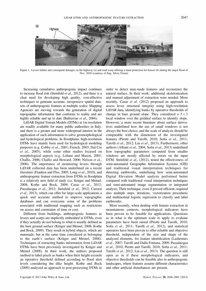
Figure 1. Levees failure and consequent damages on the highway (a) and road scarp offering a main protection for houses (b) during the major flood ofNov. 2010 (courtesy of Eng. Silvia Tizian)

2047LIDAR DTMS AND ANTHROPOGENIC FEATURE EXTRACTION

Increasing cumulative anthropogenic impact continuesto increase flood risk (Steinfeld et al., 2012), and there is aclear need for developing high quality, cost-effectivetechniques to generate accurate, inexpensive spatial data-sets of anthropogenic features at multiple scales: MappingAgencies are moving towards the generation of digitaltopographic information that conforms to reality and arehighly reliable and up to date (Baltsavias et al., 2004).LiDAR Digital Terrain Models (DTMs) at 1m resolution

are readily available for many public authorities in Italy,and there is a greater and more widespread interest in theapplication of such information to solve geomorphologicaland hydrological problems. In floodplains, high-resolutionDTMs have mainly been used for hydrological modelingpurposes (e.g. Cobby et al., 2001; French, 2003; Dal Cinet al., 2005), while some other studies focused onmorphological aspects (e.g. Lohani and Mason, 2001;Challis, 2006; Challis and Howard, 2006; Nelson et al.,2006). The importance of monitoring levees throughLiDAR collected data has been underlined on a recentliterature (Franken and Flos, 2005; Long et al., 2010), andanthropogenic feature extraction from DTMs in floodplainis a relatively new field of study (i.e. Krüger and Meinel,2008; Kothe and Bock, 2009; Casas et al., 2012;Passalacqua et al., 2012; Steinfeld et al., 2012; Cazorziet al., 2013), which can offer for large-scale applications aquick and accurate method to improve topographicdatabases and can overcome some of the problemsassociated with traditional mapping such as restrictionson access and constraints of time or cost.Different from buildings, anthropogenic features as

levees and scarps are implicitly embedded in DTMs, evenif they actually do not belong to what is usually defined asthe bare ground surface (Krüger and Meinel, 2008; Kotheand Bock, 2009). They result in hybrid objects, which aremanmade, but at the same time considered as belongingto the earth’s surface (Krüger and Meinel, 2008).Techniques of extracting banks information from LiDARDTMs have been previously investigated by Krüger andMeinel (2008). In their work, the authors proposedmethod to label pixels as banks when their height exceedsan operative threshold defined according to flood alertlevels considering the dike height. Kothe and Bock(2009) analyzed an approach to post-processing DTMs in

Copyright © 2013 John Wiley & Sons, Ltd.

order to detect man-made features and reconstruct thenatural surface. In their work, additional skeletonizationand manual adjustment of extraction were needed. Morerecently, Casas et al. (2012) proposed an approach toassess levee structural integrity using high-resolutionLiDAR data, identifying banks by operative thresholds ofchange in bare ground slope. They considered a 3� 3local window over the gridded surface to identify slope.However, a more recent literature about surface deriva-tives underlined how the use of small windows is notalways the best choice, and the scale of analysis should becomparable with the dimension of the investigatedfeatures (Pirotti and Tarolli, 2010; Sofia et al., 2011;Tarolli et al., 2012; Lin et al., 2013). Furthermore, otherauthors (Albani et al., 2004, Sofia et al., 2013) underlinedhow topographic parameters computed from smallerwindows are mostly affected by errors on the inputDTM. Steinfeld et al., (2012), tested the effectiveness ofsemi-automated Geographic Information Systems (GIS)and traditional visual interpretation techniques fordetecting earthworks, underlining how semi-automatedDigital Elevation Model analysis performed bettercompared with traditional visual interpretation techniquesand semi-automated image segmentation or integratedanalysis. Their technique, even if proved efficient, requiredalso multiple steps, iterations, vectorization proceduresand multinomial logistic regression to classify and labelearthworks.More recently, when dealing with feature extraction in

mountainous contexts, morphological indicators havebeen proven to be feasible for applications. Questionsas in what is the optimum scale to apply to evaluateparameters have been raised (Pirotti and Tarolli, 2010;Sofia et al., 2011; Tarolli et al., 2012), and statisticaloperators have been proven to offer reliable and objectivethreshold, independent of the size and shape of theanalyzed elements, for feature identification (Lashermeset al., 2007; Tarolli and Dalla Fontana, 2009; Passalacquaet al., 2010; Pirotti and Tarolli, 2010; Sofia et al., 2011;Tarolli et al., 2012; Lin et al., 2013). The question is stillopen as in if these morphological indicators, andobjective thresholds can be feasible also in anthropogeniclandscapes, where features assume different characteristicsand other artificial disturbances are present.

Hydrol. Process. 28, 2046–2061 (2014)

2048 G. SOFIA, G. D. FONTANA AND P. TAROLLI

In this work, three geomorphometric parameters (GPs)are tested to verify their suitability for feature extractionin floodplains. All these parameters are evaluatedaccording to different approaches, and they are computedfor different scales. A statistical analysis of the produceddatasets is applied, then, to identify outliers to defineautomatically objective thresholds for feature extraction.The same statistical approach is used in a post-processingapproach to discard false positives (FPs) and produce amap of the potential features.

STUDY AREA

The study area is a simple squared squared-shaped area(Figure 2), located in the lower part of the Veneto plain(North-Eastern Italy).The area is crossed by a dense drainage network,

mainly composed of channels and ditches, as typical foragricultural landscapes (Figure 2a), and it is characterizedby high levels of flood hazard (Figure 2b). Banks, leveesand scarps offer the major flood protection, especiallyconsidering that in this part of Italy, the average groundelevation is at the sea level or lower. The study areapresents an average height of about 2.5 m a.s.l., (medianof ~1 m) with a minimum of �0.45 m a.s.l., and amaximum of 7.5 m (on the embankments). 70% of thearea has a height lower than 3.5 m a.s.l.The study area has an average slope of about 3.5�, with

a minimum of 0� and a maximum of about 50� (dataderived from the 1 m DTM). However, almost 95% of thearea has a slope lower than 10� (80% is actually below 5�),while slopes above 10� are related to agricultural practices

Figure 2. Location of the test area for anthropogenic feature extraction, its m(levees and scarps) as derived from official cartography are shown. Locations

to 12 – are


(plowings with slopes ranging around 10�–15�), andembankments and scarps (>20�). The highest slope values(>30�) are localized pixels (about 0.5% of the area) relatedto some noise on the embankments.The roughness of the area, computed according to

Cavalli et al. (2008), presents a minimum of 0 m, amaximum of 0.5 m and an average value of 0.05 m. 98%of the area has a roughness lower than 0.2 m, theremaining area has a relatively higher (but still low)roughness, related mainly to plowings.

Investigated features and field survey campaign

Two different types of anthropogenic features havebeen analyzed (Figure 2a, Figure 3): levees (L1, L2, L3,L4 in Figure 2a) and scarps (S1, S2, S3 in Figure 2a).According to some designed standards, in Italy, definitioncriteria have been specified by various national andregional guidance documents to define and classify leveesand scarps: levees are built along one or both banks ofchannels (as the example of L1, on the main channel ofthe study area, and L2, L3 and L4 on one or both banksof minor channels, in Figure 2a) for flood protectionpurposes. In this part of Italy, due to the elevationcharacteristics, they are usually characterized by widthranging from 10 up to 40 or 50 m, trapezoidal crosssection, and heights that range between 1 and 3 m, andthey are generally passable.According to standards, scarps are instead abrupt

differences in ground level, due to artificial causes (i.e.roads, or escarpments along channels that are too small tobe considered as levees). In our study area, examples ofscarps are S1 and S2 (Figure 2a), located on the right side

ain characteristic (a) and flood level hazards (b). Anthropogenic featuresthat have been surveyed on the field to verify cartography – labelled from 1identified

Hydrol. Process. 28, 2046–2061 (2014)

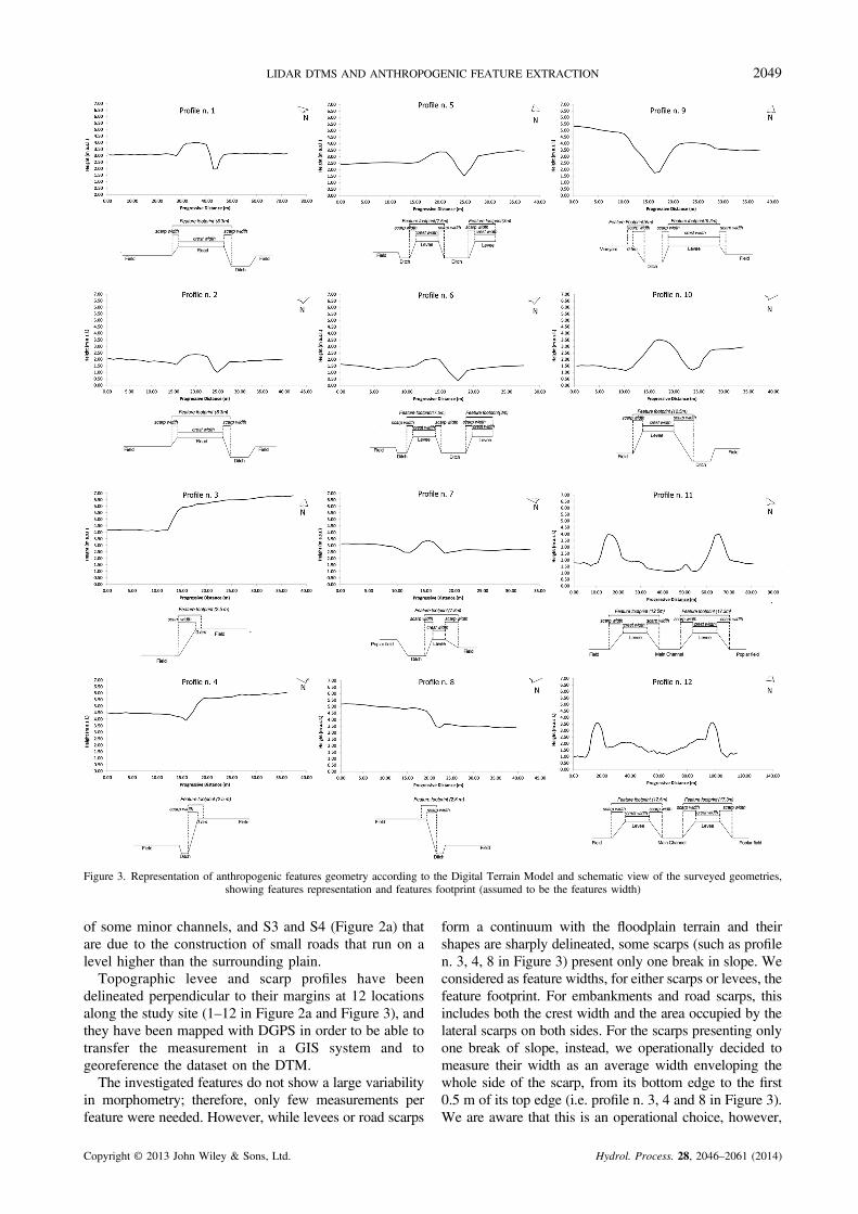
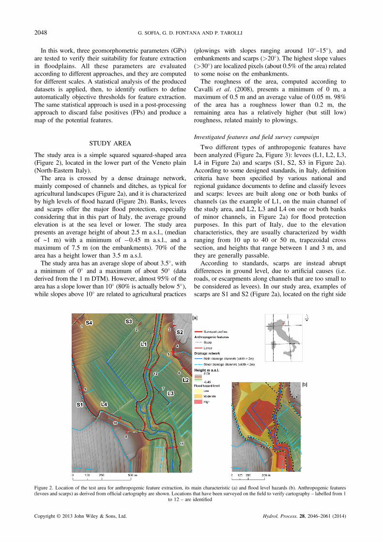
Figure 3. Representation of anthropogenic features geometry according to the Digital Terrain Model and schematic view of the surveyed geometries,showing features representation and features footprint (assumed to be the features width)


of some minor channels, and S3 and S4 (Figure 2a) thatare due to the construction of small roads that run on alevel higher than the surrounding plain.Topographic levee and scarp profiles have been

delineated perpendicular to their margins at 12 locationsalong the study site (1–12 in Figure 2a and Figure 3), andthey have been mapped with DGPS in order to be able totransfer the measurement in a GIS system and togeoreference the dataset on the DTM.The investigated features do not show a large variability

in morphometry; therefore, only few measurements perfeature were needed. However, while levees or road scarps


form a continuum with the floodplain terrain and theirshapes are sharply delineated, some scarps (such as profilen. 3, 4, 8 in Figure 3) present only one break in slope. Weconsidered as feature widths, for either scarps or levees, thefeature footprint. For embankments and road scarps, thisincludes both the crest width and the area occupied by thelateral scarps on both sides. For the scarps presenting onlyone break of slope, instead, we operationally decided tomeasure their width as an average width enveloping thewhole side of the scarp, from its bottom edge to the first0.5 m of its top edge (i.e. profile n. 3, 4 and 8 in Figure 3).We are aware that this is an operational choice, however,

Hydrol. Process. 28, 2046–2061 (2014)


(1) according to the official Italian standards, in itscartographic representation (RTMs), this type of scarps isrepresented as a continuous line that actually represents thelocation of the top edge of the scarp itself, and no standardexists on how to actually measure the element width; and(2) the feature width is needed, in this work, for thedefinition of the buffer width to be used for the extractionquality evaluation (Chapt. 4), and this only requires abuffer wide enough to soundly envelope the actualpositioning of the features, since at this stage, we wantedto test what parameter is able to better capture the featurelocation, and we are not interested in the analysis of featuredimensions in the digital domain.The same features have been mapped on the input

LiDAR DTM (Figure 3) to gain insights about the shapesand measures of the features as they are represented inthe DTM.

Airborne Laser Scanner Data and considered DTM

The digital support considered in this study is a LiDARDTM readily available for public authorities in Italy. In2002, the Ministry for Environment, Land and Sea(Ministero dell’Ambiente e della Tutela del Territorio edel Mare, MATTM), the Department of Civil Protectionand the Mininstry of Defense, in agreement with theregional governments, promoted the ‘Extraordinary Plan ofEnvironmental Remote Sensing’ (Piano Straordinario diTelerilevamento Ambientale, PST-A). The aim of thisproject is to create as quickly as possible and makeavailable a database to support decision making in all areassubject to hydrogeological risk. In particular, the projectinvolves the acquisition by the Ministry of topographicinformation produced by a remote sensing technique withairborne LiDAR. The LiDAR data considered in this studywere acquired in 2010, within the framework of the PST-A,using an OPTECH ALTM 3100C laser scanning system.The average flying altitude was approximately 1200 m a.s.l., with an average speed of 70 ms�1. The flightlines wereflown with an overlap between adjacent stripes of about30%. The LiDAR wavelength was about 0.4–0.8 nm, themaximum pulse repetition frequency was about 100 kHz,and the scan frequency was 100–70 Hz. The maximumscan angle was 25�. First and last return echoes wererecorded, producing a raw point cloud with an averagedensity of about 3 points/m2. The initial processing of the

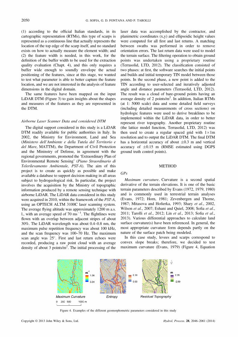
Figure 4. Examples of the different geomorph


laser data was accomplished by the contractor, andplanimetric coordinates (x,y) and ellipsoidic height valueswere computed for all first and last returns. A matchingbetween swaths was performed in order to removeorientation errors. The last return data were used to modelthe terrain surface. The filtering operation to obtain groundpoints was undertaken using a proprietary routine(Terrasolid, LTD, 2012). The classification consisted oftwo phases: at first, the software searches the initial pointsand builds and initial temporary TIN model between thosepoints. In the second phase, a new point is added to theTIN according to user-selected and iteratively adjustedangle and distance parameters (Terrasolid, LTD, 2012).The result was a cloud of bare-ground points having anaverage density of 2 points/m2. In addition, Italian RTMs(at 1: 5000 scale) data and some detailed field surveys(including detailed measurements of cross sections) onhydrologic features were used to derive breaklines to beimplemented within the LiDAR data, in order to betterrepresent river topography. Another proprietary routine(the lattice model function, Terrasolid, LTD, 2012) wasthen used to create a regular spaced grid with 1�1mresolution and to output the LiDAR DTM. The final DTMhas a horizontal accuracy of about �0.3 m and verticalaccuracy of �0.15 m (RMSE estimated using DGPSground truth control points).

METHOD

GPs

Maximum curvature. Curvature is a second spatialderivative of the terrain elevations. It is one of the basicterrain parameters described by Evans (1972, 1979, 1980)and is commonly used in terrestrial terrain analyses(Evans, 1972; Horn, 1981; Zevenbergen and Thorne,1987; Mitasova and Hofierka, 1993; Shary et al., 2002,Wilson et al., 2007; Eshani and Quiel, 2008; Sofia et al.,2011; Tarolli et al., 2012; Lin et al., 2013; Sofia et al.,2013). Various differential approaches to calculate landsurface curvature(s) have been referenced. In general, themost appropriate curvature form depends partly on thenature of the surface patch being modeled.In this case study, levees and scarps correspond to

convex slope breaks; therefore, we decided to testmaximum curvature (Evans, 1979) (Figure 4, Equation

ometric parameters considered in this study

Hydrol. Process. 28, 2046–2061 (2014)


(2)) as optimal for feature recognition. This curvaturemeasure is independent of slope, and it is based solely onsurface geometry; therefore, it can be optimal to beapplied in areas with zero gradients (Tarolli et al., 2012),as floodplains can potentially be.The local surface is approximated by a quadratic

function with reference to a coordinate system (x,y,z)and five coefficients (a to f) (Evans, 1979; Wood, 1996),and maximum curvature (Equation (1)) is found bydifferentiating the surface equation.

Curvaturemax ¼ �a� bþffiffiffiffiffiffiffiffiffiffiffiffiffiffiffiffiffiffiffiffiffiffiffiffiffiffiffia� bð Þ2 þ c2

q(1)

To perform analysis at multiple scales, maximumcurvature can be evaluated generalizing its computationaccording to a moving window approach (Wood, 1996).

Cmax ¼ q:Curvaturemax (2)

where Curvaturemax derives from Equation (1), and q is ageneralization parameter connect to the size of theprocessed neighbourhood and to the DTM grid size (alsodefined as gridsize �windowsize in Wood, 1996).In this work, we tested three different shapes of a

moving window (see Chapt. 3.2); therefore, curvaturegeneralization has been done considering q evaluatedaccording to Equation (3).

q ¼ g� ffiffiffin

p(3)

where g is the grid resolution of the DTM and n is theprocessed neighbourrhood (number of pixels) consid-ered for the computation within the moving window. Ifthe moving window is rectangular, q equals to thegeneralization proposed by Wood (1996).

Residual topography. The second approach we want totest is based among consideration of having to extractlocal scale, high-relief features by removing the large-scale low relief landscape form. Similar approaches havebeen tested in other environments for landform character-ization (Carturan et al., 2009) and for feature extraction(Doneus and Briese, 2006; Humme et al., 2006; Hillerand Smith, 2008; Kothe and Bock, 2009, Cazorzi et al.,2013). The core idea is to apply a low-pass filter to theDTM, providing a smoothed elevation model represent-ing an approximation of the large-scale landscape forms.By subtracting this smoothed map from the originalDTM, an approximation of the local relief is achieved,where only local topographic features are preserved, inspite of large-scale landscape forms (Figure 4). Thederived model represents a map of residual topography(Cavalli et al., 2008).This map is evaluated as

RTw ¼ EDTM � �Ew (4)

where �Ew is the average elevation of cells within aneighbourhood (w) around the gridcell with elevation


EDTM (Doneus and Briese, 2006; Humme et al., 2006;Cavalli et al., 2008; Hiller and Smith, 2008; Carturanet al., 2009).

Entropy. In floodplain context, levees and scarps canbe related to height values that highly differ from of thedistribution of heights of the surrounding areas. Wesuggest that these features can be identified by measuringthe elevation organization and its degree of randomness.Agrarian landscape can be characterized by smoothed andwell-organized values of elevation, while the heightscorresponding to scarps and levees represent suddenbreaks in height values within the low relief of thefloodplain surface. Shannon and Weaver (1949) intro-duced the concept of entropy as a measure of randomnessfor digital signal processing. As Vieux (1993) andMendicino (1997) reported, in the field of topographicsurfaces described by a DTM, entropy can become ameasure of spatial variability, since the total amount ofdisorder in the elevation data distribution, is interpretable,indirectly, as the DTM information content. Entropy hasbeen considered for applications of surface morphology,i.e. in Sofia et al. (2011).Entropy is evaluated as

Entropy ¼ �XNbins

i¼1

pi� logpi (5)

where pi is the proportion of pixels within the consideredneighbourhood that are assigned to each class i accordingto Equation (6)

pi ¼ Ni=Nbins (6)

where Ni is the number of pixels within the consideredclass I, and Nbins is the number of considered bins.For class and bins evaluation, we considered as interval

0.01 times the DTM standard deviation and valuesranging from zero to 100 times the DTM standarddeviation. This operative choice was done for two mainreasons: (1) it offers an objective classification of binsbased upon the actual measurement reported on the DTMand (2) other works (Tarolli and Dalla Fontana, 2009;Pirotti and Tarolli, 2010; Cazorzi et al., 2013) showed theeffectiveness of standard deviation as an objective methodfor feature recognition.Entropy is low when the heights within a local window

have similar values (smooth surface) and high when theyvary significantly. In this study, the proposed idea is thatthe presence of an anthropogenic feature whose height iscaptured within the considered neighbourhood wouldresult in a higher level of entropy (Figure 4).

Testing different approaches to account for scale

It is well known that GPs are strongly scale dependent(Wood, 1996; Pirotti and Tarolli, 2010; Tarolli et al.,2012), and the effects of scales have already beenassessed in numerous works in literature, dealing withnatural features (i.e. Pirotti and Tarolli, 2010; Tarolli

Hydrol. Process. 28, 2046–2061 (2014)


et al., 2012). The proposed idea is to test scale effectsalso in floodplain and to see if scale accountingthrough a squared moving window (Wood, 1996) canbe a good approach also in anthropogenic landscapes.Within the context of feature classification, in fact,appropriate scales for derivation of the local geometryhave to be selected according to the semantic terrainmodel implied by the application (Schmidt et al., 2003),and the elevation characteristics captured by terrain areof course different in mountainous environments andfloodplains.In different approaches reported in literature (Wood,

1996; Pirotti and Tarolli, 2010; Sofia et al., 2011; Tarolliet al., 2012), filters are computed using a squared windowwith a local coordinate system (x, y, z) defined with theorigin at the pixel of interest. In some other applications,however, it is preferable to compute the moving filters ina non-rectangular window (Glasbey and Jones, 1997). Forexample, Davies (1984) showed the benefits of circularwindows and octagonal approximations in the context ofedge detection. Circular filters are also at the base of sometopographic evaluation, as it has been applied, i.e. inCarturan et al. (2009) and Cazorzi et al. (2013).Considering this literature review, for the present work,

three different shapes of moving window have beenapplied and tested: rectangular, circular and annulus-

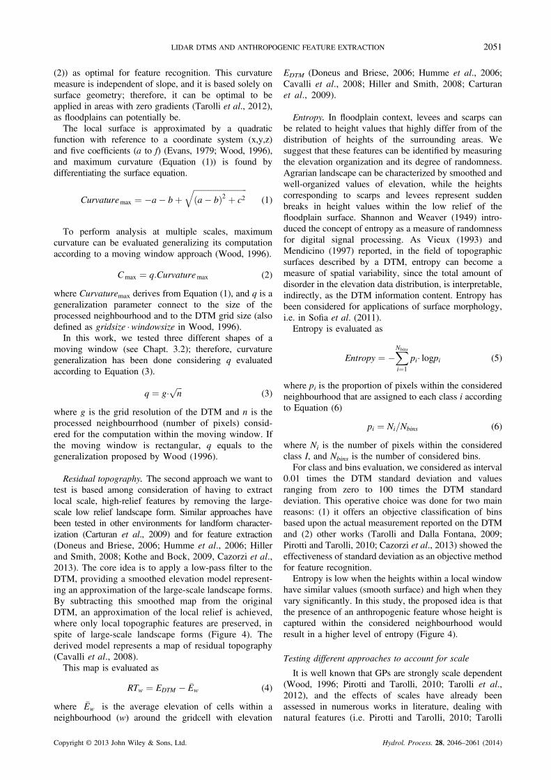
Figure 5. Tested kernel shapes (rectangular, circular and annulu


shaped kernels (Figure 5). The figure also shows anexample of the effect of kernel size and shape onmaximum curvature.By defining the shape of a neighbourhood as a

rectangle, the processed pixels defined by the kernel sizecorrespond to the same cells in the output block. Thekernel sizes (ksize) need to be large enough for a reasonablenumber of data to be processed, and its minimum width(three cells) relies on the fact that sampling windows arecentred on the cell of interest.When defining the shape of the kernel as a circle, the

corresponding processed block on the output raster willbe the minimum-bounding square who encompasses thecircular neighbourhood with the diameter 2r. Any cellcompletely encompassed by the circle is included inprocessing the neighbourhood. For the circle-shapedkernel, the diameter parameter is measured in cells, andthe computational constraints for the minimum diametersize (five cells) are two: (1) in order to evaluate curvature,the minimum number of processed cells is six(considering that surface is approximated by a quadraticfunction with six coefficients, and (2) as for therectangular kernel, the sampling windows are centredon the cell of interest.By defining the shape of the kernel as an annulus, the

considered neighbourhood comprises a smaller circle

s) and effect of kernel shape and size on maximum curvature

Hydrol. Process. 28, 2046–2061 (2014)


within a larger circle (a donut shape, Figure 5). Thecorresponding processed block on the output raster willbe the minimum-bounding square who encompasses theannular neighbourhood. The required parameters are theinner (2rin) and outer (2rout) diameters: cells that falloutside the diameter of the inner circle, but inside, thediameter of the outer circle will be included in processingthe neighbourhood. For the annulus-shaped kernel, themain size constraint is that the inner diameter must besmaller than the outer one, and the minimum widths aretherefore three cells for the inner diameter and five cellsfor the outer one.In this application features, dimensions vary, and

therefore the analysis has been carried out consideringscaling from 3 up to 55 m for the rectangular kernel, andfrom 5 up to 55 cells for the circular kernel and theannulus-shaped one.

Feature extraction

Different authors (Lashermes et al., 2007; Tarolli andDalla Fontana, 2009; Passalacqua et al., 2010; Pirotti andTarolli, 2010; Sofia et al., 2011; Tarolli et al., 2012; Linet al., 2013) underlined how statistical operators candescribe natural process signatures on surfaces. The ideathat we want to test in the present work is that a statisticalapproach can be used also to automatically identifyanthropogenic features as levees and scarps. In thecontext of floodplains and agrarian landscape, the basicidea is that embankments normally show a much sharpershape than natural terrain features, and they mark localmaxima of the elevation, with heights that representoutliers in the elevation matrix. Consequently, theyrepresent outliers also within the derived GPs (maximumcurvature, residual topography and entropy).One of the most frequently used graphic techniques to

identify outliers on a distribution, is the boxplot, proposedby Tukey (1977). The boxplot is constructed byidentifying the distribution median (Q2) and the samplefirst and third quartile (Q1 and Q3). The length of the boxequals the interquartile range (Equation (7))

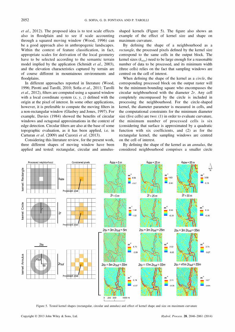
Figure 6. Example of residual topography map (a) evaluated for the rectan(Fncup = 0.23 m), and the features der


IQR� ¼ Q3 � Q1 (7)

which is a robust measure of the scale.An interval (fence) is then defined by considering a

lower bound (Fnclow, Equation (8)) and an upper bound(Fncup, Equation (9)).

Fnclow ¼ Q1 � 1:5�IQR� (8)

Fncup ¼ Q3 þ 1:5�IQR� (9)

According to Tukey (1977), points outside the fencescan be classified as potential outliers.The idea is that convex features can be identified by GP

values falling outside the upper bound (Equation (10))

GP > Fncup GP (10)

where GP is the considered geomorphometric parameter(maximum curvature, entropy, residual topography) andFncup is the upper bound as defined by Equation (9).Figure 6 shows an example of residual topography map

(a) evaluated for the rectangular kernel (ksize = 21), thederived boxplot and the identified threshold, and thefeatures derived after thresholding the map (b).

Post-processing of extractions

After the thresholding, the product is a binary map withpixel values 1 for potential features and 0 for landscapepixels (Figure 6b). The binary map can be automaticallyclustered into fragments (potential features) having thesame values (i.e. elements A and B in Figure 7). Thesefragments might comprise extraneous details as well asthe actual features, and this usually requires the user toselect manually which elements are features and whichones are instead FPs. In this section, an automaticprocedure is proposed, to improve further the quality ofthe extractions. The proposed idea is to discardautomatically extractions according to their dimension,eliminating small details that can be considered asbackground noise. The basic assumption is that scarps

gular kernel (ksize = 21), the derived boxplot and the identified thresholdived after thresholding the map (b)

Hydrol. Process. 28, 2046–2061 (2014)

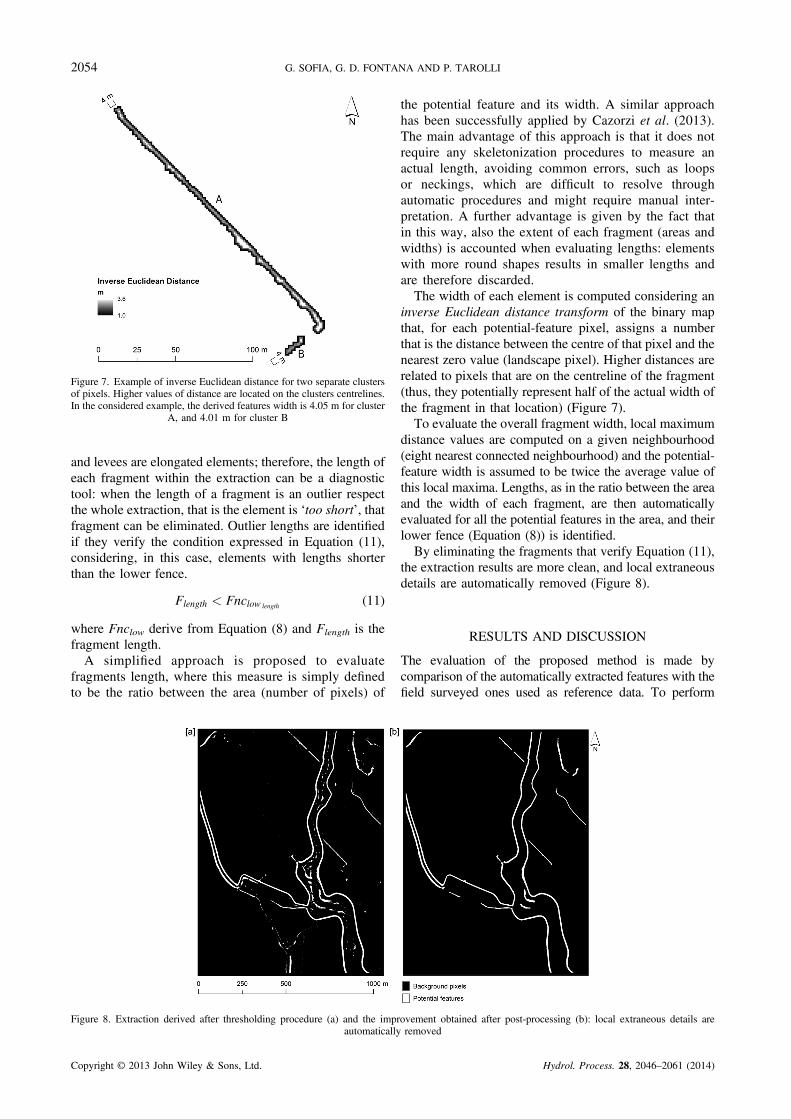
Figure 7. Example of inverse Euclidean distance for two separate clustersof pixels. Higher values of distance are located on the clusters centrelines.In the considered example, the derived features width is 4.05 m for cluster

A, and 4.01 m for cluster B


and levees are elongated elements; therefore, the length ofeach fragment within the extraction can be a diagnostictool: when the length of a fragment is an outlier respectthe whole extraction, that is the element is ‘too short’, thatfragment can be eliminated. Outlier lengths are identifiedif they verify the condition expressed in Equation (11),considering, in this case, elements with lengths shorterthan the lower fence.

Flength < Fnclow length (11)

where Fnclow derive from Equation (8) and Flength is thefragment length.A simplified approach is proposed to evaluate

fragments length, where this measure is simply definedto be the ratio between the area (number of pixels) of

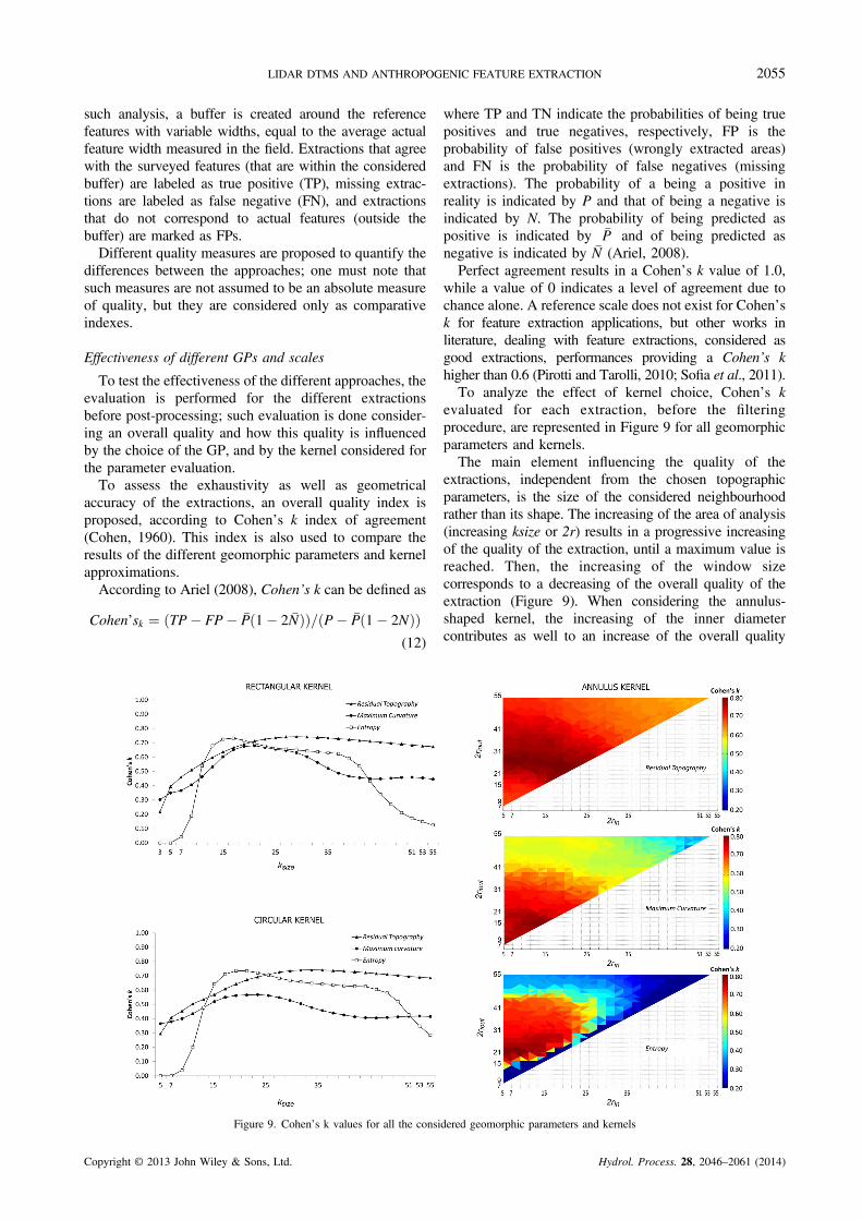
Figure 8. Extraction derived after thresholding procedure (a) and the impautomatically


the potential feature and its width. A similar approachhas been successfully applied by Cazorzi et al. (2013).The main advantage of this approach is that it does notrequire any skeletonization procedures to measure anactual length, avoiding common errors, such as loopsor neckings, which are difficult to resolve throughautomatic procedures and might require manual inter-pretation. A further advantage is given by the fact thatin this way, also the extent of each fragment (areas andwidths) is accounted when evaluating lengths: elementswith more round shapes results in smaller lengths andare therefore discarded.The width of each element is computed considering an

inverse Euclidean distance transform of the binary mapthat, for each potential-feature pixel, assigns a numberthat is the distance between the centre of that pixel and thenearest zero value (landscape pixel). Higher distances arerelated to pixels that are on the centreline of the fragment(thus, they potentially represent half of the actual width ofthe fragment in that location) (Figure 7).To evaluate the overall fragment width, local maximum

distance values are computed on a given neighbourhood(eight nearest connected neighbourhood) and the potential-feature width is assumed to be twice the average value ofthis local maxima. Lengths, as in the ratio between the areaand the width of each fragment, are then automaticallyevaluated for all the potential features in the area, and theirlower fence (Equation (8)) is identified.By eliminating the fragments that verify Equation (11),

the extraction results are more clean, and local extraneousdetails are automatically removed (Figure 8).

RESULTS AND DISCUSSION

The evaluation of the proposed method is made bycomparison of the automatically extracted features with thefield surveyed ones used as reference data. To perform

rovement obtained after post-processing (b): local extraneous details areremoved

Hydrol. Process. 28, 2046–2061 (2014)


such analysis, a buffer is created around the referencefeatures with variable widths, equal to the average actualfeature width measured in the field. Extractions that agreewith the surveyed features (that are within the consideredbuffer) are labeled as true positive (TP), missing extrac-tions are labeled as false negative (FN), and extractionsthat do not correspond to actual features (outside thebuffer) are marked as FPs.Different quality measures are proposed to quantify the

differences between the approaches; one must note thatsuch measures are not assumed to be an absolute measureof quality, but they are considered only as comparativeindexes.

Effectiveness of different GPs and scales

To test the effectiveness of the different approaches, theevaluation is performed for the different extractionsbefore post-processing; such evaluation is done consider-ing an overall quality and how this quality is influencedby the choice of the GP, and by the kernel considered forthe parameter evaluation.To assess the exhaustivity as well as geometrical

accuracy of the extractions, an overall quality index isproposed, according to Cohen’s k index of agreement(Cohen, 1960). This index is also used to compare theresults of the different geomorphic parameters and kernelapproximations.According to Ariel (2008), Cohen’s k can be defined as

Cohen’sk ¼ TP� FP� �P 1� 2�Nð Þð Þ= P� �P 1� 2Nð Þð Þ(12)

Figure 9. Cohen’s k values for all the consi


where TP and TN indicate the probabilities of being truepositives and true negatives, respectively, FP is theprobability of false positives (wrongly extracted areas)and FN is the probability of false negatives (missingextractions). The probability of a being a positive inreality is indicated by P and that of being a negative isindicated by N. The probability of being predicted aspositive is indicated by �P and of being predicted asnegative is indicated by �N (Ariel, 2008).Perfect agreement results in a Cohen’s k value of 1.0,

while a value of 0 indicates a level of agreement due tochance alone. A reference scale does not exist for Cohen’sk for feature extraction applications, but other works inliterature, dealing with feature extractions, considered asgood extractions, performances providing a Cohen’s khigher than 0.6 (Pirotti and Tarolli, 2010; Sofia et al., 2011).To analyze the effect of kernel choice, Cohen’s k

evaluated for each extraction, before the filteringprocedure, are represented in Figure 9 for all geomorphicparameters and kernels.The main element influencing the quality of the

extractions, independent from the chosen topographicparameters, is the size of the considered neighbourhoodrather than its shape. The increasing of the area of analysis(increasing ksize or 2r) results in a progressive increasingof the quality of the extraction, until a maximum value isreached. Then, the increasing of the window sizecorresponds to a decreasing of the overall quality of theextraction (Figure 9). When considering the annulus-shaped kernel, the increasing of the inner diametercontributes as well to an increase of the overall quality

dered geomorphic parameters and kernels

Hydrol. Process. 28, 2046–2061 (2014)

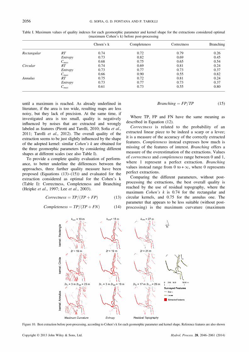
Table I. Maximum values of quality indexes for each geomorphic parameter and kernel shape for the extractions considered optimal(maximum Cohen’s k) before post-processing

Choen’s k Completeness Correctness Branching

Rectangular RT 0.74 0.72 0.79 0.26Entropy 0.73 0.82 0.69 0.45Cmax 0.68 0.75 0.65 0.54

Circular RT 0.74 0.69 0.81 0.24Entropy 0.73 0.77 0.73 0.37Cmax 0.66 0.90 0.55 0.82

Annulus RT 0.75 0.72 0.81 0.24Entropy 0.73 0.77 0.73 0.37Cmax 0.61 0.73 0.55 0.80


until a maximum is reached. As already underlined inliterature, if the area is too wide, resulting maps are lessnoisy, but they lack of precision. At the same time, ifinvestigated area is too small, quality is negativelyinfluenced by noises that are extracted and wronglylabeled as features (Pirotti and Tarolli, 2010; Sofia et al.,2011; Tarolli et al., 2012). The overall quality of theextraction seems to be just slightly influenced by the shapeof the adopted kernel: similar Cohen’s k are obtained forthe three geomorphic parameters by considering differentshapes at different scales (see also Table I).To provide a complete quality evaluation of perform-

ance, to better underline the differences between theapproaches, three further quality measure have beenproposed (Equations (13)–(15)) and evaluated for theextraction considered as optimal for the Cohen’s k(Table I): Correctness, Completeness and Branching(Heipke et al., 1997; Lee et al., 2003).

Correctness ¼ TP= TPþ FPð Þ (13)

Completeness ¼ TP= TPþ FNð Þ (14)

Figure 10. Best extraction before post-processing, according to Cohen’s k for ea


Branching ¼ FP=TP (15)

Where TP, FP and FN have the same meaning asdescribed in Equation (12).Correctness is related to the probability of an

extracted linear piece to be indeed a scarp or a levee;it is a measure of the accuracy of the correctly extractedfeatures. Completeness instead expresses how much ismissing of the features of interest. Branching offers ameasure of the overestimation of the extractions. Valuesof correctness and completeness range between 0 and 1,where 1 represent a perfect extraction. Branchingvalues instead range from 0 to +1, where 0 representsperfect extractions.Comparing the different parameters, without post-

processing the extractions, the best overall quality isreached by the use of residual topography, where themaximum Cohen’s k is 0.74 for the rectangular andcircular kernels, and 0.75 for the annulus one. Theparameter that appears to be less suitable (without post-processing) is the maximum curvature (maximum

ch geomorphic parameter and kernel shape. Reference features are also shown

Hydrol. Process. 28, 2046–2061 (2014)

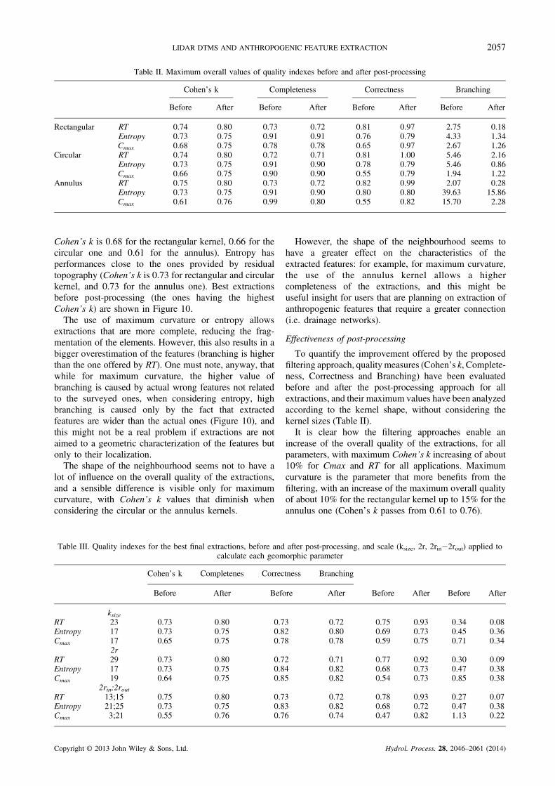
Table II. Maximum overall values of quality indexes before and after post-processing

Cohen’s k Completeness Correctness Branching

Before After Before After Before After Before After

Rectangular RT 0.74 0.80 0.73 0.72 0.81 0.97 2.75 0.18Entropy 0.73 0.75 0.91 0.91 0.76 0.79 4.33 1.34Cmax 0.68 0.75 0.78 0.78 0.65 0.97 2.67 1.26

Circular RT 0.74 0.80 0.72 0.71 0.81 1.00 5.46 2.16Entropy 0.73 0.75 0.91 0.90 0.78 0.79 5.46 0.86Cmax 0.66 0.75 0.90 0.90 0.55 0.79 1.94 1.22

Annulus RT 0.75 0.80 0.73 0.72 0.82 0.99 2.07 0.28Entropy 0.73 0.75 0.91 0.90 0.80 0.80 39.63 15.86Cmax 0.61 0.76 0.99 0.80 0.55 0.82 15.70 2.28


Cohen’s k is 0.68 for the rectangular kernel, 0.66 for thecircular one and 0.61 for the annulus). Entropy hasperformances close to the ones provided by residualtopography (Cohen’s k is 0.73 for rectangular and circularkernel, and 0.73 for the annulus one). Best extractionsbefore post-processing (the ones having the highestCohen’s k) are shown in Figure 10.The use of maximum curvature or entropy allows

extractions that are more complete, reducing the frag-mentation of the elements. However, this also results in abigger overestimation of the features (branching is higherthan the one offered by RT). One must note, anyway, thatwhile for maximum curvature, the higher value ofbranching is caused by actual wrong features not relatedto the surveyed ones, when considering entropy, highbranching is caused only by the fact that extractedfeatures are wider than the actual ones (Figure 10), andthis might not be a real problem if extractions are notaimed to a geometric characterization of the features butonly to their localization.The shape of the neighbourhood seems not to have a

lot of influence on the overall quality of the extractions,and a sensible difference is visible only for maximumcurvature, with Cohen’s k values that diminish whenconsidering the circular or the annulus kernels.

Table III. Quality indexes for the best final extractions, before andcalculate each geom

Cohen’s k Completenes Correc

Before After Befo

ksizeRT 23 0.73 0.80 0.7Entropy 17 0.73 0.75 0.8Cmax 17 0.65 0.75 0.7

2rRT 29 0.73 0.80 0.7Entropy 17 0.73 0.75 0.8Cmax 19 0.64 0.75 0.8

2rin;2routRT 13;15 0.75 0.80 0.7Entropy 21;25 0.73 0.75 0.8Cmax 3;21 0.55 0.76 0.7


However, the shape of the neighbourhood seems tohave a greater effect on the characteristics of theextracted features: for example, for maximum curvature,the use of the annulus kernel allows a highercompleteness of the extractions, and this might beuseful insight for users that are planning on extraction ofanthropogenic features that require a greater connection(i.e. drainage networks).

Effectiveness of post-processing

To quantify the improvement offered by the proposedfiltering approach, quality measures (Cohen’s k, Complete-ness, Correctness and Branching) have been evaluatedbefore and after the post-processing approach for allextractions, and their maximum values have been analyzedaccording to the kernel shape, without considering thekernel sizes (Table II).It is clear how the filtering approaches enable an

increase of the overall quality of the extractions, for allparameters, with maximum Cohen’s k increasing of about10% for Cmax and RT for all applications. Maximumcurvature is the parameter that more benefits from thefiltering, with an increase of the maximum overall qualityof about 10% for the rectangular kernel up to 15% for theannulus one (Cohen’s k passes from 0.61 to 0.76).

after post-processing, and scale (ksize, 2r, 2rin�2rout) applied toorphic parameter

tness Branching

re After Before After Before After

3 0.72 0.75 0.93 0.34 0.082 0.80 0.69 0.73 0.45 0.368 0.78 0.59 0.75 0.71 0.34

2 0.71 0.77 0.92 0.30 0.094 0.82 0.68 0.73 0.47 0.385 0.82 0.54 0.73 0.85 0.38

3 0.72 0.78 0.93 0.27 0.073 0.82 0.68 0.72 0.47 0.386 0.74 0.47 0.82 1.13 0.22

Hydrol. Process. 28, 2046–2061 (2014)

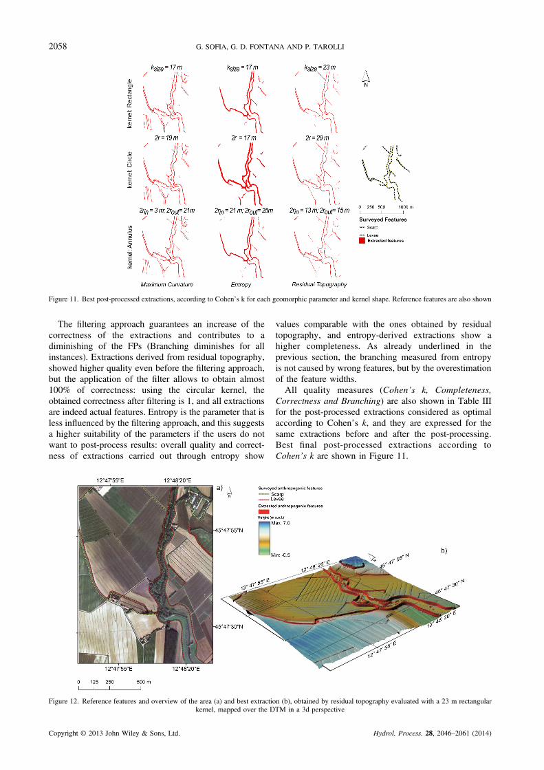
Figure 11. Best post-processed extractions, according to Cohen’s k for each geomorphic parameter and kernel shape. Reference features are also shown


The filtering approach guarantees an increase of thecorrectness of the extractions and contributes to adiminishing of the FPs (Branching diminishes for allinstances). Extractions derived from residual topography,showed higher quality even before the filtering approach,but the application of the filter allows to obtain almost100% of correctness: using the circular kernel, theobtained correctness after filtering is 1, and all extractionsare indeed actual features. Entropy is the parameter that isless influenced by the filtering approach, and this suggestsa higher suitability of the parameters if the users do notwant to post-process results: overall quality and correct-ness of extractions carried out through entropy show

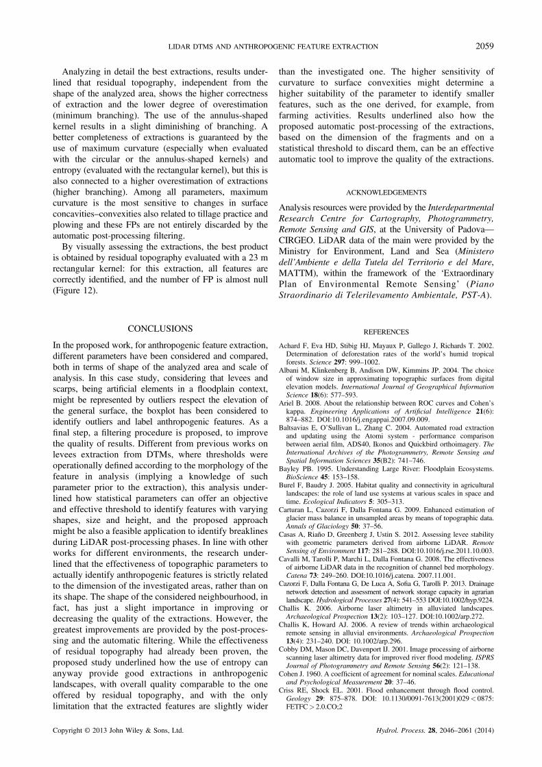
Figure 12. Reference features and overview of the area (a) and best extractiokernel, mapped over the D


values comparable with the ones obtained by residualtopography, and entropy-derived extractions show ahigher completeness. As already underlined in theprevious section, the branching measured from entropyis not caused by wrong features, but by the overestimationof the feature widths.All quality measures (Cohen’s k, Completeness,

Correctness and Branching) are also shown in Table IIIfor the post-processed extractions considered as optimalaccording to Cohen’s k, and they are expressed for thesame extractions before and after the post-processing.Best final post-processed extractions according toCohen’s k are shown in Figure 11.

n (b), obtained by residual topography evaluated with a 23 m rectangularTM in a 3d perspective

Hydrol. Process. 28, 2046–2061 (2014)


Analyzing in detail the best extractions, results under-lined that residual topography, independent from theshape of the analyzed area, shows the higher correctnessof extraction and the lower degree of overestimation(minimum branching). The use of the annulus-shapedkernel results in a slight diminishing of branching. Abetter completeness of extractions is guaranteed by theuse of maximum curvature (especially when evaluatedwith the circular or the annulus-shaped kernels) andentropy (evaluated with the rectangular kernel), but this isalso connected to a higher overestimation of extractions(higher branching). Among all parameters, maximumcurvature is the most sensitive to changes in surfaceconcavities–convexities also related to tillage practice andplowing and these FPs are not entirely discarded by theautomatic post-processing filtering.By visually assessing the extractions, the best product

is obtained by residual topography evaluated with a 23 mrectangular kernel: for this extraction, all features arecorrectly identified, and the number of FP is almost null(Figure 12).

CONCLUSIONS

In the proposed work, for anthropogenic feature extraction,different parameters have been considered and compared,both in terms of shape of the analyzed area and scale ofanalysis. In this case study, considering that levees andscarps, being artificial elements in a floodplain context,might be represented by outliers respect the elevation ofthe general surface, the boxplot has been considered toidentify outliers and label anthropogenic features. As afinal step, a filtering procedure is proposed, to improvethe quality of results. Different from previous works onlevees extraction from DTMs, where thresholds wereoperationally defined according to the morphology of thefeature in analysis (implying a knowledge of suchparameter prior to the extraction), this analysis under-lined how statistical parameters can offer an objectiveand effective threshold to identify features with varyingshapes, size and height, and the proposed approachmight be also a feasible application to identify breaklinesduring LiDAR post-processing phases. In line with otherworks for different environments, the research under-lined that the effectiveness of topographic parameters toactually identify anthropogenic features is strictly relatedto the dimension of the investigated areas, rather than onits shape. The shape of the considered neighbourhood, infact, has just a slight importance in improving ordecreasing the quality of the extractions. However, thegreatest improvements are provided by the post-proces-sing and the automatic filtering. While the effectivenessof residual topography had already been proven, theproposed study underlined how the use of entropy cananyway provide good extractions in anthropogeniclandscapes, with overall quality comparable to the oneoffered by residual topography, and with the onlylimitation that the extracted features are slightly wider


than the investigated one. The higher sensitivity ofcurvature to surface convexities might determine ahigher suitability of the parameter to identify smallerfeatures, such as the one derived, for example, fromfarming activities. Results underlined also how theproposed automatic post-processing of the extractions,based on the dimension of the fragments and on astatistical threshold to discard them, can be an effectiveautomatic tool to improve the quality of the extractions.

ACKNOWLEDGEMENTS

Analysis resources were provided by the InterdepartmentalResearch Centre for Cartography, Photogrammetry,Remote Sensing and GIS, at the University of Padova—CIRGEO. LiDAR data of the main were provided by theMinistry for Environment, Land and Sea (Ministerodell’Ambiente e della Tutela del Territorio e del Mare,MATTM), within the framework of the ‘ExtraordinaryPlan of Environmental Remote Sensing’ (PianoStraordinario di Telerilevamento Ambientale, PST-A).

REFERENCES

Achard F, Eva HD, Stibig HJ, Mayaux P, Gallego J, Richards T. 2002.Determination of deforestation rates of the world’s humid tropicalforests. Science 297: 999–1002.

Albani M, Klinkenberg B, Andison DW, Kimmins JP. 2004. The choiceof window size in approximating topographic surfaces from digitalelevation models. International Journal of Geographical InformationScience 18(6): 577–593.

Ariel B. 2008. About the relationship between ROC curves and Cohen’skappa. Engineering Applications of Artificial Intelligence 21(6):874–882. DOI:10.1016/j.engappai.2007.09.009.

Baltsavias E, O’Sullivan L, Zhang C. 2004. Automated road extractionand updating using the Atomi system - performance comparisonbetween aerial film, ADS40, Ikonos and Quickbird orthoimagery. TheInternational Archives of the Photogrammetry, Remote Sensing andSpatial Information Sciences 35(B2): 741–746.

Bayley PB. 1995. Understanding Large River: Floodplain Ecosystems.BioScience 45: 153–158.

Burel F, Baudry J. 2005. Habitat quality and connectivity in agriculturallandscapes: the role of land use systems at various scales in space andtime. Ecological Indicators 5: 305–313.

Carturan L, Cazorzi F, Dalla Fontana G. 2009. Enhanced estimation ofglacier mass balance in unsampled areas by means of topographic data.Annals of Glaciology 50: 37–56.

Casas A, Riaño D, Greenberg J, Ustin S. 2012. Assessing levee stabilitywith geometric parameters derived from airborne LiDAR. RemoteSensing of Environment 117: 281–288. DOI:10.1016/j.rse.2011.10.003.

Cavalli M, Tarolli P, Marchi L, Dalla Fontana G. 2008. The effectivenessof airborne LiDAR data in the recognition of channel bed morphology.Catena 73: 249–260. DOI:10.1016/j.catena. 2007.11.001.

Cazorzi F, Dalla Fontana G, De Luca A, Sofia G, Tarolli P. 2013. Drainagenetwork detection and assessment of network storage capacity in agrarianlandscape. Hydrological Processes 27(4): 541–553 DOI:10.1002/hyp.9224.

Challis K. 2006. Airborne laser altimetry in alluviated landscapes.Archaeological Prospection 13(2): 103–127. DOI:10.1002/arp.272.

Challis K, Howard AJ. 2006. A review of trends within archaeologicalremote sensing in alluvial environments. Archaeological Prospection13(4): 231–240. DOI: 10.1002/arp.296.

Cobby DM, Mason DC, Davenport IJ. 2001. Image processing of airbornescanning laser altimetry data for improved river flood modeling. ISPRSJournal of Photogrammetry and Remote Sensing 56(2): 121–138.

Cohen J. 1960. A coefficient of agreement for nominal scales. Educationaland Psychological Measurement 20: 37–46.

Criss RE, Shock EL. 2001. Flood enhancement through flood control.Geology 29: 875–878. DOI: 10.1130/0091-7613(2001)029< 0875:FETFC> 2.0.CO;2

Hydrol. Process. 28, 2046–2061 (2014)


Dal Cin C, Moens L, Dierickx P, Bastin G, Zech Y. 2005. An integratedapproach for realtime floodmap forecasting on the Belgian Meuseriver’. Natural Hazards 36(1–2): 237–256.

Davies ER. 1984. Circularity — A new principle underlying the design ofaccurate edge orientation operators. Image andVisionComputing2: 134–142.

Doneus M, Briese C. 2006. Full-waveform airborne laser scanning as atool for archaeological reconnaissance. In: From Space to Place. 2ndInternational Conference on Remote Sensing in Archaeology, CampanaS, Forte M (eds. BAR International Series 1568), 99–105.Archaeopress: Oxford.

Ellis EC. 2004. Long-term ecological changes in the densely populatedrural landscapes of China. In Ecosystems and Land Use Change,DeFries RS, Asner GP, Houghton RA (eds). American GeophysicalUnion: Washington, DC; 303–320.

Ellis EC, Wang H, Xiao H, Peng K, Liu XP, Li SC, Ouyang H, Cheng X,Yang LZ. 2006. Measuring long-term ecological changes in denselypopulated landscapes using current and historical high resolutionimagery. Remote Sensing of Environment 100(4): 457–473.

Eshani AH, Quiel F. 2008. Geomorphometric feature analysis usingmorphometric parameterization and artificial neural networks.Geomorphology 99: 1–12.

Evans IS. 1972. General geomorphology, derivatives of altitude anddescriptive statistics. In Spatial Analysis in Geomorphology, ChorleyRJ (ed). Methuen & Co. Ltd: London; pp. 17–90.

Evans IS. 1979. An integrated system of terrain analysis and slopemapping. Final report on grant DA-ERO-591-73-G0040, University ofDurham, England.

Evans IS. 1980. An integrated system of terrain analysis and slopemapping. Zeitschrift für Geomorphologic Suppl-Bd 36: 274–295.

Foley JA, DeFries R, Asner GP, Barford C, Bonan G, Carpenter SR. 2005.Global consequences of land use. Science 309: 570–574.

Franken P, Flos S. 2005. Using a helicopter based laser altimetry system(FLI-MAP) to carry out effective dike maintenance and constructionpolicy. In Floods, from defense to managements, Van Alphen, van Beek& Taal (eds), Taylor & Francis Group: London; 145–151.

French JR. 2003. Airborne LiDAR in support of geomorphological andhydraulic modeling. Earth Surface Processes and Landforms 28(3):321–335. DOI: 10.1002/esp.484

Gergel SE. 2002. Assessing cumulative impacts of levees and dams onfloodplain ponds: A neutral-terrain model approach. EcologicalApplications 12: 1740–1754. DOI: 10.1890/1051-0761(2002)012[1740:ACIOLA]2.0.CO;2.

Glasbey CA, Jones R. 1997. Fast computation of moving average andrelated filters in octagonal windows. Pattern Recognition Letters 18(6):555–565. DOI:10.1016/S0167-8655(97)00045-7.

Heipke C, Mayer H, Wiedemann C, Jamet O. 1997. Automatedreconstruction of topographic objects from aerial images usingvectorized map information. International Archives of Photogrammetryand Remote Sensing 23: 47–56.

Heyne RA, Pinter, N. 2011. Levee effects upon flood levels: an empiricalassessment. Hydrological Processes. DOI: 10.1002/hyp.8261.

Hiller JK, Smith M. 2008. Residual relief separation: digital elevationmodel enhancement for geomorphological mapping. Earth SurfaceProcesses and Landforms 33: 2266–2276. DOI: 10.1002/esp.1659.

Horn BKP. 1981. Hill shading and the reflectance map. Proceedings of theIEEE 69(1): 14–47.

Humme A, Lindenbergh R, Sueur C. 2006. Revealing Celtic fields from lidardata using kriging based filtering. Proceedings of the ISPRS CommissionV Symposium, Dresden, 25–27 September, Vol. XXXVI, part 5.

Köthe R, Bock M. 2009. Preprocessing of Digital Elevation Models –derived from Laser Scanning and Radar Interferometry – for TerrainAnalysis in Geosciences. Proceedings of Geomorphometry, Zurich,Switzerland, 31 August - 2 September.

Krüger T, Meinel G. 2008. Using Raster DTM for Dike Modelling. in:Oosterom P, Zlatanova S, Penninga F, Fendel EM (eds). Advances in3D Geoinformation Systems. Springer Berlin Heidelberg, Berlin,Heidelberg, 101–113. DOI: 10.1007/978-3-540-72135-2_6

Lagacherie P, Diot O, Domange N, Gouy V, Floure C, Kao C, Moussa R,Robbez-Masson J, Szleper V. 2004. An indicator approach fordescribing the spatial variability of human-made stream network inregard with herbicide pollution in cultivated watersheds. EcologicalIndicators 6: 265–279.

Lashermes B, Foufoula-Georgiou E, Dietrich WE. 2007. Channel networkextraction from high resolution topography using wavelets. GeophysicalResearch Letters 34: L23S04. DOI:10.1029/2007GL031140.

Lee S, Shan J, Bethel JS. 2003. Class-guided building extraction fromIkonos imagery. Photogrammetric Engineering and Remote Sensing 69(2): 143–150.


Lin CW, Tseng C-M, Tseng Y-H, Fei L-Y, Hsieh Y-C, Tarolli P. 2013.Recognition of large scale deep-seated landslides in forest areas ofTaiwan using high resolution topography. Journal of Asian EarthSciences 62: 389–400. DOI:10.1016/j.jseaes.2012.10.022

Lohani B, Mason DC. 2001. Application of airborne scanning laseraltimetry to the study of tidal channel geomorphology. ISPRS Journalof Photogrammetry and Remote Sensing 56(2): 100–120. DOI:10.1016/S0924-2716(01)00041-7

Long G, Mawdesley MJ, Smith M, Taha A. 2010. Simulation of airborneLiDAR for the assessment of its role in infrastructure asset monitoring.In Proceedings of the international Conference on computing in civiland building enginerering, Tizani W (ed). Nottingham University Press,Nottingham, UK; Paper 215, 429.

Marra F, Zanon F, Penna D, Mantese N, Zoccatelli D, Cavalli M, MarchiM. 2011. Hydrometeorological and hydrological analysis for the Nov 1,2010 flood event in North-eastern Italy. Geophysical ResearchAbstracts 13: EGU2011–10727-1.

Mendicino G. 1997. Analysis of the information content of environmentaldata using GIS procedures. In, Harmancioglu NB, Alpaslan MN, OzkulSD, Singh VP (eds). Integrated Approach to Environmental DataManagements Systems, NATO ASI Series, Vol. 31 Kluwer AcademicPulishers, pp. 387–400.

Mitasova H, Hofierka J. 1993. Interpolation by Regularized Spline withTension: II. Application to Terrain Modeling and Surface GeometryAnalysis. Mathematical Geology 25: 641–655.

Nelson PA, Smith JA, Miller AJ. 2006. Evolution of channelmorphology and hydrologic response in an urbanizing drainage basin.Earth Surface Processes and Landforms 31(9): 1063–1079. DOI:10.1002/esp.1308

Passalacqua P, Tarolli P, Foufoula-Georgiou E. 2010. Testing space-scalemethodologies for automatic geomorphic feature extraction from lidarin a complex mountainous landscape. Water Resources Research 46:W11535. DOI:10.1029/2009WR008812.

Passalacqua P, Belmont P, Foufoula-Georgiou E. 2012. Automaticgeomorphic feature extraction from lidar in flat and engineeredlandscapes. Water Resources Research 48: W03528. DOI:10.1029/2011WR010958

Passmore DG, Macklin MG. 2001. Late Holocene alluvial sedimentbudgets in an upland gravel bed river: the River South Tyne, NorthernEngland. In: River Basin Sediment Systems: Archives of EnvironmentalChange, Maddy D, Macklin MG, Woodward J, (eds). Balkema:Rotterdam; 423–444.

Pirotti F, Tarolli P. 2010. Suitability of LiDAR point density and derivedlandform curvature maps for channel network extraction. HydrologicalProcesses 24: 1187–1197. DOI: 10.1002/hyp.758

Schmidt J, Evans IS, Brinkmann J. 2003. Comparison of polynomialmodels for land surface curvature calculation. International Journal ofGeographic Information Science 17(8): 797–814.

Schrott L, Niederheide A, Hankammer M, Hufschmidt G, Dikau R. 2002.Sediment storage in mountain catchment: geomorphic coupling andtemporal variability (Reintal, Bavarian Alps, Germany). Zeitschrift fürGeomorphologie (Supplement) 127: 175–196.

Shannon CE, Weaver W. 1949. The Mathematical Theory of Commu-nication, University of Illinois Press: Urbana, Illinois.

Shary PA, Sharaya LS, Mitusov AV. 2002. Fundamental quantitativemethods of land surface analysis. Geoderma 107: 1–32.

Sofia G, Tarolli P, Cazorzi F, Dalla Fontana G. 2011. An objectiveapproach for feature extraction: distribution analysis and statisticaldescriptors for scale choice and channel network identification.Hydrology and Earth System Sciences 15: 1387–1402. DOI:10.5194/hess-15-1387-2011.

Sofia G, Pirotti F, Tarolli P. 2013. Variations in multiscale curvaturedistribution and signatures of LiDAR DTM errors. Earth SurfaceProcesses and Landforms. DOI: 10.1002/esp.3363.

Sparks RE. 1995. Need for ecosystem management of large riversand their floodplains. BioScience 45: 168–182. DOI: 10.2307/1312556.

Stein JL, Stein JA, Nix HA. 2002. Spatial analysis of anthropogenic riverdisturbance at regional and continental scales: identifying the wildrivers of Australia. Landscape and Urban Planning 60: 1–25. DOI:10.1016/S0169-2046(02)00048-8.

Steinfeld CMM, Kingsford RT. 2011. Disconnecting the floodplain:Earthworks and their ecological effect on a dryland floodplain in theMurray-Darling Basin, Australia. River Research and Applications.DOI: 10.1002/rra.1583.

Steinfeld CMM, Kingsford RT, Laffan S. 2012. Semi-automated GIStechniques for detecting floodplain earthworks. HydrologicalProcesses. DOI: 10.1002/hyp.9244

Hydrol. Process. 28, 2046–2061 (2014)


Tarolli P, Dalla Fontana G. 2009. Hillslope to valley transitionmorphology: new opportunities from high resolution DTMs.Geomorphology 113: 47–56. DOI:10.1016/j.geomorph.2009.02.006.

Tarolli P, Sofia G, Dalla Fontana G. 2012. Geomorphic features extractionfrom high resolution topography: landslide crowns and bank erosion.Natural Hazards 61(1): 65–83. DOI:10.1007/s11069-010-9695-2.

Terrasolid, Ltd.x 2012. TerraScan Users Guide, Helsinki, Finland, 156 pp.,URL: https://www.terrasolid.com (last date accessed: November 2012).

Thoms MC. 2003. Floodplain-river ecosystems: Lateral connections andthe implications of human interference. Geomorphology 56: 335–349.DOI: 10.1016/S0169- 555X(03)00160-0.

Tockner K, Stanford JA. 2002. Riverine flood plains: present state andfuture trends. Environmental Conservation 29: 308–330. DOI: 10.1017/S037689290200022X.


Tukey JW. 1977. Exploratory Data Analysis. Addison-Wesley, Reading, MA.Vieux BE. 1993. DEM aggregation and smoothing effects on surface

runoff modeling. Journal of Computing in Civil Engineering 7(3):310–338.

Wilson MFJ, O’Connel B, Brown C, Guinan JC, Grehan AJ. 2007.Multiscale terrain analysis of multibeam bathymetry data for habitatmapping on the continental slope. Marine Geodesy 30: 3–35.

Wood JD. 1996. The Geomorphological Characterisation of DigitalElevation Models. Ph.D. Thesis, University of Leicester.

Yin H, Li C. 2001. Human impact on floods and flood disasters on theYangtze River. Geomorphology 41: 105–109. DOI: 10.1016/S0169-555X(01)00108-8 .

Zevenbergen LW, Thorne C. 1987. Quantitative analysis of land surfacetopography. Earth Surface Processes and Landforms 12: 47–56.

Hydrol. Process. 28, 2046–2061 (2014)

https://www.terrasolid.com

high‐resolution topography and anthropogenic feature extraction: testing geomorphometric...

Documents