HYDROLOGICAL PROCESSESHydrol. Process. 23, 502–514 (2009)Published online 19 November 2008 in Wiley InterScience(www.interscience.wiley.com) DOI: 10.1002/hyp.7167

Improving hydrological information acquisition from DEMprocessing in floodplains

Augusto C. V. Getirana1,2* Marie-Paule Bonnet,2 Otto C. Rotunno Filho1 and Webe J. Mansur1

1 Programa de Engenharia Civil, COPPE-Universidade Federal do Rio de Janeiro, CP 68506,CEP 21945-970, Rio de Janeiro, RJ, Brazil2 Universite de Toulouse 3, LMTG, CNRS, UMR5563,UR154,IRD, F-31400 Toulouse, France

Abstract:

Extraction of hydrological information from digital elevation models (DEMs) is a required step when conducting any spatiallydistributed hydrological modelling. In particular, automated methods are proposed to extract the drainage structure from theDEM. However, a realistic river network is not always derived from conventional DEM processing methods. Indeed, inaccuracyoccurs in flat areas corresponding to floodplains. In these areas, additional sources of information are required to extract thecorrect drainage direction from the DEM. In this study, it is demonstrated that traditional approaches of DEM-preprocessingsuch as the commonly known ‘stream burning’ fail to provide correct maps of drainage directions and catchment areas whenthe extension of flat areas is large. A new method is proposed to take advantage of available imagery data. This method isbased on a ‘double DEM burning’ process: DEM is first burned in the main rivers using the channel network, and then in thefloodplain using the spatial distribution of floodplains provided by classified satellite images. In this sense, the method hasbeen referred to as the floodplain burning approach (or simply FB approach). Spatial distribution of floodplains is derived froma multitemporal SAR image classification. A system of equations is used to vary the elevation offset required to be ‘burnt’in each cell representing the floodplain, according to the minimal distance from the channel network, which is calculated bya distance transformation. The FB approach was applied to a sub-basin located within the larger Amazon River basin. Theregion is characterized by large floodplain extensions. Basin delineation maps derived from the new method were comparedwith those obtained from the traditional stream burning method and highlighted more realistic results. Copyright 2008 JohnWiley & Sons, Ltd.

KEY WORDS digital elevation model; floodplain; river network; watershed delineation

Received 11 March 2008; Accepted 15 September 2008

INTRODUCTION

Spatially distributed hydrological models are widely usedto assess the spatio-temporal streamflow generation inwatersheds. These models involve the definition of theinternal drainage structure described by flow directionfrom cell to cell, the river network segments and therelated sub-watersheds. Over recent decades several auto-mated or semi-automated methods have been developedto retrieve data from digital elevation models (DEMs)(O’Callaghan and Mark, 1984; Band, 1986; Jenson andDomingue, 1988; Tribe, 1992; Eash, 1994). However,despite the improvements provided by the proposedmethods, a realistic drainage structure cannot always beachieved. First, DEMs are not free from inaccuracies dueto approximations and imaging of the relief and misin-terpretation of land characteristics. Second, conventionalDEM processing algorithms, in particular the well-knownD8 algorithm (Jenson and Domingue, 1988), generallyfail to provide correct flow direction in flat surfaces. TheD8 algorithm is based on comparisons between the ele-vation of each DEM cell and the elevations of its eight

* Correspondence to: Augusto C. V. Getirana, Programa de EngenhariaCivil, COPPE-Universidade Federal do Rio de Janeiro, CP 68506,CEP21945-970, Rio de Janeiro, RJ, Brazil.E-mail: augusto@coc.ufrj.br

neighbouring cells. A flow direction is then attributedpointing towards the cell giving the steepest downslope.But ambiguities may arise if surrounding cells have thesame elevation as the central cell. Other methods thatassume multiple flow directions for a cell have alreadybeen proposed in the literature (Tarboton, 1997; Seibertand McGlynn, 2007). These methods improve the obser-vation of surface flow dispersion and the acquisition ofsome hydro-geological characteristics. However, when itcomes to watershed delineation for hydrological mod-elling, the D8 approach is recommended on account ofits deterministic basis.

Flat areas and depressions are common in griddedDEMs. Most of them are spurious and the result of mis-takes in the DEM generation process whereas some ofthem represent real terrain features. So far, several meth-ods have been proposed to handle depressions and flatareas. Some of the algorithms assume that depressionsand flat areas are spurious features and simply recom-mend removing them. Band (1986) proposes to increasethe elevation of these cells until a downslope flowpathtowards an adjacent cell is found. O’Callaghan and Mark(1984) proposed to smooth the elevation data before anyother DEM pre-processing. A second group of meth-ods handle depressions and flat areas as true features.For example, Martz and de Jong (1988) proposed to

Copyright 2008 John Wiley & Sons, Ltd.

IMPROVING HYDROLOGICAL INFORMATION ACQUISITION FROM DEM PROCESSING IN FLOODPLAINS 503

fill depressions by increasing the elevation cell up tothe elevation enabling overflow, but this method requireshigh accuracy of the DEM and small extensions of theflat areas (Freeman, 1991). All these methods implic-itly assume that depressions are linked with elevationunderestimation. On the other hand, Garbrecht and Martz(1997) and Martz and Garbrecht (1998, 1999) argue thatdepressions are related to both underestimation and over-estimation of DEM values. They proposed two algorithmsto handle spurious depressions and flat areas. The firstalgorithm simulates breaching of the outlet of closeddepressions to eliminate those expected due to eleva-tion overestimation. The second algorithm provided flowdirection in flat areas based on the surrounding slope,thus producing more realistic results. More recently, Zhuet al. (2006) developed an algorithm to deal with a large-scale basin, but fundamentals are similar to the previouslymentioned methods. All these methods handle depres-sions and flat areas as spurious features or true featureswith small extensions. Under the framework of largebasins and, in particular, at tropical basins, flat areas anddepressions are true large features mostly correspondingto floodplains and they cannot be treated with the abovementioned corrective measures.

An alternative to the already mentioned methods, anapproach known as ‘stream burning’ (SB), has beendeveloped to obtain better agreement between DEMderived from flow directions and the river network. Firstintroduced by Hutchinson (1989), it proposes the use ofadditional hydrographical data to force the flow routeto the cells which represent the streamlines. The SBapproach can be summarized as follows: (a) conversionof the digital channel network to a raster format;(b) identification of DEM cells where the channel net-work is overlaid; (c) reduction of DEM cell elevationsidentified as streamlines to ensure the stream will flowto the outlet. This approach has given good results inHutchinson (1989) and Saunders (1999). However, aswill be demonstrated here, this method may fail todetermine flow directions in regions such as floodplainslocated in the Amazon basin.

Turcotte et al. (2001) suggested the use of digitalriver and lake network (DRLN) built from map data asancillary data to improve flow direction predictions fromDEMs. For DEM cells overlapped by the digital riversand lakes network, flow directions are determined usingthe digital network connections only. The flow directionsof the other DEM cells are determined using the D8approach.

This present paper proposes an original use of remotelysensed imagery to help define the internal drainage flowstructure at the watershed scale. Remote sensing datahave become increasingly popular in hydrological stud-ies, but mainly for land cover and use. More recently,radar altimetry has been used to survey water level infloodplains and rivers (Birkett, 1998; De Oliveira Cam-pos et al., 2001; Birkett et al., 2002; Maheu et al., 2003;Calmant and Seyler, 2006) to compute discharge in largerivers (Kouraev et al., 2004; Leon et al, 2006; Zakharova

et al., 2006). The proposed method advantageously com-bines DEM, digital river and floodplains network derivedfrom classified satellite images to improve flow directionsand consequently watershed delineation algorithms, withemphasis on flow direction in floodplains. Seasonality offloodplain extension (Alsdorf et al., 2007) is captured bythe fact that the floodplain network includes occasionallyflooded areas. The method, derived from the Turcotteet al. (2001) approach, has been applied to the DemeniRiver basin, a tributary of the Negro River located in theAmazonian basin.

It is beyond the scope of this paper to review con-ventional methods of DEM processing to obtain flowdirections and watershed delineation, which are welldocumented elsewhere (O’Callaghan and Mark, 1984;Palacios-Velez and Cuevas-Renaud, 1986; Jenson andDomingue, 1988; Fairfield and Leymarie, 1991; Tribe,1992; Martz and Garbrecht, 1995; Wang and Yin, 1998;Jones, 1998, 2002).

This paper is organized in five sections: the first sectiongives a brief overview of the development of hydrologicaldata from altimetry radars and highlights the importanceof improving hydrological information acquisition forlarge-scale hydrological modelling. The second sectionpresents the development of the proposed method andits theoretical basis; the third section describes thematerial used. In the fourth section, the results obtainedare compared to those based on the conventional D8approach and on the stream burning method. Finally,the fifth section details the conclusions derived from theresults.

WHY SHOULD FLOW ROUTING PREDICTIONAND WATERSHED DELINEATION BE IMPROVED

FOR LARGE-SCALE HYDROLOGICALMODELLING?

In many hydrological modelling studies, simple proce-dures are employed to retrieve major pieces of infor-mation such as flow directions, flow accumulated areas,basin delineation, and the length and slope of riverreaches for every grid cell but generally lead to poorresults as extensively discussed in the literature. Toreduce this kind of data degradation, different upscalingmethods have been suggested over recent years (Wanget al., 2000; Reed, 2003; Paz et al., 2006; Paz and Col-lischonn, 2007). These methods preserve the high res-olution data during hydrological information extractionand combine them with the low resolution grid. Thus,DEM pre-processing is essential to achieve flow routesand therefore to estimate river length and river slope.

Previous modelling studies of the Amazon Basin haveused water balance and water transport models to estimatethe river discharge and flooded area of the basin (Costaand Foley, 1997; Coe et al., 2002; Costa et al., 2002;Ribeiro Neto et al., 2005 and more recently Coe et al.,2007). Up to now, these studies have been limited to thecontinental scale in part because of the rough scale of the

Copyright 2008 John Wiley & Sons, Ltd. Hydrol. Process. 23, 502–514 (2009)DOI: 10.1002/hyp

504 A. C. V. GETIRANA ET AL.

gridded climatological data available, ranging from 1° to0Ð5° resolution.

More recent studies have proposed a method thattakes advantage of satellite radar altimetry and allowswater level to be surveyed in large rivers and lakes(Birkett, 1998; Birkett et al., 2002; Calmant and Seyler,2006). In particular, Leon et al. (2006) developed amethod enabling one to define discharge distributionfor large basins, such as the upper Negro River Basin,from altimetry water level. The characterization of runoffdistribution along the river network is a promisingtechnique to be applied jointly with a spatially distributedhydrological model at a regional scale allowing one todevelop a comparative analysis with proposed modellingstudies of the Amazon basin that do not include this typeof approach. However, taking advantage of virtual gaugestations, where the ground tracks of radar satellites crosscut the river channel or the floodplain, and conductingrainfall–runoff modelling at the regional scale requireexact positioning of the DEM-extracted channel networkand correct delineation of the watershed. The presenceof flat surfaces and the inaccuracies found in the DEMprevent correct positioning, leading to the developmentof a new approach as proposed in this study.

THE PROPOSED METHOD

The proposed method aims first to reduce the eleva-tion of DEM cells overlapped by cells in the digitalchannel network—river cells (denoted CR hereafter) andsecondly to reduce the elevation of the DEM cells over-lapped by the cells in a floodplain map (denoted CFP

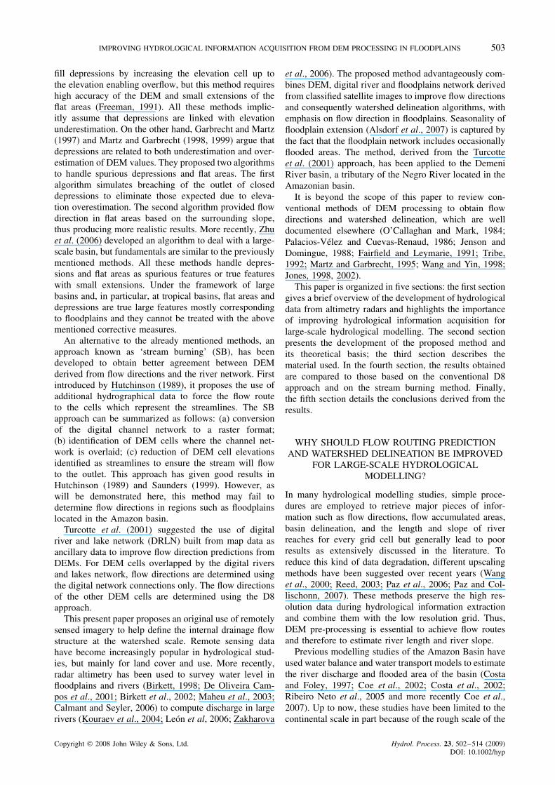
hereafter). In order to smooth the DEM adjustments,the elevation modifications are introduced based on thedistance to the closest streamline. To avoid detrimentalchanges to the DEM, elevation adjustments of CFP areonly performed in the presence of continuous connectionswith the CR, according to Figure 1. The elevation adjust-ment of each CFP varies according to the distance toa CR. This property, first introduced by Turcotte et al.(2001), takes into account a valley configuration at across-section of an originally flat surface. The methodis applied in four steps that make up the DEM pre-processing procedure and leads to the creation of a mod-ified DEM. The four steps are as follows:

- distance transformation;- elevation offset calculation;- floodplain burning process;- filling of depressions.

As previously mentioned, for hydrological modelling,the D8 approach is recommended because of its deter-ministic basis. As a result, this approach was selectedto provide the watershed delineations. The DEM post-processing, which includes the D8 approach, is used toextract information from the DEM. This step includesflow direction computation, area accumulation and basindelineation.

Figure 1. Schematic view of river cells (CR) and floodplain cells (CFP)and distance map of the corresponding CFP cells. Values correspond tothe minimal distance di, which is the distance between a CFP and theclosest CR. Not connected CFP are not considered in the distance mapcalculation. di calculation takes into account only non-interrupted ways

as represented by the arrows

Depression filling and the other phases of DEMpost-processing have been described in the literature(Jenson and Domingue, 1988; Tribe, 1992; Planchonand Darboux, 2001) and will not be detailed here. Themethod to fill depressions adopted in this study is the oneproposed by Planchon and Darboux (2001) as availablein the software Terrain Analysis System (TAS, 2007).The authors proposed a method that first inundates thesurface with a thick layer of water and then removesthe excess water. It can also replace depressions witha surface either strictly horizontal, or slightly sloping.The following sections describe the aforementioned threesteps of DEM pre-processing.

Distance transformation

The distance transformation (DT) enables one to assignthe distance (denoted di hereafter) to the nearest streamcell to each pixel of the grid considered. The methodattributes distance value only if a continuous pathwayis found between the floodplain and the river cells.Algorithms computing the Euclidean distance transform,yielding the real Euclidean distance between pixel cen-tres, have been published elsewhere (Danielsson, 1980;Yamada, 1984), but tend to be rather complex. As a result,algorithms that focus only on a small neighbourhood ata time, while providing a reasonable approximation tothe Euclidean distance, are needed (Borgefors, 1986).According to these methods, it is assumed that globaldistances in the image can be approximated by propa-gating local distances, i.e. between neighbouring pixels.Different values have already been suggested in the liter-ature for the a and b distances: a D 1 and b D infinity, or

Copyright 2008 John Wiley & Sons, Ltd. Hydrol. Process. 23, 502–514 (2009)DOI: 10.1002/hyp

IMPROVING HYDROLOGICAL INFORMATION ACQUISITION FROM DEM PROCESSING IN FLOODPLAINS 505

Figure 2. Example of the proposed steps in a schematic flat surface where black and grey pixels are, respectively, CR and CFP: (a) distancetransformation; (b) hypothetical elevation offset calculation; and (c) floodplain burning process. Values in (a) correspond to di of each pixel. A flat

10 m high DEM surface was considered within the framework of the FB approach given in (c)

a D 1 and b D 1 (Rosenfeld and Pfaltz, 1966); a D 1 andb D p

2 (Montanari, 1968); a D 2 and b D 3 (Rosenfeldand Kak, 1982); and a D 3 and b D 4 (Borgefors, 1984).Since this work deals with geographical distances, thevalues of a D 1 and b D p

2 were considered better suitedand therefore used.

DT methods provide the distance map (Borgefors,1986; Paglieroni, 1992; Ogniewicz and Kubler, 1995),which in this case, is a raster of real values. For illustra-tion purposes the proposed DT method was applied to theschematic river given in Figure 1, leading to the distancemap presented in Figure 2a, where the black pixels areused as reference.

The value of the lowest continuous distance betweenitself and a stream river cell CR has been attributed toeach floodplain cell CFP. For example, the pixel markedwith a circle has been assigned the value 4Ð24 becausethe shortest continuous distance between itself and anyCR is the one defined with the arrow. The other distancemarked with a crossed arrow is not realistic because it isnot continuous. This is why the two pixels unconnected toany CR were not attributed any value. They were simplynot considered.

Elevation offset calculation

The objective of this step is to define valleys forall transverse sections of river reaches surrounded by afloodplain by applying an elevation offset (hi) to eachCFP:

Emodi D Ei � hi �1�

where Emodi is the modified elevation and Ei is theoriginal elevation.

The offset hi must vary inversely to the distance valueto avoid inconsistent modification of the DEM and toprovide a valley shape to each cross-section. In otherwords: (i) hi takes larger values for CFP closer to CR

and it tends toward zero (or another predefined value) forCFP further away from CR; (ii) it increases or decreasesasymptotically; and (iii) it can be fully expressed in termsof maximum radial influence (as explained below). In thissense, numerous equations can be used to achieve thisobjective.

To compute hi as a function of the distance, Turcotteet al. (2001) proposed Equations (2) and (3) with two

coefficients: maximum radial influence (Rm) and flaringcoefficient (˛). These authors explain that Rm must belarge enough so that the overall modification in elevationswill eliminate all discrepancies in the flow directionfield while being sufficiently small at the same timeto maintain the information originally provided by theDEM. ˛ is calculated as a function of Rm in order toensure hi D 0Ð5 if di D Rm and hi D 1Ð5 if di D Rm � 1.This relation is expressed as follows:

hi D 1

2

(Rm

di

)1/˛

�2�

˛ D ln�Rm� � ln�Rm � 1�

ln�3��3�

The relation given in Equation (3) is well suited to caseswhere di is small. However, it is no longer adequate forlarge floodplains. In these areas, di reaches hundreds ofdistance units and the proposed relation means that hi

tends to infinite values for a small di and then decreaseswith increasing di. Finally, hi achieves feasible valuesonly in the last five or seven more distant CFP (in theirexample, Turcotte et al. used Rm D 4).

To evaluate the system of equations, high values of Rm

were tested with the aim of representing large floodplains.However, no tested value enabled suitable values to beobtained for hi. An example, for which it was assumedthat the maximum radial influence Rm was equal to 100and, consequently, the flaring coefficient is ˛ D 0Ð0091,is given in Figure 3a. In addition, with respect to largefloodplains, particularly in tropical forests, flooded areasmay be covered with trees and, depending on the captorused to acquire the elevation data, the DEM is ruled bythe canopy elevation rather than water surface. This isthe case for the global SRTM DEM, which was acquiredwith a radar sensor (Rabus et al., 2003). Valeriano et al.(2006) reported the exaggerating and damping effects oftrees in modelled surfaces of forested areas. They insistedthat canopy effects must be considered when handlingSRTM data of forested areas. Indeed, these differencesin DEM can be in excess of 20 m in certain floodplains.These effects may create artificial islands in the floodplainor even artificial obstructions, likely to greatly affect thedrainage structure of the DEM. In this sense, a reduction

Copyright 2008 John Wiley & Sons, Ltd. Hydrol. Process. 23, 502–514 (2009)DOI: 10.1002/hyp

506 A. C. V. GETIRANA ET AL.

Figure 3. Variation of hi as a function of di: (a) with Turcotte et al.’s (2001) equations, with Rm D 100 and ˛ D 0Ð0091 and; (b) with the new systemof equations, with Rm D 100, hmin D 2, ˛ D 1Ð4491 and ˇ D 48 (hi is in a logarithmic scale in both graphics for better display)

of a single unit (0Ð5 rounded to 1) from the most distantCFP may not be sufficient to cause the flow to turntowards a more likely direction.

Given these difficulties, it seems necessary to define asystem of equations that takes into account inputs suchas the minimal offset (hmin) in the most distant CFP cell,when di D Rm and also the maximum offset subtractedfrom a CFP cell when di D 1. Therefore, still followingthe premises (i) and (ii) and taking into account that theminimum distance between two pixels is equal to 1, thefollowing equations are proposed:{

hi D H if di D 0

hi D ˇ.(

1di

)1/˛if di > 0

�4�

˛ D � ln�Rm�

ln�hmin� � ln�ˇ��5�

ˇ D k.H �6�

where hi is the elevation offset for cell i and ˇ isthe highest value attributed to a CFP cell. It can beexpressed as a function of H, which is the constant offsetvalue attributed to all CR cells. k is a coefficient definedby the user and must be a positive real number lessthan 1.

It is worth pointing out that the inverse power lawalso depends on hmin and H. This property is reflectedin curves such as the one presented in Figure 3b. Inthis example, the maximum radial influence Rm wasassumed to be 100, ˇ to be 48, hmin to be 2 and a cal-culated flaring coefficient ˛ equal to 1Ð4491. The newcurve keeps all the properties of the relation proposedby Turcotte et al. (2001) except for the difference of oneunit of height (1Ð5–0Ð5) between the two most distantCFP cells. In fact, this difference is only useful whenintegers are used. While working with real numbers,there will always be differences between two CFP neigh-bours.

Figure 2b illustrates the result obtained from the dis-tance map presented in Figure 2a using the system of

Equation (4). Results were obtained with H D 10, � D0Ð5 and ˛ D 0Ð3. The black pixels denote CR and thegrey ones CFP.

Floodplain burning process (FB process)

Once the elevation offsets of floodplain cells areknown, the DEM is burned with the offset elevationmatrix according to Equation (1).

Since the matrices of Figure 2a, b represent a flat sur-face area with constant 10 m high elevations, the contin-uation of the FB process results in the new elevationsshown in Figure 2c. Figure 4 gives a general schemeof all steps proposed in the FB approach and, in thesequence, in the D8 approach.

The cases presented in the latter figures are hypothet-ical. In real cases, the values of Rm are acquired fromthe floodplain chart; hmin, H and � values depend ongeographical characteristics and ˛ is derived from empir-ical relations between the other coefficients. The generalguidance for parameters selection is to find the set cor-responding to the minimal change of the DEM informa-tion while providing the most realistic flow directionswithin the floodplain. As discussed by Getirana et al.(submitted paper), among the five parameters introducedby the method only three require user adjustment: H,hmin and �. Change in the elevation offset is obtainedif two of these parameters are varying, H and hmin or� and hmin. Variation of H and hmin is recommendedbecause changes of � mainly affect the cells close to theriver and have an insignificant impact on remote flood-plain cells. It is unlikely to produce coherent results.Values of H and hmin are tightly related but Getiranaet al. (submitted paper) demonstrated that hmin is the mostsensitive parameter. The calibration method requires thechoice of some discrete H values for the river depth.For each of these values hmin is varied until no signifi-cant change in drained area is detected. The best pair ofvalues (H,hmin) is the one that leads to the most coher-ent results while minimizing DEM changes. The rangeof hmin variation is related to vegetation and it could bereduced if pre-analysis based on land-use images wasconducted.

Copyright 2008 John Wiley & Sons, Ltd. Hydrol. Process. 23, 502–514 (2009)DOI: 10.1002/hyp

IMPROVING HYDROLOGICAL INFORMATION ACQUISITION FROM DEM PROCESSING IN FLOODPLAINS 507

Figure 4. Scheme of sequence of products obtained in each process. Thefloodplain burning approach (thick line limits) is combined with the D8approach (dotted limits), thereby improving hydrological data acquisition

IMPLEMENTING THE METHOD TO THE CASESTUDY

The work presented here is part of a hydrologicalmodelling study of the Negro River basin. With an area ofabout 712 000 km2 the Negro River Basin extends fromlatitude 3°140S to 5°80N and from longitude 72°570W to

58°160W. It is an international basin with its area dividedamong Brazil (82%), Colombia (10%), Venezuela (6%)and Guiana (2%). The Negro River basin has its springat the border between Colombia and Venezuela at theconfluence of the Guainıa River and Casiquiare River andit is one of the main tributaries of the Amazon River.

In order to demonstrate the improvements broughtabout by the proposed method a sub-watershed of theNegro River was selected, the Demeni River basin. Twogauge stations (Ajuricaba and Jalauaca) have been set upin the river. These stations, with coordinates (�62Ð62 E,0Ð88N) and (�62Ð76 E, 0Ð30N) (Figure 5) respectively,are both operated by the Brazilian Water Agency (ANA- Agencia Nacional de Aguas). Annual average dischargeis 490 m3 s�1 in Ajuricaba and 525 m3 s�1 in Jalauaca.In this basin, the large extension of permanently andperiodically flooded areas prevents acquisition of coher-ent flow directions with the traditional D8 algorithm. Inthe following sections, the source of data used withinthe framework of this study is presented, along with theresults obtained by the conventional D8 algorithm.

The digital elevation model

The DEM used in this study is that of the Shuttle RadarTopography Mission (SRTM DEM) (Rabus et al., 2003).The linear vertical absolute height error is approximately16 m and the linear vertical relative height error isapproximately 10 m (Farr et al., 2007). In quantitativeterms the mapping products derived from the SRTM datawere to be sampled over a grid of 1 arcsec resolution(¾30 m), but in this study the SRTM DEM with a spatialresolution of 3 arcsec (¾90 m) which is freely availableat NASA (2007) was preferred.

Digital channel network acquisition

The contributing area for each gauge station was esti-mated to be approximately 18 247 km2 for Ajuricaba and24 356 km2 for Jalauaca. This watershed delineation wasderived from the GTOPO30 DEM ‘burned’ with a digitalchannel network resulting from a manual vectorization ofrivers identified in the 1995/1996 JERS-1 images (Mulleret al., 1999, 2000; Seyler et al., 1999) and it is avail-able in HyBAm (2008) for the whole Amazon River

Figure 5. Geographic location of the study area. As a tributary of the Negro River, Demeni River basin is situated in the northern Amazon basin

Copyright 2008 John Wiley & Sons, Ltd. Hydrol. Process. 23, 502–514 (2009)DOI: 10.1002/hyp

508 A. C. V. GETIRANA ET AL.

Figure 6. Scheme for the acquisition of distance and elevation maps in the study area

basin. The GTOPO30 DEM is a grid with a resolu-tion of approximately 1 km (30 arcsec) developed by USGeological Survey Eros Data Center (Sioux Falls, Sioux,Dakota). The same digital channel network was used inthis work. Nevertheless, a number of corrections had to beintroduced to reposition streamlines and to georeferenceall vectors to match the other raster images. The origi-nal 1995 JERS-1 image of the study area and the resultof this process are shown in Figure 6 as 1995 ‘JERS-1Mosaic’ and ‘Digital Channel Network’ respectively.

Floodplain map

The land cover image used to identify the spatial distri-bution of flooded areas was obtained from a classificationof multitemporal JERS-1 images. These images are twomosaics of the northern part of South America acquiredby the L-band SARS JERS-1 Japanese satellite operatedby the Japanese Space Agency as part of the GlobalRainforest Mapping project. These images exhibiting a3 arcsec resolution (¾90 m on the Equator line) wereacquired between October and November 1995, duringthe high water season, and on May and July 1996, dur-ing the low water season. The multi-seasonality of thesemosaics led to a classification based on occasionally orpermanently flooded regions. A complete description ofthe classification process can be found in Frappart et al.(2005) and Martinez and Le Toan (2007). Briefly, theclassification approach was restricted to a simple butrobust classifier based on the threshold of each individualmosaic in order to retrieve pre-defined classes. Decisionrules of the classification were derived by analysis ofbackscattering responses and by using values reported inthe literature for these environments (Hess et al., 1995,2003; Saatchi et al., 2000; Martinez and Le Toan, 2007).

The classifier assigns a status to each pixel in accor-dance with flood conditions: never flooded; occasionallyflooded; and permanently flooded. Also the broad landcover type is furnished: permanent open water, grass-land, shrubland and forest. For example, an occasionally

flooded grassland is dry at the low water stage but floodedat the high water stage. This leads to an eight-themeclassification with a number of combinations betweenflood status and the simplification of a number of landcover types. Examples of simplifications are: open waterareas correspond exclusively to permanently flooded openwater areas; by definition permanently flooded grass-lands are open water areas; never flooded grasslands arecombined with the never flooded shrublands class; per-manently flooded shrublands are not considered sinceswamps are very unusual in the Amazon basin (Junk,1993). The classes can be numbered in the followingorder: (1) permanent water; (2) occasionally flooded for-est; (3) never flooded forest; (4) never flooded savannah;(5) occasionally flooded non-vegetated/herbaceous areas;(6) permanently flooded forest; (7) occasionally floodedsavannah; and (8) submerged vegetation.

According to Martinez and Le Toan (2007), the clas-sification accuracy is higher than 90% for forest areasand 70% for grasslands and shrublands due to the lowsensitivity of L-band data to low vegetation and smoothsurfaces. The classified image corresponding to the areastudied is presented in Figure 6 as ‘Classified Image’.Flooded areas were then defined as all the classes thataccount for the presence of water in the image, i.e. classes1, 2, 5, 6, 7 and 8. This selection enables one to capturethe floodplain seasonality as mentioned by Alsdorf et al.(2007). To improve the results, methodological artefactscaused by the relief or narrow rivers were identified andcorrected manually. The image was also ortorectified asa function of the SRTM image. The final result of thisprocess is shown in the same figure as ‘Selected Classes’.This is a binary image which assigned a value of 1 to theCFP pixels and zero to the other pixels.

RESULTS AND DISCUSSION

As derived from the multitemporal SAR image classi-fication, 10Ð2% of the incremental basin area (i.e. the

Copyright 2008 John Wiley & Sons, Ltd. Hydrol. Process. 23, 502–514 (2009)DOI: 10.1002/hyp

IMPROVING HYDROLOGICAL INFORMATION ACQUISITION FROM DEM PROCESSING IN FLOODPLAINS 509

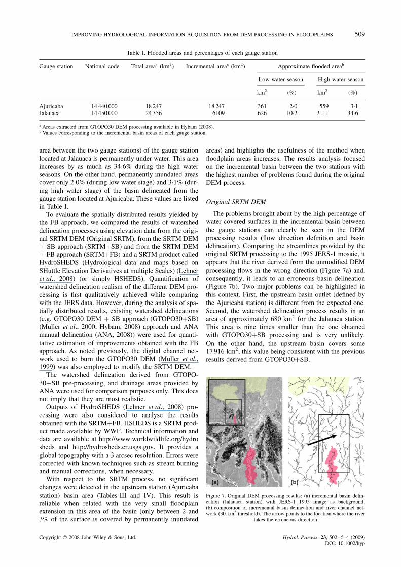
Table I. Flooded areas and percentages of each gauge station

Gauge station National code Total areaa (km2) Incremental areaa (km2) Approximate flooded areab

Low water season High water season

km2 (%) km2 (%)

Ajuricaba 14 440 000 18 247 18 247 361 2Ð0 559 3Ð1Jalauaca 14 450 000 24 356 6109 626 10Ð2 2111 34Ð6a Areas extracted from GTOPO30 DEM processing available in Hybam (2008).b Values corresponding to the incremental basin areas of each gauge station.

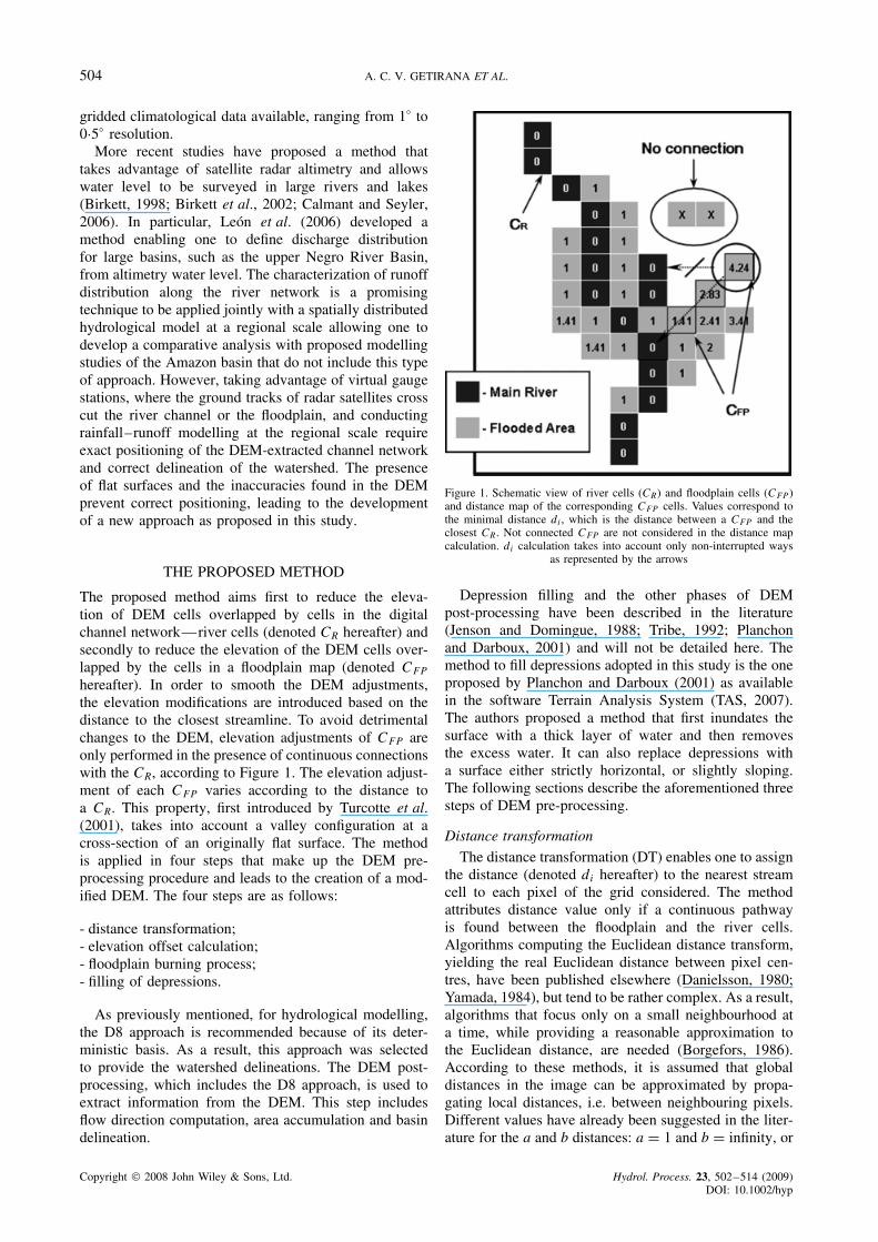
area between the two gauge stations) of the gauge stationlocated at Jalauaca is permanently under water. This areaincreases by as much as 34Ð6% during the high waterseasons. On the other hand, permanently inundated areascover only 2Ð0% (during low water stage) and 3Ð1% (dur-ing high water stage) of the basin delineated from thegauge station located at Ajuricaba. These values are listedin Table I.

To evaluate the spatially distributed results yielded bythe FB approach, we compared the results of watersheddelineation processes using elevation data from the origi-nal SRTM DEM (Original SRTM), from the SRTM DEMC SB approach (SRTMCSB) and from the SRTM DEMC FB approach (SRTMCFB) and a SRTM product calledHydroSHEDS (Hydrological data and maps based onSHuttle Elevation Derivatives at multiple Scales) (Lehneret al., 2008) (or simply HSHEDS). Quantification ofwatershed delineation realism of the different DEM pro-cessing is first qualitatively achieved while comparingwith the JERS data. However, during the analysis of spa-tially distributed results, existing watershed delineations(e.g. GTOPO30 DEM C SB approach (GTOPO30CSB)(Muller et al., 2000; Hybam, 2008) approach and ANAmanual delineation (ANA, 2008)) were used for quanti-tative estimation of improvements obtained with the FBapproach. As noted previously, the digital channel net-work used to burn the GTOPO30 DEM (Muller et al.,1999) was also employed to modify the SRTM DEM.

The watershed delineation derived from GTOPO-30CSB pre-processing, and drainage areas provided byANA were used for comparison purposes only. This doesnot imply that they are most realistic.

Outputs of HydroSHEDS (Lehner et al., 2008) pro-cessing were also considered to analyse the resultsobtained with the SRTMCFB. HSHEDS is a SRTM prod-uct made available by WWF. Technical information anddata are available at http://www.worldwildlife.org/hydrosheds and http://hydrosheds.cr.usgs.gov. It provides aglobal topography with a 3 arcsec resolution. Errors werecorrected with known techniques such as stream burningand manual corrections, when necessary.

With respect to the SRTM process, no significantchanges were detected in the upstream station (Ajuricabastation) basin area (Tables III and IV). This result isreliable when related with the very small floodplainextension in this area of the basin (only between 2 and3% of the surface is covered by permanently inundated

areas) and highlights the usefulness of the method whenfloodplain areas increases. The results analysis focusedon the incremental basin between the two stations withthe highest number of problems found during the originalDEM process.

Original SRTM DEM

The problems brought about by the high percentage ofwater-covered surfaces in the incremental basin betweenthe gauge stations can clearly be seen in the DEMprocessing results (flow direction definition and basindelineation). Comparing the streamlines provided by theoriginal SRTM processing to the 1995 JERS-1 mosaic, itappears that the river derived from the unmodified DEMprocessing flows in the wrong direction (Figure 7a) and,consequently, it leads to an erroneous basin delineation(Figure 7b). Two major problems can be highlighted inthis context. First, the upstream basin outlet (defined bythe Ajuricaba station) is different from the expected one.Second, the watershed delineation process results in anarea of approximately 680 km2 for the Jalauaca station.This area is nine times smaller than the one obtainedwith GTOPO30CSB processing and is very unlikely.On the other hand, the upstream basin covers some17 916 km2, this value being consistent with the previousresults derived from GTOPO30CSB.

Figure 7. Original DEM processing results: (a) incremental basin delin-eation (Jalauaca station) with JERS-1 1995 image as background;(b) composition of incremental basin delineation and river channel net-work (30 km2 threshold). The arrow points to the location where the river

takes the erroneous direction

Copyright 2008 John Wiley & Sons, Ltd. Hydrol. Process. 23, 502–514 (2009)DOI: 10.1002/hyp

510 A. C. V. GETIRANA ET AL.

Table II. Estimated areas (km2) provided by the automated watershed delineation processes

Gaugestation

GTOPO30CSB OriginalSRTM

HSHEDS SRTMCSB SRTMCFB

Ajuricaba 18 246Ð8 17 915Ð8 17 805Ð7 17 870Ð7 17 868Ð8Jalauacaa 6109Ð0 680Ð4 3996Ð9 4130Ð0 5524Ð6a Values corresponding to the incremental basin areas between gauge stations.

Figure 8. Detail of the watershed delineation and river network results achieved with SRTMCSB and SRTMCFB: (a) 1995 JERS-1 image with thefloodplains in white; composition of incremental basin delineation and river channel network (30 km2 threshold) for (b) SRTMCSB; (c) HSHEDS;

and (d) SRTMCFB

Figure 9. Magnified view of the watershed delineation and river network results achieved with SRTMCSB and SRTMCFB: (a) 1995 JERS-1 imagewith the floodplains in white; (b) distance map with the regions modified by the method (darker colours account for smaller distances); detail of river

channel network with the distance map as background (c) SRTMCSB; (d) HSHEDS; and (e) SRTMCFB

SRTM DEM C SB approach

Application of the SB approach to the original SRTMDEM led to some slightly better results. However, incon-sistencies can still be found. SRTMCSB processingresulted in 17 870Ð7 km2 for Ajuricaba station basin and4130Ð0 km2 for the incremental basin area (Table II).As presented in Figures 8a and b, the method allowsthe main river to be correctly depicted but many por-tions of the basin corresponding to floodplains and trib-utaries are excluded. Streamlines are erroneously posi-tioned and create unreal rivers. To highlight these inac-curacies, Figure 9 shows magnified images (as depictedin the defined region in Figure 8a) of the 1995 JERS-1image (Figure 9a), the distance map (Figure 9b) and thechannel network with the distance map in the backgroundfrom the SB approach (Figure 9c) and the FB approach

(Figure 9d). As shown in Figure 8b and detailed inFigure 9c, the SB approach could not provide an accu-rate description of all the flooded areas and rivers in theregion, as indicated in the JERS-1 image and in the back-ground image. One can observe in the marked area ofFigure 9c that the resulting river network follows differ-ent directions compared with the JERS-1 image and thedistance map.

HydroSHEDS

Most inconsistencies resulting from SRTMCSB arefound in HSHEDS processing outputs. The drainagearea of Ajuricaba basin did not present great changes(17 805Ð7 km2). On the other hand, HSHEDS resulted ina drainage area of 3996Ð9 km2 or 65Ð33% ofGTOPO-30CSB results. These areas are consistent with

Copyright 2008 John Wiley & Sons, Ltd. Hydrol. Process. 23, 502–514 (2009)DOI: 10.1002/hyp

IMPROVING HYDROLOGICAL INFORMATION ACQUISITION FROM DEM PROCESSING IN FLOODPLAINS 511

SR-TMCSB, which are justified by the simpler treatmentgiven to the HydroSHEDS product. Figures 8c and 9dpresent details of basin delineation obtained by HSHEDS.

SRTM DEM C FB approach

As mentioned above, the proposed method introducesfive coefficients requiring adjustment in order to obtaina relevant watershed delineation but minimizing DEMchanges. After a few trials and errors, the best fittedcoefficient values were: H D 50, hmin D 10, Rm D 409,� D 0Ð8 and ˛ D 4Ð3380. Following application of the FBapproach, the modified DEMs passed through the tradi-tional D8 approach (flow direction—flow accumulationand watershed delineation steps) (Jenson and Domingue,1988), as depicted in Figure 4.

Improvements brought about by the FB approachare clearly illustrated in Figure 8c. All mismatch areasevidenced in Figure 8b were repaired and portionsnot considered in the basin were now better fitted.Figure 9d reaffirms this progress. One can verify thatmismatching streamlines in Figure 9c (SB approach) arecorrected following application of the new approach(Figure 9d).

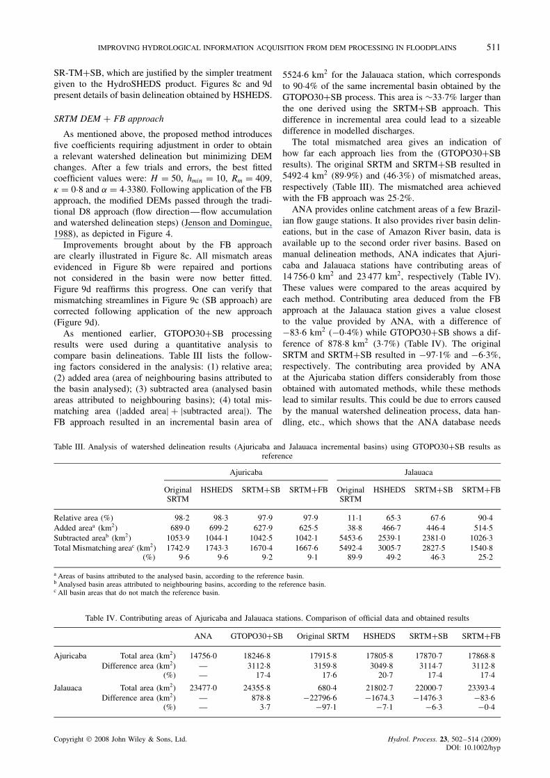
As mentioned earlier, GTOPO30CSB processingresults were used during a quantitative analysis tocompare basin delineations. Table III lists the follow-ing factors considered in the analysis: (1) relative area;(2) added area (area of neighbouring basins attributed tothe basin analysed); (3) subtracted area (analysed basinareas attributed to neighbouring basins); (4) total mis-matching area (jadded areaj C jsubtracted areaj). TheFB approach resulted in an incremental basin area of

5524Ð6 km2 for the Jalauaca station, which correspondsto 90Ð4% of the same incremental basin obtained by theGTOPO30CSB process. This area is ¾33Ð7% larger thanthe one derived using the SRTMCSB approach. Thisdifference in incremental area could lead to a sizeabledifference in modelled discharges.

The total mismatched area gives an indication ofhow far each approach lies from the (GTOPO30CSBresults). The original SRTM and SRTMCSB resulted in5492Ð4 km2 (89Ð9%) and (46Ð3%) of mismatched areas,respectively (Table III). The mismatched area achievedwith the FB approach was 25Ð2%.

ANA provides online catchment areas of a few Brazil-ian flow gauge stations. It also provides river basin delin-eations, but in the case of Amazon River basin, data isavailable up to the second order river basins. Based onmanual delineation methods, ANA indicates that Ajuri-caba and Jalauaca stations have contributing areas of14 756Ð0 km2 and 23 477 km2, respectively (Table IV).These values were compared to the areas acquired byeach method. Contributing area deduced from the FBapproach at the Jalauaca station gives a value closestto the value provided by ANA, with a difference of�83Ð6 km2 (�0Ð4%) while GTOPO30CSB shows a dif-ference of 878Ð8 km2 (3Ð7%) (Table IV). The originalSRTM and SRTMCSB resulted in �97Ð1% and �6Ð3%,respectively. The contributing area provided by ANAat the Ajuricaba station differs considerably from thoseobtained with automated methods, while these methodslead to similar results. This could be due to errors causedby the manual watershed delineation process, data han-dling, etc., which shows that the ANA database needs

Table III. Analysis of watershed delineation results (Ajuricaba and Jalauaca incremental basins) using GTOPO30CSB results asreference

Ajuricaba Jalauaca

OriginalSRTM

HSHEDS SRTMCSB SRTMCFB OriginalSRTM

HSHEDS SRTMCSB SRTMCFB

Relative area (%) 98Ð2 98Ð3 97Ð9 97Ð9 11Ð1 65Ð3 67Ð6 90Ð4Added areaa (km2) 689Ð0 699Ð2 627Ð9 625Ð5 38Ð8 466Ð7 446Ð4 514Ð5Subtracted areab (km2) 1053Ð9 1044Ð1 1042Ð5 1042Ð1 5453Ð6 2539Ð1 2381Ð0 1026Ð3Total Mismatching areac (km2) 1742Ð9 1743Ð3 1670Ð4 1667Ð6 5492Ð4 3005Ð7 2827Ð5 1540Ð8

(%) 9Ð6 9Ð6 9Ð2 9Ð1 89Ð9 49Ð2 46Ð3 25Ð2a Areas of basins attributed to the analysed basin, according to the reference basin.b Analysed basin areas attributed to neighbouring basins, according to the reference basin.c All basin areas that do not match the reference basin.

Table IV. Contributing areas of Ajuricaba and Jalauaca stations. Comparison of official data and obtained results

ANA GTOPO30CSB Original SRTM HSHEDS SRTMCSB SRTMCFB

Ajuricaba Total area (km2) 14756Ð0 18246Ð8 17915Ð8 17805Ð8 17870Ð7 17868Ð8Difference area (km2) — 3112Ð8 3159Ð8 3049Ð8 3114Ð7 3112Ð8

(%) — 17Ð4 17Ð6 20Ð7 17Ð4 17Ð4Jalauaca Total area (km2) 23477Ð0 24355Ð8 680Ð4 21802Ð7 22000Ð7 23393Ð4

Difference area (km2) — 878Ð8 �22796Ð6 �1674.3 �1476Ð3 �83Ð6(%) — 3Ð7 �97Ð1 �7Ð1 �6Ð3 �0Ð4

Copyright 2008 John Wiley & Sons, Ltd. Hydrol. Process. 23, 502–514 (2009)DOI: 10.1002/hyp

512 A. C. V. GETIRANA ET AL.

to be revised and updated with more accurate informa-tion. Finally, based on comparisons with the JERS data,it can be stated that the proposed method achieved thebest result among all the methods.

CONCLUSIONS

This paper presents a new approach based on the ‘burn-ing’ concept to obtain better results in basin delineationand streamline acquisition in floodplains of large basins.To do this, the spatial distribution of flooded areas isdetermined by means of satellite images. Distance trans-formation concepts are used to determine the eleva-tion offset distribution in the floodplains. A system ofequations is formed to calculate the elevation offset ineach pixel. This system of equations is a generalizationof the approach first developed by Turcotte et al. (2001).The new system supports application of the method tolarge floodplains (high Rm values) by adding two newparameters: H and hmin. This modification is requiredfirst to avoid extremely large (¾1) values during thecalculation of offset elevations and second to compensatefor inaccuracies in the DEM caused by the vegetation intropical forests, as discussed by Valeriano et al. (2006).This work also introduces the use of information result-ing from multitemporal SAR image classification aimingto identify floodplains and to ‘burn’ these areas.

In practice, a multitemporal JERS-1 classified image(Martinez and Le Toan, 2007) was considered to delineatefloodplains. The results obtained were qualitatively com-pared with satellite images from JERS-1 radar. Improve-ments were achieved by application of the FB approach,changing elevations of the original DEM for pixelslocated on floodplains. A new DEM was obtained inwhich flat surfaces corresponding to flooded areas withgrossly defined flow directions were replaced by valleysforcing the water flow to the closest river.

A limitation of the method is the requirement of flood-plain spatial distribution. However, this information willbe available at the global scale from the GLOBCOVERESA/JRC project, which will provide a global land covermap with 300 m resolution using MERIS data, and alsoby the Global Inundated Wetlands Earth Science DataRecord (IW-ESDR) NASA/JPL project, based on PAL-SAR ALOS data (Hess et al., 2008). Alternatively tosatellite data, this information can be deduced from fieldsurveys or aerial photography. Another limitation of themethod is the evaluation of two parameters combin-ing satisfactorily watershed delineation and low DEMchanges. On the other hand, the proposed approach seemsto give much better results in flat and flooded areas thanother existing ‘burning’ methods. Also it is well-suitedto large basins where floodplains tend to be large.

The coefficients were defined using a trial and errormethod. By taking advantage of previous knowledge ofvegetation heights, the DEM was corrected as a functionof vegetation types recognized in the classified satelliteimage. Unfortunately, this information is not available for

the area studied. It is important to note that the methodproposed in this paper can be applied to a broad class ofproblems, and that the algorithm has been implemented toobtain more consistent topological information as inputsto the MGB distributed model (Collischonn et al., 2007)within the framework of a hydrological modelling studyof the Negro River basin.

ACKNOWLEDGEMENTS

The authors would like to thank CNPq and CAPES(Projeto 516/05) in Brazil and IRD and CNRS in Francefor financial support. Grateful acknowledgements are alsodue to Jean-Michel Martinez (IRD) for providing theJERS-1 classified image and making important helpfulsuggestions. This work is part of the ANR Program(TCCYFLAM) and from the CNPq/IRD joint researchprogram. It benefited from data made available byAgencia Nacional de Aguas (ANA) and Observatoire deRecherche en Environnement Hybam (INSU).

REFERENCES

ANA (Agencia Nacional de Aguas). 2008. Hydrological database,http://hidroweb.ana.gov.br.

Alsdorf D, Bates P, Melack J, Wilson M, Dunne T. 2007. Spa-tial and temporal complexity of the Amazon flood measuredfrom space. Geophysical Research Letters 34: L08402–L08406,DOI:10Ð1029/2007GL029447.

Band LE. 1986. Topographic partition of watersheds with digitalelevation models. Water Resources Research 22: 15–24.

Birkett CM. 1998. Contribution of the Topex NASA radar altimeter tothe global monitoring of large rivers and wetlands. Water ResourcesResearch 34(5): 1223–1239.

Birkett CM, Mertes LAK, Dunne T, Costa M, Jasinski J. 2002.Altimetric remote sensing of the Amazon: application of satellite radaraltimetry. Journal of Geophysical Research 107(D20): 8059–8079,10Ð1029/2001JD000609.

Borgefors G. 1984. Distance transformation in arbitrary dimensions.Computer Vision Graphics and Image Processing 27: 321–345.

Borgefors G. 1986. Distance transformations in digital images. ComputerVision Graphics and Image Processing 34: 344–371.

Calmant S, Seyler F. 2006. Surface waters from space: rivers. ComptesRendus Geosciences Internal Geophysics (Space Physics) 338:1113–1122.

Coe MT, Costa MH, Botta A, Birkett C. 2002. Long-term simulationsof discharge and floods in the Amazon Basin. Journal of GeophysicalResearch 107(D20): 8044–8060, 10Ð1029/2001JD000740.

Coe MT, Costa MH, Howard EA. 2007. Simulating the surface watersof the Amazon River basin: impacts of new river geomorphic and flowparameterizations. Hydrological Processes 22(14): 2542–2553. DOI:10Ð1002/hyp.6850.

Collischonn W, Allasia D, Silva BC, Tucci CEM. 2007. The MGB-IPHmodel for large-scale rain fall-runoff modeling. Hydrological SciencesJournal 52(5): 878–895.

Costa MH, Foley JA. 1997. Water balance of the Amazon Basin:dependence on vegetation cover and canopy conductance. Journal ofGeophysical Research 102(D20): 23973–23989.

Costa MH, Oliveira CHC, Andrade RG, Bustamante TR, Silva FA,Coe MT. 2002. A macroscale hydrological data set of river flow routingparameters for the Amazon Basin. Journal of Geophysical Research107(D20): 8039–8047, DOI: 10Ð1029/2000JD000309.

Danielsson PE. 1980. Euclidean distance mapping. Computer Graphicsand Image Processing 14(3): 227–248.

De Oliveira Campos I, Mercier F, Maheu C, Cochonneau G, Kosuth P,Blitzkow D, Cazenave A. 2001. Temporal variations of river basinwaters from Topex/Poseidon satellite altimetry. Application to theAmazon basin. C.R. Academic Science Paris 333: 633–643.

Eash DA. 1994. A geographic information system procedure to quantifydrainage-basin characteristic. Water Resources Bulletin 30: 1–8.

Copyright 2008 John Wiley & Sons, Ltd. Hydrol. Process. 23, 502–514 (2009)DOI: 10.1002/hyp

IMPROVING HYDROLOGICAL INFORMATION ACQUISITION FROM DEM PROCESSING IN FLOODPLAINS 513

Fairfield J, Leymarie P. 1991. Drainage networks from grid digitalelevation models. Water Resources Research 27(5): 709–717.

Farr TG, Paul A, Rosen PA, Caro E, Crippen R, et al. 2007. TheShuttle Radar Topography Mission. Revue of Geophysics 45:RG2004–RG2036, DOI:10Ð1029/2005RG000183.

Frappart F, Seyler F, Martinez JM, Leon JG, Cazenave A. 2005. Flood-plain water storage in the Negro River basin estimated from microwaveremote sensing of inundation area and water levels. Remote Sensing ofEnvironment 99(4): 387–399 DOI:10Ð1016/j.rse.2005Ð08Ð016.

Freeman TG. 1991. Calculating catchment area with divergent flow basedon a regular grid. Computers and Geosciences 17(3): 413–422.

Garbrecht J, Martz W. 1997. The assignment of drainage direction overflat surfaces in raster digital elevation models. Journal of Hydrology193: 204–213.

Getirana ACV, Bonnet M-P, Martinez J-M. (in revision). “Evaluatingparameter effects in a DEM ‘burning’ process based on land coverdata”. Hydrological Processes .

Hess LL, Melack JM, Filoso S, Wang Y. 1995. Delineation of inundatedarea and vegetation along the Amazon floodplain with the SIR-CSynthetic Aperture Radar. IEEE Transactions On Geosciences andRemote Sensing 33(4): 896–903.

Hess LL, Melack JM, Novo EMLM, Barbosa CCF, Gastil M. 2003.Dual-season mapping of wetland inundation and vegetation for thecentral Amazon basin. Remote Sensing of Environment 87: 404–428.

Hess LL, Novo EMLM, Costa M, Chapman B, Durieux L, Forsberg B,Pellon F. 2008. Seasonal mapping of inundation and vegetation inwetlands of Northern South-America—mid term results. ALOS K&C10th Science Team Meeting, 23–26 June, Tokyo.

Hutchinson MF. 1989. A new procedure for gridding elevation and streamline data with automatic removal of spurious pits. Journal of Hydrology106: 211–232.

HyBAm (Hydrologie du Bassin Amazonien). 2008. Base de donnees,http://mafalda.teledetection.fr/hybam/whybam2/index.php.

Jenson SK, Domingue JO. 1988. Extracting topographic structure fromdigital elevation data for geographic information system analysis.Photogrammetric Engineering and Remote Sensing 54: 1593–1600.

Jones KH. 1998. A comparison of algorithms used to compute hill slopeas a property of DEM. Computers and Geosciences 24(4): 315–323.

Jones R. 2002. Algorithms for using a DEM for mapping catchmentareas of stream sediment samples. Computers and Geosciences 28:1051–1060.

Junk WJ. 1993. Wetlands of tropical South America. In Wetlands of theWorld: Inventory, Ecology and Management , Vol. 1, Whigham DF,Dykyjova D, Hejny S (eds). Kluwer Academic Publishers; 679–739.

Kouraev A, Sakharova EA, Samain O, Mognard-Campbell N, CazenaveA. 2004. Ob’ river discharge from Topex/Poseidon satellite altimetry.Remote Sensing of Environment 93: 238–245.

Lehner B, Verdin K, Jarvis A. 2008. New global hydrography derivedfrom spaceborne elevation data. EOS, Transactions, AGU 89(10):93–94.

Leon JG, Calmant S, Seyler F, Bonnet MP, Cauhope M, Frappart F,Fillizola N. 2006. Rating curves and estimation of average depth atthe upper Negro river based on satellite altimeter data and modelleddischarges. Journal of Hydrology 328(3–4): 481–496.

Maheu C, Cazenave A, Mechoso R. 2003. Water level fluctuationsin the La Plata basin (South America) from Topex/Poseidonaltimetry. Geophysical Research Letters 30(3): 1143–1146,DOI:10Ð1029/2002GL016033.

Martinez J-M, Le Toan T. 2007. Mapping of flood dynamics andspatial distribution of vegetation in the Amazon floodplain usingmultitemporal SAR data. Remote Sensing of Environment 108(3):209–223 DOI:10Ð1016/j.rse.2006Ð11Ð012.

Martz LW, de Jong E. 1988. CATCH: a FORTRAN program formeasuring catchment area from digital elevation models. Computersand Geosciences 14(5): 627–640.

Martz LW, Garbrecht J. 1995. Automated recognition of valley lines anddrainage networks from grid digital elevation models: a review and anew method—comment. Journal of Hydrology 167: 393–396.

Martz LW, Garbrecht J. 1998. The treatment of flat areas and depressionsin automated drainage analysis of raster digital elevation models.Hydrological Processes 12: 843–855.

Martz LW, Garbrecht J. 1999. An outlet breaching algorithm for thetreatment of closed depressions in a raster DEM. Computers andGeosciences 25: 835–844.

Montanari U. 1968. A method for obtaining skeletons using a quasi-Euclidean distance. Journal of Associated Computer Machinery 15:600–624.

Muller F, Seyler F, Cochonneau G, Guyot JL. 1999. Utilisationd’imagerie radar (ROS) JERS-1 pour l’obtention de reseaux de

drainage. Exemple du Rio Negro (Amazonie). In InternationalSymposium on hydrological and geochemical processes in large scaleriver basins, Manaus 99, Brazil.

Muller F, Cochonneau G, Guyot J-L, Seyler F. 2000. Watershedextraction using together DEM and drainage network: application to thewhole Amazonian basin. In 4th International Conference on IntegratingGIS and Environmental Modeling (GIS/EM4), Alberta, Canada.

NASA. 2007. SRTM web page with C-band data. Available online at:ftp://e0srp01u.ecs.nasa.gov/.

O’Callaghan JF, Mark DM. 1984. The extraction of drainage networksfrom digital elevation data. Computer Vision Graphics and ImageProcessing 28: 323–344.

Ogniewicz RL, Kubler O. 1995. Hierarchic Voronoi skeletons. PatternRecognition 28(3): 343–359.

Paglieroni DW. 1992. Distance transforms: properties and machine visionapplications. Graphical Models and Image Processing 54: 56–74.

Palacios-Velez OL, Cuevas-Renaud B. 1986. Automated river-course,ridge and basin delineation from digital elevation data. Journal ofHydrology 86: 299–314.

Paz AR, Collischonn W. 2007. River reach length and slope estimates forlarge-scale hydrological models based on a relatively high-resolutiondigital elevation model. Journal of Hydrology 343: 127–139.DOI:10Ð1016/j.jhydrol.2007Ð06Ð006.

Paz AR, Collischonn W, Lopes da Silveira A L. 2006. Improve-ments in large-scale drainage networks derived from digital ele-vation models. Water Resources Research 42: W08502–W08508,DOI:10Ð1029/2005WR004544.

Planchon O, Darboux F. 2001. A fast, simple and versatile algorithmto fill the depressions of digital elevation models. CATENA 46(2–3):159–176.

Rabus B, Eineder M, Roth A, Bamler R. 2003. The shuttle radartopography mission—a new class of digital elevation models acquiredby spaceborne radar. Journal of Photogrammetry and Remote Sensing57: 241–262.

Reed SM. 2003. Deriving flow directions for coarse-resolution (1–4 km)gridded hydrologic modeling. Water Resources Research 39(9): 1238,DOI:10Ð1029/2003WR001989.

Ribeiro Neto A, Vieira da Silva R, Collischonn W, Tucci CEM. 2005.Hydrological modelling in Amazonia—use of the MGB-IPH modeland alternative data base. In Proceedings of VII IAHS ScientificAssembly, Foz do Iguacu, Brasil.

Rosenfeld A, Kak AC. 1982. Digital Picture Processing, 2nd edn, Vol.2. Academic Press: New York.

Rosenfeld A, Pfaltz J. 1966. Sequential operations in digital pictureprocessing. Journal of the Association of Computer Machinery 13:471–494.

Saatchi SS, Nelson B, Podest E, Holt J. 2000. Mapping Land-cover typesin the Amazon Basin using 1 km J-ERS-1 mosaic. InternationalJournal Of Remote Sensing 21(6–7): 1201–1234.

Saunders W. 1999. Preparation of DEMs for use in environmentalmodeling analysis. ESRI User Conference, July 24–30, 1999, SanDiego, California.

Seibert J, Mcglynn BL. 2007. A new triangular multiple flow directionalgorithm for computing upslope areas from gridded digitalelevation models. Water Resources Research 43: W04501–W04508,DOI:10Ð1029/2006WR005128.

Seyler F, Muller F, Cochonneau G, Guyot JL. 1999. Delimitation debassins versants a partir d’un modele numerique de terrain.Comparaison de differentes methodes pour le bassin du RioNegro (Amazone). In International Symposium on hydrological andgeochemical processes in large scale river basins, Manaus 99, Brazil.

Tarboton DG. 1997. A new method for the determination of flowdirections and upslope in grid digital elevation models. WaterResources Research 33(2): 309–319.

TAS (Terrain Analysis System). 2007. Software freely available inhttp://www.sed.manchester.ac.uk/geography/research/tas/.

Tribe A. 1992. Automated recognition of valley lines and drainagenetworks from grid digital elevation models: a review and a newmethod. Journal of Hydrology 139: 263–293.

Turcotte R, Fortin J-P, Rousseau AN, Massicote S, Villeneuve J-P. 2001.Determination of the drainage structure of a watershed using adigital elevation model and digital river and lake network. Journalof Hydrology 240: 225–242.

Valeriano MM, Kuplich TM, Storino M, Amaral BD, Mendes Jr JN,Lima DJ. 2006. Modeling small watersheds in Brazilian Amazoniawith shuttle radar topographic mission-90 m data. Computers andGeosciences 32(8): 1169–1181.

Copyright 2008 John Wiley & Sons, Ltd. Hydrol. Process. 23, 502–514 (2009)DOI: 10.1002/hyp

514 A. C. V. GETIRANA ET AL.

Wang M, Hjelmfelt AT, Garbrecht J. 2000. DEM aggregation forwatershed modeling. Journal of American Water Resources Association36(3): 579–584.

Wang X, Yin Z-Y. 1998. A comparison of drainage networks derivedfrom digital elevation models at two scales. Journal of Hydrology 210:221–241.

Yamada H. 1984. Complete euclidean distance transformation by paralleloperation. In Proceedings of the 7th International Conference onPattern Recognition; 69–71.

Zakharova E, Kouraev A, Cazenave A. 2006. Amazon river dischargeestimated from the Topex/Poseidon altimetry. C.R. Geosciences 338:188–196.

Zhu Q, Tian Y, Zhao J. 2006. An efficient depression processingalgorithm for hydrologic analysis. Computers and Geosciences 32:615–263.

Copyright 2008 John Wiley & Sons, Ltd. Hydrol. Process. 23, 502–514 (2009)DOI: 10.1002/hyp