Hierarchical X–FEM for n–phase flow (n > 2)

Sergio Zlotnik a Pedro Dıez b,∗

aGroup of Dynamics of the Lithosphere (GDL) Institute of Earth Sciences “JaumeAlmera”, CSIC Lluıs Sole i Sabarıs s/n, 08028 Barcelona, Spain

bLaboratori de Calcul Numeric, Departament de Matematica Aplicada IIIUniversitat Politecnica de Catalunya Campus Nord UPC, 08034 Barcelona, Spain

Abstract

The eXtended Finite Element Method (X–FEM) has been successfully used in two-phase flow problems involving a moving interface. In order to simulate problemsinvolving more than two phases, the X–FEM has to be further eXtended. Theproposed approach is presented in the case of a quasistatic Stokes n-phase flowand it is based on using an ordered collection of level set functions to describethe location of the phases. A level set hierarchy allows describing triple junctionsavoiding overlapping or “voids” between materials. Moreover, an enriched solutionaccounting for several simultaneous phases inside one element is proposed. Theinterpolation functions corresponding to the enriched degrees of freedom requireredefining the associated ridge function accounting for all the level sets.

The computational implementation of this scheme involves calculating integralsin elements having several materials inside. An adaptive quadrature accounting forthe interfaces locations is proposed to accurately compute these integrals.

Examples of the hierarchical X–FEM approach are given for a n–phase Stokesproblem in 2 and 3 dimensions.

Key words: multiphase flow; level set methods; enrichment; eXtended FiniteElement Method (X–FEM)

∗ Corresponding author.Email addresses: szlotnik@ija.csic.es (Sergio Zlotnik), pedro.diez@upc.es

(Pedro Dıez).URLs: www.ija.csic.es/gt/sergioz/ (Sergio Zlotnik), www-lacan.upc.es

(Pedro Dıez).

Preprint submitted to Elsevier Science 20 February 2009

1 Introduction

Level set methods are becoming increasingly popular for the solution of fluidproblems involving moving interfaces [10]. In the two-phase case, the level setmethods can predict the evolution of complex interfaces including changes intopology such as deforming bubbles, break up and coalescence, etc. This kindof flow is encountered in a wide range of industrial and natural applications.Since the introduction of the level set method by Osher and Sethian [8], alarge amount of bibliography has been published. See, for instance, the citedreview by Sethian and Smereka [10] and the work by Osher and Fedkiw [7].

Despite the term multiphase is widely used in the literature, most works usinglevel sets for tracking material interfaces limit the number of phases to two.This restriction comes from the use of the sign of a level set function to describethe materials location. There are some works handling n–phase models (n > 2)based on several level set functions. For example, Tan and Zabaras [11] use thelevel set technique combined with features of front tracking methods to modelthe microstructure evolution in the solidification of multi–component alloys. Inthis work each component is defined by a level set function: the sign limits thesolid–liquid interface. Two algorithms to simulate triple junctions where theinterfaces motion depends on surface tension and bulk energies were proposedby Zhao et. al. [13] and Ruuth [9]. These works use a number of level setfunctions equal to the number of materials. They require adding some furtherrestrictions to the model in order to prevent overlapping or vacuum betweenphases. Recently Dolbow et al. [?] presented a similar technique to enforceconservation laws across interfaces described using the Patterned InterfaceReconstruction method.

In this work we propose a different approach to describe and to model n-phaseflow problems based on X–FEM. The main ingredients are: level sets and an en-riched solution. We avoid the geometrical inconsistency (overlapping or voids)by introducing a hierarchy between the level sets. Moreover, the enrichment ofthe solution is extended to account for triple (or multiple) junctions inside anelement. This allows for handling gradient discontinuities across the interface.In the following sections the hierarchy between level sets and the multipleenrichment are presented in the context of a n-phase flow problem. Computa-tional considerations on how to integrate discontinuous function on elementsare discussed next. Finally, in order to show the behavior of the proposed ap-proach we present several application examples in 2D and 3D of n–phase flowproblems driven by gravitational forces.

2

2 Problem statement

The hierarchical X–FEM is developed to simulate a flow problem with n phases(n > 2). An n–phase fluid governed by the Stokes equation is considered.The inertia term is neglected and the problem is thus quasi–static. This is acommon situation in geophysical modeling, where creeping (very slow) flowarises (e.g. [14]). The governing equations are written in terms of velocity uand pressure p as

∇ · (η∇su) +∇p = ρg, (1a)

∇ · u = 0 (1b)

where η is the viscosity, ρ the density, and g the gravitational accelerationvector. The symmetrized gradient operator ∇s is defined as 1

2(∇> +∇). Den-

sity and viscosity fields are constant in each phase and discontinuous acrossinterfaces. Equation (1) is quasi–static and it does not contain any explicittime dependence; the transient character of the solution is due to the motionof the phases. For the sake of a simple presentation, the problem is describedby equation (1), that is the expression of the balance law in strong form. Thecomplete description of the Boundary Value Problem is therefore omitted andwould require, along with the boundary conditions, to explicitly enforce thecontinuity of the normal stresses across the interfaces where the viscosity is dis-continuous. This is naturally treated in the weak form of the problem adoptedin the practical implementation. The Stokes problem is discretized using thestandard mini element (triangular element with enhanced linear velocities andlinear pressure), which is the simpler option fulfilling the LBB condition.

The location of the different phases is described by a collection of level setfunctions. The level sets represent material properties and they are conse-quently transported by the motion of the fluid. Thus the evolution of each oneof the level sets, describing phase locations, is determined by pure advectionequation

φ(i) + u · ∇φ(i) = 0 (2)

where u is the velocity field, solution of the Stokes problem (1), and φ(i) isthe level set number i. In the applications, equation (2) is solved using lineartriangular elements and using the two-step third order Taylor-Galerkin time-marching scheme, especially designed to deal with the advective character ofthe problem [3].

3

3 Describing a n–phase fluid with n− 1 level sets

The level set technique is widely used in two and three dimensions to track onefree interface between two materials, see for example [12,1,14]. This section isdevoted to generalize this strategy to n-phase flows.

3.1 Two phases with a single level set

The location of the interface between two materials is described using a levelset function φ(1). The superscript (1) denotes the number of level set and itis useful when 3 or more phases have to be described. This superscript is notstrictly necessary in this section, it is used here to keep a consistent notation inthe following sections. The sign of the level set φ(1) describes a partition of thedomain Ω in two subdomains Ω1 and Ω2 using the following sign convention

φ(1)(x, t) =

> 0 for x ∈ Ω1

= 0 for x on the interface

< 0 for x ∈ Ω2

(3)

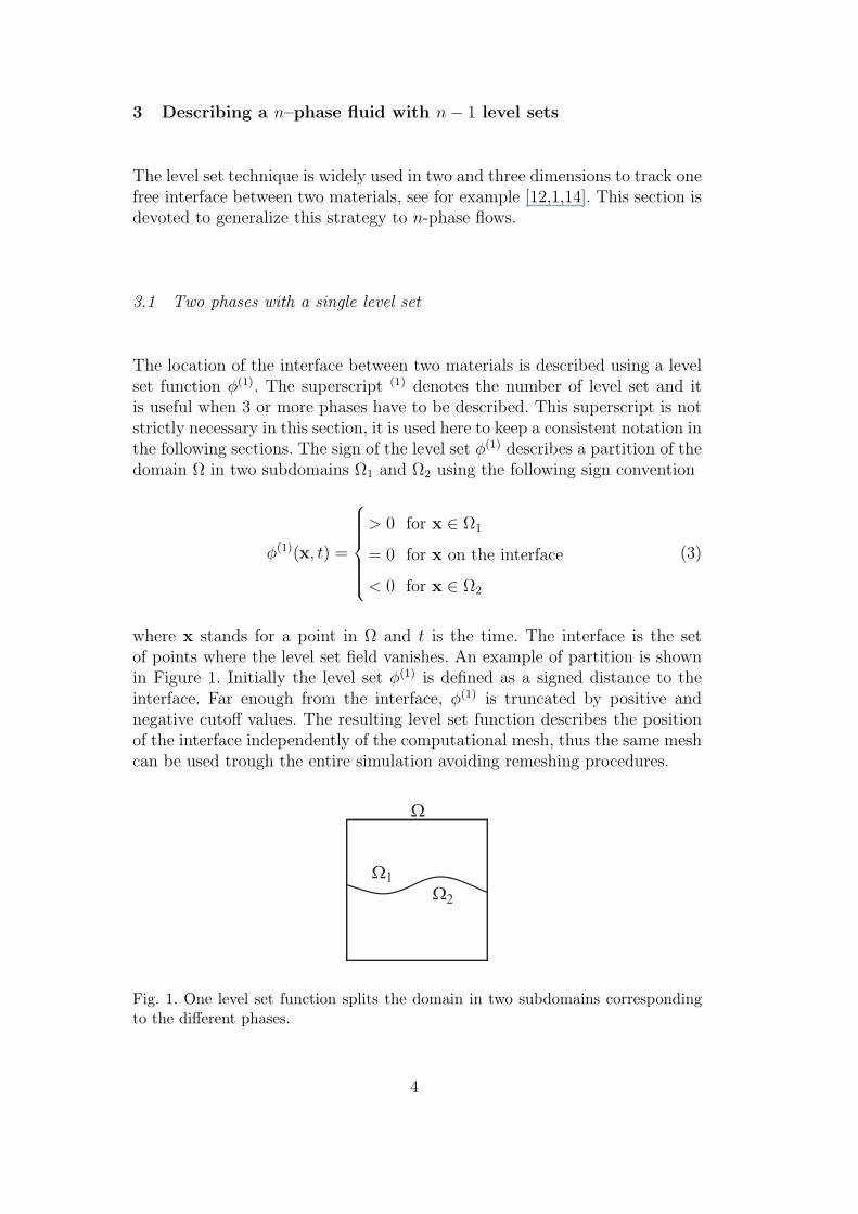
where x stands for a point in Ω and t is the time. The interface is the setof points where the level set field vanishes. An example of partition is shownin Figure 1. Initially the level set φ(1) is defined as a signed distance to theinterface. Far enough from the interface, φ(1) is truncated by positive andnegative cutoff values. The resulting level set function describes the positionof the interface independently of the computational mesh, thus the same meshcan be used trough the entire simulation avoiding remeshing procedures.

Ω

Ω1

Ω2

Fig. 1. One level set function splits the domain in two subdomains correspondingto the different phases.

4

3.2 Tracking more than two phases: hierarchy of level sets

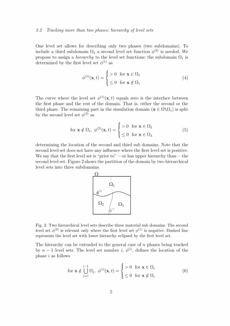
One level set allows for describing only two phases (two subdomains). Toinclude a third subdomain Ω3 a second level set function φ(2) is needed. Wepropose to assign a hierarchy to the level set functions: the subdomain Ω1 isdetermined by the first level set φ(1) as

φ(1)(x, t) =

> 0 for x ∈ Ω1

≤ 0 for x /∈ Ω1

(4)

The curve where the level set φ(1)(x, t) equals zero is the interface betweenthe first phase and the rest of the domain. That is, either the second or thethird phase. The remaining part in the simulation domain (x ∈ Ω\Ω1) is splitby the second level set φ(2) as

for x /∈ Ω1, φ(2)(x, t) =

> 0 for x ∈ Ω2

≤ 0 for x ∈ Ω3

(5)

determining the location of the second and third sub domains. Note that thesecond level set does not have any influence where the first level set is positive.We say that the first level set is “prior to” —or has upper hierarchy than— thesecond level set. Figure 2 shows the partition of the domain by two hierarchicallevel sets into three subdomains.

Ω

Ω1

Ω2 Ω3

φ(1)

φ(2)

Fig. 2. Two hierarchical level sets describe three material sub domains. The secondlevel set φ(2) is relevant only where the first level set φ(1) is negative. Dashed linerepresents the level set with lower hierarchy eclipsed by the first level set.

The hierarchy can be extended to the general case of n phases being trackedby n − 1 level sets. The level set number i, φ(i), defines the location of thephase i as follows

for x /∈i−1⋃

j=1

Ωj, φ(i)(x, t) =

> 0 for x ∈ Ωi

≤ 0 for x /∈ Ωi

(6)

5

for all i = 1, . . . , n− 2. The level set with lowest hierarchy, φ(n−1), determinesthe location of the last two phases in the remaining space as

for x /∈n−2⋃

j=1

Ωj, φ(n−1)(x, t) =

> 0 for x ∈ Ωn−1

≤ 0 for x ∈ Ωn

(7)

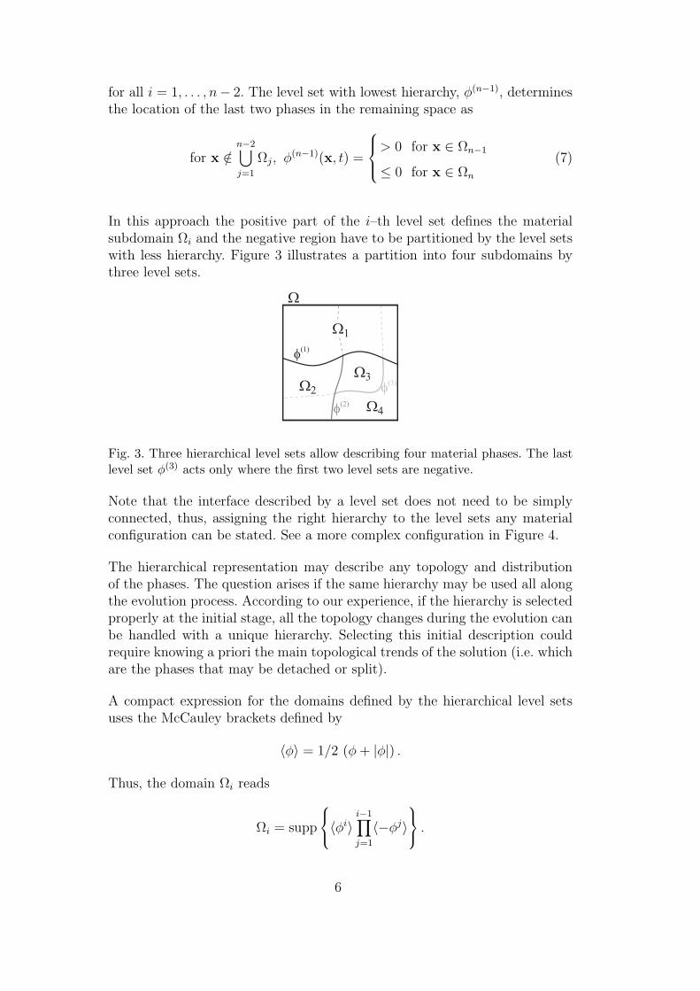
In this approach the positive part of the i–th level set defines the materialsubdomain Ωi and the negative region have to be partitioned by the level setswith less hierarchy. Figure 3 illustrates a partition into four subdomains bythree level sets.

Ω

Ω1

Ω2

Ω3

Ω4

φ(1)

φ(2)

φ(3)

Fig. 3. Three hierarchical level sets allow describing four material phases. The lastlevel set φ(3) acts only where the first two level sets are negative.

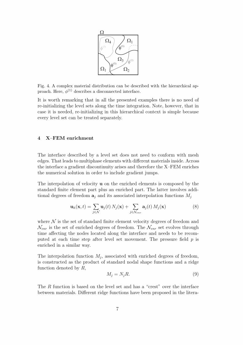
Note that the interface described by a level set does not need to be simplyconnected, thus, assigning the right hierarchy to the level sets any materialconfiguration can be stated. See a more complex configuration in Figure 4.

The hierarchical representation may describe any topology and distributionof the phases. The question arises if the same hierarchy may be used all alongthe evolution process. According to our experience, if the hierarchy is selectedproperly at the initial stage, all the topology changes during the evolution canbe handled with a unique hierarchy. Selecting this initial description couldrequire knowing a priori the main topological trends of the solution (i.e. whichare the phases that may be detached or split).

A compact expression for the domains defined by the hierarchical level setsuses the McCauley brackets defined by

〈φ〉 = 1/2 (φ + |φ|) .

Thus, the domain Ωi reads

Ωi = supp

〈φ

i〉i−1∏

j=1

〈−φj〉 .

6

Ω

Ω1

Ω1

Ω2

Ω3

Ω4

φ(1)

φ(1)

φ(2)

φ(3)

Fig. 4. A complex material distribution can be described with the hierarchical ap-proach. Here, φ(1) describes a disconnected interface.

It is worth remarking that in all the presented examples there is no need ofre-initializing the level sets along the time integration. Note, however, that incase it is needed, re-initializing in this hierarchical context is simple becauseevery level set can be treated separately.

4 X–FEM enrichment

The interface described by a level set does not need to conform with meshedges. That leads to multiphase elements with different materials inside. Acrossthe interface a gradient discontinuity arises and therefore the X–FEM enrichesthe numerical solution in order to include gradient jumps.

The interpolation of velocity u on the enriched elements is composed by thestandard finite element part plus an enriched part. The latter involves addi-tional degrees of freedom aj and its associated interpolation functions Mj

uh(x, t) =∑

j∈Nuj(t) Nj(x) +

∑

j∈Nenr

aj(t) Mj(x) (8)

where N is the set of standard finite element velocity degrees of freedom andNenr is the set of enriched degrees of freedom. The Nenr set evolves throughtime affecting the nodes located along the interface and needs to be recom-puted at each time step after level set movement. The pressure field p isenriched in a similar way.

The interpolation function Mj, associated with enriched degrees of freedom,is constructed as the product of standard nodal shape functions and a ridgefunction denoted by R,

Mj = NjR. (9)

The R function is based on the level set and has a “crest” over the interfacebetween materials. Different ridge functions have been proposed in the litera-

7

ture, see for example [1,6]. In the following a ridge function properly definedin the elements with multiple interfaces in introduced. The rationale followsthe ideas proposed by Moes and co-authors in [6].

4.1 Two phases, one Ridge

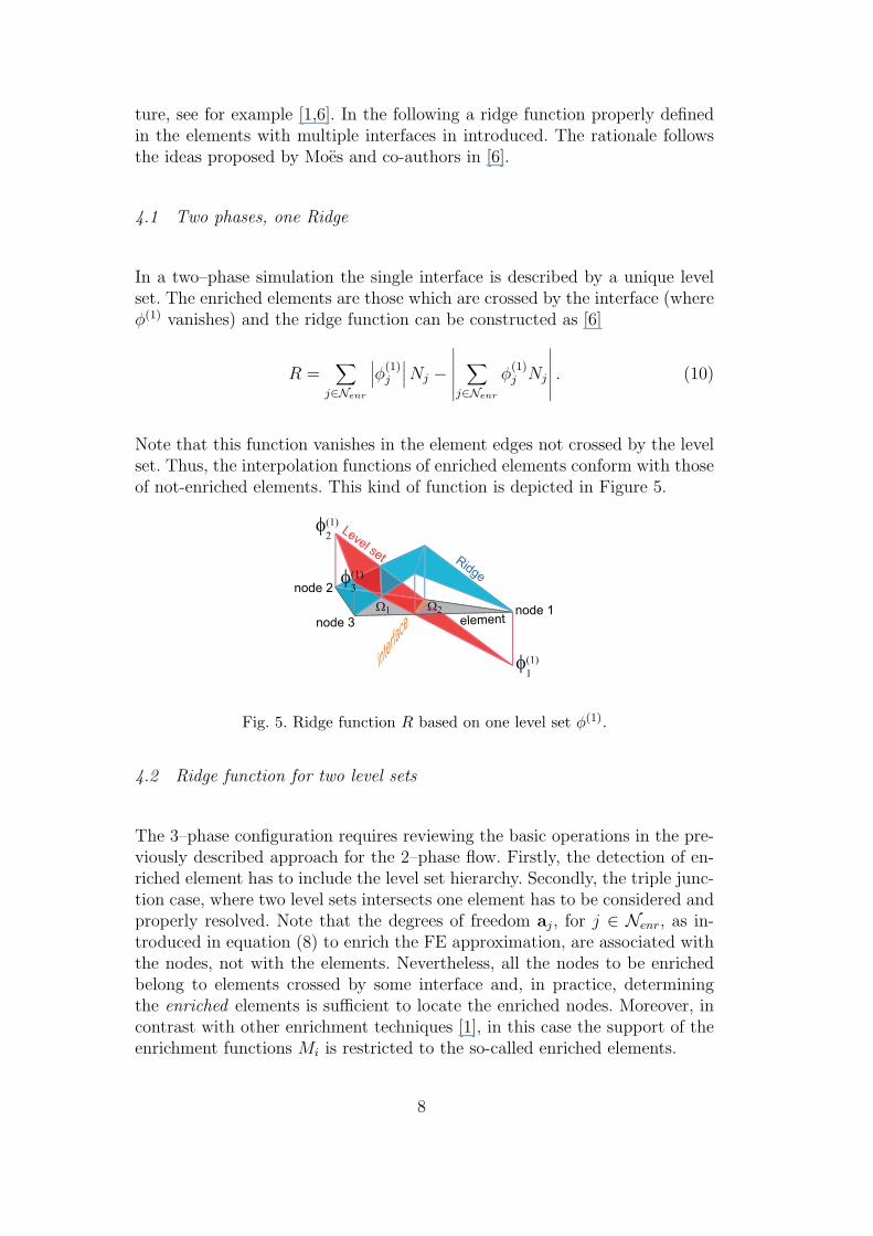
In a two–phase simulation the single interface is described by a unique levelset. The enriched elements are those which are crossed by the interface (whereφ(1) vanishes) and the ridge function can be constructed as [6]

R =∑

j∈Nenr

∣∣∣φ(1)j

∣∣∣ Nj −∣∣∣∣∣∣

∑

j∈Nenr

φ(1)j Nj

∣∣∣∣∣∣. (10)

Note that this function vanishes in the element edges not crossed by the levelset. Thus, the interpolation functions of enriched elements conform with thoseof not-enriched elements. This kind of function is depicted in Figure 5.

node 1

Ridge

Level set

node 2

node 3 element

interfac

e

φ(1)2

φ(1)3

φ(1)1

Ω1 Ω2

Fig. 5. Ridge function R based on one level set φ(1).

4.2 Ridge function for two level sets

The 3–phase configuration requires reviewing the basic operations in the pre-viously described approach for the 2–phase flow. Firstly, the detection of en-riched element has to include the level set hierarchy. Secondly, the triple junc-tion case, where two level sets intersects one element has to be considered andproperly resolved. Note that the degrees of freedom aj, for j ∈ Nenr, as in-troduced in equation (8) to enrich the FE approximation, are associated withthe nodes, not with the elements. Nevertheless, all the nodes to be enrichedbelong to elements crossed by some interface and, in practice, determiningthe enriched elements is sufficient to locate the enriched nodes. Moreover, incontrast with other enrichment techniques [1], in this case the support of theenrichment functions Mi is restricted to the so-called enriched elements.

8

The detection for elements to be enriched is the following: elements have tobe marked to enrich if they are crossed by the interface described by φ(1)

or crossed by the interface described by φ(2) and being φ(1) negative. Thisstatement is easily encoded. In the code repository(or in http://www.ija.csic.es/gt/sergioz/main/codes.htm) we providea highly vectorized MATLAB function named crossedByLevelSet acceptingany element type in any number of dimensions and returns if the element hasto be enriched or not.

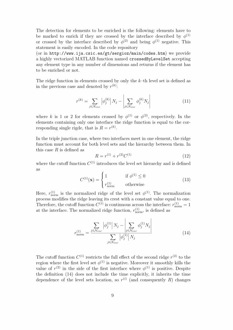
The ridge function in elements crossed by only the k–th level set is defined asin the previous case and denoted by r(k):

r(k) =∑

j∈Nenr

∣∣∣φ(k)j

∣∣∣ Nj −∣∣∣∣∣∣

∑

j∈Nenr

φ(k)j Nj

∣∣∣∣∣∣(11)

where k is 1 or 2 for elements crossed by φ(1) or φ(2), respectively. In theelements containing only one interface the ridge function is equal to the cor-responding single rigde, that is R = r(k).

In the triple junction case, where two interfaces meet in one element, the ridgefunction must account for both level sets and the hierarchy between them. Inthis case R is defined as

R = r(1) + r(2)C(1) (12)

where the cutoff function C(1) introduces the level set hierarchy and is definedas

C(1)(x) =

1 if φ(1) ≤ 0

r(1)norm otherwise

(13)

Here, r(1)norm is the normalized ridge of the level set φ(1). The normalization

process modifies the ridge leaving its crest with a constant value equal to one.Therefore, the cutoff function C(1) is continuous across the interface: r(1)

norm = 1at the interface. The normalized ridge function, r(1)

norm, is defined as

r(1)norm =

∑

j∈Nenr

∣∣∣φ(1)j

∣∣∣ Nj −∣∣∣∣∣∣

∑

j∈Nenr

φ(1)j Nj

∣∣∣∣∣∣∑

j∈Nenr

∣∣∣φ(1)j

∣∣∣ Nj

(14)

The cutoff function C(1) restricts the full effect of the second ridge r(2) to theregion where the first level set φ(1) is negative. Moreover it smoothly kills thevalue of r(2) in the side of the first interface where φ(1) is positive. Despitethe definition (14) does not include the time explicitly, it inherits the timedependence of the level sets location, so r(i) (and consequently R) changes

9

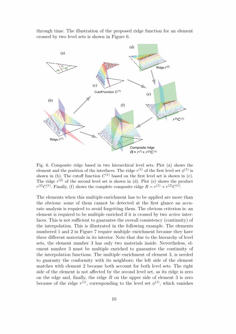
through time. The illustration of the proposed ridge function for an elementcrossed by two level sets is shown in Figure 6.

Composite ridge

R= r (1) + r (2)C (1)

r (2)C (1)

(d)

Cutoff function C (1)

(c)

Ridge r (2)

(b)

Ridge r (1)

(a)

Ω1

Ω2

Ω3

(e)

(f)

Fig. 6. Composite ridge based in two hierarchical level sets. Plot (a) shows theelement and the position of the interfaces. The ridge r(1) of the first level set φ(1) isshown in (b). The cutoff function C(1) based on the first level set is shown in (c).The ridge r(2) of the second level set is shown in (d). Plot (e) shows the productr(2)C(1). Finally, (f) shows the complete composite ridge R = r(1) + r(2)C(1).

The elements when this multiple-enrichment has to be applied are more thanthe obvious: some of them cannot be detected at the first glance an accu-rate analysis is required to avoid forgetting them. The obvious criterion is: anelement is required to be multiple enriched if it is crossed by two active inter-faces. This is not sufficient to guarantee the overall consistency (continuity) ofthe interpolation. This is illustrated in the following example. The elementsnumbered 1 and 2 in Figure 7 require multiple–enrichment because they havethree different materials in its interior. Note that due to the hierarchy of levelsets, the element number 3 has only two materials inside. Nevertheless, el-ement number 3 must be multiple–enriched to guarantee the continuity ofthe interpolation functions. The multiple–enrichment of element 3, is neededto guaranty the conformity with its neighbors; the left side of the elementmatches with element 2 because both account for both level sets. The rightside of the element is not affected by the second level set, as its ridge is zeroon the edge and, finally, the ridge R on the upper side of element 3 is zerobecause of the ridge r(1), corresponding to the level set φ(1), which vanishes

10

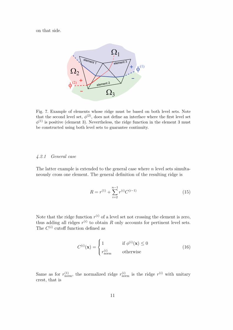
on that side.

φ(1)

φ(2)

+

+ -

-

Ω1

Ω2

Ω3

element 1

element 2

element 3

Fig. 7. Example of elements whose ridge must be based on both level sets. Notethat the second level set, φ(2), does not define an interface where the first level setφ(1) is positive (element 3). Nevertheless, the ridge function in the element 3 mustbe constructed using both level sets to guarantee continuity.

4.2.1 General case

The latter example is extended to the general case where n level sets simulta-neously cross one element. The general definition of the resulting ridge is

R = r(1) +n−1∑

i=2

r(i)C(i−1) (15)

Note that the ridge function r(i) of a level set not crossing the element is zero,thus adding all ridges r(i) to obtain R only accounts for pertinent level sets.The C(i) cutoff function defined as

C(i)(x) =

1 if φ(i)(x) ≤ 0

r(i)norm otherwise

(16)

Same as for r(1)norm, the normalized ridge r(i)

norm is the ridge r(i) with unitarycrest, that is

11

r(i)norm =

∑

j∈Nenr

∣∣∣φ(i)j

∣∣∣ Nj −∣∣∣∣∣∣

∑

j∈Nenr

φ(i)j Nj

∣∣∣∣∣∣∑

j∈Nenr

∣∣∣φ(i)j

∣∣∣ Nj

= 1−

∣∣∣∣∣∣∑

j∈Nenr

φ(i)j Nj

∣∣∣∣∣∣∑

j∈Nenr

∣∣∣φ(i)j

∣∣∣ Nj

(17)

4.3 Numerical integration in multiphase elements

The X–FEM implementation requires computing integrals of discontinuousfunctions in elements crossed by the level set. The traditional quadraturerules, for example Gauss quadratures, are designed to integrate polynomi-als and regular functions that are fairly approximated by polynomials. Thesequadratures are not expected to show a good performance integrations dis-continuous functions.

To preclude the problem associated with discontinuities and to calculate theintegrals accurately it is usual to split multiphase elements in single-materialsubdomains. In these subdomains functions are continuous and standard quadra-tures provide accurate results.

The computational effort and algorithmic involvement of defining each inte-gration subdomain depends on the shape of the elements and on the numberof spatial dimensions involved. For example, with only one level set triangularelements are split into one triangle and one quadrilateral or into two triangles.This geometrical splitting is coded straightforwardly based on the elementgeometry and the level set. The same operation for quadrilateral elements ismuch mode cumbersome because the number of possible geometrical divisionsis much higher. In particular, the splitting of a quadrilateral generates three-,four- and five-sides polygons. Further subdivisions are needed to integrate infive-sided shapes with standard quadratures.

In three dimensions the number shapes generated by cutting elements by onelevel set increases rapidly. Tetrahedral elements cutted by a plane interfacemust by split into five single-material tetrahedrals. This partition of the ele-ment is much more complicated to code and computationally demanding. Theelement subdivision is increasingly involved if the number of phases is larger.

Using the hierarchical level set approach element are split in polygonal single-material subdomains with any number of sides. The general case of detecting

12

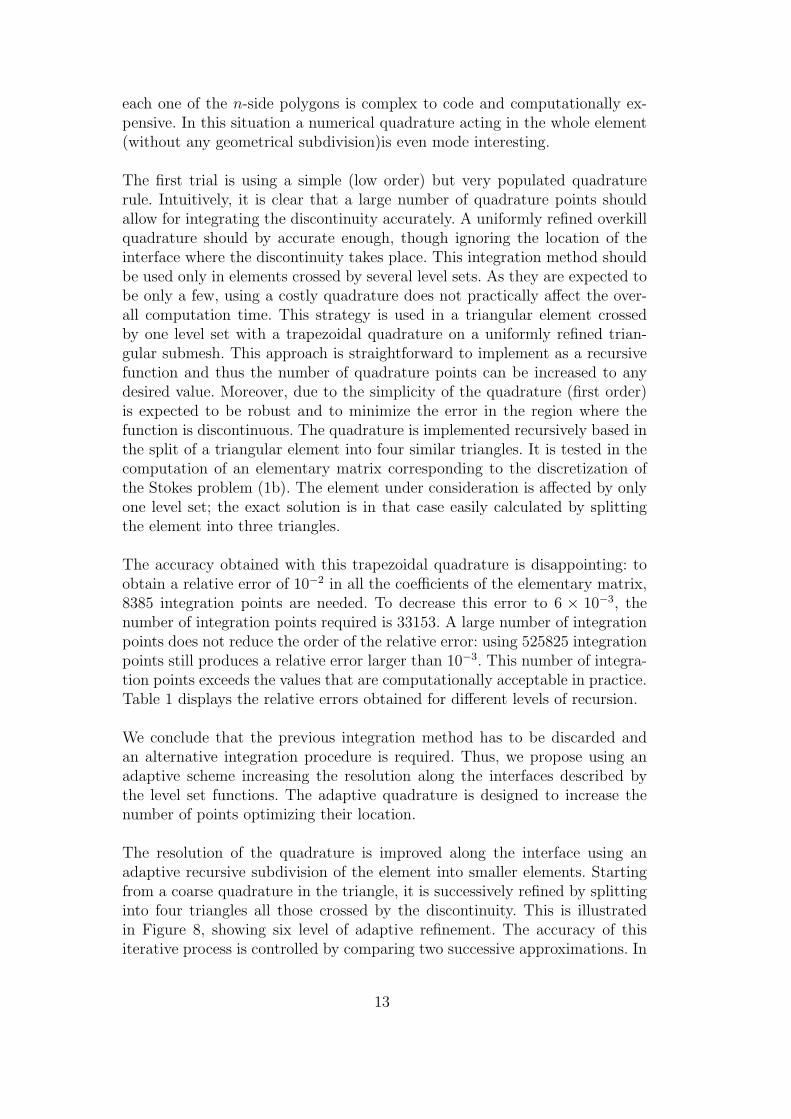
each one of the n-side polygons is complex to code and computationally ex-pensive. In this situation a numerical quadrature acting in the whole element(without any geometrical subdivision)is even mode interesting.

The first trial is using a simple (low order) but very populated quadraturerule. Intuitively, it is clear that a large number of quadrature points shouldallow for integrating the discontinuity accurately. A uniformly refined overkillquadrature should by accurate enough, though ignoring the location of theinterface where the discontinuity takes place. This integration method shouldbe used only in elements crossed by several level sets. As they are expected tobe only a few, using a costly quadrature does not practically affect the over-all computation time. This strategy is used in a triangular element crossedby one level set with a trapezoidal quadrature on a uniformly refined trian-gular submesh. This approach is straightforward to implement as a recursivefunction and thus the number of quadrature points can be increased to anydesired value. Moreover, due to the simplicity of the quadrature (first order)is expected to be robust and to minimize the error in the region where thefunction is discontinuous. The quadrature is implemented recursively based inthe split of a triangular element into four similar triangles. It is tested in thecomputation of an elementary matrix corresponding to the discretization ofthe Stokes problem (1b). The element under consideration is affected by onlyone level set; the exact solution is in that case easily calculated by splittingthe element into three triangles.

The accuracy obtained with this trapezoidal quadrature is disappointing: toobtain a relative error of 10−2 in all the coefficients of the elementary matrix,8385 integration points are needed. To decrease this error to 6 × 10−3, thenumber of integration points required is 33153. A large number of integrationpoints does not reduce the order of the relative error: using 525825 integrationpoints still produces a relative error larger than 10−3. This number of integra-tion points exceeds the values that are computationally acceptable in practice.Table 1 displays the relative errors obtained for different levels of recursion.

We conclude that the previous integration method has to be discarded andan alternative integration procedure is required. Thus, we propose using anadaptive scheme increasing the resolution along the interfaces described bythe level set functions. The adaptive quadrature is designed to increase thenumber of points optimizing their location.

The resolution of the quadrature is improved along the interface using anadaptive recursive subdivision of the element into smaller elements. Startingfrom a coarse quadrature in the triangle, it is successively refined by splittinginto four triangles all those crossed by the discontinuity. This is illustratedin Figure 8, showing six level of adaptive refinement. The accuracy of thisiterative process is controlled by comparing two successive approximations. In

13

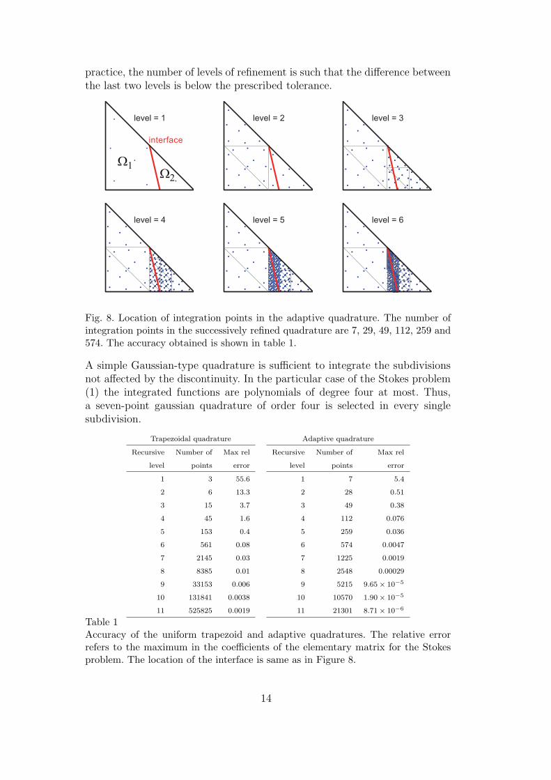
practice, the number of levels of refinement is such that the difference betweenthe last two levels is below the prescribed tolerance.

level = 1

interface

Ω1

Ω2

level = 2 level = 3

level = 4 level = 5 level = 6

Fig. 8. Location of integration points in the adaptive quadrature. The number ofintegration points in the successively refined quadrature are 7, 29, 49, 112, 259 and574. The accuracy obtained is shown in table 1.

A simple Gaussian-type quadrature is sufficient to integrate the subdivisionsnot affected by the discontinuity. In the particular case of the Stokes problem(1) the integrated functions are polynomials of degree four at most. Thus,a seven-point gaussian quadrature of order four is selected in every singlesubdivision.

Trapezoidal quadrature

Recursive Number of Max rel

level points error

1 3 55.6

2 6 13.3

3 15 3.7

4 45 1.6

5 153 0.4

6 561 0.08

7 2145 0.03

8 8385 0.01

9 33153 0.006

10 131841 0.0038

11 525825 0.0019

Adaptive quadrature

Recursive Number of Max rel

level points error

1 7 5.4

2 28 0.51

3 49 0.38

4 112 0.076

5 259 0.036

6 574 0.0047

7 1225 0.0019

8 2548 0.00029

9 5215 9.65× 10−5

10 10570 1.90× 10−5

11 21301 8.71× 10−6

Table 1Accuracy of the uniform trapezoid and adaptive quadratures. The relative errorrefers to the maximum in the coefficients of the elementary matrix for the Stokesproblem. The location of the interface is same as in Figure 8.

14

The adaptive quadrature drastically improves the accuracy with respect tothe uniform trapezoidal integration and sufficient accuracy is obtained witha reasonable amount of integration points. Recall that this strategy is onlyneeded in the elements affected by the interface. However, the computationaleffort to integrate the stiffness matrices in these elements is important.

An alternative integration procedure is based on the Constrained DelaunayTriangulation (or tetrahedralization, in both cases corresponding to the acronymCDT), as used for instance by Wall and coauthors [4]. This idea is allowingto automatically split the element into monophasic subdomains and thus touse in each subdomain a simple quadrature. A second alternative is providedby Daux et al. [2] based in the recursive splitting of the domains (triangles ortetrahedra) following the interfaces. Comparing the cost of these approacheswith the one introduced here is beyond the scope of this paper.

The adaptive quadrature is used in examples presented in next section pro-viding satisfactory results.

5 Numerical examples

The strategy developed in the previous Sections is tested here in some stan-dard application examples. The n–phase X–FEM approach is used to simulategravitational Rayleigh–Taylor instabilities in 2 and 3 dimensions. The modelsare composed by n ≥ 3 immiscible materials governed by the Stokes equa-tion (1). The driving force in all models is the gravity; the density contrastmakes the buoyant layers (with lower density than the overlying layers) toflow upward and the denser layers to flow downward.

5.1 Two-dimensional 3-phase instabilities

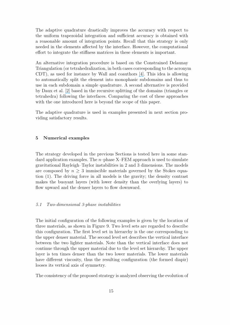
The initial configuration of the following examples is given by the location ofthree materials, as shown in Figure 9. Two level sets are regarded to describethis configuration. The first level set in hierarchy is the one corresponding tothe upper denser material. The second level set describes the vertical interfacebetween the two lighter materials. Note than the vertical interface does notcontinue through the upper material due to the level set hierarchy. The upperlayer is ten times denser than the two lower materials. The lower materialshave different viscosity, thus the resulting configuration (the formed diapir)looses its vertical axis of symmetry.

The consistency of the proposed strategy is analyzed observing the evolution of

15

0 10

0.5

0.5

1

1.5

g

Fig. 9. Initial configuration with three materials. The upper material is denser thanthe other two. The viscosity of the materials is indicated in Figure 13.

different indicators. First, the vertical velocity of the instability (the velocity ofthe growing diapir) at a given moment in time is used to study the consistenceof the solution. Note that this velocity is a common indicator to validateRayleigh–Taylor models. Second, the global convergence of the solution usinga L2 norm is studied for a series of uniformly refined meshes and also at agiven moment in time.

0 1

0

0.5

0.5 0 10.5 0 10.5

0 10.5 0 10.5 0 10.5

1

1.5

0

0.5

1

1.5

0

0.5

1

1.5

0

0.5

1

1.5

0

0.5

1

1.5

0

0.5

1

1.5nn=122, ne=209 nn=232, ne=421 nn=458, ne=865

nn=911, ne=1763 nn=1822, ne=3579 nn=3612, ne=7153

(a) (b) (c)

(d) (e) (f)

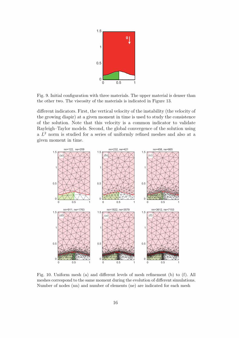
Fig. 10. Uniform mesh (a) and different levels of mesh refinement (b) to (f). Allmeshes correspond to the same moment during the evolution of different simulations.Number of nodes (nn) and number of elements (ne) are indicated for each mesh

16

0 1000 2000 3000 4000

number of elements

adaptive mesh

uniform mesh

gro

win

g v

elo

city

10−0.66

10−0.63

10−0.6

10−0.57

10−0.54

10−0.51

Fig. 11. Dependence of the velocity of the growing diapir with the mesh. Two seriesof meshes are shown: the triangles correspond to uniformly refined meshes, thecircles correspond to adaptively refined meshes.

Some simple configurations of two–phase Rayleigh–Taylor instabilities allowfor an analytical calculation of the growing velocity. This macroscopic veloc-ity is a meaningful quantity of interest that can be compared with analogicalexperiments in some cases. Nevertheless, for the three-phase case no analyt-ical solution is available. Therefore, no direct quantitative error assessmentcan be performed. A numerical convergence analysis is carried out for thisproblem. Figure 11 shows the convergence of the diapir growing velocity asa function of the number of elements in the mesh. The diapir growing ve-locity is calculated as the vertical ascending velocity of the triple junctionpoint at a given moment in time which is a quantity of interest for the prob-lem under consideration. This velocity generally coincides with the maximumvelocity in all the domain. Two series of simulation are performed: one refin-ing the mesh uniformly (marked with triangles), the other refining the meshwith an adaptive scheme near the interface (marked with circles). The meshis adapted heuristically, using the multiphase character of the elements asremeshing indicator. In practice the elements crossed by one or more inter-faces are subdivided performing a given number of recursive refinements. Inthe examples, see figure 10, five levels or recursivity are used. The adaptivityhelps to converge faster and with less elements than the uniform refinement. Auniform mesh and several adaptive meshes with different refinement levels aredisplayed in Figure 10. The curve corresponding to the uniform refinement infigure 11 exhibits some oscillations. This is due to the fact that the quantityunder consideration (growing velocity) is measured at a given time. The timestep is set as a function of the Courant number and hence varies from mesh tomesh. Consequently, the exact time in which this velocity is computed slightlyvaries for the different points of the curve. However, the global behavior of the

17

curve seems to converge to the same value as the adaptive refinement and theoscillations are reduced as number of elements increases. The convergence isthus demonstrated for this standard quantity of interest in the diapir growingproblem.

10−2

10−1

100

10−7

10−6

10−5

10−4

10−3

elem size

L2 nor

m o

f the

err

or

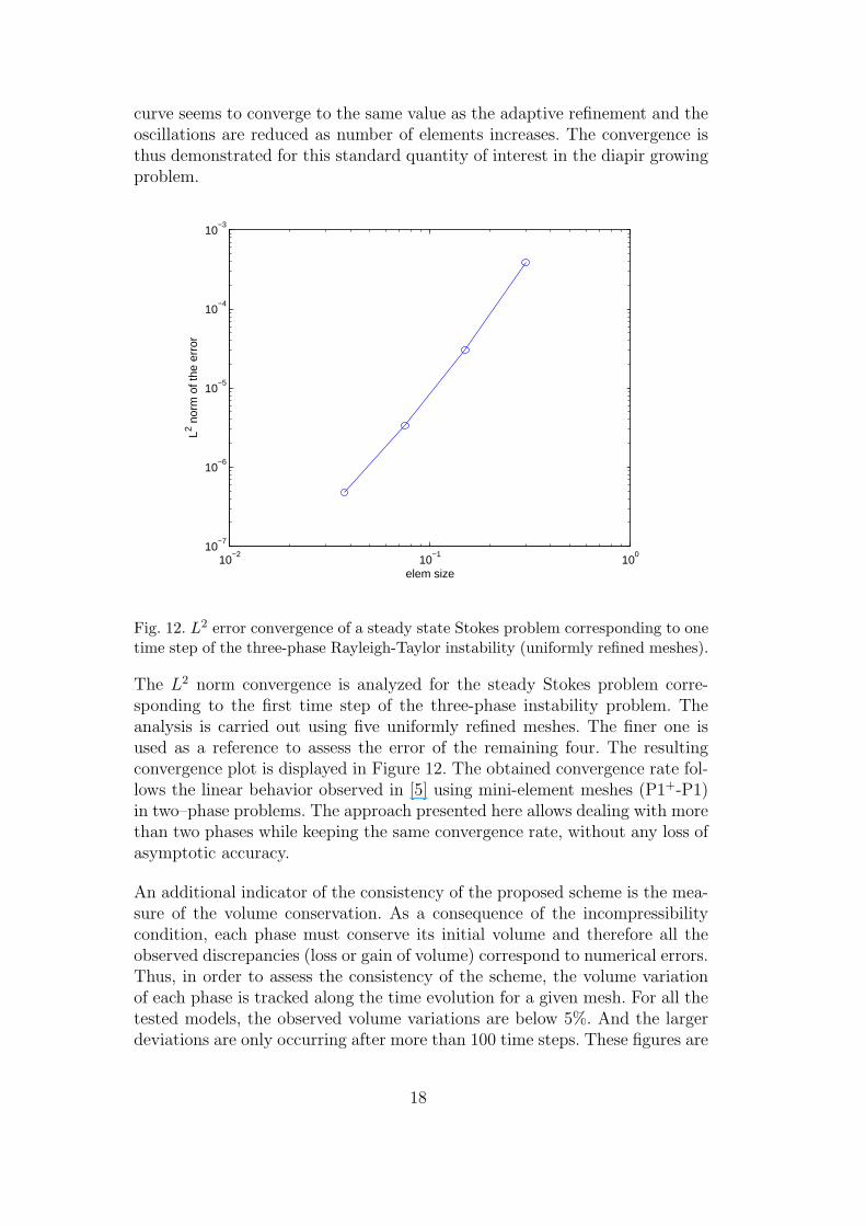
Fig. 12. L2 error convergence of a steady state Stokes problem corresponding to onetime step of the three-phase Rayleigh-Taylor instability (uniformly refined meshes).

The L2 norm convergence is analyzed for the steady Stokes problem corre-sponding to the first time step of the three-phase instability problem. Theanalysis is carried out using five uniformly refined meshes. The finer one isused as a reference to assess the error of the remaining four. The resultingconvergence plot is displayed in Figure 12. The obtained convergence rate fol-lows the linear behavior observed in [5] using mini-element meshes (P1+-P1)in two–phase problems. The approach presented here allows dealing with morethan two phases while keeping the same convergence rate, without any loss ofasymptotic accuracy.

An additional indicator of the consistency of the proposed scheme is the mea-sure of the volume conservation. As a consequence of the incompressibilitycondition, each phase must conserve its initial volume and therefore all theobserved discrepancies (loss or gain of volume) correspond to numerical errors.Thus, in order to assess the consistency of the scheme, the volume variationof each phase is tracked along the time evolution for a given mesh. For all thetested models, the observed volume variations are below 5%. And the largerdeviations are only occurring after more than 100 time steps. These figures are

18

satisfactory, specially considering that no level set reinitialization procedure isused. Note however that the hierarchical level set approach would allow usingany reinitialization procedure in a very simple manner because each level setfunction may be updated independently as for a standard two–phase model.

0 0.5 10

0.5

1

1.5Step 14

(a)

(b)

(c)

(d)

0 0.5 10

0.5

1

1.5Step 28

0 0.5 10

0.5

1

1.5Step 42

0 0.5 10

0.5

1

1.5Step 56

0 0.5 10

0.5

1

1.5

Step 70

0 0.5 10

0.5

1

1.5

0 0.5 10

0.5

1

1.5

0 0.5 10

0.5

1

1.5

0 0.5 10

0.5

1

1.5

0 0.5 10

0.5

1

1.5

0 0.5 10

0.5

1

1.5

0 0.5 10

0.5

1

1.5

0 0.5 10

0.5

1

1.5

0 0.5 10

0.5

1

1.5

0 0.5 10

0.5

1

1.5

0 0.5 10

0.5

1

1.5

0 0.5 10

0.5

1

1.5

0 0.5 10

0.5

1

1.5

0 0.5 10

0.5

1

1.5

0 0.5 10

0.5

1

1.5

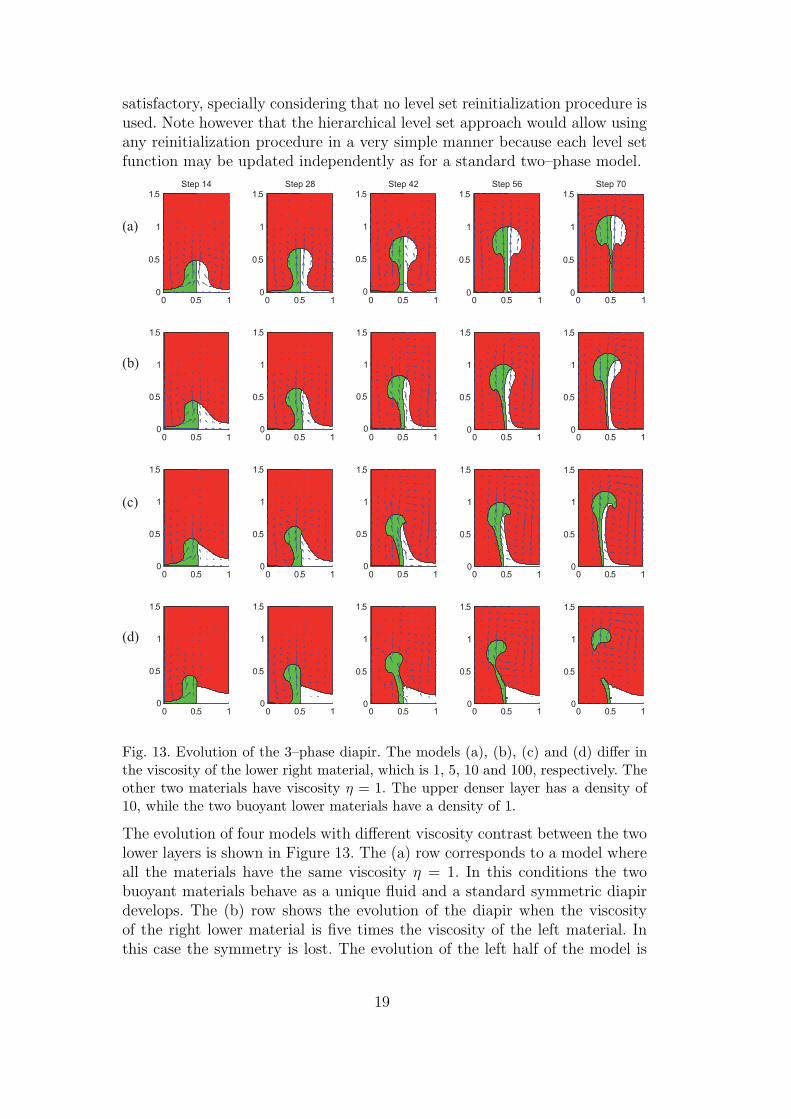
Fig. 13. Evolution of the 3–phase diapir. The models (a), (b), (c) and (d) differ inthe viscosity of the lower right material, which is 1, 5, 10 and 100, respectively. Theother two materials have viscosity η = 1. The upper denser layer has a density of10, while the two buoyant lower materials have a density of 1.

The evolution of four models with different viscosity contrast between the twolower layers is shown in Figure 13. The (a) row corresponds to a model whereall the materials have the same viscosity η = 1. In this conditions the twobuoyant materials behave as a unique fluid and a standard symmetric diapirdevelops. The (b) row shows the evolution of the diapir when the viscosityof the right lower material is five times the viscosity of the left material. Inthis case the symmetry is lost. The evolution of the left half of the model is

19

similar to the (a) row while the right half of the model is controlled by theviscosity contrast between the right material and the overburden layer. Themodels of the third and fourth rows have a viscosity ratio between the twolower layers of 10 and 100, respectively. The very viscous right material ofthe last model is almost stopped, while the left material develops the diapiralone. In this example the main pattern of generated flow changes. In theearly stages (1st and 2nd snapshots) the high viscosity of the right materialinhibits the movement in the right half and the flow is concentrated in the leftpart of the domain. This bends the diapir to the left. Once the material gainsenough height to loose the influence of the viscous layer (last two snapshots),the main flow moves to the right half of the model because there is more spacefacilitating the return flow. This latter inflexion bends the diapir rightward.

The conclusion on this qualitative test, is that the results show a complexbehavior corresponding with the nature of the problem analyzed.

5.2 Three-dimensional instabilities

Two examples of gravitational instabilities in 3D are presented next. Firstly, aRayleigh–Taylor instability similar to the 2D example of the previous section ispresented. Secondly, an instability where the material phases lays horizontallyis shown. In both cases the domain is a square box.

The first example involves three materials: an upper and denser phase, andtwo lower and buoyant fluids with a viscosity ratio of five between them. Sameas in the previous case the level set φ(1) (with highest hierarchy) determinesthe location of the upper material and has an initial sinusoidal perturbationto induce the development of the instability. The second level set representsthe interface between the two lower fluids and is initially set parallel to onewall of the domain. A uniform structured mesh of 512 (8 × 8 × 8) 27-nodedhexahedra is used in the simulations.

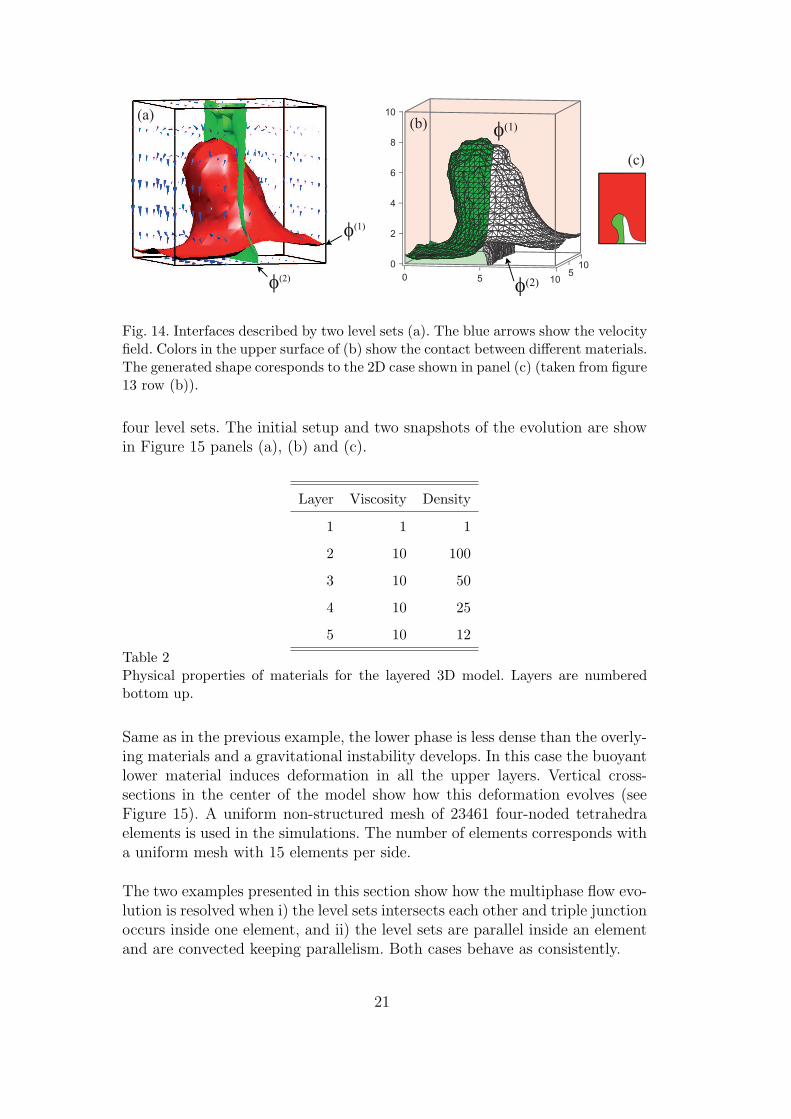
Figure 14 shows the location of both level sets after some time-steps. In panel(a) the two level sets are shown. Due to the hierarchy, the vertical level set isonly relevant below the red surface. Panel (b) shows the same surfaces at thesame time with the interface described by φ(1) drawn in two different colorsto emphasize the two lower materials and facilitate the comparison with the2D model. Note that the contact between colors is where the second interface(described by φ(2)) intersects. This 3D example is comparable to the (b) rowof Figure 13. A snapshot of the 2D model is included in panel (c), showingthe comparable asymmetric pattern developed.

The second example, involves five different materials with the physical prop-erties described in table 2. Contacts between these materials are described by

20

0 5 105100

2

4

6

8

10

(b)φ(1)

φ(2)

φ(1)

φ(2)

(a)

(c)

Fig. 14. Interfaces described by two level sets (a). The blue arrows show the velocityfield. Colors in the upper surface of (b) show the contact between different materials.The generated shape coresponds to the 2D case shown in panel (c) (taken from figure13 row (b)).

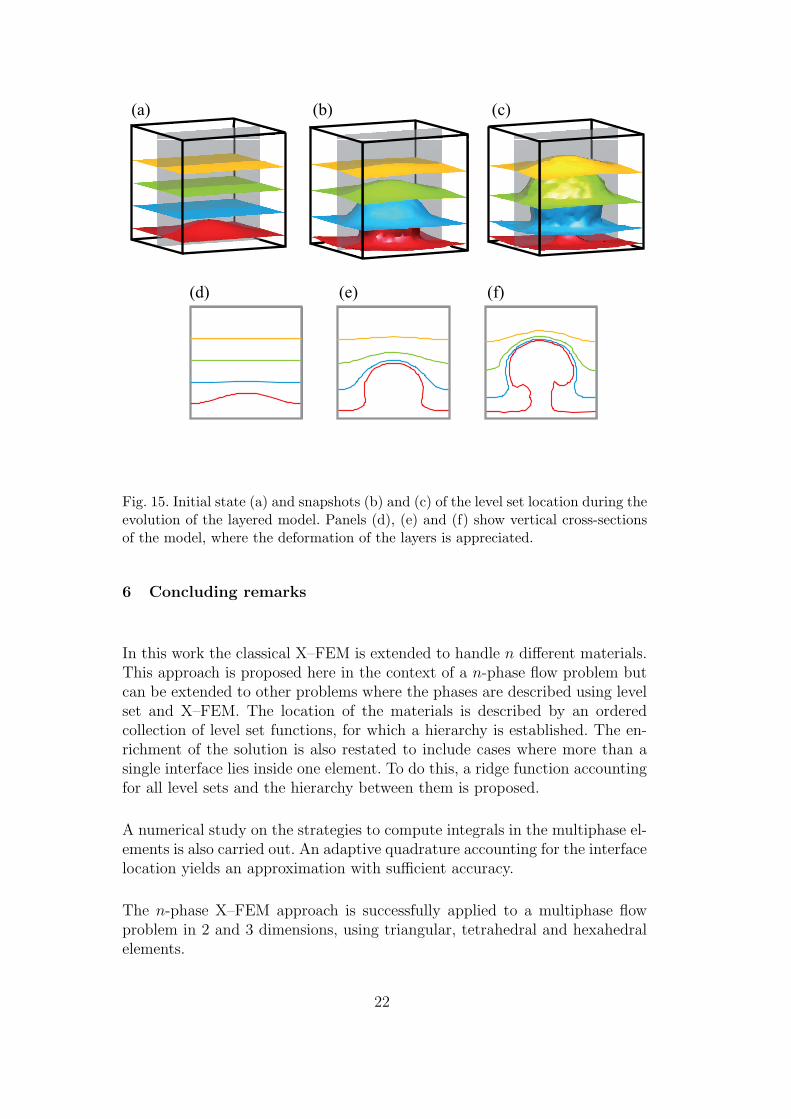
four level sets. The initial setup and two snapshots of the evolution are showin Figure 15 panels (a), (b) and (c).

Layer Viscosity Density

1 1 1

2 10 100

3 10 50

4 10 25

5 10 12

Table 2Physical properties of materials for the layered 3D model. Layers are numberedbottom up.

Same as in the previous example, the lower phase is less dense than the overly-ing materials and a gravitational instability develops. In this case the buoyantlower material induces deformation in all the upper layers. Vertical cross-sections in the center of the model show how this deformation evolves (seeFigure 15). A uniform non-structured mesh of 23461 four-noded tetrahedraelements is used in the simulations. The number of elements corresponds witha uniform mesh with 15 elements per side.

The two examples presented in this section show how the multiphase flow evo-lution is resolved when i) the level sets intersects each other and triple junctionoccurs inside one element, and ii) the level sets are parallel inside an elementand are convected keeping parallelism. Both cases behave as consistently.

21

(a) (b) (c)

(d) (e) (f)

Fig. 15. Initial state (a) and snapshots (b) and (c) of the level set location during theevolution of the layered model. Panels (d), (e) and (f) show vertical cross-sectionsof the model, where the deformation of the layers is appreciated.

6 Concluding remarks

In this work the classical X–FEM is extended to handle n different materials.This approach is proposed here in the context of a n-phase flow problem butcan be extended to other problems where the phases are described using levelset and X–FEM. The location of the materials is described by an orderedcollection of level set functions, for which a hierarchy is established. The en-richment of the solution is also restated to include cases where more than asingle interface lies inside one element. To do this, a ridge function accountingfor all level sets and the hierarchy between them is proposed.

A numerical study on the strategies to compute integrals in the multiphase el-ements is also carried out. An adaptive quadrature accounting for the interfacelocation yields an approximation with sufficient accuracy.

The n-phase X–FEM approach is successfully applied to a multiphase flowproblem in 2 and 3 dimensions, using triangular, tetrahedral and hexahedralelements.

22

Acknowledgements

This research has been supported by Ministerio de Educacion y Ciencia,Grants DPI2007-62395, SAGAS CTM2005-08071-C03-03/MAR and the Span-ish Team Consolider-Ingenio 2010 nrCSD2006-00041.

References

[1] J. Chessa and T. Belytschko. An extended finite element method for two–phasefluids. Transactions of the ASME, pages 10–17, 2003.

[2] C. Daux, N. Moes, J. Dolbow, N. Sukumar, and T. Belytschko. Arbitrarybranched and intersecting cracks with the extended finite element method.International Journal for Numerical Methods in Engineering, 48:1741–1760,2000.

[3] J. Donea and A. Huerta. Finite Element Methods for Flow Problems. Wiley,Chichester, West Sussex PO19 8SQ, England, 2002.

[4] A. Gerstenberger and W. A. Wall. An extended finite element method /lagrangemultiplier based approach for fluid-structure interaction. Computer Methods inApplied Mechanics and Engineering, in press:(doi:10.1016/j.cma.2007.07.002),2007.

[5] G. Legrain, N. Moes, and A. Huerta. Stability of incompressible formulationsenriches with X–FEM. Computer Methods in Applied Mechanics andEngineering, 197:1835–1849, 2008.

[6] N. Moes, M. Cloirec, P. Cartaud, and J. F. Remacle. A computational approachto handle complex microstructure geometries. Computer Methods in AppliedMechanics and Engineering, 192:3163–3177, 2003.

[7] S. Osher and R. Fedkiw. Level set methods: an overview and some recentresults. Journal of Computational Physics, 169:463–502, 2001.

[8] S. Osher and J.A. Sethian. Front propagating with curvature dependent speed:algorithms based on hamiltonjacobi formulations. Journal of ComputationalPhysics, 79:12–49, 1988.

[9] S. J. Ruuth. A diffusion–generated approach to multiphase motion. Journal ofComputational Physics, 145:166–192, 1998.

[10] J.A. Sethian and P. Smereka. Level set methods for fluid interfaces. AnnualReview of Fluid Mechanics, 35:341–372, 2003.

[11] L. Tan and N. Zabaras. A level set simulation of dendritic solidification ofmulti-component alloys. Journal of Computational Physics, 221:9–40, 2007.

23

[12] G. J. Wagner, N. Moes, W. K. Liu, and T. Belytschko. The extended finiteelement method for rigid particles in Stokes flow. International Journal forNumerical Methods in Engineering, 51(3):293–313, 2001.

[13] H.-K. Zhao, T. Chan, B. Merriman, and Osher. A variational level set approachto multiphase motion. Journal of Computational Physics, 127:179–195, 1996.

[14] S. Zlotnik, P. Dıez, M. Fernandez, and J. Verges. Numerical modelling oftectonic plates subduction using X–FEM. Computer Methods in AppliedMechanics and Engineering, 196:4283–4293, 2007.

24