hierarchical, heterogeneous control of non-linear dynamical systems using reinforcement learning

Journal of Machine Learning Research vol:1–10, 2012 Submitted 16.04.2012; Published publication date

Hierarchical, Heterogeneous Control of Non-LinearDynamical Systems using Reinforcement Learning

Ekaterina Abramova1 [email protected]

Luke Dickens1 [email protected]

Daniel Kuhn1 [email protected]

Aldo Faisal1,2 [email protected]

1: Imperial College London, Dept. of Computing, 180 Queen’s Gate, SW7 2RH, UK

2: Imperial College London, Dept. of Bioengineering, Prince Consort Road, SW7 2AZ, UK

Abstract

Non-adaptive methods are currently state of the art in approximating solutions to non-linear optimal control problems. These carry a large computational cost associated withiterative calculations and have to be solve individually for different start and end points. Inaddition they may not scale well for real-world problems and require considerable tuning toconverge. As an alternative, we present a novel hierarchical approach to non-Linear Controlusing Reinforcement Learning to choose between Heterogeneous Controllers, including lo-calised optimal linear controllers and proportional-integral-derivative (PID) controllers, il-lustrating this with solutions to benchmark problems. We show that our approach (RLHC)competes in terms of computational cost and solution quality with state-of-the-art controlalgorithm iLQR, and offers a robust, flexible framework to address large scale non-linearcontrol problems.

Keywords: Non-linear dynamics, reinforcement learning, hierarchical control, optimalcontrol, LQR control, PID control, robotic arm control, cart on pole swing up & control.

1. Introduction

Controlling problems with complex, non-linear dynamics, even involving uncertainty andnoise, as encountered in robotics, production-line control, neuroprosthetics, transportation,vehicle steering and piloting, shop-floor-control and other engineering areas is a fundamen-tal problem (Todorov and Li, 2005; H.J., 2011). Even though the general problem can beformulated as Hamilton-Jacobi-Bellman partial differential equation, it’s solution is oftenintractable (Bryson and Ho, 1975). Therefore, current state-of-the-art methods use approx-imative iterative solutions: non-linear Model Predictive Control (NMPC) which solves amoving horizon window problem (Kwon et al., 1983) and iterative Linear Quadratic Regu-lators (iLQR) which use locally optimal feedback controllers that are improved iteratively(Li and Todorov, 2004). More importantly, often the model equations of the system to becontrolled are not known, and there machine learning solutions are desirable. These aretypically based on classic reinforcement learning techniques (Sutton and Barto, 1998), whichgeneralise temporal difference and actor-critic methods to continuous state, time and actionsolutions for control e.g. Doya (2000); and more recently Gaussian Process ReinforcementLearning (PILCO) (Deisenroth and Rasmussen, 2011), which uses Gaussian Processes to

c© 2012 E. Abramova1, L. Dickens1, D. Kuhn1 & A. Faisal1,2.

Abramova1 Dickens1 Kuhn1 Faisal1,2

model and express uncertainty of unknown dynamics and policy within a planning reinforce-ment learning algorithm. However, MPC can lack stability over the infinite horizon unlessan appropriate Lyapunov function (corresponding to the value function) is used (Kalman,1960), and iLQR and Doya’s continuous reinforcement learning are computationally expen-sive. Although PILCO is extremely data efficient, i.e. it learns very fast from interactionswith the environment, the intensive offline calculations to optimise parameters for the policymay be challenging for more complex (or very high-dimensional) real-world tasks.

Our algorithm is presented here as a proof of principle - Reinforcement Learning withHeterogeneous Control (RLHC) - it forms a hierarchical learning infrastructure for effectiveand efficient learning of non-linear control problems. RLHC uses a reinforcement learningalgorithm to map from a setup of discretized ’symbolic’ states to a heterogeneous set of localcontrollers that operate directly on task kinematics. In this paper we focus on optimal linearcontrollers and proportional-integral-derivative (PID) controllers and let the symbolic levelof RLHC learn which to use in which situation. We note that by decomposing the probleminto a selection between local control strategies we are effectively implementing a hierarchicaldivide-and-conquer strategy that allows us to push back the curse of dimensionality problemthat we would encounter by learning to control the whole control problem monolithically.We demonstrate RLHC’s effectiveness on two non-linear control problems with simultaneousminimisation of a cost function: a two-joint robot arm and the swing up and stopping ofan inverted pendulum on a cart. We note that in contrast to other algorithms we arenot learning the dynamics of the task yet, but will argue that once the structure of thecontrol problem has been defined it greatly simplifies learning. Section 2 briefly summarisesPID, Linear Quadratic Regulator (LQR) and iLQR control and reinforcement learning,and Section 3 describes our RLHC method. We describe the test problems and report ourexperimental results in Section 4, and conclude with a discussion in Section 5.

2. Background

In contrast to state of the art engineering solutions, adolescent humans are able to learn tocontrol and master complex dynamical systems, such as catching a ball (Faisal and Wolpert,2009), riding a bicycle (which has over 600 degrees of freedom), in the matter of a few hoursof practice. Conversely, neuroscientists are mystified (Scott, 2004; Diedrichsen et al., 2010;Wolpert et al., 2011; Tramper et al., 2011) how it is that the brain formulates tasks ata symbolic level (e.g. “to prepare a cup of coffee fill water into the coffee maker”) andeffortlessly generates control signals that operate at the level of firing of action potentialof motor neurons in the spinal chord which actuate our muscles. Moreover, these humanmotor control strategies seem to be optimal with respect to minimising noise ((Harris andWolpert, 1998), see Faisal et al. (2008)), timing (Faisal and Wolpert, 2009), and energyexpenditure (Taylor and Faisal, 2011). Intriguingly it appears that low-level motor controlof the spinal chord in terms of limb movements appear to be locally invariant, even linearcontrol primitives that operate directly at the kinematic level (Mussa-Ivaldi et al., 1994;Thoroughman and Shadmehr, 2000; d’Avella et al., 2003; Berniker et al., 2009; Hart andGiszter, 2010) while higher level behavioural control is achieved by sequential compositionof action sequences, from action primitives (e.g. “grab cup”,“pour water”,“add powdered

2

Hierarchical, Heterogeneous Control using Reinforcement Learning

coffee”,“stir black liquid”, etc.). We take this symbolic-kinematic organisation of the brain’scontrol strategy as inspiration for a novel algorithm.

Control theory studies dynamical systems described by a differential equation x =f(x,u), where the control vector u is chosen with the goal to force the state vector xto a desirable region of the state space. We solve the continuous system dynamics in dis-crete time using Runge-Kutta approximations (Strogatz, 2001). In this case the dynamicequations reduce to xk+1 = g(xk,uk), where xk and uk denote the state and control attime step k.

Proportional-integral-derivative (PID) control A PID controller is a simple feed-back controller, which aims to minimize the error ek between the current state and aprescribed target state. At time step k, the control uk is given by

uk = Kpek +Ki

N∑k=0

ek +Kdek − ek−1

∆t(1)

whereN is the total number of steps, Kp,Ki,Kd are the proportional, integral and derivativegain parameters, respectively, and ∆t represents the length of a time interval (Astrom andHagglund, 2006). The first term in Equation (1) is a simple error contribution to thecontrol. The integral and derivative terms act as a forcing term for slow convergence anddamping force for anticipated future oscillations, respectively. It should be noted that thePID control obtained is not necessarily optimal.

Linear Optimal Control Optimal Control theory aims to find a control law which ma-nipulates a dynamical system, while minimizing the associated cost. In the Linear QuadraticRegulator (LQR) problem the dynamics are linear, with the form xk+1 = Axk + Buk,where A represents the system control matrix and B the control gain matrix. The costs arequadratic and given by

J(x,u) =1

2xN

TQfxN +N−1∑k=0

(1

2uk

TRuk +1

2xk

TQxk) (2)

where N is the total number of time steps, R is the control cost matrix, Q is the state costmatrix and Qf is the final state cost matrix. The LQR problem has a closed form solution(Anderson and Moore, 1989). Indeed, the optimal control is linear in x, and it is calculatedvia

uk = −Lkxk (3)

where Lk = ((R + BTVk+1B)−1BTVk+1A) is the feedback gain matrix at time k. Thematrix Vk appearing in the formula for Lk encodes the quadratic cost-to-go function and iscomputed recursively through Vk = Q+ATVk+1A−ATVk+1B(R+BTVk+1B)−1BTVk+1Afor k = 1, . . . , N − 1 and VN = Qf (Kwakernaak and Sivan, 1972). The matrix Lk does notdepend on x and can therefore be computed offline.

3


Non-Linear Optimal Control Non-linear Optimal Control deals with systems involvingnon-linear dynamics, and is regarded as one of the most challenging areas of control theory(Primbs et al., 1999). In general, there is no analytical solution (Bryson and Ho, 1975),and instead approximate solutions are computed using iterative methods. The deterministicnon-linear optimal control problem we choose to study has the following general form xk+1 =A(xk)xk + B(xk)uk. Here the A and B matrices depend on the state vector xk and makethe system non-linear.

The iterative Linear Quadratic Regulator (iLQR) is a non-linear control method, whichmaintains a representation of a single trajectory and improves it locally with locally optimalLQR controllers. This is an iterative method, where each iteration begins with an arbitrarycontrol trajectory ut and a corresponding state trajectory xt. The system is linearizedaround xt and ut, and an affine control update is calculated using the Levenberg-Marquardtmethod. iLQR has been shown to solve non-linear systems of a fixed inverted pendulumand a 2-link 6-muscle model of the human arm (Todorov and Li, 2005).

Reinforcement Learning Reinforcement Learning assumes an agent that repeatedly in-teracts with the world through actions, and observes the resulting state and reward. Theagent’s objective is to maximize some aggregated reward signal. Model-free reinforcementlearning typically makes no assumption about system dynamics other than the Markov-property1, and can optimise control purely by interacting with the system dynamics. Stan-dard algorithms for discrete state problems include Monte-Carlo (MC) Control, SARSAand Q-learning, and the Markov Decision Process (MDP) defines a class of discrete statecontrol problems that satisfy the Markov property. We refer to Sutton and Barto (1998)for more details on reinforcement learning and MDPs.

Any model-free reinforcement learning algorithm could be used for RLHC, but here weemploy ε-greedy on-policy MC Control with iterative updating. This keeps a table of valuesQ(s, a) ∈ R, one for each state-action pair (s, a), which aim to approximate the expectedfuture discounted return Qπ(s, a) = E(

∑∞k=0 γ

krk+1|s0 = s, a0 = a, π)We use Iterative MC Control with a step-size parameter adapted from Kushner and Yin

(2003). This learns by repeatedly sampling sequences of states s, actions a and immediaterewards (costs) r from starting to terminal state (called traces). For each trace and time-step k, the discounted sum of future rewards, Rk, from visited state-action pair, (sk, ak), isused as a sample for the updates

N(sk, ak)← N(sk, ak) + 1

α(sk, ak) = 1/(1 +N(sk, ak))p

Q(sk, ak)← Q(sk, ak) + α(sk, ak)Rk

where N(s, a) keeps count2, of how many times state each (s, a) has been visited, and withp ∈ (0, 1), determines a decaying state-action dependent step-size parameter, α(s, a).

Predictions Q(s, a) are then exploited by the policy, π preferentially choosing betteractions, such that Pr(ak|sk) equals 1− ε if ak=arg maxaQ(sk, a) and ε

|A|−1 otherwise. Tra-ditional reinforcement learning operates in discrete state space, but suffers from the curse

1. The Markov-property requires subsequent state and reward to depend only on previous state and action.2. Initialised to zero

4


of dimensionality as the number of states grows (Bellman and Dreyfus, 1958). Continuousstate and action methods, e.g. those in Doya (2000); Deisenroth and Rasmussen (2011),alleviate this, but remain computationally expensive. The powerful model based PILCOmethod of Rasmussen and Deisenroth has shown exceptional data efficiency on the cart poletask, requiring only 17.5s of interaction with a physical system to learn the cart-pole problem(Deisenroth and Rasmussen, 2011). However their offline policy optimisation can be expen-sive; they report a 1 hour parameter optimization time on the cart pole task (Rasmussenand Deisenroth, 2008) using a 2008 work station. Gaussian processes require an inversionof the kernel matrices which can become intractable when the number of data points re-quired is very large, e.g. when the task itself is complex or with very high dimensional statespace. In spite of the success of PILCO, we offer an alternative that compromises on bothdata efficiency and accuracy, but may offer greater scalability. Our algorithm combines theefficient local optimisation of LQR with the flexibility of reinforcement learning.

3. Reinforcement Learning Heterogeneous Control

RLHC combines MDP with optimal control and chooses between a number of availablecontrollers (locally linear optimal controllers and PID controllers) interpreted as actions. Ittakes advantage of the MDP’s ability to deal with non-linear systems. Traditional non-linearoptimal control methods (iLQR) need as many locally linear optimal controllers as there areincremental number of steps, which is computationally costly. RLHC dramatically reducesthe number of such controllers necessary by combining locally linear but continuous controlusing a reinforcement learning algorithm (pure reinforcement learning approach for solvingfor example the cart pole system, would involve exploring a state space of approximately180 ∗ 180 ∗ 300 = 107, whereas RLHC operated on a max state space of 25 ∗ 26 = 650).The use of optimal control in RLHC reduces the number of state-action pairs that wouldneed to be explored if solving the problem with reinforcement learning alone. This thereforereduces the state complexity, allowing for faster learning of how to join controllers togetherfor global use. For the outline of RLHC please see Algorithm 1.

Optimal control satisfies the Markov property since its dynamics at iteration step kdepend only on the state and controller at k − 1, therefore optimal control problem canbe mapped into a finite MDP. RLHC deals in two spaces, which we define as Formula-tion Space describing every aspect of optimal control problem, such as continuous optimalcontrol state x and Process Space describing every aspect of the MDP, such as discretestates {s1, s2, ..., sm}. Therefore process space contains process states and formulation spacecontains formulation states. We demonstrate RLHC on two non-linear control problems:robotic arm and inverted pendulum on the cart (cart-pole).

Robotic Arm (RA) Robot arm control is a well known non-linear control problemrelevant to both robotics and prosthetics. The approximation methods to non-linear armdynamics have been extensively studied (Mason, 2001; Li and Todorov, 2004; Todorov andLi, 2005; Li and Todorov, 2007). The model is shown in (Fig. 1(a)) where l1 and l2 are thelengths of link 1 and link 2, while m1 and m2 represent point masses at the centers of link1 and link 2, respectively.

5


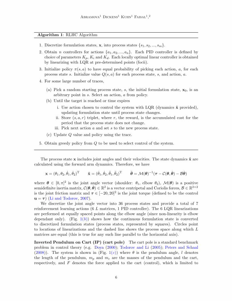
Algorithm 1: RLHC Algorithm

1. Discretize formulation states, x, into process states {s1, s2, ..., sm}.2. Obtain n controllers for actions {a1, a2, ..., an}. Each PID controller is defined by

choice of parameters Kp, Ki and Kd. Each locally optimal linear controller is obtainedby linearizing with LQR at pre-determined points (focii).

3. Initialize policy π(s, a) to have equal probability of picking each action, a, for eachprocess state s. Initialize value Q(s, a) for each process state, s, and action, a.

4. For some large number of traces,

(a) Pick a random starting process state, s, the initial formulation state, x0, is anarbitrary point in s. Select an action, a from policy.

(b) Until the target is reached or time expires

i. Use action chosen to control the system with LQR (dynamics x provided),updating formulation state until process state changes.

ii. Store (s, a, r) triplet, where r, the reward, is the accumulated cost for theperiod that the process state does not change.

iii. Pick next action a and set s to the new process state.

(c) Update Q value and policy using the trace.

5. Obtain greedy policy from Q to be used to select control of the system.

The process state x includes joint angles and their velocities. The state dynamics x arecalculated using the forward arm dynamics. Therefore, we have

x = (θ1, θ2, θ1, θ2)T x = (θ1, θ2, θ1, θ2)

T θ =M(θ)−1(τ − C(θ, θ)− Bθ)

where θ ∈ [0, π]2 is the joint angle vector (shoulder: θ1, elbow θ2), M(θ) is a positivesemidefinite inertia matrix, C(θ, θ) ∈ R2 is a vector centripetal and Coriolis forces, B ∈ R2×2

is the joint friction matrix and τ ∈ [−20, 20]2 is the joint torque (defined to be the controlu = τ ) (Li and Todorov, 2007).

We discretize the joint angle vector into 36 process states and provide a total of 7reinforcement learning actions (6 L matrices, 1 PID controller). The 6 LQR linearizationsare performed at equally spaced points along the elbow angle (since non-linearity is elbowdependant only). (Fig. 1(b)) shows how the continuous formulation state is convertedto discretized formulation states (process states, represented by squares). Circles pointto locations of linearizations and the dashed line shows the process space along which Lmatrices are equal (this is true for any such line parallel to the horizontal axis).

Inverted Pendulum on Cart (IP) (cart pole) The cart pole is a standard benchmarkproblem in control theory (e.g. Doya (2000); Todorov and Li (2005); Peters and Schaal(2008)). The system is shown in (Fig. 1(c)) where θ is the pendulum angle, l denotesthe length of the pendulum, mp and mc are the masses of the pendulum and the cart,respectively, and F denotes the force applied to the cart (control), which is limited to

6


[−20, 20]. The system has a stable equilibrium for θ ∈ {−π, π}, and the target state is theunstable equilibrium at (θ, θ) = 0.

The task is to control the the cart pole to target from any starting angle θ ∈ [−π, π]and starting velocity θ ∈ [−0.5π, 0.5π].

A simple linear controller (LQR) can only solve the problem effectively from some ofthe starting states, typically those in the vicinity of the target.

The process state x includes the cart position z, cart velocity z, pendulum angle θ andangular velocity θ. This and the state dynamics from Lozano et al. (2000) are given by

x = (z, z, θ, θ)T x = (z, z, θ, θ)T M(q)q2 + C(q, q)q +G(q) = τ

where q = [z, θ]T, τ = [F, 0]T and

M(q) =

(mp +mc mpl cos θmpl cos θ mpl

2

), C(q, q) =

(0 −mplθ sin θ0 0

)We discretize θ and θ into 25 process states at equal intervals and provide a total

of 9 reinforcement learning actions (5 feedback gain matrices, obtained at equally spacedintervals of θ formulation space, 4 arbitrarily chosen PID controllers).

4. Results

The results show that RLHC can (optimally) control the systems tested and can reasonablycompete with the speed and accuracy of iLQR. The results are reported as ’relative cost

differences’(JRLOC -Jalgo)|JLQR| 100% (where Jalgo is either a LQR or an iLQR cost) because the

acquired cost for starting states further away from the target could be higher simply dueto the distance travelled. Negative values indicate that RLHC is less costly. The RLHCperformance was tested on several different cost functions and targets (various targets forrobot arm and only one target for cart pole, since only one is defined) and the results showedconsistency.

Robotic Arm The final time-step values of θ1, θ2 for RLHC, LQR and iLQR are shownin (Fig. 1(d)). All algorithms take the arm to target with a small end point error of up to2∗10−3 for both θ1 and θ2. Here RLHC did not seem to benefit from the inclusion of a PIDcontroller, as it did not form part of the optimal policy. The crucial comparison of costsincurred for controlling the system can be seen for RLHC vs LQR (in Fig. 1(f )) and RLHCvs iLQR (in Fig. 1(h)), with the 36 initial states labeled as in Fig. 1(b). A small circle inFig. 1(h) indicates location of the target (state 15). The two cost comparing figures revealthat RLHC solves the problem almost as well as iLQR (max 3% worse) and by up to 89%better than LQR. This means that RLHC uses a reduced number of controllers (vs. iLQR)and reduced number of state discretizations (vs. reinforcement learning solutions alone)while still being able so solve the problem effectively. The mean CPU usage for: RLHC(unoptimized) 280.5 ticks, LQR 7.4 ticks and iLQR 95.3. RLHC was trained on 1500 traces.

Cart Pole The final time-step state values (see Fig. 1(e)) show that RLHC does the bestfrom all of the algorithms in taking the system to the target for most of the starting states,and it is evident that some starting states are harder to learn than others (for example

7


LQR struggles to take most non-linear states to target repeatedly i.e. those furthest awayfrom the target). For RLHC, the PID controllers were advantageous and were picked bythe MC learner. RLHC performs better than LQR in most states by up to 100%, exceptfor two states where we did not learn well and are worse by up to 477% (Fig. 1(g)). Crucialcomparison to iLQR (Fig. 1(i)) reveals that for the cart pole problem RLHC actually canbeat the performance of iLQR for almost all of the starting states by up to 75%, althoughat a detriment of two states it struggled to learn (worse by up to 477%). It should be notedhowever that iLQR needed help to solve some of the starting states, namely those closerto the θ = 0 target. Initial control trajectory u0 = 0 actually lets the pendulum drop forthe first iteration of iLQR, which seemed to be suboptimal when compared to LQR andRLHC. Therefore we supplied iLQR with a different initial u0 trajectory: u0 = 1, u0 = −1and u0 = uLQR (the latter corresponding to the u obtained from performing LQR controlon that starting state). The mean CPU usage for: RLHC (unoptimized) 402.2 ticks, LQR5.4 ticks and iLQR 349.4. RLHC was trained on 2000 traces.

5. Discussion

We presented a proof-of-principle framework to learn to control non-linear control problemsand demonstrated it on two standard benchmark optimal control problems – robot armcontrol and swing-up and balancing of the pole on the cart.

Our approach solved the non-linear optimal control problem by combining reinforce-ment learning with heterogeneous sets of local controllers. This allowed us to use a reducednumber of linearized controllers for x trajectory calculation compared to state-of-the-artiLQR. In addition we showed that we were effectively pushing back the curse of dimen-sionality as the algorithm operated and searched within a greatly reduced state space (byapproximately 1.5 ∗ 104).

Given random initialisation of parameters we found that RLHC learns the control prob-lem quickly (in the order of a few minutes) for more start-end point pairs than the state-of-the-art iLQR algorithm (as the iterative approximations fail to converge). Reinforcementlearning approaches have been applied to the pole on a cart problem in recent years (e.g.Doya (2000)) but not focussed on optimal control solutions that simultaneously minimise acost function. More recently, Deisenroth and Rasmussen (2011) have shown that the poleon a cart problem can be learnt using function-approximation methods combined with rein-forcement learning in a very numerically efficient way with a handful of data points — whilelearning the dynamics (at an increased offline computational cost required for optimizationof the control policy, in the order of hours). We approach the non-linear optimal problemfrom a different, neuro-inspired point of view and which approximates very well the non-linear optimal-control solution (with known dynamics). Given this proof-of-principle, ourfuture work is to use this hierarchical structure to divide-and-conquer the learning problemof the dynamics. The open structure of our framework makes it straightforward to test vari-ants of reinforcement learning algorithms including actor-critic methods (Peters and Schaal,2008) and internal forward models (planning) e.g. Deisenroth and Rasmussen (2011).

We have shown that the RLHC algorithm matches and sometimes beats the accuracy ofcontrolling the robot arm control and inverted pendulum on a cart problems to target whileminimising quadratic control costs. In perspective RLHC offers a novel way of learning

8


an important class of non-linear control problems. Our proof-of-principle for the RLHCframework demonstrates how it may be used for solving harder non-linear problems whereiterative linearisation algorithms may fail to converge, or where the curse of dimensionalitymakes monolithic learning of the control problem too hard.

Acknowledgments

We would like to acknowledge the financial support of the UK EPSRC for this research.

References

B.D.O. Anderson and J.B. Moore. Optimal control: linear quadratic methods. Prentice-Hall, 1989.

K.J. Astrom and T. Hagglund. Advanced PID control. The ISA Society, 2006.

R. Bellman and S. Dreyfus. Dynamic programming and the reliability of multicomponent devices.Operations Research, 6(2):200–206, 1958.

M. Berniker, A. Jarc, E. Bizzi, and M.C. Tresch. Simplified and effective motor control based onmuscle synergies to exploit musculoskeletal dynamics. Proceedings of the National Academy ofSciences, 106(18):7601, 2009.

A.E. Bryson and Y.C. Ho. Applied optimal control: optimization, estimation, and control. Hemi-sphere Pub, 1975.

A. d’Avella, P. Saltiel, E. Bizzi, et al. Combinations of muscle synergies in the construction of anatural motor behavior. Nature neuroscience, 6(3):300–308, 2003.

M. P. Deisenroth and C. E. Rasmussen. Pilco: A model-based and data-efficient approach to policysearch. In Lise Getoor and Tobias Scheffer, editors, ICML, pages 465–472. Omnipress, 2011.

J. Diedrichsen, R. Shadmehr, and R.B. Ivry. The coordination of movement: optimal feedbackcontrol and beyond. Trends in cognitive sciences, 14(1):31–39, 2010.

K. Doya. Reinforcement learning in continuous time and space. Neural Comp., 12(1):219–245, 2000.

A.A. Faisal and D.M. Wolpert. Near optimal combination of sensory and motor uncertainty in timeduring a naturalistic perception-action task. Journal of neurophysiology, 101(4):1901–1912, 2009.

A.A. Faisal, L.P.J. Selen, and D.M. Wolpert. Noise in the nervous system. Nature Reviews Neuro-science, 9(4):292–303, 2008.

C.M. Harris and D.M. Wolpert. Signal-dependent noise determines motor planning. Nature, 394(6695):780–784, 1998.

C.B. Hart and S.F. Giszter. A neural basis for motor primitives in the spinal cord. The Journal ofNeuroscience, 30(4):1322–1336, 2010.

Kappen H.J. Optimal control theory and the linear bellman equation. Inference and Learning inDynamic Models, pages 363–387, 2011. Published.

R.E. Kalman. Contributions to the theory of optimal control. Bol. Soc. Mat. Mexicana, 5(2):102–119, 1960.

Harold J. Kushner and G. George Yin. Stochastic Approximation and Recursive Algorithms andApplications. Springer, 2nd edition, 2003.

H. Kwakernaak and R. Sivan. Linear optimal control systems, volume 172. Wiley-Interscience NewYork, 1972.

9


WH Kwon, AM Bruckstein, and T. Kailath. Stabilizing state-feedback design via the moving horizonmethod. International Journal of Control, 37(3):631–643, 1983.

W. Li and E. Todorov. Iterative linear-quadratic regulator design for nonlinear biological move-ment systems. In Proceedings of the First International Conference on Informatics in Control,Automation, and Robotics, pages 222–229, 2004.

W. Li and E. Todorov. Iterative linearization methods for approximately optimal control and esti-mation of non-linear stochastic system. International Journal of Control, 80(9):1439–1453, 2007.

R. Lozano, I. Fantoni, and D.J. Block. Stabilization of the inverted pendulum around its homoclinicorbit. Systems & control letters, 40(3):197–204, 2000.

M.T. Mason. Mechanics of robotic manipulation. The MIT Press, 2001.

F.A. Mussa-Ivaldi, S.F. Giszter, and E. Bizzi. Linear combinations of primitives in vertebrate motorcontrol. Proceedings of the National Academy of Sciences, 91(16):7534, 1994.

J. Peters and S. Schaal. Natural actor-critic. Neurocomputing, 71(7):1180–1190, 2008.

J.A. Primbs, V. Nevistic, and J.C. Doyle. Nonlinear optimal control: A control lyapunov functionand receding horizon perspective. Asian Journal of Control, 1(1):14–24, 1999.

C. Rasmussen and M. Deisenroth. Probabilistic inference for fast learning in control. Recent Advancesin Reinforcement Learning, pages 229–242, 2008.

S.H. Scott. Optimal feedback control and the neural basis of volitional motor control. Nature ReviewsNeuroscience, 5(7):532–546, 2004.

S.H. Strogatz. Nonlinear dynamics and chaos: with applications to physics, biology, chemistry, andengineering (studies in nonlinearity). Westview Press, 2001.

R.S. Sutton and A.G. Barto. Reinforcement learning, volume 9. MIT Press, 1998.

S. Taylor and A. Faisal. Does the cost function of human motor control depend on the internalmetabolic state? BMC Neuroscience, 12(Suppl 1):P99, 2011.

K.A. Thoroughman and R. Shadmehr. Learning of action through adaptive combination of motorprimitives. Nature, 407(6805):742, 2000.

E. Todorov and W. Li. A generalized iterative lqg method for locally-optimal feedback control ofconstrained nonlinear stochastic systems. In American Control Conference, pages 300–306, 2005.

J.J. Tramper, J.L. van den Broek, W.A.J.J. Wiegerinck, H.J. Kappen, and C.C.A.M. Gielen.Stochastic optimal control predicts human motor behavior in time-constrainedsensorimotor tasks.Biological Cybernetics, page xx, 2011. Accepted.

D.M. Wolpert, J. Diedrichsen, and J.R. Flanagan. Principles of sensorimotor learning. NatureReviews Neuroscience, 2011.

10


(a) 2D RA system (b) RA process space (c) IP system

(d) RA θ1 and θ2 at T (e) IP θ and θ at time T

(f ) RA costs LQR vs RLHC (g) IP costs LQR vs RLHC

(h) RA costs iLQR vs RLHC (i) IP costs improved iLQR vs RLHC

Figure 1: Tested systems’ figures.

11

hierarchical, heterogeneous control of non-linear dynamical systems using reinforcement learning

Documents