hidden sector photon coupling of resonant cavities
TRANSCRIPT

Hidden Sector Photon Coupling of Resonant Cavities
Stephen R. Parker,1, ∗ Gray Rybka,2 and Michael E. Tobar1
1School of Physics, The University of Western Australia, Crawley 6009, Australia2University of Washington, Seattle, Washington 98195, USA
(Dated: April 26, 2013)
Many beyond the standard model theories introduce light paraphotons, a hypothetical spin-1 fieldthat kinetically mixes with photons. Microwave cavity experiments have traditionally searched forparaphotons via transmission of power from an actively driven cavity to a passive receiver cavity, withthe two cavities separated by a barrier that is impenetrable to photons. We extend this measurementtechnique to account for two-way coupling between the cavities and show that the presence of aparaphoton field can alter the resonant frequencies of the coupled cavity pair. We propose anexperiment that exploits this effect and uses measurements of a cavities resonant frequency toconstrain the paraphoton-photon mixing parameter, χ. We show that such an experiment canimprove sensitivity to χ over existing experiments for paraphoton masses less than the resonantfrequency of the cavity, and eliminate some of the most common systematics for resonant cavityexperiments.
I. INTRODUCTION
Some Standard Model extension theories postulate theexistence of a hidden sector of particles that interact veryweakly with standard model particles [1, 2]. One pro-posed form of hidden sector particle interaction is thespontaneous kinetic mixing of the photon and the hid-den sector photon [3]. Massive hidden sector photons areknown as paraphotons [4] and are classified as a type ofWeakly Interacting Slim Particle (WISP), a hypotheticalgroup of particles with sub-eV masses [5]. Experimentsto detect paraphotons place bounds on the kinetic mixingparameter, χ, as a function of the possible hidden sectorphoton mass.
Laboratory based searches for paraphotons have beenconducted for several years [6–12] with some recenttests using microwave frequency resonant cavities [13–15]. Electromagnetic resonances in otherwise isolatedcavities could become coupled in the presence of a para-photon field. If one resonant cavity is actively driven,this coupling can be seen as photons in the driven cavitymixing with paraphotons, which then cross the bound-ary between cavities, and then mixing back into photonsin the undriven cavity. Resonant regeneration is presenteven at the subphoton level [16], and by measuring thepower transmitted between the two cavities a bound canbe placed on the probability of kinetic mixing betweenphotons and paraphotons. This arrangement is knownas a Light Shining through a Wall (LSW) experimentand has been the focus of microwave frequency resonantcavity paraphoton searches [13, 14]. As these searchesrely on measuring very low levels of microwave power thefundamental limitation to their sensitivity is imposed bythe thermal noise in the detector cavity and amplifica-tion system. However, in practice they have been limitedby microwave power leakage from the emitter to detec-
tor cavity which is indistinguishable from a paraphotoneffect [13]. The prospect of LSW has also inspired somespeculative work on exploiting the paraphoton for datatransmission and communications [17, 18].
Previous LSW formalism [19] has been focused on theone way flow of paraphotons from a driven emitter cav-ity to an undriven detection cavity. However, it is alsopossible to treat the two-way exchange of paraphotons asa weak coupling between the cavities, creating a systemanalogous to two spring-mass oscillators connected via athird weak spring. When both cavities are actively driventhe paraphoton mediated coupling will cause a phase-dependent shift in the resonant frequencies and qualityfactors of the system. This opens up the possibility ofconducting experiments that constrain the strength ofphoton-paraphoton mixing by observing this coupling in-duced resonant frequency shift. When given the option itis preferable to make a measurement of frequency ratherthan power due to the quality and precision of frequencystandards, instrumentation and techniques.
Although we focus on the paraphoton, the conceptsdeveloped in this paper can be extended and applied toLSW based searches for other hypothetical particles thatmix with the photon such as fermionic minicharged par-ticles [20, 21].
II. FUNDAMENTAL NORMAL MODES
As described in Jaeckel & Ringwald [19] the renormal-izable Lagrangian for low energy photons and parapho-tons is given by
L = −1
4FµνFµν −
1
4BµνBµν
−1
2χFµνBµν +
1
2m2γ′BµBµ,
(1)
where Fµν is the field strength tensor for the photon fieldAµ, Bνµ is the field strength tensor for the paraphoton
arX
iv:1
304.
6866
v1 [
hep-
ph]
25
Apr
201
3

2
0
0.5
1
1.5
2
2.5
0 0.2 0.4 0.6 0.8 1
|G|
mr
FIG. 1. (color online) Numerical simulation of the absolutevalue of geometry factors as a function of the paraphotonmass ratio, mr = mγ′/ω0, for two identical cube cavities over-lapping in space (GS , full line) and separated by a distanceof L (G, dashed line) where L is the length of the cubic cav-ities, in this case set to 1. The normalized resonant modeused is given by A(x) = 2 sin (πx) sin (πy) and the resonantfrequency is ω0 =
√2π [19].
field Bµ, χ is the photon-paraphoton kinetic mixing pa-rameter and mγ′ is the paraphoton mass. From eq. (1)the equations of motion for the electromagnetic fields intwo spatially separated resonant cavities, A1 and A2, andthe universal paraphoton field B are(
∂µ∂ν + χ2m2γ′)A1 = χm2
γ′B (2)(∂µ∂ν + χ2m2
γ′)A2 = χm2
γ′B (3)(∂µ∂ν +m2
γ′)B = χm2
γ′ (A1 +A2) . (4)
The cavity fields can be broken down in to time andspatial components,
A1,2 (x, t) = a1,2 (t)A1,2 (x) , (5)
where the spatial component satisfies the normalisationcondition ∫
V
d3x|A1,2 (x) |2 = 1. (6)
Due to the infinite nature of the paraphoton field we usethe retarded massive Greens function to find the para-photon field from equation (4),
B (x, t) = χm2γ′
∫V 1
d3yexp (ikb|x− y|)
4π|x− y|a1A1 (y)
+
∫V 2
d3yexp (ikb|x− y|)
4π|x− y|a2A2 (y)
.
(7)
Dw
w0
w+
w-
w1
w2
0.1 1
1
Detuning x Hc2L
FractionalFrequency
Hwêw0L
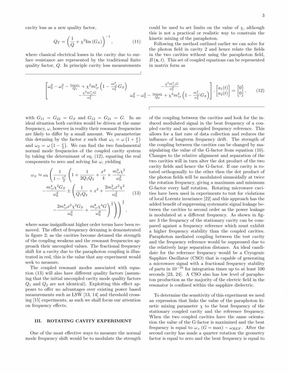
FIG. 2. (color online) Log-Log plot of resonant frequencies rel-ative to a common central frequency, ω0, as a function of de-tuning for a pair of cavities that are coupled (black, full, equa-tion (13)) and uncoupled (gray, dashed, ω1,2/ω0 = (1± x/2)).The detuning, x, is given as a factor of the square of the para-photon kinetic mixing parameter, χ. The magnitude of thefractional frequency shift is proportional to the values of pa-rameters Q1, Q2, G, GS and χ used in eq. (13).
In the absence of a paraphoton field the resonant fre-quency, ω0, of a cavity is given by
∇2A (x) = ω20A (x) . (8)
We can now solve for the photon field in cavity 1 bysubstituting the paraphoton field of eq. (7) in to eq. (2)and utilizing eq. (8) and the normalization conditionsfrom (6) we find that:(ω20 − ω2
1 − iω0ω1
Q1+ χ2m2
γ′
(1−
m2γ′
ω20
G11
))a1 (t)
=χ2m4
γ′G12
ω20
a2 (t)
(9)
G11 = ω20
∫V 1
d3x
∫V 1
d3yexp (ikb|x− y|)
4π|x− y|
×A1 (y) ·A1 (x)
G12 = ω20
∫V 1
d3x
∫V 2
d3yexp (ikb|x− y|)
4π|x− y|
×A2 (y) ·A1 (x) ,
(10)
where ω1 is the driving frequency of the cavity and G12
is the standard G-function found in the literature [13, 19]that describes the two cavity fields, geometries and rel-ative positions while G11 (henceforth GS) is the G-function for a cavity field overlapped spatially with itselfand represents losses in the cavity due to photon to para-photon conversion. Numerical calculations of G and GSfor a simple cube cavity system (Fig. 1) indicate that themagnitude of GS is larger than the magnitude of G asone would expect. We can represent the total electrical
3
cavity loss as a new quality factor,
QT =
(1
Q+ χ2Im (GS)
)−1, (11)
where classical electrical losses in the cavity due to sur-face resistance are represented by the traditional finitequality factor, Q. In principle cavity loss measurements
could be used to set limits on the value of χ, althoughthis is not a practical or realistic way to constrain thekinetic mixing of the paraphoton.
Following the method outlined earlier we can solve forthe photon field in cavity 2 and hence relate the fieldsin the two cavities without using the paraphoton field,B (x, t). This set of coupled equations can be representedin matrix form as
ω20 − ω2
1 − iω0ω1
Q1+ χ2m2
γ′
(1− m2
γ′ω2
0GS
)−χ
2m4γ′G
ω20
−χ2m4
γ′G
ω20
ω20 − ω2
2 − iω0ω2
Q2+ χ2m2
γ′
(1− m2
γ′ω2
0GS
) . [a1(t)
a2(t)
]=
[00
], (12)
with G11 = G22 = GS and G12 = G21 = G. In anideal situation both cavities would be driven at the samefrequency, ω, however in reality their resonant frequenciesare likely to differ by a small amount. We parameterizethis detuning by the factor x such that ω1 = ω
(1 + x
2
)and ω2 = ω
(1− x
2
). We can find the two fundamental
normal mode frequencies of the coupled cavity systemby taking the determinant of eq. (12), equating the realcomponents to zero and solving for ω, yielding
ω± ≈ ω0
(1
1− x2
2
(1 +
1
2Q1Q2+x2
4+m2γ′χ
2
ω20
−m4γ′χ
2GS
ω40
±
(1
Q1Q2+ x2 +
2m2γ′x
2χ2
ω20
−2m4
γ′x2χ2GS
ω40
+m8γ′χ
4G
ω80
) 12
12
,
(13)
where some insignificant higher order terms have been re-moved. The effect of frequency detuning is demonstratedin figure 2; as the cavities become detuned the strengthof the coupling weakens and the resonant frequencies ap-proach their uncoupled values. The fractional frequencyshift for a cavity due to the paraphoton coupling is illus-trated in red, this is the value that any experiment wouldseek to measure.
The coupled resonant modes associated with equa-tion (13) will also have different quality factors (assum-ing that the initial uncoupled cavity mode quality factorsQ1 and Q2 are not identical). Exploiting this effect ap-pears to offer no advantages over existing power basedmeasurements such as LSW [13, 14] and threshold cross-ing [15] experiments, as such we shall focus our attentionon frequency effects.
III. ROTATING CAVITY EXPERIMENT
One of the most effective ways to measure the normalmode frequency shift would be to modulate the strength
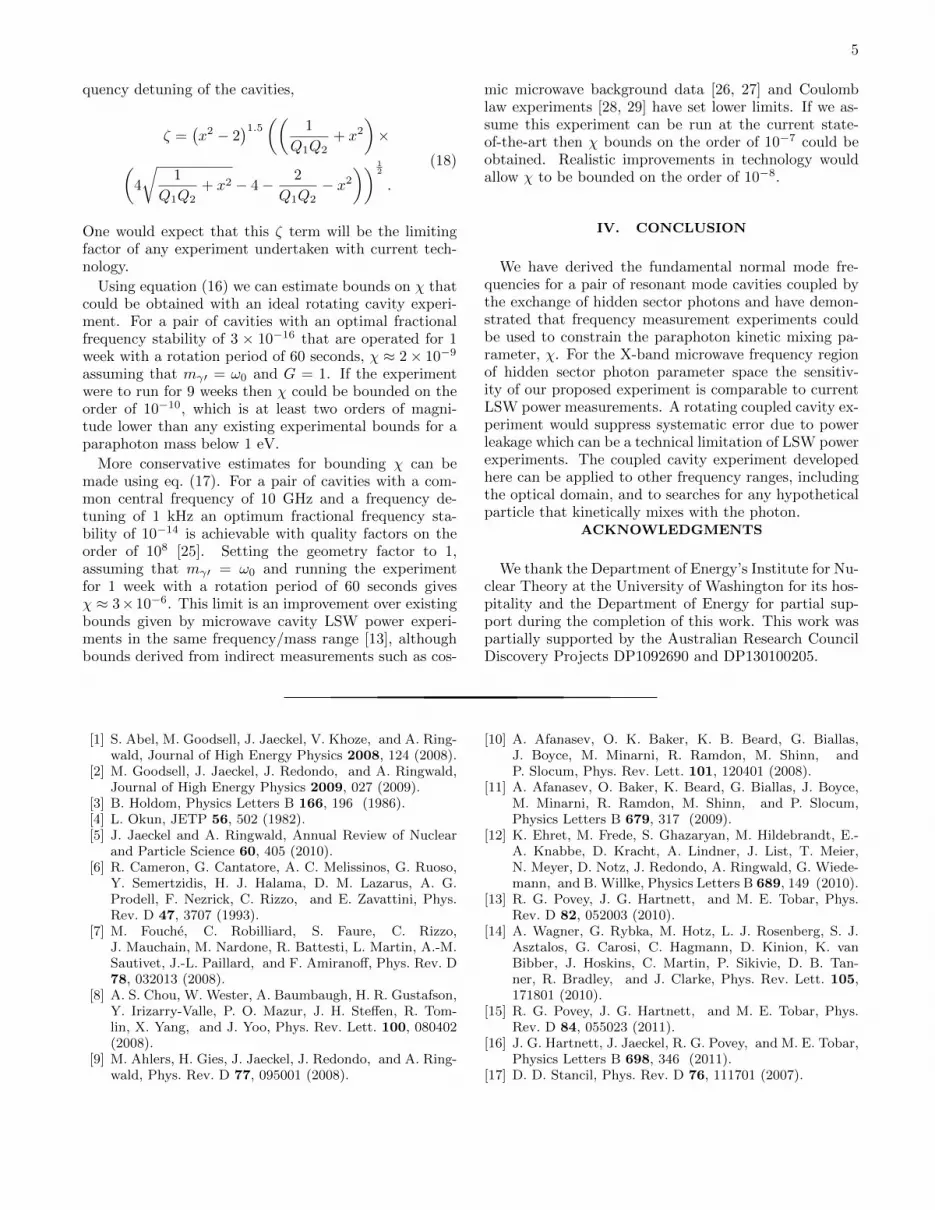
of the coupling between the cavities and look for the in-duced modulated signal in the beat frequency of a cou-pled cavity and an uncoupled frequency reference. Thisallows for a fast rate of data collection and reduces theinfluence of longterm frequency drift. The strength ofthe coupling between the cavities can be changed by ma-nipulating the value of the G-factor from equation (10).Changes to the relative alignment and separation of thetwo cavities will in turn alter the dot product of the twocavity fields and hence the G-factor. If one cavity is ro-tated orthogonally to the other then the dot product ofthe photon fields will be modulated sinusoidally at twicethe rotation frequency, giving a maximum and minimumG-factor every half rotation. Rotating microwave cavi-ties have been used in experiments to test for violationsof local Lorentz invariance [22] and this approach has theadded benefit of suppressing systematic signal leakage be-tween the cavities to second order as the power leakageis modulated at a different frequency. As shown in fig-ure 3 the frequency of the stationary cavity can be com-pared against a frequency reference which must exhibita higher frequency stability than the coupled cavities.Paraphoton mediated coupling between the test cavityand the frequency reference would be suppressed due tothe relatively large separation distance. An ideal candi-date for the reference frequency would be a CryogenicSapphire Oscillator (CSO) that is capable of generatinga microwave signal with a fractional frequency stabilityof parts in 10−16 for integration times up to at least 100seconds [23, 24]. A CSO also has low level of parapho-ton production as the majority of the electric field in theresonator is confined within the sapphire dielectric.
To determine the sensitivity of this experiment we needan expression that links the value of the paraphoton ki-netic mixing parameter χ to the beat frequency of thestationary coupled cavity and the reference frequency.When the two coupled cavities have the same orienta-tion the value of the G-factor is maximised and the beatfrequency is equal to ω+ (G = max) − ωREF . After thesecond cavity has made a quarter rotation the geometryfactor is equal to zero and the beat frequency is equal to

4
Freq. Ref.
ωREF
ω
ω
δω
ω+
ω-
FIG. 3. (color online) Schematic of a rotating paraphotoncoupled cavities experiment. The two empty cavities sep-arated by an impenetrable barrier (red plane) and activelydriven at frequency ω, although the resonant frequencies ofthe cavities may be slightly detuned (ω+ and ω−). One cav-ity is rotated orthogonally to the other. The frequency of thestationary cavity is compared to a stable frequency reference(ωREF ) to produce the beat frequency (δω).
ω+ (G = 0)−ωREF . Hence the fractional stability of thecavity / reference beat frequency for an integration timeequal to a quarter of the rotation period is
δω =(ω+ (G = max)− ωREF )− (ω+ (G = 0)− ωREF )
ω0
=ω+ (G = max)− ω+ (G = 0)
ω0,
(14)
where ω+ is defined in equation (13). This is the stabil-ity of the frequency shift first illustrated in Fig. 2 (redlabel) and then plotted explicitly in figure 4 as a functionof frequency detuning and cavity losses. There are tworegimes that the experiment could operate in. The first isthe ideal situation where the cavities feature extremelyhigh quality factors and suffer from minimal frequency
µ c2 µ c4
0.001 0.01 0.1 1 10 100 1000
0.001
0.01
0.1
1
Detuning x or Cavity Loss Q-1
FrequencyShiftDw
w0
FIG. 4. (color online) Log-Log plot of the normalized frac-tional resonant frequency shift due to paraphoton cavity cou-pling as a function of cavity frequency detuning and losses(from eq. (13) and eq. (14)). Both the cavity frequency de-tuning, x, and the cavity losses, Q−1, are given as a factorof χ2. The frequency shift is plotted a function of x (withQ−1 = 0) and as a function of Q−1 (with x = 0); both curvesoverlap. The vertical gray dashed line indicates where thedependence of the frequency shift changes. In the first regionthe frequency shift is proportional to χ2 and in the secondregion it is proportional to χ4.
detuning such that
Q−1 + x < χ2, (15)
in this scenario the frequency shift is independent of thedetuning and cavity losses and is proportional to χ2.When the conditions set by eq. (15) are broken the fre-quency shift changes as a function of the detuning andcavity losses and is proportional to χ4.
To find analytical sensitivity expressions we take a se-ries expansion of ω+ around χ = 0 to second order in χ,substitute back in to equation (14) and solve for χ. Inthe situation where eq. 15 holds true we can approximatethe experimental sensitivity as
χ ≈
√2δωω4
0√NGm4
γ′, (16)
where N is the number of measurements taken. Thisshows that at a fundamental level the frequency signal isproportional to χ2 whereas traditional LSW power mea-surements are proportional to χ4. Unfortunately for anyexperiment implemented using current technology it islikely that the conditions in eq. (15) will be broken andthe experimental sensitivity will be
χ =
( √2δωζω8
0√NG2m8
γ′
) 14
, (17)
where ζ is a term describing the quality factors and fre-
5
quency detuning of the cavities,
ζ =(x2 − 2
)1.5(( 1
Q1Q2+ x2
)×(
4
√1
Q1Q2+ x2 − 4− 2
Q1Q2− x2
)) 12
.
(18)
One would expect that this ζ term will be the limitingfactor of any experiment undertaken with current tech-nology.
Using equation (16) we can estimate bounds on χ thatcould be obtained with an ideal rotating cavity experi-ment. For a pair of cavities with an optimal fractionalfrequency stability of 3 × 10⁻¹⁶ that are operated for 1week with a rotation period of 60 seconds, χ ≈ 2× 10⁻⁹
assuming that mγ′ = ω0 and G = 1. If the experimentwere to run for 9 weeks then χ could be bounded on theorder of 10−10, which is at least two orders of magni-tude lower than any existing experimental bounds for aparaphoton mass below 1 eV.
More conservative estimates for bounding χ can bemade using eq. (17). For a pair of cavities with a com-mon central frequency of 10 GHz and a frequency de-tuning of 1 kHz an optimum fractional frequency sta-bility of 10−14 is achievable with quality factors on theorder of 108 [25]. Setting the geometry factor to 1,assuming that mγ′ = ω0 and running the experimentfor 1 week with a rotation period of 60 seconds givesχ ≈ 3×10⁻⁶. This limit is an improvement over existingbounds given by microwave cavity LSW power experi-ments in the same frequency/mass range [13], althoughbounds derived from indirect measurements such as cos-
mic microwave background data [26, 27] and Coulomblaw experiments [28, 29] have set lower limits. If we as-sume this experiment can be run at the current state-of-the-art then χ bounds on the order of 10−7 could beobtained. Realistic improvements in technology wouldallow χ to be bounded on the order of 10−8.
IV. CONCLUSION
We have derived the fundamental normal mode fre-quencies for a pair of resonant mode cavities coupled bythe exchange of hidden sector photons and have demon-strated that frequency measurement experiments couldbe used to constrain the paraphoton kinetic mixing pa-rameter, χ. For the X-band microwave frequency regionof hidden sector photon parameter space the sensitiv-ity of our proposed experiment is comparable to currentLSW power measurements. A rotating coupled cavity ex-periment would suppress systematic error due to powerleakage which can be a technical limitation of LSW powerexperiments. The coupled cavity experiment developedhere can be applied to other frequency ranges, includingthe optical domain, and to searches for any hypotheticalparticle that kinetically mixes with the photon.
ACKNOWLEDGMENTS
We thank the Department of Energy’s Institute for Nu-clear Theory at the University of Washington for its hos-pitality and the Department of Energy for partial sup-port during the completion of this work. This work waspartially supported by the Australian Research CouncilDiscovery Projects DP1092690 and DP130100205.
[1] S. Abel, M. Goodsell, J. Jaeckel, V. Khoze, and A. Ring-wald, Journal of High Energy Physics 2008, 124 (2008).
[2] M. Goodsell, J. Jaeckel, J. Redondo, and A. Ringwald,Journal of High Energy Physics 2009, 027 (2009).
[3] B. Holdom, Physics Letters B 166, 196 (1986).[4] L. Okun, JETP 56, 502 (1982).[5] J. Jaeckel and A. Ringwald, Annual Review of Nuclear
and Particle Science 60, 405 (2010).[6] R. Cameron, G. Cantatore, A. C. Melissinos, G. Ruoso,
Y. Semertzidis, H. J. Halama, D. M. Lazarus, A. G.Prodell, F. Nezrick, C. Rizzo, and E. Zavattini, Phys.Rev. D 47, 3707 (1993).
[7] M. Fouche, C. Robilliard, S. Faure, C. Rizzo,J. Mauchain, M. Nardone, R. Battesti, L. Martin, A.-M.Sautivet, J.-L. Paillard, and F. Amiranoff, Phys. Rev. D78, 032013 (2008).
[8] A. S. Chou, W. Wester, A. Baumbaugh, H. R. Gustafson,Y. Irizarry-Valle, P. O. Mazur, J. H. Steffen, R. Tom-lin, X. Yang, and J. Yoo, Phys. Rev. Lett. 100, 080402(2008).
[9] M. Ahlers, H. Gies, J. Jaeckel, J. Redondo, and A. Ring-wald, Phys. Rev. D 77, 095001 (2008).
[10] A. Afanasev, O. K. Baker, K. B. Beard, G. Biallas,J. Boyce, M. Minarni, R. Ramdon, M. Shinn, andP. Slocum, Phys. Rev. Lett. 101, 120401 (2008).
[11] A. Afanasev, O. Baker, K. Beard, G. Biallas, J. Boyce,M. Minarni, R. Ramdon, M. Shinn, and P. Slocum,Physics Letters B 679, 317 (2009).
[12] K. Ehret, M. Frede, S. Ghazaryan, M. Hildebrandt, E.-A. Knabbe, D. Kracht, A. Lindner, J. List, T. Meier,N. Meyer, D. Notz, J. Redondo, A. Ringwald, G. Wiede-mann, and B. Willke, Physics Letters B 689, 149 (2010).
[13] R. G. Povey, J. G. Hartnett, and M. E. Tobar, Phys.Rev. D 82, 052003 (2010).
[14] A. Wagner, G. Rybka, M. Hotz, L. J. Rosenberg, S. J.Asztalos, G. Carosi, C. Hagmann, D. Kinion, K. vanBibber, J. Hoskins, C. Martin, P. Sikivie, D. B. Tan-ner, R. Bradley, and J. Clarke, Phys. Rev. Lett. 105,171801 (2010).
[15] R. G. Povey, J. G. Hartnett, and M. E. Tobar, Phys.Rev. D 84, 055023 (2011).
[16] J. G. Hartnett, J. Jaeckel, R. G. Povey, and M. E. Tobar,Physics Letters B 698, 346 (2011).
[17] D. D. Stancil, Phys. Rev. D 76, 111701 (2007).

6
[18] J. Jaeckel, J. Redondo, and A. Ringwald, EPL (Euro-physics Letters) 87, 10010 (2009).
[19] J. Jaeckel and A. Ringwald, Physics Letters B 659, 509(2008).
[20] B. Dobrich, H. Gies, N. Neitz, and F. Karbstein, Phys.Rev. Lett. 109, 131802 (2012).
[21] B. Dobrich, H. Gies, N. Neitz, and F. Karbstein, Phys.Rev. D 87, 025022 (2013).
[22] P. L. Stanwix, M. E. Tobar, P. Wolf, M. Susli, C. R.Locke, E. N. Ivanov, J. Winterflood, and F. van Kann,Phys. Rev. Lett. 95, 040404 (2005).
[23] C. R. Locke, E. N. Ivanov, J. G. Hartnett, P. L. Stanwix,and M. E. Tobar, Review of Scientific Instruments 79,
051301 (2008).[24] J. G. Hartnett, N. R. Nand, and C. Lu, Applied Physics
Letters 100, 183501 (2012).[25] B. Komiyama, IEEE Transactions on Instrumentation
and Measurement IM-36, 2 (1987).[26] J. Jaeckel, J. Redondo, and A. Ringwald, Phys. Rev.
Lett. 101, 131801 (2008).[27] A. Mirizzi, J. Redondo, and G. Sigl, Journal of Cosmol-
ogy and Astroparticle Physics 2009, 026 (2009).[28] E. R. Williams, J. E. Faller, and H. A. Hill, Phys. Rev.
Lett. 26, 721 (1971).[29] D. F. Bartlett and S. Logl, Phys. Rev. Lett. 61, 2285
(1988).