heterogeneous network games: conflicting preferences

Heterogeneous network games: conflicting preferences

> Penélope Hernández Universitat de València and ERI-CES, Spain

>Manuel Muñoz-Herrera Universitat de València and ERI-CES, Spain

>Ángel Sánchez Universidad Carlos III, Spain

February, 2011

DPEB 04/11

Heterogeneous Network Games:

Conflicting Preferences

Penelope Hernandez† Manuel Munoz-Herrera‡ Angel Sanchez§

July 7, 2010

Abstract

We propose a model of network games with heterogeneity introduced by endow-ing players with types that generate preferences among their choices. We study twoclasses of games: strategic complements or substitutes in payoffs. The payoff functiondepends on the network structure, and we ask how does heterogeneity shape players’decision making, what is its effect on equilibria, conditions of stability, and welfare.Heterogeneity in players’ type establishes the existence of thresholds which determinethe Nash equilibrium conditions in a network game. Network configurations in equilib-rium can be satisfactory if each player chooses the action corresponding to her type orfrustrated when at least one player is not. Also, equilibria can be specialized if all play-ers are choosing the same action (only in strategic complements), or hybrid when bothactions coexist. A refinement of the Nash equilibria through stochastic mutations ofpairs of neighbors limits multiplicity to a subset of Stable Equilibrium Configurations.We find that the Nash networks are absorbing states from where it is possible to leaveonly through mutations and that such mutations in most cases will lead to a frustratedhybrid configuration which, for most networks, is the risk dominant equilibrium.

JEL Code: C72, D03, D85, L14, Z13

∗The authors wish to thank participants of the Workshop COST-WG4 Evolution and Co-evolution.The first and the second authors thank financial support from the MCI (SEJ2007-66581) and GeneralitatValenciana (PROMETEO/2009/068) is gratefully acknowledged.

†ERI-CES, , Facultad de Economıa. Avda. dels Tarongers, s/n. 46022 Valencia. Spain.‡ERI-CES, , Facultad de Economıa. Avda. dels Tarongers, s/n. 46022 Valencia. Spain.§GISC, Departamento de Matematicas, Universidad Carlos III de Madrid; Instituto de Ciencias

Matematicas, CSIC-UAM-UC3M-UCM, Madrid, and BIFI, Universidad de Zaragoza

2

1 Introduction

In a population or society, agents can be involved in different social and economic interac-tions, aiming to coordinate (anti-coordinate) choices with their counterparts. Interactionsthus define a social network, the neighbors of a specific agent being those with whom sheinteracts. As a consequence, agents’ wellbeing depends on the behavior adopted by them-selves and their neighbors. Examples such as acquiring a specific technology (input) betweencompanies, getting involved in a riot, or job search, show the relevance of the network forthe decisions made by the agents. Within this approach, past and current literature haveconsidered players as homogeneous, in the sense that their only difference arises from thespecific number of contacts every agent has. In such framework, it is generally the case thatan agent chooses an action if the number of her neighbors making that same choice is higherthan a given threshold. This paper proposes a model of network games with individual-levelheterogeneity introduced by endowing players with types that generate preferences over anaction among their choices. We advance the field in the direction of a more realistic modelingby going beyond contextually different agents and considering intrinsically different agents.Thus, this paper is motivated by the consideration that when endowing players with prefer-ences over their choice set, the game played might be different depending on a player’s andher opponents’ type, even if they have the same degree. We ask how does heterogeneity intypes and degree shape players’ decision making and payoffs, what is its effect upon equi-librium when local information is available, the conditions of stability for equilibrium, andhow does this affect welfare.

As a general framework for the strategic interactions that take place in such setting, westudy two classes of network games: strategic complements (SC) or strategic substitutes(SS). For both cases we find how heterogeneity affects the structure and conditions of thegame depending on the type of players interacting. The games can be played between twoplayers of different or same type, generating multiple cases. This will lead to conflictingpreferences when two players of different (the same) type interact in games with strategiccomplements (substitutes).

A game with strategic complements in payoffs can be considered as a coordination game,where each player faces a binary choice set. When players are endowed with types, they willprefer one action rather than the other, so that even though they wish to coordinate, thepayoff differs if the coordination occurs in the preferred choice or in the one a player dislikes.However, payoffs are higher by coordinating in the disliked option than in the case of anti-coordination, when the agent is left alone in choosing her favorite action. There are manyexamples of strategic complements in the literature. One simple case is that of coauthorschoosing an operating system or a specific technology to work with. Consider two brandsA and B among which they can choose. Type A players will receive higher payoff whencoordinating in (A,A), whereas type B players will receive higher payoff when coordinatingon (B,B). However, it is clear that, due to their interest in working together, players of bothtypes prefer to coordinate in the action they dislike rather than sticking to their preferredaction and being left with an incompatible operating system or technology.

The situation is the opposite in games with strategic substitutes, which can be seen as anti-

3

coordination games. Players are better off when anti-coordinating. If each one chooses theaction they prefer in view of their type, both maximize their payoffs. As before, even if eachone chooses the disliked option, but still anti-coordinate, they will receive a higher payoffthan in the case of coordination, while coordinating in the disliked choices gives the lowestpayoff. This type of games are very common in examples such as differentiation of a productbetween two companies. Say for example, they can either produce in low quantities at highprices (high quality) focusing on a segment of the population with high income, or choose forhigh levels of production at low prices (low quality) targeting a wider range of population,that of a lower income. When each firm has a level of capital (type) that makes it prefer aparticular choice between high and low quality, and their preferences are opposite, the bestpossible outcome arises when each one of them produces what they like. On the contrary,for each one of them the worst situation arises when competing for the same segment ofcustomers in a quality setting that is not the firm’s preferred one.

To go from the above described 2×2 setting to a game in a social network, we assume thatthere is a fixed social (or geographic, or financial) structure where each player wants toadopt an action determined by her type, and interacts strategically with her neighbors. Inthis scenario, our main results can be summarized as follows: To begin with, we obtain twospecific thresholds, one for each type of player and depending on her degree, such that heraction changes when the number of her neighbors adopting the same action as hers goesabove or below the threshold. In other words, we show that a player has incentives to adoptthe behavior she likes if the number of her neighbors choosing the same (opposite) actionexceeds a given type-dependent threshold for games with SC (SS). In this context, a relevantfeature of our model is that heterogeneity in types generates heterogeneity in thresholds. Aplayer who likes a specific action has a lower threshold of acceptance for such choice thana player who dislikes it, even with the same degree. Heterogeneity in players’ degree alsoprovides a wider range of thresholds, because a specific player’s threshold depends on hertype and degree. We subsequently study equilibria, finding specific network configurationsthat depend on the class of game being played. Thus, we obtain networks that we denote assatisfactory, where all players choose the action they like, which is the action correspondingto their type. We also find frustrated networks, situations when at least one player choosesthe action she dislikes. These configurations, when considering the action profiles, are inturn subdivided into specialized, where every player chooses the same action, which is onlypossible in games with SC, and hybrid where both actions coexist.

We then refine this set of six (two) network game configurations in equilibrium in SC (SS)through a process of stochastic mutations. We follow the pioneering work of Foster andYoung (1990), who were the first to argue that in games with multiple strict Nash equilibria,some equilibria are more likely to emerge than others in the presence of continual smallstochastic shocks. To this end, we use myopic best response as our dynamical rule andconsider a class of mutations that affects two neighbors simultaneously. In this way, weobtain a proper subset of equilibria configurations which are stable, and show that most ofthem are in the class of frustrated hybrid networks, implying that full coordination is veryproblematic in SC, and that there will generally be agents that choose the action they do notlike. As a last step in the characterization of equilibria, we carry out a welfare analysis andshow that the stable equilibria are risk-dominant in the sense of Harsanyi and Selten (1989),

4

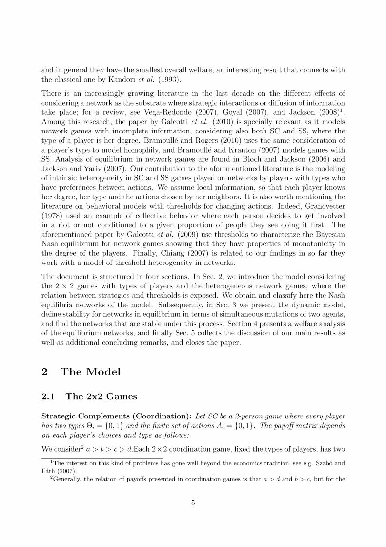
and in general they have the smallest overall welfare, an interesting result that connects withthe classical one by Kandori et al. (1993).

There is an increasingly growing literature in the last decade on the different effects ofconsidering a network as the substrate where strategic interactions or diffusion of informationtake place; for a review, see Vega-Redondo (2007), Goyal (2007), and Jackson (2008)1.Among this research, the paper by Galeotti et al. (2010) is specially relevant as it modelsnetwork games with incomplete information, considering also both SC and SS, where thetype of a player is her degree. Bramoulle and Rogers (2010) uses the same consideration ofa player’s type to model homophily, and Bramoulle and Kranton (2007) models games withSS. Analysis of equilibrium in network games are found in Bloch and Jackson (2006) andJackson and Yariv (2007). Our contribution to the aforementioned literature is the modelingof intrinsic heterogeneity in SC and SS games played on networks by players with types whohave preferences between actions. We assume local information, so that each player knowsher degree, her type and the actions chosen by her neighbors. It is also worth mentioning theliterature on behavioral models with thresholds for changing actions. Indeed, Granovetter(1978) used an example of collective behavior where each person decides to get involvedin a riot or not conditioned to a given proportion of people they see doing it first. Theaforementioned paper by Galeotti et al. (2009) use thresholds to characterize the BayesianNash equilibrium for network games showing that they have properties of monotonicity inthe degree of the players. Finally, Chiang (2007) is related to our findings in so far theywork with a model of threshold heterogeneity in networks.

The document is structured in four sections. In Sec. 2, we introduce the model consideringthe 2 × 2 games with types of players and the heterogeneous network games, where therelation between strategies and thresholds is exposed. We obtain and classify here the Nashequilibria networks of the model. Subsequently, in Sec. 3 we present the dynamic model,define stability for networks in equilibrium in terms of simultaneous mutations of two agents,and find the networks that are stable under this process. Section 4 presents a welfare analysisof the equilibrium networks, and finally Sec. 5 collects the discussion of our main results aswell as additional concluding remarks, and closes the paper.

2 The Model

2.1 The 2x2 Games

Strategic Complements (Coordination): Let SC be a 2-person game where every player

has two types Θi = {0, 1} and the finite set of actions Ai = {0, 1}. The payoff matrix depends

on each player’s choices and type as follows:

We consider2 a > b > c > d.Each 2×2 coordination game, fixed the types of players, has two

1The interest on this kind of problems has gone well beyond the economics tradition, see e.g. Szabo andFath (2007).

2Generally, the relation of payoffs presented in coordination games is that a > d and b > c, but for the

5

01 0

11 a,b c,c0 d,d b,a

θ1 = 1; θ2 = 0

11 0

11 a,a c,d0 d,c b,b

θ1 = 1; θ2 = 1

01 0

01 b,b d,c0 c,d a,a

θ1 = 0; θ2 = 0

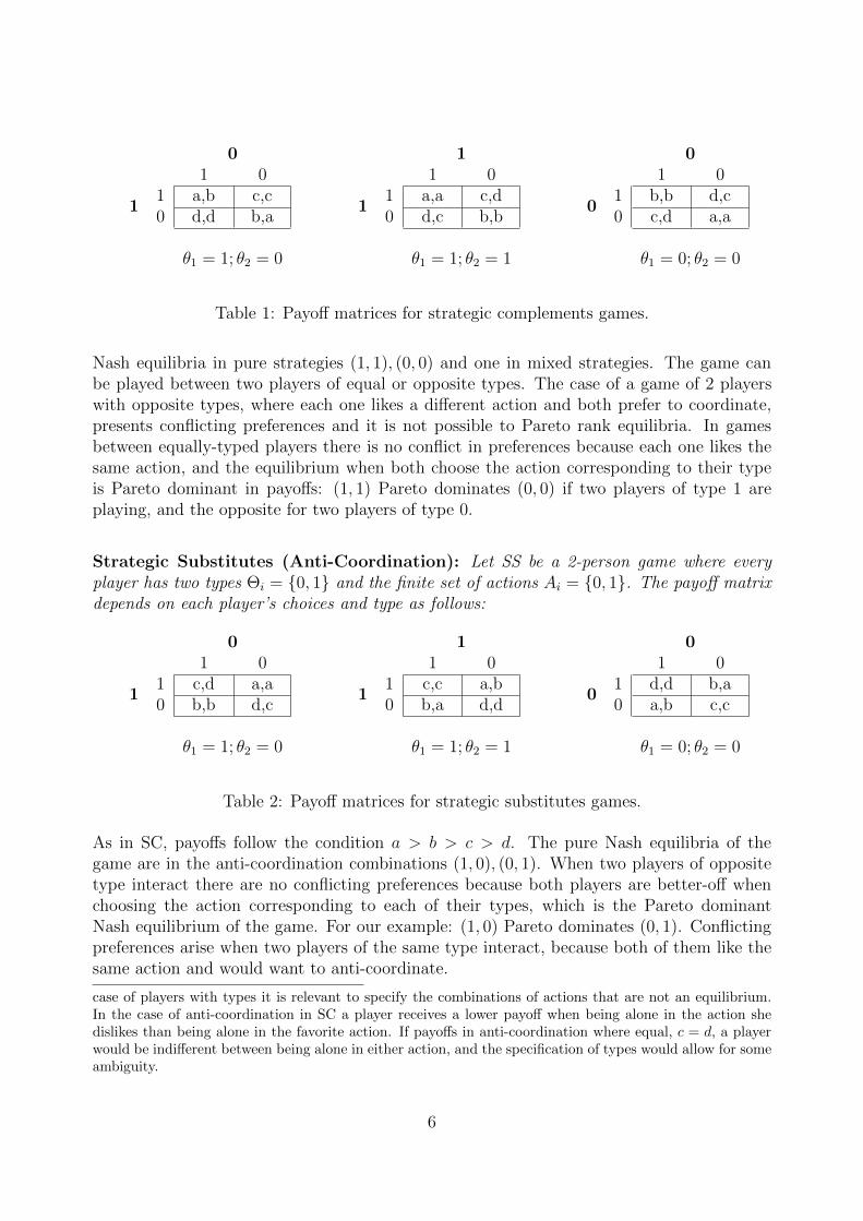
Table 1: Payoff matrices for strategic complements games.

Nash equilibria in pure strategies (1, 1), (0, 0) and one in mixed strategies. The game canbe played between two players of equal or opposite types. The case of a game of 2 playerswith opposite types, where each one likes a different action and both prefer to coordinate,presents conflicting preferences and it is not possible to Pareto rank equilibria. In gamesbetween equally-typed players there is no conflict in preferences because each one likes thesame action, and the equilibrium when both choose the action corresponding to their typeis Pareto dominant in payoffs: (1, 1) Pareto dominates (0, 0) if two players of type 1 areplaying, and the opposite for two players of type 0.

Strategic Substitutes (Anti-Coordination): Let SS be a 2-person game where every

player has two types Θi = {0, 1} and the finite set of actions Ai = {0, 1}. The payoff matrix

depends on each player’s choices and type as follows:

01 0

11 c,d a,a0 b,b d,c

θ1 = 1; θ2 = 0

11 0

11 c,c a,b0 b,a d,d

θ1 = 1; θ2 = 1

01 0

01 d,d b,a0 a,b c,c

θ1 = 0; θ2 = 0

Table 2: Payoff matrices for strategic substitutes games.

As in SC, payoffs follow the condition a > b > c > d. The pure Nash equilibria of thegame are in the anti-coordination combinations (1, 0), (0, 1). When two players of oppositetype interact there are no conflicting preferences because both players are better-off whenchoosing the action corresponding to each of their types, which is the Pareto dominantNash equilibrium of the game. For our example: (1, 0) Pareto dominates (0, 1). Conflictingpreferences arise when two players of the same type interact, because both of them like thesame action and would want to anti-coordinate.

case of players with types it is relevant to specify the combinations of actions that are not an equilibrium.In the case of anti-coordination in SC a player receives a lower payoff when being alone in the action shedislikes than being alone in the favorite action. If payoffs in anti-coordination where equal, c = d, a playerwould be indifferent between being alone in either action, and the specification of types would allow for someambiguity.

6

2.2 The Network Game

Our next step is to proceed from the 2 × 2 games to the network game. To that end, weneed to define a network structure to model the manner in which agents interact. This socialnetwork is denoted as Γ and represented by (N,g), where N = {1, . . . , N} is a finite set ofplayers, and g is the set of undirected links in the network, given by the adjacency matrixof the corresponding graph. The relationship between two players i and j in the network(N,g) is expressed by gij ∈ {0, 1}. When there is a link between them gij = 1, and wesay (i, j) are neighbors. In case they are not connected gij = 0. The set of i’s neighbors isNi(g) = {j ∈ {1, . . . , N}|gij = 1}. A player’s degree is ki(g) = |Ni(g)| = ni the cardinalityof the set Ni(g).

On top of this social network, we introduce the network game in the following way: Playerscan choose actions in a binary set Ai = {0, 1} and have a type that belongs to a set oftypes Θi = {0, 1}. A player i of type θi = 1 likes action ai = 1 and dislikes ai = 0, whichsymmetrically holds for a player of type θi = 0. We use linear payoff functions dependenton a player’s type and choice, where each receives benefit from own and neighbor’s actions.We denote aNi(Γ) as the vector of actions taken by i’s neighbors. The class of game playedis either SC or SS, and correspondingly the payoff function of player i is:

vi(θi, ai, aNi(Γ)) = λθiai[1 + δm

ni�

j=1

I{aj=ai} + (1− δm)ni�

j=1

I{aj �=ai}], (1)

where I{aj=ai} is the indicator function of those neighbors choosing the same action as playeri, and I{aj �=ai} indicates neighbors choosing the opposite; the parameter λθi

ai= α if ai = θi,

and λθiai= β if ai �= θi. The type of game played is specified through the multiplier δm, that

takes value 1 in SC games and 0 in SS games. In all cases, we will assume that payoffs verifythe condition 0 < β < α < 2β, which as we will see below, has different implications for theactions of the players in the two games. Thus, the network game is represented by

Γ = �{1, . . . , N}, {gij}i,j∈{1,...,N}, vi,Θi, Ai�. (2)

In what follows, we will assume local partial information. By this, we mean that a playerin the network knows her degree ki, her type θi, and the set of actions associated to herneighbors aNi , but not their types. In this informational context, player i’s strategy canthen be described as the following map:

σi : θi → Ai, i ∈ {1, . . . , N}. (3)

As can be seen from Eq. (3) the payoff functions depend on the player’s degree ki andidentity, that is, on her type θi. Hence, it is not sufficient for two players of the same degreeki = kj to make the same choice ai = aj in order to have the same payoff function nor toreceive equal payoffs. There is a different payoff function for a player when choosing theaction she likes than when not doing so.

7

Given the local 3 information context we are considering, the equilibrium concept to focuson in the next step is Nash equilibrium.

Definition 1 Nash Equilibrium: An action profile (σ∗1, . . . , σ

∗N) is a Nash equilibrium in

the network game Γ, if and only if

vi(θi, σ∗1, . . . , σ

∗N) ≥ vi(θi, σ

∗1, . . . , σi, . . . , σ

∗N), ∀ σ∗

i�= σi, i ∈ N, and θi ∈ Θ. (4)

We now study separately the equilibria for the two classes of games we are considering.

2.2.1 Strategic Complements

For games with strategic complements, the four payoff functions depending on the player’stype and choice can be written as

vi(1, 1, (aj1 , . . . , ajni)) = α(1 + χi),

vi(1, 0, (aj1 , . . . , ajni)) = β(1 + ni − χi),

vi(0, 0, (aj1 , . . . , ajni)) = α(1 + ni − χi),

vi(0, 1, (aj1 , . . . , ajni)) = β(1 + χi), (5)

where χi =�

ni

j=1 I{aj=1} is the number of i’s neighbors choosing 1, and (ni − χi) =�ni

j=1 I{aj=0} those choosing action 0.

To find the Nash equilibria of the network game in SC, notice that a player is better offchoosing the action she likes than not doing so with the same number of neighbors choosingher same and opposite action. In particular, the condition on the values of α and β introducedabove implies that being alone in the choice one likes gives lower payoffs than choosing thedisliked action and having neighbors making the same choice, i.e., β(1 + ni) > α.

In order to formalize the Nash equilibria, let us define two thresholds, τ(ni) and τ(ni), thatwill be functions of player i’s degree for each type of player in a network game. We definethese thresholds independently of the class of game being played as they will be useful inboth cases. The thresholds are

τ(ni) = � β

α + βni −

α− β

α + β� (6)

τ(ni) = � α

α + βni +

α− β

α + β, � (7)

where �. . .� and �. . .� denote respectively the maximum lower integer or the minimum higherinteger of the real number considered. It can be shown from the payoff functions thatτ(ni) > τ(ni); in fact,

τ(ni)− τ(ni) =α− β

α + βni + 2(

α− β

α + β)− 2 > 0. (8)

8

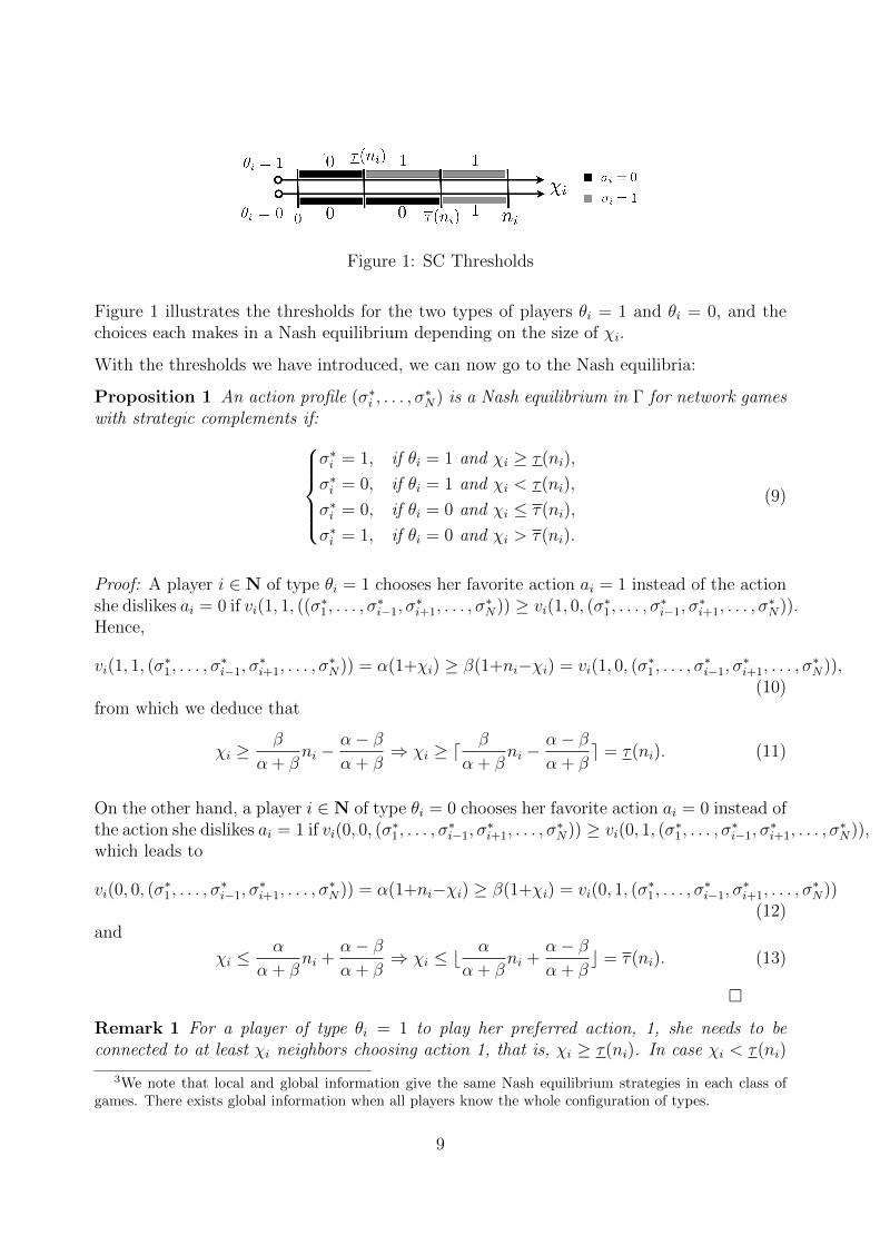
Figure 1: SC Thresholds

Figure 1 illustrates the thresholds for the two types of players θi = 1 and θi = 0, and thechoices each makes in a Nash equilibrium depending on the size of χi.

With the thresholds we have introduced, we can now go to the Nash equilibria:

Proposition 1 An action profile (σ∗i, . . . , σ∗

N) is a Nash equilibrium in Γ for network games

with strategic complements if:

σ∗i= 1, if θi = 1 and χi ≥ τ(ni),

σ∗i= 0, if θi = 1 and χi < τ(ni),

σ∗i= 0, if θi = 0 and χi ≤ τ(ni),

σ∗i= 1, if θi = 0 and χi > τ(ni).

(9)

Proof: A player i ∈ N of type θi = 1 chooses her favorite action ai = 1 instead of the actionshe dislikes ai = 0 if vi(1, 1, ((σ∗

1, . . . , σ∗i−1, σ

∗i+1, . . . , σ

∗N)) ≥ vi(1, 0, (σ∗

1, . . . , σ∗i−1, σ

∗i+1, . . . , σ

∗N)).

Hence,

vi(1, 1, (σ∗1, . . . , σ

∗i−1, σ

∗i+1, . . . , σ

∗N)) = α(1+χi) ≥ β(1+ni−χi) = vi(1, 0, (σ

∗1, . . . , σ

∗i−1, σ

∗i+1, . . . , σ

∗N)),

(10)from which we deduce that

χi ≥β

α + βni −

α− β

α + β⇒ χi ≥ � β

α + βni −

α− β

α + β� = τ(ni). (11)

On the other hand, a player i ∈ N of type θi = 0 chooses her favorite action ai = 0 instead ofthe action she dislikes ai = 1 if vi(0, 0, (σ∗

1, . . . , σ∗i−1, σ

∗i+1, . . . , σ

∗N)) ≥ vi(0, 1, (σ∗

1, . . . , σ∗i−1, σ

∗i+1, . . . , σ

∗N)),

which leads to

vi(0, 0, (σ∗1, . . . , σ

∗i−1, σ

∗i+1, . . . , σ

∗N)) = α(1+ni−χi) ≥ β(1+χi) = vi(0, 1, (σ

∗1, . . . , σ

∗i−1, σ

∗i+1, . . . , σ

∗N))

(12)and

χi ≤α

α + βni +

α− β

α + β⇒ χi ≤ � α

α + βni +

α− β

α + β� = τ(ni). (13)

�Remark 1 For a player of type θi = 1 to play her preferred action, 1, she needs to be

connected to at least χi neighbors choosing action 1, that is, χi ≥ τ(ni). In case χi < τ(ni)

3We note that local and global information give the same Nash equilibrium strategies in each class ofgames. There exists global information when all players know the whole configuration of types.

9

player i adopts her disliked behavior. On the contrary, a player i of type θi = 0 needs to be

connected to at most χi neighbors choosing action 1, that is, χi ≤ τ(ni). In case χi > τ(ni)player i adopts her disliked behavior. If the number of neighbors choosing 1 a given player

has is χi < τ(ni), independently of her type, such player chooses σi = 0, and when χi > τ(ni)she chooses σi = 1. The case in between, where τ(ni) ≤ χi ≤ τ(ni) grants any player to

choose the action corresponding to her type.

2.2.2 Strategic Substitutes

Let us now turn to games with SS, in which as before there are four payoff functions de-pending on a player’s type and choice:

vi(1, 1, (a1, . . . , ajni)) = α(1 + ni − χi)

vi(1, 0, (a1, . . . , ajni)) = β(1 + χi)

vi(0, 0, (a1, . . . , ajni)) = α(1 + χi)

vi(0, 1, (a1, . . . , ajni)) = β(1 + ni − χi). (14)

Reasoning along the same lines as in the previous case, we see that in the case of gameswith SS, a player is better off choosing the action she likes than not doing so with the samenumber of neighbors choosing her same and opposite action. The extreme case of being alonein the choice one likes having all the neighbors coordinating in the same action gives lowerpayoffs than making the disliked choice and having neighbors making the opposite decision,β(1 + ni) > α.

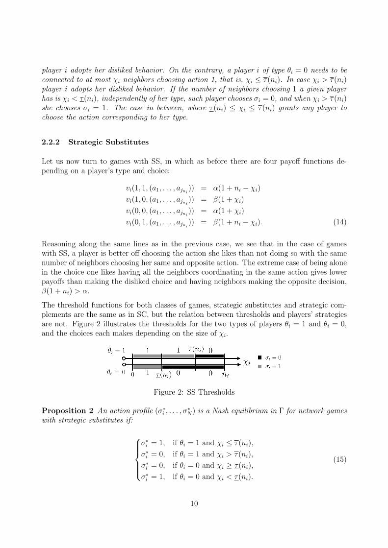
The threshold functions for both classes of games, strategic substitutes and strategic com-plements are the same as in SC, but the relation between thresholds and players’ strategiesare not. Figure 2 illustrates the thresholds for the two types of players θi = 1 and θi = 0,and the choices each makes depending on the size of χi.

Figure 2: SS Thresholds

Proposition 2 An action profile (σ∗i, . . . , σ∗

N) is a Nash equilibrium in Γ for network games

with strategic substitutes if:

σ∗i= 1, if θi = 1 and χi ≤ τ(ni),

σ∗i= 0, if θi = 1 and χi > τ(ni),

σ∗i= 0, if θi = 0 and χi ≥ τ(ni),

σ∗i= 1, if θi = 0 and χi < τ(ni).

(15)

10

Proof: As in the previous case: Player i ∈ N of type θi = 1 chooses her favorite actionai = 1 instead of the action she dislikes ai = 0 if vi(1, 1, (σ∗

1, . . . , σ∗i−1, σ

∗i+1, . . . , σ

∗N)) ≥

vi(1, 0, (σ∗1, . . . , σ

∗i−1, σ

∗i+1, . . . , σ

∗N)), and therefore

vi(1, 1, (σ∗1, . . . , σ

∗i−1, σ

∗i+1, . . . , σ

∗N)) = α(1+ni−χi) ≥ β(1+χi) = vi(1, 0, (σ

∗1, . . . , σ

∗i−1, σ

∗i+1, . . . , σ

∗N)),

(16)leading to

χi ≤α

α + βni +

α− β

α + β⇒ χi ≤ � α

α + βni +

α− β

α + β� = τ(ni). (17)

In the opposite case, player i ∈ N of type θi = 0 chooses her favorite action ai = 0 instead ofthe action she dislikes ai = 1 if vi(0, 0, (σ∗

1, . . . , σ∗i−1, σ

∗i+1, . . . , σ

∗N)) ≥ vi(0, 1, (σ∗

1, . . . , σ∗i−1, σ

∗i+1, . . . , σ

∗N)),

and we have

vi(0, 0, (σ∗1, . . . , σ

∗i−1, σ

∗i+1, . . . , σ

∗N)) = α(1+χi) ≥ β(1+ni−χi) = vi(0, 1, (σ

∗1, . . . , σ

∗i−1, σ

∗i+1, . . . , σ

∗N)),

(18)and hence

χi ≥β

α + βni −

α− β

α + β⇒ χi ≥ � β

α + βni −

α− β

α + β� = τ(ni). (19)

�Remark 2 For a player of type θi = 1 to play her preferred action 1, she needs to be

connected to at most χi neighbors choosing action 1, that is, χi ≤ τ(ni). In case χi > τ(ni)player i adopts her disliked behavior. A player i of type θi = 0 needs to be connected to

at least χi neighbors choosing action 1, that is, χi ≥ τ(ni). In case χi < τ(ni) player i

adopts her disliked behavior. If the number of neighbors a given player has, choosing 1 is

χi < τ(ni), independently of her type, a player chooses σi = 1, and when χi > τ(ni) she

chooses σi = 0. The case in between, where τ(ni) ≤ χi ≤ τ(ni) grants any player to choose

the action corresponding to her type.

Remark 3 For the network games discussed in Galeotti et al. (2010), under incomplete

information the authors show that the Bayesian Nash equilibrium payoff is non-decreasing

(non-increasing) in the degree of the players for the case of SC (SS). While, due to the exis-

tence of types in the population, a similar result cannot be proven here, we find it noticeable

that the Nash equilibria we obtain are reminiscent of that structure in the sense that the

payoff is non-increasing or non-decreasing on the number of neighbors playing 1, χi. In fact,

the result of Galeotti et al. is recovered when there is only one type of players in the network.

2.3 Equilibrium Configurations

In the previous subsection we have seen what are the conditions for players of each typeto choose an action. These conditions, when applied to the network game as a whole,lead to a variety of equilibrium configurations associated to the choices each player makesand to the distribution of types. In order to classify all these equilibrium networks, in whatfollows we introduce some notation. Beginning with the actions, a network can be specialized

11

(S) or hybrid (H). A specialized action profile is one in which all players make the samechoice. Therefore, there are configurations specialized in action one, S1, or in action zero,S0. In a hybrid action profile, both actions are present. Second, regarding players’ types, anetwork can be frustrated (F ) or satisfactory (S). In a satisfactory configuration, each playerchooses her favorite action corresponding to her type, and in the frustrated one at least oneplayer adopts the disliked choice. As a result, we may observe six (two) different networkconfigurations in SC (SS) depending on the distribution of types and the action profile:SS1, SS0, FS1, FS0, SH , FH (SH , FH) (subindices refer to the category in terms of actions).Note that we are claiming that specialized networks only exist in SC games. This is due to thefact that the anti-coordination condition on the payoffs for SS does not allow an equilibriumwhere all players make the same choice. Finally, satisfactory specialized configurations areonly possible under a very strong restriction to the type of the players: Indeed, SS1 and FS1

require that the set {θi = 0} = ∅, whereas SS0 and FS0 require {θi = 1} = ∅.

We now discuss the condition under which the different equilibrium configurations arise. Asindicated above, the first proposition below refers only to SC games:

Proposition 3 The configuration of a network Γ(N,g) in equilibrium is frustrated spe-cialized when all players choose one same action, so that ai = aj, ∀ i, j ∈ {1, . . . , N}. A

network is specialized in action 1(0) if and only if the following three conditions are jointly

satisfied:

1. Players of type θi = 1 have χi ≥ τ(ni)(χi < τ(ni)) neighbors

2. Players of type θi = 0 have χi > τ(ni)(χi ≤ τ(ni)) neighbors

3. All players of degree ki(g) = 0 are θi = 1(θi = 0)

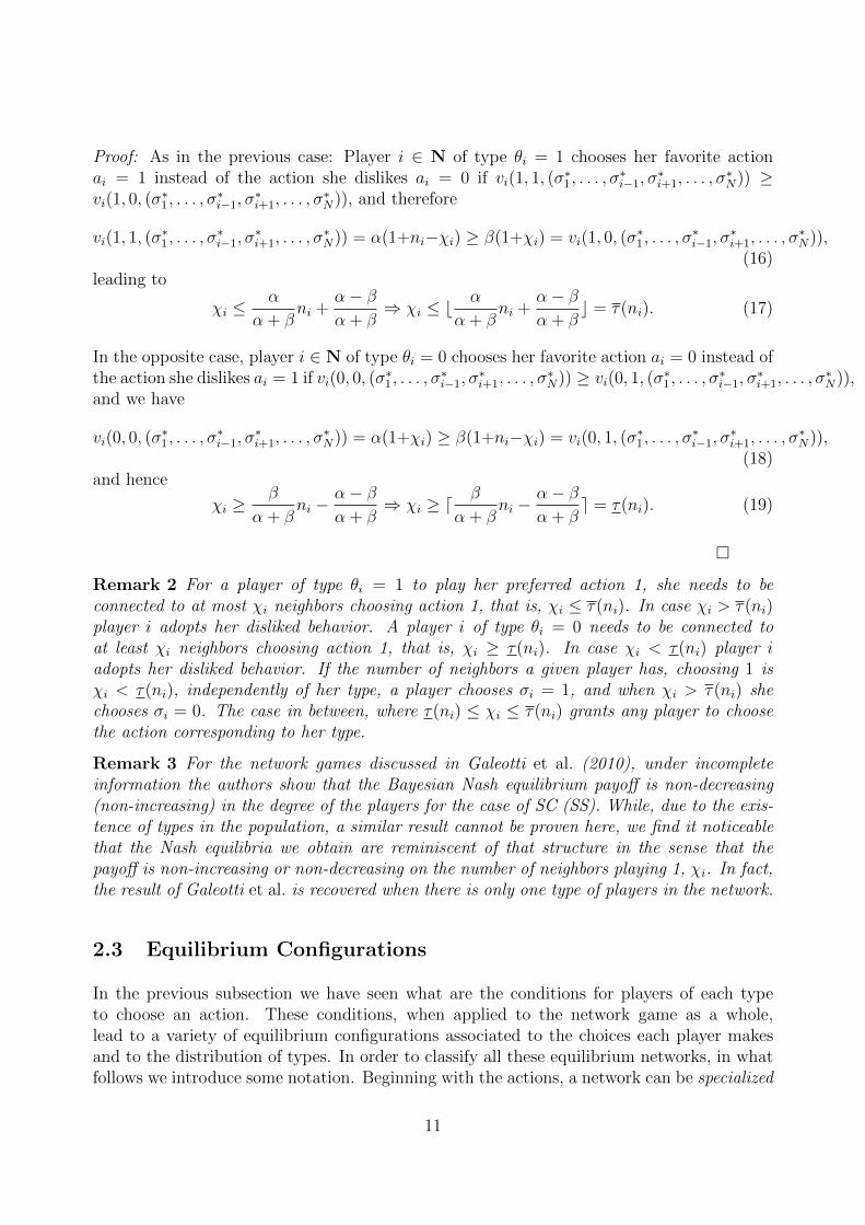
Example 1 If a situation in which all players are of degree ki(g) = 2, like in a circle (see

Fig. 3, middle graph), with just one neighbor of the same type, all players can sustain the

action they like. To specialize such a network, it is necessary for a player who dislikes the

specialized choice to have both of her neighbors of the opposite type. The same idea and

opposite symmetric conditions hold for the case of a network specialized in action 0. Figure3 illustrates some cases.

Figure 3: Frustrated Specialized Configurations. The first digit refers to the type, the seconddigit refers to the action.

12

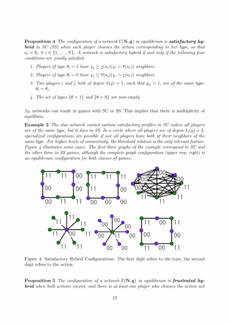
Proposition 4 The configuration of a network Γ(N,g) in equilibrium is satisfactory hy-brid in SC (SS) when each player chooses the action corresponding to her type, so that

ai = θi, ∀ i ∈ {1, . . . , N}. A network is satisfactory hybrid if and only if the following four

conditions are jointly satisfied:

1. Players of type θi = 1 have χi ≥ τ(ni)(χi < τ(ni)) neighbors

2. Players of type θi = 0 have χi ≤ τ(ni)(χi > τ(ni)) neighbors

3. Two players i and j both of degree k(g) = 1, such that gij = 1, are of the same type:

θi = θj

4. The set of types {θ = 1} and {θ = 0} are non-empty.

SH networks can result in games with SC or SS. This implies that there is multiplicity ofequilibria.

Example 2 The star network cannot sustain satisfactory profiles in SC unless all players

are of the same type, but it does in SS. In a circle where all players are of degree ki(g) = 2,specialized configurations are possible if not all players have both of their neighbors of the

same type. For higher levels of connectivity, the threshold relation is the only relevant feature.

Figure 4 illustrates some cases. The first three graphs of the example correspond to SC and

the other three to SS games, although the complete graph configuration (upper row, right) is

an equilibrium configuration for both classes of games.

Figure 4: Satisfactory Hybrid Configurations. The first digit refers to the type, the seconddigit refers to the action.

Proposition 5 The configuration of a network Γ(N,g) in equilibrium is frustrated hy-brid when both actions coexist, and there is at least one player who chooses the action not

13

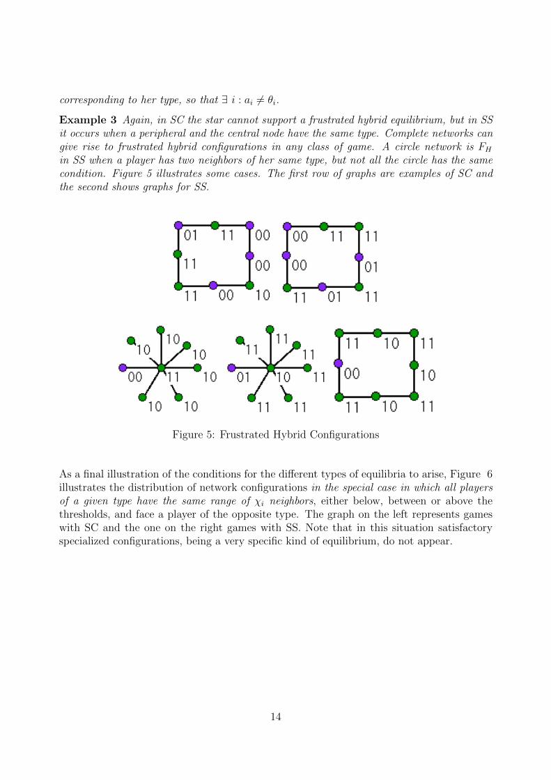
corresponding to her type, so that ∃ i : ai �= θi.

Example 3 Again, in SC the star cannot support a frustrated hybrid equilibrium, but in SS

it occurs when a peripheral and the central node have the same type. Complete networks can

give rise to frustrated hybrid configurations in any class of game. A circle network is FH

in SS when a player has two neighbors of her same type, but not all the circle has the same

condition. Figure 5 illustrates some cases. The first row of graphs are examples of SC and

the second shows graphs for SS.

Figure 5: Frustrated Hybrid Configurations

As a final illustration of the conditions for the different types of equilibria to arise, Figure 6illustrates the distribution of network configurations in the special case in which all players

of a given type have the same range of χi neighbors, either below, between or above thethresholds, and face a player of the opposite type. The graph on the left represents gameswith SC and the one on the right games with SS. Note that in this situation satisfactoryspecialized configurations, being a very specific kind of equilibrium, do not appear.

14

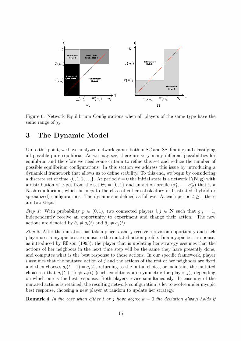
Figure 6: Network Equilibrium Configurations when all players of the same type have thesame range of χi.

3 The Dynamic Model

Up to this point, we have analyzed network games both in SC and SS, finding and classifyingall possible pure equilibria. As we may see, there are very many different possibilities forequilibria, and therefore we need some criteria to refine this set and reduce the number ofpossible equilibrium configurations. In this section we address this issue by introducing adynamical framework that allows us to define stability. To this end, we begin by consideringa discrete set of time {0, 1, 2, . . .}. At period t = 0 the initial state is a network Γ(N,g) witha distribution of types from the set Θi = {0, 1} and an action profile (σ∗

1, . . . , σ∗N) that is a

Nash equilibrium, which belongs to the class of either satisfactory or frustrated (hybrid orspecialized) configurations. The dynamics is defined as follows: At each period t ≥ 1 thereare two steps:

Step 1: With probability p ∈ (0, 1), two connected players i, j ∈ N such that gij = 1,independently receive an opportunity to experiment and change their action. The newactions are denoted by ai �= ai(t) and aj �= aj(t).

Step 2: After the mutation has taken place, i and j receive a revision opportunity and eachplayer uses a myopic best response to the mutated action profile. In a myopic best response,as introduced by Ellison (1993), the player that is updating her strategy assumes that theactions of her neighbors in the next time step will be the same they have presently done,and computes what is the best response to those actions. In our specific framework, playeri assumes that the mutated action of j and the actions of the rest of her neighbors are fixedand then chooses ai(t+ 1) = ai(t), returning to the initial choice, or maintains the mutatedchoice so that ai(t + 1) �= ai(t) (such conditions are symmetric for player j), dependingon which one is the best response. Both players revise simultaneously. In case any of themutated actions is retained, the resulting network configuration is let to evolve under myopicbest response, choosing a new player at random to update her strategy.

Remark 4 In the case when either i or j have degree k = 0 the deviation always holds if

15

xi(t + 1) = θi. Therefore, the case of an isolated component can be treated as a network on

its own, and a network of only one node lacks of any interest. If gij = 0, so that i and j

are not neighbors, the mutation corresponds to an equivalent case of a unilateral deviation,

which is never a Nash equilibrium; myopic best response dynamics would immediately revert

the action to the original choice. The same argument holds if only one player mutates, either

i or j, even if they are connected. It is important to note that the resulting network after the

dynamics does not need to be a Nash equilibrium configuration, although it can subsequently

converge to one.

Stable Equilibrium: A Nash-network E(Γ) is stable if in time t + 1, for any pair of

mutated neighbors i, j ∈ N their myopic best response coincides with the previous action:

ai(t+1) = ai(t) and aj(t+1) = aj(t), i.e., the network configuration returns to its initial state.

We will denote by SSC(Γ) the set of stable networks in games with strategic complements,

and SSS(Γ) the set of stable networks in games with strategic substitutes.

3.1 Stable Equilibria in SC

As before, we discuss separately the two cases of SS and SC games, beginning with theformer.

Proposition 6 The set of Stable Equilibria in SC is a proper non-empty set of the Nash

equilibrium network: SSC(Γ) ⊂ E(Γ)

Proof : In order to prove that there exist equilibrium networks that are not stable in SC,we proceed to compute the stability conditions for each possible combination of types andactions. We obtain conditions that depend on χi, which is the number of neighbors ofplayer i taking action 1. However, to those conditions one needs to add the correspondingones arising from the fact that the starting configuration is a Nash equilibrium. Thesetwo sets of constraints, taken together, lead to a more restrictive condition than the Nashequilibrium one alone, and therefore, the set of stable networks is included in the set of Nashequilibrium.

The details of the proof go as follows: Let us fix two mutated and connected nodes i, j ∈ N.First, take the same type θi = θj and the same associated actions ai = aj for 0 or 1. Second,one has to consider the case of type inequality, θi �= θj, and explore two cases: When eachagent chooses her preferred action, θi = ai, θj = aj, and the opposite case, θi �= ai or θj �= aj.This study of six cases covers the most relevant instances and the remaining possibilities canbe checked in the same way. We now go into the details of these cases, whereas the completeset of conditions is provided in table 3.

I- Let i, j ∈ N be two connected nodes, gij = 1, such that i �= j and θi = θj = 1. Supposethat the choices made by the pair of players at time t are ai = aj = 1. The dynamics act asfollows:

Step 1: A mutation affects (i, j) ⇒ ai = aj = 0.

16

Step 2: Myopic Best Response (MBR). The new actions are: Player at node i plays ai(t+1) =1 (same condition holds for player j), iff:

χi − 1 ≥ τ(ni) = � β

α + βni −

α− β

α + β� ⇒

χi ≥ � β

α + βni −

α− β

α + β�+ 1 = � β

α + βni −

α− β

α + β+ 1� = �β(ni + 2)

α + β�. (20)

II- Let i, j ∈ N be two connected nodes, gij = 1, such that i �= j and θi = θj = 0. Supposethat the choices made by the pair of players at time t are ai = aj = 0. The dynamics act asfollows:


Step 2: MBR: Player at node i plays ai(t + 1) = 0 (same condition holds for player j),iff:

χi + 1 ≤ τ(ni) = � α

α + βni +

α− β

α + β� ⇒

χi ≤ � α

α + βni +

α− β

α + β� − 1 = � α

α + βni +

α− β

α + β− 1� = �αni − 2β

α + β�. (21)

III- Let i, j ∈ N be two connected nodes, gij = 1, such that i �= j and θi = θj = 1. Supposethat the choices made by the pair of players at time t are ai = 1 = θi, aj = 0 �= θj. Thedynamics act as follows:

Step 1: A mutation affects (i, j) ⇒ ai = 0, aj = 1.

Step 2: MBR: Player at node i plays ai(t+ 1) = 1 iff:

χi + 1 ≥ τ(ni) = � β

α + βni −

α− β

α + β� ⇒

χi ≥ � β

α + βni −

α− β

α + β� − 1 = � β

α + βni −

α− β

α + β− 1� = �βni − 2α

α + β�. (22)

Player at node j plays aj(t+ 1) = 0 iff:

χj − 1 < τ(nj) = � β

α + βnj −

α− β

α + β� ⇒

χj < � β

α + βnj −

α− β

α + β�+ 1 = � β

α + βnj −

α− β

α + β+ 1� = �β(nj + 2)

α + β�. (23)

IV- Let i, j ∈ N be two connected nodes, gij = 1, such that i �= j and θi = θj = 0. Supposethat the choices made by the pair of players at time t are ai = aj = 1 �= θi = θj. Thedynamics act as follows:


17

Step 2: MBR : Player at node i plays ai(t + 1) = 1 (same condition holds for player j),iff:

χi − 1 > τ(ni) = � α

α + βni +

α− β

α + β� ⇒

χi > � α

α + βni +

α− β

α + β�+ 1 = � α

α + βni +

α− β

α + β+ 1� = �αni − 2β

α + β�. (24)

V- Let i, j ∈ N be two connected nodes, gij = 1, such that i �= j and θi = 1, θj = 0. Supposethat the choices made by the pair of players at time t are ai = 1, aj = 0. The dynamics actas follows:

Step 1: A mutation affects (i, j) ⇒ ai = 0, aj = 1.


χi + 1 ≥ τ(ni) = � β

α + βni −

α− β

α + β� ⇒

χi ≥ � β

α + βni −

α− β

α + β� − 1 = � β

α + βni −

α− β

α + β− 1� = �βni − 2α

α + β�. (25)


χj − 1 ≤ τ(nj) = � α

α + βnj +

α− β

α + β� ⇒

χj ≤ � α

α + βnj +

α− β

α + β�+ 1 = � α

α + βnj +

α− β

α + β+ 1� = �α(nj + 2)

α + β�. (26)

VI- Let i, j ∈ N be two connected nodes, gij = 1, such that i �= j and θi = 1, θj = 0. Supposethat the choices made by the pair of players at time t are ai = 0 �= θi, aj = 1 �= θj. Thedynamics act as follows:

Step 1: A mutation affects (i, j) ⇒ ai = 1, aj = 0


χi − 1 < τ(ni) = � β

α + βni −

α− β

α + β� ⇒

χi < � β

α + βni −

α− β

α + β�+ 1 = � β

α + βni −

α− β

α + β+ 1� = �β(ni + 2)

α + β�. (27)


χj + 1 > τ(nj) = � α

α + βnj +

α− β

α + β� ⇒

χj > � α

α + βnj +

α− β

α + β� − 1 = � α

α + βnj +

α− β

α + β− 1� = �αnj − 2β

α + β�. (28)

18

θi = θj = 1 θi = θj = 0 θi = 1, θj = 0ai = aj = 1 χi ≥ τ(ni) + 1 χi > τ(ni) + 1 χi ≥ τ(ni) + 1

χj ≥ τ(nj) + 1 χj > τ(nj) + 1 χj > τ(nj) + 1ai = aj = 0 χi < τ(ni)− 1 χi ≤ τ(ni)− 1 χi < τ(ni)− 1

χj < τ(nj)− 1 χj ≤ τ(nj)− 1 χj ≤ τ(nj)− 1ai = 1, aj = 0 * χi ≥ τ(ni)− 1 * χi > τ(ni)− 1 * χi ≥ τ(ni)− 1

* χj < τ(nj) + 1 * χj ≤ τ(nj) + 1 * χj ≤ τ(nj) + 1ai = 0, aj = 1 * χi < τ(ni) + 1 * χi ≥ τ(ni) + 1 * χi < τ(ni) + 1

* χj ≥ τ(nj)− 1 * χj > τ(nj)− 1 * χj > τ(nj)− 1

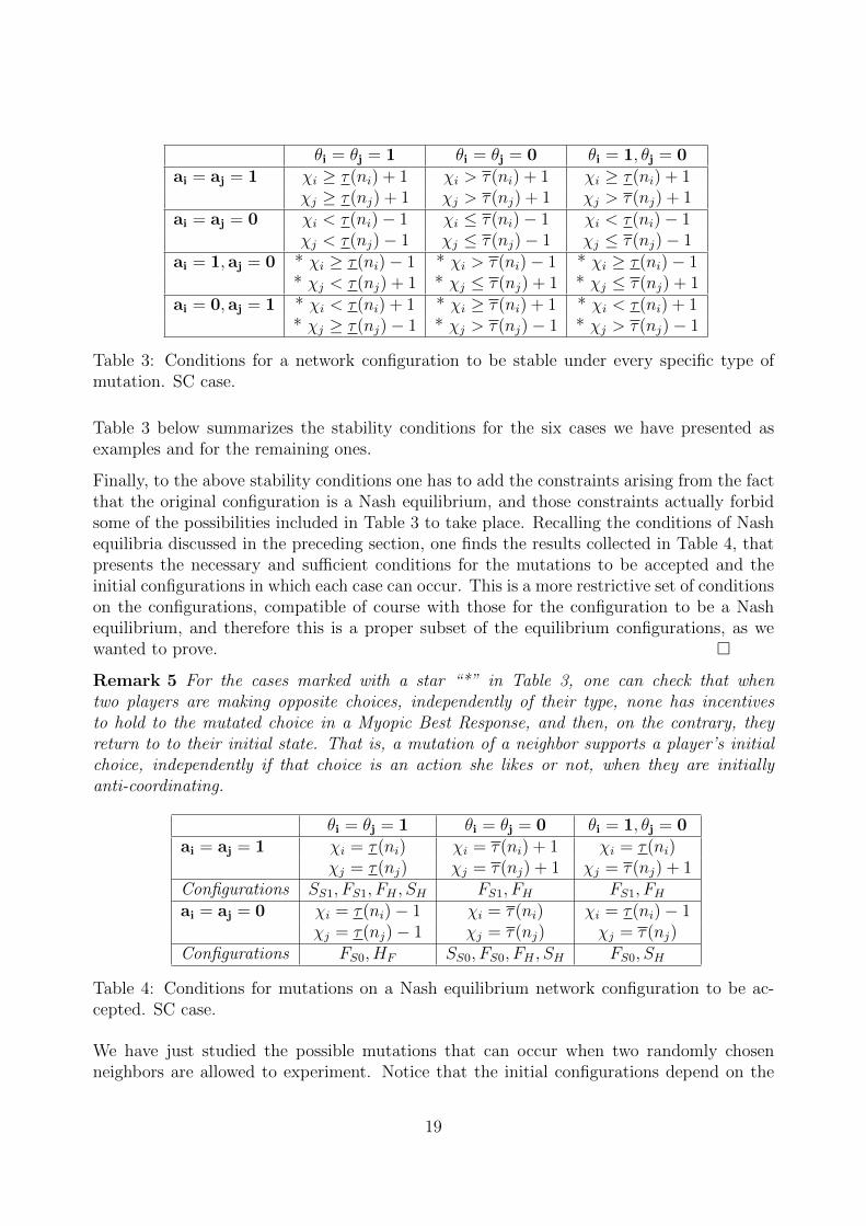
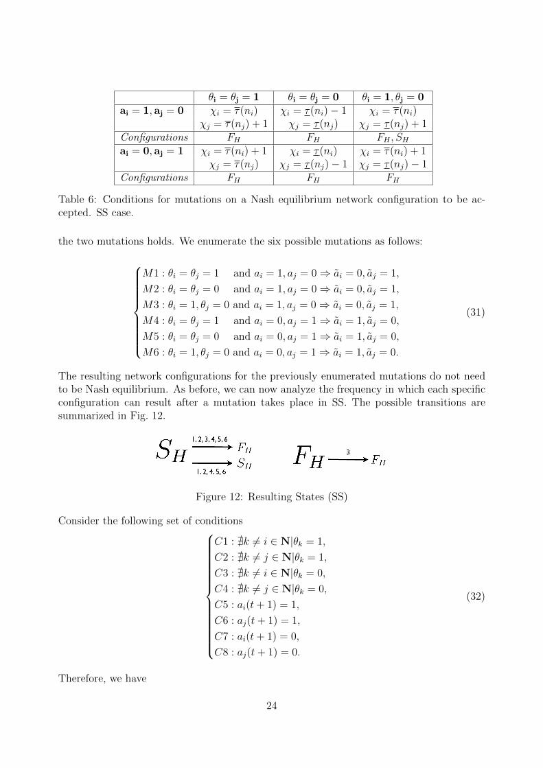
Table 3: Conditions for a network configuration to be stable under every specific type ofmutation. SC case.

Table 3 below summarizes the stability conditions for the six cases we have presented asexamples and for the remaining ones.

Finally, to the above stability conditions one has to add the constraints arising from the factthat the original configuration is a Nash equilibrium, and those constraints actually forbidsome of the possibilities included in Table 3 to take place. Recalling the conditions of Nashequilibria discussed in the preceding section, one finds the results collected in Table 4, thatpresents the necessary and sufficient conditions for the mutations to be accepted and theinitial configurations in which each case can occur. This is a more restrictive set of conditionson the configurations, compatible of course with those for the configuration to be a Nashequilibrium, and therefore this is a proper subset of the equilibrium configurations, as wewanted to prove. �Remark 5 For the cases marked with a star “*” in Table 3, one can check that when

two players are making opposite choices, independently of their type, none has incentives

to hold to the mutated choice in a Myopic Best Response, and then, on the contrary, they

return to to their initial state. That is, a mutation of a neighbor supports a player’s initial

choice, independently if that choice is an action she likes or not, when they are initially

anti-coordinating.

θi = θj = 1 θi = θj = 0 θi = 1, θj = 0ai = aj = 1 χi = τ(ni) χi = τ(ni) + 1 χi = τ(ni)

χj = τ(nj) χj = τ(nj) + 1 χj = τ(nj) + 1Configurations SS1, FS1, FH , SH FS1, FH FS1, FH

ai = aj = 0 χi = τ(ni)− 1 χi = τ(ni) χi = τ(ni)− 1χj = τ(nj)− 1 χj = τ(nj) χj = τ(nj)

Configurations FS0, HF SS0, FS0, FH , SH FS0, SH

Table 4: Conditions for mutations on a Nash equilibrium network configuration to be ac-cepted. SC case.

We have just studied the possible mutations that can occur when two randomly chosenneighbors are allowed to experiment. Notice that the initial configurations depend on the

19

distribution of types and choices made by the pair of randomly chosen neighbors. Hence,for example, no case in the first row in Table 4 can arise from a FS0 as the initial condition,because at least two players (i, j) must be choosing action one.

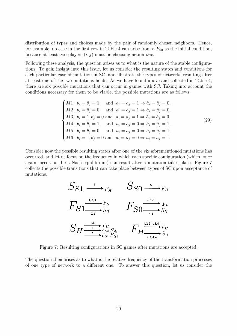
Following these analysis, the question arises as to what is the nature of the stable configura-tions. To gain insight into this issue, let us consider the resulting states and conditions foreach particular case of mutation in SC, and illustrate the types of networks resulting afterat least one of the two mutations holds. As we have found above and collected in Table 4,there are six possible mutations that can occur in games with SC. Taking into account theconditions necessary for them to be viable, the possible mutations are as follows:

M1 : θi = θj = 1 and ai = aj = 1 ⇒ ai = aj = 0,


M3 : θi = 1, θj = 0 and ai = aj = 1 ⇒ ai = aj = 0,



M6 : θi = 1, θj = 0 and ai = aj = 0 ⇒ ai = aj = 1.

(29)

Consider now the possible resulting states after one of the six aforementioned mutations hasoccurred, and let us focus on the frequency in which each specific configuration (which, onceagain, needs not be a Nash equilibrium) can result after a mutation takes place. Figure 7collects the possible transitions that can take place between types of SC upon acceptance ofmutations.

Figure 7: Resulting configurations in SC games after mutations are accepted.

The question then arises as to what is the relative frequency of the transformation processesof one type of network to a different one. To answer this question, let us consider the

20

following set of conditions:

C1 : �k �= i ∈ N|θk = 1,

C2 : �k �= j ∈ N|θk = 1,

C3 : �k �= i ∈ N|θk = 0,

C4 : �k �= j ∈ N|θk = 0,

C5 : ai(t+ 1) = 1,

C6 : aj(t+ 1) = 1,

C7 : ai(t+ 1) = 0,

C8 : aj(t+ 1) = 0.

(30)

With this notation, it is straightforward to see that the following transitions are possi-ble:

• FS1 → SH iff conditions c3, c4, c7, c8 hold for mutation 2 (M2) in Eq. (29), or iff c4, c8in M1.

• FS1 → FH iff c7 or c7, c8 hold in M3.

• S0 → SH iff c1, c2, c7, c8 hold in M4, or iff c1, c5, c8 hold in M6.

• SH → FS0 iff c1, c2, c5, c6 hold in M1.

• SH → FS1 iff c3, c4, c5, c6 hold in M5.

• SH → SH iff c3, c4, c7, c8 hold in M2, or iff c1, c2, c7, c8 hold in M4, or iff c1, c5, c8 inM6.

• SH → FS1 iff c4, c5, c6 hold in M6.

In the remaining cases if one or both mutations hold, the resulting configuration will nec-essarily be frustrated hybrid. From this enumeration and the list of possible processes, itbecomes clear that, generally speaking, the result of the acceptance of a mutation will veryoften be frustrated hybrid, and, on the other hand, specialized configurations are by far themost unstable ones.

In view of the large number of conditions and possibilities we have summarized above, wefind it illuminating to discuss a few examples of the mutation process.

Example 4 Let Γ be a complete frustrated specialized network FS1 (see Fig. 8). There is

a pair of neighbor players θi = 1 and θj = 0 whose actions mutate. Both players then

revise simultaneously and follow their myopic best response. For definiteness, let us choose

2α ≥ 3β, so that player i has incentives to return to the same action she had in time t in

which ai(t) = ai(t+ 1) = θi, however, player j, responding myopically to the action she has

observed in her present time, chooses aj(t+1) = θj. The resulting state is a frustrated hybrid

configuration that is not a Nash equilibrium.

Example 5 Let Γ be a complete satisfactory hybrid network SH (see Fig. 9). There is

a pair of neighbor players θi = 1 and θj = 0 whose actions mutate. Both players then

revise simultaneously and follow their myopic best response. Consider again that 2α ≥ 3β,

21

→ →

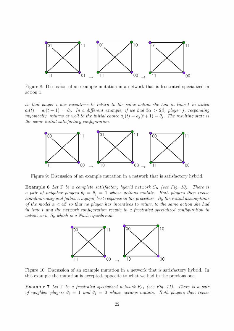
Figure 8: Discussion of an example mutation in a network that is frustrated specialized inaction 1.

so that player i has incentives to return to the same action she had in time t in which

ai(t) = ai(t + 1) = θi. In a different example, if we had 3α > 2β, player j, responding

myopically, returns as well to the initial choice aj(t) = aj(t+ 1) = θj. The resulting state is

the same initial satisfactory configuration.

→ →

Figure 9: Discussion of an example mutation in a network that is satisfactory hybrid.


a pair of neighbor players θi = θj = 1 whose actions mutate. Both players then revise

simultaneously and follow a myopic best response in the procedure. By the initial assumptions

of the model α < 4β so that no player has incentives to return to the same action she had

in time t and the network configuration results in a frustrated specialized configuration in

action zero, S0 which is a Nash equilibrium.

→

Figure 10: Discussion of an example mutation in a network that is satisfactory hybrid. Inthis example the mutation is accepted, opposite to what we had in the previous one.

Example 7 Let Γ be a frustrated specialized network FS1 (see Fig. 11). There is a pair

of neighbor players θi = 1 and θj = 0 whose actions mutate. Both players then revise

22

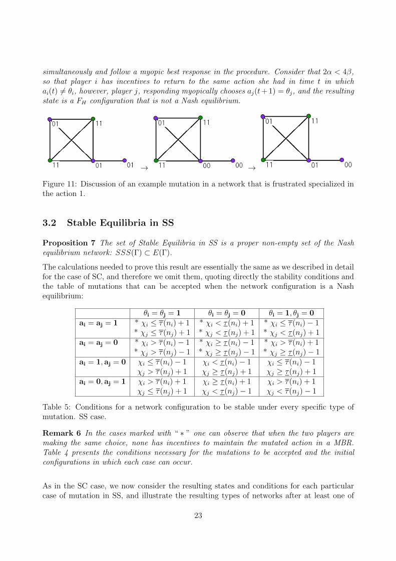
simultaneously and follow a myopic best response in the procedure. Consider that 2α < 4β,so that player i has incentives to return to the same action she had in time t in which

ai(t) �= θi, however, player j, responding myopically chooses aj(t+1) = θj, and the resulting

state is a FH configuration that is not a Nash equilibrium.

→ →

Figure 11: Discussion of an example mutation in a network that is frustrated specialized inthe action 1.

3.2 Stable Equilibria in SS

Proposition 7 The set of Stable Equilibria in SS is a proper non-empty set of the Nash

equilibrium network: SSS(Γ) ⊂ E(Γ).

The calculations needed to prove this result are essentially the same as we described in detailfor the case of SC, and therefore we omit them, quoting directly the stability conditions andthe table of mutations that can be accepted when the network configuration is a Nashequilibrium:

θi = θj = 1 θi = θj = 0 θi = 1, θj = 0ai = aj = 1 * χi ≤ τ(ni) + 1 * χi < τ(ni) + 1 * χi ≤ τ(ni)− 1

* χj ≤ τ(nj) + 1 * χj < τ(nj) + 1 * χj < τ(nj) + 1ai = aj = 0 * χi > τ(ni)− 1 * χi ≥ τ(ni)− 1 * χi > τ(ni) + 1

* χj > τ(nj)− 1 * χj ≥ τ(nj)− 1 * χj ≥ τ(nj)− 1ai = 1, aj = 0 χi ≤ τ(ni)− 1 χi < τ(ni)− 1 χi ≤ τ(ni)− 1

χj > τ(nj) + 1 χj ≥ τ(nj) + 1 χj ≥ τ(nj) + 1ai = 0, aj = 1 χi > τ(ni) + 1 χi ≥ τ(ni) + 1 χi > τ(ni) + 1

χj ≤ τ(nj) + 1 χj < τ(nj)− 1 χj < τ(nj)− 1

Table 5: Conditions for a network configuration to be stable under every specific type ofmutation. SS case.

Remark 6 In the cases marked with “ ∗ ” one can observe that when the two players are

making the same choice, none has incentives to maintain the mutated action in a MBR.

Table 4 presents the conditions necessary for the mutations to be accepted and the initial

configurations in which each case can occur.

As in the SC case, we now consider the resulting states and conditions for each particularcase of mutation in SS, and illustrate the resulting types of networks after at least one of

23

θi = θj = 1 θi = θj = 0 θi = 1, θj = 0ai = 1, aj = 0 χi = τ(ni) χi = τ(ni)− 1 χi = τ(ni)

χj = τ(nj) + 1 χj = τ(nj) χj = τ(nj) + 1Configurations FH FH FH , SH

ai = 0, aj = 1 χi = τ(ni) + 1 χi = τ(ni) χi = τ(ni) + 1χj = τ(nj) χj = τ(nj)− 1 χj = τ(nj)− 1

Configurations FH FH FH

Table 6: Conditions for mutations on a Nash equilibrium network configuration to be ac-cepted. SS case.

the two mutations holds. We enumerate the six possible mutations as follows:

M1 : θi = θj = 1 and ai = 1, aj = 0 ⇒ ai = 0, aj = 1,


M3 : θi = 1, θj = 0 and ai = 1, aj = 0 ⇒ ai = 0, aj = 1,



M6 : θi = 1, θj = 0 and ai = 0, aj = 1 ⇒ ai = 1, aj = 0.

(31)

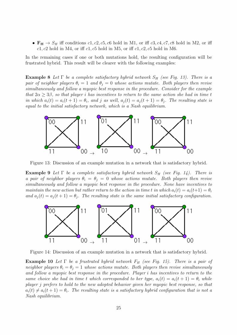
The resulting network configurations for the previously enumerated mutations do not needto be Nash equilibrium. As before, we can now analyze the frequency in which each specificconfiguration can result after a mutation takes place in SS. The possible transitions aresummarized in Fig. 12.

Figure 12: Resulting States (SS)

Consider the following set of conditions

C1 : �k �= i ∈ N|θk = 1,

C2 : �k �= j ∈ N|θk = 1,

C3 : �k �= i ∈ N|θk = 0,

C4 : �k �= j ∈ N|θk = 0,

C5 : ai(t+ 1) = 1,

C6 : aj(t+ 1) = 1,

C7 : ai(t+ 1) = 0,

C8 : aj(t+ 1) = 0.

(32)

Therefore, we have

24

• FH → SH iff conditions c1, c2, c5, c6 hold in M1, or iff c3, c4, c7, c8 hold in M2, or iffc1, c2 hold in M4, or iff c1, c5 hold in M5, or iff c1, c2, c5 hold in M6.

In the remaining cases if one or both mutations hold, the resulting configuration will befrustrated hybrid. This result will be clearer with the following examples:

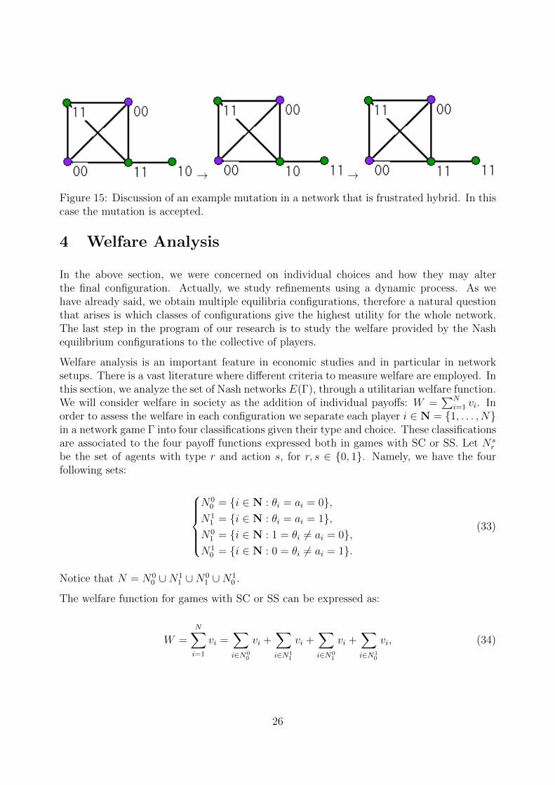
Example 8 Let Γ be a complete satisfactory hybrid network SH (see Fig. 13). There is a

pair of neighbor players θi = 1 and θj = 0 whose actions mutate. Both players then revise

simultaneously and follow a myopic best response in the procedure. Consider for the example

that 2α ≥ 3β, so that player i has incentives to return to the same action she had in time t

in which ai(t) = ai(t + 1) = θi, and j as well, aj(t) = aj(t + 1) = θj. The resulting state is

equal to the initial satisfactory network, which is a Nash equilibrium.

→ →



a pair of neighbor players θi = θj = 0 whose actions mutate. Both players then revise

simultaneously and follow a myopic best response in the procedure. None have incentives to

maintain the new action but rather return to the action in time t in which ai(t) = ai(t+1) = θiand aj(t) = aj(t+ 1) = θj. The resulting state is the same initial satisfactory configuration.

→ →


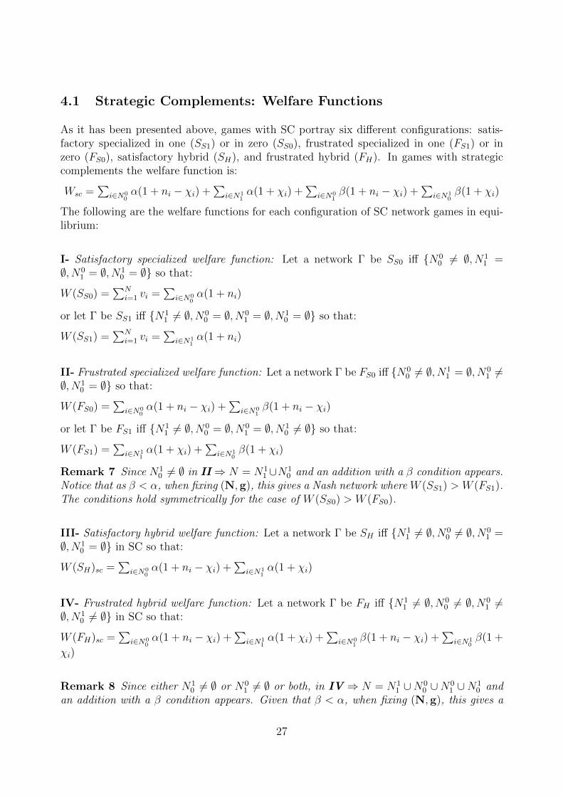
Example 10 Let Γ be a frustrated hybrid network FH (see Fig. 15). There is a pair of

neighbor players θi = θj = 1 whose actions mutate. Both players then revise simultaneously

and follow a myopic best response in the procedure. Player i has incentives to return to the

same choice she had in time t which corresponded to her type, ai(t) = ai(t + 1) = θi whileplayer j prefers to hold to the new adopted behavior given her myopic best response, so that

ai(t) �= ai(t+ 1) = θi. The resulting state is a satisfactory hybrid configuration that is not a

Nash equilibrium.

25

→ →

Figure 15: Discussion of an example mutation in a network that is frustrated hybrid. In thiscase the mutation is accepted.

4 Welfare Analysis

In the above section, we were concerned on individual choices and how they may alterthe final configuration. Actually, we study refinements using a dynamic process. As wehave already said, we obtain multiple equilibria configurations, therefore a natural questionthat arises is which classes of configurations give the highest utility for the whole network.The last step in the program of our research is to study the welfare provided by the Nashequilibrium configurations to the collective of players.

Welfare analysis is an important feature in economic studies and in particular in networksetups. There is a vast literature where different criteria to measure welfare are employed. Inthis section, we analyze the set of Nash networks E(Γ), through a utilitarian welfare function.We will consider welfare in society as the addition of individual payoffs: W =

�N

i=1 vi. Inorder to assess the welfare in each configuration we separate each player i ∈ N = {1, . . . , N}in a network game Γ into four classifications given their type and choice. These classificationsare associated to the four payoff functions expressed both in games with SC or SS. Let N s

r

be the set of agents with type r and action s, for r, s ∈ {0, 1}. Namely, we have the fourfollowing sets:

N00 = {i ∈ N : θi = ai = 0},

N11 = {i ∈ N : θi = ai = 1},

N01 = {i ∈ N : 1 = θi �= ai = 0},

N10 = {i ∈ N : 0 = θi �= ai = 1}.

(33)

Notice that N = N00 ∪N

11 ∪N

01 ∪N

10 .

The welfare function for games with SC or SS can be expressed as:

W =N�

i=1

vi =�

i∈N00

vi +�

i∈N11

vi +�

i∈N01

vi +�

i∈N10

vi, (34)

26

4.1 Strategic Complements: Welfare Functions

As it has been presented above, games with SC portray six different configurations: satis-factory specialized in one (SS1) or in zero (SS0), frustrated specialized in one (FS1) or inzero (FS0), satisfactory hybrid (SH), and frustrated hybrid (FH). In games with strategiccomplements the welfare function is:

Wsc =�

i∈N00α(1 + ni − χi) +

�i∈N1

1α(1 + χi) +

�i∈N0

1β(1 + ni − χi) +

�i∈N1

0β(1 + χi)

The following are the welfare functions for each configuration of SC network games in equi-librium:

I- Satisfactory specialized welfare function: Let a network Γ be SS0 iff {N00 �= ∅, N1

1 =∅, N0

1 = ∅, N10 = ∅} so that:

W (SS0) =�

N

i=1 vi =�

i∈N00α(1 + ni)

or let Γ be SS1 iff {N11 �= ∅, N0

0 = ∅, N01 = ∅, N1

0 = ∅} so that:

W (SS1) =�

N

i=1 vi =�

i∈N11α(1 + ni)

II- Frustrated specialized welfare function: Let a network Γ be FS0 iff {N00 �= ∅, N1

1 = ∅, N01 �=

∅, N10 = ∅} so that:

W (FS0) =�

i∈N00α(1 + ni − χi) +

�i∈N0

1β(1 + ni − χi)

or let Γ be FS1 iff {N11 �= ∅, N0

0 = ∅, N01 = ∅, N1

0 �= ∅} so that:

W (FS1) =�

i∈N11α(1 + χi) +

�i∈N1

0β(1 + χi)

Remark 7 Since N10 �= ∅ in II ⇒ N = N

11 ∪N1

0 and an addition with a β condition appears.

Notice that as β < α, when fixing (N,g), this gives a Nash network where W (SS1) > W (FS1).The conditions hold symmetrically for the case of W (SS0) > W (FS0).

III- Satisfactory hybrid welfare function: Let a network Γ be SH iff {N11 �= ∅, N0

0 �= ∅, N01 =

∅, N10 = ∅} in SC so that:

W (SH)sc =�

i∈N00α(1 + ni − χi) +

�i∈N1

1α(1 + χi)

IV- Frustrated hybrid welfare function: Let a network Γ be FH iff {N11 �= ∅, N0

0 �= ∅, N01 �=

∅, N10 �= ∅} in SC so that:

W (FH)sc =�

i∈N00α(1 + ni − χi) +

�i∈N1

1α(1 + χi) +

�i∈N0

1β(1 + ni − χi) +

�i∈N1

0β(1 +

χi)

Remark 8 Since either N10 �= ∅ or N

01 �= ∅ or both, in IV ⇒ N = N

11 ∪N

00 ∪N

01 ∪N

10 and

an addition with a β condition appears. Given that β < α, when fixing (N,g), this gives a

27

Nash network where W (UH) > W (FH). We can generate a relation between I and III where

W (US) > W (SH) given that in the specialized network each player receives benefit from all

of her links but in the hybrid each player receives only from those neighbors making her same

action. Nevertheless, we cannot condition that W (FS) � W (FH) nor that W (FS) � W (SH).Each of this relations depends on the distribution of types even when fixing (N,g). This is

supported by the consideration that a specialized network allows that every player receives

benefit from each of her neighbors, and even if a player i is choosing her disliked action,

she can receive a higher payoff in a specialized configuration than in an satisfactory hybrid,

where she makes the choice she likes but is connected to the minimum neighbors necessary

to support it. Therefore we can generate the following sequence of welfare functions:

If W (FH) ≥ W (FS) ⇒ W (US) > W (SH) > W (FH) ≥ W (FS)

If W (SH) > W (FS) ≥ W (FH) ⇒ W (US) > W (SH) > W (FS) ≥ W (FH)

If W (FS) ≥ W (SH) ⇒ W (US) > W (FS) > W (SH) > W (FH)

4.2 Strategic Substitutes: Welfare Functions

Games with SS portray two different configurations: satisfactory hybrid (SH), and frustratedhybrid (FH). The welfare function in SS is:

Wss =�

i∈N00α(1 + χi) +

�i∈N1

1α(1 + ni − χi) +

�i∈N0

1β(1 + χi) +

�i∈N1

0β(1 + ni − χi)

In each configuration the welfare function for a network game in equilibrium is:

I- Satisfactory hybrid welfare function: Let a network Γ be SH iff {N11 �= ∅, N0

0 �= ∅, N01 =

∅, N10 = ∅} in SS so that:

W (SH)ss =�

i∈N00α(1 + χi) +

�i∈N1

1α(1 + ni − χi)

II- Frustrated hybrid welfare function: Let a network Γ be FH iff {N11 �= ∅, N0

0 �= ∅, N01 �=

∅, N10 �= ∅} in SS so that:

W (FH)ss =�

i∈N00α(1 + χi) +

�i∈N1

1α(1 + ni − χi) +

�i∈N0

1β(1 + χi) +

�i∈N1

0β(1 + ni −

χi)

Remark 9 Since either N10 �= ∅ or N

01 �= ∅ or both, in II ⇒ N = N

11 ∪N

00 ∪N

01 ∪N

10 and

an addition with a β condition appears. Given that β < α, when fixing (N,g), this gives a

Nash network where W (UH) > W (FH).

Concluding Remarks

Networks of economic, technological or social interaction are nowadays recognized as a keystructure to understand how agents behave and contribute to the general economic activity.

28

However, for all their ubiquity, they have not been considered in the body of economicliterature until the beginning of this century. Work carried out so far on this subject hasfocused on modeling and understanding the effects of having a (possibly complex) networkof interactions among identical actors, in a homogeneous setup, where the only source ofdifference is the pattern of connections a given agent has. The main novelty of this paper isthe introduction of intrinsic diversity in this scenario by analyzing the case in which there aretwo types of agents. While, admittedly, this is still a very simplified model, our results showthat allowing for heterogeneity in the economic interactions on the network leads to a wealthof interesting results even when sufficiently detailed local information is available.

The results we have obtained by studying a heterogeneous model are a noteworthy contri-bution to the research on games on networks. Thus, by means of a stability concept, weadvance the field in the direction of equilibrium refinements in an informationally rich (albeitnot complete) context. We have shown that the knowledge of the neighbors an agent hasas well as their actions does not prevent us from classifying the possible equilibria and fromlater refining them to a proper subset dominated by frustrated hybrid configurations. ForSC games, this implies that even if the desirable outcome is that every player contributes,it will not be possible to reach such a situation in general. For both SC and SS games, theconsequence of this result is that most of the times there will be frustrated players playingthe action they do not like. Looking in detail to the structure of the network, it can beseen that those frustrated individuals will be those with the smallest degrees, in particularthe leaves of the network. It is also interesting to note that the equilibria we have foundwhen there are two types of agents on the network is not unrelated to the homogeneous caseconsidered by Galeotti et al. (2010), in the sense that we have been able to show a mono-tonicity property on the number of neighbors an agent has choosing one of the two actions.On the other hand, our welfare analysis shows that the most frequent equilibria correspondto low benefits for the society, a result reminiscent of that of Kandori et al. (1993) aboutthe selection of the risk-dominant equilibrium when everybody interacts with everybody else(complete graph). This result deserves further study because of the implications it may havein situations such as technologies competing for different segments of the market. We notein addition that while we have been looking mainly at a local information setup, our studyshould be further extended to other informational contexts, in order to check what can besaid about the equilibria under other hypotheses.

29

References

1. Bloch, F., Jackson M.O. (2006) “Definition of Equilibrium in Network FormationGames”. International Journal of Game Theory. 34, 305-318

2. Bramoulle, Y., Kranton, R. (2007) “Public Goods In Networks” Journal of EconomicTheory. 135. 478-494

3. Bramoulle, Y., Rogers, B.W. (2010) “Diversity and Popularity in Social Networks”.Working Paper.

4. Chiang, Y. (2007) “Birds of Moderately Different Feathers: Bandwagon Dynamicsand the Threshold Heterogeneity of Network Neighbors”. Journal of MathematicalSociology, Vol. 31, No. 1, 47-69

5. Foster, D., Young, H. P. (1990) “Stochastic Evolutionary Games Dynamics”. Theo-retical Population Biology. No. 38, 219-232

6. Galeotti, A., Goyal, S., Jackson, M.O., Vega-Redondo, F., and Yariv, L. (2010), “Net-work Games”. The Review Of Economic Studies 77, 218-244.

7. Granovetter, M. (1978) “Threshold Models of Collective Behavior”. The AmericanJournal Of Sociology, Vol. 83, No. 6, 1420-1443

8. Harsanyi, Selten (1989) “A General Theory of Equilibrium Selection in Games”. TheMIT Press.

9. Jackson, M.O., Yariv, L. (2007), “Difussion Of Behavior And Equilibrium PropertiesIn Network Games”. American Economic Review. Forthcoming.

10. Jackson, M.O., Watts, A. (2001), “The Evolution of Social and Economic Networks”.Journal of Economic Theory. 106, 265-295

11. Jackson, M.O. (2008) “Social And Economic Networks” Princeton University Press

12. Kandori, M., Mailath, G., Rob, R. (1993) “Learning , Mutation , and Long RunEquilibria in Games”. Econometrica. Vol. 61, No. 1, 29-56

13. Morris, S. (2000) “Contagion”. The Review Of Economic Studies 67, 57-78.

14. Szabo, G., Fath, G. (2007) “Evolutionary Game Theory on Graphs”. Physics Reports446, 97-216.

15. Szidarovszky, F., Szilagyi, M., Zhao, J. (2008), “An n-person battle of sexes game”.Physica A, 387, 3669-3677

16. Vega-Redondo, F. (2007) “Complex Social Networks.” Cambridge University Press.

17. Young, P. (1993) “The Evolution of Conventions”. Econometrica. Vol. 61, No. 1,57-84

30

heterogeneous network games: conflicting preferences

Documents