groups, matrices, and vector spaces
TRANSCRIPT
Groups, Matrices, and Vector Spaces
James B. Carrell
A Group Theoretic Approach to Linear Algebra

Groups, Matrices, and Vector Spaces
James B. Carrell
Groups, Matrices, and VectorSpacesA Group Theoretic Approach to LinearAlgebra
123
James B. CarrellDepartment of MathematicsUniversity of British ColumbiaVancouver, BCCanada
ISBN 978-0-387-79427-3 ISBN 978-0-387-79428-0 (eBook)DOI 10.1007/978-0-387-79428-0
Library of Congress Control Number: 2017943222
Mathematics Subject Classification (2010): 15-01, 20-01
© Springer Science+Business Media LLC 2017This work is subject to copyright. All rights are reserved by the Publisher, whether the whole or partof the material is concerned, specifically the rights of translation, reprinting, reuse of illustrations,recitation, broadcasting, reproduction on microfilms or in any other physical way, and transmissionor information storage and retrieval, electronic adaptation, computer software, or by similar or dissimilarmethodology now known or hereafter developed.The use of general descriptive names, registered names, trademarks, service marks, etc. in thispublication does not imply, even in the absence of a specific statement, that such names are exempt fromthe relevant protective laws and regulations and therefore free for general use.The publisher, the authors and the editors are safe to assume that the advice and information in thisbook are believed to be true and accurate at the date of publication. Neither the publisher nor theauthors or the editors give a warranty, express or implied, with respect to the material contained herein orfor any errors or omissions that may have been made. The publisher remains neutral with regard tojurisdictional claims in published maps and institutional affiliations.
Printed on acid-free paper
This Springer imprint is published by Springer NatureThe registered company is Springer Science+Business Media, LLCThe registered company address is: 233 Spring Street, New York, NY 10013, U.S.A.
Foreword
This book is an introduction to group theory and linear algebra from a geometricviewpoint. It is intended for motivated students who want a solid foundation in bothsubjects and are curious about the geometric aspects of group theory that cannot beappreciated without linear algebra. Linear algebra and group theory are connected invery pretty ways, and so it seems that presenting them together is an appropriate goal.Group theory, founded by Galois to study the symmetries of roots of polynomialequations, was extended by many nineteenth-century mathematicians who were alsoleading figures in the development of linear algebra such as Cauchy, Cayley, Schur,and Lagrange. It is amazing that such a simple concept has touched somany rich areasof current research: algebraic geometry, number theory, invariant theory, represen-tation theory, combinatorics, and cryptography, to name some. Matrix groups, whichare part matrix theory, part linear algebra, and part group theory, have turned out to berichest source of finite simple groups and the basis for the theory of linear algebraicgroups and for representation theory, two very active areas of current research thathave linear algebra as their basis. The orthogonal and unitary groups are matrixgroups that are fundamental tools for particle physicists and for quantum mechanics.And to bring linear algebra in, we should note that every student of physics also needsto know about eigentheory and Jordan canonical form.
For the curious reader, let me give a brief description of what is covered. After abrief preliminary chapter on combinatorics, mappings, binary operations, and rela-tions, the first chapter covers the basics of group theory (cyclic groups, permutationgroups, Lagrange’s theorem, cosets, normal subgroups, homomorphisms, and quo-tient groups) and gives an introduction to the notion of a field. We define the basicfieldsQ,R, andC, and discuss the geometry of the complex plane. We also state thefundamental theorem of algebra and define algebraically closed fields. We thenconstruct the prime fields Fp for all primes p and define Galois fields. It is especiallynice to have finite fields, since computations involving matrices over F2 are delight-fully easy. The lovely subject of linear coding theory,which requiresF2,will be treatedin due course. Finally, we define polynomial rings and prove the multiple root test.
v
We next turn to matrix theory, studying matrices over an arbitrary field. Thestandard results on Gaussian elimination are proven, and LPDU factorization isstudied. We show that the reduced row echelon form of a matrix is unique, therebyenabling us to give a rigorous treatment of the rank of a matrix. (The uniquenessof the reduced row echelon form is a result that most linear algebra books curiouslyignore.) After treating matrix inverses, we define matrix groups, and give examplessuch as the general linear group, the orthogonal group, and the n� n permutationmatrices, which we show are isomorphic to the symmetric group SðnÞ. We concludethe chapter with the Birkhoff decomposition of the general linear group.
The next chapter treats the determinant. After defining the signature of a per-mutation and showing that it is a homomorphism, we define detðAÞ via the alter-nating sum over the symmetric group known as Leibniz’s formula. The proofsof the product formula (that is, that det is a homomorphism) and the other basicresults about the determinant are surprisingly simple consequences of the definition.The determinant is an important and rich topic, so we treat the standard applicationssuch as the Laplace expansion and Cramer’s rule, and we introduce the importantspecial linear group. Finally, we consider a recent application of the determinantknown as Dodgson condensation.
In the next chapter, finite-dimensional vector spaces, bases, and dimension arecovered in succession, followed by more advanced topics such as direct sums,quotient spaces, and the Grassmann intersection formula. Inner product spaces overR and C are covered, and in the appendix, we give an introduction to linear codingtheory and error-correcting codes, ending with perfect codes and the hat game, inwhich a player must guess the color of her hat based on the colors of the hats herteammates are wearing.
The next chapter moves us on to linear mappings. The basic properties such asthe rank–nullity theorem are covered. We treat orthogonal linear mappings and theorthogonal and unitary groups, and we classify the finite subgroups of SOð2;RÞ.Using the Oð2;RÞ dichotomy, we also obtain Leonardo da Vinci’s classificationthat all finite subgroups of Oð2;RÞ are cyclic or dihedral. This chapter also coversdual spaces, coordinates, and the change of basis formulas for matrices of linearmappings.
We then take up eigentheory: eigenvalues and eigenvectors, the characteristicpolynomial of a linear mapping, and its matrix and diagonalization. We show howthe Fibonacci sequence is obtained from the eigenvalue analysis of a certaindynamical system. Next, we consider eigenspace decompositions and prove that alinear mapping is semisimple—equivalently, that its matrix is diagonalizable—ifand only if its minimal polynomial has simple roots. We give a geometric proofof the principal axis theorem for both Hermitian and real symmetric matrices andfor self-adjoint linear mappings. Our proof of the Cayley–Hamilton theorem uses asimple inductive argument noticed by the author and Jochen Kuttler. Finally,returning to the geometry of R3, we show that SOð3;RÞ is the group of rotations ofR3 and conclude with the computation of the rotation groups of several of thePlatonic solids.
vi Foreword
Following eigentheory, we cover the normal matrix theorem and quadraticforms, including diagonalization and Sylvester’s law of inertia. Then we classifylinear mappings, proving the Jordan–Chevalley decomposition theorem and theexistence of the Jordan canonical form for matrices over an algebraically closedfield. The final two chapters concentrate on group theory. The penultimate chapterestablishes the basic theorems of abstract group theory up to the Jordan-Schreiertheorem and gives a treatment of finite group theory (e.g., Cauchy’s theorem andthe Sylow theorems) using the very efficient approach via group actions and theorbit-stabilizer theorem. We also classify the finite subgroups of SOð3;RÞ. Theappendix to this chapter contains a description of how Polish mathematiciansreconstructed the German Enigma machine before the Second World War via grouptheory. This was a milestone in abstract algebra and to this day is surely the mostsignificant application of group theory ever made.
The final chapter is an informal introduction to the theory of linear algebraicgroups. We give the basic definitions and discuss the basic concepts: maximal tori,the Weyl group, Borel subgroups, and the Bruhat decomposition. While theseconcepts were already introduced for the general linear group, the general notionscame into use relatively recently. We also consider reductive groups and invarianttheory, which are two topics of contemporary research involving both linear algebraand group theory.
Acknowledgements: The author is greatly indebted to the editors at Springer, AnnKostant (now retired) and Elizabeth Loew, who, patiently, gave me the opportunityto publish this text. I would also like to thank Ann for suggesting the subtitle.I would like to thank several colleagues who made contributions and gave mevaluable suggestions. They include Kai Behrend, Patrick Brosnan, Kiumars Kaveh,Hanspeter Kraft, Jochen Kuttler, David Lieberman, Vladimir Popov, EdwardRichmond, and Zinovy Reichstein. I would also like to thank Cameron Howie forhis very careful reading of the manuscript and many comments.
May 2017 Jim Carrell
Foreword vii
Contents
1 Preliminaries . . . . . . . . . . . . . . . . . . . . . . . . . . . . . . . . . . . . . . . . . . . . 11.1 Sets and Mappings . . . . . . . . . . . . . . . . . . . . . . . . . . . . . . . . . . . 1
1.1.1 Binary operations . . . . . . . . . . . . . . . . . . . . . . . . . . . . 21.1.2 Equivalence relations and equivalence classes . . . . . . . 4
1.2 Some Elementary Combinatorics . . . . . . . . . . . . . . . . . . . . . . . . 61.2.1 Mathematical induction . . . . . . . . . . . . . . . . . . . . . . . . 71.2.2 The Binomial Theorem . . . . . . . . . . . . . . . . . . . . . . . . 8
2 Groups and Fields: The Two Fundamental Notions of Algebra . . .. . . . 112.1 Groups and homomorphisms . . . . . . . . . . . . . . . . . . . . . . . . . . . 11
2.1.1 The Definition of a Group . . . . . . . . . . . . . . . . . . . . . . 122.1.2 Some basic properties of groups . . . . . . . . . . . . . . . . . 132.1.3 The symmetric groups SðnÞ . . . . . . . . . . . . . . . . . . . . . 142.1.4 Cyclic groups . . . . . . . . . . . . . . . . . . . . . . . . . . . . . . . 152.1.5 Dihedral groups: generators and relations . . . . . . . . . . 162.1.6 Subgroups . . . . . . . . . . . . . . . . . . . . . . . . . . . . . . . . . . 182.1.7 Homomorphisms and Cayley’s Theorem . . . . . . . . . . . 19
2.2 The Cosets of a Subgroup and Lagrange’s Theorem . . . . . . . . . 232.2.1 The definition of a coset . . . . . . . . . . . . . . . . . . . . . . . 232.2.2 Lagrange’s Theorem . . . . . . . . . . . . . . . . . . . . . . . . . . 25
2.3 Normal Subgroups and Quotient Groups . . . . . . . . . . . . . . . . . . 292.3.1 Normal subgroups . . . . . . . . . . . . . . . . . . . . . . . . . . . . 292.3.2 Constructing the quotient group G=H . . . . . . . . . . . . . 302.3.3 Euler’s Theorem via quotient groups. . . . . . . . . . . . . . 322.3.4 The First Isomorphism Theorem . . . . . . . . . . . . . . . . . 34
2.4 Fields . . . . . . . . . . . . . . . . . . . . . . . . . . . . . . . . . . . . . . . . . . . . . 362.4.1 The definition of a field. . . . . . . . . . . . . . . . . . . . . . . . 362.4.2 Arbitrary sums and products . . . . . . . . . . . . . . . . . . . . 38
2.5 The Basic Number Fields Q, R, and C . . . . . . . . . . . . . . . . . . . 402.5.1 The rational numbers Q. . . . . . . . . . . . . . . . . . . . . . . . 40
ix
2.5.2 The real numbers R. . . . . . . . . . . . . . . . . . . . . . . . . . . 402.5.3 The complex numbers C . . . . . . . . . . . . . . . . . . . . . . . 412.5.4 The geometry of C . . . . . . . . . . . . . . . . . . . . . . . . . . . 432.5.5 The Fundamental Theorem of Algebra . . . . . . . . . . . . 45
2.6 Galois fields . . . . . . . . . . . . . . . . . . . . . . . . . . . . . . . . . . . . . . . . 472.6.1 The prime fields Fp . . . . . . . . . . . . . . . . . . . . . . . . . . . 472.6.2 A four-element field . . . . . . . . . . . . . . . . . . . . . . . . . . 482.6.3 The characteristic of a field . . . . . . . . . . . . . . . . . . . . . 492.6.4 Appendix: polynomials over a field . . . . . . . . . . . . . . . 51
3 Matrices . . . . . . . . . . . . . . . . . . . . . . . . . . . . . . . . . . . . . . . . . . . . . . . . 573.1 Introduction to matrices and matrix algebra . . . . . . . . . . . . . . . . 57
3.1.1 What is a matrix? . . . . . . . . . . . . . . . . . . . . . . . . . . . . 583.1.2 Matrix addition . . . . . . . . . . . . . . . . . . . . . . . . . . . . . . 593.1.3 Examples: matrices over F2 . . . . . . . . . . . . . . . . . . . . . 603.1.4 Matrix multiplication . . . . . . . . . . . . . . . . . . . . . . . . . . 613.1.5 The Algebra of Matrix Multiplication . . . . . . . . . . . . . 633.1.6 The transpose of a matrix . . . . . . . . . . . . . . . . . . . . . . 643.1.7 Matrices and linear mappings . . . . . . . . . . . . . . . . . . . 65
3.2 Reduced Row Echelon Form . . . . . . . . . . . . . . . . . . . . . . . . . . . 683.2.1 Reduced row echelon form and row operations. . . . . . 683.2.2 Elementary matrices and row operations . . . . . . . . . . . 703.2.3 The row space and uniqueness of reduced row
echelon form . . . . . . . . . . . . . . . . . . . . . . . . . . . . . . . . 723.3 Linear Systems . . . . . . . . . . . . . . . . . . . . . . . . . . . . . . . . . . . . . . 77
3.3.1 The coefficient matrix of a linear system . . . . . . . . . . . 773.3.2 Writing the solutions: the homogeneous case . . . . . . . 783.3.3 The inhomogeneous case. . . . . . . . . . . . . . . . . . . . . . . 793.3.4 A useful identity . . . . . . . . . . . . . . . . . . . . . . . . . . . . . 82
4 Matrix Inverses, Matrix Groups and the LPDU Decomposition . . .. . . . 854.1 The Inverse of a Square Matrix . . . . . . . . . . . . . . . . . . . . . . . . . 85
4.1.1 The definition of the inverse . . . . . . . . . . . . . . . . . . . . 854.1.2 Results on Inverses . . . . . . . . . . . . . . . . . . . . . . . . . . . 864.1.3 Computing inverses . . . . . . . . . . . . . . . . . . . . . . . . . . . 88
4.2 Matrix Groups . . . . . . . . . . . . . . . . . . . . . . . . . . . . . . . . . . . . . . 934.2.1 The definition of a matrix group . . . . . . . . . . . . . . . . . 934.2.2 Examples of matrix groups . . . . . . . . . . . . . . . . . . . . . 944.2.3 The group of permutation matrices . . . . . . . . . . . . . . . 95
4.3 The LPDU Factorization. . . . . . . . . . . . . . . . . . . . . . . . . . . . . . . 1004.3.1 The basic ingredients: L, P, D, and U . . . . . . . . . . . . . 1004.3.2 The main result . . . . . . . . . . . . . . . . . . . . . . . . . . . . . . 1024.3.3 Matrices with an LDU decomposition . . . . . . . . . . . . . 1054.3.4 The Symmetric LDU Decomposition. . . . . . . . . . . . . . 107
x Contents
4.3.5 The Ranks of A and AT . . . . . . . . . . . . . . . . . . . . . . . . 108
5 An Introduction to the Theory of Determinants . . . . . . . . . . . . . . . . 1135.1 An Introduction to the Determinant Function . . . . . . . . . . . . . . . 114
5.1.1 The main theorem . . . . . . . . . . . . . . . . . . . . . . . . . . . . 1145.1.2 The computation of a determinant . . . . . . . . . . . . . . . . 115
5.2 The Definition of the Determinant . . . . . . . . . . . . . . . . . . . . . . . 1195.2.1 The signature of a permutation . . . . . . . . . . . . . . . . . . 1195.2.2 The determinant via Leibniz’s Formula . . . . . . . . . . . . 1215.2.3 Consequences of the definition . . . . . . . . . . . . . . . . . . 1225.2.4 The effect of row operations on the determinant . . . . . 1235.2.5 The proof of the main theorem . . . . . . . . . . . . . . . . . . 1255.2.6 Determinants and LPDU . . . . . . . . . . . . . . . . . . . . . . . 1255.2.7 A beautiful formula: Lewis Carroll’s identity . . . . . . . 126
5.3 Appendix: Further Results on Determinants . . . . . . . . . . . . . . . . 1305.3.1 The Laplace expansion . . . . . . . . . . . . . . . . . . . . . . . . 1305.3.2 Cramer’s Rule . . . . . . . . . . . . . . . . . . . . . . . . . . . . . . . 1325.3.3 The inverse of a matrix over Z . . . . . . . . . . . . . . . . . . 134
6 Vector Spaces . . . . . . . . . . . . . . . . . . . . . . . . . . . . . . . . . . . . . . . . . . . 1356.1 The Definition of a Vector Space and Examples . . . . . . . . . . . . 136
6.1.1 The vector space axioms . . . . . . . . . . . . . . . . . . . . . . . 1366.1.2 Examples . . . . . . . . . . . . . . . . . . . . . . . . . . . . . . . . . . . 138
6.2 Subspaces and Spanning Sets . . . . . . . . . . . . . . . . . . . . . . . . . . . 1416.2.1 Spanning sets. . . . . . . . . . . . . . . . . . . . . . . . . . . . . . . . 142
6.3 Linear Independence and Bases . . . . . . . . . . . . . . . . . . . . . . . . . 1456.3.1 The definition of linear independence . . . . . . . . . . . . . 1456.3.2 The definition of a basis . . . . . . . . . . . . . . . . . . . . . . . 147
6.4 Bases and Dimension . . . . . . . . . . . . . . . . . . . . . . . . . . . . . . . . . 1516.4.1 The definition of dimension. . . . . . . . . . . . . . . . . . . . . 1516.4.2 Some examples . . . . . . . . . . . . . . . . . . . . . . . . . . . . . . 1526.4.3 The Dimension Theorem . . . . . . . . . . . . . . . . . . . . . . . 1536.4.4 Finding a basis of the column space . . . . . . . . . . . . . . 1566.4.5 A Galois field application . . . . . . . . . . . . . . . . . . . . . . 157
6.5 The Grassmann Intersection Formula . . . . . . . . . . . . . . . . . . . . . 1626.5.1 Intersections and sums of subspaces . . . . . . . . . . . . . . 1626.5.2 Proof of the Grassmann intersection formula. . . . . . . . 1636.5.3 Direct sums of subspaces. . . . . . . . . . . . . . . . . . . . . . . 1656.5.4 External direct sums . . . . . . . . . . . . . . . . . . . . . . . . . . 167
6.6 Inner Product Spaces . . . . . . . . . . . . . . . . . . . . . . . . . . . . . . . . . 1696.6.1 The definition of an inner product . . . . . . . . . . . . . . . . 1696.6.2 Orthogonality. . . . . . . . . . . . . . . . . . . . . . . . . . . . . . . . 1706.6.3 Hermitian inner products . . . . . . . . . . . . . . . . . . . . . . . 1736.6.4 Orthonormal bases. . . . . . . . . . . . . . . . . . . . . . . . . . . . 174
Contents xi
6.6.5 The existence of orthonormal bases. . . . . . . . . . . . . . . 1756.6.6 Fourier coefficients . . . . . . . . . . . . . . . . . . . . . . . . . . . 1766.6.7 The orthogonal complement of a subspace . . . . . . . . . 1776.6.8 Hermitian inner product spaces . . . . . . . . . . . . . . . . . . 178
6.7 Vector Space Quotients . . . . . . . . . . . . . . . . . . . . . . . . . . . . . . . 1836.7.1 Cosets of a subspace . . . . . . . . . . . . . . . . . . . . . . . . . . 1836.7.2 The quotient V=W and the dimension formula . . . . . . 184
6.8 Appendix: Linear Coding Theory . . . . . . . . . . . . . . . . . . . . . . . . 1876.8.1 The notion of a code . . . . . . . . . . . . . . . . . . . . . . . . . . 1876.8.2 Generating matrices . . . . . . . . . . . . . . . . . . . . . . . . . . . 1886.8.3 Hamming distance . . . . . . . . . . . . . . . . . . . . . . . . . . . . 1886.8.4 Error-correcting codes . . . . . . . . . . . . . . . . . . . . . . . . . 1906.8.5 Cosets and perfect codes . . . . . . . . . . . . . . . . . . . . . . . 1926.8.6 The hat problem . . . . . . . . . . . . . . . . . . . . . . . . . . . . . 193
7 Linear Mappings . . . . . . . . . . . . . . . . . . . . . . . . . . . . . . . . . . . . . . . . . 1977.1 Definitions and Examples . . . . . . . . . . . . . . . . . . . . . . . . . . . . . . 197
7.1.1 Mappings. . . . . . . . . . . . . . . . . . . . . . . . . . . . . . . . . . . 1977.1.2 The definition of a linear mapping . . . . . . . . . . . . . . . 1987.1.3 Examples . . . . . . . . . . . . . . . . . . . . . . . . . . . . . . . . . . . 1987.1.4 Matrix linear mappings . . . . . . . . . . . . . . . . . . . . . . . . 2007.1.5 An Application: rotations of the plane. . . . . . . . . . . . . 201
7.2 Theorems on Linear Mappings . . . . . . . . . . . . . . . . . . . . . . . . . . 2057.2.1 The kernel and image of a linear mapping . . . . . . . . . 2057.2.2 The Rank–Nullity Theorem . . . . . . . . . . . . . . . . . . . . . 2067.2.3 An existence theorem . . . . . . . . . . . . . . . . . . . . . . . . . 2067.2.4 Vector space isomorphisms . . . . . . . . . . . . . . . . . . . . . 207
7.3 Isometries and Orthogonal Mappings . . . . . . . . . . . . . . . . . . . . . 2117.3.1 Isometries and orthogonal linear mappings . . . . . . . . . 2117.3.2 Orthogonal linear mappings on Rn . . . . . . . . . . . . . . . 2127.3.3 Projections. . . . . . . . . . . . . . . . . . . . . . . . . . . . . . . . . . 2137.3.4 Reflections. . . . . . . . . . . . . . . . . . . . . . . . . . . . . . . . . . 2137.3.5 Projections on a general subspace . . . . . . . . . . . . . . . . 2157.3.6 Dimension two and the Oð2;RÞ-dichotomy. . . . . . . . . 2167.3.7 The dihedral group as a subgroup of Oð2;RÞ . . . . . . . 2187.3.8 The finite subgroups of Oð2;RÞ . . . . . . . . . . . . . . . . . 219
7.4 Coordinates with Respect to a Basis and Matrices of LinearMappings . . . . . . . . . . . . . . . . . . . . . . . . . . . . . . . . . . . . . . . . . . 2227.4.1 Coordinates with respect to a basis . . . . . . . . . . . . . . . 2227.4.2 The change of basis matrix . . . . . . . . . . . . . . . . . . . . . 2237.4.3 The matrix of a linear mapping . . . . . . . . . . . . . . . . . . 2257.4.4 The Case V ¼ W . . . . . . . . . . . . . . . . . . . . . . . . . . . . . 2267.4.5 Similar matrices. . . . . . . . . . . . . . . . . . . . . . . . . . . . . . 2287.4.6 The matrix of a composition T � S . . . . . . . . . . . . . . . 228
xii Contents
7.4.7 The determinant of a linear mapping . . . . . . . . . . . . . . 2287.5 Further Results on Mappings . . . . . . . . . . . . . . . . . . . . . . . . . . . 232
7.5.1 The space LðV ;WÞ . . . . . . . . . . . . . . . . . . . . . . . . . . . 2327.5.2 The dual space . . . . . . . . . . . . . . . . . . . . . . . . . . . . . . 2327.5.3 Multilinear maps . . . . . . . . . . . . . . . . . . . . . . . . . . . . . 2347.5.4 A characterization of the determinant . . . . . . . . . . . . . 235
8 Eigentheory . . . . . . . . . . . . . . . . . . . . . . . . . . . . . . . . . . . . . . . . . . . . . 2398.1 The Eigenvalue Problem and the Characteristic Polynomial . . . . 239
8.1.1 First considerations: the eigenvalue problem formatrices . . . . . . . . . . . . . . . . . . . . . . . . . . . . . . . . . . . . 240
8.1.2 The characteristic polynomial . . . . . . . . . . . . . . . . . . . 2418.1.3 The characteristic polynomial of a 2� 2 matrix . . . . . 2438.1.4 A general formula for the characteristic polynomial . . 244
8.2 Basic Results on Eigentheory . . . . . . . . . . . . . . . . . . . . . . . . . . . 2518.2.1 Eigenpairs for linear mappings . . . . . . . . . . . . . . . . . . 2518.2.2 Diagonalizable matrices . . . . . . . . . . . . . . . . . . . . . . . . 2528.2.3 A criterion for diagonalizability. . . . . . . . . . . . . . . . . . 2548.2.4 The powers of a diagonalizable matrix . . . . . . . . . . . . 2558.2.5 The Fibonacci sequence as a dynamical system . . . . . 256
8.3 Two Characterizations of Diagonalizability. . . . . . . . . . . . . . . . . 2598.3.1 Diagonalization via eigenspace decomposition . . . . . . 2598.3.2 A test for diagonalizability . . . . . . . . . . . . . . . . . . . . . 261
8.4 The Cayley–Hamilton Theorem . . . . . . . . . . . . . . . . . . . . . . . . . 2688.4.1 Statement of the theorem. . . . . . . . . . . . . . . . . . . . . . . 2688.4.2 The real and complex cases. . . . . . . . . . . . . . . . . . . . . 2688.4.3 Nilpotent matrices . . . . . . . . . . . . . . . . . . . . . . . . . . . . 2698.4.4 A proof of the Cayley–Hamilton theorem . . . . . . . . . . 2698.4.5 The minimal polynomial of a linear mapping . . . . . . . 271
8.5 Self Adjoint Mappings and the Principal Axis Theorem. . . . . . . 2748.5.1 The notion of self-adjointness . . . . . . . . . . . . . . . . . . . 2748.5.2 Principal Axis Theorem for self-adjoint linear
mappings . . . . . . . . . . . . . . . . . . . . . . . . . . . . . . . . . . . 2758.5.3 Examples of self-adjoint linear mappings . . . . . . . . . . 2778.5.4 A projection formula for symmetric matrices . . . . . . . 278
8.6 The Group of Rotations of R3 and the Platonic Solids . . . . . . . . 2838.6.1 Rotations of R3 . . . . . . . . . . . . . . . . . . . . . . . . . . . . . . 2838.6.2 The Platonic solids . . . . . . . . . . . . . . . . . . . . . . . . . . . 2868.6.3 The rotation group of a Platonic solid . . . . . . . . . . . . . 2878.6.4 The cube and the octahedron. . . . . . . . . . . . . . . . . . . . 2888.6.5 Symmetry groups . . . . . . . . . . . . . . . . . . . . . . . . . . . . 290
8.7 An Appendix on Field Extensions . . . . . . . . . . . . . . . . . . . . . . . 294
Contents xiii
9 Unitary Diagonalization and Quadratic Forms . . . . . . . . . . . . . . . . . 2979.1 Schur Triangularization and the Normal Matrix Theorem. . . . . . 297
9.1.1 Upper triangularization via the unitary group . . . . . . . 2989.1.2 The normal matrix theorem . . . . . . . . . . . . . . . . . . . . . 2999.1.3 The Principal axis theorem: the short proof . . . . . . . . . 3009.1.4 Other examples of normal matrices . . . . . . . . . . . . . . . 301
9.2 Quadratic Forms . . . . . . . . . . . . . . . . . . . . . . . . . . . . . . . . . . . . . 3059.2.1 Quadratic forms and congruence . . . . . . . . . . . . . . . . . 3059.2.2 Diagonalization of quadratic forms . . . . . . . . . . . . . . . 3069.2.3 Diagonalization in the real case . . . . . . . . . . . . . . . . . . 3079.2.4 Hermitian forms . . . . . . . . . . . . . . . . . . . . . . . . . . . . . 3089.2.5 Positive definite matrices . . . . . . . . . . . . . . . . . . . . . . . 3089.2.6 The positive semidefinite case . . . . . . . . . . . . . . . . . . . 310
9.3 Sylvester’s Law of Inertia and Polar Decomposition . . . . . . . . . 3139.3.1 The law of inertia . . . . . . . . . . . . . . . . . . . . . . . . . . . . 3139.3.2 The polar decomposition of a complex linear
mapping. . . . . . . . . . . . . . . . . . . . . . . . . . . . . . . . . . . . 315
10 The Structure Theory of Linear Mappings . . . . . . . . . . . . . . . . . . . . 31910.1 The Jordan–Chevalley Theorem . . . . . . . . . . . . . . . . . . . . . . . . . 320
10.1.1 The statement of the theorem . . . . . . . . . . . . . . . . . . . 32010.1.2 The multiplicative Jordan–Chevalley decomposition . . 32210.1.3 The proof of the Jordan–Chevalley theorem . . . . . . . . 32310.1.4 An example . . . . . . . . . . . . . . . . . . . . . . . . . . . . . . . . . 32410.1.5 The Lie bracket . . . . . . . . . . . . . . . . . . . . . . . . . . . . . . 326
10.2 The Jordan Canonical Form . . . . . . . . . . . . . . . . . . . . . . . . . . . . 32810.2.1 Jordan blocks and string bases . . . . . . . . . . . . . . . . . . 32810.2.2 Jordan canonical form . . . . . . . . . . . . . . . . . . . . . . . . . 32910.2.3 String bases and nilpotent endomorphisms . . . . . . . . . 33010.2.4 Jordan canonical form and the minimal
polynomial. . . . . . . . . . . . . . . . . . . . . . . . . . . . . . . . . . 33310.2.5 The conjugacy class of a nilpotent matrix . . . . . . . . . . 334
11 Theorems on Group Theory . . . . . . . . . . . . . . . . . . . . . . . . . . . . . . . . 33711.1 Group Actions and the Orbit Stabilizer Theorem . . . . . . . . . . . . 338
11.1.1 Group actions and G-sets . . . . . . . . . . . . . . . . . . . . . . 33811.1.2 The orbit stabilizer theorem. . . . . . . . . . . . . . . . . . . . . 34111.1.3 Cauchy’s theorem . . . . . . . . . . . . . . . . . . . . . . . . . . . . 34111.1.4 Conjugacy classes . . . . . . . . . . . . . . . . . . . . . . . . . . . . 34311.1.5 Remarks on the center . . . . . . . . . . . . . . . . . . . . . . . . . 34411.1.6 A fixed-point theorem for p-groups . . . . . . . . . . . . . . . 34411.1.7 Conjugacy classes in the symmetric group . . . . . . . . . 345
11.2 The Finite Subgroups of SOð3;RÞ . . . . . . . . . . . . . . . . . . . . . . . 34911.2.1 The order of a finite subgroup of SOð3;RÞ . . . . . . . . . 349
xiv Contents
11.2.2 The order of a stabilizer Gp . . . . . . . . . . . . . . . . . . . . 35111.3 The Sylow Theorems . . . . . . . . . . . . . . . . . . . . . . . . . . . . . . . . . 354
11.3.1 The first Sylow theorem . . . . . . . . . . . . . . . . . . . . . . . 35411.3.2 The second Sylow theorem . . . . . . . . . . . . . . . . . . . . . 35511.3.3 The third Sylow theorem. . . . . . . . . . . . . . . . . . . . . . . 35511.3.4 Groups of order 12, 15, and 24 . . . . . . . . . . . . . . . . . . 356
11.4 The Structure of Finite Abelian Groups . . . . . . . . . . . . . . . . . . . 35911.4.1 Direct products . . . . . . . . . . . . . . . . . . . . . . . . . . . . . . 35911.4.2 The structure theorem for finite abelian groups . . . . . . 36111.4.3 The Chinese Remainder Theorem . . . . . . . . . . . . . . . . 362
11.5 Solvable Groups and Simple Groups . . . . . . . . . . . . . . . . . . . . . 36411.5.1 The definition of a solvable group. . . . . . . . . . . . . . . . 36411.5.2 The commutator subgroup . . . . . . . . . . . . . . . . . . . . . . 36611.5.3 An example: Að5Þ is simple. . . . . . . . . . . . . . . . . . . . . 36711.5.4 Simple groups and the Jordan–Hölder theorem . . . . . . 36911.5.5 A few brief remarks on Galois theory . . . . . . . . . . . . . 370
11.6 Appendix: SðnÞ, Cryptography, and the Enigma . . . . . . . . . . . . . 37411.6.1 Substitution ciphers via Sð26Þ . . . . . . . . . . . . . . . . . . . 37411.6.2 The Enigma. . . . . . . . . . . . . . . . . . . . . . . . . . . . . . . . . 37511.6.3 Rejewski’s theorem on idempotents in SðnÞ . . . . . . . . 377
11.7 Breaking the Enigma . . . . . . . . . . . . . . . . . . . . . . . . . . . . . . . . . 379
12 Linear Algebraic Groups: an Introduction . . . . . . . . . . . . . . . . . . . . 38312.1 Linear Algebraic Groups. . . . . . . . . . . . . . . . . . . . . . . . . . . . . . . 383
12.1.1 Reductive and semisimple groups . . . . . . . . . . . . . . . . 38512.1.2 The classical groups . . . . . . . . . . . . . . . . . . . . . . . . . . 38612.1.3 Algebraic tori . . . . . . . . . . . . . . . . . . . . . . . . . . . . . . . 38612.1.4 The Weyl group . . . . . . . . . . . . . . . . . . . . . . . . . . . . . 38812.1.5 Borel subgroups. . . . . . . . . . . . . . . . . . . . . . . . . . . . . . 39012.1.6 The conjugacy of Borel subgroups . . . . . . . . . . . . . . . 39112.1.7 The flag variety of a linear algebraic group. . . . . . . . . 39212.1.8 The Bruhat decomposition of GLðn;FÞ . . . . . . . . . . . . 39312.1.9 The Bruhat decomposition of a reductive group . . . . . 39512.1.10 Parabolic subgroups. . . . . . . . . . . . . . . . . . . . . . . . . . . 396
12.2 Linearly reductive groups . . . . . . . . . . . . . . . . . . . . . . . . . . . . . . 39812.2.1 Invariant subspaces . . . . . . . . . . . . . . . . . . . . . . . . . . . 39812.2.2 Maschke’s theorem . . . . . . . . . . . . . . . . . . . . . . . . . . . 39812.2.3 Reductive groups. . . . . . . . . . . . . . . . . . . . . . . . . . . . . 39912.2.4 Invariant theory . . . . . . . . . . . . . . . . . . . . . . . . . . . . . . 400
Bibliography . . . . . . . . . . . . . . . . . . . . . . . . . . . . . . . . . . . . . . . . . . . . . . . . 403
Index . . . . . . . . . . . . . . . . . . . . . . . . . . . . . . . . . . . . . . . . . . . . . . . . . . . . . . 407
Contents xv
Chapter 1Preliminaries
In this brief chapter, we will introduce (or in many cases recall) some elemen-tary concepts that will be used throughout the text. It will be convenient tostate them at the beginning so that they will all be in the same place.
1.1 Sets and Mappings
A set is a collection of objects called the elements of X. If X is a set, thenotation x ∈ X will mean that x is an element of X. Sets are frequentlydefined in terms of a property. For example, if R denotes the set of all realnumbers, then the set of all positive real numbers is denoted by the expression{r ∈ R | r > 0}. One can also define a set by listing its elements, an examplebeing the set consisting of the integers 1, 2, and 3, which could be denotedby either
{1, 2, 3},
or, more clumsily,
{r ∈ R | r is an integer and 1 ≤ r ≤ 3}.
A set with exactly one element is called a singleton.The union of two sets X and Y is the set
X ∪ Y = {a | a ∈ X or a ∈ Y }
whose elements are the elements of X together with the elements of Y . Theintersection of X and Y is the set
c© Springer Science+Business Media LLC 2017J.B. Carrell, Groups, Matrices, and Vector Spaces,DOI 10.1007/978-0-387-79428-0 1
1
2 1 Preliminaries
X ∩ Y = {a | a ∈ X and a ∈ Y }.
The difference of X and Y is the set
X\Y = {x ∈ X | x /∈ Y }.
Note that Y does not need to be a subset of X for one to speak about thedifference X\Y . Notice that set union and difference are analogous to additionand subtraction. Intersection is somewhat analogous to multiplication. Forexample, for any three sets X,Y,Z, one has
X ∩ (Y ∪ Z) = (X ∩ Y ) ∪ (X ∩ Z),
which is analogous to the distributive law a(b + c) = ab + ac for real numbersa, b, c. The product of X and Y is the set
X × Y = {(x, y) | x ∈ X and y ∈ Y }.
We call (x, y) an ordered pair. That is, when X = Y , then (x, y) �= (y, x)unless x = y. The product X × X can be denoted by X2. For example, R × R
is the Cartesian plane, usually denoted by R2.
A mapping from X to Y is a rule F that assigns to every element x ∈ Xa unique element F (x) ∈ Y . The notation F : X → Y will be used to denotea mapping from X to Y ; X is called the domain of F , and Y is called itstarget. The image of F is
F (X) = {y ∈ Y | y = F (x) for some x ∈ X}.
For example, if F : R → R is the mapping F (r) = r2, then F (R) is the setof all nonnegative reals. The composition of two mappings F : X → Y andG : W → X is the mapping F ◦ G : W → Y defined by G ◦ F (w) = F (G(w)).The composition F ◦ G is defined whenever the domain of F is contained inthe image of G.
1.1.1 Binary operations
The following notion will be used in the definition of a field.
Definition 1.1. A binary operation on a set X is a function
F : X × X → X.
1.1 Sets and Mappings 3
Example 1.1. Let Z denote the set of integers. There are two binary opera-tions on Z called addition and multiplication. They are defined, respectively,by F+(m,n) = m + n and F·(m,n) = mn. Note that division is not a binaryoperation on Z.
We also need the notion of a subset being closed with respect to a binaryoperation.
Definition 1.2. Let F be a binary operation on a set A. A subset B of Asuch that F (x, y) ∈ B whenever x, y ∈ B is said to be closed under the binaryoperation F .
For example, let A = Z and let B be the set of all nonnegative integers.Then B is closed under both addition and multiplication. The odd integersare closed under multiplication, but not closed under addition, since, forinstance, 1 + 1 = 2.
If F is a mapping from X to Y and y ∈ Y , then the inverse image of y is
F−1(y) = {x ∈ X | F (x) = y}.
Of course, F−1(y) may not have any elements; that is, it may be the emptyset. For example, if F : R → R is the mapping F (r) = r2, then F−1(−1) isempty. Notice that if y �= y′, then F−1(y) ∩ F−1(y′) is the empty set.
The notion of the inverse image of an element is useful in defining somefurther properties of mappings. For example, a mapping F : X → Y is oneto one, or injective, if and only if F−1(y) is either empty or a single elementof X for all y ∈ Y . In other words, F is injective if and only if F (x) = F (x′)implies x = x′. Similarly, F is onto, or equivalently, surjective, if F−1(y) isnonempty for all y ∈ Y . Alternatively, F is surjective if and only if F (X) = Y .A mapping F : X → Y that is both injective and surjective is said to bebijective. A mapping that is injective, surjective, or bijective will be calledan injection, surjection, or bijection respectively. A bijective map F : X → Yhas an inverse mapping F−1, which is defined by putting F−1(y) = x if andonly if F (x) = y. It follows directly from the definition that F−1 ◦ F (x) = xand F ◦ F−1(y) = y for all x ∈ X and y ∈ Y .
The following proposition gives criteria for injectivity and surjectivity.
Proposition 1.1. Suppose F : X → Y is a mapping and suppose there existsa mapping G : Y → X such that G ◦ F (x) = x for all x ∈ X. Then F is injec-tive and G is surjective. Moreover, F is bijective if and only if G ◦ F andF ◦ G are the identity mappings on X and Y respectively.
4 1 Preliminaries
1.1.2 Equivalence relations and equivalenceclasses
We now want to define an equivalence relation on a set. This will give us away of partitioning a set into disjoint subsets called equivalence classes. Thenotion of equivalence is a generalization of the notion of equality. First, weneed to recall what a relation on a set is.
Definition 1.3. Let S be a nonempty set. A subset E of S × S is called arelation on S. If E is a relation on S, and a and b are elements of S, we willsay that a and b are related by E and write aEb if and only if (a, b) ∈ E.A relation E on S is called an equivalence relation when the following threeconditions hold for all a, b, c ∈ S:
(i) (E is reflexive) aEa,
(ii) (E is symmetric) if aEb, then bEa, and
(iii) (E is transitive) if aEb and bEc, then aEc.
If E is an equivalence relation on S and a ∈ S, then the equivalence class ofa is defined to be the set of all elements b ∈ S such that bEa. An element ofan equivalence class is called a representative of the class.
Before proving the main property of an equivalence relation, we will con-sider two basic examples.
Example 1.2. The model on which the notion of an equivalence relation isbuilt is equality. On an arbitrary nonempty set S, let us say that sEt if andonly if s = t. The equivalence classes consist of the singletons {s}, as s variesover S. �
The second example is an equivalence relation on the integers frequentlyused in number theory.
Example 1.3 (The Integers Modulo m). Let m denote an integer, and con-sider the pairs of integers (r, s) such that r − s is divisible by m. That is,r − s = km for some integer k. This defines a relation Cm on Z × Z calledcongruence modulo m. When (r, s) ∈ Cm, one usually writes r ≡ s mod(m).We claim that congruence modulo m is an equivalence relation. For exam-ple, rCmr, and if rCms, then certainly sCmr. For transitivity, assume rCmsand sCmt. Then r − s = 2i and s − t = 2j for some integers i and j. Hencer − t = (r − s) + (s − t) = 2i + 2j = 2(i + j), so rCmt. Hence Cm is an equiv-alence relation on Z. �
Here is the basic result on equivalence relations.
1.1 Sets and Mappings 5
Proposition 1.2. Let E be an equivalence relation on a set S. Then everyelement a ∈ S is in its own equivalence class, and two equivalence classes areeither disjoint or equal. Therefore, S is the disjoint union of the equivalenceclasses of E.
Proof. Every element is equivalent to itself, so S is the union of its equivalenceclasses. We have to show that two equivalence classes are either equal ordisjoint. Suppose C1 and C2 are equivalence classes, and let c ∈ C1 ∩ C2. Ifa ∈ C1, then aEc. If C2 is the equivalence class of b, then cEb, so aEb. Hence,a ∈ C2, so C1 ⊂ C2. Similarly, C2 ⊂ C1, so C1 = C2. �
Definition 1.4. The set of equivalence classes of an equivalence relation Eon S is called the quotient of S by E.
6 1 Preliminaries
1.2 Some Elementary Combinatorics
Combinatorics deals with the properties of various kinds of finite sets. Anonempty set X is said to be finite if there exist an integer n > 0 and abijection σ : {1, 2, . . . , n} → X. If X is finite, the number of elements of Xis denoted by |X|. If X is the empty set, we define |X| = 0. The followingresult is an example of an elementary combinatorial result.
Proposition 1.3. Let X be finite set that is the union of mutually disjoint(nonempty) subsets X1, . . . , Xk. Then
|X| =k∑
i=1
|Xi|.
In particular, if Y is a proper subset of X, then |Y | < |X|.Proof. We will consider the case k = 2 first and then finish the proof by apply-ing the principle of mathematical induction, which is introduced in the nextsection. Suppose X = X1 ∪ X2, where X1 ∩ X2 is empty and both X1 and X2
are nonempty. Let |X1| = j and |X2| = k. By definition, there exist bijectionsσ1 : {1, . . . , i} → X1 and σ2 : {1, . . . , j} → X2. Define σ : {1, . . . , i + j} → Xby σ(r) = σ1(r) if 1 ≤ r ≤ i and σ(r) = σ2(r − i) if i + 1 ≤ r ≤ i + j. By con-struction, σ is a bijection from {1, . . . , i + j} to X = X1 ∪ X2. Therefore,|X| = i + j = |X1| + |X2|. �
This identity applies, for example, to the equivalence classes of an equiv-alence relation on a finite set. Another application (left to the reader) iscontained in the following proposition.
Proposition 1.4. If X and Y are finite sets, then
|X ∪ Y | = |X| + |Y | − |X ∩ Y |.
Here is another consequence.
Proposition 1.5. Let X and Y be finite and F : X → Y . Then
|X| =∑
y∈Y
|F−1(y)|. (1.1)
In particular, if F is surjective, then |X| ≥ |Y |.Proof. Let y ∈ Y . By definition, F−1(y) is a nonempty subset of X if and onlyif y ∈ F (X). Moreover, F−1(y) ∩ F−1(y′) is empty if y �= y′ for any y′ ∈ Y .Thus, X can be written as the disjoint union of nonempty subsets
1.2 Some Elementary Combinatorics 7
X =⋃
y∈F (X)
F−1(y).
Since |F−1(y)| = 0 if y /∈ F (X), the identity (1.1) follows fromProposition 1.3. �
Proposition 1.6 (The Pigeonhole Principle). Let X and Y be finite setswith |X| = |Y |, and suppose F : X −→ Y is a mapping. If F is either injectiveor surjective, then F is a bijection.
Proof. If F is injective, then |F−1(y)| is either 0 or 1 for all y ∈ Y . But if|F−1(y)| = 0 for some y ∈ Y , then
|X| =∑
y∈Y
|F−1(y)| < |Y |,
which is impossible, since |X| = |Y |. Thus, F is surjective. On the other hand,if F is surjective, then |F−1(y)| ≥ 1 for all y. Thus,
|Y | ≤∑
y∈Y
|F−1(y)| = |X|.
Since |X| = |Y |, |F−1(y)| = 1 for all y, so F is a bijection. �
1.2.1 Mathematical induction
Mathematical induction is a method of proof that allows one to prove propo-sitions that state that some property holds for the set of all positive integers.Here is an elementary example.
Proposition 1.7 (The Principle of Mathematical Induction). A propositionP (n) defined for each positive integer n holds for all positive integers provided:
(i) P (n) holds for n = 1, and
(ii) P (n + 1) holds whenever P (n) holds.
The proof is an application of the fact that every nonempty set of positiveintegers has a least element. �
Let us now finish the proof of Proposition 1.3. Let P (k) be the conclusion ofthe proposition when X is any finite set that is the union of mutually disjoint(nonempty) subsets X1, . . . , Xk. The statement P (1) is true, since X = X1.Now assume that P (i) holds for i < k, where k > 1. Let Y1 = X1 ∪ · · · Xk−1
and Y2 = Xk. Now X = Y1 ∪ Y2, and since Y1 and Y2 are disjoint, |X| =
8 1 Preliminaries
|Y1| + |Y2|, as we already showed. Now apply the principle of mathematicalinduction: since P (k − 1) holds, |Y1| = |X1| + · · · |Xk−1|. Thus,
|X| = |Y1| + |Y2| = |X1| + · · · |Xk−1| + |Xk|,
which is exactly the assertion that P (k) holds. Hence Proposition 1.3 is provedfor all k. �
Here is a less pedestrian application.
Proposition 1.8. For every positive integer n,
1 + 2 + · · · + n =n(n + 1)
2. (1.2)
Proof. Equality certainly holds if n = 1. Suppose (1.2) holds for an integerk > 0. We have to show that it holds for k + 1. Applying (1.2) for k, we seethat
1 + 2 + · · · + k + (k + 1) =k(k + 1)
2+ (k + 1).
But
k(k + 1)2
+ (k + 1) =k(k + 1) + 2(k + 1)
2=
(k + 2)(k + 1)2
,
so indeed (1.2) holds for (k + 1). Hence, by the principle of mathematicalinduction, (1.2) holds for all positive integers n.
Induction proofs can often be avoided. For example, one can also see theidentity (1.2) by observing that the sum of the integers in the array
1 2 · · · (n − 1) nn (n − 1) · · · 2 1
is n(n + 1), since there are n columns, and each column sum is n + 1.
1.2.2 The Binomial Theorem
The binomial theorem is a formula for expanding (a + b)n for any positiveinteger n, where a and b are variables that commute. The formula uses thebinomial coefficients. First we note that if n is a positive integer, then bydefinition, n! = 1 · 2 · · · n: we also define 0! = 1. Then the binomial coefficientsare the integers
1.2 Some Elementary Combinatorics 9
(n
i
)=
n!i! (n − i)!
, (1.3)
where 0 ≤ i ≤ n.One can show that the binomial coefficient (1.3) is exactly the number of
subsets of {1, 2, . . . , n} with exactly i elements. The binomial theorem statesthat
(a + b)n =n∑
i=0
(n
i
)an−ibi. (1.4)
A typical application of the binomial theorem is the formula
2n =n∑
i=0
(n
i
).
This shows that a set with n elements has exactly 2n subsets.The binomial theorem is typical of the kind of result that is most easily
proven by induction. The multinomial theorem is a generalization of thebinomial theorem that gives a formula for expanding quantities such as (a +b + c)3. Let n be a positive integer and suppose n1, n2, . . . , nk are nonnegativeintegers such that n1 + · · · + nk = n. The associated multinomial coefficientis defined as (
n
n1, n2, · · · , nk
)=
n!n1!n2! · · · nk!
.
This multinomial coefficient is the number of ways of partitioning a set with nobjects into k subsets, the first with n1 elements, the second with n2 elements,and so forth. The multinomial theorem goes as follows.
Theorem 1.9 (Multinomial theorem). Let a1, . . . , ak be commuting vari-ables. Then
(a1 + a2 + · · · + ak)n =∑
n1+···+nk=n
(n
n1, n2, · · · , nk
)an11 an2
2 · · · ank
k . (1.5)
Chapter 2Groups and Fields: The TwoFundamental Notions of Algebra
Algebra is the mathematical discipline that arose from the problem of solvingequations. If one starts with the integers Z, one knows that every equa-tion a + x = b, where a and b are integers, has a unique solution. However,the equation ax = b does not necessarily have a solution in Z, or it mighthave infinitely many solutions (take a = b = 0). So let us enlarge Z to therational numbers Q, consisting of all fractions c/d, where d �= 0. Then bothequations have a unique solution in Q, provided that a �= 0 for the equationax = b. So Q is a field. If, for example, one takes the solutions of an equationsuch as x2 − 5 = 0 and forms the set of all numbers of the form a + b
√5,
where a and b are rational, we get a larger field, denoted by Q(√
5), calledan algebraic number field. In the study of fields obtained by adjoining theroots of polynomial equations, a new notion arose, namely, the symmetries ofthe field that permute the roots of the equation. Evariste Galois (1811–1832)coined the term group for these symmetries, and now this group is calledthe Galois group of the field. While still a teenager, Galois showed that theroots of an equation are expressible by radicals if and only if the group of theequation has a property now called solvability. This stunning result solvedthe 350-year-old question whether the roots of every polynomial equation areexpressible by radicals.
2.1 Groups and homomorphisms
We now justly celebrate the Galois group of a polynomial, and indeed, theGalois group is still an active participant in the fascinating theory of ellipticcurves. It even played an important role in the solution of Fermat’s lasttheorem. However, groups themselves have turned out to be central in allsorts of mathematical disciplines, particularly in geometry, where they allowus to classify the symmetries of a particular geometry. And they have also
c© Springer Science+Business Media LLC 2017J.B. Carrell, Groups, Matrices, and Vector Spaces,DOI 10.1007/978-0-387-79428-0 2
11
12 2 Groups and Fields: The Two Fundamental Notions of Algebra
become a staple in other disciplines such as chemistry (crystallography) andphysics (quantum mechanics).
In this section we will define the basic concepts of group theory startingwith the definition of a group itself and the most basic related concepts suchas cyclic groups, the symmetric group. and group homomorphisms. We willalso prove some of the beginning results in group theory such as Lagrange’stheorem and Cayley’s theorem.
2.1.1 The Definition of a Group
The notion of a group involves a set with a binary operation that satisfiesthree natural properties. Before stating the definition, let us mention somebasic but very different examples to keep in mind. The first is the integersunder the operation of addition. The second is the set of all bijections of aset, and the third is the set of all complex numbers ζ such that ζn = 1. Wenow state the definition.
Definition 2.1. A group is a set G with a binary operation written (x, y) →xy such that
(i) (xy)z = x(yz) for all x, y, z ∈ G;
(ii) G contains an identity element 1 such that 1x = x1 = x for all x ∈ G,and
(iii) if x ∈ G, then there exists y ∈ G such that xy = 1. In this case, we saythat every element of G has a right inverse.
Property (i) is called the associative law. In other words, the group oper-ation is associative. In group theory, it is customary to use the letter e todenote an identity. But it is more convenient for us to use 1. Note that prop-erty (iii) involves being able to solve an equation that is a special case ofthe equation ax = b considered above. There are several additional proper-ties that one can impose to define special classes of groups. For example, wemight require that the group operation be independent of the order in whichwe take the group elements. More precisely, we make the following definition.
Definition 2.2. A group G is said to be commutative or abelian if and onlyif for all x, y ∈ G, we have xy = yx. A group that is not abelian is said to benonabelian.
Example 2.1 (The Integers). The integers Z form a group under addition.The fact that addition is associative is well known. Zero is an additive identity.In fact, it is the only additive identity. An additive inverse of m ∈ Z is itsnegative −m: m + (−m) = 0. Moreover, Z is abelian: m + n = n + m for allm,n ∈ Z. �
2.1 Groups and homomorphisms 13
The group G = {1,−1} under multiplication is an even simpler exampleof an abelian group. Before we consider some examples of groups that arenonabelian, we will introduce a much more interesting class of groups, namelythe finite groups.
Definition 2.3. A group G is said to be finite if the number |G| of elementsin the set G is finite. We will call |G| the order of G.
The order of G = {1,−1} is two, while Z is an infinite group. Of course,it is not clear yet why we say that the abelian groups are not as interestingas the finite groups. But this will become evident later.
2.1.2 Some basic properties of groups
Before going on to more examples of groups, we would like to prove a propo-sition that gives some basic consequences of the definition of a group. Inparticular, we will show that there is only one identity element 1, and we willalso show that every element x in a group has a unique two-sided inverse x−1.The reader may find the proofs amusing. Before we state this proposition,the reader may want to recall that we already noticed these facts in Z: thereis only one additive identity, 0, and likewise only one right inverse, −m, foreach m. Moreover, −m is also a left inverse of m. These properties are usuallystated as part of the definition of a group, but for reasons we cannot explainnow, we have chosen to use a minimal set of group axioms.
Proposition 2.1. In every group, there is exactly one identity element, 1.Furthermore, if y is a right inverse of x, then xy = yx = 1. Hence, a rightinverse is also a left inverse. Therefore, each x ∈ G has a two-sided inversey, which is characterized by the property that either xy = 1 or yx = 1. More-over, each two sided inverse is unique.
Proof. To prove the uniqueness of 1, suppose the 1 and 1′ are both identityelements. Then 1 = 1 · 1′ = 1′. Thus the identity is unique. Now let x have aright inverse y and let w be a right inverse of y. Then
w = 1w = (xy)w = x(yw) = x1 = x.
Since w = x, it follows that if xy = 1, then yx = 1. Thus, every right inverse isa two-sided inverse. We will leave the assertion that inverses are unique as anexercise. �
From now on, we will refer to the unique left or right inverse of x as theinverse of x. The notation for the inverse of x is x−1. The next result is theformula for the inverse of a product.
Proposition 2.2. For all x, y ∈ G, we have (xy)−1 = y−1x−1.
14 2 Groups and Fields: The Two Fundamental Notions of Algebra
Proof. Let w = y−1x−1. Then it suffices to show that w(xy) = 1. But
w(xy) = (wx)y = ((y−1x−1)x)y = (y−1(x−1x))y = (y−11)y = y−1y = 1.
�If x1, x2, . . . , xn are arbitrary elements of a group G, then the expression
x1x2 · · · xn will stand for x1(x2 · · · xn), where x2 · · · xn = x2(x3 · · · xn) and soon. This gives an inductive definition of the product of an arbitrary finitenumber of elements of G. Moreover, by associativity, pairs (· · · ) of parenthesescan be inserted or removed in the expression x1x2 · · · xn without making anychange in the group element being represented, provided the new expressionmakes sense. (For example, you can’t have an empty pair of parentheses,and the number of left parentheses has to be the same as the number ofright parentheses.) Thus the calculation in the proof of Proposition 2.2 canbe simplified to
(y−1x−1)(xy) = y−1(x−1x)y−1 = y1y−1 = 1.
2.1.3 The symmetric groups S(n)
We now come to the symmetric groups, also known as the permutationgroups. They form the single most important class of finite groups. All per-mutation groups of order greater than two are nonabelian, but more impor-tantly, permutation groups are one of the foundational tools in the disciplineof combinatorics. The symmetric group is undoubtedly the single most fre-quently encountered finite group in mathematics. In fact, as we shall soonsee, all finite groups of order n can be realized inside the symmetric groupS(n). This fact, known as Cayley’s theorem, will be proved at the end of thissection.
Let X denote a set. A bijective mapping σ : X → X will be calleda permutation of X. The set of all permutations of X is denoted by Sym(X)and (due to the next result) is called the symmetric group of X. WhenX = {1, 2, . . . , n}, Sym(X) is denoted by S(n) and called (somewhat inaccu-rately) the symmetric group on n letters.
Proposition 2.3. The set Sym(X) of permutations of X is a group undercomposition whose identity element is the identity map idX : X → X. If|X| = n, then |Sym(X)| = n!.
Proof. That Sym(X) is a group follows from the fact that the composi-tion of two bijections is a bijection, the inverse of a bijection is a bijec-tion, and the identity map is a bijection. The associativity follows fromthe fact that composition of mappings is associative. Now suppose thatX = {x1, . . . , xn}. To define an element of Sym(X), it suffices, by the pigeon-hole principle (see Chap. 1), to define an injection σ : X → X. Note that
2.1 Groups and homomorphisms 15
there are n choices for the image σ(x1). In order to ensure that σ is one toone, σ(x2) cannot be σ(x1). Hence there are n − 1 possible choices for σ(x2).Similarly, there are n − 2 possible choices for σ(x3), and so on. Thus the num-ber of injective maps σ : X → X is n(n − 1)(n − 2) · · · 2 · 1 = n!. Therefore,|Sym(X)| = n!. �
In the following example, we will consider a scheme for writing down theelements of S(3) that easily generalizes to S(n) for all n > 0. We will also seethat S(3) is nonabelian.
Example 2.2. To write down the six elements σ of S(3), we need a way toencode σ(1), σ(2), and σ(3). To do so, we represent σ by the array
(1 2 3
σ(1) σ(2) σ(3)
).
For example, if σ(1) = 2, σ(2) = 3, and σ(3) = 1, then
σ =(
1 2 32 3 1
).
We will leave it to the reader to complete the list of elements of S(3). Ifn > 2, then S(n) is nonabelian: the order in which two permutations areapplied matters. For example, if n = 3 and
τ =(
1 2 33 2 1
),
then
στ =(
1 2 31 3 2
),
while
τσ =(
1 2 32 1 3
).
Hence στ �= τσ. �
2.1.4 Cyclic groups
The next class of groups we will consider consists of the cyclic groups. Beforedefining these groups, we need to explain how exponents work. If G is a groupand x ∈ G, then if m is a positive integer, xm = x · · · x (m factors). We definex−m to be (x−1)m. Also, x0 = 1. Then the usual laws of exponentiation holdfor all integers m,n:
16 2 Groups and Fields: The Two Fundamental Notions of Algebra
(i) xmxn = xm+n,
(ii) (xm)n = xmn.
Definition 2.4. A group G is said to be cyclic if there exists an elementx ∈ G such that for every y ∈ G, there is an integer m such that y = xm.Such an element x is said to generate G.
In particular, Z is an example of an infinite cyclic group in which zm isinterpreted as mz. The multiplicative group G = {1,−1} is also cyclic. Theadditive groups Zm consisting of integers modulo a positive integer m form animportant class of cyclic groups, which we will define after discussing quotientgroups. They are the building blocks of the finite (in fact, finitely generated)abelian groups. However, this will not be proven until Chap. 11. Notice thatall cyclic groups are abelian. However, cyclic groups are not so common. Forexample, S(3) is not cyclic, nor is Q, the additive group of rational numbers.We will soon prove that all finite groups of prime order are cyclic.
When G is a finite cyclic group and x ∈ G is a generator of G, one oftenwrites G =< x >. It turns out, however, that a finite cyclic group can haveseveral generators, so the expression G =< x > is not necessarily unique.To see an example of this, consider the twenty-four hour clock as a finitecyclic group. This is a preview of the group Zm of integers modulo m, wherem = 24.
Example 2.3. Take a clock with 24 hours numbered 0 through 23. Thegroup operation on this clock is time shift by some whole number n of hours.A forward time shift occurs when n is positive, and a backward time shiftoccurs when n is negative. When n = 0, no shift occurs, so hour 0 will be theidentity. A one-hour time shift at 23 hours sends the time to 0 hours, whilea two-hour time shift sends 23 hours to 1 hour, and so on. In other words,the group operation is addition modulo 24. The inverse of, say, the ninthhour is the fifteenth hour. Two hours are inverse to each other if shifting oneby the other puts the time at 0 hour. This makes the 24-hour clock into agroup of order 24, which is in fact cyclic, since repeatedly time shifting byone hour starting at 0 hours can put you at any hour. However, there areother generators, and we will leave it as an exercise to find all of them. �
Another interesting finite cyclic group is the group Cn of nth roots of unity,that is, the solutions of the equation ζn = 1. We will postpone the discussionof Cn until we consider the complex numbers C.
2.1.5 Dihedral groups: generators and relations
In the next example, we give an illustration of a group G that is describedby giving a set of its generators and the relations the generators satisfy. The
2.1 Groups and homomorphisms 17
group we will study is called the dihedral group. We will see in due course thatthe dihedral groups are the symmetry groups of the regular polygons in theplane. As we will see in this example, defining a group by giving generatorsand relations does not necessarily reveal much information about the group.
Example 2.4. (Dihedral Groups) The dihedral groups are groups that aredefined by specifying two generators a and b and also specifying the rela-tions that the generators satisfy. When we define a group by generators andrelations, we consider all words in the generators, in this case a and b: theseare all the strings or products x1x2 · · · xn, where each xi is either a or b,and n is an arbitrary positive integer. For example, abbaabbaabba is a wordwith n = 16. Two words are multiplied together by placing them side by side.Thus,
(x1x2 · · · xn)(y1y2 · · · yp) = x1x2 · · · xny1y2 · · · yp.
This produces an associative binary operation on the set of words. The nextstep is to impose some relations that a and b satisfy. Suppose m > 1. Thedihedral group D(m) is defined to be the set of all words in a and b with theabove multiplication that we assume is subject to the following relations:
am = b2 = 1, ab = bam−1. (2.1)
It is understood that the cyclic groups < a > and < b > have orders m andtwo respectively. By (2.1), a−1 = am−1 and b = b−1. For example, if m = 3,then a3 = b2 = 1, so
aaabababbb = (aaa)(bab)(ab)(bb) = (a2)(ab) = a3b = b.
The reader can show that D(3) = {1, a, a2, b, ab, ba}. For example, a2b =a(ab) = a(ba2) = (ab)a2 = ba4 = ba. Hence, D(3) has order 6. We will givea more convincing argument in due course. �
Example 2.5. Let us now verify that D(2) is a group. Since the multiplica-tion of words is associative, it follows from the requirement that a2 = b2 = 1and ab = ba that every word can be collapsed to one of 1, a, b, ab, ba. Butab = ba, so D(2) = {1, a, b, ab}. To see that D(2) is closed under multipli-cation, we observe that a(ab) = a2b = b, b(ab) = (ba)b = ab2 = a, (ab)a =(ba)a = ba2 = b, and (ab)(ab) = (ba)(ab) = ba2b = b2 = 1. Therefore, D(2) isclosed under multiplication, so it follows from our other remarks that D(2)a group. Note that the order of D(2) is 4. �
It turns out that D(m) is a finite group of order 2m for all m > 0. Thiswill be proved in Example 2.12. But first we must define subgroups and showthat every subgroup H of a group G partitions G into disjoint subsets gH,called cosets, all of which have the same number of elements when G is finite.
18 2 Groups and Fields: The Two Fundamental Notions of Algebra
Another computation of the order |D(m)| uses the fact that D(m) is thesymmetry group of a regular m-gon and a principle called O(2,R)-dichotomy.The details of this are in Section 7.3.7.
2.1.6 Subgroups
We now single out the most important subsets of a group: namely those thatare also groups.
Definition 2.5. A nonempty subset H of a group G is called a subgroup ofG if whenever x, y ∈ H, we have xy−1 ∈ H.
In particular, since every subgroup is nonempty, every subgroup H ofG contains the identity of G, hence also the inverses of all of its elements.Moreover, by definition, H is closed under the group operation of G. Finally,associativity of the group operation on H follows from its associativity in G.Consequently, every subgroup of G is also a group. Thus we have proved thefollowing result.
Proposition 2.4. A subset H of a group G is a subgroup if and only if His a group under the group operations of G. That is, H is closed under thegroup operation and contains the identity of G, and the inverse of an elementof H is its inverse in G.
Example 2.6. Suppose G denotes the integers. The even integers make upa subgroup of G, since the difference of two even integers is even. On theother hand, the odd integers do not, since the difference of two odd integersis even. �
Example 2.7. Here are some other examples of subgroups.
(i) Let m ∈ Z. Then all integral multiples mn of m form the subgroup mZ
of Z.
(ii) In every group, the identity element 1 determines the trivialsubgroup {1}.
(iii) If H and K are subgroups of a group G, then H ∩ K is also a subgroupof G.
(iv) If G =< a > is a finite cyclic group and k ∈ Z, then H =< ak > is asubgroup of G. Note that < ak > need not be a proper subgroup of < a >.If |G| = n, then H = G if and only if the greatest common divisor of k andn is 1. �(v) The dihedral group D(m) generated by a and b defined in Example 2.4has a cyclic subgroup of order m, namely < a >. The subgroup < b > is cyclicof order two. �
2.1 Groups and homomorphisms 19
Here is a nice criterion for a subgroup.
Proposition 2.5. Let G be a group and suppose H is a nonempty finite sub-set of G such that for every a, b ∈ H, we have ab ∈ H. Then H is a subgroupof G.
Proof. Consider the mapping La : G → G defined by left multiplication bya. That is, La(g) = ag. This mapping is injective; for if ag = ag′, then leftmultiplication by a−1 gives g = g′. By assumption, if a ∈ H, then La(h) ∈ Hfor all h ∈ H. Hence, since H is finite, the pigeonhole principle implies thatLa is a bijection of H onto H. Now H contains an element a, so there existsan h ∈ H such that La(h) = ah = a. But since G is a group, it follows thath = 1. Thus, H contains the identity of G. It follows that a has a rightinverse, since La(h) = 1 for some h ∈ H. Hence every element a ∈ H has aninverse in H, so H satisfies the property that for every a, b ∈ H, ab−1 ∈ H.Consequently, H is a subgroup, by definition. �Remark. Note that for a group G and a ∈ G, the left-multiplication map-ping La : G → G is a bijection. For La is injective by the proof of the aboveproposition. It is also surjective, since if g ∈ G, the equation La(x) = ax = ghas a solution, namely x = a−1g. The same remark holds for right multipli-cation Ra : G → G, which is defined by Ra(g) = ga.
2.1.7 Homomorphisms and Cayley’s Theorem
One often needs to compare or relate groups. The basic tool for this is givenby the notion of a homomorphism.
Definition 2.6. If G and H are groups, then a mapping ϕ : G → H is saidto be a homomorphism if and only if ϕ(gg′) = ϕ(g)ϕ(g′) for all g, g′ ∈ G.A bijective homomorphism is called an isomorphism. If there exists an iso-morphism ϕ : G → H, we will say that G and H are isomorphic and writeG ∼= H. The kernel of a homomorphism ϕ : G → H is defined to be
ker(ϕ) = {g ∈ G | ϕ(g) = 1 ∈ H}.
Here is an interesting example that we will generalize several times.
Example 2.8. Let R∗ denote the nonzero real numbers. Multiplication by
a ∈ R∗ defines a bijection μa : R → R given by μa(r) = ar. The distributive
law for R says that
μa(r + s) = a(r + s) = ar + as = μa(r) + μa(s)
for all r, s ∈ R. Thus μa : R → R is a homomorphism for the additive groupstructure on R. Since a �= 0, μa is in fact an isomorphism. Furthermore, the
20 2 Groups and Fields: The Two Fundamental Notions of Algebra
associative and commutative laws for R imply that a(rs) = (ar)s = (ra)s =r(as). Hence,
μa(rs) = rμa(s).
Combining these two identities says that μa is a linear mapping of R. (Linearmappings will be studied in great detail later.) The linear mappings μa forman important group, denoted by GL(1,R) called the general linear groupof R. The corresponding general linear group GL(n,R) of linear bijectionsof R
n will be introduced in Section 4.2. I claim that R∗ and GL(1,R) are
isomorphic via the homomorphism μ : R∗ → GL(1,R) defined by μ(a) = μa.We leave this claim as an exercise. The cyclic subgroup < −1 >= {−1, 1} ofR
∗ is the one-dimensional case of an important subgroup O(n) of GL(n,R)called the orthogonal group. We may thus denote < −1 > by O(1). �
Example 2.9. If g ∈ G, the mapping σg : G → G defined by putting σg(h) =ghg−1 is an isomorphism. The mapping σg is called conjugation by g. Anisomorphism of the form σg is called an inner automorphism of G. An iso-morphism σ : G → G that is not of the form σg for some g ∈ G is said to bean outer automorphism of G. �
Notice that if G is abelian, then its only inner automorphism is the identitymap IG(g) = g for all g ∈ G.
Proposition 2.6. The image of a homomorphism ϕ : G → G′ is a subgroupof G′, and its kernel is a subgroup of G.
We leave this as an exercise. An example of an outer automorphism ϕ :G → G is given by letting G be any abelian group and putting ϕ(g) = g−1.For example, if G = Z, then ϕ(m) = −m.
The next result, known as Cayley’s theorem, reveals a nontrivial funda-mental property of the symmetric group.
Theorem 2.7. Every finite group G is isomorphic to a subgroup of Sym(G).Hence if |G| = n, then G is isomorphic to a subgroup of S(n).
Proof. As already noted in the remark following Proposition 2.5, the mappingLa : G → G defined by left multiplication by a ∈ G is a bijection of G. Thus,by definition, La ∈ Sym(G). Now let ϕ : G → Sym(G) be defined by ϕ(a) =La. I claim that ϕ is a homomorphism. That is, ϕ(ab) = ϕ(a)ϕ(b). For ifa, b, c ∈ G, then
ϕ(ab)(c) = Lab(c) = (ab)c = a(bc) = La(Lb(c))
by associativity. But
ϕ(a)ϕ(b)(c) = ϕ(a)(Lb(c)) = La(Lb(c)),
2.1 Groups and homomorphisms 21
so indeed ϕ is a homomorphism. Hence H = ϕ(G) is a subgroup of Sym(G).To show that ϕ : G → H is an isomorphism, it suffices to show that ϕ isinjective. But if ϕ(a) = ϕ(b), then ag = bg for all g ∈ G. This implies a = b,so ϕ is indeed injective. �
Exercises
Exercise 2.1.1. Let S be a finite set. Show that Sym(S) is a group.
Exercise 2.1.2. Show that S(n) is nonabelian for all n > 2.
Exercise 2.1.3. Let G = S(3) and let σ1, σ2 ∈ G be given by
σ1 =(
1 2 32 1 3
)and σ2 =
(1 2 31 3 2
).
(i) Compute σ1σ2 and σ2σ1 as arrays.
(ii) Likewise, compute σ1σ2σ−11 .
Exercise 2.1.4. The purpose of this exercise is to enumerate the elements ofS(3). Let σ1, σ2 ∈ G be defined as in Exercise 2.1.3. Show that every elementof S(3) can be expressed as a product of σ1 and σ2.
Exercise 2.1.5. In part (iii) of Example 2.7, we asserted that if G =< a >is a finite cyclic group of order n and if m ∈ Z, then H =< am > is a subgroupof G, and H = G if and only if the greatest common divisor of m and n is1. Prove this. Note: the greatest common divisor (gcd) of m and n is thelargest integer dividing both m and n. The key property of the gcd is thatthe gcd of m and n is d if and only if there exist integers a and b such thatam + bn = d.
Exercise 2.1.6. For the notation in this exercise, see Example 2.8. Provethat R
∗ and GL(1,R) are isomorphic via the mapping μ : R∗ → GL(1,R)defined by μ(a) = μa.
Exercise 2.1.7. Suppose Alice, Bob, Carol, and Ted are seated in the samerow at a movie theater in the order ABCT . Suppose Alice and Ted switchplaces, then Ted and Carol switch, and finally Bob and Ted switch. PuttingA = 1, B = 2, C = 3 and T = 4, Do the same if Ted and Carol switch first,then Bob and Ted switch, and Alice and Ted switch last. Compare the results.
Exercise 2.1.8. Suppose only Alice, Bob, and Carol are seated in a row.Find the new seating arrangement if Alice and Bob switch, then Bob andCarol switch, and finally Alice and Bob switch again. Now suppose Bob andCarol switch first, then Alice and Bob switch, and finally Bob and Carolswitch again.
22 2 Groups and Fields: The Two Fundamental Notions of Algebra
(i) Without computing the result, how do you think the seating arrangementsdiffer?
(ii) Now compute the new arrangements and comment on the result.
Exercise 2.1.9. Prove Proposition 2.6. That is, show that if G and G′ aregroups and ϕ : G → G′ is a homomorphism, then the image of ϕ is a subgroupof G′, and its kernel is a subgroup of G.
Exercise 2.1.10. Let G be a group and g ∈ G. Prove that the inner auto-morphism σg : G → G defined by σg(h) = ghg−1 is an isomorphism.
Exercise 2.1.11. Let Aut(G) denote the set of all automorphisms of agroup G.
(i) Prove that Aut(G) is a group;
(ii) Prove that the inner automorphism σg : G → G defined by σg(h) = ghg−1
is an element of Aut(G);
(iii) Prove that the mapping Φ : G → Aut(G) defined by Φ(g) = σg is a homo-morphism; and
(iv) Describe the kernel of Φ. The kernel is called the center of G.
(v) Show that if G is finite, then Aut(G) is also finite.
2.2 The Cosets of a Subgroup and Lagrange’s Theorem 23
2.2 The Cosets of a Subgroup and Lagrange’sTheorem
Suppose G is a group and H is a subgroup of G. We are now going to use Hto partition G into mutually disjoint subsets called cosets. In general, cosetsare not subgroups; they are translates of H by elements of G. Hence there isa bijection of H onto each of its cosets. Actually, cosets come in two varieties:left cosets and right cosets. When G is a finite group, every pair of cosetsof both types of a subgroup H have the same number of elements. This isthe key fact in the proof of Lagrange’s Theorem, which was one of the firsttheorems in group theory and is still an extremely useful result.
2.2.1 The definition of a coset
Suppose G is a group and H is a subgroup of G.
Definition 2.7. For every x ∈ G, the subset
xH = {g ∈ G | g = xh ∃h ∈ H}
is called the left coset of H containing x. Similarly, the subset
Hx = {g ∈ G | g = hx ∃h ∈ H}
of G is called the right coset of H containing x. Note, xH and Hx bothcontain x, since 1 ∈ H. The set of left cosets of H is denoted by G/H, whilethe set of right cosets of H is denoted by H\G. We will call x a representativeof either coset xH or Hx.
Let us make some basic observations. Since x ∈ xH, it follows that G isthe union of all the left cosets of H:
G =⋃x∈G
xH.
Of course, a similar assertion holds for the right cosets. Since two cosets xHand yH may intersect or even coincide, the above expression for G needs tobe made more precise. To do so, we will consider how two cosets xH and yHintersect. The answer might be a little surprising.
Proposition 2.8. Two left cosets xH and yH of the subgroup H of G areeither equal or disjoint. That is, either xH = yH or xH ∩ yH is empty. Fur-thermore, xH = yH if and only if x−1y ∈ H. Consequently, G is the disjointunion of all the left cosets of H.
24 2 Groups and Fields: The Two Fundamental Notions of Algebra
Proof. We will show that if xH and yH have at least one element in com-mon, then they coincide. Suppose z ∈ xH ∩ yH. Then z = xh = yk. Nowwe observe that xH ⊂ yH. For if u ∈ xH, then u = xj for some j ∈ H.Since x = ykh−1, u = ykh−1j. But kh−1j ∈ H, since H is a subgroup. Thusu ∈ yH. Similarly, yH ⊂ xH, so indeed, xH = yH. Thus, two left cosetsthat have a nonempty intersection coincide. Consequently, two cosets areeither equal or disjoint. To prove the second statement, assume xH = yH.Then xh = yk for some h, k ∈ H, so x−1y = hk−1 ∈ H. On the other hand,if x−1y ∈ H, then y = xh for some h ∈ H. Thus xH and yH have y as acommon element. Therefore, xH = yH by the first statement of the proposi-tion. The final statement follows from the fact that every element of G is ina coset. �
If G is abelian, then xH = Hx for all x ∈ G and all subgroups H. Innonabelian groups, it is often the case that xH �= Hx. Left and right cosetsmay be different. We will see that subgroups H such that xH = Hx for allx ∈ G play a special role in group theory. They are called normal subgroups.Let us now consider some examples.
Example 2.10. Let us find the cosets of the subgroup mZ of Z. By defini-tion, every coset has the form k + mZ = {k + mn | n ∈ Z}. Suppose we beginwith m = 2. In this case, mZ = 2Z is the set of even integers. Then 2Z and1 + 2Z are cosets. Similarly, 3 + 2Z is also a coset, as is 4 + 2Z. We couldcontinue, but it is better to check first whether all these cosets are distinct.For example, 4 + 2Z = 0 + 2Z, since 4 − 0 is even. Similarly, 3 − 1 ∈ 2Z, so3 + 2Z = 1 + 2Z. Thus when m = 2, there are only two cosets: the even inte-gers and the odd integers. Now suppose m is an arbitrary positive integer.Then by similar reasoning, the cosets are
mZ, 1 + mZ, 2 + mZ, . . . , (m − 1) + mZ.
In other words, mZ has m distinct cosets. Note that since mZ is an abeliangroup,the right cosets and the left cosets are the same: k + mZ = mZ + k for allintegers k. �
In number theory, one says that two integers r and s are congruent mod-ulo m if their difference is a multiple of m: r − s = tm. When r and s arecongruent modulo m, one usually writes r ≡ s mod(m). Interpreted in termsof congruence, Proposition 2.8 says that r ≡ s mod(m) if and only if r and sare in the same coset of mZ if and only if r + mZ = s + mZ.
Example 2.11 (Cosets in R2). Recall that R
2 = R × R denotes the setof all ordered pairs {(r, s) | r, s ∈ R}. By the standard identification, R2 isthe Cartesian plane. It is also an abelian group by componentwise addi-tion: (a, b) + (c, d) = (a + c, b + d). The solution set � of a linear equation
2.2 The Cosets of a Subgroup and Lagrange’s Theorem 25
rx + sy = 0 is a line in R2 through the origin (0, 0). Note that (0, 0) is the
identity element of R2. Note also that every line � through the origin is a sub-group of R2. By definition, every coset of � has the form (a, b) + �, and thusthe cosets of � are lines in R
2 parallel to �. For if (u, v) ∈ �, then ru + sv = 0;hence r(a + u) + s(b + v) = (ra + sb) + (ru + sv) = ra + sb. Thus the coset(a, b) + � is the line rx + sy = d, where d = ra + sb. If d �= 0, this is a line inR
2 parallel to �, which verifies our claim. Consequently, the coset decompo-sition of R2 determined by a line � through the origin consists of � togetherwith the set of all lines in R
2 parallel to �. Finally, we remark that everysubgroup of R2 distinct from R
2 and {(0, 0)} is a line through the origin, sowe have determined all possible cosets in R
2: every coset is either R2, a point,or a line. In Exercise 2.2.7, the reader is asked to carefully supply the detailsof this example. �
The final example of this section verifies our claim about the order of thedihedral group.
Example 2.12 (The order of the dihedral group D(m) is 2m). Let m bea positive integer. In this example, we will compute a coset decompositionof the dihedral group D(m) and use it to show that |D(m)| = 2m. Recallfrom Example 2.4 that D(m) is generated by two elements a and b satisfyingam = 1, b2 = 1, and ab = bam−1. Let H denote the cyclic subgroup < a >,and let us compute the cosets of H. One is H, and another is bH, since b /∈ H.Now consider abH. Since ab = ba−1, it follows that abH = bH. Furthermore,b2H = H. Thus the coset decomposition of D(m) into left cosets of H has tobe
D(m) = H⋃
bH.
Since |H| = m, and |bH| = |H| due to the fact that Lb(h) = bh defines abijection of H to bH, it follows that |D(m)| = m + m = 2m. �
2.2.2 Lagrange’s Theorem
The most important consequence of the fact that the cosets of a subgroup ofa finite group partition the group into subsets all having the same numberof elements is the famous theorem of Lagrange, which we will now prove. Wefirst note the following result.
Proposition 2.9. If G is a group and H is a finite subset of G, then forevery a ∈ G, |aH| = |Ha| = |H|.Proof. Recall that the left multiplication mapping La : G → G defined byLa(g) = ag is injective. Since La(H) = aH, we conclude that |aH| = |H|.Similarly, |Ha| = |H|. �
26 2 Groups and Fields: The Two Fundamental Notions of Algebra
We now prove Lagrange’s theorem. It is undoubtedly the most frequentlycited elementary result on finite groups.
Theorem 2.10. Suppose G is a finite group and H is a subgroup of G. Thenthe order of H divides the order of G. In fact,
|G|/|H| = |G/H|.
Proof. Every element of G is in a unique left coset of H, and by the previouslemma, any two cosets have the same number of elements. Since distinctcosets are disjoint, we may conclude that |G| = |G/H||H|. �
Definition 2.8. If |G| is finite, the common value of |G/H| and |H\G| iscalled the index of H in G.
Since the left and right cosets in an abelian group are the same, it is alsopossible to define the index of a subgroup of an infinite abelian group.
Definition 2.9. If a subgroup H of an arbitrary abelian group G has onlyfinitely many cosets, then the index of H in G is defined to be |G/H|. If G/His infinite, we say that H has infinite index in G.
For example, by Example 2.10, the index of H = mZ in G = Z is exactlym. Let us now consider the order of an element x �= 1.
Definition 2.10. Let G be a group. An element x �= 1 ∈ G is said to havefinite order if xm = 1 for some m > 0. The order of an element x of finite orderis the smallest integer n > 0 such that xn = 1. By assumption, the identityhas order one.
Notice that if x has order n > 0 and xm = 1 for some m > 0, then ndivides m. Reason: By definition, m ≥ n. Dividing m by n, we can writem = sn + r, where s and r are nonnegative integers and 0 ≤ r < n. But thenxm = xsnxr = xr = 1. Since r < n, it follows by the definition of n that r = 0.Of course, groups that are not finite need not have any elements of finiteorder (example?). Another remark is that an element and its inverse have thesame order. Let us now derive the first of several applications of Lagrange’stheorem.
Proposition 2.11. Every element in a finite group G has finite order, andthe order of every element divides the order of the group.
Proof. If x ∈ G, the powers x, x2, x3, . . . cannot all be distinct. Hence thereare positive integers r < s such that xr = xs. Consequently, xs−r = 1. Henceevery element of G has finite order. Let x have order n. Then the cyclic group< x >= {1, x, . . . , xn−2, xn−1} is a subgroup of G of order n, so by Lagrange,n divides |G|. �
2.2 The Cosets of a Subgroup and Lagrange’s Theorem 27
Recall that an integer p > 1 is said to be prime if its only positive inte-ger divisors are 1 and p. The next result is an immediate consequence ofProposition 2.11.
Corollary 2.12. A group of prime order is cyclic.
Another useful result is the following.
Proposition 2.13. In a finite group, the number of elements of prime orderp is divisible by p − 1.
Proof. By Lagrange, two distinct subgroups of prime order p meet exactlyat 1, for their intersection is a subgroup of both. But in a group of orderp, every element except the identity has order exactly p, since p is prime.Thus the number of elements of order p is m(p − 1) where m is the numberof subgroups of order p. �
The reader may wonder whether Lagrange’s theorem has a converse: does agroup of order m have a subgroup of order k for every divisor k of m? It turnsout that the answer is no. For example, a group of order 12 need not have asubgroup of order 4. However, there is a famous theorem of Cauchy that saysthat if a prime p divides |G|, then G contains an element of order p. Whatone can say in general about the converse of Lagrange’s theorem is partiallyanswered by the Sylow theorems, which describe the Sylow subgroups of G,namely those subgroups whose order is the highest power pm of a prime pdividing |G|. These results are all proved in Chap. 11.
Exercises
Exercise 2.2.1. Suppose G is a group and H is a subgroup of G. Show thatthe relation on G given by x ≡ y if and only if x−1y ∈ H is an equivalencerelation whose equivalence classes are exactly the left cosets of H. Concludethat G is the disjoint union of its left cosets. This gives an alternative proofof Proposition 2.8.
Exercise 2.2.2. Let G have order 15 and let H have order 8. Does thereexist a surjective homomorphism ϕ : G → H?
Exercise 2.2.3. Let G have order 9 and let G′ have order 20. Describe theset of all homomorphisms ϕ : G → G′.
Exercise 2.2.4. Suppose G is a finite cyclic group.
(i) Show that every subgroup of G is also cyclic.
(ii) Show that for every divisor k of m, there exists a cyclic subgroup of Ghaving order k.
28 2 Groups and Fields: The Two Fundamental Notions of Algebra
Exercise 2.2.5. Show that if ϕ is a homomorphism on a group G and if His the kernel of ϕ, then ϕ is constant on each coset of H, and ϕ takes differentvalues on different cosets.
Exercise 2.2.6. Let G be an abelian group, and suppose x and y are ele-ments of G of finite orders m and n respectively.
(i) Show that the order of xy is the least common multiple of m and n.
(ii) Give an explicit example of a finite nonabelian group G containing non-commuting elements x and y such that the order of xy is not the least commonmultiple of m and n. (Try S(3).)
Exercise 2.2.7. Consider the plane R2 = {(x, y) | x, y ∈ R}, and define addi-tion on R
2 by (x, y) + (u, v) = (x + u, y + v).
(i) Show that R2 is an abelian group under addition.
(ii) Let a, b ∈ R, and put � = {(x, y) | ax + by = 0}. Thus � is a line in R2
through the origin (0, 0). Show that � is a subgroup of R2, and conclude thatlines through the origin in R
2 are subgroups.
(iii) Show that if (r, s) ∈ R2, then the coset (r, s) + � of � is a line in R
2. Infact, show that (r, s) + � is the line ax + by = ar + bs. Conclude from thisthat any two cosets of � coincide or are disjoint.
Exercise 2.2.8. Consider the group Z24 as defined in the 24-hour clockexample. Find the number of elements of order n for each divisor of 24.
2.3 Normal Subgroups and Quotient Groups 29
2.3 Normal Subgroups and Quotient Groups
Suppose G is a group and H is a subgroup of G. Recall that G/H is the setof all left cosets of H in G. The plan in this section is to define what is calleda normal subgroup of G and to show that when H is a normal subgroupof G, then G/H is also a group. The group G/H is called the quotient ofG by H.
2.3.1 Normal subgroups
Suppose H is a subgroup of an arbitrary group G. Let us consider what itmeans to impose the condition that a left coset xH is also a right coset Hy.
Proposition 2.14. Suppose the left coset xH coincides with the right cosetHy for a pair x, y ∈ G. Then x = hy for some h ∈ H, so Hy = Hx. ThusxH = Hx, and consequently, xHx−1 = H.
Proof. Left to the reader.
It follows that the subgroups H of G such that every left coset of H is aright coset are characterized by the property that xHx−1 = H for all x ∈ G.From now on, such subgroups will be called normal subgroups.
Definition 2.11. Let H be a subgroup of G. The normalizer of H in G isdefined to be NG(H) = {g ∈ G | gHg−1 = H}.
We leave it as an exercise to show that NG(H) is a subgroup of G andH is a normal subgroup of NG(H). For example, if G is abelian, then everysubgroup is normal. By the above proposition, NG(H) consists of those x ∈ Gsuch that the coset xH is also a right coset.
Example 2.13. Let m be a positive integer, and let G denote the dihedralgroup D(m) with generators a and b satisfying am = b2 = 1 and ab = bam−1.Let us show that the cyclic subgroup H =< a > of order m is normal. Tosee this, note that since b = b−1, we know that bab−1 = am−1. It follows thatb ∈ NG(H). Moreover, a ∈ NG(H), so G = NG(H), since NG(H) containsthe generators a, b of G. Therefore, < a > is normal in D(m). Now considerthe subgroup < b >. Since aba−1 = bam−1a−1 = bam−2, aba−1 /∈< b > unlessm = 2. But in this case, as we have already seen, G is abelian. Therefore, form > 2, < b > is not normal in D(m). �
The following proposition gives a well-known condition for a subgroup tobe normal.
30 2 Groups and Fields: The Two Fundamental Notions of Algebra
Proposition 2.15. Let G be a finite group and suppose H is a subgroup ofindex two. Then H is normal in G.
Proof. Recall that G is the disjoint union of both its left cosets and its rightcosets. Hence if x /∈ H, then
G = H ∪ xH = H ∪ Hx.
This implies that xH = Hx for every x ∈ G. Therefore, H is normal. �
Since |D(m)| = 2m (by Example 2.12) and the cyclic subgroup < a > hasorder m, it follows that < a > has index two. This gives another proof that< a > is normal.
The next proposition gives a method for producing normal subgroups.
Proposition 2.16. Let G and G′ be groups, and let ϕ : G → G′ be a homo-morphism with kernel H. Then H is normal in G.
Proof. Let h ∈ H and take any g ∈ G. Then
ϕ(ghg−1) = ϕ(g)ϕ(h)ϕ(g−1) = ϕ(g)1ϕ(g−1) = ϕ(gg−1) = 1.
Thus, ghg−1 ∈ H for all g ∈ G and h ∈ H. Therefore, G = NG(H), so H isnormal. �
2.3.2 Constructing the quotient group G/H
We will now construct the quotient group G/H of G by a normal subgroupH.
Proposition 2.17. Suppose H is a normal subgroup of G. Then the setG/H of left cosets of H has a natural group structure under the binaryoperation G/H × G/H → G/H defined by (xH, yH) → xyH. Moreover, thenatural mapping π : G → G/H sending g ∈ G to its coset gH is a homomor-phism. Similarly, the set of right cosets of H admits a group structure definedanalogously.
Proof. The first step is to show that the rule (xH, yH) → xyH doesn’tdepend on the way the cosets are represented. Thus, suppose xH = uHand yH = vH. I claim that xyH = uvH. To see this, we must show that(xy)−1(uv) ∈ H. Since xH = uH and vH = yH, x−1u = h1 ∈ H and y−1v =h2 ∈ H, so
(xy)−1(uv) = y−1x−1uv = y−1x−1uyy−1v = y−1h1yh2 ∈ H,
2.3 Normal Subgroups and Quotient Groups 31
since y−1h1y ∈ H, due to the fact that H is a normal subgroup. There-fore, xyH = uvH, as claimed. We leave it as an exercise to verify thatthe group operation is associative. The other group properties are routine:1 ∈ G/H is the identity coset H and the inverse (xH)−1 is equal to x−1H.Thus G/H satisfies the group axioms. Finally, it is evident that π is ahomomorphism. �
The map π : G → G/H is called the quotient map. The quotient groupG/H is often referred to as G modulo H, or simply G mod H. The terminol-ogy for the group of right cosets is the same.
Remark. It is worth noting that when H is normal in G, the product ofthe two cosets xH and yH is the coset xyH, where by the product of xHand yH, we mean the set (xH)(yH) ⊂ G consisting of all elements of theform xhyk, where h, k ∈ H. We will leave the verification of this claim as anexercise.
Example 2.14 (Example 2.8 continued). Since R∗ is abelian, O(1) = {±1}
is a normal subgroup. Each element of the quotient group R∗/O(1) is a coset
that can be uniquely written rO(1), where r is a positive real number. Notethat the set R>0 of all positive reals is also a subgroup of R
∗. In fact, themapping ϕ : R>0 → R
∗/O(1) given by ϕ(r) = rO(1) is an isomorphism, soR>0
∼= R∗/O(1). �
Example 2.15. One of the most important examples of a quotient group isthe group Zm = Z/mZ of integers modulo m, where m is a positive integer.Since Z is an abelian group under addition, the subgroup mZ is normal in Z,so it follows that Zm is indeed a group. As we noted after Example 2.10, theindex of mZ in Z is m. Thus |Z/mZ| = |Zm| = m. �
Here are two more interesting examples.
Example 2.16. Viewing R as an additive abelian group and Z as a normalsubgroup, the quotient S = R/Z of R modulo Z can be pictured by taking theunit interval [0, 1] in R and identifying 0 and 1, thus producing a circle thatrepresents S. The quotient map π : R → R/Z wraps the real line R aroundthe circle S an infinite number of times so that each interval [n, n + 1] repeatswhat happened on [0, 1]. We will see below that the group operation on S canbe explicitly realized using complex numbers and the complex exponential.In fact, S is then realized concretely as the unit circle in the complex plane.
�
Example 2.17. The plane R2, which consists of all pairs (x, y) of real num-
bers, is an abelian group under the addition (u, v) + (x, y) = (u + x, v + y).Let Z
2 denote the subgroup consisting of all pairs (m,n) of integers m andn. The quotient group T = R
2/Z2 is called a torus. One can visualize T bytaking the unit square S in R
2 with vertices (0, 0), (1, 0), (0, 1), and (1, 1)
32 2 Groups and Fields: The Two Fundamental Notions of Algebra
and first identifying the horizontal edge from (0, 0) to (1, 0) with the hori-zontal edge from (0, 1) to (1, 1) placing (0, 0) on (0, 1) and (1, 0) on (1, 1).The result is a horizontal cylinder of length one. Next, identify the left edgecircle with the right circle in the same way, placing the point (0, 0) on (1, 1).This produces a curved surface that looks like the surface of a doughnut or,in mathematical terminology, a torus. �
When G is a finite group and H is normal in G, Lagrange’s theorem givesus the following.
Proposition 2.18. The quotient group G/H has order |G/H| =|G||H| . Hence,
|H| and |G/H| both divide |G|.By Cauchy’s theorem, which we mentioned above, if a prime p divides
|G|, then G contains an element of order exactly p. This tells us somethinginteresting about a group G of order 2p: G has an element a of order p and anelement b of order two. Moreover, the cyclic subgroup < a > is normal, sinceits index in G is two. Thus, bab−1 = ar. Then G = D(2p) when r = p − 1.But there are other possibilities. For example, if r = 1, then ab = ba, so thisimplies that G is abelian. In fact, in the abelian case, the element ab hasorder 2p, provided p �= 2. Hence G =< ab >.
2.3.3 Euler’s Theorem via quotient groups
There are several beautiful applications of Lagrange’s theorem and quotientgroups to number theory. One of the nicest is the proof of Euler’s theorem thatwe now give. First, let us recall the greatest common divisor, or gcd, (m,n) oftwo integers m and n, already defined in Exercise 2.1.5. By definition, (m,n)is the largest positive integer d dividing both m and n, and (m,n) = d if andonly if there exist integers r and s such that rm + sn = d. When (m,n) = 1,we say that m and n are relatively prime. The proof of this characterizationof (m,n) can be found in any book on elementary number theory. Euler’sphi function φ : Z>0 → Z>0 is defined as follows: if m ∈ Z>0, then φ(m) isthe number of integers a ∈ [1,m] such that (a,m) = 1.
Theorem 2.19 (Euler’s theorem). Let m and a be positive integers suchthat (a,m) = 1. Then
aφ(m) ≡ 1 mod(m).
Euler’s theorem was published in 1736 and hence preceded groups andLagrange’s theorem. Thus the proof given here cannot be Euler’s originalproof. Despite its antiquity, the theorem has a modern application: it turnsout to be one of the ideas that RSA encryption is based on. After defining acertain finite abelian group Um known as the group of units modulo m, we

2.3 Normal Subgroups and Quotient Groups 33
will apply Lagrange’s theorem to deduce the result. The key turns out to bethe fact that the order of Um is φ(m).
Before defining Um, we need to observe that the additive group Zm of inte-gers modulo m also has an associative and commutative multiplication suchthat 1 + mZ is a multiplicative identity. For those already familiar with thenotion of a ring, these claims follow because Zm is also a ring. The construc-tion of the multiplication will be repeated (in more detail) in Section 2.6.1,so we may omit some details. The product on Zm is given by the rule
(a + mZ)(b + mZ) = ab + mZ.
This definition is independent of the integers a and b representing theircorresponding cosets. Furthermore, this multiplication is associative andcommutative, and 1 + mZ is a multiplicative identity. We will say thatthe coset a + mZ in Zm is a unit if there exists a coset b + mZ suchthat (a + mZ)(b + mZ) = 1 + mZ. This is saying that there is a solutionto the equation rx = 1 in Zm. Now let Um ⊂ Zm denote the set of unitcosets. Then Um contains a multiplicative identity 1 + mZ, and each ele-ment a + mZ of Um is invertible. That is, there exists b + mZ such that(a + mZ)(b + mZ) = 1 + mZ. To finish showing that Um is a group, in factan abelian group, we must prove the following assertion.
Claim 1: The product of two units is a unit.
Proof. Let a + mZ and b + mZ be units with inverses c + mZ and d + mZ
respectively. Then, omitting parentheses, we have
(a + mZ)(b + mZ)(c + mZ)(d + mZ) = (a + mZ)(c + mZ)(b + mZ)(d + mZ)
= (1 + mZ)(1 + mZ) = 1 + mZ.
Consequently, Um is a group.
Claim 2: |Um| = φ(m).
Proof. Every element of Um is a coset a + mZ represented by an integer asuch that 0 < a < m. It will suffice to show that a + mZ is a unit if andonly if (a,m) = 1. Suppose first that a + mZ is a unit. Then there existsan integer b such that (a + mZ)(b + mZ) = 1 + mZ. Thus ab − 1 = mn forsome n ∈ Z, so ab − mn = 1. We conclude that (a,m) = 1. Conversely, if(a,m) = 1, then there exist integers b, c such that ab + cm = 1, from which itfollows that (a + mZ)(b + mZ) = 1 + mZ. Thus, a + mZ ∈ Um, finishing theproof of Claim 2.
To prove Euler’s theorem, we must show that for every integer a such that(a,m) = 1, aφ(m) ≡ 1 mod(m). Let a denote a + mZ. Then a ∈ Um, so byLagrange’s theorem, aφ(m) = aφ(m) + mZ = 1 + mZ. This is equivalent to theconclusion of the theorem, so we are done. �
34 2 Groups and Fields: The Two Fundamental Notions of Algebra
The groups of units Um are interesting in themselves, because they givenontrivial examples of finite abelian groups. Let us consider a couple of exam-ples.
Example 2.18. Let us calculate Um for m = 8 and 10. As above, let adenote a + mZ. Then U8 = {1, 3, 5, 7}. A simple check shows that everyelement of U8 has order two. For example, 32 = 9 = 1. In particular, U8
cannot be cyclic. On the other hand, U10 = {1, 3, 7, 9} has at least oneelement of order 4 (find one!). Consequently, U10 is cyclic.
2.3.4 The First Isomorphism Theorem
Finally, let us prove one of the most fundamental results in group theory.
Theorem 2.20. (The first isomorphism theorem) Let ϕ : G → G′ be a sur-jective group homomorphism, and let H = ker(ϕ). Then ϕ induces an iso-morphism Φ : G/H → G′ for which Φ(gH) = ϕ(g).
Proof. Since H = ker(ϕ), Proposition 2.16 implies that H is a normalsubgroup. To see that Φ is well defined, we must show that its definitionis independent of the representative g of gH. But all representatives have theform gh for some h ∈ H, while ϕ(gh) = ϕ(g)ϕ(h) = ϕ(g), so Φ is well defined.Suppose Φ(gH) = Φ(kH). Then ϕ(g) = ϕ(k). Since ϕ(k−1) = ϕ(k)−1 (due tothe fact that ϕ(k)ϕ(k−1) = ϕ(kk−1) = 1), we thus have ϕ(k−1g) = ϕ(k−1)ϕ(g) = 1. Therefore, k−1g ∈ H, and so kH = gH. Therefore, Φ is injective.It is clearly surjective, so Φ is an isomorphism. �
There is a second isomorphism theorem, but it is not as useful, and wewill not mention it here.
Exercises
Exercise 2.3.1. Show that if H is a subgroup of G, then NG(H) is a sub-group of G and H is a normal subgroup of NG(H).
Exercise 2.3.2. Show that S(3) has both normal subgroups and subgroupsthat aren’t normal by showing that the subgroup H1 = {e, σ1σ2, σ2σ1} isnormal, while the subgroup H2 = {e, σ1} is not normal.
Exercise 2.3.3. The center of a group G is defined as Z(G) = {g ∈ G | gh =hg ∀ h ∈ G}. Show that Z(G) is a normal subgroup.
Exercise 2.3.4. Show that the center of S(3) is the trivial subgroup.
Exercise 2.3.5. Show that S(3) contains a proper nontrivial normal sub-group H.
2.3 Normal Subgroups and Quotient Groups 35
Exercise 2.3.6. Is U12 cyclic? What about U16?
Exercise 2.3.7. A primitive element of a cyclic group G is an element x ∈ Gsuch that G = 〈x〉. Let G be a cyclic group of order m > 1. The purpose ofthis exercise is to study the number of primitive elements of G. First apply thefundamental theorem of arithmetic (Theorem 2.27) to factor m = pa1
1 · · · pak
k ,where p1, . . . , pk are the prime factors of m and ai ≥ 1 for all i.
(i) Show that the number of primitive elements of G is φ(m), where φ isEuler’s φ-function.
(ii) Next, prove that for every prime p and integer a > 0,
φ(pa) = pa − pa−1 = pa(1 − 1/p).
(Just stare hard at 1, 2, . . . , pa.)
(iii) Now show that if m and n are relatively prime positive integers, thenφ(mn) = φ(m)φ(n). (This is elementary.)
(iv) Finally, conclude that the number of primitive elements of G is
φ(m) = m
k∏i=1
(1 − 1/pi).
This is a well-known expression for the Euler function.
Exercise 2.3.8. Define a mapping ϕ : Z4 → Z10 by ϕ(x) = 5x. That is, forevery a ∈ Z, ϕ(a + 4Z) = (5a + 10Z).
(i) Show that ϕ is a well-defined homomorphism.
(ii) Find the kernel and image of ϕ.
Exercise 2.3.9. Prove that if G is a finite group such that G/Z(G) is cyclic,then G is abelian. (Recall that Z(G) is the center of G.)
36 2 Groups and Fields: The Two Fundamental Notions of Algebra
2.4 Fields
We now come to the second fundamental topic in this introduction to abstractalgebra, the notion of a field. Roughly speaking, a field is a set F with twobinary operations, addition and multiplication. The first requirement is thatF be an abelian group under addition; the second is that if 0 denotes theadditive identity of F, then F
∗ = F − {0} is an abelian group under multipli-cation. In addition, addition and multiplication are related by the distribu-tive laws. The reader is undoubtedly already familiar with examples of fields.For example, the rational numbers, Q, consisting of all quotients m/n withm,n ∈ Z and n �= 0, form a field, as do the real numbers R. A third veryimportant field is the complex numbers C, which allow one to solve an equa-tion like x2 + 1 = 0 by adjoining the imaginary numbers to R. The complexnumbers are an indispensable tool for physicists, chemists, and engineers aswell as mathematicians. We will also consider another class of fields calledGalois fields. Galois fields are finite: as we will show, the rings Zp, where pis a prime, form a class of Galois fields called the prime fields. The simplestprime field is Z2, in which 0 represents off, 1 represents on, and addition by 1changes off to on and on to off. Galois fields are a tool of coding theory andcomputer science.
2.4.1 The definition of a field
The definition of a field is long but not difficult, due to the fact that everycondition in the definition is a familiar arithmetic property of the real num-bers.
Definition 2.12. A field is a set F that has two binary operations F+(a, b) =a + b and F·(a, b) = ab. These operations are called addition and multiplica-tion respectively. They are required to satisfy the following conditions:
(i) F is an abelian group under addition.
(ii) Let 0 ∈ F be the additive identity, and put
F∗ = {x ∈ F | x �= 0}.
Then F∗ is an abelian group under multiplication. In particular, F∗ contains
a multiplicative identity 1, and 0 �= 1.
(iii) The distributive law holds: a(b + c) = ab + ac for all a, b, c ∈ F.
The associativity, commutativity, and distributivity of addition and mul-tiplication are called the arithmetic properties of F. One of the consequencesof these properties is that the identity
2.4 Fields 37
a0 = 0 (2.2)
holds for all a ∈ F. To see this, use the distributive law to infer a0 =a(0 + 0) = a0 + a0. Then a0 + (−a0) = (a0 + a0) + (−a0). Now applying asso-ciativity of addition gives the identity, since
0 = a0 + (a0 + (−a0)) = a0 + 0 = a0.
In the above definition, we referred to the additive and multiplicative iden-tities as well as to the additive and multiplicative inverses. The uniquenessfollows from the fact that identities and inverses in groups are unique.
From now on, the additive inverse of a ∈ F will be denoted by −a, and itsmultiplicative inverse will be denoted by a−1, provided a �= 0. We next provea fundamental and useful property that all fields possess.
Proposition 2.21. Let F be a field, and suppose a, b ∈ F satisfy ab = 0.Then either a = 0 or b = 0. Put another way, if neither a nor b is zero,then ab �= 0.
Proof. Suppose ab = 0 but a �= 0. Then
0 = a−10 = a−1(ab) = (a−1a)b = 1b = b.
Therefore, b = 0. �
We will consider the rational numbers Q, the real numbers R, and thecomplex numbers C in the next section. After that, we will construct theprime fields Fp having p elements, where p is a prime. To conclude this section,let us describe the simplest prime field F2 in more concrete terms than in theintroduction.
Example 2.19. Computers use two states O and I that interact. We willcall this setup O|I. We describe it as follows: let O|I = {0, 1}, with 0 denot-ing the additive identity and 1 the multiplicative identity. To make O|I afield, we have to completely define the two binary operations. Multiplica-tion is forced on us by the definition of a field and (2.2). That is, 0 · 0 = 0,0 · 1 = 0, and 1 · 1 = 1. (Here we are denoting multiplication ab by a · b forclarity.) Furthermore, addition by 0 is also already determined. Thus itremains to define 1 + 1. But if one puts 1 + 1 = 1, then necessarily 0 = 1,so we are forced to set 1 + 1 = 0. With this stipulation, 1 is its own additiveinverse. Thus addition corresponds to the operation of changing the statefrom 0 to 1 and 1 to 0. When p > 2, however, multiplication is nontrivial. Weleave it to the reader to show that in fact, O|I satisfies all the field axioms(see Exercise 2.4.2). �
Finally, we make a useful though obvious definition.
38 2 Groups and Fields: The Two Fundamental Notions of Algebra
Definition 2.13. Let F be a field. A subset F′ of F is said to be a subfield
of F if F′ is a field under the addition and multiplication of F.
2.4.2 Arbitrary sums and products
Just as for groups, one frequently has to express the sums and prod-ucts of more than three elements in a field. For a, b, c, d ∈ F, we can puta + b + c = a + (b + c) and then put a + b + c + d = a + (b + c + d). But is itthe case that a + b + c + d = ((a + b) + c) + d? The answer is yes. Moreover,a + b + c + d = (a + b) + (c + d) too. For, if e = a + b, then (a + b) + (c +d) = e + (c + d) = (e + c) + d = ((a + b) + c) + d. In fact, no matter how oneassociates the terms a, b, c, d, their sum will always have the same value.
More generally, defining the sum of any n elements a1, . . . , an ∈ F induc-tively by
a1 + a2 + · · · + an = (a1 + a2 + · · · + an−1) + an
as in Section 2.1.2 allows us to ignore parentheses. Moreover, if a′1, . . . , a
′n are
the same elements as a1, . . . , an, but taken in a different order, then
n∑i=1
ai =n∑
i=1
a′i.
In other words, arbitrary finite sums of elements in a field are well definedand may be computed by associating them in any manner or rearrangingthem in any way. These claims can be proved via mathematical induction,though their proofs are tedious (that is, no fun). Thus we will not attemptthem. The analogous results for products are also true and proved in exactlythe same way.
Exercises
Exercise 2.4.1. Show that in a field, the additive identity cannot have amultiplicative inverse.
Exercise 2.4.2. Finish Example 2.19 by showing that if O|I denotes the set{0, 1} with addition 0 + 0 = 0, 0 + 1 = 1 + 0 = 1, 1 + 1 = 0 and multiplica-tion 0 · 0 = 0, 0 · 1 = 1 · 0 = 0, and 1 · 1 = 1, then O|I is a field.
Exercise 2.4.3. Let a1, . . . , an be elements of a field F. Let a′1, . . . , a
′n be
the same elements, but taken in a different order. Use induction to show that
n∑i=1
ai =n∑
i=1
a′i
2.4 Fields 39
andn∏
i=1
ai =n∏
i=1
a′i.
Exercise 2.4.4. Consider the set Q of all pairs (a, b), where a, b ∈ Z andb �= 0. Consider two pairs (a, b) and (c, d) to be the same if ad = bc. Nowdefine operations of addition and multiplication on Q as follows:
(a, b) + (c, d) = (ad + bc, bd) and (a, b)(c, d) = (ac, bd).
Show that Q is a field. Can you identify Q?
Exercise 2.4.5. Let F = {a + b√
2 | a, b ∈ Q}.
(i) Show that F is a subfield of the real numbers R.
(ii) Find (1 − √2)−1 and (3 − 4
√2)−1.
40 2 Groups and Fields: The Two Fundamental Notions of Algebra
2.5 The Basic Number Fields Q, R, and C
We now describe the most familiar examples of fields: the rational numbersQ, the real numbers R, and the complex numbers C. We will assume that thereal numbers exist and will not attempt to construct them.
2.5.1 The rational numbers Q
The set of rational numbers Q consists of all fractions a/b, where a, b ∈ Z
and b �= 0. By assumption, b/b = 1, provided b �= 0. Addition is defined bythe rule
a/b + c/d = (ad + bc)/bd,
and multiplication is defined by
(a/b)(c/d) = ac/bd.
In particular, if c �= 0, then ac/bc = a/b. Moreover, a/b = 0 if and only ifa = 0. One easily checks that −(a/b) = −a/b. The multiplicative inverse ofa/b �= 0 is b/a. That is,
(a/b)−1 = b/a,
provided a, b �= 0.That the rationals satisfy all the field axioms follows from the arithmetic
properties of the integers. Of course, Z is not a field, since the only nonzerointegers with multiplicative inverses are ±1. In fact, one can show that everyfield containing Z also contains a subfield indistinguishable from Q. In otherwords, Q is the smallest field containing Z. The integers form a structureknown as a ring. In other words, a field is a ring in which every nonzeroelement has a multiplicative inverse. We have already encountered examplesof rings: for example, the integers modulo a composite number (see Exam-ple 2.15). The n × n matrices over a field defined in the next chapter will giveother examples of rings.
2.5.2 The real numbers R
The construction of the real numbers involves some technical mathematicsthat would require a lengthy digression. Thus we will simply view R as theset of all decimal expansions
2.5 The Basic Number Fields Q, R, and C 41
±a1a2 · · · ar.b1b2 · · · ,
where all ai and bj are integers between 0 and 9 and a1 �= 0 unless r=1. Notethat there can be infinitely many bj to the right of the decimal point but onlyfinitely many aj to the left. It is also necessary to identify certain decimalexpansions. For example, 1 = .999999 . . . . In these terms, Q is the set of realnumbers ±a1a2 · · · ar.b1b2 · · · such that the decimal part b1b2 · · · is eitherfinite (that is, all bi = 0 for i sufficiently large) or eventually repeats itself adinfinitum. Examples are 1 = 1.000 . . . or 1/3 = .333 . . . .
The real numbers have the useful property of having an ordering; everyreal number x is either positive, negative, or 0, and the product of two num-bers with the same sign is positive. This makes it possible to solve linearinequalities such as a1x1 + a2x2 + · · · + anxn > 0, although we will not needto treat such ideas in this text. The reals also have the Archimedean prop-erty: if a, b > 0, then there exists an x > 0 such that ax > b. In other words,inequalities in R always have solutions.
2.5.3 The complex numbers C
The set of complex numbers C is a field containing R and the square roots ofnegative real numbers. Put another way, if a is a positive real number, thenthe equation x2 + a = 0 has two complex roots. It is therefore possible togive a meaning to the square root of a negative number such as
√−a. Thesenumbers are said to be imaginary.
The definition of C starts with R2, namely the set of all ordered pairs (a, b)
of real numbers a and b with the usual componentwise addition:
(a, b) + (c, d) = (a + c, b + d).
The interesting feature is the definition of multiplication:
(a, b)(c, d) = (ac − bd, ad + bc). (2.3)
Then we have the following proposition.
Proposition 2.22. The set R2 with addition and multiplication defined as
above is a field. The zero element 0 is (0, 0) and the multiplicative identity 1is (1, 0). The additive inverse of (a, b) is
−(a, b) = (−a,−b),
and the multiplicative inverse of (a, b) �= (0, 0) is
42 2 Groups and Fields: The Two Fundamental Notions of Algebra
(a, b)−1 =1
a2 + b2(a,−b).
The proof is a straightforward calculation and will be omitted. We willnow simplify the notation by identifying the pair (a, 0) with the real numbera. (Note: in fact, the mapping R → R
2 sending a → (a, 0) is an injective fieldhomomorphism.) Since (a, 0)(r, s) = (ar, as), we obtain after this identifica-tion that
a(r, s) = (ar, as).
This operation is the usual scalar multiplication on R2. Later will we will say
that C is a vector space over R.Next, denote (0, 1) by i. Then (a, b) may be written
(a, b) = a(1, 0) + b(0, 1) = a + bi.
Addition and multiplication are then given by the rules
(a+ bi) + (c+ di) = (a+ c) + (b+ d)i and (a+ bi)(c+ di) = (ac− bd) + (ad+ bc)i.
In particular, i2 = −1, and if a + bi �= 0, then
(a + bi)−1 =a − bi
a2 + b2.
We now make the following definition.
Definition 2.14. We will call a + bi as defined above a complex number andlet C denote the set of all complex numbers a + bi with a and b arbitrary realnumbers.
Summarizing the above discussion, we have the following assertion.
Proposition 2.23. The set of complex numbers C = {a + bi | a, b ∈ R} withthe definitions of addition and multiplication given above is a field containingR as a subfield in which every element a ∈ R different from zero has twodistinct square roots ±√
a.
The first component a of a + bi is called its real part, and the secondcomponent b is called its imaginary part. The points of C with imaginarypart zero are called real points, and the points of the form bi with real partzero are called imaginary points.
2.5 The Basic Number Fields Q, R, and C 43
2.5.4 The geometry of C
We now make some definitions for complex numbers that lead to some beau-tiful connections with the geometry of R2. First of all, the complex conjugateζ of ζ = a + ib is defined by ζ = a − ib. It is straightforward to check thefollowing identities:
ω + ζ = ω + ζ (2.4)
and
ωζ = ω ζ. (2.5)
The real numbers are obviously the numbers ζ ∈ C for which ζ = ζ. Geomet-rically speaking, complex conjugation is a mapping with domain and targetR
2 sending a point to its reflection through the real axis.The length of the complex number ζ = a + ib is defined as the length of
the point (a, b) ∈ R2. That is, |ζ| = (a2 + b2)1/2. One calls |ζ| the modulus of
ζ. Since ζζ = (a + bi)(a − bi) = a2 + b2,
|ζ| = (ζζ)1/2.
Applying this to the formula for an inverse, we get the lovely formula
ζ−1 =ζ
|ζ|2 ,
if ζ �= 0. This gives a nice geometric fact about inversion: if |ζ| = 1, thenζ−1 = ζ. In other words, the inverse of a complex number of modulus one isits reflection through the real axis.
The complex numbers ζ = x + yi of unit length are the points of R2 onthe unit circle
S1 = {(x, y) | x2 + y2 = 1}.
Since every point of S1 can be expressed in the form (cos θ, sin θ) for a uniqueangle θ such that 0 ≤ θ < 2π, we can parameterize the unit circle by intro-ducing the complex exponential function
eiθ := cos θ + i sin θ. (2.6)
The following proposition uses this observation.
44 2 Groups and Fields: The Two Fundamental Notions of Algebra
Proposition 2.24. Every ζ ∈ C can be represented as ζ = |ζ|eiθ for someθ ∈ R. Two values of θ parameterize the same point of C if and only if theirdifference is a multiple of 2π.
The unique value of θ in [0, 2π) such that ζ = |ζ|eiθ is called the argumentof ζ. A key property of the complex exponential is the identity
ei(θ+μ) = eiθeiμ, (2.7)
which follows from the trigonometric formulas for the sine and cosine of thesum of two angles. (We will give a simple geometric proof of this identityusing rotations in the plane.) The identity (2.7) can be interpreted group-theoretically too.
Proposition 2.25. The complex exponential defines a homomorphism πfrom the additive group R to the multiplicative group C
∗ of nonzero com-plex numbers. The image π(R) is the subgroup S1 of C
∗ consisting of thecomplex numbers of length one.
The identity (2.7) implies De Moivre’s identity: for every integer n > 0,
(cos θ + i sin θ)n = cos nθ + i sin nθ.
It also gives a geometric interpretation of complex multiplication: if ζ = |ζ|eiθand ω = |ω|eiμ, then
ωζ = (|ω|eiμ)(|ζ|eiθ) = (|ω||ζ|)ei(μ+θ). (2.8)
In other words, the product ωζ is obtained by multiplying the lengths of ωand ζ and adding their arguments (modulo 2π).
Example 2.20 (The mth roots of unity). Suppose m is a positive integerand put θ = 2π/m. Let
Cm = {1, eiθ, . . . , ei(m−1)θ}.
The elements of Cm are distinct solutions of the polynomial equation zm −1 = 0. We call Cm the set of mth roots of unity. We leave it as an exercise toshow that Cm is a cyclic subgroup of the multiplicative subgroup C
∗ of C oforder m. Since zm − 1 = 0 has at most m solutions in C (see the discussionin Section 2.5.5), Cm gives all mth roots of unity. The points of Cm are them equally spaced points on the unit circle S1 including 1. �
Here is a surprisingly nice consequence of Proposition 2.9 (cf. Lagrange’stheorem).
Proposition 2.26. Suppose G is a finite subgroup of C∗ of order m. ThenG = Cm. Therefore, the only finite subgroups of C∗ are the cyclic groups Cm
of mth roots of unity.
2.5 The Basic Number Fields Q, R, and C 45
Proof. Since G is finite of order m, it follows that for all z ∈ G, zm = 1, byLagrange. In particular, G ⊂ Cm. It follows immediately that G = Cm. �
2.5.5 The Fundamental Theorem of Algebra
Suppose z denotes an arbitrary element of C and let n be a positive integer.A function f : C → C of the form f(z) = α0z
n + α1zn−1 + · · · + αn−1z + αn,
where the coefficients α0, α1, . . . , αn ∈ C, is called a complex polynomial. Ifα0 �= 0, we say that f has degree n. The roots of f are the elements ζ ∈ C suchthat f(ζ) = 0. As noted earlier, the polynomial z2 + 1 has real coefficientsbut no real roots, However, ζ = ±i are a pair of roots in C. Consequently,z2 + 1 = (z + i)(z − i). The fundamental theorem of algebra is the followingremarkable generalization of this example.
Theorem 2.27. Every complex polynomial
f(z) = zn + α1zn−1 + · · · + αn−1z + αn
with n > 0 has a complex root. That is, there exists ζ ∈ C such that f(ζ) = 0.
The fundamental theorem of algebra poses a conundrum to algebraists: theonly known algebraic proof is long and complicated. The best proofs, in thesense of explaining why in particular the theorem is true, come from complexanalysis and topology. The proof using complex analysis is extremely elemen-tary and elegant, so it is invariably included in complex analysis courses.
It follows from division with remainders (see Proposition 2.36) that if f(z)is a complex polynomial such that f(ζ) = 0, then there exists a complexpolynomial g(z) such that
f(z) = (z − ζ)g(z).
Applying the fundamental theorem of algebra to g(z) and so forth, it followsthat there are not necessarily distinct ζ1, . . . , ζn ∈ C such that
f(z) = (z − ζ1)(z − ζ2) · · · (z − ζn).
Thus every complex polynomial f(z) can be expressed as a product of linearpolynomials. A field F that has the property that every polynomial withcoefficients in F of positive degree has a root in F is said to be algebraicallyclosed. For example, C is algebraically closed, but R isn’t. A fundamentalresult in algebra, which is well beyond the scope of this discussion, says thatevery field is a subfield of an algebraically closed field.
46 2 Groups and Fields: The Two Fundamental Notions of Algebra
Exercises
Exercise 2.5.1. Express the following complex numbers in the form a + ib:
(i)2 − 3i
1 + 2i, and (ii)
(2 + i)(3 − 2i)4 − 2i
.
Exercise 2.5.2. Find the inverse of
(2 + i)(3 − 2i)4 − 2i
without explicitly computing the fraction.
Exercise 2.5.3. Express all solutions of the equation x3 + 8 = 0 in the formreiθ and graph them as elements of C = R
2.
Exercise 2.5.4. Find α1, . . . , α4 such that
x4 − 1 = (x − α1)(x − α2)(x − α3)(x − α4).
Exercise 2.5.5. Find all (x1, x2, x3) ∈ C3 satisfying the equations
ix1 + 2x2 + (1 − i)x3 = 0,
−x1 + ix2 − (2 + i)x3 = 0.
Exercise 2.5.6. If necessary, look up formulas for cos(θ + μ) and sin(θ + μ),and use them to prove formula De Moivre’s identity. That is, show thatei(θ+μ) = eiθeiμ.
Exercise 2.5.7. Suppose p(x) is a polynomial with real coefficients. Showthat all the roots of p(x) = 0 occur in conjugate pairs λ, λ ∈ C. Concludethat a real polynomial of odd degree has a real root.
Exercise 2.5.8. An nth root of unity α is called primitive if for every nthroot of unity β, there is an integer r ≥ 0 such that β = αr. Prove that forevery n > 0, there exists a primitive nth root of unity.
Exercise 2.5.9. Let a, b, c, d be arbitrary integers. Show that there existintegers m and n such that (a2 + b2)(c2 + d2) = m2 + n2.
2.6 Galois fields 47
2.6 Galois fields
A field F which is finite is called a Galois field. We have already encounteredan example of a Galois field in Example 2.19, namely the two-element fieldO|I, or F2 as it is usually called. In this section, we will construct a Galoisfield with a prime number of elements for every prime.
2.6.1 The prime fields Fp
Let p denote an arbitrary prime. Our goal is to construct a field Fp, calleda prime field, having exactly p elements. We have already defined a fieldwith two elements, and since every field has to contain at least two elements,(namely the additive and multiplicative identities), F2 is the smallest field.Let us now define Fp. Putting Fp = Zp = Z/pZ gives us an additive abeliangroup with p elements. It remains to define a multiplication on Fp such thatFp − {0} is an abelian group. Given two cosets a = a + pZ and b = b + pZ,define
ab = (a + pZ)(b + pZ) = ab + pZ.
Since(a + mp)(b + np) = ab + p(an + bm + mnp),
this coset multiplication is well defined. It is immediate that the coset 1 + pZis a multiplicative identity. Associativity of multiplication and the distributivelaw follow easily from the arithmetic of Z.
Now recall the Euler group Up ⊂ Z/pZ = Fp of units modulo p. We showedthat Up is an abelian group whose order is φ(p) = p − 1. This says that infact, Fp − {0} = Up. Therefore, Fp − {0} is an abelian group, and hence wehave proved the following theorem.
Theorem 2.28. If p is a prime, then Fp is a field.
There is another proof that doesn’t use Euler groups, which althoughlonger, is also instructive. First, one notes that a property of fields we alreadyproved holds for Fp. Claim. If p be a prime number and ab = 0 in Fp, theneither a = 0 or b = 0 (or both). For since ab = 0 in Fp is the same thingas saying that p divides the product ab in Z, the claim follows from the factthat if the prime number p divides ab, then either p divides a or p divides b.This is immediate from the following theorem.
Theorem 2.29 (Fundamental theorem of arithmetic). Every integer m > 1can be factored m = p1p2 · · · pk, where p1, p2, . . . , pk are not necessarily dis-tinct primes. Moreover, the number of times each prime pi occurs in thisfactorization is unique.
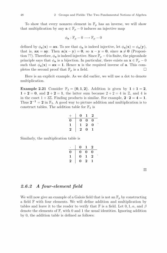
48 2 Groups and Fields: The Two Fundamental Notions of Algebra
To show that every nonzero element in Fp has an inverse, we will showthat multiplication by any a ∈ Fp − 0 induces an injective map
φa : Fp − 0 −→ Fp − 0
defined by φa(x) = ax. To see that φa is indeed injective, let φa(x) = φa(y),that is, ax = ay. Then a(x − y) = 0, so x − y = 0, since a �= 0 (Proposi-tion ??). Therefore, φa is indeed injective. Since Fp − 0 is finite, the pigeonholeprinciple says that φa is a bijection. In particular, there exists an x ∈ Fp − 0such that φa(x) = ax = 1. Hence x is the required inverse of a. This com-pletes the second proof that Fp is a field. �
Here is an explicit example. As we did earlier, we will use a dot to denotemultiplication.
Example 2.21 Consider F3 = {0,1,2}. Addition is given by 1 + 1 = 2,1 + 2 = 0, and 2 + 2 = 1, the latter sum because 2 + 2 = 4 in Z, and 4 isin the coset 1 + 3Z. Finding products is similar. For example, 2 · 2 = 4 = 1.Thus 2−1 = 2 in F3. A good way to picture addition and multiplication is toconstruct tables. The addition table for F3 is
+ 0 1 20 0 0 01 1 2 02 2 0 1
.
Similarly, the multiplication table is
· 0 1 20 0 0 01 0 1 22 0 2 1
.
�
2.6.2 A four-element field
We will now give an example of a Galois field that is not an Fp by constructinga field F with four elements. We will define addition and multiplication bytables and leave it to the reader to verify that F is a field. Let 0, 1, α, and βdenote the elements of F, with 0 and 1 the usual identities. Ignoring additionby 0, the addition table is defined as follows:
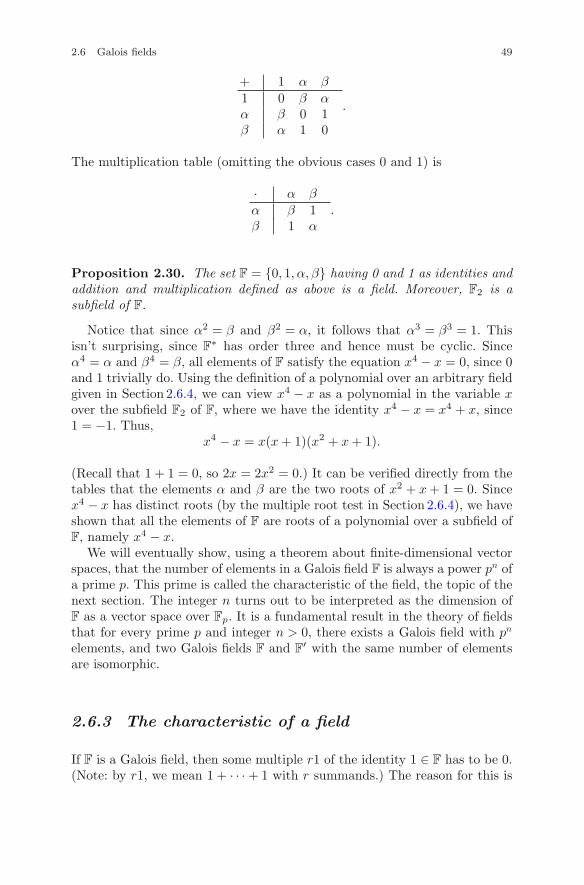
2.6 Galois fields 49
+ 1 α β
1 0 β αα β 0 1β α 1 0
.
The multiplication table (omitting the obvious cases 0 and 1) is
· α β
α β 1β 1 α
.
Proposition 2.30. The set F = {0, 1, α, β} having 0 and 1 as identities andaddition and multiplication defined as above is a field. Moreover, F2 is asubfield of F.
Notice that since α2 = β and β2 = α, it follows that α3 = β3 = 1. Thisisn’t surprising, since F
∗ has order three and hence must be cyclic. Sinceα4 = α and β4 = β, all elements of F satisfy the equation x4 − x = 0, since 0and 1 trivially do. Using the definition of a polynomial over an arbitrary fieldgiven in Section 2.6.4, we can view x4 − x as a polynomial in the variable xover the subfield F2 of F, where we have the identity x4 − x = x4 + x, since1 = −1. Thus,
x4 − x = x(x + 1)(x2 + x + 1).
(Recall that 1 + 1 = 0, so 2x = 2x2 = 0.) It can be verified directly from thetables that the elements α and β are the two roots of x2 + x + 1 = 0. Sincex4 − x has distinct roots (by the multiple root test in Section 2.6.4), we haveshown that all the elements of F are roots of a polynomial over a subfield ofF, namely x4 − x.
We will eventually show, using a theorem about finite-dimensional vectorspaces, that the number of elements in a Galois field F is always a power pn ofa prime p. This prime is called the characteristic of the field, the topic of thenext section. The integer n turns out to be interpreted as the dimension ofF as a vector space over Fp. It is a fundamental result in the theory of fieldsthat for every prime p and integer n > 0, there exists a Galois field with pn
elements, and two Galois fields F and F′ with the same number of elements
are isomorphic.
2.6.3 The characteristic of a field
If F is a Galois field, then some multiple r1 of the identity 1 ∈ F has to be 0.(Note: by r1, we mean 1 + · · · + 1 with r summands.) The reason for this is
50 2 Groups and Fields: The Two Fundamental Notions of Algebra
that since F is finite, the multiples r1 of 1 cannot all be distinct. Hence therehave to be two distinct positive integers m and n such that m1 = n1 in F. Thisimplies m1 − n1 = 0. But by associativity of addition, m1 − n1 = (m − n)1.Assuming without loss of generality that m > n, it follows that there existsa positive integer r such that r1 = 0 in F.
I claim that the least positive integer r such that r1 = 0 is a prime. Forif r can be expressed as a product r = ab, where a, b are positive integers,then r1 = (ab)1 = (a1)(b1) = 0. Thus, by Proposition 2.21, a1 = 0 or b1 = 0.But by the minimality of r, one of a and b is r, so r is a prime, say r = p.The prime p is the characteristic of F. In general, one makes the followingdefinition:
Definition 2.15. Let F be an arbitrary field. If some nonzero multiple q1of 1 equals 0, we say that F has positive characteristic. In that case, thecharacteristic of F is defined to be the smallest positive integer q such thatq1 = 0. If all multiples q1 are nonzero, we say that F has characteristic 0.
Example 2.22. The characteristic of the field F4 defined above is two. Thecharacteristic of Fp is p. �
Summarizing the above discussion, we state the following proposition.
Proposition 2.31. If a field F has positive characteristic, then its charac-teristic is a prime p, and pa = 0 for all a ∈ F.
Proof. We already proved that if the characteristic of F is positive, then ithas to be a prime. If p1 = 0, then by the distributive law,
pa = a + · · · + a = 1a + · · · + 1a = (1 + · · · + 1)a = (p1)a = 0a = 0
for all a ∈ F. �
Proposition 2.32. The characteristics of Q, R, and C are all 0. Moreover,the characteristic of every subfield of a field of characteristic 0 is also 0.
The notion of the characteristic has a nice application.
Proposition 2.33. SupposeF is a field of characteristic p > 0. Then for alla1, . . . , an ∈ F,
(a1 + · · · + an)p = ap1 + · · · + ap
n.
This is an application of the binomial theorem. We will leave the proof asan exercise. A consequence of the previous proposition is that ap = a for everya ∈ Fp. Thus ap−1 = 1. This also gives a formula for a−1 for every a ∈ Fp,namely, a−1 = ap−2.
2.6 Galois fields 51
Example 2.23. The formula a−1 = ap−2 for the inverse of a nonzero ele-ment a of Fp actually isn’t so easy to apply without a computer. For exam-ple, to compute the inverse of 5 in F23, one needs to find 521, which is476837158203125. After that, one has to reduce 476837158203125 modulo23. The result is 14. Thus 5−1 = 14 in F23. But this can be seen easily with-out having to do a long computation, since 5 · 14 = 70 = 69 + 1. �
The result ap−1 = 1 in Fp translates into a well-known result from elemen-tary number theory known as Fermat’s little theorem.
Proposition 2.34. Let p be prime. Then for every integer a �≡ 0 mod p,a(p−1) ≡ 1 mod p.
We leave the proof as an exercise. Notice that Fermat’s little theorem is aspecial case of Euler’s theorem, since if p is prime, then φ(p) = p − 1. Hereis another interesting property of Fp.
Proposition 2.35. The product of all the nonzero elements of Fp is −1.
Proof. This follows by noting that {2,3, . . . ,p − 2} can be partitioned intopairs {a,b} such that a−1 = b. We will leave the proof of this to the reader.Therefore, 2 · 3 · · · (p − 2) = 1 in Fp. The result follows by multiplying by−1 = p − 1. �
Proposition 2.35 stated in number-theoretic terms is one of the assertionsof Wilson’s theorem: (q − 1)! ≡ −1 mod q if and only if q is prime. Wilson’stheorem gives a test for determining whether a number is prime, but theproblem is that implementing this test requires knowing (q − 1)!. It turns outthat Fermat’s little theorem gives a much easier test, known as the Fermatprimality test. In this test, one checks whether aq−1 ≡ 1 mod q for some“random” values of a. If the congruence fails for any value of a, then q isn’tprime, while if it holds for several values, then the probability that q is aprime is very high. Knowing large primes is useful, for example, in employingRSA encryption.
2.6.4 Appendix: polynomials over a field
The purpose of this appendix is to define the polynomials over a field F.For each integer i > 0, let xi denote a symbol, and suppose that every pairof these symbols xi and xj can be multiplied with the result xixj = xi+j
for all i, j > 0. We will denote x1 simply by x. We will put x0 = 1 ∈ F. Thesymbol x is sometimes called an indeterminate. Note that xi = x · · · x (withi factors). We assume that each symbol xi can be multiplied by an arbi-trary element of F, so that 0xi = 0, 1xi = xi, and (axi)(bxj) = (ab)xi+j . LetF[x] denote the set of all expressions f(x) = a0 + a1x + a2x
2 + · · · + anxn,
52 2 Groups and Fields: The Two Fundamental Notions of Algebra
a0, a1, . . . , an ∈ F and n ≥ 0. Then f(x) is called a polynomial over F. Weagree that two polynomials f(x) = a0 + a1x + a2x
2 + · · · + anxn and g(x) =
b0 + a1x + b2x2 + · · · + bmxm are equal if ai = bi for every value of i. If
an �= 0, we say that f has degree n and write deg(f) = n. The value of f(x)at r ∈ F is by definition f(r) = a0 + a1r + a2r
2 + · · · + anrn. Thus, a poly-
nomial f(x) determines a function f : F → F. However, if F is a Galois field,then there exist polynomials f(x) ∈ F[x] such that the function f : F → F isidentically zero, so polynomials should not be thought of as the same thingas functions.
Example 2.24. For example, if F = F2 and f(x) = x2 + x, then f(1) =f(0) = 0. Hence the function corresponding to f(x) is identically zero onF2. However, in the field F4 containing F2 defined in Section 2.6.2, the poly-nomial f(x) satisfies f(α) = f(β) = 1. (Recall that α and β satisfy x2 + x +1 = 0. �
Addition and multiplication of polynomials are defined as follows. Additionamounts to adding together the coefficients of each corresponding power xi
of x. For example,
(3x2 − 2x + 1) + (x4 − x3 − 3x2 + x) = x4 − x3 − x + 1.
Multiplication of two polynomials uses the above rules and the distributivelaw. Thus,
(3x2 − 2x + 1)(x4 − x3 − 2x2 + x) = 3x6 − 5x5 − 7x4 + 6x3 − 4x2 + x.
When the field F has characteristic zero, for example F = Q, R, or C, thereis a more natural formulation of F[x] that avoids the problem encounteredin F2[x], where polynomials can define the zero function. In that case, letx : F → F denote the identity function x(r) = r for all r ∈ F. If i > 0, thenxi denotes the function xi(r) = ri. Then F[x] may be defined as the set of allfunctions f : F → F of the form
f(x) = a0 + a1x + a2x2 + · · · + anx
n,
where a0, a1, . . . , an ∈ F. Addition and multiplication are defined pointwiseas above.
In the remainder of this section, we are going to consider two propertiesof polynomials over an arbitrary field. The first is that F[x] admits divisionwith remainder.
Proposition 2.36 (Division with remainder for polynomials). Supposef(x) and g(x) are in F[x]. Then there exists a unique expression
f(x) = q(x)g(x) + r(x),
2.6 Galois fields 53
where q(x), r(x) ∈ F[x] and deg(r) < deg(g). In particular, if a ∈ F is a rootof f , i.e., f(a) = 0, then f(x) = (x − a)g(x) for some g(x) ∈ F[x].
Proof. This can be proved by induction on the degree of f(x). We will omitthe details.
The second property is a test for when a polynomial has a multiple root.We say that a is a multiple root of p(x) ∈ F[x] if there exists a polynomialq(x) ∈ F[x] such that p(x) = q(x)(x − a)2. To state the second property, weneed to define the derivative of a polynomial. Suppose n > 0 and p(x) =anx
n + an−1xn−1 + · · · + a1x + a0. Then the derivative of p(x) is defined to
be the polynomial
p′(x) = nanxn−1 + (n − 1)an−1x
n−2 + · · · + 2a2x + a1.
The derivative of a constant polynomial is defined to be zero. This definitionagrees with the classical formula for the derivative of a polynomial. Thederivative of a sum is the sum of the derivatives, and Leibniz’s formula forthe derivative of a product holds: (pq)′ = p′q + pq′.
Proposition 2.37. Let p(x) ∈ F[x]. Then p(x) = (x − a)2q(x) for some q(x)∈ F[x] if and only if p(a) = p′(a) = 0.
Proof. Suppose p(x) = (x − a)2q(x). Then it is obvious from Leibniz thatp(a) = p′(a) = 0. Suppose, conversely, that p(a) = p′(a) = 0. Then p(x) =(x − a)s(x), where s(x) ∈ F[x], so p′(x) = (x − a)′s(x) + (x − a)s′(x) = s(x) +(x − a)s′(x). Hence, 0 = p′(a) = s(a). This means that s(x) = (x − a)t(x) forsome t(x) ∈ F[x], and thus p(x) = (x − a)2q(x), as claimed. �
One says that a ∈ F is a simple root of p(x) ∈ F[x] if and only if (x −a) divides p(x) but (x − a)2 does not. A root that is not simple is calleda multiple root. The next result formulates Proposition 2.37 as a test forwhether a root of p(x) is simple.
Corollary 2.38 (The simple root test). Let p(x) ∈ F[x]. Then a is a simpleroot if and only if p(a) = 0 but p′(a) �= 0, and a is a multiple root if and onlyif p(a) = p′(a) = 0.
Exercises
Exercise 2.6.1. Write out the addition and multiplication tables for thefield F7. Also, indicate the location of the multiplicative inverse for eachnonzero element.
Exercise 2.6.2. Find both −(6 + 6) and (6 + 6)−1 in F7.
Exercise 2.6.3. Show that Q, R, and C all have characteristic zero.
54 2 Groups and Fields: The Two Fundamental Notions of Algebra
Exercise 2.6.4. Let F be a field and suppose that F′ ⊂ F is a subfield. Showthat F and F
′ have the same characteristic.
Exercise 2.6.5. Show that the characteristic of Fp is p.
Exercise 2.6.6. Let F and F′ be fields. Show that every field homomorphism
ϕ : F → F′ is injective.
Exercise 2.6.7. Suppose that the field F contains Fp as a subfield. Showthat the characteristic of F is p.
Exercise 2.6.8. Suppose that F is a field of characteristic p > 0. Show thatall multiples of 1 including 0 form a subfield of F with p elements. (Thissubfield is in fact a copy of Fp.)
Exercise 2.6.9. Prove Proposition 2.33. That is, show that if F is a finitefield of characteristic p, then for all a1, . . . , an ∈ F,
(a1 + · · · + an)p = ap1 + · · · + ap
n.
Exercise 2.6.10. Use Proposition 2.33 to show that ap = a in Fp. Use thisto deduce Fermat’s little theorem.
Exercise 2.6.11. In the definition of the field F4 in Section 2.6.2, can wealter the definition of multiplication by putting α2 = β2 = 1 and still get afield?
Exercise 2.6.12. Suppose F is a field of characteristic p. Show that if a, b ∈F and ap = bp, then a = b.
Exercise 2.6.13. A field of characteristic p is said to be perfect if everyelement is a pth power. Show that every Galois field is perfect. (Hint: use thepigeonhole principle.)
Exercise 2.6.14. Use Fermat’s little theorem to find 9−1 in Fp for p = 11,13, 23, and 29. Use these results to solve the congruence equation 9x ≡ 15mod p for the above values of p.
Exercise 2.6.15. A primitive element of Fp is an element β such that
Fp = {0, 1, β, β2, . . . , βp−2}.
It can be shown that for every prime p, Fp contains a primitive element. Findat least one primitive element β for Fp when p = 5, 7, and 11.
Exercise 2.6.16. Write out the addition and multiplication tables for Z6.Is Z6 a field? If not, why not?
2.6 Galois fields 55
Exercise 2.6.17. Let p be a prime. Let φp : Z → Fp be the quotient map-ping a �→ a, where a = a + pZ. Show that for all a, b ∈ Z,
(1) φp(a + b) = φp(a) + φp(b), and
(2) φp(ab) = φp(a)φp(b).
Thus, φ is a homomorphism of rings. Use these two facts to deduce thataddition and multiplication in Fp are associative from the fact that they areassociative in Z.
Exercise 2.6.18. Using the definition of the derivative of a polynomialf(x) ∈ F[x] in Section 2.6.4, show that the product rule for differentiationholds. That is, if f(x), g(x) ∈ F[x], then (fg)′ = f ′g + fg′.
Exercise 2.6.19. Let F be a field of characteristic p. Show that for everyn > 0, xpn − x = 0 has only simple roots in F.
Chapter 3Matrices
Matrix theory is deeply embedded in the foundations of algebra. The idea ofa matrix is very simple, and useful examples and ideas present themselvesimmediately, as we shall soon see. So it is surprising that their structureturns out to be subtle. Matrices also represent abstract objects called linearmappings, which we will treat after vector spaces. The main results in thetheory of linear mappings, including the Cayley–Hamilton theorem, Jordandecomposition, and Jordan canonical form, are strikingly beautiful.
More down to earth, matrices represent systems of linear equations inseveral variables. Such a linear system has the form Ax = b, where A, x,and b are all matrices, and Ax is the product of A and x. In this form, alinear system is a special case of the basic algebraic equation ax = b. Matrixalgebra arises from addition and multiplication in a field, and it satisfiessome of the field axioms: for example, the associative and distributive laws.However, matrices usually do not have multiplicative inverses. When they dois a topic that will be taken up in the next chapter. The first goal of thischapter is matrix algebra and the procedure known as row reduction, whichamounts to replacing a matrix A by a unique matrix in what is called reducedrow echelon form. The reduced row echelon form of a matrix is used to solvelinear systems. It also tells us the rank of the matrix and gives the inverse ofA when one exists. Prove the existence of an LPDU factorization, which ishow one understands how the matrix is constructed.
3.1 Introduction to matrices and matrix algebra
The purpose of this section is to introduce the notion of a matrix, give somemotivation, and make the basic definitions used in matrix algebra.
c© Springer Science+Business Media LLC 2017J.B. Carrell, Groups, Matrices, and Vector Spaces,DOI 10.1007/978-0-387-79428-0 3
57
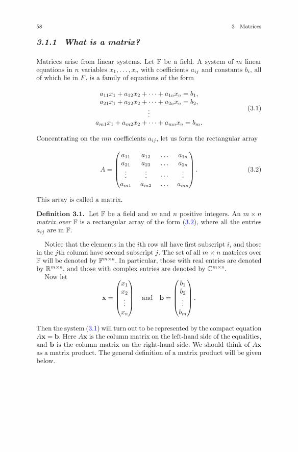
58 3 Matrices
3.1.1 What is a matrix?
Matrices arise from linear systems. Let F be a field. A system of m linearequations in n variables x1, . . . , xn with coefficients aij and constants bi, allof which lie in F , is a family of equations of the form
a11x1 + a12x2 + · · · + a1nxn = b1,a21x1 + a22x2 + · · · + a2nxn = b2,
...am1x1 + am2x2 + · · · + amnxn = bm.
(3.1)
Concentrating on the mn coefficients aij , let us form the rectangular array
A =
⎛⎜⎜⎜⎝
a11 a12 . . . a1n
a21 a23 . . . a2n
...... · · · ...
am1 am2 . . . amn
⎞⎟⎟⎟⎠ . (3.2)
This array is called a matrix.
Definition 3.1. Let F be a field and m and n positive integers. An m × nmatrix over F is a rectangular array of the form (3.2), where all the entriesaij are in F.
Notice that the elements in the ith row all have first subscript i, and thosein the jth column have second subscript j. The set of all m × n matrices overF will be denoted by F
m×n. In particular, those with real entries are denotedby R
m×n, and those with complex entries are denoted by Cm×n.
Now let
x =
⎛⎜⎜⎜⎝
x1
x2
...xn
⎞⎟⎟⎟⎠ and b =
⎛⎜⎜⎜⎝
b1b2...
bm
⎞⎟⎟⎟⎠ .
Then the system (3.1) will turn out to be represented by the compact equationAx = b. Here Ax is the column matrix on the left-hand side of the equalities,and b is the column matrix on the right-hand side. We should think of Axas a matrix product. The general definition of a matrix product will be givenbelow.
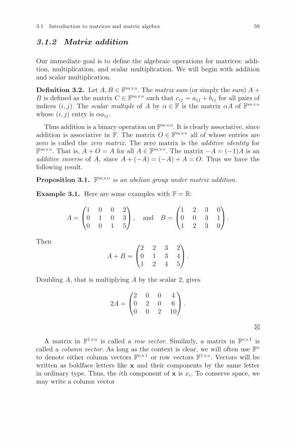
3.1 Introduction to matrices and matrix algebra 59
3.1.2 Matrix addition
Our immediate goal is to define the algebraic operations for matrices: addi-tion, multiplication, and scalar multiplication. We will begin with additionand scalar multiplication.
Definition 3.2. Let A,B ∈ Fm×n. The matrix sum (or simply the sum) A +
B is defined as the matrix C ∈ Fm×n such that cij = aij + bij for all pairs of
indices (i, j). The scalar multiple of A by α ∈ F is the matrix αA of Fm×n
whose (i, j) entry is αaij .
Thus addition is a binary operation on Fm×n. It is clearly associative, since
addition is associative in F. The matrix O ∈ Fm×n all of whose entries are
zero is called the zero matrix. The zero matrix is the additive identity forF
m×n. That is, A + O = A for all A ∈ Fm×n. The matrix −A = (−1)A is an
additive inverse of A, since A + (−A) = (−A) + A = O. Thus we have thefollowing result.
Proposition 3.1. Fm×n is an abelian group under matrix addition.
Example 3.1. Here are some examples with F = R:
A =
⎛⎝
1 0 0 20 1 0 30 0 1 5
⎞⎠ , and B =
⎛⎝
1 2 3 00 0 3 11 2 3 0
⎞⎠ .
Then
A + B =
⎛⎝
2 2 3 20 1 3 41 2 4 5
⎞⎠ .
Doubling A, that is multiplying A by the scalar 2, gives
2A =
⎛⎝
2 0 0 40 2 0 60 0 2 10
⎞⎠ .
�
A matrix in F1×n is called a row vector. Similarly, a matrix in F
n×1 iscalled a column vector. As long as the context is clear, we will often use F
n
to denote either column vectors Fn×1 or row vectors F
1×n. Vectors will bewritten as boldface letters like x and their components by the same letterin ordinary type. Thus, the ith component of x is xi. To conserve space, wemay write a column vector
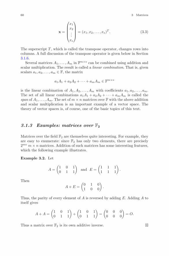
60 3 Matrices
x =
⎛⎜⎜⎜⎝
x1
x2
...xn
⎞⎟⎟⎟⎠ = (x1, x2, . . . , xn)T . (3.3)
The superscript T , which is called the transpose operator, changes rows intocolumns. A full discussion of the transpose operator is given below in Section3.1.6.
Several matrices A1, . . . , Am in Fm×n can be combined using addition and
scalar multiplication. The result is called a linear combination. That is, givenscalars a1, a2, . . . , am ∈ F, the matrix
a1A1 + a2A2 + · · · + amAm ∈ Fm×n
is the linear combination of A1, A2, . . . , Am with coefficients a1, a2, . . . , am.The set of all linear combinations a1A1 + a2A2 + · · · + amAm is called thespan of A1, . . . , Am. The set of m × n matrices over F with the above additionand scalar multiplication is an important example of a vector space. Thetheory of vector spaces is, of course, one of the basic topics of this text.
3.1.3 Examples: matrices over F2
Matrices over the field F2 are themselves quite interesting. For example, theyare easy to enumerate: since F2 has only two elements, there are precisely2mn m × n matrices. Addition of such matrices has some interesting features,which the following example illustrates.
Example 3.2. Let
A =(
1 0 10 1 1
)and E =
(1 1 11 1 1
).
Then
A + E =(
0 1 01 0 0
).
Thus, the parity of every element of A is reversed by adding E. Adding A toitself gives
A + A =(
1 0 10 1 1
)+
(1 0 10 1 1
)=
(0 0 00 0 0
)= O.
Thus a matrix over F2 is its own additive inverse. �
3.1 Introduction to matrices and matrix algebra 61
Example 3.3. Here is how one might design a scanner to analyze black-and-white photographs. A photo is a rectangular array consisting of manyblack and white dots. By giving the white dots the value 0 and the black dotsthe value 1, a photo is therefore transformed into a (very large) matrix overF2. Now suppose one wants to compare two black-and-white photographs tosee whether they are in fact identical. Suppose they have each been encodedas m × n matrices A and B. It turns out to be very inefficient for a computerto scan the two matrices to see in how many positions they agree. However,when A and B are added, the sum A + B has a 1 in every component whereA and B differ, and a 0 wherever they coincide. For example, the sum of twoidentical photographs is the zero matrix, and the sum of a photograph andits negative is the all-ones matrix. An obvious measure of how similar thetwo matrices A and B are is the number of nonzero entries of A + B, i.e.,Σi,j(aij + bij). This is an easily tabulated number, which is known as theHamming distance between A and B. �
Example 3.4. Random Key Cryptography. Suppose Rocky the flyingsquirrel wants to send a message to his sidekick, Bullwinkle the moose, andhe wants to make sure that the notorious villains Boris and Natasha won’tbe able to learn what it says. Here is what the ever resourceful squirrel mightdo. First he could assign the numbers 1 to a, 2 to b, and so forth up to 26to z. He then computes the binary expansion of each integer between 1 and26. Thus 1 = 1, 2 = 10, 3 = 11, 4 = 100, . . . , 26 = 11010. He now convertshis message into a sequence of five-digit strings (1 = 00001, etc.). The resultis an encoding of the message, which is referred to as the plaintext. To makethings more compact, he arranges the plaintext into an m × n matrix, callit P . Now the deception begins. Rocky and Bullwinkle have already selectedan m × n matrix of five-digit strings of 0’s and 1’s, which we call Q. Thismatrix is what cryptographers sometimes call a key. Rocky will send thematrix P + Q to Bullwinkle, where the addition of strings is performed in(F2)5×1. Bullwinkle will be able to recover P easily by adding Q. Indeed,(P + Q) + Q = P + (Q + Q) = P + 2Q = P . This is good, since Bullwinkle,being a moose, is somewhat mathematically challenged and finds subtractiondifficult. Even if Boris and Natasha manage to intercept the ciphertext P +Q, they need to know the key Q to recover P . However, the key Q mustbe sufficiently random so that neither Boris nor Natasha can guess it. Thesquirrel’s encryption scheme is extremely secure if the key Q is a one-timepad, that is, it is used only once. �
3.1.4 Matrix multiplication
Matrix addition and scalar multiplication are simple and natural opera-tions. The product of two matrices, on the other hand, is a little more
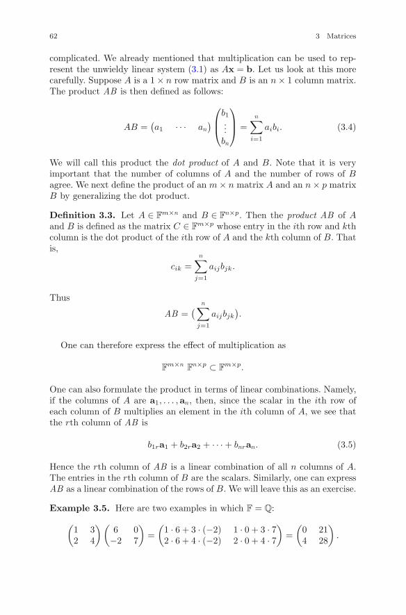
62 3 Matrices
complicated. We already mentioned that multiplication can be used to rep-resent the unwieldy linear system (3.1) as Ax = b. Let us look at this morecarefully. Suppose A is a 1 × n row matrix and B is an n × 1 column matrix.The product AB is then defined as follows:
AB =(a1 · · · an
)⎛⎜⎝
b1...bn
⎞⎟⎠ =
n∑i=1
aibi. (3.4)
We will call this product the dot product of A and B. Note that it is veryimportant that the number of columns of A and the number of rows of Bagree. We next define the product of an m × n matrix A and an n × p matrixB by generalizing the dot product.
Definition 3.3. Let A ∈ Fm×n and B ∈ F
n×p. Then the product AB of Aand B is defined as the matrix C ∈ F
m×p whose entry in the ith row and kthcolumn is the dot product of the ith row of A and the kth column of B. Thatis,
cik =n∑
j=1
aijbjk.
Thus
AB =( n∑
j=1
aijbjk
).
One can therefore express the effect of multiplication as
Fm×n
Fn×p ⊂ F
m×p.
One can also formulate the product in terms of linear combinations. Namely,if the columns of A are a1, . . . ,an, then, since the scalar in the ith row ofeach column of B multiplies an element in the ith column of A, we see thatthe rth column of AB is
b1ra1 + b2ra2 + · · · + bnran. (3.5)
Hence the rth column of AB is a linear combination of all n columns of A.The entries in the rth column of B are the scalars. Similarly, one can expressAB as a linear combination of the rows of B. We will leave this as an exercise.
Example 3.5. Here are two examples in which F = Q:
(1 32 4
)(6 0
−2 7
)=
(1 · 6 + 3 · (−2) 1 · 0 + 3 · 72 · 6 + 4 · (−2) 2 · 0 + 4 · 7
)=
(0 214 28
).
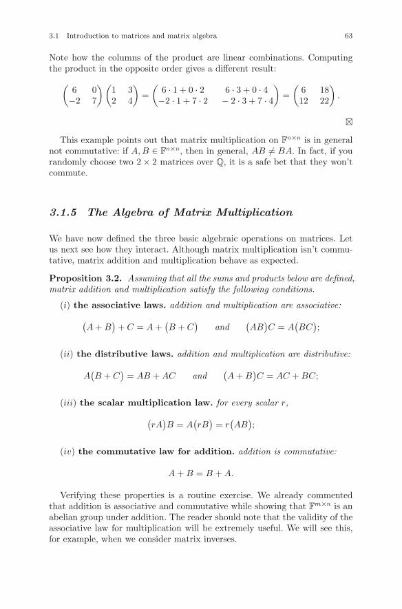
3.1 Introduction to matrices and matrix algebra 63
Note how the columns of the product are linear combinations. Computingthe product in the opposite order gives a different result:
(6 0
−2 7
)(1 32 4
)=
(6 · 1 + 0 · 2 6 · 3 + 0 · 4
−2 · 1 + 7 · 2 − 2 · 3 + 7 · 4
)=
(6 1812 22
).
�
This example points out that matrix multiplication on Fn×n is in general
not commutative: if A,B ∈ Fn×n, then in general, AB �= BA. In fact, if you
randomly choose two 2 × 2 matrices over Q, it is a safe bet that they won’tcommute.
3.1.5 The Algebra of Matrix Multiplication
We have now defined the three basic algebraic operations on matrices. Letus next see how they interact. Although matrix multiplication isn’t commu-tative, matrix addition and multiplication behave as expected.
Proposition 3.2. Assuming that all the sums and products below are defined,matrix addition and multiplication satisfy the following conditions.
(i) the associative laws. addition and multiplication are associative:
(A + B
)+ C = A +
(B + C
)and
(AB
)C = A
(BC
);
(ii) the distributive laws. addition and multiplication are distributive:
A(B + C
)= AB + AC and
(A + B
)C = AC + BC;
(iii) the scalar multiplication law. for every scalar r,
(rA
)B = A
(rB
)= r
(AB
);
(iv) the commutative law for addition. addition is commutative:
A + B = B + A.
Verifying these properties is a routine exercise. We already commentedthat addition is associative and commutative while showing that Fm×n is anabelian group under addition. The reader should note that the validity of theassociative law for multiplication will be extremely useful. We will see this,for example, when we consider matrix inverses.
64 3 Matrices
The n × n matrix In having ones everywhere on its diagonal and zeroseverywhere off the diagonal is called the identity matrix. One sometimeswrites In = (δij), where δij is the Kronecker delta, which is defined by therule δii = 1 while δij = 0 if i �= j. For example,
I2 =(
1 00 1
)and I3 =
⎛⎝
1 0 00 1 00 0 1
⎞⎠ .
A convenient way to define In is to write out its columns. Let ei denote thecolumn vector whose ith component is 1 and whose other components are 0.Then
In = (e1 e2 · · · en).
The reason In is called the identity matrix is due to the following fact.
Proposition 3.3. Let A be an m × n matrix over F. Then ImA = A andAIn = A. In particular, the ith column of A is Aei.
Proof. This follows immediately from the definition of matrixmultiplication. �
3.1.6 The transpose of a matrix
The transpose of an m × n matrix A is the n × m matrix AT whose ith row isthe ith column of A. That is, if A = (aij), then AT = (crs), where crs = asr.The definition becomes clearer after working an example.
Example 3.6. If
A =
⎛⎝
1 23 45 6
⎞⎠ ,
then
AT =(
1 3 52 4 6
).
�
For another example, note that ei = (0, . . . , 0, 1, 0, . . . , 0)T , where 1 is inthe ith component. Note that A and AT have the same entries on the diag-onal. Also note that the transpose of AT is A:
(AT )T = A.
3.1 Introduction to matrices and matrix algebra 65
Definition 3.4. A matrix A that is equal to its own transpose is calledsymmetric.
An example of a 2 × 2 symmetric matrix is
(1 33 5
).
Clearly, a symmetric matrix is square (but not uninteresting). For example,the symmetric matrices over R are all turn out to be diagonalizable due toa fundamental result called the principal axes theorem. But this will not beexplained for quite a while.
The transpose of a sum is as expected, but the transpose of a product hasa twist, as we note in the next proposition.
Proposition 3.4. For every m × n matrices A and B,
(A + B)T = AT + BT .
Furthermore, if A is m × n and B is n × p, then
(AB
)T = BT AT .
Proof. The first identity is immediate. To prove the product identity, notethat the (i, j) entry of BT AT is the dot product of the ith row of BT andthe jth column of AT . This is the same thing as the dot product of the jthrow of A and the ith column of B, which is the (j, i) entry of AB and hencethe (i, j) entry of (AB)T . Thus (AB)T = BT AT . �
It is suggested that the reader try this proof on an example.
3.1.7 Matrices and linear mappings
One way to look at matrix multiplication is that it defines a mapping. LetF
n = Fn×1 and F
m = Fm×1. Then for every A ∈ F
m×n, say A = (a1 · · · an),we obtain a mapping
TA : Fn → Fm, where TA(x) = Ax = x1a1 + · · · + xnan.
Note that TA(ei) = ai for each index i, and TA is uniquely determined bythe TA(ei).
Proposition 3.5. For every A ∈ Fm×n, the mapping TA : Fn → F
m associ-ated to A is in fact a homomorphism with domain F
n and target Fm. That
is, A(x + y) = Ax + Ay for every x,y ∈ Fn.
66 3 Matrices
Proof. This is simply an application of the distributive law formultiplication. �
We will frequently use this proposition in geometric examples.
Example 3.7. (Rotations of R2). One such example is a rotation of R2 givenby the mapping
Rθ
(xy
)=
(x cos θ − y sin θx sin θ + y cos θ
).
Here, Rθ is the matrix mapping associated to the matrix
Rθ =(
cos θ − sin θsin θ cos θ
). (3.6)
Recalling that C = R2, multiplication by the complex exponential eiθ =
cos θ + i sin θ sends z = x + iy to
eiθz = (cos θ + i sin θ)(x + iy) = (x cos θ − y sin θ) + i(x sin θ + y cos θ).
Therefore, the matrix mapping given by Rθ is the same as multiplication bythe complex exponential eiθ. �
Now suppose A ∈ Fm×n and B ∈ F
n×p. Then TAB is the mapping withdomain F
p and target Fm defined by TAB(u) = (AB)u for every u ∈ Fp. Since
by associativity (AB)u = A(Bu), it follows that TA ◦ TB = TAB . Therefore,we have the following.
Proposition 3.6. If A ∈ Fm×n and B ∈ F
n×p, then the matrix mappingTAB : Fp → F
m satisfiesTAB = TA ◦ TB .
That is, TAB is the composition of the matrix mappings TB : Fp → Fn and
TA : Fn → Fm. Hence matrix multiplication corresponds to the composition of
matrix mappings.
Exercises
Exercises 3.1.1. As an experiment, construct three matrices A,B,C ofdimensions such that AB and BC are defined. Then compute AB and (AB)C.Next compute BC and A(BC) and compare your results. If A and B are alsosquare, do AB and BA coincide?
Exercises 3.1.2. Prove the assertion (A + B)T = AT + BT inProposition 3.4 without writing down matrix entries.
3.1 Introduction to matrices and matrix algebra 67
Exercises 3.1.3. Suppose A and B are symmetric n × n matrices. (You caneven assume n = 2.)
(i) Must AB be symmetric? That is, are the n × n symmetric matrices closedunder multiplication?
(ii) If the answer to (i) is no, find a condition that ensures that AB issymmetric.
Exercises 3.1.4. Suppose B has a column of zeros. How does this affect aproduct of the form AB? What if A has a row of zeros?
Exercises 3.1.5. State a rule for expressing the rows of AB as linear com-binations of the rows of B. (Suggestion: use the transpose identity and theresult expressing the columns of AB).
Exercises 3.1.6. Verify Proposition 3.3 for all A in Fm×n.
Exercises 3.1.7. Let F = R. Find all 2 × 2 matrices A =(
a bc d
)such that
AB = BA, where B =(
1 23 4
).
Exercises 3.1.8. Assume here that F = F3. Find all 2 × 2 matrices A =(a bc d
)such that AC = CA, where C =
(1 21 2
). Is your result here any
different from the result you obtained in Exercise 3.1.7.
Exercises 3.1.9. Let F be a field. Prove that if S ∈ F2×2 commutes with
every matrix A =(
a bc d
)∈ F
2×2, then S = aI2 for some a ∈ F. Matrices of
the form aIn are called scalar matrices.
Exercises 3.1.10. Let p be a prime, and let A be the 2 × 2 matrix over Fp
such that aij = 1 for each i, j. Compute Am for every integer m ≥ 1. (Notethat Am stands for the mth power of A.)
Exercises 3.1.11. Let A be the n × n matrix over Q such that aij = 2 forall i, j. Find a formula for Aj for every positive integer j.
Exercises 3.1.12. Give an example of a 2 × 2 matrix A such that everyentry of A is either 0 or 1 and A2 = I2 as a matrix over F2, but A2 �= I2 asa matrix over Q.
68 3 Matrices
3.2 Reduced Row Echelon Form
The standard procedure for solving a linear system is to use a process calledGaussian elimination to put the system in a standard form in which it isready to solve. This process involves using row operations to put the coef-ficient matrix into a standard form called reduced row echelon form. It willturn out that every matrix can be put into this standard form by a pre-multiplication. We will later see that row operations preserve two importantquantities associated to A: the row space of A and its null space.
3.2.1 Reduced row echelon form and rowoperations
Definition 3.5. A matrix A is said to be in row echelon form if
(i) the first nonzero entry in each row of A is to the right of the first nonzeroentry in the preceding row (and hence in all preceding rows), and
(ii) every entry above a first nonzero entry is zero.
The first nonzero entry in a row is called its pivot entry or corner entry.A matrix A in row echelon form is said to be in reduced row echelon form,or simply, to be reduced, if each corner entry is 1. Here are some examples ofreduced matrices:
⎛⎝
1 0 0 20 1 0 30 0 1 5
⎞⎠ ,
⎛⎝
1 2 3 0 90 0 0 1 40 0 0 0 0
⎞⎠ ,
(0 1 3 0 90 0 0 1 0
).
The zero matrix O ∈ Fm×n and the identity matrix In are reduced also.
A row operation on a matrix A replaces one of the rows of A by a newrow. The three row operations we will now define are called the elementaryrow operations.
Definition 3.6. Let A be a matrix over F with rows a1, . . . ,am. The ele-mentary row operations over F on A are as follows:
(I) interchange the ith row ai and the jth row aj , where i �= j;
(II) replace the ith row ai with a nonzero scalar multiple rai, where r ∈ F;
(III) replace the ith row ai by ai + raj , where r ∈ F, r �= 0, and i �= j. Thatis, replace ai by itself plus a nonzero multiple of some other row.
Row operations of type I are called row swaps. The type II operations arecalled row dilations, and operations of type III are called transvections. Thenext proposition gives the basic property of row operations.
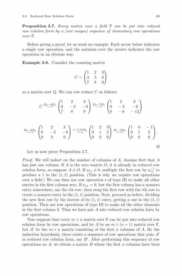
3.2 Reduced Row Echelon Form 69
Proposition 3.7. Every matrix over a field F can be put into reducedrow echelon form by a (not unique) sequence of elementary row operationsover F.
Before giving a proof, let us work an example. Each arrow below indicatesa single row operation, and the notation over the arrows indicates the rowoperation in an obvious way.
Example 3.8. Consider the counting matrix
C =
⎛⎝
1 2 34 5 67 8 9
⎞⎠
as a matrix over Q. We can row reduce C as follows:
CR2−4R1−→
⎛⎝
1 2 30 − 3 − 67 8 9
⎞⎠ R3−7R1−→
⎛⎝
1 2 30 − 3 − 60 − 6 − 12
⎞⎠
R3−2R2−→⎛⎝
1 2 30 − 3 − 60 0 0
⎞⎠ (−1/3)R2−→
⎛⎝
1 2 30 1 20 0 0
⎞⎠ R1−2R2−→
⎛⎝
1 0 − 10 1 20 0 0
⎞⎠ .
�Let us now prove Proposition 3.7.
Proof. We will induct on the number of columns of A. Assume first that Ahas just one column. If A is the zero matrix O, it is already in reduced rowechelon form, so suppose A �= O. If a11 �= 0, multiply the first row by a−1
11 toproduce a 1 in the (1, 1) position. (This is why we require row operationsover a field.) We can then use row operation s of type III to make all otherentries in the first column zero. If a11 = 0, but the first column has a nonzeroentry somewhere, say the ith row, then swap the first row with the ith row tocreate a nonzero entry in the (1, 1) position. Next, proceed as before, dividingthe new first row by the inverse of its (1, 1) entry, getting a one in the (1, 1)position. Then use row operations of type III to make all the other elementsin the first column 0. Thus we have put A into reduced row echelon form byrow operations.
Now suppose that every m × n matrix over F can be put into reduced rowechelon form by row operations, and let A be an m × (n + 1) matrix over F.Let A′ be the m × n matrix consisting of the first n columns of A. By theinduction hypothesis, there exists a sequence of row operations that puts A′
in reduced row echelon form, say B′. After performing this sequence of rowoperations on A, we obtain a matrix B whose the first n columns have been
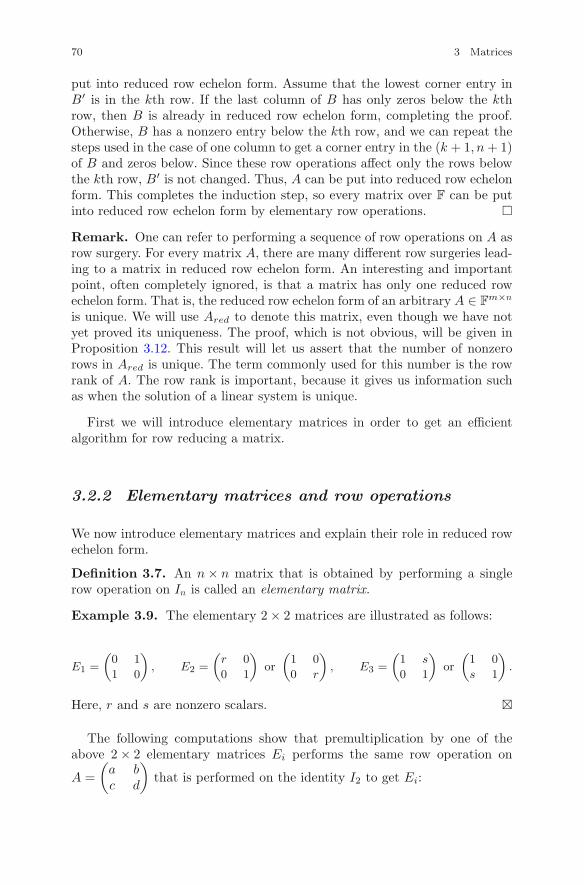
70 3 Matrices
put into reduced row echelon form. Assume that the lowest corner entry inB′ is in the kth row. If the last column of B has only zeros below the kthrow, then B is already in reduced row echelon form, completing the proof.Otherwise, B has a nonzero entry below the kth row, and we can repeat thesteps used in the case of one column to get a corner entry in the (k + 1, n + 1)of B and zeros below. Since these row operations affect only the rows belowthe kth row, B′ is not changed. Thus, A can be put into reduced row echelonform. This completes the induction step, so every matrix over F can be putinto reduced row echelon form by elementary row operations. �
Remark. One can refer to performing a sequence of row operations on A asrow surgery. For every matrix A, there are many different row surgeries lead-ing to a matrix in reduced row echelon form. An interesting and importantpoint, often completely ignored, is that a matrix has only one reduced rowechelon form. That is, the reduced row echelon form of an arbitrary A ∈ F
m×n
is unique. We will use Ared to denote this matrix, even though we have notyet proved its uniqueness. The proof, which is not obvious, will be given inProposition 3.12. This result will let us assert that the number of nonzerorows in Ared is unique. The term commonly used for this number is the rowrank of A. The row rank is important, because it gives us information suchas when the solution of a linear system is unique.
First we will introduce elementary matrices in order to get an efficientalgorithm for row reducing a matrix.
3.2.2 Elementary matrices and row operations
We now introduce elementary matrices and explain their role in reduced rowechelon form.
Definition 3.7. An n × n matrix that is obtained by performing a singlerow operation on In is called an elementary matrix.
Example 3.9. The elementary 2 × 2 matrices are illustrated as follows:
E1 =
(0 1
1 0
), E2 =
(r 0
0 1
)or
(1 0
0 r
), E3 =
(1 s
0 1
)or
(1 0
s 1
).
Here, r and s are nonzero scalars. �
The following computations show that premultiplication by one of theabove 2 × 2 elementary matrices Ei performs the same row operation on
A =(
a bc d
)that is performed on the identity I2 to get Ei:
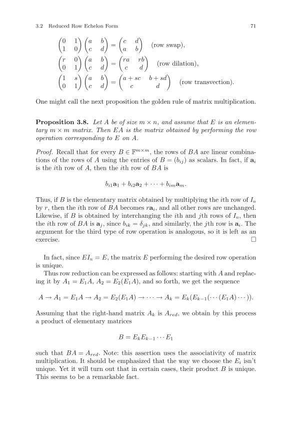
3.2 Reduced Row Echelon Form 71
(0 11 0
) (a bc d
)=
(c da b
)(row swap),
(r 00 1
) (a bc d
)=
(ra rbc d
)(row dilation),
(1 s0 1
) (a bc d
)=
(a + sc b + sd
c d
)(row transvection).
One might call the next proposition the golden rule of matrix multiplication.
Proposition 3.8. Let A be of size m × n, and assume that E is an elemen-tary m × m matrix. Then EA is the matrix obtained by performing the rowoperation corresponding to E on A.
Proof. Recall that for every B ∈ Fm×m, the rows of BA are linear combina-
tions of the rows of A using the entries of B = (bij) as scalars. In fact, if ai
is the ith row of A, then the ith row of BA is
bi1a1 + bi2a2 + · · · + bimam.
Thus, if B is the elementary matrix obtained by multiplying the ith row of In
by r, then the ith row of BA becomes rai, and all other rows are unchanged.Likewise, if B is obtained by interchanging the ith and jth rows of In, thenthe ith row of BA is aj , since bik = δjk, and similarly, the jth row is ai. Theargument for the third type of row operation is analogous, so it is left as anexercise. �
In fact, since EIn = E, the matrix E performing the desired row operationis unique.
Thus row reduction can be expressed as follows: starting with A and replac-ing it by A1 = E1A, A2 = E2(E1A), and so forth, we get the sequence
A → A1 = E1A → A2 = E2(E1A) → · · · → Ak = Ek(Ek−1(· · · (E1A) · · · )).
Assuming that the right-hand matrix Ak is Ared, we obtain by this processa product of elementary matrices
B = EkEk−1 · · · E1
such that BA = Ared. Note: this assertion uses the associativity of matrixmultiplication. It should be emphasized that the way we choose the Ei isn’tunique. Yet it will turn out that in certain cases, their product B is unique.This seems to be a remarkable fact.
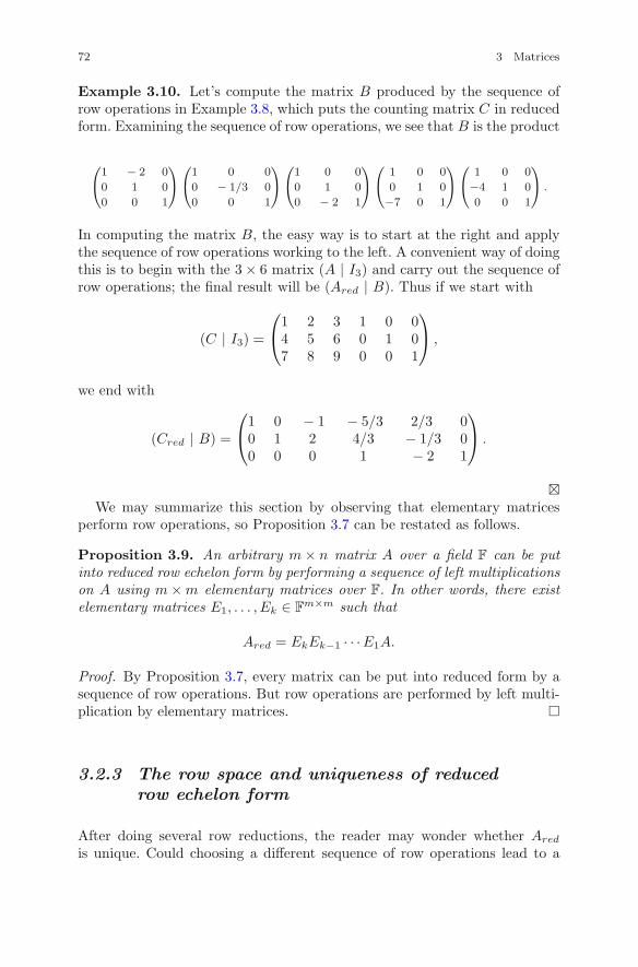
72 3 Matrices
Example 3.10. Let’s compute the matrix B produced by the sequence ofrow operations in Example 3.8, which puts the counting matrix C in reducedform. Examining the sequence of row operations, we see that B is the product
⎛⎝1 − 2 0
0 1 0
0 0 1
⎞⎠⎛⎝1 0 0
0 − 1/3 0
0 0 1
⎞⎠⎛⎝1 0 0
0 1 0
0 − 2 1
⎞⎠⎛⎝
1 0 0
0 1 0
−7 0 1
⎞⎠⎛⎝
1 0 0
−4 1 0
0 0 1
⎞⎠ .
In computing the matrix B, the easy way is to start at the right and applythe sequence of row operations working to the left. A convenient way of doingthis is to begin with the 3 × 6 matrix (A | I3) and carry out the sequence ofrow operations; the final result will be (Ared | B). Thus if we start with
(C | I3) =
⎛⎝
1 2 3 1 0 04 5 6 0 1 07 8 9 0 0 1
⎞⎠ ,
we end with
(Cred | B) =
⎛⎝
1 0 − 1 − 5/3 2/3 00 1 2 4/3 − 1/3 00 0 0 1 − 2 1
⎞⎠ .
�We may summarize this section by observing that elementary matrices
perform row operations, so Proposition 3.7 can be restated as follows.
Proposition 3.9. An arbitrary m × n matrix A over a field F can be putinto reduced row echelon form by performing a sequence of left multiplicationson A using m × m elementary matrices over F. In other words, there existelementary matrices E1, . . . , Ek ∈ F
m×m such that
Ared = EkEk−1 · · · E1A.
Proof. By Proposition 3.7, every matrix can be put into reduced form by asequence of row operations. But row operations are performed by left multi-plication by elementary matrices. �
3.2.3 The row space and uniqueness of reducedrow echelon form
After doing several row reductions, the reader may wonder whether Ared
is unique. Could choosing a different sequence of row operations lead to a
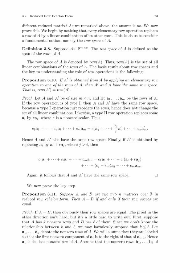
3.2 Reduced Row Echelon Form 73
different reduced matrix? As we remarked above, the answer is no. We nowprove this. We begin by noticing that every elementary row operation replacesa row of A by a linear combination of its other rows. This leads us to considera fundamental notion, namely the row space of A.
Definition 3.8. Suppose A ∈ Fm×n. The row space of A is defined as the
span of the rows of A.
The row space of A is denoted by row(A). Thus, row(A) is the set of alllinear combinations of the rows of A. The basic result about row spaces andthe key to understanding the role of row operations is the following:
Proposition 3.10. If A′ is obtained from A by applying an elementary rowoperation to one of the rows of A, then A′ and A have the same row space.That is, row(A′) = row(A).
Proof. Let A and A′ be of size m × n, and let a1, . . . ,am be the rows of A.If the row operation is of type I, then A and A′ have the same row space,because a type I operation just reorders the rows, hence does not change theset of all linear combinations. Likewise, a type II row operation replaces someai by rai, where r is a nonzero scalar. Thus
c1a1 + · · · + ciai + · · · + cmam = c1a′1 + · · · +
ci
ra′
i + · · · + cma′m.
Hence A and A′ also have the same row space. Finally, if A′ is obtained byreplacing ai by ai + raj , where j > i, then
c1a1 + · · · + ciai + · · · + cmam = c1a1 + · · · + ci(ai + raj)+ · · · + (cj − rci)aj + · · · + cmam.
Again, it follows that A and A′ have the same row space. �
We now prove the key step.
Proposition 3.11. Suppose A and B are two m × n matrices over F inreduced row echelon form. Then A = B if and only if their row spaces areequal.
Proof. If A = B, then obviously their row spaces are equal. The proof in theother direction isn’t hard, but it’s a little hard to write out. First, supposethat A has k nonzero rows and B has � of them. Since we don’t know therelationship between k and �, we may harmlessly suppose that k ≤ �. Leta1, . . . ,ak denote the nonzero rows of A. We will assume that they are labeledso that the first nonzero component of ai is to the right of that of ai+1. Hencea1 is the last nonzero row of A. Assume that the nonzero rows b1, . . . ,b� of
74 3 Matrices
B are labeled in the same way. The first step is to show that a1 = b1. This isdone as follows. Suppose the corner entries in a1 and b1 aren’t in the samecomponent; say the corner entry of a1 is to the left of the corner entry of b1.Then obviously a1 can’t be a linear combination of the bi. By symmetry, thecorner entries of a1 and b1 are in the same component. Since b1 is a linearcombination of the ai, the only possibility is b1 = r1a1, and in fact, r1 = 1,due to the fact that the corner entries of a1 and b1 are both one. Now, thematrices
A1 =(a2a1
)and B1 =
(b2
b1
)
have the same second row and are, by assumption, in reduced row echelonform. Suppose the corner entry in b2 is to the right of that of a2. Then b2
cannot be a linear combination of the ai, so once again a2 and b2 have tohave their corner entries in the same component. Hence, b2 = a2 + r1a1. Butsince A1 is in reduced row echelon form, a2 + r1a1 has r1 in the componentcorresponding to the corner entry of a1. But since B1 is also in reduced rowechelon form and b1 = a1, it follows that b2 has a zero in that component.Consequently, r1 = 0. Thus, b2 = a2. One can now repeat this argument toshow that b3 = a3, b4 = a4, and so on, eventually arriving at the conclusionbi = ai for 1 ≤ i ≤ k. Finally, we have to show that � = k. If k < �, thenbk+1 �= 0, and it lies in row(B) = row(A). Hence, bk+1 is a linear combinationof
∑riai with some ri �= 0. But this is impossible, because the component of
bk+1 corresponding to the corner entry is to the left of that of ak due to thefact that ak = bk. This shows that k = � and hence finishes the proof thatA = B. �
Finally, we answer the basic question.
Proposition 3.12. The reduced row echelon form of an arbitrary matrixA ∈ F
m×n is unique.
Proof. If two different sequences of row operations yield two different reducedrow echelon forms B and C for A, then by the previous proposition, we obtaina contradiction to row(A) = row(B) = row(C). Hence B = C. �
The fact that the reduced row echelon form of a matrix A is unique meansthat the number of nonzero rows of Ared depends only on A. This leads tothe following important definition.
Definition 3.9. Suppose A ∈ Fm×n. Then the number of nonzero rows in
Ared is called the rank of A.
3.2 Reduced Row Echelon Form 75
When we study vector spaces, we will show that the rank of A is actuallythe dimension of the row space of A. For square matrices, it turns out thatrank is a measure of how far the matrix is from being invertible.
Finally, note that Proposition 3.9 and the above discussion imply the fol-lowing.
Proposition 3.13. A matrix A ∈ Fn×n has rank n if and only if there exist
elementary matrices E1, . . . , Ek ∈ Fn×n such that
Ek · · · E1A = In.
Proof. By definition, A has rank n if and only if Ared has n nonzero rows.But since A ∈ F
n×n, Ared has n nonzero rows if and only if Ared = In. Thus,A has rank n implies by Proposition 3.9 that Ek · · · E1A = In for suitableelementary matrices E1, . . . , Ek. Conversely, if there exist elementary matri-ces E1, . . . , Ek such that Ek · · · E1A = In, then Ared = In by the uniquenessof the reduced form. �
Definition 3.10. When the rank of an n × n matrix A over a field F is n,we will say that A is nonsingular. Otherwise, A is said to be singular.
Exercises
Exercises 3.2.1. Make a list of all the row reduced 2 × 3 matrices over F2.
Exercises 3.2.2. Let F = F3. Find the reduced row echelon form of thefollowing matrices:
(2 11 2
),
⎛⎝
0 1 2 11 2 0 11 0 0 0
⎞⎠ ,
⎛⎝
1 2 02 1 10 2 1
⎞⎠ .
Exercises 3.2.3. True or False (give a brief reason to justify your answer).
(i) Two square matrices that can be row reduced to the same reduced rowechelon form are equal.
(ii) If a 3 × 3 matrix A has the property that each row contains two zeros anda one, and each column contains two zeros and a one, then A is nonsingular.
Exercises 3.2.4. If an n × n matrix has the property that each row andeach column has exactly one nonzero entry, is it nonsingular?
Exercises 3.2.5. The field is F2. Consider the following matrices:
A1 =
⎛⎝
1 1 01 0 11 1 1
⎞⎠ , A2 =
⎛⎜⎜⎝
1 0 1 00 1 1 01 1 0 01 0 0 1
⎞⎟⎟⎠ .
76 3 Matrices
Find matrices B1 and B2 that are products of elementary matrices such thatBiAi is reduced for i = 1, 2.
Exercises 3.2.6. Prove that if E is an elementary n × n matrix and F isthe elementary matrix that performs the inverse (i.e., reverse) operation, thenFE = EF = In.
Exercises 3.2.7. Write down all the 3 × 3 elementary matrices E over F2,and for each E, find the matrix F defined in the previous exercise such thatFE = EF = I3.
Exercises 3.2.8. In this exercise, we will introduce column operations.
(i) Define the notion of reduced column echelon form for an m × n matrix.
(ii) Next, define the three types of column operations.
(iii) Show how to perform column operations using elementary matrices.
3.3 Linear Systems 77
3.3 Linear Systems
So far, we have defined matrices, introduced matrix algebra, and studiedrow operations and the reduced form of a matrix. Let us now go back andconsider a problem that motivated the introduction of matrices: how to findthe solution set of a system of linear equations.
3.3.1 The coefficient matrix of a linear system
Recall from (3.1) that a linear system of m equations in n variables withcoefficients and constants in a field F has the form
a11x1 + a12x2 + · · · + a1nxn = b1,a21x1 + a22x2 + · · · + a2nxn = b2,
...am1x1 + am2x2 + · · · + amnxn = bm.
(3.7)
These equations can be expressed compactly in an array called the coefficientmatrix, consisting of the coefficients and constants as follows:
(aij | b) =
⎛⎜⎜⎜⎝
a11 a12 · · · a1n b1a21 a22 · · · a2n b2...
... · · · ......
am1 am2 · · · amn bm
⎞⎟⎟⎟⎠ . (3.8)
The solution set of the system (3.7) is the set of all x = (x1, x2, . . . , xn)T ∈ Fn
that satisfy each equation.The procedure for finding the solution set called Gaussian elimination
is to use row operations to bring (aij | b) into reduced form. Since rowoperations can be performed by premultiplication using elementary matrices,it is natural to use the matrix equation form of the system, namely Ax = b,where A = (aij) is the coefficient matrix and b is the column of constants.The key point is the following: for every elementary matrix E ∈ F
m×m, thematrix equations Ax = b and EAx = Eb are equivalent in the sense thatthey have exactly the same solution sets. For if Ax = b, then EAx = Eb.Conversely, if EAx = Eb, then multiplying by the elementary matrix F suchthat FE = In recovers the original system; that is,
Ax = (FE)Ax = F (EAx) = F (Eb) = (FE)b = b.
Thus we have the following statement.
78 3 Matrices
Proposition 3.14. Let A ∈ Fm×n and suppose B is a product of elementary
matrices such that BA = Ared. Then the linear system Ax = b is equivalentto the reduced system Aredx = c, where c = Bb
3.3.2 Writing the solutions: the homogeneous case
We now describe how to express the solutions. For this, we need to distinguishbetween two types of systems. A linear system of the form Ax = 0 is said tobe homogeneous, while a linear system Ax = b, where b �= 0, is said to beinhomogeneous. The solution set of a homogeneous system Ax = 0 is calledthe null space of A and denoted by N (A). The previous proposition showsthat N (A) = N (Ared). That is,
Ax = 0 if and only if Aredx = 0.
The coefficient matrix of a homogeneous system Ax = 0 is simply defined asA. Thus, the coefficient matrix will be of size m × n instead of m × (n + 1).Let us now consider a homogeneous example.
Example 3.11. The homogeneous system
x1 + x2 + 2x3 + 0x4 + 3x5 − x6 = 0,
x4 + 2x5 + 0x6 = 0,
with coefficients in Q has coefficient matrix
A =(
1 1 2 0 3 − 10 0 0 1 2 0
).
Note that A is already reduced and has corners in the first and fourthcolumns. Thus we can solve for the corresponding corner variables x1 andx4 in terms of the noncorner variables x2, x3, x5, x6. This gives
x1 = −2x3 − 3x5 + x6,
x4 = −2x5.
Notice that x2 doesn’t appear in these equations, but it will appear in thesolution. The upshot is that the variables corresponding to A’s corner columnsare functions of the remaining variables, which we will call the free variables.Since there are six variables, we form the vector
s = (−2x3 − 3x5 + x6, x2, x3,−2x5, x5, x6)T ∈ Q6,
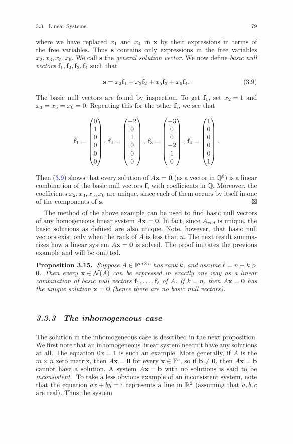
3.3 Linear Systems 79
where we have replaced x1 and x4 in x by their expressions in terms ofthe free variables. Thus s contains only expressions in the free variablesx2, x3, x5, x6. We call s the general solution vector. We now define basic nullvectors f1, f2, f3, f4 such that
s = x2f1 + x3f2 + x5f3 + x6f4. (3.9)
The basic null vectors are found by inspection. To get f1, set x2 = 1 andx3 = x5 = x6 = 0. Repeating this for the other fi, we see that
f1 =
⎛⎜⎜⎜⎜⎜⎜⎝
010000
⎞⎟⎟⎟⎟⎟⎟⎠
, f2 =
⎛⎜⎜⎜⎜⎜⎜⎝
−201000
⎞⎟⎟⎟⎟⎟⎟⎠
, f3 =
⎛⎜⎜⎜⎜⎜⎜⎝
−300
−210
⎞⎟⎟⎟⎟⎟⎟⎠
, f4 =
⎛⎜⎜⎜⎜⎜⎜⎝
100001
⎞⎟⎟⎟⎟⎟⎟⎠
.
Then (3.9) shows that every solution of Ax = 0 (as a vector in Q6) is a linear
combination of the basic null vectors fi with coefficients in Q. Moreover, thecoefficients x2, x3, x5, x6 are unique, since each of them occurs by itself in oneof the components of s. �
The method of the above example can be used to find basic null vectorsof any homogeneous linear system Ax = 0. In fact, since Ared is unique, thebasic solutions as defined are also unique. Note, however, that basic nullvectors exist only when the rank of A is less than n. The next result summa-rizes how a linear system Ax = 0 is solved. The proof imitates the previousexample and will be omitted.
Proposition 3.15. Suppose A ∈ Fm×n has rank k, and assume � = n − k >
0. Then every x ∈ N (A) can be expressed in exactly one way as a linearcombination of basic null vectors f1, . . . , f� of A. If k = n, then Ax = 0 hasthe unique solution x = 0 (hence there are no basic null vectors).
3.3.3 The inhomogeneous case
The solution in the inhomogeneous case is described in the next proposition.We first note that an inhomogeneous linear system needn’t have any solutionsat all. The equation 0x = 1 is such an example. More generally, if A is them × n zero matrix, then Ax = 0 for every x ∈ F
n, so if b �= 0, then Ax = bcannot have a solution. A system Ax = b with no solutions is said to beinconsistent. To take a less obvious example of an inconsistent system, notethat the equation ax + by = c represents a line in R
2 (assuming that a, b, care real). Thus the system
80 3 Matrices
ax + by = cdx + ey = f
represents the points where two lines in R2 intersect. If the lines are distinct
parallel lines (e.g., a = d, b = e, c �= f), then they have empty intersection, sothe system is inconsistent. If the lines are distinct and nonparallel, they meetin a unique point. There is another way in which a system can be inconsistent.If it is overdetermined, that is, if there are more equations than variables, thenit may be inconsistent. For example, three lines in R
2 which are mutuallynonparallel will meet only if the third passes through the unique intersectionpoint of the first two. We now state the criterion for an inhomogeneous linearsystem to be consistent.
Proposition 3.16. The inhomogeneous linear system Ax = b is consistentif and only if the rank of its coefficient matrix (A | b) is the same as the rankof A. In particular, if A is of size m × n and has rank m, then the systemAx = b is always consistent.
Proof. If the ranks are different, then the rank of (A | b) is larger thanthe rank of A. This implies that if BA = Ared, then the equivalent systemBAx = Aredx = Aredb contains an equation of the form 0x1 + · · · + 0xn =c, where c �= 0. Such an equation is clearly inconsistent. Therefore, if theinhomogeneous linear system is consistent, the ranks of A and (A | b) arethe same. We leave the argument for the converse to the reader. If A has rankm, then so does (A | b), so Ax = b is consistent. �
Example 3.12. The system
3x + 3y = 1x − y = 2x + 2y = 0
.
has coefficient matrix ⎛⎝
3 3 11 − 1 21 2 0
⎞⎠ .
This matrix has rank three, so the system is inconsistent. �
Let us now summarize our discussion.
Proposition 3.17. Suppose that A ∈ Fm×n has rank k, and consider an
inhomogeneous linear system Ax = b. This system is consistent if and onlyif the rank of (A | b) is the same as the rank of A. Assume so and let p0 ∈ F
n
be a particular solution. Then every solution can be written in the formx = p0 + w, where w ∈ N (A). If k = n, then N (A) = {0}, and consequently
3.3 Linear Systems 81
p0 is the unique solution. If k < n, let � = n − k, and suppose f1, . . . , f� areA’s basic null vectors. Thus, every x ∈ F
n of the form
x = p0 +�∑
i=1
aifi (all ai ∈ F) (3.10)
is a solution, and every solution can be written in the form (3.10) for a uniquechoice of the ai.
Proof. Suppose x satisfies Ax = b. Then
A(x − p0) = Ax − Ap0 = b − b = 0.
Thus, w = x − p0 ∈ N (A), so x = p0 + w, as claimed. If k = n, we knowfrom Proposition 3.15 that N (A) = {0}, so w = 0. Thus p0 is the uniquesolution. Now suppose k < n. There exist fundamental solutions f1, . . . , f�with � = n − k, and w can be uniquely written w =
∑�i=1 aifi. This implies
the final assertion. �
Example 3.13. To illustrate this result, consider the inhomogeneous linearsystem
x1 + x2 + 2x3 + 0x4 + 3x5 − x6 = 1,
x4 + 2x5 + 0x6 = −1.
Note that the coefficient matrix A is taken from Example 3.11, so solving asabove, we see that
x1 = 1 − 2x3 − 3x5 + x6,
x4 = −1 − 2x5.
Therefore, p0 = (1, 0, 0,−1, 0, 0)T is a particular solution of the inhomoge-neous linear system. Hence, every solution has the form p0 + s, where s isthe general solution vector of the homogeneous linear system Ax = 0. �
Remark. Notice that if A ∈ Fm×n, then N (A) is an abelian group. In fact,
it is a subgroup of Fn. Proposition 3.17 says that the set of solutions of a
consistent linear system Ax = b is a coset p0 + N (A) of N (A). The cosetrepresentative p0 is a particular solution.
Remark. Our final remark is that Ax = b is consistent if and only if b is alinear combination of the columns of A. This follows from the identity (3.5).We will also discuss this fact in more detail when the column space of amatrix is introduced.
82 3 Matrices
3.3.4 A useful identity
Suppose A ∈ Fm×n. Since each corner of Ared occupies a unique row and a
unique column, the rank k of A satisfies both k ≤ m and k ≤ n. If k < n,then there exists at least one free variable, so A will always have a basic nullvector. There is a simple but important relationship, already pointed out,between the rank k and the number of basic null vectors, or equivalently, thenumber of free variables:
rank(A) + # free variables = n. (3.11)
We will restate this identity several times, each time in a more general form.In its most general form, the identity (3.11) is the rank–nullity theorem. Forexample, if m < n, then there exists at least one free variable. In particular,a system Ax = b cannot have a unique solution.
The identity (3.11) has the following useful consequence for n × n matrices.
Proposition 3.18. Let A ∈ Fn×n. Then A is nonsingular if and only if
N (A) = {0}.Proof. Suppose A is nonsingular. By definition, A has rank n, so Ared = In.This implies N (A) = N (Ared) = {0}. Conversely, if N (A) = {0}, then Ax =0 implies x = 0. Hence there cannot be any free variables, so by the identity(3.11), the rank of A is n. Thus A is nonsingular. �
Remark. In the next chapter, we will develop some techniques for bringinga matrix into reduced row echelon form that are useful for solving linearsystems.
Exercises
Exercises 3.3.1. Show that the null space of a matrix over a field is anabelian group.
Exercises 3.3.2. Let C denote the counting matrix of Example 3.8. Find
an equation in a, b, c that determines when the system C
⎛⎝
xyz
⎞⎠ =
⎛⎝
abc
⎞⎠ is
consistent. (Hint: row reduce.)
Exercises 3.3.3. The field is F2. Consider the following matrices:
A1 =
⎛⎝
1 1 01 0 10 1 1
⎞⎠ , A2 =
⎛⎜⎜⎝
1 0 1 00 1 1 01 1 0 01 0 0 1
⎞⎟⎟⎠ .
Find basic null vectors for both A1 and A2.
3.3 Linear Systems 83
Exercises 3.3.4. Which of the following can happen and which cannot?Provide explanations.
(i) A is of size 15 × 24 and has exactly seven basic null vectors;
(ii) A is of size 3 × 3, and Ax = b is consistent for all b.
(iii) A is of size 12 × 12, three of A’s columns are zero, and A has 10 basicnull vectors.
Chapter 4Matrix Inverses, Matrix Groupsand the LPDU Decomposition
In this chapter we continue our introduction to matrix theory beginningwith the notion of a matrix inverse and the definition of a matrix group. Fornow, the main example of a matrix group is the group GL(n,F) of invertiblen × n matrices over a field F and its subgroups. We will also show that everymatrix A ∈ F
n×n can be factored as a product LPDU , where each of L, P ,D, and U is a matrix in an explicit subset of F
n×n. For example, P is apartial permutation matrix, D is diagonal, and L and U are lower and uppertriangular respectively. The expression A = LPDU tells us a lot about A: forexample, D contains the pivots dii of A and also tells us the rank of A bycounting the number of nonzero pivots. In addition, A’s determinant (whichwill be defined in the next chapter) is determined by PD as ±d11 · · · dnn.When A is invertible, each of L, P , D, and U lies in a certain subgroup ofGL(n,F). For example, P lies in the group of n × n permutation matrices,which is a matrix group isomorphic to S(n).
4.1 The Inverse of a Square Matrix
We now come to the interesting question of when an n × n matrix over a fieldF has an inverse under matrix multiplication. Since every nonzero element ofa field has an inverse, the question for 1 × 1 matrices is already settled. Themain fact turns out to be that an n × n matrix over F is invertible if andonly if its rank is n.
4.1.1 The definition of the inverse
We begin with an essential definition:
c© Springer Science+Business Media LLC 2017J.B. Carrell, Groups, Matrices, and Vector Spaces,DOI 10.1007/978-0-387-79428-0 4
85
86 4 Matrix Inverses, Matrix Groups and the LPDU Decomposition
Definition 4.1. Let F be a field and suppose A ∈ Fn×n. We say that A is
invertible if there exists B ∈ Fn×n such that AB = BA = In. We will say that
B is an inverse of A, and likewise, that A is an inverse of B.
Example 4.1. All 2 × 2 elementary matrices are invertible. Their inversesare given as follows:
E1 =(
0 11 0
)⇒ E−1
1 =(
0 11 0
),
E2 =(
r 00 1
)⇒ E−1
2 =(
r−1 00 1
),
and
E3 =(
1 s0 1
)⇒ E−1
3 =(
1 −s0 1
).
�
In fact, we already noted that if E ∈ Fn×n is an elementary matrix and F
is the elementary matrix that reverses the row operation that E effects, thenFE = EF = In. In other words, doing a row operation and then undoing itproduces the same result as first undoing it and then doing it, and the resultis that nothing changes. Thus every elementary matrix is invertible. Notethat the definition can apply only to square matrices, but if A is square, wecan consider both left and right inverses of A. A left inverse of A ∈ F
n×n isa matrix B ∈ F
n×n such that BA = In, and a right inverse of A is a matrixB ∈ F
n×n such that AB = In. It is useful to note (as was already noted forgroups) that when an inverse exists, it is unique. This is one of the niceconsequences of the associativity of matrix multiplication we have previouslymentioned.
Proposition 4.1. An invertible n × n matrix has a unique inverse.
Proof. Suppose A ∈ Fn×n has two inverses B and C. Then B = BIn =
B(AC) = (BA)C = InC = C. Thus B = C. �
4.1.2 Results on Inverses
Elementary matrices are the key to understanding when inverses exist andhow to find them. As we already noted above, if E ∈ F
n×n is elementary,then there exists an elementary matrix F ∈ F
n×n such that FE = EF = In.Thus elementary matrices are invertible. In fact, the inverse of an elementarymatrix has the same type. Our first result about inverses is that a nonsingular
4.1 The Inverse of a Square Matrix 87
matrix (that is, an element of Fn×n of rank n) is invertible. Recall that byProposition 3.13, A ∈ F
n×n is nonsingular if and only if there exist elementarymatrices E1, . . . , Ek ∈ F
n×n such that Ek · · · E1A = In. In particular, if A isnonsingular, we can assert that A has a left inverse.
Proposition 4.2. Let A in Fn×n. If A is nonsingular, then A is invertible.
In fact, let E1, . . . , Ek ∈ Fn×n be elementary matrices such that Ek · · · E1A =
In, and let F1, . . . , Fk ∈ Fn×n denote the elementary matrices such that
FiEi = In. Then A = F1 · · · Fk and A−1 = Ek · · · E1. Consequently, if A isnonsingular, then A−1 is also nonsingular.
Proof. Let B = Ek · · · E1 and C = F1 · · · Fk. Then by associativity of multi-plication,
CB = (F1 · · · Fk)(Ek · · · E1) = In,
since FiEi = In for each i. Now BA = In by assumption, so
A = InA = (CB)A = C(BA) = CIn = C.
Thus A = F1 · · · Fk, as claimed. Since CB = In and A = C, we have AB = In,which proves that A is invertible. We leave it to the reader to show that if Ais nonsingular, then so is A−1. �
Therefore, nonsingular matrices are invertible. In fact, the converse is alsotrue, which will be important in our discussion of matrix groups.
Theorem 4.3. Let A ∈ Fn×n. Then A is nonsingular if and only if A is
invertible if and only if A is a product of elementary matrices.
Proof. By Proposition 4.2, a nonsingular matrix is invertible. To show thatan invertible matrix is nonsingular, let A be invertible, and suppose BA = In.Now suppose Ax = 0. Then x = (BA)x = B(Ax) = B0 = 0, so by Proposi-tion 3.18, it follows that A is nonsingular. If A is nonsingular, then by Propo-sition 4.2, A is a product of elementary matrices. Conversely, a product ofelementary matrices is invertible, so the proof is finished. �
Notice that all that is required in the proof of the above theorem is that Ahave a left inverse B. To expand on this observation, we will prove one lastresult.
Proposition 4.4. Let A ∈ Fn×n. Then if A has either a left inverse B (that
is, BA = In) or a right inverse C (that is, AC = In), then A is invertible.
Proof. Suppose A has a left inverse B. Arguing as in the proof of Theorem4.3, we conclude that Ax = 0 implies x = 0, so A is nonsingular. Therefore,A is invertible. Now suppose A has a right inverse C. Then C has a leftinverse A, so C is invertible. Thus, A is invertible too. �
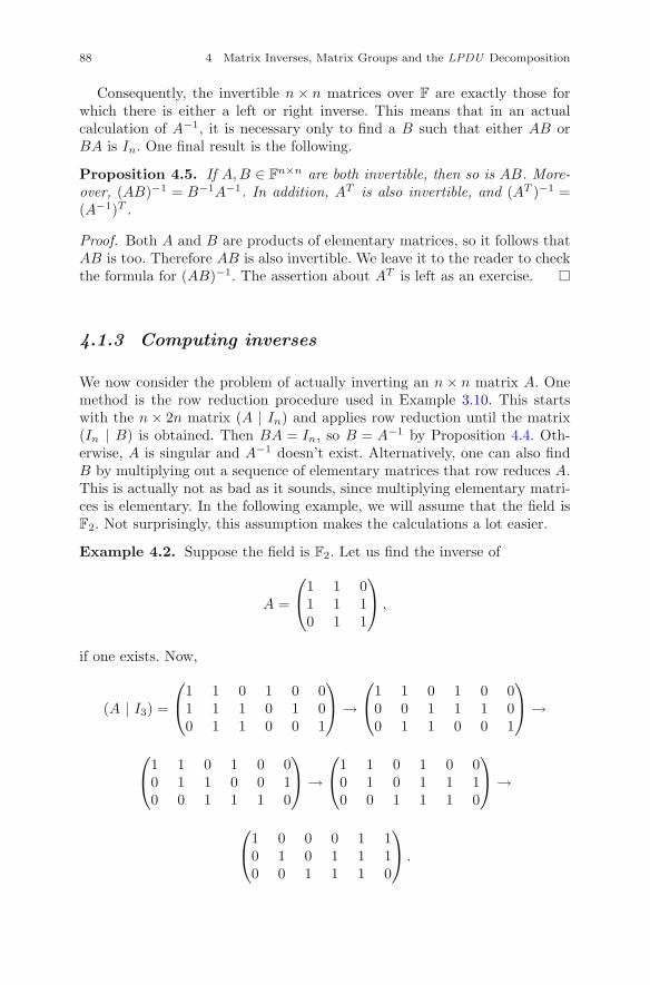
88 4 Matrix Inverses, Matrix Groups and the LPDU Decomposition
Consequently, the invertible n × n matrices over F are exactly those forwhich there is either a left or right inverse. This means that in an actualcalculation of A−1, it is necessary only to find a B such that either AB orBA is In. One final result is the following.
Proposition 4.5. If A,B ∈ Fn×n are both invertible, then so is AB. More-
over, (AB)−1 = B−1A−1. In addition, AT is also invertible, and (AT )−1 =(A−1)T .
Proof. Both A and B are products of elementary matrices, so it follows thatAB is too. Therefore AB is also invertible. We leave it to the reader to checkthe formula for (AB)−1. The assertion about AT is left as an exercise. �
4.1.3 Computing inverses
We now consider the problem of actually inverting an n × n matrix A. Onemethod is the row reduction procedure used in Example 3.10. This startswith the n × 2n matrix (A | In) and applies row reduction until the matrix(In | B) is obtained. Then BA = In, so B = A−1 by Proposition 4.4. Oth-erwise, A is singular and A−1 doesn’t exist. Alternatively, one can also findB by multiplying out a sequence of elementary matrices that row reduces A.This is actually not as bad as it sounds, since multiplying elementary matri-ces is elementary. In the following example, we will assume that the field isF2. Not surprisingly, this assumption makes the calculations a lot easier.
Example 4.2. Suppose the field is F2. Let us find the inverse of
A =
⎛⎝1 1 0
1 1 10 1 1
⎞⎠ ,
if one exists. Now,
(A | I3) =
⎛⎝1 1 0 1 0 0
1 1 1 0 1 00 1 1 0 0 1
⎞⎠ →
⎛⎝1 1 0 1 0 0
0 0 1 1 1 00 1 1 0 0 1
⎞⎠ →
⎛⎝1 1 0 1 0 0
0 1 1 0 0 10 0 1 1 1 0
⎞⎠ →
⎛⎝1 1 0 1 0 0
0 1 0 1 1 10 0 1 1 1 0
⎞⎠ →
⎛⎝1 0 0 0 1 1
0 1 0 1 1 10 0 1 1 1 0
⎞⎠ .
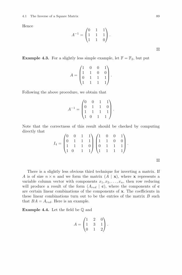
4.1 The Inverse of a Square Matrix 89
Hence
A−1 =
⎛⎝0 1 1
1 1 11 1 0
⎞⎠ .
�
Example 4.3. For a slightly less simple example, let F = F2, but put
A =
⎛⎜⎜⎝
1 0 0 11 1 0 00 1 1 11 1 1 1
⎞⎟⎟⎠ .
Following the above procedure, we obtain that
A−1 =
⎛⎜⎜⎝
0 0 1 10 1 1 01 1 1 11 0 1 1
⎞⎟⎟⎠ .
Note that the correctness of this result should be checked by computingdirectly that
I4 =
⎛⎜⎜⎝
0 0 1 10 1 1 11 1 1 01 0 1 1
⎞⎟⎟⎠
⎛⎜⎜⎝
1 0 0 11 1 0 00 1 1 11 1 1 1
⎞⎟⎟⎠ .
�
There is a slightly less obvious third technique for inverting a matrix. IfA is of size n × n and we form the matrix (A | x), where x represents avariable column vector with components x1, x2, . . . , xn, then row reducingwill produce a result of the form (Ared | c), where the components of care certain linear combinations of the components of x. The coefficients inthese linear combinations turn out to be the entries of the matrix B suchthat BA = Ared. Here is an example.
Example 4.4. Let the field be Q and
A =
⎛⎝1 2 0
1 3 10 1 2
⎞⎠ .
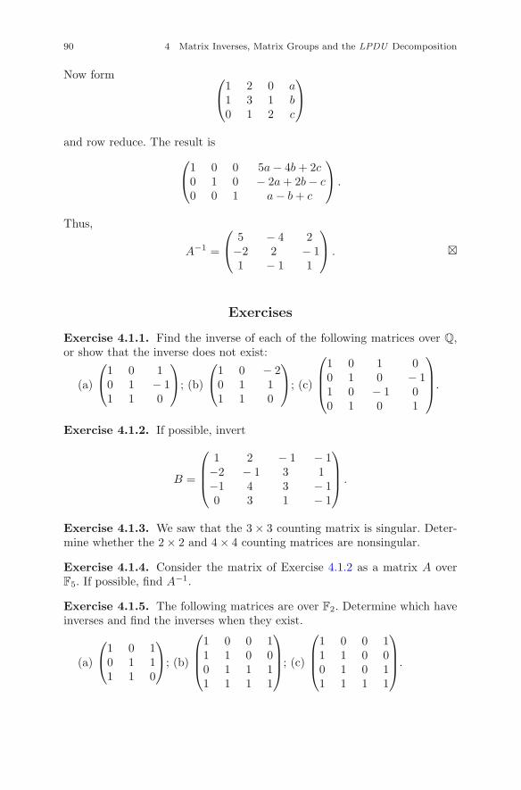
90 4 Matrix Inverses, Matrix Groups and the LPDU Decomposition
Now form ⎛⎝1 2 0 a
1 3 1 b0 1 2 c
⎞⎠
and row reduce. The result is⎛⎝1 0 0 5a − 4b + 2c
0 1 0 − 2a + 2b − c0 0 1 a − b + c
⎞⎠ .
Thus,
A−1 =
⎛⎝ 5 − 4 2
−2 2 − 11 − 1 1
⎞⎠ . �
Exercises
Exercise 4.1.1. Find the inverse of each of the following matrices over Q,or show that the inverse does not exist:
(a)
⎛⎝1 0 1
0 1 − 11 1 0
⎞⎠; (b)
⎛⎝1 0 − 2
0 1 11 1 0
⎞⎠; (c)
⎛⎜⎜⎝
1 0 1 00 1 0 − 11 0 − 1 00 1 0 1
⎞⎟⎟⎠.
Exercise 4.1.2. If possible, invert
B =
⎛⎜⎜⎝
1 2 − 1 − 1−2 − 1 3 1−1 4 3 − 10 3 1 − 1
⎞⎟⎟⎠ .
Exercise 4.1.3. We saw that the 3 × 3 counting matrix is singular. Deter-mine whether the 2 × 2 and 4 × 4 counting matrices are nonsingular.
Exercise 4.1.4. Consider the matrix of Exercise 4.1.2 as a matrix A overF5. If possible, find A−1.
Exercise 4.1.5. The following matrices are over F2. Determine which haveinverses and find the inverses when they exist.
(a)
⎛⎝1 0 1
0 1 11 1 0
⎞⎠; (b)
⎛⎜⎜⎝
1 0 0 11 1 0 00 1 1 11 1 1 1
⎞⎟⎟⎠; (c)
⎛⎜⎜⎝
1 0 0 11 1 0 00 1 0 11 1 1 1
⎞⎟⎟⎠.
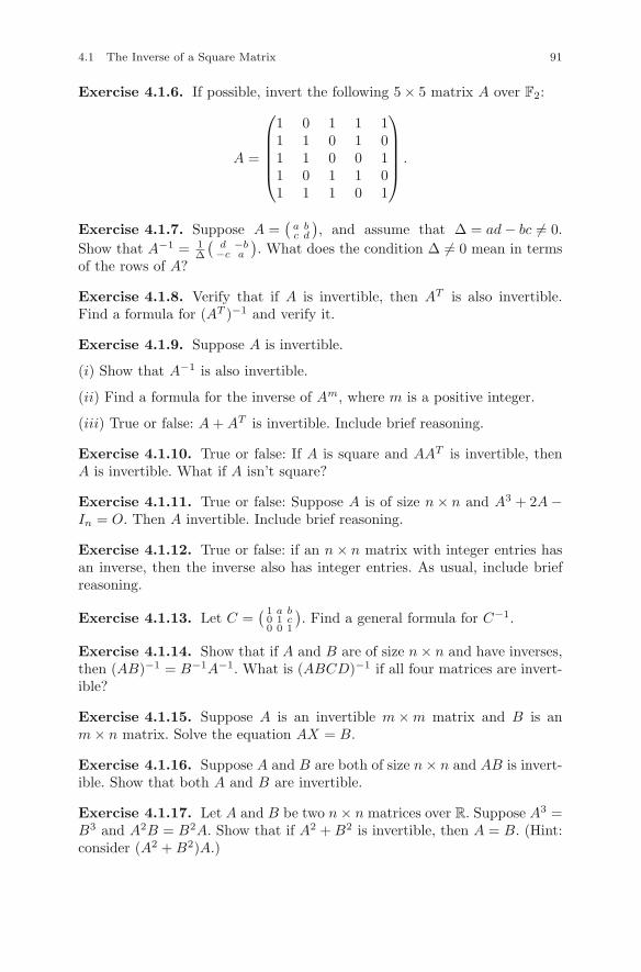
4.1 The Inverse of a Square Matrix 91
Exercise 4.1.6. If possible, invert the following 5 × 5 matrix A over F2:
A =
⎛⎜⎜⎜⎜⎝
1 0 1 1 11 1 0 1 01 1 0 0 11 0 1 1 01 1 1 0 1
⎞⎟⎟⎟⎟⎠ .
Exercise 4.1.7. Suppose A =(a bc d
), and assume that Δ = ad − bc �= 0.
Show that A−1 = 1Δ
(d −b
−c a
). What does the condition Δ �= 0 mean in terms
of the rows of A?
Exercise 4.1.8. Verify that if A is invertible, then AT is also invertible.Find a formula for (AT )−1 and verify it.
Exercise 4.1.9. Suppose A is invertible.
(i) Show that A−1 is also invertible.
(ii) Find a formula for the inverse of Am, where m is a positive integer.
(iii) True or false: A + AT is invertible. Include brief reasoning.
Exercise 4.1.10. True or false: If A is square and AAT is invertible, thenA is invertible. What if A isn’t square?
Exercise 4.1.11. True or false: Suppose A is of size n × n and A3 + 2A −In = O. Then A invertible. Include brief reasoning.
Exercise 4.1.12. True or false: if an n × n matrix with integer entries hasan inverse, then the inverse also has integer entries. As usual, include briefreasoning.
Exercise 4.1.13. Let C =( 1 a b
0 1 c0 0 1
). Find a general formula for C−1.
Exercise 4.1.14. Show that if A and B are of size n × n and have inverses,then (AB)−1 = B−1A−1. What is (ABCD)−1 if all four matrices are invert-ible?
Exercise 4.1.15. Suppose A is an invertible m × m matrix and B is anm × n matrix. Solve the equation AX = B.
Exercise 4.1.16. Suppose A and B are both of size n × n and AB is invert-ible. Show that both A and B are invertible.
Exercise 4.1.17. Let A and B be two n × n matrices over R. Suppose A3 =B3 and A2B = B2A. Show that if A2 + B2 is invertible, then A = B. (Hint:consider (A2 + B2)A.)
92 4 Matrix Inverses, Matrix Groups and the LPDU Decomposition
Exercise 4.1.18. Let A and B be n × n matrices over F.
(i) Show that if the inverse of A2 is B, then the inverse of A is AB.
(ii) Suppose A, B, and A + B are all invertible. Find the inverse of A−1 +B−1 in terms of A, B, and A + B.
Exercise 4.1.19. You are a cryptographer assigned to crack the clevercipher constructed as follows. First, let the sequence 01 represent A, 02 repre-sent B, and so forth up to 26, which represents Z. For clarity, a space betweenwords is indicated by inserting 00. A text can thus be unambiguously encodedas a sequence. For example, 1908040002090700041507 is the encoding of thephrase “the big dog.” Since this string of integers has length 22, we willthink of it as a vector in Q
22. Suppose a text has been encoded as a sequenceof length 14,212. Now, 14,212 = 44 × 323, so the sequence can be brokeninto 323 consecutive intervals of length 44. Next, suppose each subinterval istransposed and multiplied on the left by a single 44 × 44 matrix C. The newsequence obtained by transposing again and laying the products end to endwill be the enciphered message, and it is your job to decipher it. Discuss thefollowing questions.
(i) How does one produce an invertible 44 × 44 matrix in an efficient way,and how does one find its inverse?
(ii) How many of the subintervals will you need to decipher to break thewhole cipher by deducing the matrix C?
4.2 Matrix Groups 93
4.2 Matrix Groups
The purpose of this section is to introduce the concept of a matrix group andproduce a number of examples. A matrix group is essentially a collection ofmatrices that lie in some F
n×n that forms a group under matrix multiplica-tion, where the identity is In. Thus the axioms defining a matrix group aremodest, but they are enough to ensure that matrix groups form an interest-ing central part of algebra. In the final chapter, we will outline the theoryof the structure of matrix groups that are defined by some equations. Thesegroups are known as linear algebraic groups. The matrix group structure willbe useful in stating and proving some of the main results on matrices in laterchapters.
4.2.1 The definition of a matrix group
We begin with the main definition.
Definition 4.2. Let F be a field. A subset G of Fn×n is called a matrix groupif it satisfies the following three conditions:
(i) if A,B ∈ G, then AB ∈ G (that is, G is closed under multiplication);
(ii) In ∈ G; and
(iii) if A ∈ G, then A is invertible, and A−1 ∈ G.
Remark. Since matrix multiplication is associative, every matrix group Gis a group under matrix multiplication with identity the identity matrix, andthe inverse of every A ∈ G given by A−1.
The most basic example of a matrix group G ⊂ Fn×n is the general linear
group over F, which is denoted by GL(n,F). By definition,
GL(n,F) = {A ∈ Fn×n | A−1 exists}. (4.1)
Thus, GL(n,F) is the set of all invertible elements of Fn×n.
Proposition 4.6. The set GL(n,F) is a matrix group. Moreover, everymatrix group G ⊂ F
n×n is a subgroup of GL(n,F).
Proof. By Proposition 4.5, GL(n,F) is closed under multiplication. Moreover,In ∈ GL(n,F). Finally, if A is invertible, so is A−1. Therefore, GL(n,F) is amatrix group. �
A subgroup of a matrix group is called a matrix subgroup. For example,{In} is a subgroup of every matrix group G ⊂ GL(n,F). One usually calls
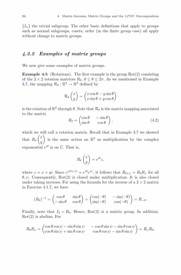
94 4 Matrix Inverses, Matrix Groups and the LPDU Decomposition
{In} the trivial subgroup. The other basic definitions that apply to groupssuch as normal subgroups, cosets, order (in the finite group case) all applywithout change to matrix groups.
4.2.2 Examples of matrix groups
We now give some examples of matrix groups.
Example 4.5 (Rotations). The first example is the group Rot(2) consistingof the 2 × 2 rotation matrices Rθ, 0 ≤ θ ≤ 2π. As we mentioned in Example3.7, the mapping Rθ : R2 → R
2 defined by
Rθ
(xy
)=
(x cos θ − y sin θx sin θ + y cos θ
)
is the rotation of R2 through θ. Note that Rθ is the matrix mapping associatedto the matrix
Rθ =(
cos θ − sin θsin θ cos θ
), (4.2)
which we will call a rotation matrix. Recall that in Example 3.7 we showed
that Rθ
(xy
)is the same action on R
2 as multiplication by the complex
exponential eiθ is on C. That is,
Rθ
(xy
)= eiθz,
where z = x + yi. Since ei(θ+ψ) = eiθeiψ, it follows that Rθ+ψ = RθRψ for allθ, ψ. Consequently, Rot(2) is closed under multiplication. It is also closedunder taking inverses. For using the formula for the inverse of a 2 × 2 matrixin Exercise 4.1.7, we have
(Rθ)−1 =(
cos θ sin θ− sin θ cos θ
)=
(cos(−θ) − sin(−θ)sin(−θ) cos(−θ)
)= R−θ.
Finally, note that I2 = R0. Hence, Rot(2) is a matrix group. In addition,Rot(2) is abelian. For
RθRψ =(
cos θ cos ψ − sin θ sinψ − cos θ sinψ − sin θ cos ψcos θ sin ψ + sin θ cos ψ cos θ cos ψ − sin θ sin ψ
)= RψRθ,
4.2 Matrix Groups 95
as can be seen by noticing that each term in the matrix stays the same afterflipping θ and ψ. This also follows from the observation that eiθeiψ = eiθeiθ,since C∗ is an abelian group. This is worth noting, since among other reasons,abelian matrix groups are rather rare. Another fact to notice is that thereis an explicit group isomorphism φ : S1 → Rot(2), which is defined by firstsetting z = eiθ and then putting φ(z) = Rθ. We leave it as an exercise to showthat φ is, as claimed, a well-defined isomorphism. �
The next example of a matrix group plays a fundamental role in the Euclid-ean geometry of Rn.
Definition 4.3 (The orthogonal group). Let Q ∈ Rn×n. We say that Q is
orthogonal if QTQ = In (i.e., Q−1 = QT ). The set of all n × n orthogonalmatrices is called the orthogonal group of degree n. The orthogonal group isdenoted by O(n,R).
Thus, Q ∈ Rn×n is orthogonal if and only if when Q = (q1 q2 · · · qn),
then qTi qj = δij for all 1 ≤ i, j ≤ n.
Proposition 4.7. O(n,R) is a subgroup of GL(n,R).
Proof. We first show that if Q,R ∈ O(n,R), then QR ∈ O(n,R). We have tocheck that (QR)T (QR) = In. But
(QR)T (QR) = (RTQT )(QR) = RT (QTQ)R = RT InR = In,
so O(n,R) is closed under multiplication. Clearly In ∈ O(n,R), so it remainsto verify that Q ∈ O(n,R) implies Q−1 ∈ O(n,R). But Q−1 = QT , so wehave to check that (QT )TQT = In. This amounts to showing that QQT = In,which holds due to the fact that QTQ = In. This completes theverification. �
The alert reader may have noticed that the definition of the orthogonalgroup O(n,R) actually had nothing to do with R. That is, we could just aseasily defined O(n,F) in exactly the same way for any field F. In fact, thematrix groups of the type O(n,F) form an important class known as theorthogonal groups over F. One frequently concentrates on O(n,R) becauseits properties are related to the geometry of n-dimensional Euclidean space.
In the following section, we will give an example of a matrix group closelyrelated to the symmetric group.
4.2.3 The group of permutation matrices
Recall that ei is the column vector such that In = (e1 · · · en). If σ ∈ S(n),put Pσ = (eσ(1) · · · eσ(n)). Thus,
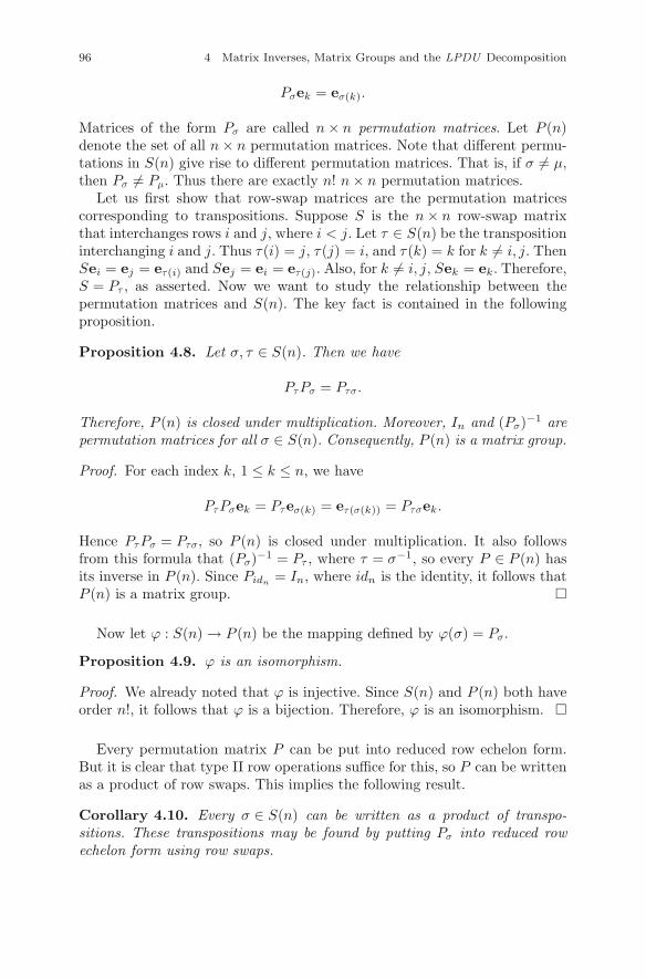
96 4 Matrix Inverses, Matrix Groups and the LPDU Decomposition
Pσek = eσ(k).
Matrices of the form Pσ are called n × n permutation matrices. Let P (n)denote the set of all n × n permutation matrices. Note that different permu-tations in S(n) give rise to different permutation matrices. That is, if σ �= μ,then Pσ �= Pμ. Thus there are exactly n! n × n permutation matrices.
Let us first show that row-swap matrices are the permutation matricescorresponding to transpositions. Suppose S is the n × n row-swap matrixthat interchanges rows i and j, where i < j. Let τ ∈ S(n) be the transpositioninterchanging i and j. Thus τ(i) = j, τ(j) = i, and τ(k) = k for k �= i, j. ThenSei = ej = eτ(i) and Sej = ei = eτ(j). Also, for k �= i, j, Sek = ek. Therefore,S = Pτ , as asserted. Now we want to study the relationship between thepermutation matrices and S(n). The key fact is contained in the followingproposition.
Proposition 4.8. Let σ, τ ∈ S(n). Then we have
PτPσ = Pτσ.
Therefore, P (n) is closed under multiplication. Moreover, In and (Pσ)−1 arepermutation matrices for all σ ∈ S(n). Consequently, P (n) is a matrix group.
Proof. For each index k, 1 ≤ k ≤ n, we have
PτPσek = Pτeσ(k) = eτ(σ(k)) = Pτσek.
Hence PτPσ = Pτσ, so P (n) is closed under multiplication. It also followsfrom this formula that (Pσ)−1 = Pτ , where τ = σ−1, so every P ∈ P (n) hasits inverse in P (n). Since Pidn
= In, where idn is the identity, it follows thatP (n) is a matrix group. �
Now let ϕ : S(n) → P (n) be the mapping defined by ϕ(σ) = Pσ.
Proposition 4.9. ϕ is an isomorphism.
Proof. We already noted that ϕ is injective. Since S(n) and P (n) both haveorder n!, it follows that ϕ is a bijection. Therefore, ϕ is an isomorphism. �
Every permutation matrix P can be put into reduced row echelon form.But it is clear that type II row operations suffice for this, so P can be writtenas a product of row swaps. This implies the following result.
Corollary 4.10. Every σ ∈ S(n) can be written as a product of transpo-sitions. These transpositions may be found by putting Pσ into reduced rowechelon form using row swaps.
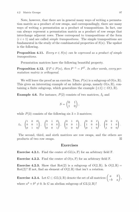
4.2 Matrix Groups 97
Note, however, that there are in general many ways of writing a permuta-tion matrix as a product of row swaps, and correspondingly, there are manyways of writing a permutation as a product of transpositions. In fact, onecan always represent a permutation matrix as a product of row swaps thatinterchange adjacent rows. These correspond to transpositions of the form(i i + 1) and are called simple transpositions. The simple transpositions arefundamental in the study of the combinatorial properties of S(n). The upshotis the following.
Proposition 4.11. Every σ ∈ S(n) can be expressed as a product of simpletranspositions.
Permutation matrices have the following beautiful property.
Proposition 4.12. If P ∈ P (n), then P−1 = PT . In other words, every per-mutation matrix is orthogonal.
We will leave the proof as an exercise. Thus, P (n) is a subgroup of O(n,R).This gives an interesting example of an infinite group, namely O(n,R), con-taining a finite subgroup, which generalizes the example {±1} ⊂ O(1,R).
Example 4.6. For instance, P (2) consists of two matrices, I2 and
S =(
0 11 0
),
while P (3) consists of the following six 3 × 3 matrices;
I3,
⎛⎝1 0 0
0 0 1
0 1 0
⎞⎠ ,
⎛⎝0 1 0
1 0 0
0 0 1
⎞⎠ ,
⎛⎝0 1 0
0 0 1
1 0 0
⎞⎠ ,
⎛⎝0 0 1
1 0 0
0 1 0
⎞⎠ ,
⎛⎝0 0 1
0 1 0
1 0 0
⎞⎠ .
The second, third, and sixth matrices are row swaps, and the others areproducts of two row swaps. �
Exercises
Exercise 4.2.1. Find the center of GL(n,F) for an arbitrary field F.
Exercise 4.2.2. Find the center of O(n,F) for an arbitrary field F.
Exercise 4.2.3. Show that Rot(2) is a subgroup of O(2,R). Is O(2,R) =Rot(2)? If not, find an element of O(2,R) that isn’t a rotation.
Exercise 4.2.4. Let G ⊂ GL(2,R) denote the set of all matrices(
a b−b a
),
where a2 + b2 �= 0. Is G an abelian subgroup of GL(2,R)?
98 4 Matrix Inverses, Matrix Groups and the LPDU Decomposition
Exercise 4.2.5. Show that Q ∈ Rn×n is orthogonal if and only if its rows
q1, . . . ,qn satisfy the condition qiqTj = δij . That is, qiqT
i = 1, while qiqTj =
0 if i �= j.
Exercise 4.2.6. Show that if Q ∈ Rn×n is orthogonal, then so is QT . Con-
clude that a symmetric orthogonal matrix satisfies Q2 = In; hence Q is itsown inverse. Give an example of a 2 × 2 symmetric orthogonal matrix differ-ent from I2.
Exercise 4.2.7. Without computing, try to guess the inverse of the matrix
A =
⎛⎜⎜⎝
1 0 1 00 1 0 − 11 0 − 1 00 1 0 1
⎞⎟⎟⎠ .
(Hint: consider the columns.)
Exercise 4.2.8. Let S1 =
⎛⎝0 1 0
1 0 00 0 1
⎞⎠ and S2 =
⎛⎝1 0 0
0 0 10 1 0
⎞⎠. Show that
every 3 × 3 permutation matrix is a product involving only S1 and S2.
Exercise 4.2.9. Let S1 and S2 be the permutation matrices defined in Exer-cise 4.2.8. Show that (S1S2)3 = I3.
Exercise 4.2.10. Show that every permutation matrix P satisfies the iden-tity P−1 = PT , and conclude that P (n) is a subgroup of O(n,R).
Exercise 4.2.11. Show that the following two matrices are permutationmatrices and find their inverses:
⎛⎜⎜⎜⎜⎝
0 0 0 0 10 0 0 1 00 0 1 0 00 1 0 0 01 0 0 0 0
⎞⎟⎟⎟⎟⎠ ,
⎛⎜⎜⎜⎜⎝
0 0 1 0 00 0 0 0 11 0 0 0 00 1 0 0 00 0 0 1 0
⎞⎟⎟⎟⎟⎠ .
Exercise 4.2.12. A signed permutation matrix is a square matrix Q of theform
Q = P (±e1 ± e2 · · · ± en),
where P ∈ P (n).
(i) Show that the set SP (n) of n × n signed permutation matrices is a sub-group of O(n,R) of order 2nn!.
4.2 Matrix Groups 99
(ii) Prove that P (n) is a normal subgroup of SP (n).
(iii) Describe the quotient group SP (n)/P (n).
Exercise 4.2.13. Prove that every finite group G of order n is isomorphicto a subgroup of O(n,R).
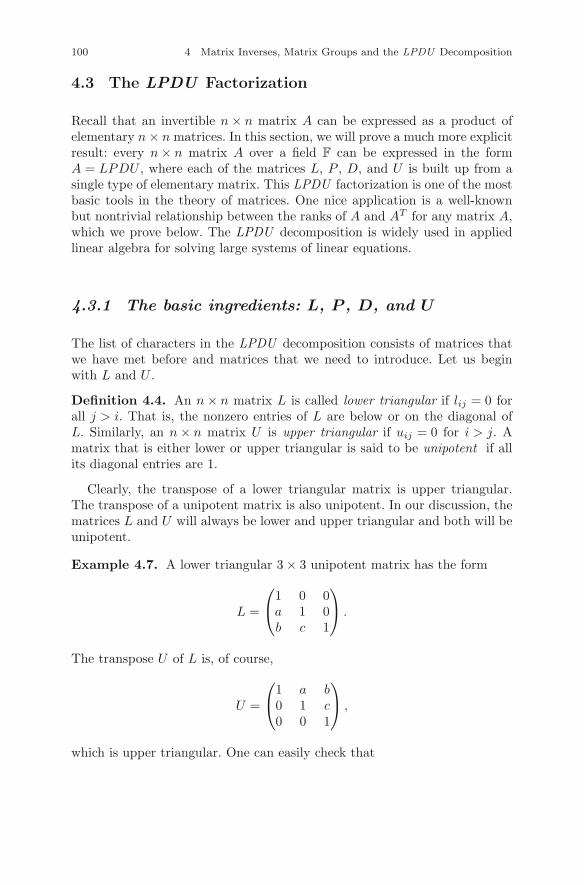
100 4 Matrix Inverses, Matrix Groups and the LPDU Decomposition
4.3 The LPDU Factorization
Recall that an invertible n × n matrix A can be expressed as a product ofelementary n × n matrices. In this section, we will prove a much more explicitresult: every n × n matrix A over a field F can be expressed in the formA = LPDU , where each of the matrices L, P , D, and U is built up from asingle type of elementary matrix. This LPDU factorization is one of the mostbasic tools in the theory of matrices. One nice application is a well-knownbut nontrivial relationship between the ranks of A and AT for any matrix A,which we prove below. The LPDU decomposition is widely used in appliedlinear algebra for solving large systems of linear equations.
4.3.1 The basic ingredients: L, P , D, and U
The list of characters in the LPDU decomposition consists of matrices thatwe have met before and matrices that we need to introduce. Let us beginwith L and U .
Definition 4.4. An n × n matrix L is called lower triangular if lij = 0 forall j > i. That is, the nonzero entries of L are below or on the diagonal ofL. Similarly, an n × n matrix U is upper triangular if uij = 0 for i > j. Amatrix that is either lower or upper triangular is said to be unipotent if allits diagonal entries are 1.
Clearly, the transpose of a lower triangular matrix is upper triangular.The transpose of a unipotent matrix is also unipotent. In our discussion, thematrices L and U will always be lower and upper triangular and both will beunipotent.
Example 4.7. A lower triangular 3 × 3 unipotent matrix has the form
L =
⎛⎝1 0 0
a 1 0b c 1
⎞⎠ .
The transpose U of L is, of course,
U =
⎛⎝1 a b
0 1 c0 0 1
⎞⎠ ,
which is upper triangular. One can easily check that
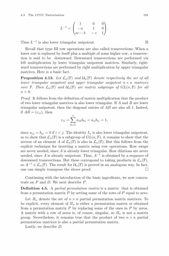
4.3 The LPDU Factorization 101
L−1 =
⎛⎝ 1 0 0
−a 1 0ac − b − c 1
⎞⎠ .
Thus L−1 is also lower triangular unipotent. �Recall that type III row operations are also called transvections. When a
lower row is replaced by itself plus a multiple of some higher row, a transvec-tion is said to be downward. Downward transvections are performed vialeft multiplication by lower triangular unipotent matrices. Similarly, right-ward transvections are performed by right multiplication by upper triangularmatrices. Here is a basic fact.
Proposition 4.13. Let Ln(F) and Un(F) denote respectively the set of alllower triangular unipotent and upper triangular unipotent n × n matricesover F. Then Ln(F) and Un(F) are matrix subgroups of GL(n,F) for alln > 0.
Proof. It follows from the definition of matrix multiplication that the productof two lower triangular matrices is also lower triangular. If A and B are lowertriangular unipotent, then the diagonal entries of AB are also all 1. Indeed,if AB = (cij), then
cii =n∑
k=1
aikbki = aiibii = 1,
since aij = bij = 0 if i < j. The identity In is also lower triangular unipotent,so to show that Ln(F) is a subgroup of GL(n,F), it remains to show that theinverse of an element A of Ln(F) is also in Ln(F). But this follows from theexplicit technique for inverting a matrix using row operations. Row swapsare never needed, since A is already lower triangular. Row dilations are neverneeded, since A is already unipotent. Thus, A−1 is obtained by a sequence ofdownward transvections. But these correspond to taking products in Ln(F),so A−1 ∈ Ln(F). The result for Un(F) is proved in an analogous way. In fact,one can simply transpose the above proof. �
Continuing with the introduction of the basic ingredients, we now concen-trate on P and D. We next describe P .
Definition 4.5. A partial permutation matrix is a matrix that is obtainedfrom a permutation matrix P by setting some of the rows of P equal to zero.
Let Πn denote the set of n × n partial permutation matrix matrices. Tobe explicit, every element of Πn is either a permutation matrix or obtainedfrom a permutation matrix P by replacing some of the ones in P by zeros.A matrix with a row of zeros is, of course, singular, so Πn is not a matrixgroup. Nevertheless, it remains true that the product of two n × n partialpermutation matrices is also a partial permutation matrix.
Lastly, we describe D.
102 4 Matrix Inverses, Matrix Groups and the LPDU Decomposition
Definition 4.6. A diagonal matrix is a square matrix D = (dij) all of whoseoff-diagonal entries are zero; that is, dij = 0 for all i �= j.
Since a diagonal matrix D is invertible if and only if its diagonal entriesdii are all different from 0 and the product of two diagonal matrices is alsodiagonal, we obtain the following result.
Proposition 4.14. The set Dn(F) of all n × n invertible diagonal matricesover F is a matrix subgroup of GL(n,F).
4.3.2 The main result
We now derive the LPDU decomposition.
Theorem 4.15. Every n × n matrix A over a field F can be expressed in theform A = LPDU , where L ∈ Ln(F), P ∈ Πn , D ∈ Dn(F), and U ∈ Un(F).The partial permutation matrix P is always unique. If A is invertible, thenP is a full permutation matrix, and in that case, P and D are both unique.
This result can be expressed in the form of a product of sets, three ofwhich are matrix groups:
Fn×n = Ln(F) · Πn · Dn(F) · Un(F).
Thus every n × n matrix over F is the product of the four types of matricesLn(F), Πn , Dn(F), and Un(F). Specializing to invertible matrices, we have
GL(n,F) = Ln(F) · P (n) · Dn(F) · Un(F).
In particular, GL(n,F) is the product of four of its subgroups: Ln(F), P (n),Dn(F), and Un(F). This is a fundamental result in the theory of matrix groups.
Remark. It is also possible to define an LPDU decomposition for nonsquarematrices. If A ∈ F
m×n, where say m < n, then we can augment A by addingn − m rows of zeros to make A an n × n matrix. Of course, in this situation,the last n − m rows of P will also be zero.
The proof of the theorem is in the same spirit as the proof of the resultthat every matrix can be put into reduced row echelon form by a sequenceof row operations, but it is somewhat more complicated, since both row andcolumn operations are used. The reader may wish to look first at the examplefollowing the proof to get an idea of what is going on in an explicit case.
Proof of Theorem 4.15. We will first prove the existence of the LPDU decom-position. Let A ∈ F
n×n be given. If A = O, put P = O and L = D = U = In.
4.3 The LPDU Factorization 103
Thus suppose A �= O. If A’s first column is zero, go to the right until youreach the first nonzero column, say it’s the jth. Let δj be the first nonzeroentry (from the top), and suppose δj occurs in the ith row. That is, δj = aij .Perform a sequence of downward transvections to make the entries below δjequal to zero. This transforms the jth column of A into
(0 · · · 0 δj 0 · · · 0)T . (4.3)
Thus, we can premultiply A by a lower triangular unipotent matrix L1 tobring the jth column of A into the form (4.3). (Of course, this requires thatthe matrix entries lie in a field.) The next step is to use δj to annihilateall the entries in the ith row of A to the right of the jth column. Sincepostmultiplying by elementary matrices performs column operations, thisamounts to multiplying L1A on the right by a sequence of unipotent uppertriangular elementary matrices. This produces an upper triangular unipotentmatrix U1 such that the first j − 1 columns of (L1A)U1 are zero, the jth hasthe form (4.3), and the ith row is
(0 · · · 0 δj 0 · · · 0), (4.4)
where δj �= 0. We now have the first j columns and ith row of A in the desiredform, and from now on, they won’t change.
To continue, scan to the right until we find the first nonzero column inL1AU1 to the right of the jth column, and suppose this column is the mth.Let bkm be its first nonzero entry, and put δm = bkm. Of course, k �= i. Nowrepeat the previous process by forming L2L1AU1U2 with suitable lower andupper triangular unipotent matrices L2 and U2. Continuing the process, weeventually obtain a lower triangular unipotent matrix L′ and an upper tri-angular unipotent matrix U ′ such that each row and column of L′AU ′ hasat most one nonzero entry. Thus we may write L′AU ′ = PD for some partialpermutation matrix P , where D is a diagonal matrix. The matrix D is notunique, since some of the columns of PD may be zero. But the entry of Din the nonzero columns is, of course, the corresponding entry in PD. Sincewe can take any entries we want in the other columns of D, we can assumethat D is nonsingular. Unraveling, we get A = LPDU , where L = (L′)−1 andU = (U ′)−1. This proves the existence of the LPDU decomposition.
We must now show that P is unique. So suppose A = LPDU = L′P ′D′U ′
are two LPDU decompositions of A. We have to show P = P ′. But we canwrite L−1L′P ′ = PDU(D′U ′)−1, so P = P ′ will follow from the next lemma.
Lemma 4.16. Suppose P and Q are n × n partial permutation matricessuch that PN = MQ, where M is lower triangular unipotent and N is non-singular and upper triangular. Then P = Q.
Proof. We claim that P and Q have the same zero columns. For if the jthcolumn of Q is zero, then the jth column of MQ, and hence of PN , is also
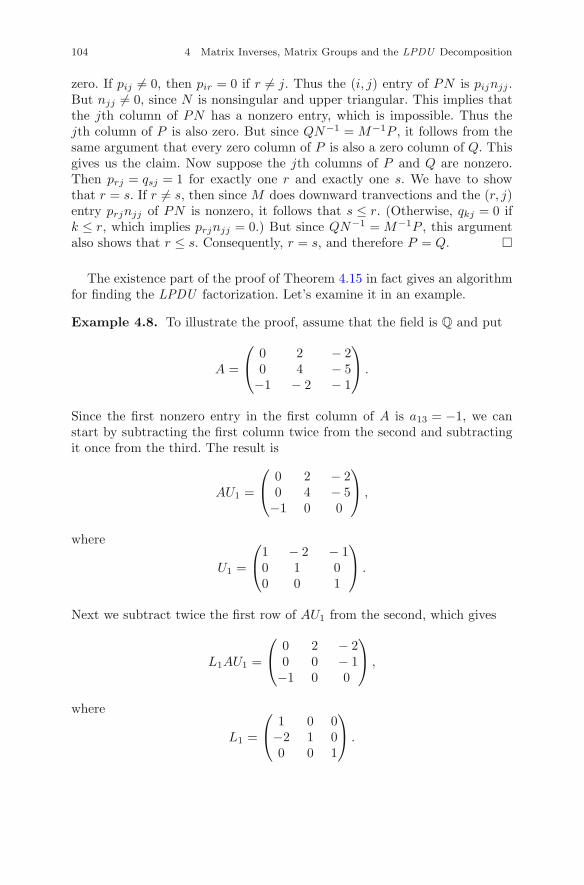
104 4 Matrix Inverses, Matrix Groups and the LPDU Decomposition
zero. If pij �= 0, then pir = 0 if r �= j. Thus the (i, j) entry of PN is pijnjj .But njj �= 0, since N is nonsingular and upper triangular. This implies thatthe jth column of PN has a nonzero entry, which is impossible. Thus thejth column of P is also zero. But since QN−1 = M−1P , it follows from thesame argument that every zero column of P is also a zero column of Q. Thisgives us the claim. Now suppose the jth columns of P and Q are nonzero.Then prj = qsj = 1 for exactly one r and exactly one s. We have to showthat r = s. If r �= s, then since M does downward tranvections and the (r, j)entry prjnjj of PN is nonzero, it follows that s ≤ r. (Otherwise, qkj = 0 ifk ≤ r, which implies prjnjj = 0.) But since QN−1 = M−1P , this argumentalso shows that r ≤ s. Consequently, r = s, and therefore P = Q. �
The existence part of the proof of Theorem 4.15 in fact gives an algorithmfor finding the LPDU factorization. Let’s examine it in an example.
Example 4.8. To illustrate the proof, assume that the field is Q and put
A =
⎛⎝ 0 2 − 2
0 4 − 5−1 − 2 − 1
⎞⎠ .
Since the first nonzero entry in the first column of A is a13 = −1, we canstart by subtracting the first column twice from the second and subtractingit once from the third. The result is
AU1 =
⎛⎝ 0 2 − 2
0 4 − 5−1 0 0
⎞⎠ ,
where
U1 =
⎛⎝1 − 2 − 1
0 1 00 0 1
⎞⎠ .
Next we subtract twice the first row of AU1 from the second, which gives
L1AU1 =
⎛⎝ 0 2 − 2
0 0 − 1−1 0 0
⎞⎠ ,
where
L1 =
⎛⎝ 1 0 0
−2 1 00 0 1
⎞⎠ .
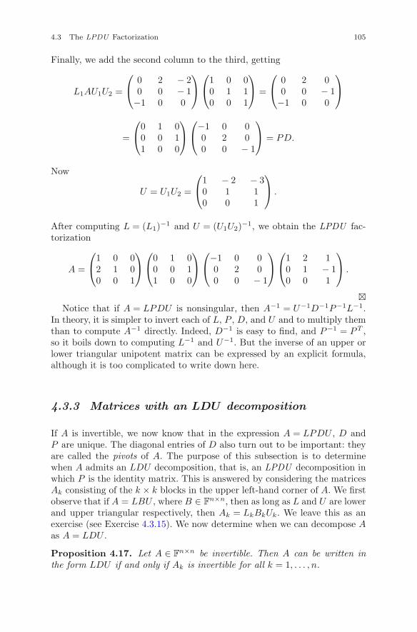
4.3 The LPDU Factorization 105
Finally, we add the second column to the third, getting
L1AU1U2 =
⎛⎝ 0 2 − 2
0 0 − 1−1 0 0
⎞⎠
⎛⎝1 0 0
0 1 10 0 1
⎞⎠ =
⎛⎝ 0 2 0
0 0 − 1−1 0 0
⎞⎠
=
⎛⎝0 1 0
0 0 11 0 0
⎞⎠
⎛⎝−1 0 0
0 2 00 0 − 1
⎞⎠ = PD.
Now
U = U1U2 =
⎛⎝1 − 2 − 3
0 1 10 0 1
⎞⎠ .
After computing L = (L1)−1 and U = (U1U2)−1, we obtain the LPDU fac-torization
A =
⎛⎝1 0 0
2 1 00 0 1
⎞⎠
⎛⎝0 1 0
0 0 11 0 0
⎞⎠
⎛⎝−1 0 0
0 2 00 0 − 1
⎞⎠
⎛⎝1 2 1
0 1 − 10 0 1
⎞⎠ .
�Notice that if A = LPDU is nonsingular, then A−1 = U−1D−1P−1L−1.
In theory, it is simpler to invert each of L, P , D, and U and to multiply themthan to compute A−1 directly. Indeed, D−1 is easy to find, and P−1 = PT ,so it boils down to computing L−1 and U−1. But the inverse of an upper orlower triangular unipotent matrix can be expressed by an explicit formula,although it is too complicated to write down here.
4.3.3 Matrices with an LDU decomposition
If A is invertible, we now know that in the expression A = LPDU , D andP are unique. The diagonal entries of D also turn out to be important: theyare called the pivots of A. The purpose of this subsection is to determinewhen A admits an LDU decomposition, that is, an LPDU decomposition inwhich P is the identity matrix. This is answered by considering the matricesAk consisting of the k × k blocks in the upper left-hand corner of A. We firstobserve that if A = LBU , where B ∈ F
n×n, then as long as L and U are lowerand upper triangular respectively, then Ak = LkBkUk. We leave this as anexercise (see Exercise 4.3.15). We now determine when we can decompose Aas A = LDU .
Proposition 4.17. Let A ∈ Fn×n be invertible. Then A can be written in
the form LDU if and only if Ak is invertible for all k = 1, . . . , n.
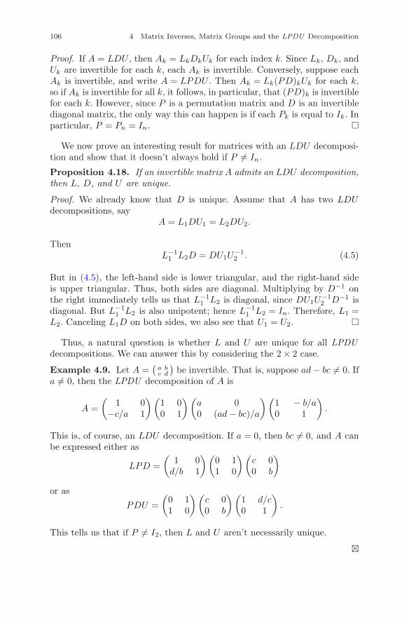
106 4 Matrix Inverses, Matrix Groups and the LPDU Decomposition
Proof. If A = LDU , then Ak = LkDkUk for each index k. Since Lk, Dk, andUk are invertible for each k, each Ak is invertible. Conversely, suppose eachAk is invertible, and write A = LPDU . Then Ak = Lk(PD)kUk for each k,so if Ak is invertible for all k, it follows, in particular, that (PD)k is invertiblefor each k. However, since P is a permutation matrix and D is an invertiblediagonal matrix, the only way this can happen is if each Pk is equal to Ik. Inparticular, P = Pn = In. �
We now prove an interesting result for matrices with an LDU decomposi-tion and show that it doesn’t always hold if P �= In.
Proposition 4.18. If an invertible matrix A admits an LDU decomposition,then L, D, and U are unique.
Proof. We already know that D is unique. Assume that A has two LDUdecompositions, say
A = L1DU1 = L2DU2.
ThenL−1
1 L2D = DU1U−12 . (4.5)
But in (4.5), the left-hand side is lower triangular, and the right-hand sideis upper triangular. Thus, both sides are diagonal. Multiplying by D−1 onthe right immediately tells us that L−1
1 L2 is diagonal, since DU1U−12 D−1 is
diagonal. But L−11 L2 is also unipotent; hence L−1
1 L2 = In. Therefore, L1 =L2. Canceling L1D on both sides, we also see that U1 = U2. �
Thus, a natural question is whether L and U are unique for all LPDUdecompositions. We can answer this by considering the 2 × 2 case.
Example 4.9. Let A =(a bc d
)be invertible. That is, suppose ad − bc �= 0. If
a �= 0, then the LPDU decomposition of A is
A =(
1 0−c/a 1
)(1 00 1
)(a 00 (ad − bc)/a
) (1 − b/a0 1
).
This is, of course, an LDU decomposition. If a = 0, then bc �= 0, and A canbe expressed either as
LPD =(
1 0d/b 1
)(0 11 0
)(c 00 b
)
or as
PDU =(
0 11 0
) (c 00 b
) (1 d/c0 1
).
This tells us that if P �= I2, then L and U aren’t necessarily unique.
�
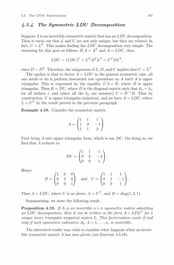
4.3 The LPDU Factorization 107
4.3.4 The Symmetric LDU Decomposition
Suppose A is an invertible symmetric matrix that has an LDU decomposition.Then it turns out that L and U are not only unique, but they are related. Infact, U = LT . This makes finding the LDU decomposition very simple. Thereasoning for this goes as follows. If A = AT and A = LDU , then
LDU = (LDU)T = UTDTLT = UTDLT ,
since D = DT . Therefore, the uniqueness of L, D, and U implies that U = LT .The upshot is that to factor A = LDU in the general symmetric case, all
one needs to do is perform downward row operations on A until A is uppertriangular. This is expressed by the equality L′A = B, where B is uppertriangular. Then B = DU , where D is the diagonal matrix such that dii = biifor all indices i, and (since all the bii are nonzero) U = D−1B. Thus byconstruction, U is upper triangular unipotent, and we have A = LDU , whereL = UT by the result proved in the previous paragraph.
Example 4.10. Consider the symmetric matrix
A =
⎛⎝1 1 1
1 3 − 11 1 2
⎞⎠ .
First bring A into upper triangular form, which is our DU . On doing so, wefind that A reduces to
DU =
⎛⎝1 1 1
0 2 − 20 0 1
⎞⎠ .
Hence
D =
⎛⎝1 0 0
0 2 00 0 1
⎞⎠ and U =
⎛⎝1 1 1
0 1 − 10 0 1
⎞⎠ .
Thus A = LDU , where U is as above, L = UT , and D = diag(1, 2, 1).
Summarizing, we state the following result.
Proposition 4.19. If A is an invertible n × n symmetric matrix admittingan LDU decomposition, then A can be written in the form A = LDLT for aunique lower triangular unipotent matrix L. This factorization exists if andonly if each symmetric submatrix Ak, k = 1, . . . , n, is invertible.
The interested reader may wish to consider what happens when an invert-ible symmetric matrix A has zero pivots (see Exercise 4.3.16).
108 4 Matrix Inverses, Matrix Groups and the LPDU Decomposition
4.3.5 The Ranks of A and AT
The LPDU decomposition turns out to tell us something a little surprisingabout the rank of a matrix and the rank of its transpose. Recall that therank of A is the number of nonzero rows in Ared and is well defined, since thereduced form of A is unique. We shall now apply the LPDU decompositionto find another description of the rank.
Suppose A ∈ Fm×n. We may as well assume the A is square (i.e., m = n),
since otherwise, we may add either rows or columns of zeros to make A squarewithout having any effect on its rank. Thus assume that A ∈ F
n×n. First ofall, we make the following assertion.
Proposition 4.20. If we write A = LPDU , the rank of A is the number ofnonzero rows in the partial permutation matrix P . Put another way, the rankof A is the number of ones in P .
Proof. In fact, the proof of Theorem 4.15 shows that when we put A in LPDUform, the nonzero entries of PD are the pivots of A, and they become thecorner entries of Ared after row permutations. �
We will now prove a nice fact.
Theorem 4.21. For every matrix A over a field F, A and AT have the samerank.
Proof. As usual, we may assume that A is n × n. Writing A = LPDU , wesee that AT = UTDPTLT . This is almost the LPDU decomposition of AT .All we need to do is notice that there exists another nonsingular diagonalmatrix D′ such that DPT = PTD′. But P and PT obviously have the samenumber of ones, so A and AT have the same rank. �
This result is indeed a little surprising, because without knowledge ofLPDU , there isn’t any obvious reason that A and AT are related in this way.In fact, we needed to do quite a bit of work to obtain LPDU . In particular, wefirst needed to prove the uniqueness of Ared to define rank, then we neededto show the existence of the LPDU decomposition, and finally, we had toestablish the uniqueness of the partial permutation matrix P . Recall thatthe rank of a matrix tells us the number k of basic null vectors of a linearsystem Ax = 0. Namely, if A ∈ F
m×n, then k = n − rank(A).The result on the rank of AT gives a simple proof of a well-known result
in the theory of matrices.
Corollary 4.22. Suppose A ∈ Fm×n and assume that M ∈ F
m×m and N ∈Fn×n are both nonsingular. Then the rank of MAN equals the rank of A.
4.3 The LPDU Factorization 109
Proof. First, notice that A and MA have the same rank. Indeed, since M isnonsingular, it is a product of elementary matrices, so A and MA have thesame reduced forms. Thus A, MA, and ATMT have the same rank. Simi-larly, ATMT and NTATMT have the same rank, since NT is nonsingular.Therefore A and MAN also have the same rank. �
Exercises
Exercise 4.3.1. Find the LPDU decompositions and ranks of the followingmatrices over Q:
⎛⎝0 1 1
2 0 11 1 0
⎞⎠ ,
⎛⎝0 0 3
0 2 11 1 1
⎞⎠ ,
⎛⎝1 0 1
0 2 − 11 − 1 0
⎞⎠ .
Exercise 4.3.2. Find the LPDU decompositions and ranks of the trans-poses of the matrices in Exercise 4.3.1.
Exercise 4.3.3. Suppose A = LPDU . What can you say about the LPDUdecomposition of A−1 if it exists? What about (A−1)T ?
Exercise 4.3.4. Let
A =
⎛⎝1 a b
0 1 c0 0 1
⎞⎠ .
Find a formula expressing A as a product of upper triangular transvections(i.e., elementary matrices of type III).
Exercise 4.3.5. Find a general formula for the inverse of the general 4 × 4upper triangular unipotent matrix
U =
⎛⎜⎜⎝
1 a b c0 1 d e0 0 1 f0 0 0 1
⎞⎟⎟⎠ .
Exercise 4.3.6. Show directly that an invertible upper triangular matrix Bcan be expressed as B = DU , where D is a diagonal matrix with nonzerodiagonal entries and U is an upper triangular matrix all of whose diagonalentries are ones. Is this still true if B is singular?
Exercise 4.3.7. Find the LDU decomposition of the matrix
A =
⎛⎝1 1 1
1 − 1 02 0 0
⎞⎠ .
110 4 Matrix Inverses, Matrix Groups and the LPDU Decomposition
Exercise 4.3.8. Let F = F3. Find the LPDU decomposition of
⎛⎜⎜⎝
0 1 2 11 1 0 22 0 0 11 2 1 0
⎞⎟⎟⎠ .
Exercise 4.3.9. Find a 3 × 3 matrix A such that the matrix L in the A =LPDU decomposition isn’t unique.
Exercise 4.3.10. Assume that A ∈ Rn×n is symmetric and has an LDU
decomposition. Show that if all the diagonal entries of D are nonnegative,then A can be written A = CCT , where C is lower triangular. This expressionis called the Cholesky decomposition of A.
Exercise 4.3.11. Find the number of 2 × 2 matrices over F2 having rank 2,and do the same for 3 × 3 matrices of rank 3.
Exercise 4.3.12. Suppose p is prime. Find a formula for |GL(2,Fp)|. (Wewill find a formula for |GL(n,Fp)| for every n in Chap. 6.)
Exercise 4.3.13. Find the rank of each of the following matrices:
⎛⎝1 2 3
1 4 91 8 27
⎞⎠ ,
⎛⎝1 2 2
1 4 41 8 8
⎞⎠ .
Can you see a general result?
Exercise 4.3.14. Write each of the matrices⎛⎜⎜⎝
1 1 2 11 − 1 0 22 0 0 11 2 1 − 1
⎞⎟⎟⎠ and
⎛⎜⎜⎝
0 0 0 10 0 2 20 2 4 41 2 4 − 3
⎞⎟⎟⎠
in the form LPDU , where U = LT .
Exercise 4.3.15. This is an exercise in matrix multiplication. Let A ∈ Fn×n
be expressed as A = LBU , where L and U are lower and upper triangularelements of F
n×n respectively and B ∈ Fn×n is arbitrary. Show that Ak =
LkBkUk for each k = 1, . . . , n. (Recall that Ak is the k × k matrix in theupper left-hand corner of A.)
Exercise 4.3.16. Prove the following result.
4.3 The LPDU Factorization 111
Proposition 4.23. Let A be a symmetric invertible matrix. Then thereexists an expression A = LPDU with L,P,D,U as usual such that :
(i) U = LT ,
(ii) P = PT = P−1, and
(iii) PD = DP .Conversely, if L,P,D,U satisfy the above three conditions, then LPDU issymmetric.
Exercise 4.3.17. Suppose p is prime. Find a formula for
|{A ∈ GL(n,Fp) | A = LDU}|.
Chapter 5An Introduction to the Theoryof Determinants
In this chapter, we will introduce and study a remarkable function calledthe determinant, which assigns to an n × n matrix A over a field F a scalardet(A) ∈ F having two remarkable properties: det(A) �= 0 if and only if Ais invertible, and if B is also in F
n×n, then det(AB) = det(A) det(B). Thelatter property is referred to as the product formula. From a group-theoreticstandpoint, the determinant is a group homomorphism det : GL(n,F) → F
∗.In particular, det(In) = 1. A further remarkable property of the determinantis that det(AT ) = det(A). This implies, for example, that if A is orthogonal,that is, ATA = In, then det(A)2 = 1. Thus the determinant of an orthogo-nal matrix A satisfies det(A) = ±1. As can be imagined, the definition of afunction of n2 variables having all the properties claimed above is nontrivial.We will define det(A) via the classical formula attributed to Leibniz in 1683.This is not intended to imply that the notion of the determinant of a matrixpreceded the notion of a matrix, since in fact, Leibniz’s definition was appliedto the coefficients of a linear system. If A ∈ F
n×n, the determinant of A isdefined to be
det(A) =∑
π∈S(n)
sgn(π) aπ(1)1aπ(2)2 · · · aπ(n)n.
For example, det(
a bc d
)= ad − bc. Note that since there is a term for every
element π of the symmetric group S(n), the determinant of A contains n!terms. The symbol sgn(π), which is known as the signature of π, is either 1or −1, depending on whether π is an even or odd permutation. (One defini-tion is that π is even (respectively odd) if it can be expressed as a productof an even number (respectively odd number) of transpositions. However, itisn’t clear that permutations cannot be expressed both ways.) Thus, sgn(π)must be defined precisely. In fact, we will prove that the signature is a homo-morphism from the group S(n) to the multiplicative cyclic group {± 1} such
c© Springer Science+Business Media LLC 2017J.B. Carrell, Groups, Matrices, and Vector Spaces,DOI 10.1007/978-0-387-79428-0 5
113
114 5 An Introduction to the Theory of Determinants
that sgn(τ) = −1 if τ is a transposition. This justifies the ad hoc definitionwe gave above.
Of course, properties such as the product formula were not proved untilthe introduction of matrices. The determinant function has proved to be sucha rich topic of research that between 1890 and 1929, Thomas Muir publisheda five-volume treatise on it entitled The History of the Determinant. We willdiscuss Charles Dodgson’s fascinating formula generalizing the formula for a2 × 2 determinant. Interest in Dodgson’s formula has recently been revived,and it is now known as Dodgson condensation. The reader will undoubtedlyrecall that Charles Dodgson wrote Alice in Wonderland under the pen nameLewis Carroll.
Before diving into the signature and the proofs of the properties of thedeterminant mentioned above, we will state the main theorem (Theorem 5.1)on determinants, which lists its important properties. Then we will derive anefficient method for computing a determinant. A reader who wants to knowonly how to compute a determinant can skip the technical details of its defin-ition. After those remarks, we will introduce the signature of a permutation,and finally, we will prove the main theorem.
Some further basic properties of the determinant such as the Laplaceexpansion and Cramer’s rule are derived in the appendix. The Laplace expan-sion is frequently used to define the determinant by induction. This approachhas the drawback that one is required to show that the Laplace expansionsalong any two rows or columns give the same result (which is true, but messyto prove). The appendix also contains a proof of Cramer’s rule and a char-acterization of matrices with integer entries whose inverses have only integerentries.
5.1 An Introduction to the Determinant Function
This section is an exposition on the determinant function, stating its proper-ties and describing how the determinant is calculated. It is intended for thereader who needs to know only the basic facts about the determinant. Forsuch readers, we recommend also perusing Section 5.3.1 for further compu-tational techniques.
5.1.1 The main theorem
We will assume that all matrices are defined over the same arbitrary fieldF. The essential properties of the determinant function are captured in thefollowing theorem.
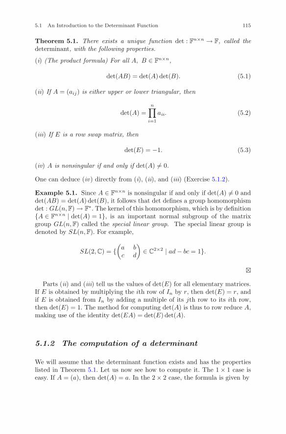
5.1 An Introduction to the Determinant Function 115
Theorem 5.1. There exists a unique function det : Fn×n → F, called thedeterminant, with the following properties.
(i) (The product formula) For all A, B ∈ Fn×n,
det(AB) = det(A) det(B). (5.1)
(ii) If A = (aij) is either upper or lower triangular, then
det(A) =n∏
i=1
aii. (5.2)
(iii) If E is a row swap matrix, then
det(E) = −1. (5.3)
(iv) A is nonsingular if and only if det(A) �= 0.
One can deduce (iv) directly from (i), (ii), and (iii) (Exercise 5.1.2).
Example 5.1. Since A ∈ Fn×n is nonsingular if and only if det(A) �= 0 and
det(AB) = det(A) det(B), it follows that det defines a group homomorphismdet : GL(n,F) → F
∗. The kernel of this homomorphism, which is by definition{A ∈ F
n×n | det(A) = 1}, is an important normal subgroup of the matrixgroup GL(n,F) called the special linear group. The special linear group isdenoted by SL(n,F). For example,
SL(2,C) = {(
a bc d
)∈ C
2×2 | ad − bc = 1}.
�
Parts (ii) and (iii) tell us the values of det(E) for all elementary matrices.If E is obtained by multiplying the ith row of In by r, then det(E) = r, andif E is obtained from In by adding a multiple of its jth row to its ith row,then det(E) = 1. The method for computing det(A) is thus to row reduce A,making use of the identity det(EA) = det(E) det(A).
5.1.2 The computation of a determinant
We will assume that the determinant function exists and has the propertieslisted in Theorem 5.1. Let us now see how to compute it. The 1 × 1 case iseasy. If A = (a), then det(A) = a. In the 2 × 2 case, the formula is given by
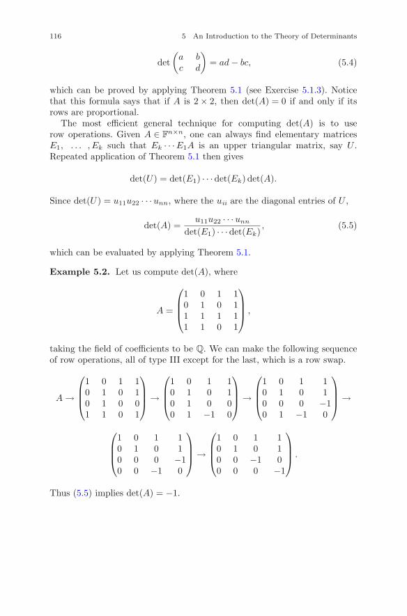
116 5 An Introduction to the Theory of Determinants
det(
a bc d
)= ad − bc, (5.4)
which can be proved by applying Theorem 5.1 (see Exercise 5.1.3). Noticethat this formula says that if A is 2 × 2, then det(A) = 0 if and only if itsrows are proportional.
The most efficient general technique for computing det(A) is to userow operations. Given A ∈ F
n×n, one can always find elementary matricesE1, . . . , Ek such that Ek · · · E1A is an upper triangular matrix, say U .Repeated application of Theorem 5.1 then gives
det(U) = det(E1) · · · det(Ek) det(A).
Since det(U) = u11u22 · · · unn, where the uii are the diagonal entries of U ,
det(A) =u11u22 · · · unn
det(E1) · · · det(Ek), (5.5)
which can be evaluated by applying Theorem 5.1.
Example 5.2. Let us compute det(A), where
A =
⎛
⎜⎜⎝
1 0 1 10 1 0 11 1 1 11 1 0 1
⎞
⎟⎟⎠ ,
taking the field of coefficients to be Q. We can make the following sequenceof row operations, all of type III except for the last, which is a row swap.
A →
⎛
⎜⎜⎝
1 0 1 10 1 0 10 1 0 01 1 0 1
⎞
⎟⎟⎠ →
⎛
⎜⎜⎝
1 0 1 10 1 0 10 1 0 00 1 −1 0
⎞
⎟⎟⎠ →
⎛
⎜⎜⎝
1 0 1 10 1 0 10 0 0 −10 1 −1 0
⎞
⎟⎟⎠ →
⎛
⎜⎜⎝
1 0 1 10 1 0 10 0 0 −10 0 −1 0
⎞
⎟⎟⎠ →
⎛
⎜⎜⎝
1 0 1 10 1 0 10 0 −1 00 0 0 −1
⎞
⎟⎟⎠ .
Thus (5.5) implies det(A) = −1.
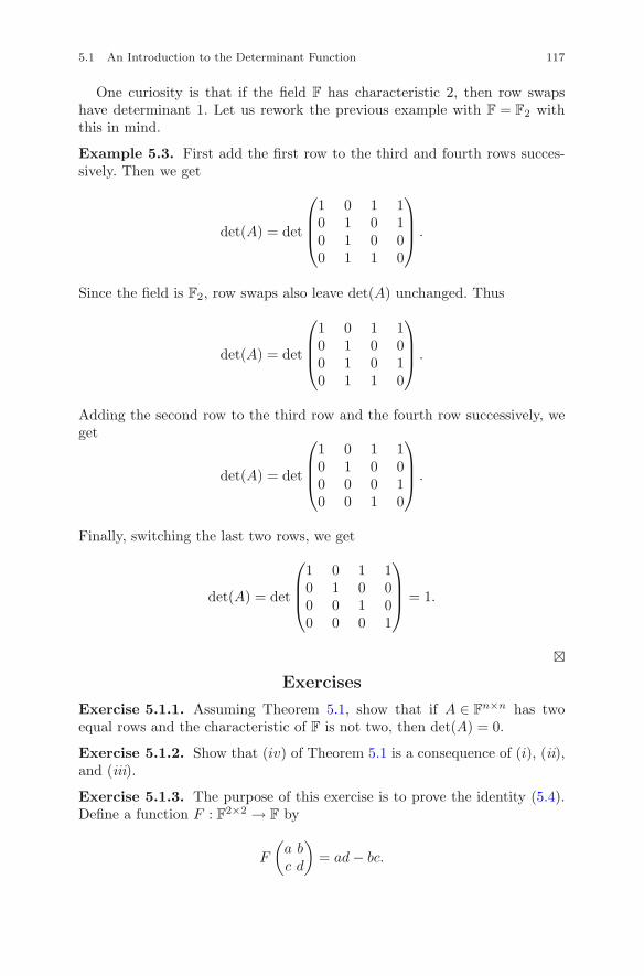
5.1 An Introduction to the Determinant Function 117
One curiosity is that if the field F has characteristic 2, then row swapshave determinant 1. Let us rework the previous example with F = F2 withthis in mind.
Example 5.3. First add the first row to the third and fourth rows succes-sively. Then we get
det(A) = det
⎛
⎜⎜⎝
1 0 1 10 1 0 10 1 0 00 1 1 0
⎞
⎟⎟⎠ .
Since the field is F2, row swaps also leave det(A) unchanged. Thus
det(A) = det
⎛
⎜⎜⎝
1 0 1 10 1 0 00 1 0 10 1 1 0
⎞
⎟⎟⎠ .
Adding the second row to the third row and the fourth row successively, weget
det(A) = det
⎛
⎜⎜⎝
1 0 1 10 1 0 00 0 0 10 0 1 0
⎞
⎟⎟⎠ .
Finally, switching the last two rows, we get
det(A) = det
⎛
⎜⎜⎝
1 0 1 10 1 0 00 0 1 00 0 0 1
⎞
⎟⎟⎠ = 1.
�Exercises
Exercise 5.1.1. Assuming Theorem 5.1, show that if A ∈ Fn×n has two
equal rows and the characteristic of F is not two, then det(A) = 0.
Exercise 5.1.2. Show that (iv) of Theorem 5.1 is a consequence of (i), (ii),and (iii).
Exercise 5.1.3. The purpose of this exercise is to prove the identity (5.4).Define a function F : F2×2 → F by
F
(a bc d
)= ad − bc.
118 5 An Introduction to the Theory of Determinants
Show that F satisfies the conditions in Theorem 5.1, and conclude thatF (A) = det(A).
Exercise 5.1.4. Let A =(
a bc d
). Without appealing to Theorem 5.1, show
the following:
(i) det(A) = 0 if and only if the rows of A are proportional. Conclude thatA has rank 2 if and only if ad − bc �= 0.
(ii) A is invertible if and only if det(A) �= 0. In that case,
A−1 =1
det(A)
(d −b
−c a
).
Exercise 5.1.5. Use Theorem 5.1 to prove that if B and C are square matri-ces over F, then
det(
B ∗O C
)= det(B) det(C).
Exercise 5.1.6. Compute
det
⎛
⎜⎜⎝
1 1 −1 02 1 1 10 −1 2 01 1 −1 1
⎞
⎟⎟⎠
in two cases: first when the field is Q and second, when the field is F3.
Exercise 5.1.7. Express
A =
⎛
⎝1 2 −12 1 10 −1 2
⎞
⎠
in the form A = LPDU , and use your result to compute det(A) in the fol-lowing cases:
(a) F = Q;
(b) F = F2; and
(c) F = F3.
Exercise 5.1.8. Show that the image of det : Fn×n → F∗ is, in fact, all of
F∗.
5.2 The Definition of the Determinant 119
5.2 The Definition of the Determinant
Before formally defining the determinant function, we have to define the sig-nature sgn(σ) of a permutation σ ∈ S(n). As already mentioned, the signatureis a homomorphism from S(n) to the multiplicative group {+1,−1}.
5.2.1 The signature of a permutation
Recall the isomorphism ϕ : S(n) → P (n) defined by ϕ(σ) = Pσ, where Pσ isthe permutation matrix whose ith column is eσ(i). The signature sgn(σ) ofthe permutation σ ∈ S(n) will tell us whether one requires an even or oddnumber of row swaps Si to write Pσ = S1 · · · Sk. Correspondingly, we will callπ even or odd.
Definition 5.1. Suppose σ ∈ S(n). If n > 1, define the signature sgn(σ) ofσ to be
sgn(σ) =∏
i<j
σ(i) − σ(j)i − j
. (5.6)
If n = 1, put sgn(σ) = 1.
Clearly, sgn(σ) is a nonzero rational number. There is at least one examplein which the value of sgn(σ) is clear.
Example 5.4. The identity permutation idn ∈ S(n) has signaturesgn(idn) = 1. �
As usual, we will denote idn by 1. We now establish the properties of sgn.We first show that sgn(σ) ∈ {±1}.
Proposition 5.2. For every σ ∈ S(n), sgn(σ) = ±1.
Proof. The case n = 1 is clear, so suppose n > 1. Since σ is a bijection of{1, 2, . . . , n} and
σ(i) − σ(j)i − j
=σ(j) − σ(j)
j − i,
it follows that
(sgn(σ))2 =∏
i�=j
σ(i) − σ(j)i − j
.
Moreover, sinceσ(σ−1(i)) − σ(σ−1(j)) = i − j,
each possible value of (i − j) occurs the same number of times in the numer-ator and denominator. Hence sgn(σ)2 = 1, so the proof is done. �
120 5 An Introduction to the Theory of Determinants
Let N(σ) = {(i, j) | i < j, σ(i) > σ(j)}, and put n(σ) = |N(σ)|. By thedefinition of sgn(σ) and Proposition 5.2,
sgn(σ) = (−1)n(σ).
Here is an an example.
Example 5.5. Recall that σij ∈ S(n) denotes the transposition that switchesi and j while leaving all other k, 1 ≤ k ≤ n, unchanged. Let us computesgn(σ12). Now σ12 interchanges 1 and 2 and leaves every k between 3 andn unchanged. Thus, (1, 2) is the only pair (i, j) such that i < j for whichσ12(i) > σ12(j). Hence n(σ12) = 1, so sgn(σ12) = −1. �
We now establish the main properties of the signature.
Proposition 5.3. The signature mapping sgn : S(n) → {±1} has the follow-ing properties:
(i) sgn is a group homomorphism; that is, for all σ, τ ∈ S(n),
sgn(τσ) = sgn(τ)sgn(σ);
(ii) if σ is any transposition, then sgn(σ) = −1; and
(iii) for all σ ∈ S(n), sgn(σ−1) = sgn(σ).
Proof. To prove (i), it will suffice to show that n(τσ) = n(τ) + n(σ) for anarbitrary pair τ , σ ∈ S(n). Suppose i < j and write
τ(σ(i)) − τ(σ(j))i − j
=τ(σ(i)) − τ(σ(j))
σ(i) − σ(j)· σ(i) − σ(j)
i − j.
The left-hand side is negative if and only ifτ(σ(i)) − τ(σ(j))
σ(i) − σ(j)and
σ(i) − σ(j)i − j
have different signs. Thus, (i, j) ∈ N(τσ) if and only if (i, j) ∈ N(σ) or(σ(i), σ(j)) ∈ N(τ). Since there is no pair (i, j) ∈ N(τσ) such that (i, j) ∈N(σ) and (σ(i), σ(j)) ∈ N(τ), it follows that n(τσ) = n(τ) + n(σ). This com-pletes the proof of (i). For (ii), we can use the result of Example 5.5. Letσab denote the transposition interchanging a �= b. As an exercise, the readershould check that
σab = σ1bσ2aσ12σ2aσ1b. (5.7)
Hence, by (i) and the result that sgn(σ12) = −1 (by Example 5.5),
sgn(σab) = sgn(σ1b)sgn(σ2a)sgn(σ12)sgn(σ2a)sgn(σ1b) = sgn(σ12) = −1.
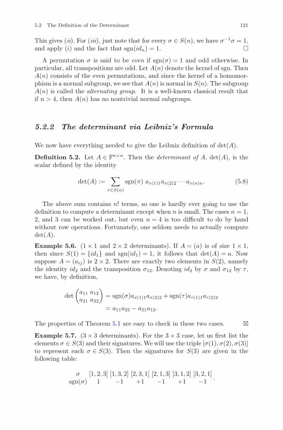
5.2 The Definition of the Determinant 121
This gives (ii). For (iii), just note that for every σ ∈ S(n), we have σ−1σ = 1,and apply (i) and the fact that sgn(idn) = 1. �
A permutation σ is said to be even if sgn(σ) = 1 and odd otherwise. Inparticular, all transpositions are odd. Let A(n) denote the kernel of sgn. ThenA(n) consists of the even permutations, and since the kernel of a homomor-phism is a normal subgroup, we see that A(n) is normal in S(n). The subgroupA(n) is called the alternating group. It is a well-known classical result thatif n > 4, then A(n) has no nontrivial normal subgroups.
5.2.2 The determinant via Leibniz’s Formula
We now have everything needed to give the Leibniz definition of det(A).
Definition 5.2. Let A ∈ Fn×n. Then the determinant of A, det(A), is the
scalar defined by the identity
det(A) :=∑
π∈S(n)
sgn(π) aπ(1)1aπ(2)2 · · · aπ(n)n. (5.8)
The above sum contains n! terms, so one is hardly ever going to use thedefinition to compute a determinant except when n is small. The cases n = 1,2, and 3 can be worked out, but even n = 4 is too difficult to do by handwithout row operations. Fortunately, one seldom needs to actually computedet(A).
Example 5.6. (1 × 1 and 2 × 2 determinants). If A = (a) is of size 1 × 1,then since S(1) = {id1} and sgn(id1) = 1, it follows that det(A) = a. Nowsuppose A = (aij) is 2 × 2. There are exactly two elements in S(2), namelythe identity id2 and the transposition σ12. Denoting id2 by σ and σ12 by τ ,we have, by definition,
det(
a11 a12
a21 a22
)= sgn(σ)aσ(1)1aσ(2)2 + sgn(τ)aτ(1)1aτ(2)2
= a11a22 − a21a12.
The properties of Theorem 5.1 are easy to check in these two cases. �
Example 5.7. (3 × 3 determinants). For the 3 × 3 case, let us first list theelements σ ∈ S(3) and their signatures. We will use the triple [σ(1), σ(2), σ(3)]to represent each σ ∈ S(3). Then the signatures for S(3) are given in thefollowing table:
σ [1, 2, 3] [1, 3, 2] [2, 3, 1] [2, 1, 3] [3, 1, 2] [3, 2, 1]sgn(σ) 1 −1 +1 −1 +1 −1 .
122 5 An Introduction to the Theory of Determinants
Hence,
det(A) = a11a22a33 − a11a32a23 + a21a32a13
−a21a12a33 + a31a12a23 − a31a22a13.
Rewriting this as
det(A) = a11a22a33 + a21a32a13 + a31a12a23 +−a11a32a23 − a21a12a33 − a31a22a13,
one sees that det(A) is the sum of the products of three entries, either twoor three of which are on a diagonal of A parallel to its main diagonal, lessthe sum of the products of three entries, either two or three of which are ona diagonal of A parallel to its antidiagonal, that is, the diagonal from thenortheast corner of A to its southwest corner. This is a standard expressionfor a 3 × 3 determinant known as the rule of Sarrus. Warning: the rule ofSarrus does not generalize to the 4 × 4 case. �
5.2.3 Consequences of the definition
Several parts of Theorem 5.1 follow directly from the definition. Let us firstprove part (ii).
Proposition 5.4. Suppose A is of size n × n and either upper or lower tri-angular. Then
det(A) = a11a22 · · · ann.
Proof. We will suppose that A is upper triangular and leave the lower tri-angular case as an exercise (not a very hard one at that). The point is thatin this case, the only nonzero term in (5.2) is a11a22 · · · ann, which corre-sponds to the identity permutation. For if σ ∈ S(n) is different from idn,then σ(i) > i for some i; hence aσ(i)i = 0, since A is upper triangular. Thus,sgn(σ)aσ(1)1aσ(2)2 · · · aσ(n)n = 0. �
Suppose now that P ∈ Fn×n is a permutation matrix. In this case, det(P )
has a very pretty interpretation.
Proposition 5.5. Assume that P ∈ Fn×n is a permutation matrix, say P =
Pμ. Then det(P ) = sgn(μ).
Proof. Recall that Pμ =(eμ(1) eμ(2) · · · eμ(n)
). Writing P = (pij), we have
pμ(i)i = 1 for all i, while all other prs are equal to 0. Therefore, the onlynonzero term in the expression for det(P ) is
5.2 The Definition of the Determinant 123
sgn(μ)pμ(1)1pμ(2)2 · · · pμ(n)n = sgn(μ).
�
The following result about the determinant of the transpose is going to beused in several places in the rest of this section.
Proposition 5.6. For every A ∈ Fn×n,
det(AT ) = det(A).
Proof. Since AT = (bij), where bij = aji, formula (5.2) implies
det(AT ) :=∑
σ∈S(n)
sgn(σ) a1σ(1)a2σ(2) · · · anσ(n). (5.9)
Now if σ(i) = j, then σ−1(j) = i, so aiσ(i) = aσ−1(j)j . Thus,
sgn(σ) a1σ(1)a2σ(2) · · · anσ(n) = sgn(σ) aσ−1(1)1aσ−1(2)2 · · · aσ−1(n)n
= sgn(σ−1) aσ−1(1)1aσ−1(2)2 · · · aσ−1(n)n,
since by Proposition 5.3, sgn(σ−1) = sgn(σ). But the correspondence σ →σ−1 is a bijection of S(n), so we can conclude that
∑
σ∈S(n)
sgn(σ) a1σ(1)a2σ(2) · · · anσ(n) =∑
τ∈S(n)
sgn(τ) aτ(1)1)aτ(2)2 · · · aτ(n)n.
Thus det(AT ) = det(A). �
5.2.4 The effect of row operations on thedeterminant
In order to prove the product formula det(AB) = det(A) det(B) for allA,B ∈ F
n×n, we will demonstrate how a row operation changes the determi-nant. In fact, we will show that for every elementary matrix E, det(EA) =det(E) det(A). Since det(A) = det(AT ), it follows that the product formulaholds for AB if either A or B is a product of elementary matrices. First weprove the following result.
Proposition 5.7. Suppose that E ∈ Fn×n is the elementary matrix obtained
from In by multiplying the ith row of In by r ∈ F. Then for every A ∈ Fn×n,
det(EA) = r det(A) = det(E) det(A).
124 5 An Introduction to the Theory of Determinants
Proof. Certainly det(E) = r, while det(EA) = r det(A), since every term inthe expansion of det(A) is multiplied by r. �
We next prove a result for swap matrices.
Proposition 5.8. Suppose A ∈ Fn×n and S ∈ F
n×n is a row swap matrix.Then
det(SA) = −det(A) = det(S) det(A).
Proof. Suppose S is a row swap matrix. Put SA = B = (bij) and let τdenote the transposition such that S = Pτ . Then bij = aτ(i)j . We will com-pute det(B) using the result that det(B) = det(BT ). First of all, for everyσ ∈ S(n),
b1σ(1)b2σ(2) · · · bnσ(n) = aτ(1)σ(1)aτ(2)σ(2) · · · aτ(n)σ(n)
= aτ(1)μτ(1)aτ(2)μτ(2) · · · aτ(n)μτ(n)
= a1μ(1)a2μ(2) · · · anμ(n),
where μ = στ . Thus,
det(B) =∑
σ∈S(n)
sgn(σ)b1σ(1)b2σ(2) · · · bnσ(n)
=∑
σ∈S(n)
sgn(σ)a1μ(1)a2μ(2) · · · anμ(n)
= −∑
μ∈S(n)
sgn(μ)a1μ(1)a2μ(2) · · · anμ(n)
= −det(A).
The third equality uses two facts; first, if μ = στ , then sgn(μ) = −sgn(σ),and second, if σ varies through all of S(n), then so does μ = στ . Thus,det(SA) = −det(A). To finish the proof, we need to show that det(S) = −1.But det(S) = det(SIn) = −det(In) = −1, since det(In) = 1. Alternatively,since S = Pτ , it follows that det(S) = sgn(τ) = −1 by Proposition 5.5. �
The next step is to show that det(EA) = det(A) if E is a transvection, thatis, an elementary matrix of type III. Suppose A ∈ F
n×n and let a1, . . . ,andenote its rows. Let E be of type III, say E is obtained from In by replacingthe ith row of In by itself plus r times the jth row. Then the ith row of EAis ai + raj , and the other rows are unchanged. Hence by (5.9), each term inthe expansion of det(EA) has the form
sgn(σ)a1σ(1) . . . a(i−1)σ(i−1)(aiσ(i) + rajσ(i))ai+1σ(i+1 . . . anσ(n).
Thus, det(EA) is of the form det(A) + r det(C), where C ∈ Fn×n has the
property that its ith and jth rows both coincide with aj . If we apply the
5.2 The Definition of the Determinant 125
fact that det(SB) = −det(B) whenever S is a row swap matrix, then we seethat if S swaps the ith and jth rows, we get C = SC, so det(C) = det(SC) =−det(C). Thus 2 det(C) = 0. It follows that det(C) = 0 as long as the char-acteristic of the field F is different from two. The formula det(C) = 0 when F
has characteristic two and two rows of C coincide requires a special argument,which is given in the appendix to this chapter. �
The following proposition summarizes what was proved in this sectionmodulo showing that det(C) = 0 in characteristic two if C has two equalrows.
Proposition 5.9. If E ∈ Fn×n is any elementary matrix, then det(EA) =
det(E) det(A) for all A ∈ Fn×n. Moreover, det(E) = r if E multiplies the ith
row of In by r, det(E) = −1 if E is a row swap, and det(E) = 1 if E is atransvection.
5.2.5 The proof of the main theorem
We are now ready to complete the proof of the main theorem. Parts (ii) and(iii) of the main theorem have already been verified. Let A ∈ F
n×n, and letus first show that det(A) �= 0 if and only if A is nonsingular. There existelementary matrices E1, . . . , Ek such that Ek · · · E1A = Ared, so
det(A) =det(Ared)∏i det(Ei)
.
Hence det(A) �= 0 if and only if det(Ared) �= 0. But since Ared is upper trian-gular, det(Ared) �= 0 if and only if Ared = In if and only if A is nonsingular.It remains to prove the product formula. If A and B are both nonsingular,then the validity of the product formula is clear, for both A and B and henceAB are products of elementary matrices. On the other hand, if either A orB is singular, I claim that AB is singular. If not, then (AB)−1A is a leftinverse of B, so B is nonsingular. Similarly, B(AB)−1 is a right inverse ofA, so A is also nonsingular. Hence, if det(A) det(B) = 0, then det(AB) = 0.This finishes the proof of the product formula. �
5.2.6 Determinants and LPDU
Recall from Chap. 4 that every A ∈ Fn×n can be written A = LPDU , where
L and U are respectively lower and upper triangular unipotent matrices, P isa unique partial permutation matrix, and D is an invertible diagonal matrix.
126 5 An Introduction to the Theory of Determinants
Clearly, det(A) = 0 unless P is a full permutation matrix. Furthermore, wehave the following proposition.
Proposition 5.10. If A = LPDU is nonsingular, then
det(A) = det(P ) det(D) = ±det(D).
Thus, up to sign, the determinant of an invertible matrix is the product of itspivots. If A = LDU , then det(A) = det(D).
Proof. Just use the product rule and the fact that det(L) = det(U) = 1, sinceL and U are triangular and have ones on their diagonals. �
Recall from Proposition 4.17 that an invertible A ∈ Fn×n has an LDU
decomposition if and only if each Ak is also invertible, where Ak is the k × ksubmatrix in the upper left-hand corner of A, and that the pivots of A are thediagonal entries of D. Let d1, . . . , dn be these pivots. Then Ak = LkDkUk, so
det(Ak) = det(Dk) = d1 · · · dk.
This gives us the following result.
Proposition 5.11. If A ∈ Fn×n satisfies the condition that each Ak, 1 ≤
k ≤ n, is invertible, then A has an LDU decomposition, and the kth pivot ofA in its LDU decomposition is
dk =det(Ak)
det(Ak−1). (5.10)
5.2.7 A beautiful formula: Lewis Carroll’s identity
The theory of determinants is a remarkably rich topic, and we have barelyscratched its surface. Many of the foremost mathematicians of the nine-teenth century, among them Gauss, Laplace, Lagrange, Cayley, Sylvester,and Jacobi, discovered some of its important properties and applications. Anexample is the Jacobian of a mapping and the change of variables formula. Inthis section, we will consider a determinantal curiosity from the nineteenthcentury that has recently been found to have connections to contemporary
mathematics. The formula det(
a bc d
)= ad − bc turns out to have a gener-
alization to n × n matrices that was discovered by Charles Dodgson, a profes-sor of mathematics at Oxford who, as is well known, wrote Alice’s Adventuresin Wonderland and Through the Looking Glass under the pseudonym LewisCarroll. Dodgson found an identity involving the determinant of an n × nmatrix A that is analogous to the formula in the 2 × 2 case. Let AC be the
5.2 The Definition of the Determinant 127
(n − 2) × (n − 2) submatrix of A obtained by deleting the first and last rowsand the first and last columns. If n = 2, put det(AC) = 1. Also, let ANW
denote the (n − 1) × (n − 1) submatrix in the upper left-hand corner of A,and define ANE , ASW , and ASE to be the (n − 1) × (n − 1) submatrices inthe other three corners of A. Dodgson’s formula asserts that
det(AC) det(A) = det(ANW ) det(ASE) − det(ANE) det(ASW ) (5.11)
(see C.L. Dodgson, Proc. Royal Soc. London 17, 555–560 (1860)). If det(AC) �=0, this substantially cuts down on the difficulty of finding det(A). Of course,if det(AC) = 0, then the identity says nothing about det(A), although it doessay something about the four determinants at the corners. This formula isreferred to as Dodgson condensation. Dodgson himself supplied the term con-densation. In the 1980s, it was noticed that Dodgson condensation is relatedto the problem of counting alternating sign matrices (ASMs). Eventually,the problem of enumerating the ASMs was given an elegant solution usingstatistical mechanics.
128 5 An Introduction to the Theory of Determinants
Exercises
Exercise 5.2.1. Two matrices A,B ∈ Fn×n are said to be similar if A =
CBC−1 for some C ∈ GL(n,F). Show that similar matrices have the samedeterminant.
Exercise 5.2.2. Suppose P is an n × n matrix over C such that PP = P .What is det(P )? What is det(Q) if Q4 = Q−1?
Exercise 5.2.3. Which of the following statements are true. Give your rea-soning or supply a counter example.
(i) The determinant of a real symmetric matrix is always nonnegative.
(ii) If A is a 2 × 3 real matrix, then det(AAT )Gal(E/Q)0.
(iii) If A is a square real matrix, then det(AAT )Gal(E/Q)0.
Exercise 5.2.4. An n × n matrix A over R is called skew-symmetric ifAT = −A. Show that if A is a skew-symmetric n × n matrix and n is odd,then A cannot be invertible.
Exercise 5.2.5. Let H ∈ Rn×n be a Hadamard matrix. That is, suppose
HHT = nIn. Find det(H).
Exercise 5.2.6. Recall that SL(n,F) denotes the set of all A ∈ Fn×n such
that det(A) = 1. Prove that SL(n,F) is a matrix group and a proper normalsubgroup of GL(n,F) if the characteristic of F is different from 2.
Exercise 5.2.7. Find the 3 × 3 permutation matrices that lie in SL(3,R).
Exercise 5.2.8. Let SO(n,R) denote the set of all n × n orthogonal matri-ces Q such that det(Q) = 1. Show that SO(n,R) is a matrix group and aproper normal subgroup of O(n,R).
Exercise 5.2.9. If A ∈ Cm×n, define AH = A
T, where A is the matrix
obtained by conjugating each entry of A. An n × n matrix U over C is calledunitary if U−1 = UH . What are the possible values of the determinant ofdet(U) of a unitary matrix U?
Exercise 5.2.10. An n × n matrix K over C is called Hermitian if K =KH . (See the previous exercise for the definition of KH .) Show that if K isHermitian, then det(K) is a real number.
Exercise 5.2.11. Determine whether
A =
⎛
⎜⎜⎝
1 0 2 10 1 0 11 1 1 11 1 0 1
⎞
⎟⎟⎠
has an LDU decomposition over both Q and F3. If it does in either case, findits pivots.
5.2 The Definition of the Determinant 129
Exercise 5.2.12. Suppose A is a square matrix over F such that each rowsums to zero. Find det(A).
Exercise 5.2.13. Show that the condition in Proposition 7.27 that F (A) =0 if two rows of A are equal is equivalent to the condition that F (SA) =−F (A) if S is a row swap matrix.
Exercise 5.2.14. Find all values x ∈ R for which det(A(x)) = 0 when
A(x) =
⎛
⎝1 x 2x 1 x2 3 1
⎞
⎠ .
Exercise 5.2.15. Repeat the previous exercise for the matrix
B(x) =
⎛
⎜⎜⎝
1 x 1 x1 0 x 10 x 1 11 0 1 0
⎞
⎟⎟⎠ .
Exercise 5.2.16. Why does condition (ii) in Theorem 7.27 imply that thedeterminant changes sign under a row swap?
Exercise 5.2.17. Recall that SL(n,F) = {A ∈ Fn×n such that det(A) = 1}.
Let SL(n,Z) denote Zn×n ∩ SL(n,Q). Show that SL(n,Z) is a matrix group.
Exercise 5.2.18. Show that if P ∈ Zn×n is a row swap, then GL(n,Z) =
SL(n,Z) ∪ PSL(n,Z).
130 5 An Introduction to the Theory of Determinants
5.3 Appendix: Further Results on Determinants
The purpose of this appendix is to briefly introduce the Laplace expansionof a determinant and explain Cramer’s rule.
5.3.1 The Laplace expansion
In this section, we will obtain some further properties of the determinant,beginning with the Laplace expansion, which is the classical way of calculatingan n × n determinant as a sum of (n − 1) × (n − 1) determinants. After theLaplace expansion, we will state Cramer’s rule, which gives a closed formfor inverting a nonsingular matrix. The Laplace expansion also allows one toshow by induction that the determinant of a matrix with two equal rows iszero.
Suppose A is of size n × n, and let Aij denote the (n − 1) × (n − 1) sub-matrix obtained from A by deleting its ith row and jth column.
Theorem 5.12. For every A ∈ Fn×n, we have
det(A) =n∑
i=1
(−1)i+jaij det(Aij). (5.12)
This is the Laplace expansion along the jth column. The correspondingLaplace expansion along the ith row is
det(A) =n∑
j=1
(−1)i+jaij det(Aij). (5.13)
Proof. Since det(A) = det(AT ), it suffices to prove (5.12). For simplicity, wewill assume j = 1, the other cases being similar. Now,
det(A) =∑
σ∈S(n)
sgn(σ) aσ(1)1aσ(2)2 · · · aσ(n)n
= a11
∑
σ(1)=1
sgn(σ)aσ(2)2 · · · aσ(n)n +
a21
∑
σ(1)=2
sgn(σ)aσ(2)2 · · · aσ(n)n +
+ · · · + an1
∑
σ(1)=n
sgn(σ)aσ(2)2 · · · aσ(n)n.
5.3 Appendix: Further Results on Determinants 131
Suppose σ(1) = r. Let us evaluate
ar1
∑
σ(1)=r
sgn(σ)aσ(2)2 · · · aσ(n)n.
Let P ′σ denote the element of F(n−1)×(n−1) obtained from Pσ by deleting the
first column and the rth row. Then P ′σ ∈ P (n − 1), so P ′
σ = Pσ′ for a uniqueσ′ ∈ S(n − 1). Note that det(Pσ) = (−1)(r−1) det(P ′
σ), since if bringing P ′σ to
In−1 by row swaps uses t steps, one needs t + σ(1) − 1 row swaps to bringPσ to the identity. Thus,
∑
σ(1)=r
sgn(σ)aσ(2)2 · · · aσ(n)n =∑
σ(1)=r
(−1)r−1sgn(σ′)aσ(2)2 · · · aσ(n)n
= (−1)r+1 det(Ar1).
Substituting this into the above calculation for r = 1, . . . , n gives theresult. �
Example 5.8. If A is of size 3 × 3, expanding det(A) along the first columngives
det(A) = a11(a22a33 − a32a23) − a21(a12a23 − a13a32) + a31(a12a23 − a13a22).
This is the well-known formula for the triple product a1 · (a2 × a3) of therows of A.
Example 5.9. The Laplace expansion is useful for evaluating det(A) whenA has entries that are functions. In fact, this situation will arise when weconsider the characteristic polynomial of a square matrix A. Consider thematrix
Cx =
⎛
⎝1 − x 2 0
2 1 − x −10 −1 2 − x
⎞
⎠ .
Suppose we want to find all values of x ∈ C such that Cx has rank less that3, i.e., Cx is singular. The obvious way to proceed is to solve the equationdet(Cx) = 0 for x. Clearly, row operations aren’t going to be of much help infinding det(Cx), so we will use Laplace, as in the previous example. Expandingalong the first column gives
det(Cx) = (1 − x)((1 − x)(2 − x) − (−1)(−1)
) − 2(2(2 − x) − 0(−1)
)
= −x3 + 4x − 7.
Hence Cx is singular at the three complex roots of x3 − 4x + 7 = 0.
132 5 An Introduction to the Theory of Determinants
We can now finish the proof that det(C) = 0 when two rows of C areidentical. This will complete the proof of Theorem 5.1.
Proposition 5.13. Suppose C ∈ Fn×n has two equal rows. Then
det(C) = 0.
Proof. Suppose the ith and jth rows of C are equal and S is the matrixthat swaps these rows. Then SC = C, so det(SC) = det(C), while det(SC) =−det(C), since det(S) = −1. Hence 2 det(C) = 0. Thus, as long as the char-acteristic of F is different from 2, det(C) = 0. The hard case is that in whichthe characteristic of F is 2. In this case, the signatures do not contribute tothe determinant, since 1 = −1 in F, so
det(C) =∑
π∈S(n)
cπ(1)1cπ(2)2 · · · cπ(n)n. (5.14)
Let us now assume that the characteristic of F is two. By the usual for-mula, det(A) = ad − bc for A ∈ F
2×2, it follows that if a = c and b = d, thendet(A) = ad − ad = 0. Hence we may assume as our induction hypothesisthat proposition holds for n ≥ 2. Let A ∈ F
(n+1)×(n+1) have two equal rows,say the first two rows. Using the Laplace expansion for det(A) along thefirst column, we get that a11 det(A11) = a21 det(A21), and the other termsare zero, since the induction hypothesis implies det(B) = 0 if B ∈ F
n×n hastwo equal rows. Consequently, det(A) = 2a11 det(A11) = 0. This finishes theinduction step, so the proposition is proved. �
Remark. As mentioned above, algebra texts often define the determinantinductively via the Laplace expansion. This avoids the problem of introducingthe signature of a permutation. Leibniz was aware of the Laplace expansion,for example, well before the time of Laplace (1749–1827). The drawback ofthis approach is that in order for it to be of use, one needs to know that allpossible row and column expansions have the same value. The only way toshow that fact is to appeal to a formula such as the Leibniz formula, whichavoids using rows and columns. The Laplace expansion is useful as a compu-tational tool for matrices with few nonzero entries or when row operations areimpractical, such as for a characteristic polynomial. But it would be uselessto attempt to use Laplace for calculating even a 5 × 5 determinant, whichcould be done easily with row operations.
5.3.2 Cramer’s Rule
Cramer’s rule is a closed formula for the inverse of a square matrix withnonzero determinant. Recall that if A is of size 2 × 2, then
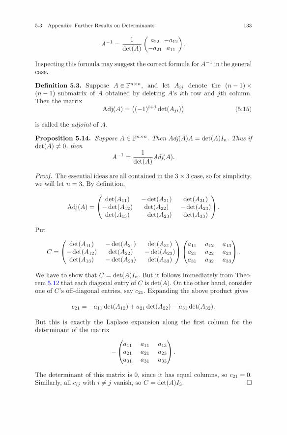
5.3 Appendix: Further Results on Determinants 133
A−1 =1
det(A)
(a22 −a12
−a21 a11
).
Inspecting this formula may suggest the correct formula for A−1 in the generalcase.
Definition 5.3. Suppose A ∈ Fn×n, and let Aij denote the (n − 1) ×
(n − 1) submatrix of A obtained by deleting A’s ith row and jth column.Then the matrix
Adj(A) =((−1)i+j det(Aji)
)(5.15)
is called the adjoint of A.
Proposition 5.14. Suppose A ∈ Fn×n. Then Adj(A)A = det(A)In. Thus if
det(A) �= 0, then
A−1 =1
det(A)Adj(A).
Proof. The essential ideas are all contained in the 3 × 3 case, so for simplicity,we will let n = 3. By definition,
Adj(A) =
⎛
⎝det(A11) −det(A21) det(A31)
−det(A12) det(A22) −det(A23)det(A13) −det(A23) det(A33)
⎞
⎠ .
Put
C =
⎛
⎝det(A11) −det(A21) det(A31)
−det(A12) det(A22) −det(A23)det(A13) −det(A23) det(A33)
⎞
⎠
⎛
⎝a11 a12 a13
a21 a22 a23
a31 a32 a33
⎞
⎠ .
We have to show that C = det(A)In. But it follows immediately from Theo-rem 5.12 that each diagonal entry of C is det(A). On the other hand, considerone of C’s off-diagonal entries, say c21. Expanding the above product gives
c21 = −a11 det(A12) + a21 det(A22) − a31 det(A32).
But this is exactly the Laplace expansion along the first column for thedeterminant of the matrix
−⎛
⎝a11 a11 a13
a21 a21 a23
a31 a31 a33
⎞
⎠ .
The determinant of this matrix is 0, since it has equal columns, so c21 = 0.Similarly, all cij with i �= j vanish, so C = det(A)I3. �
134 5 An Introduction to the Theory of Determinants
5.3.3 The inverse of a matrix over Z
In most of our examples of inverting a matrix A, the entries of A are integers.But experience tells us that usually, at some time during the row operations,denominators appear. In fact, Cramer’s rule, Proposition 5.14, tells us thatwhen det(A) = ±1, then A−1 also has integral entries. The question whetherthis is the whole story will now be answered.
Proposition 5.15. Suppose A is an invertible matrix with integral entries.Then A−1 has integral entries if and only if det(A) = ±1.
Proof. The if statement follows from Cramer’s rule. Conversely, suppose A−1
is integral. Then det(A) and det(A−1) both are integers. But
det(AA−1) = det(A) det(A−1) = det(In) = 1,
so the only possibility is that det(A) = det(A−1) = ±1. �
A somewhat deeper fact is the following result.
Proposition 5.16. An n × n matrix over Z is invertible over Z if and onlyif it can be expressed as a product of elementary matrices all of which aredefined over Z.
We will skip the proof. Of course, row swap matrices are always integral.The restriction of sticking to elementary matrices over Z means that one canmultiply a row only by ±1 and replace it by itself plus an integral multipleof another row. Let GL(n,Z) = {A ∈ Z
n×n | det(A) = ±1} and SL(n,Z) =GL(n,Z) ∩ SL(n,R). The latter groups, especially SL(2,Z), are examples ofmodular groups and are very important in number theory, topology, andcomplex analysis, to name a few areas where they are used.
Proposition 5.17. GL(n,Z) and SL(n,Z) are matrix groups.
Chapter 6Vector Spaces
A vector space is a set V whose elements, called vectors, can be added andsubtracted: in fact, a vector space is an abelian group under addition. Avector space also has an operation called scalar multiplication whereby theelements of a field F act on vectors. When we speak of a vector space, we alsomention the scalars by saying that V is a vector space over F. For example,F
n, Fm×n are two examples of vector spaces over F, and the row space andnull space of a matrix over F are two more examples. Another example is theset C([a, b]) of all continuous real-valued functions on a closed interval [a, b],which is a vector space over R. Here, one needs the theorem that the sum oftwo continuous real-valued functions on [a, b] is continuous in order to speakof (vector) addition in this vector space.
One of the most important concepts associated with a vector space is itsdimension. The definition of dimension requires quite a bit of preliminarygroundwork. One must first introduce linear independence and the notion ofa basis and then prove the fundamental result about bases: if a vector spacehas a finite basis, then every two bases B and B′ have the same numberof elements; that is, |B| = |B′|. We then call |B| the dimension of V . Thisdefinition turns out to coincide with one’s intuitive notion that a line is one-dimensional, a plane is two-dimensional, space is three-dimensional, and afterthat, you have to deal with objects such as spacetime, which you cannotactually picture. After covering the basic topics, we will investigate somespecial topics such as direct sums of subspaces, the Grassmann intersectionformula, and quotient vector spaces. The reader is also advised to look at theappendix, which is an exposition of linear coding theory. This is an interestingcontemporary topic involving vector spaces over finite fields.
c© Springer Science+Business Media LLC 2017J.B. Carrell, Groups, Matrices, and Vector Spaces,DOI 10.1007/978-0-387-79428-0 6
135
136 6 Vector Spaces
6.1 The Definition of a Vector Space and Examples
The purpose of this section is to introduce the definition of an abstract vectorspace and to recall a few old examples as well as to add a few new ones. Inthis section, it will be useful (but not absolutely necessary) to have studiedthe material in Chap. 2 on groups and fields.
6.1.1 The vector space axioms
Put as succinctly as possible, a vector space over a field F consists of anabelian group V under addition whose elements are called vectors. Vectorsadmit a multiplication by the elements of F, the field of scalars. Additionand scalar multiplication interact in a way that we will state precisely below.The definition below of a vector space is given in full detail so that it is notnecessary to know the definition of an abelian group.
Definition 6.1. Let F be a field and suppose V is a set with a binary oper-ation + called addition assigning to any two elements a and b of V a uniquesum a + b ∈ V . Suppose also that there is a second operation, called scalarmultiplication, assigning to every r ∈ F and a ∈ V a unique scalar multiplera ∈ V . Addition and scalar multiplication have the following properties.
(1) Addition is commutative: a + b = b + a for all a,b ∈ V .
(2) Addition is also associative: (a+b)+c = a+(b+c) for all a,b, c ∈ V .
(3) V contains an additive identity 0: that is, 0 + a = a for all a ∈ V .
(4) For every element v of V , there is an element −v such that
v + (−v) = 0.
Thus −v is an additive inverse of v.
(5) For all a ∈ V , 1a = a, where 1 is the multiplicative identity of F.
(6) Scalar multiplication is associative: if r, s ∈ F and a ∈ V , then
(rs)a = r(sa).
(7) Scalar multiplication is distributive: if r, s ∈ F and a,b ∈ V , then
r(a + b) = ra + rb and (r + s)a = ra + sa.
6.1 The Definition of a Vector Space and Examples 137
Then V is called a vector space over F.
The first four axioms say that a vector space is an abelian group V underaddition with identity 0. The properties that scalar multiplication must sat-isfy along with addition are specified by properties (5), (6) and (7). As provedin the group setting, the additive identity 0 and additive inverses are unique.To remind the reader, we will repeat the proofs (word for word) for vectorspaces.
Proposition 6.1. In a vector space, there can be only one zero vector. Fur-thermore, the additive inverse of a vector is always unique.
Proof. Let 0 and 0′ both be additive identities. Then
0 = 0 + 0′ = 0′,
by the definition of an additive identity. Hence the zero vector is unique. Nowsuppose −v and −v′ are both additive inverses of v ∈ V . Then
−v = −v + 0 = −v + (v − v′) = (−v + v) + (−v′) = 0 + (−v′) = −v′.
Hence, additive inverses are also unique. �
Proposition 6.2. In a vector space V , 0v = 0 for all v ∈ V , and r0 = 0for every scalar r. Moreover, −v = (−1)v.
Proof. Let v be arbitrary. Now, by properties (4) and (7) of the definition,
v = 1v = (1 + 0)v = 1v + 0v = v + 0v.
Adding −v to both sides and using associativity gives 0v = 0. For the secondassertion, note that
0 = 0v = (1 + (−1))v = 1v + (−1)v = v + (−1)v.
Hence, (−1)v is an additive inverse of v, so (−1)v = −v for all v ∈ V . �
If v1, . . . ,vk ∈ V , then one can define the sum
v1 + · · · + vk =k∑
i=1
vi
inductively as (v1 + · · ·+vk−1)+vk. Just as for sums in a field, the terms inthis sum can be associated in any convenient way. Similarly, the summandsvi can be taken in any order without changing the sum, since addition iscommutative. Recall that an expression
∑ki=1 rivi, where r1, . . . , rk ∈ F, is
called a linear combination of v1, . . . ,vk ∈ V .
138 6 Vector Spaces
6.1.2 Examples
Example 6.1. As mentioned above, the basic example of a vector spaceover the field F is the set F
n of all column n-tuples of elements of F, whereaddition and scalar multiplication are carried out componentwise:
a + b =
⎛
⎜⎜⎜⎝
a1
a2
...an
⎞
⎟⎟⎟⎠ +
⎛
⎜⎜⎜⎝
b1b2...bn
⎞
⎟⎟⎟⎠ =
⎛
⎜⎜⎜⎝
a1 + b1a2 + b2
...an + bn
⎞
⎟⎟⎟⎠
and
ra = r
⎛
⎜⎜⎜⎝
a1
a2
...an
⎞
⎟⎟⎟⎠ =
⎛
⎜⎜⎜⎝
ra1
ra2
...ran
⎞
⎟⎟⎟⎠ .
The elements of Fn are called column vectors. �
Example 6.2. Let Fm×n denote the m × n matrices over F. In the previousexample, we considered F
n, which is the same as Fn×1. The elements of F1×n
are called row vectors. We have already defined matrix addition and scalarmultiplication for m×n in an analogous way in Chap. 3, so we refer the readerthere. These operations make Fm×n a vector space over F. One can express theelements of Fmn as matrices, so as a vector space, Fm×n is indistinguishablefrom F
mn. �
Example 6.3. (See Example 3.2.) When F = F2, the elements of Fn are
binary strings, which are called n-bit strings. Binary strings are usually writ-ten as rows instead of columns, and the commas between components areomitted. For example, there are 23 3-bit strings, 000, 100, 010, 001, 110, 101,011, and 111. Binary strings are the fundamental objects of coding theory,but one can just as well consider p-ary strings of length n, namely elementsof the vector space (Fp)n written as row vectors as in the binary case. Acommon notation for (Fp)n is V (n, p). Thus V (n, p) consists of the pn stringsa1a2 . . . an where each ai ∈ Fp. �
Example 6.4. Let S be any set and define FS to be the set of all F-valued
functions whose domain is S. We define addition and scalar multiplicationpointwise as follows. If μ, φ ∈ F
S , then μ+φ ∈ FS is defined by the condition
(μ + φ)(s) = μ(s) + φ(s)
for all s ∈ S. Also, if a ∈ F, then aμ is defined by
6.1 The Definition of a Vector Space and Examples 139
(aμ)(s) = aμ(s)
for all s ∈ S. These operations make FS a vector space over F. Notice that
Fn is nothing but FS , where S = {1, 2, . . . , n}. Indeed, specifying the n-tuple
a = (a1, a2, . . . , an)T ∈ Fn is the same as defining the function fa : S → F by
fa(i) = ai. �
Example 6.5. The set Pn of all polynomial functions with domain R anddegree at most n consists of all functions p : R → R such that for every r ∈ R,
p(r) = anrn + an−1r
n−1 + · · · + a1r + a0,
where the coefficients a0, a1, . . . , an are fixed elements of R. If we let x : R → R
be the identity function defined by x(r) = r for all r ∈ R, then the abovepolynomial can be written p(x) = anx
n + an−1xn−1 + · · · + a1x + a0. Then
Pn is a real vector space. �
Example 6.6. (Polynomials over F) For an arbitrary field F, let x denote aquantity that admits multiplication by itself so that xixj = xi+j and scalarmultiples axk for all a ∈ F and all integers i, j, k ≥ 0. Let F[x] denote the setof all polynomial expressions
f(x) = anxn + an−1x
n−1 + · · · + a1x + a0,
where the coefficients a0, a1, . . . , an ∈ F, and n is an arbitrary nonnegativeinteger. The polynomials of degree at most n can be identified with F
n+1,so there is a well defined addition and scalar multiplication on F[x] so thatpolynomials are added by adding the coefficients of xi for all i. �
Example 6.7. The set C[a, b] of all continuous real-valued functions on [a, b]with the usual pointwise addition and scalar multiplication of Example 6.4 isa slightly more exotic example of a vector space. To see that C[a, b] is closedunder addition and scalar multiplication requires knowing a basic theoremfrom calculus: the sum of two continuous functions is continuous, and anyscalar multiple of a continuous function is continuous. Hence f + g and rfbelong to C[a, b] for all f and g in C[a, b] and real scalars r. �
Example 6.8. Consider the differential equation
y′′ + ay′ + by = 0, (6.1)
where a and b are real constants. This is an example of a homogeneous linearsecond-order differential equation with constant coefficients. The set of twicedifferentiable functions on R that satisfy (6.1) is a real vector space. �
140 6 Vector Spaces
Exercises
Exercise 6.1.1. Suppose V is a vector space over the field F. Show that ifv is a nonzero element of V and a is a scalar such that av = 0, then a = 0.Conclude that if av = bv, where a, b ∈ F, then a = b.
Exercise 6.1.2. Suppose V is a vector space over the field F, and a ∈ F
is nonzero. Let μa : V → V be defined by μa(v) = av. Show that μa is abijection.
Exercise 6.1.3. Consider the set S of all A ∈ Fn×n for which A = AT . True
or false: S is a vector space.
Exercise 6.1.4. Let A ∈ Fm×n.
(i) Show that N (A) = {v ∈ Fn | Av = 0} is a vector space.
(ii) Suppose b ∈ Fn. When is the solution set {x | Ax = b} a vector space?
Exercise 6.1.5. Is the unit circle x2 + y2 = 1 in R2 a vector space?
Exercise 6.1.6. When is a line ax + by = c in R2 a vector space?
6.2 Subspaces and Spanning Sets 141
6.2 Subspaces and Spanning Sets
The purpose of this section is to introduce, study, and give examples of sub-spaces and spanning sets. Throughout this section, let V be a vector spaceover an arbitrary field F.
Definition 6.2. A nonempty subset W of V is called a linear subspace ofV , or simply a subspace, provided the following two conditions hold for alla,b ∈ W :
(i) a + b ∈ W , and(ii) ra ∈ W whenever r ∈ F.
In particular, every subspace of a vector space contains the zero vector0. In fact, {0} is itself a subspace, called the trivial subspace. The followingproposition is an immediate consequence of this definition.
Proposition 6.3. A subspace W of V is also a vector space over F underthe addition and scalar multiplication induced from V .
We leave the proof to the reader.
Example 6.9. Suppose A ∈ Fm×n. Then the solution set N (A) of the homo-
geneous equation Ax = 0 is a subspace of Fn. For if Axi = 0 for i = 1, 2,then
A(x1 + x2) = Ax1 + Ax2 = 0 + 0 = 0,
whileA(rx) = rAx = r0 = 0.
Therefore, N (A) is indeed a subspace. �
Example 6.10. The subspaces of R2 are easily described. They are {0},
every line through 0, and R2 itself. We will consider the subspaces of R
3
below. This example shows that subspaces when viewed as geometric objectsneed to be linear; that is, they need to be lines, planes, etc., through the zerovector 0. �
Example 6.11. Let F be a field and suppose F′ is a subfield of F. Then F
is a vector space over F′, vectors being the elements of F and scalars being
the elements of F′. Note that elements of F
′ are also vectors, but that isirrelevant. In particular, a field is a vector space over itself. For example,R is a vector space over Q, and C is a vector space over R and also a vec-tor space over Q. Note that C as a vector space over R is very differentfrom C as a vector space over Q. It will turn out that the dimension ofC as a vector space over R is two, while its dimension as a vector spaceover Q is not finite (although we have yet to define what the dimensionof a vector space is). �
142 6 Vector Spaces
6.2.1 Spanning sets
We will now consider the most basic method for constructing subspaces.
Definition 6.3. Let v1, . . . ,vk be arbitrary elements of V . The span ofv1, . . . ,vk is by definition the subset of V consisting of all linear combinations
k∑
i=1
aivi,
where a1, . . . , ak are arbitrary elements of F. The span of v1, . . . ,vk is denotedby span{v1, . . . ,vk}.
Proposition 6.4. For all v1, . . . ,vk in V , span{v1, . . . ,vk} is a subspaceof V .
This follows readily from the definitions, so we will skip the details. How-ever, the reader might benefit from writing them all out.
Example 6.12 (lines and planes). The subspace spanned by a single nonzerovector v is called the line spanned by v. Thus, the line spanned by v consistsof all scalar multiples av with a ∈ F, so we will frequently denote it byFv instead of span{v}. A pair of vectors in V are said to be noncollinearif neither lies on the line spanned by the other; in other words, their spanisn’t a line. A subspace spanned by two noncollinear vectors u,v is calleda plane. Thus a plane always has the form span{u,v}, but span{u,v} isn’tnecessarily a plane. It may be a line or even {0}. �
Example 6.13. Let F = Fp. If v ∈ Fn, one can ask how many elements Fv
has. If v = 0, the answer is clearly one. Otherwise, recall from Exercise 6.1.1that if a, b ∈ F and a �= b, then av �= bv. Consequently, the multiples of v areall distinct, and therefore |Fv| = |F| = p. If a and b are noncollinear elementsof Fp, then the plane they span has p2 elements. More generally, we can askhow many elements an arbitrary subspace of Fn has. �
Example 6.14. We saw in Example 6.9 that the null space N (A) of a matrixA ∈ F
m×n is a subspace of Fn. Recall from Example 3.11 that N (A) is
spanned by the basic null vectors f1, . . . , fk obtained from the reduced rowechelon form Ared of A. Recall also that k = n − rank(A), where rank(A)is the number of nonzero rows in Ared. Now suppose F = Fp. Since everyv ∈ N (A) has an expansion v = a1f1 + · · · + akfk with all ai ∈ F, it followsthat |N (A)| ≤ pk. �
6.2 Subspaces and Spanning Sets 143
The next two examples illustrate the other two subspaces associated witha matrix.
Example 6.15. Recall from Section 3.2.3 that if A ∈ Fm×n, then row(A) is
defined as the set of all linear combinations of the rows of A. Hence row(A)is a subspace of F
n = F1×n. Recall that if B is obtained from A by row
operations, then row(A) = row(B). One of our main results on matrix theoryis that two matrices in reduced row echelon form are equal if and only ifthey have the same row space. Because of this fact, we called the number ofnonzero rows in A’s reduced row echelon form the rank of A. �
Example 6.16. A matrix A ∈ Fm×n also has a column space col(A): namely,
the set of all linear combinations of the columns of A. The column space is asubspace of Fm = F
m×1. The column space has an important interpretationin terms of linear systems. If A has columns a1, . . . ,an, then by definition, b ∈col(A) if and only if there are scalars c1, . . . , cn such that b = c1a1+· · ·+cnan.Thus the column space of A consists of all b ∈ F
m for which the linear systemAx = b has a solution. �
Example 6.17. Assume that a and b are vectors in F3. The cross product
a × b is defined to be
a × b = (a2b3 − a3b2,−(a1b3 − a3b1), a1b2 − a2b1)T . (6.2)
By direct calculation, aT (a×b) = bT (a×b) = 0. Furthermore, if a and b arenoncollinear, it can be seen that a × b �= 0. We thus obtain a homogeneousequation satisfied by all vectors in span{a,b}: if a×b = (r, s, t)T , then suchan equation is rx + sy + tz = 0. In the case F = R, this is interpreted asmeaning that a × b is orthogonal to the plane spanned by a and b. �
Exercises
Exercise 6.2.1. Which of the following subsets of R2 are not subspaces?
(i) The line x = y;
(ii) The unit circle;
(iii) The line 2x + y = 1;
(iv) The first octant x, y ≥ 0.
Exercise 6.2.2. Prove that all lines through the origin and planes throughthe origin in R
3 are subspaces.
Exercise 6.2.3. Let p be a prime. Show that a subset of V (n, p) that isclosed under addition is a subspace.
Exercise 6.2.4. Assume n > 1. Find a subspace of V (n, p) that contains ppoints. Next find a subspace that contains p2 points.
144 6 Vector Spaces
Exercise 6.2.5. Show that the plane x + y + z = 0 in V (3, 2) has fourelements. Find a spanning set for this plane.
Exercise 6.2.6. Find an equation for the plane in V (3, 2) through the origincontaining both (1, 1, 1) and (0, 1, 1).
Exercise 6.2.7. Find a spanning set in V (4, 2) for the solution space of theequation w+x+y +z = 0. How many solutions in V (4, 2) does this equationhave?
Exercise 6.2.8. Find a spanning set for the plane 3ix − y + (2 − i)z = 0in C
3.
Exercise 6.2.9. Find an equation for the plane in R3 through the origin
containing both (1, 2,−1)T and (3, 0, 1)T .
Exercise 6.2.10. Describe all subspaces of C3. What about C4?
Exercise 6.2.11. Find the number of subspaces of the vector space V (n, p)in the following cases:
(i) n = p = 2;
(ii) n = 2, p = 3; and
(iii) n = 3, p = 2.
Exercise 6.2.12. Let F be an arbitrary field. Show that if a,b ∈ F3, then
a × b �= 0 if and only if a and b are not collinear.
6.3 Linear Independence and Bases 145
6.3 Linear Independence and Bases
As usual, let V denote a vector space over an arbitrary field F. In order tounderstand the structure of V , especially its dimension, we need to intro-duce two new ideas: linear independence and bases. Linear independence isabout uniquely representing the elements of V as linear combinations, and thenotion of a basis concerns both linear independence and spanning the wholeof V . As we mentioned in the introduction, the notion of the dimension of Vdepends on the existence of a basis.
6.3.1 The definition of linear independence
To put it informally, a nonempty set of vectors is linearly independent if noone of them is a linear combination of the others. For example, two vectorsare linearly independent if they aren’t collinear, and three vectors are linearlyindependent if they don’t all lie in a plane through the origin. That is, theyaren’t coplanar. In general, two, three, or any finite number of vectors fail tobe linearly independent when they are subject to a linear constraint. Let usnow state this formally.
Definition 6.4. Let v1, . . . ,vk be in V . Then we say that v1, . . . ,vk arelinearly independent (or simply independent) if the equation
a1v1 + a2v2 + · · · + akvk = 0, (6.3)
with a1, a2, . . . , ak ∈ F, is satisfied only when a1 = a2 = · · · = ak = 0. If(6.3) has a nontrivial solution (i.e., some ai �= 0), we say that v1, . . . ,vk arelinearly dependent (or simply dependent).
We will also say that a nonempty finite subset S of V is independent ordependent if the vectors that are its elements are respectively independent ordependent. Notice that if two of the vi coincide or if one of them is zero, thenv1, . . . ,vk are dependent. Notice also that we are defining linear independenceonly for a finite number of vectors. The reader might want to contemplatehow to do this for infinite sets. Another way to think about independence ispointed out by the following proposition.
Proposition 6.5. A set of vectors is linearly dependent if and only if oneof them can be expressed as a linear combination of the others.
Proof. Let v1, . . . ,vk be the vectors, and suppose one of the vectors, say v1,is a linear combination of the others. Then
v1 = a2v2 + · · · + akvk.
146 6 Vector Spaces
Thusv1 − a2v2 − · · · − akvk = 0,
so (6.3) has a nontrivial solution with a1 = 1. Therefore, v1, . . . ,vk are depen-dent. Conversely, suppose v1, . . . ,vk are dependent. This means that thereis a nontrivial solution a1, a2, . . . , ak of (6.3). We can assume (by reindexingthe vectors) that a1 �= 0. Thus
v1 = b2v2 + · · · + bkvk,
where bi = −ai/a1, for i ≥ 2, so the proof is done. �
Note how the fact that F is a field was used in the above proof. The nextproposition gives one of the important properties of linearly independent sets.
Proposition 6.6. Assume that v1, . . . ,vk ∈ V are linearly independent, andsuppose v is in their span. Then v =
∑ki=1 aivi for exactly one linear com-
bination of v1, . . . ,vk.
Proof. By assumption, there exists an expression
v = r1v1 + r2v2 + · · · + rkvk,
where r1, . . . , rk ∈ F. Suppose there is another expression, say
v = s1v1 + s2v2 + · · · + skvk,
where the si are also elements of F. By subtracting the second expressionfrom the first and collecting terms, we get that
0 = v − v = (r1 − s1)v1 + (r2 − s2)v2 + · · · + (rk − sk)vk.
Since the vi are independent, every coefficient ri − si is equal to 0. �
When V = Fm, checking linear independence involves solving a homoge-
neous linear system. Viewing vectors in Fm as column vectors, consider the
m × n matrixA = (a1 · · · an).
By the theory of linear systems, we have the following result.
Proposition 6.7. The vectors a1, . . . ,an in Fm are linearly independent
exactly when the system Ax = 0 has only the trivial solution, that is, whenN (A) = {0}. In particular, the columns a1, . . . ,an of A are independent ifand only if rank(A) = n, so more than m vectors in F
m are linearly depen-dent.
6.3 Linear Independence and Bases 147
Proof. The first statement follows from the definitions. The second followsfrom the identity rank(A) + # free variables = n. Since rank(A) ≤ m, thereexist free variables whenever n > m, so N (A) �= {0}. Thus a1, . . . ,an aredependent when n > m. �
6.3.2 The definition of a basis
We will now explain the second main ingredient in the notion of dimension.A basis combines the notions of independence and spanning. From now on,we will restrict our attention to vector spaces that have a finite spanning set.Thus we make the following definition.
Definition 6.5. A vector space V is said to be finite-dimensional if V hasa finite spanning set.
Note that the trivial vector space is finite-dimensional, since it is spannedby 0. Vector spaces such as the space of all continuous functions on [a, b] aretherefore excluded from our considerations. Here, finally, is the definition ofa basis.
Definition 6.6. A collection of vectors in V that is linearly independentand spans V is called a basis of V .
One of the main results we will prove is that every finite-dimensional vectorspace has a basis. In fact, every vector space has a basis, but the proof that aspanning set exists in the infinite-dimensional case is beyond our scope. Forthe remainder of this section, we will consider examples of bases.
Example 6.18 (The standard basis of Fn). Recall that ei denotes the ithcolumn of In. Then {e1, . . . , en} is called the standard basis of Fn. Since
⎛
⎜⎝a1
...an
⎞
⎟⎠ = a1e1 + · · · + anen
and In has rank n, it follows that e1, . . . , en indeed give a basis of Fn. �
Example 6.19 (Lines and planes). A nonzero vector in Rn spans a line
through 0, and clearly a single nonzero vector is linearly independent. Hencea line through 0 has a basis consisting of a single element. (The choice of basisis not unique unless F = F2.) A plane P containing the origin is spanned byany pair of noncollinear vectors in P , and two noncollinear vectors in P arelinearly independent. Thus P has a basis consisting of two vectors. (Thechoice of basis is again not unique unless F = F2.) �
148 6 Vector Spaces
It should be noted that the trivial vector space {0} does not have a basis,since in order to contain a linearly independent subset it has to contain anonzero vector. The next result gives an elementary but useful property ofbases.
Proposition 6.8. The vectors v1, . . . ,vn in V form a basis of V if and onlyif every vector v in V admits a unique expression
v = a1v1 + a2v2 + · · · + anvn,
where a1, a2, . . . , an are elements of F.
Proof. We leave this as an exercise. �
Remark. Proposition 6.8 shows that a basis B of V sets up a one-to-onecorrespondence, or bijection, ΦB : V → F
n by ΦB(v) = (a1, a2, . . . , an)T .The mapping ΦB also preserves linear combinations; that is, ΦB(av+ bw) =aΦB(v) + bΦB(w) for all a, b ∈ F and v,w ∈ V . In particular, ΦB is anisomorphism in the sense of abelian groups between V and F
n. The n-tuple(a1, a2, . . . , an)T assigns coordinates to v with respect to the basis B. We willdiscuss coordinates in detail in the next chapter.
Proposition 6.9. Let A ∈ Fm×n. If A has rank m, its rows are a basis of
row(A). If A has rank n, its columns are a basis of col(A).
Proof. We leave the proof to the reader. �
If the rank of A is less than n, Proposition 6.7 tells us that its columnsare dependent. However, the columns still span col(A), so it is natural to askwhether there is a basis of col(A) consisting of some of A’s columns. This isthe problem of finding a basis of V contained in a spanning set. The solutionis treated below.
Example 6.20 (Basis of the null space). Let A be an m × n matrix over F.The basic null vectors span the null space N (A). They are also independent,as can be seen by writing out the equation for independence and lookingat the corner components. Thus the basic null vectors determine a basis ofN (A). �
Exercises
Exercise 6.3.1. Determine whether (0, 2, 1, 0)T , (1, 0, 0, 1)T , and (1, 0, 1, 1)T
are linearly independent as vectors in R4. If so, do they form a basis of R4?
Exercise 6.3.2. Are (0, 0, 1, 0)T , (1, 0, 0, 1)T , and (1, 0, 1, 1)T independentin V (4, 2) = (F2)4?
6.3 Linear Independence and Bases 149
Exercise 6.3.3. Show that every nonempty subset of a linearly independentset is linearly independent.
Exercise 6.3.4. We say that u1,u2, . . . ,uk ∈ Rn are mutually orthogonal
unit vectors if uTi uj = 0 whenever i �= j and uT
i ui = 1 for all i. Show thatif u1,u2, . . . ,uk are mutually orthogonal unit vectors, then they are linearlyindependent.
Exercise 6.3.5. Show that m linearly independent vectors in Fm are a basis.
Exercise 6.3.6. Prove the assertion made in Example 6.20 that the basicnull vectors are a basis of N (A).
Exercise 6.3.7. Use the theory of linear systems to show the following:
(i) More than m vectors in Fm are dependent.
(ii) Fewer than m vectors in Fm cannot span F
m.
Exercise 6.3.8. Let u, v, and w be a basis of R3.
(i) Determine whether 3u + 2v + w, u + v + 0w, and −u + 2v − 3w areindependent.
(ii) Do the vectors in part (i) span R3? Supply reasoning.
(iii) Find a general necessary and sufficient condition for the vectors a1u +a2v + a3w, b1u+ b2v + b3w, and c1u+ c2v + c3w to be independent, wherethe ai, bj , ck are arbitrary scalars.
Exercise 6.3.9. Suppose V is a vector space that contains an infinite subsetS such that every finite nonempty subset of S is linearly independent. Showthat V cannot be a finite-dimensional vector space.
Exercise 6.3.10. Recall that R[x] denotes the space of all polynomials withcoefficients in R. For each positive integer m, let R[x]m ⊂ R[x] denote thesubset of all polynomials of degree at most m.
(i) Show that R[x]m is a subspace of R[x].
(ii) Show that the powers 1, x, . . . , xm are linearly independent for all positiveintegers m. (Hint: use induction.)
(iii) Find a basis for each R[x]m.
(iv) Show that R[x] is not finite-dimensional.
(v) Exhibit (without proof) a basis for R[x].
Exercise 6.3.11. Suggest a definition for the notion of a basis of a vectorspace that isn’t finite-dimensional.
150 6 Vector Spaces
Exercise 6.3.12. True or false: v1, . . . ,vr ∈ V (n, 2) are linearly indepen-dent if and only if v1 + · · · + vr �= 0.
Exercise 6.3.13. Suppose B = {v1, . . . ,vn} is a basis of V . Consider themapping ΦB : V → F
n defined by ΦB(v) = (a1, a2, . . . , an)T if v = a1v1 +· · · + anvn. Show that ΦB is a bijection that preserves linear combinations;that is, ΦB(av + bw) = aΦB(v) + bΦB(w) for all a, b ∈ F and v,w ∈ V .Conclude that ΦB is an isomorphism in the sense of abelian groups betweenV and F
n.
6.4 Bases and Dimension 151
6.4 Bases and Dimension
Much of the groundwork for the definition of the dimension of a finite-dimensional vector space has now been laid, and the ever alert reader hasundoubtedly guessed that the dimension is the number of vectors in a basis.However, there is still the question whether a basis exists and whether allbases have the same number of elements. It turns out that answering thisquestion is nontrivial.
6.4.1 The definition of dimension
Throughout this section, V denotes a finite-dimensional vector space over afield F. Here is one of the most important definitions in the theory of vectorspaces.
Definition 6.7. Suppose V �= {0}. Then the dimension of V is defined to bethe number of elements in a basis of V . The dimension of V will be denotedby dimV or by dimF V in case there is a chance of confusion about whichfield is being considered. When V = {0}, we will define the dimension of Vto be 0.
As already mentioned, this definition is based on two assertions: everynontrivial finite-dimensional vector space V has a basis, and any two baseshave the same number of elements. These claims, being far from obvious, needto be proved. They comprise the dimension theorem, which will be stated andproved below.
As we already noted above (also see Exercise 6.3.7), Fn can’t contain morethan n independent vectors, and fewer than n vectors can’t span. This impliesthat every basis of Fn has n elements. We also know that there is a basis withn vectors, namely the standard basis. This implies the following.
Proposition 6.10. For every field F, Fn has a basis, and every basis has nelements. Thus, dimF
n = n.
An intuitive interpretation of dimV is either the maximal number of inde-pendent vectors in V or the minimal number of spanning vectors, providedthese are the same. This definition certainly gives the correct result for Fn asjust noted.
There is a subtlety in the definition of dimension that is worth pointingout. Namely, V can often be viewed as a vector space over different fields,so the field has to be specified when talking about V ’s dimension. In fact,suppose V is a finite-dimensional vector space over F. When F
′ is a subfieldof F, then V is automatically also a vector space over F′. In this case, dimF V
152 6 Vector Spaces
and dimF′ V will be different if F �= F′. For example, let F = C and V = C
n.By the previous proposition, dimC V = n. But R is a subfield of C, and infact Cn is still a finite-dimensional vector space over R. Indeed, since C = R
2,C
n = R2n. Thus, dimR C
n = 2n. In general, if V is a finite-dimensional vectorspace over C with dimC V = n, then dimR V = 2n.
6.4.2 Some examples
Before proving the dimension theorem, let’s consider some examples.
Example 6.21 (Lines and Planes). Let V = Fn. If v �= 0, then a line Fv in V
has a basis consisting of v and hence has dimension one. If P = span{a1,a2},where a1 and a2 are noncollinear, then dimV = 2. �
Example 6.22 (Dimension of a Hyperplane). Again, let V = Fn. Then we
saw that dim V = n. The dimension of the hyperplane a1x1 + · · · + anxn = 0in V is n − 1, provided some ai in nonzero, since the n − 1 basic null vectorsform a basis of the hyperplane (see Example 6.20). �
Example 6.23 (Dimension of Fm×n). As noted earlier, the vector space
Fm×n of m × n matrices over F is indistinguishable from F
mn, so we wouldexpect that dimF
m×n = mn. Now, the matrix analogue of the standard basisof Fn is the set of m × n matrices Eij that have a 1 in the ith row and jthcolumn and a zero everywhere else. We leave the proof that they form a basisas an exercise. Therefore, dimF
m×n = mn, as expected. �
Example 6.24. By Exercise 6.3.10, we see that if dimR[x]m denotes thespace of real polynomials of degree at most m. then dimR[x]m = m + 1 forall m ≥ 0, a basis being 1, x, . . . , xm. �
Example 6.25. Let a1, . . . , am be real constants. Then the solution spaceof the homogeneous linear differential equation
y(m) + a1y(m−1) + · · · + am−1y
′ + amy = 0
is a vector space over R. It turns out, by a theorem on differential equations,that the dimension of this space is m. For example, when m = 4 and ai = 0for 1 ≤ i ≤ 4, then the solution space is the vector space R[x]3 of the previousexample. The solution space W of the equation y′′+y = 0 consists of all linearcombinations of the functions sinx and cos x. We leave it as an exercise toshow that sin x and cos x are linearly independent, so dimW = 2. �
Example 6.26 (Symmetric n × n matrices). Let Fn×ns denote the set of
symmetric n × n matrices over F. Now, Fn×ns is certainly a subspace of Fn×n
(exercise). The basis {Eij | 1 ≤ i, j ≤ n} of Fn×n doesn’t contain a basis of
6.4 Bases and Dimension 153
Fn×ns , however, since Eij isn’t symmetric if i �= j. To repair this problem, we
put Sij = Eij + Eji when i �= j. Then Sij ∈ Fn×ns , and I claim that the Sij
(1 ≤ i < j ≤ n) together with the Eii (1 ≤ i ≤ n) are a basis of Fn×ns . They
certainly span Fn×ns , since if A = (aij) is symmetric, then
A =∑
i<j
aij(Eij + Eji) +∑
i
aiiEii.
We leave it as an exercise to verify that this spanning set is also independent.In particular, counting the number of basis vectors, we see that
dimFn×ns = (n − 1) + (n − 2) + · · · + 2 + 1 + n = n(n + 1)/2,
by the well-known formula for the sum of the first n positive integers. �
Example 6.27 (Skew-symmetric matrices). A square matrix A ∈ Fn×n is
called skew-symmetric if AT = −A. The set Fn×nss of skew-symmetric n × n
matrices over F is another interesting subspace of Fn×n. If the characteristicof the field F is two, then skew-symmetric and symmetric matrices are thesame thing, so for the rest of this example suppose char(F) �= 2. For example,if (
a bc d
)T
= −(
a bc d
),
then a = −a, d = −d, b = −c, and c = −b. Thus a 2 × 2 skew-symmetricmatrix has the form (
0 b−b 0
),
so E12 − E21 is a basis. We leave it as an exercise to show that dimFn×nss =
n(n − 1)/2 for all n. �
6.4.3 The Dimension Theorem
We will now prove the dimension theorem. This settles the question whethera basis exists and the definition of dimension makes sense.
Theorem 6.11 (The dimension theorem). Let V denote a finite-dimensionalvector space with at least one nonzero element. Then V has a basis. In fact,every spanning set for V contains a basis, and every linearly independentsubset of V is contained in a basis. Moreover, any two bases of V have thesame number of elements.
154 6 Vector Spaces
Proof. We’ll begin by showing that every finite spanning set contains a basis.Let w1, . . . ,wk span V , and consider the set of all subsets of {w1, . . . ,wk}that also span V . Let {v1, . . . ,vr} be any such subset where r is minimal.There is no problem showing that such a subset exists, since {w1, . . . ,wk}has only finitely many subsets. We now show that v1, . . . ,vr are independent.So suppose
a1v1 + · · · + arvr = 0,
but ai �= 0. Then
vi =−1ai
∑
j �=i
ajvj ,
so if vi is deleted from {v1, . . . ,vr}, we still have a spanning set, contradictingthe minimality of r. Thus v1, . . . ,vr are independent, so every spanning setcontains a basis. In particular, since V has a finite spanning set, it has abasis.
We next show that every linearly independent set in V can be extended toa basis. Let w1, . . . ,wm be independent, and put W = span{w1, . . . ,wm}.I claim that if v /∈ W , then w1, . . . ,wm,v are independent. To see this,suppose
a1w1 + · · · + amwm + bv = 0.
If b �= 0, it follows (as in the last argument) that v ∈ W , contrary to thechoice of v. Thus b = 0. But then each ak is equal to zero as well, since thewi are independent. Now suppose W �= V . We will use the basis v1, . . . ,vr
of V obtained above to obtain a basis containing w1, . . . ,wm. If each vi isin W , then W = V , contrary to assumption. So let i be the first index suchthat vi /∈ W. By the previous paragraph, w1, . . . ,wm,vi are independent.Hence they form a basis for W1 = span{w1, . . . ,wm,vi}. Repeating thisconstruction with W1 replacing W and so on, we eventually obtain a subspaceWk that contains all vj . Thus Wk = V , so the basis of Wk just constructed is abasis of V containing w1, . . . ,wm. This proves that every linearly independentset is contained in a basis.
It remains to show that any two bases of V have the same number ofelements. Suppose u1, . . . ,um and v1, . . . ,vn are two bases of V . If m �= n,we may assume without loss of generality that m ≤ n. By definition, we cancertainly write
v1 = r1u1 + r2u2 · · · + rmum. (6.4)
Since v1 �= 0, some ri is nonzero, so we may suppose, by renumbering theindices of the uj if necessary, that r1 �= 0. I claim that v1,u2, . . . ,um is alsoa basis of V . To see this, we must show that v1,u2, . . . ,um are independentand span. Suppose that
6.4 Bases and Dimension 155
x1v1 + x2u2 · · · + xmum = 0.
If x1 �= 0, thenv1 = y2u2 + · · · + yjum,
where yi = −xi/x1. Since r1 �= 0, we get two distinct ways of expandingv1 in terms of the first basis, which contradicts the uniqueness statement inProposition 6.8. Hence x1 = 0. It follows immediately that all xi are equal tozero (why?), so v1,u2, . . . ,um are independent. The fact that v1,u2, . . . ,um
span V follows from (6.4), since r1 �= 0. Hence we have produced a new basisof V in which v1 replaces u1. Now write
v2 = x1v1 + x2u2 + · · · + um.
Since v1, . . . ,vm are independent, there exists j ≥ 2 such that xj �= 0. Thus,after reindexing again, we can assume that x2 �= 0. Repeating the aboveargument, we see that u2 can be replaced by v2, giving another new basisv1,v2,u3 . . . ,um of V . Continuing this process, we will eventually replace allthe ui, which implies that v1, . . . ,vm must be a basis of V . But if m < n,it then follows that vn is a linear combination of v1, . . . ,vm, contradictingthe linear independence of v1, . . . ,vn. Thus m = n, and the proof of thedimension theorem is finished. �
The dimension theorem has several useful consequences.
Corollary 6.12. If W is a subspace of a finite-dimensional vector space V ,then W is finite-dimensional, and dim W ≤ dim V with equality exactly whenW = V . In particular, every subset of V containing more that dim V elementsis dependent.
Proof. This is an exercise. �
Corollary 6.13. If dim V = m, then every set of m linearly independentvectors in V forms a basis. Similarly, every set of m vectors that span V isalso a basis.
Proof. This is also an exercise. �
Concentrating on linear systems, we may consider the following example.
Example 6.28 (Linear systems). By Example 6.20, we know that dimN (A)is the number of free variables in the system Ax = 0. Thus the fundamentalidentity (3.11) for an m × n homogeneous linear system Ax = 0 can now beexpressed in terms of dimension as follows:
156 6 Vector Spaces
dim N (A) + rank(A) = n. (6.5)
However, we can say even more. The rows of Ared are certainly linearlyindependent (why?), so they form a basis of row(A), the span of the rows ofA. Thus, rank(A) = dim row(A), so for every A ∈ F
m×n, we also have
dim N (A) + dim row(A) = n. (6.6)
This seems to be a more elegant statement than that of (3.11). There is yetanother improvement from knowing rank(A) = rank(AT ). Since rank(A) =dim row(A), we have dim row(A) = dim row(AT ) = dim col(A). Thus,
dim N (A) + dim col(A) = n. (6.7)
Since col(A) = {b ∈ Fm | Ax = b ∃ x ∈ F
n}, dimN (A) and dim col(A)refer to the linear system Ax = b. (Recall that understanding this equationis one of our main motivations.) The identity (6.7) is sometimes called therank–nullity identity. �
6.4.4 Finding a basis of the column space
Suppose {a1, . . . ,an} is a spanning set for a subspace W of Fm. We know
that some subset of this set is a basis. Is there is an efficient procedure forextracting a basis of W? If we view the ai as column vectors and form them × n matrix A =
(a1 a2 · · · an
), then W = col(A). Thus we know the
dimension of W : dim W = rank(A). Hence by Corollary 6.13, it suffices tofind rank(A) independent columns. Somewhat surprisingly, one can proceedby finding Ared. This follows from the next proposition.
Proposition 6.14 The columns of a matrix A ∈ Fm×n that correspond to a
corner entry in Ared are a basis of col(A).
Proof We can assume that A has rank m. As shown above, it suffices toshow that the columns of A that correspond to a corner entry in Ared areindependent. Since Ared = BA with B invertible, it follows that Ax = 0 ifand only if Aredx = 0. In particular, every expression of linear dependenceamong a subset of the columns of A is also an expression of linear dependenceamong those columns of Ared. For example, if the fifth column of A is thesum of the first four columns of A, this also holds for the columns of Ared.of Ared containing a corner entry are standard basis vectors of F
m, hence
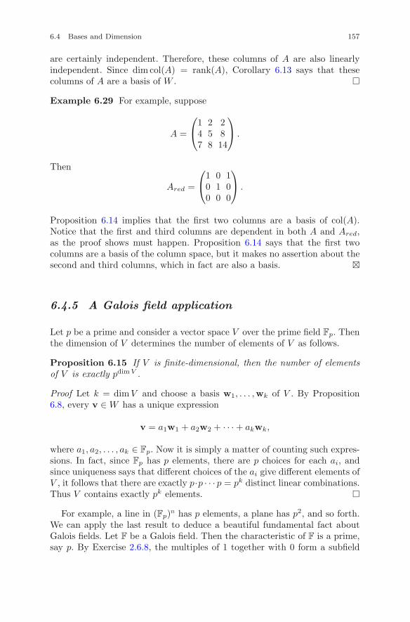
6.4 Bases and Dimension 157
are certainly independent. Therefore, these columns of A are also linearlyindependent. Since dim col(A) = rank(A), Corollary 6.13 says that thesecolumns of A are a basis of W . �
Example 6.29 For example, suppose
A =
⎛
⎝1 2 24 5 87 8 14
⎞
⎠ .
Then
Ared =
⎛
⎝1 0 10 1 00 0 0
⎞
⎠ .
Proposition 6.14 implies that the first two columns are a basis of col(A).Notice that the first and third columns are dependent in both A and Ared,as the proof shows must happen. Proposition 6.14 says that the first twocolumns are a basis of the column space, but it makes no assertion about thesecond and third columns, which in fact are also a basis. �
6.4.5 A Galois field application
Let p be a prime and consider a vector space V over the prime field Fp. Thenthe dimension of V determines the number of elements of V as follows.
Proposition 6.15 If V is finite-dimensional, then the number of elementsof V is exactly pdimV .
Proof Let k = dim V and choose a basis w1, . . . ,wk of V . By Proposition6.8, every v ∈ W has a unique expression
v = a1w1 + a2w2 + · · · + akwk,
where a1, a2, . . . , ak ∈ Fp. Now it is simply a matter of counting such expres-sions. In fact, since Fp has p elements, there are p choices for each ai, andsince uniqueness says that different choices of the ai give different elements ofV , it follows that there are exactly p·p · · · p = pk distinct linear combinations.Thus V contains exactly pk elements. �
For example, a line in (Fp)n has p elements, a plane has p2, and so forth.We can apply the last result to deduce a beautiful fundamental fact aboutGalois fields. Let F be a Galois field. Then the characteristic of F is a prime,say p. By Exercise 2.6.8, the multiples of 1 together with 0 form a subfield
158 6 Vector Spaces
with p elements. This subfield is indistinguishable from Fp, but we will denoteit by F
′. It follows from the field axioms that F is a vector space over F′ (see
Example 6.11). Moreover, since F itself is finite, it follows by definition thatF is finite-dimensional (over F′), since every a ∈ F has the expression a = 1a,so F spans itself over F
′, since 1 ∈ F′. Applying Proposition 6.15, we get the
following result.
Proposition 6.16 Let F be a finite field of characteristic p. Then |F| = pn,where n is the vector space dimension of F over the subfield F
′ of F consistingof all multiples of 1: that is, n = dimF′ F.
Recall that in Section 2.6.2, we considered a field F = {0, 1, α, β}, whereα + β = 1. Thus, for example, {1, α} is a basis, and F has 4 = 22 elements,in agreement with the above result. It can be shown that for every prime pand every n > 0, there is a unique Galois field of order pn. Combining theprevious two results, we get the following corollary.
Corollary 6.17 Let F be a Galois field of characteristic p, and let q = pn
denote |F|. Then if V is a finite-dimensional vector space over F, we have
|V | = qdimFV = pn dimF V .
Here is another corollary.
Corollary 6.18 Let F be a Galois field with q = pm elements. Then thegeneral linear group GL(n,F) has order
|GL(n,F)| = (qn − 1)(qn − q)(qn − q2) · · · (qn − qn−1). (6.8)
Proof The elements of GL(n,F) may be described as the elements A of Fn×n
whose columns form a basis of Fn. Consequently, the first i columns of A haveto form a basis of an i-dimensional subspace of Fn. Thus, there are qn − 1choices for A’s first column, qn − q choices for its second column, since theonly restriction on the second column is that it not lie on the line spannedby the first column, and in general, there are qn − qi−1 choices for the ithcolumn, since the span of the first i − 1 columns has qi−1 elements. �
Exercises
Exercise 6.4.1 Find a basis for the subspace of R4 spanned by
(1, 0,−2, 1)T , (2,−1, 2, 1)T , (1, 1, 1, 1)T , (0, 1, 0, 1)T , (0, 1, 1, 0)T
that contains the first and fifth vectors.
6.4 Bases and Dimension 159
Exercise 6.4.2 Consider the matrix A =
⎛
⎝1 2 0 1 22 0 1 −1 21 1 −1 1 0
⎞
⎠ as an
element of R3×5.
(i) Show that the basic null vectors of Ax = 0 are a basis of N (A).
(ii) Find a basis of col(A).
(iii) Repeat (i) and (ii) when A is considered as a matrix over F3.
Exercise 6.4.3 Prove that cos x and sin x are linearly independent on theopen interval (0, 2π).
Exercise 6.4.4 Let W be a subspace of V , and let w1, . . . ,wk ∈ W. Showthat if w1, . . . ,wk are independent, then w1,w2, . . . ,wk,v are also indepen-dent for every v ∈ V such that v /∈ W .
Exercise 6.4.5 Prove Corollary 6.12. That is, suppose V is a finite-dimensionalvector space over a field F, and let W be a subspace of V . Show the following:
(i) W is finite-dimensional.
(ii) In fact, dimW ≤ dim V .
(iii) If dimW = dim V , then W = V .
Exercise 6.4.6 Prove Corollary 6.13. That is, show that if dimV = m, thenevery set of m linearly independent vectors in V forms a basis, and similarly,every set of m vectors that span V is also a basis.
Exercise 6.4.7 True or false: For every A ∈ Fn×n, rank(A) ≥ rank(A2).
Prove your answer.
Exercise 6.4.8 Consider the subspace W of V (4, 2) = (F2)4 spanned by1011, 0110, and 1001.
(i) Find a basis of W and compute |W |.(ii) Extend your basis to a basis of (F2)4.
Exercise 6.4.9 Construct at least two proofs of the statement that for everymatrix A, dim col(A) = dim row(A).
Exercise 6.4.10 Let A and B be n × n matrices.
(i) Show that N (A) ⊂ N (BA). When is N (BA) = N (A)?
(ii) Show that col(A) ⊃ col(AB). When is col(AB) = col(A)?
(iii) Show that AB = O if and only if col(B) ⊂ N (A).
160 6 Vector Spaces
Exercise 6.4.11 Consider the set Fn×ns of symmetric n × n matrices
over F.
(i) Show that Fn×ns is a subspace of Fn×n.
(ii) Show that the set of matrices Sij with i < j defined in Example 6.26together with the Eii make up a basis of Fn×n
s .
Exercise 6.4.12 Let Fn×nss be the n × n skew-symmetric matrices over F.
(i) Show that Fn×nss is a subspace of Fn×n.
(ii) Find a basis of Fn×nss and compute its dimension.
(iii) Find a basis of Fn×n that uses only symmetric and skew-symmetric
matrices.
Exercise 6.4.13 Let F be a field, and suppose V and W are subspacesof Fn.
(i) Show that V ∩ W is a subspace of Fn.
(ii) Let V + W = {u ∈ Fn | u = v + w, where v ∈ V,w ∈ W}. Show that
V + W is a subspace of Fn.
(iii) Show that dim(V + W ) ≤ dim V + dim W .
Exercise 6.4.14 Let W and Y be subspaces of a vector space V of dimen-sion n. What are the minimum and maximum dimensions that W ∩ X canhave? Discuss the case that W is a hyperplane (i.e., dimW = n − 1) and Xis a plane (i.e., dimX = 2).
Exercise 6.4.15 Suppose X is a finite set, say |X| = n, and let F = Fp. LetV = F
X . That is, V is the set of all maps with domain X and target F. Showthat V is an F-vector space, find a basis, and compute dim V .
Exercise 6.4.16 Show that the set of n × n upper triangular matrices overF is a subspace of Fn×n. Find a basis and its dimension.
Exercise 6.4.17 Let F be a Galois field of characteristic p, and let F′ be
the subfield of F consisting of all multiples of 1. If V is a finite-dimensionalvector space over F, show that dimF′ V = dimF′ FdimF V . Conclude that
|V | = pdimF′ F dimF V .
Exercise 6.4.18 Let |F| = q, where q = pn, p a prime. Show that everyelement of F is a root of the polynomial xq − x ∈ Fp[x].
Exercise 6.4.19 Let V = R as a vector space over Q. Is dim V finite orinfinite? Discuss.
6.4 Bases and Dimension 161
Exercise 6.4.20 Let V be a vector space over Fp of dimension n. A linearlyindependent subset of V with m elements is called an m-frame in V . Showthat the number of m-frames in V is exactly
(pn − 1)(pn − p) · · · (pn − pm−2)(pn − pm−1).
(Use Proposition 6.15 and part of the proof of the dimension theorem.)
Exercise 6.4.21 Use Exercise 6.4.20 to show that the number of subspacesof dimension m in an n-dimensional vector space V over Fp is
(pn − 1)(pn − p) · · · (pn − pm−2)(pn − pm−1)(pm − 1)(pm − p) · · · (pn − pm−2)(pm − pm−1)
.
(The set of m-dimensional subspaces of a finite-dimensional vector space isan important object, called a Grassmann variety.)
Exercise 6.4.22 Let V be a vector space. A complete flag in V is a sequenceof subspaces
V1 ⊂ V2 ⊂ · · · ⊂ Vn−1 ⊂ V
such that dim Vi = i. The set Flag(V ) of all complete flags in V is called theflag variety of V .
(i) Let B ⊂ GL(n,F) denote the set of all invertible upper triangular elementsof Fn×n. Show that there exists a bijection
Φ : GL(n,F)/B → Flag(Fn).
(ii) Suppose F is Galois. Find a formula for the number of flags in Fn. That
is, find |Flag(Fn)|.Exercise 6.4.23 (This is more challenging.) Consider a square array oflights numbered 1 to 9 inclusively: that is,
1 2 34 5 67 8 9
Turning a light on or off also changes all the on–off states of the lights directlyabove and below and to the left and right. For instance, if the center light(light number 5) is turned on, then lights 2, 4, 5, 6, and 8 also change theirstate.
(i) If all the lights are off, can they all be turned on?
(ii) How can you turn on just light number 1?
(iii) Is it possible to turn all the lights off from every starting configuration?
162 6 Vector Spaces
6.5 The Grassmann Intersection Formula
The intersection of a pair of nonparallel planes P1 and P2 in R3 through
the origin is a line through the origin. This may seem obvious, but whatwould the answer be if instead of being planes in R
3, P1 and P2 were three-dimensional subspaces of R4? The purpose of this section is to answer thisquestion; that is, if W and Y are arbitrary subspaces of a finite-dimensionalvector space V , what is dim(W ∩Y )? The answer is given by the Grassmannintersection formula, which gives dim(W ∩ Y ) in terms of the dimensions ofW , Y , and a subspace W +Y known as the sum of W and Y . After that, wewill introduce direct sums of subspaces and will derive conditions for sumsof subspaces to be direct. These results on direct sums will be used when westudy eigentheory in Chap. 8.
6.5.1 Intersections and sums of subspaces
Let V be a vector space over a field F with subspaces W and Y . The simplestway of building a new subspace is by taking the intersection W ∩ Y .
Proposition 6.19 The intersection W ∩ Y of the subspaces W and Y ofV is also a subspace of V . More generally, the intersection of an arbitrarycollection of subspaces of V is also a subspace.
Proof This is an exercise. �
Proposition 6.19 is a generalization of the fact that the solution space ofa homogeneous linear system is a subspace of F
n. The solution space of asingle homogeneous linear equation is a hyperplane in F
n, and so the solutionspace of a homogeneous linear system is the intersection of a finite numberof hyperplanes in F
n.Another simple way of forming a new subspace is to take the subspace
spanned by W and Y . This is defined as follows.
Definition 6.8 The subspace spanned by W and Y or alternatively, the sumof W and Y , is defined to be the set of sums
W + Y = {w + y | w ∈ W,y ∈ Y }.
More generally, we can form the sum V1 + · · · + Vk of an arbitrary (finite)number of subspaces V1, V2, . . . , Vk of V . The sum V1+ · · ·+Vk is also writtenas
∑ki=1 Vi, or more simply
∑Vi.
Proposition 6.20 The sum∑k
i=1 Vi of the subspaces V1, V2, . . . , Vk of V isalso a subspace of V . It is, in fact, the smallest subspace of V containingevery Vi.
6.5 The Grassmann Intersection Formula 163
Proof We leave the proof as another exercise. �
6.5.2 Proof of the Grassmann intersectionformula
We now return to the question of what one can say about the dimension ofthe intersection of two subspaces. For example, what is the dimension of theintersection of two three-dimensional subspaces of R4? The answer is givenby the Grassmann intersection formula, which relates the dimensions of W ,Y , W + Y , and W ∩ Y . Before looking at the formula, the reader can try toguess the answer.
Theorem 6.21 If W and Y are finite-dimensional subspaces of a vectorspace V , then W + Y is finite-dimensional, and
dim(W + Y ) = dimW + dim Y − dim(W ∩ Y ). (6.9)
Proof Since W ∩ Y is a subspace of W , it is finite-dimensional. Hence, weknow that W ∩ Y has a basis, say x1, . . . ,xk. The dimension theorem allowsus to extend this basis to a basis of W , say
x1, . . . ,xk,wk+1, . . . ,wk+r.
Likewise, since Y is also finite-dimensional, we can extend the basis of W ∩Yto a basis of Y , say
x1, . . . ,xk,yk+1, . . . ,yk+s.
I claim that
B = {x1, . . . ,xk,wk+1, . . . ,wk+r,yk+1, . . . ,yk+s}
is a basis of W + Y . It is not hard to see that B is a spanning set, so W + Yis finite-dimensional even though V is an arbitrary vector space. To see thatB is independent, suppose
k∑
i=1
αixi +k+r∑
j=k+1
βjwj +k+s∑
m=k+1
γmym = 0. (6.10)
Thus, ∑γmym = −(∑
αixi +∑
βjwj
).
Since the left-hand term is in Y and the one on the right is in W , we have
164 6 Vector Spaces
∑γmym ∈ Y ∩ W.
Thus ∑γmym =
∑δixi
for some δi ∈ F. Hence
∑δixi +
∑(−γm)ym = 0.
Therefore, all the δi and γm are zero. In particular, (6.10) becomes the expres-sion ∑
αixi +∑
βjwj = 0.
But this implies that all the αi and βj are 0 also. Consequently, B is inde-pendent. Since B spans W + Y , it forms a basis of W + Y , so dim(W + Y ) =k + r + s. It remains to count dimensions. We have
dim(W + Y ) = k + r + s = (k + r) + (k + s) − k,
and hence dim(W + Y ) = dimW + dim Y − dim(W ∩ Y ). �
Notice that the Grassmann intersection formula doesn’t mention dimV ,which is why we don’t need to require that V be finite-dimensional. However,if it is, then dim(W + Y ) ≤ dim V , so we get a nice corollary.
Corollary 6.22 If W and Y are subspaces of a finite-dimensional vectorspace V , then
dim(W ∩ Y ) ≥ dim W + dim Y − dim V. (6.11)
In particular, if dim W + dim Y > dim V , then dim(Y ∩ W ) > 0.
Now let us see what can be said about two three-dimensional subspacesW and Y of a five-dimensional space V . Since the sum of the dimensions ofW and Y is 6, they meet in at least a line, although the intersection can alsohave dimension two or three. If dimV decreases, then intuitively, dim(Y ∩W )should increase, since there is less room to maneuver. This is exactly whatthe inequality tells us. If dimV = 4, then dim(W ∩ Y ) ≥ 3 + 3 − 4 = 2, soW and Y contain a common plane. However, once dimV is at least 6, theinequality no longer tells us anything.
Example 6.30 (Intersection of hyperplanes). Let H1 and H2 be distincthyperplanes in F
n. Then
dim(H1 ∩ H2) ≥ (n − 1) + (n − 1) − n = n − 2.
6.5 The Grassmann Intersection Formula 165
But since the hyperplanes are distinct, dim(H1 ∩ H2) < n − 1, so dim(H1 ∩H2) = n − 2 exactly. �
Here is a nice example.
Example 6.31. Recall that Fn×ns and F
n×nss denote, respectively, the spaces
of of n × n symmetric and n × n skew-symmetric matrices (see Example6.26). Let’s assume now that the characteristic of F is not equal to 2. Thenan arbitrary A ∈ F
n×n can be expressed as the sum of a symmetric matrixand a skew-symmetric matrix. Namely,
A =12(A + AT ) +
12(A − AT ). (6.12)
Thus Fn×n = Fn×ns +F
n×nss . Moreover, since char(F) �= 2, the only matrix that
is both symmetric and skew-symmetric is the zero matrix. That is, Fn×ns ∩
Fn×nss = {0}. Hence by the Grassmann intersection formula,
dimFn×n = dim(Fn×n
s ) + dim(Fn×nss ).
Note that we already knew this result from Section 6.4.2, where we showedthat dim(Fn×n
s ) = n(n + 1)/2 and dim(Fn×nss ) = n(n − 1)/2. �
As we will see in the next section, this example shows that Fn×n is the
direct sum of Fn×ns and F
n×nss . This is a stronger assertion than simply saying
that Fn×n = F
n×ns + F
n×nss , which is a consequence of (6.12). In particular, it
implies that every square matrix can be uniquely expressed via (6.12) as thesum of a symmetric matrix and a skew-symmetric matrix, except when thecharacteristic is two.
6.5.3 Direct sums of subspaces
By the Grassmann intersection formula, two subspaces W and Y of V suchthat dim(W ∩ Y ) = 0 have the property that dim(W + Y ) = dim W +dim Y , and conversely. An explicit example of this was considered above.This observation is related to the following definition.
Definition 6.9. We say that V is the direct sum of two subspaces W andY if V = W +Y and for every v ∈ V , the expression v = w+y with w ∈ Wand y ∈ Y is unique. If V is the direct sum of W and Y , we write V = W ⊕Y .More generally, we say that V is the direct sum of the subspaces V1, . . . , Vk
if V =∑
Vi and for every v ∈ V , the expression v =∑
vi, where eachvi ∈ Vi, is unique. (Equivalently, if 0 =
∑vi, where each vi ∈ Vi, then each
vi = 0.) In this case, we write V =⊕k
i=1 Vi.
166 6 Vector Spaces
Proposition 6.23. Suppose V is a finite-dimensional vector space with sub-spaces W and Y . Then the following conditions are all equivalent to the asser-tion that V = W ⊕ Y :
(i) V = W + Y and W ∩ Y = {0}.(ii) V = W + Y and dim V = dim W + dim Y .
(iii) dim V = dim W + dim Y and W ∩ Y = {0}.Proof. That conditions (i), (ii), and (iii) are equivalent follows from theGrassmann intersection formula. Thus it suffices to show that (i) is equivalentto V = W ⊕ Y . Assume (i), and suppose v = w + y = w′ + y′. Thenw − w′ = y′ − y is an element of W ∩ Y = {0}. Thus w = w′ and y′ = y.Hence V = W ⊕ Y . On the other hand, if V = W ⊕ Y and W ∩ Y �= {0},then every nonzero v ∈ W ∩ Y has two expressions v = v + 0 = 0 + v. Thisviolates the definition of a direct sum, so W ∩ Y = {0}. �
Corollary 6.24. Suppose dim V = dim(W +Y ) and dim(W ∩Y ) = 0. ThenV = W ⊕ Y .
Proof. If dim V = dim(W + Y ), then W + Y = V . Therefore, the resultfollows from Proposition 6.23. �
Referring back to Example 6.31, we get the following assertion.
Proposition 6.25. Assume char(F) �= 2. Then Fn×n = F
n×ns ⊕ F
n×nss . Thus,
every square matrix over F can be uniquely expressed as in (6.12) as the sumof a symmetric matrix and a skew-symmetric matrix, both over F.
We will need the following extended version of Proposition 6.23.
Proposition 6.26. Suppose V is finite-dimensional and V1, . . . , Vk are sub-spaces of V such that V =
∑ki=1 Vi. Then V =
⊕ki=1 Vi if and only if
dim V =∑k
i=1 dim Vi.
Proof. Suppose V =∑k
i=1 Vi, and dim V =∑k
i=1 dim Vi. Choose a basis ofeach Vi and consider the union B of these bases. Then B clearly spans V ,since the part in Vi spans Vi. Hence we get a spanning set in V with dimVelements. It follows that B is a basis of V . Now suppose the sum isn’t direct.Then there exists an element v with two different decompositions
v =k∑
i=1
xi =k∑
i=1
yi,
where the xi and yi are in Vi for each i. Thus xj �= yj for some index j.Hence v has to have two different expansions in terms of B. This contradicts
6.5 The Grassmann Intersection Formula 167
the uniqueness of the expansion in a basis; hence the sum must be direct.Conversely, suppose V =
⊕ki=1 Vi. Forming B as in the previous case, it
follows that B is independent, since the sum is direct. Thus B is a basis, andtherefore, dim V = |B| =
∑ki=1 dim Vi.
�
6.5.4 External direct sums
Let V and W be arbitrary vector spaces over the same field F. Then we canform a new vector space V × W containing both V and W as subspaces.Recall from Chap. 1 that V ×W denotes the Cartesian product of V and W ,namely the set of all ordered pairs (v,w), where v ∈ V and w ∈ W .
Definition 6.10. The external direct sum of V and W is the Cartesian prod-uct V × W with addition defined componentwise by
(v1,w1) + (v2,w2) = (v1 + v2,w1 + w2),
and scalar multiplication defined similarly by
r(v,w) = (rv, rw).
The alert reader will have noted that Fk ×Fm = F
k+m. Thus the externaldirect sum is a generalization of the construction of Fn. This operation canalso be extended (inductively) to any finite number of vector spaces over F.In fact, Fn is just the n-fold external direct sum of F.
We leave it to the reader to show that V and W can both be consideredsubspaces of V × W .
Proposition 6.27. If V and W are finite-dimensional vector spaces over F,then so is their external direct sum, and dim(V × W ) = dim V + dim W .
Proof. We leave this as an exercise. �
Exercises
Exercise 6.5.1. Suppose W and Y are two subspaces of a finite-dimensionalvector space V such that W ∩ Y = {0}. Show that dimW + dim Y ≤ dim V .
Exercise 6.5.2. Prove Proposition 6.27.
Exercise 6.5.3. If two 22-dimensional subspaces of Rn always meet in at
least a line, what can you say about n?
168 6 Vector Spaces
Exercise 6.5.4. Do two subspaces of R26 of dimensions 5 and 17 have to
meet in more than 0? What about a subspace of dimension 22 and a subspaceof dimension 13?
Exercise 6.5.5. Suppose W and Y are two subspaces of (Fp)n. Find expres-sions for |W ∩ Y | and |W + Y |.
6.6 Inner Product Spaces 169
6.6 Inner Product Spaces
In this section, we will study the notion of an inner product on a real vectorspace. We will also study the notion of a Hermitian inner product on a com-plex vector space, though not in as much detail. An inner product on a realvector space V allows one to measure distances and angles between vectors.Similarly, a Hermitian inner product permits one to do the same for vec-tors in a complex vector space. The main result of this section is that everyfinite-dimensional inner product space has a special type of basis known asan orthonormal basis. This is a basis having the properties of the standardbasis of Rn.
6.6.1 The definition of an inner product
We will first treat the real case.
Definition 6.11. Let V be a real vector space. An inner product on V is arule that associates to every a,b ∈ V a unique scalar (a,b) ∈ R having thefollowing properties for all a,b, c ∈ V and r ∈ R:
(i) (a,b) = (b,a),
(ii) (a + b, c) = (a, c) + (b, c),
(iii) (ra,b) = (a, rb) = r(a,b), and
(iv) if a �= 0, then (a,a) > 0.
The property in condition (iv) is called positive definiteness. A real vectorspace V with an inner product is called an inner product space. Clearly,(0,0) = 0, so (a,a) ≥ 0 for all a ∈ V . Thus the following definition makessense.
Definition 6.12. Let V be an inner product space as in the previous defi-nition. Then the length of a ∈ V is defined by
|a| =√
(a,a), (6.13)
and the distance between a and b in V is defined by
d(a,b) = |a − b|. (6.14)
The basic example of an inner product space is Rn with the Euclidean
inner product defined in the next example.
170 6 Vector Spaces
Example 6.32 (Euclidean n-space). The dot product on Rn defined in
Section 3.1.6 by
a · b = aTb =n∑
i=1
aibi (6.15)
defines an inner product by setting (a,b) = a ·b. The dot product is referredto as the Euclidean inner product on R
n. �
The next example gives an important inner product on Rn×n. First, we
have to define the trace of an n × n matrix. If A ∈ Fn×n, define the trace of
A to be Tr(A) =∑n
i=1 aii.
Example 6.33. Let V = Rn×n. For A,B ∈ V , put
(A,B) = Tr(ABT).
This defines an inner product on Rn×n known as the Killing form. The veri-
fication of the axioms for an inner product is left as an exercise. Notice, forexample, that if A and B are diagonal matrices, say A = diag(a1, . . . , an) andB = diag(b1, . . . , bn), then
(A,B) = Tr(ABT ) = Tr(diag(a1b1, . . . , anbn)) =n∑
i=1
aibi.
Thus the Killing form coincides with the Euclidean inner product on diagonalmatrices. �
6.6.2 Orthogonality
As we just saw, an inner product on a real vector space V has natural lengthand distance functions. We will now see that it allows one to imitate otherEuclidean properties of Rn, namely the notion of angles. The starting pointis orthogonality.
Definition 6.13. We say that a pair of vectors a, and b in an inner productspace V are orthogonal if
(a,b) = 0. (6.16)
Here are a couple of simple properties.
Proposition 6.28. In an inner product space V , the zero vector is orthog-onal to every vector. In fact, 0 is the only vector orthogonal to itself. Twovectors a,b ∈ R
n are orthogonal if and only if∑n
i=1 aibi = 0.
6.6 Inner Product Spaces 171
Proof. Left to the reader. �
Orthogonality is a generalization of the notion of perpendicularity in R2.
Two vectors a = (a1, a2)T and b = (b1, b2)T in R2 are perpendicular exactly
when the triangle with sides a and b is a right triangle. This is the caseexactly when |a+b|2 = |a|2 + |b|2, by the Pythagorean theorem. The readershould check that this identity holds if and only if a1b1 + a2b2 = 0, that is, ifa · b = 0. On an inner product space V , orthogonality can be characterizedin a similar manner.
Proposition 6.29. Two vectors a and b in an inner product space V areorthogonal if and only if |a + b|2 = |a|2 + |b|2.Proof. Since |a + b|2 = (a + b,a + b), one gets that
|a + b|2 = (a,a) + 2(a,b) + (b,b) = |a|2 + 2(a,b) + |b|2.
Hence (a,b) = 0 if and only if |a + b|2 = |a|2 + |b|2. �
We now discuss orthogonal decomposition. If a,b ∈ V and b �= 0, we claimthat there exists a unique λ ∈ R such that a = λb+ c and (b, c) = 0. To seethis, write c = a−λb. Using the properties of the inner product, we see that(b, c) = 0 if and only if λ = (a,b)/(b,b). By the previous proposition, thisvalue of λ gives |a|2 = λ2|b|2 + |c|2. Hence we get the following result.
Proposition 6.30. Let a and b be elements of an inner product space V ,and suppose b �= 0. Then a can be uniquely decomposed as a linear combina-tion of two orthogonal vectors b and c as
a = λb + c, (6.17)
where λ = (a,b)/(b,b) and c = a − λb.
In particular, since |c|2 ≥ 0, it follows that
|a|2 ≥ ((a,b)/(b,b))2|b|2.
Taking square roots gives a famous inequality.
Proposition 6.31 (Cauchy–Schwarz inequality). For every a,b ∈ V ,
|(a,b)| ≤ |a||b|, (6.18)
with equality if and only if a is a multiple of b.
172 6 Vector Spaces
Proof. The inequality surely holds when b = 0. Thus suppose b �= 0. Then(6.18) follows from the inequality before the proposition, and equality holdsif and only if c = 0, or equivalently, if and only if a is a multiple of b. �
The Cauchy–Schwarz inequality for Rn says that
|n∑
i=1
aibi| ≤( n∑
i=1
a2i
)1/2( n∑
i=1
b2i
)1/2
.
The vector
Pb(a) =((a,b)/(b,b)
)b
is called the orthogonal projection of a on b. Our final definition is theangle between two nonzero vectors. By the Cauchy–Schwarz inequality,−1 ≤ (a,b)
|a||b| ≤ 1. Hence there exists a unique θ ∈ [0, π] such that
cos θ =(a,b)|a||b| . (6.19)
Definition 6.14. The angle between two nonzero vectors a and b in aninner product space V is defined to be the unique angle θ ∈ [0, π] such that(6.19) holds.
In particular, (a,b) = 0 if and only if the angle between a and b is π/2.In physics books, the identity
a · b = |a||b| cos θ
is sometimes taken as a definition of the dot product. But this definition isnot as easy to work with as the usual one.
Inner products can exist on infinite-dimensional vector spaces. This givesa method for extending properties of Rn to the infinite-dimensional setting.A particularly important example is the following.
Example 6.34. (An inner product on C[a, b]) Let C[a, b] be the space of allcontinuous real-valued functions on the closed interval [a, b] in R. The innerproduct of f, g ∈ C[a, b] is defined by
(f, g) =∫ b
a
f(t)g(t)dt.
The first three axioms for the inner product on C[a, b] are verified by applyingstandard facts about integration proved (or at least stated) in calculus. Thepositive definiteness property requires that we verify that (f, f) > 0 if f �= 0.
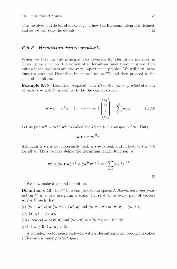
6.6 Inner Product Spaces 173
This involves a little bit of knowledge of how the Riemann integral is defined,and so we will skip the details. �
6.6.3 Hermitian inner products
When we take up the principal axis theorem for Hermitian matrices inChap. 9, we will need the notion of a Hermitian inner product space. Her-mitian inner products are also very important in physics. We will first intro-duce the standard Hermitian inner product on C
n, and then proceed to thegeneral definition.
Example 6.35 (Hermitian n-space). The Hermitian inner product of a pairof vectors w, z ∈ C
n is defined to be the complex scalar
w • z = wT z =(w1 w2 · · · wn
)
⎛
⎜⎜⎜⎝
z1z2...zn
⎞
⎟⎟⎟⎠ =n∑
i=1
wizi. (6.20)
Let us put wH = wT ; wH is called the Hermitian transpose of w. Thus,
w • z = wHz.
Although w • z is not necessarily real, w • w is real, and in fact, w • w ≥ 0for all w. Thus we may define the Hermitian length function by
|w| = (w • w)1/2 = (wHw)1/2 =( n∑
i=1
|wi|2)1/2
.
�We now make a general definition.
Definition 6.15. Let V be a complex vector space. A Hermitian inner prod-uct on V is a rule assigning a scalar (w, z) ∈ C to every pair of vectorsw, z ∈ V such that
(i) (w + w′, z) = (w, z) + (w′, z) and (w, z + z′) = (w, z) + (w, z′),
(ii) (z,w) = (w, z),
(iii) (αw, z) = α(w, z) and (w, αz) = α(w, z), and finally,
(iv) if w �= 0, (w,w) > 0.
A complex vector space endowed with a Hermitian inner product is calleda Hermitian inner product space.
174 6 Vector Spaces
6.6.4 Orthonormal bases
In this section we will show that every finite-dimensional inner product spaceadmits a type of basis called an orthonormal basis, which is analogous to thestandard basis e1, . . . , en of Euclidean n-space R
n. Let V denote a real innerproduct space.
Definition 6.16. A set U of unit vectors in V is called orthonormal if everypair of distinct elements of U are orthogonal to each other.
Example 6.36. The standard basis e1, . . . , en determines an orthonormalset in Euclidean n-space R
n. �
Proposition 6.32. Every orthonormal subset U of V is linearly indepen-dent. (That is, every finite subset of U is independent.) In particular, if V isfinite-dimensional, then every orthonormal set in V having dim V elementsis a basis of V .
Proof. Suppose u1, . . . ,um are orthonormal, and assume that
m∑
i=1
aiui = 0.
Then for every index j,
( m∑
i=1
aiui,uj
)= (0,uj) = 0.
Since (ui,uj) equals 0 if i �= j and equals 1 if i = j, the left-hand side is
m∑
i=1
ai(ui,uj) = aj ,
so aj = 0 for all j. Therefore, u1, . . . ,um are independent. Hence if |U| =dim V, then U is a basis of V . �
Definition 6.17. An orthonormal basis of V is a basis that is an orthonor-mal set.
Proposition 6.33. A collection of vectors u1,u2, . . . ,un in Rn is an ortho-
normal basis of Rn if and only if the matrix U = (u1 u2 . . .un) is orthogonal.Thus the set of U ∈ F
n×n whose columns are an orthonormal basis of Rn isexactly the orthogonal group O(n,R).
6.6 Inner Product Spaces 175
Proof. Recall that U is orthogonal if and only if UTU = In. But UTU =(uT
i uj) = (ui · uj) = In if and only if u1,u2, . . . ,un are orthonormal. �
For example, the standard basis vectors e1, . . . , en in Rn are the columns
of In. Here are some more examples.
Example 6.37. The vectors
u1 =1√3(1, 1, 1)T , u2 =
1√6(1,−2, 1)T , u3 =
1√2(1, 0,−1)T
form an orthonormal basis of R3. Moreover, u1 and u2 constitute an ortho-normal basis of the plane x − z = 0. �
Example 6.38. The matrix
Q =12
⎛
⎜⎜⎝
1 1 1 1−1 1 −1 11 −1 −1 11 1 −1 −1
⎞
⎟⎟⎠
is orthogonal. Hence its columns form an orthonormal basis of R4. Since QT
is also orthogonal, the rows of B form another orthonormal basis of R4. �
6.6.5 The existence of orthonormal bases
We now show that every finite-dimensional inner product space has an ortho-normal basis. In fact, we show a little more.
Proposition 6.34. Let V be an inner product space. Then every nontrivialfinite-dimensional subspace W of V admits an orthonormal basis.
Proof. We prove this by induction on dimW . Note that every subspace of Vis also an inner product space via restricting the inner product on V to W .If dimW = 1, the result is true, since a unit vector in W is an orthonormalbasis. Thus suppose dim W = m > 1 and that the result is true for everysubspace of W of dimension at most m − 1. Let u be a unit vector in Wand let H = {x ∈ W | (x,u) = 0}. Then H is a subspace of W . Since|u| = 1, u /∈ H. It follows from Corollary 6.12 that dimH < m. Thus, by theinduction hypothesis, H admits an orthonormal basis, say U . Now I claimthat U and u combine to give an orthonormal basis of W . Clearly, U and uform an orthonormal set, so it suffices to check that they span W . Let x bean arbitrary element of W , and let y = x − (x,u)u. Then
(y,u) = (x,u) − (x,u)(u,u) = 0,
176 6 Vector Spaces
since (u,u) = 1. Thus y ∈ H, so y is a linear combination of the elements ofU . Since x = y + (x,u)u, x is in the span of u and U . Therefore W has anorthonormal basis, so the result is proven. �
The above proof gives us the following
Corollary 6.35. If u is a unit vector in a finite-dimensional inner productspace V , then
H = {x ∈ V | (x,u) = 0}
is a hyperplane in V . That is, dim H = dim V − 1.
Here is an example not involving Rn.
Example 6.39. Let V denote the set of functions f(x) = ax2 + bx + c on[−1, 1], where a, b, c are arbitrary real numbers. For f, g ∈ V , let (f, g) =∫ 1
−1f(x)g(x)dx. In other words, V is a three-dimensional subspace of the
inner product space C[−1, 1]. The functions 1, x, and x2 are a basis of V ,but unfortunately they aren’t orthonormal. For although x is orthogonal to 1and x2, 1 and x2 aren’t orthogonal to each other:
∫ 1
−11x2dx = 2/3. To correct
this, we replace x2 with x2 − r, where r is chosen such that (1, x2 − r) = 0.Since (1, 1) = 2, it is easy to see that we should let r = 1/3. Thus 1, x, x2 −1/3 are orthogonal on [−1, 1]. We therefore obtain the orthonormal basis bynormalizing. The result is u1 = 1/
√2, u2 =
√3/2 x, and u3 = c(x2 − 1/3)
where c =( ∫ 1
−1(x2 − 1/3)2dx
)−1/2. �
6.6.6 Fourier coefficients
We are now going to see one of the reasons that an orthonormal basis isvery useful. If v1,v2, . . . ,vn is a basis of a vector space V , how does oneexpress an arbitrary element v of V as a linear combination of these basisvectors? If V = F
n, then this involves solving the linear system Ax = v, whereA =
(v1 v2 · · · vn
). That is, x = A−1v. But if V is arbitrary, we don’t yet
have a general method. On the other hand, if V has an orthonormal basis,there is a simple elegant solution.
Proposition 6.36. Let u1,u2, . . . ,un be an orthonormal basis of V . Thenif w ∈ V , we have
w =n∑
1=i
(w,ui)ui. (6.21)
Proof. Let w =∑n
1=i xiui. Then (w,uj) =∑n
1=i xi(ui,uj) = xj , since theui are orthonormal. �
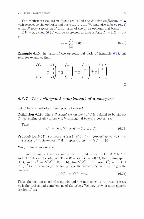
6.6 Inner Product Spaces 177
The coefficients (w,ui) in (6.21) are called the Fourier coefficients of wwith respect to the orthonormal basis u1, . . . ,un. We may also refer to (6.21)as the Fourier expansion of w in terms of the given orthonormal basis.
If V = Rn, then (6.21) can be expressed in matrix form In = QQT ; that
is,
In =n∑
1=i
uiuTi . (6.22)
Example 6.40. In terms of the orthonormal basis of Example 6.38, onegets, for example, that
⎛
⎜⎜⎝
1000
⎞
⎟⎟⎠ =14
⎛
⎜⎜⎝
1111
⎞
⎟⎟⎠ − 14
⎛
⎜⎜⎝
−11
−11
⎞
⎟⎟⎠ +14
⎛
⎜⎜⎝
1−1−11
⎞
⎟⎟⎠ +14
⎛
⎜⎜⎝
11
−1−1
⎞
⎟⎟⎠ .
�
6.6.7 The orthogonal complement of a subspace
Let U be a subset of an inner product space V .
Definition 6.18. The orthogonal complement of U is defined to be the setU⊥ consisting of all vectors v ∈ V orthogonal to every vector in U .
Thus,U⊥ = {v ∈ V | (v,u) = 0 ∀ u ∈ U}. (6.23)
Proposition 6.37. For every subset U of an inner product space V , U⊥ isa subspace of V . Moreover, if W = span U , then W ∩ U⊥ = {0}.Proof. This is an exercise.
It may be instructive to visualize W⊥ in matrix terms. Let A ∈ Rm×n,
and let U denote its columns. Then W = span U = col(A), the column spaceof A, and W⊥ = N (AT ). By (6.6), dimN (AT ) + dim row(AT ) = m. Butrow(AT ) and W = col(A) certainly have the same dimension, so we get theidentity
dimW + dimW⊥ = m. (6.24)
Thus, the column space of a matrix and the null space of its transpose areeach the orthogonal complement of the other. We now prove a more generalversion of this.
178 6 Vector Spaces
Proposition 6.38. Let W be a subspace of a finite-dimensional inner prod-uct space V and W⊥ its orthogonal complement. Then V = W ⊕ W⊥. Thus,dim V = dim W + dim W⊥. In particular, every v ∈ V can be orthogonallydecomposed in exactly one way as v = w + y, where w ∈ W and y ∈ W⊥.
Proof. By Proposition 6.34, we may choose an orthonormal basis of W , sayu1, . . . ,uk. Let v ∈ V and put
y = v −k∑
i=1
(v,ui)ui. (6.25)
Since the ui are orthonormal, we have (y,ui) = 0 for all i. Thus, by definition,y ∈ W⊥. But this says that if w =
∑ki=1(v,ui)ui, then v = w+y. Therefore,
V = W + W⊥. Since W ∩ W⊥ = {0}, we get V = W ⊕ W⊥ by Proposition6.23. Hence, dim W + dim W⊥ = dim V . �Definition 6.19. Let v = w+y be the above decomposition of v ∈ V withw ∈ W . Then w is called the component of v in W .
Thus if u1, . . . ,uk is an orthonormal basis of W , the component of anarbitrary vector v ∈ V is
w =k∑
i=1
(v,ui)ui. (6.26)
In particular, if W is a line, say W = Rw, then the component of an arbitraryv in V can be easily worked out, since
u =w
(w,w)1/2
is an orthonormal basis for W . In particular,
v = (v,u)u +(v − (v,u)u
).
6.6.8 Hermitian inner product spaces
The results about orthonormal bases in the case of an inner product spaceall have analogues for the Hermitian inner product spaces that were intro-duced in Section 6.6.3. Recall that the main example of a Hermitian innerproduct space is Cn with the Hermitian inner product (w, z) = wHz. A basisw1, . . . ,wn of a Hermitian inner product space V is said to be a Hermitianorthonormal basis, provided each |wi| is equal to 1 and (wi,wj) = 0 if i �= j.By imitating the proof of Proposition 6.34, one can prove the following result.
6.6 Inner Product Spaces 179
Proposition 6.39. Every finite-dimensional Hermitian inner product spacehas a Hermitian orthonormal basis. Moreover, the identity (6.21) holds forevery Hermitian orthonormal basis.
Orthogonal complements are defined in the Hermitian case in exactly thesame way as in the real case, and the Hermitian version of Proposition 6.38goes through without any change. Hermitian orthonormal bases of C
n arerelated to unitary matrices in the same way that orthonormal bases of R
n
are related to orthogonal matrices. Recall that if U ∈ Cn×n, then UH = (U)T .
Definition 6.20. A matrix U ∈ Cn×n is said to be unitary if UHU = In.
The set of all n × n unitary matrices is denoted by U(n).
Thus, unitary matrices are to the Hermitian inner product on Cn as orthog-
onal matrices are to the Euclidean inner product on Rn.
Proposition 6.40. U(n) is a matrix group that is a subgroup of GL(n,C).
Proof. Exercise. �
Thus U(n) is called the unitary group.
Exercises
Exercise 6.6.1. A nice application of Cauchy–Schwarz is the following fact:if a and b are unit vectors in R
n such that a · b = 1, then a = b. Prove this.
Exercise 6.6.2. Prove the law of cosines: if a triangle has sides with lengthsa, b, c, and θ is the angle opposite the side of length c, then c2 = a2 + b2 −2ab cos θ. (Hint: Consider c = b − a.)
Exercise 6.6.3. Show that the Killing form (A,B) = Tr(ABT ) introducedin Example 6.33 is an inner product on the space R
2×2 of real 2 × 2 matricesand find an orthonormal basis.
Exercise 6.6.4. Show that the orthogonal complement with respect to theKilling form of the space of 2×2 symmetric real matrices is the space of 2×2skew symmetric real matrices. Conclude R
2×2 = R2×2s ⊕ R
2×2ss .
Exercise 6.6.5. The proof that the Killing form on Rn×n is an inner product
requires showing that (A,B) = (B,A). Show this by proving the followingstatements.
(i) For all A,B ∈ Rn×n, Tr(AB) = Tr(BA);
(ii) For all A,B ∈ Rn×n, Tr(ABT ) = Tr(BAT )
Exercise 6.6.6. Orthogonally decompose the vector (1, 2, 2)T in R3 as p+q,
where p is required to be a multiple of (3, 1, 2)T and q is orthogonal to p.
180 6 Vector Spaces
Exercise 6.6.7. In this exercise, we consider the inner product space V =C[−1, 1] of continuous real-valued functions on [−1, 1] with inner productdefined by (f, g) =
∫ 1
−1f(t)g(t)dt.
(i) Show that the functions 1 and x are orthogonal. In fact, show that xk andxm are orthogonal if k is even and m is odd.
(ii) Find the projection of x2 on the constant function 1.
(iii) Use this to obtain the orthogonal decomposition of x2 on [−1, 1] in whichone of the components has the form r1.
Exercise 6.6.8. Consider the real vector space V = C[0, 2π] with the innerproduct defined by (f, g) =
∫ 2π
0f(t)g(t)dt.
(i) Find the length of sin2 x in V .
(ii) Compute the inner product (cosx, sin2 x).
(iii) Find the projection of sin2 x on each of the functions 1, cos x, and sinxin V .
(iv) Are 1, cos x, and sinx mutually orthogonal as elements of V ?
(v) Compute the orthogonal projection of sin2 x onto the subspace W of Vspanned by 1, cos x, and sin x.
Exercise 6.6.9. Assume f ∈ C[a, b]. The average value of f over [a, b] isdefined to be
1b − a
∫ b
a
f(t)dt.
Show that the average value of f over [a, b] is the projection of f on 1. Doesthis suggest an interpretation of the average value?
Exercise 6.6.10. Let f, g ∈ C[a, b]. Give a formula for the scalar t thatminimizes
||f − tg||2 =∫ b
a
(f(x) − tg(x))2dx.
Exercise 6.6.11. Show that the Hermitian inner product on Cn satisfies all
the conditions listed in Definition 6.15.
Exercise 6.6.12. Consider the plane P in R3 given by the equation x− y +
2z = 0.
(i) Find an orthonormal basis of P .
(ii) Find the expansion of (1, 1, 0)T in terms of this orthonormal basis.
6.6 Inner Product Spaces 181
Exercise 6.6.13. Find the expansion of (2, 0, 0)T in terms of the orthonor-mal basis of Example 6.37.
Exercise 6.6.14. The Gram–Schmidt method gives an algorithm for pro-ducing an orthonormal basis of an inner product space starting from a generalbasis. Here is how it works for R
3. Let v1,v2,v3 be a basis. First put
u1 =v1
|v1| .
Next, put
v′2 = v2 − (v2 · u1)u1 and u2 =
v′2
|v′2|
.
Finally, put
v′3 = v3 − (v3 · u1)u1 − (v3 · u2)u2 and u3 =
v′3
|v′3|
.
Verify that u1,u2,u3 form an orthonormal basis of R3 having the propertythat span{u1} = span{v1} and span{u1,u2} = span{v1,v2}. Why are v′
2
and v′3 both nonzero?
Exercise 6.6.15. Generalize the Gram–Schmidt method from R3 to R
4.
Exercise 6.6.16. Let W denote the hyperplane w + x − y + z = 0 in R4.
(i) Find the component of (1, 1, 1, 1)T in W .
(ii) Find an orthonormal basis of W .
(iii) Find an orthonormal basis of R4 containing the orthonormal basis of
part (ii).
(iv) Expand (1, 1, 1, 1)T in terms of the basis in part (iii).
Exercise 6.6.17. Show that if W is a subspace of a finite-dimensional innerproduct space V , then (W⊥)⊥ = W .
Exercise 6.6.18. Recall that the group P (n) of n×n permutation matricesis a subgroup of O(n,R). Show that the set of all left cosets O(n,R)/P (n) isin one-to-one correspondence with the set of all orthonormal bases of Rn.
Exercise 6.6.19. Let V be an inner product space. Show that the distancefunction d(a,b) = |a − b| on V × V Defines a metric on V in the sense thatfor all a,b, c ∈ V , we have the following properties:
(i) d(a,b) ≥ 0 and d(a,b) = 0 if and only if a = b.
(ii) d(a,b) = d(b,a), and
(iii) d(a, c) ≤ d(a,b) + d(b, c).Another quite different example of a metric is given in the Appendix.
182 6 Vector Spaces
Exercise 6.6.20. Let V be a finite-dimensional inner product space andW a subspace. The distance d(v,W ) from an arbitrary vector v ∈ V tothe subspace W is defined to be the minimum distance d(v,w) as w rangesover W .
(i) If v ∈ W , show that the distance from v to W is 0.
(ii) Suppose v = w + y is the orthogonal decomposition of v with w ∈ Wand y ∈ W⊥. Show that d(v,w) ≤ d(v,w′) for all w′ ∈ W and concludethat d(v,W ) = |y|. (This fact is called the principle of least squares.)
Exercise 6.6.21. Find the distance from (1, 1, 1, 1)T to the subspace of R4
spanned by (2, 0,−1, 1)T and (0, 0, 1, 1)T .
Exercise 6.6.22. If K is a subspace of Cn with the Hermitian inner product,show that dim K + dim K⊥ = n, where K⊥ is the orthogonal complement ofK with respect to the Hermitian inner product.
Exercise 6.6.23. Find a Hermitian orthonormal basis of the subspace of C3
spanned by (1, i, 0)T and (2,−i, 1)T , and then extend this basis to a Hermitianorthonormal basis of C3.
Exercise 6.6.24. Prove Proposition 6.40. That is, show that U(n) is amatrix group.
Exercise 6.6.25. The complex analogue of the Killing form on Cn×n is
(J,K) = Tr(JKH). Show that (J,K) defines a Hermitian inner product onC
2×2.
6.7 Vector Space Quotients 183
6.7 Vector Space Quotients
In the penultimate section of this chapter, we will construct the quotientvector space V/W of a vector space V by a subspace W . Since V is anabelian group and every subspace is a normal subgroup, this construction isan application of the construction of the quotient group G/H of a group Gby a normal subgroup H (see Proposition 2.17). Thus, the space of cosetsV/W is also an abelian group, and the natural map π : V → V/W is a grouphomomorphism.
Since we are not formally using results from group theory in this chapter,we will instead construct V/W from scratch. We will then show that ifV is finite-dimensional, then V/W is a finite-dimensional vector space anddim(V/W ) = dimV − dim W . Unfortunately, the vector space V/W doesn’tadmit a useful geometric interpretation; one must think of V/W as anabstract vector space.
6.7.1 Cosets of a subspace
Let V be a vector space over F and let W be a subspace. The cosets of Wwere introduced in Section 2.2 in the setting of groups. Redefining them fromscratch in the vector space setting goes as follows.
Definition 6.21. A coset of W is a subset of V of the form
v + W = {v + w | w ∈ W}, (6.27)
where v ∈ V .
The cosets of W are the equivalence classes of an equivalence relation EW
on V . Namely, if u,v ∈ V , let us write uEWv if v − u ∈ W . If uEWv, wewill say that u and v are equivalent modulo W .
Proposition 6.41. Let W be a subspace of a vector space V . Then EW isan equivalence relation on V , and the equivalence classes of this equivalencerelation are exactly the cosets of W .
Proof. Clearly vEWv, since v − v = 0 ∈ W . If uEWv, then vEWu, sinceW is closed under scalar multiplication, and (u− v) = (−1)(v − u). Finally,if uEWv and vEWw, then uEWw, since w − u = (w − v) + (v − u), andW is closed under addition. Hence EW is an equivalence relation on V . LetC denote the equivalence class of v and consider v + W . If y ∈ C, theny−v = w ∈ W . Hence y = v+w, so y ∈ v+W . Therefore, C ⊂ v+W . Onthe other hand, suppose y ∈ v + W . Then y = v + w for some w ∈ W . Butthen y − v ∈ W , so yEWv. Therefore, v + W ⊂ C. Hence the equivalenceclasses are exactly the cosets of W . �
184 6 Vector Spaces
Example 6.41. For example, suppose V = R3 and W is a plane through
0. Then the coset v + W is simply the plane through v parallel to W . Thecosets are all the planes in R
3 parallel to W . �
6.7.2 The quotient V/W and the dimensionformula
We will refer to the set of cosets V/W as the quotient space of V modulo W .Two cosets (v + W ) and (y + W ) may be added by putting
(v + W ) + (y + W ) = (v + y) + W. (6.28)
To make V/W into a vector space over F, we also have to define scalarmultiplication, which we do in a natural way: for a ∈ F and v ∈ V , put
a(v + W ) = av + W. (6.29)
The proof that addition is a well-defined binary operation uses the samereasoning as for the quotient group. We need to show that the rule (6.28) isindependent of the way we write a coset. That is, suppose v + W = v′ + Wand y+W = y′+W . Then we have to show that (v+y)+W = (v′+y′)+W .But this is so if and only if
(v + y) − (v′ + y′) ∈ W,
which indeed holds, since
(v + y) − (v′ + y′) = (v − v′) + (y − y′) ∈ W,
due to the fact that W is a subspace and both v − v′ and y − y′ are inW . Therefore, addition on V/W is well defined. The proof for scalar multi-plication is analogous. The zero element is 0 + W , and the additive inverse−(v+W ) of v+W is −v+W . Properties such as associativity and commu-tativity of addition follow from corresponding properties in V ; we will omitall the details. Hence V/W is an F-vector space, which is the first assertion ofthe following proposition. The second assertion gives a formula for dimV/Win the finite-dimensional setting.
Proposition 6.42. Let V be a vector space over a field F and suppose W isa subspace of V . Then the set V/W of cosets of W in V with addition andscalar multiplication defined as in (6.28) and (6.29) is a vector space over F.If V is finite-dimensional, then
6.7 Vector Space Quotients 185
dim V/W = dim V − dim W. (6.30)
Proof. To check the dimension formula (6.30), let w1, . . . ,wk be a basis ofW , and extend this to a basis
w1, . . . ,wk,v1, . . . ,vn−k
of V . Then I claim that the cosets v1+W, . . . ,vn−k+W give a basis of V/W .To see that they are independent, put vi + W = αi if 1 ≤ i ≤ n − k, andsuppose there exist a1, . . . , an−k ∈ F such that
∑n−ki=1 aiαi = 0 + W . This
means that∑n−k
i=1 aivi ∈ W . Hence there exist b1, . . . , bk ∈ F such that
n−k∑
i=1
aivi =k∑
j=1
bjwj .
But the fact that the vi and wj constitute a basis of V implies that all ai
and bj are zero. Therefore, α1, . . . , αn−k are linearly independent. We leavethe fact that they span V/W as an exercise. �
Here is an example that shows how V/W can interpreted.
Example 6.42. Suppose A ∈ Fm×n, and recall that N (A) ⊂ F
n is the nullspace of A. By Proposition 3.17, the elements of the quotient space F
n/N (A)are the solution sets of the linear systems Ax = b, where b varies throughFm. The zero element N (A) corresponds to the homogeneous linear system
Ax = 0, while the element p0 + N (A) corresponds to the inhomogeneouslinear system Ax = b, where A(p0) = b. Suppose p0,q0 ∈ F
n, and supposeA(p0) = b and A(q0) = c. By definition, (p0 + N (A)) + (q0 + N (A)) =(p0 + q0) + N (A). But A(p0 + q0) = b+ c, so here the addition of cosets ofN (A) corresponds to the addition of linear systems. �
Exercises
Exercise 6.7.1. Prove that the cosets α1, . . . , αn−k defined in the proof ofProposition 6.42 span V/W .
Exercise 6.7.2. Let W be the subspace of V = (F2)4 spanned by 1001,1101, and 0110. Write down all elements of W , and find a complete set ofcoset representatives for V/W . That is, find an element in each coset.
Exercise 6.7.3. Let A and B be arbitrary subsets of a vector space V overF. Define their Minkowski sum to be
A + B = {x + y | x ∈ A, y ∈ B}.
Show that if A and B are cosets of a subspace W of V , then so is A + B.
186 6 Vector Spaces
Exercise 6.7.4. Let V and W be any two subspaces of Fn.
(i) Find a formula for dim(V + W )/W .
(ii) Are the dimensions of (V + W )/W and V/(V ∩ W ) the same?
Exercise 6.7.5. Find a basis of the quotient R4/W , where W is the sub-
space of R4 spanned by (1, 2, 0, 1) and (0, 1, 1, 0).
Exercise 6.7.6. Let V be a vector space over Fp of dimension n, and let Wbe a subspace of dimension k.
(i) Show that every coset of W has pk elements. (Find a bijection from W tox + W .)
(ii) Show that the number of cosets of W is p(n−k).
6.8 Appendix: Linear Coding Theory 187
6.8 Appendix: Linear Coding Theory
In 1948, a mathematician and electrical engineer named Claude Shannonpublished a fundamental paper entitled “A Mathematical Theory of Commu-nication.” This was followed in 1950 by a groundbreaking paper by RichardHamming on error-detecting codes. These papers laid the foundations for cod-ing theory and the theory of error-detecting codes, both of which have beencrucial components of the electronic revolution brought about by computersand the Internet. The purpose of this appendix is to give a brief introduc-tion to linear coding theory and to explain how error detection operates. Theideas we will introduce here depend on concepts from the theory of finite-dimensional vector spaces over a Galois field. In the final section, we will playthe hat game.
6.8.1 The notion of a code
In mathematics, a code is just a subset of a vector space over a Galois field.Let p be a prime, and recall that V (n, p) denotes the vector space (Fp)n
over the field Fp. Subsets of V (n, p) are called p-ary codes of length n. Theelements of a code C are called its codewords, and the number of codewordsis denoted by |C|.
A p-ary linear code of length n is a code C ⊂ V (n, p) that is also a subspace.By definition, all linear codes are finite-dimensional. For example, a code C ⊂V (n, 2) consists of binary strings, i.e., strings of 0’s and 1’s, of length n. Sucha code C is linear if and only if the sum of two codewords is again a codeword.Having the structure of a vector space gives a linear code some advantagesover nonlinear codes, one of them being that a linear code is completelydetermined once any set of codewords that spans it is given. A basis of alinear code is called a set of basic codewords. Recall from the dimensiontheorem that two bases of a finite-dimensional vector space always have thesame number of elements, namely the dimension of C. If C ⊂ V (n, p), thendim C determines the number of codewords by the formula |C| = pdimC .
Example 6.43. The equation x1 +x2 +x3 +x4 = 0 over F2 defines a linearcode C = N (M), where M =
(1 1 1 1
). Since dim(C) = 3, there are 8 = 23
codewords. Rewriting the defining equation as x1+x2+x3 = x4 shows that x4
can be viewed as a check digit, since it is uniquely determined by x1, x2, x3,which can be arbitrarily given. Here, the codewords are the 4-bit stringswith an even number of 1’s. A set of basic codewords is {1001, 0101, 0011},although there are also other choices. (How many?) �
188 6 Vector Spaces
6.8.2 Generating matrices
A generating matrix for a linear code C is a matrix of the form M = (Im | A)whose row space is C. Notice that a generating matrix is in reduced rowechelon form. We know from Proposition 3.12 that the reduced row echelonform of a matrix is unique, so the generating matrix for a linear code isunique.
Example 6.44. Let p = 2. If
M =
⎛
⎝1 0 0 1 1 10 1 0 1 0 10 0 1 0 1 1
⎞
⎠ ,
then C = row(M) has 8 elements. Besides the rows of M and the null word,the elements of C are
110010, 101100, 011110, 111001.
�
Codes defined by an m×n generating matrix have the following property:every element of C = row(M) can be expressed as a matrix product ofthe form (x1 . . . xm)M . (To see this, transpose the fact that the columnspace of MT consists of all vectors of the form MT (x1 . . . xm)T .) Thus, toevery x = (x1 . . . xm) ∈ F
m, there corresponds a unique codeword c(x) =(x1 . . . xm)M ∈ C. For a generating matrix M as above,
c(x) = x1 . . . xm
m∑
i=1
ai1xi · · ·m∑
i=1
ai(n−m)xi ∈ Fn.
Since x1, . . . , xm ∈ F are arbitrary, the first m entries x1 . . . xm are called themessage digits, and the last n − m digits are called the check digits.
6.8.3 Hamming distance
Hamming distance is a natural distance function on V (n, p) meant to solve thefollowing problem. If c is a codeword for a code C ⊂ V (n, p), and anotherstring c′ that differs from c only by a transposition is received during atransmission, can one determine whether c′ is the result of an error in sendingor receiving c? Before making the definition, let us first define the weight ω(v)of an arbitrary v ∈ V (n, p).
6.8 Appendix: Linear Coding Theory 189
Definition 6.22. Suppose v = v1 . . . vn ∈ V (n, p). Define the weight ω(v)of v to be the number of nonzero components of v. That is,
ω(v) = |{i | vi �= 0}|.
The Hamming distance d(u,v) between any pair u,v ∈ V (n, p) is defined as
d(u,v) = ω(u − v).
For example, ω(1010111) = 5. The only vector of weight zero is the zerovector. Therefore, ω(u − v) = 0 exactly when u = v. The reason d(u,v) iscalled the distance is due to the following result.
Proposition 6.43. Suppose u,v,w ∈ V (n, p). Then:
(i) d(u,v) ≥ 0, and d(u,v) = 0 if and only if u �= v;
(ii) d(u,v) = d(v,u); and
(iii) d(u,w) ≤ d(u,v) + d(v,w).
Property (iii) is called the triangle inequality. It says that the length ofone side of a triangle cannot exceed the sum of the lengths of the other twosides. In general, if S is any set, then a function d : S × S → R satisfying (i),(ii), and (iii) is called a metric on S, and d(s, t) is defined to be the distancebetween s, t ∈ S. The notion of a metric is a natural generalization of themetric on a finite-dimensional inner product space. See Exercise 6.6.19 forthis.
Proof. Properties (i) and (ii) are clear, but the triangle inequality requiresproof. For the triangle inequality, first consider the case that u and v differin every component. Thus d(u,v) = n. Let w be any vector in V (n, p), andsuppose d(u,w) = k. Then u and w agree in n − k components, which tellsus that v and w cannot agree in those n−k components, so d(v,w) ≥ n−k.Thus
d(u,v) = n = k + (n − k) ≤ d(u,w) + d(v,w).
In the general case, let u,v,w be given, and let u′,v′ and w′ denote thestrings obtained by dropping the components where u and v agree. Thus weare in the previous case, so
d(u,v) = d(u′,v′) ≤ d(u′,w′) + d(u,w′).
But d(u′,w′) ≤ d(u,w) and d(v′,w′) ≤ d(v,w), since dropping componentsdecreases the Hamming distance. Therefore,
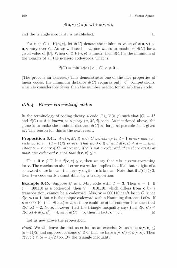
190 6 Vector Spaces
d(u,v) ≤ d(u,w) + d(v,w),
and the triangle inequality is established. �
For each C ⊂ V (n, p), let d(C) denote the minimum value of d(u,v) asu,v vary over C. As we will see below, one wants to maximize d(C) for agiven value of |C|. When C ⊂ V (n, p) is linear, then d(C) is the minimum ofthe weights of all the nonzero codewords. That is,
d(C) = min{ω(c) | c ∈ C, c �= 0}.
(The proof is an exercise.) This demonstrates one of the nice properties oflinear codes: the minimum distance d(C) requires only |C| computations,which is considerably fewer than the number needed for an arbitrary code.
6.8.4 Error-correcting codes
In the terminology of coding theory, a code C ⊂ V (n, p) such that |C| = Mand d(C) = d is known as a p-ary (n,M, d)-code. As mentioned above, thegame is to make the minimal distance d(C) as large as possible for a givenM . The reason for this is the next result.
Proposition 6.44. An (n,M, d)-code C detects up to d − 1 errors and cor-rects up to e = (d − 1)/2 errors. That is, if c ∈ C and d(v, c) ≤ d − 1, theneither v = c or v /∈ C. Moreover, if v is not a codeword, then there exists atmost one codeword c such that d(v, c) ≤ e.
Thus, if v /∈ C, but d(v, c) ≤ e, then we say that c is c error-correctingfor v. The conclusion about error-correction implies that if all but e digits of acodeword c are known, then every digit of c is known. Note that if d(C) ≥ 3,then two codewords cannot differ by a transposition.
Example 6.45. Suppose C is a 6-bit code with d = 3. Then e = 1. Ifc = 100110 is a codeword, then v = 010110, which differs from c by atransposition, cannot be a codeword. Also, w = 000110 can’t be in C, sinced(c,w) = 1, but c is the unique codeword within Hamming distance 1 ofw. Ifx = 000010, then d(c,x) = 2, so there could be other codewords c′ such thatd(c′,x) = 2. Note, however, that the triangle inequality says that d(c, c′) ≤d(c,x) + d(x, c′) = 4, so if d(C) = 5, then in fact, c = c′. �
Let us now prove the proposition.
Proof. We will leave the first assertion as an exercise. So assume d(v, c) ≤(d− 1)/2, and suppose for some c′ ∈ C that we have d(v, c′) ≤ d(v, c). Thend(v, c′) ≤ (d − 1)/2 too. By the triangle inequality,
6.8 Appendix: Linear Coding Theory 191
d(c, c′) ≤ d(c,v) + d(v, c′) ≤ (d − 1)/2 + (d − 1)/2 = d − 1,
so indeed c = c′. �
Example 6.46. For the binary 4-bit code of Example 6.43 given by x1 +x2 + x3 + x3 + x4 = 0, one can check that d(C) = 2. Thus C detects a singleerror, but e = 1/2, so there is no error correction. However, some additionalinformation, such as the component where an error occurs, may allow errorcorrection. Here, the linear equation defining the code enables that to bepossible.
Designing codes that maximize d(C) given |C| is a basic problem in codingtheory. The next example is a binary (n,M, d) = (8, 16, 4) linear code C thatmaximizes d(C) for M = 16. This code is sometimes denoted by C8 andcalled the extended Hamming code.
Example 6.47. Let
A =
⎛
⎜⎜⎝
1 0 0 0 1 1 1 00 1 0 0 1 1 0 10 0 1 0 1 0 1 10 0 0 1 0 1 1 1
⎞
⎟⎟⎠ .
Then C8 is defined to be row(A). Since every row of A has weight 4, theminimum distance d(C8) is at most 4. But every sum of the rows of A can beseen to have weight at most 4, so d(C8) = 4. Since A is a generating matrix,M = |C8| = 24 = 16. �
We will now show that d(C8) is maximal for M = 16 and n = 8.
Proposition 6.45. The code C8 with 16 codewords maximizes |C| amongall 8-bit binary linear codes with d(C) ≥ 4.
Proof. Since dimC8 = 4, we have to show that there are no 8-bit binarylinear codes C with d(C) ≥ 4 and dimC ≥ 5, hence 32 codewords. Thisturns out to be a routine argument involving row reduction. Suppose C issuch a code. By taking a spanning set for C as the rows of a k × 8 matrixA, we can use row operations to put A into reduced row echelon form Ared
without affecting C. Note that k ≥ 5. By reordering the columns, we cansuppose that Ared is a generating matrix (Ir | M), where r ≥ 5. Hence Mhas at most three columns. But the requirement d(C) ≥ 4 implies that allentries of M are 1. This shows that there must exist codewords of weighttwo, a contradiction. Thus dimC < 5, so |C| = 16 is the maximum. �
192 6 Vector Spaces
6.8.5 Cosets and perfect codes
A code C ⊂ V (n, p) with minimum distance d(C) = d ≥ 3 and e = (d−1)/2 ≥1 is called perfect if every x ∈ V (n, p) is within e of some codeword c. SinceProposition 6.44 says that every x ∈ V (n, p) is within distance e of at mostone codeword, every element in V (n, p) is within e of exactly one codeword.It is convenient to state this condition in a geometric way by bringing in thenotion of a ball. Assume r > 0. The ball of radius r centered at v ∈ V (n, p)is defined to be
Br(v) = {w ∈ V (n, p) | d(w,v) ≤ r}. (6.31)
Thus, a code C ⊂ V (n, p) with d(C) ≥ 3 and e ≥ 1 is perfect if and only ifV (n, p) is the disjoint union of the balls Be(c) as c varies over C. That is,
V (n, p) =⋃
c∈C
Be(c) (disjoint union). (6.32)
Example 6.48. Consider the binary linear code C = {000, 111}. Note thatd = 3, so e = 1. Now
V (3, 2) = {000, 100, 010, 001, 110, 101, 011, 111}.
The first four elements are within 1 of 000, and the last four are within 1 of111. Therefore, C is perfect. �
What makes perfect codes so nice is that there is a simple numerical crite-rion for deciding whether C is perfect. First note that for every v ∈ V (n, p),we have |Be(v)| = |Be(0)|. Hence we have the following.
Proposition 6.46. A code C ⊂ V (n, p) is perfect if and only if
|C||Be(0)| = pn.
Thus, if C is linear of dimension k, then C is perfect if and only if |Be(0)| =pn−k.
One can check this criterion in the previous example, since
Be(0) = {000, 100, 010, 001},
while |C| = 2. Notice that a necessary condition for a binary code C oflength n with e = 1 to be perfect is that n + 1 = 2m for some m, sinceB1(0) = {0, e1, . . . , en}. Thus perfect codes with e = 1 must have length 3,7, 15, and so on. Here is an example with n = 7.
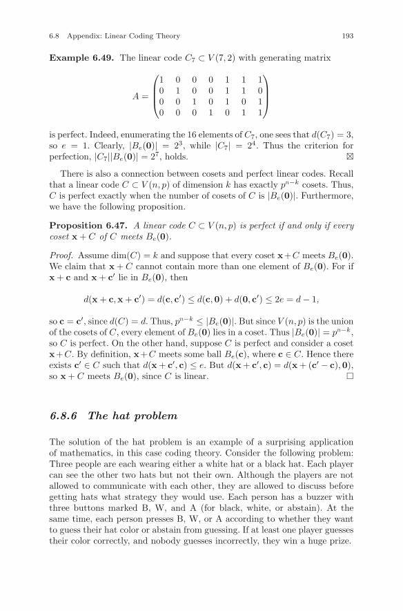
6.8 Appendix: Linear Coding Theory 193
Example 6.49. The linear code C7 ⊂ V (7, 2) with generating matrix
A =
⎛
⎜⎜⎝
1 0 0 0 1 1 10 1 0 0 1 1 00 0 1 0 1 0 10 0 0 1 0 1 1
⎞
⎟⎟⎠
is perfect. Indeed, enumerating the 16 elements of C7, one sees that d(C7) = 3,so e = 1. Clearly, |Be(0)| = 23, while |C7| = 24. Thus the criterion forperfection, |C7||Be(0)| = 27, holds. �
There is also a connection between cosets and perfect linear codes. Recallthat a linear code C ⊂ V (n, p) of dimension k has exactly pn−k cosets. Thus,C is perfect exactly when the number of cosets of C is |Be(0)|. Furthermore,we have the following proposition.
Proposition 6.47. A linear code C ⊂ V (n, p) is perfect if and only if everycoset x + C of C meets Be(0).
Proof. Assume dim(C) = k and suppose that every coset x+C meets Be(0).We claim that x + C cannot contain more than one element of Be(0). For ifx + c and x + c′ lie in Be(0), then
d(x + c,x + c′) = d(c, c′) ≤ d(c,0) + d(0, c′) ≤ 2e = d − 1,
so c = c′, since d(C) = d. Thus, pn−k ≤ |Be(0)|. But since V (n, p) is the unionof the cosets of C, every element of Be(0) lies in a coset. Thus |Be(0)| = pn−k,so C is perfect. On the other hand, suppose C is perfect and consider a cosetx+C. By definition, x+C meets some ball Be(c), where c ∈ C. Hence thereexists c′ ∈ C such that d(x+ c′, c) ≤ e. But d(x+ c′, c) = d(x+ (c′ − c),0),so x + C meets Be(0), since C is linear. �
6.8.6 The hat problem
The solution of the hat problem is an example of a surprising applicationof mathematics, in this case coding theory. Consider the following problem:Three people are each wearing either a white hat or a black hat. Each playercan see the other two hats but not their own. Although the players are notallowed to communicate with each other, they are allowed to discuss beforegetting hats what strategy they would use. Each person has a buzzer withthree buttons marked B, W, and A (for black, white, or abstain). At thesame time, each person presses B, W, or A according to whether they wantto guess their hat color or abstain from guessing. If at least one player guessestheir color correctly, and nobody guesses incorrectly, they win a huge prize.
194 6 Vector Spaces
A pretty good strategy would be to agree that two players abstain andthe third makes a random guess. The probability of winning is 0.5. But thisstrategy doesn’t make any use of fact that each player can see the othertwo hats. Instead, consider the following strategy. Suppose the players agreethat they will play under the assumption that the array is not either BBBor WWW. Why does this help? First of all, there are eight possible arrays,so if the players can find an algorithm to guarantee that they avoid theset F = {BBB,WWW} and do not make a mistake, then they will have aprobability of 6/8 = 0.75 of winning. Now let’s analyze what happens if thehat array is BWB, for example. The first player sees WB, and knows thatboth BWB and WWB lie outside F but can’t take the chance of an incorrectguess. So the first player must hit A. The same is true of the third player.The second player is the key. That player sees BB, so is forced to press W orotherwise land in F . If the array is outside of F , this strategy is guaranteedto produce a victory. The question is why, and the answer is that the 3-bitcode C2 = {000, 111} in V (3, 2) is a perfect code with e = 1.
Let us now see whether this strategy can be extended to seven playersusing the perfect linear code C7 in the previous example. The players agreein the strategy session to proceed as if the hat array is not in C7. Since|C7| = 24, the probability that the hat array is in C7 is 24/27 = 1/8, sothe probability of this being a winning assumption is 7/8. They all needto memorize the 16 codewords of C7. Suppose their assumption is correct.Then in order to win, they proceed as follows. Since the hat array x1 . . . x7
differs in exactly one place from a codeword c1 . . . c7, let us suppose that thediscrepancy occurs at x1. Then player #1 sees c2 . . . c7 and must make thechoice c1 +1. Player #2 sees x1c3 . . . c7. But since d(C7) = 3, she knows thatwhatever x2 is, x1x2c3 . . . c7 /∈ C. Therefore, in order to not make a mistake,she must abstain, as do the other five players. Assuming that the hat arrayx1 . . . x7 is not in C7, they have won the game. The odds that they win themillion bucks are a pretty good 7/8.
Can you devise a strategy for how to proceed if there are four, five, or sixplayers? Since there are no perfect codes in V (n, 2) for n = 4, 5, 6, it isn’t clearhow to proceed. More information about this problem and related questionscan be found in the article “The Hat Problem and Hamming Codes,” by M.Bernstein, in Focus Magazine, November 2001.
Exercises
Exercise 6.8.1. List all binary linear codes C of length 3 with four code-words.
Exercise 6.8.2. Find a formula for the number of linear codes C ⊂ V (n, p)of dimension k. (Suggestion: count the number of linearly independent subsetsof V (n, p) having k elements.)
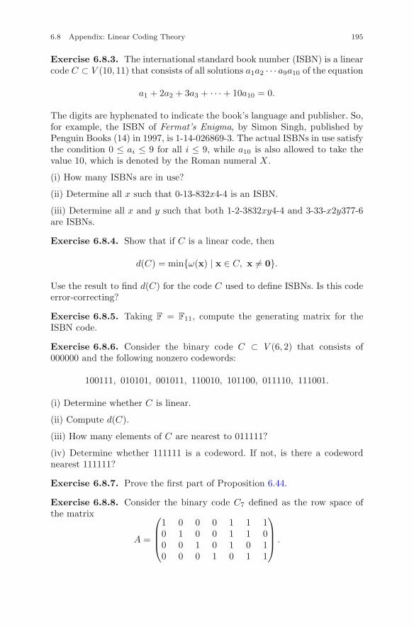
6.8 Appendix: Linear Coding Theory 195
Exercise 6.8.3. The international standard book number (ISBN) is a linearcode C ⊂ V (10, 11) that consists of all solutions a1a2 · · · a9a10 of the equation
a1 + 2a2 + 3a3 + · · · + 10a10 = 0.
The digits are hyphenated to indicate the book’s language and publisher. So,for example, the ISBN of Fermat’s Enigma, by Simon Singh, published byPenguin Books (14) in 1997, is 1-14-026869-3. The actual ISBNs in use satisfythe condition 0 ≤ ai ≤ 9 for all i ≤ 9, while a10 is also allowed to take thevalue 10, which is denoted by the Roman numeral X.
(i) How many ISBNs are in use?
(ii) Determine all x such that 0-13-832x4-4 is an ISBN.
(iii) Determine all x and y such that both 1-2-3832xy4-4 and 3-33-x2y377-6are ISBNs.
Exercise 6.8.4. Show that if C is a linear code, then
d(C) = min{ω(x) | x ∈ C, x �= 0}.
Use the result to find d(C) for the code C used to define ISBNs. Is this codeerror-correcting?
Exercise 6.8.5. Taking F = F11, compute the generating matrix for theISBN code.
Exercise 6.8.6. Consider the binary code C ⊂ V (6, 2) that consists of000000 and the following nonzero codewords:
100111, 010101, 001011, 110010, 101100, 011110, 111001.
(i) Determine whether C is linear.
(ii) Compute d(C).
(iii) How many elements of C are nearest to 011111?
(iv) Determine whether 111111 is a codeword. If not, is there a codewordnearest 111111?
Exercise 6.8.7. Prove the first part of Proposition 6.44.
Exercise 6.8.8. Consider the binary code C7 defined as the row space ofthe matrix
A =
⎛
⎜⎜⎝
1 0 0 0 1 1 10 1 0 0 1 1 00 0 1 0 1 0 10 0 0 1 0 1 1
⎞
⎟⎟⎠ .
196 6 Vector Spaces
in V (7, 2).
(i) Compute d(C) and e.
(ii) Find the unique element of C that is nearest to 1010010. Do the samefor 1110001.
Exercise 6.8.9. Let r be a positive integer and let x ∈ V (n, 2). Considerthe ball Br(x) of radius r about x, i.e., Br(x) = {y ∈ V (n, 2) | d(x,y) ≤ r}.Show that
|Br(x)| =r∑
i=0
(n
i
).
Exercise 6.8.10. Generalize Exercise 6.8.9 from V (n, 2) to V (n, p).
Exercise 6.8.11. * Show that if C ⊂ V (n, 2) is a linear code such thatdim(C) = k and C is e-error-correcting, then
e∑
i=0
(ni
)≤ 2(n−k).
Conclude that if e = 1, then 1 + n ≤ 2n−k.
Exercise 6.8.12. Suppose C ⊂ V (n, 2) is a linear code with dim C = k andd ≥ 3. Prove that C is perfect if and only if
e∑
i=0
(ni
)= 2(n−k). (6.33)
In particular, if e = 1, then C is perfect if and only if
(1 + n)2k = 2n. (6.34)
Exercise 6.8.13. Consider the code C = {00000, 11111} ⊂ V (5, 2).
(i) Determine e.
(ii) Show that C is perfect.
Exercise 6.8.14. Show that every binary [2k−1, 2k−1−k]-code with d = 3is perfect. Notice that C7 is of this type.
Exercise 6.8.15. Can there exist a perfect code with n = 5 and e = 2?
Exercise 6.8.16. Suppose n ≡ 2 mod(4). Show that there cannot be aperfect binary [n, k]-code with e = 2.
(iii) Does C present any possibilities for a five-player hat game?
Exercise 6.8.17. Show that every binary [23, 12]-code with d = 7 is perfect.
Chapter 7Linear Mappings
The purpose of this chapter is to introduce linear mappings. Let V and Wbe vector spaces over a field F. A linear mapping is a mapping T : V → Wwith domain V and target W that preserves linear combinations. The basicsituation we will consider is that both V and W are finite-dimensional. Herewe already know quite a bit, since an m × n matrix A over F defines a linearmapping TA : F
n → Fm by putting TA(x) = Ax (see Section 3.1.7). The
basic rules of matrix algebra tell us that TA preserves linear combinations.Thus, linear mappings are a generalization of matrix theory, and many ideasfrom matrix theory, such as the rank of a matrix A, its null space N (A),and the column space col(A), have natural interpretations in terms of linearmappings, as we shall see.
7.1 Definitions and Examples
In this section, we will define linear mappings and introduce several termsthat we will use to explain the basic theory of linear mappings. We will alsogive several examples to illustrate some of the interesting types of linearmappings.
7.1.1 Mappings
Recall from Chap. 1 that if X and Y are sets, then a mapping F : X → Y isa rule that assigns to each element of the domain X a unique element F (x)in the target Y . The image of F is the subset of the target F (X) = {y ∈ Y |y = F (x) ∃ x ∈ X}. A mapping F : Fn → F
m is completely determined by
c© Springer Science+Business Media LLC 2017J.B. Carrell, Groups, Matrices, and Vector Spaces,DOI 10.1007/978-0-387-79428-0 7
197
198 7 Linear Mappings
its component functions f1, f2, . . . , fm, which are obtained by writing
F (x) =m∑
i=1
fi(x)ei =
⎛
⎜⎝f1(x)
...fm(x)
⎞
⎟⎠ ,
where e1, . . . , em is the standard basis of Fm. If V and W are arbitrary vectorspaces over a field F and W is finite-dimensional, we can also define compo-nent functions h1, . . . , hm of F with respect to an arbitrary basis w1, . . . ,wm
of W in the same way by writing
F (v) =m∑
i=1
hi(v)wi.
The component functions with respect to a basis are uniquely determinedby F .
7.1.2 The definition of a linear mapping
In linear algebra, the most important mappings are those that preserve linearcombinations. These are called linear mappings.
Definition 7.1. Suppose V and W are vector spaces over a field F. Then amapping T : V → W is said to be linear if
(i) for all x,y ∈ V , T (x + y) = T (x) + T (y), and
(ii) for all r ∈ F and all x ∈ V , T (rx) = rT (x).
If W = F, then T is called a linear function.
By definition, a linear mapping T preserves linear combinations: for allr, s ∈ F and all x,y ∈ V
T (rx + sy) = rT (x) + sT (y).
Thus a linear mapping also preserves linear combinations of an arbitrary num-ber of vectors. Conversely, every mapping that preserves linear combinationsis a linear mapping.
7.1.3 Examples
We now present some basic examples of linear mappings. The reader shouldnote that some of the examples don’t require a particular basis or choice ofcoordinates in their definition.
7.1 Definitions and Examples 199
Example 7.1 (Identity mapping). The mapping
IV : V → V
defined by IV (x) = x is called the identity mapping. This mapping is clearlylinear. If V = F
n, then IV = TIn. �
Example 7.2. If a ∈ Rn, the dot product with a defines a linear function
Sa : Rn → R by Sa(x) = a · x = aTx. It turns out that every linear functionS : Rn → R has the form Sa for some a ∈ R
n. For example, let aT = (1 2 0 1).Then the linear function Sa : R4 → R has the explicit form
Sa(x) = (1 2 0 1)
⎛
⎜⎜⎝
x1
x2
x3
x4
⎞
⎟⎟⎠ = x1 + 2x2 + x4.
We will consider the analogue of this function for an arbitrary inner productspace in the next example. �
Example 7.3. More generally, suppose V is an inner product space ofdimension m. Then for every linear mapping T : V → R, there exists aunique w ∈ V such that T (v) = (v,w). In fact, if u1, . . . ,um constitute anorthonormal basis of V , then I claim that
w =m∑
i=1
T (ui)ui.
The reader should check that T (v) = (v,w) does in fact hold for all v ∈ Vand that this choice of w is unique. �
Example 7.4 (Diagonal mappings). Let T : R2 → R2 be the mapping
T
(x1
x2
)=
(μ1x1
μ2x2
), (7.1)
where μ1 and μ2 are real scalars. We leave it as an exercise to show that Tis linear. In (7.1), T (e1) = μ1e1 and T (e2) = μ2e2. If both μ1 and μ2 arenonzero, the image under T of a rectangle with sides parallel to e1 and e2 isa parallel rectangle whose sides have been dilated by μ1 and μ2 and whosearea has been changed by the factor |μ1μ2|. If μ1μ2 �= 0, then T maps a circleabout the origin to an ellipse about the origin. For example, the image of theunit circle x2 + y2 = 1 is the ellipse
(w1
μ1)2 + (
w2
μ2)2 = 1,
200 7 Linear Mappings
as can be seen by putting w1 = μ1x1 and w2 = μ2x2.�
In general, a linear mapping T : V → V is called semisimple if there exista basis v1, . . . ,vn of V and scalars μ1, . . . , μn in F such that T (vi) = μivi
for all i. Note that we are not requiring that any or all μi be nonzero; butif all μi = 0, then T is the zero linear mapping. The basis v1, . . . ,vn of Vfor which T (vi) = μivi is called an eigenbasis, and the scalars μ1, . . . , μn arecalled the eigenvalues of T . The existence of an eigenbasis for T says a greatdeal about how T acts. The question of when a linear mapping T admits aneigenbasis is very basic. It will be solved when we study the classification oflinear mappings. The solution is nontrivial, and not all linear mappings aresemisimple.
Example 7.5. Recall from Example 6.17 that the cross product of two vec-tors a,b ∈ R
3 is defined as
a × b = (a2b3 − a3b2,−(a1b3 − a3b1), a1b2 − a2b1)T . (7.2)
The cross product defines a linear mapping Ca : R3 → R3 by
Ca(v) = a × v.
Notice that Ca(a) = 0. A basic property of Ca is that Ca(x) is orthogonalto both a and x. It follows that Ca cannot be semisimple unless a = 0 (seeExample 7.4). �
7.1.4 Matrix linear mappings
Recall from Section 3.1.7 that if A ∈ Fm×n, then the mapping TA : Fn → F
m
defined by TA(x) = Ax is called a matrix linear mapping. Every matrixlinear mapping is certainly linear. We now show that every linear mappingT : Fn → F
m is a matrix linear mapping.
Proposition 7.1. Every linear mapping T : Fn → Fm is of the form TA for
a unique A ∈ Fm×n. In fact,
A =(T (e1) T (e2) · · · T (en)
).
Conversely, if A ∈ Fm×n, then TA is a linear mapping with domain F
n andtarget Fm.
Proof. Since x =∑n
i=1 xiei,
T (x) = T( n∑
i=1
xiei)
=n∑
i=1
xiT (ei) =(T (e1) T (e2) · · · T (en)
)x.
7.1 Definitions and Examples 201
Thus, T = TA, where A =(T (e1) T (e2) · · · T (en)
). Furthermore, A is
uniquely determined by T , since if two linear mappings S, T : Fn → Fm have
the property that S(ei) = T (ei) for i = 1, . . . , n, then S(x) = T (x) for allx ∈ F
n. The claim that every TA is linear has already been shown. ��In particular, a linear function T : Fn → F is given by a 1×n matrix. Thus,
there exists a unique a ∈ Fn such that T (x) = aTx. Hence there exist unique
scalars a1, a2, . . . , an ∈ F such that T (x) =∑n
i=1 aixi. When F = R, we mayexpress this fact in terms of the dot product as T (x) = a · x in Example 7.2.
Example 7.6. For example, the matrix of the identity mapping IFn on Fn
is the identity matrix In. That is, IFn = TIn. We will sometimes use In to
denote IFn , provided no confusion is possible. �
Recall from Section 3.1.7 that if S : Fp → F
n and T : Fn → F
m arelinear mappings with matrices S = TA and T = TB respectively, then thecomposition T ◦S : Rp → R
m is the matrix linear mapping associated to BA.That is,
TB ◦ TA = TBA.
Writing MT for the matrix of T etc., we therefore have the identity
MT◦S = MTMS .
We will not repeat the proof, but it is short. Somewhat surprisingly, the keyfact is that matrix multiplication is associative.
7.1.5 An Application: rotations of the plane
The relationship between composition and matrix multiplication can beapplied to the group Rot(2) of rotations of R2 to give an extremely prettyand simple proof of the sum formulas for the trigonometric functions sineand cosine. Recall that Rθ : R2 → R
2 is the rotation of R2 about the originthrough θ. Computing the images of R(e1) and R(e2), we have
Rθ(e1) = cos θe1 + sin θe2
andRθ(e2) = − sin θe1 + cos θe2.
I claim that rotations are linear. This can be seen as follows. Suppose x andy are any two noncollinear vectors in R
2, and let P be the parallelogramthey span. Then Rθ rotates the whole parallelogram P about 0 to a new
202 7 Linear Mappings
parallelogram Rθ(P ) with edges Rθ(x) and Rθ(y) at 0. Since the diagonalx + y of P is rotated to the diagonal of Rθ(P ), it follows that
Rθ(x + y) = Rθ(x) + Rθ(y).
Similarly, for every scalar r,
Rθ(rx) = rRθ(x).
Therefore, Rθ is linear, as claimed. The matrix Rθ of Rθ, calculated via theabove formula, is Rθ = (Rθ(e1) Rθ(e2)). Hence
Rθ =(
cos θ − sin θsin θ cos θ
). (7.3)
(This verifies the formula of Example 4.5.) Thus
Rθ
(xy
)=
(cos θ − sin θsin θ cos θ
)(xy
)=
(x cos θ − y sin θx sin θ + y cos θ
).
Let us now apply this result to trigonometry. If one first applies a rotationRψ and follows that by the rotation Rθ, the outcome is the rotation Rθ+ψ.Hence,
Rθ+ψ = Rθ ◦ Rψ = Rψ ◦ Rθ.
Therefore, since composition of linear mappings corresponds to multiplicationof their matrices, Rθ+ψ = RθRψ = RψRθ. In particular,
(cos(θ + ψ) − sin(θ + ψ)sin(θ + ψ) cos(θ + ψ)
)=
(cos θ − sin θsin θ cos θ
)(cos ψ − sin ψsin ψ cos ψ
).
Expanding the product and comparing both sides gives us the trigonometricformulas for the sine and cosine of θ + ψ:
cos(θ + ψ) = cos θ cos ψ − sin θ sin ψ
andsin(θ + ψ) = sin θ cos ψ + cos θ sin ψ.
Exercises
Exercise 7.1.1. Let X and Y be sets and φ : X → Y a mapping. Recallfrom Chap. 1 that φ is injective if and only if for x ∈ X, φ(x) = φ(x′) impliesx = x′, φ is surjective if and only if φ(X) = Y , and φ is a bijection if andonly if it is both injective and surjective. Show the following:
7.1 Definitions and Examples 203
(i) φ is injective if and only if there exists a mapping ψ : F (X) → X suchthat ψ ◦ φ is the identity mapping IX : X → X.
(ii) φ is surjective if and only if there exists a mapping ψ : Y → X such thatφ ◦ ψ is the identity mapping IY , and
(iii) φ is a bijection if and only if there exists a mapping ψ : Y → X suchthat ψ ◦ φ = IX and φ ◦ ψ = IY .
Exercise 7.1.2. Show that every linear function T : R → R has the formT (x) = ax for some a ∈ R.
Exercise 7.1.3. Determine whether any of the following functions f : R2 →R are linear:
(i) f(x, y) = xy,
(ii) f(x, y) = x − y,
(iii) f(x, y) = ex+y.
Exercise 7.1.4. Suppose T : Fn → Fm is an arbitrary mapping and write
T (v) = (f1(v), f2(v), . . . , fm(v))T .
Show that T is linear if and only if each component function fi is a linearfunction.
Exercise 7.1.5. Find the matrix of the following linear mappings:
(i) S(x1, x2, x3) = (2x1 − 3x3, x1 + x2 − x3, x1, x2 − x3)T .
(ii) T (x1, x2, x3, x4) = (x1 − x2 + x3 + x4, x2 + 2x3 − 3x4)T .
(iii) T ◦ S.
Exercise 7.1.6. Let V be a vector space over F, and let W be a subspaceof V . Let π : V → V/W be the quotient map defined by π(v) = v+W. Showthat π is linear.
Exercise 7.1.7. Let S : U → V and T : V → W be linear mappings. Showthat T ◦ S is also linear.
Exercise 7.1.8. Suppose A is a real m×n matrix. Show that when we viewboth row(A) and N (A) as subspaces of Rn,
row(A) ∩ N (A) = {0}.
Is this true for matrices over other fields, for example Fp or C?
204 7 Linear Mappings
Exercise 7.1.9. Let V = C, and consider the mapping S : V → V definedby S(z) = αz, where α ∈ C.
(i) Describe S as a mapping S : R2 → R2.
(ii) Is S linear over R? If so, find its matrix in R2×2.
Exercise 7.1.10. Show that every mapping S : C → C that is linear overC has the form S(z) = αz for a unique A ∈ C.
Exercise 7.1.11. Let TA : R2 → R2 be the matrix linear mapping associ-
ated to the matrix A =(
a bc d
). The purpose of this exercise is to determine
when T is linear over C. That is, since by definition, C = R2 (with complex
multiplication), we may ask when TA(αβ) = αTA(β) for all α, β ∈ C. Showthat a necessary and sufficient condition for TA to be C-linear is that a = dand b = −c.
Exercise 7.1.12. Show that every rotation Rθ defines a C-linear map Rθ :C → C. Relate this map to the complex exponential eiθ.
Exercise 7.1.13. Let C∞(R) be the space of infinitely differentiable func-tions on the real line R. A function f ∈ C∞(R) is said to be even iff(−x) = f(x) for all x ∈ R and odd if f(−x) = −f(x) for all x ∈ R. LetC∞(R)ev and C∞(R)odd denote the set of even and odd functions in C∞(R)respectively.
(i) Show that C∞(R)ev and C∞(R)odd are subspaces of C∞(R).
(ii) Show that the mapping D : C∞(R) → C∞(R) defined by D(f) = f ′
sends C∞(R)ev to C∞(R)odd.
Exercise 7.1.14. Let F be a Galois field, and let p be the characteristic ofF. Let T : F → F be the mapping defined by T (x) = xp. Recall that the setof multiples m1 of 1 in F, where m = 0, 1, . . . , p − 1, forms a subfield F
′ = Fp
of F and that F is a vector space over F′. Show that T is a linear mapping ofF with respect to this vector space structure. The linear mapping T is calledthe Frobenius map.
Exercise 7.1.15. As in Exercise 7.1.14, let F be a Galois field of character-istic p, and let V = F
n×n. Show that the mapping F : V → V defined byF (A) = Ap is a linear mapping.
7.2 Theorems on Linear Mappings 205
7.2 Theorems on Linear Mappings
In this section, we will define some more terms and prove several resultsabout linear mappings, including a result that will generalize the rank–nullityidentity dimN (A) + dim col(A) = n derived in Example 6.28.
7.2.1 The kernel and image of a linear mapping
The kernel and image are two natural subspaces associated with a linearmapping. Let T : V → W be linear. The image of T has been defined inChap. 1. It will be denoted by im(T ). The other natural subspace associatedwith T is its kernel. First note that every linear mapping T maps 0 to 0,since
T (0) = T (00) = 0T (0) = 0.
Definition 7.2. The kernel of T is defined to be the set
ker(T ) = {v ∈ V | T (v) = 0}.
Since a linear mapping is a group homomorphism, the notion of the kernelof a linear mapping is a special case of the notion of the kernel of a homo-morphism. Suppose V = F
n, W = Fm, and T = TA, i.e., T (x) = Ax. Then
ker(TA) and im(TA) are related to linear systems. In fact, ker(TA) = N (A),while im(TA) is the set of vectors b ∈ F
m for which Ax = b has a solution.Thus, im(TA) = col(A), so both ker(TA) and im(TA) are subspaces. This ismore generally true for arbitrary linear mappings.
Proposition 7.2. The kernel and image of a linear mapping T : V → Ware subspaces of V and W respectively.
Proof. We leave this as an exercise. ��The following result gives a very useful characterization of injective (equiv-
alently, one-to-one) linear mappings. The proof is almost word for word theproof given in Chap. 2 for the group-theoretic analogue.
Proposition 7.3. A linear mapping T is injective if and only if ker(T ) ={0}.Proof. Suppose ker(T ) = {0} and T (x) = T (y). Then T (x − y) = 0, sox − y ∈ ker(T ). But this says that x − y = 0, so T is injective. Conversely,if T is injective and x ∈ ker(T ), then T (x) = 0 = T (0), so x = 0. Thusker(T ) = {0}. ��
206 7 Linear Mappings
7.2.2 The Rank–Nullity Theorem
Let A ∈ Fm×n and recall the rank–nullity identity dimN (A)+dim col(A) = n
(see (6.7)). The general rank–nullity theorem generalizes this identity to alinear mapping T : V → W , where V is finite-dimensional.
Theorem 7.4 (Rank–Nullity Theorem). Let V and W be vector spaces overF, and suppose dim V is finite. Then for every linear mapping T : V → W ,
dim ker(T ) + dim im(T ) = dim V. (7.4)
Proof. If ker(T ) = V , then im(T ) = {0}, so there is nothing to prove. On theother hand, if dim ker(T ) = 0, then T is injective. Thus if v1,v2, . . . ,vn is abasis of V , it follows that T (v1), . . . , T (vn) is a basis of im(T ). To verify this,it suffices to show that the T (vi) are independent. But if
∑aiT (vi) = 0,
then T (∑
aivi) = 0, so∑
aivi = 0, since T is injective. Hence all ai areequal to zero, since v1,v2, . . . ,vn are independent. Thus, dim im(T ) = dimV .Now suppose dim ker(T ) = k > 0. By the dimension theorem (Theorem6.11), we may choose a basis v1,v2, . . .vk of ker(T ) and extend it to a basisv1,v2, . . . ,vn of V . Let wi = T (vi). I claim that wk+1, . . . ,wn are a basisof im(T ). To see that they span, let w ∈ im(T ), say w = T (v). Write v =∑
aivi. Then
w = T (v) =n∑
i=1
aiT (vi) =n∑
i=k+1
aiwi.
The proof that wk+1, . . . ,wn are independent is identical to the proof in thecase dim ker(T ) = 0, so we will leave it to the reader. Hence dim im(T ) =n − k, which proves the result. ��
7.2.3 An existence theorem
The rank–nullity theorem tells us something about the behavior of a givenlinear mapping, but we do not yet know how to construct linear mappings.The following existence result will show that there is considerable flexibilityin defining a linear mapping T : V → W , provided we have a basis of V (forexample, if V is finite-dimensional). We will show that the values of T on abasis of V can be arbitrarily described.
Proposition 7.5. Let V and W be vector spaces over F, and let v1, . . . ,vn
be a basis of V . Suppose w1, . . . ,wn are arbitrary vectors in W . Then thereexists a unique linear mapping T : V → W such that T (vi) = wi for each i.In other words, a linear mapping is uniquely determined by giving its valueson a basis.
7.2 Theorems on Linear Mappings 207
Proof. The proof is surprisingly simple. Since every x ∈ V has a uniqueexpression
x =n∑
i=1
rivi,
we obtain a mapping T : V → W by setting
T (x) =n∑
i=1
riwi.
In fact, T is linear. Indeed, if y ∈ V , say
y =n∑
i=1
sivi,
then x + y =∑
(ri + si)vi, so
T (x + y) =n∑
i=1
(ri + si)wi =n∑
i=1
riwi +n∑
i=1
siwi = T (x) + T (y).
Similarly, T (rv) = rT (v). Moreover, T is unique, since every linear mappingis determined on a basis. ��
If V = Fn and W = F
m, there is an even simpler proof by appealing tomatrix theory. Let B = (v1 v2 . . .vn) and C = (w1 w2 . . .wn). Then thematrix A of T satisfies AB = C. But B is invertible, since v1, . . . ,vn is abasis of Fn, so A = CB−1.
7.2.4 Vector space isomorphisms
We will now answer the following question. When are two vector spaces indis-tinguishable as far as their algebraic properties are concerned? The answeris given by the notion of isomorphism.
Definition 7.3. We will say that two vector spaces V and W over the samefield F are isomorphic if there exists a bijective linear mapping T : V → W .Such a linear mapping T is called an isomorphism.
In other words, an isomorphism is a linear mapping that is both injectiveand surjective. A vector space isomorphism is also a group isomorphism. Thepoint of the definition is that although two vector spaces V and W may lookquite different, isomorphic vector spaces are indistinguishable if one consid-ers only their internal algebraic properties (addition, scalar multiplication,
208 7 Linear Mappings
etc.). For example, one space V may be the solution space of a homogeneouslinear differential equation with real coefficients, and the other, W , may bea far less exotic vector space such as R
n. The question is, when are V andW isomorphic? The quite simple answer, provided by the next result, is anapplication of the dimension theorem and the fact that linear mappings aredetermined by assigning arbitrary values to a basis.
Proposition 7.6. Two finite-dimensional vector spaces V and W over thesame field are isomorphic if and only if they have the same dimension.
Proof. Suppose dim V = dimW . To construct an isomorphism T : V → W ,choose bases v1, . . . ,vn of V and w1, . . . ,wn of W , and let T : V → W be theunique linear mapping (guaranteed by Proposition 7.5) such that T (vi) = wi
if 1 ≤ i ≤ n. Since im(T ) is a subspace of W containing a basis of W , it followsthat T is surjective. By the rank–nullity theorem, dim ker(T ) = 0; hence Tis injective by Proposition 7.3. The converse follows from the rank–nullitytheorem (Theorem 7.4) by similar reasoning. ��
The set of isomorphisms T : V → V in fact forms a group, called thegeneral linear group of V , which is denoted by GL(V ). If V = F
n, then infact, GL(V ) = GL(n,F).
Exercises
Exercise 7.2.1. Let the field be F2 and consider the matrix
A =
⎛
⎜⎜⎜⎜⎝
1 1 1 1 10 1 0 1 01 0 1 0 11 0 0 1 11 0 1 1 0
⎞
⎟⎟⎟⎟⎠.
(i) Find a basis of im(A).
(ii) How many elements are in im(A)?
(iii) Is (01111)T in im(A)?
(iv) Without any further computation, find a basis of im(AT ).
Exercise 7.2.2. Let A be a real 3 × 3 matrix such that the first row of A isa linear combination of A’s second and third rows.
(i) Show that N (A) is either a line through the origin or a plane containingthe origin.
(ii) Show that if the second and third rows of A span a plane P , then N (A)is the line through the origin orthogonal to P .
7.2 Theorems on Linear Mappings 209
Exercise 7.2.3. Prove Proposition 7.2 using only the basic definition of alinear mapping. That is, show that the kernel and image of a linear mappingT are subspaces of the domain and target of T respectively.
Exercise 7.2.4. Consider the mapping Ca : R3 → R3 defined by
Ca(v) = a × v,
where a × v is the cross product of a and v.
(i) Show that Ca is linear and find its matrix.
(ii) Describe the kernel and image of Ca.
Exercise 7.2.5. Suppose a ∈ R3. Find the kernel of the linear mapping
Ca + I3.
Exercise 7.2.6. Suppose T : R2 → R2 is a linear mapping that sends pair
of noncollinear vectors to noncollinear vectors. Suppose x and y in R2 are
noncollinear. Show that T sends every parallelogram with sides parallel to xand y to another parallelogram with sides parallel to T (x) and T (y).
Exercise 7.2.7. Find the kernel and image of the linear mapping Sa : Rn →R defined by Sa(x) = a · x.
Exercise 7.2.8. Determine ker(Ca) ∩ im(Ca) for the cross product linearmapping Ca : R3 → R
3 for every nonzero a.
Exercise 7.2.9. Suppose V is a finite-dimensional vector space and T : V →V is a linear mapping such that T ◦ T = O. Show that im(T ) ⊂ ker(T ). Isthe converse true?
Exercise 7.2.10. Suppose V is a finite-dimensional vector space and T :V → V is a linear mapping such that im(T ) ⊂ ker(T ). Show that dimV isan even integer.
Exercise 7.2.11. Suppose A is a symmetric real n × n matrix.
(i) Show that col(A) ∩ N (A) = {0}.
(ii) Conclude that Rn = N (A) ⊕ col(A).
(iii) Suppose A2 = O. Show that A = O.
Exercise 7.2.12. Find a nonzero 2 × 2 symmetric matrix A over C suchthat A2 = O.
Exercise 7.2.13. Show that if V is a finite-dimensional vector space and Tis a linear mapping with domain V , then dimT (V ) ≤ dim V .
210 7 Linear Mappings
Exercise 7.2.14. Suppose A is a square matrix over an arbitrary field. Showthat if Ak = O for some positive integer k, then dimN (A) > 0.
Exercise 7.2.15. Recall that if x,y ∈ Rn, then x·y = xTy. Use this to prove
that for every A ∈ Rn×n, ATA and A have the same null space. Conclude
that ATA and A have the same rank.
Exercise 7.2.16. This exercise deals with the inverse of a linear mappingT . Let V be a vector space over F, and let T : V → V be a linear mappingsuch that ker(T ) = 0 and im(T ) = V . That is, T is an isomorphism. Provethe following statements.
(i) There exists a linear mapping S : V → V with the property that S(y) = xif and only if T (x) = y. Note: S is called the inverse of T .
(ii) Show that S is an isomorphism, and S ◦ T = T ◦ S = IV .
(iii) If V = Fn, A is the matrix of T , and B is the matrix of S, then
BA = AB = In.
Exercise 7.2.17. Let S : Rn → Rm and T : Rm → R
p be two linear map-pings both of which are injective. Show that the composition T ◦ S is alsoinjective. Conclude that if A is of size m × n and has N (A) = {0}, and B isof size n × p and has N (B) = {0}, then N (BA) = {0} too.
Exercise 7.2.18. Suppose V and W are vector spaces of the same dimensionover a field F, and let T : V → W be a linear mapping. Show that if T iseither injective or surjective, then T is an isomorphism.
Exercise 7.2.19. Let W be a subspace of a finite-dimensional vector spaceV . Show there exists a linear mapping T : V → V such that ker(T ) = W .
Exercise 7.2.20. Suppose T : V → W is linear. Show that there exists aunique linear mapping T : V/ ker(T ) → W such that T (v + ker(T )) = T (v).
Exercise 7.2.21. Let U , V , and W be finite-dimensional vector spaces overthe same field F, and let S : U → V and T : V → W be linear. Show that:
(i) TS is injective if and only if S is injective and im(S) ∩ ker(T ) = {0}.
(ii) TS is surjective if and only if T is surjective and V = im(S) + ker(T ).
(iii) Conclude that TS is an isomorphism if and only if S is injective, T issurjective, and dim U = dim W .
7.3 Isometries and Orthogonal Mappings 211
7.3 Isometries and Orthogonal Mappings
Throughout this section, V will denote a real finite-dimensional inner prod-uct space. Recall that the inner product on V defines a distance functiond(a,b) = |a − b|. Linear mappings T : V → V that preserve distances arecalled isometries. (Actually, as we will see below, a distance-preserving mapis automatically linear, so the definition can be simplified.) The isometries ofV form an important group, called O(V ). When V = R
n, O(V ) is the matrixgroup O(n,R) of all orthogonal n × n matrices over R. We will first considerisometries in general and then specialize to rotations and reflections. Finally,we will consider the isometries of R2. Here we prove the O(2,R)-dichotomy:every isometry of R
2 is either a rotation or a reflection. We will also showthat the dihedral group D(m) can be realized as the group of all isometriesof a regular m-gon in R
2. This will give another proof that the order of D(m)is 2m.
7.3.1 Isometries and orthogonal linear mappings
A mapping S : V → V is said to be orthogonal if
(S(x), S(y)) = (x,y) (7.5)
for all x,y ∈ V . The term orthogonal comes from the fact that an orthogonalmapping preserves the orthogonal relationship between orthogonal pairs ofvectors. Since orthogonal mappings preserve inner products, they preservelengths of vectors, distances between vectors, and angles between vectors,since the angle θ between v and w is found by the identity
v · w = |v||w| cos θ.
It turns out that all orthogonal mappings are linear.
Proposition 7.7. Let S : V → V be orthogonal. Then S is linear. In fact,the orthogonal mappings are exactly the isometries. In particular, all distance-preserving mappings on V are linear. Conversely, every isometry is orthogo-nal.
Proof. To show that S is linear, we first show that for all a,b ∈ V , |S(a +b) − S(a) − S(b)|2 = 0. But
|S(a+b)−S(a)−S(b)|2 = (S(a+b)−S(a)−S(b), S(a+b)−S(a)−S(b))
= (S(a + b), S(a + b)) + (S(a), S(a)) + (S(b), S(b)) − 2(S(a + b), S(a))
212 7 Linear Mappings
−2(S(a + b), S(b)) + 2(S(a), S(b)).
Using the fact that S is orthogonal, it follows that
|S(a + b) − S(a) − S(b)|2 = (a + b,a + b) + (a,a) + (b,b)
−2(a + b,a) − 2(a + b,b) + 2(a,b).
Expanding further, one sees that the right-hand side is zero. Thus, S(a+b) =S(a)+S(b). The proof that S(ra) = rS(a) for all r ∈ F is similar. Therefore,every orthogonal mapping is linear. To see that S is an isometry, note that
|S(b) − S(a)|2 = |S(b − a)|2= (S(a − b), S(a − b))= (b − a,b − a)= |b − a|2.
This completes the proof that orthogonal mappings are isometries. We willleave the rest of the proof as an exercise. ��
More generally, every mapping F : V → V that preserves distances turnsout to be orthogonal, and hence is an isometry (see Exercise 7.3.3).
7.3.2 Orthogonal linear mappings on Rn
We are now going to show that the matrix of an isometry is orthogonal, andconversely, that every orthogonal matrix defines an isometry.
Proposition 7.8. Every isometry T : Rn → Rn is the matrix linear map-
ping associated with a unique orthogonal matrix. Conversely, every orthogonalmatrix defines a unique isometry.
Proof. Suppose T : Rn → Rn is an isometry. Since T is linear, T = TQ for a
unique Q ∈ Rn×n. But T is orthogonal, so TQ(x) · TQ(y)=Qx · Qy=x · y for
all x,y∈Rn. Thus
(Qx)T (Qy) = (xTQT )(Qy) = xT (QTQ)y = xTy (7.6)
for all x,y ∈ Rn. Setting Qei = qi, (7.6) implies qT
i qj = eTi ej . HenceQTQ = In, so Q is orthogonal. We leave the converse to the reader. ��
Recall that the set of orthogonal n × n matrices is the orthogonal groupO(n,R), so O(n,R) is also the group of isometries of Rn.
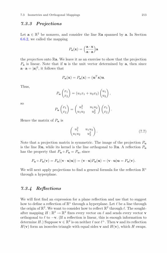
7.3 Isometries and Orthogonal Mappings 213
7.3.3 Projections
Let a ∈ R2 be nonzero, and consider the line Ra spanned by a. In Section
6.6.2, we called the mapping
Pa(x) =(a · xa · a
)a
the projection onto Ra. We leave it as an exercise to show that the projectionPa is linear. Note that if u is the unit vector determined by a, then sincea · a = |a|2, it follows that
Pu(x) = Pa(x) = (uTx)u.
Thus,
Pu
(x1
x2
)= (u1x1 + u2x2)
(u1
u2
),
so
Pu
(x1
x2
)=
(u21 u1u2
u1u2 u22
) (x1
x2
).
Hence the matrix of Pu is(
u21 u1u2
u1u2 u22
). (7.7)
Note that a projection matrix is symmetric. The image of the projection Pu
is the line Ru, while its kernel is the line orthogonal to Ru. A reflection Pu
has the property that Pu ◦ Pu = Pu, since
Pu ◦ Pu(v) = Pu((v · u)u)) = (v · u)Pu(u) = (v · u)u = Pu(v).
We will next apply projections to find a general formula for the reflection Rn
through a hyperplane.
7.3.4 Reflections
We will first find an expression for a plane reflection and use that to suggesthow to define a reflection of Rn through a hyperplane. Let � be a line throughthe origin of R2. We want to consider how to reflect R2 through �. The sought-after mapping H : R2 → R
2 fixes every vector on � and sends every vector vorthogonal to � to −v. (If a reflection is linear, this is enough information todetermine H.) Suppose v ∈ R
2 is on neither � nor �⊥. Then v and its reflectionH(v) form an isosceles triangle with equal sides v and H(v), which H swaps.
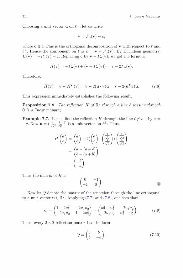
214 7 Linear Mappings
Choosing a unit vector u on �⊥, let us write
v = Pu(v) + c,
where c ∈ �. This is the orthogonal decomposition of v with respect to � and�⊥. Hence the component on � is c = v − Pu(v). By Euclidean geometry,H(v) = −Pu(v) + c. Replacing c by v − Pu(v), we get the formula
H(v) = −Pu(v) + (v − Pu(v)) = v − 2Pu(v).
Therefore,
H(v) = v − 2Pu(v) = v − 2(u · v)u = v − 2(uTv)u. (7.8)
This expression immediately establishes the following result.
Proposition 7.9. The reflection H of R2 through a line � passing through0 is a linear mapping.
Example 7.7. Let us find the reflection H through the line � given by x =−y. Now u = ( 1√
2, 1√
2)T is a unit vector on �⊥. Thus,
H
(ab
)=
(ab
)− 2(
(ab
)·(
1√21√2
))
(1√21√2
)
=(
a − (a + b)b − (a + b)
)
=(−b
−a
).
Thus the matrix of H is (0 −1
−1 0
). �
Now let Q denote the matrix of the reflection through the line orthogonalto a unit vector u ∈ R
2. Applying (7.7) and (7.8), one sees that
Q =(
1 − 2u21 −2u1u2
−2u1u2 1 − 2u22
)=
(u22 − u2
1 −2u1u2
−2u1u2 u21 − u2
2
). (7.9)
Thus, every 2 × 2 reflection matrix has the form
Q =(
a bb −a
), (7.10)
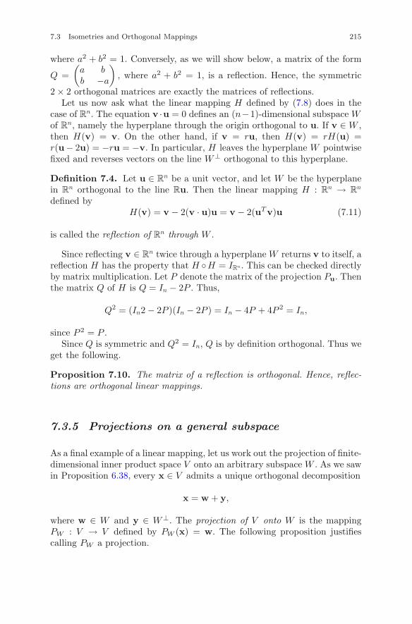
7.3 Isometries and Orthogonal Mappings 215
where a2 + b2 = 1. Conversely, as we will show below, a matrix of the form
Q =(
a bb −a
), where a2 + b2 = 1, is a reflection. Hence, the symmetric
2 × 2 orthogonal matrices are exactly the matrices of reflections.Let us now ask what the linear mapping H defined by (7.8) does in the
case of Rn. The equation v ·u = 0 defines an (n−1)-dimensional subspace Wof Rn, namely the hyperplane through the origin orthogonal to u. If v ∈ W ,then H(v) = v. On the other hand, if v = ru, then H(v) = rH(u) =r(u− 2u) = −ru = −v. In particular, H leaves the hyperplane W pointwisefixed and reverses vectors on the line W⊥ orthogonal to this hyperplane.
Definition 7.4. Let u ∈ Rn be a unit vector, and let W be the hyperplane
in Rn orthogonal to the line Ru. Then the linear mapping H : R
n → Rn
defined byH(v) = v − 2(v · u)u = v − 2(uTv)u (7.11)
is called the reflection of Rn through W .
Since reflecting v ∈ Rn twice through a hyperplane W returns v to itself, a
reflection H has the property that H ◦H = IRn . This can be checked directlyby matrix multiplication. Let P denote the matrix of the projection Pu. Thenthe matrix Q of H is Q = In − 2P . Thus,
Q2 = (In2 − 2P )(In − 2P ) = In − 4P + 4P 2 = In,
since P 2 = P .Since Q is symmetric and Q2 = In, Q is by definition orthogonal. Thus we
get the following.
Proposition 7.10. The matrix of a reflection is orthogonal. Hence, reflec-tions are orthogonal linear mappings.
7.3.5 Projections on a general subspace
As a final example of a linear mapping, let us work out the projection of finite-dimensional inner product space V onto an arbitrary subspace W . As we sawin Proposition 6.38, every x ∈ V admits a unique orthogonal decomposition
x = w + y,
where w ∈ W and y ∈ W⊥. The projection of V onto W is the mappingPW : V → V defined by PW (x) = w. The following proposition justifiescalling PW a projection.
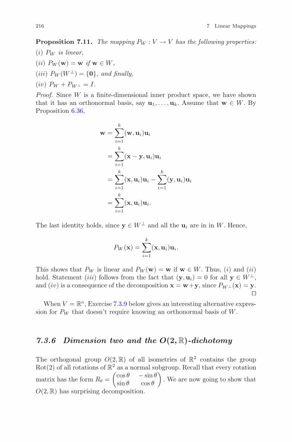
216 7 Linear Mappings
Proposition 7.11. The mapping PW : V → V has the following properties:
(i) PW is linear,
(ii) PW (w) = w if w ∈ W ,
(iii) PW (W⊥) = {0}, and finally,
(iv) PW + PW⊥ = I.
Proof. Since W is a finite-dimensional inner product space, we have shownthat it has an orthonormal basis, say u1, . . . ,uk. Assume that w ∈ W . ByProposition 6.36,
w =k∑
i=1
(w,ui)ui
=k∑
i=1
(x − y,ui)ui
=k∑
i=1
(x,ui)ui −k∑
i=1
(y,ui)ui
=k∑
i=1
(x,ui)ui.
The last identity holds, since y ∈ W⊥ and all the ui are in in W . Hence,
PW (x) =k∑
i=1
(x,ui)ui.
This shows that PW is linear and PW (w) = w if w ∈ W . Thus, (i) and (ii)hold. Statement (iii) follows from the fact that (y,ui) = 0 for all y ∈ W⊥,and (iv) is a consequence of the decomposition x = w+y, since PW⊥(x) = y.
��When V = R
n, Exercise 7.3.9 below gives an interesting alternative expres-sion for PW that doesn’t require knowing an orthonormal basis of W .
7.3.6 Dimension two and the O(2,R)-dichotomy
The orthogonal group O(2,R) of all isometries of R2 contains the group
Rot(2) of all rotations of R2 as a normal subgroup. Recall that every rotation
matrix has the form Rθ =(
cos θ − sin θsin θ cos θ
). We are now going to show that
O(2,R) has surprising decomposition.
7.3 Isometries and Orthogonal Mappings 217
Theorem 7.12 (The O(2,R)-dichotomy). Every 2 × 2 orthogonal matrix is
either a rotation matrix(
a −bb a
)or a reflection matrix
(a bb −a
). Here
a2 + b2 = 1, so a = cos θ and b = sin θ for some θ. Consequently, everyisometry of R2 is either a rotation or a reflection.
Proof. We will first use the coset decomposition of O(2,R). Note that by theproduct formula, det : O(2,R) → R
∗ is a homomorphism. We have shownthat det(Q) = ±1 for all Q ∈ O(2,R), since QTQ = I2. But by Exercise2.2.5, the value of a homomorphism on a coset of its kernel is constant andtakes different values on different cosets. Let Q ∈ O(2,R). Since the columnsof Q are orthogonal unit vectors, we have
Q =(
a cb d
),
where a2 + b2 = 1, c2 + d2 = 1 and ac + bd = 0. After some simplification,it follows that there are exactly two possibilities for Q:
Q1 =(
a −bb a
)and Q2 =
(a bb −a
), where a2 + b2 = 1.
Now, det(Q1) = a2 + b2 = 1, while det(Q2) = −a2 − b2 = −1. Thus Q1
constitutes the kernel of det, so it follows that the kernel is Rot(2). Nowevery element of the form Q2 can be written
Q2 =(
1 00 −1
)(a −bb a
)=
(a cc −a
),
where c = −b. Thus we have to show that Q2 is a reflection. We have
(a cc −a
)( −ca + 1
)= −
( −ca + 1
)
and (a cc −a
)(a + 1
c
)=
(a + 1
c
).
Put v =( −c
a + 1
)and w =
(a + 1
c
), and note that v and w are orthogonal.
Hence if v (and equivalently w) is nonzero, there exists an orthonormal basisu1 = v/|v| and u2 = w/|w| of R2 such that Q2u1 = −u1 and Q2u2 = u2. Ifv = w = 0, then a = −1 and c = 0. But in this case,
Q2 =(−1 0
0 1
).
218 7 Linear Mappings
In either case, Q2 is the matrix of a reflection. This shows that every elementof O(2,R) is either a rotation or a reflection. ��
The O(2,R)-dichotomy rests on the fact that the kernel of the determinanthomomorphism on O(2,R) has two cosets: the identity coset Rot(2) and itscomplement, which is the coset consisting of reflection matrices. In general,the determinant determines a surjective homomorphism of O(n,R) → {±1}with kernel the group O(n,R) ∩ SL(n,R). We will denote this group bySO(n,R). In particular, Rot(2) = SO(2,R). (Also see Exercise 5.2.13.) SinceSO(n,R) is a normal subgroup of O(n,R), we may apply the first isomor-phism theorem (Theorem 2.20) to deduce that O(n,R)/SO(n,R) ∼= {±1}.Thus, SO(n,R) also has exactly two left cosets, and therefore
O(n,R) = SO(n,R) ∪ QSO(n,R), (7.12)
where Q is any element of O(n,R) such that det(Q) = −1. However, it is notas easy to describe this coset as in the case n = 2.
Since the product of a rotation matrix R and a reflection matrix Q is areflection matrix, one can ask how to determine the reflections RQ and QR.Similarly, if Q1 and Q2 are reflections, how does one describe the rotationQ1Q2? These questions are taken up in the exercises. There is another nicefact.
Proposition 7.13. Every finite subgroup of SO(2,R) is cyclic.
Proof. In fact, SO(2,R) is isomorphic to the circle group S1 in C∗ via the
isomorphism ϕ(Rθ) = eiθ (see Section 4.2.2). The fact that ϕ is an isomor-
phism is due to the formula Rθ
(xy
)= eiθz, where z = x+ iy. But we showed
that every finite subgroup of C∗ is cyclic in Proposition 2.26, so the same
holds for SO(2,R). ��
7.3.7 The dihedral group as a subgroup of O(2,R)
Recall that the dihedral group D(m) (m ≥ 1) was originally defined by givinggenerators a and b satisfying the relations am = b2 = 1 and ab = ba−1. In thissection we will show that D(m) can be realized geometrically as a subgroupof O(2,R). Consider the rotation matrix a = R2π/m and the reflection matrix
b =(
1 00 −1
). Then am = b2 = I2. Moreover, it can be checked directly
that aba = b, so ab = ba−1. Thus the subgroup D(m) of O(2,R) generatedby a and b is a copy of D(m).
Now suppose m > 1, and let {m} denote an m-sided regular polygon in R2
centered at the origin having a vertex at(
10
). For example, the vertices of
7.3 Isometries and Orthogonal Mappings 219
{m} can be placed at the mth roots of unity e2πi/m. Then {m} is symmetric
about the x-axis. If m = 1, we will assume {m} = {(
10
)}. Let O({m}) ⊂
O(2,R) be the set of all orthogonal matrices that send {m} onto itself.
Proposition 7.14. Assume m ≥ 1. Then O({m}) = D(m).
Proof. We will leave it to the reader to verify that O({m}) is a subgroupof O(2,R). By construction, it follows that {m} is sent onto itself by botha and b. Thus D(m) ⊂ O({m}). Since |D(m)| = 2m, it suffices to showthat |O({m})| = 2m also. Since the vertices of {m} are equidistant fromthe origin and elements of O({m}) preserve lengths, it follows that O({m})has to permute the vertices of {m}. But an element of O({m}) is a linearmapping on R
2, so it is determined by its values on two noncollinear vectors.Thus, O({m}) has to be finite. Let O+ = O({m}) ∩ SO(2,R). Being a finitesubgroup of SO(2,R), we know that O+ is cyclic. This implies that |O+| = m,since because {m} has m vertices, no element of O+ can have order greaterthan m. But a ∈ O+, so O+ is the cyclic group generated by a. Since b ∈O({m}), it follows that det : O({m}) → {±1} is surjective, so as above,
O({m}) = O+ ∪ b O+.
Therefore, |O({m})| = 2m, as claimed. ��
7.3.8 The finite subgroups of O(2,R)
We now classify the finite subgroups of O(2,R). It turns out that there are nomajor surprises. Every finite subgroup of O(2,R) is either cyclic or dihedral.
Theorem 7.15. The only finite subgroups of O(2,R) are:
(i) the groups {I2, b}, where b is a reflection;
(ii) the cyclic groups Cm consisting of rotations Rθ, where θ = 2kπ/m with0 ≤ k ≤ m − 1; and
(iii) the dihedral groups D(m) of symmetries of {m}, where m > 1.
Proof. We have already shown that every finite subgroup of SO(2,R) is cyclic.Suppose G is a subgroup of O(2,R) that is not contained in SO(2,R). Thenby the O(2,R)-dichotomy, G contains a reflection b. If G �= {1, b}, then Galso contains a rotation different from I2. So let G+ = G ∩ SO(2,R). Thendet : G → {±1} is surjective, so as above, G = G+ ∪ bG+. Thus, G = D(m),where m = |G+|. ��
220 7 Linear Mappings
This theorem (or rather its content) is attributed to Leonardo da Vinci.He was the first to explicitly list the symmetries of a regular polyhedron{m}. Leonardo’s interest in symmetries involved architecture, in particularquestions such as whether one can add structures at the corners of a buildingwithout destroying the rotational or reflective symmetry. Many interestingfacts about symmetries can be found on the Internet as well as in a pair ofclassic books: Symmetry, by H. Weyl, and Geometry, by H.S.M. Coxeter. Inthe penultimate chapter, we will discuss the symmetry groups of the Platonicsolids and classify all the finite subgroups of SO(3,R). The classification is aconsiderably more difficult proof.
Exercises
Exercise 7.3.1. Suppose a ∈ Rn is nonzero.
(i) Show that the projection
Pa(x) =(a · xa · a
)a
onto the line Ra is linear.
(ii) Using the formula for Pa, verify that Pa fixes every vector on Ra andsends every vector orthogonal to a to 0.
(iii) Verify that Pa ◦ Pa = Pa.
Exercise 7.3.2. Let u and v be an orthonormal basis of R2. Show directlythat the following formulas hold for all x ∈ R
2:
(i) Pu(x) + Pv(x) = x, and
(ii) Pu(Pv(x)) = Pv(Pu(x)) = 0.
Exercise 7.3.3. Let V be an inner product space, and suppose S : V → Vpreserves distances. Show that S is orthogonal, and conclude that S : V → Vpreserves distances if and only if S is an isometry.
Exercise 7.3.4. Find the matrix of each of the following linear mappings:
(i) the rotation R−π/4 of R2 through −π/4,
(ii) the reflection H of R2 through the line x = y,
(iii) the matrices of H ◦ R−π/4 and R−π/4 ◦ H, where H is the reflection ofpart (ii),
(iv) the matrix of the rotation H ◦ R−π/4 ◦ H of R2.
7.3 Isometries and Orthogonal Mappings 221
Exercise 7.3.5. Let H be the reflection of R2 through the line � throughthe origin, and let H ′ be the reflection through �⊥. Describe the followinglinear mappings:
(i) HRθ and H ′RθH,
(ii) HRθH, and
(iii) RθHR−θ.
Exercise 7.3.6. Let V = C and consider the mapping T : V → V definedby T (z) = z. Describe T as a linear mapping with domain and target R
2,and find its matrix. Also, give a geometric interpretation of T .
Exercise 7.3.7. Show directly that a reflection H of Rn is orthogonal by
checking that for all x and y in Rn,
H(x) · H(y) = x · y.
Exercise 7.3.8. Find the reflection of R3 through the plane P if:
(i) P is the plane x + y + z = 0;
(ii) P is the plane ax + by + cz = 0.
Exercise 7.3.9. This exercise gives a formula for the projection on a sub-space W of Rm that does not require having an orthonormal basis of W . LetA ∈ R
m×n be a matrix whose columns are a basis of W .
(i) Let x ∈ Rn. Under what condition is Ax the projection of x on W?
(ii) Prove that ATA is invertible. (Hint: consider xTATAx.)
(iii) Prove that A(ATA)−1ATx ∈ W if x ∈ Rm, and A(ATA)−1ATx = x if
x ∈ W .
(iv) Next show that for every v ∈ Rm,
v − A(ATA)−1ATv
is orthogonal to W . Hint: show that AT (v − A(ATA)−1ATv) = 0.
(v) Conclude that A(ATA)−1ATx is the projection of x ∈ Rm onto W . Thus,
PW has matrix A(ATA)−1AT .
Exercise 7.3.10. Let Q =(
a bb −a
), where a2 + b2 = 1. Show that
Q is a reflection by demonstrating that Q can be written in the form(1 − 2u2
1 −2u1u2
−2u1u2 1 − 2u22
), where u2
1 + u22 = 1, and verifying that Q is the reflec-
tion through the line R
(−u2
u1
).
222 7 Linear Mappings
7.4 Coordinates with Respect to a Basisand Matrices of Linear Mappings
We now come to a technical question. Suppose V and W are finite-dimensionalvector spaces over the same field F of dimensions n and m respectively, andlet T : V → W be a linear mapping. How can we represent T? For example,if V and W are F
n and Fm respectively, then T is a matrix linear map-
ping, hence is determined by a unique element A ∈ Fm×n. The assignment
T → A = MT ∈ Fm×n depends on the fact that there are natural coordinates
on Fn and F
m. Recall that for a general vector space, coordinates depend onchoosing a basis. So, in order to represent a linear mapping T : V → W asa matrix, we must first choose bases for both V and W . The first job in thissection is to show how to define the matrix of an arbitrary linear mappingT with respect to a choice of bases for V and W , and the second job is toinvestigate how a different choice of these bases affects the matrix of T . Theresult is called the change of basis formula.
7.4.1 Coordinates with respect to a basis
As usual, let V be a finite-dimensional vector space over F, and let B ={v1,v2, . . . ,vn} be a basis of V . Recall that every v ∈ V has a uniqueexpression
v = r1v1 + r2v2 + · · · + rnvn.
The scalars r1, . . . , rn are called the coordinates of v with respect to B. Wewill write v = (r1, r2, . . . , rn)B. Notice that the notion of coordinates assumesthat the basis B is ordered. The term coordinate deserves some explanation.A coordinate is actually a function on V with target F. A basis B as abovedetermines n coordinate functions x1, . . . , xn, which are defined by puttingxi(v) = ri when v has the (above) expansion in the basis B. The coordinatesof v are the values of the coordinate functions on v. Note that the coordinatefunctions are linear: xi(av + bw) = axi(v) + bxi(w).
Finding the coordinates of a vector in Fn with respect to a basis is a
familiar problem in matrix inversion. Here is a preliminary example.
Example 7.8. Let us choose two different bases of R2, say
B = {(
12
),
(01
)} and B′ = {
(11
),
(1
−1
)}.
Expanding e1 in terms of these two bases gives two different sets of coordi-nates. By inspection,
7.4 Coordinates with Respect to a Basis and Matrices of Linear Mappings 223
e1 =(
10
)= 1
(12
)− 2
(01
)
and
e1 =(
10
)=
12
(11
)+
12
(1
−1
).
Thus, e1 = (1,−2)B, while e1 = (12 , 12 )B′ . �
7.4.2 The change of basis matrix
The first question is how the coordinates of v with respect to B and B′ arerelated. This is answered by setting up a linear system as follows: expandingthe basis B′ in terms of the basis B gives
(11
)= a
(12
)+ b
(01
)and
(1
−1
)= c
(12
)+ d
(01
).
Expressed in matrix form, these equations become
(1 11 −1
)=
(1 02 1
)(a cb d
).
Thus, (a cb d
)=
(1 02 1
)−1 (1 11 −1
)=
(1 1
−1 −3
).
Now suppose v has coordinates (r, s)B and (x, y)B′ with respect to B and B′.Then
v =(
1 02 1
)(rs
)=
(1 11 −1
)(xy
).
Therefore, (rs
)=
(1 1
−1 −3
) (xy
).
We can imitate this in the general case. Let
B = {v1,v2, . . . ,vn}
andB′ = {v′
1,v′2, . . . ,v
′n}
224 7 Linear Mappings
be two bases of V . Define the change of basis matrix MBB′ ∈ F
n×n to be thematrix (aij) with entries determined by
v′j =
n∑
i=1
aijvi.
For example, suppose n = 2. Then
v′1 = a11v1 + a21v2,
v′2 = a12v1 + a22v2.
In matrix form as above, this looks like
(v′1 v′
2) = (v1 v2)(
a11 a12
a21 a22
)= (v1 v2)MB
B′ ,
where
MBB′ =
(a11 a12
a21 a22
).
Notice that (v1 v2) is a generalized matrix in the sense that it is a 1 × 2matrix with vector entries. A nice general property of this notation is thatwhenever v1, . . . ,vn is a basis of V and (v1 · · ·vn)A = (v1 · · ·vn)B, thenA = B.
Returning to the general case, let B and B′ be the two bases of V definedabove. Then,
(v′1 v′
2 · · · v′n) = (v1 v2 · · · vn)MB
B′ . (7.13)
Example 7.9. For B and B′ as in Example 7.8, we have
MBB′ =
(1 1
−1 −3
). �
Proposition 7.16. Let B and B′ be bases of V . Then
MB′B = (MB
B′)−1.
AlsoMB
B = In.
Proof. First of all, the identity MBB = In is clear. For the rest of the proof,
let us assume n = 2 for simplicity. Now,
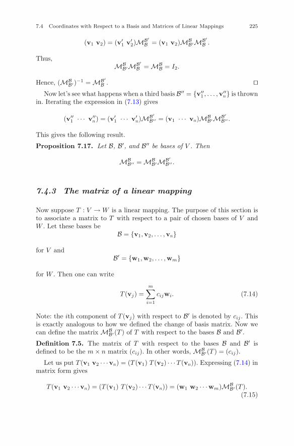
7.4 Coordinates with Respect to a Basis and Matrices of Linear Mappings 225
(v1 v2) = (v′1 v′
2)MB′B = (v1 v2)MB
B′MB′B .
Thus,MB
B′MB′B = MB
B = I2.
Hence, (MBB′)−1 = MB′
B . ��Now let’s see what happens when a third basis B′′ = {v′′
1 , . . . ,v′′n} is thrown
in. Iterating the expression in (7.13) gives
(v′′1 · · · v′′
n) = (v′1 · · · v′
n)MB′B′′ = (v1 · · · vn)MB
B′MB′B′′ .
This gives the following result.
Proposition 7.17. Let B, B′, and B′′ be bases of V . Then
MBB′′ = MB
B′MB′B′′ .
7.4.3 The matrix of a linear mapping
Now suppose T : V → W is a linear mapping. The purpose of this section isto associate a matrix to T with respect to a pair of chosen bases of V andW . Let these bases be
B = {v1,v2, . . . ,vn}
for V andB′ = {w1,w2, . . . ,wm}
for W . Then one can write
T (vj) =m∑
i=1
cijwi. (7.14)
Note: the ith component of T (vj) with respect to B′ is denoted by cij . Thisis exactly analogous to how we defined the change of basis matrix. Now wecan define the matrix MB
B′(T ) of T with respect to the bases B and B′.
Definition 7.5. The matrix of T with respect to the bases B and B′ isdefined to be the m × n matrix (cij). In other words, MB
B′(T ) = (cij).
Let us put T (v1 v2 · · ·vn) = (T (v1) T (v2) · · · T (vn)). Expressing (7.14) inmatrix form gives
T (v1 v2 · · ·vn) = (T (v1) T (v2) · · · T (vn)) = (w1 w2 · · ·wm)MBB′(T ).
(7.15)
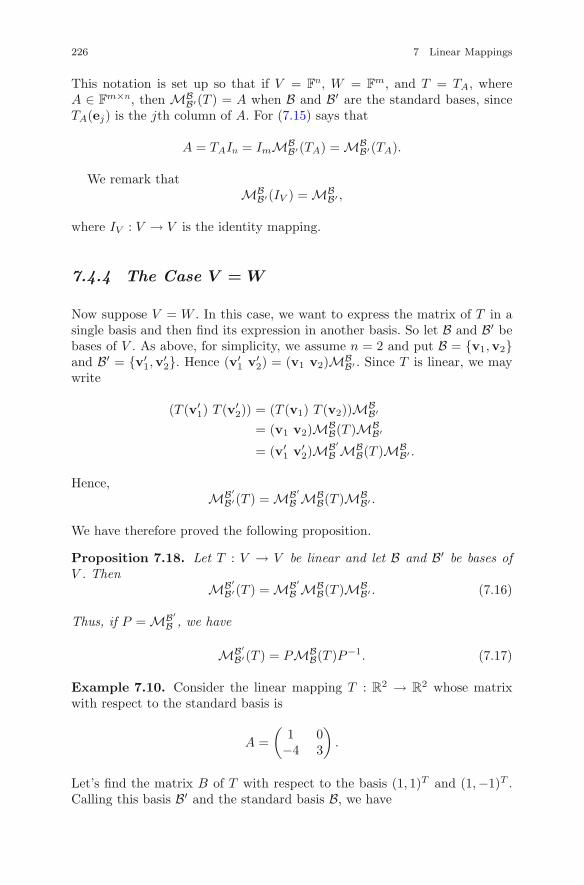
226 7 Linear Mappings
This notation is set up so that if V = Fn, W = F
m, and T = TA, whereA ∈ F
m×n, then MBB′(T ) = A when B and B′ are the standard bases, since
TA(ej) is the jth column of A. For (7.15) says that
A = TAIn = ImMBB′(TA) = MB
B′(TA).
We remark thatMB
B′(IV ) = MBB′ ,
where IV : V → V is the identity mapping.
7.4.4 The Case V = W
Now suppose V = W . In this case, we want to express the matrix of T in asingle basis and then find its expression in another basis. So let B and B′ bebases of V . As above, for simplicity, we assume n = 2 and put B = {v1,v2}and B′ = {v′
1,v′2}. Hence (v′
1 v′2) = (v1 v2)MB
B′ . Since T is linear, we maywrite
(T (v′1) T (v′
2)) = (T (v1) T (v2))MBB′
= (v1 v2)MBB(T )MB
B′
= (v′1 v′
2)MB′B MB
B(T )MBB′ .
Hence,MB′
B′(T ) = MB′B MB
B(T )MBB′ .
We have therefore proved the following proposition.
Proposition 7.18. Let T : V → V be linear and let B and B′ be bases ofV . Then
MB′B′(T ) = MB′
B MBB(T )MB
B′ . (7.16)
Thus, if P = MB′B , we have
MB′B′(T ) = PMB
B(T )P−1. (7.17)
Example 7.10. Consider the linear mapping T : R2 → R2 whose matrix
with respect to the standard basis is
A =(
1 0−4 3
).
Let’s find the matrix B of T with respect to the basis (1, 1)T and (1,−1)T .Calling this basis B′ and the standard basis B, we have
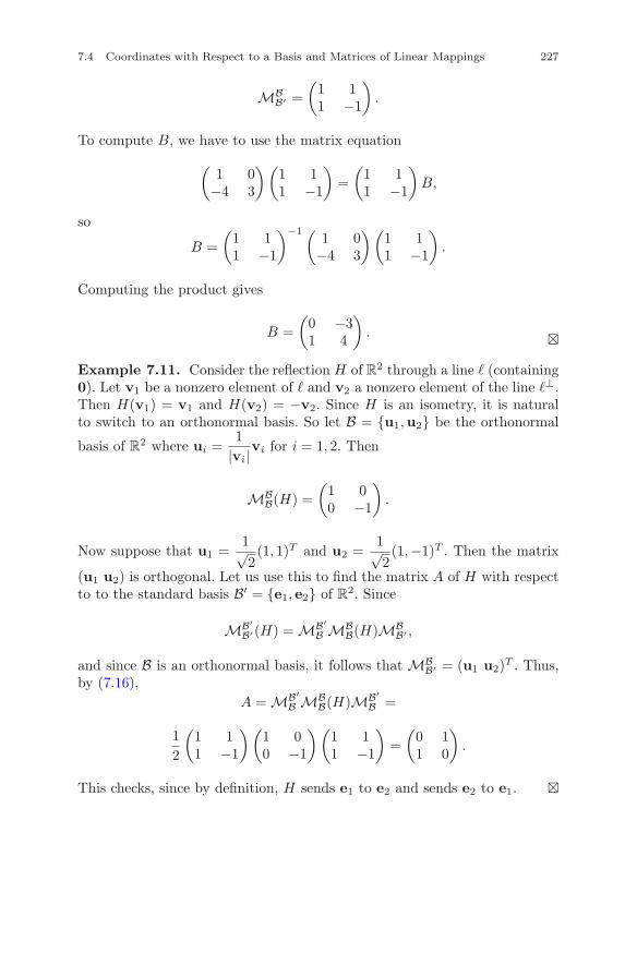
7.4 Coordinates with Respect to a Basis and Matrices of Linear Mappings 227
MBB′ =
(1 11 −1
).
To compute B, we have to use the matrix equation
(1 0
−4 3
)(1 11 −1
)=
(1 11 −1
)B,
so
B =(
1 11 −1
)−1 (1 0
−4 3
) (1 11 −1
).
Computing the product gives
B =(
0 −31 4
). �
Example 7.11. Consider the reflection H of R2 through a line � (containing0). Let v1 be a nonzero element of � and v2 a nonzero element of the line �⊥.Then H(v1) = v1 and H(v2) = −v2. Since H is an isometry, it is naturalto switch to an orthonormal basis. So let B = {u1,u2} be the orthonormal
basis of R2 where ui =1
|vi|vi for i = 1, 2. Then
MBB(H) =
(1 00 −1
).
Now suppose that u1 =1√2(1, 1)T and u2 =
1√2(1,−1)T . Then the matrix
(u1 u2) is orthogonal. Let us use this to find the matrix A of H with respectto to the standard basis B′ = {e1, e2} of R2. Since
MB′B′(H) = MB′
B MBB(H)MB
B′ ,
and since B is an orthonormal basis, it follows that MBB′ = (u1 u2)T . Thus,
by (7.16),A = MB′
B MBB(H)MB′
B =
12
(1 11 −1
) (1 00 −1
) (1 11 −1
)=
(0 11 0
).
This checks, since by definition, H sends e1 to e2 and sends e2 to e1. �
228 7 Linear Mappings
7.4.5 Similar matrices
The relationship between the matrices of a linear mapping in different basessuggests that we recall a term introduced in Exercise 5.2.6.
Definition 7.6. Let A and B be n×n matrices over F. Then we say that Ais similar to B if there exists an invertible P ∈ F
n×n such that B = PAP−1.
It is not hard to see that similarity is an equivalence relation on Fn×n
(exercise: check this). An equivalence class for this equivalence relation iscalled a conjugacy class of Fn×n. The meaning of a conjugacy class is givenin the next proposition.
Proposition 7.19. Let V be a finite-dimensional vector space over F suchthat dim V = n. Then the matrices that represent a given linear mappingT : V → V form a conjugacy class of Fn×n.
Recall that a linear mapping T : V → V is semisimple if there exists a basisB = {v1, . . . ,vn} of V for which T (vi) = μivi for some scalars μ1, . . . , μn inF. Thus a linear mapping T is semisimple if and only if the conjugacy classof its matrix with respect to some basis of V contains a diagonal matrix. Thesemisimple linear mappings T : V → V are classified in the next chapter.Conjugacy classes are also important in group theory. We will say more aboutthis in Chap. 11.
7.4.6 The matrix of a composition T ◦ S
Suppose S, T : V → V are linear mappings. Recall that we saw in Proposi-tion 3.6 that when V = F
n, then MT◦S = MTMS . We will now prove thatthis fact also holds in general.
Proposition 7.20. Assume that V is a finite-dimensional vector space withbasis B. Then
MBB(T ◦ S) = MB
B(T )MBB(S).
Proof. We leave this to the reader.
7.4.7 The determinant of a linear mapping
The product identity det(AB) = det(A) det(B) and the fact that det(A−1) =det(A)−1 imply that two similar matrices always have the same determinant,since
7.4 Coordinates with Respect to a Basis and Matrices of Linear Mappings 229
det(PAP−1) = det(P ) det(A) det(P−1) = det(A).
Using this, one can define the determinant of a linear mapping T : V → V ,provided V is finite-dimensional. The definition goes as follows.
Definition 7.7. Let V be a finite-dimensional vector space and supposeT : V → V is linear. Then the determinant det(T ) of T is defined to bedet(A), where A ∈ F
n×n is any matrix representing T with respect to somebasis of V .
In order to show that det(T ) is well defined, we need to show that det(T )is independent of the choice of basis of V . But by Proposition 7.18, if A and Bare matrices of T with respect to different bases, then A and B are similar,i.e., B = PAP−1 for some invertible P ∈ F
n×n. Hence, det(B) = det(A).Thus, det(T ) is indeed well defined.
Example 7.12. Suppose T : V → V is semisimple. Then there exists a basisfor which the matrix of T is a diagonal matrix D = diag (μ1 · · · μn). Thusdet(T ) = μ1 . . . μn, since the determinant of a diagonal matrix is the productof the diagonal entries. �
Example 7.13. Let V be a finite-dimensional inner product space, and letT : V → V be an isometry. Since the determinant of an orthogonal matrix is±1 (since QTQ = In), it follows that det(T ) = ±1 also. �
Proposition 7.21. If S, T : V → V are linear mappings on a finite-dimensional vector space V , then det(T ◦ S) = det(T ) det(S).
Proof. Apply Proposition 7.20 and the product formula. ��For example, we have the following.
Proposition 7.22. Suppose T : V → V is a linear mapping such thatdet(T ) �= 0. Then there exists a linear mapping S : V → V such thatT ◦ S = S ◦ T = IV . In particular, T is a bijection.
Proof. Choose a basis B of V and let A be the matrix of T with respectto B. Since det(T ) �= 0, det(A) �= 0 too, so A has an inverse A−1. Now letS : V → V be the linear mapping whose matrix with respect to B is A−1.Then by Proposition 7.20,
MBB(T ◦ S) = MB
B(T )MBB(S) = AA−1 = In.
Therefore, T ◦ S = IV . Similarly, S ◦ T = IV too. The assertion that T is abijection follows immediately from Proposition 1.1 or Exercise 7.1.1. ��
230 7 Linear Mappings
Exercises
Exercise 7.4.1. Find the coordinates of the standard basis e1, e2, e3 of R3
in terms of the basis (1, 1, 1)T , (1, 0, 1)T , (0, 1, 1)T , and find the matrix of thelinear mapping T ((x1, x2, x3)T ) = (4x1 + x2 − x3, x1 + 3x3, x2 + 2x3)T withrespect to this basis.
Exercise 7.4.2. Consider the basis (1, 1, 1)T , (1, 0, 1)T , and (0, 1, 1)T of R3.Find the matrix of the linear mapping T : R
3 → R3 defined by T (x) =
(1, 1, 1)T × x with respect to this basis.
Exercise 7.4.3. Let H : R2 → R2 be the reflection through the line 2x = y.
Find a basis of R2 such that the matrix of H is diagonal.
Exercise 7.4.4. Show that every projection Pa : R2 → R2 is semisimple by
explicitly finding a basis for which the matrix of Pa is diagonal. Also, findthis diagonal matrix.
Exercise 7.4.5. Let Rθ be the usual rotation of R2. Does there exist a basisof R2 for which the matrix of Rθ is diagonal?
Exercise 7.4.6. Show that matrix similarity is an equivalence relation onF
n×n.
Exercise 7.4.7. Find the matrix MBB(Ca) of the cross product Ca = a × x
in the following cases:
(i) a = e1 and B is the standard basis;
(ii) a = e1 and B is the basis {e1, e2 + e3, e2 − e3}.
Exercise 7.4.8. Let V = (F2)2×2, and let T : V → V be defined by T (B) =
AB − BA, where A =(
0 11 0
)as an element of V .
(i) Show that T is a linear mapping.
(ii) Find the matrix of T with respect to a suitable basis (of your choice)of V .
(iii) Find det(T ).
Exercise 7.4.9. Let V be a finite-dimensional vector space, and supposeT : V → V is a linear mapping. Find the relationship between betweenN (MB
B(T ))
and N (MB′B′(T )
), where B and B′ are any two bases of V .
Exercise 7.4.10. Let T : V → V be a linear mapping, where V has finitedimension. Show that the kernel of T is nontrivial if and only if det(T ) = 0.

7.4 Coordinates with Respect to a Basis and Matrices of Linear Mappings 231
Exercise 7.4.11. Suppose the characteristic of F is different from 2, and letV = F
n×n. Let T : V → V be the linear mapping given by T (A) = AT . Finda basis of V for which the matrix of T is diagonal. (Hint: recall that A is thesum of a symmetric matrix and a skew-symmetric matrix.)
Exercise 7.4.12. Let V = F4 = {0, 1, α, β} be the four-element Galois fieldconsidered as a vector space over the prime field F2 (see Section 2.6.2).
(i) Show that 1 and α form a basis of V .
(ii) Show that the Frobenius map F : V → V given by F (x) = x2 is a linearmapping.
(iii) Find the matrix of F with respect to the basis of (i).
(iv) Is F semi-simple?
232 7 Linear Mappings
7.5 Further Results on Mappings
As usual, all vector spaces will be over the field F. If V and W are vectorspaces, the space L(V,W ) denotes the space of all linear mappings T : V →W . If V = F
n and W = Fm, then L(V,W ) = F
m×n. The purpose of thissection is to study L(V,W ) for various choices of V and W .
7.5.1 The space L(V,W )
Mappings F : V → W can be added using pointwise addition and can bemultiplied by scalars in a similar way. That is, if F,G : V → W are twomappings, their sum F + G is the mapping formed by setting
(F + G)(v) = F (v) + G(v).
Scalar multiplication is defined by putting
(aF )(v) = aF (v)
for any scalar a. Hence, one can form linear combinations of mappings. Itisn’t hard to see that the set of all mappings with domain V and target W isa vector space over F. Now let L(V,W ) denote the set of all linear mappingswith domain V and target W . Then L(V,W ) is a vector space over F underthe pointwise addition and scalar multiplication defined above. The followingresult gives the dimension of L(V,W ) in the finite-dimensional case.
Proposition 7.23. Suppose V and W are finite-dimensional vector spaces,say dim V = n and dim W = m. Then dim L(V,W ) = mn.
Proof. Choose bases B of V and B′ of W . Then T has matrix MT = MBB′(T ),
and putting φ(T ) = MT defines a linear mapping Φ : L(V,W ) → Fm×n.
In fact, Φ is a bijection, and therefore Φ is an isomorphism. This impliesdim L(V,W ) = dimF
m×n = mn, since an isomorphism preserves dimension.��
7.5.2 The dual space
The space V ∗ = L(V,F) of linear maps (or linear functions) from V to F iscalled the dual space of V . If V is a finite-dimensional vector space, then theprevious result says that dimV ∗ = dim V. It turns out that even though Vand V ∗ have the same dimension, there usually is no natural isomorphism
7.5 Further Results on Mappings 233
between them unless there is some additional structure. For example, if V isa finite-dimensional inner product space, then there is a natural isomorphism(see below). Given a basis of V , however, there is a natural basis of V ∗ knownas the dual basis, which we now describe. If v1, . . . ,vn is a basis of V , thenthe dual basis v∗
1, . . . ,v∗n of V ∗ is defined by specifying how each v∗
i acts onthe basis v1, . . . ,vn. Since a linear mapping is uniquely defined by giving itsvalues on a basis, this suffices to define a unique element of V ∗. Thus put
v∗i (vj) =
{1 if i = j,0 if i �= j.
(7.18)
More succinctly, v∗i (vj) = δij . To justify the term dual basis, we prove the
following proposition.
Proposition 7.24. If v1, . . . ,vn is a basis of V , then v∗1, . . . ,v
∗n is a basis
of V ∗.
Proof. Since V and V ∗ have the same dimension, it suffices to show that thedual basis vectors are independent. Suppose
∑ni=1 aiv∗
i = 0. By (7.18),
( n∑
i=1
aiv∗i
)(vj) =
n∑
i=1
aiv∗i (vj) = aj .
Hence each aj is equal to zero, so v∗1, . . . ,v
∗n are indeed independent. ��
Example 7.14. In fact, the dual basis for V = Fn is already quite familiar.
Recall that the ith component function xi : Fn → F is defined by
xi(a1, · · · , an) = ai
for i = 1, . . . , n. Then each xi is in V ∗. In fact, x1, . . . , xn is the basis of V ∗
dual to the standard basis e1, . . . , en. �Example 7.15. Here is an infinite-dimensional example. Let V = F[x].Then the evaluation at an element r ∈ F is the map er : V → F definedby er(f) = f(r). Then er ∈ V ∗ for every r ∈ F. The kernel of er consists ofall f ∈ F[x] such that f(r) = 0.
Let us now consider the case mentioned above in which V is a finite-dimensional inner product space.
Proposition 7.25. Let V be a finite-dimensional inner product space overR. If v ∈ V , let ϕv : V → R be the element of V ∗ defined by
ϕv(x) = (v,x),
where ( , ) is the inner product on V . Then the mapping Φ : V → V ∗ definedby Φ(v) = ϕv is an isomorphism.
234 7 Linear Mappings
Proof. It is clear, by the properties of an inner product, that ϕv ∈ V ∗. Sincedim V = dim V ∗, we have only to show that Φ is injective. But if Φ(v) = 0,then (v,x) = 0 for all x ∈ V . In particular, (v,v) = 0, so v = 0 by thedefinition of an inner product, and hence by Proposition 7.3, Φ is injective.
��In a similar vein, a Hermitian inner product on a finite-dimensional vector
space V over the complex numbers enables one to define an isomorphism fromV to V ∗, although the definition is slightly different, since (αx,v) = α(x,v)for a Hermitian inner product (see Example 6.35).
It turns out that there is always a natural isomorphism between V andV ∗∗. This is an interesting exercise.
7.5.3 Multilinear maps
Let V and W be vector spaces over F. A mapping
T : V × V × · · · × V → W (k factors)
is called k-multilinear if for all i = 1, . . . , k, the mapping Si : V → W definedby
Si(x) = T (v1, . . . ,vi−1,x,vi+1, . . . ,vk)
is a linear mapping for every v1, . . . ,vi−1,vi+1, . . . ,vk ∈ V .
Example 7.16. Let V = F and define T (r1, r2, . . . , rk) = r1r2 · · · rk. ThenT is k-multilinear on V . �
More interestingly, let V = Fn, where elements of F
n are viewed ascolumns. Define D : Fn×n = F
n × · · · × Fn → F by
D(v1,v2, . . . ,vn) = det(v1v2 . . .vn).
Proposition 7.26. The mapping D is n-multilinear.
Proof. Fix a1, . . . ,an ∈ Fn, and put Sj(x) = D(a1, . . . ,aj−1,x,aj+1, . . . ,an).
We must show that Sj(x + y) = Sj(x) + Sj(y), and Sj(rx) = rSj(x) for allx,y ∈ F
n and r ∈ F. Let aj = (a1ja2j . . . anj)T . By (5.9),
D(a1, . . . ,an) =∑
σ∈S(n)
sgn(σ) a1σ(1)a2σ(2) · · · anσ(n).
Put x = (x1j , x2j , . . . , xnj)T and y = (y1j , y2j , . . . , ynj)T . For each σ ∈ S(n),there exists exactly one index i such that σ(i) = j. Thus, each term in theexpansion of Sj(x + y) has the form
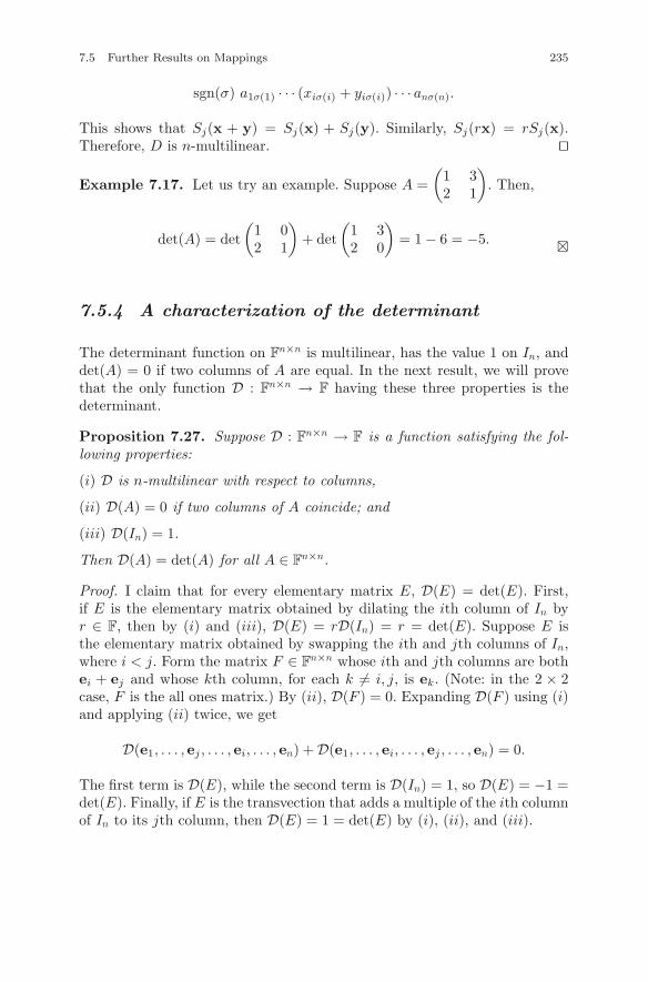
7.5 Further Results on Mappings 235
sgn(σ) a1σ(1) · · · (xiσ(i) + yiσ(i)) · · · anσ(n).
This shows that Sj(x + y) = Sj(x) + Sj(y). Similarly, Sj(rx) = rSj(x).Therefore, D is n-multilinear. ��
Example 7.17. Let us try an example. Suppose A =(
1 32 1
). Then,
det(A) = det(
1 02 1
)+ det
(1 32 0
)= 1 − 6 = −5. �
7.5.4 A characterization of the determinant
The determinant function on Fn×n is multilinear, has the value 1 on In, and
det(A) = 0 if two columns of A are equal. In the next result, we will provethat the only function D : F
n×n → F having these three properties is thedeterminant.
Proposition 7.27. Suppose D : Fn×n → F is a function satisfying the fol-lowing properties:
(i) D is n-multilinear with respect to columns,
(ii) D(A) = 0 if two columns of A coincide; and
(iii) D(In) = 1.
Then D(A) = det(A) for all A ∈ Fn×n.
Proof. I claim that for every elementary matrix E, D(E) = det(E). First,if E is the elementary matrix obtained by dilating the ith column of In byr ∈ F, then by (i) and (iii), D(E) = rD(In) = r = det(E). Suppose E isthe elementary matrix obtained by swapping the ith and jth columns of In,where i < j. Form the matrix F ∈ F
n×n whose ith and jth columns are bothei + ej and whose kth column, for each k �= i, j, is ek. (Note: in the 2 × 2case, F is the all ones matrix.) By (ii), D(F ) = 0. Expanding D(F ) using (i)and applying (ii) twice, we get
D(e1, . . . , ej , . . . , ei, . . . , en) + D(e1, . . . , ei, . . . , ej , . . . , en) = 0.
The first term is D(E), while the second term is D(In) = 1, so D(E) = −1 =det(E). Finally, if E is the transvection that adds a multiple of the ith columnof In to its jth column, then D(E) = 1 = det(E) by (i), (ii), and (iii).
236 7 Linear Mappings
The next step is to show that for every elementary matrix E and A ∈F
n×n, D(AE) = D(E)D(A). (Recall that column operations are done viaright multiplication.) This follows from the previous proposition if E is arow dilation. If E is a column swap, an argument similar to showing thatD(E) = −1 shows that D(AE) + D(A) = 0. Therefore, D(AE) = −D(A) =D(E)D(A). Likewise, D(AE) = D(A) = D(E)D(A) when E is a transvection.This completes the second step.
Now suppose A ∈ Fn×n has rank n. Then there exist elementary matrices
E1, . . . , Ek such that A = E1 · · · Ek. Applying D(AE) = D(E)D(A) andusing the product formula (Theorem 5.1) for the determinant, one gets
D(A) = D(E1) · · · D(Ek) = det(E1) · · · det(Ek) = det(A).
On the other hand, if A has rank less than n, then the column reduced formof A has a column of zeros, so for suitable elementary matrices E1, . . . , Ek,AE1 · · · Ek has a column of zeros. Thus, D(A) = 0 = det(A). This completesthe proof that D(A) = det(A) for all A ∈ F
n×n. ��Notice that what the proposition shows is that two functions D1 and D2
on Fn×n satisfying (i)–(iii) have to coincide. But it cannot actually be used
as a definition of the determinant.
Exercises
Exercise 7.5.1. Let V be a finite-dimensional inner product space. Showhow to define an inner product on V ∗ in two ways:
(i) using a basis and the dual basis;
(ii) without appealing to a basis.
Exercise* 7.5.1. Let V be any finite-dimensional vector space. Define thedouble dual V ∗∗ of V to be (V ∗)∗. That is, V ∗∗ is the dual of the dual spaceof V . Show that the map Δ : V → V ∗∗ defined by the condition
Δ(v)(ϕ) = ϕ(v) (7.19)
for all v ∈ V and ϕ ∈ V ∗ is an isomorphism. Thus Δ is a natural isomorphismfrom V onto V ∗∗.
Exercise* 7.5.2. Let V and W be a pair of finite-dimensional vector spacesover F and let T : V → W be linear. Define the adjoint map T ∗ : W ∗ → V ∗
byT ∗(ω)(v) = ω(T (v))
for all ω ∈ W ∗ and v ∈ V .
7.5 Further Results on Mappings 237
(i) Show that T ∗ is a well-defined linear map.
(ii) Suppose v1, . . .vn is a basis of V , and w1, . . . ,wm is a basis of W , andlet the matrix of T with respect to these bases be A. Find the matrix of T ∗
with respect to the dual bases of W ∗ and V ∗.
(iii) Show that if T is injective, then T ∗ is surjective. Also show the reverse:if T is surjective, then T ∗ is injective.
(iv) Show that dim im(T ) = dim im(T ∗).
(v) Show that if V is a subspace of W , then there exists a natural surjectivelinear map S : W ∗ → V ∗.
Chapter 8Eigentheory
Suppose V is a finite-dimensional vector space over F and T : V → V is alinear mapping. An eigenpair for T consists of a pair (λ,v), where λ ∈ F
and v ∈ V is a nonzero vector such that T (v) = λv. The scalar λ is calledan eigenvalue of T , and v is called an eigenvector of T corresponding to λ.We will say that the linear mapping T is semisimple if there exist eigen-pairs (λ1,v1), . . . , (λn,vn) for T such that v1, . . . ,vn form a basis of V . Abasis consisting of eigenvectors is known as an eigenbasis, and the problem offinding an eigenbasis (or whether one exists) is an important step in under-standing the structure of a linear mapping. The aim of this chapter is todevelop the theory of eigenpairs and eigenbases and to eventually obtain acharacterization the semisimple linear mappings. We will also introduce sev-eral geometric notions, such as the definition of a dynamical system, and wewill give a number of group-theoretic applications of eigentheory. One of thenicest applications is the proof of another classical theorem of Euler, whichin modern terms says that SO(3,R) consists of all rotations of R
3 aboutthe origin. We will also discuss the symmetries of the Platonic solids, andfinally, we will prove the celebrated Cayley–Hamilton theorem, which will beapplied later in the proofs of Jordan canonical form and the Jordan–Chevalleydecomposition theorem.
8.1 The Eigenvalue Problem and the CharacteristicPolynomial
The purpose of this section is to introduce the basic terms and concepts con-nected with eigentheory: eigenvalues, eigenvectors, eigenpairs, eigenspaces,the characteristic polynomial, and the characteristic equation. As above, V
c© Springer Science+Business Media LLC 2017J.B. Carrell, Groups, Matrices, and Vector Spaces,DOI 10.1007/978-0-387-79428-0 8
239
240 8 Eigentheory
is a finite-dimensional vector space over F, and T : V → V is a linear map-ping. When V = F
n, then T = TA, where A ∈ Fn×n is the matrix of T with
respect to the standard basis.
8.1.1 First considerations: the eigenvalue problemfor matrices
The problem of finding eigenpairs for a linear mapping T will be attackedvia matrix theory by solving it for the matrix A of T with respect to abasis of V and then showing how an eigenpair for A determines an eigenpairfor T . Suppose dim V = n, so that A ∈ F
n×n. On the level of matrix theory,the eigenvalue problem is to find the values of λ ∈ F such that the linearsystem Ax = λx has a nontrivial solution. The variables are λ and x, so thisis a nonlinear problem because of the λx term. The way to circumvent thisdifficulty is by breaking the problem down into two separate problems. Thefirst is to determine all λ ∈ F such that N (A − λIn) �= {0}. Since the nullspace of a square matrix is nonzero if and only if its determinant is zero, theproblem is to determine all λ ∈ F such that
det(A − λIn) = 0. (8.1)
One calls (8.1) the characteristic equation of A. The eigenvalues of A are thesolutions λ in F of the characteristic equation. The second problem, whichis straightforward, is to find the null space N (A − λIn) corresponding to aneigenvalue. The null space N (A − λIn) is called the eigenspace of A corre-sponding to λ and denoted by Eλ(A). For every nonzero v ∈ N (A − λIn),(λ,v) is an eigenpair.
Remark. The properties of the determinant imply that det(A − λIn) is apolynomial in λ of degree n. Hence finding eigenvalues of A requires findingthe roots of a polynomial. If n > 2, there is no easy way to do this, but thereare a few remarks we can and will make later. The roots of polynomials ofdegree at most four can be found with great difficulty by radicals, but thereis no general formula for roots of a polynomial of degree five or more. This isa famous result in Galois theory involving the Galois group of the equation.There are analytic techniques for approximating roots. On the other hand,the fundamental theorem of algebra guarantees that every A ∈ C
n×n has ncomplex eigenvalues. This does not mean, however, that square matrices overC always admit an eigenbasis, as we will see.
Let us now consider an example.
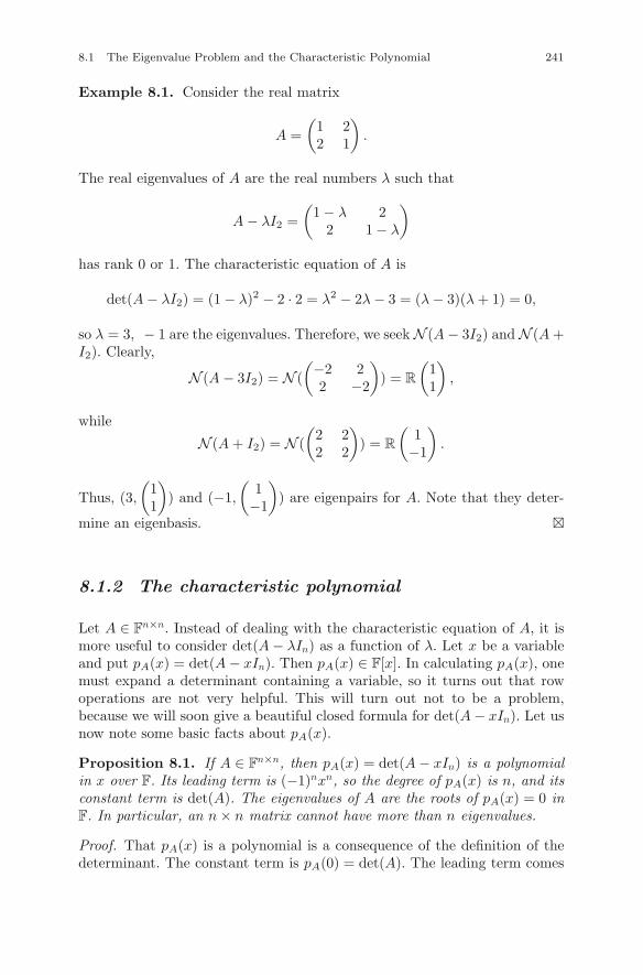
8.1 The Eigenvalue Problem and the Characteristic Polynomial 241
Example 8.1. Consider the real matrix
A =(
1 22 1
).
The real eigenvalues of A are the real numbers λ such that
A − λI2 =(
1 − λ 22 1 − λ
)
has rank 0 or 1. The characteristic equation of A is
det(A − λI2) = (1 − λ)2 − 2 · 2 = λ2 − 2λ − 3 = (λ − 3)(λ + 1) = 0,
so λ = 3, − 1 are the eigenvalues. Therefore, we seek N (A − 3I2) and N (A +I2). Clearly,
N (A − 3I2) = N ((
−2 22 −2
)) = R
(11
),
while
N (A + I2) = N ((
2 22 2
)) = R
(1
−1
).
Thus, (3,
(11
)) and (−1,
(1
−1
)) are eigenpairs for A. Note that they deter-
mine an eigenbasis. �
8.1.2 The characteristic polynomial
Let A ∈ Fn×n. Instead of dealing with the characteristic equation of A, it is
more useful to consider det(A − λIn) as a function of λ. Let x be a variableand put pA(x) = det(A − xIn). Then pA(x) ∈ F[x]. In calculating pA(x), onemust expand a determinant containing a variable, so it turns out that rowoperations are not very helpful. This will turn out not to be a problem,because we will soon give a beautiful closed formula for det(A − xIn). Let usnow note some basic facts about pA(x).
Proposition 8.1. If A ∈ Fn×n, then pA(x) = det(A − xIn) is a polynomial
in x over F. Its leading term is (−1)nxn, so the degree of pA(x) is n, and itsconstant term is det(A). The eigenvalues of A are the roots of pA(x) = 0 inF. In particular, an n × n matrix cannot have more than n eigenvalues.
Proof. That pA(x) is a polynomial is a consequence of the definition of thedeterminant. The constant term is pA(0) = det(A). The leading term comes
242 8 Eigentheory
from the term(a11 − x) · · · (ann − x)
in the Leibniz expansion, which is clearly (−1)nxn. The last claim followsfrom the fact that a polynomial over F of degree n cannot have more than nroots in F. �
One calls pA(x) the characteristic polynomial of A. The characteristic poly-nomial needn’t have any roots in F. However, one of the basic results in thetheory of fields is that given f(x) ∈ F[x], there exists a field F
′ containingF such that f(x) factors into linear terms in F
′[x]. That is, F′ contains allroots of f(x) = 0. We will give a proof of this result in the appendix (seeSection 8.7) at the end of this chapter. Although the fundamental theorem ofalgebra (Theorem 2.27) guarantees that the characteristic polynomial of ann × n matrix over R has n complex roots, none of these roots need be real,as the next example points out.
Example 8.2. The characteristic polynomial of the matrix
J =(
0 −11 0
)
is x2 + 1 = 0. Hence J is a real matrix that has no real eigenvalues. In fact,there cannot be real eigenvalues, since J is the rotation of R2 through π/2:no nonzero vector is rotated into a multiple of itself. On the other hand, if Jis treated as a 2 × 2 complex matrix with eigenvalues ±i, solving for corre-sponding eigenvectors gives eigenpairs (i, (−1, i)T ) and (−i, (1, i)T ). Thus Jhas two C-eigenvalues and two independent eigenvectors in C
2. In particular,J has an eigenbasis for C
2. Thus,
(0 −11 0
)(1 1−i i
)=
(1 1−i i
)(i 00 −i
),
so J = MDM−1, where M =(
1 1−i i
). �
The following example illustrates another possibility.
Example 8.3. Let K =(
0 −ii 0
). The characteristic polynomial of K is
x2 − 1, so the eigenvalues of K are ±1. Thus K is a complex matrix withreal eigenvalues. Notice that K = iJ , which explains why its eigenvalues arei times those of J . �
The next Proposition gives an important property of the characteristicpolynomial.
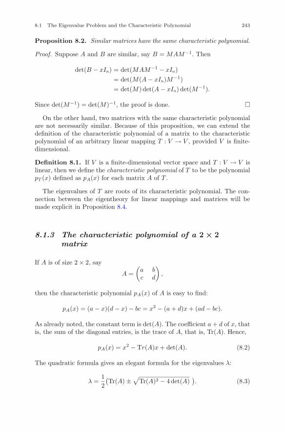
8.1 The Eigenvalue Problem and the Characteristic Polynomial 243
Proposition 8.2. Similar matrices have the same characteristic polynomial.
Proof. Suppose A and B are similar, say B = MAM−1. Then
det(B − xIn) = det(MAM−1 − xIn)= det(M(A − xIn)M−1)= det(M) det(A − xIn) det(M−1).
Since det(M−1) = det(M)−1, the proof is done. �
On the other hand, two matrices with the same characteristic polynomialare not necessarily similar. Because of this proposition, we can extend thedefinition of the characteristic polynomial of a matrix to the characteristicpolynomial of an arbitrary linear mapping T : V → V , provided V is finite-dimensional.
Definition 8.1. If V is a finite-dimensional vector space and T : V → V islinear, then we define the characteristic polynomial of T to be the polynomialpT (x) defined as pA(x) for each matrix A of T .
The eigenvalues of T are roots of its characteristic polynomial. The con-nection between the eigentheory for linear mappings and matrices will bemade explicit in Proposition 8.4.
8.1.3 The characteristic polynomial of a 2 × 2matrix
If A is of size 2 × 2, say
A =(
a bc d
),
then the characteristic polynomial pA(x) of A is easy to find:
pA(x) = (a − x)(d − x) − bc = x2 − (a + d)x + (ad − bc).
As already noted, the constant term is det(A). The coefficient a + d of x, thatis, the sum of the diagonal entries, is the trace of A, that is, Tr(A). Hence,
pA(x) = x2 − Tr(A)x + det(A). (8.2)
The quadratic formula gives an elegant formula for the eigenvalues λ:
λ =12(Tr(A) ±
√Tr(A)2 − 4 det(A)
). (8.3)
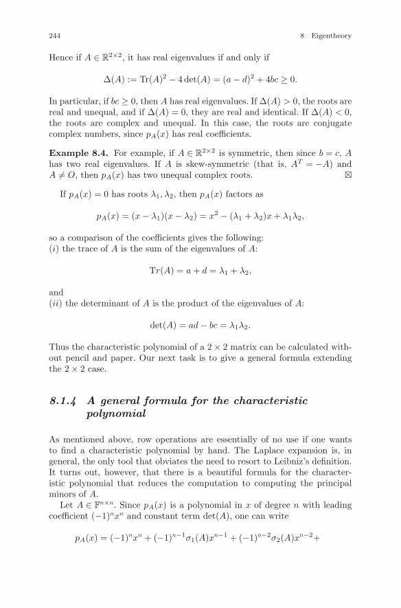
244 8 Eigentheory
Hence if A ∈ R2×2, it has real eigenvalues if and only if
Δ(A) := Tr(A)2 − 4 det(A) = (a − d)2 + 4bc ≥ 0.
In particular, if bc ≥ 0, then A has real eigenvalues. If Δ(A) > 0, the roots arereal and unequal, and if Δ(A) = 0, they are real and identical. If Δ(A) < 0,the roots are complex and unequal. In this case, the roots are conjugatecomplex numbers, since pA(x) has real coefficients.
Example 8.4. For example, if A ∈ R2×2 is symmetric, then since b = c, A
has two real eigenvalues. If A is skew-symmetric (that is, AT = −A) andA �= O, then pA(x) has two unequal complex roots. �
If pA(x) = 0 has roots λ1, λ2, then pA(x) factors as
pA(x) = (x − λ1)(x − λ2) = x2 − (λ1 + λ2)x + λ1λ2,
so a comparison of the coefficients gives the following:(i) the trace of A is the sum of the eigenvalues of A:
Tr(A) = a + d = λ1 + λ2,
and(ii) the determinant of A is the product of the eigenvalues of A:
det(A) = ad − bc = λ1λ2.
Thus the characteristic polynomial of a 2 × 2 matrix can be calculated with-out pencil and paper. Our next task is to give a general formula extendingthe 2 × 2 case.
8.1.4 A general formula for the characteristicpolynomial
As mentioned above, row operations are essentially of no use if one wantsto find a characteristic polynomial by hand. The Laplace expansion is, ingeneral, the only tool that obviates the need to resort to Leibniz’s definition.It turns out, however, that there is a beautiful formula for the character-istic polynomial that reduces the computation to computing the principalminors of A.
Let A ∈ Fn×n. Since pA(x) is a polynomial in x of degree n with leading
coefficient (−1)nxn and constant term det(A), one can write
pA(x) = (−1)nxn + (−1)n−1σ1(A)xn−1 + (−1)n−2σ2(A)xn−2+
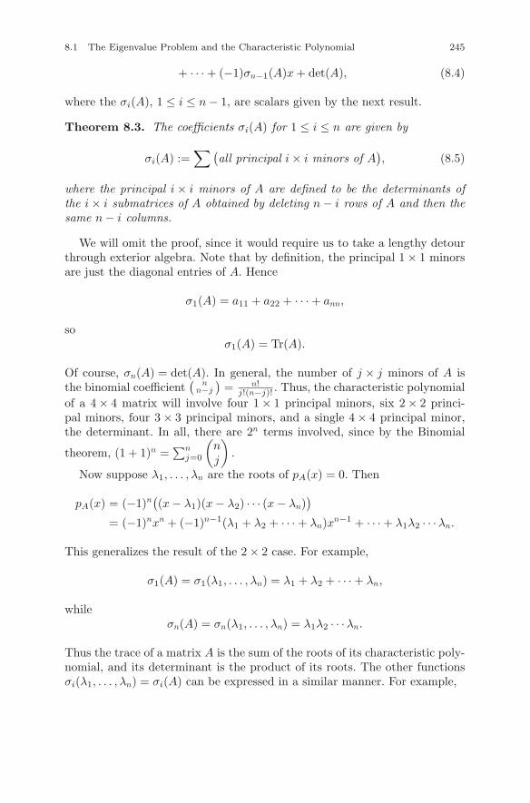
8.1 The Eigenvalue Problem and the Characteristic Polynomial 245
+ · · · + (−1)σn−1(A)x + det(A), (8.4)
where the σi(A), 1 ≤ i ≤ n − 1, are scalars given by the next result.
Theorem 8.3. The coefficients σi(A) for 1 ≤ i ≤ n are given by
σi(A) :=∑ (
all principal i × i minors of A), (8.5)
where the principal i × i minors of A are defined to be the determinants ofthe i × i submatrices of A obtained by deleting n − i rows of A and then thesame n − i columns.
We will omit the proof, since it would require us to take a lengthy detourthrough exterior algebra. Note that by definition, the principal 1 × 1 minorsare just the diagonal entries of A. Hence
σ1(A) = a11 + a22 + · · · + ann,
soσ1(A) = Tr(A).
Of course, σn(A) = det(A). In general, the number of j × j minors of A isthe binomial coefficient
( nn−j
)= n!
j!(n−j)! . Thus, the characteristic polynomialof a 4 × 4 matrix will involve four 1 × 1 principal minors, six 2 × 2 princi-pal minors, four 3 × 3 principal minors, and a single 4 × 4 principal minor,the determinant. In all, there are 2n terms involved, since by the Binomial
theorem, (1 + 1)n =∑n
j=0
(nj
).
Now suppose λ1, . . . , λn are the roots of pA(x) = 0. Then
pA(x) = (−1)n((x − λ1)(x − λ2) · · · (x − λn)
)= (−1)nxn + (−1)n−1(λ1 + λ2 + · · · + λn)xn−1 + · · · + λ1λ2 · · · λn.
This generalizes the result of the 2 × 2 case. For example,
σ1(A) = σ1(λ1, . . . , λn) = λ1 + λ2 + · · · + λn,
whileσn(A) = σn(λ1, . . . , λn) = λ1λ2 · · · λn.
Thus the trace of a matrix A is the sum of the roots of its characteristic poly-nomial, and its determinant is the product of its roots. The other functionsσi(λ1, . . . , λn) = σi(A) can be expressed in a similar manner. For example,
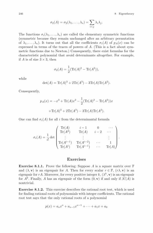
246 8 Eigentheory
σ2(A) = σ2(λ1, . . . , λn) =∑i<j
λiλj .
The functions σi(λ1, . . . , λn) are called the elementary symmetric functions(symmetric because they remain unchanged after an arbitrary permutationof λ1, . . . , λn). It turns out that all the coefficients σi(A) of pA(x) can beexpressed in terms of the traces of powers of A. (This is a fact about sym-metric functions due to Newton.) Consequently, there exist formulas for thecharacteristic polynomial that avoid determinants altogether. For example,if A is of size 3 × 3, then
σ2(A) =12(Tr(A)2 − Tr(A2)),
whiledet(A) = Tr(A)3 + 2Tr(A3) − 3Tr(A)Tr(A2).
Consequently,
pA(x) = −x3 + Tr(A)x2 − 12(Tr(A)2 − Tr(A2))x
+Tr(A)3 + 2Tr(A3) − 3Tr(A)Tr(A2).
One can find σi(A) for all i from the determinantal formula
σi(A) =1i!
det
⎛⎜⎜⎜⎜⎜⎝
Tr(A) i − 1 0 · · ·Tr(A2) Tr(A) i − 2 · · ·
......
...Tr(Ai−1) Tr(Ai−2) · · · 1Tr(Ai) Tr(Ai−1) · · · Tr(A)
⎞⎟⎟⎟⎟⎟⎠
.
Exercises
Exercise 8.1.1. Prove the following: Suppose A is a square matrix over F
and (λ,v) is an eigenpair for A. Then for every scalar r ∈ F, (rλ,v) is aneigenpair for rA. Moreover, for every positive integer k, (λk,v) is an eigenpairfor Ak. Finally, A has an eigenpair of the form (0,v) if and only if N (A) isnontrivial.
Exercise 8.1.2. This exercise describes the rational root test, which is usedfor finding rational roots of polynomials with integer coefficients. The rationalroot test says that the only rational roots of a polynomial
p(x) = anxn + an−1x
n−1 + · · · + a1x + a0
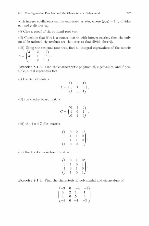
8.1 The Eigenvalue Problem and the Characteristic Polynomial 247
with integer coefficients can be expressed as p/q, where (p, q) = 1, q dividesan, and p divides a0.
(i) Give a proof of the rational root test.
(ii) Conclude that if A is a square matrix with integer entries, then the onlypossible rational eigenvalues are the integers that divide det(A).
(iii) Using the rational root test, find all integral eigenvalues of the matrix
A =
⎛⎝3 −2 −2
3 −1 −31 −2 0
⎞⎠ .
Exercise 8.1.3. Find the characteristic polynomial, eigenvalues, and if pos-sible, a real eigenbasis for:
(i) the X-files matrix
X =
⎛⎝1 0 1
0 1 01 0 1
⎞⎠ ,
(ii) the checkerboard matrix
C =
⎛⎝0 1 0
1 0 10 1 0
⎞⎠ ,
(iii) the 4 × 4 X-files matrix
⎛⎜⎜⎝
1 0 0 10 1 1 00 1 1 01 0 0 1
⎞⎟⎟⎠ ,
(iv) the 4 × 4 checkerboard matrix
⎛⎜⎜⎝
1 0 1 00 1 0 11 0 1 00 1 0 1
⎞⎟⎟⎠ .
Exercise 8.1.4. Find the characteristic polynomial and eigenvalues of
⎛⎜⎜⎝
−3 0 −4 −40 2 1 14 0 5 4
−4 0 −4 −3
⎞⎟⎟⎠
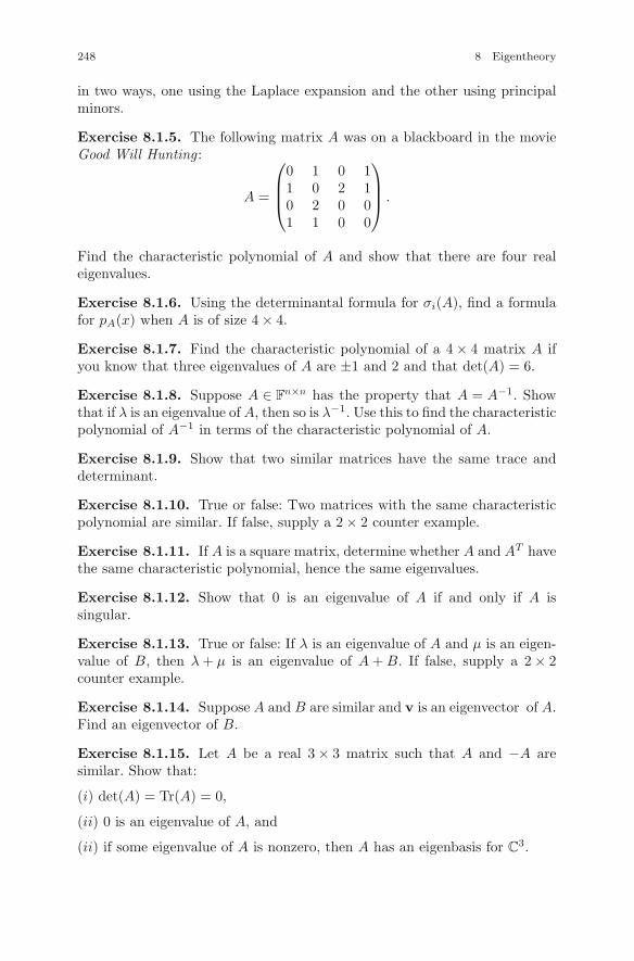
248 8 Eigentheory
in two ways, one using the Laplace expansion and the other using principalminors.
Exercise 8.1.5. The following matrix A was on a blackboard in the movieGood Will Hunting :
A =
⎛⎜⎜⎝
0 1 0 11 0 2 10 2 0 01 1 0 0
⎞⎟⎟⎠ .
Find the characteristic polynomial of A and show that there are four realeigenvalues.
Exercise 8.1.6. Using the determinantal formula for σi(A), find a formulafor pA(x) when A is of size 4 × 4.
Exercise 8.1.7. Find the characteristic polynomial of a 4 × 4 matrix A ifyou know that three eigenvalues of A are ±1 and 2 and that det(A) = 6.
Exercise 8.1.8. Suppose A ∈ Fn×n has the property that A = A−1. Show
that if λ is an eigenvalue of A, then so is λ−1. Use this to find the characteristicpolynomial of A−1 in terms of the characteristic polynomial of A.
Exercise 8.1.9. Show that two similar matrices have the same trace anddeterminant.
Exercise 8.1.10. True or false: Two matrices with the same characteristicpolynomial are similar. If false, supply a 2 × 2 counter example.
Exercise 8.1.11. If A is a square matrix, determine whether A and AT havethe same characteristic polynomial, hence the same eigenvalues.
Exercise 8.1.12. Show that 0 is an eigenvalue of A if and only if A issingular.
Exercise 8.1.13. True or false: If λ is an eigenvalue of A and μ is an eigen-value of B, then λ + μ is an eigenvalue of A + B. If false, supply a 2 × 2counter example.
Exercise 8.1.14. Suppose A and B are similar and v is an eigenvector of A.Find an eigenvector of B.
Exercise 8.1.15. Let A be a real 3 × 3 matrix such that A and −A aresimilar. Show that:
(i) det(A) = Tr(A) = 0,
(ii) 0 is an eigenvalue of A, and
(ii) if some eigenvalue of A is nonzero, then A has an eigenbasis for C3.
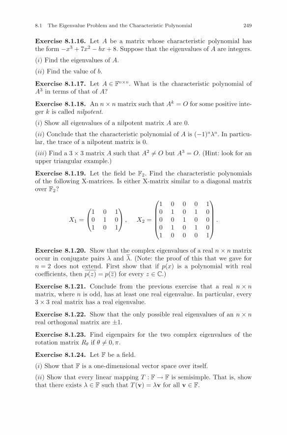
8.1 The Eigenvalue Problem and the Characteristic Polynomial 249
Exercise 8.1.16. Let A be a matrix whose characteristic polynomial hasthe form −x3 + 7x2 − bx + 8. Suppose that the eigenvalues of A are integers.
(i) Find the eigenvalues of A.
(ii) Find the value of b.
Exercise 8.1.17. Let A ∈ Fn×n. What is the characteristic polynomial of
A3 in terms of that of A?
Exercise 8.1.18. An n × n matrix such that Ak = O for some positive inte-ger k is called nilpotent.
(i) Show all eigenvalues of a nilpotent matrix A are 0.
(ii) Conclude that the characteristic polynomial of A is (−1)nλn. In particu-lar, the trace of a nilpotent matrix is 0.
(iii) Find a 3 × 3 matrix A such that A2 �= O but A3 = O. (Hint: look for anupper triangular example.)
Exercise 8.1.19. Let the field be F2. Find the characteristic polynomialsof the following X-matrices. Is either X-matrix similar to a diagonal matrixover F2?
X1 =
⎛⎝1 0 1
0 1 01 0 1
⎞⎠ , X2 =
⎛⎜⎜⎜⎜⎝
1 0 0 0 10 1 0 1 00 0 1 0 00 1 0 1 01 0 0 0 1
⎞⎟⎟⎟⎟⎠ .
Exercise 8.1.20. Show that the complex eigenvalues of a real n × n matrixoccur in conjugate pairs λ and λ. (Note: the proof of this that we gave forn = 2 does not extend. First show that if p(x) is a polynomial with realcoefficients, then p(z) = p(z) for every z ∈ C.)
Exercise 8.1.21. Conclude from the previous exercise that a real n × nmatrix, where n is odd, has at least one real eigenvalue. In particular, every3 × 3 real matrix has a real eigenvalue.
Exercise 8.1.22. Show that the only possible real eigenvalues of an n × nreal orthogonal matrix are ±1.
Exercise 8.1.23. Find eigenpairs for the two complex eigenvalues of therotation matrix Rθ if θ �= 0, π.
Exercise 8.1.24. Let F be a field.
(i) Show that F is a one-dimensional vector space over itself.
(ii) Show that every linear mapping T : F → F is semisimple. That is, showthat there exists λ ∈ F such that T (v) = λv for all v ∈ F.
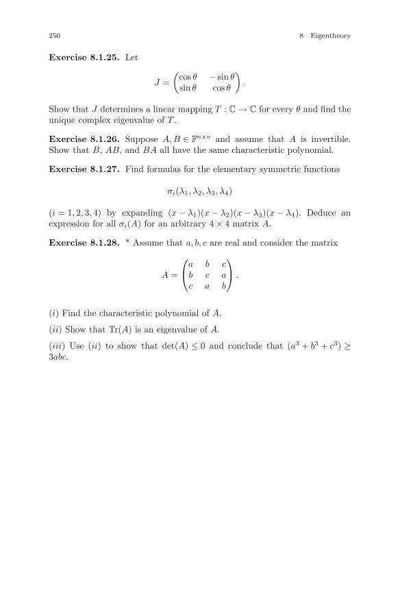
250 8 Eigentheory
Exercise 8.1.25. Let
J =(
cos θ − sin θsin θ cos θ
).
Show that J determines a linear mapping T : C → C for every θ and find theunique complex eigenvalue of T .
Exercise 8.1.26. Suppose A,B ∈ Fn×n and assume that A is invertible.
Show that B, AB, and BA all have the same characteristic polynomial.
Exercise 8.1.27. Find formulas for the elementary symmetric functions
σi(λ1, λ2, λ3, λ4)
(i = 1, 2, 3, 4) by expanding (x − λ1)(x − λ2)(x − λ3)(x − λ4). Deduce anexpression for all σi(A) for an arbitrary 4 × 4 matrix A.
Exercise 8.1.28. * Assume that a, b, c are real and consider the matrix
A =
⎛⎝a b c
b c ac a b
⎞⎠ .
(i) Find the characteristic polynomial of A.
(ii) Show that Tr(A) is an eigenvalue of A.
(iii) Use (ii) to show that det(A) ≤ 0 and conclude that (a3 + b3 + c3) ≥3abc.
8.2 Basic Results on Eigentheory 251
8.2 Basic Results on Eigentheory
We now return to the general problem of understanding the eigentheory of alinear mapping T : V → V . We have already shown how to obtain eigenpairsfor a matrix, but it remains to show, first, how an eigenpair for a matrixdetermines an eigenpair for the linear mapping that the matrix represents,and second, how an eigenbasis for a matrix determines an eigenbasis for thislinear mapping. We will also mention a sufficient condition for the existence ofan eigenbasis that will be generalized in the next section. Finally, we will givea couple of nice applications of eigentheory. In particular, we will introducethe notion of a dynamical system and use it to study the Fibonacci sequence.
8.2.1 Eigenpairs for linear mappings
Throughout this section, V will denote a finite-dimensional vector space overa field F, and T : V → V will be a linear mapping. Our first objective is toexplain the correspondence between eigenpairs for matrices and eigenpairsfor linear mappings. Suppose dimV = n.
Claim. Assume that A = MBB(T ) is the matrix of T with respect to a
basis B = {v1, . . . ,vn} of V . Let (μ,x) be an eigenpair for A, where x =(x1, . . . , xn)T ∈ F
n. If
v =n∑
i=1
xivi = (v1 v2 · · ·vn)x,
then (λ,v) is an eigenpair for T .
Proof. Recall that by (7.15), A is determined from
(T (v1) T (v2) · · · T (vn)) = (v1 v2 · · ·vn)A.
Since Ax = μx,
T (v) = (T (v1) T (v2) · · · T (vn))x= (v1 v2 · · ·vn)Ax
= μ(v1 v2 · · ·vn)x= μv.
Thus (μ,v) is indeed an eigenpair for T . Summarizing, we have the followingresult.
252 8 Eigentheory
Proposition 8.4. Let T : V → V be linear, and let A = MBB(T ) be the
matrix of T with respect to a basis B of V . Then every eigenpair (μ,x) for Agives an eigenpair (μ,v) for T, where v is the element of V whose coordinateswith respect to B are the components of x. Conversely, an eigenpair (μ,v)for T gives a corresponding eigenpair (μ,x) for A in the same manner.
8.2.2 Diagonalizable matrices
Recall from Example 8.1 that the matrix(
1 22 1
)has eigenvalues 3 and
−1 and corresponding eigenspaces R
(11
)and R
(1
−1
). When this data is
encoded in a matrix equation, we see that
(1 22 1
)(1 11 −1
)=
(3 −13 1
)=
(1 11 −1
)(3 00 −1
).
This expression has the form AP = PD, where the columns of P are linearlyindependent eigenvectors and the entries of D are the corresponding eigen-values. Since P is invertible, we get the factorization A = PDP−1, whereD is diagonal. Thus, A is similar to a diagonal matrix over F. Let us nowintroduce the following term.
Definition 8.2. A matrix A ∈ Fn×n is said to be diagonalizable over F if A
can be written A = PDP−1, where D,P ∈ Fn×n and D is diagonal. In other
words, A is diagonalizable over F if it is similar over F to a diagonal matrixD ∈ F
n×n.
We now describe what it means to say that a matrix is diagonalizable.Assume A ∈ F
n×n.
Proposition 8.5. Suppose w1, . . . ,wn is an eigenbasis of Fn for A withcorresponding eigenvalues λ1, . . . , λn in F. Then A is diagonalizable over F.In fact, A = PDP−1, where P = (w1 · · · wn) and D = diag(λ1, . . . , λn).Conversely, if A = PDP−1, where P and D are in F
n×n, P is invertible, andD is diagonal, then the columns of P are an eigenbasis of Fn for A, and thediagonal entries of D are the corresponding eigenvalues. That is, if the ithcolumn of P is wi, then (λi,wi) is an eigenpair for A.
Proof. Let w1, . . . ,wn be an eigenbasis, and put P = (w1 · · · wn). Then
AP = (Aw1 · · · Awn) = (λ1w1 · · · λnwn) = (w1 · · · wn)D, (8.6)
where D = diag(λ1, . . . , λn). Thus AP = PD, so A is diagonalizable overF. The converse is proved in a similar manner. �
8.2 Basic Results on Eigentheory 253
Recall, a linear mapping having an eigenbasis is called semisimple. Findingan eigenbasis for a linear mapping reduces to the problem of diagonalizingits matrix.
Proposition 8.6. Suppose dim V = n, B = {v1, . . . ,vn} is a basis of Vand A = MB
B(T ) is the matrix of T with respect to B. Then T is semisimpleif and only if A is diagonalizable over F, say A = PDP−1, and an eigenbasisw1, . . . , wn for T is given by
(w1 w2 · · ·wn) = (v1 v2 · · ·vn)P. (8.7)
Proof. The proof is similar to the last, but we will give it anyway. Assume thenotation already in use above, and suppose A = PDP−1, where P,D ∈ F
n×n
and D is diagonal. Then
(T (v1) T (v2) · · · T (vn)) = (v1 v2 · · ·vn)PDP−1,
so(T (v1) T (v2) · · · T (vn))P = (v1 v2 · · ·vn)PD.
Thus if w1, . . . ,wn are defined by
(w1 w2 · · ·wn) = (v1 v2 · · ·vn)P,
then since P is nonsingular, w1, . . . ,wn form a basis of V such that
T (w1 w2 · · ·wn) = T (v1 v2 · · ·vn)P= (T (v1) T (v2) · · · T (vn))P= (v1 v2 · · ·vn)(PDP−1)P= (v1 v2 · · ·vn)PD
= (w1 w2 · · ·wn)D.
Consequently, since D is diagonal, w1, . . . ,wn form a basis of V such thatT (wi) = λiwi for each i. Hence T is semisimple. The converse is proved byreversing the argument. �
Consequently, we have the following corollary.
Corollary 8.7. A linear mapping T : V → V is semisimple if and only ifits matrix with respect to some basis of V is diagonal, and consequently itsmatrix with respect to any basis of V is diagonalizable.
254 8 Eigentheory
8.2.3 A criterion for diagonalizability
The following proposition states a well-known criterion for diagonalizability.Since we will prove a stronger result later, the proof will be omitted. We willalso give what amounts to a one-line proof in Example 8.10.
Proposition 8.8. An n × n matrix A over F with n distinct eigenvalues inF is diagonalizable. More generally, if V is a finite-dimensional vector spaceover F and T : V → V is a linear mapping with dim V distinct eigenvaluesin F, then T is semisimple.
The criterion for A ∈ Fn×n to have distinct eigenvalues, given that its
eigenvalues lie in F, is that its characteristic polynomial have simple roots.The multiple root test (Corollary 2.38) applied to pA(x) therefore gives thefollowing.
Proposition 8.9. A square matrix A over F has no repeated eigenvalues inF if pA(x) and its derivative (pA)′(x) have no common roots in F.
Example 8.5. The counting matrix
C =
⎛⎝1 2 3
4 5 67 8 9
⎞⎠
has characteristic polynomial pC(x) = −x3 + 15x2 − 18x; hence C has threedistinct real eigenvalues. It follows that C is diagonalizable. �
Example 8.6. The matrix
A =
⎛⎜⎜⎝
0 1 0 11 0 2 10 2 0 01 1 0 0
⎞⎟⎟⎠ ,
which is seen on a blackboard in the movie Good Will Hunting, has charac-teristic polynomial
pA(x) = x4 − 7x2 − 2x + 4.
Now, −1 is a root, and hence
pA(x) = (x + 1)(x3 − x2 − 6x + 4).
Since −1 is not a root of q(x) = x3 − x2 − 6x + 4 = 0, it follows that pA(x)has four distinct roots as long as q(x) has three distinct roots. But q′(x) =3x2 − 2x − 6 has roots
8.2 Basic Results on Eigentheory 255
r =2 ±
√76
6,
and
q(2 +
√76
6) < 0, while q(
2 −√
766
) > 0.
Thus q and q′ have no roots in common, so q has three distinct roots. More-over, it follows from the two inequalities above that q has three real roots.(Reason: the coefficient of x3 is positive.) Thus A has four distinct real eigen-values; hence A is diagonalizable. �
Note that the Good Will Hunting matrix A is real and symmetric. Aswe will see later, the principal axis theorem therefore guarantees that A isdiagonalizable.
8.2.4 The powers of a diagonalizable matrix
In this section, we will consider the powers of a square matrix A. Let us beginwith the following observation. Suppose A ∈ F
n×n has an eigenpair (λ,v) andlet k be a positive integer. Since Akv = Ak−1(Av) = Ak−1(λv) = λAk−1v, itfollows by iteration that
Akv = λkv.
Now suppose A can be diagonalized as A = PDP−1. Then for every positiveinteger k,
Ak = (PDP−1)(PDP−1) · · · (PDP−1) = PDkP−1.
If D = diag(λ1, λ2, . . . , λn), then Dk = diag((λ1)k, (λ2)k, . . . , (λn)k
). Let P =
(v1 v2 · · · vn). Setting v =∑
aivi, we have
Akv =∑
aiAkvi =
∑ai(λi)kvi. (8.8)
If A ∈ Rn×n and all its eigenvalues are real, one can say more:
(i) If A has only nonnegative eigenvalues, then A has a kth root for everypositive integer k. In fact, A
1k = PD
1k P−1.
(ii) If none of the eigenvalues of A are 0, then the negative powers of A arefound from the formula A−k = (A−1)k = PD−kP−1.
(iii) If all the eigenvalues λ of A satisfy |λ| < 1, then limm→∞ Am = O.
256 8 Eigentheory
More generally, if A ∈ Cn×n, there are corresponding statements. The
reader should attempt to formulate them. For nondiagonalizable matrices,kth roots need not exist.
8.2.5 The Fibonacci sequence as a dynamicalsystem
The Fibonacci numbers ak are defined by the Fibonacci sequence (ak)as follows. Starting with arbitrary integers a0 and a1, put a2 = a0 + a1,a3 = a2 + a1, and in general, put ak = ak−1 + ak−2 if k ≥ 2. The Fibonaccisequence can also be defined by the matrix identity
(ak+1
ak
)=
(1 11 0
)(ak
ak−1
),
provided k ≥ 1. Hence putting
F =(
1 11 0
),
we obtain that(
ak+1
ak
)= F
(ak
ak−1
)= F 2
(ak−1
ak−2
)= · · · = F k
(a1
a0
).
Thus putting
vk =(
ak+1
ak
),
for k = 0, 1, 2, . . . , we can therefore express the Fibonacci sequence in theform
vk = F kv0. (8.9)
Such a sequence is called the dynamical system defined by F . To analyze theFibonacci sequence, we will diagonalize F . The characteristic equation of Fis x2 − x − 1 = 0, so the eigenvalues are
φ =1 +
√5
2, μ =
1 −√
52
.
One checks that N (F − φI2) = R(φ, 1)T and N (F − μI2) = R(μ, 1)T . There-fore, as in the previous example, F is diagonalized by
8.2 Basic Results on Eigentheory 257
F =(
φ μ1 1
) (φ 00 μ
)(φ μ1 1
)−1
.
Hence, by (8.9),
(am+1
am
)= Fm
(a1
a0
)=
(φ μ1 1
) (φm 00 μm
)(φ μ1 1
)−1 (a1
a0
).
Since(
φ μ1 1
)−1
=1
φ − μ
(1 −μ
−1 φ
), we get
(am+1
am
)=
1φ − μ
(φm+1 − μm+1 −μφm+1 + μm+1φ
φm − μm μφm + μmφ
) (a1
a0
).
For example, if a0 = 0 and a1 = 1, we see that
am =φm − μm
φ − μ=
1√5 · 2m
((1 +√
5)m − (1 −√
5)m). (8.10)
Notice that
limm→∞
am+1
am= lim
m→∞φm+1 − μm+1
φm − μm= φ,
since limm→∞(μ/φ)m = 0. Therefore, for large m, the ratio am+1/am isapproximately φ. A little further computation gives the precise formulas
a2m =[φ2m
√5
]and a2m+1 =
[φ2m+1
√5
]+ 1,
where [r] denotes the integer part of the real number r.
The eigenvalue φ =1 +
√5
2is the so-called golden ratio. It comes up in
many unexpected and interesting ways. For more information, one can consultThe Story of φ, the World’s Most Astonishing Number, by Mario Livo.
Exercises
Exercise 8.2.1. Diagonalize the following matrices when possible:
A =(
1 −1−1 1
), B =
⎛⎝1 0 1
0 1 01 0 1
⎞⎠ , C =
⎛⎜⎜⎝
−3 0 −4 −40 2 1 14 0 5 4
−4 0 −4 −3
⎞⎟⎟⎠ .
258 8 Eigentheory
Exercise 8.2.2. A 4 × 4 matrix over R has eigenvalues ±1, trace 3, anddeterminant 0. Can A be diagonalized over R? What about over Q?
Exercise 8.2.3. Determine which of the following matrices are diagonaliz-able over the reals:⎛⎝
1 0 −1
−1 1 1
2 −1 −2
⎞⎠ ,
⎛⎝0 1 1
1 0 1
1 −1 1
⎞⎠ ,
⎛⎝2 −1 1
1 0 1
1 −1 −2
⎞⎠ ,
⎛⎝0 1 0
1 0 −1
0 1 0
⎞⎠ .
Exercise 8.2.4. Find all possible square roots, if any exist, of the followingmatrices: (
2 11 2
),
(1 22 1
),
(1 −11 −1
).
Exercise 8.2.5. Do the same as in Problem 8.2.4 for the 4 × 4 all 1’s matrix.
Exercise 8.2.6. Compute the nth power of each matrix of Exercise 8.2.4and also that of the 3 × 3 all 1’s matrix.
Exercise 8.2.7. Let F denote the Fibonacci matrix. Find F 4 in two ways,once directly and once using eigentheory.
Exercise 8.2.8. Assuming a0 = 0 and a1 = 1, find the thirteenth andfifteenth Fibonacci numbers using eigentheory.
Exercise 8.2.9. Show directly that
φm − μm
φ − μ=
1√5 · 2m
((1 +√
5)m − (1 −√
5)m)
is an integer, thus explaining the strange expression in Section 5.1.
Exercise 8.2.10. Let A =(
1 22 1
). Find A10.
Exercise 8.2.11. Give an example of a 2 × 2 matrix A over C that does nothave a square root.
Exercise 8.2.12. If possible, find a square root for A =(
1 10 1
).
Exercise 8.2.13. Suppose G is a finite subgroup of GL(n,C) of order m.Show that if g ∈ G, then every eigenvalue of g is an mth root of unity.
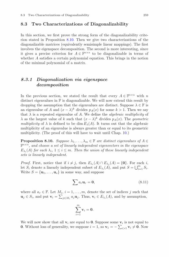
8.3 Two Characterizations of Diagonalizability 259
8.3 Two Characterizations of Diagonalizability
In this section, we first prove the strong form of the diagonalizability crite-rion stated in Proposition 8.10. Then we give two characterizations of thediagonalizable matrices (equivalently semisimple linear mappings). The firstinvolves the eigenspace decomposition. The second is more interesting, sinceit gives a precise criterion for A ∈ F
n×n to be diagonalizable in terms ofwhether A satisfies a certain polynomial equation. This brings in the notionof the minimal polynomial of a matrix.
8.3.1 Diagonalization via eigenspacedecomposition
In the previous section, we stated the result that every A ∈ Fn×n with n
distinct eigenvalues in F is diagonalizable. We will now extend this result bydropping the assumption that the eigenvalues are distinct. Suppose λ ∈ F isan eigenvalue of A and (x − λ)k divides pA(x) for some k > 1. Then we saythat λ is a repeated eigenvalue of A. We define the algebraic multiplicity ofλ as the largest value of k such that (x − λ)k divides pA(x). The geometricmultiplicity of λ is defined to be dim Eλ(A). It turns out that the algebraicmultiplicity of an eigenvalue is always greater than or equal to its geometricmultiplicity. (The proof of this will have to wait until Chap. 10.)
Proposition 8.10. Suppose λ1, . . . , λm ∈ F are distinct eigenvalues of A ∈F
n×n, and choose a set of linearly independent eigenvectors in the eigenspaceEλi
(A) for each λi, 1 ≤ i ≤ m. Then the union of these linearly independentsets is linearly independent.
Proof. First, notice that if i �= j, then Eλi(A) ∩ Eλj
(A) = {0}. For each i,let Si denote a linearly independent subset of Eλi
(A), and put S =⋃m
i=1 Si.Write S = {u1, . . . ,us} in some way, and suppose
∑arur = 0, (8.11)
where all ar ∈ F. Let Mi, i = 1, . . . , m, denote the set of indices j such thatuj ∈ Si, and put vi =
∑j∈Mi
ajuj . Thus, vi ∈ Eλi(A), and by assumption,
m∑i=1
vi = 0.
We will now show that all vi are equal to 0. Suppose some vi is not equal to0. Without loss of generality, we suppose i = 1, so v1 = −
∑i>1 vi �= 0. Now
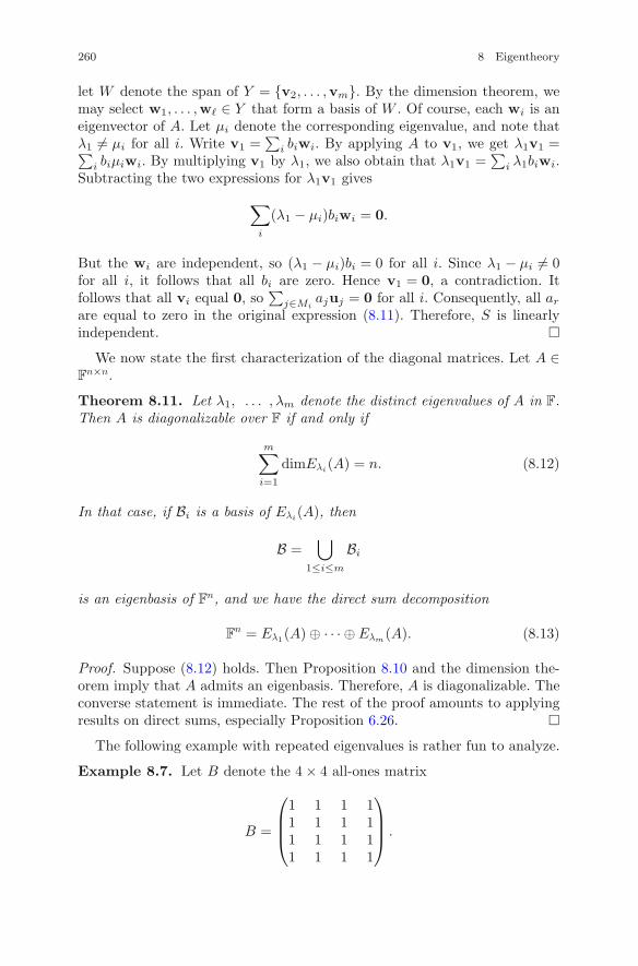
260 8 Eigentheory
let W denote the span of Y = {v2, . . . ,vm}. By the dimension theorem, wemay select w1, . . . ,w� ∈ Y that form a basis of W . Of course, each wi is aneigenvector of A. Let μi denote the corresponding eigenvalue, and note thatλ1 �= μi for all i. Write v1 =
∑i biwi. By applying A to v1, we get λ1v1 =∑
i biμiwi. By multiplying v1 by λ1, we also obtain that λ1v1 =∑
i λ1biwi.Subtracting the two expressions for λ1v1 gives
∑i
(λ1 − μi)biwi = 0.
But the wi are independent, so (λ1 − μi)bi = 0 for all i. Since λ1 − μi �= 0for all i, it follows that all bi are zero. Hence v1 = 0, a contradiction. Itfollows that all vi equal 0, so
∑j∈Mi
ajuj = 0 for all i. Consequently, all ar
are equal to zero in the original expression (8.11). Therefore, S is linearlyindependent. �
We now state the first characterization of the diagonal matrices. Let A ∈F
n×n.
Theorem 8.11. Let λ1, . . . , λm denote the distinct eigenvalues of A in F.Then A is diagonalizable over F if and only if
m∑i=1
dimEλi(A) = n. (8.12)
In that case, if Bi is a basis of Eλi(A), then
B =⋃
1≤i≤m
Bi
is an eigenbasis of Fn, and we have the direct sum decomposition
Fn = Eλ1(A) ⊕ · · · ⊕ Eλm
(A). (8.13)
Proof. Suppose (8.12) holds. Then Proposition 8.10 and the dimension the-orem imply that A admits an eigenbasis. Therefore, A is diagonalizable. Theconverse statement is immediate. The rest of the proof amounts to applyingresults on direct sums, especially Proposition 6.26. �
The following example with repeated eigenvalues is rather fun to analyze.
Example 8.7. Let B denote the 4 × 4 all-ones matrix
B =
⎛⎜⎜⎝
1 1 1 11 1 1 11 1 1 11 1 1 1
⎞⎟⎟⎠ .
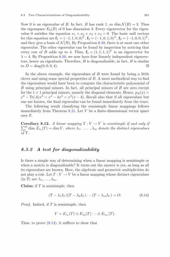
8.3 Two Characterizations of Diagonalizability 261
Now 0 is an eigenvalue of B. In fact, B has rank 1, so dimN (B) = 3. Thusthe eigenspace E0(B) of 0 has dimension 3. Every eigenvector for the eigen-value 0 satisfies the equation x1 + x2 + x3 + x4 = 0. The basic null vectorsfor this equation are f1 = (−1, 1, 0, 0)T , f2 = (−1, 0, 1, 0)T , f3 = (−1, 0, 0, 1)T ,and they give a basis of N (B). By Proposition 8.10, there is at most one othereigenvalue. The other eigenvalue can be found by inspection by noticing thatevery row of B adds up to 4. Thus, f4 = (1, 1, 1, 1)T is an eigenvector forλ = 4. By Proposition 8.10, we now have four linearly independent eigenvec-tors, hence an eigenbasis. Therefore, B is diagonalizable; in fact, B is similarto D = diag(0, 0, 0, 4). �
In the above example, the eigenvalues of B were found by being a littleclever and using some special properties of B. A more methodical way to findthe eigenvalues would have been to compute the characteristic polynomial ofB using principal minors. In fact, all principal minors of B are zero exceptfor the 1 × 1 principal minors, namely the diagonal elements. Hence, pB(x) =x4 − Tr(A)x3 = x4 − 4x3 = x3(x − 4). Recall also that if all eigenvalues butone are known, the final eigenvalue can be found immediately from the trace.
The following result classifying the semisimple linear mappings followsimmediately from Theorem 8.11. Let V be a finite-dimensional vector spaceover F.
Corollary 8.12. A linear mapping T : V → V is semisimple if and only if∑mi dim Eλi
(T ) = dim V , where λ1, . . . , λm denote the distinct eigenvaluesof T .
8.3.2 A test for diagonalizability
Is there a simple way of determining when a linear mapping is semisimple orwhen a matrix is diagonalizable? It turns out the answer is yes, as long as allits eigenvalues are known. Here, the algebraic and geometric multiplicities donot play a role. Let T : V → V be a linear mapping whose distinct eigenvalues(in F) are λ1, . . . , λm.
Claim: if T is semisimple, then
(T − λ1IV )(T − λ2IV ) · · · (T − λmIV ) = O. (8.14)
Proof. Indeed, if T is semisimple, then
V = Eλ1(T ) ⊕ Eλ2(T ) · · · ⊕ Eλm(T ).
Thus, to prove (8.14), it suffices to show that
262 8 Eigentheory
(T − λ1IV )(T − λ2IV ) · · · (T − λmIV )vi = 0,
provided vi ∈ Eλi(T ) for some i. But this is clear, since
(T − λiIV )(T − λjIV ) = (T − λjIV )(T − λiIV )
for all i and j. Thus, the left-hand side of (8.14) can be factored into the formC(T − λiIV ), and since C(T − λiIV )vi = C0 = 0, (8.14) follows. �
There is another way to prove (8.14). To do so, we need to evaluate a poly-nomial f(x) = anx
n + an−1xn−1 + · · · + a1x + a0 in F[x] on a matrix in F
n×n.The value of f at A is defined to be f(A) = anA
n + an−1An−1 + · · · + a1A +
a0In. Thus, f(A) ∈ Fn×n. Similarly, if and T : V → V is a linear mapping,
then by definition,
f(T ) = anTn + an−1T
n−1 + · · · + a1T + a0IV ,
where T i means T composed with itself i times. Thus, f(T ) is also a linearmapping with domain and target V . Note that if A = PDP−1, where A ∈F
n×n, then f(A) = f(PDP−1) = Pf(A)P−1. Thus, if A = Pdiag(λ1, λ2 . . . ,λn)P−1 and g(x) = (x − λ1)(x − λ2) · · · (x − λm), then
g(A) = g(PDP−1) = Pg(D)P−1 = Pdiag(g(λ1), g(λ2), . . . , g(λm))P−1.
But diag(g(λ1), g(λ2), . . . , g(λm)) = O, so g(A) = O also. �The useful fact is that the converse is also true. We state and prove that
next.
Theorem 8.13. Suppose the distinct eigenvalues of a linear mapping T :V → V are λ1, . . . , λm. Then T is semisimple if and only if
(T − λ1IV )(T − λ2IV ) · · · (T − λmIV ) = O. (8.15)
Proof. The “only if” implication was just proved. The “if” assertion, whichis harder to prove, is based on the following lemma.
Lemma 8.14. Suppose T1, T2, . . . , TN : V → V are linear mappings that sat-isfy the following properties:
(i) T1 ◦ T2 ◦ · · · ◦ TN = O,
(ii) Ti ◦ Tj = Tj ◦ Ti for all indices i, j,
(iii) for each i = 1, . . . , N − 1, ker(Ti) ∩ ker(Ti+1 ◦ · · · ◦ TN ) = {0}.Then V = ker(T1) ⊕ ker(T2) ⊕ · · · ⊕ ker(TN ).
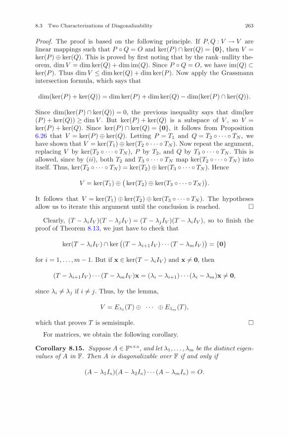
8.3 Two Characterizations of Diagonalizability 263
Proof. The proof is based on the following principle. If P,Q : V → V arelinear mappings such that P ◦ Q = O and ker(P ) ∩ ker(Q) = {0}, then V =ker(P ) ⊕ ker(Q). This is proved by first noting that by the rank–nullity the-orem, dim V = dim ker(Q) + dim im(Q). Since P ◦ Q = O, we have im(Q) ⊂ker(P ). Thus dimV ≤ dim ker(Q) + dim ker(P ). Now apply the Grassmannintersection formula, which says that
dim(ker(P ) + ker(Q)) = dim ker(P ) + dim ker(Q) − dim(ker(P ) ∩ ker(Q)).
Since dim(ker(P ) ∩ ker(Q)) = 0, the previous inequality says that dim(ker(P ) + ker(Q)) ≥ dim V . But ker(P ) + ker(Q) is a subspace of V , so V =ker(P ) + ker(Q). Since ker(P ) ∩ ker(Q) = {0}, it follows from Proposition6.26 that V = ker(P ) ⊕ ker(Q). Letting P = T1 and Q = T2 ◦ · · · ◦ TN , wehave shown that V = ker(T1) ⊕ ker(T2 ◦ · · · ◦ TN ). Now repeat the argument,replacing V by ker(T2 ◦ · · · ◦ TN ), P by T2, and Q by T3 ◦ · · · ◦ TN . This isallowed, since by (ii), both T2 and T3 ◦ · · · ◦ TN map ker(T2 ◦ · · · ◦ TN ) intoitself. Thus, ker(T2 ◦ · · · ◦ TN ) = ker(T2) ⊕ ker(T3 ◦ · · · ◦ TN ). Hence
V = ker(T1) ⊕(ker(T2) ⊕ ker(T3 ◦ · · · ◦ TN )
).
It follows that V = ker(T1) ⊕ ker(T2) ⊕ ker(T3 ◦ · · · ◦ TN ). The hypothesesallow us to iterate this argument until the conclusion is reached. �
Clearly, (T − λiIV )(T − λjIV ) = (T − λjIV )(T − λiIV ), so to finish theproof of Theorem 8.13, we just have to check that
ker(T − λiIV ) ∩ ker((T − λi+1IV ) · · · (T − λmIV )
)= {0}
for i = 1, . . . , m − 1. But if x ∈ ker(T − λiIV ) and x �= 0, then
(T − λi+1IV ) · · · (T − λmIV )x = (λi − λi+1) · · · (λi − λm)x �= 0,
since λi �= λj if i �= j. Thus, by the lemma,
V = Eλ1(T ) ⊕ · · · ⊕ Eλm(T ),
which that proves T is semisimple. �For matrices, we obtain the following corollary.
Corollary 8.15. Suppose A ∈ Fn×n, and let λ1, . . . , λm be the distinct eigen-
values of A in F. Then A is diagonalizable over F if and only if
(A − λ1In)(A − λ2In) · · · (A − λmIn) = O.
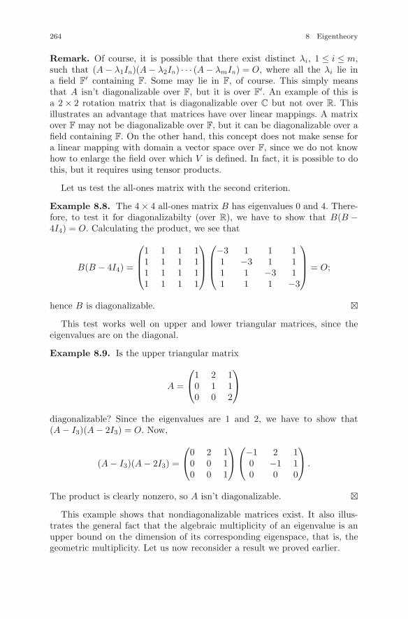
264 8 Eigentheory
Remark. Of course, it is possible that there exist distinct λi, 1 ≤ i ≤ m,such that (A − λ1In)(A − λ2In) · · · (A − λmIn) = O, where all the λi lie ina field F
′ containing F. Some may lie in F, of course. This simply meansthat A isn’t diagonalizable over F, but it is over F
′. An example of this isa 2 × 2 rotation matrix that is diagonalizable over C but not over R. Thisillustrates an advantage that matrices have over linear mappings. A matrixover F may not be diagonalizable over F, but it can be diagonalizable over afield containing F. On the other hand, this concept does not make sense fora linear mapping with domain a vector space over F, since we do not knowhow to enlarge the field over which V is defined. In fact, it is possible to dothis, but it requires using tensor products.
Let us test the all-ones matrix with the second criterion.
Example 8.8. The 4 × 4 all-ones matrix B has eigenvalues 0 and 4. There-fore, to test it for diagonalizabilty (over R), we have to show that B(B −4I4) = O. Calculating the product, we see that
B(B − 4I4) =
⎛⎜⎜⎝
1 1 1 11 1 1 11 1 1 11 1 1 1
⎞⎟⎟⎠
⎛⎜⎜⎝
−3 1 1 11 −3 1 11 1 −3 11 1 1 −3
⎞⎟⎟⎠ = O;
hence B is diagonalizable. �
This test works well on upper and lower triangular matrices, since theeigenvalues are on the diagonal.
Example 8.9. Is the upper triangular matrix
A =
⎛⎝1 2 1
0 1 10 0 2
⎞⎠
diagonalizable? Since the eigenvalues are 1 and 2, we have to show that(A − I3)(A − 2I3) = O. Now,
(A − I3)(A − 2I3) =
⎛⎝0 2 1
0 0 10 0 1
⎞⎠
⎛⎝−1 2 1
0 −1 10 0 0
⎞⎠ .
The product is clearly nonzero, so A isn’t diagonalizable. �
This example shows that nondiagonalizable matrices exist. It also illus-trates the general fact that the algebraic multiplicity of an eigenvalue is anupper bound on the dimension of its corresponding eigenspace, that is, thegeometric multiplicity. Let us now reconsider a result we proved earlier.
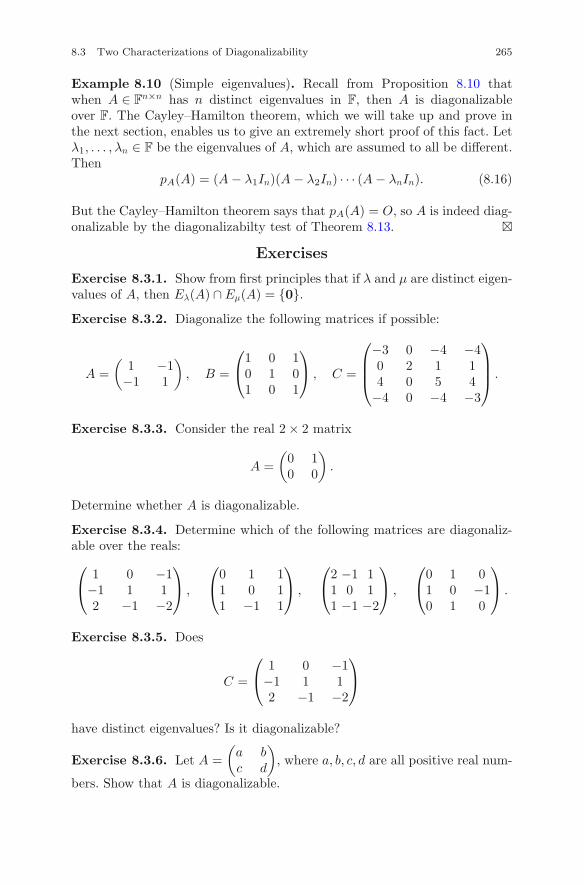
8.3 Two Characterizations of Diagonalizability 265
Example 8.10 (Simple eigenvalues). Recall from Proposition 8.10 thatwhen A ∈ F
n×n has n distinct eigenvalues in F, then A is diagonalizableover F. The Cayley–Hamilton theorem, which we will take up and prove inthe next section, enables us to give an extremely short proof of this fact. Letλ1, . . . , λn ∈ F be the eigenvalues of A, which are assumed to all be different.Then
pA(A) = (A − λ1In)(A − λ2In) · · · (A − λnIn). (8.16)
But the Cayley–Hamilton theorem says that pA(A) = O, so A is indeed diag-onalizable by the diagonalizabilty test of Theorem 8.13. �
Exercises
Exercise 8.3.1. Show from first principles that if λ and μ are distinct eigen-values of A, then Eλ(A) ∩ Eμ(A) = {0}.
Exercise 8.3.2. Diagonalize the following matrices if possible:
A =(
1 −1−1 1
), B =
⎛⎝1 0 1
0 1 01 0 1
⎞⎠ , C =
⎛⎜⎜⎝
−3 0 −4 −40 2 1 14 0 5 4
−4 0 −4 −3
⎞⎟⎟⎠ .
Exercise 8.3.3. Consider the real 2 × 2 matrix
A =(
0 10 0
).
Determine whether A is diagonalizable.
Exercise 8.3.4. Determine which of the following matrices are diagonaliz-able over the reals:⎛⎝ 1 0 −1
−1 1 12 −1 −2
⎞⎠ ,
⎛⎝0 1 1
1 0 11 −1 1
⎞⎠ ,
⎛⎝2 −1 1
1 0 11 −1 −2
⎞⎠ ,
⎛⎝0 1 0
1 0 −10 1 0
⎞⎠ .
Exercise 8.3.5. Does
C =
⎛⎝ 1 0 −1
−1 1 12 −1 −2
⎞⎠
have distinct eigenvalues? Is it diagonalizable?
Exercise 8.3.6. Let A =(
a bc d
), where a, b, c, d are all positive real num-
bers. Show that A is diagonalizable.
266 8 Eigentheory
Exercise 8.3.7. Suppose A is the matrix in Exercise 8.3.6. Show that A hasan eigenvector in the first quadrant and another in the third quadrant.
Exercise 8.3.8. Show that if A ∈ Rn×n admits an eigenbasis for R
n, it alsoadmits an eigenbasis for C
n.
Exercise 8.3.9. Let a ∈ R3, and let Ca : R3 → R
3 be the cross productmap Ca(v) = a × v. Find the characteristic polynomial of Ca and determinewhether Ca is semisimple.
Exercise 8.3.10. Let V = Fn×n and let T : V → V be the linear map defined
by sending A ∈ V to AT . That is, T(A) = AT .
(i) Show that the only eigenvalues of T are ±1.
(ii) Prove that if the characteristic of F is different from two, then T semi-simple.
Exercise 8.3.11. Find an example of a nondiagonalizable 3 × 3 matrix Awith real entries that is neither upper nor lower triangular such that everyeigenvalue of A is 0.
Exercise 8.3.12. Let A be a 3 × 3 matrix with eigenvalues 0, 0, 1. Showthat A3 = A2.
Exercise 8.3.13. Let A be a 2 × 2 matrix such that A2 + 3A + 2I2 = O.Show that −1,−2 are eigenvalues of A.
Exercise 8.3.14. Suppose A is a 2 × 2 matrix such that A2 + A − 3I2 = O.Show that A is diagonalizable.
Exercise 8.3.15. Let U be an upper triangular matrix over F with distinctentries on its diagonal. Show that U is diagonalizable.
Exercise 8.3.16. Suppose that a 3 × 3 matrix A over R satisfies the equa-tion A3 + A2 − A + 2I3 = O.
(i) Find the eigenvalues of A.
(ii) Is A diagonalizable? Explain.
Exercise 8.3.17. We say that two n × n matrices A and B are simultane-ously diagonalizable if they are diagonalized by the same matrix M , that is,if they share a common eigenbasis. Show that two simultaneously diagonal-izable matrices A and B commute; that is, AB = BA.
Exercise 8.3.18. This is the converse to Exercise 8.3.17. Suppose A,B ∈F
n×n commute.
(i) Show that for every eigenvalue λ of A, B(Eλ(A)) ⊂ Eλ(A).
(ii) Conclude that if S is the subset of Fn×n consisting of diagonalizable
matrices such that AB = BA for all A,B ∈ S, then the elements of S aresimultaneously diagonalizable.
8.3 Two Characterizations of Diagonalizability 267
Exercise 8.3.19. Let U be an arbitrary upper triangular matrix over F pos-sibly having repeated diagonal entries. Show by example that U may not bediagonalizable, and give a condition to guarantee that it will be diagonalizablewithout any diagonal entries being changed.
Exercise 8.3.20. Let V be a finite dimensional vector space over Fp, p aprime, and let μ be the mapping with domain and target L(V, V ) defined byμ(T ) = T p. Show that μ is linear and find its characteristic polynomial whenV = (Fp)2. Is μ diagonalizable?
268 8 Eigentheory
8.4 The Cayley–Hamilton Theorem
The Cayley–Hamilton theorem gives an interesting and fundamental rela-tionship between a matrix and its characteristic polynomial, which is relatedto our considerations about diagonalizabilty in the previous section. It is, infact, one of the most famous and useful results in matrix theory.
8.4.1 Statement of the theorem
The version of the Cayley–Hamilton theorem we will prove below is statedas follows.
Theorem 8.16 (Cayley–Hamilton theorem). Let F be a field and supposeA ∈ F
n×n. Then A satisfies its characteristic polynomial, that is, pA(A) = O.Consequently, if V is a finite-dimensional vector space over F and T : V → Vis linear, then pT (T ) = OV , where OV is the zero mapping on V .
The proof we give below in Section 8.4.4 was noticed by Jochen Kuttlerand myself. It is more straightforward than the usual proof based on Cramer’srule. We first prove that PA(A) = O inductively just using matrix theory andthe assumption that F contains all the eigenvalues of A. The second step inthe proof, which doesn’t involve matrix theory, is to show that there existsa field F
′ containing F such that all the roots of pA(x) = 0 lie in F. We sayF
′ is a splitting field for pA. Thus, pA(A) = O holds in F′n×n, and hence
pA(A) = O in Fn×n too. And since it holds for A, it also holds for T .
8.4.2 The real and complex cases
If A is a real n × n matrix, its eigenvalues all lie in C, and if A is diagonalizableover C, say A = MDM−1, then
pA(A) = pA(MDM−1) = MpA(D)M−1 = Mdiag(pA(λ1), pA(λ2), . . . , pA(λn))M−1 = O,
by the argument in Section 8.3.2. With some ingenuity, one can fashion aproof for arbitrary complex matrices (in particular, real matrices) by showingthat every square matrix over C is the limit of a sequence of diagonalizablematrices.
Here is an important 2 × 2 example.
Example 8.11. For example, the characteristic polynomial of the matrixJ =
(0 −11 0
)is x2 + 1. Cayley–Hamilton asserts that J2 + I2 = O, which is
easy to check directly. Notice that the eigenvalues of J are ±i, so J is diago-nalizable over C, though not over R. �
8.4 The Cayley–Hamilton Theorem 269
8.4.3 Nilpotent matrices
A square matrix A is said to be nilpotent if Am = O for some integer m > 0.For example,
A =(
1 −11 −1
)
is nilpotent, since A2 = O. It follows directly from the definition of an eigen-value that a nilpotent matrix cannot have a nonzero eigenvalue. (Convinceyourself of this.) Thus if an n × n matrix A is nilpotent, its characteristicpolynomial pA(x) is equal to (−1)nxn.
Proposition 8.17. If an n × n matrix A is nilpotent, then An = O.
Proof. Just apply Cayley–Hamilton. �
More generally, we also have the following definition.
Definition 8.3. A linear mapping T : V → V is said to be nilpotent if itsonly eigenvalue is 0.
So the previous proposition implies the following result.
Proposition 8.18. If T : V → V is nilpotent, then (T )dimV = O.
8.4.4 A proof of the Cayley–Hamilton theorem
We will first show that pA(A) = O for every A ∈ Fn×n, provided all the eigen-
values of A lie in F. We will induct on n, the case n = 1 being trivial, since ifA = (a), then pA(x) = a − x and thus pA(A) = pA(a) = 0. Assume the resultfor n − 1, where n > 1. Let (λ1,v1) be an eigenpair for A, and extend v1 toa basis B of Fn. Then A is similar to B = MB
B(TA), so pA(x) = pB(x), andhence it suffices to show that pB(B) = O. Now
B =
⎛⎜⎜⎜⎝
λ1 ∗ · · · ∗0... B1
0
⎞⎟⎟⎟⎠ ,
where B1 ∈ F(n−1)×(n−1). It follows from this block decomposition that
det(B − xIn) = (λ1 − x) det(B1 − xIn−1). Since pA(x) = pB(x) and theeigenvaluesλ1, λ2, . . . , λn of A all lie in F, it follows that the eigenvalues ofB are in F, so the eigenvalues λ2, . . . , λn of B1 are also in F. These all beingelements of F, we may apply the induction hypothesis to B1. First, notice
270 8 Eigentheory
the following fact about block matrix multiplication: if C1 and C2 are of size(n − 1) × (n − 1), then
⎛⎜⎜⎜⎝
c1 ∗ · · · ∗0... C1
0
⎞⎟⎟⎟⎠
⎛⎜⎜⎜⎝
c2 ∗ · · · ∗0... C2
0
⎞⎟⎟⎟⎠ =
⎛⎜⎜⎜⎝
c1c2 ∗ · · · ∗0... C1C2
0
⎞⎟⎟⎟⎠ .
Now calculate pB(B). By the previous comment,
pB(B) = (−1)n(B − λ1In)(B − λ2In) · · · (B − λnIn)
= (−1)n
⎛⎜⎜⎜⎝
0 ∗ · · · ∗0... B1 − λ1In−1
0
⎞⎟⎟⎟⎠
⎛⎜⎜⎜⎝
∗ ∗ · · · ∗0... C0
⎞⎟⎟⎟⎠ ,
whereC = (B1 − λ2In−1) · · · (B1 − λnIn−1).
But clearly C = pB1(B1), so by the induction hypothesis, it follows thatC = O. Thus
pB(B) = (−1)n
⎛⎜⎜⎜⎝
0 ∗ · · · ∗0... B1 − λ1In−1
0
⎞⎟⎟⎟⎠
⎛⎜⎜⎜⎝
∗ ∗ · · · ∗0... O0
⎞⎟⎟⎟⎠ .
Carrying out the multiplication, one sees immediately that pB(B) = O. �The assumption that all the roots of the characteristic polynomial of A lie
in F is actually unnecessary, due to the next result.
Lemma 8.19. Let F be a field. Then for every polynomial f(x) ∈ F[x], thereexists a field F
′ containing F and all the roots of f(x) = 0.
We will give a proof of this fact in Section 8.7. Thus the eigenvalues of Alie in an extension F
′ of F, so pA(A) = O. All that remains to be proved isthat a linear mapping also satisfies its characteristic polynomial. Let V be afinite-dimensional vector space over F and T : V → V a linear mapping. Thenfor every matrix A of T with respect to a basis of V , we have pA(A) = O.But as noted already, the matrix of pT (T ) with respect to this basis is pA(A).Since pA(A) = O, it follows that pT (T ) is zero also. �
8.4 The Cayley–Hamilton Theorem 271
8.4.5 The minimal polynomial of a linear mapping
Let V be as usual and T : V → V a linear mapping. By the Cayley–Hamiltontheorem, pT (T ) = OV , and therefore there exists a polynomial f(x) ∈ F[x] ofleast degree and leading coefficient one such that f(T ) = OV . This followsby division with remainder. For if f1 and f2 satisfy the minimal polynomialcriterion, then f1 and f2 must have the same degree k. Then g = f1 − f2 isa polynomial of degree at most k − 1 such that g(T ) = O. Thus g = 0. Theminimal polynomial of T will be denoted by μT . The minimal polynomialμA of a matrix A ∈ F
n×n is defined in exactly the same way, and if A is thematrix of T , then μA = μT .
Proposition 8.20. Suppose T : V → V is a linear mapping whose eigenval-ues lie in F, and let λ1, . . . , λm denote T ’s distinct eigenvalues in F. Then theminimal polynomial μT (x) of T divides the characteristic polynomial pT (x),and q(x) = (x − λ1) · · · (x − λm) divides μT (x).
Proof. Since the degree of μT (x) is at most n, division with remainder in F[x]allows us to write pT (x) = h(x)μT (x) + r(x), where either r = 0 or deg r <deg μT . But pT (T ) = p(T ) = O, r(T ) = O also. By the definition of μT , itfollows that r = 0; hence polynomial p(x) divides pT (x). To conclude thatq(x) divides μT (x), use division with remainder again. Let (λj ,v) be aneigenpair for T , and write μT (x) = f(x)(x − λj) + r. Since μT (T )v = (T −λj)v = 0, it follows that rIn = 0, so r = 0. Thus q divides μT . �
The following corollary restates the diagonalization criterion of Theorem8.13. As above, let q(x) = (x − λ1) · · · (x − λm), where λ1, . . . , λm denote T ’sdistinct eigenvalues.
Corollary 8.21. The linear mapping T : V → V is semisimple if and onlyif its minimal polynomial is q(x).
Proof. If T is semisimple, then all of its eigenvalues lie in F, and by Theorem8.13, q(T ) = O. Therefore, q(x) is the minimal polynomial of T . Conversely,if q(x) is T ’s minimal polynomial, then the criterion of Theorem 8.13 impliesthat T is semisimple. �
Exercises
Exercise 8.4.1. Verify the Cayley–Hamilton theorem directly for
A =
⎛⎝1 0 1
0 1 01 0 1
⎞⎠ .
272 8 Eigentheory
Exercise 8.4.2. Give a direct proof for the 2 × 2 case. That is, show that
A =(
a bc d
)= A2 − Tr(A)A + det(A)I2 = O.
Apparently, this was Cayley’s contribution to the theorem.
Exercise 8.4.3. The following false proof of the Cayley–Hamilton theoremis well known and very persistent. In fact, it actually appears in an alge-bra book. Since setting x = A in pA(x) = det(A − xIn) gives det(A − AIn) =det(A − A) = 0, it follows that pA(A) = O. What is incorrect about this“proof”?
Exercise 8.4.4. Show that a 2 × 2 matrix A is nilpotent if and only ifTr(A) = det(A) = 0. Use this to find a 2 × 2 nilpotent matrix with all entriesdifferent from 0.
Exercise 8.4.5. Use the Cayley–Hamilton theorem to deduce that A ∈F
n×n is nilpotent if and only if all eigenvalues of A are 0.
Exercise 8.4.6. Show that a nonzero nilpotent matrix is not diagonalizable.
Exercise 8.4.7. Without using the Cayley–Hamilton theorem, show that ifan n × n matrix A is nilpotent, then in fact An = O. (Hint: use inductionon n. Choose a basis of N (A) and extend to a basis of Fn. Then apply theinduction to col(A).)
Exercise 8.4.8. * Prove that every A ∈ Cn×n is the limit of a sequence of
diagonalizable matrices, and thus deduce the Cayley–Hamilton theorem overC in another way.
Exercise 8.4.9. Test the following matrices to determine which are diago-nalizable.
(i)(
0 11 0
)and
(1 10 0
)(F = F2).
(ii)
⎛⎝2 −1 1
0 1 10 0 2
⎞⎠ (F = Q).
(iii)
⎛⎝1 −1 2
0 2 00 0 2
⎞⎠ (F = Q).
(iv)
⎛⎜⎜⎝
5 4 2 10 1 −1 −1
−1 −1 3 01 1 −1 2
⎞⎟⎟⎠ (F = Q). Note that the characteristic
polynomial is x4 − 11x3 + 42x2 − 64x + 32 = (x − 1)(x − 2)(x − 4)2.
8.4 The Cayley–Hamilton Theorem 273
(v)
⎛⎜⎜⎝
2 1 2 10 1 2 22 2 0 01 1 2 2
⎞⎟⎟⎠ (F = F3).
Exercise 8.4.10. Find the minimal polynomials of the matrices in parts(i)–(iii) of Exercise 8.4.9.
Exercise 8.4.11. Show that the characteristic polynomial of an n × nmatrix divides a power of its minimal polynomial.
Exercise 8.4.12. This exercise shows the minimal polynomial exists with-out appealing to Cayley–Hamilton. Show that if V is a finite dimensionalvector space and T : V → V is linear, then the powers T 0, T, T 2, . . . T k arelinearly dependent for some k > 0. Conclude that the minimal polynomial ofT exists.
274 8 Eigentheory
8.5 Self Adjoint Mappings and the Principal AxisTheorem
We now return to inner product spaces (both real and Hermitian) to treat oneof the most famous results in linear algebra: every matrix that is symmetricover R or Hermitian over C is diagonalizable. Moreover, it has an ortho-normal eigenbasis. This result is known as the principal axis theorem. It isalso commonly referred to as the spectral theorem. Our goal is to presenta geometric proof that explains some of the intuition underlying the ideasbehind symmetric and Hermitian matrices. We will first treat self-adjointlinear mappings. These are the linear mappings whose matrices with respectto an orthonormal basis are symmetric in the real case and Hermitian in thecomplex case.
8.5.1 The notion of self-adjointness
Let V be either a real or Hermitian finite-dimensional inner product space.The inner product of x and y in V will be denoted by (x,y). Consider alinear mapping T : V → V such that
(T (x),y) = (x, T (y))
for all x,y ∈ V . In the case that V is a real vector space, we will say thatT is a self-adjoint linear mapping, and in the complex case, we will say thatT is a Hermitian self-adjoint linear mapping. The connection between self-adjointness and matrix theory comes from the following result.
Proposition 8.22. Let V be a finite-dimensional Hermitian inner productspace (respectively inner product space) over C (respectively R). Then a linearmapping T : V → V is self-adjoint if and only if its matrix with respect to anarbitary Hermitian orthonormal basis (respectively orthonormal basis) of Vis Hermitian (respectively symmetric).
The proof is an exercise. A matrix K ∈ Cn×n is said to be Hermitian if
KH = K. We remind the reader that AH = (A)T . Consequently, we get thefollowing corollary.
Corollary 8.23. A linear mapping T : Rn → Rn is self-adjoint if and only
if T = TA, where A is symmetric. Similarly, a linear mapping T : Cn → Cn
is Hermitian self-adjoint if and only if T = TK , where K is Hermitian.
Proof. Let us give a proof in the real case. If T is self-adjoint, then T (ei) ·ej = ei · T (ej). This implies that aij = aji. Thus A = AT . The converse issimilar. �
8.5 Self Adjoint Mappings and the Principal Axis Theorem 275
It is more natural to consider the Hermitian case first. The reason for thiswill be clear later. The geometric consequences of the condition that a linearmapping is Hermitian self-adjoint are summed up in the following.
Proposition 8.24. Suppose T : V → V is a Hermitian self-adjoint linearmapping. Then:
(i) all eigenvalues of T are real;
(ii) eigenvectors of T corresponding to distinct eigenvalues are orthogonal;
(iii) if W is a subspace of V such that T (W ) ⊂ W , then T (W⊥) ⊂ W⊥;
(iv) im(T ) = ker(T )⊥; and
(v) consequently, V = ker(T ) ⊕ im(T ).
Proof. We will first show that T has only real eigenvalues. Since C is alge-braically closed, T has dim V complex eigenvalues. Let λ be any eigen-value and suppose (λ,w) is a corresponding eigenpair. Since (T (w),w) =(w, T (w)), we see that (λw,w) = (w, λw). This implies λ|w|2 = λ|w|2. Since|w| �= 0, we have λ = λ, so all eigenvalues of T are real. For (ii), assume that λand μ are distinct eigenvalues of T with corresponding eigenvectors v and w.Then (T (v),w) = (v, T (w)), so (λv,w) = (v, μw). Hence, (λ − μ)(v,w) =0. (Recall that by (i), λ, μ ∈ R.) Since λ �= μ, we get (ii). For (iii), let x ∈ Wand y ∈ W⊥. Since T (x) ∈ W , (T (x),y) = 0. But (x, T (y)) = (T (x),y), so(x, T (y)) = 0. Since x is arbitrary, it follows that T (y) ∈ W⊥; hence (iii)follows. For (iv), first note that im(T ) ⊂ ker(T )⊥. Indeed, if y = T (x) andw ∈ ker(T ), then
(w,y) = (w, T (x)) = (T (w),x) = 0.
By Proposition 6.38, dim V = dim ker(T ) + dim ker(T )⊥, and by the rank–nullity theorem (Theorem 7.4), dim V = dim ker(T ) + dim im(T ). Hence,dim im(T ) = dim ker(T )⊥, so im(T ) = ker(T )⊥. Part (v) follows from (iv),since V = W ⊕ W⊥ for every subspace W of V . �
8.5.2 Principal Axis Theorem for self-adjointlinear mappings
We will now prove the principal axis theorem, starting with the Hermitianversion.
Theorem 8.25. (The Hermitian Principal Axis Theorem) Suppose V is afinite-dimensional Hermitian vector space, and let T : V → V be Hermitianself-adjoint. Then there exists a Hermitian orthonormal basis of V consistingof eigenvectors of T .
276 8 Eigentheory
Proof. We will induct on dimV . The result is certainly true if dimV = 1.Suppose it holds when dimV ≤ n − 1, and let dimV = n. Let λ ∈ R be anyeigenvalue of T , and let us replace T by S = T − λIV . If V = ker(S), there isnothing to prove, since every Hermitian orthonormal basis of V is an eigen-basis. Thus we may assume that V �= ker(S). Note that S is also self-adjoint,and ker(S) and im(S) are both stable under T , since S and T commute.Moreover, by the previous proposition, V decomposes into the orthogonaldirect sum V = ker(S) ⊕ im(S). Since 0 < dim ker(S) ≤ n − 1 and likewise,0 < dim im(S) ≤ n − 1, it follows by induction that ker(S) and im(S) eachadmits a Hermitian orthonormal eigenbasis for T . This finishes the proof. �
Corollary 8.26. If K ∈ Cn×n is Hermitian, then there exists an eigenbasis
w1,w2, . . . ,wn for K that is Hermitian orthonormal. Hence, there exists aunitary matrix U ∈ C
n×n such that KU = UD, where D is real diagonal.Thus, K = UDU−1 = UDUH .
Proof. Put U = (w1 w2 . . . wn). �
Similarly, we have the real principal axis theorem.
Theorem 8.27. (The real Principal Axis Theorem) Suppose V is a finite-dimensional inner product space, and let T : V → V be self-adjoint. Thenthere exists an orthonormal basis of V consisting of eigenvectors of T .
Proof. The proof is identical to that of the Hermitian principal axis theoremonce we prove that T has only real eigenvalues. For this, we appeal to thematrix A of T with respect to an orthonormal basis of V . This matrix issymmetric, hence also Hermitian. Therefore, A has only real eigenvalues.But the eigenvalues of A are also the eigenvalues of T , so we have the desiredresult. �
Corollary 8.28. If A ∈ Rn×n is symmetric, then there exists an orthonor-
mal eigenbasis u1,u2, . . . ,un for A. Consequently, there exists an orthogonalmatrix Q such that A = QDQ−1 = ADQT , where D is real diagonal.
Proof. Take Q = (u1 u2 . . . un). �
Remark. Symmetric and Hermitian matrices satisfy the condition thatAAH = AHA. Thus they are normal matrices, and hence automatically admita Hermitian orthonormal basis, by the normal matrix theorem, which we willprove in Chap. 9. The proof is conceptually much simpler, but it doesn’tshed any light on the geometry. There are infinite-dimensional versions of thespectral theorem for bounded self-adjoint operators on Hilbert space that thereader can read about in a book on functional analysis. The finite-dimensionalspectral theorem is due to Cauchy.
8.5 Self Adjoint Mappings and the Principal Axis Theorem 277
8.5.3 Examples of self-adjoint linear mappings
Let us now consider some examples.
Example 8.12 (Projections). Let W be a subspace of Rn. Recall from
Section 7.3.5 that the projection PW : Rn → Rn is defined by choosing an
orthonormal basis u1, . . . ,um of W and putting
PW (x) =m∑
i=1
(x · ui)ui.
Certainly PW is linear. To see that it is self-adjoint, extend the orthonormalbasis of W to an orthonormal basis u1, . . . ,un of R
n. If 1 ≤ i, j ≤ m, thenPW (ui) · uj = ui · PW (uj) = ui · uj . On the other hand, if one of the indicesi, j exceeds m, then PW (ui) · uj = 0 and ui · PW (uj) = 0. Thus, PW is self-adjoint. �
Example 8.13 (Reflections). Let H be a hyperplane in Rn, say H = (Ru)⊥,
where u is a unit vector. Recall that the reflection of Rn through H is thelinear mapping Q(v) = v − 2(v,u)u. Then Q = In − 2PW , where W = Ru.Since the sum of two self-adjoint maps is evidently self-adjoint, all reflectionsare also self-adjoint. �
Example 8.14. Recall that in Example 6.33 we introduced the inner prod-uct on R
n×n given by the Killing form
(A,B) = Tr(ABT ),
where Tr(A) is the trace of A. In this example, we show that the linearmapping T : Rn×n → R
n×n defined by T (A) = AT is self-adjoint with respectto the Killing form. In other words, (AT , B) = (A,BT ) for all A,B. To seethis, note that
(AT , B) = Tr(AT BT ) = Tr((BA)T ) = Tr(BA),
while(A,BT ) = Tr(A(BT )T ) = Tr(AB).
But Tr(AB) = Tr(BA) for all A,B ∈ Rn×n, so T is self-adjoint. �
In fact, the identity Tr(AB) = Tr(BA) holds for all A,B ∈ Fn×n, where F
is any field.
Example 8.15. Here is another way to show that T (A) = AT is self-adjointon R
n×n. We will show that T admits an orthonormal eigenbasis. Notice thatsince T 2 = IW , where W = R
n×n, its only eigenvalues are ±1. An eigenbasis
278 8 Eigentheory
consists of the symmetric matrices Eii and (Eij + Eji)/√
2, where i �= j witheigenvalue λ = 1, and the skew-symmetric matrices (Eij − Eji)/
√2 for i �= j
with eigenvalue λ = −1. We claim that this eigenbasis is orthonormal (theverification is an exercise), so T is self-adjoint. A consequence of this ortho-normal basis is that every real matrix can be orthogonally decomposed asthe sum of a symmetric matrix and a skew-symmetric matrix. (Recall thatwe already proved in Chap. 6 that every square matrix over an arbitrary fieldof characteristic different from two can be uniquely expressed as the sum ofa symmetric matrix and a skew-symmetric matrix.) �
The next example is an opportunity to diagonalize a 4 × 4 symmetricmatrix (one that was already diagonalized in Chap. 8) without any calcula-tions.
Example 8.16. Let B be the 4 × 4 all-ones matrix. The rank of B is clearlyone, so 0 is an eigenvalue and N (B) = E0 has dimension three. In fact,E0 = (R(1, 1, 1, 1)T )⊥. Thus, (1, 1, 1, 1)T is also an eigenvector. In fact, allthe rows sum to 4, so the eigenvalue for (1, 1, 1, 1)T is 4. Consequently, Bis orthogonally similar to D = diag(4, 0, 0, 0). To produce Q such that B =QDQT , we need to find an orthonormal basis of E0. One can simply look fororthogonal vectors orthogonal to (1, 1, 1, 1)T . In fact, v1 = 1/2(1, 1,−1,−1)T ,v2 = 1/2(1,−1, 1,−1)T , and v3 = 1/2(1,−1,−1, 1)T will give such an ortho-normal basis after they are normalized. We can thus write
B =12
⎛⎜⎜⎝
1 1 1 11 1 −1 −11 −1 1 −11 −1 −1 1
⎞⎟⎟⎠
⎛⎜⎜⎝
4 0 0 00 0 0 00 0 0 00 0 0 0
⎞⎟⎟⎠
⎛⎜⎜⎝
1 1 1 11 1 −1 −11 −1 1 −11 −1 −1 1
⎞⎟⎟⎠ 1
2.
Notice that the orthogonal matrix Q used here is symmetric, soQ−1 = Q. �
8.5.4 A projection formula for symmetricmatrices
One of the nice applications of the principal axis theorem is that it enablesone to express any symmetric matrix as a linear combination of orthogonalprojections. Suppose A ∈ R
n×n is symmetric, and let (λ1,u1), . . . , (λn,un) beeigenpairs for A that give an orthonormal eigenbasis of Rn. Then if x ∈ R
n,the projection formula (6.21) gives
x = (uT1 x)u1 + · · · + (uT
n x)un.
Hence
8.5 Self Adjoint Mappings and the Principal Axis Theorem 279
Ax = λ1(uT1 x)u1 + · · · + λn(uT
n x)un.
ThusA = λ1u1uT
1 + · · · + λnunuTn . (8.17)
Since uiuTi is the matrix of the projection of Rn onto the line Rui, the identity
(8.17) indeed expresses A as a linear combination of orthogonal projections.This formula holds in the Hermitian case as well, provided one uses theHermitian inner product.
The projection formula (8.17) can be put in a more elegant form. Ifμ1, . . . , μk are the distinct eigenvalues of A and E1, . . . , Ek are the corre-sponding eigenspaces, then
A = μ1PE1 + μ2PE2 + · · · + μkPEk. (8.18)
For example, in the case of the all-ones matrix of Example 8.16,
A = 0PE0 + 4PE4 = 4PE4 .
Exercises
Exercise 8.5.1. Let Ca : R3 → R3 be the cross product map Ca(v) = c × v.
True or false: Ca is self-adjoint.
Exercise 8.5.2. Prove Proposition 8.22.
Exercise 8.5.3. Are rotations of R3 self-adjoint?
Exercise 8.5.4. Orthogonally diagonalize the following matrices:
⎛⎝1 0 1
0 1 01 0 1
⎞⎠ ,
⎛⎝1 1 3
1 3 13 1 1
⎞⎠ ,
⎛⎜⎜⎝
1 0 1 00 1 0 11 0 1 00 1 0 1
⎞⎟⎟⎠ .
(Try to diagonalize the first and third matrices without pencil and paper.You can also find an eigenvalue of the second by inspection.)
Exercise 8.5.5. Let A =(
a bb c
)∈ R
2×2.
(i) Show directly that both roots of the characteristic polynomial of A arereal.
(ii) Prove that A is orthogonally diagonalizable without appealing to theprincipal axis theorem.
280 8 Eigentheory
Exercise 8.5.6. Suppose B is a real symmetric 3 × 3 matrix such that(1, 0, 1)T ∈ N (B − I3), and (1, 1, − 1)T ∈ N (B − 2I3). If det(B) = 12,find B.
Exercise 8.5.7. Answer each question true or false. If true, give a briefreason. If false, give a counter example.
(i) The sum and product of two symmetric matrices are symmetric.
(ii) If two symmetric matrices A and B have the same eigenvalues, countingmultiplicities, then A and B are orthogonally similar (A = QBQ−1, where Qis orthogonal).
Exercise 8.5.8. Suppose A is a 3 × 3 symmetric matrix such that the trace
of A is 4, the determinant of A is 0, and v1 =
⎛⎝1
01
⎞⎠ and v2 =
⎛⎝1
11
⎞⎠ are
eigenvectors of A that lie in the image of TA.
(i) Find the eigenvalues of A.
(ii) Find the eigenvalues corresponding to v1 and v2.
(iii) Finally, find A itself.
Exercise 8.5.9. Suppose A and B in Rn×n are both symmetric and have a
common eigenbasis. Show that AB is symmetric.
Exercise 8.5.10. Suppose A, B, and AB are symmetric. Show that A andB are simultaneously diagonalizable. Is BA symmetric?
Exercise 8.5.11. Let W be a subspace of Rn. Simultaneously orthogonallydiagonalize PW and PW ⊥ .
Exercise 8.5.12. • Suppose A ∈ R3×3 is symmetric and the trace of A is
an eigenvalue. Show that if A is invertible, then det(A)Tr(A) < 0.
Exercise 8.5.13. • Assume that a, b, c are all real. Let
A =
⎛⎝a b c
b c ac a b
⎞⎠ .
(i) Show that if Tr(A) = 0, then det(A) = 0 too.
(ii) Diagonalize A if det(A) = 0 but Tr(A) �= 0.
Exercise 8.5.14. Using Exercise 8.5.12 and the matrix A in Exercise 8.5.13,show that if a + b + c > 0, then
a3 + b3 + c3 − 3abc > 0.
8.5 Self Adjoint Mappings and the Principal Axis Theorem 281
Exercise 8.5.15. • Diagonalize
A =
⎛⎜⎜⎝
aa ab ac adba bb bc bdca cb cc cdda db dc dd
⎞⎟⎟⎠ ,
where a, b, c, d are arbitrary real numbers. (Note: it may help to factor A.)
Exercise 8.5.16. Prove that a real symmetric matrix A whose only eigen-values are ±1 is orthogonal.
Exercise 8.5.17. Suppose A ∈ Rn is symmetric. Show that if Ak = O for
some positive integer k, then A = O.
Exercise 8.5.18. Give a direct proof of the principal axis theorem in the2 × 2 Hermitian case.
Exercise 8.5.19. Show that two real symmetric matrices A and B havingthe same characteristic polynomial are orthogonally similar. In other words,A = QBQ−1 for some orthogonal matrix Q.
Exercise 8.5.20. • Let A ∈ Rn be symmetric, and let λm and λM be its
minimum and maximum eigenvalues respectively.
(i) Use formula (8.17) to show that for every x ∈ Rn, we have
λmxTx ≤ xT Ax ≤ λMxTx.
(ii) Use this inequality to find the maximum and minimum values of |Ax| onthe ball |x| ≤ 1 in R
n.
(iii) Show that the maximum and minimum values of xT Ax for |x| = 1 areeigenvalues of A.
Exercise 8.5.21. Show that if Q ∈ Rn is orthogonal and symmetric, then
Q2 = In. Moreover, if 1 is not an eigenvalue of Q, then Q = −In.
Exercise 8.5.22. Find the eigenvalues of K =(
2 3 + 4i3 − 4i −2
)and diag-
onalize K.
Exercise 8.5.23. Unitarily diagonalize the rotation Rθ =(
cos θ − sin θsin θ cos θ
).
Exercise 8.5.24. Using only the definition, show that the trace and deter-minant of a Hermitian matrix are real.
Exercise 8.5.25. Describe the relationship between U(1,C) and SO(2,R).
282 8 Eigentheory
Exercise 8.5.26. Let SU(2,C) ⊂ U(2,C) denote the set of 2 × 2 unitarymatrices of determinant one.
(i) Show that SU(2,C) is a matrix group.
(ii) Describe the eigenvalues of the elements of SU(2,C).
Exercise 8.5.27. Consider a 2 × 2 unitary matrix U such that one of U ’scolumns is in R
2. Is U orthogonal?
Exercise 8.5.28. Suppose W is a complex subspace of Cn. Show that theprojection PW is Hermitian.
Exercise 8.5.29. Show how to alter the Killing form to define a Hermitianinner product on C
n×n.
Exercise 8.5.30. Verify that the basis in Example 8.15 is indeed anorthonormal basis of Rn×n.
Exercise 8.5.31. Find a one-to-one correspondence between the set of allisometries Φ : R2 → R
2 and O(2,R).
Exercise 8.5.32. Give a proof of the real principal axis theorem for a self-adjoint T : V → V by reducing it to the case of a symmetric n × n matrix bychoosing an isometry Φ : V → R
n (n = dim V ).
Exercise 8.5.33. Let V be a finite-dimensional inner product space, andsuppose T : V → V is linear. Define the adjoint of T to be the map T ∗ : V →V determined by the condition that
(T ∗(x),y) = (x, T (y))
for all x,y ∈ V .
(i) Show that the adjoint T ∗ is a well-defined linear mapping.
(ii) If V = Rn, find the matrix of T ∗.
8.6 The Group of Rotations of R3 and the Platonic Solids 283
8.6 The Group of Rotations of R3 and the PlatonicSolids
The purpose of this section is give an application of eigentheory to grouptheory. We will show that the set of rotations of R
3 is the matrix groupSO(3,R) of 3 × 3 orthogonal matrices of determinant one. After that, wewill describe the Platonic solids and study their rotations.
8.6.1 Rotations of R3
The classical definition of a rotation of R3 originated with Euler. A mappingρ : R3 → R
3 that fixes every point on a line through the origin, called theaxis of ρ, and rotates every plane orthogonal to the axis through the samefixed angle θ is called a rotation of R3. We will let Rot(R3) denote the set ofall rotations of R3. Notice that it is not at all clear that Rot(R3) is a group.It must be shown that the composition of two rotations with different axesis also a rotation.
Our first objective is to show that rotations are linear. We will then showthat the matrix of a rotation is orthogonal and has determinant one. Thus,Rot(R3) ⊂ SO(3,R). It is clear from the definition that a rotation preserveslengths and angles. Since the inner product on R
3 has the property that
x · y = |x||y| cos α
for all nonzero x,y ∈ R3, α being the angle between x and y, it follows that
every transformation of R3 preserving both lengths and angles also preservesdot products. Thus if ρ ∈ Rot(R3), then
ρ(x) · ρ(y) = x · y. (8.19)
Therefore every rotation is orthogonal. Hence, by Proposition 7.7, we haveat once the following result.
Proposition 8.29. Every rotation ρ of R3 is an orthogonal linear mapping.Consequently, the matrix of ρ with respect to the standard orthonormal basisof R3 is orthogonal.
We will henceforth identify a rotation with its matrix with respect to thestandard orthonormal basis, so that Rot(R3) ⊂ O(3,R). We will now classifythe elements of O(3,R) that are rotations.
Claim: every rotation ρ of R3 has determinant one. Indeed, a rotation ρ fixes aline L through the origin pointwise, so ρ has eigenvalue 1. Moreover, the plane
284 8 Eigentheory
orthogonal to L is rotated through an angle θ, so there exists an orthonormalbasis of R3 for which the matrix of ρ has the form
⎛⎝1 0 0
0 cos θ − sin θ0 sin θ cos θ
⎞⎠ .
Hence det(ρ) = 1, which gives the claim. Therefore, Rot(R3) ⊂ SO(3,R). Wewill now prove a theorem.
Theorem 8.30. Rot(R3) = SO(3,R).
Proof. It remains to show that SO(3,R) ⊂ Rot(R3), i.e., that every elementof SO(3,R) is a rotation. Note that by our definition, the identity mapping I3is a rotation. Namely, I3 is the rotation that fixes every line L through 0 androtates every plane parallel to L⊥ through zero degrees. Let σ ∈ SO(3,R).I claim that 1 is an eigenvalue of σ, and moreover, if σ �= I3, the eigenspaceE1 of 1 is a line. To see this, we have to characterize σ’s eigenvalues. Sincecomplex eigenvalues occur in conjugate pairs, every 3 × 3 real matrix hasa real eigenvalue; and since the real eigenvalues of an orthogonal matrixare either 1 or −1, the eigenvalues of σ are given by one of the followingpossibilities (recall that det(σ) = 1):
(i) 1 of multiplicity three,
(ii) 1,−1, where −1 has multiplicity two, and
(iii) 1, λ, λ, where |λ| = 1 and λ �= λ (since the complex roots of thecharacteristic polynomial of a real matrix occur in conjugate pairs).
In every case, 1 is an eigenvalue of σ, so dim E1(σ) ≥ 1. Suppose σ �= I3 butdim E1(σ) > 1. Then dim E1(σ) = 3 is impossible, so dimE1(σ) = 2. Thus σfixes the plane E1(σ) pointwise. Since σ preserves angles, it also has to sendthe line L = E1(σ)⊥ to itself. Thus L is an eigenspace. Since σ �= I3, the onlypossible eigenvalue for σ on L is −1. In this case, R3 has a basis, so that thematrix of σ is ⎛
⎝1 0 00 1 00 0 −1
⎞⎠ ,
contradicting the fact that det(σ) = 1. Thus, if σ �= I3, dimE1 = 1. Therefore,σ fixes every point on a unique line L through the origin and maps the planeL⊥ orthogonal to L into itself. For if u ∈ L and u · v = 0, then
u · v = σ(u) · σ(v) = u · σ(v) = 0.
Thus if v ∈ L⊥, then we must have σ(v) ∈ L⊥ as well. It remains to showthat σ rotates L⊥. Let u1,u2,u3 be an orthonormal basis in R
3 such that
8.6 The Group of Rotations of R3 and the Platonic Solids 285
u1,u2 ∈ L⊥ and u3 ∈ L, i.e., σ(u3) = u3. Since σu1 and σu2 are orthogonalunit vectors on L⊥, we can choose an angle θ such that
σu1 = cos θu1 + sin θu2
andσu2 = ±(sin θu1 − cos θu2).
In matrix terms, this says that if Q = (u1 u2 u3), then
σQ = Q
⎛⎝cos θ ± sin θ 0
sin θ ±(− cos θ) 00 0 1
⎞⎠ .
Since det(σ) = 1 and det(Q) �= 0, it follows that
det
⎛⎝cos θ ± sin θ 0
sin θ ±(− cos θ) 00 0 1
⎞⎠ = 1.
The only possibility is that
σQ = Q
⎛⎝cos θ − sin θ 0
sin θ cos θ 00 0 1
⎞⎠ . (8.20)
Thus σ rotates the plane L⊥ through θ, so it follows that σ ∈ Rot(R3). Thisproves that SO(3,R) = Rot(R3). �
The fact that Rot(R3) = SO(3,R) gives an interesting corollary.
Corollary 8.31. Rot(R3) is a matrix group. Hence, the composition of tworotations of R3 is another rotation.
Remark. The fact that the composition of two rotations is a rotation iscertainly not obvious from the definition of a rotation. This result is due toEuler. (Thus it may be said that Euler proved that Rot(R3) is a group beforegroups were defined. This is the second brush with groups associated withEuler, the first being the group Um of multiplicative units in Zm.) The axis ofthe product of two rotations was found using what are called the Euler anglesof the rotation. The most efficient way of finding the axis of the product oftwo rotations is to represent each rotation as a unit quaternion, say q1 andq2. Then the axis is read off from the quaternionic product q = q1q2. Thereader is referred to any article on unit quaternions for further details.
Notice that the orthogonal matrix Q defined above may be chosen to bean element of SO(3,R). Therefore, the above argument gives another result.
286 8 Eigentheory
Proposition 8.32. Given σ∈SO(3,R), there exists an element Q∈SO(3,R)such that
σ = Q
⎛⎝cos θ − sin θ 0
sin θ cos θ 00 0 1
⎞⎠ Q−1.
8.6.2 The Platonic solids
In order to apply our result about SO(3,R), we will first define the Pla-tonic solids and then determine their rotation groups. A half-space H inR
3 consists of all points lying on or on one side of a plane P in R3. If P
has the equation ax + by + cz = d, then there are two half-spaces, P+ andP−, which are defined respectively by the inequalities ax + by + cz ≥ d andax + by + cz ≤ d. A set R in R
3 is called bounded if there exists M > 0 suchthat |r| < M for all r ∈ R. It is convex if for every two points x,y in R, thestraight line segment between x and y is also in R. The intersection of acollection of half-spaces in R
3 is always convex.
Definition 8.4. A convex polyhedron P in R3 is by definition a bounded
region in R3 that is the intersection of a finite number of half-spaces in R
3.
It turns out that we can require that the half-spaces H1, . . . , Hk that defineP have the property that each Fi = P ∩ Hi is a polygon in R
3. These polygonsare the faces of P. Two distinct faces Fi and Fj are either disjoint, meet ina common vertex, or meet along an edge common to both. The vertices andedges of all the Fi constitute the sets vertices and edges of P. The boundary ofP is the union of all its faces Fi. For example, a cube is a convex polyhedronwhose boundary is made up of 6 faces, 12 edges, and 8 vertices. Notice thatthe faces of a cube are squares of side 1. Hence they are regular polygons oftype {4} in the notation of Section 7.3.7. To give an idea of the startlinglyoriginal ideas of Euler, yet another of his famous (and surprising) theoremsstates that for every convex polyhedron in R
3 with V vertices, E edges,and F faces, F − E + V = 2. This number, which can be also be defined forthe boundaries of arbitrary piecewise linear solids in R
3, is called the Eulercharacteristic. For example, for the surface of a piecewise linear doughnut inR
3, F − E + V = 0.A convex polyhedron P with the property that all faces of P are congruent
regular polygons and every vertex is on the same number of faces is called aPlatonic solid. Up to position in R
3 and volume, there are exactly five Platonicsolids: the tetrahedron, the cube, the octahedron, the dodecahedron, and theicosahedron (or soccer ball). The Platonic solids were known to the classicalGreek mathematician-philosophers. Plato famously attempted to associatefour of them with the classical elements (earth, air, fire, and water), andlater Kepler attempted to improve on Plato by associating them with the
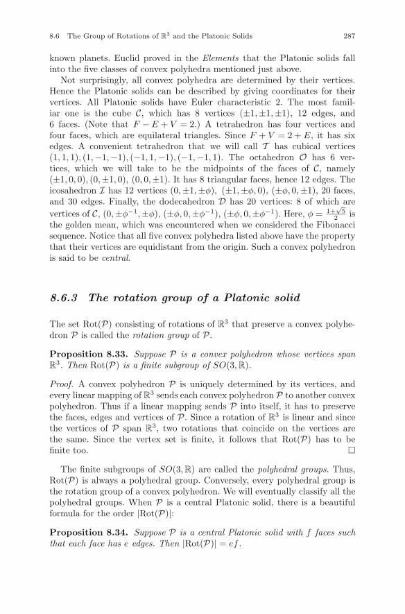
8.6 The Group of Rotations of R3 and the Platonic Solids 287
known planets. Euclid proved in the Elements that the Platonic solids fallinto the five classes of convex polyhedra mentioned just above.
Not surprisingly, all convex polyhedra are determined by their vertices.Hence the Platonic solids can be described by giving coordinates for theirvertices. All Platonic solids have Euler characteristic 2. The most famil-iar one is the cube C, which has 8 vertices (±1,±1,±1), 12 edges, and6 faces. (Note that F − E + V = 2.) A tetrahedron has four vertices andfour faces, which are equilateral triangles. Since F + V = 2 + E, it has sixedges. A convenient tetrahedron that we will call T has cubical vertices(1, 1, 1), (1,−1,−1), (−1, 1,−1), (−1,−1, 1). The octahedron O has 6 ver-tices, which we will take to be the midpoints of the faces of C, namely(±1, 0, 0), (0,±1, 0), (0, 0,±1). It has 8 triangular faces, hence 12 edges. Theicosahedron I has 12 vertices (0,±1,±φ), (±1,±φ, 0), (±φ, 0,±1), 20 faces,and 30 edges. Finally, the dodecahedron D has 20 vertices: 8 of which arevertices of C, (0,±φ−1,±φ), (±φ, 0,±φ−1), (±φ, 0,±φ−1). Here, φ = 1+
√5
2 isthe golden mean, which was encountered when we considered the Fibonaccisequence. Notice that all five convex polyhedra listed above have the propertythat their vertices are equidistant from the origin. Such a convex polyhedronis said to be central.
8.6.3 The rotation group of a Platonic solid
The set Rot(P) consisting of rotations of R3 that preserve a convex polyhe-dron P is called the rotation group of P.
Proposition 8.33. Suppose P is a convex polyhedron whose vertices spanR
3. Then Rot(P) is a finite subgroup of SO(3,R).
Proof. A convex polyhedron P is uniquely determined by its vertices, andevery linear mapping of R3 sends each convex polyhedron P to another convexpolyhedron. Thus if a linear mapping sends P into itself, it has to preservethe faces, edges and vertices of P. Since a rotation of R3 is linear and sincethe vertices of P span R
3, two rotations that coincide on the vertices arethe same. Since the vertex set is finite, it follows that Rot(P) has to befinite too. �
The finite subgroups of SO(3,R) are called the polyhedral groups. Thus,Rot(P) is always a polyhedral group. Conversely, every polyhedral group isthe rotation group of a convex polyhedron. We will eventually classify all thepolyhedral groups. When P is a central Platonic solid, there is a beautifulformula for the order |Rot(P)|:
Proposition 8.34. Suppose P is a central Platonic solid with f faces suchthat each face has e edges. Then |Rot(P)| = ef .
288 8 Eigentheory
The proof will be given in Proposition 11.7 as an application of the orbitstabilizer theorem. Thus the rotation group of a central cube C or octahedronO has order 24. As we will prove next, both of these groups are isomorphic tothe symmetric group S(4). A central regular tetrahedron has four triangularfaces, so its rotation group has order 12. A central regular dodecahedron Dand icosahedron I both have rotation groups of order 60. In fact, Rot(I) =Rot(D) ∼= A(5).
8.6.4 The cube and the octahedron
Since the rotation group of a central cube C has order 24, one might suspectthat it is isomorphic to S(4). We will verify this, but first let us give anexplicit description of Rot(C). For convenience, suppose the six vertices ofC are (±1,±1,±1). Since all rotations of C send faces to faces, they alsopermute the six midpoints of the faces. The midpoints being ±e1,±e2, and±e3, the orthogonal matrices that permute these vectors have the form
σ = (±eπ(1) ± eπ(2) ± eπ(3)),
where π ∈ S(3). The matrices of this form are called signed permutationmatrices. They form the subgroup SP (3) of O(3,R). Note that |SP (3)| = 48.Observe that if σ ∈ SP (3), then
detσ = det (±eπ(1) ± eπ(2) ± eπ(3)) = (−1)rsgn(π),
where r is the number of −1’s. This implies that |SP (3) ∩ SO(3,R)| = 24.It is evident that Rot(C) = SP (3) ∩ SO(3,R), so we get another proof that|Rot(C)| = 24. For simplicity, let G denote Rot(C). To see that G ∼= S(4), letD1,D2,D3,D4 denote the four diagonals of C. Since G leaves C invariant, itfollows that each element of G permutes the four diagonals. Thus if σ ∈ G,then σ(Di) = Dπ(i) for a unique π ∈ S(4). We will show that the mappingϕ : G → S(4) given by ϕ(σ) = π is an isomorphism. The proof that ϕ is ahomomorphism is left to the reader. To show that ϕ is a bijection, it suf-fices, by the pigeonhole principle, to show that ϕ is injective, since G andS(4) have the same order. Consider the four vectors d1 = e1 + e2 + e3, d2 =−e1 + e2 + e3, d3 = e1 − e2 + e3, and d4 = −e1 − e2 + e3, which lie on thefour diagonals of C and point upward. Let Di be the diagonal determinedby di. Then for each i, σ(di) = εidπ(i), where each εi is either 1 or −1depending on whether σ(di) points up or down. Since {d1,d2,d3} and{ε1dπ(1), ε2dπ(2), ε3dπ(3)} are both bases of R3 for every choice of signs andeach σ ∈ Rot(C) is a linear mapping, it follows that σ is uniquely determinedby the matrix identity
8.6 The Group of Rotations of R3 and the Platonic Solids 289
σ(d1 d2 d3
)=
(σ(d1) σ(d2) σ(d3)
)=
(ε1dπ(1) ε2dπ(2) ε3dπ(3)
).
Now assume ϕ(σ) = (1). Then
σ(d1 d2 d3
)=
(ε1d1 ε2d2 ε3d3
)=
(d1 d2 d3
)diag(ε1, ε2, ε3).
Hence, σ = DED−1, where D =(d1 d2 d3
)and E = diag(ε1, ε2, ε3). In order
to be in G, σ must be orthogonal, with detσ = 1. In particular, σ−1 = σT
and det E = 1. Since E−1 = E , it follows that σ = σ−1; hence to be orthog-onal, σ must be symmetric. This implies that DED−1 = (DT )−1EDT , orequivalently, DT DE = EDT D. By direct calculation,
DT D =
⎛⎝3 1 1
1 3 −11 −1 3
⎞⎠ ,
so the only way DT DE = EDT D can occur with E = diag(±1,±1,±1) anddet E = 1 is if E = I3, for at least one entry of E , say εi, must be 1. If theother diagonal entries are −1, then EDT D �= DT DE . For example, when ε1 =
ε3 = −1 and ε2 = 1, then the first column of DT DE is
⎛⎝−3
−1−1
⎞⎠, while that of
EDT D is
⎛⎝−3
1−1
⎞⎠ . We conclude that σ = I3, and consequently, ϕ is injective.
This proves that ϕ is an isomorphism, so Rot(C) ∼= S(4). �The octahedron O can be viewed as the unique convex polyhedron whose
vertices are the midpoints of the faces of the cube C, and every rotation of Cis thus a rotation of the octahedron and conversely. Thus Rot(C) = Rot(O).
Perhaps a more enlightening way to realize Rot(C) is to describe the rota-tions directly by finding the axes about which C can be rotated. For example,every coordinate axis Rei is such a line; C can be rotated by π/2, π, and3π/2 about each coordinate axis. This gives a total of nine distinct rotations.One can also rotate C through π around the lines x = y and x = −y in thexy-plane. Repeating this for the other two coordinate planes gives six morerotations, so we have now accounted for 15 rotations, 16 including the iden-tity. There are four more lines of symmetry about which one might be able torotate C, namely the four diagonals joining opposite vertices. It seems to bea little harder to visualize whether there any rotations through these lines,so let us take a slightly different approach. Recall that the alternating groupA(3) can be realized as the 3 × 3 permutation matrices of determinant 1. Oneelement σ ∈ A(3) is the rotation
290 8 Eigentheory
σ =
⎛⎝0 0 1
1 0 00 1 0
⎞⎠
sending e1 → e2 → e3 → e1. Clearly,
⎛⎝1
11
⎞⎠ is an eigenvector, so ϕ is in fact
a rotation about the line R
⎛⎝1
11
⎞⎠ . Since σ clearly has order 3, it is the rota-
tion through 2π/3. In this way, we account for another eight elements ofRot(C), since there are four diagonals, so we now have constructed all 24rotations of C.
8.6.5 Symmetry groups
The geometric side of group theory is symmetry. To understand this aspect,suppose S is a subset of Rn. A symmetry of S is defined to be an orthogonallinear mapping ϕ : Rn → R
n such that ϕ(S) = S. The set of all symmetriesof S will be denoted by O(S). Recall that an orthogonal linear mapping isa linear map ϕ that preserves the inner product on R
n. Since ϕ must alsopreserve lengths, distances, and angles, it preserves the geometry of S. Weknow that an orthogonal linear mapping ϕ : Rn → R
n is an orthogonal n × nmatrix, so the set of symmetries of S is thus
O(S) = {ϕ ∈ O(n,R) | ϕ(S) = S}.
In particular, O(Rn) = O(n,R). The first thing to note is the following.
Proposition 8.35. For every S ⊂ Rn, the set of symmetries O(S) is a sub-
group of O(n,R).
Proof. If ϕ and ψ are elements of O(S), then ψϕ and ϕ−1 are also symmetriesof S. Hence ψϕ−1 ∈ O(S), so O(S) is indeed a subgroup. �
Of course, it is possible, in fact likely, that the only element of O(S) is In.For example, let n = 2 and let S = {(1, 0), (2, 0), (3, 0)}. On the other hand,if S is the unit circle x2 + y2 = 1 in R
2, then O(S) = O(2,R). When S isa convex polyhedron in R
3 (or even in Rn), then O(S) has to permute the
vertices of S. But since elements of O(S) preserve lengths, O(S) can move avertex only into another vertex having the same distance from the origin. Butif S is contained in R
n and has n linearly independent vertices of differentlengths, then O(S) is the trivial group.
8.6 The Group of Rotations of R3 and the Platonic Solids 291
Example 8.17. Let us consider the n-cube C(n) in Rn defined by
C(n) = {(x1, x2, . . . , xn) | −1 ≤ xi ≤ 1 for all i = 1, 2, . . . , n}.
The matrix group SP (n) consisting of all n × n matrices of the form
(±eπ(1) ± eπ(2) · · · ± eπ(n)),
where π ∈ S(n), permutes the vectors ±e1,±e2, . . . ,±en and hence sendsC(n) to C(n). In fact, SP (n) = O(C(n)). �
Rotations in Rn for n > 3 are harder to define. We know that every rotation
of R3 is given by an element of SO(3,R). It can be shown by a similar
analysis that every element of SO(4,R) is given by a matrix that is a rotationin two orthogonal planes in R
4. In general, elements of O(n,R) satisfy thenormal matrix criterion AT A = AAT . This implies, by the normal matrixtheorem (see Theorem 9.2), that A is unitarily diagonalizable. That is, forevery A ∈ O(n,R), there is a Hermitian orthonormal basis of Cn consistingof eigenvectors of A. Then, associated to every pair of eigenvalues λ, λ of A,there exists a two-plane V in R
n such that A is a rotation of V through eiλ.(Recall that since A is orthogonal, its eigenvalues satisfy |λ| = 1.)
Remark. The study of symmetry via group theory has been successful inseveral disciplines, e.g., chemistry, physics, and materials science. The symme-tries of a class of pure carbon molecules called fullerenes offer a prime exam-ple. The most widely known of the fullerenes is a carbon molecule denotedby C60 (not to be confused with the cyclic group of order 60), named buck-minsterfullerene (or buckyball for short) after Buckminster Fuller for its sim-ilarity to his famous geodesic domes, which is one of the most rigid moleculesever discovered. Buckminsterfullerene is a truncated icosahedron. To obtaina picture of the buckyball, we have to consider the truncated icosahedron,which is the solid obtained by cutting off each vertex of the icosahedron by aplane orthogonal to the line through the vertex and the center of the icosa-hedron at the same distance from the center for each vertex. To get a modelfor the truncated icosahedron, just take a close look at a soccer ball. Sinceevery vertex of the icosahedron lies on five faces, the vertices are replacedby 12 regular pentagons. Hence, the truncated icosahedron has 60 vertices.It also has 32 faces. The symmetry group of the vertices of the truncatedicosahedron is the same as for the icosahedron.
Exercises
Exercise 8.6.1. Prove the following: Suppose G is a subgroup of O(3,R)and let
G+ = G ∩ SO(3,R).
292 8 Eigentheory
Then either G+ = G or G has exactly two cosets, and |G| = 2|G+|.
Exercise 8.6.2. Let P be a central Platonic solid. Let O(P) be the set ofall orthogonal matrices preserving P.
(i) Verify that O(P) is a subgroup of O(3,R).
(ii) Show that |O(P)| = 2|Rot(P)|.
Exercise 8.6.3. Consider the cube C with vertices at (±1,±1,±1). For therotations of C through the diagonal along (1, 1, 1), where do the vertices go?Even though this was worked out in the text, try to do it anyway withoutlooking back.
Exercise 8.6.4. Let H denote the reflection through the xy-plane in R3.
Show how to express the reflection through the yz-plane in the form Hσ,where σ is a rotation.
Exercise 8.6.5. The symmetry group of the central 3-cube C of the previousexercise permutes the diagonals of C, but it has order 48, which is twice theorder of S(4). Describe all the nonrotational symmetries.
Exercise 8.6.6. Show that
SP (n) = {σ ∈ O(n,R) | σ = (±eπ(1) ± eπ(2) · · · ± eπ(n)), π ∈ S(n)}
is a subgroup of O(n,R) of order 2nn!. Elements of SP (n) are called signedpermutation matrices.
Exercise 8.6.7. Consider the n-cube C(n) with its 2n vertices at the points(±1,±1, . . . ,±1). Show that the symmetry group of the set of vertices ofC(n) is the group SP (n). Does this imply that the symmetry group of C(n)is SP (n)?
Exercise 8.6.8. The 4-cube C(4) has eight diagonals. They are representedby the semidiagonals ±e1 + ±e2 + ±e3 + e4. Show that the symmetry groupof C(4) does not act transitively on the diagonals. Find a pair of diagonalsD1 and D2 such that no σ ∈ Sym(C(4)) satisfies σ(D1) = D2.
Exercise 8.6.9. Let T be the central regular tetrahedron in R3 described
above. Show that the group O(T ) is isomorphic to S(4) and that Rot(T ) isisomorphic to A(4).
Exercise 8.6.10. Construct a convex polyhedron P by taking two copies ofa tetrahedron, say T1 and T2, and gluing them together along two faces. Theresult is a convex polyhedron with six faces, nine edges, and five vertices.Assuming that P is central, compute the order of O(P ).
8.6 The Group of Rotations of R3 and the Platonic Solids 293
Exercise 8.6.11. For a subset S of R3, let Rot(S) denote the group of allσ ∈ SO(3,R) such that σ(S) = S. Find Rot(S) in the following cases:
(a) S is the half-ball {x2 + y2 + z2 ≤ 1, z ≥ 0},
(b) S is the solid rectangle {−1 ≤ x ≤ 1,−2 ≤ y ≤ 2,−1 ≤ z ≤ 1}.
Exercise 8.6.12. Suppose H is a reflection of R2. Show that there is a
rotation ρ of R3 such that ρ(x) = H(x) for all x ∈ R
2. (Hint: consider theline through which H reflects R
2.)
Exercise 8.6.13. Let G be a subgroup of O(n,R). True or false: if G is notcontained in SO(n,R), then G is normal in O(n,R).
Exercise 8.6.14. Describe how the alternating group A(4) acts on the cubein R
3 with vertices (±1,±1,±1).
294 8 Eigentheory
8.7 An Appendix on Field Extensions
The purpose of this Appendix is to prove that given a field F and a polynomialf ∈ F[x], there exists a field F
′ containing both F and all the roots of f(x) = 0.The field F
′ is called a splitting field for the polynomial f .To begin, we will construct a field F
′ containing F and at least one rootof f . Let x be a variable, and put V = F[x]. Then V is a vector space over F
with an infinite basis 1, x, x2, . . . . Given a nonconstant polynomial f ∈ V ,let W be the subspace of V consisting of all polynomials of the form h = gf ,for some g ∈ F[x]. We leave it to the reader to check that W is indeed asubspace of V . Now form the quotient vector space V/W . Recall that theelements of V/W are cosets g + W , where g ∈ V , and that coset addition isgiven by (g + W ) + (h + W ) = (g + h) + W . Scalar multiplication by a ∈ F
is given in an analogous way: a(g + W ) = ag + W . Recall also that two cosetsg + W and h + W are the same if and only if h − g ∈ W . That is, h − g = qffor some q ∈ F[x]. Since both V and W are infinite-dimensional, the followingresult may at first glance be surprising.
Proposition 8.36. The quotient vector space V/W is a finite-dimensionalvector space over F. In fact, dim V/W = deg(f).
Proof. To prove that dimV/W= deg(f), we exhibit a basis. Let k= deg(f)−1.Given g ∈ F[x], put g = g + W . For convenience, let us set α = x and αi = xi
for each nonnegative integer i. We claim that 1, α, α2, . . . , αk is a basis ofV/W . We first show independence. Suppose there exist a0, a1, . . . , ak ∈ F suchthat
k∑i=0
axαi = 0.
By definition, this means that
h(x) =k∑
i=0
aixi ∈ W.
Thus h = gf for some g ∈ F[x]. This is impossible unless g = 0, so all ai areequal to zero. To show that 1, α, . . . , αk span, let g ∈ F[x] and apply divisionwith remainder to write g = qf + r, where q, r ∈ F[x] and deg(r) < deg(f).Then g = r. But r is in the span of 1, α, . . . , αk, so we have found a basis ofV/W . Thus dimV/W = deg(f), which finishes the proof. �
An element f ∈ F[x] is said to be irreducible if there is no factorizationf = gh in which both g and h lie in F[x] and both g and h have positivedegree. The next theorem gives an important and fundamental result in fieldtheory.
8.7 An Appendix on Field Extensions 295
Theorem 8.37. If f ∈ F[x] is irreducible, then V/W can be given the struc-ture of a field F
′ such that F is a subfield of F′. Moreover, α = x + W is aroot of f in F
′.
Proof. We must first define multiplication on V/W . Let g, h ∈ F[x], and putgh = gh. To prove that this definition makes sense, it is necessary to show thatif g1 = g2 and h1 = h2, then g1h1 = g2h2. This is analogous to the proof thatZm admits an associative and commutative multiplication given in Chap. 2,so we will omit the details. Note that 0 is the additive identity, and 1 is themultiplicative identity. It remains to prove that if g �= 0, then g−1 exists. Thatis, there exists h ∈ F[x] such that hg = 1. Since f is irreducible and g �= 0, fby definition doesn’t divide g. Therefore, f and g have no common factor ofpositive degree. This means there exist polynomials a, b ∈ F[x] such that af +bg = 1, by the algorithm for computing the greatest common divisor of twopolynomials. Consequently, in F
′, bg = 1. Hence V/W with this multiplicationis a field. We now have F
′. Note that F is contained in F′ as the subfield
{r | r ∈ F ⊂ F[x]}. Finally, we must show that f(α) = 0. Let f(x) =∑
cixi.
Now,f(α) =
∑ciα
i =∑
cixi = f = 0,
so α is indeed a root. Therefore, the proof is finished. �
Example 8.18. Let F = Q and notice that x2 + x − 1 is irreducible in Q[x].Its roots φ and μ were considered in Section 8.2.5. In particular, φ = 1+
√5
2 .The field Q
′ has dimension two over Q. A vector space basis of Q′ over Q is1,
√5. �
Finally, we need to modify the above construction to get a splitting fieldF
′ for f . Notice that f ∈ F[x] ⊂ F′[x], but f is no longer irreducible in F
′[x],since it has the root α = x in F
′. Choose a new variable, say z, and considerF
′[z]. Dividing f(z) by (z − α) gives f(z) = g(z)(z − α), for some g ∈ F′[z].
Now deg(g) = deg(f) − 1, so if deg(f) = 2, then Proposition 8.36 implies thatF
′ necessarily contains all roots of f , as in the above example. If deg(f) > 2,we check whether g is irreducible in F
′[z]. If so, we repeat the constructionwith g to obtain a field extension of F′ (and hence F) containing a root β of gdifferent from α. Of course, β is also root of f . If g isn’t irreducible, factor ituntil another irreducible factor is found and then perform another extension.By continuing in this manner, one eventually obtains a field extension of Fcontaining all roots of the original polynomial f . In fact, this process willstop after at most deg(f) steps, since a polynomial of degree m has at mostm distinct roots. �
Chapter 9Unitary Diagonalizationand Quadratic Forms
As we saw in Chap. 8, when V is a finite-dimensional vector space over F, thena linear mapping T : V → V is semisimple if and only if its eigenvalues lie in F
and its minimal polynomial has only simple roots. It would be useful to havea result that would allow one to predict that T is semisimple on the basis of acriterion that is simpler than finding the minimal polynomial, which, after all,requires knowing the roots of the characteristic polynomial. In fact, we alsoproved that when F = C or R, every self-adjoint operator is semisimple andeven admits a Hermitian orthonormal basis. The matrices associated to self-adjoint operators, that is, Hermitian and symmetric matrices respectively,happen to be in a larger class of matrices said to be normal consisting ofall A ∈ C
n×n such that AAH = AHA. The normal matrix theorem assertsthat the normal matrices are exactly those A ∈ C
n×n that can be unitarilydiagonalized, or equivalently, admit a Hermitian orthonormal basis. The firstgoal in this chapter is to prove this theorem. The second goal is to consider thetopic of quadratic forms to which our diagonalization results may be applied.For example, we will classify the positive definite real quadratic forms orequivalently, the positive definite symmetric matrices. We will also introducean equivalence relation on the set of all real quadratic forms called congruenceand classify the equivalence classes. This result is known as Sylvester’s lawof inertia.
9.1 Schur Triangularization and the Normal MatrixTheorem
The key to understanding which matrices can be unitarily diagonalized is theSchur triangularization theorem, which says that an arbitrary n × n matrixover C is similar via a unitary matrix to an upper triangular matrix. Put
c© Springer Science+Business Media LLC 2017J.B. Carrell, Groups, Matrices, and Vector Spaces,DOI 10.1007/978-0-387-79428-0 9
297
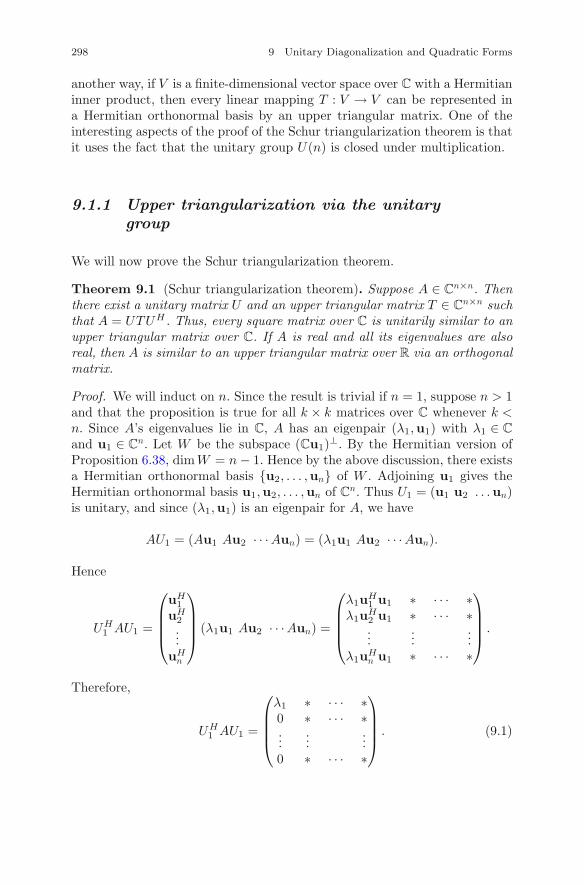
298 9 Unitary Diagonalization and Quadratic Forms
another way, if V is a finite-dimensional vector space over C with a Hermitianinner product, then every linear mapping T : V → V can be represented ina Hermitian orthonormal basis by an upper triangular matrix. One of theinteresting aspects of the proof of the Schur triangularization theorem is thatit uses the fact that the unitary group U(n) is closed under multiplication.
9.1.1 Upper triangularization via the unitarygroup
We will now prove the Schur triangularization theorem.
Theorem 9.1 (Schur triangularization theorem). Suppose A ∈ Cn×n. Then
there exist a unitary matrix U and an upper triangular matrix T ∈ Cn×n such
that A = UTUH . Thus, every square matrix over C is unitarily similar to anupper triangular matrix over C. If A is real and all its eigenvalues are alsoreal, then A is similar to an upper triangular matrix over R via an orthogonalmatrix.
Proof. We will induct on n. Since the result is trivial if n = 1, suppose n > 1and that the proposition is true for all k × k matrices over C whenever k <n. Since A’s eigenvalues lie in C, A has an eigenpair (λ1,u1) with λ1 ∈ C
and u1 ∈ Cn. Let W be the subspace (Cu1)⊥. By the Hermitian version of
Proposition 6.38, dim W = n − 1. Hence by the above discussion, there existsa Hermitian orthonormal basis {u2, . . . ,un} of W . Adjoining u1 gives theHermitian orthonormal basis u1,u2, . . . ,un of Cn. Thus U1 = (u1 u2 . . .un)is unitary, and since (λ1,u1) is an eigenpair for A, we have
AU1 = (Au1 Au2 · · · Aun) = (λ1u1 Au2 · · · Aun).
Hence
UH1 AU1 =
⎛⎜⎜⎜⎝
uH1
uH2...
uHn
⎞⎟⎟⎟⎠ (λ1u1 Au2 · · · Aun) =
⎛⎜⎜⎜⎝
λ1uH1 u1 ∗ · · · ∗
λ1uH2 u1 ∗ · · · ∗...
......
λ1uHn u1 ∗ · · · ∗
⎞⎟⎟⎟⎠ .
Therefore,
UH1 AU1 =
⎛⎜⎜⎜⎝
λ1 ∗ · · · ∗0 ∗ · · · ∗...
......
0 ∗ · · · ∗
⎞⎟⎟⎟⎠ . (9.1)
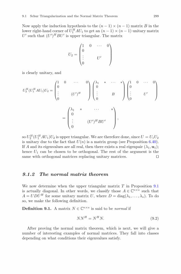
9.1 Schur Triangularization and the Normal Matrix Theorem 299
Now apply the induction hypothesis to the (n − 1) × (n − 1) matrix B in thelower right-hand corner of UH
1 AU1 to get an (n − 1) × (n − 1) unitary matrixU ′ such that (U ′)HBU ′ is upper triangular. The matrix
U2 =
⎛⎜⎜⎜⎝
1 0 · · · 00... U ′
0
⎞⎟⎟⎟⎠
is clearly unitary, and
UH2 (UH
1 AU1)U2 =
⎛⎜⎜⎜⎝
1 0 · · · 00... (U ′)H
0
⎞⎟⎟⎟⎠
⎛⎜⎜⎜⎝
λ1 ∗ · · · ∗0... B0
⎞⎟⎟⎟⎠
⎛⎜⎜⎜⎝
1 0 · · · 00... U ′
0
⎞⎟⎟⎟⎠
=
⎛⎜⎜⎜⎝
λ1 ∗ · · · ∗0... (U ′)HBU ′
0
⎞⎟⎟⎟⎠ ,
so UH2 (UH
1 AU1)U2 is upper triangular. We are therefore done, since U = U1U2
is unitary due to the fact that U(n) is a matrix group (see Proposition 6.40).If A and its eigenvalues are all real, then there exists a real eigenpair (λ1,u1);hence U1 can be chosen to be orthogonal. The rest of the argument is thesame with orthogonal matrices replacing unitary matrices. ��
9.1.2 The normal matrix theorem
We now determine when the upper triangular matrix T in Proposition 9.1is actually diagonal. In other words, we classify those A ∈ C
n×n such thatA = UDUH for some unitary matrix U , where D = diag(λ1, . . . , λn). To doso, we make the following definition.
Definition 9.1. A matrix N ∈ Cn×n is said to be normal if
NNH = NHN. (9.2)
After proving the normal matrix theorem, which is next, we will give anumber of interesting examples of normal matrices. They fall into classesdepending on what conditions their eigenvalues satisfy.
300 9 Unitary Diagonalization and Quadratic Forms
Theorem 9.2 (The normal matrix theorem). A matrix A ∈ Cn×n is unitar-
ily diagonalizable if and only if A is normal.
Proof. The “only if” part is straightforward and left as an exercise. SupposeA is normal. Write A = UTUH , where U is unitary and T is upper triangular.Since AHA = AAH and U is unitary, it follows that TTH = THT . Hence itsuffices to show that an upper triangular normal matrix is diagonal. The keyis to compare the diagonal entries of THT and TTH . The point is that forevery n × n complex matrix B, the kth diagonal entry of BHB is the squareof the length of the kth column of B, while the kth diagonal entry of BBH isthe square of the length of the kth row. But in an upper triangular matrix B,if the square of the length of the kth row equals the square of the length ofthe kth column for all k, then B is diagonal (the proof is left to the reader).Thus an upper triangular normal matrix is in fact diagonal. Therefore, A isindeed unitarily diagonalizable. ��Corollary 9.3. If A ∈ C
n×n is normal, then two eigenvectors of A with dis-tinct eigenvalues are Hermitian orthogonal.
Proof. We leave this as an exercise. ��
9.1.3 The Principal axis theorem: the short proof
Recall that a matrix A ∈ Cn×n is Hermitian if and only if AH = A. A real
Hermitian matrix is, of course, symmetric. It is clear that every Hermitianmatrix is normal. Furthermore, using the normal matrix theorem, we mayeasily prove the following result.
Proposition 9.4. The eigenvalues of a Hermitian matrix are real. In fact,the Hermitian matrices are exactly the normal matrices having real eigenval-ues.
Proof. Let A be Hermitian, and write A = UDUH . Then A = AH if and onlyif UHAU = UHAHU if and only if D = DH if and only if D is real. ��
Of course, the fact that Hermitian matrices have real eigenvalues wasproved from first principles in Chap. 8. The normal matrix theorem immedi-ately implies the following.
Theorem 9.5 (Principal axis theorem). A complex matrix A is Hermitianif and only if A can be unitarily diagonalized as A = UDUH , where D is areal diagonal matrix. Similarly, a real matrix A is symmetric if and only ifA can be orthogonally diagonalized A = QDQT , where D is also real.
9.1 Schur Triangularization and the Normal Matrix Theorem 301
Proof. The Hermitian case is immediate, but if A is real symmetric, oneneeds to argue a little more to show that U can be taken to be orthogonal.By the Schur triangulation theorem, A = QTQT , where Q is orthogonal andT is real and upper triangular. But since A is symmetric, it follows that Tis symmetric, and since T is also upper triangular, it has to be diagonal.Therefore, A = QDQT , as desired. ��
This proof is surprisingly brief, but it does not lead to any of the insightsof the first version of the principal axis theorem.
9.1.4 Other examples of normal matrices
To obtain other classes of normal matrices, one can impose other conditionson D in the expression A = UDUH . Here is another example obtained in thisway.
Example 9.1 (Skew-Hermitian matrices). A matrix J is said to be skew-Hermitian if JH = −J . It is easy to see that J is skew-Hermitian if and only ifiJ is Hermitian. Since Hermitian matrices are normal, so are skew-Hermitianmatrices. Also, the nonzero eigenvalues of a skew-Hermitian matrix are pureimaginary: they have the form iλ for a nonzero λ ∈ R that is an eigenvalueof iJ . A real skew-Hermitian matrix S is skew-symmetric, i.e., ST = −S. Forexample,
J =(
0 1−1 0
)and S =
⎛⎝
0 1 2−1 0 2−2 −2 0
⎞⎠
are both skew-symmetric. The diagonal entries of a skew-symmetric matrixare zero, so the trace of a skew-symmetric is also zero. The determinant of askew-symmetric matrix of odd order is also 0 (see Exercise 9.1.3 below), soa skew-symmetric matrix of odd order has 0 as an eigenvalue. The matrix Jabove shows that the determinant of a skew-symmetric matrix of even ordercan be nonzero. Note that the characteristic polynomial of S is −λ3 − 9λ, sothe eigenvalues of S are 0,±3i, confirming the observation that all nonzeroeigenvalues of a skew-Hermitian matrix are purely imaginary. Moreover, thenonzero eigenvalues of S occur in conjugate pairs, since S is real. �
The normal matrix theorem gives the following structure theorem, whichdescribes the nonsingular skew-symmetric matrices.
Proposition 9.6. Assume that n is even, say n = 2m, and A ∈ Rn×n is an
invertible skew-symmetric matrix. Then there exists an orthonormal basisx1, y1,x2,y2, . . . ,xm, ym of R
n such that A sends each real two-planeRxk + Ryk onto itself, and the matrix of A on this two-plane has the form
302 9 Unitary Diagonalization and Quadratic Forms
Jλk=
(0 λk
−λk 0
),
where λk is a nonzero real number such that iλk is an eigenvalue of A. (Thisbasis is not necessarily unique, however.) Thus there exists an orthogonalmatrix Q such that A = Q diag(Jλ1 , . . . , Jλm
) QT . In particular, a nonsin-gular real skew-symmetric matrix is similar via the matrix group O(n,R) toa matrix that is the direct sum of nonzero two-dimensional skew-symmetricblocks Jλk
.
Proof. Since A is real, its eigenvalues occur in conjugate pairs. Moreover,since A is skew-symmetric, iA is Hermitian, so iA has only real eigenval-ues. Thus the eigenvalues of A can be sorted into pairs ± iλk, where λk isa nonzero real number, since det(A) �= 0 and k varies from 1 to m. Note,however, that we are not claiming that the λk are all distinct. We maychoose a Hermitian orthonormal basis of Cn consisting of eigenvectors of A,and since eigenvectors for different eigenvalues are Hermitian orthogonal byCorollary 9.3, we may choose a Hermitian orthonormal basis of Cn consist-ing of pairs {uk,uk}, where Auk = iλkuk. We now observe that this meansthat xk = (uk + uk)/
√2 and yk = i(uk − uk)/
√2 also are a basis over C of
span{uk,uk}. Moreover, xk and yk have the additional property that bothlie in R
n and are Euclidean orthogonal: (xk)Tyk = 0. Furthermore, A leavesthe real two-plane Pk = Rxk + Ryk that they span invariant, and the matrixof A with respect to this basis of Pk is Jλk
. Finally, note that the planes Pi
and Pj are also orthogonal if i �= j. Hence the matrix Q = (x1 y1 · · · xm ym)is orthogonal and A = Q diag(Jλ1 , . . . , Jλm
) QT . ��One can extend the above result to odd skew-symmetric matrices. We will
leave this to the reader.Another natural condition one can put on the eigenvalues of a normal
matrix is that they all have modulus one. This is investigated in the followingexample.
Example 9.2. Let K = UDUH , where every diagonal entry of D is a unitcomplex number. Then D is unitary, hence so is K. Conversely, every uni-tary matrix is normal (see Exercise 9.1.10). Thus the unitary matrices areexactly the normal matrices such that every eigenvalue has modulus one. Forexample, the skew-symmetric matrix
J =(
0 −11 0
)
is clearly orthogonal, hence unitary. The matrix J has eigenvalues ±i, andwe can easily compute that Ei = C(1,−i)T and E−i = C(1, i)T . Thus
J = U1DUH1 =
1√2
(1 1i −i
) (−i 00 i
)1√2
(1 −i1 i
).
9.1 Schur Triangularization and the Normal Matrix Theorem 303
The basis constructed in the above proposition is u1 =1√2
(1i
)and u′
1 =
1√2
(1−i
). The way U acts as a complex linear mapping of C2 can be inter-
preted geometrically as follows: U rotates vectors on the complex line C(1, i)T
spanned by (1, i)T (thought of as a real two-plane) through π2 and rotates vec-
tors on the orthogonal axis by − π2 . Of course, as a mapping on R
2, U is simplythe rotation Rπ/2. �
Exercises
Exercise 9.1.1. Show that A ∈ Cn×n is unitarily diagonalizable if and only
if AH is.
Exercise 9.1.2. True or false (discuss your reasoning):
(i) A complex symmetric matrix is normal.(ii) The real part of a Hermitian matrix is symmetric and the imaginary
part is skew-symmetric.(iii) The real part of a normal matrix is normal.(iv) If a normal matrix N has real eigenvalues, then N is Hermitian.
Exercise 9.1.3. Unitarily diagonalize the skew-symmetric matrices
J =(
0 1−1 0
)and S =
⎛⎝
0 1 2−1 0 2−2 −2 0
⎞⎠ .
Exercise 9.1.4. Let
A =
⎛⎜⎜⎝
0 −1 0 −21 0 0 00 0 0 12 0 −1 0
⎞⎟⎟⎠ .
Express A as Qdiag(Jλ, Jμ)QT as in Proposition 9.6.
Exercise 9.1.5. Formulate a result similar to Proposition 9.6 for skew-symmetric matrices A ∈ R
n×n, where n is odd, that have the property thatdim N (A) = 1.
Exercise 9.1.6. Let S be a skew-Hermitian n × n matrix. Show the follow-ing:
(i) If n is odd, then det(S) is pure imaginary (but possibly zero), and if nis even, then det(S) is real.
(ii) If S is skew-symmetric, then det(S) = 0 if n is odd, and det(S) ≥ 0 if nis even.
304 9 Unitary Diagonalization and Quadratic Forms
Exercise 9.1.7. Show from the definition of the determinant that the deter-minant of a Hermitian matrix is real.
Exercise 9.1.8. Prove Corollary 9.3. That is, show that two eigenvectorsfor different eigenvalues of a normal matrix are Hermitian orthogonal.
Exercise 9.1.9. If possible, find an example of a 3 × 3 real matrix N suchthat N is normal, but N is neither symmetric nor skew-symmetric.
Exercise 9.1.10. Let U ∈ U(n). Show the following.
(i) Every eigenvalue of U also has modulus 1.
(ii) det(U) has modulus 1.
(iii) |Tr(U)| ≤ n.
Exercise 9.1.11. Suppose Q is an n × n orthogonal matrix with no realeigenvalues. True or false: n is even and det(Q) = 1.
Exercise 9.1.12. Suppose all eigenvalues of a unitary matrix Q are 1. Trueor false: Q = In.
Exercise 9.1.13. Let N (n) denote the set of normal n × n complex matri-ces. Prove that N (n) is not a subspace of Cn×n.
Exercise 9.1.14. Suppose A and B are commuting normal matrices. Provethe following:
(i) A + B and AB are also normal, and
(ii) A and B are simultaneously diagonalizable.
Exercise 9.1.15. Suppose, as in Exercise 9.1.14, that A and B are commut-ing normal matrices. What are the possible eigenvalues of A + B?
Exercise 9.1.16. Formulate the notion of a normal operator on a Hermitianinner product space from the definition of a normal matrix.
Exercise 9.1.17. True or false (discuss your reasoning):
(i) If A is normal and U is unitary, then UAUH is normal.
(ii) If A is normal and invertible, then A−1 is normal.
(iii) If A ∈ Rn×n, then AAT and ATA have the same eigenvalues.
(iv) If A is normal and k is a positive integer, then Ak is normal.
9.2 Quadratic Forms 305
9.2 Quadratic Forms
A quadratic form over a field F is a function q : Fn → F of the form q(r1, . . . ,rn) =
∑i,j aijrirj , where all the aij are in F. Quadratic forms are used in
many areas. For example, Lagrange’s four squares theorem says that everypositive integer n is the sum of the squares of four integers. That is, thereexist a, b, c, d ∈ Z such that n = a2 + b2 + c2 + d2. Every real quadratic formcan be expressed via a real symmetric matrix; hence every real quadratic formcan be written as a sum of squares. In this section, we will develop some of thebasic properties of quadratic forms over F such as diagonalization. We willalso consider an interesting equivalence relation on the symmetric matricesover F called congruence, and we will prove Sylvester’s law of inertia, whichclassifies the equivalence classes of congruent symmetric matrices over thereals R. A consequence of this is the classification of positive definite matri-ces. We will also treat the corresponding equivalence relation for Hermitianmatrices and Hermitian quadratic forms.
9.2.1 Quadratic forms and congruence
Throughout this section, we will assume that the field F has characteristicdifferent from two. A quadratic form on F
n is a function q : Fn → F such that
q(r1, . . . , rn) =n∑
i,j=1
aijrirj ,
where all aij are in F. Since the characteristic of F is not two, one can supposethat the coefficients aij of q are symmetric by replacing aij by bij = 1
2 (aij +aji). This leaves q unchanged, but by making its coefficients symmetric, wecan associate a unique symmetric matrix to q in order to bring in our previousresults on symmetric matrices. Indeed, q is expressed in terms of B by theidentity
q(r1, . . . , rn) = rTBr where r =
⎛⎜⎝
r1...rn
⎞⎟⎠ .
Conversely, a symmetric matrix A ∈ Fn×n defines the quadratic form
qA(r1, . . . , rn) = rTAr.
Under a change of coordinates on Fn of the form r = Cs, where C ∈ F
n×n
is invertible, the quadratic form qA is transformed into a new quadratic form
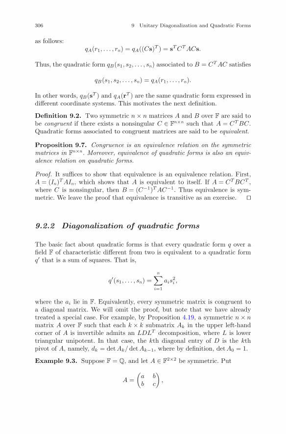
306 9 Unitary Diagonalization and Quadratic Forms
as follows:qA(r1, . . . , rn) = qA((Cs)T ) = sTCTACs.
Thus, the quadratic form qB(s1, s2, . . . , sn) associated to B = CTAC satisfies
qB(s1, s2, . . . , sn) = qA(r1, . . . , rn).
In other words, qB(sT ) and qA(rT ) are the same quadratic form expressed indifferent coordinate systems. This motivates the next definition.
Definition 9.2. Two symmetric n × n matrices A and B over F are said tobe congruent if there exists a nonsingular C ∈ F
n×n such that A = CTBC.Quadratic forms associated to congruent matrices are said to be equivalent.
Proposition 9.7. Congruence is an equivalence relation on the symmetricmatrices in F
n×n. Moreover, equivalence of quadratic forms is also an equiv-alence relation on quadratic forms.
Proof. It suffices to show that equivalence is an equivalence relation. First,A = (In)TAIn, which shows that A is equivalent to itself. If A = CTBCT ,where C is nonsingular, then B = (C−1)TAC−1. Thus equivalence is sym-metric. We leave the proof that equivalence is transitive as an exercise. ��
9.2.2 Diagonalization of quadratic forms
The basic fact about quadratic forms is that every quadratic form q over afield F of characteristic different from two is equivalent to a quadratic formq′ that is a sum of squares. That is,
q′(s1, . . . , sn) =n∑
i=1
ais2i ,
where the ai lie in F. Equivalently, every symmetric matrix is congruent toa diagonal matrix. We will omit the proof, but note that we have alreadytreated a special case. For example, by Proposition 4.19, a symmetric n × nmatrix A over F such that each k × k submatrix Ak in the upper left-handcorner of A is invertible admits an LDLT decomposition, where L is lowertriangular unipotent. In that case, the kth diagonal entry of D is the kthpivot of A, namely, dk = det Ak/det Ak−1, where by definition, detA0 = 1.
Example 9.3. Suppose F = Q, and let A ∈ F2×2 be symmetric. Put
A =(
a bb c
),
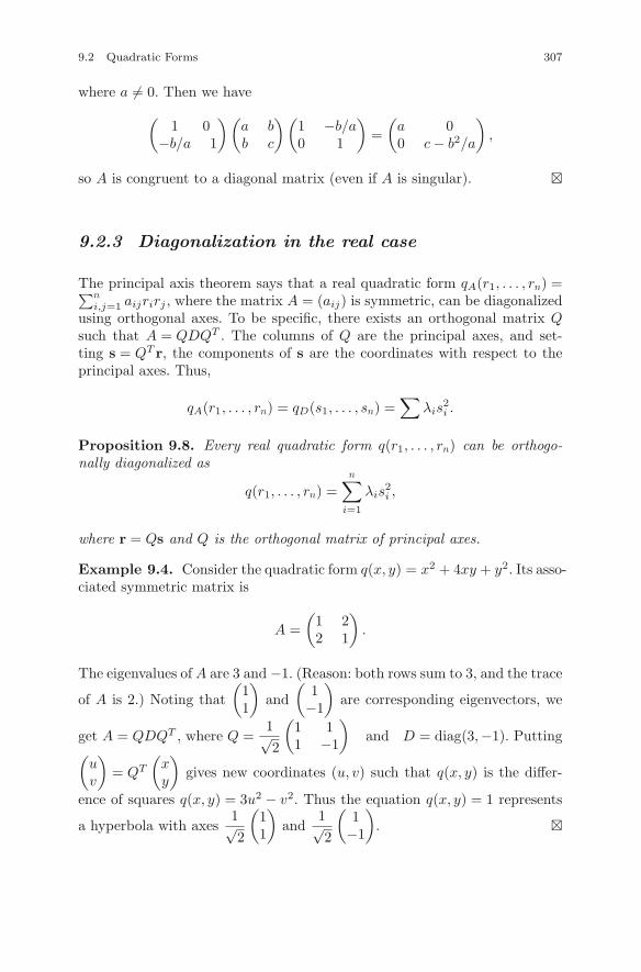
9.2 Quadratic Forms 307
where a �= 0. Then we have
(1 0
−b/a 1
)(a bb c
)(1 −b/a0 1
)=
(a 00 c − b2/a
),
so A is congruent to a diagonal matrix (even if A is singular). �
9.2.3 Diagonalization in the real case
The principal axis theorem says that a real quadratic form qA(r1, . . . , rn) =∑ni,j=1 aijrirj , where the matrix A = (aij) is symmetric, can be diagonalized
using orthogonal axes. To be specific, there exists an orthogonal matrix Qsuch that A = QDQT . The columns of Q are the principal axes, and set-ting s = QT r, the components of s are the coordinates with respect to theprincipal axes. Thus,
qA(r1, . . . , rn) = qD(s1, . . . , sn) =∑
λis2i .
Proposition 9.8. Every real quadratic form q(r1, . . . , rn) can be orthogo-nally diagonalized as
q(r1, . . . , rn) =n∑
i=1
λis2i ,
where r = Qs and Q is the orthogonal matrix of principal axes.
Example 9.4. Consider the quadratic form q(x, y) = x2 + 4xy + y2. Its asso-ciated symmetric matrix is
A =(
1 22 1
).
The eigenvalues of A are 3 and −1. (Reason: both rows sum to 3, and the trace
of A is 2.) Noting that(
11
)and
(1
−1
)are corresponding eigenvectors, we
get A = QDQT , where Q =1√2
(1 11 −1
)and D = diag(3,−1). Putting
(uv
)= QT
(xy
)gives new coordinates (u, v) such that q(x, y) is the differ-
ence of squares q(x, y) = 3u2 − v2. Thus the equation q(x, y) = 1 represents
a hyperbola with axes1√2
(11
)and
1√2
(1
−1
). �
308 9 Unitary Diagonalization and Quadratic Forms
Remark. If q is a quadratic form on Rn and c ∈ R is a constant, the level
set Vc = {(r1, . . . , rn) | q(r1, . . . , rn) = c} is called a quadratic variety. It is anexample of a real algebraic variety. When n = 2, a quadratic variety is calleda conic section. If q has matrix A and both eigenvalues of A are positive,then Vc is an ellipse or a circle when c > 0. (It is a circle if A has equaleigenvalues.) If both eigenvalues are positive and c < 0, then Vc is actually asubset of C2 that does not meet R
2. If A’s eigenvalues have different signs,then Vc is a hyperbola in R
2. In R3, the quadratic varieties are surfaces whose
type is classified by the number of positive and negative eigenvalues of theassociated symmetric matrix.
9.2.4 Hermitian forms
When A ∈ Cn×n is Hermitian, a quadratic function uA : Cn → C of the form
uA(z1, . . . , zn) =n∑
i,j=1
aijzizj = zHAz, where z =
⎛⎜⎝
z1...zn
⎞⎟⎠
is called a Hermitian form. Every Hermitian form can be unitarily diagonal-ized. All Hermitian forms are real-valued, since
(zHAz)H = zHAHzHH = zHAz.
Similarly, a skew-Hermitian form takes only pure imaginary values. By anargument similar to that in Proposition 9.9, we get the following.
Proposition 9.9. Let A ∈ Cn×n be normal, so A = UDUH , where U is uni-
tary and D = diag(λ1, . . . , λn). Let w1, . . . , wn be the coordinates on Cn com-
ing from a Hermitian orthonormal eigenbasis of Cn consisting of the columnsof U . Then
uA(z1, . . . , zn) =n∑
i=1
λiwiwi =n∑
i=1
λi|wi|2.
9.2.5 Positive definite matrices
Given a real quadratic form q (or more generally, a Hermitian quadratic formh), when does q (or h) have a strict maximum or minimum at the origin?This corresponds to all the eigenvalues of its matrix being either positive or
9.2 Quadratic Forms 309
negative. A minimum is attained if all are positive, and a maximum occursif they are all negative. Thus one makes the following definition.
Definition 9.3. A real symmetric n × n matrix A is called positive definiteif
xTAx > 0 for all nonzero x ∈ Rn.
An n × n Hermitian matrix A is positive definite if and only if
zHAz > 0 for all nonzero z ∈ Cn.
The following result describes the positive definite matrices in severalequivalent ways.
Proposition 9.10. For a real symmetric (respectively complex Hermitian)matrix A, the following conditions are equivalent:
(i ) all eigenvalues of A are positive;
(ii) A is positive definite;
(iii) the upper left k × k submatrix Ak has det(Ak) > 0 for all k; and
(iv) A has an LDLT decomposition in which D has positive diagonal entries.
Proof. For simplicity, we will give the proof for only the real symmetriccase. The changes necessary to prove the Hermitian case are routine afterreplacing xTAx by zHAz. We will show that each statement implies the fol-lowing one and (iv) implies (i). Assume that A ∈ R
n×n is symmetric, and(i) holds. Applying the principal axis theorem, we have A = QTDQ, whereQ = (q1 · · ·qn) is orthogonal and D = diag(λ1, . . . , λn) with all λi > 0. Thus,if x =
∑ni=1 xiqi, then xTAx =
∑ni=1 λix
2i , which is positive unless x = 0.
Thus (i) implies (ii). Now suppose A is positive definite, and recall that ifk ≤ n, then R
k ⊂ Rn as R
k = {x ∈ Rn | xi = 0 for all i > k}. Being sym-
metric, it follows that Ak is positive definite on Rk for all k. Consequently, all
eigenvalues of Ak are positive, so det(Ak) > 0 for all k. We conclude that (ii)implies (iii). Moreover, by Proposition 4.17, (iii) immediately implies (iv).The last implication, (iv) implies (i), follows from the law of inertia, whichwill be proved below. ��
We say that a symmetric matrix A ∈ Rn×n is negative definite if −A is pos-
itive definite, with a similar definition for the Hermitian case. Thus a negativedefinite matrix has only negative eigenvalues and has an LDLT decompo-sition with negative pivots. Note that this means that (−1)k det(Ak) > 0.Finally, a symmetric matrix that has both positive and negative eigenvaluesis called indefinite.
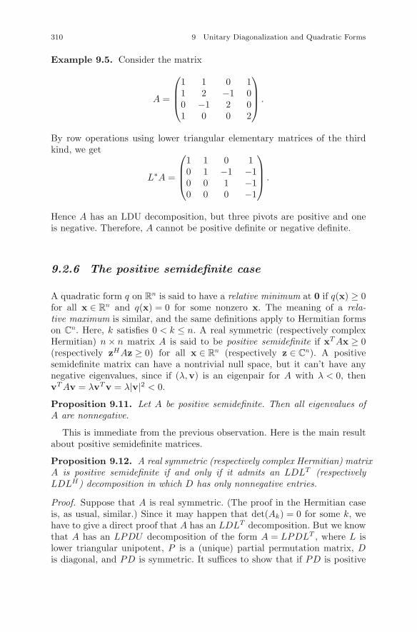
310 9 Unitary Diagonalization and Quadratic Forms
Example 9.5. Consider the matrix
A =
⎛⎜⎜⎝
1 1 0 11 2 −1 00 −1 2 01 0 0 2
⎞⎟⎟⎠ .
By row operations using lower triangular elementary matrices of the thirdkind, we get
L∗A =
⎛⎜⎜⎝
1 1 0 10 1 −1 −10 0 1 −10 0 0 −1
⎞⎟⎟⎠ .
Hence A has an LDU decomposition, but three pivots are positive and oneis negative. Therefore, A cannot be positive definite or negative definite.
9.2.6 The positive semidefinite case
A quadratic form q on Rn is said to have a relative minimum at 0 if q(x) ≥ 0
for all x ∈ Rn and q(x) = 0 for some nonzero x. The meaning of a rela-
tive maximum is similar, and the same definitions apply to Hermitian formson C
n. Here, k satisfies 0 < k ≤ n. A real symmetric (respectively complexHermitian) n × n matrix A is said to be positive semidefinite if xTAx ≥ 0(respectively zHAz ≥ 0) for all x ∈ R
n (respectively z ∈ Cn). A positive
semidefinite matrix can have a nontrivial null space, but it can’t have anynegative eigenvalues, since if (λ,v) is an eigenpair for A with λ < 0, thenvTAv = λvTv = λ|v|2 < 0.
Proposition 9.11. Let A be positive semidefinite. Then all eigenvalues ofA are nonnegative.
This is immediate from the previous observation. Here is the main resultabout positive semidefinite matrices.
Proposition 9.12. A real symmetric (respectively complex Hermitian) matrixA is positive semidefinite if and only if it admits an LDLT (respectivelyLDLH) decomposition in which D has only nonnegative entries.
Proof. Suppose that A is real symmetric. (The proof in the Hermitian caseis, as usual, similar.) Since it may happen that det(Ak) = 0 for some k, wehave to give a direct proof that A has an LDLT decomposition. But we knowthat A has an LPDU decomposition of the form A = LPDLT , where L islower triangular unipotent, P is a (unique) partial permutation matrix, Dis diagonal, and PD is symmetric. It suffices to show that if PD is positive
9.2 Quadratic Forms 311
semidefinite, then PD is a diagonal matrix with nonnegative entries. SupposeA is of size n × n and P �= In nor is P obtained by setting some rows of In
equal to 0. To simplify the notation, suppose the first row of P is nonzero.Let’s assume that the ith column is de1, where i > 1 and d �= 0. Since PD issymmetric, its first column is dei. Thus PD interchanges e1 and ei. Puttingy = y1e1 + yiei, we get
yTPDy = (y1e1 + yiei)T (dy1ei + dyie1) = 2dy1yi.
Hence, if PD is positive semidefinite, then dy1yi ≥ 0 for all y1, yi ∈ R. Sincei > 1, this is clearly impossible, so if the first row of PD is nonzero, it hasd in the (1, 1) entry. The argument is the same for all other rows, so PD isdiagonal. Moreover, the entries of D must be nonnegative, so every positivesemidefinite real symmetric matrix can be written LDLT . The converse isleft as an exercise. ��Example 9.6. Suppose A ∈ R
m×n. Then ATA is symmetric, so we can askwhether ATA is positive or positive semidefinite. In fact, for every x ∈ R
n,xTATAx = (Ax)TAx = |Ax|2, so xTATAx ≥ 0. Hence ATA is positive semi-definite. In particular, all eigenvalues of ATA are nonnegative. If N (A) = {0},then |Ax| > 0, provided x �= 0, so ATA is positive definite. The same is truefor AAT . �
Exercises
Exercise 9.2.1. Let A ∈ R2×2 be symmetric.
(i) Show that if det(A) > 0, then A is either positive definite or negativedefinite.
(ii) Also show that if Tr(A) = 0, then A is indefinite.
Exercise 9.2.2. Suppose A is a symmetric matrix such that det(A) �= 0 andA has both positive and negative diagonal entries. Explain why A has to beindefinite.
Exercise 9.2.3. Show that if A is a positive definite 3 × 3 matrix, then thecoefficients of its characteristic polynomial alternate in sign. Also show thatif A is negative definite, the coefficients are all negative.
Exercise 9.2.4. Give an example of a 3 × 3 symmetric matrix A such thatthe coefficients of the characteristic polynomial of A are all negative, but Ais not negative definite. (Could your answer be a diagonal matrix?)
Exercise 9.2.5. Let A ∈ Rn×n be positive definite and suppose S ∈ R
n×n isnonsingular.
(i) When is SAS−1 positive definite?
312 9 Unitary Diagonalization and Quadratic Forms
(ii) Is Am positive definite for all integers m? (Note: A0 = In.)
Exercise 9.2.6. Describe the quadratic surface (x y z)A(x y z)T = 1 forthe following choices of A:
⎛⎝
1 2 −12 0 33 −1 2
⎞⎠ and
⎛⎝
2 4 22 2 12 1 5
⎞⎠ .
Exercise 9.2.7. Decide whether g(x, y, z) = x2 + 6xy + 2xz + 3y2 − xz + z2
has a maximum, minimum, or neither at (0, 0, 0).
Exercise 9.2.8. Let A ∈ Rn×n, and suppose Ai = 0 for some i < n. Does
this mean that A has a zero eigenvalue?
Exercise 9.2.9. Let A ∈ Rm×n have the property that N (A) �= {0}. Is ATA
positive semidefinite? Can it be positive definite?
Exercise 9.2.10. For the following pairs A,B of symmetric matrices, deter-mine whether A and B are congruent.
(i) A and B have the same characteristic polynomial.
(ii) det(A) < 0, det(B) > 0.
(iii) A =(
1 22 1
)and B =
(1 22 −1
).
(iv) A and B are similar.
(v) A and B are positive definite.
(vi) AB = BA.
Exercise 9.2.11. Show that if a symmetric (respectively Hermitian) matrixA is semipositive definite, then A has a symmetric (respectively Hermitian)kth root M for all k > 0. (That is, Ak = M .) Moreover, if A is positivedefinite, so is M .
Exercise 9.2.12. Show that the product AB of a positive definite matrixA and a symmetric matrix B has real eigenvalues, even though AB is notnecessarily symmetric. (Hint: show that AB is similar to a symmetric matrix.Exercise 9.2.11 may help.)
9.3 Sylvester’s Law of Inertia and Polar Decomposition 313
9.3 Sylvester’s Law of Inertia and PolarDecomposition
In the final section of this chapter, we will prove two interesting results aboutcongruence classes of Hermitian matrices. The first is a famous result ofSylvester that classifies the congruence class of a Hermitian matrix in termsof its signature. The signature of a Hermitian matrix is a triple that tabulatesthe number of eigenvalues that are positive, negative, or zero. The law ofinertia says that two Hermitian matrices are congruent if and only if theirsignatures coincide. This result tells us, for example, that the signs of thepivots of a real symmetric matrix determine its signature. The second resultsays that every element of GL(n,C) has a unique factorization as KU , whereK is positive definite Hermitian and U is unitary. This gives the structureof the congruence class with signature (n, 0, 0). Namely, the class consistingof positive definite Hermitian matrices is in one-to-one correspondence withthe coset space GL(n,C)/U(n). Similarly, the congruence class of positivedefinite real symmetric matrices is in one-to-one correspondence with thecoset space GL(n,R)/O(n,R).
9.3.1 The law of inertia
Let A ∈ Cn×n be Hermitian, and let n+(A), n−(A), and n0(A) denote, respec-
tively, the number of positive, negative, and zero eigenvalues of A. For exam-ple, n0(A) = dimN (A). We will call the triple (n+(A), n−(A), n0(A)) thesignature of A. Sylvester’s law of inertia, to be proved next, gives an elegantanswer to the question of determining the signature of A. Since by Corollary4.22, congruent matrices have the same rank, it follows from the rank–nullitytheorem that if A and B are congruent, then n0(A) = n0(B). For simplicity,we will state and prove the law of inertia in the real symmetric case only.The Hermitian version may be formulated without any surprises and provedin essentially the same way.
Theorem 9.13 (Sylvester’s law of inertia). Let A and B be congruent realsymmetric matrices. Then A and B have the same signature. That is,
n+(A) = n+(B), n0(A) = n0(B) and n−(A) = n−(B).
Conversely, two real symmetric matrices having the same signature are con-gruent. In particular, if a real symmetric matrix A has a symmetric LDUdecomposition A = LDLT , then the signs of its eigenvalues are the same asthe signs on the diagonal of D (which are the pivots of A).
314 9 Unitary Diagonalization and Quadratic Forms
Proof. First choose orthogonal matrices P and Q such that A = PDPT andB = QEQT , where D and E are diagonal. Notice that without affectingthese expressions, we may assume that the positive diagonal entries of Dare d1, . . . , ds and that those of E are e1, . . . , et. This follows from the factthat for every permutation matrix P , PDPT = PDP−1 and D have the samediagonal up to the permutation corresponding to P . Notice that A and D, aswell as B and E, have the same eigenvalues, hence the same signature. Thus,to show that if A and B are congruent, then they have the same signature, itwill suffice to show that D and E have the same signature. Write B = CACT ,where C ∈ R
n×n is invertible. Thus
B = CACT = CPDPTCT = QEQT .
Hence E = MDMT , where M = QTCP . To show that D and E have thesame signature, it suffices to show that n+(D) = n+(E), since D and E, beingcongruent, have n0(D) = n0(E), as remarked above. Let us assume n+(D) =s < n+(E) = t, and let fi(x) ∈ (Rn)∗ denote the ith component function ofMTx. Since xTEx = xTMDMTx, when xT = (x1, . . . , xt, 0, . . . , 0), we have
t∑i=1
eix2i =
n∑j=1
djfj(x1, . . . , xt, 0, . . . , 0)2. (9.3)
Since t > s, there exist a1, . . . , at ∈ R not all zero such that
fj(a1, . . . , at, 0, . . . , 0) = 0 for j = 1, . . . , s.
Indeed, fewer than t homogeneous equations in t variables have a nontrivialsolution. Thus,
0 <t∑
i=1
eia2i =
n∑j=s+1
djfj(a1, . . . , at, 0, . . . , 0)2 ≤ 0,
since dj ≤ 0 if j > s. This is a contradiction, so we must have n+(D) =n+(E). This shows that D and E have the same signature, and hence sodo A and B. We will leave the proof of the converse as an exercise. ��Example 9.7. Let
A =
⎛⎝
1 1 21 1 32 3 2
⎞⎠ .
Then the quadratic form associated to A is
Q(x, y, z) = x2 + 2xy + 4xz + 2y2 + 6yz + 2z2.
9.3 Sylvester’s Law of Inertia and Polar Decomposition 315
A routine calculation gives
LA = DU =
⎛⎝
1 1 20 1 10 0 −3
⎞⎠ =
⎛⎝
1 0 00 1 00 0 −3
⎞⎠
⎛⎝
1 1 20 1 10 0 1
⎞⎠ .
Since A is nonsingular and symmetric, the expression LA = DU implies thatA = UTDU . Hence A is congruent to diag(1, 1,−3), so its signature is (2, 1, 0).The quadratic surface
x2 + 2xy + 4xz + 2y2 + 6yz + 2z2 = 1
is a hyperboloid of one sheet. �
Remark. The law of inertia also holds in the Hermitian case. In fact, theproof is essentially the same, so we will leave the details to the reader.
9.3.2 The polar decomposition of a complex linearmapping
Recall that every nonzero complex number has a unique polar representa-tion z = |z|eiθ with 0 ≤ θ < 2π. The purpose of this section is to generalizethis fact to linear mappings. Recall that eiθ is an element of the group ofunit complex numbers. By definition, this group is U(1) = {z ∈ C | zzH = 1}.The polar representation says that group-theoretically, C
∗ = GL(1,C) =(R>0)U(1). This representation generalizes to the n × n case when we replaceU(1) by the n × n unitary group and R>0 by the set of positive definite n × nHermitian matrices (which is not a group).
Proposition 9.14. Every A ∈ GL(n,C) can be uniquely expressed in eitherof two ways as A = KU = UK ′, where U ∈ U(n), K is the unique Hermitianpositive definite matrix such that K2 = AAH , and K ′ = UHKU .
Proof. Let H = AAH . Then H is Hermitian. Since A is nonsingular, H is pos-itive definite. (Proof: let (λ,x) be an eigenpair for H. Since A is nonsingular,AHx �= 0. Thus,
0 < |AHx|2 = (AHx)HAHx = xH(AAH)x = xH(λx) = λ|x|2,
so λ > 0.) By the result of Exercise 9.2.11, we can write H = K2, where Kis also positive definite Hermitian. Now put U = K−1A. Then A = KU , soit suffices to show that U is unitary. But
316 9 Unitary Diagonalization and Quadratic Forms
UUH = K−1A(AH(K−1)H) = K−1H(K−1)H = K−1K2K−1 = In,
so U is indeed unitary. The U ′K ′ factorization follows because
KU = (UUH)KU = U(UHKU) = UK ′,
and K ′ = UHKU is also positive definite Hermitian by the law of inertia.Finally, to prove uniqueness, notice that if K is Hermitian positive definiteand A = KU , then necessarily K2 = AAH , since K = AUH , so KH = UAH ,and hence K2 = KKH = (AUH)(UAH) = AAH . But the square root of apositive definite matrix is unique (verify this), so the polar representationmust be unique. ��
The real version of the polar representation takes an expected similar form.The proof is identical to the complex case.
Proposition 9.15. Every A ∈ GL(n,R) can be uniquely expressed in eitherof two ways as A = SQ = QS′, where Q ∈ O(n,R), S is the unique positivedefinite real matrix such that S2 = AAT , and S′ = QTSQ.
Polar decomposition gives rise to a nice interpretation of the coset spacesGL(n,C)/U(n) and GL(n,R)/O(n,R). Let PD(n,C) (respectively PD(n,R))denote the n × n positive definite Hermitian (respectively positive defi-nite real symmetric) matrices. Neither PD(n,C) nor PD(n,R) is a group,because neither is closed under multiplication. However, PD(n,C) andPD(n,R) are both closed under inverses. The upshot of polar decompo-sition is that the quotient maps π : GL(n,C) → GL(n,C)/U(n) and π :GL(n,R) → GL(n,R)/O(n,R) have the property that π(PD(n,C)) = GL(n,C)/U(n) and π(PD(n,R)) = GL(n,R)/O(n,R). This gives a surjective map-ping π : PD(n,C) → GL(n,C)/U(n) with a corresponding map in the realcase defined in exactly the same way. I claim that π is injective in each case.Here is the proof in the real case. (The complex case is essentially the same.)Suppose R, T ∈ PD(n,R) and π(R) = π(T ). That is, RO(n,R) = TO(n,R).By the criterion for equality of left cosets, it follows that R−1T ∈ O(n,R).Since R−1 is also positive definite, Exercise 9.2.12 implies that R−1T has realeigenvalues. But if R−1T ∈ O(n,R), this implies that the eigenvalues of R−1Tare either 1 or −1. But −1 is impossible, for if −1 is an eigenvalue, there existsa nonzero x ∈ R
n such that R−1T (x) = −x. Thus T (x) = R(−x) = −R(x),so
xTT (x) = −xTR(x).
9.3 Sylvester’s Law of Inertia and Polar Decomposition 317
Since R and T are both positive definite, this is impossible. Hence 1 is theonly eigenvalue of R−1T . But since R−1T ∈ O(n,R), R−1T is also normal,hence is unitarily diagonalizable by the normal matrix theorem (Theorem9.2). Hence R−1T = In, so R = T . Therefore, we have proved the followingresult.
Proposition 9.16. The mappings π : PD(n,C) → GL(n,C)/U(n) and π :PD(n,R) → GL(n,R)/O(n,R) are bijective.
Chapter 10The Structure Theory of LinearMappings
Throughout this chapter, V will be a finite-dimensional vector space over F.Our goal is to prove two theorems that describe the structure of an arbi-trary linear mapping T : V → V having the property that all the roots ofits characteristic polynomial lie in F. To describe this situation, let us saythat F contains the eigenvalues of T . A linear mapping T : V → V is alsocalled an endomorphism of V , and in this chapter, we will usually use thatterm. The structure theory for the endomorphisms of V is one of the nicestchapters in the theory of finite-dimensional vector spaces. The first result wewill prove, known as the Jordan–Chevalley decomposition, asserts that everyendomorphism T as above can be uniquely expressed as the sum T = S + Nof a semisimple endomorphism S and nilpotent endomorphism N such thatTS = ST and SN = NS (hence TN = NT ). The endomorphisms S and Nare called, respectively, the semisimple part of T and the nilpotent part of T ,and the expression T = S + N is known as the Jordan–Chevalley decomposi-tion of T .
The second structure theorem, known as the Jordan canonical form, is arefinement of the Jordan–Chevalley decomposition. It says that there existsa basis of V such that the matrix of T is a direct sum of Jordan blocks.A Jordan block is a matrix of the form J = μIn + N, where N is an uppertriangular n × n matrix with ones on the superdiagonal and zeros everywhereelse. In particular, N is nilpotent. Notice that μ is the unique eigenvalue ofJ . A matrix J in this form is said to be in Jordan canonical form.
These structure theorems require that all the eigenvalues of the endomor-phism T lie in F. If F is algebraically closed, for example if F = C, then theyapply to all endomorphisms. We can satisfy this eigenvalue assumption byletting V = F
n, since then we are dealing with n × n matrices over F, andby the appendix to Chap. 8, there exists an extension field F
′ of F containingevery eigenvalue of A. Thus A can be decomposed as A = S′ + N ′, where S′
c© Springer Science+Business Media LLC 2017J.B. Carrell, Groups, Matrices, and Vector Spaces,DOI 10.1007/978-0-387-79428-0 10
319
320 10 The Structure Theory of Linear Mappings
and N ′ are matrices over F′ that have the same roles as S and N ; that is, S′
is semisimple, N ′ is nilpotent, S′N ′ = N ′S′, and AS′ = S′A.
10.1 The Jordan–Chevalley Theorem
From now on, assume that V is a vector space over F such that dim V = n,and suppose T : V → V is an arbitrary linear mapping whose characteristicpolynomial is pT (x) = (x − λ1)μ1 · · · (x − λm)μm , where λ1, . . . , λm are thedistinct eigenvalues of T and all λi lie in F. By the Cayley–Hamilton theorem,
pT (T ) = (T − λ1IV )μ1 · · · (T − λmIV )μm = O. (10.1)
By Theorem 8.13, a necessary and sufficient condition that T be semisimple isthat (T − λ1IV ) · · · (T − λmIV ) = O. The Jordan–Chevalley theorem, whichwe will presently prove, will answer the question of how far T varies frombeing semisimple.
10.1.1 The statement of the theorem
To state the theorem, we need to define the invariant subspaces of T .
Definition 10.1. The subspaces Ci = ker(T − λiIV )μi ⊂ V are called theinvariant subspaces of T . If A is the matrix of T with respect to a basis of V ,then the subspaces Ci = N ((A − λiIn)μi) are the invariant subspaces for A.
Note that T (Ci) ⊂ Ci, so each Ci is invariant under T and similarly for A.The invariant subspaces are also called the cyclic subspaces of T or A.
Lemma 10.1. Let Ti = (T − λiIV )μi so that Ci = ker(Ti). Then
V = C1 ⊕ C2 ⊕ · · · ⊕ Cm.
Proof. We will apply Lemma 8.14. Thus we have to check that Ti ◦ Tj = Tj ◦Ti for all i and j, T1 ◦ · · · ◦ Tm = O, and ker(Ti) ∩ ker(Ti+1 ◦ · · · ◦ Tm) = {0}for all i. In fact, the first statement is clear, and the second is the Cayley–Hamilton theorem. Thus, we need to check only that ker(Ti) ∩ ker(Ti+1 ◦ · · · ◦Tm) = {0} for all i. Note first that Eλi
(T ) ∩ ker(Ti+1 ◦ · · · ◦ Tm) = {0}. Forif v ∈ Eλi
(T ), then
Ti+1 ◦ · · · ◦ Tm(v) = (λi − λi+1)μi+1 · · · (λi − λm)μmv.
10.1 The Jordan–Chevalley Theorem 321
Thus if v ∈ Eλi(T ) ∩ ker(Ti+1 ◦ · · · ◦ Tm), then v = 0. Now suppose μi > 1
and take v ∈ ker(Ti) ∩ ker(Ti+1 ◦ · · · ◦ Tm) such that v �= 0. Let a ≤ μi bethe least positive integer such that (T − λiIV )av = 0. By the previous case,we may assume a > 1, so let w = (T − λiIV )a−1v. Then by definition, w ∈Eλi
(T ) and w �= 0. But w ∈ ker(Ti+1 ◦ · · · ◦ Tm) also, which implies w = 0,contradicting the choice of w. Hence v = 0, so the lemma is proved. �
Let us now state the theorem.
Theorem 10.2 (Jordan–Chevalley decomposition theorem). Let T : V → Vbe an endomorphism all of whose eigenvalues lie in F and whose characteristicpolynomial is given by (10.1), where λ1, . . . , λm are the distinct eigenvaluesof T . Suppose C1, C2, . . . , Cm are the invariant subspaces of T . Then
V = C1 ⊕ C2 ⊕ · · · ⊕ Cm. (10.2)
Let S : V → V be the unique endomorphism such that S(v) = λiv if v ∈ Ci.Then:
(i) S is semisimple, and the linear mapping N = T − S is nilpotent;
(ii) S and N commute, and both commute with T : SN = NS, NT = TN ,and ST = TS;
(iii) the decomposition T = S + N of T into the sum of a semisimple linearmapping and a nilpotent linear mapping that commute is unique; and finally,
(iv) dim Ci = μi for all i.
The proof is given in the next section. The reader who wishes to see anexample in which the decomposition is explicitly computed can go directlyto Example 10.1.
Definition 10.2. The decomposition T = S + N is called the Jordan–Chevalley decomposition of T . The mapping S is called the semisimple partof T , and N is called its nilpotent part.
Corollary 10.3. An n × n matrix A over F whose eigenvalues all lie in F
can be expressed in exactly one way as a sum A = L + M of two commutingmatrices L and M over F such that L is diagonalizable and M is nilpotent.
Proof. First, let TA = TL + TM be the Jordan–Chevalley decomposition ofTA. This gives the decomposition A = L + M , as asserted. �
The Jordan–Chevalley decomposition enables us finally to clear up anintriguing question: is the algebraic multiplicity of an eigenvalue always anupper bound for its geometric multiplicity?
322 10 The Structure Theory of Linear Mappings
Corollary 10.4. Let λ be an eigenvalue of an endomorphism T : V → Vhaving algebraic multiplicity μ. Then dim Eλ(T ) ≤ μ.
Proof. Let λi be an eigenvalue. By part (iv) of the Jordan–Chevalley theorem,the algebraic multiplicity of λi, namely μi, is the dimension of the invariantsubspace Ci. But Eλi
(T ) ⊂ Ci, so the geometric multiplicity of λi, namelydim Eλi
(T ), is at most μi. �
10.1.2 The multiplicative Jordan–Chevalleydecomposition
There is also a multiplicative version of the Jordan–Chevalley decompositionfor nonsingular matrices. Let us first mention that the notion of a unipotentmatrix used in the LPDU decomposition is a special case of what is generallyknown as a unipotent matrix: a matrix A ∈ F
n×n is called unipotent if A − In
is nilpotent.
Proposition 10.5. Suppose A ∈ GL(n,F) and all the eigenvalues of A lie inF. Then one can write A uniquely in the form A = AsAu, where As is semi-simple, Au is unipotent, and AsAu = AuAs. Moreover, this decomposition isunique.
Proof. Let A = S + N be the Jordan–Chevalley decomposition of A. Sincethe eigenvalues of A and S are the same, it follows that S is nonsingular.Put As = S, so that As is semisimple. Next put Au = In + S−1N . Since Sand N commute, S−1N is nilpotent; hence Au is unipotent. This shows thatA = AsAu and AsAu = AuAs. To prove uniqueness, note that A = As(In +N) = As + AsN . Since As and N commute, A = As + AsN is the Jordan–Chevalley decomposition of A. Hence, As and Au are unique. �
This product decomposition applies to all A ∈ GL(n,C), for example, orto every GL(n,F) with F algebraically closed. The matrices As and Au areknown as the semisimple and unipotent parts of A. The multiplicative versionof the Jordan–Chevalley decomposition implies an interesting fact about finitesubgroups of GL(n,C), or indeed GL(n,F) if F is algebraically closed ofcharacteristic zero.
Proposition 10.6. Let F be algebraically closed of characteristic zero. Thenevery finite subgroup G < GL(n,F) consists of diagonalizable matrices.
Proof. Assume A ∈ G, and write its Jordan–Chevalley decomposition as A =AsAu. Since G is finite, A has finite order, say m. Then Am = (AsAu)m =(As)m(Au)m = In. Now (As)m is semisimple, and (Au)m is unipotent, soby the uniqueness of the multiplicative Jordan–Chevalley decomposition,
10.1 The Jordan–Chevalley Theorem 323
(As)m = (Au)m = In. To finish the proof, we have to show that (Au)m = In
implies Au = In. Write Au = In + N , where N is nilpotent. Then
(Au)m = In + mN +(
m
2
)N2 + · · · + Nm.
Hence, mN(In +(m2
)N + · · · + Nm−1) = O. Since In +
(m2
)N + · · · + Nm−1
is unipotent, it is invertible, so N = O. Therefore Au = In, so A = As. �
In fact, the above proof shows that there is a stronger conclusion.
Proposition 10.7. Suppose F is algebraically closed of characteristic p andthe order of G < GL(n,F) is prime to p. Then every element of G is diago-nalizable.
Proof. By Lagrange’s theorem, the order m of every A ∈ G is prime to p,since |G| is. Therefore, by the above argument, mN = O, so N = O. HenceAu = In, so A = As. �
If F has characteristic p, then there exist finite subgroups of GL(n,F)of order p all of whose elements are unipotent. For example, a transvectionmatrix In + Eij , where i �= j, generates a subgroup of GL(n,F) of order pisomorphic to the additive group of Fp.
Remark. When F = C, the proof of Proposition 10.6 can also be done usingthe standard Hermitian inner product on C
n. If one averages the inner prod-ucts (Av, Aw) over all A ∈ G, then one obtains a Hermitian inner producton C
n for which the matrices A ∈ G are normal. Thus, every element of G isunitarily diagonalizable, by the normal matrix theorem.
10.1.3 The proof of the Jordan–Chevalley theorem
As proved in Lemma 10.1,
V = C1 ⊕ · · · ⊕ Cm.
Thus each v ∈ V has a unique expression v =∑m
i=1 ci with ci ∈ Ci. ApplyingProposition 7.5, there exists a unique linear mapping S : V → V defined bysetting
S(v) =m∑
i=1
λici. (10.3)
324 10 The Structure Theory of Linear Mappings
Moreover, by definition, S is semisimple. Now put N = T − S. We claim thatN is nilpotent. For this, it suffices to show that there exists an integer r > 0such that Nr = O on V . By definition, if v ∈ Ci, then
Nμi(v) = (T − S)μi(v) = (T − λiIV )μi(v) = 0.
But V is the sum of the Ci, so Nr = O on V if r > μi for all i. This showsthat N is nilpotent and completes the verification of part (i). We will leavepart (ii), that T , S, and N all commute with each other, to the reader.We next prove part (iii): the decomposition T = S + N satisfying (i) and(ii) is unique. Let T = S′ + N ′ be another decomposition of T , where S′ issemisimple, N ′ is nilpotent, and S′N ′ = N ′S′. Since S′ is semisimple, we canwrite V = W1 ⊕ · · · ⊕ Wk, where the Wi are the eigenspaces for S′, and sinceTS′ = S′T , it follows that T (Wi) ⊂ Wi for each i. Thus, N ′(Wi) ⊂ Wi also.But since N ′ is nilpotent, ker(N ′) ∩ Wi �= {0}. Thus, there exists v ∈ Wi
such that (T − S′)v = 0. This means that T (v) = S′(v) = νiv, where νi isthe eigenvalue of S on Wi. Thus, every eigenvalue of S′ is an eigenvalue of T .Now it follows from the argument in Lemma 10.1 that Cj = ker(T − λjIn)μj+k
for all k ≥ 0. Thus if νi = μj , then Wi ⊂ Cj . But this implies Wi = Cj , since∑dim Wj =
∑dim Ci = dim V . Hence S′ = S and N ′ = N .
It remains to prove (iv), that is, that μi = dim Ci for all i. Note that thematrix A of T has the block form
A =
⎛⎜⎜⎜⎝
A1 O · · · OO A2 · · · O...
.... . .
...O · · · O Am
⎞⎟⎟⎟⎠ ,
where Ai is the matrix of T on Ci. It follows from the product rule fordeterminants that
pA(x) = pA1(x) · · · pAm(x) = (x − λ1)�1 · · · (x − λm)�m , (10.4)
since the only eigenvalue of Ai is λi. Therefore, dim Ci = �i = μi. Thisproves (iv). �
10.1.4 An example
The following example shows that even the 3 × 3 case can be a little compli-cated.
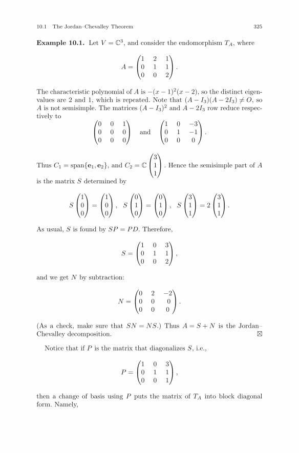
10.1 The Jordan–Chevalley Theorem 325
Example 10.1. Let V = C3, and consider the endomorphism TA, where
A =
⎛⎝1 2 1
0 1 10 0 2
⎞⎠ .
The characteristic polynomial of A is −(x − 1)2(x − 2), so the distinct eigen-values are 2 and 1, which is repeated. Note that (A − I3)(A − 2I3) �= O, soA is not semisimple. The matrices (A − I3)2 and A − 2I3 row reduce respec-tively to ⎛
⎝0 0 10 0 00 0 0
⎞⎠ and
⎛⎝1 0 −3
0 1 −10 0 0
⎞⎠ .
Thus C1 = span{e1, e2}, and C2 = C
⎛⎝3
11
⎞⎠ . Hence the semisimple part of A
is the matrix S determined by
S
⎛⎝1
00
⎞⎠ =
⎛⎝1
00
⎞⎠ , S
⎛⎝0
10
⎞⎠ =
⎛⎝0
10
⎞⎠ , S
⎛⎝3
11
⎞⎠ = 2
⎛⎝3
11
⎞⎠ .
As usual, S is found by SP = PD. Therefore,
S =
⎛⎝1 0 3
0 1 10 0 2
⎞⎠ ,
and we get N by subtraction:
N =
⎛⎝0 2 −2
0 0 00 0 0
⎞⎠ .
(As a check, make sure that SN = NS.) Thus A = S + N is the Jordan–Chevalley decomposition. �
Notice that if P is the matrix that diagonalizes S, i.e.,
P =
⎛⎝1 0 3
0 1 10 0 1
⎞⎠ ,
then a change of basis using P puts the matrix of TA into block diagonalform. Namely,
326 10 The Structure Theory of Linear Mappings
P−1AP =
⎛⎝1 2 0
0 1 00 0 2
⎞⎠ .
By choosing P more carefully, we can guarantee that P−1TP is in Jordancanonical form. For this, see Example 10.4.
10.1.5 The Lie bracket
Given two endomorphisms S, T : V → V , their Lie bracket [S, T ] is definedby [S, T ] = S ◦ T − T ◦ S. Thus [S, T ] is an endomorphism of V that mea-sures how much S and T fail to commute. Now let g�(V ) denote the vectorspace of all endomorphisms of V . Recall from Section 7.5.1 that g�(V ) hasdimension (dimV )2. By fixing S, one obtains an endomorphism of g�(V ),called the adjoint of S, which is denoted by ad(S) and defined by the rulead(S)(T ) = [S, T ]. For example, if V = F
n, then g�(V ) = Fn×n, and we know
that a basis of g�(V ) is given by the matrices Eij . Then if i �= j, we havead(Eij)(Eji) = Eii − Ejj . We leave it as an exercise to compute ad(Eij)(Ers)for all r, s (see Exercise 10.1.6) below). Now suppose F is algebraically closed.Then a basic theorem about the adjoint mapping says that if we denotethe semisimple and nilpotent parts of S by Sss and Snilp, then the Jordan–Chevalley decomposition of ad(S) is ad(S) = ad(Sss) + ad(Snilp). In otherwords, ad(S)ss = ad(Sss) and ad(S)nilp = ad(Snilp). We ask the reader toverify this when g�(V ) = F
2×2 in the exercises below.
Exercises
Exercise 10.1.1. Show that invariant subspaces of a linear mapping T areactually invariant under T . That is, T (Ci) ⊂ Ci for each i.
Exercise 10.1.2. Discuss the Jordan–Chevalley decomposition of the fol-lowing types of endomorphisms or matrices:
(i) rotations of R2 (i.e., elements of SO(2,R)),
(ii) rotations of R3,
(iii) the cross product mapping Ca(x) = a × x on R3, and
(iv) 2 × 2 complex matrices of determinant and trace zero.
Exercise 10.1.3. Let A ∈ Fn×n. Show how to express the semisimple and
nilpotent parts of A2 and A3 in terms of those of A.
10.1 The Jordan–Chevalley Theorem 327
Exercise 10.1.4. Describe all real 2 × 2 matrices that are both symmetricand nilpotent.
Exercise 10.1.5. Find the Jordan–Chevalley decomposition of the matricesin parts (i)–(iii) of Exercise 8.5.9.
Exercise 10.1.6. Consider the standard basis Eij , 1 ≤ i, j ≤ 2, of F2×2.
(i) Compute the matrices of ad(E11) and ad(E12) with respect to the standardbasis.
(ii) Calculate the Jordan–Chevalley decomposition of each of ad(E11) andad(E12).
Exercise 10.1.7. Show that an n × n matrix A is unipotent if and only ifits characteristic polynomial is (1 − x)n.
Exercise 10.1.8. Prove that the Lie bracket on g�(V ) satisfies the Jacobiidentity
[R, [S, T ]] + [T, [R,S]] + [S, [T,R]] = 0.
Exercise 10.1.9. Show that the Jacobi identity on g�(V ) can be restatedas the identity
ad([S.T ]) = [ad(S), ad(T )].
This says that if g�(V ) is made into a ring where the multiplication is R ◦ S =[R,S], then ad is a ring homomorphism.
Exercise 10.1.10. Let T : C9 → C9 be an endomorphism with characteris-
tic polynomial
(t + 1)2(t − 1)3(t2 + 1)2 = (t + 1)(t − 1)3(t − i)2(t + i)2,
and suppose the minimal polynomial of T is (t + 1)(t − 1)2(t2 + 1)2. What isthe rank of the nilpotent part of T on each invariant subspace of T?
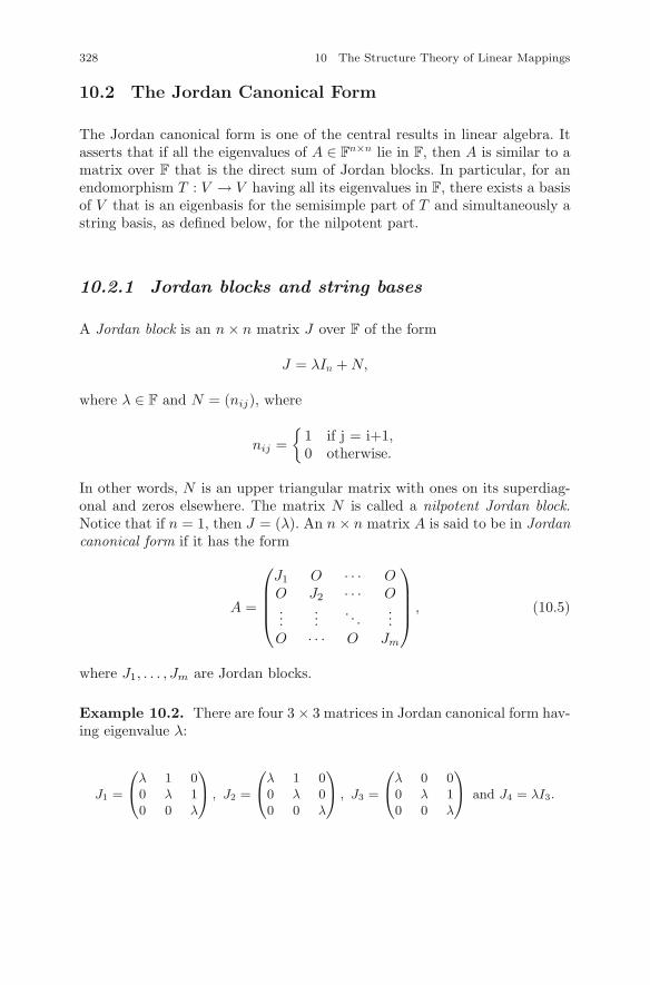
328 10 The Structure Theory of Linear Mappings
10.2 The Jordan Canonical Form
The Jordan canonical form is one of the central results in linear algebra. Itasserts that if all the eigenvalues of A ∈ F
n×n lie in F, then A is similar to amatrix over F that is the direct sum of Jordan blocks. In particular, for anendomorphism T : V → V having all its eigenvalues in F, there exists a basisof V that is an eigenbasis for the semisimple part of T and simultaneously astring basis, as defined below, for the nilpotent part.
10.2.1 Jordan blocks and string bases
A Jordan block is an n × n matrix J over F of the form
J = λIn + N,
where λ ∈ F and N = (nij), where
nij ={
1 if j = i+1,0 otherwise.
In other words, N is an upper triangular matrix with ones on its superdiag-onal and zeros elsewhere. The matrix N is called a nilpotent Jordan block.Notice that if n = 1, then J = (λ). An n × n matrix A is said to be in Jordancanonical form if it has the form
A =
⎛⎜⎜⎜⎝
J1 O · · · OO J2 · · · O...
.... . .
...O · · · O Jm
⎞⎟⎟⎟⎠ , (10.5)
where J1, . . . , Jm are Jordan blocks.
Example 10.2. There are four 3 × 3 matrices in Jordan canonical form hav-ing eigenvalue λ:
J1 =
⎛⎝
λ 1 00 λ 10 0 λ
⎞⎠ , J2 =
⎛⎝
λ 1 00 λ 00 0 λ
⎞⎠ , J3 =
⎛⎝
λ 0 00 λ 10 0 λ
⎞⎠ and J4 = λI3.
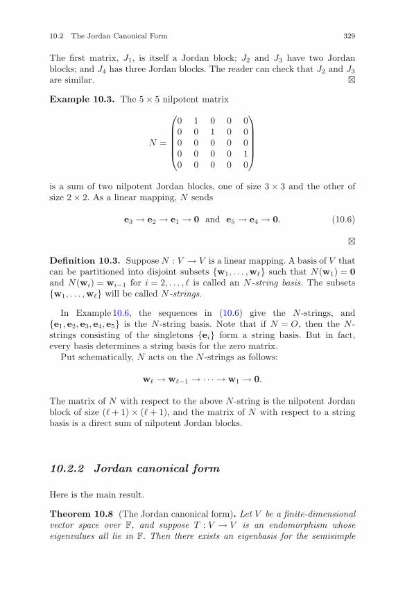
10.2 The Jordan Canonical Form 329
The first matrix, J1, is itself a Jordan block; J2 and J3 have two Jordanblocks; and J4 has three Jordan blocks. The reader can check that J2 and J3
are similar. �
Example 10.3. The 5 × 5 nilpotent matrix
N =
⎛⎜⎜⎜⎜⎝
0 1 0 0 00 0 1 0 00 0 0 0 00 0 0 0 10 0 0 0 0
⎞⎟⎟⎟⎟⎠
is a sum of two nilpotent Jordan blocks, one of size 3 × 3 and the other ofsize 2 × 2. As a linear mapping, N sends
e3 → e2 → e1 → 0 and e5 → e4 → 0. (10.6)
�
Definition 10.3. Suppose N : V → V is a linear mapping. A basis of V thatcan be partitioned into disjoint subsets {w1, . . . ,w�} such that N(w1) = 0and N(wi) = wi−1 for i = 2, . . . , � is called an N -string basis. The subsets{w1, . . . ,w�} will be called N -strings.
In Example 10.6, the sequences in (10.6) give the N -strings, and{e1, e2, e3, e4, e5} is the N -string basis. Note that if N = O, then the N -strings consisting of the singletons {ei} form a string basis. But in fact,every basis determines a string basis for the zero matrix.
Put schematically, N acts on the N -strings as follows:
w� → w�−1 → · · · → w1 → 0.
The matrix of N with respect to the above N -string is the nilpotent Jordanblock of size (� + 1) × (� + 1), and the matrix of N with respect to a stringbasis is a direct sum of nilpotent Jordan blocks.
10.2.2 Jordan canonical form
Here is the main result.
Theorem 10.8 (The Jordan canonical form). Let V be a finite-dimensionalvector space over F, and suppose T : V → V is an endomorphism whoseeigenvalues all lie in F. Then there exists an eigenbasis for the semisimple
330 10 The Structure Theory of Linear Mappings
part of T that is also a string basis for the nilpotent part of T . Thus, thereexists a basis of V for which the matrix A of T has the form
A =
⎛⎜⎜⎜⎝
J1 O · · · OO J2 · · · O...
.... . .
...O · · · O Jm
⎞⎟⎟⎟⎠ , (10.7)
where each Ji is a Jordan block. Note: the Jordan blocks do not necessarilyhave different eigenvalues.
Let us review the situation. By the Jordan–Chevalley decomposition the-orem, V is the direct sum of the invariant subspaces C1, . . . , Cm of T . Hence,choosing a basis of each Ci and taking the union of these bases gives abasis of V for which the semisimple part S of T is the diagonal matrixdiag(λ1Iμ1 , . . . , λmIμm
), where μi = dim Ci. Thus, if we show that each Ci
has a string basis for the nilpotent part N of T , then we obtain a basis of Vfor which the matrix of T is in Jordan canonical form. This will be done inthe next section.
10.2.3 String bases and nilpotent endomorphisms
We will now prove that a nilpotent endomorphism N : V → V of an arbitraryfinite-dimensional vector space has a string basis. We begin by noticing thatstring bases have the following property.
Proposition 10.9. In a string basis of V to N , the number of strings isdim ker(N).
Proof. Let the strings be v(i)ki
→ · · · → v(i)1 → 0 for i = 1, . . . , �. Certainly the
terminal vectors v(i)1 , 1 ≤ i ≤ �, span ker(N). Let w ∈ ker(N), and use the
string basis to write w =∑
i,j aijv(i)j . Then N(w) = 0, so
∑i,j aijv
(i)j−1 =
0, where v(i)j−1 = 0 if j = 1. Thus, ai,j = 0 if j > 1. Consequently, w =∑
i ai1v(i)1 . This proves that the v(i)
1 , 1 ≤ i ≤ �, span ker(N). Since the v(i)1
are linearly independent, dim ker(N) = �. �
We now prove the main result.
Proposition 10.10. Suppose N : V → V is a nilpotent linear mapping.Then V admits a string basis for N .
10.2 The Jordan Canonical Form 331
Proof. We will induct on dimV . The case dim V = 1 is obvious, so assumethat the proposition is true if dimV < r, and suppose dimV = r. We mayas well assume N �= O, so N(V ) �= {0}. Let W = ker(N) and U = im(N).By the rank–nullity theorem (cf. Theorem7.4) we have dim U + dim W =dim V . Since N is nilpotent, dimW > 0, so dim U < dim V . By definition,N(U) ⊂ U , so N is a nilpotent linear mapping on U . Hence, dim(U ∩ W ) >0. Now apply the induction hypothesis to U to get a basis of N -strings.By Proposition 10.9, there are exactly dim(U ∩ W ) N -strings in every stringbasis of U . Let
v(i)ki
→ · · · → v(i)2 → v(i)
1
(i = 1, . . . , � = dim(U ∩ W )) be these strings. Since v(i)ki
∈ im(N), there exists
v(i)ki+1 ∈ V such that N(v(i)
ki+1) = v(i)ki
. Thus we can form a new N -string
v(i)ki+1 → v(i)
ki→ · · · → v(i)
2 → v(i)1 (10.8)
in V . Now adjoin to the strings in (10.8) additional wj ∈ W so that the v(i)1
and the wk form a basis of W . The number of wk is exactly dim W − dim(U ∩W ). Now count the number of vectors. We have dimU vectors from the strings(10.8), and there are dim(U ∩ W ) of these strings, each contributing a basisvector of W . Hence because of how the string basis of U was obtained, wehave a total of
dim U + dim(U ∩ W ) + (dim W − dim(U ∩ W )) = dimU + dim W
vectors. But as noted above, dim U + dim W = dim V , so it suffices to showthat these vectors are independent. Thus suppose
∑i,j
aijv(i)j +
∑bkwk = 0. (10.9)
Applying N to (10.9) gives an expression
∑i,j
aijv(i)j−1 = 0,
where for each i, 1 < j ≤ ki + 1. But then all these aij are equal to zero.Hence the original expression (10.9) becomes
∑ai1v
(i)1 +
∑bkwk = 0.
Thus the remaining coefficients are also zero, since the v(i)1 and the wk form
a basis of W . Hence, we have constructed an N -string basis of V . �
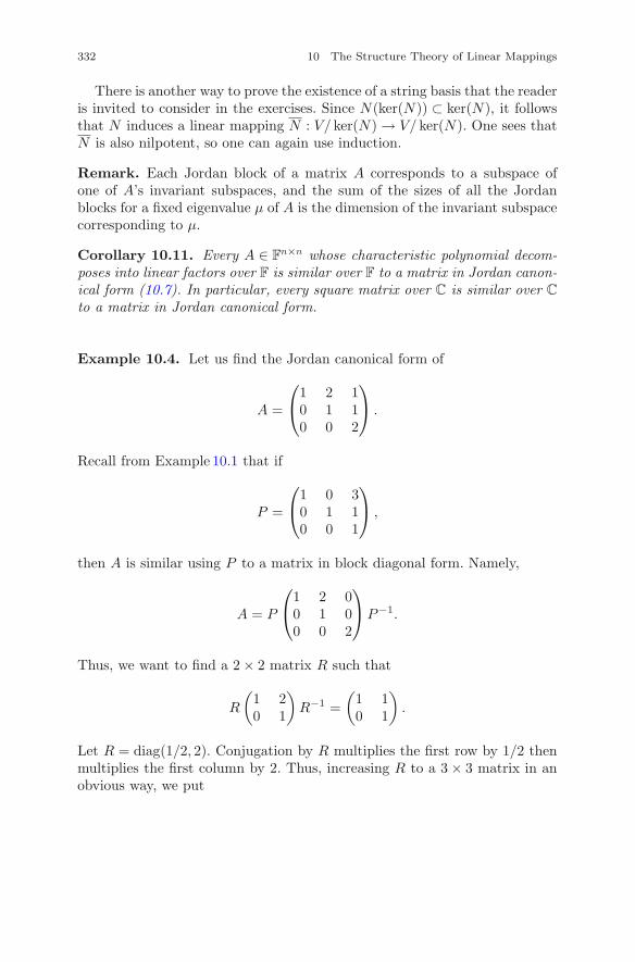
332 10 The Structure Theory of Linear Mappings
There is another way to prove the existence of a string basis that the readeris invited to consider in the exercises. Since N(ker(N)) ⊂ ker(N), it followsthat N induces a linear mapping N : V/ ker(N) → V/ ker(N). One sees thatN is also nilpotent, so one can again use induction.
Remark. Each Jordan block of a matrix A corresponds to a subspace ofone of A’s invariant subspaces, and the sum of the sizes of all the Jordanblocks for a fixed eigenvalue μ of A is the dimension of the invariant subspacecorresponding to μ.
Corollary 10.11. Every A ∈ Fn×n whose characteristic polynomial decom-
poses into linear factors over F is similar over F to a matrix in Jordan canon-ical form (10.7). In particular, every square matrix over C is similar over C
to a matrix in Jordan canonical form.
Example 10.4. Let us find the Jordan canonical form of
A =
⎛⎝1 2 1
0 1 10 0 2
⎞⎠ .
Recall from Example 10.1 that if
P =
⎛⎝1 0 3
0 1 10 0 1
⎞⎠ ,
then A is similar using P to a matrix in block diagonal form. Namely,
A = P
⎛⎝1 2 0
0 1 00 0 2
⎞⎠ P−1.
Thus, we want to find a 2 × 2 matrix R such that
R
(1 20 1
)R−1 =
(1 10 1
).
Let R = diag(1/2, 2). Conjugation by R multiplies the first row by 1/2 thenmultiplies the first column by 2. Thus, increasing R to a 3 × 3 matrix in anobvious way, we put
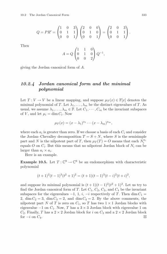
10.2 The Jordan Canonical Form 333
Q = PR′ =
⎛⎝1 0 3
0 1 10 0 1
⎞⎠
⎛⎝2 0 0
0 1 00 0 1
⎞⎠ =
⎛⎝2 0 3
0 1 10 0 1
⎞⎠ .
Then
A = Q
⎛⎝1 1 0
0 1 00 0 2
⎞⎠ Q−1,
giving the Jordan canonical form of A.
10.2.4 Jordan canonical form and the minimalpolynomial
Let T : V → V be a linear mapping, and suppose μT (x) ∈ F[x] denotes theminimal polynomial of T . Let λ1, . . . , λm be the distinct eigenvalues of T . Asusual, we assume λ1, . . . , λm ∈ F. Let C1, · · · , Cm be the invariant subspacesof V , and let μi = dim Ci. Now
μT (x) = (x − λ1)a1 · · · (x − λm)am ,
where each ai is greater than zero. If we choose a basis of each Ci and considerthe Jordan–Chevalley decomposition T = S + N , where S is the semisimplepart and N is the nilpotent part of T , then μT (T ) = O means that each Nai
i
equals O on Ci. But this means that no nilpotent Jordan block of Ni can belarger than ai × ai.
Here is an example.
Example 10.5. Let T : C9 → C9 be an endomorphism with characteristic
polynomial
(t + 1)2(t − 1)3(t2 + 1)2 = (t + 1)(t − 1)3(t − i)2(t + i)2,
and suppose its minimal polynomial is (t + 1)(t − 1)2(t2 + 1)2. Let us try tofind the Jordan canonical form of T . Let C1, C2, C3, and C4 be the invariantsubspaces for the eigenvalues −1, 1, i, −i respectively of T . Then dimC1 =2, dim C2 = 3, dimC3 = 2, and dimC4 = 2. By the above comments, thenilpotent part N of T is zero on C1, so T has two 1 × 1 Jordan blocks witheigenvalue −1 on C1. Now, T has a 3 × 3 Jordan block with eigenvalue 1 onC2. Finally, T has a 2 × 2 Jordan block for i on C3 and a 2 × 2 Jordan blockfor −i on C4. �
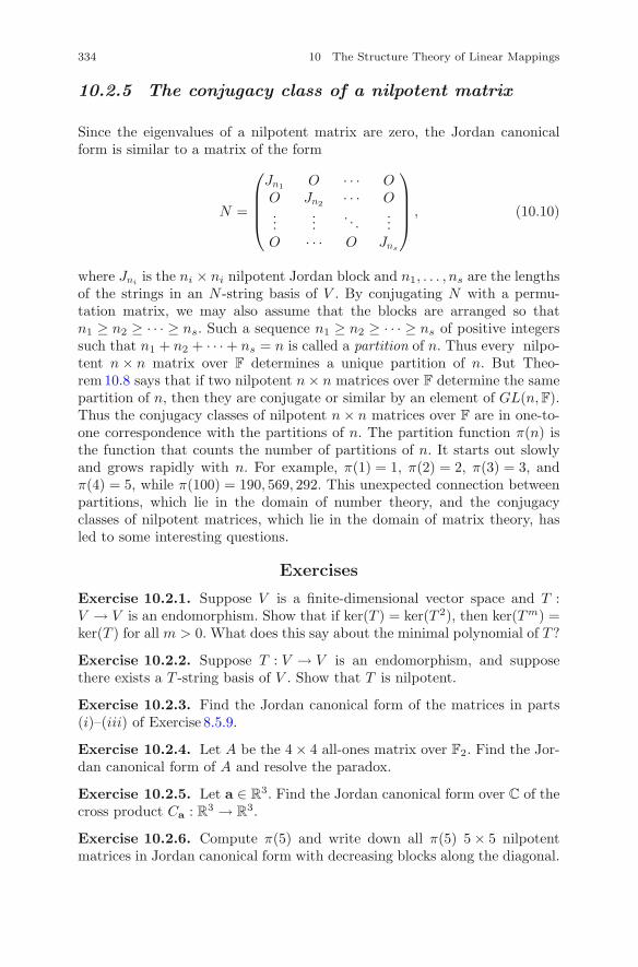
334 10 The Structure Theory of Linear Mappings
10.2.5 The conjugacy class of a nilpotent matrix
Since the eigenvalues of a nilpotent matrix are zero, the Jordan canonicalform is similar to a matrix of the form
N =
⎛⎜⎜⎜⎝
Jn1 O · · · OO Jn2 · · · O...
.... . .
...O · · · O Jns
⎞⎟⎟⎟⎠ , (10.10)
where Jniis the ni × ni nilpotent Jordan block and n1, . . . , ns are the lengths
of the strings in an N -string basis of V . By conjugating N with a permu-tation matrix, we may also assume that the blocks are arranged so thatn1 ≥ n2 ≥ · · · ≥ ns. Such a sequence n1 ≥ n2 ≥ · · · ≥ ns of positive integerssuch that n1 + n2 + · · · + ns = n is called a partition of n. Thus every nilpo-tent n × n matrix over F determines a unique partition of n. But Theo-rem 10.8 says that if two nilpotent n × n matrices over F determine the samepartition of n, then they are conjugate or similar by an element of GL(n,F).Thus the conjugacy classes of nilpotent n × n matrices over F are in one-to-one correspondence with the partitions of n. The partition function π(n) isthe function that counts the number of partitions of n. It starts out slowlyand grows rapidly with n. For example, π(1) = 1, π(2) = 2, π(3) = 3, andπ(4) = 5, while π(100) = 190, 569, 292. This unexpected connection betweenpartitions, which lie in the domain of number theory, and the conjugacyclasses of nilpotent matrices, which lie in the domain of matrix theory, hasled to some interesting questions.
Exercises
Exercise 10.2.1. Suppose V is a finite-dimensional vector space and T :V → V is an endomorphism. Show that if ker(T ) = ker(T 2), then ker(Tm) =ker(T ) for all m > 0. What does this say about the minimal polynomial of T?
Exercise 10.2.2. Suppose T : V → V is an endomorphism, and supposethere exists a T -string basis of V . Show that T is nilpotent.
Exercise 10.2.3. Find the Jordan canonical form of the matrices in parts(i)–(iii) of Exercise 8.5.9.
Exercise 10.2.4. Let A be the 4 × 4 all-ones matrix over F2. Find the Jor-dan canonical form of A and resolve the paradox.
Exercise 10.2.5. Let a ∈ R3. Find the Jordan canonical form over C of the
cross product Ca : R3 → R3.
Exercise 10.2.6. Compute π(5) and write down all π(5) 5 × 5 nilpotentmatrices in Jordan canonical form with decreasing blocks along the diagonal.
10.2 The Jordan Canonical Form 335
Exercise 10.2.7. Show that the nilpotent matrix N in (10.10) is similar viaa permutation matrix to a nilpotent matrix N ′ in Jordan canonical form suchthat the block sizes form a decreasing sequence.
Exercise 10.2.8. True or false. State your reasoning.
(i) Two matrices over F with the same characteristic polynomial must besimilar.
(ii) Two matrices with the same minimal polynomial must be similar.
Exercise 10.2.9. Show without appealing to Jordan canonical form that ifA ∈ F
n×n and all the roots of pA(x) lie in F, then A is similar over F to anupper triangular matrix. (Hint: Assume first that A is nilpotent. Let k bethe least positive integer for which Ak = O. Then
N (A) ⊂ N (A2) ⊂ · · · ⊂ N (Ak) = Fn.
Now construct a basis B of Fn such that B = MB
B(A) is upper triangular.Then show that B can’t have any nonzero entries on its diagonal. Finally,consider the Jordan–Chevalley decomposition of A.)
Exercise 10.2.10. Let N : V → V be a nilpotent linear mapping, where Vis a finite-dimensional vector space.
(i) Show that N(ker(N)) ⊂ ker(N), and conclude that N induces a nilpotentlinear mapping N : V/ ker(N) → V/ ker(N).
(ii) Show by induction that V admits an N -string basis subordinate to Nusing induction on dimV with part (i).
Exercise 10.2.11. This exercise requires the use of limits. Let A ∈ Cn×n.
Show that A is nilpotent if and only if there exists a homomorphism ϕ : C∗ →GL(n,C) such that limt→0 ϕ(t)Aϕ(t)−1 = O. This fact is a special case of theHilbert–Mumford criterion.
Chapter 11Theorems on Group Theory
Our treatment of matrix theory and the theory of finite-dimensional vectorspaces and their linear mappings is finished, and we now return to the theoryof groups. The most important results in group theory are of two types: deepresults about finite groups, and results about linear algebraic groups. Linearalgebraic groups are matrix subgroups of some GL(n,F) that are solutionsof polynomial equations. We give an introduction to this subject in the lastchapter. One of the deepest results in finite group theory is the theoremthat all finite groups of odd order are solvable. Another result, which is trulyremarkable, is that all the finite simple groups have now been described. Thiswas accomplished by a joint effort of many mathematicians who filled in thedetails of an ambitious program that eventually consumed more than 10,000pages in mathematics research journals. The final step in this project was thediscovery of a so-called sporadic simple group known as the monster, whoseorder is
80801742479451287588645990461710757005754368 × 109,
a number that is said to exceed the number of elementary particles in theuniverse. But the discovery of this monstrous group did not close the subject.In fact, it opened up several fascinating questions in areas such as numbertheory that are usually not related to group theory. Moreover, there are evenconjectures that the monster has deep yet to be discovered connections tophysics. Linear algebraic groups, which we will briefly introduce in the lastchapter, are closely related to two of the major areas of pure mathematics,algebraic geometry and representation theory. It is harder to state results inthis area succinctly, but we will make an attempt in the next chapter. In thelast fifty years, there has been a massive amount of important research inthese three areas.
c© Springer Science+Business Media LLC 2017J.B. Carrell, Groups, Matrices, and Vector Spaces,DOI 10.1007/978-0-387-79428-0 11
337
338 11 Theorems on Group Theory
Our starting point is the theory of group actions and orbits, which isthe collection of ideas necessary for the orbit stabilizer theorem. The mainconsequence of the theory of orbits is Cauchy’s theorem and a collectionof theorems known as the Sylow theorems, originally proved in 1872 by aNorwegian high-school teacher, Ludwig Sylow, which still form one of themost basic sets of tools in the theory of finite groups. If G has order mpn,where p is prime, n ≥ 1, and m is prime to p, then a subgroup H of order pn
is called a Sylow p-subgroup. The Sylow theorems describe several propertiesof the Sylow subgroups of a finite group G. For example, according to thefirst Sylow theorem, G has a Sylow p-subgroup for every prime p dividing theorder of G, and by the second Sylow theorem, any two Sylow p-subgroupsof G are conjugate. The finite abelian groups are completely classified bythe Sylow theorems. The orbit method will also be used to show that theonly finite subgroups of SO(3,R) are the dihedral groups, cyclic rotationgroups, and the symmetry groups of the Platonic solids. This extends ourclassification of the finite subgroups of SO(2).
11.1 Group Actions and the Orbit StabilizerTheorem
We will now lay the foundation for a number of results on the structure offinite groups. The basic notion is the idea of a group action, which leadsdirectly to a simple yet extremely powerful observation known as the orbitstabilizer theorem, which is the basis for several counting arguments employedbelow. Following the usual practice in group theory, from now on we will writeH < G (or equivalently, G > H) whenever H is a proper subgroup of G andwrite H ≤ G if H is a subgroup that may coincide with G.
11.1.1 Group actions and G-sets
Let X be a set (finite or infinite), and recall that Sym(X) denotes the groupof all bijections of X.
Definition 11.1. A group G is said to act on X if there exists a homomor-phism ϕ : G → Sym(X). If such a homomorphism ϕ exists, then g ∈ G actson X by sending each element x ∈ X to the element g · x defined by
g · x = ϕ(g)(x).
A mapping ϕ : G → Sym(X) is a homomorphism if and only if for everyg, h ∈ G and x ∈ X, we have
(gh) · x = g · (h · x). (11.1)
11.1 Group Actions and the Orbit Stabilizer Theorem 339
The corresponding mapping G × X → X sending (g, x) → g · x will becalled an action of G on X, and we will say that X is a G-set. Note that ifG acts on X, then the identity of G acts as the identity bijection on X; thatis, 1 · x = x for all x ∈ X. In general, there may be other elements of G thatact as the identity on X, namely the elements of ker(ϕ).
Definition 11.2. Let X be a G-set, and suppose x ∈ X. The set
G · x = {y ∈ X | y = g · x ∃ g ∈ G}
is called the G-orbit of x. The stabilizer Gx of x is defined by
Gx = {g ∈ G | g · x = x}.
For each x ∈ X, the mapping G → X defined by g → g · x of G onto G · x iscalled the orbit map associated to x. Finally, the action of G on X is said tobe transitive if given any pair of elements x, y ∈ X, there exists g ∈ G suchthat g · x = y.
For example, every orbit G · x is also a G-set and G acts transitively (inthe obvious way) on G ·x. In particular, the orbit map g → g ·x of G to G ·x issurjective. The symmetric group S(n) acts transitively on Xn = {1, 2, . . . , n}.Another transitive action is given in the following example.
Example 11.1. A group G acts on itself by left multiplication as follows:if g ∈ G, let Lg : G → G be the map given by Lg(h) = gh. This mapis called left translation by g. Left translation is a bijection of G, and themapping ϕ : G → Sym(G) defined by ϕ(g) = Lg is a homomorphism, byassociativity. Recall that left translation was already used in the proof ofCayley’s theorem (Theorem 2.7). In the proof of Proposition 2.5 it was shownthat left translation by g is a bijection of G. �
Proposition 11.1. Let X be a G-set, and suppose x ∈ X. Then the stabi-lizer Gx is a subgroup of G. Moreover, the stabilizer of g ·x is gGxg
−1. Conse-quently, if Gx is finite and x and y lie in the same G-orbit, then |Gx| = |Gy|.
The proof is left to the reader. We next show that a group action on Xdefines an equivalence relation on X whose equivalence classes are exactlythe orbits of G.
Definition 11.3. Let X be a G-set, and let x, y ∈ X. Then we say that xis congruent to y modulo G if x ∈ G · y.
Proposition 11.2. Let X be a G-set. Then congruence modulo G is anequivalence relation on X whose equivalence classes are the G-orbits. There-fore, the G-orbits give a decomposition of X into disjoint subsets.
340 11 Theorems on Group Theory
Proof. Since 1 · x = x, x ∈ G · x, so every element of X is congruent to itself.If x is congruent to y, then x ∈ G · y. Thus x = g · y, so y = g−1 · x. Hencey is congruent to x. Finally, if x is congruent to y, and y is congruent to z,then x = g · y and y = h · z, so x = g · (h · z) = (gh) · z. Hence x ∈ G · z, sox is congruent to z. It follows that congruence modulo G is an equivalencerelation. �
Corollary 11.3 (The orbit identity). Suppose a group G acts on a finite setX. Then G has finitely many orbits, say O1, . . . ,Or, and |X| = |O1| + · · · +|Or|.
Example 11.2 (Left and right cosets). Suppose H is a subgroup of G. ThenH acts on G on the left by h · a = ha (h ∈ H, a ∈ G). The orbits of thisaction are the right cosets Ha of H. Similarly, H acts on G on the right byh · a = ah−1. The orbits of the right action are the left cosets aH of H. �
Example 11.3 (Double cosets). Let H and K be subgroups of G. Then theproduct group H × K acts on G by (h, k) · a = hak−1. The orbits of thisaction have the form HaK. An orbit of the H × K-action on G is called adouble coset of the pair (H,K), or sometimes an (H,K)-double coset. Thussuch double cosets are either disjoint or equal. �
Recall that in a finite group G, all cosets aH of a subgroup H have exactly|H| elements. This isn’t true for double cosets, however. For example, thenumber of elements in HaH is |H| if a ∈ H, while |HaH| > |H| if a /∈ H.The reader may wish to find a formula for |HaH|. (See Exercise 11.1.16.)
Example 11.4. We have already seen that GL(n,F) has a decomposition
GL(n,F) = L(n,F) · P (n) · D(n,F) · U(n,F), (11.2)
where L(n,F) and U(n,F) are respectively the lower triangular and uppertriangular unipotent n × n matrices over F. Let T (n,F) = D(n,F) · U(n,F).Then T (n,F) is the subgroup of GL(n,F) consisting of all invertible uppertriangular n × n matrices over F. Thus,
GL(n,F) = L(n,C) · P (n) · T (n,F)
is a double coset decomposition of GL(n,F) consisting of the double cosetsL(n,F)σT (n,F), where σ varies over the group P (n) of n × n permutationmatrices. This particular decomposition is called the Birkhoff decomposition.There is a similar decomposition
GL(n,F) = T (n,F) · P (n) · T (n,F),
called the Bruhat decomposition. We will discuss the Bruhat decompositionin the final chapter. �
11.1 Group Actions and the Orbit Stabilizer Theorem 341
11.1.2 The orbit stabilizer theorem
We now come to the orbit stabilizer theorem, which gives a powerful methodfor counting the number of elements in an orbit of a finite group.
Theorem 11.4 (The orbit stabilizer theorem). Let G be a finite group andlet X be a G-set. Then for every x ∈ X, the mapping g → g · x induces abijection πx : G/Gx → G · x from the coset space G/Gx to the orbit G · x.Hence
|G · x| =|G||Gx|
.
In particular, |G · x| divides |G|.
Proof. The proof is similar to the proof of Lagrange’s Theorem. Fix x ∈ Xand let H denote the stabilizer Gx. For each a ∈ G and h ∈ H,
(ah) · x = a · (h · x) = a · x.
Hence, we can define a map πx : G/H → G · x by setting πx(aH) = a · xfor every aH ∈ G/H. This map is certainly surjective, since the orbit mapG → G · x is surjective. To finish the proof, we need to show that πx isinjective. Suppose πx(aH) = πx(bH). Then a ·x = b ·x, so a−1b ·x = x. Thus
a−1b ∈ H, and therefore aH = bH. Hence πx is injective. Since |G/H| =|G||H|
by Lagrange, the proof is complete. �
11.1.3 Cauchy’s theorem
Lagrange’s theorem, which says that the order of a subgroup of a finite groupG divides the order of G, does not have a converse. For example, the alter-nating group A(4) has order 12, but it has no subgroup of order 6. Our firstapplication of the orbit stabilizer theorem is Cauchy’s theorem, which guar-antees, however, that a group whose order is divisible by a prime p has anelement of order p. Cauchy’s proof of this theorem, which appeared in 1845,was unsatisfactory, being very long, hard to understand, and, as was noticedaround 1980, logically incorrect, although the flaw was fixable. The theoremitself is historically important as a precursor of the Sylow theorems. As wewill now see, it also is an example of a nontrivial result whose proof is madeboth elegant and brief by a clever application of the orbit stabilizer theorem.
Proposition 11.5 (Cauchy’s theorem). A finite group G whose order isdivisible by a prime p has an element of order p.
342 11 Theorems on Group Theory
Proof. Define
Σ = {(a1, a2, . . . , ap) | all ai ∈ G and a1a2 · · · ap = 1}.
Since (a1, a2, . . . , ap) ∈ Σ if and only if ap = (a1a2 · · · ap−1)−1, it follows that|Σ| = |G|p−1. Thus p divides |Σ|. Note that the cyclic group Cp =< ζ > oforder p acts on Gp = G × G × · · · × G by rightward cyclic shifts. That is, foreach r = 1, . . . , p,
ζr · (g1, g2, . . . , gp) = (gp−r+1, . . . , gp, g1, . . . , gp−r).
This action is well defined on Σ, since if a1a2 · · · ap = 1, then (ajaj+1 · · · ap)(a1 · · · aj−1) = 1 also, due to the fact that in every group, if xy = 1, thenyx = 1 too. Since |Cp| = p, the stabilizer of an arbitrary element of Σ hasorder one or p. Thus, the orbit stabilizer theorem implies that every orbitof Cp has either one or p elements. Since Σ is the disjoint union of orbits,it follows that the number of elements of Σ whose orbits consist of a singleelement is divisible by p. But the orbit of σ = (1, 1, . . . , 1) has one element,so there are at least p− 1 more elements τ ∈ Σ such that Cp · τ = {τ}. Everysuch τ has the form (t, t, . . . , t), where t �= 1, so it follows that tp = 1. �
From Cauchy’s theorem one immediately concludes the following.
Corollary 11.6. If G is finite and the order of every element of G is divisibleby p, then the order of G is pn for some n.
In the second application of the orbit stabilizer theorem, we will provethe formula for the order of the rotation group of a Platonic solid stated inSection 8.7.
Proposition 11.7. If P is a Platonic solid with f faces and if each face hase edges, then |Rot(P)| = ef .
Proof. Let X denote the set consisting of the f faces of P. Now, Rot(P) actson X, and it can be shown that for every two faces, there is an element ofRot(P) that takes one face into the other. To see this, one has only to verifythat every two adjacent faces can rotated one into the other in Rot(P), whichcan be seen by inspection. The orbit stabilizer theorem says that |Rot(P)| =f |H|, where H is the subgroup of Rot(P) consisting of all rotations that fix aface. But the faces are regular polygons with e edges, so H has order at moste. In fact, the order of H is exactly e. This is evident for the cube, tetrahedron,and octahedron. It also holds for the dodecahedron and icosahedron, but wewill skip the details. Therefore, |Rot(S)| = ef . �
11.1 Group Actions and the Orbit Stabilizer Theorem 343
11.1.4 Conjugacy classes
The action of G on itself defined by g · a = gag−1 is called the conjugationaction. We have already seen this action in a number of contexts, for examplein the question of when an invertible matrix is diagonalizable. Recall thatan orbit of this action is called a conjugacy class. Conjugation defines anaction, since the mapping ϕ : G → Sym(G) defined by ϕ(g)(a) = gag−1 is ahomomorphism. Recall that ϕ(g) is in fact the inner automorphism σg. Wewill denote the conjugacy class of a ∈ G by Ga.
Definition 11.4. If a ∈ G, the centralizer ZG(a) of a is defined to be
ZG(a) = {g ∈ G | gag−1 = a}.
In other words, the centralizer of a consists of all g ∈ G commuting witha. Note that the cyclic group < a > generated by a satisfies < a >≤ ZG(a).Clearly, ZG(a) is the stabilizer Ga of a ∈ G for the conjugation action, soZG(a) is a subgroup of G. If a ∈ Z(G), the center of G, then ZG(a) = G.The orbit stabilizer theorem applied to the conjugation action of G on itselfhas the following consequence.
Proposition 11.8. Let G be finite. Then for every a ∈ G, the number of ele-ments of the G-conjugacy class Ga is |G|/|ZG(a)|. Consequently, |Ga| divides|G|.
To test the power of our results so far, let us consider what what can besaid about groups of order 15.
Example 11.5 (Groups of order 15). By Cauchy’s theorem, G contains ele-ments a and b of orders 3 and 5 respectively. A natural question is whetherthe center of G is trivial. If not, then |Z(G)| =3, 5, or 15. Any one of thesepossibilities implies that G/Z(G) is cyclic, so G is abelian by the result inExercise 11.1.7. But if G is abelian, then ab has order 15, so G = C15. So sup-pose Z(G) = (1). Since G is the union of the distinct conjugacy classes andthe order of a conjugacy class divides |G|, we have |G| = 15 = 1 + 3m + 5n,where m is the number of conjugacy classes of order 3, n the number of order5, and 1 is the order of the conjugacy class of the identity. The only solutionto this equation in nonnegative integers is m = 3 and n = 1. Thus, three con-jugacy classes have order 3, and one has order 5. Consider a conjugacy classGx such that |Gx| = 3. By the orbit stabilizer theorem, |ZG(x)| = 5. Sincex ∈ ZG(x), it follows that x has order 5, so all elements of Gx have order 5,since the elements in a conjugacy class all have the same order. This givesnine elements of order 5. But by Proposition 2.13, the number of elementsof order p in G is divisible by p − 1. Since 4 does not divide 9, we obtaina contradiction. Thus, |Z(G)| > 1, so by the remarks above, G is the cyclicgroup C15. �
344 11 Theorems on Group Theory
To summarize, we have
Proposition 11.9. If G has order 15, then G is cyclic.
11.1.5 Remarks on the center
Recall from Section 2.1 that the center of a group G is defined to be thesubgroup
Z(G) =⋂
g∈G
ZG(g) = {g ∈ G | ag = ga ∀a ∈ G}.
The center of G is a normal subgroup. Note that if G is finite, then the orderof its center is the number of elements of G whose conjugacy class consistsof a single element. We now consider a nontrivial example.
Proposition 11.10 (The center of GL(n,F)). The center of GL(n,F) con-sists of the subgroup of scalar matrices {cIn | c ∈ F
∗}.
Proof. Let C belong to the center of GL(n,F). We will first show that C isdiagonal. If the characteristic of F is greater then two, then any matrix Ccommuting with all elementary matrices of type I is diagonal. If the char-acteristic is two, then row operations of type three must also be used tosee that C is diagonal. But a nonsingular diagonal matrix that commuteswith any row swap matrix has the form C = cIn for some c ∈ F
∗, sowe are done. �
Let Z denote the center of GL(n,F). The quotient group GL(n,F)/Z isdenoted by PGL(n,F) and is referred to as the projective general linear group.By a similar argument, the center of SL(n,F) consists of all cIn such thatcn = 1. For example, if F = C, then Z is the group of nth roots of unity.
11.1.6 A fixed-point theorem for p-groups
We have already shown that G is a p-group if and only if every subgroup ofG is also a p-group. We will now prove a well known result about p-groupswhich is a consequence of a fixed-point formula that we will also use in theproof of the Sylow theorems.
Suppose G is a group acting on a set X. We say that x ∈ X is a G-fixedpoint if Gx = G, that is, the stabilizer Gx of x is all of G. Let XG denote theset of G-fixed points in X. The fixed-point formula goes as follows.
11.1 Group Actions and the Orbit Stabilizer Theorem 345
Proposition 11.11. Suppose G is a p-group acting on a finite set X suchthat p divides |X|. Then |XG| is also divisible by p.
Proof. Let O1, . . . ,Or be the orbits of G. Since |Oi| = |G|/|Gx| for everyx ∈ Oi, it follows that either |Oi| = 1 or |Oi| is divisible by p. By the orbitidentity, |X| =
∑|Oi|, and the fact that p divides |X|, it follows that the
number of orbits such that |Oi| = 1 is also divisible by p. This is |XG|, whichgives the result. �
Now G acts on itself by conjugation, and the set of fixed points for thisaction is the center Z(G) of G. Thus we have the following corollary.
Corollary 11.12. The center of a p-group G is nontrivial.
Proof. Since the fixed-point set of the conjugation action is Z(G) and 1 ∈Z(G), it follows that |Z(G)| = mp for some m ≥ 1. �
Here is another corollary.
Proposition 11.13. If |G| = p2, then G is abelian.
The proof is left to the reader. �
11.1.7 Conjugacy classes in the symmetric group
We will now derive a well-known result describing the conjugacy classes inS(n). To this end, we need to introduce cycles and disjoint cycle notation.
Definition 11.5. An element σ of S(n) is called a k-cycle if the followingtwo conditions hold:
(i) There exists an integer i in [1, n] such that i, σ(i), σ2(i), . . . , σk−1(i) areall distinct and σk(i) = i.
(ii) σ(j) = j for all j in [1, n] distinct from σm(i) for all m = 1, . . . , k.
The k-cycle σ as defined above will be denoted by (i σ(i) σ2(i) · · · σk−1(i)).There are other possible representations of this k-cycle, as the following exam-ple illustrates.
Example 11.6. For example, a transposition (ij) is a 2-cycle. The permu-tation σ = [2, 3, 4, 1] in S(4) that sends 1 to 2, 2 to 3, 3 to 4, and 4 to 1 isthe 4-cycle (1234). It can also be represented as (2341), (3412), or (4123). Inother words, a representation of a k-cycle in S(n) is not unique. �
346 11 Theorems on Group Theory
The ambiguity in cycle notation pointed out in the above example can beavoided by letting the leading entry of a cycle (a1a2 . . . ak) be the least integeramong the ai. The identity is represented by the cycle (1). Cycles are mul-tiplied, like transpositions, by composing their permutations. For example,(123)(13) = [1, 3, 2, 4] = (23). Two cycles that don’t share a common lettersuch as (13) and (24) are said to be disjoint. Disjoint cycles have the propertythat they commute, since they act on disjoint sets of letters. Hence the prod-uct of two or more disjoint cycles can be written in any order. For example,in S(6), we have (13)(24)(56) = (56)(24)(13). Nondisjoint cycles, however, donot in general commute: for example, nondisjoint transpositions never com-mute, since (ab)(bc) = (abc), while (bc)(ab) = (acb). Two more examples are(123)(13) = (23) (as above), while (13)(123) = (12); also (123)(34) = (1234),while (34)(123) = (1243). The important point is that every element of S(n)can expressed as a product of disjoint cycles, as we now prove.
Proposition 11.14. Every element σ of S(n) different from (1) can be writ-ten as a product of one or more disjoint cycles of length greater than one.The disjoint cycles are unique up to their order.
Proof. Given σ, we can construct a cycle decomposition as follows. Let ibe the first integer in [1, n] such that σ(i) �= i. Now consider the sequencei, σ(i), σ2(i), . . . . Since all σj(i) ∈ [1, n], there has to be a least k > 1 suchthat σk(i) ∈ {i, σ(i), . . . , σk−1(i)}. I claim that σk(i) = i. For if σk(i) = σ�(i),where � satisfies 1 ≤ � < k, then σ(σk−1(i)) = σ(σ�−1(i)). Thus σk−1(i) =σ�−1(i), since σ is a bijection. Since � < k, this contradicts the definition ofk. Hence σk(i) = i. It follows that (iσ(i) · · · σk−1(i)) is a k-cycle. Now repeatthis construction starting with the least j ∈ [1, n] such that j > i and j doesnot occur in the cycle we have just constructed. Proceeding in this way, weeventually construct a family of disjoint cycles whose product is σ such thateach j ∈ [1, n] such that σ(j) �= j belongs to exactly one cycle (and no j suchthat σ(j) = j appears in any cycle). For the uniqueness, suppose σ has twodisjoint cycle representations, say σ = c1 · · · ck = c′
1 . . . c′�. Assuming that i is
the least integer such that σ(i) �= i, it follows that i occurs in some cj andsome c′
m. We can assume that j = m = 1, so by construction, c1 = c′1. By
repeating the argument, we may conclude that each ci is a c′j for a unique j
and conversely, so the disjoint cycle representations of σ coincide up to orderof the factors. �
Example 11.7. Let’s express the element σ = [2, 3, 1, 5, 4] ∈ S(5) as a prod-uct of disjoint cycles. Now, σ(1) = 2, σ(2) = 3, σ(3) = 1. Thus, (123) will bea cycle. The other will be (45), so σ = (123)(45). Similarly, τ = [5, 3, 2, 1, 4]will have (154) and (23) as its disjoint cycles, so τ = (154)(23) �
We can now describe the conjugacy classes in S(n).
11.1 Group Actions and the Orbit Stabilizer Theorem 347
Proposition 11.15. Two elements of S(n) are conjugate if and only if theirdisjoint cycle representations have the same number of cycles of each length.
Proof. Suppose σ is a k-cycle, say σ = (i σ(i) · · · σk−1(i)). Then ψ = τστ−1
is also a k-cycle. To see this, let τ−1(j) = i. Since ψk = (τστ−1)k = τσkτ−1,it follows that ψk(j) = τσk(i) = τ(i) = j. If m < k, then ψm(j) �= j, so(j ψ(j) · · · ψk−1(j)) is a k-cycle. But if ψ contains another cycle, then revers-ing this argument shows that σ also contains another cycle, which cannothappen by assumption. Thus ψ is a k-cycle. It follows that two elements inthe same conjugacy class have the same cycle structure. For if σ = c1 · · · ck,where the ci are mutually disjoint cycles, then
τστ−1 = (τc1τ−1)(τc2τ
−1) · · · (τckτ−1),
and the cycles (τciτ−1) are also mutually disjoint. Conversely, if two per-
mutations ψ and σ have the same disjoint cycle structure, then they areconjugate. To see this, let ψ = c1 · · · cs and σ = d1 · · · ds be disjoint cyclerepresentations of ψ and σ, where cr and dr have the same length for each r.Write cr = (i ψ(i) · · · ψm(i)) and dr = (j σ(j) · · · σm(j)), and let τr ∈ S(n)be the product of the transpositions (σk(i) ψk(j)) for k = 0, . . . ,m−1. Thesetranspositions commute pairwise, so the order in the product is irrelevant.We leave it to the reader to check that τrcrτ
−1r = dr, while τjcrτ
−1j = cr for
j �= r. Consequently, if τ = τ1 · · · τs, then τψτ−1 = σ. Therefore, ψ and σ areconjugate. �
For example, (12)(34) and (13)(24) must be conjugate, since they are prod-ucts of two disjoint 2-cycles. Clearly (23)(12)(34)(23) = (13)(24).
Remark. Therefore, each conjugacy class of S(n) corresponds to a uniquepartition n = a1 + a2 + · · · + am, where a1 ≥ a2 ≥ · · · ≥ am > 0, andconversely, every such partition of n determines a unique conjugacy class.Recall also that by Jordan canonical form, the conjugacy classes of nilpotentn×n matrices over C are also in one-to-one correspondence with the partitionsof n. It follows that conjugacy classes of nilpotent matrices over C are in one-to-one correspondence with the conjugacy classes of P (n), the group of n×npermutation matrices.
Exercises
Exercise 11.1.1. Let G be an arbitrary group. The conjugation action isthe action of G on itself defined by g · h = ghg−1. Show that the conjugationaction is indeed a group action.
Exercise 11.1.2. Show that if X is a G-set and y = g·x, then Gy = gGxg−1.
348 11 Theorems on Group Theory
Exercise 11.1.3. Does g · a = ag define an action of a group G on itself? Ifnot, adjust the definition so as to get an action.
Exercise 11.1.4. Prove Proposition 11.1.
Exercise 11.1.5. Show that a subgroup H of a group G is normal in G ifand only if H is a union of G-conjugacy classes.
Exercise 11.1.6. Show directly that ZG(a) is a subgroup of G.
Exercise 11.1.7. • Show that if G/Z(G) is cyclic, then G is abelian (andhence G = Z(G)).
Exercise 11.1.8. Let G = S(3). Write out all three G-conjugacy classes.Also, find all six centralizers.
Exercise 11.1.9. Recall the signature homomorphism sgn : S(n) → {±1}.Show that if σ ∈ S(n) is a k-cycle, then sgn(σ) = (−1)k−1.
Exercise 11.1.10. Write out the conjugacy classes for the dihedral groupsD(3) and D(4). (Think geometrically.)
Exercise 11.1.11. Describe the centers of the dihedral groups D(n) for n =3 and 4.
Exercise 11.1.12. Let p and q be distinct primes. Show that a group oforder pq is abelian and hence cyclic if and only if its center is nontrivial.Show by example that there exist groups of order pq whose center is trivial.
Exercise 11.1.13. Generalize the fact that all groups of order 15 are cyclicby showing that if p and p + 2 are both prime, then every group of orderp(p + 2) is cyclic.
Exercise 11.1.14. Show that if |G| = 65, then G is cyclic.
Exercise 11.1.15. Suppose |G| = 30. Show that there are two elements oforder 3 and four of order 5. How many elements of order 2 are there?
Exercise 11.1.16. • Let G be a finite group and H a subgroup. Find aformula for the order of the double coset |HaH| if a /∈ H.
Exercise 11.1.17. Let σ = (1632457) ∈ S(7).(i) Find the disjoint cycle representation of σ.(ii) What is the partition of 7 corresponding to σ?(iii) Determine the sign sgn(σ) of σ.(iv) Finally, express σ as the product of simple transpositions.
11.2 The Finite Subgroups of SO(3,R) 349
11.2 The Finite Subgroups of SO(3,R)
Before continuing our treatment of group theory, we will pause to give ageometric application of the orbit method. Our plan is to determine theorders of the polyhedral groups, that is, the finite subgroups of SO(3,R),and give a partial classification of these groups that will extend the resultthat every finite subgroup of O(2,R) is either a cyclic group Cm consistingof m rotations or a dihedral group D(m) consisting of m rotations and mreflections. In both cases, Cm and D(m) act on the m-sided regular polygon{m} centered at the origin in R
2. The complete classification of the polyhedralgroups is a natural extension to the Platonic solids of the two-dimensionalclassification, but the proof is much more complicated, and we will skip someof the details. It turns out that the list of finite subgroups of SO(3,R) is briefand easy to state. Here is the result.
Theorem 11.16. Every polyhedral group is isomorphic to one of Cm, D(m),A(4), S(4), A(5), and each of these groups is the rotation group of a convexpolyhedron in R
3.
Polyhedral groups of orders 12, 24, and 60 have already been discussed inSection 8.7.2. They occur as the rotation groups of the Platonic solids (seeSection 8.7).
11.2.1 The order of a finite subgroup of SO(3,R)
Let G be polyhedral. Our plan is to apply the orbit stabilizer theorem tocount the number of elements in G in terms of the set of what are knownas its poles. We first introduce some notation. Let G× = G \ {I3}, and letS2 = {(x, y, z) ∈ R
3 | x2 + y2 + z2 = 1} be the unit sphere in R3. A point
p of S2 is called a pole of G if the stabilizer Gp satisfies Gp �= {I3}. Henceeach pole is on the axis of rotation of some σ ∈ G×. Since G consists of linearmappings, Gp = G−p for every p ∈ S2. Let P denote the set of all poles of G,and note that P = −P. Hence we can write P = P+∪P−, where P− = −P+,and the union is disjoint. Since each σ ∈ G× fixes a unique doubleton, andif p,q ∈ S2 satisfy q �= ±p, then Gq ∩ Gp is empty, and it follows that G×
can be expressed as a disjoint union
G× =⋃
p∈P+
(Gp)×.
This leads to the observation that
|G×| =∑
p∈P+
|(Gp)×|.
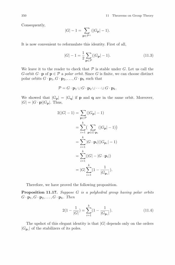
350 11 Theorems on Group Theory
Consequently,|G| − 1 =
∑
p∈P+
(|Gp| − 1).
It is now convenient to reformulate this identity. First of all,
|G| − 1 =12
∑
p∈P(|Gp| − 1). (11.3)
We leave it to the reader to check that P is stable under G. Let us call theG-orbit G · p of p ∈ P a polar orbit. Since G is finite, we can choose distinctpolar orbits G · p1, G · p2, . . . , G · pk such that
P = G · p1 ∪ G · p2 ∪ · · · ∪ G · pk.
We showed that |Gp| = |Gq| if p and q are in the same orbit. Moreover,|G| = |G · p||Gp|. Thus,
2(|G| − 1) =∑
p∈P(|Gp| − 1)
=k∑
i=1
( ∑
p∈G·pi
(|Gp| − 1))
=k∑
i=1
|G · pi|(|Gpi| − 1)
=k∑
i=1
(|G| − |G · pi|)
= |G|k∑
i=1
(1 − 1|Gpi
| ).
Therefore, we have proved the following proposition.
Proposition 11.17. Suppose G is a polyhedral group having polar orbitsG · p1, G · p2, . . . , G · pk. Then
2(1 − 1|G| ) =
k∑
i=1
(1 − 1|Gpi
| ). (11.4)
The upshot of this elegant identity is that |G| depends only on the orders|Gpi
| of the stabilizers of its poles.
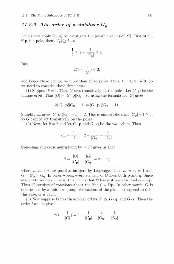
11.2 The Finite Subgroups of SO(3,R) 351
11.2.2 The order of a stabilizer Gp
Let us now apply (11.4) to investigate the possible values of |G|. First of all,if p is a pole, then |Gp| ≥ 2, so
12
≤ 1 − 1|Gp| ≤ 1.
But2(1 − 1
|G| ) < 2,
and hence there cannot be more than three poles. Thus, k = 1, 2, or 3. Sowe need to consider these three cases.
(1) Suppose k = 1. Then G acts transitively on the poles. Let G ·p be theunique orbit. Thus |G| = |G · p||Gp|, so using the formula for |G| gives
2(|G · p||Gp| − 1) = |G · p|(|Gp| − 1).
Simplifying gives |G ·p|(|Gp|+1) = 2. This is impossible, since |Gp|+1 ≥ 3,so G cannot act transitively on the poles.
(2) Next, let k = 2 and let G · p and G · q be the two orbits. Then
2(1 − 1|G| ) = 2 − 1
|Gp| − 1|Gq| .
Canceling and cross multiplying by −|G| gives us that
2 =|G||Gp| +
|G||Gq| = m + n,
where m and n are positive integers by Lagrange. Thus m = n = 1 andG = Gp = Gq. In other words, every element of G fixes both p and q. Sinceevery rotation has an axis, this means that G has just one axis, and q = −p.Thus G consists of rotations about the line � = Rp. In other words, G isdetermined by a finite subgroup of rotations of the plane orthogonal to �. Inthis case, G is cyclic.
(3) Now suppose G has three polar orbits G ·p, G · q, and G · r. Then theorder formula gives
2(1 − 1|G| ) = 3 − 1
|Gp| − 1|Gq| − 1
|Gr|.
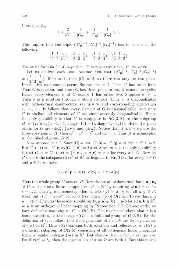
352 11 Theorems on Group Theory
Consequently,
1 +2
|G| =1
|Gp| +1
|Gq| +1
|Gr|> 1.
This implies that the triple (|Gp|−1, |Gq|−1, |Gr|−1) has to be one of thefollowing:
(12,12,
1m
), (12,13,13), (
12,13,14), (
12,13,15).
The order formula (11.4) says that |G| is respectively 2m, 12, 24, or 60.Let us analyze each case. Assume first that (|Gp|−1, |Gq|−1, |Gr|−1)
= (12,12,
1m
). If m = 1, then |G| = 2, so there can only be two poles.Hence, this case cannot occur. Suppose m = 2. Then G has order four.Thus G is abelian, and since G has three polar orbits, it cannot be cyclic.Hence every element σ of G except 1 has order two. Suppose σ �= 1.Then σ is a rotation through π about its axis. Thus, σ is diagonalizablewith orthonormal eigenvectors, say u,v,w and corresponding eigenvalues1, −1, −1. It follows that every element of G is diagonalizable, and sinceG is abelian, all elements of G are simultaneously diagonalizable. Hencethe only possibility is that G is conjugate in SO(3,R) to the subgroupH = {I3,diag(1,−1,−1),diag(−1, 1,−1),diag(−1,−1, 1)}. Here, the polarorbits for G are {±u}, {±v}, and {±w}. Notice that if α, β, γ denote thethree rotations in H, then α2 = β2 = γ2 and αβ = γ. Thus H is isomorphicto the dihedral group D(2).
Now suppose m > 2. Since |G| = 2m, |G·p| = |G·q| = m, while |G·r| = 2.But G · (−r) = −G ·r, so |G · (−r)| = 2 also. Since m > 2, the only possibilityis that G · r = G · (−r) = {± r}, so σ(r) = ± r for every σ ∈ G. Now letP denote the subspace (Rr)⊥ of R3 orthogonal to Rr. Then for every σ ∈ Gand p ∈ P , we have
0 = r · p = σ(r) · σ(p) = ± r · σ(p).
Thus the whole group G acts on P . Now choose an orthonormal basis u1,u2
of P , and define a linear mapping ϕ : P → R2 by requiring ϕ(ui) = ei for
i = 1, 2. Then ϕ is a isometry; that is, ϕ(x · y) = x · y for all x,y ∈ P .Next, put τ(σ) = ϕσϕ−1 for all σ ∈ G. Then τ(σ) ∈ O(2,R). To see this, putμ = τ(σ). Then, as the reader should verify, μ(a)·μ(b) = a·b for all a,b ∈ R
2,so μ is an orthogonal linear mapping by Proposition 7.7. Consequently, wehave defined a mapping τ : G → O(2,R). The reader can check that τ is ahomomorphism, so the image τ(G) is a finite subgroup of O(2,R). By thedefinition of τ , it follows that the eigenvalues of σ on P are the eigenvaluesof τ(σ) on R
2. Thus τ(G) contains both rotations and reflections, so τ(G) isa dihedral subgroup of O(2,R) consisting of all orthogonal linear mappingsfixing a regular polygon {m} in R
2. But observe that in fact, τ is injective.For if τ(σ) = I2, then the eigenvalues of σ on P are both 1. But this means
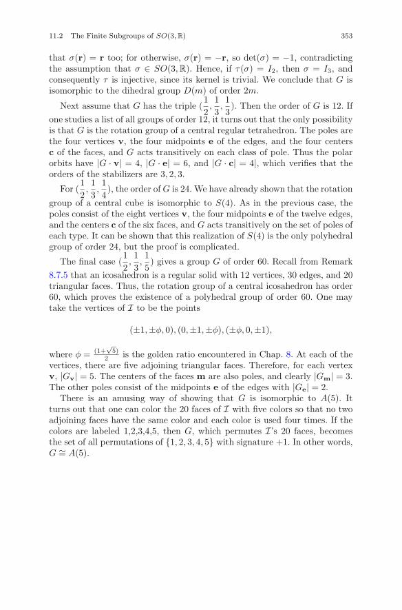
11.2 The Finite Subgroups of SO(3,R) 353
that σ(r) = r too; for otherwise, σ(r) = −r, so det(σ) = −1, contradictingthe assumption that σ ∈ SO(3,R). Hence, if τ(σ) = I2, then σ = I3, andconsequently τ is injective, since its kernel is trivial. We conclude that G isisomorphic to the dihedral group D(m) of order 2m.
Next assume that G has the triple (12,13,13). Then the order of G is 12. If
one studies a list of all groups of order 12, it turns out that the only possibilityis that G is the rotation group of a central regular tetrahedron. The poles arethe four vertices v, the four midpoints e of the edges, and the four centersc of the faces, and G acts transitively on each class of pole. Thus the polarorbits have |G · v| = 4, |G · e| = 6, and |G · c| = 4|, which verifies that theorders of the stabilizers are 3, 2, 3.
For (12,13,14), the order of G is 24. We have already shown that the rotation
group of a central cube is isomorphic to S(4). As in the previous case, thepoles consist of the eight vertices v, the four midpoints e of the twelve edges,and the centers c of the six faces, and G acts transitively on the set of poles ofeach type. It can be shown that this realization of S(4) is the only polyhedralgroup of order 24, but the proof is complicated.
The final case (12,13,15) gives a group G of order 60. Recall from Remark
8.7.5 that an icosahedron is a regular solid with 12 vertices, 30 edges, and 20triangular faces. Thus, the rotation group of a central icosahedron has order60, which proves the existence of a polyhedral group of order 60. One maytake the vertices of I to be the points
(±1,±φ, 0), (0,±1,±φ), (±φ, 0,±1),
where φ = (1+√5)
2 is the golden ratio encountered in Chap. 8. At each of thevertices, there are five adjoining triangular faces. Therefore, for each vertexv, |Gv| = 5. The centers of the faces m are also poles, and clearly |Gm| = 3.The other poles consist of the midpoints e of the edges with |Ge| = 2.
There is an amusing way of showing that G is isomorphic to A(5). Itturns out that one can color the 20 faces of I with five colors so that no twoadjoining faces have the same color and each color is used four times. If thecolors are labeled 1,2,3,4,5, then G, which permutes I’s 20 faces, becomesthe set of all permutations of {1, 2, 3, 4, 5} with signature +1. In other words,G ∼= A(5).
354 11 Theorems on Group Theory
11.3 The Sylow Theorems
Given a finite group G, what can one say about its subgroups? BothLagrange’s theorem and Cauchy’s theorem make assertions about the sub-groups of G in terms of the order of G, which is the most basic invariant ofa finite group. The Sylow theorems, which were discovered by Sylow in 1872during his research on algebraic equations, give much more precise informa-tion. Suppose |G| = pnm, where p is a prime that is prime to m and n ≥ 1.A subgroup of G of order pn is called a Sylow p-subgroup. Sylow’s theoremsassert the following: if 1 ≤ k ≤ n, there exists a subgroup H of order pk,and every such H is contained in a Sylow p-subgroup; all Sylow p-subgroupsfor a given prime p are conjugate in G; and finally, the number of Sylowp-subgroups of G is congruent to one modulo p and divides |G|. The proofsgiven below are elegant and brief, and above all, they explain why the the-orems are true. The tools used are Cauchy’s theorem, the orbit stabilizertheorem, and the fixed-point result for p-groups in Proposition 11.11.
11.3.1 The first Sylow theorem
As above, let G be a finite group and p a prime p dividing |G|, say |G| = pnm,where (p,m) = 1. We now prove the first Sylow theorem, which ensures thatSylow p-subgroups always exist and a bit more.
Theorem 11.18. For each k such that 1 ≤ k ≤ n, G contains a subgroup oforder pk, and every subgroup of order pk is contained in a Sylow p-subgroupof G.
Proof. Suppose H is a subgroup of G of order pk, where 1 ≤ k < n. We willshow that H is contained in a subgroup K of G of order pk+1. Iterating thisargument will yield a subgroup of G of order pn that contains H, giving therequired Sylow p-subgroup. The existence of a subgroup of order pk, for eachk ≤ n, then follows by applying this result to the subgroup generated by anelement of order p, whose existence is guaranteed by Cauchy’s theorem. Now,H acts on X = G/H by left translation. Moreover, H is a p-group, and |X|is divisible by p. Therefore, Proposition 11.11 tells us that either the fixed-point set XH is empty or |XH | = jp for some j > 0. But 1H ∈ XH , so thelatter holds. Note that gH ∈ (G/H)H if and only if gH ∈ NG(H)/H, sinceHgH = gH if and only if gHg−1 = H. Thus, NG(H)/H is a group whoseorder is divisible by p. By Cauchy’s theorem, NG(H)/H contains a subgroupK of order p. Consider the inverse image H ′ = π−1(K) of the quotientmap π : NG(H) → NG(H)/H. Then H ′ is a subgroup of NG(H) containingH, which π maps to K. Thus, by the isomorphism theorem, Theorem 2.20,H ′/H ∼= K, so [H ′ : H] = |K| = p. But Lagrange’s theorem implies that|H ′| = pk+1, so the proof is complete. �
11.3 The Sylow Theorems 355
11.3.2 The second Sylow theorem
The second Sylow theorem asserts that for a given prime p, every pair ofSylow p-subgroups of G are conjugate. This says that a finite group G isrigid in the sense that all subgroups of G of certain orders are isomorphic byan inner automorphism of G.
Theorem 11.19. Every pair of Sylow p-subgroups of a finite group G areconjugate, and if p divides |G|, then the number of Sylow p-subgroups of Galso divides |G|.
Proof. Let H and K be Sylow p-subgroups of G, and let H act on G/K. Itsuffices to show that the fixed-point set (G/K)H is nonempty, say HgK =gK. For if HgK = gK, it follows that gKg−1 = H. Suppose (G/K)H isempty. Then the orbit stabilizer theorem implies that for every H-orbit O,|O| is a multiple of p, since H is a p-group. This implies that p divides |G/K|,which contradicts the assumption that |K| = pn. Consequently, every twoSylow p-subgroups are conjugate. Thus G acts transitively via conjugationon the set of its Sylow p-subgroups, so by another application of the orbitstabilizer theorem, the number of Sylow p-subgroups of G divides |G|. �
The fact that Sylow p-subgroups are conjugate gives the following result.
Corollary 11.20. If G is a finite abelian group, then G contains a uniqueSylow p-subgroup for every prime p dividing |G|.
11.3.3 The third Sylow theorem
The third Sylow theorem is analogous to the result that in a finite group, thenumber of elements of order p is divisible by p − 1.
Theorem 11.21. If G is a finite group and p is a prime dividing |G|, thenthe number of Sylow p-subgroups of G is congruent to 1 modulo p and divides|G|.
Proof. Assume that the prime p divides |G|, and let Sp denote the set of Sylowp-subgroups of G. Fix S ∈ Sp, and let NS denote the normalizer NG(S).I claim that the only Sylow p-subgroup of NS is S. For if R ∈ Sp satisfiesR < NS , then there exists g ∈ NS such that gSg−1 = R. But since gSg−1 = Sby the definition, it follows that R = S. Thus, if R,S ∈ Sp and R �= S, then|NR ∩ NS | cannot be divisible by |S|. Now let NS act on Sp. Certainly,S is a fixed point; i.e. NS · S = S. On the other hand, if R �= S, then|NS · R| is divisible by p. Indeed, by the orbit stabilizer theorem, |NS · R| =|NS |/|NR ∩ NS |, so this follows from the fact that the denominator is notdivisible by |S|. Therefore, the orbit identity implies that |Sp| = 1 + mp. �
356 11 Theorems on Group Theory
11.3.4 Groups of order 12, 15, and 24
We will now look at some examples.
Example 11.8. First consider groups of order 12. In such a group, thenumber of Sylow 2-subgroups is either 1 or 3, and the number of Sylow3-subgroups is either 1 or 4. The direct products C3 ×C4 = C12 and C3 ×U8,where U8 is the group of units modulo 8, are both abelian groups of order12; hence each has exactly one Sylow subgroup of order 3 and one of order4. Note: the direct product of G and H is the group G × H consisting of allthe pairs (g, h) with g ∈ G and H ∈ H with the almost obvious group struc-ture. The general definition is given in Definition 11.6 below. The alternatinggroup A(4) has four cyclic subgroups of order 3 generated respectively by(123), (134), (124), and (234). Thus there are eight elements of order 3. Thisleaves exactly three elements of order 2 or 4. Thus the Sylow 2-subgroup,which has order 4, has to be normal. This group turns out to be the well-known Klein 4-group
V4 = {(1), (12)(34), (14)(23), (13)(24)},
consisting of all elements of S(4) that are the product of two disjoint trans-positions. In fact, V4 is normal in S(4). The dihedral group D(6) has sixrotations, which form a cyclic normal subgroup. The two rotations of order 3determine a normal subgroup, which is therefore the unique Sylow 3-subgroupof D(6). By the O(2,R) dichotomy, the remaining six elements are reflections.Since reflections about orthogonal lines commute, and since a six-sided regu-lar polygon P in R
2 has three pairs of orthogonal lines through which P maybe reflected, there are three Sylow 2-subgroups. Thus D(6) has one Sylow3-subgroup and three Sylow 2-subgroups. �
Example 11.9. Returning to the group of order 15, we see that the numberof Sylow 3-subgroups has the form 1+3m and divides 15. The only possibilityis that there is exactly one Sylow 3-subgroup. Similarly, the number of Sylow5-subgroups has the form 1 + 5m and divides 15. Hence there is exactly oneSylow 5-subgroup. The order of an element has to divide 15, so the possibleorders are 3, 5, and 15. Since we just showed that there are two elements oforder 3 and four elements of order 5, there has to be an element of order 15(in fact, eight of them). Thus we see once again that a group of order 15 iscyclic. �
Example 11.10. The symmetric group S(4) and the matrix group SL(2,F3)both have order 24. Are they isomorphic? A necessary condition for two finitegroups to be isomorphic is that they have the same Sylow subgroups. By thethird Sylow theorem, the number of Sylow 3-subgroups in a group of order24 is one or four, and the number of Sylow 2-subgroups is one or three. Wewill now show that S(4) has three Sylow 2-subgroups. Recall that S(4) is
11.3 The Sylow Theorems 357
isomorphic to the group of all rotations of the unit cube C in R3 centered at
the origin. Let S1 denote the intersection of the cube with the xy-plane, andlabel the vertices of S as 1, 2, 3, 4 in a clockwise manner, with 1 denotingthe vertex in the first octant. The subgroup
H1 = {(1), (1234), (1432), (13)(24), (12)(34), (14)(23), (13), (24)}
is a copy of D(4). The first four elements are rotations of S1, which rotateC about the z-axis. The other four elements are reflections of S1, which arerotations of the cube through π/2. The other two Sylow 2-subgroups arecopies of D(4), which act the same way on the squares S2 and S3 obtainedby intersecting the cube with the other two coordinate hyperplanes. It turnsout that SL(2,F3) has only one Sylow subgroup H of order 8, so H is normal.The details are tedious, so we will omit them. For example, the elements oforder 4 are (
1 11 2
),
(2 11 1
),
(1 22 2
),
(2 21 2
).
Thus, S(4) and SL(2,F3) have different Sylow 2-subgroups, so they cannotbe isomorphic. �
Exercises
Exercise 11.3.1. Show that A(4) does not have a subgroup of order 6; hencethe converse of Lagrange’s theorem is false.
Exercise 11.3.2. Determine the Sylow subgroups for the dihedral groupD(6).
Exercise 11.3.3. Let p and q be distinct primes, and let G be a group oforder pq. Show that the following statements are equivalent:
(i) G is abelian.
(ii) The center Z(G) is nontrivial.
(iii) G is cyclic.
Give an example of a group of order pq that is not cyclic.
Exercise 11.3.4. True or false with reasoning: every group of order 10 isabelian.
Exercise 11.3.5. Show that if p and p+2 are both prime, then every groupof order p(p + 2) is cyclic.
Exercise 11.3.6. Let p be a prime. Show that U(n,Fp) and L(n,Fp) areSylow p-subgroups of both GL(n,Fp) and SL(n,Fp). How is U(n,Fp) conju-gated onto L(n,Fp)?
358 11 Theorems on Group Theory
Exercise 11.3.7. Suppose p = 5 and n = 3.
(i) How many Sylow p-subgroups does GL(n,Fp) have?
(ii) Answer part (i) for SL(n,Fp).
Exercise 11.3.8. Find the orders of all the Sylow p-subgroups of GL(n,Fp)for primes p ≤ 7.
Exercise 11.3.9. Consider the group Un of units modulo n for n = 50.
(i) Discuss the Sylow subgroups of Un.
(ii) Determine whether Un is cyclic. (Suggestion: consider part (i).)
Exercise 11.3.10. The order of Un is 100 if n = 202. Is either of the Sylowsubgroups cyclic?
Exercise 11.3.11. • Let G be a finite group. Show that if |G| = mp, wherep is prime and p > m, then there is only one Sylow p-subgroup H, and H isnormal in G.
Exercise 11.3.12. • Show that a group of order pq, p and q distinct primes,is cyclic whenever p does not divide q − 1 and q does not divide p − 1.
11.4 The Structure of Finite Abelian Groups 359
11.4 The Structure of Finite Abelian Groups
So far, we have encountered a few examples of finite abelian groups: the cyclicgroups Cm, the multiplicative group F
∗ of a Galois field F, the center Z(G)of an arbitrary finite group G, and the subgroups of all these groups. Moreinterestingly, as we saw in Section 2.1, the group of multiplicative units (i.e.,invertible elements) in Z/nZ is an abelian group Un of order φ(n), where φ isEuler’s phi-function. We will now describe the structure of all finite abeliangroups. The Sylow theorems imply a finite abelian group is the direct productof its Sylow subgroups. After that, the job is to describe the abelian p-groups.
11.4.1 Direct products
The direct product of a finite number of groups is a generalization of thedirect sum of a finite number of vector spaces. And as for vector spaces, directproducts in the group setting come in two flavors, internal and external. Thesimpler case is the external direct product, so we will introduce it first.
Definition 11.6. Let G1 and G2 be arbitrary groups. Their external directproduct is the usual Cartesian product G1 × G2 with the group operation
(g1, h1)(g2, h2) = (g1g2, h1h2).
It is easy to check that the external direct product G1×G2 is a group withidentity (1, 1), where 1 denotes both the identity of G1 and that of G2. Thenotion of external direct product can be extended without difficulty from twogroups to any finite number of groups. We will leave the details to the reader.Note that if V1 and V2 are vector spaces over different fields, then V1 × V2 isan abelian group but not a vector space. If V1 and V2 have the same scalarfield F, then the external direct sum of vector spaces applies, and V1 × V2 isa vector space over F.
Proposition 11.22. Suppose G = G1 ×G2 ×· · ·×Gm is the external directproduct of the groups G1, G2, . . . , Gm. Then:
(i) G is abelian if each Gi is, and
(ii) for every σ ∈ S(m), G ∼= Gσ(1) × Gσ(2) × · · · × Gσ(m).
Proof. We leave the proof to the reader. �
We will now consider the internal direct product, which for groups is ageneralization of the internal direct sum of subspaces (keeping in mind thatsubspaces of a vector space are normal subgroups). Let A1, A2, . . . , Ak besubsets of the group G. Define A1A2 · · · Ak to be the totality of products
360 11 Theorems on Group Theory
a1a2 · · · ak, where each ai is in Ai. Also, define < A1, A2, . . . , Ak > to be thesmallest subgroup of G containing each Ai. Suppose each Ai is normalizedby G; that is, gAig
−1 = Ai for all g ∈ G. Then AiAj = AjAi for all i, j. Forif we choose any ai ∈ Ai for each i, it follows that aiaj = aj(a−1
j aiaj), soAiAj ⊂ AjAi. Hence by symmetry, AiAj = AjAi. Consequently, the productA1A2 · · · Ak is independent of how the sets Ai are ordered.
We now need the following lemma.
Lemma 11.23. If H1,H2, . . . ,Hk are normal subgroups of G, then the prod-uct H1H2 · · · Hk is a normal subgroup of G, and
< H1,H2, . . . , Hk >= H1H2 · · · Hk.
Proof. We will use induction to prove that H1H2 · · · Hk is a subgroup ofG, which will show that < H1,H2, . . . , Hk >= H1H2 · · · Hk, since H1H2 · · ·Hk ⊂< H1,H2, . . . , Hk >. Notice that if H1H2 · · · Hk is a subgroup, then ithas to be normal, since for all g ∈ G,
g(H1H2 · · · Hk)g−1 = (gH1g−1)(gH2g
−1) · · · (gHkg−1),
and every Hi is a normal subgroup. The lemma holds for k = 1, so assumek > 1 and that it holds for k − 1. Thus H = H1H2 · · · Hk−1 is a subgroup ofG. We need to show that HHk is a subgroup, so we must show that if a, b ∈ Hand g, h ∈ Hk, then (ag)(bh)−1 ∈ HHk. Now, (ag)(bh)−1 = a(gh−1)b−1 ∈HHkH = HHk, since HHk = HkH by the remark preceding the lemma.Hence H1H2 · · · Hk is a subgroup, so the proof is complete. �
We now come to the internal direct product of an arbitrary number ofnormal subgroups.
Definition 11.7. Let G be a group and let H1,H2, . . . , Hk be normal sub-groups of G. We say that G is the internal direct product of H1,H2, . . . , Hk
ifG =< H1,H2, . . . , Hk >,
and for each i with 1 ≤ i < k,
< H1,H2, . . . , Hi > ∩Hi+1 = (1).
If G is the internal direct product of H1, . . . , Hk, we will write G =((H1, . . . , Hk)).
Proposition 11.24. Let G = ((H1,H2, . . . , Hk)). Then for each g ∈ G,there exists exactly one expression g = h1h2 · · · hm, where hi ∈ Hi for eachi. In particular, if G is finite, then
11.4 The Structure of Finite Abelian Groups 361
|G| =m∏
i=1
|Hi|. (11.5)
Proof. An expression g = h1h2 · · · hm exists by Lemma 11.23. Assumeg = h1 · · · hm = k1 · · · km with hi, ki ∈ Hi for all i. Then hmk−1
m ∈<H1, . . . ,Hm−1 >. Therefore, hmk−1
m = 1, so h1 · · · hm−1 = k1 · · · km−1. Con-tinuing in this manner, it follows that hi = ki for each i. This shows that theabove expression for g is unique.
�
Proposition 11.25. Suppose G = ((H1,H2, . . . , Hk)). Then G ∼= H1×H2×· · · × Hk.
Proof. Define a map ϕ : H1 × · · · × Hk → G by ϕ(h1, . . . , hk) = h1 · · · hk. ByProposition 11.24, ϕ is a bijection. Since Hi and Hj commute elementwisefor all i and j, it also follows that ϕ is also a homomorphism, so ϕ is anisomorphism. �
Example 11.11. Let’s reconsider U8 (see Example 2.18). For simplicity, wedenote the coset m + 8Z by m. Thus U8 = {1, 3, 5, 7}. Since U8 is abelian,every subgroup is normal. Using coset multiplication, we have 3 · 5 = 15 = 7.Hence if H1 = {1, 3} and H2 = {1, 5}, then U8 = ((H1,H2)) ∼= H1 × H2. �
Example 11.12. Let’s next consider U15 = {1, 2, 4, 7, 8, 11, 13, 14}. Since|U15| = 8, the possible orders of its elements are 1, 2, 4, and 8. It is easyto check that 2, 7, 8, and 13 have order 4, and 4, 11, and 14 have order 2.Moreover, 22 = 72 = 82 = 132 = 4. Thus < a > ∩ < 11 >=< a > ∩ < 14 >=(1) for a = 2, 7, 8, 13. Hence if H =< a >, K =< 11 >, and L =< 14 >, wehave
U15 = ((H,K)) ∼= H × K ∼= ((H,L)) ∼= H × L = C4 × C2.
�
11.4.2 The structure theorem for finite abeliangroups
Suppose G is a finite abelian group of order pn11 · · · pnm
m , where p1, p2, . . . , pm
are the distinct prime factors of |G|, and let Gi denote the unique Sylowpi-subgroup G. The first of two results about the structure of G is stated asfollows.
Proposition 11.26. Let G be as above. Then G is the direct product (bothinternal and external) of its Sylow subgroups G1, . . . , Gm.
362 11 Theorems on Group Theory
Proof. Since G is abelian, its Sylow subgroups are normal and commuteelementwise. Let us induct on m. Assume that the product G1 · · · Gi isdirect for each i < m. By Proposition 11.24, |G1 · · · Gi| = pn1
1 · · · pnii . Thus
G1 · · · Gm−1 ∩ Gm = (1), since every element of Gm has order pkm for
some k, and pm does not divide |G1 · · · Gm−1|. Therefore, the productG1 · · · Gm is direct, and consequently, G = ((G1, . . . , Gm)). It follows thatG ∼= G1 × · · · × Gm. �
It remains to give a complete description of the abelian p-groups in moredetail. This turns out to be surprisingly complicated, so we will simply outlinethe proof. Here is the main result:
Theorem 11.27. A finite abelian group of order pn, p a prime, is isomor-phic to a product of cyclic p-groups. In particular, every finite abelian groupG is the external direct sum of cyclic groups of prime power order.
Proof. The proof is by induction on n. Choose an element y ∈ G of maximalorder, and let H =< y >. By induction, G/H is a product of cyclic groups,say G/H =< a1H > × · · · × < akH >. Now G/H is also a p-group, so foreach i, apri
i = ysi for some ri, si > 0. We assert that pri divides si. Putji = si/pri and ui = aiy
−ji . Then it turns out that G =< u1 > × · · · × <uk > ×H, which gives the induction step and finishes the proof (moduloomitted details). �
Example 11.13. According to the theorem, if G is abelian of order 16, thenthe possibilities for G are
C2 × C2 × C2 × C2, C4 × C2 × C2, C4 × C4, C8 × C2, C16.
11.4.3 The Chinese Remainder Theorem
Applying the above results gives the following corollary.
Corollary 11.28. Suppose G is a finite cyclic group. Then its Sylow sub-groups G1, . . . , Gm are cyclic of prime power order, and G = G1 × · · · × Gm.
Proof. Since G is cyclic, division with remainder tells us that every subgroupof G is also cyclic. Hence the Sylow subgroups of G are cyclic, so the resultfollows from Proposition 11.26. �
In particular, let n = pn11 · · · pnm
m , as usual. Since the additive group Z/nZis cyclic, its Sylow subgroups are (Z/pn1
1 Z), . . . , (Z/pnmm Z). Therefore,
Z/nZ ∼= (Z/pn11 Z) × · · · × (Z/pnm
m Z).
11.4 The Structure of Finite Abelian Groups 363
�As a corollary, one gets the Chinese remainder theorem: given congruence
equationsx ≡ a1 mod(pn1
1 ), . . . , x ≡ am mod(pnmm ),
there exists a unique class w +nZ in Z/nZ such that setting x = w solves allthe above congruences.
Exercises
Exercise 11.4.1. Find at least three values of n such that Un is cyclic. Isthere a general rule?
Exercise 11.4.2. • Show that in every cyclic group, the number of elementsof order m is divisible by φ(m). Give an example of a finite abelian group inwhich the number of elements of order m is not divisible by φ(m).
Exercise 11.4.3. Suppose each Gi is cyclic. When is G = G1×G2×· · ·×Gm
cyclic?
Exercise 11.4.4. Suppose G can be expressed as a direct product HK.Show that
(i) K ∼= G/H, and
(ii) G ∼= H × G/H.
Exercise 11.4.5. Find all the ways of decomposing U21 as a product ofcyclic subgroups.
Exercise 11.4.6. Let F be a Galois field. It is a theorem that the multi-plicative group F
∗ of F is always cyclic. Prove directly that F∗ is cyclic in thefollowing cases:
(i) |F| = 16,
(ii) |F| = 32, and
(ii) |F| = 25.
Exercise 11.4.7. Let G be a group, H a subgroup, and N a normal sub-group of G. Then G is said to be the semidirect product of H and N if atleast one of the following statements holds.
(i) G = NH and N ∩ H = 1.
(ii) Every element of G can be written in a unique way as a product nh,where n ∈ N and h ∈ H.
(iii) The natural inclusion homomorphism H → G composed with the naturalprojection G → G/N induces an isomorphism H ∼= G/N .
(iv) There exists a homomorphism G → H that is the identity on H whosekernel is N .
Show that the all four statements are equivalent.
364 11 Theorems on Group Theory
11.5 Solvable Groups and Simple Groups
One of the most celebrated results in classical algebra is the unsolvability ofthe quintic. Roughly, this means that there exist polynomials f(x) of degreefive with rational coefficients whose roots cannot be expressed in terms ofradicals involving those coefficients. More precisely, there is no formula thatexpresses the roots of an arbitrary fifth-degree polynomial f(x) = x5+a1x
4+a2x
3 + a3x2 + a4x + a5 starting from an algebraic combination α of the
coefficients ai of f , takes an mth root α1/m for some m, then repeats theprocess on the coefficients of α1/m and so on until a closed formula that givesall the roots of f(x) is obtained. Unsolvable quintics can be quite ordinary:2x5+10x+5 is an example. The definitive criterion for solvability by radicalsfirst appeared in Galois’s posthumous 1846 paper: a polynomial is solvableby radicals if and only if its Galois group is solvable. (For a definition ofthe Galois group of a polynomial, see Section 11.5.5.) The Galois group of2x5+10x+5 turns out to be S(5), which, as we will see below, is not a solvablegroup. The simple groups lie at the opposite end of the group spectrum fromthe solvable groups, and in fact, they serve as the main source of examplesof unsolvable groups. Recall that a nontrivial group G is said to be simpleif its only normal subgroups are G itself and the trivial subgroup (1). Afamous classical result is that the alternating groups A(n) for n > 4 aresimple. It follows that the symmetric groups S(n) for n > 4 are not solvable.Simple groups play a role in the structure theory because of compositionseries and the Jordan–Holder theorem, which we will state without proofbelow. As mentioned in the introduction to this chapter, the finite simplegroups have now been classified, the final step not having come until 1982with the construction of the Monster.
11.5.1 The definition of a solvable group
The process described above for solving by radicals hints at what the defini-tion of a solvable group might be. To define solvability, we must first introducethe notion of a subnormal series in a group.
Definition 11.8. A subnormal series for a group G is a finite sequence ofsubgroups
G = H1 > H2 > · · · > Hr−1 > Hr = (1) (11.6)
of G such that Hi+1 is normal in Hi for i = 1, . . . , r − 1. The quotient groupsHi/Hi+1 are called the factors of the subnormal series (11.6).
For example, if H �= (1) is a proper normal subgroup of G, then G > H >(1) is an example of a subnormal series. A simple group G has no nontrivial
11.5 Solvable Groups and Simple Groups 365
normal subgroups, so G > (1) is the only subnormal series for G. A subnormalseries (11.6) is called a composition series if each factor is a simple group. IfH is normal in G, then G/H is simple if and only if there exists no normalsubgroup N of G such that H < N < G. (The proof of this assertion is anexercise.) Thus a composition series is a subnormal series of maximal length.It follows that every finite group has a composition series.
Now we can define what a solvable group is.
Definition 11.9. A group G is called solvable if it has a subnormal series(11.6) such that each factor Hi/Hi+1 is abelian.
Of course, abelian groups are solvable. The next result points out an impor-tant class of solvable groups.
Proposition 11.29. Every p-group is solvable.
Proof. Suppose |G| = pn. If n = 1, then surely G is solvable, so let us argueby induction on n. Assume that all p-groups of order pn−1 are solvable. By thefirst Sylow theorem, G has a subgroup H of order pn−1, and by assumption,H is solvable. To show that G is solvable, it suffices to show that H is normalin G, since in that case, G/H has order p and hence is abelian. Let H act onG/H by left multiplication. The orbit stabilizer theorem then says that forevery orbit O, either |O| = 1 or |O| = p. But the latter case cannot occur,since the orbit of the coset H is itself. It follows that every orbit is a singlepoint. Thus HgH = gH for all g ∈ G. This implies that H is normal in G. �
A famous result in finite group theory known as Burnside’s theorem (1904)states that a finite group whose order is divisible by at most two primes issolvable. Burnside’s proof used techniques from outside group theory, so itremained an open problem to find a purely group-theoretic proof. Such aproof was not discovered until 1970. In 1963, Walter Feit and John Thompsonpublished a 255-page paper proving that every finite group of odd order issolvable, hence ensuring that there are nonabelian solvable groups that arenot p-groups. Note that the Feit–Thompson theorem implies Burnside’s resultfor two odd primes.
The symmetric groups S(3) and S(4) are both solvable. (For example,apply Burnside’s theorem.) We will leave this claim as an exercise for S(3)and give a proof for S(4) in the next example. It turns out, however, thatS(n) is not solvable for n > 4.
Example 11.14 (S(4) is solvable). We need to display a subnormal seriesfor S(4) whose derived factors are abelian. The alternating group A(4) (seeSection 5.2) is normal in S(4) and S(4)/A(4) ∼= C2, so it is abelian. Thus,S(4) > A(4) is a first step. As we have seen, the Klein 4-group V4 (seeExample 11.8) is a normal subgroup of A(4) of order 4. Since the orderof A(4) is 12, A(4)/V4 has order three, and hence it is also abelian. ButV4 is abelian, since it has order p2. It follows that S(4) > A(4) > V4 >(1) is a subnormal series for S(4) whose factors are abelian. Hence S(4) issolvable. �
366 11 Theorems on Group Theory
11.5.2 The commutator subgroup
In this section, we will find an explicit test for solvability. To do so, we needto introduce the commutator subgroup of a group and its derived series. Thecommutator subgroup of G is the smallest subgroup of G that contains allproducts of the form ghg−1h−1, where g, h ∈ G. This subgroup is denotedby [G,G].
Proposition 11.30. The commutator subgroup [G,G] of G is normal inG, and G/[G,G] is abelian. In particular, if G is simple, then G = [G,G].Moreover, if N is a normal subgroup of G such that G/N is abelian, then Ncontains [G,G].
Proof. We will leave the proof as an exercise. �
The commutator groups for S(n) provide a nice example. Recall thatA(n) = ker(sgn), where sgn : S(n) → {±1} is the signature homomorphismdefined by the expression
sgn(σ) =∏
i<j
σ(i) − σ(j)i − j
.
It follows from the fact that sgn is a homomorphism that [S(n), S(n)] ≤ A(n).
Proposition 11.31. The commutator subgroup of S(n) is A(n) for all n.
Proof. We just showed that [S(n), S(n)] ≤ A(n). Notice that all 3-cycles inS(n) are commutators, since
(abc) = (acb)(ab)(abc)(ab).
To show that A(n) = [S(n), S(n)], it thus suffices to show that A(n) is gener-ated by 3-cycles. To see this, recall that S(n) is generated by transpositions;hence elements of A(n) are products of an even number of transpositions.These products can be either disjoint, such as (ab)(cd), or nondisjoint, suchas (ab)(bc). Thus the claim follows from the two identities
(ab)(cd) = (acb)(acd), and (ab)(bc) = (abc).
�
The commutator subgroup of G has its own commutator subgroup. Toavoid making the notation too clumsy, let G(1) denote [G,G], and for eachi > 1 define G(i) = [G(i−1), G(i−1)]. The derived series of G is the sequence
G ≥ G(1) ≥ G(2) ≥ · · · ≥ G(i) ≥ · · · . (11.7)
11.5 Solvable Groups and Simple Groups 367
Proposition 11.32. A group G is solvable if and only if its derived serieshas the property that G(k) is the identity subgroup for some k.
Proof. The if assertion follows immediately from Proposition 11.30 and thedefinition of a solvable group. The only if assertion follows from the secondassertion of Proposition 11.30, since if H/N is abelian, then N contains[H,H]. For if G = N1 > N2 > · · · > Nk−1 > Nk = 1 is a subnormal seriessuch that Ni/Ni+1 is abelian for all i, then G(i) < Ni+1. Thus G(k−1) = 1. �
Corollary 11.33. Subgroups and quotients of a solvable group are solvable.
Proof. Let G be solvable. If H is a subgroup of G, then its derived seriessatisfies H(i) < G(i), so the derived series of H has to terminate at theidentity, since the derived series of G does. Likewise, if N is normal in G,then the derived series of G/N is the image of the derived series of G, so itlikewise terminates. �
We now give a nontrivial example of a solvable matrix group.
Proposition 11.34. The upper triangular subgroup T (n,F) < GL(n,F) issolvable.
Proof. First notice that every element T ∈ T (n,F) can be factored as T =DU = V D, where D ∈ D(n,F) and both U and V are in U(n,F). Moreover,D(n,F) < NGL(n,F)(U(n,F)). This implies that the commutator of T (n,F) iscontained in U(n,F), for if A = DU and B = EV are in T (n,F), then thereexist W,Y ∈ U(n,F) such that UE = EW and D−1V −1 = Y D−1. Thus,
[A,B] = ABA−1B−1
= (DU)(EV )(U−1D−1)(V −1E−1)= (DE)(WV U−1Y )(D−1E−1).
Hence [A,B] ∈ U(n,F). Thus it suffices to show that U(n,F) is solvable. Foreach k with 1 ≤ k < n, let Uk = {U ∈ U(n,F) | uij = 0 if 0 < j − i ≤ k}. Inother words, Uk consists of all U ∈ U(n,F) that have zero on the first throughkth superdiagonals. We leave it to the reader to check that [Uk, Uk] < Uk+1.But [Un, Un] = {In}, so it follows from Proposition 11.32 that T (n,F) issolvable. �
11.5.3 An example: A(5) is simple
In this section, we will prove that the alternating group A(5) is simple. Theproof uses the following characterization of a normal subgroup, whose proofis left to the reader.
368 11 Theorems on Group Theory
Proposition 11.35. A subgroup H of a group G is normal in G if and onlyif H is a union of G-conjugacy classes.
Proposition 11.36. A(5) is simple.
Proof. It suffices to show that no subgroup of A(5) is a union of A(5)-conjugacy classes. To prove this, we have to describe these conjugacy classes.Since A(5) is normal in S(5), A(5) is the union of S(5)-conjugacy classes.Note that the S(5)-conjugacy classes in A(5) are unions of A(5)-conjugacyclasses. By Proposition 11.15, the conjugacy classes in S(5) are representedby
(1), (12), (123), (1234), (12345), (12)(34), and (123)(45).
Since the signature of a k-cycle is 1 if k is odd and −1 is k is even, it followsthat A(5) is the union of the S(5)-conjugacy classes of the elements
(1), (123), (12345), and (12)(34). (11.8)
Let us first compute the orders of the A(5)-conjugacy classes of these ele-ments. By Proposition 11.8, we need to compute their centralizers in A(5).But ZA(5)(1) = A(5), ZA(5)(123) = 〈(123)〉, ZA(5)(12345) = 〈(12345)〉, andZA(5)((12)(34)) = {1, (12), (34), (12)(34)}. Since |A(5)| = 60, Proposition11.8 implies that the conjugacy classes in A(5) of the elements in (11.8) haverespectively 1, 20, 12, and 15 elements. Since these classes give a total of 48elements, we have to account for another 12 elements. The reader can checkthat (12)(12345)(12) = (13452) is not conjugate in A(5) to (12345). Thus itsA(5)-conjugacy class accounts for the remaining 12 elements. Therefore, theorder of a normal subgroup of A(5) must be a sum of 1 and some subset of12, 12, 15, and 20. Hence the order of a nontrivial normal subgroup of A(5)can be only one of 13, 16, 21, 25, 28, 33, 36, 40, 45, and 48. But none of thesenumbers divides 60, so A(5) must be simple. �
In fact, A(n) is simple for all n ≥ 5. The standard proof of this is to showthat every normal subgroup of A(n) for n ≥ 5 contains a 3-cycle. But theonly normal subgroup of A(n) that contains a 3-cycle is all of A(n), so A(n)is simple. A complete proof can be found in Abstract Algebra, by Dummitand Foote (pp. 128–130). The alternating groups also appear in another classof finite simple groups. To describe this class, we first consider the matrixgroups SL(2,Fp). Since the center Z(G) of a group G is always a normalsubgroup, the question is whether G/Z(G) is simple. Now, Z(SL(2,Fp)) ={cI2 | c2 = 1} is nontrivial for p > 2. The quotient group PSL(2, p) =SL(2,Fp)/Z(SL(2,Fp)) is called the projective linear group of degree two.
11.5 Solvable Groups and Simple Groups 369
Let us next compute |PSL(2, p)|. Since SL(2,Fp) is the kernel of the homo-morphism det : GL(2,Fp) → (Fp)∗, and det is surjective, |SL(2,Fp)| =|GL(2,Fp)|/(p − 1). But from a computation from Chap. 6, |GL(2,Fp)| =(p2 − 1)(p2 − p) (since (p2 − 1)(p2 − p) is the number of pairs of linearlyindependent vectors in (F2)2). Thus if p > 2, then
|PSL(2, p)| =|SL(2,Fp)|
2=
(p2 − 1)(p2 − p)2(p − 1)
=p(p2 − 1)
2.
It follows that |PSL(2, 2)| = 6, while |PSL(2, 3)| = 12 and |PSL(2, 5)| = 60.In fact, using fractional linear transformations and projective geometry, onecan write down explicit isomorphisms PSL(2, 2) ∼= S(3), PSL(2, 3) ∼= A(4),and PSL(2, 5) ∼= A(5). The general result is that if p > 3, then PSL(2, p) issimple. The proof takes several pages to write down, and we will skip it.
11.5.4 Simple groups and the Jordan–Holdertheorem
The Jordan–Holder theorem is stated as follows:
Theorem 11.37. Any two composition series for a group G have the samenumber of composition factors, and their composition factors are isomorphicup to order.
The proof is somewhat long and complicated, and we will omit it. As wenoted earlier, a finite group always admits at least one composition series,while infinite groups need not admit any. The integers, for example, do nothave a composition series.
Example 11.15. For example, the cyclic group C12 gives a nice illustrationof the Jordan–Holder Theorem. The group C12 has three composition series:
C12 > C6 > C3 > (1), C12 > C6 > C2 > (1), and C12 > C4 > C2 > (1).
The corresponding composition factors taken in order are
{C2, C2, C3}, {C2, C3, C2}, and {C3, C2, C2}.
Two groups with isomorphic composition factors need not be isomorphic,however, as the following example shows. �
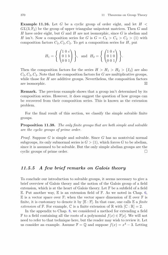
370 11 Theorems on Group Theory
Example 11.16. Let G be a cyclic group of order eight, and let H <GL(3,F2) be the group of upper triangular unipotent matrices. Then G andH have order eight, but G and H are not isomorphic, since G is abelian andH isn’t. Now a composition series for G is G = C8 > C4 > C2 > (1) withcomposition factors C2, C2, C2. To get a composition series for H, put
H1 =
{ ⎛
⎝1 0 c0 1 b0 0 1
⎞
⎠}
, and H2 =
{⎛
⎝1 0 c0 1 00 0 1
⎞
⎠}
.
Then the composition factors for the series H > H1 > H2 > {I3} are alsoC2, C2, C2. Note that the composition factors for G are multiplicative groups,while those for H are additive groups. Nevertheless, the composition factorsare isomorphic. �
Remark. The previous example shows that a group isn’t determined by itscomposition series. However, it does suggest the question of how groups canbe recovered from their composition series. This is known as the extensionproblem.
For the final result of this section, we classify the simple solvable finitegroups.
Proposition 11.38. The only finite groups that are both simple and solvableare the cyclic groups of prime order.
Proof. Suppose G is simple and solvable. Since G has no nontrivial normalsubgroups, its only subnormal series is G > (1), which forces G to be abelian,since it is assumed to be solvable. But the only simple abelian groups are thecyclic groups of prime order. �
11.5.5 A few brief remarks on Galois theory
To conclude our introduction to solvable groups, it seems necessary to give abrief overview of Galois theory and the notion of the Galois group of a fieldextension, which is at the heart of Galois theory. Let F be a subfield of a fieldE. Put another way, E is an extension field of F. As we noted in Chap. 6,E is a vector space over F; when the vector space dimension of E over F isfinite, it is customary to denote it by [E : F]. In that case, one calls E a finiteextension of F. For example, C is a finite extension of R with [C : R] = 2.
In the appendix to Chap. 8, we considered a method for extending a fieldF to a field containing all the roots of a polynomial f(x) ∈ F[x]. We will notneed to refer to that technique here, but the reader may wish to review it. Letus consider an example. Assume F = Q and suppose f(x) = x4 − 3. Letting
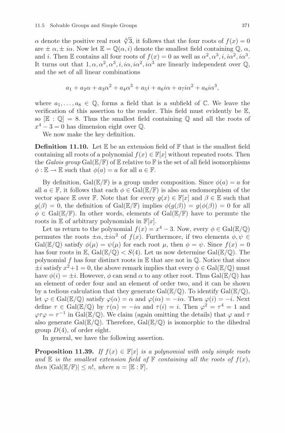
11.5 Solvable Groups and Simple Groups 371
α denote the positive real root 4√
3, it follows that the four roots of f(x) = 0are ± α,± iα. Now let E = Q(α, i) denote the smallest field containing Q, α,and i. Then E contains all four roots of f(x) = 0 as well as α2, α3, i, iα2, iα3.It turns out that 1, α, α2, α3, i, iα, iα2, iα3 are linearly independent over Q,and the set of all linear combinations
a1 + a2α + a3α2 + a4α
3 + a5i + a6iα + a7iα2 + a8iα
3,
where a1, . . . , a8 ∈ Q, forms a field that is a subfield of C. We leave theverification of this assertion to the reader. This field must evidently be E,so [E : Q] = 8. Thus the smallest field containing Q and all the roots ofx4 − 3 = 0 has dimension eight over Q.
We now make the key definition.
Definition 11.10. Let E be an extension field of F that is the smallest fieldcontaining all roots of a polynomial f(x) ∈ F[x] without repeated roots. Thenthe Galois group Gal(E/F) of E relative to F is the set of all field isomorphismsφ : E → E such that φ(a) = a for all a ∈ F.
By definition, Gal(E/F) is a group under composition. Since φ(a) = a forall a ∈ F, it follows that each φ ∈ Gal(E/F) is also an endomorphism of thevector space E over F. Note that for every g(x) ∈ F[x] and β ∈ E such thatg(β) = 0, the definition of Gal(E/F) implies φ(g(β)) = g(φ(β)) = 0 for allφ ∈ Gal(E/F). In other words, elements of Gal(E/F) have to permute theroots in E of arbitrary polynomials in F[x].
Let us return to the polynomial f(x) = x4 − 3. Now, every φ ∈ Gal(E/Q)permutes the roots ±α,±iα2 of f(x). Furthermore, if two elements φ, ψ ∈Gal(E/Q) satisfy φ(μ) = ψ(μ) for each root μ, then φ = ψ. Since f(x) = 0has four roots in E, Gal(E/Q) < S(4). Let us now determine Gal(E/Q). Thepolynomial f has four distinct roots in E that are not in Q. Notice that since±i satisfy x2+1 = 0, the above remark implies that every φ ∈ Gal(E/Q) musthave φ(i) = ±i. However, φ can send α to any other root. Thus Gal(E/Q) hasan element of order four and an element of order two, and it can be shownby a tedious calculation that they generate Gal(E/Q). To identify Gal(E/Q),let ϕ ∈ Gal(E/Q) satisfy ϕ(α) = α and ϕ(iα) = −iα. Then ϕ(i) = −i. Nextdefine τ ∈ Gal(E/Q) by τ(α) = −iα and τ(i) = i. Then ϕ2 = τ4 = 1 andϕτϕ = τ−1 in Gal(E/Q). We claim (again omitting the details) that ϕ and τalso generate Gal(E/Q). Therefore, Gal(E/Q) is isomorphic to the dihedralgroup D(4), of order eight.
In general, we have the following assertion.
Proposition 11.39. If f(x) ∈ F[x] is a polynomial with only simple rootsand E is the smallest extension field of F containing all the roots of f(x),then |Gal(E/F)| ≤ n!, where n = [E : F].
372 11 Theorems on Group Theory
The fundamental theorem of Galois theory stated below explains the cor-respondence between the subfields of E containing F and the subgroups ofGal(E/F).
Theorem 11.40. Let E be an extension field of the field F that is obtainedby adjoining all the roots of an irreducible polynomial f(x) over F with sim-ple roots. Then there is a one-to-one correspondence between subgroups ofGal(E/F) and fields K such that F ⊂ K ⊂ E in which a subgroup H corre-sponds to the subfield K = E
H of elements of E fixed by all elements of H, anda subfield K such that F ⊂ K ⊂ E corresponds to Gal(E/K). Furthermore, ifH is a normal subgroup, then Gal(K/F) ∼= Gal(E/F)/Gal(E/K), where K isthe fixed subfield E
H .
Returning to Q(α, i), let us determine what the theorem says. The groupGal(E/Q(i)) is the subgroup of Gal(E/Q) containing all elements of Gal(E/Q)fixing i. The element τ fixes i and generates a cyclic group < τ > of order four.Therefore, Gal(E/Q(i)) is evidently < τ >. Notice that < τ > is a normalsubgroup of Gal(E/Q). Note also that Gal(Q(i)/Q) ∼= C2. The conclusionfrom this is that |Gal(E/Q)| = 8, which bypasses the tedious calculationsmentioned above and shows that geq ∼= D(4).
Exercises
Exercise 11.5.1. Show directly that S(3) is solvable.
Exercise 11.5.2. True or false: a nonabelian simple group is its own com-mutator.
Exercise 11.5.3. True or false: all dihedral groups are solvable.
Exercise 11.5.4. Show, without using the Sylow theorems, that the Klein4-group is normal in A(4). (Suggestion: make a list of the conjugacy classesof A(4) and show that V4 is a union of conjugacy classes.)
Exercise 11.5.5. Show that if H is normal in G, then G/H is simple if andonly if there does not exist a normal subgroup N of G such that H < N < G.
Exercise 11.5.6. Show that a solvable group has an abelian normal sub-group.
Exercise 11.5.7. Prove that a finite group G is solvable if and only if Ghas a subnormal series whose factors are cyclic.
Exercise 11.5.8. Suppose a finite group G contains a subgroup H that isnot solvable. Can G itself be solvable? If so, give an example.
11.5 Solvable Groups and Simple Groups 373
Exercise 11.5.9. Suppose G = H0 > H1 > · · · > Hk is a subnormal series.Show that if G is finite, then |G| = h1 · · · hk, where hi = |Hi−1/Hi| is theorder of the ith factor.
Exercise 11.5.10. Show that the elementary matrix matrix E =(
1 λ0 1
)
over a field F �= F2 is a commutator in GL(2,F). Use this to show thatGL(2,F) is its own commutator.
Exercise 11.5.11. Explain why Z does not have a composition series.
Exercise 11.5.12. Show that every finite group has a composition series.
Exercise 11.5.13. Does S(5) possess two distinct composition series?
374 11 Theorems on Group Theory
11.6 Appendix: S(n), Cryptography,and the Enigma
One of the most interesting chapters in the history of World War 2 is howthe British cryptographers at Bletchley Park were able to solve the Germancipher machine known as the Enigma enabling the Allied military to readvirtually all the top secret military transmissions of the German military.However, until just before the beginning of World War 2, the British had noidea what sort of cipher the German military was using and were shockedto learn that the mathematicians of the Polish cipher bureau had been ableto decipher the Enigma since 1932. Just before Germany invaded Poland in1939, the Poles were able to give the British an actual German Enigma theyhad reverse engineered along with their knowledge of how to operate it.
The main tool the Polish cryptographers used was group theory. Theiraccomplishment still stands as both the first and undoubtedly most importantuse of abstract algebra in cryptography or any other endeavor outside of puremathematics. Since we are primarily interested in the role of group theory,we will not mention many of the fascinating aspects of this story, such as,for example, how Enigma led to the development of the computer. There isan article by the principal character, Marian Rejewski, in the Annals of theHistory of Computing, Vol. 3, Number 3, July, 1981, which gives a fascinatingfirst-hand account. There are now many books and articles on the Enigma.Enigma, by W. Kozachuk (published in 1984), is an excellent, though noteasy to find, account. It is the only book that contains appendices writtenby Rejewski himself explaining his breakthroughs. Kozachuk was himself aPolish army officer and a military historian. Another excellent account isgiven in Intercept, by Jozef Garlinski. Both books are fascinating.
11.6.1 Substitution ciphers via S(26)
A cipher is an algorithm for disguising a message so that only the senderand the intended recipient for can read it. Cryptology, the mathematicaldiscipline of ciphers, consists of two areas, cryptography and cryptanalysis.A cryptographer makes ciphers and a cryptanalyst tries to break them. Asubstitution cipher is created by permuting the alphabet using an elementof S(26). A substitution cipher is one of the oldest ciphers in existence. Letus consider an example. The following ciphertext can be deciphered in a fewminutes by analyzing the frequencies of the letters in the message. Guessingthe letters used in the one- and two-letter words is useful.
F KVZSDVS XNZVNNSKZOFOSK OL ULWESO
ZOK ULHDRSWK ZK CLKOFCUWSR DLWON XNZOSNSFR
11.6 Appendix: S(n), Cryptography, and the Enigma 375
Let us make a few observations. The frequencies of letters in the ciphertextshould roughly correspond to the frequencies of letters in plaintext, that is,the message in English that has been enciphered. Notice, for example, thatthere are eight S’s, so there is a strong probability that S represents E orI. There are six Z’s, so Z is another candidate for E or I. But there are nocommonly used two-letter words that begin with E, and several that beginwith I, so Z very likely represents I. Since I has now been used, and the onlytwo one-letter words are A and I, we may infer that F represents A. Thisis a start, but there is still work to do. One of the obvious ways of makingthis cipher stronger would be to remove the spaces between words, since thatwould conceal the one and two letter words.
11.6.2 The Enigma
A more sophisticated substitution cipher than the simple substitutiondescribed above could employ several substitutions. For example, one mightencipher the first letter by a permutation σ1, the second by another permu-tation σ2, the third by σ3, and so on. Since there are 26! possible substi-tutions, if the sequence of permutations was sufficiently random and didn’trepeat often, the cipher would be very hard to break, and statistics wouldbe of little help. This sort of variation of the substitution cipher has longbeen incorporated in commercial cipher machines. The most famous of thesemachines is the Enigma, which was manufactured in Germany and adaptedby the German military in 1929 for its military transmissions. In 1928, thePolish Cipher Bureau was tipped off that the German military was interestedin the Enigma when an Enigma machine was inadvertently shipped to Polandmarked as radio parts. The cipher bureau learned of the misplaced packagethrough customs because of the anxiety of the German officials who hadmistakenly sent the wrong package, which they demanded to have returnedimmediately. The mistake was discovered on a Saturday, so Polish customshad time to allow the cipher bureau experts to inspect the contents of thepackage, which they realized was an Enigma cipher machine. It was carefullyrepackaged and returned, and apparently the Germans never suspected thatthe Poles had learned about their error.
Around then, the Poles noticed that the German military began to usean entirely new system of encipherment. They correctly surmised the source,and the cipher bureau purchased a commercial Enigma for further study. Thechief of the cipher bureau made the astute observation that traditional cryp-tological methods (linguistics and statistics) would not be of any use againstsuch a machine, and he organized a course in the mathematics departmentat the University of Poznan to train cryptologists, hoping that he would findsome brilliant students. There were indeed three outstanding students, who
376 11 Theorems on Group Theory
were recruited, and by 1932, they had actually succeeded in recreating a Ger-man military Enigma, the so-called the Enigma double. This breakthroughwas based on a brilliant observation about permutation groups by MarianRejewski.
To explain the role group theory played in helping Rejewski and his col-leagues duplicate the Enigma, we need to describe how it worked. It somewhatresembled a portable typewriter. It had a keyboard with a key for each let-ter but no space bar, no shift, and no keys for punctuation. Mounted aboveand behind the keyboard where the keys would strike the paper was a lampboard displaying 26 lights labeled a through z. Pressing a key had the affectof causing one of the lamps to light up. An Enigma required an operator,who typed in the plaintext, and an assistant, who recorded the ciphertext asthe lamps were lit up in sequence. If, say, a was pressed five times in suc-cession, a sequence of five lamps lit up. For example, pressing aaaaa mightproduce bsfgt. The sequence would eventually reappear, but not for a longtime, in fact, not until a had been pressed (26)3 times. Curiously, due to theway the keyboard was wired to the lamp board, if a was pressed, the lampcorresponding to a could not light up. Eventually, the British cryptographersfigured out how to exploit this feature to their great benefit. Once a messagewas enciphered, it was sent in Morse code. A recieved enciphered messagewas deciphered in exactly the same way. After it was decoded from the Morsecode to reveal the ciphertext, the operator typed the ciphertext on the key-board, and the assistant read off the plaintext as the lamps lit up one afteranother.
Now let us turn to how the machine functioned, which will explain whyenciphering and deciphering were the same process. The original version ofthe Enigma contained three adjacent rotors on a horizontal axle. Each of therotors had 26 terminals equally spaced around both its left-hand and right-hand circumferences. The terminals around each circumference representedthe alphabet arranged in the usual order, and each terminal on the left cir-cumference of a rotor was wired internally to a single terminal on the right.When a key was pressed, a current passed through the left rotor from theleft-hand terminal to one on the right, then through the middle rotor, andfinally through the right-hand rotor, thereby undergoing three permutationsσL, σM , σR in that order. The current then passed through a fixed disk atthe end of the axle with 26 terminals around its inner circumference, eachwired to another terminal. This disk was called the reflector. The current thenreturned through the right-hand rotor, middle rotor, and left-hand rotor tothe key that had caused its lamp to illuminate.
Let ρ denote the permutation of the reflector. Suppose the a key is struck.Then the lamp that is illuminated by striking a is
σ−1L σ−1
M σ−1R ρσRσMσL(a).
11.6 Appendix: S(n), Cryptography, and the Enigma 377
Suppose this is w. Notice that ρ has the property that ρ = ρ−1. In agroup, such an element is called an idempotent. The permutation σ−1
L σ−1M σ−1
R
ρσRσMσL, being conjugate to the idempotent ρ, is also idempotent. Thus ifpressing a lights up w, then pressing w lights up a. This was a most conve-nient feature of Enigma and explains why encipherment and deciphermentwere performed in the same way.
What complicated the encipherment is that each rotor could be indepen-dently rotated through all 26 positions. Every time a key was pressed, the firstrotor moved forward one terminal. This shift corresponded to the cyclic per-mutation π = (abc . . . xyz), of order 26. Hence the second letter of plaintextwould be enciphered by
π−1σ−1L πσ−1
M σ−1R ρσRσMπ−1σLπ.
Notice that we have inserted π−1σLπ for σL, since the middle and right rotorswere stationary. Without conjugating by π, all three rotors would advance1/26 revolution together. As soon as the first 26 letters had been encipheredand the left-hand rotor had made a complete revolution, the middle rotoradvanced 1/26th of a revolution. The 27th letter was thus enciphered by
σ−1L π−1σ−1
M πσ−1R ρσRπ−1σMπσL
since π26 = (1). As soon as 262 = 626 letters were enciphered, the right-hand rotor moved forward 1/26th of a revolution, and so on. The rotors thuskept cycling through different permutations until 263 = 17576 keys had beenpressed, after which the cycle repeated.
11.6.3 Rejewski’s theorem on idempotentsin S(n)
We will now pause to analyze some properties of idempotents in S(n). Totake a quick example, note that (ab)(cd)(ef) is an idempotent, but (ab)(bd)is not. Since an idempotent ρ has the property that ρ2 = 1, it follows thatρ’s disjoint cycles must be transpositions, since a k-cycle has order k. Thereflector ρ on the Enigma was the product of 13 disjoint transpositions, sinceevery terminal had to be paired with a different terminal, since pairing aterminal with itself would mean that sometimes pressing a key would fail toilluminate a lamp, since a key could not light up its own lamp. Thus, by thebinomial theorem, the total number of possible Enigma reflectors is
26!213
= 49229914688306352 × 106.
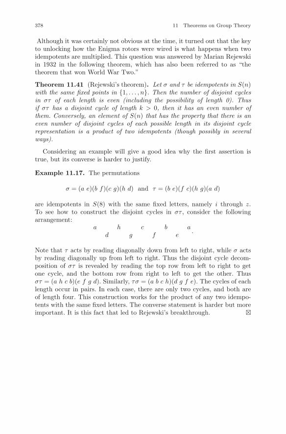
378 11 Theorems on Group Theory
Although it was certainly not obvious at the time, it turned out that the keyto unlocking how the Enigma rotors were wired is what happens when twoidempotents are multiplied. This question was answered by Marian Rejewskiin 1932 in the following theorem, which has also been referred to as “thetheorem that won World War Two.”
Theorem 11.41 (Rejewski’s theorem). Let σ and τ be idempotents in S(n)with the same fixed points in {1, . . . , n}. Then the number of disjoint cyclesin στ of each length is even (including the possibility of length 0). Thusif στ has a disjoint cycle of length k > 0, then it has an even number ofthem. Conversely, an element of S(n) that has the property that there is aneven number of disjoint cycles of each possible length in its disjoint cyclerepresentation is a product of two idempotents (though possibly in severalways).
Considering an example will give a good idea why the first assertion istrue, but its converse is harder to justify.
Example 11.17. The permutations
σ = (a e)(b f)(c g)(h d) and τ = (b e)(f c)(h g)(a d)
are idempotents in S(8) with the same fixed letters, namely i through z.To see how to construct the disjoint cycles in στ , consider the followingarrangement:
a h c b ad g f e
.
Note that τ acts by reading diagonally down from left to right, while σ actsby reading diagonally up from left to right. Thus the disjoint cycle decom-position of στ is revealed by reading the top row from left to right to getone cycle, and the bottom row from right to left to get the other. Thusστ = (a h c b)(e f g d). Similarly, τσ = (a b c h)(d g f e). The cycles of eachlength occur in pairs. In each case, there are only two cycles, and both areof length four. This construction works for the product of any two idempo-tents with the same fixed letters. The converse statement is harder but moreimportant. It is this fact that led to Rejewski’s breakthrough. �
11.7 Breaking the Enigma 379
11.7 Breaking the Enigma
As we noted above, for two Enigmas with the same initial rotor settings, enci-phering and deciphering were the same operation. The operator who receiveda message had only to type in the ciphertext as the assistant read off the plain-text on the lamp board. To ensure that the starting positions were alwaysthe same, a daily key schedule was compiled in a codebook issued to all theEnigma operators. If on September 5, 1940, the daily key was xsf , then onthat day all Enigmas would begin sending and deciphering with the left rotorset at x, the middle at s, and the right at f . To increase security, each oper-ator also selected another three-letter key, a so-called telegram key, e.g., arf .Then before enciphering took place, the operator, with the Enigma set to thedaily key xsf , enciphered the telegram key arf . As an error-detecting device,the operator actually typed arfarf , producing a six-letter string, let us saywkuygh. This six-letter string was then sent by Morse code as the first six let-ters of the enciphered message. After sending his doubly enciphered telegramkey, the operator set his rotors to arf and proceeded to encipher the plain-text. The operator on the receiving end, with his Enigma set to the dailykey xsf , typed in wkuygh. The deciphered string arfarf told him to resethis rotors to arf before typing in the ciphertext. Of course, if somethinglike arfark was received, this signaled a transmission error, and the messagewasn’t deciphered until the doubly enciphered telegram key was resent. Thedouble enciphering of the telegram key was necessary. Radio transmissionscould be disrupted by static, and there was always the possibility of humanerror under the difficulties experienced in wartime. But it turned out to bethe weak link. To see why, see whether you can detect a pattern in the firstsix-letter groups from fifteen messages all intercepted on September 5. Notethat all groupings are double encipherings of different telegram keys.
wkuygh wctyuo qvtnno kophau evprmuqmlnxz wvqymk dgybhj bxcdla mijwcedbobth yoeiaw ntplbu yugicf lhmqzp
The interesting feature of these six-letter groups is that whenever two havethe same first letter, they have the same fourth letter, and conversely. Thisalso holds for the second and fifth letters and the third and sixth letters. Agood cryptographer would notice this feature immediately, but an untrainedeye (such as the author’s) might not see it for quite a while, or ever. Thisclearly suggested a double encryption hypothesis. Working on this assump-tion, Rejewski had the wonderful insight to string together the first and fourthletters of all the first six-letter groups for all the intercepted messages on aparticular day, since they were all enciphered with the same daily key: xsfin the case of September 5. Here is what the above fifteen intercepts give:
380 11 Theorems on Group Theory
dbd . . . mwyi . . . qnlq . . . odb . . . fv . . . er . . . kh . . . .
However, working with 60–80 daily intercepts, he was sometimes able tostring together the whole alphabet, getting an element π ∈ S(26). Let us seewhat the construction of π tells us. Looking at the first grouping, we knowthat the operator typed arfarf , which produced wkuygh. So typing a onthe keyboard produced w on the lamp board via an idempotent σ1. Nowlet σ2 be the idempotent that sends a to y. Then since π(w) = y, we haveπσ1(a) = σ2(a). But since all the Enigmas were set up on September 5 withthe same daily key xsf , the pairings σ1 and σ2 would be the same for allEnigmas. Hence πσ1 = σ2. Consequently, π = σ2σ1 in S(26)! Thus we seethe surprising way in which the product of two idempotents figured. It wouldbe possible, though not easy, to find the disjoint cycle representation of π,and from this, one might be able to deduce σ1 and σ2. Recall that neitherσ1 nor σ2 could have any fixed letters. Let us call such idempotents pairings.Thus, it might be possible to find the pairings σ1 and σ2 from π. Repeatingthis process for the second and fifth and the third and sixth letters gave twomore elements of S(26) that were also products of two pairings. There wasan unavoidable problem, however: a factorization into pairings is not unique.Let us take a couple of simple examples to illustrate how the pairings mightbe found.
Example 11.18. Let us shorten the alphabet to a through h, and let π =(ahc)(dgb). We want to write this as στ , where σ and τ are pairings. Wecan clearly see that e → e and f → f . Imitating the procedure illustratedafter Rejewski’s theorem, consider the three possibilities taking the cyclicpermutations of b, d, g into account:
a h c ab g d
,
a h c ag d b
,
anda h c a
d b g.
Thus there are three possible solutions:
σ = (a b)(h g)(c d)(e f), τ = (a d)(c g)(b h)(e f),
σ = (a g)(d h)(b c)(e f), τ = (a b)(c d)(g h)(e f),
σ = (a d)(b h)(c g)(e f), τ = (a g)(c d)(d h)(e f).
11.7 Breaking the Enigma 381
Notice that we included (e f) in each solution in order to ensure that σ andτ are pairings, not just idempotents. The transposition (e f) disappears inthe product.
Example 11.19. Consider the permutation
π = (d e p z v l y q)(a r o n j f m x)(b g k tu)(w s c i h).
Thus we consider pairs of arrays such as
d e p z v l y q dx m f j n o r a
andb g k t u b
h i c s w.
One possible solution is therefore
σ = (d x)(e m)(f p)(j z)(n v)(l o)(r y)(a q)(b h)(g i)(k c)(s t)(u w)
and
τ = (a d)(q r)(o y)(ln )(j v)(f z)(m p)(e x)(b w)(u s)(t c)(k i)(g h).
Since we obtain all solutions by cyclicly permuting the second rows of thetwo arrays, there are 128 solutions in all.
Rejewski’s solution helped reveal the some of the pairings. If he had knownthe daily keys, then he would have gotten some real insight into the wiring ofthe rotors. But it wasn’t always necessary to know the daily keys, because theEnigma operators often chose easy to guess keys such as aaa or abc, or theymight always choose the same key. But what turned out to be a huge breakfor the Poles was that French intelligence uncovered a disgruntled Germancode clerk who sold them the daily keys for a two-month period in 1932.They were given to the Poles, who used this windfall along with Rejewski’sfactorizations. Using several other clever and imaginative devices, the threePolish cryptographers were able to decipher their first Enigma message at theend of 1932. By 1934, they had completely solved the puzzle of the wiringof the rotors and were able to build an exact replica of the Enigma (anEnigma double). What made this even more amazing was that Poland waseconomically depressed, having become an independent country only at theend of the First World War, and the financial outlay for this project wasa serious strain on its national treasury. Yet because of the wisdom of thehead of its cipher bureau and the ingenuity of its cryptographers, the Poles
382 11 Theorems on Group Theory
were years ahead of the British and French, who despite their great economicadvantage, had been unable to unravel the Enigma’s mystery.
Rejewski had even constructed a primitive computer, which he called abomb, to test for the daily keys. Fortunately, a couple of months before Ger-many’s shocking invasion of Poland in September 1939, two of the duplicateEnigmas were handed over to the French, who gave one to the British. Withthis windfall, the British cryptographers at Bletchley Park were immediatelyable to decipher a certain amount of the intercepted radio traffic, somewhereon the order of 150 intercepts per day. But after the war started, the Ger-mans upgraded their system, so the cryptanalysts were stymied until theyfigured out what modifications the Germans had made. In 1943, the British,under the leadership of Alan Turing, built the first true electronic computerto test for the daily keys. They also called it the bomb, apparently in honorof the Polish original. With the bomb, the Bletchley Park cryptanalysts wereeventually able to read virtually all of the top secret communications of theGerman High Command, often before the officers for whom the communiqueswere intended.
The breaking of the Enigma surely shortened the war. In fact, after learn-ing in the 1970s the extent to which the British had penetrated the Enigmaciphers, the head of German Enigma security, a mathematical logician, statedthat it was a good thing, since it must have shortened the war. He was happyto learn that a fellow logician, Alan Turing, had played such an importantrole. A well-known German mathematician, who was responsible for the secu-rity of the Enigmas for a branch of the German military, was quoted in anobituary as saying that it was a job he hadn’t been very good at.
Acknowledgments The above account of how the Enigma was broken was originally
explained to me by my colleague Professor Hugh Thurston, who was a British cryptanalyst
at Bletchley Park during the war. He characterized the code-breaking activity at Bletchley
Park as “one of the few just war efforts human history can boast of.”
Chapter 12Linear Algebraic Groups: anIntroduction
The purpose of this chapter is to give a brief informal introduction, with veryfew proofs, to the subject of linear algebraic groups, a far-reaching general-ization of matrix theory and linear algebra. A very readable treatment withmuch more information is contained in the book Linear Algebraic Groupsand Finite Groups of Lie Type, by Gunter Malle and Donna Testerman. Alinear algebraic group is a matrix group G contained in a general linear groupGL(n,F), for some field F and positive integer n, whose elements are preciselythe roots, or zeros, of a finite set of polynomial equations in n2 variables.Linear algebraic groups have proved to be indispensable in many areas ofmathematics, e.g., number theory, invariant theory, algebraic geometry, andalgebraic combinatorics, to name some. The results we will describe concern,for the most part, the case F = C, but results that are valid for C are usuallytrue whenever F is algebraically closed and of characteristic zero. There is alsoa great deal of interest in linear algebraic groups over a field of characteristicp > 0, since many such groups give examples of finite simple groups.
12.1 Linear Algebraic Groups
In order to define what a linear algebraic group is, we must first make someremarks about polynomials on F
n×n. Let V be a finite-dimensional vectorspace over F with basis v1, . . . ,vn, and let x1, . . . , xn be the dual basis of V ∗.Thus xi : V → F is the linear function defined by xi(vj) = δij , where δij is theKronecker delta function. A monomial in x1, . . . , xn is a function of the formxa1i1
xa2i2
· · · xakik
: V → F, where a1, . . . , ak are positive integers, 1 ≤ ij ≤ n forall indices and i1 < i2 < · · · < ik. A polynomial function in x1, . . . , xn over Fis a linear combination over F of a finite set of monomials. Thus a typical
c© Springer Science+Business Media LLC 2017J.B. Carrell, Groups, Matrices, and Vector Spaces,DOI 10.1007/978-0-387-79428-0 12
383
384 12 Linear Algebraic Groups: an Introduction
polynomial has the form
f(x1, . . . , xn) =∑
ci1i2...ikxa1i1
xa2i2
· · · xakik
,
where the coefficients ci1i2...ik are in F, and only finitely many are nonzero. LetF[x1, . . . , xn] denote the set of all such polynomials. If V = F
n×n with basisEij , 1 ≤ i, j ≤ n, then the dual basis is denoted by xij , where 1 ≤ i, j ≤ n. Abasic example of a polynomial in F[xij ] is given by the determinant
det(xij) =∑
π∈S(n)
sgn(π) xπ(1)1xπ(2)2 · · · xπ(n)n.
We now define what it means for a matrix group to be closed.
Definition 12.1. A subgroup G of GL(n,F) is said to be closed if G consistsof the common zeros of a finite set of polynomials f1, . . . , fk ∈ F[xij ]. A closedsubgroup G of GL(n,F) is called a linear algebraic group.
The group GL(n,F) is by default a linear algebraic group, since GL(n,F)is the set of common zeros of the empty set of polynomials on F
n×n. The spe-cial linear group SL(n,F) is a closed subgroup of GL(n,F), since SL(n,F)is defined by the setting det(xij) − 1 = 0. That is, SL(n,F) consists of thematrices A such that det(A) − 1 = 0. The groups P (n), U(n,F), L(n,F), andD(n,F) involved in the LPDU are also closed subgroups of GL(n,F), as isT (n,F). For example, T (n,F), the subgroup consisting of all upper triangu-lar elements of GL(n,F), is the set of zeros of the polynomials xij , wherei > j. The elements of the group P (n) of n × n permutation matrices satisfythe equations xij(xij − 1) = 0 for all i, j, since every entry of a permutationmatrix is zero or one. But these equations don’t capture the fact that thecolumns of P are orthogonal; for that, we use the identity PTP = In. Thus,P ∈ P (n) if and only if P satisfies the set of polynomial equations
∑
k
xkixkj = δij and xij(xij − 1) = 0 (i, j, k = 1, . . . , n).
Hence P (n) is a linear algebraic group; in fact, this example shows that linearalgebraic groups can be finite. (The reader may wish to show that in fact,every finite subgroup of GL(n,F) is closed.)
From the definition of a linear algebraic group, it is clear that the inter-section of two linear algebraic groups is a linear algebraic group, and theproduct of two linear algebraic groups is also a linear algebraic group. Inorder to understand the importance of the condition that the elements of alinear algebraic group are cut out by polynomial equations, one must intro-duce some basic concepts from algebraic geometry, in particular, the notionof an affine variety. What is very useful is that the important subgroups of alinear algebraic group themselves also turn out to be linear algebraic groups.
12.1 Linear Algebraic Groups 385
We know make a general definition that applies to arbitrary groups. Thereason for the terminology should become clear later.
Definition 12.2. A group G, not necessarily a linear algebraic group, is saidto be connected if G has no normal subgroup of finite index greater than one.
By definition, a finite group different from {1} cannot be connected. Tosee another example of a nonconnected group, consider O(n,F) for whichthe characteristic of F is different from two. In that case, P (n) is naturallyembedded as a subgroup of O(n,F). Thus, the determinant homomorphismdet : O(n,F) → {±1} is surjective. Consequently, by the first isomorphismtheorem, its kernel is a proper normal subgroup of index two. If the charac-teristic of F is zero, then GL(n,F), SL(n,F), and SO(n,F) are all connected.
Exercise 12.1.1. Show that if F is a Galois field, then GL(n,F) is not con-nected.
12.1.1 Reductive and semisimple groups
We will now get a bit technical for a while in order to focus on two of themost important classes of linear algebraic groups: reductive and semisim-ple groups. We will concentrate on linear algebraic groups G < GL(n,C).Each such G has a unique maximal, closed, normal, and connected solvablesubgroup Rad(G), called the radical of G. For example, if G = GL(n,C),then Rad(G) = C
∗In. (Note: C∗In is closed, since it is the set of all zeros inGL(n,C) of the polynomials xij and xii − xjj , where i �= j). If G = T (n,C)or D(n,C), then Rad(G) = G, since G is solvable. We now state the firstmain definition.
Definition 12.3. Let G < GL(n,C) denote a connected linear algebraicgroup. Then G is called reductive if the only unipotent element of Rad(G)is the identity. It is called semisimple if the only closed, normal, connectedabelian subgroup of G is the identity. It is called simple if G is nonabelianand G has no nontrivial closed normal subgroup. Finally, G is almost simpleif every closed normal subgroup of G is finite.
It is not hard to see that a semisimple linear algebraic group is reduc-tive, but the converse isn’t true. For example, by the above remarks, thegeneral linear group GL(n,C) is reductive. However, GL(n,C) is not semi-simple, since its radical C∗In is a nontrivial closed normal connected abeliansubgroup. Another example of a reductive group that is not semisimple isD(n,C). The special linear group SL(n,C) is semisimple. This is hard toprove from first principles, so we will omit the proof. Note that SL(n,C)contains a normal abelian subgroup, namely its center Z = {ζIn | ζn = 1}.But Z is not connected, since {In} is a normal subgroup of finite index.
386 12 Linear Algebraic Groups: an Introduction
12.1.2 The classical groups
A list of all semisimple linear algebraic groups over C has been known sincethe early part of the twentieth century. There are four infinite families knownas the classical groups, and five exceptional groups, which we will not describehere. When C is replaced by a Galois field, all the classical and exceptionalgroups become what are called groups of Lie type. With the exception of 26so-called sporadic groups, all the finite simple groups are of this type. We havealready encountered three of the families of classical groups: SL(n,C) (thespecial linear groups), SO(2n,C) (the even orthogonal groups), and SO(2n +1,C) (the odd orthogonal groups). It may seem artificial to distinguish theeven and odd special orthogonal groups, but the mechanism used to classifythe semisimple groups forces us to put these groups into different categories.The fourth family consists of the symplectic groups Sp(2n,C). By definition,
Sp(2n,C) = {A ∈ GL(2n,C) | AΩAT = Ω},
where
Ω =(
O In
−In O
).
If A ∈ Sp(2n,C), then A−1 = ΩATΩ−1, and since Ω2 = −I2n, we get A−1 =−ΩATΩ. Also, by definition, det(AAT ) = 1, so det(A) = ±1. In fact, it canbe shown that det(A) = 1, so Sp(2n,C) < SL(n,C). This follows by showingthat Sp(2n,C) is connected, since the kernel of det is a normal subgroup. Thesymplectic groups are used in symplectic geometry, physics, and the theoryof alternating quadratic forms.
12.1.3 Algebraic tori
A linear algebraic group T < GL(n,C) is called an algebraic torus, or simplya torus, if T is connected and abelian and every element of T is semisimple.Algebraic tori are basic examples of reductive groups. This follows from themultiplicative Jordan–Chevalley decomposition, since the only unipotent ele-ment of a torus is the identity. If T is a subgroup of a linear algebraic groupG < GL(n,C), we call T a subtorus of G if T is an algebraic torus in GL(n,C).A subtorus T of G that is not a proper subgroup of any other subtorus in Gis called a maximal torus in G. For example, D(n,C) is a maximal torus inGL(n,C). More generally, we have the following.
Proposition 12.1. Every maximal torus T < GL(n,C) is conjugate toD(n,C).
12.1 Linear Algebraic Groups 387
Exercise 12.1.2. Show that T ={(
a b−b a
)| a, b ∈ C, a2 + b2 �= 0
}and
D(2,C) are both maximal tori in GL(2,C), and prove that they are conjugatein GL(2,C).
Exercise 12.1.3. Let T be the algebraic torus defined in the previous exer-cise. Show that D(2,R) and T ∩ GL(2,R) are not conjugate in GL(2,R).
We next state an important fact.
Theorem 12.2. Every reductive linear algebraic group G contains a maxi-mal torus, and any two maximal tori in G are conjugate by an element of G.Moreover, if T < G is an algebraic torus, then T is contained in a maximaltorus.
Let us now describe some maximal tori for classical groups.
Case 1: SL(n,C). This is the easiest case to describe. In fact, the subgroupof all diagonal matrices in SL(n,C), that is, SL(n,C) ∩ D(n,C), is a maximaltorus.
Case 2: SO(2n,C). Starting with the maximal torus T = {diag(t, t−1) | t ∈C
∗} in SL(2,C), one can conjugate T into SO(2,C), since
R = Pdiag(t, t−1)P−1 =(
a b−b a
),
where a = (t2 + 1)/t, b = (−it2 + 1)/t, and P =1√2
(1 ii 1
). We will call R
a rotation matrix. It turns out that the set of all matrices of the form
R =
⎛
⎜⎜⎜⎝
R1 O · · · OO R2 · · · O...
.... . .
...O O · · · Rn
⎞
⎟⎟⎟⎠ ,
where R1, . . . , Rn are arbitrary rotation matrices, is a maximal torus inSO(2n,C).
Case 3: SO(2n + 1,C). To obtain a maximal torus in SO(2n + 1,C), con-sider the natural inclusion homomorphism i : SO(2n,C) → SO(2n + 1,C)defined by
R →(
R 00 1
).
Then the image of R is a maximal torus in SO(2n + 1,C).
Case 4: Sp(2n,C). Finally, the set of all T = diag(x1, . . . , xn, x−11 , . . . , x−1
n ),where each xi is in C
∗, is a maximal torus for Sp(2n,C).
388 12 Linear Algebraic Groups: an Introduction
A maximal torus T in a linear algebraic group G defines a group actionof T on G by conjugation, namely (t, g) → t · g = tgt−1. This action givesrise to the so-called roots and weights of the pair (G,T ), which completelydetermine G up to isomorphism (in the sense of linear algebraic groups) whenG is semisimple. Space does not permit us to elaborate on this theme, sinceit requires introducing the Lie algebra of G. Instead, we will concentrate onanother group that we have already seen in a special case. This is the Weylgroup of (G,T ). We will then discuss the role of the Weyl group in the theoryof linear algebraic groups.
12.1.4 The Weyl group
The Weyl group of a pair (G,T ) consisting of a linear algebraic group Gand a maximal torus T < G is the group W (G,T ) = NG(T )/T . We will seebelow that if G = GL(n,C) and T = D(n,C), then W (G,T ) is isomorphic tothe group P (n) of n × n permutation matrices. Recall that P (n) is a basiccomponent of the LPDU decomposition in GL(n,C). The matrices P and Dare always unique, though L and U need not be. We will give some examplesof Weyl groups and then explain how they play a role similar to that of P (n)for GL(n,C) for arbitrary reductive linear algebraic groups. Let us begin witha fundamental result.
Theorem 12.3. If G is reductive, then the normalizer NG(T ) is also a linearalgebraic group, and the Weyl group W (G,T ) is finite.
For simplicity, we will denote W (G,T ) by W as long as it is clear what Gand T are. Since any two maximal tori in G are conjugate, the Weyl groupof (G,T ) is independent of the choice of T up to an isomorphism induced byan inner automorphism of G. The following result computes W when G iseither GL(n,C) or SL(n,C).
Proposition 12.4. If G = GL(n,C) or SL(n,C), then W ∼= S(n).
Proof. Suppose first that G = GL(n,C) and T = D(n,C). We will showthat NG(T ) is the semidirect product P (n)T . Note that if P ∈ P (n) andD = diag(d1, . . . , dn), then PDP−1 = diag(dσ(1), . . . , dσ(n)), where σ ∈ S(n)is the unique permutation such that P = Pσ. To see this, it suffices to checkthat PDP−1 = diag(dσ(1), . . . , dσ(n)) whenever σ = (i i + 1) is a simple trans-position. Since (i i + 1) is conjugate to (12), it suffices to let σ = (12) andassume that D is of size 2 × 2. Hence we get the result, since
PDP−1 =(
0 11 0
)(a 00 b
) (0 11 0
)=
(b 00 a
).
12.1 Linear Algebraic Groups 389
Since P (n) ∩ T = (1), the subgroup H generated by P (n) and T is the semi-direct product of P (n) and T , and H ≤ NG(T ). Moreover, transvections,or elementary matrices of type III, do not normalize T . For example, in the2 × 2 case,
(1 0u 1
) (a 00 b
) (1 0
−u 1
)=
(a 0
u(a − b) b
).
It follows that NG(T ) = H = P (n)T , as claimed. It follows from Exercise11.4.7 that W ∼= P (n) via the natural homomorphism P (n) → W defined byP → PT . Hence W ∼= S(n) also. When G = SL(n,C), the above argumentdoesn’t work, because if P = Pσ and sgn(σ) = −1, then P /∈ SL(n,C), sincedet(Pσ) = sgn(σ). This is fixed by replacing a Pσ with sgn(σ) = −1 by thematrix RPσ, where R = diag(−1, 1, . . . , 1). It is clear that conjugation byRPσ has the same effect as conjugation by Pσ, so W ∼= S(n) in the SL(n,C)case also. �
We will skip the details for the computation of the Weyl groups of theremaining classical groups. The complete result is contained in the followingtheorem.
Theorem 12.5. The Weyl groups of the classical groups are as follows:
(i) for G = GL(n,C) or SL(n,C), W ∼= S(n);
(ii) for G = SO(2n + 1,C) or SP (2n,C), W ∼= SP (n), where SP (n) denotesthe group of signed permutation matrices; and
(iii) for G = SO(2n,C), W ∼= SP (n)+, the subgroup of SP (n) consisting ofall signed permutation matrices having an even number of minus signs.
The group SP (n) consists of all elements of O(n,C) having integer entries.In other words, every element of SP (n) is obtained from a permutation matrixP by allowing ± 1 wherever a 1 occurs in P . Thus the order of SP (n) is 2nn!.Since det(Pσ) = sgn(σ) for the permutation matrix Pσ associated to σ ∈ S(n),it follows that SP (n)+ = SP (n) ∩ SL(n,C). Thus |SP (n)+| = 2n−1n!.
Each of the Weyl groups above is generated by reflections of Rn. We willgive a minimal set of reflections that generate in each case. Such reflectionsare called simple.
Case 1: W = P (n). For each i = 1, . . . , n − 1, let Hi denote the reflectionthrough the hyperplane orthogonal to ei − ei+1. The matrix of Hi withrespect to the standard basis is the row swap matrix Pi obtained from In byswapping the ith and (i + 1)st rows. Then P1, . . . , Pn−1 are the simple reflec-tions generating W . Note that Pi is the permutation matrix correspondingto the simple transposition (i i + 1).
Case 2: W = SP (n). Here the simple reflections are P1, . . . , Pn−1 togetherwith the reflection Pn = diag(1, . . . , 1,−1), which reflects R
n through thehyperplane xn = 0.
390 12 Linear Algebraic Groups: an Introduction
Case 3: W = SP (n)+. In the final case, the simple reflections consist ofP1, . . . , Pn−1 together with the reflection Hn through the hyperplane orthog-onal to en−1 + en. The matrix of Hn is −Pn−1. Thus the simple reflectionsare P1, . . . , Pn−2,±Pn−1.
The simple reflections listed above arise from the root systems of typesA,B,C,D in the theory of reflection groups (that is, groups generated byreflections). The simple reflections allow one to define the notion of the lengthof an element w of W as the minimal k such that there exists an expressionw = Pi1 · · · Pik with each Pj a simple reflection. The length of w is denoted by�(w). We will mention below an interesting role that the length function plays.An excellent source for information and further study on reflection groups,including their root systems, is Reflection Groups and Coxeter Groups (Cam-bridge Studies in Advanced Mathematics), by James E. Humphreys.
12.1.5 Borel subgroups
If G is a connected linear algebraic group, a closed, connected subgroup B ofG that is solvable and not properly contained in any other closed, connectedsolvable subgroup of G is called a Borel subgroup of G. Borel subgroups playa very important role in the structure theory of linear algebraic groups, aswe will presently see. We have already seen that the upper triangular sub-groups T (n,C) and T (n,C) ∩ SL(n,C) of GL(n,C) and SL(n,C) are solv-able. It turns out that they are Borel subgroups of GL(n,C) and SL(n,C)respectively. This is easy to see for n = 2. The commutator ABA−1B−1 ofA,B ∈ GL(2,C) is in general not in T (2,C). In fact, let G be a closed sub-group of GL(2,C) properly containing T (2,C). Then there exists A ∈ Gsuch that the entry a21 is nonzero. Then one can find B ∈ T (2,C) suchthat C = ABA−1B−1 has a nonvanishing (2, 1) entry. For example, assumingad − bc = 1 to avoid denominators, then
(a bc d
)(1 10 1
)(d −b
−c a
)(1 −10 1
)=
(1 − ac a2 + ac − 1−c2 1 + ac + c2
).
It follows that every commutator subgroup G(i) is nontrivial, so G cannotbe solvable. Hence, T (2,C) is a Borel subgroup of GL(2,C). The reader canthen extend this reasoning to conclude that T (n,C) is a Borel subgroup ofGL(n,C). Similarly, T (n,C) ∩ SL(n,C) is a Borel subgroup of SL(n,C).
The existence of a Borel subgroup B in a linear algebraic group G followsfrom the fact that an algebraic torus is a connected solvable (in fact, abelian)linear algebraic group. Now, if H is any closed connected solvable linearalgebraic group such that T ≤ H ≤ G, then either H is maximal or there
12.1 Linear Algebraic Groups 391
exists a closed connected solvable linear algebraic group H ′ of G such thatH < H ′. We need to know that iterating this remark will produce a maximalclosed connected solvable linear algebraic group B ≤ G such that T ≤ B. Infact, if G < GL(n,C), then there cannot be a strictly increasing sequence oflinear algebraic groups
H1 < H2 < · · · < Hk < Hk+1 < · · · < G.
The tool needed to guarantee this is a fundamental theorem in abstract alge-bra known as the Hilbert basis theorem, which is a result about ideals inF[x1, . . . , xm]. The existence of a Borel subgroup B such that T ≤ B thusfollows. It can also be shown that every Borel subgroup in a linear algebraicgroup G < GL(n,C) can be obtained as G ∩ B for some Borel B in GL(n,C).
Remark. The Borel subgroups of the orthogonal groups and the symplecticgroups are harder to describe, but a nice description is given in the above-mentioned book by Malle and Testerman on page 38.
12.1.6 The conjugacy of Borel subgroups
Every subgroup H < GL(n,C) conjugate to a linear algebraic group G <GL(n,C) is also a linear algebraic group. For if H = gGg−1, and p(X)is a polynomial on C
n×n such that p(X) = 0 if X ∈ G, then the functionq(X) = p(g−1Xg) is also a polynomial on C
n×n such that q(Y ) = 0 if Y ∈ H,since q(Y ) = p(g−1Y g) = p(g−1gXg−1g) = p(X) = 0. It follows that everysubgroup of G that is conjugate to a Borel subgroup is itself a Borel subgroup.Thus the lower triangular matrices also give Borel subgroups in GL(n,C),and those in SL(n,C) give a Borel subgroup in SL(n,C). Moreover, thereare also Borel subgroups that are quite hard to describe.
The Borel subgroups of a reductive linear algebraic group G have twofundamental and deep properties: any two Borel subgroups of G are conjugateby an element of G, and the normalizer of every Borel subgroup of B < Gis B itself (cf. Malle and Testerman). These two facts give rise to a niceparameterization of the set of Borel subgroups of G.
Proposition 12.6. Let BG denote the set of all Borel subgroups of G, andlet B denote a fixed Borel subgroup. Then the mapping gB → gBg−1 definesa bijection between the space of left cosets G/B and BG.
Recall that we showed that every maximal torus T in G is contained in aBorel subgroup B of G. We just remarked that NG(B) = B for every Borelsubgroup, and in fact, NG(T ) ∩ B = T . Since T < B, it makes sense to definewBw−1 by nwBn−1
w for every representative nw of w in the Weyl group Wof (G,T ). The interesting point is that wBw−1 is also a Borel subgroup of G
392 12 Linear Algebraic Groups: an Introduction
containing T . Moreover, if w1, w2 ∈ W , then w1Bw−11 = w2Bw−1
2 if and onlyif w1 = w2.
Theorem 12.7. The correspondence sending w ∈ W to wBw−1 is a bijec-tion from the Weyl group of (G,T ) onto the set of Borel subgroups of Gcontaining T . In particular, the number of Borel subgroups of G containingT is |W |.
12.1.7 The flag variety of a linear algebraic group
If B is a Borel subgroup of G, then the coset space G/B turns out to havethe structure of an algebraic variety, which is the fundamental concept inthe field of algebraic geometry. This allows one to use results from algebraicgeometry to study the abstract set BG of all Borel subgroups in G. WhenG = GL(n,C), we can explicitly describe G/B in terms from linear algebra.Let us suppose B = T (n,C) and fix A ∈ GL(n,C). Let U be an arbitraryelement of B. Since multiplication on the right by each U performs rightwardcolumn operations, the spans of the first k columns of A and AU are the samefor all k. Let Vk denote this subspace. Since A is invertible, dimVk = k forall k. Thus the coset AB uniquely determines a strictly increasing sequenceof subspaces of Cn, namely
V1 ⊂ V2 ⊂ · · · ⊂ Vn−1 ⊂ Cn. (12.1)
Conversely, every such sequence uniquely determines a coset of G/B. Thisgives us a bijection from G/B onto the set of all sequences of the form (12.1).These sequences are called complete flags in C
n. The set of complete flags inC
n is often denoted by Flag(Cn). It has many applications in geometry andrelated areas. If G is an arbitrary reductive group and B a Borel subgroup,then the coset space G/B is known as the flag variety of G.
Now let T be a maximal torus in a reductive group G and let B be a Borelsubgroup of G such that T < B. Consider the action of T on the flag varietyG/B by left translation given explicitly by (t, gB) → tgB. As we have alreadyseen in the proofs of the Sylow theorems, it is often very useful to know thefixed-point set of a group action.
Proposition 12.8. The fixed-point set (G/B)T of the left multiplicationaction of T on G/B is precisely the set of cosets wB as w varies throughthe Weyl group. In particular, T has exactly |W | fixed points on G/B.
Proof. Suppose TgB = gB. Then g−1Tg < B, so T < gBg−1. Thus gBg−1 is aBorel subgroup of G containing T . Therefore, by Cartan’s theorem, gBg−1 =wBw−1 for some w ∈ W . Consequently, gB = wB by Proposition 12.6. �
12.1 Linear Algebraic Groups 393
The fact that the number of fixed points of T on G/B is |W | translatesinto a statement about the topology of the flag variety G/B of G, namely,the Euler characteristic of G/B is |W |, the order of the Weyl group. This is afamous theorem of Andre Weil that was discovered around 1930. The Eulercharacteristic is a topological invariant of a space that generalizes the numberF − E + V , which measures the number of holes in a two-dimensional surfacewithout boundary.
Example 12.1. It is interesting to compute (G/B)T when G = GL(n,C) intwo ways. First, let us view GL(n,C)/B as the complete flags in C
n. Notethat if T = T (n,C), then every flag of the form
Cei1 ⊂ spanC{ei1 , ei2} ⊂ · · · ⊂ spanC{ei1 , ei2 , . . . , ein−1} ⊂ Cn
is fixed by T . Here i1, i2, . . . , in−1 are n − 1 distinct integers in [1, n]. Sincethere are exactly n! such flags, and |S(n)| = n!, these flags comprise theT -fixed points. Now let us compute (G/B)T another way, this time usingthe LPDU decomposition. The points (or cosets) PB, where P ∈ P (n), arefixed under T , because TPB = PTB, since the normalizer in GL(n,C) of Tis P (n). Thus, P−1TP = T , so TP = PT , whence TPB = PB. Hence, thepoints PB as P ranges over P (n) are fixed under T . But in the LPDUdecomposition of an element of GL(n,C), we know that P and D are unique.Thus if P, P ′ ∈ P (n), then PB = P ′B if and only if P = P ′. Therefore, since|P (n)| = n!, we have found (GL(n,C)/B)T in two (equivalent) ways. �
12.1.8 The Bruhat decomposition of GL(n, F)
We are now going to discuss how the LPDU decomposition generalizes toan arbitrary reductive linear algebraic group G < GL(n,F), where F is anarbitrary field. We will begin by finding a slightly different version of LPDUfor G = GL(n,F). According to LPDU , we can decompose GL(n,F) as theproduct of four subgroups, namely
GL(n,F) = L(n,F)P (n)D(n,F)U(n,F).
Of course, D(n,F)U(n,F) is the upper triangular Borel subgroup T (n,F).Another Borel subgroup of GL(n,F) is, in fact, the set T (n,F)− of all lowertriangular elements of GL(n,F). Since T (n,F) and T (n,F)− are Borel sub-groups containing the maximal torus D(n,F), they are conjugate by an ele-ment of the Weyl group P (n). In fact, this element is
P0 = (en en−1 · · · e2 e1).
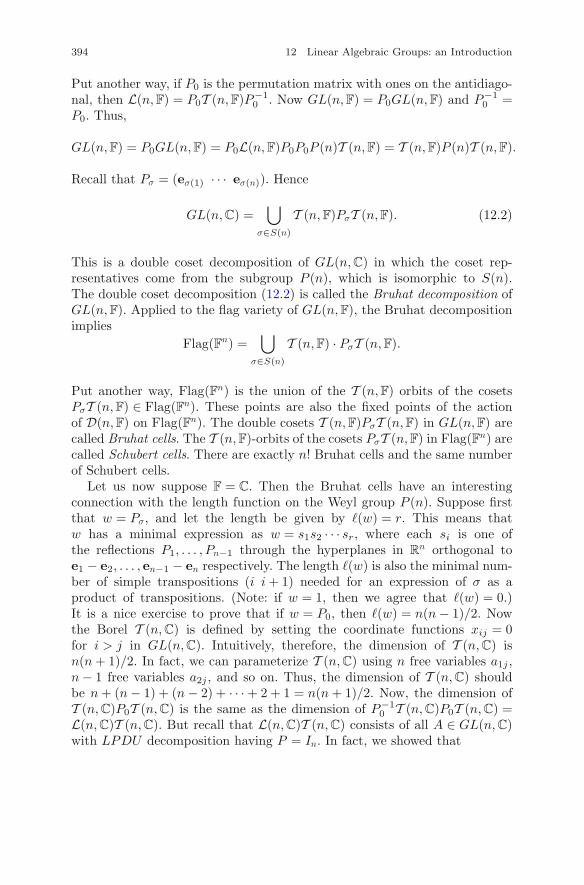
394 12 Linear Algebraic Groups: an Introduction
Put another way, if P0 is the permutation matrix with ones on the antidiago-nal, then L(n,F) = P0T (n,F)P−1
0 . Now GL(n,F) = P0GL(n,F) and P−10 =
P0. Thus,
GL(n,F) = P0GL(n,F) = P0L(n,F)P0P0P (n)T (n,F) = T (n,F)P (n)T (n,F).
Recall that Pσ = (eσ(1) · · · eσ(n)). Hence
GL(n,C) =⋃
σ∈S(n)
T (n,F)PσT (n,F). (12.2)
This is a double coset decomposition of GL(n,C) in which the coset rep-resentatives come from the subgroup P (n), which is isomorphic to S(n).The double coset decomposition (12.2) is called the Bruhat decomposition ofGL(n,F). Applied to the flag variety of GL(n,F), the Bruhat decompositionimplies
Flag(Fn) =⋃
σ∈S(n)
T (n,F) · PσT (n,F).
Put another way, Flag(Fn) is the union of the T (n,F) orbits of the cosetsPσT (n,F) ∈ Flag(Fn). These points are also the fixed points of the actionof D(n,F) on Flag(Fn). The double cosets T (n,F)PσT (n,F) in GL(n,F) arecalled Bruhat cells. The T (n,F)-orbits of the cosets PσT (n,F) in Flag(Fn) arecalled Schubert cells. There are exactly n! Bruhat cells and the same numberof Schubert cells.
Let us now suppose F = C. Then the Bruhat cells have an interestingconnection with the length function on the Weyl group P (n). Suppose firstthat w = Pσ, and let the length be given by �(w) = r. This means thatw has a minimal expression as w = s1s2 · · · sr, where each si is one ofthe reflections P1, . . . , Pn−1 through the hyperplanes in R
n orthogonal toe1 − e2, . . . , en−1 − en respectively. The length �(w) is also the minimal num-ber of simple transpositions (i i + 1) needed for an expression of σ as aproduct of transpositions. (Note: if w = 1, then we agree that �(w) = 0.)It is a nice exercise to prove that if w = P0, then �(w) = n(n − 1)/2. Nowthe Borel T (n,C) is defined by setting the coordinate functions xij = 0for i > j in GL(n,C). Intuitively, therefore, the dimension of T (n,C) isn(n + 1)/2. In fact, we can parameterize T (n,C) using n free variables a1j ,n − 1 free variables a2j , and so on. Thus, the dimension of T (n,C) shouldbe n + (n − 1) + (n − 2) + · · · + 2 + 1 = n(n + 1)/2. Now, the dimension ofT (n,C)P0T (n,C) is the same as the dimension of P−1
0 T (n,C)P0T (n,C) =L(n,C)T (n,C). But recall that L(n,C)T (n,C) consists of all A ∈ GL(n,C)with LPDU decomposition having P = In. In fact, we showed that
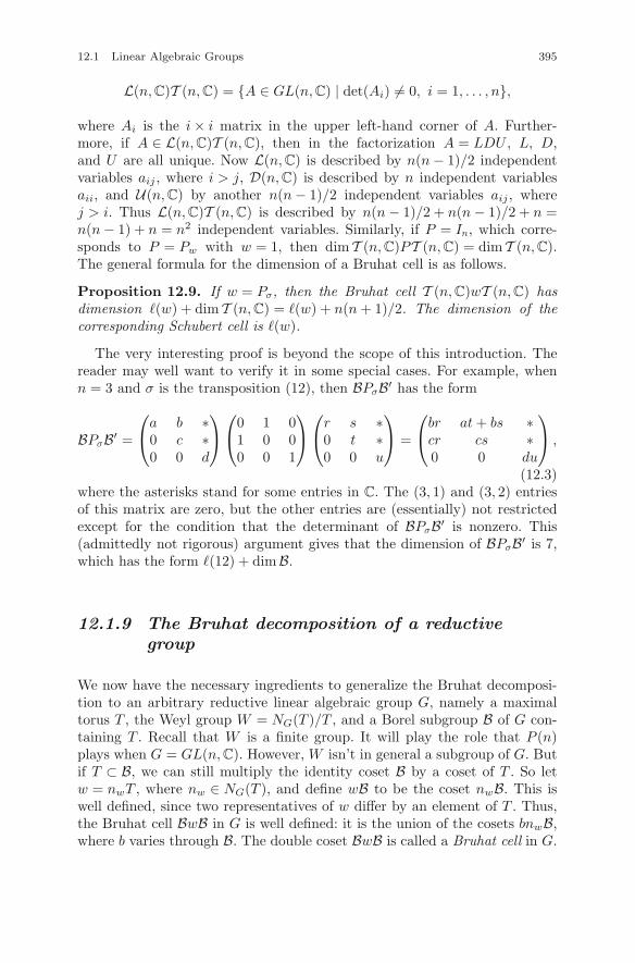
12.1 Linear Algebraic Groups 395
L(n,C)T (n,C) = {A ∈ GL(n,C) | det(Ai) �= 0, i = 1, . . . , n},
where Ai is the i × i matrix in the upper left-hand corner of A. Further-more, if A ∈ L(n,C)T (n,C), then in the factorization A = LDU , L, D,and U are all unique. Now L(n,C) is described by n(n − 1)/2 independentvariables aij , where i > j, D(n,C) is described by n independent variablesaii, and U(n,C) by another n(n − 1)/2 independent variables aij , wherej > i. Thus L(n,C)T (n,C) is described by n(n − 1)/2 + n(n − 1)/2 + n =n(n − 1) + n = n2 independent variables. Similarly, if P = In, which corre-sponds to P = Pw with w = 1, then dim T (n,C)PT (n,C) = dim T (n,C).The general formula for the dimension of a Bruhat cell is as follows.
Proposition 12.9. If w = Pσ, then the Bruhat cell T (n,C)wT (n,C) hasdimension �(w) + dim T (n,C) = �(w) + n(n + 1)/2. The dimension of thecorresponding Schubert cell is �(w).
The very interesting proof is beyond the scope of this introduction. Thereader may well want to verify it in some special cases. For example, whenn = 3 and σ is the transposition (12), then BPσB′ has the form
BPσB′ =
⎛
⎝a b ∗0 c ∗0 0 d
⎞
⎠
⎛
⎝0 1 01 0 00 0 1
⎞
⎠
⎛
⎝r s ∗0 t ∗0 0 u
⎞
⎠ =
⎛
⎝br at + bs ∗cr cs ∗0 0 du
⎞
⎠ ,
(12.3)where the asterisks stand for some entries in C. The (3, 1) and (3, 2) entriesof this matrix are zero, but the other entries are (essentially) not restrictedexcept for the condition that the determinant of BPσB′ is nonzero. This(admittedly not rigorous) argument gives that the dimension of BPσB′ is 7,which has the form �(12) + dim B.
12.1.9 The Bruhat decomposition of a reductivegroup
We now have the necessary ingredients to generalize the Bruhat decomposi-tion to an arbitrary reductive linear algebraic group G, namely a maximaltorus T , the Weyl group W = NG(T )/T , and a Borel subgroup B of G con-taining T . Recall that W is a finite group. It will play the role that P (n)plays when G = GL(n,C). However, W isn’t in general a subgroup of G. Butif T ⊂ B, we can still multiply the identity coset B by a coset of T . So letw = nwT , where nw ∈ NG(T ), and define wB to be the coset nwB. This iswell defined, since two representatives of w differ by an element of T . Thus,the Bruhat cell BwB in G is well defined: it is the union of the cosets bnwB,where b varies through B. The double coset BwB is called a Bruhat cell in G.
396 12 Linear Algebraic Groups: an Introduction
In the flag variety G/B, the B-orbit B · wB of the coset wB is called a Schubertcell. The LPDU decomposition of GL(n,C) generalizes as follows.
Theorem 12.10. Let G be a reductive linear algebraic group over C, B aBorel subgroup of G, and T a maximal torus in G such that T < B. Then Gis the union of the Bruhat cells BwB as w varies through W , so G = BWB.Moreover, NG(T ) ∩ B = T ; hence if w �= w′ in W , then wB �= w′B. Thus, thenumber of distinct Bruhat cells in G is the order of W . Finally, the dimensionof the Bruhat cell BwB is �(w) + dimB.
12.1.10 Parabolic subgroups
A closed subgroup P of a linear algebraic group G is called parabolic if Pcontains a Borel subgroup. We will classify the parabolic subgroups of Gafter we give an example.
Example 12.2. Consider the standard case G = GL(n,C), B = T (n,C),and T = D(n,C). As we have seen, W = S(n) ∼= P (n). Now suppose j + k =n. Let P (j, k) < P (n) denote the subgroup consisting of permutation matri-ces with block decomposition
P =(
P1 OO P2
),
where P1 ∈ P (j) and P2 ∈ P (k). But P = Pτ for a unique τ ∈ S(n). SinceP1 = Pμ and P2 = Pν for unique μ ∈ S(j) and ν ∈ S(k), we can definean injective homomorphism ϕ : S(j) × S(k) → S(n) by ϕ(μ × ν) = τ . LetS(j, k) < S(n) denote the image of ϕ. Then S(j, k) ∼= P (j, k). Then BP (j, k)Bis the set of all matrices of the form
(A ∗O B
),
where A ∈ GL(j,C) and B ∈ GL(k,C). Hence, BP (j, k)B is a closed sub-group of GL(n,C).
More generally, let P(j1, . . . , jk) denote all matrices of the form⎛
⎜⎜⎜⎝
A1 ∗ · · · ∗O A2 · · · ∗...
.... . .
...O O · · · Ak
⎞
⎟⎟⎟⎠ ,
where Ai ∈ GL(ji,C) and j1 + · · · + jk = n. Then the P(j1, . . . , jk) are theparabolic subgroups of GL(n,C) containing T (n,C). �
12.1 Linear Algebraic Groups 397
Now suppose G is reductive and fix a maximal torus T and a Borel sub-group B such that T < B < G. Let P be a parabolic subgroup in G containingB, and define the Weyl group WP to be NP(T )/T . Then we have the followingtheorem.
Theorem 12.11. The parabolic subgroup P is a union of certain Bruhatcells. In particular, P = BWPB. Moreover, the number of Bruhat cells in Pis |WP |.
Not every subgroup Z < W gives a parabolic subgroup in this manner. Forexample, let σ = (i j) be a transposition that is not simple; that is, |i − j| > 1.Then if Z = {In, Pσ}, BZB is not a subgroup of GL(n,C). A natural questionthen is which subgroups of Weyl groups have the form WP for some parabolicP. In fact, these subgroups can be described in a simple way. An elementP �= 1 of W is called simple if BPB ∪ B is a subgroup of G. Note that if Pis simple, then P 2 = 1. (We leave the proof to the reader.) Hence the simpleelements have order two. Let S ⊂ W denote the set of all simple elements.In the standard case, the simple elements are the reflections Pσ, where σis a simple transposition. The next result is a complete description of theparabolic subgroups of the reductive group G.
Theorem 12.12. A subgroup Z < W has the property that BZB is a par-abolic subgroup of G such that B < BZB if and only if there exists a subsetJ of S such that Z =< σ | σ ∈ J >. Moreover, every parabolic subgroup of Gis conjugate in G to a parabolic P containing B.
Corollary 12.13. The set of simple reflections in W generates W .
Proof. Let Z be the subgroup of W such that G = BZB. Since G = BWB,it follows that W = Z. �
Corollary 12.14. Every parabolic subgroup of GL(n,C) containing T (n,C)has the form P(j1, . . . , jk) for some choice of the ji.
398 12 Linear Algebraic Groups: an Introduction
12.2 Linearly reductive groups
Let us now treat a new idea. Suppose G < GL(n,F) is a linear algebraicgroup. How does one describe the G-sets in V = F
n? This is one of the ques-tions treated in an area known as representation theory. The main question iswhat one can say if we restrict the notion of G-sets to G-invariant subspaces.A subspace W of V that is also a G-set is called a G-invariant subspace.Two of the basic questions are which G-invariant subspaces have comple-mentary G-invariant subspaces and which G-invariant subspaces do not haveany nontrivial proper G-invariant subspaces.
12.2.1 Invariant subspaces
Suppose G < GL(n,F) is a linear algebraic group, and let V denote Fn. A
G-invariant subspace W of V is called G-irreducible if there is no nontrivialG-invariant subspace U of W . We say that G is linearly reductive or completelyreducible if whenever W is a nontrivial G-invariant subspace of V , thereexists a G-invariant subspace U of V such that V = U ⊕ W . If V has noproper G-invariant subspace except {0}, then we say that G acts irreduciblyon V . For example, GL(n,F) acts irreducibly on F
n.Here are two basic examples. First of all, we have the following result.
Proposition 12.15. If T < GL(n,F) is an algebraic torus, then T is lin-early reductive.
Proof. (sketch) By definition, every element of T is semisimple, and since Tis abelian, it follows that all elements of T are simultaneously diagonalizable.Thus, T is conjugate to a subgroup of D(n,F). It follows from this that T islinearly reductive. �
The second basic example is the group P (n) of n × n permutation matri-ces acting on R
n. Observe that the line � = R(e1 + e2 + · · · + en) is stableunder P (n), so the hyperplane H orthogonal to � is also. This hyperplanehas equation x1 + x2 + · · · + xn = 0 and is clearly invariant under P (n).
Proposition 12.16. The only nontrivial P (n)-invariant subspaces of Rn areH and �. In particular, the action of P (n) on H is irreducible.
Exercise 12.2.1. Prove this proposition.
12.2.2 Maschke’s theorem
Maschke’s theorem says the following.
12.2 Linearly reductive groups 399
Theorem 12.17. A finite group G < GL(n,F) is linearly reductive if eitherF is of characteristic zero or |G| is prime to the characteristic of F.
Proof. Let V = Fn and suppose W is a G-invariant subspace of V . Let T :
V → W be any linear mapping such that T (w) = w if w ∈ W . We now alterT using an averaging trick. In order to do this, we will use the fact that |G|is invertible in F. This is guaranteed, since the characteristic of F either iszero or is prime to |G|. Let ϕ : V → W be defined by
ϕ(v) =1
|G|∑
g∈G
g ◦ T (g−1(v)). (12.4)
Then ϕ(w) = w if w ∈ W , and for every h ∈ G and v ∈ V , ϕ(h(v)) =h(ϕ(v)). (The proof of this is left for the reader.) Now, kerϕ ∩ W = {0},so by the rank–nullity theorem, V = W ⊕ ker ϕ. But ker ϕ is G-invariant,since if v ∈ ker ϕ, then ϕ(g(v)) = g(ϕ(v)) = g0 = 0. �
12.2.3 Reductive groups
When G < GL(n,F) is linearly reductive, it follows that V = Fn admits a
direct sum decomposition
V = W1 ⊕ W2 ⊕ · · · ⊕ Wk,
where each Wi is a G-irreducible subspace. We just saw that if the char-acteristic of F is zero, then every finite subgroup G < GL(n,F) is linearlyreductive. Reductive groups are fundamental partly because of the followingclassical result.
Theorem 12.18. If F is algebraically closed of characteristic zero, thenevery reductive subgroup G < GL(n,F) is linearly reductive.
The mapping ϕ used in the proof of Maschke’s theorem is known asa Reynolds operator. When G is not finite but F = C, the proof uses aReynold’s-type operator defined by the Haar integral over G. It was an openquestion until the 1980s whether reductive subgroups of GL(n,F), F alge-braically closed of positive characteristic, are linearly reductive. The answeris yes if the notion of linearly reductive is replaced by a slightly weaker notion.
400 12 Linear Algebraic Groups: an Introduction
12.2.4 Invariant theory
Suppose G < GL(n,F), where F has characteristic zero. A polynomialf ∈ F[x1, . . . , xn] is said to be G-invariant if f is constant on every G-orbit. In other words, for all (a1, . . . , an) ∈ F
n, we have f(g(a1, . . . , an)) =f(a1, . . . , an) for all g ∈ G. For example, if G acts on F
n×n by conjugation,then the determinant det ∈ F[xij ], 1 ≤ i, j ≤ n, is GL(n,F)-invariant. Weremark that G-invariants need to be defined differently when F has positivecharacteristic.
In the nineteenth century, mathematicians who worked in the field ofinvariant theory concentrated on the problem of constructing invariants, espe-cially fundamental invariants, namely G-invariant polynomials f1, . . . , fk suchthat every G-invariant f can be written uniquely as
f =∑
cα1,...,αkfα11 · · · fαk
k , (12.5)
where all cα1,...,αkare in F. David Hilbert, one of the greatest mathematicians
of the nineteenth and twentieth centuries, was the first to realize that a newapproach had to be taken in order to further the field, and he proved in 1888that such invariants must exist in a certain general setting without explicitlyconstructing them. This approach was initially condemned, but eventuallyit was redeemed by his famous 1893 paper that established bounds on thedegrees of the (unknown) generators. Hilbert’s paper not only revolutionizedinvariant theory, it established a new field called commutative algebra, whichis still a very active area.
An important example illustrating invariant theory is the fundamentaltheorem on symmetric polynomials. A polynomial f ∈ F[x1, . . . , xn] is saidto be symmetric if
f(x1, . . . , xn) = f(xσ(1), . . . , xσ(n))
for all σ ∈ S(n). Since S(n) and P (n) are isomorphic via the isomorphismσ → Pσ, symmetric polynomials are exactly the P (n)-invariant polynomialsfor the natural action of P (n) on F
n. Recall the elementary symmetric func-tions σ1, σ2, . . . , σn, which were defined when we discussed the characteristicpolynomial. Namely,
σ1 = x1 + · · · + xn, σ2 =∑
i<j
xixj , . . . , σn = x1 · · · xn.
The fundamental theorem on symmetric polynomials is the following.
Theorem 12.19. Let F be a field of characteristic zero. Then every sym-metric polynomial f ∈ F[x1, . . . , xn] can be expressed in exactly one way inthe form f = g(σ1, σ2, . . . , σn) for some g ∈ F [x1, . . . , xn].
12.2 Linearly reductive groups 401
This basic fact has a beautiful generalization known as the Chevalley–Shephard–Todd theorem. I will state a special case originally proved byChevalley in 1955. By a reflection of F
n, we mean an element of GL(n,F)having order two that fixes pointwise a hyperplane in F
n.
Theorem 12.20. Assume that the field F has characteristic zero, and letG < GL(n,F) be a finite group generated by reflections. Then there exist G-invariants τ1, . . . , τn ∈ F[x1, . . . , xn] such that every G-invariant f ∈ F[x1, . . . ,xn] can be expressed uniquely as f = g(τ1, . . . , τn) for some g ∈ F[x1, . . . , xm].
Recall that Weyl groups are examples of finite groups generated by reflec-tions. A very simple case of Chevalley’s theorem is illustrated by the followingexample.
Example 12.3. Consider the group SP (n) of n × n signed permutationmatrices. Recall that a signed permutation matrix is an orthogonal matrixwhose only entries are 0 and ±1. The fundamental invariants of SP (n) areeasy to guess: they are τ1 = x2
1 + · · · + x2n, τ2 =
∑i<j x2
ix2j , and in general,
τk(x1, . . . , xn) = σk(x21, . . . , x
2n) for all k = 1, . . . , n. �
Finally, let us mention a result that connects invariant theory and reduc-tive groups.
Theorem 12.21. Suppose F is algebraically closed and G < GL(n,F) isreductive. Assume that v �= 0 is a vector in F
n such that g(v) = v for allg ∈ G. Then there exists a G-invariant f ∈ F[x1, . . . , xn] such that f(v) �= 0but f(0) = 0.
This implies, for example, that there exist invariant polynomials f1, . . . , fksuch that every G-invariant f can be represented as in (12.5). Invariant theoryfor reductive groups is now called geometric invariant theory, or GIT for short.GIT was founded in a famous 1965 paper by David Mumford in which heconjectured the above theorem.
Bibliography
Groups and FieldsAlperin, J. L.; Bell, Rowen B. Groups and representations. Graduate Texts in Math-ematics, 162. Springer-Verlag, New York, 1995.Artin, Michael Algebra. Prentice Hall, Inc., Englewood Cliffs, NJ, 1991.Dummit, David S.; Foote, Richard M. Abstract algebra. Third edition. John Wileyand Sons, Inc., Hoboken, NJ, 2004.Herstein, I. N. Abstract algebra. Third edition. With a preface by Barbara Cortzenand David J. Winter. Prentice Hall, Inc., Upper Saddle River, NJ, 1996.Humphreys, John F. A course in group theory. Oxford Science Publications. TheClarendon Press, Oxford University Press, New York, 1996.Rotman, Joseph J. An introduction to the theory of groups. Fourth edition. GraduateTexts in Mathematics, 148. Springer-Verlag, New York, 1995.van der Waerden, B. L. Modern Algebra. Vol. I. Translated from the second revisedGerman edition by Fred Blum. With revisions and additions by the author. FrederickUngar Publishing Co., New York, N. Y., 1949.
Matrix TheoryGantmacher, F. R. The theory of matrices. Vol. 1. Translated from the Russian by K.A. Hirsch. Reprint of the 1959 translation. AMS Chelsea Publishing, Providence,RI, 1998.Herstein, I. N.; Winter, David J. Matrix theory and linear algebra. Macmillan Pub-lishing Company, New York; Collier Macmillan Publishers, London, 1988.Strang, Gilbert Linear algebra and its applications. Second edition. Academic Press[Harcourt Brace Jovanovich, Publishers], New York-London, 1980.
DeterminantsLang, Serge Linear algebra. Reprint of the third edition. Undergraduate Texts inMathematics. Springer-Verlag, New York, 1989.
© Springer Science+Business Media LLC 2017J.B. Carrell, Groups, Matrices, and Vector Spaces,DOI 10.1007/978-0-387-79428-0
403
404 Bibliography
Muir, Thomas A treatise on the theory of determinants. Revised and enlarged byWilliam H. Metzler Dover Publications, Inc., New York 1960.Shilov, Georgi E. Linear algebra. Revised English edition. Translated from theRussian and edited by Richard A. Silverman. Dover Publications, Inc., New York,1977.Turnbull, H. W. The theory of determinants, matrices, and invariants. 3rd ed. DoverPublications, Inc., New York 1960.
Vector SpacesArtin, Michael Algebra. Prentice Hall, Inc., Englewood Cliffs, NJ, 1991.Birkhoff,Garrett;MacLane, SaundersASurvey ofModernAlgebra.MacmillanCom-pany, New York, 1941.Halmos, PaulR.Finite-dimensional vector spaces. Reprinting of the 1958 second edi-tion. Undergraduate Texts in Mathematics. Springer-Verlag, New York-Heidelberg,1974.Hoffman, Kenneth; Kunze, Ray Linear algebra. Second edition Prentice-Hall, Inc.,Englewood Cliffs, N.J. 1971.Lang, Serge Linear algebra. Reprint of the third edition. Undergraduate Texts inMathematics. Springer-Verlag, New York, 1989.Samelson, Hans An introduction to linear algebra. Pure and Applied Mathematics.Wiley-Interscience [John Wiley and Sons], New York-London-Sydney, 1974.Herstein, I. N.; Winter, David J. Matrix theory and linear algebra. Macmillan Pub-lishing Company, New York; Collier Macmillan Publishers, London, 1988.
Linear TransformationsCoxeter, H. S. M. Introduction to geometry. Reprint of the 1969 edition. WileyClassics Library. John Wiley & Sons, Inc., New York, 1989.Gelfand, I. M. Lectures on linear algebra. With the collaboration of Z. Ya. Shapiro.Translated from the second Russian edition by A. Shenitzer. Reprint of the 1961translation. Dover Books on Advanced Mathematics. Dover Publications, Inc., NewYork, 1989.Herstein, I. N.; Winter, David J. Matrix theory and linear algebra. Macmillan Pub-lishing Company, New York; Collier Macmillan Publishers, London, 1988.Weyl, H. Symmetry. Reprint of the 1952 original. Princeton Science Library. Prince-ton University Press, Princeton, NJ, 1989.
EigentheoryLax, Peter D. Linear algebra. Pure and Applied Mathematics (New York). AWiley-Interscience Publication. John Wiley and Sons, Inc., New York, 1997.Strang, Gilbert Linear algebra and its applications. Second edition. Academic Press[Harcourt Brace Jovanovich, Publishers], New York-London, 1980.
Bibliography 405
Unitary Diagonalization and Quadratic FormsGelfand, I. M. Lectures on linear algebra. With the collaboration of Z. Ya. Shapiro.Translated from the second Russian edition by A. Shenitzer. Reprint of the 1961translation. Dover Books on Advanced Mathematics. Dover Publications, Inc., NewYork, 1989.Samelson, Hans An introduction to linear algebra. Pure and Applied Mathematics.Wiley-Interscience [John Wiley and Sons], New York-London-Sydney, 1974.Strang, Gilbert Linear algebra and its applications. Second edition. Academic Press[Harcourt Brace Jovanovich, Publishers], New York-London, 1980.
Theory of Linear MappingsBirkhoff,Garrett;MacLane, SaundersASurvey ofModernAlgebra.MacmillanCom-pany, New York, 1941.Gelfand, I. M. Lectures on linear algebra. With the collaboration of Z. Ya. Shapiro.Translated from the second Russian edition by A. Shenitzer. Reprint of the 1961translation. Dover Books on Advanced Mathematics. Dover Publications, Inc., NewYork, 1989.Hoffman, Kenneth; Kunze, Ray Linear algebra. Second edition Prentice-Hall, Inc.,Englewood Cliffs, N.J. 1971.Strang, Gilbert Linear algebra and its applications. Second edition. Academic Press[Harcourt Brace Jovanovich, Publishers], New York-London, 1980.
Linear Algebraic GroupsAlperin, J. L.; Bell, Rowen B. Groups and representations. Graduate Texts in Math-ematics, 162. Springer-Verlag, New York, 1995.Dieudonné, Jean: Carrell, James B. Invariant Theory, Old and New. Academic Press,New York-London, 1971.Humphreys, James E. Linear algebraic groups. Graduate Texts in Mathematics, No.21. Springer-Verlag, New York-Heidelberg, 1975.Humphreys, James E. Reflection groups and Coxeter groups. Cambridge Studies inAdvanced Mathematics, 29. Cambridge University Press, Cambridge, 1990.Malle, Gunter; Testerman, Donna Linear algebraic groups and finite groups of Lietype. Cambridge Studies in Advanced Mathematics, 133. Cambridge UniversityPress, Cambridge, 2011.
Index
SymbolsG-set, 339k-cycle, 341m-frame, 161p-ary linear code of length n, 187p-group, 344
AAbelian group, 12Adjoint, 133, 282Adjoint map, 236Algebraically closed field, 45Algebraic torus, 384Alternating group, 121Angle between vectors, 172Associative law, 12
BBasic codewords, 187Basic null vectors, 79Basis, 147Bijective, 3Binary operation, 2Birkhoff decomposition, 340Borel sgn, 392Bounded set, 286Bruhat cell, 396Bruhat decomposition, 340, 395
CCenter, 340Centralizer, 339Characteristic equation, 240Characteristic of a field, 50
Characteristic polynomial, 243Cipher, 375Closed subgroup, 382Code, 187Codewords, 187Commutator subgroup, 367Complete flag, 161Completely reducible, 400Complex conjugate, 43Complex exponential, 43Complex number, 42Complex polynomial, 45Composition series, 362Congruent matrices, 306Conjugacy class, 339Conjugation, 20Conjugation action, 339Connected group, 383Convex polyhedron, 286Convex set, 286Coordinates, 222Corner entry, 68Coset, 23Coset of a subspace, 183Cross product, 143, 200Cyclic group, 16Cyclic subspaces, 320
DDaily key, 376Derivative of a polynomial, 53Derived series , 363Diagonalizable matrix, 252Direct sum, 165Domain of a mapping, 2Dot product, 62
© Springer Science+Business Media LLC 2017J.B. Carrell, Groups, Matrices, and Vector Spaces,DOI 10.1007/978-0-387-79428-0
407
408 subject Index
Double coset, 336Double dual, 236Dual basis, 233Dual space, 232Dynamical system, 256
EEigenpair, 239Eigenvalue, 239Eigenvector, 239Equivalence class, 4Equivalence relation, 4Equivalent linear systems, 77Euler’s theorem, 32Extended Hamming code, 191External direct product, 355External direct sum, 167
FFermat’s little theorem, 51Fibonacci numbers, 256Field, 36Finite-dimensional vector space, 147Fixed point, 340Flag variety, 161, 394Fourier expansion, 177Free variables, 78Frobenius map, 204Fundamental theorem of algebra, 45
GGalois field, 47Galois group, 368General linear group, 93General solution vector, 79Golden ratio, 349Greatest common divisor, 21, 32Group, 12Group action, 338
HHamming distance, 61, 189Hermitian inner product, 173Hermitian matrix, 128Hermitian transpose, 173Homomorphism, 19
IIdempotent, 374
Imaginary numbers, 41Imaginary part, 42Inconsistent system, 79Index of a subgroup, 26Injective, 3Inner automorphism, 20Inner product, 169Inner product space, 169Internal direct product, 356Invariant subspace, 320Inverse image, 3Irreducible polynomial, 294Irreducible subspace, 400Isomorphism, 19Isomorphism of vector spaces, 207
JJordan block, 328Jordan–Chevalley decomposition, 321
KKernel, 19Kernel of a linear mapping, 205Killing form, 170Klein 4-group, 352Kronecker delta, 64
LLength of a Weyl group element, 392Lie bracket, 326Linear algebraic group, 382Linear combination, 60, 137Linear function, 198Linear mapping, 20Linear subspace, 141Linearly independence, 145Linearly reductive, 400
MMapping, 2Matrix, 58Matrix linear mapping, 200Metric, 181Minimal polynomial, 271Modular group, 134Multiplicative unit, 33
NNegative definite matrix, 309
subject Index 409
Nilpotent matrix, 269Nilpotent part, 321Noncollinear vectors, 142Nonsingular matrix, 75Normal matrix, 299Normal subgroup, 24Null space, 78
OOrbit, 335Order of a group, 13Order of an element, 26Orthogonal complement, 177Orthogonal group, 95Orthogonal group over F, 95Orthogonal mapping, 211Orthogonal projection, 172Outer automorphism, 20
PPairings, 377Parabolic subgroup, 398Partial permutation matrix, 101Partition, 334Perfect code, 192Perfect field, 54Permutation, 14Phi function, 32Plaintext, 61, 372Plane, 142Platonic solid, 286Polar decomposition, 315Polar orbit, 350Pole, 345Polyhedral group, 345Polynomial, 52Positive definite matrix, 309Prime field, 47Primitive element, 35Projection, 213Projective linear group, 365
QQuadratic form, 305Quadratic variety, 308Quotient, 5Quotient group, 29
RRadical of a group, 383
Rank of a matrix, 74Real part, 42Reductive group, 383Reflection, 213, 215Relation, 4Relative maximum, 310Relative minimum, 310Ring, 40Roots of unity, 44Rotation of R3, 283
SScalar multiplication, 42Schubert cell, 396Self adjoint, 274Semidirect product, 359Semisimple group, 383Semisimple linear mapping, 200Semisimple part, 321, 322Signature of a permutation, 119Signature of a quadratic form, 313Signed permutation matrix, 98Similar matrices, 128, 228Simple group, 361Simple reflection, 391, 399Simple root, 53Simple transposition, 97Skew-Hermitian matrix, 301Skew-symmetric matrix, 128Solution set, 77Solvable group, 362Span, 60Spanning set, 142Special linear group, 115Splitting field, 294Stabilizer, 339Standard basis, 147String basis, 329Subfield, 38Subgroup, 18Subnormal series, 361Sum of subspaces, 162Surjective, 3Sylow subgroup, 350Symplectic group, 388
TTarget, 2Telegram key, 376Torus, 31Trace of a matrix, 170
410 Index
Transitive action, 339Transpose, 64Triangle inequality, 189
UUnipotent, 322Unipotent matrix, 100
Unipotent part, 322Unitary matrix, 128, 179
WWeight of a codeword, 189Weyl group, 390