determinants of multidiagonal matrices
TRANSCRIPT

ELA
DETERMINANTS OF MULTIDIAGONAL MATRICES∗
KATARZYNA FILIPIAK† , AUGUSTYN MARKIEWICZ† , AND ANETA SAWIKOWSKA‡
Abstract. The formulas presented in [Molinari, L.G. Determinants of block tridiagonal matri-
ces. Linear Algebra Appl., 2008; 429, 2221–2226] for evaluating the determinant of block tridiagonal
matrices with (or without) corners are used to derive the determinant of any multidiagonal matri-
ces with (or without) corners with some specified non-zero minors. Algorithms for calculation the
determinant based on this method are given and properties of the determinants are studied. Some
applications are presented.
Key words. Multidiagonal matrix with corners, Multidiagonal matrix without corners, Deter-
minant.
AMS subject classifications. 15A15.
1. Introduction. The first purpose of this paper is to present and discuss algo-
rithms for calculation of the determinant of multidiagonal matrices with (or without)
corners. The second purpose is to compare them with some other algorithms in the
case of pentadiagonal matrix with (or without) corners.
We consider the determinant of a multidiagonal matrix of order n with and
without corners, i.e., matrices A(p) = (ai,j) and B(p) = (bi,j) with ai,j = 0 ifp−12 < |i − j| < n − p−1
2 and bi,j = 0 if |i − j| > p−12 , where p (odd) denotes
the number of diagonals. In particular, tridiagonal and pentadiagonal matrices with
corners are of the form:
∗Received by the editors on October 25, 2011. Accepted for publication on November 3, 2012
Handling Editor Natalia Bebiano.†Department of Mathematical and Statistical Methods, Poznan University of Life Sciences, Wo-
jska Polskiego 28, 60-637 Poznan, Poland ([email protected]).‡Institute of Plant Genetics, Polish Academy of Science, Strzeszynska 34, 60-479 Poznan, Poland.
102
Electronic Journal of Linear Algebra ISSN 1081-3810 A publication of the International Linear Algebra SocietyVolume 25, pp. 102-118, November 2012
http://math.technion.ac.il/iic/ela

ELA
Determinants of multidiagonal matrices 103
A(3)=
a1,1 a1,2 a1,n
a2,1 a2,2 a2,3
a3,2 a3,3 a3,4
a4,3 a4,4 a4,5. . .
. . .. . .
. . .
. . .. . .
. . .. . .
an−3,n−4 an−3,n−3 an−3,n−2
an−2,n−3 an−2,n−2 an−2,n−1
an−1,n−2 an−1,n−1 an−1,n
an,1 an,n−1 an,n
,
A(5)=
a1,1 a1,2 a1,3 a1,n−1 a1,n
a2,1 a2,2 a2,3 a2,4 a2,n
a3,1 a3,2 a3,3 a3,4 a3,5
a4,2 a4,3 a4,4 a4,5. . .
. . .. . .
. . .
. . .. . .
. . .. . .
an−2,n−4 an−2,n−3 an−2,n−2 an−2,n−1 an−2,n
an−1,1 an−1,n−3 an−1,n−2 an−1,n−1 an−1,n
an,1 an,2 an,n−2 an,n−1 an,n
.
There are many papers about the determinants of tridiagonal matrices without
corners, see e.g. El-Mikkawy [2]. The problem of pentadiagonal matrices without
corners is also well studied in the literature too. Numerical algorithms for the de-
terminant of pentadiagonal matrices are given e.g. by Sweet [10], Evans [3], Sogabe
[8], [9]. Salkuyeh [7] and Molinari [6] give the formula for the determinant of block-
tridiagonal matrices without corners, which in special case is a multidiagonal matrix
without corners.
The problem of multidiagonal matrices with corners is not so widely studied in
the literature. For example, Molinari [6] gives a formula to derive the determinant of
tridiagonal matrix with corners. In the same paper the author gives also a formula
for a determinant of block-tridiagonal matrix with (or without) corners, i.e., a matrix
Electronic Journal of Linear Algebra ISSN 1081-3810 A publication of the International Linear Algebra SocietyVolume 25, pp. 102-118, November 2012
http://math.technion.ac.il/iic/ela

ELA
104 K. Filipiak, A. Markiewicz, and A. Sawikowska
of the form
A =
A1 B1 C1
C2 A2 B2
. . .. . .
. . .
Ck−1 Ak−1 Bk−1
Bk Ck Ak
,(1.1)
where the matrices Ai, Bi, Ci are m × m and Bi, Ci are nonsingular for every i =
1, 2, . . . , k. In case of block-tridiagonal matrix without corners, i.e. with Bk = C1 = 0,
the matrices Bi are nonsingular for every i = 1, 2, . . . , k − 1 while Ci are nonsingular
for every i = 2, . . . , k.
The aim of this paper is to show that the formulas presented by Molinari [6] may
be used to find the determinant of any multidiagonal matrices with some specified
non-zero minors. In the case when n = p−12 k, Molinari’s formulas can be applied
directly, while in the remaining cases it is enough to use respective Schur complement
of matrices and then apply Molinari’s formulas.
We derive two algorithms for the calculation of determinant of pentadiagonal
matrices with corners and study their computational complexity. We show that the
algorithm based on the method presented in Sogabe [9] is more efficient in general
then the algorithm based on Molinari’s formula. However in some particular cases
Molinari’s formula gives an analytical solution independent of the size of the matrix
(see Section 4).
For the problem of deriving the determinant of pentadiagonal matrices without
corners, we compare the computational complexity of five algorithms. We show that
Sogabe’s [9] algorithm is much more efficient in general.
2. Determinant of multidiagonal matrix. Let n = p−12 k, where p (odd) is
the number of diagonals. Let A(p) (respectively, B(p)) denote an n × n p-diagonal
matrix with (respectively, without) corners. Then A(p) (respectively, B(p)) can be
presented as the block-tridiagonal matrix (1.1) with m = p−12 . Molinari [6] shows
that
detA(p) = (−1)m(k−1) · det (T − Im) · det (B1 · · ·Bk)(2.1)
with
T =
k∏
i=1
Ti, Ti =
(
−B−1i Ai −B−1
i Ci
Im 0m
)
,(2.2)
where Im (0m) is the identity (zero) matrix of order m. Moreover,
detB(p) = (−1)m(k−1) · detT11 · det (B1 · · ·Bk−1) ,(2.3)
Electronic Journal of Linear Algebra ISSN 1081-3810 A publication of the International Linear Algebra SocietyVolume 25, pp. 102-118, November 2012
http://math.technion.ac.il/iic/ela

ELA
Determinants of multidiagonal matrices 105
where T11 is the upper left block of size m ×m of the transfer matrix T =∏k
i=1 Ti
with
T1 =
(
−B−11 A1 −B−1
1
I2 02
)
, Tk =
(
−Ak −Ck
I2 02
)
,
and the remaining Ti (i = 2, . . . , k − 1) as in (2.2).
Assume now n 6= p−12 k. Then we may present matrices A(p) and B(p) as
A(p) =
(
U XA
YA Z
)
, B(p) =
(
U XB
YB Z
)
,
where U is the upper left block of A(p) or B(p) of order p−12 k, XA (respectively, XB)
consists of n − p−12 k last columns of A(p) (respectively, B(p)), YA (respectively, YB)
consists of n− p−12 k last rows of A(p) (respectively, B(p)), and Z is the submatrix of
A(p) or B(p) of order n− p−12 k.
Recalling the formula for the determinant of a partitioned matrix, we have
detA(p) = detZ · det(U −XAZ−1YA)(2.4)
and
detB(p) = detZ · det(U −XBZ−1YB).(2.5)
Observe that U − XAZ−1YA and U − XBZ
−1YB are p-diagonal matrices with and
without corners, respectively, and the formulas (2.1) and (2.3) can be used.
3. Determinant of pentadiagonal matrix.
3.1. Pentadiagonal matrix with corners. In this section first we describe
an algorithm for computing the determinant of pentadiagonal matrices with corners,
based on the method of Sogabe [9] and then we compare this new algorithm with the
method based on block-tridiagonal matrices of Molinari [6]. We assume n ≥ 6.
3.1.1. Algorithm. The algorithm consists of the following three steps:
Step 1. Transform A(5) into the matrix with Bk = 0.
Step 2. Transform into a Hessenberg matrix.
Step 3. Transform into an upper triangular matrix.
We show that the algorithm presented here takes 38n − 113 operations for n ≥ 9.
For n = 8, n = 7, and n = 6 there are an additional 2, 4, and 7 operations needed,
respectively.
Electronic Journal of Linear Algebra ISSN 1081-3810 A publication of the International Linear Algebra SocietyVolume 25, pp. 102-118, November 2012
http://math.technion.ac.il/iic/ela
ELA
106 K. Filipiak, A. Markiewicz, and A. Sawikowska
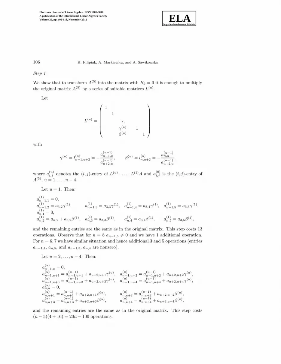
Step 1
We show that to transform A(5) into the matrix with Bk = 0 it is enough to multiply
the original matrix A(5) by a series of suitable matrices L(u).
Let
L(u) =
1
1. . .
γ(u) 1
β(u) 1
with
γ(u) = l(u)n−1,u+2 = −
a(u−1)n−1,u
a(u−1)u+2,u
, β(u) = l(u)n,u+2 = − a
(u−1)n,u
a(u−1)u+2,u
,
where a(u)i,j denotes the (i, j)-entry of L(u) · . . . · L(1)A and a
(0)i,j is the (i, j)-entry of
A(5), u = 1, . . . , n− 4.
Let u = 1. Then:
a(1)n−1,1 = 0,
a(1)n−1,2 = a3,2γ
(1), a(1)n−1,3 = a3,3γ
(1), a(1)n−1,4 = a3,4γ
(1), a(1)n−1,5 = a3,5γ
(1),
a(1)n,1 = 0,
a(1)n,2 = an,2 + a3,2β
(1), a(1)n,3 = a3,3β
(1), a(1)n,4 = a3,4β
(1), a(1)n,5 = a3,5β
(1),
and the remaining entries are the same as in the original matrix. This step costs 13
operations. Observe that for n = 8 an−1,5 6= 0 and we have 1 additional operation.
For n = 6, 7 we have similar situation and hence additional 3 and 5 operations (entries
an−1,4, an,5, and an−1,3, an,4 are nonzero).
Let u = 2, . . . , n− 4. Then:
a(u)n−1,u = 0,
a(u)n−1,u+1 = a
(u−1)n−1,u+1 + au+2,u+1γ
(u), a(u)n−1,u+2 = a
(u−1)n−1,u+2 + au+2,u+2γ
(u),
a(u)n−1,u+3 = a
(u−1)n−1,u+3 + au+2,u+3γ
(u), a(u)n−1,u+4 = a
(u−1)n−1,u+4 + au+2,u+4γ
(u),
a(u)n,u = 0,
a(u)n,u+1 = a
(u−1)n,u+1 + au+2,u+1β
(u), a(u)n,u+2 = a
(u−1)n,u+2 + au+2,u+2β
(u),
a(u)n,u+3 = a
(u−1)n,u+3 + au+2,u+3β
(u), a(u)n,u+4 = a
(u−1)n,u+4 + au+2,u+4β
(u),
and the remaining entries are the same as in the original matrix. This step costs
(n− 5)(4 + 16) = 20n− 100 operations.
Electronic Journal of Linear Algebra ISSN 1081-3810 A publication of the International Linear Algebra SocietyVolume 25, pp. 102-118, November 2012
http://math.technion.ac.il/iic/ela

ELA
Determinants of multidiagonal matrices 107
Now, let
L(n−3) =
1
1. . .
1
β(n−3) 1
with β(n−3) = −a(n−4)n,n−3
a(n−4)n−1,n−3
. Then
a(n−3)n,n−3 = 0, a
(n−3)n,n−2 = a
(n−4)n,n−2 + a
(n−4)n−1,n−2β
(n−3),
a(n−3)n,n−1 = a
(n−4)n,n−1 + a
(n−4)n−1,n−1β
(n−3), a(n−3)n,n = a
(n−4)n,n + a
(n−4)n−1,nβ
(n−3),
which costs 8 operations. We denote the matrix L(n−3) · · ·L(1)A(5) by L.
It is easy to calculate that the first step of the algorithm costs 20n−79 operations.
Step 2
This step is similar to the Step 1 in Sogabe [8]. Observe however, that the number of
operations increases since the last column of the obtained matrix is nonzero.
Let
Φ(u) =
Iu
1
φu+2,u+1 1
In−u−2
with
φu+2,u+1 = −f(u−1)u+2,u
f(u−1)u+1,u
,
where f(u)i,j denotes the (i, j)-entry of Φ(u) · · ·Φ(1)L and f
(0)i,j is the (i, j)-entry of L,
u = 1, . . . , n− 2.
Let u = 1, . . . , n− 4. Then
f(u)u+2,u = 0,
f(u)u+2,u+1 = f
(u−1)u+2,u+1 + f
(u−1)u+1,u+1φu+2,u+1,
f(u)u+2,u+2 = f
(u−1)u+2,u+2 + f
(u−1)u+1,u+2φu+2,u+1,
f(u)u+2,u+3 = f
(u−1)u+2,u+3 + f
(u−1)u+1,u+3φu+2,u+1, f
(u)u+2,n = f
(u−1)u+1,nφu+2,u+1,
Electronic Journal of Linear Algebra ISSN 1081-3810 A publication of the International Linear Algebra SocietyVolume 25, pp. 102-118, November 2012
http://math.technion.ac.il/iic/ela

ELA
108 K. Filipiak, A. Markiewicz, and A. Sawikowska
and the remaining entries are the same as in Φ(u−1) · · ·Φ(1)L. This step costs (n −4)(7 + 2) = 9n− 36 operations. Observe that for a similar reason as in Step 1 with
u = 1, we have additional 1 and 2 operations for n = 7, 8 and n = 6, respectively.
Let u = n− 3. Then
f(n−3)n−1,n−3 = 0,
f(n−3)n−1,n−2 = f
(n−4)n−1,n−2 + f
(n−4)n−2,n−2φn−1,n−2,
f(n−3)n−1,n−1 = f
(n−4)n−1,n−1 + f
(n−4)n−2,n−1φn−1,n−2, f
(n−3)n−1,n = f
(n−4)n−1,n + f
(n−4)n−2,nφn−1,n−2,
and the remaining entries are the same as in Φ(n−4) · · ·Φ(1)L. This step costs 8
operations.
Let u = n− 2. Then
f(n−2)n,n−2 = 0, f
(n−2)n,n−1 = f
(n−3)n,n−1 + f
(n−3)n−1,n−1φn,n−1,
f(n−2)n,n = f
(n−3)n,n + f
(n−3)n−1,nφn,n−1,
and the remaining entries are the same as in Φ(n−3) · · ·Φ(1)L. This step costs 6
operations.
Thus, to obtain the Hessenberg matrix
Ω=
ω1,1 ω1,2 ω1,3 ω1,n−1 ω1,n
ω2,1 ω2,2 ω2,3 ω2,4 ω2,n
ω3,2 ω3,3 ω3,4 ω3,5 ω3,n
ω4,3 ω4,4 ω4,5 ω4,6 ω4,n
. . .. . .
. . ....
. . .. . .
. . ....
ωn−3,n−4 ωn−3,n−3 ωn−3,n−2 ωn−3,n−1 ωn−3,n
ωn−2,n−3 ωn−2,n−2 ωn−2,n−1 ωn−2,n
ωn−1,n−2 ωn−1,n−1 ωn−1,n
ωn,n−1 ωn,n
,
with ωi,j = 0 if 2 < j − i < n − 2 and i − j < 1 it is necessary to make 9n − 22
operations.
Step 3
This step is based on the method presented by Sogabe [9]. The difference is that this
step takes more operations since the entries ω1,n−1, ω1,n and ω2,n are nonzero.
Electronic Journal of Linear Algebra ISSN 1081-3810 A publication of the International Linear Algebra SocietyVolume 25, pp. 102-118, November 2012
http://math.technion.ac.il/iic/ela

ELA
Determinants of multidiagonal matrices 109
Let
Λ(u) =
Iu−1
1
α(u) 1
In−u−1
with
α(u) = λ(u)u+1,u = −
ω(u−1)u+1,u
ω(u−1)u,u
,
where ω(u)i,j denotes the (i, j)-entry of Λ(u) · · ·Λ(1)Ω and ω
(0)i,j is the (i, j)-entry of Ω,
u = 1, . . . , n− 1.
Let u = 1, . . . , n− 5. Then
ω(u)u+1,u = 0,
ω(u)u+1,u+1 = ω
(u−1)u+1,u+1 + ω
(u−1)u,u+1α
(u), ω(u)u+1,u+2 = ω
(u−1)u+1,u+2 + ω
(u−1)u,u+2α
(u),
ω(u)u+1,n−1 = ω
(u−1)u,n−1α
(u), ω(u)u+1,n = ω
(u−1)u+1,n + ω
(u−1)u,n α(u),
and the remaining entries are the same as in Λ(u−1) · · ·Λ(1)Ω. This step costs 9(n−5)
operations.
Let u = n− 4. Then
ω(n−4)n−3,n−4 = 0,
ω(n−4)n−3,n−3 = ω
(n−5)n−3,n−3 + ω
(n−5)n−4,n−3α
(n−4),
ω(n−4)n−3,n−2 = ω
(n−5)n−3,n−2 + ω
(n−5)n−4,n−2α
(n−4),
ω(n−4)n−3,n−1 = ω
(n−5)n−3,n−1 + ω
(n−5)n−4,n−1α
(n−4), ω(n−4)n−3,n = ω
(n−5)n−3,n + ω
(n−5)n−4,nα
(n−4),
and the remaining entries are the same as in Λ(n−5) · · ·Λ(1)Ω. This step costs 10
operations.
Let u = n− 3. Then
ω(n−3)n−2,n−3 = 0,
ω(n−3)n−2,n−2 = ω
(n−4)n−2,n−2 + ω
(n−4)n−3,n−2α
(n−3),
ω(n−3)n−2,n−1 = ω
(n−4)n−2,n−1 + ω
(n−4)n−3,n−1α
(n−3), ω(n−3)n−2,n = ω
(n−4)n−2,n + ω
(n−4)n−3,nα
(n−3),
and the remaining entries are the same as in Λ(n−4) · · ·Λ(1)Ω. This step costs 8
operations.
Let u = n− 2. Then
ω(n−2)n−1,n−2 = 0, ω
(n−2)n−1,n−1 = ω
(n−3)n−1,n−1 + ω
(n−3)n−2,n−1α
(n−2),
ω(n−2)n−1,n = ω
(n−3)n−1,n + ω
(n−3)n−2,nα
(n−2),
Electronic Journal of Linear Algebra ISSN 1081-3810 A publication of the International Linear Algebra SocietyVolume 25, pp. 102-118, November 2012
http://math.technion.ac.il/iic/ela

ELA
110 K. Filipiak, A. Markiewicz, and A. Sawikowska
and the remaining entries are the same as in Λ(n−3) · · ·Λ(1)Ω. This step costs 6
operations.
Let u = n− 1. Then
ω(n−1)n,n−1 = 0, ω
(n−1)n,n = ω
(n−2)n,n + ω
(n−2)n−1,nα
(n−3),
and the remaining entries are the same as in Λ(n−2) · · ·Λ(1)Ω. This step costs 4
operations.
Summing-up, Step 3 of this algorithm takes 9n− 12 operations.
3.1.2. Molinari’s [6] method. Let n = 2k, k ≥ 3 is integer. From (2.1)
detA = det (T − I4) ·k∏
i=1
detBi.
It is easy to check that for i = 1, . . . , k − 1
B−1i =
(
a2i−1,2i+1 0
a2i,2i+1 a2i,2i+2
)−1
=
(
1a2i−1,2i+1
0
−a2i,2i+1
di
1a2i,2i+2
)
with di = detBi = a2i−1,2i+1a2i,2i+2 and
B−1k =
(
an−1,1 0
an,1 an,2
)−1
=
(
1an−1,1
0
−an,1
dk
1an,2
)
with dk = detBk = an−1,1an,2. Calculating all di (i = 1, . . . , k) can be done in k
operations. To obtain −B−1i Ai and −B−1
i Ci, i = 2, . . . , k, i.e.,
−B−1i Ai =
(
a2i−1,2i−1
ei
a2i−1,2i
ei
a2i−1,2i−1fi − a2i,2i−1
a2i,2i+2a2i−1,2ifi − a2i,2i
a2i,2i+2
)
, i = 1, . . . , k − 1,
−B−1k Ak =
(
an−1,n−1
ek
an−1,n
ek
an−1,n−1fk − an,n−1
an,2an−1,nfk − an,n
an,2
)
and
−B−11 C1 =
(
a1,n−1
e1
a1,n
e1
a1,n−1f1 a1,nf1 − a2,n
a2,4
)
,
−B−1i Ci =
(
a2i−1,2i−3
ei
a2i−1,2i−2
ei
a2i−1,2i−3fi a2i−1,2i−2fi − a2i,2i−2
a2i,2i+2
)
, i = 2, . . . , k − 1,
Electronic Journal of Linear Algebra ISSN 1081-3810 A publication of the International Linear Algebra SocietyVolume 25, pp. 102-118, November 2012
http://math.technion.ac.il/iic/ela

ELA
Determinants of multidiagonal matrices 111
−B−1k Ck =
(
an−1,n−3
ek
an−1,n−2
ek
an−1,n−3fk an−1,n−2fi − an,n−2
an,2
)
,
with ei = −a2i−1,2i+1 and fi =a2i,2i+1
di, i = 1, . . . , k − 1, ek = −an−1,1, and fk =
an,1
dk, 10 and 6 operations for every i = 1, . . . , k are performed, respectively. Thus,
determination of a single Ti requires 17 operations (1 + 10 + 6).
Now multiply Ti and Ti+1, i = 1, 3, . . . , k− 1 if k is even and i = 1, 3, . . . , k− 2 if
k is odd.
Consider the case that k is even. Let us denote by Gl the products T2l−1 · T2l,
l = 1, 2, . . . , k2 . Determination of each Gl costs 28 operations. We have k2 such
matrices, that are in fact 4-by-4 matrices with no zeros. Now, every product of two
4-by-4 matrices with no zeros costs 7 · 16 operations (we have k2 − 1 such products in
∏k2
l=1 Gl), and we obtain that the determination of the matrix T can be performed in
173k + 28 · k2 + 112 · (k2 − 1) = 87k − 112 operations for even k.
Now consider the case that k is odd. As in previous case, every Gl = T2l−1 · T2l,
l = 1, 2, . . . , k−12 , costs 28 operations. Now, every product of two 4-by-4 matrices with
no zeros costs 7·16 operations (we have k−12 −1 such products in
∏
k−1
2
l=1 Gl) and the last
multiplication, G(k−1)/2 · Tk costs 56 operations. We obtain that the determination
of the matrix T can be performed in 17k+ 28 · k−12 + 112(k−1
2 − 1) + 56 = 87k− 126
operations for odd k.
Finally, determination of T−I4 costs 87k−108 operations for even k and 87k−122
for odd k.
The next step is to calculate the determinant of T − I4. Since this is the 4-by-4
matrix, it is enough to transform it into the triangular matrix, costing 40 operations
and additional 3 for product of diagonal entries. We obtain the following operation
counts: 87k − 65 for even k and 87k − 79 for odd k.
Observe that according to (2.1), we have to calculate also the determinant of the
product of matrices Bi. It is equivalent to calculate the product of determinants of
2-by-2 lower triangular matrices, that we in fact have already derived and denoted
by di. Thus to obtain the final cost of this algorithm it is enough to perform k − 1
additional multiplications. By (2.1) we have one additional multiplication.
Summing-up, using the method of Molinari [6], deriving the determinant of pen-
tadiagonal matrix with corners can be performed in 88k − 65 operations for even k,
and in 88k − 79 for k odd.
Electronic Journal of Linear Algebra ISSN 1081-3810 A publication of the International Linear Algebra SocietyVolume 25, pp. 102-118, November 2012
http://math.technion.ac.il/iic/ela

ELA
112 K. Filipiak, A. Markiewicz, and A. Sawikowska
Let n = 2k + 1, k ≥ 3 is integer. From (2.4)
detA = an,n · det(Z − 1
an,nXAYA)
with
XTA =
(
a1,n a2,n 0 . . . 0 an−2,n an−1,n
)
,
YA =(
an,1 an,2 0 . . . 0 an,n−2 an,n−1
)
.
Observe that the matrix U − 1an,n
XAYA is a tridiagonal block matrix with corners,
with Ai, Bi, Ci the same as in (1.1), except
A1 =
(
a1,1 − an,1e1 a1,2 − an,2e1
a2,1 − an,1e2 a2,2 − an,2e2
)
,
Ak =
(
an−2,n−2 − an,n−2en−2 an−2,n−1 − an,n−1en−2
an−1,n−2 − an,n−2en−1 an−1,n−1 − an,n−1en−1
)
,
C1 =
(
−an,n−2e1 a1,n−1 − an,n−1e1
−an,n−2e2 −an,n−1e2
)
,
Bk =
(
−an,1en−1 −an,2en−2
an−1,1 − an,1en−1 −an,2en−1
)
with eu =au,n
an,n, u = 1, 2, n − 2, n − 1. Determination of U − 1
an,nXAYA can be
performed in 36 operations. Now, we can use again the formula (2.1) for n = 2k.
Thus, we need the following number of operations:
• determination of di, i = 1, . . . , k − 1, and dk: (k − 1) + 3 = k + 2 operations,
• determination of −B−1i Ai, i = 1, . . . , k − 1, and −B−1
k Ak: 10(k − 1) + 16 =
10k + 6 operations,
• determination of −B−1i Ci, i = 2, . . . , k, −B−1
1 C1 and −B−1k Ck: 6(k − 2) +
9 + 16 = 6k + 13 operations.
Summing-up, the determination of every Ti can be achieved in 17k + 21 operations.
The remaining part follows exactly as in the case of even n with respective k.
Recall that for deriving the determinant of A(5) it is necessary to multiply the deter-
minant of U − 1an,n
XAYA by an,n, which gives us one additional operation. Finally
we obtain 88k − 43 for even k and 88k − 57 for odd k.
For comparison, we have the following computational counts for the computation
of the determinant of an n× n (n ≥ 9) pentadiagonal matrix with corners:
Electronic Journal of Linear Algebra ISSN 1081-3810 A publication of the International Linear Algebra SocietyVolume 25, pp. 102-118, November 2012
http://math.technion.ac.il/iic/ela
ELA
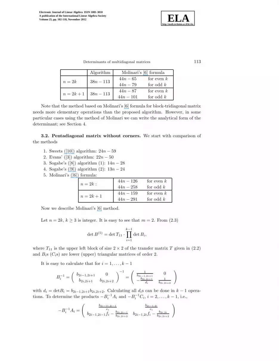
Determinants of multidiagonal matrices 113
Algorithm Molinari’s [6] formula
n = 2k 38n− 11344n− 65
44n− 79
for even k
for odd k
n = 2k + 1 38n− 11344n− 87
44n− 101
for even k
for odd k
Note that the method based on Molinari’s [6] formula for block-tridiagonal matrix
needs more elementary operations than the proposed algorithm. However, in some
particular cases using the method of Molinari we can write the analytical form of the
determinant; see Section 4.
3.2. Pentadiagonal matrix without corners. We start with comparison of
the methods
1. Sweets ([10]) algorithm: 24n− 59
2. Evans’ ([3]) algorithm: 22n− 50
3. Sogabe’s ([8]) algorithm (1): 14n− 28
4. Sogabe’s ([9]) algorithm (2): 13n− 24
5. Molinari’s ([6]) formula:
n = 2k :44n− 126
44n− 258
for even k
for odd k
n = 2k + 144n− 159
44n− 291
for even k
for odd k
Now we describe Molinari’s [6] method.
Let n = 2k, k ≥ 3 is integer. It is easy to see that m = 2. From (2.3)
detB(5) = detT11 ·k−1∏
i=1
detBi,
where T11 is the upper left block of size 2× 2 of the transfer matrix T given in (2.2)
and Bis (Cis) are lower (upper) triangular matrices of order 2.
It is easy to calculate that for i = 1, . . . , k − 1
B−1i =
(
b2i−1,2i+1 0
b2i,2i+1 b2i,2i+2
)−1
=
(
1b2i−1,2i+1
0
− b2i,2i+1
di
1b2i,2i+2
)
with di = detBi = b2i−1,2i+1b2i,2i+2. Calculating all dis can be done in k − 1 opera-
tions. To determine the products −B−1i Ai and −B−1
i Ci, i = 2, . . . , k − 1, i.e.,
−B−1i Ai =
(
b2i−11,2i−1
ei
b2i−1,2i
ei
b2i−1,2i−1fi − b2i,2i−1
b2i,2i+2b2i−1,2ifi − b2i,2i
b2i,2i+2
)
Electronic Journal of Linear Algebra ISSN 1081-3810 A publication of the International Linear Algebra SocietyVolume 25, pp. 102-118, November 2012
http://math.technion.ac.il/iic/ela

ELA
114 K. Filipiak, A. Markiewicz, and A. Sawikowska
and
−B−1i Ci =
(
b2i−1,2i−3
ei
b2i−1,2i−2
ei
b2i−1,2i−3fi b2i−1,2i−2fi − b2i,2i−2
b2i,2i+2
)
with ei = −b2i−1,2i+1, fi =b2i,2i+1
di, 10(k − 2) and 6(k − 2) operations are performed,
respectively. Moreover, Tk and T1 can be obtained in 7 and 13 operations, respectively.
Thus, Tis can be achieved in 17k− 13 operations ((k− 1) + (10+ 6)(k− 2) + 7+13).
Let now multiply Ti and Ti+1, i = 1, 3, . . . , k−1 if k is even and i = 1, 3, . . . , k−2
if k is odd.
First consider the case that k is even. Let us denote by Gl the products T2l−1 ·T2l,
l = 1, 2, . . . , k2 . Determination of G1 can be done in 26 operations, each Gl, l =
2, . . . , k2 − 1, in 28 operations, and G k
2in 27 operations. All matrices Gl are 4-by-4
matrices with no zeros, and every product of two 4-by-4 matrices with no zeros can
be performed in 7 · 16 operations (we have k2 − 1 such products in
∏k2
l=1 Gl). Thus, to
obtain the matrix T we need (17k−13)+26+28(k2 −2)+27+112 ·(k2 −1) = 87k−128
operations for even k.
Next consider the case that k is odd. Similarly as in previous case, the determi-
nation of every Gl = T2l−1 · T2l, l = 2, . . . , k−12 − 1 can be achieved in 28(k−1
2 − 1)
operations and the determination of G k−1
2
costs additional 27 operations. Now, every
product of two 4-by-4 matrices with no zeros can be performed in 7 ·16 operations (we
have k−12 − 2 such products in
∏
k−1
2
l=2 Gl) and the last multiplication, T T1 ·∏
k−1
2
l=2 GTl ,
in 48 operations. We obtain that the determination of the matrix T can be obtained
in (17k − 13) + 27 + 28 · (k−12 − 1) + 112(k−1
2 − 2) + 48 = 87k − 260 operations for
odd k.
Finally, detT11 can be obtained in 3 operations. Multiplying all necessary deter-
minants according to formula (2.3) we get additional k − 1 operations.
Summing-up, the determination of detB(5) can be achieved in 88k − 126 opera-
tions for even k and in 88k − 256 for odd k.
Let n = 2k + 1, k ≥ 3 is integer. From (2.5)
detB = bn,n · det(U − 1
bn,nXBYB)
with
XTB =
(
0 · · · 0 bn−2,n bn−1,n
)
,
YB =(
0 · · · 0 bn,n−2 bn,n−1
)
.
Electronic Journal of Linear Algebra ISSN 1081-3810 A publication of the International Linear Algebra SocietyVolume 25, pp. 102-118, November 2012
http://math.technion.ac.il/iic/ela

ELA
Determinants of multidiagonal matrices 115
The calculation of U − 1bn,n
XBYB can be done in 10 operations. As a result we obtain
pentadiagonal matrix of the form (1.1) with Ak replaced by
(
bn−2,n−2 − bn,n−2en−2 bn−2,n−1 − bn,n−1en−2
bn−1,n−2 − bn,n−2en−1 bn−1,n−1 − bn,n−1en−1
)
with eu =bu,n
bn,n, u = n − 2, n − 1. Observe that it does not change the number of
operations to calculate the determinant in comparison with even n, i.e., this step
costs 88k− 126 operations for even k and 88k− 258 for odd k. Thus, multiplying the
above determinant by bn,n (one additional operation) we get that it can be done in
88k − 115 operations for even k and in 88k − 247 operations for odd k.
4. Applications. Tridiagonal matrices with corners arise, for example, in theory
of experiments in the characterization of D-optimal design of experiment (Filipiak et
al., [4]). One of the step is to derive the determinant of the matrix
W3 = αIn − (Hn +HTn )
α > 2, with Hn - the cyclic permutation matrix given by
Hn =
(
0T 1
In−1 0
)
.
Using the respective formula from Molinari [6], we obtain
detW3 = −2 + tr
[
(
α −1
1 0
)n]
= −2 + xn + x−n
where x is the eigenvalue of
(
α −1
1 0
)
, i.e., x = α+√α2−42 .
Similarly we may construct pentadiagonal matrix with corners
W5 = αIn − (Hn +HTn )− (H2
n +H2nT).
with n = 2k. Using (2.1) we obtain
detW5 = (−1)2(k−1) det(Sk − I4) =
4∏
i=1
(λki − 1),
where λi is the ith eigenvalue of
S =
α −1 −1 −1
−α− 1 α+ 1 1 0
1 0 0 0
0 1 0 0
.
Electronic Journal of Linear Algebra ISSN 1081-3810 A publication of the International Linear Algebra SocietyVolume 25, pp. 102-118, November 2012
http://math.technion.ac.il/iic/ela

ELA
116 K. Filipiak, A. Markiewicz, and A. Sawikowska
This implies that the λis are the solutions of the characteristic polynomial of the form[
1− 12 (2α+ 1−
√4α+ 9)λ + λ2
]
·[
1− 12 (2α+ 1 +
√4α+ 9)λ+ λ2
]
= 0,
i.e.,
λ1 = 14
[
1 + 2α−√4α+ 9−
√2√
2α2 − 3−√4α+ 9− 2α(
√4α2 + 9− 2)
]
λ2 = 14
[
1 + 2α−√4α+ 9 +
√2√
2α2 − 3−√4α+ 9− 2α(
√4α2 + 9− 2)
]
λ3 = 14
[
1 + 2α+√4α+ 9−
√2√
2α2 − 3 +√4α+ 9 + 2α(
√4α2 + 9 + 2)
]
λ4 = 14
[
1 + 2α+√4α+ 9 +
√2√
2α2 − 3 +√4α+ 9 + 2α(
√4α2 + 9 + 2)
]
.
Now consider the following matrix:
W = (In +Hn +HTn )⊗ Ir
where ⊗ denotes the Kronecker product. Then
detW = det(In +Hn +HTn ),
which is tridiagonal matrix with corners. From Molinari [6] it can be seen that
detW = (−1)n+1 · 2 + tr
[
(
1 −1
1 0
)n]
.
Since the matrix
(
1 −1
1 0
)
is a 6-involutory matrix, i.e.,
(
1 −1
1 0
)6
= I2,
and moreover,
(
1 −1
1 0
)3
= −I2,
it is easy to calculate that
detW =
0 for n = 3u
−3 for n 6= 3u and n even
3 for n 6= 3u and n odd.
The generalization to block matrices is interesting for the study of transport
in discrete structures such as nanotubes or molecules (see e.g. Kostyrko et al. [5],
Compernolle et al. [1], Yamada [11]).
Electronic Journal of Linear Algebra ISSN 1081-3810 A publication of the International Linear Algebra SocietyVolume 25, pp. 102-118, November 2012
http://math.technion.ac.il/iic/ela

ELA
Determinants of multidiagonal matrices 117
5. Discussion. It can be seen that the method based on Molinari’s [6] formula
for block-tridiagonal matrices needs more elementary operations than the algorithm
proposed in Section 2 and Sogabe’s [9] algorithm, respectively. Moreover, the formula
for the evaluation of transition matrix T requires k (k− 1) inversions of matrices Bi.
However, in some particular cases Molinari’s method may be more useful. Consider
an example based on Example 2 of Sogabe [8]. Assume A(5) is 103 × 103 matrix of
the form
A(5) =
0.2 −1.3 1.2 0.1 0.3
0.3 0.2 −1.3 1.2 0.1
0.1 0.3 0.2 −1.3 1.2. . .
. . .. . .
. . .. . .
. . .. . .
. . .. . . 1.2
1.2 0.1 0.3 0.2 −1.3
−1.3 1.2 0.1 0.3 0.2
.
The proposed algorithm gives detA(5) = ∞, while Molinari’s algorithm detA(5) =
1.5179∗1079, and this is the same result as determinant obtained directly using Math-
ematica and R. For the same matrix of order 100, we have 9.15866∗1064 for proposedalgorithm and 8.28367 ∗ 107 for Molinari’s algorithm and using direct calculations of
Mathematica and R.
It is worth noting that for the example of pentadiagonal matrix with corners
based on Example 1 of Sogabe [8] we get the same value of determinant for both
methods.
It can be seen that if the determinants of Bi are close to zero, Molinari’s [6]
method may be not stable.
Acknowledgment. The research of K. Filipiak and A. Markiewicz was partially
supported by the National Science Center Grant DEC-2011/01/B/ST1/01413.
REFERENCES
[1] S. Compernolle, L. Chibotaru, and A. Coulemans. Eigenstates and transmission coefficients of
finite-sized nanotubes. J. Chem. Phys., 119:2854–2873, 2003.
[2] M. El-Mikkawy. A note on a three-term recurrence for a tridiagonal matrix. Appl. Math. Comput.,
139:503–511, 2003.
[3] D.J. Evans. A recursive algorithm for determining the eigenvalues of a quindiagonal matrix.
Comput. J., 18:70–73, 1975.
[4] K. Filipiak, A. Markiewicz, and R. Rozanski. Maximal determinant over a certain class of
matrices and its application to D-optimality of designs. Linear Algebra Appl., 436:874–887,
2012.
Electronic Journal of Linear Algebra ISSN 1081-3810 A publication of the International Linear Algebra SocietyVolume 25, pp. 102-118, November 2012
http://math.technion.ac.il/iic/ela
ELA
118 K. Filipiak, A. Markiewicz, and A. Sawikowska
[5] T. Kostyrko, M. Bartkowiak, and G.D. Mahan. Reflection by defects in a tight-binding model
of nanotubes. Phys. Rev., B, 59:3241–3249, 1999.
[6] L.G. Molinari. Determinants of block tridiagonal matrices. Linear Algebra Appl., 429:2221–2226,
2008.
[7] D.K. Salkuyeh. Comments on “A note on a three-term recurrence for a tridiagonal matrix”.
Appl. Math. Comput., 176:442–444, 2006.
[8] T. Sogabe. A fast numerical algorithm for the determinant of a pentadiagonal matrix. Appl.
Math. Comput., 196:835–841, 2008a.
[9] T. Sogabe. A note on A fast numerical algorithm for the determinant of a pentadiagonal matrix.
Appl. Math. Comput., 201:561–564, 2008b.
[10] R.A. Sweet. A recursive relation for the determinant of a pentadiagonal matrix. Comm. ACM,
12:330–332, 1969.
[11] H. Yamada. Electronic localization properties of a double strand of DNA: a simple model with
long range correlated hopping disorder. Internat. J. Modern Phys. B, 18:1697–1716, 2004.
Electronic Journal of Linear Algebra ISSN 1081-3810 A publication of the International Linear Algebra SocietyVolume 25, pp. 102-118, November 2012
http://math.technion.ac.il/iic/ela