Globally Convergent Methods for NonlinearEquations�M. Ferrisy S. LucidizJuly 1991Abstract. We are concerned with enlarging the domain of convergence for solution methods of nonlinearequations. To this end, we produce a general framework in which to prove global convergence. Our frameworkrelies on several notions: the use of a merit function, a generalization of a forcing function and conditions onthe choice of direction. We also incorporate the idea of a nonmonotone stabilization procedure as a meansof producing very good practical rates of convergence. The general theory is specialized to yield severalwell known results from the literature and is also used to generate three new algorithms for the solution ofnonlinear equations. Numerical results for these algorithms applied to the nonlinear equations arising fromnonlinear complementarity problems are given.1 IntroductionIn this paper we shall be concerned with proving global convergence of an algorithm to solvenonlinear equations. The algorithm we propose uni�es many of the results given in theliterature and also allows us to give new criteria under which a method can be expected tobe globally convergent.There are many known results on the global convergence of Newton type methods fornonlinear equations. Most of these methods are based on the use of a merit function. Sev-eral di�erent types of merit function have been proposed in the literature (see for example[Bur80, SB80, Pol76, HPR89, HX90]). One of the main di�erences between many of theapproaches is whether or not the underlying equations are smooth or nonsmooth. In thesmooth case, global convergence is proven in many instances: we note in particular the resultsof Stoer[SB80]. However, many of the approaches for solving the nonlinear complementarityproblem consider reformulations of the problem as a system of nonsmooth equations. Globalconvergence can also be established here, for example, some pertinent results are given in[HPR89, Ral91].�This material is partially based on research supported by the Air Force O�ce of Scienti�c ResearchGrant AFOSR{89{0410, the National Science Foundation Grant CCR 9157632 and Istituto di Analisi deiSistemi ed Informatica del CNRyComputer Sciences Department, University of Wisconsin, Madison, Wisconsin 53706zIstituto di Analisi dei Sistemi ed Informatica del CNR, Viale Manzoni 30, 00185 Roma, Italy1

The emphasis of this paper will be on establishing many of the known results under verygeneral conditions on a merit function via the use of a auxiliary function (a generalization ofthe familiar notion of a forcing function). While most of the paper deals with general condi-tions which a search direction must satisfy, the motivation for these conditions comes fromconsidering Newton and Gauss{Newton methods for systems of n equations in n unknowns.Several new ideas are encompassed in our framework. For instance, a nonmonotone stabi-lization procedure is used to overcome some of the di�culties associated with ill{conditioningand to enable a steps of length one to be taken much more frequently in Newton{type meth-ods. Computationally, this has proven very e�ective, see for example, [GLL86] where thepoor performance on the Rosenbrock problem has been overcome by nonmonotone linesearch(also [BS91]).For di�erent problems, several types of merit function have been proposed in the liter-ature. By far the most popular is to use the Euclidean norm of the residual as the meritfunction. Other forms which can be considered are p{norm merit functions and 1{normmerit functions. We will show that all of these forms of merit function can be treated in ourframework.While there is a wide literature on Gauss{Newton methods for the nonlinear least squaresproblem, only limited attention has been given to modi�cations of the search direction.In this paper, we propose several modi�cations of the search direction when the Newtondirection cannot be found. Most of these �nd their basis in solving the equations in a leastsquares sense; see the survey paper of [Fra88] for several search direction modi�cations inleast squares problems.Much of this work was motivated by a desire to solve nonlinear complementarity problems.We are interested in using the smooth equations determined by Mangasarian[Man76] whichare equivalent to the nonlinear complementarity problem. The essential di�erence is thatwhile in least squares problems, the optimal value will not be zero, in this case it is, and sovarious new methods have been proposed. In particular, the method of Subramanian[Sub85]gives a direction which is consistent. The results in this paper show that our method can beused to establish global convergence in the case where the Jacobian is singular at the solutionpoint (Dennis and Schnabel [DS83] give other results using the trust region approach).The paper is organized as follows. The main theoretical results of the paper are givenin Section 2. We describe the notion of a nonmonotone stabilization algorithm and givegeneral conditions which are required for such a technique to give global convergence. Theseconditions are formulated in terms of a merit function, an auxiliary function (which resemblesa forcing function) and the directions determined by the algorithm in question. We provea general convergence result under these assumptions, without specifying the particularmerit function, the auxiliary function or the direction, but only the conditions they mustsatisfy. We give several applications of this theory in Section 3 and describe three newalgorithms which satisfy our conditions. Section 4 outlines several instances of work inthe literature which can be formulated as special cases of our framework. In Section 5 ofthe paper we present some numerical results when the proposed algorithms are applied tononlinear complementarity problems. Several standard examples are solved, including some2

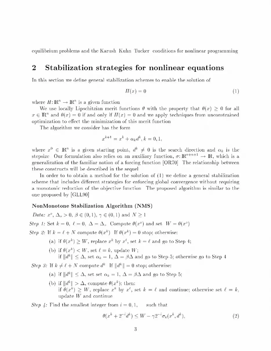
equilibrium problems and the Karush{Kuhn{Tucker conditions for nonlinear programming.2 Stabilization strategies for nonlinear equationsIn this section we de�ne general stabilization schemes to enable the solution ofH(x) = 0 (1)where H: IRn ! IRn is a given function.We use locally Lipschitzian merit functions � with the property that �(x) � 0 for allx 2 IRn and �(x) = 0 if and only if H(x) = 0 and we apply techniques from unconstrainedoptimization to e�ect the minimization of this merit function.The algorithm we consider has the formxk+1 = xk + �kdk; k = 0; 1; . . .where x0 2 IRn is a given starting point, dk 6= 0 is the search direction and �k is thestepsize. Our formulation also relies on an auxiliary function, �: IRn+n+1 ! IR, which is ageneralization of the familiar notion of a forcing function [OR70]. The relationship betweenthese constructs will be described in the sequel.In order to to obtain a method for the solution of (1) we de�ne a general stabilizationscheme that includes di�erent strategies for enforcing global convergence without requiringa monotonic reduction of the objective function. The proposed algorithm is similar to theone proposed by [GLL90].NonMonotone Stabilization Algorithm (NMS)Data: xo, �o > 0, � 2 (0; 1), 2 (0; 1) and N � 1.Step 1: Set k = 0; ` = 0; � = �o. Compute �(xo) and set W = �(xo).Step 2: If k = `+N compute �(xk). If �(xk) = 0 stop; otherwise:(a) if �(xk) �W , replace xk by x`, set k = ` and go to Step 4;(b) if �(xk) < W , set ` = k, update W ;if kdkk � �, set �k = 1, � = �� and go to Step 5; otherwise go to Step 4.Step 3: If k 6= ` +N compute dk. If kdkk = 0 stop; otherwise:(a) if kdkk � �, set set �k = 1, � = �� and go to Step 5;(b) if kdkk > �, compute �(xk); then:if �(xk) � W , replace xk by x`, set k = ` and continue; otherwise set ` = k,update W and continue.Step 4: Find the smallest integer from i = 0; 1; . . . such that�(xk + 2�idk) � W � 2�i�k(xk; dk); (2)3

and set �k = 2�i, ` = k + 1, update W and continue.Step 5: Set xk+1 = xk + �kdk, k = k + 1, and go to Step 2. 4In the description of the algorithm, ` denotes the index of the last accepted point wherethe objective function has been evaluated. For later reference we introduce a new index jwhich is set initially at j = 0 and incremented each time we de�ne ` = k. Then we indicateby fx`(j)g the sequence of points where the objective function is evaluated and by fWjg thesequence of reference values. Furthermore, we also need the index q(k) de�ned by:q(k):= max [j : `(j) � k]; (3)thus `(q(k)) is the largest iteration index not exceeding k where the merit function wasevaluated.In order to complete the description of the algorithm we must specify the the criterionemployed for updating Wj. The reference value Wj for the merit function is initially set to�(xo). Whenever a point x`(j) is generated such that �(x`(j)) < Wj , the reference value isupdated by taking into account a pre�xed number m(j) �M of previous function values ofthe merit function. To be precise, we require that the updating rule for Wj+1 satis�es thefollowing condition.Given M � 0, let m(j + 1) be such thatm(j + 1) � min [m(j) + 1;M ];and let Fj+1 = max0� i�m(j+1) �(x`(j+1� i)); (4)choose the value Wj+1 to satisfy �(x`(j+1)) � Wj+1 � Fj+1: (5)These conditions on the reference values include several ways of determining the sequencefWjg in an implementation of the algorithm. For example, any of the following updatingrules can be used: Wj+1 = Fj+1 = max0� i�m(j+1) �(x`(j+1� i)); (6)Wj+1 = max24�(x`(j+1)); 1m(j + 1) + 1 m(j+1)Xi=0 �(x`(j+1� i))35 ; (7)Wj+1 = min �Fj+1; 12 �Wj + �(x`(j+1))�� : (8)We note that (6) is the easiest to satisfy, while (7) and (8) de�ne conditions which guarantee\mean descent". 4

We now describe the conditions which will ensure the global convergence of the afore-mentioned method. We will make frequent use of the following compactness assumption onthe level set of the merit functionC: 0: = fx j �(x) � �(x0)g is boundedThe auxiliary function, �, the merit function, � and the search direction must satisfy thefollowing properties:A1: �k(xk; dk)! 0 implies �(xk)! 0A2: 0 � ��k(xk; dk) � �D(xk; dk)A3: F p3q(k) dk p2 � L2�k(xk; dk), p2 � 1, p3 > 0, L2 > 0 and dk � L3where �D(x; v) is the Dini upper directional derivative of � at x in the direction v, de�ned as�D(x; v) = lim sup�#0 �(x+ �v)� �(x)�and q(k) is de�ned in (3) and Fq(k) in (4).It is easy to show that assuming (C) and (A2), the following assumption implies (A3).A3': dk p2 � L2�k(xk; dk), p2 � 2, L2 > 0In order to prove convergence of our model algorithm, we must �rst prove that the stepsizerule can be satis�ed. The ensuing lemma establishes the existence of a step satisfying (2).Lemma 1 Let � be locally Lipschitzian and 2 (0; 1) be arbitrary. Suppose that assumptions(A1), (A2) and (A3) hold. Then, at Step 4 of Algorithm NMS, there exists a scalar �� > 0such that for all � 2 [0; ��] �(xk + �dk) � Wq(k) � ��k(xk; dk)Proof By the stopping criteria of Step 2 and Step 3, and by using assumptions (A1) and(A3) we have that �k(xk; dk) 6= 0. Assumption (A2) implies that �D(xk; dk) < 0 and thusdk 6= 0. Assume therefore that dk 6= 0 but that the conclusion of the lemma is false. Thenthere exists a sequence f�lg converging to zero such that�(xk + �ldk) > Wq(k) � �l�k(xk; dk)Using the de�nition of Wq(k) it can be seen that�(xk + �ldk)� �(xk) > � �l�k(xk; dk)Dividing both sides by �l and passing to the limit we see�D(xk; dk) � � �k(xk; dk)Assumption (A2) gives ��k(xk; dk) � � �k(xk; dk)which implies that �k(xk; dk) = 0, which is a contradiction.5

We shall need the following technical lemma in order to prove the convergence of themodel algorithm.Lemma 2 Suppose � is locally Lipschitzian and �, � and fdkg satisfy Assumption (A2),then:(a) if fxkg converges to �x and Assumption (A3) holds then f�k(xk; dk)g is bounded;(b) if fxkg is bounded and limk!1kdkk = 0 then limk!1 �k(xk; dk) = 0.Proof (a) Since � is locally Lipschitzian and fxkg converges, it follows that there exists aconstant L > 0 such that for all k ����D(xk; dk)��� � L dk By assumption (A2), we see L dk � ����D(xk; dk)��� � �k(xk; dk)The boundedness of f�k(xk; dk)g now follows from (A3).(b) If the conclusion of part (b) is false, then we have that lim supk!1 �k(xk; dk) = �� > 0:Since fxkg is bounded, we can �nd a subsequence k 2 K such thatlimk2K �k(xk; dk) = �� > 0; (9)limk2K xk = �x; (10)limk2K kdkk = 0: (11)Then repeating the reasoning of part (a) we obtain:L dk � ����D(xk; dk)��� � �k(xk; dk); k 2 K (12)and, by using (11) and (12), we have:limk2K �k(xk; dk) = 0; (13)which contradicts (9).The next lemma shows some properties of the sequence fxkg produced by AlgorithmNMS.Lemma 3 Assume that Assumption (C) holds and that Algorithm NMS produces an in�nitesequence fxkg; then: 6

(a) fxkg remains in a compact set;(b) the sequence fFjg is non increasing and has a limit F̂ ;(c) let s(j) be an index in the set f`(j); `(j � 1); . . . ; `(j �m(j))g such that:�(xs(j)) = Fj = max0�i�m(j) �(x`(j�i)); (14)then, for any integer k, there exist indices hk and jk such that:0 < hk � k � N(M + 1); hk = s(jk);Fjk = �(xhk) < Fq(k):Proof The proof of lemma follows, with minor modi�cation from the proofs of Lemma 1and Lemma 2 of [GLL90].The following result is central to our development. We show that the merit functionconverges to a limit and also the product of the step size and the auxiliary function tendsto zero. Note that both of these conclusions are trivial in the case of a monotone line searchprocedure.Lemma 4 Let fxkg be a sequence produced by the algorithm. Suppose that Assumptions(A1), (A2), (A3) and (C) hold and that � is locally Lipschitzian. Then: limk!1 �(xk) existsand limk!1 �k�k(xk; dk) = 0.Proof Let fxkgK denote the set (possibly empty) of points satisfying the test at Step 2 (b)or at Step 3 (a), so that: kdkk � �o�t; �k = 1 for k 2 K (15)where the integer t increases with k 2 K. It follows from (15) that, if K is an in�nite set,wehave kdkk ! 0, for k !1 and by (b) of Lemma 2:limk!1k2K �k�k(xk; dk) = 0: (16)Now let s(j) and q(k) be the indices de�ned by (14) and (3). We prove by inductionthat, for any i � 1, we have:limj!1 �s(j)�i�s(j)�i(xs(j)�i; ds(j)�i) = 0; (17)limj!1 �(xs(j)�i) = limj!1 �(xs(j)) = limj!1Fj = F̂ : (18)7

Assume �rst that i = 1. If s(j) � 1 2 K, (17) holds with k = s(j) � 1. Otherwise, ifs(j) � 1 =2 K, recalling the acceptability criterion of the nonmonotone line search, we canwrite: Fj = �(xs(j)) = �(xs(j)�1 + �s(j)�1ds(j)�1)� Fq(s(j)�1) + �s(j)�1�s(j)�1(xs(j)�1); ds(j)�1):It follows that: Fq(s(j)�1) � Fj � �s(j)�1�s(j)�1(xs(j)�1); ds(j)�1) (19)Therefore, if s(j)� 1 =2 K for an in�nite subsequence, from (b) of Lemma 4 and (19) we getlimj!1�s(j)�1�s(j)�1(xs(j)�1); ds(j)�1)! 0; (20)so that (17) hold for i = 1.It follows from (A3) and (20) thatlimj!1�s(j)�1F p3q(s(j)�1) ds(j)�1 p2 = 0and since f�kg, fFkg, fdkg are bounded above and p2 � 1, p3 > 0 thatlimj!1�s(j)�1Fq(s(j)�1) ds(j)�1 = 0We consider two cases. Suppose �rst that lim supj!1 �s(j)�1 ds(j)�1 > 0. Then, sincelimj!1 Fj exists, it follows that limj!1 Fj = 0. However, by recalling that, by the de�nitionof Fj and the description of the algorithm, we have that �(xs(j)�1) � Fq(s(j)�1), hence itis immediate that limj!1 �(xs(j)�1) = limj!1 Fj = 0. Then (18) clearly holds for i = 1.Otherwise, lim supj!1 �s(j)�1 ds(j)�1 = 0, which implies that limj!1 �s(j)�1 ds(j)�1 = 0.This in turn shows that xs(j) � xs(j)�1 ! 0, so that (18) holds for i = 1 by the uniformcontinuity of � on the the compact set containing fxkg (see (a) of Lemma 3).Assume now that (17) and (18) hold for a given i and consider the point xs(j)�(i+1).Reasoning as before, we can again distinguish the case s(j)� (i+ 1) 2 K, when (16) holdswith k = s(j)� (i+ 1), and the case s(j)� (i+ 1) =2 K, in which we have:�(xs(j)�i) � Fq(s(j)�(i+1)) + �s(j)�(i+1)�su(xs(j)�(i+1); ds(j)�(i+1))and hence:Fq(s(j)�(i+1)) � �(xs(j)�i) � �s(j)�(i+1)�s(j)�(i+1)(xs(j)�(i+1); ds(j)�(i+1)): (21)Then, using (16), (18), (21) and we can assert that equation (17) holds with i replaced byi+ 1. 8

Invoking (A3) and using a similar argument to that above we see thatlimj!1�s(j)�(i+1)Fq(s(j)�(i+1)) ds(j)�(i+1) = 0Again, we must consider two cases. Suppose �rst that lim supj!1 �s(j)�(i+1) ds(j)�(i+1) >0. Then since limj!1 Fj exists, it follows that limj!1 Fj = 0, and using, again, that�(xs(j)�(i+1)) � Fq(s(j)�(i+1) we have limj!1 �(xs(j)�(i+1)) = limj!1 Fj = 0. Thus, inthis case, (18) holds for j + 1. In the other case, lim supj!1 �s(j)�(i+1) ds(j)�(i+1)) =0, which implies that limj!1 �s(j)�(i+1) ds(j)�(i+1) = 0. This implies, moreover, that xs(j)�i � xs(j)�(i+1) ! 0, so that by (18) and the uniform continuity of � on the compactset containing fxkg: limj!1 �(xs(j)�(i+1)) = limj!1 �(xs(j)�i) = limj!1Fj;so that (18) is satis�ed with i replaced by i+ 1, which completes the induction.Now let xk be any given point produced by the algorithm. Then by (c) of Lemma 3there is a point xhk 2 fxs(j)g such that0 < hk � k � (M + 1)N: (22)Then, we can write: xk = xhk � hk�kXi=1 �hk�idhk�iand this implies, by (17) and (22), that:limk!1 kxk � xhkk = 0: (23)From the uniform continuity of �, it follows thatlimk!1 �(xk) = limk!1 �(xhk ) = limj!1Fj; (24)so that we have proved that limk!1 �(xk) exists.If k =2 K, we obtain �(xk+1) � Fq(k) � �k�k(xk; dk) and hence we have that:Fq(k) � �(xk+1) � �k�k(xk; dk): (25)Therefore by (16), (24), (25), we can conclude that:limk!1�k�k(xk; dk) = 0:9

We shall need the following assumption to complete our convergence proof.A4 for every sequence fxkg converging to �x, every convergent sequence fdkg and everysequence f�kg of positive scalars converging to zerolimk!1��k(xk; dk) � lim supk!1 �(xk + �kdk)� �(xk)�kwhenever the limit in the left hand side exists.This assumption is a strengthening of (A2). In fact, we note that if � is subdi�erentiallyregular [Cla83] then both (A2) and (A4) are equivalent to0 � ��k(xk; dk) � �0(xk; dk)We are now able to prove our convergence result.Theorem 5 Let � be a locally Lipschizian merit function and suppose that (A1), (A2), (A3)and (C) hold. Then1. If lim supk!1 �k > 0, then limk!1 �(xk) = 0.2. If lim supk!1 �k = 0 and if �x is an accumulation point of fxkg where (A4) holds, then�(�x) = 0.Proof Suppose that lim supk!1 �k = �� > 0. Since fxkg is bounded can �nd a subse-quence k 2 K such that limk2K �k = �� and limk2K xk = �x. By Lemma 2, it follows thatn�k(xk; dk) j k 2 K o is bounded. By taking further subsequences if necessary we may as-sume that limk2K �k = �� and limk2K �k(xk; dk) exists. However, from Lemma 4 we havelimk2K �k�k(xk; dk) = 0. Since �� > 0, it follows that limk2K �k(xk; dk) = 0. The assumption(A1) gives limk2K �(xk) = 0. Hence limk!1 �(xk) = 0 since from Lemma 4 the sequencef�(xk)g converges.Otherwise, lim supk!1 �k = 0 implying that limk!1 �k = 0. Let �x be an accumulationpoint of fxkg where (A4) holds and let nxk j k 2 K o converge to �x. Using Lemma 2, we mayassume that nxk j k 2 K o, ndk j k 2 K o, f�k j k 2 K g and n�k(xk; dk) j k 2 K o convergefor some subsequence k 2 K. Now, for su�ciently large values of k and k 2 K, we have that�k < 1 and, hence, that �k, k 2 K, is eventually produced at Step 4. Then by the propertiesof the linesearch (2) �(xk + (�k=�)dk)�Wq(k) > � (�k=�)�k(xk; dk)and by the de�nition of Wq(k) we have�(xk + (�k=�)dk)� �(xk) > � (�k=�)�k(xk; dk)10

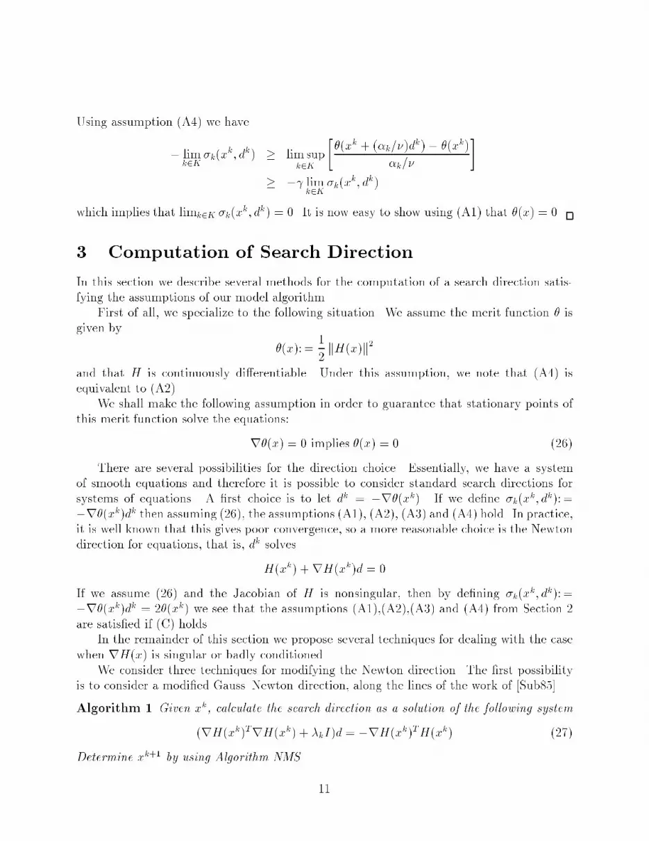
Using assumption (A4) we have� limk2K �k(xk; dk) � lim supk2K "�(xk + (�k=�)dk)� �(xk)�k=� #� � limk2K �k(xk; dk)which implies that limk2K �k(xk; dk) = 0. It is now easy to show using (A1) that �(�x) = 0.3 Computation of Search DirectionIn this section we describe several methods for the computation of a search direction satis-fying the assumptions of our model algorithm.First of all, we specialize to the following situation. We assume the merit function � isgiven by �(x):= 12 kH(x)k2and that H is continuously di�erentiable. Under this assumption, we note that (A4) isequivalent to (A2).We shall make the following assumption in order to guarantee that stationary points ofthis merit function solve the equations:r�(x) = 0 implies �(x) = 0 (26)There are several possibilities for the direction choice. Essentially, we have a systemof smooth equations and therefore it is possible to consider standard search directions forsystems of equations. A �rst choice is to let dk = �r�(xk). If we de�ne �k(xk; dk):=�r�(xk)dk then assuming (26), the assumptions (A1), (A2), (A3) and (A4) hold. In practice,it is well known that this gives poor convergence, so a more reasonable choice is the Newtondirection for equations, that is, dk solvesH(xk) +rH(xk)d = 0If we assume (26) and the Jacobian of H is nonsingular, then by de�ning �k(xk; dk):=�r�(xk)dk = 2�(xk) we see that the assumptions (A1),(A2),(A3) and (A4) from Section 2are satis�ed if (C) holds.In the remainder of this section we propose several techniques for dealing with the casewhen rH(x) is singular or badly conditioned.We consider three techniques for modifying the Newton direction. The �rst possibilityis to consider a modi�ed Gauss{Newton direction, along the lines of the work of [Sub85].Algorithm 1 Given xk, calculate the search direction as a solution of the following system(rH(xk)TrH(xk) + �kI)d = �rH(xk)TH(xk) (27)Determine xk+1 by using Algorithm NMS. 11

In an implementation of this algorithm we need to specify �k. In order that the results fromSection 2 might be applied we propose to de�ne �k: = cmax0�i�M(N+1) H(xk�i) (whereN and M are the constants used in Algorithm NMS). Note that the perturbation to theGauss{Newton direction gets smaller as we approach the solution.Proposition 6 If we set �k(xk; dk):= rH(xk)dk 2+�k dk 2 then assuming (C) and (26),any accumulation point �x of the sequence of points fxkg produced by Algorithm 1 is a solutionof (1).Moreover, if there exists an accumulation point �x of fxkg where the Jacobian matrixrH(�x) is nonsingular then the sequence fxkg converges superlinearly to �x, the stepsize �k = 1is accepted for su�ciently large k and condition kdkk � �o�k holds eventually for any �o > 0and � > 0.Proof We show that assumptions (A1), (A2), (A3) and (A4) are satis�ed. First of all, wenote that �k(xk; dk) = �r�(xk)dk and so assumptions (A2) and (A4) are satis�ed. Further-more, if �k(xk; dk)! 0, then either �k ! 0 or kdk ! 0. In the �rst case, �(xk)! 0 is clear,and in the second, the same conclusion follows from the de�nition of dk and (26). In orderto obtain the �rst part of (A3) we note that, by de�nition of Fq(k), we have:Fq(k) � max0�i�M(N+1) �(xk�i);and then we can take p2 = 2 and p3 = 1=2. For the second part of (A3) we have�k dk 2 � �k(xk; dk) � ���r�(xk)dk���� r�(xk) dk � H(xk) rH(xk) dk and, hence, the boundedness of fdkg follows from (C) and the fact that �k � c H(xk) .As regards the superlinear convergence rate, �rst we observe that the Hessian matrixr2�(�x) = rH(�x)TrH(�x) is positive de�nite. Since �x is an accumulation point of fxkg,there exists an index �k such that the point x�k is su�ciently close to �x so as to have: min �rH(x�k)TrH(x�k) + ��kI� � 12 min �r2�(�x)� > 0; (28)where we have indicated by min(B) the minimum eigenvalue of a matrix B. By (27) and(28) we have kd�kk � 2 min(r2�(�x))kr�(x�k)k;and by repeating, with minor modi�cations, the same reasonings of the proof of Proposition1.12 in [Ber82] and by recalling that Theorem 5 implies that �(xk) ! 0, we have thatlimk!1 xk = �x. Finally we can observe that the matrix rH(xk)TrH(xk) + �kI, with�k = cmax0�i�M(N+1) H(xk�i , satis�es the Dennis{More condition which ensures both thatthe unit stepsize is eventually accepted by the linesearch technique and that the sequencefxkg converges superlinearly (see, for example, [Ber82, Proposition 1.15]). Finally, the laststatement of the proposition follows from the superlinear convergence rate of fxkg.12

In the second case we take as our direction a solution of a modi�ed system of equations,where the Jacobian of H has been modi�ed by a diagonal matrix. Unfortunately, the newdirection might not even be a descent direction for our merit function, so in certain cases werevert to taking the direction of steepest descent for the merit function. A full descriptionof the method is given below.Algorithm 2 Let � > 0, L4 > 0, L5 > 0 and L6 > 0. Given xk, if H(xk) = 0 stop,else compute the smallest nonnegative integer m such that the matrix rH(xk) + m�I hascondition number less than L6=kH(xk)k.Calculate the search direction, dk, as a solution of the following system(rH(xk) +m�I)d = �H(xk)Evaluate �k(xk; dk):= �r�(xk)dk. If �k(xk; dk) < 0 let dk = �dk.If �k(xk; dk) < L4 r�(xk) 3 or �k(xk; dk) < L5 dk 3 then let dk = �r�(xk). Calculatexk+1 by using Algorithm NMS.Proposition 7 Assuming (C) and (26), any accumulation point �x of the sequence of pointsfxkg produced by Algorithm 2 is a solution of (1).Moreover, if there exists a accumulation point �x of fxkg where the Jacobian matrixrH(�x) is nonsingular then the sequence fxkg converges superlinearly to �x, the stepsize �k = 1is accepted for su�ciently large k and condition kdkk � �o�k holds eventually for any �o > 0and � > 0.Proof The global convergence property of the algorithm follows easily by noting that theconditions of the algorithm are determined precisely to ensure the satisfaction of assumptionsA1, A2 and A3'.By using the assumption that the matrix rH(�x) is nonsingular and recalling that the�rst part of the proposition ensures that r�(�x) = 0, we can �nd a neighborhood of �x suchthat for any x 2 and x 6= �x we have:�(rH(x)) � L6kH(x)k; (29) min �(rH(x)TrH(x)� � 12 min �(rH(�x)TrH(�x)� > 0; (30)kr�(x)k � 1 max (rH(x)TrH(x)) min264 1L4 ; min �(rH(x)TrH(x)�3L5 375 ; (31)where we have indicated by �(B), max(B) and min(B) the condition number, the maximumeigenvalue and the minimum eigenvalue of a matrix B.Since �x is an accumulation point of the sequence fxkg there an index �k such that x�k 2 .Therefore by (29) we have that the direction d�k is computed by solving the system:rH(x�k)d�k = �H(x�k);13

or, equivalently, by solving the following system:rH(x�k)TrH(x�k)d�k = �r�(x�k): (32)This direction d�k satis�es all the tests of Algorithm 2. In fact we have:��k(x�k; d�k) � r�(x�k)T �rH(x�k)TrH(x�k)��1r�(x�k)� kr�(x�k)k2 max �rH(x�k)TrH(x�k)� > 0:Then by the preceding relation, (31) and (32) we obtain:��k(x�k; d�k) � L4kr�(x�k)k3;��k(x�k; d�k) � L5kr�(x�k)k3 min �rH(x�k)TrH(x�k)�3 � L5kd�kk3:Now the superlinear convergence property follows by repeating the same steps of the secondpart of the proof of Proposition 6 after having noted that by (32) and (30) we have thatkd�kk � 2 min (rH(�x)TrH(�x))kr�(x�k)k:In practice, the constants in the algorithm have to be chosen appropriately. Further-more, the choice of � can be estimated from a calculation of the condition number of thematrix rH(x) + �I at the previous iteration. Normally this information is available from afactorization routine.In the third case we try to modify the above technique in such a way as to guarantee atleast that for appropriate choice of � we obtain a descent direction for the merit function.Algorithm 3 Let � > 0, L4 2 (0; 1) and L5 2 (0; 1). Given xk, if H(xk) = 0 stop, elsecompute the smallest nonnegative integer m such that the following system�rH(xk) +m�I�d = � �m�rH(xk)T + I�H(xk) (33)admits a solution dk which satis�es the conditions:�k(xk; dk) � L4min hkr�(xk)k3; kr�(xk)k2i (34)�k(xk; dk) � L5min hkdkk3; kdkk2i (35)where �k(xk; dk):= �r�(xk)dk.Evaluate xk+1 by using Algorithm NMS. 14

Proposition 8 Assuming (C) and (26), any accumulation point �x of the sequence of pointsfxkg produced by Algorithm 3 is a solution of (1).Moreover, if there exists a accumulation point �x of fxkg where the Jacobian matrixrH(�x) is nonsingular then the sequence fxkg converges superlinearly to �x, the stepsize �k = 1is accepted for su�ciently large k and condition kdkk � �o�k holds eventually for any �o > 0and � > 0.Proof First we must show that condition (34) and (35) are satis�ed for su�ciently large � toshow the algorithm is well de�ned. Let C1: = maxx20 kH(x)k and C2: = maxx20 kr�(x)k.By (33) we have: 1 � krH(xk)km� ! kdk � kH(xk)k+ kr�(xk)km� :Therefore for m � m1 with m1: = max [2C1; 1] =� we obtain:kdkk � 2C1 + 2C2: = C3: (36)Now, again from (33) we obtain:dk = �r�(xk)� 1m� �rH(xk)dk +H(xk)� (37)If we premultiply (37) by �r�(xk)T and we take into account (36)then we have:�k(xk; dk) � kr�(xk)k2 � 1m�kr�(xk)kC4; (38)where C4: = C3maxx20 krH(xk)k+ C1. By introducing the scalarm2: = max hm1; C4=((1 � L4)�kr�(xk)k)i(condition (26) yields kr�(xk)k 6= 0) we can see that for all m � m2 (38) implies (34).Now, if we premultiply (37) by (dk)T and we use again (36), we have:kdkk2 � �k(xk; dk) + 1m�C4C3 (39)Recalling that conditions (26) and (34) yield that �k(xk; dk) 6= 0 we can de�nem3: = max hm2; C3C4L5=((1� L5)��k(xk; dk))iand we can observe that, for all m � m3, (39) implies (35).Now the global and superlinear convergence properties of Algorithm 3 follow directly byrepeating, with minor modi�cations, the same arguments of proof of Proposition 715

4 Examples of the MethodIn this section we will give examples of the application of the method to several probleminstances. In fact, some well known results from the literature can be cast in our framework.In [HPR89], the following method is described. Let �(x) = 12 kH(x)k2 and choose thesearch direction to satisfy H(xk) +G(xk; dk) = 0at each iteration. Here,G(xk; d) is an appropriate approximation of the directional derivativeof H in the direction d at xk. The assumptions made in [HPR89] are essentially equivalentto the ones we make in Section 2. This can be seen by de�ning �k(xk; dk):= 2�(xk).In the same paper, a Gauss{Newton method is also proposed. The same merit functionis used. In this case, the direction is calculated by solvingmind2IRnH(xk)TG(xk; d) + 12 k(d)The assumptions made to prove convergence are essentially equivalent to (A1), (A2),(A3') and (C). Particular instances of functions k which are considered are� k(d) = dTBkd where Bk is a symmetric positive de�nite n� n matrix� k(d) = G(xk; d) 2 + �k kdk2 where �k is a nonnegative scalar.In [HPR89] the conditions on k require in the �rst case that the sequence fBkg shouldhave eigenvalues which are bounded away from zero and in the second case that f�kg shouldbe bounded away from zero. In the model we propose, we can relax these conditions byessentially using the following forms� k(d) = dTBkd+ c1Fk kdk2 where Bk is a symmetric positive semide�nite n�n matrix� k(d) = G(xk; d) 2 + c1Fk kdk2The motivation for this type of approach comes from the work of [Sub85] and can be thoughtof a a generalization of Algorithm 1 from the previous section.The work of Burdakov [Bur80] can also be seen to be a special case of the method givenin Section 2. In this case, the merit function is given by �(x):= kH(x)kr for some r > 0.An interesting extension to the work of Pshenichny and Danilin [PD78] on minimaxproblems can be seen by using our formulation. In this case the merit function is given by�(x) = max1�i�n jHi(x)jwhere Hi are assumed to be continuously di�erentiable functions whose gradients satisfy aLipschitz condition. By de�ning the setI�: = fi j jHi(x)j � �(x)� �gthe linearization method of Pshenichny and Danilin has been shown to converge under thefollowing assumptions: 16

1. 9� > 0 such that for all x with �(x) > 0, �(x) � �(x0) the linearized systemrHi(xk)d+Hi(xk) = 0; i 2 I� (40)is solvable.2. Let d(x) denote the minimum norm solution of (40). Then, 9c > 0 such that for all xwith �(x) > 0 we have kd(x)k � c�(x)3. fx j �(x) � �(x0)g is bounded.It can be shown that these assumptions imply the assumptions of the previous section. Let�k(xk; dk) = ��(xk), for some � 2 (0; 1). Assumption (A1) is then immediate. Assumption(A2) follows from [PD78, Theorem 6.1] since it is shown that there exists an �� > 0 such thatfor all � 2 (0; ��k) �(xk + �dk)� �(xk) � ����(xk)for any � < 1. Assumption (A3) follows immediately from 2. For assumption (A4), it isproven in [Kiw85] that � is subdi�erentially regular and hence (A4) is equivalent to (A2).5 Application to Nonlinear Complementarity Prob-lemsWe consider applying the algorithms described in Section 3 to solve the nonlinear comple-mentarity problem, NCP(F), namely to �nd x 2 IRn such thatz � 0; F (z) � 0; hz; F (z)i = 0 (41)for a given function F : IRn ! IRn. We will use the following equivalent set of equationsHi(x) = (Fi(x)� xi)2 � Fi(x) jFi(x)j � xi jxij ; i = 1; . . . ; n (42)The solution of these equations was shown to be equivalent to the nonlinear complementarityproblem. In particular, Mangasarian[Man76] proved the following theorem.Theorem 9 x solves NCP(F) if and only if H(x) = 0, where H is de�ned in (42).In particular, note that H is di�erentiable.It can be shown that our regularity condition (26) is equivalent toPni=1 [Fi(x)(Fi(x)� jFi(x)j � xi)2 + xi(xi � jxij � Fi(x))(Fi(x)� jFi(x)j � xi)]rFi(x)+ [Fi(x)(Fi(x)� jFi(x)j � xi)(xi � jxij � Fi(x)) + xi(xi � jxij � Fi(x))2] ei = 0implying that x is a solution of NCP(F).Other algorithmic approaches for solving NCP(F) have been tried. Recently, much em-phasis has been placed on approaches using nonsmooth equations[Rob88, Pan89, HPR89,HX90]. We mention that there are many ways of formulating this problem as a system ofnonsmooth equations. For example, the following ways are well{known.17

1. The min operator technique, whereHi(z):= minfzi; Fi(z)gor equivalently H(z):= z � (z � F (z))+where the \plus" operator signi�es projection onto the positive orthant, that is (x+)i: =maxfxi; 0g. It is easy to see that H(z) = 0 if and only if z solves (41). In the a�necase, the above H has been termed the \natural residual".2. The Minty equations H(x):= F (x+) + x� x+It is easy to show that H(x) = 0 implies that z: = x+ solves (41) and if z solves (41)then x: = z � F (z) satis�es H(x) = 0.We favor using the di�erentiable equations (42) since the direction �nding subproblemconsists of solving a set of linear equations, rather than a mixed linear complementarityproblem. Furthermore, we believe that the trade{o� for this easier subproblem manifestsitself in the form of ill{conditioning for which the nonmonotone line search technique hasproven e�ective[GLL86].The condition (26) appears to be a mild assumption on the problem in this case. Cer-tainly it is not implied by the conditions which are assumed to guarantee convergence forthe nonsmooth algorithms mentioned above. In particular, the following example satis�es(26) but is not regular in the sense of [HPR89].Example 10 Let F (x) = " 1� x2x1 #. The solution set of this linear complementarity prob-lem is f(0; �) j 0 � � � 1g. It can be shown that r�(x) = 0 implies that x solves the linearcomplementarity problem and thus (26) is satis�ed. However, all the solution points are notregular in the sense of [HPR89, page 15].In order to justify performing a standard Newton method, we need the Jacobian of H tobe nonsingular. Mangasarian[Man76] gives the following su�cient conditions to guaranteethis nonsingularity.Proposition 11 Let x solve NCP(F) and satisfy x + F (x) > 0. If rF (x) has nonsingularprincipal minors, then rH(x) is nonsingular.We present some results on standard nonlinear complementarity problems found in theliterature. A fuller description of the problems can be found in [HX90]. Note that an entryof F in the table signi�es that the algorithm failed to converge.In all the above examples we used the starting points suggested in [HX90]. In somecases, we added extra starting points when the points chosen in the aforementioned paper18

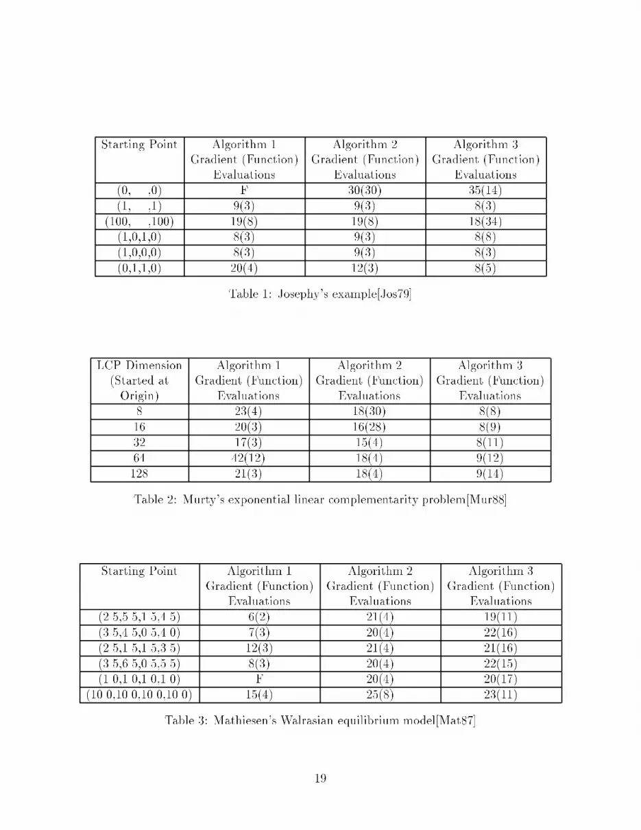
Starting Point Algorithm 1 Algorithm 2 Algorithm 3Gradient (Function) Gradient (Function) Gradient (Function)Evaluations Evaluations Evaluations(0,. . . ,0) F 30(30) 35(14)(1,. . . ,1) 9(3) 9(3) 8(3)(100,. . . ,100) 19(8) 19(8) 18(34)(1,0,1,0) 8(3) 9(3) 8(8)(1,0,0,0) 8(3) 9(3) 8(3)(0,1,1,0) 20(4) 12(3) 8(5)Table 1: Josephy's example[Jos79]LCP Dimension Algorithm 1 Algorithm 2 Algorithm 3(Started at Gradient (Function) Gradient (Function) Gradient (Function)Origin) Evaluations Evaluations Evaluations8 23(4) 18(30) 8(8)16 20(3) 16(28) 8(9)32 17(3) 15(4) 8(11)64 42(12) 18(4) 9(12)128 21(3) 18(4) 9(14)Table 2: Murty's exponential linear complementarity problem[Mur88]Starting Point Algorithm 1 Algorithm 2 Algorithm 3Gradient (Function) Gradient (Function) Gradient (Function)Evaluations Evaluations Evaluations(2.5,5.5,1.5,4.5) 6(2) 21(4) 19(11)(3.5,4.5,0.5,4.0) 7(3) 20(4) 22(16)(2.5,1.5,1.5,3.5) 12(3) 21(4) 21(16)(3.5,6.5,0.5,5.5) 8(3) 20(4) 22(15)(1.0,1.0,1.0,1.0) F 20(4) 20(17)(10.0,10.0,10.0,10.0) 15(4) 25(8) 23(11)Table 3: Mathiesen's Walrasian equilibrium model[Mat87]19

Starting Point Algorithm 1 Algorithm 2 Algorithm 3Gradient (Function) Gradient (Function) Gradient (Function)Evaluations Evaluations Evaluationsx1 19(3) 15(3) 18(22)x2 23(4) 28(4) Fx1 = (0:2; 0:2; 0:2; 0:1; 0:1; 0:2; 0:5; 0:0; 4:0; 0:0; 0:0; 0:0; 0:4; 0:0)x2 = (0:1; 0:1; 0:1; 0:1; 0:1; 0:2; 0:5; 0:0; 4:0; 0:0; 0:0; 0:0; 0:4; 0:0)Table 4: Scarf's economic equilibrium model[Sca73]Starting Point Algorithm 1 Algorithm 2 Algorithm 3Gradient (Function) Gradient (Function) Gradient (Function)Evaluations Evaluations Evaluations(1,. . . ,1) 15(3) 15(3) 13(18)(10,. . . ,10) 11(2) 11(2) 9(15)Table 5: Nash noncooperative game example[Har88]Starting Point Algorithm 1 Algorithm 2 Algorithm 3Gradient (Function) Gradient (Function) Gradient (Function)Evaluations Evaluations Evaluations(0,. . . ,0) 28(23) 28(40) 42(101)(1,. . . ,1) 33(18) 29(32) 27(72)x1 34(20) 25(40) 24(62)x1 = (1:0; 1:1; . . . ; 1:9; 1:0; 1:1; . . . ; 1:9; 1:0; 1:1; . . . ; 1:9; 1:0:1:1; . . . ; 1:9; 1:0; 1:1)Table 6: Tobin's spatial price equilibrium model[Tob88]20

Starting Point Algorithm 1 Algorithm 2 Algorithm 3Gradient (Function) Gradient (Function) Gradient (Function)Evaluations Evaluations Evaluationsx1 53(7) 28(40) Fx2 17(3) 29(32) 30(52)x3 24(4) 28(40) 54(79)x4 19(3) 29(32) 39(31)x1 = (0; 2; 2; 0; 0; 2; 0; 0; 1; 1; 0; 0; 0; 0; 0)x2 = (0; 3; 3; 0; 0; 3; 0; 0; 1; 1; 0; 0; 0; 0; 0)x3 = (0; 10; 10; 0; 0; 10; 0; 0; 1; 1; 0; 0; 0; 0; 0)x4 = (0; 5; 5; 0; 0; 5; 0; 0; 1; 1; 0; 0; 0; 0; 0)Table 7: Powell's nonlinear programming problem[Pow69]Starting Point Algorithm 1 Algorithm 2 Algorithm 3Gradient (Function) Gradient (Function) Gradient (Function)Evaluations Evaluations Evaluations(0,. . . ,0) F 33(24) 35(34)(10,. . . ,10) 22(5) 18(5) 17(4)Table 8: Spatial competition example[Har86]21

were considered too close to an optimal point. Furthermore, the functions and gradients werecoded without any problem speci�c knowledge. In particular, the use of �xing a numeraire inthe economic equilibrium problems was not used to force the Jacobian to be nonsingular atthe solution. Needless to say, this would improve our results, but this removes the essentialdi�culty of the problems. While it is true that some of the iteration counts given above arerelatively large, we wish to emphasize that all these results were obtained with one settingof the algorithm parameters and without particular �xes for speci�c problems.References[Ber82] D.P. Bertsekas. Constrained Optimization and Lagrange Multiplier Methods. Aca-demic Press, New York, 1982.[BS91] R.S. Bain and W.E. Stewart. Application of robust nonmonotonic descent criteriato the solution of nonlinear algebraic equation systems. Computers in ChemicalEngineering, 15:203{208, 1991.[Bur80] O.P. Burdakov. Some globally convergent modi�cations of Newtons's method forsolving systems of nonlinear equations. Soviet Math Doklady, 22(2):376{379, 1980.[Cla83] F.H. Clarke. Optimization and Nonsmooth Analysis. John Wiley & Sons, NewYork, 1983.[DS83] J.E. Dennis and R.B. Schnabel. Numerical Methods for Unconstrained Optimiza-tion and Nonlinear Equations. Prentice-Hall, New Jersey, 1983.[Fra88] C. Fraley. Algorithms for nonlinear least squares. Technical Report SOL 88.16,Stanford University, July 1988.[GLL86] L. Grippo, F. Lampariello, and S. Lucidi. A nonmonotone line search techniquefor Newton's method. SIAM Journal of Numerical Analysis, 23:707{716, 1986.[GLL90] L. Grippo, F. Lampariello, and S. Lucidi. A class of nonmonotone stabilizationmethods in unconstrained optimization. Technical Report IASI-CNR R.290, 1990(to appear in Numerische Mathematik).[Har86] P.T. Harker. Alternative models of spatial competition. Operations Research,34:410{425, 1986.[Har88] P.T. Harker. Accelerating the convergence of the diagonalization and projectionalgorithms for �nite{dimensional variational inequalities. Mathematical Program-ming, 41:29{50, 1988. 22

[HPR89] S.-P. Han, J.-S. Pang, and N. Rangaraj. Globally convergent Newton methods fornonsmooth equations. Department of Mathematical Sciences, The Johns HopkinsUniversity, Baltimore, MD 21218, 1989.[HX90] P.T. Harker and B. Xiao. Newton's method for the nonlinear complementar-ity problem: A B{di�erentiable equation approach. Mathematical Programming,48:339{358, 1990.[Jos79] N.H. Josephy. Newton's method for generalized equations. Technical SummaryReport 1965, Mathematics Research Center, University of Wisconsin, Madison,Wisconsin, 1979.[Kiw85] K.C. Kiwiel. Methods of Descent for Nondi�erentiable Optimization. Springer{Verlag, 1985.[Man76] O.L. Mangasarian. Equivalence of the complementarity problem to a system ofnonlinear equations. SIAM Journal of Applied Mathematics, 31:89{92, 1976.[Mat87] L. Mathiesen. An algorithm based on a sequence of linear complementarity prob-lems applied to a Walrasian equilibrium model: An example. Mathematical Pro-gramming, 37:1{18, 1987.[Mur88] K.G. Murty. Linear Complementarity, Linear and Nonlinear Programming.Helderman{Verlag, Berlin, 1988.[OR70] J.M. Ortega and W.C. Rheinboldt. Iterative Solution of Nonlinear Equations inSeveral Variables. Academic Press, 1970.[Pan89] J.-S. Pang. A B{di�erentiable equation based, globally and locally quadraticallyconvergent algorithm for nonlinear programs, complementarity and variational in-equality problems. Department of Mathematical Sciences, The Johns HopkinsUniversity, Baltimore, MD 21218, 1989.[PD78] B.N. Pshenichny and Yu. M. Danilin. Numerical Methods in Extremal Problems.MIR Publishers, Moscow, 1978.[Pol76] E. Polak. On the global stabilization of locally convergent algorithms. Automatica,12:337{349, 1976.[Pow69] M.J.D. Powell. A method for nonlinear constraints in minimization problems. InR. Fletcher, editor, Optimization, pages 283{298. Academic Press, London, 1969.[Ral91] D. Ralph. Global convergence of damped Newton's method for nonsmooth equa-tions, via the path search. Technical Report 90{1181, Computer Science Depart-ment, Cornell University, Ithaca, NY 14853, 1991.23

[Rob88] S.M. Robinson. Newton's method for a class of nonsmooth functions. Workingpaper, Department of Industrial Engineering, University of Wisconsin, Madison,Wisconsin, 1988.[SB80] J. Stoer and R. Bulirsch. Introduction to Numerical Analysis. Springer{Verlag,New York, 1980.[Sca73] H.E. Scarf. The Computation of Economic Equilibria. Yale University Press, NewHaven, Conneticut, 1973.[Sub85] P.K. Subramanian. Iterative Methods of Solution for Complementarity Problems.PhD thesis, University of Wisconsin, Madison, Wisconsin, 1985.[Tob88] R.L. Tobin. A variable dimension solution approach for the general spatial equi-librium problem. Mathematical Programming, 40:33{51, 1988.

24