globalization, creative destruction, and labor share change: evidence on the determinants and...

1

Globalization, creative destruction, and labor share change: Evidence on the

determinants and mechanisms from longitudinal plant-level data* / Petri Böckerman**

& Mika Maliranta***

Abstract

We examine the sources and micro-level mechanisms of the changes in the labor share of

value added. We link the micro-level dynamics of the labor share change with that of

productivity and wage growth. Using a useful variant of the decomposition method we

make a distinction between the change in the average plant and the micro-level

restructuring. With Finnish plant-level data covering three decades we show that micro-

level restructuring is the link between the declining labor share and increasing productivity

in 12 manufacturing industries of four regions, and that increased international trade is a

factor underlying those shifts.

JEL Classification: F16; J31

Key words: Globalization; International trade; Foreign ownership; Micro-level

restructuring; Labor share

* This study is funded by the Finnish Work Environment Fund (Työsuojelurahasto).

Financial support from the Yrjö Jahnsson Foundation is gratefully acknowledged (Grant

No. 5745 and 5765). Data construction and decomposition computations have been carried

out at Statistics Finland following the terms and conditions of confidentiality. This part of

the work has been done in the context of a joint project by the Helsinki School of

Economics (HSE), Statistics Finland and the Research Institute of the Finnish Economy

(ETLA) funded by the Academy of Finland (Project No. 114827). To obtain access to the

longitudinal plant-level data, please contact the Research Laboratory of the Business

2

Structures Unit, Statistics Finland, FI-00022, Finland. The industry-region panel and

programs that are used to produce the estimates of the paper are available for replication

purposes. We are grateful to Kristiina Huttunen and Pekka Sauramo for useful comments.

Paul A. Dillingham has kindly checked the English language. The usual disclaimer applies.

** Labour Institute for Economic Research, Pitkänsillanranta 3A, FI-00530 Helsinki,

Finland. Fax: +358-9-25357332. Tel.: +358-9-25357330. E-mail:

[email protected]

*** Corresponding author. The Research Institute of the Finnish Economy, Lönnrotinkatu

4B, FI-00120 Helsinki, Finland. Fax: +358-9-601753. Tel.: +358-9-60990219. E-mail:

[email protected]

3

1. Introduction

The labor share of value added was regarded as “a magic constant” for decades (Solow

1958). The constancy of the labor share was also treated as one of the stylized facts of

economic growth (e.g. Gollin 2002). In contrast to this, there are several industrialized

countries in which the labor share has declined substantially over the past few decades (e.g.

Blanchard 1997, 2006). Secular decline in the labor share since the early 1980s has been

much more pronounced in Europe and Japan (roughly 10 percentage points) than in Anglo-

Saxon countries, including the United States (about 3-4 percentage points) (see, for

example, IMF 2007). Within Europe, the strongest decline in the labor share has been

experienced in Austria, Finland, Ireland, and the Netherlands.

Globalization has potential effects on the labor share through several different channels

(e.g. Guscina 2006). Falling trade costs increase competition in product markets, which

according to some models leads to a higher, not lower labor share. However, globalization

may increase investors’ required returns to capital and erode employees’ bargaining power

(e.g. Rodrik 1997; Slaughter 2007), both of which squeeze the labor share. Globalization

also leads to increased specialization between countries. The Heckscher-Ohlin theorem

predicts that capital-rich countries will specialize in the production of capital-intensive

goods (e.g. Takayama 1972), which contributes to a decline in the return to labor in the

industrialized countries. Therefore, the labor share may fall as the process of globalization

continues.1 Furthermore, both international trade and foreign direct investments (FDIs)

could function as the channels of technological diffusion and encourage firms to adopt a

variety of labor-saving technologies (e.g. Grossman and Helpman 1991), which boost

firms’ productivity and squeeze the labor share. It is important to know how the effects

4

emerge: Are the labor shares declining because of increasing productivity or falling wages?

When it comes to evidence-based policy recommendations, what is most badly needed is

knowledge about the micro-level mechanisms behind increasing productivity or falling

wages.

Modern growth theories emphasize the role of intra-industry micro-level restructuring as

one of the key mechanisms for explaining industry productivity growth (e.g. Aghion and

Howitt 2006). In the economic geography literature the role of micro-level restructuring

among heterogeneous firms has also gained attention in recent years (see Audretsch et al.

2008; Baldwin and Okubo 2006; Okubo et al. 2008). Furthermore, research in the field of

international trade has indicated that globalization is an important stimulant of productivity-

enhancing micro-restructuring (“creative destruction”) within industries (e.g. Bernard et al.

2007; Lileeva 2008). In particular, Bernard and Jensen (2004) show that exporting does not

increase plant productivity growth but has positive aggregate productivity effects because it

is associated with the reallocation of resources from less efficient to more efficient plants.2

We contribute to the literature by distinguishing between two intrinsically different micro-

level mechanisms underlying the industry labor share changes: 1) the labor share change of

the average plant and 2) the micro-structural change. Furthermore, we both formally and

empirically link the micro-level dynamics of the labor share change, productivity growth

and wage growth. These links emerge due to the fact that industry productivity and wage

growth together determine the change in the labor share. Both industry productivity and

wage growth have their micro-level mechanisms analogous to that of the labor share

change. This paper examines whether increased competition owing to the exposure to

international trade and foreign ownership forces the plants with the highest share of labor

5

income to decrease their market shares and eventually forces them out of business. This

hypothesis is closely related to the modern theoretical insights. Specifically, Melitz (2003)

argues that an increase in an industry’s exposure to international trade will lead to inter-

firm reallocations towards more productive firms by increasing competitive pressures.

Our approach allows a coherent tracking of the roles of the micro-level dynamics of

productivity and wage growth that together determine the micro-level dynamics of the labor

share change. We take advantage of longitudinal plant-level data from the Finnish

manufacturing sector over a period of 30 years. To preview, the results show that

globalization stimulates productivity-enhancing and the labor share curbing micro-level

restructuring within industries. Wage increases in the industries correspond reasonably

closely to those of the plants, which implies that micro-level restructuring does not

contribute much to the industries’ wage increases.

The link between the labor share and globalization is not well understood. Existing

evidence about the effects of globalization on the labor share is based on cross-country

studies (e.g. European Commission 2007, 2008; Guscina 2006; Harrison 2002; Jaumotte

and Tytell 2007; Jayadev 2007). The main problem with the cross-country studies is that

there are a large number of contributing factors across countries that are identified with a

relatively small number of observations, i.e. the curse of dimensionality plagues the cross-

country approach. Cross-country regressions are therefore likely to suffer from omitted

variable and parameter heterogeneity biases. The differences in the data characteristics

make it hard to conduct a reliable comparison of the plant-level dynamics of the labor share

across countries.3 This makes it particularly useful to provide a detailed analysis of one

country. To study the effects of globalization, we construct a panel of industries and regions

6

from the micro-level components of the labor share. While using the same plant-level data

in the analysis of industries and regions within the same country, data comparability

problems can be largely bypassed.

The role of labor market regulations and other institutional aspects has gained considerable

attention in the cross-country comparisons of the labor share dynamics (e.g. Azmat et al.

2007; Bentolila and Saint-Paul 2003; IMF 2007). In contrast to this research, we show that

there are large differences in the micro-level dynamics of the labor share across regions

within the same country that share exactly the same institutions and regulations. Hence, the

focus on one country allows us to isolate the effects of globalization on the labor share

more clearly, because we are able to avoid, by construction, the problems that emerge from

the complex interactions between a variety of labor market institutions and openness that

Agell (1999) and Rodrik (2008) have pointed out.

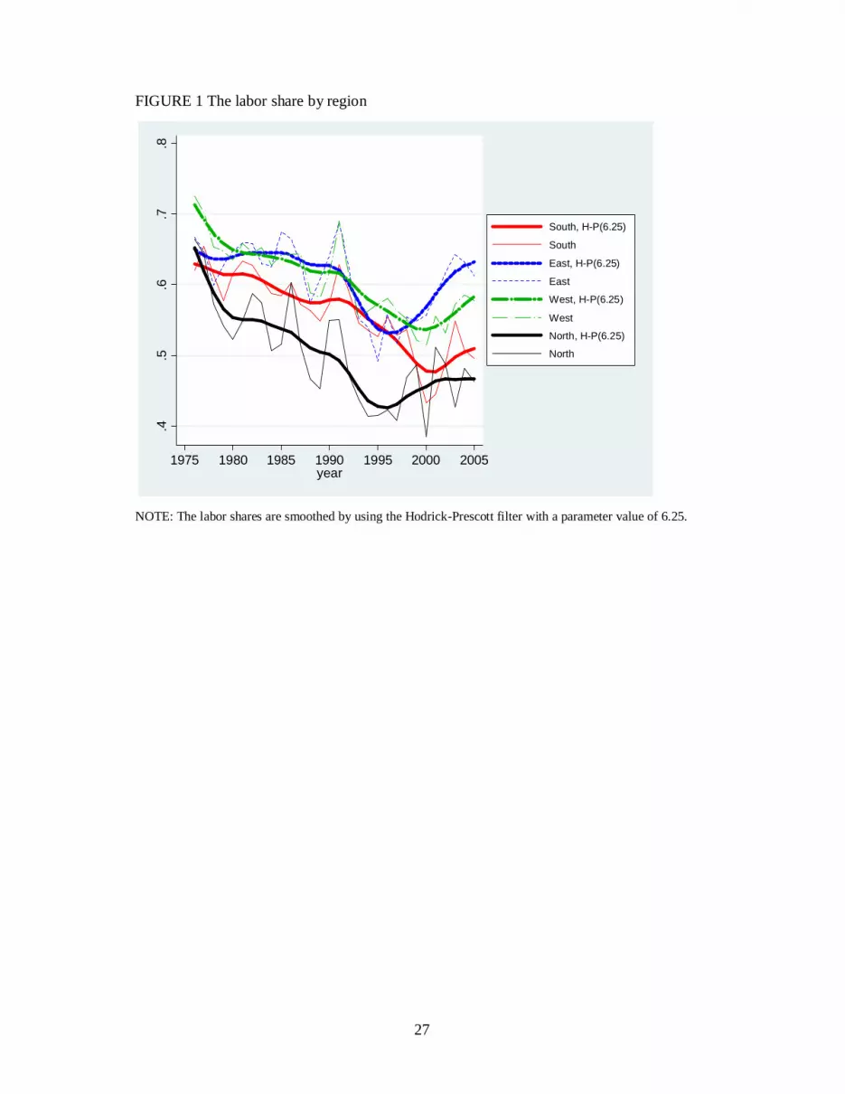
The Finnish case provides an excellent opportunity to analyze the effects of globalization,

because the openness of the economy has greatly increased during the past few decades. At

the same time, there has been a considerable decline in the labor share. Figure 1 exhibits the

trends in the manufacturing sector in four Finnish regions. Plenty of variation in the trends

provides us with an interesting opportunity to identify the mechanisms underlying these

changes.

=== FIGURE 1 HERE ===

The structure of the paper is as follows. Section 2 introduces the decomposition method.

Section 3 describes the longitudinal plant-level data. Section 4 reports the results from the

7

decomposition of the labor share and relates the micro-level components to the changes in

international trade and foreign ownership. The last section concludes.

2. Decomposition of the labor share into its micro-level components

The starting point of our analysis is the fact that the industry (or aggregate) labor share

declines when industry labor productivity growth exceeds industry wage growth (measured

in nominal terms). The existing studies in the literature assume that these industry or more

aggregate level changes represent changes in a representative firm, and, as a consequence,

the role of the micro-level restructuring is ignored. The novelty of this paper is that we

formally and empirically distinguish between the two intrinsically different mechanisms of

the industry change in the labor share: 1) the change in the average plant and 2) the change

due to plant-level restructuring.

The literature provides several different methods to decompose aggregate productivity

growth (e.g. Bartelsmans and Doms 2000; Foster et al. 2001; Kruger 2008). In this paper

we adopt a formula that has several useful properties that make the interpretation of the

components easy in this context. Our method has some important resemblances to those

proposed by Maliranta (1997), Vainiomäki (1999) and, more recently, by Diewert and Fox

(2009).4 The within component is defined as the weighted average of the changes in the

labor shares of the continuing plants. The between component is negative when there is a

systematic structural change among continuing plants in terms of value added towards

those plants that have a lower labor share. In addition, it is possible to separate the entry

and exit components. The total effect of entries and exits is the difference between the total

8

aggregate change in the labor share and the aggregate change in the labor share among the

continuing units.

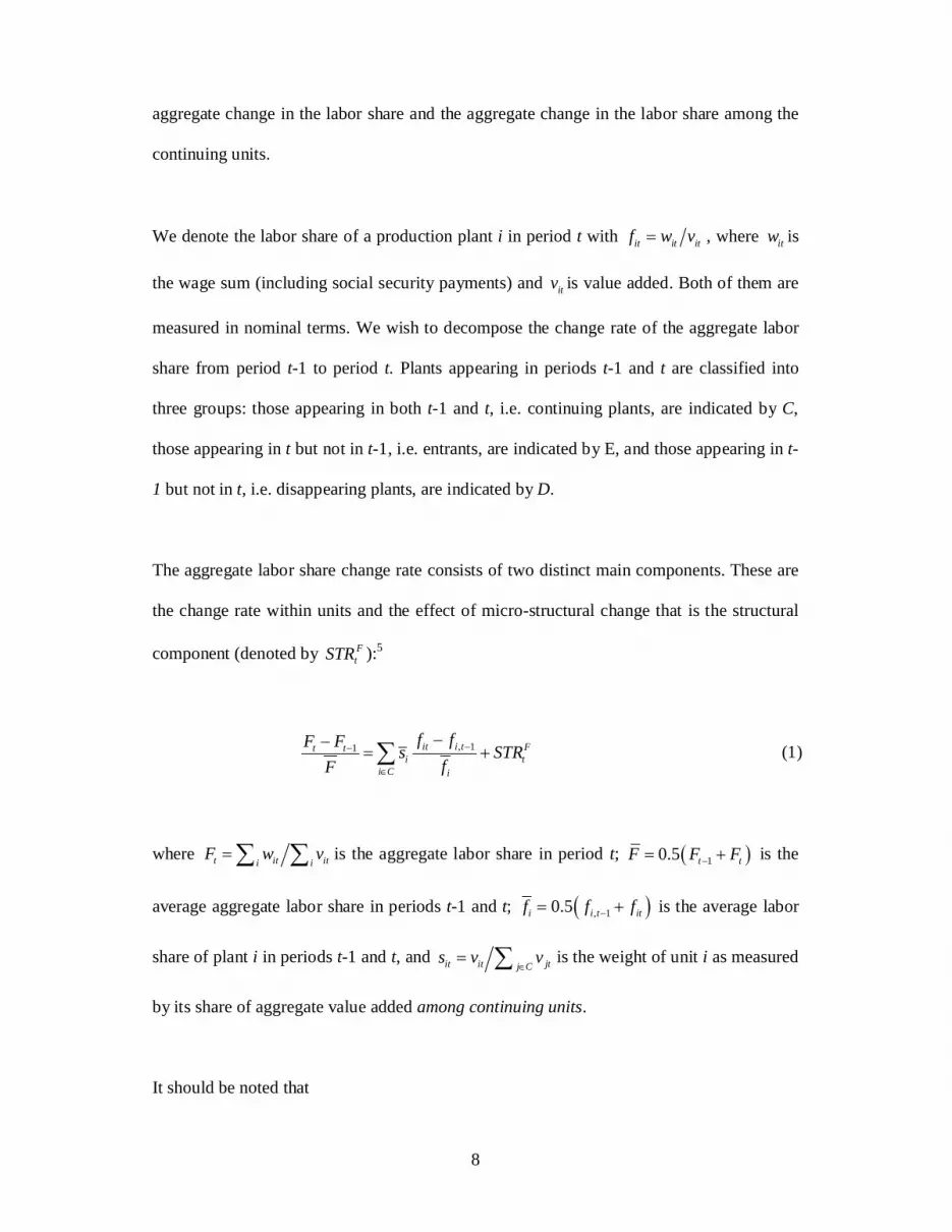
We denote the labor share of a production plant i in period t with it it itf w v= , where itw is

the wage sum (including social security payments) and itv is value added. Both of them are

measured in nominal terms. We wish to decompose the change rate of the aggregate labor

share from period t-1 to period t. Plants appearing in periods t-1 and t are classified into

three groups: those appearing in both t-1 and t, i.e. continuing plants, are indicated by C,

those appearing in t but not in t-1, i.e. entrants, are indicated by E, and those appearing in t-

1 but not in t, i.e. disappearing plants, are indicated by D.

The aggregate labor share change rate consists of two distinct main components. These are

the change rate within units and the effect of micro-structural change that is the structural

component (denoted by FtSTR ):5

, 11 it i t Ft ti t

i C i

f fF F s STRfF

−−

∈

−−= +∑ (1)

where t it iti iF w v= ∑ ∑ is the aggregate labor share in period t; ( )10.5 t tF F F−= + is the

average aggregate labor share in periods t-1 and t; ( ), 10.5i i t itf f f−= + is the average labor

share of plant i in periods t-1 and t, and it it jtj Cs v v

∈= ∑ is the weight of unit i as measured

by its share of aggregate value added among continuing units.

It should be noted that

9

1

1

logt t t

t

F F FFF

−

−

−≅ and

, 1

, 1

logit i t it

i i t

f f ff f

−

−

−≅ .

Consequently, here the within component is similar to a Divisia index of the growth rate of

the total factor productivity but now applied to the continuing plants (where the change rate

is relevant) and used for the estimation of the growth rate of the labor share. It describes the

change rate of the labor share in a “representative” plant.

The structural component consists of four sub-components

( ) ( ) ( )1 1 , 11 , 1

E C D Ct t t t it i tF E D i i

t t t it i t ii C i C i

F F F F f ff f FSTR S S s s sF F F f F

− − −− −

∈ ∈

− − − −= − + − +

∑ ∑ (2)

where Xi ii X i X

F w v∈ ∈

= ∑ ∑ is the aggregate labor share among the group { }, ,X E C D∈ ,

and Xi ii X i

S v v∈

= ∑ ∑ is the value added share of the group { }, ,X E C D∈ .

The direct contribution of the entering plants to the aggregate growth rate of the labor share

is gauged by the first component of the Equation (2). It is positive when the average labor

share of the new plants (weighted by the value added share) in the period t is higher than

that of those who appeared also in the period t-1. The magnitude of the contribution is

dependent on the value added share of the new plants in the period t.

10

The second component, the exit component, is analogous to the entry component.

Therefore, one of the great advantages of this decomposition method is that entries and

exits are treated symmetrically. The exit component is negative when the average labor

share of the disappearing plants (weighted by the value added share) is higher than that of

those plants that appear also in the next period t. The magnitude of the contribution is

dependent on the value added share of the disappearing plants before they leave, i.e. in the

period t-1 (see also Maliranta 1997, 2003; Diewert and Fox 2009).

The third component is the between component, which captures the effect of the value

added share changes among the continuing plants on the aggregate labor share change rate.

This component is negative when the low labor share plants (i.e. high profitability plants)

increase their market shares at the cost of the high labor share plants (i.e. low profitability

plants). The between component, like the within component, is defined among the

continuing plants only. As a result, entering or disappearing plants do not have any direct

effect on those components. So, in principle it is possible that the between component is

negative even when all continuing plants increase their value added shares. This is the case

when there are exits from the markets.

The fourth component on the right-hand side of the Equation (2) can be called the

convergence component. It is a kind of the within component, which is negative when those

plants that have a low labor share level tend to have a high growth rate of the labor share.

Because the plants’ levels of the labor share are calculated as the average level in period t-1

and t this gauge should not be plagued by the so-called regression towards the mean

phenomenon (see, for example, Friedman 1992).

11

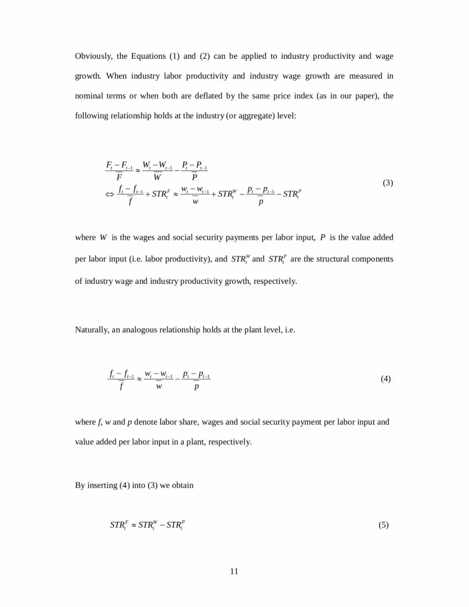
Obviously, the Equations (1) and (2) can be applied to industry productivity and wage

growth. When industry labor productivity and industry wage growth are measured in

nominal terms or when both are deflated by the same price index (as in our paper), the

following relationship holds at the industry (or aggregate) level:

1 1 1

1 1 1

t t t t t t

F W Pt t t t t tt t t

F F W W P PF W Pf f w w p pSTR STR STR

f w p

− − −

− − −

− − −≈ −

− − −⇔ + ≈ + − −

(3)

where W is the wages and social security payments per labor input, P is the value added

per labor input (i.e. labor productivity), and WtSTR and P

tSTR are the structural components

of industry wage and industry productivity growth, respectively.

Naturally, an analogous relationship holds at the plant level, i.e.

1 1 1t t t t t tf f w w p pf w p

− − −− − −≈ − (4)

where f, w and p denote labor share, wages and social security payment per labor input and

value added per labor input in a plant, respectively.

By inserting (4) into (3) we obtain

F W Pt t tSTR STR STR≈ − (5)

12

which shows how the structural components of the labor share change, wage growth and

productivity growth are related to each other.

Analysis of the micro-level components of the labor share is particularly useful in the

Finnish context, because the wage bargaining system adopted in Finland has distinct

implications on the evolution of the micro-level components. The coverage of collective

agreements is roughly 95% of all employees in Finland, one of the highest rates among the

OECD countries (Layard and Nickell 1999). Minimum increases in nominal wages are

determined by collective bargaining. The Finnish ‘wage increase formula’ defines the scope

for nominal wage cost increases as the sum of the core inflation target (e.g. 2% per annum)

and the average increase in productivity across the whole economy. Nominal wages are

therefore not encouraged to adjust to the changes in labor productivity that are considered

to be isolated to certain sectors or regions. Specifically, wage increases have not been tied

to plant-level (real or nominal) productivity advances.

Because of the attributes of the Finnish wage bargaining system, our expectation is that

wage growth takes place mainly through the within plant component and therefore intra-

industry restructuring is not a significant source of industry wage growth. If industry

productivity growth equals industry wage growth (i.e. the aggregate labor share is stable)

and industry productivity growth exceeds plant productivity growth, the within component

of the labor share change has a positive contribution and the restructuring component has

the opposite (negative) contribution. This paper looks at how globalization drives wedges

between these balances.

13

3. Data

The micro-structural components of the labor share are calculated by the use of

longitudinal plant-level panel data that has been constructed especially for economic

research purposes by the Research Laboratory of Statistics Finland. Our data are based

on the Annual Industrial Statistics Surveys that basically cover all manufacturing plants

employing at least five persons up to 1994. Since 1995 it has included all the plants

owned by firms that have no fewer than 20 persons. Maliranta (2003) has examined in

detail how sensitive the patterns of productivity components are to the change in the

cut-off limit from 5 to 20 in the period 1975-1994. The result was that the cut-off limit

made little difference. This is because larger plants account for a substantial share of the

total input usage. Still, to make our decompositions as comparable as possible over all

the years we have harmonized the coverage of our data. We have included all the plants

that have at least 5 persons and are owned by a firm that has no fewer than 20 persons.

Our data are exceptionally good when it comes to the coverage, the content and the

length of time series. However, as always with these kinds of data, our data are not

perfect, either. Data include outliers that might be influential in an economic analysis. A

transparent procedure is therefore needed to clean the data. We have adopted an

approach similar to that of Mairesse and Kremp (1993). Those observations are deemed

as outliers whose log of the labor share differs by more than 4.4 standard deviations

from the input-weighted industry average in that year. We have performed the

decomposition computations for each pair of the consecutive years. If a plant is

classified as an outlier in either an initial (i.e. in year t-1) or an end year (i.e. in year t) it

is not included in this computation (but is possibly included in earlier and later periods).

14

This way we have avoided causing artificial entries or exits by removing outliers. In the

course of our analysis we noted that a single plant might sometimes have an impact on

one of the components of our interest that is simply unbelievable. A more detailed

inspection of these cases revealed that the changes in value added or labor input are

sometimes erroneous beyond reasonable doubt. Since, on certain occasions, these errors

are very influential in our decomposition calculations, further cleaning is needed to

obtain reliable results. For this reason, the decompositions are made in two rounds. If

the absolute value of the contribution of a single plant to one of the components is

greater than four percentage points, the plant is classified as an outlier in the first round.

This is quite a conservative criterion since, as we will see below, usually the size of

these components is less than four percentage points at the level of industry and region.

These outliers, accounting for 11.4 percent of the total hours in the whole period, are

removed in the second round, which generates our final decomposition results.

To examine the effects of globalization, we have computed the micro-level components

of the labor share change rate, productivity growth rate and wage growth rate for 12

industries and four regions over the period 1976-2005. Our industry classification is

close to the two-digit standard industry classification, but we have combined some

industries. Our industries are the following: “Food” (NACE 15-16), “Textile” (17-19),

“Wood” (20), “Paper” (21), “Printing” (22), “Chemicals” (23-25), “Minerals” (26),

“Metal products” (27-28), “Machinery” (29 and 34-35), “Electrical equipment” (30-31),

“Communications equipment” (32-33), and “Other” (36-37). This classification is

dictated by our need for a reliable measurement of the decompositions of the labor

shares by industries and regions.6

15

Finland is divided into five provinces (the so-called NUTS2 level in the European

Union). However, we exclude the province of Åland, because the small number of

plants in this island community means that the measures of the micro-level components

of the labor shares would not be reliable. The use of these classifications gives us a

panel data that has 4×12=48 observations per year. Since the components can be

calculated for 29 pairs of years (1975-1976, 1976-1977,… , 2004-2005), in principal we

have 1392 observations. Since we use lagged explanatory variables, the number of

observations is slightly smaller in our econometric analysis, however.

Productivity and wage growth rates are computed by using the industry-specific

deflators that are implicit price indexes of output obtained from the Finnish National

Accounts. We have used a “chain-index” procedure. For each pair of the consecutive

years, value added (and wages plus social security payments) of the end year (i.e. t) is

converted into the price level of the initial year (i.e. t-1). The use of price indexes is not

necessary in our analysis. (We obtained similar results with nominal measures.) The

main point here is that we use the same deflators for both productivity and wage growth

(or no deflators at all) to obtain consistent results for productivity, wage and labor share

change (see, for example, Feldstein 2008).

Globalization is measured by two variables, which capture the exposure to international

trade and foreign ownership.7 The exposure to international trade is measured by dividing

exports by the gross output. This is the measure that has been most frequently used in the

literature to describe the effects of globalization on the labor share. For example, it has been

used by Harrison (2002) and Guscina (2006), among others. The share of foreign-owned

16

plants in an industry and a region is defined on the basis of output share. A 20% threshold

is used in classifying a particular plant as foreign owned.

4. Results

4.1. Descriptive evidence

To remove the temporary fluctuations, we have taken advantage of the Hodrick-Prescott

filter with the parameter value of 6.25 for the descriptive part of the analysis, as proposed

by Ravn and Uhlig (2002). We have standardized the differences in industry structures

between regions. Industries are weighted by the average value-added share in Finland in the

years t and t-1.

The changes in the labor share of the “representative” plant in industries and in regions are

shown in Figure 2.8 Contrary to the picture of strong decline in the labor shares at the

manufacturing level (Figure 1), Figure 2 reveals that at the plant level the tendency has

been increasing, not decreasing, labor shares. The main exception is the period of strong

economic growth around the mid-’90s when the labor shares declined in all four regions.


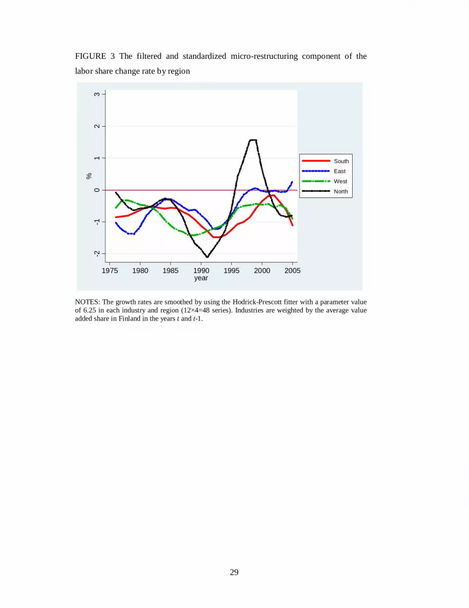
Continuous micro-level restructuring, involving the entries of new profitable plants, their

subsequent expansion as well as the contraction or disappearance of low profitability

plants, has been an essential part of the development in the labor share. Figure 3 shows that

intra-industry restructuring has curbed the labor share in all four regions. The effect started

17

to get stronger in the mid-’80s and was strongest just before and during the depression of

the early 1990s.9


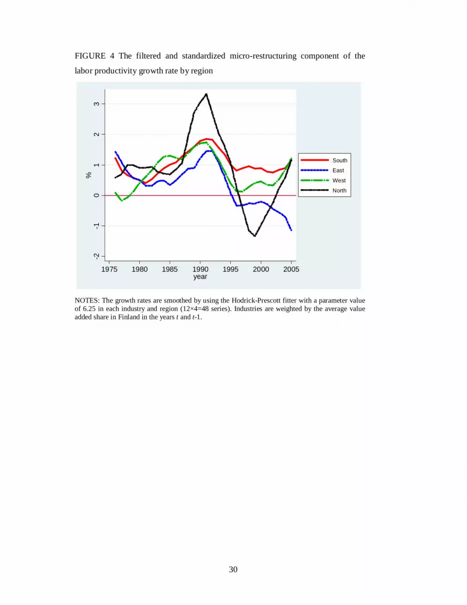
Figure 4 documents the contribution of intra-industry restructuring to labor productivity

growth in the regions. Essentially it is a mirror image of that found for the labor share

changes. Productivity-enhancing restructuring intensified during the 1980s and peaked on

the eve of the depression. Despite some decline after the early 1990s productivity-

enhancing restructuring has remained an important source of productivity growth of the

industries in Southern Finland until recent years.


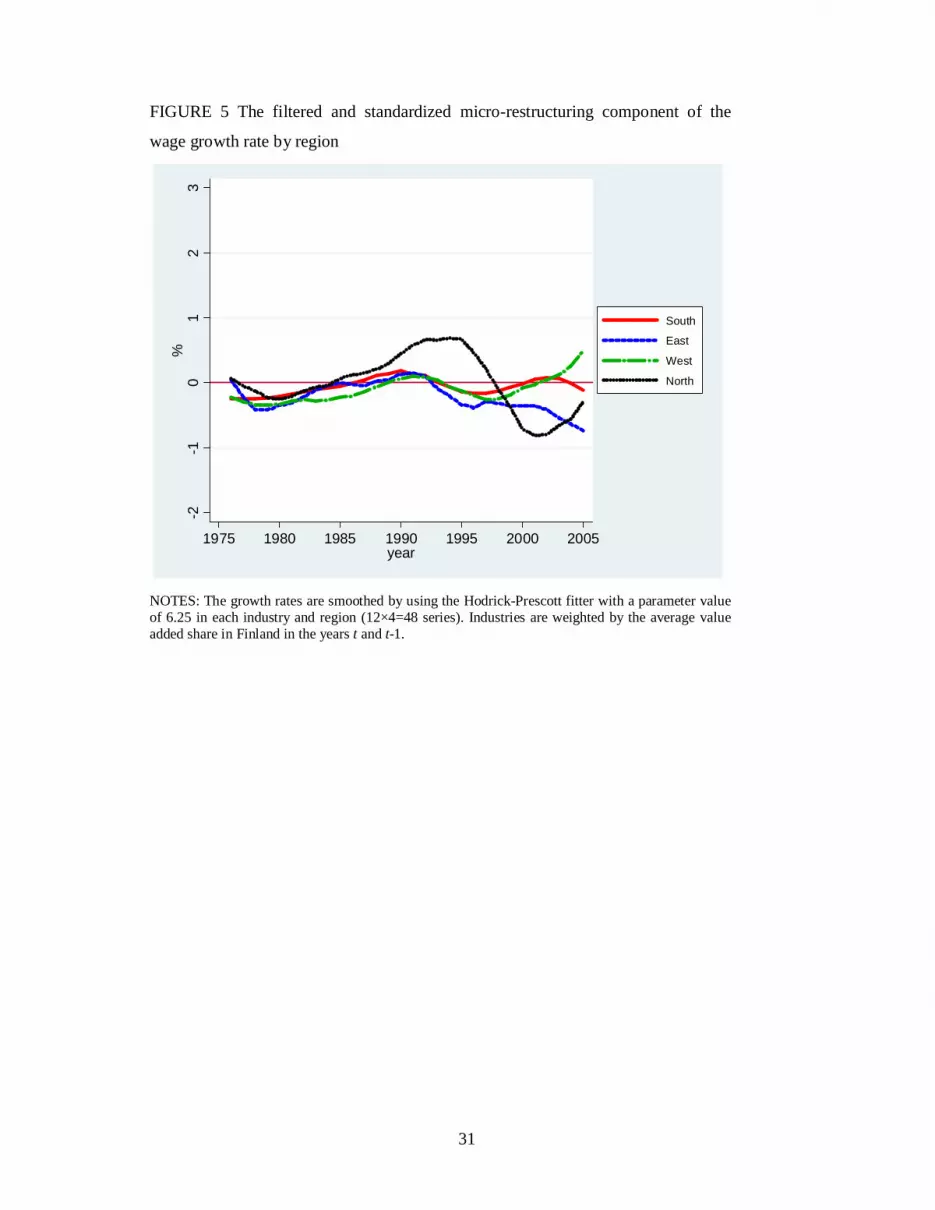
Figure 5 reveals that micro-level restructuring has had only a moderate effect on wage

growth in all four regions. If anything, some indication of a negative contribution can be

found in Eastern and Northern Finland during the 2000s.


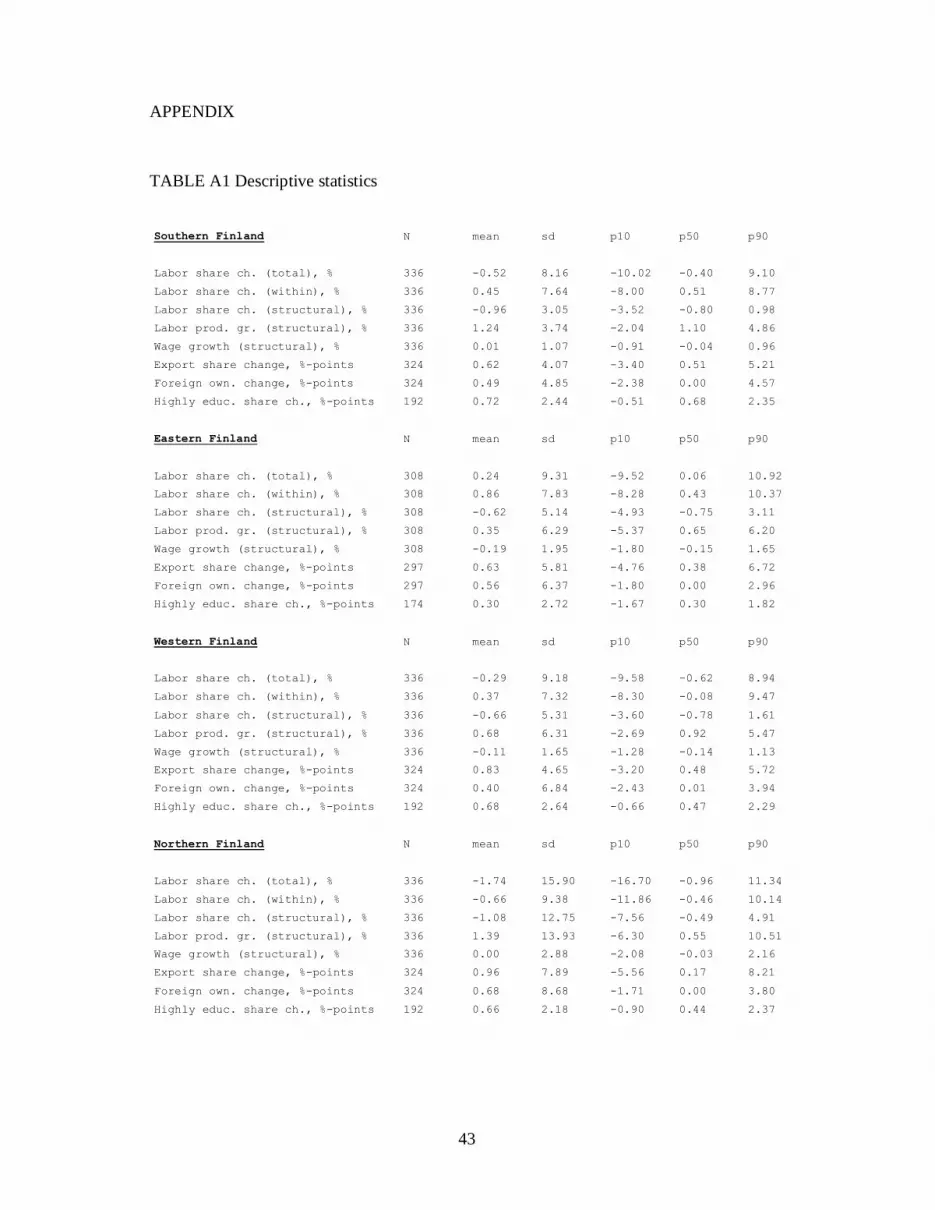
The total change in the labor share is decomposed in Table A1 into the within and structural

components, respectively. Decline in the labor share has been clearly deepest in Northern

Finland. In contrast, the labor share has increased in Eastern Finland. The structural

component of labor productivity growth has been smallest in Eastern Finland and largest in

Northern and Southern Finland.

18

The exposure to international trade has increased most strongly in Northern Finland (Table

A1). Foreign ownership has increased in all regions and, again, growth has been strongest

in Northern Finland. We also examine the role of skill upgrading that is measured by the

change in highly educated employees (those having tertiary education). Growth has been

fastest in Southern and slowest in Eastern Finland.

To summarize, there have been considerable differences in the micro-level dynamics of the

labor share across regions within the same country that have shared exactly the same

institutions and regulations. This variation has been neglected in the literature. It can be

exploited when we estimate the effect of globalization on the labor share change.

4.2. Estimates

We use Prais-Winsten regressions with panel-corrected standard errors as our baseline

specifications for the period 1978-2005.10 The estimator is based on the principle of

estimating the amount of autocorrelation and then re-weighting the standards errors to

correct them. Therefore, it is a weighted least squares estimator. The estimator is preferable

in terms of efficiency to OLS in our context, because we have a considerable number of

repeated observations on fixed units (industry × regions) with a potential first-order serial

correlation. We assume that the structure of the AR (1) process is similar in each panel of

the data, as recommended by Beck and Katz (1995). A further advantage of Prais-Winsten

regressions is that we are able to incorporate cross-sectional correlation to the model when

the number of time-series observations is less than the number of cross-sectional

observations, whereas standard feasible generalized least squares cannot (Chen et al. 2005).

The sample consists of 1316 observations (4 regions, 12 industries and 28 years).11

19

If the focus were the within plant changes, we would use those approximately 150 000

plant-level observations that are available in our original panel data. However, since in this

paper we are particularly interested in the structural components, the industry-region panel

constructed by the decomposition computations is much more useful to our purposes. The

aim is to identify an additional role of the exposure to globalization, i.e. to study whether

there is evidence of a structural change in terms of valued added towards those plants that

have a lower labor share because of globalization. With these data we can consistently

analyze the role of plant-level changes (i.e. within plant changes) and micro-structural

components in industry development.

The dependent variables of the models are the industry growth rates of the labor share,

labor productivity and wage, and their micro-level components by regions. The explanatory

variables are the measures of globalization along with the control variables. The control

variables include a full set of the unreported fixed industry-region effects. Prais-Winsten

regressions do not contain separate year effects. However, it is assumed that disturbances

are heteroscedastic and contemporaneously correlated across panels (i.e. industry ×

regions).

The variables that capture the changes in the exposure to international trade and foreign

ownership are included in the models as lagged up to two years. There are two reasons for

this. First, and most importantly, it should take some time before the effects on the labor

share change appear. Specifically, Maliranta (2005) shows that it is worthwhile taking into

account the lagged effects when examining the influences of international trade on

restructuring. Second, the contemporary correlation between the exposure to international

trade and the labor share change could be the reverse, because a decline in the labor share

20

improves the competitiveness of domestic production that tends to increase export volume

in a small open economy.

The lagged effect is arguably closer to the causal effect. That being said, we cannot directly

address the possibility that the measures of globalization may be endogenous, because our

data do not contain appropriate economic instruments for globalization that could be

claimed to be truly independent of the micro-level components of the labor share change. In

this sense, we document essentially correlations between globalization and different micro-

level components of the labor share change. However, we are able to test the strict

exogeneity of the regressors by including the lead values of the measures of globalization

among the explanatory variables. Furthermore, to examine the robustness of the baseline

estimates we have estimated GMM specifications that allow us to instrument potentially

endogenous variables with their lagged levels in the dynamic setting. This modeling

framework offers the second-best solution dealing with endogeneity problems, since our

data do not contain appropriate economic instruments. The problems regarding the causal

interpretation of the estimates are even more apparent in the cross-county studies (e.g.

European Commission 2007, 2008; Guscina 2006; Harrison 2002; Jaumotte and Tytell

2007; Jayadev 2007). One important advantage of our approach is that the labor market

regulations and other institutional aspects are similar for all units of observation (industry ×

region) in the estimations, because we focus on one country.

All models are estimated by taking advantage of unfiltered data. The use of filtered data to

estimate models is not an appropriate strategy for two reasons. First, the Hodrick-Prescott

filter smoothes the data and leads to a complicated pattern of autocorrelation with future

and past components in the dependent variables. This most likely would lead to spurious

21

regression results (Meyer and Winker 2005). Second, the pre-filtering of the dependent

variables would mean that they are measured with an error. This generates a systematic

pattern of heteroskedasticity (Saxonhouse 1977). It would be very difficult to construct an

econometric model to tackle both of these problems.

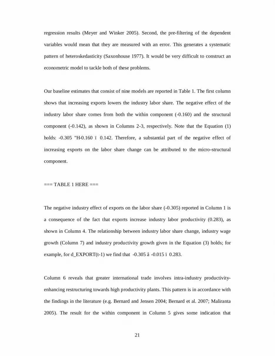
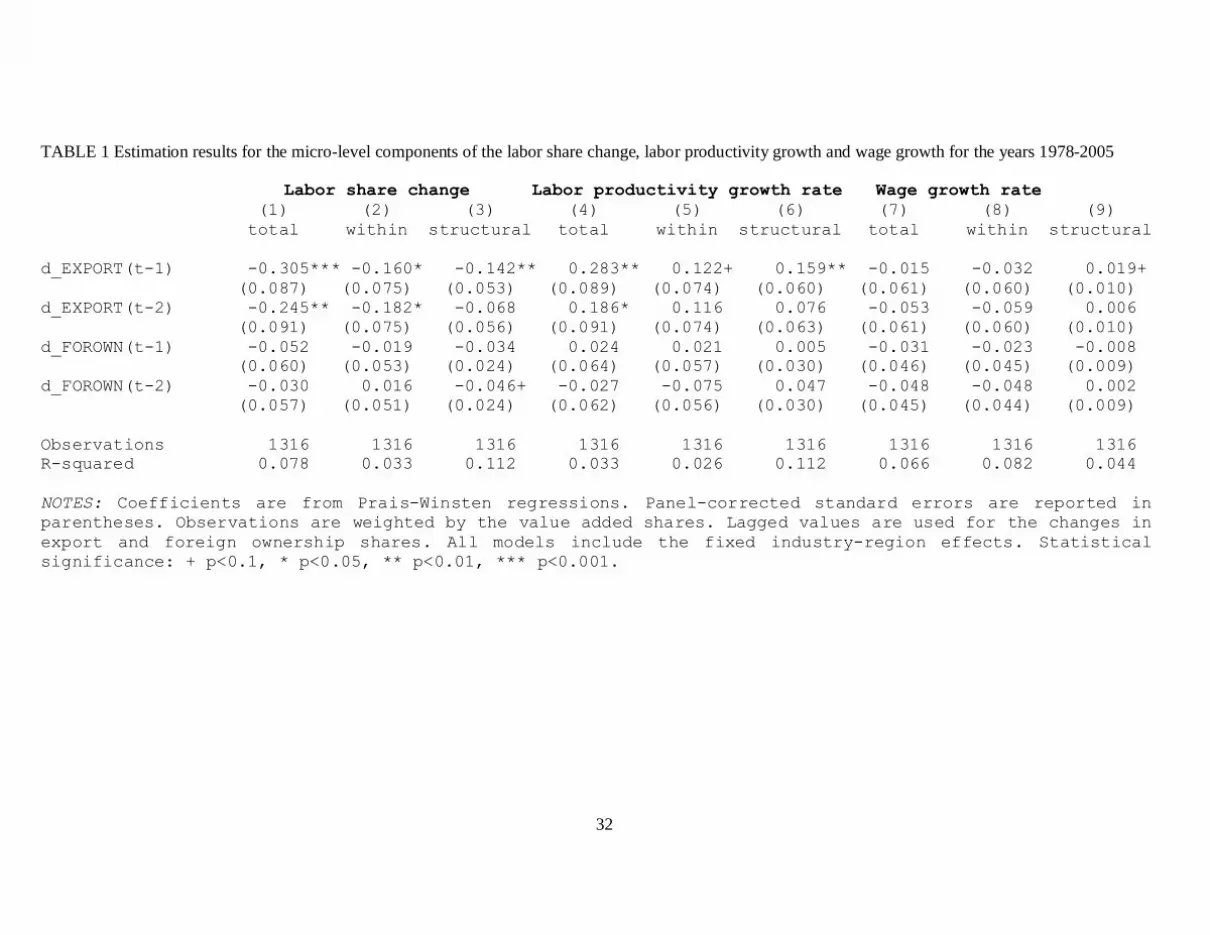
Our baseline estimates that consist of nine models are reported in Table 1. The first column

shows that increasing exports lowers the industry labor share. The negative effect of the

industry labor share comes from both the within component (-0.160) and the structural

component (-0.142), as shown in Columns 2-3, respectively. Note that the Equation (1)

holds: -0.305 ≈ -0.160 – 0.142. Therefore, a substantial part of the negative effect of

increasing exports on the labor share change can be attributed to the micro-structural

component.

=== TABLE 1 HERE ===

The negative industry effect of exports on the labor share (-0.305) reported in Column 1 is

a consequence of the fact that exports increase industry labor productivity (0.283), as

shown in Column 4. The relationship between industry labor share change, industry wage

growth (Column 7) and industry productivity growth given in the Equation (3) holds; for

example, for d_EXPORT(t-1) we find that -0.305 ≈ -0.015 – 0.283.

Column 6 reveals that greater international trade involves intra-industry productivity-

enhancing restructuring towards high productivity plants. This pattern is in accordance with

the findings in the literature (e.g. Bernard and Jensen 2004; Bernard et al. 2007; Maliranta

2005). The result for the within component in Column 5 gives some indication that

22

exporting increases plants’ productivity, but the statistical significance is much lower than

for the structural component. The industry productivity effect is approximately a sum of

these two channels, i.e. 0.283 ≈ 0.122 + 0.159.

Column 7 of Table 1 shows that exports have no effect on industry wage growth. This fact

explains why the productivity effect has such a large dominance in the determination of the

labor share change. Exporting has only a weakly significant positive effect on the micro-

structural component of industry wage growth (Column 9).

Overall, the results reveal that micro-level restructuring is an important channel through

which exporting reduces the industry labor share. The effect comes essentially from the

restructuring component of labor productivity growth. The restructuring component of

industry wage growth has a minor role to play, which can be seen from the empirical

counterpart of the Equation (5) for the subcomponents of the restructuring component of

labor share change: -0.142 ≈ 0.019 – 0.159.

The results point out that the exposure to international trade is clearly a more important

determinant of the micro-level components of the labor share change than foreign

ownership. Foreign ownership does not have an effect on labor productivity or wage

growth. However, a small negative impact prevails on the structural component of the labor

share change (Column 3).

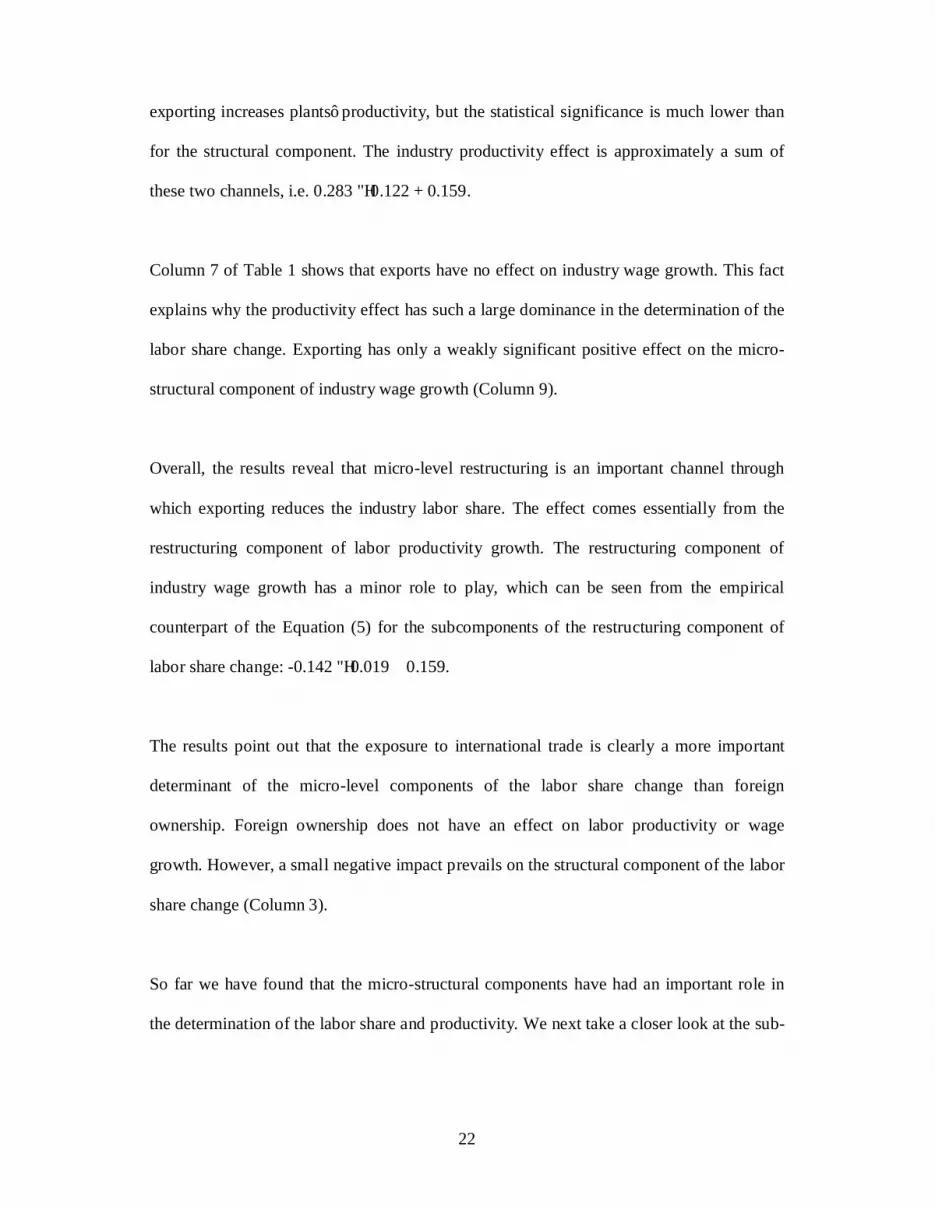
So far we have found that the micro-structural components have had an important role in

the determination of the labor share and productivity. We next take a closer look at the sub-

23

components of the structural component, as described earlier in the Equation (2). This

decomposition allows us to pinpoint the exact sources of the effects.

Table 2 reports the estimates for the labor share change. Column 1 in Table 2 is the same as

Column 3 in Table 1. It is approximately the sum of the estimates of Columns 2-5 in Table

2 so that one can read the contribution of each sub-component to the structural component.

We discover that the negative effect of the structural component on the labor share change

emerges through the exits of plants, i.e. those plants with a particularly high share of labor

income are eventually forced out of business as exports increase.


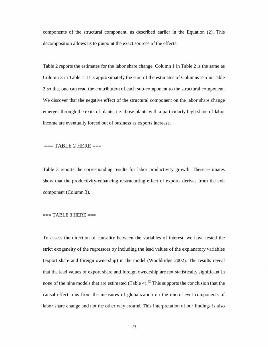
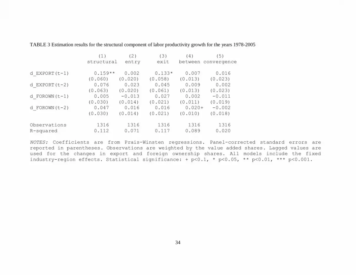
Table 3 reports the corresponding results for labor productivity growth. These estimates

show that the productivity-enhancing restructuring effect of exports derives from the exit

component (Column 3).


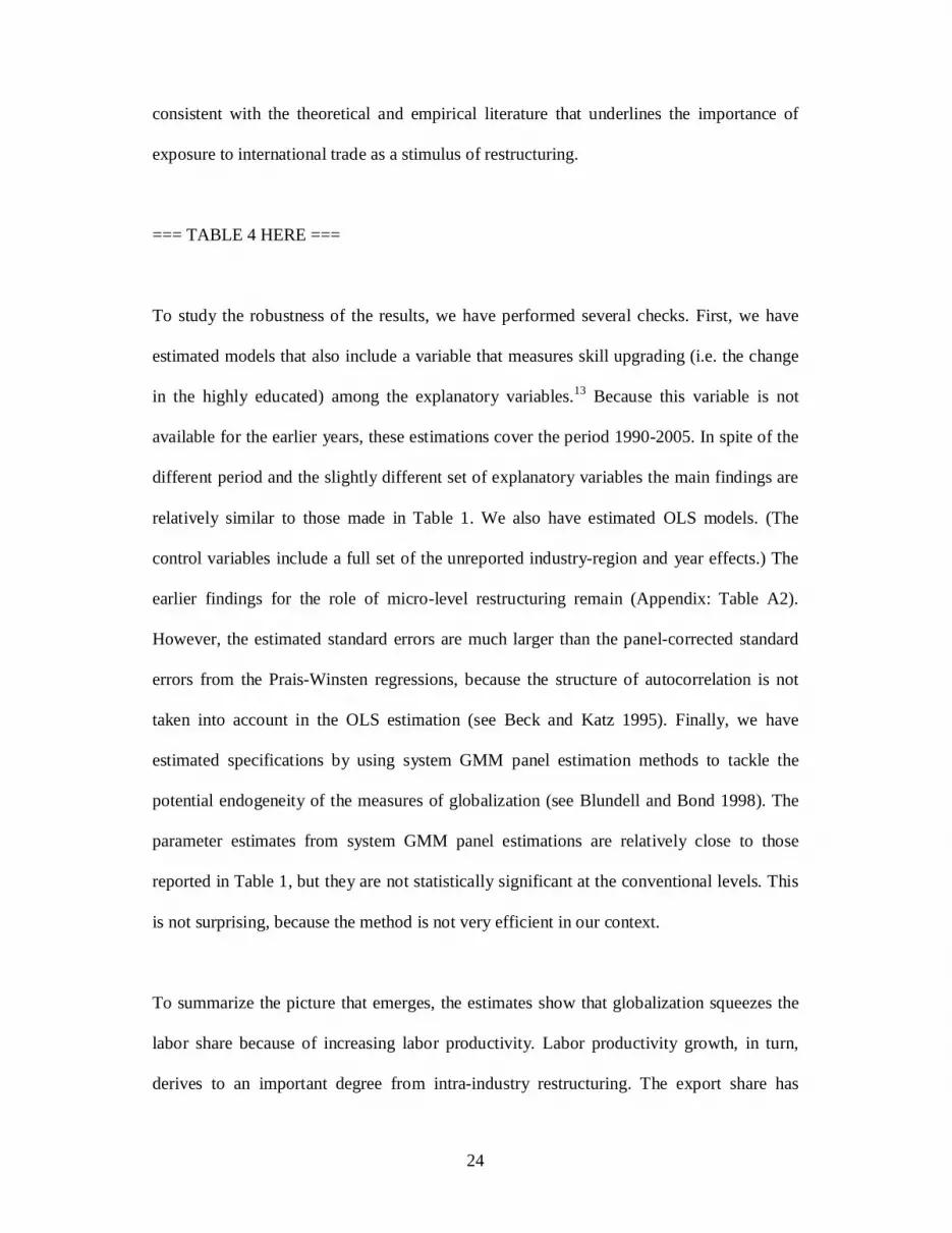
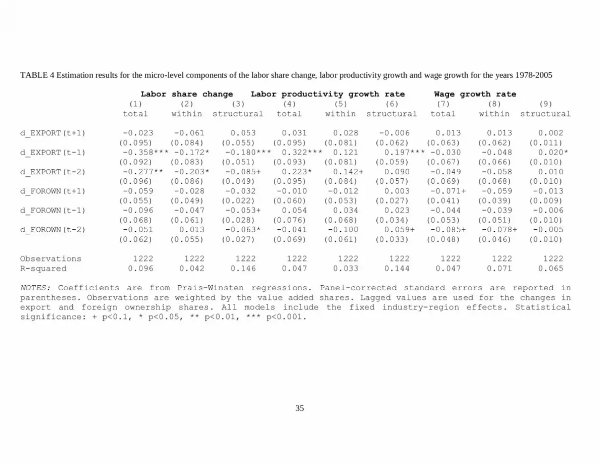
To assess the direction of causality between the variables of interest, we have tested the

strict exogeneity of the regressors by including the lead values of the explanatory variables

(export share and foreign ownership) in the model (Wooldridge 2002). The results reveal

that the lead values of export share and foreign ownership are not statistically significant in

none of the nine models that are estimated (Table 4).12 This supports the conclusion that the

causal effect runs from the measures of globalization on the micro-level components of

labor share change and not the other way around. This interpretation of our findings is also

24

consistent with the theoretical and empirical literature that underlines the importance of

exposure to international trade as a stimulus of restructuring.


To study the robustness of the results, we have performed several checks. First, we have

estimated models that also include a variable that measures skill upgrading (i.e. the change

in the highly educated) among the explanatory variables.13 Because this variable is not

available for the earlier years, these estimations cover the period 1990-2005. In spite of the

different period and the slightly different set of explanatory variables the main findings are

relatively similar to those made in Table 1. We also have estimated OLS models. (The

control variables include a full set of the unreported industry-region and year effects.) The

earlier findings for the role of micro-level restructuring remain (Appendix: Table A2).

However, the estimated standard errors are much larger than the panel-corrected standard

errors from the Prais-Winsten regressions, because the structure of autocorrelation is not

taken into account in the OLS estimation (see Beck and Katz 1995). Finally, we have

estimated specifications by using system GMM panel estimation methods to tackle the

potential endogeneity of the measures of globalization (see Blundell and Bond 1998). The

parameter estimates from system GMM panel estimations are relatively close to those

reported in Table 1, but they are not statistically significant at the conventional levels. This

is not surprising, because the method is not very efficient in our context.

To summarize the picture that emerges, the estimates show that globalization squeezes the

labor share because of increasing labor productivity. Labor productivity growth, in turn,

derives to an important degree from intra-industry restructuring. The export share has

25

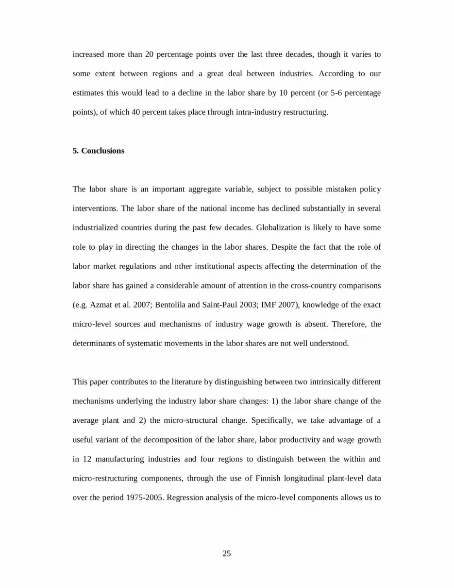
increased more than 20 percentage points over the last three decades, though it varies to

some extent between regions and a great deal between industries. According to our

estimates this would lead to a decline in the labor share by 10 percent (or 5-6 percentage

points), of which 40 percent takes place through intra-industry restructuring.

5. Conclusions

The labor share is an important aggregate variable, subject to possible mistaken policy

interventions. The labor share of the national income has declined substantially in several

industrialized countries during the past few decades. Globalization is likely to have some

role to play in directing the changes in the labor shares. Despite the fact that the role of

labor market regulations and other institutional aspects affecting the determination of the

labor share has gained a considerable amount of attention in the cross-country comparisons

(e.g. Azmat et al. 2007; Bentolila and Saint-Paul 2003; IMF 2007), knowledge of the exact

micro-level sources and mechanisms of industry wage growth is absent. Therefore, the

determinants of systematic movements in the labor shares are not well understood.

This paper contributes to the literature by distinguishing between two intrinsically different

mechanisms underlying the industry labor share changes: 1) the labor share change of the

average plant and 2) the micro-structural change. Specifically, we take advantage of a

useful variant of the decomposition of the labor share, labor productivity and wage growth

in 12 manufacturing industries and four regions to distinguish between the within and

micro-restructuring components, through the use of Finnish longitudinal plant-level data

over the period 1975-2005. Regression analysis of the micro-level components allows us to

26

examine not only the effects of international trade and other factors on the labor share

changes but also to look at the distinct micro-level mechanisms.

The most important finding is that we identify an additional role of the exposure to

international trade: there is evidence of a systematic micro-structural change in terms of

value added towards those plants that have a lower labor share. Globalization squeezes the

labor share because of increasing labor productivity. Labor productivity growth, in turn, is

predominantly a consequence of intra-industry restructuring. Furthermore, the negative

effect of exporting on industry labor share change emerges through the exits of plants, i.e.

those plants with a particularly high share of labor income are forced out of business as

exports increase. In contrast, wage formation has been largely insulated from the influences

of increasing international trade over a period of three decades. This carries an important

policy lesson. Taken that globalization boosts labor productivity while wages do not fall, it

will eventually also benefit employees in the long run. However, this requires flexibility of

labor markets so that employees from the exiting plants move to more productive and

profitable jobs. Greater wage flexibility between plants would be one way to mitigate this

pressure (see Moene and Wallerstein 1997).

27

FIGURE 1 The labor share by region

.4.5

.6.7

.8

1975 1980 1985 1990 1995 2000 2005year

South, H-P(6.25)

South

East, H-P(6.25)

East

West, H-P(6.25)

West

North, H-P(6.25)

North

NOTE: The labor shares are smoothed by using the Hodrick-Prescott filter with a parameter value of 6.25.

28

FIGURE 2 The filtered and standardized within component of the labor share

change rate by region

-.04

-.02

0.0

2.0

4

1975 1980 1985 1990 1995 2000 2005year

South

East

West

North

NOTES: The growth rates are smoothed by using the Hodrick-Prescott fitter with a parameter value of 6.25 in each industry and region (12×4=48 series). Industries are weighted by the average value added share in Finland in the years t and t-1.

29

FIGURE 3 The filtered and standardized micro-restructuring component of the

labor share change rate by region

-2-1

01

23

%

1975 1980 1985 1990 1995 2000 2005year

South

East

West

North


30


labor productivity growth rate by region

-2-1

01

23

%

1975 1980 1985 1990 1995 2000 2005year

South

East

West

North


31


wage growth rate by region

-2-1

01

23

%

1975 1980 1985 1990 1995 2000 2005year

South

East

West

North


32

TABLE 1 Estimation results for the micro-level components of the labor share change, labor productivity growth and wage growth for the years 1978-2005

Labor share change Labor productivity growth rate Wage growth rate (1) (2) (3) (4) (5) (6) (7) (8) (9) total within structural total within structural total within structural d_EXPORT(t-1) -0.305*** -0.160* -0.142** 0.283** 0.122+ 0.159** -0.015 -0.032 0.019+ (0.087) (0.075) (0.053) (0.089) (0.074) (0.060) (0.061) (0.060) (0.010) d_EXPORT(t-2) -0.245** -0.182* -0.068 0.186* 0.116 0.076 -0.053 -0.059 0.006 (0.091) (0.075) (0.056) (0.091) (0.074) (0.063) (0.061) (0.060) (0.010) d_FOROWN(t-1) -0.052 -0.019 -0.034 0.024 0.021 0.005 -0.031 -0.023 -0.008 (0.060) (0.053) (0.024) (0.064) (0.057) (0.030) (0.046) (0.045) (0.009) d_FOROWN(t-2) -0.030 0.016 -0.046+ -0.027 -0.075 0.047 -0.048 -0.048 0.002 (0.057) (0.051) (0.024) (0.062) (0.056) (0.030) (0.045) (0.044) (0.009) Observations 1316 1316 1316 1316 1316 1316 1316 1316 1316 R-squared 0.078 0.033 0.112 0.033 0.026 0.112 0.066 0.082 0.044 NOTES: Coefficients are from Prais-Winsten regressions. Panel-corrected standard errors are reported in parentheses. Observations are weighted by the value added shares. Lagged values are used for the changes in export and foreign ownership shares. All models include the fixed industry-region effects. Statistical significance: + p<0.1, * p<0.05, ** p<0.01, *** p<0.001.

33

TABLE 2 Estimation results for the structural component of the labor share change for the years 1978-2005

(1) (2) (3) (4) (5) structural entry exit between convergence d_EXPORT(t-1) -0.142** 0.031 -0.155* -0.028 0.004 (0.053) (0.030) (0.070) (0.033) (0.030) d_EXPORT(t-2) -0.068 0.008 -0.073 0.015 -0.028 (0.056) (0.028) (0.070) (0.033) (0.030) d_FOROWN(t-1) -0.034 0.012 -0.036 0.017 -0.030 (0.024) (0.014) (0.022) (0.026) (0.026) d_FOROWN(t-2) -0.046+ -0.022 -0.008 -0.028 0.013 (0.024) (0.014) (0.023) (0.025) (0.025) Observations 1316 1316 1316 1316 1316 R-squared 0.112 0.119 0.128 0.045 0.037 NOTES: Coefficients are from Prais-Winsten regressions. Panel-corrected standard errors are reported in parentheses. Observations are weighted by the value added shares. Lagged values are used for the changes in export and foreign ownership shares. All models include the fixed industry-region effects. Statistical significance: + p<0.1, * p<0.05, ** p<0.01, *** p<0.001.

34

TABLE 3 Estimation results for the structural component of labor productivity growth for the years 1978-2005

(1) (2) (3) (4) (5) structural entry exit between convergence d_EXPORT(t-1) 0.159** 0.002 0.133* 0.007 0.016 (0.060) (0.020) (0.058) (0.013) (0.023) d_EXPORT(t-2) 0.076 0.023 0.045 0.009 0.002 (0.063) (0.020) (0.061) (0.013) (0.023) d_FOROWN(t-1) 0.005 -0.013 0.027 0.002 -0.011 (0.030) (0.014) (0.021) (0.011) (0.019) d_FOROWN(t-2) 0.047 0.016 0.016 0.020+ -0.002 (0.030) (0.014) (0.021) (0.010) (0.018) Observations 1316 1316 1316 1316 1316 R-squared 0.112 0.071 0.117 0.089 0.020 NOTES: Coefficients are from Prais-Winsten regressions. Panel-corrected standard errors are reported in parentheses. Observations are weighted by the value added shares. Lagged values are used for the changes in export and foreign ownership shares. All models include the fixed industry-region effects. Statistical significance: + p<0.1, * p<0.05, ** p<0.01, *** p<0.001.

35

TABLE 4 Estimation results for the micro-level components of the labor share change, labor productivity growth and wage growth for the years 1978-2005

Labor share change Labor productivity growth rate Wage growth rate (1) (2) (3) (4) (5) (6) (7) (8) (9) total within structural total within structural total within structural d_EXPORT(t+1) -0.023 -0.061 0.053 0.031 0.028 -0.006 0.013 0.013 0.002 (0.095) (0.084) (0.055) (0.095) (0.081) (0.062) (0.063) (0.062) (0.011) d_EXPORT(t-1) -0.358*** -0.172* -0.180*** 0.322*** 0.121 0.197*** -0.030 -0.048 0.020* (0.092) (0.083) (0.051) (0.093) (0.081) (0.059) (0.067) (0.066) (0.010) d_EXPORT(t-2) -0.277** -0.203* -0.085+ 0.223* 0.142+ 0.090 -0.049 -0.058 0.010 (0.096) (0.086) (0.049) (0.095) (0.084) (0.057) (0.069) (0.068) (0.010) d_FOROWN(t+1) -0.059 -0.028 -0.032 -0.010 -0.012 0.003 -0.071+ -0.059 -0.013 (0.055) (0.049) (0.022) (0.060) (0.053) (0.027) (0.041) (0.039) (0.009) d_FOROWN(t-1) -0.096 -0.047 -0.053+ 0.054 0.034 0.023 -0.044 -0.039 -0.006 (0.068) (0.061) (0.028) (0.076) (0.068) (0.034) (0.053) (0.051) (0.010) d_FOROWN(t-2) -0.051 0.013 -0.063* -0.041 -0.100 0.059+ -0.085+ -0.078+ -0.005 (0.062) (0.055) (0.027) (0.069) (0.061) (0.033) (0.048) (0.046) (0.010) Observations 1222 1222 1222 1222 1222 1222 1222 1222 1222 R-squared 0.096 0.042 0.146 0.047 0.033 0.144 0.047 0.071 0.065 NOTES: Coefficients are from Prais-Winsten regressions. Panel-corrected standard errors are reported in parentheses. Observations are weighted by the value added shares. Lagged values are used for the changes in export and foreign ownership shares. All models include the fixed industry-region effects. Statistical significance: + p<0.1, * p<0.05, ** p<0.01, *** p<0.001.

36

References

Agell, J. (1999) ‘On the benefits from rigid labor markets: Norms, market failures, and

social insurance,’ The Economic Journal 109, F143-F164

Aghion, P., and P. Howitt (2006) ‘Appropriate growth policy: A unifying framework,’

Journal of the European Economic Association 2-3, 269-314

Audretsch, D.B., O. Falck, M.P. Feldman, and S. Heblich (2008) ‘The lifecycle of regions,’

Centre for Economic Policy Research, Discussion Paper No. 6757

Azmat, G., A. Manning, and J. Van Reenen (2007) ‘Privatization, entry regulation and the

decline of labor’s share of GDP: A cross-country analysis of the network industries,’ Centre

for Economic Policy Research, Discussion Paper No. 6348

Baldwin, R.E., and T. Okubo (2006) ‘Heterogeneous firms, agglomeration and economic

geography: Spatial selection and sorting,’ Journal of Economic Geography 6, 323-346

Bartelsmans, E.J., and M. Doms (2000) ‘Understanding productivity: Lessons from

longitudinal microdata,’ Journal of Economic Literature 38, 596-594

Bartelsmans, E.J., J. Haltiwanger, and S. Scarpetta (2009) ‘Measuring and analyzing cross-

country differences in firm dynamics,’ in Producer Dynamics: New Evidence from Micro

Data, ed. Timothy Dunne, J. Bradford Jensen and Mark J. Roberts (Chicago: University of

Chicago Press)

37

Beck, N., and J.N. Katz (1995) ‘What to do (not to do) with time-series cross-section data,’

American Political Science Review 89, 634-647

Bentolila, S., and G. Saint-Paul (2003) ‘Explaining movements in the labor share,’

Contributions to Macroeconomics 3, Article 9

Bernard, A.B., and J.B. Jensen (2004) ‘Exporting and productivity in the USA,’ Oxford

Review of Economic Policy 20, 343-357

Bernard, A.B., J.B. Jensen, S.J. Redding, and P.K. Scott (2007) ‘Firms in international

trade,’ Journal of Economic Perspectives 21, 105-130

Blanchard, O. (1997) ‘The medium run,’ Brookings Papers on Economic Activity 2, 89-158

Blanchard, O. (2006) ‘European unemployment: The evolution of facts and ideas,’

Economic Policy 45, 6-59

Blundell, R., and S. Bond (1998) ‘Initial conditions and moment restrictions in dynamic

panel data models,’ Journal of Econometrics 87, 115-143

Chen, X., S. Lin, and W.R. Reed (2005) ‘Another look at what to do with time-series cross-

section data,’ Unpublished

38

Diewert, W.E., and K.A. Fox (2009) ‘On measuring the contribution of entering and exiting

firms to aggregate productivity growth,’ in Index Number Theory and the Measurement of

Prices and Productivity, ed. W. Erwin Diewert, Bert M. Balk, Dennis Fixler, Kevin J. Fox

and Alice Nakamura (Victoria: Trafford Publishing)

European Commission (2007) Employment in Europe (Brussels: European Commission)

European Commission (2008) Income Inequality and Wage Share: Patterns and

Determinants (Brussels: European Commission)

Feldstein, M.S. (2008) ‘Did wages reflect growth in productivity?’ National Bureau of

Economic Research, Working Paper No. 13953

Foster, L., J. Haltiwanger, and C.J. Krizan (2001) ‘Aggregate productivity growth: Lessons

from microeconomic evidence,’ in New Developments in Productivity Analysis, ed. Charles

R. Hulten, Edwin R. Dean and Michael J. Harper (Chicago: University of Chicago Press)

Friedman, M. (1992) ‘Do old fallacies ever die?’ Journal of Economic Literature 30, 2129-

2132

Gollin, D. (2002) ‘Getting income shares right,’ Journal of Political Economy 110, 458-

474

Grossman, G.M., and E. Helpman (1991) Innovation and Growth in the Global Economy

(Cambridge, MA: The MIT Press)

39

Guscina, A. (2006) ‘Effects of globalization on labor’s share in national income,’ IMF

Working Paper No. 294

Harrison, A.E. (2002) ‘Has globalization eroded labor’s share? Some cross-country

evidence,’ Berkeley, CA: University of California at Berkeley and NBER

Helpman, E., M.J. Melitz, and S.R. Yeaple (2004) ‘Export versus FDI with heterogeneous

firms,’ The American Economic Review 94, 300-316

IMF (2007) World Economic Outlook (Washington, CD: IMF)

Jaumotte, F., and I. Tytell (2007) ‘How has the globalization of labor affected the labor

share in advanced countries?’ IMF Working Paper No. 298

Jayadev, A. (2007) ‘Capital account openness and labour share of income,’ Cambridge

Journal of Economics 31, 423-443

Kruger, J.J. (2007) ‘Productivity and structural change: A review of the literature,’ Journal

of Economic Surveys 22, 330-363

Kyyrä, T., and M. Maliranta (2008) ‘The micro-level dynamics of declining labour share:

Lessons from the Finnish great leap,’ Industrial and Corporate Change 17, 1147-1172

40

Layard, R., and S. Nickell (1999) ‘Labor market institutions and economic performance,’ in

Handbook of Labor Economics, Volume 3C, Orley Ashenfelter and David Card

(Amsterdam: North-Holland)

Lileeva, A. (2008) ‘Trade liberalization and productivity dynamics: Evidence from

Canada,’ Canadian Journal of Economics 41, 360-390.

Mairesse, J., and E. Kremp (1993) ‘A look at productivity at the firm level in eight French

service industries,’ Journal of Productivity Analysis 4, 211-234

Maliranta, M. (1997) ‘Plant-level explanations for the catch-up process in Finnish

manufacturing: A decomposition of aggregate labour productivity growth,’ in The

Evolution of Firms and Industries. International Perspectives, Ed. Seppo Laaksonen

(Helsinki: Statistics Finland)

Maliranta, M. (2003) Micro-level Dynamics of Productivity Growth. An Empirical Analysis

of the Great Leap in the Finnish Manufacturing Productivity in 1975-2000 (Helsinki:

Helsinki School of Economics A-230)

Maliranta, M. (2005) ‘R&D, international trade and creative destruction – Empirical

findings from Finnish manufacturing industries,’ Journal of Industry, Competition and

Trade 5, 27-58

Melitz, M.J. (2003) ‘The impact of trade on intra-industry reallocations and aggregate

industry productivity,’ Econometrica 71, 1695-1725

41

Meyer, M., and P. Winker (2005) ‘Using HP filtered data for econometric analysis: Some

evidence from Monte Carlo simulations,’ AStA Advances in Statistical Analysis 89, 303-

320

Moene, K.O., and M. Wallerstein (1997) ‘Pay Inequality,’ Journal of Labor Economics 15,

403-430.

Okubo, T., P.M. Picard, and J-F Thisse (2008) ‘Spatial selection of heterogeneous firms,’

Centre for Economic Policy Research, Discussion Paper No. 6978

Prais, S.J., and C.B. Winsten, C (1954) ‘Trend estimators and serial correlation,’ Cowles

Foundation Discussion Paper No. 383

Ravn, M.O., and H. Uhlig (2002) ‘On adjusting the Hodrick-Prescott filter for the

frequency of observations,’ The Review of Economics and Statistics 84, 371-376

Ripatti, A., and J. Vilmunen (2001) ‘Declining labor share: Evidence of a change in the

underlying production technology?’ Bank of Finland, Discussion Paper No. 10/2001

Rodrik, D. (1997) Has Globalization Gone too Far? (Washington, DC: Institute for

International Economics)

42

Rodrik, D. (2008) One Economics, Many Recipes: Globalization, Institutions, and

Economic Growth (Princeton, NJ: Princeton University Press)

Saxonhouse, G.R. (1977) ‘Regressions from samples having different characteristics,’ The

Review of Economics and Statistics 59, 234-237

Sauramo, P. (2004) ‘Is the labour share too low in Finland?’ in Collective Bargaining and

Wage Formation. Performance and Challenges, ed. Hannu Piekkola and Kenneth Snellman

(Heidelberg: Physica-Verlag)

Slaughter, M.J. (2007) ‘Globalization and declining unionization in the United States,’

Industrial Relations 46, 329-346

Solow, R.M. (1958) ‘A skeptical note on the constancy of relative shares,’ The American

Economic Review 48, 618-631

Takayama, A. (1972) International Trade (New York: Holt, Rinehart and Winston, Inc)

Vainiomäki, J. (1999) ‘Technology and skill upgrading: Results from linked worker-plant

data for Finnish manufacturing,’ in The Creation and Analysis of Employer-Employee

Matched Data, ed. John C. Haltiwanger, Julia Lane, James R. Spletzer, Jules J. M.

Theuwes and Kenneth R. Troske (Amsterdam: North-Holland)

Wooldridge, J.M. (2002) Econometric Analysis of Cross Section and Panel Data

(Cambridge, MA: MIT Press)

43

APPENDIX

TABLE A1 Descriptive statistics Southern Finland N mean sd p10 p50 p90

Labor share ch. (total), % 336 -0.52 8.16 -10.02 -0.40 9.10

Labor share ch. (within), % 336 0.45 7.64 -8.00 0.51 8.77

Labor share ch. (structural), % 336 -0.96 3.05 -3.52 -0.80 0.98

Labor prod. gr. (structural), % 336 1.24 3.74 -2.04 1.10 4.86

Wage growth (structural), % 336 0.01 1.07 -0.91 -0.04 0.96

Export share change, %-points 324 0.62 4.07 -3.40 0.51 5.21

Foreign own. change, %-points 324 0.49 4.85 -2.38 0.00 4.57

Highly educ. share ch., %-points 192 0.72 2.44 -0.51 0.68 2.35

Eastern Finland N mean sd p10 p50 p90

Labor share ch. (total), % 308 0.24 9.31 -9.52 0.06 10.92

Labor share ch. (within), % 308 0.86 7.83 -8.28 0.43 10.37



Wage growth (structural), % 308 -0.19 1.95 -1.80 -0.15 1.65




Western Finland N mean sd p10 p50 p90


Labor share ch. (within), % 336 0.37 7.32 -8.30 -0.08 9.47



Wage growth (structural), % 336 -0.11 1.65 -1.28 -0.14 1.13




Northern Finland N mean sd p10 p50 p90


Labor share ch. (within), % 336 -0.66 9.38 -11.86 -0.46 10.14



Wage growth (structural), % 336 0.00 2.88 -2.08 -0.03 2.16




44

DERIVATION OF THE EQUATIONS (1) AND (2)

The aggregate labor share is

(A.1) iti it itt i

it t iti

w v wFv v v

= =∑ ∑∑

In period t plants can be divided into two groups: plants that appeared also in period t-1,

(continuing plants, denoted by C) and plants that made an entry after t-1 (entering plants,

denoted by E). Then the aggregate labor share can be written as follows:

(A.2) 1

jt jtit itt i C j E

t it t jt

jt jtit it j E j Ei C i Ct

t it t jti C j E

jt jt jtitj E j E j Ei Ct

t it t jti C j E

jt jt jit itj E j Ei C i Ct

it t it ti C i C

v wv wFv v v v

v wv wF

v v v v

v v wwF

v v v v

v v ww wF

v v v v

∈ ∈

∈ ∈∈ ∈

∈ ∈

∈ ∈ ∈∈

∈ ∈

∈ ∈∈ ∈

∈ ∈

= +

⇔ = +

⇔ = − +

⇔ = − +

∑ ∑

∑ ∑∑ ∑∑ ∑

∑ ∑ ∑∑∑ ∑

∑ ∑∑ ∑∑ ∑

tj E

jtj E

jt jtit itj E j Ei C i Ct

it t jt iti C j E i C

v

v ww wF

v v v v

∈

∈

∈ ∈∈ ∈

∈ ∈ ∈

⇔ = + −

∑∑

∑ ∑∑ ∑∑ ∑ ∑

In a similar manner we can define the aggregate labor share in period t-1:

(A.3) , 1 , 1 , 11

, 1 1 , 1

i t i t i tit i

i t t i ti

w v wF

v v v− − −

−− − −

= =∑ ∑∑

In period t-1 plants can be divided into two groups: plants that survive until period t

(continuing plants, denoted by C) and plants that disappear after period t-1.

45

(A.4)

, 1, 1 , 1 , 11

1 , 1 1 , 1

, 1 , 1 , 1 , 11

1 , 1 1 , 1

, 1 , 1 , 11

1 , 1 1

1

j ti t i t k tt i C k D

t i t t k t

i t i t k t k ti C i C k D k Dt

t i t t k ti C k D

k t i t k t kk D i C k Dt

t i t ti C

wv w vF

v v v v

v w v wF

v v v v

v w v wF

v v v

−− − −− ∈ ∈

− − − −

− − − −∈ ∈ ∈ ∈−

− − − −∈ ∈

− − −∈ ∈ ∈−

− − −∈

= +

⇔ = +

⇔ = − +

∑ ∑

∑ ∑ ∑ ∑∑ ∑

∑ ∑ ∑∑

, 1

, 1

, 1 , 1 , 1 , 1 , 11

, 1 1 , 1 1 , 1

, 1 , 1 , 1 , 11

, 1 1 , 1 , 1

tk D

k tk D

i t k t i t k t k ti C k D i C k D k Dt

i t t i t t k ti C i C k D

i t k t k t i ti C k D k D i Ct

i t t k t i ti C k D i C

v

w v w v wF

v v v v v

w v w wF

v v v v

−∈

−∈

− − − − −∈ ∈ ∈ ∈ ∈−

− − − − −∈ ∈ ∈

− − − −∈ ∈ ∈ ∈−

− − − −∈ ∈ ∈

⇔ = − +

⇔ = + −

∑∑

∑ ∑ ∑ ∑ ∑∑ ∑ ∑∑ ∑ ∑ ∑∑ ∑ ∑

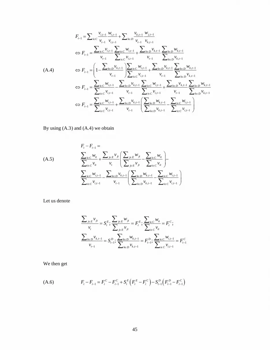
By using (A.3) and (A.4) we obtain

(A.5)

1

, 1 , 1 , 1 , 1

, 1 1 , 1 , 1

t t

jt jtit itj E j Ei C i C

it t jt iti C j E i C

i t k t k t i ti C k D k D i C

i t t k t i ti C k D i C

F F

v ww wv v v v

w v w wv v v v

−

∈ ∈∈ ∈

∈ ∈ ∈

− − − −∈ ∈ ∈ ∈

− − − −∈ ∈ ∈

− =

+ − −

− −

∑ ∑∑ ∑∑ ∑ ∑∑ ∑ ∑ ∑∑ ∑ ∑

Let us denote

, 1 , 1 , 1

1 1 11 , 1 , 1

; ; ;

; ;

jt jt itj E j EE E Ci Ct t t

t jt itj E i C

k t k t i tD D Ck D k D i Ct t t

t k t i tk D i C

v w wS F F

v v v

v w wS F F

v v v

∈ ∈ ∈

∈ ∈

− − −∈ ∈ ∈− − −

− − −∈ ∈

= = =

= = =

∑ ∑ ∑∑ ∑

∑ ∑ ∑∑ ∑

We then get

(A.6) ( ) ( )1 1 1 1 1C C E E C D D C

t t t t t t t t t tF F F F S F F S F F− − − − −− = − + − − −

46

This shows that the aggregate labor share change, i.e. 1t tF F −− , is the change in the

aggregate labor share change among the continuing plants, i.e. 1C C

t tF F −− , plus the entry

effect, i.e. ( )E E Ct t tS F F− , plus the exit effect, i.e. ( )1 1 1

D D Ct t tS F F− − −− − .

The change in the aggregate labor share among the continuing plants can be further

decomposed as follows:

(A.7)

, 11

, 1

, 1 , 11

, 1 , 1

, 1 , 1

, 1 , 1

0.5

0.5

it i tC C i C i Ct t

it i ti C i C

i t i tC C it itt t

it i t it i ti C i C

i t i tit it

it i t it i ti C i C

w wF F

v v

v wv wF Fv v v v

w vw vv v v v

−∈ ∈−

−∈ ∈

− −−

− −∈ ∈

− −

− −∈ ∈

− = −

⇔ − = + −

+ + −

∑ ∑∑ ∑

∑ ∑

∑ ∑

Let us use the following expressions

( ), 1

, 1 , 1, 1

, 1, 1

, 1

; ; 0.5 ;

; ; 0.5

it i ti C i Cit i t it i t i

it i ti C i C

i titit i t

it i ti C i C

w wf f f f f

v v

vv s sv v

−∈ ∈− −

−∈ ∈

−−

−∈ ∈

= = + =

= =

∑ ∑∑ ∑

∑ ∑

Then, inserting (A.7) into (A.6) we obtain

(A.8) ( ) ( ) ( ) ( )1 , 1 , 1 1 1 1E E C D D C

t t i it i t it i t i t t t t t ti C i CF F s f f s s f S F F S F F− − − − − −∈ ∈

− = − + − + − − −∑ ∑

This formula has been used in Kyyrä and Maliranta (2008). In this paper, we turn this

decomposition into a rate form. We can do this by dividing all the terms of (A.8) by the

average aggregate labor share, i.e. ( )10.5 t tF F F −= + . Then we have

47

(A.9) ( ) ( ) ( ) ( )1 1 1, 1 , 11

E E C D D Ct t t t t ti it i t it i t ii C i Ct t

S F F S F Fs f f s s fF FF F F F F

− − −− −∈ ∈−− −− −−

= + + −∑ ∑

One of our main goals in this paper is to look at the growth rate of the labor share within

the plants. Therefore we would like to develop the first component of the right-hand side of

(A.9).

(A.10)

( ) ( ) ( ) ( )

( ) ( ) ( )

, 1 , 1 , 1 , 1

, 1 , 1 , 1 1

i it i t i it i t i it i t i it i ti C i C i C i C

i i

i it i t i it i t i it i ti C i C i C i

i i

s f f s f f s f f s f fF F f f

s f f s f f s f f fF f f F

− − − −∈ ∈ ∈ ∈

− − −∈ ∈ ∈

− − − −= + −

− − − ⇔ = + −

∑ ∑ ∑ ∑

∑ ∑ ∑

Inserting (A.10) into (A.9) we get

(A.11)

( ) ( ) ( )

( ) ( )

, 1 , 11, 1

1 1 1

1it i t it i tt t i ii i it i ti C i C i C

i i

E E C D D Ct t t t t t

f f f fF F f fs s s sF f f F F

S F F S F FF F

− −−−∈ ∈ ∈

− − −

− − −= + − + − +

− −−

∑ ∑ ∑

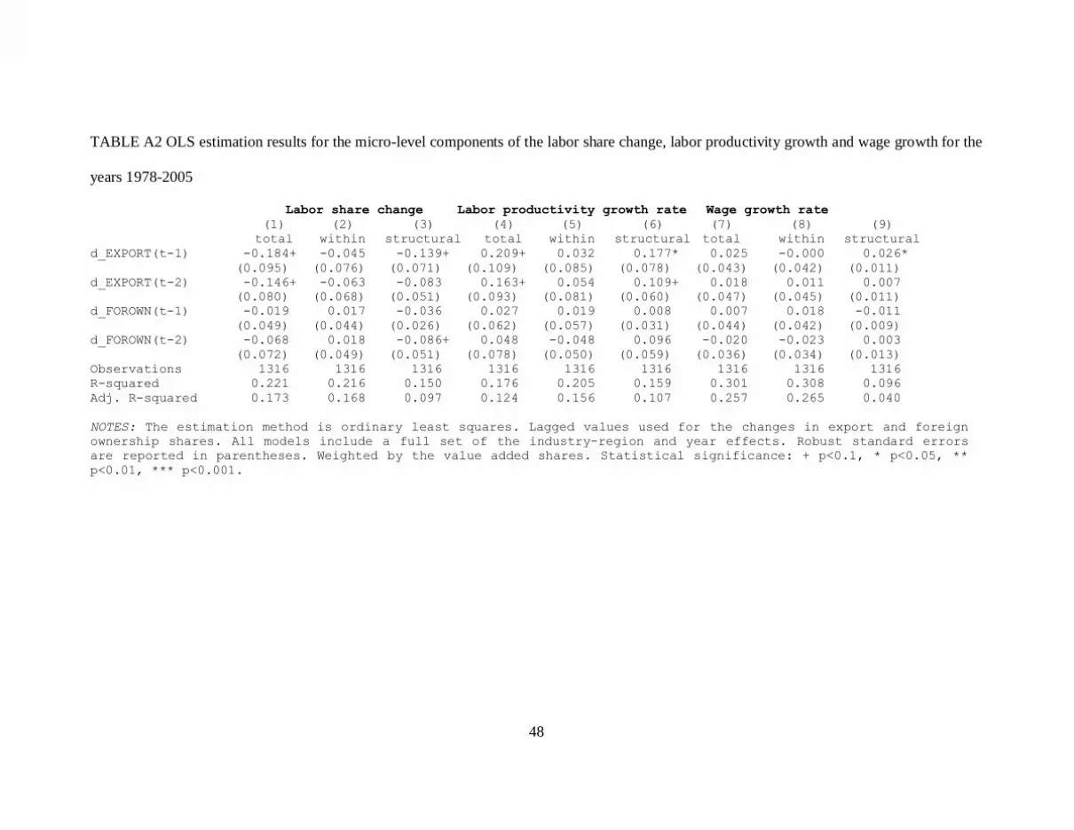
48

TABLE A2 OLS estimation results for the micro-level components of the labor share change, labor productivity growth and wage growth for the

years 1978-2005

Labor share change Labor productivity growth rate Wage growth rate (1) (2) (3) (4) (5) (6) (7) (8) (9) total within structural total within structural total within structural d_EXPORT(t-1) -0.184+ -0.045 -0.139+ 0.209+ 0.032 0.177* 0.025 -0.000 0.026* (0.095) (0.076) (0.071) (0.109) (0.085) (0.078) (0.043) (0.042) (0.011) d_EXPORT(t-2) -0.146+ -0.063 -0.083 0.163+ 0.054 0.109+ 0.018 0.011 0.007 (0.080) (0.068) (0.051) (0.093) (0.081) (0.060) (0.047) (0.045) (0.011) d_FOROWN(t-1) -0.019 0.017 -0.036 0.027 0.019 0.008 0.007 0.018 -0.011 (0.049) (0.044) (0.026) (0.062) (0.057) (0.031) (0.044) (0.042) (0.009) d_FOROWN(t-2) -0.068 0.018 -0.086+ 0.048 -0.048 0.096 -0.020 -0.023 0.003 (0.072) (0.049) (0.051) (0.078) (0.050) (0.059) (0.036) (0.034) (0.013) Observations 1316 1316 1316 1316 1316 1316 1316 1316 1316 R-squared 0.221 0.216 0.150 0.176 0.205 0.159 0.301 0.308 0.096 Adj. R-squared 0.173 0.168 0.097 0.124 0.156 0.107 0.257 0.265 0.040 NOTES: The estimation method is ordinary least squares. Lagged values used for the changes in export and foreign ownership shares. All models include a full set of the industry-region and year effects. Robust standard errors are reported in parentheses. Weighted by the value added shares. Statistical significance: + p<0.1, * p<0.05, ** p<0.01, *** p<0.001.

49

1 This conclusion depends on the form of the production function. Obviously with Cobb-Douglas there would

be no change in the labor share within industries.

2 On the other hand, in an analysis of productivity-enhancing restructuring in the Finnish manufacturing

industries, Maliranta (2005) finds evidence on the positive effects for imports but less so for exports.

3 Bartelsmans et al. (2009) note the same fact in the context of cross-country comparisons of productivity

dynamics.

4 Maliranta (2003) provides an illustration of the features of various methods applied in the literature. 5 Derivation of the Equations 1-2 is presented in the Appendix.

6 The assignment of plants to industries is not particularly problematic for two reasons. First, a plant is

defined in the Annual Industrial Statistics Survey as a local kind-of-activity unit. It is a specific physical

location, which is specialized in the production of certain types of products or services. Second, in this paper

we use a relatively aggregated industry classification.

7 Helpman et al. (2004) stress that multinational firms have the highest productivity. Therefore, they could be

especially important in productivity dynamics as well. It is unfortunate that we do not have this information

for our analysis for a long enough period. Because we take advantage of a panel of industries and regions, we

are not able to incorporate import penetration into the models by using OECD’s STAN database.

8 Ripatti and Vilmunen (2001), Sauramo (2004), and Kyyrä and Maliranta (2008) provide earlier evidence on

the development of the labor share in Finland.

9 In Southern and Western Finland the contribution of micro-level restructuring returned to the level of the

mid-’80s, whereas in Eastern Finland the effect has been zero since the mid-’90s. The trends of Northern

50

Finland follow those of the other regions except that variation has been stronger. Higher volatility of the

components may be partly due to the fact that this region is smaller than the others in terms of value added.

10 Prais and Winsten (1954) present the idea of the estimation method.

11 We have dropped one panel, which is the manufacture of telecommunication equipment in Eastern Finland,

because it has missing values in one year (1981) and had only a few plants in some other years. So we have a

balanced panel where the total number of observations in the baseline model is 4×12×28-28=1316.

12 The only exception is that the lead value of foreign ownership is significant at the 10% level in the model

for wage growth.

13 The estimates are not reported in the tables, but they are available upon request.

globalization, creative destruction, and labor share change: evidence on the determinants and...

Documents