arX

iv:0

804.

1513

v1 [

mat

h.D

G]

9 A

pr 2

008

GEOMETRY OF WHIPS AND CHAINS

STEPHEN C. PRESTON

1. Introduction

The purpose of this note is to explore the geometry of the inextensiblestring (or whip) which is fixed at one end and free at the other end. Inthe absence of gravity, the inextensible string is a geodesic motion inthe space of curves in R

2 parametrized by length and passing througha fixed point. This is a submanifold of the space of all curves in R

2,and the Lagrange multiplier from the constraint is the tension in thestring. Hence the string satisfies a wave equation, where the tensionis generated by the velocity implicitly by solving a one-dimensionalLaplace equation.

The situation seems closely analogous to the motion of an incom-pressible fluid, where the configuration space is the space of volume-preserving diffeomorphisms, a submanifold of the space of all diffeomor-phisms, and the Lagrange multiplier is the pressure. This is also a geo-desic motion, but the Riemannian geometry is still not well-understood.It is our hope that understanding the one-dimensional situation betterwill help in understanding the two- and three-dimensional versions.

Part of the problem with the inextensible string is that the geo-desic equation is not an ordinary differential equation on an infinite-dimensional manifold (unlike the situation for incompressible fluids).The derivative loss cannot be avoided, and thus one must treat it asa hyperbolic partial differential equation. However, since the tensionmust be zero at the free end, the equation degenerates at the free end,and the standard approach to symmetric hyperbolic equations mustbe modified to deal with this. Although these issues are not discussedhere, we will study them in a forthcoming paper.

The other serious issue is that since the tension is not given by apositive function of the speed, position, and time, but rather givenimplicitly by the solution of an ordinary differential equation, it is pos-sible for tension to become negative. This corresponds to the differen-tial equation changing type from hyperbolic to elliptic, and drasticallycomplicates the problem. We show that in the absence of gravity, the

1

2 STEPHEN C. PRESTON

tension is always nonnegative, while with gravity, the tension is non-negative as long as the string hangs below the fixed point.

To better understand the necessary conditions on weak solutions(which has remained controversial in recent papers on falling stringswith kinks), we consider the corresponding finite-dimensional model:a system of N particles linked by rigid massless rods. In the absenceof gravity, this is also a geodesic motion on an N -torus with a certainRiemannian metric. The geodesic equation ends up being a sort of dis-cretization of the wave equation for the inextensible string, which stillconserves energy. Furthermore, the tension in the chain converges tothe tension in the corresponding whip as N → ∞. As a result, the Rie-mannian curvature of T

N converges to the Riemannian curvature of thespace of curves, and one can therefore understand the geometry of theinfinite-dimensional space quite well by studying the finite-dimensionalapproximation.

This suggests that one may be able to use the same approach tostudy incompressible fluids. Namely, take a collection of particles ona torus T

2 in a grid, and constrain them so that the areas of quadri-laterals are constant. (One could consider constraining triangle areas,but this seems too rigid; it does not appear possible to approximatea general area-preserving diffeomorphisms by such maps.) The curva-ture of the finite-dimensional manifold should approach that of the fullarea-preserving diffeomorphism group, and hence one expects one couldunderstand the geometry of fluid mechanics well by a finite-dimensionalapproximation.

2. Discrete string

Let us compute the geometry of a discrete string (a chain), whichwe model by n + 1 point masses joined in R

2 by rigid rods of length 1n

whose mass is negligible. We assume the 0th point is fixed at the originwhile the nth point is free.

The unconstrained Lagrangian is

L =1

2

n∑

i=1

|xi|2 −

n∑

i=1

g〈xi, e2〉.

In addition the constraints are given by

|xi − xi−1|2 =

1

n2, 1 ≤ i ≤ n.

Therefore the equations of motion are

(1) xi = −ge2 + λi+1(xi+1 − xi) + λi(xi−1 − xi)

GEOMETRY OF WHIPS AND CHAINS 3

for 1 ≤ i ≤ n, where we are fixing x0 = 0 and λn+1 = 0 to make theequations satisfied also at the endpoints.

The constraint equations determine the Lagrange multipliers λ, whichare obviously just the discrete tensions. We get

|vi−vi−1|2 = −λi+1〈xi−xi−1,xi+1−xi〉+

2

n2λi−λi−1〈xi−xi−1,xi−1−xi−2〉

for 1 ≤ i < n (again using λn+1 = 0), while for i = 0 we get

|v1|2 − g〈x1, e2〉 = −λ2〈x1,x2 − x1〉 +

1

n2λ1.

We can simplify these λ-equations somewhat if we change variables.For each 1 ≤ i ≤ n, let xi = xi−1 + 1

n(cos θi, sin θi), where θi ∈ S1.

Then

〈xi − xi−1,xi+1 − xi〉 =1

n2cos (θi+1 − θi)

while

|vi − vi−1|2 =

1

n2|θi|

2.

So the constraint equation for λ becomes

(2) − cos (θi+1 − θi)λi+1 + 2λi − cos (θi − θi−1)λi−1 = |θi|2

for 2 ≤ i ≤ n and

(3) − cos (θ2 − θ1)λ2 + λ1 = |θ1|2 − ng sin θ1.

For the evolution equation, we have

(4) θi = λi+1 sin (θi+1 − θi) − λi−1 sin (θi − θi−1)

for 2 ≤ i ≤ n and

(5) θ1 = λ2 sin (θ2 − θ1) − ng cos θ1.

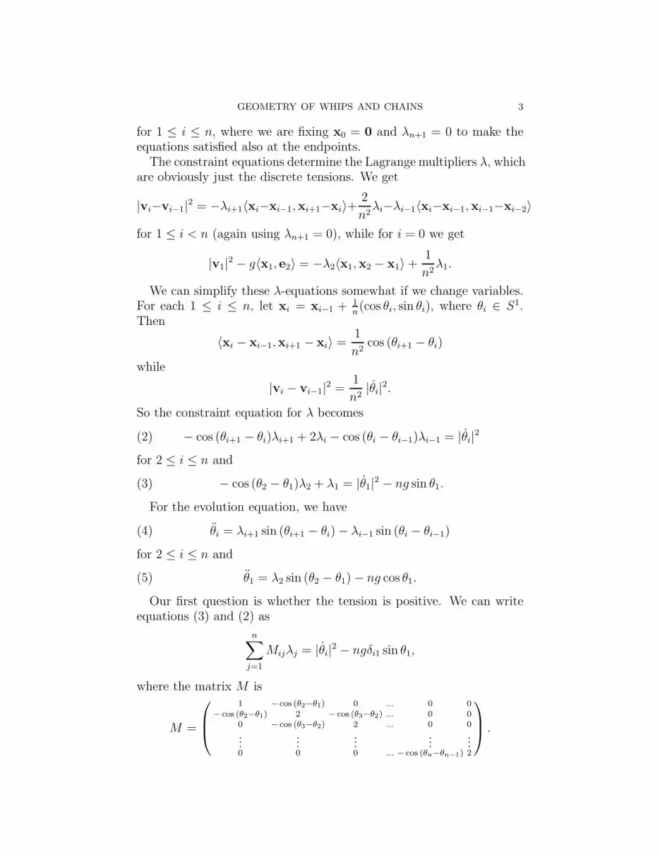
Our first question is whether the tension is positive. We can writeequations (3) and (2) as

n∑

j=1

Mijλj = |θi|2 − ngδi1 sin θ1,

where the matrix M is

M =

1 − cos (θ2−θ1) 0 ... 0 0− cos (θ2−θ1) 2 − cos (θ3−θ2) ... 0 0

0 − cos (θ3−θ2) 2 ... 0 0

......

......

...0 0 0 ... − cos (θn−θn−1) 2

.

4 STEPHEN C. PRESTON

If we let ai = cos (θi+1 − θi) for 1 ≤ i ≤ n−1, then standard Gaussianelimination yields

b1 −a1 0 ... 0 | 1 0 0 ... 0

0 b2 −a2 ... 0 |a1

b11 0 ... 0

0 0 b3 ... 0 |a1a2

b1b2

a2

b21 ... 0

......

...... |

......

......

0 0 0 ... bn |Qn−1

i=1

aibi

Qn−1

i=2

aibi

Qn−1

i=3

aibi

... 1

where the sequence bi is defined by b1 = 1, bi+1 = 2−a2

i

bi. Since |ai| ≤ 1

for every i, we see that every bi satisfies 1 ≤ bi ≤ 2.Reducing further, we obtain the inverse matrix

(6) M ij =

n∑

m=max i,j

1

bm

m−1∏

k=i

ak

bk

m−1∏

l=j

al

bl.

Thus the tensions are

λi = M i1(|θ1|2 − ng sin θ1) +

n∑

j=2

M ij |θj |2.

If every ai ≥ 0, then every component of M−1 is nonnegative. So aslong as |θi+1 − θi| ≤ π for every 1 ≤ i ≤ n − 1 and sin θ1 ≤ 0, we will

have all tensions λi ≥ 0, regardless of |θi|. If any ai < 0, then some

M ij < 0, and thus if θk = δjk, then λi < 0. Additionally, we always

have M11 > 0, so that if sin θ1 > 0, then when all θk = 0, we haveλ1 = −ngM11 sin θ1.

Let us now look at the curvature; we will assume for the momentthat g = 0 to get a purely geometric problem. We consider Mn = (S1)n

as a submanifold of R2n, with induced Riemannian metric given bythe kinetic energy formula above. We know that the equation of aconstrained geodesic is always

d2xk

dt2∂k = Bk

(

dxi

dt∂i,

dxj

dt∂j

)

∂k.

For any vector u ∈ TθMn, we have 〈uk −uk−1, xk −xk−1〉 = 0, for every1 ≤ k ≤ n. So uk − uk−1 = 1

nηk(− sin θk, cos θk) for some ηk ∈ R. In

terms of the η’s, we can write (using (4))

(7) Bk(u, u) = λ(u, u)k+1(xk+1 − xk) + λ(u, u)k(xk−1 − xk),

for 1 ≤ k ≤ n, where

(8) λ(u, u)i =

n∑

j=1

M ij |ηj|2.

GEOMETRY OF WHIPS AND CHAINS 5

Since the ambient space is flat, the curvature is, by the Gauss-Codazzi formula,

〈R(u, v)v, u〉 = 〈B(u, u), B(v, v)〉 − 〈B(u, v), B(u, v)〉.

To simplify this, we first compute

〈B(u, u), B(v, v)〉 =1

n2

n∑

k=1

λ(u, u)k+1λ(v, v)k+1 + λ(u, u)kλ(v, v)k

− λ(u, u)k+1λ(v, v)k cos (θk+1 − θk)

− λ(u, u)kλ(v, v)k+1 cos (θk+1 − θk)

=1

n2λ(v, v)1

(

λ(u, u)1 − λ(u, u)2 cos (θ2 − θ1))

+1

n2

n∑

k=2

2λ(u, u)kλ(v, v)k

− λ(u, u)k−1λ(v, v)k cos (θk − θk−1)

− λ(u, u)k+1λ(v, v)k cos (θk+1 − θk)

=1

n2

n∑

k=1

n∑

l=1

Mkl(θ)λ(u, u)lλ(v, v)k

=1

n2

n∑

i=1

n∑

j=1

M ij(θ)|ηi|2|ξj|

2.

Similarly we have

〈B(u, v), B(u, v)〉 =1

n2

n∑

i=1

n∑

j=1

M ij(θ)ηiξiηjξj.

Therefore the curvature is

(9) 〈R(u, v)v, u〉 =1

n2

n∑

i,j=1

M ij(θ)[

η2i ξ

2j − ηiξiηjξj

]

=1

2n2

n∑

i,j=1

M ij(θ)[

ηiξj − ηjξi

]2.

Thus the curvature is nonnegative in every section if and only if ev-ery M ij(θ) ≥ 0, which also happens if and only if every tension isnonnegative regardless of the initial velocity.

To get a bound on the curvature, we want a bound on the componentsM ij . We see from equation (6) that M ij ≤ max(n + 1 − i, n + 1 − j).The extreme case is when all θ’s are the same (so that ai = 1 forevery i), which corresponds to a straight string. Then we have M ij =

6 STEPHEN C. PRESTON

max(n + 1 − i, n + 1 − j). Therefore the sectional curvature satisfies0 < K < n.

3. Smooth string

Now let us consider the continuum model of an smooth inextensi-ble string. The configuration space is the set CL,0 of all C∞ mapsη : [0, 1] → R

2 such that η(0) = 0 and 〈η′(s), η′(s)〉 ≡ 1. This is aclosed submanifold of C0 = {η ∈ C∞([0, 1], Rd) | η(0) = 0}. The tan-gent spaces are

TηC0 = {X ∈ C∞([0, 1], R2) |X(s) ∈ Tη(s)R2 ∀s, X(0) = 0}

andTηCL,0 = {X ∈ TηC0 | 〈X

′(s), η′(s)〉 = 0 ∀s}.

The Riemannian metric is defined by

〈〈X, Y 〉〉 =

∫ 1

0

〈X(s), Y (s)〉η(s) ds.

In this metric, the orthogonal space to TηCL,0 is

(

TηCL,0

)⊥=

{

Y ∈ C∞([0, 1], R2)∣

∣

∣Y (s) =

d

ds

(

σ(s)η′(s))

for some σ ∈ C∞([0, 1], R) with σ(1) = 0}

.

The orthogonal projection of a vector X ∈ TηC0 should be

PL(X) = X −d

ds(ση′),

where σ satisfies

(10) σ′′(s) − 〈η′′(s), η′′(s)〉σ(s) = 〈X ′(s), η′(s)〉, σ(1) = 0,

but we have a problem with the boundary condition at s = 0. We wantPL to map into TηCL,0, but

PL(X)(0) = X(0) − σ′(0)η′(0) − σ(0)η′′(0) = −σ′(0)η′(0) − σ(0)η′′(0).

Now η′′(0) is orthogonal to η′(0), so if η′′(0) 6= 0, we need both σ(0) = 0and σ′(0) = 0, which will generally be impossible. So we do not havea nice orthogonal projection. There are two ways to get around this.

(1) Consider only curves with η′′(0) = 0. This forces X ′′(0) = 0 aswell, and then we have to worry about PL(X) also satisfying(PL(X))′′(0) = 0. This forces ηiv(0) = 0 and X iv(0) = 0, andso on... We end up being forced to require that all derivativesof η exist at s = 0 (which is why I assumed η ∈ C∞([0, 1], R2))and that all even derivatives of η vanish at s = 0. Alternatively,

GEOMETRY OF WHIPS AND CHAINS 7

η extends to a C∞ curve on [−1, 1] such that η(−s) = −η(s).This observation leads to the second idea.

(2) We could assume from the start that η is the restriction of anodd curve on [−1, 1]. Then the tangent space will automati-cally require X odd. We then have two boundary conditionsfor (10): σ(−1) = 0 and σ(1) = 0. Finally, the solution of (10)will automatically be even in s by symmetry, and then we canjust restrict to [0, 1]. The advantage of this approach is thatwe don’t need to assume any more smoothness than is abso-lutely necessary for (10) to make sense. This is of course thesame kind of trick that’s used to get simple solutions to theconstant-coefficient linear wave equation with one free and onefixed boundary.

Either of these two tricks will force σ′(0) = 0, so we may as well assumethis as our other boundary condition.

These difficulties do not arise if both ends of the curve are free.If both ends of the curve are fixed, we need oddness through both

endpoints, again as with the simplest wave equation.Now, the first thing we do with the orthogonal projection is to com-

pute the second fundamental form B : TηCL,0 × TηCL,0 →(

TηCL,0

)⊥

defined by B(X, Y ) = ∇XY − PL(∇XY ). We obtain

(11) B(X, Y ) =d

ds

(

σXY (s)η′(s))

where

(12) σ′′XY (s) − κ2(s)σXY (s) = −〈X ′(s), Y ′(s)〉.

This formula implies the geodesic equation

d2η

dt2= B

(

dη

dt,dη

dt

)

,

or more explicitly,

ηtt(s, t) = ∂s

(

σXX(s, t)ηs(s, t))

,

∂2sσXX(s, t) − |ηss(s, t)|

2σXX(s, t) = −|ηst(s, t)|2,

with boundary conditions as discussed.If we want to incorporate gravity, then we have

ηtt(s, t) = ∂s

(

σ(s, t)ηs(s, t))

− ge2(13)

σss(s, t) − |ηss(s, t)|2σ(s, t) = −|ηst(s, t)|

2,(14)

with boundary condition σ(1, 0) = 0. To determine the boundarycondition at s = 1, we assume ηss(0, t) = 0 as before. If we want

8 STEPHEN C. PRESTON

ηtt(0, t) = 0, we must have σs(0, t)ηs(0, t) = ge2, which cannot be sat-isfied unless e2 ‖ ηs(0, t). Instead, motivated in part by the finite caseabove, we set σs(0, t) = g〈e2, ηs(0, t)〉, which is equivalent to forcingthe acceleration parallel to the curve to be zero.

If, as before, we use the fact that |ηs| ≡ 1 to write ηs(s, t) =(

cos θ(s, t), sin θ(s, t))

, then differentiating the first of equations (13)with respect to s yields

θtt(s, t) = 2σs(s, t)θs(s, t) + σ(s, t)θss(s, t)(15)

σss(s, t) − θs(s, t)2σ(s, t) = −θt(s, t)

2(16)

with boundary conditions σs(0, t) = g cos θ(0, t) and σ(1, t) = 0.Now we want to compute the curvature; again we assume g = 0 to get

a purely geometric formula. Formula (11) gives, via the Gauss-Codazziequations, the curvature formula:

〈〈R(X, Y )Y, X〉〉 = 〈〈B(X, X), B(Y, Y )〉〉 − 〈〈B(X, Y ), B(X, Y )〉〉

=

∫ 1

0

⟨

d

ds

(

σXX(s)η′(s))

,d

ds

(

σY Y (s)η′(s))

⟩

−

⟨

d

ds

(

σXY (s)η′(s))

,d

ds

(

σXY (s)η′(s))

⟩

ds

=

∫ 1

0

σXX(s)(

− σ′′Y Y (s) + κ2(s)σY Y (s)

)

ds

−

∫ 1

0

σXY (s)(

− σ′′XY (s) + κ2(s)σXY (s)

)

ds.

If we denote the Green function of equation (12) by G(s, q), so that

σXY (s) =

∫ 1

0

G(s, q)〈X ′(q), Y ′(q)〉 dq,

then the curvature formula becomes

〈〈R(X, Y )Y, X〉〉 =

∫ 1

0

∫ 1

0

G(s, q)(

|X ′(q)|2 |Y ′(s)|2

− 〈X ′(q), Y ′(q)〉 〈X ′(s), Y ′(s)〉)

ds dq

=1

2

∫ 1

0

∫ 1

0

G(s, q)

d∑

i,j=1

(

X ′i(s)Y

′j (q) − X ′

j(q)Y′i (s)

)2ds dq,

using the symmetry of the Green function. Thus if G(s, q) ≥ 0 for alls and q, we get nonnegative curvature.

GEOMETRY OF WHIPS AND CHAINS 9

To prove positivity of G(s, q), we first compute:

G(q, q) =

∫ 1

0

G(s, q) δ(s − q) ds

= −

∫ 1

0

G(s, q)(

Gss(s, q) − κ2(s)G(s, q))

ds

=

∫ 1

0

Gs(s, q)2 + κ2(s)G(s, q)2 ds > 0.

So G(q, q) > 0. We also know that Gs(s = q+, q)−Gs(s = q−, q) = −1.Since the boundary conditions are Gs(0, q) = 0 and G(1, q) = 0, wecan say the following.

(1) If G(0, q) < 0, then G(s, q) < 0 for s near 0. As long asG(s, q) < 0, we have Gss(s, q) ≤ 0, which implies Gs is non-increasing. Since Gs(0, q) = 0, this means Gs(s, q) ≤ 0 as longas G(s, q) < 0. Thus there is no way G(s, q) can increase to 0or any positive number on 0 < s < q. This makes G(q, q) > 0impossible, a contradiction. Therefore G(0, q) > 0, and further-more G(s, q) > 0 for all s ∈ (0, q).

(2) If Gs(1, q) > 0 then G(s, q) < 0 for s close to 1. As long asG(s, q) < 0, we have Gss(s, q) ≤ 0, and so Gs(s, q) is nonincreas-ing. So Gs(s, q) > 0 as long as G(s, q) < 0, so G cannot havea turning point on q < s < 1. This again makes G(q, q) > 0impossible, implying a contradiction. So Gs(1, q) < 0, whichimplies G(s, q) > 0 for all s ∈ (q, 1).

This proves that the curvature is nonnegative as long as η is smooth.In fact the sectional curvature must be strictly positive in all nontrivialtwo-planes, since it can only vanish if there is a c such that X ′(s) =cY ′(s) for every s. Since X(0) = Y (0), we must have X(s) = cY (s) forall s, which means X and Y are linearly dependent in TηCL,0.

Polarizing the formula for curvature, we obtain

〈〈R(Y, X)X, W 〉〉 =

∫ 1

0

∫ 1

0

G(s, q)(

|X ′(q)|2 〈Y ′(s), W ′(s)〉

− 〈X ′(q), Y ′(q)〉 〈X ′(s), W ′(s)〉)

ds dq

= −

∫ 1

0

∫ 1

0

(

|X ′(q)|2⟨

∂

∂s

(

G(s, q)Y ′(s))

, W (s)

⟩

+ 〈X ′(q), Y ′(q)〉

⟨

∂

∂s

(

G(s, q)X ′(s))

, W (s)

⟩

ds dq.

10 STEPHEN C. PRESTON

Therefore the curvature operator is

Y 7→ PL

( ∂

∂s

[

∫ 1

0

G(s, q)(

− |X ′(q)|2Y ′(s) + 〈X ′(q), Y ′(q)〉X ′(s))

dq]

.

Even for smooth X, this operator is not bounded in L2. (By contrast,the curvature operator in the volumorphism group for a fixed C1 vectorfield X is bounded in L2 and in any other Sobolev space.)

4. Convergence

We don’t have a good existence and uniqueness result for the continu-ous equation; the closest we have is Reeken [R2], who proved short-timeexistence for a chain in R

3 in something like the Sobolev space H17 withinitial conditions close to a chain hanging straight down (for technicalreasons, Reeken assumes the chain is hanging from (0, 0,∞) with non-constant gravity). This result is already quite difficult. It is conceivablethat we could get a simpler result using the two-dimensional equationderived above. Of course, the finite-dimensional approximation is theflow of a vector field on a compact manifold (a bounded subset of thetangent space T (S1)n, since the kinetic energy is bounded). Thus thefinite-dimensional approximation has a unique solution existing for alltime and for any n. We can thus ask whether solutions of the PDE canbe constructed as limits of the ODE as n → ∞.

It is easy to see that if we knew a smooth solution of the PDE existed,then the discrete model would converge to it. Let us write

θn :

{

1

n,2

n, . . . , 1

}

× R → S1 and σn :

{

1

n,2

n. . . , 1

}

× R → R.

We will set θn( kn, t) = θk(t) and σn( k

n, t) = 1

n2 λk(t) for 1 ≤ k ≤ n.Then equations (2) and (4) become

(17)d2

dt2θn

(

kn, t

)

= n2σn

(

k+1n

, t)

sin[

θn

(

k+1n

, t)

− θn

(

kn, t

)]

− n2σn

(

k−1n

, t)

sin[

θn

(

kn, t

)

− θn

(

k−1n

, t)]

and

(18) − cos[

θn

(

k+1n

, t)

− θn

(

kn, t

)]

σn

(

k+1n

, t)

+ 2σn

(

kn, t

)

− cos[

θn

(

kn, t

)

− θn

(

k−1n

, t)]

σn

(

k−1n

, t)

=1

n2

(

d

dtθn

(

kn, t

)

)2

The operators appearing in equations (17) and (18) are symmet-ric discretizations of derivative operators; if σ and θ are sufficiently

GEOMETRY OF WHIPS AND CHAINS 11

smooth, we can write

n2σ(

x + 1n, t

)

sin[

θ(

x + 1n, t

)

− θ(

x, t)]

− n2σ(

x − 1n, t

)

sin[

θ(

x, t)

− θ(

x − 1n, t

)]

= σ(x)θ′′(x) + 2σ′(x)θ′(x) + O(

1n2

)

and

− n2 cos[

θ(

x + 1n, t

)

− θ(

x, t)]

σ(

x + 1n, t

)

+ 2n2σ(

x, t)

− n2 cos[

θ(

x, t)

− θ(

x − 1n, t

)]

σ(

x − 1n, t

)

= θ′(x)2σ(x) − σ′′(x) + O(

1n2

)

where the constant in O(

1n2

)

depends on the C4 norms of both θ andσ.

Therefore, we can say that if σ and θ form a sufficiently solution of(13), then the motion of the discrete chain with n elements convergesto the motion of the smooth chain as n → ∞. We have convergence notonly of the position and velocity, but also of the acceleration and thetension, which is not necessarily typical (for example, a system withstrong returning force to a submanifold has position and velocity con-verging to the geodesic motion on the submanifold, but the accelerationdoes not converge).

Because the convergence is so strong, we can speculate about conver-gence of the motion in the nonsmooth case. Suppose the continuousstring has a kink in it. There has been some serious analysis of thepossible jump conditions one should impose on the equations in thiscase. See for example Reeken [R1], who used energy conservation andmomentum conservation to classify possible motions of a kink. AlsoD. Serre used an approach similar to yours, relaxing the constraint to|x′(s)| ≤ 1 and requiring that the tension always be nonnegative, andderived jump conditions. But this only sets up the differential equa-tions, and there’s no guarantee that they have solutions. (Serre foundblowup phenomena in a couple of examples.)

Indeed, since we expect the motion of n constrained particles to con-verge to the motion of a chain, the fact that the particles can (ideally)support negative tension in certain motions (when there is an acute-angle kink or when the chain starts with the first link above the fixedpoint) seems to suggest that the motion of the continuous string shouldalso support negative tension. Of course this destroys the actual equa-tions, which suggests that the motion of n constrained particles has nolimit in some cases.

12 STEPHEN C. PRESTON

We will look at the limit as n → ∞ by examining the inverse ma-trix M ij given by (6). We expect the components of this matrix to

converge to the Green function as 1nM ij ≈ G

(

in, j

n

)

. To understand

what happens to M ij , we first look at the sequence bi appearing in itsdefinition. We have

bi+1 = 2 −a2

i

bi

, where ai = cos (θi+1 − θi).

Now if the discrete curve approaches something smooth, then we willhave

θi+1 − θi ≈1

nκi,

where κi = θ( i+1/2

n

)

, the approximate curvature. Thus as long as thecurve is smooth, we will have ai ≈ 1 and thus also bi ≈ 1.

Numerically experimenting, we find that the sequence bi is approxi-mated very well by

(19) bi = 1 +1

nf(

in

)

,

where f satisfies the differential equation

(20) f ′(s) = κ2(s) − f 2(s),

with initial condition f(0) = 0. This equation of course comes fromthe Riccati trick f(s) = y′(s)/y(s), where y′′(s) − κ2(s)y(s) = 0.

Now suppose there is a kink in the curve, say of angle α at positionso with so ≈ k/n for some integer k. Then θk+1−θk = α, and so all ai’sare close to 1 except for ak = cos α. We then have bk+1 being ratherfar from 1, which means for equation (19) to be valid, we must havelims→so

f(s) = +∞. In fact this is precisely what happens numerically: f

satisfies equation (20) to the left of so with initial condition f(0) = 0; falso satisfies (20) to the right of so with condition lim

s→so

f(s) = +∞. In

particular, f does not depend on the size of the kink, only the fact thatthere is one. If there are multiple kinks, we get the same condition: fapproaches infinity from the right side of the kink.

Knowing ai and bi, we know M ij . Recall from (6) the formula

M ij =n

∑

m=max i,j

1

bm

m−1∏

k=i

ak

bk

m−1∏

l=j

al

bl

.

GEOMETRY OF WHIPS AND CHAINS 13

Pick any x and y in [0, 1] and s ≥ max(x, y). For large n, choose i = nx,

j = ny, and m = ns. Since ak ≈ 1 −κ2

k

2n2 except at the kink, we have

ns−1∏

k=nxak →

{

1 if so /∈ (x, s)

cos α if so ∈ (x, s)as n → ∞

for any x and s. On the other hand, we have

ns−1∏

k=nxbk = exp

ns−1∑

k=nxln

[

1 +1

nf(k

n

)]

= exp

1

n

ns−1∑

k=nxf(k

n

)

+ O(1

n

)

→ exp

(∫ s

x

f(σ) dσ

)

.

Thus we have

G(x, y) =

∫ 1

max(x,y)

φ(x, s)φ(y, s)e−R s

xf(σ) dσe−

R s

yf(τ) dτ ds

where

φ(x, s) =

{

cos α x < so < s

1 otherwise.

Thus we see G(x, y) ≥ 0 even if the curve has one or more kinks. Soin the absence of gravity, the curvature is nonnegative in all sections.

If there is gravity, then G(x, y) may be negative, if the string ispointing upwards at the fixed point. If we use a generalized curvaturethat incorporates the Hessian of the potential energy, then we will alsoget negative generalized curvature in this case.

References

R1. M. Reeken, The equation of motion of a chain, Math. Z. 155 no. 3, 219–237(1977).

R2. M. Reeken, Classical solutions of the chain equation I, Math. Z. 165 143–169(1979).

S. D. Serre, Un modele relaxe pour les cables inextensibles. RAIRO Modl. Math.Anal. Numr. 25, no. 4, 465–481 (1991).

Department of Mathematics, University of Colorado, Boulder, CO

80309-0395

E-mail address : Stephen.Preston@colorado.edu