Geodesic Shooting for Computational Anatomy

MICHAEL I. MILLER,Center of Imaging Science & Department of Biomedical Engineering, The John HopkinsUniversity, 301 Clark Hall, Baltimore, MD 21218, USA

ALAIN TROUVÉ, andCMLA, ENS de Cachan, 61 Avenue du Président Wilson, 94235 Cachan CEDEX, France

LAURENT YOUNESCenter for Imaging Science & Department of Applied Math and Statistics, The Johns Hopkin,3245 Clark Hall, Baltimore, MD 21218, USAMICHAEL I. MILLER: mim@cis.jhu.edu; ALAIN TROUVÉ: trouve@cmla.ens-cachan.fr; LAURENT YOUNES:laurent.younes@jhu.edu

AbstractStudying large deformations with a Riemannian approach has been an efficient point of view togenerate metrics between deformable objects, and to provide accurate, non ambiguous and smoothmatchings between images. In this paper, we study the geodesics of such large deformationdiffeomorphisms, and more precisely, introduce a fundamental property that they satisfy, namelythe conservation of momentum. This property allows us to generate and store complexdeformations with the help of one initial “momentum” which serves as the initial state of adifferential equation in the group of diffeomorphisms. Moreover, it is shown that this momentumcan be also used for describing a deformation of given visual structures, like points, contours orimages, and that, it has the same dimension as the described object, as a consequence of thenormal momentum constraint we introduce.

1. IntroductionOver the past several years we have been studying natural shapes using homogeneous orbitsof imagery constructed via the action of transformation groups on exemplars or templates.The mathematical structure of group action as a model in image analysis has been pioneeredby Grenander [13], the idea being to introduce the group actions in the very nature of theobjects themselves, through the notion of deformable templates. Roughly speaking, adeformable template simply is an “object or exemplar” Itemp on which a group G acts andgenerates, through the orbit = G · Itemp, a whole family of new objects. The interest of thisapproach is to concentrate the modeling effort on the group G, and not on the family ofobjects .

Since the earliest introduction by Silicon Graphics Incorporated of special purpose graphicshardware for object rendering, group action as a model in image analysis has been thesubject of a wide range of research in computer vision. Naturally, the analytical andcomputational properties of the low-dimensional matrix Lie groups form the core dogma ofmodern Computer graphics. In sharp contrast, however, for the study of imagery generatedfrom natural or biological shapes, the finite dimensional matrix groups are replaced by theirinfinite dimensional analogue, the more general diffeomorphisms [7,11,16,22,23,36].

NIH Public AccessAuthor ManuscriptJ Math Imaging Vis. Author manuscript; available in PMC 2010 July 6.

Published in final edited form as:J Math Imaging Vis. 2006 January 31; 24(2): 209–228. doi:10.1007/s10851-005-3624-0.

NIH

-PA Author Manuscript

NIH

-PA Author Manuscript

NIH

-PA Author Manuscript

The anatomical orbit or deformable template is made into a metric space with a metricdistance between elements by constructing curves through the space of diffeomorphismsconnecting them; the length of the curve becomes the basis for the construction, the metricdistance corresponding to the geodesic shortest length curves. This gives rise to a naturalvariational problem describing the geodesic flows between elements in the orbit, with thesolution of the associated Euler-Lagrange equations giving the optimal flow ofdiffeomorphisms and thus the metric between the shapes. The obtained setting shares severalsimilarities with the mechanics of perfect fluids, for which the Euler-Lagrange equation hasbeen derived by Arnold (Eq. (1) of [2]) for the group of divergence-free volume-preservingdiffeomorphisms. As well these results become another example of the general Euler-Poincaré principle of [19] applied to an infinite dimensional setting.

Interestingly, as emphasized by Arnold [1] in his study, one of the most beautiful aspects ofstudying diffeomorphisms with a Lie group point of view is that many fundamental aspectswhich can be proved in the finite dimensional case can be formally extended to retrievewell-known equations of mechanics. One of the purposes of this paper is to develop infinitedimensional analogues, for the study of high dimensional shapes via diffeomorphisms, ofseveral of the well known properties of Lie groups in rigid body mechanics. In particular weshall focus on the interpretation of the Euler equation as an expression of the evolution ofthe generalized momentum of diffeomorphoc flow of least energy in both Eulerian andLagrangian coordinates.

Such a point of view will link our geodesic formulation to a conservation of momentum lawin Lagrangian coordinates providing a powerful method for studying and modelingdiffeomorphic evolution of shape. It will imply that the momentum of the diffeomorphicflow at any place along the geodesic can be generated from the momentum at the origin,thus providing the vehicle for geodesic generation via shooting.

This same conservation of momentum of the diffeomorphic flow, allows us to deriveequations for the geodesic evolution of the elements in the orbit , t ∈ [0, 1], I ∈ .This unifies various geodesic evolutions associated with orbits of sparse finite dimensionallandmarked shapes as well as the evolutions of dense images. Of special interest is the factthat for the special case of image matching, geodesic evolution of elements in the orbit linksus to the notion of normal motion familiar to the rapidly growing community working inlevel set methods. Interestingly, as we show, the momentum of the diffeomorphic flow isnormal to the level sets associated with geodesic motion. By solving the partial differentialequations which are associated with the conservation of momentum, we will be able tocontrol by specifying the initial conditions (within a specific class of momentum whichdepends on the considered imaging problem) a wide range of arbitrarily large deformations;this provides new possibilities for learning shape models of deformable templates, or fordesigning new numerical matching procedures.

This second point of view in terms of the conservation of momentum law also sheds newlight on a large number of high dimensional evolution based Active Model Methods inComputer Vision, including active snakes and contours [6,12,18,20,29,31,37,40,41,43],active surfaces and deformable models [8,9,21,24,25,28,30,33,39,40,42]. In such approachesvector fields are defined which give the boundary manifold of the shape some velocity ofmotion, usually following the gradient of an energy to form an attractive force to pull theboundary. The power of such methods is that they parameterize motion only associated witha submanifold of the imagery, not the entire extrinsic background space. For example, todeform a planar simply connected shape via an active contour method, the dimension of themotion is determined by the dimension of the boundary of the region, which is substantiallyless than the dimension of the plane. Historically such approaches have not been studied

MILLER et al. Page 2

J Math Imaging Vis. Author manuscript; available in PMC 2010 July 6.

NIH

-PA Author Manuscript

NIH

-PA Author Manuscript

NIH

-PA Author Manuscript

globally as diffeomorphic action. In fact it is well known that such methods cannot preventself intersection nor ensure topological consistency, for which the addition of otherconstraints become necessary [14,15]. From the conservation law in Lagrangian coordinatesdescribing geodesic motion in the metric space of diffeomorphic action, we introduce thenormal momentum motion which constrains the momentum to the bounding manifold, andextends the velocity of motion of the shape to the entire background space, thereby givingthe global property that the resulting integrated vector field generates a diffeomorphism onthe entire extrinsic space. This in turn carries the smooth submanifold diffeomorphically. Asthe analysis shows, this global property seems to be required to generate geodesic motions.

2. The Basic Set Up2.1. Right Invariant Metric on Group of Diffeomorphisms

The basic component of our models is the group of one-to-one, smooth, transformations(diffeomorphisms) of a bounded subset Ω ⊂ ℝd. In this paper, we consider diffeomorphismsemerging as flows of non-autonomous differential equations. A time dependent vector fieldon Ω is a function:

(v(t, x) will also be denoted vt(x)). The associated ordinary differential equation is

The flow of this ODE is a function φv which depends on time and space, such that

and φ(0, x) = x for all x ∈ Ω. We will also use the notation for φ(t, x) and

(1)

It is well-known that, under some smoothness conditions on v, such is at all times adiffeomorphism of Ω.

The groups that we consider are precisely composed with such flows for v belonging to aspecified functional class. More precisely, we assume that a Hilbert space ℊ is given, theelement of which being smooth enough vector fields on Ω, and denote the norm and innerproduct on this space by || ||ℊ, ⟨,⟩ℊ. We now define (following [35]) the group G as the set offunctions for time-dependent vector fields v satisfying

MILLER et al. Page 3

J Math Imaging Vis. Author manuscript; available in PMC 2010 July 6.

NIH

-PA Author Manuscript

NIH

-PA Author Manuscript

NIH

-PA Author Manuscript

i.e. for v belonging to L1([0, 1], ℊ). We will always assume that ℊ can be embedded in thespace of ( , || ||1, ∞), containing vector fields on Ω, which vanish on ∂Ω, where

From this definition, it appears that the main ingredient in the construction of G is theHilbert space ℊ.

Fixing v ∈ ℊ, one can define the linear form w ↦ ⟨v, w⟩g, which will be denoted Lv. Wetherefore have the identity

(we use the standard notation (M, w) for the linear form M applied to w). By definition, Lvbelongs to the dual, ℊ* of ℊ, and L can be seen as an operator L: ℊ → ℊ* (this is the canonicalduality operator of ℊ on its dual). As we shall see, this operator turns out to be a key featurein our analysis. For the moment, we point out the fact that Lv is a linear form on ℊ which is aspace of smooth vector fields. Therefore, Lv itself can be a singular object (a generalizedfunction, or a distribution). Here are a few examples of distributions M which qualify aselements of ℊ*, under our running assumption that ℊ is embedded in the space of C1

functions:

i. L1 vector fields of Ω: if ψ: Ω ↦ ℝd is integrable, define

ii. Let now μ be any measure on Ω, and ψ be μ integrable. Define

iii. Dirac measures: as a particular case of the previous, define, for x ∈ Ω and a ∈ ℝd,

This will be denoted .

iv. Differential operators: if (fi, j, 1 ≤ i, j ≤ d) are integrable functions, define

MILLER et al. Page 4

J Math Imaging Vis. Author manuscript; available in PMC 2010 July 6.

NIH

-PA Author Manuscript

NIH

-PA Author Manuscript

NIH

-PA Author Manuscript

It is important to notice that, although L is defined in a rather abstract way in the previouslines, numerical procedures to compute geodesics can be derived most of the time from theknowledge of its inverse (of Green kernel) K = L−1. This K is a smoothing kernel, the choiceof which, within a specific range of available kernels, being the starting point of anypractical procedure. We do not detail numerical algorithms in this paper, but the reader canrefer to [4,5,17,23] for examples of choices of K.

2.2. Energy and Momenta

Consider a time-dependent diffeomorphism v ∈ L1([0, 1], ℊ), and let ( , t ∈ [0, 1]) be theassociated flow, defined in the previous section. Along time, each point x ∈ Ω, considered asa particle, evolves on the trajectory , its velocity at time t being by definition

. In other terms, for y ∈ Ω, vt(y) is the instantaneous velocity of the particle which isat y at time t. It is called the Eulerian velocity at y at time t.

So, at each time, we have an Eulerian velocity field, y ↦ vt(y), and we define the kinetic

energy of the system to be . The total energy spent during the deformation pathnow is

Note that, in classical fluid mechanics, the kinetic energy is the sum of particle kineticenergies, which, for a homogeneous fluid with mass density given by ρ yields

This is the L2 norm of v, which cannot be used in our context, since we require that ℊ isembedded in (we need some kind of Sobolev norms). However, in analogy with standardmechanical systems, we may define the global momentum of the system at time t to be thelinear form Mt ∈ ℊ* such that E(vt) = (Mt, vt)/2, which, with the notation of the previoussection, yields.

So, if vt is the Eulerian velocity field at time t, the momentum at time t is given by Lvt. Itwill be called the momentum in Eulerian coordinates.

2.3. Lagrangian and Eulerian FramesThe Eulerian frame, as introduced above, describes mechanical quantities as they areobserved in the current configuration at each time. The Lagrangian frame, on the contrary,

MILLER et al. Page 5

J Math Imaging Vis. Author manuscript; available in PMC 2010 July 6.

NIH

-PA Author Manuscript

NIH

-PA Author Manuscript

NIH

-PA Author Manuscript

describes quantities as seen from the initial configuration. For example, the diffeomorphism provides the position at time t of the particle which was at x at time 0, which is a

Lagrangian notion. For the velocity, we create a Lagrangian velocity field by pulling backthe previously defined velocity vt, setting

The operation

defines a fundamental Lie group operation, and is called the adjoint action of G on its Liealgebra (which here is ℊ), denoted Adφv. We have obtained the relation

To interpret the adjoint action pictorially, the new vector field under the adjoint action v →(dφ)v ◦ φ−1 has to be interpreted as the transformation of v under the deformation generatedby φ. Figure 1 shows how the field vl at location x is transported by the flow to the value v(y)at location y = φ(x) by pushing forward (using φ) the Lagrangian frame on which vl isdrawn. Note that the orientation of the vector v(x) drawn on the deformed sheet is alsochanged (through the action of (dφ)).

2.4. Momentum in Eulerian and Lagrangian CoordinatesThe momentum Mt = Lvt, which has been defined in Eulerian coordinates, also admits aLagrangian version. It can be computed by expressing the kinetic energy at time t, which is(Lvt, vt)/2, under the form , being then the Lagrangian momentum. This isstraightforward, since, by definition of an adjoint operator:

This leads to the definition for the momentum in Lagrangian coordinates. TheLagrangian frame takes here the role of a Galilean, or reference frame, and we will retrievebelow the fundamental principle of mechanics, which states that the Lagrangian momentumis constant over time along any energy minimizing path. Before this, we make a briefinteruption in our discussion to describe the relation between the classical mechanics of arigid body, and geodesic equation in matrix Lie groups. This simple description will help tounderstand the formalism in our infinite dimensional group of diffeomorphisms.

MILLER et al. Page 6

J Math Imaging Vis. Author manuscript; available in PMC 2010 July 6.

NIH

-PA Author Manuscript

NIH

-PA Author Manuscript

NIH

-PA Author Manuscript

3. Euler Equation and Conservation of the Momentum for Lie Groups ofMatrices

In this part, we derive the Euler equation for extremal paths of the kinetic energy in the caseof Lie groups of matrices. This derivation is well-known in the context of classical solidmechanics [1], but this simpler case, which can be derived completly without too muchtechnicalities, may be helpful to understand the case of diffeomorphisms.

Let G ⊂ ℳd(ℝ) be a Lie group of d × d matrices with Lie algebra ℊ. The case of interest iswhen G is a group of 3D rotations, which models the position of a rigid body with fixedcenter of mass. In this case, ℊ is the vector space of antisymmetric 3 × 3 matrices. Let t ↦ gtbe a trajectory in this group. Then, the angular velocity at ∈ ℊ is given by the equation

. This is to be related to our previous definition of Eulerian velocity, which was

in which the (left) product of matrices is replaced by the (right) composition of functions.

Returning to the matrix case, we define the kinetic energy at time t to be (Jat, at)/2, for somesymmetric positive definite operator J: ℊ → ℊ*. In the case of the rigid body, the angularvelocity can be identified to a 3-vector ωt, and J can be seen as a 3 × 3 matrix which onlydepends on the geometry of the object, called the inertia operator and, with some abuse ofnotation,

(note that here the notation (,) refers to the sum of products of coordinates, i.e. the usualinner product on Euclidean spaces, after identification between ℊ and ℊ*). The total energy is

We retrieve again the analogy with the diffeomorphisms by letting

so that J takes the role of L in the previous section.

We now compute the Euler equation for least energy paths between two fixed endpoints g0and g1. We recall that the Lie bracket on ℊ is [a, b] = ab − ba.

Theorem 1The Euler-Lagrange equation for the kinetic energy is given by

MILLER et al. Page 7

J Math Imaging Vis. Author manuscript; available in PMC 2010 July 6.

NIH

-PA Author Manuscript

NIH

-PA Author Manuscript

NIH

-PA Author Manuscript

(2)

where is defined by duality through the equalities .

Proof—Let (t ↦ g0(t)) be an extremal curve for the kinetic energy and ((t, h) ↦ g(t, h)) bea smooth deformation around h = 0 (g(t, 0) = g0(t)): Let a(t, h) and A(t, h) be such that

(3)

Writing , we get i.e.

(4)

The curve A(t, h) can vary freely in ℊ, with boundary conditions A(0, h) = A(1, h) = 0. From

we get

(5)

Using the duality relation, we get so that by integration by part, wefinally obtain the Euler equation

(6)

We know from Lagrangian mechanics that the motion of a body with inertial operator Jwithout external forces are extremal paths of the kinetic energy. Hence, Eq. (6) is theevolution equation of a body. We recognize in this equation the momentum to the body

and the Euler equation is then:

(7)

The momentum in the body here is to relate to the momentum in Eulerian coordinates fordiffeomorphisms. However, if we study the motion of the body in a fixed static reference

MILLER et al. Page 8

J Math Imaging Vis. Author manuscript; available in PMC 2010 July 6.

NIH

-PA Author Manuscript

NIH

-PA Author Manuscript

NIH

-PA Author Manuscript

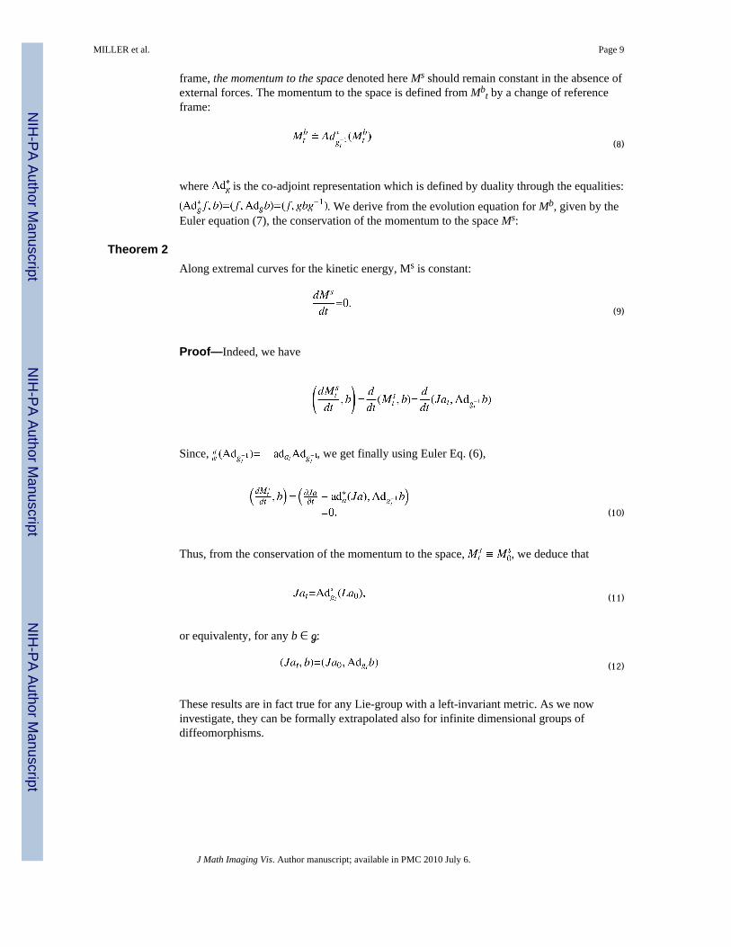
frame, the momentum to the space denoted here Ms should remain constant in the absence ofexternal forces. The momentum to the space is defined from Mb

t by a change of referenceframe:

(8)

where is the co-adjoint representation which is defined by duality through the equalities:

. We derive from the evolution equation for Mb, given by theEuler equation (7), the conservation of the momentum to the space Ms:

Theorem 2Along extremal curves for the kinetic energy, Ms is constant:

(9)

Proof—Indeed, we have

Since, , we get finally using Euler Eq. (6),

(10)

Thus, from the conservation of the momentum to the space, , we deduce that

(11)

or equivalenty, for any b ∈ ℊ:

(12)

These results are in fact true for any Lie-group with a left-invariant metric. As we nowinvestigate, they can be formally extrapolated also for infinite dimensional groups ofdiffeomorphisms.

MILLER et al. Page 9

J Math Imaging Vis. Author manuscript; available in PMC 2010 July 6.

NIH

-PA Author Manuscript

NIH

-PA Author Manuscript

NIH

-PA Author Manuscript

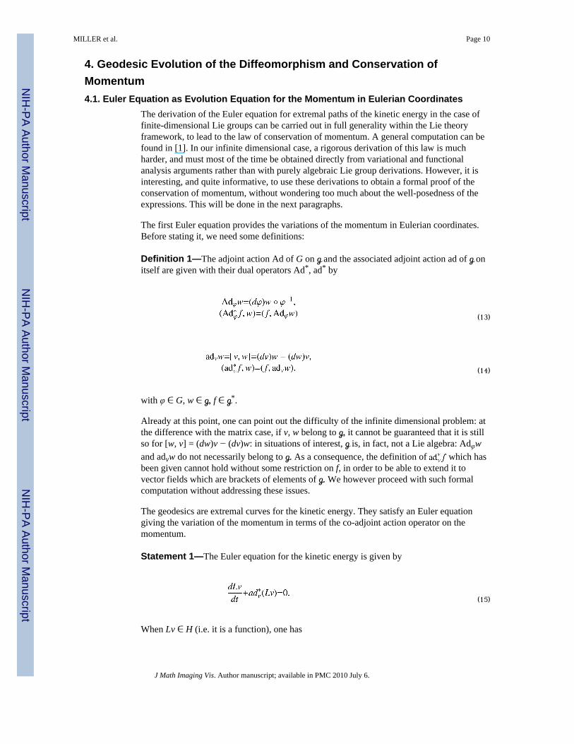
4. Geodesic Evolution of the Diffeomorphism and Conservation ofMomentum4.1. Euler Equation as Evolution Equation for the Momentum in Eulerian Coordinates

The derivation of the Euler equation for extremal paths of the kinetic energy in the case offinite-dimensional Lie groups can be carried out in full generality within the Lie theoryframework, to lead to the law of conservation of momentum. A general computation can befound in [1]. In our infinite dimensional case, a rigorous derivation of this law is muchharder, and must most of the time be obtained directly from variational and functionalanalysis arguments rather than with purely algebraic Lie group derivations. However, it isinteresting, and quite informative, to use these derivations to obtain a formal proof of theconservation of momentum, without wondering too much about the well-posedness of theexpressions. This will be done in the next paragraphs.

The first Euler equation provides the variations of the momentum in Eulerian coordinates.Before stating it, we need some definitions:

Definition 1—The adjoint action Ad of G on ℊ and the associated adjoint action ad of ℊ onitself are given with their dual operators Ad*, ad* by

(13)

(14)

with φ ∈ G, w ∈ ℊ, f ∈ ℊ*.

Already at this point, one can point out the difficulty of the infinite dimensional problem: atthe difference with the matrix case, if v, w belong to ℊ, it cannot be guaranteed that it is stillso for [w, v] = (dw)v − (dv)w: in situations of interest, ℊ is, in fact, not a Lie algebra: Adφwand advw do not necessarily belong to ℊ. As a consequence, the definition of which hasbeen given cannot hold without some restriction on f, in order to be able to extend it tovector fields which are brackets of elements of ℊ. We however proceed with such formalcomputation without addressing these issues.

The geodesics are extremal curves for the kinetic energy. They satisfy an Euler equationgiving the variation of the momentum in terms of the co-adjoint action operator on themomentum.

Statement 1—The Euler equation for the kinetic energy is given by

(15)

When Lv ∈ H (i.e. it is a function), one has

MILLER et al. Page 10

J Math Imaging Vis. Author manuscript; available in PMC 2010 July 6.

NIH

-PA Author Manuscript

NIH

-PA Author Manuscript

NIH

-PA Author Manuscript

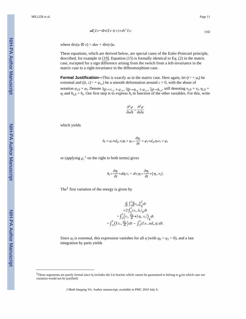
(16)

where div(u ⊗ v) = duv + div(v)u.

These equations, which are derived below, are special cases of the Euler-Poincaré principle,described, for example in [19]. Equation (15) is formally identical to Eq. (2) in the matrixcase, excepted for a sign difference arising from the switch from a left-invariance in thematrix case to a right-invariance in the diffeomorphism case.

Formal Justification—This is exactly as in the matrix case. Here again, let (t ↦ φt) beextremal and ((t, ε) ↦ φt,ε) be a smooth deformation around ε = 0, with the abuse ofnotation φt,0 = φt. Denote , still denoting vt,0 = vt, ηt,0 =ηt and ht,0 = ht. Our first step is to express ht in function of the other variables. For this, write

which yields

or (applying on the right to both terms) gives

The1 first variation of the energy is given by

Since φt is extremal, this expression vanishes for all η (with η0 = η1 = 0), and a lastintegration by parts yields

1These arguments are purely formal since ht includes the Lie bracket which cannot be guaranteed to belong to ℊ (in which case ourvariation would not be justified).

MILLER et al. Page 11

J Math Imaging Vis. Author manuscript; available in PMC 2010 July 6.

NIH

-PA Author Manuscript

NIH

-PA Author Manuscript

NIH

-PA Author Manuscript

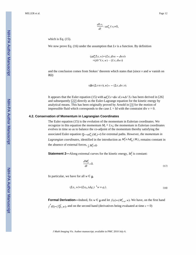
which is Eq. (15).

We now prove Eq. (16) under the assumption that Lv is a function. By definition

and the conclusion comes from Stokes’ theorem which states that (since v and w vanish on∂Ω)

It appears that the Euler equation (15) with has been derived in [26]and subsequently [22] directly as the Euler-Lagrange equation for the kinetic energy byanalytical means. This has been originally proved by Arnold in [3] for the motion ofimpressible fluid which corresponds to the case L = Id with the constraint div v = 0.

4.2. Conservation of Momentum in Lagrangian CoordinatesThe Euler equation (15) is the evolution of the momentum in Eulerian coordinates. Werecognize in this equation the momentum Mt ≐ Lvt; the momentum in Eulerian coordinatesevolves in time so as to balance the co-adjoint of the momentum thereby satisfying theassociated Euler equation for extremal paths. However, the momentum in

Lagrangian coordinates, identified in the introduction as , remains constant inthe absence of external forces, .

Statement 2—Along extremal curves for the kinetic energy, is constant:

(17)

In particular, we have for all w ∈ ℊ,

(18)

Formal Derivation—Indeed, fix w ∈ ℊ and let . We have, on the first hand

, and on the second hand (derivatives being evaluated at time ε = 0)

MILLER et al. Page 12

J Math Imaging Vis. Author manuscript; available in PMC 2010 July 6.

NIH

-PA Author Manuscript

NIH

-PA Author Manuscript

NIH

-PA Author Manuscript

Note here that Adφ◦φ′= Adφ Adφ′. Now, if φ0 = id and at ε = 0, we have for any w′,

(19)

Applying this to w′ = Adφt−1 and v = vt, we get

by Eq. (15). This completes the proof,

Although the conservation of momentum has only been derived from formal arguments, wecan check that, when it is satisfied, the generated deformation paths do provide extremalcurves of the kinetic energy. The perturbation of the end point of the path ( , t ∈ [0, 1]) attime 1 under a perturbation of vt is given by [22]:

(20)

with , the derivative being taken at ε = 0 (we have used the notation of Eq. (1)).

Assume that this expression vanishes (so that the end point remains unchanged). Thefirst variation of the kinetic energy is given by

. Now, using (20) and the fact that dφ0t

φt1 = dφ00 φ01dφ0t φt0, we get easily that so that, by linearity,

(21)

4.3. Coadjoint Transport of Structures Along a Geodesic

For M ∈ ℊ*, the evolution is called coadjoint transport. The fact that themomentum evolves by coadjoint transport along a geodesic implies the conservation of

MILLER et al. Page 13

J Math Imaging Vis. Author manuscript; available in PMC 2010 July 6.

NIH

-PA Author Manuscript

NIH

-PA Author Manuscript

NIH

-PA Author Manuscript

several properties whenever they are initially true, for Lv0. These properties will turn out tobe of main importance for image processing applications.

In this section, we assume that M0 = Lv0 is given, and that the coadjoint transport is well defined at all considered times.

4.3.1. Coadjoint Evolution of the Support—Let Supp(M) denote the support of amomentum M ∈ ℊ*. It is defined by the complementary of the union of all open sets Ω′ ⊂ Ωwhich are such that (M, w) = 0 whenever w ∈ ℊ vanishes outside Ω′. We have the property:

Statement 3: If , then

Indeed, assume that M0 vanishes Ω′ ⊂ Ω. Let w have its support included in φ0t (Ω′). Then(Mt, w) = (M0, dφ0t)−1 w ◦ φ0t and w ◦ φ0t vanishes outside Ω′, which implies that (Mt, w) =0. Thus Supp(Mt) ⊂ φ0t (Supp(M0)), and the reverse inclusion is true by inverting the rolesof M0 and Mt.

As a first example, consider the case when M0 is finitely supported, and more precisely asum of Dirac measures. This is legitimate since our hypotheses on L imply that Diracmeasures belong to ℊ*, therefore have the form Lv0 for some v0 ∈ ℊ. So, we assume that

(22)

where (xi)1≤i≤n is a finite family of points in Ω (landmarks) and (ai)1≤i≤n is a finite family of

vectors in ℝd. We write , where, by definition

(23)

Denoting xi (t) ≐ φt (xi), we obtain the fact that Mt is supported on {x1(t), …, xN (t)}. Moreprecisely, a rapid computation shows that

(24)

with

(25)

MILLER et al. Page 14

J Math Imaging Vis. Author manuscript; available in PMC 2010 July 6.

NIH

-PA Author Manuscript

NIH

-PA Author Manuscript

NIH

-PA Author Manuscript

so that the momentum remains a sum of Dirac measures. This is a special case of theproperty considered in the next section.

4.3.2. Coadjoint Transport of Measure—Measure-based momenta are given by

(26)

where μ0 is a measure on Ω and ν0 is measurable and μ0-integrable. They generate a largeclass of geodesic evolutions, and have the attractive property that the momentum Lvt can beexplicitly computed from the momentum at the origin.

Statement 4: Assume that (M0, w) = ∫Ω⟨ν0, w⟩dμ0 then the linear momentum functionalevolves according to

(27)

i.e. μt (A) = μ(φt0(A)) for any measurable set A.

The statement follows straightforwardly from the substitutions

(28)

Point-supported momentum evolution considered in the previous section, clearly is aparticular case of this statement. As another illustration, consider the case of measures whichare supported by submanifolds of Ω. In this case, the initial momentum is concentratedalong the boundary Σ0 of a k-dimensional C 1 sub-manifold in Ω ⊂ ℝd.

Let σ0 by the surface measure (given as the induced volume form on the sub-manifold) andlet μ0 be supported by Σ0, such that for any smooth function on Ω, ∫Ωf dμ0 = ∫Σ0f α0dσ0 forsome density α0 (not necessary positive) on the surface. Let ν0: Ω → ℝd (the values of ν0outside Σ0 will not be important) and define

(29)

Using Statements 3 and 4, we get that the tranported measure μt is located on the transportedsub-manifold Σt ≐ φt (Σ0) (whose smoothness is preserved by the regularity of thediffeomorphisms in G) and can be written as μt = αt σt where σt is the k-dimensional volumemeasure on Σt. Moreover, if νt = d(φt0)*γ0 ◦ φt0, Statement 4 gives us the evolution of themomentum

MILLER et al. Page 15

J Math Imaging Vis. Author manuscript; available in PMC 2010 July 6.

NIH

-PA Author Manuscript

NIH

-PA Author Manuscript

NIH

-PA Author Manuscript

(30)

In the case where the sub-manifold is Ω itself, then σt = σ0 is the Lebesgue’s measure λ onΩ, and αt = α0 ◦ φt,0|dφt,0|.

4.3.3. Coadjoint Transport of Orthogonality—The last property transported bygeodesic evolution which is considered here is the normality with respect to a smoothsubmanifold of Ω. Since normality will be extensively studied in the next section, we hereprovide an illustration in a particular case.

Assume that ν0, in Eq. (26) can be expressed as

(31)

where and ( ) are two families of functions on Ω and 1 ≤ r ≤ d. Then, we get fromStatement 4 that

(32)

where and . Equation (32) can be interpreted as a normality propertyof the geodesic motion under initial condition (31). Indeed, let

Assume that Σ0 is not empty and denotes for any x ∈ Σ0.Under appropriate transversality conditions, mainly

Σ0 can be equipped with a structure of (d − r)-dimensional C1 manifold and N0(x) is exactlythe space of vectors normal to Σ at location x.

We then deduce easily that

and equality (32) implies for any x ∈ Σt

MILLER et al. Page 16

J Math Imaging Vis. Author manuscript; available in PMC 2010 July 6.

NIH

-PA Author Manuscript

NIH

-PA Author Manuscript

NIH

-PA Author Manuscript

(33)

where is the set of normal vectors to Σt at location x.

We deduce that if the momentum is normal to some k-dimensional sub-manifold Σ0, thisnormality property is preserved by coadjoint transport along a geodesic.

In the case of r = 1 and , Σ0 is exactly the level set for threshold value 0 of f0 and thenormality of the initial momentum to the level sets is preserved under geodesic motion.Since the threshold value is arbitrary, we deduce that the property is true for all level sets.

5. The Normal Momentum Motion Constraint5.1. Heuristic Analysis

The conservation of momentum is a general property of geodesics in a group ofdiffeomorphisms with a right invariant metric. More can be said in the situation whendiffeomorphisms are associated to deformations of geometric structures or images, which isthe situation of interest for our applications. In this setting we are still looking for curveswith shortest length in G, but we partially relax the fixed end-point condition by theconstraint that the initial template is correctly mapped to the target: because there is a wholerange of diffeomorphisms which deform one given structure into another, this condition isweaker than the fixed end-point condition, which means that there are more degrees offreedom for the optimization, and therefore more constraints on the minimum. For imagematching, these additional constraints may essentially be summarized by the statement themomentum along the geodesic path is at all times normal to the level sets of the image. Thisis what we call the normal momentum constraint, which is described in this section.

We start with a heuristic analysis, for which I0, the image, is a smooth function defined onΩ. Let I1 be in the orbit of I0 for the group G of diffeomorphisms: there exists ψ ∈ G suchthat I0 ◦ ψ−1 = It. By compactness and semi-continuity arguments, one can prove theexistence of a geodesic path φ = (φt) such that

(34)

Let be such a solution and consider a first order expansion around t = 0, φt(x) ≃ x +

tv0(x) so that . By definition, the cost to go from I0 to It is(still at first order) t|v0|L. However, any u ∈ ℊ such that ⟨∇I0, u⟩ℝd = ⟨∇I0, v0⟩ℝd, will lead tothe same It so that the least deformation cost from I0 to It should be t|pI0 (v0)| where pI0 (v0)the unique solution of the minimization problem:

(35)

Since ( ) is a geodesic path minimizing the deformation cost from I0 to I1, it minimizesalso the deformation cost from I0 to It yielding

MILLER et al. Page 17

J Math Imaging Vis. Author manuscript; available in PMC 2010 July 6.

NIH

-PA Author Manuscript

NIH

-PA Author Manuscript

NIH

-PA Author Manuscript

(36)

Introduce the set ℊI0 = {h ∈ ℊ | ⟨∇ I0(x), h(x)⟩ℝd = 0, ∀x ∈ Ω}: the constraints in can be

restated as u − v0 ∈ ℊI0 so that pI0 (v) is the orthogonal projection of v on , the spaceorthogonal to ℊI0. Hence, equality (36), translates to

(37)

Now, the fact that ⟨∇I0(x), h(x)⟩ ≡ 0 means that h is a vector field which is tangent to thelevel sets of I0, and since ⟨v0, h⟩L = (Lv0, h), we see that Lv0 vanishes when applied to anysuch vector field, or, that Lv0 is a linear form which is normal to the level sets of I0.

5.2. Rigorous ResultWe now pass to a rigorous derivation of this property. Since it will be interesting to alsoconsider images which are not smooth, we provide a new definition of the set ℊI0.Obviously, when I0 is smooth, h ∈ ℊI0 is equivalent to the fact that, for any function f whichis C1 on Ω, one has

Applying the divergence theorem (we assume that ∂Ω is smooth enough and take advantageon the fact that elements of ℊ vanish on ∂Ω), we get

Since this has a meaning when I0 ∈ L2(Ω), we now define

Definition 2—When I ∈ L2(Ω), we denote

We still denote by pI the orthogonal projection on . The group G is assumed to be built asdescribed in Section 2.1 (in particular ℊ is continuously embedded in C1(Ω, ℝd)).

Theorem 3. (Normal Momentum Constraint): Assume that I0 ∈ L2(Ω) and let be ageodesic path solution of (34). Then, for almost all t ∈ [0, 1]

MILLER et al. Page 18

J Math Imaging Vis. Author manuscript; available in PMC 2010 July 6.

NIH

-PA Author Manuscript

NIH

-PA Author Manuscript

NIH

-PA Author Manuscript

The proof is given in Appendix A.

5.3. ExamplesConsider again the case of smooth I, so that the condition h ∈ ℊI is equivalent to h ∈ ℊ andfor all x ∈ Ω, ⟨∇x I, h(x)⟩ℝd = 0. Using notation (23), we get that

so that and finally,

(38)

Vector fields v such that

(39)

where ν is normal2 to the level sets of I belong to and it can be shown that they form adense subset.

For non-smooth I, we can similarly introduce ωf (I), as the unique element of ℊ such that, forh ∈ V, ⟨ωf (I), h⟩ = ⟨ I, div(h f)⟩L2(Ω), and conclude that

(40)

This implies that any element v ∈ ℊI is such that Lv can be expressed as a limit

where f N ∈ C1(Ω, ℝ). The particular case when I is the indicator function of a smoothdomain B ⊂ Ω (which can be interpreted as a smooth shape) is quite interesting. For x ∈ ∂B,let ν(x) be the outward normal to ∂Ω and denote σB be the uniform measure on ∂B. Then

In this case, we obtain a dense subspace of ℊI by considering elements v ∈ ℊ such that

(41)

for some measure μ on ∂B (the boundary of the shape).

2When I has smooth level sets, we say that a vector field ν is normal to its level sets when, denoting by Ωi the set {I ≤ i}, v(x) isnormal to ∂ Ωi if x ∈ ∂Ωi for some i and x = 0 otherwise.

MILLER et al. Page 19

J Math Imaging Vis. Author manuscript; available in PMC 2010 July 6.

NIH

-PA Author Manuscript

NIH

-PA Author Manuscript

NIH

-PA Author Manuscript

Remark—We close this section with a technical, but important, remark. We have callednormal momentum constraint the property that vt ⊥ ℊIt at almost all times. We have shownthat this property is always true for geodesics minimizing (34). But there is anotherimportant issue, which is how much it constrains vt, or, in other terms, how big ℊI is for agiven image I. That this is relevant, and sometimes non-trivial, may be seen from thefollowing example: assume that we are in 2 dimensions (d = 2) and that I is a C1 image, witha non-vanishing gradient, at least on a dense subset of Ω. Then, on any point x such that ∇ x I≠ = 0, we can de-fine in a unique way a positively oriented orthonormal frame (τ (x) ν (x))such that ν (x) = ∇x I/|∇x I|. Then, if h ∈ ℊI and h(x) ≠ = 0, we must have h/|h| = ± τ in a smallball around x. Now h, as an element of ℊ must be smooth (depending on the choice made forL, and h/|h| has the same smoothness as h: this is impossible to achieve when τ itself is notsmooth enough, which in such a case forces h(x) = 0. We thus get the property that hvanishes whenever τ (x) does not meet the smoothness requirements of ℊ, which may verywell be everywhere on Ω (or on a dense subset, which is the same since h is continous), inwhich case ℊI = {0} and the constraint is void, contrary to our intuition that the momentumshould be aligned with ν. We see that, for the constraint to really be effective, we need somesmoothness requirement on I. Fortunately, as illustrated by the example above, thissmoothness is only required for the level sets of I, which must have a smooth boundary.With such an assumption, for example, one can show that if v ⊥ ℊI and

for some measure μ on Ω and some vector field on ξ Ω, then ξ must be (μ-almosteverywhere) orthogonal to the level sets of I. From a practical point of view smoothness oflevel sets may easily be obtained using algorithms such as mean curvature motion ([27]).

5.4. Conservation and Normality Property Check for Inexact MatchingHere, we give a brief account of situations in which proofs of conservation of momentumand the normality property can be carried on in a well-defined context, and retrieve theevolutions described in the previous section.

It is hard to make rigorous, in full generality, the variational argument we have used in theproof of Eq. (15). Notice that the well-definiteness of the conservation of momentum Eq.(17) is an issue by itself, since, when w ∈ ℊ, and φt is the diffeomorphism generated by ageodesic, there is a priori no reason for (dφt)−1w ◦ φt) to belong to ℊ: one must be able todefine Lv0 on spaces which are bigger than ℊ, which means that Lv0 needs to be somewhatsmoother (as a distribution) than a generic element of ℊ*.

However, there is a setting in which such a fact is true and easy to obtain: it is when thesearch for the geodesic is done with an approximation of the target, with some L2 penaltyterm added to control the error. We summarize this setting in the case of landmark matching,shape matching and image matching. In these three situations, we will retrieve the coadjointtransport of measure-based momenta. In all cases, results in [11,35] ensure the existence ofminimizers of the variational problem.

5.4.1. Inexact Landmark Matching—In this section, we assume that a measured space( , ρ), together with two measurable functions x, y: → Ω are given. The diffeomorphismφ is searched to minimize

MILLER et al. Page 20

J Math Imaging Vis. Author manuscript; available in PMC 2010 July 6.

NIH

-PA Author Manuscript

NIH

-PA Author Manuscript

NIH

-PA Author Manuscript

When ρ is discrete, this relates to point-based matching, x representing the landmark originalpositions and y giving the landmark target positions. If we express U in function of v, thisrequires the minimization of

The main point here is to notice that the optimal solution v generates a geodesic in Gbetween id and .

Proposition 1: Denote the linear form on ℊ such that . Let v be aminimizer of Ũ. Then, letting

(42)

Proof: The proof of this result is a direct consequence of the identity, valid for s, t ∈ [0, 1],v, h ∈ L2([0, 1], ℊ),

(43)

the proof of which being carried on with usual ODE arguments and being omitted here. It isthen straightforward to obtain (42), using the definition of the linear forms , for x ∈ Ωand a ∈ ℝd.

Equation (42) is a conservation of momentum equation for

When is finite, this is equation (31) with . Equation (42) now isexactly (24), since

MILLER et al. Page 21

J Math Imaging Vis. Author manuscript; available in PMC 2010 July 6.

NIH

-PA Author Manuscript

NIH

-PA Author Manuscript

NIH

-PA Author Manuscript

5.4.2. Inexact Shape Matching—We now consider the comparison of a binary set-indicator function, I0 = 1Ω0 (Ω ̄0 ⊂ Ω having smooth boundaries) and a smooth function I1,through the minimization of

over GL. We have

Proposition 2: Let v be a minimizer of over L2([0, 1], ℊ). Then

(44)

where , ν1 is the outward normal to ∂ Ω1 and σ1 is the volume measure on ∂ Ω1.

Proof: Taking a variation v + εh, the main issue is to compute the derivative of

This integral can be rewritten

Since the last term is constant, we see that the problem boils down to the computation of thederivative of the first term, which can be written, after a change of variable and letting f1 =1/2 − I1,

Define u by . Simple computations, which can be, for example, foundin [10], yields the fact that

Now the conclusion is a direct consequence of Eq. (43) and of the divergence theorem.

Here again, one straighforwardly checks that the conservation of momentum is satisfied. Wehave in particular

MILLER et al. Page 22

J Math Imaging Vis. Author manuscript; available in PMC 2010 July 6.

NIH

-PA Author Manuscript

NIH

-PA Author Manuscript

NIH

-PA Author Manuscript

Letting , and this can be rewritten

which is under the general form of a measure-based momentum.

5.4.3. Inexact Image Matching—In this section, we let I0 and I1 be two smooth enough(say C1) functions defined on Ω (images). We consider the image matching problem whichcorresponds to minimizing, over G,

This problem is equivalent to minimizing

This matching problem has been studied, in particular in [4], to show that the optimalsolution should satisfy, at each time t,

(45)

in which we have introduced the notation: , and |dφ| for the Jacobianof φ. This equation is in fact an equation of conservation of momentum, with

as can be deduced from Eq. (30), with . Moreover, we can check alsothe normality property (31) which holds here with with r = 1 and f0 = I0. This allows us toconclude that for the geodesic path in the image space generated by inexact matching, thelifting of the path in G defines a geodesic for which the momentum stays normal to the levelsets of the current image I0 ◦ φt,0 at time t.

MILLER et al. Page 23

J Math Imaging Vis. Author manuscript; available in PMC 2010 July 6.

NIH

-PA Author Manuscript

NIH

-PA Author Manuscript

NIH

-PA Author Manuscript

6. Geodesic Evolution in the OrbitThus far we have concentrated on the evolution of the flow of diffeomorphisms and itsconservation of momentum. For all of our image understanding work we use the flow (φt, t∈ [0, 1]) to act on the elements in the orbits of a given template I = Itemp. Now weexamine the geodesic flows in the orbit {It = I ◦ φt, t ∈ [0, 1]}, I ∈ , and provide theassociated evolution equations.

6.1. Geodesic Evolution Equation of Landmark PointsHere we examine the finite dimensional landmark orbit denoted n, consisting of n-shapesIN = (x1, …, xn), each landmark (xi)1≤i≤n is in Ω ⊂ ℝd; correspondingly (ai)1≤i≤n are a finitefamily of vectors in ℝd. Denoting by xi (t) =̇ φt (xi), the trajectory in Ω of the point xi underthe flow φt gives

(46)

where ai (t) = (dxt (t) φt,0)*ai. From the identity

(47)

we deduce that . To prove (47), one needs to remark that

Now,

Hence we get the following geodesic evolution in the orbit of landmarks.

Proposition 3 (Landmark Transport)—The landmarks are transported along thegeodesic according to the following equations with velocity vector field satisfying

where K(x, y) is the Green kernel associated with L:3

MILLER et al. Page 24

J Math Imaging Vis. Author manuscript; available in PMC 2010 July 6.

NIH

-PA Author Manuscript

NIH

-PA Author Manuscript

NIH

-PA Author Manuscript

(49)

Note that the expression of vt from Eq. (48) can be introduced into the system (49), yieldingan evolution equation which only depends on the landmarks in the orbit.

We notice the reduction of the vector field to the range space of the Green’s kernelstravelling over the landmark trajectories is as in [17].

There is a straightforward extension of this result to geodesic curve evolution, in which x(0)is a parametrized curve σ ↦ x(σ) for σ ∈ [0, L] and

where ν0(σ) is normal to x(0). In this case, we have

with

•,

•.

6.2. Geodesic Image EvolutionAssume here that dμ = α (x)dx has a density with respect to Lebesgue’s measure on Ω. Inthis case, dμt = |dφt0|α ◦ φt0dx and

(50)

From the conservation of momentum in Lagrangian coordinates for image based motion, weget for Lv0 = α0 ∇ I0 that Lvt = αt |dφt,0|∇It where αt = α0 ◦ φt,0, It = I0 ◦ φt,0. Let zt = αt |dφt,0|so that Lvt = zt ∇ It.

Since we get .Moreover, we get easily . Hence we get the following geodesic evolutionequation in image space.

3The explicit form for L−1 depending on the kernel K is defined as follows. For any x, y ∈ Ω, the bilinear form Kx,y on ℝd × ℝddefined by

(49)

MILLER et al. Page 25

J Math Imaging Vis. Author manuscript; available in PMC 2010 July 6.

NIH

-PA Author Manuscript

NIH

-PA Author Manuscript

NIH

-PA Author Manuscript

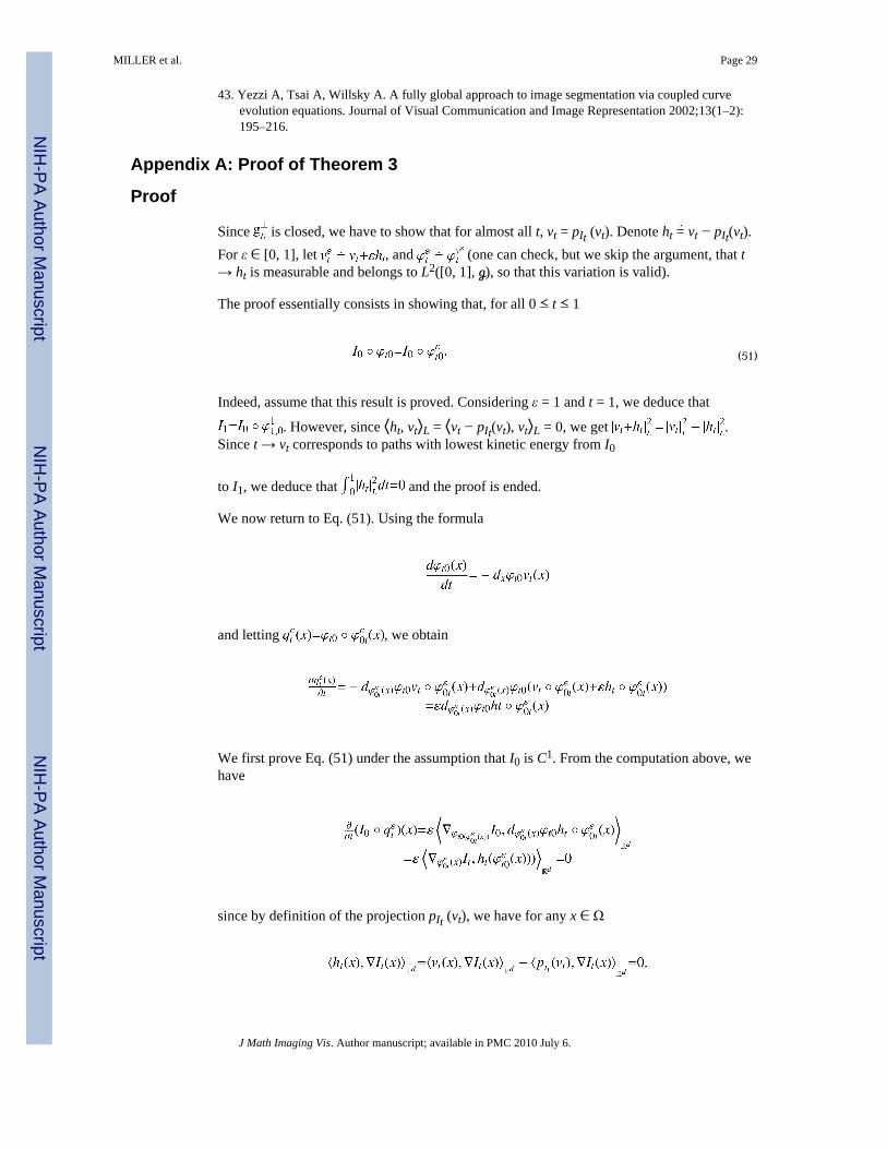
Proposition 4 (Image Transport)—The image is transported along the geodesicaccording to the following equations: with vector field vt = L−1(zt ∇It):

•,

•.

Notice that these equations appear as a limit case of the evolution equations which havebeen studied in [34] for image comparison.

As illustrated above, the pair (I0, μ) provides a device for modeling deformations. In thecases we have studied, I0 was representing some geometrical structure (a curve, an image),which evolved with time accordi to the generated deformation, and μ, essentially quantifiesthe speed and direction of the deformation.

We get from this a natural way to represent the deformation of a template. UsingGrenander’s original terminology, I0 would precisely be the template and μ is the generatorof the deformation. Thus, fixing I0, and letting μ vary, we get a model which representsperturbations of the template.

An example of deformations of an image is provided in Fig. 2. The images have beenobtained by solving Eq. (50) from an initial image g of a slice of macaque brain, and taking

where X is a Gaussian process.

7. Computational ResultsThe following results illustrate the computation of the momentum Lv0 = α0∇I0 (as describedin Section 6.2) from geodesic paths between two images. These geodesics are computedusing F. Beg’s implementation of image matching, as described in [4]. In these experiments,the operator L is (∇ + c Identity),2 implemented via fast Fourier transform. The shootingalgorithm solves the equation provided in Proposition 4 with initial condition (I0, z0 = α0).

Figure 3 shows the three objects studied, a smooth Gaussian bump for shift, circles for scale,and two mitochondria examin g both forward and inverse shooting.

Shown in Fig. 4–6 are examples illustrating the image based momentum and thediffeomorphisms generated via geodesic shooting. Figure 4 shows the results of thetranslation experiment. Panels 1 and 2 show I0 and I1; panel 3 shows the diffeomorphismgenerated via geodesic shooting applied to I0, and illustrates how solving the conservation ofmomentum equation allows to recover I1 from I0 and Lv0.

Shown in panel 4 is the density α showing the concentration near the boundary of I0.Superposed in panel 5 are the predicted directions of the momentum, given by α0∇I0, andthe value Lv0 obtained from Beg’s algorithm. In almost all case they appear as one lineindicating a good accuracy of the algorithm. Panel 6 indicates that the vector field V0demonstrating that while α and the momentum Lv0 are highly localized, the velocity ofmotion extends over the entire object.

MILLER et al. Page 26

J Math Imaging Vis. Author manuscript; available in PMC 2010 July 6.

NIH

-PA Author Manuscript

NIH

-PA Author Manuscript

NIH

-PA Author Manuscript

Shown in Fig. 5 are similar results for the scale experiment.

Shown in Fig. 6 are two sets of results for the geodesic shooting of the mitochondria. Theorganization of the results are the same as for the translation and scale experiments. Shownin Fig. 6 are two sets of results for the geodesic shooting of the mitochondria. Theorganization of the results are the same as for the translation and scale experiments.

AcknowledgmentsMichael I. Miller was supported by grants from the National Institute of Wealth numbers P41-RR15241-01A1,U24-RR0211382-01, P20-MH071616-01.

References1. Arnold, VI. Mathematical Methods of Classical Mechanics. 1. Springer; 1978. 19892. Arnold V, Khesin B. Topological methods in hydrodynamics. Ann Rev Fluid Mech 1992;24:145–

166.3. Arnold VI. Sur la géometrie differentielle des groupes de Lie de dimension infinie et ses

applications à l’hydrodynamique des fluides parfaits. Ann Inst Fourier (Grenoble) 1966;1:319–361.4. Beg MF, Miller MI, Trouvé A, Younes L. Computing large deformation metric mappings via

geodesics flows of diffeomorphisms. Int J Comp Vis February;2005 61(2):139–157.5. Camion, V.; Younes, L. Geodesic interpolating splines. In: Figueiredo, MAT.; Zerubia, J.; Jain,

AK., editors. EMM-CVPR 2001, Vol. 2134 of Lecture Notes in Computer Sciences. Springer-Verlag; 2001. p. 513-527.

6. Chen, T.; Metaxas, D. Medical Image Computing and Computer-Assisted Intervention—Miccai2000, Vol. 1935 of Lecture Notes in Computer Science. Springer-Verlag; 2000. Image segmentationbased on the integration of Markov random fields and deformable models; p. 256-265.

7. Christensen GE, Rabbitt RD, Miller MI. Deformable templates using large deformation kinematics.IEEE Trans Image Processing 1996;5(10):1435–1447.

8. Cohen I, Cohen L, Ayache N. Using deformable surfaces to segment 3-d images and inferdifferential structures. Computer Vision Graphics Image Processing 1992;56(2):242–263.

9. Cootes T, Taylor C, Cooper D, Graham J. Active shape models—Their training and application.Comp Vision and Image Understanding 1995;61(1):38–59.

10. Delfour, MC.; Zolésio, J-P. Shapes and Geometries. Analysis, Differential Calculus andOptimization. SIAM; 2001.

11. Dupuis P, Grenander U, Miller M. Variational problems on flows of diffeomorphisms for imagematching. Quart App Math 1998;56:587–600.

12. Garrido A, De la Blancà NP. Physically-based active shape models: Initialization and optimization.Pattern Recognition 1998;31(8):1003–1017.

13. Grenander, U. General Pattern Theory. Oxford Univeristy Press; 1994.14. Grenander, U.; Chow, Y.; Keenan, D. HANDS: A Pattern Theoretic Study of Biological Shapes.

Springer-Verlag; New York: 1990.15. Grenander U, Miller MI. Representations of knowledge in complex systems. J Roy Stat Soc B

1994;56(3):549–603.16. Grenander U, Miller MI. Computational anatomy: An emerging discipline. Quart App Math

1998;56:617–694.17. Joshi S, Miller MI. Landmark matching via large deformation diffeomorphisms. IEEE Trans Image

Processing 2000;9(8):1357–1370.18. Kass M, Witkin A, Terzopolous D. Snakes: Active contour models. International Journal of

Computer Vision 1988;1(4):321–331.19. Marsden, JE.; Ratiu, TS. Introduction to Mechanics and Symmetry. Springer; 1994.

MILLER et al. Page 27

J Math Imaging Vis. Author manuscript; available in PMC 2010 July 6.

NIH

-PA Author Manuscript

NIH

-PA Author Manuscript

NIH

-PA Author Manuscript

20. Mignotte M, Meunier J. A multiscale optimization approach for the dynamic contour-basedboundary detection issue. Computerized Medical Imaging and Graphics 2001;25(3):265–275.[PubMed: 11179703]

21. Miller, M.; Joshi, S.; Maffitt, DR.; McNally, JG.; Grenander, U. Mitochondria, membranes andamoebae: 1, 2 and 3 dimensional shape models. In: Mardia, K., editor. Statistics and Imaging. Vol.II. Carfax Publishing; Abingdon, Oxon: 1994.

22. Miller M, Trouvé A, Younes L. On the metrics and Euler-Lagrange equations of computationalanatomy. Annual Review of Biomedical Engineering 2002;4:375–405.

23. Miller M, Younes L. Group actions, homeomorphisms, and matching: A general framework.International Journal of Computer Vision 2001;41(1/2):61–84.

24. Montagnat, J.; Delingette, H. Cvrmed-Mrcas’97, Vol. 1205 of Lecture Notes in Computer Science.Springer-Verlag; 1997. Volumetric medical images segmentation using shape constraineddeformable models; p. 13-22.

25. Montagnat J, Delingette H, Ayache N. A review of deformable surfaces: Topology, geometry anddeformation. Image and Vision Computing 2001;19(14):1023–1040.

26. Mumford, D. Questions Mathématiques En Traitement Du Signal et de L’Image. Vol. Chap 3.Institut Henri Poincaré; 1998. Pattern theory and vision; p. 7-13.

27. Osher S, Sethian JA. Front propagating with curvature dependent speeds: Algorithms based onHamilton-Jacobi formulation. Journal of Comp Physics 1988;79:12–49.

28. Pham D, Xu C, Prince J. Current methods in medical image segmentation. Ann Rev BiomedEngng 2000;2:315–337. [PubMed: 11701515]

29. Schultz N, Conradsen K. 2d vector-cycle defonnable templates. Signal Processing 1998;71(2):141–153.

30. Sclaroff S, Liu LF. Deformable shape detection and description via model-based region grouping.IEEE Transactions on Pattern Analysis and Machine Intelligence 2001;23(5):475–489.

31. Staib L, Duncan J. Boundary finding with parametrically deformable models. IEEE Trans PatternAnalysis and Machine Intelligence 1992;14:1061–1075.

32. Staib L, Duncan J. Model-based deformable surface finding for medical images. IEEE TransMedical Imaging 1996;15(5):1–13.

33. Terzopoulos D, Metaxas D. Dynamic models with local and global deformations: Deformablesuperquadrics. IEEE Trans Patt Anal Mach Intell 1991;13:703–714.

34. Trouvé A, Younes L. Local geometry of deformable template. SIAM Journal of MathmaticalAnalysis. to appear.

35. Trouvé A. Action de groupe de dimension infinie et reconnaissance de formes. CR Acad Sci Paris,Série I, No 321 1995:1031–1034.

36. Trouvé A. Diffeomorphisms groups and pattern matching in image analysis. Int J Computer Vision1998;28:213–221.

37. Vaillant M, Davatzikos C. Finding parametric representations of the cortical sulci using an activecontour model. Medical Image Analysis 1997;1(4):295–315. [PubMed: 9873912]

38. Westin, CF.; Lorigo, LM.; Faugeras, O.; Grimson, WEL.; Dawson, S.; Norbash, A.; Kikinis, R.Medical Image Computing and Computer-Assisted Intervention—MICCAI 2000, Vol. 1935 ofLecture Notes in Computer Science. Springer-Verlag; 2000. Segmentation by adaptive geodesicactive contours; p. 266-275.

39. Xu, C.; Pham, DL.; Prince, JL. Finding the brain cortex using fuzzy segmentation, isosurfaces anddeformable surface models. XVth Int. Conf. on info Proc. in Medical Imaging; June 1997;

40. Xu, C.; Pham, DL.; Prince, JL. Medical image segmentation using deformable models. In:Fitzpatrick, J.; Sonka, M., editors. SPIE Handbook on Medical Imaging - Volume III: MedicalImage Analysis. SPIE; Bellingham, WA: 2000. p. 129-174.

41. Xu C, Prince JL. Gradient vector flow: A new external force for snakes. CVRP. Nov;199742. Xu, C.; Prince, JL. Gradient vector flow deformable models. In: Bankman, I., editor. Handbook of

Medical Imaging. Academic Press; San Diego, CA: 2000.

MILLER et al. Page 28

J Math Imaging Vis. Author manuscript; available in PMC 2010 July 6.

NIH

-PA Author Manuscript

NIH

-PA Author Manuscript

NIH

-PA Author Manuscript

43. Yezzi A, Tsai A, Willsky A. A fully global approach to image segmentation via coupled curveevolution equations. Journal of Visual Communication and Image Representation 2002;13(1–2):195–216.

Appendix A: Proof of Theorem 3

Proof

Since is closed, we have to show that for almost all t, vt = pIt (vt). Denote ht =̇ vt − pIt(vt).For ε ∈ [0, 1], let , and (one can check, but we skip the argument, that t→ ht is measurable and belongs to L2([0, 1], ℊ), so that this variation is valid).

The proof essentially consists in showing that, for all 0 ≤ t ≤ 1

(51)

Indeed, assume that this result is proved. Considering ε = 1 and t = 1, we deduce that

. However, since ⟨ht, vt⟩L = ⟨vt − pIt(vt), vt⟩L = 0, we get .Since t → vt corresponds to paths with lowest kinetic energy from I0

to I1, we deduce that and the proof is ended.

We now return to Eq. (51). Using the formula

and letting , we obtain

We first prove Eq. (51) under the assumption that I0 is C1. From the computation above, wehave

since by definition of the projection pIt (vt), we have for any x ∈ Ω

MILLER et al. Page 29

J Math Imaging Vis. Author manuscript; available in PMC 2010 July 6.

NIH

-PA Author Manuscript

NIH

-PA Author Manuscript

NIH

-PA Author Manuscript

This implies which yields Eq. (51) in this case. When I0 is not smooth, theproof goes by showing that

for smooth f on Ω and which can be done either by a direct (heavy)computation, or by using a density argument, based on the fact that, by the divergencetheorem, this is true for smooth I0 (we skip the details).

MILLER et al. Page 30

J Math Imaging Vis. Author manuscript; available in PMC 2010 July 6.

NIH

-PA Author Manuscript

NIH

-PA Author Manuscript

NIH

-PA Author Manuscript

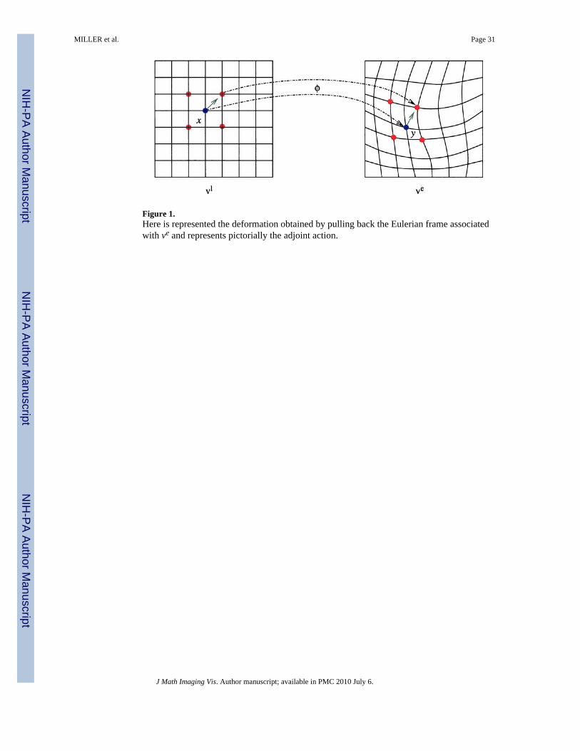
Figure 1.Here is represented the deformation obtained by pulling back the Eulerian frame associatedwith ve and represents pictorially the adjoint action.

MILLER et al. Page 31

J Math Imaging Vis. Author manuscript; available in PMC 2010 July 6.

NIH

-PA Author Manuscript

NIH

-PA Author Manuscript

NIH

-PA Author Manuscript

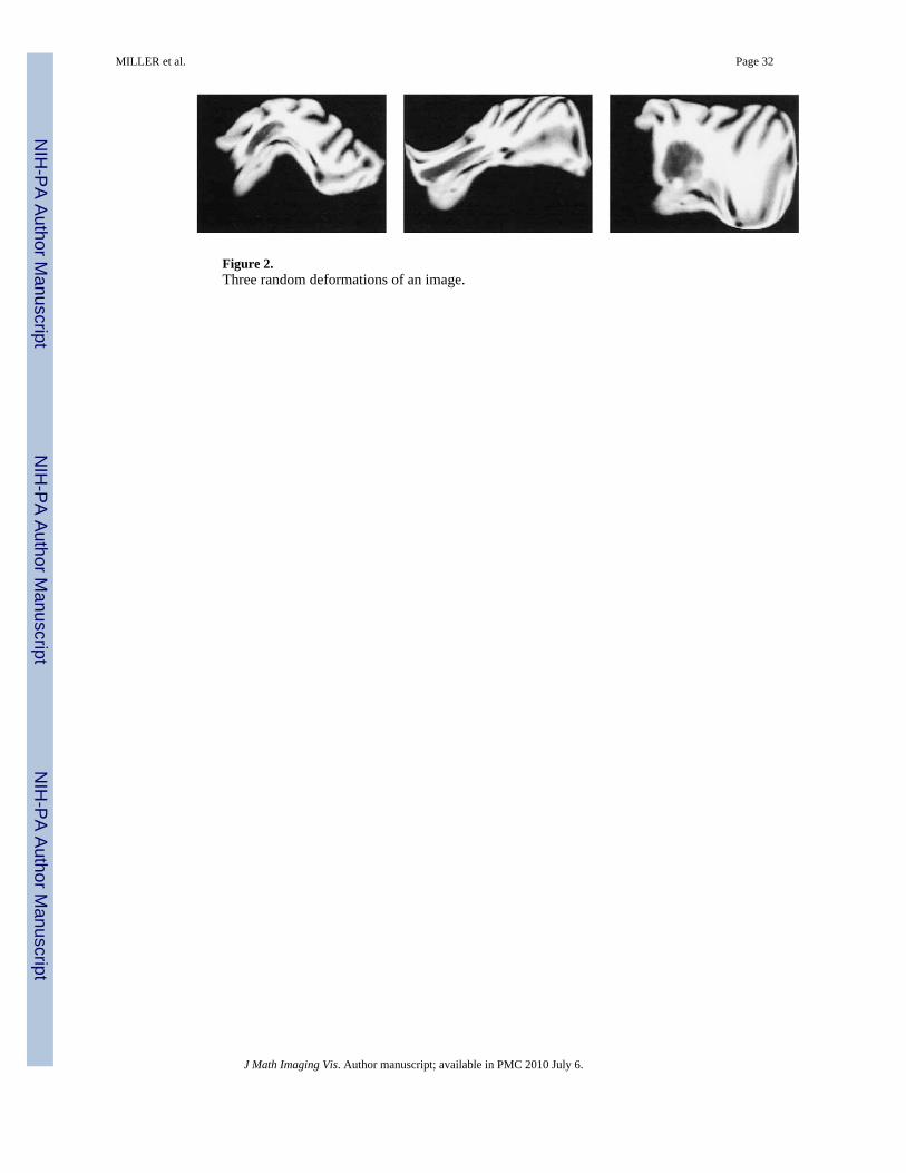
Figure 2.Three random deformations of an image.

MILLER et al. Page 32

J Math Imaging Vis. Author manuscript; available in PMC 2010 July 6.

NIH

-PA Author Manuscript

NIH

-PA Author Manuscript

NIH

-PA Author Manuscript

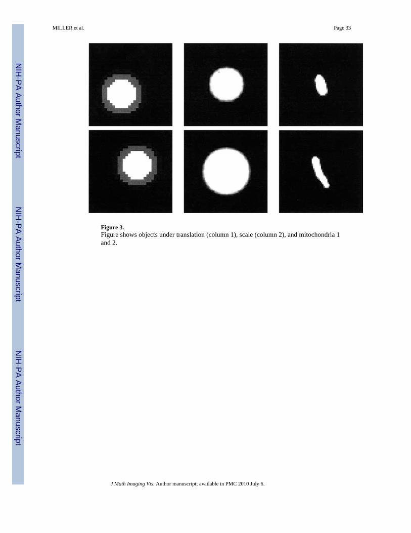
Figure 3.Figure shows objects under translation (column 1), scale (column 2), and mitochondria 1and 2.

MILLER et al. Page 33

J Math Imaging Vis. Author manuscript; available in PMC 2010 July 6.

NIH

-PA Author Manuscript

NIH

-PA Author Manuscript

NIH

-PA Author Manuscript

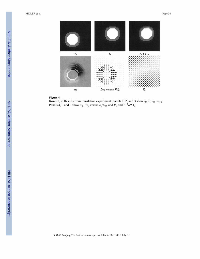
Figure 4.Rows 1, 2: Results from translation experiment. Panels 1, 2, and 3 show I0, I1, I0 ◦ φ10.Panels 4, 5 and 6 show α0, Lv0 versus α0∇I0, and V0 and L−1α∇ I0.

MILLER et al. Page 34

J Math Imaging Vis. Author manuscript; available in PMC 2010 July 6.

NIH

-PA Author Manuscript

NIH

-PA Author Manuscript

NIH

-PA Author Manuscript

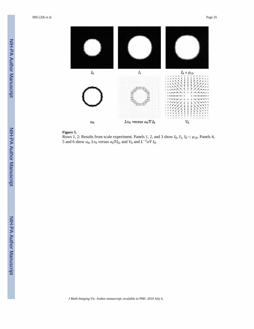
Figure 5.Rows 1, 2: Results from scale experiment. Panels 1, 2, and 3 show I0, I1, I0 ◦; φ10. Panels 4,5 and 6 show α0, Lv0 versus α0∇I0, and V0 and L−1α∇ I0.

MILLER et al. Page 35

J Math Imaging Vis. Author manuscript; available in PMC 2010 July 6.

NIH

-PA Author Manuscript

NIH

-PA Author Manuscript

NIH

-PA Author Manuscript

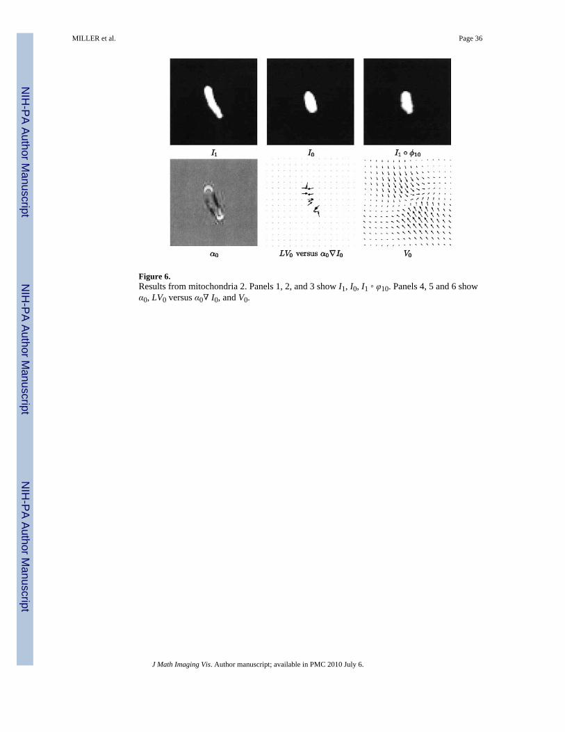
Figure 6.Results from mitochondria 2. Panels 1, 2, and 3 show I1, I0, I1 ◦ φ10. Panels 4, 5 and 6 showα0, LV0 versus α0∇ I0, and V0.

MILLER et al. Page 36

J Math Imaging Vis. Author manuscript; available in PMC 2010 July 6.

NIH

-PA Author Manuscript

NIH

-PA Author Manuscript

NIH

-PA Author Manuscript

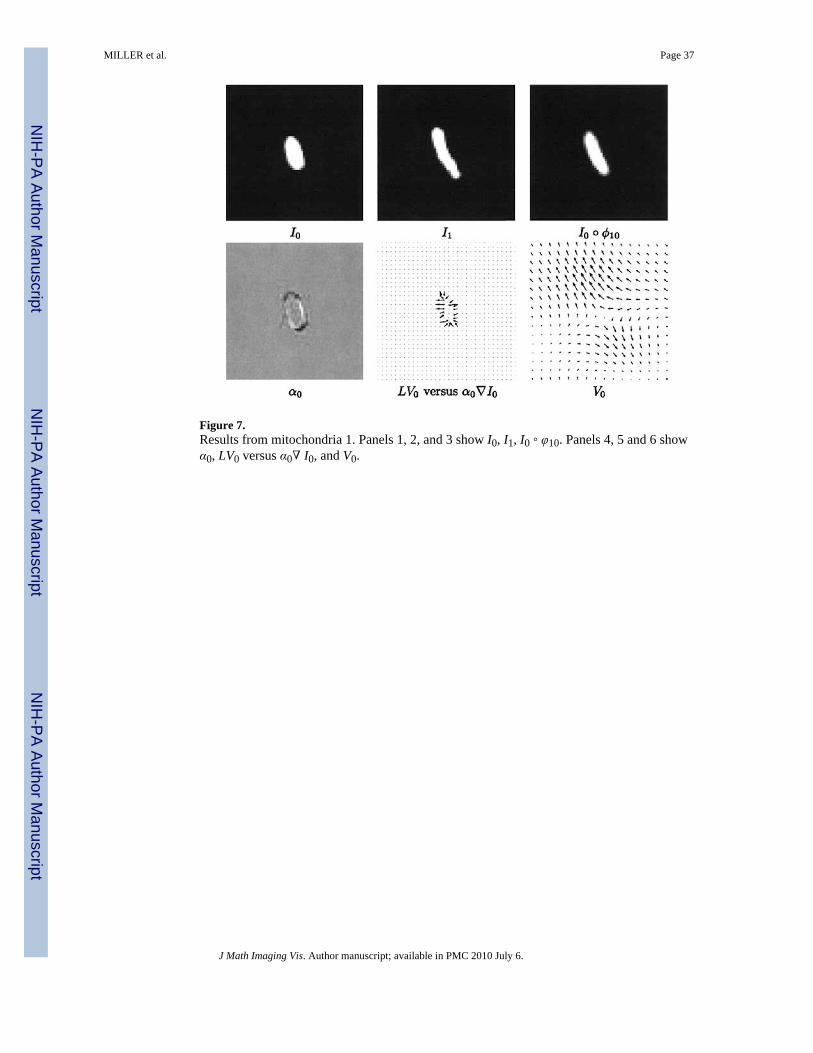
Figure 7.Results from mitochondria 1. Panels 1, 2, and 3 show I0, I1, I0 ◦ φ10. Panels 4, 5 and 6 showα0, LV0 versus α0∇ I0, and V0.

MILLER et al. Page 37

J Math Imaging Vis. Author manuscript; available in PMC 2010 July 6.

NIH

-PA Author Manuscript

NIH

-PA Author Manuscript

NIH

-PA Author Manuscript