.1"',, II .,

"itf,t'l; ",'"p,"'~.l~,,, .

UTILIZATION OF RIVER CURRENTFOR SMALL SCALE ELECTRICITYGENERATION IN BANGLADESH

By

NAZMUL HUDA AL MAMUN

JULY, 2001

A THESIS SUBMITTED TO THE DEPARTMENT OF MECHANICAL ENGINEERING

BANGLADESH UNIVERSITY OF ENGINEERING & TECHNOLOGY (BUET) IN

PARTIAL FULFILMENT OF THE REQUIREMENT FOR THE DEGREE OF MASTER

OF SCIENCE IN MECHANICAL ENGINEERING

-- --. ---.

111111111 1111111111111111111111 III#95663#

----""'--~.- --~~--=---DEPARTMENT OF MECHANICAL ENGINEERING

BANGLADESH UNIVERSITY OF ENGINEERING & TECHNOLOGY(BUET), DHAKA

'.

CERTIFICATE OF APPROVAL

The thesis titled "Utilization of River Current for Small Scale Electricity Generation

in Bangladesh" submitted by Nazmul Huda Al Mamun, Student No. 9610025P, to the

Mechanical Engineering Department of Bangladesh University of Engineering &

Technology has been accepted as satisfactory for partial fulfillment of the

requirements for the degree of Master of Science in Mechanical Engineering on July

19,2001.

BOARD OF EXAMINERS

~_"-.Dr. Md. Quamrul IslamProfessor. Department of Mechanical EngineeringBUET, Dhaka-1000

~~ ,Dr. Md. Abdur Rashid SarkarProfessor & HeadDepartment of Mechanical EngineeringBUET, Dhaka-1000

(/6O)Q~. ~Dr. A. K. M. SadrulISIaIl1Professor, Department of Mechanical EngineeringBUET, Dhaka-1000

.~+-.UJV.IDr. Shahidul Islam KhanProfessor & HeadDepartment of Electrical & Electronic EngineeringBUET, Dhaka-) 000

Dr. Abul Fazal M. SalehProfessor, Institute of Flood Control & Drainage ResearchBUET, Dhaka-1000

Chairman(Supervisor)

Member

Member

Member(External)

Member(External)

CANDIDATE'S DECLARATION

It is hereby declared that this thesis or any part of it has not been submitted

elsewhere for the award of any degree or diploma or publication.

Signature of the Candidate

~o2JT/g/.2.lm1Nazmul Huda AI MamuuCandidate

Counter Signature of the Supervisor

Dr. Md. Quamrul IslamProfessor, Department of Mechanical EngineeringSUET, Dhaka-J 000

ToMy Parents & Sisters

.; .. -

ACKNOWLEDGEMENT

At the very beginning, the author wish to express his gratitude to the Almighty

Allah, who is the most Gracious and Merciful.

The author then would like to take this opportunity of expressing his heartfelt

gratitude and indebtedness to his thesis supervisor Dr. Md. Quamrul Islam,

Professor, Department of Mechanical Engineering, BUET, Dhaka, for his

valuable suggestions in the course of the present work. At the same time the

author feels grateful to Dr. A K M Sadrul Islam, Professor, Department of

Mechanical Engineering, BUET, Dhaka, for his continuous guidance,

suggestions and encouragement. Without their help the entire project would be,

but failure. ,

The author is highly indebted to Dr. Abul Fazal M. Saleh, Professor, Institute

of Flood Control & Drainage Research, BUET, Dhaka for his valuable

suggestions and kind cooperation during the project.

The author expresses his gratitude to Prof. Dr. David Infield and Dr. D. J.

Sharpe of CREST, Loughborough University, UK, for their assistance and

valuable suggestions regarding the project.

Thanks are due to many colleagues and friends specially Md. Mamun and Md.

Zakir Hossain of BUET, Mr. Sultan Ahmed, Ph. D. student of the department

and M A Mijan for their kind cooperation and help in various ways.

The author is also grateful to the staff and workers of the department, and

Welding and Foundry shop of BUET.

The author feels obliged to express his gratitude to his parents and sisters who

sheared the troubles.

Finally, each and everybody related either directly or indirectly with the project

deserve special thanks for their helpful cooperation, without which it would be

impossible to carry out the project.

CONTENTS

Abstract i

List of Symbols ii

Greek Alphabets v

Chapter I INTRODUCTION

Chapter 2 LITERATURE REVIEW AND

EXISTING THEORIES

2.1 LITERATURE REVIEW 4

2.2 EXISTING THEORIES 6

2.2.1 INTRODUCTION 6

2.2.2 AXIAL MOMENTUM THEORY 6

2.2.3 BLADE ELEMENT THEORY 13

2.2.4 STRIP THEORY 15

2.2.5 TIP AND HUB LOSSES 17

2.2.6 THRUST, TORQUE AND POWER

COEFFICIENTS 20

2.2.7 RELATlONS FOR MAXIMUM

POWER 21

Chapter 3 RIVER CURRENT POTENTIAL IN BANGLADESH

3.1 LOCATION 23

32 THE RIVER SYSTEM 23

3.3 THE RIVER SITES 25

Chapter 4 RIVER CURRENT: A SOURCE OF ENERGY

4.1 POWER FROM FLOWING WATER 39

4.2 MINIUM USEFUL RIVER CURRENT 41

4.3 SITE SELECTION 42

4.4 MEASUREMENT OF RIVER CURRENT 42

Chapter 5 DESIGN & FABRICATION OF WATER

CURRENT TURBINE

5.1 CHOICE OF TURBINE ROTOR 44

52 DESIGN OF TURBINE BLADE 44

5.3 CHOICE OF TURBING ROTOR 49

5.4 ROTOR SHAFT BEARING 49

Chapter 6 PERFORMANCE ANALYSIS 53

Chapter 7 COST ESTIMATION 63

Chapter 8 CONCLUSION 66

References 68Appendix A Common Rivers in Bangladesh 72Appmdix 13 11List a/Rivers in Bangladesh 74Appendix C The Ganges, The Brahmaputra,

The Meghna River Basin 80Appendix D River Current Data 82Appendix E Tahle (~l(CjC)l!lill'Angle of Attack &

Li/i Coefficient a/Different A ir/i)ils 121Appendix F C,. vs TSR/iJr dilferent nllmher ajhlades

& Dif/erent Drag/Lifi Ratio 123Appendix G t.J.:perimental Data 125Appendix H Tohle jiJr Power 01ltPllt and Cost oj Energy 132Appendix I Power Coefficient vs. Tip Speed Ralio al

Different Velocities and Pitch Angles 134

•. '"1" ,

ABSTRACTThe power crisis in Bangladesh and elsewhere in the Third World highlights the need for

new technologies, which local communities can use to improve their lifestyle. Many arid, \

areas are characterized by having large rivers or canals flowing through them. Under this

project a study has been performed to assess the potential of electrical energy from river

currents at different locations of Bangladesh. In this context 23 sites of different rivers

have been considered as test cases.

After getting an idea about the river current velocity at different rivers in Bangladesh, this

thesis describes the development of a new, simple, and relatively inexpensive technology,

which if used in right circumstances, can generate power from the rivers. The water

current turbine- just can be thought of as a wind turbine inserted into the river current- a

model of which has been tried and tested for power generation. The technical details

especially the aerodynamic design of the turbine rotor has been introduced in the thesis.

The turbine model consisting of three NACA 4412 blades with average rotor radius of

221 mm has been tested for harnessing the kinetic energy from water. It should be

mentioned here that no twist angle has been introduced in the blade.

A chapter of this thesis devoted to analyze the performance of the model illustrates the

working range of a water turbine in terms of tip speed ratio under certain river current

velocity and the effect of pitch angle in power generation. It has been found that the

turbine will run at tip speed ratios between 3.2 to 6 when the pitch angle is 5° and the

river current velocity of 0.65 m/s. But this operating region squeezes if the pitch angle is

reduced to 00. Also the peak value of the power coefficient (Cp) is 40% when the pitch

angle is 5°, but when there is no pitch angle power coefficient reduces by 10%. If the

turbine is operated at a very low river current velocity in that case there is a remarkable

shifting of the operating range. At a river current velocity of 0.25 mis, the turbine will run

at tip speed ratios between 0.7 to 2.

I'"

Hence, the conclusion is drawn that selection of the turbine rotor should be such that the

rotor can rotate at a high speed as possible because the faster the loaded rotor turns the

cheaper will be the transmission.

<~~~f'.,

,

a

a'

A

B

C

dA

dCo

dCl

dO

dL

dm

dP

dQ

dT

F

m

N

P

P

LIST OF SYMBOLSaxial interference factor

tangential interference factor

turbinc disk area, 1lR2

cross sectional far ahead of the rotor

wake cross sectional area

number of blades

chord of the blade

blade drag coefficicnt, dOl (0.5 pC W2 dr)

blade lift coefficicnt, dLi (0.5 pC W2 dr)

power cocfficient, PI (0.5 p A V;,)

maximum power coefficient

blade elemental area, C dr

elemental power coefficient, dPI (0.5 p A V;)

elemental torque coefficient, dQI (0.5 p A V; R)

elemental thrust coefficient, dQI (0.5 p A V;)

bladc elemental drag force

blade elemental lift force

differential mass

blade elcmental power

blade elemental torque

blade elemental thrust

Prandtl's loss factor

tip loss factor

. hub loss factor

mass of water flowing through the rotor in unit time

rpm of the rotor

turbine power

pressure immediately in front of the rotor

pressure immediately behind the rotor

III

r local blade radius

rhllh hub radius

R rotor radius

T thrust force

U water velocity through the turbine

V water velocity far behind the rotor

V" undisturbed water velocity

W relative water velocity

IV

a

131'

llclT

IT

GREEK ALPHABETS

angle of attack

blade twist angle

cfficiency of the rotor

tip speed ratio

dcsign tip speed ratio

local tip speed ratio

dcnsity of water

solidity, BC/2m

angle of relative water vclocity

wake rotational velocity

angular velocity of rotor

• •

v

II

ehapter 1: INTRODUCTION

Bangladesh is a sub-tropical country located between 20°34' and 26°38'N

latitude and 88"01' and 92°41'E longitude. It has an area of 148,393 Sq. km

with a population of about 130 million. The pereapita GOP of the country is

US$240 whereas the per capita consumption of commercial energy is 67

KGOE (Kilogram of Oil Equivalent) and generation of electricity is 90 kWh,

which is one of the lowest among the developing countries [1]. In total, only

10% of households have electricity connections [2]; whereas the rest of the

population depend on some sort of renewable sources of energy for cooking,

lighting etc. During thc last few years some government and non-government

organizations have attempted to introduce renewable energy technologies such

as solar home systems, biogas etc. to the rural areas [3]. Some studies have also

been reported for mini-hydro potential in the country [4,5] that has not been

implemented yet.

Bangladesh is a riverine country. Energy extraction from river currents has not

yct been studied extcnsively. A study has recently been undertaken to assess

the potential of energy li'om river currents and this research illustrates a

preliminary survey and suggests a suitable water turbine for small-scale

electricity generation.

To meet high economic growth, the demand of electricity in developing

economics has been growing at a remarkably high rate. But Bangladesh is at a

very low level of electrification with 4.35 million consumers having the

,.,

privilcgc of elcctricity use [6]. In Bangladesh, at present about 60% of total

primary energy is supplied by renewable energy sources (e.g. biomass fuels,

hydropower) [7]. Hydro is the original and the most exploitcd renewable

source of elcctrical cnergy.

The world primary cnergy demand in 1992 was some 167 million barrels of oil

equivalent per day of which 86% was provided by fossil fuels. The second

largest source was hydro at about 6%, followed by nuclear at about 5% [8].

Many large rivcrs and canals in Bangladesh flow for hundred? of kilometers

through tcrrain where the installation of conventiomil h'ydro plants is

impossible because of lack of potential head. In these areas there is often a

necd for powcr for irrigation pumping or domestic use. But the demand is not

conccntrated enough to warrant connection to any centralized energy supply

such as, a grid. In this situation the moving water in the canal or river can be

used as an cnergy resource. Like most other renewable energies, this resource

is diffuse but it is prcdictable, reliable and available 24 hours a day. A water

current specd of I m/s represents a kinetic energy density of 500 W1m2 of river

cross-section. Speeds of this order are commonly found in rivers or canals

throughout the world [9]. Water current turbines (WeT) make use of the

kinetic energy in the flowing water to provide a power source for water

pumping or electricity generation [10]. In Bangladesh, the majority of the rural

population lives along the river or canal banks. Thus the power users live next

to the resource.

The ann of this research is to design a turbine so that it can generate a

reasonable amount of power at about 0.5m/s to 1.5m/s water flow. The focus

here on electricity generation is primarily because it offers the greatest

potential as an economic activity through which water current turbines can

stimulate rural development. Other activities for which weTs may have a role

includc:

i) Irrigation and raising water for live stock

ii) Providing water for village industries

2

Another possibility is pumping water for human consumption, but in view of

the health problems associated with this use of river water, the viability of

WeTs for village watcr supply applications is not considered.

3

Chapter 2 : LITERATURE REVIEW

AND EXISTING THEORIES

2.1 LITERATURE REVIEW

The water current turbine extracts energy from the driving water and converts

it into a mechanical power in contrast to a propeller, which adds energy into the

air/water from another energy source. Because of the similarity of the water

turbine and the propeller, it is possible to use the same theoretical development

for the performance analysis. The propeller theory was based on two different

independent approaches. One is the momentum theory approach and the other

is the blade element theory approach.

The first description of the axial momentum theory was given by Rankine [11]

in 1865 and was improved later by Froude [12]. The basis of the theory is the

determination of the forces acting on the rotor, which produce the motion of

the fluid. It also predicts the ideal efficiency of the rotor. Later on Betz [13]

included the rotational wake effects in the thcory.

Modern propcller theory has developed from the concept of free vortices being

shed form thc rotating blades. Thesc vortices define a slipstream and generate

induced velocitics. The theory can be attributed to the work of Lanchester [14]

and Flamm 115.1 for the original concept. Later, Joukowski [16] introduced thef PI

induced velocity analysis. Prandtl [17] and Goldstein [18.1 developed separately ;: ,~:

the circulation distribution or tip loss analysis. Recently, Wilson, Lissaman and

4

Walker [19] have further analyzed the aerodynamic performance of wind

turbines (Basically the water current turbine can be thought of as an under

water wind turbine which floats on the surface of a river with the rotor

completely submerged). They have introduced a new method to apply tip loss,

which is sometimes referred as the linear method. This method is based on the

assumption that the axial and tangential induced velocities are localized at the

blade and only a fraction of these occur in the plane of the rotor.

Modified blade element theory or strip theory is the most frequently used

theory for performance analysis of horizontal axis wind turbine. The technique,

which assumes local two dimensional flow at each radial rotor station, is a

design analysis approach in which the airfoil sectional aerodynamics, chord

and pitch angles are required in order to determine forces and the torque.

Walker [20] has developed a method to determine the blade shapes for

maximum power. According to his method, the blade chord and twist are

continuously varied at each radial station until the elemental power coefficient

has been maximized. This is obtained when every radial element of the blade is

operating at the airfoil's maximum lift to drag ration. This results in the lift

coefficient and angle of attack being identical at each radial element. Anderson

[21] has compared near-optimum and optimum blade shapes for turbines

operating at both constant tip speed ratio and constant rotational speed.

Shepherd [22] has suggested a simplified method for design and performance

analysis, which can be carried out on a hand-held calculator by elimination of

iteration processes. It is based on the use of the ideal and optimized analysis to

determine the blade geometry.

Milborrow [23] worked out in the field of rotor performance, blade loadings,

stresses and size limits of horizontal axis wind turbines. In order to identify the

variables, which influence performance and blade loadings, simplified methods

of analysis have been developed and used to illustrate the process of rotor

design.

Garman [24] developed two water current turbine systems namely "Mark 1"

machine swept area of which is up to 5 square meters depending on river5

speed. It can pump water through a lift of 5 meters at a maximum rate of some

24 cubic meters per hour. The another is the smaller "Low Cost" version swept

area of which is up to 3.75 square meters. It can pump water through a lift of 5

mters ata a maximum rate of about 6 cubic meters per hour.

2.2 EXISTING THEORIES

2.2.1 Introduction

The performance calculation of water turbines is mostly based upon a steady

flow, in which the influence of the turbulence of the atmospheric boundary

layer is neglected. Most existing theoretical models are based on the

combination of momentum theory and blade element theory. This combined

theory is known as modified blade element theory or strip theory. It has been

assumed that the strip theory approach is adequate for the performance analysis

of water turbincs. The basic thcoretical development of strip theory has been

incorporated in this chapter. Effects of wake rotation, tip and hub losses for

maximum power are presented as well.

2.2.2 Axial Momentum Theory

Thc following assumptions are made in establishing the momentum theory.

a) incompressible and inviscid fluid

b) infinite number of blades

c) thrust loading is uniform over the disc

d) static pressure far ahead and far behind the rotor are equal to the

undisturbcd ambient static pressure

c) uni form 11ow far ahead and far behind of the turbine

2.2.2.1 Based on Non-rotating Wake

Thc axial momentum theory has been presented by Rankine in 1865 and has

been modified by Froude. The basis of the theory is the determination of the

forces acting on a rotor to produce the motion of the fluid. The theory has been

found uscful in predicting ideal cfficiency of a rotor and may be applied for

water turbines.

6

Considering the control volume in Figure 2.2.1, where the boundary of the

control volume is far ahead and far behind the rotor, the conservation of mass

may be expressed as,

m = pA,V~ = pAU = pA,V (2.2.2.1 )

where,

m = mass of water flowing through the rotor in unit time

V00 = undisturbed water velocity

U = water velocity through the rotor

V = water velocity far behind the rotor

A ~ turbine disc area

A I = cross-sectional area far ahead of the rotor

Az = cross-sectional area at the wake region far behind the rotor

The thrust T on the rotor is obtained by equating the rate of change of

momentum of the flow,

T = m(V., - V) = pA,V~ - pA,V' (2.2.2.2)

p -

---

~ Control Volume1- - - - - - - - - - - - - ~ - - - :....- - - - - - - - - - - - - -,

I

Rotor I---~I

I

vP, I

I

I

A, IIIII- -_I---

u

A

II

IIL. . .1

IV~ ,P~A L -_II -----_

Figure 2.2.1 Control Volume of a Water Turbine

Introducing equation (2.2.2.1) leads to the expression

7

T = pAU(Vw - V) (2.2.2.3)

The thrust on the rotor can also be expressed from the pressure difference over

the rotor area as,

where,

p+ = pressure immediately in front of the rotor

P- = pressure immediately behind the rotor

Now applying Bernoulli's equation,

For upstream of the rotor: Pw +.!.. pV~ = P' +.!.. pU'2 21 , _ 1 ,

For downstream of the rotor: P + - pV- = P + - pU-w 2 2

Subtracting equation (2.2.2.6) from equation (2.2.2.5), one obtains

P' -p- =~p(V~ -V')

(2.2.2.4)

(2.2.2.5)

(2.2.2.6)

(2.2.2.7)

Therefore, the expression for the thrust from equation (2.2.2.4) becomes,

T=.!..p0(V' -V')2 w

Balancing the equations (2.2.2.3) and (2.2.2.8),

1 , ,2PA(V~ -V )=pAU(Voo-V)

(2.2.2.8)

or, U = _V_w_+_V_2

(2.2.2.9)

The velocity at the rotor U is often defined in terms of an axial interference

factor' a 1 as,

(2.2.2.10)

Balancing equations (2.2.2.9) and (2.2.2.10), the wake velocity can be

expressed as,

(2.2.2.11)

(2.2.2.12)

The change in kinetic energy of the mass flowing through the rotor area in unit

time is the power absorbed by the rotor,

P = L'>KE/sec= ~m(V~ -V') = ~ pAU(V~ - V')

With equations (2.2.2.10) and (2.2.2.11), the expressions for power becomes,

8

P = 2pAV~a(l- a)'

. I dP 0Maximum power occurs w len, - =da

, dl" 1 ,1herefore, - = 2pAV~ (1- 4a + 3a-) = 0

da

which leads to an optimum interference factor,

I({=~

3

(2.2.2.13)

Inserting this value in equation (2.2.2.13), maximum power becomes,

(2.2.2.14)

The fraction 16/27 is related to the power of an undisturbed flow arriving at an

area A, whereas, in reality the mass flow rate through A is not AV~ but AU.

Hence, the maximum efficiency for maximum power can be written as,

,] ell =16 I

=27 (1-a)

16 1

27 (1- 1)3

8

9(2.2.2.15)

This model does not take into account additional effects of wake rotation. As

thc initial stream is not rotational, interaction with a rotating water turbine will

cause the wakc to rotate in opposite direction. If there is rotational kinetic

energy in the wake in addition to translational kinctic energy, then from the

thermodynamic considerations one may expect lower power extraction than in

the case of thc wake having only translation. In the following section, the wake

rotation will be taken into account.

2.2.2.2 Effect of Wake Rotation

Considering the effcct of wakc rotation, the assumption is made that at the

upstream of the rotor. the flow is entirely axial and the downstream flow

rotates with an angular velocity w but remains irrotationa1. This angular

velocity is considered to be small in comparison to the angular velocity Q of

the water turbine. This assumption maintains the approximation of axial

momentum theory that the pressure in the. wake is equal to the free stream

pressure.

9

-----

Non-RotatIOnal Row

---------Rafi'/in9 Dl!Vire

---

--_ ---- -/~"-----7./'\

I ,: \, ,I '

Rat ational ~I .

I 'I

!- - ---dr---

.. - ":"- ----------

-----

------

v.

-- --- ----

---Figure 2.2.2 Streamtube Model Showing the Rotation of Wake

(2.2.2.16)

The wake rotation IS opposite III direction of the rotor and represents an

additional loss of kinetic energy for the water turbinc rotor. Power is equal to

the product of thc torquc Q acting on the rotor and thc angular velocity Q of

the rotor. In order to obtain the maximum power it is necessary to have a high

angular velocity and low torque bccause high torque will result in large wake

rotational energy. The angular velocity w of the wake and the angular velocity

Q of the rotor are related by an angular interference factor a',

, angular velocity of the wake (Va = --~~---~------- ~-twice the angular velocity of the rotor 2Q

The annular ring through which a blade element will pass IS illustrated III

Figure 2.2.3.

lO

Figure 2.2.3 Blade Element Annular Ring

Using the relation for momentum flux through the ring the axial thrust force dT

can be expressed as,

tiT = tim (V~ - V) = P dA U (V~ - V)

Inserting equations (2.2.2.10) and (2.2.2. 11)

U=V~(I-a)

V =V~(1-2a)

and expressing the area of the annular ring dA as,

dA = 2m'd,.

The expression for the thrust becomes,

dT = 4mpV~a(l- a)dr

(2.2.2.17)

(2.2.2. I 0)

(2.2.2.1 I)

(2.2.2.18)

(2.2.2.19)

The thrust force may also be calculated from the pressure difference over the

blades by applying Bernoulli's equation. Since the relative angular velocity

changes from n to (n+ w) , while the axial components of the velocity remain

unchanged, Bernoulli's equation gives,

I,' Ir _ I (n )'., I,..,n"- --p ••+w I --P" r2 2

or, P' - p- = pen + ~W)W,.22

I I

i ' ,~ .\ .I ,"\: L

or.

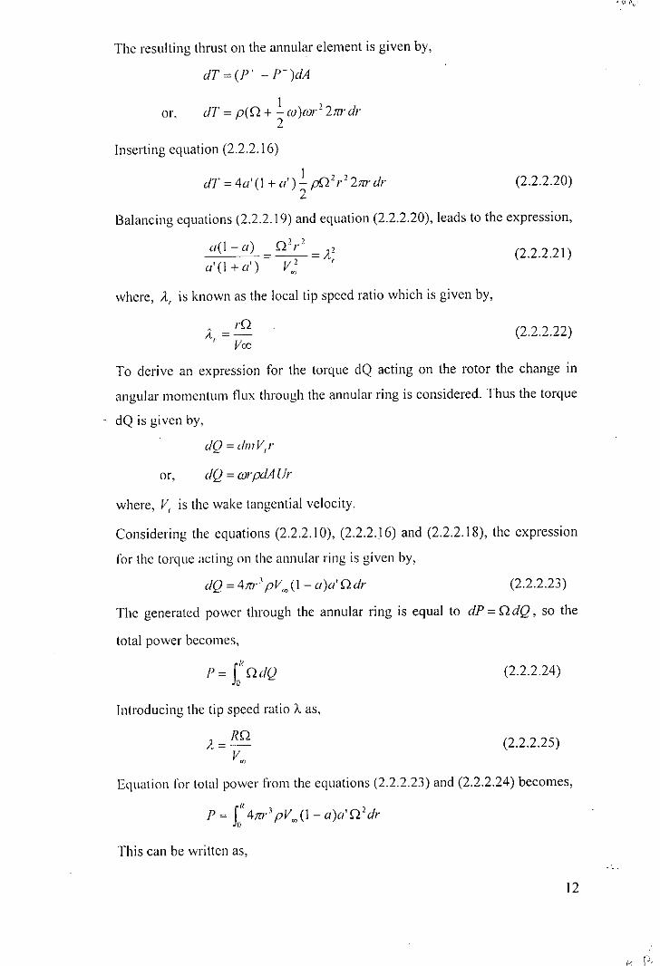
The resulting thrust on the annular element is given by,

dT=(V -r)dA

dT = pen + ~ w)wr' 2m'dr2

Inserting equation (2.2.2.16)

dT = 40' (I + a') ~ pn' 1" 2nr dr2

(2.2.2.20)

(2.2.2.21)

Balancing equations (2.2.2.19) and equation (2.2.2.20), leads to the expression,

0(1-0) = n'r' =Je'0'(1 +0') V~ '

where, Je,. is known as the local tip speed ratio which is given by,

rnJe =~, Voo

(2.2.2.22)

To derive an expression for the torque dQ acting on the rotor the change in

angular momentum nux through the annular ring is considered. Thus the torque

dQ is given by,

dO=dmVr- ,or, dQ = wrpdA VI'

where, V, is the wake tangential velocity.

Considering the equations (2.2.2. I0), (2.2.2.16) and (2.2.2.18), the expression

for the torque acting on the annular ring is given by,

(2.2.2.23)

The generatcd powcr through the annular ring is equal to dP = ndQ, so the

total power bccomes,

r"I' = Jo ndQ

Introducing thc tip speed ratio A.as,

(2.2.2.24)

(2.2.2.25)

Equation lor total power ii'om the equations (2.2.2.23) and (2.2.2.24) becomes,

fN '\ 2P = J" 4m' pVoo (I - 0)0' n dr

This can be writtcn as,

12

I~ \)

P=~PAV: ;, fu"a'(l-a)A;dA,

where, A is thc turbine swept area which is givcn by A = nR 2.

The power coeftleient is defined as,

PC,,=---

1 c4V'2P w

Inserting equation (2.2.2.26) power coefficient can be written as,

c,' =~ r" a'(I-a) A; dA,.A- J"

Rearranging equation (2.2.2.21),

, I 1 4 )a = - - + - 1+ - a(I - a2 2 A2,

(2.2.2.26)

(2.2.2.27)

(2.2.2.28)

Substituting this value in equation (2.2.2.27) and taking the derivative equal to

zero, the relation betwccn A,. and a for maximum power becomes,

A = (l-a)(4a _I)', (1-3a)

(2.2.2.29)

Introducing equation (2.2.2.29) into equation (2.2.2.21) the relationship

between ({ and a' is obtained as,

I 1 - 3(1a=--

40 -1

This relation will be used latcr for design purposes.

(2.2.2.30)

2.2.3. Blade Element Theory

With the bladc elcmcnt thcory, the forccs acting on a differcntial element ofthc

blade may be calculated. Then integration is carried out over the length of the

blade to determine the performance of the entire rotor.

Thc assumptions in cstablishing blade elcmcnt theory are:

(a) There is no interference between adjacent blade elements along each

blade.

(b) The forces acting on a blade element are solely due to the lift and drag

characteristics of the sectional profile of the element.

(c) The pressure in the far wake is equal to the free stream pressure.

13

.'i-

'.

x ,..;V.,1I-0)

Figure 2.2.4 Velocity Diagram of a Blade Element.

The aerodynamic force components acting on the blade element are the lift

force dL, perpendicular to the resulting velocity vector and the drag force dO

acting in the direction of the resulting velocity vector. The expressions for the

sectional lift and drag forces may respectively be introduced as,

dL = C-,!-pW'Cdr2

dD = Cd ~ pW 'cdr

(2.2.3.1)

(2.2.3.2)

The thrust and torque experienced by the blade element are respectively

exprcssed as,

dT = dLcos~ + dDsin~

dQ = (dL sin ~ - dD cos~)r

(2.2.3.3)

(2.2.3.4)

where, ~ is the angle of rclative water velocity.

Assuming that the rotor has B blades, the expressions for the thrust and torque

become,

14

or,

and

or,

dT = BC ~ pW'(C, cosrjJ+ Cd sinrjJ)dr

dT=BC~PW'C,COSrjJ(l+ ~:: tanrjJ)dr

dQ = BC ~ pW' (C, sinrjJ- Cd cosrjJ)rdr

dQ = BC ~ pW'C, SinrjJlI- Cd _l_\dr2 C,tanrjJj

(2.2.3.5)

(2.2.3.6)

(2.2.3.7)

According to thc Figurc 2.2.4 the expression for relative velocity W can be

written as.

W = (I - a)V ~ = (I + a' )Orsin rjJ cosrjJ

Introducing the following trigonometric relations based on Figure 2.2.4,

and

(l-o)V I-a ItanrjJ= ~ =--

(I + a' )Or I + a' A,

fJI = rjJ- a

(2.2.3.8)

(2.2.3.9)

(2.2.3.4)

where, fJI is the blade twist angle and a is the angle of attack.

The local solidity ratio IT is given by,

BC0=-

2m'

The equations of elemental thrust and torque for the blade element theo,ry

become rcspectively,

, oC, coslj; ( c, ) I ,dT = (I - 0) - . , I + -: tan rjJ - pV;, 2Jrr drsm- rjJ C, 2

and

, oC, sin rjJ( Cd I ) I 2 1dQ = (I + (/')" , I - - -- - pO r 2Jrr drcos- rjJ C, tanrjJ 2

(2.2.3.5)

(2.2.3.6)

2.2.4 Strip Theory

From thc axial momentum and bladc element theories a series of relationships

can bc devclopcd to detcrmine the performance of a water turbine.

15

By equating the thrust, determined from the momentum theory equation

(2,2.2.19) to equation (2.2.3.5) of blade clement theory for an annular clement

at radius 1', one obtains,

dTI1WIll~llll1111 =: dTbladl.: I,;lclnent

or, a 0(', eos~ ( c" do)-- = -- 1+ -tan,!,1-a 4sin'~ c,

(2.2.4.1 )

Equating the angular momentum, determined from the momentum theory

equation (2,2.2,23) with equation (2.2,3.6) of blade element theory, one finds,

dQmnmclllUlll = dQblade elemenl

or, _0'_ = _o(~"_('I __C"_1_)1+ a' 4cos~ l C, tan~

(2.2.4.2)

(2.2.4.5)

Equations (2.2.4.1) and (2.2.4.2), which determinc the axial and angular

intcrference factors contain drag terms. It has been suggested in [25] and [26]

that the drag terms should be omitted in calculation of a and a' on the basis

that the retarded air due to drag is confincd to thin helical sheets in the wake

and have little effects on the induced flow. However, in reference [27] and [28]

drag terms have been included. Omitting the drag terms the induction factors a

and a' may be calculated with the following equations,

a 0(', cos~ (2.2.4.3)=1-a 4sin' ~

a' aC, (2.2.44)=1+ a' 4cos~

Considering the equations (2.2.4.3) and (2.2.3.5), elemental thrust can be

written as,

(C )1dT = 4a(l - aV + c:: tan ~ 2. pV ~ 2w dr

From equations (2.24.4) and (2.2.3.6), clemental torque can be obtained as,

(C 1)1dQ = 4a'(I- a) 1- _d -- - pV~D.2w3 drC, tan~ 2

Elemental power is given by,

(2.24.6)

or,

dP = dQD.

dP=4a'(I-a/l- C:" _1_).!-PV~D.22W3drl C, tan ~ 2(2.2.4.7)

16

Introducing the local tip spccd ratio It,.,

rQIt =-, Vif,

Equations of total thrust, torque and power become,

I ,8 IA (C )T = - pAV- -, a(l- a) 1+ _d tan~ It,. dlt,.2 ~;t-0 C,

I ,8 Ii (C I I )]f)=-pYlV-R- a'(I-a) 1--' --It dll."" 2 ~ It' 0 C, tan ~ ' ,

and

P=~PyjV'~ CAa'(l_a)(l_ Cd _1_ll'dll.2 <7) A2 Jo C, tan q> JI./ I

(2.2.2.22)

(2.2.4.8)

(2.2.4.9)

(2.2.4.10)

These equations arc valid only for a water turbine having infinite number of

blades. The elrect of the finite blade number will be discussed in the next

section.

2.2.5 Tip and Hub Losses

In the preceding sections, the rotor was assumed to have possessed an infinite

number of blades with an infinitely small chord. In reality, however, the

number of blades is finite. According to the theory discussed previously, the

water imparts a rotation to the rotor, thus dissipating some of its kinetic energy

or velocity and creating a pressure difference between one side of the blade and

the other. At tip and hub, however, this pressure difference leads to secondary

now effects. The now becomes three-dimensional and tries to equalize the

pressure dillerence as shown in Figure 2.2.5. This effect is more pronounced as

one approaches the tip. It results in a reduction of the torque on the rotor and

thus in a reduction of the power output.

17

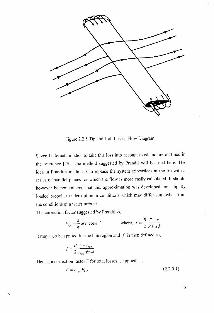
Figure 2.2.5 Tip and Hub Losses Flow Diagram.

Several alternate models to take this loss into account exist and are outlined in

the reference (29]. The method suggested by Prandtl will be used here. The

idea in Prandtl's method is to replace the system of vortices at the tip with a

series of parallel planes for which the flow is more easily calculated. It should

however be remembered that this approximation was developed for a lightly

loaded propeller under optimum conditions which may differ somewhat from

the conditions of a water turbine.

The correction factor suggested by Prandtl is,

f- 2 -/. =-orc case'1/1'

J[

B R-rwhere, .r ="2 R sin IjJ

',\

It may also be applied for the hub region and f is then defined as,

I-Ienee, a correction factor F for total losses is applied as,

f" f- f-. = '/If I • ~hll"(2.2.5.1)

18

The loss factor F may be introduced in several ways for the rotor performance

calculation. In the method adoptcd by Wilson and Lissaman [30], the induction

• factors a and a' arc multiplied with F, and thus the axial and tangential

vclocities in the rotor plane as seen by the blades are modified. It is further

assumed that these corrections only involve the momentum formulas.

Thus the thrust and torque from momentum theory become,

dT = 4mpV ~ aF(1 - aF) dr

dQ = 4nrJ pVwa' 1'(1 - aF)0. dr

Thc results orthe blade e1cment theory remain unchanged.

, DC', eosrjJ( c, ) I 1dT=(I-a)' . , 1+-' tanrjJ -pVw2nrdrSlll'rjJ C, 2

(2.2.5.2)

(2.2.5.3)

(2.2.3.5)

and dQ = (1+ 0')' aC, tanrjJ(I _ Cd -I_)~ p0.' r' 21CdreosrjJ C, tanrjJ 2

(2.2.3.6)

Equation (2.2.3.6) can also be written as,

, aC, ( Cd I ) I , ,dQ=(I-o) -.- 1--, -- -pVw2nr drSlllrjJ C, tanrjJ 2

Balancing the equations (2.2.5.2) with (2.2.3.5) one finds,

0(', cosrjJ(1- a)' ( c, )aF(1 - of) = . , 1+-,' tan rjJ

4 Sill' rjJ C,

and considering thc cquations (2.2.5.3) and (2.2.5.4)

'}'(I }') (I )' 0(', (1 Cd I )(l ~ -(1' = -(J -.- ----4 SillrjJ C, tan rjJ

(2.2,5.4)

(2.2.5.5)

(2.2.5.6)

Omitting thc drag terms in equations (2.2.5.3) and (2.2.5.4) the following

expressions yield,

0(' '''(1 )'}"(I }") , eos I" - U(I' -(.{' =------4sin'rjJ

(2.2.5.7)

(2.2.5.8), aC(l-a)'a 1'(1- aF) = --'---

4sinrjJ

From the equations (2.2.5.7) and (2.2.5.8), the final expressions for elemental

thrust unci torque become respectively,

(2.2.5,9)

19

.,', I~.: (.

, ; .

and

d 1- -( C', 1 J ' ,Q = 4a' '(1- al') 1- --,' -- pV;'trr'drC, tan9

(2.2.5.10)

2,2.6 Thrust, Torque and Power Coefficients

Elemental thrust, torque and power coefficients are respectively defined as,

and

de.,. =

dPde}' =----

1 YlV'2 P if,

(2.2.6.1 )

(2.2.6.2)

or (2.2.6.3)

Considering the equations (2.2.5.9) and (2.2.6.1), elemental thrust coefficient

can be wri ttcn as,

8 (C')dC',= -, aF(I- aF) 1+_01 tan9 I'dI'R' C',

(2.2.6.4)

Again, from the equations (2.2.5.10) and (2.2.6.3), elemental torque coefficient

is givcn by,

dC'"=-;'a' F(I-aF)(I- Cd _1_Jr2 dr, R' C, tan9

(2.2.6.5)

Elemental power cocfticient can be obtained from the equation (2.2.6.3) as,

dCI'= ~O a'F(I- aF/I- Cd _1_)1'2 drR'V~ l C, tan9

(2.2.6.6)

Finally, total thrust. torquc and power coefficients can be obtained by the

following equations,

8 r" (C JC,=-, J, aF(I-aF) 1+-oItan9 I'dI'II' (( C,

(2.2.6.7)

20

8 i" (C, 1 ) ,Co = - a' F(I- aF) 1--' -- r" dr" R' 0 C, tanqj

C' 8 0 I" 'F(I 1')ll Cd 1 ) 2 d,=-- a~-a~ ----rr, R' V 0 C tan"~ I ~

2,2.7 Relations for Maximum Power

(2.2.6.8)

(2.2.6.9)

For maximum power output thc relation between a and a' may be expressed

by the equation (2.2.2.30) as.

, I - 3aa=--

4a -1

Introducing the equations of induction factors from equations (2.2.4.3) and

(2.2.4.4) as,

a ae, cosqj=----

I-a 4sin'qj

and

a' aC',=

I+a' 4cosqj

From the above equations the following expression yields,

aC', = 4(1- cosqj)

The local solidity IT can bc written as,

IX'(1"=-

27rr

Equation (2.2.7.1) transforms into,

Local tip speed ratio A, is given by, .

1'0,1".=-Voo

(2.2.7.1)

(2.2.7.2)

The relationship bctween local tip speed ratio and induction factors may be

exprcssed by thc cquation (2.2.3.8) as,

1 - a 1tanqj=---

I+ a' A,.

21

Now replacing the values of (1- a) and (I + a') from the equations (2.2.4.3)

and (2.2.4.4) and inscrting the value of iJL'l. from the equation (2.2.7.1), the

following relation can be deduced,

..1.= sin~(2cos~ -1), (I - cos~)(2 cos~ + 1)

and this can be reduced to,

2 1~ = -arc tan-

3 A,

(2.2.7.3)

(2.2.7.4)

Equation of blade twist angle from equation (2.2.3.9) can be written as,

Pi =~-aThe equations (2.2.7.2), (2.2.2.22), (2.2.7.4) and (2.2.3.9) may be used to

calculate the blade configurations.

22

Chapter 3 : RIVER CURRENTPOTENTIAL IN BANGLADESH

3.2 THE RIVER SYSTEM

Bangladesh has about 15000 miles (24000 km) of rivers, streams and canals.

These together cover about 7 per cent of country's surface [25]. The discharge

carried by these river systems has a wide seasonal fluctuation peaking at the

monsoon (July to September). The River systems of Bangladesh is shown in

Appendix- A. A list of rivers with their location and length has been given in

Appendix B. All the rivers in Bangladesh belong to the following three river

systems:

a) Tile Ganges-Patlma River System: Starting from the Southern slopes of

the Himalayas it travels 2400km of Indian territory and enters23

Bangladesh near Rajshahi. While in India the Ganges is charged by

water from many tributaries including thc Karnali, the Gandak and the

Kosi.

From the entrancc into Bangladesh territory, the river flows another 70

miles (I 12 km) beforc joining the Brahmaputra-Jamuna at Goalundo,

170 miles (270 km) north of the Bay of Bengal. In Bangladesh, the river

receivcs onc tributary, the Mahnanda, joining it at the left bank in

Rajshahi. The Ganges drains a total area of 430,000 sq. miles (Ll

million sq. km).

b) T/Ie Bra/IIIUlplitra-Jamlilla: It rcaehes Bangladesh from the State of

Assam. forming the border with India over a distance of 45 miles (72

km). Upon entering Bangladesh, the Brahmaputra Jamuna branches into

two. The main course flows to the south through a wide and highly

unstable channel, filled with islands and sand bars, built from its own

movement, until it meets the Ganges-Padma at Goalundo. From here

the eonlluents flow in south-easterly course to join the Meghna at

Chandpur. The minor channel, the Old Brahmaputra, was the main

course of the river only 200 years ago. It flows southeast to meet the

Meghna at Bhairab Bazar.

The Brahmaputra-Jamuna drains an area of 360,000 sq. mile (930,000

sq. km). Peak flows of up to 2500,000 eusecs are reached between mid

June and early September [30].

c) TIle Meg/ilia System: The headwaters of the Meghna enter through two

arms, the Surma and the Kushiyara, both of which have similar origins.

The annual average discharge is around 125,000 cusecs, about the same

as that of the Nile. Flood flow is in the order of 420,000 cusecs.

The Ganges, the Brahmaputra and the Meghna river basin is shown in

Append ix C.

3.3 THE RIVER SITES

24

3.3 THE RIVER SITES

Under this project, different sites of different rivers have been studied. They

are as follow:

!. The Ganges at Hardinge Bridge

II. The Ganges at Gorai Railway Bridge

II!. The Bengali River at Shimulbari

IV. The Tulshiganga River at Naogaon

v. The Atrai River at Atrai

v!. The Bengali River at Khanpur

VII. The Mohananda River at Chapainawabganj

VII!. The Mohananda River at Rohanpur

IX. The Tulshiganga River at Sonamukhi

x. The Atrai River at Chakharihorpur

x!. The Nagar River at Bogra

xii. The Atrai River at Singra

XII!. The Atrai River at Nowhata

XIV. The Atrai River at Mohadevpur

xv. The Kushiyara River at Sheola

xv!. The Piyan River at Jaflong

xvii. The Ichamoti River at Thandachari

XVII!. The Matamuhuri River at Lama

XIX. The Sangu River at Bandarban

xx. The Halda River at Panchapukuria

xx!. The Bogkhali River at Ramu

XXI!. The Atrai River at Noldangar Hat

XXIII. The Brahammaputra River at Bahdurabad

The river current data (Appendix D) of the above mentioned stations have been

collected from the Bangladesh Water Development Board, Dhaka. These data

are from mostly from the year 1997 to 2000. But except 2/3 stations, other

stations don't have a complete set of data for the year round. So it is very

25

difficult to take a concrete decision on the river current potential of a particular

station.

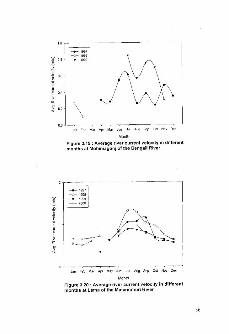
At almost all the stations the river current velocity is above 0.4 m/s from July

to October. Nawhata, Bogra, Sonamukhi, and Chapainawabgonj show very

poor river current velocity. At these stations the river current velocity is less

than 0.5 m/s.

Rohanpur, Singra, Chakharihorpur, Khanpur, Atrai, Noagaon, Noldargarhat

and Mohimagonj show moderate river current velocity. At these stations the

river current is between 0.5 m/s to 0.75 m/s from July to November.

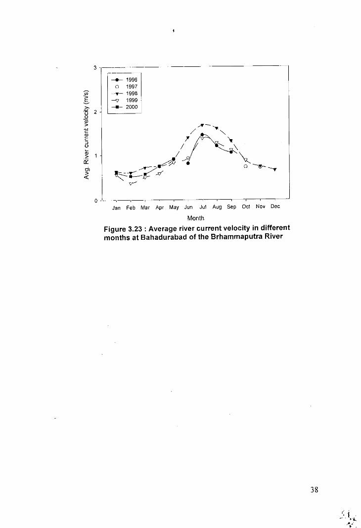
River current is more than 0.9 m/s at Ramu, Panchapukuria, Lama, Bandarban,

Sheola, Jaflong, Hardinge Bridge, and Gorai Railway Bridge stations. So these

stations are very good potential in river current.

The average river current velocity distributions over the year at the above

mentioned stations have been shown from Figure 3.1 to 3.23.

26

4

___ 1996

o 1997--'0- 1998-V 1999

Jan Feb Mar Apr May Jun Jul Aug Sep Oct Nov Dec

Month

Figure 3.1 : Average river current velocity in differentmonths at the Hardinge Bridge of the Ganges

3 -------- -.----

.!!!.s 2

.i:'.0oID>C:g 1:JU

Q;>a::til 0-

~

___ 1997

-0- 1998-.- 1999-';)- 2000

Jan Feb Mar Apr May Jun Jul Aug Sep Oct Nov Dec

Month

Figure 3.2: Average river current velocity in differentmonths at the Gorai Bridge of the Gorai River

27

1.0

--e-- 1997

"' 0.8 -0- 1998E --..- 1999

~.13 0.60(ij>Ci" 04.'50

li;> 0.2 .ii'

'"><{ 0.0 .

. ~y.,

Jan Feb Mar Apr May Jun Jul Aug Sep Ocl Nov Dec

Month

Figure 3.3 : Average river current velocity in differentmonths at Singra of theAtrai River

0.55.-

0.50. -i ~;lli9~~ ---T- 1999.s 045. ---~.13o OAO-(ij>c~ 0.35-

aQ) 0,30>ii'0) 0.25

~0.20

0.15 --,Jan Feb Mar Apr May Jun Jul Aug Sep Oct Nov Dec

Month

Figure 3.4 : Average river current velocity in differentmonths at Nowhata of the Atrai River

28

. ,

.,1

2 - -- 1997-0- 1998

~ -?- 1999.s ------z..0 10Q)>c~5"Q; 0---")> 0iYOl><{

~~--,~----~ ,-Jan Feb Mar Apr May Jun Jul Aug Sep Oct Nov Dec

Month

Figure 3.5 : Average river current velocity in differentmonths at Shimulbari of theBengali River

0.6

__ 1997

"' 0.5 -0- 1998

E -?- 1999

Z.0.4.0

0Q)>C 0.3~:J"Q;

0.2>iYOl \><{ 01 -

0.0 --,Jan Feb Mar Apr May Jun Jul Aug Sep Oct Nov Dec

Month

Figure 3.6 : Average river current velocity in differentmonths at Bogra of the Nagar River

29

~r)'• I\i\-.n

0.7 -

0.6

.!!?-S 0.5Z'.(30 0.4 -W>C

0.3 -~::>u~ 0.2<1>>iYOJ 0.1><{

0.0

___ 1997

-0- 1998~ 1999

- --,- ~'---------'--'------'-~--.Jan Feb Mar Apr May Jun Jul Aug Sep Oct Nov Dec

Month

Figure 3.7: Average river current velocity in differentmonths at Sonamukhi of the Tulshiaanaa River

0.7

0.6 [ • 1997

<n -0- 1999

E 0.5 -Z'.(30 0.4W>C

0.3~::>uill 0.2>iYOJ 0.1><{

0.0 -

Jan Feb Mar Apr May Jun Jul Aug Sep Oct Nov Dec

Month

Figure 3.8 : Average river current velocity in differentmonths at Naogaon of the Tulshiganga River

30

0.8 ._-- -- ---"---

0.7 -e-- 1997

V> -{)- 1999

E ---06

~.00 0.5a;>C 0.4~:;L>Q; 0.3>ii:Ol 0.2><{

0.1

0.0

0.7

Jan Feb. Mar Apr May Jun Jul Aug Sep Oct Nov Dec

Month

Figure 3.9 : Average river current velocity in differentmonths at Atrai of the Atrai River

0.6 -

0.5

'"0.4

ro0>- 0.3 -

0.2 .

01

-e-- 1997-{)- 1998-T- 1999

0.0 --- - -,-------.T.~-'--- --'----,--------,------1--."Jan Feb Mar Apr May Jun Jul Aug Sep Oct Nov Dec

Month

Figure 3.10: Average river current velocity in differentmonths at Rohanpur of the Mohananda River

31

2 - -~---- ~~-~-~~--~~

___ 1997

-0- 1998.!{! ---T- 1999E- -<r- 2000~'0oQj>

~ 1:;u

'">ii:rn><{

aJan Feb Mar Apr May Jun Jul Aug Sep Oct Nov Dec

Month

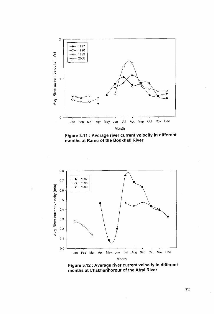
Figure 3.11 : Average river current velocity in differentmonths at Ramu of the Boqkhali River

0.8

0.7 -___ 1997

-0- 1998~ -T- 1999E- 0.6 - -----~'00 0.5 -Qj>C 0.4 -~:JU~ 0.3'"

~

>ii:rn 0.2><{

0.1 -

0.0 ----1--1~-'

Jan Feb Mar Apr May Jun Jul Aug Sep Oct Nov Dec

Month

Figure 3.12: Average river current velocity in differentmonths at Chakharihorpur of the Atrai River

32

1.2___ 1997

1.1 . -0- 1998!!'. --.- 1999.S- 1.0 . -V- 2000

""'"0 0.9Qj>C 0.8 .~:J0

W 0.7 .>0"

'"0.6 ~

>

~

<{

05 .

04 ---I--'--r"------, ~Jan Feb Mar Apr May Jun Jul Aug Sep Oct Nov Dec

Month

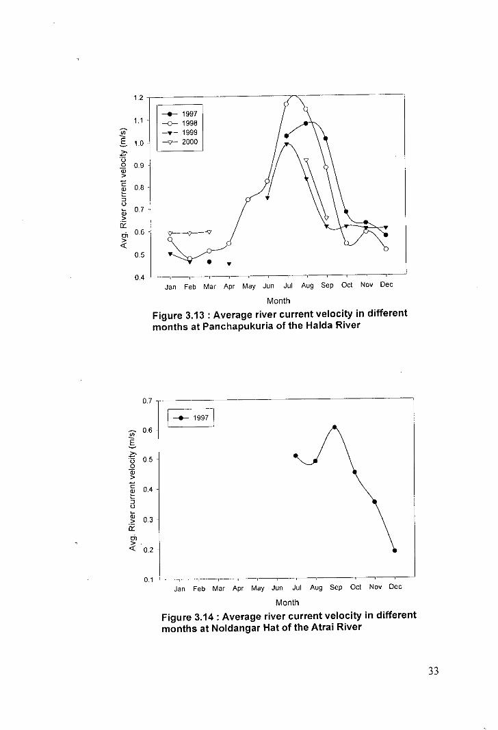
Figure 3.13: Average river current velocity in differentmonths at Panchapukuria of the Halda River

0.7 .

0.6 .

F-;;;-I<nE

"" 05'"0Qj>C 04~:J0

W 03>0"

'"><{ 0.2 .

0.1 .-1--~-'---""----'Jan Feb Mar Apr May Jun Jul Aug Sep Oct Nov Dec

Month

Figure 3.14: Average river current velocity in differentmonths at Noldangar Hat of the Atrai River

33

1.4

---- 19971.2 --D- 1998

V> -T- 1999E -y- 2000z;- 1.0 ..130a;>C 08<Dto::>L)

Q; 06."0::

'"><{ 0.4

0.2Jan Feb Mar Apr May Jun Jul Aug Sep Oct Nov Dec

MonthFigure 3.15: Average river current velocity in differentmonths at Jaflong of the Piyan River

2____ 1997

--D- 1998~ ----T- 1999.s -y- 2000z;-.13oa;>c~";L)

Q;>ii:

1o

Jan Feb Mar Apr May Jun Jul Aug Sep Oct Nov Dec

Month

Figure 3.16: Average river current velocity in differentmonths at Sheola of the Kushiyara River

34

0.4 -

0.8 -

07 -

"'E 0.6

~oo 0.5-Qj>c~OJo(jj 0.3-

."0::OJ 0.2-

~0.1

___ 1997--{)- 1998-T- 1999

0.0 ----',- ----r-~-T~-'~~'--,~Jan Feb Mar Apr May Jun Jul Aug Sep Oct Nov Dec

Month

Figure 3.17 : Average river current velocity in differentmonths at Chapainawabgonj of the Mohananda River

2- ~---

___ 1997--{)- 1998

~ ---T- 1999oS -<:J- 2000.?:'.[3oQj>C!'!:;oQ;>iX'0>~

0--Jan Feb Mar Apr May Jun Jul Aug Sep Oct Nov Dec

Month

Figure 3.18: Average river current velocity in differentmonths at Bandarban of the Sanau River

35

\

____ 1997--0-- 1998--.- 1999

1.0

0.0 - ---,---.'I--~l---'.-----Jan Feb Mar Apr May Jun Jul Aug Sep Oct Nov Dec

(j) 0.8-E.i:'.uou; 0.6>c:Q)

l:::Jo 0.4-Q;

.2:lY

'"~ 02

Month

Figure 3.19: Average river current velocity in differentmonths at Mohimagonj of the Bengali River

2____ 1997

--0-- 1998Ul --.- 1999E ~ 2000.i:'.uou;>

~ 1-:;uQ;>iY

oJan Feb Mar Apr May Jun Jul Aug Sep Oct Nov Dec

Month

Figure 3.20 : Average river current velocity in differentmonths at Lama of the Matamuhuri River

36

1.0 .

~(/) 0.8-E~'uoiii 0.6>C~::>u 0,4-iii

"0::r 0.2

0.0

__ 1997

-{}- 1998~ 1999

,--,~-,'--~---.-r---r-------'----'-~-.~~Jan Feb Mar Apr May Jun Jul Aug Sep Oct Nov Dec

Month

Figure 3.21 : Average river current velocity in differentmonths at Khanpur of the Bengali river

1.0 l-- 1997Ul

-{}- 1998

E 0.8 ~ 1999---

~'u0Qj 0.6 .>Ci'!:;u 0.4 .iii>ocOJ

~> 0.2 .-0:

0.0 . --,~Jan Feb Mar Apr May Jun Jut AU9 Sep Oct Nov Dec

Month

Figure 3.22 : Average river current velocity in differentmonths at Mohadevpur of the Atrai River

37

3.-------___ 1996

o 1997--'1'- 1998--<:J 1999___ 2000

o ._-,--,~--r-~-~-.'-~-~-~-~-~-Jan Feb Mar Apr May Jun Jul Aug Sep Oct Nov Dec

Month

Figure 3.23 : Average river current velocity in differentmonths at Bahadurabad of the Brhammaputra River

38

<i..". ,.•.....•••lo~.

[4.1.1]

Chapter 4 : RIVER CURRENT:

A SOURCE OF ENERGY

It should be mentioned here that this research is dealing with the extraction of

kinetic energy from a freely flowing river or canal in situations where it is

impractical, both on engineering or economic grounds, to create a static head of

water by the construction of any sort of dam or barrage. Compared to the

energy available from a static head of water, river currents are a very diffuse

energy source. For example, a river speed of one meter per second is

equivalent, in energy terms, to a static head of only 50mm [24]. Thus any static

head of water available should always be exploited (using the relevant

technology) in preference to a freely flowing river or canal. But river currents

have many advantages as an energy source. Besides of providing a reliable and

predictable energy supply over the 24 hrs per day, relatively simple

technologies can convert river current energy to provide electrical energy or

provide pumped watcr in sufficient quantities for economically viable small-

scale irrigated agriculture.

4.1 Power From Flowing Water

The power available ii'om the flowing water can be calculated from the

following equation:

I' = ~pAV3<l 2 a

1\ available power (watts)

39

~... ,', .(, :.I ,

p density of water (1000 kg/m)

A area of flow perpendicular to the current direction from which

power is to be extracted (m2)

Va water velocity (m/s)

In practice, it is not possible to extract all the power available in a river current

for two reasons:

(i) to give up all its kinetic energy the water would have to stop, which

clearly can't be done;

(ii) turbine rotor must be used to convert the water's kinetic energy into

shaft power, and this rotor is bound to be subject to drag forces which

will dissipate some orthe power.

Adding a constant to represent the conversion efficiency from energy flux in

the flowing water to power output of the turbine shaft, equation [4.1.1]

becomes:

I )P, = - pA,V, Cll. 2 .. [4.1.2]

P, turbine shaft power (watts)

As area of water current (perpendicular to the current direction)

interrupted by the turbine rotor (m2)

Vs free stream velocity measured at the upstream from the turbine

(m/s)

Cp coefficient of performance of the turbine rotor

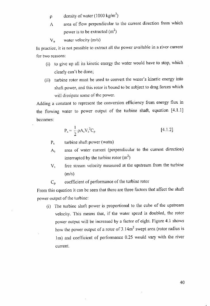
From this equation it can be seen that there are three factors that affect the shaft

power output of the turbine:

(i) The turbine shaft power is proportional to the cube of the upstream

velocity. This means that, if the water speed is doubled, the rotor

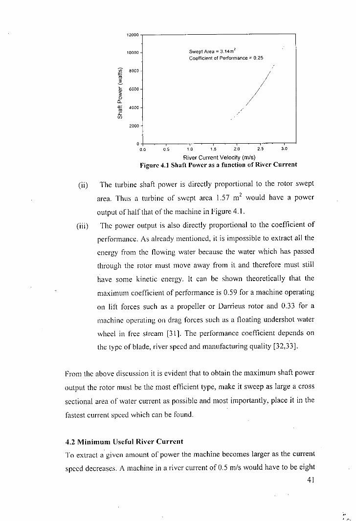
power output will be increased by a factor of eight. Figure 4.1 shows

how the power output of a rotor of 3.14m2 swept area (rotor radius is

1m) and coefficient of performance 0.25 would vary with the river

current.

40

Swept Area = 3.14m2

Coefficient of Performance = 0.25

12000

10000

"' 8000'i5~Q; 6000;,0

"-'" 4000'"£if)

2000

00.0 0.5 1.0 1.5 20 2.5 3.0

River Current Velocity (m/s)Figure 4.1 Shaft Power as a funelion of River Currenl

(ii) The turbine shaft power is directly proportional to the rotor swept

area. Thus a turbine of swept area 1.57 m2 would have a power

output of half that of the machine in Figure 4.1.

(iii) The power output is also dircctly proportional to the coefficient of

pcrformancc. As already mentioned, it is impossible to extract all the

energy from the flowing water because the water which has passed

through the rotor must move away from it and therefore must still

have some kinetic energy. It can be shown theoretically that the

maximum coefficient of performance is 0.59 for a machine operating

on lift forces such as a propeller or Darrieus rotor and 0.33 for a

machinc operating on drag forces such as a floating undershot water

wheel in frce stream [31]. The performance coefficient depends on

the type of blade, river speed and manufacturing quality [32,33].

From the above discussion it is evident that to obtain the maximum shaft power

output the rotor must be the most efficient type, make it sweep as large a cross

sectional area of water current as possible and most importantly, place it in the

fastest current spced which can be found.

4.2 Minimum Useful River Current

To extract a given amount of power the machine becomes larger as the current

speed decreases. A machine in a river current of 0.5 m/s would have to be eight

41

times the size of one in current of Im/s to produce the same shaft power as

evident hom Figure 4.1.

As can be seen II'om Figure 4.1, the level of energy flux in river currents of less

than O.4m/s is so low that there would have to be very special economic

conditions to justify the construction of a machine large enough to extract

useful amount of power.

Using a cluct to artificially increase the water velocity through the turbine rotor

might be an improvement in energy extracted per unit area of current

intercepted. However, the considerable increase in capital cost and the

increascd difficulties of transporting and maneuvering the machine eliminate

the ducted frec stream turbine from further consideration as a low cost water

current turbine.

4.3 Site Selection

In the last section it has been established the minimum river speed for any form

of kinetic energy extraction to be viable. Like conventional water powered

devices, river current turbine is a sitc- specific technology. For example, the

diameter of the machine rotor will depend on the river current.

Bcfore starting work on thc construction of a turbine, it is necessary to survey

the proposed site for the machine to provide the following basic information:

(i) the maximum and minimum river current over the months that the

machine will be used;

(ii) environmcntal hazards such as floating debris, river traffic, etc.;

(iii) rivcr depth at the position where the turbine will operate.

4.4 Measurement of River Current

The river currcnt can vary by as much as 10 pcrcent within 30 or 40 meters up

or down stream from a givcn spot l24]. Bearing in mind that a 10 percent

increasc in river speed gives a 33 percent increase in rotor shaft power, the

importance of accurate river current measurement for selecting the best site

will clearly be appreciated.42

Accuratc spccd mcasurcmcnt is also necessary to select the correct rotor swept

area to ensure that the required amount of power is produced.

43

Chapter 5: DESIGN AND FABRICATION OF

WATER CURRENT TURBINE

5.1 Choice of Turbine Rotor

The function of the turbine rotor is to convert as much as possible of the kinetic

energy nux through it into useable shalt power. The range of possible turbine

rotors is similar to the different types use to extract energy from the wind.

There are two basic types of rotor operating on different principles:

(i) Rotors, which have their effective surfaces mov1l1g 111the

direction of the current and are pushed round by the drag of the

water, e.g .. under shot water wheel as shown in Figure 5.1.

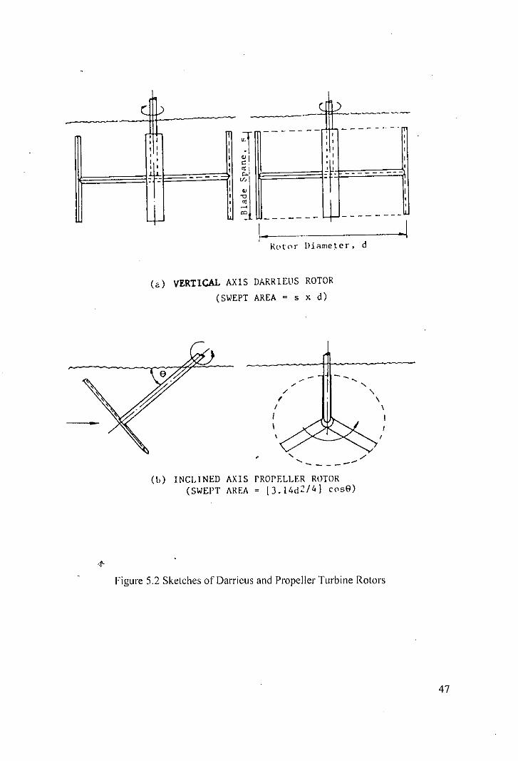
(ii) Rotors, which have their effective surfaces moving at an angle

to the direction of the water and operate on lift forces, e. g.,

propeller rotor and Darrieus rotor as shown in Figure 5.2.

In this research, the inclined axis rotor is of propeller type with 3 blades of

airfoil shaped.

5.2 Design of turbine blade

The design of a rotor consists of two steps:

1. Choice of basic parameters such as

• number of blades B

• radius of the rotor R44

• type of airfoil and

• selection of design tip speed ratio A".

2. Calculations of the blade twist angle fir and the chord C at a number of

positions along the blade, in order to produce maximum power at a

given tip speed ratio by each section of the blade.

The design procedure is describcd in the following sections:

The selection of the number of blades B affects the power coefficient.

Although B has no influence on the tip speed ratio of a certain windmill, for the

lower design tip speed ratios, in general, a higher number of blades is chosen

table A. This is done because the influence of B on Cp is larger at lower tip

speed ratios. A second reason is that choice of a high number of blades B for a

high design tip speed ratio will lead to very small and thin blades which results

in manufacturing problems and a negative influence on the lift and drag

properties of the blades.

Table A

Design tip speed ratio, Ad Number of blades, B

1 6 - 20

2 4 - 12

3 3 - 6

4 2-4

5-8 2 - 3

8 ~15 I - 2

A second important factor that affects the power coefficient is the drag. Drag

affects the expected power coef/lcient via the CdlCI ratio. This will influence

the size and, even more, the speed ratio of the design. Promising airfoils have a

minimum CeI/CI ratio between O.I-0.0 I (Appendix E).

45

.".0>

"T1

IJ"

"~"V>

(fJ,,-"n:;-o....,~o!'?='IJ"

C='0-"~</>:;-o~:E!'?"~:;-"!!.

-- ---- - - - ----

-'I-- .d

h

r- ~ w • IFLOATING UNDERSHOT WATERWHEEL(SWEPT AREA • w x h)

Figure 6.1 Sketch of Floating Undershot Waterwheel

( )--~-~-----; t

, ', t, t

'~!r'

--------

~ .1R['t0r I)iameter, d

(G) VERTICAL AXIS DARRIEUS ROTOR(SWEPT AREA = s x d)

/,II\

-- - "-

"- \\II

I

" ./.•••..• - - - ---(L) INCLINW AXIS PROPELLER ROTOR

(SWEPT AREA. [3.14d2/4] cpsB)

Figure 5.2 Sketches of Darrieus and Propeller Turbine Rotors

47

A large Cd/CI ratio restricts the design tip speed ratio. At lower tip speed ratios

the use of more blades compensates the power loss due to drag (Appendix F).

In this collection of maximum power coefficients it is seen that for a range of

design speeds I~ Ad ~ 10 the maximum theoretically attainable power

coefficients lie between 0.35~ (Cp)",,,,~0.5.

Due to deviations, howcvcr, of the ideal geomctry and hub losses for example,

these maximums will lie between 0.3 and 0.4. This result shows that the choice

of the design tip speed ratio hardly affects the power output.

The design of an airfoil blades for a given water current velocity Va and power

demand P can be performed now.

Let us first chose the airfoil of NACA 4412.

Appendix E. (Cd/CI)",;" = 0.0 I

Appendix F : I~ Ad~IO; let Ad= 4

Tah/e A :Number of blades, B = 3

Appendix F : (Cp)",,,, = 0.5

For conservative design, Cp = (Cp)",,,, x 0.8 = 0.5 x 0.8 = 0.4

Now,

Rotor Radius, R=2P

7[pV;'C"

For Power output, P = 8.5 watt

(5.2.1)

Free stream velocity, Vu = 0.65 m/s

Then from Eg. (5.2.1), the rotor radius be 223 mm. The density of water has

been considered as 1000 kg/m]

Thus the Design values for the model are:

Blade airfoil type : NACA 4412

Rotor radius : 223mm

Blade length. : 170 mm

Hub radius : 38 mm

Root Chord : 143 mm

Tip Chord : 68 mm

48

Number of Blades • : 3

5.3 Choice of Turbine Rotor

Different blade materials can be used for rotor construction. Some have been

tested by Peter Garman [24]:

(i) solid aluminium alloy;

(ii) laminated hardwood sheathed with glass fiber reinforced plastic

(GRP);

(iii) steel spar with polyurethane foam filled GRP fairing;

(iv) untreated hardwood;

(v) ferrocement (a) untreated, (b) painted, (c) sheathed with Al alloy

sheet;

(vi) steel spar, timber fairing sheathed with AI alloy sheet.

From the performance point of view surface finish is critical, and any

deterioration causes drastic shaft power reduction. This is because the blade

velocity of lift- powered rotors is twice (in the case of the Darrieus rotors) or

three times (in the casc of propeller rotors) that of the river current and so drag

produced by surface friction is a very important consideration [24]. In

consideration of this AI alloy maintains its surface highly finished and hence,

high level of performance can be maintained. For this reason Al- blades have

been used to fabricate the model.

5.4 Rotor Shaft Bearing

Thc rotor shalt must be carried in bearings, which support it in the correct

position relative to the river current and allow it to rotate as freely as possible.

If the shalt is to be supported at each end by a bearing mounted on a frame, at

least one of the bearings must allow some axial movement to take up flexing of

the fj'ame.

The inclined axis propeller rotor has one bearing above the water for which a

single row ball bearing is suitable. The bearing used is the grease- lubricated

self- aligning type. The bearing at the bottom of the rotor shaft is under water

and hence must be scaled. This bearing locates just behind the rotor shaft, takes

49

'j" L,~~'..r~m::,..',.'

a small radial load and allows some axial movement of the shaft relative to the

ti'ame.

...

X Section ofbladeNACA 4412

RotorLifting Winch

• v

Load

Pontoon

Figure 5.3 Schematic Diagram of the Zero Head Water Current

Turbine

50

...

Figure 5.4 Water Current Turbine Model

Figure 5.5 Blades oflhe Turbine Model

51

Figurc 5,6 Flumc where the Turbine Model has been tested

Figul'c 5.7 Turbine Model in the Flume

52

Chapter 6 : PERFORMANCE ANALYSIS

In analyzing the rotor performance, an important parameter that comes in front

is the tip speed ratio (TSR) which is used in setting the correct transmission

ratio. It is the ratio of the tl'ee stream velocity and the blade tip velocity.

Mathematically,

TSR= velocily al Ihe blade lipvelocily 0/ Fee slreall1

2rr N RVelocilyal Ihe blade lip------60where N =rpll1o/fhe rolor

R = 1'0101' radius

The value of tip speed ratio depends on the type of rotor, the number of blades,

and the load on it.

It has been mentioned earlier that the propeller type rotors operate on lift

forces. The turbine blades having an airfoil cross section which when moves at

an angle relative to the current direction, produces a lift force at right angles to

the relative velocity of the water as seen from the blade. Figure 6. I shows how

the relative velocity is found by vector addition of the stream velocity and

blade tip velocity.

As can be seen from Figure 6.1 the lift force acting on the blade can be

resolved into two components: parallel and normal to the plane of rotation. The

parallel component makes the rotor turn alid the normal component bends the

blade. The lift force is proportional to the angle of attack (a) up to the stall

53

I.

angle of the hydrofoil. As load is applied to the turbine, it slows down. This has

the effect of increasing a. (the angle between the blade chord and the velocity

of water relative to the blade, VR) and hence, increasing the lift force. As

further load is applied. a. increases until eventually it exceeds the stall angle of

the hydrofoil scction and thaI part of the blade no longer contributes to the

power output of the rotor. Once large areas of the blades are in the stalled

condition, the turbine simply stops. This is evident from Figures 6.2 (a), 6.2 (b)

and 6.2 (c).

Figure 6.2 shows the pcrformancc curves for the turbine model. These curves

are cquivalent to powcr vcrsus rotational speed curves but by plotting Cp vs. tip

spced ratio curves become independent of river speed and therefore, more

widely applicable.

From the curves of Figure 6.2 (a) it can be seen that the model consisting of

NACA 4412 airfoil blades will run at tip speed ratios between 3.2 to 6 when

the pitch angle is 5° But this operating region squeezes if the pitch angle is

reduced to 0" i.e. the pitch angle is absent in this case. This is also true for the

Figure 6.2 (b) where the range of tip speed ratio for turbine operation is 0.7 to

3.5.

At a very low water velocity power coefficient is not more than 15% giving no

pitch angle. If a pitch angle is introduced, then Cp will increase but ai the same

time the operating range will decrease. This is apparent in Figure 6.2 (b). To

obtain the maximum power output from a rotor it should be loaded until it is

running as close to the tip speed ratio for maximum Cp.

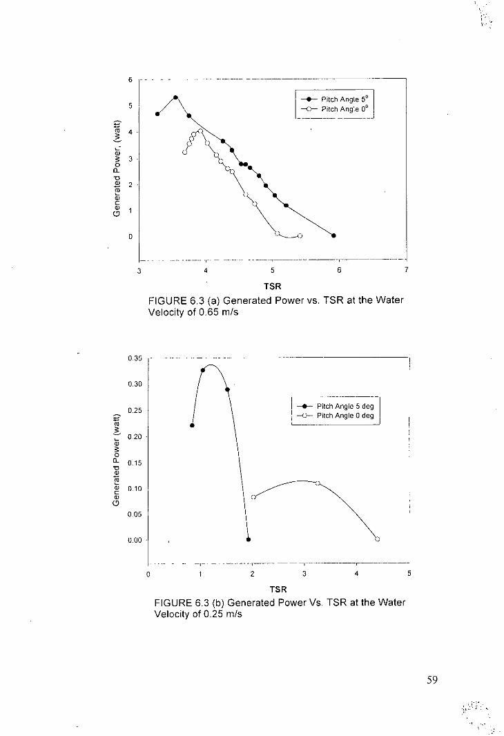
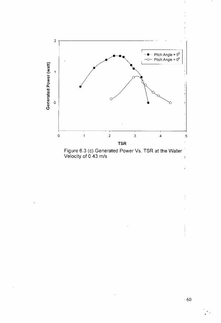
Figure 6.3 (a), 6.3 (b) and 6.3 (c) show the power generated by the rotor at

different tip speed ratio at 0.65 mis, 0.25 mls and 0.43 m/s water velocity

respectively for both 0" and 5° pitch angles. The generated power is very low

(less than 0.5 watt) when the velocity is 0.25 mls but when it is 0.65 m/s the

output power increases sharply. It should be mentioned here that the average

rotor radius is taken as 221 mm in input power calculation.

54

Duc to the changc of watcr velocity the change rpm at no load conditions has

been shown in Figurc 6.4. No doubt the rpm would be higher at a particular

water current vclocity whcn a pitch angle is introduced at the rotor blade.

Increasc of input power with the increase of water velocity has been shown in

Figure 6.5. Power input changes in cube with the water velocity.

Figurc 6.6 shows the vclocity profile in the flume. The velocity is zero at the

bottom surface of the flume. While moving upward from the surface the

velocity increases and it is constant at the boundary layer. But again the

velocity decreases at the upper surface of the water.

55

LIFTFORCE

TURBINE BLADE(AIRFOIL

SHAPE)

WhereVs • Water Current Velocity (absolute)UB Blade Tip Velocity (absolute)VR ~ Velocity of Water Relative to BladeFp = Component of Lift Force in Plane of

Rotor RotationFN Component of Lift Force Normal to

Plane of Rotor Rotation

Figure 6.1 Airfoil Hydrodynamics

-- ---.....,Fp I

I

IIIIII

FN 1IIIIIIII

56

I,

0.5

0.4

0.3

a.U 02

0.1

0.0

3 4 5

TSR

____ Pitch Angle = 0°

-0- Pitch Angle = 5°

6 7

0.5

0.4

0.3

a.U 0.2

0.1 -

0.0

Figure 6.2 (a) Cp VS. TSR at water velocity of 0.65m/s forthe pitch angle of 00 and 50

---.- Pilch Angle = SO--0- Pilch Angle = 0°

o 2 3 4 5

TSR. Figure 6.2 (b) Cp Vs. TSR at the water velocity of 0.43 m/s

for the pitch angle of 0° and SO

57

~, J •J 'i

0.5

0.4 -

0.3

D..U 02

0.1

0.0

-e- PitchAngle = 00

--0-- Pitch Angle = 5°

o 2

TSR3 4 5

Figure 6.2 (c) Cp VS. TSR at water velocity of 0.25m/s forthe Pitch Angle of 00 and 50

58

~-Q)

" 3-o0-"022.ro:vcQ) 1-~

o

---- - -_ .._ ... "[ . - --- ..

-e--- Pitch Angle SO-0- Pitch Angle 00

----.,------------1----------- _..3 4 5 6 7

TSR

FIGURE 6.3 (a) Generated Power VS. TSR at the WaterVelocity of 0.65 m/s

035 I

0.30

0.25Bro~ 020 .:v"00- o 15"02l"Q) 0.10cQ)

~0.05

0.00 .

[

--------~-------------+--- Pitch Angle 5 deg-0- Pitch Angle a deg

--[- _._..- -1---- --- -- -,-~-----r--------a 2 3 4 5

TSR

FIGURE 6.3 (b) Generated Power Vs. TSR at the WaterVelocity of 0.25 m/s

59

___ Pitch Angle = 5°

-0- Pitch Angle = 0°

2 --

~OJ;:o0-"0OJ-~OJc: aOJ(')

a 2 3 4 5

TSR

Figure 6.3 (c) Generated Power Vs. TSR at the WaterVelocity of 043 m/s

60

!

1,I,'I

!

~ Pitch Angle 5 deg--0- Pitch Angle 0 deg

I~ I0,2 0.3 04 0.5 0.6 O.Z

Water Velocity (m/s) iFIGURE 6.4 Change of rpm of the rotor at no load condition due to;1change of water velocity,

200

180

l: 1600;e"0l: 1400U"0III 1200...J0Z 100n;:;;a. 800::

60

16

14--'"~ 12~E0~ 10

'"J::-0 8--::'!

a.c: 6~'" il;:0 4a. I

2

00.2 03 04 05 0.6 0.7

Water Velocity (m/s)

FIGURE 65 Input Power to the Rotor vs. Water Velocity j!

surface

or: 180cQl 150cIII 12 -•..

.!!l0III 90

tQl

> 6

3

053 0.54 0.55 0.56 0.57 058 0.59

Water Velocity (m/s)

Figure 6.6 Water Velocity Profile in the Flume

62

Chapter 7: COST ESTIMATION

Cost of Power Generated by the Water Current Turbine Model

There are three main aspects to the socio-economic appraisal of the water

current turbincs for power gcneration. These are:

(i) economic analysis- to establish the maximum costs above which water

current turbines are unlikely to be economically attractive to the

consumers;

(ii) considcration of social factors; and

(iii) if thcy do appear to the economically viable and socially acceptable, then

the systcmatic comparison of water current turbines with alternative

renewable energy systems technology to detcrmine which system is likely

to be the most socially acceptable and constitute the best value for money.

But this scction just focuses on the cost of manufacturing the water current

turbine model and then estimates the cost of energy generated by the turbine

model.

Table 7.1: Construction Cost of the Water Current Turbine Model

Item Price

3 aerodynamic shaped blades Tk.500.00

Shan, Hub and Bearings Tk.400.00

Floats Tk.100.00

Flat bars Tic 50.00

63

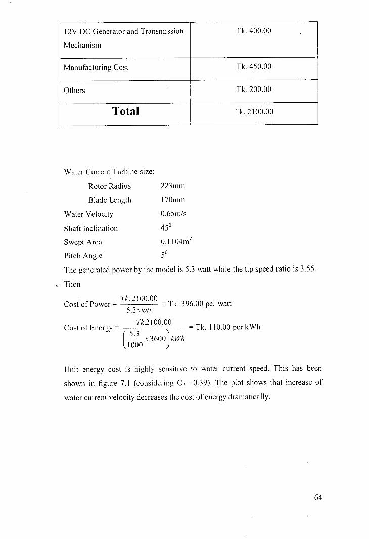
12V DC Generator and Transmission Tk.400.00

Mechanism

Manufacturing Cost Tk.450.00

Others Tk.200.00

Total Tk. 2100.00

Water CutTent Turbine size:

Rotor Radius

Blade Length

Water Velocity

Shaft Incl ination

Swept Area

Pitch Angle

223mm

170mm

0.65m/s

45°

0.1 104m2

5°The generated power by the model is 5.3 watt while the tip speed ratio is 3.55.

Then

Tk.2100.00Cost of Power = = Tic 396.00 per watt

5.3 wall

. Tk2100.00Cost 01 Energy = (0 J = Tk. 110.00 per kWh

5.~ x 3600 kWh1000

Unit energy cost is highly sensitive to water current speed. This has been

shown in figure 7.1 (considering CI' =0.39). The plot shows that increase of

water current velocity decreases the cost of energy dramatically.

64

60

~50

:s:~•..Ql 40Q.

~'->. 30OJ••Qll:

W- 200.•..til0U 10

o06 0.8 1.0 1.2 1.4 1.6

Water Velocity (m/s)

Figure 7.1 Variation of Energy Cost with Water Velocity

The data has been given inappendix H.

65

Chapter 8 CONCLUSION

It has been mentioned earlier that the water current turbine can be thought of as

an under water windmill which floats on the surface of a river with the rotor

completely submcrged. It requires neither dams nor diversion of a portion of

thc water flow. It is teetered in free stream in a river or canal and extracts a

portion of the kinetic energy li'om the moving water. Mooring is from one bank

only and so navigation in thc river or canal is not affected.

At the end of the thesis the following conclusions can be made:

From thc analysis of river current data for different stations at different

rivers. it is clear that the rivers in Hill tracts and Sylhet (South East and

North East region of Bangladesh) are highly potential for power generation

in small scale. Some of the rivers in northwest part of Bangladesh are

moderately potential having a river current velocity in a range of 0.5 m/s to

0.8 m/s. The rivers in the southern part of Bangladesh could not be

considered in this analysis due to unavailability of data.

From thc performancc analysis of the model it is evident that the water

current turbine is not feasible for very low water velocity. The turbine is

suggested for the water velocity of not less than 0.45m/s.

At 0.25m/s the available water power at the turbine rotor with an

inclination of 45° is 17walt considering the rotor radius is 1m. If CI' is 0.3

the power output will be about 5 watt. But for the same turbine working

66

,under the water veloeity of 0.45 m/s the available power will be 10lwatt

and the power output will be 30 watt.

Generally speaking. it is desirable to seleet as high speed a rotor as

possible, bceausc thc faster thc loaded rotor turns the cheapcr will be the

transmission. Rcducing the number of blades or the blade chord length

tcnds to incrcase the rotational spced, but smooth running and struetural

considcrations set minimums for both these variables.

Finally. thc following suggcstions can be considered for further investigations:

(i) Thc river currcnt velocity of other rivers in Bangladesh especially in the

southwest part can bc studicd for selecting the favorable sitcs for power

extraetion with thc help of this small-scale power-generating turbine.

(ii) Automatic variable pitch reaction turbine can be studied for f1ll1her

improvemcnt of thc water currcnt turbine.

(iii) Performancc of low cost bladc profile (circular arc profile) can also be

studied. Becausc this type of blade shows that their performanee IS as

closc as to that of other airfoil shaped wind turbine blades.

(iv) Bladcs having twist angle can be investigated for the improvement of

performancc of the turbine.

(v) Thc design of the pontoon may be given an aerodynamic shape, which

will reducc the drag loss.

67

REFERENCES

[1] World Bank, World Development Report 1998/1999, Oxford University

Press.

[2] Unnayan Probah: 1991-1995 (in Bengali), ,.July 1995, Ministry of Energy

and Mineral Resources, Gov!. of Bangladesh.

[3] Khan 1-1. .J., Aug 1999, "Sustainable Rural Energy", Technical Keynote

Paper presented at the Sustainable Environment Management Program,

LGED, Dhaka.

[4] Wcrszko I-I., May 18-19, 1998, "Identification of I-lydroelectrie Power

Potential in Bangladesh", Proceedings of the Workshop on prospects of

Small hydropower Generation in Bangladesh, Dhaka.

[5] Chourdhury G. A., "Potential Small Hydro Power Sites in Bangladesh",

May 18-19, 1998. Proceedings of the Workshop on prospects of Small

hydropower Generation in Bangladesh, Dhaka, pp. 23-32.

[6] Mohiuddin M. G., "Electric Industry Restructuring Experiences and

Challenges", 20-23 November 2000, Proceedings of the International

Conference and Workshop on Critical Issues in Energy and Development-

Challenges for the OIC Countries, Dhaka, pp. 288-303

[7] Islam M. N., "Somc observations of Global Energy Scenario and Critical

Issues in Energy Development 61' Bangladesh", 20-23 November 2000,

Proceedings of the International Conference and Workshop on Critical

Issues in Energy and Development- Challenges for the OIC Countries,

Dhaka, pp. 17-54.

68

[8] O' Donnell 1. H. D., Johnston t. K., "Hydro- UK's Dependable

Renewable", 17-19 November 1993, Proccedings of the International

confercncc on Rencwable Energy- Clean Powcr 2001, pp. 107-110.

[9] Water turbine case study- Water Supply fiJI' 5000 Di.\placed People, .Juba,

Sudan, , January 1991, Thropton Energy Service, UK.

[10] Sexon P., Garman P.. "Water Current turbines for Sudan: Using the

Energy in the Nile", January 1991, Waterlines Journal, Vol. 9, No.3, pp.

30-37.

[11] Bctz A., "GotingerNachr", 1919, pp193.

[12] Golding S., "On the Yoret Theory of Screw Propellers", 1929, Proc. of

Royal Scotland, A123, pp, 440.

[13] Theodorsen T., 'The Theory of Propellers, I-Determination of the

Circulation Function and the Mass Coefficient for Dual-Rotation

Propellers". 1944, NACA Report 775.

[14] Theodorsen T., "The Theory of Propellers, IV-Thrust,Energy and

Efficiency Formulas for Single and Dual-Rotating Propellers with Ideal

circulation Distribution", 1944, NACA Report 778.

[15] Theodorsen T., the Theory of' Propellers, 1948, McGraw Hill Book Co.

Inc., New York.

[16] Crigler 1. L., "Application of Theodorsen's Theory to Propeller Design",

NACA Report 924.

[17] Lerbs H. W., "Moderately Loaded Propellers with a Finite Number of

Blades and an Arbitrary Distribution of Circulation", 1957, Trans. Soc.

Naval Architects and Marine Engrs., pp. 60, 73-117.

[18] Rohbaeh C.. Worobel R., Performance Characteristics of

Aerodynamically Optimum Turbines for Wind Energy Generators, May

1975. American Helicopter Soc., Preprint No. S-996.

[19] Wilson R.E., Lissaman P. B. S., Walker S. N., Aerodynamic Performance

(Jf Wind Turbines, 1976, Oregon State University, Corvallis, Or., NTIS,

USA.

[20] Walker S. N., "Performance and Optimum Design Analysis/Computation

for Propeller Type Wind Turbines", Ph.D Thesis, May 1976, Oregon

State University, Oregon.

69

.'

[21] Anderson M. B., "Blade Shapes for Horizontal Axis Wind Turbines",

April 1980, Proc. of Second BWEA Wind Energy Workshop, Cranfield.

[22] Shepherd D. G., "Note on a Simplified Approach to Design Point

Performance Analysis of HAWT Rotors", 1984, Journal of Wind

Engineering, Vol. 8, NO.2.

[23] Milborrow D. J., "Performance, Blade Loads and Size Limits for

Horizontal Axis Wind Turbines", Central Electricity Research

Laboratories, Kelvin Avenue, Leatherhead, Surrey.

[24] Garman P., 1986, Water Current Turbines: A Fieldworker's Guide,

Intermediate Technology Publications, London.

[25] Wilson R. E., February 1981, "Aerodynamic Potpouri", Proceedings of the

DOEINASA Wind Turbine Dynamics Conference, NASA CP-2185,

DOE CONF-801226

[26] Wilson R. E., Lissaman P. B. S., May 1974, Applied Aerodynamics of

Wind Power Machines, Oregon State University, Corvallis, Oregon

97331, USA

[27] Griffiths R. T., Woollard M. G., 1978, "Performance of the Optimal Wind

Turbine", Journal of Applied Energy, No.4, pp. 261-172

[28] Heil K., 1979, 'Theoretical and Experimental Analysis of the Behaviour

of Horizontal Axis Wind Rotors (in Dutch)", Ir. Thesis, Eindhoven

University of Technology, R 365

[29] Worstell M. I-I., April 9-11, 1980, "Aerodynamics Performance of the

DOE/SANDIA 17 m Vertical Axis Wind Turbine in the Two Bladed

Configuration", AIAA/SERI Wind Energy Conference, Colorado, pp.

304-306

[30] Rahman A. A., Hug S., Conway G. R., Environmental Aspects of Surface

WaleI' Syslems of Bangladesh, 1990, The University Press Limited,

Dhaka, pp. 2-5.

[31] Golding E. W., 1976, The Generalion of Electricity by Wind Power, E.

and F. N. Spon Ltd., London

[32] Garman P., 1982, "Final Report to the Royal Netherlands Government on

the Overseas Testing of the Prototype River Current Turbine", ITDG,

London

70

[33] Garman P., 1983. "The Application of the Vertical Axis Water Turbine in

Developing Countries", M Phil thesis, Reading University, UK

71

Appendix A

72

1 r~011\

20 l.() COMiles• , ! '. __•••••• 1

SC.\ LE

-----

_._._.--~.'.-

o

"

111lctnnrion:\1 fl.t'\lnd.l1 '"Rive" &. Kh,hrigure in (llcie in<iIl';llc,Border/Common HI''';District Boundary

BANGLADESHCOMMON /BOfWEt;LEOEND

N

1

S 1. Kokri-[':C\:Jli:.52. Saloni.l"53. ~luhu"54. Fe"i55. Sangu56. ~lJlhJ:'Cull\Hi57. lioi

36. Sari-Gowain37. Surma38. Kushiyara39. SODai-DardaJ40. Juri41. Manu42. DhaJai43. Lungi344. Khowai45. Surong46. Sonai47. hoore48. Dijni49. Sailo50. Duwill

INDIA

21.°

J.4.5.6.

23°7.8.

73

Appendix B

74

Rivers of Bangladesh showing location and length *

Sf. No. Rivers Locatiol/ Lel/gtlt (km)

I Algi Barisal 9.7

2 A Iipu (- Da ra ta na-G IIasiak ha Ii Khuln3 74.0

3 Amu::1 Barisal 0.0

4 Anderson Khal Comilla 4.8

5 Atrai Faridpur, Barisal 160.9

6 Bahia Sylhet 69.2

7 Baliatali 8arisal 22.5

8 Balli Dhak~, 45.1

9 Banar Mymcnsingh, Dhl<al{a 162.5

10 Rangali Rangpur, Bogra 93.3

11 Bamoshi Mymensingh, Dhkal,;a 238.1

12 Baral Pabna, Rajshahi 146.4

13 Barisal Buriswar Khulna, Barisal 157.7

14 Bogabati Jcssore 72.4

15 Betna-Kholpetua Jcssorc, Khulna 191.5

16 Bhadra Jcssore, Khulna 193.1

17 Bhairab (lower) Jcssorc, Khulna 159.3

18 Hhairab (upper) Kushtia 88.5

19 Bhattakhal Sylhet 38.6

20 Ilhogai-Kangsa Mymensingh 225.3

21 Ilishkhali Barisal 96.5

22 Bogl,hali Chittagong 57.9

23 Brhama putra-.Jamu na Rangpur, Pabna, & 276.7Mymensingh

24 Buriganga Ohal,a 43.4

25 Bu rildlOra-Ch ilii Ral1gpur 38.6

26 Burungail Khal Dhaka 0.0

27 ella IHJa n3-Arkandi Faridpur 77.2

28 Chellakhali Mymensingh 38.6

29 Chitra Kustia, Jcssorc 170.6

30 Oahuk Dinajpur 12.9

31 Oakatia Com ilia, Noal<lJali 207.6

32 Oauki (spill from Piyan) Sylhet 12.9

33 Daurchar KajaJ Barisal 53.1

34 Dhalai Sylhet 40.2

35 Dhalcswari Mymcnsingh, Dhaka 160.9

75

36 Dhanu- Boulai-Ghorautra,

Mymensingh, Sylhet 234.9

37 Dharh, Rangpul" 72.4

38 Dhepa Dinajpur 45.1

39 Ohollogoda Comilla 45.1

40 Dhulia 8arisal 16.1

41 Dhurang Chillagong 49.9

42 Doani-Charalkata- Rangpur, Bogra, & 450.5Jam IInCWCSW3 ri- Ka fa toa Pabun

43 Dudhkumar Rangpur 41.8

44 Fali.irn i-Barnai Rajshahi 74.0

45 Feni Chillagong, Noal,hali 82.1

46 Ganges Rajshahi, Pabua, 374.9Faridpur, & Dhal,"

47 Gazikhali Dhal,a 38.6

48 Ghagat Rangpur 236.5

49 Ghior Dhaka 51.5

50 Ghoramara Dinajpur 12.9

51 Godai (spill from Musakhan) Rajshahi 29.0

52 GolI,hali Kiwi Barisal 17.7

53 Gopaldi Barisal 24.1

54 Go ra i-Mod h IImati- Ba leswa r Kustia, Faridpur, 371.7Jcsso~e,Khulna, &Barisal

55 Gumti-Burinadi Com ilia 133.5

56 Halda Chillagong 104.6

57 Hatia (Bay of Hengal) Chillagong 90.1

58 Hawra Camilla 12.9

59 lehamati (Trihutary of Chillagong 33.8Karnafuli)

60 lehamati (Western Boundary) Khulna, Pabua 38.6

lehamati (Spill from Ganges)

61 lehamoti (out fall of Hangali) Bogra 53.1

62 Jadukata Sylhet 19.3

63 Jamuna Oinajpur, Bogra, & 207.6Rajshahi

64 Jangalia-Kauakhali Barisal 35.4

65 .Jhcnai Mymcnsingh 120.7

66 Juri Sylhet 16.1

67 Kaeha Barisal 33.8

68 Kali.ua Barisal 29.0

76

l

69 Kalagachia Don Barisal 8.0

70 Kahtia Barisal 11.3

71 Kaliganga-Botch ua Dhal" 35.4

72 Karangi Sylhet 41.8

73 Karatoa-A trai-G urgumanai- Dinajpur, Rajshahi, & 596.9Hurasagar Pabna

74 Karkhana Barisal 25.7

75 Karnafuli Chittagong, 123.9Chittagong Hill Tracts

76 Karnapara Khat Dhaka 6.4

77 Katakhali Rangpur 27.4

78 Khagdon Barisal 24.1

79 Khajanchi Nadi (spill from Sylhet 32.2Surma)

80 Kharuvaj Rangpur 24.1

81 KhuldlUria Dinajpur 61.1

82 Khowai Sylhet 57.9

83 Kobadakh Jessore, Khulna 259.0

84 Karom Dinajpur 19.3i

85 Kumar Faridpur 162.5

86 Kumar Jcssosrc, Khulna 144.8

87 Kushiyara Sylhet 228.5

88 Kutubdia Channel Chittagong 32.2

89 Lal,hya Dhaka 72.4

90 Li tt Ic- fcri- Da lia t ia Noalihali, Com ilia 194.7

91 Lohalia Barisal 67.6

92 Lohaganj Mymensingh 77.2

93 Lower Kumer Faridpur 22.5

94 Lungla Sylhet 45.1

95 Madaripur Bcel Route Faridpur 51.5

96 Madhapur Khal (spill from Sylhet 8.0Surma)

97 Manu Sylhet 70.8

98 Mahasingh Sylhet 32.2

99 Mogra Mymensingh 128.7

100 Mohcshkhali channel Chittagong 37.0

101 Matamuhuri Chittagong 122.3

102 Mahtabhanga Kushtia, Rajshahi 156.1

103 Mohananda Rajshahi 90.1

104 Muhuri Noakhali 67.6

77

,

, \

\.;

l \.

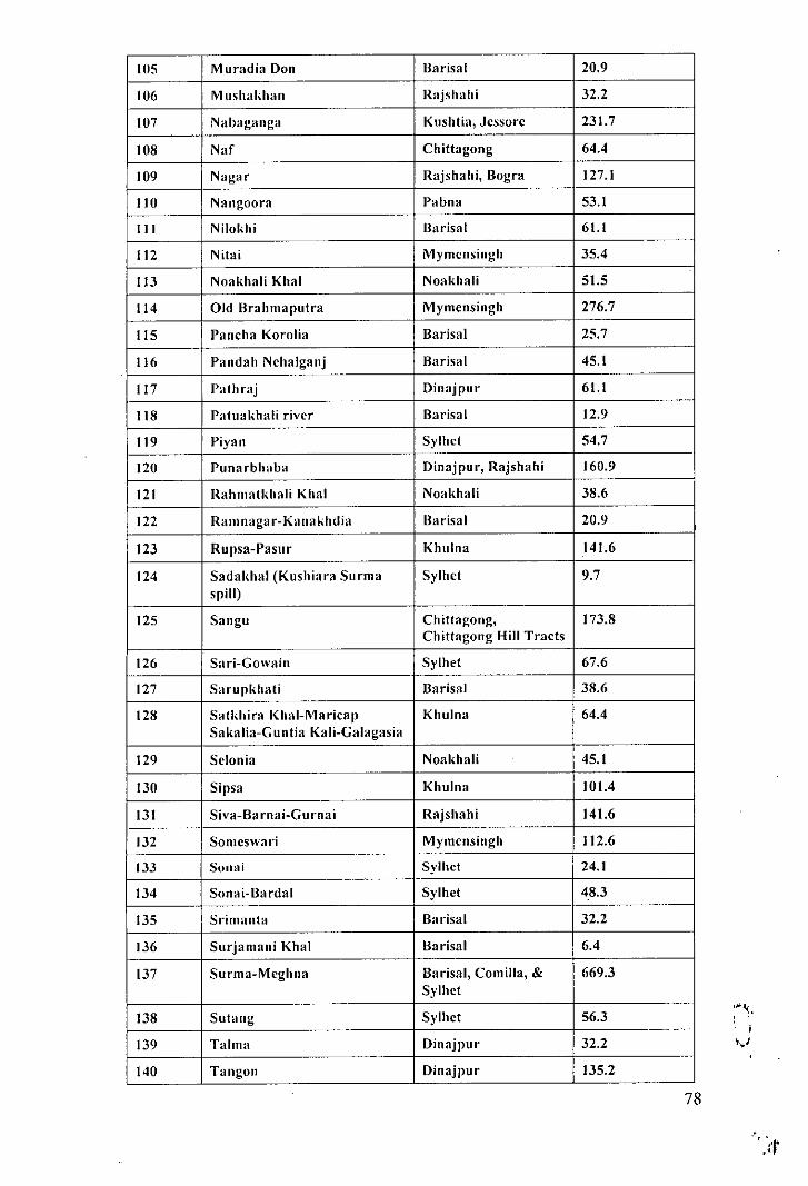
105 Muradia Don Barisal 20.9

106 M lIshali.han Rajshahi 32.2

107 Nabaganga Kushtia, Jcssorc 231.7

108 Nar Chittagong 64.4

109 Nagar Rajshahi, Bogra 127.1

110 Nangoora Pabna 53.1

III Niloldli Burisal 61.1

112 Nitai Mymcnsingh 35.4

113 Noakhali Khal Noakhali 51.5

114 Old Brahmapntra Mymensingh 276.7

115 Paneha Korolia Barisal 25.7

116 Pandah Nehalganj Barisal 45.1

117 Path raj Dinajpur 61.1

118 Patuakhali river Barisal 12.9

119 Piyan Sylhe! 54.7

120 Punarbhaba Dinajpur, Rajshahi 160.9

121 Rahma!I,hali Khal Noakhali 38.6

122 Ram naga r-Ka naldllJia Barisal 20.9

123 Rupsa-Pasur Khulna 141.6

124 Sadakhal (Kushiara Surma Sylhct 9.7spill)

125 Sangu Chittagong, 173.8Chitta gong Hill Trac!s

126 Sari-Gawain Sylhe! 67.6

127 Sarupkhati Barisal 38.6

128 Satkhira Khal-Maricap Khulna 64.4Sakalia-Cuntia Kali-Calagasia

129 Sclonia Noal,hali 45.1

130 Sipsa Khulua 101.4

131 Siva-Ba rnai-Gu rnai Rajshahi 141.6

132 Somcswari Mymcnsingh 112.6

133 Sonai Sylhct 24.1

134 Sonai-Bardal Sylhct 48.3

135 Srimanta Barisal 32.2

136 Surjamani Khal Barisal 6.4

137 Surma-Mcghna Barisal, Com ilia, & 669.3Sylhc!

138 Sutang Sylhc! 56.3

139 Talm:l Dinajpur 32.2

140 Tangon Dinajpur 135.2

78

>"

141 Tcntulia Barisal 83.7

142 Tccsta Rangpur 112.6

143 Tial,hali-Dhankhali Don Barisal 51.5

144 Titas Comilla 54.7

145 Tongi Khal Dhal,a 16.1

146 Torl{i Barisal 27.4

147 Turag Dhaka 70.8

* Sourcc: Dcpartmcnt of Watcr Resource Engineering, Bangladesh Universityof Engineering and Technology, Dhaka-IOOO, Bangladesh.

79

'.

,

,

Appendix C

80

r

,,"-," ..---'II LHASA

l--'~-"i'

I '

~

!RATS E OZOWO

-----..-.. r' ~-.~r

,) ,.~'~"

C"ti'I,NA

~~.-.~' ..

"

.~-:;,..•l._:'.

-~.

---- .' .): --:--._ I. "

-:- .. : ~( .~ \ i; I-- r-"-;' \

) .

_:"

------" ..•I N

... ' ".".

;;.• -:.~,:~~ ;':.~7:'-':". ",'

,1' •..• 1::,. ..•.

The Ganges, The Brahmaputra arid The Meghna River Basin

, .

• 1lHOP •••••

}_o'

"~I/:i

..... -

.KOT~--~/-

---'--".

LEGEND:N Bangladosh bordorN '..••ma1lonal boundary

• Important locationN Minor rive rN Major river

8r.ahmaputra river basinGanges river basinMeghna river basin

I

00

Appendix D

82

The Grlllges at Hnrdinge Bridge

Ycar Month Velocity (Daily mean) and corresponding Watcr level Max. Velocity

Max. W.L (111) Min. W.L (111) Average Recorded (m/5)

Mean pWD Mean pWD Mean (of the month)

Velocity Velocity Velocity(1ll/5) (I11/S) (I11/S)

Jan

Feb

Mar

Apr 00945 4.945 0.0717 4.69 0.0831 0.1764

1996 May 0.1821 7.09 0.0949 5.22 0.1385 0.2327

Jun 0.2841 5.81 0.1794 6.73 0.23175 0.5440

lui 2.0392 13.395 0.7683 9.84 1.40375 28243

Aug 2.6557 13.93 1.3385 11.43 1.9971 3.3292

SCI' 3.1378 14.49 0.9413 10.39 2.03955 3.8353

Oct 1.4784 1211 0.6675 10.01 1.07295 2.0168

Nov 0.6294 99 0.3829 8.48 0.50615 0.9339

Dec 03723 8.41 0.2577 7.59 0.315 0.5733

The Ganges at Hardinge Bridge

Year Month Velocity (Daily mean) and corresponding Water level Max. Velocity

Max. W.L (111) Min. W.L (111) Average Recorded (m/5)

Mean pWD Mean pWD Mean (of the month)

Velocity Velocity Velocity(111/5) (I11/S) (I11/S)

Jan 0.2638 7.21 0.1566 6.46 0.2102 0.3975

Feb 0.1754 6.46 0.0822 5.86 0.1288 0.2869

Mar 0.1089 580 0.0261 5.19 0.0675 0.1735

Apr 0.17 6.01 0.0474 5.11 0.1087 0.2371

1997 May 0.1148 5.80 0.0828 5.65 0.0988 0.1990

Jun 03394 8.105 0.1080 5.885 0.2237 0.6274

lui

Aug

Sep

Oct

Nov 0.6184 8.95 0.4893 8.395 0.55385 0.9277

Dec 0.7937 9.82 0.4064 8.08 0.60005 0.9584

83

The Ganges at Hardinge Bridge

Year Month Velocity (Daily mean) and corresponding Water level Max. Velocity

Max. W.L (m) Min. W.L (m) Average Recorded (m/s)

Mean PWD Mean PWD Mean (of the month)

Velocity Velocity Velocity(m/s) (m/s) (m/s)

Jan 0.5621 8.635 0.3402 7.04 0.45115 0.6997

Feb 0.3993 6.52 0.2236 5.82 0.31145 0.4629

Mar 02274 5.735 0.1870 5.365 0.2072 0.3003

Apr 0.2849 6.040 0.2019 5.515 0.2434 0.3738

1998 May 0.3344 7.343 0.2817 6.193 0.30805 0.4028

Jun 0.5607 9.62 0.3428 7.488 0.45175 0.8018

lui 2.6638 1374 0.9381 10.88 1.80095 3.0253

Aug 32980 14.8 2.5546 13.395 2.9263 3.6485

Sep 3.3240 15.19 1.3392 12.26 2.3316 3.7220

Oct 1.4276 12.535 0.9677 11.455 1.19765 2.01683

Nov 10144 11.73 0.5109 9.365 0.76265 1.4305

Dec 0.4688 8.87 0.2708 7.465 0.3698 0.7884

The Ganges at Hardinge Bridge

Year Month Velocity (Daily mean) and corresponding Water level Max. Velocity

Max. W.L (m) Min. W.L (m) Average Recorded (m/s)

Mean PWD Mean PWD Mean (of the month)

Velocity Velocity Velocity(m/s) (m/5) (m/s)

Jail 0.2698 7.29 0.2304 6.94 0.2501 0.3351

Feb 0.2281 6875 0.1614 5.9 0.19475 0.2634

Mar 0.1649 5855 0.1219 5.31 0.1434 0.2175

Apr o 1521 5.22 0.1104 5.115 0.13125 0.1952

1999 May 0.2446 6.795 0.1234 5.69 0.184 0.2962

JUIl 0.6882 10.175 0.2549 6.875 0.47155 0.8948

lui 1.6849 12.66 1.0449 11.605 1.3649 2.344

Aug 2.9427 14.085 2.2159 13.535 2.5793 3.7610

Sep 3.2864 14.385 2.8026 13.54 3.0445 3.7873

Oct 2.224 13.075 1.2431 11.92 1.73355 2.9144

Nov 0.9775 11.245 0.3901 8.66 0.6838 1.1527

Dec

84

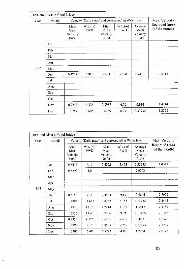
The Gorai River at Gorai Bridge

Year Month Velocity (Daily mean) and corresponding Water level Max. Velocity

Max. W.L (m) Min. W.L (m) Average Recorded (m/s)

Mean PWD Mean PWD Mean (of the month)

Velocity Velocity Velocity(m/s) (m/s) (m/s)

Jan

Fcb

Mar

Apr

1997 May

Jun 04272 5.985 0403 5.990 04151 0.5914

Jul

Aug

Sep

Oct

Nov 0.9293 6.525 0.8987 6.70 0.914 1.4114

Dec 1.0767 6.605 0.6780 6.27 0.87735 1.2370

The Gorai River at Gorai Bridge

Year Month Velocity (Daily mean) and corresponding Water level Max. Velocity

Max. W.L (m) Min. W.L (m) Average Recorded (m/s)

Mean PWD Mean PWD Mean (of the month)

Velocity Velocity Velocity(m/s) (m/s) (m/s)

Jan 0.6655 6.17 04392 5.475 0.55235 1.0625

Fcb 0.6293 5.0 0.6293

Mar

Apr

1998 May

JUIl 0.5158 7.16 0.4534 682 0.4846 0.7696

Jul 1.4805 11.615 0.8388 8.185 1.15965 2.2446

Aug 1.4820 13.15 1.2414 11.87 1.3617 2.3152

Scp 1.5555 13.43 0.7136 9.94 1.13455 2.1386

Ocl 0.9334 9.125 0.6706 8485 0.802 1.5320

Nov 1.4988 7.11 0.9587 8.755 1.22875 2.1217

Dec 1.5305 6.48 0.9223 4.85 1.2264 2.0125

85

The Gorai River al Gor<li Bridge

Year Month Velocity (Daily mean) and corresponding Water level Max. Velocity

Max. W.L (m) Min. W.L (m) Avcrage Recorded (m!s)

Mean PWD Mean PWD Mean (of the month)

Velocity Velocity Velocity(m!s) (m!s) (m!s)

Jan 0.9988 5.88 0.887 5.66 0.9429 1.2699

Feb 0.2330 5.29 0.1608 5.445 0.1969 0.4050

Mar 0.2046 4.63 0.2031 4.77 0.20385 0.3307

Apr 0.2000 458 0.1934 4.45 0.1967 0.3089

1999 May 0.2757 5.06 0.2148 4.81 0.24525 0.4749

Jun 1.2025 9.085 0.4880 6.235 0.84525 1.6849

lui 1.5815 11.100 1.3528 11.13 1.46715 2.1086

Aug 1.6178 12.305 1.3456 11.35 1.4817 2.3620

Sep 1.8367 12.445 1.4507 11.85 1.6437 2.3096

Oct 1.0441 10.74 0.8828 9.92 0.96345 1.6456

Nov 07544 9.054 0.6719 7.59 0.71315 1.1738

Dec 1.0816 6.82 0.7531 6.285 0.91735 1.2262

Thc Gorai Rivcr at Gorai Bridge

Year Month Velocity (Daily mean) and corresponding Water level Max. Velocity

Max. W.L (m) Min. W.L (m) Averagc Recorded (m!s)

Mean PWD Mean PWD Mean (of the month)

Velocity Velocity Velocity(m/s) (m/s) (m/s)

Jan 0.8074 5.885 0.7881 5.455 0.79775 1.0864

Feb 0.7240 5.34 0.6874 5.03 0.7057 0.9991

Mar 0.5377 4.88 0.5099 4.61 0.5238 0.6625

Apr

2000 May

Jun

lui

Aug

Sep

Oct

Nov

Dec

86

The Atrai River at Singra

Year Month Velocity (Daily mean) and corresponding Water level Max. Velocity

Max. W.L (m) Min. W.L (m) Average Recorded (m/s)

Mean PWD Mean PWD Mean (of the month)Velocity Velocity Velocity

(m/s) (m/s) (m/s)

Jan

Feb

Mar

1997 Apr

May

Jun

J"I 0.549 12.52 0.549 0.988

Aug 0.521 11.98 0.402 11.39 0.4615 0.941

Sep 0.583 11.99 0.509 11.93 0.546 0.941

Oct 0.403 11.14 0.366 11.85 0.3845 0.824

Nov 0280 10.58 0.197 9.95 0.2385 0.471

Dec 0093 9.06 0076 8.79 00845 0.189

The Atrai River at Singra

Year Month Velocity (Daily mean) and corresponding Water level Max. Velocity

Max. W.L (m) Min. W.L (m) Average Recorded (m/s)

Mean PWD Mean PWD Mean (of the month)Velocity Velocity Velocity

(m/s) (m/s) (m/s)

Jan

Feb

Mar

Apr1998 May

JUll

Jul 0.940 12.935 0.432 12.060 0.686 1.159

Aug 0.952 12.74 0.911 12.93 0.9315 1.159

Sep 0.814 12.82 0.810 12.78 0.812 1.159

Oct 0.570 11.81 0.278 11.22 0.424 0.928

Nov 0.370 11.080 0.282 10.57 0.326 0.697

Dec 0.200 10.10 0.094 9.47 0.147 0.466

87

The Atrai River at Singra

Year Month Velocity (Daily Illean) and corresponding Water level Max. Velocity

Max. W.L (Ill) Min. W.L (Ill) Average Recorded (m/5)

Mean PWD Mean PWD Mean (of the month)

Velocity Velocity Velocity(Ill/S) (Ill/S) (Ill/S)

Jan

Feb

Mar

Apr

1999 May

Jun 0.0247 8.965 0.0247 0.0458

Jul 08513 12.715 0.2007 10.92 0.526 1.2515

Aug 0.7125 12.425 0.5537 11.89 0.6331 0.8357

SCI' 07383 12.84 0.7123 12.83 0.7253 1.0505

Oct

Nov

Dec

The Mohananda River at Chapainawabgonj

Year Month Velocity (Daily mean) and corresponding Water level Max. Velocity

Max. W.L (Ill) Min. W.L (Ill) Average Recorded (m/5)

Mean PWD Mean PWD Mean (of the month)

Velocity Velocity Velocity(Ill/S) (Ill/S) (Ill/S)

Jan

Feb

Mar

Apr

1997 May

Jun

Jul 0.206 20.15 0.206 0.283

Aug 0.226 20.75 0.21 18.99 0.218 0.354

SCI' 0.429 19.96 0.268 19.64 0.3485 0.706

Oct 0.207 16.85 0.167 15.17 0.187 0.354

Nov

Dcc

88

Thc Mohananda River at Chapainawabgonj

Year Month Velocity (Daily mean) and corresponding Water level Max. Velocity

Max. W.L (m) Mill. W.L (m) Average Recorded (mls)

Mean PWD Mean PWD Mean (of the month)

Velocity Velocity Velocity(mls) (m/s) (m/s)

Jan

Feb

Mar

Apr

1998 May

lUll

Jul 0.425 20.6 0.137 16.95 0.281 0.812

Aug 0.338 21.075 0.265 21.795 0.3015 0.604

Scp 0.657 22.07 0.099 22.62 0.378 1.112

Oct 0.411 18.3 0.383 18.425 0.397 0.697

Nov o 190 15.37 0.189 16.24 0.1895 0.35

Dec 0.138 14.6 0.093 13.99 0.1155 0.281

The Mohananda River at Chapainawabgonj

Year Month Velocity (Daily mean) and corresponding Water level Max. Velocity

Max. W.L (m) Min. W.L (111) Average Recorded (mls)

Mean PWD Mean PWD Mean . (of the mOl1th)

Velocity Velocity Velocity(I11/S) (I11/S) (I11/S)

Jan

Fcb

Mar

Apr

1999 May

lun 0.1940 14.39 0.1932 13.27 0.1936 0.3230

Jul 0.6781 19.93 0.2689 17.93 0.4735 0.9466

Aug 0.7246 21.425 0.6550 20.330 0.6898 1.0090

Scp 07636 2238 0.7319 21.48 0.74775 1.1129

Oct

Nov

Dcc

89

The Atrai River at Nowhata

YC<lr Month Vclocity (Daily mean) and corresponding Water level Max. Velocity

Max. W.L (m) Min. W.L(m) Average Recorded (m/s)

Mean PWD Mean PWD Mean (of the month)

Vclocity Velocity Velocity(m/s) (mls) (mls)

Jan

Feb

Mar

Apr

1997 May

lun

Jul 0.463 14.2 0.463 0.66

Aug 0.436 14.00 0.42 14.05 0.428 0.824

Sep 0.525 14.71 0.47 14.71 0.4975 0.706

Oct 0.471 13.51 0.393 14.11 0.432 0.706

Nov

Dec

The Atrai Rivcr at Nowhata

Year Month Velocity (Daily mean) and corresponding Water level Max. Velocity

Max. W.L (m) Min. W.L(m) Average Recorded (m/s)

Mean PWD Mean PWD Mean (of the month)Velocity Velocity Velocity(mls) (mls) (mls)

Jan

Feb

Mar

Apr

1998 May

lun

Jul 0.437 14.75 0.437 0.627

Aug 0366 14.165 0.333 14.65 0.3495 0.604

SCI' 0.377 14.88 0.344 14.91 0.3605 0.697

Oct 0.306 1451 0.251 13.94 0.2785 0.697

Nov 0.273 14.11 0.085 13.01 0.179 0.512

Dec

90

The Alrai River at Nowhala

Year Month Velocity (Daily mean) and corresponding Water level Max. Velocity

Max. W.L (m) Min. W.L (m) Average Recorded (m/s)

Mean PWD Mean PWD Mean (of the month)

Velocity Velocity Velocity(m/s) (m/5) (m/s)

Jan

Feb

Mar

Apr

1999 May

JUll

lui 02384 14.5 0.1965 14.56 0.21745 0.4546

Aug 0.2314 14.165 0.1567 13.85 0.19405 0.4200

Sep 0.2285 14.69 0.2201 14.54 0.2243 0.4477

Oct

Nov

Dec

The Mohan<lnda River at Rohanpur

Year Month Velocity (Daily mcan) and corrcsponding Water level Max. Velocity

Max. W.L (m) Min. W.L (m) Average Recorded (m/s)

Mean PWD Mean PWD Mean (of the month)

Velocity Velocity Velocity(m/5) (m/5) (m/5)

Jan

Feb

Mar

Apr

1997 May

JUll

lui 0.424 21.06 0.424 0.589

Aug 0.49 21.210 0.449 20.380 0.4695 0.706

Sep 0.501 20.31 0.464 20.76 0.4825 0.941

Oct 0.282 17.69 0.236 14.6 0.259 0.354

Nov 0.2 15.14 0.156 14.76 0.178 0.330

Dec

91

The Mohananda River at Rohanpur

Year Month Vclocity (Daily mcan) and corrcsponding Water Icvel Max. Velocity

Max. W.L (m) Min. W.L (m) Average Recorded (m!5)

Mcan PWD Mcan PWD Mean (of the month)

Velocity Velocity Velocity(m!s) (m!s) (m!s)

Jan

Feb

Mar

Apr

1998 May

Jun

Jul 0.434 21.05 0.279 16.945 0.3565 0.697

Aug 0.612 23.580 0.311 22.35 0.4615 0.812

Sep 0.651 24.3 0.54 21.79 0.5955 0.928

Oct 0.667 19.84 0.51 19.35 0.5885 0.858

Nov 0.304 16.88 0.185 15.92 0.2445 0.512

Dcc 0.125 15.17 0.077 14.58 0.101 0.235

The Mohan3nda River at Rohanpur

Year Month Velocity (Daily mean) and corresponding Water level Max. Velocity

Max. W.L (m) Min. W.L(m) Average Recorded (m!5)

Mean PWD Mean PWD Mean (of the month)

Velocity Velocity Vclocity(rn!s) (rn!s) (rn!s)

Jan

Fcb

Mar

Apr

1999 May

JUIl 0.0736 14.29 000 14.21 0.0368 0.1151

Jul 0.2790 20.80 0.\788 18.14 0.2289 0.4546

Aug 0.3363 22.080 0.2822 20.72 0.30925 0.5239

Sep 0.3553 22.715 0.2727 22.25 0.314 0.4893

Oct

Nov

Dcc

92

The Bengali River at Shimulbari

Year Month Velocity (Daily mean) and corresponding Water level Max. Velocity

Max. W.L (m) Min. W.L (01) Average Recorded (01/5)

Mean PWD Mean PWD Mean (of the month)

Velocity Velocity Velocity(m/5) (m/s) (m/s)

Jan

Feb

Mar

Apr 0.095 13.165 0.085 13.040 0.09 0.142

1997 May 0.074 13.040 0.068 13.015 0.071 0.128

lUll 0.566 15.0 0.\14 13.24 0.34 0.675

J"I 0.985 16.72 0.745 16085 0.865 1.18

Aug 0.581 15.885 0.394 14.96 0.4875 0.759

Sep 0937 16.485 0.91 16.345 0.9235 1.138

Oct 0.572 15.785 0.239 14.505 0.4055 0.787

Nov 0.183 \4.10 0.155 13.8\ 0.169 0.24

Dec o 154 13.73 0.131 13.765 0.1425 0.184

The Bengali River at Shimulbari

Year Month Velocity (Daily mean) and corresponding Water level Max. Velocity

Max. W.L (m) Min. W.L (m) Average Recorded (m/s)

Mean PWD Mean PWD Mean (of the month)

Velocity Velocity Velocity(m/s) (m/s) (01/5)

Jan 0.071 13.72 0.055 13.755 0.063 0.100

Feb 0.117 13548 0.081 13.267 0.099 0.184

Mar

Apr

1998 May

lun

J"I

Aug

Sep

Oct

Nov

Dec

93

The Bengali River at Shimulbari

Ycar Month Velocity (Daily mcan) and corresponding Water level Max. Velocity

Max. W.L (m) Min. W.L (m) Average Recorded (m/5)

Mean PWD Mean PWD Mean (of the month)

Velocity Velocity Velocity(m/5) (01/5) (01/5)

Jan

Feb

Mar

Apr

1999 May

JlIn

Jul 1.007 ] 7.745 0.997 17.275 1.002 1.264

Aug 0.984 17.28 0.9]4 16.32 0.949 1.222

Sep 0.891 16.86 0.891 1.096

Oct 0.969 17.69 0.540 15.565 0.7545 1.236

Nov 0.468 15.165 0.194 13.85 0.331 0.661

Dec

The Bengali river at Khanplir

Year Month Velocity (Daily mean) and corresponding Water level Max. Velocity

Max. W.L (01) Min. W.L (01) Average Recorded (m/5)

Mean PWD Mean PWD Mean (of the month)

Velocity Velocity Velocity(m/5) (m/5) (m/5)

Jan

Feb

Mar

Apr

1997 May

Jun 0.439 8.7 0.439 0.563

Jul 0656 ] 1.985 0.183 9.765 0.4195 0.857

Aug 0.474 11.00 0.448 ]0.675 0.46] 0.59

Sop 0.668 11.875 0.613 11.39 0.6405 0.829

Oct 0.485 10.885 0.]78 9.2 0.3315 0.59

Nov 0252 8.67 0.]7] 8.59 0.21 ]5 0.338

Dec 0.198 8.63 0.164 8.55 O.]81 0.240

94

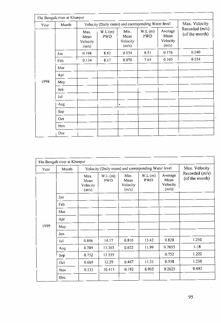
The Bengal i river at Khanpur

Year Month Velocity (Daily mean) and corresponding Water level Max. Velocity

Max. W.L (m) Min. W.L (m) Average Recorded (m/s)

Mean PWD Mean PWD Mean (of the month)

Velocity Velocity Velocity(m/s) (m/s) (m/s)

Jail 0.198 8.62 0.154 8.51 0176 0.240

Feb 0.134 8.17 0.076 7.65 0.105 0.254

Mar

Apr

1998 May

Jun

lui

Aug .Sep

Oct

Nov

Dec

The Bengali river at Khanpur

Year Month Velocity (Daily mean) and corresponding Water level Max. Velocity

Max. W.L (m) Min. W.L (m) Average Recorded (m/s)

Mean PWD Mean PWD Mean (of the month)

Velocity Velocity Velocity(m/s) (m/s) (m/s)

Jan

Feb

Mar

Apr

1999 May

JUIl

lui 0.846 14.17 0.810 13.42 0.828 1.250

Aug 0.789 13.365 0.622 11.99 0.7055 1.18

Sep 0.752 13.555 0.752 1.222

Oct 0.669 12.29 0.447 11.31 0.558 1.236

Nov 0.333 10.415 0.192 8.905 0.2625 0.493

Dec

95

The Nagar River at Bogra

Year Month Velocity (Daily mean) and corresponding Water level Max. Velocity

Max. W.L (m) Min. W.L (m) Average Recorded (m/s)

Mean PWD Mean PWD Mean (of the month)

Velocity Velocity Velocity(m/s) (m/s) (m/5)

Jan

Feb

Mar

Apr

1997 May

Jun 0.041 11.38 0.072

Jul 0466 1375 0.031 11.355 0.2485 0.618

Aug 0465 1366 0.207 11.92 0.336 0.618

Sep 0.512 14.085 0.328 12.72 042 0.675

Oct 0.318 12.175 0.299 11.747 0.3085 045

Nov 0.147 11.550 0.11 11.467 0.1285 0.226

Dcc o 142 I 1.51 0.123 1149 0.1325 0.226

The Nagar River at Bogra

Year Month Velocity (Daily mean) and corresponding Water level Max. Velocity

Max. W.L (m) Min. W.L (m) Average Recorded (m/s)

Mean PWD Mean PWD Mean (of the month)

Velocity Velocity Velocity(m/s) (m/s) (m/5)

Jan 0.157 I 1.65 0.153 11.63 0.155 0.240

Feb 0086 11493 0.01 11.165 0.048 0.142

Mar

Apr

1998 May

JUIl

Jul

Aug

Sep

Oct

Nov

Dec

96

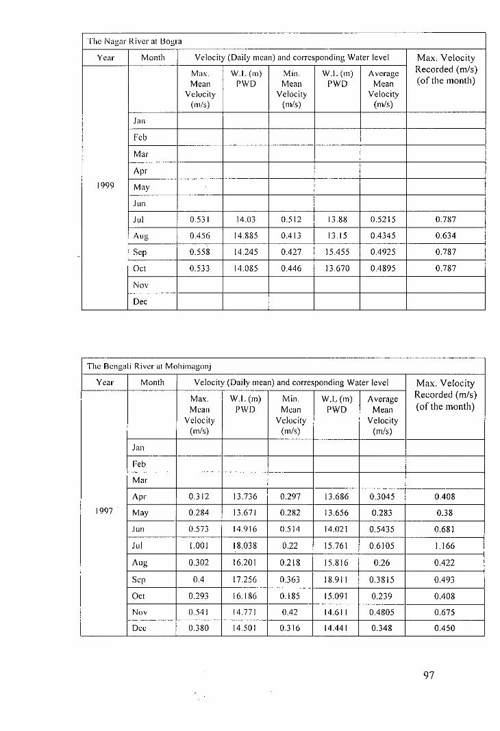
The Nagar River at Bogra

Year Month Velocity (Daily mcan) and corrcsponding Water level Max. Velocity

MClx. W.L (m) Min. W.L (m) Average Recorded (m/s)

Mean PWD Mean PWD Mean (of the month)Velocity Velocity Velocity(m/s) (m/s) (m/s)

Jan

Fcb

Mar

Apr

1999 May

Jun

Jul 0531 14.03 0.512 1388 0.5215 0.787

Aug 0.456 14.885 0.413 13.15 0.4345 0.634

Sep 0.558 14245 0.427 15.455 0.4925 0.787

Oct 0.533 14085 0.446 13.670 0.4895 0.787

Nov

Dec

The Bcngali Rivcr at Mohirnagonj

Year Month Velocity (Daily mean) and corresponding Water level Max. Velocity

Max. W.L (m) Min. W.L (m) Average Recorded (m/s)Mean PWD Mean PWD Mean (of the month)

Velocity Velocity Velocity(m/s) (m/s) (m/s)

Jail

Feb

Mar

Apr 0.312 13.736 0.297 13.686 0.3045 0.408

1997 May 0.284 13.671 0.282 13.656 0.283 0.38

JUIl 0.573 14.916 0.514 14.021 0.5435 0.681

Jul 1.001 18.038 0.22 15.761 0.6105 1.166

Aug 0.302 16.201 0.218 15.816 0.26 0.422

Sep 0.4 17.256 0.363 18.911 0.3815 0.493

Oct 0.293 16.186 0.185 15.091 0.239 0.408

Nov 0541 14.771 0.42 14.611 0.4805 0.675

Dec 0.380 14.501 0.316 14.441 0.348 0.450

97

The Bengali River at Mohimagonj ,

Year Month Velocity (Daily mean) and corresponding Water level Max. Velocity

Max. W.L (m) Min. W.L (m) Average Recorded (m/5)

Mean PWD Mean PWD Mean (of the 1110nth)

Velocity Vclocity Velocity(m/s) (m/s) (m/5)

Jail 0272 14.396 0.256 13.346 0.264 0.338

Feb 0.120 14.216 0.077 14.046 0.0985 0.226

Mar

Apr1998 May

Jun

Jul

Aug

Scp

Oct

Nov

Dec

The Bengali River at Mohimagonj

Year Month Velocity (Daily mean) and corresponding Water Icvel Max. Velocity

Max. W.L (m) Min. W.L (m) Average Recorded (m/s)

Mean PWD Mean PWD Mean (of the month)

Velocity Velocity Velocity(m/5) (m/5) (m/5)

Jan

feb

Mar

Apr

1999 May

Jun

Jul 0.977 18.201 0.706 17.951 0.8415 1.194

Aug 0670 17.769 0.459 16.639 0.5645 0.885

Sep 1.00 18.619 0.504 17.056 0.752 1.208

Oct 0.924 18096 0.462 16.466 0.693 1.152

Nov 0.388 15.81 0221 14.756 0.3045 0.493

Dec

98

"""'1.,

The Tulshiganga River at Sonamukhi

Year Month Velocity (Daily mean) and corresponding WaleI' level Max. Velocity

Max. W.L (111) Min. W.L (111) Average Recorded (m/5)

Mean PWD Mean PWD Mean (of the month)

Velocity Velocity - Velocity(m/5) (111/5) (m/s)

Jan

Feb

Mar

Apr1997 May

lun 0.082 11.62 0.07 11.26 0.076 o 128Jul 0.746 1555 0.258 13.025 0.502 0.885

Aug 0.257 13.125 0.091 11.73 0.174 0.338

SCI' 0.424 14.99 0.40 I 14.455 0.4125 0.675

Oct 0.242 13.075 0.1 12.225 0.171 0.324

Nov 0.068 11.575 0.023 10.980 0.0455 0.086

Dec 0.39 10.97 0.35 10.96 0.37 0.44

The Tulshiganga River at Sonamukhi

Year Month Velocity (Daily l11ean)and corresponding Water level Max. Velocity

Max. W.L (111) Min. W.L (m) Average Recorded (m/5)

Mean PWD Mean PWD Mean (of the month)Velocity Velocity Velocity(111/s) (111/5) (m/s)

Jan 0.019 10.95 0.013 10.935 0.016 0.044

Feb 0.013 10.91 0.010 10.735 00115 0.029

Mar

Apr

1998 May

lun

Jul

Aug

Sep

Oct

Nov

Dec

99

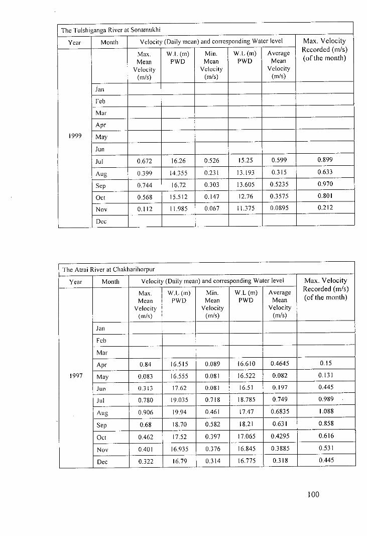
The Tulshiganga River at Sonamukhi

Year Month Vclocity (Daily mcan) and corresponding Water level Max, Velocity

Max. W.L (m) Min. W.L (111) Average Recorded (111/5)

Mean PWD Mcan PWD Mean (of the month)

Velocity Velocity Vclocity(m/s) (m/s) (111/5)

Jan

Feb

Mar

Apr

1999 May

Jun

Jul 0,672 16,26 0,526 15,25 0,599 0,899

Aug 0399 14.355 0,231 13,193 0,315 0,633

Sep 0.744 16,72 0.303 13,605 0,5235 0,970

Oct 0.568 15.512 0,147 12,76 0,3575 0,801

Nov 0,112 11.985 0067 11.375 0,0895 0,212

Dec

The Atrai River at Chakharihorpur

Year Month Velocity (Daily mean) and corresponding Water level Max, Velocity

Max. W,L (m) Min. W,L (111) Average Recorded (m/s)

Mean PWD Mean PWD Mean (of the month)

Velocity Velocity Velocity(m/s) (111/5) (111/5)

Jan

Feb

Mar

Apr 0,84 16,515 0,089 16,610 0.4645 0,15

1997 May 0,083 16,555 0,081 16,522 0,082 0,131

lUll 0.313 17.62 0,081 16,51 0,197 0.445

Jul 0,780 19,035 0,718 18,785 0,749 0,989

Aug 0.906 19,94 0.461 17.47 0,6835 1,088

Sep 0,68 18,70 0,582 18,21 0,631 0,858

Oct 0.462 17,52 0,397 17,065 0.4295 0,616

Nov 0.40 I 16,935 0,376 16,845 0,3885 0.531

Dec 0.322 16,79 0,314 16,775 0.318 0.445

100

The Atrai River at Chakharihorpur

Year Month Velocity (Daily mean) and corresponding Water level Max. Velocity

Max. W.L (m) Min. W.L (m) Average Recorded (m/s)

Mean PWD Mean PWD Mean (of the month)

Vclocity Velocity Velocity(m/5) (m/5) (m/5)

Jan 0.282 16.7 0.269 16.675 0.2755 0.399

Feb 0.235 16.645 0.226 16.545 0.2305 0.354

Mar 0.152 16.47 0.114 16.305 0.133 0.249

Apr

1998 May

Jun

Jul

Aug

Sep

Oct

Nov

Dec

The Atrai River at Chakharihorpur

Year Month Velocily (Daily mean) and corresponding Water level Max. Velocity

Max. W.L (m) Min. W.L (m) Average Recorded (m/s)

Mean PWD Mean PWD Mean (of the month)

Velocity Velocity Velocity(m/5) (m/5) (m/5)

Jan

Feb

Mar

Apr

1999 May

lun

Jul 0.486 20.68 0.452 19.85 0.469 0.616

Aug 0.465 20.51 0.395 18.835 0.43 0.596

Sep 0.501 21.45 0.437 18.435 0.469 0.662

Oct 0.444 19.675 0.422 19.245 0.433 0.662

Nov 0.403 18.205 0.391 17.965 0.397 0.596

Dec

101

The Tulshiganga River at Naogaon

Year Month Velocity (Daily mean) and corresponding Water level Max. Velocity

Max. W.L (m) Min. W.L(m) Average Recorded (m/s)

Mean PWD Mean PWD Mean (of the month)

Velocity Velocity Velocity(m/s) (m/s) (m/s)

Jail

Feb

Mar

Apr

1997 May

Jun

Jul 0.475 13.75 0.475 0.629

Aug 0.471 1351 0.292 12.45 0.3815 0.629

Sep 0.881 14.43 0.45 13.3 0.6655 1.088

Oct 0.453 13.24 0.272 11.64 0.3625 0.596

Nov 0.158 10.71 0.123 10.79 0.1405 0.236

Dec 0.00 10.45 0.00 10.5 0.00

The Tulshiganga River at Naogaon

Year Month Velocity (Daily mean) and corresponding Water level Max. Velocity

Max. W.L (m) Min. W.L (m) Avcragc Recorded (m/s)

Mean PWD Mean PWD Mean (of the month)

Velocity Velocity Velocity(m/s) (m/s) (m/s)

Jail

Feb

Mar

Apr

1999 May

JUIl

Jul 0.4675 14.04 0.466 14.81 0.46675 0.642

Aug 0.423 13.48 0.414 13.42 0.4185 0.596

Sep 0.443 13.7 0.443 0.596

Oct 0.434 13.98 0.391 13.275 0.4125 0.583

Nov 0.368 12.31 0.319 11.605 0.3435 0.531

Dec

102

The Atrai River at Mohadevpur

Year Month Velocity (Daily mean) and corresponding Water level Max. Velocity

Max. W.L (m) Min. W.L (m) Average Recorded (m/s)

Mean PWD Mean PWD Mean (of the month)

Velocity Velocity Velocity(m/s) (m!s) (m!s)

Jan

Feb

Mar

Apr 0.096 13.35 0.069 1322 0.0825 o 1571997 May 0.084 13.36 0.083 13.45 0.0835 0.137

JUI1 0.223 14.85 0.084 13.39 0.1535 0.334

Jul 0.884 17.46 0.319 15.21 0.6015 1.153

Aug 0.387 15.510 0.289 15.1 0.338 0.581

Scp 0.884 16.47 0.862 16.19 0.873 1.488

Oct 0.319 14.23 0.27 13.98 0.2945 0.445

Nov 0.252 13.92 0.243 13.86 0.2475 0.380

Dec 0.236 13.81 0.231 13.79 0.2335 0.367

The Atrai River at Mohadevpur

Year Month Velocity (Daily mean) and corresponding Water level Max. Velocity

Max. W.L (m) Min. W.L (m) Average Recorded (m/s)

Mean PWD Mean PWD Mean (of the month)

Velocity Velocity Velocity(m!s) (m!s) (m!s)

Jan 0222 13.74 0.206 13.69 0.214 0.354

Feb 0.157 13.63 0.145 13.55 0.151 0.268

Mar o 119 13.46 0.113 13.35 0.116 0.236

Apr

1998 May

Jun

Jul

Aug

SCI'Oct

Nov

Dee

103

The Atrai River at Mohadevpur

Year Month Velocity (Daily mean) and corresponding Water level Max. Velocity

Max. W.L (Ill) Min. W.L (Ill) Average Rccordcd (m/s)

Mean PWD Mean PWD Mean (oftl~e month)

Velocity Velocity Velocity(111/5) (111/5) (111/5)

Jan

Feb

Mar

Apr

1999 May

Jun

Jul 0.923 18.285 0.278 15.94 0.6005 1.299

Aug 0.318 16715 0.271 15.165 0.2945 0.489

Sop 0.925 18.315 0.263 15.105 0.594 1.219

Oct 0.267 15.075 0.257 15.045 0.262 0.380

Nov 0.238 14.17 0.227 14.33 0.2325 0.354

Dec

The Alrai River a1 Atrai

Year Month Velocity (Daily mean) and corresponding Water level Max. Velocity

Max. W.L (Ill) Min. W.L (111) Average Recorded (m/s)

Mean PWD Mean PWD Mean (ofthe month)

Velocity Velocity Velocity(111/5) (111/5) (111/5)

Jan

Feb

Mar

Apr

1997 May

lun 0.186 8.92 0.00 8.46 0.093 0.275

Jui 0.780 13.445 0.502 11.425 0.641 0.989

Aug 0.530 12.035 0.527 11.98 0.5285 0.694

Sep 0.762 1253 0.755 12.49 0.7585 0.957

Oct 0.525 12.045 0.493 11.370 0.509 0.694

Nov 0.243 10.445 0.230 9.93 0.2365 0.367

Dec 0.219 9.53 0.195 9.08 0.207 0.314

104

The Alrai River at Atrai

Year Month Vclocity (Daily mean) and corresponding Water level Max. V clocity

Max. W.L (m) Min. W.L (m) Average Recorded (m/5)

Mean PWD Mean PWD Mean (of the month)

Velocity Velocity Velocity(m/s) (m/s) (m/s)

Jan

Feb

Mar

Apr

1999 May

Jun

Jul 0.503 13.515 0.503 0.681

Aug 0.428 13.275 0.313 12.315 0.3705 0.629

Scp 0.476 13.445 0.332 12.665 0.404 0.662

Oct 0.495 13.69 0.422 12.7 0.4585 0.714

Nov 0.381 11.265 0.365 11.985 0.373 0.531

Dec

The Atrai River at Noldangar Hat

Year Month Velocity (Daily mean) and corresponding Water level Max. Velocity

Max. W.L (m) Min. W.L(m) Average Recorded (m/s)

Mean PWD Mean PWD Mean (of the month)

Velocity Velocity Velocity(m/s) (m/s) (m/s)

Jan

Feb

Mar

Apr

1997 May

JUIl

Jul 0.626 13.265 0.387 10.63 0.5065 0.793

Aug 0.49 12.645 0.486 12.66 0.488 0.694

Scp 0.605 13.15 0.601 13.04 0.603 0.793

Oct 0508 12.73 0.391 12.165 0.4495 0.694

Nov 0.392 11.48 0.308 10.7 0.35 0.531

Dec 0.232 9.755 0.144 8.865 0.188 0.354

105

The Bogkhali River at Ramu

Year Month Velocily (Daily mean) and corresponding Water level Max. Velocity

Max. W.L (m) Min. W.L(m) Average Recorded (m/s)

Mean PWD Mean PWD Mean (of the month)

Velocity Velocity Velocity(m/s) (m/s) (m/s)

Jan

Feb

Mar

Apr

1997 May 0.649 3.105 0.48 2.49 0.5645 0.782

Jun 0.922 3995 0.797 3.31 0.8595 1.155

Jul 1.185 5.97 0.863 4.39 1.024 1.613

Aug 0.899 4.35 0.76 3.48 0.8295 1.191

Sep 0.976 3.78 0.767 3.145 0.8715 1.305

Oel 1.018 4.07 0700 2.9 0.859 1.442

Nov 0.523 2.875 0.523 2.78 0.523 0.585

Dec 0.471 2.72 0.47 2.74 0.4 705 0.561

Ramu The Bogkhali River at Ramu

Year Month Velocity (Daily mean) and corresponding Water level Max. Velocity

Max. W.L (m) Min. W.L (m) Average Recorded (m/s)

Mean PWD Mean PWD Mean (of the month)

Velocity Velocity Velocity(m/s) (m/s) (m/s)

Jan 0.459 2.715 0.453 2.64 0.456 0.539

Feb 0.393 2.45 0.389 2.63 0.391 0.483

Mar 0.409 2.45 0.387 2.53 0.398 0.483

Apr 0.566 2.64 0.405 2.45 0.4855 0.671

1998 May

JUIl 0.486 4.66 0.72 3.55 0.603 1.098

Jul 1.398 505 1.169 3.765 1.2835 1.737

Aug 1.596 6.14 1.15 3.91 1.373 2.11

Sep 0.891 4.1 0.731 3.165 0.811 1.098

Oct 0.794 3.61 0.655 3.145 0.7245 0.947

Nov 0.742 3.32 0.592 3.05 0.667 0.915

Dec 0.685 2.90 0.65 2.94 0.6675 0.743

106

\ .j, .

The Sangu River at Bandarban

Year Month Velocity (Daily mean) and corresponding Water level Max. Velocity

Max. W.L (m) Min. W.L (m) Average Recorded (m/s)

Mean PWD Mean PWD Mean (of the month)

Velocity Velocity Velocity(Ill!S) (Ill!S) (Ill!S)

Jan 0.409 4.7 0.409 4.65 0.409 0.458

Feb 0.403 4.62 0.397 4.57 0.4 0.434

Mar

Apr 0.365 4.39 0.339 4.41 0.352 0.408

1999 May

Jun 1.229 14.30 0.704 6.68 0.9665 1.425

Ju1 1.128 9.40 0.789 7.165 0.9585 1.277

Aug 0.817 8.13 0.723 6.70 0.77 0.947

Sep 0.837 6.97 0.744 6.81 0.7905 0.996

Oct 0.742 6.68 0.705 6.10 0.7235 0.903

Nov 0.679 6.00 0.674 5.85 0.6765 0.801

Dec 0.675 5.765 0.673 5.47 0.674 0.787

The Sangu River al Bandarban

Year Month Velocity (Daily mean) and corresponding Water level Max. Velocity

Max. W.L (Ill) Min. W.L (Ill) Average Recorded (m/s)

Mean PWD Mean PWD Mean (of the month)

Velocity Velocity Velocity(Ill!S) (Ill!S) (Ill!S)

Jan 0.585 5.25 0.541 4.61 0.563 0.666

Feb 0.550 4.45 0.537 4.56 0.5435 0.650

Mar 0530 4.52 0.514 4.43 0.522 0.633

Apr

2000 May

Jun

Jul

Aug 0854 7.23 0.793 6.915 0.8235 0.966

Scp 0.758 6.54 0.707 6.06 0.7325 0.897

OCI

Nov

Dec

113

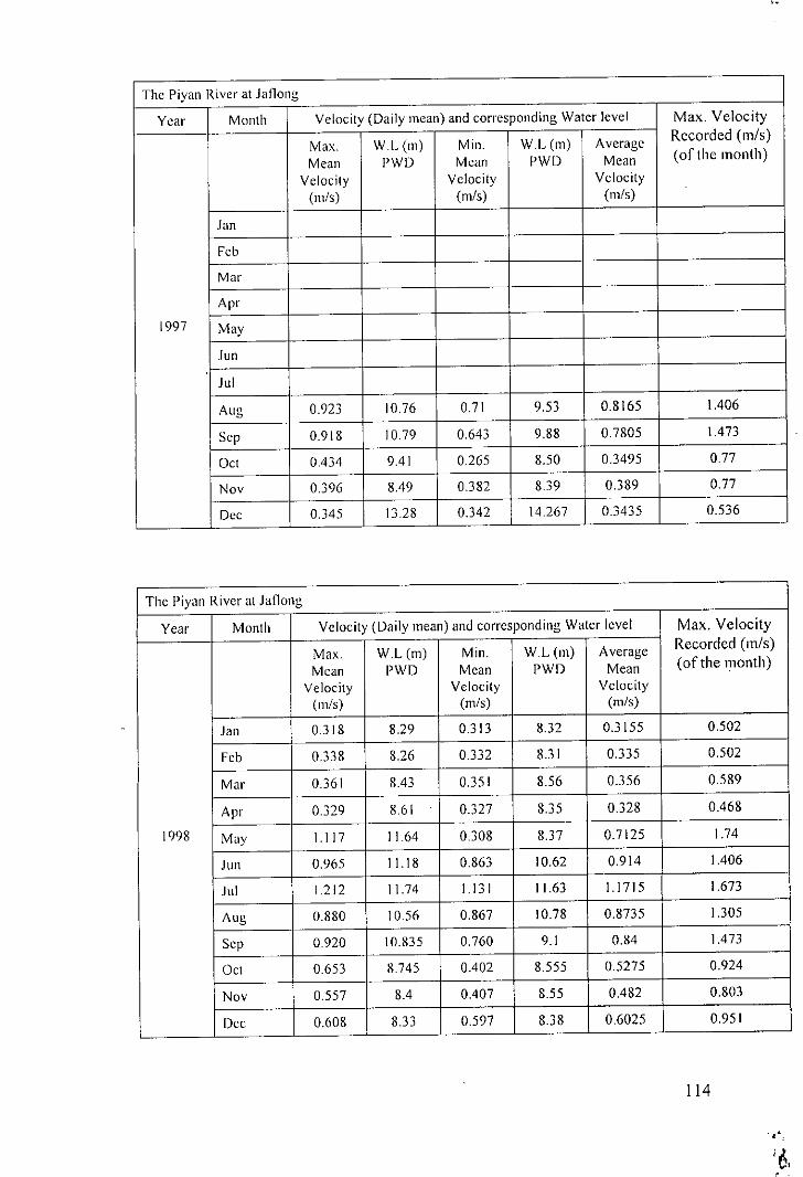
The Piyan River at Jatlong

Year Month Velocity (Daily mean) and corresponding Water level Max. Velocity

Max. W.L (m) Min. W.L (m) Average Recorded (m/s)

Mean PWD Mean PWD Mean (of the month)

Velocity Velocity Velocity(m/s) (m/s) (m/s)

Jan

Feb

Mar

Apr

1997 May

lun

lui

Aug 0.923 10.76 0.71 9.53 0.8165 1.406

SCI' 0.918 1079 0.643 9.88 0.7805 1.473

Oct 0434 941 0.265 8.50 0.3495 0.77

Nov 0.396 849 0.382 839 0.389 0.77

Dec 0.345 13.28 0.342 14.267 0.3435 0.536

The Piyan River at Jaflong

Year Month Velocity (Daily mean) and corresponding Water level Max. Velocity

Max. W.L (m) Min. W.L (m) Average Recorded (m/s)

Mean PWD Mean PWD Mean (of the month)

Velocity Velocity Velocity(m/s) (m/s) (m/s)

Jan 0.318 8.29 0.313 8.32 0.3155 0.502

Feb 0.338 8.26 0.332 8.31 0.335 0.502

Mar 0.361 843 0.351 8.56 0.356 0.589

Apr 0.329 861 0.327 8.35 0.328 0.468

1998 May 1.1 17 1164 0.308 8.37 0.7125 1.74

Jun 0.965 11.18 0.863 10.62 0.914 1406

lui 1.212 11.74 1.131 11.63 1.1715 1.673

Aug 0.880 1056 0.867 10.78 0.8735 1.305

SCI' 0920 10.835 0.760 9.1 0.84 1.473

Oct 0.653 8.745 0402 8.555 0.5275 0.924

Nov 0.557 84 0407 8.55 0482 0.803

Dec 0.608 8.33 0.597 8.38 0.6025 0.951

114

..

The Piyan River at Janong

YC<lr Month Velocity (Daily mcan) and corrcsponding Water level Max. Velocity

Max. W.L (m) Min. W.L (m) Average Recorded (m/s)

Mean PWD Mean PWD Mean (of the month)

Velocity Velocity Velocity(Ill/S) (Ill/S) (Ill/S)

Jan 0.499 8.27 0.418 825 0.4585 0.763

Feb 0.466 8.2 0.452 8.23 0.459 0.683

Mar 0.481 8.20 0.421 8.22 0.451 0.629

Apr 0.417 8.21 0.39 8.27 0.4035 0.67

1999 May 0.699 9.105 0.699 1.245

Jun

Jul 1.143 10.67 0.838 12225 0.9905 1.539

Aug 0.899 10.64 0.692 10.02 0.7955 1.245

Sep 0.752 9.195 0675 9.950 0.7135 1.272

Oct 0.986 8.665 0.702 8.940 0.844 1.499

Nov 0.954 8.545 0.539 8.23 0.7465 1.439

Dec 0.418 823 0.382 8.19 0.4 0.576

The Piyan River at Jaflong.

Year Month Velocity (Daily mean) and corresponding Wat~r level Max. Velocity

Max. W.L (111) Min. W.L (Ill) Average Recorded (l11/s)

Mean PWD Mean PWD Mean (of the month)

Velocity Velocity Velocity(I11/S) (Ill/S) (I11/S)

Jan 0.429 816 0.419 8.07 0.424 0.6

Feb 0.626 7.96 0.417 8.04 0.5215 0.585

Mar 0.434 7.975 0.413 8030 0.4235 0.583

Apr

2000 May 1.125 11.585 0.317 8.445 0.721 1.727

Jun 0.926 10.96 0.845 12.115 0.8855 1.459

Jul

Aug

Sop

Oct

Nov

Dec

115

The River Kushiyara at Sheola

Year Month Velocity (Daily mean) and corresponding Water level Max. Velocity

Max. W.L (01) Min. W.L (01) Average Recorded (m/s)

Mean PWD Mean PWD Mean (of the month)

Velocity Velocity Velocity(m/s) (m/s) (m/s)

Jan

fcb

Mar

Apr

1997 May

Jun

J"I

Aug 0.997 11.95 0.991 11.92 0.994 1.284

Sep 1.12 12.475 1.079 12.385 1.0995 1.4

Oct 1.235 13.38 0.635 9.39 0.935 1.602

Nov 0.532 7.085 0.456 6.45 0.494 0.693

Dec 0.472 6.09 0.386 5.335 0.429 0.614

The River Kushiyara at Sheola

Year Month Velocity (Daily mean) and corresponding Water level Max. Velocity

Max. W.L (01) Min. W.L (01) Average Recorded (m/s)

Mean PWD Mean PWD Mean (of the month)

Velocity Velocity Velocity(01/5) (m/s) (01/5)

Jan 0.359 5.] 75 0.331 4.99 0.345 0.527

feb 0.322 4.73 0.316 4.555 0.319 0.484

Mar 1.034 1069 0.29 4.74 0.662 1.349

Apr 0.512 7.355 0.468 7.705 0.49 0.756

1998 May 0.811 9.96 0.44 ] 6.55 0.626 1.073

Jun 1.515 13.915 1.148 ]2.765 1.3315 1.972

Jul 1.498 ]4.03 1.140 12.88 1.319 1.924

Aug 1.435 13.695 1.408 12.955 1.4215 1.786

Sep 1.465 13.295 1.196 11.185 1.3305 1.813

Oct 0.642 8.88 0.292 7.12 0.467 1.308

Nov 0.473 6.215 0.412 7.25 0.4425 0.865

Dec 0.307 5.485 0.274 4.970 0.2905 0.623

116

The River Kusl1iyara at Sheola

Year Month Velocity (Daily mean) and corresponding Water level Max. Velocity

Max. W.L (m) Min. W.L(m) Average Recorded (m/s)

Mean PWD Mean PWD Mean (of the month)

Velocity Vclocity Velocity(m/s) (m/s) (m/s)

Jan 0.328 4.67 0271 4.58 0.2995 0.527

Feb 0.301 4.43 0.230 4.20 0.2655 0.499

Mar 0.257 4.01 0.241 396 0.249 0.392

Apr 0.384 519 0.372 4.355 0.378 0.543

1999 May 0.693 9.21 0.274 3.885 0.4835 0844

Jun

Jul 1.34 13.65 1.314 12.89 1.327 1.807

Aug 1.385 13.215 1.229 12.765 1.307 1.762

SCI' 1.301 13.1 1.085 12.26 1.193 1.694

Oct 1.109 12.29 1.047 11.915 1.078 1.341

Nov 0.791 7.99 0.718 6.78 0.7545 1.018

Dec 0561 6.105 0.397 5.695 0.479 0.829

The River Kushiyara al Sheola

Year Month Velocity (Daily mean) and corresponding Water level Max. Velocity

Max. W.L (m) Min. W.L (m) Average Recorded (m/s)

Mean PWD Mean PWD Mean (of the month)

Velocity Velocity Velocity(m/s) (m/s) (m/s)

Jan 0.402 4.91 0.321 5.060 0.3615 0.588

Fcb 0.399 5.26 0.293 4.48 0.346 0.558

Mar 0.608 7.777 0.306 4.35 0.457 0.762

Apr 0.391 5.98 0.360 5.78 03755 0.581

2000 May 1.483 13.225 0.689 9.745 1.086 1.852

JUIl 1.060 12.625 1.023 12.585 1.0415 1.446

Jul

Aug

SCI'Oct

Nov

Dec

117

The Bogkhali River at Ralllll

Year Month Velocity (Daily mean) and corresponding Water level Max. Velocity

Max. W.L (m) Mill. W.L (m) Average Recorded (m/5)

Mean PWD Mean PWD Mean (of the month)

Velocity Velocity Velocity(m/s) (m/s) (m/s)

Jan 0.543 2.87 0.542 2.85 0.5425 0.655

Feb 0.504 2.78 0.474 2.65 0.489 0.587

Mar

Apr 0.369 3.41 0.326 2.61 0.3475 0.503

1999 May

JUll 0.896 5.965 0.629 367 0.7625 1.619

Jul 1.016 3.93 0.765 3.61 0.8905 1.242

Aug 1.177 4.41 0.968 3.785 1.0725 1.429

Sep 0.945 3.69 0.832 3.4 0.8885 1.181

Oct 0.597 3.55 0.521 3.00 0559 0.698

Nov 0.552 2.41 0.539 2.67 0.5455 0.605

Dec 0.612 2.57 0.56 2.42 0.586 0.698

The Bogkhali River at Rmllu

Year Month Velocity (Daily mean) and corresponding Water level Max. Vclocily

Max. W.L (m) Min. W.L (m) Average Recorded (m/5)

Mean PWD Mean PWD Mean (ofthc month)

Velocity Velocity Velocity(m/s) (m/s) (m/s)

Jan 0.587 2.49 0.547 2.43 0.567 0.664

Feb 0.518 2.55 0.509 2.54 0.5135 0.633

Mar 0.589 2.63 0.533 2.59 0.561 0.699

Apr

2000 May

Jun

Jul

Aug 0.859 4.05 0.714 3.78 0.7865 1.086

Scp 09 4.12 0.788 3.71 0.844 1.18

Oct

Nov

Dec

107

The Matamuhuri River at Lama

Year Month Velocity (Daily mcan) and corrcsponding Water level Max. Velocity

Max. W.L (m) Mill. W.L (m) Average Recorded (m/s)

Mean PWD Mean PWD Mean (of the month)

Velocity Velocity Velocity(m/s) (m/s) (m/s)

Jan

Feb

Mar

Apr

1997 May 0.712 6.59 0.516 6.06 0.614 0.884

Jun 0.901 7.99 0.725 7.07 0.813 1.305

Jul 1.265 9.8 0.829 7.74 1.047 1.829

Aug 1072 7.76 1.070 7.65 1.071 1.442

Sep 1.381 8.31 • 0.924 7.43 1.1525 1.829

Oct 0.689 6.54 0.628 6.08 0.6585 0.809

Nov 0598 6.03 059 5.93 0.594 0.67

Dec 0574 5.85 0.527 5.63 0.5505 0.67

The Matamuhuri River at Lama

Year Month Velocity (Daily mean) and corresponding Water level Max. Velocity

Max. W.L (m) Min. W.L (m) Average Recorded (m/s)

Mean PWD Mean PWD Mean (of the month)

Velocity Velocity Velocity(m/5) (m/s) (111/5)

Jail 0.646 5.58 0.634 5.59 0.64 0.742

Feb 0.646 614 0.64 5.56 0643 0.762

Mar 0.683 6.08 0.636 6.12 06595 0.784

Apr 0.763 6.245 0.656 6.07 0.7095 0.833

1998 May

JUIl 0.956 7.05 0.776 6.43 0.866 1.394

Jul 1.673 12.655 0.972 8.755 1.3225 2.116

Aug 1.533 9.65 1.048 8.09 1.2905 1.832

Sep 1.124 9.09 0.947 7.86 1.0355 1.445

Oct 0.994 7.645 0.939 7.39 0.9665 1.428

Nov 08 7.29 0.668 7.38 0.734 1.055

Dec 0.619 7.28 0612 7.30 0.6155 0.743

108

The Matamuhuri River at Lama

Year Month Velocity (Daily l11ean) and corresponding Water level Max. Velocity

Max. W.L (111) Min. W.L (111) Average Recorded (m/s)

Mean PWD Mean PWD Mean (of the month)

Velocity Velocity Velocity(l11/s) (l11/s) (m/s)

Jan 0.543 723 0.519 7.21 0.531 0.688

Feb 0.515 721 0.504 721 0.5095 0.672

Mar

Apr 0.341 7.15 0.339 7.16 0.34 0.467

1999 May

Jun 0.915 8.63 0.508 6.965 0.7115 1.127

Jul 0.879 7.60 0872 7.50 08755 1.086

Aug 0959 7.86 0.759 6.98 0.859 1.293

Sep 0833 7.51 0.761 7.33 0.797 0.937

Oct 0.695 7.15 0.672 6.87 0.6835 0.877

Nov 0.645 7.00 0.599 6.88 0.624 0.777

Dec 0.651 6.86 0.607 6.81 0.629 0.787

The Matamuhuri River at Lama

Year Month Velocity (Daily mean) and corresponding Water level Max. Velocity

Max. W.L (111) Min. W.L (01) Average Recorded (m/s)

Mean PWD Mean PWD Mean (of the month)

Velocity Velocity Velocity(l11/s) (l11/s) (l11/s)

Jan 0.546 6.84 0.535 6.84 0.5405 0.605

Feb 0.499 6.83 0.498 6.83 0.4985 0.605

Mar 0.593 6.84 0.589 6.85 0.591 0.664

Apr

2000 May

JUIl

Jul .

Aug 1.002 772 0.846 727 0.964 1.292

Scp 0.872 737 0.657 6.95 0.7645 1.180

Oct

Nov

Dec

109

The J-Ialda River at Panchapukuria

Year Month Velocity (Daily mean) and corresponding Water level Max. Velocity

Max. W.L (m) Min. W.L (m) Average Recorded (m/s)

Mean PWD Mean PWD Mean (of the month)

Velocity Velocity Velocity(m/s) (m/s) (m/s)

Jan

Feb

Mar 0503 4.14 0.427 4.01 0.465 0.83

Apr

1997 May

JUIl

J III 1.127 7.34 0.92 5.77 1.0235 1.522

Aug 1.086 7.09 1.068 6.60 1.077 1.522

SCI' 1.092 6.91 0.928 6.03 1.0 I 1.523

Oct 0.693 4.96 0.665 4.74 0.679 1.049

Nov 0.654 4.71 0.606 4.61 0.63 1.049

Dec 0.59 4.83 0.557 4.50 0.5735 0.83

The Halda River at Panchapukuria

Year Month Velocity (Daily mean) and corresponding Water level Max. Velocity

Max. W.L (m) Min. W.L (m) Average Recorded (m/s)

Mean PWD Mean PWD Mean (or the month)

Velocity Velocity Velocity(Ill/s) (Ill/s) (m/s)

Jan 0.667 4.65 0.466 4.46 0.5665 0.862

Feb 0.562 4.38 0.399 4.27 0.4805 0.717

Mar 0.614 459 0.412 4.28 0.513 0.669

Apr 0.701 4.85 0.389 4.83 0.545 0.868

1998 May 0.847 5.21 0.628 4.61 0.7375 0.944

Jun 0.835 5.42 0.806 5.76 0.8205 0.946

Jul 1.310 8.73 1.015 6.68 11625 1.666

Aug 1.192 8.47 1088 6.83 1.14 1.534

SCI' 1.1 7.12 0.663 5.51 0.8815 1.776

Oct 0.54 4.67 0.54 0.609

Nov 0665 5.6 0517 4.64 0.591 0.894

Dcc 0.517 4.67 0.507 4.59 0.512 0.624

110

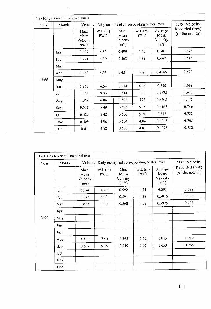
The Halda River at Panchapukuria

Year Month Velocity (Daily mean) and corresponding Water level Max. Velocity

Max. W.L (m) Min. W.L (m) Average Recorded (m/s)

Mean PWD Mean PWD Mean (of the month)

Velocity Velocity Velocity(m/s) (m/s) (m/s)

Jan 0507 4.52 0.499 4.45 0503 0.628

Feb 0.471 4.39 0.463 4.33 0.467 0.541

Mar

Apr 0.462 4.33 0.45 I 4.2 0.4565 0.529

1999 May

Jun 0.978 6.54 0.514 4.98 0.746 1.098

Jul l.361 9.93 0.614 5.4 0.9875 1.612

Aug 1.069 6.84 0.592 5.29 0.8305 1.175

Sep 0.638 5.49 0.595 5.15 0.6165 0.746

Oct 0.626 5.42 0.606 5.20 0.616 0.733

Nov 0.609 4.96 0.604 4.84 0.6065 0705

Dec 0.61 482 0.605 4.87 0.6075 0.732

The Halda River at Panchapukuria

Year Month Velocity (Daily mean) and corresponding Water level Max. Velocity

Max. W.L (m) Min. W.L (m) Average Recorded (m/s)

Mean PWD Mean PWD Mean (of the month)

Velocity Velocity Velocity(m/s) (m/s) (m/s)

Jan 0.594 4.76 0.592 4.74 0.593 0.688

Feb 0.592 4.62 0.591 4.55 0.5915 0.666

Mar 0.627 4.66 0.568 4.58 0.5975 0.733

Apr

2000 May

Jun

Jul .

Aug I 135 7.50 0.695 5.62 0.915 1.282

Scp 0.657 5.14 0.649 5.07 0.653 0.765

Oct

Nov.

Dec .

111

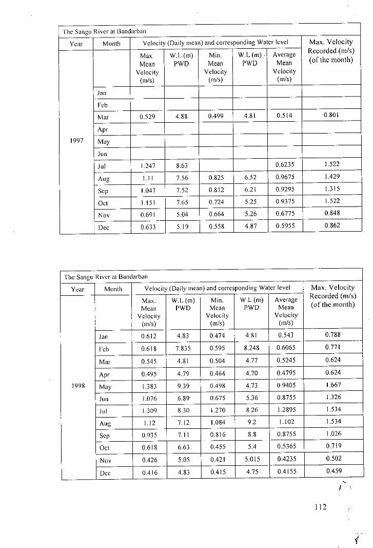
The Sangu River at l3andarban.

Year Month Vclocity (Daily mcan) and corresponding Watcr level Max. Velocity

Max. W.L (m) Min. W.L (m) . Average Recorded (m/5)

Mean PWD Mean PWD Mean (or the month)

Velocity Velocity Velocity(m!s) (m!s) (m!s)

Jan

Fcb

Mar 0.529 4.88 0.499 4.81 0.514 0.801

Apr

1997 May

JUll

Jul 1.247 8.63 0.6235 1.522

Aug 1.1 I 7.56 0.825 6.52 0.9675 1.429

Scp 1.047 7.52 0.812 6.21 0.9295 1.315

Oct 1.151 7.65 0.724 5.25 0.9375 1.522

Nov 0.691 5.04 0.664 5.26 0.6775 0.848

Dec 0.633 5.19 0.558 4.87 0.5955 0.862

The Sangu River at L3andarban

Year Month Velocity (Daily mean) and corresponding Water level Max. Velocity

Max. W.L (m) Min. W.L (m) Average Recorded (m!5)

Mean PWD Mean PWD Mean (ofthe month)

Velocity Velocity Velocity(m!s) (m!s) (m!5)

Jan 0.612 4.83 0474 4.81 0.543 0.788

Fcb 0.618 7.835 0595 8.248 0.6065 0.771

Mar 0.545 4.81 0.504 4.77 0.5245 0.624

Apr 0.495 4.79 0.464 4.70 0.4 795 0.624

1998 May 1.383 9.39 0.498 4.73 0.9405 1.667

Jun 1.076 6.89 0.675 5.36 0.8755 1.326

J"I 1.309 8.30 1.270 8.26 1.2895 1.534

Aug 1.12 7.12 1.084 9.2 1.102 1.534

Scp 0.935 7.11 0.816 8.8 0.8755 1.026

Oct 0.618 6.63 0.455 5.4 0.5365 0.719

Nov 0426 5.05 0.42 I 5.015 0.4235 0.502

Dcc 0.416 4.83 0.415 4.75 0.4155 0.459

112

The River Brammaputra at l3ahadurabad

Year Month Velocity (Daily mean) and corresponding Water level Max. Velocity

Max. W.L (m) Min. W.L (m) Average Recorded (m/s)

Mean PWD Mean PWD Mean (of the month)

Velocity Velocity Velocity(m/s) (m/s) (m/s)

Jan

Feb

Mar

Apr

1996 May

Jun 0.936 18.015 0.682 16.81 0.81 1.92

Jul 1.731 19.930 1168 19.24 1.45 2.77

Aug 1.248 19.110 1.159 18.61 1.20 2.42

Sep 1.188 18.995 0.907 17.41 1.05 2.33

Oct

Nov

Dec

The River BralllJ11aputra at Bahadurabad

Year Month Velocity (Daily mean) and corresponding Water level Max. Velocity

Max. W.L (m) Min. W.L(m) Average Recorded (m/s)

Mean PWD Mean PWD Mean (of the month)

Velocity Velocity Velocity(m/s) (m/s) (m/s)

Jan

Feb

Mar

Apr

1997 May

lUll

Jul

Aug

Sep

Oct 0.768 14.145 0.682 14.27 0.73 1.38

Nov 0.754 15.305 0.693 14.455 0.72 1.58

Dee

118

/'

•

The River Bralllmaputra at Bahadurabad

Year Month Velocity (Daily mean) and corresponding Water level Max. Velocity

Max. W.L (Ill) Min. W.L (Ill) Average Recorded (m/s)

Mean PWD Mean PWD Mean (of the month)

Velocity Velocity Velocity(Ill/s) (Ill/s) (Ill/s) .

Jan 0.696 13.16 0.587 13.28 0.64 1.23

Feb 0.649 13.035 0.577 12.96 0.61 1.15

Mar 0.793 14.315 0.645 13.00 0.72 1.52

Apr 0.806 14.67 0.685 14.72 075 1.63

1998 May 0.994 17.55 0.806 15.105 0.90 1.94

lUll 1.442 19.3 1.341 19.10 1.39 2.7

Jul 1.855 11.905 1.494 19.49 1.67 3.34

Aug 1.696 20.065 1.498 19.485 1.60 3.26

Scp 1.710 20.28 0904 17.68 1.31 3.29

Oct 0.961 17.095 0.784 16.35 0.87 2.54

Nov 0.753 14.895 0.725 14.825 0.74 1.61

Dec 0725 14.825 0.602 13.96 0.66 1.61

The River Bralllmaputra at Bahadurabad

Year Month Velocity (Daily Illean) and corresponding Water level Max. Velocity

Max. W.L (Ill) Min. W.L (Ill) Average Recorded (m/s)

Mean PWD Mean PWD Mean (of the month)

Velocity Velocity Velocity(Ill/s) (Ill/s) (Ill/s) ,

Jan 0.62 13.67 0.515 13.425 0.57 1.28

Feb 0.515 13.34 0.238 13.24 0.38 1.07

Mar 0.524 13.385 0.489 13.09 0.51 1.1 I

Apr 0.659 14.205 0.513 13.22 0.59 1.38

1999 May 0939 17.06 0.730 15.22 0.83 2.08

Jun 1.019 17.855 0.847 16.68 0.93 3.20

Jul 1.49 19.22 1.242 18.875 1.37 3.29

Aug 1.591 19.70 0.955 18.1 1.27 3.29

Sep 1.346 19.14 0.882 17.59 1. I I 2.85

Oct 0.92 17.735 0.834 16.995 0.88 2.35

Nov

Dec

119

The River Brammaputra at Bahadurabad

Year Month Velocity (Daily mean) and corresponding Water level Max. Velocity

Max. W.L (In) Min. W.L (In) Average Recorded (m/s)

Mean PWD Mean PWD Mean (of the month)Velocity Velocity Velocity

(In/s) (In/s) (In/s)

Jan 0.665 1400 0.546 13.64 061 1.14

Feb 0.552 1359 0.515 13.325 0.53 1.30

Mar 0.645 13.71 0.508 13.27 0.58 1.16

Apr 0.912 1505 0.593 13.66 0.75 1.776

2000 May 1.003 17.045 0.813 15.365 0.91 2678

Jun

lui

Aug

Scp

Oct

Nov

Dec

120

Appendix E

121

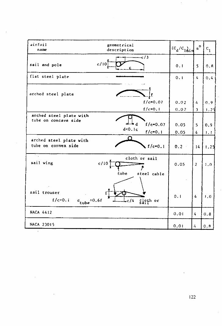
airf1.1il geometrical(Cd/Cl~it 0 Cldescription aname

sail and pole C/IO! ~f3 O. I 5 O.R

flat steel plat•• O. I I, 0.4.-

arched steel plate r_~!ff/c-0.07 0.02 I. 0.9ffe-D. I 0.07 3 1.2'

arched steel plate with~f/C-0.07

tube on concave side0.05 5 0.9

d<O. Ic f/c~O. I 0.05 4 I. I

arched steel.plate with~f/C~O.1tube on convex side 0.2 14 I .2'

cloth or sailsail wing c/IO t=<?- 0.05 2 1.0t

tube steel cable

satI trouser't~fh.' O. I 4 1.0f/c=O. i d b =0.6ftu e

NACA 4412 0.01 4 0.8

NACA 23015 0.01 I, 0.1\

122

Appendix F

123

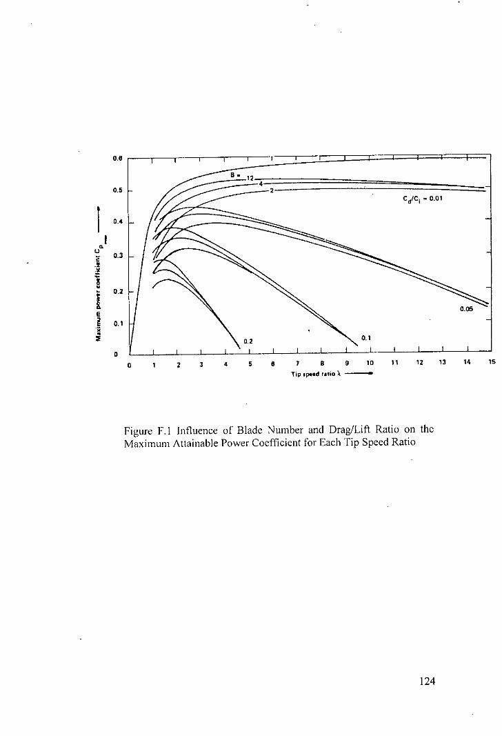
0.8

•0.5 2CJC, .0.01

1 D.'

I"u 0.3C

.!."~u

I 0.2

E0.05

~ 0.1.;•:E 0.1

0

0 2 J • 5 8 1 8 9 10 11 12 13 " 15

Tip .p•• d ratio). -

Figure F.l Influence of Blade Number and Drag/Lift Ratio on theMaximum Attainable Power Coefficient for Each Tip Speed Ratio

124

Appendix G

125

.,•••.~.

Data for Pitch Angle 5°, Shaft Inclination 45°, and Water Velocity 0.65 m/s

Spring Applied Difference N Torque. Q Q Tip Speed Power Input Power PowerGauge Load (gm) , F (gm) RPM N-m rad/s Ratio, A Output, Po Power to Coefficien Density,

(watt) the shaft, t, Cp,

(gm) (watt/m-)Pi (watt)

0 0 0 175 0 18.3 I7 5.9177 0 13.45 0 0

700 372.5 327.5 154 0.0723 16.119 5.2075 I. I 65 13.45 0.0866 10.55288

1200 745 455 149 0.1004 15.595 5.0385 1.566 I 13.45 0.1164 14.18524

1700 1117.5 582.5 145 0.1286 15.177 4.9032 1.9511 13.45 0.1451 17.6727

2200 1490 710 142 0.1567 14.863 4.8018 2.3289 13.45 0.1731 21.09529

2700 1872.5 827.5 138 0.1826 14.444 4.6665 2.6379 13.45 0.1961 23.89384

3500 2617.5 882.5 136 0.1948 14.235 4.5989 2.7724 13.45 0.2061 25.11265

3900 3000 900 134 0.1986 14.025 4.5312 2.7858 13.45 0.2071 25.23401

4600 3500 1100 130 0.2428 13.607 4.396 3.3033 13.45 0.2456 29.92092

5250 4000 1250 126 0.2759 13.188 4.2607 3.6382 13.45 0.2705 32.95486

5600 4500 1100 122 0.2428 12.769 4.1255 3.1 13.45 0.2305 28.07963

6100 4908 1192 119 0.2631 12.455 4.024 3.2767 13.45 0.2436 29.67988

7200 5408 1792 111 0.3955 11.618 3.7535 4.5948 13.45 0.3416 41.61979 !

8000 5816 2184 105 0.482 10.99 3.5506 5.2972 13.45 0.3938 47.98227 .

8400 6316 2084 97 0.4599 10.153 3.2801 4.6696 13.45 0.3472 42.29688

126

"

Experimental Data for Pitch Angle 5°, Shaft Inclination 45°, and Water Velocity 0.43 m/s

Spring Applied Difference N Torque, Q Q Tip Speed Power Input Power PowerGauge Load (gm) , F (gm) RPM N-m radls Ratio, A Output, Po Power to Coefficien Density,(gm) (watt) the shaft, t, Cp (watt/m2

)

Pi (watt)

0 0 0 104 0 10.885 3.5168 0 3.8131 0 0

750 372.5 377.5 96 0.0833 10.048 3.2463 0.8371 3.8131 0.2195 6.04544

1300 745 555 87 0.1225 9.1059 2.9419 1.1154 3.8131 0.2925 8.054748

1750 1117.5 632.5 84 0.1396 8.7919 2.8405 1.2273 3.8131 0.3219 8.862975

2400 1490 910 75 0.2008 7.85 2.5361 1.5766 3.8131 0.4135 11.38524

2750 1872.5 877.5 71 0.1937 7.4313 2.4009 1.4392 3.8131 0.3774 10.3931

3550 2617.5 932.5 64 0.2058 6.6986 2.1642 1.3786 3.8131 0.3615 9.955625

4000 3000 1000 55 0.2207 5.7566 1.8598 1.2705 3.8131 0.3332 9.174923

4700 3500 1200 41 0.2648 4.2913 1.3864 1.1365 3.8131 0.2981 8.207385

4900 4000 900 25 0.1986 2.6167 0.8454 0.5197 3.8131 0.1363 3.753377

4500 stall

...--.,. _ ........•'1 ~<.::....-..-.'t"'~

127

;'•.. /'

Experimental Data for Pitch Angle 5°, Shaft Inclination 45°, and Water Velocity 0.25 m/s

Spring Applied Difference N Torque, Q Q Tip Speed Power Input Power PowerGauge Load (gm) , F (gm) RPM N-m radls Ratio, Ie Output, Po Power to Coefficien Density,(gm) (watt) the shaft, t, Cp

,(watt!m-)

Pi (watt)0 0 0 57 0 5.966 1.9275 0 0.7653 0 0

650 372.5 277.5 45 0.0612 4.71 1.5217 0.2885 0.7653 0.3769 2.612849

1200 745 455 31 0.1004 3.2446 1.0483 0.3258 0.7653 0.4258 2.951291

1500 1117.5 382.5 25 0.0844 2.6167 0.8454 0.2209 0.7653 0.2886 2.000831

128

Experimental Data for Pitch Angle 0°, Shaft Inclination 45°, and Water Velocity 0.65 m/s

Spring Applied Difference N Torque, Q Q Tip Speed Power Input Power PowerGauge Load (gm) , F (gm) RPM N-m rad/s Ratio, A Output, Po Power to Coefficien Density,(gm) (watt) the shaft, t, Cp (watt/m2)

Pi (watt)0 0 160 0 16.75516 5.413206 0 13.45725 0 0

400 372.5 27.5 150 0.00607 15.70796 5.07488 0.095346 13.45725 0.007085 0.863645

1200 745 455 143 0.10043 14.97492 4.838053 1.50393 13.45725 0.111756 13.62255

1500 1117.5 382.5 140 0.084427 14.66077 4.736555 1.237769 13.45725 0.091978 1121168

2000 1490 510 136 0.11257 14.24189 4.601225 1.603206 13.45725 0.119133 14.52179

2700 1872.5 827.5 130 0.18265 13.61357 4.39823 2.486517 13.45725 0.184772 22.5228

3500 2617.5 882.5 128 0.19479 13.40413 4.330565 2.610988 13.45725 0.194021 23.65025

4000 3000 1000 125 0.220725 13.08997 4.229067 2.889283 13.45725 0.214701 26.17105

4600 3500 1100 123 0.242798 12.88053 4.161402 3.12736 13.45725 0.232392 28.32754

5300 4000 1300 119 0.286943 12.46165 4.026072 3.575777 13.45725 0.265714 32.38929

6000 4500 1500 116 0.331088 12.14749 3.924574 4.021883 13.45725 0.298864 36.4301

6400 4908 1492 113 0.329322 11.83333 3.823077 3.896973 13.45725 0.289582 35.29867

6850 5408 1442 112 0.318285 11.72861 3.789244 3.733047 13.45725 0.2774 33.81383

7200 5816 1384 III 0.305483 11.62389 3.755412 3.550906 13.45725 0.263866 32.16401

7600 6316 1284 109 0.283411 11.41445 3.687746 3.23498 13.45725 0.240389 29.30236

129

Experimental Data for Pitch Angle 0°, Shaft Inclination 45°, and Water Velocity 0.43 m/s

Spring Applied Difference N Torque, Q Q Tip Speed Power Input Power PowerGauge Load (gm) . F (gm) RPM N-m rad/s Ratio, Ie Output, Po Power to Coefficien Density,

(watt) the shaft, t, Cp,(gm) (watt/m-)

Pi (watt)0 0 85 0 8.901179 4.377629 0 3.815047 0 0

500 372.5 127.5 76 0.028142 7.958701 3.914115 0.223977 3.815047 0.058709 2.028779

1000 745 255 72 0.056285 7.539822 3.708109 0.424378 3.815047 0.111238 3.844003

1450 1117.5 332.5 66 0.073391 6.911504 3.3991 0.507243 3.815047 0.132958 4.5945891950 1490 460 64 0.101534 6.702064 3.296097 0.680484 3.815047 0.178368 6.1638052500 1872.5 627.5 57 0.138505 5.969026 2.935587 0.82674 3.815047 0.216705 7.4885832750 2617.5 132.5 40 0.029246 4.18879 2.060061 0.122506 3.815047 0.032111 1.109652

3000 stall

130

Experimental Data for Pitch Angle 00, Shaft Inclination 450, and Water Velocity 0.25 m/s

Spring Applied Difference N Torque, Q Q Tip Speed Power Input Power PowerGauge Load (gm) , F (gm) RPM N-m rad/s Ratio, Ie Output, Po Power to Coefficien Density(gm) (watt) the shaft, t, Cp (watt/m2

)Pi (watt)

0 0 50 0 5.235988 4.39823 0 0.765661 0 0

500 372.5 127.5 37 0.028142 3.874631 3.25469 0.109042 0.765661 0.142415 0.987695

900 745 155 23 0.034212 2.408554 2.023186 0.082402 0.765661 0.107623 0.746398 I

1I 17.5 stallI

I31

Appendix H

132

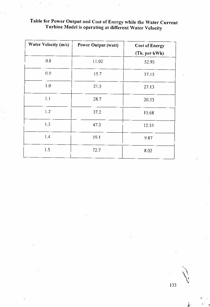
Table for Power Output and Cost of Energy while the Water CurrentTurbine Model is operating at different Water Velocity

-Water Velocity (m/s) Power Output (watt) Cost of Energy

(Tk. per kWh)

0.8 11.02 52.93

0.9 15.7 37.15

1.0 21.5 27.13

1.1 28.7 20.33

1.2 37.2 15.68

1.3 47.3 12.33

1.4 59.1 9.87

1.5 72.7 8.02

~133

,.

'.' ~'"

Appendix I

134

0.5

0.4.....- Cp at 0.65 m/s

-0- Cpat 0.43 m/s

-0.---T- Cp al 0.25 m/s

~ 0.3C(1)'0IE 0.2(1)0U

~;0 0.100-

0.0

o 2 3 4 5 6 7

Tip Speed Ratio (A)

Fig. 1.1 Power Coefficient VS. Tip Speed Ratio at DifferentWater Velocities with Pitch Angle 50

0.35-e- Cp at0.65 m/s

0,30 -0- Cpat 0.43 mls.............-Cp at 0.25 mls

-0.0.25

~C 0.20

'"'0IE 0.15'"0U~ 0.10;000-

0.05

0.00

2 3 4 5 6

Tip Speed Ratio (A)

Fig. 1.2 Power Coefficient VS. Tip Speed Ratio at Different

Water Velocities with Pitch Angle 00

~•..•..!'~!~!tl',tt.~lVr ,":7.s:..q:~S~,~t,~-!.:'7:~-(}~~ 135

.,••,••••••"- . ,I "" • • 'i

'~~~i~ii:-,.''.ffi';/~.~"!"'!,..g"'~