fusion of flir automatic target recognition algorithms

Information Fusion 4 (2003) 247–258

www.elsevier.com/locate/inffus

Fusion of FLIR automatic target recognition algorithms

Syed A. Rizvi a,*, Nasser M. Nasrabadi b

a Department of Engineering Science and Physics, College of Staten Island, City University of New York,

2800 Victory Blvd., Staten Island, NY 10314, USAb US Army Research Laboratory, ATTN: AMSRL-SE-SE, 2800 Powder Mill Road, Adelphi, MD 20783, USA

Received 15 November 2001; received in revised form 17 December 2002; accepted 4 April 2003

Abstract

In this paper, we investigate several fusion techniques for designing a composite classifier to improve the performance (prob-

ability of correct classification) of forward-looking infrared (FLIR) automatic target recognition (ATR). The motivation behind the

fusion of ATR algorithms is that if each contributing technique in a fusion algorithm (composite classifier) emphasizes on learning

at least some features of the targets that are not learned by other contributing techniques for making a classification decision, a

fusion of ATR algorithms may improve overall probability of correct classification of the composite classifier. In this research, we

propose to use four ATR algorithms for fusion. The individual performance of the four contributing algorithms ranges from 73.5%

to about 77% of probability of correct classification on the testing set. The set of correctly classified targets by each contributing

algorithm usually has a substantial overlap with the set of correctly identified targets by other algorithms (over 50% for the four

algorithms being used in this research). There is also a significant part of the set of correctly identified targets that is not shared by all

contributing algorithms. The size of this subset of correctly identified targets generally determines the extent of the potential im-

provement that may result from the fusion of the ATR algorithms. In this research, we propose to use Bayes classifier, committee of

experts, stacked-generalization, winner-takes-all, and ranking-based fusion techniques for designing the composite classifiers. The

experimental results show an improvement of more than 6.5% over the best individual performance.

Published by Elsevier B.V.

1. Introduction

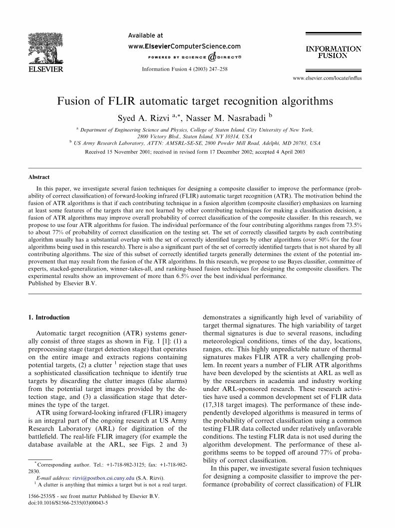
Automatic target recognition (ATR) systems gener-

ally consist of three stages as shown in Fig. 1 [1]: (1) a

preprocessing stage (target detection stage) that operates

on the entire image and extracts regions containing

potential targets, (2) a clutter 1 rejection stage that uses

a sophisticated classification technique to identify true

targets by discarding the clutter images (false alarms)

from the potential target images provided by the de-tection stage, and (3) a classification stage that deter-

mines the type of the target.

ATR using forward-looking infrared (FLIR) imagery

is an integral part of the ongoing research at US Army

Research Laboratory (ARL) for digitization of the

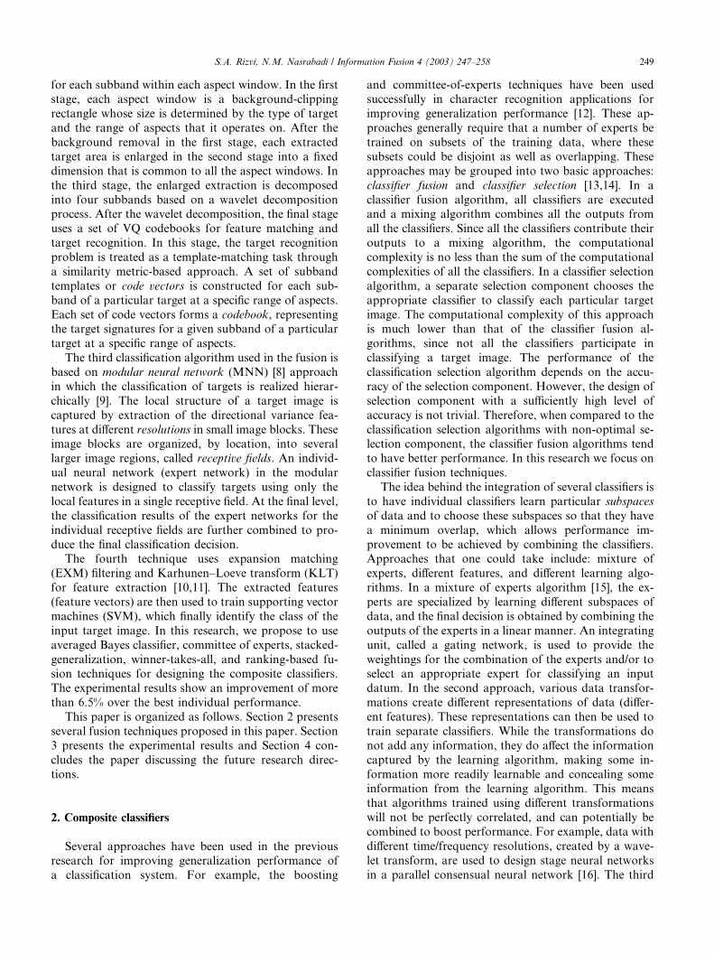
battlefield. The real-life FLIR imagery (for example the

database available at the ARL, see Figs. 2 and 3)

*Corresponding author. Tel.: +1-718-982-3125; fax: +1-718-982-

2830.

E-mail address: [email protected] (S.A. Rizvi).1 A clutter is anything that mimics a target but is not a real target.

1566-2535/$ - see front matter Published by Elsevier B.V.

doi:10.1016/S1566-2535(03)00043-5

demonstrates a significantly high level of variability of

target thermal signatures. The high variability of targetthermal signatures is due to several reasons, including

meteorological conditions, times of the day, locations,

ranges, etc. This highly unpredictable nature of thermal

signatures makes FLIR ATR a very challenging prob-

lem. In recent years a number of FLIR ATR algorithms

have been developed by the scientists at ARL as well as

by the researchers in academia and industry working

under ARL-sponsored research. These research activi-ties have used a common development set of FLIR data

(17,318 target images). The performance of these inde-

pendently developed algorithms is measured in terms of

the probability of correct classification using a common

testing FLIR data collected under relatively unfavorable

conditions. The testing FLIR data is not used during the

algorithm development. The performance of these al-

gorithms seems to be topped off around 77% of proba-bility of correct classification.

In this paper, we investigate several fusion techniques

for designing a composite classifier to improve the per-

formance (probability of correct classification) of FLIR

mail to: [email protected]

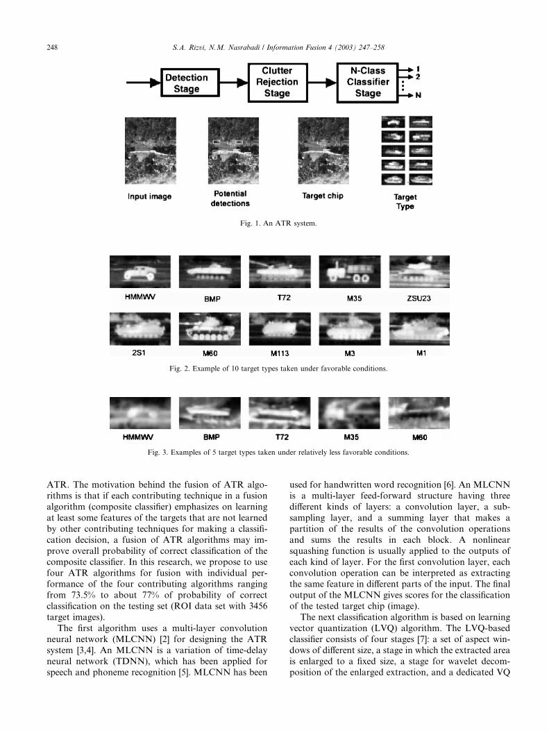
Fig. 1. An ATR system.

Fig. 2. Example of 10 target types taken under favorable conditions.

Fig. 3. Examples of 5 target types taken under relatively less favorable conditions.

248 S.A. Rizvi, N.M. Nasrabadi / Information Fusion 4 (2003) 247–258

ATR. The motivation behind the fusion of ATR algo-rithms is that if each contributing technique in a fusion

algorithm (composite classifier) emphasizes on learning

at least some features of the targets that are not learned

by other contributing techniques for making a classifi-

cation decision, a fusion of ATR algorithms may im-

prove overall probability of correct classification of the

composite classifier. In this research, we propose to use

four ATR algorithms for fusion with individual per-formance of the four contributing algorithms ranging

from 73.5% to about 77% of probability of correct

classification on the testing set (ROI data set with 3456

target images).

The first algorithm uses a multi-layer convolution

neural network (MLCNN) [2] for designing the ATR

system [3,4]. An MLCNN is a variation of time-delay

neural network (TDNN), which has been applied forspeech and phoneme recognition [5]. MLCNN has been

used for handwritten word recognition [6]. An MLCNNis a multi-layer feed-forward structure having three

different kinds of layers: a convolution layer, a sub-

sampling layer, and a summing layer that makes a

partition of the results of the convolution operations

and sums the results in each block. A nonlinear

squashing function is usually applied to the outputs of

each kind of layer. For the first convolution layer, each

convolution operation can be interpreted as extractingthe same feature in different parts of the input. The final

output of the MLCNN gives scores for the classification

of the tested target chip (image).

The next classification algorithm is based on learning

vector quantization (LVQ) algorithm. The LVQ-based

classifier consists of four stages [7]: a set of aspect win-

dows of different size, a stage in which the extracted area

is enlarged to a fixed size, a stage for wavelet decom-position of the enlarged extraction, and a dedicated VQ

S.A. Rizvi, N.M. Nasrabadi / Information Fusion 4 (2003) 247–258 249

for each subband within each aspect window. In the firststage, each aspect window is a background-clipping

rectangle whose size is determined by the type of target

and the range of aspects that it operates on. After the

background removal in the first stage, each extracted

target area is enlarged in the second stage into a fixed

dimension that is common to all the aspect windows. In

the third stage, the enlarged extraction is decomposed

into four subbands based on a wavelet decompositionprocess. After the wavelet decomposition, the final stage

uses a set of VQ codebooks for feature matching and

target recognition. In this stage, the target recognition

problem is treated as a template-matching task through

a similarity metric-based approach. A set of subband

templates or code vectors is constructed for each sub-

band of a particular target at a specific range of aspects.

Each set of code vectors forms a codebook, representingthe target signatures for a given subband of a particular

target at a specific range of aspects.

The third classification algorithm used in the fusion is

based on modular neural network (MNN) [8] approach

in which the classification of targets is realized hierar-

chically [9]. The local structure of a target image is

captured by extraction of the directional variance fea-

tures at different resolutions in small image blocks. Theseimage blocks are organized, by location, into several

larger image regions, called receptive fields. An individ-

ual neural network (expert network) in the modular

network is designed to classify targets using only the

local features in a single receptive field. At the final level,

the classification results of the expert networks for the

individual receptive fields are further combined to pro-

duce the final classification decision.The fourth technique uses expansion matching

(EXM) filtering and Karhunen–Loeve transform (KLT)

for feature extraction [10,11]. The extracted features

(feature vectors) are then used to train supporting vector

machines (SVM), which finally identify the class of the

input target image. In this research, we propose to use

averaged Bayes classifier, committee of experts, stacked-

generalization, winner-takes-all, and ranking-based fu-sion techniques for designing the composite classifiers.

The experimental results show an improvement of more

than 6.5% over the best individual performance.

This paper is organized as follows. Section 2 presents

several fusion techniques proposed in this paper. Section

3 presents the experimental results and Section 4 con-

cludes the paper discussing the future research direc-

tions.

2. Composite classifiers

Several approaches have been used in the previousresearch for improving generalization performance of

a classification system. For example, the boosting

and committee-of-experts techniques have been usedsuccessfully in character recognition applications for

improving generalization performance [12]. These ap-

proaches generally require that a number of experts be

trained on subsets of the training data, where these

subsets could be disjoint as well as overlapping. These

approaches may be grouped into two basic approaches:

classifier fusion and classifier selection [13,14]. In a

classifier fusion algorithm, all classifiers are executedand a mixing algorithm combines all the outputs from

all the classifiers. Since all the classifiers contribute their

outputs to a mixing algorithm, the computational

complexity is no less than the sum of the computational

complexities of all the classifiers. In a classifier selection

algorithm, a separate selection component chooses the

appropriate classifier to classify each particular target

image. The computational complexity of this approachis much lower than that of the classifier fusion al-

gorithms, since not all the classifiers participate in

classifying a target image. The performance of the

classification selection algorithm depends on the accu-

racy of the selection component. However, the design of

selection component with a sufficiently high level of

accuracy is not trivial. Therefore, when compared to the

classification selection algorithms with non-optimal se-lection component, the classifier fusion algorithms tend

to have better performance. In this research we focus on

classifier fusion techniques.

The idea behind the integration of several classifiers is

to have individual classifiers learn particular subspaces

of data and to choose these subspaces so that they have

a minimum overlap, which allows performance im-

provement to be achieved by combining the classifiers.Approaches that one could take include: mixture of

experts, different features, and different learning algo-

rithms. In a mixture of experts algorithm [15], the ex-

perts are specialized by learning different subspaces of

data, and the final decision is obtained by combining the

outputs of the experts in a linear manner. An integrating

unit, called a gating network, is used to provide the

weightings for the combination of the experts and/or toselect an appropriate expert for classifying an input

datum. In the second approach, various data transfor-

mations create different representations of data (differ-

ent features). These representations can then be used to

train separate classifiers. While the transformations do

not add any information, they do affect the information

captured by the learning algorithm, making some in-

formation more readily learnable and concealing someinformation from the learning algorithm. This means

that algorithms trained using different transformations

will not be perfectly correlated, and can potentially be

combined to boost performance. For example, data with

different time/frequency resolutions, created by a wave-

let transform, are used to design stage neural networks

in a parallel consensual neural network [16]. The third


approach is to design several classifiers with differentlearning algorithms and combine them with a mixing

strategy. In this approach each component classifier

naturally creates different learning subspaces. The third

approach is discussed in this section to design and

combine the several classifiers.

Let us define the notation that is used in this section.

Suppose that we have a set of K classifiers, Ck, each of

which classifies targets into one of Q distinct classes,where k ¼ 1; 2; . . . ;K. The output vector of classifier Ck,

given a target X, is represented by a column vector

yk ¼ fyk;q; q ¼ 1; 2; . . . :;Qg; ð1Þwhere qth component of the output vector, yk;q, repre-sents the estimated posteriori probability that target X

belongs to the class q, estimated by classifier Ck. We can

then express the estimated posteriori probability as thedesired posteriori probability pðqjXÞ plus an error

ek;qðXÞ:yk;q ¼ pðqjXÞ þ ek;qðXÞ: ð2ÞFor notational convenience, we do not explicitly express

the dependence of outputs yk;q upon variable X, where X

is the input of each individual classifier Ck. The groundtruth class of a target X is hT. The output vector of a

composite classifier, Ck, given a target X, is represented

by a column vector

yðXÞ ¼ fyqðXÞ; q ¼ 1; 2; . . . ;Qg; ð3Þwhere yqðXÞ, the qth component of the output vector, is

the estimated posteriori probability that target X be-

longs to the class q. The classification decision of clas-sifier Ck is

hk ¼ argmax16 q6Qyk;q: ð4Þ

The final decision of a composite classifier C is

h ¼ argmax16 q6Qyq: ð5Þ

The first step in the design of the composite classifier

is to express the outputs of the different classifiers in

terms of the probability of correct classification. In one

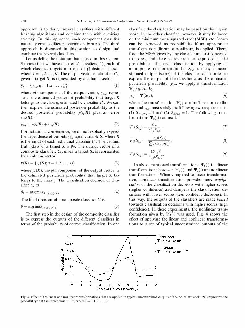
Fig. 4. Effect of the linear and nonlinear transformations that are applied to t

probability that the target class is ‘‘i’’, where i ¼ 0; 1; 2; . . . ; 9.

classifier, the classification may be based on the highestscore. In the other classifier, however, it may be based

on the minimum mean squared error (MSE), etc. Scores

can be expressed as probabilities if an appropriate

transformation (linear or nonlinear) is applied. There-

fore, the MSEs given by any classifier are first converted

to scores, and these scores are then expressed as the

probabilities of correct classification by applying an

appropriate transformation. Let Sk;q be the qth uncon-strained output (score) of the classifier k. In order to

express the output of the classifier k as the estimated

posteriori probability, yk;q, we apply a transformation

Wð�Þ given by

yk;q ¼ WðSk;qÞ; ð6Þ

where the transformation W(Æ) can be linear or nonlin-

ear, and yk;q must satisfy the following two requirements:

(1) 06 yk;q 6 1 and (2) Rqyk;q ¼ 1. The following trans-

formations Wkð�Þ can used:

W1ðSk;qÞ ¼Sk;qPj Sk;j

; ð7Þ

W2ðSk;qÞ ¼expðSk;qÞPj expðSk;jÞ

; ð8Þ

W3ðSk;qÞ ¼ðSk;qÞnPjðSk;jÞ

n : ð9Þ

In above mentioned transformations, W1ð�Þ is a linear

transformation; however, W2ð�Þ and W3ð�Þ are nonlineartransformations. When compared to linear transforma-

tion, nonlinear transformation provides more amplifi-

cation of the classification decisions with higher scores

(higher confidence) and dampens the classification de-

cisions with lower scores (less confident decisions). In

this way, the outputs of the classifiers are made biased

towards classification decisions with higher scores (high

confidence). In these experiments, the nonlinear trans-formation given by W3ð�Þ was used. Fig. 4 shows the

effect of applying the linear and nonlinear transforma-

tions to a set of typical unconstrained outputs of the

ypical unconstrained outputs of the neural network. WðiÞ represents the

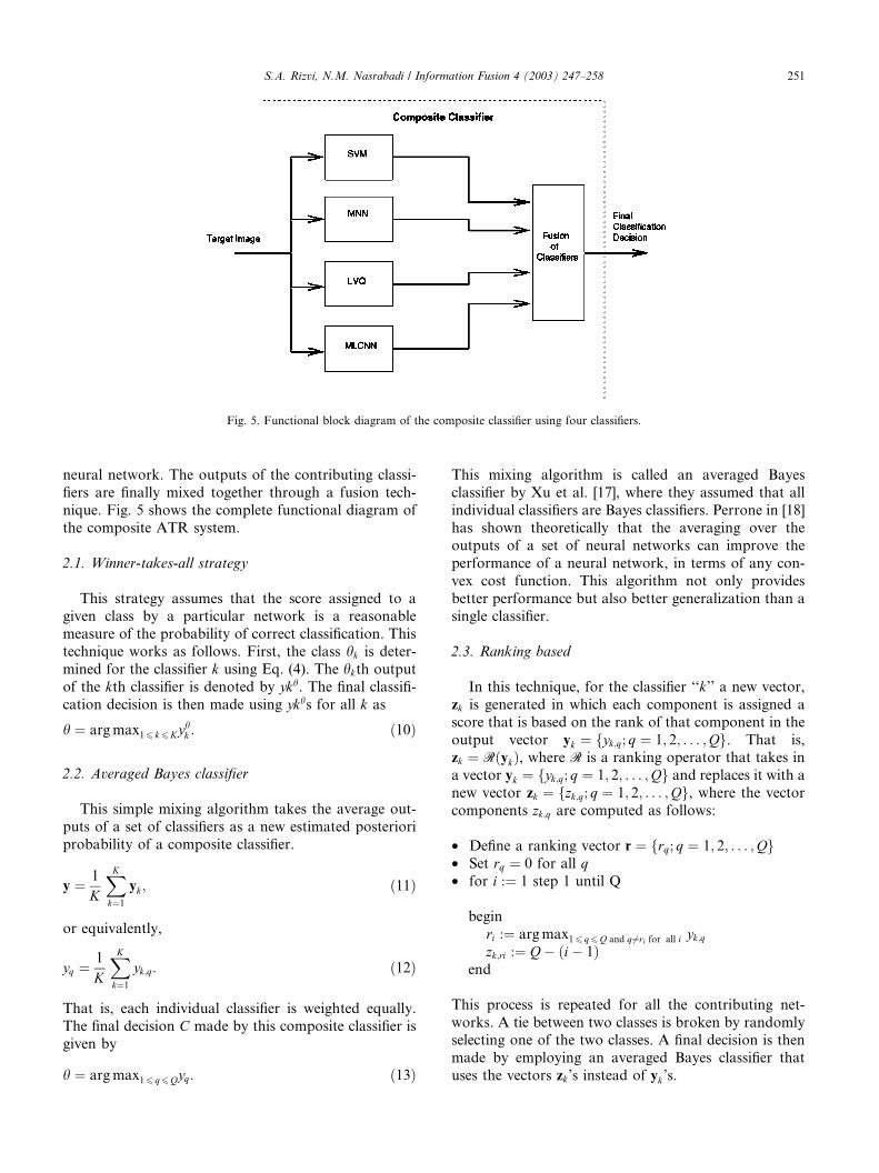
Fig. 5. Functional block diagram of the composite classifier using four classifiers.


neural network. The outputs of the contributing classi-

fiers are finally mixed together through a fusion tech-

nique. Fig. 5 shows the complete functional diagram of

the composite ATR system.

2.1. Winner-takes-all strategy

This strategy assumes that the score assigned to agiven class by a particular network is a reasonable

measure of the probability of correct classification. This

technique works as follows. First, the class hk is deter-

mined for the classifier k using Eq. (4). The hkth output

of the kth classifier is denoted by ykh. The final classifi-

cation decision is then made using ykhs for all k as

h ¼ argmax16 k6Kyhk : ð10Þ

2.2. Averaged Bayes classifier

This simple mixing algorithm takes the average out-

puts of a set of classifiers as a new estimated posteriori

probability of a composite classifier.

y ¼ 1

K

XK

k¼1

yk; ð11Þ

or equivalently,

yq ¼1

K

XK

k¼1

yk;q: ð12Þ

That is, each individual classifier is weighted equally.

The final decision C made by this composite classifier is

given by

h ¼ argmax y : ð13Þ
16 q6Q q
This mixing algorithm is called an averaged Bayes

classifier by Xu et al. [17], where they assumed that all

individual classifiers are Bayes classifiers. Perrone in [18]

has shown theoretically that the averaging over the

outputs of a set of neural networks can improve the

performance of a neural network, in terms of any con-

vex cost function. This algorithm not only provides

better performance but also better generalization than asingle classifier.

2.3. Ranking based

In this technique, for the classifier ‘‘k’’ a new vector,

zk is generated in which each component is assigned a

score that is based on the rank of that component in the

output vector yk ¼ fyk;q; q ¼ 1; 2; . . . ;Qg. That is,zk ¼ RðykÞ, where R is a ranking operator that takes in

a vector yk ¼ fyk;q; q ¼ 1; 2; . . . ;Qg and replaces it with a

new vector zk ¼ fzk;q; q ¼ 1; 2; . . . ;Qg, where the vector

components zk;q are computed as follows:

• Define a ranking vector r ¼ frq; q ¼ 1; 2; . . . ;Qg• Set rq ¼ 0 for all q• for i :¼ 1 step 1 until Q

begin

ri :¼ argmax16 q6Q and q6¼ri for all i yk;qzk;ri :¼ Q� ði� 1Þ

end

This process is repeated for all the contributing net-

works. A tie between two classes is broken by randomlyselecting one of the two classes. A final decision is then

made by employing an averaged Bayes classifier that

uses the vectors zk’s instead of yk’s.

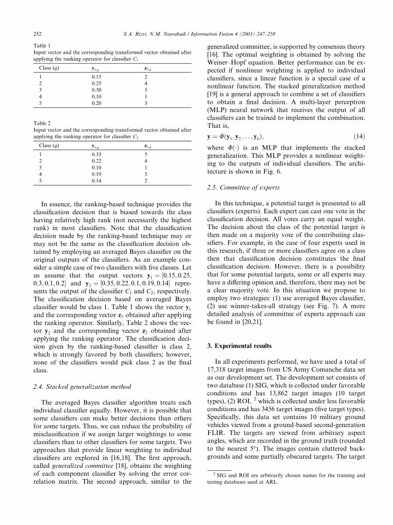
Table 1

Input vector and the corresponding transformed vector obtained after

applying the ranking operator for classifier C1

Class (q) y1;q z1;q

1 0.15 2

2 0.25 4

3 0.30 5

4 0.10 1

5 0.20 3

Table 2

Input vector and the corresponding transformed vector obtained after

applying the ranking operator for classifier C2

Class (q) y1;q z1;q

1 0.35 5

2 0.22 4

3 0.10 1

4 0.19 3

5 0.14 2

2 SIG and ROI are arbitrarily chosen names for the training and

testing databases used at ARL.


In essence, the ranking-based technique provides the

classification decision that is biased towards the class

having relatively high rank (not necessarily the highest

rank) in most classifiers. Note that the classification

decision made by the ranking-based technique may or

may not be the same as the classification decision ob-

tained by employing an averaged Bayes classifier on the

original outputs of the classifiers. As an example con-sider a simple case of two classifiers with five classes. Let

us assume that the output vectors y1 ¼ ½0:15; 0:25;0:3; 0:1; 0:2� and y2 ¼ ½0:35; 0:22; 0:1; 0:19; 0:14� repre-

sents the output of the classifier C1 and C2, respectively.

The classification decision based on averaged Bayes

classifier would be class 1. Table 1 shows the vector y1and the corresponding vector z1 obtained after applying

the ranking operator. Similarly, Table 2 shows the vec-tor y2 and the corresponding vector z2 obtained after

applying the ranking operator. The classification deci-

sion given by the ranking-based classifier is class 2,

which is strongly favored by both classifiers; however,

none of the classifiers would pick class 2 as the final

class.

2.4. Stacked generalization method

The averaged Bayes classifier algorithm treats eachindividual classifier equally. However, it is possible that

some classifiers can make better decisions than others

for some targets. Thus, we can reduce the probability of

misclassification if we assign larger weightings to some

classifiers than to other classifiers for some targets. Two

approaches that provide linear weighting to individual

classifiers are explored in [16,18]. The first approach,

called generalized committee [18], obtains the weightingof each component classifier by solving the error cor-

relation matrix. The second approach, similar to the

generalized committee, is supported by consensus theory[16]. The optimal weighting is obtained by solving the

Weiner–Hopf equation. Better performance can be ex-

pected if nonlinear weighting is applied to individual

classifiers, since a linear function is a special case of a

nonlinear function. The stacked generalization method

[19] is a general approach to combine a set of classifiers

to obtain a final decision. A multi-layer perceptron

(MLP) neural network that receives the output of allclassifiers can be trained to implement the combination.

That is,

y ¼ Uðy1; y2 . . . ; ykÞ; ð14Þwhere Uð�Þ is an MLP that implements the stacked

generalization. This MLP provides a nonlinear weight-

ing to the outputs of individual classifiers. The archi-

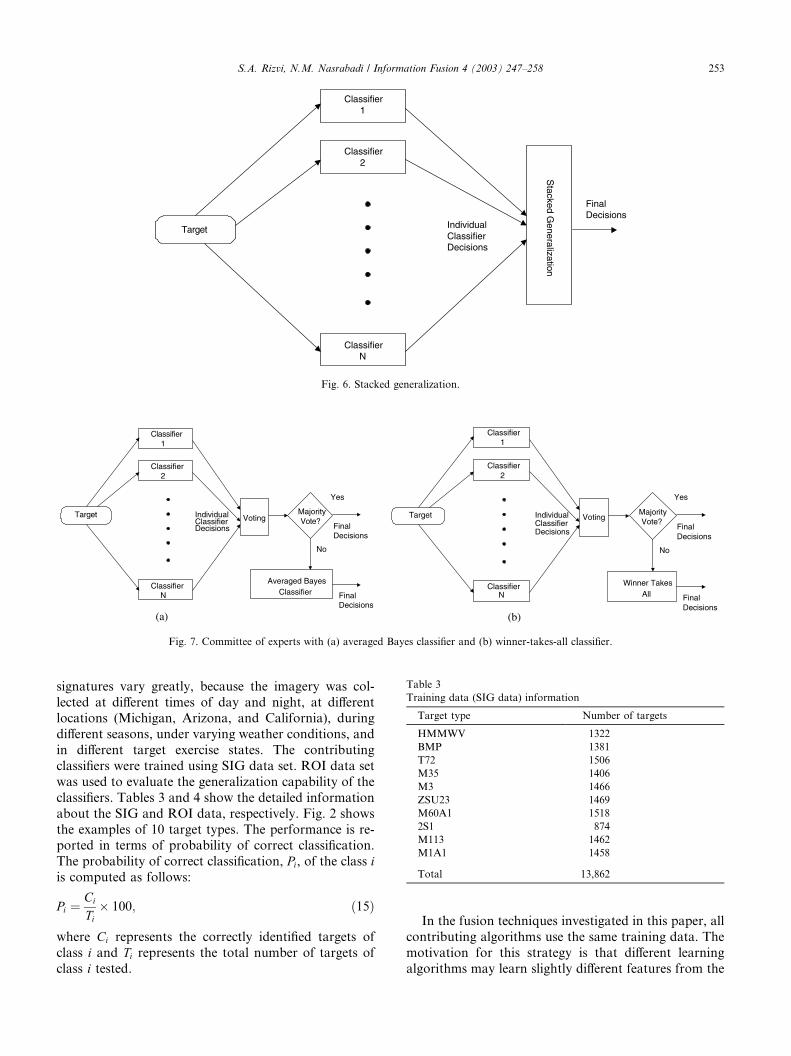
tecture is shown in Fig. 6.

2.5. Committee of experts

In this technique, a potential target is presented to all

classifiers (experts). Each expert can cast one vote in the

classification decision. All votes carry an equal weight.The decision about the class of the potential target is

then made on a majority vote of the contributing clas-

sifiers. For example, in the case of four experts used in

this research, if three or more classifiers agree on a class

then that classification decision constitutes the final

classification decision. However, there is a possibility

that for some potential targets, some or all experts may

have a differing opinion and, therefore, there may not bea clear majority vote. In this situation we propose to

employ two strategies: (1) use averaged Bayes classifier,

(2) use winner-takes-all strategy (see Fig. 7). A more

detailed analysis of committee of experts approach can

be found in [20,21].

3. Experimental results

In all experiments performed, we have used a total of

17,318 target images from US Army Comanche data set

as our development set. The development set consists of

two database (1) SIG, which is collected under favorable

conditions and has 13,862 target images (10 targettypes), (2) ROI, 2 which is collected under less favorable

conditions and has 3456 target images (five target types).

Specifically, this data set contains 10 military ground

vehicles viewed from a ground-based second-generation

FLIR. The targets are viewed from arbitrary aspect

angles, which are recorded in the ground truth (rounded

to the nearest 5�). The images contain cluttered back-

grounds and some partially obscured targets. The target

IndividualClassifierDecisions

FinalDecisions

Classifier2

Classifier1

ClassifierN

TargetS

tacked Generalization

Fig. 6. Stacked generalization.


Yes

Target Voting

Classifier2

Classifier1

ClassifierN

MajorityVote?

FinalDecisions

No

Winner TakesAll Final

Decisions


Yes

Target Voting

Classifier2

Classifier1

ClassifierN

MajorityVote?

FinalDecisions

No

Averaged BayesClassifier Final

Decisions

(b)(a)

Fig. 7. Committee of experts with (a) averaged Bayes classifier and (b) winner-takes-all classifier.

Table 3

Training data (SIG data) information

Target type Number of targets

HMMWV 1322

BMP 1381

T72 1506

M35 1406

M3 1466

ZSU23 1469

M60A1 1518

2S1 874

M113 1462

M1A1 1458

Total 13,862


signatures vary greatly, because the imagery was col-

lected at different times of day and night, at differentlocations (Michigan, Arizona, and California), during

different seasons, under varying weather conditions, and

in different target exercise states. The contributing

classifiers were trained using SIG data set. ROI data set

was used to evaluate the generalization capability of the

classifiers. Tables 3 and 4 show the detailed information

about the SIG and ROI data, respectively. Fig. 2 shows

the examples of 10 target types. The performance is re-ported in terms of probability of correct classification.

The probability of correct classification, Pi, of the class iis computed as follows:

Pi ¼Ci

Ti� 100; ð15Þ

where Ci represents the correctly identified targets of

class i and Ti represents the total number of targets of

class i tested.

In the fusion techniques investigated in this paper, all

contributing algorithms use the same training data. The

motivation for this strategy is that different learning

algorithms may learn slightly different features from the

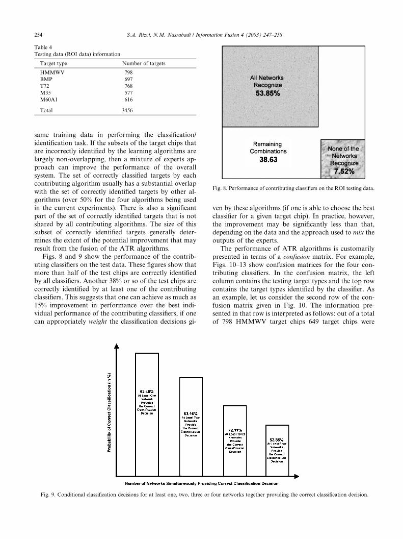
Fig. 8. Performance of contributing classifiers on the ROI testing data.

Table 4

Testing data (ROI data) information

Target type Number of targets

HMMWV 798

BMP 697

T72 768

M35 577

M60A1 616

Total 3456


same training data in performing the classification/

identification task. If the subsets of the target chips that

are incorrectly identified by the learning algorithms are

largely non-overlapping, then a mixture of experts ap-proach can improve the performance of the overall

system. The set of correctly classified targets by each

contributing algorithm usually has a substantial overlap

with the set of correctly identified targets by other al-

gorithms (over 50% for the four algorithms being used

in the current experiments). There is also a significant

part of the set of correctly identified targets that is not

shared by all contributing algorithms. The size of thissubset of correctly identified targets generally deter-

mines the extent of the potential improvement that may

result from the fusion of the ATR algorithms.

Figs. 8 and 9 show the performance of the contrib-

uting classifiers on the test data. These figures show that

more than half of the test chips are correctly identified

by all classifiers. Another 38% or so of the test chips are

correctly identified by at least one of the contributingclassifiers. This suggests that one can achieve as much as

15% improvement in performance over the best indi-

vidual performance of the contributing classifiers, if one

can appropriately weight the classification decisions gi-

Fig. 9. Conditional classification decisions for at least one, two, three or

ven by these algorithms (if one is able to choose the best

classifier for a given target chip). In practice, however,

the improvement may be significantly less than that,

depending on the data and the approach used to mix the

outputs of the experts.

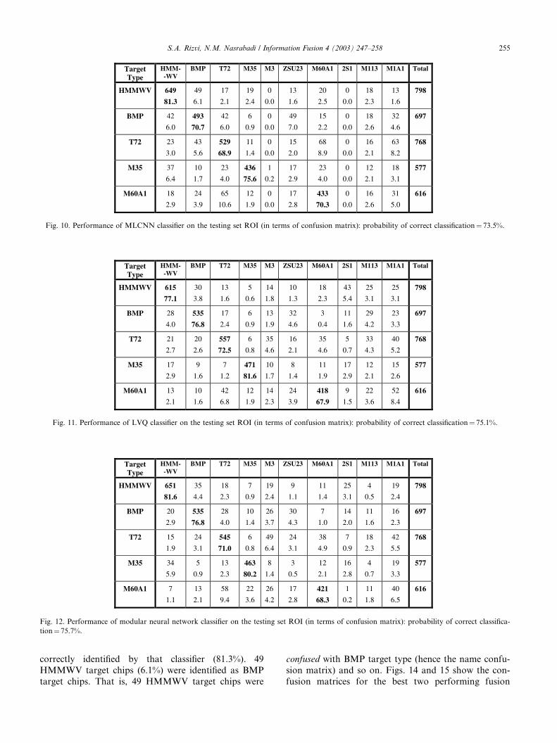
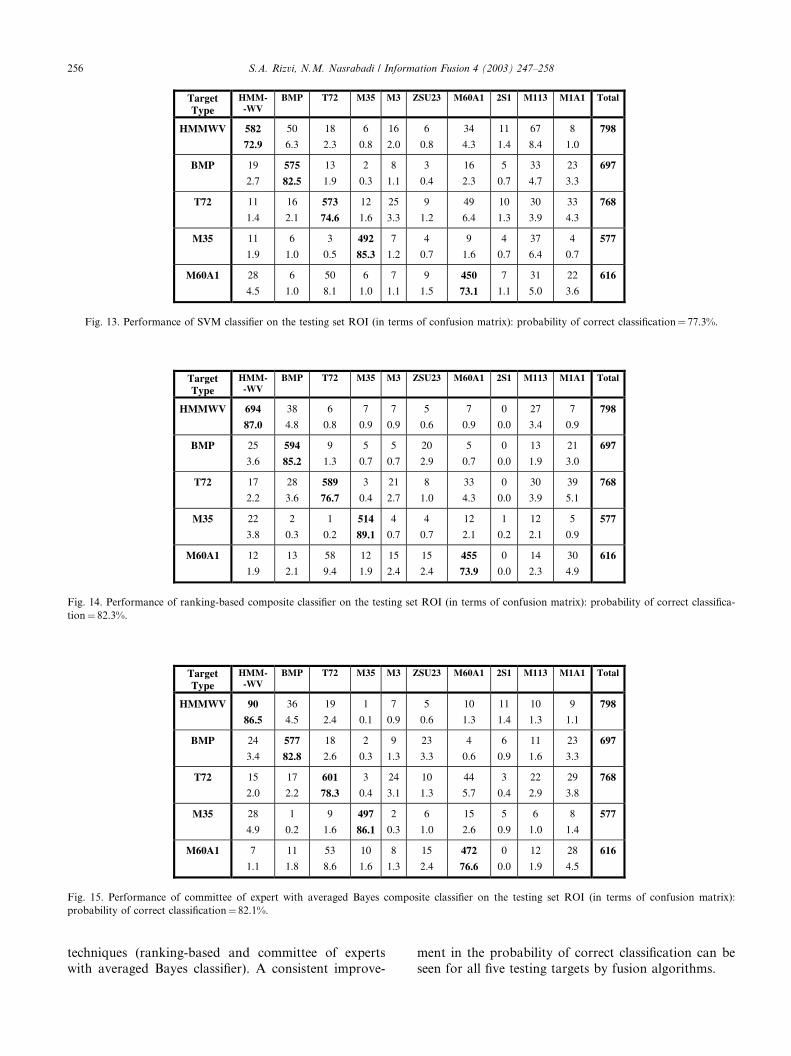
The performance of ATR algorithms is customarilypresented in terms of a confusion matrix. For example,

Figs. 10–13 show confusion matrices for the four con-

tributing classifiers. In the confusion matrix, the left

column contains the testing target types and the top row

contains the target types identified by the classifier. As

an example, let us consider the second row of the con-

fusion matrix given in Fig. 10. The information pre-

sented in that row is interpreted as follows: out of a totalof 798 HMMWV target chips 649 target chips were

four networks together providing the correct classification decision.

TargetType

HMM--WV

BMP T72 M35 M3 ZSU23 M60A1 2S1 M113 M1A1 Total

HMMWV 649

81.3

49

6.1

17

2.1

19

2.4

0

0.0

13

1.6

20

2.5

0

0.0

18

2.3

13

1.6

798

BMP 42

6.0

493

70.7

42

6.0

6

0.9

0

0.0

49

7.0

15

2.2

0

0.0

18

2.6

32

4.6

697

T72 23

3.0

43

5.6

529

68.9

11

1.4

0

0.0

15

2.0

68

8.9

0

0.0

16

2.1

63

8.2

768

M35 37

6.4

10

1.7

23

4.0

436

75.6

1

0.2

17

2.9

23

4.0

0

0.0

12

2.1

18

3.1

577

M60A1 18

2.9

24

3.9

65

10.6

12

1.9

0

0.0

17

2.8

433

70.3

0

0.0

16

2.6

31

5.0

616

Fig. 10. Performance of MLCNN classifier on the testing set ROI (in terms of confusion matrix): probability of correct classification¼ 73.5%.

TargetType

HMM--WV


HMMWV 615

77.1

30

3.8

13

1.6

5

0.6

14

1.8

10

1.3

18

2.3

43

5.4

25

3.1

25

3.1

798

BMP 28

4.0

535

76.8

17

2.4

6

0.9

13

1.9

32

4.6

3

0.4

11

1.6

29

4.2

23

3.3

697

T72 21

2.7

20

2.6

557

72.5

6

0.8

35

4.6

16

2.1

35

4.6

5

0.7

33

4.3

40

5.2

768

M35 17

2.9

9

1.6

7

1.2

471

81.6

10

1.7

8

1.4

11

1.9

17

2.9

12

2.1

15

2.6

577

M60A1 13

2.1

10

1.6

42

6.8

12

1.9

14

2.3

24

3.9

418

67.9

9

1.5

22

3.6

52

8.4

616

Fig. 11. Performance of LVQ classifier on the testing set ROI (in terms of confusion matrix): probability of correct classification¼ 75.1%.

TargetType

HMM--WV


HMMWV 651

81.6

35

4.4

18

2.3

7

0.9

19

2.4

9

1.1

11

1.4

25

3.1

4

0.5

19

2.4

798

BMP 20

2.9

535

76.8

28

4.0

10

1.4

26

3.7

30

4.3

7

1.0

14

2.0

11

1.6

16

2.3

697

T72 15

1.9

24

3.1

545

71.0

6

0.8

49

6.4

24

3.1

38

4.9

7

0.9

18

2.3

42

5.5

768

M35 34

5.9

5

0.9

13

2.3

463

80.2

8

1.4

3

0.5

12

2.1

16

2.8

4

0.7

19

3.3

577

M60A1 7

1.1

13

2.1

58

9.4

22

3.6

26

4.2

17

2.8

421

68.3

1

0.2

11

1.8

40

6.5

616

Fig. 12. Performance of modular neural network classifier on the testing set ROI (in terms of confusion matrix): probability of correct classifica-

tion¼ 75.7%.


correctly identified by that classifier (81.3%). 49

HMMWV target chips (6.1%) were identified as BMP

target chips. That is, 49 HMMWV target chips were

confused with BMP target type (hence the name confu-

sion matrix) and so on. Figs. 14 and 15 show the con-

fusion matrices for the best two performing fusion

TargetType

HMM--WV


HMMWV 582

72.9

50

6.3

18

2.3

6

0.8

16

2.0

6

0.8

34

4.3

11

1.4

67

8.4

8

1.0

798

BMP 19

2.7

575

82.5

13

1.9

2

0.3

8

1.1

3

0.4

16

2.3

5

0.7

33

4.7

23

3.3

697

T72 11

1.4

16

2.1

573

74.6

12

1.6

25

3.3

9

1.2

49

6.4

10

1.3

30

3.9

33

4.3

768

M35 11

1.9

6

1.0

3

0.5

492

85.3

7

1.2

4

0.7

9

1.6

4

0.7

37

6.4

4

0.7

577

M60A1 28

4.5

6

1.0

50

8.1

6

1.0

7

1.1

9

1.5

450

73.1

7

1.1

31

5.0

22

3.6

616

Fig. 13. Performance of SVM classifier on the testing set ROI (in terms of confusion matrix): probability of correct classification¼ 77.3%.

TargetType

HMM--WV


HMMWV 694

87.0

38

4.8

6

0.8

7

0.9

7

0.9

5

0.6

7

0.9

0

0.0

27

3.4

7

0.9

798

BMP 25

3.6

594

85.2

9

1.3

5

0.7

5

0.7

20

2.9

5

0.7

0

0.0

13

1.9

21

3.0

697

T72 17

2.2

28

3.6

589

76.7

3

0.4

21

2.7

8

1.0

33

4.3

0

0.0

30

3.9

39

5.1

768

M35 22

3.8

2

0.3

1

0.2

514

89.1

4

0.7

4

0.7

12

2.1

1

0.2

12

2.1

5

0.9

577

M60A1 12

1.9

13

2.1

58

9.4

12

1.9

15

2.4

15

2.4

455

73.9

0

0.0

14

2.3

30

4.9

616

Fig. 14. Performance of ranking-based composite classifier on the testing set ROI (in terms of confusion matrix): probability of correct classifica-

tion¼ 82.3%.

TargetType

HMM--WV


HMMWV 90

86.5

36

4.5

19

2.4

1

0.1

7

0.9

5

0.6

10

1.3

11

1.4

10

1.3

9

1.1

798

BMP 24

3.4

577

82.8

18

2.6

2

0.3

9

1.3

23

3.3

4

0.6

6

0.9

11

1.6

23

3.3

697

T72 15

2.0

17

2.2

601

78.3

3

0.4

24

3.1

10

1.3

44

5.7

3

0.4

22

2.9

29

3.8

768

M35 28

4.9

1

0.2

9

1.6

497

86.1

2

0.3

6

1.0

15

2.6

5

0.9

6

1.0

8

1.4

577

M60A1 7

1.1

11

1.8

53

8.6

10

1.6

8

1.3

15

2.4

472

76.6

0

0.0

12

1.9

28

4.5

616

Fig. 15. Performance of committee of expert with averaged Bayes composite classifier on the testing set ROI (in terms of confusion matrix):

probability of correct classification¼ 82.1%.


techniques (ranking-based and committee of experts

with averaged Bayes classifier). A consistent improve-

ment in the probability of correct classification can be

seen for all five testing targets by fusion algorithms.

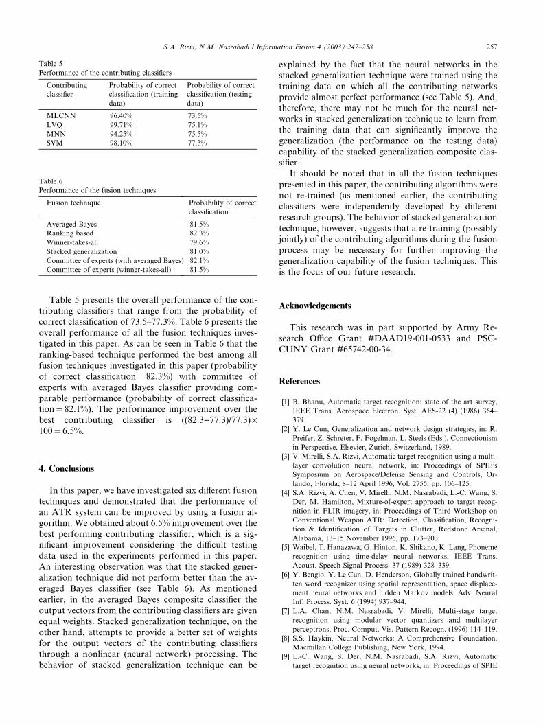
Table 5

Performance of the contributing classifiers

Contributing

classifier

Probability of correct

classification (training

data)

Probability of correct

classification (testing

data)

MLCNN 96.40% 73.5%

LVQ 99.71% 75.1%

MNN 94.25% 75.5%

SVM 98.10% 77.3%

Table 6

Performance of the fusion techniques

Fusion technique Probability of correct

classification

Averaged Bayes 81.5%

Ranking based 82.3%

Winner-takes-all 79.6%

Stacked generalization 81.0%

Committee of experts (with averaged Bayes) 82.1%

Committee of experts (winner-takes-all) 81.5%


Table 5 presents the overall performance of the con-

tributing classifiers that range from the probability of

correct classification of 73.5–77.3%. Table 6 presents the

overall performance of all the fusion techniques inves-

tigated in this paper. As can be seen in Table 6 that the

ranking-based technique performed the best among all

fusion techniques investigated in this paper (probability

of correct classification¼ 82.3%) with committee ofexperts with averaged Bayes classifier providing com-

parable performance (probability of correct classifica-

tion¼ 82.1%). The performance improvement over the

best contributing classifier is ((82.3)77.3)/77.3) ·100¼ 6.5%.

4. Conclusions

In this paper, we have investigated six different fusion

techniques and demonstrated that the performance of

an ATR system can be improved by using a fusion al-

gorithm. We obtained about 6.5% improvement over the

best performing contributing classifier, which is a sig-

nificant improvement considering the difficult testing

data used in the experiments performed in this paper.An interesting observation was that the stacked gener-

alization technique did not perform better than the av-

eraged Bayes classifier (see Table 6). As mentioned

earlier, in the averaged Bayes composite classifier the

output vectors from the contributing classifiers are given

equal weights. Stacked generalization technique, on the

other hand, attempts to provide a better set of weights

for the output vectors of the contributing classifiersthrough a nonlinear (neural network) processing. The

behavior of stacked generalization technique can be

explained by the fact that the neural networks in thestacked generalization technique were trained using the

training data on which all the contributing networks

provide almost perfect performance (see Table 5). And,

therefore, there may not be much for the neural net-

works in stacked generalization technique to learn from

the training data that can significantly improve the

generalization (the performance on the testing data)

capability of the stacked generalization composite clas-sifier.

It should be noted that in all the fusion techniques

presented in this paper, the contributing algorithms were

not re-trained (as mentioned earlier, the contributing

classifiers were independently developed by different

research groups). The behavior of stacked generalization

technique, however, suggests that a re-training (possibly

jointly) of the contributing algorithms during the fusionprocess may be necessary for further improving the

generalization capability of the fusion techniques. This

is the focus of our future research.

Acknowledgements

This research was in part supported by Army Re-

search Office Grant #DAAD19-001-0533 and PSC-

CUNY Grant #65742-00-34.

References

[1] B. Bhanu, Automatic target recognition: state of the art survey,

IEEE Trans. Aerospace Electron. Syst. AES-22 (4) (1986) 364–

379.

[2] Y. Le Cun, Generalization and network design strategies, in: R.

Preifer, Z. Schreter, F. Fogelman, L. Steels (Eds.), Connectionism

in Perspective, Elsevier, Zurich, Switzerland, 1989.

[3] V. Mirelli, S.A. Rizvi, Automatic target recognition using a multi-

layer convolution neural network, in: Proceedings of SPIE’s

Symposium on Aerospace/Defense Sensing and Controls, Or-

lando, Florida, 8–12 April 1996, Vol. 2755, pp. 106–125.

[4] S.A. Rizvi, A. Chen, V. Mirelli, N.M. Nasrabadi, L.-C. Wang, S.

Der, M. Hamilton, Mixture-of-expert approach to target recog-

nition in FLIR imagery, in: Proceedings of Third Workshop on

Conventional Weapon ATR: Detection, Classification, Recogni-

tion & Identification of Targets in Clutter, Redstone Arsenal,

Alabama, 13–15 November 1996, pp. 173–203.

[5] Waibel, T. Hanazawa, G. Hinton, K. Shikano, K. Lang, Phoneme

recognition using time-delay neural networks, IEEE Trans.

Acoust. Speech Signal Process. 37 (1989) 328–339.

[6] Y. Bengio, Y. Le Cun, D. Henderson, Globally trained handwrit-

ten word recognizer using spatial representation, space displace-

ment neural networks and hidden Markov models, Adv. Neural

Inf. Process. Syst. 6 (1994) 937–944.

[7] L.A. Chan, N.M. Nasrabadi, V. Mirelli, Multi-stage target

recognition using modular vector quantizers and multilayer

perceptrons, Proc. Comput. Vis. Pattern Recogn. (1996) 114–119.

[8] S.S. Haykin, Neural Networks: A Comprehensive Foundation,

Macmillan College Publishing, New York, 1994.

[9] L.-C. Wang, S. Der, N.M. Nasrabadi, S.A. Rizvi, Automatic

target recognition using neural networks, in: Proceedings of SPIE


Conference on Algorithms, Devices, and Systems for Optical

Information Processing, San Diego, July 1998, pp. 278–289.

[10] P. Bharadwaj, L. Carin, Infrared-image classification using hidden

Markov tress, IEEE Trans. PAMI, submitted for publication.

[11] L. Carin, FLIR classification using physics-motivated features and

support vector machines, Presentation at US Army Research

Laboratory, October 2001.

[12] H. Drucker, C. Cortes, L.D. Jackel, Y. LeCun, V. Vapnik, Boosting

and other ensemble methods, Neural Comp. 6 (1994) 1289–1301.

[13] T.K. Ho, J.J. Hull, S.N. Srihari, Decision combination in multiple

classifier systems, IEEE Trans. Pattern Anal. Mach. Intell. PAMI-

16 (1) (1994) 66–75.

[14] K. Woods, W.P. Kegelmeyer Jr., K. Bowyer, Combination of

multiple classifiers using local accuracy estimates, IEEE Trans.

Pattern Anal. Mach. Intell. PAMI-19 (4) (1997) 405–410.

[15] R.A. Jacobs, M.I. Jordan, Learning piecewise control strategies in

a modular neural network architecture, IEEE Trans. Syst. Man

Cybernet. SMC-23 (1993) 337–345.

[16] J.A. Benediktsson, J.R. Sveinsson, O.K. Ersoy, P.H. Swain,

Parallel consensual neural networks, IEEE Trans. Neural Net-

works NN-8 (1) (1997) 54–64.

[17] L. Xu, A. Krzy _zzak, C.Y. Suen, Methods of combining multiple

classifiers and their applications to handwriting recognition, IEEE

Trans. Syst. Man Cybernet. SMC-22 (2) (1992) 418–435.

[18] M.P. Perrone, General averaging results for convex optimization,

in: Proceedings of Connectionist Models Summer School, 1993,

pp. 364–371.

[19] D.H. Wolpert, Stacked generalization, Neural Networks 5 (1992)

241–259.

[20] L.-C. Wang, S.Z. Der, N.M. Nasrabadi, A committee of networks

classifier with multi-resolution feature extraction for automatic

target recognition, in: Proceedings of IEEE International Confer-

ence on Neural Networks, Vol. III, 1997.

[21] J.A. Benediksson, I. Kanellopoulos, Decision fusion methods in

classification of multisource and hyperdimensional data, IEEE

Trans. Geosci. Remote Sensing 37 (3) (1999) 1367–1377.

fusion of flir automatic target recognition algorithms

Documents