fundamentals of index coding - stanford canvas
TRANSCRIPT

Foundations and Trends R© in Communications and
Information Theory
Fundamentals of Index Coding
Suggested Citation: Fatemeh Arbabjolfaei and Young-Han Kim (2018), “Fundamen-tals of Index Coding”, Foundations and Trends R© in Communications and InformationTheory: Vol. XX, No. XX, pp 1–180. DOI: XXX.
Fatemeh Arbabjolfaei
Department of Electrical and Computer EngineeringUniversity of California, San Diego
La Jolla, CA, [email protected]
Young-Han Kim
Department of Electrical and Computer EngineeringUniversity of California, San Diego
La Jolla, CA, [email protected]
This article may be used only for the purpose of research, teaching,and/or private study. Commercial use or systematic downloading(by robots or other automatic processes) is prohibited without ex-plicit Publisher approval. Boston — Delft

Contents
1 Introduction 2
1.1 Motivation . . . . . . . . . . . . . . . . . . . . . . . . . . 21.2 Formal Definition of the Problem . . . . . . . . . . . . . . 51.3 Objectives and the Organization . . . . . . . . . . . . . . 101.A Capacity Region Under Average Error Probability Criterion 111.B Proof of Lemma 1.1 . . . . . . . . . . . . . . . . . . . . . 121.C Proof of Lemma 1.2 . . . . . . . . . . . . . . . . . . . . . 13
2 Mathematical Preliminaries 16
2.1 Directed Graphs . . . . . . . . . . . . . . . . . . . . . . . 162.2 Graph Coloring . . . . . . . . . . . . . . . . . . . . . . . . 172.3 Perfect Graphs . . . . . . . . . . . . . . . . . . . . . . . . 192.4 Graph Products . . . . . . . . . . . . . . . . . . . . . . . 20
3 Multiletter Characterizations of the Capacity 22
3.1 Confusion Graphs . . . . . . . . . . . . . . . . . . . . . . 223.2 Capacity via Confusion Graphs . . . . . . . . . . . . . . . 253.3 Capacity via Random Coding . . . . . . . . . . . . . . . . 28
4 Structural Properties of Index Coding Capacity 31
4.1 Generalized Lexicographic Products . . . . . . . . . . . . . 314.2 Special Cases . . . . . . . . . . . . . . . . . . . . . . . . 32

4.3 Capacity of a Generalized Lexicographic Product . . . . . 374.A Proof of the Converse for Theorem 4.1 . . . . . . . . . . . 40
5 Performance Limits 42
5.1 MAIS Bound . . . . . . . . . . . . . . . . . . . . . . . . . 425.2 Polymatroidal Bound . . . . . . . . . . . . . . . . . . . . 445.3 Information Inequalities and Index Coding . . . . . . . . . 505.A Proof of Proposition 5.1 . . . . . . . . . . . . . . . . . . . 565.B Proof of Proposition 5.3 . . . . . . . . . . . . . . . . . . . 575.C Proof of Proposition 5.6 . . . . . . . . . . . . . . . . . . . 58
6 Coding Schemes 63
6.1 MDS Codes . . . . . . . . . . . . . . . . . . . . . . . . . 636.2 Clique Covering . . . . . . . . . . . . . . . . . . . . . . . 656.3 Fractional Clique Covering . . . . . . . . . . . . . . . . . 676.4 Local Clique Covering . . . . . . . . . . . . . . . . . . . . 686.5 Partial Clique Covering . . . . . . . . . . . . . . . . . . . 706.6 Recursive Codes . . . . . . . . . . . . . . . . . . . . . . . 726.7 General Linear Codes . . . . . . . . . . . . . . . . . . . . 746.8 Linear Codes Based on Interference Alignment . . . . . . . 796.9 Flat Coding . . . . . . . . . . . . . . . . . . . . . . . . . 836.10 Composite Coding . . . . . . . . . . . . . . . . . . . . . . 866.A Proof of Proposition 6.5 . . . . . . . . . . . . . . . . . . . 956.B Analysis of Error Probability for Composite Coding . . . . 976.C Proof of Proposition 6.12 . . . . . . . . . . . . . . . . . . 98
7 Criticality 101
7.1 A Sufficient Condition . . . . . . . . . . . . . . . . . . . . 1017.2 Necessary Conditions . . . . . . . . . . . . . . . . . . . . 107
8 Index Coding Problems with Known Capacity 111
8.1 Problems with Broadcast Rate of Two . . . . . . . . . . . 1118.2 Problems with Very Small Capacity . . . . . . . . . . . . . 1138.3 Perfect Graphs . . . . . . . . . . . . . . . . . . . . . . . . 1158.4 Locally Acyclic Graphs . . . . . . . . . . . . . . . . . . . . 1168.5 Symmetric Neighboring Side Information . . . . . . . . . . 118

8.6 Problems with Small Number of Messages . . . . . . . . . 119
9 Capacity Approximation 127
9.1 Ramsey Numbers . . . . . . . . . . . . . . . . . . . . . . 1279.2 Approximate Capacity for Some Classes of Problems . . . 1319.A Proof of Theorem 9.1 . . . . . . . . . . . . . . . . . . . . 137
10 Index Coding and Network Coding 138
10.1 Multiple Unicast Network Coding . . . . . . . . . . . . . . 13810.2 Relationship Between Index Coding and Network Coding . 14010.A Proof of Lemma 10.1 . . . . . . . . . . . . . . . . . . . . 14610.B Proof of Lemma 10.2 . . . . . . . . . . . . . . . . . . . . 147
11 Index Coding, Distributed Storage, and Guessing Games 148
11.1 Locally Recoverable Distributed Storage Problem . . . . . 14811.2 Guessing Games on Directed Graphs . . . . . . . . . . . . 15211.3 Equivalence of Distributed Storage and Guessing Games . 15511.4 Complementarity of Index Coding and Distributed Storage 156
12 Further Reading 160
12.1 Beyond Multiple Unicast . . . . . . . . . . . . . . . . . . 16012.2 Noisy Broadcast . . . . . . . . . . . . . . . . . . . . . . . 16112.3 Distributed Servers . . . . . . . . . . . . . . . . . . . . . 16312.4 Security and Privacy . . . . . . . . . . . . . . . . . . . . . 164
Acknowledgments 166
References 167

Fundamentals of Index CodingFatemeh Arbabjolfaei1 and Young-Han Kim2
1Department of Electrical and Computer Engineering, University of
California, San Diego; [email protected] of Electrical and Computer Engineering, University of
California, San Diego; [email protected]
ABSTRACT
Index coding is a canonical problem in network informa-tion theory that studies the fundamental limit and opti-mal coding schemes for broadcasting multiple messages toreceivers with different side information. The index cod-ing problem provides a simple yet rich model for severalimportant engineering tasks such as satellite communica-tion, content broadcasting, distributed caching, device-to-device relaying, and interference management. This mono-graph aims to provide a broad overview of this fascinatingsubject, focusing on the simplest form of multiple-unicastindex coding. A unified treatment on coding schemes basedon graph-theoretic, algebraic, and information-theoretic ap-proaches is presented. Although the problem of character-izing the optimal communication rate is open in general,several bounds and structural properties are established.The relationship to other problems such as network codingand distributed storage is also discussed.
Fatemeh Arbabjolfaei and Young-Han Kim (2018), “Fundamentals of Index Cod-ing”, Foundations and Trends R© in Communications and Information Theory: Vol.XX, No. XX, pp 1–180. DOI: XXX.

1
Introduction
1.1 Motivation
We open our discussion with a simple example. Consider the wirelesscommunication system consisting of one server and three receivers, asdepicted in Figure 1.1. The server has three distinct messages x1, x2,and x3. Receiver i ∈ 1, 2, 3 is interested in message xi and has someof the other messages as side information. In particular, receiver 1 hasmessage x2 as side information, receiver 2 has x1 and x3, and receiver 3has x1. The server wishes to communicate all the messages to theirdesignated receivers using the minimum possible number of broadcasttransmissions.
The most naive strategy for the server to achieve this goal is tosend one message at a time, which takes overall three transmissions.Alternatively, if the server transmits two coded messages x1 + x2 andx3 (assuming that the messages can be represented in an alphabetwith well-defined addition), then each receiver can recover its desiredmessage using the received coded messages and its side information.Indeed, receiver 1 can recover x1 from the received message x1 + x2
and its side information x2. Similarly, receiver 2 can recover x2 fromx1 +x2 and x1. Receiver 3 can trivially recover x3. This simple example
2

1.1. Motivation 3
?
?
?
x1
x1
x1
x2
x2
x3
x3
Figure 1.1: An index coding example with three receivers.
illustrates that sending coded messages may decrease the number ofbroadcast transmissions.
Generalizing our initial example, we study the communication prob-lem depicted in Figure 1.2, which is commonly referred to as index cod-
ing. In this canonical problem in network information theory, a serverhas a tuple of n messages
xn := (x1, . . . , xn)
and broadcasts a coded message y generated from xn to n receivers.Each receiver i ∈ [n] := 1, 2, . . . , n wishes to recover the message xi
from y and a set of other messages
x(Ai) := (xj , j ∈ Ai), Ai ⊆ [n] \ i
it already has as side information. Assuming that the side informationsets A1, . . . , An are known prior to the communication, we are inter-ested in devising a coding scheme that exploits the side information atthe receivers and broadcasts the messages reliably with the minimumamount of transmissions.
The index coding problem was introduced by Birk and Kol [25, 26]in the context of satellite communication. Related formulations werealso studied in the earlier work by Celebiler and Stette [39], Wyner,

4 Introduction
replacemen
x1, . . . , xn yEncoder
Decoder 1
Decoder 2
Decoder n
x1
x2
xn
x(A1)
x(A2)
x(An)
Figure 1.2: The index coding problem.
Wolf, and Willems [152, 156], and Yeung [158]. The term “index cod-ing” is due to Bar-Yossef, Birk, Jayram, and Kol [21], who comparedthe index coding problem to the problem of zero-error source codingwith side information studied by Witsenhausen [153] and contrastedthe fact that in the index coding problem the receiver wishes to re-cover a single component of the source, the index of which is unknownto the sender. Hence, as for compound channels [27, 53, 154], the sendercan proactively encode its transmission and broadcast to the receiverin all possible configurations [48]. In addition to satellite communica-tion, index coding has applications in diverse areas such as multimediadistribution [114], interference management [81], and coded caching[103, 82]. This problem is also closely related to many other importantproblems such as network coding [122, 61, 59], locally recoverable dis-tributed storage [108, 128, 13], guessing games on directed graphs [122,162, 13], matroid theory [61], and zero-error capacity of channels [131].
Due to this significance, the index coding problem has been broadlystudied over the past two decades. Tools from various disciplines in-cluding graph theory, coding theory, and information theory have beenutilized to propose numerous nontrivial coding schemes [25, 101, 22,43, 114, 29, 8, 104, 81, 130, 7, 9, 149, 116, 80, 141, 146, 162], as well asperformance bounds [160, 22, 55, 28, 17, 141].

1.2. Formal Definition of the Problem 5
1.2 Formal Definition of the Problem
We formulate the problem more precisely. A (t1, . . . , tn, r) index code
is defined by
• n messages, where the i-th message xi = (xi1, . . . , xiti) takes val-
ues from X ti for some common finite alphabet X ,
• an encoder φ :∏n
i=1 X ti → X r that maps the message n-tuple xn
to an index y = (y1, . . . , yr) ∈ X r, and
• n decoders, where the decoder at receiver i ∈ [n], ψi : X r ×∏
j∈AiX tj → X ti , maps the received index y = φ(xn) and the
side information x(Ai) back to xi.
Thus, for every xn ∈ ∏ni=1 X ti ,
ψi(φ(xn), x(Ai)) = xi, i ∈ [n].
A (t, . . . , t, r) code will be written simply as a (t, r) code.Suppose that X is an alphabet over which linear operations are well-
defined, for example, a finite field Fq or a ring (see, for example, [47]).If the encoder of a code is a linear function of xn = (xt1
1 , . . . , xtnn ) =
(x11, . . . , x1t1 , . . . , xn1, . . . , xntn) and the decoders are also linear func-tions of xn (and y = (y1, . . . , yr)), then the code is referred to as alinear index code. If ti = 1 for all i ∈ [n], then the linear index codeis said to be a scalar linear index code. Otherwise, the code is a vector
linear index code.As an example, for the 3-message index coding problem in Fig-
ure 1.1, a (1, 1, 1, 2) index code with X = F2, the encoder defined by
y1 = x1 + x2 and y2 = x3,
and the decoders defined by
x1 = y1 + x2, x2 = y1 + x3, and x3 = y2,
where in both cases the addition operations are in F2, is a scalar linearcode.

6 Introduction
A tuple (R1, . . . , Rn) ∈ Rn≥0 of nonnegative real numbers is said to
be an achievable rate tuple for the index coding problem if there existsa (t1, . . . , tn, r) index code such that
Ri ≤tir, i ∈ [n].
The capacity region C of the index coding problem is defined as theclosure of the set of all achievable rate tuples. The ultimate goal ofstudying the index coding problem is to characterize the capacity regionof a general index coding problem and develop a simple coding schemethat achieves or approximates the capacity region.
Remark 1.1. Our definition of capacity region, with the stringent re-quirement of perfect, zero-error recovery of the messages, should bedistinguished from the more common definition of vanishing-error ca-
pacity region in network information theory that allows for arbitrarilysmall probability of error. It can be shown, however, that these twocapacity regions coincide; see Appendix 1.A for details.
The definition of the capacity region depends on the alphabet X onwhich the messages are defined and one may well denote it by CX toemphasize this dependence. As we will prove in Appendix 1.B, however,the choice of X is irrelevant to the actual capacity region itself.
Lemma 1.1. For any two finite alphabets X and X ′,
CX = CX ′ .
Consequently, we assume without loss of generality that X = F2 fora general index code and consequently that the base of logarithm is 2throughout, unless specified otherwise.
By limiting our attention to linear codes, we can similarly definelinearly achievable rate tuple and linear capacity region L . In contrastto the capacity region, the linear capacity region of the index codingproblem may depend on the chosen alphabet X and indeed does so[101] (see Section 6.7).
The capacity region, linear or nonlinear, is closed by definition.Based on the standard time-sharing argument (see, for example, [60,Sec. 4.4]), it can be readily checked to be convex.

1.2. Formal Definition of the Problem 7
In many cases, it is convenient to focus on a single performancemetric instead of a multidimensional region. Let µ = (µ1, . . . , µn) ∈Rn
≥0 be a tuple of nonnegative real numbers. The µ-directed capacity
of the index coding problem is defined as
C(µ) = maxR : Rµ ∈ C .
Remark 1.2. The capacity region can be written in terms of µ-directedcapacities as
C =⋃
µ
(R1, . . . , Rn) : Ri ≤ C(µ)µi, i ∈ [n]. (1.1)
Note that if µ = cµ′ for some constant c, then C(µ)µ = C(µ′)µ′ andthus in (1.1), it suffices to take the union only over normalized vectors,e.g., over µ such that
∑ni=1 µi = n.
The 1-directed capacity of the index coding problem is referred toas the symmetric capacity (or the capacity in short), that is,
Csym = C(1) = maxR : (R, . . . , R) ∈ C .
The symmetric capacity can be equivalently defined as
Csym = supr
sup(t,r) codes
t
r= lim
r→∞sup
(t,r) codes
t
r,
where the equality between the supremum and the limit follows byFekete’s lemma [68] and the superadditivity
sup(t,r1+r2) codes
t ≥ sup(t1,r1) codes
t1 + sup(t2,r2) codes
t2.
The reciprocal of the symmetric capacity,
β =1
Csym,
is referred to as the broadcast rate, which can be alternatively definedas
β = inft
inf(t,r) codes
r
t= lim
t→∞inf
(t,r) codes
r
t. (1.2)

8 Introduction
The linear broadcast rate is similarly defined as
λ = inft
inf(t,r) linear codes
r
t= lim
t→∞inf
(t,r) linear codes
r
t.
As with the linear capacity region L , the linear broadcast rate dependson the underlying alphabet X and will be sometimes denoted λX toemphasize this dependence. For any X , β ≤ λX .
Note that the capacity region C of the index coding problem in-cludes the simplex (R1, . . . , Rn) : Ri ≥ 0, i ∈ [n], and R1 + · · · +Rn = 1 and is included in the hypercube (R1, . . . , Rn) : 0 ≤ Ri ≤1, i ∈ [n]. Consequently, the capacity and and the broadcast rate arebounded as 1/n ≤ Csym ≤ 1 and 1 ≤ β ≤ n, respectively. Similarbounds hold for L and λ as well.
Any instance of the index coding problem is fully determined bythe side information sets A1, . . . , An, and is represented compactly bya sequence (i|Ai), i ∈ [n]. For example, the 3-message index codingproblem with A1 = 2, A2 = 1, 3, and A3 = 1 in Figure 1.1 isrepresented as
(1|2), (2|1, 3), (3|1).
Each instance of the index coding problem can be equivalently spec-ified by a directed graph G = (V,E) with n vertices, referred to as theside information graph [26, 43]. Each vertex of G corresponds to a re-ceiver (and its associated message) and there is a directed edge j → i
if and only if (iff) receiver i knows message xj as side information, i.e.,j ∈ Ai (see Figure 1.3). The reader is cautioned that in the literaturethe opposite convention is sometimes used to describe the availabilityof side information, in which there is a directed edge i→ j if j ∈ Ai.
1
2 3
Figure 1.3: The graph representation for the index coding problem with A1 =2, 3, A2 = 1, and A3 = 1, 2.

1.2. Formal Definition of the Problem 9
Either way, the number of index coding problems with n messagesis 2n(n−1), which blows up quickly with n. Even when we remove iso-
morphic (i.e., symmetric up to vertex relabeling) instances and con-centrate on nonisomorphic instances, the number of such problems isequal to that of nonisomorphic directed graphs with n vertices [147,Seq. A000273], which grows superexponentially. Throughout the mono-graph, we identify an instance of the index coding problem with itsside information graph G and often write “index coding problem G.”We also denote the broadcast rate and the capacity region of problemG with β(G) and C (G), respectively, when this dependence is to beemphasized.
The index coding problem can be also formulated as a special caseof the multiple-unicast network coding problem [2, 159]; see Section 10for a self-contained description of the latter. For example, the indexcoding problem with A1 = 2, A2 = 1, 3, and A3 = 1 can berepresented as a network coding problem depicted in Figure 1.4. In thisnetwork coding graph, each edge (solid line) represents a link of unitcapacity and each vertex represents a node. There are three messagescommunicated from source nodes on the left to destination nodes onthe right (depicted by dashed lines). Each source node is connectedto the top left node, which encodes the messages into an index (codedmessage) and communicates it to the top right node (under the capacityconstraint). The top right node is connected to each destination nodeand forwards (broadcasts) the index to all of them. The remaining edgesconnect source nodes and destination nodes directly according to theavailability pattern of side information. The essence of each problem
x1
x2
x3
x1
x2
x3
Figure 1.4: The network coding representation of the index coding problem withA1 = 2, A2 = 1, 3, and A3 = 1.

10 Introduction
instance is captured by such direct connections between the source anddestination nodes. If we consider the subgraph consisting of only sourceand destination nodes and overlap each source–destination pair, thenwe recover the side information graph in Figure 1.3.
1.3 Objectives and the Organization
As mentioned earlier, our main objectives in studying the index cod-ing problem are to characterize the capacity region for a general indexcoding instance in a computable expression and to develop the codingscheme that can achieve it. Despite their simplicity, these two closelyrelated questions are extremely difficult and precise answers to them,after twenty years of vigorous investigation, are still in terra incog-nita. There are, nonetheless, many elegant results that shed light onthe fundamental challenges in multiple-unicast network communicationand expose intriguing interplay between coding theory, graph theory,and information theory. This monograph thus aims to provide a concisesurvey of these results in a unified framework.
To facilitate the development of this framework, the rest of themonograph is organized as follows. Section 2 reviews some known re-sults in graph theory that will be recalled frequently throughout. Ourmain story starts with Section 3, which presents a few noncomputablecharacterizations of the capacity of a general index coding problem ingraph-theoretic and information-theoretic expressions. As a main appli-cation of these characterizations, we present basic structural propertiesof index coding capacity in Section 4. The next two sections developupper and lower bounds on the capacity. In Section 5, we establish afew capacity upper bounds and the relationships among them. In Sec-tion 6, we develop several coding schemes based on algebraic, graph-theoretic, and information-theoretic tools along with the correspondinglower bounds on the capacity. Section 7 is devoted to the notion of crit-icality, namely, whether the side information graph cannot be reducedwithout lowering the capacity, and presents necessary and sufficientconditions for an index coding problem to be critical. In Section 8,we combine the results in Sections 4 through 7 to characterize thecapacity of several classes of the index coding problem. The capacity

1.A. Capacity Region Under Average Error Probability Criterion 11
approximation results beyond these classes of problems are presentedin Section 9. The next two sections explore the connection between in-dex coding and other related problems. In Section 10, we relate indexcoding to the well-known multiple-unicast network coding problem. InSection 11, we present the intriguing duality between index coding, lo-cally recoverable distributed storage, and guessing games. We concludeour discussion in Section 12 by pointing out numerous variations andextensions of the basic index coding problem presented thus far. Sometechnical proofs are relegated to the end of each section.
1.A Capacity Region Under Average Error Probability Criterion
Let Xi and Xi be random variables representing the i-th message andits estimate, respectively. Suppose that (X1, . . . ,Xn) is uniformly dis-tributed over X t1×· · ·×X tn , i.e., the messages are uniformly distributedand independent of each other. A rate tuple (R1, . . . , Rn) is said to bevanishing-error achievable if for every ǫ > 0, there exists a (t1, . . . , tn)code with Ri ≤ ti/r, i ∈ [n], such that the average probability of error
Pe = P(X1, . . . , Xn) 6= (X1, . . . ,Xn) ≤ ǫ. (1.3)
Equivalently, a rate tuple (R1, . . . , Rn) is vanishing-error achievableif there exists a sequence of (⌈rR1⌉, . . . , ⌈rRn⌉, r) index codes suchthat the average probability of error P (r)
e converges to 0 as r → ∞.The vanishing-error capacity region C ∗ of the index coding problemis the closure of the set of all vanishing-error achievable rate tuples(R1, . . . , Rn).
For a general network communication problem, the vanishing-errorcapacity region and the (zero-error) capacity region are not the same[58, 150]. For a network with a single server that broadcasts multiplemessages, however, these two regions can be shown to be identical [151](see also [60, Problem 8.11]), which was rediscovered by Chan andGrant [41], and Langberg and Effros [90] in the context of networkcoding and index coding problems.
Lemma 1.2. For any index coding problem, C = C ∗.

12 Introduction
The proof is delegated to Appendix 1.C. One can similarly definevanishing-error linearly achievability. The vanishing-error linear capac-
ity region L ∗ is then defined to be the closure of the set of all vanishing-error achievable rate tuples, which is also the same as the (zero-error)linear capacity region.
Lemma 1.3. For any X = Fq, L = L ∗.
To prove Lemma 1.3, we establish the following stronger result.
Lemma 1.4. For any linear index code, if the probability of error Pe <
1/2, then Pe = 0.
Proof. Let tΣ =∑n
i=1 ti. Every linear encoder φ is specified by a matrixΦ ∈ Fr×tΣ
q such that y = φ(xn) = Φxn. Assume by contradiction that0 < Pe < 1/2. Since the probability of error is nonzero, there existdistinct xn, zn ∈ FtΣ
q such that Φxn = Φzn and x(Ai) = z(Ai) for somei ∈ [n], or equivalently, Φen = 0 and e(Ai) = 0, where en = xn − zn.Now for every xn, there exists zn = xn + en for which Φxn = Φzn andx(Ai) = z(Ai) for some i. Therefore, at most one of xn and zn can berecovered correctly and consequently the average probability of errorPe ≥ 1/2, which contradicts the assumption.
We are now ready to prove Lemma 1.3. Clearly L ⊆ L ∗. Thus,it suffices to show that L ∗ ⊆ L . Let (R1, . . . , Rn) be a vanishing er-ror linearly achievable rate tuple. Then, by definition, there exists asequence of (⌈rR1⌉, . . . , ⌈rRn⌉, r) index codes for which (1.3) is satis-fied. Therefore, there exists a sufficiently large r such that the errorprobability of the index code (⌈rR1⌉, . . . , ⌈rRn⌉, r) is less than 1/2.By Lemma 1.4, the error probability of this code is zero and thus,(R1, . . . , Rn) is also a (zero-error) linearly achievable rate tuple. Hence,we have L ∗ ⊆ L , which completes the proof.
1.B Proof of Lemma 1.1
Let I and I ′ be index coding instances defined over finite alphabetsX and X ′, respectively, and let A and A ′ be the associated sets ofachievable rate tuples. We consider two cases.

1.C. Proof of Lemma 1.2 13
Case 1. log|X | |X ′| is a rational number, i.e., log|X | |X ′| = a/b forsome a, b ∈ N. To show that the capacity regions are equal, it sufficesto show A = A ′. Suppose that R = (R1, . . . , Rn) ∈ A . Then, bydefinition, there exists a (t, r) = (t1, . . . , tn, r) code for problem I suchthat Ri ≤ ti/r, i ∈ [n]. Repeat the (t, r) code a times to constructan (at, ar) index code for problem I. Since the two instances are bothdefined on the same set of side information, and |X |a = |X ′|b, this leadsto a (bt, br) code for problem I ′. Therefore, R ∈ A ′, and thus A ⊆ A ′.By similar steps we can show A ′ ⊆ A , which completes the proof.
Case 2. log|X | |X ′| is irrational. First, we show that A ′ ⊆ CX . Sup-pose that R ∈ A ′. Then, by definition, there exists a (t, r) index codefor problem I ′ such that Ri ≤ ti/r, i ∈ [n]. For any b ∈ N sufficientlylarge, there exists a ∈ N such that a/b < log|X | |X ′| < (a + 1)/b. Con-struct a (bt, br) index code for problem I ′ by repeating the (t, r) code btimes. Since |X |a < |X ′|b < |X |a+1 and the two problems are defined onthe same set of side information, a (at, (a+1)r) code for problem I canbe constructed from the (bt, br) code for problem I ′. Letting b → ∞(and hence a→∞) proves that R ∈ CX , and thus A ′ ⊆ CX . Since CX
is closed, we have CX ′ ⊆ CX . By similar steps we can show CX ⊆ CX ′ ,which completes the proof.
1.C Proof of Lemma 1.2
We adapt Telatar’s simplification of the classical proof by Willems [151]on the invariance of the broadcast channel capacity region under theaverage and maximal error probability criteria that appeared in [60,Problem 8.11].
It is trivial to see that C ⊆ C ∗. We thus prove the other direction.Let (R1, . . . , Rn) ⊆ C ∗. Then for every ǫ > 0, there exists a sequenceof (t1, . . . , tn, r) codes with ti = ⌈rRi⌉, i ∈ [n], such that the averageprobability of error P (r)
e ≤ ǫ for r sufficiently large. Assume withoutloss of generality that Ri > 0, i ∈ [n]. (Otherwise, the message xi ofzero rate Ri = 0 is fixed and can be ignored.) We will identify the set0, 1t of all t-bit sequences with the set [2t] = 1, . . . , 2t of integersthroughout. Then the set of codewords of the (t1, . . . , tn, r) index code

14 Introduction
can be expressed as
C = φ(xn) ∈ [2r] : xn ∈ [2t1 ]× · · · × [2tn ],
which will be referred to as the codebook. For each message tuple xn,we define its probability of error as
Pe(xn) = PXn 6= Xn |Xn = xn. (1.4)
Note that Pe(xn) is either 0 or 1 for any index code. We say that acodeword φ(xn) is said to be “bad” if the corresponding Pe(xn) = 1.Since the average probability of error is
ǫ =1
2tΣ
∑
xn
Pe(xn),
there are 2tΣǫ “bad” codewords φ(xn), where tΣ =∑n
i=1 ti. Randomlyand independently permute the messages x1, . . . , xn to generate a newcodebook C that consists of codewords φ(π1(x1), . . . , π(xn)), whereπ1, . . . , πn denote the independent random permutations.
We now proceed with the multicoding technique by Marton [105]originally developed for broadcast channels. We partition the code-book C into subcodebooks C(x′
1, . . . , x′n) for a new set of message tuples
(x′1, . . . , x
′n) ∈ [2t1/r2]× · · · × [2tn/r2], each subcodebook consisting of
r2×· · ·×r2 = r2n codewords of length r. We will show that there existsa new encoder φ′(x′
1, . . . , x′n) that maps each message tuple (x′
1, . . . , x′n)
to some codeword in the corresponding subcodebook C(x′1, . . . , x
′n), so
that every codeword φ′(x′1, . . . , x
′n) is “good” (= not “bad”) and hence
distinguishable from the rest with zero error. Since the rate of the newcode is R′
i = (ti−2 log r)/r = (⌈rRi⌉−2 log r)/r, which converges to theoriginal rate Ri as r →∞, there is no asymptotic rate loss for achievingthe zero error probability. Details on the existence of φ′(x′
1, . . . , x′n) are
as follows.First note that every subcodebook has the same distribution as the
setφ(π1(x1), . . . , πn(xn)) : x1, . . . , xn ∈ [r2].
The probability that all r2n codewords in this set are “bad” is upperbounded by the probability that all r2 “diagonal” codewords, that is,

1.C. Proof of Lemma 1.2 15
all codewords in
φ(π1(x), . . . , πn(x)) : x ∈ [r2],
are “bad.” Since the permutations are independent and there are 2tΣǫ
“bad” codewords, the probability that all “diagonal” codewords are“bad” is upper bounded by
2tΣǫ∏n
i=1 2ti· 2tΣǫ− 1∏n
i=1(2ti − 1)· 2tΣǫ− 2∏n
i=1(2ti − 2)· · · 2tΣǫ− (r2 − 1)∏n
i=1(2ti − (r2 − 1))
≤( n∏
i=1
2ti
2ti − (r2 − 1)
)r2
ǫr2,
which is further upper bounded by (2ǫ)r2for r sufficiently large (since
2ti/(2ti − (r2 − 1))→ 1 as r →∞).Next, since every subcodebook has the same distribution, the ex-
pected number of subcodebooks for which all of their constituent code-words are “bad” is upper bounded by
2tΣ
r2n(2ǫ)r2
,
which is the product of the number of all subcodebooks and the prob-ability bound of (2ǫ)r2
we computed above. Since this bound tends tozero as r →∞, there exists at least one permutation tuple (π1, . . . , πn)such that every subcodebook has at least one codeword that is “good.”Hence, we can define the new encoder φ′(x′
1, . . . , x′n) that maps each
message tuple (x′1, . . . , x
′n) ∈ [2t1/r2]× · · · × [2tn/r2] to a “good” code-
word in the subcodebook C(x′1, . . . , x
′n). This completes the proof of
Lemma 1.2.
2
Mathematical Preliminaries
2.1 Directed Graphs
Throughout, unless specified otherwise, a graph G = (V,E) shall meana directed, finite, and simple graph, where V = V (G) is the set ofvertices (nodes) and E = E(G) ⊆ V × V is the set of directed edges.An edge (i, j) will be sometimes denoted in a more visual form i→ j.A graph G = (V,E) is said to be unidirectional if (i, j) ∈ E implies(j, i) /∈ E. Similarly, G is said to be bidirectional if (i, j) ∈ E implies(j, i) ∈ E. Given G, its associated undirected graph U = U(G) isdefined by V (U) = V (G) and E(U) = i, j : (i, j) ∈ E(G). Twovertices i and j of an undirected graph U are said to be adjacent ifi, j ∈ E(U). A bidirectional graph G will be sometimes identifiedwith its associated undirected graph U(G). The transpose GT of a graphG is defined by V (GT ) = V (G) and (i, j) ∈ E(GT ) iff (j, i) ∈ E(G).Thus, a graph G is bidirectional iff G = GT and is unidirectional iffE(G) ∩ E(GT ) = ∅. The complement G of a graph G is defined byV (G) = V (G) and for i 6= j, (i, j) ∈ E(G) iff (i, j) /∈ E(G). A graphG′ is a subgraph of G if V (G′) ⊆ V (G) and E(G′) ⊆ E(G) ∩ (V (G′)×V (G′)). A subgraph G′ is said to be induced by J ⊆ V (G) if V (G′) = J
and E(G′) = E(G)∩(J×J). The subgraph G′ induced by J is denoted
16

2.2. Graph Coloring 17
as G|J . A path in a graph G is a sequence of vertices i1 → i2 → · · · → iksuch that (ij , ij+1) ∈ E(G), j ∈ [k−1]. A cycle is a closed path, namely,i1 → i2 → · · · → ik = i1. A graph is said to be acyclic if it does notcontain a cycle.
A tournament is a unidirectional graph in which every pair of dis-tinct vertices is connected by a single (directed) edge.
Lemma 2.1 (Stearns [139], Erdös and Moser [66]). Every tournament onn vertices includes an acyclic induced subgraph on 1+⌊log2 n⌋ vertices.
An independent set of a graph G is a set of vertices with no edgeamong them. The independence number α(G) is the size of the largestindependent set of the graph G. A clique K of a graph G is a set ofvertices such that there is a (directed) edge from every vertex in K
to every other vertex in K. The clique number ω(G) is the size of thelargest clique of the graph G. It is easy to see that K is a clique of Giff it is an independent set of G and thus that
ω(G) = α(G). (2.1)
For an undirected graph U , the notions of graph complement U ,independent set, independence number α(U), clique, and clique num-ber ω(U) are similarly defined. It can be readily checked that (2.1)continues to hold.
2.2 Graph Coloring
A (vertex) coloring of an undirected (finite simple) graph U is a map-ping that assigns a color to each vertex such that no two adjacentvertices share the same color. The chromatic number χ(U) is the mini-mum number of colors such that a coloring of the graph U exists. Moregenerally, a b-fold coloring assigns a set of b colors to each vertex suchthat no two adjacent vertices share the same color. The b-fold chro-matic number χ(b)(U) is the minimum number of colors such that ab-fold coloring exists. The fractional chromatic number of the graph isdefined as
χf (U) = limb→∞
χ(b)(U)b
= infb
χ(b)(U)b
,

18 Mathematical Preliminaries
where the limit exists by Fekete’s lemma [68] since χ(b)(U) is subaddi-tive, i.e., χ(b1+b2)(U) ≤ χ(b1)(U) + χ(b2)(U). Consequently,
χf (U) ≤ χ(U). (2.2)
For any coloring, the vertices of the same color form an independentset. Let I be the collection of all independent sets in U . The chromaticnumber and the fractional chromatic number are characterized via thefollowing optimization problem
minimize∑
J∈I
γJ
subject to∑
J∈I:i∈J
γJ ≥ 1, i ∈ V.
When the optimization variables γJ , J ∈ I, take values in 0, 1, thenthe (integral) solution to the integer programming is the chromaticnumber. If this constraint is relaxed and γJ ∈ [0, 1], then the (rational)solution to this linear programming is the fractional chromatic number[125]. As the vertices in a clique should be colored distinctly,
ω(U) ≤ χf (U) ≤ χ(U) (2.3)
for any undirected graph U . The fractional chromatic number can bealso related to the independence number.
Lemma 2.2 (Scheinerman and Ullman [125]). For any undirected graphU ,
χf (U) ≥ |V (U)|α(U)
. (2.4)
An automorphism of an undirected graph U is a bijective functionπ : V (U)→ V (U) such that for any two vertices i, j ∈ V (U), π(i) andπ(j) are adjacent iff i and j are adjacent. An undirected graph U issaid to be vertex transitive if for any two vertices i and j of U , thereexists an automorphism π : V (U)→ V (U) such that π(i) = j.
Remark 2.1. The inequality in (2.4) holds with equality if the graphU is vertex transitive [125].

2.3. Perfect Graphs 19
2.3 Perfect Graphs
An undirected graph U = (V,E) is said to be perfect if for every inducedsubgraph U |J , J ⊆ V , the clique number equals the chromatic number,i.e., ω(U |J) = χ(U |J ). Perfect graphs can be characterized as follows.
Proposition 2.1 (Chudnovsky, Robertson, Seymour, and Thomas [45]).
An undirected graph U is perfect iff no induced subgraph of U is an oddcycle of length at least five (also known as odd hole) or the complementof one (also known as odd antihole).
Let U be an undirected graph on n vertices. For each clique K ofU , the incidence vector x(K) = (x1(K), . . . , xn(K)) is defined by
xi(K) =
1 if i ∈ K0 otherwise.
Let K be the collection of all cliques of U (and ∅). The clique polytope
of U is defined by the convex hull of the incidence vectors of cliques ofU as
P ∗(U) =
∑
K∈K
δK x(K) : δK ≥ 0 and∑
K∈K
δK = 1
. (2.5)
Another (convex) polytope associated with U is defined as
P (U) =
x ∈ Rn≥0 :
∑
i∈I
xi ≤ 1 for all independent sets I
. (2.6)
Since the incidence vector x = (x1, . . . , xn) of every clique satisfies∑
i∈I xi ≤ 1 for all independent sets I, P ∗(U) ⊆ P (U) for every U .Lovász’s perfect graph theorem states that equality holds iff U is per-fect.
Lemma 2.3 (Lovász [99]). For any graph U the following statementsare equivalent:
• U is perfect.
• P ∗(U) = P (U).
• U is perfect.

20 Mathematical Preliminaries
2.4 Graph Products
Generally speaking, a graph product is a binary operation on two (undi-rected) graphs U1 and U2 that produces a graph with the vertex setV (U1)×V (U2) and the edge set constructed from the original edge setsaccording to certain rules. In the following, i ∼ j denotes that i and j
are adjacent.Given two undirected graphs U1 and U2, the disjunctive (OR) prod-
uct U = U1 ∨ U2 is defined [119, 125] as V (U) = V (U1) × V (U2) and(i1, i2) ∼ (j1, j2) iff
i1 ∼ j1 or i2 ∼ j2.We use the notion U∨k for the disjunctive product of k copies of U .The fractional chromatic number of the disjunctive product is multi-plicative.
Lemma 2.4 (Scheinerman and Ullman [125, Cor. 3.4.2]).
χf (U1 ∨ U2) = χf (U1)χf (U2).
Note that the (integral) chromatic number satisfies the followingrelationship [125, Prop. 3.4.4]:
χ(U1 ∨ U2) ≤ χ(U1)χ(U2). (2.7)
The chromatic and fractional chromatic numbers of the power of agraph scale in the same exponential rate.
Lemma 2.5 (Scheinerman and Ullman [125, Cor. 3.4.3]).
χf (U) = limk→∞
k
√
χ(U∨k) = infk
k
√
χ(U∨k).
The Cartesian product U = U1 ∧ U2 is defined by (i1, i2) ∼ (j1, j2)iff
(i1 = j1 and i2 ∼ j2) or (i1 ∼ j1 and i2 = j2).
This product does not increase the chromatic number.
Lemma 2.6 (Sabidussi [123, Lemma 2.6]).
χ(U1 ∧ U2) = maxχ(U1), χ(U2).

2.4. Graph Products 21
The lexicographic product U = U1 U2 is defined [76] by (i1, i2) ∼(j1, j2) iff
i1 ∼ j1 or (i1 = j1 and i2 ∼ j2) .
Note that the lexicographic product of graphs is not commutative, i.e.,U1 U2 6= U2 U1. Nonetheless, its fractional chromatic number is stillmultiplicative.
Lemma 2.7 (Scheinerman and Ullman [125, Cor. 3.4.5]).
χf (U1 U2) = χf (U1)χf (U2).
The lexicographic product can be also defined for directed graphsG0 and G1 as ((i1, i2), (j1, j2)) ∈ E(G0 G1) iff
(i1, j1) ∈ E(G0) or (i1 = j1 and (i2, j2) ∈ E(G1)) .
In other words, each vertex in G0 is replaced by a copy of G1 and allvertices in one copy of G1 are connected to vertices in another copyaccording to E(G0); see Figure 2.1.
(a) (b) (c)
Figure 2.1: (a) The 3-vertex graph G0, (b) the 2-vertex graph G1, and (c) thelexicographic product G0 G1.

3
Multiletter Characterizations of the Capacity
In this section, we characterize the capacity region of a general indexcoding problem in two orthogonal approaches. First, we introduce thenotion of confusion graph and characterize the capacity region via thechromatic number and the fractional chromatic number of the confusiongraph of an index coding problem. Second, we present an information-theoretic characterization of the capacity region via Shannon’s randomcoding technique.
3.1 Confusion Graphs
The notion of confusion graph for the index coding problem was orig-inally introduced by Alon, Hassidim, Lubetzky, Stav, and Weinstein[3]. In the context of guessing games (cf. Section 11.2), an equivalentnotion was introduced independently by Gadouleau and Riis [72]. Theuse of confusion graphs in information theory traces back to the workby Shannon [134]; see also [153, 5, 86].
Consider an index coding problem represented by the side informa-tion graph G = (V,E) with V = [n] and E = (j, i) : j ∈ Ai, i ∈ [n].Let t = (t1, . . . , tn) be a length-n positive integer tuple. We say that
22

3.1. Confusion Graphs 23
two binary message n-tuples xn, zn ∈ ∏ni=10, 1ti are confusable at
position l ∈ [ti] of message i ∈ [n] if
xil 6= zil and xj = zj for all j ∈ Ai.
Equivalently, xn and zn are not confusable at position l of message i if
xil = zil or xj 6= zj for some j ∈ Ai.
As an example, consider the 3-message index coding problem with sideinformation graph shown in Figure 3.1. Let ti = 1, i ∈ [3]. Two messagetuples (x1, x2, x3) = (0, 0, 0) and (z1, z2, z3) = (0, 1, 1) are confusableat position 1 of message 2, whereas two message tuples (x1, x2, x3) =(0, 0, 0) and (z1, z2, z3) = (1, 0, 1) are not confusable at position 1 ofmessage 2 (and as a matter of fact, not confusable at any position).
The confusion relation between two tuples xn and zn are repre-sented by the confusion graph Γ(il)
t(G) at position l of message i, which
is defined as an undirected graph with∏n
i=1 2ti vertices such that everyvertex corresponds to a binary tuple xn ∈ ∏n
i=10, 1ti and two verticesare connected iff the corresponding binary tuples are confusable at po-sition l of receiver i. Figure 3.2(a), (b), and (c) show the correspondingconfusion graphs with t = (1, 1, 1) for the index coding problem inFigure 3.1. Note that each Γ(il)
t(G) is a bipartite graph.
Combining the confusability over all messages and all positions,we say that xn and zn are confusable if they are confusable at someposition l of some message i. The aggregate confusion relation amongall binary tuples is represented by the confusion graph
E (Γt(G)) =n⋃
i=1
ti⋃
l=1
E(Γ(il)t
(G)). (3.1)
1
2 3
Figure 3.1: The index coding problem (1|2, 3), (2|1), (3|1, 2).

24 Multiletter Characterizations of the Capacity
replacements 000 001
010
011
100101
110
111
(a)
000 001
010
011
100101
110
111
(b)
000 001
010
011
100101
110
111
(c)
000 001
010
011
100101
110
111
(d)
Figure 3.2: Confusion graphs for the directed graph G shown in Figure 3.1 corre-sponding to the integer tuple t = (t1, t2, t3) = (1, 1, 1). (a) Γ
(11)t
(G). (b) Γ(21)t
(G).
(c) Γ(31)t
(G). (d) Γt(G).
The confusion graph Γt(G) corresponding to t = (1, 1, 1) for the graphof Figure 3.1 is shown in Figure 3.2(d).
If the message tuples xn and zn are confusable, then some receiver,say, receiver i, cannot figure out whether its message is xi or zi basedon the side information x(Ai) or z(Ai). In comparison, if the messagetuples xn and zn are not confusable, then they can be distinguished (ifdistinct) from side information at each and every receiver. In Figure 3.2,(x1, x2, x3) = (0, 0, 0) and (z1, z2, z3) = (1, 0, 1) are not confusable.Receiver 1 can distinguish x1 and z1 based on x3 and z3. Receiver 2has nothing to distinguish as x2 = z2. Receiver 3 can distinguish x3
and z3 based on x1 and z1.
If t = (t, . . . , t), then Γt(G) is denoted simply by Γt(G).

3.2. Capacity via Confusion Graphs 25
3.2 Capacity via Confusion Graphs
Let
βt(G) := inf(t, r) codes
r
t(3.2)
be the smallest number of transmissions per message bit that is achievedby the optimal index code for t-bit messages. As discussed in (1.2), thebroadcast rate is the asymptotic limit
β(G) = inftβt(G) = lim
t→∞βt(G) (3.3)
and for every t,
β(G) ≤ βt(G). (3.4)
Alon, Hassidim, Lubetzky, Stav, and Weinstein [3] used the notionof confusion graph to characterize βt(G) and its limit β(G). Supposethat each message consists of t bits. Consider a vertex coloring of theconfusion graph Γ = Γt(G) with χ(Γ) colors. This partitions the ver-tices of Γ into χ(Γ) independent sets. By the definition of confusiongraph, no two message tuples in each independent set are confusable.Among all message tuples that belong to an independent set, every re-ceiver can figure out the desired message based on its side informationalone. Therefore, assigning a distinct codeword to each independentset yields a valid index code. The total number of codewords of thisindex code is χ(Γ), which requires r = ⌈log χ(Γ)⌉ bits to be broadcast.Conversely, consider any (t, r) index code that assigns (at most) 2r dis-tinct codewords to message tuples. By definition, all the message tuplesmapped to a codeword form an independent set of the confusion graphΓ = Γt(G). Moreover, every message tuple is mapped to some code-word so that these independent sets partition V (Γ). Thus, χ(Γ) ≤ 2r,or equivalently, r ≥ ⌈log χ(Γ)⌉.
Proposition 3.1 ([3]). For any index coding problem with side infor-mation graph G,
βt(G) =1t⌈log χ(Γt(G))⌉. (3.5)

26 Multiletter Characterizations of the Capacity
Combined with (3.3), Proposition 3.1 characterizes the broadcastrate as
β(G) = inft
1t
log χ(Γt(G)) = limt→∞
1t
logχ(Γt(G)). (3.6)
Here the equality between the infimum and the limit was justifiedin (1.2). Or more directly,
χ(Γt1+t2) ≤ χ(Γt1 ∨ Γt2) (3.7)
≤ χ(Γt1)χ(Γt2), (3.8)
where (3.7) follows since E(Γt1+t2) ⊆ E(Γt1 ∨Γt2), and (3.8) follows by(2.7). Hence, logχ(Γt) is subadditive and the second identity in (3.6)follows by Fekete’s lemma [68]. Combined with (3.4), Proposition 3.1also establishes an upper bound on the broadcast rate as
β(G) ≤ 1t⌈log χ(Γt(G))⌉. (3.9)
It turns out that the broadcast rate can also be characterized viathe fractional chromatic number of the confusion graph as
β(G) = limt→∞
1t
logχf (Γt(G)). (3.10)
Similar to (3.6), we can argue that the limit in (3.10) exists by Fekete’slemma. Recall that for a general graph Γ, χf (Γ) ≤ χ(Γ) so that onedirection of (3.10), i.e., “≥” always holds. To prove the other direction,consider ǫ > 0. For each t and the corresponding confusion graph Γt(G),Lemma 2.5 implies that for some integer k sufficiently large,
k
√
χ(Γ∨kt (G)) ≤ χf (Γt(G)) + ǫ. (3.11)
It can be also checked that E(Γkt(G)) ⊆ E(Γ∨kt (G)), which, when com-
bined with (3.11), implies that k√
χ(Γkt(G)) ≤ χf (Γt(G)) + ǫ. Hence,
1kt⌈log χ(Γkt(G))⌉ ≤ 1
t
(
log(
χf (Γt(G)) + ǫ)
+ 1)
.
Therefore, by (3.9),
β(G) ≤ limt→∞
1t
log(
χf (Γt(G)) + ǫ)
.
Taking ǫ→ 0 completes the proof of the other direction of (3.10).The discussion thus far is summarized in the following.

3.2. Capacity via Confusion Graphs 27
Proposition 3.2. For the index coding problem with side informationgraph G, the broadcast rate is
β(G) = limt→∞
1t
logχ(Γt(G)) (3.12)
= limt→∞
1t
logχf (Γt(G)). (3.13)
Another graph-theoretic quantity intimately related to integral andfractional chromatic numbers χ(Γ) and χf (Γ) is the clique number ω(Γ)(cf. (2.3)). For a general graph, there exist strict gaps between χ andχf , and between χf and ω. With the first gap asymptotically vanishingfor confusion graphs in Proposition 3.2, the following question on thesecond gap arises naturally.
Open Problem 3.1. Show that
β(G) = limt→∞
1t
logω(Γt(G))
or provide a counterexample.
Computing βt(G) in (3.2), using either Proposition 3.1 or any othermeans, is a computationally challenging problem; see [91] for the dif-ficulty of even approximating it. Regardless of its computational com-plexity, βt(G), in light of (3.9) and Proposition 3.2, provides a sequenceof computable bounds that converges to the broadcast rate from above.With no known convergent sequence of bounds from below, however, itis not known [54, Sec. III] if the broadcast rate is computable in general.
Open Problem 3.2. Does there exist a finite, terminating algorithmthat computes the broadcast rate of an arbitrary n-message index cod-ing problem within any desired precision?
A related question is as follows.
Open Problem 3.3. For a general index coding problem G, is there aninteger t = t(G) such that β(G) = βt(G)?
Proposition 3.2 can be readily generalized to the following graph-theoretic characterization of the capacity region of the index codingproblem.

28 Multiletter Characterizations of the Capacity
Theorem 3.1. The capacity region C of the index coding problem G
is the closure of all rate tuples (R1, . . . , Rn) such that
Ri ≤ti
log χ(Γt(G)), i ∈ [n], (3.14)
for some t = (t1, . . . , tn).
The proof of this result follows the same argument that estab-lished (3.9).
Remark 3.1. By adapting (3.11), the capacity region can also be char-acterized in terms of the fractional chromatic number of the confusiongraph, i.e., χ(Γt(G)) can be replaced with χf (Γt(G)) in (3.14) [12].
3.3 Capacity via Random Coding
In this section, we use Shannon’s random coding idea [133] to establishan information-theoretic characterization of the capacity region of theindex coding problem. Generating an asymptotically good code ran-domly from a random ensemble was the key step in establishing thechannel coding theorem for point-to-point channels (see, for example,[49] for the proof). Indeed, for a memoryless channel p(v|u), a randomcodebook generated according to an input distribution p(u) can achieveany rate less than I(U ;V ) with vanishing probability of decoding error.The same coding technique can be applied to the index coding problemin a straightforward manner.
Theorem 3.2. The capacity region of the index coding problem (i|Ai),i ∈ [n], with side information graph G is the closure of
∞⋃
r=1
Cr(G),
where Cr(G) is the set of all rate tuples (R1, . . . , Rn) satisfying
Ri ≤1rI(Ui;V |U(Ai)), i ∈ [n], (3.15)
for some pmf p(u1) · · · p(un) and function f : Rn+ → V that maps the
n-tuple (U1, . . . , Un) to V such that the cardinalities of U1, . . . , Un, andV are upper bounded by 2r.

3.3. Capacity via Random Coding 29
The random variables U1, . . . , Un, and V in Theorem 3.2 do notappear in the index coding problem definition, and consequently arereferred to as auxiliary random variables. We first prove the achiev-ability of rate tuples in Cr for each r = 1, 2, . . . based on randomcoding with these auxiliary variables as inputs and outputs of point-to-point communication channels. Fix a pmf p(u1) · · · p(un) and a func-tion v = f(u1, . . . , un) under the prescribed cardinality constraints.For each i ∈ [n], randomly and independently generate 2krRi sequencesuk
i (xi), xi ∈ [2krRi ], each according to∏k
j=1 pUi(uij). These codewords
constitute the codebook, which is shared among all communicatingparties. To communicate the message tuple (x1, . . . , xn), we transmity = vk(uk
1(x1), . . . , ukn(xn)) ∈ [2kr], where vj = f(u1j(x1), . . . , unj(xn)),
j = 1, . . . , k.Receiver i ∈ [n] finds the most likely xi based on the received
sequence vk and side information sequences ukj (xj), j ∈ Ai. Since the
message xi is encoded by a random codebook with input distributionp(ui) and the output (U(Ai), V ) is conditionally distributed accordingto p(u(Ai), v|ui) = p(u(Ai))p(v|ui, u(Ai)), by the same argument as inthe proof of Shannon’s channel coding theorem, decoding is successfulwith high probability (w.h.p.) if
rRi < I(Ui;U(Ai), V ) = I(Ui;V |U(Ai)),
where the last identity follows since Ui and U(Ai) are independent.The same conclusion can be also drawn by using the suboptimal jointtypicality decoding (see, for example, [60, Sec. 3.1]).
To prove the converse, namely, to show that any achievable ratetuple (R1, . . . , Rn) should lie in the closure of some Cr, we note thatfor any (t1, . . . , tn, r) index code, we must have
H(Xi |Y,X(Ai)) = 0, i ∈ [n].
Hence,rRi ≤ ti = H(Xi) = I(Xi;Y |X(Ai)), i ∈ [n].
By identifying Ui = Xi, i ∈ [n], and V = Y , the cardinalities of whichare all upper bounded by 2r, we can conclude that
Ri ≤1rI(Ui;V |U(Ai)), i ∈ [n],

30 Multiletter Characterizations of the Capacity
for some p(u1) · · · p(un) and v = f(u1, . . . , un) such that the cardinali-ties are bounded by 2r. This completes the proof of Theorem 3.2.
Remark 3.2. The rate bounds in (3.15) can be replaced by
Ri ≤I(Ui;V |U(Ai))
H(V ), i ∈ [n].
The proof of the converse follows trivially from that of Theorem 3.2since H(V ) ≤ r. For the proof of achievability, we can compress the V k
sequence losslessly in kH(V ) bits with vanishing probability of error,and conclude from Lemma 1.2 that this encoding error does not affectthe capacity region.
The characterization of the capacity region in Theorem 3.2, in lightof the preceding converse proof, is essentially automatic. As in thegraph-theoretic characterization in Theorem 3.1, the union ∪rCr con-sists of an increasing and convergent sequence of inner bounds on thecapacity region, and therefore is not computable. Such expressions areoften referred to as multiletter characterizations in network informationtheory.

4
Structural Properties of Index Coding Capacity
In this section, we apply the multiletter characterizations of the in-dex coding capacity region in the previous section to derive the basicproperties of the capacity region.
4.1 Generalized Lexicographic Products
We start with examples in which side information graphs can be decom-posed into two parts with no, one-way, complete one-way, or completetwo-way interaction (see Figure 4.1) and show that the capacity ofsuch problems can be expressed as a simple function of the capacitiesof the subproblems. To characterize the capacity for all these cases ina unified manner, we introduce a new notion of graph product as fol-lows. Suppose that G0 is a graph with vertex set V (G0) = [m]. Thegeneralized lexicographic product G = G0 (G1, . . . , Gm) is defined byV (G) = ∪m
i=1V (Gi) and E(G) consisting of (i, j) such that
i, j ∈ V (Gk) for some k and (i, j) ∈ E(Gk)
or
i ∈ V (Gk), j ∈ V (Gl) for some k 6= l and (k, l) ∈ E(G0).
31

32 Structural Properties of Index Coding Capacity
(a) (b) (c) (d)
Figure 4.1: Graph examples with (a) no interaction, (b) one-way interaction, (c)complete one-way interaction, and (d) complete two-way interaction among its twoparts (white and gray).
In other words, vertex i ∈ V (G0) is replaced by a copy of Gi and ev-ery vertex in the copy of Gk is connected to every vertex in the copyof Gl according to E(G0) (see Figure 4.2). This notion of generalizedlexicographic product extends that of lexicographic product (see Sec-tion 2.4). By relabeling the vertices, G0 G1 = G0 (G(1)
1 , . . . , G(m)1 ),
where G(1)1 , . . . , G
(m)1 are copies of G1 over disjoint vertex sets.
4.2 Special Cases
Suppose that G1 and G2 are two vertex-induced subgraphs of G suchthat V (G1) = [n1] and V (G2) = [(n1 + 1) : n] := n1 + 1, . . . , n
(a) (b)
(c) (d) (e)
Figure 4.2: (a) A 6-vertex graph that is the generalized lexicographic productG0 (G1, G2, G3), (b) the 3-vertex graph G0, (c) the 2-vertex graph G1, (d) the2-vertex graph G2, and (e) the 2-vertex graph G3.

4.2. Special Cases 33
partition V (G) = [n] and G has no edge between V (G1) and V (G2)(see Figure 4.1(a)). Then G can be viewed as G0 (G1, G2), whereG0 is the two-vertex graph in Figure 4.3(a). Consider a message tuplexn = (x1,x2), where x1 ∈ 0, 1tn1 corresponds to the index codingproblem G1 and x2 ∈ 0, 1t(n−n1) corresponds to the index codingproblem G2. Similarly consider another message tuple zn = (z1, z2),where z1 and z2 correspond to G1 and G2, respectively. By the defini-tion of confusability, xn and zn are confusable iff they are confusableat some receiver i ∈ V (G1) or confusable at some receiver i ∈ V (G2).Since there is no edge between G1 and G2, these “local” confusabil-ity conditions are equivalent to the confusability of x1 and z1 for thesubproblem G1 and the confusability of x2 and z2 for the subproblemG2, respectively. Thus, xn and zn are confusable for G iff x1 and z1 areconfusable for G1 or x2 and z2 are confusable for G2. By the definitionsof confusion graph and disjunctive product, Γt(G) = Γt(G1) ∨ Γt(G2).Now by Lemma 2.4,
logχf (Γt(G)) = log χf (Γt(G1)) + logχf (Γt(G2)),
which, along with Proposition 3.2, implies that
β(G) = limt→∞
1t
log χf (Γt(G))
= limt→∞
1t
log χf (Γt(G1)) + limt→∞
1t
log χf (Γt(G2))
= β(G1) + β(G2). (4.1)
In words, the broadcast rate is additive in those of subproblems withno interaction, which is not surprising.
Example 4.1. The side information graph G shown in Figure 4.1(a),is vertex-partitioned by 2-vertex subgraphs G1 and G2 with one edge
(a) (b) (c)
Figure 4.3: (a) A 2-vertex graph with no edge, (b) a 2-vertex graph with one edge,(c) a 2-vertex graph with two edges.

34 Structural Properties of Index Coding Capacity
and two edges, respectively. The subgraphs G1 and G2 can be fur-ther partitioned by two 1-vertex subgraphs with (complete) one-wayand complete two-way interactions, respectively. As we will see shortly,β(G1) = 1 + 1 = 2 (see (4.2)) and β(G2) = max1, 1 = 1 (see (4.7)).Therefore, by (4.1) we have β(G) = β(G1) + β(G2) = 3.
Example 4.2. If G = (V,E) with E = ∅, then by using (4.1) induc-tively, we have β(G) = |V |.
Next, consider a graph G vertex-partitioned by subgraphs G1 andG2 such that there exists an edge from every vertex in G1 to everyvertex in G2 and no edge from G2 to G1 (see Figure 4.1(c)) . Then G
can be viewed as G = G0 (G1, G2), where G0 is the 2-vertex graph inFigure 4.3(b). Since every vertex in G2 has every vertex (message) inG1 as side information and no vertex in G1 has any vertex in G2 as sideinformation, xn = (x1,x2) and zn = (z1, z2) are confusable for G iff x1
and z1 are confusable for G1, or x1 = z1 and x2 and z2 are confusablefor G2. By the definitions of confusion graph and lexicographic product,Γt(G) = Γt1(G1) Γt2(G2). Thus, by Lemma 2.7 and Proposition 3.2,
logχf (Γt(G)) = logχf (Γt1(G1)) + log χf (Γt2(G2))
and
β(G) = limt→∞
1t
logχf (Γt(G)) = β(G1) + β(G2). (4.2)
Example 4.3. For the side information graph G shown in Figure 4.1(c)we have β(G) = β(G1) + β(G2) = 3.
As a generalization of both (4.1) and (4.2), consider a graph G
vertex-partitioned by subgraphs G1 and G2 for which there exists noedge from G2 to G1, while there may be some edges from G1 to G2
(see Figure 4.1(b)). Then, β(G) can be sandwiched as β(G′′) ≤ β(G) ≤β(G′), where G′ is the graph with no edge between V (G1) and V (G2),whereas G′′ is the graph for which there is an edge from every vertexin G1 to every vertex in G2 but there is no edge from G2 to G1. Thus,by (4.1) and (4.2),
β(G) = β(G1) + β(G2). (4.3)

4.2. Special Cases 35
Example 4.4. For the side information graph G shown in Figure 4.1(b)we have β(G) = β(G1) + β(G2) = 3.
Now suppose that the graph G can be vertex-partitioned by m
subgraphs G1, . . . , Gm such that if i < j there exists no edge from Gj
to Gi, while there may be some edges from Gi to Gj . Therefore, G canbe partitioned into two graphs (G1, . . . , Gm−1) and Gm with no edgesfrom the latter to the former. Hence, by (4.3),
β(G) = β((G1, . . . , Gm−1)) + β(Gm).
Since (G1, . . . , Gm−1) can also be partitioned by two subgraphs withone-way interaction, by repeating the same argument inductively wehave the following.
Proposition 4.1 (One-way interaction). Let G be a side informationgraph that can be vertex-partitioned by m subgraphs G1, . . . , Gm suchthat if i < j there exists no edge from Gj to Gi, while there may besome edges from Gi to Gj . Then
β(G) = β(G1) + · · ·+ β(Gm). (4.4)
In particular, if G0 is an acyclic directed graph with V (G0) = [m],
β(G0 (G1, . . . , Gm)) = β(G1) + · · ·+ β(Gm). (4.5)
Remark 4.1. Let G be a graph as described in Proposition 4.1. Equa-tion (4.4) can be generalized to characterize the capacity region C ofthe index coding problem G as
C =
(ρ1R1, . . . , ρmRm) : Ri ∈ Ci, i ∈ [m],m∑
i=1
ρi ≤ 1
. (4.6)
In other words, the capacity region of G is achieved by time divisionbetween the optimal coding schemes for subproblems G1, . . . , Gm.
Example 4.5. For the index coding problem with side informationgraph G in Figure 4.4 we have β(G) = 4. In general, if G is acyclic,then C (G) = (R1, . . . , Rn) :
∑ni=1 Ri ≤ 1 and β(G) = |V (G)|.

36 Structural Properties of Index Coding Capacity
Figure 4.4: A 4-vertex acyclic graph.
Next, consider a graph G that can be vertex-partitioned by sub-graphs G1 and G2 such that there are edges from every vertex inG1 to every vertex in G2 and vice versa. Then G can be viewed asG = G0 (G1, G2), where G0 is the 2-vertex graph in Figure 4.3(c).Since every vertex in G1 has every message in G2 as side informationand every vertex in G2 has every message in G1 as side information,xn = (x1,x2) and zn = (z1, z2) are confusable for G iff x1 = z1 and x2
and z2 are confusable for G2, or x2 = z2 and x1 and z1 are confusablefor G1. By the definitions of confusion graph and Cartesian product,Γt(G) = Γt1(G1) ∧ Γt2(G2). Thus, by Lemma 2.6 and (3.6),
χ(Γt(G)) = maxχ(Γt1(G1)), χ(Γt2(G2))
and
β(G) = limt→∞
1t
log χ(Γt(G)) = maxβ(G1), β(G2). (4.7)
Example 4.6. For the side information graph G shown in Figure 4.1(d)we have β(G) = maxβ(G1), β(G2) = 2.
Now suppose that G0 is the complete graph with m vertices, i.e.,E(G0) = (i, j) : i 6= j ∈ [m]. Then, the graph G0 (G1, . . . , Gm) canbe partitioned into two graphs G0|[m−1] (G1, . . . , Gm−1) and Gm withcomplete two-way interaction among the two parts. Hence, by (4.7),
β(G0 (G1, . . . , Gm)) = maxβ(G0 |[m−1] (G1, . . . , Gm−1)), β(Gm).
Since G0|[j], j ∈ [m− 1], is also complete, by repeating the same argu-ment we have the following.

4.3. Capacity of a Generalized Lexicographic Product 37
Proposition 4.2 (Complete two-way interaction). Let G0 be a completegraph with m vertices. Then
β(G0 (G1, . . . , Gm)) = maxβ(G1), . . . , β(Gm). (4.8)
Remark 4.2. Let G0 be a complete graph with m vertices. Equation(4.8) can be generalized to characterize the capacity region C of theindex coding problem G0 (G1, . . . , Gm) as
C =
(R1, . . . ,Rm) : Ri ∈ Ci, i ∈ [m]
. (4.9)
In other words, the capacity region of G0 (G1, . . . , Gm) is achieved bysimultaneously using the optimal coding schemes for G1, . . . , Gm.
4.3 Capacity of a Generalized Lexicographic Product
We now consider the generalized lexicographic product G = G0 (G1, . . . , Gm) with an arbitrary directed graph G0 with m vertices.
Theorem 4.1 (Generalized lexicographic product [15]). Let G0 be theside information graph of an index coding problem with m messagesand capacity region C0. Let G1, . . . , Gm be the side information graphsof m index coding problems with capacity regions C1, . . . ,Cm, respec-tively. Then the capacity region of the index coding problem with sideinformation graph G = G0 (G1, . . . , Gm) is
C (G) = C0 (C1, . . . ,Cm)
:=
(ρ1R1, . . . , ρmRm) : ρ ∈ C0, Ri ∈ Ci, i ∈ [m]
. (4.10)
Remark 4.3. Since C0,C1, . . .Cm are compact, so is the RHS of (4.10).
Remark 4.4. If C0,C1, . . . ,Cm are polytopes of the form
C0 = ρ : T0ρ ≤ 1,Ci = Ri : TiRi ≤ 1, i ∈ [m],
where 1 = (1, . . . , 1) and the inequalities hold elementwise, then C isalso a polytope in R = (R1, . . . ,Rm) characterized by Fourier–Motzkinelimination of m variables ρ = (ρ1, . . . , ρm) from the linear inequalities
T0ρ ≤ 1,
TiRi ≤ ρi1, i ∈ [m].

38 Structural Properties of Index Coding Capacity
Remark 4.5. Theorem 4.1 can be specialized to the broadcast rate ofG = G0 (G1, . . . , Gm). If b = (β(G1), . . . , β(Gm)), then
β(G) =1
C0(b)≤ max
i∈[m]β(G0)β(Gi),
where C0(b) is the b-directed capacity of the index coding problem G0
(cf. Section 1.2). This implies Propositions 4.1 and 4.2 for acyclic andcomplete G0, respectively.
Achievability of (4.10) follows by constructing a code for problem G
by concatenating the index codes for problems G1, . . . , Gm as the “in-ner” codes and the index code for problem G0 as the “outer” code [15];see also [28]. The proof of the converse, which is presented in Ap-pendix 4.A, is based on the information theoretic characterization ofthe capacity region in Theorem 3.2 and the following observation.
Lemma 4.1 ([15]). For any n-message index coding problem (i|Ai),i ∈ [n], with side information graph G, let
(φ(xn), ψ1(y, x(A1)), . . . , ψn(y, x(An)))
be a (t1, . . . , tn, r) index codes under a relaxed decoding condition
ψi(φ(xn), x(Ai)) = xi, i ∈ J,
for some subset J ⊆ [n] of the messages. Then,
(ti : i ∈ J)r
∈ C (G|J ).
The following corollary, which is a generalization of the results ofRemark 4.1 and Remark 4.2, extends application of Theorem 4.1 be-yond index coding instances with side information graph in the formof a generalized lexicographic product.
Corollary 4.1. For i = 0, 1, . . . ,m, let G′i and G′′
i be side informationgraphs of index coding problems such that V (G′
i) = V (G′′i ), E(G′
i) ⊆E(G′′
i ), and C (G′i) = C (G′′
i ) = Ci. Suppose that |V (G′0)| = |V (G′′
0)| =m and let
G′ = G′0 (G′
1, . . . , G′m)

4.3. Capacity of a Generalized Lexicographic Product 39
andG′′ = G′′
0 (G′′1 , . . . , G
′′m).
Then the capacity region of any index coding problem G such that
V (G′) = V (G) = V (G′′)
andE(G′) ⊆ E(G) ⊆ E(G′′)
is
C (G) = C (G′) = C (G′′) = C0 (C1, . . . ,Cm).
Setting G1, . . . , Gm in Theorem 4.1 to be isomorphic copies of G1,we see that the broadcast rate is multiplicative under the lexicographicproduct of index coding side information graphs.
Corollary 4.2. For any two directed graphs G0 and G1,
β(G0 G1) = β(G0)β(G1).
The following demonstrates an application of Theorem 4.1.
Example 4.7. The graph in Figure 2.1(c) can be viewed as the lexi-cographic product G = G0 G1 of two smaller graphs G0 and G1 inFigures 2.1(a) and 2.1(b), respectively, with β(G0) = 2 and β(G1) =2. Hence, by Theorem 4.1, β(G) = β(G0)β(G1) = 4.
So far, we considered the union and product operations of sideinformation graphs that act on the capacity region additively and mul-tiplicatively. This allows the capacity region of a larger index codingproblem in terms of those of smaller problems. There are other sim-ple operations that may act on the capacity region in some canoni-cal manners. We recall the definitions of graph transpose GT (namely,(i, j) ∈ E(GT ) iff (j, i) ∈ E(G)) and graph complement G (namely,(i, j) ∈ E(G) iff (i, j) /∈ E(G)) from Section 2.1.
Open Problem 4.1. Show that
β(GT ) = β(G)
or provide a counterexample. Repeat the same question for C (GT ).
Open Problem 4.2. Is C (G) characterizable in terms of C (G)?

40 Structural Properties of Index Coding Capacity
4.A Proof of the Converse for Theorem 4.1
Let G = G0 (G1, . . . , Gm) and V (G) = V (G1)∪ · · · ∪ V (Gm). Let Aj ,j ∈ V (G), denote the side information set of receiver j for the indexcoding problem G, and let A′
i, i ∈ [m], denote the side informationset of receiver i for the index coding problem G0. In this notation,if j ∈ V (Gi) for some i ∈ [m], then by the definition of generalizedlexicographic product, the side information set of receiver j can bedecomposed as
Aj =(
Aj ∩ V (Gi)) ∪
(
⋃
l∈A′i
V (Gl))
.
As earlier, we write xi for (xj : j ∈ V (Gi)). We also write x(A′i) for
(xj : j ∈ ∪l∈A′iV (Gl)).
For any (t1, . . . , tm, r) index code for G = G0 (G1, . . . , Gm), weargue that the corresponding rate tuple can be factored as
ti
r=si
r
ti
si, i ∈ [m],
for some (s1, . . . , sm), so that(
s1
r, . . . ,
sm
r
)
∈ C0, (4.11a)
and for any ǫ > 0,
(1− ǫ)ti
si∈ Ci, i ∈ [m]. (4.11b)
Consequently,
(1− ǫ)(
t1
r, . . . ,
tm
r
)
∈ C0 (C1, . . . ,Cm).
Since ǫ > 0 is arbitrary, this would establish the desired proof of theconverse.
We now verify (4.11) for an appropriate (s1, . . . , sm). Let Y =φ(X1, . . . ,Xm) ∈ 0, 1r be the encoder output of the given index codefor independent and uniformly distributed messages, which induces thejoint distribution of the form
p(x1, . . . ,xm, y) = p(x1) · · · p(xm)p(y |x1, . . . ,xm) (4.12)

4.A. Proof of the Converse for Theorem 4.1 41
such that Y is a function of (X1, . . . ,Xm) and Xj is a function of(Y,X(Aj)) for every j ∈ V (G). Now let
si = I(Xi;Y |X(A′i)), i ∈ [m],
where the mutual information is evaluated under the joint distributionin (4.12). Then, by Theorem 3.2 (with Ui = Xi and V = Y ), wehave (4.11a).
For (4.11b), we can adapt random coding for rate–distortion the-ory [135] and joint typicality encoding [60, Sec. 3.6] over k copies of(X1, . . . ,Xm, Y ) to establish the following.
Lemma 4.2 ([15]). Let ǫ > 0 and si = I(Xi;Y |X(A′i)). Then for k
sufficiently large, there exist mappings
φ′i(x
k) ∈ 0, 1ksi/(1−ǫ), i ∈ [m],
andψ′
j(y′i, x
k(Aj)) ∈ 0, 1ktj , j ∈ V (Gi),
such thatψ′
j(φ′i(x
k), xk(Aj)) = xkj
for each i ∈ [m] and j ∈ V (Gi).
In words, the mappings φ′i(x
k) and ψ′j(y
′i, x
k(Aj)), j ∈ V (Gi), forma (kt1, . . . , ktn, ksi/(1−ǫ)) index code for G under the relaxed decodingcondition that only x
ki = (xk
j : j ∈ V (Gi)) is required to be recoveredcorrectly. Hence, by applying Lemma 4.1 for each i ∈ [m], we canconclude that (4.11b) holds. This completes the proof of Theorem 4.1.

5
Performance Limits
We discuss several lower bounds on the broadcast rate and outer boundson the capacity region. These bounds stipulate the limits, with varyingdegrees of tightness, on the performance of the optimal index code.
5.1 MAIS Bound
The simplest outer bound on the capacity region is a direct corollaryof the structural properties established in the previous section. FirstLemma 4.1 implies that for any achievable rate tuple R = (R1, . . . , Rn)of an n-message index coding problem G and any subgraph G′ in-duced by V ′ ⊆ V (G), the subtuple (Ri : i ∈ V ′) is included inthe capacity region of index coding problem G′. This fact, togetherwith Remark 4.1 and Example 4.5, implies that for any acyclic ver-tex induced subgraph G′ of the index coding problem G, we haveC (G) ⊆ R :
∑
i∈V (G′) Ri ≤ 1. Considering all acyclic subgraphs G′
of G, we establish the following outer bound on the capacity region ingeneral and lower bound on the broadcast rate in particular.
Theorem 5.1 (Maximal acyclic induced subgraph (MAIS) bound [22]).
The capacity region C (G) of index coding problem (i|Ai), i ∈ [n], with
42
5.1. MAIS Bound 43
side information graph G is included in the rate region RMAIS(G) thatconsists of all nonnegative rate tuples (R1, . . . , Rn) satisfying
∑
i∈J
Ri ≤ 1 (5.1)
for all J ⊆ [n] such that G|J is acyclic. In particular, the broadcastrate is lower bounded as
βMAIS(G) := maxJ⊆V (G):G|J is acyclic
|J | ≤ β(G). (5.2)
Remark 5.1. The inequality in (5.1) is active iff J is maximal, namely,there exists no superset J ′ ) J such that G|J ′ is acyclic.
Remark 5.2. Since every independent set is acyclic, the MAIS boundin (5.2) can be relaxed as α(G) ≤ β(G).
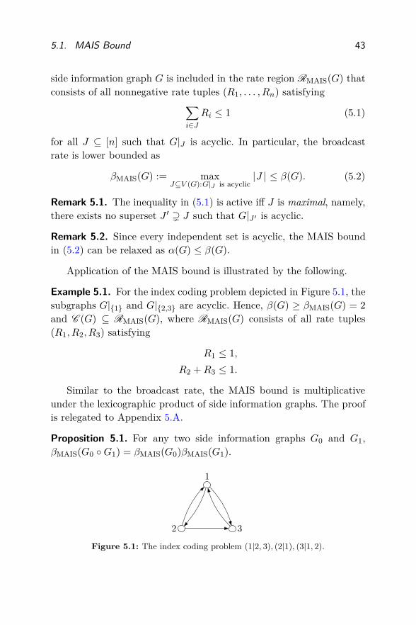
Application of the MAIS bound is illustrated by the following.
Example 5.1. For the index coding problem depicted in Figure 5.1, thesubgraphs G|1 and G|2,3 are acyclic. Hence, β(G) ≥ βMAIS(G) = 2and C (G) ⊆ RMAIS(G), where RMAIS(G) consists of all rate tuples(R1, R2, R3) satisfying
R1 ≤ 1,
R2 +R3 ≤ 1.
Similar to the broadcast rate, the MAIS bound is multiplicativeunder the lexicographic product of side information graphs. The proofis relegated to Appendix 5.A.
Proposition 5.1. For any two side information graphs G0 and G1,βMAIS(G0 G1) = βMAIS(G0)βMAIS(G1).
1
2 3
Figure 5.1: The index coding problem (1|2, 3), (2|1), (3|1, 2).
44 Performance Limits
The MAIS bound is not tight in general (see Example 5.2 in thenext section). Using Corollary 4.2 and Proposition 5.1, we can showthat the gap between the MAIS bound and the broadcast rate of theindex coding problem can be magnified to a multiplicative factor thatgrows polynomially in the number of messages of the problem.
Proposition 5.2. Let G0 be the side information graph of an indexcoding problem with n0 messages for which β(G0)/βMAIS(G0) = ρ > 1,and let G = Gk
0 with n = nk0 vertices. Then
β(G)βMAIS(G)
=(β(G0))k
(βMAIS(G0))k= ρk = nlogn0
(ρ).
5.2 Polymatroidal Bound
Let (R1, . . . , Rn) be an achievable rate tuple for the index coding prob-lem (i|Ai), i ∈ [n]. Then, there exists a (t1, . . . , tn, r) index code withencoding function φ and decoding functions ψi, i ∈ [n], such that
Ri ≤tir.
Let Xi be the uniform random variable over 0, 1ti that representsmessage i. Then,
H(Xi) = ti, i ∈ [n].
Moreover, by the independence of the random variables X1, . . . ,Xn,
H(X1, . . . ,Xn) =n∑
i=1
H(Xi).
Let Y = φ(X1, . . . ,Xn) be the random variable over 0, 1r that rep-resents the encoder output. Then,
H(Y ) ≤ r
and
H(Y |X1, . . . ,Xn) = 0.

5.2. Polymatroidal Bound 45
Since receiver i can recover its desired message based on the receivedcodeword and its side information, we also have the following decod-ability conditions
H(Xi |Y,X(Ai),X(Ci)) = H(Xi |Y,X(Ai)) = 0, i ∈ [n], (5.3)
for every Ci ⊆ Bi = [n] \ (Ai ∪ i). Now consider
Ri ≤tir
=1rH(Xi)
=1r
[H(Xi)−H(Xi |Y,X(Ai))]
=1r
[H(Xi |X(Ai))−H(Xi |Y,X(Ai))]
=1rI(Xi;Y |X(Ai))
=1r
[H(Y |X(Ai))−H(Y |Xi,X(Ai))]
≤ 1H(Y )
[H(Y |X(Ai))−H(Y |Xi,X(Ai))]. (5.4)
Define a set function f : 2[n] → [0, 1] as
f(J) =H(Y |X(J))
H(Y ), J ⊆ [n], (5.5)
where J = [n] \ J . Then (5.4) can be rewritten as
Ri ≤ f(Bi ∪ i) − f(Bi), i ∈ [n].
In the following, we explore a few properties of the set function f
defined in (5.5). First,
f(∅) =H(Y |X([n]))
H(Y )= 0 (5.6)
and
f([n]) =H(Y )
H(Y )= 1. (5.7)

46 Performance Limits
Second, since conditioning reduces entropy, for any k /∈ J ⊆ [n],
f(J) = H(Y |X(J))
≤ H(Y |X(J \ k))= f(J ∪ k). (5.8)
Third, for any J,K ⊆ [n],
H(Y )(f(J ∪K)− f(J))
= H(Y |X(J ∩K))−H(Y |X(J))
= I(Y ;X(J \K)|X(J ∩K))
= H(X(J \K)|X(J ∩K))−H(X(J \K)|Y,X(J ∩K))
= H(X(J \K)|X(K))−H(X(J \K)|Y,X(J ∩K))
≤ H(X(J \K)|X(K))−H(X(J \K)|Y,X(K))
= I(Y ;X(J \K)|X(K))
= H(Y |X(K)) −H(Y |X(J ∪K))
= H(Y )(f(K)− f(J ∩K)),
or equivalently,
f(J ∪K) + f(J ∩K) ≤ f(J) + f(K), (5.9)
which shows that f is also submodular [126, 71]. The submodularitycan be equivalently expressed as
f(J) + f(J ∪ i ∪ k) ≤ f(J ∪ i) + f(J ∪ k), (5.10)
for every J ⊆ [n] and distinct i, k /∈ J [126, Theorem 44.1]. Fourth, bythe decodability conditions (5.3) and the independence of X1, . . . ,Xn,
H(Y )(f(Bi ∪ i) − f(Bi))
= H(Y |X(Ai))−H(Y |Xi,X(Ai))
= I(Xi;Y |X(Ai))
= I(Xi;Y |X(Ai),X(Bi \ Ci))
= H(Y |X(Ai),X(Bi \ Ci))−H(Y |Xi,X(Ai),X(Bi \ Ci))
= H(Y )(f(Ci ∪ i) − f(Ci)) (5.11)
5.2. Polymatroidal Bound 47
for every Ci ⊆ Bi. By the submodularity in (5.9), we have
f(Bi ∪ i) − f(Bi) ≤ f(Ci ∪ i)− f(Ci) ≤ f(i), Ci ⊆ Bi.
Hence, the condition in (5.11) can be expressed succinctly as
f(Bi ∪ i) − f(Bi) = f(i). (5.12)
In summary, if the rate tuple (R1, . . . , Rn) is achievable, then Ri ≤f(Bi ∪ i) − f(Bi), i ∈ [n], for some submodular nondecreasing setfunction f satisfying (5.6)–(5.12). This yields an outer bound on thecapacity region (a lower bound on the broadcast rate) referred to as thepolymatroidal bound. The name follows the polymatroidal axioms usedin its expression, but the corresponding rate region is not a polymatroidin general. This bound has been introduced in [160], [55], and [28] inthe context of distributed source coding, network coding, and indexcoding, respectively.
Theorem 5.2 (Polymatroidal bound). The capacity region C (G) of theindex coding problem (i|Ai), i ∈ [n], with side information graph G
is included in RPM(G) that consists of all rate tuples (R1, . . . , Rn)
satisfying
Ri ≤ f(Bi ∪ i) − f(Bi), i ∈ [n], (5.13a)
for some set function f : 2[n] → [0, 1] such that
f(∅) = 0, (5.13b)
f([n]) = 1, (5.13c)
f(J) ≤ f(J ∪ k), k /∈ J ⊆ [n], (5.13d)
f(J) + f(J ∪ i ∪ k) ≤ f(J ∪ i) + f(J ∪ k),i, k /∈ J ⊆ [n], (5.13e)
f(i) = f(Bi ∪ i) − f(Bi), i ∈ [n]. (5.13f)
Remark 5.3. Given an index coding problem, the polymatroidal boundRPM is computed by eliminating the f variables from (5.13a)–(5.13f)through Fourier–Motzkin elimination [60, Appendix D]. A looser boundcan be computed in lower complexity by solving multiple linear pro-grams corresponding to different weighted sums of R1, . . . , Rn, for ex-ample, all linear combinations with 0–1 coefficients.

48 Performance Limits
Corollary 5.1. For any index coding problem G, the broadcast rate islower bounded as
βPM(G) := minf
maxi∈[n]
1
f(Bi ∪ i)− f(Bi)≤ β(G),
where the minimum is over all set functions f satisfying (5.13b)–(5.13f).
Remark 5.4. The quantity 1/βPM(G) is the solution to the followinglinear program with 2n + 1 variables:
maximize R
subject to R ≤ f(Bi ∪ i) − f(Bi), i ∈ [n],
f satisfies (5.13b)− (5.13f).
The last inequality (5.13f) in the polymatroidal bound is rathertechnical, but it is not known if it is inactive and can be removed toresult in the same bound.
Open Problem 5.1. Find the minimal set of inequalities from (5.13)to characterize the polymatroidal bound in general.
The polymatroidal bound is tighter than the MAIS bound.
Proposition 5.3. For any index coding problem G,
RPM(G) ⊆ RMAIS(G)
and consequently βMAIS(G) ≤ βPM(G).
The proof is presented in Appendix 5.B. The inclusion in Proposi-tion 5.3 can be strict as illustrated by the following.
Example 5.2. For the index coding problem depicted in Figure 5.2, wehave βMAIS = 2 and the MAIS outer bound is characterized by
R1 +R3 ≤ 1, R1 +R4 ≤ 1, R2 +R4 ≤ 1,
R2 +R5 ≤ 1, R3 +R5 ≤ 1.(5.14)
However, it can be shown that the polymatroidal bound yields thetighter bound βPM = 5/2 on the broadcast rate and the polymatroidalouter bound RPM is characterized by
R1 +R2 +R3 +R4 +R5 ≤ 2 (5.15)

5.2. Polymatroidal Bound 49
1
2
34
5
Figure 5.2: The index coding problem (1|2, 5), (2|1, 3), (3|2, 4), (4|3, 5), (5|1, 4).
in addition to the five inequalities in (5.14). In Section 6.3, we will seethat for this example, the polymatroidal bound is tight, i.e., β = 5/2
and the capacity region C is characterized by (5.14) and (5.15).
Example 5.3. For the index coding problem depicted in Figure 5.3, theMAIS outer bound is characterized by
R1 +R3 ≤ 1, R1 +R4 ≤ 1, R2 +R4 ≤ 1,
R2 +R5 ≤ 1, R3 +R4 ≤ 1, R3 +R5 ≤ 1,
while the polymatroidal outer bound has the additional inequality
R1 +R2 +R3 +R4 +R5 ≤ 2.
Again the capacity region can be shown to coincide with the polyma-troidal outer bound.
1
2
34
5
Figure 5.3: The index coding problem (1|2, 4, 5), (2|1, 3), (3|1, 2), (4|3, 5), (5|1, 4).
Blasiak, Kleinberg, and Lubetzky [28] showed that the polyma-troidal bound satisfies the following structural property under the lex-icographic product (cf. Corollary 4.2 and Proposition 5.1).

50 Performance Limits
Proposition 5.4. For any pair of side information graphs G0 and G1,
βPM(G0 G1) ≥ βPM(G0)βPM(G1).
Open Problem 5.2. Does the inequality in Proposition 5.4 hold withequality?
Example 5.2 shows that there is a gap between the polymatroidalbound and the MAIS bound. Using Propositions 5.1 and 5.4, this gapcan be magnified to a multiplicative factor that grows polynomially inthe number of messages of the problem, which also implies Proposi-tion 5.2 indirectly.
Proposition 5.5 ([28]). Let G0 be the side information graph of an n0-message index coding problem for which βPM(G0)/βMAIS(G0) = ρ > 1
and let G = Gk0 with n = nk
0 vertices. Then
βPM(G)
βMAIS(G)≥ (βPM(G0))k
(βMAIS(G0))k= ρk = nlogn0
(ρ).
5.3 Information Inequalities and Index Coding
For any joint distribution for the collection of n random variablesX1, . . . ,Xn, (2n − 1) entropies H(X(J)), ∅ 6= J ⊆ [n], satisfy
H(X(J ∪K ∪ L))−H(X(K ∪ L))
≤ H(X(J ∪K))−H(X(K)), J,K,L ⊆ [n], (5.16a)
or equivalently,
I(X(J);X(L)|X(K)) ≥ 0. (5.16b)
Any convex combination of these linear inequalities is a valid linearinequality on H(X(J)), J ⊆ [n], and is referred to as a Shannon-
type inequality. Surprisingly, there are some linear inequalities on theentropies that cannot be written as such convex combinations. Theseinequalities are referred to as non-Shannon-type inequalities, includingthe following example discovered by Zhang and Yeung [165]:
3H(X1,X3) + 3H(X1,X4) + 3H(X3,X4) +H(X2,X3) +H(X2,X4)
≥ 2H(X3) + 2H(X4) +H(X1,X2) +H(X1)
+H(X2,X3,X4) + 4H(X1,X3,X4). (5.17)
5.3. Information Inequalities and Index Coding 51
Matúš [107] showed that even for only four random variables, there areinfinitely many independent non-Shannon-type information inequali-ties.
Let (R1, . . . , Rn) be an achievable rate tuple for the index codinginstance (i|Ai), i ∈ [n]. Then, there exists a (t1, . . . , tn, r) index codewith encoding function φ and decoding functions ψi, i ∈ [n], such that
Ri ≤tir. (5.18)
As discussed in the previous section, a given (t1, . . . , tn, r) index code in-duces n+1 random variables Xi, i ∈ [n], and X0 = Y = φ(X1, . . . ,Xn).One can form an outer bound on the capacity region (a lower boundon the broadcast rate) of the index coding problem by considering allShannon-type inequalities that hold for (2n+1 − 1) entropies of thesen+ 1 random variables.
Define a set function h : 20∪[n] → R≥0 as
h(J) = H(X(J)), J ⊆ 0 ∪ [n]. (5.19)
Noting that H(Xi) = ti, i ∈ [n], and H(X0) ≤ r, we can rewrite (5.18)as
Ri ≤h(i)h(0) , i ∈ [n].
The independence of the random variables X1, . . . ,Xn can be expressedas
h([n]) = H(X1, . . . ,Xn) =n∑
i=1
H(Xi) =n∑
i=1
h(i). (5.20)
Since X0 = φ(X1, . . . ,Xn), we have H(X0|X1, . . . ,Xn) = 0, or equiva-lently,
h(0 ∪ [n]) = h([n]). (5.21)
The decodability condition at each receiver i ∈ [n] can be expressed asH(Xi|Y,X(Ai)) = 0, or equivalently,
h(0 ∪ i ∪Ai) = h(0 ∪Ai), i ∈ [n]. (5.22)
The conditions in (5.20)–(5.22) embody the problem formulation of in-dex coding. In addition, any entropy function satisfies (5.16), namely,

52 Performance Limits
it is nonnegative (which is already specified in the range of the h func-tion), monotonic, i.e.,
h(J) ≤ h(J ∪ k), k /∈ J ⊆ 0 ∪ [n], (5.23)
and submodular [126, Theorem 44.1], i.e.,
h(J) + h(J ∪ i ∪ k) ≤ h(J ∪ i) + h(J ∪ k)for every distinct i, k /∈ J ⊆ 0 ∪ [n]. Summarizing these conditionsyields the following outer bound on the capacity region and lower boundon the broadcast rate based on Shannon-type inequalities.
Theorem 5.3. The capacity region C (G) of the index coding problem(i|Ai), i ∈ [n], with side information graph G is included in RSh(G)
that consists of all rate tuples (R1, . . . , Rn) satisfying
Ri ≤h(i)h(0) , i ∈ [n], (5.24a)
for some set function h : 20∪[n] → R≥0 such that
h(∅) = 0, (5.24b)
h([n]) =n∑
i=1
h(i), (5.24c)
h(0 ∪ [n]) = h([n]), (5.24d)
h(0 ∪ i ∪Ai) = h(0 ∪Ai), i ∈ [n], (5.24e)
h(J) ≤ h(J ∪ k), k /∈ J ⊆ 0 ∪ [n], (5.24f)
h(J) + h(J ∪ i ∪ k) ≤ h(J ∪ i) + h(J ∪ k),i, k /∈ J ⊆ 0 ∪ [n]. (5.24g)
Remark 5.5. Under (5.24g), (5.24c) is equivalent to the more generalcondition
h(J) =∑
i∈J
h(i), J ⊆ [n]. (5.24h)
Similarly, under (5.24g), (5.24e) is equivalent to
h(0 ∪ i ∪ Ci) = h(0 ∪ Ci), Ai ⊆ Ci ⊆ [n], (5.24i)
which implies that
h(0 ∪ [n]) = h(0 ∪ ([n] \ i)), i ∈ [n]. (5.24j)

5.3. Information Inequalities and Index Coding 53
Remark 5.6. As in Remark 5.3, the outer bound RSh can be computedby Fourier–Motzkin elimination or linear programs.
Remark 5.7. For any index coding problem G, the broadcast rate islower bounded as
βSh(G) := minh
maxi∈[n]
h(0)h(i) ≤ β(G),
where the minimum is over all set functions h satisfying (5.24b)–(5.24g).Its reciprocal 1/βSh(G) is the solution to the corresponding linear pro-gram involving 2n+1 + 1 variables.
In establishing the polymatroidal outer bound RPM in Theorem 5.2,we did not explicitly use all Shannon-type inequalities. Nonetheless,RPM is as tight as the apparently stronger bound RSh, as will be verifiedin Appendix 5.C.
Proposition 5.6. RSh = RPM.
The polymatroidal bound (which, by Proposition 5.6, effectivelyuses all Shannon-type inequalities) is not tight in general and can beimproved by considering non-Shannon-type inequalities, as illustratedby the following examples.
Example 5.4. Sun and Jafar [141] showed that for the index codingproblem
(1|2, 3, 6, 7, 8, 9, 10, 11), (2|1, 3, 4, 6, 7, 8, 9, 10, 11),
(3|1, 2, 4, 5, 6, 7, 8, 9, 10, 11), (4|1, 2, 3, 5, 6, 7, 8, 9, 10, 11),
(5|1, 3, 4, 6, 7, 8, 9, 10, 11), (6|1, 4, 5, 7, 8, 9, 10, 11),
(7|2, 4, 5, 6, 8, 9, 10, 11), (8|1, 3, 5, 6, 7, 9, 10, 11),
(9|1, 2, 5, 6, 7, 8, 10, 11), (10|1, 2, 4, 6, 7, 8, 9, 11),
(11|1, 2, 3, 5, 7, 8, 9, 10),
βPM = 2.5, whereas using the Zhang–Yeung non-Shannon-type infor-mation inequality in (5.17) yields a tighter outer bound of 28/11 ≃2.5455.

54 Performance Limits
Example 5.5. Baber et al. [17] showed that for the index coding prob-lem
(1|2, 3, 4, 5, 6, 7), (2|1, 3, 7, 9, 10), (3|1, 2, 4, 8, 9),
(4|1, 3, 5, 8, 10), (5|1, 4, 6, 9, 10), (6|1, 5, 7, 8, 9),
(7|1, 2, 6, 8, 10), (8|3, 4, 6, 7, 9, 10), (9|2, 3, 5, 6, 8),
(10|2, 4, 5, 7, 8).
which has an undirected side information graph, the polymatroidalbound is βPM = 56/17 ≃ 3.2941, whereas using the Zhang–Yeunginequality (5.17) yields the lower bound of 598/181 ≃ 3.3038 and us-ing the 214 non-Shannon-type information inequalities established byDougherty, Freiling, and Zeger [56] yields an even tighter lower boundof 29523/8929 ≃ 3.3064 on the broadcast rate. Note that in [17], thisexample is discussed in the context of guessing games [122]. We con-verted it here to the corresponding index coding problem; see Section 11for the exact relationship between index coding and guessing games.
Any tuple of (2n+1 − 1) entropies H(X(J)), ∅ 6= J ⊆ 0 ∪ [n]
satisfies all Shannon and non-Shannon inequalities. These inequalitiesform the set of entropic vectors Γ∗
n+1 [159, Chapter 13]. As a point in
R2n+1−1≥0 , each entropic vector can be realized by some tuple of (n + 1)
random variables, potentially beyond (X0,X1, . . . ,Xn) induced by allindex codes. The closure Γ
∗n+1 of the set of entropic vectors is a (closed)
convex cone.The tightest outer bound on the capacity region of a general index
coding problem can be established by augmenting the monotonicityand submodularity conditions (5.24f) and (5.24g) in Theorem 5.3 bythe all-encompassing condition that the h function is entropic. Everyouter bound we have encountered thus far (including Examples 5.4and 5.5) is some relaxation of this outer bound. As a matter of fact,this outer bound coincides with the capacity region, as shown in ourthird (cf. Theorems 3.1 and 3.2) noncomputable characterization of theindex coding capacity region via entropic vectors.
Theorem 5.4. The capacity region C (G) of the index coding problem(i|Ai), i ∈ [n], with side information graph G consists of all rate tuples

5.3. Information Inequalities and Index Coding 55
(R1, . . . , Rn) satisfying
Ri ≤h(i)h(0) , i ∈ [n], (5.25a)
for some set function h : 20∪[n] → R≥0 such that
h(∅) = 0, (5.25b)
h([n]) =n∑
i=1
h(i), (5.25c)
h(0 ∪ [n]) = h([n]), (5.25d)
h(0 ∪ i ∪Ai) = h(0 ∪Ai), i ∈ [n], (5.25e)
(h(0), h(1), . . . , h(0 ∪ [n])) ∈ Γ∗n+1. (5.25f)
Indeed, by (5.24e), the rate bounds in Theorem 5.3 can be rewrittenas
Ri ≤h(i) + h(0 ∪Ai)− h(0 ∪Ai ∪ i)
h(0) , i ∈ [n],
the numerator of which can be expressed as I(Ui;V |U(Ai)) and thedenominator of which can be expressed as H(V ) for some tuple of(n + 1) random variables U1, . . . , Un, and V such that U1, . . . , Un areindependent (cf. (5.24c) and (5.25c)), H(V |U1, . . . , Un) = 0 (cf. (5.24d)and (5.25d)), and H(Ui|V,U(Ai)) = 0, i ∈ [n] (cf. (5.24e) and (5.25e)).As shown by Theorem 3.2 and Remark 3.2, any rate tuple satisfyingthese conditions is achievable — even without explicitly specifying thedecodability condition in (5.24e) and (5.25e)!
In light of Theorem 5.4, the set of entropic vectors Γ∗n+1 plays a
rather fundamental role in characterizing the capacity region, as illus-trated by Chan and Grant [40] for the general multisource networkcoding. Therefore, many fundamental questions on the capacity regionof a general index coding problem can be translated to those on theentropic vectors.
Open Problem 5.3. Is there an n-message index coding problem forwhich the characterization of the capacity region in Theorem 5.4 in-volves infinitely many non-Shannon-type inequalities?

56 Performance Limits
If the answer to this question is positive, then the correspondingindex coding capacity region is not a polyhedron. Nonetheless, thiscapacity region could be computable in the usual sense.
Open Problem 5.4. Is there a computable procedure to enumerate allextremal inequalities in Γ
∗n+1?
If the answer to this question is positive, then it also solves thecomputability question of the broadcast rate in Open Problem 3.2. Byadding more and more such extremal inequalities and computing thecorresponding lower bound on the broadcast rate, we can approach thebroadcast rate from below.
Shannon-type inequalities form an important first step in that pro-cedure. It remains open to determine how loose the corresponding poly-matroidal bound can be.
Open Problem 5.5. Is there a sequence of n-message index codingproblems Gn for which β(Gn)/βPM(Gn) ≥ nǫ for some ǫ > 0?
If the inequality in Proposition 5.4 holds with equality (see OpenProblem 5.2), then as in Proposition 5.2, the gap between the broadcastrate and the polymatroidal bound (or equivalently, the gap betweenShannon-type and non-Shannon-type inequalities) can be magnified toa polynomial multiplicative factor.
5.A Proof of Proposition 5.1
Let G = G0 G1. We establish the desired identity by proving inequal-ities in both directions.
Proof of “≥”. Suppose that V0 and V1 induce maximum acyclicsubgraphs of G0 and G1, respectively, i.e., βMAIS(Gi) = |Vi|, i = 0, 1.By the definition of lexicographic product, V0 × V1 induces an acyclicsubgraph of G, which implies that βMAIS(G) ≥ βMAIS(G0)βMAIS(G1).
Proof of “≤”. Let V ∗ ⊆ V (G0)×V (G1) be a maximum set such thatG|V ∗ is acyclic, i.e., βMAIS(G) = |V ∗|. Assume without loss of generalitythat V (G0) = [m]. Then, V ∗ can be partitioned as V ∗ = V1 ∪ · · · ∪ Vm,where Vi induces an acyclic subgraph of the i-th copy of G1 in the

5.B. Proof of Proposition 5.3 57
lexicographic product G, and thus
|Vi | ≤ βMAIS(G1), i ∈ [m].
Let J = i : Vi 6= ∅. Since G|V ∗ is acyclic, J induces an acyclic sub-graph of G0 and thus
|J | ≤ βMAIS(G0).
Hence, we have
βMAIS(G) =∑
i∈J
|Vi |
≤∑
i∈J
βMAIS(G1)
≤ βMAIS(G0)βMAIS(G1).
This completes the proof of the proposition.
5.B Proof of Proposition 5.3
We show that every inequality of the MAIS bound can be derived usingthe inequalities of the polymatroidal bound, i.e., (5.13a)–(5.13f). Firstnote that by the submodularity of the set function f in (5.13e),
f(i ∪K)− f(K) ≤ f(i ∪ J)− f(J), J ⊆ K ⊆ [n], (5.26)
for any i /∈ K. Suppose that J ⊆ V (G) induces an acyclic subgraph ofG. Assume without loss of generality that J = [m] and that j ∈ Bi forevery i < j ∈ [m]. Let Ji = i + 1, . . . ,m. Then, by the assumption,Ji ⊆ Bi. Now we have
∑
i∈J
Ri ≤m∑
i=1
(
f(i ∪Bi)− f(Bi))
(5.27)
≤m∑
i=1
(
f(i ∪ Ji)− f(Ji))
(5.28)
= f(1 ∪ J1)− f(Jm) (5.29)
≤ 1, (5.30)

58 Performance Limits
where (5.27) follows by (5.13a) and (5.28) follows by (5.26). Further-more, (5.29) holds by telescoping since Ji = i + 1 ∪ Ji+1. Finally,(5.30) follows by (5.13b), since Jm = ∅. This completes the proof of theproposition.
5.C Proof of Proposition 5.6
We first verify that RSh ⊆ RPM. Suppose that (R1, . . . , Rn) ∈ RSh.Then there exists a set function h(J), J ⊆ 0∪ [n], satisfying (5.24b)–(5.24g) such that
Ri ≤h(i)h(0) , i ∈ [n]. (5.31)
Define a set function f : 2[n] → [0, 1] as
f(J) =h(J ∪ 0) − h(J)
h(0) , (5.32)
where J = [n] \ J for J ⊆ [n]. Then (5.31) can be rewritten as
Ri ≤h(i)h(0)
=h(Ai ∪ i)− h(Ai)
h(0) (5.33)
=h(Ai ∪ 0)− h(Ai)
h(0) − h(Ai ∪ i ∪ 0) − h(Ai ∪ i)h(0) (5.34)
= f(i ∪Bi)− f(Bi), (5.35)
where (5.33) follows by (5.24h), (5.34) follows by (5.24e), and (5.35)follows by the definition of f in (5.32). We now show that the setfunction f defined in (5.32) satisfies (5.13b)–(5.13f) one by one. First,by (5.24d),
f(∅) =h([n] ∪ 0) − h([n])
h(0) = 0
and by (5.24b),
f([n]) =h(0) − h(∅)
h(0) = 1.
5.C. Proof of Proposition 5.6 59
Next, for k /∈ J ⊆ [n] and K = J ∪ k,
f(J) =h(J ∪ 0) − h(J)
h(0)
=h(K ∪ k ∪ 0) − h(K)− h(k)
h(0) (5.36)
≤ h(K ∪ 0) + h(k) − h(K)− h(k)h(0) (5.37)
=h(K ∪ 0) − h(K)
h(0)= f(K),
where (5.36) follows by (5.24h) since J = K ∪ k, and (5.37) followsby (5.24g). Next, for i, k /∈ J ⊆ [n] and K = J \ i, k ⊆ [n],
h(0)(f(J ∪ i ∪ k) + f(J))
= h(K ∪ 0) − h(K) + h(J ∪ 0) − h(J)
= h(K ∪ 0) − h(K)
+ h(K ∪ i ∪ k ∪ 0) − h(K)− h(i) − h(k) (5.38)
≤ h(K ∪ k ∪ 0) − h(K)− h(k)+ h(K ∪ i ∪ 0) − h(K)− h(i) (5.39)
= h(K ∪ k ∪ 0) − h(K ∪ k)+ h(K ∪ i ∪ 0) − h(K ∪ i) (5.40)
= h(0)(f(J ∪ i) + f(J ∪ k)),where (5.38) and (5.40) follow by (5.24h), and (5.39) follows by (5.24g).Finally, for i ∈ [n],
h(0)(f(Bi ∪ i) − f(Bi))
= h(Ai ∪ 0) − h(Ai)− h(Ai ∪ i ∪ 0) + h(Ai ∪ i)= h(Ai ∪ i) − h(Ai) (5.41)
= h(i) (5.42)
= h([n]) − h([n] \ i) (5.43)
= h(([n] \ i) ∪ 0) − h([n] \ i) (5.44)
= h(0)f(i),

60 Performance Limits
where (5.41) follows by (5.24e), (5.42) and (5.43) follow by (5.24h), and(5.44) follows by (5.24j).
We now move on to show RPM ⊆ RSh. Suppose that (R1, . . . , Rn) ∈RPM. Then there exists a set function f(J), J ⊆ [n], satisfying (5.13b)–(5.13f) such that
Ri ≤ f(Bi ∪ i) − f(Bi) = f(i). (5.45)
Define a set function h : 20∪[n] → R≥0 as
h(∅) = 0, (5.46a)
h(i) =f(i)
∑ni=1 f(i) , i ∈ [n], (5.46b)
h(J) =∑
i∈J
h(i), J ⊆ [n], (5.46c)
h(J ∪ 0) = h(J) +f(J)
∑ni=1 f(i) , J ⊆ [n]. (5.46d)
By definition,
h(0) =1
∑ni=1 f(i)
and (5.45) can be rewritten as
Ri ≤h(i)h(0) , i ∈ [n].
We now show that the set function h defined in (5.46a)–(5.46d) satisfies(5.24b)–(5.24g). The first three conditions follow by the definition of hin (5.46a), (5.46c), and (5.46d), respectively. Next, for i ∈ [n],
h(i ∪Ai ∪ 0) = h(i ∪Ai) +f(Bi)
∑nk=1 f(k)
= h(i ∪Ai) +f(Bi ∪ i) − f(i)
∑nk=1 f(k) (5.47)
= h(Ai) + h(i) +f(Bi ∪ i)− f(i
∑nk=1 f(k)
(5.48)
= h(Ai) +f(Bi ∪ i)∑n
k=1 f(k)(5.49)
= h(Ai ∪ 0),

5.C. Proof of Proposition 5.6 61
where (5.47) follows by (5.13f), (5.48) follows by (5.46c), and (5.49)follows by (5.46b).
Next, for (5.24f), we consider the following cases:
• If k = 0 and J ⊆ [n], then
h(J) ≤ h(J) +f(J)
∑ni=1 f(i)
= h(J ∪ 0)= h(J ∪ k).
• If 0 6= k /∈ J ⊆ [n], then
h(J) =∑
j∈J
h(j)
≤∑
j∈J∪k
h(j)
= h(J ∪ k).
• Otherwise, k 6= 0 ∈ J and for some K ⊆ [n],
h(J) = h(K ∪ 0)
= h(K) +f(K)
∑ni=1 f(i)
= h(K ∪ k) − h(k) +f(K)
∑ni=1 f(i) (5.50)
= h(K ∪ k) +f(K)− f(k)∑n
i=1 f(i)
≤ h(K ∪ k) +f(K \ k)∑n
i=1 f(i) (5.51)
= h(K ∪ k ∪ 0)= h(J ∪ k),
where (5.50) follows by (5.24h), and (5.51) follows by the sub-modularity of f in (5.13e).
Hence, property (5.24f) holds.

62 Performance Limits
Finally, in order to show that the set function h defined in (5.46)satisfies (5.24g), we consider the following cases:
• If 0 /∈ J and i, k 6= 0, then (5.24g) holds with equality by (5.46c).
• If 0 /∈ J , i = 0, and k 6= 0, then
(
h(J) + h(J ∪ i ∪ k))( n∑
j=1
f(j))
=∑
j∈J
f(j) +∑
j∈J
f(j) + f(k) + f(J \ k)
≤∑
j∈J
f(j) +∑
j∈J
f(j) + f(k) + f(J) (5.52)
=(
h(J ∪ i) + h(J ∪ k)( n∑
j=1
f(j)
)
,
where (5.52) follows by the monotonicity of f in (5.13d).
• Otherwise (0 ∈ J and i, k 6= 0), J = K ∪ 0 for some K ⊆ [n]
and
(
h(J) + h(J ∪ i ∪ k))( n∑
j=1
f(j))
=∑
j∈K
f(j) + f(K) +∑
j∈K∪i,k
f(j) + f(K \ i, k)
≤∑
j∈K∪i
f(j) + f(K \ i) +∑
j∈K∪k
f(j) + f(K \ k)
(5.53)
=(
h(J ∪ i) + h(J ∪ k))( n∑
j=1
f(j))
,
where (5.53) follows by (5.13e).
This completes the proof of the proposition.

6
Coding Schemes
In this section, we review some of the most interesting index codingschemes, summarized in Figure 6.1. Each coding scheme correspondsto an upper bound on the broadcast rate. Some schemes can handleasymmetric rate tuples and yield inner bounds on the capacity region.
6.1 MDS Codes
Consider the index coding problem with 3 messages represented bythe side information graph shown in Figure 6.2, in which every re-ceiver has one piece of side information. Consider a systematic (5, 3)
code (x1, x2, x3, p1, p2) over the finite field F4 = 0, 1, α, α + 1, wherep1 = x1 + x2 + x3 and p2 = x1 + αx2 + (α + 1)x3. This code has themaximum distance separable (MDS) property, which guarantees thatany three out of the five code symbols are sufficient to recover all threemessage symbols. We now employ this code for the 3-message indexcoding problem and transmit the parity symbols p1 and p2. Then, ev-ery receiver has three code symbols (including its side information)and by the MDS property, can successfully recover its desired message(along with two other messages).
63

64 Coding Schemes
MDS codes
(Proposition 6.1)
Clique covering
(Proposition 6.2)
Fractional clique
covering (Prop. 6.3)
Frac. local clique
covering (Prop. 6.4)
Fractional local partial clique covering
(Theorem 6.1)
Flat coding
(Proposition 6.10)
Cycle covering
(Remark 6.5)
Partial clique
covering (Rem. 6.4)
Composite coding
(Proposition 6.11)
Enhanced composite
coding (Thm. 6.4)
Recursive coding
(Theorem 6.2)
General vector
linear codes
General nonlinear codes
Figure 6.1: Summary of the coding schemes. Here a directed edge from scheme A toscheme B indicates that scheme A can be viewed as a special case of scheme B, thatis, the upper bound on the broadcast rate achieved by scheme A is also achievableby scheme B. The schemes in solid-lined boxes are linear (single line for scalar anddouble line for vector linear coding). The schemes in dashed-lined boxes are nonlin-ear. For the schemes in shaded boxes, corresponding inner bounds on the capacityregion are presented in addition to upper bounds on the broadcast rate. Interferencealignment (Section 6.8) is not included here since it is not applicable concretely toall index coding problems as a general-purpose coding scheme. Multiletter nonlinearcoding schemes based on coloring of confusion graphs and on generic random codingcan be found in Section 3.

6.2. Clique Covering 65
1
2 3
Figure 6.2: The index coding problem (1|2), (2|3), (3|1) with β = 2, which is achiev-able by a (5, 3) MDS code.
For a general index coding problem G, let
minindeg(G) := mini∈[n]|j : (j, i) ∈ E(G)| = min
i∈[n]|Ai |
be the minimum number of side information messages over all receivers.Consider a systematic (n+κ, n) MDS code with n message symbols andκ parity symbols. Then, given any n out of the n+κ code symbols, onecan recover all the messages. Such an MDS code exists over a sufficientlylarge alphabet. As every receiver has at least minindeg(G) messages asside information, if we employ the (n + κ, n) MDS code and transmitκ = κ(G) := n−minindeg(G) parity symbols, then every receiver willhave n code symbols and thus can recover all the message symbolsthat it does not have, including its desired message. This establishesthe following upper bound on the broadcast rate by Birk and Kol [25].
Proposition 6.1 (MDS bound [25]). For the n-message index codingproblem (i|Ai), i ∈ [n], with side information graph G,
β(G) ≤ βMDS(G) := κ(G) = n−minindeg(G) = n−mini∈[n]|Ai |.
Remark 6.1. If the graph G is a clique, then minindeg(G) = n− 1 andtransmitting the parity symbol x1 + · · ·+xn of an (n+ 1, n) MDS codeover F2 achieves β(G) = 1.
6.2 Clique Covering
Consider the 3-message index coding problem G shown in Figure 6.3.Since receiver 3 has no side information, minindeg(G) = 0. There-fore, using an MDS code, we need to transmit three symbols, which

66 Coding Schemes
1
2 3
Figure 6.3: The index coding problem (1|2), (2|1), (3|−) with β = 2, which isachievable by the clique covering scheme.
is no better than uncoded transmission of the messages. We can in-stead partition the vertices into two cliques, namely, 1, 2 and 3,and transmit x1 + x2 and x3. Then, receiver 3 receives its desired mes-sage x3 directly. Since receiver 1 has message x2 as side information, itcan successfully recover its desired message x1. Similarly, receiver 2 canrecover its desired message x2. This scheme requires two transmissions,which matches the MAIS bound in Theorem 5.1 and is thus optimal.
Generalizing this idea, we partition the vertices of the side infor-mation graph G by cliques and transmit the sum (parity) of all themessages in each clique. Since every receiver has all the other messagesinside its clique as side information, all the messages can be successfullyrecovered by their corresponding receivers. This coding scheme, whichcan be viewed as time division over a clique partition (one parity sym-bol per clique), achieves the following upper bound on the broadcastrate by Birk and Kol [25].
Proposition 6.2 (Clique covering bound [25]). The broadcast rate of then-message index coding problem G is upper bounded by the minimumnumber of cliques that partition G (or equivalently, the chromatic num-ber of the undirected complement of G), which is the solution βC(G)
to the integer program
minimize∑
J∈K
γJ (6.1a)
subject to∑
J∈K:i∈J
γJ ≥ 1, i ∈ [n], (6.1b)
γJ ∈ 0, 1, J ∈ K, (6.1c)
where K is the collection of all cliques in G.

6.3. Fractional Clique Covering 67
Remark 6.2. For the index coding problem depicted in Figure 6.2, us-ing an MDS code outperforms the clique covering scheme that requiresthree transmissions. Thus, the clique covering scheme and the MDScode for index coding are not comparable.
6.3 Fractional Clique Covering
We revisit the index coding problem in Example 5.2, the side informa-tion graph of which is reproduced in Figure 6.4. We can partition thegraph into three cliques, say, 1, 2, 3, 4, and 5, and thus, the cliquecovering scheme takes three transmissions. Instead, for messages rep-resented in two bits as xi = (xi1, xi2) ∈ F2
2, consider the vector linearcoding scheme that transmits x11 +x22, x21 +x32, x31 +x42, x41 +x52,and x51 +x12. Then every receiver can successfully recover its two bits.This scheme achieves the upper bound of 5/2 on the broadcast rate,which matches the polymatroidal bound in Theorem 5.2.
1
2
34
5
Figure 6.4: The index coding problem (1|2, 5), (2|1, 3), (3|2, 4), (4|3, 5), (5|1, 4) withβ = 5/2, which is achievable by the fractional clique covering scheme.
More generally, Blasiak, Kleinberg, and Lubetzky [29] extended theclique covering scheme and its achievable rate in (6.1) by time sharing
over all cliques so that the combined rate of each message over allparity symbols it participates in is at least one. The resulting rate βF
corresponds to the solution to the linear program obtained by relaxingthe integer constraints in (6.1c).
Proposition 6.3 (Fractional clique covering bound [29]). The broadcastrate of the n-message index coding problem G is upper bounded by theminimum number of cliques that fractionally partition G (or equiva-

68 Coding Schemes
lently, χf (G)), which is the solution βF(G) to the linear program
minimize∑
J∈K
γJ (6.2a)
subject to∑
J∈K:i∈J
γJ ≥ 1, i ∈ [n], (6.2b)
γJ ∈ [0, 1], J ∈ K. (6.2c)
For the index coding problem in Figure 6.4, using the vector linearcode is equivalent to setting
γ(J) =
1/2 J = 1, 2, 2, 3, 3, 4, 4, 5, 5, 1,0 otherwise,
which satisfies the constraints of (6.2) and achieves β = 5/2.
Remark 6.3. Fractional clique covering can be readily extended toasymmetric rates, which establishes the inner bound on the capacityregion that consists of all rate tuples (R1, . . . , Rn) satisfying
Ri ≤∑
J∈K:i∈J
δJ , i ∈ [n], (6.3a)
for some (δJ ∈ [0, 1], J ∈ K) such that∑
J∈K
δJ ≤ 1. (6.3b)
For the index coding problem in Figure 6.4, by eliminating the δJ
variables, the inner bound in (6.3) simplifies to the polymatroidal outerbound on the capacity region in (5.14) and (5.15).
6.4 Local Clique Covering
Consider the 6-message index coding problem G depicted in Figure 6.5.The graph G can be partitioned into three cliques 1, 2, 3, 4, and5, 6, and hence, by the clique covering scheme, it suffices to transmit
p1 = x1 + x2, p2 = x3 + x4, and p3 = x5 + x6.
However, since only two of the three parity symbols p1, p2, and p3 are

6.4. Local Clique Covering 69
1, 2
5, 6 3, 4
Figure 6.5: The index coding problem (1|2, 5, 6), (2|1, 5, 6), (3|1, 2, 4), (4|1, 2, 3),(5|3, 4, 6), (6|3, 4, 5) with β = 2, which is achievable by the local clique coveringscheme. Here each double circle represents a 2-vertex clique.
missing at each receiver, we can reduce the number of parity trans-missions by using a two-erasure correcting MDS code with two hyper-parity symbols, say, p1 + p2 = (x1 + x2) + (x3 + x4) and p1 + p3 =
(x1 +x2)+(x5 +x6). Then, each receiver can recover all parity symbolsp1, p2, p3, and thus its desired message. This upper bound of 2 on thebroadcast rate matches the MAIS bound and thus is tight.
More generally, consider a partition of the side information graph Ginto cliques. Suppose that each receiver has all the messages of at leastone clique as side information. Then each receiver can recover some par-ity symbols from its side information and the number of transmissionsfor the parity symbols can be reduced to exclude those parity symbolsavailable locally at each receiver. Based on this idea, Shanmugam, Di-makis, and Langberg [129] extended the clique covering scheme to local
clique covering by applying an MDS code to parity symbols for cliques.Combining this scheme with fractional covering yields the following.
Proposition 6.4 (Fractional local clique covering bound [129]). Thebroadcast rate of the index coding problem (i|Ai), i ∈ [n], with sideinformation graph G is upper bounded by the solution βFL(G) to thelinear program
minimize maxi∈[n]
∑
J∈K:J 6⊆Ai
γJ (6.4a)
subject to∑
J∈K:i∈J
γJ ≥ 1, i ∈ [n], (6.4b)
γJ ∈ [0, 1], J ∈ K. (6.4c)

70 Coding Schemes
This coding scheme achieves the fractional local chromatic num-
ber [65, 87] of G. The improvement over fractional clique covering iscaptured by the summation of γJ over cliques J 6⊆ Ai in (6.4a) ratherthan all cliques in (6.2a). Hence, compared to the regular time shar-ing of clique covering, local clique covering can be viewed as local time
sharing, in which the total transmission time is split only among thoseparity symbols not available locally at each receiver.
6.5 Partial Clique Covering
Birk and Kol [25] extended clique covering in Section 6.2 by partition-ing G with induced subgraphs (or partial cliques). By using an MDScode, each subgraph G|J then requires κ(G|J ) = |J | −minindeg(G|J )
transmissions. If G|J is a clique, then κ(G|J ) = 1 as in clique covering.As an example, consider the 5-message index coding problem G in
Figure 6.6. It can be shown that fractional local clique covering requiresβFL(G) = 4 transmissions. This upper bound on the broadcast rate canbe improved by time sharing over partial cliques. Since
κ(G|1,2) = κ(G|1,5) = κ(G|3) = 1,
κ(G|1,3,4) = κ(G|2,4,5) = 2,
setting
γJ =
1/2, J = 1, 2, 1, 5, 1, 3, 4, 2, 4, 5, 3,0, otherwise
achieves the upper bound of 7/2 on the broadcast rate.
1
2
34
5
Figure 6.6: The index coding problem (1|2, 4, 5), (2|1, 5), (3|1), (4|2, 3), (5|1, 4) withβFLP = 7/2 < βFL = 4.

6.5. Partial Clique Covering 71
In general, local time sharing over MDS codes of arbitrary sub-graphs (partial cliques) yields the following.
Theorem 6.1 (Fractional local partial clique covering bound [9]). Thebroadcast rate of the index coding problem (i|Ai), i ∈ [n], with sideinformation graph G is upper bounded by the solution βFLP(G) to thelinear program
minimize maxi∈[n]
∑
J⊆[n]:J 6⊆Ai
γJ · κ(G|J ) (6.5a)
subject to∑
J⊆[n]:i∈J
γJ ≥ 1, i ∈ [n], (6.5b)
γJ ∈ [0, 1], J ⊆ [n]. (6.5c)
Remark 6.4. Time division (instead of time sharing or fractional parti-tioning of G) over MDS codes of partial cliques yields the partial clique
covering bound, which is a special case of the fractional local partialclique covering that achieves the rate characterized by the correspond-ing integer program with γJ ∈ 0, 1 in place of (6.5c).
Remark 6.5. When the vertices in J ⊆ V (G) form a cycle, a simplelinear code over all but one edges in the cycle can achieve the rate ofκ(G|J ) = |J |−1. As an example, for the subgraphG|2,4,5 in Figure 6.6,it suffices to transmit x2 + x4 and x4 + x5 in F2, from which x2 + x5
can be computed. By restricting J to be cycles (or single-vertex sets)in (6.5) and saving one symbol per cycle, we recover the cycle covering
scheme [43, 114].
Remark 6.6. Fractional local partial clique covering can be readilyextended to the corresponding inner bound RFLP(G) on the capacityregion (cf. Remark 6.3) that consists of all rate tuples (R1, . . . , Rn)
satisfying
Ri ≤∑
J⊆[n]:i∈J
δJ
κ(G|J ), i ∈ [n], (6.6a)
for some δJ ∈ [0, 1], J ⊆ [n], such that∑
J⊆[n]:J 6⊆Ai
δJ ≤ 1, i ∈ [n]. (6.6b)

72 Coding Schemes
6.6 Recursive Codes
We can extend the fractional local partial clique covering scheme inSection 6.5 by performing local time sharing over subproblem solutionsrecursively.
Theorem 6.2 (Recursive coding inner bound [9]). The capacity regionof the index coding problem (i|Ai), i ∈ [n], with side information graphG includes the rate region RR(G) that is recursively defined as the setof all nonnegative rate tuples (R1, . . . , Rn) satisfying
Ri ≤∑
J([n]:i∈J
δJ TiJ , i ∈ [n], (6.7a)
for some δJ ≥ 0, J ( [n], and TiJ ≥ 0, i ∈ J ( [n], such that∑
J([n]:J 6⊆Ai
δJ ≤ 1, i ∈ [n], (6.7b)
(TiJ : i ∈ J) ∈ RR(G|J ), J ( [n], (6.7c)
where RR(G|J ) is the rate region for subproblem G|J with recursiontermination condition RR(G|i) = [0, 1]. In particular,
βR(G) = minR:(R,...,R)∈RR(G)
1
R. (6.8)
Given all the fascinating coding schemes we have discussed so farin this section and given the simplicity of recursive coding, it is per-haps anticlimactic to note that recursive codes, which can be viewed asvector linear index codes over some finite field, outperform fractionallocal partial clique covering in general (cf. Remark 6.6).
Proposition 6.5 ([9]). For any index coding problem G,
RFLP(G) ⊆ RR(G).
The proof is relegated to Appendix 6.A.
Remark 6.7. Recursive coding can be limited to symmetric rates at ev-ery step of recursion. This symmetric recursive coding scheme achieves

6.6. Recursive Codes 73
the upper bound βSR(G) on the broadcast rate, which is defined recur-sively as the solution to the linear program
minimize maxi∈[n]
∑
J([n]:J 6⊆Ai
γJ · βSR(G|J ) (6.9a)
subject to∑
J([n]:i∈J
γJ ≥ 1, i ∈ [n], (6.9b)
γJ ∈ [0, 1], J ( [n], (6.9c)
where βSR(G|J ) is the solution for subproblem G|J and βSR(G|i) = 1,i ∈ [n].
The structure of the linear program (6.9) is very similar to that forfractional local partial clique covering in (6.5), except that local timesharing over different subproblems is over symmetric recursive codesof rates βSR(G|J ) instead of MDS codes of rates κ(G|J ). By induction,βSR(G|J ) ≤ κ(G|J ) for every J ⊆ [n] (including J = [n]) and hence
βSR(G) ≤ βFLP(G).
This inequality is strict in general [9], as illustrated by the 5-messageindex coding problem in Figure 6.7.
1
2
34
5
Figure 6.7: The index coding problem (1|2, 5), (2|3, 4), (3|1, 4), (4|1, 3), (5|4) withβSR = 3 < βFLP = 7/2. Here the bounds are computed by solving the respectivelinear programs.
At the same time, recursion over asymmetric rates (Theorem 6.2) isricher than recursion over symmetric rates (Remark 6.7), and we have
βR(G) ≤ βSR(G),
the formal proof of which can be found in [9, Proposition 1]. Thisinequality is strict in general, as illustrated by the 7-message indexcoding problem in Figure 6.8.

74 Coding Schemes
1 2
3
45
67
Figure 6.8: The index coding problem (1|2, 3, 6, 7), (2|1, 3, 4, 6), (3|1, 2, 4, 5),(4|2, 3, 5, 6), (5|1, 3, 4, 7), (6|2, 4, 5, 7), (7|1, 2, 3, 5, 6) with βPM = β = βR = 5/2 <βSR = 8/3.
Remark 6.8. If the capacity region C (G|J ) is known for some or allsubproblems J ( [n], then the inner bound in Theorem 6.2 can be tight-ened by replacing RR(G|J ) with C (G|J ) in (6.7). The correspondinginner bound RLTS on the capacity region (along with the associatedupper bound βLTS on the broadcast rate) represents the rate regionachievable by local time sharing over optimal codes for subproblems.As illustrated by the 5-message index coding problem in Figure 6.9,however, local time sharing over subproblems is suboptimal in general.
1
2
34
5
Figure 6.9: The index coding problem (1|2, 5), (2|1, 4), (3|2), (4|5), (5|1, 3) with β =3 < βSR = βR = βLTS = 7/2. Here β is achieved by a scalar linear code (x1 + x2 +x5, x2 + x3, x4 + x5) over F2.
6.7 General Linear Codes
So far we have discussed scalar or vector linear codes based on decom-position of the side information graph. A general linear code, however,can utilize the global structure of the given index coding problem. Asa simple illustration, we revisit the 3-message index coding problem(1|2), (2|3), (3|1) in Figure 6.2. Consider any 3-by-3 matrix M such

6.7. General Linear Codes 75
thatMii = 1 and Mij = 0 if j /∈ Ai. (6.10)
We can easily check that the matrices
M1 =
1 1 0
0 1 1
1 0 1
and M2 =
1 0 0
0 1 0
1 0 1
satisfy (6.10).Consider the three linear combinations of the messages generated
by multiplying any such matrix M by the message vector [x1 x2 x3]T
from right. For example, M1 generates x1+x2, x2 +x3, and x1+x3, andM2 generates x1, x2, and x1 +x3. If we transmit these three generated(parity) symbols, receiver i can use the linear combination from row i
to recover xi since this linear combination contains only xi and x(Ai).Now note that M1 is of rank 2 and thus that any two of the threelinear combinations can determine the third; for example (x1 + x3) =
(x1 + x2) + (x2 + x3). Thus, it suffices to transmit the first two paritysymbols.
More generally, if M is of rank r, then we can transmit linear combi-nations of the messages from r independent rows of M . Therefore, anymatrix M satisfying (6.10) defines a scalar linear code and rank(M) isan upper bound on the broadcast rate. Conversely, each encoder of ascalar linear code can be expressed as y = [y1 · · · yr]T = E[x1 · · · xn]T
and each decoder i ∈ [n] can be expressed as a linear combination ofy and a subset of side information x(Ai). Hence, the row span of Emust include all the rows of some matrix M of the form (6.10), orequivalently, r ≥ rank(M). By optimizing over all such matrices M ,we establish the following upper bound on the linear broadcast rateλF2(G) and thus on the broadcast rate β(G).
Proposition 6.6 (Binary minrank bound [22]). For the index codingproblem (i|Ai), i ∈ [n], with side information graph G,
λF2(G) ≤ minrankF2(G) := minrank(M) : M ∈ Fn×n2 satisfies (6.10).
Remark 6.9. Peeters [121] showed that computing minrankF2(G) isNP-hard in |V (G)|. El Rouayheb, Chaudhry, and Sprintson [62] showedthat this computation problem is in fact NP-complete.

76 Coding Schemes
Remark 6.10. Haviv and Langberg [77] showed that the minrank ofa directed Erdös–Rényi random graph G(n, p) is lower bounded byΩ(√n) with high probability (w.h.p.). This bound was improved re-
cently by Golovnev, Regev, and Weinstein [73] as minrankF2(G(n, p)) =
Θ(n/ log n) w.h.p.
A scalar linear code can be similarly constructed in an arbitraryfinite field F. Consider any matrix M ∈ Fn×n that satisfies
Mii 6= 0 and Mij = 0 if j /∈ Ai. (6.11)
As in the binary case, any such matrix M induces a scalar linear codein F, and conversely any scalar linear code can be represented by one.There is no loss of generality in assuming that Mii = 1. Optimizingover all such matrices M , we have the following upper bound on thelinear broadcast rate λF(G) and on the broadcast rate β(G).
Proposition 6.7 (General minrank bound [101]). For the index codingproblem (i|Ai), i ∈ [n], with side information graph G,
λF(G) ≤ minrankF(G) := minrank(M) : M ∈ Fn×n satisfies (6.11).
The minrankF(G) of an undirected graph G was introduced byHaemers [74, 75] as an upper bound of the Shannon capacity Θ(G)
of G [134]. For any F and undirected (bidirectional) graph G,
α(G) ≤ Θ(G) ≤ minrankF(G) ≤ χ(G).
In particular, for the 5-message index coding problem in Figure 5.2,since Θ(G) =
√5 as shown in the celebrated work of Lovász [100] and
χ(G) = 3, minrankF(G) = 3 for every F (since it must be an integer).Therefore, a scalar linear code is in general insufficient and a vectorlinear code is needed.
As a further extension of a scalar linear code matrix M satisfying(6.11), Maleki, Cadambe, and Jafar [104] constructed a general vectorlinear code over F by considering a block matrix Fnt×nt consisting ofn2 submatrices Mij ∈ Ft×t, i, j ∈ [n], such that
det(Mii) 6= 0 and Mij = 0 if j 6= Ai. (6.12)

6.7. General Linear Codes 77
Once again there is no loss of generality in assuming that Mii = I,the identity matrix. For each t = 1, 2, . . . , the linear broadcast rate isupper bounded as
λF(G) ≤ λF, t(G)
:=1
tminrank(M) : M ∈ Fnt×nt satisfies (6.12). (6.13)
By subadditivity, we have the following multiletter characterization ofthe linear broadcast rate.
Theorem 6.3 (Linear broadcast rate). For the index coding problem(i|Ai), i ∈ [n], with side information graph G, the linear broadcast rateover F is
λF(G) = limt→∞
λF,t(G).
As for the broadcast rate, the upper bound in (6.13) convergesto the linear broadcast rate from above. With no known convergentsequence of bounds from below, however, the computability of the linearbroadcast rate is not known in general (cf. Open Problem 3.2).
Open Problem 6.1. Does there exist a finite, terminating algorithmthat computes the linear broadcast rate of an arbitrary n-message indexcoding problem within any desired precision?
All linear coding schemes from scalar (integral) MDS codes to vector(fractional) recursive codes discussed in Sections 6.1 through 6.6 areessentially independent of the code alphabet F. As long as MDS coding,or more generally, local time sharing, can be performed, the achievablerates of the coding schemes are invariant in F. For general linear codes,however, the minrank or linear broadcast rate depends heavily on thecode alphabet.
Most notably, Lubetzky and Stav [101] showed that there exists asequence of n-message index coding problem Gn such that
minrankF(Gn) ≤ nǫ and minrankF′(Gn) ≥ n1−ǫ
for ǫ≪ 1 and two finite fields F and F′ of distinct characteristics. Thisexample, inter alia, shows that the performance of optimal scalar linearcodes depends on the choice of the finite field in a strong sense.

78 Coding Schemes
The linear broadcast rate λF itself (achieved in general by a se-quence of vector linear codes) depends on F as well. This dependencerelies on a deep connection between the linear representation of ma-troids and network coding, which was originally explored in the seminalwork by Dougherty, Freiling, and Zeger [57]; see also [40]. This connec-tion has been adapted to index coding by El Rouayheb, Sprintson,Georghiades [61] and subsequently by Blasiak, Kleinberg, and Lubet-zky [28], who showed that there exists an index coding problem forwhich the linear broadcast rate λF is a function of F.
The alphabet dependence of linear index codes has been strength-ened and amplified to establish the insufficiency of linear codes com-pared to general nonlinear codes. For scalar linear codes, Lubetzkyand Stav [101] constructed a sequence of n-message index coding prob-lems Gn such that minrankF(Gn) ≥ √n for any F, yet β(Gn) ≤ nǫ
for ǫ ≪ 1, which separates the minrank from the broadcast rate in arather strong sense. For vector linear codes, the strongest separation re-sult by Blasiak, Kleinberg, and Lubetzky [28] considers multiple group-
cast (multiple receivers per message) and shows that there exists ann0-message problem G0 such that its lexicographic product Gn = Gk
0
with n = nk0 messages satisfies
λF(Gn)
β(Gn)≥ ρk = nlogn0
(ρ)
for some ρ > 1. This result can be translated to the regular (multiple-unicast) index coding problem using a technique by Maleki, Cadambe,and Jafar [104] that associates an arbitrary groupcast problem withsome multiple-unicast problem. Hence, linear codes are insufficient ingeneral and the optimal rates of scalar and vector linear codes are bothpolynomially separated from the broadcast rate. It is not known howmuch vector coding improves upon scalar coding.
Open Problem 6.2. Is there a sequence of n-message index codingproblems Gn such that
minrankF(Gn)
λF(Gn)≥ nǫ
for some ǫ > 0?

6.8. Linear Codes Based on Interference Alignment 79
6.8 Linear Codes Based on Interference Alignment
Motivated by interference alignment coding schemes for wireless in-terference channels [102, 34], Maleki, Cadambe, and Jafar [104], [81,Sec. IV] proposed a class of vector linear codes that can be constructedin a systematic manner. In this section, we discuss some examples todemonstrate how the interference alignment ideas can be used in de-signing such codes, as opposed to the intractable combinatorial opti-mization problem of minimizing the rank over all nt-by-nt matrices inTheorem 6.3. The general idea is to align undesired messages (interfer-ence) as much as possible while keeping the desired message separatefrom the interference.
To present the first interference alignment idea, which constructsa scalar linear code, we introduce the following notions: For distincti, j ∈ [n], we denote the alignment relation i⇔ j iff i /∈ Ak and j /∈ Ak
for some k 6= i, j. The set of messages is partitioned into alignment
subsets such that if i ⇔ j, then i and j belong to the same alignmentsubset. In particular, if i⇔ j and j ⇔ k, then i, j, and k belong to thesame alignment subset.
As an example, consider the index coding problem depicted in Fig-ure 6.10. In this example, the only alignment relation is 2 ⇔ 3 (since2, 3 /∈ A1) and G can be partitioned into alignment subsets 1, 2, 3,and 4. The alignment subset 2, 3 is the only one with more thanone member and we have 2 ∈ A3 and 3 ∈ A2. Consider three vectorsv1 = [1 0]T , v2 = [0 1]T , and v3 = [1 1]T on F2, with the property thatevery two of them are linearly independent. Transmitting x1 along v1,x2 and x3 along v2, and x4 along v3, we have
y = x1v1 + (x2 + x3)v2 + x4v3.
Receiver 1 has x4 as side information; so it can cancel the term x4v3
from the received sum. Since vectors v1 and v2 are linearly indepen-dent, receiver 1 can successfully recover x1 (as well as unnecessaryx2 + x3). Receiver 2 has x1 and x3 as side information and can cancelthe terms x1v1 and x3v2. Since vectors v2 and v3 are linearly indepen-dent, receiver 2 can successfully recover x2. Similarly, we can argue thatreceivers 3 and 4 can also recover their desired message successfully.

80 Coding Schemes
1 2
34
Figure 6.10: The index coding problem (1|4), (2|1, 3), (3|2, 4), (4|2, 3) with β = 2,which is achievable by the scalar interference alignment scheme.
In general, it suffices to transmit two linear combinations of themessages if every pair in the same alignment subset has each other asside information.
Proposition 6.8 ([81, 104]). Suppose that G can be partitioned intoalignment subsets such that for every pair (i, j) in an alignment subset,i ∈ Aj and j ∈ Ai. Then β(G) ≤ 2.
To prove this, partition the set of messages V (G) = [n] into align-ment subsets V1, . . . , Vm. Define the mapping f : [n] → [m] so thati ∈ Vf(i), i ∈ [n]. Choose the field size q sufficiently large so that thereexist m vectors v1, . . . ,vm in the two dimensional vector space over Fq
with every pair linearly independent. We transmit the messages withindices in Vj along the vector vj , j ∈ [m]. Receiver i then receives
∑
j∈[m]
xjvf(j) = xivf(i) +∑
j∈Ai
xjvf(j) +∑
j /∈i∪Ai
xjvf(j)
= xivf(i) +∑
j∈Ai
xjvf(j) +
∑
j /∈i∪Ai
xj
vl, (6.14)
where (6.14) follows since all j /∈ i∪Ai belong to the same alignmentset Vl by definition. After canceling the second term that depends solelyon side information messages, receiver i obtains a linear combinationof the two vectors vf(i) and vl. By the assumption that every pair(j, k) ∈ Vl has each other as side information, the two partitions Vf(i)
and Vl are distinct, and thus vf(i) and vl are linearly independent.Hence, xi can be successfully recovered at receiver i ∈ [n] and theupper bound of 2 on the broadcast rate is achievable.

6.8. Linear Codes Based on Interference Alignment 81
Next, we use interference alignment to design vector linear indexcodes for a class of index coding problems with symmetric neighboringside information. Let 0 ≤ d ≤ u ≤ u+ d ≤ n − 2 or (u, d) = (n − 1, 0)
(the latter of which corresponds to a complete G), and consider theindex coding problem with
Ai = i⊖ d, . . . , i⊖ 1, i⊕ 1, . . . , i⊕ u, i ∈ [n], (6.15)
where ⊕ and ⊖ denote addition and subtraction modulo n (over [n]),respectively. As an example, consider the index coding problem de-picted in Figure 6.11 with n = 6, u = 2, and d = 1. Consider 6 vectorsv1, . . . ,v6 such that any 5 of them are linearly independent. For ex-ample, v1 = [1 0 0 0 0]T , v2 = [0 1 0 0 0]T , v3 = [0 0 1 0 0]T ,v4 = [0 0 0 1 0]T , v5 = [0 0 0 0 1]T , and v6 = [1 1 1 1 1]T over F2.Decompose message xi into 2 independent messages xi0 and xi1 andtransmit xi0 along vi and xi1 along vi⊕1. Thus, receiver i receives
(x10 + x61)v1 + (x20 + x11)v2 + (x30 + x21)v3
+ (x40 + x31)v4 + (x50 + x41)v5 + (x60 + x51)v6.
By symmetry, it suffices to show that receiver 1 can successfully re-cover its desired message x1 = (x10, x11). Note that receiver 1 has sideinformation of x20, x21, x30, x31, x60, x61. Canceling the effect of thesemessages, receiver 1 obtains
x10v1 + x11v2 + (x40 + x31)v4 + (x50 + x41)v5 + x51v6,
which is a linear combination of 5 independent vectors and thus re-ceiver 1 can successfully recover its desired messages x10 and x11.
1 2
3
45
6
Figure 6.11: The index coding problem (1|2, 3, 6),(2|1, 3, 4),(3|2, 4, 5),(4|3, 5, 6),(5|1, 4, 6), (6|1, 2, 5) with symmetric neighbors (u = 2 and d = 1), for whichβPM = β = 5/2 is achievable by the vector interference alignment scheme.
82 Coding Schemes
Hence, this scheme achieves the upper bound of 5/2 on the broadcastrate, which coincides with the polymatroidal lower bound.
In general, if (u, d) = (n−1, 0), then, by the clique covering scheme,β = 1 is achievable. If u+ d = n− 2, then each message forms its ownalignment subset and, by Proposition 6.8, the upper bound of 2 on β isachievable. Otherwise (u+d ≤ n−3), let r = n−(u−d) and v1, . . . ,vn
be r-dimensional vectors over Fq, where q is sufficiently large that anyr of vi, i ∈ [n], are linearly independent. Decompose message xi intod+ 1 parts xi0, . . . , xid and transmit xij along vi⊕j . Receiver i receives
n∑
i=1
d∑
j=0
xijvi⊕j .
By symmetry, it suffices to show that receiver 1 can successfully recoverx1. Receiver 1 can cancel the effect of its side information xij for alli ∈ n− d+ 1, . . . , n, 2, 3, . . . , u+ 1 and obtain
d∑
j=0
x1jv1⊕j +n−d∑
i=u+2
d∑
j=0
xijvi⊕j .
This expression is the linear combination of r = n − (u − d) vectorsv1, . . . ,vd+1,vu+2, . . . ,vn that are linearly independent. Therefore, re-ceiver 1 can recover its desired messages x1j , j = 0, . . . , d. This provesthe following.
Proposition 6.9 ([81, 104]). For the index coding problem G with sym-metric neighboring side information sets in (6.15), the broadcast rateis upper bounded as
β(G) ≤ n− (u− d)
d+ 1.
As illustrated so far, interference alignment provides a systematicand intuitive framework to construct scalar or vector linear codes forsome index coding problems with certain structures (see [81, 104] formore examples). For a general index coding problem, however, it isunclear how the interference alignment perspective can be applicablebeyond the obvious interpretation of the minrank characterization ofthe linear broadcast rate in Theorem 6.3, in which interfering messagesare suppressed by the zero entries of the coding matrix M .

6.9. Flat Coding 83
6.9 Flat Coding
In this section and the next, we use Shannon’s random coding idea [133]to prove the existence of index codes of certain rates. Earlier in Sec-tion 3.3, we applied a simple form of random coding to achieve the en-tire capacity region. This development was not quite satisfactory, how-ever, since the capacity region was characterized in a noncomputablemultiletter expression. Here we take the conceptually simple randomcoding approach to the next level and apply it in a more concrete formas in the original proof of the network coding theorem [2]. This de-velopment leads to rather straightforward derivation of a computableinner bound on the capacity region, at the cost of lacking the actualcode construction as opposed to the coding schemes we have discussedin the preceding sections.
We first illustrate a simple random coding scheme, referred to asflat coding, through an example. Consider the index coding problem(1|2), (2|1, 3), (3|1) with side information graph depicted in Figure 6.12.We use the following random coding argument to find conditions underwhich a nonnegative rate triple (R1, R2, R3) is achievable with vanishing
error probability (see Appendix 1.A).Fix an integer r and let ti = ⌈rRi⌉, i ∈ [3]. For each message triple
(x1, x2, x3) ∈ Π3i=1[2ti ], generate a codeword y(x1, x2, x3) drawn uni-
formly at random from [2r]. These randomly generated codewords con-stitute a codebook, which is shared among all communicating parties.Note that codebook generation is “flat” over all messages; hence thisscheme is called flat coding. To communicate message triple (x1, x2, x3),we transmit y = y(x1, x2, x3).
1
2 3
Figure 6.12: The index coding problem (1|2), (2|1, 3), (3|1), the capacity region ofwhich is achieved by the flat coding scheme.

84 Coding Schemes
Based on y and its side information x2, receiver 1 finds a messagepair (x1, x3) such that y(x1, x2, x3) = y. Assuming that the true mes-sage triple is (x1, x2, x3), the probability of decoding error at receiver 1,that is, the probability that there exists another (x1, x3) 6= (x1, x3) suchthat y(x1, x2, x3) = y, is upper bounded as
P1 = Py(x1, x2, x3) = y for some (x1, x3) 6= (x1, x3)≤
∑
(x1,x3)6=(x1,x3)
Py(x1, x2, x3) = y (6.16)
≤ 2t12t3 − 1
2r(6.17)
≤ 2rR1+12rR3+1
2r,
where (6.16) follows by the union of the events bound and (6.17) holdssince the number of wrong triples (x1, x2, x3) is 2t12t3−1 and codewordsassigned to two different message triples are the same with probability1/2r from the random codebook construction. Thus, P1 tends to zeroas r →∞ if R1 +R3 < 1.
Based on y and its side information (x1, x3), receiver 2 finds a mes-sage x2 such that y(x1, x2, x3) = y, which is unique w.h.p. if R2 < 1.Following similar steps, decoding at receiver 3 is successful w.h.p. ifR2 +R3 < 1. Thus, if the specified rate constraints are satisfied simul-taneously, the probability of error averaged over messages and code-books tends to zero as r → ∞, and there must exist a sequenceof (⌈rR1⌉, . . . , ⌈rRn⌉, r) index codes such that the probability of er-ror P (r)
e , averaged over the messages, tends to zero as r → ∞. ByLemma 1.2, this error probability can be made to be exactly zero with-out sacrificing the rates. In summary, this flat coding scheme asymp-totically achieves the upper bound of 2 on the broadcast rate and theinner bound on the capacity region consisting of all nonnegative ratetriples (R1, R2, R3) such that
R1 +R3 ≤ 1,
R2 +R3 ≤ 1.
Since the subgraphs G|1,3 and G|2,3 are acyclic, this inner boundmatches the MAIS outer bound, characterizing the capacity region.

6.9. Flat Coding 85
More generally, consider an index coding problem with n messagesof rates R1, . . . , Rn. Fix an integer r and let ti = ⌈rRi⌉, i ∈ [n]. Foreach (x1, . . . , xn) ∈ [2t1 ]×· · ·× [2tn ], generate a codeword y(x1, . . . , xn)
drawn uniformly at random from [2r] and share the codebook amongall communicating parties. To communicate message tuple (x1, . . . , xn),we transmit y = y(x1, . . . , xn).
Let Bi = [n] \ (i ∪Ai) denote the set of interfering messagesat receiver i ∈ [n]. Receiver i finds a message tuple (xi, x(Bi)) suchthat y(xi, x(Ai), x(Bi)) = y. Then the probability of decoding er-ror at receiver i, which is the probability that there is another tuple(xi, x(Bi)) 6= (xi, x(Bi)) such that y(xi, x(Ai), x(Bi)) = y, can be upperbounded as
Pi = Py(xi, x(Ai), x(Bi)) = y for some (xi, x(Bi)) 6= (xi, x(Bi))
≤ (2ti ·∏j∈Bi2tj )− 1
2r
≤ 2rRi+1 ·∏j∈Bi2rRj+1
2r.
Therefore, Pi tends to zero as r →∞ if Ri +∑
j∈BiRj =
∑
j /∈AiRj < 1.
By taking similar steps as before, we can conclude the following.
Proposition 6.10 (Flat coding inner bound). The capacity region of theindex coding problem (i|Ai), i ∈ [n], with side information graph G
includes the rate region Rflat(G) that consists of all nonnegative ratetuples (R1, . . . , Rn) satisfying
∑
j /∈Ai
Rj ≤ 1, i ∈ [n].
In particular,
β(G) ≤ βflat(G) := κ(G) = n−mini∈[n]|Ai |.
Remark 6.11. The flat coding upper bound βflat(G) on the broadcastrate is identical to the bound βMDS(G) achieved by the MDS codes(see Section 6.1). The flat coding scheme can be thus interpreted asa random construction of an approximate MDS code, which achievesβMDS(G) asymptotically.

86 Coding Schemes
6.10 Composite Coding
We now discuss a more powerful random coding scheme, referred to ascomposite coding, that is built upon flat coding. For a concrete exam-ple, we revisit the index coding problem with side information graphdepicted in Figure 6.10 on page 80. We develop a composite codingscheme that uses message rates R1, . . . , R4 as well as two composite
rates S1,4 and S2,3,4.Fix an integer r and let ti = ⌈rRi⌉, i ∈ [4], and sJ = ⌈rSJ⌉,
J = 1, 4 and 2, 3, 4. We use a concatenated codebook structure.As the inner code, we map (x1, x4) to a composite index w1,4 =
w1,4(x1, x4) ∈ [2s1,4 ] and (x2, x3, x4) to a composite index w2,3,4 =
w2,3,4(x2, x3, x4) ∈ [2s2,3,4 ]. As the outer code, we map the compositeindices w1,4 and w2,3,4 to a codeword y = y(w1,4, w2,3,4) ∈ [2r]
and transmit it. As in flat coding, both inner and outer codes are gen-erated uniformly at random from respective codeword sets and sharedamong all communicating parties.
Decoding is performed backwards. First, each receiver i decodes yto recover the composite indices w1,4 as w1,4 and w2,3,4 as w2,3,4,which is successful w.h.p. if
S1,4 + S2,3,4 < 1.
Second, receiver i recovers xi and some other messages simultaneouslyusing x(Ai) and (w1,4, w2,3,4), assuming that the latter is correct.More specifically, receiver 1 recovers x1 from w1,4 and side informationx4, which is successful w.h.p. if
R1 < S1,4.
Similarly, receiver 3 recovers x3 from w2,3,4 and (x2, x4), which issuccessful w.h.p. if
R3 < S2,3,4,
and receiver 4 recovers x4 from w2,3,4 and (x2, x3), which is successfulw.h.p. if
R4 < S2,3,4.

6.10. Composite Coding 87
Receiver 2 recovers x2 and x4 from (w1,4, w2,3,4) and (x1, x3). Morespecifically, it finds a message pair (x2, x4) such that
w1,4(x1, x4) = w1,4 (6.18a)
andw2,3,4(x2, x3, x4) = w2,3,4. (6.18b)
To analyze the probability of error, we partition the event that somewrong pair (x2, x4) 6= (x2, x4) satisfies (6.18) into three cases: (1) x2 =
x2, x4 6= x4, (2) x2 6= x2, x4 = x4, and (3) x2 6= x2, x4 6= x4. Amongthese three cases, the first does not incur a decoding error. Thus, theprobability of decoding error at receiver 2 can be decomposed as
P2 = P(6.18) holds for some x2 6= x2, x4 = x4+ P(6.18) holds for some x2 6= x2, x4 6= x4. (6.19)
The first term in (6.19) can be upper bounded by
∑
x2 6=x2
Pw2,3,4(x2, x3, x4) = w2,3,4 ≤2t2 − 1
2s2,3,4
≤ 2rR2+1
2rS2,3,4,
which tends to zero as r →∞ if R2 < S2,3,4. The second term in (6.19)can be similarly upper bounded by
∑
x2 6=x2,x4 6=x4
Pw1,4(x1, x4) = w1,4 and w2,3,4(x2, x3, x4) = w2,3,4
≤ (2t2 − 1)(2t4 − 1)
2s1,42s2,3,4
≤ 2rR2+12rR4+1
2rS1,42rS2,3,4,
which tends to zero as r →∞ if R2+R4 < S1,4+S2,3,4. In summary,decoding at receiver 2 is successful w.h.p. if
R2 < S2,3,4,
R2 +R4 < S1,4 + S2,3,4.

88 Coding Schemes
Combining all the rate conditions, this composite coding scheme canachieve any nonnegative rate quadruple (R1, R2, R3, R4) satisfying
R1 < S1,4,
R2 < S2,3,4,
R3 < S2,3,4,
R4 < S2,3,4,
R2 +R4 < S1,4 + S2,3,4
for some S1,4 > 0 and S2,3,4 > 0 such that
S1,4 + S2,3,4 < 1.
After Fourier–Motzkin elimination of the composite rates S1,4 andS2,3,4, and taking the limit of achievable rates, the resulting compositecoding inner bound on the capacity region is characterized by
R1 +R2 ≤ 1,
R1 +R3 ≤ 1,
R1 +R4 ≤ 1,
R2 +R4 ≤ 1.
This matches the MAIS outer bound and thus is the capacity region.Note that the broadcast rate is 2, which is not achievable by MDS codesor flat coding.
We now generalize the coding scheme by introducing composite in-dices for each nonempty J ⊆ [n] and optimizing over the decoding set ateach receiver. The coding scheme involves n message rates R1, . . . , Rn
and (2n − 1) composite rates SJ , J ⊆ [n], J 6= ∅. For simplicity ofnotation, we set S∅ = 0 by convention. The overall coding scheme isillustrated in Figure 6.13.
Fix an integer r and let ti = ⌈rRi⌉, i ∈ [n], and sJ = ⌈rSJ⌉,J ⊆ [n]. As the inner code, for each J and x(J), generate a compositeindex wJ(x(J)) drawn uniformly at random from [2sJ ]. As the outercode, for each (wJ , J ⊆ [n]), generate a codeword y(wJ , J ⊆ [n]) drawnuniformly at random from [2r]. The codebook consisting of thus gen-erated wJ(·), J ⊆ [n], and y(·) is shared among all communicating

6.10. Composite Coding 89
yEncoder
Dec. 1Dec. 1
Dec. 2Dec. 2
Dec.nDec.n
x(D1)
x(D2)
x(Dn)
x(A1)x(A1)
x(A2)x(A2)
x(An)x(An)
x1
x(J)
xn
wJ , J ⊆ [n]
wJ , J ⊆ [n]
wJ , J ⊆ [n]
w1
wJ
w[n]
Encoder
Encoder
Encoder
Figure 6.13: Composite coding scheme. Encoding is performed in two steps— firstmapping x(J) to wJ and then mapping wJ , J ⊆ [n] to y. Decoding is also performedin two steps—first recovering wJ , J ⊆ [n] and then recovering x(Di).
parties. To communicate (x1, . . . , xn), we first encode wJ = wJ(x(J))
for each J and then transmit y = y(wJ , J ⊆ [n]).Decoding is performed in two steps. First, receiver i recovers the
composite indices wJ , J ⊆ [n], using y as well as its side informationx(Ai). More specifically, it finds a composite index tuple (wJ , J 6⊆ Ai)
such that y((wJ , J 6⊆ Ai), (wJ (x(J)), J ⊆ Ai)) is identical to the re-ceived y. Note that wJ(x(J)) for J ⊆ Ai is already available at receiver ifrom its side information x(Ai). As in the analysis of flat coding in Sec-tion 6.9, decoding in the first step is successful w.h.p. if
∑
J⊆[n]:J 6⊆Ai
SJ < 1. (6.20)
This condition can be interpreted as local time sharing among com-posite indices, which corresponds to a similar operation of local timesharing among subproblems as in (6.5b) and (6.6b).
Second, assuming the composite indices were recovered correctlyas wJ = wJ , receiver i recovers a subset of messages x(Di) for someDi ⊆ [n]\Ai that contains i, based on x(Ai) and the composite indiceswJ , J ⊆ [n]. More specifically, it finds a message tuple x(Di) such that
wJ(x(J ∩Di), x(J ∩Ai)) = wJ , J ⊆ Di ∪Ai.

90 Coding Schemes
The probability of decoding error in the second step at receiver i isanalyzed in Appendix 6.B, which tends to zero as r →∞ if
∑
j∈L
Rj <∑
J⊆Di∪Ai:J∩L6=∅
SJ (6.21a)
for every L ⊆ [n] such that
i ∈ L ⊆ Di. (6.21b)
Combining the rate constraints for all receivers and taking similar stepsas before, we can conclude the following.
Proposition 6.11 (Composite coding inner bound). The capacity regionof the index coding problem (i|Ai), i ∈ [n], with side information graphG includes the rate region
Rcomp(G) = co
⋃
D∈∆
⋃
S∈Σ
⋂
i∈[n]
RDi|Ai(S)
, (6.22)
where co(·) denotes the convex hull, ∆ = D : i ∈ Di ⊆ [n]\Ai, i ∈ [n],Σ = S : (6.20) holds with nonstrict inequalities for i ∈ [n], and therate region RDi|Ai
(S) consists of all rate tuples (R1, . . . , Rn) satisfy-ing (6.21) with nonstrict inequalities. In particular,
β(G) ≤ βcomp(G) := minR:(R,...,R)∈Rcomp(G)
1
R. (6.23)
Remark 6.12. It can be easily verified that the composite coding innerbound can be equivalently expressed as
Rcomp(G) = co
⋃
S∈Σ
⋂
i∈[n]
⋃
Di:i∈Di
RDi|Ai(S)
= co
⋂
i∈[n]
⋃
Di:i∈Di
⋃
S∈Σ
RDi|Ai(S)
= co
⋃
D∈∆
⋂
i∈[n]
⋃
S∈Σ
RDi|Ai(S)
.

6.10. Composite Coding 91
For each fixed D, the rate region ∪S ∩i RDi|Ai(S) in (6.22) is a
convex polytope. Hence, computing this region is equivalent to Fourier–Motzkin elimination of S from linear inequalities in (6.20) and (6.21).
Remark 6.13. An upper bound on the broadcast rate can be similarlycharacterized as the solution βcomp(D)(G) to the linear program
minimize maxi∈[n]
∑
J⊆[n]:J 6⊆Ai
γJ
subject to mini∈[n]
mini∈L⊆Di
1
|L|∑
J⊆Di∪AiJ∩L6=∅
γJ ≥ 1,
γJ ≥ 0, J ⊆ [n].
This follows by setting γJ = βcomp(D)SJ , J ⊆ [n], and Ri = 1/βcomp(D),i ∈ [n], and rearranging the expressions in (6.20) and (6.21). Optimizingover D, we have the upper bound on the broadcast rate as
β(G) ≤ βcomp(G) ≤ minD
βcomp(D)(G), (6.24)
where βcomp(G) is defined in (6.23) and derived directly from the com-posite coding inner bound Rcomp(G). The second inequality in (6.24) isstrict in general, as illustrated by the 6-message index coding problemshown in Figure 6.14 (see [10, Example 6.1] for more details).
In computing Rcomp in (6.22), we take the union over all D ∈ ∆,since at each receiver i there can be a tradeoff in choosing the decodingset Di. On the one hand, if we recover more messages at receiver i
1 2
3
45
6
Figure 6.14: The index coding problem (1|2, 6),(2|1, 3, 5),(3|1, 2, 5),(4|2, 3),(5|1, 4),(6|3, 5) with βcomp = 10/3 < minD βcomp(D) = 7/2. For this problem βMAIS = β = 3,which is achievable by the scalar linear code (x1 +x2 +x6, x1 +x4 +x5, x3 +x5 +x6)over F2.

92 Coding Schemes
(i.e., choose a larger set Di in (6.21)), then more composite indicescontribute in recovering xi (with more J on the RHS of (6.21)). Onthe other hand, recovering more messages results in more constraints onthe set of achievable rates (with each L ⊆ Di corresponding to a distinctinequality in (6.21)). Similar to the case of interference networks [20],the union over different decoding sets can be achieved automatically bymaximum likelihood decoding for the message xi at receiver i, withoutseparately specifying particular decoding sets. Also note that with theunion of all decoding sets, the constraint i ∈ L in (6.21b) becomesirrelevant and the resulting union is identical with or without it.
Time sharing among different D in (6.22) is embodied by the convexhull operation of the union over the rate regions for different D ∈ ∆.Similar to coded time sharing for interference channels [60, Remark 6.1]that improves upon uncoded time sharing, the composite coding schemecan be further improved by allocating the message rates Ri(D) andcomposite rates SJ(D) over different D and aggregating these rates.
Theorem 6.4 (Enhanced composite coding inner bound [94]). The ca-pacity region of the index coding problem (i|Ai), i ∈ [n], with sideinformation graph G includes the rate region R∗
comp(G) on the capac-ity region that consists of all rate tuples (R1, . . . , Rn) satisfying
Ri =∑
D∈∆
Ri(D), i ∈ [n], (6.25a)
for some Ri(D), i ∈ [n], D ∈ ∆, and SJ(D), J ⊆ [n], D ∈ ∆, such thatfor each i ∈ [n],
∑
j∈L
Rj(D) ≤∑
J⊆Di∪Ai:J∩L6=∅
SJ(D), i ∈ L ⊆ Di, (6.25b)
and∑
J⊆[n]:J 6⊆Ai
∑
D∈∆
SJ(D) ≤ 1. (6.25c)
It can be easily checked that the enhanced composite coding innerbound R∗
comp(G) is convex. Since R∗comp(G) includes ∪S ∩i RDi|Ai
(S)
for each D, it follows that
Rcomp(G) ⊆ R∗comp(G).
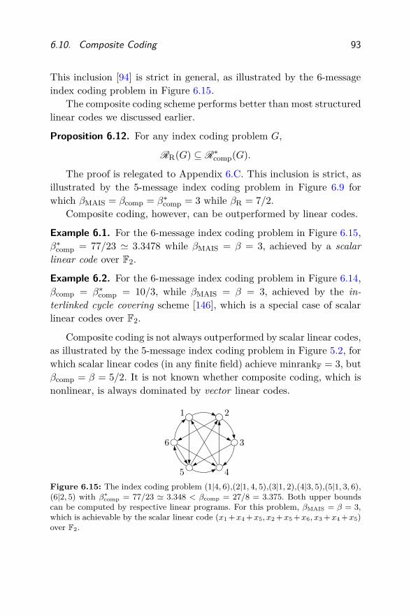
6.10. Composite Coding 93
This inclusion [94] is strict in general, as illustrated by the 6-messageindex coding problem in Figure 6.15.
The composite coding scheme performs better than most structuredlinear codes we discussed earlier.
Proposition 6.12. For any index coding problem G,
RR(G) ⊆ R∗comp(G).
The proof is relegated to Appendix 6.C. This inclusion is strict, asillustrated by the 5-message index coding problem in Figure 6.9 forwhich βMAIS = βcomp = β∗
comp = 3 while βR = 7/2.Composite coding, however, can be outperformed by linear codes.
Example 6.1. For the 6-message index coding problem in Figure 6.15,β∗
comp = 77/23 ≃ 3.3478 while βMAIS = β = 3, achieved by a scalar
linear code over F2.
Example 6.2. For the 6-message index coding problem in Figure 6.14,βcomp = β∗
comp = 10/3, while βMAIS = β = 3, achieved by the in-
terlinked cycle covering scheme [146], which is a special case of scalarlinear codes over F2.
Composite coding is not always outperformed by scalar linear codes,as illustrated by the 5-message index coding problem in Figure 5.2, forwhich scalar linear codes (in any finite field) achieve minrankF = 3, butβcomp = β = 5/2. It is not known whether composite coding, which isnonlinear, is always dominated by vector linear codes.
1 2
3
45
6
Figure 6.15: The index coding problem (1|4, 6),(2|1, 4, 5),(3|1, 2),(4|3, 5),(5|1, 3, 6),(6|2, 5) with β∗
comp = 77/23 ≃ 3.348 < βcomp = 27/8 = 3.375. Both upper boundscan be computed by respective linear programs. For this problem, βMAIS = β = 3,which is achievable by the scalar linear code (x1 +x4 +x5, x2 +x5 +x6, x3 +x4 +x5)over F2.

94 Coding Schemes
Open Problem 6.3. Is there an index coding problem with β∗comp < λF
for every F? How about β∗comp < infF λF?
Computation of composite coding bounds involves many auxiliaryrates such as Ri(D) and SJ(D) in (6.25), the number of which growsexponentially in n even for a fixed D. In addition, the number of D
can be computed, starting with Di = i and excluding Ai, as
|∆| =n∏
i=1
2n−|Ai|−1 = 2n2−n−∑n
i=1|Ai|,
which grows superexponentially in n. Therefore, although the compos-ite coding inner bound is computable in principle, it is rather difficultto compute directly.
Techniques to reduce the computational complexity of the compos-ite coding inner bound were explored in [96]. In particular, if Ai ⊆Aj ∪ Dj for some j 6= i, then receiver j already knows or will ulti-mately know more than receiver i does. Therefore, one can updateDj ← Dj ∪ i at no cost to the achievable rate region. Starting withDi ← i, i ∈ [n], we can thus build natural decoding sets D∗
i by addingnew elements to each Di iteratively. Once equipped with natural de-coding sets, we can reduce ∆ by focusing on Di that includes D∗
i . Thenumber of composite indices can be also reduced without affecting theresulting rate region; see [96, Sec. IV].
Remark 6.14. Instead of flat coding, transmission of composite in-dices can be further layered. The resulting three-layer composite coding
scheme [97] can strictly outperform the regular two-layer compositecoding scheme, at the cost of introducing more auxiliary rates. For the7-message index coding problem
(1|5), (2|3, 5, 6), (3|4, 6, 7),
(4|1, 2, 7), (5|2, 3, 4, 7), (6|3, 4, 7),
(7|1, 2, 4),
β∗comp = 3.25, but the three-layer composite coding scheme achievesβ = 3 [97, Example 2]. The latter scheme involves only 5 compositerates and 3 doubly composite rates.

6.A. Proof of Proposition 6.5 95
6.A Proof of Proposition 6.5
First note that for every G,(
1
κ(G), . . . ,
1
κ(G)
)
∈ RR(G). (6.26)
To prove this claim, set
δJ =
1κ(G) |J | = 1,
0 otherwise,
and
TiJ =
1 J = i,0 otherwise.
Then, the condition in (6.7c) is satisfied automatically since Tij ∈RR(G|J ) = [0, 1] for J = i. In addition, since
n− |Ai | ≤ κ(G), i ∈ [n], (6.27)
the condition in (6.7b) is satisfied as
∑
J([n]:J 6⊆Ai
δJ =∑
j /∈Ai
δj =∑
j /∈Ai
1
κ(G)=n− |Ai|κ(G)
≤ 1.
Therefore, by the definition of RR(G), the rate tuple (R1, . . . , Rn) suchthat
Ri =∑
J([n]:i∈J
δJTiJ = δiTii =1
κ(G)
is contained in RR(G).Now consider any (R′
1, . . . , R′n) and (δ′
J , J ⊆ [n]) that satisfy (6.6),i.e., (R′
1, . . . , R′n) ∈ RFLP(G). We show that there exist (δJ , J ( [n])
and (TiJ , i ∈ J ( [n]) such that the conditions in (6.7b) and (6.7c) aresatisfied, and
R′i ≤
∑
J([n]:i∈J
δJTiJ .
Then it follows that (R′1, . . . , R
′n) ∈ RR(G). We consider two cases.

96 Coding Schemes
Case 1. If δ′[n] = 0, the desired result follows by setting δJ = δ′
J andTiJ = 1/κ(G|J ) for each J ( [n] and each i ∈ J . Indeed, (6.7b) followsby (6.6b), and (6.7c) follows by (6.26). In addition,
R′i ≤
∑
J⊆[n]:i∈J
δ′J
κ(G|J )=
∑
J([n]:i∈J
δJTiJ .
Hence, (R′1, . . . , R
′n) ∈ RR(G).
Case 2. If δ′[n] 6= 0, then set
δJ =
δ′J +
δ′[n]
κ(G) |J | = 1,
δ′J otherwise,
and TiJ = 1/κ(G|J ). As before, the condition in (6.7c) is satisfied dueto (6.26). To check (6.7b), consider
∑
J([n]:J 6⊆Ai
δJ =∑
J([n]:J 6⊆Ai
δ′J +
∑
j /∈Ai
δ′[n]
κ(G)
≤∑
J([n]:J 6⊆Ai
δ′J + δ′
[n] (6.28)
≤ 1, (6.29)
where (6.28) follows by (6.27), and (6.29) follows by (6.6b). Finally,since κ(G|i) = 1, we have
R′i ≤
∑
J⊆[n]:i∈J
δ′J
κ(G|J )
=δ′
i
κ(G|i)+
δ′[n]
κ(G)+
∑
J([n]:i∈J,J 6=i
δ′J
κ(G|J )
=δ[n]
κ(G|i)+
∑
J([n]:i∈J,J 6=i
δJ
κ(G|J )
=∑
J([n]:i∈J
δJTjJ .
Hence, (R′1, . . . , R
′n) ∈ RR(G).
Combining both cases completes the proof that RFLP(G) ⊆ RR(G).

6.B. Analysis of Error Probability for Composite Coding 97
6.B Analysis of Error Probability for Composite Coding
Recall that receiver i finds a message tuple x(Di) such that
wJ(x(J ∩Di), x(J ∩Ai)) = wJ
for every J ⊆ Di ∪ Ai. A decoding error occurs only if there existsanother tuple x(Di) with xi 6= xi such that wJ(x(J ∩Di), x(J ∩Ai)) =
wJ for every J ⊆ Di ∪ Ai. We partition this error event accordingto each nonempty subset L ⊆ Di of erroneous message indices, i.e.,xj 6= xj iff j ∈ L. Then by the union of events bound,
Pe = P
wJ(x(J ∩Di), x(J ∩Ai)) = wJ for all J ⊆ D ∪Afor some x(Di) such that xi 6= xi
=⋃
L⊆Di:i∈L
P
wJ(x(J ∩ L), x(J \ L)) = wJ for all J ⊆ Di ∪Ai
for some x(Di) such that xj 6= xj iff j ∈ L
=∑
L⊆Di:i∈L
∑
x(Di)xj 6=xj iff j∈L
P
(
⋂
J⊆Di∪Ai
wJ(x(J ∩ L), x(J \ L)) = wJ
)
=∑
L⊆Di:i∈L
∑
x(Di)xj 6=xj iff j∈L
P
(
⋂
J⊆Di∪Ai
J∩L6=∅
wJ(x(J ∩ L), x(J \ L)) = wJ
)
≤∑
L⊆Di:i∈L
2∑
j∈Ltj−∑
J⊆Di∪Ai:J∩L6=∅sJ (6.30)
≤∑
L⊆Di:i∈L
2∑
j∈LrRj+1−
∑
J⊆Di∪Ai:J∩L6=∅rSJ ,
where (6.30) holds since for each L the number of erroneous tuplesis Πj∈L
(
2tj − 1)
, and for each erroneous tuple x(Di) with xj 6= xj iffj ∈ L, the probability that it is mapped to the same wJ = wJ(x(J))
for all J in the random codebook generation is 2−∑
sJ . Thus, the errorprobability Pe, averaged over random messages and codebooks, tendsto zero as r →∞, provided that for every L ⊆ Di with i ∈ L,
∑
j∈L
Rj <∑
J⊆Di∪Ai:J∩L6=∅
SJ .

98 Coding Schemes
6.C Proof of Proposition 6.12
We show that the rate region achieved by local time sharing of enhancedcomposite coding for subproblems is achieved by enhanced compos-ite coding itself. Then by induction on subproblems, i.e., RR(G|J ) ⊆R∗
comp(G|J ) for every J ( [n], and using the definition of RR(G)
in (6.7), it follows that RR(G) ⊆ R∗comp(G). Details are as follows.
Throughout this proof, we use the rate region T (G) ⊆ R∗comp(G),
instead of R∗comp(G) itself, which is defined exactly as R∗
comp(G) exceptthat i ∈ L is not required in (6.25b), and T (G|K) be its restrictionto the subproblem G|K . Consider any rate tuple (R1, . . . , Rn) achievedby local time sharing among all subproblems T (G|K), K ( [n], thatis, any rate tuple (R1, . . . , Rn) satisfying (6.7a) with T (G|K) in placeof RR(G|K) with some δK and (TiK , i ∈ K) ∈ T (G|K). It suffices toshow that this rate tuple (R1, . . . , Rn) satisfies (6.25a) for some Ri(D)
and SJ(D).First note that each component rate TiK for Ri can be expressed
as
TiK =∑
D(K)∈∆(K)
TiK(D(K)), i ∈ K, (6.31a)
for some TiK(D(K)), i ∈ K, D(K) ∈ ∆(K), and UJK(D(K)), J ⊆ K,
D(K) ∈ ∆(K), such that for each i ∈ K,
∑
j∈L
TjK(D(K)) ≤∑
J⊆D(K)i
∪(Ai∩K)J∩L6=∅
UJK(D(K)), L ⊆ D(K)i , (6.31b)
and
∑
J⊆KJ 6⊆Ai
∑
D(K)∈∆(K)
UJK(D(K)) ≤ 1. (6.31c)
Here,
∆(K) = (Di, i ∈ K) : i ∈ Di ⊆ K \ Ai
is the set of decoding sets for the subproblem G|K . Hence, by the
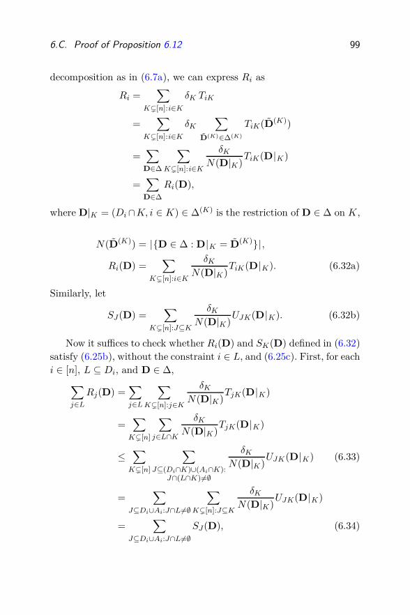
6.C. Proof of Proposition 6.12 99
decomposition as in (6.7a), we can express Ri as
Ri =∑
K([n]:i∈K
δK TiK
=∑
K([n]:i∈K
δK
∑
D(K)∈∆(K)
TiK(D(K))
=∑
D∈∆
∑
K([n]:i∈K
δK
N(D|K)TiK(D|K)
=∑
D∈∆
Ri(D),
where D|K = (Di∩K, i ∈ K) ∈ ∆(K) is the restriction of D ∈ ∆ on K,
N(D(K)) = |D ∈ ∆ : D|K = D(K)|,
Ri(D) =∑
K([n]:i∈K
δK
N(D|K)TiK(D|K). (6.32a)
Similarly, let
SJ(D) =∑
K([n]:J⊆K
δK
N(D|K)UJK(D|K). (6.32b)
Now it suffices to check whether Ri(D) and SK(D) defined in (6.32)satisfy (6.25b), without the constraint i ∈ L, and (6.25c). First, for eachi ∈ [n], L ⊆ Di, and D ∈ ∆,
∑
j∈L
Rj(D) =∑
j∈L
∑
K([n]:j∈K
δK
N(D|K)TjK(D|K)
=∑
K([n]
∑
j∈L∩K
δK
N(D|K)TjK(D|K)
≤∑
K([n]
∑
J⊆(Di∩K)∪(Ai∩K):J∩(L∩K)6=∅
δK
N(D|K)UJK(D|K) (6.33)
=∑
J⊆Di∪Ai:J∩L6=∅
∑
K([n]:J⊆K
δK
N(D|K)UJK(D|K)
=∑
J⊆Di∪Ai:J∩L6=∅
SJ(D), (6.34)

100 Coding Schemes
where (6.33) follows by (6.31b), and (6.34) follows by (6.32b). Next,for each i ∈ [n],
∑
J⊆[n]:J 6⊆Ai
∑
D∈∆
SJ(D) =∑
J⊆[n]:J 6⊆Ai
∑
D∈∆
∑
K([n]:J⊆K
δK
N(D|K)UJK(D|K)
=∑
J⊆[n]:J 6⊆Ai
∑
K([n]:J⊆K
δK
∑
D(K)∈∆(K)
UJK(D(K))
=∑
K([n]:K 6⊆Ai
δK
∑
J⊆K:J 6⊆Ai
∑
D(K)∈∆(K)
UJK(D(K))
(6.35)
≤∑
K([n]:K 6⊆Ai
δK (6.36)
≤ 1, (6.37)
where (6.35) follows since J 6⊆ Ai and J ⊆ K implies that K 6⊆ Ai,(6.36) follows by (6.31c), and (6.37) follows by (6.7b). Therefore, therate tuple (R1, . . . , Rn) we started with is contained in T (G). SinceRR(G|i) = T (G|i) = [0, 1], by induction on all subsetsK ⊆ [n], thisimplies that RR(G|K) ⊆ T (G|K) for every K ⊆ [n], and in particular,RR(G) ⊆ T (G) ⊆ R∗
comp(G). This completes the proof.

7
Criticality
Let e be an edge of the side information graph G = (V,E) of an indexcoding problem. We denote the graph resulting from removing e fromG by Ge, i.e.,
V (Ge) = V (G) and E(Ge) = E(G) \ e.
Given the index coding problem G, the edge e ∈ E is said to be critical
if C (Ge) 6= C (G), or in words, if the removal of e from G strictlyreduces the capacity region. The index coding problem G itself is saidto be critical if every e ∈ E(G) is critical. Thus, each critical graph (=index coding problem) cannot be made “simpler” into another one ofthe same capacity region.
The notion of criticality was introduced by Tahmasbi, Shahrasbi,and Gohari [143]. In this section, we present sufficient and necessaryconditions for criticality of an index coding problem.
7.1 A Sufficient Condition
Recall that a cycle in a graph G = (V,E) is a closed path i1 → i2 →· · · → ik = i1. We say that the cycle i1 → i2 → · · · → ik = i1 is a uni-
cycle or chordless cycle if it does not contain another cycle as a proper
101

102 Criticality
subgraph, or equivalently, the subgraph induced by i1, i2, . . . , ik−1has no edge other than ij → ij+1, j ∈ [k − 1]. As an example, inFigure 7.1(a), 1 → 2 → 3 → 4 → 1 is a cycle, but not a unicycle,but G|1,2,3 = 1 → 2 → 3 → 1 is a unicycle. As another example,for the graph in Figure 7.1(b), both G|1,2,3 = 1 → 2 → 3 → 1 andG|1,3,4 = 1 → 4 → 3 → 1 are unicycles. Note that if the subgraphG|J is a unicycle, then G|J ′ cannot be a unicycle for any J ′ that is aproper subset or superset of J .
1 2
34(a)
1 2
34(b)
Figure 7.1: (a) G|1,2,3 is a unicycle, but 1 → 2 → 3 → 4 → 1 is not a unicycle.(b) G|1,2,3 and G|1,3,4 are both unicycles.
Suppose that G|J is a unicycle for some J ⊆ V . Then the rate tuple(R1, . . . , Rn) satisfying
Ri =
1|J |−1 , i ∈ J,0, i /∈ J,
(7.1)
is achievable for index coding problem G, for example, using an MDScode over J . For any edge e ∈ G|J , however, the vertex-induced sub-graph Ge|J is acyclic (since there is no other cycle in G|J). Therefore,by the MAIS outer bound in (5.2), any rate tuple (R′
1, . . . , R′n) ∈ C (Ge)
must satisfy∑
i∈J
R′i ≤ 1. (7.2)
The rate tuple in (7.1), however, does not satisfy (7.2) and thus is not inC (Ge). This implies that removing edge e from G strictly reduces thecapacity region, i.e., C (Ge) 6= C (G), which establishes the followingsufficient condition for the criticality of an index coding problem.

7.1. A Sufficient Condition 103
Theorem 7.1 (Union-of-unicycles condition [11]). If every edge of Gbelongs to some unicycle, then G is critical.
Example 7.1. Consider the index coding problem G with side infor-mation graph depicted in Figure 7.1(b). Since every edge of G belongsto some unicycle, Theorem 7.1 shows that G is critical.
The union-of-unicycles condition, however, is not necessary for thecriticality of a graph, as illustrated by the following.
Example 7.2. The capacity region of the 5-message index coding prob-lem shown in Figure 7.2 is characterized by
R1 +R3 ≤ 1, (7.3a)
R1 +R4 ≤ 1, (7.3b)
R2 +R4 ≤ 1, (7.3c)
R2 +R5 ≤ 1, (7.3d)
R3 +R4 ≤ 1, (7.3e)
R3 +R5 ≤ 1. (7.3f)
Although the edge 3→ 5 does not belong to any unicycle, removing itfrom the side information graph (see Figure 5.3) reduces the capacityregion to the one characterized by (7.3) and
R1 +R2 +R3 +R4 +R5 ≤ 2. (7.4)
The union-of-unicycles condition actually captures the “criticality”with respect to the MAIS outer bound.
1
2
34
5
Figure 7.2: The index coding problem (1|2, 4, 5), (2|1, 3), (3|1, 2), (4|3, 5), (5|1, 3, 4).Although the edge 3 → 5 does not belong to any unicycle, it is critical. The capacityregion is achieved by composite coding with or without the edge 3 → 5.

104 Criticality
Proposition 7.1. An edge e belongs to some unicycle iff RMAIS(Ge) 6=RMAIS(G).
Indeed, if e belongs to a unicycle G|J , then (R1, . . . , Rn) definedin (7.1) is included in RMAIS(G). But it does not satisfy (7.2) andhence it is not included in RMAIS(Ge). Hence, RMAIS(G) 6= RMAIS(Ge).Conversely, if RMAIS(Ge) 6= RMAIS(G), then for some J , the edge ebelongs to a cycle in G|J and Ge|J is acyclic. Let Jmin be a minimalsuch subset. Then,G|Jmin is a cycle that contains e and does not containany other cycle. Hence, it is a unicycle.
Similarly, if e belongs to some unicycle, then RPM(Ge) 6= RPM(G).It is not known, however, whether the converse holds.
Open Problem 7.1. Find the sufficient and necessary condition forRPM(Ge) 6= RPM(G).
Let G∗ be the subgraph of G resulting from removing all edges ofG that do not belong to any unicycle, i.e., V (G∗) = V (G) and
E(G∗) = e ∈ E(G) : e belongs to some unicycle of G.
For example, consider the 6-message side information graph G depictedin Figure 7.3(a). The edges 3→ 4, 4→ 6, and 6→ 2 do not belong toany unicycle. The graph G∗ resulting from removing these three edgesof G is depicted in Figure 7.3(c).
1 2
3
45
6
(a)
1 2
3
45
6
(b)
1 2
3
45
6
(c)
Figure 7.3: (a) The side information graph G in which the edges 3 → 4, 4 → 6, and6 → 2 do not belong to any unicycle. (b) The subgraph Ge resulting from removingthe edge 3 → 4. (c) The subgraph G∗ resulting from removing all edges of G thatdo not belong to any unicycle.

7.1. A Sufficient Condition 105
If distinct edges e, e′, e′′, . . . do not belong to any unicycle in G, thene′, e′′, . . . do not belong to any unicycle in Ge either. Hence by applyingProposition 7.1 edge by edge, we can establish the following.
Proposition 7.2. RMAIS(G∗) = RMAIS(G).
Note that for any edge e, if the MAIS bound is tight for Ge, then
RMAIS(Ge) = C (Ge) ⊆ C (G) ⊆ RMAIS(G).
This observation, combined with Propositions 7.1 and 7.2, leads to thefollowing condition under which the capacity region of the index codingproblem G is equal to the capacity of the simpler problem Ge.
Proposition 7.3. If e does not belong to any unicycle and the MAISbound is tight for Ge, then
RMAIS(Ge) = C (Ge) = C (G) = RMAIS(G).
In particular, if the MAIS bound is tight for G∗, then
RMAIS(G∗) = C (G∗) = C (G) = RMAIS(G).
Consequently, if the MAIS bound is tight for G∗, then all the edgesthat do not belong to any unicycle can be removed without reducingthe capacity region. As an example, the capacity region of the indexcoding problem G∗ in Figure 7.3(c) is characterized by
R1 +R3 +R4 ≤ 1, (7.5a)
R1 +R3 +R5 ≤ 1, (7.5b)
R2 +R3 +R4 +R6 ≤ 1, (7.5c)
R2 +R3 +R5 +R6 ≤ 1, (7.5d)
which is equal to the MAIS bound. Thus, by Proposition 7.3, the ca-pacity region of the index coding problem G in Figure 7.3(a), as well asthat of any problem in between G∗ and G, such as Ge in Figure 7.3(b),is also characterized by (7.5).
Remark 7.1. The condition in Proposition 7.3 can be weakened forthe case of broadcast rate. For any edge e, if βMAIS(Ge) = β(Ge), thenβMAIS(G) ≤ β(G) ≤ β(Ge) = βMAIS(Ge). By Proposition 7.1, if inaddition e does not belong to any unicycle, then βMAIS(G) = βMAIS(Ge)
and thus βMAIS(G) = β(G) = β(Ge) = βMAIS(Ge).

106 Criticality
Recall from Section 2.1 that the transpose GT of an index codingproblem G satisfies V (GT ) = V (G) and
E(GT ) = (i, j) : (j, i) ∈ E(G).
In other words, the side information graphs of G and GT are of theopposite orientations, as illustrated by the pair of 5-message index cod-ing problems in Figure 7.4. Both problems are unions of unicycles andhence are critical. In fact, any index coding problem G is a union ofunicycles iff its transpose GT is a union of unicycles.
Open Problem 7.2. Is the criticality of G equivalent to the criticalityof GT (cf. Open Problem 4.1)?
The correspondence between critical problems and their capacityregions is not one-to-one. For both problems in Figure 7.4, the capac-ity region is achieved by the flat coding scheme in Section 6.9 and ischaracterized by the inequalities
R1 +R2 +R3 +R4 ≤ 1,
R1 +R2 +R4 +R5 ≤ 1,
R3 +R5 ≤ 1,
which coincides with the MAIS outer bound. Note that for any indexcoding problem G, RMAIS(G) = RMAIS(GT ) in general.
1
2
34
5
(a)
1
2
34
5
(b)
Figure 7.4: (a) The index coding problem G = (1|5), (2|5), (3|2, 4), (4|5), (5|1, 3).(b) The index coding problem GT = (1|5), (2|3), (3|5), (4|3), (5|1, 2, 4), in which everyedge is in the opposite direction of the corresponding edge in G.

7.2. Necessary Conditions 107
7.2 Necessary Conditions
We now discuss a few necessary conditions for G to be critical, whichimply the conditions under which an edge e can be removed withoutreducing the capacity region. We start with the following conditionestablished by Tahmasbi, Shahrasbi, and Gohari [143].
Proposition 7.4 (Union-of-cycles condition [143]). If G is critical, thenevery edge lies on a cycle.
To prove this, suppose that G can be vertex-partitioned by twosubgraphs G1 and G2 such that there exists no edge from G2 to G1
(see Figure 4.1(b)). The set of edges from G1 to G2 is referred to as adirected cut-set, removing which will disconnect G1 and G2. The neces-sary condition in Proposition 7.4 can be viewed as a direct applicationof Remark 4.1, which implies that every edge in a directed cut-set canbe removed without affecting the capacity region. Therefore, if G iscritical, then by the Farkas lemma [18, Th. 2.2] (which states that eachedge in a directed graph either lies on a directed cycle or belongs to adirected cut-set but not both), every edge lies on a (directed) cycle.
The second necessary condition we present is based on the relation-ship among different side information sets at the receivers. We say thatthe side information sets A1, . . . , An of an index coding problem G aredegraded if there exist i, j ∈ V (G) such that j ∈ Ai and Aj ⊆ Ai. Inthis case, the edge j → i can be removed since xj can be recovered atreceiver i. This observation leads to the following necessary condition.
Proposition 7.5 (Nondegradedness condition [11]). If G is critical, thenside information sets are nondegraded.
Next, we present another necessary condition by rephrasing Propo-sition 7.3. Suppose that G is critical, i.e., C (Ge) 6= C (G) for every edgee. If the MAIS bound is tight for Ge for some e, then
RMAIS(Ge) = C (Ge) ( C (G) ⊆ RMAIS(G).
Now this edge e must belong to a unicycle. Otherwise, by Proposi-tion 7.3, C (Ge) = C (G), which contradicts the criticality of G. Thisestablishes the following partial converse to Theorem 7.1.

108 Criticality
Proposition 7.6 (MAIS looseness condition [11]). If G = (V,E) is criti-cal, then for every edge e ∈ E that does not belong to a unicycle, theMAIS bound is loose for Ge, i.e., RMAIS(Ge) 6= C (Ge).
In other words, an edge e is not critical if it does not belong toany unicycle and the MAIS bound is tight for Ge. Recall that the edge3→ 5 in Figure 7.2 is critical and does not belong to any unicycle. Asis implied by Proposition 7.6 and verified by (7.4), the MAIS bound isnot tight for the graph resulting from removing this edge.
The following summarizes all the necessary conditions for the crit-icality of a problem that we have discussed so far.
Theorem 7.2. If G = (V,E) is critical, then
1. every edge lies on a cycle,
2. side information sets are nondegraded, and
3. for each e ∈ E that is not in some unicycle, RMAIS(Ge) 6= C (Ge).
The next three examples demonstrate that these necessary condi-tions are mutually independent.
Example 7.3. The 6-message side information graph G in Figure 7.5satisfies the union-of-cycles and nondegradedness conditions, but itdoes not satisfy the MAIS looseness condition, as the edge 6→ 1 doesnot belong to any unicycle and the MAIS bound is tight after removingthis edge. Hence, G is not critical.
Example 7.4. The 6-message side information graph G in Figure 7.6satisfies the union-of-cycles and MAIS looseness conditions, but not thenondegradedness condition as A6 ⊆ A4. Hence, G is not critical.
Example 7.5. The 6-message side information graph G in Figure 7.7satisfies the nondegradedness and MAIS looseness conditions, but notthe union-of-cycles condition, as the edge 2→ 6 does not belong to anycycle. Hence, G is not critical.
Satisfying all the necessary conditions in Theorem 7.2 at the sametime, however, does not imply the criticality.
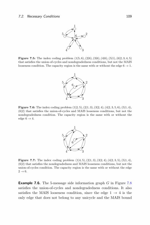
7.2. Necessary Conditions 109
1
2
34
5 6
Figure 7.5: The index coding problem (1|5, 6), (2|6), (3|6), (4|6), (5|1), (6|2, 3, 4, 5)that satisfies the union-of-cycles and nondegradedness conditions, but not the MAISlooseness condition. The capacity region is the same with or without the edge 6 → 1.
1
2
34
56
Figure 7.6: The index coding problem (1|2, 5), (2|1, 3), (3|2, 4), (4|2, 3, 5, 6), (5|1, 4),(6|2) that satisfies the union-of-cycles and MAIS looseness conditions, but not thenondegradedness condition. The capacity region is the same with or without theedge 6 → 4.
1
2
34
5
6
Figure 7.7: The index coding problem (1|4, 5), (2|1, 3), (3|2, 4), (4|2, 3, 5), (5|1, 4),(6|2) that satisfies the nondegradedness and MAIS looseness conditions, but not theunion-of-cycles condition. The capacity region is the same with or without the edge2 → 6.
Example 7.6. The 5-message side information graph G in Figure 7.8satisfies the union-of-cycles and nondegradedness conditions. It alsosatisfies the MAIS looseness condition, since the edge 1 → 4 is theonly edge that does not belong to any unicycle and the MAIS bound

110 Criticality
1
2
34
5
Figure 7.8: The index coding problem (1|2, 5), (2|1, 3), (3|2, 4), (4|1, 3, 5), (5|1, 4)that satisfies all the three necessary conditions in Theorem 7.2, but is not critical.The capacity region is the same with or without the edge 1 → 4.
is not tight after removing this edge (see Example 5.2). Nonetheless,the index coding problem G is not critical as the capacity region ischaracterized by (5.14) and (5.15) with or without the edge 1→ 4.
It is not known how the gap between Theorem 7.1 and 7.2 can beclosed.
Open Problem 7.3. Find the sufficient and necessary condition for thecriticality of G.
Remark 7.2. If G satisfies the union-of-unicycles condition, it triviallysatisfies the union-of-cycles condition and the MAIS looseness. As log-ically expected, the union-of-unicycles condition also implies the non-degradedness condition. Suppose that G has degraded side informationsets. Then, there exists an edge j → i such that Aj ⊆ Ai. This edgecannot belong to a unicycle. Indeed, if the edge j → i does not belongto any cycle, then trivially it does not belong to any unicycle. Other-wise, j → i lies on a cycle C = (j → i → · · · → k → j), which bydegradedness must have at least three vertices. Thus, k ∈ Aj and, bythe degradedness assumption, k ∈ Ai. Hence, i → · · · → k → i is alsoa cycle, which implies that C cannot be a unicycle.

8
Index Coding Problems with Known Capacity
In this section, we present several special instances of the index codingproblem for which the broadcast rate or the capacity region is known.We refer the reader to [164, 149, 116], and [146] among others foradditional classes of index coding instances with known broadcast rateor capacity region.
8.1 Problems with Broadcast Rate of Two
One of the simplest index coding problems is the one with a completeside information graph G, i.e., j ∈ Ai for all distinct i, j ∈ [n]. In thiscase, the broadcast rate is one and the rates
R1 = · · · = Rn = 1
are achievable simultaneously.If side information graph G is not complete, then j /∈ Ai for some
i 6= j. Hence, by the MAIS bound, 2 ≤ β(G). This also implies thatthere is no index coding instance with 1 < β < 2.
The following result characterizes all instances of the index codingproblem with β = 2, based on the notion of alignment subsets discussedin Section 6.8.
111

112 Index Coding Problems with Known Capacity
Proposition 8.1 ([29, 104]). The broadcast rate of the index codingproblem with side information graph G is 2 iff G is not complete andcan be partitioned into alignment subsets such that for every pair (i, j)
in an alignment subset, i ∈ Aj and j ∈ Ai.
This sufficient and necessary condition for β = 2 was establishedindependently by Maleki, Cadambe, and Jafar [104] and by Blasiak,Kleinberg, and Lubetzky [29], the latter of whom also presented apolynomial time algorithm to determine whether β = 2. The proofof sufficiency follows by Proposition 6.8. For the necessity, let i k⇐⇒ j
denote i, j /∈ Ak for distinct indices i, j, k. The following lemma can beproved by the polymatroidal outer bound in Theorem 5.2.
Lemma 8.1 ([104]). For any k + 1 distinct indices i0, i1, . . . , ik ∈ [n]
and k indices j1, . . . , jk ∈ [n], if
i0j1⇐⇒ i1
j2⇐⇒ i2j3⇐⇒ · · · jk−1⇐⇒ ik−1
jk⇐⇒ ik
and
i0 /∈ Aik,
then
Ri0 +Rj1 +Ri1 +Rj2 +Ri2 + · · ·+Rjk+Rik
≤ 1.
Returning to the proof of Proposition 8.1, suppose that i and j
belong to the same alignment subset. Then, there must exist a chainof alignment relations connecting j and i as
jj1⇐⇒ i1
j2⇐⇒ i2j3⇐⇒ · · · jk−1⇐⇒ ik−1
jk⇐⇒ i.
If j /∈ Ai (or i /∈ Aj), then by Lemma 8.1,
Rj +Rj1 +Ri1 +Rj2 +Ri2 + · · ·+Rjk+Ri ≤ 1. (8.1)
Since the length of the chain k is at least 1, the summation in (8.1)consists of at least three terms, which implies that the symmetric rateof 1/2 (i.e., the broadcast rate of 2) is not achievable.
Remark 8.1. As mentioned above, there is a dichotomy of the broad-cast rate as either β = 1 or β ≥ 2. Above β = 2, there exists anindex coding instance of the broadcast rate arbitrarily close to 2 (seeProposition 8.6 below).

8.2. Problems with Very Small Capacity 113
8.2 Problems with Very Small Capacity
At the other extreme, if an n-message side information graph G isacyclic, then uncoded transmission is optimal, that is, the broadcastrate β(G) = n and the capacity region C (G) is characterized by
R1 + · · ·+Rn ≤ 1.
If G contains a cycle, however, then partial clique covering (see Re-mark 6.5) of that cycle and the remaining single-vertex cliques achievesthe upper bound of n− 1 on the broadcast rate. Consequently, there isno index coding instance with n− 1 < β < n.
The following characterizes all instances of the index coding prob-lem with β = n− 1.
Proposition 8.2 ([115]). The broadcast rate of the n-message indexcoding problem with side information graph G is n − 1 iff G containsa cycle and there is a vertex that belongs to all cycles. In other words,β(G) = n− 1 iff βMAIS(G) = n− 1.
The sufficient condition follows immediately sinceG contains a cycle(hence β ≤ n − 1) and the removal of the common vertex induces anacyclic subgraph of n−1 vertices (hence β ≥ n−1 by the MAIS bound).The necessary condition was established by Ong [115], who establisheda stronger result—if G contains a cycle and the intersection of all cyclesis empty, then it is not just that β 6= n − 1, but that β ≤ n − 2. Theproof of this result relies on the following.
Lemma 8.2 ([115, Lemma 3]). If G has a cycle and the intersection ofall cycles is empty, then G contains a subgraph G′ (i.e., V (G′) ⊆ V (G)
and E(G′) ⊆ E(G)) that is either two disjoint cycles or of the formshown in Figure 8.1.
To establish the upper bound of n−2 on the broadcast rate, assumewithout loss of generality that G is itself a union of two disjoint cyclesor a graph of the form in Figure 8.1. Otherwise, any remaining n− n′
messages of the index coding problem G that are not in the subproblemG′ with n′ messages (of either structure) can be communicated in n−n′

114 Index Coding Problems with Known Capacity
I
KM
J
L
N
P
QR
Figure 8.1: The common subgraph structure with a single “inner” circle consistingof six paths I through N and three “outer” paths P , Q, and R. The paths do notshare common vertices except the end points. Each pair of white, gray, and blackvertices may be identical (no edges between them), but all paths other than I , K,and M must contain at least one edge.
transmissions without coding. Any additional edge (side information)in G′ can be ignored and still result in a valid upper bound on thebroadcast rate. Hence, the broadcast rate upper bound of n − 2 isachievable for G if the broadcast rate upper bound of n′−2 is achievablefor G′.
In the first case, G consists of two cycles with n1 and n2 = n − n1
vertices. Then partial clique covering of the two cycles (with partialclique numbers of n1 − 1 and n2 − 1) achieves the upper bound of(n1 − 1) + (n2 − 1) = n− 2 on the broadcast rate.
In the second case, G has the form in Figure 8.1. Then the inter-
linked cycle covering scheme by Thapa, Ong, and Johnson [146] canachieve the same upper bound of n − 2. To show this, denote the ver-tices in one of the 9 paths labeled by S ∈ I, J,K,L,M,N,P,Q,R ass0 → s1 → · · · → s−1. As some paths meet at end points, we have
i0 = n−1 = r−1, k0 = j−1 = p−1, m0 = l−1 = q−1,
j0 = q0 = i−1, l0 = r0 = k−1, n0 = p0 = m−1.
Note that every vertex except i0, k0,m0 has only one incoming edge.Consider the scalar linear code for G that transmits
xi0 + xk0 + xm0 , (8.2a)
xs + x(As), s 6= i0, k0,m0. (8.2b)

8.3. Perfect Graphs 115
The total number of transmissions is 1 + (n − 3) = n − 2. Clearly,receiver s 6= i0, k0,m0 can recover xs from (8.2b) and x(As). Receiver i0can compute along the paths N and R
(xn0 + xn1) + (xn1 + xn2) + · · · + (xn−3 + xn−2)
+ (xr0 + xr1) + (xr1 + xr2) + · · · + (xr−3 + xr−2),
which is simplified by telescoping to xn0 + xr0 + xn−2 + xr−2 . Combin-ing this with (8.2a), and using x(Ai0) = (xn−2 , xr−2), receiver i0 canrecover xi0. By symmetry, receivers k0 and m0 can similarly recovertheir messages, and thus the upper bound of n− 2 is achievable.
Combined with the MAIS bound, this argument also implies thefollowing.
Proposition 8.3 ([115]). The broadcast rate of the n-message indexcoding problem with side information graph G is n− 2 if βMAIS(G) =
n− 2.
The necessity of this condition is not known.
Open Problem 8.1. Characterize all n-message index coding instanceswith β = n− 2.
Remark 8.2. There is a trichotomy that the broadcast rate β must ben, n− 1, or ≤ n− 2. Below β = n− 2, there are index coding instanceswith n − 3 < β < n − 2 (cf. Remark 8.1). For example, the 5-messageindex coding problem in Figure 5.2 has β = 5/2 = n− 5/2 = n/2.
Open Problem 8.2. Is there an n-message index coding instance withn− 5/2 < β < n− 2?
8.3 Perfect Graphs
For an index coding problem with an undirected (bidirectional) sideinformation graph U , the MAIS bound implies α(U) ≤ β(U) and theclique covering bound implies β(U) ≤ χ(U). When U is perfect (andthus, U is perfect by Lemma 2.3),
ω(U) = α(U) = β(U) = χ(U),

116 Index Coding Problems with Known Capacity
which is achieved by the clique covering scheme [22]. The followinggeneralizes this result.
Proposition 8.4 ([162]). The capacity region of an index coding prob-lem with undirected perfect side information graph U is equal to theMAIS outer bound and is achieved by fractional clique covering.
To prove the proposition, note that the polytope associated with Uin (2.6) is equivalent to the MAIS outer bound RMAIS in Theorem 5.1.The other polytope associated with U in (2.5) is achievable by fractionalclique covering, since the rate tuple given by the incidence vector of eachclique in U is achievable (see Remark 6.3). Since U is perfect, the twopolytopes are equivalent by Lemma 2.3.
8.4 Locally Acyclic Graphs
We say that a side information graph G is locally acyclic if for everyi ∈ [n], the induced subgraph G|[n]\Ai
is acyclic. For example, the sideinformation graph depicted in Figure 8.2 is locally acyclic since thesubgraphs induced by [3] \ A1 = 1, 3, [3] \ A2 = 2, and [3] \ A3 =
2, 3 are respectively acyclic.The following characterizes the capacity region for this class of side
information graphs.
Proposition 8.5. For any index coding problem G, C (G) = Rflat(G)
iff G is locally acyclic.
The sufficiency follows by comparing the flat coding inner boundRflat in Proposition 6.10 and the MAIS outer bound RMAIS in Theo-rem 5.1. For the necessity, suppose that Rflat(G) is the capacity region
1
2 3
Figure 8.2: The index coding problem (1|2), (2|1, 3), (3|1) with β = 2, which isachievable by an MDS code.

8.4. Locally Acyclic Graphs 117
and G|[n]\Aicontains a cycle for some i ∈ [n]. Then by partial clique
covering, the rate tuple (R1, . . . , Rn) such that
Rj =
1n−1−|Ai|
j ∈ [n] \ Ai,
0 otherwise
is achievable. But
∑
j /∈Ai
Rj =n− |Ai|
n− 1− |Ai|> 1
and thus (R1, . . . , Rn) /∈ Rflat(G), which contradicts the assumptionthat Rflat(G) is the capacity region.
As a corollary to Proposition 8.5, the broadcast rate of any indexcoding problem with locally acyclic side information graph is
β(G) = κ(G) = n−minindeg(G) = n−mini|Ai |, (8.3)
which is achieved, for example, by an MDS code. Local acyclicity, how-ever, is not necessary for (8.3) to hold. For example, the 4-messageindex coding problem depicted in Figure 8.3 is not locally acyclicsince the subgraph induced by [4] \ A1 = 1, 2, 3 contains a cycle,yet κ(G) = βMAIS(G) = β(G) = 3.
Open Problem 8.3. Characterize all n-message index coding problemsG for which (8.3) holds.
1 2
34
Figure 8.3: The index coding problem (1|4), (2|1, 3), (3|2, 4), (4|3) with β = 3,which is achievable by an MDS code.

118 Index Coding Problems with Known Capacity
8.5 Symmetric Neighboring Side Information
In Proposition 6.9, we established an upper bound on the broadcastrate for index coding problems that have symmetric neighboring sideinformation, i.e.,
Ai = i⊖ d, . . . , i⊖ 1, i⊕ 1, . . . , i⊕ u, i ∈ [n], (8.4)
where⊕ and ⊖ denote addition and subtraction modulo n, respectively,and 0 ≤ d ≤ u ≤ u+d ≤ n−2 or (u, d) = (n−1, 0). The polymatroidalouter bound in Section 5.2 implies the following bound on achievablerates for these problems.
Lemma 8.3 ([104]). If (R1, . . . , Rn) is achievable for an index codingproblem with side information sets in (8.4), then
n∑
i=1
Ri ≤(d+ 1)n
n− (u− d). (8.5)
Proposition 6.9 and Lemma 8.3 characterize the broadcast rate ofthis class of index coding problems as follows.
Proposition 8.6 ([104]). For any index coding problem G with sym-metric neighboring side information sets in (8.4),
β(G) =n− (u− d)
d+ 1. (8.6)
The broadcast rate in (8.6) is also achievable by the compositecoding scheme [8]. It is unknown, however, the composite coding in-ner bound in Proposition 6.11 and the polymatroidal outer bound inTheorem 5.2 coincide and characterize the capacity region.
Open Problem 8.4. Characterize the capacity region for index codingproblems with symmetric neighboring side information sets.
Remark 8.3. By taking different values of (u, d), the broadcast rates ofall n-message index coding problems with symmetric neighboring sideinformation sets can be enumerated as
Bn = 1 ∪⌊ n
2⌋
⋃
k=1
2k
k,
2k + 1
k, . . . ,
n
k
. (8.7)

8.6. Problems with Small Number of Messages 119
For example,
B5 =
1, 2,5
2, 3, 4, 5
,
B6 =
1, 2,5
2, 3, 4, 5, 6
,
B7 =
1, 2,7
3,5
2, 3,
7
2, 4, 5, 6, 7
.
These values cover the broadcast rates of many other index codingproblems, but not all of them. For example, the 6-message index cod-ing problem in Figure 8.4 that combines the 5-message problem withbroadcast rate of 5/2 in Figure 5.2 and a separate single-message prob-lem has β = 5/2 + 1 = 7/2 /∈ B6.
1
2
34
5
6
Figure 8.4: The index coding problem (1|2, 5), (2|1, 3), (3|2, 4), (4|3, 5), (5|1, 4),(6|−) with β = β(G|1,2,3,4,5) + β(G|6) = 5/2 + 1 = 7/2.
8.6 Problems with Small Number of Messages
As mentioned earlier in Section 1.2, the number of nonisomorphic in-stances of the index coding problem with n messages grows superex-ponentially in n. In this section, we discuss the capacity regions of allindex coding problems with n ≤ 5 and the broadcast rates of all indexcoding problems with n ≤ 6.
For n = 1, there is one index coding instance (1|−), the capacityregion of which is C1 = [0, 1] and can be expressed by the inequality
1 · R1 ≤ 1.
Trivially, this instance is critical with β = 1.

120 Index Coding Problems with Known Capacity
For n = 2, there are 3 nonisomorphic index coding instances
(1|−), (2|−), (1|−), (2|1), (1|2), (2|1)
as shown in Figure 4.3. By Remark 4.1 (or more generally, by The-orem 4.1), the capacity region C
(a)2 of the first two is characterized
by[
1 1]
R ≤ 1.
By Remark 4.2 or Theorem 4.1, the capacity region C(c)2 of the third
is characterized by[
1 0
0 1
]
R ≤ 1.
The first and third problems are critical and the second one is not. Thecorresponding broadcast rates are 2, 2, and 1.
For n = 3, there are 16 nonisomorphic index coding instances asshown in Figure 8.5. For problems (a) through (f), among which only(a) is critical, the broadcast rate is 3 and the capacity region C
(a)3 is
the polytope characterized by[
1 1 1]
R ≤ 1.
For problems (g) through (l), among which (g) is critical, the broadcastrate is 2 and the capacity region C
(g)3 is characterized by
[
1 1 0
0 1 1
]
R ≤ 1.
For problem (m), which is critical, the broadcast rate is 2 and thecapacity region C
(m)3 is characterized by
1 1 0
1 0 1
0 1 1
R ≤ 1.
For problems (n) and (o), among which (n) is critical, the broadcastrate is 2 and the capacity region C
(n)3 is characterized by
[
1 0 0
0 1 1
]
R ≤ 1.

8.6. Problems with Small Number of Messages 121
(a) (b) (c) (d)
(e) (f) (g) (h)
(i) (j) (k) (l)
(m) (n) (o) (p)
Figure 8.5: Sixteen nonisomorphic 3-message index coding instances.
Finally, for problem (p), which is critical, the broadcast rate is 1 andthe capacity region C
(p)3 is characterized by
1 0 0
0 1 0
0 0 1
R ≤ 1.
For each of the 16 instances, the capacity region is achieved by thefractional (local) partial clique covering scheme and coincides with theMAIS outer bound. The criticality of each instance can be checkedby comparing the union-of-unicycles condition in Theorem 7.1 and thethree necessary conditions in Theorem 7.2, which agree for all sixteen3-message index coding instances (in fact, only the MAIS looseness con-dition in Proposition 7.6 is needed). Among the five critical instances,

122 Index Coding Problems with Known Capacity
(a), (g), (n), and (p) can be decomposed into smaller problems by The-orem 4.1 as
C(a)3 = C
(a)2 (C1,C
(a)2 ),
C(g)3 = C
(a)2 (C1,C
(c)2 ),
C(n)3 = C
(c)2 (C1,C
(a)2 ),
C(p)3 = C
(c)2 (C1,C
(c)2 ).
Hence, problem (m) is the only bona-fide 3-message index coding prob-lem, for which the flat coding inner bound and the MAIS outer boundon the capacity region coincide (cf. Proposition 8.5).
For n = 4, there are 218 nonisomorphic index coding instances. Foreach instance, the fractional local partial clique covering inner boundcoincides with the MAIS outer bound on the capacity region. In ad-dition, the broadcast rate of each instance is achievable by a scalarlinear code over F2. There are 18 critical instances, which are unionsof unicycles and have distinct capacity regions, as listed in Table 8.1.Among these, 4 problems (o), (p), (q), and (r), shown in Figure 8.6,are not decomposable into smaller problems.
(o) (p) (q) (r)
Figure 8.6: Four 4-message nonisomorphic, critical, indecomposable index codingproblems.
For n = 5, there are 9,608 nonisomorphic index coding instances.For each instance, the composite coding inner bound coincides withthe polymatroidal outer bound on the capacity region [8]. In addition,the broadcast rate is achievable by a scalar linear code over F2 for allbut 28 instances. For those few exceptions, a vector linear code over F2
with t = 2 suffices [115]. There are 136 instances that satisfy the union-of-unicycles sufficient condition in Theorem 7.1 and 175 instances that

8.6. Problems with Small Number of Messages 123
Table 8.1: Eighteen 4-message nonisomorphic critical index coding instances andtheir capacity regions.
Problem Capacity region
(a) (1|−), (2|−), (3|−), (4|−) C(a)2 (C1, C
(a)3 )
(b) (1|−), (2|3), (3|2), (4|−) C(a)2 (C1, C
(g)3 )
(c) (1|−), (2|4), (3|2), (4|3) C(a)2 (C1, C
(m)3 )
(d) (1|−), (2|3, 4), (3|2), (4|2) C(a)2 (C1, C
(n)3 )
(e) (1|−), (2|3, 4), (3|2, 4), (4|2, 3) C(a)2 (C1, C
(p)3 )
(f) (1|2), (2|1), (3|4), (4|3) C(a)2 (C
(c)2 , C
(c)2 )
(g) (1|2, 3, 4), (2|1), (3|1), (4|1) C(c)2 (C1, C
(a)3 )
(h) (1|2, 3, 4), (2|1, 3), (3|1, 2), (4|1) C(c)2 (C1, C
(g)3 )
(i) (1|2, 3, 4), (2|1, 4), (3|1, 2), (4|1, 3) C(c)2 (C1, C
(m)3 )
(j) (1|2, 3, 4), (2|1, 3, 4), (3|1, 2), (4|1, 2) C(c)2 (C1, C
(n)3 )
(k) (1|2, 3, 4), (2|1, 3, 4), (3|1, 2, 4), (4|1, 2, 3) C(c)2 (C1, C
(p)3 )
(l) (1|3, 4), (2|3, 4), (3|1, 2), (4|1, 2) C(c)2 (C
(a)2 , C
(a)2 )
(m) (1|3, 4), (2|1), (3|2), (4|2) C(m)3 (C1, C1, C
(a)2 )
(n) (1|3, 4), (2|1), (3|2, 4), (4|2, 3) C(m)3 (C1, C1, C
(c)2 )
(o) (1|4), (2|1), (3|2), (4|3)
1 1 1 01 1 0 11 0 1 10 1 1 1
R ≤ 1
(p) (1|4), (2|4), (3|2), (4|1, 3)
[
1 1 1 00 1 0 10 0 1 1
]
R ≤ 1
(q) (1|4), (2|3), (3|2, 4), (4|1, 3)
[
1 1 0 01 0 1 00 1 0 1
]
R ≤ 1
(r) (1|4), (2|1, 3), (3|2, 4), (4|2, 3)
1 1 0 01 0 1 01 0 0 10 1 0 1
R ≤ 1

124 Index Coding Problems with Known Capacity
satisfy the necessary conditions in Theorem 7.2. Both conditions failto capture the criticality and there are in fact 141 critical instances(recall Open Problem 7.3). The five instances that are critical yet notunions of unicycles are shown in Figure 8.7. The first two problems(a) and (b) are transposes of each other, while each of the next threeproblems (c), (d), and (e) is isomorphic to its transpose (recall OpenProblem 7.2). Including these 5 instances, there are 68 critical instancesthat are not decomposable into smaller problems. As mentioned earlierin Section 7.1, some instances share the same capacity region, and thereare 118 distinct capacity regions (up to relabeling). In Figure 8.7, prob-lems (a), (b), and (c), and problems (d) and (e), respectively, have thesame capacity regions. The capacity regions of all 141 critical instancescoincide with the corresponding MAIS inner bounds, except the twoindecomposable problems in Figures 5.2 and 5.3. It can be verified thatβ = 3 iff βMAIS = 3 (recall Open Problem 8.1).
(a) (b) (c) (d) (e)
Figure 8.7: Five 5-message nonisomorphic, critical, indecomposable index codingproblems that are not unions of unicycles.
For n = 6, there are 1,540,944 nonisomorphic instances. For sim-plicity, we focus on the broadcast rate. For each instance, the broad-cast rate is equal to the polymatroidal lower bound, which coincideswith either composite coding or scalar linear coding [10]; see Exam-ple 6.1. In order to isolate the problems that are critical and indecom-posable, we adapt the notion of criticality for the capacity region to theone for the broadcast rate, namely, an index coding problem G is β-
critical if β(Ge) > β(G) for every edge e. Note that β-criticality implies(C -)criticality. Hence, the necessary conditions for the C -criticality dis-cussed in Section 7.2 are also necessary for the β-criticality. In light ofRemark 7.1, the MAIS looseness condition in Proposition 7.6 can be

8.6. Problems with Small Number of Messages 125
relaxed as the condition βMAIS(Ge) 6= β(Ge) for every edge e ∈ E
that does not belong to a unicycle. In summary, we have the followingnecessary conditions for the β-criticality.
Proposition 8.7. If G = (V,E) is β-critical, then
1. every edge lies on a cycle,
2. side information sets are nondegraded, and
3. for each e ∈ E that is not in some unicycle, βMAIS(Ge) 6= β(Ge).
These conditions are mutually independent (cf. Examples 7.3–7.5)and there are 9,747 instances that satisfy all three of them. A closerexamination reveals that there are only 259 β-critical instances with6 messages. Among these, 152 instances are not decomposable intosmaller problems. For all but 13 of these 152 indecomposable instances,the composite coding upper bound coincides with the polymatroidallower bound on the broadcast rate. For the remaining 13 instances,the broadcast rate is 3 and scalar linear codes over F2 achieve it. Itcan be verified that β = 4 iff βMAIS = 4 (Open Problem 8.1), andthat β(GT ) = β(G) (Open Problem 4.1) for all 6-message index codinginstances.
We conclude this section by summarizing the collective behavior ofall index coding instances with n ≤ 6. Let B∗
n be the set of all values ofthe broadcast rate an n-message index coding problem can take (cf. Bn
in Section 8.5). We have
B∗1 = 1,
B∗2 = 1, 2,
B∗3 = 1, 2, 3,
B∗4 = 1, 2, 3, 4,
B∗5 =
1, 2,5
2, 3, 4, 5
,
B∗6 =
1, 2,5
2, 3,
13
4,
10
3,
7
2, 4, 5, 6
.

126 Index Coding Problems with Known Capacity
This brings up the following challenging question that spans beyondall the simple examples we have seen so far (see Remarks 8.1 and 8.2as well as Open Problem 8.2).
Open Problem 8.5. Characterize the set B∗n of all values of the broad-
cast rate an n-message index coding problem can take.
Simpler (but still challenging) problems are as follows.
Open Problem 8.6. Is B∗n ⊆ Q?
Open Problem 8.7. How does |B∗n| scale in n?
Similar problems can be posed for capacity regions, starting withn = 6.
Open Problem 8.8. Characterize the capacity regions of all 6-messageindex coding problems.
We can also compute the expected broadcast rate βn of the randomn-message index coding problem whose side information graph is thedirected Erdös–Rényi random graph G(n, 1/2) (i.e., βn is the uniformaverage of the broadcast rates of all 2n(n−1) index coding instancesincluding isomorphic ones):
β1 = 1,
β2 = 1.75,
β3 = 2.375,
β4 = 2.9075,
β5 = 3.3794,
β6 = 3.7960.
Open Problem 8.9. How does βn scale in n?

9
Capacity Approximation
With no computable characterization of the broadcast rate (or capac-ity) of a general index coding problem, the next step forward seemsto be approximating it. Keeping in mind that the broadcast rate β foran n-message index coding problem is O(n), we present in this sectioncapacity approximation results of sublinear multiplicative factors. Ourmain focus will be several classes of index coding problems for whichthe multiplicative factor can be tightened to O(n1−ǫ) for some ǫ > 0.
9.1 Ramsey Numbers
We first review some results in Ramsey theory which we will use inthe rest of the section to approximate the broadcast rate. Given a classG of undirected graphs and two positive integers i and j, the Ramsey
number RG(i, j) is defined as the smallest positive integer such thatevery graph in G with at least RG(i, j) vertices has a clique of sizei or an independent set of size j. If G is the class of all undirectedfinite simple graphs, then the Ramsey number is denoted by R(i, j).In general, determining Ramsey numbers for most classes G is quitedifficult, but they are easily computed for very small values of i and j.
127

128 Capacity Approximation
Lemma 9.1 (Belmonte, Heggernes, Hof, Rafiey, and Saei [23]). For anynonempty graph class G of undirected graphs,
RG(1, j) = RG(i, 1) = 1, i, j ≥ 1.
If G is the set of all edgeless graphs, i.e., all U = (V,E) with E = ∅,then
RG(2, j) = j, j ≥ 1.
Similarly, if G is the set of all complete graphs, i.e., all U = (V,E) withE = i, j : i 6= j ∈ V , then
RG(i, 2) = i, i ≥ 1.
The following upper bound on the Ramsey number is well-known.
Lemma 9.2 (Erdős and Szekeres [67]). For any i, j ≥ 1,
R(i, j) ≤(
i+ j − 2
i− 1
)
.
For some classes of graphs, this upper bound can be tightened.A graph is said to be planar if it can be drawn on a plane without
edges crossing each other. Figure 9.1 shows examples of a 4-vertexplanar graph and a 5-vertex nonplanar graph. Note that an edgelessgraph is planar. Let P be the class of undirected planar graphs. TheRamsey number for this class is completely determined; see Table 9.1.
1 2
34(a)
1
2
34
5
(b)
Figure 9.1: (a) A 4-vertex planar graph (the edge 1, 3 can be drawn such thatit does not cross 2, 4). (b) A 5-vertex nonplanar graph.
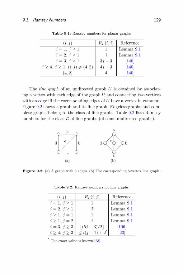
9.1. Ramsey Numbers 129
Table 9.1: Ramsey numbers for planar graphs
(i, j) RP(i, j) Referencei = 1, j ≥ 1 1 Lemma 9.1i = 2, j ≥ 1 j Lemma 9.1i = 3, j ≥ 1 3j − 3 [140]
i ≥ 4, j ≥ 1, (i, j) 6= (4, 2) 4j − 3 [140](4, 2) 4 [140]
The line graph of an undirected graph U is obtained by associat-ing a vertex with each edge of the graph U and connecting two verticeswith an edge iff the corresponding edges of U have a vertex in common.Figure 9.2 shows a graph and its line graph. Edgeless graphs and com-plete graphs belong to the class of line graphs. Table 9.2 lists Ramseynumbers for the class L of line graphs (of some undirected graphs).
a
b
c
d e
(a)
a
b
c
de
(b)
Figure 9.2: (a) A graph with 5 edges. (b) The corresponding 5-vertex line graph.
Table 9.2: Ramsey numbers for line graphs
(i, j) RL(i, j) Referencei = 1, j ≥ 1 1 Lemma 9.1i = 2, j ≥ 1 j Lemma 9.1i ≥ 1, j = 1 1 Lemma 9.1i ≥ 1, j = 2 i Lemma 9.1i = 3, j ≥ 3 ⌊(5j − 3)/2⌋ [106]i ≥ 4, j ≥ 3 ≤ i(j − 1) + 2* [23]
* The exact value is known [23].

130 Capacity Approximation
An undirected graph U = (V,E) is said to be a fuzzy circular in-
terval graph [46] if
• there exists a set F of closed intervals ejθ : a ≤ θ ≤ b of the unitcircle T = ejθ : θ ∈ [0, 2π) such that (1) no interval includesanother and (2) no point of T is an endpoint of more than oneinterval in F , and
• there exists a mapping φ : V → T such that (1) if i, j ∈ E,then φ(i) and φ(j) belong to a common interval of F , and (2)if i, j /∈ E, then either there is no interval in F that containsboth φ(i) and φ(j), or there is exactly one interval in F whoseendpoints are φ(i) and φ(j).
Note that an edgeless graph is a fuzzy circular interval graph (F =
∅) and a complete graph is a fuzzy circular interval graph (F = T).Figure 9.3 shows a more interesting example of C6. Let F be the classof fuzzy circular interval graphs. The Ramsey number for this class isgiven in Table 9.3.
1 4
25
3 6
(a)
θ0 φ(1) φ(5)
θ1
θ2 θ3
φ(2)φ(4)
θ4
φ(6) θ5
θ6
θ7θ8
φ(3)θ9
(b)
Figure 9.3: (a) The complement C6 of the cycle graph C6. (b) The fuzzy circularinterval model of C6, where the intervals [θ0, θ3], [θ2, θ6], [θ4, θ9], [θ7, θ1] are shown inthick arcs and φ(1) = φ(5) = θ0, φ(2) = φ(4) = θ3, φ(3) = θ8, and φ(6) = θ5. It iseasy to check that F and φ satisfy the aforementioned conditions. For example, theedge 3, 6 exists and the interval [θ4, θ9] contains φ(3) and φ(6). The edge 1, 2does not exist and there is exactly one interval [θ0, θ3] with endpoints φ(1) and φ(2).

9.2. Approximate Capacity for Some Classes of Problems 131
Table 9.3: Ramsey numbers for fuzzy circular interval graphs
(i, j) RF (i, j) Referencei = 1, j ≥ 1 1 Lemma 9.1i = 2, j ≥ 1 j Lemma 9.1i ≥ 1, j = 1 1 Lemma 9.1i ≥ 1, j = 2 i Lemma 9.1i ≥ 3, j ≥ 3 (i− 1)j [23]
We summarize these results as a simple bilinear upper bound onthe Ramsey number for the classes of planar, line, and fuzzy circularinterval graphs.
Lemma 9.3. For G = P,L, or F ,
RG(i, j) ≤ ij, i, j ≥ 1.
9.2 Approximate Capacity for Some Classes of Problems
Blasiak, Kleinberg, and Lubetzky [29] established the following approx-imation result for index coding instances with undirected (bidirectional)side information graphs based on the clique covering scheme discussedin Section 6.2.
Proposition 9.1 ([29]). For any n-message index coding problem withbidirectional (undirected) side information graph U ,
χ(U)
β(U)= O
(
n
log n
)
.
In other words, the clique covering scheme approximately achieves thebroadcast rate within a multiplicative factor of O(n/ log n).
To prove the proposition, we consider two cases. First, if χ(U) <
4n/log n, then trivially
χ(U)
β(U)≤ χ(U) <
4n
log n.

132 Capacity Approximation
Second, for the other case of χ(U) ≥ 4n/log n, we rely on the followinglemma relating the independence number of an undirected graph withthe chromatic number of its complement via Ramsey numbers.
Lemma 9.4 (Alon and Kahale [4]). Let U = (V,E) be an undirectedgraph with |V | = n. Let αi(m) = maxj : R(i, j) ≤ m. If χ(U) ≥(n/i) +m, then an independent set of size αi(m) can be found in U .
Continuing with the proof of Proposition 9.1, let i = (log n)/2 andm = n/i. Then for n sufficiently large,
α(U) ≥ max
j : R(12 log n, j) ≤ n
i
(9.1)
≥ max
j :
(
12 log n+ j − 2
12 log n− 1
)
≤ n
i
(9.2)
≥ 1
2log n,
where (9.1) follows by Lemma 9.4, and (9.2) follows by Lemma 9.2.Hence, by Remark 5.2, we have
χ(U)
β(U)≤ n
β(U)≤ n
α(U)≤ O
(
n
log n
)
.
This completes the proof of Proposition 9.1.Next, we consider the class of unidirectional graphs. In this case,
by Lemma 2.1, for any unidirectional graph G on n vertices and anytournament G′ resulting from adding edges with arbitrary directionbetween the vertices that are not connected in G, we have
log n ≤ β(G′) ≤ β(G).
Since uncoded transmission trivially achieves the upper bound of n onthe broadcast rate, we have the following.
Proposition 9.2 ([14]). For any n-message index coding problem withunidirectional side information graph G,
n
β(G)≤ n
log n.
In words, uncoded transmission approximately achieves the broadcastrate within a multiplicative factor of O(n/ log n).

9.2. Approximate Capacity for Some Classes of Problems 133
For general directed graphs, we have the following result by Blasiak,Kleinberg, and Lubetzky, the proof of which can be found in [29,Sec. V.B].
Proposition 9.3 ([29]). For any index coding problem with n messageswith side information graph G,
χf (U(G))
β(G)= O
(
n log log n
log n
)
.
In words, the fractional clique covering scheme approximately achievesthe broadcast rate within a multiplicative factor of O(n log log n/ log n).
Beyond Propositions 9.1 through 9.3, there is no known approxi-mation for the broadcast rate of a general (undirected/bidirectional,unidirectional, or directed) index coding problem.
Open Problem 9.1. Improve the multiplicative factors in Proposi-tions 9.1 through 9.3.
A stronger question is as follows.
Open Problem 9.2. Approximate the broadcast rate of an n-messageindex coding problem from above within a multiplicative factor ofO(n1−ǫ) for some ǫ > 0.
For now it is not even clear whether such a tight approximation isfeasible at all (cf. Open Problem 3.2).
Open Problem 9.3. Does there exist a finite, terminating algorithmthat approximates the broadcast rate β of an arbitrary n-message indexcoding problem by producing lower and upper bounds of the form
Ω(nǫ) ≤ β ≤ O(nǫ′)
for some 0 ≤ ǫ ≤ ǫ′ ≤ 1 such that ǫ′ − ǫ < 1?
The approximation results in Propositions 9.1 through 9.3 continueto hold for the linear broadcast rate. Questions similar to Open Prob-lems 9.1 through 9.3 can be asked for the linear broadcast rate λF andits minimum over all F.

134 Capacity Approximation
As attacking Open Problem 9.2 in general is very difficult, we limitourselves to studying the conditions under which a tighter approxima-tion exists. We first adapt the technique used in the proof of Proposi-tion 9.1 to present a condition under which the broadcast rate of anindex coding problem can be approximated within a factor of O(n1−ǫ)
for some ǫ > 0. The proof is relegated to Appendix 9.A.
Theorem 9.1 ([14]). Let G be a class of undirected graphs for whichRG(i, j) ≤ ciajb holds for some constants a, b, and c. For any indexcoding problem with side information graph G ∈ G such that |V (G)| =n, the clique covering scheme approximates the broadcast rate within
a multiplicative factor of 2a+1
a+b+1 c1
a+b+1na+b
a+b+1 .
As stated in Lemma 9.3, planar graphs, line graphs and fuzzy cir-cular interval graphs are three classes that satisfy the condition of The-orem 9.1 with a = b = c = 1.
Corollary 9.1. If G is a planar graph or a line graph or a fuzzy circularinterval graph with n vertices, the clique covering scheme approximatesthe broadcast rate within a multiplicative factor of (2n)2/3.
For (directed) planar graphs, we can establish a tighter approxi-mation with simple lower and upper bounds. We recall the celebratedfour-color theorem.
Lemma 9.5 (Four-color theorem [6]). Every planar graph U is four-colorable, i.e., χ(U) ≤ 4.
If the undirected graph U(G) associated with the n-vertex side in-formation graph G is planar, then
n
4≤ n
χ(U(G))(9.3)
≤ n
χf (U(G))(9.4)
≤ α(U(G)) (9.5)
≤ β(U(G)) (9.6)
≤ β(G) (9.7)
≤ n,

9.2. Approximate Capacity for Some Classes of Problems 135
where (9.3) follows by the four-color theorem, (9.4) by (2.2), (9.5) byLemma 2.2, (9.6) by Remark 5.2 and (9.7) holds since adding sideinformation decreases the broadcast rate. Similarly, if U(G) is planar,
1 ≤ β(G) ≤ χ(U(G)) ≤ 4.
The following summarizes these results.
Theorem 9.2 ([14]). For any index coding problem with side informa-tion graph G such that U(G) [U(G)] is planar, uncoded transmission[clique covering] approximates the broadcast rate within a multiplica-tive factor of four.
Remark 9.1. The approximation results in Theorems 9.1 and 9.2 holdfor the linear broadcast rate as well. For bidirectional outerplanar
graphs [42], which form a special subclass of planar graphs, the cliquecovering scheme actually achieves the scalar linear capacity [24].
Remark 9.2. For any index coding problem with planar side informa-tion graph G, and (1) G is bidirectional, (2) G is unidirectional, (3)U(G) is triangle-free, (4) G is bidirectional and triangle-free, (5) thelength of the smallest directed cycle of G is 4, or (6) the length of thesmallest directed cycle of G is at least 5, then Theorem 9.2 can be fur-ther strengthened to the factor of 2, 3, 3, 3/2, 12/5, and 2, respectively[109, 161].
Sparse graphs form another class for which we have a partial solu-tion to Open Problem 9.2. We recall the celebrated Turán’s theorem intwo forms.
Lemma 9.6 (Turán’s theorem [148]). If an undirected graph U = (V,E)
is Kr+1-free, then
|E | ≤(
1− 1
r
) |V |22.
Equivalently, for any undirected graph U = (V,E),
α(U) ≥ |V |22|E|+ |V | .

136 Capacity Approximation
Suppose that the side information graph G = (V,E) is sparse with|V | = n and |E| = O(n1+ǫ) for some ǫ < 1. Then by Turán’s theorem,
Ω(n1−ǫ) = α(U(G)) ≤ β(G) ≤ n.An argument similar to the proof of Theorem 9.2 establishes the follow-ing result by Yi and Caire [161] and by Agarwal, Flodin, and Mazum-dar [1].
Theorem 9.3 ([161, 1]). For any n-message index coding problem withside information graph G = (V,E), if |E| = O(n1+ǫ), then uncodedtransmission approximately achieves the broadcast rate within a mul-tiplicative factor of O(nǫ).
Remark 9.3. Agarwal, Flodin, and Mazumdar [1] also established tightapproximation results for several other classes of index coding prob-lems, including unit disk graphs.
In all class-specific improvements of Proposition 9.3 we have dis-cussed thus far, we approximated the broadcast rate from above using(fractional) clique covering and the trivial lower bound of β ≥ 1 or frombelow using the independence number and the trivial upper bound ofβ ≤ n (uncoded transmission).
Open Problem 9.4. Find a class of n-message index coding problemsfor which
Ω(nǫ) ≤ β ≤ O(nǫ′)
for some 0 < ǫ ≤ ǫ′ < 1.
Remark 9.4. Although approximating β itself is rather difficult for ageneral n-message index coding problem, approximating n−β is mucheasier. This complementary index coding rate, namely, the amount ofrelative improvement of the optimal index code over uncoded trans-mission, was originally studied by Chaudhry, Asad, Sprintson, andLangberg [43], who showed that n − β as well as n − λF can be ap-proximated within a multiplicative factor of O(log n log log n). Mazum-dar [108] strengthened this result and also established a factor-of-twoapproximation of both n−β and n−λF for bidirectional graphs. We willsee the complementary index coding rate again in Section 11.4 whenwe discuss the performance limit of distributed storage networks.

9.A. Proof of Theorem 9.1 137
9.A Proof of Theorem 9.1
Let U ∈ G and k be a positive integer to be specified later. We considertwo cases. First, if χ(U) < 2n/k, then trivially
χ(U)
β(U)<
2n
k.
Second, for the other case of χ(U) ≥ 2n/k, by Lemma 9.4 with i = k
and m = ⌊n/k⌋,(
n
cka+1
)
1b
= maxj : ckajb ≤ n/k
≤ maxj : RG(k, j) ≤ n/k≤ α(U)
≤ β(U)
≤ χ(U)
≤ n.
Thus,
χ(U)
β(U)≤ n
β(U)≤ n1− 1
b (cka+1)1b .
As k increases, the upper bound on χ(U)/β(U) decreases in the firstcase, and increases in the second case. Hence, to minimize the upperbound on the multiplicative gap between χ(U) and β(U), we choose
k = 2b
a+b+1 (n/c)1
a+b+1 , which makes the upper bounds in both casesequal to the desired multiplicative gap. This completes the proof of thetheorem.
10
Index Coding and Network Coding
Multiple-unicast network coding [70, 69, 159, 78] is a long-lasting andcentral open problem in information theory. As we saw earlier in Sec-tion 1 (especially in Figure 1.4), index coding is a rather special caseof multiple-unicast network coding. In this section, we take the oppo-site direction and associate a general multiple-unicast network codingproblem with a corresponding index coding problem. This associationallows a nontrivial translation of a code for the index coding problemto a code for the network coding problem, and vice versa. We elucidatethis relationship and discuss to what extent it can be leveraged to solveone problem by the solution to the other.
10.1 Multiple Unicast Network Coding
An instance of the multiple-unicast network coding problem is definedby a directed acyclic graph G = (V,E), a set of k distinct sourcenodes S = s1, . . . , sk ⊆ V , and a set of k distinct destination nodesD = d1, . . . , dk ⊆ V . We assume without loss of generality thateach source si has no incoming edges, that each destination di has nooutgoing edges, and that there exists a directed path from si to di
138

10.1. Multiple Unicast Network Coding 139
for each i ∈ [k]. Destination di wishes to receive message xi that isavailable at source si, i ∈ [k]. Each source node si encodes the messagexi into sequences carried by its outgoing edges and each intermediatenode encodes the sequences carried by its incoming edges into thosecarried by its outgoing edges.
For any node v ∈ V , let In(v) = (u, v) ∈ E be the set of itsincoming edges. Overloading this notation, for an edge e that is out-going from a source s ∈ S let In(e) = s, and for any other edgee = (u, v) let In(e) = (t, u) ∈ E. As an example, for the graph inFigure 10.1(a), In(d2) = e1, e6, In(e2) = s1, and In(e5) = e2, e3.Under this notation, a ((ti, i ∈ [k]), (te, e ∈ E)) network code can beformally defined by
• k messages, where the i-th message xi takes values in 0, 1ti ,
• |E| encoders, where the encoder fe : Πa∈In(e) 0, 1ta → 0, 1te
at edge e ∈ E maps the sequences carried by the inputs to edgee to the sequence carried by edge e, and
• k decoders, where the decoder gi : Πe∈In(di) 0, 1te → 0, 1ti atdestination di ∈ D maps the sequences carried by the inputs todestination di back to xi.
Due to the acyclic structure of the network graph G, the sequencecarried by edge e can be written as a function of the message tuple xS =
(x1, . . . , xk) alone by recursively applying the local encoding functions
fe, fa, a ∈ In(e), and so on. We refer to the resulting function f ′e(xS)
as the global encoding function at edge e.A tuple (R,C) = ((Ri, i ∈ [k]), (Ce, e ∈ E)) of nonnegative real
numbers is said to be an achievable rate–capacity tuple if there exist a((ti, i ∈ [k]), (te, e ∈ E)) network code and an integer r such that
Ri ≤tir, i ∈ [k],
andCe ≥
ter, e ∈ E.
Note that if (R,C) is achievable, then (αR, αC) is also achievable forevery rational α > 0. For a given C ∈ RE
≥0, the capacity region CN(C)
is defined as the closure of all R such that (R,C) is achievable.

140 Index Coding and Network Coding
10.2 Relationship Between Index Coding and Network Coding
Figure 1.4 illustrated that for any index coding problem, there exists anequivalent network coding problem such that the encoding function forthe network coding problem on the bottleneck edge on the top definesthe encoding problem for the index coding problem. In particular, thecapacity region of the index coding problem is identical to the capacityregion of the network coding problem for Ce = 1, e ∈ E.
In this section, we show that for any network coding problem, thereexists a corresponding index coding problem such that a code for oneyields a code for the other. This relationship was established by El-Rouayheb, Sprintson, and Georghiades for the case of linear codes [61]and by Effros, El-Rouayheb, and Langberg for the general case [59].Here we provide a slightly refined account of this relationship.
Let N be an instance of the network coding problem on a directedacyclic graph G = (V,E) with k source nodes s1, . . . , sk, k destina-tion nodes d1, . . . , dk, and k messages x1, . . . , xk. Given N , we definean instance I(N) of the index coding problem corresponding to thisnetwork coding instance by a set of k + |E| messages (xS ,xE) =
((xi, i ∈ [k]), (xe, e ∈ E)), and sets of side information Ai = In(di),i ∈ [k], and Ae = In(e), e ∈ E. For example, the butterfly network,a famous multiple-unicast network coding instance, and the side infor-mation graph of its corresponding index coding instance are depictedin Figure 10.1. The butterfly network has two source nodes s1 and s2,and seven edges. Thus, the corresponding index coding instance hasnine messages x1, x2, and xei
, i ∈ [7].A network coding instance N and the corresponding index coding
instance I(N) have the following relationship.
Theorem 10.1. Let N be a k-unicast network coding instance overthe graph G = (V,E) and let I(N) be its corresponding index codinginstance with k + |E| messages. Then a ((ti : i ∈ [k]), (te : e ∈ E))
network code exists for N iff a ((ti : i ∈ [k]), (te : e ∈ E),∑
e∈E te)
index code exists for I(N).
To prove the necessity (only if), let fe and f ′e be the local and global
encoding functions of the ((ti : i ∈ [k]), (te : e ∈ E)) network code for

10.2. Relationship Between Index Coding and Network Coding 141
s1 s2
e1
e2 e3
e4e5
e6 e7
d1d2(a)
s1 s2
e1 e2 e3 e4
e5
e6 e7
(b)
Figure 10.1: (a) The butterfly network. (b) The side information graph of thecorresponding index coding instance.
edge e ∈ E, respectively, and gi be the decoding function of destinationdi ∈ D. Let |E| = m and xE = (xe1, . . . , xem). We construct an indexcode for the index coding instance I(N) with encoding function
φ(xS ,xE) = (xe1 + f ′e1
(xS), . . . , xem + f ′em
(xS)) ∈ 0, 1∑
e∈Ete .
(10.1)
We now argue that every receiver can recover its desired message usingy = φ(xS ,xE) and its side information. The receiver for message xe,e ∈ E, has (xa : a ∈ In(e)) as side information and can perform thefollowing steps to recover xe: (1) For each a ∈ In(e), use xa + f ′
a(xS)
to compute f ′a(xS); (2) compute f ′
e(xS) = fe(f ′a(xS) : a ∈ In(e));
and (3) use xe + f ′e(xS) to compute xe. The receiver for xi, i ∈ [k],
has (xe : e ∈ In(di)) and can perform the following steps: (1) Foreach e ∈ In(di), use xe + f ′
e(xS) to compute f ′e(xS); and (2) compute
the decoding function gi(f′e(xS) : e ∈ In(di)), which is equal to xi.
Therefore, the encoder in (10.1) and aforementioned decoders define a((ti : i ∈ [k]), (te : e ∈ E),
∑
e∈E te) index code for I(N).To prove the sufficiency (if), let φ and ψi, i ∈ [k], ψe, e ∈ E,
be the encoding and decoding functions of a ((ti : i ∈ [k]), (te : e ∈E),
∑
e∈E te) index code for I(N), respectively. Let r =∑
e∈E te andpartition the set of message tuples by Py = (xS ,xE) : φ(xS ,xE) = y,y ∈ 0, 1r . Before we proceed with the proof we present two lemmasthat are proved in Appendices 10.A and 10.B.

142 Index Coding and Network Coding
Lemma 10.1. For any xS ∈ Πi∈[k]0, 1ti , if xE 6= x′E , then
φ(xS ,xE) 6= φ(xS ,x′E). (10.2)
Lemma 10.2. For every y ∈ 0, 1r , |Py| = 2∑k
i=1ti .
Thus, in a partition Py, each value of xS appears exactly once witha unique value for xE . This uniqueness allows us to define encodingfunctions for the network coding instance N as follows.
Take any fixed y. For each xS , let xE(xS) be the unique vector xE
such that (xS ,xE) ∈ Py, and let xe(xS) be the component of xE(xS)
that corresponds to edge e. Since the index code is valid,
ψe(φ(xS ,xE), (xa, a ∈ In(e))) = xe, e ∈ E,
and
ψi(φ(xS ,xE), (xa, a ∈ In(di))) = xi, i ∈ [k].
In particular, plugging in xE = xE(xS),
ψe(y, (xa(xS), a ∈ In(e))) = xe(xS), e ∈ E, (10.3a)
and
ψi(y, (xa(xS), a ∈ In(di))) = xi, i ∈ [k]. (10.3b)
Now we define the local encoding functions for the network codinginstance N by
fe(xa, a ∈ In(e)) = ψe(y, (xa, a ∈ In(e))), e ∈ E. (10.4)
Then, by (10.3a) and induction, the global encoding function at edgee satisfies
f ′e(xS) = xe(xS), (10.5)
since the global encoding functions at the edges a ∈ In(e) satisfyf ′
a(xS) = xa(xS). We also define the k decoding functions at the desti-nations as
gi(xa, a ∈ In(di)) = ψi(y, (xa, a ∈ In(di))), i ∈ [k]. (10.6)

10.2. Relationship Between Index Coding and Network Coding 143
Then, by (10.3b) and (10.5), for the given message tuple xS , the de-coding outputs at the destinations satisfy
ψi(y, (xa(xS), a ∈ In(di))) = xi, i = [k].
Therefore, the encoding functions in (10.4) and the decoding functionsin (10.6) define a valid ((ti : i ∈ [k]), (te : e ∈ E)) network code. Thiscompletes the proof of Theorem 10.1.
Theorem 10.1 implies the following relationship between the achiev-able rate tuples for a network coding instance and its correspondingindex coding instance.
Corollary 10.1. Let N be a k-unicast network coding instance overthe graph G = (V,E) and let I(N) be its corresponding index codinginstance with k+ |E| messages. Suppose that C = (Ce : e ∈ E) is ratio-nal. Then, (R,C) is achievable for N iff (R/CE ,C/CE) is achievablefor I(N), where CE =
∑
e∈E Ce.
To prove the necessity, suppose that (R,C) is achievable for N .Then, there exists a ((ti : i ∈ [k]), (te : e ∈ E)) network code and aninteger r such that
Ri ≤tir, i ∈ [k], (10.7a)
and
Ce ≥ter, e ∈ E. (10.7b)
Since C is rational, we have
Ce =ae
be, e ∈ E,
where ae, be ∈ N, e ∈ E. Let r′ be divisible by r as well as be, e ∈ E.Define t′i = (r′/r)ti, i ∈ [k], and t′e = r′Ce ≥ (r′/r)te, e ∈ E. Then, byrepeating the network code satisfying (10.7a) and (10.7b) (r′/r) timesand by appropriate zero padding (to be exact, adding r′Ce − (r′/r)tezeros for x′
e, e ∈ E), we can construct a ((t′i : i ∈ [k]), (t′e : e ∈ E)) net-work code such that
Ri ≤t′ir′, i ∈ [k],

144 Index Coding and Network Coding
and
Ce =t′er′, e ∈ E.
By Theorem 10.1, there exists a ((t′i : i ∈ [k]), (t′e : e ∈ E),∑
e∈E t′e)
index code for I(N), the rates of which are
R′i =
t′i∑
e∈E t′e
≥ Ri
CE, i ∈ [k],
and
R′e =
t′e∑
e∈E t′e
=Ce
CE, e ∈ E.
Thus, the rate tuple (R/CE ,C/CE) is also achievable for I(N).To prove the sufficiency, suppose that the rate tuple (R/CE ,C/CE)
is achievable for the index coding instance I(N). Then, there exists a((ti : i ∈ [k]), (te : e ∈ E), r) index code such that
Ri
CE≤ tir, i ∈ [k], (10.8a)
andCe
CE≤ te
r, e ∈ E. (10.8b)
On the one hand, by summing over e ∈ E, (10.8b) implies that
r ≤∑
e∈E
te. (10.9)
On the other hand, by Lemma 10.1, for any xS the function φ(xS ,xE)
is one-to-one, which implies that
2∑
e∈Ete ≤ 2r. (10.10)
Combining (10.9) and (10.10), we have∑
e∈E
te = r. (10.11)
Thus, by Theorem 10.1, there exists a ((ti : i ∈ [k]), (te : e ∈ E)) net-work code for N . Furthermore, by (10.8b) and (10.11),
Ce
CE=ter, e ∈ E.
Hence, (R/CE ,C/CE), as well as (R,C), is achievable for the networkcoding instance N .

10.2. Relationship Between Index Coding and Network Coding 145
Remark 10.1. The relationships between a network coding instanceN and its corresponding index coding instance I(N) in Theorem 10.1and Corollary 10.1 also hold for the cases with vanishing probability oferror [61, 59].
Sometimes the exact code-level relationship between N and I(N)
presented in Theorem 10.1 is referred to, perhaps for the sake of brevity,as the “equivalence” between the two classes of the problems. It shouldbe noted, however, that in the network coding problem N the goal isto achieve a larger message rate tuple R for a smaller link capacitytuple C, but that in the corresponding index coding problem I(N) thegoal is simply to achieve a larger message rate tuple (RS ,RE). Theseincompatible goals are tangent to each other only under the specialcondition RE = C/CE , which can be made valid if C is rational.
We illustrate the resulting relationship between the rate regions inCorollary 10.1 in Figure 10.2, when the rates are projected to the twodimensions (RS , CE) or (RS , RE), where RS =
∑ki=1 Ri. The rate–
capacity region RN (namely, the closure of all achievable (RS ,C))of the network coding instance is a convex cone (or triangle in twodimensions), while the capacity region CI (namely, the closure of allachievable (RS ,RE)) of the index coding instance is a bounded convexset. Corollary 10.1 implies that at RE = CE = 1, both regions containthe same set of achievable rates RS (i.e., the same interior before takingthe closure operations).
The rate-level relationship in Corollary 10.1, combined with the factthat cl(Proj(A)) ⊆ Proj(cl(A)) for any set A, implies the following.
Corollary 10.2. Let N be a k-unicast network coding instance overthe graph G = (V,E) and let I(N) be its corresponding index codinginstance with k + |E| messages. For a given (rational) link capacitytuple C, the capacity region CN (C) of the network coding instance Nsatisfies
CN(C) = cl(R : (R,C) is achievable for N)⊆ R : (R/CE ,C/CE) ∈ CI, (10.12)
where CI is the capacity region of the index coding instance I(N).

146 Index Coding and Network Coding
CE , RE
RS
RN
CI
1
Figure 10.2: The two-dimensional projections of the achievable rate–capacity re-gion RN of the network coding instance N and the capacity region CI of the cor-responding index coding instance I(N). The interiors of the regions are achievable.On the boundary, the rates are marked by solid lines/curves if achievable and bydashed lines otherwise. At CE = RE = 1, the sets of achievable RS coincide forboth regions.
Thus, the index coding capacity region can be projected to yield anouter bound on the network coding capacity region. It is not known ifthe inclusion holds in the other direction as well.
Open Problem 10.1. Is the inclusion in (10.12) strict in general?
10.A Proof of Lemma 10.1
Suppose that the edges in E are labeled in the order such that In(ej) ⊆e1, . . . , ej−1. Note that such a labeling is possible since G is acyclic.Suppose that xE = (xe1 , . . . , xem) 6= (x′
e1, . . . , x′
em) = x
′E. Then we
have one of the following two cases.
Case 1. If ej is outgoing from some source node s ∈ S and xej6= x′
ej,
then we must have φ(xS ,xE) 6= φ(xS ,x′E), since otherwise the receiver
for message xejcannot distinguish its desired message xej
from x′ej
based on φ(xS ,xE) and their common side information xs.
Case 2. Otherwise, let j ∈ [m] be the first coordinate at whichxE and x
′E differ, i.e., (xe1 , . . . , xej−1) = (x′
e1, . . . , x′
ej−1) and xj 6= x′
j .Since In(ej) ⊆ e1, . . . , ej−1 by assumption, once again we must haveφ(xS ,xE) 6= φ(xS ,x
′E).

10.B. Proof of Lemma 10.2 147
10.B Proof of Lemma 10.2
Lemma 10.1 implies that there exist at most 2∑k
i=1ti message tuples in
each Py, i.e.,
|Py | ≤ 2∑k
i=1ti , y ∈ [2r]. (10.13)
But combining all (xS ,xE) tuples over all y ∈ [2r], we must have
∑
y∈[2r ]
|Py | = |(xS ,xE)| = (2∑k
i=1ti)(2
∑
e∈Ete) = (2
∑k
i=1ti)2r,
which implies that (10.13) must hold with equality, i.e.,
|Py | = 2∑k
i=1ti , y ∈ [2r].

11
Index Coding, Distributed Storage, and
Guessing Games
As the amount of data continues to expand, it is becoming increas-ingly important to store them reliably in a distributed storage systemof interconnected servers. The index coding problem is closely relatedto the locally recoverable distributed storage problem, which studiesfundamental limits and coding schemes for such distributed storagenetworks. In an unexpected twist, the locally recoverable distributedstorage problem turns out to be equivalent to the recreational mathe-matics problem of guessing games on directed graphs. In this section,we introduce the locally recoverable distributed storage problem andthe problem of guessing games on graphs, and develop the relationshipbetween these two problems and the index coding problem.
11.1 Locally Recoverable Distributed Storage Problem
In the locally recoverable distributed storage problem, which hereafterwill be referred to as the distributed storage problem, a set of serverscollectively store data so that if a single server fails, its contents canbe efficiently reconstructed from the contents of the other servers (see,for example, [127, 120, 35]). The goal is to design a distributed storage
148

11.1. Locally Recoverable Distributed Storage Problem 149
code that maximizes the amount of data that can be stored while satis-fying the single-failure recovery constraint. Mazumdar [108] considereda distributed storage system in which each server has only access to asubset of the other servers and model the topology of the system bya directed graph. The same model was also considered independentlyand concurrently by Shanmugam and Dimakis [128].
Suppose that some data y is stored across n servers in the systemand that it can be recovered exactly by accessing all servers. Let xi
denote the content of server i ∈ [n]. Each server has access to thecontents of a subset of other servers, x(Ai), Ai ⊆ [n] \ i. The set Ai
is referred to as the recovery set of server i. The goal is to find themaximum amount of data that can be stored in the network so thatif any single server fails, its content can be still recovered from thecontents of its recovery set.
As before, we can formulate the problem more precisely by defininga (t1, . . . , tn, r) distributed storage code that consists of
• a message set [2r],
• a one-to-one encoding function xn : [2r] → ∏ni=10, 1ti that
assigns a distinct codeword xn(y) to each y ∈ [2r], (the set C =
xn(1), . . . , xn(2r) is referred to as the codebook), and
• n recovery functions, where the recovery function at server i ∈[n], fi :
∏
j∈Ai0, 1tj → 0, 1ti maps the contents x(Ai) of the
recovery set to xi.
Thus, for every xn ∈ C,
fi(x(Ai)) = xi, i ∈ [n].
A rate tuple (R1, . . . , Rn) is said to be achievable for the distributedstorage problem if there exists a (t1, . . . , tn, r) distributed storage codesuch that
Ri ≥tir, i ∈ [n].
The optimal rate region R of the distributed storage problem is definedas the closure of the set of achievable rate tuples. For any nonnegative

150 Index Coding, Distributed Storage, and Guessing Games
real tuple µ = (µ1, . . . , µn), the optimal µ-directed rate R(µ) of thedistributed storage problem is defined as
R(µ) = minR : Rµ ∈ R. (11.1)
The optimal 1-directed rate of the distributed storage problem is re-ferred to as the optimal symmetric rate
Rsym = R(1) = minR : (R, . . . , R) ∈ R.
The reciprocal of the optimal symmetric rate is sometimes referred toas the storage capacity σ [108].
Remark 11.1. The optimal rate region can be written in terms of op-timal µ-directed rates (cf. Remark 1.2) as
R =⋃
µ
(R1, . . . , Rn) : Ri ≥ R(µ)µi, i ∈ [n]. (11.2)
Note that if µ = cµ′ for some constant c, then R(µ)µ = R(µ′)µ′. Thus,it suffices to take the union in (11.2) only over normalized vectors, e.g.,over µ such that
∑ni=1 µi = n.
For any nonnegative real vector ν = (ν1, . . . , νn), the optimal ν-
weighted sum-rate R(ν) of the distributed storage problem is definedas
R(ν) = min
νT
R =n∑
i=1
νiRi : (R1, . . . , Rn) ∈ R
.
The optimal 1-weighted sum-rate R(1) is referred to simply as theoptimal sum-rate
Rsum = R(1) = min1TR : (R1, . . . , Rn) ∈ R.
Remark 11.2. The optimal rate region can be also written in terms ofoptimal ν-weighted rates as
R =⋃
ν
R = (R1, . . . , Rn) : νT
R ≥ R(ν). (11.3)
Since R(cν) = cR(ν), it suffices to take the union in (11.3) only overν such that
∑ni=1 νi = n.

11.1. Locally Recoverable Distributed Storage Problem 151
Any instance of the distributed storage problem is fully representedby a directed graph G = (V,E) referred to as the storage recovery graph
in which each vertex represents a server and there exists a directededge j → i iff server j is in the recovery set of server i, i.e, j ∈ Ai. Weidentify an instance of the distributed storage problem with its storagerecovery graph G and often write “distributed storage problem G” anduse notations like R(G), Rsym(G), and Rsum(G).
Given a storage recovery graph G and a tuple t = (t1, . . . , tn) ofpositive integers, consider the confusion graph Γ = Γt(G) as definedin Section 3.1, with vertices representing the potential contents of theservers. Suppose that two vertices x and z are not confusable. Thenthe storage network can store a single bit of information, representedby xn(0) = x and xn(1) = z, since the content of each server (say,xi or zi) can be determined by the contents of its recovery set. Tostore more information, we consider the maximal independent set of theconfusion graph Γ. Since no two content tuples among these α(Γ) tuplesare confusable, each can represent a distinct information satisfying thesingle-server failure recovery condition. Therefore, we can store r =
⌊log α(Γ)⌋ bits of information in the distributed storage network. Thisproves the existence of a (t1, . . . , tn, ⌊log α(Γt(G))⌋) distributed storagecode.
Conversely, consider any (t, r) distributed storage code, which hasat least 2r distinct n-tuples that satisfy the required function relation-ship. By definition, these n-tuples form an independent set of the confu-sion graph Γ = Γt(G). Thus, α(Γ) ≥ 2r, or equivalently, r ≤ ⌊log α(Γ)⌋.Therefore, any achievable rate tuple (R1, . . . , Rn) must satisfy
Ri ≥ti
⌊log α(Γt(G))⌋ , i ∈ [n],
for some t = (t1, . . . , tn). This establishes the following.
Proposition 11.1 ([108, 13]). The optimal rate region R of the dis-tributed storage problem G with n servers is the closure of all ratetuples (R1, . . . , Rn) such that
Ri ≥ti
log α(Γt(G)), i ∈ [n],
for some t = (t1, . . . , tn).
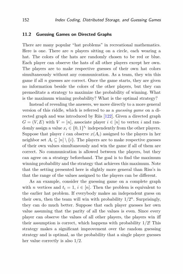
152 Index Coding, Distributed Storage, and Guessing Games
11.2 Guessing Games on Directed Graphs
There are many popular “hat problems” in recreational mathematics.Here is one. There are n players sitting on a circle, each wearing ahat. The colors of the hats are randomly chosen to be red or blue.Each player can observe the hats of all other players except her own.The players are to make respective guesses of their own hat colorssimultaneously without any communication. As a team, they win thisgame if all n guesses are correct. Once the game starts, they are givenno information beside the colors of the other players, but they canpremeditate a strategy to maximize the probability of winning. Whatis the maximum winning probability? What is the optimal strategy?
Instead of revealing the answers, we move directly to a more generalversion of this riddle, which is referred to as a guessing game on a di-rected graph and was introduced by Riis [122]. Given a directed graphG = (V,E) with V = [n], associate player i ∈ [n] to vertex i and ran-domly assign a value xi ∈ 0, 1ti independently from the other players.Suppose that player i can observe x(Ai) assigned to the players in herneighbor set Ai ⊆ [n] \ i. The players are to make respective guessesof their own values simultaneously and win the game if all of them arecorrect. No communication is allowed between the players, but theycan agree on a strategy beforehand. The goal is to find the maximumwinning probability and the strategy that achieves this maximum. Notethat the setting presented here is slightly more general than Riss’s inthat the range of the values assigned to the players can be different.
As an example, consider the guessing game on a complete graphwith n vertices and ti = 1, i ∈ [n]. Then the problem is equivalent tothe earlier hat problem. If everybody makes an independent guess ontheir own, then the team will win with probability 1/2n. Surprisingly,they can do much better. Suppose that each player guesses her ownvalue assuming that the parity of all the values is even. Since everyplayer can observe the values of all other players, the players win ifftheir assumption is correct, which happens with probability 1/2! Thisstrategy makes a significant improvement over the random guessingstrategy and is optimal, as the probability that a single player guessesher value correctly is also 1/2.

11.2. Guessing Games on Directed Graphs 153
Now we formalize the problem with the following definition. A(t1, . . . , tn,W ) guessing strategy consists of
• n guessing functions, where the guessing function of player i ∈ [n],hi :
∏
j∈Ai0, 1tj → 0, 1ti , maps the values of the neighbors
x(Ai) to xi, and
• a winning set W of n-tuples that can be guessed correctly usingthese functions, i.e.,
W :=n⋂
i=1
xn ∈n∏
j=1
0, 1tj : hi(x(Ai)) = xi
.
For the example of the complete graph with n vertices and ti = 1,i ∈ [n], the optimal guessing strategy corresponds to
hi(x(Ai)) =∑
j∈Ai
xj, i ∈ [n],
and
W =
x :n∑
i=1
xi = 0
,
where the summations are modulo 2.
Remark 11.3. This definition of guessing strategy does not includeany random guessing strategy. It can be easily verified, however, thatrandomization does not help, and we thus limit our attention to deter-ministic guessing strategies as in our definition.
Remark 11.4. For any pair of distinct tuples x, z in a winning set Wof a general guessing strategy, either xi = zi or x(Ai) 6= z(Ai) forevery i ∈ [n]. Conversely, any set W satisfying this property is a validwinning set for some guessing functions defined appropriately to satisfyhi(x(Ai)) = xi, i ∈ [n], for every x ∈W .
When the players adopt a (t,W ) strategy, everyone guesses hervalue correctly and the team win with the probability
Pwin =|W |
∏ni=1 2ti
.
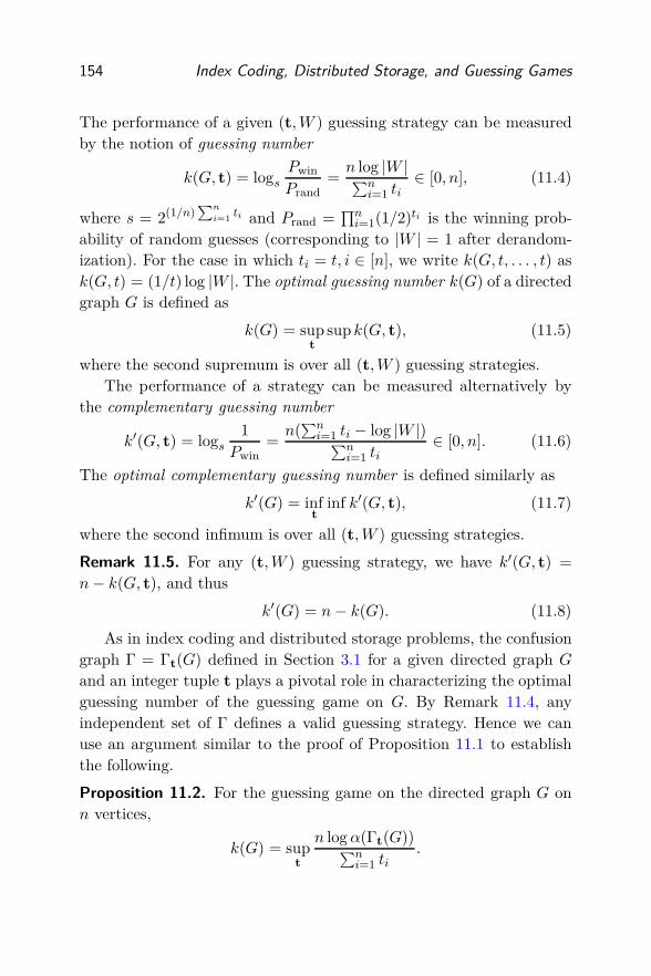
154 Index Coding, Distributed Storage, and Guessing Games
The performance of a given (t,W ) guessing strategy can be measuredby the notion of guessing number
k(G, t) = logsPwin
Prand=n log |W |∑n
i=1 ti∈ [0, n], (11.4)
where s = 2(1/n)∑n
i=1ti and Prand =
∏ni=1(1/2)ti is the winning prob-
ability of random guesses (corresponding to |W | = 1 after derandom-ization). For the case in which ti = t, i ∈ [n], we write k(G, t, . . . , t) ask(G, t) = (1/t) log |W |. The optimal guessing number k(G) of a directedgraph G is defined as
k(G) = supt
sup k(G, t), (11.5)
where the second supremum is over all (t,W ) guessing strategies.The performance of a strategy can be measured alternatively by
the complementary guessing number
k′(G, t) = logs1
Pwin=n(∑n
i=1 ti − log |W |)∑n
i=1 ti∈ [0, n]. (11.6)
The optimal complementary guessing number is defined similarly as
k′(G) = inft
inf k′(G, t), (11.7)
where the second infimum is over all (t,W ) guessing strategies.
Remark 11.5. For any (t,W ) guessing strategy, we have k′(G, t) =
n− k(G, t), and thus
k′(G) = n− k(G). (11.8)
As in index coding and distributed storage problems, the confusiongraph Γ = Γt(G) defined in Section 3.1 for a given directed graph G
and an integer tuple t plays a pivotal role in characterizing the optimalguessing number of the guessing game on G. By Remark 11.4, anyindependent set of Γ defines a valid guessing strategy. Hence we canuse an argument similar to the proof of Proposition 11.1 to establishthe following.
Proposition 11.2. For the guessing game on the directed graph G onn vertices,
k(G) = supt
n logα(Γt(G))∑n
i=1 ti.

11.3. Equivalence of Distributed Storage and Guessing Games 155
11.3 Equivalence of Distributed Storage and Guessing Games
We now consider the distributed storage problem and the guessinggame defined on the same directed graph G on n vertices. For anyinteger tuple t = (t1, . . . , tn), let s(t) = 2(1/n)
∑n
i=1ti . Then the optimal
sum-rate of the distributed storage problem G satisfies
Rsum(G) = minR∈R
n∑
i=1
Ri
= inft
∑ni=1 ti
log α(Γt(G))(11.9)
=n
supt
log α(Γt(G))log s(t)
=n
k(G), (11.10)
where (11.9) follows by Proposition 11.1, and (11.10) follows by Propo-sition 11.2. Hence, the optimal guessing number of the guessing gameon G is inversely related to the optimal sum-rate of the distributedstorage problem G.
Theorem 11.1 ([108, 13]). For any directed graph G on n vertices,
k(G) =n
Rsum(G).
In fact, the guessing game is equivalent to the distributed storageproblem in the following stronger sense, which can be used to proveTheorem 11.1 without involving confusion graphs.
Theorem 11.2. Given any directed graph G on n vertices, a (t,W )
guessing strategy exists iff a (t, r) distributed storage code exists withr = ⌊log |W |⌋.
To prove this, we show that the winning set W and the codebookC = xn(y) : y ∈ [2r ] can be used interchangeably for the two prob-lems. First, consider a (t,W ) guessing strategy. We can then constructa (t, r) distributed storage code by using the winning set of n-tuples Was the codebook C to store the data in r = ⌊log |W |⌋ bits and by using

156 Index Coding, Distributed Storage, and Guessing Games
the guessing functions hi, i ∈ [n], as the recovery functions. Conversely,consider a (t, r) distributed storage code. We can then construct a(t,W ) guessing strategy by setting W = C with |W | = 2r and by usingthe recovery function fi as the guessing function hi of player i ∈ [n],so that every tuple in W can be guessed correctly. This completes theproof of Theorem 11.2.
11.4 Complementarity of Index Coding and Distributed Storage
Let G be a directed graph on n vertices. For any integer tuple t, theconfusion graph Γ = Γt(G) is vertex transitive. Hence, by Remark 2.1,
log χf (Γ) =n∑
i=1
ti − logα(Γ). (11.11)
The left and right hand sides of (11.11) appeared in Theorem 3.1 (seeRemark 3.1 as well) and Proposition 11.1, respectively, which hints ata complementary relationship between the capacity region C (G) of theindex coding problem with side information graph G and the optimalrate region R(G) of the distributed storage problem with storage re-covery graph G. This relationship can be made more precise by thefollowing observation on the µ-directed rates.
Lemma 11.1 ([13]). For any directed graph G on n vertices and anyµ ∈ Qn
≥0,
C(µ) = supr:rµ∈Zn
≥0
r
logχf (Γrµ(G)), (11.12a)
R(µ) = infr:rµ∈Zn
≥0
r
logα(Γrµ(G)). (11.12b)
Now, by this lemma and (11.11), for any µ ∈ Qn≥0,
C(µ) = supr:rµ∈Zn
≥0
r
log χf (Γrµ(G))
= supr:rµ∈Zn
≥0
r
r∑n
i=1 µi − log α(Γrµ(G))
=
( n∑
i=1
µi −1
R(µ)
)−1
.

11.4. Complementarity of Index Coding and Distributed Storage 157
Since Q is dense in R, by the continuity of the functions C(µ) and R(µ),we can establish the following complementary relationship between theµ-directed capacity C(µ) and the µ-directed optimal rate R(µ) for anynonnegative real tuple µ.
Theorem 11.3 ([13]). For any directed graph G on n vertices and anyµ ∈ Rn
≥0,
1
C(µ)=
n∑
i=1
µi −1
R(µ). (11.13)
By Remarks 1.2 and 11.1, Theorem 11.3 establishes the complemen-tarity between the capacity region C (G) of the index coding problemand the optimal rate region R(G) of the distributed storage problem.Given C (G), Theorem 11.3 completely determines R(G) and vice versa.This relationship implies as an important special case (µ = 1) the com-plementarity between the broadcast rate β of the index coding prob-lem and the storage capacity σ (the reciprocal of the optimal symmet-ric rate) of the distributed storage problem established by Mazumdar[108], and by Shanmugam and Dimakis [128].
Corollary 11.1 ([108, 128]). For any n-message index coding problemand n-server distributed storage problem with the same side informa-tion or storage recovery graph G, we have
β(G) = n− σ(G). (11.14)
Remark 11.6. Mazumdar [108] established a stronger and direct code-level complementary relationship between index coding and distributedstorage problems that bypasses the identity in (11.11).
Remark 11.7. Similar to the linear broadcast rate λF, we can definescalar and vector linear codes as well as the linear storage capacity MF
for the distributed storage problem. Shanmugam and Dimakis [128] es-tablished the complementarity between linear index and storage codes,which implies that
λF(G) = n−MF(G).

158 Index Coding, Distributed Storage, and Guessing Games
Remark 11.8. The complementarity in Corollary 11.1, combined withthe approximation results for the complementary index coding raten − β discussed in Remark 9.4, shows that the storage capacity fora general n-server distributed storage problem can be approximatedwithin O(log n log log n) [128]. Tighter approximation results on thestorage capacity for special classes of storage recovery graphs were es-tablished in [108, 109, 1].
Equation (11.11) can also be used to relate the sum-capacity
Csum = maxR∈C
n∑
i=1
Ri
of the index coding problem with the optimal sum-rate Rsum of thedistributed storage problem.
Proposition 11.3 ([13]). For any n-message index coding problem andn-server distributed storage problem with the same side information orstorage recovery graph G, we have
1
Csum(G)= 1− 1
Rsum(G). (11.15)
To prove Proposition 11.3, consider1
Csum(G)=
1
maxR∈C (G)∑n
i=1 Ri
=1
supt
∑n
i=1ti
log χf (Γt(G))
(11.16)
= inft
∑ni=1 ti − logα(Γt(G))
∑ni=1 ti
(11.17)
= 1− 1
minR∈R(G)∑n
i=1 Ri(11.18)
= 1− 1
Rsum(G),
where (11.16) follows by Theorem 3.1, (11.17) follows by (11.11), and(11.18) follows by Proposition 11.1.
Combining Proposition 11.3, Theorem 11.1, and Remark 11.5, wecan also establish the following relationship between the optimal com-plementary guessing number and the index coding sum-capacity.

11.4. Complementarity of Index Coding and Distributed Storage 159
Corollary 11.2. For any directed graph G on n vertices,
k′(G) =n
Csum(G).
In summary, the index coding problem and the locally recoverabledistributed storage problem are equivalent in the sense that the capac-ity region C (G) of the index coding problemG completely characterizesthe optimal rate region R(G) for the distributed storage problem G
and vice versa. The optimal guessing number k(G) and its complementk′(G) of the guessing game on the same graph G are the projections ofR(G) and C (G) in a specific direction. The relationship between thethree problems is summarized in Figure 11.1.
Optimal complementary
guessing number k′(G)
Index coding
capacity region C (G)
Distributed storage
optimal rate region R(G)
Optimal guessing
number k(G)
Figure 11.1: The relationships between the index coding capacity region, the dis-tributed storage optimal rate region, the optimal guessing number, and the optimalcomplementary guessing number defined on the same directed graph. Here a di-rected arrow from problem A to problem B indicates that the solution to A impliesthe solution to B.

12
Further Reading
The literature on index coding is extensive and rapidly growing; see,for example, the dissertations of El Rouayheb [63] and Blasiak [30], aswell as a recent survey [33]. In this section, we provide a few pointersto the topics we have not covered thus far.
12.1 Beyond Multiple Unicast
Throughout this monograph, we considered multiple-unicast demandsof the messages, whereby each of multiple messages is to be recoveredat exactly one receiver. In the more general multiple-groupcast setting,there can be more than one receiver that demands the same message.As an example, consider the 3-message multiple-groupcast index cod-ing problem (1|2), (1|2, 3), (2|3), (3|2) with four receivers 1a, 1b, 2, and3. Both receivers 1a and 1b demand the same message x1, but withdifferent sets of side information x2 and (x2, x3), respectively.
An instance of the multiple-groupcast index coding problem can berepresented naturally by identifying each receiver with a directed hyper-
edge; for instance, (1, 2), (1, 2, 3), (2, 3), and (3, 2) in the aboveexample. This hypergraph extension of index coding was introduced
160

12.2. Noisy Broadcast 161
in [3], and most performance limits and coding schemes we discussedin Sections 5 and 6 can be readily adapted to such hypergraphs; see,for example, [28] for the generalization of the polymatroidal bound forhypergraphs. The broadcast rate of all multiple-groupcast index codingproblems with up to 3 receivers was characterized in [149].
In some applications, such as content distribution networks, eachreceiver may be interested in receiving any message it does not al-ready have as side information. In this pliable index coding problem[31, 138], such flexibility can reduce the amount of communication—sometimes significantly. As an example, for the 3-message pliable indexcoding problem (∗|2), (∗|3), (∗|1, 2), the broadcast rate is 1, achieved bytransmitting x2 + x3, so that x3 is communicated to receivers 1 and 3,while x2 is communicated to receiver 2. In comparison, the regular in-dex coding problem (1|2), (2|3), (3|1, 2) that is consistent with the sameside information sets requires the broadcast rate of 2. As a more triv-ial example, if no receiver has any side information about n messages,pliable index coding allows the transmission of x1 alone (β = 1), whileregular index coding requires the uncoded transmission of (x1, . . . , xn)
(β = n).Sometimes side information at a receiver may not be exactly a set
of other messages, but some functions of the messages (i.e., codewords)that were overheard from past transmissions. This problem of index
coding with coded side information was studied in [50], where both theside information at the receivers as well as the demands themselves canbe linear combinations of the messages; see also [92, 32].
As yet another variation, side information may not be shared syn-chronously between the server and receivers. In the blind index coding
problem [83], the server does not know which side information is avail-able at each receiver, but knows the amount of (coded) side information.In the problem of index coding with erroneous side information [85],the receivers may not have accurate side information.
12.2 Noisy Broadcast
One great simplification in the index coding problem is that the broad-cast link is noiseless. For some practical applications, however, this has

162 Further Reading
to be relaxed. One of the simplest instances of such relaxation is thecomplementary broadcast channel problem [155, 157, 89] depicted inFigure 12.1. This problem generalizes the 2-message index coding prob-lem (1|2), (2|1) by replacing the noiseless broadcast link with a noisybroadcast channel p(v1, v2|u) with input U and outputs V1 and V2 . Asbefore, the messages are Xi ∈ 0, 1ti , i = 1, 2, and the rates of com-munication over r uses of the broadcast channel with codeword U r andits noisy observations V r
1 and V r2 are t1/r and t2/r. Thus, a (t1, t2, r)
code for this problem is defined by the encoder U r = φ(X1,X2) andtwo decoders X1 = ψ1(V r
1 ,X2) and X2 = ψ2(V r2 ,X1). The definitions
of achievable rate pair and capacity region are the same as in the noise-less index coding problem with vanishing average probability of errorpresented in Appendix 1.A. The capacity region for this problem canbe characterized as the closed convex set consisting of all rate pairs(R1, R2) satisfying
R1 ≤ I(U ;V1),
R2 ≤ I(U ;V2)
for some p(u).The communication problem over the broadcast channel with ar-
bitrary receiver side information, which may well be called the noisy
index coding problem, is very difficult in general, even for a small num-ber of messages. For example, the capacity region of the standard two-receiver broadcast channel [48] (corresponding to (1|−), (2|−)) is still
X1, X2 Ur
p(v1, v2|u)
V r1
V r2
X1
X2
X2
X1
Encoder
Decoder 1
Decoder 2
Figure 12.1: The complementary broadcast channel in which each receiver has theother message as side information.

12.3. Distributed Servers 163
open. For several interesting special cases such as Gaussian broadcastchannels, however, the capacity region can be characterized for a coupleof receivers [163, 137, 16].
Several coding techniques have been developed for noisy index cod-ing. Algebraic codes and their performance bounds for index codingwere studied in [52]; see also [32]. Other coding techniques were devel-oped based on modulation [112] and lattices [113, 79].
12.3 Distributed Servers
In some applications, the data is geographically distributed and storedacross many locations. The distributed index coding problem, depictedin Figure 12.2, is an extension of the index coding problem to suchcommunication scenarios. This problem was first studied in [116] andgeneralized in [124] to 2n − 1 servers each encoding some nonemptysubset of messages x(J), J ⊆ [n], to its own codeword under some linkcapacity constraint.
x1
x2
x3
y1
y1,2,3
Encoder 1
Encoder 2
Encoder 3
Encoder 1, 2
Encoder 1, 3
Encoder 2, 3
Encoder 1, 2, 3
Decoder 1
Decoder 2
Decoder 3
x1
x2
x3
x(A1)
x(A2)
x(A3)
Figure 12.2: The distributed index coding problem with three messages.

164 Further Reading
Several performance limits and coding techniques for the central-ized index coding problem we discussed in Sections 5 and 6 can begeneralized to the distributed case [145, 93, 94, 95]. In particular, the(enhanced) composite coding scheme developed in Section 6.10 can beextended naturally to multiple servers by matching composite indicesto the servers that can generate them [94] and by sending the compos-ite indices cooperatively across those servers [93]; see [95] for details.When juxtaposed with a general outer bound that combines polyma-troidal axioms similar to those used in the polymatroidal bound inSection 5.2 with functional dependence separation techniques [88, 144],this distributed composite coding scheme achieves the sum-capacity forall index coding problems with up to four messages under equal linkcapacities was established in [95].
12.4 Security and Privacy
Secure communication against eavesdroppers is an important issue inmany communication networks; see, for example, the seminal paper [37]on secure network coding and its subsequent developments [36, 38, 136,64]. Consider an index coding problem in which an eavesdropper haspartial knowledge of the messages and the broadcast codeword and theserver should prevent the eavesdropper from learning any informationabout some or all messages. This secure index coding problem was firststudied in [51] in the context of scalar linear codes, and subsequentlydeveloped for general nonlinear codes in [118]. The connection betweensecure network coding and secure index coding (which parallels therelationship between nonsecure versions discussed in Section 10) wasdeveloped in [117].
One of the canonical formulations for secure index coding is the casein which the eavesdropper has full access to the broadcast codewordand some subset of messages and it must not learn any informationabout any single message (beyond the side information it already has).For this problem, the flat and composite coding schemes discussed inSection 6 can be readily extended to achieve reliable communicationand weak secrecy (namely, vanishing rate of leaked information) simul-taneously [98]. When compared to the outer bound that augments the

12.4. Security and Privacy 165
polymatroidal bound in Section 5.2 with additional inequalities basedon the secrecy constraints, the secure composite coding scheme achievesthe capacity region for all problems up to three messages [98].
Another canonical formulation is the perfectly secure index coding
problem, in which the eavesdropper has no additional side informa-tion, but it must not learn any information whatsoever about the mes-sages from the broadcast codeword (namely, zero mutual informationas in Shannon’s secrecy system [132]). This perfect secrecy constraintrequires a shared key among the server and receivers. The minimumkey length was studied and characterized approximately in [110].
Sometimes there is no adversarial eavesdropper in the system, but itis desirable to reveal each message only to its designated receiver. Thisprivate index coding problem were studied in [111] with linear codes.Another type of privacy was studied in [84], in which the demand andside information availability of each receiver should be also kept privatefrom other receivers. Index coding in this context is intimately relatedto private information retrieval [44, 19]; see [142] for this intriguingconnection.

Acknowledgments
The authors would like to thank Mike Casey at now publishers for hisconstant encouragement and patience throughout the preparation ofthis monograph, and the Editor, Raymond W. Yeung, and two anony-mous reviewers for their thorough and constructive comments, whichimproved the manuscript significantly. The authors are indebted toBernd Bandemer, Eren Sasoglu, and Lele Wang for their earlier col-laboration that started this work. The initial writing and subsequentrevisions benefited a lot from helpful discussions with the community.In particular, the authors would like to acknowledge Giuseppe Caire,Elena Grigorescu, Michael Langberg, Min Li, Yucheng Liu, Yuxin Liu,Arya Mazumdar, Lawrence Ong, Alex Sprintson, Jacques Verstraete,Xinping Yi, Ken Zeger, and Minshen Zhu. But most of all, the authorswould like to express their sincerest gratitude to Parastoo Sadeghi forher detailed reading of the manuscript at various stages and for hergenerous contribution of several technical results, which fundamentallyreshaped the manuscript.
This work was supported in part by the National Science Founda-tion (NSF) under Grant CCF-1320895 and by the Korean Institute forInformation and Communications Technology Promotion (IITP) underGrant B0132-15-1005.
166

References
[1] Agarwal, A., L. Flodin, and A. Mazumdar (2018). “Linear pro-gramming approximations for index coding”. url: https://arxiv.org/abs/1807.071
[2] Ahlswede, R., N. Cai, S.-Y. R. Li, and R. W. Yeung (2000).“Network information flow”. IEEE Trans. Inf. Theory. 46(4):1204–1216.
[3] Alon, N., A. Hassidim, E. Lubetzky, U. Stav, and A. Wein-stein (2008). “Broadcasting with side information”. In: Proc.
49th Ann. IEEE Symp. Found. Comput. Sci. Philadelphia, PA.823–832.
[4] Alon, N. and N. Kahale (1998). “Approximating the indepen-dence number via the Θ-function”. Math. Prog. 80(3): 253–264.
[5] Alon, N. and A. Orlitsky (1996). “Source coding and graph en-tropies”. IEEE Trans. Inf. Theory. 42(5): 1329–1339.
[6] Appel, K., W. Haken, and J. Koch (1977). “Every planar mapis four colorable—II: Reducibility”. Illinois J. Math. 21(3): 491–567.
[7] Arbabjolfaei, F., B. Bandemer, and Y.-H. Kim (2014). “Indexcoding via random coding”. In: Proc. 2nd Iran Workshop Com-
mun. Inf. Theory. Tehran, Iran. 1–7.[8] Arbabjolfaei, F., B. Bandemer, Y.-H. Kim, E. Sasoglu, and L.
Wang (2013). “On the capacity region for index coding”. In:Proc. IEEE Int. Symp. Inf. Theory. Istanbul, Turkey. 962–966.
167

168 References
[9] Arbabjolfaei, F. and Y.-H. Kim (2014). “Local time sharing forindex coding”. In: Proc. IEEE Int. Symp. Inf. Theory. Honolulu,HI. 286–290.
[10] Arbabjolfaei, F. (2017). “Index coding: Fundamental limits, cod-ing schemes, and structural properties”. Ph.D. Thesis. La Jolla,CA: University of California, San Diego.
[11] Arbabjolfaei, F. and Y.-H. Kim (2015a). “On critical index cod-ing problems”. In: Proc. IEEE Inf. Theory Workshop. Jeju Is-land, Korea. 9–13.
[12] Arbabjolfaei, F. and Y.-H. Kim (2015b). “Structural propertiesof index coding capacity using fractional graph theory”. In: Proc.
IEEE Int. Symp. Inf. Theory. Hong Kong. 1034–1038.[13] Arbabjolfaei, F. and Y.-H. Kim (2015c). “Three stories on a two-
sided coin: Index coding, locally recoverable distributed storage,and guessing games on graphs”. In: Proc. 53rd Ann. Allerton
Conf. Comm. Control Comput. Monticello, IL. 843–850.[14] Arbabjolfaei, F. and Y.-H. Kim (2016). “Approximate capacity
of index coding for some classes of graphs”. In: Proc. IEEE Int.
Symp. Inf. Theory. Barcelona, Spain. 2154–2158.[15] Arbabjolfaei, F. and Y.-H. Kim (2017). “Generalized lexico-
graphic products and index coding capacity region”. url: https://arxiv.org/abs/1608.0368[16] Asadi, B., L. Ong, and S. J. Johnson (2015). “Optimal coding
schemes for the three-receiver AWGN broadcast channel withreceiver message side information”. IEEE Trans. Inf. Theory.61(10): 5490–5503.
[17] Baber, R., D. Christofides, A. N. Dang, S. Riis, and E. R.Vaughan (2013). “Multiple unicasts, graph guessing games, andnon-Shannon inequalities”. In: Proc. Int. Symp. Netw. Coding.Calgary, AB. 1–6.
[18] Bachem, A. and W. Kern (1992). Linear Programming Duality:
An Introduction to Oriented Matroids. Berlin: Springer.[19] Banawan, K. and S. Ulukus (2018). “The capacity of private
information retrieval from coded databases”. IEEE Trans. Inf.
Theory. 64(3): 1945–1956.

References 169
[20] Bandemer, B., A. El Gamal, and Y.-H. Kim (2015). “Optimalachievable rates for interference networks with random codes”.IEEE Trans. Inf. Theory. 61(12): 6536–6549.
[21] Bar-Yossef, Z., Y. Birk, T. S. Jayram, and T. Kol (2006). “Indexcoding with side information”. In: Proc. 47th Ann. IEEE Symp.
Found. Comput. Sci. Berkeley, CA. 197–206.[22] Bar-Yossef, Z., Y. Birk, T. S. Jayram, and T. Kol (2011). “Index
coding with side information”. IEEE Trans. Inf. Theory. 57(3):1479–1494.
[23] Belmonte, R., P. Heggernes, P. van’t Hof, A. Rafiey, and R. Saei(2014). “Graph classes and Ramsey numbers”. Discrete Appl.
Math. 173: 16–27.[24] Berliner, Y. and M. Langberg (2011). “Index coding with outer-
planar side information”. In: Proc. IEEE Int. Symp. Inf. Theory.Saint Petersburg, Russia. 806–810.
[25] Birk, Y. and T. Kol (1998). “Informed-source coding-on-demand(ISCOD) over broadcast channels”. In: Proc. 17th Ann. IEEE
Int. Conf. Comput. Commun. (INFOCOM). San Francisco, CA.1257–1264.
[26] Birk, Y. and T. Kol (2006). “Coding on demand by an informedsource (ISCOD) for efficient broadcast of different supplementaldata to caching clients”. IEEE Trans. Inf. Theory. 52(6): 2825–2830.
[27] Blackwell, D., L. Breiman, and A. J. Thomasian (1959). “Thecapacity of a class of channels”. Ann. Math. Statist. 30(4): 1229–1241.
[28] Blasiak, A., R. Kleinberg, and E. Lubetzky (2011). “Lexico-graphic products and the power of non-linear network coding”.In: Proc. 52nd Ann. IEEE Symp. Found. Comput. Sci. PalmSprings, CA. 609–618.
[29] Blasiak, A., R. Kleinberg, and E. Lubetzky (2013). “Broad-casting with side information: Bounding and approximating thebroadcast rate”. IEEE Trans. Inf. Theory. 59(9): 5811–5823.
[30] Blasiak, A. (2013). “A graph-theoretic approach to network cod-ing”. PhD thesis. Cornell University.
170 References
[31] Brahma, S. and C. Fragouli (2015). “Pliable index coding”.IEEE Trans. Inf. Theory. 61(11): 6192–6203.
[32] Byrne, E. and M. Calderini (2017). “Error correction for indexcoding with coded side information”. IEEE Trans. Inf. Theory.63(6): 3712–3728.
[33] Byrne, E. and M. Calderini (2018). “Index coding, network cod-ing and broadcast with side-information”. In: Network Coding
and Subspace Designs. Ed. by M. Greferath, M. O. Pavčević, N.Silberstein, and M. Á. Vázquez-Castro. Cham: Springer. 247–293.
[34] Cadambe, V. R. and S. A. Jafar (2008). “Interference align-ment and degrees of freedom of the K-user interference chan-nel”. IEEE Trans. Inf. Theory. 54(8): 3425–3441.
[35] Cadambe, V. R., S. A. Jafar, H. Maleki, K. Ramchandran, andC. Suh (2013). “Asymptotic interference alignment for optimalrepair of MDS codes in distributed storage”. IEEE Trans. Inf.
Theory. 59(5): 2974–2987.[36] Cai, N. and T. Chan (2011). “Theory of secure network coding”.
Proc. IEEE. 99(3): 421–437.[37] Cai, N. and R. W. Yeung (2002). “Secure network coding”. In:
Proc. IEEE Int. Symp. Inf. Theory. Lausanne, Switzerland. 323.[38] Cai, N. and R. W. Yeung (2011). “Secure network coding on a
wiretap network”. IEEE Trans. Inf. Theory. 57(1): 424–435.[39] Celebiler, M. and G. Stette (1978). “On increasing the down-
link capacity of a regenerative satellite repeater in point-to-pointcommunications”. Proc. IEEE. 66(1): 98–100.
[40] Chan, T. and A. Grant (2008). “Dualities between entropy func-tions and network codes”. IEEE Trans. Inf. Theory. 54(10):4470–4487.
[41] Chan, T. and A. Grant (2010). “On capacity regions of non-multicast networks”. In: Proc. IEEE Int. Symp. Inf. Theory.Austin, TX. 2378–2382.
[42] Chartrand, G. and F. Harary (1967). “Planar permutation graphs”.Ann. Inst. H. Poincaré B. 3: 433–438.
References 171
[43] Chaudhry, M. A. R., Z. Asad, A. Sprintson, and M. Lang-berg (2011). “On the complementary index coding problem”.In: Proc. IEEE Int. Symp. Inf. Theory. Saint Petersburg, Rus-sia. 244–248.
[44] Chor, B., O. Goldreich, E. Kushilevitz, and M. Sudan (1995).“Private information retrieval”. In: 36th Ann. IEEE Symp. Found.
Comp. Sci. Milwaukee, WI. 41–50.[45] Chudnovsky, M., N. Robertson, P. Seymour, and R. Thomas
(2006). “The strong perfect graph theorem”. Ann. Math. 164(1):51–229.
[46] Chudnovsky, M. and P. Seymour (2005). “The structure of claw-free graphs”. In: Surv. Combin. Ed. by B. S. Webb. Cambridge:Cambridge University Press. 153–171.
[47] Connelly, J. M. (2018). “Linear network coding over ring alpha-bets”. Ph.D. Thesis. La Jolla, CA: University of California, SanDiego.
[48] Cover, T. M. (1972). “Broadcast channels”. IEEE Trans. Inf.
Theory. 18(1): 2–14.[49] Cover, T. M. and J. A. Thomas (2006). Elements of Information
Theory. Second. New York: Wiley.[50] Dai, M., K. W. Shum, and C. W. Sung (2014). “Data dissemina-
tion with side information and feedback”. IEEE Trans. Wireless
Commun. 13(9): 1536–1276.[51] Dau, S. H., V. Skachek, and Y. M. Chee (2012). “On the secu-
rity of index coding with side information”. IEEE Trans. Inf.
Theory. 58(6): 3975–3988.[52] Dau, S. H., V. Skachek, and Y. M. Chee (2013). “Error correc-
tion for index coding with side information”. IEEE Trans. Inf.
Theory. 59(3): 1517–1531.[53] Dobrushin, R. L. (1959). “Optimum information transmission
through a channel with unknown parameters”. Radio Eng. Elec-
tron. 4(12): 1–8.[54] Dougherty, R., C. Freiling, and K. Zeger (2006). “Unachievabil-
ity of network coding capacity”. IEEE Trans. Inf. Theory. 52(6):2365–2372.

172 References
[55] Dougherty, R., C. Freiling, and K. Zeger (2011a). “Network cod-ing and matroid theory”. Proc. IEEE. 99(3): 388–405.
[56] Dougherty, R., C. Freiling, and K. Zeger (2011b). “Non-Shannoninformation inequalities in four random variables”. url: http://arxiv.org/abs/1104.3602
[57] Dougherty, R., C. Freiling, and K. Zeger (2005). “Insufficiencyof linear coding in network information flow”. IEEE Trans. Inf.
Theory. 51(8): 2745–2759.[58] Dueck, G. (1978). “Maximal error capacity regions are smaller
than average error capacity regions for multi-user channels”.Probl. Control Inf. Theory. 7(1): 11–19.
[59] Effros, M., S. El Rouayheb, and M. Langberg (2015). “An equiv-alence between network coding and index coding”. IEEE Trans.
Inf. Theory. 61(5): 2478–2487.[60] El Gamal, A. and Y.-H. Kim (2011). Network Information The-
ory. Cambridge: Cambridge University Press.[61] El Rouayheb, S., A. Sprintson, and C. Georghiades (2010). “On
the index coding problem and its relation to network coding andmatroid theory”. IEEE Trans. Inf. Theory. 56(7): 3187–3195.
[62] El Rouayheb, S., M. Chaudhry, and A. Sprintson (2007). “Onthe minimum number of transmissions in single-hop wirelesscoding networks”. In: Proc. IEEE Inf. Theory Workshop. TahoeCity, CA. 120–125.
[63] El Rouayheb, S. Y. (2009). “Network and Index Coding withApplication to Robust and Secure Communications”. PhD the-
sis. Texas A & M University.[64] El Rouayheb, S., E. Soljanin, and A. Sprintson (2012). “Secure
network coding for wiretap networks of type II”. IEEE Trans.
Inf. Theory. 58(3): 1361–1371.[65] Erdös, P., Z. Füredi, A. Hajnal, P. Komjáth, V. Rödl, and Á.
Seress (1986). “Coloring graphs with locally few colors”. Dis-
crete Math. 59(1): 21–34.[66] Erdös, P. and L. Moser (1964). “On the representation of di-
rected graphs as unions of orderings”. Publ. Math. Inst. Hungar.
Acad. Sci. 9: 125–132.

References 173
[67] Erdös, P. and G. Szekeres (1935). “A combinatorial problem ingeometry”. Compositio Math. 2: 463–470.
[68] Fekete, M. (1923). “Uber die Verteilung der Wurzeln bei gewis-sen algebraischen Gleichungen mit ganzzahligen Koeffizienten”.Math. Z. 17(1): 228–249.
[69] Fragouli, C. and E. Soljanin (Dec. 2007a). “Network coding ap-plications”. Found. Trends Netw. 2(2): 135–269.
[70] Fragouli, C. and E. Soljanin (Jan. 2007b). “Network coding fun-damentals”. Found. Trends Netw. 2(1): 1–133.
[71] Fujishige, S. (2005). Submodular Functions and Optimization.Second. Amsterdam: Elsevier.
[72] Gadouleau, M. and S. Riis (2011). “Graph-theoretical construc-tions for graph entropy and network coding based communica-tions”. IEEE Trans. Inf. Theory. 57(10): 6703–6717.
[73] Golovnev, A., O. Regev, and O. Weinstein (2018). “The minrankof random graphs”. IEEE Trans. Inf. Theory. 64.
[74] Haemers, W. (1978). “An upper bound for the Shannon capacityof a graph”. Colloq. Math. Soc. Janos Bolyai. 25: 267–272.
[75] Haemers, W. (1979). “On some problems of Lovász concerningthe Shannon capacity of a graph”. IEEE Trans. Inf. Theory.25(2): 231–232.
[76] Hammack, R., W. Imrich, and S. Klavzar (2011). Handbook of
Product Graphs. Second. Boca Raton, FL: CRC Press.[77] Haviv, I. and M. Langberg (2012). “On linear index coding for
random graphs”. In: Proc. IEEE Int. Symp. Inf. Theory. Cam-bridge, MA. 2231–2235.
[78] Ho, T. and D. Lun (2008). Network Coding: An Introduction.Cambridge: Cambridge University Press.
[79] Huang, Y.-C. (2017). “Lattice index codes from algebraic num-ber fields”. IEEE Trans. Inf. Theory. 63(4): 2098–2112.
[80] Huang, X. and S. El Rouayheb (2015). “Index coding and net-work coding via rank minimization”. In: Proc. IEEE Inf. Theory
Workshop. Jeju Island, Korea. 14–18.[81] Jafar, S. A. (2014). “Topological interference management through
index coding”. IEEE Trans. Inf. Theory. 60(1): 529–568.

174 References
[82] Ji, M., G. Caire, and A. F. Molisch (2016). “Fundamental limitsof caching in wireless D2D networks”. IEEE Trans. Inf. Theory.62(2): 849–869.
[83] Kao, D. T. H., M. A. Maddah-Ali, and A. S. Avestimehr (2017).“Blind index coding”. IEEE Trans. Inf. Theory. 63(4): 2076–2097.
[84] Karmoose, M., L. Song, M. Cardone, and C. Fragouli (2017).“Private broadcasting: An index coding approach”. In: Proc.
IEEE Int. Symp. Inf. Theory. Aachen, Germany. 2543–2547.[85] Kim, J.-W. and J.-S. No (2017). “Index coding with erroneous
side information”. IEEE Trans. Inf. Theory. 63(12): 7687–7697.[86] Körner, J. and A. Orlitsky (1998). “Zero-error information the-
ory”. IEEE Trans. Inf. Theory. 44(6): 2207–2229.[87] Körner, J., C. Pilotto, and G. Simonyi (2005). “Local chro-
matic number and Sperner capacity”. J. Combin. Theory Ser.
B. 95(1): 101–117.[88] Kramer, G. (1998). Directed Information for Channels with Feed-
back. Dr. sc. thchn. Dissertation, Swiss Federal Institute of Tech-nology (ETH) Zurich. Konstanz: Hartung-Gorre Verlag.
[89] Kramer, G. and S. Shamai (2007). “Capacity for classes of broad-cast channels with receiver side information”. In: Proc. IEEE
Inf. Theory Workshop. Tahoe City, CA. 313–318.[90] Langberg, M. and M. Effros (2011). “Network coding: Is zero er-
ror always possible?” In: Proc. 49th Ann. Allerton Conf. Comm.
Control Comput. Monticello, IL. 1478–1485.[91] Langberg, M. and A. Sprintson (2011). “On the hardness of
approximating the network coding capacity”. IEEE Trans. Inf.
Theory. 57(2): 1008–1014.[92] Lee, N., A. G. Dimakis, and R. W. Heath (2015). “Index coding
with coded side-information”. IEEE Comm. Lett. 19(3): 319–322.
[93] Li, M., L. Ong, and S. J. Johnson (2017). “Improved boundsfor multi-sender index coding”. In: Proc. IEEE Int. Symp. Inf.
Theory. Aachen, Germany. 3060–3064.

References 175
[94] Liu, Y., P. Sadeghi, F. Arbabjolfaei, and Y.-H. Kim (2017). “Onthe capacity for distributed index coding”. In: Proc. IEEE Int.
Symp. Inf. Theory. Aachen, Germany. 3065–3069.[95] Liu, Y., P. Sadeghi, F. Arbabjolfaei, and Y.-H. Kim (2018a).
“Capacity theorems for distributed index coding”. url: http://arxiv.org/abs/1801.090[96] Liu, Y., P. Sadeghi, F. Arbabjolfaei, and Y.-H. Kim (2018b).
“Simplified composite coding for index coding”. In: Proc. IEEE
Int. Symp. Inf. Theory. Vail, CO. 456–460.[97] Liu, Y., P. Sadeghi, and Y.-H. Kim (2018c). “Three-layer com-
posite coding for index coding”. In: Proc. IEEE Inf. Theory
Workshop. Guangzhou, China.[98] Liu, Y., B. N. Vellambi, P. Sadeghi, and Y.-H. Kim (2018d). “On
the capacity region for secure index coding”. In: Proc. IEEE Inf.
Theory Workshop. Guangzhou, China.[99] Lovász, L. (1972). “Normal hypergraphs and the perfect graph
conjecture”. Discrete Math. 2(3): 253–267.[100] Lovász, L. (1979). “On the Shannon capacity of a graph”. IEEE
Trans. Inf. Theory. 25(1): 1–7.[101] Lubetzky, E. and U. Stav (2009). “Nonlinear index coding out-
performing the linear optimum”. IEEE Trans. Inf. Theory. 55(8):3544–3551.
[102] Maddah-Ali, M. A., A. S. Motahari, and A. K. Khandani (2008).“Communication over MIMO X channels: Interference align-ment, decomposition, and performance analysis”. IEEE Trans.
Inf. Theory. 54(8): 3457–3470.[103] Maddah-Ali, M. A. and U. Niesen (2014). “Fundamental limits
of caching”. IEEE Trans. Inf. Theory. 60(5): 2856–2867.[104] Maleki, H., V. R. Cadambe, and S. A. Jafar (2014). “Index
coding: An interference alignment perspective”. IEEE Trans.
Inf. Theory. 60(9): 5402–5432.[105] Marton, K. (1979). “A coding theorem for the discrete memory-
less broadcast channel”. IEEE Trans. Inf. Theory. 25(3): 306–311. issn: 0018-9448.
[106] Matthews, M. M. and D. P. Sumner (1985). “Longest paths andcycles in K1,3-free graphs”. J. Graph Theory. 9(2): 269–277.

176 References
[107] Matúš, F. (2007). “Infinitely many information inequalities”. In:Proc. IEEE Int. Symp. Inf. Theory. Nice, France. 41–44.
[108] Mazumdar, A. (2015). “Storage capacity of repairable networks”.IEEE Trans. Inf. Theory. 61(11): 5810–5821.
[109] Mazumdar, A., A. McGregor, and S. Vorotnikova (2017). “Stor-age capacity as an information-theoretic analogue of vertex cover”.url: https://arxiv.org/abs/1706.09197.
[110] Mojahedian, M. M., M. R. Aref, and A. Gohari (2017). “Per-fectly secure index coding”. IEEE Trans. Inf. Theory. 63(11):7382–7395.
[111] Narayanan, V., V. M. Prabhakaran, J. Ravi, V. K. Mishra, B. K.Dey, and N. Karamchandani (2018). “Private index coding”. In:Proc. IEEE Int. Symp. Inf. Theory. Vail, CO. 596–600.
[112] Natarajan, L., Y. Hong, and E. Viterbo (2015a). “Index codesfor the Gaussian broadcast channel using quadrature amplitudemodulation”. IEEE Comm. Lett. 19(8): 1291–1294.
[113] Natarajan, L., Y. Hong, and E. Viterbo (2015b). “Lattice indexcoding”. IEEE Trans. Inf. Theory. 61(12): 6505–6525.
[114] Neely, M. J., A. S. Tehrani, and Z. Zhang (2013). “Dynamicindex coding for wireless broadcast networks”. IEEE Trans. Inf.
Theory. 59(11): 7525–7540.[115] Ong, L. (2017). “Optimal finite-length and asymptotic index
codes for five or fewer receivers”. IEEE Trans. Inf. Theory.63(11): 7116–7130.
[116] Ong, L., C. K. Ho, and F. Lim (2016a). “The single unipriorindex coding problem: The single sender case and the multisender extension”. IEEE Trans. Inf. Theory. 62(6): 3165–3182.
[117] Ong, L., J. Kliewer, and B. N. Vellambi (2018). “Secure network-index code equivalence: Extension to non-zero error and leak-age”. In: Proc. IEEE Int. Symp. Inf. Theory. Vail, CO. 841–845.
[118] Ong, L., B. N. Vellambi, P. L. Yeoh, J. Kliewer, and J. Yuan(2016b). “Secure index coding: Existence and construction”. In:Proc. IEEE Int. Symp. Inf. Theory. Barcelona, Spain. 2834–2838.

References 177
[119] Ore, O. (1962). Theory of Graphs. Providence, RI: AmericanMathematical Society.
[120] Papailiopoulos, D., A. G. Dimakis, and V. Cadambe (2013).“Repair optimal erasure codes through Hadamard designs”. IEEE
Trans. Inf. Theory. 59(5): 3021–3037.[121] Peeters, R. (1996). “Orthogonal representations over finite fields
and the chromatic number of graphs”. Combinatorica. 16(3):417–431.
[122] Riis, S. (2007). “Information flows, graphs and their guessingnumbers”. Elec. J. Comb. 14(R44): 1–17.
[123] Sabidussi, G. (1957). “Graphs with given group and given graph-theoretical properties”. Canad. J. Math. 9(4): 515–525.
[124] Sadeghi, P., F. Arbabjolfaei, and Y.-H. Kim (2016). “Distributedindex coding”. In: Proc. IEEE Inf. Theory Workshop. Cam-bridge, UK. 330–334.
[125] Scheinerman, E. R. and D. H. Ullman (2011). Fractional Graph
Theory: A Rational Approach to the Theory of Graphs. NewYork: Dover Publications.
[126] Schrijver, A. (2003). Combinatorial Optimization. 3 vols. Berlin:Springer-Verlag.
[127] Shah, N. B., K. V. Rashmi, P. V. Kumar, and K. Ramchan-dran (2012). “Distributed storage codes with repair-by-transferand nonachievability of interior points on the storage-bandwidthtradeoff”. IEEE Trans. Inf. Theory. 58(3): 1837–1852.
[128] Shanmugam, K. and A. G. Dimakis (2014). “Bounding multipleunicasts through index coding and locally repairable codes”. In:Proc. IEEE Int. Symp. Inf. Theory. Honolulu, HI. 296–300.
[129] Shanmugam, K., A. G. Dimakis, and M. Langberg (2013). “Lo-cal graph coloring and index coding”. In: Proc. IEEE Int. Symp.
Inf. Theory. Istanbul, Turkey. 1152–1156.[130] Shanmugam, K., A. G. Dimakis, and M. Langberg (2014). “Graph
theory versus minimum rank for index coding”. In: Proc. IEEE
Int. Symp. Inf. Theory. Honolulu, HI. 291–295.

178 References
[131] Shanmugam, K., M. Asteris, and A. G. Dimakis (2015). “On ap-proximating the sum-rate for multiple-unicasts”. In: Proc. IEEE
Int. Symp. Inf. Theory. Hong Kong. 381–385.[132] Shannon, C. E. (1949). “Communication theory of secrecy sys-
tems”. Bell Syst. Tech. J. 28(4): 656–715. issn: 0005-8580.[133] Shannon, C. E. (1948). “A mathematical theory of communica-
tion”. Bell Syst. Tech. J. 27(3): 379–423, 27(4), 623–656.[134] Shannon, C. E. (1956). “The zero error capacity of a noisy chan-
nel”. IRE Trans. Inf. Theory. 2(3): 8–19.[135] Shannon, C. E. (1959). “Coding theorems for a discrete source
with a fidelity criterion”. In: IRE Int. Conv. Rec. Vol. 7, part 4.142–163.
[136] Silva, D. and F. R. Kschischang (2011). “Universal secure net-work coding via rank-metric codes”. IEEE Trans. Inf. Theory.57(2): 1124–1135.
[137] Sima, J. and W. Chen (2014). “Joint network and Gelfand–Pinsker coding for 3-receiver Gaussian broadcast channels withreceiver message side information”. In: Proc. IEEE Int. Symp.
Inf. Theory. Honolulu, HI. 81–85.[138] Song, L. and C. Fragouli (2018). “A polynomial-time algorithm
for pliable index coding”. IEEE Trans. Inf. Theory. 64(2): 979–999.
[139] Stearns, R. (1959). “The voting problem”. Amer. Math. Monthly.66(9): 761–763.
[140] Steinberg, R. and C. A. Tovey (1993). “Planar Ramsey num-bers”. J. Combin. Theory Ser. B. 59(2): 288–296.
[141] Sun, H. and S. A. Jafar (2015). “Index coding capacity: How farcan one go with only Shannon inequalities?” IEEE Trans. Inf.
Theory. 61(6): 3041–3055.[142] Sun, H. and S. A. Jafar (2017). “The capacity of private infor-
mation retrieval”. IEEE Trans. Inf. Theory. 63(7): 4075–4088.[143] Tahmasbi, M., A. Shahrasbi, and A. Gohari (2015). “Critical
graphs in index coding”. IEEE J. Sel. Areas Commun. 33(2):225–235.

References 179
[144] Thakor, S., A. Grant, and T. Chan (2016). “Cut-set boundson network information flow”. IEEE Trans. Inf. Theory. 62(4):1850–1865.
[145] Thapa, C., L. Ong, and S. J. Johnson (2016). “Graph-theoreticapproaches to two-sender index coding”. In: Proc. IEEE Global
Telecommun. Conf. Washington, DC. 1–6.[146] Thapa, C., L. Ong, and S. J. Johnson (2017). “Interlinked cycles
for index coding: Generalizing cycles and cliques”. IEEE Trans.
Inf. Theory. 63(6): 3692–3711.[147] “The On-Line Encyclopedia of Integer Sequences” (n.d.). url:
http://oeis.org/A000273.[148] Turán, P. (1941). “Eine extremalaufgabe aus der graphentheo-
rie”. Mat. Fiz. Lapok. 48: 436–452.[149] Unal, S. and A. B. Wagner (2016). “A rate–distortion approach
to index coding”. IEEE Trans. Inf. Theory. 62(11): 6359–6378.[150] Urbanke, R. and Q. Li (1998). “The zero-error capacity region
of the 2-user synchronous BAC is strictly smaller than its Shan-non capacity region”. In: Proc. IEEE Inf. Theory Workshop.Killarney, Ireland. 61.
[151] Willems, F. M. J. (1990). “The maximal-error and average-errorcapacity region of the broadcast channel are identical: A directproof”. Probl. Control Inf. Theory. 19(4): 339–347.
[152] Willems, F. M. J., J. K. Wolf, and A. D. Wyner (1989). “Com-municating via a processing broadcast satellite”. In: Proc. IEEE/
CAM Inf. Theory Workshop. Cornell, NY. 3–1.[153] Witsenhausen, H. S. (1976). “The zero-error side information
problem and chromatic numbers”. IEEE Trans. Inf. Theory.22(5): 592–593.
[154] Wolfowitz, J. (1960). “Simultaneous channels”. Arch. Rational
Mech. Anal. 4(1): 371–386.[155] Wu, Y. (2007). “Broadcasting when receivers know some mes-
sages a priori”. In: Proc. IEEE Int. Symp. Inf. Theory. Nice,France. 1141–1145.

180 References
[156] Wyner, A. D., J. K. Wolf, and F. M. J. Willems (2002). “Com-municating via a processing broadcast satellite”. IEEE Trans.
Inf. Theory. 48(6): 1243–1249.[157] Xue, F. and S. Sandhu (2007). “PHY-layer network coding for
broadcast channel with side information”. In: Proc. IEEE Inf.
Theory Workshop. Lake Tahoe, CA. 108–113.[158] Yeung, R. W. (1995). “Multilevel diversity coding with distor-
tion”. IEEE Trans. Inf. Theory. 41(2): 412–422.[159] Yeung, R. W. (2008). Information Theory and Network Coding.
New York: Springer.[160] Yeung, R. W. and Z. Zhang (1999). “Distributed source coding
for satellite communications”. IEEE Trans. Inf. Theory. 45(4):1111–1120.
[161] Yi, X. and G. Caire (2018). Private communication.[162] Yi, X., H. Sun, S. A. Jafar, and D. Gesbert (2018). “TDMA is
optimal for all-unicast DoF region of TIM if and only if topologyis chordal bipartite”. IEEE Trans. Inf. Theory. 64(3): 2065–2076.
[163] Yoo, J. W., T. Liu, and F. Xue (2009). “Gaussian broadcastchannels with receiver message side information”. In: Proc. IEEE
Int. Symp. Inf. Theory. Seoul, Korea. 2472–2476.[164] Yu, H. and M. J. Neely (2014). “Duality codes and the inte-
grality gap bound for index coding”. IEEE Trans. Inf. Theory.60(11): 7256–7268.
[165] Zhang, Z. and R. W. Yeung (1998). “On characterization ofentropy function via information inequalities”. IEEE Trans. Inf.
Theory. 44(4): 1440–1452.