A Paper presented to the MSC User Conference, Daventry, UK

June 18th 1999

FATIGUE ANALYSIS OF AN F16 NAVIGATION POD

NWM Bishop1, N Davies2, A Caserio1, S Kerr1

1MacNeal Schwendler Corporation, Lyon Way, Frimley, Camberley, Surrey, UK, GU16 5ER.2Marconi Naval Systems Ltd, Product Assurance Group, West Hanningfield Road, Great Baddow, Essex, CM2 8HN.

ABSTRACT

An F16 POD containing optical equipment has been analysed using MSC.Fatigue. The purpose of the analysis was to showthat current procedures could be improved in 3 ways. Firstly, a more accurate and widely applicable procedure based uponthe Dirlik algorithm is used to compute fatigue damage from output PSD’s of stress. Secondly, these calculations areperformed on Principal stress axes (current FEA solvers such as NASTRAN, ABAQUS and ANSYS do not allow rotation oftransfer functions onto Principal planes). Lastly, the calculations are automatically performed over the entire region ofinterest. Results for fatigue life are presented for a number of input loading conditions.

1. INTRODUCTION

The Marconi Electronic Systems (MES) Atlantic POD isdesigned to attach to the fuselage of the F16 aircraft, (seeFigure 1). Its primary purpose is to provide night vision for the pilot via its forward looking infrared (FLIR) system.The infrared pictures can be seen by the pilot using hishead-up display unit (HUD) in the cockpit.

Figure 1. Atlantic Navigation POD attached to F16

The POD is basically a 10 inch diameter, 97 inch long, tube with a front and rear bulkhead containing three primaryunits; the electronics module, the environmental control unit and, most importantly, the sensor head assembly. Thesensor head is mounted at the very front of the POD on two parallel longitudinal arms that attach primarily to theforward bulkhead. An early version of the Atlantic POD isshown in Figure 2. The sensor head houses the infra red

cameras, lens assemblies and other sensors used for highspeed, low level night time sorties.

During the conceptual design of the POD, the sensor headmounting arms were ‘tuned’ to give the right response sothat boresight error resulting from vibration of the sensorcould be minimised. The consequence, however, of thistuning was a weakening of the rear of the arms, as they were reduced from a thick solid section to a thinner cut-out one.

Figure 2. Concept Stage Atlantic Navigation POD

It was required to assess whether this weakening of thestructure would cause problems under the severe randomvibration loads applied to the POD. For this reason it wasdecided to perform a random vibration fatigue analysis onthe POD structure to the levels and duration’s defined in the POD test certification specification. An example of thetypes of input loads that might be used are shown in Figure

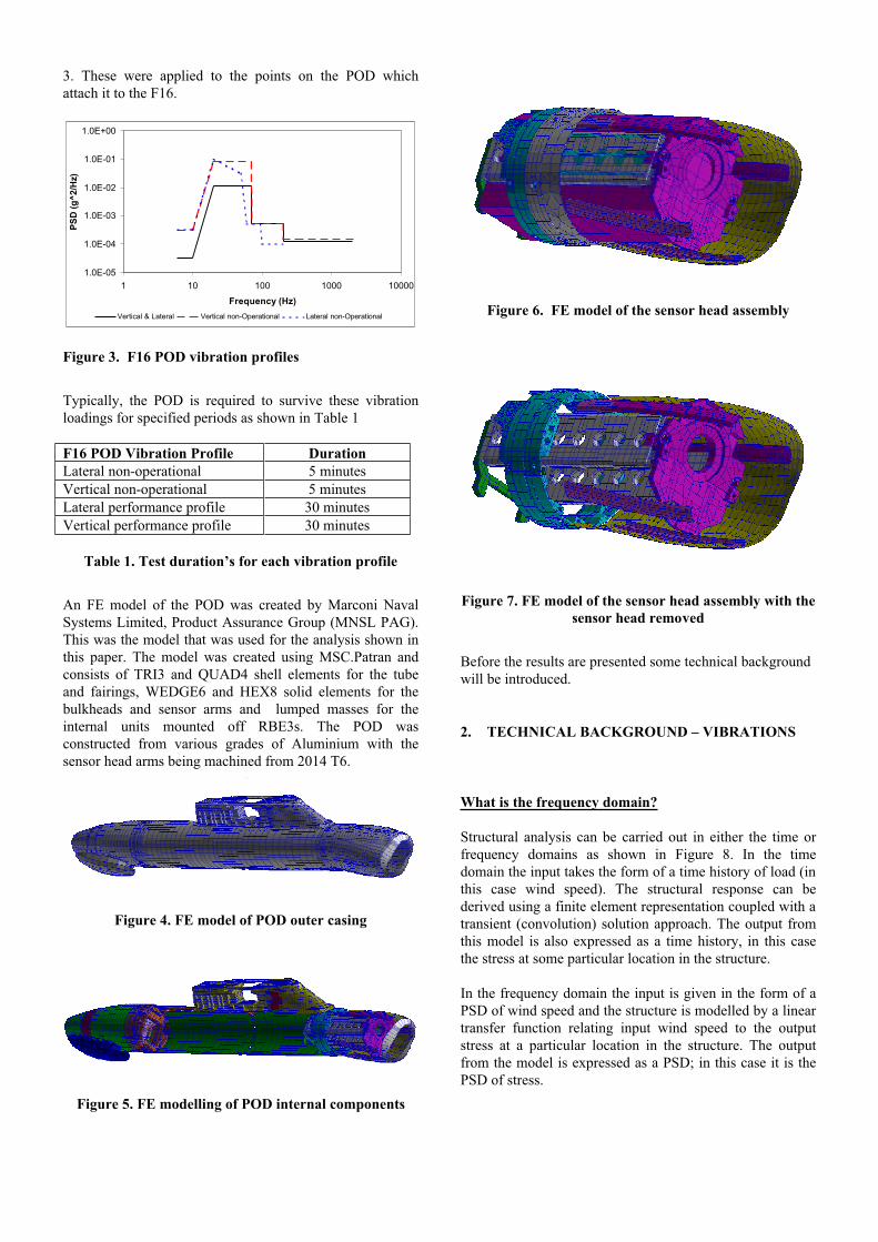
3. These were applied to the points on the POD whichattach it to the F16.

Figure 3. F16 POD vibration profiles

Typically, the POD is required to survive these vibrationloadings for specified periods as shown in Table 1

F16 POD Vibration Profile DurationLateral non-operational 5 minutesVertical non-operational 5 minutesLateral performance profile 30 minutesVertical performance profile 30 minutes

Table 1. Test duration’s for each vibration profile

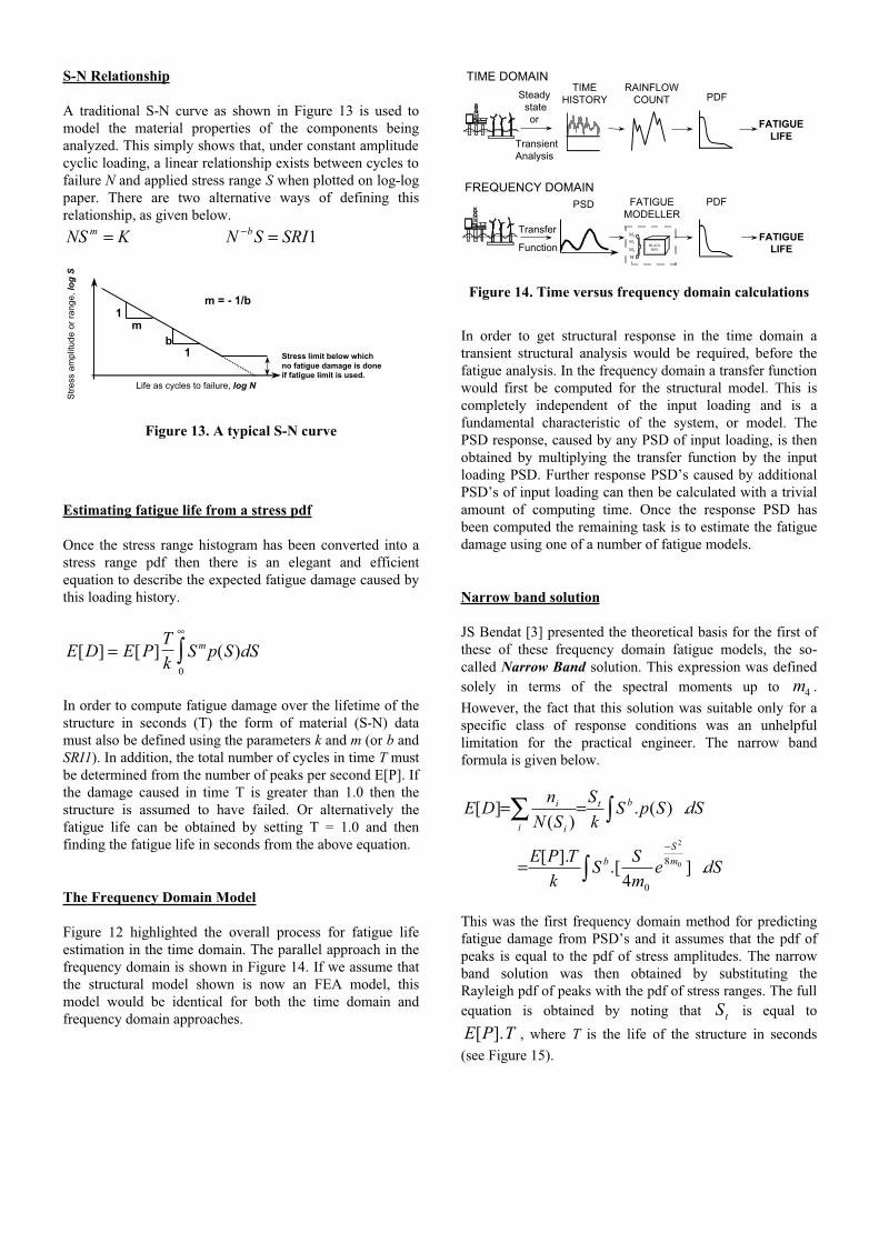
An FE model of the POD was created by Marconi NavalSystems Limited, Product Assurance Group (MNSL PAG).This was the model that was used for the analysis shown inthis paper. The model was created using MSC.Patran andconsists of TRI3 and QUAD4 shell elements for the tubeand fairings, WEDGE6 and HEX8 solid elements for thebulkheads and sensor arms and lumped masses for theinternal units mounted off RBE3s. The POD wasconstructed from various grades of Aluminium with thesensor head arms being machined from 2014 T6.

Figure 4. FE model of POD outer casing

Figure 5. FE modelling of POD internal components

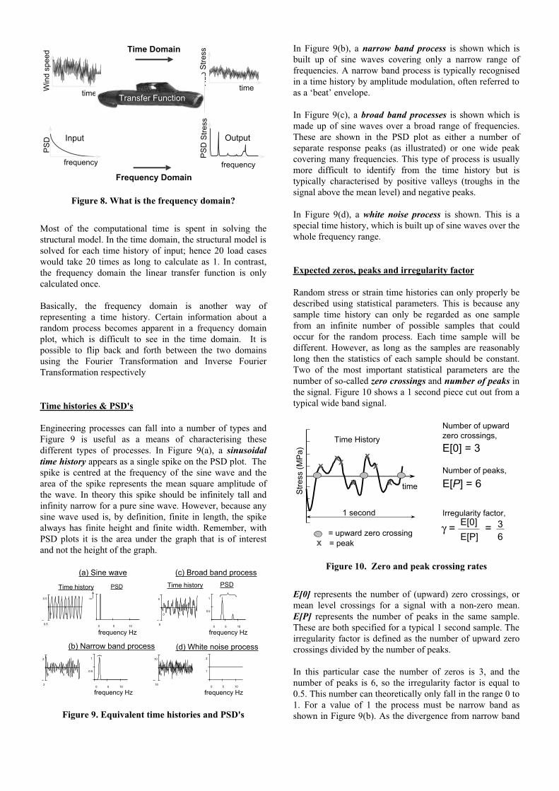
Figure 6. FE model of the sensor head assembly

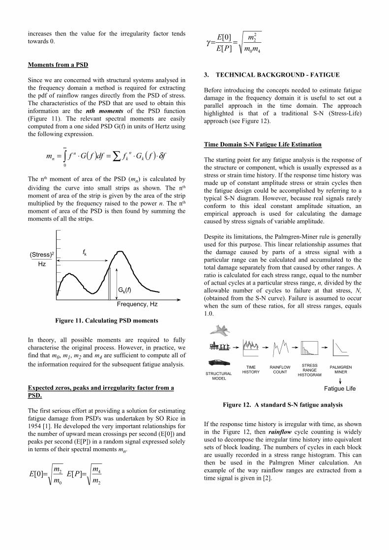
Figure 7. FE model of the sensor head assembly with the sensor head removed

Before the results are presented some technical background will be introduced.

2. TECHNICAL BACKGROUND – VIBRATIONS

What is the frequency domain?

Structural analysis can be carried out in either the time orfrequency domains as shown in Figure 8. In the timedomain the input takes the form of a time history of load (in this case wind speed). The structural response can bederived using a finite element representation coupled with a transient (convolution) solution approach. The output fromthis model is also expressed as a time history, in this casethe stress at some particular location in the structure.

In the frequency domain the input is given in the form of aPSD of wind speed and the structure is modelled by a linear transfer function relating input wind speed to the outputstress at a particular location in the structure. The outputfrom the model is expressed as a PSD; in this case it is thePSD of stress.

1.0E-05

1.0E-04

1.0E-03

1.0E-02

1.0E-01

1.0E+00

1 10 100 1000 10000

Frequency (Hz)

PSD

(g^2

/Hz)

Vertical & Lateral Vertical non-Operational Lateral non-Operational

frequency

timeWin

d sp

eed

Frequency Domain

Time Domain

PS

D S

tress

Output

PS

D

frequency

Input

timeHub

Stre

ss

Transfer Function

Figure 8. What is the frequency domain?

Most of the computational time is spent in solving thestructural model. In the time domain, the structural model is solved for each time history of input; hence 20 load caseswould take 20 times as long to calculate as 1. In contrast,the frequency domain the linear transfer function is onlycalculated once.

Basically, the frequency domain is another way ofrepresenting a time history. Certain information about arandom process becomes apparent in a frequency domainplot, which is difficult to see in the time domain. It ispossible to flip back and forth between the two domainsusing the Fourier Transformation and Inverse FourierTransformation respectively

Time histories & PSD's

Engineering processes can fall into a number of types andFigure 9 is useful as a means of characterising thesedifferent types of processes. In Figure 9(a), a sinusoidaltime history appears as a single spike on the PSD plot. The spike is centred at the frequency of the sine wave and thearea of the spike represents the mean square amplitude ofthe wave. In theory this spike should be infinitely tall andinfinity narrow for a pure sine wave. However, because anysine wave used is, by definition, finite in length, the spikealways has finite height and finite width. Remember, withPSD plots it is the area under the graph that is of interestand not the height of the graph.

0.5

Time history PSD

0 5

0.50 5 10

frequency Hz

(a) Sine wave

0 5

2

2

0 5 10

0.5

1

frequency Hz

(b) Narrow band process

Time history PSD

0 5

5

5

0 5 10

0.5

1

(c) Broad band process

frequency Hz

0 5

10

10

0 5 10

1

2

frequency Hz

(d) White noise process

∞

Figure 9. Equivalent time histories and PSD's

In Figure 9(b), a narrow band process is shown which isbuilt up of sine waves covering only a narrow range offrequencies. A narrow band process is typically recognisedin a time history by amplitude modulation, often referred to as a ‘beat’ envelope.

In Figure 9(c), a broad band processes is shown which ismade up of sine waves over a broad range of frequencies.These are shown in the PSD plot as either a number ofseparate response peaks (as illustrated) or one wide peakcovering many frequencies. This type of process is usuallymore difficult to identify from the time history but istypically characterised by positive valleys (troughs in thesignal above the mean level) and negative peaks.

In Figure 9(d), a white noise process is shown. This is aspecial time history, which is built up of sine waves over the whole frequency range.

Expected zeros, peaks and irregularity factor

Random stress or strain time histories can only properly bedescribed using statistical parameters. This is because anysample time history can only be regarded as one samplefrom an infinite number of possible samples that couldoccur for the random process. Each time sample will bedifferent. However, as long as the samples are reasonablylong then the statistics of each sample should be constant.Two of the most important statistical parameters are thenumber of so-called zero crossings and number of peaks in the signal. Figure 10 shows a 1 second piece cut out from a typical wide band signal.

= upward zero crossing= peak

time

Stre

ss (M

Pa)

1 second

Number of upward zero crossings,E[0] = 3

Number of peaks,

E[P] = 6

Irregularity factor,

γ = E[0]E[P]

= 36

Time History

xx

x

xx

x

x

x

Figure 10. Zero and peak crossing rates

E[0] represents the number of (upward) zero crossings, ormean level crossings for a signal with a non-zero mean.E[P] represents the number of peaks in the same sample.These are both specified for a typical 1 second sample. The irregularity factor is defined as the number of upward zerocrossings divided by the number of peaks.

In this particular case the number of zeros is 3, and thenumber of peaks is 6, so the irregularity factor is equal to0.5. This number can theoretically only fall in the range 0 to 1. For a value of 1 the process must be narrow band asshown in Figure 9(b). As the divergence from narrow band

increases then the value for the irregularity factor tendstowards 0.

Moments from a PSD

Since we are concerned with structural systems analysed inthe frequency domain a method is required for extractingthe pdf of rainflow ranges directly from the PSD of stress.The characteristics of the PSD that are used to obtain thisinformation are the nth moments of the PSD function(Figure 11). The relevant spectral moments are easilycomputed from a one sided PSD G(f) in units of Hertz using the following expression.

( ) ( )∑∫ ⋅⋅=⋅=∞

ffGfdffGfm kn

kn

n δ0

The nth moment of area of the PSD (mn) is calculated bydividing the curve into small strips as shown. The nth

moment of area of the strip is given by the area of the stripmultiplied by the frequency raised to the power n. The nth

moment of area of the PSD is then found by summing themoments of all the strips.

(Stress)2

Hz

Frequency, Hz

Gk(f)

fk

Figure 11. Calculating PSD moments

In theory, all possible moments are required to fullycharacterise the original process. However, in practice, wefind that m0, m1, m2 and m4 are sufficient to compute all ofthe information required for the subsequent fatigue analysis.

Expected zeros, peaks and irregularity factor from a PSD.

The first serious effort at providing a solution for estimating fatigue damage from PSD's was undertaken by SO Rice in1954 [1]. He developed the very important relationships for the number of upward mean crossings per second (E[0]) and peaks per second (E[P]) in a random signal expressed solely in terms of their spectral moments mn.

2

4

0

2 ][]0[mmPE

mmE ==

40

22

][]0[

mmm

PEE ==γ

3. TECHNICAL BACKGROUND - FATIGUE

Before introducing the concepts needed to estimate fatiguedamage in the frequency domain it is useful to set out aparallel approach in the time domain. The approachhighlighted is that of a traditional S-N (Stress-Life)approach (see Figure 12).

Time Domain S-N Fatigue Life Estimation

The starting point for any fatigue analysis is the response of the structure or component, which is usually expressed as astress or strain time history. If the response time history was made up of constant amplitude stress or strain cycles thenthe fatigue design could be accomplished by referring to atypical S-N diagram. However, because real signals rarelyconform to this ideal constant amplitude situation, anempirical approach is used for calculating the damagecaused by stress signals of variable amplitude.

Despite its limitations, the Palmgren-Miner rule is generally used for this purpose. This linear relationship assumes thatthe damage caused by parts of a stress signal with aparticular range can be calculated and accumulated to thetotal damage separately from that caused by other ranges. Aratio is calculated for each stress range, equal to the number of actual cycles at a particular stress range, n, divided by the allowable number of cycles to failure at that stress, N,(obtained from the S-N curve). Failure is assumed to occurwhen the sum of these ratios, for all stress ranges, equals1.0.

STRUCTURALMODEL

TIMEHISTORY

RAINFLOWCOUNT

STRESSRANGE

HISTOGRAM

PALMGRENMINER

Fatigue Life

Figure 12. A standard S-N fatigue analysis

If the response time history is irregular with time, as shownin the Figure 12, then rainflow cycle counting is widelyused to decompose the irregular time history into equivalent sets of block loading. The numbers of cycles in each blockare usually recorded in a stress range histogram. This canthen be used in the Palmgren Miner calculation. Anexample of the way rainflow ranges are extracted from atime signal is given in [2].

S-N Relationship

A traditional S-N curve as shown in Figure 13 is used tomodel the material properties of the components beinganalyzed. This simply shows that, under constant amplitude cyclic loading, a linear relationship exists between cycles to failure N and applied stress range S when plotted on log-logpaper. There are two alternative ways of defining thisrelationship, as given below.

KNS m = 1SRISN b =−

Stre

ss a

mpl

itude

or r

ange

, log

S

Life as cycles to failure, log N

1m

b1

m = - 1/b

Stress limit below whichno fatigue damage is doneif fatigue limit is used.

Figure 13. A typical S-N curve

Estimating fatigue life from a stress pdf

Once the stress range histogram has been converted into astress range pdf then there is an elegant and efficientequation to describe the expected fatigue damage caused bythis loading history.

E D E PTk

S p S dSm[ ] [ ] ( )=∞

∫0

In order to compute fatigue damage over the lifetime of thestructure in seconds (T) the form of material (S-N) datamust also be defined using the parameters k and m (or b and SRI1). In addition, the total number of cycles in time T must be determined from the number of peaks per second E[P]. If the damage caused in time T is greater than 1.0 then thestructure is assumed to have failed. Or alternatively thefatigue life can be obtained by setting T = 1.0 and thenfinding the fatigue life in seconds from the above equation.

The Frequency Domain Model

Figure 12 highlighted the overall process for fatigue lifeestimation in the time domain. The parallel approach in thefrequency domain is shown in Figure 14. If we assume thatthe structural model shown is now an FEA model, thismodel would be identical for both the time domain andfrequency domain approaches.

FREQUENCY DOMAINFATIGUE

MODELLER

BLACKBOX

M0

M1

M2

M4

TransferFATIGUE

LIFEFunction

PSD PDF

TransientAnalysis

RAINFLOWCOUNT

TIMEHISTORY

TIME DOMAIN

FATIGUELIFE

PDFSteady state

or

Figure 14. Time versus frequency domain calculations

In order to get structural response in the time domain atransient structural analysis would be required, before thefatigue analysis. In the frequency domain a transfer function would first be computed for the structural model. This iscompletely independent of the input loading and is afundamental characteristic of the system, or model. ThePSD response, caused by any PSD of input loading, is thenobtained by multiplying the transfer function by the inputloading PSD. Further response PSD’s caused by additionalPSD’s of input loading can then be calculated with a trivialamount of computing time. Once the response PSD hasbeen computed the remaining task is to estimate the fatiguedamage using one of a number of fatigue models.

Narrow band solution

JS Bendat [3] presented the theoretical basis for the first ofthese of these frequency domain fatigue models, the so-called Narrow Band solution. This expression was definedsolely in terms of the spectral moments up to m4 .However, the fact that this solution was suitable only for aspecific class of response conditions was an unhelpfullimitation for the practical engineer. The narrow bandformula is given below.

dSSpSkS

SNnDE bt

i i

i ∫∑ == .)(.)(

][

dSemSS

kTPE m

Sb∫

−

= .]4

.[].[0

2

8

0

This was the first frequency domain method for predictingfatigue damage from PSD’s and it assumes that the pdf ofpeaks is equal to the pdf of stress amplitudes. The narrowband solution was then obtained by substituting theRayleigh pdf of peaks with the pdf of stress ranges. The full equation is obtained by noting that St is equal toE P T[ ]. , where T is the life of the structure in seconds(see Figure 15).

Narrow band signal Pdf of peaks(given by Rayleigh function)

Pdf of stress amplitude(rainflow cycles given bytwice stress amplitude)

Figure 15. The basis of the narrow band solution

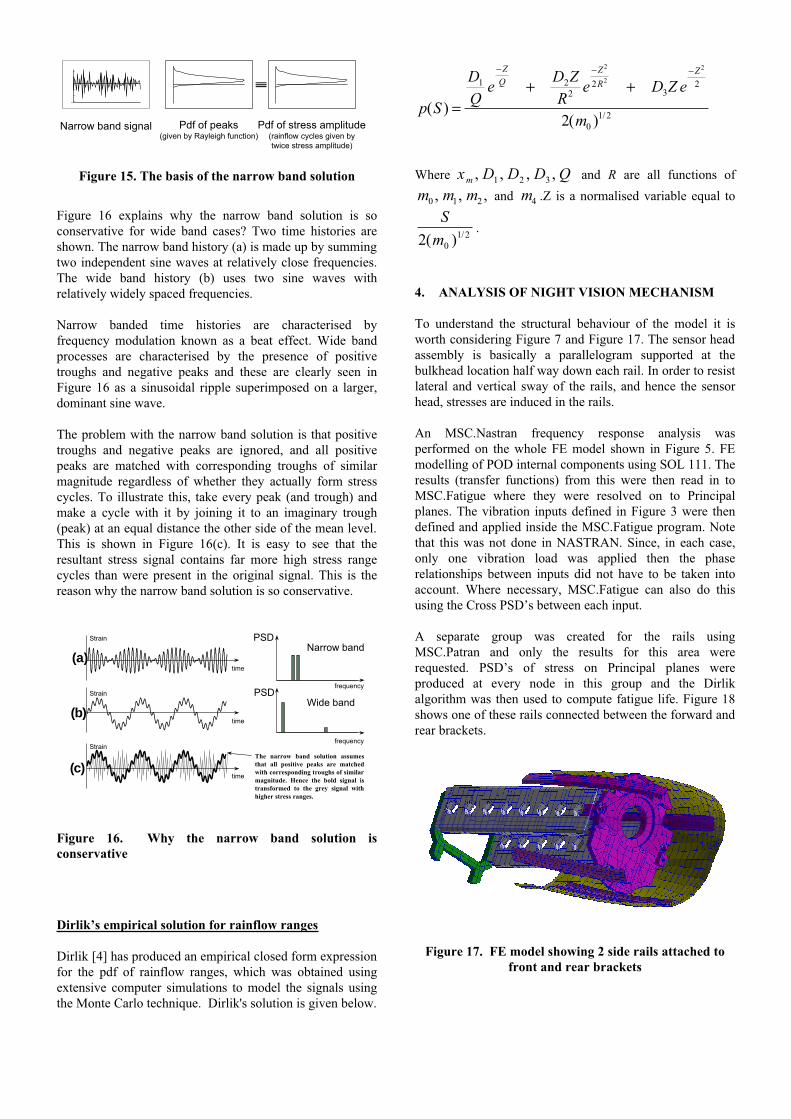
Figure 16 explains why the narrow band solution is soconservative for wide band cases? Two time histories areshown. The narrow band history (a) is made up by summing two independent sine waves at relatively close frequencies.The wide band history (b) uses two sine waves withrelatively widely spaced frequencies.

Narrow banded time histories are characterised byfrequency modulation known as a beat effect. Wide bandprocesses are characterised by the presence of positivetroughs and negative peaks and these are clearly seen inFigure 16 as a sinusoidal ripple superimposed on a larger,dominant sine wave.

The problem with the narrow band solution is that positivetroughs and negative peaks are ignored, and all positivepeaks are matched with corresponding troughs of similarmagnitude regardless of whether they actually form stresscycles. To illustrate this, take every peak (and trough) andmake a cycle with it by joining it to an imaginary trough(peak) at an equal distance the other side of the mean level. This is shown in Figure 16(c). It is easy to see that theresultant stress signal contains far more high stress rangecycles than were present in the original signal. This is thereason why the narrow band solution is so conservative.

time

time

time

frequency

frequency

Narrow band

Wide band

PSD

PSD

Strain

Strain

StrainThe narrow band solution assumesthat all positive peaks are matchedwith corresponding troughs of similarmagnitude. Hence the bold signal istransformed to the grey signal withhigher stress ranges.

(a)

(b)

(c)

Figure 16. Why the narrow band solution isconservative

Dirlik’s empirical solution for rainflow ranges

Dirlik [4] has produced an empirical closed form expression for the pdf of rainflow ranges, which was obtained usingextensive computer simulations to model the signals usingthe Monte Carlo technique. Dirlik's solution is given below.

p S

DQ

e D ZR

e D Z e

m

ZQ

ZR

Z

( )( ) /=

+ +− − −

1 22

23

2

01 2

2

2

2

2

Where x D D D Qm , , , ,1 2 3 and R are all functions ofm m m0 1 2, , , and m4 .Z is a normalised variable equal to

Sm2 0

1 2( ) / .

4. ANALYSIS OF NIGHT VISION MECHANISM

To understand the structural behaviour of the model it isworth considering Figure 7 and Figure 17. The sensor head assembly is basically a parallelogram supported at thebulkhead location half way down each rail. In order to resist lateral and vertical sway of the rails, and hence the sensorhead, stresses are induced in the rails.

An MSC.Nastran frequency response analysis wasperformed on the whole FE model shown in Figure 5. FEmodelling of POD internal components using SOL 111. The results (transfer functions) from this were then read in toMSC.Fatigue where they were resolved on to Principalplanes. The vibration inputs defined in Figure 3 were thendefined and applied inside the MSC.Fatigue program. Notethat this was not done in NASTRAN. Since, in each case,only one vibration load was applied then the phaserelationships between inputs did not have to be taken intoaccount. Where necessary, MSC.Fatigue can also do thisusing the Cross PSD’s between each input.

A separate group was created for the rails usingMSC.Patran and only the results for this area wererequested. PSD’s of stress on Principal planes wereproduced at every node in this group and the Dirlikalgorithm was then used to compute fatigue life. Figure 18shows one of these rails connected between the forward and rear brackets.

Figure 17. FE model showing 2 side rails attached to front and rear brackets

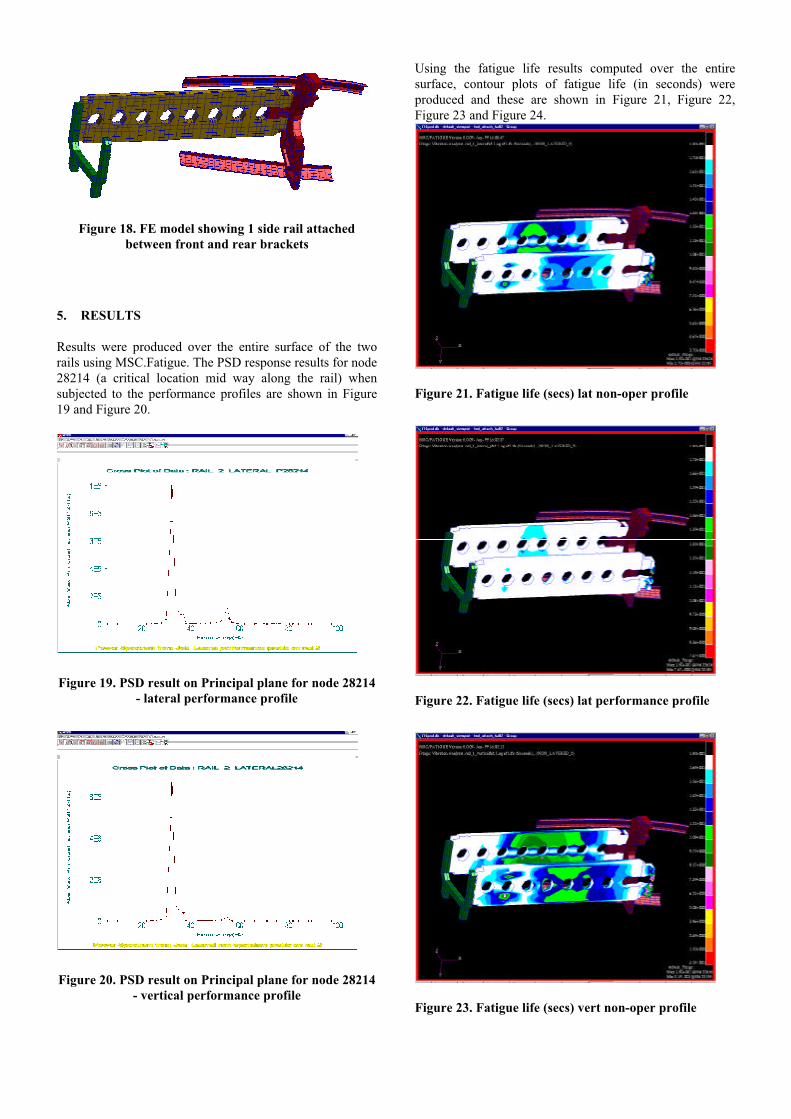
Figure 18. FE model showing 1 side rail attached between front and rear brackets

5. RESULTS

Results were produced over the entire surface of the tworails using MSC.Fatigue. The PSD response results for node 28214 (a critical location mid way along the rail) whensubjected to the performance profiles are shown in Figure19 and Figure 20.

Figure 19. PSD result on Principal plane for node 28214 - lateral performance profile

Figure 20. PSD result on Principal plane for node 28214 - vertical performance profile

Using the fatigue life results computed over the entiresurface, contour plots of fatigue life (in seconds) wereproduced and these are shown in Figure 21, Figure 22,Figure 23 and Figure 24.

Figure 21. Fatigue life (secs) lat non-oper profile

Figure 22. Fatigue life (secs) lat performance profile

Figure 23. Fatigue life (secs) vert non-oper profile

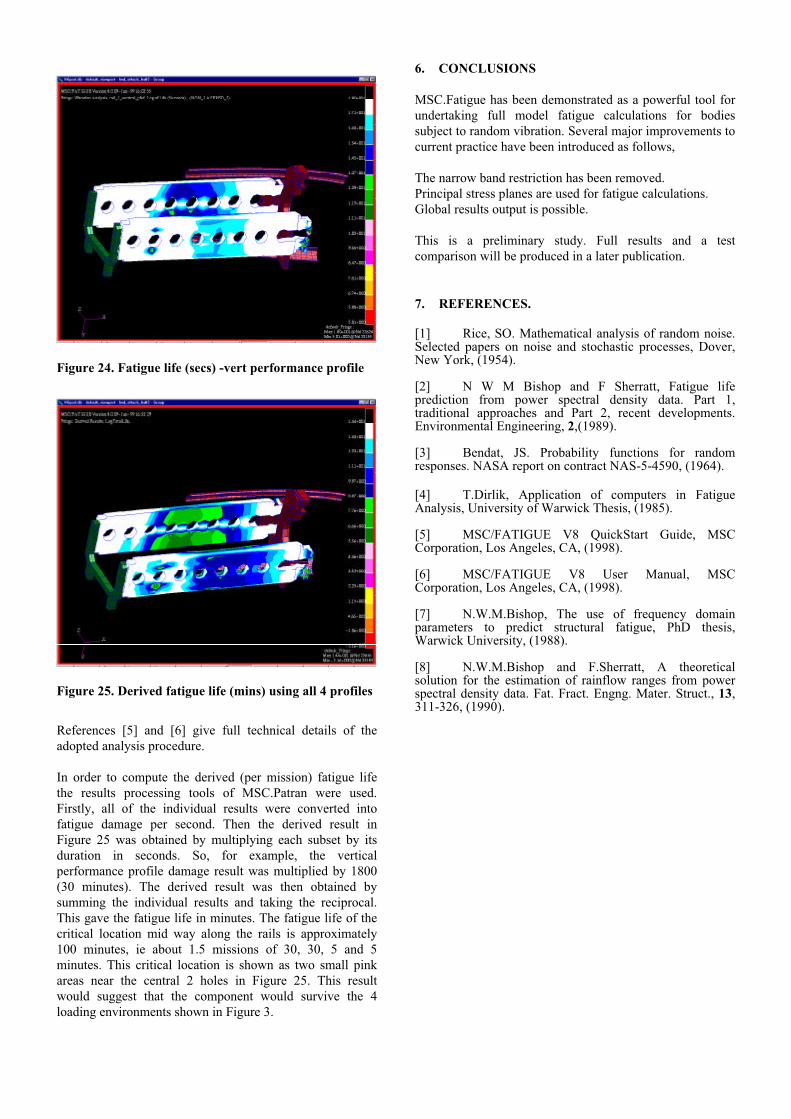
Figure 24. Fatigue life (secs) -vert performance profile

Figure 25. Derived fatigue life (mins) using all 4 profiles

References [5] and [6] give full technical details of theadopted analysis procedure.

In order to compute the derived (per mission) fatigue lifethe results processing tools of MSC.Patran were used.Firstly, all of the individual results were converted intofatigue damage per second. Then the derived result inFigure 25 was obtained by multiplying each subset by itsduration in seconds. So, for example, the verticalperformance profile damage result was multiplied by 1800(30 minutes). The derived result was then obtained bysumming the individual results and taking the reciprocal.This gave the fatigue life in minutes. The fatigue life of thecritical location mid way along the rails is approximately100 minutes, ie about 1.5 missions of 30, 30, 5 and 5minutes. This critical location is shown as two small pinkareas near the central 2 holes in Figure 25. This resultwould suggest that the component would survive the 4loading environments shown in Figure 3.

6. CONCLUSIONS

MSC.Fatigue has been demonstrated as a powerful tool forundertaking full model fatigue calculations for bodiessubject to random vibration. Several major improvements to current practice have been introduced as follows,

The narrow band restriction has been removed.Principal stress planes are used for fatigue calculations.Global results output is possible.

This is a preliminary study. Full results and a testcomparison will be produced in a later publication.

7. REFERENCES.

[1] Rice, SO. Mathematical analysis of random noise.Selected papers on noise and stochastic processes, Dover,New York, (1954).

[2] N W M Bishop and F Sherratt, Fatigue lifeprediction from power spectral density data. Part 1,traditional approaches and Part 2, recent developments.Environmental Engineering, 2,(1989).

[3] Bendat, JS. Probability functions for randomresponses. NASA report on contract NAS-5-4590, (1964).

[4] T.Dirlik, Application of computers in FatigueAnalysis, University of Warwick Thesis, (1985).

[5] MSC/FATIGUE V8 QuickStart Guide, MSCCorporation, Los Angeles, CA, (1998).

[6] MSC/FATIGUE V8 User Manual, MSCCorporation, Los Angeles, CA, (1998).

[7] N.W.M.Bishop, The use of frequency domainparameters to predict structural fatigue, PhD thesis,Warwick University, (1988).

[8] N.W.M.Bishop and F.Sherratt, A theoreticalsolution for the estimation of rainflow ranges from powerspectral density data. Fat. Fract. Engng. Mater. Struct., 13,311-326, (1990).