Forward and backward motion control of a vibro-impact capsulesystem

Yang Liua,∗, Ekaterina Pavlovskaiab, Marian Wiercigrochb, Zhike Pengc

aSchool of Engineering, Robert Gordon University, Garthdee Road, Aberdeen, UK, AB10 7GJbCentre for Applied Dynamics Research, School of Engineering, King’s College, University of Aberdeen,

Aberdeen, UK, AB24 3UEcState Key Laboratory of Mechanical System and Vibration, Shanghai Jiao Tong University, Shanghai,

P. R. China, 200240

Abstract

A capsule system driven by a harmonic force applied to its inner mass is considered inthis study. Four various friction models are employed to describe motion of the capsule indifferent environments taking into account Coulomb friction, viscous damping, Stribeckeffect, pre-sliding, and frictional memory. The non-linear dynamics analysis has beenconducted to identify the optimal amplitude and frequency of the applied force in orderto achieve the motion in the required direction and to maximize its speed. In addition,a position feedback control method suitable for dealing with chaos control and coexistingattractors is applied for enhancing the desirable forward and backward capsule motion.The evolution of basins of attraction under control gain variation is presented and it isshown that the basin of the desired attractors could be significantly enlarged by slightadjustment of the control gain improving the probability of reaching such an attractor.

Keywords: capsule, vibro-impact, friction, motion control, position feedback control.

1. Introduction

In the last few years, there was a growing interest in developing mobile mechanismsfor minimally invasive surgical operation [1, 2, 3, 4] and engineering pipeline inspection[5, 6, 7]. Particularly, investigation of a capsule system moving under internal force whenovercoming environmental resistance has attracted significant attention, e.g. [8, 9, 10, 11].The merit of such a system is its simplicity in mechanical design and control which doesnot require any external driving mechanisms while allows it to move independently in acomplex environment unaccessible to the legged and wheeled mechanisms [12, 13]. How-

∗Corresponding author. Tel. +44-1224-262420, e-mail: y.liu8@rgu.ac.uk.

Preprint submitted to International Journal of Non-Linear Mechanics November 7, 2014

ever, any small uncertainties in friction or system parameters may lead to qualitativechange of the dynamics of the capsule system [14]. Therefore understanding of the dy-namics and motion control under different frictional environments for such a system isessential.

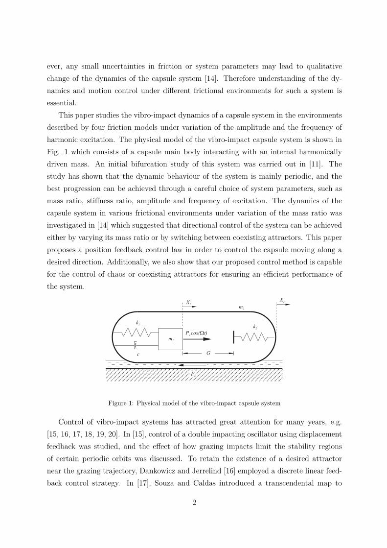
This paper studies the vibro-impact dynamics of a capsule system in the environmentsdescribed by four friction models under variation of the amplitude and the frequency ofharmonic excitation. The physical model of the vibro-impact capsule system is shown inFig. 1 which consists of a capsule main body interacting with an internal harmonicallydriven mass. An initial bifurcation study of this system was carried out in [11]. Thestudy has shown that the dynamic behaviour of the system is mainly periodic, and thebest progression can be achieved through a careful choice of system parameters, such asmass ratio, stiffness ratio, amplitude and frequency of excitation. The dynamics of thecapsule system in various frictional environments under variation of the mass ratio wasinvestigated in [14] which suggested that directional control of the system can be achievedeither by varying its mass ratio or by switching between coexisting attractors. This paperproposes a position feedback control law in order to control the capsule moving along adesired direction. Additionally, we also show that our proposed control method is capablefor the control of chaos or coexisting attractors for ensuring an efficient performance ofthe system.

k1

c

m1

P cos( t)d W

G

k2

X1

X2

m2

FS

Figure 1: Physical model of the vibro-impact capsule system

Control of vibro-impact systems has attracted great attention for many years, e.g.[15, 16, 17, 18, 19, 20]. In [15], control of a double impacting oscillator using displacementfeedback was studied, and the effect of how grazing impacts limit the stability regionsof certain periodic orbits was discussed. To retain the existence of a desired attractornear the grazing trajectory, Dankowicz and Jerrelind [16] employed a discrete linear feed-back control strategy. In [17], Souza and Caldas introduced a transcendental map to

2

determine the value of parameter perturbation for controlling the vibro-impact systemswhich exhibited desired unstable periodic orbit embedded in a chaotic attractor. Leeand Yan studied the control algorithms for position control of an impact oscillator andsynchronization of two impact oscillators in [18]. A feedback control technique using asmall-amplitude damping signal was studied in [19] for suppressing chaotic behaviour ofan impact oscillator. Later on, Wang et al. [20] developed an impulsive control methodto stabilize the chaotic motion for a class of vibro-impact systems. In [21], Liu et al. pro-posed an intermittent control method for a class of non-autonomous dynamics systemsthat naturally exhibited coexisting attractors, and demonstrated its applicability to animpact oscillator numerically and experimentally. Basically, vibro-impact systems mainlyfall into two categories: the impact oscillator with fixed impact body, e.g. [22, 23] and theimpact oscillator with one-side drifting impact body e.g. [24, 25, 26]. However this paperstudies the control of a vibro-impact system with impact body drifting forward and back-ward which has never been considered in the literature before. Compared to the impactoscillator with fixed impact body, this structure induces more complicated dynamics whenexperiences various environmental resistance. Both optimization and directional controlissues must be considered for our proposed system, while only optimization is needed forthe impact oscillator with one-side drifting impact body. This paper also uses basins ofattraction for the first time to investigate the possibility of switching between coexistingattractors by using the proposed control method.

The rest of this paper is organized as follows. In Section 2, mathematical modellingof the vibro-impact capsule system is presented, and the four different friction modelsused in this paper are briefly introduced. In Section 3, a non-linear dynamic analysisof the capsule system is conducted by varying the amplitude of excitation. In Section4, influence of excitation frequency on capsule dynamics is investigated, and its globaland local optima are studied. In Section 5, forward and backward motion control of thecapsule system is studied by using a position feedback control law. Here the capabilitiesof the proposed control method for the control of chaos and coexisting attractors aredemonstrated through extensive numerical studies. Finally, some concluding remarks aredrawn in Section 6.

3

2. Mathematical Modelling

2.1. Equations of motionThis work considers a two degrees-of-freedom dynamical system depicted in Fig. 1,

where a movable internal mass m1 is driven by a harmonic force with amplitude Pd andfrequency Ω interacting with a rigid capsule m2 via a linear spring with stiffness k1 anda viscous damper with damping coefficient c. X1 and X2 represent the absolute displace-ments of the internal mass and the capsule, respectively. The internal mass contacts aweightless plate connected to the capsule by a secondary linear spring with stiffness k2

when the relative displacement X1 − X2 is larger or equals to the gap G. When the forceacting on the capsule exceeds the threshold of the dry friction force Fb between the capsuleand the supporting environmental surface, the bidirectional motion of the capsule occurs,and the friction force Fs is applied to the capsule.

To simplify the analysis, we introduce the following non-dimensional variables

τ = Ω0t, xi = k1

Pf

Xi, yi = dxi

dτ= k1

Ω0Pf

Xi, yi = dyi

dτ= k1

Ω20Pf

Xi, fs = Fs

Pf

, fb = Fb

Pf

,

and parameters

Ω0 =√

k1

m1, ω = Ω

Ω0, α = Pd

Pf

, ξ = c

2m1Ω0, δ = k1

Pf

G, β = k2

k1, γ = m2

m1,

where i = 1, 2, and Pf is the threshold of Coulomb friction. The considered systemoperates in bidirectional stick-slip phases which contain the following modes: stationarycapsule without contact, moving capsule without contact, stationary capsule with contact,moving capsule with contact. A detailed consideration of these modes and dimensionalform of the equations of motion can be found in [11]. The comprehensive equations ofmotion for the vibro-impact capsule system are written as

x1 = y1,

y1 = α cos(ωτ) + (x2 − x1) + 2ξ(y2 − y1) − H3β(x1 − x2 − δ),

x2 = y2 (H1(1 − H3) + H2H3) , (1)

y2 = (H1(1 − H3) + H2H3) (−fs − (x2 − x1) − 2ξ(y2 − y1)

+ H3β(x1 − x2 − δ)) /γ.

where H(·) is the Heaviside function and functions Hi (i = 1, 2, 3) are defined as

H1 = H(| (x2 − x1) + 2ξ(y2 − y1) | −fb),

H2 = H(| (x2 − x1) + 2ξ(y2 − y1) − β(x1 − x2 − δ) | −fb),

H3 = H(x1 − x2 − δ).

4

2.2. Friction models

In [14], the environmental resistance was described by four different friction mod-els given in Table 1 which took into account Coulomb friction, viscous damping, Stribeckeffect, pre-sliding, and frictional memory. As it is known, the Coulomb friction model pro-vides the first approximation of dry frictional contact, and the Coulomb viscous dampingmodel takes into account the viscosity of lubricated contact. Both Coulomb Stribeck andseven-parameter models [27] describe the friction of thicker lubricated contact, while thelater one can comprehensively interpret the resistant force at a very low relative speed.The work in [14] has revealed that when the weight of the internal mass is smaller thanthe weight of the capsule, the nature of the friction mechanism becomes less significant asit does not influence so much the capsule dynamics. This paper further investigates thecapsule dynamics under variation of the amplitude and frequency of external excitationusing these four friction models, and proposes a control method which can switch thesystem state from chaotic to periodic motion or from a current attractor to a desired one.

Table 1: Friction models [14]

Friction model Description Static friction Dynamic friction fs Threshold fb

Coulomb Dry contact 0 sign(x2) 1Coulomb viscousdamping

Lubricated contact 0 sign(x2) + µvx2 1

Coulomb Stribeck Thicker lubricatedcontact

0 sign(x2) +sign(x2) e−|x2|/vs

2

Seven-parameter Lubricated contactat very low relativespeed

ksx2 sign(x2) + µvx2 +sign(x2)

1+( x2vs

(τ−τd))2

2

3. Influence of Excitation Amplitude

This section compares capsule dynamic responses with dry, lubricated, and thickerlubricated contact surfaces, and investigates the influence of amplitude of excitation oncapsule motion. The comparison was carried out using the bifurcation diagrams as shownin Fig. 2 where the velocity y∗

1, which is a projection of the Poincare map on the y1

axis, was plotted as a function of the amplitude of excitation for the systems with (a)the Coulomb, (b) the Coulomb viscous damping, (c) the Coulomb Stribeck, and (d) theseven-parameter models. The main attractors of the system are shown by black dots and

5

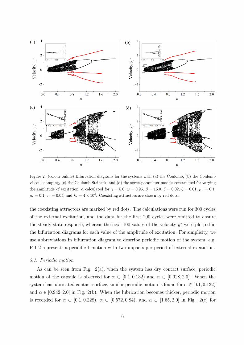
Figure 2: (colour online) Bifurcation diagrams for the systems with (a) the Coulomb, (b) the Coulombviscous damping, (c) the Coulomb Stribeck, and (d) the seven-parameter models constructed for varyingthe amplitude of excitation, α calculated for γ = 5.0, ω = 0.95, β = 15.0, δ = 0.02, ξ = 0.01, µv = 0.1,µs = 0.1, τd = 0.05, and ks = 4 × 104. Coexisting attractors are shown by red dots.

the coexisting attractors are marked by red dots. The calculations were run for 300 cyclesof the external excitation, and the data for the first 200 cycles were omitted to ensurethe steady state response, whereas the next 100 values of the velocity y∗

1 were plotted inthe bifurcation diagrams for each value of the amplitude of excitation. For simplicity, weuse abbreviations in bifurcation diagram to describe periodic motion of the system, e.g.P-1-2 represents a periodic-1 motion with two impacts per period of external excitation.

3.1. Periodic motion

As can be seen from Fig. 2(a), when the system has dry contact surface, periodicmotion of the capsule is observed for α ∈ [0.1, 0.132) and α ∈ [0.928, 2.0]. When thesystem has lubricated contact surface, similar periodic motion is found for α ∈ [0.1, 0.132)and α ∈ [0.942, 2.0] in Fig. 2(b). When the lubrication becomes thicker, periodic motionis recorded for α ∈ [0.1, 0.228), α ∈ [0.572, 0.84), and α ∈ [1.65, 2.0] in Fig. 2(c) for

6

the system with the Coulomb Stribeck model, and α ∈ [0.1, 0.228), α ∈ [0.724, 0.914),and α ∈ [1.722, 2.0] in Fig. 2(d) for the system with the seven-parameter model. Ourbifurcation study reveals that the system has similar dynamic response when its contactsurface is dry and thinly lubricated, and periodic motion of the system can be obtainedwhen the amplitude of the harmonic force Pd is greater than the threshold of friction Pf

(i.e. α > 1). When the capsule has thicker lubricated contact, capsule motion becomesmore complicated and the range of excitation amplitude for periodic motion is quitenarrow. Therefore forward and backward motion control of the capsule system throughadjusting excitation amplitude is limited.

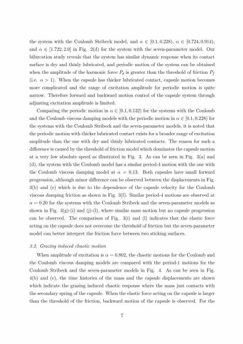
Comparing the periodic motion in α ∈ [0.1, 0.132) for the systems with the Coulomband the Coulomb viscous damping models with the periodic motion in α ∈ [0.1, 0.228) forthe systems with the Coulomb Stribeck and the seven-parameter models, it is noted thatthe periodic motion with thicker lubricated contact exists for a broader range of excitationamplitude than the one with dry and thinly lubricated contacts. The reason for such adifference is caused by the threshold of friction model which dominates the capsule motionat a very low absolute speed as illustrated in Fig. 3. As can be seen in Fig. 3(a) and(d), the system with the Coulomb model has a similar period-4 motion with the one withthe Coulomb viscous damping model at α = 0.13. Both capsules have small forwardprogression, although minor difference can be observed between the displacements in Fig.3(b) and (e) which is due to the dependence of the capsule velocity for the Coulombviscous damping friction as shown in Fig. 3(f). Similar period-4 motions are observed atα = 0.20 for the systems with the Coulomb Stribeck and the seven-parameter models asshown in Fig. 3(g)-(i) and (j)-(l), where similar mass motion but no capsule progressioncan be observed. The comparison of Fig. 3(i) and (l) indicates that the elastic forceacting on the capsule does not overcome the threshold of friction but the seven-parametermodel can better interpret the friction force between two sticking surfaces.

3.2. Grazing induced chaotic motion

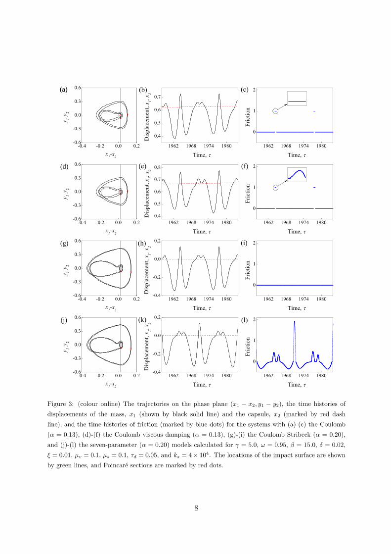
When amplitude of excitation is α = 0.802, the chaotic motions for the Coulomb andthe Coulomb viscous damping models are compared with the period-1 motions for theCoulomb Stribeck and the seven-parameter models in Fig. 4. As can be seen in Fig.4(b) and (e), the time histories of the mass and the capsule displacements are shownwhich indicate the grazing induced chaotic response where the mass just contacts withthe secondary spring of the capsule. When the elastic force acting on the capsule is largerthan the threshold of the friction, backward motion of the capsule is observed. For the

7

-0.4 -0.2 0.0 0.2-0.6

-0.3

0.0

0.3

0.6

1962 1968 1974 1980

0

1

2

-0.4 -0.2 0.0 0.2-0.6

-0.3

0.0

0.3

0.6

1962 1968 1974 19800.4

0.5

0.6

0.7

0.8

1962 1968 1974 1980

0

1

2

-0.4 -0.2 0.0 0.2-0.6

-0.3

0.0

0.3

0.6

1962 1968 1974 1980-0.4

-0.2

0.0

0.2

1962 1968 1974 1980

0

1

2

-0.4 -0.2 0.0 0.2-0.6

-0.3

0.0

0.3

0.6

1962 1968 1974 1980-0.4

-0.2

0.0

0.2

1962 1968 1974 1980

0

1

2

1962 1968 1974 1980

0.4

0.5

0.6

0.7

(l)

(a)

(k)(j)

(i)(h)(g)

(f)(e)(d)

(c)(b)

y 1-y2

x1-x

2

Fric

tion

Time,

y 1-y2

x1-x

2

Dis

plac

emen

t, x 1, x

2

Time,

Fric

tion

Time,

y 1-y2

x1-x

2

Dis

plac

emen

t, x 1, x

2

Time,

Fric

tion

Time,

(a)

y 1-y2

x1-x

2

Dis

plac

emen

t, x 1, x

2

Time,

Fric

tion

Time,

Dis

plac

emen

t, x 1, x

2

Time,

Figure 3: (colour online) The trajectories on the phase plane (x1 − x2, y1 − y2), the time histories ofdisplacements of the mass, x1 (shown by black solid line) and the capsule, x2 (marked by red dashline), and the time histories of friction (marked by blue dots) for the systems with (a)-(c) the Coulomb(α = 0.13), (d)-(f) the Coulomb viscous damping (α = 0.13), (g)-(i) the Coulomb Stribeck (α = 0.20),and (j)-(l) the seven-parameter (α = 0.20) models calculated for γ = 5.0, ω = 0.95, β = 15.0, δ = 0.02,ξ = 0.01, µv = 0.1, µs = 0.1, τd = 0.05, and ks = 4 × 104. The locations of the impact surface are shownby green lines, and Poincare sections are marked by red dots.

8

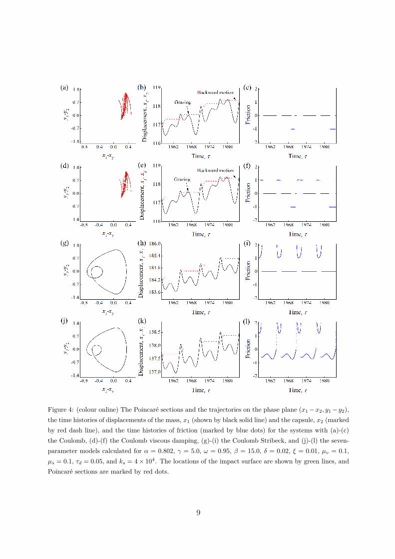
Figure 4: (colour online) The Poincare sections and the trajectories on the phase plane (x1 − x2, y1 − y2),the time histories of displacements of the mass, x1 (shown by black solid line) and the capsule, x2 (markedby red dash line), and the time histories of friction (marked by blue dots) for the systems with (a)-(c)the Coulomb, (d)-(f) the Coulomb viscous damping, (g)-(i) the Coulomb Stribeck, and (j)-(l) the seven-parameter models calculated for α = 0.802, γ = 5.0, ω = 0.95, β = 15.0, δ = 0.02, ξ = 0.01, µv = 0.1,µs = 0.1, τd = 0.05, and ks = 4 × 104. The locations of the impact surface are shown by green lines, andPoincare sections are marked by red dots.

9

displacements of the systems with the Coulomb Stribeck and the seven-parameter models,only forward period-1 motions are observed in Fig. 4(h) and (k). In this case, the speedof the capsule with thicker lubricated contact is much faster than the speed with dry andthinly lubricated contacts although its frictional threshold is larger than the other twocases. This observation reveals that at some situations, larger friction may help to retainsystem stability and keeps system response in an optimal regime.

3.3. Evolution of chaotic motion

-1.4 -0.7 0.0 0.7-4

-2

0

2

4

-1.4 -0.7 0.0 0.7-4

-2

0

2

4

-1.4 -0.7 0.0 0.7-4

-2

0

2

4

-1.4 -0.7 0.0 0.7-4

-2

0

2

4

-1.4 -0.7 0.0 0.7-4

-2

0

2

4

-1.4 -0.7 0.0 0.7-4

-2

0

2

4

-1.4 -0.7 0.0 0.7-4

-2

0

2

4

-1.4 -0.7 0.0 0.7-4

-2

0

2

4

y 1-y

2

x1-x

2

(a)

y 1-y

2

x1-x

2

y 1-y

2

x1-x

2

y 1-y

2

x1-x

2

y 1-y

2

x1-x

2

y 1-y

2

x1-x

2

y 1-y

2

x1-x

2

=1.6=1.4=1.3=1.1

(h)(g)(f)(e)

(d)(c)(b)

y 1-y

2

x1-x

2

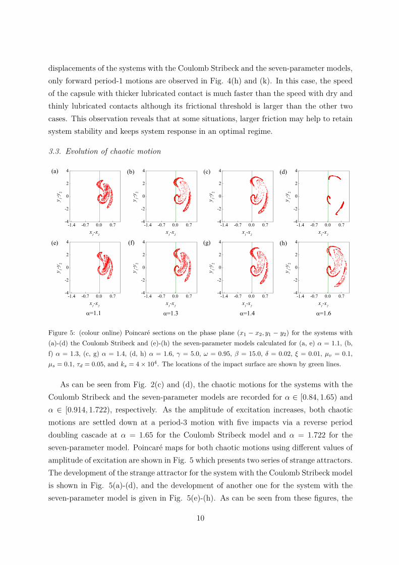
Figure 5: (colour online) Poincare sections on the phase plane (x1 − x2, y1 − y2) for the systems with(a)-(d) the Coulomb Stribeck and (e)-(h) the seven-parameter models calculated for (a, e) α = 1.1, (b,f) α = 1.3, (c, g) α = 1.4, (d, h) α = 1.6, γ = 5.0, ω = 0.95, β = 15.0, δ = 0.02, ξ = 0.01, µv = 0.1,µs = 0.1, τd = 0.05, and ks = 4 × 104. The locations of the impact surface are shown by green lines.

As can be seen from Fig. 2(c) and (d), the chaotic motions for the systems with theCoulomb Stribeck and the seven-parameter models are recorded for α ∈ [0.84, 1.65) andα ∈ [0.914, 1.722), respectively. As the amplitude of excitation increases, both chaoticmotions are settled down at a period-3 motion with five impacts via a reverse perioddoubling cascade at α = 1.65 for the Coulomb Stribeck model and α = 1.722 for theseven-parameter model. Poincare maps for both chaotic motions using different values ofamplitude of excitation are shown in Fig. 5 which presents two series of strange attractors.The development of the strange attractor for the system with the Coulomb Stribeck modelis shown in Fig. 5(a)-(d), and the development of another one for the system with theseven-parameter model is given in Fig. 5(e)-(h). As can be seen from these figures, the

10

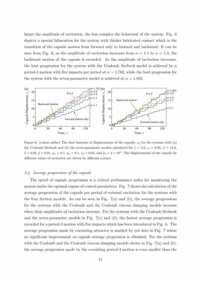
larger the amplitude of excitation, the less complex the behaviour of the system. Fig. 6depicts a special bifurcation for the system with thicker lubricated contact which is thetransition of the capsule motion from forward only to forward and backward. It can beseen from Fig. 6, as the amplitude of excitation increases from α = 1.1 to α = 1.3, thebackward motion of the capsule is recorded. As the amplitude of excitation increases,the best progression for the system with the Coulomb Stribeck model is achieved by aperiod-3 motion with five impacts per period at α = 1.762, while the best progression forthe system with the seven-parameter model is achieved at α = 1.882.

0 30 60 90 1200

5

10

15

20

0 30 60 90 1200

5

10

15

20P-3-5

Backward motion

=2.0=1.762

=1.4=1.3

Cap

sule

Dis

plac

emen

t, x 2

Time,

=1.1

Forward motion only

(b)

Cap

sule

Dis

plac

emen

t, x 2

Time,

=2.0=1.882

=1.4=1.3

=1.1

(a)

Backward motion

Forward motion only

P-3-5

Figure 6: (colour online) The time histories of displacements of the capsule, x2 for the systems with (a)the Coulomb Stribeck and (b) the seven-parameter models calculated for γ = 5.0, ω = 0.95, β = 15.0,δ = 0.02, ξ = 0.01, µv = 0.1, µs = 0.1, τd = 0.05, and ks = 4 × 104. The displacements of the capsule bydifferent values of excitation are shown by different colours.

3.4. Average progression of the capsule

The speed of capsule progression is a critical performance index for monitoring thesystem under the optimal regime of control parameters. Fig. 7 shows the calculation of theaverage progression of the capsule per period of external excitation for the systems withthe four friction models. As can be seen in Fig. 7(a) and (b), the average progressionsfor the systems with the Coulomb and the Coulomb viscous damping models increasewhen their amplitudes of excitation increase. For the systems with the Coulomb Stribeckand the seven-parameter models in Fig. 7(c) and (d), the fastest average progression isrecorded for a period-3 motion with five impacts which has been introduced in Fig. 6. Theaverage progression made by coexisting attractor is marked by red dots in Fig. 7 whereno significant improvement on capsule average progression is obtained. For the systemswith the Coulomb and the Coulomb viscous damping models shown in Fig. 7(a) and (b),the average progression made by the coexisting period-3 motion is even smaller than the

11

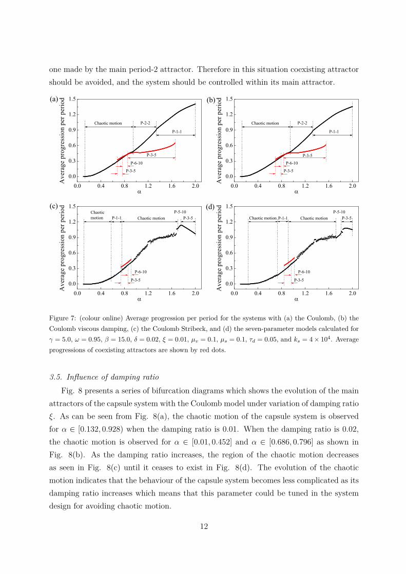
one made by the main period-2 attractor. Therefore in this situation coexisting attractorshould be avoided, and the system should be controlled within its main attractor.

0.0 0.4 0.8 1.2 1.6 2.0

0.0

0.3

0.6

0.9

1.2

1.5

0.0 0.4 0.8 1.2 1.6 2.0

0.0

0.3

0.6

0.9

1.2

1.5

0.0 0.4 0.8 1.2 1.6 2.0

0.0

0.3

0.6

0.9

1.2

1.5

0.0 0.4 0.8 1.2 1.6 2.0

0.0

0.3

0.6

0.9

1.2

1.5

P-3-5

P-6-10

P-3-5

P-1-1

Ave

rage

pro

gres

sion

per

per

iod

Chaotic motion

(a) (b)

(c) (d)

P-2-2

Ave

rage

pro

gres

sion

per

per

iod

Chaotic motion P-2-2

P-1-1

P-3-5

P-6-10

P-3-5

P-5-10Chaotic motionP-1-1

Ave

rage

pro

gres

sion

per

per

iod

Chaotic motion P-3-5

P-6-10

P-3-5

Ave

rage

pro

gres

sion

per

per

iod

P-5-10Chaotic motionP-1-1Chaotic motion P-3-5

P-6-10

P-3-5

Figure 7: (colour online) Average progression per period for the systems with (a) the Coulomb, (b) theCoulomb viscous damping, (c) the Coulomb Stribeck, and (d) the seven-parameter models calculated forγ = 5.0, ω = 0.95, β = 15.0, δ = 0.02, ξ = 0.01, µv = 0.1, µs = 0.1, τd = 0.05, and ks = 4 × 104. Averageprogressions of coexisting attractors are shown by red dots.

3.5. Influence of damping ratioFig. 8 presents a series of bifurcation diagrams which shows the evolution of the main

attractors of the capsule system with the Coulomb model under variation of damping ratioξ. As can be seen from Fig. 8(a), the chaotic motion of the capsule system is observedfor α ∈ [0.132, 0.928) when the damping ratio is 0.01. When the damping ratio is 0.02,the chaotic motion is observed for α ∈ [0.01, 0.452] and α ∈ [0.686, 0.796] as shown inFig. 8(b). As the damping ratio increases, the region of the chaotic motion decreasesas seen in Fig. 8(c) until it ceases to exist in Fig. 8(d). The evolution of the chaoticmotion indicates that the behaviour of the capsule system becomes less complicated as itsdamping ratio increases which means that this parameter could be tuned in the systemdesign for avoiding chaotic motion.

12

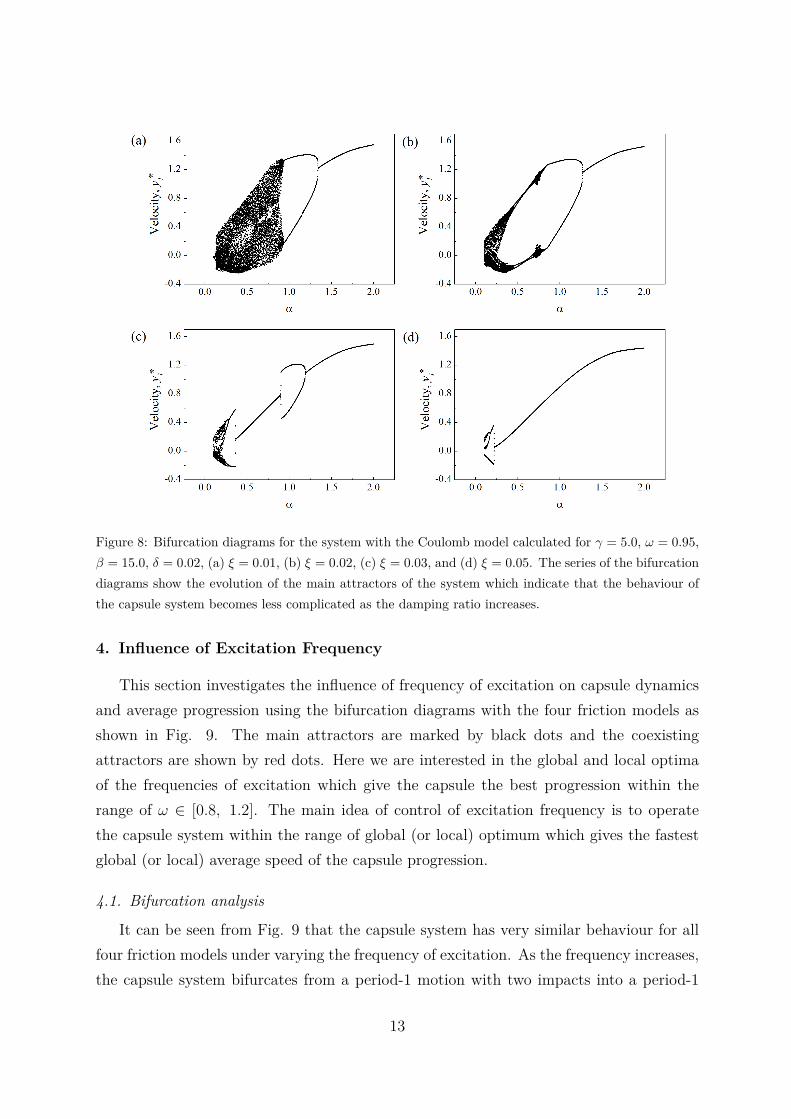
Figure 8: Bifurcation diagrams for the system with the Coulomb model calculated for γ = 5.0, ω = 0.95,β = 15.0, δ = 0.02, (a) ξ = 0.01, (b) ξ = 0.02, (c) ξ = 0.03, and (d) ξ = 0.05. The series of the bifurcationdiagrams show the evolution of the main attractors of the system which indicate that the behaviour ofthe capsule system becomes less complicated as the damping ratio increases.

4. Influence of Excitation Frequency

This section investigates the influence of frequency of excitation on capsule dynamicsand average progression using the bifurcation diagrams with the four friction models asshown in Fig. 9. The main attractors are marked by black dots and the coexistingattractors are shown by red dots. Here we are interested in the global and local optimaof the frequencies of excitation which give the capsule the best progression within therange of ω ∈ [0.8, 1.2]. The main idea of control of excitation frequency is to operatethe capsule system within the range of global (or local) optimum which gives the fastestglobal (or local) average speed of the capsule progression.

4.1. Bifurcation analysis

It can be seen from Fig. 9 that the capsule system has very similar behaviour for allfour friction models under varying the frequency of excitation. As the frequency increases,the capsule system bifurcates from a period-1 motion with two impacts into a period-1

13

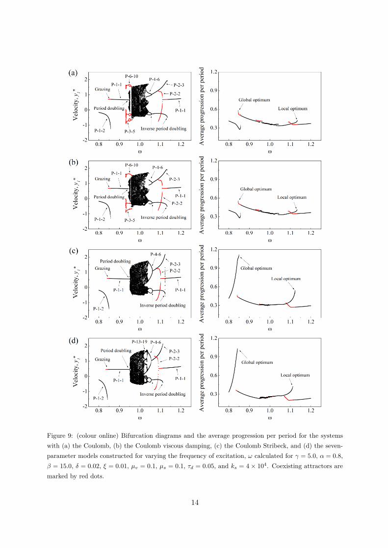
Figure 9: (colour online) Bifurcation diagrams and the average progression per period for the systemswith (a) the Coulomb, (b) the Coulomb viscous damping, (c) the Coulomb Stribeck, and (d) the seven-parameter models constructed for varying the frequency of excitation, ω calculated for γ = 5.0, α = 0.8,β = 15.0, δ = 0.02, ξ = 0.01, µv = 0.1, µs = 0.1, τd = 0.05, and ks = 4 × 104. Coexisting attractors aremarked by red dots.

14

motion with one impact through a grazing bifurcation followed by a period doublingcascade leading to chaos. Then the chaotic motion bifurcates into a period-1 motion withone impact through an inverse period doubling cascade.

Coexisting attractors are recorded for ω ∈ [0.9312, 0.959] and ω ∈ [0.9304, 0.9612]for the capsule system with the Coulomb and the Coulomb viscous damping models,respectively. Both of them are observed as a period-3 motion with five impacts, whichbifurcates into a period-6 motion with ten impacts followed by a period-3 motion with fiveimpacts as the frequency of excitation decreases, and eventually through period doublingcascade leads to the chaotic motion. However these coexisting attractors do not havesignificantly higher average progression of the system.

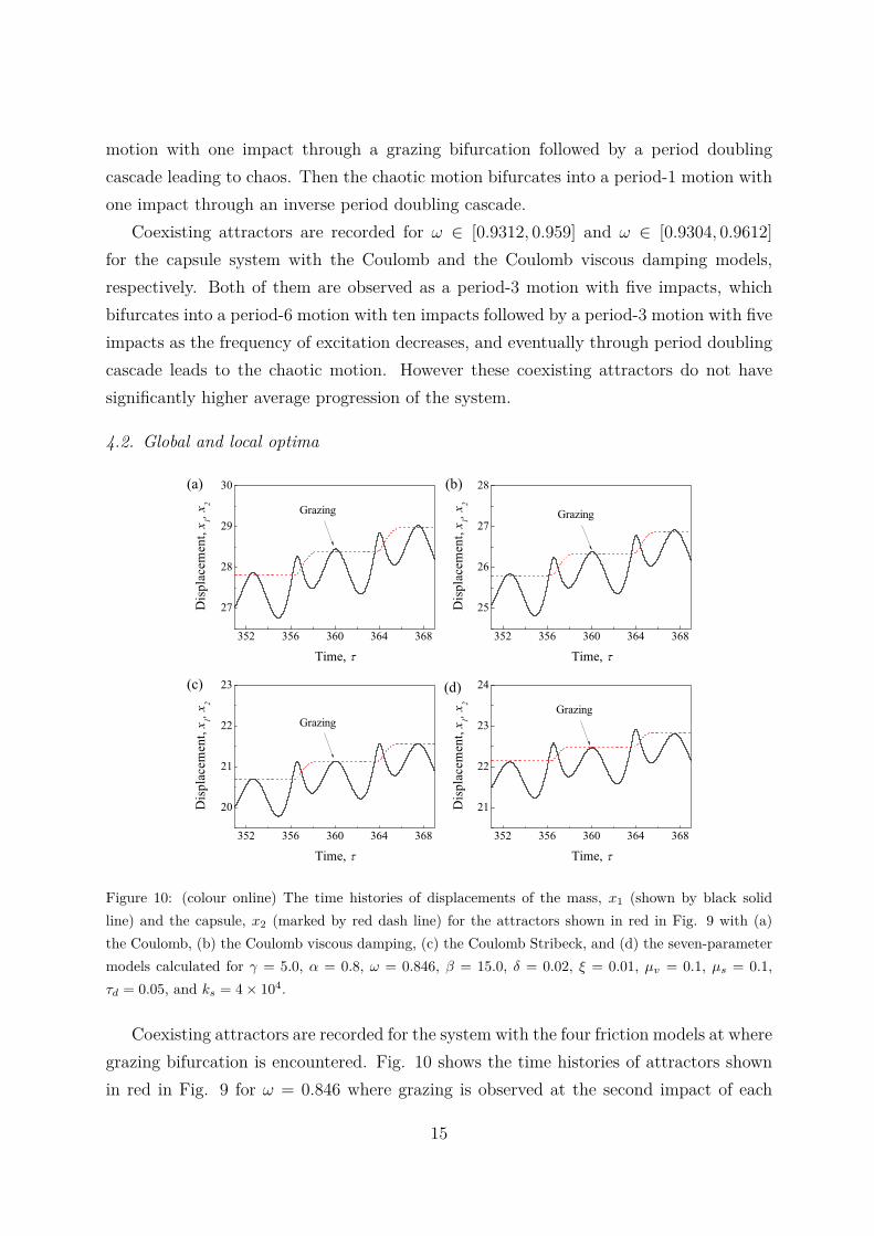
4.2. Global and local optima

352 356 360 364 368

27

28

29

30

352 356 360 364 368

25

26

27

28

352 356 360 364 368

20

21

22

23

352 356 360 364 368

21

22

23

24

Dis

plac

emen

t, x 1, x

2

Time,

Grazing

Dis

plac

emen

t, x 1, x

2

Time,

Grazing

Dis

plac

emen

t, x 1, x

2

Time,

Grazing

(d)(c)

(b)

Dis

plac

emen

t, x 1, x

2

Time,

Grazing

(a)

Figure 10: (colour online) The time histories of displacements of the mass, x1 (shown by black solidline) and the capsule, x2 (marked by red dash line) for the attractors shown in red in Fig. 9 with (a)the Coulomb, (b) the Coulomb viscous damping, (c) the Coulomb Stribeck, and (d) the seven-parametermodels calculated for γ = 5.0, α = 0.8, ω = 0.846, β = 15.0, δ = 0.02, ξ = 0.01, µv = 0.1, µs = 0.1,τd = 0.05, and ks = 4 × 104.

Coexisting attractors are recorded for the system with the four friction models at wheregrazing bifurcation is encountered. Fig. 10 shows the time histories of attractors shownin red in Fig. 9 for ω = 0.846 where grazing is observed at the second impact of each

15

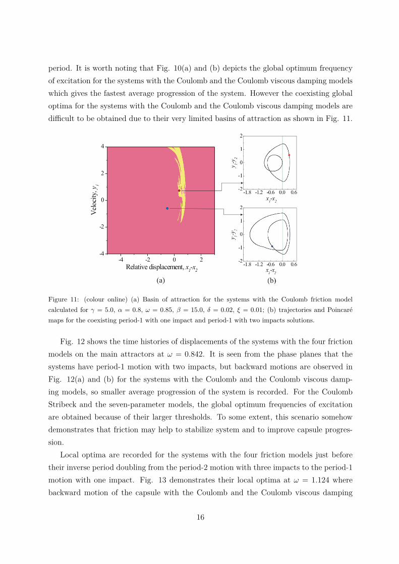
period. It is worth noting that Fig. 10(a) and (b) depicts the global optimum frequencyof excitation for the systems with the Coulomb and the Coulomb viscous damping modelswhich gives the fastest average progression of the system. However the coexisting globaloptima for the systems with the Coulomb and the Coulomb viscous damping models aredifficult to be obtained due to their very limited basins of attraction as shown in Fig. 11.

Figure 11: (colour online) (a) Basin of attraction for the systems with the Coulomb friction modelcalculated for γ = 5.0, α = 0.8, ω = 0.85, β = 15.0, δ = 0.02, ξ = 0.01; (b) trajectories and Poincaremaps for the coexisting period-1 with one impact and period-1 with two impacts solutions.

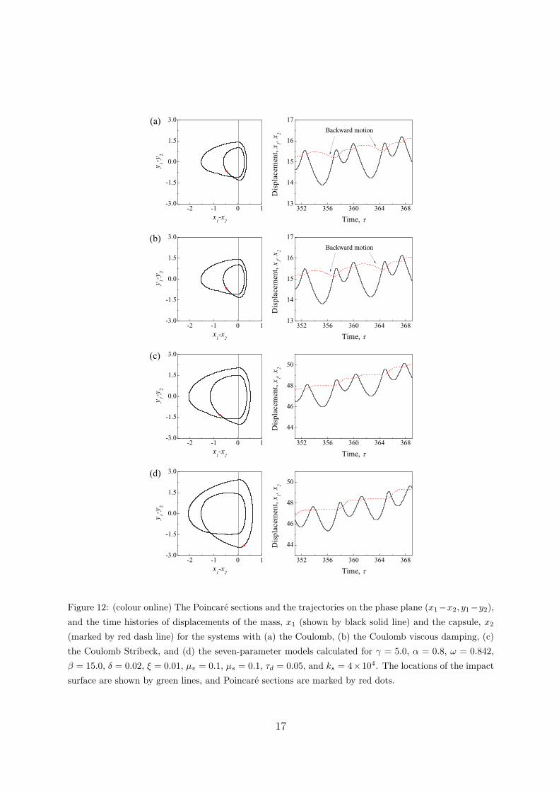
Fig. 12 shows the time histories of displacements of the systems with the four frictionmodels on the main attractors at ω = 0.842. It is seen from the phase planes that thesystems have period-1 motion with two impacts, but backward motions are observed inFig. 12(a) and (b) for the systems with the Coulomb and the Coulomb viscous damp-ing models, so smaller average progression of the system is recorded. For the CoulombStribeck and the seven-parameter models, the global optimum frequencies of excitationare obtained because of their larger thresholds. To some extent, this scenario somehowdemonstrates that friction may help to stabilize system and to improve capsule progres-sion.

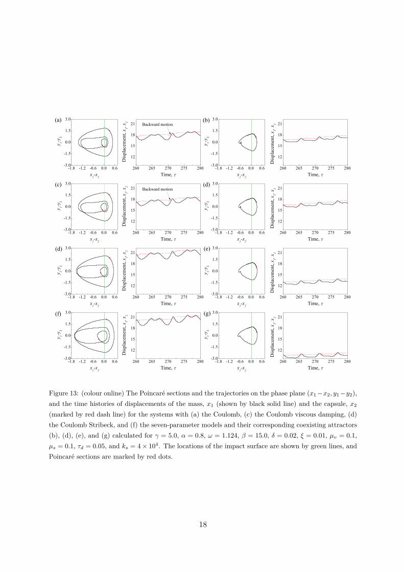
Local optima are recorded for the systems with the four friction models just beforetheir inverse period doubling from the period-2 motion with three impacts to the period-1motion with one impact. Fig. 13 demonstrates their local optima at ω = 1.124 wherebackward motion of the capsule with the Coulomb and the Coulomb viscous damping

16

-2 -1 0 1-3.0

-1.5

0.0

1.5

3.0

352 356 360 364 36813

14

15

16

17

-2 -1 0 1-3.0

-1.5

0.0

1.5

3.0

352 356 360 364 36813

14

15

16

17

-2 -1 0 1-3.0

-1.5

0.0

1.5

3.0

352 356 360 364 368

44

46

48

50

-2 -1 0 1-3.0

-1.5

0.0

1.5

3.0

352 356 360 364 368

44

46

48

50(d)

(c)

(b)

y 1-y2

x1-x

2

(a)

Dis

plac

emen

t, x 1, x

2

Time,

Backward motion

y 1-y2

x1-x

2

Dis

plac

emen

t, x 1, x

2

Time,

Backward motion

y 1-y2

x1-x

2

Dis

plac

emen

t, x 1, x

2

Time,

y 1-y2

x1-x

2

Dis

plac

emen

t, x 1, x

2

Time,

Figure 12: (colour online) The Poincare sections and the trajectories on the phase plane (x1 −x2, y1 −y2),and the time histories of displacements of the mass, x1 (shown by black solid line) and the capsule, x2

(marked by red dash line) for the systems with (a) the Coulomb, (b) the Coulomb viscous damping, (c)the Coulomb Stribeck, and (d) the seven-parameter models calculated for γ = 5.0, α = 0.8, ω = 0.842,β = 15.0, δ = 0.02, ξ = 0.01, µv = 0.1, µs = 0.1, τd = 0.05, and ks = 4×104. The locations of the impactsurface are shown by green lines, and Poincare sections are marked by red dots.

17

-1.8 -1.2 -0.6 0.0 0.6-3.0

-1.5

0.0

1.5

3.0

260 265 270 275 280

12

15

18

21

-1.8 -1.2 -0.6 0.0 0.6-3.0

-1.5

0.0

1.5

3.0

260 265 270 275 280

12

15

18

21

-1.8 -1.2 -0.6 0.0 0.6-3.0

-1.5

0.0

1.5

3.0

260 265 270 275 280

12

15

18

21

-1.8 -1.2 -0.6 0.0 0.6-3.0

-1.5

0.0

1.5

3.0

260 265 270 275 280

12

15

18

21

-1.8 -1.2 -0.6 0.0 0.6-3.0

-1.5

0.0

1.5

3.0

260 265 270 275 280

12

15

18

21

-1.8 -1.2 -0.6 0.0 0.6-3.0

-1.5

0.0

1.5

3.0

260 265 270 275 280

12

15

18

21

-1.8 -1.2 -0.6 0.0 0.6-3.0

-1.5

0.0

1.5

3.0

260 265 270 275 280

12

15

18

21

-1.8 -1.2 -0.6 0.0 0.6-3.0

-1.5

0.0

1.5

3.0

260 265 270 275 280

12

15

18

21(g)(f)

(e)(d)

(d)(c)

(b)

y 1-y2

x1-x

2

(a)D

ispl

acem

ent,

x 1, x2

Time,

Backward motion

y 1-y2

x1-x

2

Dis

plac

emen

t, x 1, x

2

Time,

y 1-y2

x1-x

2

Dis

plac

emen

t, x 1, x

2

Time,

Backward motion

y 1-y2

x1-x

2

Dis

plac

emen

t, x 1, x

2

Time,

y 1-y2

x1-x

2

Dis

plac

emen

t, x 1, x

2

Time,

y 1-y2

x1-x

2

Dis

plac

emen

t, x 1, x

2

Time,

y 1-y2

x1-x

2

Dis

plac

emen

t, x 1, x

2

Time,

y 1-y2

x1-x

2

Dis

plac

emen

t, x 1, x

2

Time,

Figure 13: (colour online) The Poincare sections and the trajectories on the phase plane (x1 −x2, y1 −y2),and the time histories of displacements of the mass, x1 (shown by black solid line) and the capsule, x2

(marked by red dash line) for the systems with (a) the Coulomb, (c) the Coulomb viscous damping, (d)the Coulomb Stribeck, and (f) the seven-parameter models and their corresponding coexisting attractors(b), (d), (e), and (g) calculated for γ = 5.0, α = 0.8, ω = 1.124, β = 15.0, δ = 0.02, ξ = 0.01, µv = 0.1,µs = 0.1, τd = 0.05, and ks = 4 × 104. The locations of the impact surface are shown by green lines, andPoincare sections are marked by red dots.

18

models is observed. In these cases the capsule progression in Fig. 13(a) and (c) doesnot have significant improvement in comparison with the progression obtained for theircoexisting attractors in Fig. 13(b) and (d).

5. Position Feedback Control

5.1. Control Point

0.1 0.2 0.3 0.4 0.5 0.6-1

0

1

2

3

-1.5 -1.0 -0.5 0.0 0.5

-1.4

-0.7

0.0

0.7

1.4

1700 1705 1710

-1.4

-0.7

0.0

0.7

P-1-1

Grazing

P-1-2

P-1-1

(c)(b)

(a)

Ave

rage

pro

gres

sion

per

per

iod

Control Point

y 1-y2

x1-x

2

Dis

plac

emen

t, x 1, x

2

Time,

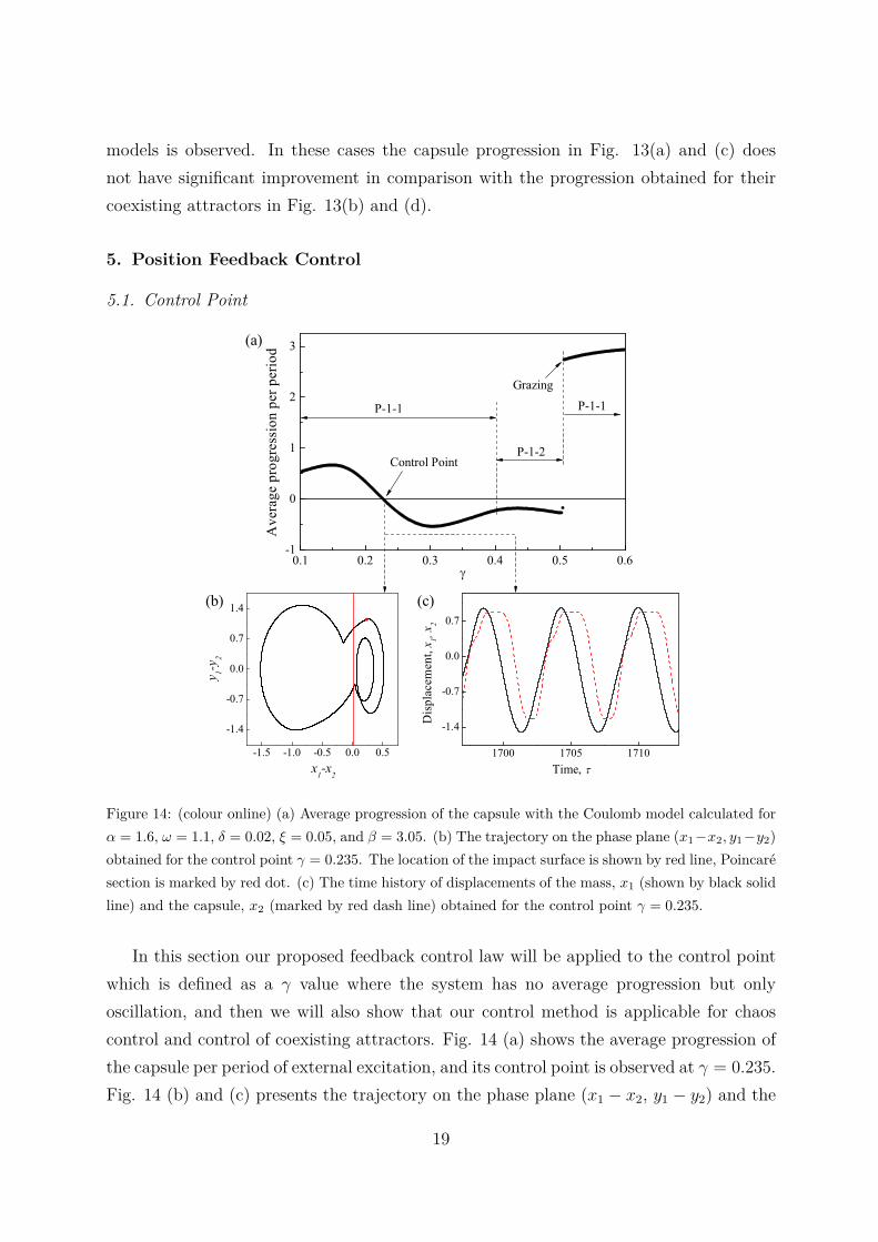
Figure 14: (colour online) (a) Average progression of the capsule with the Coulomb model calculated forα = 1.6, ω = 1.1, δ = 0.02, ξ = 0.05, and β = 3.05. (b) The trajectory on the phase plane (x1−x2, y1−y2)obtained for the control point γ = 0.235. The location of the impact surface is shown by red line, Poincaresection is marked by red dot. (c) The time history of displacements of the mass, x1 (shown by black solidline) and the capsule, x2 (marked by red dash line) obtained for the control point γ = 0.235.

In this section our proposed feedback control law will be applied to the control pointwhich is defined as a γ value where the system has no average progression but onlyoscillation, and then we will also show that our control method is applicable for chaoscontrol and control of coexisting attractors. Fig. 14 (a) shows the average progression ofthe capsule per period of external excitation, and its control point is observed at γ = 0.235.Fig. 14 (b) and (c) presents the trajectory on the phase plane (x1 − x2, y1 − y2) and the

19

time history of displacements of the mass, x1 and the capsule, x2 obtained for the controlpoint, respectively. As can be seen from Fig. 14 (c), the mass and the capsule oscillatearound their origins which leads to no average progression for the entire system.

5.2. Position feedback control

Consider the position feedback control law

u = kp |x2 − x1|,

where kp is a linear position control gain. The resulting equation of motion of the capsulesystem is described by

x1 = y1,

y1 = α cos(ωτ) + fp(x1, x2) + 2ξ(y2 − y1) − H3β(x1 − x2 − δ),

x2 = y2 (H1(1 − H3) + H2H3) , (2)

y2 = (H1(1 − H3) + H2H3) (−fs − (x2 − x1) − 2ξ(y2 − y1)

+ H3β(x1 − x2 − δ)) /γ.

where

fp(x1, x2) = kp |x2 − x1| + (x2 − x1) =

(1 − kp)(x2 − x1) if x1 > x2,

(1 + kp)(x2 − x1) if x1 < x2.(3)

As we have found in [11], the optimal parameters of the capsule system for the bestprogression and for the minimum energy consumption are different. Here we use thecontrol efficiency which is the ratio of the capsule progression per period of the externalexcitation, T to the work done by the external force and the controller over one period

Eavg = x2(T ) − x2(0)∫ T0 [α cos(ωτ) + u(τ)] · y1(τ) dτ

(4)

in order to take the energy consumption into account for evaluating our proposed positionfeedback control law.

Fig. 15 (a) presents the bifurcation diagram where the position control gain kp isused as a branching parameter. Additional windows in Fig. 15 (a) show the trajectorieson the phase plane, where the relative displacement (x1 − x2) is given on the horizontalaxis, and the relative velocity (y1 − y2) is on the vertical axis. It can be observed thatthe system response is period-one motion for all the values of the position control gainfor kp ∈ [−0.2, 0.2], and the system behaviour changes from period-one motion with one

20

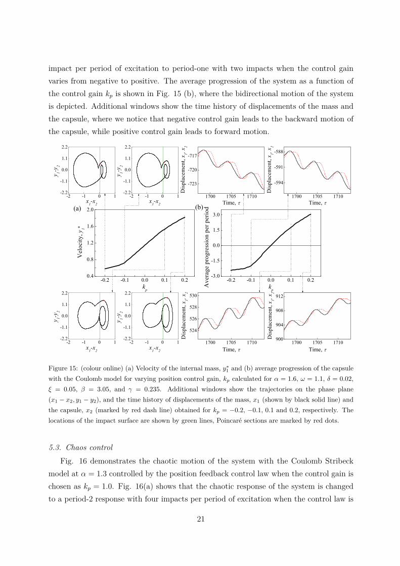
impact per period of excitation to period-one with two impacts when the control gainvaries from negative to positive. The average progression of the system as a function ofthe control gain kp is shown in Fig. 15 (b), where the bidirectional motion of the systemis depicted. Additional windows show the time history of displacements of the mass andthe capsule, where we notice that negative control gain leads to the backward motion ofthe capsule, while positive control gain leads to forward motion.

-0.2 -0.1 0.0 0.1 0.2-3.0

-1.5

0.0

1.5

3.0

-0.2 -0.1 0.0 0.1 0.20.4

0.8

1.2

1.6

2.0

-2 -1 0 1-2.2

-1.1

0.0

1.1

2.2

1700 1705 1710

-723

-720

-717

-2 -1 0 1-2.2

-1.1

0.0

1.1

2.2

1700 1705 1710

-594

-591

-588

-2 -1 0 1-2.2

-1.1

0.0

1.1

2.2

1700 1705 1710

524

526

528

530

-2 -1 0 1-2.2

-1.1

0.0

1.1

2.2

1700 1705 1710900

904

908

912

Ave

rage

pro

gres

sion

per

per

iod

kp

*

(b)

Vel

ocity

, y1

kp

(a)

y 1-y2

x1-x2

Dis

plac

emen

t, x 1, x

2

Time,

y 1-y2

x1-x2

Dis

plac

emen

t, x 1, x

2

Time,

y 1-y2

x1-x2

Dis

plac

emen

t, x 1, x

2

Time,

y 1-y2

x1-x2

Dis

plac

emen

t, x 1, x

2

Time,

Figure 15: (colour online) (a) Velocity of the internal mass, y∗1 and (b) average progression of the capsule

with the Coulomb model for varying position control gain, kp calculated for α = 1.6, ω = 1.1, δ = 0.02,ξ = 0.05, β = 3.05, and γ = 0.235. Additional windows show the trajectories on the phase plane(x1 − x2, y1 − y2), and the time history of displacements of the mass, x1 (shown by black solid line) andthe capsule, x2 (marked by red dash line) obtained for kp = −0.2, −0.1, 0.1 and 0.2, respectively. Thelocations of the impact surface are shown by green lines, Poincare sections are marked by red dots.

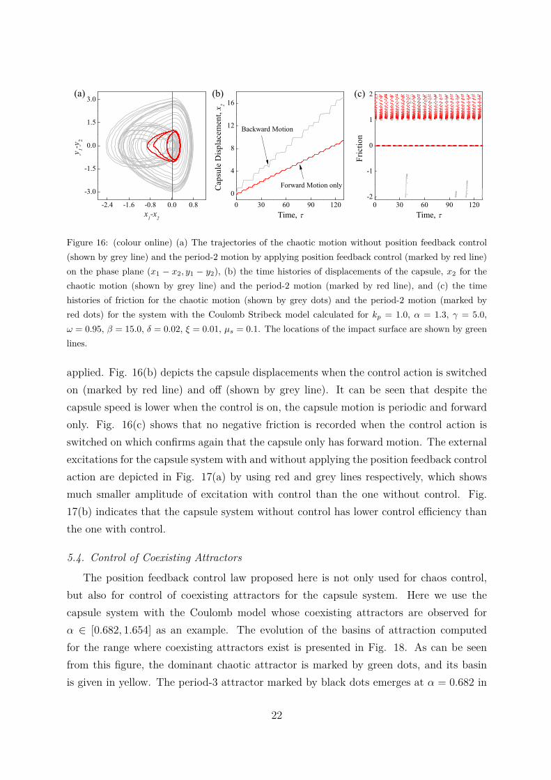
5.3. Chaos controlFig. 16 demonstrates the chaotic motion of the system with the Coulomb Stribeck

model at α = 1.3 controlled by the position feedback control law when the control gain ischosen as kp = 1.0. Fig. 16(a) shows that the chaotic response of the system is changedto a period-2 response with four impacts per period of excitation when the control law is

21

-2.4 -1.6 -0.8 0.0 0.8

-3.0

-1.5

0.0

1.5

3.0

0 30 60 90 120-2

-1

0

1

2

0 30 60 90 1200

4

8

12

16

y 1-y

2

x1-x

2

(c)(b)

Fric

tion

Time,

(a)

Forward Motion onlyCap

sule

Dis

plac

emen

t, x 2

Time,

Backward Motion

Figure 16: (colour online) (a) The trajectories of the chaotic motion without position feedback control(shown by grey line) and the period-2 motion by applying position feedback control (marked by red line)on the phase plane (x1 − x2, y1 − y2), (b) the time histories of displacements of the capsule, x2 for thechaotic motion (shown by grey line) and the period-2 motion (marked by red line), and (c) the timehistories of friction for the chaotic motion (shown by grey dots) and the period-2 motion (marked byred dots) for the system with the Coulomb Stribeck model calculated for kp = 1.0, α = 1.3, γ = 5.0,ω = 0.95, β = 15.0, δ = 0.02, ξ = 0.01, µs = 0.1. The locations of the impact surface are shown by greenlines.

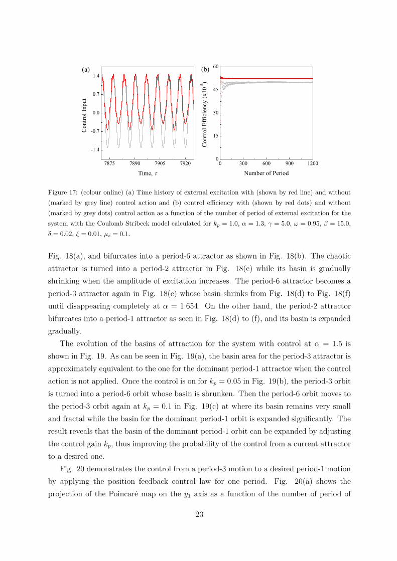
applied. Fig. 16(b) depicts the capsule displacements when the control action is switchedon (marked by red line) and off (shown by grey line). It can be seen that despite thecapsule speed is lower when the control is on, the capsule motion is periodic and forwardonly. Fig. 16(c) shows that no negative friction is recorded when the control action isswitched on which confirms again that the capsule only has forward motion. The externalexcitations for the capsule system with and without applying the position feedback controlaction are depicted in Fig. 17(a) by using red and grey lines respectively, which showsmuch smaller amplitude of excitation with control than the one without control. Fig.17(b) indicates that the capsule system without control has lower control efficiency thanthe one with control.

5.4. Control of Coexisting Attractors

The position feedback control law proposed here is not only used for chaos control,but also for control of coexisting attractors for the capsule system. Here we use thecapsule system with the Coulomb model whose coexisting attractors are observed forα ∈ [0.682, 1.654] as an example. The evolution of the basins of attraction computedfor the range where coexisting attractors exist is presented in Fig. 18. As can be seenfrom this figure, the dominant chaotic attractor is marked by green dots, and its basinis given in yellow. The period-3 attractor marked by black dots emerges at α = 0.682 in

22

0 300 600 900 12000

15

30

45

60

7875 7890 7905 7920

-1.4

-0.7

0.0

0.7

1.4

Con

trol E

ffic

ienc

y (x

10-5

)

Number of Period

(b)

Con

trol I

nput

Time,

(a)

Figure 17: (colour online) (a) Time history of external excitation with (shown by red line) and without(marked by grey line) control action and (b) control efficiency with (shown by red dots) and without(marked by grey dots) control action as a function of the number of period of external excitation for thesystem with the Coulomb Stribeck model calculated for kp = 1.0, α = 1.3, γ = 5.0, ω = 0.95, β = 15.0,δ = 0.02, ξ = 0.01, µs = 0.1.

Fig. 18(a), and bifurcates into a period-6 attractor as shown in Fig. 18(b). The chaoticattractor is turned into a period-2 attractor in Fig. 18(c) while its basin is graduallyshrinking when the amplitude of excitation increases. The period-6 attractor becomes aperiod-3 attractor again in Fig. 18(c) whose basin shrinks from Fig. 18(d) to Fig. 18(f)until disappearing completely at α = 1.654. On the other hand, the period-2 attractorbifurcates into a period-1 attractor as seen in Fig. 18(d) to (f), and its basin is expandedgradually.

The evolution of the basins of attraction for the system with control at α = 1.5 isshown in Fig. 19. As can be seen in Fig. 19(a), the basin area for the period-3 attractor isapproximately equivalent to the one for the dominant period-1 attractor when the controlaction is not applied. Once the control is on for kp = 0.05 in Fig. 19(b), the period-3 orbitis turned into a period-6 orbit whose basin is shrunken. Then the period-6 orbit moves tothe period-3 orbit again at kp = 0.1 in Fig. 19(c) at where its basin remains very smalland fractal while the basin for the dominant period-1 orbit is expanded significantly. Theresult reveals that the basin of the dominant period-1 orbit can be expanded by adjustingthe control gain kp, thus improving the probability of the control from a current attractorto a desired one.

Fig. 20 demonstrates the control from a period-3 motion to a desired period-1 motionby applying the position feedback control law for one period. Fig. 20(a) shows theprojection of the Poincare map on the y1 axis as a function of the number of period of

23

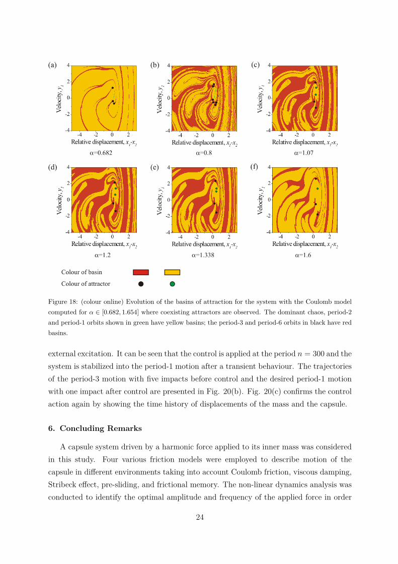
Figure 18: (colour online) Evolution of the basins of attraction for the system with the Coulomb modelcomputed for α ∈ [0.682, 1.654] where coexisting attractors are observed. The dominant chaos, period-2and period-1 orbits shown in green have yellow basins; the period-3 and period-6 orbits in black have redbasins.

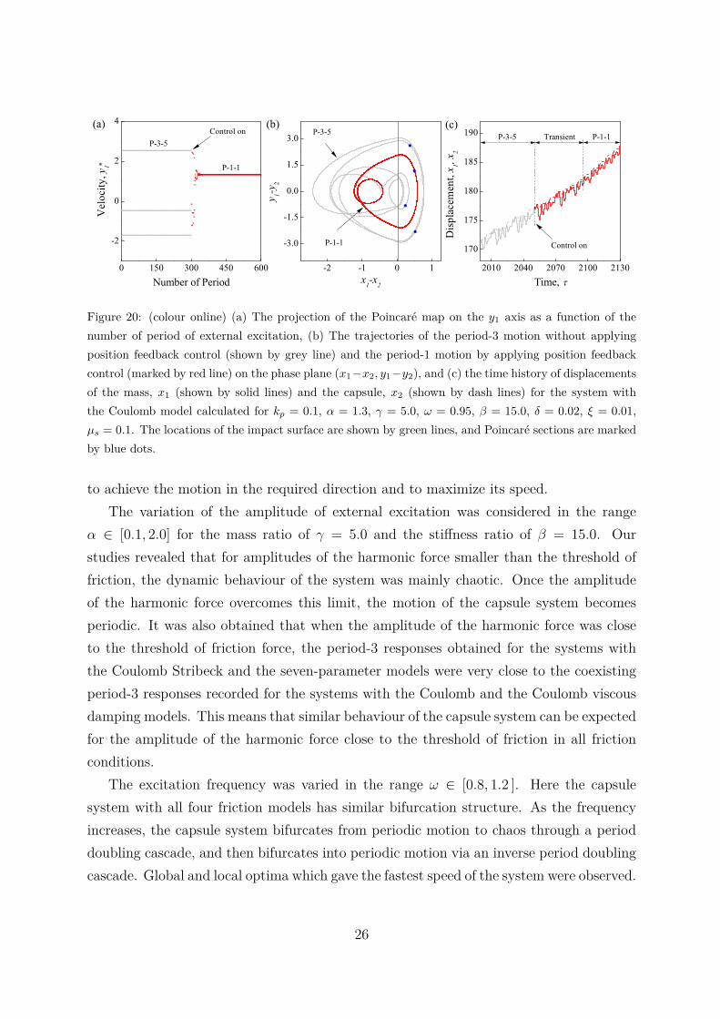
external excitation. It can be seen that the control is applied at the period n = 300 and thesystem is stabilized into the period-1 motion after a transient behaviour. The trajectoriesof the period-3 motion with five impacts before control and the desired period-1 motionwith one impact after control are presented in Fig. 20(b). Fig. 20(c) confirms the controlaction again by showing the time history of displacements of the mass and the capsule.

6. Concluding Remarks

A capsule system driven by a harmonic force applied to its inner mass was consideredin this study. Four various friction models were employed to describe motion of thecapsule in different environments taking into account Coulomb friction, viscous damping,Stribeck effect, pre-sliding, and frictional memory. The non-linear dynamics analysis wasconducted to identify the optimal amplitude and frequency of the applied force in order

24

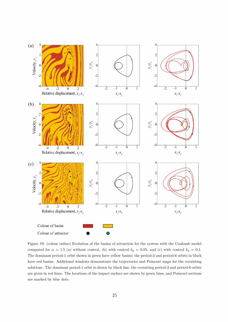
Figure 19: (colour online) Evolution of the basins of attraction for the system with the Coulomb modelcomputed for α = 1.5 (a) without control, (b) with control kp = 0.05, and (c) with control kp = 0.1.The dominant period-1 orbit shown in green have yellow basins; the period-3 and period-6 orbits in blackhave red basins. Additional windows demonstrate the trajectories and Poincare maps for the coexistingsolutions. The dominant period-1 orbit is shown by black line, the coexisting period-3 and period-6 orbitsare given in red lines. The locations of the impact surface are shown by green lines, and Poincare sectionsare marked by blue dots.

25

0 150 300 450 600

-2

0

2

4

-2 -1 0 1

-3.0

-1.5

0.0

1.5

3.0

2010 2040 2070 2100 2130

170

175

180

185

190Control on

P-1-1

P-3-5

*

Vel

ocity

, y1

Number of Period

P-1-1

P-3-5(c)(b)

y 1-y2

x1-x

2

(a)

Control on

P-1-1TransientP-3-5

Dis

plac

emen

t, x 1, x

2

Time,

Figure 20: (colour online) (a) The projection of the Poincare map on the y1 axis as a function of thenumber of period of external excitation, (b) The trajectories of the period-3 motion without applyingposition feedback control (shown by grey line) and the period-1 motion by applying position feedbackcontrol (marked by red line) on the phase plane (x1−x2, y1−y2), and (c) the time history of displacementsof the mass, x1 (shown by solid lines) and the capsule, x2 (shown by dash lines) for the system withthe Coulomb model calculated for kp = 0.1, α = 1.3, γ = 5.0, ω = 0.95, β = 15.0, δ = 0.02, ξ = 0.01,µs = 0.1. The locations of the impact surface are shown by green lines, and Poincare sections are markedby blue dots.

to achieve the motion in the required direction and to maximize its speed.The variation of the amplitude of external excitation was considered in the range

α ∈ [0.1, 2.0] for the mass ratio of γ = 5.0 and the stiffness ratio of β = 15.0. Ourstudies revealed that for amplitudes of the harmonic force smaller than the threshold offriction, the dynamic behaviour of the system was mainly chaotic. Once the amplitudeof the harmonic force overcomes this limit, the motion of the capsule system becomesperiodic. It was also obtained that when the amplitude of the harmonic force was closeto the threshold of friction force, the period-3 responses obtained for the systems withthe Coulomb Stribeck and the seven-parameter models were very close to the coexistingperiod-3 responses recorded for the systems with the Coulomb and the Coulomb viscousdamping models. This means that similar behaviour of the capsule system can be expectedfor the amplitude of the harmonic force close to the threshold of friction in all frictionconditions.

The excitation frequency was varied in the range ω ∈ [0.8, 1.2 ]. Here the capsulesystem with all four friction models has similar bifurcation structure. As the frequencyincreases, the capsule system bifurcates from periodic motion to chaos through a perioddoubling cascade, and then bifurcates into periodic motion via an inverse period doublingcascade. Global and local optima which gave the fastest speed of the system were observed.

26

It is noted that the global optima for the systems with the Coulomb and the Coulombviscous damping models are obtained for those of their co-existing attractors which havevery limited basins of attraction. The global optima for the systems with the CoulombStribeck and the seven-parameter models belong to the attractors with large basins. Thelarger thresholds of frictional force in these models result in the stabilization of the systemand improvement of capsule progression.

The variation of damping ratio has shown that the behaviour of the system becomesless complex as the damping ratio increases, which means that this parameter could betuned in the system design for avoiding chaotic motion.

The position feedback control law was applied to the capsule system with the Coulombfriction model. With the control in place, the capsule system is able to move forward andbackward under variation of its position control gain, kp. When the value of this gainvaries from negative to positive, the system response is transformed from period-onemotion with one impact to period one with two impacts, while the direction of motionchanges from backward to forward. Here the larger the control gain is, the faster theaverage progression of the capsule is.

To demonstrate the application of the proposed position feedback control law for chaoscontrol, the system with Coulomb Stribeck model was considered at α = 1.3, where forthe chosen system parameters the chaotic motion was observed. When the control lawwas applied, a period-2 response with four impacts per period of excitation was obtained.In this case the capsule speed was lower when the control was applied, but the capsulemotion was periodic and forward only. Also the capsule with control has higher controlefficiency than the one without control.

The evolution of the basins of attraction was also studied for the system with theCoulomb friction model for the range of excitation amplitude where a number of attractorscoexist, and the effect of the control law on the evolution of the basins was investigated.The result showed that the basin of the desired attractor can be significantly enlargedby adjusting the control gain slightly. Therefore, a chance of switching from the currentattractor to a desired one can be improved.

7. Acknowledgments

Dr Yang Liu would like to acknowledge the financial support for the Research Projectof State Key Laboratory of Mechanical System and Vibration (MSV201401) by ShanghaiJiao Tong University and the Small Research Grant (31841) by the Carnegie Trust for

27

the Universities of Scotland.

References

[1] F. Carpi, S. Galbiati, A. Carpi, Controlled navigation of endoscopic capsules: Con-cept and preliminary experimental investigations, IEEE Trans. Biomedical Engineer-ing 54 (2007) 2028–2036.

[2] P. Glass, E. Cheung, M. Sitti, A legged anchoring mechanism for capsule endoscopesusing micropatterned adhesives, IEEE Transactions on Biomedical Engineering 55(2008) 2759–2767.

[3] B. J. Nelson, I. K. Kaliakatsos, J. J. Abbott, Microrobots for minimally invasivemedicine, Annu. Rev. Biomed. Eng. 12 (2010) 55–85.

[4] G. Ciuti, A. Menciassi, P. Dario, Capsule endoscopy: from current achievements toopen challenges, IEEE Trans. Biomedical Engineering 4 (2011) 59–72.

[5] Z. Wang, H. Gu, A bristle-based pipeline robot for I11-constraint pipes, IEEE Trans.Mechatronics 13 (2008) 383–392.

[6] Y. Zhang, S. Jiang, X. Zhang, X. Ruan, D. Guo, A variable-diameter capsule robotbased on multiple wedge effects, IEEE/ASME Trans. Mechatronics 16 (2011) 241–254.

[7] J. Park, D. Hyun, W. Cho, T. Kin, H. Yang, Normal-force control for an in-piperobot according to the inclination of pipelines, IEEE Trans. Industrial Eletronics 58(2011) 5304–5310.

[8] H. Li, K. Furuta, F. L. Chernousko, Motion generation of the capsubot using internalforce and static friction, in: Proceedings of the 45th IEEE Conference on Decisionand Control, San Diego, CA, USA, 2006, pp. 6575–6580.

[9] F. L. Chernousko, The optimum periodic motions of a two-mass system in a resistantmedium, J. Appl. Maths Mechs. 72 (2008) 116–125.

[10] H. B. Fang, J. Xu, Dynamics of a mobile system with an internal acceleration-controlled mass in a resistive medium, J. Sound and Vibration 330 (2011) 4002–4018.

[11] Y. Liu, M. Wiercigroch, E. Pavlovskaia, H. Yu, Modelling of a vibro-impact capsulesystem, Int J Mechanical Sciences 66 (2013) 2–11.

28

[12] S. Yim, M. Sitti, Design and rolling locomotion of a magnetically actuated softcapsule endoscope, IEEE Transactions on Robotics 28 (2012) 183–194.

[13] L. J. Sliker, M. D. Kern, J. A. Schoen, M. E. Rentschler, Surgical evaluation ofa novel tethered robotic capsule endoscope using micro-patterned treads, SurgicalEndoscopy 26 (2012) 2862–2869.

[14] Y. Liu, E. Pavlovskaia, M. Wiercigroch, Vibro-impact responses of capsule systemwith various friction models, Int J Mechanical Sciences 72 (2013) 39–54.

[15] E. Gutierrez, D. K. Arrowsmith, Control of a double impacting mechanical oscillatorusing displacement feedback, Int J. Bifurcation and Chaos 14 (2004) 3095–3113.

[16] H. Dankowicz, J. Jerrelind, Control of near-grazing dynamics in impact oscillators,Proc. R. Soc. A 461 (2005) 3365–3380.

[17] S. L. T. de Souza, I. L. Caldas, Controlling chaotic orbits in mechanical systems withimpacts, Chaos, Solitons and Fractals 19 (2004) 171–178.

[18] J. Y. Lee, J. J. Yan, Control of impact oscillator, Chaos, Solitons and Fractals 28(2006) 136–142.

[19] S. L. T. de Souza, I. L. Caldas, R. L. Viana, Damping control law for a chaoticimpact oscillator, Chaos, Solitons and Fractals 32 (2007) 745–750.

[20] L. Wang, X. Xu, Y. Li, Impulsive control of a class of vibro-impact systems, Phys.Lett. A 372 (2008) 5309–5313.

[21] Y. Liu, M. Wiercigroch, J. Ing, E. Pavlovskaia, Intermittent control of coexistingattractors, Phil. Trans. R. Soc. A 371 (2013) 20120428.

[22] J. Ing, E. Pavlovskaia, M. Wiercigroch, S. Banerjee, Bifurcation analysis of an impactoscillator with a one-sided elastic constraint near grazing, Physica D 239 (2010) 312–321.

[23] L. C. Silva, M. A. Savi, A. Paiva, Nonlinear dynamics of a rotordynamic nonsmoothshape memory alloy system, Journal of Sound and Vibration 332 (2013) 608–621.

[24] E. Pavlovskaia, M. Wiercigroch, Periodic solution finder for an impact oscillator witha drift, J. Sound and Vibration 267 (2003) 893–911.

29

[25] G. W. Luo, X. H. Lv, L. Ma, Periodic-impact motions and bifurcations in dynamicsof a plastic impact oscillator with a frictional slider, European Journal of MechanicsA/Solids 27 (2008) 1088–1107.

[26] G. W. Luo, X. H. Lv, Controlling bifurcation and chaos of a plastic impact oscillator,Nonlinear Analysis: Real World Applications 10 (2009) 2047–2061.

[27] J. Wojewoda, A. Stefanski, M. Wiercigroch, T. Kapitaniak, Hysteretic effects of dryfriction: modelling and experimental studies, Phil. Trans. R. Soc. A 366 (2008) 747–765.

30