NASA/CP--1999-209758

NASA/CP-1999-209758

20000027529

Tenth Biennial Coherent Laser Radar

Technology and Applications ConferenceCompiled byM.J. KavayaMarshall Space Flight Center, Marshall Space Flight Center,Alabama

_r FFORREFEi Ei ;C,.NOTTOBETAKENFROMTHISR06'_

LIBRARYCOPY

Proceedings of a conference held ' 1 _ - I _000in Mount Hood, Oregon, iJune 28-July 2, 1999

LANGLEYRESEARCHCEN[ERLIBRARYNASA

HA_F'_ON,VIRGINIAT__

November 1999

The NASA STI Program Office...in Profile

Since its founding, NASA has been dedicated to • CONFERENCE PUBLICATION. Collectedthe advancement of aeronautics and space papers from scientific and technical conferences,science. The NASA Scientific and Technical symposia, seminars, or other meetings sponsoredInformation (STI) Program Office plays a key or cosponsored by NASA.part in helping NASA maintain this importantrole. • SPECIAL PUBLICATION. Scientific, technical,

or historical information from NASA programs,The NASA STI Program Office is operated by projects, and mission, often concerned withLangley Research Center, the lead center for subjects having substantial public interest.NASA's scientific and technical information. The

NASA STI Program Office provides access to the • TECHNICAL TRANSLATION.NASA STI Database, the largest collection of English-language translations of foreign scientificaeronautical and space science STI in the world. The and technical material pertinent to NASA'sProgram Office is also NASA's institutional mission.mechanism for disseminating the results of itsresearch and development activities. These results Specialized services that complement the STIare published by NASA in the NASA STI Report Program Office's diverse offerings include creatingSeries, which includes the following report types: custom thesauri, building customized databases,

organizing and publishing research results...even• TECHNICAL PUBLICATION. Reports of providing videos.

completed research or a major significant phaseof research that present the results of NASA For more information about the NASA STI Programprograms and include extensive data or Office, see the following:theoretical analysis. Includes compilations ofsignificant scientific and technical data and • Access the NASA STI Program Home Page atinformation deemed to be of continuing reference http://www.sti.nasa.govvalue. NASA's counterpart of peer-reviewedformal professional papers but has less stringent • E-mail your question via the Internet tolimitations on manuscript length and extent of help@sti.nasa.govgraphic presentations.

• Fax your question to the NASA Access Help• TECHNICAL MEMORANDUM. Scientific and Desk at (301) 621-0134

technical findings that are preliminary or ofspecialized interest, e.g., quick release reports, • Telephone the NASA Access Help Desk at (301)working papers, and bibliographies that contain 621-0390minimal annotation. Does not contain extensiveanalysis. • Write to:

NASA Access Help Desk• CONTRACTOR REPORT. Scientific and NASA Center for AeroSpace Information

technical findings by NASA-sponsored 7121 Standard Drivecontractors and grantees. Hanover, MD 21076-1320

llllii_iiiii_lliiNASA/CP--1999-209758 3 1176 01448 0124

Tenth Biennial Coherent Laser Radar

Technology and Applications ConferenceCompiled byM.J. KavayaMarshall Space Flight Center, Marshall Space Flight Center, Alabama

Proceedings of a conference heldin Mount Hood, Oregon,June 28-July 2, 1999

National Aeronautics and

Space Administration

Marshall Space Flight Center • MSFC, Alabama 35812

rNovember1999

Available from:

NASA Center for AeroSpace Information National Technical Information Service7121 Standard Drive 5285 Port Royal RoadHanover, MD 21076-1320 Springfield, VA 22161(301) 621-0390 (703) 487-4650

ii

Table of Contents

CLRC '99 Sponsors ..................................................................................................................iv

ConferenceDigestWelcome......................................................................................................................vConferenceChair..............................................._.........................................................vConferenceOrganization...........................................................:.................................vExhibits..........................................................................................................................vForeward.......................................................................................................................vScope.., ............................................................................................., .........•...............vPastConferences..........................................................................................................viTopicsto bePresented..........;..................... .................................................................viAcknowledgements........:..........................................:..................:.................................vi

Conference Program Committee ...........................................................................................vii

Conference Advisory Committee ...................................... ....................................................viii

Conference Schedule ....:....L............. .,........._.......,.I..L..,. ...................................................... ix

Conference Abstracts and Papers ...................................................................................1-316

Index ............................. ......._............:.............................:...............................................317-319

ili

CLRC '99 SPONSORS

National Aeronautics and Space AdministrationHeadquarters/Office of Earth Science

National Aeronautics and Space Administration/Marshall Space Flight Center/

Global Hydrology and Climate Center

National Polar-orbiting Operational Environmental SatelliteSystem Integrated Program Office

National Aeronautics and Space Administration/New Millennium Program

Air Force Research Laboratory/Directed Energy Directorate

National Aeronautics and Space Administration/Langley Research Center

iv

CONFERENCE DIGEST

WELCOME, TO THE 10TH BIENNIAL COHERENT LASERRADAR TECHNOLOGY AND APPLICATIONS CONFERENCE(CLRC)

Location:Timberline LodgeMt. Hood, OregonJune 28 - July 2, 1999

CLRC'99 Conference Chair:Dr. Michael J. KavayaNASA Marshall Space Flight CenterGlobal Hydrology and Climate CenterHuntsville, AL 35812256-922-5803michael.kavaya@msfc.nasa.gov

CLRC'99 Organization:Debra G. Hallmark and L. Gayle BrownUniversities Space Research Association (USRA)4950 Corporate Drive, Suite 100Huntsville, AL 35805256-895-0582http://space.hsv.usra.edu

Exhibits Presented by:• Coherent Technologies, Inc.• DFM Engineering• Ontar Corporation

Foreward:The tenth conference on Coherent Laser Radar: Technology and Applications is the latest in aseries beginning in 1980 which provides a forum for exchange of information on recent events,current status, and future directions of coherent laser radar (or lidar or ladar) technology andapplications.

Scope:This conferenceemphasizesthe latest advancementsin the coherentlaser radar field, includingtheory, modeling, components, systems, instrumentation, measurements, calibration, dataprocessing techniques, operational uses, and comparisons with other remote sensingtechnologies.

v

Past Conferences:Year Location Chair Co-chair1980 Aspen, CO USA Huffaker none1983 Aspen, CO USA Huffaker Vaughan1985 UnitedKingdom Vaughan Huffaker1987 Aspen,CO USA Bilbro Wemer1989 Munich,Germany Wemer Bilbro1991 Snowmass,CO USA Hardesty Flamant1993 Paris, France Flamant Menzies1995 Keystone,CO USA Menzies Steinvall1997 Sweden Steinvall Kavaya1999 Mount Hood, OR USA Ka'vaya Willetts

Topics to be presented:• AircraftOperations• AircraftMissions• VibrationMeasurements• DIAL "• Theory and Simulation• Spacebome Lidars• New Technology• Target Characterization• Detection Advances• Laser Advances

• System Advances• CW Lidars• Wind Measurements

Acknowledgements:I greatly appreciate the Sponsors and the Program Committee members for theircontributionstothe CLRC'99. Their dedicationand commitmentto the CoherentLaser Radar Programis highlycommended. I wouldalso like to give a specialthankyou to Debra and Gayle for the planning"andexecution of the CLRC'99 and the ConferenceDigest.

Michael J. Kavaya

v±

ConferenceProgramCommittee

Steven B. AlejandroUSAF/AFRL, Albuquerque, NM USA

Kasuhiro AsaiTohuko Institute of Technology, Japan

Alain DabasMeteo-France, Toulouse, France

Rod G. FrehlichUniversity of Colorado, Boulder, CO USA

Sammy W. HendersonCoherent Technologies, Inc., Lafayette, CO USA

J. Fred HolmesOregon Graduate Institute, Portland, OR USA

Steven C. JohnsonNASAJMarsha//Space Fright Center, Huntsville, AL USA

Michael J, KavayaNASAJMarsha//Space Fright Center/Global Hydrology and Climate Center, Huntsville, AL USA

Dennis K. KillingerUniversity of South Florida, Tampa, FL USA

Paul F. McManamonUSAF/AFRL, Dayton, OH USA

Stephan RahmDLR German Aerospace Center, Wessling, Germany

Richard D. RichmondUSAF/AFRL, Dayton, OH USA

Barry J. RyeNOAA Environmental Technology Laboratory, Boulder, CO USA

Upendra N. SinghNASA Langley Research Center, Hampton, VA USA

David M. TrattJet Propulsion Laboratory, Pasadena, CA USA

David V. WillettsDefence Evaluation and Research Agency (DERA), Great Ma/vem, UK

Peter WinzerTechnische Universitat Wien, Wien, Austria

vii

Conference Advisory Committee

James W, BilbroNASA / Marshall Space Flight Center, Huntsville, AL USA

Pierre H. FlamantLMD, Ecole Polytechnique, Palaiseau, France

R. Michael HardestyNOAA Environmental Technology Laboratory, Boulder, CO USA

R. Milton HuffakerCoherent Technologies, Inc., Lafayette, CO USA

Robert T. MenziesJet Propulsion Laboratory, Pasadena, CA USA

Ove SteinvallNational Defence Research Institute (FOA), Linkoping Sweden

J. Michael VaughanDefence Evaluation and Research Agency (DERA), Great Malvern, UK

Christian WernerGerman AerospaCe Establishment (DLR), Munich, Germany

viii

ConferenceSchedule

Sunday, June 276:00p.m.- 9:00p.m. ReceptionandRegistration/Check-in

Monday,June 288:00a.m.- 8:10a.m. OpeningRemarks/Information MichaelKavaya8:00a.m. RegistrationContinued8:10a.m.- 9:50a.m. Session1 - AircraftOperations MiltonHuffaker,Presider9:50a.m.- 10:10a.m. Break10:10a.m.- 10:50a.m. Session2 - AircraftMissions FredHolmes,Presider10:50a.m.- 11:40a.m. Session3 -Special FredHolmes,Presider11:40a.m.- 1:10p.m. Lunch1:10p.m.-3:10p.m. Session4 -VibrationMeasurements PaulMcManamon,Presider3:10p.m.- 3:30p.m. Break3:30p.m.-4:30p.m. Session5 - DIAL OveSteinvall,Presider4:30p.m.- 5:10p.m. Session6 -TheoryandSimulation RodFrehlich,Presider5:10p.m.- 7:00p.m. FreeTime7:00p.m.-8:00p.m. PanelDiscussion- MarketsforCLR DennisKiliinger,Presider

Tuesday, June 298:00a.m.- 9:30a.m. Session7 -SpaceborneLidars- 1 DennisKillinger,Presider9:30a.m.- 9:50a.m. Break9:50a.m.- 11:10aom. Session7 -SpaceborneLidars- 1 (Continued) DennisKilUnger,Presider11:10a.m.- 11:15a.m. Announcements DebraHallmark,ConferenceOrganizer11:15a.m.- 11:20a.m. Contest GayleBrown,ConferenceOrganizer11:20a.m.- 11:50a.m. GroupPhotograph11:50a.m.- 1:00p.m. Lunch1:00p.m. -2:00p.m. FreeTime2:00p.m.- 3:30p.m, DepartforTrainRide3:30p.m.- 7:30p.m. TrainRideandDinner7:30 p.m.- 9:00p.m. ReturntoLodge

Wednesday, June 308:00a.m.- 9:20a.m. Session8 - NewTechnology RichardRichmond,Presider9:20a.mo- 9:40a.m. Break9:40a.m.- 12:20p.m. Session9-Target Characterization RobertMenzies,Presider12:20p.m.- 7:00p.m. Lunch/ FreeTime/ PosterSet-up7:00p.m.- 8:00p.m. Reception7:00p.m.- 8:00p.m. Session10- Posters

Thursday, July 18:00a.m.- 9:30a.m. Session11- DetectionAdvances BarryRye,Presider9:30a.m.- 9:50a.m. Break9:50a.m.- 10:30a.m. Session11- DetectionAdvances(Continued) BarryRye,Presider10:30a.m.- 11:30a.m. Session12 - LaserAdvances ChristianWemer,Presider11:30a.m.- 1:20p.m. LunchandAdvisoryCommitteeLunch1:20p.m.-2:30 p.m. Session13-SystemAdvances AlainDabas,Presider2:30p.m.- 3:30p.m. Session14- CWLidars MjchaelVaughan,Presider3:30p.m.- 3:50p,m. Break3:50p.m.- 5:50p.m. Session15-Wind Measurements DavidTratt,Presider5:50p.m.- 7:00p.m. FreeTime7:00p.m.- 9:00p.m. ThemeDinner

Friday, July 28:30a.m.- 9:30a.m. Session16- SpaceborneLidars- 2 KasuhiroAsaiandDavidWilletts,Presiders9:30a.m.- 9:50a.m. Break9:50a.m.- 11:50a.m. Session16-SpaceborneLidars-2 (Continued) KasuhiroAsaiandDavidWilletts,Presiders11:50a.m.- 11:55a.m. ClosingRemarks MichaelKavaya11:55a.m.- 12:00noon ClosingRemarks DaveWilletts12:00noon ENDOFCONFERENCE

ix

Abstracts

Monday, June 28

AircraftOperations AircraftMissionsPresider: Milton Huffaker Presider: Fred Holmes

10:10.10:308:10- 8:40 The Multi-center Airborne Coherent Atmospheric WindCoherent Pulsed Lidar Sensing of Wake Vortex Position Sensor: Recent Measurements and Future Applicationsand Strength, Winds and Turbulence in Airport Terminal Jeffry Rotherme/, NASA/MSFC/Global Hydrology andAreas Climate Center, R. Michael Hardesty, James N. Howell, Lisa(Invited) Philip Brockman, Sen C. Barker Jr., Grady J. Koch, S. Darby, NOAA Environmental Technology Laboratory,NASA Langley Research Center and Dung Phu hi Nguyen, Dean R. Cutten, University of Alabama in Huntsville/GlobalCharles L. Britt Jr., Research Triangle Institute I-lydro/ogy and Climate Center, David M. Tratt, and Robert t.A two m=crometercoherent pulsedtransceiverand real time Menzies, Jet Propulsion Laboratorydata system have been developed as a sensor for the The atmospheric lidar remote sensing groups of NOAAAircraft VoortexSpacing System (AVOSS) element of the Environmental Technology Laboratory, Jet PropulsionNASA _Terminal_Area Productivity (TAP) Program for Laboratoryand NASA Marshall Space Flight Center jointlyincreasing airport throughput under Instrument developedan airbornescanningcoherentDopplerlidar. WeMeteorologicalConditions (IMC). The system has been describe the system, present recent measurementsdeployed to Norfolk, JFK and DFW airports. Results of (includingthe first wind fields measured withina hurricanemeasurementsand intercomparisonswith othersensorsare using Doppler lidar), and describe prospective instrumentdescribed, improvementsandresearchapplications.

8:40 - 9:00 10:30 - 10:50Concept of a cw-Laser Doppler Sensor as True-Airspeed WIND Instrument Results of Ground TestsInstrument F. K_pp(I), R. H_ring(1_, M. K/ie/I J, E. Nage#I), O.Juergen Streicher, Ines Leike, Stephan Rahm, Christian Reitebuch(1),M. Schrecke/!j, J. Streiche/_, Ch. Werne#1_,Wemer, DLR - Lidar Group. and Richard Bogenberger, G. Wildgrube#2), C. Loth(_),Ch. Boite#_), P. Delvillem, Ph.Daimler Chrysler Aerospace, Germany Drobinskf% P. H. Flamant_3),B. Romand 3),L. Sauvage(% D.A virtual instrument was designed based on LabView to Bruneau(4), M. Meissonnie/s) (1) DLR - Arbeitsgruppeoptimize a.cw-Doppler lidar for airborne applications. The LIDAR, (2) Modulab, 80636 Mgnchen, Germany, (3) LMD,optics parameters and the atmosphere can be selected. CNRS, 91128 Palaiseau Cedex, France, (4) ServiceFlying in high altitude is a real challenge for the sensor to d'Aeronomie / CNRS / UPMC, 75252 Paris Cedex 05,deteotsingle particles.and estimate the Doppler shift. France, [5) INSU / DT 77 Av Denfert Rochereau, 75014

Paris, France9:00-9:30 An airborne coherent Doppler Lidar to retrieve mesoscaleAirborne Turbulence Detection and Warning: ACLAIM wind fields has been developed in the frame of theFranco-Flight Test Results GermanWIND project.The instrumentis basedon a pulsed(Invited) Stephen M. Hannon and Hal R. Bagley, Coherent C02 laser transmitter, heterodyne detection and wedgeTechnologies, Inc., Dave C. Soreide, Boeing Defense and scanner.The performanceof the instrumentoperatingon theSpace Group, David A Bowd/e, University of Alabama in groundis reported.Huntsville, Rodney K. Bogue and L. Jack Ehemberger,

NASA Dryden Fright Research Center An airborne coherent Doppler Lidar to retrieve mesoscaleThe Airborne Coherent Lidar for Advanced Inflight wind fields hasbeen developedin the frame of the Franco-Measurements(ACLAIM), a 2 _m pulsedDopplerlidar, was German WIND project.The instrumentis basedon a pulsedrecentlyflighttested aboard a researchaircraft. This paper C02 laser transmitter, heterodyne detection and wedgepresents results from these initial flights, with validated scanner.The performanceof the instrumentoperatingon thedemonstration of Doppler lidar wind turbulence detection ground is reported.several kilometersahead of the aircraft.

9:30 - 9:50Juneau Airport Doppler Lidar Deployment: Extraction of SPECIALAccurate Turbulent Wind Statistics Presider: Fred HolmesStephen M. Harmon, Coherent Technologies, Inc. and RodFrah/ich, Larry Comman, Robert Goodrich, Douglas Norris, 10:50- 11:20John Williams, National CenterforAtmosphericResearch Improving Scientific Capabilities in Space in the 21stA 2 _m pulsed Doppler lidar was deployed to the Juneau Century: the NASA New Millennium ProgramAirportin 1998 to measureturbulenceand windshear in and (Invited) Cat,o/A. Raymond and David Crisp, Jet Propulsionaround the departure and arrival corridors. This paper Laboratorypresents a summary of the deployment and results of NASA's New MillenniumProgram(NMP) has been charteredanalysis and simulationwhich addresses important issues to identify and validate in space emerging, revolutionaryregarding the measurement requirements for accurate technologiesthatwill enable less costly,more capable futureturbulentwindstatisticsextraction, science missions. A shuttle-borne demonstration of a

coherent Doppler wind lidar is the second NMP missionwithin theEarthScienceEnterpnse.

11:20- 11:40 14:10- 14:30A CoherentFMCWLidarMappingSystemfor Automated Comparisonof Pulsed Waveform and CW Lidar forTissueDebridment RemoteVibrationMeasurementDonaldP. Hutchinson,RogerK.Richards,GlennO.AIIgood, Sammy W. Henderson,J. Alex L. Thomson,Stephen M.OakRidgeNationalLaboratory Harmon,andPhilipGatt,CoherentTechnologies,Inc.TheOakRidgeNationalLaboratory(ORNL)isdevelopinga A pulsedlidarcapableoflongrangemeasurementof targetprototype850-nmFMCWlidarsystemfor mappingtissue vibrationhasbeendeveloped.Inthepaperwe describethedamageinburncasesfor the U.S.ArmyMedicalResearch pulsedlidarwaveformandits measurementcapability,theandMaterialCommand.Thelasersystemwillprovidea 3D- noisesourceslimitingaccuratevelocitymeasurements,andimagemap of the burnandsurroundingarea and provide performancecomparisonswithcwlidar.tissuedamageassessment.

14:30- 14:50Solid-StateCoherentArrayLadarforVibrationImagingPhilipGatt,StephenM. Hannon,CoherentTechnologies,Inc.,RogerStettnerandHowardBailey,AdvancedScientific

Vibration Measurements Concepts,andMattDierking,AFRI_/SNJMPresider:PaulMcManamon We reportonworkto developa novel2 I_mcoherentarray

technologyfor vibrationimagingapplications.The 10x1013:10- 13:30 focal planeheteredynearrayimagerutilizesan extendedLaser Doppler Vibration Lidar Sensing of Structural wavelengthInGaAsdetectorarrayindiumbump-bondedto aDefectsin Bridges novelbackplanesamplingchip. The backplanesamplingDennisKi/linger,PriyavadanMamidipudi,Universityof South chip,whichhas an expectedsamplerateof 500 MHz/pixelFlorida and J Potter, J. Daly, E. Thomas, Litton Laser and a bufferdepthof 32 samples,is wellsuitedto theSystems,andShen-enChen,WestVirginiaUniversity doublet pulse ladar waveform for vibration sensingLaser DopplerVibration(LDV) LidarSensorshave the applications.Inthispaper,we presentthe top-levelsystempotentialtobeusedfortheremotedetectionandmappingof designandtheoreticalperformancepredictions.thefundamentalvibrationmodesofa distantobjectsuchasa bridge. Structuraldefectsin the bridgecan be observed 14:50-15:10as shiftsin the nodeandanti-nodelocation.A laboratory Precision Targetingand identificationusing LADARHE-Ne LDV systemhas providedpreliminarydata of Vibrometryvibratingtargetsanda COzLDVlidaris beingdevelopedto ChyauN. Shen,NavalAir WarfareCenterAircraft Divisionprovidesuchmeasurementsatrangesupto 1km. and Alexander R. Lovett, Office of the Deputy Under

Secretaryof DefenseforAdvancedSystemsandConcepts13:30-13:50 In FY-98, the Deputy Under Secretaryof Defense forEvaluationof Laser-Vibration-SensingTechnologyfrom AdvancedSystemsand Conceptsinitiatedthe PrecisionanAirbornePlafform Targeting and Identification(PTI) Advanced ConceptR.M. Heindchs,S. Kaushik,D.G. /(ocher,S. Marcus,G.A. TechnologyDemonstrations(ACTD) to operationallyReinhardt, 7".Stephens,and C.A. Pdmmerman,Lincoln evaluatesensortechnologiesfor targetclassificationandLaboratory,MassachusettsInstituteof Technology identification.One of the technologiesbeingevaluatedisLincolnLaboratoryhas begunan effortto evaluatethe coherentCO2 laserradar(LADAR)vibrometer.Thispapercapabilityof an airbornelaservibrometerto make high- will present description of the ACTD program.resolutionvibrationmeasurementsof groundtargets. This MeasurementsandfielddatacollectionsmadewiththeNavypaperwillpresentdetailsof eachof the majorelementsof ruggardizedLADARsystemwillbe discussed.Resultsofthis effort. This will primarilyinvolvethe performance operationalevaluationconductedat Ft. Blisswill also bepredictionof laservibrometryas expressedby the noise- discussed.Finally,futureplanswillbedescdbed.equivalentvibrationamplitude. The contributionto thislimitingnoiselevelfromatmospheric-pistonturbulenceandspeckle broadeningas well as the system-dependent DIALcontributionsfromplatformvibrationsandpointingjitterwillbe discussed.Laboratorymeasurements,whichconfirmthe Presider:OveSteinvalltheoreticalnoise predictionsfor speckle, will also bepresented. 15:30- 15:50

DifferentialAbsorptionMeasurementsof Atmospheric13:50- 14:10 WaterVaporwitha CoherentLidarat 2050.532nm2 MicronCWVibrationSensingLaserRadar GradyJ. Koch,RichardE. Davis,NASA LangleyResearchRichardD.Richmond,AFRL/SNJM Center,Amin Dharamsi,OldDominionUniversity,MulugetaThis paperdescribesa 2 micron CW laser radar vibration Petres, Science and Technology Corporation, John C.sensor and presents preliminaryresults from a field trail McCarthy,Sanders--ALockheedMartinCompanyconductedat RedstoneArsenal dudngJuly '98. Datawas A coherentlidarbased on a Ho:Tm:YLFlaser was used tocollectedfrom a variety of targets,at several rangesand probe water vapor by a differential absorption lidarvaryingatmosphericconditions. Also,similarsystemswith technique.This measurementsuggestsa dual-uselidar forwavelengthsat 1.5 and 10.6 micronsalso took part in the measuringboth atmosphericwind and water vapor at antrials to allow later determination of the wavelength eyesafewavelength.While the water vapor measurementdependenceofsignalsandinterferingeffects, was successful, disadvantages of the absorption line

coupledwithexcessivefrequencyjitter of the injectionseedlaser limited the accuracyof the measuredwater vaporconcentration. Analysisand designswill be presentedonthe selection of an optimum absorption line and anenhancedseedlaser.

is:s0-16:10 Tuesday,June29Realtime Special Analysis of Heterodyne DIAL Signals atVery High Repetition RateHo/ger Linn6, Jens BOsenberg, Max-P/anck-/nstitut fC/r

Meteorologie, Germany, Dieter Hasselmann, Institut for SpaceborneLidars-1Meteoro/ogieder Universit_t HamburgAn advanced algorithm for realtime spectral analysis of Presider: DennisKillinger

hetreodyne lidar data is presented. Examples of 8:00-8:30measurements performed with a very high repetition ratesystem demonstrate that an implemented version of this NASA's Earth Science Enterprise Embraces Active

Laser Remote Sensing From Spacealgorithmcan retrievewidespeedand backscatteredenergy (/nvited) Michael R. Luther, Deputy Associate Administratorat excellent resolution and accuracy. Simultaneousmeasurements of water vapor and wind are feasible, for Earth Science, Granville E. Paules III,

Office of Earth Science, NASA Headquarters

16:10- 16:30 Several objectivesof NASA's Earth Science Enterprise areBoundary Layer Wind and Water Vapor Measurements accomplished, and in some cases, uniquely enabled by theUsingtheNOAAMini-MOPADopplerLidar advantages of earth-orbiting active lidar (laser radar)W. Alan Brewer, Volker Wulfmeyer, R. Michael Hardesty, sensors. With lidar, the photons that provide the excitationillumination for the desired measurement are both controlledNOAA/ERL/Environmental Technology Laboratory and Barry and well known. The controlled characteristics include whenJ. Rye, University of Colorado/NOAA, EnvironmentalTechnology Laboratoq/ and where the illumination occurs, the wavelength,

bandwidth, pulse length, and polarization. These advantagesThe NOAA Environmental Technology Laboratory has translate into high signal levels, excellent spatial resolution,developed a multiple-wavelength (line tunable from 9-11

and independence from time of day and the sun's position.pm), low-pulse-energy (1-3 mS), high-pulse-rate (up to 500Hz) CO2 Doppler lidar for simultaneous investigation of As the lidar technology has rapidly matured, ESE scientificboundary layer wind and water vapor profiles. In this paper endeavors have begun to use lidar sensors over the last 10we present single-wavelength, Doppler results and years. Several more lidar sensors are approved for future

flight. The applications include both altimetry (rangefinding)preliminary watervaporDIALmeasurements, and profiling. Hybrid missions, such as the approved

Geoscience Laser Altimeter System (GLAS) sensor to fly onthe ICESAT mission, will do both at the same time. Profilingapplications encompass aerosol, cloud, wind, and molecular

Theory and Simulation concentration measurements. Recent selection of thePresider: Rod Frehlich PICASSO Earth System Science Pathfinder mission and the

complementary CLOUDSAT radar-based mission, both16:30 - 16:50 flying in formation with the EOS PM mission, will fully exploitCoherent Lidar Returns in Turbulent Atmosphere from the capabilitiesof multiple sensor systems to accomplishSimulation of Beam Propogation criticalscienceneedsrequiringsuch profiling. To roundoutA.Be/monte, B. J. Rye, W. A. Brewer, R. M. Hardesty, NOAA the briefinga reviewof past and planned ESE missions willERL be presented.This paper describeswhat we believe to be the first use ofsimulations of beam propagation in three-dimensional 8:30-9:00random media to study the effects of atmosphericrefractive SPARCLE: A Mission Overviewturbulence on coherent lidar performance. Our method (Invited) G. D. Emmitt, Simpson Weather Associates, M.provides the tools to analyze laser radar with general Kavaya, T. Miller, Global Hydrology and Climaterefractive turbulence conditions, beam-angle and beam- Center/NASA/MSFCoffset misalignment, and arbitrary transmitter and receiver The SPAce Readiness Coherent Lidar Experimentgeometries. (SPARCLE) is a NASA mission to demonstrate for the first

time the measurement of tropospheric winds from a space16:50-17:10 platform using coherent Doppler Wind Lidar (DWL).Effect of Refractive Turbulence on Doppler Lidar SPARCLE is scheduled to launch in early 2001 on boardOperation in Atmosphere. Numerical Simulation one of the shuttleorbiters. While primarilya demonstrationV. A. Banakh and I. N. Sma/ikho, /nstitute of Atmospheric of the technology'sperformance at ranges of 300-350 km,Optics of the Russian Academy of Sciences, Russia and the missionwill also address sampling issues criticalto theChristian Wemer, DLRLidarGroup, Germany design and operation of the follow-on missions. In thisStudy of the refractive turbulence effect on operation of paper, we provide a brief overview of the SPARCLEDoppler lidar systems in atmosphere is based on numerical instrument and the experiments being planned.simulation of turbulent distortions of sounding laser beam.For simulationthe sounding range is divided into set layers 9:00 -9:30on the front border of each layer a random phase screen is Atmospheric Dynamic Mission: Project Status,placed. The beam diffra(_tioninside each layer is computed Concepts Review and Technical Baselineusing the fast Fourier transform. Sounding both by ground (Invited) Hans Reiner Schulte, Domier SatellffensYstemebased lidar systems and by spacebome ones are considered GmbH, Germanyand obtained results are compared. The status of the Atmospheric Dynamic Mission Phase A

study will be presented. The study objective is the definitionof a Doppler wind Lidar demonstration mission in the frameof the European Earth Explorer programme. In particular, areview of the compared coherent and incoherent LIDARinstrument concepts and the evolving technical baseline willbe presented.

9:50 - 10:20 circularlypolarizedlightat beam deflectionangles of 30 orSPARGLE Coherent Lidar Transceiver 45 degreesare presented.(Invited) Mark Phillips, Dane Schnal, Carl Colson, CharleyHale, David D'Epagnier, Matt Gibbens and Sammy Portions of this work were performed under the auspices ofHenderson, Coherent Technologies Inc. the U.S. Department of Energy under contract no. W-7405-This paper discusses the design of the coherent lidar Eng-48.transceiver being developed by Coherent Technologies Incfor the NASA program, SPARCLE S(.S__.ceReadiness 8:20-8"40CoherentLidar E_xperiment).The paper also discussesrisk Tunable Highly-Stable Master/Local Oscillator Lasers forreductionactivitiesperformedduringthe designphaseof the Coherent Lidar Applicationsprogram, addressing injection-seeded operation and Charley P. Hale, Sammy W. Henderson, and David M.frequencyoffset-locking. D'Epagnier, CoherentTechnologies, Inc.

We reporton the developmentand performance of diode-10:20-10:40 pumped near-infrared single frequency cw lasers forUser Requirements for a Space-borne Doppler Wind applicationin coherentlidarsystems. FrequencystabilityofLidar 1 kHz over millisecondtime pedods, fast piezoelectricA.Stoffe/en, G.J. Marseille, KNMI, Satellite Data Division frequency tuning over 10 GHz, and programmable offsetA major deficiency in the current meteorological Global frequencylockingof twooscillatorsover_+4.5 GHz has beenObserving System is that insufficient wind informationis demonstratedat cw powerlevels of over50 roW.being observed.A space-borne DopplerWind Lidar has thepotentialto providethe lackinginformation.Requirementson 8:40 - 9:00data quality and simulationresultsof various lidar concepts, Stratified Volume Diffractive Optical Elements as Low-in the context of the ESA Earth Explorer Atmospheric mass Coherent LidarScannersDynamicsMission,are presented. Diana M. Chambers, The University of Alabama in

Huntsville, Gregory P. Nordin, The University of Alabama in10:40- 11:10 Huntsville, Michael J. Kavaya, NASA Marshall Space FrightComparing the Intrinsic, Photon Shot Noise Limited CenterSensitivity of Coherent and Direct Detection Doppler A significant reductionof the mass of transmissive lidarWind Lidar scannerscan be achievedby usingdiffractiongratingsrather(Invited) Jack A. McKay, Remote Sensor Concepts, LLC than prisms. StratifiedVolume DiffractiveOptical ElementsCoherent and direct (noncoherent, optical) detection of (SVDOE's) are high efficiency gratings well-suited to thisDopplerwindspeeds are compared,on the basisof Cramer- application since they can be designed for arbitraryRao shotnoise limits, to determinethe relativelaserenergy- incidenceangles(e.g. normal incidence)and are insensitivereceiver aperture productsneededto achieve any specified to incident polarization. We present designs andmeasurement precision.The results show that coherent is performance predictions based on a coherent lidarnot fundamentally more sensitivethan direct,and that the instrumentoperatingat 2 p.manda 30° deflectionangle.shorter wavelengthof directdetectionin fact leads to higherintrinsicsensitivity for direct than for coherent. It will be 9:00- 9:20shownwhy it is that,despitethisresult,coherentdetectionin A Hollow Waveguide Integrated Optic Subsystem for apractice will generally be substantiallymore sensitive than 10.6p.mRange-Doppler Imaging Lidarthe directdetectionDopplerwind lidar. R. M. Jenkins, R. Foord, R. W. J. Devereux, J. Quarrell, A.

F. Block/ey, Defence Evaluation and Research Agency and7".Papetti, D. Graham, C. Ingrain, Technology DevelopmentCorporation

Wednesday, June 30 The design, manufacture and trial of a hollow waveguideintegrated optic subsystem for an heterodyne Range-Doppler Lidar operating at 10.6 microns are described. Thetdats were undertaken at the Army Missile Optical Range,

New Technology Huntsville, Alabama. The results of the work, includingPresider: Richard Richmond images of targets, are presented and described.

8:00 - 8:20Rectangular Relief Diffraction Gratings for Coherent

Lidar Beam Scanning Target CharacterizationH.J. Cole, NASA Marshall Space Flight Center, D.M.Chambers, University of Alabama in Hunstville, S.N. Dixit, Presider: RobertMenziesLawrence Livermore National Laboratory, J.A. Bntten,Lawrence Livermore National Laboratory, B.W. Shore, 9:40-10:00Lawrence Livermore National Laboratory, M.J. Kavaya, Comparison of Continuous Wave CO2 Doppler LidarG/obal Hydrology and Climate Center/NASA/MSFC Calibration Using Earth Surface Targets in LaboratoryThe applicationof specializedrectangularrelief transmission and Airborne Measurementsgratings to coherent lidar beam scanning is presented. Two Maurice A. Jat'zembski, NASA/MSFC/Global Hydrology andtypes of surface relief transmission grating approaches are Climate Center, Vandana Sdvastava, Universities Spacestudied with an eye toward potential insertionof a constant Research Association/Global Hydrology and Climate Centerthickness, diffractive scanner where refractive wedges now Earth's surface signal was measured using a continuousexist. The first diffractive approach uses vertically oriented wave 9.1 micron lidar over varying Californian terrain duringrelief structure in the surface of an optical flat; illumination of a 1995 NASA airborne mission. These measurements werethe diffractive scanner is off-normal in nature. The second compared with laboratory backscatter measurements ofgrating design case describes rectangular relief structure various Earth surfaces giving good agreement, suggestingslanted at a prescribed angle with respect to the surface. In that the lidar efficiency can be estimated fairly well usingthis case, illumination is normal to the diffractive scanner. In Earth's surface signal.both cases, performance predictions for 2.0 micron,

10:00.10:20 will presentresultsof polarimetricmeasurementswhichEffect of Aerosol Partical Microstructure on Accuracy of differentiatethe probablereflectancemechanismsoperatingCW Doppler Lidar Estimate of Wind Velocity in materias commonly employed in lidar hard targetV. A. Banakh and/. N. Sma/ikho, /nstitute of Atmosphenc calibration.Optics of the Russian Academy of Sciences, Russia andCh. Wemer, DLR Lidar Group, Germany 11:40 - 12:00The effect of non-Gaussian fluctuationsof photocurrenton Backscatter Modeling at 2.1 Micron Wavelength foraccuracy of Doppler lidar estimation of wind velocity in Space-based and Airborne Lidars Using Aerosolatmosphere is studied. Comparative analysis of factors Physico-chemical and Lidar Datasetscausingthe non-Gaussianfluctuationsof lidarphotocurrent, V. Srlvastava, Global Hydrology and Climatenamely, correlation of particles suspended in a turbulent Center/Universities Space Research Association, J.flow, strong fluctuations of number and size of particles in Rothermel and M. Jarzembski, Global Hydrology andsounding volume of limited size, variation of backscattering Climate Center, NASA, A. D. Clarke, University of Hawaii,coefficient with height is carried out. Error of Doppler lidar HI, D. R. Cutten and D. A. Bowdle, Global Hydrology andestimate of wind velocity as function of factor listed above is Climate Center/UAH, J. D. Spinhime, NASA Goddard Spacecalculated. Flight Center, R. T.Menzies, Jet Propulsion Laboratory

Aerosol backscatter, between 0.35-11 micron wavelength10:20-10:40 range, was modeled and compared with continuous waveVALID: Experimental Tests to Validate a and pulsed lidar measurements. Lidar data converted toMultiwavelength Backscatter Database and 2.1micron backscatteryielded midtropospheric2.1 micronIntercompare Wind Lidar Concepts backscatter background .mode of ~8xl0l°m'lsr "1 andPierre H. Flamant, Laboratoire de Met_orologie boundary layer mode of ~2xl0"Tm'lsr_, which are -20 andDynaminque, France -4 times higher than 9.1 micron backscatter modes,ESA is funding in 1999 an experimental activity (1) to build a respectively.multiwavelength backscatter database to validate a scailinglaw derived in a previous study, and (2) intercompare the 12:00- 12:20most relevant wind lidar concepts to space applications. Comparison of Predicted and Measured 2 t_m AerosolVALID willproceedintwo steps: Step 1 in May.mid-Junefor Backscatter from the1998 ACLAIM Flight Testsbackscatterdata, lidarswith wavelengths ranging from UV David A. 8owdle, University of Alabama in Huntsville/Global(0.32 I_m) to IR (10.6 pm) willbe operatedon thesame site: Hydrology and Climate Center, Stephen M. Hannon.Step 2 in mid-Julywil involvecoherentand incoherentlidar Coherent Technologies, /nc., Rodney K. Bogue, NASAtechniqueson thesame site. Dryden Flight Research Center

The 1998 Airborne Coherent Lidar for Advanced Inflight10:40 - 11:00 Measurements (ACLAIM) flighttestswere conducteaaboardA Southern California Perspective of the April, 1998 a well-instrumentedresearchaircraft. This paper presentsTrans-Pacific Asian Dust Event comparisons of 2 _m aerosol backscatter coefficientDavid M. Tratt, Jet Propulsion Laboratory/California Institute predictionsfrom aerosol sampling data and mie scatteringof Technology, Robert Frouin, University of Ca/ifomia, San codeswiththoseproducedbythe ACLAIM instrument.Diego, Douglas L. Westpha/, Naval Research LaboratoryIn late April, 1998 the JPL coherent lidar observed anextreme Asian dustepisode. The resultantpeak backscattercoefficients exceeded prevailing upper-troposphericbackground conditions by at least two orders of magnitude. Poster SessionAn analysis of this event will be presented using the lidarprofiles, concurrent sunphotometer opacity data, and Wednesday,P.M.,June30transport modeling.

11:00 - 11:20 The NASA Coherent Lidar Technology Advisory TeamA Global Backscatter Database for Modelling Space- Michael J. Kavaya, NASA Marshall Space FrightBorne Doppler Wind Lidar Center/Global Hydrology and Climate CenterJ.M. Vaughan, Defence Evaluation & Research Agency, The motivation. _urpose. history, membership, and currentU.K., A Culoma, European Space Agency, Netherlands, activities of the NASA Coherent Lidar Technology AdvisoryPierre H. Flamant, Laboratoire Meteorologie Dynamique, Team (CLTAT) will be discussed.France, C. Flesia, University of Geneva, Switzerland, N.Geddes, Defence Evaluation & Research Agency, U.K. Pre-Launch End-To-End Testing Plans for the SPAceAvailable data on atmospheric backscatter over the Readiness Coherent Lidar Experiment (SPARCLE)wavelength range 0.35 to 10.6 _m is reviewed. The most Michael J. Kavaya, NASA Marshall Space Flightcomprehensive data sets derive from measurements over Center/Global Hydrologyand Climate Centerthe Atlantic and Pacific in the late '80s and early '90s. A The motivation, trade-offs, and plans for conducting atable at 10.6 p.m combined with wavelength scaling thoroughpre-launchtest of the SPAce ReadinessCoherentequations is proposed as a useful measure of global LidarExperiment(SPARCLE) Lidarwillbediscussed.backscatter.

Cornparison of CO2 Lidar Backscatter With Particle Size11:20 - 11:40 Distribution and GOES-7 Data in Hurricane JulietteLidar Hard Target Calibration: Retroreflection Maurice A. Jarzembski, NASA/Marshall Space FlightMechanisms at 2 p.m Center/Global Hydrology and Climate Center, VandanaD. A. Haner and D. M. Tratt, Jet Propulsion Snvastava, Universities Space Research Association/GlobalLaboratory/Cafifornia Institute of Technology Hydrology and Climate Center, Eugene W. McCaul, Jr.,The choice of field target materials depends upon the Universities Space Research Association/Global Hydrologytransmitter/receiver polarizaiton characteristics. The and Climate Center, Gary J. Jedlovec, NASA/Marshalldepolarization of linear light on and off the retropeak Space Flight Center/Global Hydrology and Climate Center,increases generally; whereas the magnitude of the circular Robert J. Atkinson, Lockheed Martin Corp./Global Hydrologypolarization reversal is mechanism dependent. This paper and Climate Center, Rudy F. Pueschel, NASA/Ames

Research Center, Dean R: Cutten, University of Alabama, depolarization,etc.), lidar backscatteringcoefficients in the/-luntsville/G/obal Hydrology and Climate Center free troposphere.Backscatter measurements using 9.1 and 10.6 microncontinuouswave lidars were obtained along with particle Pointing Knowledge for SPARCLE and Space-basedsize distributionsin 1995 HurricaneJulietteat altitude-11.7 Doppler Wind Lidars in Generalkm. Agreement between lidarbackscatter and cloud particle G. D. Emmitt, Simpson Weather Associates, T. Miller and G.size distribution was excellent. Measurements also Spiers, NASA/MSFCcorrelated well with concurrent GOES-7 infrared images of The SPAce Readiness Coherent Lidar Experimentcloud top height. (SPARCLE) will fly n a space shuttle to demonstrate the use

of a coherent Doppler wind lidar to accurately measureAerosol Backscatter From Airborne Continuous Wave global troposphericwinds. To achieve the LOS accuracyCO= Lidars Over Western North America and The Pacific goal of ~ 1 m/s, the lidarsystemmust be able to accountforOcean the orbiter's velocity (~ 7750 m/s) and the rotationalMaurice A. Jarzembski, NASA/Marshall Space Fright componentof the earth'ssurface motion (~ 450 m/s). ForCenter/Global Hydrology and Climate Center, Vandana SPARCLE this requiresknowledgeof the attitude (roll,pitchSrivastava, Universities Space Research Association/Global and yaw) of the laser beam axis within an accuracyof 80Hydrology and Climate Center, Jeffry Rothermel, microradians.(~ 15 arcsec). SinceSPARCLE can not use aNASA/Marshall Space Fright Center/Global Hydrology and dedicated star tracker from its earth-viewing orbiter bayClimate Center location,a dedicatedGPS/INS will be attached to the lidarAerosol backscatter measurements using two continuous instrumentrack. Sinceeven the GPS/INS has unacceptablewave CO2 Doppler lidars were obtained over western North ddfts in attitude information, the SPARCLE team hasAmerica and the Pacific Ocean during a 1995 NASA developed a way to periodically scan the instrument itself toairborne mission. Similarities and differences for aerosol obtain <10 microradian (2 arcsec) attitude knowledgeloading over land and ocean were observed. Mid- accuracy that can then be used to correct the GPS/INStropospheric aerosol backscatter background mode was output on a 30 minute basis.~6x10"llmlsr "1,consistent with previous lidar datasets.

Heterodyne Efficiency - Theory and PracticePerformance Analysis for the Space Readiness Stephan Rahm, Adelina Ouisse, DLR- Lidar Group,Coherent Lidar Experiments Germany, and Frank /-/_fner, Daimler Chrysler Aerospace,Gary D. Spiers, University of Alabama in Huntsville GermanyAn overview of the anticipated performanceof the Space Heterodyneefficiencyas major qualityindicatorof a DopplerReadiness Coherent Lidar Experimentwill be providedand lidar is discussed in detail to find an optimal receiversome of the considerationsand issues that went into configurationfor a spaceborneapplication. A comparisonproducingthe analysisdiscussed, between theorywithnumericalsimulationsand experimentis

presented for heterodyningtwo Gaussian beams and alsoThe Effect of Optical Aberrations on the Performance Of specklesof a roughtarget.A Coherent Doppler LidarGary D. Spiers, University of Alabama in Huntsville Enhanced Double-Edge Technique for Doppler LidarAn understandingof the linkagebetween opticalaberrations Peter J. Winzer, Walter R. Leeb, Technische Universit_tand the performanceof a coherent Dopplerlidar is essential Wien, Europe, and Alexandru F. Popescu, European Spaceto ensuringthat a design can be achieved practically. We Agency/ESTEC/TOS-MM, The Netherlands, Europepresent results from a back propagated local oscillator We present an enhanced version of the double-edgeheterodynemixingmodel that permitsparameterizationover Doppler lidar that - by making use of transmissionandmanyof the variablestypicallyof interestto a coherent lidar reflectionof a single edge filter - efficientlyuses all inputdesigner, powerand doeswithoutmutualfrequencystabilizationof two

edges. A comparison with the conventional dquble-edgeDoppler Frequency Estimation and Quality Control by technique reveals increased measurement accuracy.Neural Networks.ZARADER J.L (1); GAS B (1); DOBRINSKI P (2_; DABAS A (3) Estimation of Return Signal Spectral Width in Incoherent(I) Laboratoiredes Instrumentset Syst_mes,Univers!t_Paris Backscatter Heterodyne LidarVI, _2jLaboratoirede M_tdorologieDynamique,Palaiseau Barry J. Rye, NOAA ERL(3) Centre National de Recherche M_tdorologique, The sensitivityof estimatesof Doppler shiftand returnpowerM_t6o-France,Toulouse to errors inthe assumedsignalbandwidthis examined. TheWe proposein thispaper a studyof spectrumanalysisusing precisionof estimatingthe bandwidthitself is considered'andneural networks. The signal is simulated by the model compared to its optical limit which is comparablewith theproposedby Zrnic. Contrary to the classical approach,the estimationprecisionof the Dopplershift.resolutionis givenby the structureof the network (numberofoutput cells). The results are given in function of the 1.5-1_m Coherent Lidar Using Injection-seeded, LDspectrum width (), the frequency Doppler (Fd) and the Pumped Er,Yb:Glass Lasersignal to noise ratio (SNR). A parameter (not statistical),. Kimio Asaka, Takayuki Yanagisawa and Yoshihito Hirano,estimatedat each shoot, give an estimationof the "quality Mitsubishi Electnc Corporation, Japancontrol." A 1.5-1_mcoherentlidar was developed. It incorporatesan

injectionseeded LD pumped Er,Yb:Glassmedia as a slaveShipborne Backscattering-Lidar Experiments in Western laser and a microchipEr,Yb:Glassmodulefor a seed and asPacific Region by Research Ship "Mirai" a local source.At a repetitionrate of 40-Hz and wavelengthKouroh Tamamushi, Tetuya Sugata, Kazuhiro Asai, Tohoku of 1.534-p.m the laser emits a single frequency, injectionInstitute of Technology, Japan, Ichiro matsui, Nobuo seeded pulse of 4.0-mJ. It was used to measure windSugimoto, National lnstituteofEnvironmentalStudies, Japan velocity to distances longer than 5-km with a goodThe 0.53 and 1.06 micronmetersbackscatteringlidarswere agreementbetween theexperimentaldata and theory.equippedon thedeck of Japanese researchship "Mirai"andthe experiments were carded out in the Western Pacificregions in 1999's winter in order to acquire the data set ofthe heightof PBL, clouds (frequency,height, optical depth,

Specification of a Coherent Laser Radar for Air Data 8:40- 9:00Measurements for Advanced Aircraft Multiple Wavelength Heterodyne Array Sensing forChrister Karlsson, Per-Otto Amtzen, GtJran Hansson and Space OpticsMetrologyStan Zyra, Defence Research Establishment (FOA), and Lenore McMackin, David G. Voelz, Air Force ResearchThomas Lampe, SAABAB Laboratory and Harold McIntire, Matthew Fetrow andRequirementson componentsand subsystemsof a CLR Kenneth Bishop, Applied Technology Assoc. 's, Inc.systemfor use as an opticalair data systemfor thefull flight Large space optical systemsthat are designedto deploy toenvelopeof an advancedfixedwing aircraftare discussed.A opticaltolerancesafter reachingtheir positionin orbit requiredetailed specification of such a test system and its non-contactsurfacemeasurement as partof an autonomousimplementationina podare presented, deploymentcontrolsystem. We demonstrate the use of

variable sensitivity, multi-wavelength heterodyne arrayMeasurements of Aircraft Wake Vortex Structure By interferometry for the automated measurement and controlCW Coherent Laser Radar of adaptive optical systems with applications to remoteM Harris, R I Young, Electronics Sector and J M Vaughan, spaceoperation.Microwave Management AssociatesMeasurementshave been performedon aircraft duringtheir 9:00 - 9:30approachto landing,revealingdetailsof the vortexstructure. Imaging Coherent Receiver Development for 3-D LidarThe data demonstrates the sensitivity of the results to (invited) Donald P. Hutchinson, RogerK. Richards, Marc L.atmospheric conditions with unpredictable trajectories, Simpson, Oak RidgeNationalLaboratoryinstabilitiesandvortex breakup beingcommonlyobserved. Oak Ridge NationalLaboratoryhas been developing

advanced coherent IR heterodyne receivers for plasmaPolarimetry of Scattered Light Using Coherent Laser diagnostics in fusion reactors for over 20 years. RecentRadar progress in wide-band IR detectors and high-speedM Harris, Defence Evaluation andResearchAgency, U.K. electronics has significantly enhanced the measurementDual-channelheterodynedetectionhas been usedto measure capabilitiesof imagingcoherentreceivers.Currently,we areboth the co- and cross-polarized components of light developing a 3-D lidar system based on quantum-well IRbackscatteredfrom moving solidtargets. This processallows photodetector (QWIP) focal plane arrays and a MEMS-the time-varying amplitudes and phases of the two based CO2 laser local oscillator.1 In this paper we discusscomponents to be measuredandhence the light'spolarisation the implications of these new enabling technologies toellipsecan beevaluated and followedin real time. implement long wavelength IR imaging lidar eye,terns.

END OF POSTER SESSION 9:50- 10:10What Can Really Be Gained Using Telescope Arrays inCoherent Lidar ReceiversPeter J. Winzer, Vienna University of Technology, Austria,Europe

Thursday, July 1 We compare the performance of single-telescope receiversto that of phased and non-phased arrays, showing that non-,"phased arrays perform generally worse than single-telescope receivers, and that the average carrier-to-noise

Detection Advances ratio gain of phased arrays with respect to single-telescopePresider: Barry Rye receiversincreasesless than proportionallywith the number

of array apertures.8:00 - 8:20Stokes Polarimetry for Laser Radar Applications 10:10 - 10:30James K. Boger, Applied Technology Associate, David G. Receiver Arrays in Lidar Wind Measurement From SpaceVoelz, AFRL/DEBS, Lenore McMackin, AFRL/VSSS, Ken Adeline Ouisse, and Ines Leike, DLR - Lidar Group,MacDonald, Boeing North American GermanyWe have demonstrated a visible-wavelength imaging The speckle effect is a problem in wind measurements.technique that uses a referenced polarization measurement Telescope or detector surface multiplication can reduce thisto estimate the amplitude and phase of the wavefront effect. This article gives an overview on the Work performedemanating from a coherently illuminated target. The image of at DLR on this topic and focuses on results obtained for athe target is then recovered by Fourier transformation, detector array.

8:20 - 8:40Vibrating Target and Turbulence Effects on a 1.5 Micron Laser AdvancesMulti-Element Detector Coherent Doppler Lidar Presider: ChristianWemerPri Mamidipudi and Dennis Killinger, University of SouthFlorida 10:30 - 10:50A 1.5 microndiodelaser coherentDopplerlidar witha multi- Coherent Laser Radar Using an Injection Seeded Q-element 2 x 2 balancedheterodynedetectorarray has been Switched Ebrium: Glass Laserused to measure the returnsfrom several rotatingtargets in Andrew McGrath, Jesper Munch and Peter Veitch, Thethe laboratory. The multi-detectordecorrelationtimes,cross University of Adelaide, Australiacorrelationof specklepatterns,and increasedS/N ratiosdue We have developed and demonstrated the first injection-to coherent integration of the multiple signals have been seeded, long pulse, Q-switched,Er:glass laser for Dopplerstudied, sensingof clear air turbulence and wind shear. The laser

produces transform-limited,eye-safe pulses, achieving asingle-shotvelocity resolutionof 1 m/s. We shall presentresultsand a__optimized,nextgenerationdesign.

CWLidars10:50 - 11:10 Presider: MichaelVaughanHigh Efficiency End-Pumped Ho:Tm:YLF Disk AmplifierJirong Yu1,Upendra N. Singh2, Mu/ugeta Petros1, Theresa J.Axenson_and Norman P. Bames2 _Science and Technology 14:30 - 14:50Corporation, 2NASALangley Research Center, Analysis of Continuous-Wave Multistatic Coherent LaserRadar for RemoteWind MeasurementsWe describe a diode-pumped, room temperatureHO;Tm:YLF diskamplifierwith optical-to-opticalefficiencyof Eric P. Magee, Air Force Institute of Technology, AF/T/ENG,

Timothy J. Kane, The Pennsylvania State University5.6%. An end-pump configuration is used and the amplifier's The purpose of this research is to investigate the feasibilityefficiency is augmented by a higher pump density and abetter mode overlap between the pump and probe beam. of utilizing a multistatic configuration for measuring 3-

dimensional vector winds with a continuous-wave (CW) lidar.This highly efficient disk amplifier is a promising candidate A CW transmitter can be used in the multistatic configurationfor use in an efficient, space coherent lidar system, because the spatial resolution is determined by the system

geometry and thus decoupled from the velocity resolution.11:10 - 11:30 The narrow spectral width of the CW transmitter improvesA Proposed 1.55 _.m Solid State Laser System for the lowerboundon the mean frequencyestimation. DetailedRemote Wind Sensing signal-to-noiseratiocalculationsfor the CW transmittercaseArun Kumar Sridharan, Todd Rutherford, William M. Tu//och, will be presented.and Robert L. Byer, Stanford University

We will describe a novel design for a laser-diode-pumped 14:50- t5:t0Yb:YAG master oscillator power amplifier laser system Ranging Performance of an FMCW Semiconductor Lasercoupled to an optical parametricamplifier(OPA) based on Radar with Linearisation of the Frequency Sweepperiodically-poled lithium niobate (PPLN) to achieve a 1 _s Christer Karisson and Fredrik Olsson, Defence Researchpulsed output at 1.55 p.mof 2 J at 10 Hz, which is adequate Establishment (FOA)for remote global wind sensing applications. The performance of an FMCW semiconductor laser radar,

using only the monochromatic peak of the signal spectrum,has been experimentally studied. The measurements

System Advances indicate the possibilityto achieve a spectral width of thePresider: Alain Dabas signal peak that is transformlimited,which permits the use

of a verynarrowdetectionbandwidth.This, in turn, allowsfor13:20 - 13:50 a relativelyhighsignal-to-noiseratiofor a low outputpower.Optical Phased Arrays for Electronic Beam Control(Invited) Terry A Dorschner, Raytheon Systems Company 15:10 - 15:30The state of the art of optical phasedarrays (OPA's) will be Interference of Backscatter From Two Droplets in areviewed and prospective applications discussed, FocusedContinuous Wave CO2 Doppler Lidar Beamhighlightinglaser radar and other active sensors. Current Maurice A. Jat-zembski, Global Hydrology and ClimateOPA performance levels wilt be summadzed and the near- Center/NASA/MSFC, Vandana Srivastava, Global Hydrologyterm performance potentialforecasted. Comparisonswith and Climate Center/Universities Space Researchconventional and emerging new technologies for beam Associationcontrolwillbe made. Superpositionof backscatterfrom two siliconeoil dropletsin

a lidar beam was observedas an interferencepattern on a13:50 - 14:10 single backscatterpulsewitha distinctperiodicityof 2=, alsoHigh-Efficiency Autonomous Coherent Lidar agreeingextremelywell with theory. SlightlydifferingdropletPhilip Gatt and Sammy W. Henderson, Coherent speeds caused phase differences in backscatter, resulting inTechnologies, Inc. the interference pattern.We report on work to achieve and maintain coherent lidarsystem efficiency of better than 10% in a field, airborne, orspace environment. This is achieved with efficient systemdesign, careful initial alignment and the combination of WindMeasurementstable mechanical design and auto-alignment techniquesto Presider: DavidTrattmaintainthat alignmentduringthe missionlifetime.

15:50 - 16:1014:10 - 14:30 Ground-based Remote Sensing of Wind Vector. Newest1.5 and 2 pm Coherent Lidar Study for Wind Velocity and Results to Become a GuidelineBackscattering Measurement. J. B(_senberg H.Danzeisen, D. Engelbart, K. Fritzsche, V.GasDard Gu_rit(1)c2),B6atrice Augere(2),Jean-Pierre Klein, Ch.MiJnkel, T.Trickl, Ch.Wemer L. WoppowaCariou_ Philippe Drobinski<1),Pierre H. Ftamant(_) Methods which are in discussion to become a guideline in1) Laboratoire de Meteorologie Dynamique; 2)Office the German organization VDI will be presented. The VDINational d'Etudes et de Recherches Aerospatiales "Richtlinie VDI 3786 ,,Umweltmeteorologie", is divided inThe potential of 1.5 pm and 2 pm solid-state technologies to many parts. VDI 3786,Part 14 shows the possibilities ofmultipurpose Coherent Doppler Lidar (HDL) application to remote sensing and describes the wind profilemeasure wind velocity and species concentration in the measurements. It is necessary for comparison with otherplanetary boundary layer, are discussed. Transverse instruments to have a guideline which describes also thecoherence of a backscattered signal and its influence on calibrationand performance tests.power estimation accuracy are tested using hard targetreturns. The instrument design, signal processing technique 16:10 -16:30and experimentalresultswillbe presented. The Accuracy of the True Radial Velocity Measurements

in the Turbulent AtmosphereAlexander P. She/ekhov, Inst. of Atmospheric Optics,Russian FederationAs a rule the accuracy of the Doppler measurements isstudiedusingthe assumptionthat the frequency estimation

is equal to approximately the average Doppler shift or is Friday, July 2proportional to the average true radial velocity. But thefrequency estimationmay be proportionalto the true radialvelocity, In this paper the accuracy of the trueradial velocitymeasurement is investigatedfor the differentstate of the Spaceborne Lidars - 2turbulent atmosphere, the differentvalues of the signal-to- Presiders: KasuhiroAsai and DavidWillettsnoise ratio, the number of the samples and otherparameters. The cases of the stable, unstable, and 8:00-8:30indifferentstratificationareconsidered. SPARCLE Optical System Design and Operational

Characteristics16:30-16:50 (Invited) Farzin Amzajerdian, Bruce R. Peters, Ye Li,Doppler Lidar Observations of Wind Features Near TTmothyS. Blackwell, and Patrick Reardon, The University ofComplex Terrain Alabama in HuntsvilleLisa S. Darby, A/fred J. Bedard, and Robert M. Banta, The SPAceReadinessCoherentLidarExperiment(SPARCLE)National Oceanic and Atmospheric AdministraUon/ETL is the firstdemonstrationof a coherentDopplerwind lidar inIn the last decade the NOANETL TEA CO2 Doppler lidar space.SPARCLE willbe flownaboarda space shuttlein themeasurements have contributed significantly to the middle part of 2001 as a stepping stone towards theunderstandingof wind flowfeatures associatedwithcomplex developmentand deploymentof a long-life-timeoperationalterrain. Positingthis Doppler lidarnear mountainousterrain instrumentin the later part of next decade. SPARCLE is anhas proven to be an effective setting for measuringterrain- ambitiousprojectthat is intendedto evaluate thesuitabilityofinduced flows and the interactionof these flows with the coherent lidar for wind measurements, demonstrate theambient (larger-scale) meteorologicalconditions. In this maturityof the technologyfor space application,and providepaper we briefly review noteworthyresults from air quality a useable data set for model developmentand validation.experiments at two such sites (near Denver, CO and This paperdescribesthe SPARCLE's opticalsystem design,Vancouver, B. C.), and then present more detailed results fabricationmethods, assembly and alignment techniques,from the Colorado Springs, CO airport where we andits anticipatedoperationalcharacteristics.investigated wind features that could be hazardous to

aviation. Coherentdetectionis highlysensitiveto aberrationsin thesignal phase front, and to relative alignment between the

16:50- 17:10 signal and the local oscillator beams. Consequently,theBistatic Laser Doppler Wind Sensor at 1.5 p.m performance of coherent lidars is usually limited by theM Harris, Defence Evaluation and Research Agency, U.K. optical'quality of the transmitter/receiveropticalsystem. ForA wind sensor using a bistatic configurationhas been SPARCLE having a relativelylarge aperture (25 cm) and asuccessfully demonstrated. This confers improved range very long operating range (400 km), compared to theresolution at the expense of reduced CNR and increased previouslydeveloped 2-micren coherent lidars, the opticalalignment complexity. System performance has been performance requirements are even more stringent. Incomparedwiththe resultsof a theoreticalanalysis, addition with stringent performance requirements, the

physicaland environment constraintsassociated with this17:10- 17:30 instrumentfurther challenge the limit of optical fabrication

Measuring Turbulence Parameters With Coherent Lidars technologies.A. Dabas, M6t_o-France CNRM/GMEI, FRANCE, Ph.Drobinski, NRS Laboratoire de M6t6orologieDynamique/Ecole Polytechnique, FRANCE, R. M. Hardesty, 8:30 -8:50A. Brewer, NOAA Environmental Technology Laboratory, V. Optical Design and Analyses of SPARCLE Telescope

Ye Li, Farzin Amzajerdian, Bruce Peters, Tim Blackwell, PatWulfmeyer, NCAR Atmospheric Technology Division Reardon, University of Alabama in HuntsvilleWe present Doppler lidar measurements of the atmosphericdissipative rate of turbulence obtained during a campaign SPARCLE demands a high level of performance from itsorganized by the Environmental Technology Laboratory of telescope system under stringent physical andthe National Oceanic and Atmospheric Administration. Two environmental constraints. To meet the SPARCLEhigh resolution Doppler lidars and a Portable Automated demanding requirements, the telescope system designMesonet including a sonic anemometer (from the National utilizes state-of-the-art optical fabrication and coatingCenter for Atmospheric Research)were involved. Lidars and technologies. This paper describes the telescope design,sonic-anemometer measurements are compared, provides its fabdcaUon and alignment tolerances, and

discusses itssensitivity and performance analyses.

17:30 - 17:50 8:50 - 9:10The Prediction of the Doppler Measurement AccuracyUsing a Priori Information about the Turbulent A Program of an ISSIJapanese Experiment ModuleAtmosphere (JEM) borne Coherent Doppler LidarAlexander P. She/ekhov, A/exei L. Afanas'ev, Inst. of Toshikazu /tabe, Kohei Mizutani,, Communications

Research Laboratory, Japan, Mitsuo Ishizu, National SpaceAtmospheric Optics, Russian FederationThe accuracy of the Doppler frequency measurement of the Development Agency of Japan, Japan, Kazuhiro Asai,parameters of the turbulent atmosphere is studied for the Tohoku Institutes of Technology, Japancases of the stable, unstable, and indifferent stratification. A feasibility study on key technologies for a ISS/JapaneseThe theoretical prediction of the Doppler measurement Experiment Module borne coherent Doppler Iidar was startedaccuracy is based on the turbulent atmosphere models of to measure tropospheric winds from space from 1997 FYKaimal and Palmer. under the support of one of the Phase II studies of Ground

Research Announcement of NASDA and Japan SpaceForum. The following key technologies are being studied.(1) multi joule 2 mm laser slaved by a frequency stabilizedCW laser(2) a conical scanning transmitting and receiving telescope(3) a coherent detection system, which can compensateDoppler shift due to spacecraft movement.

9:10 - 9:30Results of the Aladin Impact Study 11:20 - 11:50Christian Wemer, /nes Leike and Juergen Streicher, DLR - Follow-on Missions to SPARCLELidar Group, Germany, Wemer Wergen and Alexander (Invited) G. D. Emmitt, Simpson Weather Associates, T. L.Cress, Deutscher Wetterdienst, Victor Banakh and Igor Miller, NASA/MSFC/Global Hydrology and Climate CenterSma/ikho, Institute of Atmospheric Optics/Russian Academy Global troposphedcwind observationsare considered theof Sciences, Russia number one unaccomodatedatmospheric observation forESA is planning to perform the Atmospheric Dynamic the new sedes of NPOESS platforms. The operationalMission from the InternationalSpace Station. There is no meteorologycommunitieshave longrecognizedthe potentialfull coverageand there is limitedobservationtime caused by for improved forecastingskill if accuratewind observationsother orientation of the space station. To answer the were available aroundthe globe. Recent analyses suggestquestionof the usefulnessof a Doppler tidar on the space thatwind observationssuchas those that couldbe made bystationthe so called targeted observationwas mentioned, a space-based Doppler wind lidars would even result inBoth, sensor specialistsand numerical weather prediction greaterimprovementsthanbettertemperaturesoundings. Inscientists worked together. A Doppler lidar simulation thispaperwe presenta roadmap that beginswith the NASAprogramwas developedwhich containsa virtual instrument approved SPACe Readiness Coherent Lidar Experimentand the atmosphere with wind, clouds and turbulence (SPARCLE) and ends with an operational DWL on aparameters. By flying over the targeted area LOS NPOESSplatform.components were calculated which were used forassimilationin a forecast program instead of rawinsondedate and pilotobservations.

9:50 - 10:10Coherent Doppler Lidar Data Products from Space-Based PlatformsRodFreh/ich,Universityof ColoradoThe performance of coherent Doppler lidar estimates ofradial velocity are determined for space based platformsusing computer simulationswith pulse accumulation. Theeffects of wind shear, wind turbulence, and variations inaerosolbackscatterare included.

10:10 - 10:40Considerations for Designing a Space Based CoherentDoppler Lidar(Invited) Gary D. Spiers, University of Alabama in Huntsville,Michael J. Kavaya, Global Hydrology and ClimateCenter/NASA Marshall Space Flight CenterAn overview of some of the considerations particular to aspace based coherent Doppler lidar for measuring thevelocity and position of a target is provided.

10:40 - 11:00Wind measurements by a 2 pm Space LidarJ.B Ghibaudo, J.Y. Labandibar ; ALCATEL Space Industries,France, Faucheux ; QUANTEL, Av de I'Atlantique, France,A. Cosentino ;ALENIA, 2 Via dei Romani, Italy, P. Laporta;Politecnico di Milano, Italy, P. Flamant ; Laboratoire deM6tdorologie Dynamique, Ecole Polytechnique, France,Armandillo ; European Space Agency, The NederlandsALCATEL presents the main results of the feasibility studyunder ESA contract on a 2 IJm coherent lidar instrumentcapable to measure wind velocity in the planetary boundarylayer. ACATEL emphasises the results of the 2 pm coherentdetection chain and a 2 pm laser breadboards. Theimplementation of such an instrument on the InternationalSpace Station is also presented with the expectedperformance.

11:00 - 11:20Development Of Prototype Micro-Lidar Using NarrowLinewidth Semiconductor Lasers For Mars BoundaryLayer Wind and Dust Opacity ProfilesRobert T. Menzies, Greg Cardell, Meng Chiao, CarlosEsproles, Siamak Forouhar, Hamid Hemmati and DavidTratt, Jet Propulsion Laboratory, California Institute ofTechnologyA compact Doppler lidar based on semiconductor diode andfiber laser technology has been developed for boundarylayer wind and opacity profiling. This Serves as a prototypefor a miniature lidar concept suitable for deployment on thesurface of Mars. The lidar uses coherent detection at 1.5 i_mwavelength.

10

AIRCRAFT OPERATIONS

Presider: Milton Huffaker

11

CoherentPulsedLidarSensingof WakeVortexPositionandStrength,Windsand Turbulencein the TerminalArea

Philip Brockman, Ben C. Barker Jr., Grady J. Koch - NASA Langley Research Center Hampton, VADung Phu Chi Nguyen, Charles L.,Britt Jr. - Research Triangle Institute Hampton VA

Mulugeta Petros - Science and Technology Corp. Hampton VA

Introduction The system determines wind velocities along theline-of-sight by measuring the Doppler shift of the laser

NASA Langley Research Center (LaRC) has field- return due to aerosols entrained in the wind, andtested a 2.0 gm, 100 Hertz, pulsed coherent lidar to calculates range by measuring the elapsed time for thedetect and characterize wake vortices and to measure laser pulse return. Laser parameters include aatmospheric winds and turbulence. [Ref. 1] The wavelength of 2.0 gm, pulse energy of 7.5 mJ, pulsequantification of aircraft wake-vortex hazards is being repetition rate of I00 Hz, and full width half-maximumaddressed by the Wake Vortex Lidar (WVL) Project as pulse width of 400 nanoseconds. Airport topographypart of Aircraft Vortex Spacing System (AVOSS), determines the siting position for the lidar, whichwhich is under the Reduced Spacing Operations typically is offset between 350 meters and 1.2Element of the Terminal Area Productivity (TAP) kilometers from ihe runway centerline. At these ranges,Program. [Ref. 2, 3] These hazards currently set the vortices have been tracked even in moderate rain and

minimum, fixed separation distance between two light fog. Maximum range capability depends onaircraft and affect the number of takeoff and landing• atmospheric conditions; the longest range detection ofoperations on a single runway under Instrument wake vortices to date is approximately 3 kilometers.Meteorological Conditions (IMC). The AVOSS The lidar is scanned in a vertical plane, typicallyconcept seeks to safely reduce aircraft separation perpendicular to the runway centerline, butdistances, when weather conditions permit, to increase measurements can be made in other planes. Thethe operational capacity of major airports, effective range resolution of the lidar is approximatelyThe current NASA wake-vortex research efforts

30 meters, and the velocity resolution is on the order offocus on developing and validating wake vortex 0.5 meters per second, depending on processingencounter models, wake decay and advection models, parameters. The scan rate, integration time, range ofand wake sensing technologies. These technologies the measurement, and the laser beam diameterwill be incorporated into an automated AVOSS that can determine the vertical resolution, which is typically lessproperly select safe separation distances for different

than 0.5 meters. The lidar provides a velocity field inweather conditions, based on the aircraft pair and the plane being scanned.predicted/measured vortex behavior. [Ref. 2, 3] The Lidar returns are processed in real time. Internalsensor subsystem efforts focus on developing and

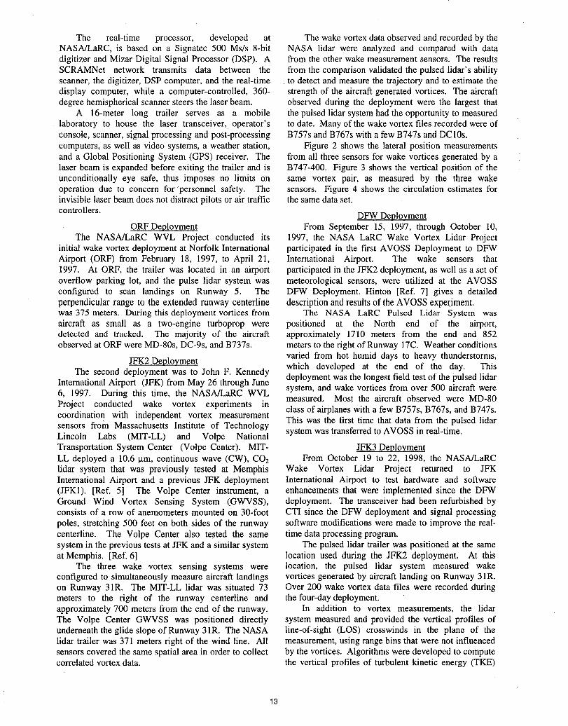
lidar products include various velocity displays, vortexvalidating wake sensing technologies, positions, and vortex circulations. Figure 1 shows a

The lidar system has been field-tested to provide plot of the measured velocity versus elevation angle inreal-time wake vortex trajectory and strength data to four adjacent range bins. The displayed velocities areAVOSS for wake prediction verification. Wake the maximum detected velocities towards and awayvortices, atmospheric winds, and turbulence products from the lidar; the plots are centered at the ambienthave been generated from processing the lidar data wind velocity. These maximum vortex velocities arecollected during deployments to Norfolk (ORF), John determined from Fast Fourier Transforms (FFT) of theF. Kennedy (JFK), and Dallas/Fort Worth (DFW) heterodyne signal using the highest and lowestInternational Airports. frequencies that have magnitudes above a

Pulsed Lidar System Description predetermined threshold. After the passage of eachCoherent Technologies, Incorporated (CTI) aircraft, a file, containing the times each vortex exits

developed the Tm: YAG, solid-state, laser transceiver the top, bottom, left, or right limits of the corridors, theused in the NASA pulsed coherent lidar system, time that any vortex above a threshold circulation staysPulsed lidar has been selected as the baseline within predetermined corridors at the scanplane, andtechnology for an operational wake vortex sensor due to the time the vortex falls below the threshold circulation,its range resolution and long-range capability. CTI first is transmitted to AVOSS to confirm predictions ofdemonstrated the application of this technology to wake vortex behavior. The file also includes vortex lateralvortex measurement in 1994. [Ref. 4] and vertical position and circulation versus time.

12

The real-time processor, developed at The wake vortex data observed and recorded by theNASA/LaRC, is based on a Signatec 500 Ms/s 8-bit NASA lidar were analyzed and compared with datadigitizer and Mizar Digital Signal Processor (DSP). A from the other wake measurement sensors. The resultsSCRAMNet network transmits data between the from the comparison validated the pulsed lidar's abilityscanner, the digitizer, DSP computer, and the real-time to detect and measure the trajectory and to estimate thedisplay computer, while a computer-controlled, 360- strength of the aircraft generated vortices. The aircraftde_ee hemispherical scanner steers the laser beam. observed during the deployment were the largest that

A 16-meter long trailer serves as a mobile the pulsed lidar system had the opportunity to measuredlaboratory to house the laser transceiver, operator's to date. Many of the wake vortex files recorded were ofconsole, scanner, signal processing and post-processing B757s and B767s with a few B747s and DC10s.computers, as well as video systems, a weather station, Figure 2 shows the lateral position measurementsand a Global Positioning System (GPS) receiver. The from all three sensors for wake vortices generated by alaser beam is expanded before exiting the trailer and is B747-400. Figure 3 shows the vertical position of theunconditionally eye safe, thus imposes no limits on same vortex pair, as measured by the three wakeoperation due to concern for 'personnel safety. The sensors. Figure 4 shows the circulation estimates forinvisible laser beam does not distract pilots or air traffic the same data set.

controllers. DFW DeploymentORFDeployment From September 15, 1997, through October 10,

The NASA/LaRC WVL Project conducted its 1997, the NASA LaRC Wake Vortex Lidar Projectinitial wake vortex deployment at Norfolk International participated in the first AVOSS Deployment to DFWAirport (ORF) from February 18, 1997, to April 21, International Airport. The wake sensors that1997. At ORF, the trailer was located in an airport participated in the JFK2 deployment, as well as a set ofoverflow parking lot, and the pulse lidar system was meteorological sensors, were utilized at the AVOSSconfigured to scan landings on Runway 5. The DFW Deployment. Hinton [Ref. 7] gives a detailedperpendicular range to the extended runway centerline description and results of the AVOSS experiment.was 375 meters. During this deployment vortices from The NASA LaRC Pulsed Lidar System wasaircraft as small as a two-engine turboprop were positioned at the North end of the airport,detected and tracked. The majority of the aircraft approximately 1710 meters from the end and 852observed at ORF were MD-80s, DC-9s, and B737s. meters to the right of Runway 17C. Weather conditions

varied from hot humid days to heavy thunderstorms,JFK2Deployment which developed at the end of the day. This

The second deployment was to John F. Kennedy deployment was the longest field test of the pulsed lidarInternational Airport (JFK) from May 26 through Junesystem, and wake vortices from over 500 aircraft were

6, 1997. During this time, the NASA/LaRC WVL measured. Most the aircraft observed were MD-80Project conducted wake vortex experiments in class of airplanes with a few B757s, B767s, and B747s.coordination with independent vortex measurement This was the first time that data from the pulsed lidarsensors from Massachusetts Institute of Technology system was transferred to AVOSS in real-time.Lincoln Labs (MIT-LL) and Volpe NationalTransportation System Center (Volpe Center). MIT- JFK3 DeploymentLL deployed a 10.6 I.tm,continuous wave (CW), CO2 From October 19 to 22, 1998, the NASA/LaRClidar system that was previously tested at Memphis Wake Vortex Lidar Project returned to JFKInternational Airport and a previous JFK deployment International Airport to test hardware and software(JFK1). [Ref. 5] The Volpe Center instrument, a enhancements that were implemented since the DFWGround Wind Vortex Sensing System (GWVSS), deployment. The transceiver had been refurbished byconsists of a row of anemometers mounted on 30-foot CTI since the DFW deployment and signal processingpoles, stretching 500 feet on both sides of the runway software modifications were made to improve the real-centerline. The Volpe Center also tested the same time data processing program.system in the previous tests at JFK and a similar system The pulsed lidar trailer was positioned at the sameat Memphis. [Ref. 6] location used during the JFK2 deployment. At this

The three wake vortex sensing systems were location, the pulsed lidar system measured wakeconfigured to simultaneously measure aircraft landings vortices generated by aircraft landing on Runway 31R.on Runway 31R. The MIT-LL lidar was situated 73 Over 200 wake vortex data files were recorded duringmeters to the right of the runway centerline and the four-day deployment.approximately 700 meters from the end of the runway. In addition to vortex measurements, the lidarThe Volpe Center GWVSS was positioned directly system measured and provided the vertical profiles ofunderneath the glide slope of Runway 31R. The NASA line-of-sight (LOS) crosswinds in the plane of thelidar trailer was 371 meters right of the wind line. All measurement, using range bins that were not influencedsensors covered the same spatial area in order to collect by the vortices. Algorithms were developed to computecorrelated vortex data. the vertical profiles of turbulent kinetic energy (TKE)

13

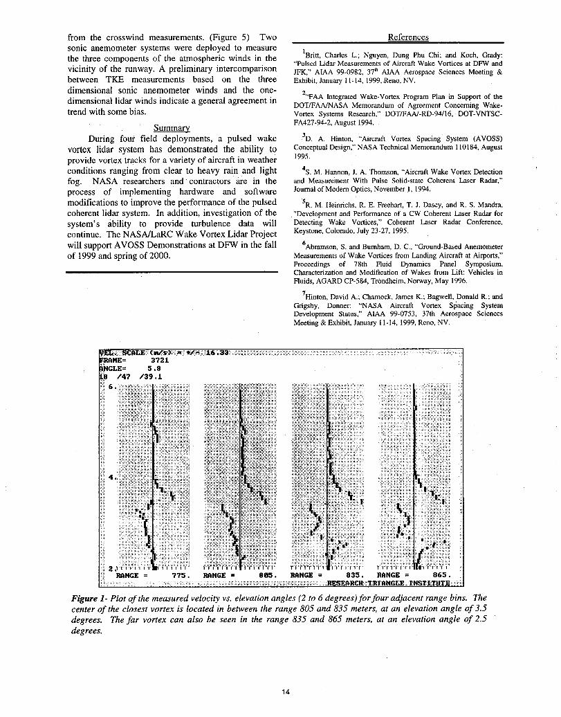
from the crosswind measurements. (Figure 5) Two Referencessonic anemometer systems were deployed to measurethe three components of the atmospheric winds in the tBritt, Charles L.; Nguyen, Dung Phu Chi; and Koch, Grady:"Pulsed Lidar Measurements of Aircraft Wake Vortices at DFW andvicinity of the runway. A preliminary intercomparison JFK." AIAA 99-0982. 37t" AIAA Aerospace Sciences Meeting &between TKE measurements based on the three Exhibit, January 11_14,1999,Reno, NV.dimensional sonic anemometer winds and the one-dimensional lidar winds indicate a general agreement in 2"FAA Integrated Wake-Vortex Program Plan in Support of the

DOT/FAA/NASA Memorandum of Agreement Concerning Wake-trend with some bias. VortexSystemsResearch." DOT/FAA/-RD-94/16, DOT-VNTSC-

Summary FA427-94-2, August 1994.

During four field deployments, a pulsed wake 3D. A. Hinton, "Aircraft Vortex SpacingSystem(AVOSS)vortex lidar system has demonstrated the ability to ConceptualDesign,"NASATechnicalMemoranduml10184,Augustprovide vortex tracks for a variety of aircraft in weather 1995.

conditionsranging from clear to heavy rain and light 4s M. Harmon. J. A. Thomson, "Aircraft Wake Vortex Detection 'fog. NASA researchers andcontractors are in the and Measurement With Pulse Solid-state Coherent Laser Radar,"process of implementing hardware and software Joumal of Modem Optics,November1,1994.

modifications to improve the performance of the pulsed SR.M. Heinrichs. R. E Freehart. T. J. Dasey, and R S. Mandra,coherent lidar system. In addition, investigation of the "Development and Performance of a CW Coherent Laser Radar for

system's ability to provide turbulence data will DetectingWake Vortices," Coherent Laser Radar Conference,continue. The NASA/LaRC Wake Vortex Lidar Project Keystone,Colorado,July23-27,1995.

will support AVOSS Demonstrations at DFW in the fall 6Abramson, S. and Burnham, D. C.,"Ground-BasedAnemometerof 1999 and spring of 2000. Measurements of Wake Vortices from Landing Aircraft at Airports,"

Proceedings of 78th Fluid Dynamics Panel Symposium.Characterization and Modification of Wakes from Lift: Vehicles inFluids, AGARD CP-584, Trondheim, Norway, May 1996.

7Hinton, David A.; Chamock, James K.: Bagwell. Donald R.; andGrigsby, Donner: "NASA Aircraft Vortex Spacing SystemDevelopment Status," AIAA 99-0753. 37th Aerospace SciencesMeeting & Exhibit. January 11-14. 1999.Reno, NV.

_ANE= 3721:IHGLE= 5.8

L86 ./47 /3'J .1

_i;i •

4.

i':f:!iii ...:.:::i_'!:_,Z:i',_i _%i';_ii!i:_i_:_:_ :::,i:,_.,i ........

:_:,:!;!:_,i:?:_i::' i:

2.1 m:i':, i. r k i_i:':i:i::::i_i_RAHGE: 775. Rt_HGE: 885. RAIqGE: 835, RAFIGE: 865.

: ::: ::'i : '_::_..... ::!'' --;::'-.,_i_::_:,::_::'_::_::;,"_+_?_:";_:+_!-_:'_;_:_ii'!:i_::_:;_+:i_+i_::::.:RE,SEA,RCH:::TR]PIIIIGIiE:IIqSTI,_UTE::::_:::

Figure 1- Plot of the measured velocity vs. elevation angles (2 to 6 degrees)for four adjacent range bins. The

center of the closest vortex is located in between the range 805 and 835 meters, at an elevation angle of 3.5

degrees. The far vortex can also be seen in the range 835 and 865 meters, at an elevation angle of 2.5degrees.

14

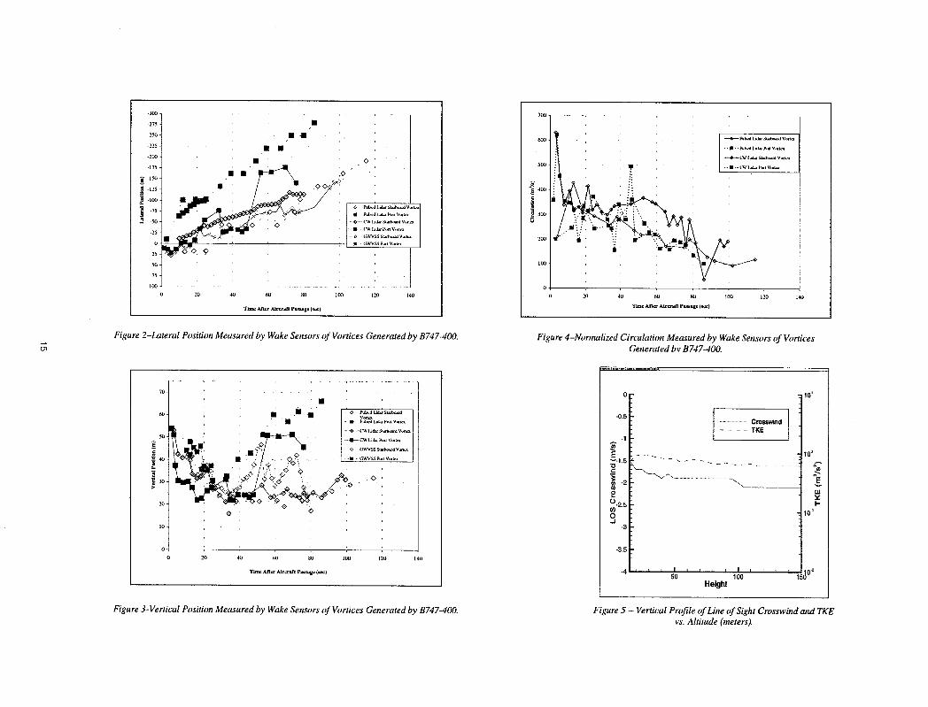
75+...... 7,+tt.........-225 1 ' • • , . --If--P._.,SL_P_ Vo_

,75+ iio ,+_+., .. . !i .

-_" 1 zl_ "__:_" _;'_" ' I ................ I __o :,:,."!", . '..,.,4 _.do _>" ' ' _................... _' 1_' '

o-_.._--_ , _ _ I • ,,wvssP_,v.... I

:'i"_°°:° ..... I *_o ...... ltX) 1"_'¢

,2t .........i.. ............_ _ .........:+ .+L. o_0 20 4o 60 80 l(x) 120 140 20 40 60 8O 1oo 12o t40

Time MI_ AircraftP_ge (scc) TimeAI_" Aircraft P_age (_,.¢)

Figure 2-Lateral Position Measured by Wake Sensors of Vortices Generated by B747-400. Figure 4-Normalized Circulation Measured by Wake Sensors of Vortices_n Generated by B747-400.

70 q ' " .... ' ' " " ' " 0 10', []

• i i ._" ,[.......... -0.5 ]

60q

I ].. • _t,._u,_P,_v_ ...................Crosswind-- e-..+(:wIJda stat,o_dv.mcx TKE

' _'!' I I'<l'' _ ........ ---,4o__ ,_ : ,_ _: .....:::;.:::,+_+;7 _.,+......_..... ....... ,oo+/ i+yt ° ....................................................................+),,,4--_.n,+" ;. . _ .o i._ "-'-'_

20 4 0.2. 5 I,-

@ ,0 _ 104

,,.l_oH -3

o q -3.5

20 4o 60 80 llJO 12o 140

I I ( I I I I [ I l ._0"2Time AllgrAircraft Passage(_) -4 I l T 50 100 15

Height

Figure 3-Vertical Position Measured by Wake Sensors of Vortices Generated by B747-400. Figure 5 - Vertical Profile of Line of Sight Crosswuzdand TKEvs. Altitude (meters).

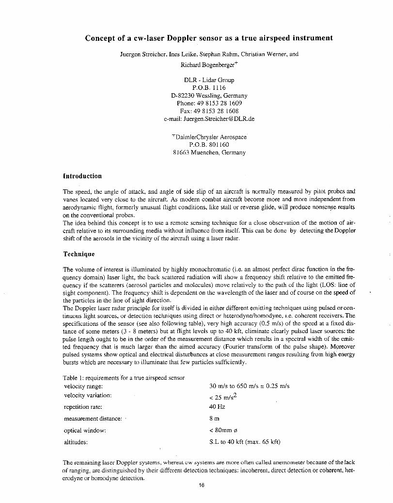
Concept of a cw-laser Doppler sensor as a true airspeed instrument

Juergen Streicher, Ines Leike, Stephan Rahm, Christian Werner, and

Richard Bogenberger+

DLR - Lidar GroupP.O.B. 1116

D-82230 Wessling, GermanyPhone: 49 8153 28 1609Fax: 49 8153 28 1608

e-mail: Juergen.Streicher@DLR.de

+DaimlerChrysler AerospaceP.O.B. 801160

81663 Muenchen, Germany

Introduction

The speed, the angle of attack, and angle of side slip of an aircraft is normally measured by pitot probes andvanes located very close to the aircraft. As modern combat aircraft become more and more independent fromaerodynamic flight, formerly unusual flight conditions, like stall or reverse glide, will produce nonsense resultson the conventional probes.The idea behind this concept is to use a remote sensing technique for a close observation of the motion of air-craft relative to its surrounding media without influence from itself. This can be done by detecting the Dopplershift of the aerosols in the vicinity of the aircraft using a laser radar.

Technique

The volume of interest is illuminated by highly monochromatic (i.e. an almost perfect dirac function in the fre-quency domain) laser light, the back scattered radiation will show a frequency shift relative to the emitted fre-quency if the scatterers (aerosol particles and molecules) move relatively to the path of the light (LOS: line ofsight component). The frequency shift is dependent on the wavelength of the laser and of course on the speed ofthe particles in the line of sight direction.The Doppler laser radar principle for itself is divided in either different emitting techniques using pulsed orcon-tinuous light sources, or detection techniques using direct or heterodyne/homodyne, i.e. coherent receivers. Thespecifications of the sensor (see also following table), very high accuracy (0.5 m/s) of the speed at a fixed dis-tance of some meters (3 - 8 meters) but at flight levels up to 40 kft, eliminate clearly pulsed laser sources: thepulse length ought to be in the order of the measurement distance which results in a spectral width of the emit-ted frequency that is much larger than the aimed accuracy (Fourier transform of the pulse shape). Moreoverpulsed systems show optical and electrical disturbances at close measurement ranges resulting from high energybursts which are necessary to illuminate that few particles sufficiently.

Table i: requirementsfor a true airspeed sensorvelocity range: 30 m/s to 650 m/s _ 0.25 m/s

velocity variation: < 25 rrds2

repetition rate: 40 Hz

measurement distance: 8 m

optical window: < 80mm ¢

altitudes: S.L to 40 kft (max. 65 kft)

The remaining laser Doppler systems, whereat cw systems are more often called anemometer because of the lack

of ranging, are distinguished by their different detection techniques: incoherent, direct detection or coherent, het-erodyne or homodyne detection.

16

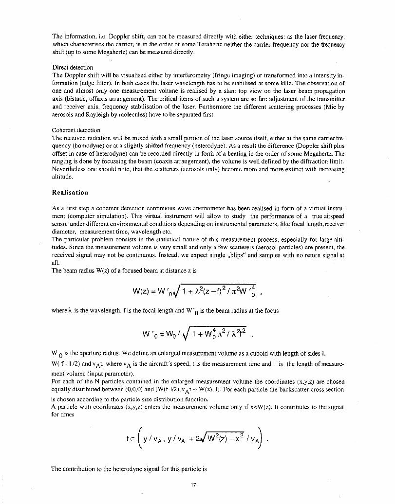
The information, i.e. Doppler shift, can not be measured directly with either techniques: as the laser frequency,which characterises the carrier, is in the order of some Terahertz neither the carrier frequency nor the f_equencyshift (up to some Megahertz) can be measured directly.

Direct detection

The Doppler shift will be visualised either by interferometry (fringe imaging) or transformed into a intensity in-formation (edge filter). In both cases the laser wavelength has to be stabilised at some kHz. The observation ofone and almost only one measurement volume is realised by a slant top view on the laser beam propagationaxis (bistatic, offaxis arrangement). The critical items of such a system are so far: adjustment of the transmitterand receiver axis, frequency stabilisation of the laser. Furthermore the different scattering processes (Mie byaerosols and Rayleigh by molecules) have to be separated first.

Coherent detection

The received radiation will be mixed Witha small portion of the laser source itself, either at the same carrier fre-quency (homodyne) or at a slightly shifted frequency (heterodyne). As a result the difference (Doppler shift plusoffset in case of heterodyne) can be recorded directly in form of a beating in the order of some Megahertz. Theranging is done by focussing the beam (coaxis arrangement), the volume is well defined by the diffraction limit.Nevertheless one should note, that the scatterers (aerosols only) become more and more extinct with increasingaltitude.

Realisation

As a first step a coherent detection continuous wave anemometer has been realised in form of a virtual instru-ment (computer simulation). This virtual instrument will allow to study the performance of a true airspeedsensor under different environmental conditions depending on instrumental parameters, like focal length, receiverdiameter, measurement time, wavelength etc.The particular problem consists in the statistical nature of this measurement process, especially for large alti-tudes. Since the measurement volume is very small and only a few scatterers (aerosol particles) are present, thereceived signal may not be continuous. Instead, we expect single ,,blips" and samples with no return signal atall.

The beam radius W(z) of a focused beam at distancez is

,/W(z) = W '0 1 + _,2(z _f)2 / _t2W ,40 '

where', is the wavelength, f is the focal length and W"0 is the beam radius at the focus

_ 4W 'o = Wo/ 1 + W 0 11;2 / _2f2

W 0 is the aperture radius. We define an enlarged measurement volume as a cuboid with length of sides 1,

W( f - 1/2) and VAt, where vA is the aircraft's speed, t is the measurement time and 1 is the length of measure-

ment volume (input parameter).For each of the N particles contained in the enlarged measurement volume the coordinates (x,y,z) are chosen

equally distributed between (0,0,0) and (W(f-l/2),VAt + W(z), 1).For each particle the backscatter cross sectionis chosen according to the particle size distribution function.

A particle with coordinates (x,y,z) enters the measurement volume only if x<W(z). It contributes to the signalfor times

te (Y/VA, y/V A + 2_/W2(z) -- X2 / VA)

The contribution to the heterodyne signal for this particle is

17

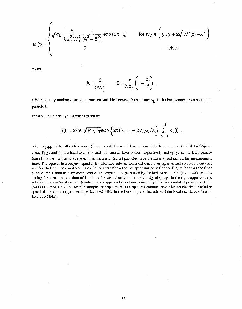
f

2 exp (2= i _) for tvA e y, y + 2_W2(z)-x 2ZkWo(A+BKk(t ) = 0 else

where

2' B- 1- ,2W° 7,zk

x is an equally random distributed random variable between 0 and 1 and _k is the backscatter cross section of

particle k.

Finally, the heterodyne signal is given by

N

S(t)=2Re _/-_PTeXp{2/tit(VOFF--2VLOS/X } ,_ Kk(t ) .n=l

where vOFF is the offset frequency (frequency difference between transmitter laser and local oscillator frequen-

cies), PLO andPT are local oscillator and transmitter laser power, respectively and VLOS is the LOS projec-

tion of the aerosol particles speed. It is assumed, that all particles have the same speed during the measurementtime. The optical heterodyne signal is transformed into an electrical current using a virtual receiver front end,and finally frequency analysed using Fourier transform (power spectrum peak finder). Figure 2 shows the frontpanel of the virtual true air speed sensor. The expected blips caused by the lack of scatterers (about 400 particlesduring the measurement time of 1 ms) can be seen clearly in the optical signal (graph in the right upper comer),whereas the electrical current (center graph) apparently contains noise only. The accumulated power spectrum(500000 samples divided by 512 samples per spectra--- 1000 spectra) contains nevertheless clearly the relativespeed of the aircraft (symmetric peaks at _+5MHz in the bottom graph include still the local oscillator offset ofhere 250 MHz).

18

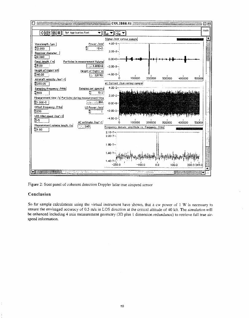
_"x r

_ZmV Versussa_ ................................................................._t/b_m j Power/mWJ 4.0E-3-, ............................. _ ............................................ i'Wavelength

_I 1E+31 i

Receiverdiameter J ' 2"0E-3-i . •

O.OE+O-III __, ._= I I . , . • __ ,, " '.iili a " "-" "'1"* -r"- :t15.ooi [:_;t;_9,E,,+ol-2.OE-3-iHeight of flight/kft] Height of flight/ml ! i

_ i_40.0____0..........j _! .4.0E_3_], i

A,rorof*ve,oo,ty/ms'-,I 0 ,00'000_00'000300000'_00'000500'00,

Sampling frequency /MHz I Samples per speotraI 4.0E-2 .............................................................................................................................................................................................................t . .

Measurement time /sl Particles during.re,eas.urementt..me 2.0E-2-

_ o.o_+o-IOffsetfrequency/MhzI LO Power /mWI

_[250_ i _L_r'--[li -2"0E-2- I _:::

LOS Wind speedIm_^-II _4.OE_2_Ij._] _O.t,m.te/m.'-,Jo ,oo;oo200'000300'0°0_oo'0oo_oooo,''Measurement volume length /m] _j Frequenoy domain : amplitude vs.frequen_ ::::

_,l, .uu j 2.1E-7-_ i:2.0E-7- i iI

! ii1.8E-7-i i

1.4E-7-i' _ _ I. I _ _ , _ . ,V I_ I _i_!-250.0 -I00.0 0.0 100.0 200.0 249£

iiiiiii i ii i i ii i i iiiiii ........

Figure 2: front panel of coherent detection Doppler lidar true airspeed sensor

Conclusion

So far sample calculations using the virtual instrument have shown, that a cw power of i W is necessary toensure the envisaged accuracy of 0.5 m/s in LOS direction at the critical altitude of 40 kft. The simulation willbe enhanced including 4 axis measurement geometry (3D plus t dimension redundance) to retrieve full true air-speed information.

19

AirborneTurbulence DetectionandWarning:ACLAIMFlight Test Results

Stephen M. Hannon andHal R. Bagley David A. Bowdle

CoherentTechnologies,Inc. Universityof Alabamain Huntsville655AspenRidgeDrive GlobalHydrologyand ClimateCenter

Lafayette,Colorado USA 80026 Huntsville,Alabama USAVoice:(303)604-2000,Fax:( 303)-604-2500

e-mail:steveh@ctilidar.com Rodney K. Bogue and L. Jack

Dave C. Soreide EhernbergerNASADrydenFlightResearchCenter

BoeingDefenseand SpaceGroup Edwards,California USASeattle,WashingtonUSA

INTRODUCTION

The Airborne Coherent Lidar for Advanced Inflight Measurements (ACLAIM) is a NASA/DrYden-lead program to develop and demonstrate a 2 p.mpulsed Doppler lidar for airborne look-aheadturbulence detection and warning. Advanced warning of approaching turbulence can significantlyreduce injuries to passengers and crew aboard commercial airliners. The ACLMM instrument is akey asset to the ongoing Turbulence component of NASA's Aviation Safety Program, aimed atreducing the accident rate aboard commercial airliners by a factor of five over the next ten years andby a factor of ten over the next twenty years. As well, the advanced turbulence warning capabilitycan prevent "unstarts" in the inlet of supersonic aircraft engines by alerting the flight controlcomputer which then adjusts the engine to operate in a less fuel efficient, and more turbulence-tolerant, mode.

Initial flight tests of the ACLAIM were completed in March and April or"1998. This paper andpresentation gives results from these initial flights, with validated demonstration of Doppler lidarwind turbulence detection several kilometers ahead of the aircraft.

SENSOR DESCRIPTION AND MEASUREMENT CONFIGURATION

Figure 1 shows a picture of the ACLAIM hardware as installed aboard the National Center forAtmospheric Research (NCAR) Electra research aircraft. The Doppler lidar system, designed andbuilt by Coherent Technologies, Inc., operated at an eyesafe wavelength of 2.0125 p.m(Tm:YAG)with a pulse energy of 12 mJ and a pulse repetition frequency of 100 Hz. The pulse duration was460 nsec (70 m) and the output range resolution was typically 100 m. For these initial flights, theACLAIM operated with a single line of sight directed 2 deg down and 0.5 deg out from the aircraftaxis. With a nominal 2 deg pitch angle, the line of sight was reasonably well matched to the flighttrack. The aperture diameter was 10 cm (8 cm beam diameter) and the optics were usually focusedat a nominal range of 1 km. A variety of real-time data displays were available during the flight,including signal to noise, estimated backscatter, relative airspeed ahead and a short-term-averagevelocity structure function at 300 m separation. Raw data samples were recorded at the 100megasample!sec rate out to 9.5 km and are available for post-processing.

The Electra is four-engine turboprop, with a maximum airspeed of 310 knots (160 m/s) and an

20

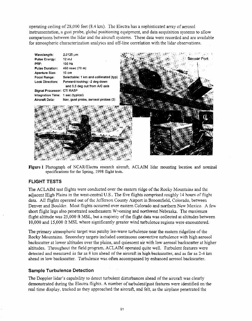
operating ceiling of 28,000 feet (8.4 km). The Electra has a sophisticated array of aerosol

instrumentation, a gust probe, global positioning equipment, and data acquisition systems to allowcomparisons between the lidar and the aircraft systems. These data were recorded and are availablefor atmospheric characterization analyses and off-line correlation with the lidar observations.

Wavelength: 2.0125_am ....Pulse Energy: 12mJ

PRF: 100 HzPulse Duration: 460 nsec (70 m)

Aperture Size: 10cmFocalRange: Selectable:1 km andcollimated(typ)LookDirection: Forward-looking:-2 deg down

and0.5 deg outfrom A/C axisSignal Processor: CTI RASPIntegrationTime: 1 sec (typical)Aircraft Data: Nav,gust probe,aerosolprobes(3)

Figure 1 Photograph of NCAR/Electra research aircraft, ACLAIM lidar mounting location and nominalspecifications for the Spring, 1998 flight tests.

FLIGHT TESTS

The ACLAIM test flights were conducted over the eastern ridge of the Rocky Mountains and the

adjacent High Plains in the west-central U.S.. The five flights comprised roughly 14 hours of flightdata. All flights operated out of the Jefferson County Airport in Broomfield, Colorado, betweenDenver and Boulder. Most flights occurred over eastern Colorado and northern New Mexico. A few

short flight legs also penetrated southeastern Wyoming and northwest Nebraska. The maximumflight altitude was 25,000 ft MSL, but a majority of the flight data was collected at altitudes between

10,000 and 15,000 ft MSL where significantly _eater wind turbulence regions were encountered.

The primary atmospheric target was patchy lee-wave turbulence near the eastern ridgeline of theRocky Mountains. Secondary targets included continuous convective turbulence with high aerosol

backscatter at lower altitudes over the plains, and quiescent air with low aerosol backscatter at higheraltitudes. Throughout the field pro_am, ACLAIM operated quite well. Turbulent features weredetected and measured as far as 8 krn ahead of the aircraft in high backscatter, and as far as 2-4 kmahead in low backscatter. Turbulence was often accompanied by enhanced aerosol backscatter.

Sample Turbulence Detection

The Doppler lidar's capability to detect turbulent disturbances ahead of the aircraft was clearlydemonstrated during the Electra flights. A number of turbulent/gust features were identified on thereal time display, tracked as they approached the aircraft, and felt, as the airplane penetrated the

21

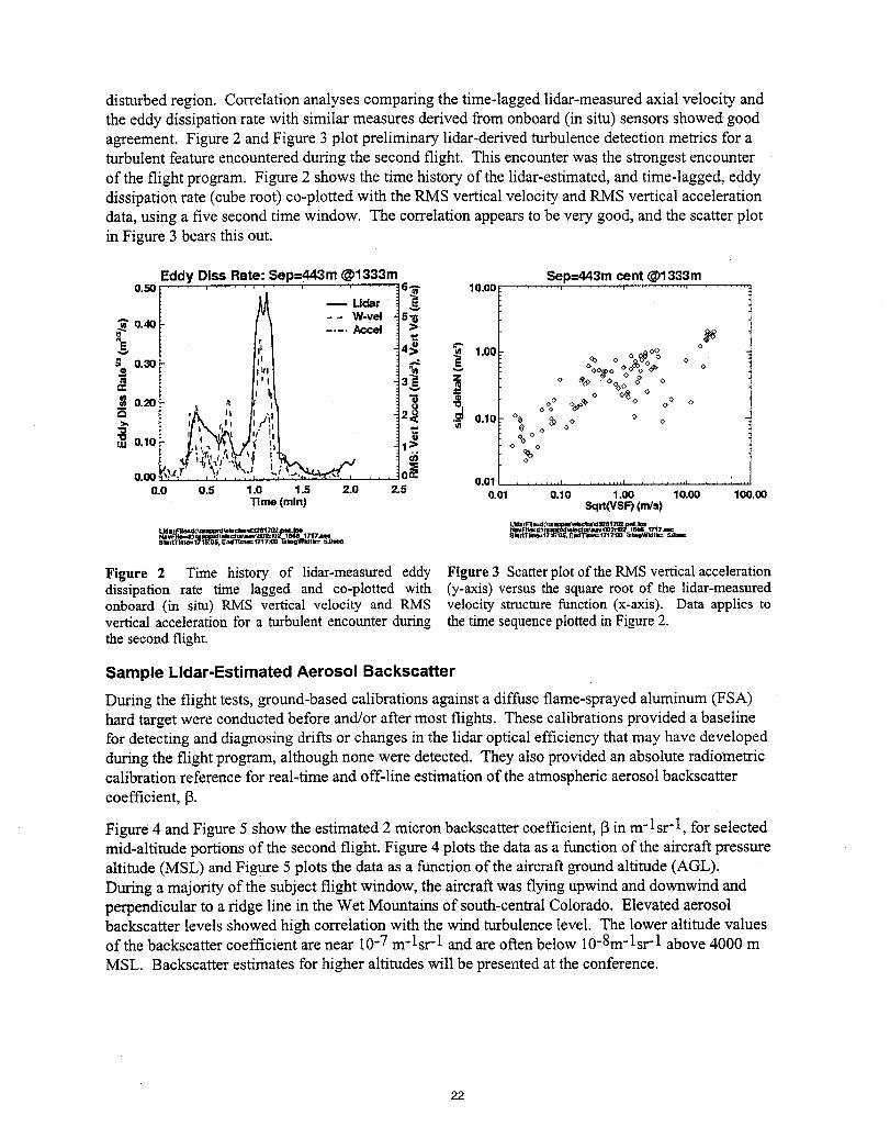
disturbed region. Correlation analyses comparing the time-lagged lidar-measured axial velocity andthe eddy dissipation rate with similar measures derived from onboard (in situ) sensors showed goodagreement. Figure 2 and Figure 3 plot preliminary lidar-derived turbulence detection metrics for aturbulent feature encountered during the second flight. This encounter was the strongest encounterof the flight program. Figure 2 shows the time history of the lidar-estimated, and time-lagged, eddydissipation rate (cube root) co-plotted with the RMS vertical velocity and RMS vertical accelerationdata, using a five second time window. The correlation appears to be very good, and the scatter plotin Figure 3 bears this out.

Eddy Diss Rate: Sep=443m @1333m Sep=443m cent @1333mo.5o ......................... 6_ lO.OO , , ,

-- W-vel 5>_

_" 0.40 .... gccei 4__ _ °_%_o30 , _ _ loo + o _+_oO_o

= '" ! " "+°?°+ °i'1 3 z o _, -o% <t *I I "_

olp_. ° v°_{_o° oo

.o.,o,, ,+_:o.,o°,°+° °PI"'* °o.® .... o.o,..............................,...

0.0 0.5 1.0 1.5 2.0 2.5 0.01 0.10 1.00 10.00 100.110Time (rain) Sqrt(VSF) (m/s)

LfdafFlle=d:\amR_l_alect_d_617_ l_d._Lldlllgtllle_;_rll_lll_l_ctlll_1326171_ Joe ttavFIkl=d_r Ioclrlltl;lw_80"2tlg2 1_46 17"17J11€:8fllt'Tlml_1_ NTZala=t717:00 _gWIdtk=_1t'1'1;114_'1711S[05, EndTia11_1717.qDQ _r_,gt_lz= 5.01_

Figure 2 Time history of lidar-measured eddy Figure 3 Scatterplotof the RMSverticalaccelerationdissipation rate time lagged and co-plotted with (y-axis) versusthe square root of the lidar-measuredonboard (in situ) RMS vertical velocity and RMS velocity structure function (x-axis). Data applies tovertical accelerationfor a turbulentencounter during the time sequenceplottedin Figure2.the secondflight.

Sample Lidar-Estimated Aerosol Backscatter

During the flight tests, ground-based calibrations against a diffuse flame-sprayed aluminum (FSA)hard target were conducted before and/or after most flights. These calibrations provided a baselinefor detecting and diagnosing drifts or changes in the lidar optical efficiency that may have developedduring the flight program, although none were detected. They also provided an absolute radiometriccalibration reference for real-time and off-line estimation of the atmospheric aerosol backscattercoefficient, 13.

Figure 4 and Figure 5 show the estimated 2 micron backscatter coefficient, 13in m-1sr-1, for selectedmid-altitude portions of the second flight. Figure 4 plots the data as a function of the aircraft pressurealtitude (MSL) and Figure 5 plots the data as a function of the aircraft ground altitude (AGL).During a majority of the subject flight window, the aircraft was flying upwind and downwind andperpendicular to a ridge line in the Wet Mountains of south-central Colorado. Elevated aerosolbackscatter levels showed high correlation with the wind turbulence level. The lower altitude valuesof the backscatter coefficient are near 10-7 m-lsr -1 and are often below 10-8m-lsr -1 above 4000 mMSL. Backscatter estimates for higher altitudes will be presented at the conference.

22

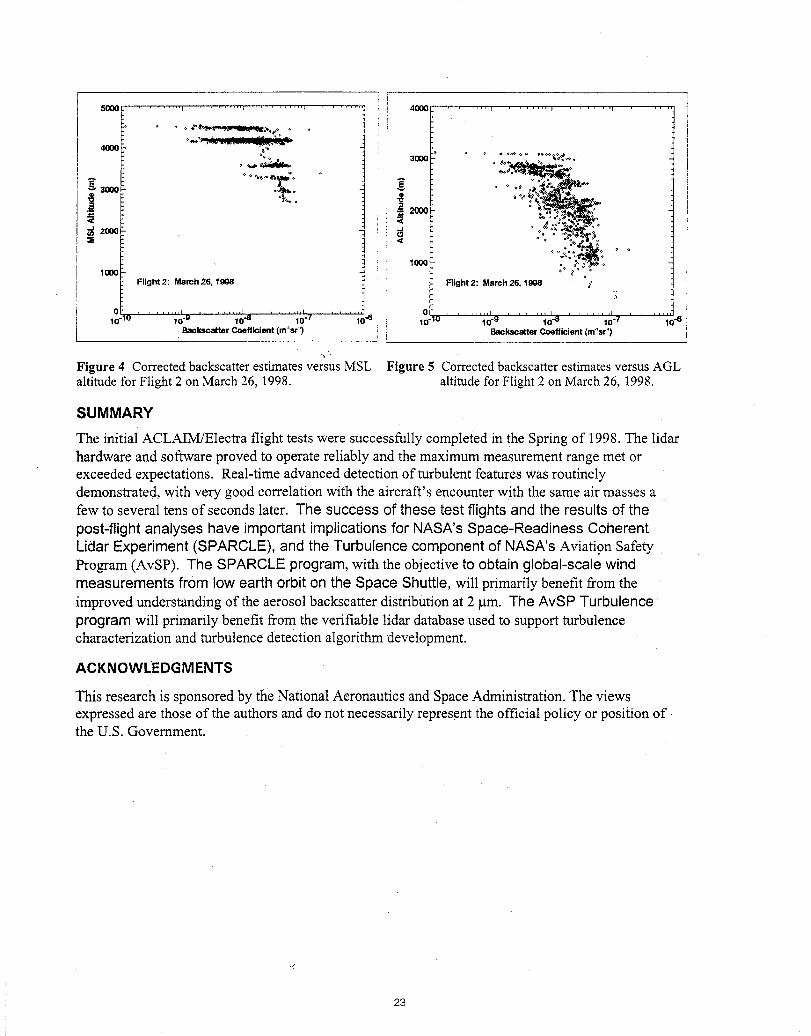
5000 _ J _ ........ 4000 ........ _ ........ p ........ _ ........

4(]00 °_°_k_Al__ _ _ m o^o _ o

, _,/_,_ 3000 ...._.-o

_ 2(X)O

(n 2000

Flight2: March26, 1gO8 Flight 2: March26, 1998 / ..

0 : , , ,,,,,i I ; _ _=,lll ........ I ....... 0 ........ I ........ I ........ I ........

10"10 10.9 10"8 10"7 10..6 10 10"g 10_ 10"7 10"6Bamkscatter Coefficient (m"sr") Backscatter Coefficient (m"sr _)

.,)

Figure 4 Corrected backscatter estimates versus MSL Figure 5 Corrected backscatter estimates versus AGLaltitude for Flight 2 on March 26, 1998. altitude for Flight 2 on March 26, 1998.

SUMMARY

The initial ACLAIM/Electra flight tests were successfully completed in the Spring of 1998. The lidarhardware and software proved to operate reliably and the maximum measurement range met orexceeded expectations. Real-time advanced detection of turbulent features was routinelydemonstrated, with very good correlation with the aircraft's encounter with the same air masses afew to several tens of seconds later. The success of these test flights and the results of thepost-flight analyses have important implications for NASA's Space-Readiness CoherentLidar Experiment (SPARCLE), and the Turbulence component of NASA's Aviation SafetyProgram(AvSP). The SPARCLE program, with theobjectiveto obtain global-scale windmeasurements from low earth orbit on the Space Shuttle, will primarily benefit from theimproved understanding of the aerosol backscatter distribution at 2 _m. The AvSP Turbulenceprogramwill primarily benefit from the verifiable lidar database used to support turbulencecharacterization and turbulence detection algorithm development.

ACKNOWLEDGMENTS

This research is sponsored by the National Aeronautics and Space Administration. The viewsexpressed are those of the authors and do not necessarily represent the official policy or position ofthe U.S. Government.

23

JuneauAirportDopplerLidar Deployment: Extractionof AccurateTurbulentWind Statistics

Stephen M. Hannon

CoherentTechnologies,Inc.655AspenRidgeDrive

Lafayette,Colorado USA 80026(303)604-2000,e-mail:steveh@ctilidar.com

Rod Frehlich, Larry Cornman, Robert Goodrich, Douglas Norris, John Williams

ResearchApplicationProgramNationalCenterforAtmosphericResearch

Boulder,Colorado80307USA

INTRODUCTION

A 2 _tmpulsed Doppler lidar was deployed to the Juneau Airport in 1998to measure turbulence andwind shear in and around the departure and arrival corridors. The primary objective of themeasurement program was to demonstrate and evaluate the capability of a pulsed coherent lidar toremotely and unambiguously measure wind turbulence.

Lidar measurements were coordinated with flights of an instrumented research aircraft operated byrepresentatives of the University of North Dakota (UND) under the direction of the National Centerfor Atmospheric Research (NCAR). The data collected is expected to aid both turbulencecharacterization as well as airborne turbulence detection algorithm development activities withinNASA and the FAA. This paper presents a summary of the deployment and results of analysis andsimulation which address important issues regarding the measurement requirements for accurateturbulent wind statistics extraction.

SENSOR DESCRIPTION

The Doppler lidar was an eyesafe coherent Doppler lidar operating at a wavelength of 2.012 p,mwitha pulse energy of 4.5 mJ (nominal), a pulse duration of 400-500 nsec (FWHM intensity), a pulserepetition frequency (PRF) of 100 Hz, a beam diameter of 5 cm (e2 intensity full width), and a hardaperture of 10 cm. An 8'x7'x8' (WxLxH) wood frame fiberglass shelter housed the lidar, scanner,and contrql and signal processing electronics. Lidar data was collected and processed at100 Hz using a CTI-developed RASP (Real-time Advanced Signal Processor). The nominal velocitybandwidth was +22 m/sec (+43 knots). During most of the Juneau data collection, an extendedbandwidth mode was utilized with a velocity range of _+45m/sec (_+87knots).

The lidar data was ported in real time to a remote operations center via an RF modem link. Agraphical user interface (GUI) in the operations center enabled the operator to manipulate the scannerand signal processing configuration. The radial range resolution of the sensor, which is defined bythe pulse duration and the processed range gate size, was 75-100 m. The minimum transverseresolution, which is defined by the beam width, was approximately 15cm at 3 km. For a scanningconfiguration, the transverse resolution is defined by the slew rate and integration time.

24

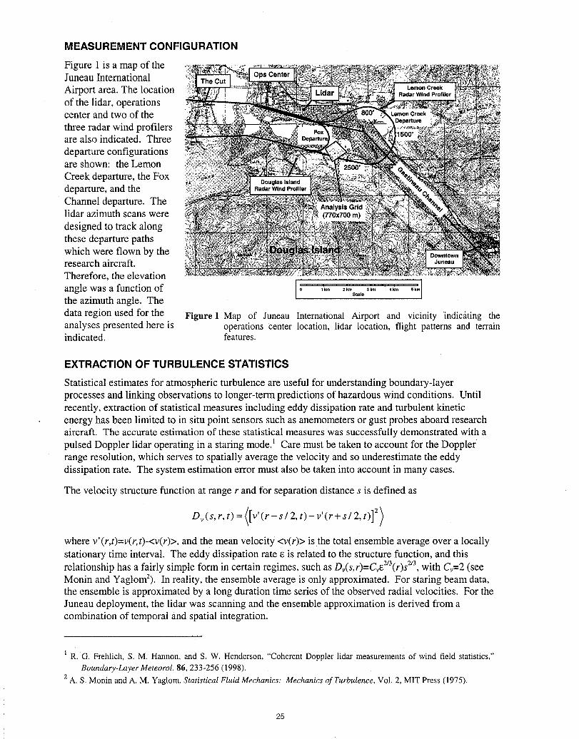
MEASUREMENT CONFIGURATION

Figure 1 is a map of theJuneau International OpsCenter

Airport area. The locationof the lidar, operationscenter and two of thethree radar wind profilersare also indicated. Threedeparture configurationsare shown: the Lemon

Creek departure, the Fox Douglas Island

departure, and the RadarWindProfilerChannel departure. Thelidar azimuth scans weredesigned to track along ,,:,,_these departure pathswhich were flown by theresearch aircraft.Therefore, the elevation

angle was a function of 1_,1the azimuth angle. The

data region used for the Figure 1 Map of Juneau International Airport and vicinity indic_itingtheanalyses presented here is operationscenter location, lidar location, flight patterns and terrainindicated, features.

EXTRACTION OF TURBULENCE STATISTICS

Statistical estimates for atmospheric turbulence are useful for understanding boundary-layerprocesses and linking observations to longer-term predictions of hazardous wind conditions. Untilrecently, extraction of statistical measures including eddy dissipation rate and turbulent kineticenergy has been limited to in situ point sensors such as anemometers or gust probes aboard researchaircraft. The accurate estimation of these statistical measures was successfully demonstrated with apulsed Doppler lidar operating in a staring mode.l Care must be taken to account for the Dopplerrange resolution, which serves to spatially average the velocity and so underestimate the eddydissipation rate. The system estimation error must also be taken into account in many cases.

The velocity structure function at range r and for separation distance s is defined as

Dv(s,r,t)=([v'(r-s/2, t)-v'(r+sl2, t)] 2)

where v'(r,t)=v(r,t)-<v(r)>, and the mean velocity <v(r)> is the total ensemble average over a locallystationary time interval. The eddy dissipation rate _ is related to the structure function, and thisrelationship has a fairly simple form in certain regimes, such as Dr(s,r)=Cv_3(r)s2/3,with C_=2(seeMonin and Yaglom2). In reality, the ensemble average is only approximated. For staring beam data,the ensemble is approximated by a long duration time series of the observed radial velocities. For theJuneau deployment, the lidar was scanning and the ensemble approximation is derived from acombination of temporal and spatial integration.

I R. G. Frehlich, S. M. Hannon, and S. W. Henderson, "Coherent Doppler lidar measurements of wind field statistics,"

Boundary-Layer Meteorol. 86, 233-256 (1998).

2 A. S. Monin and A. M. Yaglom, Statistical Fluid Mechanics: Mechanics of Turbulence, Vol. 2, MIT Press (1975).

25

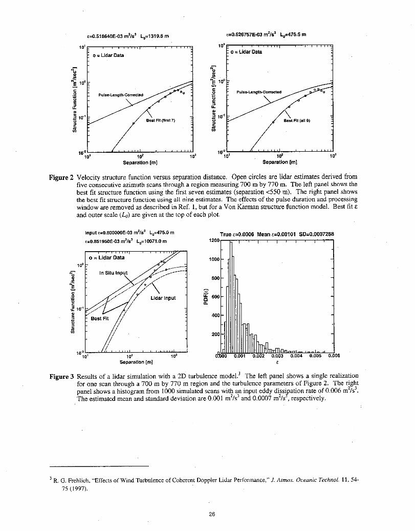
E=O.518640E-03m2/s3 Lo=1319.6m _=0.626757E-03 m2/s3 Lo=476.5 rn

101- ' ' ' ' ''''1 _ , , , ,,,,. 101[:: , i i I illw I , i i , ,_,,.

o = LldarData _ o= LidarData

Q)

_1o o _10 °€ €0 0 Pulse-Length-Corrected

= u \o \ cۥ-i "_

u. U.

10"1 _ 10"1

,= ,=

101 102 10= 101 102 10_Separation [m] Separation [m]

Figure 2 Velocity structure function versus separation distance. Open circles are lidar estimates derived fromfive consecutive azimuth scans through a region measuring 700 mby 770 m. The left panel shows thebest fit structure function using the first seven estimates (separation <550 m). The right panel showsthe best fit structure function using all nine estimates. The effects of the pulse duration and processingwindow are removed as described in Ref. 1, but for a Von Karman structure function model. Best fitand outer scale (Lo)are given at the top of each plot.

Input _=0.600000E-03 m2/s3 Lo=475.0m True _=0.0006 Mean _=0.00101 SD=0.0007268

E=0.851950E-03mils3 Lo=10071.0m

lOOOlO0

04

Q 800

•€-° Lidar Input _ 600

t_ 10"1

Best Fit /// 400u

200

I I111/ I I I i i iilI

10"10' 102 10a 0.001 0.002 0.003 0.004 0.005 0.006Separation [m]

Figure 3 Results of a lidar simulation with a 2D turbulence model.3 The left panel shows a single realizationfor one scan through a 700 m by 770 m region and the turbulence parameters of Figure 2. The right

Ph_le:hOWted_st:gral_ _OnmdlarO_eSivm_itatned:oa_litmh/aningot.gddydmi_Ss_,a_One_eel f 0.006 m2/s 3.• . . . . p ' y.

3R. G. Frehlich, "Effects of Wind Turbulence of Coherent Doppler Lidar Performance," J. Atmos. Oceanic Technol. 11, 54-75 (1997).

26

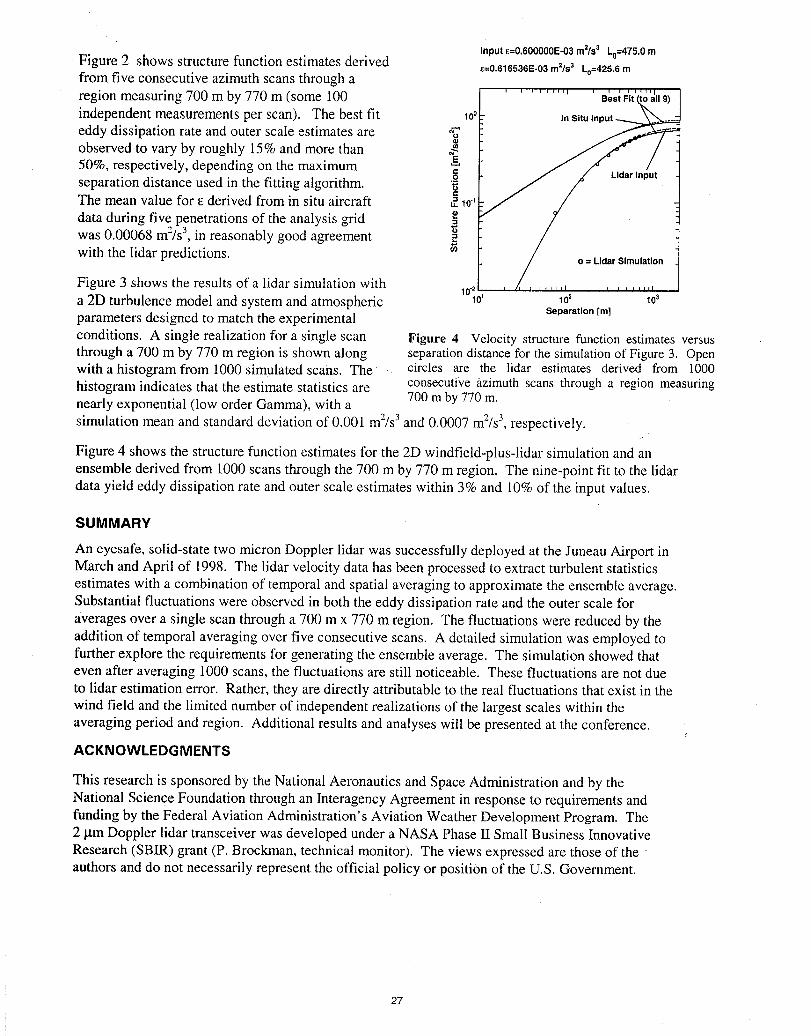
Input_=0.600000E-03m2/s3 L0=475.0mFigure 2 shows structure function estimates derived

_=0.616536E-03 m2/s3 Lo=425.6mfrom five consecutive azimuth scans through aregion measuring 700 m by 770 m (some 100independent measurements per scan). The best fit 100

eddy dissipation rate and outer scale estimates are -_observed to vary by roughly 15% and more than

50%, respectively, depending on the maximum _'separation distance used in the fitting algorithm, o

¢.,

The mean value for _ derived from in situ aircraft _ 10"

data during five penetrations of the analysis grid" 3 "_

was 0.00068 m-/s, in reasonably good agreement ._with the lidar predictions.

Figure 3 shows the results of a lidar simulation with

a 2D turbulence model and system and atmospheric 10' 102 103parameters designed to match the experimental Separation [m]

conditions. A single realization for a single scan Figure 4 Velocity structure function estimates versusthrough a 700 m by 770 m region is shown along separation distance for the simulation of Figure 3. Openwith ahistogramfrom 1000 simulated scans. The circles are the lidar estimates derived from 1000histogram indicates that the estimate statistics are consecutive azimuth scans through a region measuring

700 m by 770 m.nearly exponential (low order Gamma), with a"_ 3

simulation mean and standard deviation of 0.001 m2/s3 and 0.0007 m'/s, respectively.

Figure 4 shows the structure function estimates for the 2D windfield-plus-lidar simulation and an

ensemble derived from 1000 scans through the 700 m by 770 m region. The nine-point fit to the lidardata yield eddy dissipation rate and outer scale estimates within 3% and 10% of the input values.

SUMMARY

An eyesafe, solid-state two micron Doppler lidar was successfully deployed at the Juneau Airport inMarch and April of 1998. The lidar velocity data has been processed to extract turbulent statisticsestimates with a combination of temporal and spatial averaging to approximate the ensemble average.Substantial fluctuations were observed in both the eddy dissipation rate and the outer scale for

averages over a single scan through a 700 m x 770 m region. The fluctuations were reduced by theaddition of temporal averaging over five consecutive scans. A detailed simulation was employed tofurther explore the requirements for generating the ensemble average. The simulation showed thateven after averaging 1000 scans, the fluctuations are still noticeable. These fluctuations are not due

to lidar estimation error. Rather, they are directly attributable to the real fluctuations that exist in thewind field and the limited number of independent realizations of the largest scales within theaveraging period and region. Additional results and analyses will be presented at the conference.

ACKNOWLEDGMENTS

This research is sponsored by the National Aeronautics and Space Administration and by theNational Science Foundation through an Interagency Agreement in response to requirements andfunding by the Federal Aviation Administration's Aviation Weather Development Program. The2 gm Doppler lidar transceiver was developed under a NASA Phase 1I Small Business InnovativeResearch (SBIR) grant (P. Brockman, technical monitor). The views expressed are those of theauthors and do not necessarily represent the official policy or position of the U.S. Government.

27

AIRCRAFTMISSIONS

Presider: Fred Holmes

28

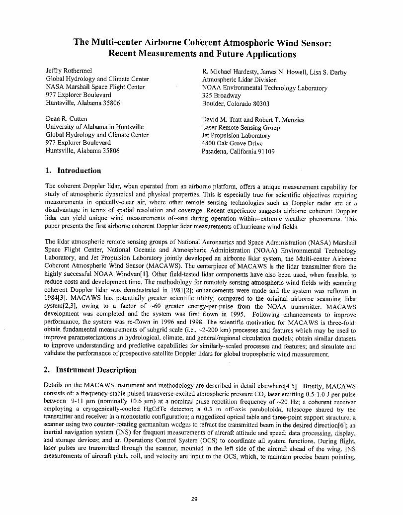
The Multi-center Airborne Coherent Atmospheric Wind Sensor:Recent Measurements and Future Applications

Jeffry Rothermel R. Michael Hardesty, James N. Howell, Lisa S. DarbyGlobal Hydrology and Climate Center Atmospheric Lidar DivisionNASA Marshall Space Flight Center NOAA Environmental Technology Laboratory977 Explorer Boulevard 325 BroadwayHuntsville, Alabama 35806 Boulder, Colorado 80303

Dean R. Cutten David M. Tratt and Robert T. MenziesUniversity of Alabama in Huntsville Laser Remote Sensing GroupGlobal Hydrology and Climate Center Jet Propulsion Laboratory977 Explorer Boulevard 4800 Oak Grove Drive

Huntsville, Alabama 35806 Pasadena, California 91109

1. Introduction

The coherent Doppler lidar, when operated from an airborne platform, offers a unique measurement capability forstudy of atmospheric dynamical and physical properties. This is especially true for scientific objectives requiringmeasurements in optically-clear air, where other remote sensing technologies such as Doppler radar are at adisadvantage in terms of spatial resolution and coverage. Recent experience suggests airborne coherent Dopplerlidar can yield unique wind measurements of--and during operation within--extreme weather phenomena. Thispaper presents the first airborne coherent Doppler lidar measurements of hurricane wind fields.

The lidar atmospheric remote sensing groups of National Aeronautics and Space Administration (NASA) MarshallSpace Flight Center, National Oceanic and Atmospheric Administration (NOAA) Environmental TechnologyLaboratory, and Jet Propulsion Laboratory jointly developed an airborne lidar system, the Multi-center AirborneCoherent Atmospheric Wind Sensor (MACAWS). The centerpiece of MACAWS is the lidar transmitter from thehighly successful NOAA Windvan[l]. Other field-tested lidar components have also been used, when feasible, toreduce costs and development time. The methodology for remotely sensing atmospheric wind fields with scanningcoherent Doppler lidar was demonstrated in 198112]; enhancements were made and the system was reflown in198413]. MACAWS has potentially greater scientific utility, compared to the original airborne scanning lidarsystem[2,3], owing to a factor of-60 greater energy-per-pulse from the NOAA transmitter. MACAWS

development was completed and the system was first flown in 1995. Following enhancements tO improveperformance, the system was re-flown in 1996 and 1998. The scientific motivation for MACAWS is three-fold:obtain fundamental measurements of subgrid scale (i.e., -2-200 km) processes and features which may be used toimprove parameterizations in hydrological, climate, and general/regional circulation models; obtain similar datasetsto improve understanding and predictive capabilities for similarly-scaled processes and features; and simulate andvalidate the performance of prospective satellite Doppler lidars for global tropospheric wind measurement.

2. Instrument Description

Details on the MACAWS instrumentand methodology are described in detail elsewhere[4,5]. Briefly, MACAWSconsists of: a frequency-stable pulsed transverse-excited atmospheric pressure CO 2 laser emitting 0.5-1.0 J per pulsebetween 9-11 gm (nominally 10.6 gm) at a nominal pulse repetition frequency of-20 Hz; a coherent receiveremploying a cryogenically-cooled HgCdTe detector; a 0.3 m off-axis paraboloidal telescope shared by thetransmitter and receiver in a monostatic configuration; a ruggedized optical table and three-point support structure; ascanner using two counter-rotating germanium wedges to refract the transmitted beam in the desired direction[6]; aninertial navigation system (INS) for frequent measurements of aircraft attitude and speed; data processing, display,and storage devices; and an Operations Control System (OCS) to coordinate all system functions. During flight,laser pulses are transmitted through the scanner, mounted in the left side of the aircraft ahead of the wing. INSmeasurements of aircraft pitch, roll, and velocity are input to the OCS, which, to maintain precise beam pointing,

29

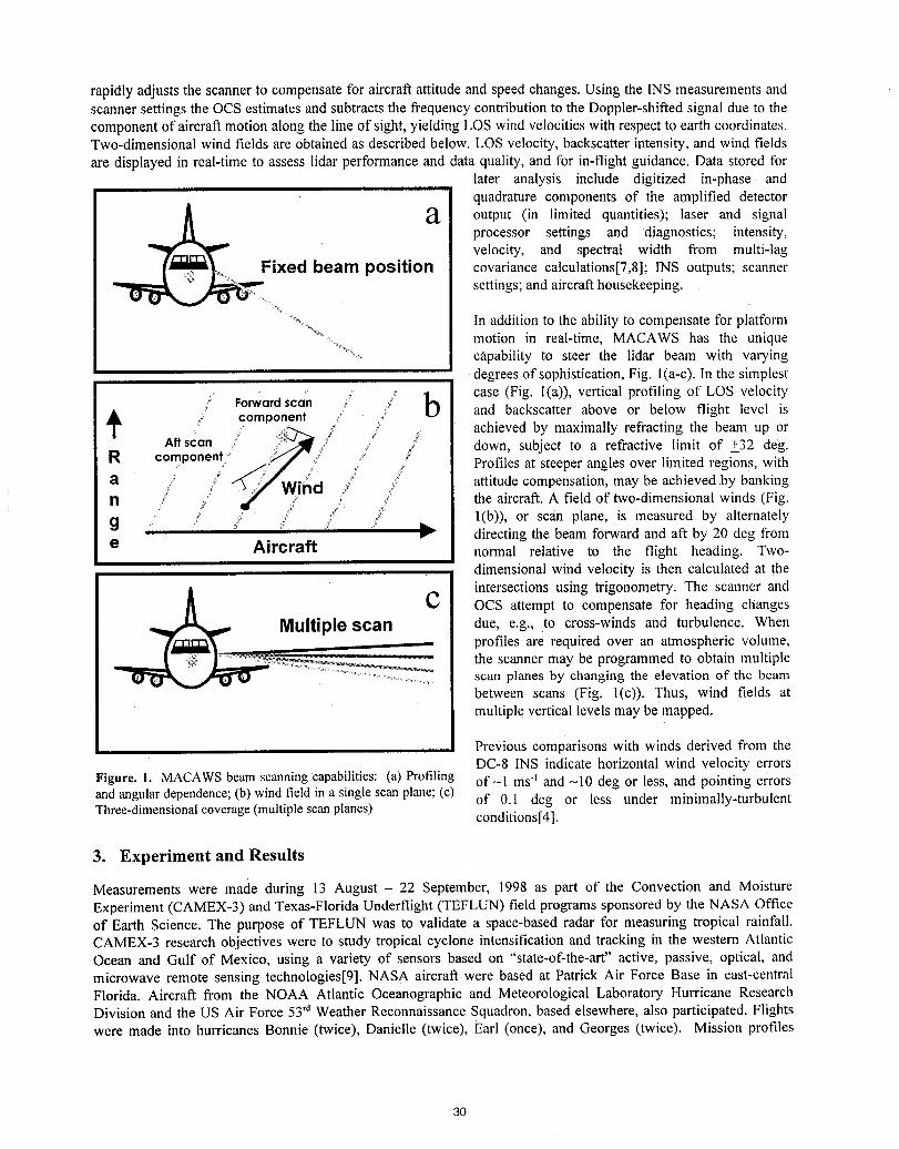
rapidly adjusts the scanner to compensate for aircraft attitude and speed changes. Using the INS measurements andscanner settings the OCS estimates and subtracts the frequency contribution to the Doppler-shifted signal due to thecomponent of aircraft motion along the line of sight, yielding LOS wind velocities with respect to earth coordinates.Two-dimensional wind fields are obtained as described below. LOS velocity, backscatter intensity, and wind fieldsare displayed in real-time to assess lidar performance and data quality, and for in-flight guidance. Data stored for

later analysis include digitized in-phase andquadrature components of the amplified detector

a output (in limited quantities); laser and signal

processor settings and diagnostics; intensity,velocity, and spectral width from multi-lag

Fixed beam position covariance calculations[7,8]; INS outputs; scanner........_ settings; and aircraft housekeeping.

_o In addition to the ability to compensate for platformmotion in real-time, MACAWS has the unique

"....... capability to steer the lidar beam with varyingdegrees of sophistication, Fig. l(a-c). In the simplest

J ,o o,o oon_ _ b case (Fig. l(a)), vertical profiling of LOS velocity"_ :_ and backscatter above or below flight level is:? component / _ achieved by maximally refracting the beam up or

down, subject to a refractive limit of +32 deg.R Profiles at steeper angles over limited region s, witha attitude compensation, may be achieved,by bankingn the aircraft. A field of two-dimensional winds (Fig.

l(b)), or scan plane, is measured by alternatelygw- directing the beam forward and aft by 20 deg from

e Aircraft normal relative to the flight heading. Two-dimensional wind velocity is then calculated at theintersections using trigonometry. The scanner and

C OCS attempt to compensate for heading changes

Multiplescan due, e.g., to cross-winds and turbulence. When- profiles are required over an atmospheric volume,

.................._z_ .......... the scanner may be programmed to obtain multiple..................................................scan planes by changing the elevation of the beam

between scans (Fig. l(c)). Thus, wind fields atmultiple vertical levels may be mapped.

Previous comparisons with winds derived from theDC-8 INS indicate horizontal wind velocity errors

Figure. 1. MACAWSbeamScanningcapabilities: (a) Profiling of _1 ms" and _10 deg or less, and pointing errorsand angulardependence;(b) windfieldin a singlescanplane;(c) of 0.l deg or less under minimally-turbulentThree-dimensionalcoverage(multiplescanplanes) conditions[4].

3. Experiment and Results

Measurements were made during 13 August - 22 September, 1998 as part of the Convection and MoistureExperiment (CAMEX-3) and Texas-Florida Underflight (TEFLUN) field programs sponsored by the NASA Officeof Earth Science. The purpose of TEFLUN was to validate a space-based radar for measuring tropical rainfall.CAMEX-3 research objectives were to study tropical cyclone intensification and tracking in the western AtlanticOcean and Gulf of Mexico, using a variety of sensors based on "state-of-the-art" active, passive, optical, andmicrowave remote sensing technologies[9]. NASA aircraft were based at Patrick Air Force Base in east-centralFlorida. Aircraft from the NOAA Atlantic Oceanographic and Meteorological Laboratory Hurricane ResearchDivision and the US Air Force 53_dWeather Reconnaissance Squadron, based elsewhere, also participated. Flightswere made into hurricanes Bonnie (twice), Danielle (twice), Earl (once), and Georges (twice). Mission profiles

3O

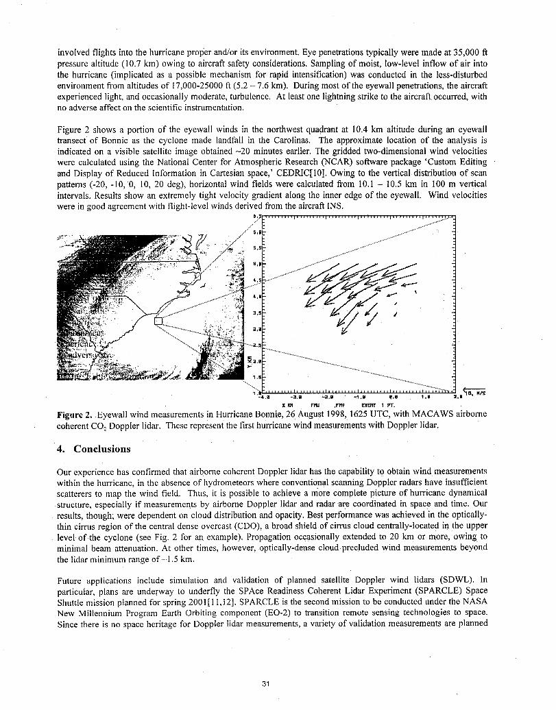
involvedflightsinto the hurricaneproperand/oritsenvironment.Eyepenetrationstypicallywere madeat 35,000ftpressurealtitude(10.7 km) owingto aircraft safetyconsiderations.Samplingof moist,low-levelinflowof air intothe hurricane (implicatedas a possiblemechanismfor rapid intensification)was conductedin the less-disturbedenvironmentfromaltitudesof 17,000-25000ft (5.2- 7.6 km). Duringmostof the eyewallpenetrations,the aircraftexperiencedlight,and occasionallymoderate,turbulence. At leastonelightningstriketo the aircraftoccurred,withnoadverseaffectonthe scientificinstrumentation.

Figure 2 shows a portion of the eyewall winds in the northwest quadrant at 10.4 km altitude during an eyewalltransect of Bonnie as the cyclone made landfall in the Carolinas. The approximate location of the analysis isindicated on a visible satellite image obtained -20 minutes earlier. The gridded two-dimensional wind velocitieswere calculated using the National Center for Atmospheric Research (NCAR) software package 'Custom Editing 'and Display of Reduced Information in Cartesian space,' CEDRIC[10]. Owing to the vertical distribution of scanpatterns (-20, -I0, 0, 10, 20 deg), horizontal wind fields were calculated from 10.1 - 10.5 km in 100 m verticalintervals. Results show an extremely tight velocity gradient along the inner edge of the eyewall: Wind velocitieswere in good agreement with flight-level winds derived from the aircraft INS.

./.f"

X _ FI_ ,P'd¥ UIfER'f 1 PT.

Figure 2. Eyewall wind measurements in Hurricane Bonnie, 26 August 1998, 1625 UTC, with MACAWS airbornecoherent CO2Doppler lidar. These represent the first hurricane wind measurements with Doppler lidar.

4. Conclusions

Our experience has confirmed that airborne coherent Doppler lidar has the capability to obtain wind measurementswithin the hurricane, in the absence of hydrometeors where conventional scanning Doppler radars have insufficientscatterers to map the wind field, Thus, it is possible to achieve a niore complete picture of hurricane dynamicalstructure, especially if measurements by airborne Doppler lidar and radar are coordinated in space and time. Our

: results, though; were dependent on cloud distribution and opacity. Best performance was achieved in the optically-thin cirrus region of the central dense overcast (CDO), a broad shield of cirrus cloud centrally-located in the upperlevel of the cyclone (see Fig. 2 for an example). Propagation occasionally extended to 20 km or more, owing tominimal beam attenuation. At other times, however, optically-dense cloud precluded wind measurements beyondthe lidar minimum range of-l.5 km.

Future applications include simulation and validation of planned satellite Doppler wind lidars (SDWL). Inparticular, plans are underway to underfly the SPAce Readiness Coherent Lidar Experiment (SPARCLE) SpaceShuttle mission planned for spring 2001[1I, 12]. SPARCLE is the second mission to be conducted under the NASANew Millennium Program Earth Orbiting component (EO-2) to transition remote sensing technologies to space.Since there is no space heritage for Doppler lidar measurements, a variety of validation measurements are planned

31

throughout the two-week shuttle mission. MACAWS will provide fine-spatial resolution measurements with whichto evaluate the representativeness of SPARCLE winds.

Finally, we note that technological maturity may be defined in a number of ways, such as turnkey system operation,system miniaturization, or measurements from space. Our experience suggests perhaps another criterion formaturity, namely successful operation in a hostile meteorological environment.

5. Acknowledgments

We gratefully acknowledge the assistance of W.A. Brewer, S.P. Sandberg, and R.M. Banta, NOAA EnvironmentalTechnology Laboratory; R.D. Marchbanks and A.M. Weickmann, U. Colorado, Cooperative Institute for Researchin Environmental Sciences; C. Esproles, Jet Propulsion Laboratory; S.H. Harper and R.W. Lee, Lassen Research;S.C. Johnson, NASA Marshall Space Flight Center; P.A. Kromis, Computer Sciences Corporation; and the DC-8staff of NASA Dryden Flight Research Center. In particular, we gratefully acknowledge Dr. Ramesh Kakar, NASAOffice of Earth Science, without whose support this program would not be possible.

6. References

1. Post, M.J. and R.E. Cupp: Optimizing a pulsed Doppler lidar. Appl. Opt. 29 (1990) 4145-4158.2. Bilbro, J.W., G.H. Fichtl, D.E. Fitzjarrald, and M. Krause: Airborne Doppler lidar wind field measurements.

Bull. Amer. Meteor. Soc. 65 (1984) 348-359.3. Bilbro, J.W., C.A. Dimarzio, D.E. Fitzjarrald, S.C. Johnson, and W.D. Jones: Airborne Doppler .lidar

measurements. Appl. Opt. 25 (1986) 3952-3960.4. Rothermel, J., D.R. Cutten, R.M. Hardesty, R.T. Menzies, J.N. Howell, S.C. Johnson, D.M. Tratt, L.D. Olivier,

and R.M. Banta: The Multi-center Airborne Coherent Atmospheric Wind Sensor, MACAWS. Bull. Amer.Meteor. Soe., 79, 581-599 (1998).

5. Howell, J.N., R.M. Hardesty, J. Rothermel, R.T. Menzies: Overview of the first Multicenter Airborne CoherentAtmospheric Wind Sensor (MACAWS) experiment: conversion of a ground-based lidar for airborneapplications. Proe. Soc. Photo. Instrum. Eng., 2833, 116-127 (1996).

6. Amirault, C. T., C. A. Dimarzio: Precision pointing using a dual-wedge scanner. Appl. Opt.,24, i302-1308(1985).

7. Lee, R.W. and K.A. Lee, 1980: A poly-pulse-pair signal processor for coherent Doppler lidar. Reprints,Topical Meeting Coherent Laser Radar for the Atmos., Aspen CO, Opt. Soc. Amer., paper WA2, 1-4.

8. Rye, B.J. and R.M. Hardesty, 1994: Spectral matched filters in coherent laser radar. J. Modern Opt., 41, 2131-2144.

9. More information on CAMEX-3 may be found on the World Wide Web at the following uniform resourcelocator: http://_ohrc.msfc.nasa._ov/camex3/.

10. Mohr, C.G. and L.J. Miller, 1983: CEDRIC - A software package for Cartesian space editing, synthesis, anddisplay of radar fields under interactive contr0k Preprints, 21st Conf. Radar Meteor., Edmonton, Alta.,Canada, Amer. Meteor. Soc., 569-574.

11. M.J. Kavaya and G. D. Emmitt: The Space Readiness Coherent Lidar Experiment (SPARCLE) Space ShuttleMission. Invited paper 3380-02, Proc. SPIE Vol. 3380, p. 2-11, Conference on Laser Radar Technology andApplications III, 12th Annual International Symposium on Aerospace/Defense Sensing, Simulation, andControls, AeroSense, Orlando, FL (14 April 1998).

12. M. J. Kavaya and G. D. Emmitt: Tropospheric Wind Measurements From Space: The SPARCLE Mission AndBeyond. Invited paper OS4-1, Digest of the 19th International Laser Radar Conference (ILRC), p 553,NASA/CP- 198-207671/PT2, Annapolis, MD USA (July 1998).

32

WIND InstrumentResults of ground tests

F. KiSpp{1),R. H_ing {l),M. Klier{1),E. Nagel{1),O. Reitebuch{1),M. Schrecker{1),

J. Streicher{_),Ch. Werner{Z},G. Wildgruber{2),C. Loth{3},Ch. Boitel{3),P. Delville{3),Ph. Drobinski{3),P. H. Flamant{3},B. Romand{3},L. Sauvage{3),

D. Bt'uneau{4},M. Meissonnier{5}

(1) DLR - Arbeitsgruppe LIDARD-82230 Wessling, Germany

tel : 49 8153 28 1321fax :49 8153 28 1608

e-mail : oliver.reitebuch@dlr.de

(2) Modulab, 80636 Mianchen,Germany(3) LMD, CNRS, 91128 Palaiseau Cedex, France

(4) Service d'Aeronomie / CNRS / UPMC, 75252 Paris Cedex 05, France(5) INSU / DT 77 Av Denfert Rochereau, 75014 Paris, France

An airborne coherent Doppler Lidar to retrieve mesoscale windfields has been developed in the frame of the Franco-GermanWIND project. The instrument is based on a pulsed C02 lasertransmitter, heterodyne detection and wedge scanner. Theperformance of the instrument operating on the ground isreported.

1. Introduction

WIND developed within a common project by CNRS-CNES / DLR is an airborne coherent infraredDoppler lidar for wind velocity measurement. The system is based on pulsed CO2 laser technology,heterodyne detection and a conical Scanning SYstem. Tests and validation measurements of the WINDinstrument were done on the ground before integration on aircraft. During December 3 to December 8, 1998several field tests totalling several hours of experiments were made at Palaiseau with several weatherconditions like clear air, snow and rain. The objective was to retrieve the wind field and to check theinstrumentperformance. Intercomparison of wind measurements were made using radiosonde soundingsfrom Trappes located approximately 12 km west of Palaiseau.

33

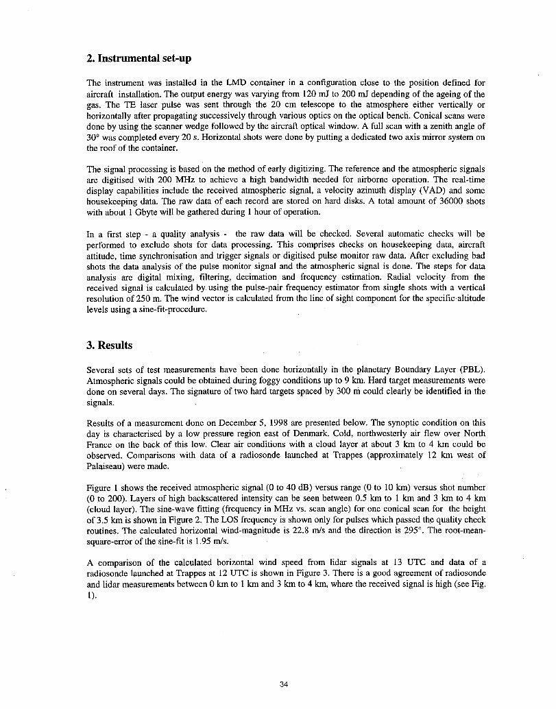
2. Instrumental set-up

The instrumentwas installed in the LMD container in a configurationclose to the position defined foraircraft installation.The outputenergy was varyingfrom 120 nff to 200 mJ depending of the ageing of thegas. The TE laser pulse was sent through the 20 cm telescope to the atmosphere either vertically orhorizontallyafterpropagatingsuccessively throughvarious optics on the optical bencfi. Conical scans weredone by using thescanner wedge followed by the aircraftopticalwindow.A full scanwith a zenith angle of30° was completedevery 20 s. Horizontalshots were done by puttinga dedicatedtwo axis mirrorsystem onthe roof of the container.

The signal processingis based on the methodof early digitizing.The referenceandthe atmosphericsignalsare digitised with 200 MHz to achieve a high bandwidth needed for airborne operation. The real-timedisplay capabilities include the received atmospheric signal, a velocity azimuthdisplay (VAD) and somehousekeeping data. The raw dataof each record are stored on hard disks. A total amountof 36000 shotswith about 1 Gbyte will be gatheredduringI hourof operation.

In a first step - a quality analysis - the raw data will be checked. Several automaticchecks will beperformed to exclude shots for data processing. This comprises checks on housekeeping data, aircraftattitude,time synchronisationand triggersignals or digitised pulse monitorraw data. Afterexcluding badshots the data analysisof the pulse monitorsignal and the atmosphericsignal is done. The steps for dataanalysis are digital mixing, filtering, decimation and frequency estimation. Radial velocity from thereceived signal is calculated by using the pulse-pair frequency estimator from single shots with a verticalresolution of 250 m. The wind vector is calculated from the line of sight component for the specific,altitudelevels using a sine-fit-procedure.

3. Results

Several sets of test measurements have been done horizontally in the planetary Boundary Layer (PBL).Atmospheric signals could be obtained during foggy conditions up to 9 km. Hard target measurements weredone on several days. The signature of two hard targets spaced by 300 m Couldclearly be identified in thesignals.

Results of a measurement done on December 5, 1998 are presented below. The synoptic condition on thisday is characterised by a low pressure region east of Denmark. Cold, northwesterly air flew over NorthFrance on the back of this low. Clear air conditions with a cloud layer at about 3 km to 4 km could beobserved. Comparisons with data of a radiosonde launched at Trappes (approximately 12 km west ofPalaiseau) were made.

Figure 1shows the received atmospheric signal (0 to 40 dB) versus range (0 to 10 km) versus shot number(0 to 200). Layers of high backscattered intensity can be seen between 0.5 km to 1 km and 3 km to 4 km(cloud layer). The sine-wave fitting (frequency in MHz vs. scan angle) for one conical scan for the heightof 3.5 km is shown in Figure 2. The LOS frequency is shown only for pulses which passed the quality checkroutines. The calculated horizontal wind-magnitude is 22.8 m/s and the direction is 295°. The root-mean-square-error of the sine,fit is 1.95 m/s.

A comparison of the calculated horizontal wind speed from lidar signals at 13 UTC and data of aradiosonde launched at Trappes at 12 UTC is shown in Figure 3. There is a good agreement of radiosondeand lidar measurements between 0 km to 1km and 3 km to 4 km, where the received signal is high (see Fig.1).

34

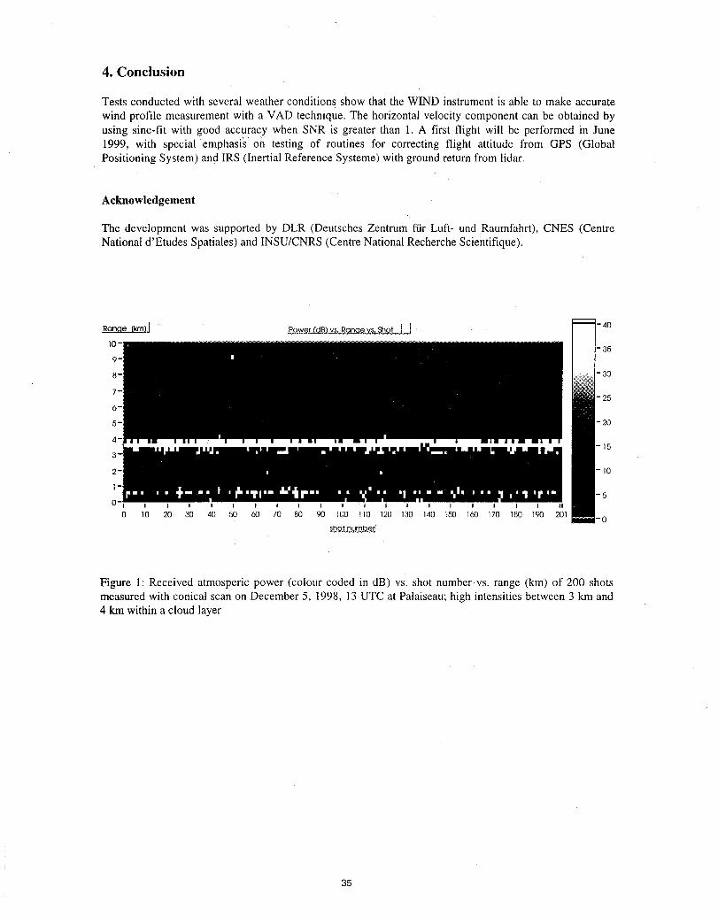
4. Conclusion

Tests conducted with several weather conditions show that the WIND instrument is able to make accuratewind profile measurement with a VAD technique. The horizontal velocity component can be obtained by

using sine-fit with good accuracy when SNR is greater than 1. A first flight will be performed in June1999, with special emphasis on testing of routines for correcting flight attitude from GPS (GlobalPositioning System) and IRS (Inertial Reference Systeme) with ground return from lidar.

Acknowledgement

The development was supported by DLR (Deutsches Zentrum ffir Luft- und Raumfahrt), CNES (CentreNationald'Etudes Spatiales) and INSU/CNRS (CentreNationalRecherche Scientifique).

Rancle (km)! powe[ (dB)ys_Ranc_evs,S_ - 40

-359-

8- 30

25

5- 20

15

2- I0

I5o. . , . . , , . , , , , , , , , , , , , .

0 I0 20 30 40 50 60 70 80 90 100 110 120 130 140 150 160 170 180 190 201-0

shot numbe_

Figure 1: Received atmosperic power (colour coded in dB) vs. shot number.vs, range (km) of 200 shotsmeasured with conical scan on December 5, 1998, 13UTC at Palaiseau; high intensities between 3 km and4 km within a cloud layer

35

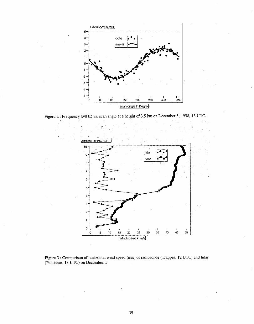
Frequency In MHzt

data

2- . /'<'", . !_.-1- " • •

0-

-2

-3 •

-4

-5 I I I i I i I t10 50 1O0 150 200 250 300 360

scan angle In Degre_

Figure 2 : Frequency (MHz) vs. scan angle at a height of 3.5 km on December 5, 1998, 13 UTC.

Figure 3 : Comparison of horizontal wind speed (m/s) of radiosonde (Trappes, 12 UTC) and lidar(Palaiseau, 13 UTC) on December, 5

36

SPECIAL

Presider: Fred Holmes

37

Improving Scientific Capabilities in Space in the 21st Century: the NASA NewMillennium Program

Carol A. Raymond (Jet Propulsion Laboratory, MS 183-501, 4800 Oak Grove Drive, Pasadena, CA 91109;818-354-8690; cravmond@ipl.nasa.gov)

David Crisp (Jet Propulsion Laboratory, MS 180-404, 4800 Oak Grove Drive, Pasadena, CA 91109; 818-354-7969; dcrisp(_,pop.ipl.nasa.gov)

NASA's New Millennium Program (NMP) has been chartered to identify and validate in space emerging,revolutionary technologies that will enable less costly, more capable future science missions. The programutilizes a unique blend of science guidance and industry partnering to ferret out technology solutions toenable science capabilities in space which are presently technically infeasible, or unaffordable. Thosetechnologies which present an unacceptably high risk to future science missions (whether small PI-led oroperational) are bundled into technology validation missions. These missions seek to validate thetechnologies in a manner consistent with their future uses, thus reducing the associated risk to the first user,and obtaining meaningful science data as well.

The SPAce Readiness Coherent Lidar Experiment (SPARCLE) was approved as the second NMP EarthObserving mission (EO2) in October 1997, and assigned to Marshall Space Flight Center for,mplementation. Leading up to mission confirmation, NMP sponsored a community workshop in March1996 to draft Level-1 requirements for a doppler wind lidar mission, as well as other space-based lidarmissions (such as DIAL). Subsequently, a study group was formed and met twice to, makerecommendations on how to perform a comparison of coherent and direct detection wind lidars in space.These recommendations have guided the science validation plan for the SPARCLE mission, and willensure that future users will be able to confidently assess the risk profile of future doppler wind missionsutilizing EO2 technologies. The primary risks to be retiredare: (1) Maintenance of optical alignmentsthrough launch and operations on orbit, and (2) Successful velocity estimation compensation for theDoppler shift due to the platform motion, and due to the earth's rotation. This includes the need to accountfor all sources of error associated with pointing control and knowledge. The validation obiectives are: (1)Demonstrate measurement of tropospheric winds from space using a scanning coherent Doppler lidartechnique that scales to meet future research (e.g. ESSP) and operational (e.g. NPOESS) missionrequirements. Specifically, produce and validate LOS wind data with single shot accuracy of 1-2 m/s inregions of high signal-to-noise ratio (SNR), and low atmospheric wind turbulence and wind shear, (2)Collect the atmospheric and instrument performance data in various scanning modes necessary to validateand improve instrument performance models that will enable the definition of future missions with greaterconfidence. Such data include aerosol backscatter data over much of the globe, and high SNR data such asthat from surface returns, and (3) Produce a set of raw instrument data with which advanced signalprocessing techniques can be developed. This objective will permit future missions to better understandhow to extract wind information from low backscatter regions of the atmosphere.

To date, four NMP technology validation missions are in the implementation phase, and three others areseeking final approval for implementation. Deep Space 1 (DS1), launched in July 1998, is slated to visitasteroid 1992 KD in July 1999. DS1 has successfully validated a solar electric (ion) propulsion system. Inaddition, two innovative compact instruments, the Miniature Integrated Camera Spectrometer (MICAS)and the Plasma Experiment for Planetary Exploration (PEPE) have been validated. The Mars MicroprobeProject (DS2) was launched in January 1999 as a piggyback on the Mars 98 lander, carrying two tinyprobes that will crash land into the south polar region of Mars in December 1999. The primary validationexperiments on DS2 are a non-ablative aeroshell entry vehicle, and several microinstruments within theprobe. The first Earth Observing NMP mission (EO1), set to launch in December of 1999, willdemonstrate a lightweight, low-cost system to replace the Landsat ETM+ instrument, and will include avalidation of a hyperspectral imager. EO2 (SPARCLE) will test a coherent doppler wind lidar from ashuttle platform in 2001. Pending final approval, Space Technology (ST) 3 will validate technologies for aseparated spacecraft optical interferometer, and ST4/Champollion will demonstrate technologies for samplereturn as well as carrying out the objectives of the planned Champollion comet lander.

38

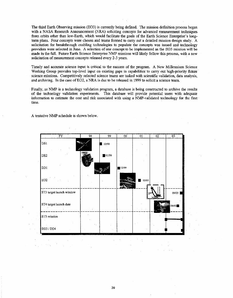
The third Earth Observing mission (EO3) is currently being defined. The mission definition process beganwith a NASA Research Announcement (NRA) soliciting concepts for advanced measurement techniquesfrom orbits other than low-Earth, which would facilitate the goals of the Earth Science Enterprise's long-term plans. Four concepts were chosen and teams formed to carry out a detailed mission design study. Asolicitation for breakthrough enabling technologies to populate the concepts was issued and technologyproviders were selected in June. A selection of one concept to be implemented as the EO3 mission will bemade in the fall. Future Earth Science Enterprise NMP missions will likely follow this process, with a newsolicitation of measurement concepts released every 2-3 years.

Timely and accurate science input is critical to the success of the program. A New Millennium ScienceWorking Group provides top-level input on existing gaps in capabilitiesto carry out high-priority futurescience missions. Competitively selected science teams are tasked with scientific validation, data analysis,and archiving. In the case ofEO2, a NRA is due to be released in 1999 to solicit a science team.

Finally, as NMP is a technology validation program, a database is being constructed to archive the resultsof the technology validation experiments. This database will provide potential users with adequateinformation to estimate the cost and risk associated with using a NMP-validated technology for the firsttime.

A tentative NMP schedule is shown below.

FY 98 99 00 01 02 03

DS1 I0/98 '

DS2 • 01/99

EO 1 • 12/99

EO tST3 target launch window 09/03 III

ST4 target launch date

ST5mission

EO3 / EO4

39

A COHERENT FMCW LIDAR MAPPING SYSTEM FOR AUTOMATED TISSUEDEBRIDMENT

Donald Hutchinson, Sc.D., Roger Richards, Ph.D., Glenn Allgood, Ph.D.Instrumentation and Controls Division, Oak Ridge National Laboratory

Oak Ridge, TN 37831

Introduction

The Oak Ridge National Laboratory (ORNL) is developing a prototype 850-nm FMCW lidarsystem for mapping tissue damage in burn cases for the U.S. Army Medical Research andMaterial Command. The first phase of this project involved the development a prototype FMCWlaser radar system for mapping tissue damage in burn cases for the U.S. Army Medical Researchand Material Command. In its final form, the laser system will provide a 3-D image map of theburn and surrounding area and provide tissue damage assessment. The local coordinates of thedamaged tissue will be reconciled with real-world coordinates for ultimately positioning andcontrolling a pulsed laser for automated removal of the dead or necrotic tissue.

Evaluation of Laser Interaction with Tissue

The first task was to chose the optimum laser wavelength for providing a returnsignalforranging. The wavelength selection was derived from models available in the literature on IRlaser interaction with tissue. The laser wavelength for this lidar system is in the near-infrared at850 nm. This choice was based on two considerations: (1) Low relative absorption in skin and(2) high scattering from hemogblin. 850 nm is near the minimum in skin absorption, while theabsorption coefficient for whole blood is nearly 10 times higher. The "absorption" coefficient isprimarily due to scattering, more so for blood than skin. Our initial model for the debridementmeasurement assumes a two layer target, the skin surface which reflects a portion of the incidentlight due to a Fresnel relectivity of ~3.5%(skin index of refraction -1.31) and a layer containingblood in undamaged tissue below the burn damaged skin. The return laser signal should thencontain primarily two components, one from the surface and one from the blood layer below theburn.

Development of FMCW Lidar Breadboard

Once the wavelength was chosen, a solid state laser at the appropriate wavelength was purchasedand a prototype lidar system constructed. The lidar is a Michleson interferometer design with achirped-frequency laser diode. The laser is a distributed-feedback diode, Model SDL- 5722-H1,which produces approximately 150-mW of power at a wavelength of 850-nm. The laser diode isisolated from stray-light feedback from the optics system with a ferrite isolator. In order tocalibrate the lidar system, measurements were made of the thickness of a fused silica optical flat.The reference mirror was blocked for these measurements to simulate the return phase producedonly by the thickness of the target. The blue curve in Figure 1 represents the captured returnfrom a 0.6463-inch thick fused silica optical flat.

4O

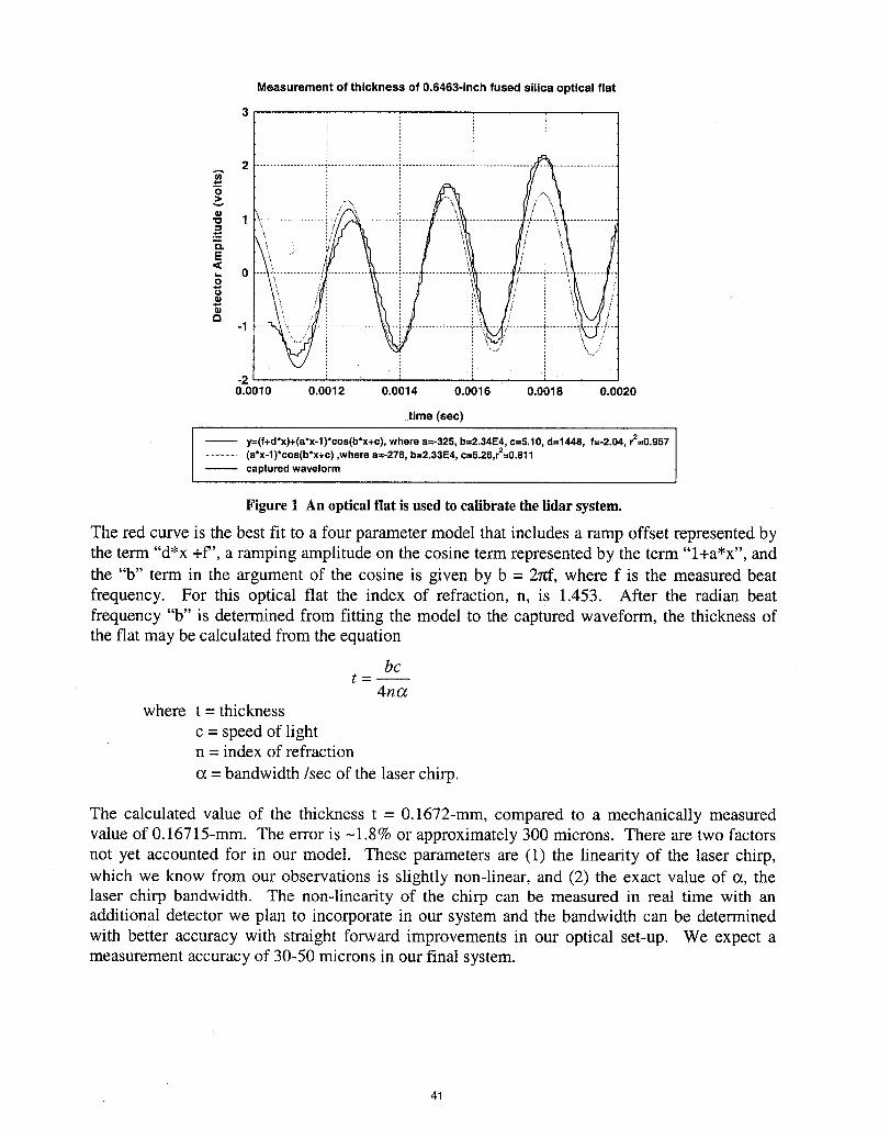
Measurement of thickness of 0.6463-inch fused silica optical flat

3

A 2

I +...................._../i _,...........:!.......... _................

o

-1/

-20.0010 0.0012 0.0014 0.0016 0.0018 0.0020

time (sec)

I y=(f+d*x)+(a*x-1)*cos(b*x+c), where a=-325, b=2.34E4, c--5.10, d=1448, f=-2.04, r2=0.957

(a*x-1)*cos(b*x+c) ,where a=-278, b=2.33E4, c=5.26,r2=0.811captured waveform

Figure 1 An optical fiat is used to calibrate the lidar system.

The red curve is the best fit to a fourparametermodel thatincludes a ramp offset represented bythe term "d*x +f", a rampingamplitudeon the cosine term represented by the term "l+a*x", andthe "b" term in the argumentof the cosine is given by b = 2nf, where f is the measuredbeatfrequency. For this optical fiat the index of refraction, n, is 1.453. After the radian beatfrequency"b" is determinedfrom fitting the model to the capturedwaveform, the thickness ofthe fiat maybe calculatedfrom the equation

bct-

4n_where t = thickness

c = speed of lightn = index of refraction

= bandwidth/sec of the laser chirp.

The calculated value of the thickness t = 0.1672-mm, compared to a mechanically measuredvalue of 0.16715-mm. The error is -1.8% or approximately300 microns. There are two factorsnot yet accountedfor in our model. These parameters are (1) the linearity of the laser chirp,which we know from our observations is slightly non-linear,and (2) the exact value of c_,thelaser chirp bandwidth. The non-linearity of the chirp can be measured in real time with anadditionaldetector we plan to incorporate in our system and the bandwidth can be determinedwith better accuracy with straight forward improvements in our optical set-up. We expect ameasurementaccuracyof 30-50 microns in our final system.

41

VIBRATIONMEASUREMENTSPaul McManamon

42

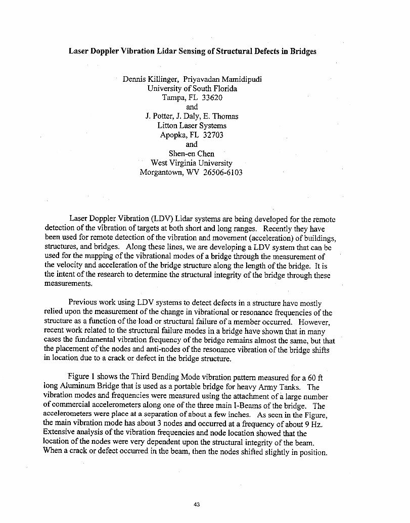
Laser Doppler Vibration Lidar Sensing of Structural Defects in Bridges

Dennis Killinger, Priyavadan MamidipudiUniversity of South Florida

Tampa, FL 33620and

J. Potter, J. Daly, E. ThomasLitton Laser SystemsApopka, FL 32703

andShen-en Chen

West Virginia UniversityMorgantown, WV 26506-6103

Laser Doppler Vibration (LDV) Lidar systems are being developed for the remotedetection of the Vibrationof targets at both short and long ranges. Recently they havebeen used for remote detection of the vibration and movement (acceleration) of buildings,structures, and bridges, Along these lines, we are developing a LDV system that can beused for the mapping of the vibrational modes of a bridgethrough the measurement ofthe velocity and acceleration of the bridge structure along the length of the bridge: It isthe intent of the research to determine the structural integrity of the bridge through thesemeasurements.

Previous work using LDV systems to detect defects in a structure have mostlyrelied upon the measurement of the change in vibrational or resonance frequencies of thestructure as a function of the load or structural failure of a member occurred. However,recent workrelated to the structural failure modes in a bridge have shown that in manycases the fundamental vibration frequency of the bridge remains almost the same, but thatthe placement of the nodes and anti-nodes of the resonance vibration of the bridge shiftsin location due to a crack or defect in the bridge structure.

Figure 1shows the Third Bending Mode vibration pattem measured for a 60 ftlong Aluminum Bridge that is used as a portable bridge for heavy Army Tanks. Thevibration modes and frequencies were measured using the attachment of a large numberof commercial accelerometers along one of the three main I-Beams of the bridge. Theaccelerometers were place at a separation of about a few inches. As seen in the Figure,the main vibration mode has about 3 nodes and occurred at a frequency of about 9 Hz.Extensive analysis of the vibration frequencies and node location showed that thelocation of the nodes were very dependent upon the structural integrity of the beam.When a crack or defect occurred in the beam, then the nodes shifted slightly in position.

43

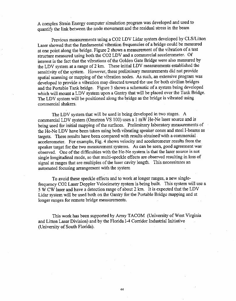
A complex Strain Energy computer simulation program was developed and used toquantify the link between the node movement and the residual stress in the beam

Previous measurements using a CO2 LDV Lidar system developed by CLS/LittonLaser showed that the fundamental vibration frequencies of a bridge could be measuredat one point along the bridge. Figure 2 shows a measurement of the vibration of a teststructure measured using both the CO2 LDV and a commercial accelerometer. Ofinterest is the fact that the vibrations of the Golden Gate Bridge were also measured bythe LDV system at a range of 2 km. These initial LDV measurements established thesensitivity of the system. However, these preliminary measurements did not providespatial scanning or mapping of the vibration nodes. As such, an extensive program wasdeveloped to provide a vibration map directed toward the use for both civilian bridgesand the Portable Tank bridge. Figure 3 shows a schematic of a system being developedwhich will mount a LDV system upon a Gantry that will be placed over the Tank Bridge.The LDV system will be positioned along the bridge as the bridge is vibrated usingcommercial shakers.

The LDV system that will be used is being developed in two stages. Acommercial LDV system (Ometron VS 100) uses a 1 mW He-Ne laser source and isbeing used for initial mapping of the surfaces. Preliminary laboratory measurements ofthe He-Ne LDV have been taken using both vibrating speaker cones and steel I-beams astargets. These results have been compared with results obtained'with a commercialaccelerometer. For example, Fig. 4 shows velocity and accelerometer results from thespeaker target for the two measurement systems. As can be seen, good agreement wasobserved. One of the difficulties with the He-Ne system is that the laser source is notsingle longitudinal mode, so that multi-speckle effects are observed resulting in loss ofsignal at ranges that are multiples of the laser cavity length. This necessitates anautomated focusing arrangement with the system

To avoid these speckle effects and to workat longer ranges, a new single-frequency CO2 Laser Doppler Velocimetry system is being built. This system will use a5 W CW laser and have a detection range of about 2 km. It is expected that the LDVLidar system will be used both on the Gantry for the Portable Bridge mapping and atlonger ranges for remote bridge measurements.

This work has been supported by Army TACOM (University of West Virginiaand Litton Laser Division) and by the Florida I-4 Corridor Industrial Initiative(University of South Florida).

44

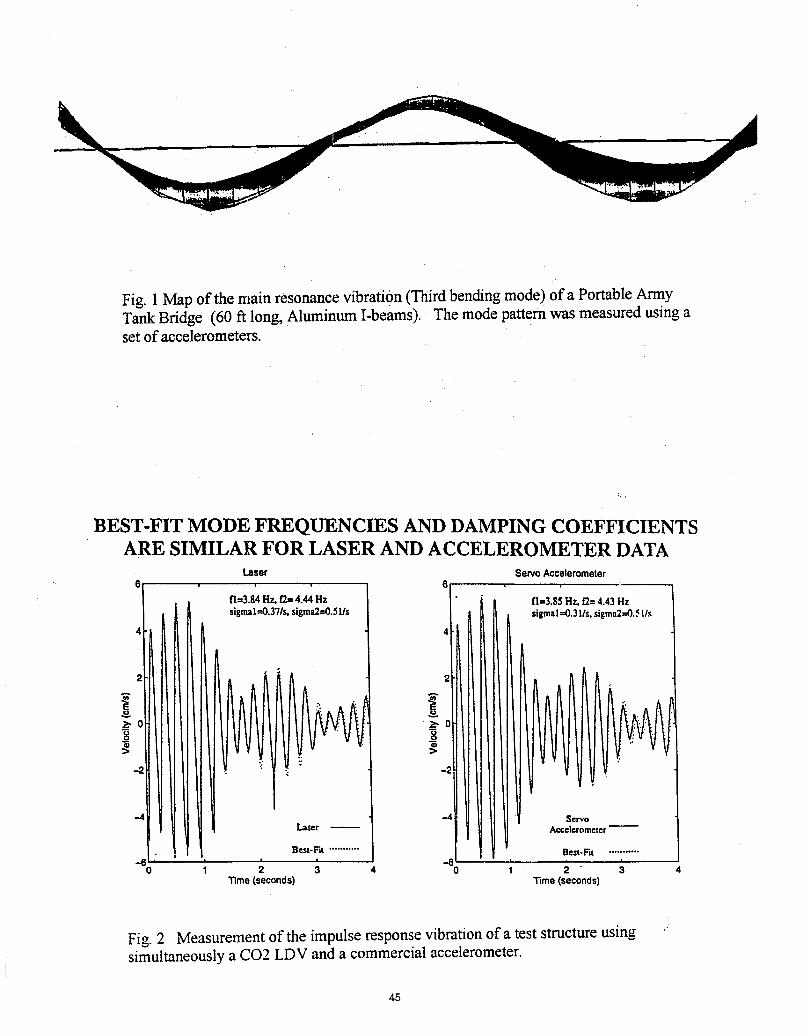
Fig. 1Map of the main resonance vibration (Tllird bending mode) of a Portable ArmyTank Bridge (60 ft long, Aluminum I-beams). The mode pattern was measured using aset of accelerometers.

BEST-FIT MODE FREQUENCIES AND DAMPING COEFFICIENTSARE SIMILAR FOR LASER AND ACCELEROMETER DATA

Laser ServoAccelerometer6 6

n=3.84Hz,fT.=4.44Hz 1"I=3.85Hz,12=4.43HzsigmaI=0.37/s,sigma2:--0.5lls sigma1---0.3!Is, sigma2=0.51Is

4

g g2"0 0

_> ..7

-2 -. -2

--4 ,--4 $ervolaser Accelerometer

Best-Fit ........... Best-Fit ...........

-60 1 2 4 0 1 3Time (seconds) Time (seconds)

Fig. 2 Measurement of the impulse response vibration of a test structure usingsimultaneously a CO2 LDV and a commercial accelerometer.

45

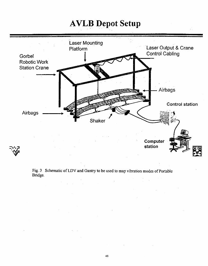
AVLB Depot Setup

"Laser MountingPlatform .... Laser Output & Crane

Gorbel | ControlCablingRoboticWorkStation Crane

1=

• i

Airbags

Control station

Airbags _ f _.Shaker

Computer

_-_4 station

Fig. 3 Schematic of LDV and Gantry to be used to map vibration modes of PortableBridge.

46

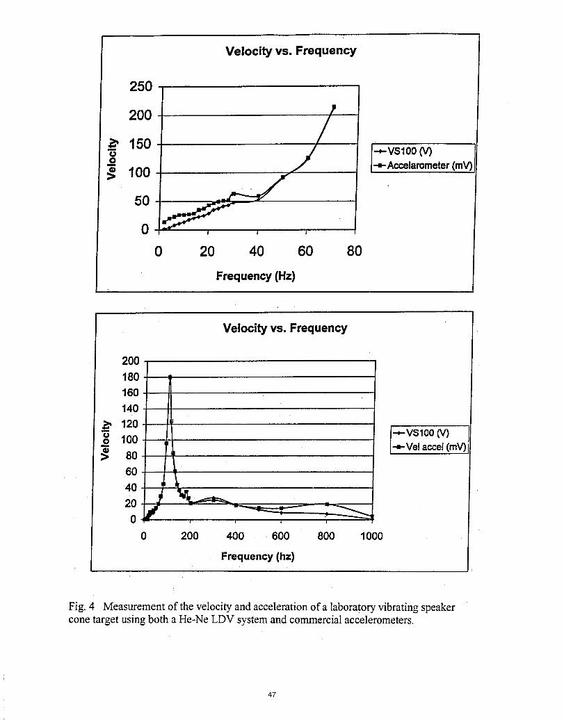
Velocity vs. Frequency

250

200

__150 I-'-vsl°°(v)_> 100 I.-=-Accelammeter(mV)

50

O I l I

0 20 40 60 80

Frequency(Hz)

Velocity vs. Frequency

200180160140120

_' 100 --._VSlOO(v)

_> 80 "=-Velaccel(mV),

oo20 J0 = , , , ,

0 200 400 600 800 1000

Frequency(hz)

Fig. 4 Measurement of the velocity and acceleration of a laboratory vibrating speakercone target using both a He-Ne LDV system and commercial accelerometers.

47

Evaluation of Laser-Vibration-Sensing Technology From An Airborne Platform *}

R.M. Heinrichs, S. Kaushik, D.G. Kocher, S. Marcus, G.A. Reinhardt, T. Stephens, andC.A. Primmerman

LincolnLaboratoryMassachusettsInstituteof Technology

244 Wood StreetLexington,MA 02420

(78I)-981-7945, (781)981-5069 (fax), heinrichs@ll.mit.edu

Abstract

Lincoln Laboratory has begun an effort to evaluate the capability of an airborne laser vibrometer to makehigh-resolution vibration measurements of ground targets. This paper will present details of each of the majorelementsof this effort. This will primarily involve the performance prediction of laser vibrometry as expressed bythe noise-equivalent vibration amplitude. The contribution to this limiting noise level from atmospheric-pistonturbulence and speckle broadening as well as the system-dependentcontributions from platform vibrationsandpointing jitter will be discussed. Laboratory measurements, which confirm the theoretical noise predictions forspeckle, will also be presented.

Introduction

The ability to make remote-vibration measurements from an airborne platform has a variety Ofapplications.The goal of the present effort is to generate a feasibility assessment of the laser-vibrometry concept and to estimatethe ultimate resolution capability that such a system would potentially have. This has primarily included analysisand laboratory measurements. A point design for a laser-vibrometry system on board a high-altitude airborneplatform has been developed and the basic characteristics of the system have been defined, resulting in an overallperformance evaluation. This includes the effects of speckle and platform vibration and pointing jitter as well asconsiderations of atmospheric piston turbulence, laser phase noise, and algorithm performance. Laboratorymeasurements have also been performed, which verify the predictions for the effects of target speckle, algorithmperformance, and atmospheric turbulence. This paper briefly presents the overall results of the analysis, followed byselected results from the laboratory experiments.

System Analysis

The nominal airborne platform chosen for the vibrometer point design is capable of maintaining altitudes inexcess of 20 km with a loitering velocity of 200 m/s. The laser is assumed to be a continuous wave (CW) erbium-doped fiber laser. The CW requirement is necessary in order to maximize the number of independent specklerealizations that can be averaged over in a given interval of time. The laser beam is directed from the platformtowards the ground, typically within 45• of nadir. The pointing requirements for the beam on the ground aredictated by two different coherence lengths. The first is the signal-phase-coherence length, which is the distanceover which the beam spot on the ground can move before the signal phase changes due to the generation of a newspeckle realization. This distance is on the order of the spot diameter, meaning that the laser-spot position on theground must be maintained to within about 25% of the spot diameter over some period of time in order to maintainsignal coherence. As discussed below, other speckle-broadening effects cause this time to be quite short, typically• 1 ms. The second coherence length is referred to as the vibration-coherence-length. This is the distance on theground over which the vibration phase of the ground target remains essentially constant. This distance can besignificantly larger than the laser-spot diameter depending on the nature of the target.

For the airborne platform, the signal bandwidth is dominated by the so-called speckle bandwidth. This isthe spectral broadening of the signal due to the rate at which the signal phase changes as the target specklerealization changes. One way to view speckle broadening is to consider the velocity spread of the return signal dueto the fact that different points of the illuminated spot are moving at different velocities relative to the platform. In

"This research is sponsored by the Defense Advanced Research Projects Agency, under Air Force Contract F19628-95-C-0002.

§ "The views expressed are those of the authors and do not reflect the official policy or position of the U.S.government."

48

effect, the illuminated spot is rotating relative to the laser radar, with the front part of the spot moving towards andthe rear part of the spot moving away from the airborne platform (Figure 1). The speckle-broadened bandwidth fora nadir-pointing coherent laser radar is independent of wavelength and given approximately by: 2_/2VJD,where Vpis the airborne platform velocity and D is the aperture diameter. For a nominal 20-cm aperture diameter and 200-m/s velocity, the speckle bandwidth is about 1.4 kHz.

The carrier-to-noise ratio (CNR) of the nominal system has been calculated and is shown in Figure 2. Incalculating this quantity, a typical diffuse ground reflectivity of 20% at the 1.5-_m wavelength is assumed, as wellas a 20-cm aperture diameter, a 20-km range, 70% detector quantum efficiency, 30% heterodyne mixing efficiency,50% round-trip optical efficiency, and a signal bandwidth of 10 x the speckle bandwidth (~ i0 kHz). The CNR is

proportional to the transmitted power, the laser wavelength, and to the cube of the transmit/receive aperture diameter(DA is from the solid angle subtended by the receiver and another factor of DA is from the inverse dependence ofthe speckle bandwidth on the aperture diameter). A functional block diagram of the vibrometer is shown in Figure3. The system is a bistatic coherent laser radar in which the return light is frequency shifted in an acousto-opticmodulator (AOM). This is done in order to remove the positive/negative velocity ambiguity and to reduce systemsensitivity to any unshifted component that may come out of the AOM on axis. The platform motion-compensationsystem consists of a Kalman filter, which utilizes accelerometer, pointing, and platform-navigation information toprovide control signals for the variable downmixing synthesizer and error-correction signals for the digital-outputstream. The estimated computational power required for a single-channel system with real-time data processing isapproximately 10MFLOPS.

System Performance Evaluation

This section presents the results of system-performance calculations, which account for limitations due tospeckle broadening, platform compensation, atmospheric turbulence and laser phase noise. The total,phase-noisevariance of the system is assumed to be a sum of the uncorrelated variances from each of these effects:

where the different contributions are from speckle, platform pointing-jitter and vibration, atmospheric pistonturbulence, and laser phase noise, respectively. The impact of each of these noise sources is quantified according tothe noise-equivalent vibration amplitude (NEVA = (_./2_)o). Calculations of the NEVA for each of these terms hasbeen performed and is summarized below.

The speckle-limited NEVA includes the CNR performance calculation, which includes the effect ofdetector noise. The signal detected by a coherent laser radar from a vibrating target is frequency modulated (FM) bythe vibration frequency. The speckle-limited N-EVA is determined by assuming a spectrogram-processingtechnique_ in which the raw data are broken into sequences of length approximately equal to the inverse specklebandwidth. The Cramer-Rao-limited performance is then assumed for the first-moment estimation of the FFT's ofeach sequence.2 A final FFT of the first-moment frequency estimates versus sequence time produces the vibrationalspectrum, with Os being given by the single-sequence first-moment standard deviation divided by the square root ofthe number of sequences. For the airborne scenario assumed here, the speckle bandwidth is about 1.4 kHz and atypical sequence length would be about 1.4 ms.

The next noise term to consider is due to platform vibration and pointing jitter. Pointing jitter affectssystem performance by generating a varying contribution from the line-of-sight (LOS) platform velocity to theDoppler-shifted signal. Platform vibrations impact more directly towards the high-precision LOS velocitymeasurements that the system makes. Both of these effects must ultimately be compensated for by measuring thepointing jitter with angle-rate sensors and the platform vibrations with accelerometers and removing thesecontributions in post processing (or by varying the frequency of an IF downmixing oscillator). The Allied SignalRing Laser Gyro Model RL-34 angle-rate sensor was identified as a candidate for providing the requiredmeasurement resolution for pointing-jitter compensation. Correspondingly, the BEI / Sundstrand QA-700 ServoAccelerometer was also identified as providing high-resolution platform-vibration measurements. The residual errorsources from each of these devices was taken into consideration in the system-performance analysis.

Atmospheric turbulence can affect the performance of the laser vibrometer in two ways: mixing efficiencyloss due to wavefront distortion and signal clutter due to atmospheric-piston variations. The greatest contribution isdue to piston variations. Kolmogorov turbulence theory dictates that, within the inertial subrange, the atmospheric-piston contribution should contribute as an f4/3 power law to the NEVA. These have been modeled for typicalatmospheric-turbulence cases and included in the overall performance analysis.

49

The final noise term considered is due to laser-phase fluctuations. The nominal CW, 1.5-_tm,fiber laserwould require active frequency stabilization to a level that has already been demonstrated in laboratoryenvironments.3 A model has been developed for the frequency dependence of the uncompensated laser-phasefluctuations and it too has been included in the performance analysis.

Putting all the laser-vibrometry noise sources together, the combined sensitivity prediction for the airbornevibrometer is shown in Figure 4. This figure shows the NEVA predicted for each of the major contributors:platform pointing jitter, speckle broadening, laser phase noise, and atmospheric-piston variations. Also shown is thetotal noise prediction for the system. As can be seen, atmospheric-piston variation dominates the performance forthis system. This limits the sensitivity of the system to vibration amplitudes of several microns at 1-Hz frequencieswith the noise level decreasing (sensitivity improving) as fv"4/3,where fv is the ground-vibration frequency. Thepower-law dependence is representative of the dominant noise source of atmospheric-piston fluctuations.

Laboratory Measurements

Laboratorymeasurementshave been conductedthat verify the expected performanceof a laser vibrometerin the presence of speckle broadeningandsimulated atmospheric turbulence. The basic laboratorysetup involvesmeasurementsfrom a rotatingtarget, for speckle simulation, or from a fixed target with atmospheric-turbulence-simulatingphase screens translatedacross the beam. Only the results of the speckle-broadeningmeasurementsarepresentedhere. The laser used for these measurementswas a 1.06-_m CW micro-laserdeveloped by Micracor. Thebeamfrom the laser was collimatedanddirectedonto the rotatingtarget whose rotation rate was preciselycontrolledwith a direct-drivemotor to produce a spectralbroadeningof 4 kHz. The results of measurementswhere the targetwas not vibratingare shown in Figure 5. In this case, the average noise level for the measurementwas within 2 dBof the predicted measurementsensitivity from the Cramer-Rao analysis of the spectrogramalgorithm., This resultaddsconfidence to ourpredictionsfor the speckle-limited sensitivityand spectrogram-algorithmperformancefor theflight system.

Conclusions

In conclusion,Lincoln Laboratoryhas undertakenan effort to evaluate the ultimateresolution capabilityofremote laser vibrometryfrom an airborneplatform. This effort has involved a combinationof systems analysis,theoretical modeling, and laboratory measurements. The results to date have indicated the general efficacy of theapproach. Nevertheless, laser vibrometry from an airborne platform remains technically challenging andinvestigations are continuing.

References

1. A.L. Kachelmyer and K.I. Schultz, "Spectrogram Processing of Laser Vibration Data," SPIE 1936, 78 (1993).2. B.J. Rye and R.M. Hardesty, "Discrete Spectral Peak Estimation in Incoherent Backscatter Heterodyne Lidar I:

Spectral Accumulation and the Cramer-Rao Lower Bound," IEEE Trans. Geosci. Remote Sensing, 31, 16(1993).

3. M. Kourogi, C. Shin, and M. Ohtsu, "A 250 Hz spectral linewidth 1.5-pm MQW-DFB laser diode withnegative-electrical-feedback," IEEE Photonics Tech. Lett., 6, 496 (1991).

5O

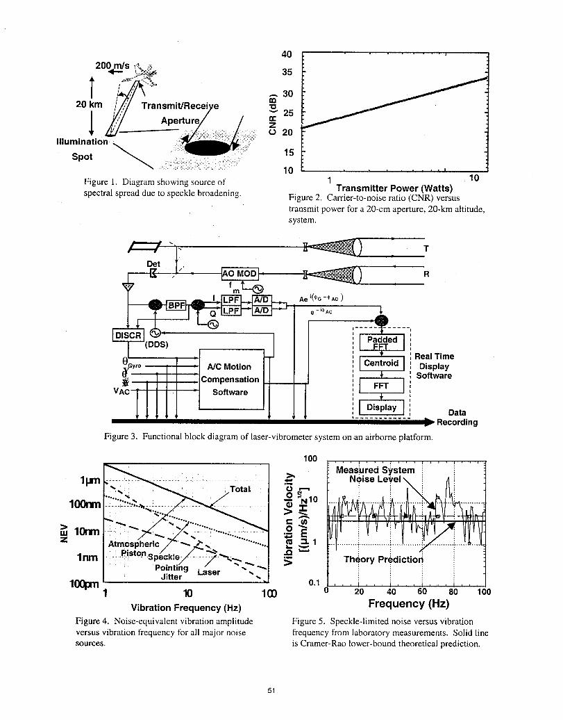
200m/s_,_._ 40 _ • - • ,

30

20km ///_ Transmit/Recei _m_25

: _ 20

Illumination _Spot _i:' 1510

Figure 1. Diagram showing source of 1 10Transmitter Power (Watts)

spectral spread due to speckle broadening. Figure 2. Carrier-to-noise ratio (CNR) versustransmit power for a 20-cm aperture, 20-km altitude,system.

m

Det '/. _ _,, .

f _m

Ae =(% +*AC )

e -iOAC

,I I'(DDS) Padded ,FFT ',

_) [ "J t :RealTime,to I " A/C Motion I centr°id I Display_.G _ l I / _lCompensation + Software

VACi[[[ J ;i Software ] FFTJ+I Display ] Data

............. III Recording

Figure 3. Functional block diagram of laser-vibrometer system on an airborne platform.

100' ' ' I ' ' ' _ ' ' ' I ' ' ' ' ' ' -

_: .. i Meas_uredSystem::

_>' NOise LeVel

lpm ;-....-.,,.•,..........................................i... _i..........."Totaii '_

.......lOOnm ..... , .. _ o.....;.,,,_,.+..._..'.'_*=o_ . . :................................................................. ;

lnm .....:.,.:,.-T ......_pec,=e/i ...... _. _,.;_.... Pointing Lase'/r _"-,.._'`" _ Theory PredictiorJitter ,_

100pm 0.1 . .. _,,,,,,,, .... ,, ,,1 10 100 20 4o 60 80 1oo

Vibration Frequency (Hz) Frequency (Hz)Figure 4. Noise-equivalent vibration amplitude Figure 5. Speckle-limited noise versus vibrationversus vibration frequency for all major noise frequency from laboratory measurements. Solid linesources, is Cramer-Rao lower-bound theoretical prediction.

51

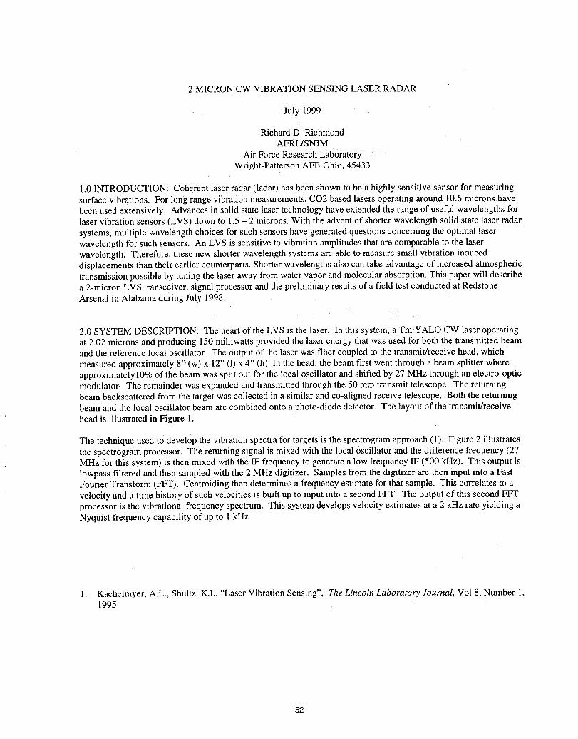
2 MICRON CW VIBRATION SENSING LASER RADAR

July 1999

Richard D. RichmondAFRL/SNJM

Air Force Research Laboratory .:iWright-Patterson AFB Ohio, 45433

1 0INTRODUCTION: Coherent laser radar (ladar) has been shown to be a highly sensitive sensor for measuringsurface vibrations. For long range vibration measurements, CO2 based lasers operating around 10.6 microns havebeen used extensively. Advances in solid state laser technology have extended the range of useful wavelengths forlaser vibration sensors (LVS) down to 1.5 - 2 microns. With the advent of shorter wavelength solid state laser radarsystems, multiple wavelength choices for such sensors have generated questions concerning the optimal laserwavelength for such sensors. An LVS is sensitive to vibration amplitudes that are comparable to the laserwavelength. Therefore, these new shorter wavelength systems are able to measure small vibration induceddisplacements than their earlier counterparts. Shorter wavelengths also can take advantage of increased atmospherictransmission possible by tuning the laser away from water vapor and molecular absorption. This paper will describea 2-micron LVS transceiver, signal processor and the preliminfiryresults of a field test conducted at RedstoneArsenal in Alabama during July 1998.

2.0 SYSTEM DESCRIPTION: The heart of the LVS is the laser. In this system, a Tm:YALO CW laser operatingat 2.02 microns and producing 150 milliwatts provided the laser energy that was used for both the transmitted beamand the reference local oscillator. The output of the laser was fiber coupled to the transmit/receive head, whichmeasured approximately 8'"(w) x 12" (1)x 4" (h). In the head, the beam first went through a beam splitter whereapproximately i0% of the beam was split out for the local oscillator and shifted by 27 MHz through an electro-opticmodulator. The remainder was expanded and transmitted through the 50 mm transmit telescope. The returningbeam backscattered from the target was collected in a similar and c0-aligned receive telescope. Both the returningbeam and the local oscillator beam are combined onto a photo-diode detector. The layout of the transmit/receivehead is illustrated in Figure 1.

The technique used to develop the vibration spectra for targets is the spectrogram approach (1). Figure 2 illustratesthe spectrogram processor. The returning signal is mixed with the local oscillator and the difference frequency (27MHz for this system) is then mixed with the IF frequency to generate a low frequency IF (500 kHz). This output islowpass filtered and then sampled with the 2 MHz digitizer. Samples from the digitizer are then input into a FastFourier Transform (FFT). Centroiding then determines a frequency estimate for that sample. This correlates to avelocity and a time history of such velocities is built up to input into a second FFT. The output of this second FFTprocessor is the vibrational frequency spectrum. This system develops velocity estimates at a 2 kHz rate yielding aNyquist frequency capability of up to 1 kHz.

I. Kachelmyer, A.L., Shultz, K.I., "Laser Vibration Sensing", The Lincoln Laboratory Journal, Vol 8, Number l,1995

52

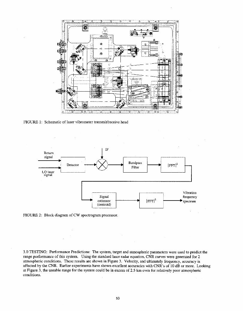
FIGURE 1: Schematic of laser vibrometer transmit/receive head

L IFReturn

signal ._:_i _ _-_

Detector _ Bandpass _ [FFTI2FilterLO laser I

signal

f Vibration

Signal frequencyestimator [FFTI2 _ spectrum(centroid)

FIGURE 2: Block diagram of CW spectrogram processor.

3.0 TESTING: Performance Predictions: The system, target and atmospheric parameters were used to predict therange performance of this system. Using the standard laser radar equation, CNR curves were generated for 2atmospheric conditions. These results are shown in Figure 3. Velocity, and ultimately frequency, accuracy isaffected by the CNR. Earlier experiments have shown excellent accuracies with CNR's of 10 dB or more. Lookingat Figure 3, the useable range for the system could be in excess of 2.5 km even for relatively poor atmosphericconditions.

53

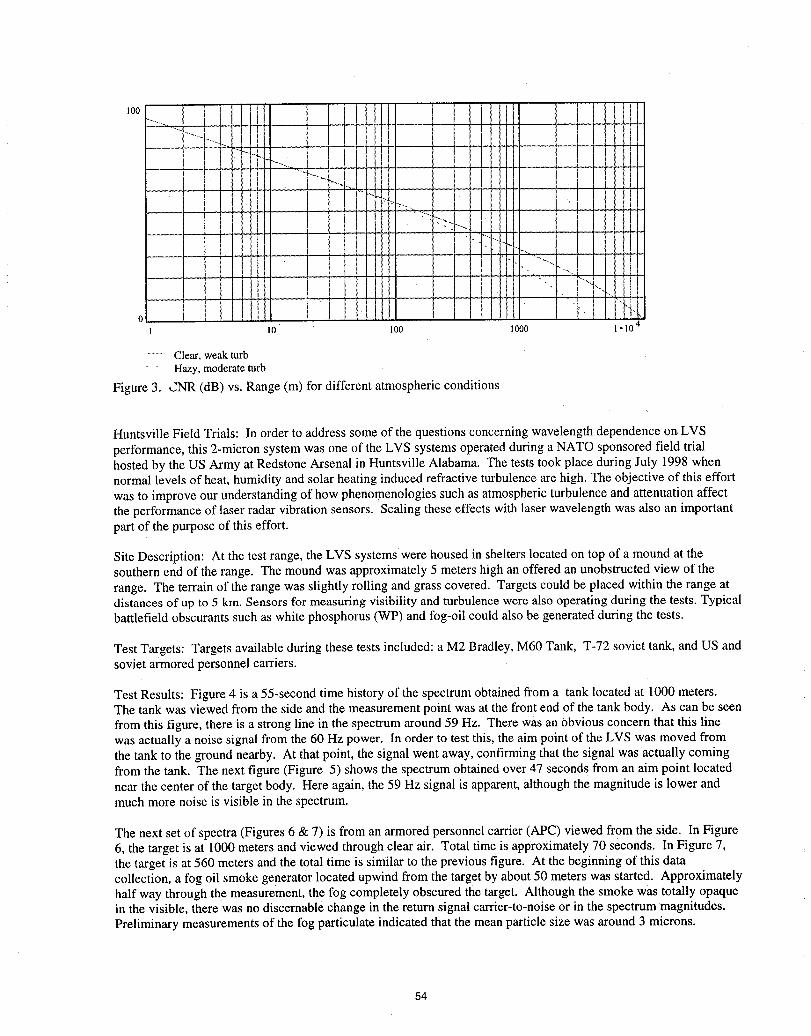
,00....... i liil i i I t_J I *

10 100 1000 1° 10 4

..............Clear, weak turb" ° Hazy, moderate turb

Figure 3. CNR (dB) vs. Range (m) for different atmospheric conditions

Huntsville Field Trials: In order to address some of the questions concerning wavelength dependence on,LVSperformance, this 2-micron system was one of the LVS systems operated during a NATO sponsored field trialhosted by the US Army at Redstone Arsenal in Huntsville Alabama. The tests took place during July 1998 whennormal levels of heat, humidity and solar heating induced refractive turbulence are high. The objective of this effortwas to improve our understanding of how phenomenologies such as atmospheric turbulence and attenuation affectthe performance of laser radar vibration sensors. Scaling these effects with laser wavelength was also an importantpart of the purpose of this effort.

Site Description: At the test range, the LVS systems were housed in shelters located on top of a mound at thesouthern end of the range. The mound was approximately 5 meters high an offered an unobstructed view of therange. The terrain of the range was slightly rolling and grass covered. Targets could be placed within the range atdistances of up to 5 km. Sensors for measuring visibility and turbulence were also operating during the tests. Typicalbattlefield obscurants such as white phosphorus (WP) and fog-oil could also be generated during the tests.

Test Targets: Targets available during these tests included: a M2 Bradley, M60 Tank, T-72 soviet tank, and US andsoviet armored personnel carriers.

Test Results: Figure 4 is a 55-second time history of the spectrum obtained from a tank located at 1000 meters.The tank was viewed from the side and the measurement point was at the front end of the tank body. As can be seenfrom this figure, there is a strong line in the spectrum around 59 Hz. There was an Obviousconcern that this linewas actually a noise signal from the 60 Hz power. In order to test this, the aim point of the LVS was moved fromthe tank to the ground nearby. At that point, the signal went away, confirming that the signal was actually comingfrom the tank. The next figure (Figure 5) shows the spectrum obtained over 47 seconds from an aim point locatednear the center of the target body. Here again, the 59 Hz signal is apparent, although the magnitude is lower andmuch more noise is visible in the spectrum.

The next set of spectra (Figures 6 & 7) is from an armored personnel carrier (APC) viewed from the side. In Figure6, the target is at 1000 meters and viewed through clear air. Total time is approximately 70 seconds. In Figure 7,the target is at 560 meters and the total time is similar to the previous figure. At the beginning of this datacollection, a fog oil smoke generator located upwind from the target by about 50 meters was started. Approximatelyhalf way through the measurement, the fog completely obscured the target. Although the smoke was totally opaquein the visible, there was no discernable change in the return signal carrier-to-noise or in the spectrum magnitudes.Preliminary measurements of the fog particulate indicated that the mean particle size was around 3 microns.

54

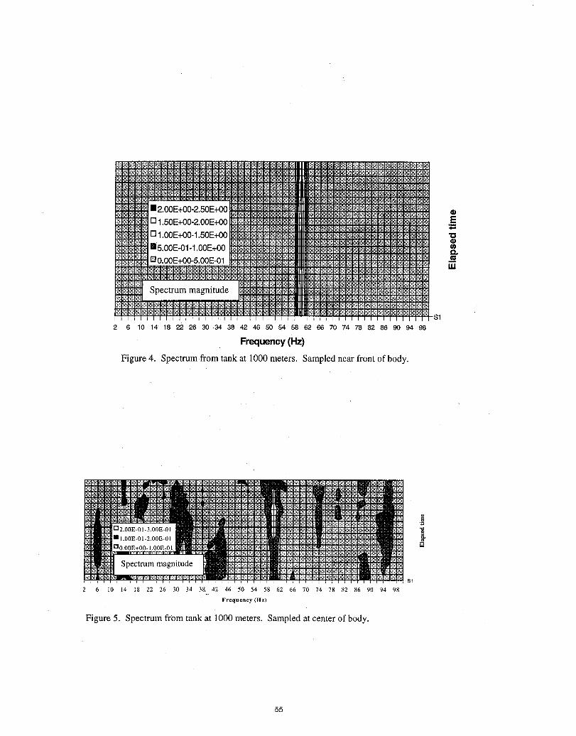
E,m

¢n

ttl

t_

$1

2 6 t0 14 18 22 26 30 34 38. 42 46 50 54 58 62 66 70 74 78 82 86 90 94 98

Frequency (ltz)

Figure 5. Spectrum from tank at 1000 meters. Sampled at center of body.

55

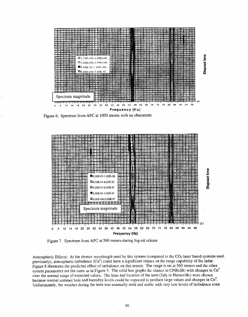
E

m

Spectrum magnitude"$1

2 6 10 14 18 22 26 30 34 38 42 46 50 54 58 62 66 70 74 78 82 86 90 94 98

Frequency (Hz)

Figure 6. Spectrum from APC at 1000 meters with no obscurants

Ek_

€/1Q.

Iltl

$1

2 6 10 14 18 22 26 30 34 38 42 46 50 54 58 62 66 70 74 78 82 86 90 94 98

Frequency (Hz)

Figure 7. Spectrum from APC at 560 meters during fog-oil release

Atmospheric Effects: At the shorter wavelength used by this system (compared to the CO 2 laser based systems usedpreviously), atmospheric turbulence (Cn 2) could have a significant impact on the range capability of the ladar.Figure 8 illustrates the predicted effect of turbulence on this sensor. The range is set at 560 meters and the othersystem parameters are the same as in Figure 3. The solid line graphs the chance in CNR(dB) with changes in Cnzover the normal range of expected values. The time and location of the tests (July in Huntsville) were chosenbecause normal summer heat and humidity levels could be expected to produce large values and changes in Cn z.Unfortunately, the weather during the tests was unusually mild and stable with very low levels of turbulence even

56

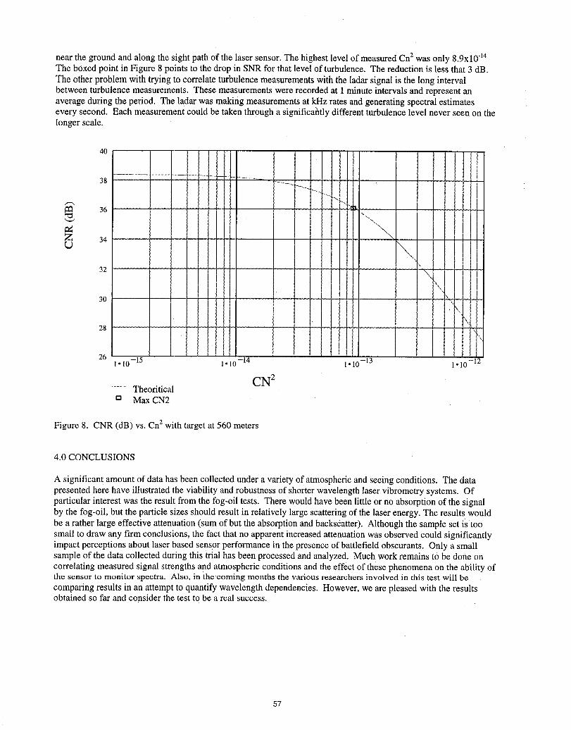
near the ground and along the sight path of the laser sensor. The highest level of measured Cn 2 was only 8.9x10q4The boxed point in Figure 8 points to the drop in SNR for that level of turbulence. The reduction is less that 3 dB.The other problem with trying to correlate turbulence measurements with the ladar signal is the long intervalbetween turbulence measurements. These measurements were recorded at 1 minute intervals and represent anaverage during the period. The ladar was making measurements at kHz rates and generating spectral estimatesevery second. Each measurement could be taken through a significahtly different turbulence level never seen on thelonger scale.

Figure 8. CNR (dB) vs. Cn 2 with target at 560 meters

4.0 CONCLUSIONS

A significan_!amount of data has been collected under a variety of atmospheric and seeing conditions. The datapresented here have illustrated the viability and robustness of shorter wavelength laser vibrometry systems. Ofparticular interest was the result from the fog-oil tests. There would have been little or no absorption of the signalby the fog-oil, but the particle sizes should result in relatively large scattering of the laser energy. The results wouldbe a rather large effective attenuation (sum of but the absorption and backscatter). Although the sample set is toosmall to draw any firm conclusions, the fact that no apparent increased attenuation was observed could significantlyimpact perceptions about laser based sensor performance in the presence of battlefield obscurants. Only a smallsample of the data collected during this trial has been processed and analyzed. Much work remains tObe done oncorrelating measured signal strengths and atmospheric conditions and the effect of these phenomena on the ability ofthe sensor to monitor spectra. Also, in the coming months the various researchers involved in this test will becomparing results in an attempt to quantifYwavelength dependencies. However, we are pleased with the resultsobtained so far and consider the test to be a real success.

57

Comparison of Pulsed Waveform and CW Lidarfor Remote Vibration Measurement

Sammy W. Henderson, J. Alex L. Thomson, Stephen M. Hannon, and Philip GattCoherent Technologies, Inc.

655 Aspen Ridge DriveLafayette, Colorado USA 80026

(303)-604-2000

INTRODUCTION

Continuous wave (cw) lidar systems have been utilized for several years to measure thevibrations of remotely located structures and vehicles. The measured vibration spectra allowsidentification of the vehicle and/or the detection of irregular vibrations indicating structural orengine failure. As an example, a cw lidar operating at 2-microns was successfully utilized tomeasure the vibration spectra of various targets at ranges up to 2 km as part of the RedstoneArsenal Combined Experiments in Laser Radar Program _ in July, 1998. We have recentlydeveloped an agile pulsed waveform coherent lidar2'3which is similar to pulse pair and poly-pulse-pair waveforms which are routinely used in microwave Doppler radar for both hard targetand aerosol target applications. We have extended these waveforms to eyesafe, near infraredoptical wavelengths (2-micron initially demonstrated). The base waveform format comprises apair of pulselets (doublet pulse), each of duration 't, separated by Ts seconds. The rangeresolution is governed by the pulselet duration "c,while the velocity precision is inverselyproportional to the pulselet separation, Ts. Figure 1 and 2 illustrate the base pulse format and thebasic measurement principle.

The agile waveform has the following advantages over cw lidar.• The range resolution provided by the waveform eliminates spurious signals due to scatter of

haze, clouds, netting, etc. between the lidar and the target. Also, range resolved vibrationspectra of the target offers significant additional discrimination ability in many cases.

• The pulsed waveform increases detection probability by optimizing CNR, providing greaterrange at fixed average power or decreased average power at fixed range.

• The short widely-spaced pulses of the waveform allow efficient data collection andprocessing.

• The doublet waveform is well suited to allow possible implementation of the DPCA(Displaced Phase Center Antenna) technique4 of virtually stopping the platform motion tosignificantly reduce velocity measurement noise due to speckle and turbulence. This willprovide a significant sensitivity advantage when measurements are made from a high-speedplatform, e.g., an airplane or satellite.

58

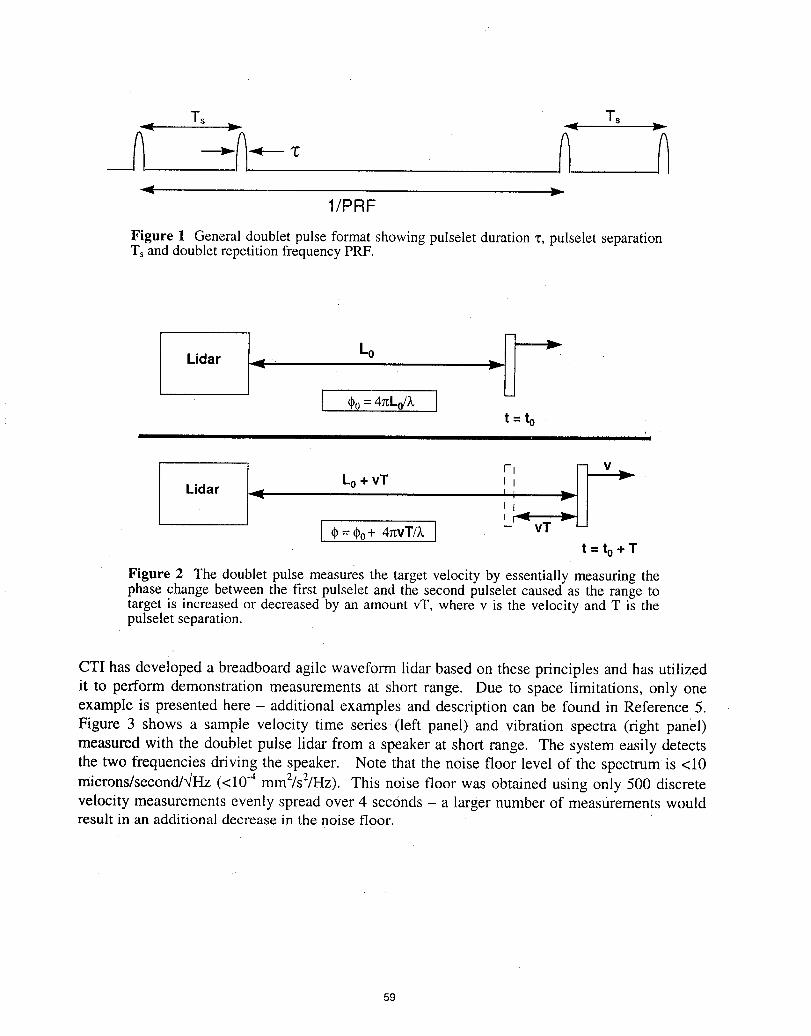
Ts Ts

1/PRF

Figure 1 Generaldoubletpulse formatshowingpulselet duration"_,pulselet separationTsand doubletrepetitionfrequencyPRF.

I It=t o

I ILidar , --_ L°+ vT __ _[ I

It=to+T

Figure 2 The doublet pulse measures the target velocity by essentially measuring thephase change between the first pulselet and the second pulselet caused as the range totarget is increased or decreased by an amount vT. where v is the velocity and T is thepulselet separation.

CTI has developed a breadboard agile waveform lidar based on these principles and has utilizedit to perform demonstration measurements at short range. Due to space limitations, only oneexample is presented here - additional examples and description can be found in Reference 5.Figure 3 shows a sample velocity time series (left panel) and vibration spectra (right panel)measured with the doublet pulse lidar from a speaker at short range. The system easily detectsthe two frequencies driving the speaker. Note that the noise floor level of the spectrum is <i0microns/second/'_Hz (<10 .4 mm2/s2ffr-Iz).This noise floor was obtained using only 500 discretevelocity measurements evenly spread over 4 seconds - a larger number of measurements wouldresult in an additional decrease in the noise floor.

59

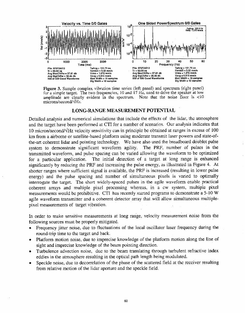
Velocity vs. Time 0/0 Gates One Sided PowerSpectrum0/0 Gates3 10 0 = I FsAvg: 125.0 Hz

2 . _ RMS: f.270 mmJs

1 10"2

1-3 ..............

0 1000 2000 3000 0 10 20 30 40 S0 60Time (ms) Frequency (Hz)

File: 970729013 TsAvg = 151,75 us File:970729013 TsAvg = 151.75usTr = 60.00 ns Vamb/2 = 3.32 mm/s Tr = 6.0.00ns: Vamb/2 = 3.32 mndsAvgMonCNRw =37.81 db Vrma = 1.270 mnVs Avg MonCNRw = 37.81 db Vrms = 1.270 rendsAvgSIgCNRw = 36.46 db Vavg = 0.015 mm/s Avg SigCNRw = 36.46 db Vavg = 0.015 rends500 of 500 Good Waveforms Mon Width = 16 samples 500 of 500 Good Waveforms Mort Width = 16 samples

Sig Width = 12 samples SJgWidth = 12 samples

Figure 3. Sample complex vibration time series (left panel) and spectrum (right panel)for a simple target. The two frequencies, 10 and 17 Hz, used to drive the speaker at lowamplitude are c!early evident in the spectrum. Note that the noise floor is <i0microns/second/_!Hz.

LONG-RANGE MEASUREMENT POTENTIAL

Detailed analysis and numerical simulations that include the effects of the lidar, the atmosphereand the target have been performed at CTI for a number of scenarios. Our analysis indicates that10 micron/second/'4Hz velocity sensitivity can in principle be obtained at ranges in excess of 100km from a airborne or satellite-based platform using moderate transmit laser powers and state-of-the-art coherent lidar and pointing technology. We have also used the breadboard doublet pulsesystem to demonstrate significant waveform agility. The PRF, number of pulses in thetransmitted waveform, and pulse spacing can be varied allowing the waveform to be optimizedfor a particular application. The initial detection of a target at long range is enhancedsignificantly by reducing the PRF and increasing the pulse energy, as illustrated in Figure 4. Atshorter ranges where sufficient signal is available, the PRF is increased (resulting in lower pulseenergy) and the pulse spacing and number of simultaneous pixels is varied to optimallyinterrogate the target. The short widely-spaced pulses in the agile waveform enable practicalcoherent arrays and multiple pixel processing whereas, in a cw system, multiple pixelmeasurements would be prohibitive. CTI has recently started programs to demonstrate a 5-10 Wagile waveform transmitter and a coherent detector array that will allow simultaneous multiple-pixel measurements of target vibration.

In order to make sensitive measurements at long range, velocity measurement noise from thefollowing sources must be properly mitigated.• Frequency jitter noise, due to fluctuations of the local oscillator laser frequency during the

round-trip time to the target and back.• Platform motion noise, due to imprecise knowledge of the platform motion along the line of

sight and imprecise knowledge of the beam pointing direction.

• Turbulence advection noise, due to the beam translating through turbulent refractive indexeddies in the atmosphere resulting in the optical path length being modulated.

• Speckle noise, due to decorrelation of the phase of the scattered field at the receiver resultingfrom relative motion of the lidar aperture and the speckle field.

6O

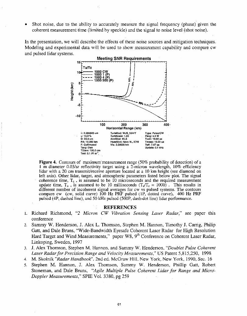
• Shot noise, due to the ability to accurately measure the signal frequency (phase) given thecoherent measurement time (limited by speckle) and the signal to noise level (shot noise).

In the presentation, we will describe the effects of these noise sources and mitigation techniques.Modeling and experimental data will be used to show measurement capability and compare cwand pulsed lidar systems.

MeetingSNR Requirements................. ,..].| .... i .........15.' , i

:Tu/Tc / i10 "-----'-- 1000 CW i........... 1000 11P I"---- 10004 P I

-"....... 1000 500 (p) ,,,_i5

o / t

-s ..-...-..:..'........"-

-10_..................................100 200 300 400-

Horizontal Range (km)_.:2.096349 um TurbMod: WJS_NAVY Type: Pulse/CWn: 10.0 % TurbScale: 1.00 Pavg: 4.0 WD: 20.0 cm AtmMod: MLS Tcoh: 10.00 us

PA: 10.000 km HazeMod: Navy M., IC10 Tmeas: 10.00 usF: Collimated V|s: 5.00000 km Teff: 7.07 usTarg: Disk Update: 0.1 kHzTDiam: 100.0 cmTref: 0.1/PI sr"1,

Figure 4. Contours of maximum'measurement range (50% probability of detection) of a1 m diameter 0.03/sr reflectivity target using a 2-micron wavelength, 10% efficiencylidar with a 20 cm transmit/receive aperture located at a 10 km height (see diamond onleft axis). Other lidar, target, and atmospheric parameters listed below plot. The signalcoherence time, To, is assumed to be i0 microseconds and the required measurementupdate time, Tu , is assumed to be 10 milliseconds (TJTc = 1000) . This results indifferent number of incoherent signal averages for cw vs pulsed systems. The contourscompare cw (cw, solid curve) 100 Hz PRF pulsed (1P, dotted curve), 400 Hz PRFpulsed (4P, dashed line), and 50 kHz pulsed (500P, dash-dot line) lidar performance.

REFERENCES

t. Richard Richmond, "2 Micron CW Vibration Sensing Laser Radar," see paper thisconference

2. Sammy W. Henderson, J. Alex L. Thomson, Stephen M. Hannon, Timothy J. Carrig, PhilipGatt, and Dale Bruns, "Wide-Bandwidth Eyesafe Coherent Laser Radar for High ResolutionHard Target and Wind Measurements," paper W8, 9th Conference on Coherent Laser Radar,Linkoping, Sweden, 1997

3. J. Alex Thomson, Stephen M. Hannon, and Sammy W. Henderson, "Doublet Pulse CoherentLaser Radar for Precision Range and Velocity Measurements," US Patent 5,815,250, 1998

4. M. Skolnik "Radar Handbook". 2nd ed. McGraw Hill, New York, New York, 1990, Sec. 165. Stephen M. Hannon, J. Alex Thomson, Sammy W. Henderson, Phillip Gatt, Robert

Stoneman, and Dale Bruns, "Agile Multiple Pulse Coherent Lidar for Range and Micro _-Doppler Measurements," SPIE Vol. 3380, pg 259

61

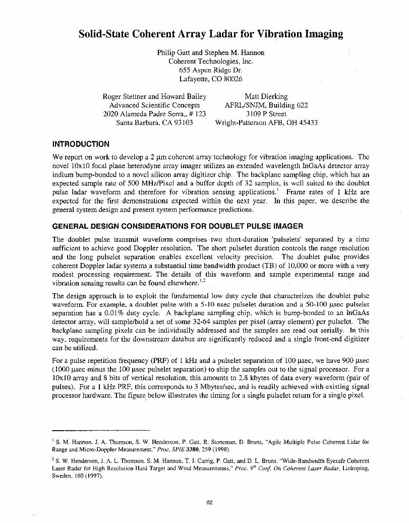
Solid-State Coherent Array Ladar for Vibration Imaging

Philip Gattand StephenM. HannonCoherentTechnologies, Inc.

655 Aspen Ridge Dr.Lafayette, CO 80026

Roger Stettner and Howard Bailey Matt DierkingAdvanced Scientific Concepts AFRL/SNJM, Building 622

2020 Alameda Padre Serra,, # 123 3109 P StreetSanta Barbara, CA 93103 Wright-Patterson AFB, OH 45433

INTRODUCTION

We report on work to develop a 2 _tmcoherent array technology for vibration imaging applications. Thenovel 10xl0 focal plane heterodyne array imager utilizes an extended wavelength InGaAs detector arrayindium bump-bonded to a novel silicon array digitizer chip. The backplane sampling chip, which has anexpected sample rate of 500 MHz/Pixel and a buffer depth of 32 samples, is well suited to the doubletpulse ladar waveform and therefore for vibration sensing applications. _ Frame rates of I kHz areexpected for the first demonstrations expected within the next year. In this paper, we describe thegeneral system design and present system performance predictions.

GENERAL DESIGN CONSIDERATIONS FOR DOUBLET PULSE IMAGER

The doublet pulse transmit waveform comprises two short-duration 'pulselets' separated by a timesufficient to achieve good Doppler resolution. The short pulselet duration controls the range resolutionand the long pulselet separation enables excellent velocity precision. The doublet pulse providescoherent Doppler ladar systems a substantial time bandwidth product (TB) of 10,000 or more with a verymodest processing requirement. The details of this waveform and sample experimental range andvibration sensing results can be found elsewhere.l'2

The design approach is to exploit the fundamental low duty cYClethat characterizes the doublet pulsewaveform. For example, a doublet pulse with a 5-10 nsec pulselet duration and a 50-100 gsec pulseletseparation has a 0.01% duty cycle. A backplane sampling chip, which is bump-bonded to an InGaAsdetector array, will sample/hold a set of some 32-64 samples per pixel (array element) per pulselet. Thebackplane sampling pixels can be individually addressed and the samples are read out serially. In thisway, requirements for the downstream databus are significantly reduced and a single front-end digitizercan be utilized.

For a pulse repetition frequency (PRF) of 1 kHz and a pulselet separation of 100 p,sec, we have 900/xsec(1000 _tsecminus the I00 gsec pulselet separation) to ship the samples out to the signal processor. For a10xl0 array and 8 bits of vertical resolution, this amounts to 2.8 kbytes of data every waveform (pair ofpulses). For a 1 k_HzPRF, this corresponds to 3 Mbytes/sec, and is readily achieved with existing signalprocessor hardware. The figure below illustrates the timing for a single pulselet return for a single pixel.

S. M. Hannon, J. A. Thomson, S. W. Henderson. P. Gatt, R. Stoneman, D. Bruns, "Agile Multiple Pulse Coherent Lidar forRange and Micro-Doppler Measurement," Proc. SPIE 3380, 259 (1998).

2 S. W. Henderson, J. A. L. Thomson, S. M. Hannon, T. J. Carrig, P. Gatt, and D. L. Bruns, "Wide-Bandwidth Eyesafe CoherentLaser Radar tbr High Resolution Hard Target and Wind Measurements," Proc. 9thCot_ On Coherent Laser Radar, Linkoping,Sweden. 160 (1997).

62

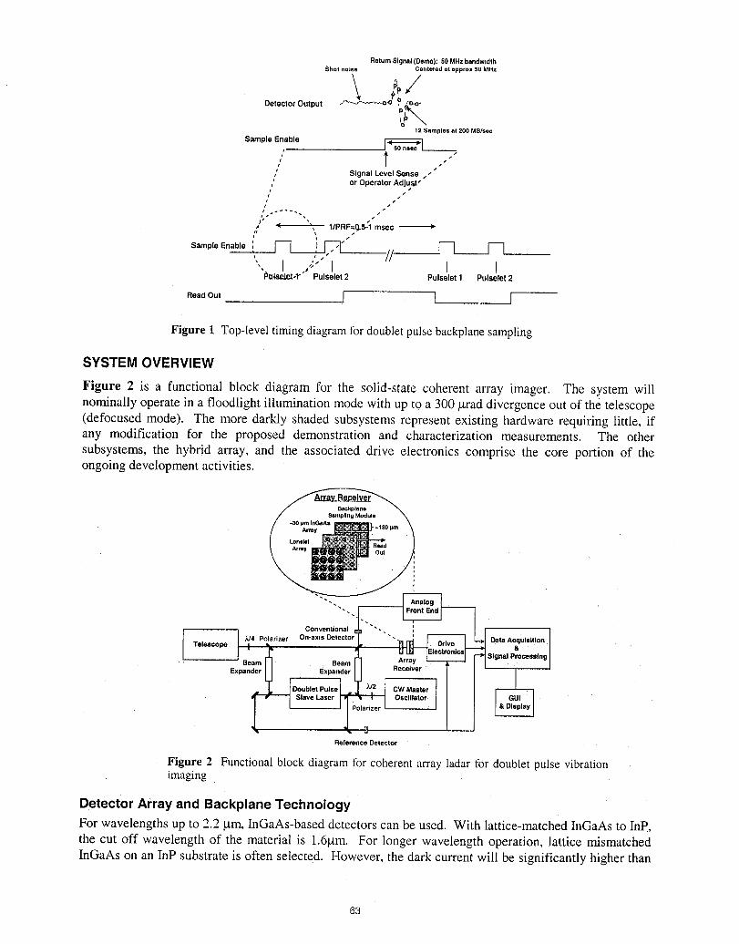
ReturnSignal(Demo):50 MHzbandwidthShot noise Centered at npprox 50 MHz

/DetectorOutput

12 Samples at 200 MS/sac

Sample Enable ___

J l • • • •

,' Signal Level Sense , •"

,,' or Operator Adjus_t•

i" s• •1,s ".

/, •

,,x < _, I/PRF=0.5-"I msec

Sample Enable ,,_ _• " // Ul v-l__I_ulsalet-1"" Pulselet2 Pulselet1 Pulselet2

ReadOut I l I

Figure 1 Top-leveltimingdiagramfor doubletpulsebackplanesampling

SYSTEM OVERVIEW

Figure 2 is a functional block diagram for the solid-state coherent array imager. The system willnominally operate in a floodlight illumination mode with up to a 300 _trad divergence out of the telescope(defocused mode). The more darkly shaded subsystems represent existing hardware requiring little, ifany modification for the proposed demonstration and characterization measurements. The othersubsystems, the hybrid array, and the associated drive electronics comprise the core portion of theongoing development activities.

Backplane_mpllng Module

pm

ii

\i

M4 Polarizer Conventional " Data Acquisition

Telescope anB__ &.

J Beam Array SignalProcessln,Exp Expander Receiver

DoubletPulse CW MasterSlave Laser -- Oscillator

Reference Detector

Figure 2 Functional block diagram for coherent array ladar for doublet pulse vibrationimaging

Detector Array and Backplane TechnologyFor wavelengths up to 2.2 gm. InGaAs-based detectors can be used. With lattice-matched InGaAs to InP,the cut off wavelength of the material is 1.6gm. For longer wavelength operation, lattice mismatchedInGaAs on an InP substrate is often selected. However, the dark current will be significantly higher than

63

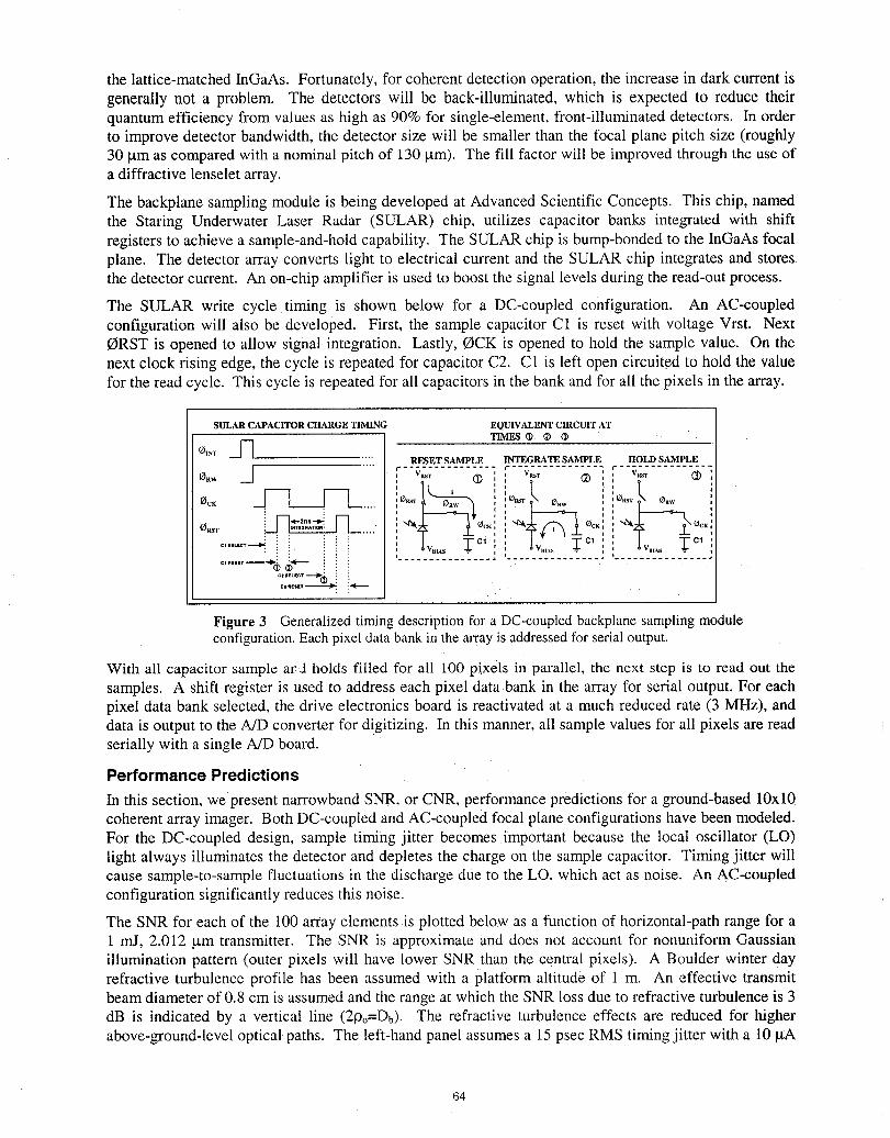
the lattice-matched InGaAs. Fortunately, for coherent detection operation, the increase in dark current isgenerally not a problem. The detectors will be back-illuminated, which is expected to reduce theirquantum efficiency from values as high as 90% for single-element, front-illuminated detectors. In orderto improve detector bandwidth, the detector size will be smaller than the focal plane pitch size (roughly30 p.m as compared with a nominal pitch of 130 gin). The fill factor will be improved through the use ofa diffractive lenselet array.

The backplane sampling module is being developed at Advanced Scientific Concepts. This chip, namedthe Staring Underwater Laser Radar (SULAR) chip, utilizes capacitor banks integrated with shiftregisters to achieve a sample-and-hold capability. The SULAR chip is bump-bonded to the InGaAs focalplane. The detector array converts light to electrical current and the SULAR chip integrates and stores.the detector current. An on-chip amplifier is used to boost the signal levels during the read-out process.

The SULAR write cycle timing is shown below for a DC-coupled configuration. An AC-coupledconfiguration will also be developed. First, the sample capacitor C1 is reset with voltage Vrst. NextORST is opened to allow signal integration. Lastly, OCK is opened to hold the sample value. On thenext clock rising edge, the cycle is repeated for capacitor C2. C1 is left open circuited to hold the valuefor the read cycle. This cycle is repeated for all capacitors in the bank and for all the pixels in the array.

SULAR CAPACITOR CHARGE TIMING EQUIVALENT CIRCUIT AT

_INT __ TIMES (_ _) (_RESET SAMPLE INTEGRATE SAMPLE HOLD SAMPLE

................ ,- .............. . ,I"..............* VltsT Oh i i VRST (_

ORw ._[ V,_T (i) ,, o ,_ ,,,,' _ ORw * ' _ ORW

• : * i ti -_--2n.--_ , ".4"__ OcK : , "4__ OCK

:: ' " L tCt uLt¢'r _ : ! VBIAS " a t

...... ---'_ _'*-- ! i ...............

Figure 3 Generalized timing description for a DC-coupled backplane sampling moduleconfiguration. Each pixel data bank in the array is addressed for serial output.

With all capacitor sample ard holds filled for all 100 pixels in parallel, the next step is to read out thesamples. A shift register is used to address each pixel data bank in the array for serial output. For eachpixel data bank selected, the drive electronics board is reactivated at a much reduced rate (3 MHz), and

data is output to the A/D converter for d!gitizing. In this manner, all sample values for all pixels are readserially with a single A/D board.

PerformancePredictions

In this section, we present narrowband SNR, or CNR, performance predictions for a ground-based 10xl0coherent array imager. Both DC-coupled and AC-coupled focal plane configurations have been modeled.For the DC-coupled design, sample timing jitter becomes important because the local oscillator (LO)light always illuminates the detector and depletes the charge on the sample capacitor. Timing jitter willcause sample-to-sample fluctuations in the discharge due to the LO, which act as noise. An AC-coupledconfiguration significantly reduces this noise.

The SNR for each of the i00 array elements is plotted below as a function of horizontal-path range for a

I mJ, 2.012 gm transmitter. The SNR is approximate and does not account for nonuniform Gaussianillumination pattern (outer pixels will have lower SNR than the central pixels). A Boulder winter dayrefractive turbulence profile has been assumed with a platform altitude of I m. An effective transmitbeam diameter of 0.8 cm is assumed and the range at which the SNR loss due to refractive turbulence is 3

dB is indicated by a vertical line (29o=Db). The refractive turbulence effects are reduced for higherabove-ground-level optical paths. The left-hand panel assumes a 15 psec RMS timing jitter with a 10 gA

64

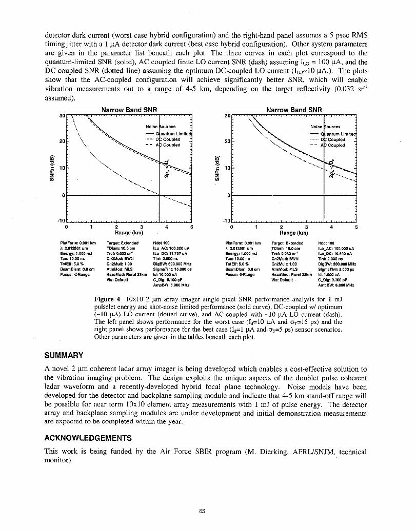
detector dark current (worst case hybrid configuration) and the right-hand panel assumes a 5 psec RMS

timing jitter with a 1 gA detector dark current (best case hybrid configuration). Other system parametersare given in the parameter list beneath each plot. The three curves in each plot correspond to thequantum-limited SNR (solid), AC coupled finite LO current SNR (dash) assuming ILO= 100 _tA, and theDC coupled SNR (dotted line) assuming the optimum DC-coupled LO current (ILo-10 gA.). The plots

show that the AC-coupled configuration will achieve significantly better SNR, which will enablevibration measurements out to a range of 4-5 km, depending on the target reflectivity (0.032 srLassumed).

Narrow BandSNR NarrowBandSNR", ...... i ......... i ......... i ...... ''1 .............. _...i ......... i ......... i ......

,, Noise Sources Noise ;ources

" "_ _ ""'_A

,, ,_ C uantum Limited ",,, _ C uantum Limited...... m3 Coupled - ".,, ...... [_3 Coupled20 '" 20

",,,,,.,,,,,,,, _"_ 3 Coupled 3 Coupled

," 10 "'_'- - _" 10n- n-

,,,z ...........................i .............io o

-10", ........ , ......... , ......... _........ , .......... 10 , ........ , ......... , ......... , ........ , .........0 1 2 3 4 5 1 2 3 4 5

Range (km) Range (km)

PlatForm: 0.001 km Target:Extended Ndet100 PlatForm:0.001km Target: Extended Ndet100X: 2.012501um TDiam:10.0 cm ILo_AC:10O.00OuA _.:2.012501um TDiam:10.0 cm ILo_AC:100.000uAEnergy: 1.000 mJ Tref: 0.032 $r "1 ILo DC: 11.757 uA Energy: 1,000 mJ Tref: 0.032 sr "1 ILo_DC: 10.690 uATau: 10,00ns Cn2Mod: BWN Tint: 2.000ns Tau: 10.00 na Cn2Mod:BWN Tint:2.000 nsTotEff:5.0% Cn2Mult:1.00 DlgBW:500.000MHz TotEff:5.0 % Cn2Mult:1.00 DIgBW:500.000MHzBeamDlam:0.8cm AtmMod: MLS SlgmaTint:15.000ps BeamDiam:0.8cm AtmMod: MLS SlgmaTint:5.000paFocus: @Range HazeMod:Rural23km Id:10,000uA Focus:@Range HazeMod:Rural23km Id:1,000 uA

VIa: Default C Dig: 0.100pF Via: Default C Dig:0.100 pFAmpBW: 6.000 MHz AmpBW: 6.000 MHz

Figure 4 10xl0 2 _m array imager single pixel SNR performance analysis for t mJpulselet energy and shot-noise limited performance (sold curve), DC-coupled w! optimum(-10 FtA)LO current (dotted curve), and AC-coupled with -10 gA LO current (dash).The left panel shows performance for the worst case (Id=10 gA and (_-r=15ps) and theright panel shows performance for the best case (Id=l FtAand CYT=5ps) sensor scenarios.Other parameters are given in the tables beneath each plot.

SUMMARY

A novel 2 lam coherent ladar array imageris being developed which enables a cost-effective solution tothe vibration imaging problem. The design exploits the unique aspects of the doublet pulse coherentladar waveform and a recently-developed hybrid focal plane technology. Noise models have beendeveloped for the detector and backplane sampling module and indicate that 4-5 km stand-off range will

be possible for near term i0x10 element array measurements with 1 mJ of pulse energy. The detectorarray and backplane sampling modules are under development and initial demonstration measurementsare expected to be completed within the year.

ACKNOWLEDGEMENTS

This work is being funded by the Air Force SBIR program (M. Dierking, AFRL/SNJM, technicalmonitor).

65

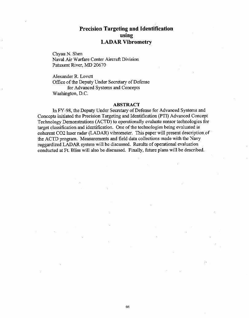
Precision Targeting and Identificationusing

LADAR Vibrometry

Chyau N. ShenNaval Air Warfare Center Aircraft DivisionPatuxent River, MD 20670

Alexander R. LoverOffice of the Deputy Under Secretary of Defense

for Advanced Systems and ConceptsWashington, D.C.

ABSTRACT

In FY-98, the Deputy Under Secretaryof Defense for Advanced Systems andConcepts initiated the Precision Targeting and Identification (PTI) Advanced ConceptTechnology Demonstrations (ACTD) to operationally evaluate sensor technologies fortarget classification and identification. One of the technologies being evaluated iscoherent CO2 laser radar (LADAR) vibrometer. This paper will present description,ofthe ACTD program. Measurements and field data collections made with the Navyruggardized LADAR system will be discussed. Results of operational evaluationconducted at Ft. Bliss will also be discussed. Finally, future plans will be described.

66

DIAL

Presider: Ove Steinvall

67

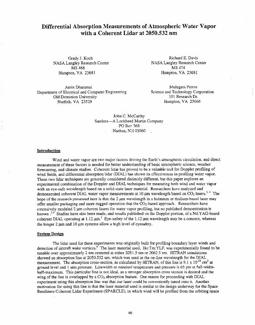
Differential Absorption Measurements of Atmospheric Water Vaporwith a Coherent Lidar at 2050.532 nm

Grady J. Koch Richard E. DavisNASA Langley Research Center NASA Langley Research Center

MS 468 MS 474

Hampton, VA 23681 Hampton, VA 23681

Amin Dharamsi Mulugeta PetrosDepartment of Electrical and Computer Engineering Science and Technology Corporation

Old Dominion University 101 Research Dr.Norfolk. VA 23529 Hampton, VA 23666

John C. McCarthySanders--A Lockheed Martin Company

PO Bo:, _68Nashua, NH 03060

Introduction

Wind and water vapor are two major factors driving the Earth's atmospheric circulation, and directmeasurement of these factors is needed for better understanding of basic atmospheric science, weatherforecasting, and climate studies. Coherent lidar has proved to be a valuable tool for Doppler profiling ofwind fields, and differential absorption lidar (DIAL) has shown its effectiveness in profiling water vapor.These two lidar techniques are generally considered distinctly different, but this paper explores anexperimental combination of the Doppler and DIAL techniques for measuring both wind and water vaporwith an eye-safe wavelength based on a solid-state laser material. Researchers have analyzed anddemonstrated coherent DIAL water vapor measurements at 10 gm wavelength based on CO2lasers.Lz Thehope of the research presented here is that the 2 g.mwavelength in a holmium or thulium-based laser mayoffer smaller packaging and more rugged operation that the CO2-basedapproach'. Researchers haveextensively modeled 2 [amcoherent lasers for water vapor profiling, but no published demonstration isknown .3.4Studies have also been made, and results published on the Doppler portion, of a Nd:YAG-basedcoherent DIAL operating at 1.12 grn.5 Eye-safety of the 1.12 gm wavelength may be a concern, whereasthe longer 2 gm and 10 [amsystems allow a high level of eyesafety.

System Design

The lidar used for these experiments was originally built for profiling boundary layer winds anddetection of aircraft wake vortices.6 The laser material used, Ho:Tm:YLF, was experimentally found to betunable over approximately 2 nm centered at either 2051.5 nm or 2062.5 nm. HITRAN simulationsshowed an absorption line at 2050.532 nm, which was used as the on-line wavelength for the DIALmeasurement. The absorption cross-section, as calculated by HITRAN, of this line is 9.1 x 1024cm2 atground level and I atm pressure. Linewidth at standard temperature and pressure is 65 pm at full-width-half-maximum. This particular line is not ideal, as a stronger absorption cross section is desired and thewing of the line is overlapped by a CO2absorption feature. One reason for proceeding with DIALexperiment using this absorption line was that our laser could be conveniently tuned onto it. Anothermotivation for using this line is that the laser material used is similar to the design underway for the SpaceReadiness Coherent Lidar Experiment (SPARCLE), in which wind will be profiled from the orbiting space

68

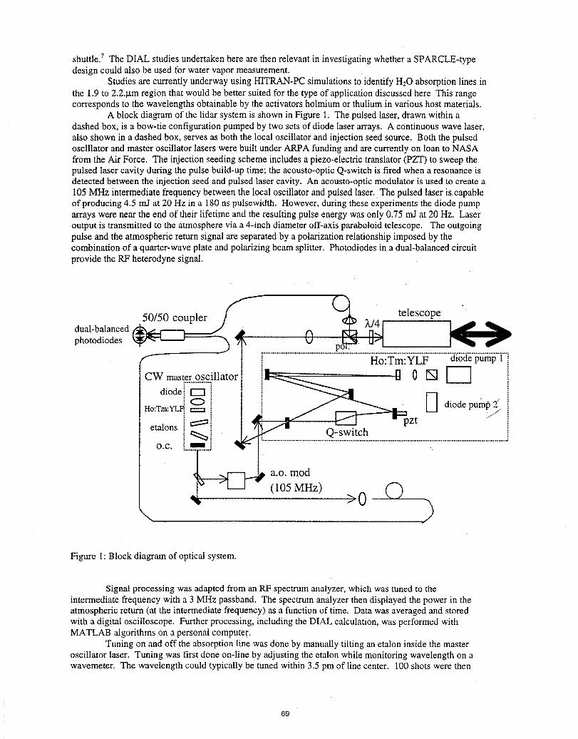
shuttle.7 The DIAL studies undertaken here are then relevant in investigating whether a SPARCLE-typedesign could also be used for water vapor measurement.

Studies are currently underway using HITRAN-PC simulations to identify H20 absorption lines inthe 1.9 to 2.2.p.m region that would be better suited for the type of application discussed here This rangecorresponds to the wavelengths obtainable by the activators holmium or thulium in various host materials.

A block diagram of the lidar system is shown in Figure 1. The pulsed laser, drawn within adashed box, is a bow-tie configuration pumped by two sets of diode laser arrays. A continuous wave laser,also shown in a dashed box, serves as both the local oscillator and injection seed source. Both the pulsedoscillator and master oscillator lasers were built under ARPA funding and are currently on loan to NASAfrom the Air Force. The injection seeding scheme includes a piezo-electric translator (PZT) to sweep thepulsed laser cavity during the pulse build-up time; the acousto-optic Q-switch is fired when a resonance isdetected between the injection seed and pulsed laser cavity. An acousto-optic modulator is used to create a105 MHz intermediate frequency between the local oscillator and pulsed laser. The pulsed laser is capableof producing 4.5 mJ at 20 Hz in a 180 ns pulsewidth. However, during these experiments the diode pumparrays were near the end of their lifetime and the resulting pulse energy was only 0.75 mJ at 20 Hz. Laseroutput is transmitted to the atmosphere via a 4-inch diameter off-axis paraboloid telescope. The outgoingpulse and the atmospheric return signal are separated by a polarization relationship imposed by thecombination of a quarter-wave plate and polarizing beam splitter. Photodiodes in a dual-balanced circuitprovide the RF heterodyne signal.

50/50 coupler X/4 telescope . A ,,..dual-balanced t3 I'k[

photodiodes _ _ ........................V.............P.._.:.."._2. ...................................!._......_.

"-- [ i Ho:Tm:YLF diodepump 1 1

CW master oscillator I [--__.__ ['] 0 [] [-"-] [

di°dei I''1 [ [ i_ r---'l , [Ho:Tm:YL__ U diode pump 2 [

i_.._[ | _ - Q-switch io.c. ..........................................................................................::.......................................

p, a.o. mod(105 MHz) O>0

Figure 1:Block diagram of optical system.

Signal processing was adapted from an RF spectrum analyzer, which was tuned to theintermediate frequency with a 3 MHz passband. The spectrum analyzer then displayed the power in theatmospheric return (at the intermediate frequency) as a function of time. Data was averaged and storedwith a digital oscilloscope. Further processing, including the DIAL calculation, was performed withMATLAB algorithms on a personal compute_'.

Tuning on and off the absorption line was done by manually tilting an etalon inside the masteroscillator laser. Tuning was first done on-line by adjusting the etalon while monitoring wavelength on awavemeter. The wavelength could typically be tuned within 3.5 pm of line center. 100 shots were then

69

averaged of the atmospheric return. Such a large number of averages is required to reduce speckle noise.During the 100shot averaging period the laser wavelength might drift as much as 3 pm from its startingwavelength. These errors in drift and on-center tuning degrade the accuracy of the DIAL measurement,and a stabilized laser design is currently under development. After the on-line shots.were recorded themaster oscillator laser was then manually tuned off line, typically to 2051.934 nm. The tuning to off-linewould require as much as 2.5 minutes to accomplish, as the wavelength could require this long to stabilizeafter the etalon adjustment. 100 shots of off-line data were then acquired. Such a long time between onand off line measurements is too longbecause the atmosphere can change characteristics in this interval.Designs are also underway to use two different master oscillator lasers---one tuned on-line and the otheroff-line. Switching between the two could take place in a matter of seconds.

Sample DIAL Measurement

The only availablecorrelative measurementtocompare with the DIAL measurementwere reportsof ground-level temperatureand relative humidity from a weather station atNorfolk InternationalAirport,some 25 miles distant fromour laboratory. To compare with this ground-levelmeasurementthe laser wasdirected near horizontal. A straight horizontalpath was not possible from the window of our laboratorydue to obstructionby trees, so thebeam was directedat 15° elevation. The laserbeam was directed inazimuthto be perpendicularto the ambient winddirectionto keep theDoppler shift frompushing theheterodynedatmospheric return out of the signalprocessing passband. In a zenith-looking mode (whichwould provide the most useful scientific data)this passbandissue would not exist. Figure 2 showssmoothed atmosphericreturns tuned both on andoff the watervapor line. 100 shots were averaged of theon andoff wavelengths. The differentialabsorption is readilyapparent as seen by the difference in sl_)pebetween the two lines. Databefore 200 m range is notdisplayedsince during the period of time

corresponding to this range thephotodetectors are saturatedby internalreflections of the 6utgoing laserpulse. .-

10 .... 0 .................... ......................

..... ....... ,.....i................

..... ......i, ..............,,.: "o

0 I I I I ' ' , l , l , , , , , , , , , l , m t , i I t I i

0 500 "1000 1500

range (m)

Figure 2: Water vapor DIAL measurements. Six such measurements were made on different days.

7O

A DIAL calculation was made based on the points indicated in Figure 2. Data beyond 600 mrange was not considered as the signal-to-noise ratio has dropped so low beyond this point that a DIALcalculation at a further range would be unreliable. The water vapor concentration calculated from thesedata points is 5.2 x 1017 molecules/cm3; the concentration based on the weather station measurements of21.1°C and 45% relative humidity is 2.8 x 1017molecules/cm3. If the weather station data is accepted astruth then the DIAL measurement has an 86% error. A desired accuracy for meteorological and scientificpurposes is less than 20%. Sources of error in the DIAL measurement are wavelength jitter, speckle, lowsignal-to-noise ratio (due to limited pulse energy), and a long time between on-line and off-linemeasurements. A stronger, non-overlapped absorption line would also enhance accuracy by making thedifference between on and off line absorption more pronounced.

Conclusions

Though the coherent DIAL measurements were successful with this 2 gm wavelength system, theaccuracy of the measurement must be be improved to be useful for scientific applications. Toward thisgoal a master oscillator is being built which includes an output coupler mounted on a PZT. This laser willbe locked to the absorption line using a wavelength modulation technique. Replacement of'the pulsedoscillator pump diodes would allow a higher pulse energy for enhanced signal to noise ratio and DIALaccuracy. Alternate pulsed laser designs are being considered with regard to pulse repetition frequency (toallow more averaging for speckle noise reduction) and selection of a line with a stronger absorption crosssection.

References

1. R.M. Hardesty, "Coherent DIAL measurement of range-resolved water vapor concentration," Appl.Opt., Vol. 23, pp. 2545-2553, 1984.

2. W.A. Brewer, V. Wulfmeyer, R.M. Hardesty, and B.J. Rye, "Combined wind and water-vapormeasurements using the NOAA mini-MOPA Doppler lidar," Nineteenth International Laser RadarConference, NASA publication NASA/CP-1998-207671/PT2, pp.565-568, 1998

3. M.J. Kavaya, S.W. Henderson, E.C. Russell, R.M. Huffaker, and R.G. Frehlich, "Monte Carlo computersimulations of _ound-based and space-based coherent DIAL water vapor profiling," Appl. Opt., Vol.28, No. 5, pp.840-851, 1989.

4. C.J. Grund, R.M. Hardesty, and B.J. Rye, "Feasibility of Tropospheric Water Vapor Profiling UsingInfrared Heterodyne Differential Absorption Lidar," DOE report DE-A103-94ER61761, 1995.

5. S. Lehmann, J. Bosenberg, F. Jansen, and H. Linne, "All Solid State Heterodyne DIAL System forSimultaneous Water Vapor and Wind Measurements," Nineteenth International Laser RadarConference, NASA publication NASA/CP- 1998-207671/PT2, pp.763-765, 1998.

6. G.J. Koch, B.C. Barker, and C.L. Britt, "Development of an Operation Wake Vortex Sensor Based onPulsed Coherent Lidar," 9thconference on Coherent Laser Radar, 1997.

7. U.N. Singh, J. Yu, M. Petros, N.P. Barnes, and M.W. Phillips, "2-Micron Diode-Pumped Pulsed LaserTransmitter for SPARCLE: A Coherent Wind Lidar Shuttle Mission," Nineteenth International LaserRadar Conference, NASA publication NASA/CP- 1998-207671/PT2, pp.603-607, 1998.

71

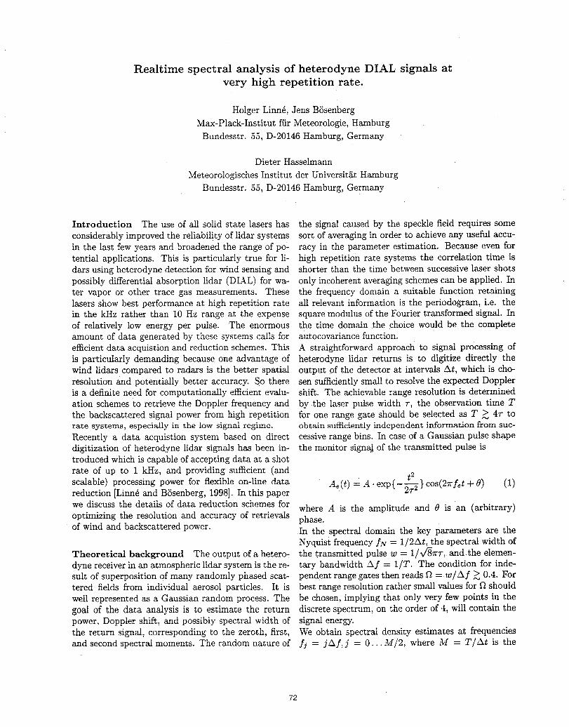
Realtime spectral analysis of heterodyne DIAL signals atvery high repetition rate.

Holger Linn_, Jens Bhsenberg

Max-Plack-Institut fiir Meteorologie, Hamburg

Bundesstr. 55, D-20146 Hamburg, Germany

Dieter Hasselmann

Meteorologisches Institut der Universit_t Hamburg

Bundesstr. 55, D-20146 Hamburg, Germany

Introduction The use of all solid state lasers has the signal caused by the speckle field requires some

considerably improved the reliabil!ty of lidar systems sort of averaging in order to achieve any useful accu-in the last few years and broadened the range of po- racy in the parameter estimation. Because even fortential applications. This is particularly true for li- high repetition rate systems the correlation time isdars using heterodyne detection for wind sensing and shorter than the time between successive laser shotspossibly differential absorption lidar (DIAL) for wa- only incoherent averaging schemes can be applied. Inter vapor or other trace gas measurements. These the frequency domain a suitable function retaininglasers show best performance at high repetition rate all relevant information is the periodogram, i.e. thein the kHz rather than 10 Hz range at the expense square modulus of the Fourier transformed signal. Inof relatively low energy per pulse. The enormous the time domain the choice would be the completeamount of data generated by these systems calls for autocovariance function.efficient data acquistion and reduction schemes. This A straightforward approach to signal processing of

is particularly demanding because one advantage of heterodyne lidar returns is to digitize directly thewind lidars compared to radars is the better spatial output of the detector at intervals At, which is cho-resolution and potentially better accuracy. So there sen sufficiently small to resolve the expected Doppleris a definite need for computationally efficient evalu- shift. The achievable range resolution is determined

ation schemes to retrieve the Doppler frequency and by the laser pulse width 7", the observation time Tthe backscattered signal power from high repetition for one range gate should be selected as T >_ 4T torate systems, especially in the low signal re,me, obtain sufficiently independent information from suc-

Recently a data acquistion system based on direct cessive range bins. In case of a Gaussian pulse shapedigitization of heterodyne lidar signals has been in- the monitor Sign_ of the transmitted pulse istroduced Which is capable of accepting data at a shot

rate of up to 1 kHz, and providing sufficient (and t2

scalable) processing power for fle_ble on-line data Ae(t) A. exp(--_T 2 } COS(2_'f_t . 8) (1)reduction [Linn_ and Bhsenberg, 1998]. In this paper

we discuss the details of data reduction schemes for where A is the amplitude and 0 is an (arbitrary)optimizing the resolution and accuracy of retrievals phase.of wind and backscattered power. In the spectral domain the key parameters are the

Nyquist frequency fg = 1/2At, the spectral width of

Theoretical background The output of a hetero- the transmitted pulse w = 1/x/r87r7", and the elemen-dyne receiver in an atmospheric lidar system is the re- tary bandwidth Af = lIT. The condition for inde-sult of superposition of many randomly phased scat- pendent range gates then reads f_ -= w/Af >_0.4. Fortered fields from individual aerosol particles. It is best range resolution rather small values for _ shouldwell represented as a Gaussian random process. The be chosen, implying that only very few points in the

goal of the data analysis is to estimate the return discrete spectrum, on the order of 4, will contain thepower, Doppler shift, and possibly spectral width of signal energy.the return signal, corresponding to the zeroth, first, We obtain spectral density estimates at frequenciesand second spectral moments. The random nature of fj =jAf, j = 0... M/2, where M = T/At is the

72

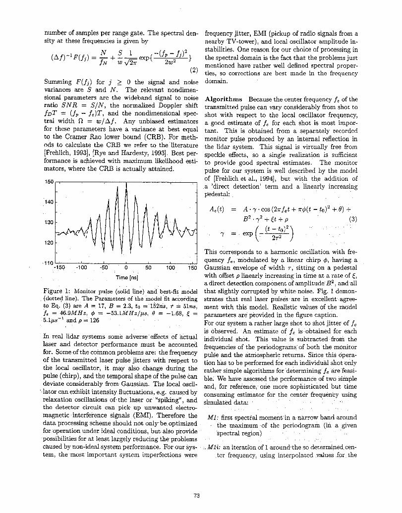
number of samples per range gate. The spectral den- frequency jitter, EMI (pickup of radio signals from asity at these frequencies is _ven by nearby TV-tower), and local oscillator amplitude in-

N S 1 _(f __fj)2 stabilities. Onereasonforourchoiceofprocessingin(Af)-lF(fi) = TNN+ -- exp{ _w2-- } the spectral domain is the fact that the problems justw _ mentioned have rather well defined spectral proper-

(2) ties, so corrections are best made in the frequency

Summing F(fj) for j > 0 the signal and noise domain.variances are S and N. The relevant nondimen-

sional parameters are the wideband signal to noise Algorithms Because the center frequency fe of theratio SNR = S/N, the normalized Doppler shift transmitted pulse can vary considerably from shot tofDT = (fp -- re)T, and the nondimensional spec- shot with respect to the local oscillator frequency,tral width f_ = w/Af. Any unbiased estimators a good estimate of fe for each shot is most impor-for these parameters have a variance at best equal tant. This is obtained from a separately recorded

to the Cramer Rao lower bound (CRB). For meth- monitor pulse produced by an internal reflection inods to calculate the CRB we refer to the literature the lidar system. This signal is virtually free from[Frehlich, 1993], [Rye and Hardesty, 1993]. Best per- speckle effects, so a single realization is sufficientformance is achieved with maximum likelihood esti- to provide good spectral estimates. The monitormators, where the CRB is actually attained, pulse for our system is well described by the model

15o of [Frehlich et al., 1994], but with the addition of

[1't I li[tl)[l! [[1111' ' a 'direct detection'tepedestal: rm and a linearly increasing

140 I

Ae(t) = A._.cos(27rfet+_r¢(t-to) 2+e)+

B2 "_,2+ _t + p (3)130

L (t_to)2_" v = exp( _ •

120 \ /

This corresponds to a harmonic oscillation with fre-

, , quency re, modulated by a linear chirp ¢, having a11°-15o -100 -50 0 50 100 150 Gaussian envelope of width r, sitting on a pedestal

Time[ns] with offset p linearly increasing in time at a rate of _,a direct detection component of amplitude" B 2, and all

Figure 1: Monitor pu!se (solid line) and best-fit model that slightly corrupted by white noise. Fig. 1 demon-(dotted line). The Parameters of the model fit according strates that: real laser pulses are in excellent agree-to Eq. (3) are A = 17, B = 2.3, to = 152ns, r = 51ns, ment with this: model. Realistic values of the model

fe = 46.9MHz, _ = -53.1MHz/izs. _ = -1.68, _ = parameters are provided in the figure caption.5:l/_s-1 and p = 126 For our system a rather large shot to shot jitter of fe

is observed. An estimate of fe is obtained for eachIn real lidar systems some adverse effects Of actual individual shot. This value is subtracted from the

laser and detector performance must be accounted frequencies of the periodograms 0f both themonitorfor. Some of the common problems are: the frequency pulse and the atmospheric returns. Since this opera-of the transmitted laser pulse jitters with respect to tion has to be performed for each individual shot onlythe local oscillator, it may also change during the rather Simple algorithms for'determining fe are feasi-pulse (chirp), and.the temporal shape of the pulse can ble: We have assessed the performance of two simpledeviate considerably from Gaussian. The local oscil- and, for reference, one more sophisticated but timelator can exhibit intensity fluctuations, e.g. caused by consuming estimator for the center :frequency usingrelaxation oscillations of, the laser or "spiking", and simulated data:the detector circuit can pick up unwanted electro-

magnetic interference signals (EMI). Therefore the MI: first specti-al moment in a narrow band _arounddata processing scheme should not only be optimized the maximum of the periodogram (in a _venfor operation under ideal conditions, but also provide spectral re,on)possibilities for at least largely reducing the problemscaused by non-ideal system performance. For our sys- ,.Mli: an iteration of 1 around.the so determined cen-tem, the most importan_ system imperfections were ter frequency, using interpolated values for the

73

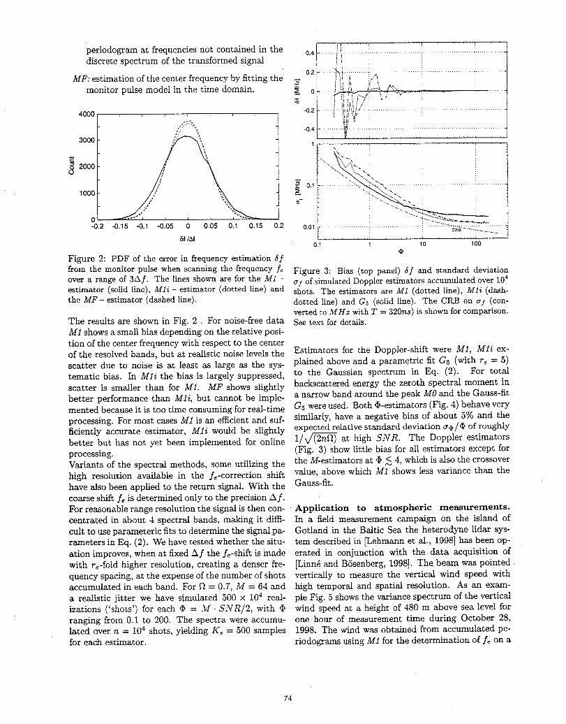
' ,I .

periodogram at frequencies not contained in the 0.4.......... _............:....................... i........

discrete spectrum of the transformed signal .: i :0.2........"..'_i...........: _....................:........................:..............

;_ _ :,'_ : :MF: estimation of the center frequency by fitting the _ , ,, , _. , : !

monitor pulse model in the time domain. = 0 ......._.. i._ _-;....v........ --! i.'-.:/ :

-0.2 ....... L --_i.lr_i:,_.-._...................... !....................... i..............4000 , i _ iii _' : "

•,.'.:.=:.,,,... .,, -i -o.4............_,_.........i........................!........................!..............,'.. ., ] _. .:, ..... , ........ ,

3000 :.: "_ _ ........ .

ii ! "" ' ' i

0'_2000 j_ '.,..__[...',,..'V, :

OOOo I, a-o.2-0.15-0.1-0.050 0.050.10.10.2 0.0,........................:....................:,........................ 16f/_f

0.1 1 10 100

Figure 2: PDF of the error in frequency estimation 6ffrom the monitor pulse when scanning the frequency f_ Figure 3: Bias (top panel) 6f and sta.udard deviationover a range of 3Af. The lines shown are for the M1 - o'/of simulated Doppler estimators accumulated over 104estimator (solid line), Mli - estimator (dotted line) and shots. The estimators are M1 (dotted line), Mii (dash-the MF- estimator (dashed line), dotted line) and G_ (solid line). The ClUB on crf (con-

verted to MHz with T = 320ns) is shown for comparison.The results are shown in Fig. 2. For noise-free data See text for details.M1 shows a small bias depending on the relative posi-tion of the center frequency with respect to the centerof the resolved bands, but at realistic noise levels the Estimators for the Doppler-shift were M1, Mli ex-scatter due to noise is at least as large as the sys- plained above and a parametric fit G5 (with re = 5)tematic bias. In Mli the bias is largely suppressed, to the Gaussian spectrum in Eq. (2). For totalscatter is smaller than for M1. MF shows slightly backscattered energy the zeroth spectral moment in

better performance than Mli, but cannot be imple- a narrow band around the peak MO and the Gauss-fitmented because it is too time consuming for real-time G_ were used. Both _-estimators (Fig. 4) behave very

processing. For most cases M1 is an e_cient and suf- similarly, have a negative bias of about 5% and theficiently accurate estimator, Mli would be slightly expected relative standard deviation _/_ of roughlybetter but has not yet been implemented for online 1/(2k/_ at high SNR. The Doppler estimatorsprocessing. (Fig. 3) show little bias for all estimators except forVariants of the spectral methods, some utilizing the the M-estimators at • < 4, which is also the crossoverhigh resolution available in the fe-correction shift value, above which M1 shows less variance than thehave also been applied to the return signal. With the Gauss-fit.coarse shift fe is determined only to the precision Af.For reasonable range resolution the signal is then con- Application to atmospheric measurements.centrated in about 4 spectral bands, making it diffi- In a field measurement campaign on the island of

cult to use parameteric fits to determine the signa2 pa- Gotland in the Baltic Sea the heterodyne lidar sys-rameters in Eq. (2). We have tested whether the situ- tern described in [Lehmann et al., 1998] has been op-

ation improves, when at fixed .'kf the ]_-shift is made erated in conjunction with the data acquisition ofwith re-fold higher resolution, creating a denser fre- [Linn_ and Bhsenberg, 1998]. The beam was pointed.quency spacing, at the expense of the number Of shots vertically to measure the vertical wind speed withaccumulated in each band. For _ = 0.7, M = 64 and high temporal and Spatial resolution. As an exam-a realistic jitter we have simulated 500 x 104 real- pie Fig. 5 shows the variance spectrum of the vertical

izations ('shots') for each • = M • SNR/2, with • wind speed at a height of 480 m above sea level forranging from 0.1 to 200. The spectra were accumu- one hour of measurement time during October 28,lated over n = 104 shots, yietding K, = 500 samples 1998. The wind was obtained from accumulated pe-for each estimator, riodograms using M1 for the determination of f_ on a

74

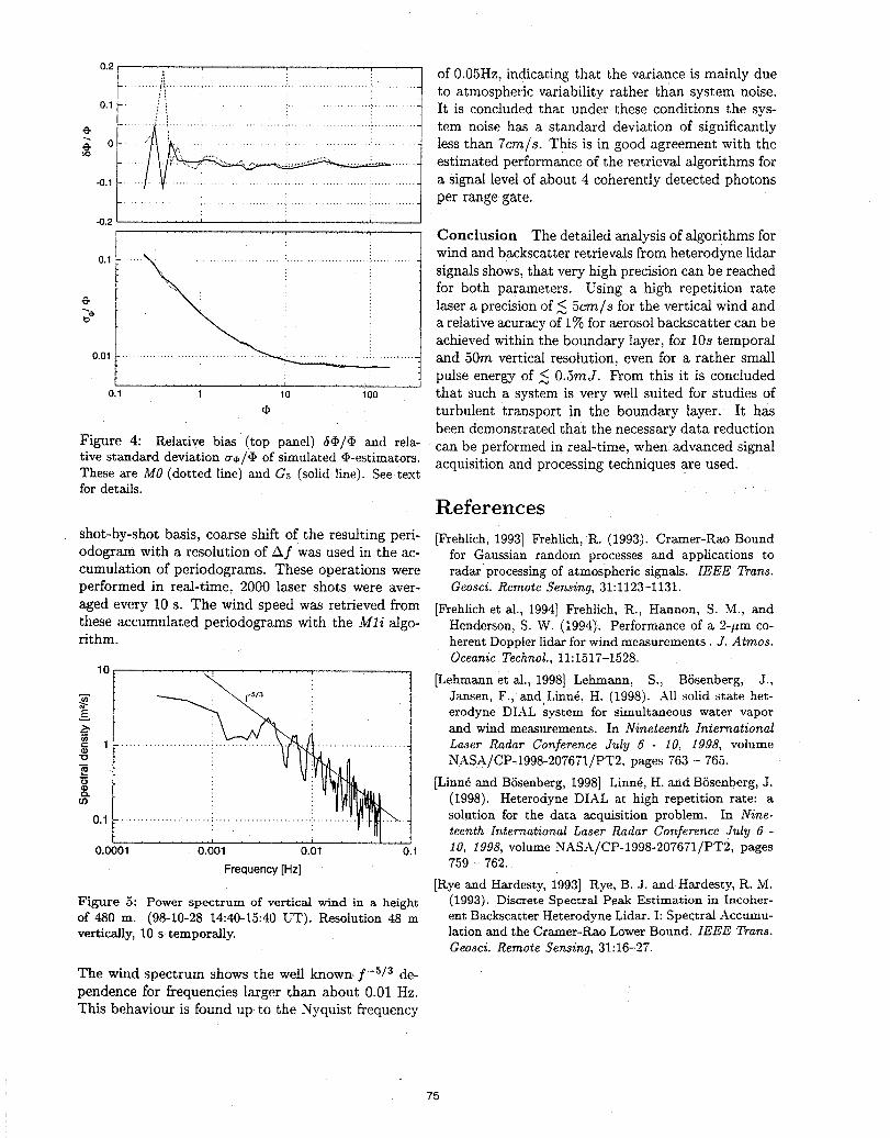
0.2L. _ _ of 0.05Hz, indicating that the variance is mainly due.............................................. i............ to atmospheric variability rather than system noise.

o.1_ .i!'_ ......................... :............. It is concluded that under these conditions the sys-.... !

. L i.:[ '_i .iii i.......................................... tem noisehasastandarddeviationofsignificantly' less than 7crn/s. This is in good agreement with the0 ................ ......

] . '_ ............... i ................ i estimated performance of the retrieval algorithms for

_.1_. ::/__:::::::- asignallevel ofabout 4 coherentlydetected photons

t ................... :...................... ::.................................... per range gate.-o 2 i

Conclusion The detailed analysis of algorithms for/

0.1_ .....\----- ...................... wind and backscatter retrievals from heterodyne lidar

L _ signals shows, that very high precision can be reached[ for both parameters. Using a high repetition racee \ " laser a precision of _<5cm/s for the vertical wind and

_e [ x_,, a relative acuracy of 1% for aerosol backscatter can beachieved within the boundary layer, for 10s temporal

0.01[-...................................... _ ..... and 50m vertical resolution, even for a rather smallf pulse energy of _< 0.5mJ. From this it is concluded

0.1 i ....... io 100 ' ' that such a system is very well suited for studies of¢ turbulent transport in the boundary layer. It has

been demonstrated that the necessary data reduction

Figure 4: l_elative bias (top panel) (f¢/'_ and rela- can be performed in real-time, when advanced signalrive standard deviation a4/'_ of simulated (I)-estimators. acquisition and processing techniques are used.These are MO (dotted line) and G5 (solid line). See.textfor details.

References

shot-by-shot basis, coarse shift of the resulting peri- [Frehlich. 1993] Frehlich. R. (1993). Cramer-Rao Boundodogram with a resolution of Af was used in the ac- for Ganssian random processes and applications tocumulation of periodograms. These operations were radar processing of atmospheric signals. IEEE Trans.performed in real-time, 2000 laser shots were aver- Geosci. Remote Sensing, 31:1123-1131.

aged every 10 s. The wind speed was retrieved from [Frehlich e_ al., 1994] Frehlich, 1%.,Hannon, S. M., andthese accumulated periodograms with the Mli algo- Henderson, S. W. (1994). Performance of a 2-pro co-rithm, herent Doppler lidar for wind measurements. J. Atmos.

Oceanic Technol.. 11:1517-!528.10 .......

<'_ t [Lehmannetal.,1998] Lehmann, S., B6senberg, J.,

_ \ ] Jansen. F., and Linn_. H. (1998). All solid s_ate het-erodyne DIAL svstem for simultaneous water vapor

>- \ and wind measurements. In Nineteenth International1 .. Laser Radar Conference July 6 - 10, 1998. volume

__ _ NASA/CP-1998-207671!PT2, pages 763 - 765.

t [Linnd and BSsenberg, 1998] Linn_, H. and BSsenberg, J.(1998). Heterodyne DIAL at high repetition rate: a(D

solution for the data acqmskion problem. In Nine-0.1 _ teenth International Laser Radar Conference July 6 -0.0001 0.001 ...... 0.})1 0.1 10, 1998, volume NASAiCP-1998-207671/PT2, pages

759 - 762.Frequency[Hz][l_ye and Hardesty, 1993] P_ye, B. J. and I-lardesty, R. M.

Figure 5: Power spectrum of vertical wind in a height (1993). Discrete Spectral Peak Estima_mn in Incoher-of 480 m. (98-10-28 14:40-15:40 UT). l%esolution 48 m ent Backscatter Heterodyne Lidar. h Spectral Accumu-vertically, 10 s temporally, la_ion and the Cramer-Rao Lower Bound. IEEE Trans.

Geosci. Remote Sensing, 31:16-27.

The wind spectrum shows the well known, f-5/3 de-pendence for frequencies larger than about 0.01 Hz.This behaviour is found up to the Nyquist frequency

75

Boundary Layer Wind and Water Vapor Measurements using the NOAAmini-MOPA Doppler lidar

W. Alan Brewer, Volker Wulfmeyer, and R. Michael HardestyNOAA/ERL/Environmental Technology Laboratory

325 Broadway, Boulder, CO 80303abrewer@etl.noaa.gov (303) 497-7859 ! (FAX: -5318)

Barry J. RyeCooperative Institute for Research in Environmental Sciences

University of Colorado/NOAA. Environmental Technology Laboratory325 Broadway, Boulder, CO 80303

Abstract

The NOAA Environmental Technology Laboratory has developed a multiple-wavelength (linetunable from 9-11 _tm), low-pulse-energy (1-3 mJ), high-pulse-rate (up to 500 Hz) CO2 Dopplerlidar for simultaneous investigation of boundary layer wind and water vapor profiles. In thispaper we present single-wavelength; Doppler results and preliminarywater vapor DIALmeasurements.

76

THEORY AND SIMULATION

Presider: Rod Frehlich

77

COHERENT LIDAR RETURNS IN TURBULENT ATMOSPHEREFROM SIMULATION OF BEAM PROPAGATION

A. Belmonte, B.J. Rye, W. A. Brewer, R. M. HardestyEnvironmental Technology Laboratory

R/E/ET2,NOAA ERL

325 BroadwayBoulder, CO 80303-3328

Introduction Early analytical work on the problem _'2explained onlythe reduction of lidar efficiency caused by beam

This paper describes what we believe to be the first use spreading in bistatic systems. The discussion of moreof simulations of beam propagation in three- realistic lidars with common transmit/receive antennasdimensional random media to study the effects of (monostatic geometry)3"4predicted that the averageatmospheric refractive turbulence on coherent lidar signal-to-noise ratio (SNR) of perfectly aligned systems

should be generally rather higher than was given by theperformance. The results presented here are based onpropagation through an atmosphere characterized by bistatic model - indeed, that under some conditions ituniform refractive turbulence; transmitted and virtual could be higher than expected when no turbulence was(back-propagated) local oscillator beams are assumed to present. This result could be explained physically by

• be matched, perfectly aligned, Gaussian, and truncated noting that, on application of the reciprocity theorem, aat the antenna aperture by an amount that would lidar return can be expressed as the overlap integral ofmaximize system antenna efficiency in the absence of the transmitter and back-propagated local oscillator5"6

beams in the target plane. This reduces the problem ofturbulence. However, our method provides the tools toanalyze laser radar with general refractive turbulence calculating lidar returns to one of computing irradianceconditions, beam-angle and beam-offset misalignment, along the two beampropagation paths, a method used inandarbitrarytransmitterandreceiver geometries, the simulations reported here. The signal enhancement

that occurs in the monostatic geometry arises because

Refractive turbulence in atmospheric backscatter 'both small-scale scintillation and large-scale beamcoherent lidar wander are common to the two beams. For the lidar

application, other authors7 have used expansions basedon the path-integral formulation to describe the problem

Any reader who has worked with coherent lidars knows in the limits of weak and strong turbulence, with somehow to difficult is to predict the performance of the approximations. While the analytical approach leads toinstrument. It is not unusual to find out that the effective understanding of the basic physical problems, it is usualiidar range has been drastically reduced in relation to to consider only the higher moments of the field. Theseprevious measurements. Explanations such as low moments are usually difficult to estimate and no simpleaerosol concentration, increased atmospheric analytical solutions are known outside those obtainedabsorption, and technical problems such as for simplified beam geometries (defined throughmisalignment or laser performance are the most untruncated Gaussian functions) and unrealisticfrequently cited when the lidar system whatever the atmospheric characterization (usually by randomlaser wavelength. At shorter wavelengths, the effects of wedges where only beam wander and no scintillation isrefractive turbulence on ground-based systems have considered).certainly to be included among these factors (see figure1). It is so closely related and strongly dependent on The simulations used here are based on the well-near field and misalignment problems, that it is often established method of modeling the atmosphere by a sethard to establish the exact cause of lidar dysfunction, of two-dimensional Gaussian random phase screensSo, we are required to study the features of coherent with an appropriate phase power spectral density)laser radar behavior under realistic conditions if we Though the accuracy of the moments from simulation ofwant to assess properly the feasibility of proposed plane and spherical waves in random media is wellmeasurements, define new applications or maximize the established,9 we have extended this approach to thesystem performance, more complex problem of Gaussian and truncated

Gaussian beams propagation. Before applying the

78

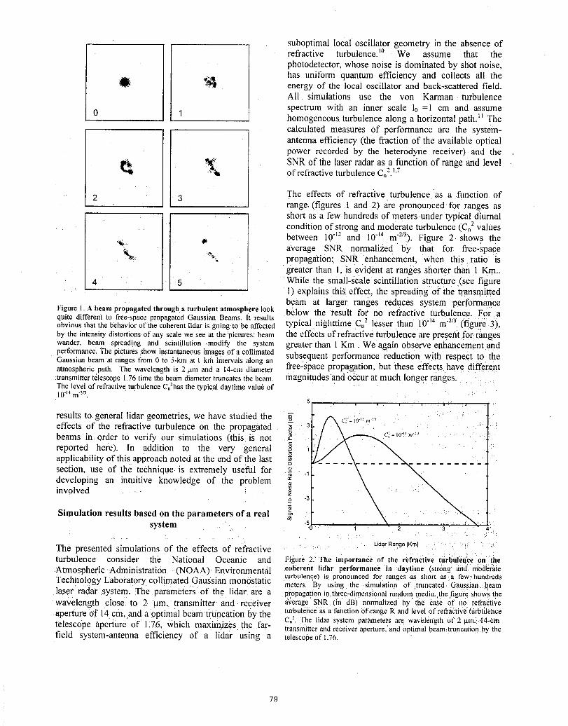
suboptimal local oscillator geometry in the absence ofrefractive turbulence.I° We assume that thephotodetector, whose noise is dominated by shot noise,has uniform quantum efficiency and collects all the

O _ energy of the local oscillator and back-scattered field.All simulations use the yon Karman turbulencespectrum with an inner scale 10=1 cm and assume

0 1 homogeneousturbulencealong a horizontalpath.ll Thecalculated measures of performance are the system-antennaefficiency(the fractionof the availableopticalpower recorded by the heterodyne receiver) and theSNR of the laser radar as a functionof range and levelof refractive turbulence Ca2.1.7

2 3 The effects of refractive turbulence as a function ofrange (figures I and 2) are pronouncedfor ranges asshort as a few hundreds of meters under typical diurnal

, condition of strong and moderate turbulence (Cnz valuesbetween 10"12 and 10"14 m'2/3). Figure 2 shows theaverage SNR normalized by that for free-space% , propagation: SNR enhancement, when this.ratio isgreater than 1, is evident at ranges shorter than 1 Kin..

4 5 While the small-scale scintillation structure .(see figure1) explains thig effect, the spreading of the transmittedbeam at larger ranges reduces system 'performance

Figure 1.A beam propagated through a turbulent atmosphere look below the result for no refractive turbulence. For aquite different to free-space propagated Gaussian Beams It resultsobvious that the behavior of the coherent lidar is going tobe affected typical nighttime C..- lesser than I0:14 m "2/3 (figure: 3),by the intensity distortions of any scale we see at the pictures: beam the effects of refractive turbulence are present for,rangeswander, beam spread!ng and scintillation modify the system greater than 1 Km. We again observe enhancement and

performance The pictures show instantaneous images of a collimated subsequent performance reduction with respect to theGaussian beamat ranges from 0 to 5-km at 1 km intervals along anatmospheric path. The wavelength is 2 _tm and a 14-cm diameter free-space propagation, but these effects have differenttransmitter telescope 1.76 time the beam diameter truncates the beam. magnitudesand ocizurat much longer ranges.The level of refractive turbulence C,"has the typical daytime value of10"14m"2_3

results to general lidar geometries, we have studied theeffects of the refractive turbulence on the propagatedbeams in order to verify our simulations (this is not

reported here). In addition to the very general _applicability of this approach noted at the end of the lastsection, use of the technique is extremely useful for =odeveloping an intuitive knowledge of the probleminvolved 5z

o -3

Simulation results based on the parameters of a realsystem -50 1 2 3 4"

The presented simulations of the effects of refractive LidarRange[Km]turbulence consider the National Oceanic and Figure 2. The importance of the refractive turbul'im_ze on the

Atmospheric Administration (NOAA) Environmental ,coherent lidar performance in daytime (strong _irid!m0d;er:hteturbulence) is pronounced for ranges as short as a few,hundreds

TeChnology Laboratory collimated Gaussian mon6static meters. By using the simulation of truncated Gaussian.beamlaser radar system, The parameters of the lidar are a propagation, in three-dimensional random media, the figure, shows, thewavelength close to 2 lam. transmitter and receiver average SNR, (in dB) normalized by the case of no refractive

aperture Of 14 cm, and a optimal beam truncation by the tttrbulence as a function of_range R and level Ofrefractive turbtilenceC°", The lidar system parameters are wavelength of: (2 p.m., ,14-Cm

telescope aperture of 1176, which maximizes the far- transmitter and recewer aperture, and optimal beam_truncatio0 by thefield system-antenna efficiency of a lidar Using a telescope ofl.76.

79

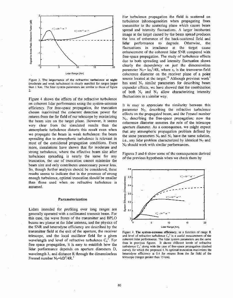
For turbulence propagation the field is scattered on

turbulence inhomogeneities when propagating fromtransmitter to the scattering plane which causes beam

_- ,._=_o,,,,:, spread and intensity fluctuations. A larger incoherentg image at the target caused by the beam spread produces

the loss of coherence of the back-scattered field anda

o lidar performance to degrade. Otherwise, the_" fluctuations in irradiance at the target cause•5 enhancement of the coherent lidar SNR compared withz free-space propagation. The study of turbulence effects.__ due to both spreading and intensity fluctuation showsco

20 5 10 1_ 20 clearly the dependency on just the dimensionless,)

parameter NT= kro'/4R, where r0 is the transverse-fieldLidarRange[Km] coherence diameter on the receiver plane of a point

Figure 3. The importance of the refractive turbulence at night source located at the target. _2Although previous work 1(moderateandweakturbulence)is clearlymanifestforrangeslarger has used NT similar parameters for describing beamthan 1Km. The lidar system parameters are similar to those of figure expander effects, we have showed that the combination2. of both NF and NT allow characterizing intensity

fluctuations in a similar way.Figure 4 shows the effects of the refractive turbulence

on coherent lidar performance using the system-antenna It is easy to appreciate the similarity between thisefficiency. For free-space propagation, the truncation parameter NT, describing the refractive turbulencechosen maximized the coherent detection power for effects on the propagated beam, and the Fresnel numberreturns from the far field of our telescope by minimizing Nv, describing the free-space propagation: now thethe beam size on the target plane. However, it seems coherence diameter assumes the role of the telescopevery clear from the simulated results than the aperture diameter. As a consequence, we might expectatmospheric turbulence distorts this result even when that any atmospheric propagation problem defined bywe propagate the beam in weak turbulence: the beam the same parameters NFand NThave the same solution,spreading due to atmospheric turbulence is relevant in i.e., any lidar problem characterized by identical NTandmost of the considered propagation conditions. Even NF should work with similar performances.more, simulations have shown that for moderate and

strong turbulence, where the effective beam size after Figures 5 and 6 show some of the consequences derivedturbulence spreading is nearly the same for any of the previous hypothesis when we check them bytruncation, the use of truncation cannot minimize thebeam size and only contributes unnecessary power loss.So, though further analysis should be Considered, these o.6results seems to indicate that in the presence of strong

enough turbulence, optimal truncation should be smaller _ 0.2 c:_o._

than those used when no refractive turbulence is _ 04assumed. .__

_, 0.3

Parameterization :-_ ,J° _'='" _0.2 / -Lidars intended for profiling over long ranges are _ o.1

generally operated with a collimated transmit beam. For .a_.._....,._ c:=_o"m:'this case, the wave fronts of the transmitter and BPLO o _ ....beams are planar at the lidar antenna, and the physics of 0 _ lO 15 20the SNR and heterodyne efficiency are described by the ,_da_Range[KinI

transmitter field at the exit of the aperture, the receiver Figure 4. The system-antenna efficiency, as a function or"range Rtelescope, and the local oscillator field for a given and level of refractive turbulence Co" is a useful measurement of thewavelength and level of refractive turbulence C, 2. For coherent lidar performance. The lidar system parameters are the same

than in previous figures. It shows different levels of refractivefree space propagation, it is easy to establish how the turbulenceC"-' along with the caseof tree-spacepropagation(dashedlidar performance depends on aperture diameters D, curve), for which the proposed 1.76 optimal truncation maximizes thewavelength L, and distance R through the dimensionless heterodyne efficiency at 0.4 for returns from the far field of theFresnel number NF=kD2/4R. telescope (ranges greater than 15 km).

8O

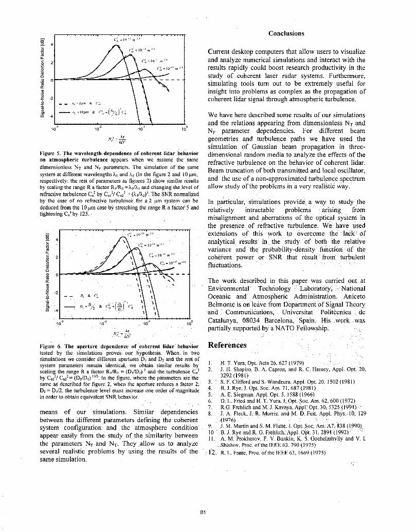
........................ ConclusionsI

Current desktop computers that allow users to visualize" c:,=,,,,,m.... and analyzenumericalsimulationsand interactwith theg 2

c_,=_0-,'m:, results rapidly could boost research productivity in the_. study of coherent laser radar systems. Furthermore,.9 0 ----

simulating tools turn out to be extremely useful forinsight into problems as complex as the propagation of'6

z -2 coherent lidar signal through atmospheric turbulence.

-4 We have here described some results of our simulationsand the relations appearing from dimensionless NT and

lo.3 10.2 16' 1°° NF parameter dependencies. For different beam,v:= 4_ geometries and turbulence paths we have used the/ag"

simulation of Gaussian beam propagation in three-Figure 5. The wavelength dependence of coherent lidar behavior dimensional random media to analyze the effects of theon atmospheric turbulence appears when we assume the same refractive turbulence on the behavior of coherent lidar.dimensionless NT and NF parameters. The simulation of the same Beam truncation of both transmitted and local oscillator,system at different wavelengths X] and L_,(in the figure 2 and 10gin,respectively; the rest of parameters as figures 2) show similar results and the use of a non-approximated turbulence spectrumby scaling the range R a factor R)/R2 =;k.2/X_and changing the level of allow study of the problems in a very realistic way.refractive turbulence C.2by C,)"/C,2! = (k)/k2)3.The SNR normalized

by the case of no refractive turbulence for a 2 _m System can be In particular, simulations provide a way to study thededuced from the 10p.m case by stretching the range R a factor 5 and relatively intractable problems arising fromtightening C.2by 125. misalignment and aberrations of the' optical system in

the presence of refractive turbulence. We have usedE c:,=_0-,:_:, extensions of this work to Overcome the lack of"o

__ c:,_,,)-,,_-:, analytical results in the study of both the relative_0 variance and the probability-density function.of theo_ 2 c.-,=_0-,,_-,, coherent power or SNR that result from turbulent

,0-"_.... fluctuations.toQ9 0

,- The work described in this paper was carried out ata Environmental Technology Laboratory, NationalZ -2

o, Oceanic and Atmospheric Administration. AnicetoBelmonteis on leavefrom:Departmentof SignalTheory

'_ and CommunicatiOns, Universitat Potitecnica de

_o"_ _o_ _o" _oo Catalunya, 08034 Barcelona, Spain. His work was

u'- 4_ partially supported by a NATO Fellowship.t." - kD:

Figure 6. The aperture dependence'of coherent lidar behavior Referencestested by the simulations proves our hypothesis. When in twosimulations we consider different apertures D_ and D2 and the rest ofsystem parameters remain identical, we obtain similar results by 1. H.T. Yura.Opt. Acta26. 627 (1979)scaling the range R a factor R)/R2 = (D_/D2)2and the turbulence C,2 2. J.H. Shapiro. B. A. Capron. and R. C. Hamey, Appl. Opt. 20.by C,12/C,2-'= (DJD0 n/3.In the figure, where the parametersare the 3292 (1981)same as described for figure 2. when the aperturereduces a factor2, 3. S.F. Cliffordand S. Wandzura.Appl. Opt. 20. 1502 (1981)D_,= D_/2, the turbulence level must increase one orderof magn tude 4. B.J. Rye, J. Opt. Soc. Am. 71. 687 (1981)in orderto obtainequivalent SNR behavior. 5. A.E. Siegman, Appl. Opt. 5. 1588 (1966)

6. D.L. Fried and H. T. Yura.J,Opt, Soc. Am. 62. 600 (1972)7. R.G. Frehlich and M. J. Kavaya. Appl; Opt. 30_532.5 (1991)

means of our simulations. Similar dependencies 8. J. A Fleck. J. R. Morris'.and M. D. Felt. Appl. Phys.;10. 129between the :differentparameters defining the coherent (1976)system configuration: and the atmosphere condition 9: j.M. Martinand S..M. Flatte.J. Opt.,Soc: Am. A7, 838 (1990).

appear easily from the study of the similarity between 10. B, J. Rye aridR. G. Frehlich. Appl. opt. 31. 2891'(1992)11. A.M. Prokhorov. F. V. Bunkin. K S. Gochelashvily and V. I.the parameters NF and NT. They allow us to analyze Shishov. Proc. of the IEEE 63. 790 (1975)several realistic problems by using the results of the 12. R.L. Fante. Proc. of the IEEE 63. 1669 (1975)same simulation.

81

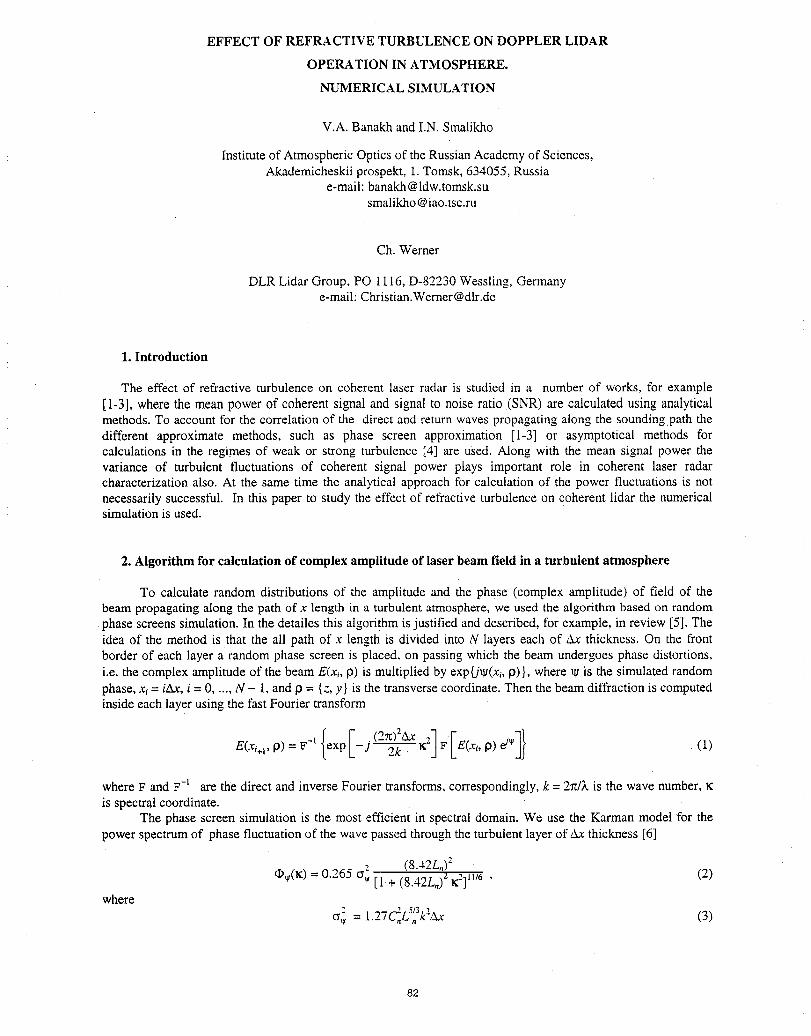
EFFECT OF REFRACTIVE TURBULENCE ON DOPPLER LIDAR

OPERATION IN ATMOSPHERE.

NL_IERICAL SIMULATION

V.A. Banakh and I.N. Smalikho

Institute of Atmospheric Optics of the Russian Academy of Sciences,Akademicheskii prospekt, 1. Tomsk, 634055, Russia

e-mail: banakh@ldw.tomsk.susmalikho @iao.tsc.ru

Ch. Werner

DLR Lidar Group. PO 1116, D-82230 Wessling, Germanye-mail: Christian.Werner @dlr.de

1. Introduction

The effect of refractive turbulence on coherent laser radar is studied in a number of works, for example[1-3], where the meanpower of coherent signal and signal to noise ratio (SNR) arecalculated using analyticalmethods.To account for the correlation of the direct and returnwaves propagating along the sounding,path thedifferent approximate methods, such as phase screen approximation [1-3] or asymptotical methods forcalculations in the regimes of weak or strong turbulence [4] areused. Along with the mean signal power thevariance of turbulent fluctuations of coherent signal power plays important role in coherent laser radarcharacterizationalso. At the same time the analytical approach for calculation of the power fluctuationsis notnecessarily successful. In this paper to study the effect of refractive turbulence on coherent lidar the numericalsimulationis used.

2. Algorithm for calculation of complex amplitude of laser beam field in a turbulent atmosphere

To calculate random distributions of the amplitude and the phase (complex amplitude) of field of thebeam propagatingalong the path of x length in a turbulent atmosphere,we used the algorithm basedon randomphase screens simulation. In the detailes this algorithm is justified and described, for example, in review [5]. Theidea of the method is that the all path of x length is divided into N layers each of Ax thickness. On the frontborder of each layer a random phase screen is placed, on passing which the beam undergoes phase distortions,i.e. the complex amplitude of the beam E(xi, O) is multiplied by exp{j_(xi, p)}, where 11/isthe simulated randomphase, xi = lax, i = 0..... N - i, and p = {:, y } is the transverse coordinate. Then the beam diffraction is computedinside each layer using the fast Fourier transform

E(xi+l,P) = F-l {exp F . (2_t)2_x ,1 r-L-j LE(x,,o> (,>where F and F-_ are the direct and inverse Fourier transforms, correspondingly, k =2rt/)_is the wave number, K:is spectral coordinate.

The phase screen simulation is the most efficient in spectral domain. We use the Karman model for thepower spectrum of phase fluctuation of the wave passed through the turbulent layer of Ax thickness [6]

2 (8.42L,)2_v(K) = 0.265 _ [I + (8.42L_)z1_]u/6 ' (2)

where2 5/3k_Ax(r_, = 1.27C_L_._'_. (3)

82

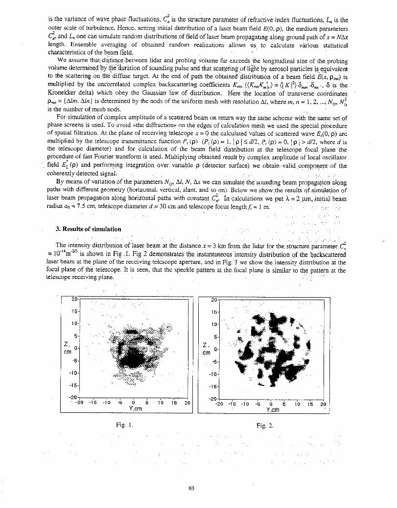
is the variance of wave phase fluctuations, _is the structure parameter of refractive index fluctuations, L, is the

outer scale of turbulence. Hence, setting initial distribution of a laser beam field E(0, p), the medium parametersC_,,and L, one can simulate random distributions of field of laser beam propagating along _ound path ofx = NAxlength. Ensemble averaging of obtained random realizations :allows-us: to calculate vitribus statisticalcharacteristics of the beam field.

We assume that,distance-between lidar and probing volume far exceeds the longitudinal size of thelprobingvolume determinedby i_d;d_ration of sounding pulse and that scattering of light by aerosol particles is e,quivalentto the scattering on theediffuse target. At the end of path the obtained distribution of a beam field E(X,p,,,,) is

multiplied by the uncorrelated complex backscattering coefficients K/,, ((K,,_Km_,)= ([ K [z)8m,,,8,, ,, .8 is theKronekker delta) which obey the Gaussian law of distribution. Here the location of transverse coordinates

p,_ = {Aim, Aln} is determined by the nods of the uniform mesh with resolution Al, where m, n = 1, 2.... _N:y, N_is the number of mesh nods.

Fdr,simulation of complex amplitude of a scattered beam on return way ihe same'scheme with the same set ofphase screens is used. To avoid <<thediffraction>>on the edges of calculation,mesh we used the special procedureof spatial filtration.At the plane of receiving telescope x = 0 the calculated values of scattered wave Es(0,p) aremultiplied by the telescope transmittance function Pt (P) (P, (P) = 1, [p [< d/2, Pt (P)= O, [p I> d/2, where d isthe telescope diameter) and for calculation of the beam field distribution at the telescope focal plane theprocedure of fast Fourier transform is used. Multiplying obtained result by complex amplitude of local oscillator

field EL (p) and perfo_ng integration over variable p (detector surface) we obtain valid .cgmponcnt.-of the,coherently detected signal. . ........ , :,...... _

By means of variation of the parameters N-y,Al, N, Ax we can simulate the sounding beam propagation: alongpaths with different geometry (horizontal, vertical, slant, and so on). Below we:show:the results ofsimulation of

laser beam propagation along horizontal paths with constant .C_. In calculations we put )_= 2 gm,_initia!, beamradius a0= 7.5 cm, telescope diameter d = 30cm and telescope,focus lengthf = 1m. - - : ,..... _: ,,

3, Results Ofsimulation . ,:..... : :

The intensity distribution of laser beam at the distance x = 3 km from the lidar for ;thestructure,:parameter C],= 10t4m-m is shown in Fig.1. Fig 2 demonstrates the instantaneous intensity distribution of the backscatteredlaser beam at the plane of the receiving telescope aperture, and in Fig. 3 we show the intensity distribution ai thefocal plane of the telescope. It is seen, that the speckle pattern at the focal plane is similar to the pattern at thetelescope receiving planel , :: "

' ' 20_ "'" 20-' • . i

.:: _: , 15-1..... ".....

/,/ Io-I ,,

: 5-!

Zmi Z

• ,-5-1

2_ -10-1

-20 -;5 -i'o As o 5 1'0 is 20 -20J,-2o-i_-io-_ 6 _ ib 15 20Y,cm Y cm

Fig. 1. Fig. 2.

• .. . .

83

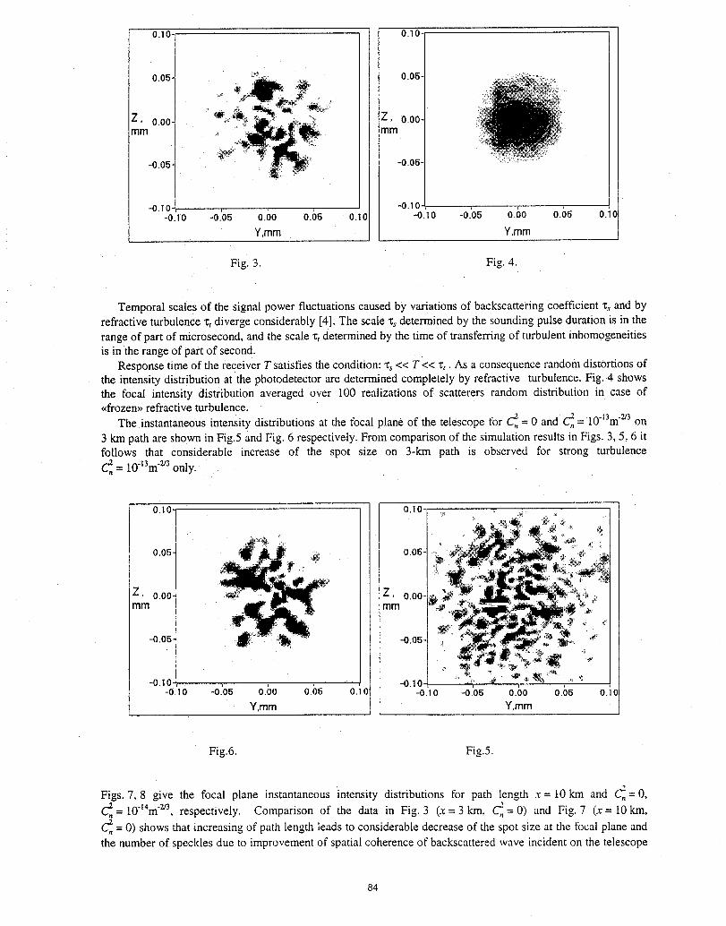
-0.io-! -0.o.--0 . I 0 "0 . 0 _ 0 . O0 0 . O_ 0 I I "0 " I 0 BO 10_ 0 m O0 0 " O_ 0 . I _

Y,mm Y,mm

Fig. 3. Fig. 4,

Temporal scales of the signal power fluctuations caused by variations of backscattering coefficient z, and byrefractive turbulence "c,diverge considerably [4]. The scale z, determined by the sounding pulse duration is in therange of part of microsecond, and the scale z, determined by the time of transferring of turbulent inhomogeneitiesis in the range of part of sect nd.

Response time of the receiver T satisfies the condition: "c,<< T << 1:, As a consequence random distortions ofthe intensity distribution at the photodetector are determined completely by refracnve turbulence. Fig..4 showsthe focal intensity distribution averaged over 100 realizations of scatterers random distribution in case of<<frozen>,refractive turbulence.

The instantaneous intensity distributions at the focal plane of the telescope for _ = 0 and _ = 10"13m"2r3on

3 km path are shown in Fig.5 and Fig. 6 respectively. From comparison of the simulation results in Figs. 3, 5, 6 itfollows that considerable increase of the spot size on 3-km path is observed for strong turbulence

= 10"t3m "2r3only.

0.10n 0.I0 L

0.05- _ 0.06-]!

Z ' 0 m00 -- Z ) 0 .00 m

mm mm

-0.06- -0.05-

-o.10..! -o.lo-o.lo -0.'05 0.bo o.b5 o.10 -o.1o -0.'05 o.bo 0.05 o.1

Y,mrn Y,mm

Fig.6. Fig.5.

Figs. 7,8 give the focal plane instantaneous intensity distributions for path length x = 10km and C_= 0,

C_,= 10"t4m"v3, respectively. Comparison of the data in Fig. 3 (x= 3 kin, C_= 0) and Fig. 7 (x= 10 km,

= 0) shows that increasing of path length leads to considerable decrease of the spot size at the focal plane andthe number of speckles due to improvement of spatial coherence of backscattered wave incident on the telescope

84

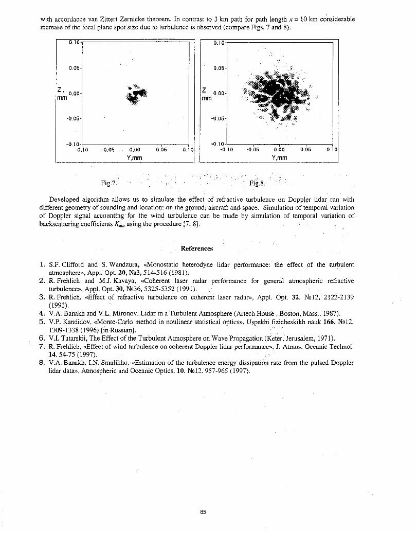
with accordance van Zittert Zernicke theorem. In contrast to 3 km path for path length x = 10 km considerableincrease of the focal plane spot size due to turbulence is observed (compare Figs. 7 and 8).

0.10 0.10-,

0.05 0.05- :'

mmZ'o.oo :_;'_'_''!' : __Zmmo.oo4 ,'

-0.05 -0.05 '_:': ;iN

-0.I0 -0.10 ,-o.1o -0.05 o.bo o._5 o.1o -o.1o -0.05 o.bo o.b5 o.1

Y,mm Y,mmi

Fig.7. :: _ • Fig.& i:

Developed algorithm allows us to simulate the effect of refractive turbulence on Doppler lidar run withdifferent geometry of sounding and locatior!: on:the gr.ound,:aircraftand space. Simulation of temporal variationof Doppler signal accounting for the wind turbulence can be made by simulation of temporal variation ofbackscattering coefficients Kin,using the procedure [7, 8].

References

1. S.F. Clifford and S. Wandzura, <<Monostaticheterodyne lidar performance: the effect of the turbulentatmosphere>>,Appl. Opt. 20, No._,514-516 (i 981).

2. R. Frehlich and M.J. Kavaya, <<Coherentlaser radar performance for general atmospheric refractiveturbulences,,Appl. Opt. 30, No_36,5325-5352 (1991).

g. R. Frehlich, <<Effectof refractive turbulence on coherent laser radar>_,Appl. Opt. 32, No12, 2!22-2139(1993).

4. V.A. Banakh and V.L. Mironov, Lidar in a Turbulent Atmosphere (Artech House, Boston, Mass., 1987).5. V.P. Kandidov, <<Monte-Carlomethod in nouiinear statistical optics_, Uspekhi fizicheskikh nauk 166, No12,

1309-1338 (1996) [in Russian].6. V.I. Tatarskii, The Effect of the Turbulent Atmosphere on Wave Propagation (Keter, Jerusalem, 1971).7. R. Frehlich, <<Effectof wind turbulence on coherent Doppler lidar performance>_,J. Atmos. Oceanic Technol.

14. 54-75 (1997)i ,8. V.A. Banakh, I.N. Smalikho, <<Estimationof the turbulence energy dissipation rate from the pulsed Doppler

lidar data>t,Atmospheric and Oceanic Optics, 11).No12. 957-965 (1997).

85

SPACEBORNE LIDARS- 1

Presider: Dennis Killinger

86

Abstract for the Coherent Laser Radar Technology and Applications Conference

NASA's Earth Science Enterprise Embraces Active LaserRemote Sensing From Space

Michael R. Luther

Deputy Associate Administrator for Earth Science

Granville E. Paules III

Lead TechnologistOffice of Earth Science

NASA HeadquartersOffice of Earth ScienceMail Code YF300 E. Street, SWWashington, DC 20546

granville paules(&.hq.nasa.gov

and

mluther@mail.hq.nasa.gov

Several objectives of NASA's Earth Science Enterprise are accomplished, and in some cases, uniquelyenabled by the advantages of earth-orbiting active lidar (laser radar) sensors. With lidar, the photons thatprovide the excitation illumination for the desired measurement are both controlled and well known. Thecontrolled characteristics include when and where the illumination occurs, the wavelength, bandwidth,pulse length, and polarization. These advantages translate into high signal levels, excellent spatialresolution, and independence from time of day and the sun's position. As the lidar technology has rapidlymatured, ESE scientific endeavors have begun to use lidar sensors over the last 10 years. Several more lidarsensors are approved for future flight. The applications include both altimetry (rangefinding) and profiling.Hybrid missions, such as the approved Geoscience Laser Altimeter System (GLAS) sensor to fly on theICESat mission, will do both at the same time. Profiling applications encompass aerosol, cloud, wind, andmolecular concentration measurements. Recent selection of the PICASSO Earth System SciencePathfmder mission and the complementary CLOUDSAT radar -based mission, both flying in formationwith the EOS PM mission, will fully exploit the capabilities of multiple sensor systems to accomplishcritical science needs requiring such profiling. To round out the briefing a review of past and planned ESEmissions will be presented.

87

SPARCLE: A MISSION OVERVIEW

G.D. Emmitt

Simpson:Weather AssociatesCharlottesville,Va 22902

804-979-3571 : _

M. KavayaT. Miller

Global Hydrology and Climate CenterNASA/MSFC

Huntsville, AL256-922-5858

Abstract

The SPAce Readiness Coherent Lidar Experiment (SPARCLE) is a NASA mission todemonstrate for the first time the measurement of tropospheric winds from a spaceplatform using coherent Doppler Wind Lidar (DWL). SPARCLE is scheduled for launchin early 2001 on board one of the shuttle orbiters. While primarily a demonstration of thetechnology's performance at ranges of 300-350 km, the mission will also addresssampling issues critical to the design and operation of follow-on missions. In this paperwe provide a brief overview of the SPARCLE instrument and the experiments beingplanned.

Introduction

Over the last few decades, lidars have been used to measure the line-of -sight componentof the winds. The lidars have been operated from buildings, vans and aircraft. Severalcountries (and agencies within) currently operate wind lidars from the ground. Only a fewhave installed Doppler lidars in aircraft. Within the USA, the lead agencies for airborneDoppler lidar are the DoD, NASA and NOAA. While the ground-based lidars employboth direct and coherent detection technology, most of the airborne systems are coherentlidars. Building upon the heritage of airborne flight, NASA has chosen a coherentdetection lidar concept for its New Millennium Program's Earth Observing - 02 Mission.In keeping with the NMP's charter to demonstrate the readiness of new technologies forscientific research and applications, the mission is known as the SPAce ReadinessCoherent Lidar Experiment or SPARCLE.

SPARCLE has several objectives, some of which are clearly related to demonstrating thetechnology and others that are more oriented towards demonstrating the accuracy and

88

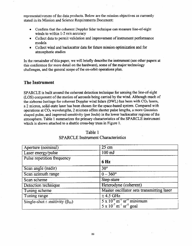
representativenessof the dataproducts.Belowarethe missionobjectivesas currentlystated in its MissionandScienceRequirementsDocument:

• Confirm that the coherent Doppler lidar technique can measure line-of-sightwinds to within 1-2 m/s accuracy

• Collect data to permit validation and improvement of instrument performancemodels

• Collect wind and backscatter data for future mission optimization and foratmospheric studies

In the remainder of this paper, we will briefly describe the instrument (see other papers atthis conference for more detail on the hardware), some of the major technologychallenges, and the general scope of the on-orbit operations plan.

TheInstrument

SPARCLE is built around the coherent detection technique for sensing the line-of-sight(LOS) component of the motion of aerosols being carried by the wind. Although much ofthe airborne heritage for coherent Doppler wind lidars (DWL) has been with CO2lasers,a 2 micron, solid-state laser has been chosen for the space-based system. Compared withoperations at CO2wavelengths, 2 microns offers shorter pulse lengths, a more Gaussianshaped pulse, and improved sensitivity (per Joule) in the lower backscatter regions of theatmosphere. Table 1 summarizes the primary characteristics of the SPARCLE instrumentwhich is shown attached to a shuttle cross-bay truss in Figure 1.

Table 1SPARCLEInstrumentCharacteristics

Aperture (nominal) 25 cmLaser energy/pulse 100 mJPulse repetition frequency

6 I-Iz

Scan angle (nadir) 30°Scan azimuth range 0 - 360°Scan scheme Step-stareDetection technique Heterodyne (coherent)Tuning scheme Master oscillator sets transmitting laserTuning range + 4.5 GHzSingle-shot smsitivity (1350) 5 x 10-am"t sr"lminimum

5 x 10-7m1 sr1 goal

89

/

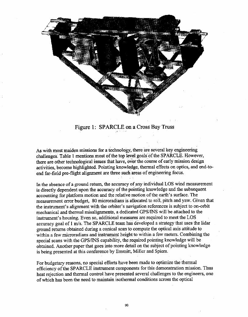
Figure 1: SPARCLE on a Cross Bay Truss

As with most maiden missions for a technology, there are several key engineering

challengeS:.Table 1 mentions most of the top level goals of the SPARCLE. However,there are other technological issues that have, tixi_rthe course of early mission designactivities, become highlighted. Pointing knowledge, thermal effects on optics, and end-to-end far-field pre-flight alignment are three such areas of engineering focus.

In the absence of a ground return, the accuracy of any individual LOS wind measurementis directly dependent upon the accuracy of the pointing knowledge and the subsequentaccounting for platform motion and the relative motion of the earth's surface. Themeasurement error budget, 80 microradians is allocated to roll, pitch and yaw. Given thatthe instrument's alignment with the orbiter's navigation references is subject to on-orbitmechanical and thermal misalignments, a dedicated GPS/INS will be attached to theinstrument's housing. Even so, additional measures are required to meet the LOSaccuracy goal of 1 m/s. The SPARCLE team has developed a strategy that uses the lidarground returns obtained during a conical scan to compute the optical axis attitude towithin a few microradians and instrument height to within a few meters. Combining thespecial scans with theGPS/INS capability, the required pointing knowledge will beobtained. Another paper that goes into more detail on the subject of pointing knowledgeis being presented at this conference by Emmitt, Miller and Spiers.

For budgetary reasons, no special efforts have been made to optimize the thermalefficiency of the SPARCLE instrument components for this demonstration mission. Thusheat rejection and thermal control have presented several challenges to the engineers, oneof which has been the need to maintain isothermal conditions across the optical

90

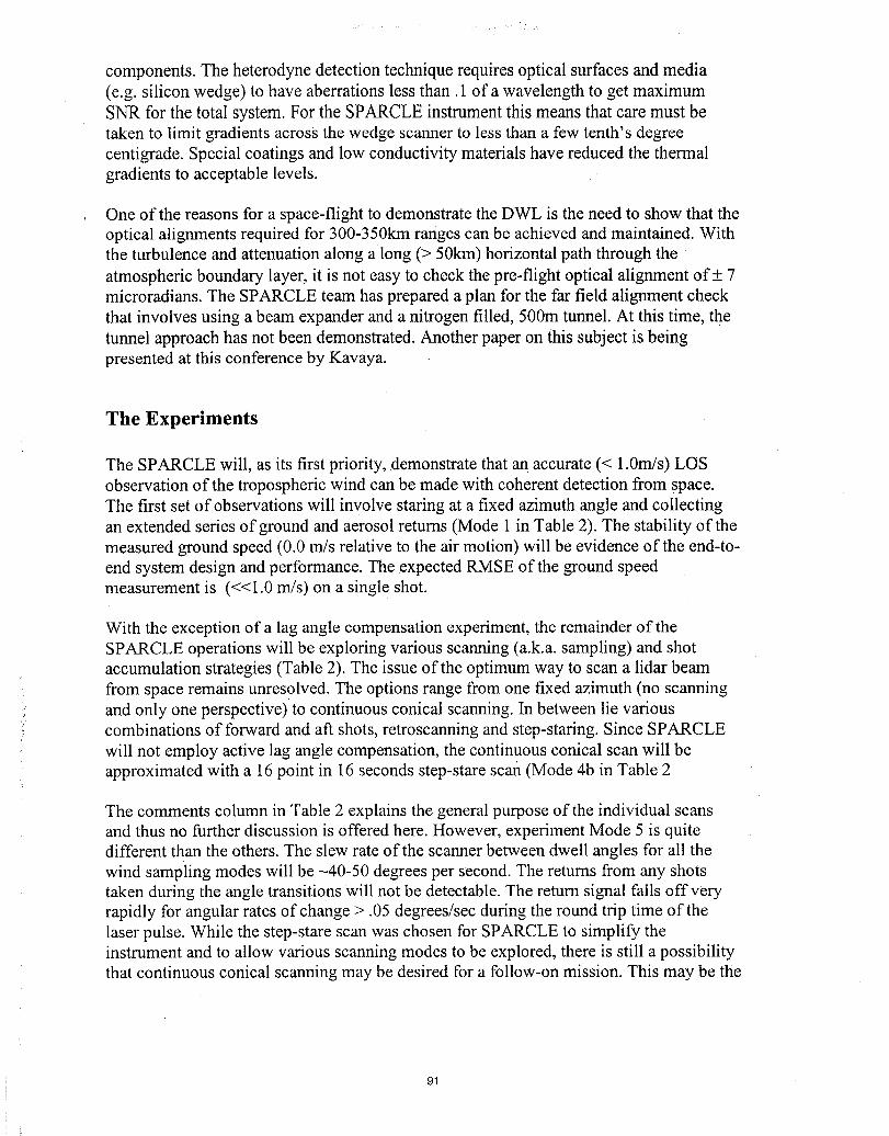
components. The heterodyne detection technique requires optical surfaces and media(e.g. silicon wedge) to have aberrations less than. 1 of a wavelength to get maximumSNR for the total system. For the SPARCLE instrument this means that care must betaken to limit gradients across the wedge scanner to less than a few tenth's degreecentigrade. Special coatings and low conductivity materials have reduced the thermalgradients to acceptable levels.

, One of the reasons for a space-flight to demonstrate the DWL is the need to show that theoptical alignments required for 300-350km ranges can be achieved and maintained. Withthe turbulence and attenuation along a long (> 50km) horizontal path through theatmospheric boundary layer, it is not easy to check the pre-flight optical alignment of+ 7microradians. The SPARCLE team has prepared a plan for the far field alignment checkthat involves using a beam expander and a nitrogen filled, 500m tunnel. At this time, thetunnel approach has not been demonstrated. Another paper on this subject is beingpresented at this conference by Kavaya.

The Experiments

The SPARCLE will, as its first priority, demonstrate that an accurate (< 1.0m/s) LOSobservation of the tropospheric wind can be made with coherent detection from space.The first set of observations will involve staring at a fixed azimuth angle and collectingan extended series of ground and aerosol returns (Mode 1 in Table 2). The stability of themeasured ground speed (0.0 m/s relative to the air motion) will be evidence of the end-to-end system design and performance. The expected RMSE of the ground speedmeasurement is (<<1.0 m/s) on a single shot.

With the exception of a lag angle compensation experiment, the remainder of theSPARCLE operations will be exploring various scanning (a.k.a. sampling) and shotaccumulation strategies (Table 2). The issue of the optimum way to scan a lidar beamfrom space remains unresolved. The options range from one fixed azimuth (no scanningand only one perspective)to continuous conical scanning. In between lie variouscombinations of forward and aft shots, retroscanning and step-stating. Since SPARCLEwill not employ active lag angle compensation, the continuous conical scan will beapproximated with a 16point in 16 seconds step-stare scan (Mode 4b in Table 2

The comments column in Table 2 explains the general purpose of the individual scansand thus no further discussion is offered here. However, experiment Mode 5 is quitedifferent than the others. The slew rate of the scanner between dwell angles for all thewind sampling modes will be -40-50 degrees per second. The returns from any shotstaken during the angle transitions will not be detectable. The return signal falls off veryrapidly for angular rates of change > .05 degrees/see during the round trip time of thelaser pulse. While the step-stare scan was chosen for SPARCLE to simplify theinstrument and to allow various scanning modes to be explored, there is still a possibilitythat continuous conical scanning may be desired for a follow-on mission. This may be the

91

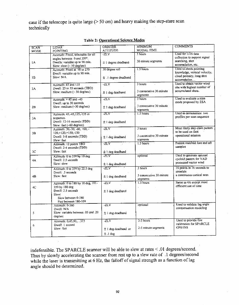
case if the telescopeis quitelarge (> 50 cm) andheavymakingthe step-starescantechnically

Table 2: Operational Science Modes

SCAN LIDAR ORBITER. MINIMUM COMMENTSMODE POINTING ATTITUDE MODALTIME

Azimuth: Fixed, selectable tbr all -ZLV 3 hours Used for LOSdataangles between 0 and 359°. collection to support signal

IA Dwells: variable up to 90 rain. + 1 degreedeadband 30 minute segments searching, shotSlew: slow (~ !0 deg/sec) accumulation,etc.Azimuth: Fixed at 90 or 270 30 degree roll 1.5hours Used to check pointingDwell: variable up to 90 rain. knowledge, vertical velocity,

cloud porosity, long shot1B Slew: N/A + .1 degree deadband accumulation...

Azimuth: 45 and 135 -ZLV 3 hours Used to obtain vector wind2A Dwell: 25 to 35 seconds (TBD) obs with highest number of

Slew: medium (- 30 deg/sec) __.1deg deadband 3 consecutive 30,minute accumulated shots.segments

Azimuth: + 45 and -45 -ZLV 3 hours Used to evaluate a scanDwell: up to 30 seconds mode proposed by ESA

2B Slew: medium (~30 deg/sec) + 1deg deadband 3 consecutive 30 minute- segments

Azimuth: 45,-45,135,-135 in -ZLV 1.5hours Used to demonstrate two3A sequence, profiles per scan sequence

Dwell: 12-16 seconds (TBD) __.1deg deadbandSlew: fast (-60 deg/sec)Azimuth: 30,-30, -60, +60, - -ZLV 3 hours Most likely step-stare pattern

3B 120,+120,+150,-150 to be used on firstDwell: 5-8 seconds (TBD) + 1deg deadband 3consecutive 30 minute operational missionSlew: thst segmentsAzimuth: 12points TBD -ZLV 1.5hours Fastest matched tore and aftDwell: 2-4 seconds (TBD) samples

3C Slew: fast + 1deg deadbandAzimuth: 0 to 359 by 10deg -ZLV optional Used to generate optimal

4A Dwell: 2.5 seconds cycloid pattern for VADSlew: slow __.1deg deadband processed vector wind

Azimuth: 0 to 359 by 22.5 deg -ZLV ' 3 hours 16points in 16seconds toDwell: .5 seconds simulate

4B Slew: fast +_.1deg deadband 3 consecutive 30 minute a continuous conical scansegments

Azimuth: 0 to 180by 10deg, 181- -ZLV 1.5hours Same as 4A except more4C 359 by 180deg efficient use of time

Dwell: 2.5 seconds _ 1deg deadbandSlew:

Slow between 0-180Fast between 180-359

Azimuth: 0-360 -ZLV optional Used to validate lag angleDwell: N/A compensation modeling

5 Slew: variable between .05and .20 + I deg deadbanddeg/sec

Azimuth: 0,45,90,...315 -ZLV 3-5 hours Used to provide fine6 Dwell: 1 second calibration tbr SPARCLE

Slew: fast + 1deg deadband or 2-5 minute segments GPS/INS

+ .1 deg

indefensible. The SPARCLE scanner will be able to slew at rates < .01 degrees/second.Thus by slowly accelerating the scanner from rest up to a slew rate of. 1degrees/secondwhile the laser is transmitting at 6 Hz, the falloff of signal strength as a function of lagangle should be determined.

92

A goal of the SPARCLE is to record 50 hours of raw level 0 data out of the receiver A/Dchannels. This will amount to - 100 Gbytes of data, uncompressed. While there isexpected opportunities for downlinking some of the raw data during the flight, the plan istoo have -100 Gbytes of mass storage on-board. Some on-board processing of the rawdata will be done as part of the pointing knowledge algorithms and to facilitate findingthe ground return in the case of extremely poor (> 3 degrees error) pointing knowledge atturn on. Downlinking of this processed data and ground-based processing of downlinkedstreams of raw data will provide the SPARCLE team with real-time evidence of theperformance of the SPARCLE instrument. Experiment scheduling will be effected by thereal-time analysis of the processed data and the global weather conditions.

Since SPARCLE is a first step on the road to a fully operational wind lidar, there will bea significant effort to validate instrument's performance as well as the data products. Avalidation plan has been prepared for the NMP. In addition to the global network of windobserving systems (Rawindsondes, scatterometers, cloudtracked winds, surfacemeteorological towers/bouys,etc.), groundbased and airborne Doppler lidars will providemany opportunities for comparison. Global weather model analyses will also be used toidentify where the SPARCLE observations and the inferred winds differ and agree.

Although the SPARCLE instrument will have a very modest sensitivity which will limitmost of its observations to the boundary layer and clouds, it is still possible that theSPARCLE mission will return, on occasion, sufficient global data coverage todemonstrate a positive impact on weather forecasts and phenomenological diagnostics(e.g. hurricanes, orographic cyclogenesis, etc).

Acknowledgements

The authors recognize the support from NASA Headquarters and the contributions of thefollowing organizations to the SPARCLE mission: University of Alabama at Huntsville,Marshall Space Flight Center, Jet Propulsion Laboratory, Langley Research Center,National Oceanographic and Atmospheric Administration, Goddard Space Flight Center,Coherent Technologies Inc. and Simpson Weather Associates, Inc.

93

Atmospheric Dynamic Mission:Project Status, Concepts Review and Technical Baseline

Hans Reiner Schulte, Dornier SatellitensystemeGmbH, 88039 Friedrichshafen,GermanyDidier Moranqais, Matra Marconi Space, 31077 Toulouse, France

1) IntroductionThe Atmospheric Dynamics Mission (ADM) study is one of four Earth Explorer Core Missions phaseA studiesin the frame of the ESA EOPP/Envelope Programme. This programme is directed towardsresearch/demonstration missions addressing understanding of different Earth system processes. The particularaim of the ADM is the measurement of vertically resolved wind fields for assimilation in numerical weatherprediction models to alleviate a deficiency in the current observational network and to support climate research.The actual measured quantity is a single horizontal wind vector component measured in vertical of lkmextension from ground up to 20km altitude. The measurement is performed by a Doppler wind lidar in clear airand above optically thick clouds. In the ADM study a trade off between various coherent and incoherentinstrument concepts covering the wavelengths range from 0.355/_mtol0.6/_m has been performed to identifythe most promising solution in view of measurement requirements, mission constraints and technicalfeasibility. This process has led to the selection of a baseline for the ADM mission featuring a direct detectionlidar instrument on boardof a dedicated small satellite in a 400km sun synchronous (dawn-dusk) orbit.

2) Trade-off ProcessThe instrument trade-off was based on fixed boundary conditions derived from mission constraints (Table 2).Although originally an accommodation on the international space station (ISS) was foreseen the missionconstraints where from the beginning selected in view of representativeness for a later operational mission on asmall satellite in a polar orbit. Main criteria in the trade-off where compliance to the observationalrequirements for the ADM mission (Table 1) and technical maturity/feasibility.

Table 1: Measurement Requirements Table 2: TechnicalConstraints

Troposphere Stratosphere Precursor MissionAltitude Range 0-16 km 16-20km Orbit altitude 400 kmVertical Integration Length . <1.0 km <2.0 km Payload Mass 226.5 kgHorizontal Integration Length 50 km ,PayloadVolume 86x117x24 cm_Number of Profiles 100per hour Power < 1kWProfile Separation > 200 kmWind Observation Accuracy < 2 m/sReliability >80 % noCorrelated Error <0.1 rn/s requirement

3) Candidate Instrument ConceptsConsidering availability of laser technology, CO2 gas laser, 2/_msolid state laser (Tm:YLuAG) and frequencytripled Nd:YAG were identified as most promising for the transmitter while Nd:YAG on its base frequency andon the doubled frequency where rejected for eye safety reasons. For the CO, laser a wavelength of 9.1 lpm andfor the Tm:YLuAG laser a wavelength of 2.0218/.tm have been selected-to benefit from low atmosphericattenuation at these frequencies. Three instrument designs where performed to sufficient level of detail to judgefeasibility and maturity of needed technologies and to allow assessment of measurement performance. Keycharacteristics of the three designs are given inTable 3.

The CO,_gas laser based instrument and the 2/_m solid state laser based instrument designs are both coherentlidar instruments exploiting aerosol backscattering. Different strategies for the processing of the heterodynesignal where adopted. In the gas laser concept a fixed frequency LO is used and electrical processing isemployed to compensate for earth rotation and satellite pointing induced Doppler variations which, for anaccommodation on the space-station, are much larger than the bandwidth resulting from the wind velocitymeasurement interval. In the 2/_m instrument design a tuneable LO-laser is employed to account for thepredictable Doppler shift, thus generating a heterodyne signal at fixed center frequency to be processed in abandwidth determined by the wind search range. For selecting a more convenient located LO frequency (orfrequency range) in both cases a deliberate squint looking of the LOS was introduced to generate a meanDoppler shift due to the spacecraft motion. The coherent instruments employ both the same processing

94

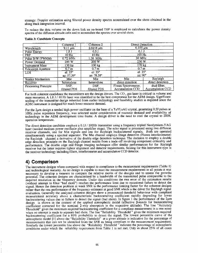
strategy: Doppler estimation using filtered power density spectra accumulated over the shots obtained in thealong track integration interval.

To reduce the data volume on the down link an on-board DSP is employed to calculates the power densityspectra of the different altitude cells and to accumulate the spectra over several shots.

Table 3: Candidate Concepts

Coherent 1 Coherent 2 Direct DetectionWavelength 9.11/am 2.0218/am 0.355/amPulse Energy 1.8 J ' 0.5 J 0.t JPRF 10Hz 10Hz 100HzPulse B/W (FWHM) 0.72 MHz 1.26 MHz 30 MHzPower Demand 200 W 200 W 230 WInstrument Mass 130kg 100 kg 170kgTelescope Aperture 0.7 m 0.7 m 0.7 mLOS el: 35° el: 35° el: 35°

az: 57.39° az: 78.58° az: 90°Scatter Mechanism Mie Mie Mie RayleighReceiver heterodyne heterodyne direct detection direct detectionProcessing Principle DSP, DSP, Fizeau Spectrometer, dual filter,

filtered PDS filtered PDS Accumulation CCD Accumulation CCD

For both coherent candidates the transmitters are the design drivers. The CO2gas laser is critical in volume andmass resources. A 1.8 J / 10 Hz laser was identified to be the best compromise for the ADM design. Significantscaling of the transmitter design inherited from earlier technology and feasibility studies is required since theADM instrument is designed for much lower resourcedemand.

For the 2/amdesign a seeded high power oscillator on the base of a TuYLuAGcrystal, generating 0.5J pulses at10Hz pulse repetition frequency, was selected under consideration of resource demand and availability oftechnology in the ADM development time frame. A design driver is the need to cool the crystal to 200Koperation temperature.

The direct detection candidate employs a 0.1J / 100Hz transmitter using a frequency tripled Neodymium-YAGlaser (seeded medium power oscillator plus amplifier stage). The echo signal is processed using two differentreceiver channels, one for Mie signals and one for Rayleigh backscattered signals. Both are operatedsimultaneously using a spectral separator. The Mie channel employs fringe detection (Fizeau interferometer)the Rayleigh channel a derivative of the double edge detection technique. The decision to employ a doubleedge detection principle on the Rayleigh channel results from a trade-off involving component criticality andperformance. The double edge and fringe imaging techniques offer similar performances for the Rayleighreceiver but the latter requires tighter alignment and detector requirements. Seizing for this instrument type isthe receiver technology including filters, interferometer and accumulationCCD detector.

4) ComparisonThe instrument designs where compared with respect to compliance to the measurement requirements (Table 1)and technological maturity. As no design is capable to meet the measurement requirements in all points it wasnecessary to develop a measure to compare the relative merits of the designs and to assess the growthspotential. The coherent designs are characterised by a bandwidth of the transmitted pulse comparable to therequired resolution in the frequency domain. Under this conditions the rms error of the estimation results(without attempt to filter "bad shots") reaches the performance limit due to occasional failure to detect thesignal. Hence the detection problem at week SNR is the performance limiting factor for the coherent designsrather than the rms performance of the frequency estimator at good SNR which is the driver for Rayleigh signalevaluation. Generally the analysed coherent designs show a pronounced threshold behaviour with compliantmeasurement accuracy above a characteristic backscattering coefficient rapidly degrading for lowerbackscattering values due to failure to detect the signal (bad shots). In figure 1 the performance of the 2/_mdesign is shown in the context of the applied atmospheric model (effective _istands for backscatteringcoefficient corrected for the nominal 2-way absorption in the respective altitude). The line "AccuracyThreshold" gives the minimum required backscattering coefficient for a compliant measurement in arms sensewhen no attempt is made to separate bad shots. The line "Reliability Threshold " gives the minimum requiredbackscattering coefficient for a 80% probability to detect the signal. The lowest percentile curve of theatmospheric model [1] above the "Reliability Threshold" at a given altitude is indicative for the percentage ofmeasurements that can not be identified from the SNR as being compliant to the measurement requirement.Similarly the lowest percentile line above the "Reliability Threshold " indicates the percentage of atmosphericconditions under which the reliability requirement from Table 1 is not met. Only in about 25% of all cases

95

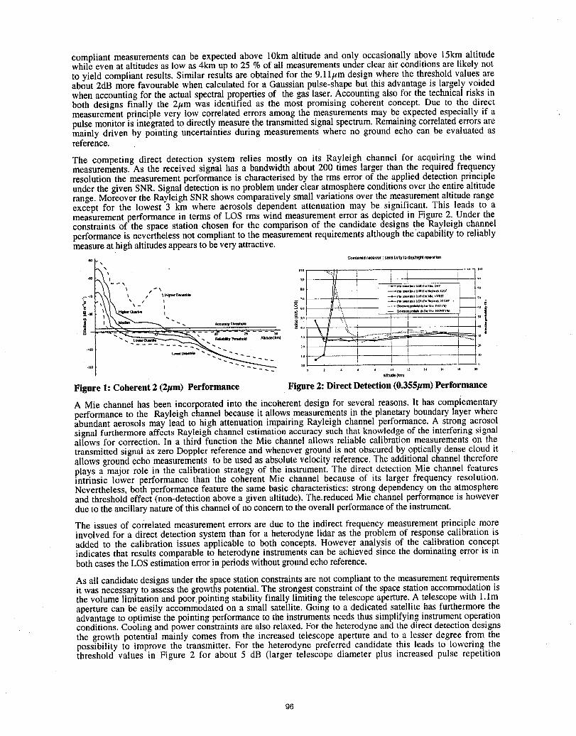
compliant measurements can be expected above 10km altitude and only occasionally above 15km altitudewhile even at altitudes as low as 4km up to 25 % of all measurements under clear air conditions are likely notto yield compliant results. Similar results are obtained for the 9.11/_mdesign where the threshold values areabout 2dB more favourable when calculated for a Gaussian pulse-shape but this advantage is largely voidedwhen accounting for the actual spectral properties of the gas laser. Accounting also for the technical risks inboth designs finally the 2/_m was identified as the most promising coherent concept. Due to the directmeasurement principle very low correlated errors among the measurements may be expected especially if apulse monitor is integrated to directly measure the transmitted signal spectrum. Remaining correlated errors aremainly driven by pointing uncertainties during measurements where no ground echo can be evaluated asreference.

The competing direct detection system relies mostly on its Rayleigh channel for acquiring the windmeasurements. As the received signal has a bandwidth about 200 times larger than the required frequencyresolution the measurement performance is characterised by the rms error of the applied detection principleunder the given SNR. Signal detection is no problem under clear atmosphere conditions over the entire altituderange. Moreover the Rayleigh SNR shows comparatively small variations over the measurement altitude rangeexcept for the lowest 3 km where aerosols dependent attenuation may be significant. This leads to ameasurement performance in terms of LOS rms wind measurement error as depicted in Figure 2. Under theconstraints of the space station chosen for the comparison of the candidate designs the Rayleigh channelperformance is nevertheless not compliant to the measurement requirements although the capability to reliablymeasure at high altitudes appears to be veryattractive.

Combln_lrecei'alr: sensitivityto day_ opera*Jon

"_\ " '.... % r i i ....

.... _ ........ ,: ,o _ _ol_Nhdd _ Ikm] _.ly

_t_tude(kin)

Figure I: Coherent 2 (2pm) Performance Figure 2: Direct Detection (0.355pm) Performance

A Mie channel has been incorporated into the incoherent design for several reasons. It has complementaryperformance to the Rayleigh channel because it allows measurements in the planetary boundary layer whereabundant aerosols may lead to high attenuation impairing Rayleigh channel performance. A strong aerosolsignal furthermore affects Rayleigh channel estimation accuracy such that knowledge of the interfering signalallows for correction. In a third function the Mie channel allows reliable calibration measurements on thetransmitted signal as zero Doppler reference and whenever ground is not obscured by optically dense cloud itallows ground echo measurements to be used as absolute velocity reference. The additional channel thereforeplays a major role in the calibration strategy of the instrument. The direct detection Mie channel featuresintrinsic lower performance than the coherent Mie channel because of its larger frequency resolution.Nevertheless, both performance feature the same basic characteristics: strong dependency on the atmosphereand threshold effect (non-detection above a given altitude). The.reduced Mie channel performance is howeverdue to the ancillary nature of this channel of no concern to the overall performance of the instrument.

The issues of correlated measurement errors are due to the indirect frequency measurement principle moreinvolved for a direct detection system than for a heterodyne lidar as the problem of response calibration isadded to the calibration issues applicable to both concepts. However analysis of the calibration conceptindicates that results comparable to heterodyne instruments can be achieved since the dominating error is inboth cases the LOSestimation error in periods without ground echo reference.

As all candidate designs under the space station constraints are not compliant to the measurement requirementsit was necessary to assess the growths potential. The strongest constraint of the space station accommodation isthe volume limitation and poor pointing stability finally limiting the telescope aperture. A telescope with 1.lmaperture can be easily accommodated on a small satellite. Going to a dedicated satellite has furthermore theadvantage to optimise the pointing performance to the instruments needs thus simplifying instrument operationconditions. Cooling and power constraints are also relaxed. For the heterodyne and the direct detection designsthe growth potential mainly comes from the increased telescope aperture and to a lesser degree from thepossibility to improve the transmitter. For the heterodyne preferred candidate this leads to lowering thethreshold values in Figure 2 for about 5 dB (larger telescope diameter plus increased pulse repetition

96

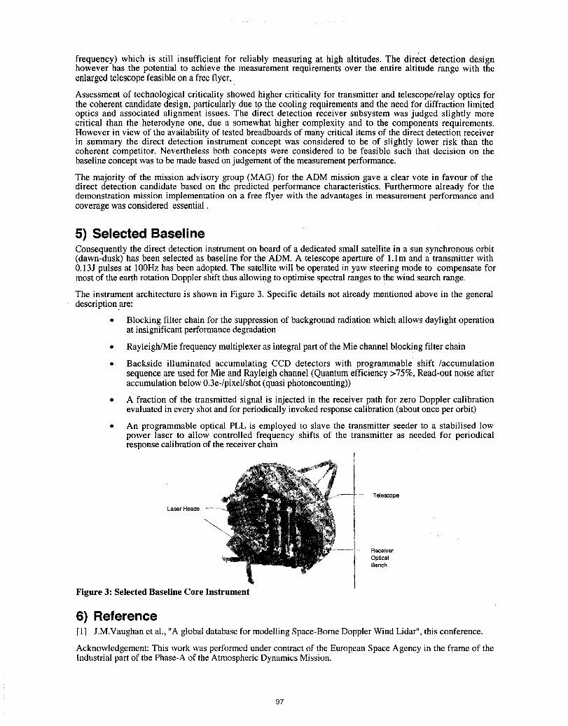
frequency) which is still insufficient for reliably measuring at high altitudes. The direct detection designhowever has the potential to achieve the measurement requirements over the entire altitude range with theenlarged telescope feasible on a free flyer,

Assessment of technological criticality showed higher criticality for transmitter and telescope/relay optics forthe coherent candidate design, particularly due to the cooling requirements and the need for diffraction limitedoptics and associated alignment issues. The direct detection receiver subsystem was judged slightly morecritical than the heterodyne one, due a somewhat higher complexity and to the components requirements.However in view of the availability of tested breadboards of many critical items of the direct detection receiverin summary the direct detection instrument concept was considered to be of slightly lower risk than thecoherent competitor. Nevertheless both concepts were considered to be feasible such that decision on thebaseline concept was to be made based onjudgement of the measurement performance.

The majority of the mission advisory group (MAG) for the ADM mission gave a clear vote in favour of thedirect detection candidate based on the predicted performance characteristics. Furthermore already for thedemonstration mission implementation on a free flyer with the advantages in measurement performance andcoverage was considered essential.

5) SelectedBaselineConsequently the direct detection instrument on board of a dedicated small satellite in a sun synchronous orbit(dawn-dusk) has been selected as baseline for the ADM. A telescope aperture of 1.1m and a transmitter with0.13J pulses at 100Hz has been adopted. The satellite will be operated in yaw steering mode to compensate formost of the earth rotation Doppler shift thus allowing tOoptimise spectral ranges to the wind search range.

The instrument architecture is shown in Figure 3. Specific details not already mentioned above in the generaldescription are:

• Blocking filter chain for the suppression of background radiation which allows daylight operationat insignificant performance degradation

• Rayleigh/Mie frequency multiplexeras integral part of the Mie channel blockingfilter chain

• Backside illuminated accumulating CCD detectors with programmable • shift /accumulationsequence are used for Mie and Rayleigh channel (Quantum efficiency >75%, Read-out noise afteraccumulation below 0.3e-/pixel/shot (quasi photoncounting))

• A fraction of the transmitted signal is injected in the receiver path for zero Doppler calibrationevaluated in every shot and for periodically invoked response calibration (about once per orbit)

• An programmable optical PLL is employed to slave the transmitter seeder to a stabilised lowpower laser to allow controlled frequency shifts of the transmitter as needed for periodicalresponse calibration of the receiver chain

Telescope

LaserHeads

Receiver

OpticalBench

Figure 3: Selected Baseline Core Instrument

6) Reference[1] J.M.Vaughan et al., "A global database for modelling Space-Borne Doppler Wind Lidar", this conference.

Acknowledgement: This work was performed under contract of the European Space Agency in the frame of theIndustrial part of the Phase-A of the Atmospheric Dynamics Mission.

97

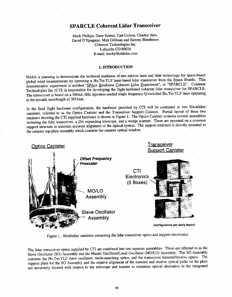
SPARCLE Coherent Lidar Transceiver

Mark Phillips, DaneSchnal,Carl Colson,CharleyHale,David D'Epagnier, MattGibbensandSammyHenderson

CoherentTechnologies Inc.LafayetteCO80026

E-mail: markp@ctilidar.com

1. INTRODUCTION

NASA is planning to demonstrate the technical readiness of two micron laser and lidar technology for space-basedglobal wind measurements by operating a Ho,Tm:YLF laser-based lidar transceiver from the Space Shuttle. Thisdemonstration experiment is entitled "SPAce Readiness Coherent Lidar Experiment", or "SPARCLE". CoherentTechnologies Inc (CTI) is responsible for developing the flight-hardened coherent lidar transceiver for SPARCLE.The transceiver is based on a 100mJ, 6Hz injection-seeded single frequency Q-switched Ho,Tm:YLF laser operatingat the eyesafe wavelength of 205 lnm.

In the final flight hardware configuration, the hardware provided by CTI will be contained in two Hitchhikercanisters, referred to as the Optics Canister and the Transceiver Support Canister. Partial layout of these twocanisters showing the CTI supplied hardware is shown in Figure 1. The Optics Canister contains several assembliesincluding the lidar transceiver, a 25x expanding telescope, and a wedge scanner. These are mounted on a commonsupport structure to maintain accurate alignment of the optical system. The support structure is directly mounted tothe canister top-plate assembly which contains the canister optical window.

Optics Canister TransceiverSupport Canister

Offset Frequency

CTIElectronics(5 Boxes)

MO/LOAssembly

Slave Oscillator

Assembly

Configurationperearly layout

Figure 1. Hitchhiker canisters containing the lidar transceiver optics and support electronics

The lidar transceiver optics supplied by CTI are combined into two separate assemblies. These are referred to as theSlave Oscillator (SO) Assembly and the Master Oscillator/Local Oscillator (MO/LO) Assembly. The SO Assemblycontains the Ho,Tm:YLF slave oscillator, mode-matching optics, and the transceiver transmit/receive optics. Thesupport plate for the SO Assembly and the relative alignment of the transmit and receive optical paths on the plateare accurately located with respect to the telescope and scanner to minimize optical aberration in the integrated

98

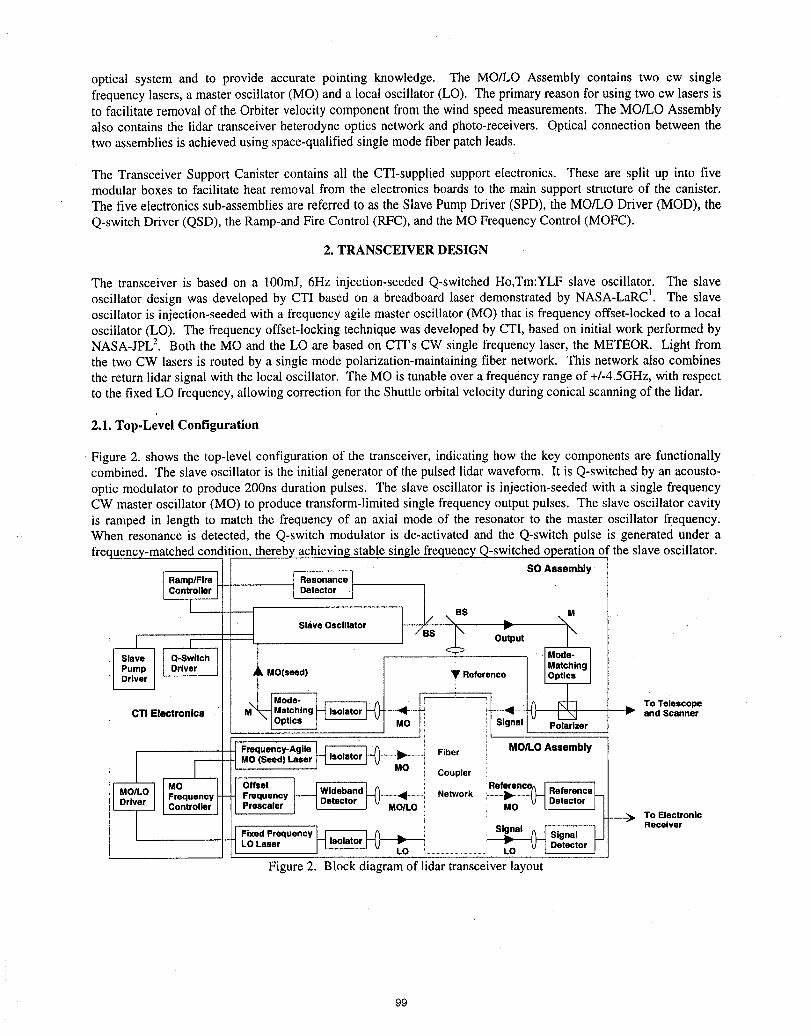
optical system and to provide accurate pointing knowledge. The MO/LO Assembly contains two cw singlefrequency lasers, a master oscillator (MO) and a local oscillator (LO). The primary reason for using two cw lasers isto facilitate removal of the Orbiter velocity component from the wind speed measurements. The MO/LO Assemblyalso contains the lidar transceiver heterodyne optics network and photo-receivers. Optical connection between thetwo assemblies is achieved using space-qualified single mode fiber patch leads.

The Transceiver Support Canister contains all the CTI-supplied support electronics. These are split up into fivemodular boxes to facilitate heat removal from the electronics boards to the main support structure of the canister.The five electronics sub-assemblies are referred to as the Slave Pump Driver (SPD), the MO/LO Driver (MOD), theQ-switch Driver (QSD), the Ramp-and Fire Control (RFC), and the MO Frequency Control (MOFC).

2. TRANSCEIVER DESIGN

The transceiver is based on a 100mJ, 6Hz injection-seeded Q-switched Ho,Tm:YLF slave oscillator. The slaveoscillator design was developed by CTI based on a breadboard laser demonstrated by NASA-LaRCI. The slaveoscillator is injection-seeded with a frequency agile master oscillator (MO) that is frequency offset-locked to a localoscillator (LO). The frequency offset-locking technique was developed by CTI, based on initial work performed byNASA-JPL2. Both the MO and the LO are based on CTI's CW single frequency laser, the METEOR. Light fromthe two CW lasers is routed by a single mode polarization-maintaining fiber network. This network also combinesthe return lidar signal with the local oscillator. The MO is tunable over a frequency range of +/-4.5GHz, with respectto the fixed LO frequency, allowing correction for the Shuttle orbital velocity during conical scanning of the lidar.

2.1. Top,Level Configuration

Figure 2. shows the top-level configuration of the transceiver, indicating how the key components are functionallycombined. The slave oscillator is the initial generator of the pulsed lidar waveform. It is Q-switched by an acousto-optic modulator to produce 200ns duration pulses. The slave oscillator is injection-seeded with a single frequencyCW master oscillator (MO) to produce transform-limited single frequency output pulses. The slave oscillator cavityis ramped in length to match the frequency of an axial mode of the resonator to the master oscillator frequency.When resonance is detected, the Q-switch modulator is de-activated and the Q-switch pulse is generated under afrequency-matched condition, thereby achieving stable single frequency Q-switched operation of the slave oscillator.

Resonance[ SO Assembly

Detector [ _BS\BS \M

SlaveOscillator

ou°u'l_,MO(seed) _' Reference

....... <l_ _ I "NJ and ScannerCTIElectronics -Signal Polarizer

Frequency-Agile _ MO/LO Assembly

MO (Seed)Laser ........M_O0.._,..i Fiber e_

Coupler

OffsetFrequency .........'_---i Network i.Re!_ encPrescaler MO/LO ! :; MO

LO _ t ........ w _ To ElectronicFixed Frequency _ _ ReceiverLO Laser LO

Figure 2. Block diagram of lidar transceiver layout

99

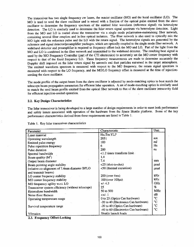
The transceiver has two single frequency cw lasers, the master oscillator (MO) and the local oscillator (LO). TheMO is used to seed the slave oscillator and is mixed with a fraction of the optical pulse emitted from the slaveoscillator to determine the frequency spectrum of the emitted lidar waveform (reference signal) via heterodynedetection. The LO is similarly used to determine the lidar return signal spectrum via heterodyne detection. Lightfrom the MO and LO is routed about the transceiver via a single mode polarization-maintaining fiber network,

containing several fiber couplers and in-line optical isolators. The fiber network is also used to optically mix theMO light with the reference pulse and the LO with the return signal. The heterodyne signals are generated by thereference and signal detector/preamplifier packages, which are optically couPled to the single mode fiber network. Awideband detector and preamplifier is required to frequency offset-lock the MO and LO. Part of the light from theMO and LO is combined in the fiber network and transmitted to the wideband detector. The resulting beat signal is

used by the MO Frequency Controller (part of the CTI electronics) to accurately set the MO center frequency withrespect to that of the fixed frequency LO. Three frequency measurements are made to determine accurately theDoppler shift imposed on the lidar return signal by aerosols and dust particles entrained in the target atmosphere.The emitted waveform spectrum is measured with respect to the MO frequency, the return signal spectrum ismeasured with respect to the LO frequency, and the MO/LO frequency offset is measured at the time of injection-seeding the slave oscillator.

The mode profile of the output beam from the slave oscillator is adjusted by mode-matching optics to best match thetelescope beam propagation parameters for efficient lidar operation. A set of mode-matching optics is similarly usedto match the seed beam profile emitted from the optical fiber network to that of the slave oscillator intracavity fieldfor efficient injection-seeded operation.

2.2. Key Design Characteristics

The lidar transceiver is being developed to a large number of design requirements in order to meet both Performanceand safety issues associated with operation of the hardware from the Space Shuttle platform. Some of the keyperformance characteristics derived from these requirements are listed in Table 1.

Table 1. Key lidar transceiver characteristics

Parameter Characteristic UnitLaser material Ho,Tm:YLF

Operating wavelength 2051 nmEmitted pulse energy 100 mJPulse repetition frequency 6 HzPulse duration 200 nsSpectral bandwidth < 1.2 times transform limitBeam quality (M2) 1.4Output beam diameter 7.4 mmBeam pointing angle stability <25 (shot-to-shot) _trad(relative co-alignment of 7.4mm diameter BPLO <50 (thermal excursion) gradand transmit beams)LO center frequency stability 200 (over 4ms) kHzMO center frequency stability 100 (over 100N) kHzMO frequency agility w.r.t. LO +/- 4.5 GHzTransceiver system efficiency (without telescope) 25 %Heterodyne bandwidth 50 to 500 MHzNoise floor flatness <+/- 1 dB

Operating temperature range 0 to 25 (Optics Can hardware) °C-20 to 40 (Electronics Can hardware) °C

Survival temperature range -20 to 40 (Optics Can hardware) °C-40 to 60 (Electronics Can hardware) °C

Vibration Shuttle launch loads

2.3. Frequency Offset-Locking

100

As part of the risk reduction activities planned for SPARCLE, CTI recently demonstrated locking of cw singlefrequency master and local oscillator frequencies to a center frequency accuracy of 10kHz over a frequency offsettuning range of +/-4.4GHz. This accuracy is maintained over tens of seconds. The intrinsic short term frequencystability of each laser is less than 100kHz over a 100 microsecond period, This frequency variation is super-imposedon the offset frequency selected by the locking electronics. The offset-locking circuitry includes a wideband detectorand preamplifier and a closed loop circuit that is part of the master oscillator frequency controller (MOFC). Theoutput of the controller drives the master oscillator piezo-electric stretcher element so as to achieve the correct MOfrequency with respect to the LO frequency. The beat frequency between the two lasers is detected by the widebanddetector and compared with a preset frequency in the electronic circuit. The piezo-electric stretcher is then adjustedin length until the beat frequency matches the preset frequency value.

As part of the recent offset-locl_ingdemonstration, CTI showed that the two lasers could be frequency offset-lockedover discrete frequency steps of 1GHz, selected arbitrarily between -4.4GHz and +4.4GHz. A 30ms period wasrequired after initial instruction to change frequency for the master oscillator to re-establish its characteristic stabilityof less than 100kHz frequencyjitter over 100microseconds.

2.4. Injection-Seeded Operation

CTI has also demonstrated injection-seeded Q-switched operation of a slave oscillator breadboard laser,reconfigured to match the flight hardware layout. A 15mW single frequency Ho,Tm:YLF laser with 50dB opticalisolation was used to seed the slave oscillator through the first diffraction order of the Q-switch3. Seeding was foundto be extremely stable with an efficiency (percentage of pulses seeded) exceeding 99%. Typical data indicated apulse duration (intensity FHWM) of about 200ns, single frequency operation of the seeded laser at a frequency offsetfrom the seed laser frequency by 25.5MHz (due to seeding through the Q-switch), and a pulse spectral bandwidth ofabout 1.4 MHz. The FFT spectrum indicated that axial mode beating in the laser was suppressed by more than 40dBfrom the seeded frequency component, verifying stable injection-seeded operation of the laser. The time-bandwidthproduct for the injection-seeded pulses was 0.277, verifying the ability of the ramp-and-fire seeding technique toproduce near-transform limited single frequency injection-seeded Q-switched operation.

3. DEVELOPMENT STATUS

The lidar transceiver is currently in the detailed design phase. In addition to completing the detailed design of theinstrument, we are performing risk reduction measurements to demonstrate the MO/LO frequency stability and thepointing stability of the slave oscillator and transmit/receive optical mounts over the operational and storageenvironmental and vibration levels. All performance requirements have been demonstrated under laboratoryconditions using the breadboard SO laser and prototype MO and LO lasers. Initial testing indicates that mirrormounts for the slave oscillator meet the alignment tolerance requirements over the operational temperature range, butadditional testing is required to verify this. It also remains to test the full slave oscillator with flight hardware overthe same operational temperature range. Prototype master and local oscillators have been shown to maintainfrequency and amplitude settings subsequent to experiencing the expected launch vibration spectrum. CTI iscurrently assessing the frequency stability of the master and local oscillators as a function of thermal cycling over thesurvival and operational temperature ranges. Details Of these results and other ongoing test activities prior to CDRwill be discussed in the meeting.

REFERENCES

1. Yu et al., "125-mJ diode-pumped injection-seeded Ho,Tm:YLF laser", Opt. Lett., 2__33,780-782 (May 15, 1998).2. Menzies et al., "Frequency-agile Tm,Ho:YLF local oscillator for a scanning Doppler Wind Lidar in Earth

Orbit", Paper Tu4, 9 th Conference on Coherent Laser Radar, Linkoping, Sweden (1997).3. Henderson et al., "Fast resonance-detection technique for single-frequency operation of injection-seeded

Nd:YAG lasers", Opt. Lett., 11, 715-717 (November 1986).

101

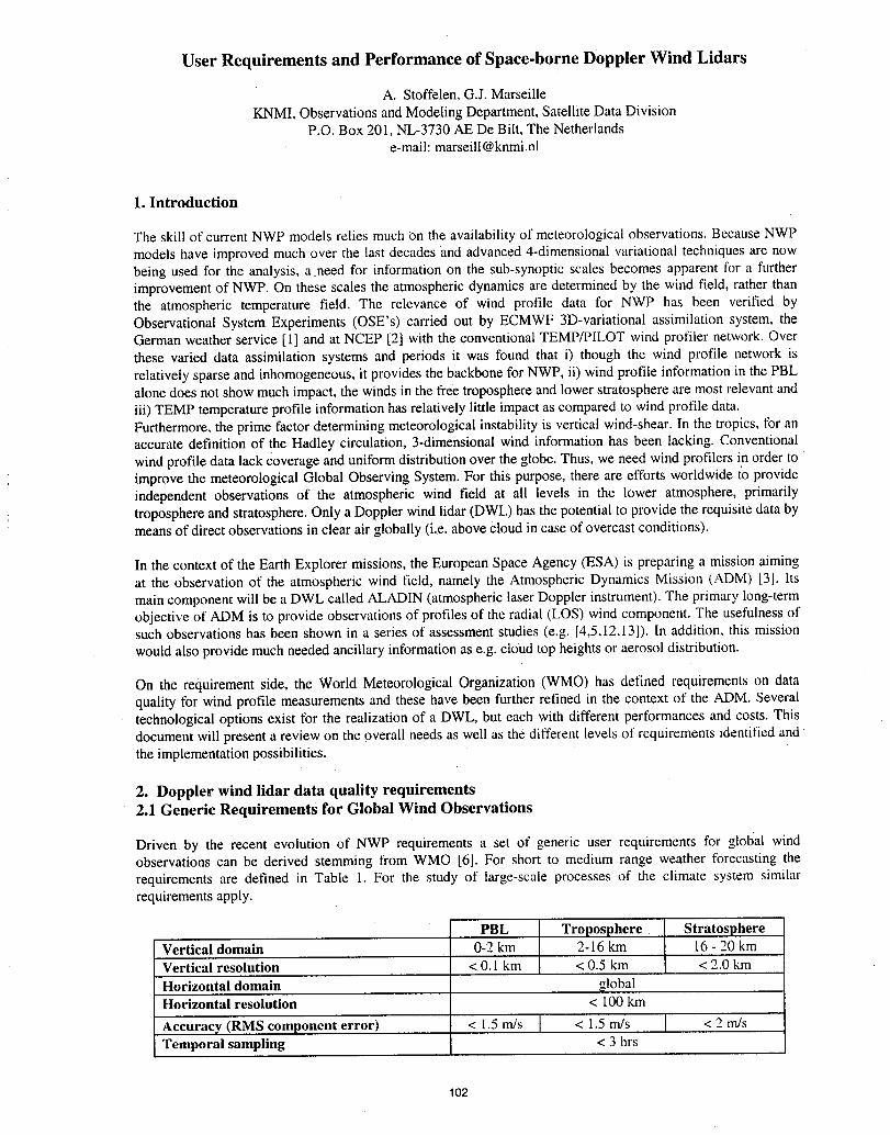
User Requirements and Performance of Space-borne Doppler Wind Lidars

A. Stoffelen, G.J. MarseilleKNMI, Observations and Modeling Department, Satellite Data Division

P.O. Box 201, NL-3730 AE De Bilt, The Netherlandse-maih marseill@knmi.nl

1. Introduction

The skill of current NWP models relies muchon the availabilityof meteorological observations. Because NWPmodels have improved much over the last decades and advanced4-dimensional variational techniquesare nowbeing used for the analysis, a need for informationon the sub-synoptic scales becomes apparent for a furtherimprovementof NWP. On these scales the atmosphericdynamics are determinedby the wind field, rather thanthe atmospheric temperature field. The relevance of wind profile data for NWP has been verified byObservational System Experiments (OSE's) carriedout by ECMWF 3D-variational assimilation system, theGermanweather service [l] and at NCEP [2] with the conventionalTEMP/PILOTwind profiler network. Overthese varied data assimilation systems and periods it was found that i) though the wind profile network isrelativelysparse and inhomogeneous,it provides the backbone forNWP, ii) wind profile intbrmationin the PBLalonedoes notshow much impact,the winds in the free troposphereand lower stratosphere are most relevant andiii) TEMP temperatureprofile informationhas relativelylittle impactas comparedto windprofile data.Furthermore,the prime factor determiningmeteorological instabilityis vertical wind-shear. In the tropics, for anaccuratedefinition of the Hadley circulation,3-dimensional wind informationhas been lacking. Conventionalwindprofile datalackCoverageanduniformdistributionover the globe. Thus, we need windprofilers in order toimprove the meteorologicalGlobal Observing System.For this purpose, there are efforts worldwidet'oprovideindependent observations of the atmospheric wind field at all levels in the lower atmosphere, primarilytroposphereandstratosphere.Only a Doppler windlidar(DWL) has thepotential to provide the requisite data bymeansof directobservations in clear airglobally (i.e. above cloud in case of overcastconditions).

In the context of the EarthExplorer missions, the EuropeanSpace Agency (ESA) is preparing a mission aimingat the observation of the atmospheric wind field, namely the Atmospheric Dynamics Mission (ADM) [3J. Itsmain componentwill be a DWL called ALADIN (atmospheric laser Doppler instrument).The primary long-termobjective of ADM is to provide observationsof profiles of the radial (LOS) windcomponent. The usefulnessofsuch observations has been shown in a seriesof assessment studies (e.g. [4,5,12,13]). In addition, this missionwouldalso provide muchneededancillary informationas e.g. cloud top heights or aerosol distribution.

On the requirementside, the World Meteorological Organization(WMO) has defined requirements on dataqualityfor wind profile measurementsand these have been further refined in the context of the ADM. Severaltechnological options exist for the realizationof a DWL, but each with different performances and costs. Thisdocumentwill presenta review on the overall needsas well as the different levels of requirements identifiedandthe implementationpossibilities.

2. Doppler wind lidar data quality requirements2.1 Generic Requirements for Global Wind Observations

Driven by the recent evolution of NWP requirements a set of generic user requirements for global windobservations can be derived stemming from WMO [6]. For short to medium range weather forecasting therequirements are defined in Table l. For the study of large-scale processes of the climate system similarrequirementsapply.

PBL Troposphere StratosphereVertical domain 0-2 km 2-16 km 16 - 20 kmVertical resolution < 0.1 km < 0.5 km < 2.0 km

Horizontal domain globalHorizontal resolution < 100km

Accuracy (RMS component error) < 1.5 m/s < 1.5 m/s < 2 m/sTemporal sampling < 3 hrs

102

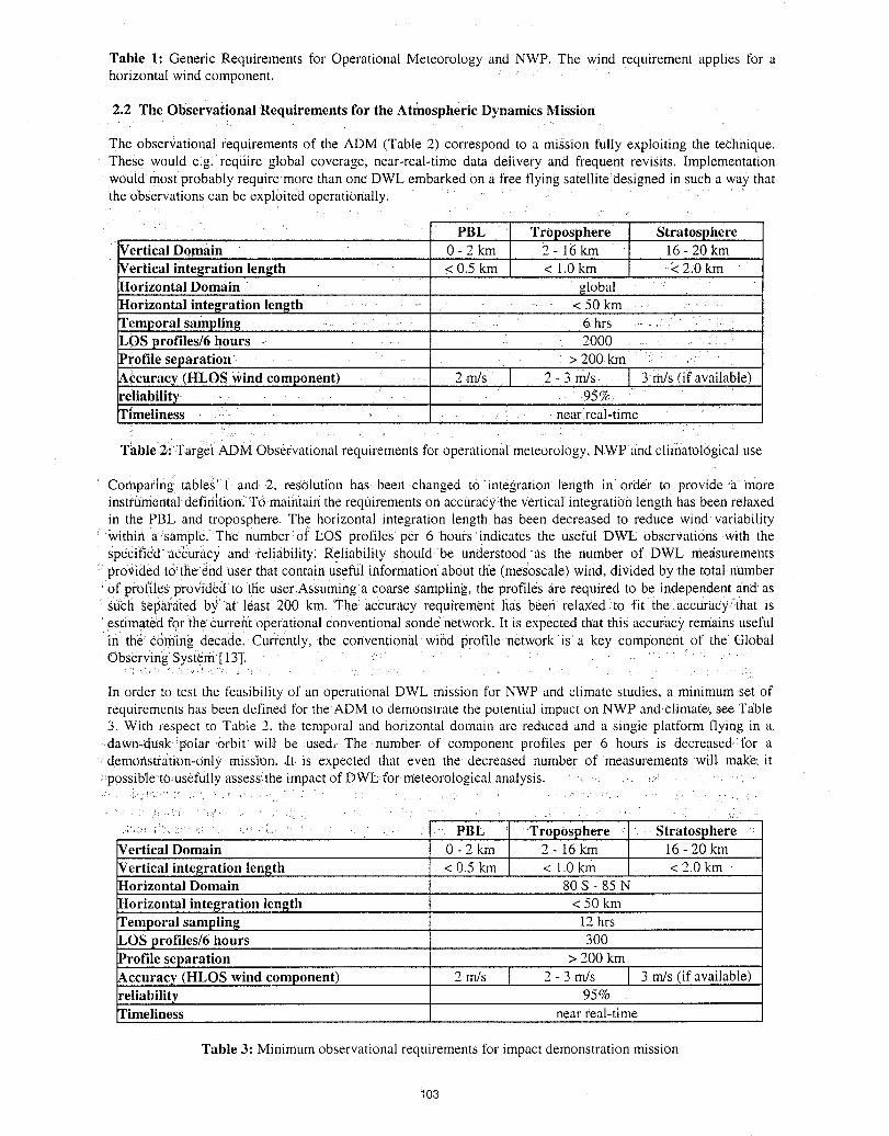
Table 1: Generic Requirements for Operational Meteorology and NWP. The wind requirement applies for ahorizontal wind component.

2.2 The Observational Requirements for the Atmospheric Dynamics Mission

The observational requirements of the ADM _,Table2) correspond to a mission fully exploiting the technique.These would e.g. require global coverage, near-real-time data delivery and frequent revisits. Implementationwould most probably reqmre more than one DWL embarked on a free flying satellitedesigned in such a way thatthe observations can be exploited operationally.

'_ " ...... PBL Troposphere Stratosphere

Vertical Domain 0 - 2 km 2 - 16km " 16- 20 kmVertical integration length _ 0.5 km < 1.0 km < 2.0 kmHorizontal Domain ' _lobal " "Horizontal integration length ................ .< 50 km .......l'emporal sampling ................ _. , . 6hi:s ...... • . ." :- ,LOS profiles/6 hours ...... 2000 . . ::Profile separation • " > 20Okra : : , •Accuracv (HLOS Windcomponent) 2 rrVs 2- 3 m/s. I 3 rn/s(i:favailable)reliabilitv..... ,- " .. - " 95%--.. " - ,rlmeliness : : , .-, .: . near[real-time

Thble.:2::Target. ADM Observational requirements for operational meteorology, NWP .andclimatological use

Comparing tables' I and .2, resolution has been changed to integration' length in order to provide oa moreinsttfimental-defiriitionlTOmaintainthe requirements on accuracy the Verticalintegration .length has been relaxedin the PBL and troposphere. The horizontal integration length has been decreased to reduce wind variabilitywithin a-sample. The number:of LOS profiles per 6 hours indicates the useful DWL Observations with.thespocified_accuracy and reliability: Reliability shouldbe understood"as the number of DWL me_isurementsprovided tO_the"_nduser that contain usefu'linformation:about the (me'sosCalepwind. divided by the total numberof profiles proxiidedto the user.Assuming a coarse sampling, the profiles are required to be independent and asstieh separated b3_'a( least 200 km. _The accuracy requirement has been relax_ed;to fit the accuracy.:(hat isestimated for the current operational conventional sonde n_twork. It is expected that this accuracy remains usefulin the CiSri'iln_decade. Currently,-the conventional wind profile networkis'a key Component of the GlobalObserving System [1.3],

[n order to test the feasibility of an operational DWL mission for NWP and climate studies, a minimum set ofrequirements has been defined for the ADM to demonstrate the potential tmpact on NWP and-climate:,see Tzible3. With respect to Table 2, the temporal and horizontal domain are reduced and a single platform flying in a_

•dawmdusk-polar .orbit' wil:l be used,..The •number. of component profiles per 6. hours is decreased:for a. demonstration-only .missit)n..It. is expected that even thedecreased number of measurements will, make:•it:,possibleto-usefully assess':theimpact of DWE:for.meteorological analysis.• ' : -.:. .,. , >' . .... •

.... ; ...... , . . . .. ,

• . : , ,. . 2':,%: ,' ' , : = i . ' i: ...... , , :, : : , >[.

•::,, ;_":..:..... , :., . i " - • , .. ." PBL " ,'Troposphere _ . Stratosphere ,:Vertical Domain 0 - 2 km 2 - 16 km t6 - 20 km

Vertical integration length < 0.5 km < 1.0 km < 2.0 kmHorizontal Domain 80 S - 85 N

Horizontal integration length < 50 kmremporal sampling 12 hrsLOS profiles/6 hours 300Profile separation > 200 km_,ccuracv (HLOS wind component) 2 m/s 2 - 3 m/s 3 m/s (if available):eliabilit v 95%Hmeliness near real-time

Table 3: Minimum observational requirements for impact demonstration mission

103

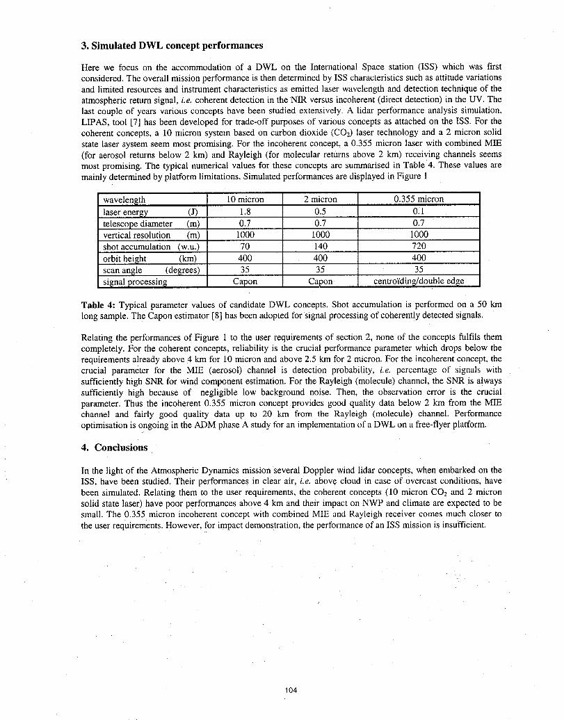
3. Simulated DWL concept performances

Here we focus on the accommodationof a DWL on the InternationalSpace station (ISS) which was firstconsidered.The overallmission performanceis thendetermined by ISS characteristicssuch as attitudevariationsand limited resources and instrumentcharacteristics as emittedlaser wavelengthand detection techniqueof theatmosphericreturnsignal, i.e. coherent detectionin theNIR versus incoherent (direct detection) in the UV. Thelast couple of years various concepts have been studied extensively. A lidar performance analysis simulation,LIPAS, tool [7] has been developed for trade-offpurposes of various concepts as attached on the ISS. For thecoherent concepts, a 10 micron system based on carbon dioxide (CO2) laser technology and a 2 micron solidstate laser system seem most promising.For the incoherent concept, a 0.355 micron laser with combined MIE(for aerosol returns below 2 km) and Rayleigh (for molecular returns above 2 kin) receiving channels-seemsmost promising. The typical numericalvalues for these concepts are summarisedin Table 4. These values aremainlydeterminedby platformlimitations.Simulatedperformancesaredisplayedin Figure I

wavelength 10 micron 2 micron 0.355 micronlaserenergy (J) 1.8 0.5 0.1telescope diameter (m) 0.7 0.7 0.7vertical resolution (m) 1000 1000 1000shot accumulation (w.u.) 70 140 720

orbit height (km) 400 400 400scan angle (degrees) 35 35 35signal processing Capon Capon centro'fdin_double edge

Table 4: Typical parameter values of candidate DWL concepts. Shot accumulation is performed on a 50 kmlong sample. The Capon estimator [8] has been adopted for signal processing of coherently detected signals.

Relating the performances of Figure i to the user requirements of section 2, none of the concepts fulfils themcompletely. For the coherent concepts, reliability is the crucial performance parameter which drops below therequirements already above 4 km for 10 micron and above 2.5 km for 2 micron. For the incoherent concept, thecrucial parameter for the MIE (aerosol) channel is detection probability, i.e. percentage of signals withsufficiently high SNR for wind component estimation. For the Rayleigh (molecule) channel, the SNR is alwayssufficiently high because of negligible low background noise. Then, the observation error is the crucialparameter. Thus the incoherent 0.355 micron concept provides good quality data below 2 km from the MIEchannel and fairly good quality data up to 20 km from the Rayleigh (molecule) channel. Performanceoptimisation is ongoing in the ADM phase A study for an implementation of a DWL on a free-flyer platform.

4. Conclusions

In the light of the Atmospheric Dynamics mission several Doppler wind lidar concepts, when embarked on theISS, have been studied. Their performances in clear air, i.e. above cloud m case of overcast conditions, havebeen simulated. Relating them to the user requirements, the coherent concepts (10 micron CO, and 2 micronsolid state laser) have poor performances above 4 km and their impact on NWP and climate are expected to besmall. The 0.355 micron incoherent concept with combined MIE and Rayleigh receiver comes much closer tothe user requirements. However, for impact demonstration, the performance of an ISS mission is insufficient.

104

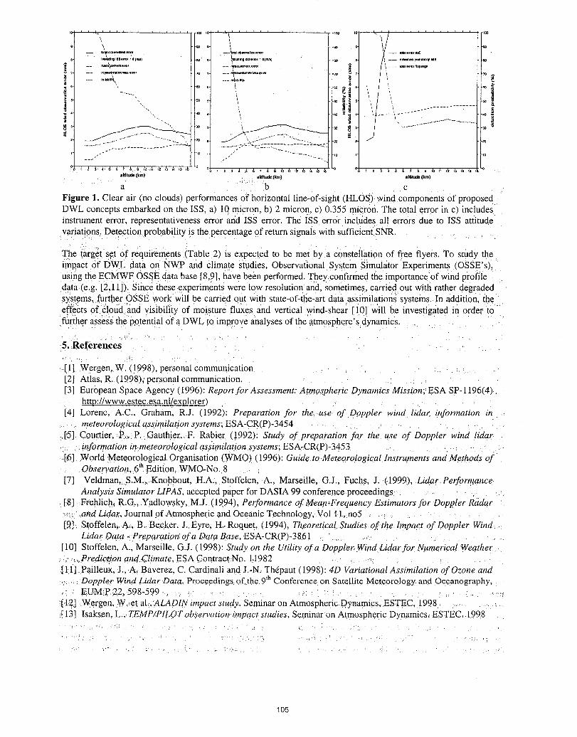
! "1t' ......................I0 i0 I"t rio

altitude(kin) altitude(kin) altltud_(kin)

a b c

Figure 1. Clear air (no clouds) performances of horizontal line-of-sight (HLOS) wind components of proposedDWL concepts embarked on the ISS, a) 10 micron, b) 2 micron, c) 0.355 mi(ron. The total error in c) includesinstrument error, representativeness error and ISS error. The ISS error includes all errors due to ISS attitude

•variations. Detection probability is the.percentage of return signals with sufficient SNR.

The target s,et of requirements (Table 2) is expected to be met by a constellation of free flyers. To study theimpact Of DWL data on NWP and climate studies, Observational System Simulator Experiments (OSSE's),using the ECMWF OSSE data base [8,9], have been performed. They :confirmed the importance of wind pi'ofile

data (e.g. [2,11]). since these.experiments were low resolution and, sometimes, carried, out with rather degradedsystems,.further OSSE work will be carried OUt with state-of-tile-art data assimilations systems. In addition, (heet_feCtsof €loud and visibifity of moisture fluxes and vertical wind-shear [l_0] will be investigated in order tO

further assess the potential of a DWL to improve analyses of the .atmosphere's dynamics.

-5.Ret'erences:.

[!] Wergen,.W. (1998), personal communication[2] Atlas, R. (1998); personal communication.[3] European Space Agency (1996): Report for Assessment: Atmospheric _Qynamics Mission; ESA SP-1196(4)..

http://www.estec.esa.nl/explorer)[4] Lorenc, A.C., Graham, R.J. (1992): Preparation for theuse of Dopp_er wi.nd lida_ information in

meteorological assimilation systems; ESA:CR,(P)-3454 , .[-'5]Courtier,;P;, P. Gauthier, F. Rabier (!992): Study of preparation far the use of Doppler wind lidar

. information in meteorological assimilation systems; ESA-CR(.P-)-3453 ....•[f!] XVortd Meteorolog!cal Orgamsation (WMO) (1996): Guid¢.toMeteo, ro]ogical Instruments and Methods of

Observation, 6thEditi'on, WMO-No. 8

[7] Veldman, S.M..,Knobbout, H.A., Stoffelen, A., Marsei}le, G.J., Fuchs, J. (-1999), Lidar PerformanceAnalysis Simulator LIPAS, accepted paper for DASIA 99 conference proceedings - -

[8] Frehlich, R.G.,,Yadlowsky; M.J. (,1_94), Performance of M_ean,Frequency.Estimators for Doppler Radar:_ .1a(7.d Lidar,, Journal of Atmospheric and Oceanic Technology, Vol 11..no5 , :[.9,]: Stoffelen_ A.. B._Beeker. L Eyre. H, Roquet, (1994), Theoretical Studies.of tOe:Impact of Doppler Wind

Lidar Data : Prept!rafior_ of a Data Base, ESA-CR(P)-386 ! " .._

[10] Stoffelen. A., Marseille, G.J. (1998): Study on the Utili_ of a Doppler.,.Wind Lidar for Numerical Wea.ther"1 _.', .Prediction and.Climate, ESA.Contract:No. 1:1982 - :

_[1;1] Pailleux, J.. A, Baverez. C. Cardinali and J.-N, Th6paut (1998): 4D Variational Assimilation of Ozone and,. Doppler Wind Lidar.Data, Proceedings of_the,9 thConference on Satellite Meteorology', and Oceanography,

EUMIP 22, 5.9.8-599., : : : , • : • ....... , 1 . I ..... :i[.!_2]:Wergl_n, -W, l_et ab,:ALADIN impact study, Seminar on Atmospheric Dynamics, ESTEC, 1998 ....._[13] Isaksen. L., TEMP/PILOTobse.rvation, impact studies, Seminar on Atmospheric Dyn.amics_ ESTEC., 1998

,105

Comparing the Intrinsic, Photon Shot Noise Limited Sensitivity of Coherent and DirectDetection Doppler Wind Lidar

Jack A. McKayRemote SensorConcepts,LLC

3200 19th StNWWashington,DC 20010

j.a.mckay@worldnet.att.net

Introduction comparison of a Rayleigh backscatterdirectdetectionDoppler wind lidar(DWL) to an aerosol backscatter,

Remotemeasurementof atmosphericwind speeds with coherentalternative."direct" detection Doppler lidar, i.e., opticalinterferometryfor Dopplershift measurement,has long Approachbeen considered as an alternative to coherent,heterodyne techniques. Direct detection offers some TheCRLB yieldsan estimateof the minimumstatisticalpracticaladvantages,including eliminationof the local uncertaintyof the knowledge of the centroid of aoscillator,eliminationofwavefront phase preservation frequencydistribution,based on the concept of eachconcerns,availabilityof verymatureand efficient laser photon being a randomsampling of that distribution.technology, and the possibility of using Rayleigh Here all questions of optics and detector quantum(molecular) backscatterto overcome dependenceon efficiencies are set aside, so that the result will notatmosphericaerosols.These advantagesare particularly depend on any assumptionof hardware performancesignificantforthe measurementof global wind profiles parameters. Let us suppose that the receiver systemfrom low Earthorbit, and concepts for satellitebased would, absentthe Doppler analysisoptics (the Fabry-direct detection systems are currently under Perot interferometerof the direct detection systems),developmentin the United Statesandin Europe. measure N photocounts, and that the source signal

spectrum can reasonably be described by a GaussianThe principal liability of direct detection appears to be with 1/e width Avo. Then the CRLB to the standardits relatively low sensitivity. In 1986 a study by R.T. deviation of the measurement, 6v, is given by2Menzies1 concluded that direct detection, aerosol

backscatter systems would require roughly an order of 6v = _:Ave/(2N)1/2 (1)magnitudehigher laserpower-receiver aperture productthan coherent systemsto achievethe same measurement where the factor _: is unity for a perfect, losslessaccuracy. The high cost of spaceflight systems with Doppler analyzer, which could simply measure thehigh laseroutput power and large receiver aperture has frequency of each photon without loss and withoutdeterreddevelopment of the directdetection alternative, degradationof the source spectrum. In reality, Kwill be

greater than I, due not to imperfectionsof hardwarebutThe work by Menzies did not yield explicit reasons for to the physics of the Doppler analyzer.this large difference in sensitivitybetween coherent anddirect detection. The Menzies study included optical For the coherent system, the intrinsic loss mechanismsand detection efficiency estimates, and aerosol include speckle noise at high levels, and small signalbackscatter wavelength dependences, so it is not clear suppression at low3. The minimum theoreticallywhether the difference found was a fundamental achievable value of_: is about 2.3 (Figure 1).property of direct versus coherent detection, or was aconsequence of assumptions of system parameters. The intrinsic lossesof directdetection Doppler analysis

are due to the Fabry-Perot etalon that is used forHere the physicsof direct andcoherent detection,in the frequency shift determination, via either the "fringeframework of the Cramer-Rao Lower Bound (CRLB) imaging" technique generally associated with P.B.estimateto measurementprecision, is explored, in order Hays4and D. Rees5,or the "edge technique", developedto determine whether direct detection is in fact by CNRS6and advocated by Gentry and Korb7.N inintrinsically less sensitive than coherent detection, in Eq. (1) for direct detection is the number of potentialtheory and in practice. The analysis is extended from photocounts, i.e., the number incident on the etalon.the aerosol-only systems considered by Menzies to a The factor _: describes photon losses due to etalon

106

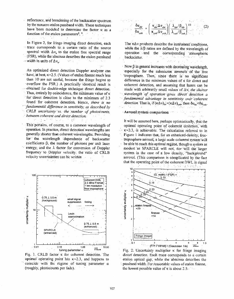
reflectance, and broadening of the backscatter spectrum . .... :

bythe nonzero etalon passbandwidth. Thesetechniques 6Uqj_= I naj_AVa_)()_dJ[Sa_') ,/z (2)have been modeled to determinethe factor .K as a &tcoh _ Kcoh._V¢o£)_ _,.oh]_.o_):function of the etalon parameters_, 9.

In Figure 2, for fringe:imaging ,direct detection, each The'KAy products describe the instmmentconditions,trace corresponds to.a certain ratio of the source while the MI3ratios are defined by the wavelength ofspectral width Ave to the etalon free spectTal range operation .and the corresponding atmospheric(FSR),while.theabscissa'describes the etalon passband backscatter. -. :.... ':width in units ofAv e. .

Now 13ingeneral inci'easeswith decreasingwa,;,eleiagth,An optimized direct detection Doppler analyzer can especially for-the submicron aerosols_ 0f',the flee

have.atbest,._=2.5.(ValuesofetalongmessemuCh less troposphere. Then, singe .there is no significantthan 10-.are not useful, because the fringe begins to difference in the minimum values of K for direct andoVerflOwthe FSR.) A practically identical result is coherent detection, and assuming that lasers can be.obtained:for double-edge technique direct detection, made with arbitrarily small values of Av; the shorterThus, entirely by coincidence_-theminimum value_of K wavelength of _operation' gives di)_oet_dete'cfion afordirect detection is close to the min'imum of 2.3 fimdamentiil advantage m sensitivity over._¢oherentfound' for coherentdeteCtion. Hence, there is no detection. :Thatis_if(KA_v)dli=(KAv)_o_;'then6Ud_i<gU¢oh.

"fundamenti_l difference:in sensitivity, as described by .....

CRLB uncertainty :vs. the number of photocounts, Aerosol system comparisonbetween, coherent and direct detection.-

"" ..... - " Itwill be assumed here, perhaps optimistically, that theThis!pertains, of course, to a-commonwavelength of optimaloperating point of coheretit !det_ctiori,"withoperation. In practice,:direct.detection wavelengthsare K=2.3, is achievable. The calculation, referred to ingenerallyshorter than coherent wavelengths. Providing Figure. 1 indicates that, f0ran enhanced-density; free-for the wavelength -dependence of backscatter troposphereaerosol, a large scale coherent system_willcoefficients-[3,:the number of photons per unit laser be able"tOreach thisoptimal regii_e; though,a systemasenergy, ,and the _. factor for conversion of Doppler modest"as SPARCLE will not, r_or'will thelargerfrequency to DOppler velocity; the ratio of CRLB system in the case Of a low densi67,_"backgmufid"velocity uncertainties'can be written aerosol (This comparison is complicated by the..fact

...... ' that the operating point of the coherent DWL is signal. _ . • , , _ .!

lO i i i I i t i i9 .......

100 ' ' ''''"1 ' ' ''''"1 , , ,,,[,, a :. -'"--&0.10 ......... : .....

.o.ereo.o.,2.5 MHz FWHM.I[1 km resolution 6[free troposphere "_ "_.._.20 _ - J . . .,., 5

(background) small signal_. . suppression fading _ , .J ,

" ' ] \i J =_....... ....... 1_ =10finesse- _..__ _

,o i>'LA - -.- Levin .- .

_ ,1_ _"__'imati°n 2 -= _- "_ 0.75 J, 0.5 m

/ _ (enhanced)SPARCLE

(enhanced)

Fringe imager]1 t I - I 1 I'. I I I

1 I I I IIIlII I "1 I IIIIIJ I I f I III 0.1 2 4 6 8 1.0

O,Ol O.lO 1.oo lO.OO (FPI FVVHM) 1 (Gaussian lie)

tuhingparameter_z ...... Fig. 2: Uncertainty multiplier _ for fringe imagingFig. I CRLB factor K t'or coherent detection. The direct:detection: Each trace corresponds to a certainoptimal operating pointhas _=2.3, and happens to etalon optical gap, while 'the abscissa describes thecoincide with the t'egime of tuning parameter _ passbandwidth. For reasonablevaluesofetalon finesse,(roughly, ph0tocounts per fade), the lowest possible value of n is about 2.5_

107

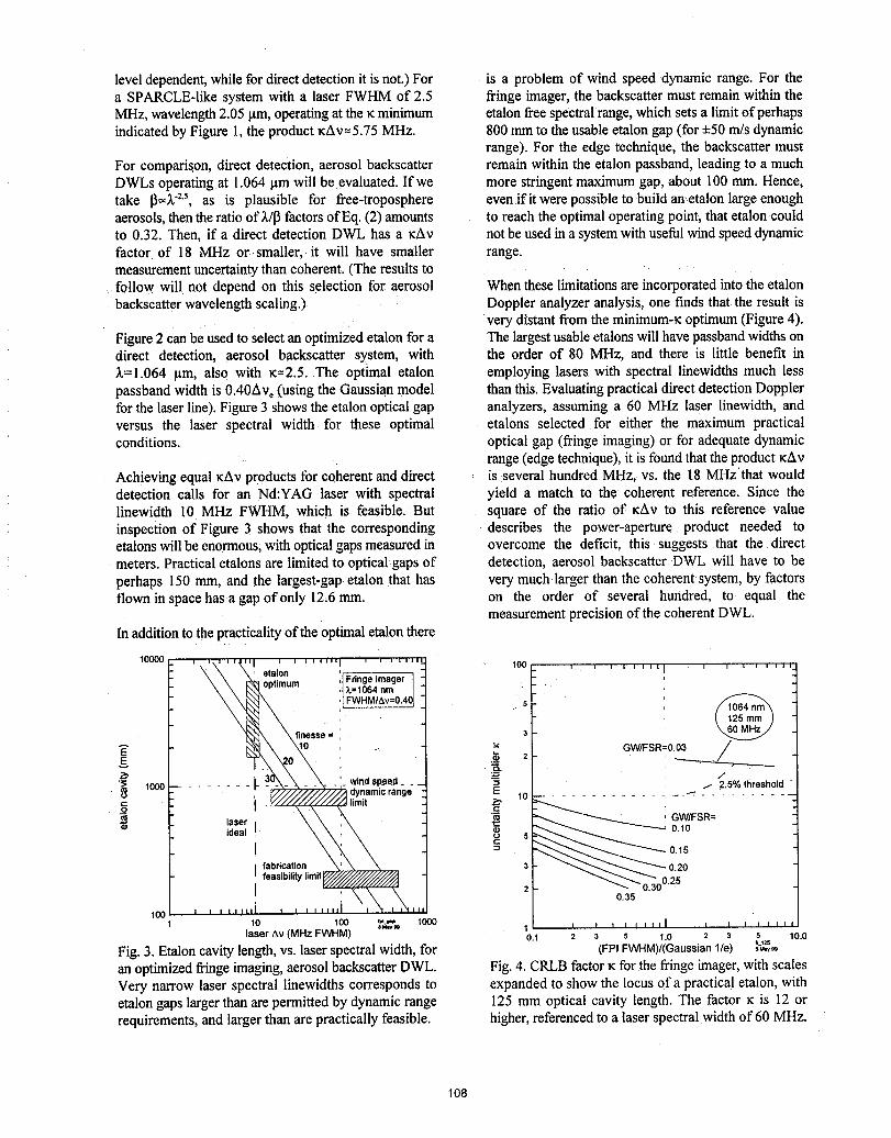
level dependent,while for directdetection it is not.) For is a problem of wind speed dynamic range. For thea SPARCLE-Iike system with a laser FWHM of 2.5 fringe imager, the backscatter must remain within theMHz, wavelength2.05 _tm,operating at the Kminimum etalon free spectral range, which sets a limitof perhapsindicated by Figure 1, the product KAy=5.75MHz. 800 mm to the usable etalon gap (for 4:50m/s dynamic

range). For the edge technique, the backscatter mustFor comparison, direct detection, aerosol backscatter remain within the etalon passband, leading to a muchDWLs operatingat 1.064 lamwill be evaluated. If we more stringent maximum gap, about 100ram. Hence,take 13=;_zS, as is plausible for free-troposphere even ifitwere possibleto build an,etalon large enoughaerosols,then the ratio of\/13 factors of Eq. (2) amounts to reach the optimal operating point, that etaloncouldto 0.32. Then, if a direct detection DWL has a _:Av not be used ina systemwith usefulwind speed dynamicfactor of 18 MHz or smaller, it will have smaller range.measurementuncertaintythan coherent. (The results tofollow will not depend on this selection for aerosol Whenthese limitationsare incorporated into the etalonbackscatter wavelength scaling.) Doppler analyzer analysis, one finds that the result is

very distant from the minimum-_ optimum (Figure 4).Figure 2 can be used to select an optimized etalon for a The largest usable etalons will have passband widths ondirect detection, aerosol backscatter system, with the order of 80 MHz, and there is little benefit in_,=1.064 pm, also with _=2.5. The optimal etalon employing lasers with spectral linewidths much lesspassband width is 0.40Av, (using the Gaussian model than this. Evaluating practical direct detection Dopplerfor the laser line).Figure 3 showsthe etalon optical gap analyzers, assuming a 60 MHz laser linewidth, andversus the laser spectral width for these optimal etaions selected for either the. maximum practicalconditions, optical gap (fringe imaging) or for adequate dynamic

range (edge technique), it is found that the product tcAvAchieving equal KAyproducts for coherent and direct is several hundred MHz, vs. the 18 MHzthat woulddetection calls for an Nd:YAG laser with spectral yield a match to the coherent reference. Since thelinewidth 10 MHz FWHM, which is feasible. But square of the ratio of tcAv to this referencevalueinspection of Figure 3 shows that the corresponding describes the power-aperture product needed toetalons will be enormous,with optical gaps measured in overcome the deficit, this suggests that the directmeters. Practical etalons are limited to optical gaps of detection, aerosol backscatter DWL will have to beperhaps 150 mm, and the largest-gap etalon that has very much larger than the coherent system, by factorsflown in spacehasagapofonly 12.6mm. on the order of several hundred, to equal the

measurement precision of the coherent DWL.In addition to the practicalityof the optimal etalon there

10o00•, ,, ,, ,"_ ''_'1 _ _ _ ''_'=1 ' ' ' ''J_' 100

^_ti.... JFnnge Imager I\\m e_, ,,,u., ,]Z=1064nm |

_'_ \finesse = : z

_'3N_X X -- •' windpp_eed '_......... r - - - '- . " - 2.5% threshold

"' I "_'//////</////_limit :>. 10 ..........................o \\laser "_ GWIFSR=\\,\ = o.Ioideal _ . _ S

I 0.15

fabrication 3

' feasibility Iimit_I100 I I I I IIIll I I I I Illll II

10 100 _-_ 1000i M=/te

laser AV(MHz FWHM) 0.t 2 3 5 1.0 2 3 5 10.0

Fig. 3. Etalon cavity length, vs. laser spectralwidth, for (FPIFWHM)/(Gaussianlie) ....5M_

anoptimizedfringe imaging,aerosolbackscatterDWL. Fig.4. CRLBfactorKfor the fringe imager,with scalesVery narrow laser spectral linewidths correspondsto expandedto show the locus of a practicaletalon, withetalongaps largerthan arepermittedby dynamicrange 125 mm optical cavity length. The factor _ is 12 orrequirements,and largerthanare practicallyfeasible, higher,referencedto a laserspectral widthof 60 MHz.

108

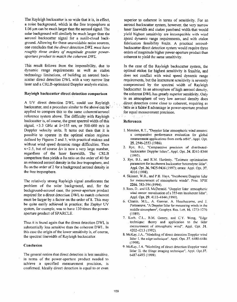
The Rayleigh backscatter is so wide that it is, in effect, superior to coherent in terms of sensitivity. For ana noise background, which in the free troposphere at aerosol backscatter system, however, the very narrow1.06p,mcan be much larger than the aerosol signal. The laser linewidth and etalon passband width that wouldsolar background will similarly be much larger than the yield highest sensitivity are incompatible with windaerosol backscatter signal for a sunlit-cloud back- speed dynamic range requirements, and with etalonground. Allowing for these unavoidable noise sources, fabrication feasibility limits. A practical aerosol-one concludesthat the direct detection DWL must have backscatterdirectdetection systemwould require threeroughly three orders of magnitude greater power- ordersof magnitudehigher power-apertureproduct thanaperture product to match the coherent DWL. coherent to yield the same sensitivity.

This result follows from the impossibility, due to In the case of the Rayleigh backscatter system, thedynamic range requirements as well as etalon optimal etalon for highest sensitivity is feasible, andtechnology limitations, of building an aerosol back- does not conflict with wind speed dynamic rangescatter direct detection DWL with a very narrow line requirements, but the instrument sensitivity is severelylaser and a CRLB-optimized Doppler analysis etalon, compromised by the spectral width of Rayleigh

backscatter. In an atmosphere of high aerosol density,Rayleigh backscatter direct detection comparison the coherent DWL has greatly superior sensitivity.Only

in an atmosphere of very low aerosol density doesA UV direct detection DWL could use Rayleigh i:: _direct detection come close to coherent, requiring asbackscatter,and a procedure similar to the above Canb_e_ .Jittle as a fa_t0r8 advantage inpower-aperture productapplied to compare this to the same coherent/aerosol for equal measurement precision.reference system above. The difficultyIwith Rayl.eigh ._. -_ :" _:: ......_backscatter is, of course, the great spectralwidth of this Referencessignal, =3.3 GHz at _,=355 nm, or 500-600 m/s inDoppler velocity units. It turns out then that it is 1.Menzies,R.T.,"Dopplerlidaratmosphericwindsensors:possible to operate in the optimal etalon regimes a comparative performance evaluation tbr globaldefined by Figures 2 and 3, with practical etalons and measurement applications fromearthorbit",Appl. Opt.

without wind speed dynamic range difficulties. Then 25,2546-2553(1986).K=2.5, but of course Av is now a very large number, 2. Rye, B.J., "Comparative precision of distributed-

backscatterDopplerlidars".Appl.Opt. 34. 8341-8344regardless of the laser linewidth. The CRLB (1995).comparison then yields a _Suratio on the order of 40 for 3. Rye, B.J., and R.M. Hardesty,"Estimateoptimizationan enhancedaerosol density in the free troposphere, and parametersforincoherentbackscatterheterodynelidar",6u on the order of 2 for a background aerosol density in Appl.Opt.36, 9425,9436(1997);errata:Appl.Opt.37,the free troposphere. 4016(1998).

4. Skinner,W.R.,and P.B. Hays."IncoherentDopplerlidarThe relatively strong Rayteigh signal ameliorates the tbr measurementof atmosphericwinds",Proc. SPIEproblem of the solar background, and, for the 2266,383-394(1994).background-aerosol case, the power-aperture product 5. Rees.D..andI.S.McDermid,"Dopplerlidar atmosphericwindsensor:reevaluationof a 355-nmincoherentlidar".required for a direct detection DWL to match coherent Appl.Opt.29, 4133-4144(1990).must be larger by a factor on the order of 8. This may 6. Chanin, M.L., A. Gamier. A. Hauchecorne.and J.be quite easily achieved in practice; the Zephyr UV Porteneuve,"ADopplerlidartbrmeasuringwindsin thesystem, for example,was to have 130times the power- middleatmosphere",Geophys. Res.Lett.16.1273-1276aperture product of SPARCLE. (1989).

7. Korb, C.L., B.M. Gentry,,and C.Y. Weng, "EdgeThus it is found again that the direct detection DWL is technique: theory and application to the lidarsubstantially less sensitive than the coherent DWL. In measurementof atmosphericwind", Appl. Opt. 31.this case the origin of the lower sensitivity is, of course, 4202-4213(1992).

8. McKay,J.A., ',Modelingof directdetectionDopplerwindthe spectral linewidth of Rayleigh backscatter.lidar: I. the edge technique", Appl. Opt. 37, 6480-6486(1998).

Conclusion 9. McKay, J.A. "Modeling of direct detection Doppler windlidar: II.the fringeimagingtechnique".Appl.Opt.37.

The general notion that direct detection is less sensitive, 6487-6493(1998).in terms of the power-aperture product needed toachieve a specified measurement precision, isconfirmed. Ideally direct detection is equal to or even

109

New TechnologyPresider: Richard Richmond

11o

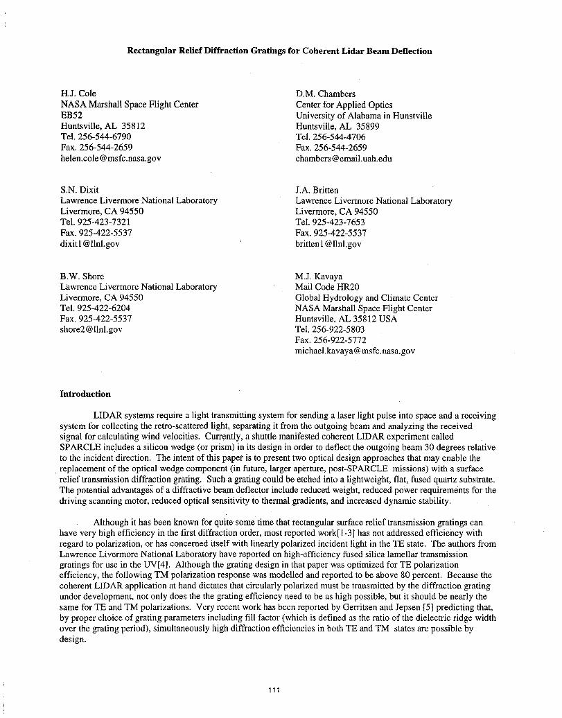
Rectangular Relief Diffraction Gratings for Coherent Lidar Beam Deflection

H.J. Cole D.M. Chambers

NASA Marshall Space Flight Center Center for Applied OpticsEB52 University of Alabama in HunstvilleHuntsville, AL 35812 Huntsville, AL 35899Tel. 256-544-6790 Tel. 256-544-4706Fax. 256-544-2659 Fax. 256-544-2659

helen.cole@msfc.nasa.gov chambers@email.uah.edu

S.N. Dixit J.A. Britten

Lawrence Livermore National Laboratory Lawrence Livermore National LaboratoryLivermore, CA 94550 Livermore, CA 94550Tel. 925-423-7321 Tel. 925-423-7653Fax. 925-422-5537 Fax. 925-422-5537

dixit 1@llnl.gov britten1@llnl.gov

B.W. Shore M.J. KavayaLawrence Livermore National Laboratory Mail Code HR20Livermore, CA 94550 Global Hydrology and Climate CenterTel. 925-422-6204 NASA Marshall Space Flight CenterFax. 925-422-5537 Huntsville, AL 35812 USAshore2@llnl.gov Tel. 256-922-5803

Fax. 256-922-5772

michael.kavaya@msfc.nasa.gov

Introduction

LIDAR systems require a light transmitting system for sending a laser light pulse into space and a receivingsystem for collecting the retro-scattered light, separating it from the outgoing beam and analyzing the receivedsignal for calculating wind velocities. Currently, a shuttle manifested coherent LIDAR experiment calledSPARCLE includes a silicon wedge (or prism) in its design in order to deflect the outgoing beam 30 degrees relativeto the incident direction. The intent of this paper is to present two optical design approaches that may enable thereplacement of the optical wedge component (in future, larger aperture, post-SPARCLE missions) with a surfacerelief transmission diffraction grating. Such a grating could be etched into a lightweight, flat, fused quartz substrate.The potential advantages of a diffractive beam deflector include reduced weight, reduced power requirements for thedriving scanning motor, reduced optical sensitivity to thermal gradients, and increased dynamic stability.

Although it has been known for quite some time that rectangular surface relief transmission gratings canhave very high efficiency in the first diffraction order, most reported work[I-3] has not addressed efficiency withregard to polarization, or has concerned itself with linearly polarized incident light in the TE state. The authors fromLawrence Livermore National Laboratory have reported on high-efficiency fused silica lamellar transmissiongratings for use in the UV[4]. Although the grating design in that paper was optimized for TE polarizationefficiency, the following TM polarization response was modelled and reported to be above 80 percent. Because thecoherent LIDAR application at hand dictates that circularly polarized must be transmitted by the diffraction gratingunder development, not only does the the grating efficiency need to be as high possible, but it should be nearly thesame for TE and TM polarizations. Very recent work has been reported by Gerritsen and Jepsen [5] predicting that,by proper choice of grating parameters including fill factor (which is defined as the ratio of the dielectric ridge widthover the grating period), simultaneously high diffraction efficiencies in both TE and TM states are possible bydesign.

111

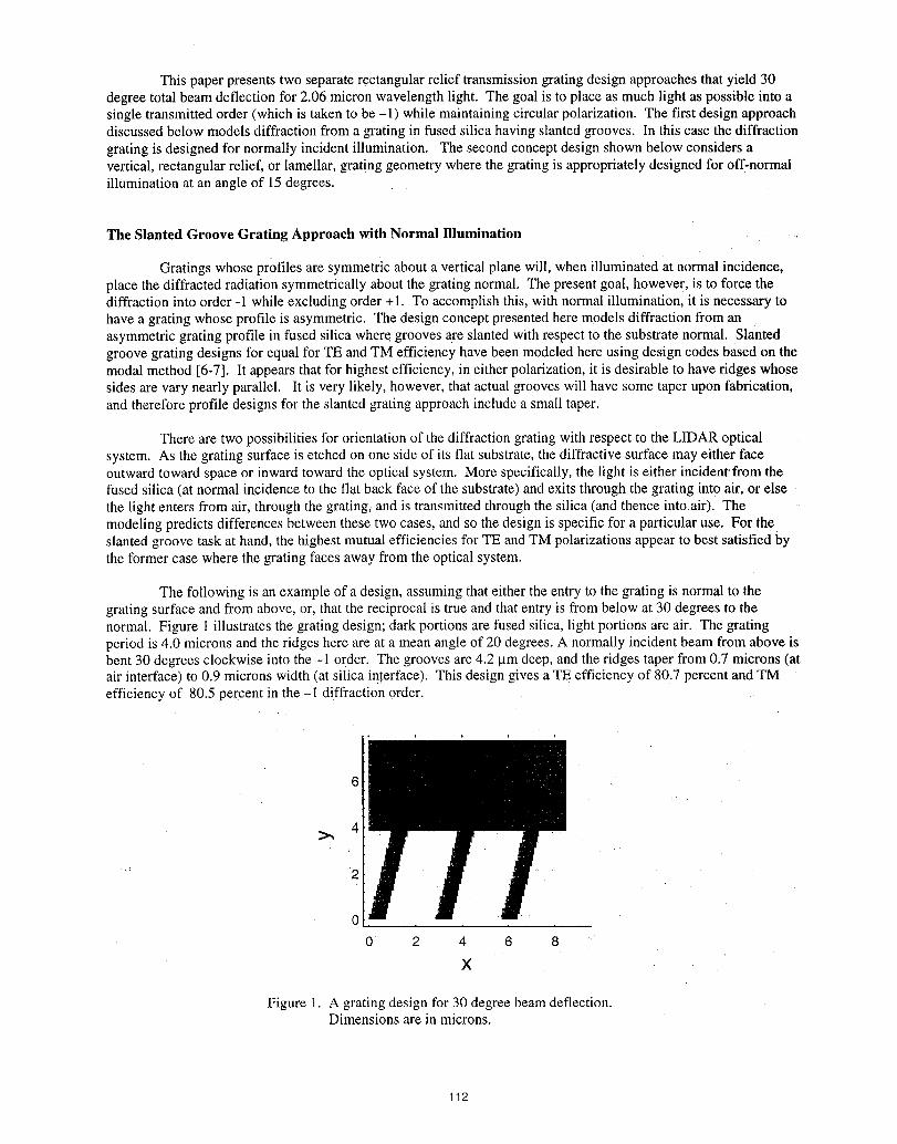
This paper presents two separate rectangular relief transmission grating design approaches that yield 30degree total beam deflection for 2.06 micron wavelength light. The goal is to place as much light as possible into asingle transmitted order (which is taken to be -1) while maintaining circular polarization. The first design approachdiscussed below models diffraction from a gating in fused silica having slanted grooves. In this case the diffractiongrating is designed for normally incident illumination. The second concept design shown below considers avertical, rectangular relief, or lamellar, grating geometry where the grating is appropriately designed for off-normalillumination at an angle of 15degrees.

The Slanted Groove Grating Approach with Normal Illumination

Gratings whose profiles are symmetric about a vertical plane will, when illuminated at normal incidence,place the diffracted radiation symmetrically about the grating normal. The present goal, however, is to force thediffraction into order -1 while excluding order +1. To accomplish this, with normal illumination, it is necessary tohave a grating whose profile is asymmetric. The design concept presented here models diffraction from anasymmetric grating profile in fused silica where grooves are slanted with respect to the substrate normal, slantedgroove grating designs for equal for TE and TM efficiency have been modeled here using design codes based on themodal method [6-7]. It appears that for highest efficiency, in either polarization, it is desirable to have ridges whosesides are vary nearly parallel. It is very likely, however, that actual grooves will have some taper upon fabrication,and therefore profile designs for the slanted grating approach include a small taper.

There are two possibilities for orientation of the diffraction grating with respect to the LIDAR opticalsystem. As the grating surface is etched on one side of its flat substrate, the diffractive surface may either faceoutward toward space or inward toward the optical system. More specifically, the light is either incident' from thefused silica (at normal incidence to the fiat back face of the substrate) and exits through the grating into air, or elsethe light enters from air, through the grating, and is transmitted through the silica (and thence intoair). Themodeling predicts differences between these two cases, and so the design is specific for a particular use. For theslanted groove task at hand, the highest mutual efficiencies for TE and TM polarizations appear to best satisfied bythe former case where the grating faces away from the optical system.

The following is an example of a design, assuming that either the entry to the grating is normal to thegrating surface and from above, or, that the reciprocal is true and that entry is from below at 30 degrees to thenormal. Figure I illustrates the grating design; clarkportions are fused silica, light portions are air. The gratingperiod is 4.0 microns and the ridges here are at a mean angle of 20 degrees. A normally incident beam from above isbent 30 degrees clockwise into the -I order. The grooves are 4.2 _m deep, and the ridges taper from 0.7 microns (atair interface) to 0.9 microns width (at silica interface). This design gives a TE efficiency of 80.7 percent and TMefficiency of 80.5 percent in the -1 diffraction order.

6

4

': 2

0

0 2 4 6 8

X

Figure 1. A grating design for 30 degree beam deflection.Dimensions are in microns.

112

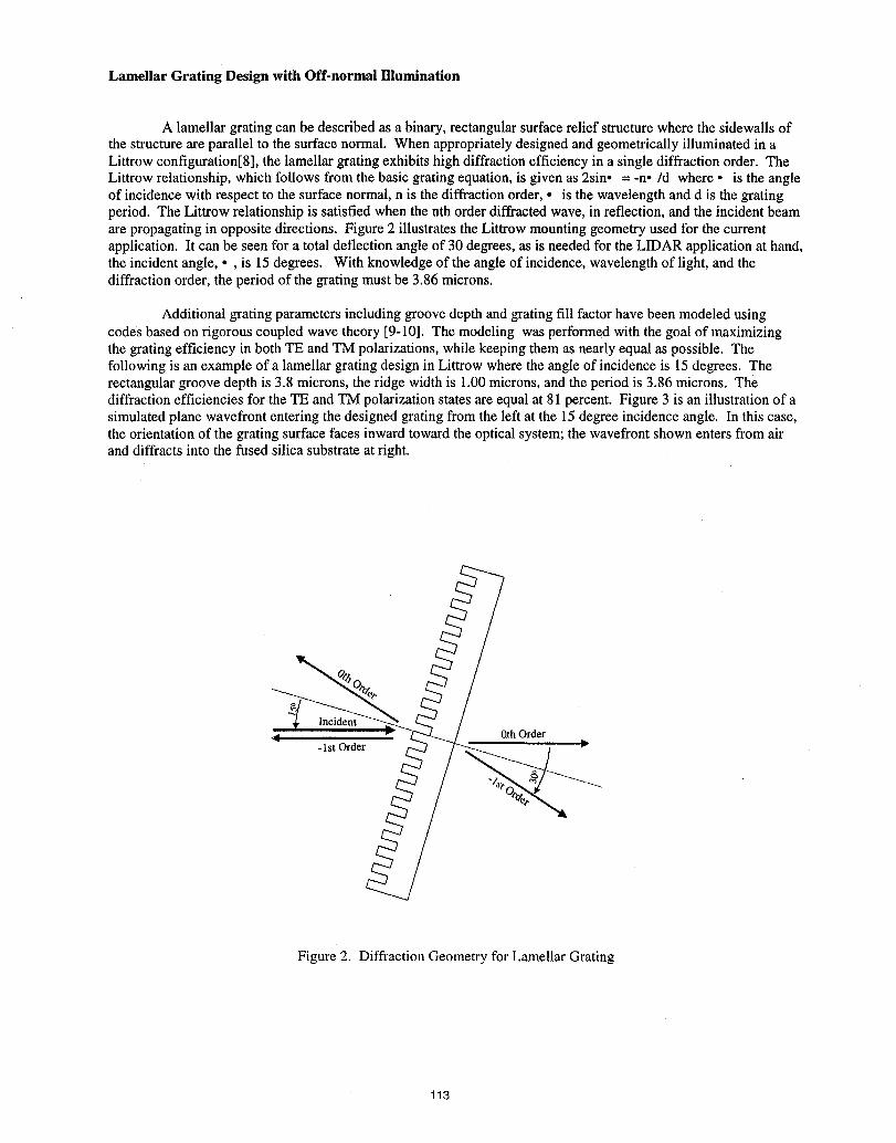
Lamellar Grating Design with Off-normal Illumination

A lamellar grating can be described as a binary, rectangular surface relief structure where the sidewalls ofthe structure are parallel to the surface normal. When appropriately designed and geometrically illuminated in aLittrow configuration[8], the lamellar grating exhibits high diffraction efficiency in a single diffraction order. TheLittrow relationship, which follows from the basic grating equation, is given as 2sin° = -no/d where • is the angleof incidence with respect to the surface normal, n is the diffraction order, • is the wavelength and d is the gratingperiod. The Littrow relationship is satisfied when the nth order diffracted wave, in reflection, and the incident beamare propagating in opposite directions. Figure 2 illustrates the Littrow mounting geometry used for the currentapplication. It can be seen for a total deflection angle of 30 degrees, as is needed for the LIDAR application at hand,the incident angle, ° , is 15 degrees. With knowledge of the angle of incidence, wavelength of light, and thediffraction order, the period of the grating must be 3.86 microns.

Additional grating parameters including groove depth and grating fill factor have been modeled usingcodes based on rigorous coupled wave theory [9-10]. The modeling was performed with the goal of maximizingthe grating efficiency in both TE and TM polarizations, while keeping them as nearly equal as possible. Thefollowing is an example of a lamellar grating design in Littrow where the angle of incidence is 15 degrees. Therectangular groove depth is 3.8 microns, the ridge width is 1.00 microns, and the period is 3.86 microns. Thediffraction efficiencies for the TE and TM polarization states are equal at 81 percent. Figure 3 is an illustration of asimulated plane wavefront entering the designed grating from the left at the 15degree incidence angle. In this case,the orientation of the grating surface faces inward toward the optical system; the wavefront shown enters from airand diffracts into the fused silica substrate at right.

Incident0th Order

- Ist Order I_

Figure 2. Diffraction Geometry for Lamellar Grating

113

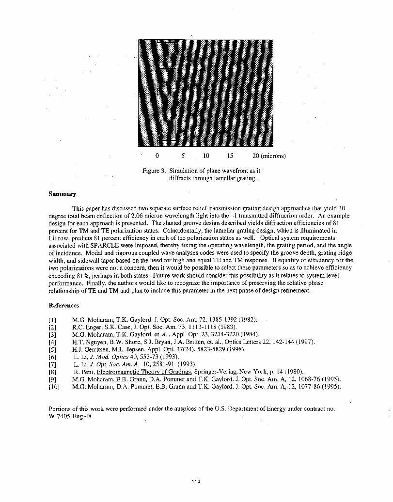
0 5 10 15 20 (microns)

Figure 3. Simulation of plane wavefront as it• diffracts through lamellar grating.

Summary

This paper has discussed two separate surface relief transmission grating design approaches that yield 30degree total beam deflection of 2.06 micron wavelength light into the -1 transmitted diffracrion order. An exampledesign for each approach is presented. The slanted _oove design described yields diffraction efficiencies of 81percent for TM and TE polarization states. Coincidentally, the lamellar grating design, which is illuminated inLittrow, predicts 81 percent efficiency in each of the polarization states as well. Optical system requirementsassociated with SPARCLE were imposed, thereby fixing the operating wavelength, the grating period, and the angleof incidence. Modal and rigorous coupled wave analyses codes were used to specify the groove depth, grating ridgewidth, and sidewall taper based on the need for high and equal TE and TM response. If equality of efficiency for thetwo polarizations were not a concern, then it would be possible to select these parameters so as to achieve efficiencyexceeding 81%, perhaps in both states. Future work should consider this possibility as it relates to system levelperformance. Finally, the authors would like to recognize the importance of preserving the relative phaserelationship of TE and TM and plan to include this parameter in the next phase of design refinement.

References

[1] M.G. Moharam, T.K. Gaylord, J. Opt. Soc. Am. 72, 1385-1392 (1982).[2] R.C. Enger, S.K. Case, J. Opt. Soc. Am. 73, 1113-1118 (1983).[3] M.G. Moharam, T.K. Gaylord, et. al., Appl. Opt. 23, 3214-3220 (1984).[4] H.T. Nguyen, B.W. Shore, S.J. Bryan, J.A. Britten, et. al., Optics Letters 22, 142-144 (1997).[5] H.J. Gerritsen, M.L. Jepsen, Appl. Opt. 37(24), 5823-5829 (1998).[6] L. Li, J. Mod. Optics 40, 553-73 (1993).[7] L. Li, J. Opt. Soc. Am. A 10, 2581-91 (1993).[8] R. Petit, Electromagnetic Theory of Gratings, Springer-Verlag, New York, p. 14(1980).[9] M.G. Moharam, E.B. Grann, D.A. Pommet and T.K. Gaylord, J. Opt. Soc. Am. A, 12, 1068-76 (1995).[10] M.G. Moharam, D.A. Pommet, E.B. Grann and T.K. Gaylord, J. Opt. Soc. Am. A, 12, 1077-86 (1995).

Portions of this work were performed under the auspices of the U.S. Department of Energy under contract no.W-7405-Eng-48.

114

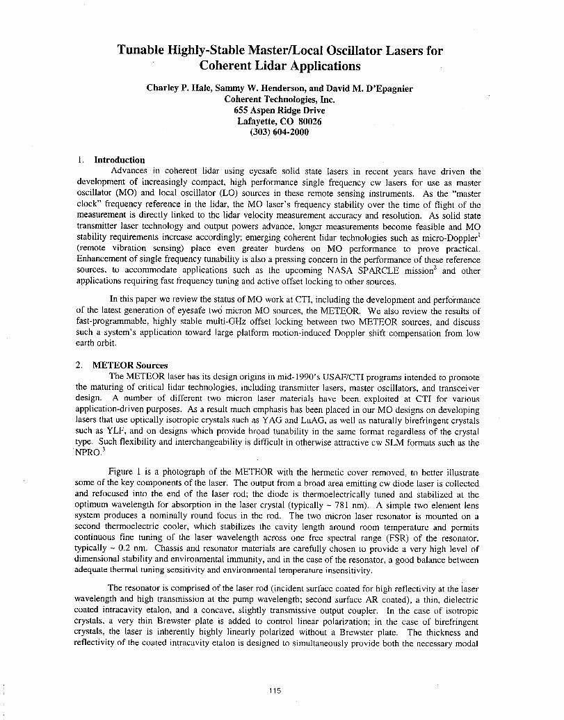
Tunable Highly-Stable Master/Local Oscillator Lasers forCoherent Lidar Applications

Charley P. Hale, Sammy W. Henderson, and David M. D'EpagnierCoherent Technologies, Inc.

655 Aspen Ridge DriveLafayette, CO 80026

(303) 604-2000

1. Introduction

Advances in coherent lidar using eyesafe solid state lasers in recent years have driven thedevelopment of increasingly compact, high performance single frequency cw lasers for use as masteroscillator (MO) and local oscillator (LO) sources in these remote sensing instruments. As the "masterclock" frequency reference in the lidar, the MO laser's frequency stability over the time of flight of themeasurement is directly linked to the lidar velocity measurement accuracy and resolution. As solid statetransmitter laser technology and output powers advance, longer measurements become feasible and MOstability requirements increase accordingly; emerging coherent lidar technologies such as micro-Doppler_(remote vibration sensing) place even greater burdens on MO performance to prove practical.Enhancement of single frequency tunability is also a pressing concern in the performance of these referencesources, to accommodate applications such as the upcoming NASA SPARCLE mission2 and otherapplications requiring fast frequency tuning and active offset locking to other sources.

In this paper we review the status of MO work at CTI, including the development and performanceof the latest generation of eyesafe two micron MO sources, the METEOR. We also review the results offast-programmable, highly stable multi-GHz offset locking between two METEOR sources, and discusssuch a system's application toward large platform motion-induced Doppler shift compensation from lowearth orbit.

2. METEOR Sources

The METEOR laser has its design origins in mid-1990's USAF/CTI programs intended to promotethe maturing of critical lidar technologies, including transmitter lasers, master oscillators, and transceiverdesign. A number of different two micron laser materials have been, exploited at CTI for variousapplication-driven purposes. As a result much emphasis has been placed in our MO designs on developinglasers that use optically isotropic crystals such as YAG and LuAG, as well as naturally birefringent crystalssuch as YLF, and on designs which provide broad tunability in the same format regardless of the crystaltype. Such flexibility and interchangeability is difficult in otherwise attractive cw SLM formats such as the

' NPRO. 3

Figure 1 is a photograph of the METEOR with the hermetic cover removed, to better illustratesome of the key components of the laser. The output from a broad area emitting cw diode laser is collectedand refocused into the end of the laser rod; the diode is thermoelectrically tuned and stabilized at theoptimum wavelength for absorption in the laser crystal (typically ~ 781 nm). A simple two element lenssystem produces a nominally round focus in the rod. The two micron laser resonator is mounted on asecond thermoelectric cooler, which stabilizes the cavity length around room temperature and permitscontinuous fine tuning of the laser wavelength across one free spectral range (FSR) of the resonator,typically - 0.2 nm. Chassis and resonator materials are carefully chosen to provide a very high level ofdimensional stability and environmental immunity, and in the case of the resonator, a good balance betweenadequate thermal tuning sensitivity and environmental temperature insensitivity.

The resonator is comprised of the laser rod (incident surface coated for high reflectivity at the laserwavelength and high transmission at the pump wavelength; second surface AR coated), a thin, dielectriccoated intracavity etalon, and a concave, slightly transmissive output coupler. In the case of isotropiccrystals, a very thin Brewster plate is added to control linear polarization; in the case of birefringentcrystals, the laser is inherently highly linearly polarized without a Brewster plate. The thickness andreflectivity of the coated intracavity etalon is designed to simultaneously provide both the necessary modal

115

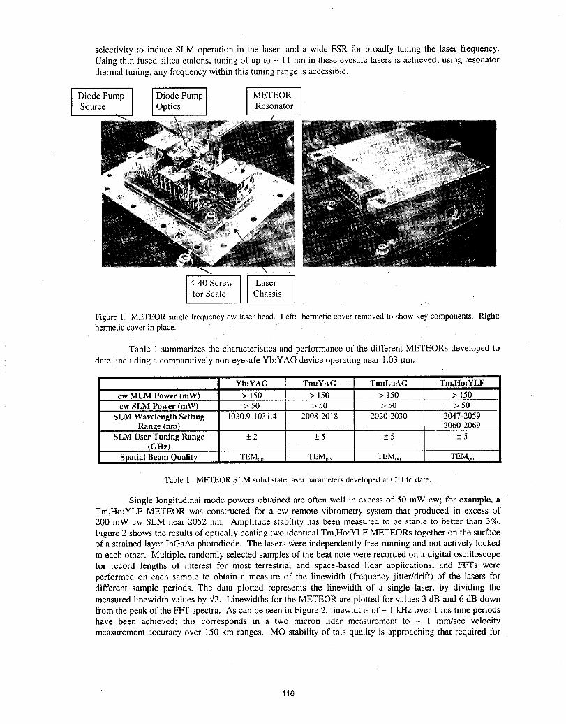
selectivity to induce SLM operation in the laser, and a wide FSR for broadly tuning the laser frequency.Using thin fused silica etalons, tuning of up to - 11 nm in these eyesafe lasers is achieved; using resonatorthermal tuning, any frequency within this tuning range is accessible.

IDiode Pump Diode Pump METEOR ,Source Optics Resonator

4-40 Screw ] I Laserfor Scale Chassis

Figure 11 METEOR single frequency cw laser head. Left: hermetic cover removed to show key components. Right:hermetic cover in place.

Table 1 summarizes the characterisucs and performance of the different METEORs developed to

date, including a comparatively non-eyesafe Yb:YAG device operating near 1.03 gtm.

Yb:YAG Tm:YAG Tm:LuAG Tm,Ho'YLF

cw MLM Power (mW) > 150 > 150 > 150 > 150cw SLM Power (mW) > 50 > 50 > 50 > 50

SLM Wavelength Setting 1030.9-103 i.4 2008-2018 2020-2030 2047-2059Range (nm) 2060-2069

SLM User Tuning Range + 2 + 5 _+5 + 5(GHz)

Spatial Beam Quality TEM.... TEM,,o TEM.... TEM....

Table 1. METEOR SLM solid state laser parameters developed at CTI to date.

Single longitudinal mode powers obtained are often well in excess of 50 mW cw; for example, aTm,Ho:YLF METEOR was constructed for a cw remote vibrometry system that produced in excess of200 mW cw SLM near 2052 nm. Amplitude stability has been measured to be stable to better than 3%.Figure 2 shows the results of optically beating two identical Tm,Ho:YLF METEORs together on the surfaceof a strained layer InGaAs photodiode. The lasers were independently free-running and not actively lockedto each other. Multiple, randomly selected samples of the beat note were recorded on a digital oscilloscopefor record lengths of interest for most terrestrial and space-based lidar applications, and FFTs wereperformed on each sample to obtain a measure of the linewidth (frequency jitter/drift) of the lasers fordifferent sample periods. The data plotted represents the linewidth of a single laser, by dividing themeasured linewidth values by _2. Linewidths for the METEOR are plotted for values 3 dB and 6 dB downfrom the peak of the FFT spectra. As can be seen in Figure 2, linewidths of- I kHz over I ms time periodshave been achieved; this corresponds in a two micron lidar measurement to - 1 mm/sec velocitymeasurement accuracy over 150 km ranges. Me stability of this quality is approaching that required for

116

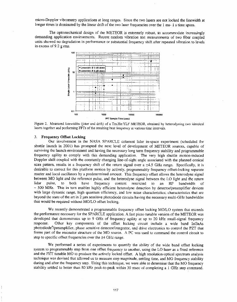
micro-Doppler vibrometry applications at long ranges. Since the two lasers are not locked the linewidth atlonger times is dominated by the linear drift of the two laser frequencies over the I ms- I s time spans.

The optomechanical design of the METEOR is extremely robust, to accommodate increasinglydemanding application environments. Recent random vibration test measurements of two fiber coupledunits showed no degradation in performance or substantial frequency shift after repeated vibration to levelsin excess of 9.2 g rms.

1O0...................................................................................................._"""i..................................................................;"-:"''";'";"'_

i _ _'.Jli_ ! ', ! i'. ; = i i

7.Ll..io,,o3ooo.nr. ; i i!! !i_IlL new dth @ 6 dB down | ! i I !; ', ....

if'. i 'I i , i_i , ,I _:, _ _ i i _ i

I , ;!J;° ; '_ i ._i_i i i i I !t ' ',1 ' ]! ' • , i i

i i :i _ J::; i i_-:

il ii ,l!_iil:j!i i i t :::',i! i i ii :;_0.1 .... [

100 1000 10000 100000

FFT SampleTime (usec)

Figure2. Measuredlinewidths(jitterand drift) of a Tm,Ho:YLFMETEOR,obtainedby heterodyningtwoidenticallaserstogetherandperformingFFTsof theresultingbeatfrequencyat varioustime intervals.

3. Frequency Offset LockingOur involvement in the NASA SPARCLE coherent lidar in-space experiment (scheduled for

shuttle launch in 2001) has prompted the next level of development of METEOR sources, capable ofsurviving the launch environment and havingthe necessary long term frequency stability and programmablefrequency agility to comply with this demanding application. The very high shuttle motion-inducedDoppler shift coupled with the constantly changing line-of-sight angle associated with the planned conicalscan pattern, results in a frequency shift of the return signal over a +4.5 GHz range. Specifically, it isdesirable to correct for this platform motion by actively, programmably frequency offset-locking separatemaster and local oscillators by a predetermined amount. This frequency offset allows the heterodyne signalbetween MO light and the reference pulse, and the heterodyne signal between the LO light and the returnlidar pulse, to both have frequency content restricted to an RF bandwidth of

- 500 MHz. This in turn enables highly efficient heterodyne detection by detector/preamplifier deviceswith large dynamic range, high quantum efficiency, and low noise characteristics; characteristics that arebeyond the state of the art in 2 lamsensitive photodiode circuits having the necessary multi-GHz bandwidthsthat would be requited without MO/LO offset locking.

We recently demonstrated a programmable frequency offset locking MO/LO system that exceedsthe performance necessary for the SPARCLE application. A fast piezo tunable version of the METEOR wasdeveloped that demonstrates up to 9 GHz of frequency agility at up to 20 kHz small-signal frequencyresponse. Other key components of the offset locking circuit include a wide band InGaAsphotodiodea/preamplifier, phase sensitive detector/integrator, and drive electronics to control the PZT thatforms part of the resonator structure of the MO source. A PC was used to command the control circuit tostep to specific offset frequencies over the +4 GHz range.

We performed a series of experiments to quantify the ability of the wide band offset lockingsystem to programmably step from one offset frequency to another, using the LO laser as a fixed referenceand the PZT tunable MO to produce the actively locked offset. A high resolution optical spectrum analysistechnique was devised that allowed us to measure step magnitude, settling time, and MO frequency stabilityduring and after the frequency step. Using this technique, we were able to determine that the MO frequencystability settled to better than 80 kHz peak-to-peak within 30 msec of completing a 1 GHz step command.

117

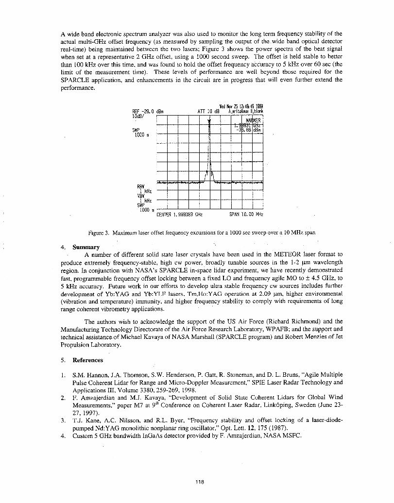
A wide band electronic spectrum analyzer was also used to monitor the long term frequency stability of theactual multi-GHz offset frequency (as measured by sampling the output of the wide band optical detectorreal-time) being maintained between the two lasers; Figure 3 shows the power spectra of the beat signalwhen set at a representative 2 GHz offset, using a 1000 second sweep. The offset is held stable to betterthan 100 ld-Izover this time, and was found to hold the offset frequency accuracy to 5 kHz over 60 sec (thelimit of the measurement time). These levels of performance are well beyond those required for theSPARCLE application, and enhancements in the circuit are in progress that will even further extend theperformance.

Wed_v 25IZ:49:49l_BREF-29.0 dBm ATTI0 dE Am'iLe_:B_blmklOdB/ I

SWF' -31i,66 dBm1000s

[

1I, I

RBW1 kHz IVBW ; lI kHz

SWP l JI000sCENTERI,999383 GHz SPAN10.O0NHz

Figure3. Maximumlaseroffsetfrequencyexcursionsfor a 1000secsweepovera 10MHzspan

4. SummaryA number of different solid state laser crystals have been used in the METEOR laser format to

produce extremely frequency-stable, high cw powe?, broadly tunable sources in the 1-2 _tm wavelengthregion. In conjunction with NASA's SPARCLE in-space lidar experiment, we have recently demonstratedfast, programmable frequency offset lockingbetween a fixed LO and frequency agile MO to + 4.5 GHz, to5 kHz accuracy. Future work in our efforts to develop ultra stable frequency cw sources includes furtherdevelopment of Yb:YAG and Yb:YLF lasers, Tm,Ho:YAG Operation at 2.09 gm, higher environmental(vibration and temperature) immunity, and higher frequency stability to comply with requirements of longrange coherent vibrometry applications.

The authors wish to acknowledge the support of the US Air Force (Richard Richmond) and theManufacturing Technology Directorate of the Air Force Research Laboratory, WPAFB; and the support andtechnical assistanceof Michael Kavaya of NASA Marshall (SPARCLE program) and Robert Menzies of JetPropulsion Laboratory.

5. References

1. S.M. Hannon, J.A. Thomson, S.W. Henderson, P. Gatt, R. Stoneman, and D. L. Bruns, "Agile MultiplePulse Coherent Lidar for Range and Micro-Doppler Measurement," SPIE Laser Radar Technology andApplications III, Volume 3380, 259-269, 1998.

2. F. Amzajerdian and M.J. Kavaya, "Development of Solid State Coherent Lidars for Global WindMeasurements," paper M7 at 9thConference on Coherent Laser Radar, Link6ping, Sweden (June 23-27, 1997).

3. T.J. Kane, A.C. Nilsson, and R.L. Byer, "Frequency stability and offset locking of a laser-diode-pumped Nd:YAG monolithic nonplanar ring oscillator," Opt. Lett. 12, 175 (1987).

4. Custom 5 GHz bandwidth InGaAs detector provided by F. Amzajerdian, NASA MSFC.

118

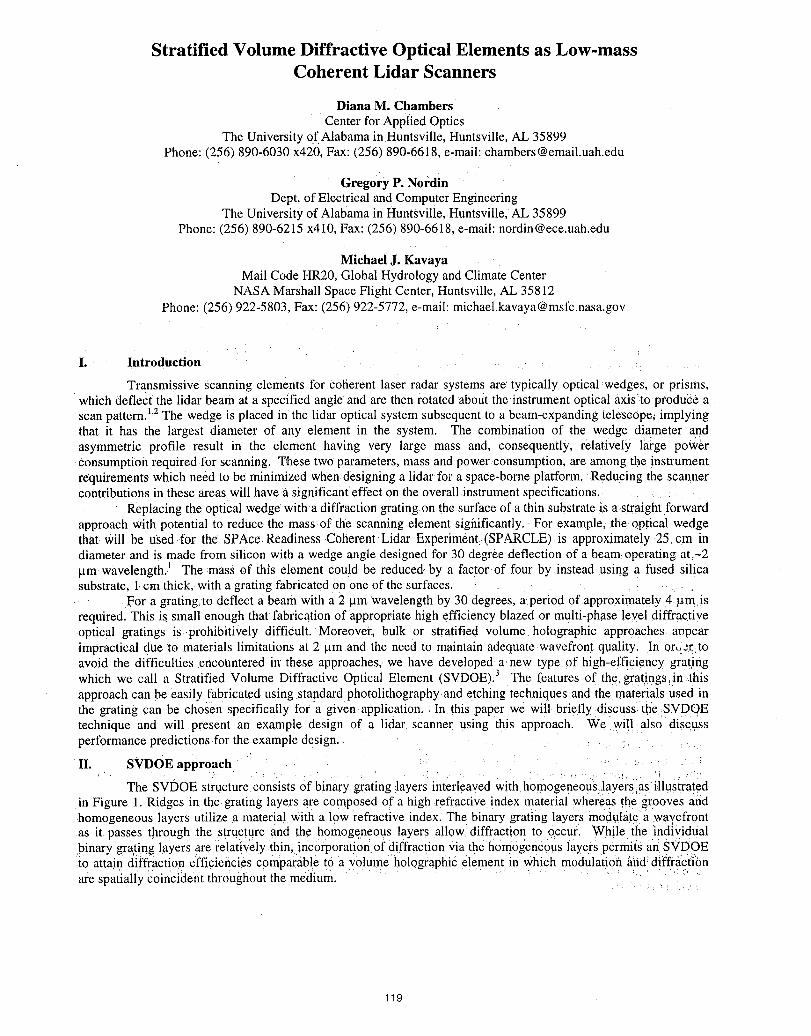
Stratified Volume Diffractive Optical Elements as Low-massCoherent Lidar Scanners

Diana M. ChambersCenter for Applied Optics

The University o(Alabama in Huntsville, Huntsville, AL 35899Phone: (256) 890-6030 x420, Fax: (256) 890-6618, e-mail: chambers@email.uah.edu

Gregory P. NordinDept. of Electrical and Computer Engineering

The University of Alabama in Huntsville,Huntsville, AL 35899Phone: (256) 890-6215 x410, Fax: (256) 890-6618, e'mail: nordin@ece.uah.edu

Michael J. KavayaMail Code HR20, Global Hydrology and Climate Center

NASA Marshall Space Flight Center, Huntsville, AL 35812Phone: (256) 922-5803, Fax: (256) 922-5772, e-mail: michael.kavaya@msfc.nasa.gov

I. Introduction

Transmissive scanningelements for coherent laser radar systems are'typically optical.wedges, or prisms,which deflect the lidar beam at a specified angle and are then rotated about the instrumentoptical axisto produce ascanpattern.l'2The wedge is placed in the lidar optical systemsubsequent to a beam-expandingtelescope; implyingthat it has the largest diameter of any element in the system. The combination of the wedge diameter andasymmetric profile result in the element having very large mass and, consequently, relatively large powerconsumptionrequiredfor scanning. These two parameters, mass and power consumption,are amongthe instrumentrequirementswhich need to be minimized when designing a lidar for a space-borne platform. Reducing the scannercontributionsin these areas will have a significanteffect on the overall.instrumentspecifications.

Replacing the optical wedge witha diffractiongratingon the surfaceof a thin substrateis a straightforwardapproach with potential tc reduce the mass of the scanningelement significantly. For example, the optical wedgethat will be used for the SPAce:Readiness Coherent Lidar Experiment (SPARCLE) is approximately 25 cm indiameterand is made from silicon with a wedge angle designed for 30 degree deflection of a beam operating at.-2gm wavelength.,t The mass of this element could be reduced by a factor of four by instead using a fused silicasubstrate,1 cm thick, with a gratingfabricated on one of thesurfaces.

For a grating to deflect a beam with a 2 _m Wavelengthby 30 degrees, a period of approximately 4tam _srequired.This is small enough that fabricationof appropriatehigh efficiency blazed or multi-phase level diffractiveoptical gratings isprohibitively difficult. Moreover, bulk or stratified volume holographic approaches.a_oearimpracticaldue to materials limitations at 2 _m and the need to maintainadequatewavefront quality. In or_Jzr toavoid the difficulties encountered in these approaches, we have developed a newtype 0f high-efficiency gratingwhich we call a Stratified Volume Diffractive Optical Element (SVDOE).3 The features of the gratings,in thisapproach can be easily fabricatedusing standardphotolithography and etching techniquesand the materialsused inthe grating can be chosen specifically for a given application. In this :paper we will briefly discuss the SVDOEtechnique and will present an example design of a lidar scanner using this approach. We will also discussperformancepredictions for the example design.

II. SVDOE approach ....

The SVDOE structure consists of binary grating ilayers interleaved with homogeneous layers:as illustrat,edin Figure 1. Ridges in the grating layers are composed of a high refractive index material whereas the grooves and.homogeneous layers utilize a material with a low refractive index. The binary _ating layers mode!latea .wavefrontas it passes through the structure and the homogeneous layers allow diffraction to occur. While the individualbinary grating layers are relatively thin, incorporauon of diffraction via the homogeneous layers permi(s an SVDOEto attain tiff-fractionefficiencies Comparable toa Volumeholographic element in Which modulation find;diffriicffOnare spatially coincident throughout the medium.

119

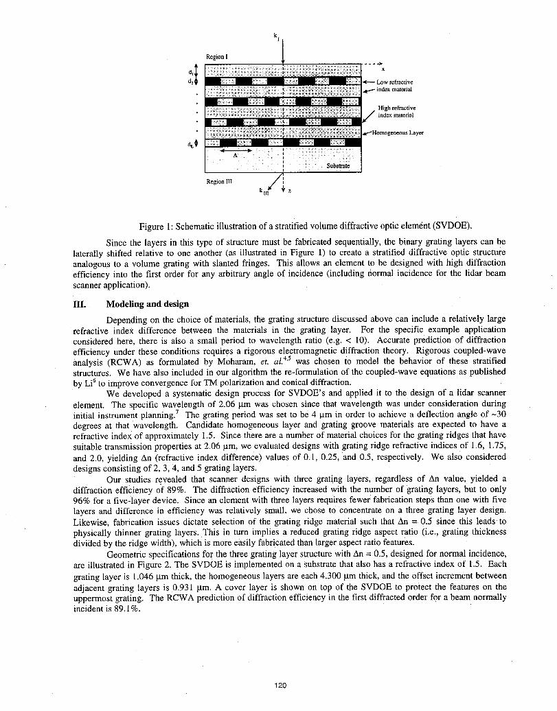
k I

RegionI 1

d2 _ Lowrefractive

indexmaterial

High refractiveindex material

dt,_

i " , " , .... Substrate,: : !

RegionIII i_,kll z

Figure 1:Schematic illustration of a stratified volume diffractive optic element (SVDOE).

Since the layers in this type of structure must be fabricated sequentially, the binary grating layers can belaterally shifted relative to one another (as illustrated in Figure 1) to create a stratified diffractive optic structureanalogous to a volume grating with slanted fringes. This allows an element to be designed with high diffractionefficiency into the first order for any arbitrary angle of incidence (including normal incidence for the lidar beamscanner application).

III. Modeling and design

Depending on the choice of materials, the grating structure discussed above can include a relatively largerefractive indeX difference between the materials in the grating layer. For the specific example applicationconsidered here, there is also a small period to wavelength ratio (e.g: < 10): Accurate prediction of diffractionefficiency under these conditions requires a rigorous electromagnetic diffraction theory. Rigorous coupled-waveanalysis (RCWA) as formulated by Moharam, et. a/.4'5was chosen to model the behavior of these stratifiedstructures. We have also included in our algorithm the re-formulation of the coupled-wave equations as publishedby Li6to improve convergence for TM polarization and conical diffraction.

We developed a systematic design process for SVDOE's and applied it to the design of a lidar scannerelement. The specific wavelength of 2.06 /am was chosen since that wavelength was under consideration duringinitial instrument planning.7 The grating period was set to be 4 lam in order to achieve a deflection angle of -30degrees at that wavelength. Candidate homogeneous layer and grating groove materials are expected to have arefractive index of approximately 1.5. Since there are a number of material choices for the grating ridges that havesuitable transmission properties at 2.06 pm, we evaluated designs with grating ridge refractive indices of 1.6, 1.75,and 2.0, yielding An (refractive index difference) values of 0.1, 0.25, and 0.5, respectively. We als0 considereddesigns consisting of 2, 3, 4, and 5 grating layers.

Our studies revealed that scanner designs with three grating layers, regardless of An value, yielded adiffraction effic!ency of 89%. The diffraction efficiency increased with the number of grating layers, but to only96% for a five-layer device. Since an element with three layers requires fewer fabrication steps than one with fivelayers and difference in efficiency was relatively small, we chose tOconcentrate on a three grating layer design.Likewise, fabrication issues dictate selection of the grating ridge material such that An = 0.5 since this leadstophysically thinner grating layers. This in turn implies a reduced grating ridge aspect ratio (i.e., grating thicknessdivided by the ridge width), which is more easily fabricated than larger aspect ratio features.

Geometric specifications for the three grating layer structure with An = 0.5, designed for normal incidence,are illustrated in Figure 2. The SVDOE is implemented on a Substrate that also has a refractive index of 1.5. Eachgrating layer is 1.046 !.tmthick, the homogeneous layers are each 4.300 _tmthick, and the offset increment betweenadjacent grating layers is 0.931 p.m.A cover layer is shown on top of the SVDOE to protect the features on theuppermost grating. The RCWA prediction of diffraction efficiency in the first diffracted order for a beam normallyincident is 89.1%.

120

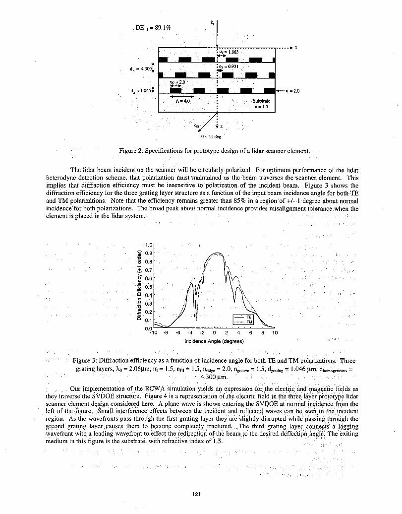
DE+I= 89.1% k_/x

: o(= 1.863-. ' i

_ = ...

:o_ =0.931dh = 4.300II I, :

w .odg = 1.046€ - a---n =2.0

A = 4;0 , Substraten= 1.5

k. z i0-31 deg

Figure 2: Specifications for prototype design of a lidar scanner element.

The lidar beam incident on the scanner will be circularly polarized. For optimum performance of the lidarheterodyne detection scheme, that polarization must maintained as the beam traverses the'_scannerelement. Thisimplies that diffraction efficiency must be insensitive to polarization, of the incident beam. Figure 3 shows thediffraction efficiency for the three grating layer structure as a function of the input beam incidence angle for both,:TEand .TM polarizations. Note that the efficiency remains greater than 85% in a region of +/-.1 degree about normalincidencefor both polarizations. The broad peak about normal incidence provides misalignment tolerance when theelement is placed in the lidar system.

1.0

_" 0.9 . .

0.8

0.7 _\ .-_0.6 ,"",. ..•_ 0.5

0.4

g o.a0.2

0.1

0.0I0 -8 -6 -4 -2 0 2 4 6 8 10

IncidenceAngle(degrees) ....

.Figure 3: Diffraction efficiency as a function of incidence angle for both .TE and TM polarizations. Threegrating layers, ko= 2.06gm, ni = 1.5;.nui= 1..5,n,dgo= 2.0,.n_oove= 1.5;dgrating= 1.046 gm, d60m0gen_o,,=

4.300 gin.

Our implementation of the RCWA simulation yields. an expression for_the electric' _ndmagneticifields asthey traverse' ti{esVDOE structUre. Figfire 4 is a representation oflti_eelectric field in the ihree,la_er prot6t"yl__ lidarscanner element design considered here. A plane wave is shown entering the svDOE:at':norn_al in_ideii_efrom the

left of the ,figure, _Smailinterference effects between theinciden't and reflected waves Can bese'e_ in the"incidentregion. As the wavefronts pass through the firsi grating layer they are slightly dlsrupied While _ass[ng 'i[_r6ughthesecond grating layer causes them to become complete!y fractured.. The third grating layer con.nepts a !'aggingWavefront Witha leading wavefront to.effect the-l:edire.c_tionof ti_ebeam to the.desired deflectiOii _ii_le_.The exitingmedium in this figure is the Substrate, Withrefracl_iveindex of i.5. ' ."'_:i 'i ,"

121

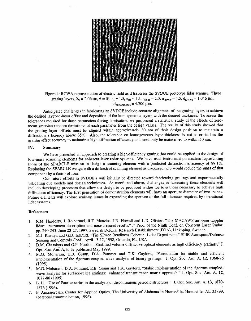
Figure 4: RCWA representation of electric field as ittraverses the SVDOE prototype lidar scanner. Threegrating layers, _ = 2.06_tm,0 = 0°, nl = 1.5, nii!= 1.5, nridgc = 2.0, ng_oove= 1.5, dgrating = 1.046 p.m,

dhomogeneous = 4.300 I.tm.

Anticipated challenges in fabricating an SVDOE include accurate alignment of the grating layers to achievethe desired layer-to-layer offset and deposition of the homogeneous layers with the desired thickness. To assess thetolerances required for these parameters during fabrication, we performed a statistical study of the effects of zero-mean gaussian random deviations of each parameter from the design values. The results of this study showed thatthe grating layer offsets must be aligned within approximately 30 nm of their design position to maintain adiffraction efficiency above 85%. Also, the tolerance on homogeneous layer thickness is not as critical as thegrating offset accuracy to maintain a high diffraction efficiency and need only be maintained to within 50 nm.

IV. Summary

We have presented an approach to creating a high-efficiency grating that could be applied to the design oflow-mass scanning elements for coherent laser radar systems. We have used instrument parameters representingthose of the SPARCLE mission to design a scanning element with a predicted diffraction efficiency of 89.1%.Replacing the SPARCLE wedge with a diffractive scanning element as discussed here would reduce the mass of thatcomponent by a factor of four.

Our future efforts in SVDOE's will initially be directed toward fabricating gratings and experimentallyvalidating our models and design techniques. As mentioned above, challenges in fabricating these elements willinclude developing processes that allow the design to be produced within the tolerances necessary to achieve highdiffraction efficiency. The first generation of demonstration elements will have an aperture diameter of two inches.Future elements will explore scale-up issues in expanding the aperture to the full diameter required by operationallidar systems.

References

1. R.M. Hardesty, J. Rothermel, R.T. Menzies, J.N. Howell and L.D. Olivier, "The MACAWS airborne dopplerlidar: instrument description and measurement results," ," Proc. of the Ninth Conf. on Coherent Laser Radar,pp. 240-243, June 23-27, 1997, Swedish Defense Research Establishment (FOA), Linkoping, Sweden.

2. M.J. Kavaya and G.D. Emmitt, "The SPAce Readiness Coherent Lidar Experiment," SPIE Aerospace/DefenseSensing and Controls Conf., April 13-17, 1998, Orlando, FL, USA

3. D.M. Chambers and G.P. Nordin, "Stratified volume diffractive optical elements as high efficiency gratings," J.Opt. Soc. Aml A, tObe published May 1999.

4. M.G. Moharam, E.B. Grann, D_A. Pommet and T.K. Gaylord, "Formulation for stable and efficientimplementation of the rigorous coupled-wave analysis of binary gratings," J. Opt. Soc. Am. A, 12, 1068-76(1995).

5. M.G. Moharam, D.A. Pommet, E.B. Grann and T.K. Gaylord, "Stable implementation of the rigorous coupled-wave analysis for surface-relief gratings: enhanced transmittance matrix approach," J_ Opt. Soc. Am. A, 12,1077-86 (1995).

6. L. Li, "Use of Fourier series in the analysis of discontinuous periodic structures," J. Opt. Soc. Am. A, 13, 1870-1876 (1996).

7. F. Amzajerdian, Center for Applied Optics, The University of Alabama in Huntsville, Huntsville, AL 35899,(personal communication, 1996).

122

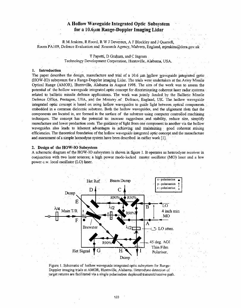
A HollowWaveguideIntegratedOptic Subsystemfor a 10.6 m Range-DopplerImagingLidar

R M Jenkins, R Foord, R W J Devereux, A F Blockley and J Quarrell,Room PA109, Defence Evaluation and Research Agency, Malyem, England, mjenkins@dera.gov.uk

T Papetti, D Graham, and C IngramTechnology Development Corporation, Huntsville, Alabama, USA.

1. Introduction

The paper describes the design, manufactureand trial of a 10.6 gm hoollowwaveguide integratedoptic(HOW-IO)subsystem fora Range-Dopplerimaging Lidar.The trialswere undertakenat the Army MissileOptical Range (AMOR), Huntsville, Alabama in August 1998. The aim of the work was to assess thepotentialof the hollow waveguide integratedoptic concept for discriminatingcoherentlaser radarsystems _related to ballistic missile defence applications. The work was jointly funded by the Ballistic MissileDefence Offic.e, Pentagon, usA, and the Ministry of Defence, England, UK. The hollow waveguideintegratedoptic concept is based on using hollowwaveguides to guide light between:optical componentsembeddedin a common dielectric substrate.Both the hollow waveguides, and the alignmentslots that thecomponentsare located in, are formed in the surface of the substrateusing computercontrolledmachiningtechniques. The concept has the potential to: increase raggedness and stability, reduce size, sn'nplifymanufactureand lowerproductioncosts.The guidiinceof light fromone componentto anothervia the hollowwaveguides also leads to inherent advantages in achieVing and maintaining good coherent mixingefficiencies.The theoreticalfoundationof the hollow waveguideintegratedoptic conceptandthe manufactureandassessmentof a simplehomodynesystemhave been described in earlierwork [1]_

2. Design of the HOW-IO SubsystemA schematic diagramof the HOW:IOsubsystem is shown in figure 1. It operatesas heterodyne receiver inconjunction with two laser sources; a high power mode-locked master oscillator (MO) laser and a lowpower c.w. local oscillator(LO) laser.

Het Ref Beam Dump IS - polarisation 0

Ip - polarisation !D C c- polarisationDump

g

k/4 Main T/R 4 inch minMO

F ALO atten.

AOI

Thin FilmHet Signal G ' I Polariser.

Dump

Figure I. Schematicof hollowwaveguideintegratedopticsubsystemfor Range-Dopplerimaging trialsat AMOR,Huntsville,Alabama.Heterodynedetection oftarget returns are facilitatedvia a singlepolarisationduplexedtransmit/receivepath.

123

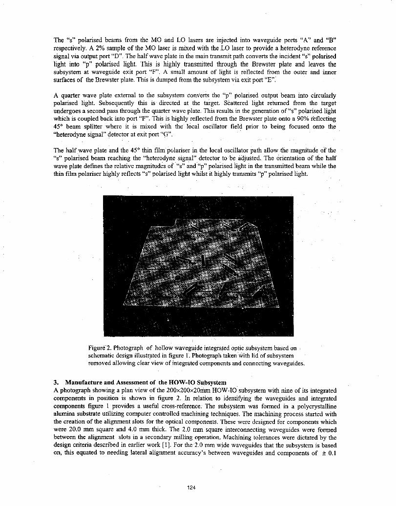
The "s" polarised beams from the MO and LO lasers are injected into waveguide ports "A" and "B"respectively. A 2% sample of the MO laser is mixed with the LO laser to provide a heterodyne referencesignal via output port "D". The half wave plate in the main transmit path converts the incident "s" polarisedlight into "p" polarised light. This is highly transmitted through the Brewster plate and leaves thesubsystem at waveguide exit port "F". A small amount of light is reflected from the outer and innersurfaces of the Brewster plate. This is dumped from the subsystem via exit port "E".

A quarter wave plate external to the subsystem converts the "p" polarised output beam into circularlypolarised light. Subsequently this is directed at the target. Scattered light returned from the targetundergoes a second pass through the quarter wave plate. This results in the generation of "s" polarised lightwhich is coupled back into port "F". This is highly reflected from the Brewster plate onto a 90% reflecting45° beam splitter where it is mixed with the local oscillator field prior to being focused onto the"heterodyne signal" detector at exit port "G".

The half wave plate and the 45° thin film polariser in the local oscillator path allow the magnitude of the"s" polar:isedbeam reaching the "heterodyne signal" detector to be adjusted. The orientation of the halfwave plate defines the relative magnitudes of "s" and "p" polarised light in the transmitted beam while thethin film polariser highly reflects "s" polarised light whilst it highly transmits "p" polarised light.

Figure2. Photograph of hollow waveguide integrated optic subsystem based onschematic design illustrated in figure 1. PhotOgraphtaken Withlid of subsystemremoved allowing clear view of integratedcomponents and connectingwaveguides.

3. Manufacture and Assessment of the HOW-IO SubsystemA photograph showing a plan view of the 200x200x20mm HOW-IO subsystem with nine of its integratedcomponents in position is shown in figure 2. In relation to identifying the waveguides and integratedcomponents figure 1 provides a useful cross-reference. The subsystem was formed in a polycrystallinealumina substrate utilizing computer controlled machining techniques. The machining process started withthe creation of the alignment slots for the optical components. These were designed for components whichwere 20.0 mm square and 4.0 mm thick. The 2.0 mm square interconnecting waveguides were formedbetween the alignment slots in a secondary milling operation. Machining tolerances were dictated by thedesign criteria described in earlier work [1]. For the 2.0 mm wide waveguides that the subsystem is basedon, this equated to needing lateral alignment accuracy's between waveguides and components of + 0.1

124

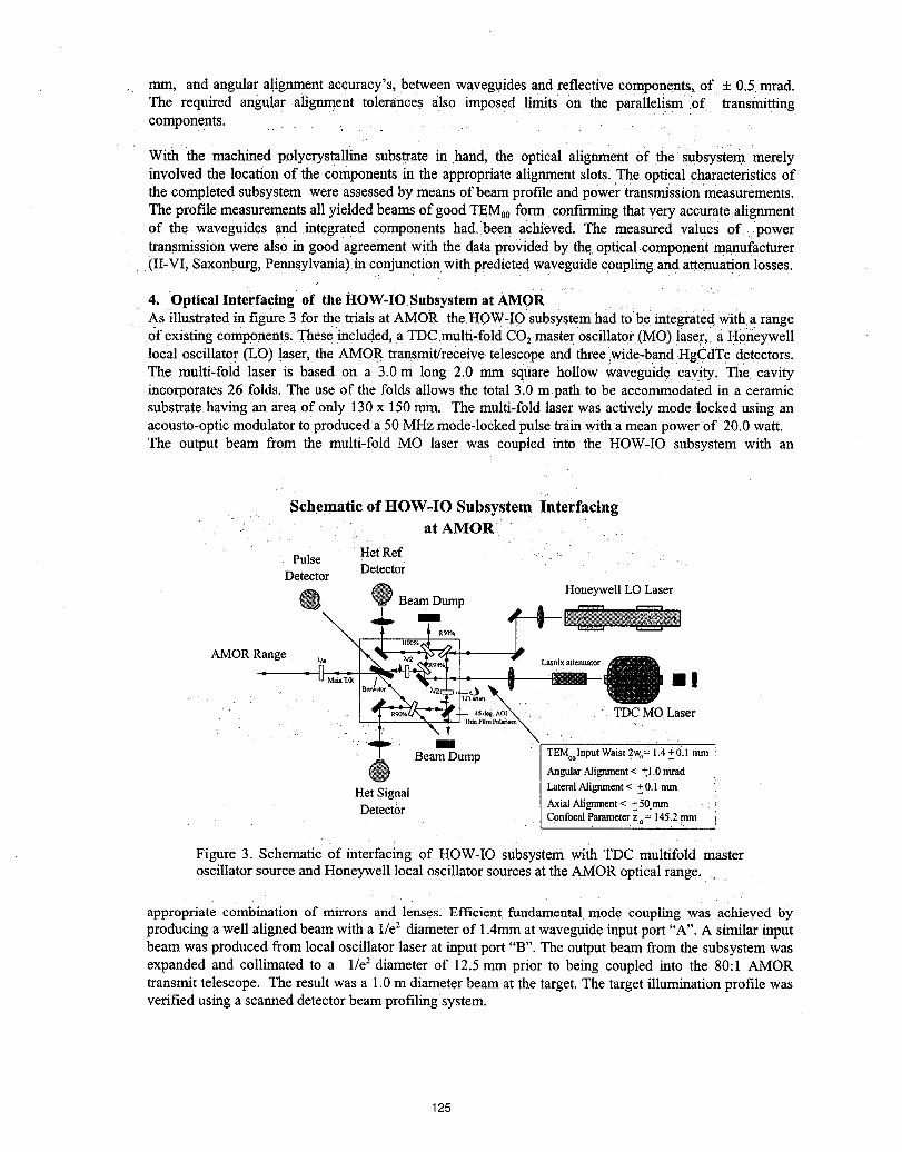
mm, and angular alignment accuracy's, between waveguides and reflective componems, of + 0.5 mrad.The required angular alignment tolerances also imposed limits on the parallelism of transmittingcomponents.

With the machined polycrystalline substrate in hand, the optical .alignment of the subsystem merelyinvolved the location of the components in the appropriate alignment slots. The optical characteristics ofthe completed subsystem were assessed by means of beam profile and power transmission measurements.The profile measurements all yielded beams of good TEM00form confLrmingthat very accurate alignmentof the waveguides and integrated components had been achieved. The measured values of powertransmission were also in good agreement with the data provided by the optical component manufacturer(II-VI, Saxonburg, Pennsylvania) in conjunction with predicted waveguide coupling and attenuation losses.

4. Optical Interfacing of the HOW-IO Subsystem at AMOR

As illustrated in figure 3 for the trials at AMOR the HOW-IO subsystem had to be integrated with a rangeof existing components. Theseincluded, a TDC multi-fold CO2master oscillator (MO) laser, a Honeywelllocal oscillator (LO) laser, the AMOR transmit/receive telescope and three wide-band HgCdTe detectors.The multi-fold laser is based on a 3.0 m long 2.0 mm square hollow waveguide cavity, The cavityincorporates 26 folds. The use of the folds allows the total 3.0 m path to be accommodated in a ceramicsubstrate having an area of only 130 x 150 mm. The multi-fold laser was actively mode locked usmg anacousto-optic modulator to produced a 50 MHz mode-locked pulse train witha mean power of 20.0 watt.The output beam from the multi-fold MO laser was coupled into the HOW-IO subsystem with an

Schematic of HOW-IO Subsystem Interfacing' • at _,_,_,_,_n.

Pulse Het Ref .Detector ......Detector

@ Beam Dump Honeywell LO Laser1

AMOR Range _

ll• , " TDCMOLaser

ll _ ......

BeamDump TEMoolnputWaist 2w.---"1.4 +0.1 mmAngular Alignment< +1.0 mrad ]

Het Signal LateralAlignment< +0.1 mm ]AxialAlignment< +50ram [

Deteet0r ConfocalParameterzo= 145.2mm I

Figure 3. Schematic of interfacing of HOW-IO subsystem with TDC multifold masteroscillator source and Honeywell local oscillator sources at the AMOR optical range....

appropriate combination of mirrors and lenses. Efficient fundamental mode coupling was achieved byproducing a well aligned beam with a 1/e2 diameter of 1.4mm at waveguide input port "A". A similar inputbeam was produced from local oscillator laser at input port "B". The output beam from the subsystem wasexpanded and collimated to a 1/e2 diameter of 12.5 mm prior to being coupled into the 80:1 AMORtransmit telescope. The result was a 1.0 m diameter beam at the target. The target illumination profile wasverified using a scanned detector beam profilingsystem.

125

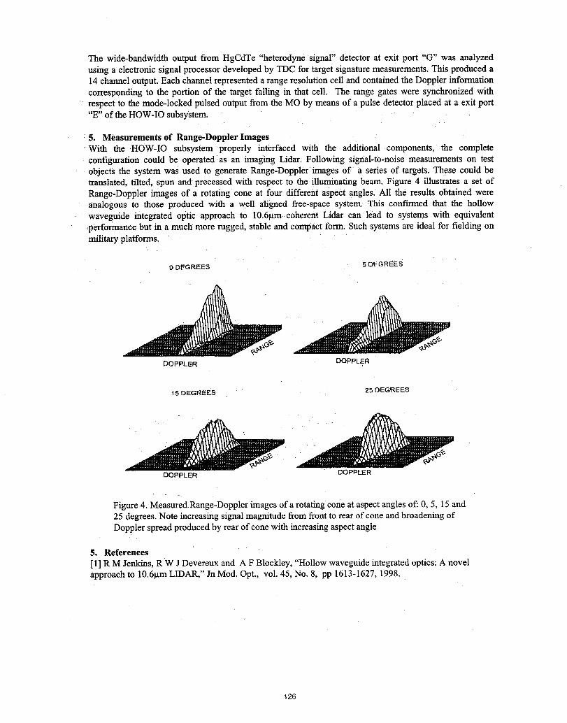
The wide-bandwidth output from HgCdTe "heterodyne signal" detector at exit port "G" was analyzedusing a electronic signal processor developed by TDC for target signature measurements. This produced a14 channel output. Each channel represented a range resolution cell and contained the Doppler informationcorresponding to the portion of the target falling in that cell. The range gates were synchronized withrespect to the mode-locked pulsed output from the MO by means of a pulse detector placed at a exit port"E" of the HOW-IO subsystem.

5. Measurements of Range-Doppler ImagesWith the HOW-IO subsystem properly interfaced with the additional components, the completeconfiguration could be operated as an imaging Lidar. Following signal-to-noise measurements on testobjects the system was used to generate Range-Doppler images of a series of targets. These could betranslated, tilted, spun and' precessed with respect to the illuminating beam. Figure 4 illustrates a set ofRange-Doppler images of a rotating cone at four different aspect angles. All the results obtained wereanalogous to those produced with a well aligned free-space system. This confirmed that the hollowwaveguide integrated optic approach to 10.6_tm coherent Lidar can lead to systems with equivalent,performance but in a much more rugged, stable and compact form. Such systems are ideal for fielding onmilitary platforms.

0 DFGREES 5 D_REES

DOPPLER DOPPLER

15 DEGREES 25 DEGREES

DOPPLER DOPPLER

Figure 4. MeasuredRange-Doppler images of a rotating cone at aspect angles of: 0, 5, 15 and25 degrees. Note increasing signal magnitude from front to rear of cone and broadening ofDoppler spread produced by rear of cone with increasing aspect angle

5. References

[1] R M Jenkins, R W J Devereux and A F Blockley, "Hollow waveguide integrated optics: A novelapproach to 10.6_tmLIDAR," Jn Mod. Opt., vol. 45, No. 8, pp 1613-1627, 1998.

126

TARGET CHARACTERIZATION

Presider: Robert Menzies

. !

i27

Comparison of continuous wave CO2 Doppler lidar calibrationusing earth surface targets in laboratory and

airborne measurements

Maurice A. JarzembskiNASA/MSFC/Global Hydrology and Climate Center

977 Explorer Blvd., Huntsville, AL 35806

Vandana Srivastava

Universities Space Research AssociationGlobal Hydrology and Climate Center

977 Explorer Blvd., Huntsville, AL 35806

1. Introduction selectedearth surfacefrom die airborne lidar data,Routinebackscatter,13,measurementsby an an average13for the surfacewas establishedand the

airborneor space-basedlidar from designated earth statisticsof lidar efficiencywas determined. Thissurfaceswith knownand fairlyuniform 13properties was compared with the actual lidar efficiencycan potentiallyoffer lidar calibration opportunities, determinedwith the standardcalibratinghard target.This can in turn be used to obtain accurate 2. LidarTheoryatmosphericaerosoland cloud 13measurementson The measuredSNRfrom a hard,target (HT)large spatial scales. This is important because with Oar[srq] usinga CWlidar is givenby,3

achievinga precisecalibrationfactorfor largepulsed rI_ PrcR 2Tp rrrf (L ) (1)lidars then need not rest solelyon using a standard SNR rrr = ,hard target procedure. Furthermore, calibration Bhvfrom designatedearth surfaceswouldprovide an in- whererangedependence,f(L), is givenby1 , (2)

Oo,i, on o Lwith active remote sensing using lasers with high - :resolution data, calibration of a space-based lidar L'- 1+ t, LL J 1 -using earth's surfaceswillbe extremelyuseful. wherehv is laserphoton energy,P is laser power,RThe calibration methodology using the is lidar beam (l/e)2 intensity radius at telescopeearth's surface initially requires measuring 13 of primarymirror,F is distanceto focal volumecenter,various earth surfaces simulated in the laboratory, and B is data system bandwidth, and q is overallusing a focusedcontinuouswave (CW)CO2Doppler lidarsystemefficiency.The transmissionefficiencyTlidar and /.hen use these 13 measurements as is given by T = exp(-2cxL).HT can stand for astandards for the earth surfacesignal from airborne standardcalibratinghard target (CHT)or earth hardor space-basedlidars. Since 13from the earth's target (EHT), since both present a surface ofsurface may be retrieved at different angles of scattering.At the lidar beam focal volume,L = F,incidence, 13would also need to be measured at Eqs.(1)-(2)reducetovariousanglesof incidencesof the differentsurfaces.

1"1wrPTtR _Tp rrr (3)In general, Earth-surface reflectance measurements SNR rrr = ,havebeenmadein the infrared,_but the use of lidars BhvF "to characterizethem and in turn use of the Earth's Using a CHT with known4 Pcar, rlcrrr can besurface to calibrate lidars has not been made. The determined.5 Once _crrr is known then measuredfeasibility of this calibration methodology is SNR_ from any other HT surfaces can lead to Orrr.demonstrated through a comparison of these Thus, PErrr for a variety of earth surfacelaboratorymeasurementswith actual earth surface13 compositionscan be characterizedin the laboratory.retrieved from the same lidar during the Subsequently,the characterizedearth surfacescan beNASA/Multi-centerAirborneCoherent Atmospheric used as calibrationtargets in flight to get rlErrr forWind Sensor(MACAWS)mission"on NASA's DC8 airborneor space-basedlidars. Lastly,onceqm-rrhasaircraft from 13 - 26 September, 1995. For the beendetermined,thenit couldbe further correctedto

128

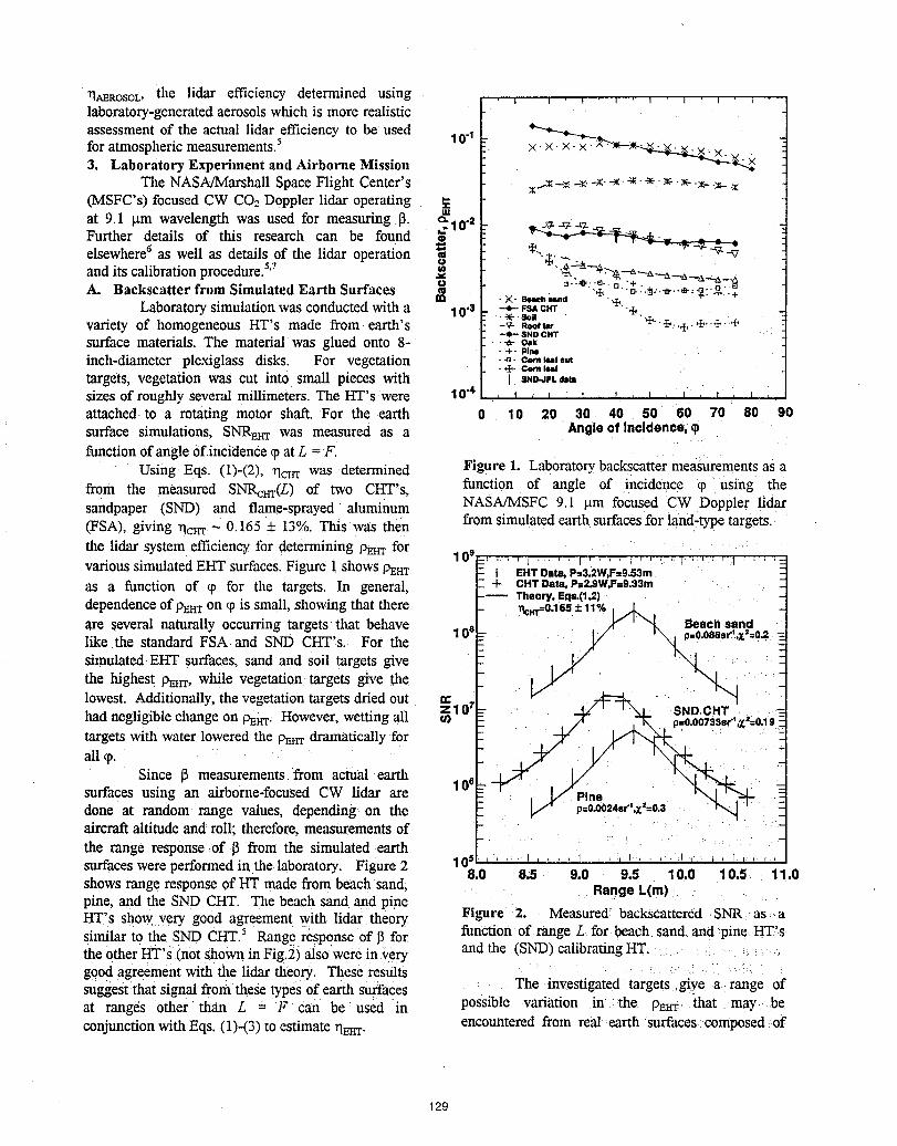
rlam_osor.,tile lidar efficiency determined using , , , , , , , ,laboratory-generatedaerosolswhichis more realistic

assessmentof the actual lidar efficiencyto be used __ ....foratmosphericmeasurements.5 104 x. ×-x- x- ^- _ ×- x3. LaboratoryExperimentandAirborneMission

TheNASA/MarshallSpaceFlight Center's xlx -_ _ _- -x.-x-,. _-.__-x-.x--.x(MSFC's)focusedCW CO2Dopplerlidar operating

ILl

at 9.1 Ixmwavelength was used for measuring IL _10 .2 _-_t..___-_ -r_._-_..= _Further details of this research can be found £ " - __..__.._elsewhere6 as well as details of the lidar operation

o "ft.""l:_:____...and its calibrationprocedureJ'7 o,A. BackscatterfromSimulatedEarthSurfaces _a -×- _..d "_ :'_"'_'"_:_:"_:+_

Laboratorysimulationwasconductedwitha 104 --,-F_ ewr -._•-_ •8oll

variety of homogeneousHT's made from earth's -v-R**f_ _......--+--.SND CHT

surface materials. The materialwas glued onto 8- ._- o,k- +- Pine

inch-diameter plexiglass disks. For vegetation ._. c.€.u._o._. ,.r_. €orn [nel

targets, vegetation was cut into small pieces with I 8.o_ptdmsizes of roughly severalmillimeters.The HT's :were 10"4 , I , t , ) , i , t , i , i , i ,attachedto a rotating motorshaft. For the earth 0 10 20 30 40 50 60 70 80 90surface simulations, SNRm_r was measured as a Angloof Incldenco,L_pfunctionof angleofincidenceq_atL =F.

Using Eqs. (1)-(2), _crrr was determined Figure1. Laborato_backscattermeasurementsasafrom the measured SNRc_(L) of two CHT's, function of angle of incidence q_ using thesandpaper (SND) and flame-sprayedaluminum NASA/MSFC9.1 _tm focused CW Doppler lidar(FSA),giving rlcrrr~ 0.165 + 13%.This was then fromsimulatedearthsurfacesforland-typetargets.the lidarsystemefficiency,for determiningP_rr forvarious simulatedEHT surfaces.Figure 1 showsPEnT 10_ .... j .... _ :• P-.3.2W,F=9,53 rnF I EHTData,as a function of q_ for the targets. In general, _ + CHT Data, P=2_W,F=9.33m

_- Theory, Eqs.0,2) .

dependenceof pm.rron q)is small,showing that there _- _:"r=°a_.±_%I_,a/ /t_ ' "_ Beach sand

v a,yoo.t.tav.°IsimulatedEHT surfaces, sand and soil targets give ]ithe highest Pmrr,while vegetation targets giycethe *lowest. Additionally,the vegetationtargets driedout ,v-

zl0 l= , .3_/_ _\1 .SND.CHT .....

targets with water lowered the P_-rrdramaticallyfor

all q). ,Since 13measurements.from actual_earth

done at random range values, depending on the "aircraftaltitude and roll; therefore,measurementsof

the range response.of I_from the simulatedearth 10__ , _, _,, _, _-. .... .surfaceswereperformedinthe:laboratory. Figure2 8.0 8.5 9.0 9.5 10.0 10.5 11.Oshowsrange responseof HT madefrom beachsan& Rangek(m)pine, and the SND CHT. The beach sand and pineHT's show very good agreement with lidar theory Figure 2. Measured backsCattered SNR_ as a

similar to the SND CHT.5 RangeresP0nseof J]for funCtiOnof range L for beaCh,sand and '.pine,HT-'s.... " ' ' " " 9 and the (SND)calibratingHT.the other HT s (not shownm F_g._)alsowere in very

good agreementwith the lidar theory. These results "suggestthat signal from these typesOfearth Surfaces The inYestigatedtargets ,give a. range ofat ranges other than L = F Can be used in possible variation in the Pzrrr that :may. be

encounteredfrom realearth surfaces composedofconjunctionwithEqs. (1)-(3)to estimateqmT.

129

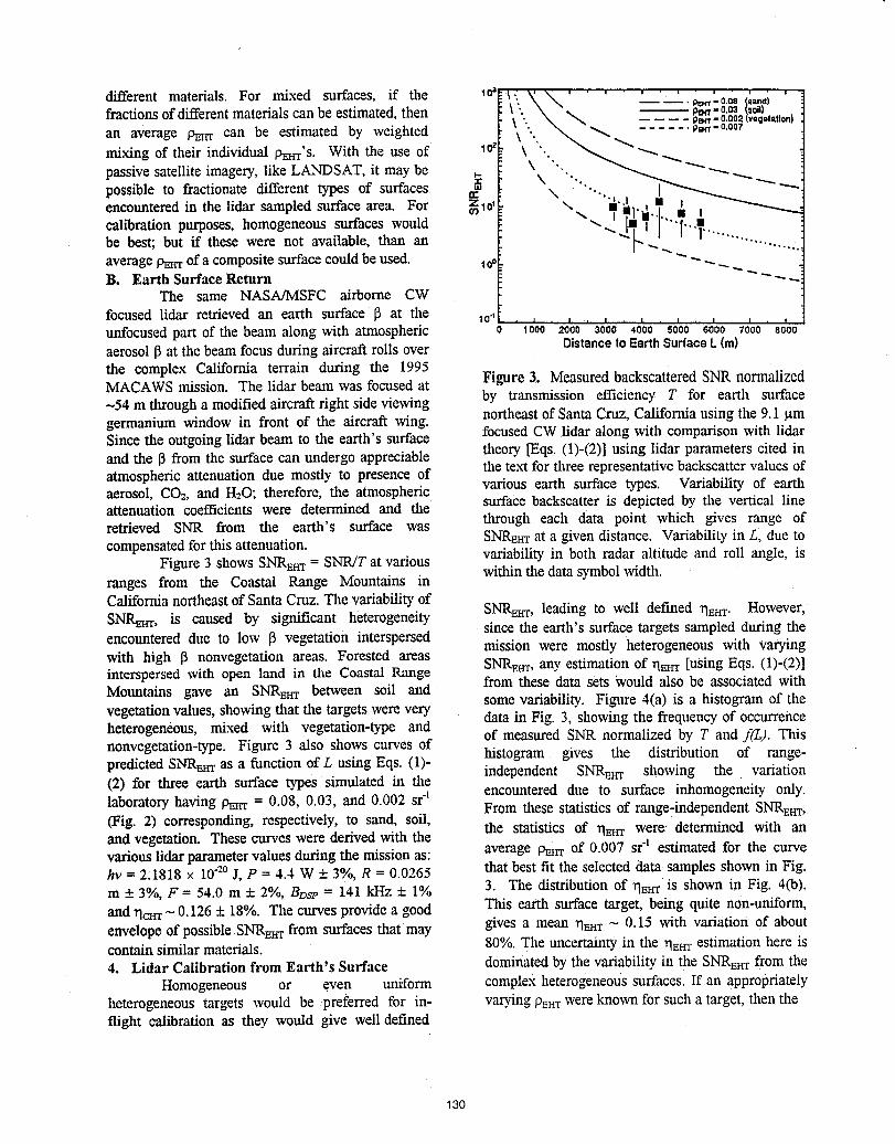
different materials. For mixed surfaces, ff the lO_, _.__, xx .... -' .' -'. _'- o.Q8(_'_,di'fractionsof differentmaterialscan be estimated,then \. ".......\ "" .... _p_-"0.0o20"°a_vogo,.,o,,_'*")-- "

\ "... _ _"_ ...... peru'-0.007an average P_icrcan be estimated by weighted \\mixing of their individual Pmrr'S. With the use of 1°_ "". _ _

passivesatelliteimagery, like LAaNDSAT,it maybe _. \ "'"'" I _ _ ""possible to fractionate difl"erenttypes of surfaces _ \\,'"'.....,..t,lmr-__@ _'"encounteredin the lidar sampledsurfacearea. For _1o' "_ _ _t]._._. i Icalibrationpurposes,homogeneous surfaces would --'-._ Ira./1_"1.... €....=.....

be best; but if these were not available, than an -._ I ,..., ........ .....averagePmrrof a compositesurfacecouldbe used. 1o* "- -_....-. ""B. Earth Surface Return

The same NASA/MSFC airborne CWfocused lidar retrievedan earth surface _ at the 10" , , , , , , , , , , , , , , , ,unfocusedpart of the beam along with atmospheric 0 1000 2000 aooo 4000 sooo sooo rooo aoooDistanceto Earth SurfaceL (m)aerosol13at the beamfocus during aircraft roils overthe complex California terrain during the 1995MACAWSmission. The lidar beam was focusedat Figure 3. MeasuredbackscatteredSNR normalized-54 m througha modifiedaircraft right sideviewing by transmission efficiency T for earth surfacegermanium window in front of the aircraft wing. northeastof Santa Cruz,California usingthe 9.1 _tmSince the outgoinglidar beam to the earth's surface focusedCWlidar along with comparisonwith lidartheory [Eqs.(1)-(2)]using lidar parameters cited inand the 13from the surface can undergo appreciableatmosphericattenuation due mostly to presence of the text for three representativebackscattervalues ofvarious earth surface types. Variability of earthaerosol, CO2, and H20; therefore, the atmosphericattenuation coefficients were determined and the surfacebackscatter is depicted by the vertical lineretrieved SNR from the earth's surface was through each data point which gives range ofcompensatedfor thisattenuation. SNREarat a givendistance. Variability in L, due to

Figure3 shows SNRmrr= SNR/Tat various variabilityin both radar altitude and roll angle, iswithinthe data symbolwidth.ranges from the Coastal Range Mountains in

Californianortheastof Santa Cruz. The variabilityof SNRmrr,leading to well defined rlErrr. However,SNRmrr, is caused by significant heterogeneity since the earth's surface targets sampledduring theencountered due to low 13vegetation interspersed mission were mostly heterogeneous with varyingwith high 13nonvegetation areas. Forested areas SNRmrr, any estimationof rlmrr [usingEqs. (1)-(2)]interspersed with open land in the Coastal Range from these data sets Wouldalso be associated withMountains gave an SNRmrr between soil and somevariability. Figure 4(a) is a histogramof thevegetationvalues,showingthat the targets were very data in Fig. 3, showingthe frequencyof occurrenceheterogeneous, mixed with vegetation-type and of measured SNR normalized by T and f(L). Thisnonvegetation-type.Figure 3 also shows curves of histogram gives the distribution of range-predictedSNRmrr as a function of L using Eqs. (1)- independent SNRmrr showing the variation(2) for three earth surface types simulated in the encountered due to surface inhomogeneity only.laboratoryhaving Pmrr= 0.08, 0.03, and 0.002 sr"] From these statisticsof range-independentSNREIrr,(Fig. 2) corresponding, respectively, to sand, soil,and vegetation. These curveswere derivedwith the the statistics of _Ei-rrwere determined with anvarious lidarparametervalues during the missionas: average Pmrrof 0.007 sr_ estimated for the curvehv = 2:1818 x 10"2°I, P = 4.4 W + 3%,R = 0.0265 that best fit the selecteddata samples shownin Fig.m _+3%,F = 54.0 m + 2°,/o,BDsv= 141 kHz + 1% 3. The distributionof rlErrris shown in Fig. 4(b).and rlcrrr- 0.126+ 18%. The curvesprovidea good This earth surface target, being quite non-uniform,envelopeof possibleSNRzrrrfrom surfacesthat may gives a mean rlmrr- 0.15 with variation of aboutcontain similarmaterials. 80%.The uncertaintyin the _qE_estimationhere is4. Lidar Calibration from Earth's Surface dominatedby the variabilityin the SNRErrrfrom the

Homogeneous or even uniform complexheterogeneoussurfaces. If an appropriatelyheterogeneous targets would be preferred for in- varyi'ngPErrrwereknownfor Sucha target, thentheflight calibration as they would give welldefined

130

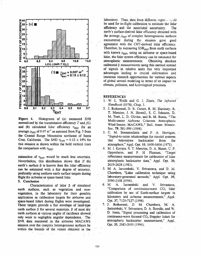
_4o - ' , ' , ' , ' i , laboratory. Thus, data from different regio:::.:,__,aldmz35 (a} • be used for in-flight calibration to estimate the lidar_ao -- efficiency and the associated uncertainty. The

,//, _ earth's surface-derived lidar efficiency obtained with

o°25 _/__ " the •average,9srrr of complex heterogeneous surfaces,O20 ;+;, encountered during the mission gave good°is _/_, agreement with the CHT-derived lidar efficiency.

°10 _ Therefore, by measuring SNRE_r from earth surfacesS ° with knownPsrrr,usingan airborneor space-based° 0 -- lidar, the lidar system efficiency can be estimated for

L 8.0 8.5 9.0 9.5 10.0 10.5 atmospheric measurements: Obtaining absoluteLOG (SNRITf(L)) calibrated _3measurements using this method instead

m40 - 'o of signals in relative units has very unportantmz35" advantages leading to crucial information andm30 • immense research opportunities for various aspects=

of global aerosol modeling in terms of its impact on25 •climate, pollution, and hydrologicalprocesses.O2o

O !//,15 '/_

°l°tu _ REFERENCESo_ S _/ 1. W. L. Wolfe and G. J. Zissis, The Infraredm 0 ///. Handbook (1978),Chap. 3.u, 0.0 0.1 0.2 0.3 0.4 0.5 0.6 0.7 2. J. Rothermel, D. R. Cutten, R. M. Hardesty, R.

T_EHT T. Menzies, 1. N. Howell, S. C. Johnson, D.M. Tratt, L. D. Olivier, and R. M. Banta, "The

Figure 4. Histograms of (a) measured SNR Multi-center Airborne Coherent Atmosphericnormalized by the transmission efficiency T and f(Z) Wind Sensor, MACAWS," Bull. Amer. Meteor.and (b) calculated lidar efficiency _qmrr for an Soc. 79, 581-599 (1998).average pzrrr°f0.07srtasassessedfr°mFig .3fi'om 3. C. M. Sonnenschein and F. A, Horrigan,the Coastal Range Mountains northeast of Santa "Signal-to-noise relationships for coa,-dalsystemsCruz, California. The SND rlcI.rr= 0.12 + 18% for that heterodyne backscatter from thethis mission is shown within the bold vertical lines atmosphere," Appl. Opt. 10, 1600-1604 (1971).for comparison with rl_ar. 4. M. I. Kavaya, R. T. Menzies, D. A. Haner, U. P.

Oppenheim, and P H. Flamant, "Targetestimation of rlzrrr would be much less uncertain, reflectance measurements for calibration of lidarNevertheless, this distribution shows that if the atmospheric backscatter data," Appl. Opt. 20,

earth's surface J3is known then the lidar efficiency 2619-2628 (1983).can be estimated with a fair degree of accuracy, 5. M. A. Jarzembski, V. Srivastava, and D. M.preferably using uniformearth surface targets during Chambers, "Lidar calibration technique usingflight for airborne or space-based lidar, laboratory-generated aerosols," Appl. Opt. 35,5. Conclusion 2096-2108 (1996).

Characterization of lidar 13 of simulated 6. M. A. Jarzembski and V. Srivastava.earth surfaces, such as vegetation and non- "Comparison of continuous-wave CO2 lidarvegetation, in the laboratory for their possible calibration by use of Earth-surface targets inapplication as calibration targets for airborne and laboratory and airborne measurements," Appl.space-based lidars during flights were investigated. Opt. 37, 7120-7127 (1998).These targets provide a fair envelope of land-type 7. L Rothermel, D. M. Chambers, M. A.earth surface 13for several materials. 13of most dry Jarzembski, V. Srivastava, D. A. Bowdle, and W.earth surfaces at various angles of incidence showed D. Jones, "Signal processing and calibration ofonly weak to negligible angular dependence. The continuous-wave focused CO,_Doppler lidars forSNR data measured+in the airborne MACAWS atmospheric backscatter measurement," Appl.

mission over the complex heterogeneous surfaces lie Opt. 35, 2083-2095 (1996).within the bounds of the values obtained in the

131

EFFECT OF AEROSOL PARTICLE MICROSTRUCTURE ON ACCURACY

OF CW DOPPLER LIDAR ESTIMATE OF WIND VELOCITY

V.A. Banakhand I.N. Smalikho

Institute of Atmospheric Optics of theRussianAcademyof Sciences,Akademicheskii prospekt, 1. Tomsk. 634055, Russia

e-mail: banakh@ldw.tomsk.susmalikho@iao.tsc.ru

Ch. Werner

DLR Lidar Group, PO 1116, D-82230 Wessling, Germanye-mail: Christian.Werner@dlr.de

1. Introduction

An estimate of radial wind velocity Vo obtained from data of cw Doppler lidar is the sum of the radial

velocity V, averaged over probing volume and the error V_[1]. Statistical independence of V, and V_as well as

statistical independence of velocity errors measured at different moments allow us to estimate the error variance2 _ '

cr_= (V_') from the temporal spectrum or structure function of wind velocity measured by Doppler !idar El].

Comparison of the experimental values _ obtained at very high signal-to noise ratio (SNR) [1] with the estimates

by formula [2]

ro (:)where L is the wavelength, to is the integration period and :s is the Doppler spectrum width (in m/s), shows that

for small probing volumes the experimental values g, far exceed (approximately in order of magnitude) the

theoretical estimates g_ based on Eq.(1). In order to explain this discrepancy between theory and experiment in

this paper we analyze the effect of aerosol particle microstructure on accuracy of wind velocity estimates from

data of cw Doppler lidar obtained at small probing volumes.

2. Algorithms of simulation

On short paths (rang-eR - 50 + I00 m or less) probing volume Ofcw Doppler lidars can measure only a.few

cubic centimeters in volumes. In this case according to rough estimates based on known data for the

rnicrostructureof atmospheric aerosol [3] it is necessary to take into account the concentration and size

distributionof particles in analysisof Doppler lidar run.

In contrast to previously used approaches of numerical simulation (see, for example Ref. 4,5) to study the

effect of aerosol microstructure we have developed the following algorithm. The entire path of sounding is

deviled into N very thin layers (slices). We assumethat within separate slice the aerosol particles move with the

same velocity. Using the lognormal probability density functionof particle size distributionwith the mean(a) and

standard deviation ffa the random realization of sizes a are simulated.Assuming that all particles have the same

complex refractive index m = n +j_ the backscattering amplitudesAi are calculatedusing Mie theory [6]. For

each wave scattered by separateparticle the initial phase _Fiis simulatedas uniformlydistributed randomvalue.

132

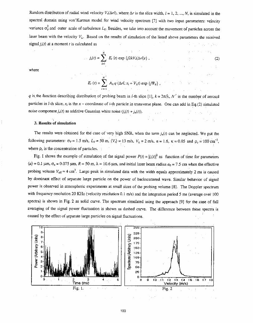
Random distribution of radial wind velocity Vr(Arl), where Ar is the slice width, l = 1, 2..... N, is simulated in the

spectral domain using von'Karman model for wind velocity spectrum [7] with two input parameters: velocity,)

variance _v and outer scale of turbulence Lv. Besides, we take into account the movement of particles across the

laser beam with the,velocity V±. Based on the results of simulation of the listed above parameters the received

signaljs(t) at a moment t is calculated as

N

js(t) = __2 Et (t) exp {j2kVr(Arl)t}, (2)!=l

where

N'

Et (t) = ___ Atiq (Arl, xi + V±t)exp {J_li} •i=l

q Is the function describitagdistribution of probing beam in l-th slice [i], k = 2rt/_,,N" is the number of aerosol

particles in/-th slice, xi is the x -coordinate of i-th particle in transverse plane. One can add in Eq.(2) simulated

noise componentj,(t) as additive Gauss±anwhite noise (]_(t)+j,(t)).

3. Results of simulation

The results were obtained for the case of very high SNR, when the term j,(t) can be neglected. We put the

following parameters: Cry= 1.5 m/s, Lv = 50 m, (V_)= 13m/s, V±= 2 m/s, n = 1.6, _:=-0.05 and Pc= 100 cm-3,

where Pcis the concentration of particles.

Fig. 1 shows the example of simulation of the signal power P(t) = l/.#)12as function of time for parameters

(a) = 0.1 btm,_, = 0.075/am, R = 50 m, _, = 10.6/am, and initial laser beam radius a0= 7.5 cm when the effective

probing volume Vetr= 4 cm3. Large peak in simulated data with the width equals approximately 2 ms is caused

by dominant effect of separate large particle on the power of backscattered wave. Similar behavior of signal

power is observed in atmospheric experiments at small sizes of the probing volume [8]. The Doppler spectrum

with frequency resolution 20 KHz (velocity resolution 0.1 m/s) and the integration period 5 ms (average over 100

spectra) is shown in Fig. 2 as solid curve. The spectrum simulated using the approach [9] for the case of full

averaging of the signal power fluctuation is shown as dashed curve. The difference between these spectra is

caused by the effect of.separate large particles on signal fluctuations.

133

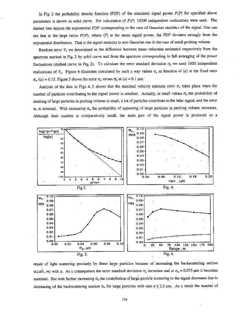
In Fig. 3 the probability density function (PDF) of the simulated signal power F(P) for specified above

parameters is shown as solid curve. For calculation of F(P) 10000 independent realizations were used. The

dashed line depicts the exponential PDF corresponding to the case of Gaussian statistics of the signal. One can

see that at the large ratios P/(P), where (P) is the mean signal power, the PDF deviates strongly from the

exponential distribution. That is the signal statistics is non-Gaussian one in the case of small probing volume.

Random error Ve we determined as the difference between mean velocities estimated respectively from the

spectrum marked in Fig. 2 by solid curve and from the spectrum corresponding to fu!l averaging of the power

fluctuations (dashed curve in Fig. 2). To calculate the error standard deviation erewe used 1000 independent

realizations of V_. Figure 4 illustrates calculated by such a way values or, as function of (a) at the fixed ratio

_, I(a) = 0.75. Figure 5 shows the error _ versus _a at (a) = 0.i _tm.

Analysis of the data in Figs. 4, 5 shows that the maximal velocity estimate error cr_takes place when the

number of particles contributing to the signalpower is smallest. Actually, at small values _a the probability of

entering of large particles in probing •volumeis small, a lot Ofparticles contribute to the tidar signal, and the error

o'e is minimal. With increasing erathe probability of appearing of large particles in probing volume increases.

Although their number is comparatively small, the main part of the signal power is produced as a

Iog[<p>F(p)]log[el -2--6--4--3-I0.;.=l _em/s° 0°°°80.09-0.10.05_06.070-._._-6- O.O4-

0.03--7*

"-, 0.02-• O.01 -

-9- "". o.oo--,o- " o.oo o.b5 o.io o.i5 o.2_

i 2 (3 4 5 6 7 8 9 10

p/<p> <_1.> , I.UTI

Fig 3. Fig. 4.

0.10-: Co, 0.10-__e, 0.09- 0.09-1

m/s o.o8- m/s o.o8-J

0.07- _ 0.07-

0.06- 0.06-0.05- 0.05-10.04- 0_04-1

0.03- 0.03-1

0.02- 0.02-i

o.o1 - _ -0.01-, _._,----_

o.oo- o,oo_i0.00 0.02 o.b4 0.06 0.08 0.1, 0 2s 5'0 _5 160 125 150 17s 200

cra. _rn Range,m

Fig. 5. Fig. 6.

result of light scattering precisely by these large particles because of increasing tlae backscattering section

_,_(a/2_,m) with a. As a consequence the error standard deviation _ increases and at cr_= 0.075 p.m it becomes

maximal. But with further increasing _ the contribution of large particle scattering to the signal decreases due to

decreasing of the backscattering section _,_for large particles with size a > 2.2 _tm. As a result the number of

134

aerosol particle contributing mainly to the lidar signal increases and _e decreases for or,> 0.075. The same

reason explains the decrease of erewith increasing (a) for specified in calculations ratio era/(a) = 0.75.

Figure 6 shows ere versus range R at (a)= 0.1 gm and to= 5 ms. Dark circles correspond to the case

ca = 0.075 _m and white circles are the result of calculation at _a _ O. It is seen that when all particles have the

same size (o'a---r0) the velocity estimate error _e increases monotonously with range R. This is in agreement

with the result of calculation ereby Eq. (1) (in inertial subrange of turbulence, when longitudinal size of probing

volume Az = (_/2) (R/ao)2< Lv, the Doppler spectrum width _. increases with the range R [1]). But in practical

situations the standard deviation qa _ 0 [3] and R - dependence of ereis not monotonous, as it follows from the

data in Fig. 6 (dark circles). With range increasing the error ae first increases and then decreases due to

significant increase of the probing volume V¢_- R3 and, consequently, the number of scattering particles. From

comparison of two curves in Fig. 6 it follows that under certain conditions the aerosol microstructure may be the

determining factor in accuracy of wind velocity statistics measurement by Doppler lidar.

References

1. V.A. Banakh; I.N. Smalikho, F. K6pp, and Ch. Werner, _Measurements of turbulent energy dissipation rate

with a cw Doppler lidar in the atmospheric boundary layer>>,J. Atmos. Oceanic Technol. (1999, accepted for

publication).

9.. R.J. Keeler, R.J. Serafin, R.L. Schwiesow, D.H. Lenschow, J.M. Vaughan, and A.A. Woodfield, ,An

airborne laser air motion sensing system. Part I: Concept and preliminary experiment>>,J. Atmos. Oceanic

Technol. 4. 113-127 (1987).

3. V.E. Zuev and G.M. Krekov, Optical Models of the Atmosphere, (Gidrometeoizdat, Leningrad, 1986), 256 p.

[in Russian].

4. R. Frehlich, ,Effect of wind turbulence on coherent Doppler lidar performance>>,J. Atmos. Oceanic Technol.

14.54-75 (1997).

5. V.A. Banakh, I.N. Smalikho, _Estimation of the turbulence energy dissipation rate from the pulsed Doppler

lidar data>>.Atmospheric and Oceanic Optics, 10. Nfll2.957-965 (1997).

6. A. Ishimaru, Wave Propagation and Scattering in Random Media (Academic Press, New York, 1978). Vol. 2.

278 p.

7. I.L. Lumtey and H.A. Panofsky, The Structure of Atmospheric Turbulence (Interscience, New York, 1964)

264 p.

8. R.M. Hardesty, R.J. Keeler, M.J. Post, and R.A. Richter, _Characteristics of coherent lidar returns from

calibration targets and aerosols>>,Appl. Opt. 20. 3763-3769 (1981).

9. V.A. Banakh, N.P. Krivolutsky, I.N. Smalikho, and Ch. Werner, _Simulation of scanning cw Doppler lidar>>,

Proc. 19-th International Laser Radar Conference, Annapolis, July 1998 / PT2, 731-734.

135

VALID : Experimental tests to validate a multiwavelength backscatter database andintercompare wind lidar concepts

Pierre H. Flamant

(1) Laboratoire de M&_orologie Dynamique,Centre National de laRecherche Scientifique

Ecole Polytechnique, 91 128 Palaisean cedex, FRANCEtel:33 169334550

fax'33 169333005

E-mail : flamant@lmd.polytechnique.fr

Abstract :

ESA is funding in 1999 an experimental activity (1) to built a multiwavelength backscatter database to validate a

scalling law derived in a previous study, and (2) intercompare the most relevant wind lidar concepts to space

applications. VALID will proceed in two steps : Step I in May-mid-June for backscatter data, lidars with

wavelengths ranging from UV (0.32 gm) to IR (10.6 gm) will be operated on the same site ; Step2 in mid-Julywill involve various coherent and incoherent lidar techniques on the same site.

136

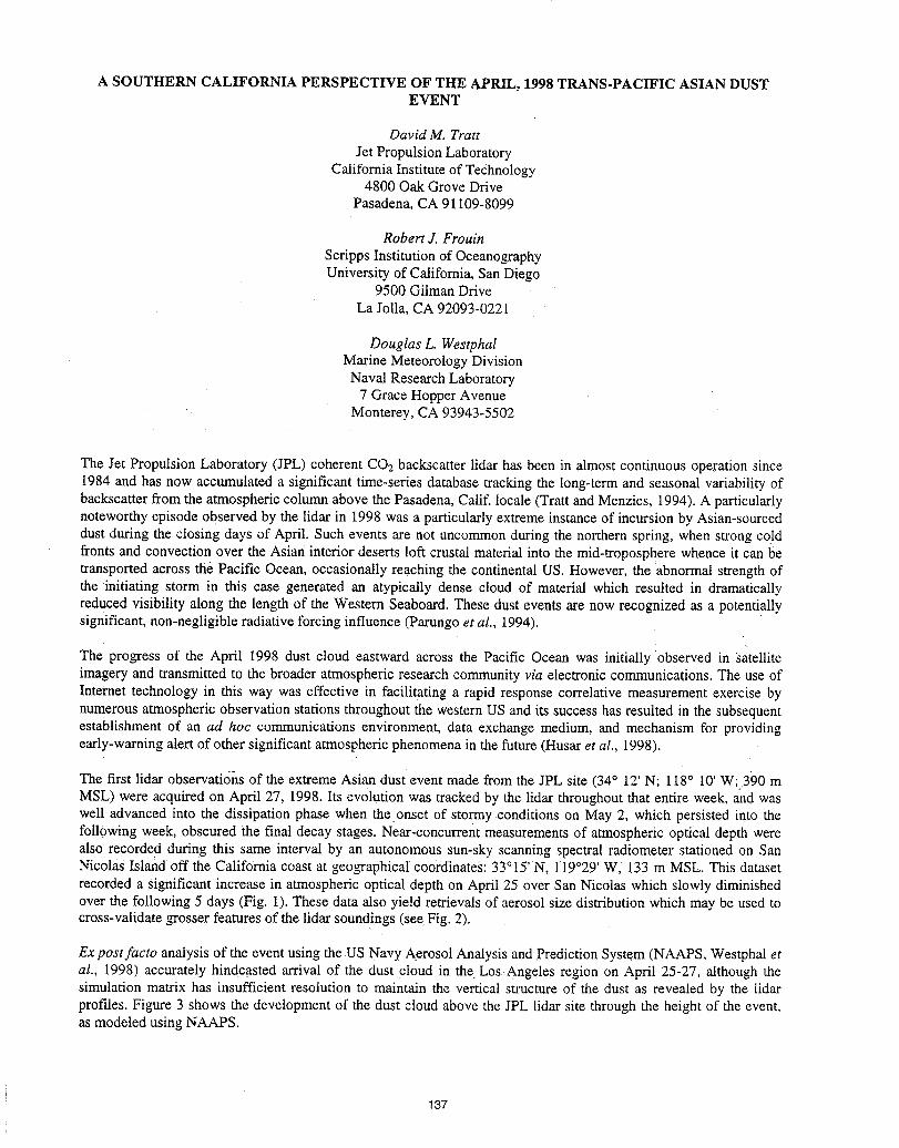
A SOUTHERN CALIFORNIA PERSPECTIVE OF THE APRIL, 1998 TRANS-PACIFIC ASIAN DUSTEVENT

David M. Tratt

Jet Propulsion LaboratoryCalifornia Institute of Technology

4800 Oak Grove DrivePasadena, CA 91109-8099

Robert J. Frouin

Scripps Institution of OceanographyUniversity of California, San Diego

9500 Gilman DriveLa JoUa, CA 92093-0221

Douglas L. WestphalMarine Meteorology Division

Naval Research Laboratory7 Grace Hopper Avenue

Monterey, CA 93943-5502

The Jet Propulsion Laboratory (JPL) coherent CO2 backscatter lidar has been in almost continuous operation since1984 and has now accumulated a significant time-series database tracking the long-term and seasonal variability ofbackscatter from the atmospheric column above the Pasadena, Calif. locale (Tratt and Menzies, 1994). A particularlynoteworthy episode observed by the lidar in 1998 was a particularly extreme instance of incursion by Asian-sourceddust during the closing days of April. Such events are not uncommon during the northern spring, when strong coldfronts and convection over the Asian interior deserts loft crustal material into the mid-troposphere whence it can betransported across the Pacific Ocean, occasionally reaching the continental US. However, the abnormal strength ofthe initiating storm in this case generated an atypically dense cloud of material which resulted in dramaticallyreduced visibility along the length of the Western Seaboard. These dust events are now recognized as a potentiallysignificant, non-negligible radiative forcing influence (Parungo et al., 1994).

The progress of the April 1998 dust cloud eastward across the Pacific Ocean was initially observed in satelliteimagery and transmitted to the broader atmospheric research community via electronic communications. The use ofInternet technology in this way was effective in facilitating a rapid response correlative measurement exercise bynumerous atmospheric observation stations throughout the western US and its success has resulted in the subsequentestablishment of an ad hoc communications environment, data exchange medium, and mechanism for providingearly-warning alert of other significant atmospheric phenomena in the future (Husar et al., 1998).

The first lidar observations of the extreme Asian dust event made from the JPL site (34° 12' N; 118° 10' W; 390 mMSL) were acquired on April 27, 1998. Its evolution was tracked by the lidar throughout that entire week, and waswell advanced into the dissipation phase when the onset of stormy conditions on May 2, which persisted into thefollowing week, obscured the final decay stages. Near-concurrent measurements of atmospheric optical depth werealso recorded during this same interval by an autonomous sun-sky scanning spectral radiometer stationed on SanNicolas Island off the California coast at geogaphicaI Coordinates: 33°15' N, 119°29' Wl 133 m MSL. This datasetrecorded a Significant increase in atmospheric optical depth on April 25 over San Nicolas which slowly diminishedover the following 5 days (Fig. 1).These data also yield retrievals of aerosol size distribution which may be used tocross-validate grosser features of the lidar soundings (see Fig. 2).

Ex post facto analysis of the event using the us Navy Aerosol Analysis and Prediction System (NAAPS, Westphal etal., 1998) accurately hindcasted arrival of the dust cloud in the LosAngeles region on April 25-27, although thesimulation matrix has insufficient resolution to maintain the vertical structure of the dust as revealed by the lidarprofiles. Figure 3 shows the development of the dust cloud above the JPL lidar site through the height of the event,as modeled using NAAPS.

137

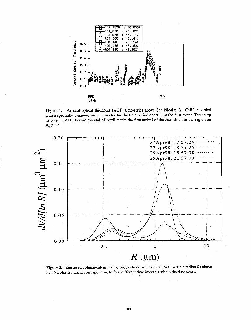
_PR _RV1998

Figure 1. Aerosol optical thickness (AOT) time-series above San Nicolas Is., Calif. recordedwith a spectrally scanning sunphotometer for the time period containing the dust event. The sharpincrease in AOT toward the end of April marks the f'n:starrival of the dust cloud in the region onApril 25.

0.20 ............... I ........ I27Apr98; 17:57:24

27Apt98; 18:57:25¢q 29Apr98; 18:57:08

29Apt98; 21:57:09 .................'_ 0.15=L

_'_ 0.10

0.05 ,,

0.000.1 1 10

R (gm)Figure 2. Retrieved column-integrated aerosol volume size distributions (particle radius R) aboveSan Nicolas Is., Calif. corresponding to four different time intervals within the dust event.

138

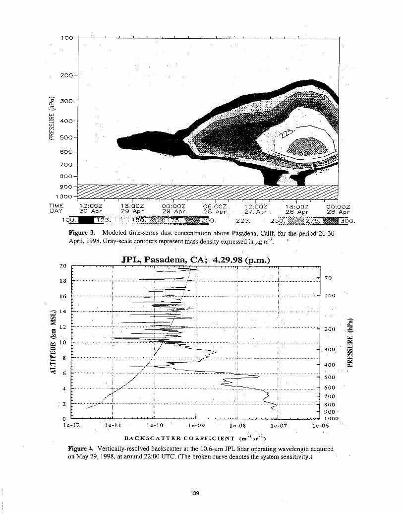
100' t I I I '1 1 I ' I I I I " I I I, I f I I

200 -

60{

700

8OO

900

1000

TIME 2:OOZ 18:QQZ O0:OOZ O6:OOZ 12:QOZ 18:0QZ O0:OOZDAY ,30 Apt 29 Apt 29 Apr 28 Apr . 27 Apr 26 Apr 26 Apr

Figure 3. Modeled time-series dust concentration above Pasadena, Calif. for the period 26-30April, 1998. Gray-scale contours represent mass density expressed in gg m3. ::

JPL, Pasadena, CA} 4.29.98 (p.m.)20 ................ . . _ . ....... ,..... ........ ...... ..

I-' - 70

18 .................................................................. -=-/ ; ................................................................................ L

.... i0016 ........................................................... _"-'-_ ................................... ;..................................................... rr

12 ....................................................,-;== ............. !-.............:.............!................. ..........'.......................... 200 --

"_ " " : , : _._2-- ' i i : ,_._ 10 ....... 7"7............. ,2 ......... _ "..... ........ ,'"'f "_": '. \[':'"'"'""'.."................... : ..... _.................. ......... _.........................

_- ! i: ' _ i' : 300 .w._

[#3

' , s .....................,,, :..[" 8 ........................................................................................................................), #2,i / ___ i 400: s" : '

: - : : ' : 500

4 : +/ : ! ! ' i 600

/ i i . : - 700

" 2 ......... _17:-.::-- "...... i........................... !...................... :....;: 800900

0 ........ ) ........ i ........ I ........ a ........ i ....... 1000

le-12 le-ll le-lO le=09 : le-08 le-07 le-06

BACKSCATTER COEFFICIENT (m'lsr "1)

Figure 4. Vertically-res01ved backscatter at the 10.6-gin JPL lidar operating wavelength acquiredon May 29, 1998, at around 22:00 UTC. (The broken curve denotes the system sensitivity.)

139

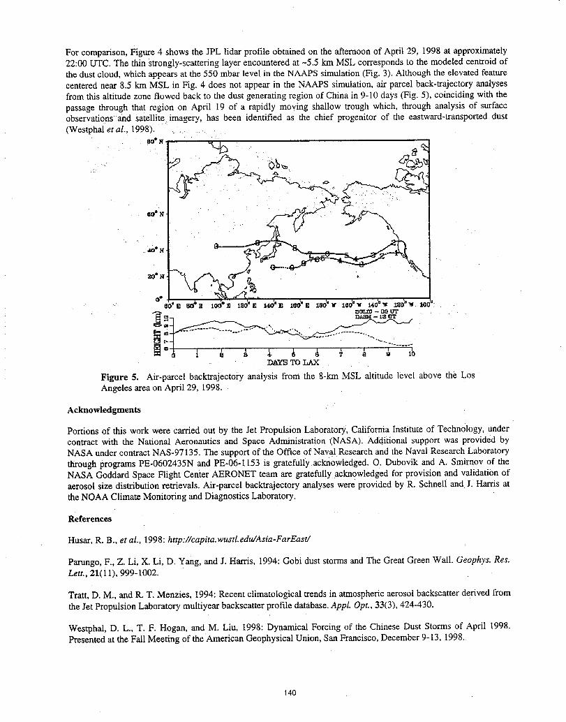
For comparison, Figure 4 shows the JPL lidar profile obtained on the afternoon of April 29, 1998 at approximately22:00 UTC. The thin strongly-scattering layer encountered at -5.5 km MSL corresponds to the modeled centroid ofthe dust cloud, which appears at the 550 mbar level in the NAAPS simulation (Fig. 3). Although the elevated featurecentered near 8.5 km MSL in Fig. 4 does not appear in the NAAPS simulation, air parcel back-trajectory analysesfrom this altitude zone flowed back to the dust generating region of China in 9-10 days (Fig. 5), coinciding with the

passage through that region on April 19 of a rapidly moving shallow trough which, through analysis of surfaceobservations and satellite imagery, has been identified as the chief progenitor of the eastward-transported dust

(Westphal et al., 1998)......

x.b

oo

_m_ - no u'r

=_ IIA.SI-I--1_ U'r

..

ID_['" •._ -.- r

Figure 5. A_-parce! backtrajectory analysis from the 8-kin MSL aldtude level above the LosAngeles area on April 29, 1998.

Acknowledgments

Portions of this work were carried out by the Jet Propulsion Laboratory, California Institute of Technology, undercontract with the National Aeronautics and Space Administration (NASA); Additional support was provided byNASA under contract NAS-97135. The support of the Office of Naval Research and the Naval Research Laboratorythrough programs PE-0602435N and PE-06-1153 is gratefully acknowledged. O. Dubovik and A. Smirnov of theNASA Goddard Space Flight Center AERONET team are gratefully acknowledged for provision and validation ofaerosol size distribution retrievals. Air-parcel backtrajectory analyses were provided by R. Schnell and J. Harris atthe NOAA Climate Monitoring and Diagnostics Laboratory.

References

Husar, R. B., et al., 1998: http://capita.wustl.edu/Asia-FarEast/

Parungo, F., Z. Li, X. Li, D. Yang, and J. Harris, 1994: Gobi dust storms and The Great Green Wall. Geophys. Res.Lett., 21(1 I), 999-1002.

Tratt, D. M., and R. T. Menzies, 1994: Recent climatological trends in atmospheric aerosol backscatter derived fromthe Jet Propulsion Laboratory multiyear backscatter profile database. Appl. Opt., 33(3), 424-430.

Westphal, D. L., T. F. Hogan, and M. Liu, 1998: Dynamical Forcing of the Chinese Dust Storms of April 1998.Presented at the Fall Meeting of the American Geophysical Union, San Francisco, December 9-13, 1998.

140

A Global Backscatter Database for Modelling Space-Borne Doppler Wind Lidar

J,M. Vaughan, Defence Evaluation & Research Agency, Malvern, U.K.

A. Culoma, European Space Agency, Noordwijk, Netherlands

Pierre H. Flamant, Laboratoire Meteorologie Dynamique, Palaiseau, France

C. Flesia, University of Geneva, Geneva, Switzerland

N. Geddes, Defence Evaluation & Research Agency, Malvern, U.K.

The aim of this study is to provide a source reference compendium and database of

atmospheric properties relevant to the design considerations of a space-borne Doppler

Wind Lidar (DWL). The broad wavelength range under consideration is 0.35_tm to

10.6Jxm. Within this range atmospheric aerosol backscatter coefficients at seven

specific wavelengths: 0.35_xm,0.53jxm, 1.06gm, 1.5gm, 2.1gm, 9.1gm and 10.6_m

are discussed on the basis of information derived from existing literature and the latest

available material that has been documented and may be considered validated. The

assessment also includes consideration of material presented and made available at

meetings of the NOAA Working Group on Space-Based Lidar Winds held up until

January 1998.

For the Atlantic region the most comprehensive database currently available at

10.6jxm is that of the SABLE and GABLE trials. These measurements were

conducted in the historically clean period, 1988-1990, well after the E1 Chichon

eruption but before the Mt Pinatubo event. They are thus likely to provide a

background level of backscatter coefficients. The measurements of backscatter were

made during 80 flights over the Atlantic in 6 different regions and/or seasons over a 3

year period. The material has been extensively analysed and presented in figures,

histogram and tabular form. For the present work the data has been further evaluated

and values of median, quartiles and deciles are shown in Table 1.

For the Pacific region measurements Of backscatter were made in theGLOBE

programme at a range of wavelengths, together with optical particle counter analysis

of aerosols. In particular, data at 1.06 _tmfrom the Globe II trial in Spring 1990 has

been presented in medians, quartiles and deciles. Modelling has also been carried out

on the particle counter measurements to provide backscatter values over the range

1016to 0.53 gm.

141

This and other material, together with general considerations of the impact of optical

properties on a space-borne lidar, and analysis of backscatter scaling laws with

wavelength are discussed. The overall conclusion is that the best currently available

representation of the global atmospheric backscatter at different wavelengths is given

by Table 1 scaled with the following equations.

The backscatter 13(_, z) at wavelength _ and height z may be determined from:

13(;_, z) = 13o(10.6_m, z) L_.(_m) j ..... 1

where 13o(10.6_m, z) is the scattering (in Table 1) at 10.6 Ixm. The scaling exponent

e_thatprovidesthe best consensusfor the wavelengthrange0.35_m - 2.1 !.tmis given

by:

o_(_,(0.35- 2.1 gm), z) 0.24 logt0(13o(10.6 Ixm, z))l- 0.62 ..... 2

For the wavelength 9.1 lxm account must be taken of the sharp resonances in refractive

index for certain materials (notably sulphates) found in the atmosphere. For this

wavelength a scaling exponent given by:

(z (9.1 Bm, z) = 1.25 log,0([3o (10.6 Ixm, z)) - 8.25 .....3

provides the best consensus fit.

Examination of data and isolated measurements in the literature shows reasonable

agreement, generally within a factor of 2 and often better, of the backscatter values

derived from Table 1 and Equations 1-3. They are thus presented as a useful measure

of the global backscatter to be expected on currently available information over the

range of wavelengths.

It should be noted that new material on atmospheric properties is of course continually

being published and made available to the scientific and lidar community. The

present work attempts to provide the best possible view of relevant atmospheric

properties at the present time. Over the coming years it may be anticipated that further

refinement of the data will be possible. In particular it may be hoped that

experimental backscatter measurements for at least one shorter wavelength, made

directly over many regions and seasons, will provide a truly authoritative global data

142

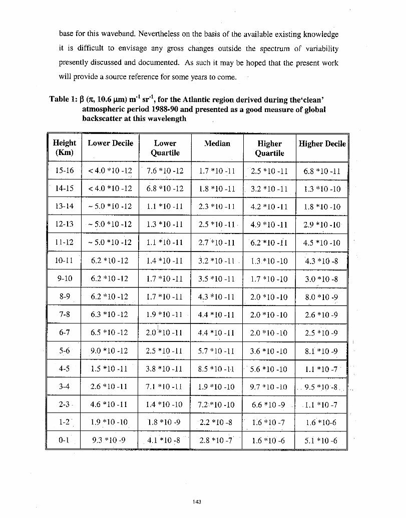
base for this waveband. Nevertheless on the basis of the available existing knowledge

it is difficult to envisage any gross changes outside the spectrum of variability

presently discussed and documented. As such it may be hoped that the present work

will provide a source reference for some years to come.

Table 1: I_(n, 10.6 _tm)m"1sr "1,for the Atlantic region derived during the'clean'atmospheric period 1988-90 and presented as a good measure of globalbackscatter at this wavelength

Height Lower Decile Lower Median Higher Higher Decile(Km) Quartile Quartile

15-16 <4.0 *10-12 7.6 "10 -12 1.7 "10-11 2,5 *10-11 6.8 *i0-11

14-15 <4.0"10-12 6.8 *10-12 1.8 *10-11 3.2 *10-11 1.3 *10-10

13-14 - 5,0 "10 -12 1.1 "10-11 2.3 *t0-11 4.2 "10 -11 1.8 "10 -10

12-13 ~ 5.10"10 -12 1.3 "10 -11 2.5 *10 -11 4.9 "10 -11 2.9 *10 -10

11-12 - 5.0 *10-12 111 '10-11 2.7 "10-11 6.2"10-11 4.5 "10 -10

10-11 6.2 "10-12 1.4 *10-11 3.2 *10-11 1.3"10-10 4.3 *10-8

9-10 6.2 "10 -12 1.7 "10 -11 3.5 "10 -11 1.7 "10 -10 3.0 "10 -8

8-9 6.2 "10 -12 1.7 *10-11 4.3 '10-11 2.0"10-10 8.0 *10-9

7-8 6.3 "10 -12 1.9 *10-11 4.4"10-11 2.0"10-10 2.6 *i0-9

6-7 6.5 *10 -12 2.0"10 -11 4.4 *10 -11 2.0 *10 -10 2.5 "10 -9

5-6 9.0 *t0-12 2.5 *10-11 5.7 *10-11 3.6 "10-10 8.1 *10-9

4-5 1.5 *10-11 3.8 "10-11 8.5 *10-1-1 5.6 *10-10 1.1 "10-7

3-4 2.6 "10 -11 7.1 "10-11 1.9 "10 -10 9.7 "10 -10 . 9.5 "10-8

2-3 4,6 *10-11 1,4 "10-10 7.2"10-10 6.6 *I0-9 1.1 *10-7

1-2 1.9 *I0 -10 1.8 *10:9 2.2 *10 -8 1'16*10 -7 1.6 "10-6

0-1 9.3 *10-9 4.1 *10-8 2.8 *10-7 _ 1.6 *10-6 5.1 *10-6

143

TARGET CALIBRATION: RETRO-REFLECTION MECHANISMS AT 2/am

David A. Haner and David M. Tratt

Jet Propulsion LaboratoryCalifornia Institute of Technology

4800 Oak Grove Drive

Pasadena, CA 91109

INTRODUCTION

With the growing use of 2-_tmeye-safe solid-state laser transmitters in coherent Doppler lidar applications, there isincreased interest in the reflectance properties of hard target calibration materials at this wavelength. One of thefactors to be considered is the polarization characteristic of the transmitter/receiver. The two fundamental lidarsystems are either based upon the backscattering of linearly polarized or circularly polarized light (Kavaya, 1987).Consequently, the response of calibration materials to the particular state of polarization of the incident radiation is•an important consideration. Ideally the calibration materials should have a similar reflectance response to that of theremote scattering medium that is being observed. Also the material should be most efficiently adapted to thepolarization characteristics of the lidar system.

There are two measurement parameters that are useful in presenting the characteristics of polarization of reflectingmaterials (see References). The first is the linear polarization ratio: _1=Iot/Isl,where ol denotes opposite linear and sldenotes same linear. The second is circular polarization ratio: _ac= Isc/Io_,where ol denotes opposite circular and scdenotes same circular. Notice that the ratios are inverted with respect to same polarization. It is the relative values ofthese polarization ratios that are used to characterize the retro-reflectance mechanism.

Measurement of these parameters is conveniently obtained by using the Stokes vectors corresponding to thepolarized backscatter at and near the retro-angle.

RETRO-REFLECTION MECHANISMS

Two distinct processes are recognized as contributing to the retro-reflection mechanism: shadow hiding and coherentbackscattering.

Shadow hiding

This type of backscattering is thought to be caused by single scattering from a particle or surface into the backwarddirection and tends to preserve the plane of linear polarization. However, it would reverse the handedness of

circularly polarized light. Generally the forward scattered light preserves the plane of linear polarization and retainsthe handedness of circularly polarized light. It is clear that both _h and _t_should tend to increase with scatteringangles less than 180°.

Coherent backscattering

This type of backscattering is thought to be caused by multiple scattering of light. The result of multiple scattering oflinearly polarized light will tend not to change the plane of polarization; thus the scattering angle dependence willappear similar for either process. However, the handedness of circularly polarized light will reverse on each impact;thus _tc will decrease for smaller scattering angle. To distinguish between which of these mechanisms is mosteffective when light is incident on a particular backscattering material; the magnitudes of _tcat the retro-angle and a

few de_ee s off-retro need to be measured for various materials with differing surface and bulk properties.

144

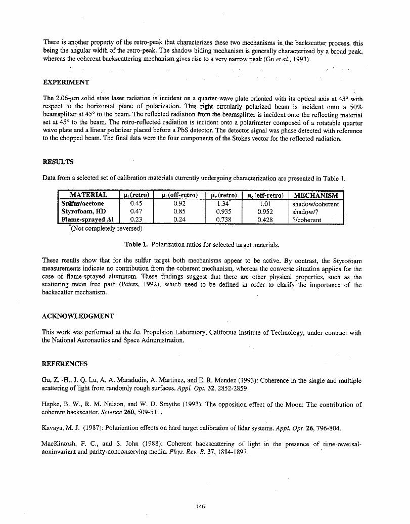
There is another propertY of the retro-peak that characterizes these two mechanisms in the backscatter process, thisbeing the angular width of the retro-peak. The shadow hiding mechanism is generally ch_acterized by a broad peak,whereas the coherent backscattering mechanism gives rise to a very narrow peak (Gu et al., 1993).

EXPERIMENT

The 2.06-_tm solid state laser radiation is incident on a quarter-wave plate oriented with its optical axis at 45° withrespect to the horizontal plane of polarization. This right circularly polarized beam is incident onto a 50%beamsplitter at 45° to the beam. The reflected radiation from the beamsplitter is incident onto the reflecting materialset at 45° to the beam. The retro-reflected radiation is incident onto a polarimeter composed of a rotatable quarterwave plate and a linear polarizer placed before a PbS detector. The detector signal was phase detected with referenceto the chopped beam. The final data were the four components of the Stokes vector for the reflected radiation.

RESULTS

Data from a selected set of calibration materials currently undergoing characterization are presented in Table I.

MATERIAL _h(retro) _q(off-retro) [tc(retro) [tc(off-retro) MECHANISMSulfur/acetone 0.45 0.92 1.34" 1.01 shadow/coherentStyrofoam, HD 0.47 0.85 0.935 0.952 shadow/?

Flame-sprayed AI 0.23 0.24 0.738 0.428 ?/coherent*(Not completely reversed)

Table 1. Polarization ratios for selected target materials.

These results show that for the sulfur target both mechanisms appear to be active. By contrast, the Styrofoammeasurements indicate no contribution from the coherent mechanism, whereas the converse situation applies for thecase of flame-sprayed aluminum. These findings suggest that there are other physical properties, such as thescattering mean free path (Peters, 1992), which need to be defined in order to clarify the importance of thebackscatter mechanism.

ACKNOWLEDGMENT

This work was performed at the Jet Propulsion Laboratory, California Institute of Technology, under contract withthe National Aeronautics and Space Administration.

REFERENCES

Gu, Z. -H., J. Q. Lu, A. A. Maradudin, A. Martinez, and E. R. Mendez (1993): Coherence in the single and multiplescattering of light from randomly rough surfaces. Appl. Opt. 32, 2852-2859.

Hapke, B. W., R. M. Nelson, and W. D. Smythe (1993): The opposition effect of the Moon: The contribution ofcoherent backscatter. Science 260, 509-511.

Kavaya, M. J. (1987): Polarization effects on hard target calibration of lidar systems.Appl. Opt. 26, 796-804.

MacKintosh, F. C., and S. John (1988): Coherent backscattering of light in the presence of time-reversal-noninvariant and parity-nonconserving media. Phys. Rev. B. 37, 1884-1897.

145

Ostro, S. J., and E. M. Shoemaker (1990): The extraordinary radar echoes from Europa, Ganymede, and Ca[list.o:Ageological perspective. Icarus 85, 335-345.

Peters, K. J., (1992): Coherent-backscatter effect: A vector formulation accounting for polarization and absorptioneffects and small or large scatterers. Phys. Rev. B. 46, 801-812.

Pitter, M., E. Jakeman, and M. Harris (1997): Heterodyne detection of coherent backscatter. Opt. Lett. 22, 393-395.

146

Backscatter modeling at 2.1micron wavelength for space-based and airborne lidars usingaerosol physico-chemicalandlidar datasets

V. Srivastava I, J. Rothermel2 , M.A. Jarzembski2, A.D. Clarke3, D.R. Cutten4, D.A. Bowdle4, J.D. Spinhirne s,and ILT. Menzies6

1 Global Hydrology and Climate Center,University Space Research Association, Huntsville, AL 35806; 2 GlobalHydrology and Climate Center, NASA, Huntsville, AL; 3 University of Hawaii, Honolulu, HI; 4 Global Hydrologyand Climate Center, UAH, Huntsville, AL; 5 NASA Goddard Space Flight Center, Greenbelt, MD; 6 Jet PropulsionLaboratory, NASA, Pasadena, CA

1. Introduction

Space-based and airborne coherent Doppler lidars designed for measuring global tropospheric wind

profiles in cloud-free air rely on backscatter, ,8, from aerosols acting as passive wind tracers. Aerosol fl distributionin the vertical can vary over as much as 5-6 orders of magnitude (Rothermel et al.,1989;1996a, Srivastava et al.,1997; Tratt et ai.,1994; Spinhime et a1.,1997 Jarzembski et a1.,1999). Thus, the design of a wavelength-specific,space-borne or airborne lidar must account for the magnitude offl in the region or features of interest.

The SPAce Readiness Coherent Lidar Experiment (Kavaya et al. 1998), under development by theNational Aeronautics and Space Administration (NASA) and scheduled for launch on the Space Shuttle in 2001,will demonstrate wind measurements from space using a solid-state 2 _tm coherent Doppler lidar. Consequently,there is a critical need to understand variability of aerosol fl at 2.1 _tm to evaluate signal detection under varyingaerosol loading conditions. Although few direct measurements of fl at 2.1 p.m exist, extensive datasetz, includingclimatologies in widely-separated locations, do exist for other wavelengths based on CO2 and Nd:YAG lidars((Rothermel et a1.1989; 1996a, Tratt et a1.,1994; Menzies et al., 1997; Spinhirne et al., 1997). Datasets also existfor the associated microphysical and chemical properties. An example of a multi-parametric dataset is that of theNASA GLObal Backscatter Experiment (GLOBE) in 1990 (Bowdle and Fitzjarrald; 1987), in which aerosolchemistry and size distributions (Clarke et al. 1993) were measured concurrently with multi-wavelength lidarbackscatter observations. More recently, continuous-wave (CW) lidar backscatter measurements at mid-infraredwavelengths have been made during the Multicenter Airborne Coherent Atmospheric Wind Sensor (MACAWS)experiment in 1995 (Jarzembski et al. 1999). Using Lorenz-Mie theory, these datasets have been used to develop amethod to convert lidar backscatter to the 2.1_tm wavelength. This paper presents comparison of modeledbackscatter at wavelengths for which backscatter measurements exist including converted fl2.1.2. Measurements

The GLOBE datasets consist of 15 flights over the Pacific Ocean on NASA's DC-8 aircraft. For ,8modeling and intercomparison, datasets primarily from flight#12 (F12) were used. This 7.5hr flight from Darwin,Australia, to Tokyo, Japan, occurred on May 3I, 1990. Several datasets from the following instruments were used.(i) University of Hawaii's Laser Optical Particle Counter (LOPC) provided thermally-differentiated aerosol sizedistributions during GLOBE from which different aerosol compositions were inferred (Clarke, 1993) and used tomodel aerosol 13at various wavelengths (Srivastava et al., 1997). (ii) Two NASA/MSFC Continuous Wave (CW)

focused 9.1 and 10.6_tm CO, lidars obtained high-resolution, high sensitivity 13data (Rothermel et al., 1996b)concurrent with the LOPC microphysics data during GLOBE, enabling excellent intercomparison with aerosol 13modeling (Srivastava et al., 1997). These lidars also obtained ,6 in 1995 during 9 flights in MACAWS, over thewestern coastal regions of North America and California, comprising - 52 flight hours of data. (iii) NASA/GSFCpulsed Nd:YAG 0.53 and 1.06 _tm lidar and NASA/JPL Pulsed CO,.9.25#m lidar measured high-resolution, verticalaerosol 13profiles (Spinhirne et al., 1997; Menzies et al., 1997) during GLOBE. /3 near the aircraft from pulsedlidars provided comparison with modeled flusing LOPC aerosol microphysics and with the CW lidars.3. Modeling

Aerosol 13zat a given wavelength (2) is a function of particle composition (complex refractive index, m),size (r), and number concentration (No). In general, if m, r, No, were well-determined, then 13_can be obtained for

any 2, (Srivastava et al., 1992, 1997). Assuming.spherical particle shape allows the use of Lorenz-Mie scattering

theory. Furthermore, aerosols can have very different composition with differing m which in turn depends on 2'.These compositions can be pure, partially mixed, or completely mixed. Different aerosol loading conditions require

147

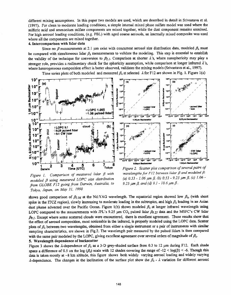
different mixing assumptions. In this paper two models are used, which are described in detail in Srivastava et al.(1997). For clean to moderate loading conditions,a simple internal mixed phase sulfate model was used where thesulfuric acid and ammonium sulfate components are mixed together,while the dust componentremains unmixed.For high aerosol loading conditions, (e.g. PBL) with aged coarse aerosols, an internally mixed composite was usedwhereallthecomponentsaremixedtogether.4. Intereomparison with iidar data

Sinceno/8measurementsat 2.1_tmexistwithconcurrentaerosolsizedistributiondata,modeledfixmustbe compared with simultaneous lidar `8xmeasurements to validate the modeling. This step is essential to establishthe validityof the techniquefor conversionto ,82.i.Comparisonat shorter2'% wherenonsphericitymayplayastrongerrole,providesa rudimentarycheckforthesphericityassumption,whilecomparisonat longerinfrared2'%where heterogeneous composition effect is better observed, validates the mixing models (Srivastava et al., 1997).

Time series plots of both modeled and measured ,84at selected 2' for F12 are shown in Fig. 1. Figure l(a)

1 0 "6 I0-* ......._ ......._ ......_ ......._ .......,, ,,_ 1o4_ ......_ ......._ ........_"'""_ ' '6'"'_";::_(a} , E(b) o

" 10-1op

10" '_'° / . pulsed lldar / + pulledllder_) 10/11 / oLOPC 10"11_ °k)l_

(: 0.10 / rg /,; , . ......; .......j ........; ,, lO._Z_ ........I .......I ...... ; ....... '_ ........l ,.,•;1 ,o%.,',"; ,;"_.,0 lO _ lol 10-, 104 lO-12 lO.11 lO-1, 104 lO 4 11)-_ lO4

...... 1 ....... 1 ....... 1 0 41--=....... 1 ........ I _ '10"5 '_', .......:o':5":":;" ......' ......."'""'_(a) o ../ ! L (all

1 _o.,I / " 104p

1 0 .4 10"71 . 0 . 10"7 .'.

i " 2 IE I /

_10"* _',_,o " ,0.o0.10 / / + pulxd Ildl_ _- •CW Ildar

_1 1_-- / / oLOPC 10"'_ _/ oLOP C10"' 10,41 _', ,,,,.J ,, .,,,d .....d ....... J , J . 12(." ,,,,,,J ....... I ....... I ....... _ ....... I *.10"1Z 10"11 lO'tO 104 104 ""I'O'T* 10_ 10"10"tl 10"11 10"10 10"1 10"l 1_ I' 1041

10"= 1 2 3 4 5 6 7 8 '"_ ='_'_" _ _"Darwin Time(UTC) Tokyo Figure 2. Scatter plot comparison of several pairs of

Figure 1. Comparison of measured lidar fl with wavelengths for F12 between lidar fl and modeled fl:

modeled ,8 using measured LOPC size distribution (a) 0.53 - 1.06 ,tim,8, (b) 0.53 - 9.25 pm ,8, (c) 1.06 -from GLOBE F12 going from Darwin, Australia, to 9.25 #m ,8,and (d) 9.1 - 10.6/_m ft.Tokyo, Japan, on May 31, 1990

shows good comparison of ,81.o6at the Nd:YAG wavelength. The equatorial region showed low `84, (with short

spike in the ITCZ region); slowly increasing to moderate loading in the subtropics, and high `sxloading in an Asiandust plume advected over the Pacific Ocean. Figure l(b) shows modeled ,sx at longer infrared wavelength usingLOPC compared to the measurements with JPL's 9.25 ktmCO2 pulsed lidar flg.25data and the MSFC's CW lidar`89.1.Except where some scattered clouds were encountered, there is excellent agreement. These results show thatthe effect of aerosol composition, most noticeable in the infrared, is properly modeled using the LOPC data. Scatter

plots of`sx between two wavelengths, obtained from either a single instrument or a pair of instruments with similarsampling characteristics, are shown in Fig.2. The wavelength pair measured by the pulsed lidars is then comparedwith the same pair modeled by the LOPC, giving excellent agreement over several orders of magnitude of`sx.5. Wavelength dependence of backscatterFigure 3 shows the 2,-dependence of,8_ as a 3-D grey-shaded surface from 0.3 to 12 _tm during F12. Each shadespans a difference of 0.5 on the log (fix) scale with 12 shades covering the range of-12 < log([3)< -6. Though thisdata is taken mostly at -8 km altitude, this figure shows both widely varying aerosol loading and widely varying

2.-dependence. The changes in the inclination of the surface plot show the fix - 2' variation for different aerosol

148

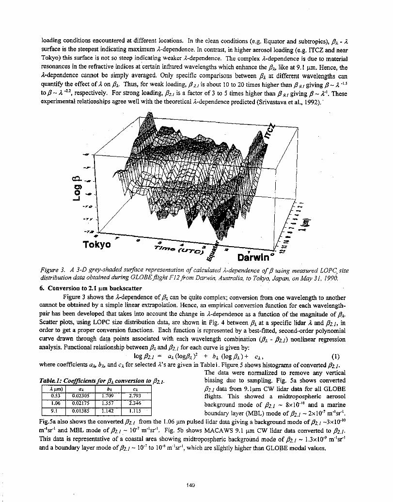
loading conditions encountered at different locations. In the clean conditions (e.g. Equator and subtropics), fix- A

surfaceis the steepest indicatingmaximumA-dependence.In contrast,in higher aerosol loading (e.g. ITCZandnearTokyo) this surface is not so steep indicating weaker A-dependence. The complex A-dependenceis due to materialresonances in the refractiveindices at certain infraredwavelengths which enhance the fix, like at 9.1 _tm. Hence, the

A-dependence cannot be simply averaged. Only specific comparisons between ,84 at different wavelengths canquantify the effect of Aon ,fix. Thus, forweak loading,fl2.1 is about 10 to 20 times higher than fl9.1giving/3- A4.5toil~ A -2.2,respectively. For strong loading, 132.1is a factor of 3 to 5 times higher than fl9.1 giving fl~ A4. These

experimentalrelationshipsagreewell with the theoretical A-dependencepredicted (Srivastavaet al., 1992).

O-,,_l

_lCO

-- 7'.R' F"

O ._. 6' _. ,,It'Tokyo ----7"Zrrno (_r.J'7-_.; -'_

Darwin°Figure 3. A 3-D grey-shaded surface representation of calculated 2-dependence of/3 using measured LOPC.sizedistribution data obtained during GLOBEflight F12from Darwin, Australia, to Tokyo, Japan, on May 31, 1990.

6. Conversion to 2.1 _tm backscatter

Figure 3 shows the A-dependence of fix can be quite complex; conversion from one wavelength to anothercannot be obtained by a simple linear extrapolation. Hence, an empirical conversion function for each wavelength-pair has been developed that takes into account the change in A-dependence as a function of the magnitude of fix.Scatterplots, using LOPC size distribution data, are shown in Fig. 4 between fl_ at a specific lidar A and fl2.1, inorderto get a proper conversion functions. Each function is represented by a best-fitted, second-order polynomialcurve drawn through data points associated with each wavelength combination (fix - fl2.1) nonlinear regressionanalysis. Functional relationship between fix and fl2.1for each curve is given by:

log/92.1 = ax(logfl_)2 + bx (log fix ) + c;_, (1)

where coefficients ax, bx, and cx for selected A's are given in Tablel. Figure5 shows histograms of converted fl2.1.The data were normalized to remove any vertical

Tabled: Coeff!cientsforfl_ conversion to fl2.1, biasing due to sampling. Fig. 5a shows convertedktm) aa b_ ca f12.1data from 9.1_m CW lidar data for all GLOBE

0.53 0.02305 1.709 2.793 flights. This showed a midtropospheric aerosol

1.06 0.02175 1.557 2.346 background mode of f12.1 ~ 8xl0"t° and a marine9.1 0.01385 1.142 1.115 boundary layer (MBL) mode offl2.1 _ 2xl0 7 m4sr4.

Fig.5a also shows the converted/32.1 from the 1.06 _tmpulsed lidar data giving a background mode of/32.1 -3x 1040m'tsr "t and MBL mode offl2.1 - 10 -7 m4sr4. Fig. 5b shows MACAWS 9.1 _tm CW lidar data converted to fl2.1.

This data is representative of a coastal area showing midtropospheric background mode of fl2.1 - 1.3x 10 -9 m4srt

and a boundary layer mode offl2.1 - 10"7to 10 -6m4sr4, which are slightly higher than GLOBE modal values.

149

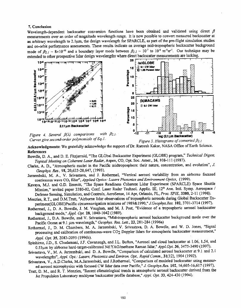
7. Conclusion

Wavelength-dependent backscatter conversion functions have been obtained and validated using direct ,8measurements over an order of magnitude wavelength range. It is now possible to convert measured backscatter atan arbitrary wavelength to 2.1_tm,the design wavelength for SPARCLE, as part of the pre-flight simulation studiesand on-orbit performance assessments. These results indicate an average mid-tropospheric backscatter background

mode of f12.1- 8xl0"]° and a boundary layer mode between fl2.1 - 10"7 to 10"6 m'lsr "l. Our technique may beextended to other prospective lidar design wavelengths where direct backscatter measurements are lacking.

10-4 20

15 .0 9.1CWIIdari. 10"6 O rl 1.06 Pulled lldar _/o

_'10 "10 25 - ' i i i i _o. (b)MACAWS

10"I$10"1210"1110"I°10"e10"810"7 10"410"6 n. _/

2.11IJmBackscatter 5 _0 ._

Figure 4. Several fl(A) comparisons with f12.1. -12 -11 -10 .9 -8 -7 -6 -5log(2.1p.mBackecatter)

Curves give second-order polynomials of Eq.l. Figure 5. Histograms of converted fl2.1

Acknowledgments: We gratefully acknowledge the support of Dr. Ramesh Kakar, NASA Office of Earth Science.ReferencesBowdle, D. A., and D. E. Fitzjarrald, "The GLObal Backscatter Experiment (GLOBE) program," Technical Digest,

Topical Meeting on Coherent Laser Radar, Aspen, CO, Opt. Soc. Amer., 16, 108-I 11 (1987).Clarke, A. D., "Atmospheric nuclei in the Pacific midtroposphere: their nature, concentration, and evolution", J.

Geophys. Res., 98, 20,633-20,647, (1993).Jarzembski, M. A., V. Srivastava, and J. Rothermel, "Vertical aerosol variability fi'om an airborne focused

continuous wave COz ffdar",Applied Optics: Lasers Photonics and Environment Optics, (I 999).Kavaya, M.J. and G.D. Emmitt, "The Space Readiness Coherent Lidar Experiment (SPARCLE) Space Shuttle

Mission," invited paper 3380-02, Conf. Laser Radar Technol. Applic. III, 12thAnn. Intl. Symp. Aerospace /Defense Sensing, Simulation, and Controls, AeroSense, 14Apr, Orlando, FL, Proc. SPIE, 3380, 2-11 (1998).

Menzies, R.T., and D.M.Tratt, "Airborne lidar observations of tropospheric aerosols during Global Backscatter Ex-periment(GLOBE)Pacific circumnavigation missions of 1989&1990," J.Geophys.Res. 102, 3701-3714 (1997).

Rothermel, J., D. A. Bowdle, J. M. Vaughan, and M. J. Post, "Evidence of a tropospheric aerosol backscatterbackground mode," A-ppl. Opt. 28, 1040-1042 (1989).

Rothermel, J., D.A. Bowdle, and V. Srivastava, "Mid-tropospheric aerosol backscatter background mode over thePacific Ocean at 9.1 btm wavelength," Geophys. Res. Lett., 23, 281-284 (1996a)

Rothermel, J., D. M. Chambers, M. A. Jarzembski, V. Srivastava, D. A. Bowdle, and W. D. Jones, "Signalprocessing and calibration of continuous-wave CO2 Doppler lidars for atmospheric backscatter measurement,"

Appl. Opt. 35, 2083-2095 (1996b).Spinhirne, J.D., S. Chudamani, J.F. Cavanaugh, and J.L. Button, "Aerosol and cloud backscatter at 1.06, 1.54, and

0.53p.mby airborne hard-target-calibrated Nd:YAG/methane Raman lidar," Appl.Opt. 36, 3475-3490 (1997).Srivastava, V., M. A. Jarzembski, and D. A. Bowdle, "Comparison of calculated aerosol backscatter at 9.1 and 2.1

wavelengths", Appl. Opt.: Lasers, Photonics and Environ. Opt., Rapid Comm., 31(12), 1904 (1992).Srivastava, V., A.D.Clarke, M.A.Jarzembski, and J.Rothermel, "Comparison of modeled backscatter using measur-

ed aerosol microphysics with focused CW lidar data over Pacific,",/.. Geophys.Res. 102, 16,605-16,617 (1997).Tratt, D. M., and R. T. Menzies, "Recent climatological trends in atmospheric aerosol backscatter derived from the

Jet Propulsion Laboratory multiyear backscatter profile database," Appl. Opt. 33, 424-430 (1994).

150

Comparisonof Predictedand Measured2 _m AerosolBackscatterfromthe 1998ACLAIMFlightTests

David A. Bowdle

University of Alabama in HuntsvilleGlobal Hydrology and Climate Center

977 Explorer BoulevardHuntsville, Alabama USA 35806

Voice: 205-922-5955, Fax: 205-922-5723, e-mail: David.Bowdle@msfc.nasa.gov

StephenM. HannonCoherent Technologies, Inc.

' Lafayette, Colorado USA

Rodney K. Bogue

NASA Dryden Flight Research CenterEdwards, California USA

ABSTRACT

The 1998 Airbome Coherent Lidar for Advanced Inflight Measurements (ACLAIM) flight

tests were conducted aboard a well-instrumented research aircraft. This paper presents

comparisons of 2 gm aerosol backscatter coefficient predictions fi:omaerosol sampling data

and mie scattering codes with those produced by the ACLAIM instrument.

151

POSTER SESSION

152

The NASA/MSFC Coherent Lidar

Technology Advisory Team

Michael J. Kavaya

NASA Marshall Space Flight Center

Global Hydrology and Climate Center, Mail Code HR20

Huntsville, Alabama 35812 USA

michael.kavaya@msfc.nasa.gov

256-922-5803

Introduction

The SPAce Readiness Coherent Lidar Experiment (SPARCLE) mission was proposed as a low-cost technology demonstration mission, using a 2-micron, 100-mJ, 6-Hz, 25-cm, coherent lidar systembased on demonstrated technology.1'2 SPARCLE was selected in late October 1997 to be NASA's NewMillennium Program (NMP) second earth-observing (EO-2) mission. To maximize the success probabilityof SPARCLE, NASA/MSFC desired expert guidance in the areas of coherent laser radar (CLR) theory,CLR wind measurement, fielding of CLR systems, CLR alignment validation, and space lidar experience.

This led to the formation of the NASA/MSFC Coherent Lidar Technology Advisory Team(CLTAT) in December 1997. A threefold purpose for the advisory team was identified as: 1) guidance tothe SPARCLE mission, 2) advice regarding the roadmap of post-SPARCLE coherent Doppler wind lidar(CDWL) space missions and the desired matching technology development plan3, and 3) general coherentlidar theory, simulation, hardware, and experiment information exchange.

The current membership of the CLTAT is shown in Table 1. Membership does not result in anyNASA or other funding at this time.

We envision the business of the CLTAT to be conducted mostly by email, teleconference, andoccasional meetings. The three meetings of the CLTAT to date, in Jan. 1998, July 1998, and Jan. 1999,have all been collocated with previously scheduled meetings of the Working Group on Space-Based LidarWinds, chaired by Dr. Wayman E. Baker4.

The meetings have been very productive. Topics discussed include the SPARCLE technologyvalidation plan including pre-launch end-to-end testing, the space-based wind mission roadmap beyondSPARCLE and its implications on the resultant technology development, the current values and proposedfuture advancement in lidar system efficiency, and the difference between using single-mode fiber opticalmixing vs. the traditional free space optical mixing.

153

Position Paper

An additional undertaking of the CLTAT is the writing of a position paper on various CLRtopics,s The initial motivation for the position paper was to obtain consensus and agreement from theCLTAT members, and provide documentation thereof, of various CDWL measurement issues important tothe SPARCLE mission. The position paper has since been expanded to include topics of importance to boththe future space wind missions, and to coherent lidar remote sensing in general. It also lists references thatdiscuss each subject. Some of the topics in the current draft of the position paper are listed in Table 2.

The CLTAT members are contributing to the discussion, the topic selection, the writing, and theediting of the position paper. The various subjects are in widely different stages of completion. A draft willbe available to the conference attendees for comments.

References

1. M.J. Kavaya and G. D. Emmitt, "The Space Readiness Coherent Lidar Experiment (SPARCLE) SpaceShuttle Mission," Proc. SPIE Vol. 3380, p. 2-11, Conference on Laser Radar Technology andApplications III, 12th Annual International Symposium on Aerospace/Defense Sensing, Simulation,and Controls, AeroSense, Orlando, FL (14 April 1998).

2. The SPARCLE WWW page is at: http://wwwghcc.msfc.nasa._ov/sparcle/3. M.J. Kavaya and G. D. Emmitt, "Tropospheric Wind Measurements From Space: The SPARCLE

Mission And Beyond," Digest of the 19th International Laser Radar Conference (ILRC), p 553,NASA/CP- 198-207671/PT2, Annapolis, MD USA (July 1998).

4. For information, contact Dr. Wayman E. Baker, NOAA/NWS/NCEP, at 301-763-8019 or atwayman.baker@noaa.gov

5. "Position Paper Of NASA's Coherent Lidar Technology Advisory Team," edited by M. Kavaya,unpublished (1999).

154

TABLE1. CLTATMEMBERS

1. Steven B. Alejandro USAF/AFRL alejands@smtpgwl .plk.af.mil2. Farzin Amzajerdian UAH/CAO Farzin.Amzajerdian @msfc.nasa.gov3. Jack L. Bufton NASA/GSFC jack.bufton@gsfc.nasa.gov4. Charles A. DiMarzio Northeastern University cdimarzio@lynx.neu.edu5. G. David Emmitt Simpson Weather Associates, U. VA gde@thunder.swa.com6. Pierre H. Flamant LMD, Ecole PolytechnJque flamant@lmdx04.polytechnique.fr7. Rod G. Frehlich U. CO/CIRES rgf@cires.colorado.edu8. R. Michael Hardesty NOAA/ETL mhardesty@etl.noaa.£1ov9. Sammy W. Henderson Coherent Technologies, Inc. sammy@ctUidar.com10. Steve C. Johnson NASA/MSFC Steve.Jehnson@msfc.nasa.gov11. Gary W. Kamerman FastMetrix, Inc. gary.kamerman @ibm.net12. Michael J. Kavaya NASA/MSFC michael.kavaya@msfc.nasa.gov13. Robert T. Menzies NASA/JPL rtm@lrs.jpl.nasa.gov14. Madison J. Post NOAA/ETL mpost@etl.noaa.cjov15. Barry J. Rye U. CO/ClRES brye@etl.noaa._ov16. Upendra N. Sin£lh NASA/LaRC u.n.sin_h@larc.nasa.£1ov17. Gary D. Spiers UAH/CAO Gary.D.Spiers@msfc.nasa.£1ov18. Christian Werner DLR (German Aerospace Establishment) christian.werner@dlr.de19. David V. Willetts DERA dvwilletts@dera.£1ov.uk20. David M. Winker NASA/LaRC d.m.winker@larc.nasa.gov

TABLE 2. CLTAT POSITION PAPER SUBJECTS

Signal-to-Noise Ratio (SNR) EquationShot Accumulation For Wind Measurement

Effect Of Single Shot Observation Time (Range Gate Length) On Wind MeasurementEffect On Wind Measurement Performance As Aerosol Backscatter Decreases

Effect Of Using A Fiber Receivervs. Free Space MixingDifference Between Theoretical And Experimental SNREffect Of Refractive Turbulence On Space-Based CDWLCorrect Receiver Direction Given Translation Of Space-Based CDWLBenefits Of Using A Balanced DetectorOptimum Beam SizesImproved SNR From Using Customized LO FieldDefinitions Of CDWL System EfficiencyOptical PreamplifierCombining Multiple Transmitter Laser BeamsCombinifig Multiple Receiver AperturesEffect Of Interaction Of Polarized Light Coherent Lidars With Aerosol BackscatterMueller Matrix Elements

Linkage Of Optical Subsystem Aberrations And Position Errors To Lidar SystemEfficiency/SNRExplanation Of Terms

155

Pre-LaunchEnd-To-EndTestingPlansfor the SPAce

Readiness Coherent Lidar Experiment (SPARCLE)

MichaelJ. Kavaya

NASA Marshall Space Flight Center

GlobalHydrologyand ClimateCenter,Mail CodeHR20

Huntsville,Alabama 35812 USA

michael,kavaya@msfc,nasa.gov

256-922-5803

IntroductionThe SPAce Readiness Coherent Lidar Experiment (SPARCLE) mission was selected in late

October 1997 to be NASA's New Millennium Program(NMP) second earth-observing (EO-2) mission, i.2The SPARCLE mission is managed by NASA Marshall Space Flight Center (MSFC), which is providingproject management, mission and science requirements,instrumentengineering, immanent integration,andspace qualification. Key SPARCLE partners include the NASA Langley Research Center (LaRC) for thepulsed solid-state laser technology, the NASA Jet Propulsion Laboratory(JPL) for the tunable continuous-wave solid-state laser technology, the University of Alabama in Huntsville Center for Applied Optics(UAH/CAO) for optomechanical design, Coherent Technologies, Inc. (CTI) for the flight laser subsystem,and Simpson Weather Associates (SWA) for science guidance. SPARCLE will utilize the NASAHitchhiker (HH) progranLmanaged by the NASA Goddard Space Flight Center (GSFC) for riding on thespace shuttle. The SPARCLE lidar is nominally a 2-micron, 100-mJ, 6-Hz, 25-cm, conically step-starescanning (30-deg. nadir angle) coherentlidar system based on demonstratedtechnology.

SPARCLE is intended to be the first step in providing global tropospheric wind vector profiles toNASA, NOAA, and other agencies. The goals of SPARCLE are: 1) to demonstrate that the coherentDopplerwind lidar (CDWL) technology and technique can provide the desired future wind measurements,2) to validate wind measurement performance prediction models for use in assessing proposed futurefollow-on missions, and 3) to measure characteristics of the atmosphere, clouds, and earth surface foroptimum design of future missions3.

In orderto achieve these goals, the SPARCLE lidar must be successful in two distinct areas. First,the quality of each optical component, and the integrationand alignment of all the components, must besufficient to achieve or exceed a Lidarsensitivity that allows adequate signal-to-noise ratio (SNR). Second,with adequate SNR, the requirement to demonstrate high accuracy wind measurement must be met.(Adequate SNR is a necessary, but not sufficient, requirement for accurate wind measurement.) Acombination of specifications on the lidar instrument, its attachment to the shuttle, use of position and

156

attitude information from lidar and non-lidar sensors, and pointing knowledge algorithms will meet thissecond requirement.

The topic of this paper is the pre-launch demonstration of the first requiremenL adequatesensitivity of the SPARCLE lidar.

SensitivityRequirementThe SPARCLE lidar sensitivity requirement reflects a compromise between the need to keep cost

and risk low by utilizing demonstrated technology and the limited accommodation resources of ashuttle/HH mission, and the need to measure the wind frequently and accurately enough throughout thetroposphere to achieve the mission goals. The requirement on the SPARCLE lidar is sensitivity to aerosolbackscatter of 5 x 10.6 m_, sr1 or better (lower). This corresponds to lidar system efficiency (LSE) ofapproximately 1%. (Note that the coherent lidar community has not converged on a single definition ofLSE. We define it here as the dimensionless quantity obtained by startingwith SNR and backing out the"noise" termhuB, and the terms for laserpulse energy,aerosolbackscattercoefficient, receiver area, 2-wayatmospheric transmission, range to the target,and the speed of light factorc/2. This is an "absolute" and nota "relative" or "normalized" definition. The LSE can theoretically approach values near 0.4 4.5.)Theassumptions that accompany the aerosolbackscatter requirementare: 300-kmorbit height, target aerosol 1km above ground level, 30-deg. laserbeam nadir angle at the shuttle (leading to 31.6-deg. nadir angle at thetarget and 348-km range to the target fora spherical earth), 0.84 1-wayatmospheric intensity transmission,250-m processed data vertical resolution, 20-m/s or :_10-m/shorizontal wind velocity search space (a prioriknowledge), single shot wind velocity estimate, and 50%probabilityof obtaining a "good" estimate6.

The aerosol backscatter coefficient requirement is simply a performance benchmark. It does notindicate that wind can not be measured in atmospheric regions with lower values. For example,accumulating 50 lidar shotsfor each wind measurement,and employinga processed data vertical resolutionof 2000 m yields good wind velocity estimates 90% of the time in air with an order of magnitude lessaerosol backscatter. These operating parameters allow 8 line-of-sight (LOS) wind measurements to becombined into 4 vector wind measurements for each 100 km of shuttle forward motion. Greater shotaccumulation would allow measurement in even "cleaner" air.

Test OptionsThe options available for testing SPARCLE LSE prior to launch were examined and contrasted.

Figure 1 shows the decision tree. The choices recommended to the SPARCLE project manager arecapitalized and underlined. A final decision of the approach thatSPARCLE will utilize is pending as of thiswriting.

A complete end-to-end test is recommended for SPARCLE due to the sensitivity of the LSE tomisalignment (and other lidar parameters),and the difficulty of bounding this misalignment with subsystemtests and analyses. Since SPARCLE must operate at nominal targetranges near 348 km, a near-field test isnot sufficiently sensitive for determiningmisalignments. For example, Figure 2 shows the decrease in SNRfor the SPARCLE lidar vs. misalignment angle between the transmitted beam direction and the back-propagated local oscillator (BPLO) direction for five differentranges of a hard target7. (The misalignmentangle shown applies to the large beam side of the SPARCLE beam-expanding telescope. Sensitivity on thesmall beam side of the telescope, which is true inside of the lidar system, is smaller by the telescopemagnification factor of 25, e.g., 10 ixradcorresponds to 250 _tmd.)In Figure2 the focal lengths of both thetransmitted and BPLO beams are set to 345 km. Examination of other values of matched and unmatchedfocal lengths yields similar results.Target ranges as largeas 2 km areinadequate to confirm alignment. Theadequacy of a 10-km target range will depend on the allocation for A0 in the overall SPARCLE sensitivitybudget, coupled to the achievable accuracy in measuring SNR during the sensitivity test. Figure 2 isconsistent with the calculated SPARCLE Rayleigh range, xD2/4_,, of 18kin.

157

• Sub-system tests plus analyses• END-TO-ENDTEST

• Near-field,short-range• FARFIELD

• Mountaintomountain• Diffusehardtarget• Aerosoltarget• Mountainside target

• Groundto Space• SIMULATEDFARFIELDATSHORTERRANGEWITHADDITIONAL OPTICS

• Singlerefractivefocusingelement• Singlereflectivefocusingmirror• TWO-MIRROR REFLECTIVE AFOCAL BEAM REDUCER

• Small sphere target• CALIBRATEDDIFFUSEHARD TARGET

• Outdoors• ENCLOSEDTUBE

• Atmospheric pressure• EVACUATEDTUBE

• SPARCLE outside evacuated tube• SPARCLE IN VACUUM

Figure 1. SPARCLE pre-launch sensitivity test decision tree

SPARCLE SNR Loss for Target Range R' I ' I ' I _ | i I ' I ' I ; I ' I '

-- R=345 km

1 _ ...... R-50 km

• - .... "--..."_ .... R,,10 km

_',...'_ ..... RI2 km

O_ --- R=I km

................. '_,._

0.012 4 li 8 10 12 t4 16 t8 20

Ae (Brad)

Figure 2. SNR vs. misalignment angle for various target ranges

An even greaterchallengethan misalignmentoccurswith the valuesof the transmitterandBPLOfocallengths.Figure3 showsSNR;¢s.focallengthfor fourtargetranges.The transmitterand BPLOfocalrangesare assumedequal to each other.The targetrangeandthe twofocal rangesmust all be greater thanapproximately20km.

158

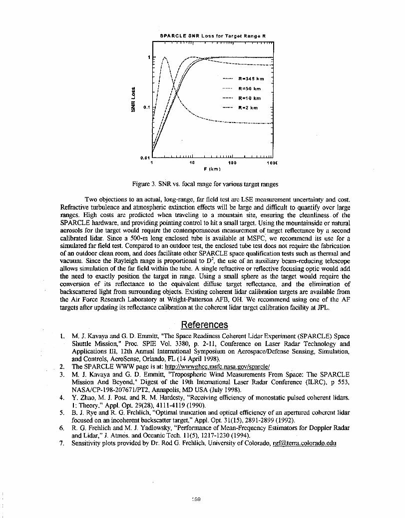
8PARCLE SNR Loss for Target Range R

t /_, ..---7.. • _~-.....; '., /" ..- ...................

i t / /'

S3t o.,h' il R,,Zkmf I "_.

I %,

L ...............

0.01

1 10 100 400(]

F (kin)

Figure 3. SNR vs. focal range for various target ranges

Two objections to an actual, long-range, far field test are LSE measurement uncertainty and cost.Refractive turbulence and atmospheric extinction effects will be large and difficult to quantify over largeranges. High costs are predicted when traveling to a mountain site, ensuring the cleanliness, of theSPARCLE hardware, and providing pointing control to hit a small target. Using the mountainside or naturalaerosols for the target would require the contemporaneous measurement of.target reflectance by a secondcalibrated lidar. Since a 500-m long enclosed tube is available at MSFC, we recommend its use for asimulated far field test. Compared to an outdoor test, the enclosed tube test does not require the fabricationof an outdoor clean room, and does facilitate other SPARCLE space qualification tests such as thermal andvacuum. Since the Rayleigh range is proportional to D2, the use of an auxiliary beam-reducing telescopeallows simulation of the far field within the tube. A single refractive or reflective focusing optic would addthe need to exactly position the target in range. Using a small sphere as the target would require theconversion of its reflectance to the equivalent diffuse target reflectance, and the elimination ofbackscattered light from surrounding objects. Existing coherent lidar calibration targets are available fromthe Air Force Research Laboratory at Wright-Patterson AFB, OH. We recommend using one of the AFtargets after updating its reflectance calibration at the coherent lidar target calibration facility at JPL.

References1. M.J. Kavaya and G. D. Emmitt, "The Space Readiness Coherent Lidar Experiment (SPARCLE) Space

Shuttle Mission," Proc. SPIE Vol. 3380, p. 2-11, Conference on Laser Radar Technology andApplications III, 12th Annual International Symposium on Aerospace/Defense Sensing, Simulation,and Controls, AeroSense, Orlando, FL (14 April 1998).

2. The SPARCLE WWW page is at: http://wwwghcc.msfc.nasa.gov/sparcle/3. M.J. Kavaya and G. D. Emmitt, ',Tropospheric Wind Measurements From Space: The SPARCLE

Mission And Beyond," Digest of the 19th International Laser Radar Conference (ILRC), p 553,NASA/CP-198-207671/PT2, Annapolis, MD USA (July 1998).

4. Y. Zhao, M. J. Post, and R. M. Hardesty, "Receiving efficiency of monostatic pulsed coherent lidars.1:Theory," Appl. Opt. 29(28), 4111-4119 (1990).

5. B.J. Rye and R. G. Frehlich, "Optimal truncation and optical efficiency of an apertured coherent lidarfocused on an incoherent backscatter target," Appl. Opt. 31(15), 2891-2899 (1992).

6. R.G. Frehlich and M. J. Yadlowsky, "Performance of Mean-Frequency Estimators for Doppler Radarand Lidar," J. Atm0s. and Oceanic Tech. 11(5), 1217-1230(1994).

7. Sensitivity plots provided by Dr. Rod G. Frehlich, University of Colorado, rgf@terra.colorado.edu

159

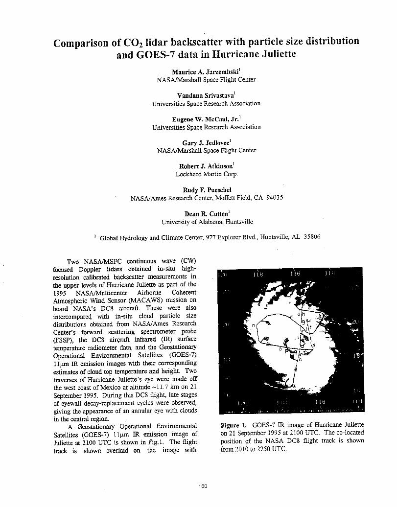
Comparison of CO2 lidar backscatter with particle size distributionand GOES-7 data in Hurricane Juliette

MauriceA. Jarzembski1NASA/MarshallSpaceFlight Center

Vandana Srivastava_UniversitiesSpaceResearchAssociation

Eugene W. McCaul, JrJUniversitiesSpaceResearchAssociation

Gary J. Jedlovec1NASA/MarshaUSpaceFlight Center

Robert J. Atkinson_LockheedMartin Corp.

Rudy F. PueschelNASA/AmesResearchCenter,MoffettField, CA 94035

Dean1LCutten_UniversityofAlabama,Huntsville

GlobalHydrologyandClimateCenter,977ExplorerBlvd.,Huntsville,AL 35806

Two NASA/MSFC continuous wave (CW)focused Doppler lidars obtained in-situ high-resolution calibrated backscatter measurements inthe upper levelsof Hurricane Iuliette as part of the1995 NASAfMulticenter Airborne CoherentAtmosphericWind Sensor (MACAWS) mission onboard NASA's DC8 aircraft. These were alsointercompared with in-situ cloud particle sizedistributionsobtained from NASA/AmesResearchCenter's forward scattering spectrometer probe(FSSP), the DC8 air_raft infrared (IR) surfacetemperatureradiometerdata, and the GeostationaryOperational Environmental Satellites (GOES-7)l l_tm IR emissionimages with their correspondingestimatesof cloud top temperatureand height. Twotraverses of Hurricane Iuliette's eye were made offthe westcoast of Mexico at altitude-11.7 km on 21September1995. During this DC8 flight, late stagesof eyewalldecay-replacementcycles were observed,givingthe appearanceof an annular eye with cloudsin the centralregion.

A Geostafionary Operational Environmental Figure 1. GOES-7IR image of Hurricane JttlietteSatellites (GOES-7) ll_tm IR emission image of on21 September1995at 2100UTC. The co-locatedJulietteat 2100 UTC is shownin Fig.1. The flight position of the NASA DC8 flight track is showntrack is shown overlaid on the image with from 2010to 2250UTC.

160

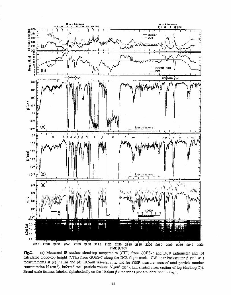
10"_-0.4

-'-,0.0

0.4O-.-=0.8

1.2• i ' •

2010 2020 2030 2040 2050 2100 21=10 2120 2130 21'40 2150 2200 2210 2220 2230 2240 2250TIME {UTC)

Fig.2. (a) Measured IR surface cloud-top temperature (cTr) from GOES-7 and DC8 radiometer and (b)calculated cloud-top height (CTH) from GOES-7 along the DC8 flight track. CW lidar backscatter 13(m4 sr4)measurementsat (c) 9.1gm and (d) 10.6p.mwavelengths;and (e) FSSP measurementsof total particle numberconcentration N (cm'3), inferred total particle volume V(txm 3 cm'3), and shaded cross section of log (dn/dlog(D)).Broad-scale features labeled alphabetically on the 10.@.m 13time series plot are identified in Fig. 1.

161

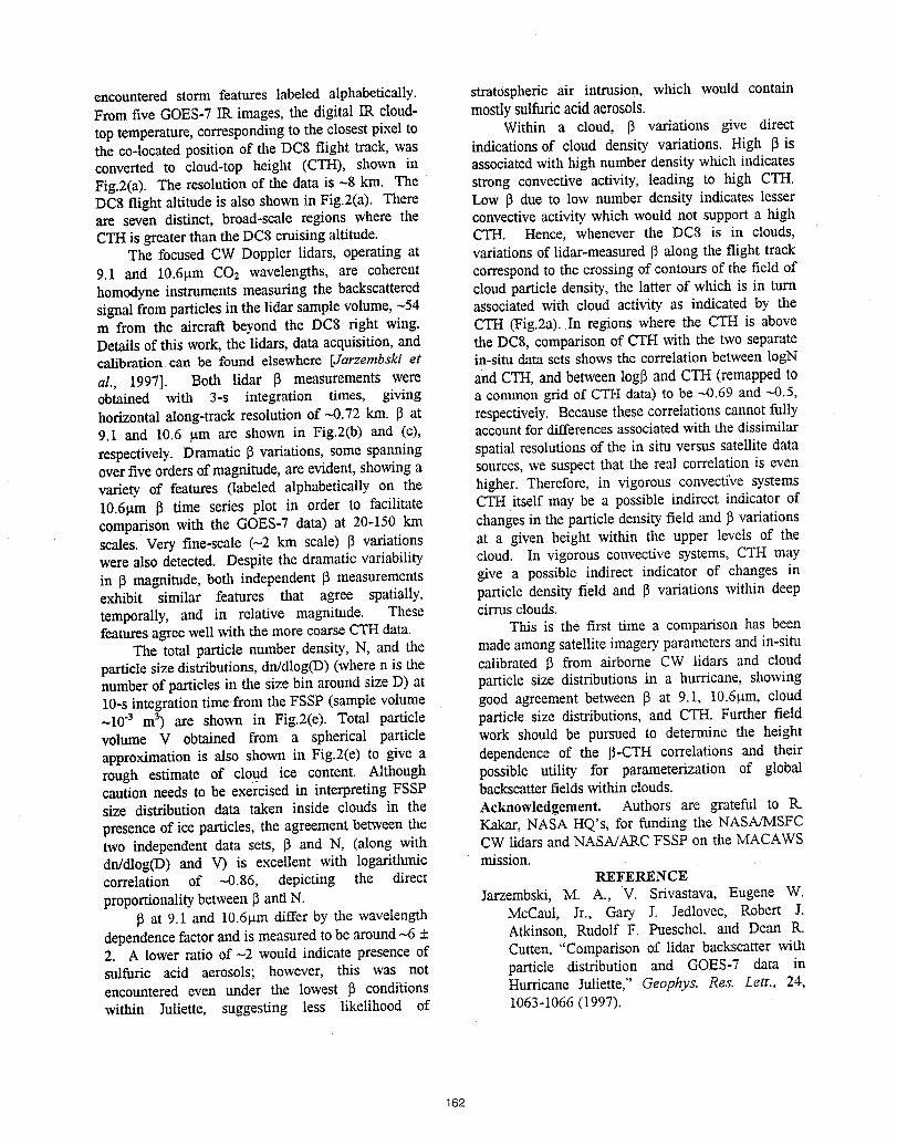
encountered storm features labeled alphabetically, stratospheric air intrusion, which would containFrom five GOES-7IR images, the digital IR cloud- mostlysulfuricacid aerosols.top temperature,correspondingto the closestpixelto Within a cloud, 13 variations give directthe co-locatedpositionof the DC8 flight track, was indicationsof cloud density variations. High 13isconverted to cloud-top height (CTH), shown in associatedwith high number densitywhich indicatesFig.2(a). The resolutionof the data is ~8 kin. The strong convectiveactivity, leading to high CTH.DC8flight altitudeis also shownin Fig.2(a). There Low 13due to low number density indicates lesserare seven distinct, broad-scale regions where the convectiveactivitywhich would not support a highCTHis greater thanthe DC8cruising altitude. CTH. Hence, whenever the DC8 is in clouds,

The focused CW Doppler lidars, operating at variationsof lidar-measured13along the flight track9.1 and 10.6}.tmCO2 wavelengths, are coherent correspondto the crossingof contoursof the field ofhomodyneinstruments measuringthe backscattered cloud particledensity, the latter of which is in turnsignalfromparticlesin the lidar samplevolume,-54 associated with cloud activity as indicated by them from the aircraft beyond the DC8 fight wing. CTH (Fig.2a). In regions where the CTH is aboveDetails of this work, the lidars, data acquisition,and the DC8, comparisonof CTH with the two separatecalibration can be found elsewhere [Jarzembskiet in-situ data sets showsthe correlationbetweenlogNal., 1997]. Both lidar 13 measurements were and CTH,and between log13and CTH (remappedtoobtained with 3-s integration times, giving a commongrid of CTH data) to be --43.69and ---0.5,horizontal along-trackresolutionof --0.72 kin. 13at respectively.Becausethese correlationscannot fully9.1 and 10.6 p.m are shown in Fig.2(b) and (c), accountfor differencesassociatedwith the dissimilarrespectively. Dramatic 13variations, some spanning spatial resolutionsof the in situ versus satellitedataoverfive ordersof magnitude,are evident,showinga sources,we suspect that the real correlation is evenvariety of features (labeled alphabetically on the higher. Therefore, in vigorous convecti\,e systems10.6p.m 13time series plot in order to facilitate CTH itself may be a possible indirect indicator ofcomparison with the GOES-7 data) at 20-150 km changesin the panicle densityfield and 13variationsscales. Very fine-scale (-2 km scale) 13variations at a given height within the upper levels of thewere also detected. Despite the dramatic variability cloud. In vigorous convectivesystems, CTH mayin 13magnitude,both independent13measurements give a possible indirect indicator of changes inexhibit similar features that agree spatially, particle densityfield and 13variations witlfin deeptemporally, and in relative magnitude. These cirrusclouds.featuresagreewellwith the more coarseCTH data. This is the first time a comparison has been

The total particle number density, N, and the madeamongsatelliteimagery,parametersand in-situparticlesizedistributions,dn/dlog(D)(where n is the calibrated 13from airborne CW lidars and cloudnumber of particlesin the sizebin around size D) at particle size distributionsin a hurricane, showing10-sintegrationtime from the FSSP (samplevolume good agreement between 13at 9.1, 10.6p.m,cloud~10 -3 m3) are shown in Fig.2(e). Total particle particle size distributions,and CTH. Further fieldvolume V obtained from a spherical panicle work should be pursued to determine the heightapproximationis also shown in Fig.2(e) to give a dependence of the 13-CTHcorrelations and theirrough estimate of cloud ice content. Although possible utility for parameterization of globalcaution needs to be exercised in interpreting FSSP backscatterfieldswithin clouds.size distribution data taken inside clouds in the Acknowledgement. Authors are grateful to R.presence of ice particles, the agreementbetween the Kakar, NASA HQ's, for funding the NASA/MSFCtwo independent data sets, 13and N, (along with CWlidars and NASA/ARCFSSP on the MACAWSdn/dlog(D) and V) is excellent with logarithmic mission.correlation of --0.86, depicting the direct REFERENCEproportionalitybetweenp anON. Jarzembski, M. A., V. Srivastava, Eugene W.

13at 9.1 and 10.6p.mdiffer by the wavelength McCaul, Yr., Gary J. Jedlovec, Robert J.dependencefactorand is measuredto be around--6+ Atkinson, Rudolf F. Pueschel, and Dean R.2. A lower ratio of _2 would indicate presence of Cutten, "Comparisonof lidar backscatter withsulfuric acid aerosols; however, this was not particle distribution and GOES-7 data inencountered even under the lowest 13conditions Hurricane Juliette," Geophys. Res. Lett., 24,within Juliette, suggesting less likelihood of 1063-1066(1997).

162

Aerosol backscatter from airborne continuous wave CO2 lidarsover western North America and the Pacific Ocean

Maurice A. JarzembskiNASA/Marshall Space Flight Center

Vandana Srivastava

Universities Space Research Association

Jeffry RothermelNASA/Marshall Space Flight Center

Authors are located at the Global Hydrology and Climate Center, 977 Explorer Blvd., Huntsville, AL 35806

1. Introduction altitudes over a combined horizontal distance of over

Atmospheric aerosol backscatter, 13,variability 30,000 Pan. Sampling was also performed duringgives a direct indication of aerosol loading. Since numerous ascents and descents between --0.1- andaerosol variability, is governed by regional sources 12-km altitude. The data over land and oceanand sinks as well as affected by its transport due to comprised 44.8% and 55.2%, respectively, of themeteorological conditions, it is important to total data.

characterize this loading at different locations and The NASA MSFC CW 9.1-_tm Doppler lidartimes. Lidars are sensitive instruments that can beam was focused at -54 m from the aircraft ahead

effectively provide high-resolution, large-scale and beyond the DC8 fight wing tip, into thesampling of the atmosphere remotely by measuring atmosphere. Measurements were obtained with a 3-saerosol 13,thereby capturing detailed temporal and integration time with resolution ranging from -4).36spatial variability of aerosol loading. Although to 0.72 krn. Details of this paper, the calibration,vertical 13profiles are usually obtained by pulsed instrument design, signal processing, andlidars, airborne-focused CW lidars, with high performance are provided elsewhere.79sensitivity and short time integration, can provide 3. BackscatterProfile Measurementshigher resolution sampling in the vertical, thereby Quasi-vertical 13profiles were obtained duringrevealing detailed structure of aerosol layers._5 various aircraft ascents and descents. The altitude for

During the 1995 NASA Multicenter Airborne the profiles was derived by pressure and not radar.Coherent Atmospheric Wind Sensor (MACAWS) Typically, a 1-kin change in altitude corresponded tomission, 6 NASA MSFC airborne-focused CW CO: roughly 10-km horizontal distance. AbsoluteDoppler lidars, operating at 9.1 and 10.6-_m uncertainty in the 13measurements was -20% forwavelength, obtained high resolution in situ aerosol high to moderate signal conditions and -34% for13measurements to characterize aerosol variability, low signal conditions, while relative uncertaintyThe observed variability in 13at 9.1-rim wavelength between adjacent _ values was less than 1%, duewith altitude is presented as well as comparison with mostly to subtle laser power fluctuations. The lidar 13some pulsed lidar profiles, sensitivity was -8 x 1012 m_sr1. A description of2. Fiight Missiou and CWLidarl)escription the main features in 13 variability as well as

The MACAWS mission consisted of nine flights intercomparison with each other and some(denoted as F1.... F9) on the NASA DC8 aircraft comparison with other pulsed lidar datasets takenduring 13 26 September 1995. Regions of over similarterrainisalsopresented.overflights included along the North American west A. Profiles over western U.S. coastal marinecoast from southern California to northern Oregon, regionthe San Joaquin and Sacramento Valleys in Fig. 1 shows 1_profiles off the coast of Oregon, aCalifornia, the Sierra Nevada and Coastal Range region affected by marine as well as land air massesMountains, and the Pacific Ocean off the coast of due to their close proximity to the coast. The heightOregon, California, and the Baja peninsula of of the coastal marine boundary layer (MBL) aerosolMexico. Approximately 52 flight hours of aerosol 13 was not very deep, going only up to -1.5-kindata at 9.1-_m wavelength were obtained at _¢arious altitude, after which 13decreased by -2 orders of

163

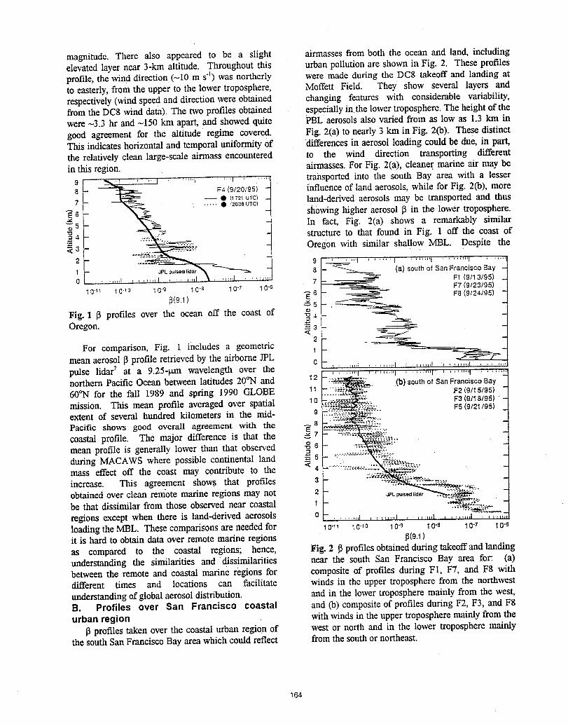
magnitude. There also appeared to be a slight airmassesfrom both the ocean and land, includingelevatedlayer near 3-kin altitude. Throughout this urbanpollutionare shownin Fig. 2. These profilesprofile,the wind direction(-i0 m s"z)was northerly were made during the DC8 takeoff and landing atto easterly,from the upper to the lower troposphere, Moffett Field. They show several layers andrespectively(windspeedand directionwere obtained changing features with considerable variability,from the DC8wind data). The two profiles obtained especiallyin the lowertroposphere.The heightof thewere -3.3 hr and ~150 km apart, and showed quite PBL aerosolsalso varied from as low as 1.3 km ingood agreement for the altitude regime covered. Fig. 2(a) to nearly 3 km in Fig. 2(b). These distinctThis indicateshorizontal and temporaluniformityof differencesin aerosol loading could be due, in part,the relativelyclean large-scaleairmass encountered to the wind direction transporting differentin this region, airmasses.For Fig. 2(a), cleaner marine air may be

9 _- -- '-. ---' ' _-" transported into the south Bay area with a lesser8 |L- _F4(9/20,'o5!_ .. influenceof land aerosols,while for Fig. 2(b), more

• _72_uu_c, land-derivedaerosols may be transported and thus6 showinghigher aerosol 13in the lower troposphere.

us In fact, Fig. 2(a) shows a remarkably similar4 structure to that found in Fig. 1 off the coast of3 Oregon with similar shallow MBL. Despite the2 ---._'_.L. ...... >

40 7 _,r_ F1(9/13/95)-41o-,,lo-,o ,o-, ,o-o -- Fz<9/2 9 I|

_(9.1) _6 i _ F8(9/24/95)_5

Oregon.Fig"1 13profiles over the ocean off the coast of <---_43 __ __2For comparison, Fig. 1 includes a geometric 1 _-_

mean aerosol_ profile retrievedby the airborneJPL e -pulse lidar7 at a 9.25-_tm wavelength over the , .,,:J , I

L ........ I ...... "1 ' .... '"1 ' " ...... I .... _'!'_

northern Pacific Ocean between latitudes 20°N and _2 L :i_. (b) south of San Francisco Bay -60°N for the fall 1989 and spring 1990 GLOBE _ L...:."_-'_- _F2(9/15/gs)--mission. This mean profile averaged over spatial 10 _,.__,.. F3(9118195)'-F'.;_,_,,t._ - ,_......>,_:_.&..... FS(9/2_/gs)extent of several hundred kilometers in the mid- 9 "'_.'_kL_-;_._;_._._....Pacific shows good overall agreement with the 8 ,_,, .... _,_,. _-..,---:__: ,,.,:coastal profile. The major difference is that the _ r- -_,-.,_._._,.,,..,__._,,,, ....mean profile is generally lower than that observed _ 6 - .-.-.-_-during MACAWS where possible continental land _ s - __".2_:;_.: ,mass effect off the coast may contribute to the <4-__'.-.,_.:"increase. This agreement shows that profiles 3

_ _:;::-.,. _obtained over clean remote marine regions may not 2 a_L,.n_)_n_..'-:r_.._.be that dissimilar from those observednear coastal 1 - --,r_-,,..regions except when there is land-derived aerosols o . .--:--ar,_r ' _,lnlll n ' ,,ll!_l I , _))r[I] _ _ 11)1111 I i tlltll

loadingthe MBL. These comparisonsare neededfor 0-- _0-_0 _0-_ _0-_ _o-r _o-_it is hard to obtain data over remote marine regions I](9.1)as compared to the coastal regions; hence, Fig. 2 _ profilesobtainedduring takeoffand landingunderstanding the similarities and dissimilarities near the south San Francisco Bay area for: (a)between the remote and coastal marine regions for compositeof profiles during F1, F7, and F8 withdifferent times and locations can facilitate winds in the upper tropospherefrom the northwestunderstandingof globalaerosoldistribution, and in the lower tropospheremainly from the west,B. Profiles over San Francisco coastal and (b) compositeof profiles during F2, F3, and F8urban region with winds in the uppertropospheremainlyfrom the

J]profilestaken over the coastal urban region of west or north and in the lower tropospheremainlythe southSan FranciscoBayarea whichcould reflect fromthe southor northeast.

164

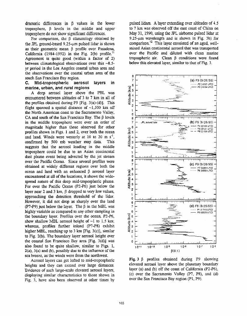
dramatic differences in 13 values in the lower pulsed lidars. A layerextendingover altitudesof 4.5troposphere, 13 levels in the middle and upper to 7 km was observedoff the east coast of China ontropospheredonot show significantdifferences. May 31, 1990,using the JPL airbornepulsed lidar at

For comparison,the 13climatology obtainedby 9.25-_tmwavelengthand is shown in Fig. 3b) forthe JPLground-based9.25-1xmpulsed lidar is shown comparison,lz This layerconsistedof an aged, well-as their geometric mean 13profile over Pasadena, mixedAsiancontinentalaerosol that was transportedCalifornia (1984-1992) in the Fig. 2(b) profile)] over the Pacific and diluted with clean marineAgreement is quite good (within a factor of 2) tropospheric air. Clean 13conditions were foundbetweenclimatologicalobservationsover this -8.5- belowthis elevatedlayer, similar to that of Fig. 3.yr period in the Los Angelescoastal urban area andthe observationsover the coastal urban area of thesouthSan FranciscoBayregion. 8 • , .......t ........ _ ........ _ ........ _ .....7 - ..:."" (a) F9 (9/26/95)C. Mid-tropospheric aerosol layers in ....._:.:.:...... ..... P2(_s_surcl5 .... /--

"*_,:',:, -- P3 (1"334 UTC}marine,urban,and rural regions _ 5 - :_.:._.':."

A deep aerosol layer above the PBL was _ 4- "...',_,'.'""".......encounteredbetweenaltitudes of 3 to 7 km in all of = _'"•--.3 -

the.profilesobtainedduringF9 [Fig.3(a)-(d)]. This<2 -_

flight spanned a spatial distance of-1,500 km offthe North American coast to the SacramentoValley, 1 - _ -0 ........ I , _r,,,4 ...... I _ = :,,,t ---='=,:',:;CAand southof the San FranciscoBay.The 13levels 8 ........ i. , ....... t ........ i ........ i ........in the middle tropospherewere over an order of 7 - OPLoutsedi;dar''" LL.:Z_'.:.'__ (b)F9(9i26/95)-

_'_-'-_ .._ -- P4(21COUTC)magnitude higher than those observed for other _ 6 -_-_--_•.... P.s_2_3_urclprofiles shownin Figs. 1 and 2, over both the ocean _ 5 _._-- - - P62_56urcand land. Winds were westerly at 10 to 20 m s4, _ 4 ...... :: ........ "'.:.,'_:..

confirmed by 500 mb weather map data. This _.3 _.:suggests that the aerosol loading in the middle <2 ....... _i:.troposphere could be due to an Asian continental 1 ...........dust plume event being advectedby the jet stream 0 ....... ,I r ,, r,_,l ..',i:over the Pacific Ocean. Since several profiles were s r ........ t ........ I ........ _ ........ _ ........obtained at widely different regions over both the 7 _- _ (e)F9(9/26/95)--- _7_22_urc_

ocean and land with an enhanced 13aerosol layer _ 5 -encounteredat all of the locations,it showsthe wide-spread nature of this deep mid-troposphericplume. _ € _._.':_ -For over the Pacific Ocean (P2-P6)just below the _ 3 , _ -layernear 2 and 3 kin, 13droppedto very low values, 2 _... -approaching the detection threshold of the lidar. _ -0 __ _ _ _,,,I , , ,,,,.I , _ ,_,.l , _ _:_,1 , = ,_,.1However,it did not drop as sharply over the land 8 ........ _ ........ _ ........ _ ........ _ ........

_"_':"- (d) F9 (9/26/95) -: (P7-P9)just belowthe layer. The 13in the MBLwas 7 - .;.).'.:'._, ..... _ (_7__urc)

highlyvariableas compa.redto anyother samplingin 6 - _!:!_. -- .=__o_ourc_-the boundary layer. Profiles over the ocean, P2-P6, _ _ - ._...._.t."-:::_L:: -show shallow MBL aerosolheight of -1 to 1.5kin; _ 4 - "__ -

whereas, profiles further inland (PT-P8) exhibit =3,--= ..'.'.'_higherMBL, reachingup to 3 km [-Fig.3(c)], similar _ 2 -

to Fig. 2(b). The boundary layer aerosolheight over _ - -'_--_ -the coastal San FranciscoBay area [Fig. 3(d)] was o , ........ I ....... .t . =:_..,..:1. _....=..:l. . ...77also found to be quite shallow, similar to Figs. 1, 10-11 10-,0 10.9 10"8 10r 10_2(a), 3(a) and (b), possibly due to the influence of the [_(9.1)seabreeze, as the winds were fromthe northwest,

Aerosollayers can get lofted to mid-tropospheric Fig. 3 13 profiles obtained during F9 showingheights and they can extend over large distances, elevatedaerosol layerabove the planetaryboundary.Evidenceof such large-scaleelevatedaerosol layers, layer (a) and (b) off the coast of California (P2-P6),displayingsimilar characteristicsto those shown in (c) over the Sacramento Valley (P7, P8), and (d)Fig. 3, have also been observedat other times by overthe San FranciscoBayregion (P1,P9).

165

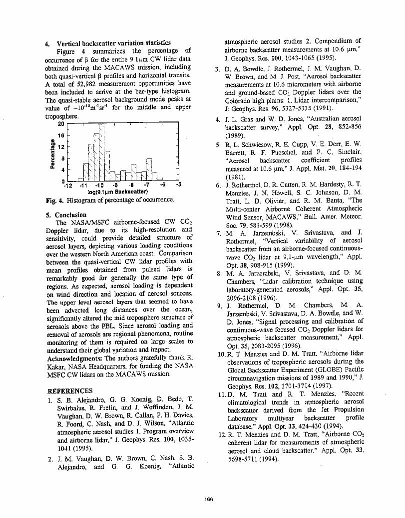
4. Verticalbackscattervariationstatistics atmosphericaerosol studies 2. CompendiumofFigure 4 summarizes the percentage of airbornebackscattermeasurementsat 10.6 _m,"

occurrenceof _ for the entire 9.1gin CW lidar data J. Geophys.Res. 100, 1043-1065(1995).

obtained during the MACAWS mission, including 3. D. A. Bowdle,J. Rothermel, J. M. Vaughan, D.both quasi-vertical _3profiles and horizontaltransits. W. Brown, and M. J. Post, "AerosolbackscatterA total of 52,982 measurementopportunitieshave measurementsat 10.6 micrometerswith airbornebeen included to arrive at the bar-type histogram, and ground-basedCO2Doppler lidars over theThe quasi-stableaerosolbackgroundmode peaks at Coloradohigh plains: 1, Lidar intercomparison,"value of -I04°m'lsr 4 for the middle and upper J: Geophys. Res. 96, 5327-5335 (1991).

troposphere. 4. J. L. Gras and W. D. Jones, "Australian aerosol20 I _ I _ _ l, _ backscatter survey," Appl. Opt. 28, 852-856

• _ I (1989).12 _ I_ 5. R.L. Schwiesow,R. E. Cupp, V. E. Derr, E. W.

8 ," i _,' "Aerosol backscatter coefficient profiles_i _i'_ Barrett, R. F. Pueschel, and P. C. Sinclair,

0 .i ?? .)F]'"I " measuredat 10.6 . L Appl.Met. 20, 184-194-12 -11 -1o -9 -8 -7 -6 -s 6. I. Rothermel, D.R. Cutten,R. M. Hardesty,R. T.

Iog(9.1gmBackscatter) Menzies, J. N. Howell, S. C. Johnson, D. M.Fig. 4. Histogramof percentageof occurrence. Tratt, L. D. Olivier, and R. M. Banta, "The

5. Conclusion Multi-center Airborne Coherent AtmosphericWind Sensor,MACAWS,"Bull. Amer. Meteor.The NASA/MSFC airborne-focused CW CO:

Doppler lidar, due to its high-resolution and Soc.79,581-599(1998).sensitivity, could provide detailed structure of 7. M. A. Jarzembski, V. Srivastava, and J.aerosol layers,depicting various loading conditions Rothermel, "Vertical variability of aerosoloverthe westernNorth Americancoast. Comparison backscatterfrom an airborne-focusedcontinuous-between the quasi-verticalCW lidar profiles with wave CO: lidar at 9.1%tmwavelength," Appl.mean profiles obtained from pulsed lidars is Opt.38,908-915 (1999).remarkably good for generally the same type of 8. M. A. Jarzembski, V. Srivastava, and D_ M.regions. As expected, aerosol loading is dependent Chambers, "Lidar calibration technique usingon wind direction and location of aerosol sources, laboratory-generatedaerosols," Appl. Opt. 35,The upper level aerosol layers that seemed to have 2096-2108 (1996).

9. J. Rothermel, D. M. Chambers, M. A.been advected long distances over the ocean,significantlyalteredthe mid tropospherestructureof Jarzembski,V. Srivastava,D. A. Bowdle,and W.aerosols above the PBL. Since aerosol loading and D. Jones, "Signal processingand calibration ofremovalof aerosolsare regionalphenomena,routine continuous-wavefocusedCO2Doppler lidars formonitoring of them is required on large scales to atmospheric backscatter measurement," Appl.understandtheir globalvariationand impact. Opt.35, 2083-2095(1996).Acknowledgments:The authors _atefully thank R. 10.R. T. Menzies and D. M. Tratt. "Airborne lidarKakar, NASA Headquarters,for funding the NASA observationsof troposphericaerosols during theMSFCCWlidarson the MACAWSmission. GlobalBackscatterExperiment(GLOBE)Pacific

circumnavigationmissionsof 1989and 1990,"J.REFERENCES Geophys.Res. 102,3701-3714(1997).

ll.D.M. Tratt and tL T. Menzies, "Recent1. S. B. Alejandro, G. G. Koenig, D. Bedo, T. climatological trends in atmospheric aerosolSwirbalus, 1L Frelin, and I. Woffinden, I. M.

Vaughan,D. W. Brown,tL Callan,P. H. Davies, backscatter derived from the Jet PropulsionP,. Foord, C. Nash, and D. I. Wilson, "Atlantic Laboratory multiyear backscatter profileatmosphericaerosolstudies I. Program overview database,"Appl.Opt.33, 424-430(1994).and airborne lidar," J. Geophys.Res. 100, 1035- 12.P,. T. Menzies and D. M. Tratt, "Airborne CO:coherent lidar for measurementsof atmospheric1041(1995). aerosol and cloud backscatter." Appl. Opt. 33.

2. J. M. Vaughan, D. W. Brown, C. Nash, S.B. 5698-5711(1994).Alejandro, and G. G. Koenig, "Atlantic

166

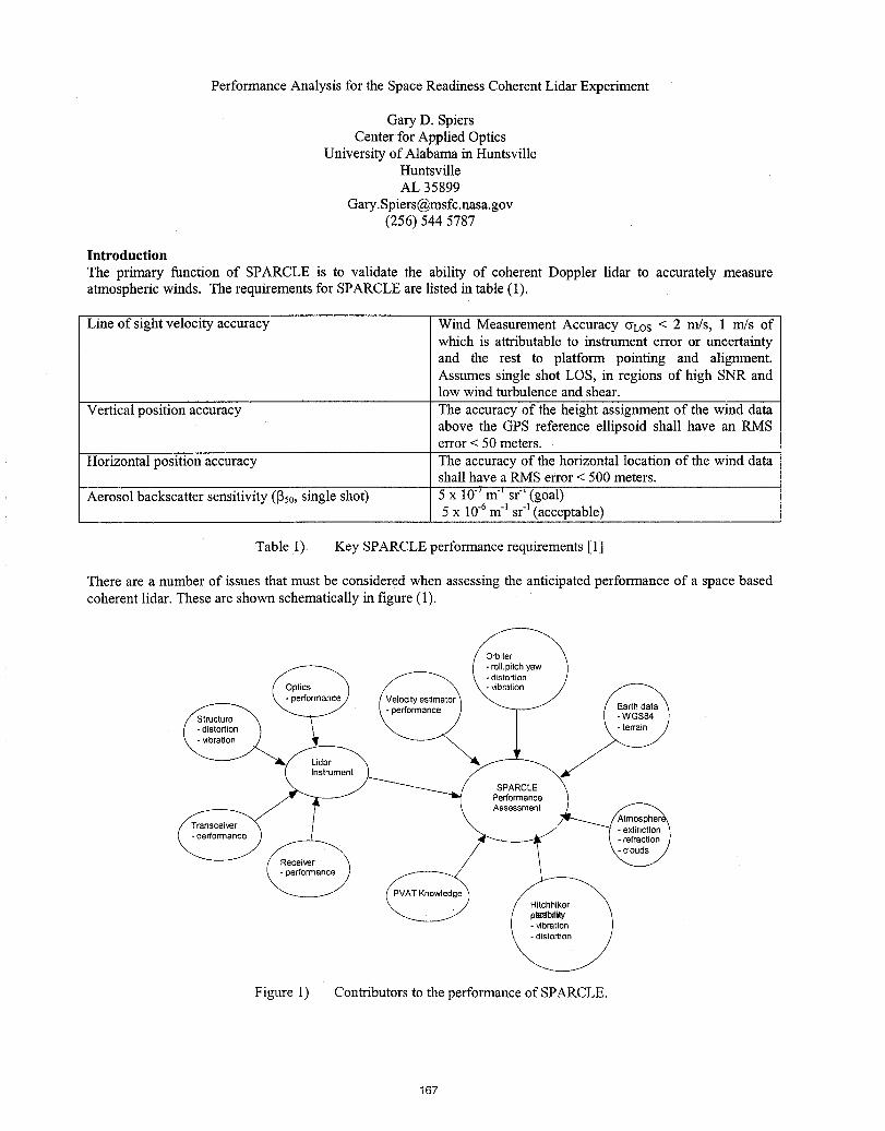
Performance Analysis for the Space Readiness Coherent Lidar Experiment

Gary D. SpiersCenter for Applied Optics

University of Alabama in HuntsvilleHuntsvilleAL 35899

Gary.Spiers@msfc.nasa.gov(256) 544 5787

Introduction

The primary function of SPARCLE is to validate the ability of coherent Doppler lidar to accurately measureatmospheric winds. The requirements for SPARCLE are listed in table (1).

Line of sight velocity accuracy Wind Measurement Accuracy CrLOS< 2 m/s, 1 rn/s ofwhich is attributable to instrument error or uncertaintyand the rest to platform pointing and alignment.Assumes single shot LOS, in regions of high SNR andlow wind turbulence and shear.

Vertical position accuracy The accuracy of the height assignment of the wind dataabove the GPS reference ellipsoid shall have an RMSerror < 50 meters.

Horizontal position accuracy The accuracy of the horizontal location of the wind datashall have a RMS error < 500 meters.

Aerosol backscatter sensitivity (1350,single shot) 5 x 10.7m-_sr-_(goal)5 X 10-6m "1sr "1(acceptable)

Table 1) Key SPARCLE performance requirements [1]

There are a number of issues that must be considered when assessing the anticipated performance of a space basedcoherent lidar. These are shown schematically in figure (1).

. distortion

-performance

Receiver

Figure 1) Contributors to the performance of SPARCLE.

167

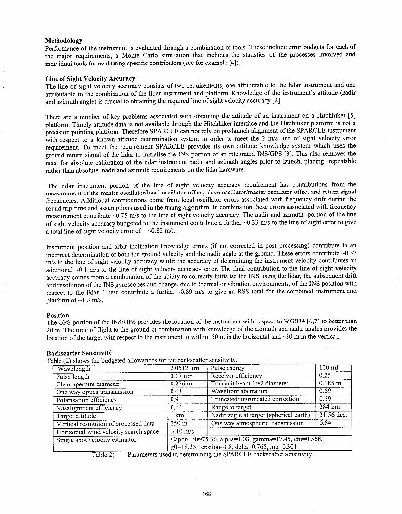
MethodologyPerformance of the instrument is evaluated through a combination of tools. These include error budgets for each ofthe major requirements, a Monte Carlo simulation that includes the statistics of the processes involved andindividual tools for evaluating specific contributors (see for example [4]).

Line of Sight Velocity AccuracyThe line of sight velocity accuracy consists of two requirements, one attributable to the lidar instrument and oneattributable to the combination of the lidar instrument and platform. Knowledge of the instrument's attitude (nadirand azimuth angle) is crucial to obtaining the required line of sight velocity accuracy [2].

There are a number of key problems associated with obtaining the attitude of an instrument on a Hitchhiker [5]platform. Timely attitude data is not available through the Hitchhiker interface and the Hitchhiker platform is not aprecision pointing platform. Therefore SPARCLE can not rely on pre-launch alignment of the SPARCLE instrumentwith respect to a known attitude determination system in order to meet the 2 rn/s line of sight velocity errorrequirement. To meet the requirement SPARCLE provides its own attitude knowledge system which uses theground return signal of the lidar to initialise the INS portion of an integrated INS/GPS [3]. This also removes theneed for absolute calibration of the lidar instrument nadir and azimuth angles prior to launch, placing repeatablerather than absolute nadir and azimuth requirements on the lidar hardware.

The lidar instrument portion of the line of sight velocity accuracy requirement has contributions from themeasurement of the master oscillator/local oscillator offset, slave oscillator/master oscillator offset and return signal

frequencies. Additional contributions come from local oscillator errors associated with frequency drift during theround trip time and assumptions used in the tuning algorithm. In combination these errors associated with frequencymeasurement contribute -0.75 m/s to the line of sight velocity accuracy. The nadir and azimuth portion of the line

of sight velocity accuracy budgeted to the instrument contribute a further ~0.33 m/s to the line of sight error to givea total line of sight velocity error of ~0.82 m/s.

Instrument position and orbit inclination knowledge errors (if not corrected in post processing) contribute to anincorrect determination of both the ground velocity and the nadir angle at the ground. These errors contribute -0.37m/s to the line of sight velocity accuracy whilst the accuracy of determining the instrument velocity contributes anadditional ~0. I m/s to the line of sight velocity accuracy error. The final contribution to the line of sight velocityaccuracy comes from a combination of the ability to correctly initialise the INS using the lidar, the subsequent driftand resolution of the INS gyroscopes and change, due to thermal or vibration environments, of the INS position withrespect to the lidar. These contribute a further -0.89 m/s to give an RSS total for the combined instrument andplatform of-l.3 rrgs.

PositionThe GPS portion of the INS/GPS provides the location of the instrument with respect to WGS84 [6,7] to better than20 m. The time of flight to the ground in combination with knowledge of the azimuth and nadir angles provides thelocation of the target with respect to the instrument to within 50 m in the horizontal and -30 m in the vertical.

Backscatter Sensitivity.Table (2) shows the budgeted allowances for the backscatter sensitivity.

Wavelength 2.0512 _tm Pulse energy 100 mJPulse length 0.17 _tm Receiver efficiency 0.25Clear aperture diameter 0.226 m Transmit beam l/e2 diameter 0.185 mOne way optics transmission 0.64 Wavefront aberration 0.69Polarisation efficiency 0.9 Truncated/untmncated correction 0.59Misalignment efficiency 0.64 Range to target 384 kmTarget altitude 1km Nadir angle at target (spherical earth) 31.56 deg.Vertical resolution of processed data 250 m One way atmospheric transmission 0.84Horizontal wind velocity search space + 10 m/sSingle shot velocity estimator Capon, b0=75.36, alpha=l.08, gamma=17.45, chi=0.568,

g0=18.25, epsilon=l.8, delta=0.765, mu=0.301Table 2) Parameters used in determining the SPARCLEbackscatter sensitivity.

168

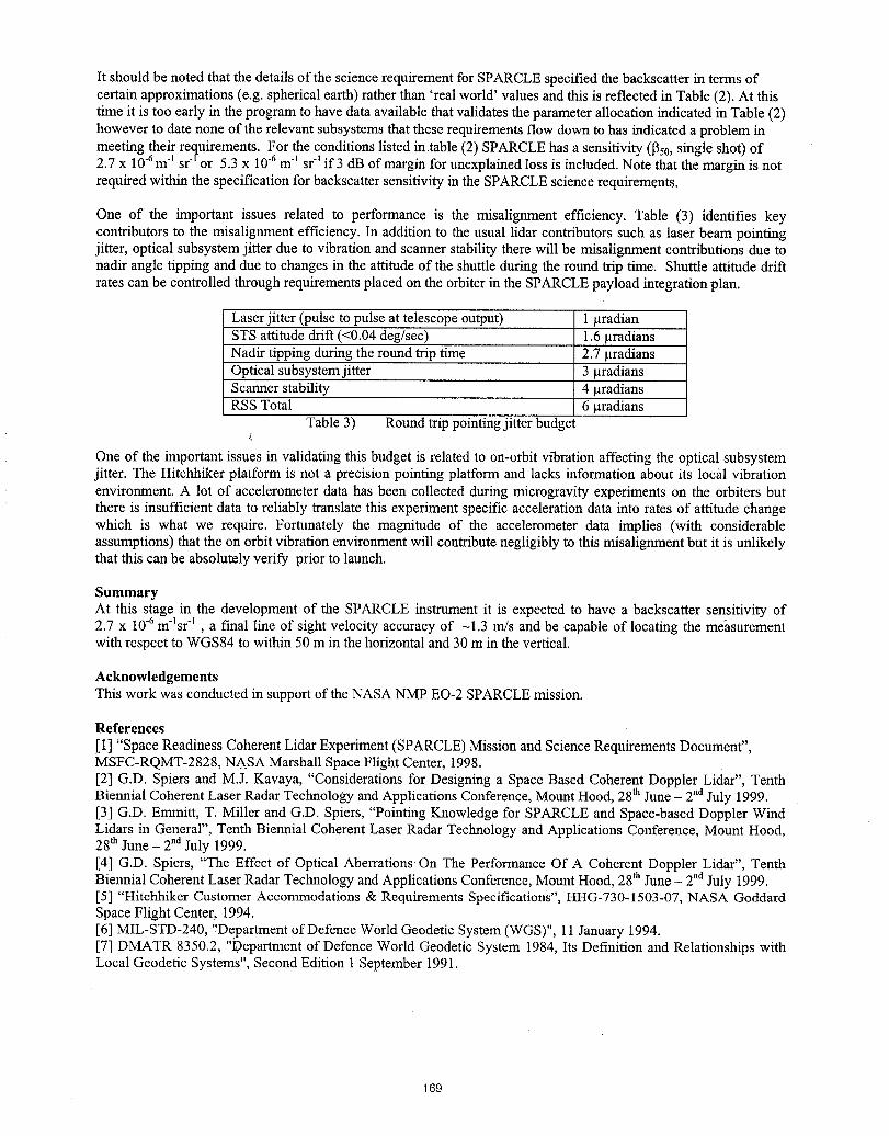
It should be noted that the details of the science requirement for SPARCLE specified the backscatter in terms ofcertain approximations (e.g. spherical earth) rather than 'real world' values and this is reflected in Table (2). At thistime it is too early in the program to have data available that validates the parameter allocation indicated in Table (2)however to date none of the relevant subsystems that these requirements flow down to has indicated a problem inmeeting their requirements. For the conditions listed in table (2) SPARCLE has a sensitivity (1350,single shot) of2.7 x 106ml srl or 5.3 x 10-6ml sr1 if3 dB of margin for unexplained loss is included. Note that the margin is notrequired within the specification for backscatter sensitivity in the SPARCLE science requirements.

One of the important issues related to performance is the misalignment efficiency. Table (3) identifies keycontributors to the misalignment efficiency. In addition to the usual lidar contributors such as laser beam pointingjitter, optical subsystem jitter due to vibration and scanner stability there will be misalignment contributions due tonadir angle tipping and due to changes in the attitude of the shuttle during the round trip time. Shuttle attitude driftrates can be controlled through requirements placed on the orbiter in the SPARCLE payload integration plan.

Laser jitter (pulse to pulse at telescope output) 1 _tradianSTS attitude drift (<0.04 deg/sec) 1.6 _tradiansNadir tipping during the round trip time 2.7 _tradiansOptical subsystem jitter 3 _tradiansScanner stability 4 _tradiansRSS Total 6 _tradians

Table 3) Round trip pointing jitter budget

One of the important issues in validating this budget is related to on-orbit vibration affecting the optical subsystemjitter. The Hitchhiker platform is not a precision pointing platform and lacks information about its local vibrationenvironment. A lot of accelerometer data has been collected during microgravity experiments on the orbiters butthere is insufficient data to reliably translate this experiment specific acceleration data into rates of attitude changewhich is what we require. Fortunately the magnitude of the accelerometer data implies (with considerableassumptions) that the on orbit vibration environment will contribute negligibly to this misalignment but it is unlikelythat this can be absolutely verify prior to launch.

SummaryAt this stage in the development of the SPARCLE instrument it is expected to have a backscatter sensitivity of2.7 x 10-6m'lsr 4 , a final line of sight velocity accuracy of -1.3 m/s and be capable of locating the measurementwith respect to WGS84 to within 50 m in the horizontal and 30 m in the vertical.

AcknowledgementsThis work was conducted in support of the NASA NMP EO-2 SPARCLE mission.

References[1] "Space Readiness CoherentLidarExperiment(SPARCLE)Mission andScience RequirementsDocument",MSFC-RQMT-2828, NASA MarshallSpace FlightCenter,1998.[2] G.D. Spiers and M.L Kavaya, "Considerationsfor Designing a Space Based CoherentDoppler Lidar", TenthBiennial Coherent LaserRadarTechnology andApplications Conference,MountHood,28thJune - 2"dJuly 1999.[3] G.D. Emmitt, T. Miller and G.D. Spiers, "Pointing Knowledge for SPARCLE and Space-based Doppler WindLidars in General", Tenth Biennial CoherentLaser Radar Technology and ApplicationsConference,Mount Hood,28_ June - 2ndJuly 1999.[4] G.D. Spiers, "The Effect of Optical AberrationsOn The PerformanceOf A Coherent Doppler Lidar", TenthBiennial Coherent Laser RadarTechnology andApplications Conference,Mount Hood, 28thJune - 2ndJuly 1999.[5] "Hitchhiker CustomerAccommodations & Requirements Specifications", HHG-730-1503-07,NASA GoddardSpaceFlight Center,1994.[6] MIL-STD-240, "Departmentof Defence WorldGeodetic System (WGS)", 11 January1994.[7] DMATR 8350.2, "Departmentof Defence World Geodetic System 1984, Its Definition andRelationships withLocalGeodetic Systems", Second Edition 1September 1991.

169

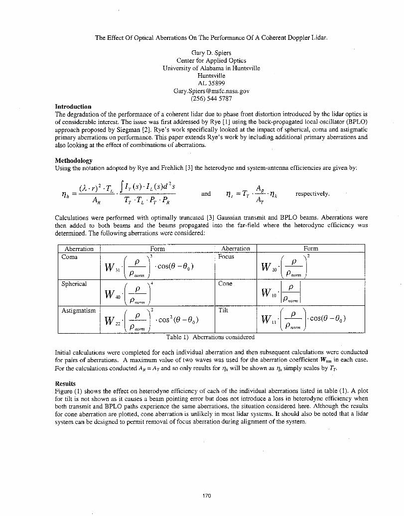
The Effect Of Optical Aberrations On The Performance Of A Coherent Doppler Lidar.

Gary D. SpiersCenter for Applied Optics

University of Alabama in HuntsvilleHuntsvilleAL 35899

Gary.Spiers @msfc.nasa.gov(256) 544 5787

Introduction

The degradation of the performance of a coherent lidar due to phase front distortion introduced by the lidar optics isof considerable interest. The issue was first addressed by Rye [1] using the back-propagated local oscillator (BPLO)approach proposed by Siegman [2]. Rye's work specifically looked at the impact of spherical, coma and astigmaticprimary aberrations on performance. This paper extends Rye's work by including additional primary aberrations andalso looking at the effect of combinations of aberrations.

MethodologyUsing the notation adopted by Rye and Frehlich [3] the heterodyne and system-antenna efficiencies are given by:

(A,.r) 2.T L fIr(s)'IL(s) d2s AR

r/h - AR Tr" TL" Pr' PR and r/s = Tr.--_.rlh respectively.

Calculations were performed with optimally truncated [3] Gaussian transmit and BPLO beams. Aberrations werethen added to both beams and the beams propagated into the far-field where the heterodyne efficiency wasdetermined. The following aberrations were considered:

Aberration Form Aberration Form

oma/,3 ocus /W3 " p .cos(O-Oo) W o"P _lorm ._

Spherical _ _4 Cone /9

W40" P ) W,0"x _On°rm

Astigmatism _ , _- Tilt (

W22" P .cos2(O-Oo) W,__ P .cos(O-Oo)Pnorrn Pnorm /

Table 1) Aberrations considered

Initial calculations were completed for each individual aberration and then subsequent calculations were conductedfor pairs of aberrations. A maximum value of two waves was used for the aberration coefficient Wr,min each case.For the calculations conducted AR= Av and so only results for r/hwill be shown as r/ssimply scales by TT.

Results

Figure (1) shows the effect on heterodyne efficiency of each of the individual aberrations listed in table (1). A plotfor tilt is not shown as it causes a beam pointing error but does not introduce a loss in heterodyne efficiency whenboth transmit and BPLO paths experience the same aberrations, the situation considered here. Although the resultsfor cone aberration are plotted, cone aberration is unlikely in most lidar systems. It should also be noted that a lidarsystem can be designed to permit removal of focus aberration during alignment of the system.

170

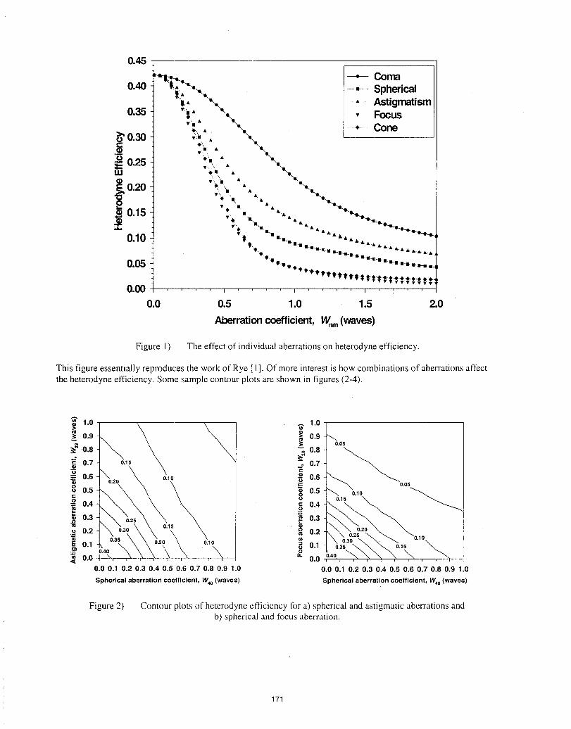
0.45

_ Coma0.40 -,-- Spherical

• Astigmatism0.35 "_ _. • Focus

v.?u•-;:, \ ..........Con,,"0.30 ,:, ,

0.25 *' " _-

0.20 - _ ,, -_

0.10 "" _= """• _'_. I Ii.! 1 _l'_ _'-B I1-•. & A • • & •.

&•,,L.• &,•.•I i-* D

0.05 '_I, . . • _=_'11=-i.=._= =_• • • • • • t tt tt t ttt-t.t._._._.t,_e._e.• e.• _e.vvvVVTv

0.00 _ .... r " .

0.0 0.5 1.0 1.5 2.0

Aberration coefficient, Wnm(waves)

Figure !) The effect of individual aberrations on heterodyne efficiency.

This figure essentially reproduces the work of Rye [1]. Of more interest is how combinations of aberrations affectthe heterodyne efficiency. Some sample contour plots are shown in figures (2-4).

1.o 1.0u_

0.9 _ >_ 0.9

_ _= 0.05\0.8 o 0.8 _." 0.7 o.ls ..; 0,7

= 0.6 0._o ._ 0.6

0.5 _ o.o5= 0 0.5 0.150•= 0.4 = 0.4

o:,=0.3 _ 0.3

.13 =..

o 0.2 _ 0.2"---- 0.25

_ 0.30E 0.1 0.10 u= 0.1 0.35 0.1513)•=--. 0.40 0

o.o " 0.00.0 0.1 0.2 0.3 0.4 0.5 0.6 0.7 0.8 0.9 ;0 0.0 0.1 0.2 0.3 0.4 0.5 0.6 0.7 0.8 0.9 1.0

Spherical aberration coefficient, W4o(waves) Spherical aberration coefficient, W4o(waves),

Figure 2) Contour plots of heterodyne efficiency for a) spherical and astigmatic aberrations andb) spherical and focus aberration.

171

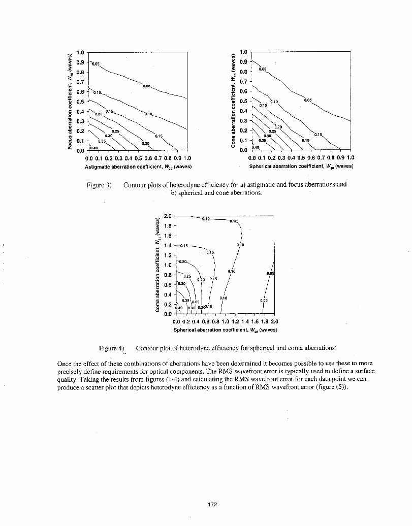
1.0 1.0

•_ 0.9 o.os =_, 0.90.8 _ 0.8 o.os

°0.7 0.7

C 0.05 '_= _ 0.6•_ 0.6 .-.-- (,3

"; 0.5 _ 0.5 . .05o oo o'- 0.4 ," 0.40 0

03 030.2 _ 0.2

o= 0.1 0.20 _ 0.1 0.15 _,,,o o

0.0 0.00.0 0.1 0.2 0.3 0.4 0.5 0.6 0.7 0.8 0.9 1.0 0.0 0.1 0.2 0,3 0.4 0.5 0.6 0.7 0.8 0.9 1.0

Astigmaticaberrationcoefficient,W._2(waves) Sphericalaberrationcoefficient,W4o(waves)

Figure 3) Contour plots of heterodyne efficiency for a) astigmatic and focus aberrations andb) spherical and cone aberrations.

Figure 4) Contour plot of heterodyne efficiency for spherical and coma aberrations

Once the effect of these combinations of aberrations have been determined it becomes possible to use these to more

precisely define requirements for optical components. The RMS wavefront error is typically used to define a surfacequality. Taking the results from figures (1-4) and calculating the RMS wavefront error for each data point we can

produce a scatter plot that depicts heterodyne efficiency as a function of RMS wavefront error (figure (5)).

172

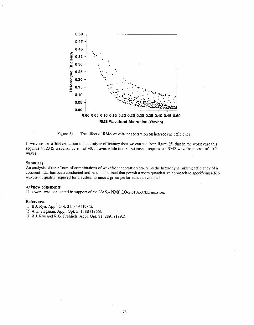
0.50

0.45

0.40

=o0.35.o 0.30LU

0.25 _"t== ==

0.20 ,q,

'_ 0.15 %.° . "',..'I" "" • "= " "-" I

0.10 .... _'. ".: . • .,:.: ...._= ,_==, '_, ,=== ,=. • • . • •

"=.= • "p. o•=. _ = ,. = = = •==.., , %_i, =,d .=• .,•. • ° •0.05 •,., , t t, i-_....._-"........

"_• ..-4,,.==,._._="Is.i._t._%di_"'-'11"''"0.00 , , , _ , _ , , t i

0.00 0.05 0.10 0.15 0.20 0.25 0.30 0.35 0.40 0.45 0.50

RMSWavefrontAberration(Waves)

Figure 5) The effect of RMS wavefront aberration on heterodyne efficiency.

If we consider a 3dB reduction in heterodyne efficiency then we can see from figure (5) that in the worst case thisrequires an RMS wavefront error of -0.1 waves while in the best case it requires an RMS wavefront error of -0.2waves.

SummaryAn analysis of the effects of combinations of wavefront aberration errors on the heterodyne mixing efficiency of acoherent lidar has been conducted and results obtained that permit a more quantitative approach to specifying RMSwavefront quality required for a system to meet a given performance developed.

AcknowledgementsThis work was conducted in support of the NASA NMP EO-2 SPARCLE mission.

References

[i] B.J. Rye, Appl. Opt. 21,839 (1982).[2] A.E. Siegman, Appl. Opt. 5, 1588 (1966).[3] B.J. Rye and R.G. Frehlich, Appl. Opt. 31, 2891 (1992).

173

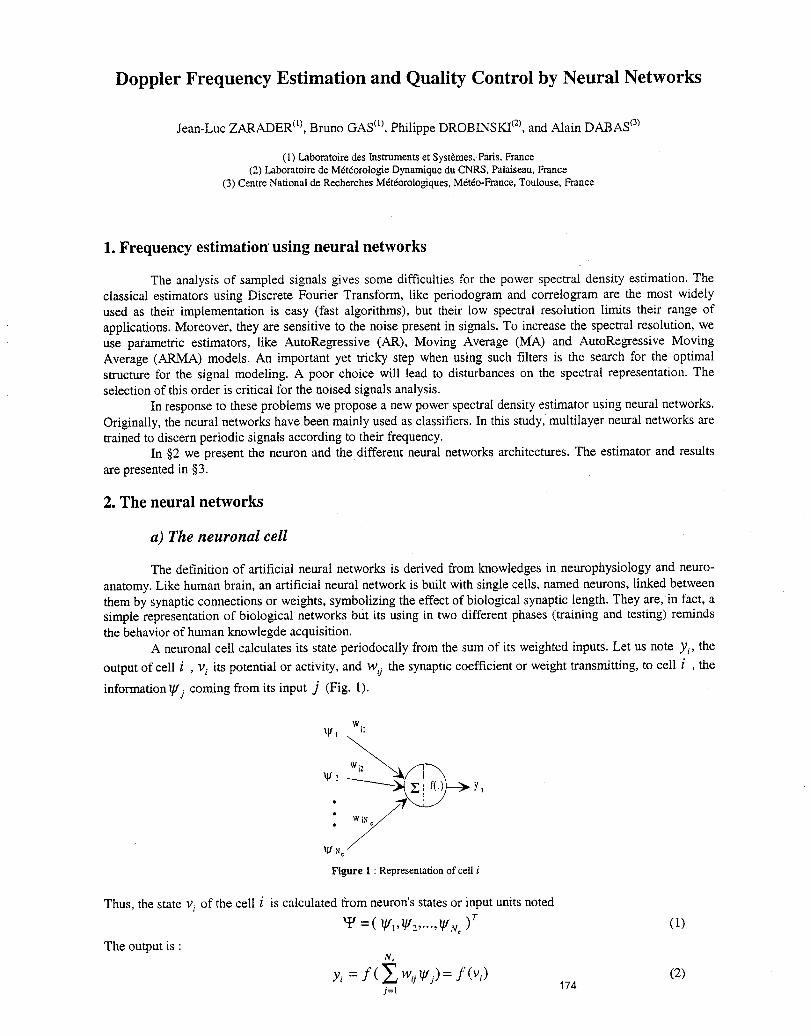
Doppler Frequency Estimation and Quality Control by Neural Networks

Jean-Luc ZARADER(l),Bruno GAS(l),Philippe DROBINSKI(2),and Alain DABAS_3)

(1) Laboratoire des Instruments et Syst_mes, Paris, France(2) Laboratoire de Mdtdorologie Dynamique du CNRS, Palaiseau, France

(3) Centre National de Recherches Mdtdorologiques,Mdtdo-France, Toulouse, France

1. Frequency estimation' using neural networks

The analysis of sampled signals gives some difficulties for the power spectral density estimation.Theclassical estimators using Discrete Fourier Transform, like periodogramand correlogramare the most widelyused as their implementationis easy (fast algorithms), but their low spectral resolution limits their range ofapplications.Moreover, they are sensitive to the noise presentin signals. To increase the spectral resolution, weuse parametric estimators, like AutoRegressive (AR), Moving Average (MA) and AutoRegressive MovingAverage (ARMA) models. An importantyet tricky step when using such filters is the search for the optimalstructure for the signal modeling. A poor choice will lead to disturbanceSon the spectral representation.Theselection of this order is critical for the noised signalsanalysis.

In response to these problems we propose a new power spectral density estimator using neural networks.Originally, the neural networks have been mainly used as classifiers. In this study, multilayer neural networks aretrained to discern periodic signals according to their frequency.

In §2 we present the neuron and the different neural networks architectures. The estimator and resultsare presented in §3.

2. The neural networks

a) The neuronal cell

The definition of artificial neural networks is derived from knowledges in neurophysiology and neuro-anatomy. Like human brain, an artificial neural network is built with single cells, named neurons, linked betweenthem by synaptic connections or weights, symbolizing the effect of biological synaptic length. They are, in fact, asimple representation of biological networks but its using in two different phases (training and testing) remindsthe behavior of human knowlegde acquisition.

A neuronal cell calculates its state periodocally from the sum of its weighted inputs. Let us note Yi, the

output of cell i , v,. its potential or activity, and wij the synaptic coefficient or weight transmitting, to cell i , the

information_j coming from its input j (Fig. l).

/1/I Wil

•"/[/_€

Figure 1 : Representation of cell i

Thus, the state vi of the cell i is calculated from neuron's states or input units noted

T=(_I,gr2....._N,)T (i)The output is :

N,

Yi = f ( Z W;jIp'j) = f (Vi) 174 (2)j=!

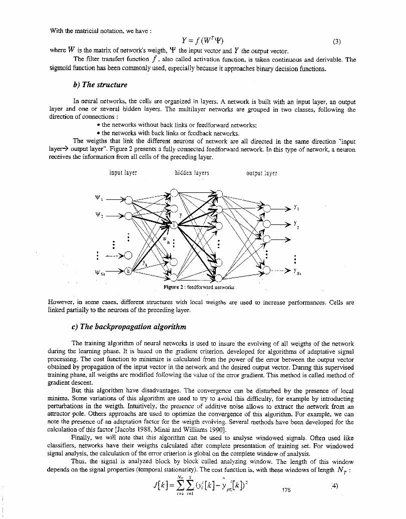
With the matricial notation, we have :

Y = f(wrff j) (3)

where W is the matrix of network's weigth, _ the input vector and Y the output vector.The filter transfert function f, also called activation function, is taken continuous and derivable. The

sigmoid function has been commonly used, especially because it approaches binary decision functions.

b) The structure

In neuralnetworks, the cells are organized in layers. A network is built with an input layer, an outputlayer and one or several hidden layers. The multilayer networks are grouped in two classes, following thedirectionof connections :

• the networks without back linksor feedforwardnetworks;• the networkswith back links or feedback networks.

The weigths that link the different neurons of network are all directed in the same direction "inputlayer'-) output layer". Figure2 presentsa fully connected feedforward network. In this type of network,a neuronreceives the informationfrom all cells of the precedinglayer.

inputlayer hiddenlayers outputlayer

Yt

Y2

" -->C) " "

_sc YNs

Figure 2 '.feedforward networks

However, in some cases, different structures with local weigths are used to increase performances. Cells arelinked partially to the neurons of the preceding layer.

c) The backpropagationalgorithm

The training-algorithm of neural networks is used to insure the evolving of all weigths of the networkduring the learning phase. It is based on the gradient criterion, developed for algorithms of adaptative signalprocessing. The cost function to minimize is calculated from the power of the error between the output vectorobtained by propagation of the input vector in the network and the desired output vector. During this supervisedtraining phase, all weigths are modified following the value of the error gradient. This method is called method ofgradient descent.

But this algorithm have disadvantages. The convergence can be disturbed by the presence of localminima. Some variations of this algorithm are used to try to avoid this difficulty, for example by introductingperturbations in the weigth. Intuitively, the presence of additive noise allows to extract the network from anattractor pole. Others approachs are used to optimize the convergence of this algorithm. For example, we cannote the presence of an adaptation factor for the weigth evolving. Several methods have been developed for thecalculation of this factor [Jacobs 1988, Minai and Williams 1990].

Finally, we will note that this algorithm can be used to analyse windowed signals. Often used likeclassifiers, networks have their weigths calculated after complete presentation of training set. For windowedsignal analysis, the calculation of the error criterion is global on the complete window of analysis.

Thus, the signal is analyzed block by block called analyzing window. The length of this window

depends on the signal properties (temporal stationarity). The cost function is, with these windows of length N T :Nr S ^

t=[ i=1

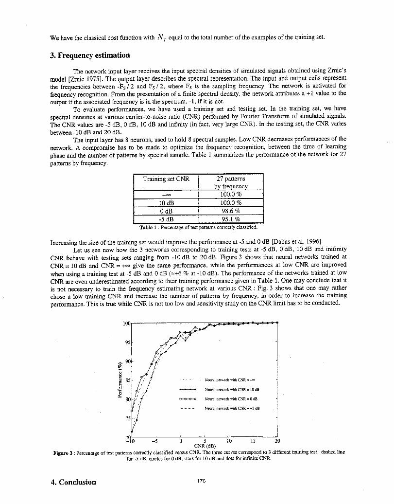
We have the classical cost function with Nv equal to the total number of the examples of the training set.

3. Frequency estimation

The network inputlayer receives the input spectral densities of simulatedsignals obtained usingZrnic'smodel [Zmic 1975]. The Output layer describes the spectral representation.The input and output cells representthe frequencies between -l_s/2 and Fs/2, where Fs is the sampling frequency. The network is activatedforfrequencyrecognition. From the presentation of a finite spectral density, the network attributes a + i value to theoutputif the associated frequencyis in the spectrum, -1, if it is not.

To evaluate performances, we have used a training set and testing set. In the training set, we havespectraldensities at various carrier-to-noiseratio (CNR) performed by Fourier Transform of simulatedsignals.The CNR values are -5 dB, 0 dB, 10dB and infinity (in fact, very large CNR). In the testing set, the CNR variesbetween -10 dB and 20 dB.

The input layer has 8 neurons, used to hold 8 spectral samples. Low CNR decreases performances of thenetwork. A compromise has to be made to optimize the frequency recognition, between the time of learningphase and the number of patterns by spectral sample. Table 1summarizes the performance of the network for 27patterns by frequency.

Training set CNR 27 patternsby frequency

+_ 100.0 %10 dB 100.0 %0 dB 98.6 %-5 dB 95.1%

Table 1 : Percentage of test patterns correctly classified.

Increasing the size of the training set would improve the performance at -5 and 0 dB [Dabas et al. 1996].Let us see now how the 3 networks corresponding to training tests at -5 dB, 0 dB, 10 dB and inifinity

CNR behave with testing sets ranging from -I0 dB to 20 dB. Figure 3 shows that neural networks trained atCNR = 10 dB and CNR = +_, give the same performance, while the performances at low CNR are improvedwhen using a training test at -5 dB and 0 dB (=+6 % at-10 dB). The performance of the networks trained at lowCNR are even underestimated according to their training performance given in Table 1. One may conclude that itis not necessary to train the frequency estimating network at various CNR : Fig. 3 shows that one may ratherchose a low training CNR and increase the number of patterns by frequency, in order to increase the trainingperformance. This is true while CNR is not too low and sensitivity study on the CNR limit has to be conducted.

100

95

_. 90

_ 85 /// _ .......... NeuralnetworkwithCNR.=+,,*

_ Neural network with C,NnR.= l0 dBi I

80 / : _ Neural network with CNR = 0 dB" - - - - Neural network with CNR = -5 dB

i --2oCNR (dB)

Figure 3 : Percentage of test patterns correctly classified versus CNR. The three curves correspond to 3 different training test : dashed linefor -5 dB, circles for 0 dB, stars for I0 dB anddots for infinite CNR.

4. Conclusion 176

Neural networks have been widely used since 1985 when the backpropagation algorithm has beendeveloped. From thet time, the main application has been pattern recognition. In this study, we have tried to use itto classify signals according to their frequency. For that purpose, we have developed a new frequency estimatorusing a neural network. The performance we have obtained are interesting in terms of resistance to noise.

Compared to others methods, they are successful also because they allow information extractioncontained in examples of training set to undertake an optimal segmentation of the representation space. Theyobtain interesting performances in generalization for examples which are not in the training set.

Future work will be dedicated to increase the spectral resolution and develop a quality control procedure[Dabas et al. 1999] taking advantage of neurol network potential.

References

Dabas, A., J.L. Zarader, and P.H. Flamant, 1996 : Decision algorithm for the ALADIN signal processor. ESAfinal report, n° 143649, 100 pp.

Dabas, A., P. Drobinski, and P.H. Flamant, 1999 : Adaptive filters for frequency estimate of heterodyne Dopplerlidar returns : Recursive implementation and quality control. J. Atmos. Oceanic Technol., 16, 361-372.

Jacobs R.A., 1988 : Increased rates of convergence through learning rate adaptation Neural Networks, 1,295-307.

Minai A.A. and R.D. Williams, 1990Acceleration of back-propagation through learning rate and momemtum adaptation, International JointConference on Neural Networks, Washington, D.C, IEEE and INNS, Lawrence Erlbaum Associates,McCaudill editor, 1676-1679.

Zmic, D.S., 1975 : Simulation of weatherlike Doppler spectra and signals. J. Appl. meteoroL, 14, 619-620.

177

Shipborne backscatter lidar experiments in western Pacific regionby research ship "Mirai"

Kouro Tamamushi, TetuyaSugata, Kazuhiro AsaiGraduate School of Engineering, Tohoku Institutes of Technology

Yagiyama Kasumi 35-1, Taihaku-Ku, Sendai 982-, JAPANE-mail : asai@titan.tohtech.ac.jp

andIchiro Matsui, Nobuo Sugimoto

National Institute for Environmental Studies (NIES)16-20nogawa, Tsukuba, Ibaraki304, Japan

E-mail:nsugimot@nies.go.jp, matsui@nies.go.jp

1.Introduction

The height distributions of Planetary Boundary Layer (PBL), aerosols, clouds are highlyrequired in order to understand the radiative budget of the earth. The height of PBL top isobserved between at a few hundred meters and at around 2 kin, and is the region of theatmosphere in direct contact with the earth surface. Moisture and heat associated with humanactivities are trapped within the PBL 1). On the other hand, cirrus clouds in the hightroposphere is thought as a blanket effect for the global warming2).

The atmospheric lidar sounding in the Western Pacific Ocean region is very important notonly scientifically as above mentioned but also from the view point of the developments ofspaceborne lidars. The reason is that only few data set of lidar backscatter experiments in thisregion have been taken. As part of Global Backscatter Experiment (GLOBE) missions in1989 and 19903), the lidar backscatter cross section measurements were carried out in PacificOcean region to support the spacebome Laser Atmospheric Wind Sounder project (LAWS),and recently PEM-West B(Pacific Exploratory Mission) were done to probe the air masstransported from the Asian continent into the Pacific troposphere in 19944). These twocampaigns have been made by using the lidars and in situ instruments, i.e. the optical particle

counter, particle impactors, equipped in NASA DC-8 research aircraft.

In Japan, a research ship "Mirai (8,800 tons displacement)", which is operated by JapanMarine Science and Technology Center (JAMSTEC) under contract of Science andTechnology Agency (STA), was available to use for studies of oceanography and atmospherefrom October 1998. Three two-months campaigns per year in the western Pacific Oceanregion are scheduled for three years from 1999. We developed the shipborne backscatterlidars in order to participate these campaigns. The primary objectives are not only to takeheight distribution data of PBL, aerosols, cirrus cloud with dependencies of the longitude andthe latitude for improving our knowledge of atmospheric circulation and climate dynamics,but also to support NASDA's spaceborne lidar projects, Mission Demonstration Satellite(MDS) -II "ELISE" mission, the ISS Japanese Experiment Module (JEM)/CDL mission 5).Especially in JEM/CDL using 2 um laser transmitter, the backscatter coefficients at 2 um inthe free troposphere are strongly desired to design the system and to estimate the sensitivity inthe oceans. The extrapolation technique will effectively work to estimate the 2 um backscattercoefficients using data set of those at 532 nm and 1064 nm3!.

In this paper, we would present our shipborne lidar system and will also give preliminary

178

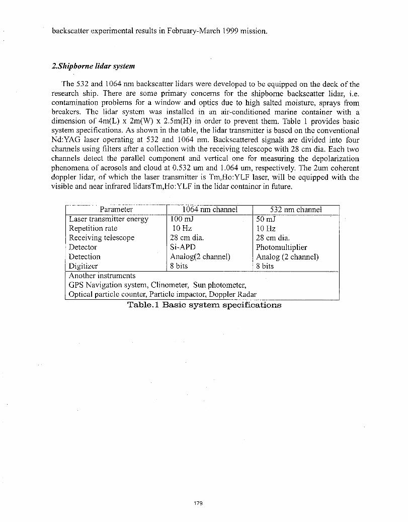
backscatter experimental results in February-March 1999 mission.

2.Shipborne lidar system

The 532 and 1064 nm backscatter lidars were developed to be equipped on the deck of theresearch ship. There are some primary concerns for the shipborne backscatter lidar, i.e.contamination problems for a window and optics due to high salted moisture, sprays frombreakers. The lidar system was installed in an air-conditioned marine container with adimension of 4m(L) x 2m(W) x 2.5m(H) in order to prevent them. Table 1 provides basicsystem specifications. As shown in the table, the lidar transmitter is based on the conventionalNd:YAG laser operating at 532 and 1064 nm. Backscattered signals are divided into fourchannels using filters after a collection with the receiving telescope with 28 cm dia. Each twochannels detect the parallel component and vertical one for measuring the depolarizationphenomena of aerosols and cloud at 0.532 um and 1.064 um, respectively. The 2um coherentdoppler lidar, of which the laser transmitter is Tm,Ho:YLF laser, will be equipped with thevisible and near infrared lidarsTm,Ho:YLF in the lidar container in future.

Parameter 1064 nm channel 532 nm channelLaser transmitter energy 100 mJ 50 mJRepetition rate 10 Hz 10 HzReceiving telescope 28 cm dia. 28 cm dia.Detector Si-APD PhotomultiplierDetection Analog(2 channel) Analog (2 channel)Digitizer 8 bits 8 bitsAnother instrumentsGPS Navigation system, Clinometer, Sun photometer,Optical particle counter, Particle impactor, Doppler Radar

Table. 1 Basic system specifications

179

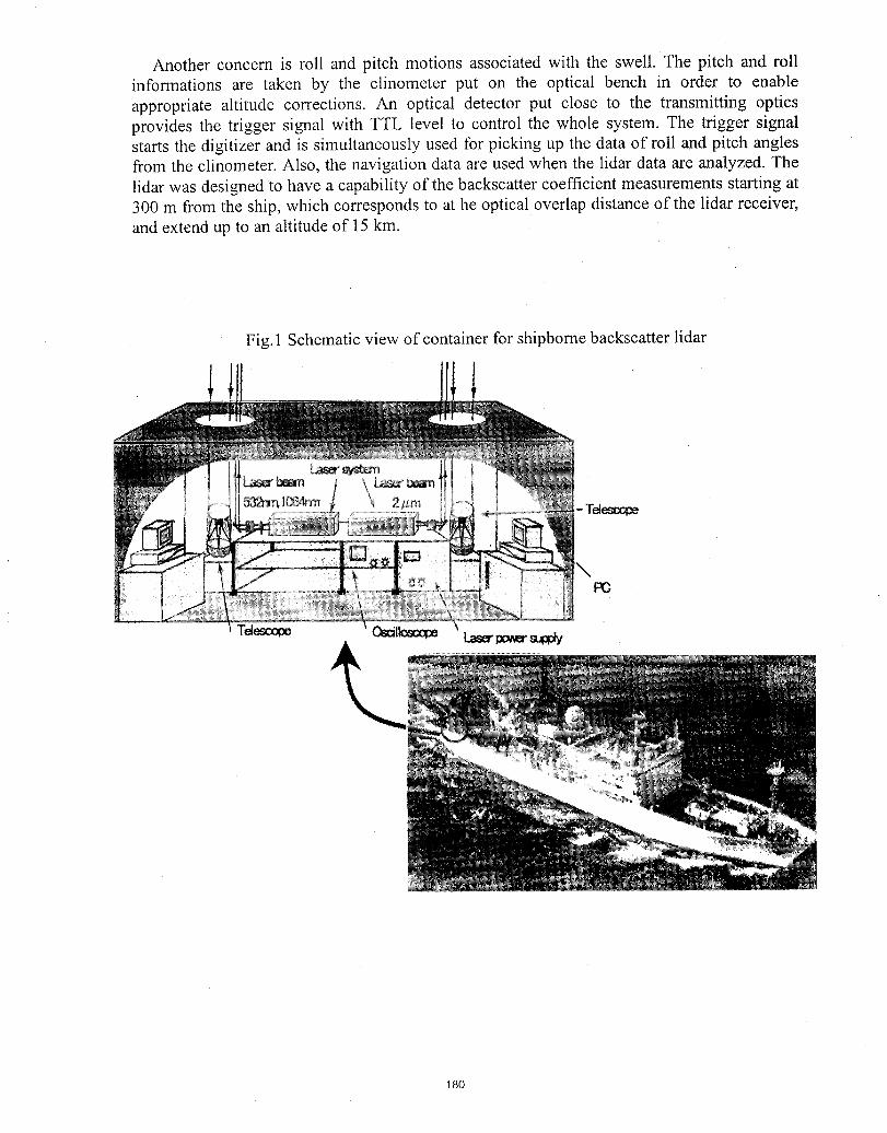
Another concern is roll and pitch motions associated with the swell. The pitch and rollinformations are taken by the clinometer put on the optical bench in order to enableappropriate altitude corrections. An optical detector put close to the transmitting opticsprovides the trigger signal with TTL level to control the whole system. The trigger signalstarts the digitizer and is simultaneously used for picking up the data of roll and pitch anglesfrom the clinometer. Also, the navigation data are used when the lidar data are analyzed. Thelidar was designed to have a capability of the backscatter coefficient measurements starting at300 m from the ship, which corresponds to at he optical overlap distance of the lidar receiver,and extend up to an altitude of 15 km.

Fig. 1 Schematic view of container for shipborne backscatter lidar

l

- Y_tescc_

\PC

180

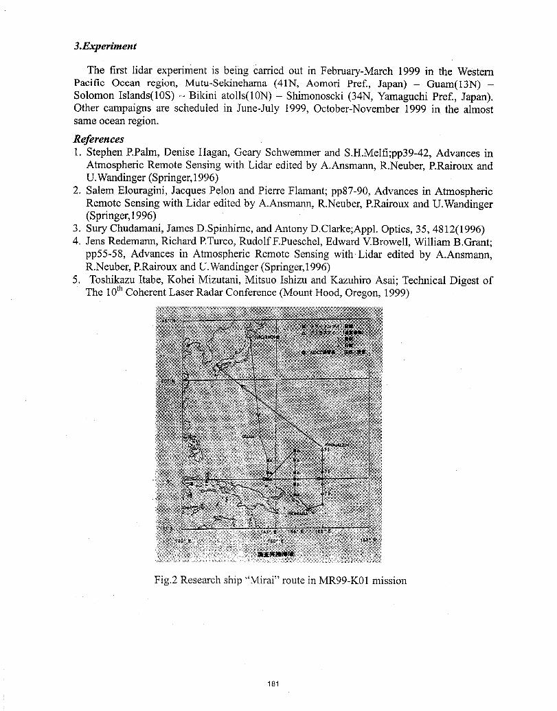
3.Experiment

The first lidar experiment is being Carried out in February-March 1999 in the WesternPacific Ocean region, Mutu-Sekinehama (41N, Aomori Pref., Japan) - Guam(13N) -Solomon Islands(10S) - Bikini atolls(10N) - Shimonoseki (34N, Yamaguchi Pref., Japan).Other campaigns are scheduled in June-July 1999, October-November 1999 in the almostsame ocean region.

References1. Stephen P.Palm, Denise Hagan, Geary Schwemmer and S.H.Melfi;pp39-42, Advances in

Atmospheric Remote Sensing with Lidar edited by A.Ansmann, R.Neuber, P.Rairoux andU.Wandinger (Springer, 1996)

2. Salem Elouragini, Jacques Pelon and Pierre Flamant; pp87-90, Advances in AtmosphericRemote Sensing with Lidar edited by A.Ansmann, R.Neuber, P.Rairoux and U.Wandinger(Springer, 1996)

3. Sury Chudamani, James D.Spinhirne, and Antony D.Clarke;Appl. Optics, 35, 4812(1996)4. Jens Redemann, Richard P.Turco, RudolfF.Pueschel, Edward V.Browell, William B.Grant;

pp55-58, Advances in Atmospheric Remote Sensing with Lidar edited by A.Ansmann,R.Neuber, P.Rairoux and U.Wandinger (Springer,1996)

5. Toshikazu Itabe, Kohei Mizutani, Mitsuo Ishizu and Kazuhiro Asai; Technical Digest ofThe 10thCoherent Laser Radar Conference (Mount Hood, Oregon, 1999)

Fig.2 Research ship "Mirai" route in MR99-K01 mission

181

Pointing Knowledge for SPARCLE and Space-based DopplerWind Lidars in General

G. D. Emmitt

Simpson Weather AssociatesCharlottesville, VA 22902

804-979-357i

T. MillerG. Spiers

NASA/MSFCHuntsville, AL 35812

256-922-5882

Abstract

The SPAce Readiness Coherent Lidar Experiment (SPARCLE) will fly on a space shuttleto demonstrate the use of a coherent Doppler wind lidar to accurately measure globaltropospheric winds. To achieve the LOS accuracy goal of- 1m/s, the lidar system mustbe able to account for the orbiter's velocity (- 7750 m/s) and the rotational component ofthe earth's surface motion (- 450 m/s). For SPARCLE this requires knowledge of theattitude( roll, pitch and yaw) of the laser beam axis within an accuracy of 80microradians.(- 15 arcsec). Since SPARCLE can not use a dedicated star tracker from itsearth-viewing orbiter bay location, a dedicated GPS/INS will be attached to the lidarinstrument rack. Since even the GPS/INS has unacceptable drifts in attitude information,the SPARCLE team has developed a way to periodically scan the instrument itself toobtain < 10 microradian (2 arcsec) attitude knowledge accuracy that can then be used tocorrect the GPS/INS output on a 30 minute basis.

Pointing Requirements for DWLs in Space

In some regards, measuring tropospheric winds from space is as much a matter ofpointing as it is a matter of detection. In general, the focus of the community of DWLtechnologists and potential data users tends to be on the laser/telescope/scanner/detector.However, pointing control and knowledge is also critical for space-based (and airborne)DWLs, with knowledge being more demanding than control.

The DWL transmits a beam of photons towards the earth and the reflected photons returnwith a frequency shift that is a linear combination of the platform's motion relative to theearth's surface, the earth's surface motion due to its rotation and the motion of the beam'starget (aerosol or clouds) relative to the ground. The task is to remove the platform andearth rotation components, leaving just the wind (or zero groun_ speed).

182

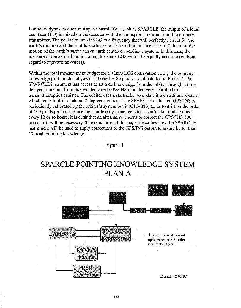
For heterodyne detection in a space-based DWL such as SPARCLE, the output of a localoscillator (LO) is mixed on the detector with the atmospheric returns from the primarytransmitter. The goal is to tune the LO to a frequency that will perfectly correct for theearth's rotation and the shuttle's orbit velocity, resulting in a measure of 0.0m/s for themotion of the earth's surface in an earth centered coordinate system. In this case, themeasure of the aerosol motion along the same LOS would be equally accurate (withoutregard to representativeness).

Within the total measurement budget for a <lm/s LOS observation error, the pointingknowledge (roll, pitch and yaw) is allotted - 80 grads. As illustrated in Figure 1, theSPARCLE instrument has access to attitude knowledge from the orbiter through a timedelayed route and from its own dedicated GPS/INS mounted very near the lasertransmitter/optics canister. The orbiter uses a startracker to update it own attitude systemwhich tends to drift at about .2 degrees per hour. The SPARCLE dedicated GPS/INS isperiodically calibrated by the •orbiter's system but it (GPS/INS) tends to drift on the orderof 100 grads per hour. Since the shuttle only maneuvers for a startracker update onceevery 12 or so hours, it is clem"that an alternative means to correct the GPS/INS 100grads drift will be •necessary,The remainder of this paper describes how the SPARCLEinstrument will be used to apply Correctionsto the GPS/INS output to assure better than50 grad pointing knowledge.

Figure 1

SPARCLEPOINTINGKNOWLEDGESYSTEM- PLAN A

Ill

1. This path is used to sendupdates on attitude alterstar tracker fixes.

Emmitt 12/01/98

183

The Algorithm

In principal, for any shot containing a signal from the earth's surface, the detectedaerosol LOS velocity can be corrected absolutely. However, with nearly 75-80% globalcoverage of cloud (including sub-visual cirrus), a significant fraction of the time therewill be no ground return. Also, even ifa return is sensed to be within an acceptabledistance of the expected range to surface, salt spray over the ocean, blowing desert sands,and dense plumes of polluted boundary layer air may act to confound the assignment ofzero velocity to the ground. Therefore the SPARCLE team decided to develop alternativeattitude knowledge by using the DWL in a dedicated scan mode.

The pointing knowledge algorithm is called LAHDSSA (Lidar Attitude/HeightDetermination and Signal SearChAlgorithm) and a general outline of its functionality ispresented in Figure 2. As the name implies, the algorithm does more than just determinethe roll, pitch and yaw of the laser/optics canister. It also serves to search for signalcapture in the event that attitude knowledge is offby > 2-3 degrees. Such a gross error inattitude knowledge is most likely to occur during initial startup when all the attitudeknowledge is based upon the orbiter's systems. Since the SPARCLE instrument will belocated a few 10's of meters away from the orbiter's attitude instruments, there is a realpotential for significant physical offsets of a few degrees. While every reasonable effortwill be made to align the laser beam axis with the orbiter's -ZLV axis prior to launch,there is no economical way to assure a better than 4-1 degree alignment on the ground.After launch, the orbiter's bay may flex due to gravity unloading and/or differentialthermal loading. In any case, there is a chance that upon startup, no signal will bedetected by the SPARCLE instrument since the receiver bandwidth is limited to the rangeof velocities associated with 4-2 degrees.

To find the signal, the LAHDSSA methodically searches a prescribed range of the twodegrees of freedom; the LO Tuning(LOT) and the Range of Regard (RoR). Figure 2describes the sequence of actions involved in searching for the signal. Once the signal isfound, the LAHDSSA performs an attitude calibration scan to determine the correctionvalues that need to be applied to the roll, pitch and yaw being reported by the SPARCLEGPS/INS. The calibration scan involves taking data at 12 azimuths in 30 degree stepswith 1 second dwells at each azimuth. The data from the surface returns are processed onboard with a nonlinear function minimization algorithm. Multiple passes through the dataresult in estimates of the roll, pitch, yaw, altitude, and radial orbiter velocity. Table 1presents the results of simulating the performance of LAHDSSA for a wide range of errorconditions. In general, we expect LAHDSSA to provide attitude knowledge to within 10-20 grads each time the calibration scan is executed. At this time, we plan to runLAHDSSA approximately every 30 minutes.The scan will be scheduled in real-time tooccur over generally cloud free areas. Since there are only three unknown attitude anglesto be solved, only three of the 12 perspectives need to have surface returns. However, the10-20 grads accuracy can only be expected when the number of perspectives with asurface return is greater than 6.

184

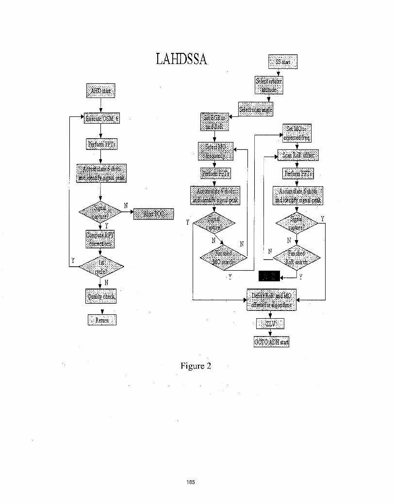
LAHDSSA

quality check 0

Figure 2

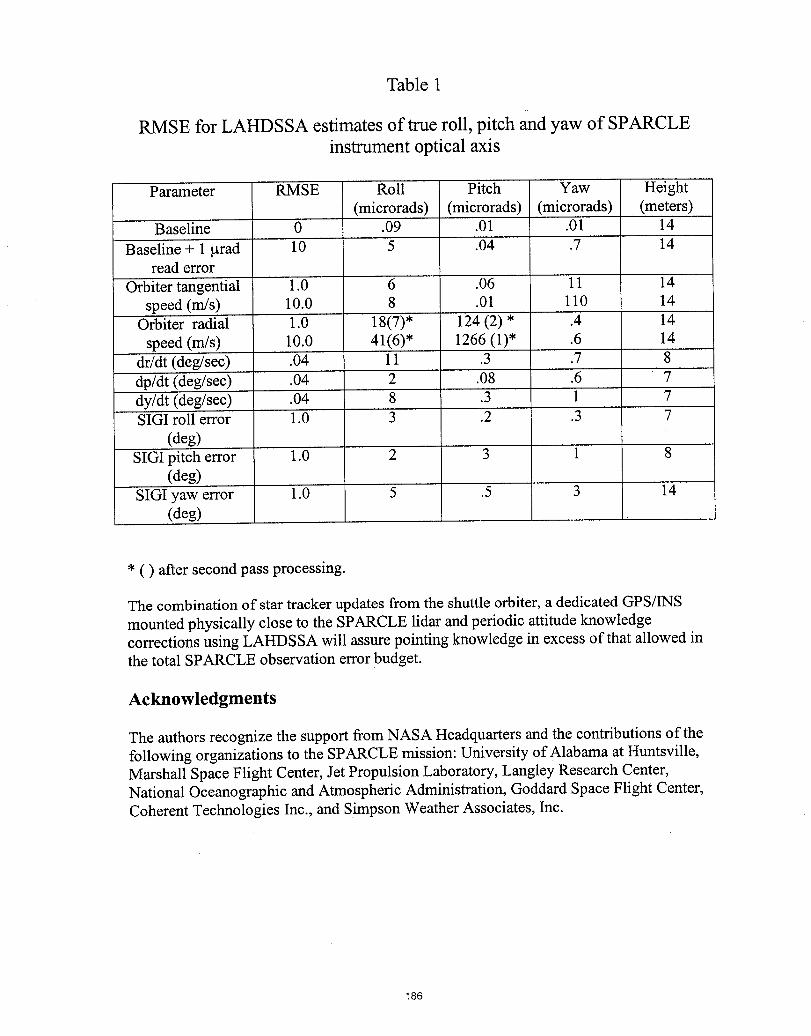
Table 1

RMSE for LAHDSSA estimates of true roll, pitch and yaw of SPARCLEinstrument optical axis

Parameter RMSE Roll Pitch Yaw Height(microrads) (microrads) (microrads) (meters)

Baseline 0 .09 .01 .01 14

Baseline + 1 grad 10 5 .04 .7 14read error

Orbiter tangential 1.0 6 .06 11 14speed (m/s) 10.0 8 .01 110 14

Orbiter radial 1.0 18(7)* 124 (2) * .4 14speed (m/s) 10.0 41(6)* 1266 (1)* .6 14

dr/dr (deg/sec) .04 11 .3 .7 8dp/dt (deg/sec) .04 2 .08 .6 7dy/dt (deg/sec) .04 8 .3 1 7SIGI roll error 1.0 3 .2 .3 7

(deg)SIGI pitch error 1.0 2 3 1 8

(deg)SIGI yaw error 1.0 5 .5 3 14

(deg)

* ( ) after second pass processing.

The combination of star tracker updates from the shuttle orbiter, a dedicated GPS/INSmounted physically close to the SPARCLE lidar and periodic attitude knowledgecorrections using LAHDSSA will assure pointing knowledge in excess of that allowed inthe total SPARCLE observation error budget.

Acknowledgments

The authors recognize the support from NASA Headquarters and the contributions of thefollowing organizations to the SPARCLE mission: University of Alabama at Huntsville,Marshall Space Flight Center, Jet Propulsion Laboratory, Langley Research Center,National Oceanographic and Atmospheric Administration, Goddard Space Flight Center,Coherent Technologies Inc., and Simpson Weather Associates, Inc.

186

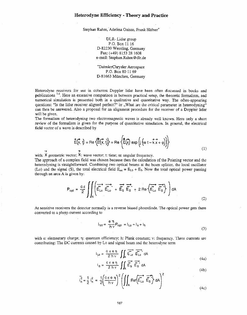
Heterodyne Efficiency - Theory and Practice

Stephan Rahm, Adetina Ouisse, Frank H_ifner.

DLR- Lidar _oupP.O. Box l l 16

D-82230 Wessling, GermanyFax: (+49) 8153 28 1608

e-mail: Stephan.Rahm@dlr.de

.DaimlerChrysler AerospaceP.O. Box 80 I 1 69

D-81663 Mtinchen, Germany

Heterodyne receivers for use in coherent Doppler lidar have been often discussed in books andpublications 1.4.Here an extensive comparison in between practical setup, the theoretic formalism, andnumerical simulation is presented both in a qualitative and quantitative way. The often-appearing

• o._,questions: "Is the lidar receiver aligned perfect?" or ,,What are the critical parameter in heterodymn_,can then be answered. Also a proposal for an alignment procedure for the receiver of a Doppler lidarwill be given.The formalism of heterodyning two electromagnetic waves is already well known. Here only a shortreview of the formalism is given for the purpose of quantitative simulation. In general, the electricalfield vector of a wave is described by

(1)with: X geometric vector; k: wave vector; t: time; co:angular frequency.The approach of a complex field was chosen because then the calculation of the Pointing vector and theheterodyning is straightforward. Combining two optical beams at the beam splitter, the local oscillator(Lo) and the signal (S), the total electrical field Etot = EL0+ Es. :Now the total optical power passingthrough an area A is given by:

Popt= _ ELo E_o + Es Es + 2 Re dA

(2)

At sensitive receivers the detector normally is a reverse biased photodiode. The optical power gets thereconverted to a photo current according to

erlttot= -_'Popt = Iko + Is + ih

(3)

with e: elementary charge; 1"1:quantum efficiency; h: Plank constant; v: frequency. Three currents arecontributing: The DC currents caused by Lo and signal beam and the heterodyne term

ILo = c aeq E_o EL.o dA2hv(4a)

Is = 2 h'---'7 . (4b)

?2 2 th 2_._J Re _s'}(4c)

187

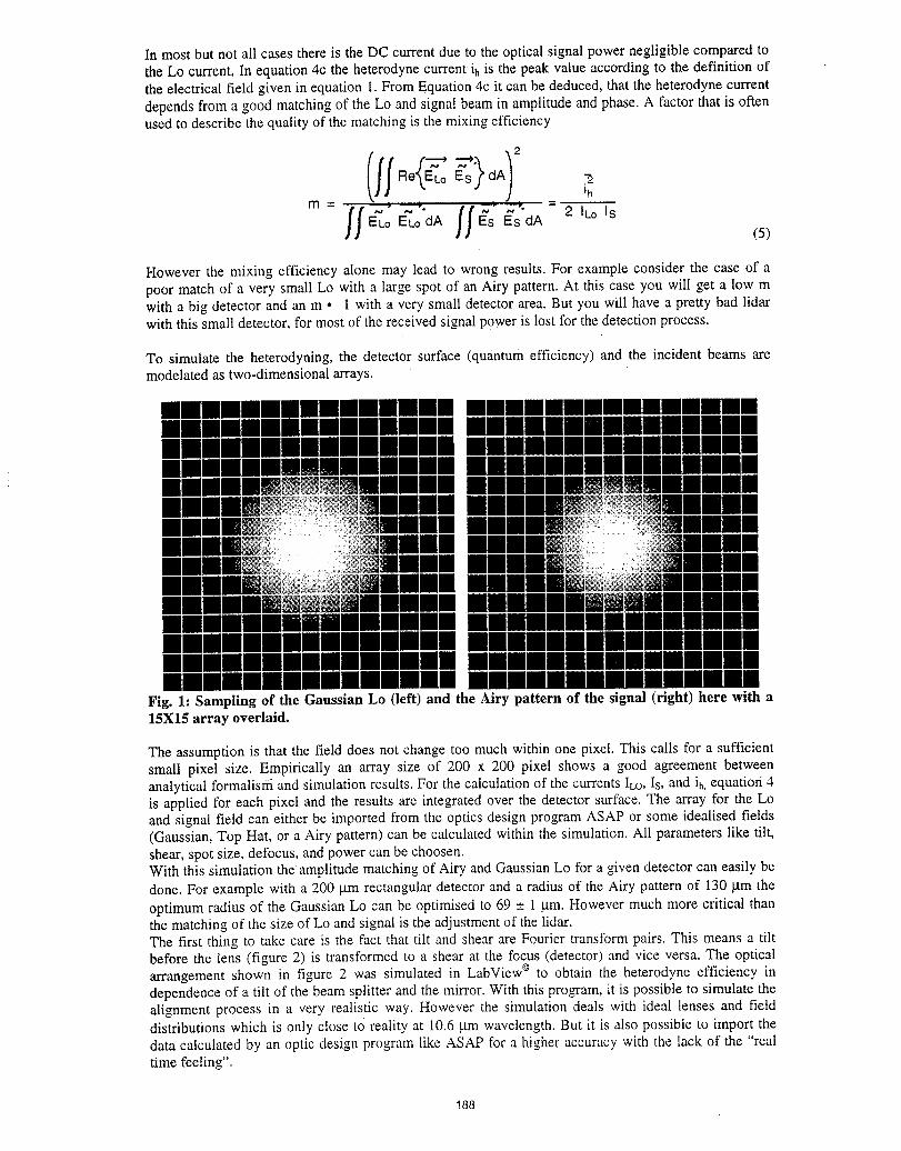
In most but not all cases there is the DC current due to the optical signal power negligible compared tothe Lo current, In equation 4c the heterodyne current ih is the peak value according to the definition ofthe electrical field given in equation I. From Equation 4c it can be deduced, that the heterodyne current

depends from a good matching of the Lo and signal beam in amplitude and phase. A factor that is oftenused to describe the quality of the matching is the mixing efficiency

Re 7E_oELo'dA dA

(5)

However the mixing efficiency alone may lead to wrong results. For example consider the case of apoor match of a very small Lo with a large spot of an Airy pattern. At this case you will get a low mwith a big detector and an m • 1 with a very small detector area. But you will have a pretty bad lidarwith this small detector, for most of the received signal power is lost for the detection process.

To simulate the heterodyning, the detector surface (quantum efficiency) and the incident beams aremodelated as two-dimensional arrays.

mmmmmmmmmmmmmmmmmmmmmmmmmmmmmmmmmmmmmmmmmmmmmmmmmmmmmmmmmmmmmmmmmmmmmmmmmmmmmmmmmmmmmmmmmmnmmmmmmmmmmmmm mmmmmmmmmmmmmmmmmmmm)))mmmmmm mmmmmmB)Emmmmmmmmmmr ii !Immmmmmmil!)! ! )lnmmmn

mmmmmmw (mmmmmmmm mmmimiilimmmmmmmml mnnmmmmmmmmmmmmmmmmmmmmmmmmmmmmmmmmmmmmmmmmmmmmmmmmmmmmmmmmmmmmmmmmmmmmmmmmmmmmmmmmmmmmmmmmmmm

Fig. 1: Sampling of the Gaussian Lo (left) and the Airy pattern of the signal (right) here with a15X15 array overlaid.

The assumption is that the field does not change too much within one pixel. This calls for a sufficientsmall pixel size. Empirically an array size of 200 x 200 pixel shows a good a_eement betweenanalytical formalisrii and simulation results. For the calculation of the currents ILO,IS, and ih.equation 4is applied for each pixel and the results are inte_ated over the detector surface. The array for the Loand signal field can either be imported from the optics design pro_am ASAP or some idealised fields(Gaussian, Top Hat, or a Airy pattern) can be calculated within the simulation. All parameters like tilt,shear, spot size, defocus, and power can be choosen.With this simulation the amplitude matching of Airy and Gaussian Lo for a given detector can easily bedone. For example with a 200 gm rectangular detector and a radius of the Airy pattern of 130 p.m theoptimum radius of the Gaussian Lo can be optimised to 69 __.I gm. However much more critical thanthe matching of the size of Lo and signal is the adjustment of the lidar.The first thing to take care is the fact that tilt and shear are Fourier transform pairs. This means a tiltbefore the lens (figure 2) is transformed to a shear at the focus (detector) and vice versa. The opticalarrangement shown in figure 2 was simulated in LabView© to obtain the heterodyne efficiency independence of a tilt of the beam splitter and the mirror. With this pro_am, it is possible to simulate thealignment process in a very realistic way. However the simulation deals with ideal lenses and fielddistributions which is only close to reality at 10.6 ,urnwavelength. But it is also possible to import thedata calculated by an optic design progam like ASAP for a higher accuracy with the lack of the "realtime feeling".

188

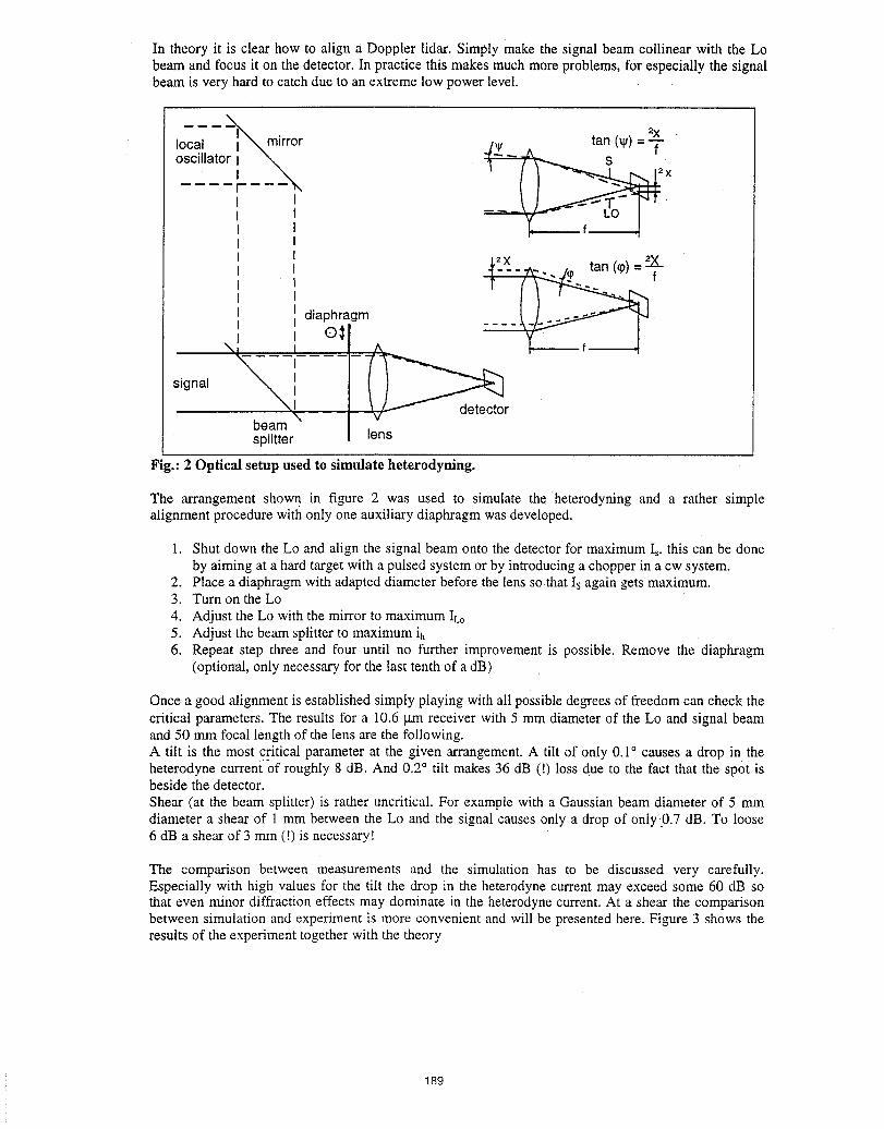
In theory it is clear how to align a Doppler lidar. Simply make the signal beam collinear with the Lobeam and focus it on the detector. In practice this makes much more problems, for especially the signalbeam is very hard to catch due to an extreme low power level.

-Ilocal %mirror 2x

oscillator __ _ tas(_) ='T

-2)( =.... . (_0)_x

diaphragmo:_ _l f

signal I

• rbeamsplitter lens

Fig.: 2 Optical setup used to simulate heterodyning.

The arrangement shown in figure 2 was used to simulate the heterodyning and a rather simplealignment procedure witfionly one auxiliary diaphragm was developed.

1. Shut down the Lo and align the signal beam onto the detector for maximum Is. this can be doneby aiming at a hard target with a pulsed system or by introducing a chopper in a cw system.

2. Place a diaphragm with adapted diameter before the lens sothat Is again gets maximum.3. Turn on the Lo

4. Adjust the Lo with the mirror to maximum ILo5. Adjust the beam splitter to maximum ih6. Repeat step three and four until no further improvement is possible. Remove the diaphragm

(optional, only necessary for the last tenth of a dB)

Once a good alignment is established simply playing with all possible degrees of freedom can check thecritical parameters. The results for a 10.6 ttm receiver with 5 mm diameter of the Lo and signal beamand 50 mm focal length of the lens are the following.A tilt is the most critical parameter at the given arrangement. A tilt of only 0.1° causes a drop in theheterodyne currentof roughly 8 dB. And 0.2° tilt makes 36 dB (!) loss due to the fact that the sp0t isbeside the detector.Shear (at the beam splitter) is rather uncritical. For example with a Gaussian beam diameter of 5 mmdiameter a shear of 1 mm between the Lo and the signal causes only a drop of only0.7 dB. To loose6 dB a shear of 3 mm (!) is necessary!

The comparison between measurements and the simulation has to be discussed very carefully.Especially with high values for the tilt the drop in the heterodyne current may exceed some 60 dB sothat even minor diffraction effects may dominate in the heterodyne current. At a shear the comparisonbetween simulation and experiment is more convenient and will be presented here. Figure 3 shows theresults of the experiment together with the theory

189

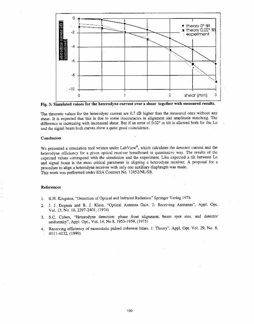
oTt ...................2" °1_ ° theory O° tilt

-_-:_._, _ = theory 0,02° til

-2 "-_ _ ,experiment

I

• -10 [

0 2 shear (ram] 3

Fig. 3: ;imulatedvalues for the heterodyne current over a shear together with measured results.

The theoretic values for the heterodyne current are0,7 dB higher than the measured ones without anyshear. It is expected that this is due to some inaccuracies in alignmentand amplitude matching. Thedifference is increasingwith increasind shear. But if an error of 0.02° in tilt is allowed both for the Loandthe signal beam both curves show a quite good coincidence.

Conclusion

We presented a simulation tool written under LabView©,which calculates the detector current and theheterodyne efficiency for a given optical receiver breadboard in quantitative way. The results of theexpected values correspond with the simulation and the experiment. Like expected a tilt between Loand signal beam is the most critical parameter in aligning a heterodyne receiver. A proposal for aprocedure to align a heterodyne receiver with only one auxiliary diaphragm was made.This work was performed under ESA Contract No. 12852/NL/SB.

References

1. R.H. Kingston, "Detection of Optical and Infrared Radiation" Springer Verlag 1978

2. J. J. Degnan and B. J. Klein, "Optical Antenna Gain. 2: Receiving Antennas", Appl. Opt.Vol. 13, No. I0, 2397-2401, (1974)

3. S.C. Cohen, "Heterodyne detection: phase front alignment, beam spot size, and detectoruniformity", Appl. Opt., Vol. 14, No 8, 1953-1959, (1975)

4. Receiving efficiency of monostatic pulsed coherent lidars. I: Theory", Appl. Opt. Vol. 29, No. 8,4111-4132, (1990)

190

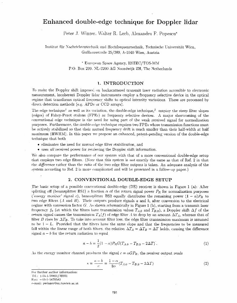
Enhanced double-edge technique for Doppler lidar

Peter J. Winzer. Walter R. Leeb, Alexandru F. Popescu*

Institut Kir Nachrichtentechnik und Hochfrequenztechnik, Technische Universitgt Wien,

Gufihausstrafie 25/389, A-1040 Wien, Austria

* European Space Agency, ESTEC/TOS-MMP.O. Box 299. NL-2200 AG Noordwijk ZH, The Netherlands

1. INTRODUCTION

To make the Doppler shift imposed on backscattered transmit laser radiation accessible to electronicmeasurement, incoherent Doppler lidar instruments employ a frequency selective device in the opticalregime that transforms optical frequency shifts to optical intensity variations. These are processed bydirect detection methods (e.g. APDs or CCD arrays).

The edge technique I as well as its w_riation, the double-edge technique," employ the steep filter slopes(edges) of Fabry-Perot eta.lons (FPEs) as frequency selective devices. A major shortcoming of the_:onventional edge technique is the need for using part of the weak received signal for normalizationImrposes. Furthermore, the double-edge technique requires two FPEs whose transmission functions mustbe actively stabilized so that their mutual frequency drift is much smaller than their half-width at halfmaximum (HWHM). In this paper we propose an enhanced, patent-pending version of the double-edgetechnique that both

• eliminates the need for mutual edge filter stabilization, and• uses all received power for retrieving the Doppler shift information.

We also compare the performance of our system with that of a more conventional double-edge setupthat employs two edge filters. (Note that this system is not exactly the same as that of Ref. 2 in thatthe d'_ffer'encerather than the ratio of the two edge filter outputs is taken. An adequate analysis of thesystem according to Ref. 2 is more complicated and will be presented in a ibllow-up paper.)

2. CONVENTIONAL DOUBLE-EDGE SETUP

The basic setup of a possible conventional double-edge (DE) receiver is shown in Figure 1 (a): Aftersplitting off (beamsplitter BS1) a fl'action a of the return signal power PR for normalization purposes('energy monitor' signal c), bemnsplitter BS2 equally distributes the remaining power (1 -a)PR totwo edge filters (.4 and B). Their outputs produce signals a and b, after conversion to the electricalregime with conwrsion factor G. As shown schematically in Figure 1 (b), starting from a transmit laserfl'equen_y .t})(at which the filters have transmission values TA,0 and Ts,o), a Doppler shift Af of the,'eturn signal causes the transmission TA(f) of edge filter A to drop by an amount ATA, whereas that oftilter B rises by ATB. To take into account filter loss. the edge filter transmission maximum is assumedto be 1 - L. Provided that the filters have the same slope and that the frequencies to be measuredtall within the linear range of both tilters, the relation ATA = ATB = AT holds, causing the differencesignal a - b for the return radiation to equal

a - b = 2(1 - ¢t)PRG(T.4.o- TB,O- 2AT). (!)

As t,he energy monitor chamml produces the signal c = (*GPR, the receiver output reads

a.- b 1 - (_ T._- ,: - _- ( .._,,,- Tao - 2'XT) (2)

I:m" [urther author information:

Tel.: +4:',-1-5880t/38901Fax: +,|3- 1-5870583

e-m_tih l)winzer(q)nt, t uwien._tc.att

191

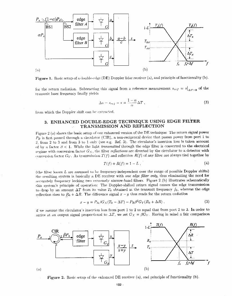
,. _Jedge

2£aP,, [ _ edge A _ 6_, a_b _l__ ! At8

l_terBi T G c , _oo_.................................2222_Z222!......i22;"...

! / iX IAT_/ iT...

fo fo+Af 'f

(..) (b)

Figure 1. Basic setup of a d{mble-e{lge (DE) Doppler lidar receiver (a), and prineiple of functionality (b).

fi}r r,he return radiation. Subtracting this signal from a reference measurement S,.e.f= StAT=o of thetransmit laser frequency finally yields

1-(.,A._ = s,._i - s = --AT , (3)

(g

from which the Doppler shift can t,{, extracted.

3. ENHANCED DOUBLE-EDGE TECHNIQUE USING EDGE FILTERTRANSMISSION AND REFLECTION

Figure 2 (a) shows the basic setup of our enhanced version of the DE technique: The return signal powerPn is first passed through a circulator (CIR), 8 non-reciprocal device that passes power from port 1 to2. from 2 to 3 and from 3 to 1 only (see e.g. Ref. 3). The circulator's insertion loss is taken account

{,f by a factor ;_ < 1. While the light trnnsmitted through the edge filter is converted to the electricalregime with conversion factor G\,_ the filter reflections are diverted by the circulator to a detector withconversion factor Gv. As transmissi{m T(.f) and reflection R(f) of any filter are always tied together by

T(.f) + R(f) = 1 - L, (4)

(t.he filter losses L are assumed to 1)e frequency-independent over the range of possible Doppler shifts)the resulting system is basically a DE receiver with one ed.qefilter only, thus eliminating the need ibruc:curately frequency locking two extremely narrow-band filters. Figure 2 .(b) illustrates schematically

this system' s principle of operation: The Doppler-shifted return signal causes the edge transmissionto drop by anamount LT from its value To obtained at the transmit frequency f0, whereas the edgereflection rises to R0 + L_R,. The difference signal x - y thus reads for the return radiation._

:r - y = PI_:iGx (To - AT) - Pnfl'2Gv(Ro + LR) , (5)

if we assume the circulator's insertion loss from port 1 to 2 to equal that from port 2 to 3. In order toarrive at an output signal proporti(mal to LT, we set Gx = flGv. Having in mind a fair comparison

; T(f) R(f)

1-L i__ /

CIR , i "'_""

Ro,..................filter / -]-G_ x-y _ To................ _i'_"

x+y ] / i \ i ATI . i / i R.,..'...

Iff_ £+Af{.) (b)

Figure 2. Basi{: setup of th{' enhanced DE receiver (a), and principle of fimctionality (b).

192 -

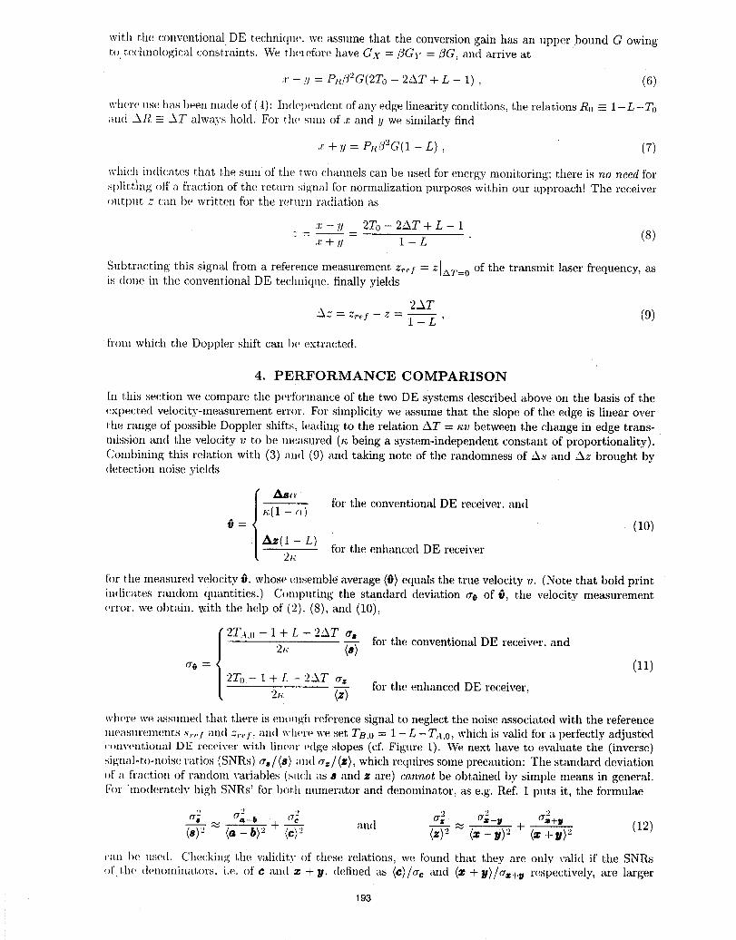
with the conventional DE te(:hni(lu(', we assume that the conversion gain has an upper bound G owingto te(:hnological constraints. We tlwret'ore have Gx = i]Gy =/]G, and arrive at

:r - !1 = PRi_"-G(2To - 2AT + L - 1), (6)

where use has been made of (4): In(lel)endent of any edge linearity conditions, the relations Ro -- 1-L-To_md AR = AT always hohh For th(_ sum of .r and y we similarly find

.,:+ y = PR,3"G(1 - L), (7)

which indicates that the sum of th(_ two (:hammls can be used for energy monitoring; there is no need for• \

spht, tmg off a.fl'action of the return signal fbr normalization purposes within our approach! The receiver,mtlmt z can be written for the retm'n radiation as

:z:- y 2T0 - 2AT + L - 1: = -- = (s):I:+ y 1 - L

Subtra(:ting this signal from a reference measurement z.,._,f= z l_,T=O of the transmit laser frequency, asis done in the conventional DE technique_ finally yields

2AT

'._kz= z.,._f - _ - 1 - L ' (9)

h'om which the Dopl)ler shift can be extracted.

4. PERFORMANCE COMPARISON

[n this section we compare the perh)rmance of the two DE systems described above on the basis of the

,_xpected velocity-measurement error. For simplicity we assume that the slope of the edge is linear overthe range of possible Doppler shifts, leading to the relation AT = _:v between the change in edge trans-mission and the velocity v to be measured (n being a system-independent constant of proportionality).Combining this relation with (3) and (9) and taking note of the randomness of ,'._ksand Az brought bydetectiounoiseyields

As_,

_:(1 - (_----_ for the conventional DE re(:eiver, and= , (10)

_z(1 - L) for the enhanced DE receiver2N

f'or the measured velocity _. whose ensemble average (0) equals the true velocity v. (Note that bold printindicates random quantities.) Computing the standard deviation ae of fi, the velocity measurement,,rror. we obtain. _ith the help of (2). (8), and (10),

{ 2TA.0 - 1 + L - 2AT a. for the conventional DE receiver, and

2,,: (s>_,_ = (11)

2T,_ - 1 + L - 2AT ?2_z for the enhanced DE receiver,2,_ (z>

where we assmned t,hatt, here is entmgh reference signal to neglect the noise asso(:iated with the referenceuleaslu'emelltS 'u,'e/ and z,.¢.j., a.n(l where we set TB.O = 1 --L- TA.O, which is valid for a perfectly adjusted('(mventional DE receiver with lin(,m' e(tge slopes (of. Figure 1). We next h_xveto evaluate tim (inverse)sigIml-to-n()ise ratios (SNRs) as/<s) ml(l az/(Z), which requires some precaution: The standard deviation

,,f"a fraction of random variables (sut:h as # and z are) cannot be obtained by simple means in general.F()r 'moderately high SNRs' for both numerator and denominator, as e.g. Ref. 1 puts it, the fornmlae

.) ._ ._ .) .) .)

a---i; a_-b + and -- "_ (12)<s)_"_ <a-b) 2 <c)_ <z>2 _ <z-y)" + (z+y) 2

(';m be used. Checking the wflidity ,,i' these relations, we found that. they are only valid if the SNRs

,)f' t.h(, de*lo*ninators, i.e. ()f c a*id z + y. defined as (e)/ae and <z + ll)/az+v respectively, are larger

193

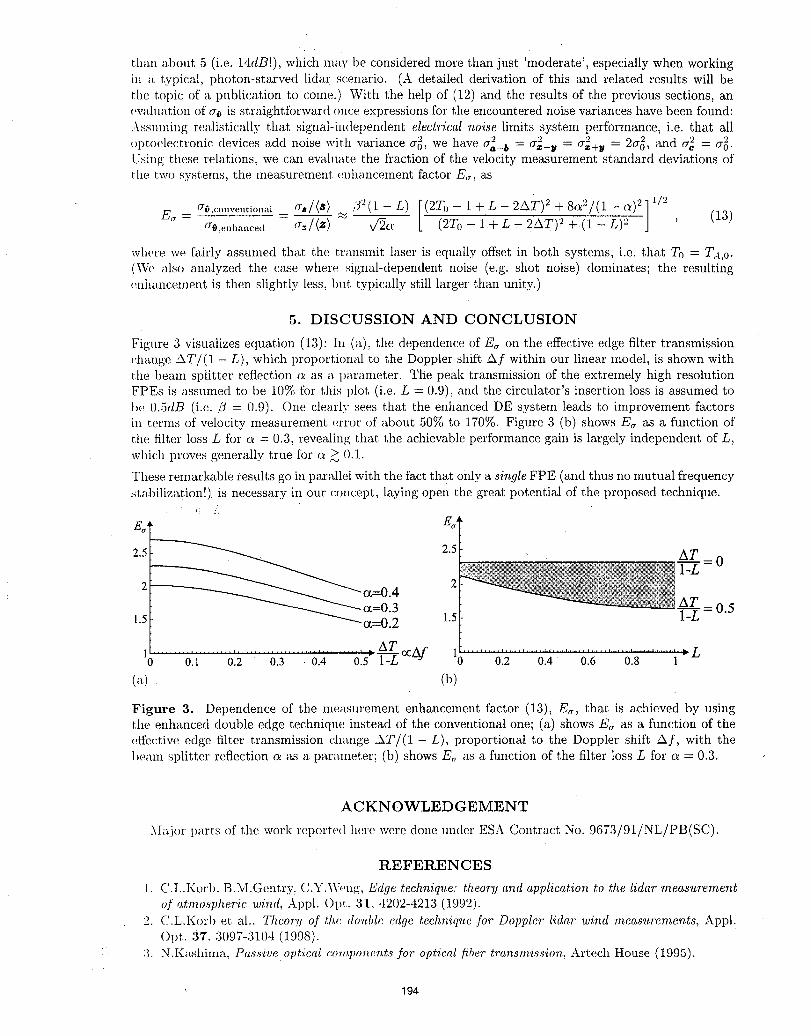
than about 5 (i.e. 14dB!), which may be considered more than just 'moderate', especially when workingin a typical, photon-starved lidar scenario. (A detailed derivation of this and related results will bet.lle topic of a publication to come.) With the help of (12) and the results of the previous sections, an(wahmtion of c_ is straightforward once expressions for the encountered noise variances have been found:

Assmning realistically that signal-independent electrical noise limits system perfbrmance, i.e. that all2 2 2 ') 2 • ')

optoelectronic devices add noise with variance a0, we have = = =_a-_ rl;,.__ %+// 2_0, and a2 = _6'Using these relations, we can ewdm_te the fraction of the velocity measurement standard deviations ofthe two systems, the measurement (mhancement factor E_, as

o'_,,:o,w.,tiona_ gs/(s) .. it2(1-L) [(2TO- llL-2AT)2 +8,._2/(1--_)'_]t/2E,- - - L _T0 -+L--2--A-T_ _-_ ---L)2 ] ' (13)

where we fairly assumed that the trm_smit laser is equally offset in both systems, i.e. that To = TA,o.(We also analyzed the case where, signal-dependent noise (e.g. shot noise) dominates; the resulting(,nhancement is then slightly less, but typically still larger than unity.)

5. DISCUSSION AND CONCLUSION

Figure 3 visualizes equation (13): In (a), the dependence of E_ on the effective edge filter transmissiont:hange AT/(1 - L), which proportional to the Doppler shift Af within our linear model, is shown withthe beam splitter reflection ct as a pa.rameter. The peak transmission of the extremely high resolutionFPEs is assumed to be 10% for this plot (i.e. L = 0.9), and the circulator's insertion loss is assumed tolm 0.5dB (i.e. l? = 0.9). One clearly sees that the enhanced DE system leads to improvement factorsin terms of velocity measurement error of about 50% to 170%. Figure 3 (b) shows E_ as a function ofthe filter loss L for c_ = 0.3, revea.ling that the achievable performance gain is largely independent of L,wlfich proves generally true for c_> 0.1.

These remarkable results go in parallel with the fact that only a single FPE (and thus no mutual frequency

stabilization!) is necessary in our concept, laying open the great potential of the proposed technique.

Eo ., Eo .'1

-I-_-_Z= 02 2

AT

_.5 _ . 1.5 ]-----L= 0.5

10........ 0'.i....... 0!2....... 013..... .0Z4 ....... 015_ AT ocAf 0.2 0.4 0.6 0.8 1 L

(a) (b)

Figure 3. Dependence of the measurement enhancement factor (13), E_, that is achieved by usingthe enhanced double edge technique instead of the conventional one; (a) shows E_ as a function of thev,ffective edge filter transmission change AT/(1 - L), proportional to the Doppler shift A f, with the

1)earn splitter reflection a as a parameter; (b) shows E_ as a function of the filter loss L for c_ = 0.3.

ACKNOWLEDGEMENT

Major parts of the work reported here were done under ESA Contract No. 9673/91/NL/PB(SC).

REFERENCES

i. C.L.Korb. B.M.Gentry, C.Y.W(,ng, Edge technique: theory and application to the lidar .measurementof atmospheric 'wind, Appl. ()p_. 31. 4202-4213 (1992).

2. C.L.Korb et, al.. Theory of t.h,(',do'able edge technique for Doppler" lidar wind measurements, Appl:Opt. 37. 3097-3104 (1998).

: 3. N.K_tshima, Passive optical c.o'm,poner_,ts Jot optical .fiber"transrnissior_,, Artech House (1995).

' 194

Estimation of return signal spectral width in incoherent backscatter heterodyne lidar

Barry J. Rye

CIRES (University of Colorado/NOAA)Environmental Technology Laborato_

R/E/ET2, NOAA ERL, 325 Broadway, Boulder, CO 80303-3328Phone: (303) 497-6509 FAX:(303) 497-5318 email: brye@etl.noaa.gov

It can often be reasonably assumed that the spectral profile of the return from an atmospheric backscatterheterodyne lidar is known. But this is not valid when the Doppler shift varies within the period over which returnpulses are accumulated, for example if the return is obtained from regions that are spatially well-separated as mayhappen in the spaceborne experiment SPARCLE, or if there is significant velocity turbulence within the scatteringvolume observed by a static system. Our interest ineStimating the signal spectrum was initiated by an experimentcarried out at ETL to simulate a SPARCLEreturn by sparse sampling of data obtained from a ground-based lidarover a period of several hours. _ Then the overall spectrum must be estimated along with the Doppler shift.andreturn power. Here we consider onlythe simplest case Whenit can be correctly assumed that the spectrum has.aGaussian profile and the only unknown is its bandwidth. Specifically, the expected autocorrelation of thediscretely-sampled photodetector output at the kth lag is assumed tObe ......

Ark : P.v{6exp[-(2"rf2k) z/2]exp(J2,'r_lk)+ 1} (1)where Px is the noise power and the unknowns are the wideband signal-to-noise ratio (SNR) 8, the Doppler shiftf,and the signal bandwidthf2; these two frequencies are assumed normalized by being divided by the receiver searchbandwidth and are therefore dimensionless. Thus, if a return signal of bandwidth that corresponds to a i m/sfrequency shift is observed within a receiver of bandwidth corresponding to50 m/s, thenf_ = 1/50= 0.02.

The precision of optical instruments is usefully compared with the limiting case Whenthe only noise in the Systemarises from photocount fluctuations which are further assumed to have Poisson statistics. The standard deviations %of the three unknowns are then given by2,3.4

cro(6)_ o-o(f) 20-o(A)_ 1

a 2 L e -- k 2 N (2)

where N is the mean photocount. It is somewhat surprising to observe that the limiting standard deviation of thebandwidth estimate is a factor of (2 better than that of the Doppler estimate because it often supposed that theformer is the more difficult measurement.

For the heterodyne receiver, the Cramer-Rao lower bounds on the three standard deviations are most simplyexpressed using formulas that apply to series with Gaussian statistics for which a derivation was provided by Poratand Freidlander.5 For _rdatatime series with the Gaussian autocorrelation of Eq. (1),6the results can be expressed in

terms of a signal covariance matrix G containing the elements gik = exp - 2zf21k -il / 2 [0 _ i < M, 0 _<k < M,

where M is the number of complex data points in the demodulated discrete data time series obtained for the returnover a range gate]. Defining the matrices Q = G_5+ I and F =Q_ with elements q_kand 3qk,where I is the identitymatrix, the estimate variances are

o-'-(8) - 1"-' (3)ZZa,,a,,i=0 k=O

M-I

where a_, = Zy.ngmk ,m=O

195

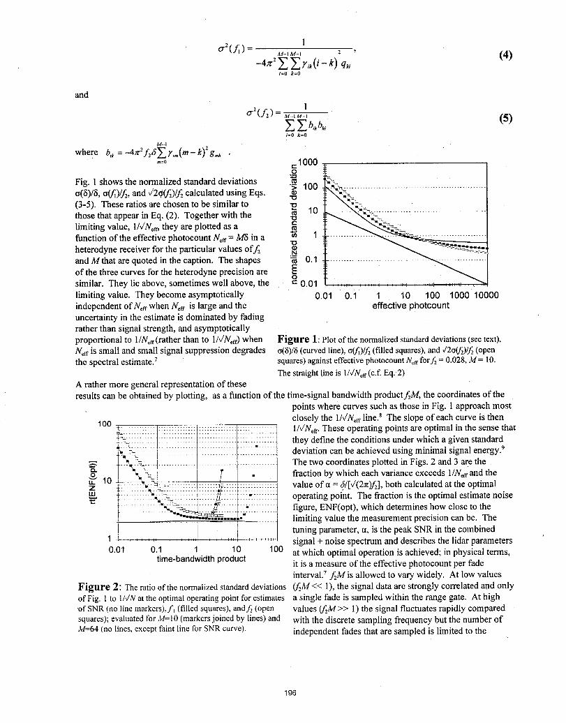
1

°'2(f) = M-,,,,_-, 2 ' (4)-4x2ZZyik(i-k) qk,

i=0 k=O

and1

°'2(A)=Z Z b,A, (s)i=0 k=O

M-I

= _ k) 2 gmk •where b_k -4x-f26_r_m(m-m:0 : 1000o

"_ _._Fig. 1shows the normalized standard deviations '_ 100_(6)/6, o_)/_, and v'2q_)/f2 calculated using Eqs. ® "_':,_L__.............................................

-. es r tio ar co eno imi,artothose that appear in Eq. (2). Together with the -o

€-

limiting value, 1A/Neff,they are plotted as afunction of the effective photocount Neff= M'6in a _ 1-oheterodyne receiver for the particular values of_and M that are quoted in the caption. The shapes _ 0.1of the three curves for the heterodyne precision are osimilar. They lie above, sometimes well above, the "- 0.01 ................................limiting value. They become asymptotically 0.01 0.1 1 10 100 1000 1 1000independent of Ngrwhen Neff is large and the effectivephotcountuncertainty in the estimate is dominated by fadingrather than signal strength, and asymptoticallyproportional to 1/N,_(rather than to 1A/NgOwhen Figure 1: Plot ofthe normalizedstandarddeviations(seetext),Neffis small and small signal suppression degrades o(6)/6(curvedline),o_)/f2 (filledsquares),and V2o(fz)/f!(openthe spectral estimate.7 squares)againsteffectivephotocountN_frforfz = 0.028,M= 10.

The straightlineis 1/4N_e_(c.f.Eq. 2)A rather more general representation of theseresults can be obtained by plotting, as a function of the time-signal bandwidth productfzM, the coordinates of the

points where curves such as those in Fig. 1 approach mostclosely the l/v'Nefrline) The slope of each curve is then

100 ±: ::: ::::: ::: :::::::::::::::::::::::::::::::::::::: : 1/VNgr.These operating points are optimal in the sense that

_::::: :::i: :: :::::::: ] I !:::: ::::::::: :::::::::: :: they define the conditions underwhich agiven standard

i %-_! [ i } t deviati°n can be achieved using minimal signal energy'9

.._',_ ................................ The two coordinates plotted in Figs. 2 and 3 are the_" ...... fraction by which each variance exceeds 1/Neffand the

zZ" 10 i !_II: !_!!_i_!:)lf il !l!ii_!:i:i:i!:i:iI value ofot=f/[((2rc)_], both calculated at the optimaloperating point. The fraction is the optimal estimate noise

T............ l :__:.;._.-!-- ........... ii figure, ENF(opt), which determines how close to the

..... , i ,, 'i ...... ] limiting value the measurement precision can be. Thetuning parameter, ct, is the peak SNR in the combined

1 signal + noise spectrum and describes the lidar parameters '0.01 0.1 1 10 100 at which optimal operation is achieved; in physical terms,

time-bandwidthproduct it is a measure of the effective photocount per fadeinterval.7 fzM is allowed to vary widely. At low values

Figure 2: The ratioof thenormalizedstandarddeviations (fzM << l), the signal data are strongly correlated and onlyof Fig. 1to 1/VNat the optimaloperatingpoint for estimates a single fade is sampled within the range gate. At high_)fSNR(no linemarkers),f_(filledsquares),andfz (open values _M>> 1) the signal fluctuates rapidly comparedsquares);evaluatedfor M=10(markersjoined by lines)and with the discrete sampling frequency but the number ofM=64(no lines,exceptfaint linefor SNRcurve), independent fades that are sampled is limited to the

196

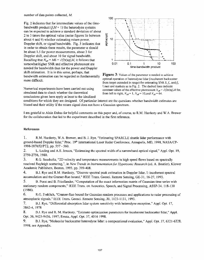
number of data points collected, M.100

Fig. 2 indicates that for intermediate values ofthe time- i!:_! _: i_:ii!i!:-i-i:!II::II: ! II: ii"!:bandwidthproduct_M= l) the heterodyne systems _ :::_i _-:: .i. i: -: : • ' "

can be expected to achieve a standard deviation of about _ ..,t._. i_o_ " i2 to 3 times the optimal value (noise figures lie between _- [ \ [ ". "_,_ _ =, _ ! _Eabout 4 and 9) whether estimating return power, _ 10 _ ._ .:i '_:::: :"!_'_;=_:-_.-_5::i . . : iDoppler shift, or signal bandwidth. Fig. 3 indicates that -_ _: ..... : :'_ : !",i:!:!: i[_ ! :[:: : " ]

in order to obtain these results, the parameter a should ......_ ....... _..._.,........\,.... .... ,i I ,i

be about 1.5 for power measurements, about 3 for _ • ..-.-.. I_-"_- - _-_" IIDoppler shift, and about I0 for signal bandwidth. I ' ' _ i!Recalling that Neff= M8 = ,i(2n)af,.M, it follows that 1 [ ......... i _ .....I ? ....... !somewhat higher SNR and effective photocount are 0.01 0.1 1 10 100needed for bandwidth than for the power and Doppler time-bandwidthproductshift estimation. It is in this sense, perhaps, thatbandwidth estimation can be regarded as fundamentally Figure 3: Valuesof the parameterctneededto achieve

optimaloperationof heterodynelidar(incoherentbackscattermore difficult, fromtargetextendedin range)for estimatingSNR&f, andf,.

Linesand markersas in Fig.2. The dashedlinesindicateNumerical experiments have been carried out using constantvaluesof theeffectivephotocountN_a= V(2n)ctfzMfor,simulated data to check whether the theoretical from leftto right,:V_= 1,N_fr= 10,andN_jr= 64.conclusions given here apply at least to the idealizedconditions for which they are designed. Of particular interest are the questions whether bandwidth estimates arebiased and their utility if the return signal does not have a Gaussian spectrum.

I am grateful to Alain Dabas for helpful comments on this paper and, of course, to R.M. Hardesty and W.A. Brewerfor the collaboration that led to the experiment described in the first reference.

References

1. R.M. Hardesty, W.A. Brewer, and B. J. Rye, "Estimating SPARCLE shuttle lidar performance withground-based Doppler lidar," Prec. 19thInternational Laser Radar Conference, Annapolis, MD, 1998, NASA/CP-1998-207652/PT2, pp. 557 - 560.

2. L. Lading and A.S. Jensen, "Estimating the spectral width of a narrowband optical signal," Appl. Opt. 19,2750-2756, 1980.

3. R.G. Seasholtz, "2D velocity and temperature measurements in high speed flows based on spectrallyresolved Rayleigh scattering,", in New Trends in Instrumentation for Hypersonic Research (ed. A. Boutier), KluwerAcademic Publishers, Boston, 1993, pp. 399-408.

4. B.J. Rye and R.M. Hardesty, "Discrete spectral peak estimation in Doppler lidar. I: incoherent spectralaccumulation and the Cramer-Rao bound," IEEE Trans. Geosci. Remote Sensing, GE-31, 16-27, 1993.5. B. Porat and B. Friedlander, "Computation of the exact information matrix of Gaussian time series with

stationary random components," IEEE Trans. on Acoustics, Speech, and Signal Processing, ASSP-34, 118-130(1986).

6. R.G. Frehlich, "Cramer-Rao bound for Gaussian random processes and applications to radar processing ofatmospheric signals," IEEE Trans. Geosci. Remote Sensing, 31, 1123-1131, 1993.

7. B.J. Rye, "Differential absorption lidar system sensitivity with heterodyne reception," Appl. Opt. 17,3862-4, 1978

8. B.J. Rye and R. M. Hardesty, "Estimate optimization parameters for incoherent backscatter lidar," Appl.Opt. 36, 9425-9436, 1997; Errata, Appl. Opt. 37, 4016 1998.

9. B.J. Rye, "Molecular backscatter heterodyne lidar: a computational evaluation," Appl. Opt. 37, 6321-6328,1998; see Appendix.

197

1.5-tJm Coherent Lidar Using Injection-seeded, LD pumpedEr,Yb:Glass Laser

Kimio Asaka, Takayuki Yanagisawa and Yoshihito Hirano

Mitsubishi Electric CorporationOfuna 5-1-1, Kamakura-city, Kanagawa, 247 JAPAN

Phone +81-467-41-2547

1. Introduction

A coherent lidar is an attractive sensor for atmospheric observation because it can measure wind

velocity even in clear air conditions. It is needed eye-safety same as other laser equipment used in the field. As

the coherent lidar in eye safe wavelength (>l.4-_m wavelength), one using 2-_m pulsed laser such as

Ho,Tm:YAG and Tm:YAG laser is reported.1"2

Compared to 2-_m, the wavelength of 1.5-tim has a ten times higher maximum permissible exposure

for human eyes. In addition, optical fiber components and devices for use in optical fiber communication are

easily available at this wavelength. Therefore, a coherent lidar, which use 1.5-gm pulsed laser, is more attractive

than a 2%1mcoherent lidar. To our knowledge, a 1.5-1Jmcoherent lidar operation to measure wind velocity

hasn't been reported yet. That because a single frequency 1.5-tim laser that had both high repetition rate and

enough power for coherent lidar wasn't provided. Nd:YAG + OPO 3 and injection-seeded, flash lamp pumped

Er:Glass laser4for 1.5-1Jmcoherent lidars were recently reported and are now under development.

We are developing a 1.5-[Jmcoherent lidar using an injection-seeded, LD pumped Er,Yb:Glass laser.

In our system, a microchip laser made of Er,Yb:Glass is used for a seed and a local source.

In this paper we describe our system and primary data of measured echo of aerosols.

2. System description

A block diagram of the developed 1.5-_tmcoherent lidar is shown in Fig. 1. Optical couplers divide

the output of a local oscillator in three beams. Two of the beams are used in heterodyne detection. The another

one is used as a seed beam in injection seeding of the pulsed laser, after its frequency is shifted by an

intermediate frequency (fi_ =85MHz) using an acousto-optics (AO) frequency shifter.

The transceiver optics is co-axial. Output beam from the pulsed laser is expanded by a telescope

(TEL) and radiated into the atmosphere using a scanner (SCN). The effective diameter of the telescope is 60-

mm. In a T/R switch, the received signal is separated from the transmitted beam and is put into a polarized

maintained optical fiber. It is mixed with the local beam at the photo receiver to generate the heterodyne beat

signal. The beat signal is sent to an AD converter.

The polarized maintained optical fiber is used in order to make the optical arrangement easily in the

receiver and to utilize a small, high reliability optical component for the optical fiber communication.

2.1 The local oscillator (LO)

A microchip laser is used as a local oscillator. It was built in a small module by Utilizing the

198

technology of LD modules for optical communication. The size of the microchip laser module is

38.6x31.8x18.5mm3. It consists of a pumping LD with a fiber lens, the coupling optics between the LD and an

Er,Yb:Glass chip, a sapphire plate and an optical isolator. The output beam from Er,Yb:Glass chip is put into

the optical fiber by a coupling lens. ATE cooler controls those temperatures. A 1-W class high brightness AI

free InGaAs LD is used for pumping.

The thickness and the reflection of output surface of the Er,Yb:Glass chip were designed as 0.28-ram

and 98.3%, respectively. The Er3. ion concentration is lxl02° cm"3and the Yb3+ion concentration is 1.5x10zl

cm"3. The Er,Yb:Glass chip was optically and thermally contacted to the sapphire plate with a transparent optics

cement. As the sapphire plate is used for thermal spreader, heat removal from the Er,Yb:Glass chip is done

along the optical axis of the microchip laser. The changes of output divergence with thermal lens effect are kept

small by this method. Then, high coupling efficiency of the output into the optical fiber is maintained.

A microchip laser that uses an isotropic material for laser medium such as Er,Yb:Glass has dual

polarized modes that are orthogonal.5 The polarization dependent isolator not only reduces a back reflection but

also extracts only one of the polarized modes for local beam.

Our microchip laser module has side mode suppression ratio more than 20-dB and a fiber coupled,

single frequency output 0f 23.2-mW is'obtained. The wavelength of output beam is 1.534-0m. By the self-

delayedlheterodyne method using a 91-km length optical fiber, the linewidth of 20.5-kHz was measured.

2.2. The pulsed laser

The laser cavity consists of two high reflective mirrors (HR). Each radius of curvature of those

mirrors is 1-m. The cavity length is about 2-m. A LiNbO3Pockels cell was used for E/O Q switching. The seed

beam from the microchip laser is injected into the cavity through the polarizer PO. The pumping module, which

was placed near the center of the cavity, consists of two Er,Yb:Glass rods, four five-stacked LD arrays and

water-cooled heat sinks. Pump energy of these LDs is 740-mJ/pulse (0.975,1Jmwavelength) at 40-Hz repetition

rate. _The polarizer PO radiates theoutput pialse from the cavity.

A block diagram of the pumping module is presented in Fig. 2. A pair of parallel lateral surface of

each Er,Yb:Glass rod is in contact with heat sinks and the rod is pumped from the other pair of parallel lateral

surface by two LD arrays. In this geometry a bifocusing of thermal lens occurs as the heat sink removes the heat

generated by pumping in the Er,Yb:Glass rod.Then, in order to compensate the bifocusing effect_ the two

Er,Yb:Glass rods are arranged in series along the optical axis of the pulsed laser; the lateral Surfaces _ contact

with the heat sinks are intersected perpendicularly each other. :,

Er,Yb:Giass is a quasi-three-level laser. For this reason, half of more of the Er3. ions must be excited

for getting a gain. Accordingly, it is desirable to reduce the volume of Er,Yb:Glass rod in order to obtain a high-

density excitation with the same pumping energy. To match this condition the Er,Yb:Glass rod was chosen as

1.2xl.2xl0mrn 3 and the Yb 3+ ion concentration and Er 3+ ion concentration are 1.5x10 2t cm -3 and 6x1019 cm -3,

respectively.

To adjust the cavity length a cavity tuner CT was developed. It has two roof prisms whose spacing is

changed by a piezoelectric translator and controlled by a cavity controller CC. A bit of output pulse power is

taken out from the HE45 mirror, then used as a reference signal in order to get the control signal of the cavity

tuner. The cavity controller changes the cavity length that the beat signal of the reference and local beams is to

become constant frequency.

199

The output pulse energy with and without seeding at 40-Hz repetition rate is 4.0-mJ and 4.6-rrd,

respectively. The pulse width of the seeded pulse is 244-ns. Power spectrums of the beat signal, which was

measured during 10-minutes, and overwritten on one screen are presented in Fig.3. The seeded-pulse frequency

is stabilized within +5.7-MHz (standard deviation).

3. Experimental results

The developed 1.5-om coherent lidar was used for wind velocity measuring. The lidar was positioned

at about 5-m above the ground and it radiated laser pulses into the atmosphere with an elevation angle of 10.

The pulse energy was 2-mJ in this measurement.

The signal processing is as follows:

Range bin width: 30-m (200-ns) Window: Hanning

Sampling frequency: 500-MSa/s Frequency bin width: 488-kHz (0.37-m/s)

An example of the measurement is presented in Fig. 4: The result has an averaged frequency

spectrum of received signals of 100 pulses. The calculated SNR using theoretical coherent lidar equation 6 is

also shown in Fig. 4. Calculation parameters of Table 1were used. It is considered that the differences between

the measured and the calculated SNR at mid-range were caused by an insufficient adjustment of the transceiver

optics. The diameters and phase front radii of the transmitted and the assumed backpropagated local beam were

not sufficiently matched at the transceiver optics in this primary measurement. Readjusting them will improve

the measured SNR.

4. Summary

We developed a 1.5-1Jmcoherent lidar that incorporates an injection seeded, LD pumped Er,Yb:Glass

laser for a slave laser and a microchip Er,Yb:Glass laser module for a seed and a local source. The laser radiates

a single frequency, injection seeded pulse of 4.0-rnJ at 1.534-1Jmwavelength with a repetition rate of 40-Hz.

Experimentally we obtained the echo of aerosols to distances several kilometers by this 1.5-1Jmcoherent lidar.

References1. R. Targ et. al. : Appl. Opt., 35 (1996) 7117.2. S. Harmon and J. Thomson : J. Mod. Opt., 41 (1994) 2175.3. T. P. Gryson et. al. : Coherent Laser Radar, Vol.19, 1995 OSA Technical Digest Series (Optical Society ofAmerica, WashingtorrDC, 1995), p.74.4. A. J. McGrath et. al. :Appl. Opt., 37 (1998) 5706.5. S. Taccheo et. al. : Opt. Lett. 20 (1995) 889.6. R. Targ, M. J. Kavaya, R. M. Huffaker and R. L. Bowles: Appl. Opt., 30 (1991) 2013.

200

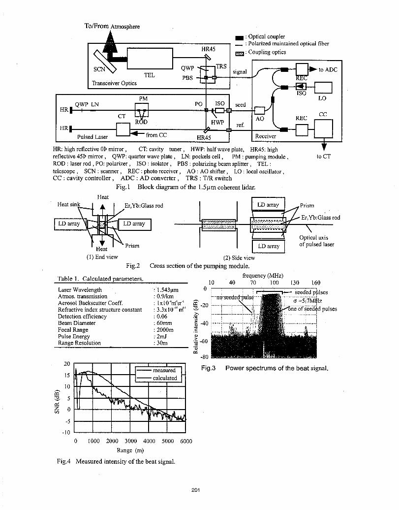
To/From Atmosphere

i : Optical coupler

_ Polarized maintained optical fiberI H_45 i_ ..Couplingoptics

TEL PBSTransceiver Optics

PM -- L_

QWP LN _ PO ISO seedHR'. : ,:CT----- HWP ref.HR| [ 1_., _ "l

Pulsed Laser L_...J"q'--from CC HR45 " Receiver _ L._

HR: high reflective 0I_mirror, CT: cavity tuner, HWP: half wave plate, HR45: highreflective 45I_mirror, QWP: quarter wave plate, LN: pockels cell, PM : pumping module, to CTROD : laser rod, PO: polarizer, ISO : isolator, PBS : polarizing beam splitter, TEL :telescope, SCN : scanner, REC : photo receiver, AO : AO shifter, LO : local oscillator,CC : cavity controller, ADC : AD converter, TRS : TiR switch

Fig. 1 Block diagram of the 1.5_tm coherent lidar.

Heat

Heat sink Er,Yb:Glassrod _ _array ,,,_Prism ,

,_,_..=,,! _ Er,Yb:Glass rod

[ _ Optical axis

LD of pulsed laser(I) End view (2) Side view

Fig.2 Cross section of the pumping module.

frequency (MHz)Table 1. Calculated parameters. 10 40 70 100 130 160

Laser Wavelength : 1.543gm 0 : seeded p_lsesAtmos. transmission : 0.9/km _,

Aerosol Backscatter Coeff. : lxl0_rrflsr" _ -20 ' _ =5i7MgzRefractive index structure constant 3.3x10 '' rd" ' , pulsesDetection efficiency : 0.06Beam Diameter : 60ram =_-40Focal Range : 2000m .=_Pulse Energy : 2mJRange Resolution : 30m '_ -60

-8020 t I

i _ _. ..[_ measured L Fig.3 Power spectrums of the beat signal.

15 / h _ k "|_ calculated 1.I0

_ 5 _

z 0 _

-5

-10

0 1000 2000 3000 4000 5000 6000

Range (m)

Fig.4 Measured intensity of the beat signal.

201

Specification of a coherent laser radar for air data measurements for advancedaircraft

Christer Karlsson, Per-Otto Arntzen, G6ran Hansson and Stan Zyra

Defence Research Establishment (FOA)

Department of Laser Systems

P. O. Box 1165, S-581 I1 LinkOping,Sweden

Tel: +46 13 378243, e-mail."chrkar@lin.foa.se

Thomas Lampe

SAAB AB

Flight test methods Department

S-581 88 Link6ping, Sweden

Requirements on components and subsystems of a CLR system for use as an optical air datasystem for the full flight envelope of an advanced fixed wing aircraft are discussed. A,detailedspecification of such a test system and its implementation in a pod are presented.

Note to the program committee:

The work above is part of a preliminary study of OADS-systems by FOA and SAAB aircraft.The discussions, results and conclusions are hardly entirely "new". However, the work shouldstill be of interest to several other CLR-groups. A poster presentation would be suitable.

202

MEASUREMENTS OF AIRCRAFT WAKE VORTEX STRUCTURE BY CW COHERENT

LASER RADAR

M Harris, R I Young

Electronics Sector, Defence Evaluation and Research Agency

Malvern, Worcestershire, WR14 3PS, UK.

J M Vaughan

Microwave Management AssOciates

(contact address: DERA Malvern)

The laser sensors group at DERA Malvern has a long history of detailed measurements of aircraft wake

vortices. The equipment used has recently been upgraded to achieve improved accuracy in determining

the core separation. The use of direction-sensing lidar giving the ability to distinguish the sign

(direction) of wind velocity allows the acquisition of superior data compared to earlier DERA trials [1].

The increased ability to define the position of the core vortex gives greater accuracy in measurements

of the circulation. The gathering of a large database allows the potential to build a comprehensive

picture of vortex evolution and decay. The upgraded equipment was deployed on a trial for Airbus

Industrie at Toulouse Blagnac during March 1998, w_h the aim of making measurements of wake

turbulence from aircraft on the final approach to the runway.

Coherent laser radar measures wind velocities by scattering laser light off atmospheric particles and

detecting the shiR in frequency of the scattered light. This Doppler shift is proportional to the line of

sight component of velocity for the particles illuminated by the probe beam. The DEILA.wake vortex

lidar transmits -5 W of CW output at a wavelength of 10.6 _tm, and is housed in a box body vehicle

complete with computers to collect the data and perform real-time analysis. A description of this

equipment is given in reference [1]. An acousto-optic modulator is used to create an offset of 43.6

MHz allowing velocity direction sensing. An extremely narrow, high attenuation notch filter eliminates

the parasitic component (due to internal light scattering) at 43.6 MHz in the detector output prior to

spectral analysis by a SAW spectrum analyser. Vortex profiles were obtained by displaying a time

sequence of spectra (fig. I) from which the well-defined outline is used to extract information on vortex

parameters.

For the trial the laser radar was sited close to the centre line, directly under the aircraft flight path. This

geometry (see fig 2) optimises the probability of vortex detection under the commonly prevailing

conditions of variable crosswind. The probe beam repeatedly scans the region of space through which

the vortex descends, with the beam focus set to the estimated vortex altitude. It is usually possible to

probe the vortex pair several times after the aircraft has passed overhead. A conically-scanned laser

203

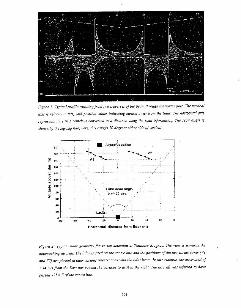
Figure l: Typical proftle resulting from two traverses of the beam through the vortex pair. The vertical

axis is velocity in m/s, with positive values indicating motion away from the lidar. The horizontal avis

represents time in s, which is converted co a distance using the scan information. The scan angle is

shown by the zig-zag line; here, this ranges 20 degrees either side of vertical.

22o • Aircraftposition !

.... ,g 180

16o .... i_...............................................................

_3 140 ......-. ..'

0 -. -._ -,_ 120 "(_ . ..

100 '. ' ....."_ ". Lidar scan angle .."_ 80 "- "...... .= - 0 +/- 20 deg. !'_ 60 "" ., " '

40 •..ff'-_. -

20 .... :........... Lidar .._..:..-:.;:'_.......i...........................i.............0-80 -60 -40 -20 0 20 40 60 8

Horizontal distance from lidar (m)

Figure 2: Typical lidar geometry for vortex detection at Toulouse Blagnac. The view is towards the

approaching aircraft. The lidar is sited on the centre line and the positions of the two vortex cores (V1

and V2) are plotted at their various intersections with the lidar beam. In this example, the crosswind of

1.34 m/s from the East has caused the vortices to drift to the right. The aircraft was inferred to have

passed _25m E of the centre line.

204

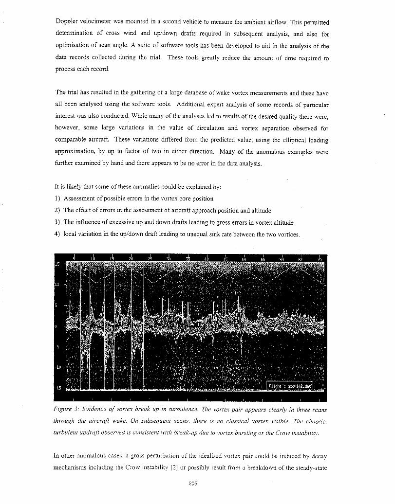
Doppler velocimeter was mounted in a second vehicle to measure the ambient airflow. This permitted

determination of cross wind and up/down drafts required in subsequent analysis, and also for

optimisation of scan angle. A suite of software tools has been developed to aid in the analysis of the

data records collected during the trial. These tools greatly reduce the amount of time required to

process each record.

The trial has resulted in the gathering of a large database of wake vortex measurements and these have

all been analysed using the software tools. Additional expert analysis of some records of particular

interest was also conducted. While many of the analyses led to results of the desired quality,there were,

however, some large variations in the value of circulation and vortex separation observed for

comparable aircraft. These variations differed from the predicted value, using the elliptical loading

approximation, by up to factor of two in either direction. Many of the anomalous examples were

further examined by hand and there appears to be no error in the data analysis.

It is likely that some of these anomalies could be explained by:

1) Assessment of possible errors in the vortex core position

2) The effect of errors in the assessment of aircraft approach position and altitude

3) The influence of excessive up and down drafts leading to gross errors in vortex altitude

4) local variation in the up/down draft leading to unequal sink rate between the two vortices.

Figure 3." Evidence of vortex break up in turbulence. The vortex pair appears clearly in three scans

through the aircra/_ wake. On subsequent scans, there is" no classical vortex visible. The chaotic,

turbulent updraJi observed is consistent with break-up due to vortex bursting or the O'ow instabilin,.

In other anomalous cases, a gross perturbation of the idealised vortex pair could be induced by decay

mechanisms including the Crow instability. [2] or possibly result from a breakdown of the steady-state

2O5

assumption in vortex formation. These explanations are consistent with the behaviour of the intercore

down draft in these cases (fig. 3) and there is also additional experimental evidence to support this

conclusion. Finally it should be noted that the anomalous results had a tendency to cluster in the early

to mid afternoon when atmospheric turbulence was at its highest due to ground heating and convection.

Hence we believe that the variability of the results was due to unfavourable conditions rather than to

any shortcomings in the lidar technique.

Summary

Laser radar has proved a useful tool for examining vortices and hence determining the necessary

separation distances between landing aircraft. Laser radar has a further role to play in the negation of

vortices. Detailed measurement of the vortex core may allow for the optimisation of aircraft wing

design to ameliorate vorticity and enhance decay. The possibility of making high-quality

measurements has been demonstrated on full-scale aircraft in the real atmosphere. Such measurements

are thus complementary to the information provided by wind tunnel studies. However, to achieve

optimum and reproducible results, the lidar measurements must be made under stringent atmospheric

conditions.

Acknowledgements

The work reported here has been funded by Airbus Industrie. The authors wish to acknowledge the

essential contributions of the other team members (within DELLAand the Airbus consortium) to the

preparation and undertaking of the trial. We are also extremely grateful to B Foord and G Constant for

technical advice and guidance.

References

[1] Coherent laser radar and the problem of aircraft wake vortices, G Constant et al. J Modem Optics

41 2153 1994

[2] A method for accelerating the destruction of aircraft wake vortices, SC Rermich & SK Lele, AIAA

98-0667, Jan 1998

206

POLARIIVIETRYOF SCATTERED LIGHT USING COHERENT LASER RADAR

M Harris

Electronics Sector

Defence Evaluation and Research Agency

Malvern, Worcestershire WR14 3PS, U.K.

Measurement of the polarisation properties of light (polarimetry) is a powerful diagnostic tool Withuses in

many applications including e!lipsometry [1]. Evaluation of the ellipse for a pure polarisation state

conventionally involves passing the fight through wave-plate and polariser elements (which can be rotated

either by mechanical or electro-optic means). Here, we will describe use of heterodyne techniques for

evaluation of the polarisation ellipse [2-5] for scattered light. The horizontally and vertically polarised

components of light scattered from depolarising surfaces were independently measured by a two-channel

coherent laser radar. Because of the phase-sensitive nature of heterodyne detection, the relative phase of

these components can be measured, and this gives all the information required to construct the polarisation

ellipse at any instant. The phenomenon of laser speckle ensures that the intensity and polarisation state

fluctuate as the beam scans across the surface of the target. The method described here allows the time-

development of the polarisation state to be followed in real time.

The experimental arrangement is depicted in Figure 1. It consists of a bistaticCW coherent laser radar [6]

with a CO, laser source giving an output of approximately 1 Watt at a wavelength of 10.6 gm. The

transmitted beam is linearly polarised with its E-vector horizontal. Scattered light from the target is

combined with the local oscillator (LO) at a beamsplitter (BS), and the two output beams from BS are

then independently sampled by a pair of detectors (D 1 and D2) thus forming a dual-channel detection

system. The two channels are arranged to detect the co-polarisedcomponent (i.e. horizontal, h) in channet

I and the cross-polarised (vertical, v) in channel 2 by means of wire-_id linear polarisers. A half-wave

plate is used to rotate the polarisation axis of the local oscillator beam prior to mixing. This allows

approximate equalisation of the LO levels at the two detectors, and under these conditions we achieve

shot-noise-dominated detection in each channel giving optimised sensitivity. The transmitted beam is

207

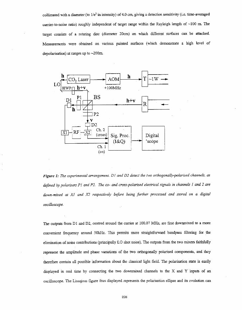
collimated with a diameter (to l/e-"in intensity) of 4.0 cm, giving a detection sensitivity (i.e. time-averaged

carrier-to-noise ratio) roughly independent of target range within the Rayleigh length of -100 m. The

target consists of a rotating disc (diameter 20cm) on which different surfaces can be attached.

Measurements were obtained on various painted surfaces (which demonstrate a high level of

depolarisation) at ranges up to -200m.

,_[CO 2Laser __ h _[_T_-IW+lOOM

P1 BS

D1 _[--7] h+vcl, j - .__

E --qp2,V]D2

2-] (cross)[ Sig. Proc. DigitalEl (I&Q) 'scope

ch.f[(co)

Figure 1: The experimental arrangement. D1 and D2 detect the two orthogonally-polarisedchannels, as

defined by polarisers P1 and P2. The co- and cross-polarised electrical signals in channels 1 and 2 are

down-mixed at X1 and X2 respectively before being further processed and stored on a digital

oscilloscope.

The outputs from D1 and D2, centred around the carrier at 100.07 MHz, are In:stdownmixed to a more

convenient frequency around 50kHz. This permits more straightforward bandpass filtering for the

elimination of noise contributions (principally LO shot noise). The outputs from the two mixers faithfully

represent the amplitude and phase variations of the two orthogonally polarised components, and they

therefore contain all possible information about the classical light field. The polarisation state is easily

displayed in real time by connecting the two downmixed channels to the X and Y inputs of an

oscilloscope. The Lissajous figure thus displayed represents the polarisation ellipse and its evolution can

208

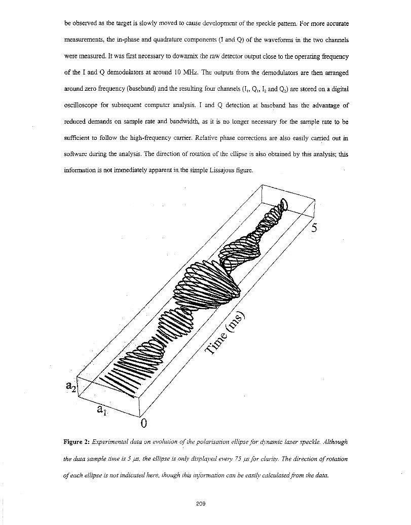
be observed as the target is slowly moved to cause development of the speckle pattem. For more accurate

measurements, the in-phase and quadrature components (I and Q) of the waveforms in the two channels

were measured. It was first necessary to downmix the raw detector output close to the operating frequency

of the I and Q demodulators at around 10 M]-tz. The outputs from the demodulators are then arranged

around zero frequency (baseband) and the resulting four channels (I_,Q_,I2and Q2)are stored on a digital

oscilloscope for subsequent computer analysis. I and Q detection at baseband has the advantage of

reduced demands on sample rate and bandwidth, as it is no longer necessary for the sample rate to be

sufficient to follow the high-frequency carrier. Relative phase corrections are also easily carried out in

software during the analysis. The direction of rotation of the ellipse is also obtained by this analysis; this

information is not immediately apparent in the simple Lissajous figure.

5

,

0

Figure 2: Experimental data on evolution of the polarisation ellipsefor dynamic laser speckle. Although

the data sample time is 5 ,as. the ellipse is only displayedevepT 75 asfor clariw. Thedirection of rotation

of each ellipse is no_indicated here, though this fl_brmation can be easily calculatedfi'om the data.

209

Typical data are presented in Figure 2, where the polarisation ellipse is plotted as a function of time. Note

that the polarisation state changes rapidly when the intensity is low (a "dark" speckle), but is

comparatively stable over a bright speckle. There is little correlation between the polarisation state from

one bright speckle to the next. Alternative methods of presentation are possible,including projection onto

the Poincar_ sphere. Such data could be used in a number of possible remote-sensing applications, as well

as for surface and sample analysis in the laboratory.

Acknowledgements: The author acknowledges the contributions of D J Wilson of DERA, J Mallott of

Heriot-Watt University, Edinburgh and M Handley of Loughborough University.

References

[1] E Collett, Polarized light:fundamentals and applications, (Dekker, New York, 1993)

[2] J H Rommers & J Howard, Plasma Phys. and Controlled Fusion, 38 1805 (1996)

[3] R Calvani, R Caponi & F Cistemino, CSELT Tech. Rep., 19 67 (1991)

[4] K Oka, T Takeda & Y Ohtsuka, J. Mod. Opt. 38 1567 (1991)

[5] C-M Feng, Y-C Huang, J-G Chang, M Chang & C Chou, Opt. Comm., 141 314 (1997)

[6] J M Vaughan, K O Steinvall, C Wemer & P H Flamant, Proc. of the IEEE 84 205 (1996)

210

DETECTION ADVANCES

Presider: Barry Rye

211

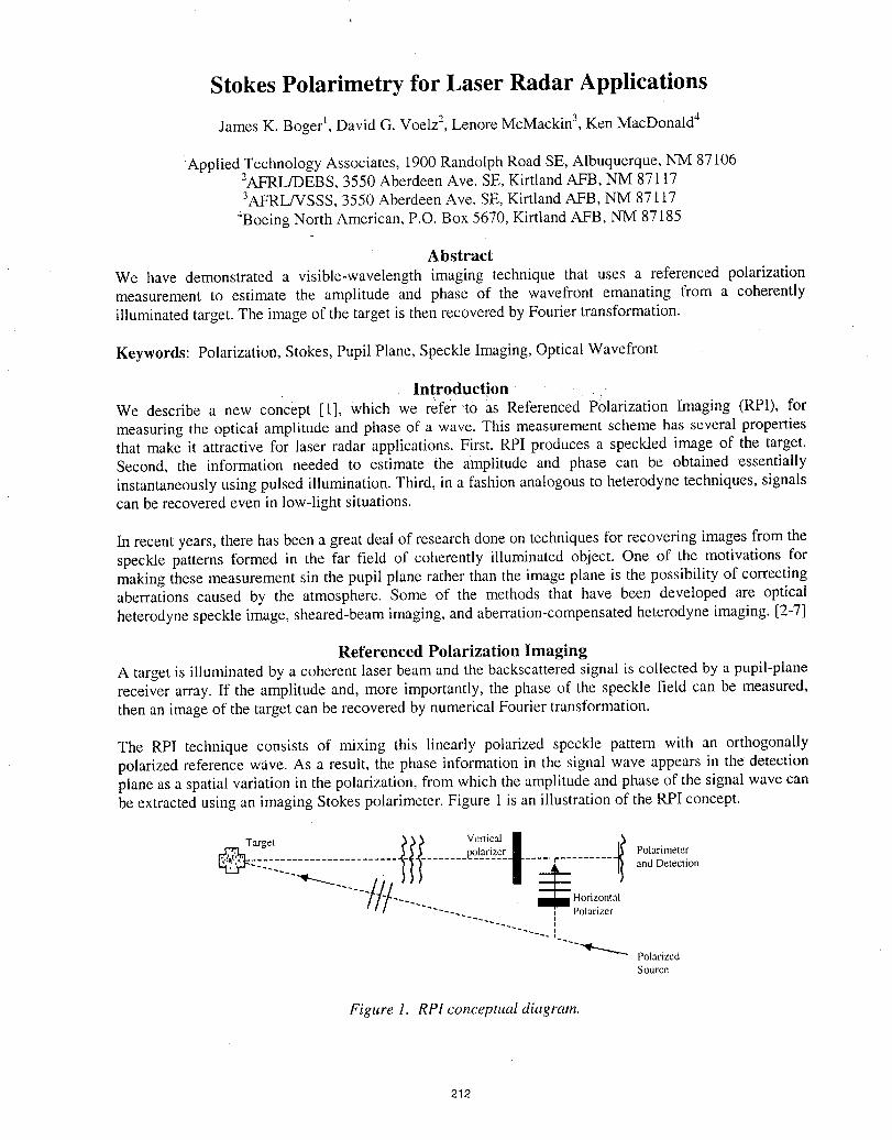
Stokes Polarimetry for Laser Radar Applications

James K. Bogerl, David G. Voelz2,Lenore McMackin3,Ken MacDonald4

_AppliedTechnology Associates, 1900 Randolph Road SE, Albuquerque, NM 871062AFRL/DEBS, 3550 Aberdeen Ave. SE, Kirtland AFB, NM 871173AFRL/VSSS, 3550 Aberdeen Ave. SE, Kirtland AFB, NM 87117

_Boeing North American, P.O. Box 5670, Kirtland AFB, NM 87185

Abstract

We have demonstrated a visible-wavelength imaging technique that uses a referenced polarizationmeasurement to estimate the amplitude and phase of the wavefront emanating from a coherentlyilluminated target. The image of the target is then recovered by Fourier transformation.

Keywords: Polarization, Stokes, Pupil Plane, Speckle Imaging, Optical Wavefront

Introduction .......We describe a new concept [l], which we refer _t0 as Referenced Polarization Imaging (RPI), formeasuring the optical amplitude and phase of a wave. This measurement scheme has several propertiesthat make it attractive for laser radar applications. First, RPI produces a speckled image of the target.Second, the information needed to estimate the amplitude and phase can be obtained essentiallyinstantaneously using pulsed illumination. Third, in a fashion analogous to heterodyne techniques, signalscan be recovered even in low-light situations.

In recent years, there has been a great deal of research done on techniques for recovering images from thespeckle patterns formed in the far field of coherently illuminated object. One of the motivations formaking these measurement sin the pupil plane rather than the image plane is the possibility of correctingaberrations caused by the atmosphere. Some of the methods that have been developed are opticalheterodyne speckle image, sheared-beam imaging, and aberration-compensated heterodyne imaging. [2-7]

Referenced Polarization ImagingA target is illuminated by a coherent laser beam and the backscattered signal is collected by a pupil-planereceiver array. If the amplitude and, more importantly, the phase of the speckle field can be measured,then an image of the target can be recovered by numerical Fourier transformation.

The RPI technique consists of mixing this linearly polarized speckle pattern with an orthogonallypolarized reference wave. As a result, the phase information in the signal wave appears in the detectionplane as a spatial variation in the polarization, from which the amplitude and phase of the signal wave canbe extracted using an imaging Stokes polarimeter. Figure I is an illustration of the RPI concept.

• ipolarizer Polarimeter............... _ and Detection

_ Horizontal, Polarizerii

'-"" PolarizedSource

Figure 1. RPI conceptual diagram.

212

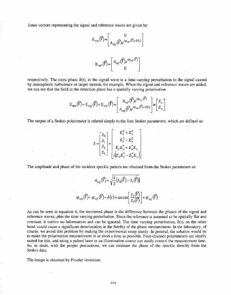
Jones vectors representing the signal and reference waves are given by:

gsig (h = I Asig (heiO._.ix (_)+_(t )

Eref (_9)= I Aref (_oeicpref(_)]

respectively. The extra phase 5(0, in the signal wave is a time-varying perturbation to the signal causedby atmospheric turbulence or target motion, for example. When the signal and reference waves are added,we can see that the field in the detection plane has a spatially varying polarization:

I zref(heicpre]'(_) 1-IEII ]gdet (h = gsig(h + gref(h=_Zsig(hei_Osig (_)+5(t)_ =

The output of a Stokes polarimeter is related simply to the four Stokes parameters, which are defined as:

s0/

2 2

S! = E_ - Ey

S = $2 ExEy + ExEy

$3 i(ExE_- ExEy )

The amplitude and phase of the incident speckle pattern are obtained from the Stokes parameters as:

Asig (h= _2 [So(h- Sl (h]

q)sig (h-_Oref (h+ _(t)= arctan[ S_3_(_l = _Osiu(h

As can be seen in equation 6, the recovered phase is the difference between the phases of the signal andreference waves, plus the time varying perturbation. Since the reference is assumed to be spatially flat andconstant, it carries no information and can be ignored. The time varying perturbation, 8(0, on the otherhand, could cause a significant deterioration in the fidelity of the phase measurement. In the laboratory, ofcourse, we avoid this problem by making the experimental setup sturdy. In general, the solution would beto make the polarization measurement in as short a time as possible. Four-channel polarimeters are ideallysuited for this, and using a pulsed laser as an illumination source can easily control the measurement time.So_ in short, with the proper precautions, we can estimate the phase of the speckle directly from theStokes data.

The image is obtained by Fourier inversion.

213

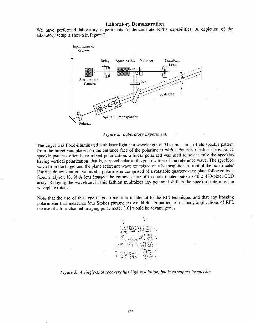
Laboratory DemonstrationWe have performed laboratory experiments to demonstrate RPI's capabilities. A depiction of thelaboratory setup is shown in Figure 2.

InputLaser@

_l 514nmRelay SpinningX/4 Polarizer Transform

Lens

Analyzer andCamera L/2

36 degree

X Spatial Filter/expander

Polarizer

Figure 2. Laboratory Experiment.

The target was flood-illuminated with laser light at a wavelength of 514 rim. The far-field speckle patternfrom the target was placed on the entrance face of the polarimeter with a Fourier-transform lens. Sincespeckle patterns often have mixed polarization, a linear polarized was used to select only the speckleshaving vertical polarization, that is, perpendicular to the polarization of the reference wave. The speckledwave from the target and the plane reference wave are mixed on a beamsplitter in front of the polarimeterFor this demonstration, we used a polarimeter comprised of a rotatable quarter-wave plate followed by a

fixed analyzer. [8, 9] A lens imaged the entrance face of the polarimeter onto a 640 x 480-pixel CCDarray. Relaying the wavefront in this fashion minimizes any potential shift in the speckle pattern as thewaveplate rotates.

Note that the use of this type of polarimeter is incidental to the RPI technique, and that any imaging

polarimeter that measures four Stokes parameters would do. In particular, in many applications of RPI,the use of a four-channel imaging polarimeter [10] would be advantageous.

,;, ,t,:." ,4; •

• ,,,;_._'_i.._ _.

Figure 3. A single-shot recovery,has high resolution, but is corrupted by speckle•

214

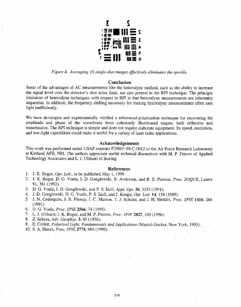
Figure 4. Averaging 10 single-shot images effectively eliminates the speckle.

ConclusionSome of the advantages of AC measurements like the heterodyne method, such as the ability to increasethe signal level over the detector's shot noise limit, are also present in the RPI technique. The principlelimitation of heterodyne techniques with respect to RPI is that heterodyne measurements are inherentlysequential. In addition, the frequency shifting necessary for making heterodyne measurements often useslight inefficiently.

We have developed and experimentally verified a referenced-polarization technique for recovering theamplitude and phase of the wavefronts from coherently illuminated targets, both reflective andtransmissive. The RPI technique is simple and does not require elaborate equipment. Its speed, resolution,and low-light capabilities could make it useful for a variety of laser radar applications.

AcknowledgementsThis work was performed under USAF contract F29601-98-C-0012 to the Air Force Research Laboratoryat Kirtland AFB, NM. The authors appreciate useful technical discussions with M. P. Fetrow of AppliedTechnology Associates and L. J. Ulibarri of Boeing.

References1. J.K. Boger, Opt. Lett., to be published May 1, 1999.2. J.K. Boger, D. G. Voelz, J. D. Gonglewski, R. Anderson, and R. E. Pierson, Proc. SOQUE, Lasers

91,381 (1992).3. D.G. Voelz, J. D. Gonglewski, and P. S. Idell, Appl. Opt. 30, 3333 (1991).4. J.D. Gonglewsld, D. G. Voelz, P. S. Idell, and J. Knopp, Opt. Lett. 14, 154 (1989).5. J.N. Cederquist, J. R. Fienup, J. C. Marron, T. J. Schultz, and J. H. Sheldin, Proc. SP1E 1416, 266

(1991).6. D.G. Voelz, Proc. SPIE2566, 74 (1995).7. L.J. Ulibarri, J. K. Boger, and M. P. Fetrow, Proc. SPIE2827, i00 (1996).8. Z. Sekera, Adv. Geophys. 3, 43 (1956).9. E. Collett, Polarized Light, Fundamentals and Applications (Marcel-Decker, New York, 1993).10. S. A. Hanes, Proc. SPIE 2774, 684 (1996).

215

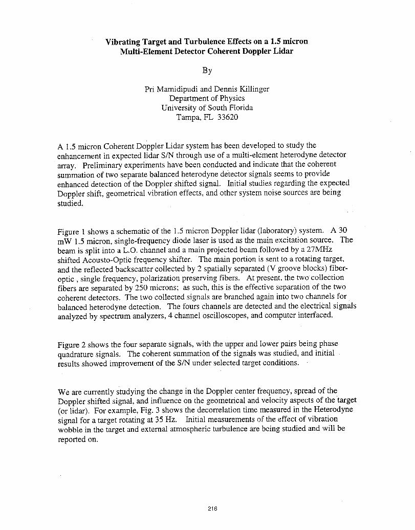
Vibrating Target and Turbulence Effects on a 1.5 micronMulti-Element Detector Coherent Doppler Lidar

By

Pri Mamidipudi and Dennis KillingerDepartment of Physics

University of South FloridaTampa, FL 33620

A 1.5 micron Coherent Doppler Lidar system has been developed to study theenhancement in expected lidar S/N through use of a multi-element heterodyne detectorarray. Preliminary experiments have been conducted and indicate that the coherentsummation of two separate balanced heterodyne detector signals seems to provideenhanced detection of the Doppler shifted signal. Initial studies regarding the expectedDoppler shift, geometrical vibration effects, and other system noise sources are beingstudied.

Figure 1 shows a schematic of the 1.5 micron Doppler lidar (laboratory) system. A 30mW 1.5 micron, single-frequency diode laser is used as the main excitation source. Thebeam is split into a L.O. channel and a main projected beam followed by a 27MHzshifted Acousto-Optic frequency shifter. The main portion is sent to a rotating target,and the reflected backscatter collected by 2 spatially separated (V groove blocks)fiber-optic, single frequency, polarization preserving fibers. At present, the two collectionfibers are separated by 250 microns; as such, this is the effective separation of the twocoherent detectors. The two collected signals are branched again into two channels forbalanced heterodyne detection. The fours channels are detected and the electrical signalsanalyzed by spectrum analyzers, 4 channel oscilloscopes, and computer interfaced.

Figure 2 shows the four separate signals, with the upper and lower pairs being phasequadrature signals. The coherent summation of the signals was studied, and initialresults showed improvement of the S/N under selected target conditions.

We are currently studying the change in the Doppler center frequency, spread of theDoppler shifted signal, and influence on the geometrical and velocity aspects of the target(or lidar). For example, Fig. 3 shows the decorrelation time measured in the Heterodynesignal for a target rotating at 35 Hz. Initial measurements of the effect of vibrationwobble in the target and external atmospheric turbulence are being studied and will bereported on.

216

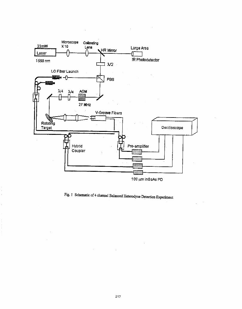
MicroscopeCollimating33row xlO Lens LargeArea

I Laser I'--"_ ' 0 _HR Mirror._ \ 0--q1550nm IRPhotodetector

r---q _J2

LOFiberLaunch

II Rotatifig I

i__:)Hybrid Pre-amplitler I"poo o,.,1oop.rnInOaAsPD

Fig.I Schematicof4 channelBalancedHeterodyneDetectionExperiment

217

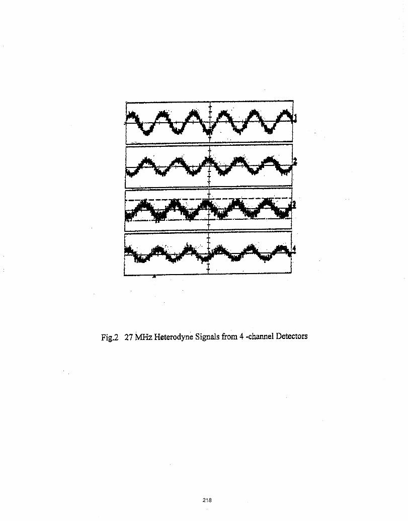
Fig.2 27 MHz Heterodyne Signals from 4 -channel Detectors

218

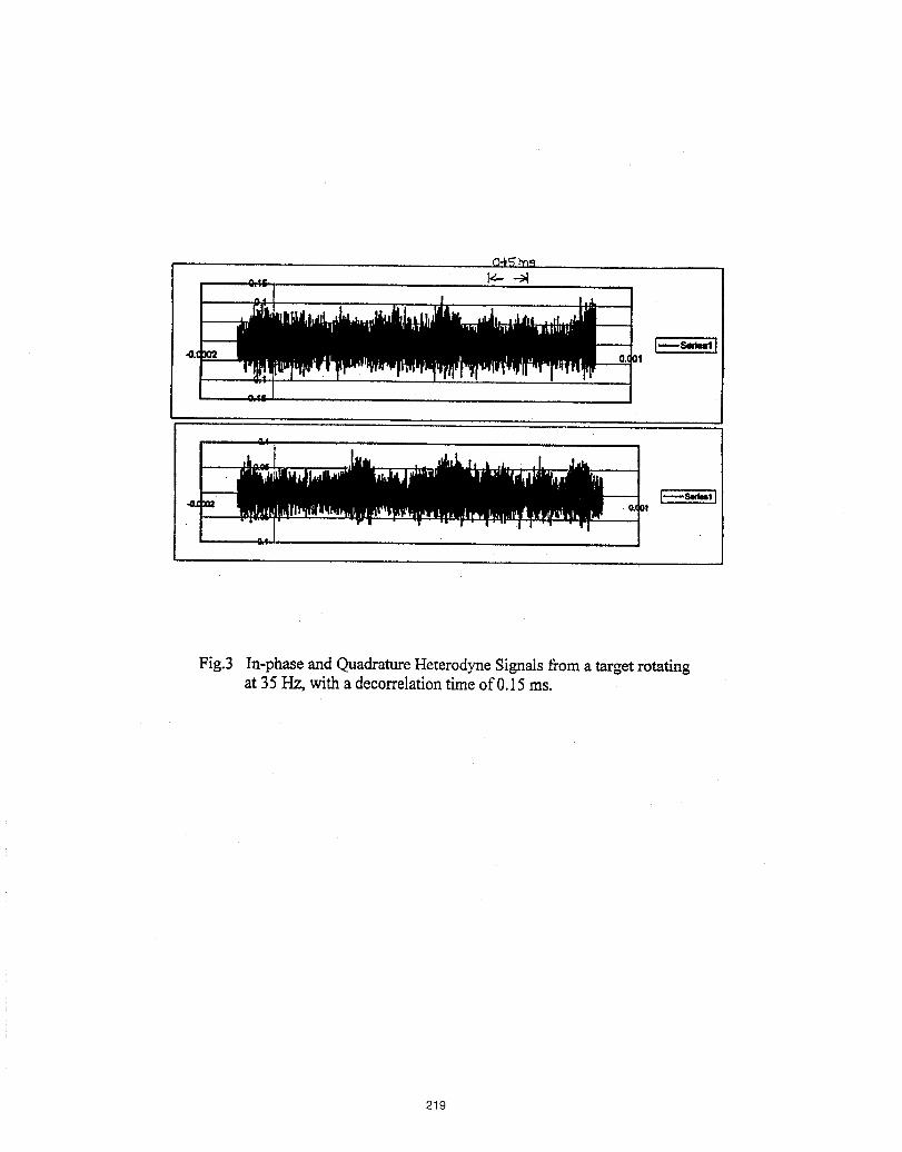
Fig.3 In-phaseand QuadratureHeterodyneSignalsfroma target rotatingat 35 Hz, with a deeorrelationtime of 0.15ms.

219

MULTIPLE WAVELENGTH HETERODYNE ARRAY SENSING FOR SPACE OPTICSMETROLOGY

Lenore McMackin and David G. VoelzAir Force Research Laboratory

3550 Aberdeen Ave SEKirtland AFB, NM 87117-5776

Harold McIntire, Matthew Fetrow and Kenneth BishopApplied Technology Assoc.'s, Inc.

1900 Randolph Rd SEAlbuquerque, NM 87106

Abstract

Largespaceopticalsystemsthatare designedto deployto opticaltolerancesafterreachingtheirpositionin orbitrequirenon-contactsurfacemeasurementaspartof anautonomousdeploymentcontrolsystem. WedemonstratetheuseOfvariablesensitivity,multi-wavelengthheterodynearrayinterferometryfor theautomatedmeasurementandcontrolof adaptiveopticalsystemswithapplicationsto remotespaceoperation.

Large, lightweight optical mirrors for space applications will require systems forcontrolling the gross aspects of the mirror surface figure. We have developed an autonomouslyoperating wavefront measurement system based on dual-wavelength heterodyne distancemeasurement techniques combined with heterodyne array imaging. A key feature of thetechnique is variable optical pathlength measurement sensitivity that allows the system tomeasure surface figure errors ranging from thousands of wavelengths down to fractions of awavelength. Automatic sensitivity tuning combined with completely digital phase measurementover the entire surface allows the integration of this device in automated sensing and opticalcorrection schemes. It is particularly suited for the measurement and control of spatially andtemporally variable optical surfaces of the kind that would be found in a space-based adaptiveoptics system. We demonstrate aspects of the automated super-heterodyne system on an opticalsurface with surface profile structure height that varies from micron to mm sized features. Wedescribe the hardware and software design of the heterodyne based measurement system thatenable it to choose the appropriate synthetic wavelength to measure given areas of the variablesurface profile. Software systems automatically select from available laser wavelengths. Spatialprocessing methods are discussed that allow the system to merge segments of images that havebeen measured at different synthetic wavelengths.

We have developed an autonomously operating adaptive optical control system based ondual-wavelength heterodyne distance measurement techniques combined with heterodyne arrayimaging' 2 In this approach the phase measurement is obtained by interfering an object andreference beam of slightly different frequencies. The resulting temporal beat frequency issampled at each point in the interference pattern and from this the optical phase is calculated.

220

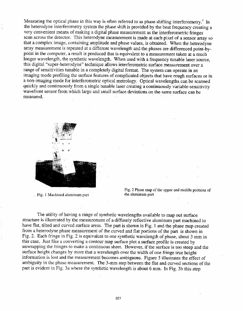
Measuring the optical phase in this way is often referred to as phase shifting interferometry. 3 Inthe heterodyne interferometry system the phase shift is provided by the beat frequency creating avery convenient means of making a digital phase measurement as the interferometric fringesscan across the detector. This heterodyne measurement is made at each pixel of a sensor array sothat a complex image, containing amplitude and phase values, is obtained. When the heterodynearray measurement is repeated at a different wavelength and the phases are differenced point-by-point in the computer, a result is produced that is equivalent to a measurement taken at a muchlonger wavelength, the synthetic wavelength. When used with a frequency tunable laser source,this digital "super-heterodyne" technique allows interferometric surface measurement over arange of sensitivities tunable in a completely digital format. The system can operate in animaging mode profiling the surface features of complicated objects that have rough surfaces or ina non-imaging mode for interferometric optical metrology. Optical wavelengths can be scannedquickly and continuously from a single tunable laser creating a continuously variable-sensitivitywavefront sensor from which large and small surface deviations on the same surface can bemeasured.

Fig. 2 Phase map of the upper and middle portions ofFig. 1 Machined aluminum part the aluminum part

The utility of having a range of synthetic wavelengths available to map out surfacestructure is illustrated by the measurement of a diffusely reflective aluminum part machined tohave flat, tilted and curved surface areas. The part is shown in Fig. 1 and the phase map createdfrom a heterodyne phase measurement of the curved and flat portions of the part is shown inFig. 2. Each fringe in Fig. 2 is equivalent to one synthetic wavelength of phase, about 3 mm inthis case. Just like a converting a contour map surface plot a surface profile is created byunwrapping the fringes to make a continuous sheet. However, if the surface is too steep and thesurface height changes by more that a wavelength over the width of one fringe true heightinformation is lost and the measurement becomes ambiguous. Figure 3 illustrates the effect ofambiguity in the phase measurement. The 3-mm step between the flat and curved sections of thepart is evident in Fig. 3a where the synthetic wavelength is about 6 mm. In Fig. 3b this step

221

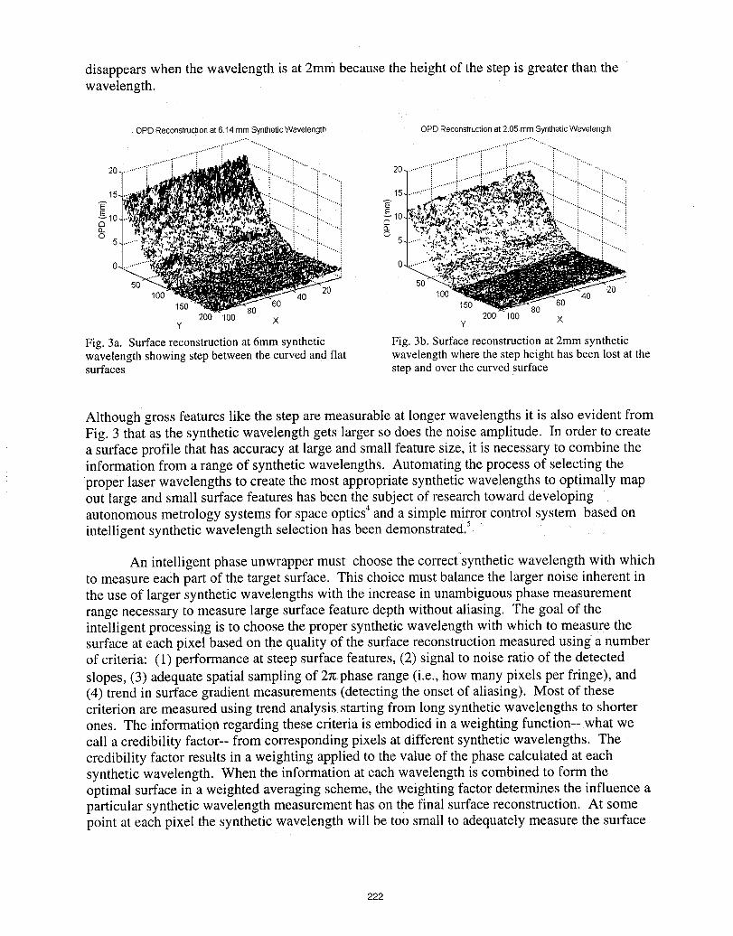
disappears when the wavelength is at 2mm because the height of the step is greater than thewavelength.

OPDReconstruc_onat 6.14mm SyntheticWavelength OPD Reconstructionat 2.05 rnmSyntheticWavelength

...........3.....................'T, .............•......................".....................T....................i _ ..... "i ".....

15. "...........i 15........ ;

1o lo.......... ,.i05- 5.

o. i o. '..........

50 20 50 201O0 40 1O0 40

150 80 150 80 60200 100 X 200 100 Xy Y

Fig. 3a. Surface reconstruction at 6mm synthetic Fig. 3b. Surface reconstruction at 2mm syntheticwavelength showing step between the curved and flat wavelength where the step height has been lost at thesurfaces step and over the curved surface

Although gross features like the step are measurable at longer wavelengths it is also evident fromFig. 3 that as the synthetic wavelength gets larger so does the noise amplitude. In order to createa surface profile that has accuracy at large and small feature size, it is necessary to combine theinformation from a range of synthetic wavelengths. Automating the process of selecting theproper laser wavelengths to create the most appropriate synthetic wavelengths to optimally mapout large and small surface features has been the subject of research toward developingautonomous metrology systems for space optics"and a simple mirror control system based onintelligent synthetic wavelength selection has been demonstrated,s::

An intelligent phase unwrapper must choose the correct synthetic wavelength with whichto measure each part of the target surface. This choice must balance the larger noise inherent inthe use of larger synthetic wavelengths with the increase in unambiguous phase measurementrange necessary to measure large surface feature depth without aliasing. The goal of theintelligent processing is to choose the proper synthetic wavelength with which to measure thesurface at each pixel based on the quality of the surface reconstruction measured using a numberof criteria: (1) performance at steep surface features, (2) signal to noise ratio of the detectedslopes, (3) adequate spatial sampling of 2_:phase range (i.e., how many pixels per fringe), and(4) trend in surface gradient measurements (detecting the onset of aliasing). Most of thesecriterion are measured using trend analysis starting from long synthetic wavelengths to shorterones. The information regarding these criteria is embodied in a weighting function-- what wecall a credibility factor-- from corresponding pixels at different synthetic wavelengths. Thecredibility factor results in a weighting applied to the value of the phase calculated at eachsynthetic wavelength. When the information at each wavelength is combined to form theoptimal surface in a weighted averaging scheme, the weighting factor determines the influence aparticular synthetic wavelength measurement has on the final surface reconstruction. At somepoint at each pixel the synthetic wavelength will be too small to adequately measure the surface

222

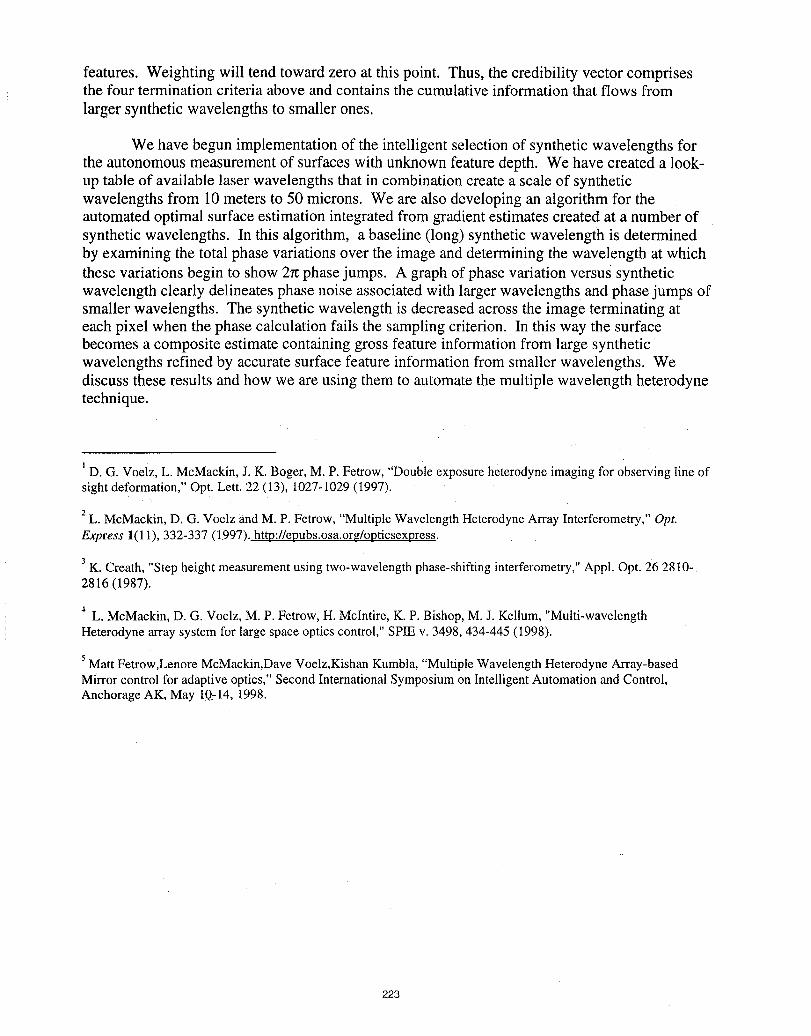
features. Weighting will tend toward zero at this point. Thus, the credibility vector comprisesthe four termination criteria above and contains the cumulative information that flows from

larger synthetic wavelengths to smaller ones.

We have begun implementation of the intelligent selection of synthetic wavelengths forthe autonomous measurement of surfaces with unknown feature depth. We have created a look-up table of available laser wavelengths that in combination create a scale of syntheticwavelengths from 10 meters to 50 microns. We are also developing an algorithm for theautomated optimal surface estimation integrated from gradient estimates created at a number ofsynthetic wavelengths. In this algorithm, a baseline (long) synthetic wavelength is determinedby examining the total phase variations over the image and determining the wavelength at whichthese variations begin to show 2rt phase jumps. A graph of phase variation versus syntheticwavelength clearly delineates phase noise associated with larger wavelengths and phase jumps ofsmaller wavelengths. The synthetic wavelength is decreased across the image terminating ateach pixel when the phase calculation fails the sampling criterion. In this way the surfacebecomes a composite estimate containing gross feature information from large syntheticwavelengths refined by accurate surface feature information from smaller wavelengths. Wediscuss these results and how we are using them to automate the multiple wavelength heterodynetechnique.

ID. G. Voelz, L. McMackin, J. K. Boger, M. P. Fetrow, "Double exposure heterodyne imaging for observing line of

sight deformation," Opt. Lett. 22 (13), 1027-1029 (1997).

2L. McMackin, D. G. Voelz and M. P. Fetrow, "Multiple Wavelength Heterodyne Array Interferometry," Opt.Express 1(11), 332-337 (1997). http://epubs.osa.org/opticsexpress.

3K. Creath, "Step height measurement using two-wavelength phase-shifting interferometry," Appl. Opt. 26 2810-

2816(1987).

4L. McMackin, D. G. Voelz, M. P. Fetrow, H. Mclntire, K. P. Bishop, M. J. Kellum, "Multi-wavelength

Heterodyne array system for large space optics control," SPIE v. 3498, 434-445 (I 998).

5Matt Fetrow,Lenore McMackin,Dave Voelz,Kishan Kumbla, "Multiple Wavelength Heterodyne Array-basedMirror control for adaptive optics," Second International Symposium on Intelligent Automation and Control,Anchorage AK, May 10-14, 1998.

223

Imaging Coherent Receiver Development for 3-D Lidar

Dr. Donald P. Hutchinson

Oak Ridge National LaboratoryP.O. Box 2008, MS-6004Oak Ridge, TN 37831

Dr. Roger K. RichardsOak Ridge National LaboratoryP.O. Box 2008, MS-6004Oak Ridge, TN 37831

Dr. Marc L. SimpsonOak Ridge National LaboratoryP.O. Box 2008, MS-6004Oak Ridge, TN 37831

Abstract

Oak Ridge National Laboratory has been developing advanced coherent IR heterodynereceivers for plasma diagnostics in fusion reactors for over 20 years. Recent progress inwide-band IR detectors and high-speed electronics has significantly enhanced themeasurement capabilities of imaging coherent receivers: Currently, we are developing a3-D lidar system based on quantum-well IR photodetector (QWIP) focal plane arrays anda MEMS-based CO2laser local oscillator) In this paper we discuss the implications ofthese new enabling technologies to implement long wavelength IR imaging lidar systems.

1 M.L. SIMPSON, C.A. Bennett, M.S. Emery, D.P. Hutchinson, G.H. Miller, R.K. Richards, andD.N. Sitter, "Coherent Imaging Using Two-dimensional Focal-Plane Arrays: Design and Applications,"Applied Optics, Vol. 36, No. 27, pp. 6913-6920, 20 September 1997.

224

What can really be gained using telescope arrays incoherent lidar receivers

Peter J. WinzerInstitut ffir Nachrichtentechnik und Hochfrequenztechnik, Technische Universitiit Wien,

GuBhausstraBe 25/389, A-1040 Wien, Austria

I. INTRODUCTION

Telescope arrays I-3 have gained increasing attention over the last years, as their use in optical receivers(both for lidar and optical communications) has the potential to mitigate the performance deterioratingspeckle effect. From the above cited references, however, it is impossible to tell what can actuallybe gained by employing a perfectly phased telescope array receiver with N subapertures of size AReach instead of a conventional, single-telescope receiver of aperture size NAR: Ref. 1 compares theperformance of such an array with that of a single-telescope receiver of aperture size AR; assumingdifferent total receive areas, however, makes it impossible to tell which fraction of the performance gain

ows to the ability of arrays to compensate for the speckle effect and which is due to the larger receivearea. Refs. 2 and 3, on the other hand, compare the performance of a perfectly phased array with thatof a non-phased array of the same size (i.e. an array whose phase control has been turned off), and claimthat the latter behaves identical to a single-telescope receiver with the same total receive area. - Thatthis claim does not hold true in general will be demonstrated below. It will further be shown

• how the performance of a single-telescope receiver relates to that of both a phased and a non-phasedtelescope array receiver of the same effective receive area, and

• what can really be gained by replacing a single-telescope receiver by a phased telescope array.

Unlike Refs. 2 and 3, we arrive at the conclusion that the improvement in terms of average carrier-to-noiseratio (CNR) of an array with respect to the single-telescope receiver does not equal N in general.

2. RELATIONS BETWEEN AVERAGE CARRIER-TO-NOISE RATIOS

A common figure of merit for heterodyne receivers is the (shot-noise limited) carrier-to-noise ratio (CNR).Following Ref. i, we define this parameter as the ratio of the intermediate frequency (IF) power (thesquared IF current averaged over a time scale long compared to the IF period but short compared to IFenvelope fluctuations) to the (local oscillator (LO) shot-noise dominated) noise power. As the speckleeffect causes £he spatial (as well as temporal) distribution of the incident optical field to be random, theIF signal amplitude (and thus also the IF power and the CNP_) become random quantities, too. In theframe of this work we are interested only in the ensemble average (CNR) of Ci'qR. (Bold print indicatesrandom quantities throughout this work.)

Slngle-telescope receiver

The IF current of a conventional heterodyne receiver with receive aperture size AR,O is given by theoverlap integral between the incident (random) optical field, represented by its complex phasor E_(_', t)

[_], and the (complex conjugated) LO field's phasor E_o,o(_ , backpropagated to the receiveaperture plane .4 with transverse coordinate f', as 4

irl_,.(t) = 2R,e{S f Ett(_,t)E_Lo,o(_d_'} , (1)A

where S stands for the detector sensitivity [A/W]. The (random) IF power then reads

= fen , " - . .,PIF, o(t) :iIF, o-(t)" 2S 2 (r'l t)Ea*(r2,t)ELo,o(rl)ELO,O(r'o)di'ldr'o (2)L/

A .4

where the overline symbol denotes the above mentioned short-term time average. The shot noise vari-ance is given by cr2 = 2eSPLO.OB, where e denotes the elementary charge, B stands for the electrical

For further author information:Tel.: +43-I-58801/38965 (or /38901)Fax: +43-I-5870583

e-maih pwinzer'_nt.tuwien.ac.at225

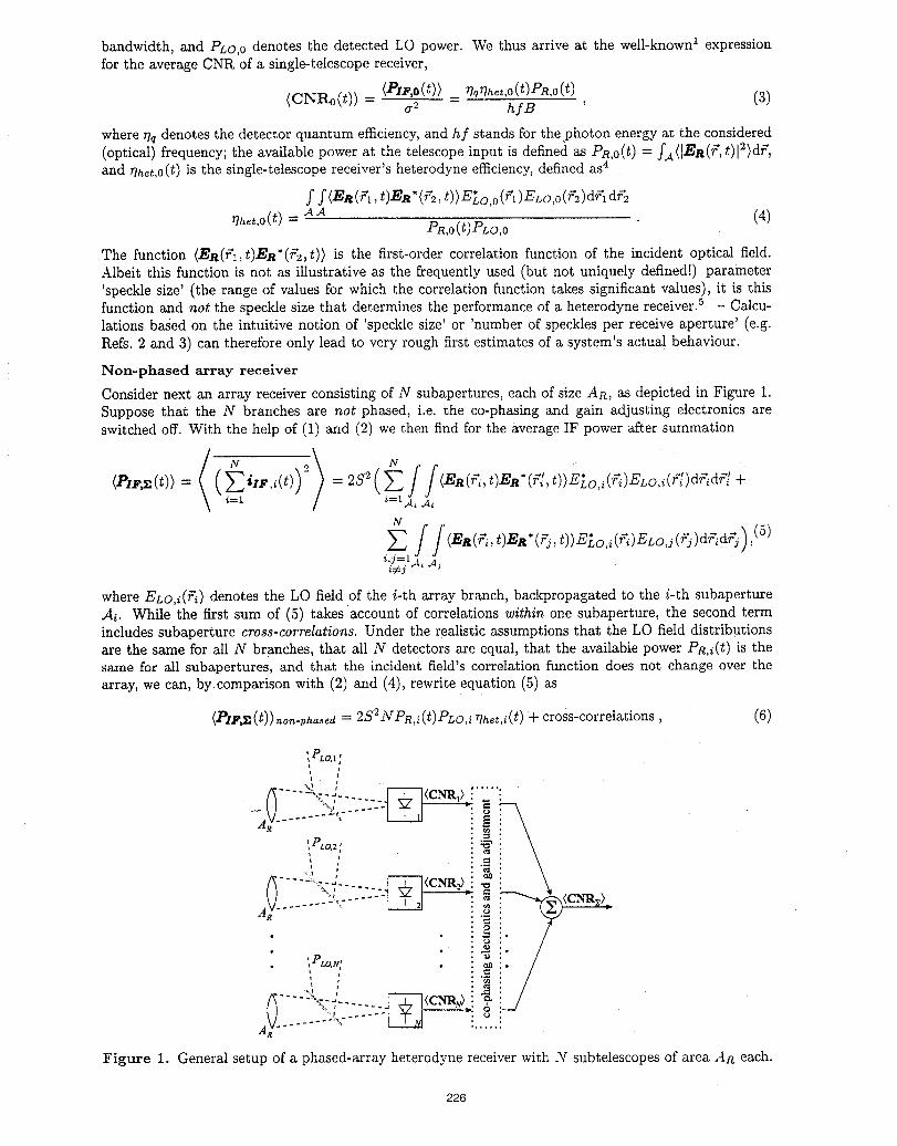
bandwidth, and PLO,Odenotes the detected LO power. We thus arrive at the well-known 1 expressionfor the average CNR of a single-telescope receiver,

(CNRo(t)) = (PIF,o(t)) 7Mlhet,o(t)PR,o(t)_ = hiB ' (3)

where _q denotes the detector quantum efficiency, and hf stands for thephoton energy at the considered(optical) frequency; the available power at the telescope input is defined as PR,o(t) = fA([ER(7, t)[2)dr +,and _het,o(t) is the single-telescope receiver's heterodyne efficiency, defined as4

f f <ER(_'1,t)ER"(_'2,t))E'Lo,o(_'_)ELO,O(r=)dr'ldr'2_he,,o(t)= _A (4)

PR,o(t)PLo,o

The function (E_(f'l, t)ER*(_'2, t)) is the first-order correlation function of the incident optical field.Albeit this function is not as illustrative as the frequently used (but not uniquely define!!) parameter'speckle size' (the range of values for which the correlation function takes significant values), it is thisfunction and not the speckle size that determines the performance of a heterodyne receiver. S - Calcu-lations based on the intuitive notion of 'speckle size' or 'number of speckles per receive aperture' (e.g.Refs. 2 and 3) can therefore only lead to very rough first estimates of a system's actual behaviour.

Non-phased array receiver

Consider next an array receiver consisting of N subapertures, each of size AR, as depicted in Figure 1.Suppose that the N branches are not phased, i.e. the co-phasing and gain adjusting electronics areswitched off. With the help of (1) and (2) we then find for the average IF power after summation

(PIp_(t)> = ilP,i(t))" = 252 ( E (ER(r_, t)ER* (r_',t))E'Loj(r_)ELo,i(r_[)dr_dr_ ' +

N

, t))E_o i(_i)ELo j (_j)d_d_ ,

i'.j=.lA_ Ajz_2

where EL04(_) denotes the LO field of the i-th array branch, backpropagated to the i-th subapertureA_. While the first sum of (5) takes account of correlations within one subaperture, the second termincludes subaperture cross-correlations. Under the realistic assumptions that the L0 field distributionsare the same for all N branches, that all N detectors are equal, that the available power PR#(t) is thesame for all subapertures, and that the incident field's correlation function does not change over thearray, we can, by comparison with (2) and (4), rewrite equation (5) as

(PIPS (t)> non-phased = 2S2 NPR,_(t) PLO,i _het,i(t) + cross-correlations, (6)

i t •

/R --\:--:-, ..... _<¢NR,> i _ :j .--- . eq .

"'_ :_: \, ,o.2 • _ i \, , .._=i \

_, : :_: \/_.........¢-_-_. Fi-I<c:_m>i,_! \

• :°ii/• ,p :-_:"• , /,O,,V_ . :

--._4 : :2_•

AV_......... _- _ :..... !

Figure 1. General setup of a phased-array heterodyne receiver wi_h .V sub_elescopes of area AR each.

226

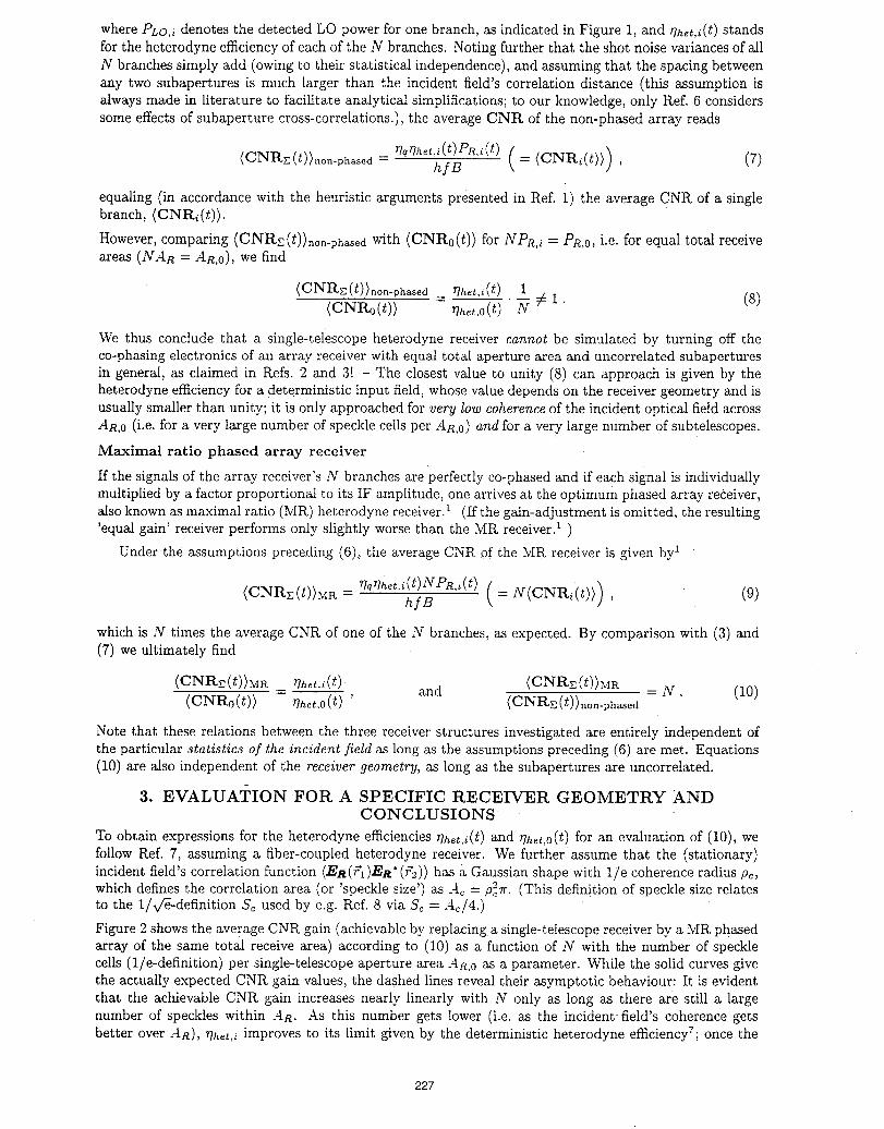
where PLO,i denotes the detected LO power for one branch, as indicated in Figure 1, and r]het,i(t) standsfor the heterodyne efficiency of each of the N branches. Noting further that the shot noise variances of all

N branches simply add (owing to their statistical independence), and assuming that the spacing betweenany two subapertures is much larger than the incident field's correlation distance (this assumption isalways made in literature to facilitate analytical simplifications; to our knowledge, only Ref. 6 considerssome effects of subaperture cross-correlations.), the average CNR of the non-phased array reads

[ \

= [ = <CNRi(t)>), (7)

equaling (in accordance with the heuristic arguments presented in Eel. 1) the average CNR of a singlebranch, (CNR_(t)).

However, comparing (CNRz(t))non-phased with (CNRo(t)) for NPR,i = PR,o, i.e. for equal total receiveareas (NAn = An,o), we find

(CNRy:(t))aon-phased = rlh..___et,i(t)1(CNRo(t)) rlhet,o(t) "N € 1. (S)

We thus conclude that a single-telescope heterodyne receiver cannot be simulated by turning off theco-phasing electronics of an array receiver with equal total aperture area and uncorrelated subapertures

in general, as claimed in Kefs. 2 and 3! - The closest value to unity (8) can approach is given by theheterodyne efficiency for a deterministic input field, whose value depends on the receiver geometry and isusually smaller than unity; it is only approached for very low coherence of the incident optical field across

AR,0 (i.e. for a very large number of speckle cells per An,0) and for a very large number of subtelescopes.

Maximal ratio phased array receiver

If the signals of the array receiver's N branches are perfectly co-phased and if each signal is individuallymultiplied by a factor proportional to its IF amplitude, one arrives at the optimum phased array receiver,also known as maximal ratio (MR) heterodyne receiver.t (If the gain-adjustment is omitted, the resulting

'equal gain' receiver performs only slightly worse than the MR receiver} )

Under the assumptions preceding (6), the average CNI_ of the MR receiver is given by I

(t)NPR,(t) / \

<CNR (t)>M= [= (9)which is N times the average CNR of one of the N branches, as expected, By Comparison with (3) and(7) we ultimately find

(CNR_ (t))Mp. rlhet.i(t) (CNRz(t))MR

(CNR0(t)) rlhet.o(t) , and (CNRE(t))non-phased = N. (10)

Note that these relations between the three receiver structures investigated are entirely independent ofthe particular statistics of the incident field as long as the assumptions preceding (6) are met. Equations(10) are also independent of the receiver geometry, as long as the subapertures are uncorrelated.

3. EVALUATION FOR A SPECIFIC RECEIVER GEOMETRY ANDCONCLUSIONS

To obtain expressions for the heterodyne efficiencies Uha,i(t) and r/h_t,o(t) for an evaluation of (10), wefollow l_ef. 7, assuming a fiber-coupled heterodyne receiver. We further assume that the (stationary)incident field's correlation function (ER(r'I)ER* (_)) has a Gaussian shape with lie coherence radius p_,which defines the correlation area (or 'speckle size') as Ac = p_,x. (This definition of speckle size relatesto the 1/x/-e-definition S_ used by e.g. Ref. 8 via $_ = A_/4.)

Figure 2 shows the average CNR gain (achievable by replacing a single-telescope receiver by a MR phasedarray of the same total receive area) according to (10) as a function of N with the number of specklecells (l/e-definition) per single-telescope aperture area AR,o as a parameter. While the solid curves givethe actually expected CNR gain values, the dashed lines reveal their asymptotic behaviour: It is evident

that the achievable CNK gain increases nearly linearly with N only as long as there are still a largenumber of speckles within AR. As this number gets lower (i.e. as the incident-field's coherence getsbetter over AR), r/h_t,i improves to its limit given by the deterministic heterodyne efficiency7; once the

227

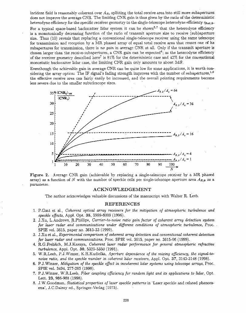
incident field is reasonably coherent over AR, splitting the total receive area into still more subapertures

does not improve the average CNR. The limiting CNR gain is thus given by the ratio of the deterministicheterodyne efficiency for the specific receiver geometry to the single-telescope heterodyne efficiency r/her,0.

For a typical space-based backscatter lidar system it can be shown s'7 that the heterodyne efficiencyis a monotonically decreasing function of the ratio of transmit aperture size to receive (sub)aperture

size. Thus (10) reveals that replacing a conventional single-telescope receiver using the same telescopefor transmission and reception by a MR phased array Of equal total receive area that reuses one of its

subapertures for transmission, there is no gain in average CNR at all. 0nly if the transmit aperture ischosen larger than the receive-subapertures, a CNR gain can be expected_; as the heterodyne efficiencyof the receiver geometry described here _ is 81% for the deterministic case and 42% for the conventionalmonostatic backscatter lidar case, the limiting CNR gain only amounts to about 3dB.

Eventhough the achievable gain in average CNR can be quite low for some applications, it is worth con-

sidering the array option: The IF signal's fading strength improves with the number of subapertures, 1'6the effective receive area can fairly easily be increased, and the overall pointing requirements becomeless severe due to the smaller subtelescope sizes.

35 (C,NR_)._ , _ AR o/Xc = 64

-/--- ..........\30 t/ _ 'AR o/Ac = 36

25 ,_€/

ii g

2O

Ii II

15 -t'€_ .................... ARo/Ac 16

,,,'// _ '

10 .t_ftl,/5 " .......................................... AR o/Ac 4

1 ='_'--'-' ................. AR.o/Ac 1l0 20 30 40 50 60 70 80 90 100

N

Figure 2. Average CNR gain (achievable by replacing a single-telescope receiver by a MR phasedarray) as a function of N with the number of speckle ceils per single-telescope aperture area AR,0 as aparameter.

ACKNOWLEDGEMENT

The author acknowledges valuable discussions of the manuscript with Waiter R. Leeb.

REFERENCES

1. P.Gatt et al., Coherent optical array receivers for the mitigation of atmospheric turbulence and

speckle effects, Appl. Opt. 35, 5999-6009 (1996).

2. J.Xu, L.Andrews, _R.PhiUips, Carrier-to-noise ratio gain factor of coherent array detection systemfor laser radar and communications under different conditions of atmospheric turbulence, Proc.SPIE vol. 3615, paper no. 3615-33 (1999).

3. J.Xu et al., Experimental comparison of coherent array detection and conventional coherent detectionfor laser radar and communications, Proc. SPIE vol. 3615, paper no. 3615-06 (1999).

4. R.G.Frehlich, M.J.Kavaya, Coherent laser radar performance for general atmospheric refractiveturbulence, Appl. Opt. 30, 5325-5350 (1991).

5. W.R.Leeb, P.J.Winzer, K.H.Kudielka, Aperture dependence of the mixing efficiency, the signal-to-noise ratio, and the speckle number in coherent lidar receivers, Appl. Opt. 37, 3143-3148 (1998).

6. P.J.Winzer, Mitigation of the speckle effect in incoherent Iidar systems using telescope arrays, Proc.SPIE vol. 3494, 277-285 (1998).

7. P.J.Winzer, W.R.Leeb, Fiber coupling efficiency for random light and its applications to lidar, Opt.Lett. 23, 986-988 (1998).

8. J.W.Goodman, Statistical properties of laser speckle patterns in 'Laser speckle and related phenom-ena', J.C.Dainty ed., Springer-Verlag (1975).

228

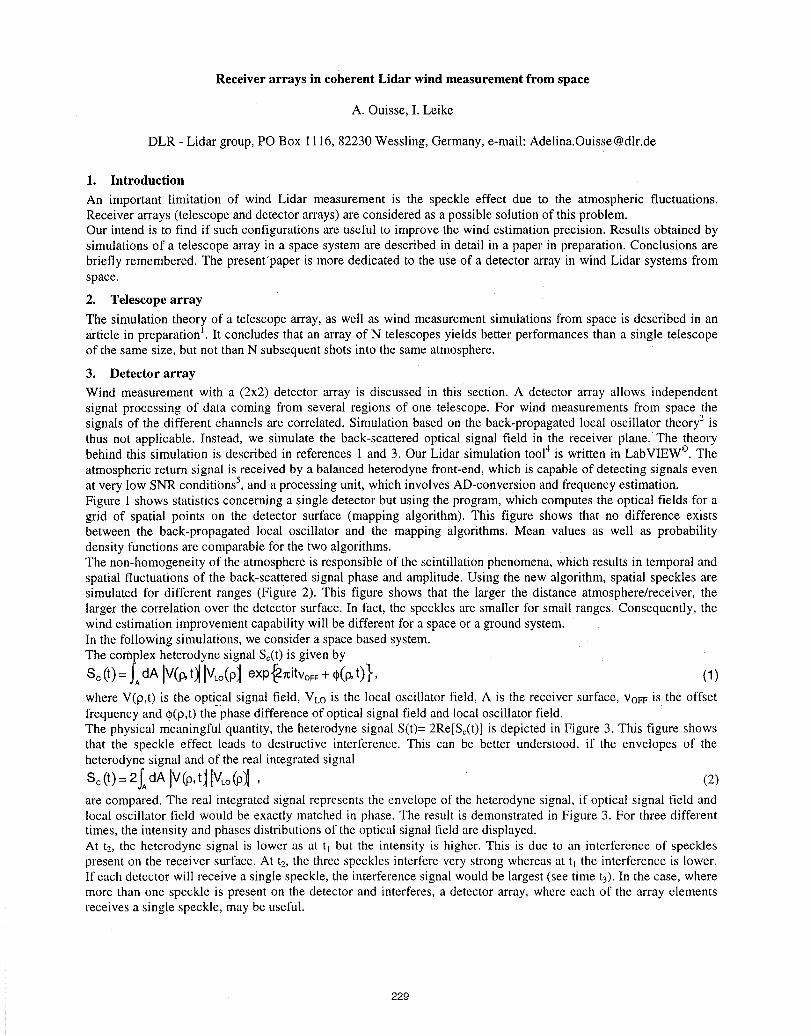
Receiver arrays in coherent Lidar wind measurement from space

A. Ouisse, I. Leike

DLR - Lidar group, PO Box 1116, 82230 Wessling, Germany, e-mail: Adelina.Ouisse@dlr.de

1. Introduction

An important limitation of wind Lidar measurement is the speckle effect due to the atmospheric fluctuations.Receiver arrays (telescope and detector arrays) are considered as a possible solution of this problem.Our intend is to find if such configurations are useful to improve the wind estimation precision. Results obtained bysimulations of a telescope array in a space system are described in detail in a paper in preparation. Conclusions arebriefly remembered. The presenrpaper is more dedicated to the use of a detector array in wind Lidar systems fromspace.

2. Telescope array

The simulation theory of a telescope array, as well as wind measurement simulations from space is described in anarticle in preparation 1. It concludes that an array of N telescopes yields better performances than a single telescopeof the same size, but not than N subsequent shots into the same atmosphere.

3. Detector array

Wind measurement with a (2x2) detector array is discussed in this section. A detector array allows independentsignal processing of data coming from several regions of one telescope. For wind measurements from space thesignals of the different channels are correlated. Simulation based on the back-propagated local oscillator theory2 isthus not applicable. Instead, we simulate the back-scattered optical signal field in the receiver plane.' The theorybehind this simulation is described in references l and 3. Our Lidar simulation tool4 is written in LabVIEW ©.Theatmospheric return signal is received by a balanced heterodyne front-end, which is capable of detecting signals evenat very low SNR conditions 5,and a processing unit, which involves AD-conversion and frequency estimation.Figure 1 shows statistics concerning a single detector but using the program, which computes the optical fields for agrid of spatial points on the detector surface (mapping algorithm). This figure shows that no difference existsbetween the back-propagated local oscillator and the mapping algorithms. Mean values as well as probabilitydensity functions are comparable for the two algorithms.The non-homogeneity of the atmosphere is responsible of the scintillation phenomena, which results in temporal andspatial fluctuations of the back-scattered signal phase and amplitude. Using the new algorithm, spatial speckles aresimulated for different ranges (Figure 2). This figure shows that the larger the distance atmosphere/receiver, thelarger the correlation over the detector surface. In fact, the speckles are smaller for small ranges. Consequently, thewind estimation improvement capability will be different for a space or a ground system.In the following simulations, we consider a space based system.

The complex heterodyne signal So(t) is given by

Sc(t) = J, dA Iv(#t)lIV,o(plexp{2.TtitvoFF+ ,(9,t)}, (1)

where V(p,t) is the optical signal field, VLo is the local oscillator field, A is the receiver surface, Vo_ is the offsetfrequency and q_(p,t)the phase difference of optical signal field and local oscillator field.The physical meaningful quantity, the heterodyne signal S(t)= 2Re[So(t)] is depicted in Figure 3. This figure showsthat the speckle effect leads to destructive interference. This can be better understood, if the envelopes of theheterodyne signal and of the real integrated signal

So(t)=2J,-dAIv ,,tlIv o o)l, (2)are compared. The real integrated signal represents the envelope of the heterodyne signal, if optical signal field andlocal oscillator field would be exactly matched in phase. The result is demonstrated in Figure 3. For three differenttimes, the intensity and phases distributions of the optical signal field are displayed.At tz, the heterodyne signal is lower as at h but the intensity is higher. This is due to an interference of specklespresent on the receiver surface. At t,, the three speckles interfere very strong whereas at h the interference is lower.If each detector will receive a single speckle, the interference signal would be largest (see time t3).In the case, wheremore than one speckle is present on the detector and interferes, a detector array, where each of the array elementsreceives a single speckle, may be useful.

229

From the simulations, it appears clearly that the fluctuations of the heterodyne signal represent not only the temporalspeckle effect but also the spatial speckle effect (see time t2).An image of the array detector is built in the receiver plane and the four resulting fields are combined with the(back-propagated) local oscillator field to obtain four optical heterodyne signals. These four signals are thenprocessed to obtain 4 electrical heterodyne currents.Figure 4 shows statistical results for a detector array with a coherent summation process61This figure shows that theresults for an array detector are comparable with those of the single detector but no improvement has been reached.That means the effect of destructive interference in the presence of several speckles on the receiver discussed abovedoes not influence the wind measurement significantly.Previous articles on array detectors 6-9deal with good SNR, which is not the case here. Thus some work has to bedone on signal processing which deal with low SNR.

4. 'Conclusion

We introduced a simulation of the back-scattered optical field in the receiver plane, which includes the temporal andspatial speckle effect. We showed that the new algorithm (mapping) and the classical back-propagated localoscillator algorithm are equivalent.The 'improvement expected by using a detector array in coherent wind Lidar is dependent of the base of the system(ground, airborne or space). This is due to the property of speckles. We showed that a detector array will notimprove the wind estimation in coherent Lidar measurement from space. This is due to the fact, that there are onlyfew speckles on the telescope and the correlation of the signals of the detectors are therefore too strong to lead to asignificant improvement.

Part of this work is supported by ESA in the frame of the contract No. 12852/NL/SB.

5. 'References

1. A. Ouisse and I. Leike, "Receivers arrays in coherent Lidar wind measurement from space", submitted toOptical Engineering (1999)

2. Ph. Salamitou et al., "Simulation in the time domain for heterodyne coherent laser radar", App. Opt. 34,499-506 (1995)

3. I. Leike, "Speckle patternsin Lidar Windmeasurementsfrom space", Proc. SPIE 3583, 373-379 (1998)4. J. Streicheret al., "ALIENS: Atmospheric LidarEnd-to-endSimulator",Proc. SPIE 3583, 380-386 (1998)

5. "Coherent Detection at Low Photon Number per Measurement Interval - DELPHI", Final Report of ESAcontractNo. 11733/95/NL/CN,TU-Wien

6. K.P. Chan andD.K. Killinger, "Coherentsummationof spatially distortedlaser Doppler signals by using a two-dimensionalheterodyne detector array",Opt. Letters 17, 1237-1239 (1992)

7. P. Gatt et al., "Coherent optical array receivers for the mitigation of atmospheric turbulence and speckleeffects", App. Optics 35 (30), 5999-6009 (1996)

8. A.R. Weeks, "Experimental verificationand theory for an eight-element multiple-apertureequal-gain coherentlaser receiver for laser communications", App. Optics 37 (21), 4782-4788 (!998)

9. X. Favreau et al., "Use of a detector array in the LMD CO2coherent laser radar",9th Conference on CoherentLaser Radar, 152-155 (1997)

230

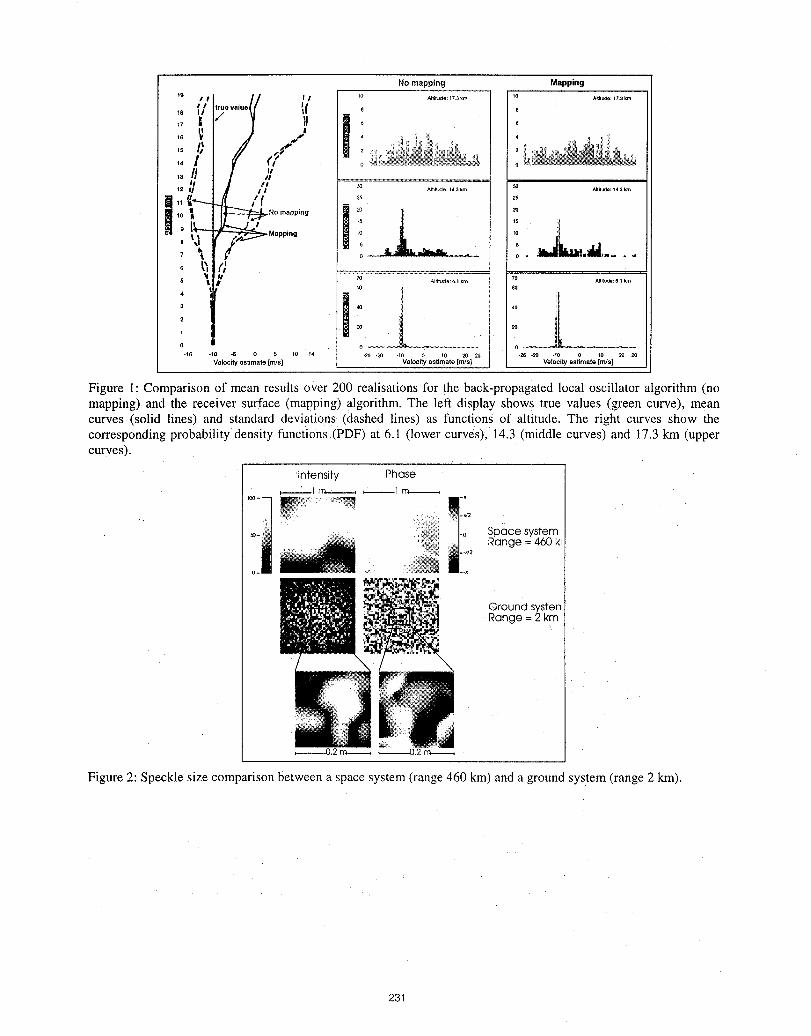
No mapping Mapping

't9 J Q I/ _ I 10 Alflfude: 17.3km 10 ARilude:17.3km

,. _I' .....,.o(I i( 017 6 e

_6 v I J / .... _t

,°1',11#

,,t' I/ ,I ,o _.......... . ..........

25 25

,,K--qJL/f,o, i i_,.o-..o,°. ,o

, '_!9 o.... I......° _)1('

Ii ..................40

22O20

"0 --0-16 -tO -6 0 5 10 t4 -26 ,20 -10 0 I0 20 26 -26 -20 .10 0 10 2O 26

Velocity estimate [m/s] Velocityestimate [m/s] Velocityestimate [m/s]

Figure 1: Comparison of mean results over 200 realisations for the back-propagated local oscillator algorithm (nomapping) and the receiver surface (mapping) algorithm, The left display shows true values (green curve), meancurves (solid lines) and standard deviations (dashed lines) as functions of altitude. The right curves show thecorresponding probability density functions (PDF) at 6.1 (lower curves), 14.3 (middle curves) and 17.3 km (,uppercurves).

Intensity Phase1 m._.____ 1 rr,-.-----

i - 2

__. Space systemRange = 460 k_

0_ :_%

Ground systenRange = 2 km

_.2_ _---0,2 rm-----

Figure 2: Speckle size comparison between a space system (range 460 km) and a ground system (range 2 km).

231

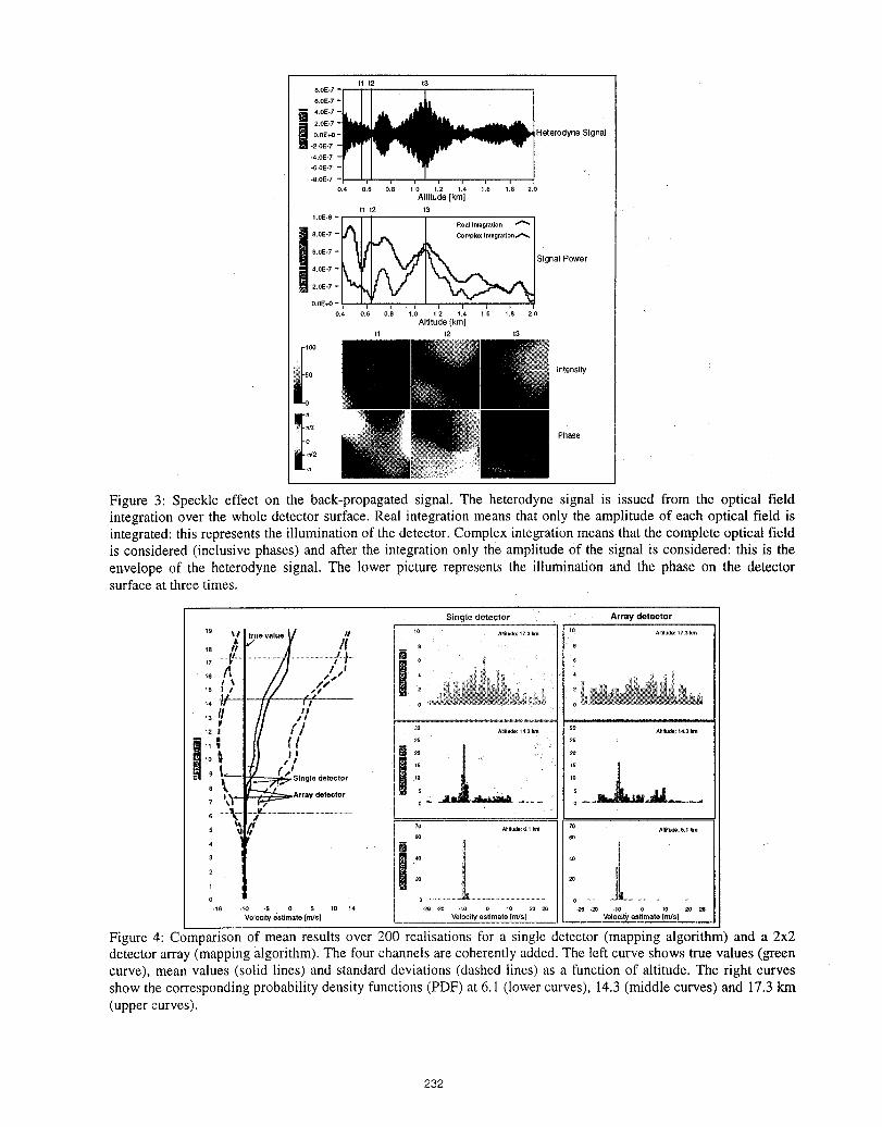
tl t2 t3

i HeterodyneSignal

0.4 0.6 0.8 1,0 1.2 1.4 1.6 1.8 2.0

Altitude [km]tl t2 t3

1.0E-6 -

_ _ l.. l . 0,a+°A......._]_ 8.0E-7- Complex Integrat ion,_.,

H+.+'-L SignalF'ower

2.0E-7-

00E'+O- I I J [ "]' I I I I I I I I I0.4 0.6 0+8 1.0 1.2 £4 1.6 1.8 2.0

Altitude [km]It 12 13

_::!5o Intensity

_'i? Phase

Figure 3: Speckle effect on the back-propagated signal. The heterodyne signal is issued from the optical fieldintegration over the whole detector surface. Real integration means that only the amplitude of each optical field isintegrated: this representsthe illumination of the detector. Complex integration meansthat the complete optical fieldis considered (inclusive phases)and after the integration only the amplitude Of the signal is considered: this is theenvelope of the heterodyne signal. The lower picture represents the illumination and the phase on the detectorsurface at three times.

Single detector Array detector

18 '_,/'. _'Uevalu19 I=#_ e_ jf_# -- 810 _. A_tilUde:17.3k_ , .11:!" Altilude:t 7.3PJ_

,°"x.........................7J..................""i? i '° '+,, ,,,, // .(I , :

,: // .'/12 I 30 : QO AMifU_ t4.3]_'11

j"', II ,,++ :_/," " Single detector 10

._p_A.e,,.,e°,o, 2........ +..=1,1.............4

3 , 40

2

z° ............... 2O

1

o ................................................... o ......

....... S 0 5 .................... Vel.lOityesOate,Os] 20 26Velocity estimate [m/s] Velocity estimate [m/s]

Figure 4: Comparison of mean results over 200 realisations for a single detector (mapping algorithm) and a 2x2detector array (mapping algorithm). The four channels are coherently added. The left curve shows true values (_eencurve), mean values (solid lines) and standard deviations (dashed lines) as a function of altitude. The right curvesshow the corresponding probability density functions (PDF) at 6.1 (lower curves), 14.3 (middle curves) and 17.3 km(upper curves).

232

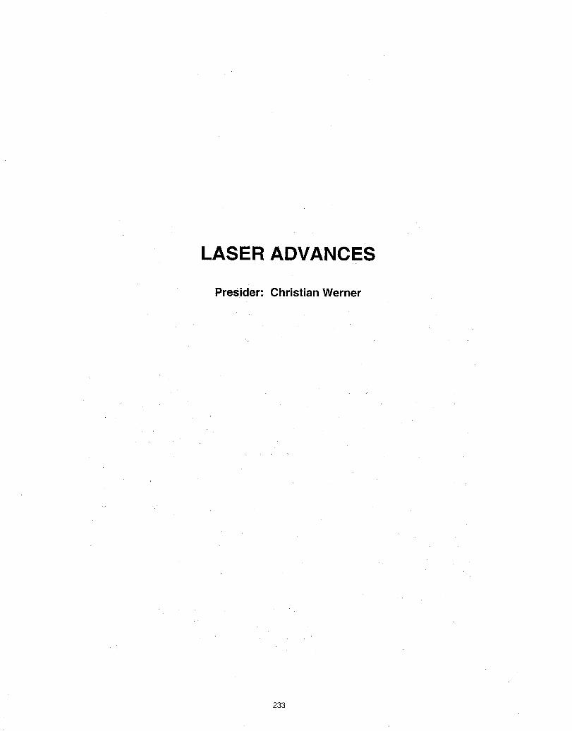
LASER ADVANCES

Presider: Christian Werner

233

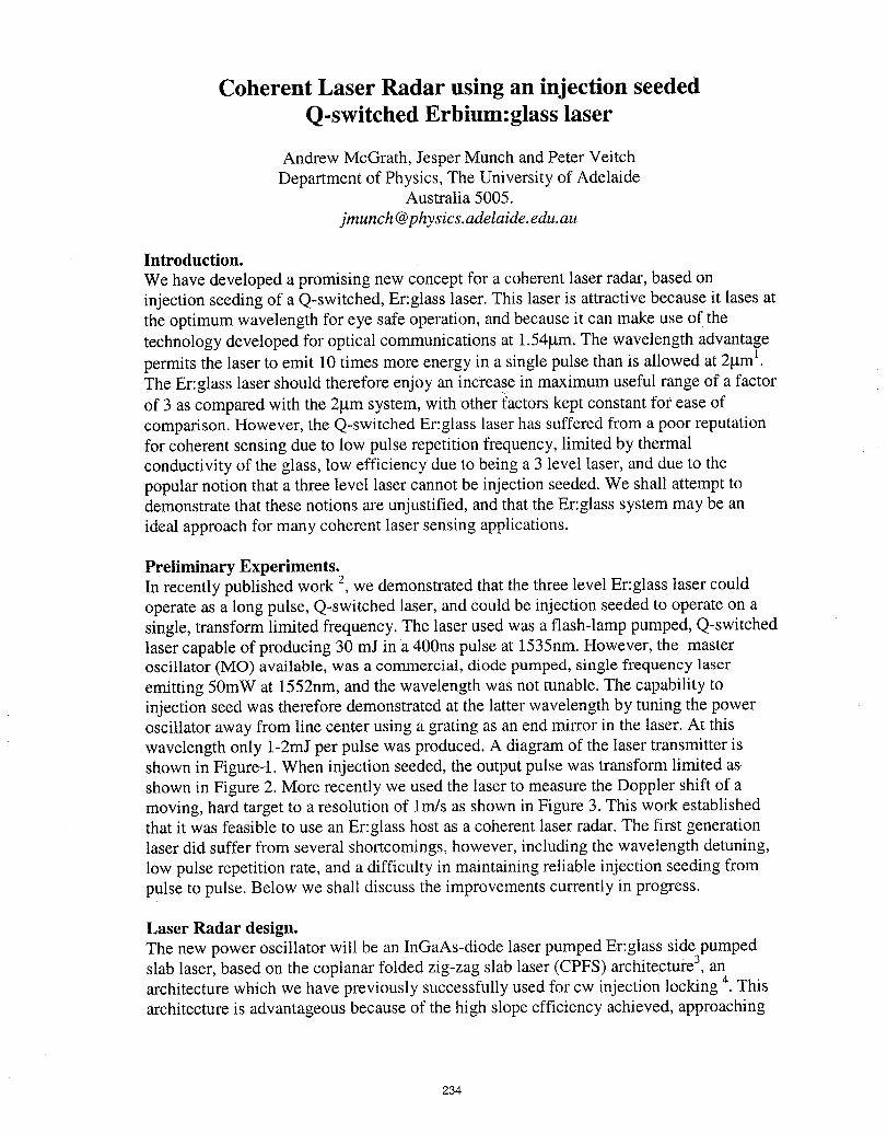
Coherent Laser Radar using an injection seededQ-switched Erbium:glass laser

Andrew McGrath, Jesper Munch and Peter VeitchDepartment of Physics, The University of Adelaide

Australia 5005.

jmunch @physics.adelaide,edu.au

Introduction.We have developed a promising new concept for a coherent laser radar, based oninjection seeding of a Q-switched, Er:glass laser. This laser is attractive because it lases atthe optimum wavelength for eye safe operation, and because it can make use of thetechnology developed for optical communications at 1.541am.The wavelength advantagepermits the laser to emit 10 times more energy in a single pulse than is allowed at 21_m_.The Er:glass laser should therefore enjoy an increase in maximum useful range of a factorof 3 as compared with the 2l_msystem, with other i_actorskept constant for ease ofcomparison. However, the Q-switched Er:glass laser has suffered from a poor reputationfor coherent sensing due to low pulse repetition frequency, limited by thermalconductivity of the glass, low efficiency due to being a 3 level laser, and due to thepopular notion that a three level laser cannot be injection seeded. We shall attempt todemonstrate that these notions are unjustified, and that the Er:glass system may be anideal approach for many coherent laser sensing applications.

Preliminary Experiments.In recently published work a, we demonstrated that the three level Er:glass laser couldoperate as a long pulse, Q-switched laser, and could be injection seeded to operate on asingle, transform limited frequency. The laser used was a flash-lamp pumped, Q-switchedlaser capable of producing 30 mJ in a 400ns pulse at 1535nm. However, the masteroscillator (MO) available, was a commercial, diode pumped, single frequency laseremitting 50mW at 1552nm, and the wavelength was not tunable. The capability toinjection seed was therefore demonstrated at the latter wavelength by tuning the poweroscillator away from line center using a grating as an end mirror in the laser. At thiswavelength only 1-2mJ per pulse was produced. A diagram of the laser transmitter isshown in Figure--1.When injection seeded, the output pulse was transform limited asshown in Figure 2. More recently we used the laser to measure the Doppler shift of amoving, hard target to a resolution of lrn/s as shown in Figure 3. This work establishedthat it was feasible to use an Er:glass host as a coherent laser radar. The first generationlaser did suffer from several shortcomings, however, including the wavelength detuning,low pulse repetition rate, and a difficulty in maintaining reliable injection seeding frompulse to pulse. Below we shall discuss the improvements currently in progress.

Laser Radar design.The new power oscillator will be an InGaAs-diode laser pumped Er:glass side pumped

• • 3 nslab laser, based on the coplanar folded zlg-zag slab laser (CPFS) architecture, aarchitecture which we have previously successfully used for cw injection locking 4.Thisarchitecture is advantageous because of the high slope efficiency achieved, approaching

234

.thatof end pumped architectures, its lack of need of optical coatings, and its ability to bescaled to high powers. Furthermore, the architecture is naturally suited for compact ringlaser geometries, ideal for injection seeding. Although a three level laser will have a highpump threshold (approximately 300mJ), the total energy deposited in the glass usingdiode laser pumping will be at least a factor of 30 lower than that of flash lamp pumping,thus permitting a corresponding increase in the PRF, while keeping the glass at acomparable average temperature. We estimate that a 30mJ laser with 500ns pulses will beable to operate close to 100Hz, and will in practice be limited by the maximum averagepower from available pulsed diode pump lasers rather than the Er:glass host. This laserwill be locked to a single frequency Er doped fiber laser.

We have already addressed and solved a major technical obstacle of reliable injectionseeding of long pulse, comparatively low gain, Q-switched oscillators. Although injectionseeding is a well-known technique, which is even available on commercial lasers, it isusually applied to short pulse, high gain lasers, initiating well above threshold. In thiscase injection seeding is very easy, because the seed is strongly amplified, and thefrequency matching criteria for the MO into the power oscillator is relaxed. For longpulse, coherent laser radar applications, a large number of round trips of the seed isrequired to produce an injection seeded output pulse, and the frequency matchingrequirements are much more stringent. We have developed and demonstrated anew. andimproved servo system specifically developed for this application 5. Our system uses thebuild-up time technique as the discriminant for frequency matching, but in contrast toexisting servos, our system utilises a discrete stepping type feedback that is much morerobust for Q-switched lasers with a narrow injection seeding range. The system has beendemonstrated on a 20mJ per pulse, 50Hz PRF, Nd:YAG ring laser, and works with highefficiency, seeding every pulse, and resulting in guaranteed transform limited outputs asshown in Figure 4.

Conclusion.We have shown that Er:glass lasers can be used as coherent laser radar transmitters, andwe are currently building a reliable, second generation device, designed to operateefficiently near line center. The resulting laser is expected to deliver 30mJ per pulse atclose to 50Hz PRF with 500ns long,transform limited pulses.This work was supported in part by _ research grant from the Australian Defence Scienceand Technology Organisation.

235

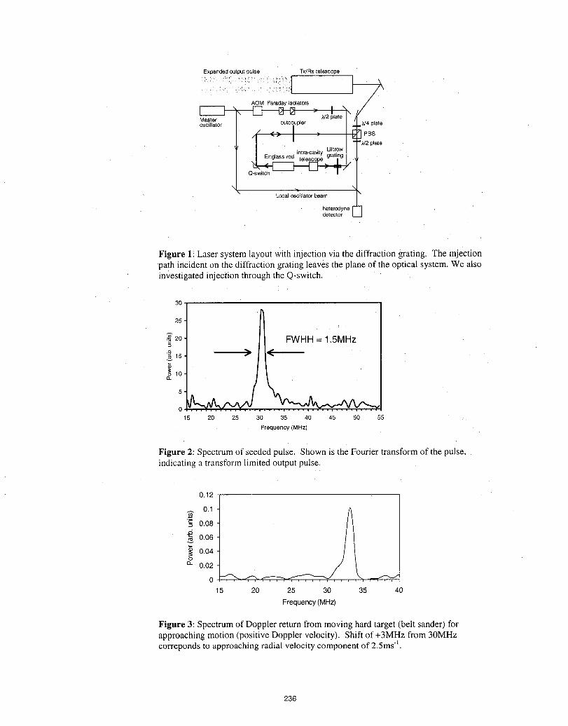
Expanded output oulse Tx/Rx telescope

AOM Faraday isolators J

.2i,ete""'/MosaSl_e_or outcoupler I / ,V4plate," .,. I _ Ir

" "" I " _7]PBs

I[o: __ intra-ca_ty !:t[Owl-'_/2DlateO-swi - !

Local oscillator beam

heterodyne -1detector

Figure 11Laser system layout with reJection via the diffraction grating. The rejectionpath incident on the diffraction grating leaves the plane of the optical system. We alsoinvestigated mjection through the Q-switch.

30

25

._=20 FWHH = 1.5MHz

_olo(3.

5

o ......15 20 25 30 35 40 45 50 55

Frequency (MHz)

Figure 2: Spectrum of seeded pulse. Shown is the Fourier transform of the pulse,indicating a transform limited output pulse.

0.12

0.1

=_0.080.06

_: 0.04o0_ 0.02

015 20 25 30 35 40

Frequency(MHz)

Figure 3: Spectrum of Doppler return from moving hard target (belt sander) forapproaching motion (positive Doppler velocity). Shift of +3MHz from 30MHzcorreponds to approaching radial velocity component of 2.5msl.

236

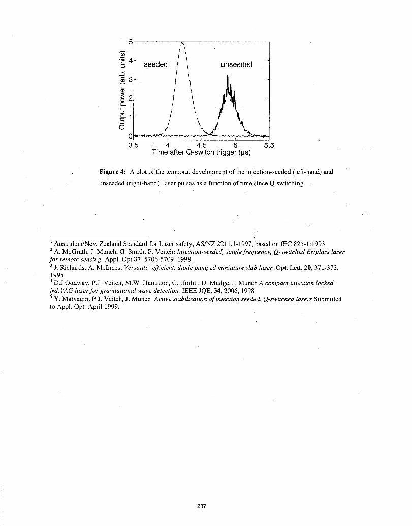
1 1 r

_-4-_ seeded unseeded.d_3

o

©03.5 4 4.5 5 5.5

Time after Q-switchtrigger(_s)

Figure 4: A plot of the temporal development of the injection-seeded (left-hand) and

unseeded (right-hand) laser pulses as a function of time since Q-switching.

l Australian/NewZealandStandardforLasersafety,AS/NZ2211.1-1997,based on IEC825-1:19932 A. McGrath, J. Munch, G. Smith, P. Veitch: Injection-seeded, single frequency, Q-switched Er:glass laserfor remote sensing, Appl. Opt 37, 5706-5709, 1998.3 j. Richards, A. McInnes, Versatile, efficient, diode pumped miniature slab laser. Opt. Lett. 20, 371-373,1995.

4 D.J Ottaway, P.J. Veitch, M.W .Hamilton, C. Hollitt, D. Mudge, J. Munch A compact injection lockedNd: YAG laser for gravitational wave detection. IEEE JQE, 34, 2006, 19985 y. Matyagin, P.J. Veitch, J. Munch Active stabilisation of injection seeded, Q-switched lasers Submittedto Appl. Opt. April 1999.

237

i

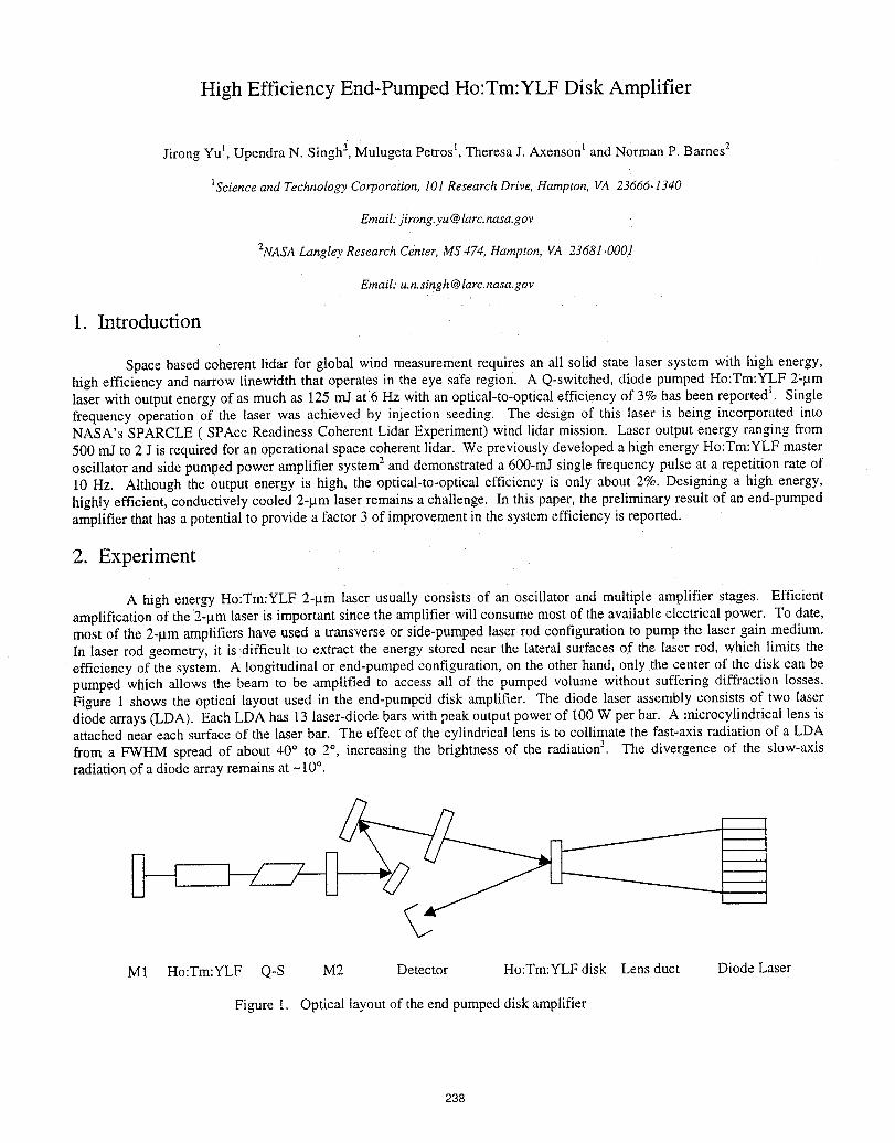
High Efficiency End-Pumped Ho:Tm:YLF Disk Amplifier

Jirong Yu l, Upendra N. Singh "2,Mulugeta Petros I, Theresa J. Axenson t and Norman P. Barnes 2

IScience and Technology Corporation, 10l Research Drive, Hampton, VA 23666-1340

Email: jirong,yu @larc.nasa.gov

2NASA Langley Research Center, MS 474, Hampton, VA 23681-000!

Email: u.n.singh@larc.nasa.gov

1. Introduction

Space based coherent lidar for global wind measurement requires an all solid state laser system with high energy,high efficiency and narrow linewidth that operates in the eye safe region. A Q-switched, diode pumped Ho:Tm:YLF 2-gmlaser with output energy of as much as 125 mJ at6 Hz with an optical-to-optical efficiency of 3% has been reported I. Singlefrequency operation of the laser was achieved by injection seeding. The design of this laser is being incorporated intoNASA's SPARCLE ( SPAce Readiness Coherent Lidar Experiment) wind lidar mission. Laser output energy ranging from500 rnJ to 2 J is required for an operational space coherent lidar. We previously developed a high energy Ho:Tm:YLF masteroscillator and side pumped power amplifier system _ and demonstrated a 600-mJ single frequency pulse at a repetition rate of10 Hz. Although the output energy is high, the optical-to-optical efficiency is only about 2%. Designing a high energy,highly efficient, conductively cooled 2-gm laser remains a challenge. In this paper, the preliminary result of an end-pumpedamplifier that has a potential to provide a factor 3 of improvement in the system efficiency is reported.

2. Experiment

A high energy Ho:Tm:YLF 2-gm laser usually consists of an oscillator and multiple amplifier stages. Efficientamplification of the 2-gm laser is important since the amplifier will consume most of the available electrical power. To date,most of the 2-gin amplifiers have used a transverse or side-pumped laser rod configuration to pump the laser gain medium.In laser rod geometry, it is difficult to extract the energy stored near the lateral surfaces of the laser rod, which limits theefficiency of the system. A longitudinal or end-pumped configuration, on the other hand, only the center of the disk can bepumped which allows the beam to be amplified to access all of the pumped volume without suffering diffraction losses.Figure I shows the optical layout used in the end-pumped disk amplifier. The diode laser assembly consists of two laserdiode arrays (LDA). Each LDA has 13 laser-diode bars with peak output power of I00 W per bar. A microcylindrical lens isattached near each surface of the laser bar. The effect of the cylindrical lens is to collimate the fast-axis radiation of a LDA

from a FWHM spread of about 40 ° to 2°, increasing the brightness of the radiation 3. The divergence of the slow-axisradiation of a diode array remains at -10 °.

M1 Ho:Tm:YLF Q-S M2 Detector Ho:Tm:YLF disk Lens duct Diode Laser

Figure I. Optical layout of the end pumped disk amplifier

238

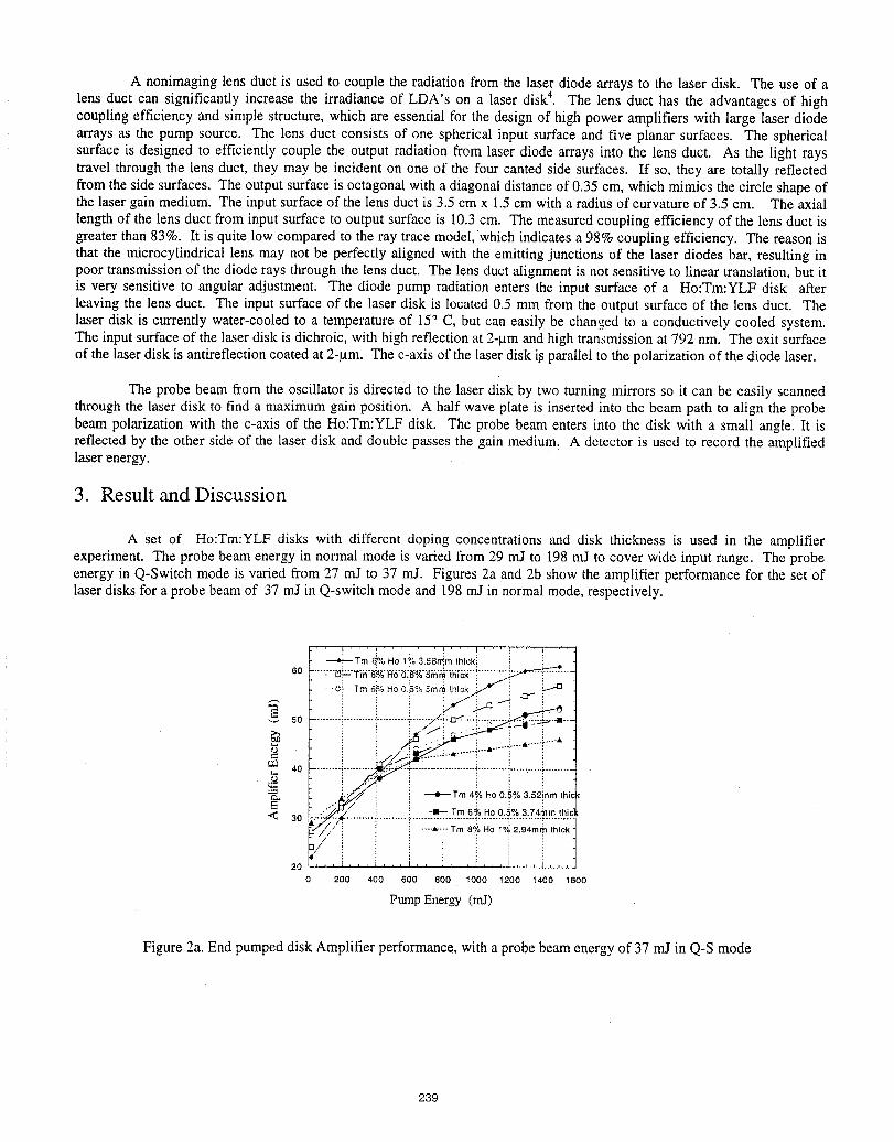
A nonimaging lens duct is used to couple the radiation from the laser diode arrays to the laser disk. The use of alens duct can significantly increase the irradiance of LDA's on a laser disk4. The lens duct has the advantages of highcoupling efficiency and simple structure, which are essential for the design of high power amplifiers with large laser diodearrays as the pump source. The lens duct consists of one spherical input surface and five planar surfaces. The sphericalsurface is designed to efficiently couple the output radiation from laser diode arrays into the lens duct. As the light raystravel through the lens duct, they may be incident on one of the four canted side surfaces. If so, they are totally reflectedfrom the side surfaces. The output surface is octagonal with a diagonal distance of 0.35 cm, which mimics the circle shape ofthe laser gain medium. The input surface of the lens duct is 3.5 cm x 1.5 cm with a radius of curvature of 3.5 cm. The axiallength of the lens duct from input surface to output surface is 10.3 cm. The measured coupling efficiency of the lens duct isgreater than 83%. It is quite low compared to the ray trace model, which indicates a 98% coupling efficiency. The reason isthat the microcylindrical lens may not be perfectly aligned with the emitting junctions of the laser diodes bar, resulting inpoor transmission of the diode rays through the lens duct. The lens duct alignment is not sensitive to linear translation, but itis very, sensitive to angular adjustment. The diode pump radiation enters the input surface of a Ho:Tm:YLF disk afterleaving the lens duct. The input surface of the laser disk is located 0.5 mm from the output surface of the lens duct. Thelaser disk is currently water-cooled to a temperature of 15° C, but can easily be changed to a conductively cooled system.The input surface of the laser disk is dichroic, with high reflection at 2-_tmand high transmission at 792 nm. The exit surfaceof the laser disk is antirefiection coated at 2-_tm. The c-axis of the laser disk i_parallel to the polarization of the diode laser.

The probe beam from the oscillator is directed to the laser disk by two turning mirrors so it can be easily scannedthrough the laser disk to find a maximum gain position. A half wave plate is inserted into the beam path to align the probebeam polarization with the c-axis of the Ho:Tm:YLF disk. The probe beam enters into the disk with a small angle. It isreflected by the other side of the laser disk and double passes the gain medium. A detector is used to record the amplifiedlaser •energy.

3. Result and Discussion

A set of Ho:Tm:YLF disks with different doping concentrations and disk thickness is used in the amplifierexperiment. The probe beam energy in normal mode is varied from 29 mJ to 198 mJ to cover wide input range. The probeenergy in Q-Switch mode is varied from 27 mJ to 37 mJ. Figures 2a and 2b show the amplifier performance for the set oflaser disks for a probe beam of 37 mJ in Q-switch mode and 198mJ in normal mode, respectively.

! ! ! ! ' i_Tn'l _',=,Ho 1% 3.58n'im thieki

• .-- ; ; : ; ,.,-"fl:oTm 6_,_,Ho 0._5%5mr_ thick_

_'_ 50 ' ' f:1/ ' " " '"" "................... :..........._'"'"'/_":....... !"";_'"", , ---::_-.-m---

; . • : : : • ..--_-'"•:: i i -t-,_3

7_. _J,')fz¢'.i_'" i i : "._ " :..'_// i ! -114- Tm 6_, Ho 0 _*/, 3 74ram thic

< 3o _Z;_ ........!..........._.........._.........._........."_......:? ........-1¢z///_ :: ..... •--,-Tm 8% Ho 1",_i2 94mrh h ck_

'/ i i ! i i i 12o i i i i,i =, i t

0 200 400 600 800 100012001400_Boo

PumpEnergy (mJ)

Figure2a. Endpumpeddisk Amplifierperformance,witha probebeamenergyof 37 mJ in Q-Smode

239

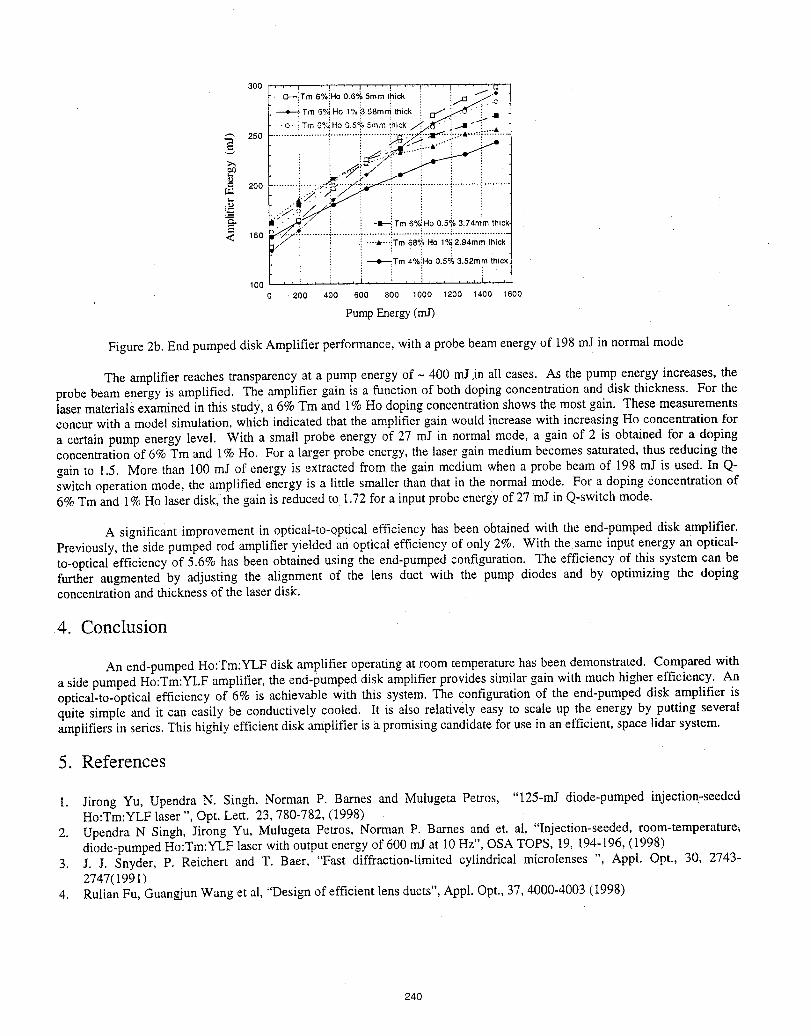
300 ', ' ' t " ' ' i ...... _ , ' ' I' ' ' i .... rl,

• _--'-iTrn 6%iHo 0.6°.)=5ram trick im .'_..J*

: i : i : f-'cr/_" .oTm 6% Ho 1%_3.58rnm thick i 11 ': . : . : .- :

.... - _rJ, o ,_Hov.5 ,,,o,'n _n_k ,.,-_..,_,., _ ............ ;....... " ..... .75_._.-_ i-,, _:..A2so i i _ ?_ ,....-i-........i2_-

!

: " "€" " : i i"

..........!-----::_-_----f-i........."..........i.........."...........i_.........= 200 __'_ ................

< i_0 15;......................:.--.:::_:,,,68_.oI;>_2.94m_t.i_k

_Tm 4%::"o 0.5_,_3.52m_ thick.

100 ' ' ' ' ...... !... i . , :,.. , i . ,, i. , ,0 200 400 600 800 1000 1200 1400 1600

PumpEnergy(mJ)

Figure 2b. End pumped disk Amplifier performance, with a probe beam energy of !98 mJ in normal mode

The amplifier reaches transparency at a pump energy of - 400 mJ jn all cases. As the pump energy increases, theprobe beam energy is amplified. The amplifier gain is a function of both doping concentration and disk thickness. For thelaser materials examined in this study, a 6% Tm and 1% Ho doping concentration shows the most gain. These measurementsconcur with a mode! simulation, which indicated that the amplifier gain would increase with increasing Ho concentration fora certain pump energy level. With a small probe energy of 27 mJ in normal mode, a gain of 2 is obtained for a dopingconcentration of 6% Tm and 1% Ho. For a larger probe energy, the laser gain medium becomes saturated, thus reducing thegain to 1.5. More than 100 mJ of energy is extracted from the gain medium when a probe beam of 198 mJ is used. In Q-switch operation mode, the amplified energy is a little smaller than that in the normal mode. For a doping concentration of6% Tm and 1% Ho laser disk, the gain is reduced to 1.72 for a input probe energy of 27 mJ in Q-switch mode.

A significant improvement in optical-to-optical efficiency has been obtained with the end-pumped disk amplifier.Previously, the side pumped rod amplifier yielded an optical efficiency of only 2%. With the same input energy an optical-to-optical efficiency of 5.6% has been obtained using the end-pumped configuration. The efficiency of this system can befurther augmented by adjusting the alignment of the lens duct with the pump diodes and by optimizing the dopingconcentration and thickness of the laser disk.

4. Conclusion

An end-pumped Ho:Tm:YLF disk amplifier operating at room temperature has been demonstrated. Compared witha side pumped Ho:Tm:YLF amplifier, the end-pumped disk amplifier provides similar gain with much higher efficiency. Anoptical-to-optical efficiency of 6% is achievable with this system. The configuration of the end-pumped disk amplifier isquite simple and it can easily be conductively cooled. It is also relatively easy to scale up the energy by putting severalamplifiers in series. This highly efficient disk amplifier is a promising candidate for use in an efficient, space lidar system.

5. References

I. Jirong Yu, Upendra N. Singh, Norman P. Barnes and Mulugeta Petros, "125-rnJ diode-pumped injection-seededHo:Tm:YLF laser ", Opt. Lett. 23,780-782, (1998)

2. Upendra N Singh, Jirong Yu, Mulugeta Petros, Norman P. Barnes and et. at, "Injection-seeded, room-temperature_diode-pumped Ho:Tm:YLF laser with output energy of 600 mJ at i0 Hz", OSA TOPS, 19, 194-196, (1998)

3. J. J. Snyder, P. Reichert and T. Baer, "Fast diffraction-limited cylindrical microlenses ", Appl. Opt., 30, 2743-2747(1991)

4. Rulian Fu, GuanNun Wang et al, "Design of efficient lens ducts", Appl. Opt., 37, 4000-4003 (1998)

240

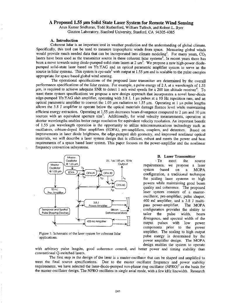
A Proposed 1.55 tim Solid State Laser System for Remote Wind SensingArun KumarSridharan,ToddRutherford,WilliamTulloch, andRobertL. Byer

GinztonLaboratory,StanfordUniversity,Stanford,CA 94305-4085

A. IntroductionCoherentlidar is an importanttool in weatherpredictionand the understandingof global climate.

Specifically, this tool can be used to measure troposphericwinds from space. Measuringglobal windswould provide much needed data that can be incorporatedinto climatemodeling1. For many years, CO2lasers have been used as the transmittersource in these coherent lidar systems2. In recent years there hasbeen a move towards usingdiode-pumpedsolid-state lasersat 2 um3. We propose a new high-powerdiode-pumped solid-state laser based on Yb:YAG and an optical parametric amplifier system to serve as thesource in lidar systems. This systemis eye-safe3with outputat 1.55 _tmandis scalable to the pulse energiesappropriateforspace based global windsensing.

The operational specifications of the proposed laser transmitterare determined by the overallperformancespecifications of the lidarsystem. For example,a pulse energyof 2 J, at a wavelengthof 1.55gm, is required to achieve adequateSNR to detect 1 m/s windspeeds for a 200 km altitude receiver4. Tomeet these system specifications we propose a new design approachthat incorporatesa novel laser-diodeedge-pumped Yb:YAG slab amplifier,operatingwith 3.8 J, 1 gs pulses at a 10 Hz repetitionrate, and anoptical parametric amplifier to convert the 1.03 gm radiationto 1.55 gin. Operatingat 1 _tspulse lengthsallows the 3.8 J amplifier to operatebelow the optical materialsdamagefluence level while maintainingefficient energyextraction. Operatingat 1.55 gm decreases beamdivergencecompared to 2 gm and 10 gmsources with an equivalent aperture size3. Additionally, for wind velocity measurements,operation atshorterwavelengths enables better range resolutionforequivalentvelocity resolution. An importantbenefitof 1.55 pm wavelength operation is the opportunity to utilize telecommunicationstechnology such asoscillators, erbium-doped fiber amplifiers (EDFA), pre-amplifiers, couplers, and detectors. Based onimprovements in laser diode brightness, the edge-pumpedslab geometry,and improved nonlinear opticalmaterials, we will describe a laser system design that is efficient, robust and meets the power and heatrequirementsof a space based laser system. This paper focuses on the power-amplifier and the nonlinearfrequencyconversionsubsystems.

,_ B. Laser Transmitter2J, 1ps,1.55 pro, 10 Hz , To meet the source

_l@],,55t.lm) Output requirements, we propose a laserXs xs system ,based on a MOPA

__'__ Txs configuration, a traditional technique

/_ i _.__.2 for scaling laser systems to highpowers while maintaining good beam

10mJ ) / quality and coherence. The proposedPre-AmpllflerJ laser system consists of a master-

oscillator, pre-amplifier, pulse shaper,\ e-_ 3.8J "l<---_ 400 mJ amplifier, and a 3.8 J multi-,/_,,. Power-Amplifier ,_'-----'-_J__ pass power-amplifier. The MOPA

CTemporalandSpatlal'_ ] Silicon._____" configuration provides the ability to

_.,Pulse Shaping Devtces_ _ Deformable Mirror tailor the pulse width, beam

N_ " >[4 ___.___- divergence, and spectral width of the130mJAmplifier output pulses with low powercomponents prior to the power

Figure1:Schematicof the iasersystemfor coherentlidar amplifier. The scaling to high outputapplications, pulse energy is determined by the

power amplifier design. The MOPAdesign enables the system to operate

with arbitrary pulse lengths, good coherence control, and better power and timing stability thanconventional Q-switched lasers.

The first step in the design of the laser is a master-oscillator that can be shaped and amplified tomeet the final source specifications. Due to the master oscillator frequency and power stabilityrequirements, we have selected the laser-diode-pumped non-planar ring oscillator (NPRO)5as the basis forthe master-oscillator design. The NPRO oscillates in single axial mode, with a few kHz linewidth. Research

241

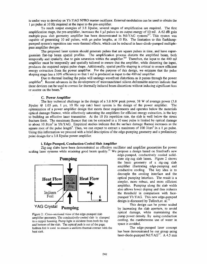
is under way to develop an Yb:YAG NPRO master oscillator. External modulation can be used to obtain the1 laspulse at 10 Hz required at the input to the pre-amplifier.

To reach output energies of 3.8 J/pulse, several stages of amplification are required. The firstamplification stage, the pre-amplifier, increases the 1_J pulses to an output energy of I0 mJ. A 62 dB gainmultiple-pass slab geometry amplifier has been demonstrated in Nd:YAG systems6'7.This system wascapable of generating 10 mJ pulses, with jas pulse lengths, at 10 Hz. The limitation to this flashlamp-pumped system's repetition rate were thermal effects, which can be reduced in laser-diode-pumped multiple-pass amplifier designs.

The proposed laser system should generate pulses that are square pulses in time, and have super-gaussian flat-top beam spatial profiles. The amplification process distorts the amplified beam, bothtemporally and Spatially, due to gain saturation within the amplifier.8'9 Therefore, the input to the 400 mJamplifier must be temporally and spatially tailored to ensure that the amplifier, while distorting the input,produces the required output pulse shape. Additionally, spatial profile shaping is critical to ensure efficientenergy extraction from the power amplifier. For the purpose of this design, we estimate that the pulseshaping stage has a 10% efficiency so that 1 mJ is produced as input to the 400 mJ amplifier.

Due to thermal loading the pulse will undergo wavefront distortions as it passes through the poweramplifier8. Recent advances in the development of micromachined silicon deformable mirrors indicate thatthese devices can be used to correct for thermally induced beam distortions without inducing significant lossor scatter on the beam.I°

C. Power AmplifierThe key technical chaUenge in the design of a 3.8 MW peak power, 38 W of average power (3.8

J/pulse @ I:03 lam, 1 las, 10 Hz rep rate) laser system is the design of the power amplifier. Theoptimization of a power amplifier design that meets these requirements and operates below the materialsoptical damage fluence, while effectively saturating the amplifiers for efficient energy extraction, is the keyto building an effective laser transmitter. At the 10 Hz repetition rate, the slab is well below the stressfracture limit. The maximum fluence that can be extracted in a 10 nsec pulse is limited by optical damageto about 10 J/cmz in Yb:YAG. Empirical studies indicate that the surface damage fluence increases as thesquare root of the pulse length9. Thus, we can expect to extract a maximum of 100 J/cm2in a 1 _ts pulse.Using this information we proceed with a brief description of the edge-pumping geometry and a preliminarypoint design fora 3.8 J/pulse power amplifier.

i. Edge-Pumped, Conduction-Cooled Slab AmplifierZig-zag slabs have been demonstrated as effective oscillator and amplifier geometries for power

scaling laser systems while retaining good beam quality.tI We propose a design based on Stanford's newedge-pumped, eonductively cooled solid-

Pumping state zig-zag slab lasers. Figure 2 showsthe basic geometry of a zig-zag slab

I amplifier illustrating edge-pumping andconductive cooling. The key idea is todecouple the cooling interface and the

Heat Flow Heat Flow optica! pumping interface. The result is a_.d _ simpler, more robust, and more efficient"_ y amplifier. Pumping along the slab width

also allows lower doping and thus reducesW_ the threShold in comparison with face-

Foil _ pumped Yb:YAG. This new edge-pumpeddesign is discussed by Tulloch,et. al. 12This design can be power scaled

YAG Crystal Pumping by increasing the slab aperture, to avoid

Figure2 : Cross-sectionalviewof theedge-pumpedslab optical damage, while maintaining theamplifiergeometry.The conductively-cooledslab is clamped pump power density. By using conductionina copperhousing.Pumplightis incidentfromboth thetop cooling, the cumbersome use of water inandbottomof the slab. The opticalpathis outof the page. space is avoided.Indiumfoil is used toensurea uniformthermalcontactwiththe The edge-pumped laser conceptheatsink. has been demonstrated by our group using

laser-diode-pumped Nd:YAG 13. A 4.5 mm

242

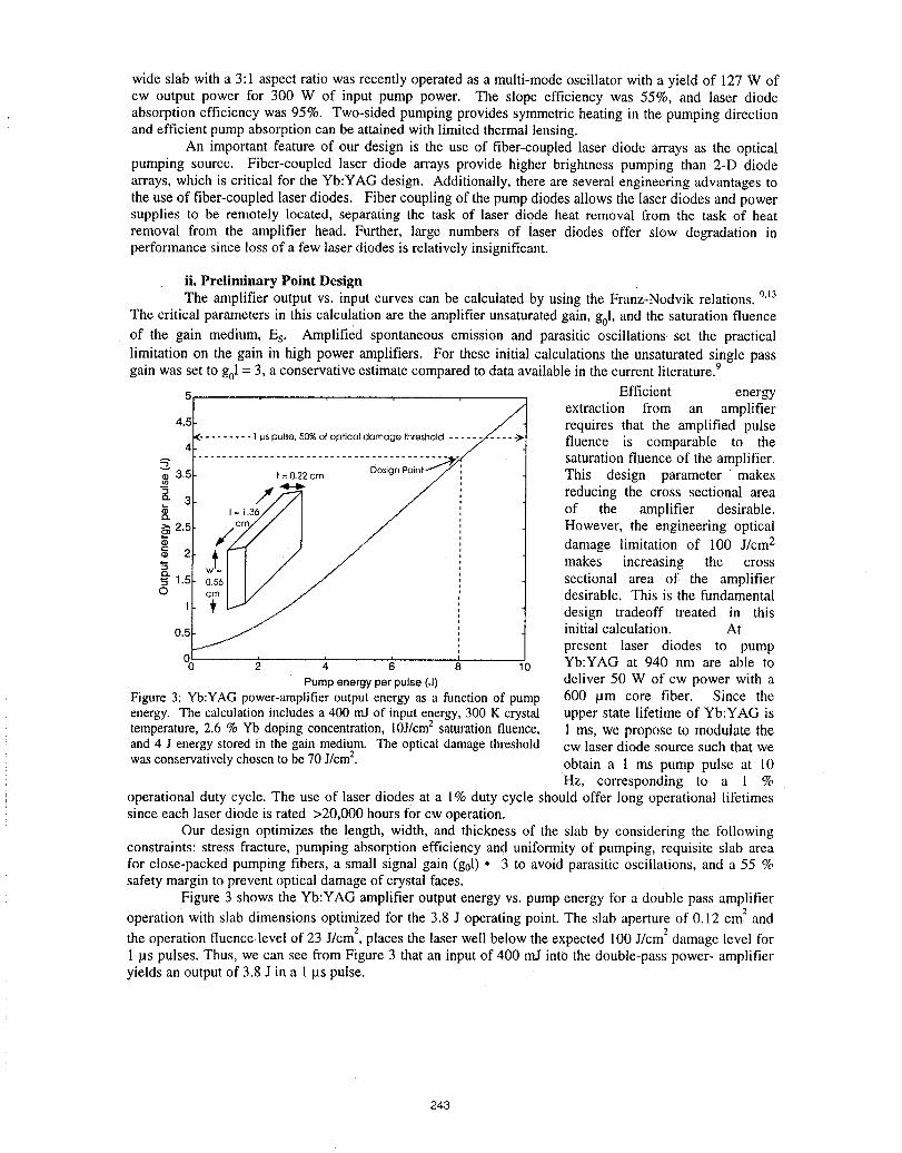
wide slab with a 3:1 aspect ratio was recently operated as a multi-mode oscillator with a yield of 127 W ofcw output power for 300 W of input pump power. The slope efficiency was 55%, and laser diodeabsorption efficiency was 95%. Two-sided pumping provides symmetric heating in the pumping directionand efficient pump absorption can be attained with limited thermal lensing.

An important feature of our design is the use of fiber-coupled laser diode arrays as the opticalpumping source. Fiber-coupled laser diode arrays provide higher brightness pumping than 2-D diodearrays, which is critical for the Yb:YAG design. Additionally, there are several engineering advantages tothe use of fiber-coupled laser diodes. Fiber coupling of the pump diodes allows the laser diodes and powersupplies to be remotely located, separating the task of laser diode heat removal from the task of heatremoval from the amplifier head. Further, large numbers of laser diodes offer slow degradation inperformance since loss of a few laser diodes is relatively insignificant.

ii. Preliminary Point DesignThe amplifier output vs. input curves can be calculated by using the Franz-Nodvik relations. 9.13

The critical parameters in this calculation are the amplifier unsaturated gain, go1, and the saturation fluenceof the gain medium, Es. Amplified spontaneous emission and parasitic oscillations set the practicallimitation on the gain in high power amplifiers. For these initial calculations the unsaturated single passgain was set to goI = 3, a conservative estimate compared to data available in the current literature.9

5 Efficient energy

_ extraction from an amplifier4.5 requires that the amplified pulse

4 (" ........ 1 ps pulse. 50% of opticQI damoge threshold , fluence is comparable to the

8 3.5 ............. i_2cm ........ t_:_gnP°_nt_S'_-J ThisSaturati°ndesignflUenCeparameterof the amplifier.makes

_ ¢__ _ reducing the cross sectional area

3 of the amplifier desirable.2.5 However, the engineering optical

$ damage limitation of I00 J/cm2

makes increasing the cross"5 1.5 sectional area of the amplifier0 desirable. This is the fundamental

1 design tradeoff treated in this0.5 initial calculation. At

present laser diodes to pump°o _ _ _ 8 10 Yb:YAG at 940 nm are able to

Pumpenergyperpulse(d) deliver 50 W of cw power with aFigure 3: Yb:YAG power-amplifier output energy as a function of pump 600 _m core fiber. Since theenergy. The calculationincludesa 400 mJ of input energy,300 K crystal upper state lifetime of Yb:YAG istemperature,2.6 % Yb dopingconcentration,10J/cm2 saturationfluence, 1 ms, we propose to modulate theand 4 J energystored in the gain medium. The opticaldamagethreshold cw laser diode source such that we

wasconservativelychosentobe 70J/cm2. obtain a I ms pump pulse at l0Hz, corresponding to a 1 %

operational duty cycle. The use of laser diodes at a 1% duty cycle should offer long operational lifetimessince each laser diode is rated >20,000 hours for cw operation.

Our design optimizes the length, width, and thickness of the slab by considering the followingconstraints: stress fracture, pumping absorption efficiency and uniformity of pumping, requisite slab areafor close-packed pumping fibers, a small signal gain (g01)° 3 to avoid parasitic oscillations, and a 55 %safety margin to prevent optical damage of crystal faces.

Figure 3 shows the Yb:YAG amplifier output energy vs. pump energy for a double pass amplifier

operation with slab dimensions optimized tbr the 3.8 J operating point. The slab aperture of 0.12 cm? and

the operation fluence level of 23 J/cm2,places the laser well below the expected 100 J/cm2damage level for1 Its pulses. Thus, we can see from Figure 3 that an input of 400 mJ into the double-pass power- amplifieryields an output of 3.8 J in a 1 _aspulse.

243

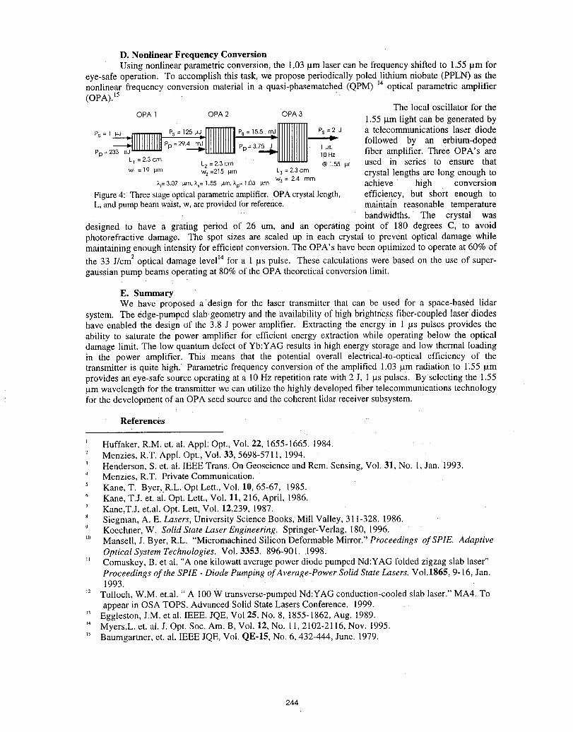
D. Nonlinear Frequency ConversionUsing nonlinear parametric conversion, the 1.03/am laser can be frequency shifted to 1.55 lam for

eye-safe operation. To accomplish this task, we propose periodically poled lithium niobate (PPLN) as thenonlinear frequency conversion material in a quasi-phasematched(QPM) 14optical parametricamplifier(OPA).15

The local oscillator for theOPA '1 OPA 2 OPA 3

1.55 gm light can be generated by

Ps = ] _ Ps : 125 Ps =2 J a telecommunicationslaser diodefollowed by an erbium-d0Ped--- 11111111[111

Pp= 1us. fiber amplifier. Three OPA's arePp = 233 #,J_ lOHz

EI=2.3cm L2=2.3cm @].S5,r used in series to ensure thatw]= 19_tm w2=215tam L3= 2.3cm crystal lengths are long enough to

Xi=3.07 !am._,s=1.55 }.tm,Lp=1.03 p.m wa = 2.4 mm achieve high conversionFigure4: Threestageopticalparametricamplifier.OPA crystallength, efficiency, but short enough toL, and pumpbeam waist,w, are providedfor reference, maintMn reasonable temperature

bandwidths. The crystal wasdesigned to have a grating period of 26 um, and an operating point of 180 degrees C, to avoidphotorefractive damage. The spot sizes are scaled up in each crystal to prevent optical damage whilemaintaining enough intensity for efficient conversion. The OPA's have been optimized to operate at 60% of

the 33 J/cm2optical damage levelt4 for a 1 /as pulse. These calculations were based on the use of super-gaussian pump beams operating at 80% of the OPA theoretical conversion limit.

E. SununaryWe have proposed a design for the laser transmitter that can be used for a space-based lidar

system. The edge-pumped slab geometry and the availabilityof high brightness fiber-coupled laser diodeshave enabled the design of the 3.8 J power amplifier. Extracting the energy in 1 /as pulses provides theability to saturate the power amplifier for efficient energy extraction while operating below the opticaldamage limit. The low quantumdefect of Yb:YAG results in high energy storage and low thermalloadingin the power amplifier. This means that the potential overall electrical-to-optical efficiency of thetransmitteris quite high. Parametricfrequency conversion of the amplified 1.03 pm radiationto 1155pmprovides an eye-safe source operatingat a 10 Hz repetition rate with 2 J, 1 _s pulses. By selecting the 1.55/am wavelength for the transmitterwe can utilizethe highly developed fiber telecommunicationstechnologyfor the development of an OPA seed sourceand thecoherent lidarreceiver subsystem.

References ,

J Huffaker, R.M. et. al. Appl: Opt., Vol. 22, 1655-1665. 1984.2 Menzies, R.T. Appi. Opt:, Vol. 33, 5698-5711, 1994.3 Henderson,S. et. al. IEEE Trans.On Geoscience andRein. Sensing, Vol. 31, No. I, Jan. 1993.4 Menzies, R.T. Private Communication.5 Kane, T. Byer,.R.L. Opt Lett.,Vol. 10, 65-67, 1985.

Kane, T.J. et. al. Opt: Lett., Vol. 11, 216, April, 1986:7 Kane,T.J. et.al. Opt. Lett, Vol. 12,239, 1987." Siegman, A. E. Lasers, University Science Books, Mill Valley, 311-328. 1986.'_ Koechner, W. Solid State Laser Engineering. Springer-Verlag. 180, 1996."_ Mansell, J. Byer, R.L. "Micromachined Silicon DeformableMirror."Proceedings of SPIE. Adaptive

OpticaISystem Technologies. Vol. 3353. 896-901. ,1998." Comaskey, B. et al. "A one kilowattaverage power diode pumpedNd:YAG folded zigzag slab laser"

Proceedings of the SPIE - Diode Pumping ofAverage-Power Solid State Lasers. Vo1.1865,9-16, Jan.1993.

_2 Tulloch, W.M. et.al. " A I00 W transverse-pumpedNd:YAGconduction-cooledslab laser." MA4. Toappear in OSA TOPS. AdvancedSolid State Lasers Conference. 1999.

,3 Eggleston, J.M. et al. IEEE. JQE,Vol 25, No. 8, 1855-1862, Aug. 1989.,4 Myers,L. et. al. J. Opt. Soc. Am. B, Vol. 12, No. 1I, 2102-2116, Nov. 1995._s Baumgartner,et. al. [EEE JQE, Vol. QE-15, No. 6, 432-444, June. 1979.

244

SYSTEM ADVANCES

Presider: Alain Dabas

245

Abstract Submission for the

Tenth Biennial Coherent Laser Radar Technology and Applications Conference

28 June to 2 July, 1999

Optical.PhasedArraysfor ElectronicBeamControl

By

TerryA Dorschner

RaytheonSystemsCompanySensorsand ElectronicsSystemsSegment

AdvancedOpticsandReconnaissanceSystemsCenter

131SpringStreetLexington,MA02421

Terry_A_Dorschner@RES.Raytheon.com

The state of the art of optical phased arrays (OPA's) will be reviewed and prospectiveapplications discussed, highlighting laser radar and other active sensors. Current OPAperformance levels will be summarized and the near-term performance potentialforecasted. Comparisons with conventional and emerging new technologies for beamcontrol will be made.

246

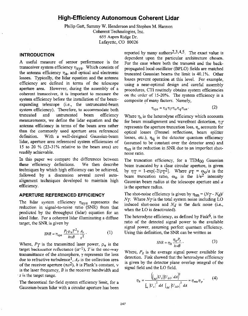
High-EfficiencyAutonomousCoherentLidarPhilip Gatt, Sammy W. Henderson and Stephen M. Harmon

Coherent Technologies, Inc.655 Aspen Ridge Dr.Lafayette, CO 80026

INTRODUCTION reported by many authors2,3,4,5. The exact value isdependent upon the particular architecture chosen.

A useful measure of sensor performance is the For the case where both the transmit and the back-transceiver system efficiency qsys. Which consists of propagated local oscillator (BPLO) fields are matchedthe antenna efficiency Tla,and optical and electronic truncated Gaussian beams the limit is 40.1%. Otherlosses. Typically, the lidar equation and the antenna losses prevent operation at this level. For example,efficiency are defined in terms of the telescope using a near-optimal design andcareful assemblyaperture area. However, during the assembly of a procedures, CTI routinely obtains system efficienciescoherent transceiver, it is important to measure the on the order of 15-20%. The system efficiency is asystem efficiency before the installation of the beam- composite of many factors. Namely,expanding telescope (i.e., the untruncated-beamsystem efficiency). Therefore, to accommodate both rlsy s = rlhqTq°qq rlsn" (2)

truncated and untruncated beam efficiency Where _his the heterodyne efficiency which accountsmeasurements, we define the lidar equation and the for beam misalignment and wavefront distortion, qTantenna efficiency in terms of the beam area rather represents the aperture truncation loss, qo accounts forthan the commonly used aperture area referenced optical losses (Fresnel reflections, beam splitterdefinition. With a well-designed Gaussian-beam losses, etc.), qq is the detector quantum efficiencylidar, aperture area referenced system efficiencies of (assumed to be constant over the detector area) and15 to 20 % (23-31% relative to the beam area) are qsn is the reduction in SN-Rdue to an imperfect shot-readily achievable, noise ratio.

In this paper we compare the differences between The truncation efficiency, for a TEM00 Gaussianthese efficiency definitions. We then describe beam truncated by a clear circular aperture, is giventechniques by which high efficiency can be achieved, by qT = 1-exp[-2/pT2]• Where 9T = O3o/ais thefollowed by a discussion several novel auto- beam truncation ratio, coo is the 1/e2 intensityalignment techniques developed to maintain high Gaussian beam radius at the telescope aperture and aefficiency, is the aperture radius.

APERTURE REFERENCED EFFICIENCY The shot-noise efficiency is given by rlsn = (NT- Nd)/N T. Where N T is the total system noise including LO

The lidar system efficiency rlsys represents the induced shot-noise and Nd is the dark noise (i.e.,reduction in signal-to-noise ratio (SNR) from that when the LO is deactivated).predicted by the throughput (lidar) equation for anideal lidar. For a coherent lidar illuminating a diffuse The heterodyne efficiency, as defined by Fink6, is thetarget, the SNR is given by ratio of the detected signal power to the available

signal power, assuming perfect quantum efficiency.PTp_tT2YAr (1) Using this definition, the SNR can be written as

SNR = rlsys hub z 2rlqPs (3)

Where, PT is the transmitted laser power, PTtis the SNR = rlh h----_target backscatter reflectance (sr-1), T is the one-waytransmittance of the atmosphere, ,{ represents the loss Where, Ps is the average signal power available for

detection. Fink showed that the heterodyne efficiencydue to refractive turbulence 1,Ar is the collection area is given by the detector plane overlap integral of theof the receiver aperture (Tta2),h is Plank's constant, vis the laser frequency, B is the receiver bandwidth and signal field and the LO field.

"z is the target range. OAdIU,IIULoidA . (4)

The theoretical far-field system efficiency limit, for a rlh= 12 [2 '----qmix?lPGaussian-beam lidar with a circular aperture has been !_o]Us da IAdIULo dA

247

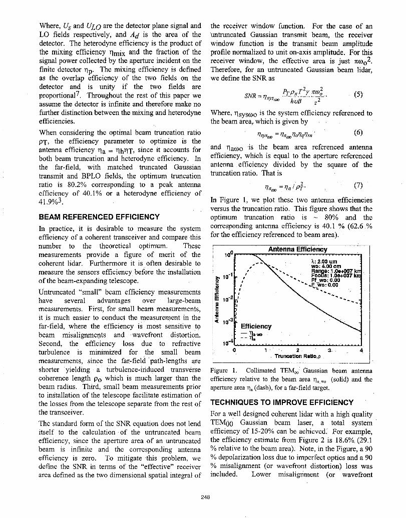
Where, Us and ULO are the detector plane signal and the receiver window function. For the case of anLO fields respectively, and Ad is the area of the untruncated Gaussian transmit beam, the receiverdetector. The heterodyne efficiency is the product of window function is the transmit beam amplitudethe mixing efficiency qmix and the fraction of the profile normalized to unit on-axis amplitude. For thissignal power collected by the aperture incident on the receiver window, the effective area is just nCOo2.finite detector rlp. The mixing efficiency is defined Therefore, for an untruncated Gaussian beam lidar,as the overlap efficiency of the two fields on the we define the SNR as

detector and is unity if the two fields are PTpxT27¢rc°2 (5)proportional 7. Throughout the rest of this paper we SNR= rlsyscoo hoB z 2assume the detector is infinite and therefore make no

further distinction between the mixing and heterodyne Where, rlsys0_ois the system efficiency referenced toefficiencies, the beam area, which is given by

When considering the optimal beam truncation ratio qsysa_o = rlacoorlorlqqsn '. (6)PT, the efficiency parameter to optimize is theantenna efficiency rla = TlhrlT, since it accounts for and rlao)o is the beam area referenced antennaboth beam truncation and heterodyne efficiency. In efficiency, which is equal to the aperture referencedthe far-field, with matched truncated Gaussian antenna efficiency divided by the square of thetransmit and BPLO fields, the optimum truncation truncation ratio. That is

ratio is 80.2% corresponding to a peak antenna rla_o=rla/P]" (7)efficiency of 40.1% or a heterodyne efficiency of41.9%3. In Figure 1, we plot these two antenna efficiencies

versus the truncation ratio. This figure shows that theBEAM REFERENCED EFFICIENCY optimum truncation ratio is - 80% and the

In practice, it is desirable to measure the system corresponding antenna efficiency is 40.1% (62.6 %efficiency of a coherent transceiver and compare this for the efficiency referenced to beam area).

number to the theoretical optimum. These AntennaEfficiency........ = ......... i ......... = .........

measurements provide a figure of merit of the 1°° _-_." ;_:2.00umcoherent lidar. Furthermore it is often desirable to .'- -'_1. wo:4.00orn

measure the sensors efficiency before the installation lo.1 ., \',, _Rango:1.Oe,007k.• . " "_ " ,, " rocus: 1.0eo,.OO7kll:

of the beam-expanding telescope. _ ,' "N. "-_ _t wo:o.oo

_. " ,,F,.-wo:0.00

Untruncated "small" beam efficiency measurements , -_~.10-_ r . _,,

have several advantages over large-beam _ ; _. -~..measurements. First, for small beam measurements,it is much easier to conduct the measurement in the < lo._far-field, where the efficiency is most sensitive to Efficiency

beam misalignments and wavefront distortion. _.*_,Second, the efficiency loss due to refractive lo4 .......................................turbulence is minimized for the small beam 0 1 2 3 4.

I Truncation Ratlo,pmeasurements, since the far-field path-lengths areshorter yielding a turbulence-induced transverse Figure 1. Collimated TEM0o Gaussian beam antenna

coherence length Po which is much larger than the efficiencyrelative to the beam area rl.... (solid)and thebeam radius. Third, small beam measurements prior apertureareaq, (dash),fora far-fieldtarget.to installation of the telescope facilitate estimation ofthe losses from the telescope separate from the rest of TECHNIQUES TO IMPROVE EFFICIENCY

the transceiver. For a well designed coherent lidar with a high qualityThe standard form of the SNR equation does not lend TEM00 Gaussian beam laser, a total systemitself to the calculation of the untruncated beam efficiency of 15-20% can be achieved: For example,efficiency, since the aperture area of an untruncated the efficiency estimate from Figure 2 is 18.6% (29.1beam is infinite and the corresponding antenna % relative to the beam area). Note, in the Figure, a 90efficiency is zero. To mitigate -this problem, we % depolarization loss due to imperfect optics and a 90define the SNR in terms of the "effective" receiver % misalignment (or wavefront distortion) loss wasarea defined as the two dimensional spatial integral of included. Lower misalignment (or wavefront

248

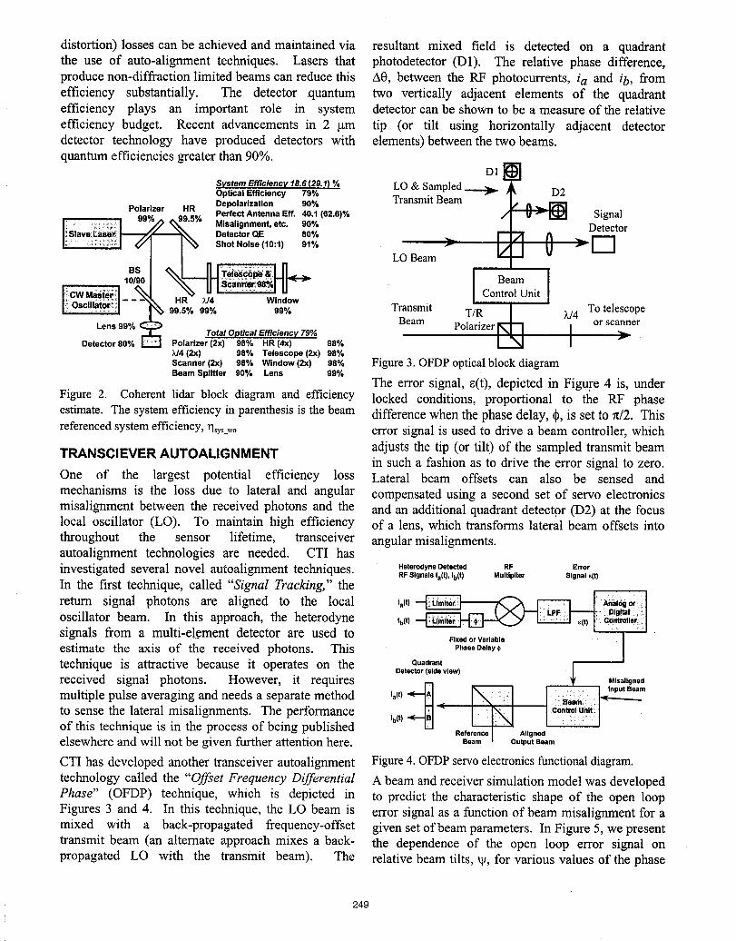
distortion) losses can be achieved and maintained via resultant mixed field is detected on a quadrantthe use of auto-alignment techniques. Lasers that photodetector (D1). The relative phase difference,produce non-diffraction limited beams can reduce this A0, between the RF photocurrents, ia and ib, fromefficiency substantially. The detector quantum two vertically adjacent elements of the quadrantefficiency plays an important role in system detector can be shown to be a measure of the relativeefficiency budget. Recent advancements in 2 _tm tip (or tilt using horizontally adjacent detectordetector technology have produced detectors with elements) between the two beams.quantum efficiencies greater than 90%.

System Efficiency 18.6(29.1) % L* & SampledOptical Efficiency 79% _ D2

Polarizer HR Depolarization 90% TransmitBeamPerfect Antenna Eft. 40.1 (62.6)% / SignalMisalignment, etc. 90% Detector

Detector QE 80% E_I 0 0Shot Noise (10:t) 91% _ _-

LO Beam

t0/90 Beam

]:cw Mas_a_'] Z/4 Window Control Unit[:;OsclllatOrli ! 99.5% 99°/o 99% Transmit To telescope

T/R ] M4

Beam Polarizer N ] or scannerLens 99"/, Total Optical Efficiency 79% ",,.-

Detector 80% Polarizer (2x) 98% HR (4x) 98% rM4 (2x) 98% Telescope (2x) 90%Scanner (2x) 980 Window (2x) 980 Figure 3. OFDP optical block diagramBeam Splitter 90% Lens 990

The error signal, _(t), depicted in Figure 4 is, underFigure 2. Coherent lidar block diagram and efficiency locked conditions, proportional to the RF phaseestimate. The systemefficiencyin parenthesisis the beam difference when the phase delay, dp,is set to n/2. Thisreferencedsystemefficiency,q,yswo error signal is used to drive a beam controller, which

TRANSCIEVER AUTOALIGNMENT adjusts the tip (or tilt) of the sampled transmit beamin such a fashion as to drive the error signal to zero.

One of the largest potential efficiency loss Lateral beam offsets can also be sensed andmechanisms is the loss due to lateral and angular compensated using a second set of servo electronicsmisalignment between the received photons and the and an additional quadrant detector (D2) at the focuslocal oscillator (LO). To maintain high efficiency of a lens, which transforms lateral beam offsets intothroughout the sensor lifetime, transceiver angular misalignments.autoalignment technologies are needed. CTI hasinvestigated several novel autoalignment techniques. HeterodyneDetected RF ErrorRF Signals ia(t), Ib(t) Multiplier Signal s(t)

In the first technique, called "Signal Tracking," thereturn signal photons are aligned to the local ia(t)_

r'--i _ /X%._ LPF : I'--"_;:

oscillator beam. In this approach, the heterodyne ib(t) _ _(t) I €ontrollerIsignals from a multi-element detector are used to ,Fixed or Variable I

estimate the axis of the received photons. This Pha.Oo,a_,, Itechnique is attractive because it operates on the Quadrant lDetector(sideview)

received signal photons. However, it requires _ M,sa,,gn_multiple pulse averaging and needs a separate method ,.(t) _ _ ] _np__.Beam

to sense the lateral misalignments. The performance _ < [ _l ico°,,**../of this technique is in the process of being published ,,,(t) _:Reference I Aligned

elsewhere and will not be given further attention here. sea.,' outputSoam

CTI has developed another transceiver autoalignment Figure4. OFDPservoelectronicsfunctionaldiagram.

technology called the "Offset Frequency Differential A beam and receiver simulation model was developedPhase" (OFDP) technique, which is depicted in to predict the characteristic shape of the open loopFigures 3 and 4. In this technique, the L* beam is error signal as a function of beam misalignment for amixed with a back-propagated frequency-offset given set of beam parameters. In Figure 5, we presenttransmit beam (an alternate approach mixes a back- the dependence of the open loop error signal onpropagated L* with the transmit beam). The relative beam tilts, _, for various values of the phase

249

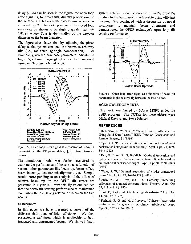
delay qb. As can be seen in the figure, the open loop system efficiency on the order of 15-20% (23-31%error signal is, for small tilts, directly proportional to relative to the beam area) is achievable using efficientthe relative tilt between the two beams when dOis designs. We concluded with a discussion of noveladjusted to n/2. The locking range of the closed loop techniques to maintain beam alignment andservo can be shown to be slightly greater than +/- demonstrated the OFDP technique's open loop tiltL/Deft, where Deft is the smaller of the detector sensing performance.diameter or the beam diameter.

DetDIsm'Tan(TIIt)/kThe figure also shows that by adjusting the phase .3 -2 -1 1 a 3delay q_,the system can lock the beams to arbitrary 3 npc,,_ ...... : ............tilts (i.e., for fixed-lag-angle compensation). For 2- --o.0, A! ...... o.no ._ -.',,

_ -- t.00

example, given the base-case parameters indicated in _ 1- "-' t_

Figure 5, al mrad lag-angle offset can be maintained _ a___ ..... •::-............ _.=_using an RF phase delay of_ 7t/4. _ i _",..-"I

g

-1 !- '_V

DetDlam*Tan(TIIt)/_ tu :::-3 o2 -1 0 1 2 3 -2 '

........ '

31 ' ........._1. -- 4.00Pit8 .., -6 -4 -2 0 2 4. 6_/ .... '. 3.00PI/8 .._ TIlt (mrad)

I_ - - 2.GoPI_ ,.'!_ Relative Beam Tip Trade5" , _. .... t.®pl_ i_,.

"i_ .... o.®Pl,'o q' i.[ _ ].i:." Figure6. Openloop errorsignal asa functionof beam tilt

[-r "_:'.._.'_".._]:, ii ' parametricin the relativetip betweenthe two beams.

This work was funded by NASA MSFC under the..... . SBIR program. The COTRs for these efforts were

-6 4 -2 0 2 4. 6 Michael Kavaya and Steve Johnson.Tilt (mrad)

RelativeSignalDelayTrade REFERENCES

Lembda:2.0Oum TotalPowen1._ _ Henderson; S. W. et. al, "CoherentLaser Radar at 2 gmBeernDt'm(.2wo):t0.00 mm I.tRatlo: 1.00

SeomOffseU(swo):o.oo ,._Imlm!Frlnoe:t6 Using Solid-StateLasers;"IEEETrans on GeoscienceandOetDInm:1.0mm SempsiCyct': t6noto_ontnt'm: o.o0 s_, Rolnot-y:.x Remote Sensing, 31 (1993) ,Tip: 0.00mind

2 Rye, B. J. "Primary aberration contribution to incoherent

Figure5. Open loop error signalas a functionof beam tilt backscatterheterodynelidar returns,"Appk Opt. 21, 839-parametric in the RF phase delay, qb,for two Gaussian 844(1982)beams. 3 Rye, B. J. and R. G. Frehlich, "Optimal truncation andThe simulation model was further exercised to opticalefficiencyof an aperturedcoherentlidarfocusedonestimate the performance_of the servo as a function of an incoherentbackscattertarget,"Appl.Opt.31,2891-2899various other parameters like beam tip, beam offset, (1992)4

beam intensity, detector misalignment, etc. Sample Wang, J. W, "Optimal truncationof a lidar transmittedresults corresponding to an analysis of the effect of beam,"Appl.Opt.27,4470-4474(1988)relative beam tip on the OFDP tilt sensor are 5 Zhao, Y., M: J. Post, and R. M. Hardesty, "Receivingpresented in Figure 6. From this figure one can see efficiencyof a pulsedcoherentlidars: Theory,"Appl. Optthat the servo tilt sensing performance is maintained 29,4111-4119(1990).even when there is strong relative tip between the two 6Fink,D,"CoherentDetectionSignal-to-Noise,"App.Opt.beams. 14,689,690(1975) :

7 Frehlich,R. G. and M. J. Kavaya, "Coherent laser radarSUMMARY : performance for general atmospheric turbulence." Appl.

In this paper we have presented a survey of the Opt. 30, 5.325-5334(1991).different definitions.of lidar efficiency. We thenpresented a definition which is applicable to bothtruncated and untruncated beams. We showed that a

250

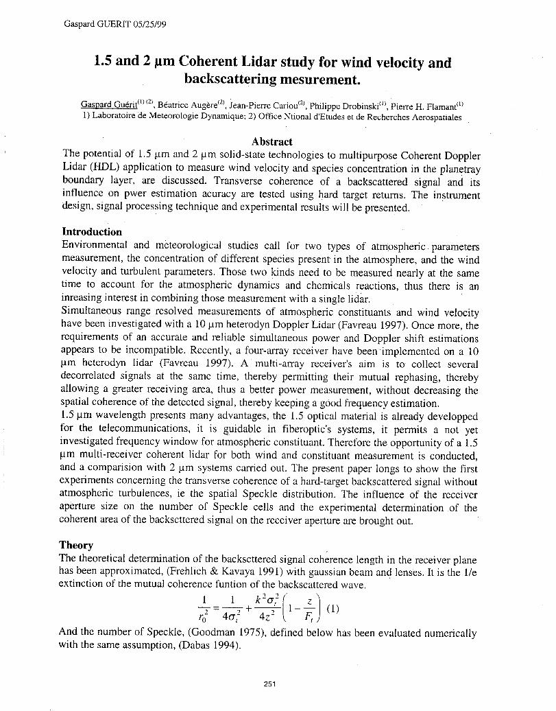
Gaspard GUERIT 05/25/99

1.5 and 2 om Coherent Lidar study for wind velocity andbackscattering mesurement.

Gaspard Gurrit (° _2_,B_atrice Aug_re _2),Jean-Pierre Cariou _2),Philippe Drobinski m, Pierre H. Flaman(')

1) Laboratoire de Meteorologie Dynamique; 2) Office Ntional d'Etudes et de Recherches Aerospatiales

Abstract

The potential of 1.5 lam and 2 btm solid-state technologies to multipurpose Coherent DopplerLidar (HDL) application to measure wind velocity and species concentration in the planetrayboundary layer, are discussed. Transverse coherence of a backscattered signal and itsinfluence on pwer estimation acuracy are tested using hard target returns. The instrumentdesign, signal processing technique and experimental results will be presented.

Introduction

Environmental and meteorological studies call for two types of atmospheric parametersmeasurement, the concentration of different species present in the atmosphere, and the windvelocity and turbulent parameters. Those two kinds need to be measured nearly at the sametime to account for the atmospheric dynamics and chemicals reactions, thus there is an

inreasing interest in combining those measurement with a single lidar.Simultaneous range resolved measurements of atmospheric constituants and wind velocityhave been investigated with a 10 btm heterodyn Doppler Lidar (Favreau 1997). Once more, therequirements of an accurate and reliable simultaneous power and Doppler shift estimationsappears to be incompatible. Recently , a four-array receiver have been implemented on a 10pm heterodyn lidar (Favreau 1997). A multi-array receiver's aim is to collect several

decorrelated signals at the same time, thereby permitting their mutual rephasing, therebyallowing a greater receiving area, thus a better power measurement, without decreasing thespatial coherence of the detected signal, thereby keeping a good frequency estimation.1.5 t,tm wavelength presents many advantages, the 1.5 optical material is already developpedfor the telecommunications, it is guidable in fiberoptic's systems, it permits a not yetinvestigated frequency window for atmospheric constituant. Therefore the opportunity of a 1.5I-tin multi-receiver coherent lidar for both wind and constituant measurement is conducted,and a comparision with 2 pm systems carried out. The present paper longs to show the firstexperiments concerning the transverse coherence of a hard-target backscattered signal withoutatmospheric turbulences, ie the spatial Speckle distribution. The influence of the receiveraperture size on the number of Speckle cells and the experimental determination of thecoherent area of the backscttered signal on the receiver aperture are brought out.

TheoryThe theoretical determination of the backscttered signal coherence length in the receiver planehas been approximated, (Frehlich & Kavaya 1991) with gaussian beam and lenses. It is the 1/eextinction of the mutual coherence funtion of the backscattered wave.

1 1 k2Gt/ _t)

, - , + 1- (1)r0" 40",- 4--_,

And the number of Speckle, (Goodman 1975), defined below has been evaluated numericallywith the same assumption, (Dabas 1994).

251

Gaspard GUERIT 05/25/99

(so )2• Mr(r,r)dR 2 ,

• M - = 1+O'te¢ (2)

lid 2 Mr (r_,r2) 2drtdr2 44Whith r0, the transverse coherence lengthin the receiver plane, ¢Yt,the ,1/e extinction of thegaussian beam after the emission telescope, Gtel,the 1/e extinction for the gaussian model ofthe emssion telescope, D the receiver aperture size which is taken infinite for the gaussianassumption, and Mr, the mutual coherence function of the backscattered signal in the receiverplane.The number of speckle cells in the receiver aperture can be evaluated invoIving the first andsecond statistical moments of the measured power of decorrelated signals, ie the mean andvariance of a great number of power measurement, (Goodman 1975).

M=aes )

Moreover, the probability density function for a set of power estimations of an integratedSpeckle pattern can be approximated by a gamma density function,

M<"exp - M (4)'M M

P(P') r(M)The determination of M allows a definition of a coherence area Acof the.backscattered signal

in the receiver apperture, (Dabas 1996), which can be approximated as followingAr

M -_1- (5), with At, the receiving apperture area.Ac

Experimental set upThe aims of the experiments carried out so far, are to observe the influence of the

receiving aperture size on a hard target backscattered signal 1.5 lam signal transversecoherence and to provide experimentally its coherance area for a given emission apperture.Furthermore a similar series of experiments with a 2 lam cw lidar is to be conducted, forcomparisxon.

DescriptionStatistical evluations call for a great number of decorrelated signal power measurements. Thatis to say that a great number of decorrelated backscattered signals need to be obtained insimilar experimental condition. A hard diffusing target is used, but its stationnarity leadsalways to the same Speckle pattern in the receiver, no statlstcal evaluation are possible thruesuch set of power values, the need of decorrelation is satisfied moving the diffusers.The condition that each measure is independant is obtained with the insurance that eachmeasure is provided by a signal backscattered by different diffusers than others, so theilluminated part of the target must be different for every iteration. It is satisfied with a rotatinghard target, considering its rotation velocity, and the dimension and place of the laser spot onthe target. The time between each measure ensure that every target backscattering spot takesplace on a different part of the target.

MaterialThe laser used is a 600 mW cw Er/Yt laser, made with two polarized Er/Yt doped fiberoptics,this laser provides two fiberoptic exit, one signal, and one local oscillator both polarised. The

252

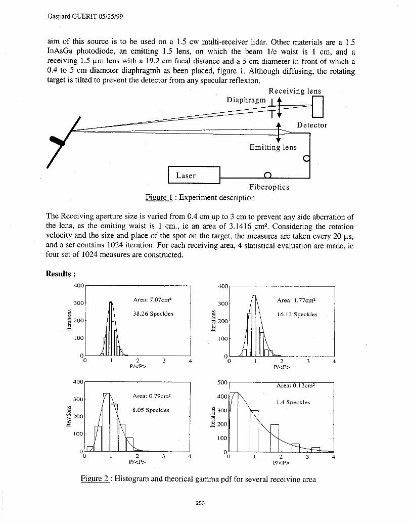
Gaspard GUERIT 05/25/99

aim of this source is to be used on a 1.5 cw multi-receiver lidar. Other materials are a 1.5

InAsGa photodiode, an emitting 1.5 lens, on which the beam 1/e waist is 1 cm, and areceiving 1.5 lam lens with a 19.2 cm focal distance and a 5 cm diameter in front of which a

0.4 to 5 cm diameterdiaphragmhas been placed, figure 1. Although diffusing,the rotatingtarget is tilted to prevent the detector from any specular reflexion.

Receiving lens

_ [Laser Emi_ng'_I DetectorFiberoptics

Figure 1 : Experiment description

The Receiving aperture size is varied from 0.4 cm up to 3 cm to prevent any side aberration ofthe lens, as the emiting waist is 1 cm., ie an area of 3.1416 cm 2. Considering the rotationvelocity and the size and place of the spot on the target, the measures are taken every 20 ItS,and a set contains 1024 iteration. For each receiving area, 4 statistical evaluation are made, iefour set of 1024 measures are constructed.

Results :

400 400

Area: 7.07cm _ Area: 1.77cm z

300 _ 300

38.26 Speckles _ 16.13 Speckles

200 _ 200

100 100

o o0 1 2 3 4 0 1 2 3 4

P/<P> P/<P>

400 500 Ai'ea: 0.13cin 2

400;

_ 300._ [ peckles200

_ 200

I00 100

o o0 1 2 3 4 0 1 2 3 4

P/<P> P/<P>

Figure 2 ' Histogram and theorical gamma pdf for several receiving area

253

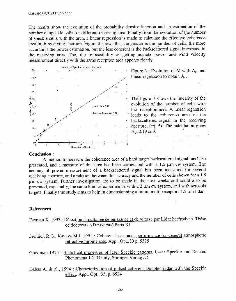
Gaspard GUERIT 05/25/99

The results show the evolution of the probability density function and an estimation of thenumber of speckle cells for different receiving area. Finally from the evolution Ofthe numberof speckle cells with the area, a linear regression is made to calculate the effective coherencearea in th receiving aperture. Figure 2 shows that the greater is the number of cells, the moreaccurate is the power estimation, but the less coherent is the backscattered Signal integrated inthe receiving area. The, the impossibility of getting acurate power and wind velocitymeasurement directly with the same reception area appears clearly.

Number of Speckles vs reception area

so/ , I Figure 3 • Evolution of M with Ar, and45 linear regression to obtain Ao.

40

35

30 Thelfigure 3 shows the linearity of the_ evolution of the number of cells with25

_ the reception area. A linear regressiong 20z leads' to the coherence area of the

15 ! backscattered signal in the receiving:_ aperture, (eq.5). The calculation gives10

At-0.19 cmz.

0 1 2 3 4 5 6 7 8Recepuon area, cm2 ,

Conclusion :A method to measurethe coherence area of a hard target backscattered signal has been

presented, and a measure of this area has been carried out with a 1.5 lam cw system. Theacuracy of power measurement of a backscattered signal has been measured for severalreceiving aperture,and a relationbetween this acuracyandthe numberof cells shown for a 1.5_tm cw system. Further investigation are to be made in the next weeks and could also bepresented, espacially, the same kind of experiments with a 2 btmcw system,and with aerosolstargets.Finallythis study aims to help in dimensionninga future multi-receptors 1.5 _m lidar.

References

Favreau X. 1997 :D6tection simultan6e de puissance et de vitesse parLidar h6t6rodyne.Th_sede doctorat de l'universit6 Paris X1

Frehlich R.G., Kavaya M.J. 1991 • Coherent laser radar performance for general atmosphericrefractive turbulences. Appl. Opt.,30 p. 5325

Goodman 1975 • Statistical properties of laser Speckle patterns, Laser Speckle and RelatedPhenomena J.C. Dainty, Springer-Verlag ed.

Dabas A. & al., 1994 • Characterization of pulsed coherent Doppler Lidar with the Speckleeffect, Appl. Opt., 33, p. 6524

254

CW LIDARS

Presider: Michael Vaughan

255

Bistatic Coherent Laser Radar Performance: CW SNR Calculations

Eric P. MAGEE*, Timothy J. KANE

Department of Electrical Engineering *Author's Current Affiliation121 Electrical Engineering East Department of Electrical and Computer Engineering

The Pennsylvania State University Air Force Institute of TechnologyUniversity Park, PA 16802 2950 P Street,Wright-Patterson AFB OH 45433-7765

Phone: (814) 863-1470, FAX: (814) 863-8457 Phone: (937) 255-6565, FAX: (937) 656-4055tjk7@psu.edu Eric.Magee@afit.af.mil

_TRODUCTION

Wind velocity can be obtained using a laser radar (LIDAR) system by measuring the Doppler shiftedbackscatter from aerosols and particulates in the atmosphere. Doppler lidar systems for wind velocity measurementscan be classified into two categories: coherent detection and incoherent detection. Under each category there arenovel approaches to measuring the return signal frequency. Regardless of the measurement process, the ultimategoal for both types is to measure a frequency shift between the transmitted laser pulse and the return laser pulse.This frequency shift is proportional to some component of the wind velocity, depending on the system configuration.How accurately these systems can measure the frequency shift, and thus the velocity, is dependent upon the system'scharacteristics. Existing Doppler lidar systems employ monQstaticconfigurations which require scanning a volumeto obtain wind speed and direction [1, 2]. Range resoluti0n in these systems is normally obtained by us!ng a pulsedlaser system. This places a fundamental limit on the range-velocity resolution product [3, 4].

The purpose of this research is to investigate the feasibility of utilizing a multistatic configuration formeasuring 3-dimensional vector winds. In the multistatic configuration, horizontal and vertical resolution aredetermined by the telescope field-of-view, laser divergence, and baseline separation distance between the laser andthe telescope. This enables the use of a continuous-wave or long pulse laser transmitter (narrow spectral width) andeliminates the dependence between range and velocity resolution.

The results of this research have shown that a multistatic pulsed Doppler lidar system will provide accurateestimates of wind velocity within the tropospheric boundary layer (up to about 5 km) with high spatial resolution.Detailed signal-to-noise ratio (SNR) calculations indicate that small transmit and receive apertures actually improvesystem performance. Therefore, a compact transmitter and receiver design can be used. The spatial resolutionachievable with this system will be better than previous anemometers (propeller as well as laser Doppler), yieldingfine scale measurements of velocity fields.

ANALYSIS

The primary coordinate system used to locate the receiver, transmitter and target is a fixed reference systemcentered at the transmitter. The z-axis of this coordinate system is in the vertical direction and the x-axis is in theeast-west direction. The-fixed coordinate system is also used to define pointing directions of the transmit and receiveoptics. A north referenced coordinate system [5, 6] is used for all signal-to-noise ratio calculations. There will be aseparate north referenced coordinate system associated with each transmitter/receiver pair. Figure 1 shows thetypical geometry for a single transmitter/receiver pair.

For a multiple (N) receiver configuration, the Doppler shift can be written in matrix notation as

Af_ =lAvw, (1)

256

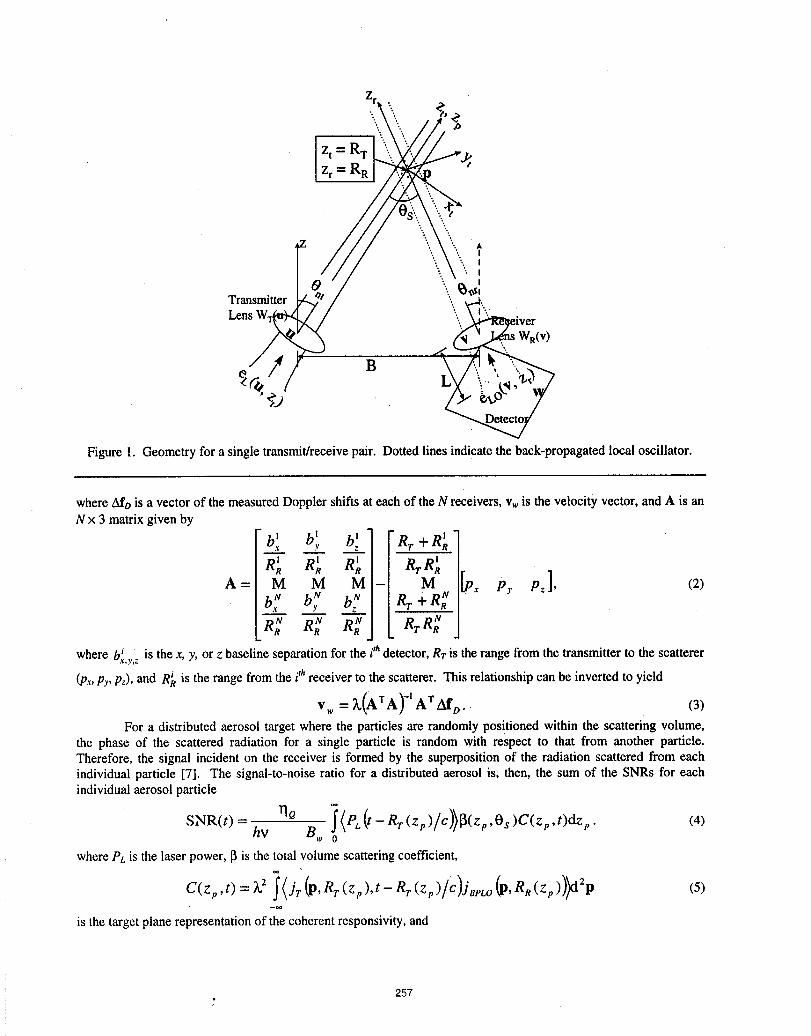
Figure 1. Geometry for a single transmit/receive pair. Dotted lines indicate the back-propagated local oscillator.

where Afo is a vector of the measured Doppler shifts at each of the N receivers, vwis the velocity vector, and A is anN x 3 matrix given by

b'., bl,,. b_ Rr + R_

R'.R'.R'. R R'.A = M M M - M Py Pz], (2)

b._ b,N. b _ Rr + R;

R; R; R; RR;where ibx _,,zis the x, y, or z baseline separation for the ithdetector, Rr is the range from the transmitter to the scatterer

(,Px,Py, Pz), and R_ is the range from the ithreceiver to the scatterer. This relationship can be inverted to yield

Vw = _,(ATAf' ATAfo. (3)For a distributed aerosol target where the particlesare randomlypositioned within the scattering volume,

the phase of the scattered radiation for a single particle is randomwith respect to that from another particle.Therefore, the signal incident on the receiver is formed by the superposition of the radiationscatteredfrom eachindividual particle [7]. The signal-to-noise ratio for a distributedaerosol is, then, the sum of the SNRs for eachindividual aerosol particle

oO

"rlQ I(PL (t- Rr(zp)/c))_J(zp,Os)C(zp,t)dzp. (4)SNR(t) = hv B_ 0

where PL is the laser power, [3is the total volume scattering coefficient,

C(z,.t) = £ 2 i (jr(p.Rr(zp).t- Rr(z_)/C)ja,w(p.RR(zp)))d2p (5)-co

is the target plane representation of the coherent responsivity, and

257

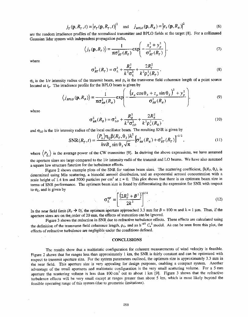
Jr (P, Rr, t) = er (p, Rr ,t) 2 and JBPLO(P,RR) = er (P,RR) 2 (6)are the random irradiance profiles of the normalized transmitter and BPLO fields at the target [8]. For a collimatedGaussian lidar system with independent propagation paths,

(jr(P, Rr)) - 21 exp/ x2r+y_ 1 (7)where

R 2 2Rrz2 ._. "'T . (8)

o?r(Rr)=O L k20_ 4 kZPo(Rr)2'_L is the 1/e intensity radius of the transmit beam, and Po is the transverse field coherence length of a point sourcelocated at zp. The irradiance profile for the BPLO beam is given by

(jBpLO(P, RR))= 1 I (xp cOsOs +zpsinOs)2 + y_ j/tG2s£(RR) exp OB.2(R R) , (9)

where

2 R_ 2R 2O2R(RR) =OLo + + (10)2 2 2 2 '

kPok Or.o (RR)and _LOis the 1/e intensity radius of the local oscillator beam. The resulting SNR is given by

SNR( Rr ,t) = (PL )qQ_( Rr 'Os ))_2 [6_R (R, ) + _]r (RT )]-'/2hvB wsin0s ff-_ , (11)

where (PL) is the average power of the CW transmitter [9]. In deriving the above expressions, we have assumed

the aperturesizes are large comparedto the l/e intensityradiiof thetransmitandLO beams. We have also assumeda square law structure functionfor the turbulenceeffects.

Figure 2 shows example plots of the SNR for various beam sizes. The scatteringcoefficient, _(Rr, Os), isdeterminedusing Mie scattering, a bimodal aerosol distribution,and an exponential aerosol concentrationwith ascale height of 1.4 kmand 5000 particles per cm 3 at z = 0. This plot shows that there is an optimumbeam size intermsof SNR performance. The optimumbeam size is foundby differentiatingthe expression for SNR with respectto gL, and is given by

oop' .._, F( 2R2 "1- B2)] 114L L 2k2 " (12)In the near field limit (Rr "-) 0), the optimum aperture approached 3.3 mm for B = 100 m and X= l gm. Thus, if theaperture sizes are on the_orderof 20 ram, the effects of truncation can be ignored.

Figure 3 shows the reduction in SNR due to refractive turbulence effects. These effects are calcuiated usingthe definition of the transverse field coherence length, Po, and an h'4/3C,z model. As can be seen from this plot, theeffects of refractive turbulence are negligible under the conditions defined.

CONCLUSIONS

The results show that a multistatic configuration for coherent measurements of wind velocity is feasible.Figure 2 shows that for ranges less than approximately ! kin, the SNR is fairly constant and can be optimized withrespect to transmit aperture size. For the system parameters outlined, the optimum size is approximately 3.3 mm inthe near field. This aperture size is very appealing for design purposes, enabling a compact system. Anotheradvantage of the small apertures and multistatic configuration is the very small scattering volume. For a 5 manaperture the scattering volume is less than 100cm3 oUt to about 1km [9]. Figure 3 shows that the refractiveturbulence effects will be very small except at ranges greater than about 5 kin, which is most likely beyond thefeasible operating range of this system (due to geometric limitations).

258

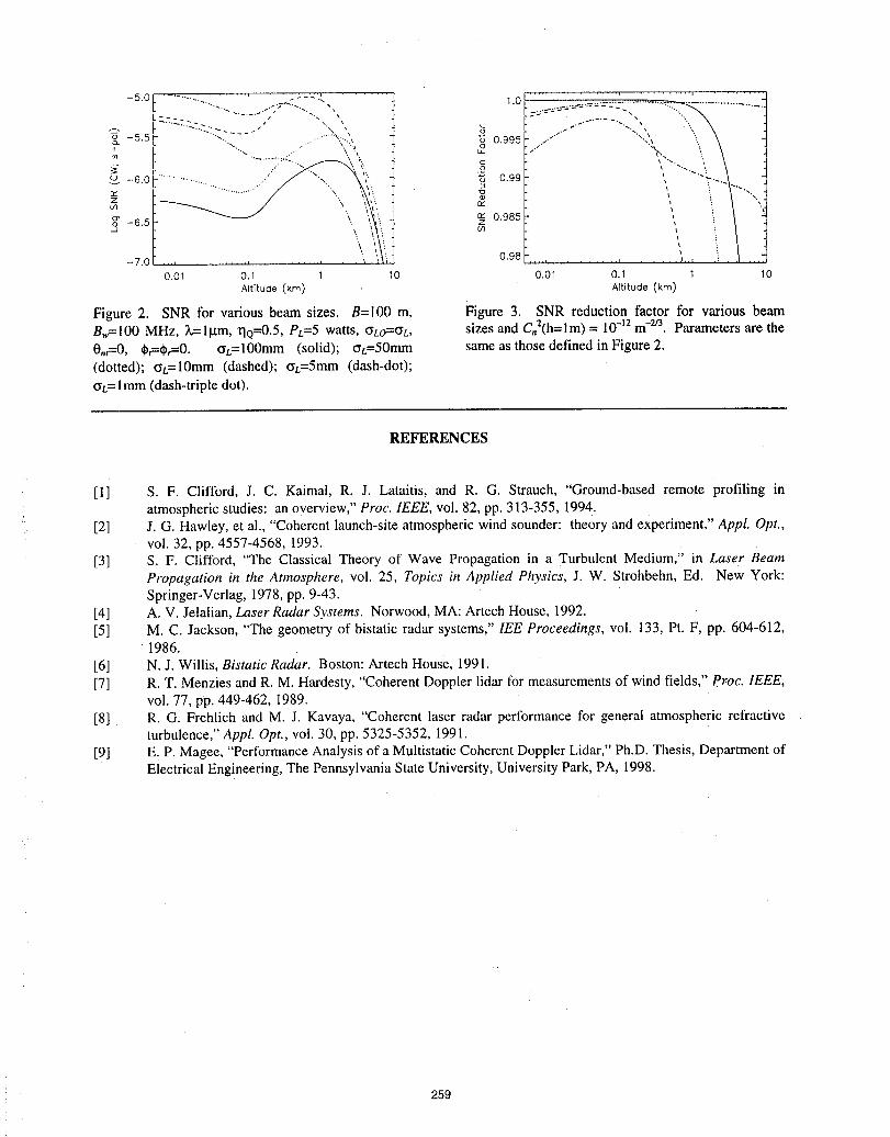
L "_---" i 1.0-5.o .........,.,.,.,..........,2; ...."".,.." \

......."" ' -1 "_ 0.995-5._ t- ....-.".... • "..., _'

',n '" ' i_... .-_" r .'"" g

.....a:::_ -6.0_ ...................................... ...' ' "_'_ 0.992: n,,O3

r.,- 0.985_' -6.5 z..J 03

-7.0 0.980.01 0.1 I 10 0.01 0.1 I 10

Altitude (kin) Altitude (kin)

Figure 2. SNR for various beam sizes, B=I00 m, Figure 3. SNR reduction factor for various beamBw=100 MHz, L-=lgm, r10=0.5, Pt.=5 watts, _LO=_b sizes and CnZ(h=lm)= 10-12m-2/3.Parameters are the0,r=0, _r=_,=0. _t=100mm (solid); _L=50mm same as those defined in Figure 2.(dotted); _L=10mm (dashed); _L=5mm (dash-dot);_t= Imm (dash-triple dot).

REFERENCES

[1] S.F. Clifford, J. C. Kaimal, R. J. Lataitis, and R. G. Strauch, "Ground-based remote profiling inatmospheric studies: an overview," Proc. IEEE, vol. 82, pp. 313-355, 1994.

[2] J.G. Hawley, et al., "Coherent launch-site atmospheric wind sounder: theory and experiment," Appl. Opt.,vol. 32, pp. 4557-4568, 1993.

[3] S.F. Clifford, "The Classical Theory of Wave Propagation in a Turbulent Medium,'; in Laser BeamPropagation in the Atmosphere, vol. 25, Topics in Applied Physics, J. W. Strohbehn, Ed. New York:

Springer-Verlag, 1978, pp. 9-43.[4] A.V. Jelalian, Laser Radar Systems. Norwood, MA: Artech House, 1992.[5] M.C. Jackson, "The geometry of bistatic radar systems," IEE Proceedings, vol. 133, Pt. F, pp. 604-612,

1986.

[6] N.J. Willis, Bistatic Radar. Boston: Artech House, 1991.[7] R.T. Menzies and R. M. Hardesty, "Coherent Doppler lidar for measurements of wind fields," Proc. IEEE,

vol. 77, pp. 44%462, 1989.[8] R.G. Frehlich and M. J. Kavaya, "Coherent laser radar performance for general atmospheric refractive

turbulence," Appl. Opt., vol. 30, pp. 5325-5352, 1991.[9] E.P. Magee, "Performance Analysis of a Multistatic Coherent Doppler Lidar," Ph.D. Thesis, Department of

Electrical Engineering, The Pennsylvania State University, University Park, PA, 1998.

259

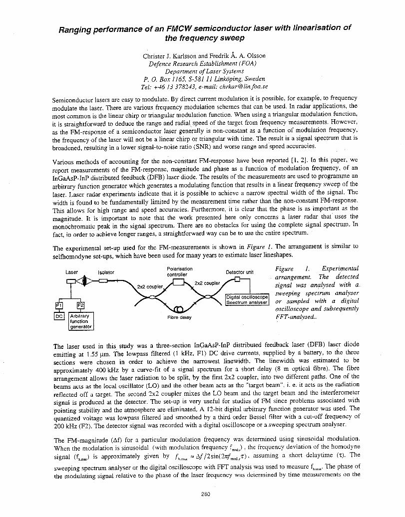
Ranging performance of an FMCW semiconductor laser with linearisation ofthe frequency sweep

Christer J. Karlsson and Fredrik A. A. Olsson

Defence Research Establishment (FOA)Department of Laser Systems

P. O. Box 1165, S-581 11 LinkOping,SwedenTel: +46 13 378243, e-mail: chrkar@lin.foa.se

Semiconductor lasers are easy tOmodulate. By direct current modulation it is possible, for example, to frequencymodulate the laser. There are various frequency modulation schemes that can be used. In radar applications, themost common is the linear chirp or triangular modulation function. When using a triangular modulation function,it is straightforward to deduce the range and radial speed of the target from frequency measurements. However,as the FM-response of a semiconductor laser generally is non-constant as a function of modulation frequency,the frequency of the laser will not be a linear chirp or triangular with time. The result is a signal spectrum that isbroadened, resulting in a lower signal-to-noise ratio (SNR) and worse range and speed accuracies.

Various methods of accounting for the non-constant FM-response have been reported [ 1, 2]. In this paper, we

report measurements of the FM-response, magnitude and phase as a function of modulation frequency, of anInGaAsP-InP distributed feedback (DFB) laser diode. The results of the measurements are used to pro_amme an

arbitrary function generator which generates a modulating function that results in a linear frequency sweep of thelaser. Laser radar experiments indicate that it is POssible to achieve a narrow spectral width of the signal. Thewidth is found to be fundamentally limited by the measurement time rather than the non-constant FM-response.This allows for high range and speed accuracies. Furthermore, it is clear that the phase is as important as themagnitude. It is important to note that the work presented here only concerns a laser radar that' uses themonochromatic peak in the signal spectrum. There are no obstacles for using the complete signal spectrum. Infact, in order to achieve longer ranges, a straightforward way can be to use the entire spectrum.

The experimental set-up used for the FM-measurements is shown in Figure I. The arrangement is similar toselfhomodyne set-ups, which have been used for many years to estimate laser lineshapes.

Polarisation Figure 1. ExperimentalLaser Isolator controller Detectorunit

er__X2 p_ arrangement. The detectedr- cou signal was analysed with a2 coupl 2x2 coupler

_ _ iDigitaloscilloscopeI sweeping spectrum analyser

I'_ [SoectrumanalyserI or sampled with a digitaloscilloscope and subsequently

_,rbitrary [ Fibre delay FFT-analvsed..unction {;]enerator ]

The laser used in this study was a three-section InGaAsP-InP distributed feedback laser (DFB) laser diodeemitting at 1.55 p.m. The lowpass filtered (1 kHz, FI) DC drive currents, supplied by a battery, to the threesections were chosen in order to achieve the narrowest linewidth. The linewidth was estimated to be

approximately 400 kHz by a curve-fit of a signal spectrum for a short delay (8 m optical fibre). The fibrearrangement allows the laser radiation to be split, by the first 2x2 coupler, into two different paths. One of thebeams acts as the local oscillator (LO) and the other beam acts as the "target beam", i. e. it acts as the radiationreflected off a target. The second 2x2 coupler mixes the LO beam and the target beam and the interferometersignal is produced at the detector. The set-up is very useful for studies of FM since problems associated withpointing stability and the atmosphere are eliminated. A 12-bit digital arbitrary function generator was used. Thequantized voltage was lowpass filtered and smoothed by a third order Besset filter with a cut-off frequency of200 kHz (F2). The detector signal was recorded with a digital oscilloscope or a sweeping spectrum analyser.

The FM-magnitude (Af) for a particular modulation frequency was determined using sinusoidal modulation.When the modulation is sinusoidal (with modulation frequency f,,,,j._),the frequency deviation of the homodyne

signal (f,_,,_) is approximately given by f_..... = Af/2sin(2zrfm,_.j: ) , assuming a short delaytime ('c). The

sweeping spectrum analyser or the digital oscilloscope with FFT analysis was used to measure f,...... The phase ofthe modulating signal relative to the phase of the laser frequency was determined by time measurements on the

260

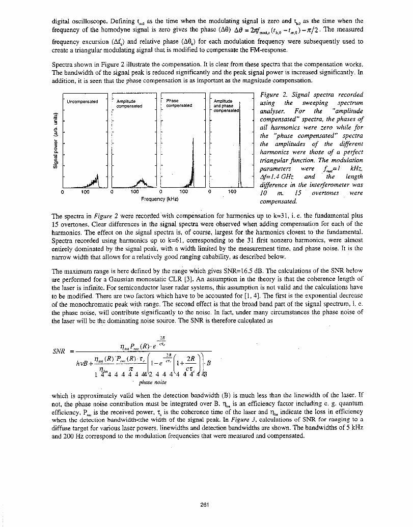
digital oscilloscope. Defining tin.o as the time when the modulating signal is zero and t_,.0as the time when the

frequency of the homodyne signal is zero gives the phase (A0) A0 = 2nfm,,d.` (4.o - t,,.0) - at/2. The measured

frequency excursion (Aft) and relative phase (A0_)for each modulation frequency were subsequently used tocreate a triangular modulating signal that is modified to compensate the FM-response.

Spectra shown in Figure 2 illustrate the compensation. It is clear from these spectra that the compensation works.The bandwidth of the signal peak is reduced significantly and the peak signal power is increased significantly. Inaddition, it is seen that the phase compensation is as important as the magnitude compensation.

t Figure 2. Signal spectra recorded

Uncompensated Amplitude Phase " Amplitude using the sweeping spectrumcompensated compensated and phase

compensated analyser. For the "amplitudecompensated" spectra, the phases of

all harmonics were zero while forthe "phase compensated" spectra

_ the amplitudes of the differento" harmonics were those of a perfect-d_" triangular function. The modulation.__

o_ parameters were .f,,a = 1 kHz,

Af= 1.4 GHz and the length__ _t difference in the interferometer was100 0 100 0 loo o lOO 10 m. 15 overtones were

Frequency(kHz) compensated.

The spectra in Figure 2 were recorded'with compensation for harmonics up to k=31, i. e. the fundamental plus15 overtones. Clear differences in the signal spectra were observed when adding compensation for each of theharmonics. The effect on the signal spectra is, of course, largest for the harmonics closest to the fundamental.Spectra recorded using harmonics up to k=61, corresponding to the 31 first nonzero harmonics, were almostentirely dominated by the signal peak, with a width limited by the measurement time, and phase noise. It is thenarrow width that allows for a relatively good ranging cabability, as described below.

The maximum range is here defined by the range which gives sNR=I6.5 dB. The calculations of the SNR beloware performed for a Gaussian monostatic CLR [3]. An assumption in the theory is that the coherence length ofthe laser is infinite. For semiconductor laser radar systems, this assumption is not valid and the calculations haveto be modified. There are two factors which have to be accounted for [ 1, 4]. The first is the exponential decreaseof the monochromatic peak with range. The second effect is that the broad band part of the signal spectrum, i. e.the phase noise, will contribute significantly to the noise. In fact, under many circumstances the phase noise ofthe laser will be the dominating noise source. The SNR is therefore calculated as

2R

n,o,P,,c(R).eSNR =

hvB + q,o,(R) -P_,_(R)._ B

1_i"4 4 4 4 4 44phase noise

which is approximately valid when the detection bandwidth (B) is much less than the linewidth of the laser. Ifnot, the phase noise contribution must be inte_ated over B. q,_,is an efficiency factor including e. g. quantumefficiency, P,_ is the received power, "c is the coherence time of the laser and q,_ indicate the loss in efficiencywhen the detection bandwidth<the width of the signal peak. In Figure 3, calculations of SNR for ranging to adiffuse target for various laser powers, linewidths and detection bandwidths are shown. The bandwidths of 5 kHzand 200 Hz correspond to the modulation frequencies that were measured and compensated.

261

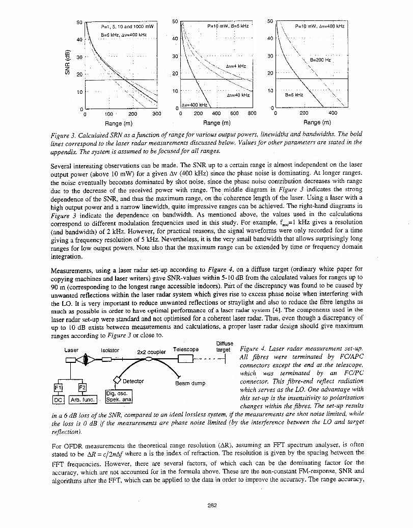
50 50 _! 50

p=l. 5, 10 and1000 mW i _i[i P=10 mW. 8=5 kHz ",", P=10 mW, &v=400 kHzB=5 kHz ,*.v=400 kHz

40 40 _-t ............ 40 \

rn.o 30 30 \' "\:_"_ , • ' 30 ..............., -.. • "_, 8=200 Hzt'_ \ • "_,, "'_ Av=4 kHz . ,, "

z ,.,- .... _i"\ ' i....20 20 ........ t,..:..... :4L, " 20 .....

........ •......... \ .....

10 10 Av-J40kHz 10 8=5 k "x,

Z X : x"" Av=4001kHz\ , i "\0 ,, I 0 0

0 I00 200 300 200 400 600 800 0 200 400

Range(m) Range(m) Range(m)

Figure 3. Calculated SRN as afunction of rangefor various output powers, linewidths and bandwidths. The boldlines correspond to the laser radar measurements discussed below. Valuesfor other parameters are stated in theappendix. The system is assumed to befocused for all ranges.

Several interesting observations can be made. The SNR up to a certain range is almost independent on the laseroutput power (above 10 mW) for a given Av (400 kHz) since the phase noise is dominating. At longer ranges,the noise eventually becomes dominated by shot noise, since the phase noise contribution decreases with rangedue to the decrease of the received power with range. The middle diagram in Figure 3 indicates the strong

dependence of the SNR, and thus the maximum range, on the coherence length of the laser. Using a laser with ahigh output power and a narrow linewidth, quite impressive ranges can be achieved. The right-hand diagrams inFigure 3 indicate the dependence on bandwidth. As mentioned above, the values used in the calculationscorrespond to different modulation frequencies used in this study. For example, f,,,,j=1 kHz gives a resolution(and bandwidth) of 2 kHz. However, for practical reasons, the signal waveforms were only recorded for a timegiving a frequency resolution of 5 kHz. Nevertheless, it is the very small bandwidth that allows surprisingly longranges for low output powers. Note also that the maximum range can be extended by time or frequency domainintegration.

Measurements, using a laser radar set-up according to Figure 4, on a diffuse target (ordinary white paper forcopying machines and laser writers) gave SNR-values within 5-10 dB from the calculated values for ranges up to90 m (corresponding to the longest range accessible indoors). Part of the discrepancy was found to be caused byunwanted reflections within the laser radar system which gives rise to excess phase noise when interfering with

the LO. It is very important to reduce unwanted reflections or straylight and also to reduce the fibre lengths asmuch as possible in order to have optimal performance of a laser radar system [4]. The components used in thelaser radar set-up were standard and not optimised for a coherent laser radar. Thus, even though a discrepancy ofup to I0 dB exists between measurements and calculations, a proper laser radar design should give maximumranges according to Figure 3 or close to.

Diffuse

Laser Isolator 2x2coupler Telescope target Figure 4. Laser radar measurement set-up.

--I 0-..,_ [_]------ All fibres were terminated by FC/APC

_g_% -_connectorsexcepttheendat_thetelescope,

which was terminated by an FC/PC

Beamdump connector. This fibre-end reflect radiationwhich serves as the LO. One advantage with

iArb." func.I IZe". aal this set-up is the insensitivi& to polarisationchanges within thefibres. The set-up results

in a 6 dB.loss of the SNR, compared to an ideal lossless system, if the measurements are shot noise limited, whilethe loss is 0 dB if the measurements are phase noise limited (by the interference between the LO and targetreflection).

For OFDR measurements the theoretical range resolution (AR), assuming an FFT spectrum analyser, is often

stated to be AR = c/2nAf where n is the index 0f refraction. The resolution is given by the spacing between the

FFT frequencies. However, there are several factors, of which each can be the dominating factor for theaccuracy, which are not accounted for in the formula above. These are the non-constant FM-response, SNR andalgorithms after the FFT, which can be applied to the data in order to improve the accuracy. The range accuracy,

262

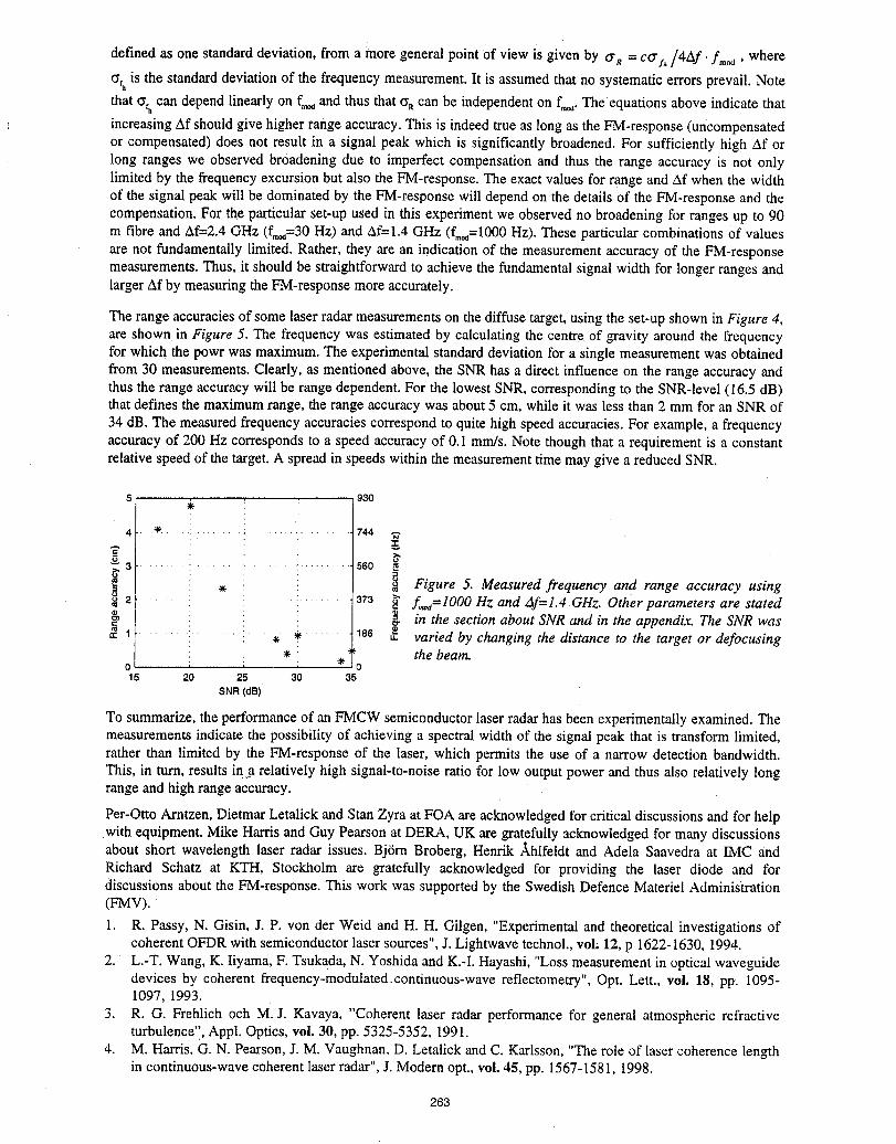
defined as one standard deviation, from a more general point of Viewis given by o-R = ctrz,/4Af, fmod, where

(yr,is the standard deviation of the frequency measurement. It is assumed that no systematic errors prevail. Note

that _f, can depend linearly on f_ and thus that (rRcan be independent on f=_.The equations above indicate that

increasing Af should give higher range accuracy. This is indeed true as long as the FM-response (uncompensatedor compensated) does not result in a signal peak which is significantly broadened. For sufficiently high &f orlong ranges we observed broadening due to imperfect compensation and thus the range accuracy is not onlylimited by the frequency excursion but also the FM-response. The exact values for range and Af when the widthof the signal peak will be dominated by the FM-response will depend on the details of the FM-response and the

compensation. For the particular set-up used in this experiment we observed no broadening for ranges up to 90m fibre and Af=2.4 GHz (fm_=30HZ) and Af=l.4 GHz (fm,_=1000HZ).These particular combinations of valuesare not fundamentally limited. Rather, they are an indication of the measurement accuracy of the FM-responsemeasurements. Thus, it should be straightforward to achieve the fundamental signal width for longer ranges andlarger Af by measuring the FM-response more accurately.

The range accuracies of some laser radar measurements on the diffuse target, using the set-up shown in Figure 4,are shown in Figure 5. The frequency was estimated by calculating the centre of _avity around the frequencyfor which the powr was maximum. The experimental standard deviation for a single measurement was obtainedfrom 30 measurements. Clearly, as mentioned above, the SNR has a direct influence on the range accuracy andthus the range accuracy will be range dependent. For the lowest SNR.,corresponding to the SNR-level (16.5 dB)that defines the maximum range, the range accuracy was about 5 cm, while it was less than 2 mm for an SNR of34 dB. The measured frequency accuracies correspond to quite high speed accuracies. For example, a frequencyaccuracy of 200 Hz corresponds to a speed accuracy of 0.I mm/s. Note though that a requirement is a constantrelative speed of the target. A spread in speeds within the measurement time may give a reduced SNR.

5. _ . 930

4 •_ ...... •.......... , ....... :....... 744

>, 3 ...... • .................. 560

_ Figure 5. Measured frequency and range accuracy using2 .......... :....... 373 _= f_=lO00 Hz and Af=l.4 GHz. Other parameters are stated

i _ in the section about SNR and in the appendix. The SNR was_: 1 ................... , , ....... la6 _. varied by changing the distance to the target or defocusing

• * the beam.0 _ o15 20 25 30 35

SNR (dB)

To summarize, the performance of an FMCW semiconductor laser radar has been experimentally examined. Themeasurements indicate the possibility of achieving a spectral width of the signal peak that is transform limited,rather than limited by the FM-response of the laser, which permits the use of a narrow detection bandwidth.This, in turn, results in__arelatively high signal-to-noise ratio for low output power and thus also relatively longrange and high range accuracy.

Per-Otto Arntzen, Dietmar Letalick and Stan Zyra at FOA are acknowledged for critical discussions and for helpwith equipment. Mike Harris and Guy Pearson at DELLA,UK are _atefully acknowledged for many discussionsabout short wavelength laser radar issues. Bj6rn Broberg, Henrik _hlfeldt and Adela Saavedra at IlVICandRichard Schatz at KTH, Stockholm are gratefully acknowledged for providing the laser diode and fordiscussions about the FM-response. This work was supported by the Swedish Defence Materiel Administration(FMV).

I. R.Passy,N.Gisin,J.P.yonderWeid andH. H.Gilgen,"ExperimentalandtheoreticalinvestigationsofcoherentOFDR withsemiconductorlasersources",J.Lightwavetechnol.,vol.12,p 1622-1630,1994.

2. L.-T. Wang, K. Iiyama, F. Tsukada, N. Yoshida and K.-I. Hayashi, "Loss measurement in optical waveguidedevices by coherent frequency-modulated.continuous-wave reflectometry", Opt. Lett., vol. 18, pp. 1095-1097, 1993.

3. R.G. Frehlich och M.J. Kavaya, "Coherent laser radar performance for general atmospheric refractiveturbulence"., Appl. Optics, voi. 30, pp. 5325-5352, 1991.

4. M. Harris, G. N. Pearson, J. M. Vaughnan. D. Letalick and C. Karlsson, "The role of laser coherence lengthin continuous-wave coherent laser radar", J. Modern opt., vol. 45, pp. 1567-1581, 1998.

263

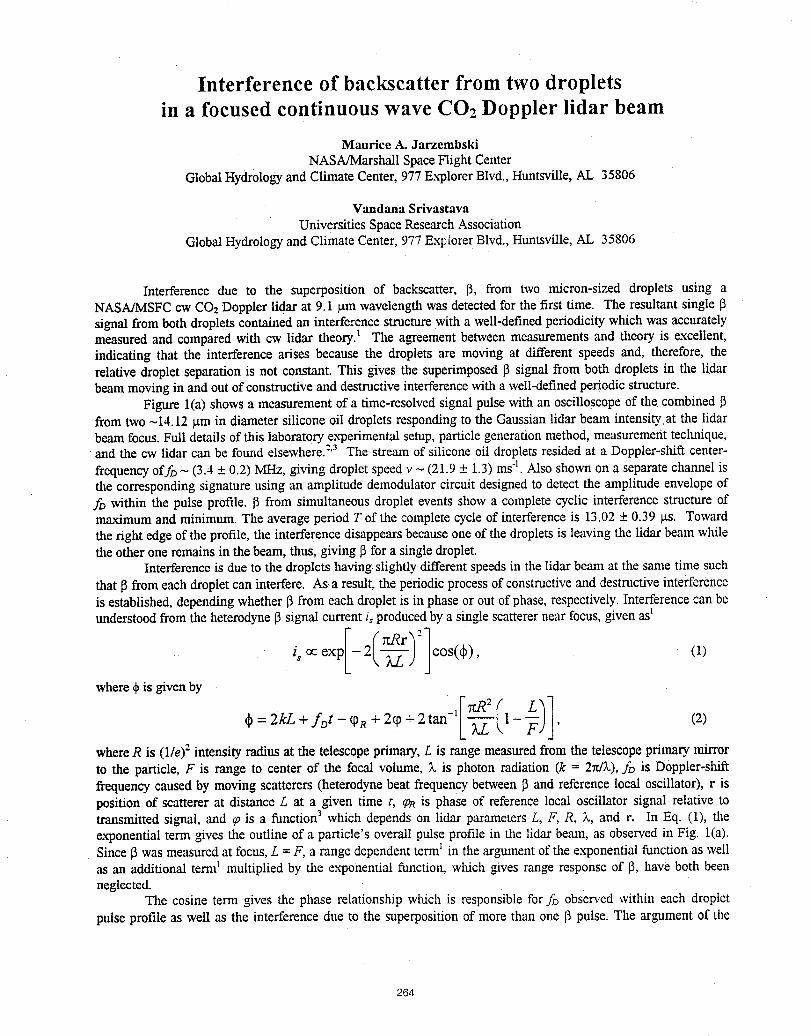
Interference of backscatter from two dropletsin a focused continuous wave CO 2 Doppler lidar beam

Maurice A. Jarzembski

NASA/Marshall Space Flight CenterGlobal Hydrology and Climate Center, 977 Explorer Blvd., Huntsville, AL 35806

Vandana Srivastava

Universities Space Research AssociationGlobal Hydrology and Climate Center, 977 ExF[orer Blvd., Huntsville, AL 35806

Interference due to the superpositionof backscatter, 13,from two micron-sized droplets using aNASA/MSFCcw CO2Dopplerlidarat 9.1 _.mwavelengthwas detectedfor the firsttime. The resultantsingle 13signalfrombothdropletscontainedan interferencestructurewith a well-definedperiodicitywhichwasaccuratelymeasuredand comparedwith cw lidar theory.1 Tile agreementbetweenmeasurementsand theory is excellent,indicatingthat the interferencearisesbecause the dropletsare movingat differentspeeds and, therefore,therelativedropletseparationis not constant.Tiffsgives the superimposed13signalfromboth dropletsin the lidarbeammovingin and outof constructiveanddestructiveinterferencewith a well-definedperiodic structure.

Figurel(a) showsa measurementof a time-resolvedsignalpulse withan oscilloscopeof the combined13fromtwo -14.12 _tmin diametersiliconeoil dropletsrespondingtothe Gaussianlidarbeam intensity,at the lidarbeamfocus.Fulldetailsofthis laboratoryexperimentalsetup,particlegenerationmethod,measuremerittechnique,

•and the cw lidar can be found elsewhere._'3 The stream of siliconeoil dropletsresidedat a Doppler-shiftcenter-frequencyoffD-- (3.4 ___0.2) MHz, giving dropletspeedv ~ (21.9+ 1.3) ms4. Alsoshownon a separatechannel isthe correspondingsignature usingan amplitudedemodulatorcircuit designedto detect the amplitudeenvelopeoffD within the pulse profile. 13from simultaneousdroplet eventsshow a completecyclic interferencestructure ofmaximumand minimum.The averageperiod T of the completecycleof interferenceis 13.02+ 0.39 _ts. Towardthe right edgeofthe profile,the interferencedisappearsbecauseoneof the dropletsis leavingthe lidar beamwhilethe other one remainsin the beam, thus, giving 13fora singledroplet.

Interferenceis dueto the dropletshaving slightlydifferentspeedsin the lidar beamat the same time suchthat 13from each dropletcan interfere. As a result,the periodicprocessof constructiveand destructiveinterferenceis established,dependingwhether 13from each dropletis in phase or out of phase, respectively.Interferencecan beunderstoodfromthe heterodyne13signalcurrent i, producedby a singlescatterernearfocus,given as1

rd_r "i, oc exp - 2 cos(qb), (1)

where_ is givenby

O0=2kL+fDt-q_ R+2_ +2tan -_ 1- , (2)

whereR is (lie)z intensity,radiusat the telescopeprimary,L is range measuredfrom the telescopeprimarymirrorto the particle, F is range to center of the focal volume, L is photon radiation (k = 2_/L), fD is Doppler-shiftfrequencycausedby moving scatterers (heterodynebeat frequencybetween13and referencelocal oscillator),r ispositionof scatterer at distanceL at a given time r, _ is phase of referencelocal oscillator signal relative totransmitted signal, and _ois a function_ which dependson lidar parametersL, F, R, L, and r. In Eq. (1), theexponentialterm givesthe outline of a particle's overallpulse profilein the lidar beam, as observedin Fig. l(a).Since13was measuredat focus,L = F, a range dependenttermI in the argumentof the exponentialfunctionas wellas an additional term_ multipliedby the exponentialfunction, which Nves range response of 13,have both beenneglected.

The cosine term gives the phase relationshipwhich is responsiblefor fD observedwithin each dropletpulse profile as well as the interferencedue to the superpositionof more than one 13pulse. The argument of the

264

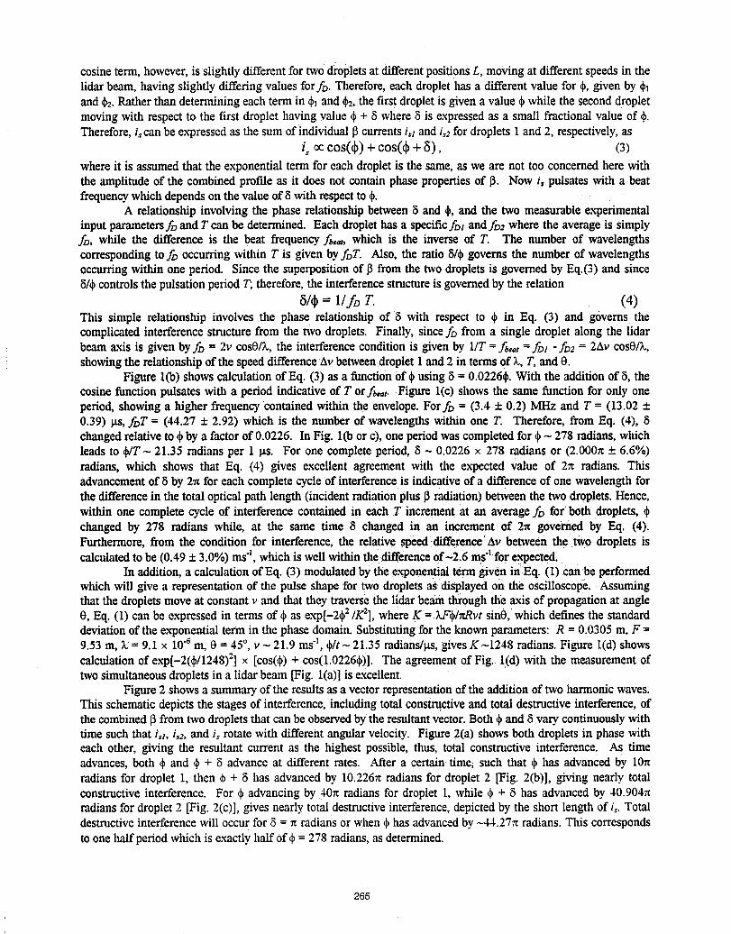
cosineterm, however,is slightlydifferentfor two dropletsat differentpositionsL, movingat differentspeedsin thelidar beam, having slightlydifferingvalues for./_.Therefore,each droplethas a differentvalue for _, given by _1and_. Ratherthan determiningeachterm in _ and _2,the first dropletis givena value_ while the seconddropletmovingwith respectto the first droplethavingvalue (_+ 8 where8 is expressedas a small fractionalvalue of _.Therefore,ixcanbe expressedas the sum of individual13currentsi_ and i_2for droplets 1 and 2, respectively,as

ix eos( )+eos( +8), (3)whereit is assumedthat the exponentialterm for each dropletis the same,as we are not too concernedhere withthe amplitudeof the combinedprofile as it does not contain phase propertiesof 13. Now ix pulsates with a beatfrequencywhich dependsonthe valueof 8 with respectto d_.

A relationshipinvolvingthe phase relationshipbetween8 and _, and the two measurableexperimentalinput parametersfDand T can be determined. Each droplethas a specificJbtand/b2 where the average is simply3_, while the difference is the beat frequency3_,,t, which is the inverseof T. The number of wavelengthscorrespondingtofD occurringwithin T is given by./bT. Also, the ratio 8/_)governs the number of wavelengthsoccurringwithin one period. Since the superpositionof 13from the two dropletsis governedby Eq.(3)and since8/_)controlsthe pulsationperiodT; therefore,the interferencestructureis governedbythe relation

81_= 1/fD r. (4)This simple relationship involves the phase relationship of 8 with respect to d_in Eq. (3) and governs thecomplicatedinterferencestructure from the two droplets. Finally,sincefD from a single droplet along the lidarbeam axis is givenby3_ = 2v cos0/_,,the interferenceconditionis givenby liT = _,o, =.ibt "./b2= 2Avcos0/X,showingthe relationshipof the speeddifferenceAvbetweendroplet I and 2 in terms of L, T,and 0.

Figure l(b) showscalculationof Eq. (3) as a functionof _)using8 = 0.0226_. With the additionof 8, thecosinefunctionpulsateswith a period indicativeof T or.Ao,t.Figure l(c) showsthe same function for only oneperiod, showinga higher frequencycontainedwithin the envelope.For3_ = (3.4 + 0.2) MHz and T = (13.02 :!:0.39) ps, ./_T = (44.27 + 2.92) which is the number of wavelengthswithin one T. Therefore, from Eq. (4), 8changedrelativeto d_by a factorof 0.0226. In Fig. l(b or c), oneperiodwascompletedford_- 278 radians,whichleads to d_/T_ 21.35 radians per 1 _ts. For one completeperiod, 8 ~ 0.0226 x 278 radians or (2.0007t+ 6.6%)radians, which shows that Eq. (4) gives excellent agreement with the expected value of 27t radians. Thisadvancementof 8 by 2n for each completecycleof interferenceis indicativeof a differenceof one wavelengthforthe differencein the total opticalpath length (incidentradiationplus13radiation)betweenthe two droplets.Hence,within one completecycle of interferencecontainedin each T incrementat an averagefo for'both droplets,changed by 278 radians while, at the same time 8 changed in an increment of 2_t governed by Eq. (4).Furthermore,from the condition for interference,the relativespeeddifference Av between the two droplets iscalculatedto be (0.49+ 3.0%)msq, which is wellwithinthe differenceof~2.6 ms"_forexpected.

In addition,a calculationof Eq. (3) modulatedby theexponentialterm given inEq. (1) Canbe performedwhichwill give a representationof the pulse shape for two dropletsas displayedon the oscilloscope. Assumingthat the dropletsmoveat constantv and that they traversethe lidarbeam throughthe axisof propagationat angle0, Eq. (1) can be expressedin terms of _ as exp[-2d_2/K2],whereK = LF_/rd_vtsin0, whichdefines the standarddeviationof the exponemialterm in the phase domain.Substitutingfor the knownparameters: R = 0.0305m, F =9.53 m, L = 9.1x 10"6m, 0 =45°, v _ 21.9 msq, dflt_ 21.35radians/_, givesK _1248 radians. Figure l(d) showscalculationof exp[-2(_b/1248)Z]x [cos(_))+ cos(!.0226_b)].The agreementof Fig. l(d) with the measurementoftwosimultaneousdropletsin a lidar beam [Fig. l(a)] is excellent.

Figure2 showsa summaryof the resultsas a vectorrepresentationof the additionof two harmonicwaves.This schematicdepictsthe stagesof interference,includingtotal constructiveand total destructiveinterference,ofthe combined13from two dropletsthat can be observedby the resultantvector.Both d_and 8 vary continuouslywithtime such that i,z, i,:, and ixrotate with differentangularvelocity. Figure2(a) showsboth droplets in phasewitheach other, giving the resultant current as the highest possible, thus, total constructiveinterference. As timeadvances,both d_and _b+ 8 advance at different rates. After a certain time, such that _ has advancedby 10rtradians for droplet 1, then d)+ 8 has advancedbv 10.2267tradians for droplet 2 [Fig. 2(b)], giving nearly totalconstructiveinterference. For ff advancingby 40n radians for droplet l, while _ + 8 has advancedby 40.904nradiansfor droplet2 [Fig. 2(c)],gives nearlytotal destructiveinterference,depictedby the short length of ix.Totaldestructiveinterferencewilloccur for 8 = Ttradiansor whenqbhasadvancedby ~44.27_tradians. This correspondsto one halfperiodwhichis exactlyhalfof qb= 278 radians,as determined.

265

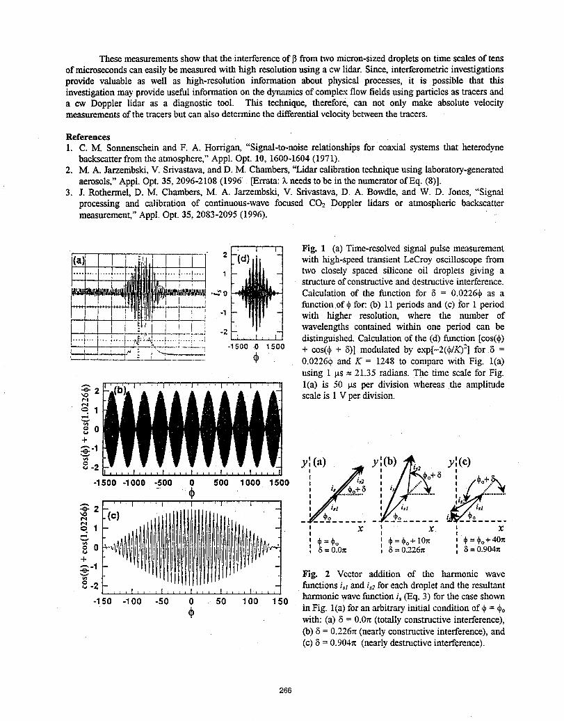
These measurements show that the interference of 15from two micron-sizeddroplets on time scales of tensof microsecondscaneasily be measured with high resolutionusing a cw lidar.Since, interferometric investigationsprovide valuable as well as high-resolution information about physical processes, it is possible that thisinvestigation may provideuseful information on the dynamicsof complex flow fields using particles as tracersanda cw Doppler lidar as a diagnostic tool. This technique, therefore, can not only make absolute velocitymeasurements of the tracers but can also determine the differential velocity between the tracers.

References

1. C. M. Sonnenscheinand F. A. Horrigan, "Signal-to-noiserelationshipsfor coaxial systemsthat heterodynebackscatterfromthe atmosphere,"Appl.Opt. 10, 1600-1604(1971):

2. M. A.Jarzembski,V. Srivastava,and D.M. Chambers,"Lidar calibrationtechniqueusing laboratory-generatedaerosols,"Appl.Opt. 35,2096-2108(1996 [Errata: L needsto be in the numeratorof Eq. (8)].

3. L Rothermel,D. M. Chambers,M. A. Jarzembski, V. Srivastava,D. A. Bowdle,and W. D. Jones, "Signalprocessing and calibration of continuous-wavefocused CO2 Doppler lidars or atmospheric backscattermeasurement,"Appl.Opt. 35,2083-2095(1996).

Fig. 1 (a) Time-resolvedsignal pulse measurementi't [ i i ] 2 with high-speedtransient LeCroy oscilloscopefrom

['t .... t....i..... _ilt[_]lit_."].... !....I....] 1 two closely spaced silicone oil droplets giving a___" ..4_,1 structure of constructive and destructive interference.

]['][In[]][_['_il "_0 Calculationof the function for5 = 0.0226_bas ai:iii_l_llIr ....... i- _.----i................ function,ofdpfor: (b) 11 periodsand (c) J_or1 period

'. I ) _ ' [_i ) -_ i j -1 with higher resolution, where the number of[ , ! t__._:o! ,--.: _/_j -z wavelengths contained within one period can be

!.... i.... i.... i.... t"_:_:_! .... i.... i '_ distinguished.Calculationof the (d) function [cos(_):--; i ; ,.. _--r--...... : 4 soo o 1soo + cos(_ + 8)] modulatedby exp[-2(dp/K):]for 8 =

.... : "''-_--" _b 0.0226@and K = 1248 to compare with Fig. l(a)using 1 _ts= 21.35radians. The time scale for Fig.l(a) is 50 _ per division whereas the amplitude

_- 2 scaleis 1 V perdivision.e-!

80+

y: (a) y[(b) _5_ y',(c)

'[ jft.... ''.,,00.,000.000. ,o0,0o0,o0o , . ,

-~ (I) I•" |

-o-2 n-"-" _ i,t , if/i,1 t,1,o ¥ _,o _Jl/ % %

• I ,

" t (F=@o+lOTt , _=d_o+40x_0 _=':I'o i8 =O.Ox , 8 =0.2267t ', 8 0.904_t+

_._-1 Fig. 2 Vector addition of the harmonic waveo,1

o -2 functionsi,t and i,2for eachdropletand the resultantharmonicwavefunctioni, (Eq.3) for the case shown-150 -100 -50 0 50 100 150

d_ in Fig. l(a) foran arbitraryinitial conditionof _ = @owith: (a) 5 = 0.0rt(totallyconstructiveinterference),(b) 5 = 0.226n(nearlyconstructiveinterference),and(c) 5 = 0.904rt (nearlydestructiveinterference).

266

WIND MEASUREMENTS

Presider: David Tratt

267

Ground-based Remote Sensing of Wind VectorLatest Results from Guideline Development

J. BOsenberg,H.Danzeisen,D. Engelbart,K. Fritzsche,V. Klein,Ch.Mtlnkel,T.Trickl,L. Woppowa, andChristianWerner

1. Introduction

Methods which are in discussion to enter a VDI guideline will be presented. The VDI ,,Richtlinie VDI 3786,,Umweltmeteorologie", is divided in many parts. VDI 3786 Part 14 shows the possibilities of remote sensingand describes the wind profile measurements. It is necessary for comparison with other instruments to have aguideline which descibes also the calibration and performance tests.Wind profiles in the atmospheric boundary layer are a very important parameter also to study atmosphericexchange processes. The wind field in the atmospheric boundary layer is highly variablein spatial and temporalscales. For a few possible applications a more frequent wind sensing is necessary, i.e.

- for airports located in low level jet areas,- for chemical plants to get information of the transport of toxic gases from leakages,- for meteorology in general to improve the weather forecast,- for environment protection purposes like dispersion studies.

T

Only a fewtechniques can be applied to getthe wind field in the boundary layer. Laser Doppler systems arecandidates.

2. Doppler Lidar

A heterodyne lidar consists of a pulsed, frequency-controlledlaser transmitter locked via a locking loop to thelocal oscillator, a transmit and receive telescope, a heterodyne detector, where the local oscillator radiation ismixed with the Doppler-shifted backscattersignal, and a signal processing system. The signal origines fromthe backscattering by small aerosol particles which move with the prevailing windspeed through the laser focusvolume. The windshifted Doppler frequencydirectly determines the line-of-sight (LOS) component (VLos) ofthe wind vector.One measures the backscattered, Doppler shifted radiation. Backscattering depends on the sizi and numberdensity of the aerosol particles available in the volume of interest. The backscatteredDoppler frequencydirectlydetermines the line-of-sight (LOS) component (VLos) of the wind vector. At CO2 laser (wavelengths _, = 10.6

_tm)a velocity component of 1 m/s corresponds to a frequencyshift, AfD of 189 kHz. This is obtained from theequation

AfD= 2 VLOS.foc

wherec is the speedof lightand VLOSis the line-of-sightcomponent.By scanningthe transceiverwith a conicalscan pattern(VAD)or by using the beamswingingtechnique

(DBS) (seefigure1)onereachesdifferentazimuthand elevationanglesto combinethe single LOS-componentsto a windvector.

268

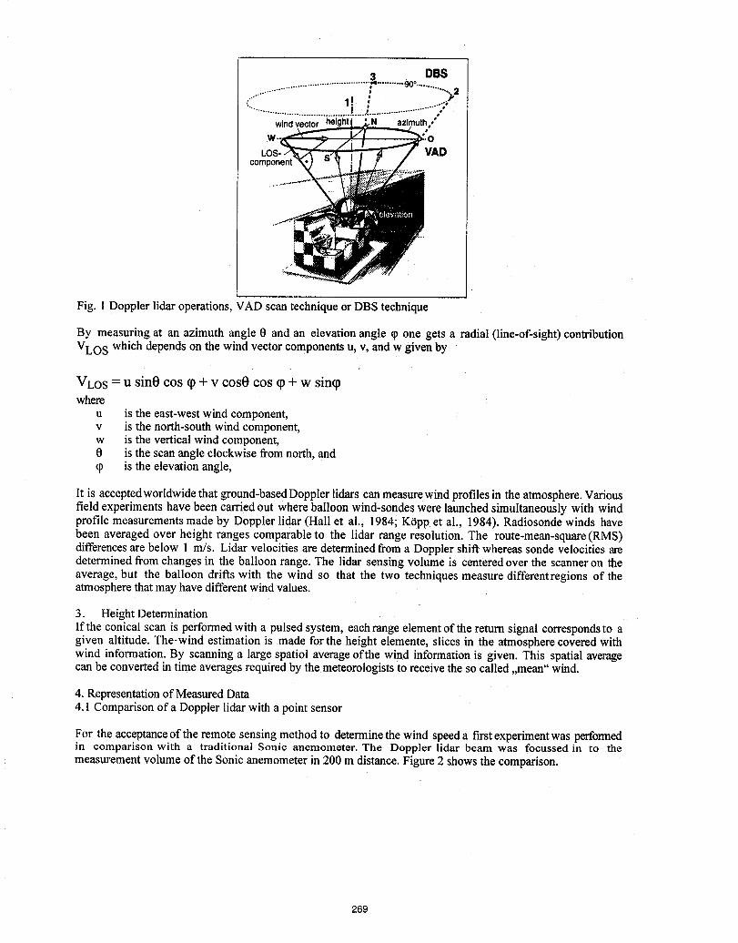
DBS

°o°°° a;" " 11: ,•-. • i

windvector azimuth,,"

LOS- VADcomponent

Fig. 1Doppler lidar operations, VAD scan technique or DBS technique

By measuring at an azimuth angle 0 and an elevation angle 9 one gets a radial (line-of-sight) contributionVLOS which depends on the wind vector components u, v, and w given by

VLO S = Usin0 cos _0+ v cos0 cos ¢p+ w sincpwhere

u is the east-west wind component,v is the north-south wind component,w is the vertical wind component,0 is the scan angle clockwise fi'omnorth, and_p is the elevation angle,

It is acceptedworldwide that ground-based Doppler lidars can measure wind profiles in the atmosphere. Variousfield experiments have been carried out where balloon wind-sondes were launched simultaneously with windprofile measurements made by Doppler lidar (Hall et al., 1984; KOpp et al., 1984). Radiosonde winds havebeen averaged over height ranges comparable to the lidar range resolution. The route-mean-square (RMS)differencesare below 1 m/s. Lidar velocities are determined from a Doppler shift whereas sonde velocities aredetermined from changes in the balloon range. The lidar sensing volume is centered over the scanner on theaverage, but the balloon drifts with the wind so that the two techniques measure differentregions of theatmosphere that may have different wind values,

3. Height DeterminationIf the conical scan is performed with a pulsed system, each range element of the return signal corresponds to agiven altitude. The-wind estimation is made for the height elemente, slices in the atmosphere covered withwind information. By scanning a large spatioi average ofthe wind information is given. This spatial averagecan be converted in time averages required by the meteorologists to receive the so called ,,mean" wind.

4. Representation of Measured Data4.1 Comparison of a Doppler lidar with a point sensor

For the acceptanceof the remote sensing method to determine the wind speeda first experiment was performedin comparison with a traditional Sonic anemometer. The Doppler lidar beam was focussed in to themeasurement volume of the Sonic anemometer in 200 m distance. Figure 2 shows the comparison.

269

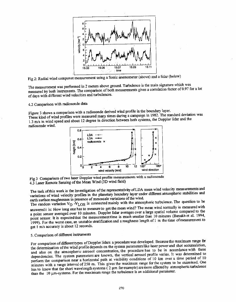
61

41

4i

21Oi'= _ I , i l'r , I , , ! l _ I t i I , _ I , i i

15:03 15:05:: 15:07 15:09 15:11

: • : time

Fig 2: Radial wind componet measurement using a Sonic anemometer(above) and a lidar (below)

The measurement was performed in 2 meters above ground. Turbulence is the main signature which wasmeasured by both instnmaents. The comparisonof both measurements gives a correlation factor of 0.97 for a lotof days with different wind velocities and turbulences.

4.2 Comparison with radiosonde data

Figure 3 shows a comparison with a radiosonde derived wind profile in the boundary layer.These kind of wind profiles were measured many times during a campaign in 1982. The standard deviation was1.3 m/s in wind speed and about 12degree in direction between both systems, the Doppler lidar and theradiosonde wind.

X I X

.....

LDA -'4-- ", X_" radiosonde x

_- (

2 4 6 8 10 12 100° 180°

windvelocity[m/s] winddirection

Fig 3 Comparisonof twolaserDopplerwindprofilemeasurementswitha radiosonde4.3LaserRemoteSensingof theMeanWind(3D wind field)

The taskof thiswork is theinvestigationof therepresentativityofLDA meanwind velocitymeasurementsandvariations of wind velocity profiles in the planetary boundary layer under differentatmospheric stabilities andearth surface roughnesses in presence of mesoscale variations of the wind.The random variation VD -VLo S is connected mainly with the atmospheric turbulence. The question to beansweredi is: How long one has to measureto get the mean wind? The mean wind normally is measured witha point sensor averaged over 10 minutes. Doppler lidar averagesover a large spatial volume compared to thepoint sensor. It is expected that the measurement time is much smaller than I0 minutes (Banakh et al. 1994,1999). For the worst case, an unstable stratification and a roughness length of 1 m the time of measurement toget 1 m/s accuracy is about 12seconds.

5. Comparison of different instruments

For comparison ofdifferenttypes of Doppler lidars a procedurewas developed. Because the maximum range forthe determination of the wind profile depends on the system parameters like laserpower and shot accumulation,and also on the atmospheric aerosol concentration, the procedure has to be in accordance with thesedependencies. The system parameters are known, the vertical aerosol profile varies. It was determined toperform the comparison near a horizontal path at visibility conditions of 10 km over a time period of 10minutes with a range interval of 250 m. This gives the maximum range for the system to be examined: Onehas to know that the short wavelength systems ( 2 _tm for example)are more affectedby atmospheric turbulencethan the 10!.tm-systems. For the maximum range the turbulence is an additional parameter.

270

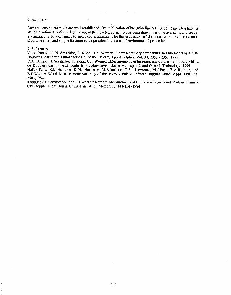
6. Summary

Remote sensing methods are well established. By publication ofhte guideline VDI 3786 page 14 a kind ofstandardisation is performedfor the use ofthe new technique. It has been shown that time averaging and spatialaveraging can be exchanged to meet the requirement for the estimation of the mean wind; Future systemsshould be small and simple for automatic operation in the area of environmental protection.

7. References

V. A. Banakh, I. N. Smalikho, F. KiSpp, Ch. Werner: "Representativity ofthe wind measurements by a CWDoppler Lidar in the Atmospheric Boundary Layer ", Applied Optics, Vol. 34, 2055 - 2067, 1995V.A. Banakh, I. Smalikho, F. KSpp, Ch. Werner: ,,Measurements ofturbulent energy dissipation rate with acw Doppler lidar in the atmospheric boundary layer", Journ. Atmospheric and Oceanic Technology, 1999HaI1,F.F.Jr.; R.M.Huffaker, R.M. Hardesty, M.E.Jackson, T.R, Lawrence, M.J.Post, R.A.Richter, andB.F.Weber: Wind Measurement Accuracy of the NOAA Pulsed Infrared Doppler Lidar. Appl. Opt. 23,2503,1984Kt_pp,F.;R.L.Schwiesow, and Ch.Werner: Remote Measurements of Boundary-Layer Wind Profiles Using aCW Doppler Lidar. Journ. Climate and Appl. Meteor. 23, 148-154 (1984)

271

ABSTRACT

The Accuracyof theTrueRadialVelocityMeasurementsin theTurbulentAtmosphereAlexanderP. Shelekhov,Instituteof AtmosphericOptics,SBRussianAcad.Science,Tomsk,RussianFederation

Asa ruletheaccuracyof theDopplermeasurementsisstudiedusingtheassumptionthatthefrequencyestimationisequaltoapproximatelytheaverageDopplershiftorisproportionalto theaveragetrueradialvelocity.Butthefrequencyestimationmaybeproportionaltothetrueradialvelocity.Inthispapertheaccuracyof thetrueradialvelocitymeasurementisinvestigatedforthedifferentstateof theturbulentatmosphere,thedifferentvaluesof thesignal-to-noiseratio,thenumberof thesamplesandotherparameters.Thecasesof thestable,unstable,andindifferentstratificationareconsidered.

272

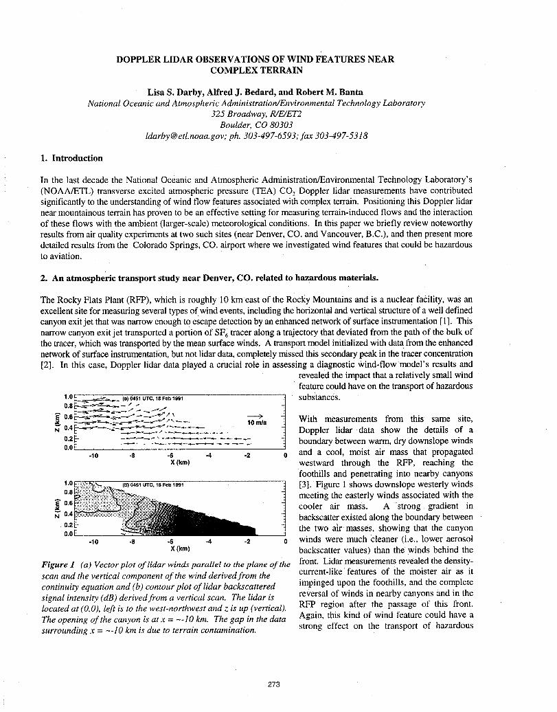
DOPPLER LIDAR OBSERVATIONS OF WIND FEATURES NEARCOMPLEX TERRAIN

Lisa S. Darby, Alfred J. Bedard, and Robert M. BantaNational Oceanic and Atmospheric Administration/Environmental Technology Laboratory.

325 Broadway, R/E/ET2Boulder, CO 80303

Idarby@etl.noaa.gov; ph. 303-497-6593; fax 303-497-5318

1. Introduction

In the last decade the National Oceanic and Atmospheric Administration/Environmental Technology Laboratory's(NOAA/ETL) transverse excited atmospheric pressure (TEA) CO_,Doppler lidar measurements have contributedsignificantly to the understanding of wind flow features associated with complex terrain. Positioning this Doppler lidarnear mountainous terrain has proven to be an effective setting for measuring terrain-induced flows and the interactionof these flows with the ambient (larger-scale) meteorological conditions. In this paper we briefly review noteworthyresults from air qualityexperiments at two such sites (near Denver, CO. and Vancouver, B.C.), and then present moredetailed results from the Colorado Springs, CO. airport where we investigated wind features that could be hazardousto aviation.

2. An atmospheric transport study near Denver, CO. related to hazardous materials.

The Rocky FlatsPlant (RFP), which is roughly 10 km east of theRocky Mountainsand is a nuclear facility, was anexcellentsite formeasuringseveraltypesof windevents, includingthehorizontalandverticalstructureof a well definedcanyonexitjet thatwas narrowenough tOescapedetectionby anenhancednetworkof surfaceinstrumentation[1]. Thisnarrowcanyonexit jet transporteda portionof SF6traceralong a trajectorythatdeviated from the pathOf the bulkofthe tracer,which was transportedby themeansurfacewinds. A transportmodelinitializedwith datafromtheenhancednetworkof surfaceinstrumentation,but not lidardata,completelymissedthis secondarypeakin the tracerconcentration[2]. In this case, Doppler lidar dataplayed a crucial role in assessing a diagnostic wind-flow model's results and

revealedthe impactthat a relatively smallwindfeaturecouldhave on the transportof hazardous

__1.0_ (a)04sl UTC,18 Feb"1991 substances.o.*__- L L ,.--,,_°'6_'_-7"_Z'--'':'' ---> "_ With measurements from this same site,0.4 L.._._,_-..__--,.-_f, ---.----.--.,--_

N" 0.2_ ..... __ -_ Doppler lidar data show the details of aboundary between warm, dry downslope windso.o_ ..... -'-'- _ _ _ ' - and a cool, moist air mass that propagated-10 -8 -6 -4 -2 0

X(km) westward through the RFP, reaching thefoothills and penetrating into nearby canyons

1.0 (b')'0aslUTC,18Feb1991 [3]. Figure I shows downslope westerly winds0.8 meeting the easterly winds associated with the

=_"0.s cooler air mass. A strong gradient ino.4 backscatter existed along the boundary between0.2E- the two air masses, showing that the canyon

-10 -8 -6 -4 -2 0 winds were much Cleaner (i.e., lower aerosolx(kin) backscatter values) than the winds behind the

Figure l (a) Vector plot of lidar winds parallel to the plane of the front. Lidar measui'ementsrevealed the density-scan and the vertical component of the wind derived from the current-like _features of the moister air as itcontinuity equation and (b) contour plot of lidar backscattered impinged upon the foothills, and the completesignal intensity (dB) derivedfrom a vertical scan. The lidar is reversal of winds in nearby canyons and in thelocated at (0,0), left is to the west-northwest and z is up (vertical). RFP region after the passage of this front.The opening of the canyon is at x = --lOkm. The gap in the data Again, this kind of wind feature could have asurrounding x = --10 km is due to terrain contamination, strong effect on the transport of hazardous

273

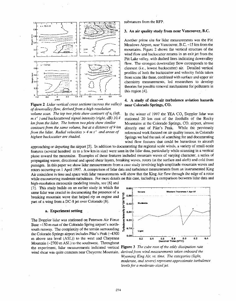
.: . _ _ ,.._.,_;.., ... substances from theRFP.=_o.4k_ _:_ _i _:,_ii_

,_'::_:_!_, ,._•_.,_,_,_,, - 3. An air quality study from near Vancouver, B.C._0.6 0 .--'--'-'--'-

....... 108__

2 Another prime site for lidar measurements was the Pitt0.4 /. _.--_ _ --.-,- -4,- Meadows Airport, near Vancouver, B.C, ~15km from the0.2 ----_'1

_.. _ _ _ mountains. Figure 2 shows the vertical structure of theo , , _ _ , , _ , _ _ , _ wind flow and backscatter returns in an exit jet from the

Pitt Lake valley, withdashed lines indicating downvalley,.0 .............. flow. The strongest downvalley flow corresponds to the

,, =9.o_m _ : .... "?i"?!i :i.

o. ,eaneatowestback.catteair e,ai,evertc] o._ 0 _'_ _o profiles of both the backscatter and velocity fields takenz _ from scans likethese, combined with surface and upperair_o., F77_" chemistry measurements, led researchers to develop

-_ /{ :_:_:!!_i:! theories for possible removal mechanisms for pollutants in0._ / / : ; ':,k-_

..... .___-_-__4 this region [4].0 I ! ! [ I I I I I I I [ I I

-1.0 -0.5 O 0.5 1.0 -1.0 -0.5 0 0.5 1.0

I_m, _.,I 4. A study of clear-air turbulence aviation hazardsFigure 2 Lidar vertical cross sections (across the valley) near Colorado Springs, CO.of downvalley flow, derivedfrom a high-resolutionvolume scan. The top two plots show contours ofu_ (left, In the winter of 1997 the TEA CO_.Doppler lidar wasm s_ ) and backscatteredsignal intensity (right, dB)10.4 stationed 20 km east of the foothills of the Rockykinfrom the lidar. The bottom twoplots show similar Mountains at the Colorado Springs, CO. airport, almostcontours from the same volume, but at a distance of 9 km directly east of Pike's Peak. While the previouslyfrom the lidar. Radial velocities > 4 m s_ and areas of referencedwork focusedon airqualityissues, in Coloradohighest backscatter are shaded. Springswe had the task of searchingfor anddocumenting

wind flow features that could be hazardous to aircraft

approachingor departingthe airport[5]. In additionto documentingthe regional scale winds, a variety of small-scalefeatures (several hundred m to a few km in size) were seen in the lidar data,particularlywhile scanning in a verticalplanetoward the mountains. Examples of these features includedmountainwaves of varying character,a series ofpropagatingwaves, directionalandspeed shear layers, breakingwaves, rotors (at thesurface and aloft) andcold frontpassages. In thispaperwe show lidarmeasurementsfrom acase studyinvolving high-amplitudemountainwaves androtorsoccurringon 1April 1997. A comparisonof lidar dataand turbulencemeasurementsfroman instrumentedKingAir coincidentin time andspacewith lidarmeasurementswill show that theKing Air flew through the edge of a rotorwhile encounteringmoderateturbulence.For moredetailson thiscase, includinga comparisonbetween lidar data andhigh-resolution mesoscalemodeling results, see [6] and[7]. This study builds on an earlier study in which the o.6o_ ................ • .....same lidar was crucial .indocumenting the presence of a _ _ a.... w.,to,nr....... __,,grbreaking mountain wave that helped rip an engine and _ o.so_-......................................................................................................

part of a wing from a DC:8 jet over Colorado [8]. ,_ 0.40[- Moderato -_

a. Experiment setting "_ o.3o_-g

EThe Doppler lidar was stationed on Peterson Air Force g o.ao_Base -150 m east of the ColoradoSpring airport's north- -_

south runway. The complexity of the terrain surrounding _. o._o_= Light

the Colorado Springs airport includes Pike's Peak (-4300 o.oo._........., ,m above sea level (ASL)) to the west and Cheyenne s.a 5.4 5:6 5.8 6.0 6.9 6.4

Decimal Time (UTC)Mountain (-2700 m ASL) to the southwest. Throughoutthe experiment, lidar measurements indicated vertical Figure 3 The cube root of the eddy dissipation ratewind shear w_ quite common near Cheyenne Mountain. derived from wind measurements taken onboard the

Wyoming King Air, vs. time. The categories (light,moderate, and severe) represent approximate turbulencelevels for a moderate-sized jet.

274

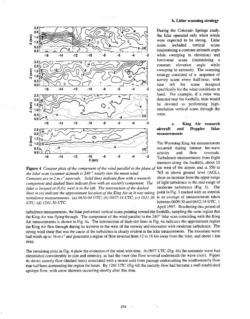
b. Lidar scanning strategy

2.5 "_ During the Colorado .Springs study,2.0

_' 1.5 the lidar operated only when winds-_ were expected to be strong. Lidar

N 1.0 3 scans included vertical scans0.50.0 (maintaining a constant azimuth angle

-16 -14 -12 -10 -8 -6 -4 -2 _¢hile sweeping in elevation) and

2.5L.,,_.,,vj _ _.,.,_ L_(3 _)__ horizontal scans (maintaining a

2"0_ _'_///_/"_ f"_ __ -_ i constant elevation angle while

A _'_--/_ _o __'_"J//'_,_!_ t"_0_ sweepingin azimuth). The scanningE 1.5 -_1.0 strategy consisted of a sequence of0.5_-'::.. survey scans every half-hour, with0.0 _ __ F'-_o"/J_ time left for scans designed

-16 .14 -12 -10 -8 -6 -4 -2 specifically for the wind conditions at

2.5_ _x_,./ll.] _ _"---_ _-_,-- _ o v t" • • :."..'._ hand. For example, if a rotor was2 0 _ _ f--_._-_-_'q__ F--.-o ':'......'.: ;._ detected near the foothills, time would

1.5_._t / -,_J -_ (_)._ .'.... ":"."_,I_ be devoted to performing high-"" 1.0_-_'" .... ""i d - ° ] .:'ii..... .'"'"':i""_ resolution vertical scans through the

0.s ""_ iii:::.:.':::_(e_ rotor.0.0_f- ._ : '. ...................... • ............... • ...... :

-16 -14 -12 -10 -8 -6 -4 -2 c. King Air research

2.5_ _ _,-J_/ _ / 4 __ ___ aircraft and Doppler lidar2"0_E_J_'_J _ _F-_ _ -- " .._ measurements

_ . _Z_ .................... • .... -_ The Wyoming King Air measurements0.5k '."_..-'.:_ ............................................. _'................... " (d_ occurred during intense lee-wave0.0_1 f,_ ...... '. .-..... activity and flow reversals.

-16 -14 -12 -10 -8 -6 -4 -2 Turbulence measurements from flightX (kin) transects along the foothills, about 10

Figure 4 Contour plots of the component of the wind parallel to the platte of km west of the airport and at 550 tothe lidar scan (scanner azimuth is 240 o,nearly into the mean wind. 765 m above ground level (AGL),Contours are in 2 m s1 intervals. Solid lines indicate flow with a westerly show an increase from the upper range

component and dashed lines indicate flow with an easterly component. The of light turbulence to the mid-range oflidar is located at (0,0); west is to the left. The intersection of the dashed moderate turbulence (Fig. 3). Thelines in (a) indicate the approximate location of the King Air as it was taking point in Fig. 3 marked with an asteriskturbulence measurements. (a) 0610:04 UTC; (b) 0937:14 UTC; (c) 1031:36 is an average of measurements taken

UTC," (d) 1241.'50 UTC. between 0609:30 and 0612:18 UTC, 1April 1997. Bracketing this period of

turbulence measurements, the lidar performed vertical scans pointing toward the foothills, sampling the same region thatthe King Air was flying-through. The component of the wind parallel to the 240 ° lidar scan coinciding with the KingAir measurements is shown in Fig. 4a. The intersection of dash-dot lines in Fig. 4a indicates the approximate region

the King Air flew through during its traverse to the west of the runway and encounter with moderate turbulence. Thestrong wind shear that was the cause of the turbulence is clearly evident in the lidar measurements. The mountain wavehad winds up to 16 m s_ and generated a region of flow reversal from 12 to 18 km away from the lidar, and about 1 kmdeep.

The remaining plots in Fig. 4 show the evolution of the wind with time. At 0937 UTC (Fig. 4b) the mountain wave haddiminished considerably in size and intensity, as had the rotor (the flow reversal underneath the wave cres.t). Figure4C shows easterly flow (dashed lines) associated with a recent cold front passage undercutting the southwesterly flowthat had been dominating the region for hours. By 1241 UTC (Fig 4d) the easterly flow had become a well establishedupslope flow, with snow showers occurring shortly after this time.

275

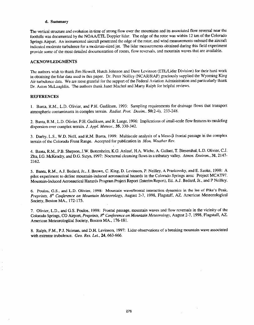
d. Summary

The verticalstructureandevolution in timeof strongflow over the mountainsand itsassociated flow reversalnear thefoothills wasdocumentedby the NOAA/ETL Doppler lidar. The edge of the rotor was within 12 kmof the ColoradoSpringsAirport. An instrumentedaircraftpenetratedthe edge of the rotor,andwindmeasurementsonboardthe aircraftindicatedmoderateturbulencefor a moderate-sizedjet. The lidar measurementsobtainedduringthis fieldexperimentprovidesome of the most detailed documentationof rotors, flow reversals, andmountainwaves that arcavailable.

ACKNOWLEDGMENTS

The authorswish to thankJim Howell, Hutch Johnson andDave Levinson (ETI._idar Division) for theirhardworkin obtainingthe lidardataused in this paper. Dr. Peter Neilley (NCAR/RAP) graciously supplied theWyoming KingAir turbulence data. We are most grateful for the support of the Federal AviationAdministrationand particularly thankDr. Aston McLaughlin. The authors thank Janet Machol and Marty Ralph for helpful reviews.

REFERENCES

1. Banta, R.M., L.D. Olivier, and P.H. Gudiksen, 1993: Sampling requirements for drainage flows that transportatmosphericcontaminantsin complex terrain. Radiat. Prot. Dosim., 50(2-4), 233-248.

2. Banta,R.M., L.D.Olivier, P.H.Gudiksen,andR. Lange, 1996: Implicationsof small-scaleflow featuresto modelingdispersionovercomplex terrain. J. AppL Meteor., 35, 330-342.

3. Darby, L.S., W.D. Neff, andR.M. Banta, 1999: Multiscale analysisof a Meso-[3frontalpassage in' the complexterrainof the ColoradoFront Range. Accepted forpublicationin Mon. Weather Rev.

4. Banta,R.M.,P.B.Shepson,J.W. Bottenheim,K.G. Anlauf,H.A.Wiebe, A. Gallant,T. Biesenthal,L.D. Olivier,C.J.Zhu, I.G.McKendry,andD.G. Steyn, 1997: Nocturnalcleansingflows in atributaryvalley. Atmos. Environ., 31, 2147-2162.

5. Banta,R.M., A.J. Bedard,Jr.,J. Brown, C. King, D. Levinson, P. Neilley, A Praskovsky,andE. Szoke, 1998: Apilot experimentto define mountain-inducedaeronauticalhazards in the ColoradoSpringsarea: Project MCAT97.Mountain-InducedAeronauticalHazardsProgramProjectReport(InterimReport),Ed. A.J. Bedard,Jr., andP Neilley.

6. Poulos, G.S., and L.D. Olivier, 1998: Mountain wave/frontal interactiondynamics in the lee of Pike's Peak,Preprints, 8'h Conference on Mountain Meteorology, August 2-7, 1998, Flagstaff, AZ. American MeteorologicalSociety, Boston MA., 172-175.

7. Olivier, L.D., andG.S. Poulos, 1998: Frontalpassage, mountainwaves andflow reversals in the vicinity of theColoradoSprings,COAirport,Preprints, 8_hConference on Mountain Meteorology, August 2-7, 1998, Flagstaff, AZ.AmericanMeteorologi_:alSociety, Boston MA., 176-181.

8. Ralph, F.M., P.J.Neiman, andD.H. Levinson, 1997: Lidarobservationsof a breakingmountainwave associatedwith extreme trubulence. Geo. Res. Let., 24, 663-666.

276

BISTATIC LASER DOPPLER WIND SENSOR AT 1.5_m

MHarrisElectronicsSector

DefenceEvaluationandResearchAgencyMalvern,WorcestershireWR143PS,U.K.

A coherent laser radar has been built using a MOPA arrangement where the masteroscillator is an external cavity semiconductor laser, and the power amplifier is anerbium-doped fibre amplifier with -1 Watt output. The beams are routed withinsingle-mode optical fibre allowing modular construction of the optical layout withstandard componentsl The system employs separate transmit and receive optics (a"bistatic" configuration), and has sufficient sensitivity for reliable Doppler wind speeddetection under moderate scattering conditions at ranges of order 100m.

The bistatic arrangement leads to a well-defined probe volume formed by theintersection of the transmitted laser beam with the virtual back-propagated localoscillator "beam" (BPLO). This could be advantageous in applications where preciselocalisation of wind speed is required (e.g. wind tunnel studies) or where the presenceof smoke, low cloud or solid objects can lead to spurious signals.

Proper alignment requires that the BPLO and transmit beam foci coincide in space,and this requirement is significantly more troublesome to achieve than in aconventional monostatic lidar. However, the difficulties are greatly mitigated by theuse of optical fibre to define the BPLO receiver mode.

The confinement of the probe volume also leads to a reduction in the signal power. Atheoretical study has been carried out on the reduction in wind signal strength incomparison to the monostatic arrangement, and the results compared withexperimental observation.

277

MEASURING TURBULENCE PARAMETERS WITH COHERENT LIDARSA. Dabas Ph. Drobinski

M6t6o-FranceCNRM/GMEI CNRS Laboratoirede M6t6orologieDynamique42 avenueCoriolis, 31057 Toulouse cedex 1. Ecole Polytechnique

FRANCE 91128 Palaiseau cedexFRANCE.

R. M. Hardesty A. BrewerNOAA Environmental Technology Laboratory NOAA EnvironmentalTechnology Laboratory

325 Broadway 325 BroadwayBoulder, Colorado, 80303 Boulder, Colorado, 80303

USA USA

V. WulfmeyerNCAR Atmospheric Technology Division

P.O. Box 30001850Table Mesa Drive

Boulder, Colorado 80307USA

A mini-campaign was held inDecember 1998near Boulder, Colorado (USA) to validate two high resolution

coherent Doppler lidars, the 10-p,mmini-MOPA lidar developed by NOAA/ETL (Brewer et al., 1997), and the 2-gm

AHRDL@jointly developed by NOAA/ETL and NCAR/ATD (Grund et al., 1997). An automatic weather station from

NCAR/ATD was deployed on the site. With a sonic-anemometer at 5 meters above the ground, the station allowed us

to make direct comparison between lidar and sonic anemometer winds. The results show the various systems reached

a good agreement as far as large-scale wind fluctuations are concerned (e.g., 5 minute-averages of recorded winds).

Regarding short-scale turbulent fluctuations, we show that a proper treatment of lidar data aimed at partially

compensating for the pulse-averaging effect produces wind spectra comparable to the spectra derived from sonic

anemometer data. The possibility of measuring dissipative ratesof turbulent kinetic energy (Mayor et al., 1997;Frehlich

et al., 1998) is thus confirmed.

The results presented below were acquired on December 7, 1998, from 20:27 GMT to 21:25 GMT (13:27 to

14:25 local time). They concern MOPA lidar exclusively (HRDL data are currently under analysis). On that day, the

weather was sunny with no clouds, the thermal stratification was unstable (z/L.-1), and the turbulent activity was rather

strong (u*.20cm s4). The mean wind (5 minute-average) was from the east (80E) at -2.5 ms4. The lidars were staringhorizontally towards the sonic anemometer at a range of 600m. The line-of-sight azimuth was approximately 350E

perpendicular to the mean wind.

Lidars were operated at a repetition rate of 200 pulses per seconds. The processing of radial velocity profiles

was done by pulse-pair-with an accumulation factor of 200, so one profile was produced every second. For the

mini-MOPA, the range incrementbetween retrieved velocities was 15m. The sonic anemometer was operated at a rate

of 20 Hz; it delivered measurements for the three wind components.

Figure 1compares 5 minute-average radial velocities from sonic anemooaeter (dotted line) and mini-MOPA

lidar. For the sonic anemometer, the radial velocity is obtained by projecting the 3D wind vector recorded by the

instrumentonto the lidar line-of-sight.For the mini-MOPA,we considered the rauial velocitymeasured by the instrument

at the range of the sonic anemometer.The figure shows differencesbetween the sensors of less than 20 cm s4. The sonic

anemometer produces a point measurement,whereas the mini-MOPA lidarmeasures the averageof the radialwind inside

the volume illuminated by the pulse (about 90 m long). This at least partially explains the differences.

Figure 2 compares wind spectra derived from the two instruments (light line: MOPA, dark line: sonic

anemometer) obtained by the Fourier transformation of time series. For the mini-MOPA, the time series is formed by

278

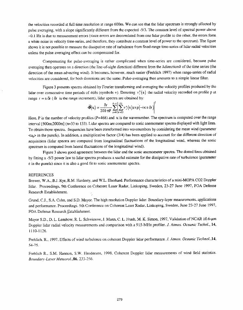
the velocities recorded at full time resolution at range 600m. We can see that the lidar spectrum is stronglyaffected by

pulse averaging, witha slope significantlydifferent from the expected -5/3. The constant level of spectral power above-0.1 Hz is due to measurement errors (since errors are decorrelated from one lidar profile to the other, the errors form

a white noise in velocitytime-series, and therefore, they contribute a constant level of power to the spectrum). The figure

shows it is not possible to measurethe dissipative rate of turbulencefrom fixed-rangetime-seriesof lidar radial velocities

unless the pulse averaging effect can be compensated for.

Compensating for pulse-averaging is rather complicated when time-series are considered, because pulse

averaging then operates on a direction (the line-of-sight direction) different from the Adirection@of the time series (the

direction of the mean advecting wind). It becomes, however, much easier (Frehlich 1997) when range-series of radial

velocities are considered, for both directions are the same. Pulse-averaging then amounts to a simple linear filter.

Figure 3 presents spectra obtained by Fourier transtbrming and averaging the velocity profiles produced by the

lidar over consecutive time periods of 468s (symbols +). Denoting v_(n) the radial velocity recorded on profile p at

range r = n& (& is the range increment), lidar spectra are obtained by:P-I I 13_ 2

rv

_q(K)=_ZZ :(n)exp(-iKn&)..... p=0 n=33

Here, P is the number of velocity profiles (P=468) and 1<is the wavenumber.The spectrum is computed over the range

interval[500m;2000m](n=33 to 133).Lidar spectra are compared to sonic anemometerspectra displayed with light lines.

To obtain those spectra, frequencieshavebeen transformed into wavenumbers byconsidering the mean wind(parameter

<uh> in the panels). In addition, a multiplicative factor (3/4) has been applied to account for the different direction of

acquisition (lidar spectra are computed from longitudinal fluctuations of the longitudinal wind, whereas the sonic

spectrum is computed from lateral fluctuations of the longitudinal wind).

Figure 3 showsgood agreement between the lidar and the sonic anemometer spectra.The dotted linesobtained

by fitting a -5/3 power law to lidar spectra produces a useful estimate for the dissipative rate of turbulence (parameter

in the panels) since it is also a good fit to sonic anemometer spectra.

REFERENCES

Brewer,W.A., B.J. Rye, R.M. Hardesty, and W.L. Eberhard. Performancecharacteristicsof a mini-MOPA CO2 Doppler

lidar. Proceedings, 9th Conference on Coherent Laser Radar, Linkoping, Sweden, 23-27 June 1997, FOA DefenseResearch Establishment.

Grund, C.J., S.A. Cohn, and S.D: Mayor. The high resolutionDoppler lidar: Boundary-layermeasurements,applications

and performance. Proceedings. 9th Conference on Coherent Laser Radar, Linkoping, Sweden, June 23-27 June 1997,

FOA Defense Research_.Establishment.

Mayor S.D., D. L. Lenshow,R. L. Schwiesow,J. Mann, C. L. Frush, M. K. Simon, 1997, Validation of NCAR 10.6-p.m

Doppler lidar radial velocity measurements and comparison with a 915-MHz profiler. J. Atmos. Oceanic Techol., 14,11!0-1126.

Frehlich. R., 1997, Effects of wind turbulence on coherent Doppler lidar performance. J. Aonos. Oceanic Technol.,14,54-75.

Frehlich R., S.M. Hannon, S.W. Henderson, 1998, Coherent Doppler lidar measurements of wind field statistics.

Boundat3,-l_xtyerMeteorol.,86. 233-256.

279

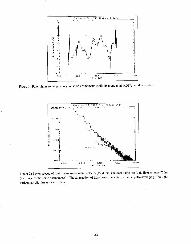
December 07, 1998. Horizontal stare,

2!- A

>, ,

_oI •

20.0 20.5 21.0 21.5 22,0Time (GMT)

Figure 1 :Five-minute running average of sonic anemometer (solid line) and mini-MOPA radial velocities.

December 07, 1998, from 20.5 to 21.0

,°°°°°FT'_.... . ......., ........, .......F10.000 F

1.000 i ""_

0.100 _ ..".,, ,_

O.OlO_-E

0.0010.001 0.0!0 0.100 !.000 10.00(

:requency (Hz)

Figure 2 :Power spectra of sonic anemometer radial velocity (solid line) and lidar velocities (light line) at range 750m

(the range of the sonic anemometer). The attenuation of lidar power densities is due to pulse-averaging. The lighthorizontal solid line is the error level.

280

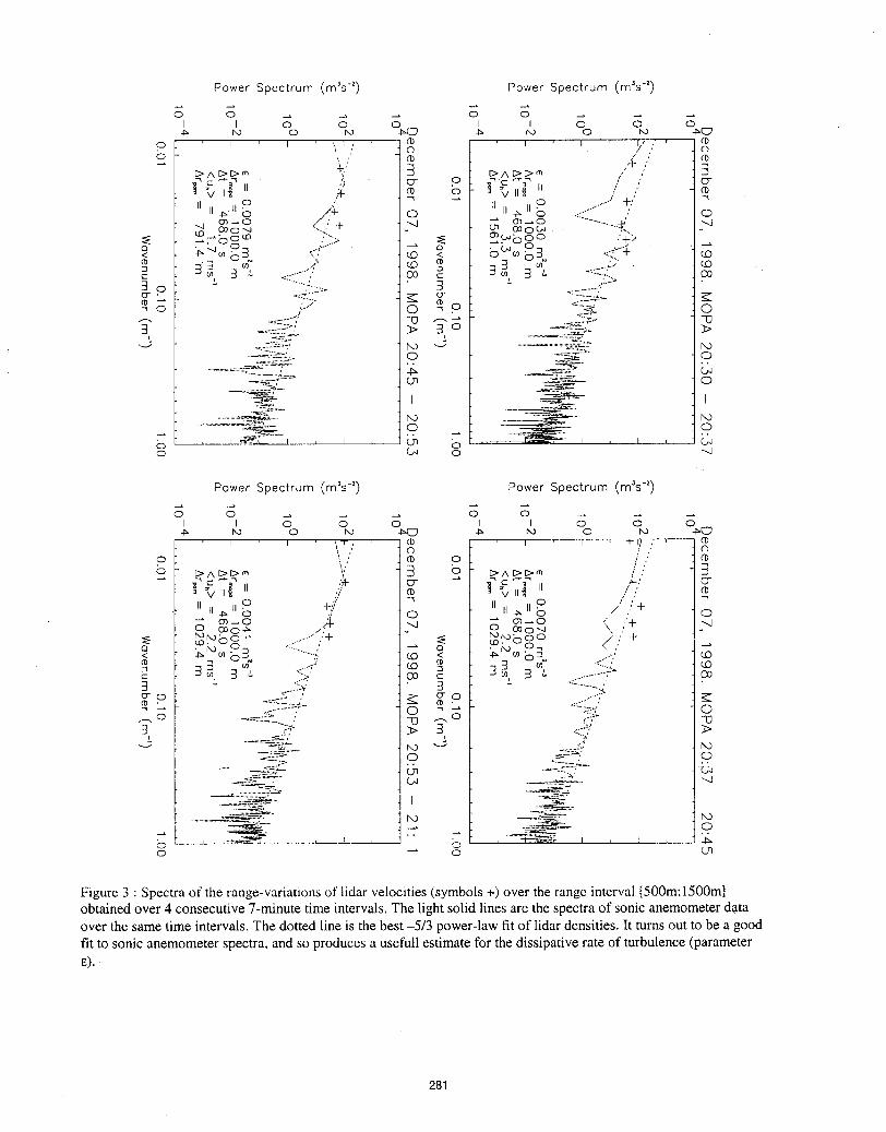
Power Spectrum (mJs") Power Spectrum (mJs-')

Power Spectrum (mJs-') Power Spectrum (m's-') 2 2 2 A

0 0 2 A 2 0 0

Figure 3 : Spectra of the range-variations of lidar velocities (symbols +) over the range interval [500m:1500ml obtained over 4 consecutive 7-minute time intervals. The light solid lines are the spectra of sonic anemometer data over the same time intervals. The dotted line is the best -513 power-law fit of lidar densities. It turns out to be a good tit to sonic anemometer spectra. and so produces a useful1 estimate for the dissipative rate of turbulence (parameter E).

ABSTRACT

The Prediction of the Doppler Measurement Accuracy Using a Priori Information About theTurbulent AatmosphereAlexander P. Shelekhov, Alexei L. Afanas'ev, Institute of Atmospheric Optics, SB RussianAcademy Science, Russian FederationThe accuracyof the Dopplerfrequencymeasurementof the parametersof the turbulentatmosphereis studiedfor the casesof the stable,unstable,and indifferentstratification.Thetheoreticalpredictionof the Dopplermeasurementaccuracyisbasedon the turbulentatmospheremodelsof Kaimal and Palmer.

282

SPACEBORNE LIDARS- 2

Presiders: Kasuhiro Asai and David Willetts

283

SPARCLE Optical System Design and OperationalCharacteristics

Farzin Amzajerdian, Bruce R. Peters, Ye Li, Timothy S. Blackwell, and Patrick ReardonCenter for Applied Optics

The University of Alabama in HuntsvilleHuntsville, AL 35899

Phone: (205) 890-6030, Fax: (205) 890-6618, E-mail: farzin.a@msfc.nasa.gov

INTRODUCTION

The SPAce Readiness Coherent Lidar Experiment (SPARCLE) is the fkst demonstration of a coherentDoppler wind lidar in space. SPARCLE will be flown aboard a space shuttle in the middle part of 2001 as astepping stone towards the development and deployment of a long-!ife-timeoperational instrument in thelater part of next decade. SPARCLE is an ambitious project that is intended to evaluate the suitability ofcoherent lidar for wind measurements, demonstrate the maturity of the technology for space application,and provide a useable data set for model development and validation. This paper describes theSPARCLE's optical system design, fabrication methods, assembly and alignment techniques, and itsanticipated operational characteristics.

Coherent detection is highly sensitive to aberrations in the signal phase front, and to relative alignmentbetween the signal and the local oscillator beams. Consequently, the performance of coherent lidars isusually limited by the optical quality of the transmitter/receiver optical system. For SPARCLE having arelatively large aperture (25 cm) and a very long operating range (400 km), compared to the previouslydeveloped 2-micron coherent lidars, the optical performance requirements are even more stringent. Inaddition with stringent performance requirements, the physical and environment constraints associatedwith this instrument further challenge the limit of optical fabrication technologies.

DESCRIPTION OF OPTICAL SYSTEM

The functions of the optical system include expanding the laser beam, directing it to the atmosphere in aconical scan pattern, receiving the backscattered radiation, while maintaining a highly accurate pointingto ensure adequate extraction of the Doppler frequency shift due to the spacecraft and earth rotationvelocities. The optical system consists of a beam expanding telescope, an optical wedge scanner, and anoptical widow used for environmentally isolating the lidar instrument. Figure 1 provides an opticalschematic showing various optical components. As shown in this figure, two mirror assemblies are usedfor providing the proper alignment between the [idar transceiver and the telescope. The telescopeexpands the transmitter beam by 25X and directs it to an optical wedge that deflects the beam by 30degrees. The wedge is rotated by a precision motor/encoder assembly in a step-stare fashion, to provide aconical pattern in the atmosphere. Compared with continuous scanning, step-stare scanning provides agreater operational flexibility, by allowing different scan patterns and laser shot accumulation. Step-starescanning also eliminates the need for a dynamic lag angle compensator for correcting the signalmisalignment due to the continuous motion of the scanner, thus reducing the complexity and cost of theinstrument's optical system. The scanner wedge is then followed by a high optical quality window thatprovides the lidar optical interface with space. The optical window is made of fused silica with a ruggedanti-reflection coating for efficiently transmitting 2-micron wavelength radiation. Both the transmittedbeam and the backscattered laser radiation from the atmosphere follow the same path to the lidartransceiver.

284

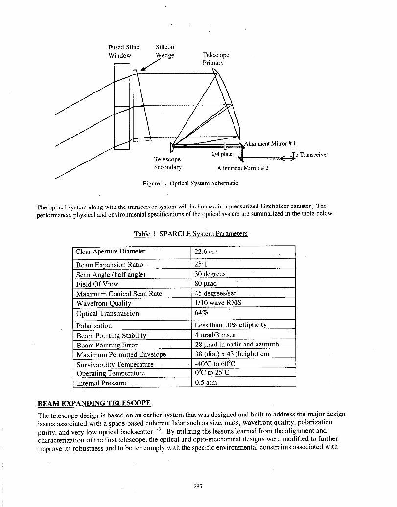
FusedSilica SiliconWindow Wedge Telescope

J Primary

11

Alignment Mirror # 1

X/4 plate TransceiverTelescopeSecondary Ali_,nmentMirror# 2

Figure1. OpticalSystemSchematic

The optical system along with the transceiver system will be housed in a pressurized Hitchhiker canister. Theperformance,physicalandenvironmentalspecificationsof the opticalsystemare summarizedin the tablebelow.

Table 1. SPARCLE System Parameters

Clear Aperture Diameter 22.6 cm

Beam Expansion Ratio : 25:1

Scan Angle (half angle) 30 degeesField Of View 80 gradMaximum Conical Scan Rate 45 degrees/sec

Wavefront Quality 1/10 wave RMS

Optical Transmission 64%

Polarization Less than 10%ellipticity

Beam Pointing Stability 4 grad/3 msecBeam Pointing Error 28 grad in nadir and azimuthMaximum Permitted Envelope 38 (dia.) x 43 (height) cm

Survivability Temperature -40°C to 60°COperating Temperature 0°C to 25°CInternal Pressure 0.5 atm

BEAM EXPANDING TELESCOPE

The telescope design is based on an earlier systemthatwas designedandbuilt to addressthe major designissues associatedwith a sPace-based coherent lidar such as size, mass,wavefront quality,polarizationpurity,andvery low opticalbackscatter_3, By utilizing the lessons learnedfrom the alignment andcharacterizationof the first telescope, the opticalandopto-mechanicaldesigns were modified to furtherimproveits robustness andto better comply with the specific environmentalconstraintsassociatedwith

285

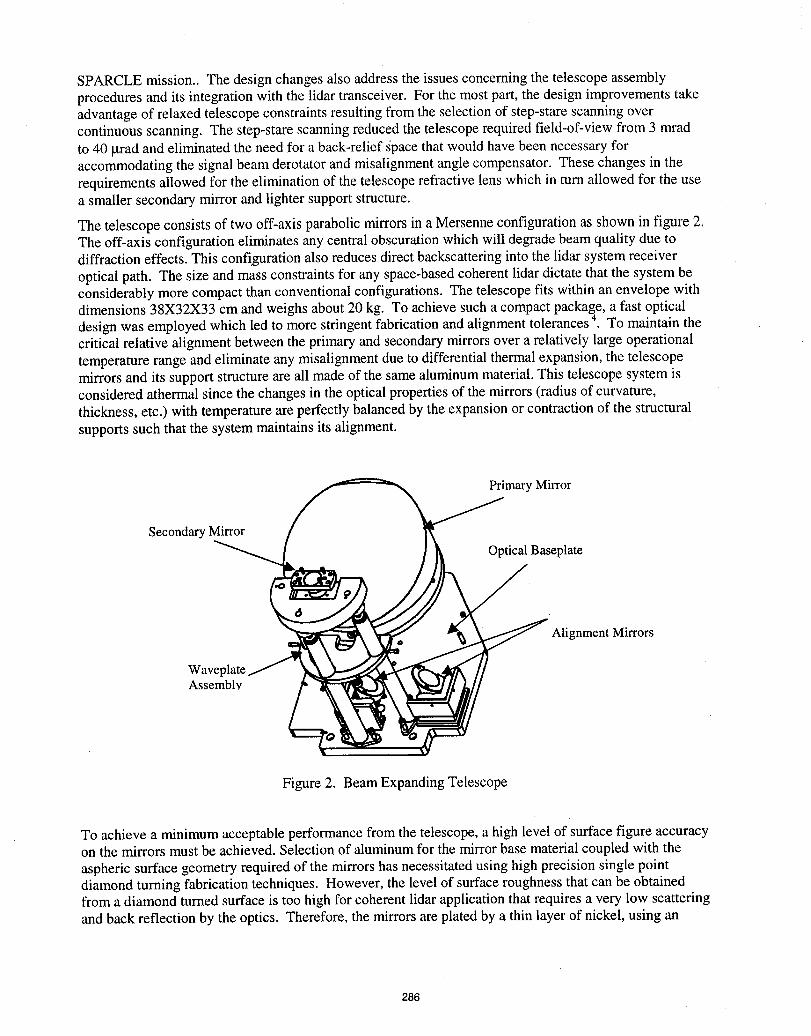
SPARCLE mission.. The design changes also address the issues concerning the telescope assemblyprocedures and its integration with the lidar transceiver. For the most part, the design improvements takeadvantage of relaxed telescope constraints resulting from the selection of step-stare scanning overcontinuous scanning. The step-stare scanning reduced the telescope required field-of-view from 3 mradto 40 grad and eliminated the need for a back-relief space that would have been necessary foraccommodating the signal beam derotator and misalignment angle compensator. These changes in therequirements allowed for the elimination of the telescope refractive lens which in turn allowed for the usea smaller secondary mirror and lighter support structure.

The telescope consists of two off-axis parabolic mirrors in a Mersenne configuration as shown in figure 2.The off-axis configuration eliminates any central obscuration which will degrade beam quality due todiffraction effects. This configuration also reduces direct backscattering into the lidar system receiveroptical path. The size and mass constraints for any space-based coherent lidar dictate that the system beconsiderably more compact than conventional configurations. The telescope fits within an envelope withdimensions 38X32X33 cm and weighs about 20 kg. To achieve such a compact package, a fast opticaldesign was employed which led to more stringent fabrication and alignment tolerances 4. To maintain thecritical relative alignment between the primary and secondary mirrors over a relatively large operationaltemperature range and eliminate any misalignment due to differential thermal expansion, the telescopemirrors and its support structure are all made of the same aluminum material. This telescope system isconsidered athermal since the changes in the optical properties of the mirrors (radius of curvature,thickness, etc.) with temperature are perfectly balanced by the expansion or contraction of the structuralsupports such that the system maintains its alignment.

Primary Mirror

Secondary Mirror

Optical Baseplate

Alignment Mirrors

Waveplate.Assembly

Figure 2. Beam Expanding Telescope

To achieve a minimum acceptable performance from the telescope, a high level of surface figure accuracyon the mirrors must be achieved. Selection of aluminum for the mirror base material coupled with theaspheric surface geometry required of the mirrors has necessitated using high precision single pointdiamond turning fabrication techniques. However, the level of surface roughness that can be obtainedfrom a diamond turned surface is too high for coherent lidar application that requires a very low scatteringand back reflection by the optics. Therefore, the mirrors are plated by a thin layer of nickel, using an

286

electroless plating technique, before finish diamond machining. The nickel-plated mirrors are then post-polished to reduce their surface roughness to an acceptable level. Finally, the mirrors are coated withgold to achieve a high surface reflectivity approaching 99%.

OPTICAL WEDGE SCANNER

The lidar scanning is achieved by a 24.7 cm rotatingsilicon wedge thatprovides a 30 degree deflectionangle. Selection of silicon as the wedge materialwas mainlydrivenby its manydesirableoptical andphysical propertiesandthe fact thatsufficiently largesilicon crystals with a single phase domaincould begrown andpolished. Because of the high index of refractionof silicon (n=3.45),the requireddeflectionanglecan be achieved by a relatively small wedge angle of 11.7 degreeswhich limits the mass of thewedge to about4 kg. The opticalwedge mass was one of the criticalconsiderations,since it directlyaffects the power drawn by the scanner motor which resultsin more heat. One of the criticalissuesassociatedwith the opticalwedge that neededto be addressedwas its sensitivityto the radialtemperatureprofile that will be generatedby the hot scanner motor andthe wedge cold surroundings. Radialtemperaturevariationsin the wedge can produce a wavefronterror due its non-symmetricalshape anditshigh dn/dT (change in indexof refraction with temperature)value. To improvethe thermalpropertiesofthe optical wedge, a rnultilayercoating is designed thatcan effectively reject anyradiationin the solar andfar-infrared regions of spectrumwhile efficiently transmittingthe lidarbeamat 2-micronwavelength. Inthis way, the wedge can be thermally decoupledfrom the surroundingenvironment,allowed to reachthermal equilibriumquicker, andtherebyminimize the impactof dn/dTby reducingthermal gradientswithin the wedge.

OPTICAL WINDOW

The lidar instrument is environmentallyisolatedby a 5 cm thick, 32 cm diameteropt!calwindow madeoffused silica. The maindesign considerationsassociatedwith the optical windoware: (1) wavefrontdistortiondue to the windowsubstratedeformationunderdifferentialpressureconditionin space; (2) de-polarization due to stress-inducedbirefringence;(3) wavefrontdistortiondueto anyspatial temperaturevariationthat may be present within the windowmaterial; and (4) Rejectionof solarradiationfor betterthermal environmentinside the canister. The opticalwindow has a multilayercoating for hightransmission at 2-micron wavelengthand high reflection overthe visible region of the spectrum.

This work was supported by NASA Marshall Space Flight Center through a cooperative agreement withThe University of Alabama in Huntsville at the Center for Applied Optics.

REFERENCES

I. Feng, A. Ahmad andF. Amzajerdian, "Design andanalysisof a spacebome lidartelescope," Proc.SPIE Vol. 2540, pp. 68-77,1995.

2. A. Ahmad,F. Amzajerdian,C. Feng andY. Li, "Design andfabricationof a compact lidar telescope,"Proc. SPIE Vol. 2832, pp. 34-42, 1996.

3. Li, Ye; Blackwell, Timothy S.; Geary, Joseph M.; Amzajerdian,Farzin;Spiers, GaryD.; Peters,Bruce R.; Chambers, Diana,"Characterizationof an optical subsystem for 2-um coherent lidars,"Proc. SPIE Vol. 3479, p. 122-1:9.

4. Peters, Bruce R.; Blackwell, Timothy S.; Li, Ye; Geary,Joseph M.; Amzajerdian,Farzin;Bailey,Deborah, "Optomechanicaldesign of a multi-axisstagefor the SPARCLEtelescope," Proc. SPIEVol. 3429, p. 48-55.

287

Optical Design and Analyses of SPARCLE Telescope

Ye Li, FarzinAmzajerdian,BrucePeters,Tim Blackwell, PatReardonCenterforAppliedOptics

University of Alabamain HuntsvilleHuntsville,AL 35899

Phone: (205) 890-6030, Fax:(205) 890-6618, E-mail:liy@email.uah.edu

1. Introduction

NASA SPace Readiness Coherent Lidar Experiment(SPARCLE) is a technology demonstrationon thespace shuttle for space-based Doppler coherent iidar atmosphericwind velocity measurement [1]. Theoptical telescope system includes a 25cm off-axis beam expanding telescope, a 25-cm silicon wedgescanner,and a 32-cm Fused Silica optical window.The 2.0 micronswavelength laser source is expandedwith this optical systemat a power of 25x and transmittedto the atmosphereat a conical scanningangle of30 degrees. The optical system also serves as receiver for the back scattered radiationsignal from theatmosphere.Coherent laser radarrecordsinformationaboutthe phase of the back-scatteredradiationwith respect to alocal referenceor local oscillator.The phase of the light contains information about the Doppler shiftedmean frequency, frequencyspectrum, and polarizationof the photons. The wind velocity information,which is the main interestof SPARCLE,is encoded in the mean frequency.The signal-to-noise ratio ofcoherent lidarsystem is very sensitive to the opticalperformanceof the transmittingandreceiving.beams.The majordesign issues for coherent detection lidar are the way€frontquality,polarizationpurity, and aminimum backscatteringfrom the optical surfaces. Eliminatingoptical degradationsfrom thermal effectson the mechanical structureand the optical componentsis also critical for the space-based coherent lidarsystem. In orderto obtain a diffraction limited optical system, the optical fabricationtechnologies andtolerances,optical testing capabilities, and alignmentsensitivities have to all be considered in the designphase to make surethat theopticalsystemcan be physicallyproduced.The SPARCLE telescope system was designed based on lessons learnedfrom the prototypetelescope[2],and employing state-of-the artoptical fabricationtechnologies. These technologies include: utilizing theLarge Optics DiamondTurningMachine (LODTM) at LawrenceLivermoreNational Lab for the primarymirror fabrication, primary mirror post polishing at Space Optics Research Labs (SORL), Laser goldplatingof the mirrorsat EpnerTechnology, opticalwindow andsilicon wedge multi-layercoatingsforhightransmission at 2-micronandhigh reflectionof solarandIRradiationat Diversified OpticalProductsInc..

2. Optical Design

2.1 Beam Expanding TelescopeThe volume of the optical canisteron the space shuttle and the step-starescanning technique used bySPARCLE constrained us to choose a two paraboloid afocal Mersenne configuration as the beamexpanding telescope. The off-axis beam expanderwas selected to eliminate the central obscuration andback scatteringof an on-axis system which would degradethe heterodynemixing efficiency and signal tonoise ratio. The all reflective optical components can be built with the same aluminum alloy as themechanical structureseliminatedifferentialthermal expansiondueto differentmaterials.The diffraction limitedbeam expanderwas designed andmodeled by using ZEMAX optical software andverified by using SYNOPSYS optical software with a full field of view of 80 micro-radians,angularmagnification of 25x, and a primary mirror aperture of 25 cm. The optical spacing between the primary andsecondary mirror is 22.5 cm with a primary mirror operating at F#/0.9 and a de-center of 15 cm. Theoptical 3D layout is Shownin Figure 1. In addition, a small optical flat with a width of 7 mm was designedon the outer radial edge of the primary mirror as a reference for optical fabrication, testing and systemintegration. The secondary mirror has a physical aperture of 3 cm with a symmetric shape to ease theoptical fabrication and optical alignment stage. A portion of the mirror at 6 mm off-axis is used fordelivering the laser beam. The backside of the secondary mirror was designed to have an optical flat

288

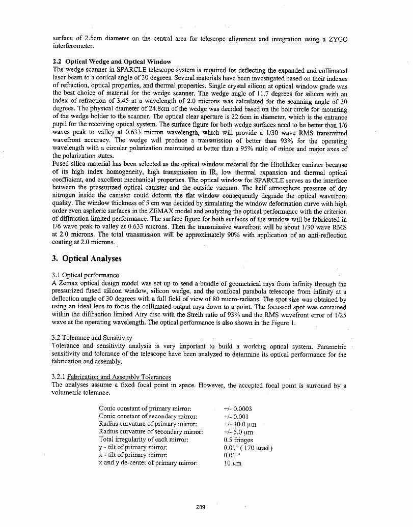
surface of 2.5cm diameter on the central area for telescope alignment and integration using a ZYGOinterferometer.

2.2 Optical Wedge and Optical WindowThe wedge scanner in SPARCLE telescope system is required for deflecting the expanded and collimatedlaser beam to a conical angle of 30 degrees. Several materials have been investigated based on their indexesof refraction, optical properties, and thermal properties. Single crystal silicon at optical window grade wasthe best choice of material for the wedge scanner. The wedge angle of 11.7 degrees for silicon with anindex of refraction of 3.45 at a wavelength of 2.0 microns was calculated for the scanning angle of 30degrees. The physical diameter of 24.8cm of the wedge was decided based on the bolt circle for mountingof the wedge holder to the scanner. The optical clear aperture is 22.6cm in diameter, which is the entrancepupil for the receiving optical system. The surface figure for both wedge surfaces need to be better than 1/6waves peak to valley at 0.633 micron wavelength, which will provide a 1/30 wave RMS transmittedwavefront accuracy. The wedge will produce a transmission of better than 93% for the operatingwavelength with a circular polarization maintained at better than a 95% ratio of minor and major axes ofthe polarization states.Fused silica material has been selected as the optical window material for the Hitchhiker canister becauseof its high index homogeneity, high transmission in IR, low thermal expansion and thermal opticalcoefficient, and excellent mechanical properties. The optical window for SPARCLE serves as the interfacebetween the pressurized optical canister and the outside vacuum. The half atmosphere pressure of drynitrogen inside the canister could deform the flat window consequently degrade the optical wavefrontquality. The window thickness of 5 cm was decided by simulating the window deformation curve with highorder even aspheric surfaces in the ZEMAX model and analyzing the optical performance with the criterionof diffraction limited performance. The surface figure for both surfaces of the window will be fabricated in1/6 wave peak to valley at 0.633 microns. Then the transmissive wavefront will be about 1/30 wave RMSat 2.0 microns. The total transmission will be approximately 90% with application of an anti-reflectioncoating at 2.0 microns.

3. Optical Analyses

3.1 Optical performanceA Zemax optical design model was set up to send a bundle of geometrical rays from infinity through thepressurized fused silicon window, silicon wedge, and the confocal parabola telescope from infmity at adeflection angle of 30 degrees with a full field of view of 80 micro-radians. The spot size was obtained byusing an ideal lens to focus the collimated output rays down to a point. The focussed spot was containedwithin the diffraction limited Airy disc with the Strelh ratio of 93% and the RMS wavefront error of 1/25wave at the operating wavelength. The optical performance is also shown in the Figure 1.

3.2 Tolerance and SensitivityTolerance and sensitivity analysis is very important: to build a working optical system. Parametricsensitivity and tolerance of the telescope have been analyzed to determine its optical performance for thefabrication and assembly.

3.2.1 Fabrication and Assembly TolerancesThe analyses assume a fixed focal point in space: However, the accepted focal point is surround by avolumetric tolerance.

Conic constant of primary mirror: +/- 0.0003Conic constant of secondary mirror: +/- 0.001Radius curvature of primary mirror: +/- 10.0 gmRadius curvature of secondary mirror: +/- 5.0 pmTotal irregularity of each mirror: 0.5 fringesy - tilt of primary mirror: 0.01 ° ( 170 gradx - tilt of primary mirror: 0.01 °

x and y de-center of primary mirror: !0 gm

289

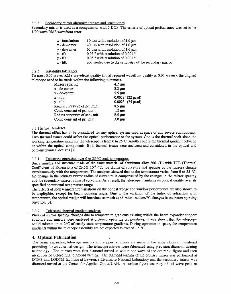
3.2.2 SecondarymirroralignmentrangesandsensitivitiesSecondary mirror is used as a compensator with 5 DOF. The criteria of optical performance was set to be1/20 wave RMS wavefront error.

z - translation: 10 _tmwith resolution of 1.0 gmx - de-center: 40 gm with resolution of 1.0 gmy - de-center: 65 gm with resolution of 1.0 gmx - tilt: 0.05 owith resolution of 0.001 oy - tilt: 0.05 owith resolution of 0.001 °z - tilt: not needed due to the symmetry of the secondary mirror

3.2.3 Instability tolerancesTo meet 0.05 waves RMS wavefront quality (Final required wavefront quality is 0.07 waves), the alignedtelescope need to be stable within the following tolerances.

Mirrors spacing: 4.2 gmx - de-center: 8.2 gmy - de-center: 5.5 gmx - tilt: 0.0013° (22 grad)y - tilt: 0.002° (35 _trad)Radius curvature ofpri, mir.: 8.5 gmConic constant ofpri, mir.: 1.2 gmRadius curvature of see.. mir.: 8.5 gmConic constant ofpri, mir.: 3.0 gm

3.3 Thermal AnalysesThe thermal effect has to be considered for any optical system used in space or any severe environment.Two thermal issues could affect the optical performance to the system. One is the thermal soak since theworking temperature range for the telescope is from 0 to 25°C. Another one is the thermal gradient betweenor within the optical components. Both thermal issues were analyzed and considered in the optical andopto-mechanical designs [3].

3.3.1 Telescope operation over 0 to 25 °C soak temperaturesSince mirrors and structure made of the same material of aluminum alloy 6061-T6 with TCE (ThermalCoefficient of Expansion) of 23.5X 10 -6/°C, the raidius of curvature and spacing of the mirrors changesimultaneously with the temperature. The analyses showed that as the temperature varies from 0 to 25 °C,the change in the primary mirror radius of curvature is compensated by the changes in the mirror spacingand the secondary mirror radius of curvature. As a result, the telescope maintains its optical quality over itsspecified operational temperature range.The effects of soak temperature variations on the optical wedge and window performance are also shown tobe negligible, except for beam pointing angle. Due to the variation of the index of refraction withtemperature, the optical wedge will introduce as much as 45 micro-radians/°C changes in the beam p0.intingdirection [3].

3.3.2 Telescope thermal gradient analysesPhysical mirror spacing changes due to temperature gradients existing within the beam expander supportstructure and mirrors were analyzed at different operating temperatures. It was shown that the telescopecould tolerate up to 2°C of steady state temperature gradients. During operation in space, the temperaturegradients within the telescope assembly are not expected to exceed 1.5 °C.

4. Optical FabricationThe beam expanding telescope mirrors and support structure are made of the same aluminum materialproviding for an athermal design. The telescope mirrors were fabricatedusing precision diamond turningtechnology. The mirrors were first diamond ttmaed to within one wave of the desirable figure and thennickel plated before final diamond turning. The diamond turning of the primary mirror was performed atDTM3 and LODTM facilities at Lawrence Livermore National Laboratory and the secondary mirror wasdiamond turned at the Center for Applied Optics/UAH. A surface figure accuracy of 1/4 wave peak to

290

valley at HeNe wavelength and a surface f'mish of about 150 angstroms RMS were achieved for eachmirror. Post-polishing the mirrors is expected to achieve a surface finish of better than 25 angstroms and afinal surface figure of about 1/6 wave P-V at HeNe. The polished mirrors will be plated with high purity ofgold to increase the reflectivity to 98.5% at 2.0 microns wavelength.High purity Fused Silica and single crystal silicon will be used to fabricate the optical window and opticalwedge scanner at DIOP. The optical surfaces will be polished to a figure accuracy of 1/6 wave peak tovalley at HeNe. Due to thermal gradient effects on the window and wedge, a special coating will be appliedto increase solar reflection and reduce mid-IR radiation transfer between the optical components. The

coatings are also required to have better than 90% transmission at 2.0 wavelength and maintain circularpolarization to within 10%.

References:1. M.J. Kavaya, G.D. Emmitt, "The Space Readiness Coherent Lidar Experiment (SPARCLE)

Space Shuttle Mission," Proc. SPIE Vol. 3380, Conference on Laser Radar Technology andapplication III, 12mAnnual International Symposium on Aerospace/Defense Sensing, Simulation,and Controls, AeroSense, Orlando, FL, 1998.

2. A. Ahmad, C. Feng, F. Amzajerdian, Y. Li "Design and Fabrication of a Compact LIDARTelescope", Proc. SPIE Vol. 2832, Denver, CO August 4-9, 1996.

3. P.J. Reardon, B.R. Peters, F. Amzajerdian, "Thermal Considerations for the SPARCLE OpticalSystem," SPIE Proc. 3707, Orlando, FL., April 6-9, 1999.

291

A program of an ISS/JEM (Japanese Experiment Module)- borne Coherent Doppler Lidar

Toshikazu Itabe. Kohei Mizutani, Mitsuo Ishizu# and Kazuhiro Asai*

Communications Research Laboratory

Ministry of Posts and TelecommunicationsNukui-kita, 4-2-l, Koganei, Tokyo 184-8795, JAPAN

Tel;+81-42-327-7546, Fac:+81-42-3276692

E-mail : itabe @crl.go.jp,mizutani @crl.go.jp

# Electronic and Information Technology Lab.Office of Research and Development

NASDA

2-I-1 ,Sengen,Tsukuba, Ibaragi, 305-0047, JAPANE-mail : Ishizu.Mitsuo @nasda.go.jp

*Tohoku Institutes of Technology

Yagiyama Kasumi 35-1 , Taihaku-Ku, Sendai 982-, JAPANE-mail : asai @titan.tohtech.ac.jp

1. Introduction

Global wind measurement, more precisely speaking global horizontal wind, is crucially important for bothNumerical Weather Prediction and studies on the global climate. Temperature and humidity profiles and surface

pressure in addition to the wind profile are needed for the initial state condition for the Numerical WeatherPrediction and the global climate model. The wind profiles are now available only from a global network of radiosonde observations at the ground. Very little information about the vertical profiles of the horizontal wind field isavailable from the ocean, in the tropics and in the Southern Hemisphere. If the present data deficiency of the globalwind could be solved, the Numerical Weather Prediction and the global climate model will be improved dramatically.

Now, global measurement of the wind profile in the troposphere can be realized only with the Doppler lidar in space.A program of Japan for development of the coherent Doppler lidar in space was started by Communications

Research Laboratories (CRL) from 1997 FY under the support of the Phase II study of Ground ResearchAnnouncement of NASDA and Japan Space Forum. Objective of the program is to make a feasibility study of thecoherent Doppler lidar tbr Japanese Exposure Module (JEM) of the International Space Station. The coherentDoppler lidar will be design to install in a standard EF(Exposed Facility) payload of ISS/JEM and the mission of thelidar is made a demonstration of the wind measurements form space. The ISS/JEM-borne coherent Doppler lidar

(JEM/CDL) can measure line-of-sight (LOS) winds in the troposphere from space in the accuracy of 1-2 m/s in thevertical resolution of about I km and the horizontal resolution I00km xl00km

There are two methods to measure the atmospheric wind with the Doppler lidar from space. One of them is a

coherent Doppler and another an incoherent one. Size of the incoherent Doppler lidar is not suitable for theISS/JEM. We consider the coherent Doppler one as only one candidate tbr ISS/JEM.

2. A Coherent Doppler Lidar tbr ISS/JEMISS/JEM-CDL will be packed in one of standard payloads of the JEM-EF (Exposed Facility), which is1850 x I000

x 800. JEM/CDL is now under the feasibility study. Present parameters of the coherent Doppler lidar are shown intable I.

Table 1 Parameters of [SS/JEM-borne CDL

Transmitting Laser Tm.Ho:YLF (X:2.06_tm), Osc.-Amp. LaserOutput 2 JouleRepetition 10pps

292

Wall-plug.efficeincy over 2% (Electrical-optical efficiency)

Transmitting Telescope off-axis Diameter 40cm

Scanning Step Scanningunder study of two methods

l) Si-wedge scannerwith one telescope

2) side-scanning withtwo telescopes

Scanning method will be selected one of them. The Si-wedge scanner is the same one of the SPARCLE of NASA.The side-scanning is used two telescopes. One of the telescopes of the side-scanning will be installed to look forwardat the angle of 60 degrees from the direction of ISS movement and another to look backward at the same angle. Theboth telescopes will be step-swinged form 6 degrees to 30 degrees around the direction of ISS movement. Now,trade-off study is under way.

LOS wind error is estimated by using an equation of the poly-pulse pair algorithm (Zrnic,1979, Kane, 1984). Thelidar parameters shown in table 1 and total optical efficiency including the heterodyne efficiency is assumed as 0.04.The following aerosol height profiles is used in the studies of the LOS wind error of JEM/CDL.

Table 2 aerosol height profile [3(z)tbr the studies the LOS wind error

Height aerosol height profile [3(z)

02 km 2x 108(1/m/str)25 km lxl0"8(1/rn/str)512 km 8xl09(1/m/str)

Results of the LOS wind error estimation will described at the conference.

The following key technologies in addition to a conceptual design of the iidar of JEM will be described also at theconference in some detail.

(1) 2fi-mTm,Ho:YLF laser with 2 joule 10Hz slaved by a frequency stabilized CW laser.(2) scanning mechanism with 40cm diameter telescope.(3) a coherent detection system, which can compensate Doppler shift due to spacecraft velocity.

3. Concluding remarksA program of Japan fg_rdevelopment of the coherent Doppler lidar in space was started by CRL from 1997 FY

under the support of the Phase II studies of the Ground Research Announcement of NASDA. Objective of theprogram is to make a feasibility study on the coherent Doppler lidar for the Japanse Exposure Module (JEM) of theInternational Space Station (ISS). The ISS/JEM-borne coherent Doppler lidar can measure tropospheric LOS windsfrom space' in an accuracy to 1-2 m/s of the vertical resolution of about 1 km and the horizontal resolution100kmx100km. Results of the feasibility study will be used for a proposal of 2ed JEM mission.

ReferancesKane T. J.. B. Zhou and R. L. Byer,!984, Potential for coherent Doppler wind velocity lidar using neodymiun laser,Appl. Opt., 31,4202-4213.Zrnic D. S.,1979, Estimation of spectral moments for weather echoes, IEEEE Trans. Geosci. Electron., GE-17, 113-128.

293

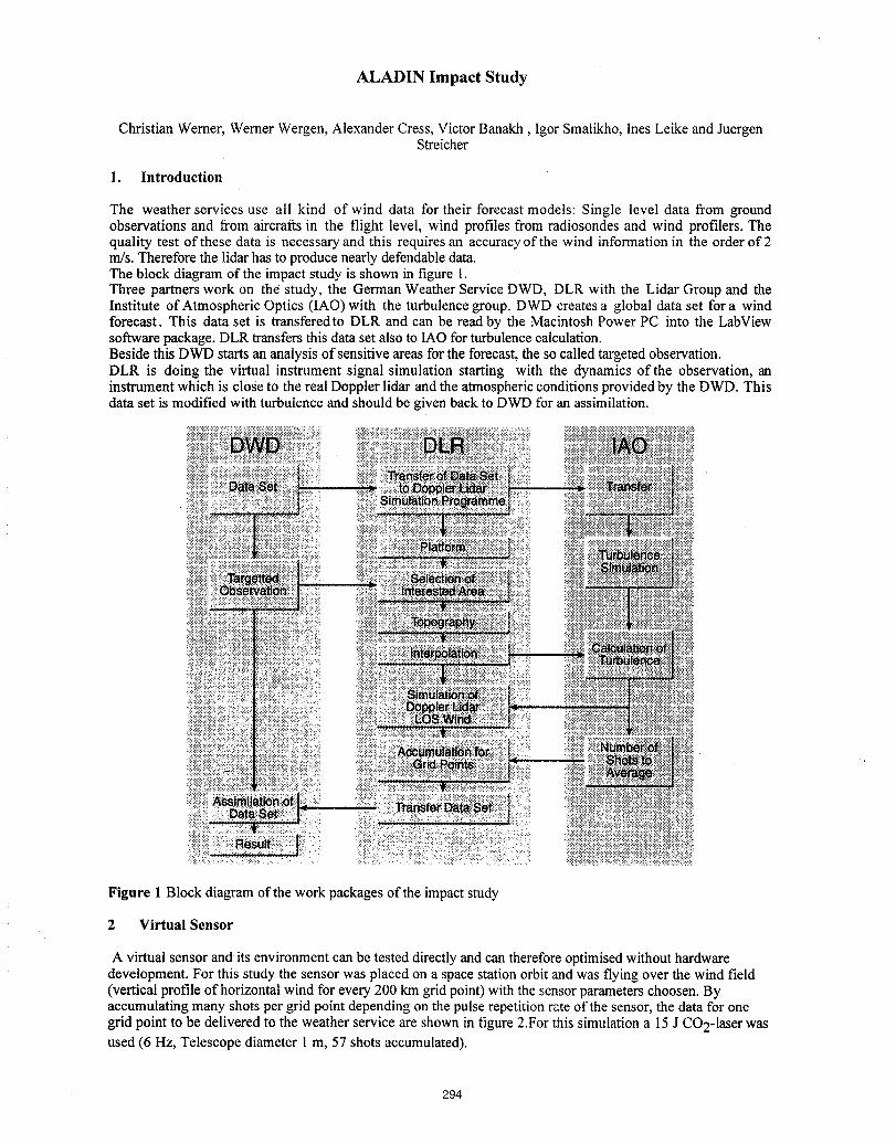
ALADIN Impact Study

Christian Wemer, Wemer Wergen, Alexander Cress, Victor Banakh, Igor Smalikho, Ines Leike and JuergenStreicher

1. Introduction

The weather services use all kind of wind data for their forecastmodels: Single level data from groundobservations and from aircraftsin the flight level, wind profiles from radiosondes and wind profilers. Thequality test of these datais necessaryand this requires an accuracyof the wind informationin the orderof 2m/s. Thereforethe lidarhas to produce nearlydefendabledata.The block diagramof the impactstudy is shown in figure 1.Three partnerswork on the study, the GermanWeather Service DWD, DLR with the Lidar Group and theInstitute of Atmospheric Optics (IAO) with the turbulencegroup. DWD createsa global data set fora windforecast. This data set is transferedto DLR and can be read by the Macintosh Power PC into the LabViewsoftware package.DLR transfersthis dataset also to IAOfor turbulencecalculation.Beside this DWD startsan analysisof sensitive areasforthe forecast,the so calledtargetedobservation.DLR is doing the virtual instrument signal simulation starting with the dynamics of the observation, aninstrument which is close to the real Doppler lidar andthe atmosphericconditionsprovidedby the DWD. Thisdataset is modifiedwith turbulenceandshould be givenback to DWD for an assimilation.

Figure 1 Block diagramof the work packages of the impactstudy

2 Virtual Sensor

A virtualsensor andits environmentcan be tested directlyandcan therefore optimisedwithout hardwaredevelopment. For this study the sensor was placed on aspace stationorbit andwas flying over the wind field(vertical profile of horizontalwind for every 200 km grid point) with thesensor parameterschoosen. Byaccumulatingmanyshots pergridpoint dependingon the pulse repetitionrate of the sensor, the datafor onegridpoint to be delivered to the weather service are shown in figure2.For this simulationa 15J CO2-1aserwasused (6 Hz, Telescope diameterI m, 57 shots accumulated).

294

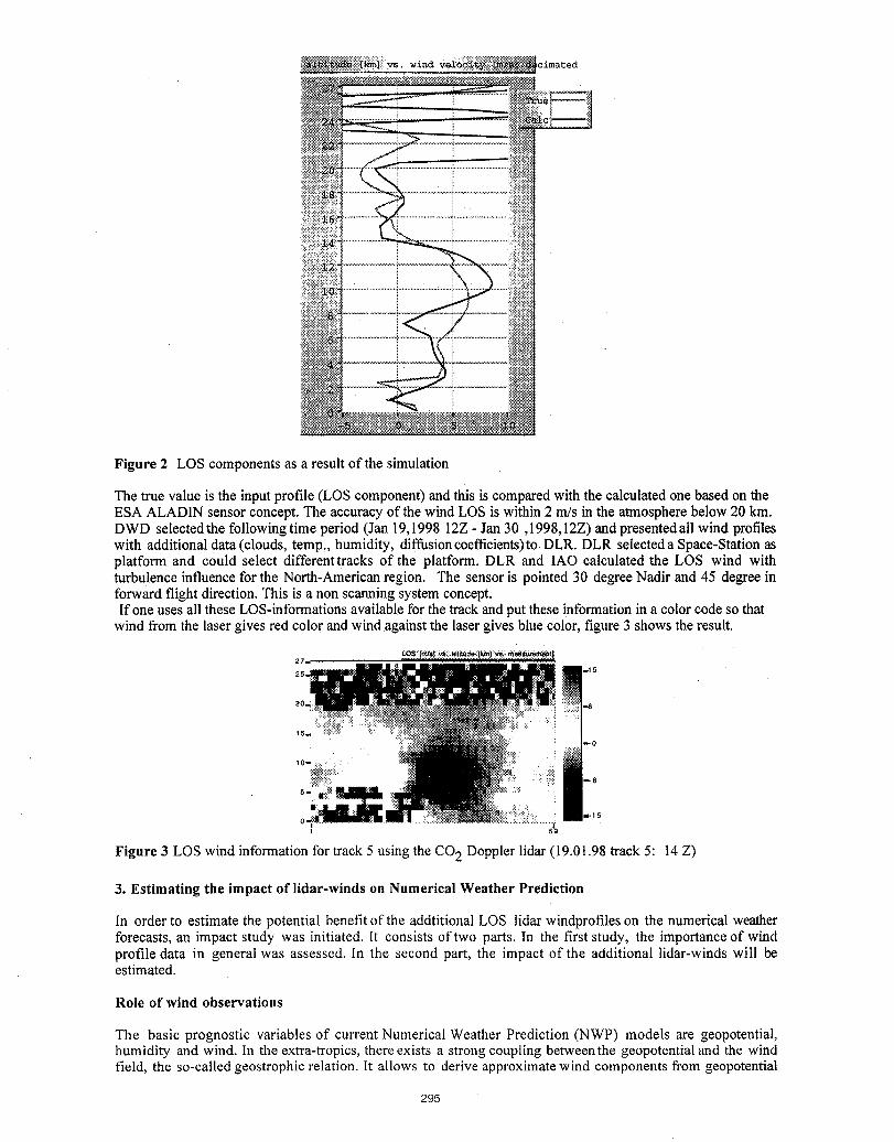
vs wind I ! i oimatod

Figure 2 LOS components as a result of the simulation

The true value is the input profle (LOS component) and this is compared with the calculated one based on theESA ALADIN sensor concept. The accuracy of the wind LOS is within 2 m/s in the atmosphere below 20 kin.DWD selected the following time period (Jan 19,1998 12Z - Jan 30,1998,12Z) and presented all wind profileswith additional data (clouds, temp,, humidity, diffusioncoefficients)to DLR. DLR selected a Space-Station asplatform and could select different tracks of the platform. DLR and IAO calculated the LOS wind withturbulence influence for the North-American region. The sensor is pointed 30 degree Nadir and 45 degree inforward flight direction. This is a non scanning system concept.If one uses all these LOS-informations available for the track and put these information in a color code so that

wind from the laser gives red color and wind against the laser gives blue color, figure 3 shows the result.

27." ........

25.

C

Figure 3 LOS wind information for track 5 using the CO2 Doppler lidar (19.01.98 track 5:14 Z)

3. Estimating the impact of lidar-winds on Numerical Weather Prediction

In order to estimate the potential benefit of the addtitional LOS lidar windprofiles on the numerical weatherforecasts, an impact study was initiated. It consists of two parts. In the first study, the importance of windprofile data in general was assessed. In the second part, the impact of the additional lidar-winds will beestimated.

Role of wind observations

The basic prognostic variables of current Numerical Weather Prediction (NWP) models are geopotential,humidity and wind. In the extra-tropics, there exists a strong coupling between the geopotential and the windfield, the so-called geostrophic relation. It allows to derive approximate wind components from geopotential

295

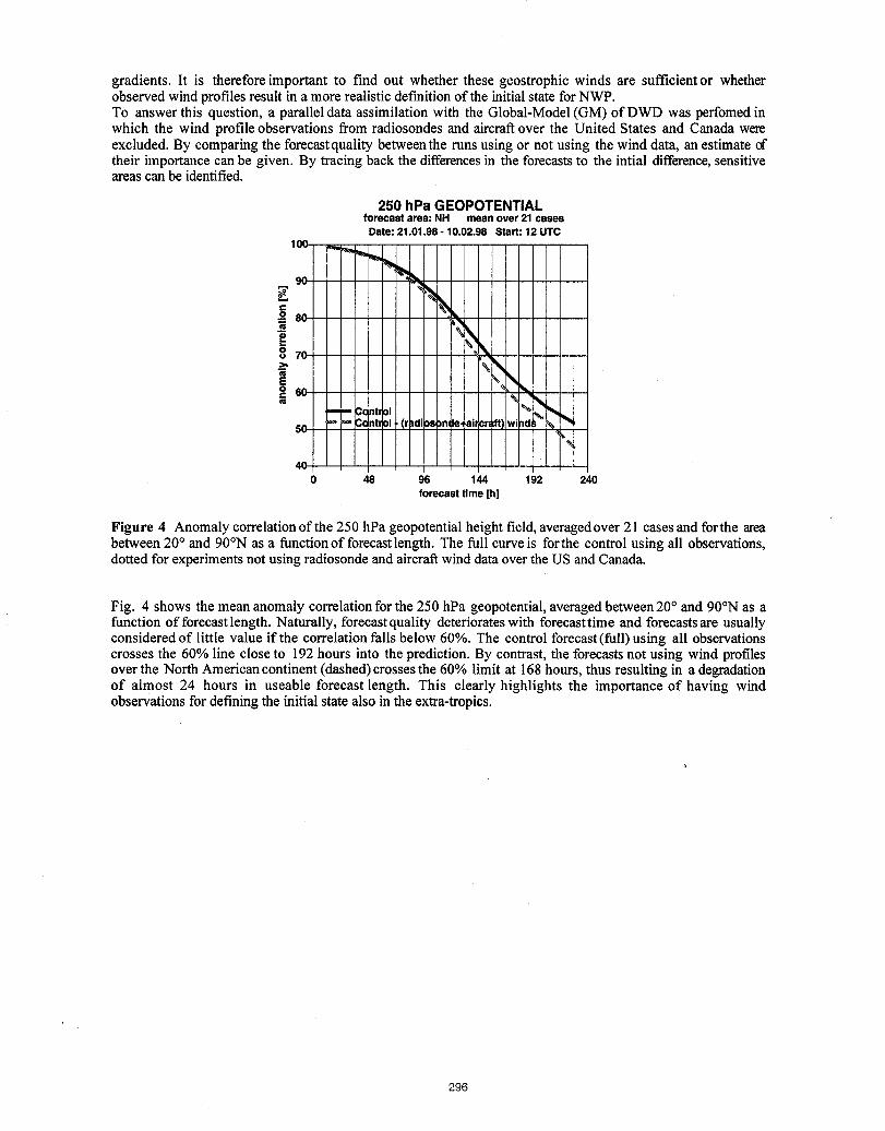
gradients. It is therefore important to find out whether these geostrophic winds are sufficientor whetherobserved wind profiles result in a more realistic definition of the initial state for NWP.To answer this question, a parallel data assimilation with the Global-Model (GM) of DWD was perfomed inwhich the wind profile observations from radiosondes and aircraftover the United States and Canada wereexcluded. By comparing the foreeastquality between the runs using or not using the wind data, an estimatetheir importance canbe given. By tracing back the differencesin the forecasts to the intial difference,sensitiveareas can be identified.

250hPa GEOPOTENTIALforecast area: NH mean over 21 cases

Date: 21.01.98 - 10.02.98 Start: 12 UTC

100 __ ....

co= 8C '

:° ' F%_ 7C !

° r'Ni 6C . :

50 '- _'- IC<_ntrDI, (r Idi )s n e ai cr ) _ _,t

40 _' i !0 48 96 144 192 240

forecast time [h]

Figure 4 Anomaly correlation of the 250 hPa geopotential height field, averagedover 21 cases and forthe areabetween 20° and 90°N as a function of forecastlength. The full curve is forthe control using all observations,dotted for experiments not using radiosonde and aircraft wind data over the US and Canada.

Fig. 4 shows the mean anomaly correlation for the 250 hPa geopotential, averaged between20 ° and 90°N as afunction of forecast length. Naturally, forecast quality deteriorates with forecast time and forecasts are usuallyconsidered of little value if the correlation falls below 60%. The control forecast (full) using all observationscrosses the 60% line close to 192 hours into the prediction. By contrast, the forecasts not using wind profilesover the North American continent (dashed) crosses the 60% limit at 168 hours, thus resulting in a degradationof almost 24 hours in useable forecast length. This clearly highlights the importance of having windobservations for defining the initial state also in the extra-tropics.

296

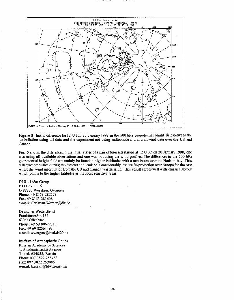
500 Hpa GeopotentialDifference Forecast - Control Interval : 40 m

30.01.98 12 UTC+OH for 30.01.98 12 UTC

I

40_ 20"1 O' 8(_

MAGICS5.2cosl- for3creThuAug2712:51:341998- TESTS/CONTOI

Figure 5 Initial differencefor 12 UTC, 30 January 1998 in the 500 hPa geopotential height field between theassimilation using all data und the experiment not using radiosonde and aircraftwind data over the US andCanada.

Fig. 5 shows the differencesin the intial states of a pair of forecastsstarted at 12 UTC on 30 January 1998, onewas using all available observations and one was not using the wind profiles. The differencesin the 500 hPageopotential height field can mainly be found in higher latititudes with a maximum over the Hudson bay. Thisdifferenceamplifies during the forecastand leads to a considerably less usefulprediction over Europe for the casewhere the wind information from the US and Canada was missing. This result agrees well with classical theorywhich points to the higher latitudes as the most sensitive areas.

DLR - Lidar GroupP.O.Box 1116D 82230 Wessling, GermanyPhone: 49 8153 282573Fax: 49 8153 281608

e-mail: Christian.W_mer@dlr.de

Deutscher WetterdienstFrankfurterStr. 13563067OffenbachPhone: 49 69 80622713Fax: 49 69 82361493e-mail: wwergen@dwd.d400.de

Institute of Atmospheric OpticsRussian Academy of Sciencesl, Akademicheskii AvenueTomsk 634055, RussiaPhone 007 3822 258483Fax: 007 3822 259086e-mail: banakh@Idw.tomsk.su

297

Coherent Doppler Lidar Data Products fromSpace-Based Platforms

Rod Frehlich

Cooperative Institute for Research in the Environmental Sciences (CIRES)University of Colorado, Campus Box 216, Boulder, CO 80309

Phone:303-492-6776 FAX:303-492-1149 Emaihrgf@cires.colorado.edu

Introduction aerosol region travels during the data processing in-terval T = MTs where M is the number of complex

Coherent Doppler lidar is a promising technique for lidar data points for each range-gate. For pulse accu-the global measurements of winds using a space-based mulation, the along-track extent of the measurementplatform. Doppler lidar produces estimates of the ra- volume L = AyN where N is the number of accu-dial component of the velocity vector averaged over mulated pulses and Ay is the horizontal separationthe resolution volume of the measurement. Profiles of between adjacent lidar pulses. The major instrumen-the horizontal vector winds are produced by scanning tal error in the radial velocity is the frequency drift in

the lidar beam or stepping the lidar beam through a the reference laser frequency (LO) which determinessequence of different angles (step-stare). The first de- zero velocity. The effects of uncorrelated velocity er-sign for space-based measurements proposed a coni- ror from pulse-to-pulse is included by adding a zero-cal scan which requires a high power laser to produce mean Gaussian random velocity error with standardacceptable signal levels for every laser pulse. Per- deviation avLO to the zero velocity reference of eachformance is improved by fixing the laser beam and pulse. To simplify the analysis, we assume the lidaraccumulating the signal from many lidar pulses for beam axis is perpendicular to the satellite track witheach range-gate [1, 2]. This also improves the spa- a nadir angle 0 where _ = 0 is pointed to the centertial averaging of the wind estimates and reduces the of the earth.threshold signal energy required for a good estimate. For a short range-gate located at range R andCoherent Doppler lidar performance for space-based for constant aerosol backscatter coefficient/_(R), theoperation is determined using computer simulations magnitude of the Doppler lidar signal for one lidarand including the wind variability over the measure- pulse is defined by the parameter [1]ment volume as well as the variations of the atmo-

spheric aerosol backscatter. ?TQ_(R)K(R)2cUTAR?TH T+1= (t)Lidar Performance 2hvR2

where r/Q is the detector quantum efficiency, K(R) isThe performance of Doppler lidar depends on the the one way irradiance extinction, UT is the trans-

lidar parameters, the atmospheric conditions, and the mitted laser pulse energy, AR is the receiver area, 'r/Hvelocity estimation algorithm. The transmitted pulse is the heterodyne efficiency, h is Planck's constant,for a solid state lidar is well approximated as a Gaus- and u is the laser frequency. _t is the effective num-sian temporal power profile with a full width at half ber of coherent photons detected per range-gate per

maximum (FWHM) pulse width At [1, 4]. The spec- pulse.tral width w = 0.1874/At and the spectral width The Space Readiness Coherent Lidar Experimentin velocity space Wv = Aw/2 where A is the wave- (SPARCLE) is the first space mission to attempt co-length. Tile illuminated aerosol target region is a herent Doppler lidar wind measurements [5] For mostnarrow pencil shaped volume that has a Gaussian experiments, the lidar beam will be fixed with a nadirintensity profile along the beam axis with a spatial angle of 30° and various azimuth angles.width (FWHM) Ar = Atc/2 where c is the speed The turbulent wind field over the resolution cell isof light in air. The line-of-sight range gate length described by the radial velocity fluctuations v(y,z)

Ap = Tc/2 is defined as the distance the illuminated where z is the distance along the lidar beam axis and

298

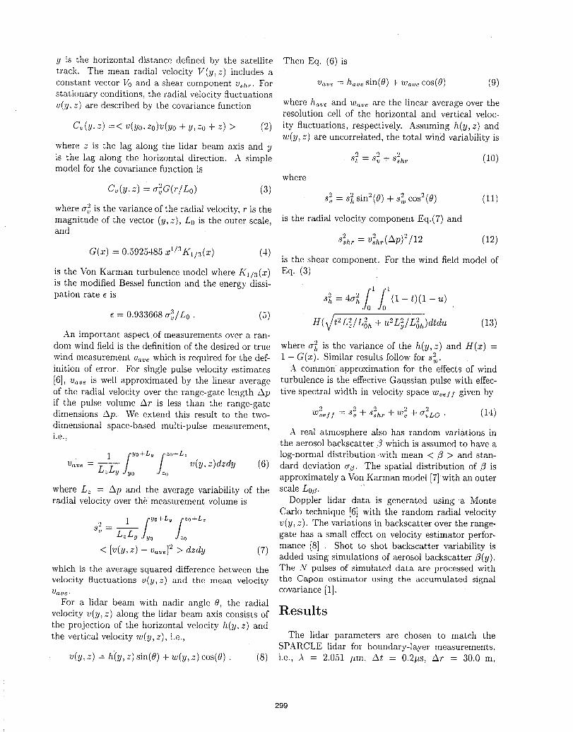
y is the horizontal distance defined by the satellite Then Eq. (6) istrack. The mean radial velocity V(y,z) includes aconstant vector P_ and a shear component v_hr. For Va,¢ = have sin(0) + "UJav e COS(0) (9)

stationary conditions, the radial velocity fluctuationsv(y, z) are described by the covariance hmction where have and waw are the linear average over the

resolution cell of the horizontal and vertical veloc-

Cv(!/, z) =< u(y0, zo)v(yo + y, z0 + z) > (2) ity fluctuations, respectively. Assuming h(y, z) andw(y, z) are uncorrelated, the total wind variability is

where z is the lag along the Iidar beam axis and y,_ o ,)

is the lag along the horizontal direction. A simple s_ : 8v -Jr-8shr (10)

model for the covariance function iswhere

cv(y, = (3) ') q .7 9

s,5= s_ sin2(0) + s;, cos-(0) (11)where cr_is the variance of the radial velocity, r is themagnitude of the vector (y, z), Lo is the outer scale, is the radial velocity component Eq.(7) andand ._

8sh r = U2hr(_p) 2/12 (12)

G(x) = 0.5925485 xl/aKt/u(x) (4)is the shear component. For the wind field model of

is the Von Karman turbulence model where Kl/3(x) Eq. (3)is the modified Bessel function and the energy dissi-

pation rate e is s_ = 4a2 (1 - t)(1 - u)

. _/ ') .') .)0.933668 a3_/Lo (5) H(vt2L_/L0h + u'L?/LSh)dtdu (13)

An important aspect of measurements over a ran-dora wind field is the definition of the desired or true where ah is the variance of the h(y, z) and H(x) =wind measurement va,_ which is required for the def- 1 - G(x). Similar results follow for s_.inition of error. For single pulse velocity estimates A common approximation for the effects of wind[6], v_ is well approximated by the linear average turbulence is the effective Gaussian pulse with effe9-of the radial velocity over the range-gate length ,._kp tive spectral width in velocity space w,_/i given byif the pulse volume ,,kr is less than the range-gate .) .) ._ ,_ ,)

dimensions '_Xp. We extend this result to the two- wT,_// = s-_+ "S'_hr+ w-_+ C_7_LO. (14)

dimensional space-based multi-pulse measurement, A real atmosphere also has random variations ini.e., the aerosol backscatter 3 which is assumed to have a

1 ['go+L,j fzo+L_ log-normal distribution .with mean < 0 > and stan-

v_,_ - L._Lu .,/yo /-__o v(y, z)dzdy (6) dard deviation c_.3. The spatial distribution of '3 isapproximately a Von Karman model [7] with an outer

where L- = ,._kpand the average variability of the scale L0_.radial velocity over th_ measurement volume is Doppler lidar data is generated using a Monte

Carlo technique [6] with the random radial velocity._ 1 fyo+L_ +L

s; _ [ = v(y, z). The variations in backscatter over the range-gate has a smal! effect on velocity estimator perfor-L: L,j _yo :omance [8] . Shot to shot backscatter variability is< [v(y, z) -v_,e] 2 > dzdy (7)added using simulations of aerosol backscatter fl(y).

which is the average squared difference between the The N pulses of simulated data are processed withvelocity fluctuations v(y,z) and the mean velocity the Capon estimator using the accumulated signalWoe. covariance [1].

For a lidar beam with nadir angle 0, the radialvelocity v(y, z) along the lidar beam axis consists of Resultsthe projection of the horizontal velocity h(y, z) andthe vertical velocity w(y,z), i.e., The lidar parameters are chosen to match the

SPARCLE lidar for boundary-layer measurements.v(y,z) = h(y,z) sin(O)+ w(y,z) cos(O). (8) i.e., A = 2.051 pro, At = 0.2!zs, &r = 30.0 m,

299

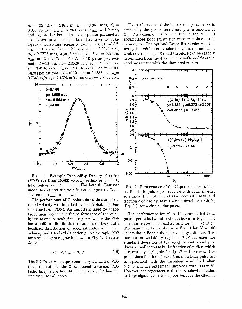
M = 32, 'Ap = 246.1 m, wv = 0.961 m/s, Ts = The performance of the lidar velocity estimates is0.051275 _s, Vse_,rch = 20.0 m/s, O'vLO = 1.0 m/s, defined by the parameters b and g as a function ofand Ay = 1.0 km. The atmospheric parameters _1. An example is shown in Fig. 2 for N = 10are chosen for a turbulent boundary layer to inves- accumulated lidar pulses per velocity estimate and

tigate a worst-case scenario, i.e., _ = 0.01 m2/s 3, a_ =</3 >. The optimal Capon filter order p is cho-Low = 1.0 km, Loh = 2.0 kin, aw = 2.2043 m/s, sen by the minimum standard deviation g and has a

Crh= 2.7772 m/s, a_= 2.3606 m/s, L0Z = 0.5 km, weak dependence on _1 and therefore can be reliablyVshr = 10 m/s/km. For N = 10 pulses per esti- determined from the data. The best-fit models are inmate, L=10 km, sw= 2.0526 m/s, Sh= 2.4157 m/s, good agreement with the simulated results.

sv= 2.4746 m/s, wvefi= 2.6546 m/s. For N = 1003! I ililil| i I iliN, I l , i,ili, I I , _,,ili I

pulses per estimate, L=100 km, sw= 2.1883 m/s, Sh=2.7365 m/s, sv= 2.6398 m/s, and wveff = 2.8092 m/s. a. 2 o oo oo o o

lO • 1 o o o o o

0 I I IIIIII I I I,,,lil , I I IIIIll I I I IIIIIII I IIIli I I I I I[1111 I I I IIIII I I I I Iltll I

2.2 _ g((t)l)=Z[l+(O1/go)_l-_+P, -2.0 %x 7,,=1.384g0=5.272_=2.007-_

,,..,1.8 '_ 8=0.8673 _=0.8757 --

1.6 . _E1"4 -_ --" c _,

u. o_1.21r. 1.0

0.80.6 i i iiiiii i i i illlll i i i iiiiii i i i Illtll

1 I I lilll I I I I I Illl I I I I II1[1|

b(@l)=exp[" (_l/bo) a]

.= 0.1 '_ bo=1.995_=1.148

O. 0.2 0.4 0.6 0.8 1.0 0.01V/Vsearch

0.001 , l lilid = ! , ,,,,,'I[ , , , ,,,Jd , , , ,,,,,I

Fig. 1. Example Probability Density Function 1 10 100 1000(PDF) (o) from 20,000 velocity estimates, N = 10 @1

lidar pulses and _1 = 3.0. The best fit Gaussian Fig. 2. Performance of the Capon velocity estima-model (- - -) and the best fit two component Gaus- tor for N=10 pulses per estimate with optimal ordersian model (__) are shown, p, standard deviation g of the good estimates, and

The performance of Doppler lidar estimates of the fraction b of bad estimates versus signal strength _1

radial velocity v is described by the Probability Den- [Eq. (1)] for a single lidar pulse.sity Function (PDF). -An important issue for space-based measurements is the performance of the veloc- The performance for N = 10 accumulated lidarity estimates in weak signal regimes where the PDF pulses per velocity estimate is shown in Fig. 3 forhas a uniform distribution of random outliers and a constant aerosol backscatter and for aj =< ,_ >.

localized distribution of good estimates with mean The same results are shown in Fig. 4 for N = 100,

value v9 and standard deviation g. An example PDF accumulated lidar pulses per velocity estimate. Thefor a weak signal regime is shown in Fig. 1. The bias backscatter variability (a,3 =< ,3 >) increases the'Av is standard deviation of the good estimates and pro-

duces a small increase in the fraction of outliers which

/Av =< Vave - vg > . (15) is essentially negligible for the N = 100 cases. Thepredictions for the effective Gaussian lidar pulse are

The PDF's are wellapproximated by aGaussian PDF in agreement with the turbulent wind field when(dashed line) but the 2-component Gaussian PDF b > 0 and the agreement improves with larger N.(solid line) is the best fit. In addition, the bias Av However, the agreement with the standard deviationwas small for all cases, at large signal levels (Ih is poor because the effective

300

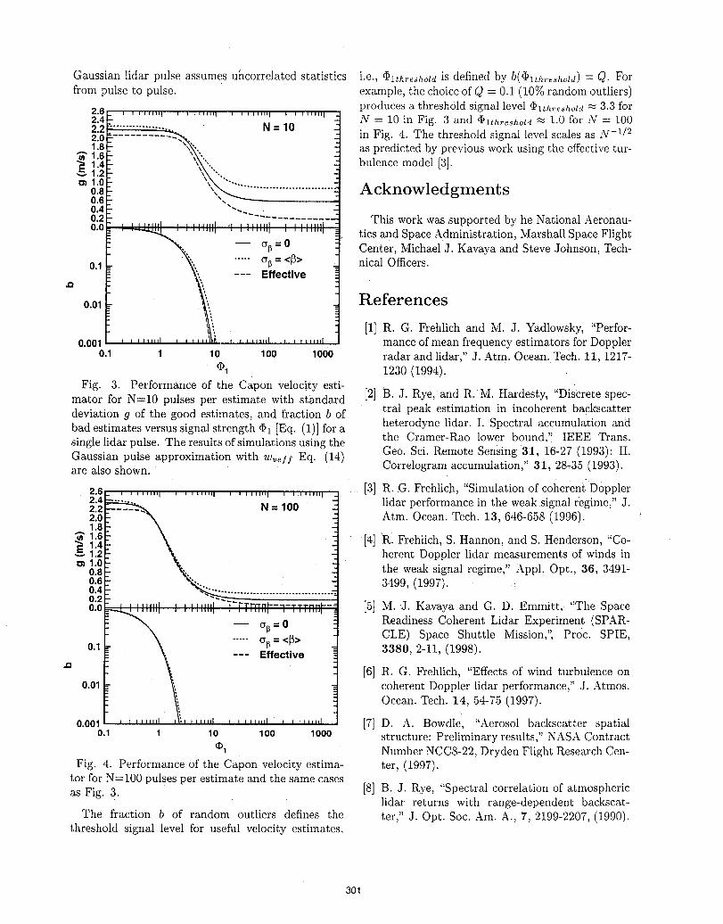
Gaussian lidar pulse assumes uhcorrelated statistics i.e., @1threshold is defined by b(@lthreshold) -7- Q. Forfrom pulse to pulse, example, the choice of Q = 0.1 (10% random outliers)

produces a threshold signa! level ¢Plth,.e_hold_ 3.3 for2,6 I i ,I,l,, I I I [l,i,q i J ,ItJtl I , I Flill; I .2.4 - N = 10 in Fig. 3 and _lthreshold _ 1.0 for N = 100

2.2 ................. . N=10 -............ - in Fig. 4. The threshold signal level scales as N -t/2

2.0

1.8 , • - as predicted by previous work using the effective tur-"-" 1.6 \'" -' "'" -- bulence model [3].1.4 \_ ",, -,,.- 1.2 _ ", -

k %.1.0 \ ....... -0.a , ..........................Acknowledgments0.60.4 "" -0.2 .... " ........... --: This work was supported by he National Aeronau-

o.o ........ ' ........ ' ......... ' ' ' ' ::llll tics and Space Administration, Marshall Space Flight

ZI III t I I IIIII I I I I

-- op= 0 Centeri Michael J. Kavaya and Steve Johnson, Tech-

0.1 }""., ".... _ = <[3> nical Officers.

J= ':,,,,. --- Effective\ References

0.01 _",

_". [1] R. G. Frehlich and M. J. Yadlowsky, "Perfor-0.001 ........ ' ...... M ........ I ........ , mance of mean frequency estimators for Doppler

0.1 1 10 100 1000 radar and !idar," J. Arm. Ocean. Tech. 11, 1217-

ap_ 1230 (1994).Fig. 3. Performance of the Capon velocity esti-

mator for N=10 pulses per estimate with standard [2] B. J. Rye, and R.M. Hardesty, "DisCrete spec-tral peak estimation in incoherent backscatterdeviation g of the good estimates, and fraction b ofheterodyne lidar. I. Spectral accumulation and

bad estimates versus signal strength @1 [Eq. (1)] for athe Cramer-Rao lower bound," IEEE Trans.single lidar pulse. The results of simulations using the

Gaussian pulse approximation with w.eH Eq. (14) Geo. Sci. Remote Sensing 31, 16-27 (1993): II.are also shown. Correlogram accumulation," 31, 28,35 (1993).

2.6 [3] R. G. Frehlich, "Simulation of coherent Doppler2.4 lidar performance in the weak signal regmm,' " J.2.22.0 Atm. Ocean. Tech. 13, 646-658(1996). '1.8i

[4] "RI FrehliCh, S. Hannon, and S: Henderson, "Co-herent Doppler lidar measurements of winds in

1.00.8 the weak signal regime," Appl. Opt., 36, 3491,0.6 3499, (1997). :0.40.20.o [5] M. J. Kavaya and G. D. Emmitt, "The Space

Readiness Coherent Lidar Experiment (SPAR-CLE) Space Shuttle Mission,", Proc. SPIE,

0.1 3380, 2-11, (1998).

"Q [6] R. G. Frehlich, "Effects of wind turbulence on0.01 coherent Doppler lidar performance," J. Atmos.

Ocean. Tech. 14, 54-T5 (1997).

0.001 [7] D. A. Bowdle, "Aerosol backscatter spatial0.1 1 10 1O0 1000 structure: Preliminary results," NASA Contract

Q_I Number NCC8-22, Dryden Flight Research Cen-Fig. 4. Performance of the Capon velocity estima- ter, (1997).

tor for N=100 pulses per estimate and the same casesas Fig. 3. [8] B. J. Rye, "Spectral correlation of atmospheric

lidar returns with range-dependent backscat-The fraction b of random outliers defines the ter," J. Opt. Soc. Am. A., 7, 2199'2207, (1990).

threshold signal level for useful velocity estimates,

301

Considerations for Designing a Space Based Coherent Doppler Lidar

Gary D. SpiersCenter for Applied Optics

University of Alabama in HuntsvilleHuntsvilleAL 35899

Gary.Spiers@msfc.nasa.gov(256) 544 5787

Michael J. KavayaMail Code SD60

Global Hydrology and Climate CenterNASA Marshall Space Flight Center

HuntsvilleAL 35812

Michael.Kavaya@msfc.nasa.gov(256) 922 5803

IntroductionAn orbiting coherent Doppler lidar for measuring winds is required to provide two basic pieces of data to the usercommunity. The first is the line of sight wind velocity and the second is knowledge of the position at which themeasurement was made. In order to provide this information in regions of interest the instrument is also required tohave a certain backscatter sensitivity level. This paper outlines some of the considerations necessary in designing acoherent Doppler lidar for this purpose.

Line of sight velocity accuracy

A lidar instrument measures wind velocity by measuring a frequencydifference between the transmitted laser beamand the return signal. This frequency difference is due to the transmitted frequency being Doppler shifted by the lineof sight velocity seen by the instrument. The line of sight velocity is comprised of velocity components due to thesatellite velocity, the earth's rotational velocity and the velocity of the target.

The magnitude of the combined line of sight velocity is given by:

los_vel := htrgtv cos(-trgta + az + orblat( lat, inc )) sin(nadalt(orbh, n, alt, lat ) )

+ vtrgtv cos(nadalt(orbh, n, alt, lat)) + hsatv cos(az) sin(n) + vsatv cos(n)

+ Vlat(lat) sin(orblat(lat, inc) + az) sin(nadalt(orbh, n, alt, tat)) (1)

where the first and second terms are the line of sight components of the target velocity with respect to the localWGS84 [1,2] earth ellipsoid surface. The third and fourth terms are the line of sight components of the spacecrafthorizontal and vertical velocities. The f'malterm is the component of the earth's rotational velocity along the line ofsight. Table 1lists the parameters and functions called out in equation (1) and table 2 lists the sensitivity of the

Symbol Parameterhtrgtv target horizontal velocityvtrgtv target vertical velocitytrgta angle of the target velocity with respect to the local meridianaz azimuth angle with respect to the spacecraft velocity vectorlat latitude of the spacecraftinc orbit inclination angle

orbh orbit height

302

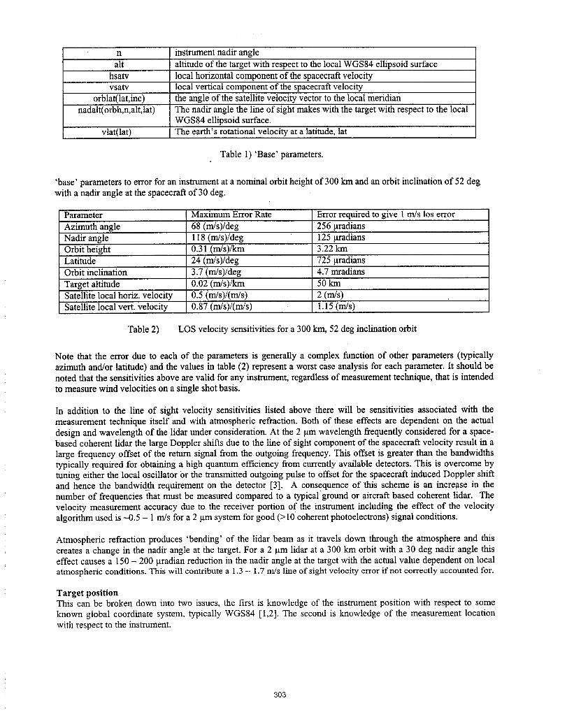
n instrument nadir anglealt altitude of the target with respect to the local WGS84 ellipsoid surface

hsatv local horizontal component of the spacecraft velocityvsaw local vertical component of the spacecraft velocity

orblat(lat,inc) the angle of the satellite velocity vector to the local meridiannadalt(orbh,n,alt,lat) The nadir angle the line of sight makes with the target with respect to the local

WGS84 ellipsoid surface.vlat(lat) The earth's rotational velocity at a latitude, lat

Table 1) 'Base' parameters.

'base' parameters to error for an instrument at a nominal orbit height of 300 km and an orbit inclination of 52 degwith a nadir angle at the spacecraft of 30 deg.

Parameter Maximum Error Rate Error required to give 1m/s los error

Azimuth angle 68 (m/s)/deg 256 _tradiansNadir angle 118(rn/s)/deg 125 _tradiansOrbit height 0.31 (m/s)/km 3.22 kmLatitude 24 (m/s)/deg 725 _tradiansOrbit inclination 3.7 (m/s)/deg 4.7 mradiansTarget altitude 0.02 (m/s)/km 50 kmSatellite local horiz, velocity 0.5 (rn/s)/(m/s) 2 (m/s)Satellite local vert. velocity 0.87 (mis)/(m/s) 1.15 (m/s)

Table 2) LOS velocity sensitivities for a 300 kin, 52 deg inclination orbit

Note that the error due to each of the parameters is generally a complex function of other parameters (typicallyazimuth and/or latitude) and the values in table (2) represent a worst case analysis for each parameter. It should benoted that the sensitivities above are valid for any instrument, regardless of measurement technique, that is intendedto measure wind velocities on a single shot basis.

In addition to the line of sight velocity sensitivities listed above there will be sensitivities associated with themeasurement technique itself and with atmospheric refraction. Both of these effects are dependent on the actualdesign and wavelength of the lidar under consideration. At the 2 _tmwavelength frequently considered for a space-based coherent lidar the large Doppler shifts due to the line of sight component of the spacecraft velocity result in alarge frequency offset of the return signal from the outgoing frequency. This offset is greater than the bandwidthstypically required for obtaining a high quantum efficiency from currently available detectors. This is overcome bytuning either the local oscillator or the transmitted outgoing pulse to offset for the spacecraft induced Doppler shiftand hence the bandwidth requirement on the detector [3]. A consequence of this scheme is an increase in thenumber of frequencies that must be measured compared to a typical ground or aircraft based coherent lidar. Thevelocity measurement accuracy due to the receiver portion of the instrument including the effect of the velocityalgorithm used is -0.5 - 1m/s for a 2 _tmsystem for good (>10 coherent photoelectrons) signal conditions.

Atmospheric refraction produces 'bending' of the lidar beam as it travels down through the atmosphere and thiscreates a change in the nadir angle at the target. For a 2 _tm lidar at a 300 km orbit with a 30 deg nadirangle thiseffect causes a 150 - 200 _tradianreduction in the nadir angle at the target with the actual value dependent on localatmospheric conditions. This will contribute a 1.3 - 1.7 m/s line of sight velocity error if not correctly accounted for.

Target positionThis can be broken down into two issues, the first is knowledge of the instrument position with respect to someknown global coordinate system, typically WGS84 [1,2]. The second is knowledge of the measurement locationwith respect to the instrument.

303

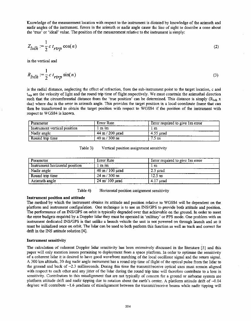
Knowledge of the measurement location with respect to the instrument is dictated by knowledge of the azimuth andnadir angles of the instrument. Errors in the azimuth or nadir angle cause the line of sight to describe a cone aboutthe 'true' or 'ideal' value. The positionof the measurement relative to the instrument is simply:

1

Zlvlh := c trtrp cos(n) (2)

in the vertical and

1

Rlvlh := _ c trtrp sin(n) (3)

is the radial distance, neglecting the effect of refraction, from the sub-instrument point to the target location, c andt_ are the velocity of light and the round trip time of flight respectively. We must constrain the azimuthal directionsuch that the circumferential distance from the 'true position' can be determined. This distance is simply (Rlvmxdaz) where daz is the error in azimuth angle. This provides the target position in a local coordinate frame that canthen be transformed to obtain the target position with respect to WGS84 if the position of the instrument withrespect to WGS84 is known.

Parameter Error Rate: Error required to give lm errorInstrument vertical position 1 m/m 1 mNadir angle 44 m / 200 _trad 4.55 _tradRound trip time 40 m / 300 ns 7.5 ns

Table 3) Vertical position assignment sensitivity

Parameter Error Rate Error required to give lm errorInstrument horizontal position 1 m/m 1 mNadir angle 40 m/100 _trad 2.5 _trad

Round trip time 24 m / 300 ns 12.5 nsAzimuth angle 24 m/100 _trad 4.17 _trad

Table 4) Horizontal position assignment sensitivity

Instrument position and attitudeThe method'by which the instrument obtains its attitude and position relative to WGS84 will be dependent on theplatform and instrument configuration. One technique is to use an INS/GPS to provide both attitude and position.The performance of an INS/GPS on orbit is typically degraded over that achievable on the ground. In order to meetthe error budgets required by a Doppler lidar they must be operated in 'military' or PPS mode. One problem with aninstrument dedicated INS/GPS is that unlike a launch vehicle the unit is not powered on through launch and so itmust be initialised once on orbit. The lidar can be used to both perform this function as well as track and correct fordrift in the INS attitude solution [4].

Instrument sensitivity

The calculation of coherent Doppler lidar sensitivity has been extensively discussed in the literature [5] and thispaper will only mention issues pertaining to deployment from a space platform. In order to optimise the sensitivityof a coherent lidar it is desired to have good wavefront matching of the local oscillator signal and the return signal.A 300 km altitude, 30 deg nadir angle instrument has a round trip time of flight of the optical pulse from the lidar tothe ground and back of-2.3 milliseconds. During this time the transmit/receive optical axes must remain alignedwith respect to each other and any jitter of the lidar during the round trip time will therefore contribute to a loss insensitivity. Contributors to this misalignment that are not typically of concern for a ground or airborne system areplatform attitude drift and nadir tipping due to rotation about the earth's center. A platform attitude drift of -0.04deg/sec will contribute -1.6 _tradians of misalignment between the transmit/receive beams while nadir tipping will

304

contribute - 2.7 _tradiansof misalignment. For a 25 cm aperture instrument a total angular offset of~7 _tradianswill result in a 3 dB reduction in SNR.

Finally it should be noted that the Doppler shift due to the component of the spacecraft platform velocity seen by thelidar is a function of the scanner azimuth angle (equation (1)). The bandwidth of the return signal that results fromthis can result in an azimuthally dependent atmospheric extinction and hence an azimuthally dependent sensitivity.

SummaryAn overview of some of the issues specific to designing a space based coherent Doppler lidar have been presentedand examples for an instrument with a 25 cm aperture in a 300 km, 52 degree inclination orbit orbit altitudepresented.

AcknowledgementsFunding for this work has been providedby Dr. RameshK. Kakar,NASA Code Y and by the NASA NMP EO-2SPARCLEprogram.

References

[1] MIL-STD-240, "Departmentof Defence WorldGeodeticSystem (WGS)", 11 January1994.[2] DMATR 8350.2, "Departmentof Defence WorldGeodetic System 1984, Its Definition and Relationships withLocalGeodetic Systems", Second Edition 1 September1991.[3] G. D. Spiers, "Analyses of CoherentLidarWind MeasurementMissions", FinalReport on ContractNo. NAS8-38609, Delivery OrderNo. 128, Report Date 8/28/96.[4] G.D. Emmitt,T. Miller andG.D. Spiers, "Pointing Knowledge for SPARCLE and Space-based Doppler WindLidarsin General", Tenth Biennial CoherentLaser RadarTechnology and ApplicationsConference, MountHood,28_ June- 2ndJuly 1999.[5] See for example R.G. Frehlich and M.J. Kavaya, "Coherent laser radarperformance for general atmosphericrefractiveturbulence",Appl. Opt. 30, 5325, December 1991.

305

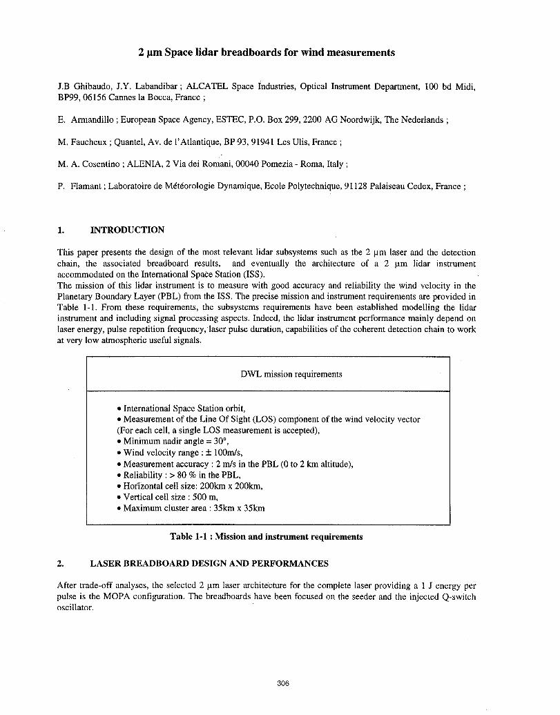
2 _tmSpace lidar breadboards for wind measurements

J.B Ghibaudo, J.Y. Labandibar ; ALCATEL Space Industries, Optical Instrument Department, I00 bd Midi,BP99, 06156 Cannes la Bocca, France ;

E. Armandillo ; European Space Agency, ESTEC, P.O. Box 299, 2200 AG Noordwijk, The Nederlands ;

M. Faucheux ; Quantel, Av. de l'Atlantique, BP.93, 91941 Les Ulis, France ;

M. A. Cosentino ; ALENIA, 2 Via dei Romani, 00040 Pomezia - Roma, Italy ;

P. Flamant ; Laboratoire de M6t6orologie Dynamique, Ecole Polytechnique, 91128 Palaiseau Cedex, France ;

1. INTRODUCTION

This paper presents the design of the most relevant lidar subsystems such as the 2 _tm laser and the detectionchain, the associated breadboard results, and eventually the architecture of a 2 lam lidar instrumentaccommodated on the International Space Station (ISS).The mission of this lidar instrument is to measure with good accuracy and reliability the wind velocity in thePlanetary Boundary Layer (PBL) from the ISS. The precise mission and instrument requirements are provided inTable 1-I. From these requirements, the subsystems requirements have been established modelling the lidarinstrument and including signal processing aspects. Indeed, the lidar instrument performance mainly depend onlaser energy, pulse repetition frequency, laser pulse duration, capabilities of the coherent detection chain to workat very low atmospheric useful signals.

DWL mission requirements

• International Space Station orbit,• Measurement of the Line Of Sight (LOS) component of the wind velocity vector(For each cell, a single LOS measurement is accepted),• Minimum nadir angle = 30°,• Wind velocity range :+ 100m/s,• Measurement accuracy : 2 mis in the PBL (0 to 2 km altitude),• Reliability :> 80 % in the PBL,• Horizontal cell size: 200km x 200km,• Vertical cell size : 500 m,• Maximum cluster area : 35km x 35km

Table 1-1 : Mission and instrument requirements

2. LASER BREADBOARD DESIGN AND PERFORMANCES

After trade-off analyses, the selected 2 _tm laser architecture for the complete laser providing a 1 J energy perpulse is the MOPA configuration.The breadboards have been focused on the seeder and the injected Q-switchoscillator.

306

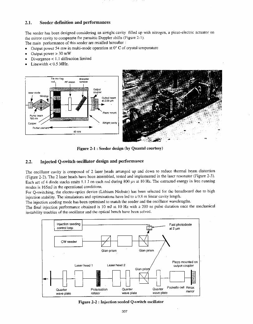
2.1. Seeder definition and performances

The seeder has been designed considering an airtight cavity filled up with nitrogen, a piezo-electric actuator onthe mirror cavity to compenste for parasitic Doppler shifts (Figure 2-1).The main performance of this seeder are recalled hereafter :• Output power 54 mw in multi-mode operation at 0° C of crystal temperature• Output power > 30 mW• Divergence < 1.1 diffraction limited• Linewidth < 0.5 MHz.

Tm,Ho:Yag Brewsterrod PF etalon window

Output)aserdiode coupler

Output beamat 2.09 _m

Piezomount

_ Airtight cavity

Peltier elemer_i__._ _-40 mm

Figure 2-1 : Seeder design (by Quantel courtesy)

2.2. Injected Q,switch oscillator design and performance

The oscillator cavity is composed of 2 laser heads arranged up and down to reduce thermal beam distortion(Figure 2-2). The 2 laser heads have been assembled, tested and implementedin the laser resonator (Figure 2-3).Each set of 4 diode stacks emits 1.1 J on each rod during 800 _s at 10Hz. The extractedenergy in free runningmodes is 165mJ in the operationalconditions.For Q-switching, the electro-optics device (LithiumNiobate) has been selected for the breadboard due to highinjection stability.The simulationsand optimisationshave led to a 0.8 m linearcavity length.The injectionseeding modehas been optimised to match theseeder and theosci!latorwavelengths.The final injection performanceobtained is 10 mJ at 10 Hz with a 200 ns pulse duration once the mechanicalinstability troublesof the oscillator and the optical bench have been solved.

] _ Fast photodiodeInjectionseeding _- at 2 IJm

control loop

CW seeder _ _-_ _

Glan prism, Glan prism

Piezo mounted onLaser head 1 Laser head 2 output coupler

"91--t U _ Glanprisl [_ _Quarter Polarisation Quarter Quarter Pockells cell Rmaxwave plate rotator wave plate wave plate mirror

Figure 2-2 : Injection seeded Q-switch oscillator

307

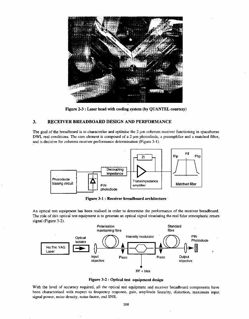
Figure 2-3 : Laser head with cooling system (by QUANTEL courtesy)

3. RECEIVER BREADBOARD DESIGN AND PERFORMANCE

The goal of the breadboard is to characterise and optimise the 2 tam coherent receiver functioning in spaceborneDWL real conditions. The core element is composed of a 2 tamphotodiode, a preamplifier and a matched filter,and is decisive for coherent receiver performance determination (Figure 3-1).

_._ FIp .Fif Fhp

[_ impedance

Photodiode Transimpedancebiasingcircuit PIN amplifier Matchedfilter

photodiode

Figure 3-1 : Receiver breadboard architecture

An optical test equipment has been realised in order to determine the performance of the receiver breadboard.The role of this optical test equipment is to generate an optical signal simulating the real lidar atmospheric returnsignal (Figure 3-2).

Polarisation Standardmaintainingfibre fibre

Optical Intensity modulator PINisolator Photodiode

Laser

Input Piezo Piezo Outputobjective objective

RF+bias

Figure 3-2 : Optical test equipment design

With the level of accuracy required, all the optical test equipmentand receiver breadboardcomponents havebeen characterised with respect to frequency response, gain, amplitude linearity, distortion, maximum inputsignalpower, noise density,noise factor, andSNR.

308

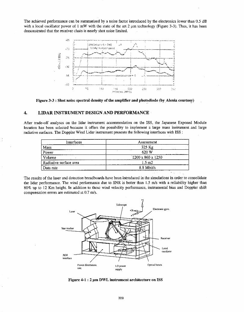
The achieved performance can be summarised by a noise factor introduced by the electronics lower than 0.5 dBwith a local oscillator power of 1 mW with the state of the art 2 gm technology (Figure 3-3). Thus, it has beendemonstrated that the receiver chain is nearly shot noise limited.

-._5 ..............................................................................................................................................................................................

Figure 3-3 : Shot noise spectral density of the amplifier and photodiode (by Alenia courtesy)

4. LIDAR INSTRUMENT DESIGN AND PERFORMANCE

After trade-off analyses on the lidar instrument accommodation on the ISS, the Japanese Exposed Modulelocation has been selected because it offers the possibility to implement a large mass instrument land largeradiative surfaces. The Doppler Wind Lidar instrument presents the following interfaces with ISS :

Interfaces Assessment

Mass 325 KIgPower 620 WVolume 1200 x 860 x 1250Radiative surface area 1.5 m2Data rate 8.8 Mbit/s

The results of the laser and detection breadboards have been introduced in the simulations in order to consolidate

the lidar performance. The wind performance due to SNR is better than 1.5 m/s with a •reliability higher than80% up to 12 Km height. In addition to these wind velocity performance, instrumental bias and Doppler shiftcompensation errors are estimated at 0.7 m/s.

N

Telescope_

Laser .X/_X_,J/Electronic gyro.

Star-tracker

.._._.._ _ _:_ _ Receiver

JEMinterface

Power distribution LO power Optical benchunit supply

Figure 4-1 : 2/am DWL instrument architecture on ISS

3O9

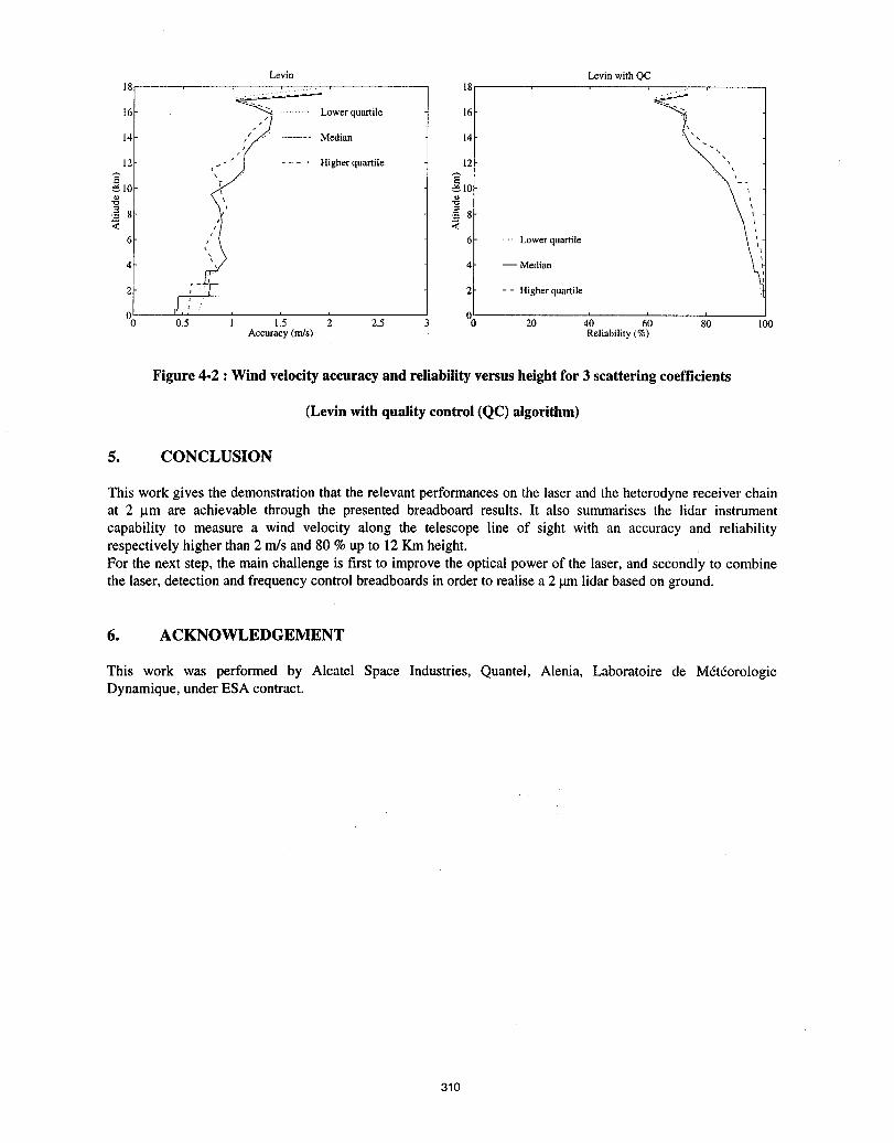
Levin Levin with QC18 18 , ......

' ' _'=_......... ' ............. ' quartile'16 ,_ Lower 16

, j14 /// Median 14

Y12 .- " " " I Higher quartile 12 N _

_10 _ 10 ' I

6 6 ..... Lower quartile

4 _ _ 4 -- Median2 2 - - Higher quartile

% 0.5 1 1.5 2 2[5 0 2'0 4'0 6'0 80 100Accuracy (m/s) Reliability (%)

Figure4-2 : Windvelocityaccuracyandreliabilityversusheightfor 3 scatteringcoefficients

(Levin with quality control (QC) algorithm)

5. CONCLUSION

This work gives the demonstration that the relevant performances on the laser and the heterodyne receiver chainat 2 _tm are achievable through the presented breadboard results. It also summarises the lidar instrumentcapability to measure a wind velocity along the telescope line of sight with an accuracy and reliabilityrespectively higher than 2 m/s and 80 % up to 12Km height.For the next step, the main challenge is first to improve the optical power of the laser, and secondly to combinethe laser, detection and frequency control breadboards in order to realise a 2 _unlidar based on ground.

6. ACKNOWLEDGEMENT

This work was performed by Alcatel Space Industries, Quantel, Alenia, Laboratoire de M&6orologieDynamique, under ESA contract.

310

DEVELOPMENT OF PROTOTYPE MICRO-LIDAR USING NARROW LINEWIDTHSEMICONDUCTOR LASERS FOR MARS BOUNDARY LAYER WIND AND DUST

OPACITY PROFILES

Robert T. Menzies, Greg Cardell, Meng Chiao, Carlos Esproles,Siamak Forouhar, Hamid Hemmati and David Tratt

Jet Propulsion Laboratory, California Institute of Technology4800 Oak GroveDrive, Pasadena, CA 91109, USA

Phone: 818-354-3787; FAX: 818-393-6984; Emaih Robert.T.Menzies@jpl.nasa.gov

1. Introduction

We have developed a compact Doppler lidar concept which utilizes recent developments insemiconductor diode laser technology in order to be considered suitable for wind and dust opacityprofiling in the Mars lower atmosphere from a surface location. The current understanding of theMars global climate and meteorology is very limited, with only sparse, near-surface data availablefrom the Viking and Mars Pathfinder landers, supplemented by long-range remote sensing of theMartian atmosphere. The in situ measurements from a lander-based Doppler lidar would providea unique dataset particularlyfor the boundary layer. The coupling of the radiative properties of thelower atmosphere with the dynamics involves the radiative absorption and scattering effects of thewind-drivendust (Haberle,et al., 1982). Variabilityin solar irradiance, on diurnal and seasonal timescales,drives vertical mixing and PBL (planetaryboundary layer) thickness. The lidar data will alsocontribute to an understanding of the impact of wind-drivendust on lander and rover operations andlifetime through an improvement in our understanding of Mars climatology.

In this paper we discuss the Mars lidar concept, and the development of a laboratory prototype forperformance studies, using local boundary layer and topographic target measurements.

2. Instrument Description

We have developed a laboratory prototype Doppler lidar utilizing a novel technique for measuringwind speed profiles. It uses technologies which provide a path towards development of a robust,low-power instrument for deployment on the surface of Mars. The lidar currently utilizescommercially available semiconductor diode laser master oscillator and fiber laser amplifier devicesin order to attain transmitter power output between 100-200 mW, depending on the transmittermodulation technique. The specific lidar wavelength selected is not constrained to a particularspectral region by the measurement objectives, consequently the 1.5 micron wavelength region hasbeen selected to be compatible with the large market of optical fiber-compatible components. Thiswavelength also makes the lidar much more convenient for various Earth boundary layermeasurement studies because it is in the Aeye safe@ region.

The lidar uses a modulated cw transmitter and heterodyne detection. Pulsed operation, desirable formany reasons when profiling is the goal, is not compatible with the very narrow-lincwidth

311

semiconductor laser transmitter required for the Doppler measurements. Diode lasers do not storepopulation inversion energy efficiently, particularly if narrow linewidth is required. For a lidarmeasurement application such as this, for which the transmitter output power is of the order ofhundreds of mW, the transmitter power requirement is a significant contributor to the overall powerbudget. Thus it is attractive to use a diode laser transmitter rather than suffer the loss of efficiencyin converting diode pump optical power to pulsed power from a crystal laser medium. Sinceheterodyne detection is used, the LO is derived by splitting a portion of the cw master oscillatoroutput. The LO component frequency is shifted 20 MHz using an acousto-optic shifter. The outputfrom the transmitter leg of the splitter passes through a modulator. This then passes through the fiberamplifier and is coupled through a transmit/receive duplexer to an off-axis afocal telescope. Thereceiver comprises a high-speed, low noise InGaAs photodiode suitable for ambient temperatureoperation, with a matched preamplifier,RF filtering,programmableamplifier,high-speedlow power12-bitanalog-to-digitalconverter (ADC), followed by Fast Fourier Transform (FFI') electronics andpower spectrum analysis and processing. The processing and control computer provides thetransmitter modulation waveform and the detected signal demodulation and correlation functions.An important consideration for this lidar is the selection of a modulation and spectrum analysisstrategy which accounts for the decorrelation time of the signals backscattered from the atmosphericaerosol. The decorrelation time in the boundary layer depends on the turbulence intensity. Therange of correlation times in the Earth=s boundary layer over land surfaces places a more stringentdemand on the lidar than is expected based on inferredcorrelationtimes for the Mars boundarylayer.

3. Summary

Laser technology is advanced to the level required for planetary missions, examples being the lasertransmitter for the Mars Observer Laser Altimeter (MOLA) currently orbiting Mars and the laser insitu water vapor sensor in the Mars Volatiles and Climate Sensor (MVACS) currently on its way toMars. The compact lidar concept described here for atmospheric wind and dust profilingmeasurements uses robust laser technology and relies on high performance signal processing as afundamental component of its operation. A prototypeDoppler lidar has been constructed for use inlocal boundary layer measurements to assess the capability to derive wind profiles using PN codemodulation of the transmitter. Incorporationof monolithic semiconductordiode lasers with 100-200mW output power will take place as these devices become available in the near future.

Acknowledgement

This work was carried out by the Jet Propulsion Laboratory, California Institute of Technology,under contract to the National Aeronautics and Space Administration.

REFERENCES

Haberle, R.M., C.B. Leovy, and J.B. Pollack (1982). Some effects of global dust storms on theatmospheric circulation of Mars. Icarus, 50, 322-367.

312

Follow-on Missions to SPARCLE

G. D. Emmitt

Simpson Weather AssociatesCharlottesville, Va. 22902

804-979-3571

T. L. MillerGlobal Hydrology and Climate Center

NASA/MSFCHuntsville, AL 35812

256-922-5882

Abstract

Global tropospheric wind observations are considered the number one unaccomodatedatmospheric observation for the new series of NPOESS platforms. The operationalmeteorology communities have long recognized the potential for improved forecastingskill if accurate wind observations were available around the globe. Recent analysessuggest that wind observations such as those that could be made by a space-basedDoppler wind lidars would even result in greater improvements than better temperaturesoundings. In this paper we present a roadmap that begins with the NASA approvedSPAce Readiness Coherent Lidar Experiment (SPARCLE) and ends ,vithan operationalDWL on an NPOESS platform.

The Importance of Global Wind Observations

There is evidence that today's weather forecast models are limited more by the lack ofgood input data for initialization than they are by imperfect modeling of the atmosphericsystem. Forecasts begin with 3D statements of the current state of the atmosphere. Theseanalyses are the consequence of integrating real observations such as those fromrawindsondes, satellite sounders, and various other remote and in situ observing systemswith the forecast model's "guess" of the global atmospheric state. Where there are no realobservations, the model uses its own guesses as the initial state for the next forecastinterval. Always assimilating and interpolating in time and space, the global modelsmove forward. Reanalyses (or hindcasting) of the model outputs and reprocessing of thereal data results in a set of analyses that are available for use by various researchcommunities, in particular the climate research community. Thus it can be asserted that toimprove our understanding of the timeline of climate variability we need to improve ourforecasting skills. To improve our forecasting skills we need better observations.

313

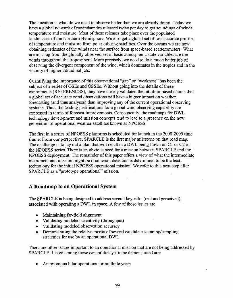
The question is what do we need to observe better than we are already doing. Today wehave a global network of rawindsondes released twice per day to get soundings of winds,temperature and moisture. Most of these releases take place over the populatedlandmasses of the Northern Hemisphere. We a!soget a global set of less accurate profilesof temperature and moisture from polar orbiting satellites. Over the oceans we are nowobtaining estimates of the winds near the surface from space-based scatterometers. Whatare missing from the globally observed set of basic atmospheric state variables are thewinds throughout the troposphere. More precisely, we need to do a much better job ofobserving the divergent component of the wind, which dominates in the tropics and in thevicinity of higher latitudinal jets.

Quantifying the importance of this observational "gap" or "weakness" has been thesubject of a series of OSEs and OSSEs. Without going into the details of theseexperiments (REFERENCES), they have clearly validated the intuition-based claims thata global set of accurate wind observations will have a bigger impact on weatherforecasting (and thus analyses) than improving any of the current operational observingsystems. Thus, the leading justifications for a global wind observing capability areexpressed in terms of forecast improvements. Consequently, the roadmaps for DWL

technology development and mission concepts tend to lead to a presence on the newgeneration of operational weather satellites known as NPOESS.

The first in a series of NPOESS platforms is scheduled for launch in the 2008-2009 timeframe. From our perspective, SPARCLE is the first major milestone on that road map.The challenge is to lay out a plan that will result in a DWL being flown on C1 or C2 ofthe NPOESS series. There is an obvious need for a mission between SPARCLE and theNPOESS deployment. The remainder of this paper offers a view of what the intermediateinstrument and mission might be if coherent detection is determined to be the besttechnology for the initial NPOESS operational mission. We refer to this next step afterSPARCLE as a "prototype operational" mission.

A Roadmap to an Operational System

The SPARCLEis beingdesignedto addressseveralkeyrisks(realandperceived)associatedwith-operatinga DWLin space.A fewof thoseissuesare:

• Maintaining far-field alignment• Validating modeled sensitivity (throughput)• Validating modeled observation accuracy• • Demonstrating the relative merits of several candidate scanning/sampling

strategies for use by an operational DWL

There are other issues important to an operational mission that are not being addressed bySPARCLE. Listed among those capabilities yet to be demonstrated are:

• Autonomous lidar operations for multiple years

314

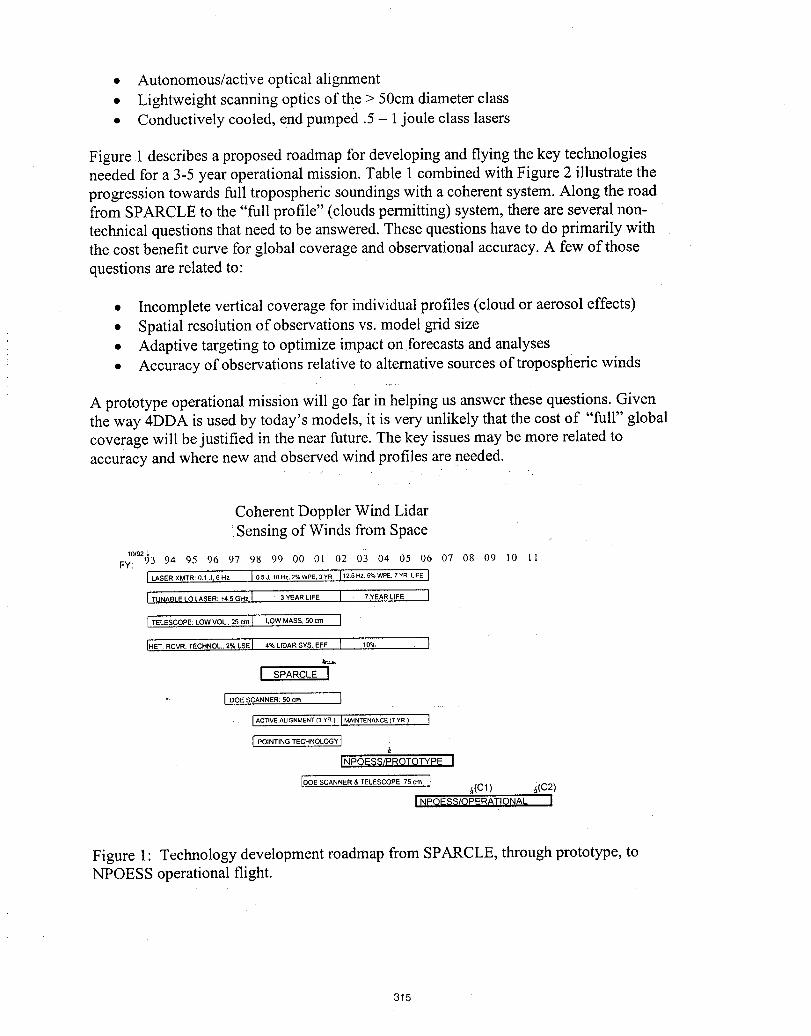
• Autonomous/active optical alignment• Lightweight scanning optics of the > 50cm diameter class• Conductively cooled, end pumped .5 - 1joule class lasers

Figure 1 describes a proposed roadmap for developing and flying the key technologiesneeded for a 3-5 year operational mission. Table 1 combined with Figure 2 illustrate theprogression towards full tropospheric soundings with a coherent system. Along the roadfrom SPARCLE to the "full profile" (clouds permitting) system, there are several non-technical questions that need to be answered. These questions have to do primarily withthe cost benefit curve for global coverage and observational accuracy. A few of thosequestions are related to:

• Incomplete vertical coverage for individual profiles (cloud or aerosol effects)• Spatial resolution of observations vs. model grid size• Adaptive targeting to optimize impact on forecasts and analyses• Accuracy of observations relative to alternative sources of tropospheric winds

A prototype operational mission will go far in helping us answer these questions. Giventhe way 4DDA is used by today's models, it is very unlikely that the cost of "full" globalcoverage will be justified in the near future. The key issues may be more related toaccuracy and where new and observed wind profiles are needed.

Coherent Doppler Wind Lidar•Sensing of Winds from Space

10/92

FY: 93 94 95 96 97 98 99 00 01 02 03 04 05 06 07 08 09 10 I I

[_SERXMTR'.O._J.GHz 105J.10HZ.2%WPE.3YRI'=.'",.'_E.'YRUFEII_NAELE_O_ER:;,.,G"'I 3_ARL,EEI ,YEAR',FE]

I TELESCOPE: LOWVOL. 25 cm I LOW MASS. 50cm I

IHET.RCVR.'ECHNO'.:=_LSEI,_oL,OARSYS.EF".1 ,O_o }

I SPARC,EI

I DOE SCANNER: 50 cm [

I ACTIVE ALIGNMENT (3 YR ) I MAINTENANCE (7 YR ) ]

[ POINTING TECHNOLOGY]

INPOE$_/PROTOTYPEI

[DOE SCANNER & TELESCOPE: 75 cm I _(Cl) &(C2)INPOESS/OPERATIONALI

Figure 1" Technology development roadmap from SPARCLE, through prototype, toNPOESS operational flight.

315

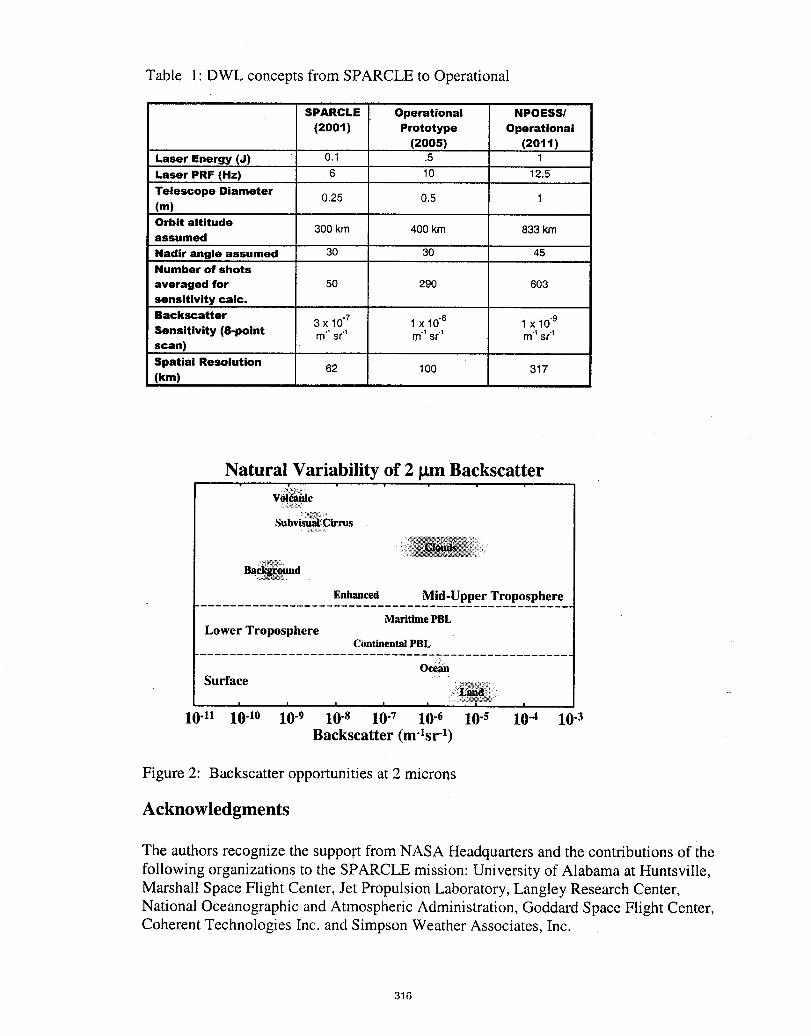
Table 1"DWL concepts from SPARCLE to Operational

SPARCLE Operational NPOESS/

(2001) Prototype Operational(2005) (2011)

Laser Energy (J) 0.1 .5 1

Laser PRF (Hz) 6 10 12.5

Telescope Diameter 0.25 0.5 1(m)Orbit altitude

300 km 400 km 833 kmassumed

Nadir angle assumed 30 30 45Number of shots

averaged for 50 290 603sensitivity calc.Backscatter

3 x 10.7 1 x 10.8 1 x 10.9Sensitivity (8-point m4 sr4 m4 sr4 m4 sr4scan)

Spatial Resolution 62 100 317(km)

Natural Variability of 2 _m Backscattero

Subv_,Cirrus

• _ •

Bac_und

Enhanced Mid-Upper Troposphere

Maritime PBLLower Troposphere

Continental PBL

Surface , _a_,...........

I I I I I I I

1041 1040 10-9 10-s 10-7 10-6 10-s 10-4 10-3Backscatter (m'tsr 1)

Figure 2: Backscatter opportunities at 2 microns

Acknowledgments

The authors recognize the suppo,rt from NASA Headquarters and the contributions of ihefollowing organizations to the SPARCLE mission: University of Alabama at Huntsville,Marshall Space Flight Center, Jet Propulsion Laboratory, Langley Research Center,National Oceanographic and Atmospheric Administration, Goddard Space Flight Center,Coherent Technologies Inc. and Simpson Weather Associates, Inc.

316

Index

A C FAbstracts, 1-10 Cardell, Greg, 311-312 Faucheux, M., 306-310Aircraft Missions, 1_28 Cariou, Jean-Pierre, 251-254 Fetrow, Matthew, 220-223Aircraft Operations, 1, 11 Chambers, Diana M., 111-114, Flamant, Pierre H., 33-36, 136,Allgcod, Glenn O., 40-41 119-122 141-143, 251-254, 306-310Amzajerdian, Farzin, 284-287, then, Shen-en, 43-47 Flesia,C., 141-143288-291 Chiao, Meng,311-312 Foord, R., 123-126Armandillo, E., 306-310 Clarke, A. D., 147-150 Forouhar,Siamak, 311-312Arntzen, Per-Otto,202 Cole, HelenJ., 111-114 Frehlich,Rod,24-27, 298-301Asai, Kazuhiro, 178-181,292- Colson, Carl,98-101 Frouin,Robert, 137-140293 Cornman,Larry,24-27 Fritzsche, K., 268-271Asaka, Kimio,198-201 Cosentino,M. A., 306-310Atkinson, Robert J., 160-162 Cress, Alexander, 294-297 G

Augere, Beatrice, 251-254 Crisp, David, 38-39 Gas, Bruno, 174-!77Axenson, Theresa J., 238-240 Culoma, A., 141-143 Gatt, Philip, 58-61,62-65, 247-

Cutten, Dean R., 29'32, 147- 250150, 160-162 Geddes, N., 141-143

B CW Lidars, 8, 255 Ghibaudo, J. B., 306-310Bagley, Hal R., 20-23 Gibbens, Matt, 98-101

Bailey, Howard, 62-65 D Goodrich,Robert,24-27Banakh,VictorA., 82-85, 132- Graham, D., 123-126135, 294-297 Dabas, Alain, 174-177,278- Grann, EricBanta, Robert M., 273-276 281 Guerit, Gaspard,251-254Barker, Ben C., Jr., 12-15 Daly,J., 43-47Barnes, Norman P., 238-240 Danzeisen, H., 268-271Bedard, Alfred J., 273-276 Darby, Lisa S., 29-32, 273-276 I'_Belmonte, Aniceto, 78-81 Davis, Richard E., 68-71 H&fner, Frank, 187-190Bishop, Kenneth, 220-223 Delville, P., 33-36 Hale, Charley P., 98-101, 115-Blackwell, Timothy S., 284- D'Epagnier, David M., 98-101, 118287, 288-291 115-118 Haner, D. A., 144-146Blockley, A. F., 123-126 Detection Advances, 7, 211 Hannon, Stephen M., 20-23,Boger, James K., 212-215 Devereux, R.W. J., 123-126 24-27, 58-61, 62-65, 151,247-Bogue, Rodney K., 20-23, 151 Dharamsi, Amin, 68-71 250Bogenberger, Richard, 16-19 DIAL, 2-3, 67 Hansson, G6ran, 202Boitel, Ch., 33-36 Dierking, Matt, 62-65 Hardesty, R. Michael; 29-32.B6senberg, Jens, 72-75, 268- Dixit, S. N., 111-114 76, 78-81,278-281271 Dorschner, Terry A., 246 H&ring, R., 33-36Bowdle, David A., 20-23, 147- Drobinski, Philippe, 33-36, 174- Harris, M., 203-206,207-210,150, 151 177, 251-254, 278-281 277Brewer, W. Alan, 76,78-81, Hasselmann, Dieter, 72-75278-281Britt, Charles L., Jr., 12-15 E Heinrichs, Richard, 48-51Hemmati, Harold, 311-312Britten, J. A., 111-114 Ehernberger, L°Jack, 20-23 Henderson, Sammy W., 58-61,Brockman, Philip, 12-15, Emmitt, G. D., 88-93, 182-186, 98-101, 115-118, 247-250Bruneau, D., 33-36 313-316 Hirano, Yoshihito, 198-201Byer, Robert L., 241-244

Engelbart, D, 268-271 Howell, James N., 29-32Esproles, Carlos, 311-312 Hutchinson, Donald P., 40-41,

224

317

I Mc SIngram, C., 123-126 MacDonald, Kenneth R., 212- Sauvage, L., 33-36Ishizu, Mitsuo, 292-293 215 Schnal, Dane, 98-101Itabe, Toshikazu, 292-293 McCarthy, John C., 68-71 Schrecker, M., 33-36

McCaul, Eugene W., Jr., 160- Schulte, Hans Reiner, 94-97162 Shelekhov, Alexander, 272,

J McGrath, Andrew, 234-237 282

Jarzembski, Maurice A., 128- Mclntire, Harold, 220-223 Shen, Chyau N., 66131,147-150, 160-162, 163- McKay, Jack A., 106-109 Shore, B. W., 111-114166, 264-266 McMackin, Lenore, 212-215, Simpson, Marc L., 224Jedlovec,Gary J., 160-162 220-223 Singh, Upendra N., 238-240

Smalikho, Igor, 82-85, 132-Jenkins, R. M., 123-126 135, 294-297

N Soreide, Dave C., 20-23

K Nagel, E., 33-36 Spaceborne Lidars - 1, 3-4,

Kane, TimothyJ., 256-259 New Technology, 4, 110 86Karlsson,Christer,202, 260- Nguyen, DungPhuChi, 12-15 Spaceborne Lidars - 2, 9-10263 Nordin,GregoryP., 119-122 Special, 1-2, 37, 283Kaushik,S., 48-51 Norris, Douglas,24-27 Spiers, Gary D., 167-169, 170-173, 182-186, 302-305Kavaya, Michael J., 88-93, Spinhirne, J. D., 147-150

111-114, 119-122, 153-155, O Sridharan, Arun K.,241-244156-159,302-305 Srivastava, Vandana, 128-131,Killinger, Dennis, 43-47, 216- Ouisse, Adelina, 187-190, 229- 147-150, 160-162, 163-166,219 232 264-266Klein, V., 268-271 Olsson, Fredrik A. A., 260-263 Stephens, T., 48-51Klier, M., 33-36 Stetter, Roger, 62-65Koch, Grady J., 12-15, 68-71Kocher,D. G., 48-51 P Stoffelen, A., 102-105St_'eicher,Juergen, 16-19, 33-KSpp,F., 33-36 Papetti,T., 123-126 36,"294-297

Paules,GranvilleE. III, 87 Suga,ta,Tetuya, 178-181

L Peters, BruceR., 284-287, Sugimoto, Nobuo, 178-181288-291 System Advances, 8, 245Labandibar,J. Y., 306-310 Petros,Mulugeta,12-15, 68-Lampe, Thomas,202 71,238-240Laporta, P. Phillips,Mark, 98-101 TLaser Advances, 7-8, 223 Popescu,AlexandruF., 191- Tamamushi,Kouro,178-181Leeb, Walter R., 191-194 194 Target Charaterization, 4-5,Leike, Ines, 16-19, 229-232, Poster Session, 5-7, 152 127294-297 Potter,J., 43-47 Theory and Simulation, 3, 77Li, Ye, 284-287, 288-291 Primmerman,C. A., 48-51 Thomas, E., 43-47Linn_,Holger,72-75 Pueschel,RudyF°, 160-162 Thomson,J. Alex L., 58-61Loth,Claude, 33-36 Tratt, David M., 29-32, 137-140Lovett,Alexander R., 66 _ 144-146, 311-312Luther,MichaelR., 87 _:_ Trickl,T., 268-271

QuarreU,J., 123-126 Tulloch,William M., 241-244

MMagee, EricP., 256-259 _ V

Mamidipudi,Priyaradan, 43-47, Rahm, Stephan, 16-19, 187- Vaughan, J. M., 141-143, 203-216-219 190 206Marcus, S., 48-51 Raymond, Carol, 38-39 Veitch. Peter, 234-237Marseille,G. J., 102-105 Reardon, Patrick,284-287, Vibration Measurements, 2,Matsui, Ichiro,178-181 288-291 42Meissonnier,M.. 33-36 Reinhardt G. A., 48-51 Voelz, David G., 212-215,220-Menzies, RobertT., 29-32, Reitebuch,O., 33-36 223147-150, 311-312 Richards,RogerK., 40-41,224Miller,T L, 88-93, 182-186, Richmond,RichardD, 52-57313-316 Romand, B, 33-36.Mizutani, Kohei,292-293 Rothermel,Jeffry, 29-32, 147-Munch,Jesper, 234-237 150, 163-166Menkel, Ch., 268-271 Rutherford,Todd,241-244

Rye, Barry J., 76, 78-81,195-197

318

WWergen, Werner, 294-297Werner, Christian, 16-19, 33-36, 82-85, 132-135, 268-271,294-297Westphal, Douglas L., 137-140Wildgruber, G., 33-36Williams, John, 24-27Wind Measurements, 8-9, 267Winzer, Peter J., 191-194, 225-228Woppowa, L., 268-271Wulfmeyer, Volker, 76, 278-281

YYanagisawa, Takayuki, 198-201Young, R. I., 203-206Yu, Jirong, 238-240

ZZarader, J. L., 174-177Zyra, Stan, 202

319

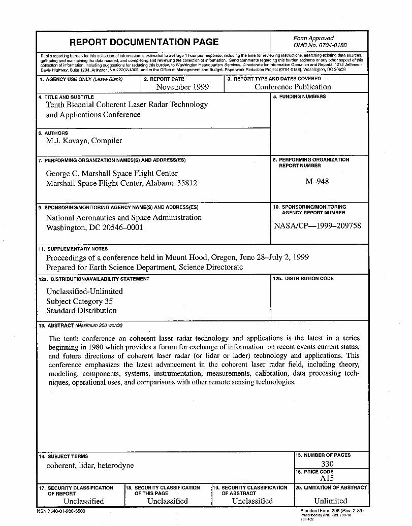
FormApprovedREPORT DOCUMENTATION PAGE OMBNo.0704-0188

Public reporting burden for this collection of information isestimated to average 1 hour per response, including the time for reviewing instructions, searching existing data sources,gathering and maintaining the data needed, end completing and reviewing the collection of information. Send comments regarding this burden estimate or any other aspect of thiscollection of information, including suggestions for reducing this burden, to Washington Headquarters Services, Directorate for Information Operation and Reports, 1215JeffersonDavis Highway, Suite 1204, Arlington, VA 22202-4302, and to the Office of Management and Budget, Paperwork Reduction Project (0704-0188),Washington, DC 20503

1. AGENCY USE ONLY (Leave Blank) 2. REPORT DATE 3. REPORTTYPE AND DATES COVERED

November 1999 Conference Publication4. TITLE AND SUBTITLE 5. FUNDING NUMBERS

Tenth Biennial Coherent Laser Radar Technologyand Applications Conference

6. AUTHORS

M.J. Kavaya, Compiler

7. PERFORMING ORGANIZATION NAMES(S) AND ADDRESS(ES) 8. PERFORMING ORGANIZATIONREPORT NUMBER

George C. Marshall Space Flight CenterMarshall Space Flight Center, Alabama 35812 M-948

9. SPONSORING/MONITORING AGENCY NAME(S) AND ADDRESS(ES) 10. SPONSORING/MONITORING

National Aeronautics and Space Administration AGENCYREPORTNUMBERWashington, DC 20546-0001 NASA/CP-- 1999-209758

11. SUPPLEMENTARY NOTES

Proceedings of a conference held in Mount Hood, Oregon, June 28-July 2, 1999Prepared for Earth Science Department, Science Directorate

12a. DISTRIBUTION/AVAILABILITY STATEMENT 12b. DISTRIBUTION CODE

Unclassified-Unlimited

Subject Category 35Standard Distribution

13. ABSTRACT (Maximum 200 words)

The tenth conference on coherent laser radar technology and applications is the latest in a seriesbeginning in 1980 which provides a forum for exchange of information on recent events current status,and future directions of coherent laser radar (or lidar or lader) technology and applications. Thisconference emphasizes the latest advancement in the coherent laser radar field, including theory,modeling, components, systems, instrumentation, measurements, calibration, data processing tech-niques, operational uses, and comparisons with other remote sensing technologies.

14. SUBJECTTERMS 15. NUMBER OF PAGES

coherent, lidar, heterodyne 33016. PRICE CODE

A1517. SECURITY CLASSIFICATION 18. SECURITY CLASSIFICATION 19. SECURITY CLASSIFICATION 20. LIMITATIONOF ABSTRACT

OF REPORT OF THIS PAGE OF ABSTRACT

Unclassified Unclassified Unclassified UnlimitedNSN 7540-01-280-5500 StandardForm298 (Rev. 2-89)

Prescribed by ANSI Std. 239-18: 298-102

NASA_r_l_ni_t Li

Nationa,Aeronauticsand IIlllJIIIJIIlllli_U_IfIJIIJISpace Administration 3 1176014480124AD33

George C. Marshall Space Flight CenterMarshall Space Flight Center, Alabama35812