formal veri cation of implementations of state ow charts
TRANSCRIPT

Formal veri�cation ofimplementations of State�ow charts
Alvaro Heiji Miyazawa
Submitted for the degree of Doctor of Philosophy
The University of York
Department of Computer Science
February 2012


To my mother.


Abstract
Simulink diagrams are widely used in industry for specifying control systems, and a par-
ticular type of block used in them is a State�ow chart. Often, the systems speci�ed are
safety-critical ones. Therefore, the issue of correctness of implementations of these systems
is relevant. We are interested in the veri�cation of implementations of State�ow charts.
In this thesis, we propose a formal model of State�ow charts in the Circus notation. The
proposed model makes a distinction between the general semantics of State�ow charts and
the speci�c aspects of each chart, and maintains the operational style used in the o�cial
informal description of the semantics of State�ow. In this way, we support the comparison
of our model to the informal description as an extra form of validation. Moreover, this
separation allows us to obtain a translation from a State�ow chart to a Circus model based
mostly on the syntactic structure of the chart.
We formalise in Z a translation strategy that supports the generation of the chart speci�c
model which is composed with the model of the semantics of State�ow charts to formalise
the execution of the chart. The translation strategy is implemented in a tool that sup-
ports the automatic generation of the complete model of a chart. The style in which the
translation strategy is speci�ed supports a very direct implementation, thus, minimising
this potential source of error.
We identify an architecture of parallel implementations based on the sequential implemen-
tations automatically generated by a code generator, and propose a re�nement strategy
that applies the Circus re�nement calculus to verify the correctness of the implementation
with respect to the proposed formal model of State�ow charts. The identi�cation of the
architecture allows us to specify the re�nement strategy in a degree of detail that renders
it suitable for formalisation in a tactical language, thus, potentially achieving a high de-
gree of automation. Moreover, this strategy is a starting point for new strategies targeting
di�erent architectural patterns.

Contents
1 Introduction 1
1.1 Objectives . . . . . . . . . . . . . . . . . . . . . . . . . . . . . . . . . . . . . 2
1.2 Thesis structure . . . . . . . . . . . . . . . . . . . . . . . . . . . . . . . . . . 4
2 Literature review 5
2.1 State�ow . . . . . . . . . . . . . . . . . . . . . . . . . . . . . . . . . . . . . 6
2.1.1 Elements of the notations . . . . . . . . . . . . . . . . . . . . . . . . 6
2.1.2 Informal semantics of State�ow charts . . . . . . . . . . . . . . . . . 9
2.1.3 Early return logic . . . . . . . . . . . . . . . . . . . . . . . . . . . . . 13
2.2 Formal models . . . . . . . . . . . . . . . . . . . . . . . . . . . . . . . . . . 14
2.2.1 Veri�cation approaches . . . . . . . . . . . . . . . . . . . . . . . . . . 15
2.2.2 Code generation approaches . . . . . . . . . . . . . . . . . . . . . . . 19
2.3 Speci�cation languages . . . . . . . . . . . . . . . . . . . . . . . . . . . . . . 20
2.4 Re�nement calculus . . . . . . . . . . . . . . . . . . . . . . . . . . . . . . . 21
2.5 Circus . . . . . . . . . . . . . . . . . . . . . . . . . . . . . . . . . . . . . . . 21
2.6 Final considerations . . . . . . . . . . . . . . . . . . . . . . . . . . . . . . . 24
3 Formal Model 25
3.1 Overview . . . . . . . . . . . . . . . . . . . . . . . . . . . . . . . . . . . . . 26
3.2 Process Simulator . . . . . . . . . . . . . . . . . . . . . . . . . . . . . . . . 31
3.2.1 Step of execution . . . . . . . . . . . . . . . . . . . . . . . . . . . . . 32
3.2.2 Transition . . . . . . . . . . . . . . . . . . . . . . . . . . . . . . . . . 35
3.2.3 Entering a state . . . . . . . . . . . . . . . . . . . . . . . . . . . . . . 42
3.2.4 Executing and exiting a state . . . . . . . . . . . . . . . . . . . . . . 48
3.3 Chart process . . . . . . . . . . . . . . . . . . . . . . . . . . . . . . . . . . . 52
3.4 Validation . . . . . . . . . . . . . . . . . . . . . . . . . . . . . . . . . . . . . 59
3.5 Final considerations . . . . . . . . . . . . . . . . . . . . . . . . . . . . . . . 60
4 Translation strategy 63
4.1 Syntax of State�ow charts . . . . . . . . . . . . . . . . . . . . . . . . . . . . 64
4.1.1 Names and Identi�ers . . . . . . . . . . . . . . . . . . . . . . . . . . 64
4.1.2 Expressions and Actions . . . . . . . . . . . . . . . . . . . . . . . . . 65
vi CONTENTS
4.1.3 State�ow objects . . . . . . . . . . . . . . . . . . . . . . . . . . . . . 66
4.2 Well-formedness conditions . . . . . . . . . . . . . . . . . . . . . . . . . . . 71
4.3 Translation strategy in Z . . . . . . . . . . . . . . . . . . . . . . . . . . . . . 72
4.3.1 Renaming functions . . . . . . . . . . . . . . . . . . . . . . . . . . . 73
4.3.2 Expression and Action functions . . . . . . . . . . . . . . . . . . . . 74
4.3.3 Identi�er and binding declaration functions . . . . . . . . . . . . . . 77
4.3.4 Action, condition and process declaration functions . . . . . . . . . . 78
4.4 Automation of the translation strategy . . . . . . . . . . . . . . . . . . . . . 82
4.4.1 Architecture . . . . . . . . . . . . . . . . . . . . . . . . . . . . . . . . 82
4.4.2 Implementation of translation rules . . . . . . . . . . . . . . . . . . . 90
4.5 Evaluation . . . . . . . . . . . . . . . . . . . . . . . . . . . . . . . . . . . . . 93
4.6 Final considerations . . . . . . . . . . . . . . . . . . . . . . . . . . . . . . . 95
5 Re�nement strategy 97
5.1 Implementations of State�ow charts . . . . . . . . . . . . . . . . . . . . . . 98
5.1.1 Architecture: data patterns . . . . . . . . . . . . . . . . . . . . . . . 99
5.1.2 Architecture: control �ow . . . . . . . . . . . . . . . . . . . . . . . . 102
5.2 Circus models of implementations . . . . . . . . . . . . . . . . . . . . . . . . 106
5.3 Re�nement strategy . . . . . . . . . . . . . . . . . . . . . . . . . . . . . . . 108
5.3.1 Data re�nement . . . . . . . . . . . . . . . . . . . . . . . . . . . . . 109
5.3.2 Normalisation . . . . . . . . . . . . . . . . . . . . . . . . . . . . . . . 113
5.3.3 Structuring . . . . . . . . . . . . . . . . . . . . . . . . . . . . . . . . 117
5.3.4 Parallelism introduction . . . . . . . . . . . . . . . . . . . . . . . . . 158
5.3.5 Action introduction . . . . . . . . . . . . . . . . . . . . . . . . . . . . 166
5.4 Final considerations . . . . . . . . . . . . . . . . . . . . . . . . . . . . . . . 167
6 Conclusions 169
6.1 Thesis contributions . . . . . . . . . . . . . . . . . . . . . . . . . . . . . . . 169
6.2 Related Work . . . . . . . . . . . . . . . . . . . . . . . . . . . . . . . . . . . 172
6.3 Future work . . . . . . . . . . . . . . . . . . . . . . . . . . . . . . . . . . . . 173
A Syntax of Circus 177
B Circus model of State�ow semantics 179
B.1 Basic de�nitions . . . . . . . . . . . . . . . . . . . . . . . . . . . . . . . . . 179
B.2 State�ow semantics . . . . . . . . . . . . . . . . . . . . . . . . . . . . . . . . 180
C Circus models of State�ow charts 197
C.1 Circus model of Shift Logic Chart . . . . . . . . . . . . . . . . . . . . . . . . 197
C.2 Circus model of Air Controller Chart . . . . . . . . . . . . . . . . . . . . . . 213
D Circus model of the implementation of Air Controller Chart 225

CONTENTS vii
E Novel re�nement laws 231

List of Figures
2.1 Executing a Set of Transitions [98]. . . . . . . . . . . . . . . . . . . . . . . . 10
2.2 Entering a State [98]. . . . . . . . . . . . . . . . . . . . . . . . . . . . . . . . 11
2.3 Executing an active State [98]. . . . . . . . . . . . . . . . . . . . . . . . . . 12
2.4 Exiting an active State [98]. . . . . . . . . . . . . . . . . . . . . . . . . . . . 12
2.5 Early return logic example. . . . . . . . . . . . . . . . . . . . . . . . . . . . 13
2.6 The Bu�er process . . . . . . . . . . . . . . . . . . . . . . . . . . . . . . . . 22
3.1 Basic architecture of State�ow models. . . . . . . . . . . . . . . . . . . . . . 25
3.2 Example of a State�ow Chart describing a car's shift logic. . . . . . . . . . . 27
3.3 Overview of the model . . . . . . . . . . . . . . . . . . . . . . . . . . . . . . 28
3.4 Structure of the Simulator process. . . . . . . . . . . . . . . . . . . . . . . . 31
3.5 Executing a Set of Transitions [98] . . . . . . . . . . . . . . . . . . . . . . . 43
3.6 Entering a State [98] . . . . . . . . . . . . . . . . . . . . . . . . . . . . . . . 44
3.7 Executing an active State [98] . . . . . . . . . . . . . . . . . . . . . . . . . . 49
3.8 Exiting a State [98] . . . . . . . . . . . . . . . . . . . . . . . . . . . . . . . . 51
3.9 Structure of the c shift logic process. . . . . . . . . . . . . . . . . . . . . . 53
4.1 Translation strategy: overview. . . . . . . . . . . . . . . . . . . . . . . . . . 63
4.2 Architecture of s2c: main packages. . . . . . . . . . . . . . . . . . . . . . . . 83
4.3 Architecture of the package Parser. . . . . . . . . . . . . . . . . . . . . . . 83
4.4 Structure of a .mdl �le. . . . . . . . . . . . . . . . . . . . . . . . . . . . . . 84
4.5 Excerpt from a .mdl �le. . . . . . . . . . . . . . . . . . . . . . . . . . . . . . 84
4.6 Architecture of the package MDL Parser. . . . . . . . . . . . . . . . . . . . . 85
4.7 State label . . . . . . . . . . . . . . . . . . . . . . . . . . . . . . . . . . . . . 85
4.8 Transition label . . . . . . . . . . . . . . . . . . . . . . . . . . . . . . . . . . 85
4.9 Architecture of the package Label Parser. . . . . . . . . . . . . . . . . . . 86
4.10 Syntax of State�ow charts: main packages. . . . . . . . . . . . . . . . . . . . 86
4.11 Syntax of State�ow charts: Objects. . . . . . . . . . . . . . . . . . . . . . . 87
4.12 Syntax of State�ow charts: Actions. . . . . . . . . . . . . . . . . . . . . . . 88
4.13 Syntax of State�ow charts: Expressions. . . . . . . . . . . . . . . . . . . . . 88
4.14 Syntax of Circus. . . . . . . . . . . . . . . . . . . . . . . . . . . . . . . . . . 89
4.15 Architecture of s2c: the Translator package. . . . . . . . . . . . . . . . . . . 89
x LIST OF FIGURES
4.16 Implementations of the translation rule for variable expressions. . . . . . . . 91
4.17 Implementations of the translation rule for the declaration of data. . . . . . 92
4.18 Implementation of simulation instance rule . . . . . . . . . . . . . . . . . . . 92
5.1 Overview of our re�nement strategy. . . . . . . . . . . . . . . . . . . . . . . 97
5.2 Air controller chart: supplied with State�ow. . . . . . . . . . . . . . . . . . . 98
5.3 Architecture of implementations of State�ow charts. . . . . . . . . . . . . . 99
5.4 Function MDLInitialize. . . . . . . . . . . . . . . . . . . . . . . . . . . . . 103
5.5 Structure of the procedure calculate output. . . . . . . . . . . . . . . . . 104
5.6 Structure of calculate step and interaction patterns with the servers. . . 104
5.7 Procedure calculate step for our example. . . . . . . . . . . . . . . . . . . 105
5.8 Parallelism in the execution of the parallel states in our example. . . . . . . 106
5.9 Overview of the models of implementations of State�ow charts. . . . . . . . 107
5.10 Action Client in implementation models. . . . . . . . . . . . . . . . . . . . . 107
5.11 Re�nement strategy: data re�nement phase. . . . . . . . . . . . . . . . . . . 110
5.12 Schema D Work Air . . . . . . . . . . . . . . . . . . . . . . . . . . . . . . . 111
5.13 Total functional retrieve relation for our example. . . . . . . . . . . . . . . . 112
5.14 Calculated total surjective functional retrieve relation: general form. . . . . 114
5.15 Re�nement strategy: normalisation phase. . . . . . . . . . . . . . . . . . . . 115
5.16 Normalisation � Example: Main action after Steps 1 and 2. . . . . . . . . . 115
5.17 Normalisation � Example: Main action at the end. . . . . . . . . . . . . . . 116
5.18 Structuring starting point. . . . . . . . . . . . . . . . . . . . . . . . . . . . . 117
5.19 Structuring target. . . . . . . . . . . . . . . . . . . . . . . . . . . . . . . . . 119
5.20 Structuring target - chart execution. . . . . . . . . . . . . . . . . . . . . . . 119
5.21 Structuring target - writing the outputs. . . . . . . . . . . . . . . . . . . . . 119
5.22 Re�nement strategy: structuring phase . . . . . . . . . . . . . . . . . . . . . 121
5.23 Structuring: body of the outmost recursion in the main action after Step 2. 121
5.24 Structuring: part of the main action after Step 2. . . . . . . . . . . . . . . . 122
5.25 Structuring: main action after Step 2 - writing outputs. . . . . . . . . . . . 122
5.26 Structuring: body of the outmost recursion in the main action after Step 3. 123
5.27 Re�nement strategy: structuring phase - input-event-var-introduction . . . . 125
5.28 parallelism-resolution: pre�xing over channel in the synchronisation set on
the right-hand side. . . . . . . . . . . . . . . . . . . . . . . . . . . . . . . . . 125
5.29 parallelism-resolution: steps for pre�xing over channel in the synchronisation
set on the right-hand side. . . . . . . . . . . . . . . . . . . . . . . . . . . . . 126
5.30 parallelism-resolution: result for pre�xing over channel in the synchronisation
set on the right-hand side. . . . . . . . . . . . . . . . . . . . . . . . . . . . . 126
5.31 parallelism-resolution: pre�xing over channel not in the synchronisation set
on either side. . . . . . . . . . . . . . . . . . . . . . . . . . . . . . . . . . . . 128
5.32 parallelism-resolution: leading interleaving on the left-hand side. . . . . . . . 129
5.33 parallelism-resolution: result for leading interleaving on the left-hand side. . . 129
LIST OF FIGURES xi
5.34 parallelism-resolution: alternation followed by sequence, on either side. . . . . 130
5.35 parallelism-resolution: steps for alternation followed by sequence, on either
side. . . . . . . . . . . . . . . . . . . . . . . . . . . . . . . . . . . . . . . . . 131
5.36 parallelism-resolution: possible results for alternation followed by sequence,
on either side. . . . . . . . . . . . . . . . . . . . . . . . . . . . . . . . . . . . 131
5.37 parallelism-resolution: steps for call action on either side. . . . . . . . . . . . 132
5.38 parallelism-resolution: leading schema operation on the left-hand side. . . . . 133
5.39 parallelism-resolution: result for leading schema operation on the left-hand
side. . . . . . . . . . . . . . . . . . . . . . . . . . . . . . . . . . . . . . . . . 133
5.40 parallelism-resolution: explicit recursion on the right-hand side. . . . . . . . . 133
5.41 parallelism-resolution: result for explicit recursion on the right-hand side. . . 133
5.42 parallelism-resolution: steps for leading pre�xing over channel in the synchro-
nisation set on the left-hand side. . . . . . . . . . . . . . . . . . . . . . . . . 134
5.43 parallelism-resolution: local event broadcast. . . . . . . . . . . . . . . . . . . 135
5.44 parallelism-resolution: steps for local event broadcast. . . . . . . . . . . . . . 135
5.45 parallelism-resolution: result for local event broadcast. . . . . . . . . . . . . . 136
5.46 Procedure copy . . . . . . . . . . . . . . . . . . . . . . . . . . . . . . . . . . 141
5.47 Re�nement strategy:structuring phase - recursion-introduction. . . . . . . . . 143
5.48 Re�nement strategy: structuring phase - assignment-introduction . . . . . . . 145
5.49 update-output starting point. . . . . . . . . . . . . . . . . . . . . . . . . . . . 146
5.50 Re�nement strategy: structuring phase - update-output . . . . . . . . . . . . 147
5.51 Re�nement strategy: structuring phase - simpli�cation . . . . . . . . . . . . 149
5.52 Re�nement strategy: structuring phase - early-return-simpli�cation . . . . . . 151
5.53 Procedure assumption-distribution. . . . . . . . . . . . . . . . . . . . . . . . . 152
5.54 Re�nement strategy: structuring phase - parallel-state-simpli�cation . . . . . 153
5.55 parallel-state-simpli�cation: example after step 2. . . . . . . . . . . . . . . . . 155
5.56 parallel-state-simpli�cation: example after step 3(a). . . . . . . . . . . . . . . 155
5.57 parallel-state-simpli�cation: example after step 3(b). . . . . . . . . . . . . . . 156
5.58 parallel-state-simpli�cation: example after step 3(c)-i. . . . . . . . . . . . . . 156
5.59 parallel-state-simpli�cation: example after step 3(c)-ii. . . . . . . . . . . . . . 157
5.60 Procedure sequential-state-simpli�cation . . . . . . . . . . . . . . . . . . . . . 157
5.61 Functions implemented the server for our example . . . . . . . . . . . . . . 159
5.62 Parallelism introduction - example of execution of parallel states. . . . . . . 159
5.63 Parallelism introduction target - execution of parallel states example. . . . . 160
5.64 Parallelism introduction target - server example. . . . . . . . . . . . . . . . 161
5.65 Re�nement strategy: parallelism introduction phase . . . . . . . . . . . . . 161
5.66 Parallelism introduction - example: portion of the main action after Step 1. 163
5.67 Re�nement strategy: action introduction phase. . . . . . . . . . . . . . . . . 166

Acknowledgements
I would like to, �rstly, thank my supervisor, Ana Cavalcanti, for all her support and
guidance. Without her encouragement and advice this thesis would not have been possible.
I would like to express my gratitude to my examiners, Professor Richard Paige and
Professor Michael Butler, whose comments and suggestions were invaluable to this thesis.
I would also like to thank my colleagues at the Department of Computer Science, and
the members of the Circus group; in particular, I am grateful to Frank Zeyda for many
discussions throughout my time in York, and Leo Freitas who helped me understand Circus
and the CZT framework.
Thanks to my family and friends whose support and friendship helped me maintain
my sanity. Special thanks to my partner, Oleg Lisagor, who read and commented on
various drafts of my thesis and gave me the all support I needed to complete this thesis,
my friends in York, André Freire, Luiza Dias, Jennifer Winter and David E�rd whose
friendship and ad hoc counselling sessions in York's many pubs were indispensable, and
my friends and former colleagues in Brazil � Ana Melo, Paulo Salem, Renata Matteoni,
Jony Arrais, Patrícia Viana, Márcio Medeiros and Renato Massaro � who have provided
me with support that, whilst di�cult to pinpoint, was indispensable.
Most importantly, I am forever indebted to my mother, who throughout my life en-
couraged me to further my studies, and always supported me in all my endeavours. I could
never possibly thank her enough. To her I dedicate this Thesis.

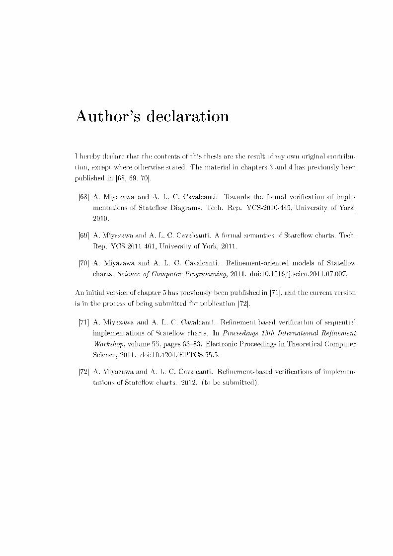
Author's declaration
I hereby declare that the contents of this thesis are the result of my own original contribu-
tion, except where otherwise stated. The material in chapters 3 and 4 has previously been
published in [68, 69, 70].
[68] A. Miyazawa and A. L. C. Cavalcanti. Towards the formal veri�cation of imple-
mentations of State�ow Diagrams. Tech. Rep. YCS-2010-449, University of York,
2010.
[69] A. Miyazawa and A. L. C. Cavalcanti. A formal semantics of State�ow charts. Tech.
Rep. YCS-2011-461, University of York, 2011.
[70] A. Miyazawa and A. L. C. Cavalcanti. Re�nement-oriented models of State�ow
charts. Science of Computer Programming, 2011. doi:10.1016/j.scico.2011.07.007.
An initial version of chapter 5 has previously been published in [71], and the current version
is in the process of being submitted for publication [72].
[71] A. Miyazawa and A. L. C. Cavalcanti. Re�nement-based veri�cation of sequential
implementations of State�ow charts. In Proceedings 15th International Re�nement
Workshop, volume 55, pages 65�83. Electronic Proceedings in Theoretical Computer
Science, 2011. doi:10.4204/EPTCS.55.5.
[72] A. Miyazawa and A. L. C. Cavalcanti. Re�nement-based veri�cations of implemen-
tations of State�ow charts. 2012. (to be submitted).


Chapter 1
Introduction
State�ow is part of the MATLAB Simulink tool [99] and consists of a statechart notation
used to de�ne charts used as blocks in control law diagrams. Control law diagrams are a
popular notation for specifying control systems, and are widely used in the avionics and
automotive industries.
While control law diagrams tackle the aspects of a system that are usually speci�ed by
di�erential equations relating inputs and outputs graphically, State�ow charts are used to
describe the aspects that are better modelled by �nite state machines. For example, in a
system with redundant subsystems, a State�ow chart can be used to specify an automated
recon�guration procedure based on individual subsystems' health monitoring statuses. An-
other example is a switch-over between modes of operation of an aircraft system based on
the phase of �ight (e.g. take-o�, climb, cruise, etc.) as commanded by the pilots and/or
indicated by aircraft sensors (e.g. weight on wheels and ground speed indicators).
Some of the systems speci�ed using Simulink diagrams and State�ow charts are safety-
critical systems. Such systems may cause death, injury, signi�cant environmental damage
or other material loss. The necessary rigour of veri�cation and validation of software
used in safety critical applications is often expressed in terms of Safety (or Software)
Integrity Levels (SILs) which are determined based on the potential severity of the unsafe
system-level conditions (hazards) that the software may contribute to and the extent of the
contribution. For example, a software controller may sometimes be assigned a lower SIL
if its outputs are checked by an independent sub-system (e.g. a monitor or an interlock)
than if the controller has full authority over the system.
Various international standards provide guidance on which design, veri�cation and
validation techniques should be used for di�erent SILs. For instance, the international
standard IEC 61508 [47] recommends the use of formal methods for the speci�cation of
safety requirements as well as for the design and development of software for SILs 2 and 3,
while highly recommending those techniques for SIL4; the standard also recommends the
use of formal proof for the veri�cation of software. Similar recommendations are re�ected
in domain-speci�c adaptations of IEC 61508 such as CENELEC 50128 [25] (for railway
control systems) and the recently published ISO 20262 [48] (for automotive applications).

2 CHAPTER 1. INTRODUCTION
In civil aerospace, the applicable standard DO-178b [83], while not mandating the use of
formal methods, explicitly recognises them as an alternative method. Finally, the currently
superseded UK Military Standard DEF STAN 00-55 [62] makes the use of formal methods
mandatory for SILs 3 and 4; it also requires explicit justi�cation to be provided if formal
methods are not used for lower SILs.
These requirements and recommendations contained in standards demonstrate that
formal techniques that are capable of dealing with modelling languages and notations used
in industry (such as MATLAB Simulink and State�ow) are useful, if not necessary.
There are several approaches to the formal analysis of state diagram notations such as
State�ow. However, most of these approaches focus on the veri�cation of properties, not
on the veri�cation of implementations; the veri�cation of implementations with respect
to a speci�cation can be seen as a particular type of property veri�cation in which the
property in question is that the implementation is a re�nement of the speci�cation. By
restricting ourselves to the veri�cation of implementations we can take advantage of speci�c
techniques (such as the re�nement calculus) that are more adequate for this task.
One of the main approaches used for the veri�cation of implementations consists of
verifying a code generator [102]. This approach makes the implementation immutable
because only generated code is correct by construction; however, in many cases, code
tailored to speci�c situations is necessary, which makes such an approach not applicable.
The veri�cation of implementations, instead of the code generator, can overcome this
problem, but can potentially increase the complexity of the task.
Arthan et al. [4] and Adams and Clayton [3] describe ClawZ, a tool for translating
Simulink diagrams into Z [109] in order to formally verify implementations in Ada. This
approach does not cover the State�ow notation and can only deal with sequential imple-
mentations; to overcome the latter limitation, concurrent aspects are speci�ed in CSP [85]
and analysed through the model checker FDR2 [30].
Cavalcanti and Clayton [17] de�ne the semantics of control law diagrams in the Circus
notation [79], which is a re�nement language that combines Z, CSP, Dijkstra's language of
guarded commands [22], and Morgan's speci�cation statement [73]. This semantics reuses
ClawZ and the CSP approach to concurrency, and extends them to cover a larger subset of
the notation, but it still does not cover the State�ow notation. A Circus model of State�ow
charts is a natural extension of previous work, allowing for the veri�cation of a broader
variety of control law diagrams.
1.1 Objectives
We are concerned with the veri�cation of implementations of State�ow charts, i.e., we
want to verify whether a program correctly implements a State�ow chart or not. We focus
this work in the State�ow variety of state diagrams because it is part of the widely used
MATLAB Simulink tool.
In order to achieve the objective of verifying implementations of State�ow charts, we
1.1. OBJECTIVES 3
need, �rst, a formal semantics of these charts and, second, techniques suitable for the
veri�cation of implementations with respect to the proposed semantics.
The formal semantics of State�ow charts needs to be suitable for formal reasoning about
the correctness of implementations; it must be written in a way that facilitates validation
and be subject to integration with models of Simulink diagrams. This last requirement is
due to the fact that State�ow charts are part of Simulink diagrams, and, in order to verify
a complete system, we must be able to cover both notations.
The veri�cation techniques must allow us to verify code and must also be consistent
with the techniques used for Simulink diagrams, so that Simulink and State�ow blocks
within the same diagram can be veri�ed in a uniform manner.
By using Circus as a speci�cation language, we are able to tackle these desired proper-
ties: ability to formally reason about the model, to verify code and to integrate the model
with the existing models of Simulink diagrams. Since Circus is a formal speci�cation lan-
guage, we can de�ne properties of models and mathematically prove whether they hold or
not.
The veri�cation of code is carried out by proving that the code is (or is not) a re�nement
of a speci�cation, and the integration with existing models of Simulink diagrams is possible
because these models were previously speci�ed in Circus [19].
Due to the informal nature of the State�ow semantics, we need to de�ne a formal model
based on the informal description contained in the State�ow User's Guide [98]. Since there
is no o�cial formal semantics with which we can formally compare our model, we must
validate it through alternative approaches.
We distinguish three main possibilities: one is based on inspection of the informal
description, the second is based on testing and is achieved by comparing a particular chart
and its model by means of simulation, and the third consists of applying the re�nement
calculus to obtain an implementation of the chart.
In order to allow for the �rst form of validation, the model presented in Chapter 3
is de�ned in a way that facilitates the comparison to the informal description, which is
given is steps in the State�ow User's Guide for each of the main semantic rules that
describe the behaviour of states and transitions. The comparison is eased by establishing
a correspondence between the steps and elements of the speci�cation.
The second form of validation can be achieved by simulation of the model and compar-
ison of the traces to the results of the simulation of charts; we can improve this validation
by using techniques for the selection of test cases of charts that yield better coverage.
Finally, by carefully applying the re�nement calculus to models of State�ow charts, we
are able to validate the interaction between the di�erent parts of the model, and spot any
deviations of the expected behaviour of the chart, which might otherwise be overlooked.
In this way, we allow for three di�erent approaches for the validation of the model.
4 CHAPTER 1. INTRODUCTION
1.2 Thesis structure
This section describes the structure of this thesis. Chapter 2 reviews some of the variants
of state diagram notations and formal speci�cation languages that can be used to formalise
the semantics of such notations. This chapter presents a brief introduction to State�ow
charts and Circus, and further reviews the existing approaches to modelling and analysis
of state diagrams.
Chapter 3 presents an operational model of State�ow charts by means of a small exam-
ple; it discusses the rationale behind the particular structure of our models, and describes
the formalisation of the semantics of State�ow charts.
Chapter 4 presents the formalisation of the translation rules necessary to support the
derivation of State�ow models as presented in Chapter 3, and discusses the implementa-
tion of these translation rules in the tool s2c that supports the automatic generation of
Circus models of State�ow charts.
Chapter 5 identi�es an architecture of implementations of State�ow charts, and pro-
poses a re�nement based veri�cation strategy that supports the veri�cation of implemen-
tation conforming to the identi�ed architecture with respect to the models discussed in
Chapters 3 and 4. The architecture described in this chapter is based on the implementa-
tions generated by the Simulink/State�ow code generator [100, 98] and extended to support
parallel implementations of State�ow charts. The veri�cation strategy takes advantage of
the architectural patterns described to provide a detailed step by step re�nement strategy
that can potentially lead to a high degree of automation.
Chapter 6 concludes with a discussion of the main contributions and limitations of our
work, potential solutions to some of the limitations, and future lines of research.

Chapter 2
Literature review
This chapter sets the scene for the remainder of the thesis by presenting a review of the
previous work and languages related to our main objective - veri�cation of implementations
of State�ow charts.
State�ow charts are a variant of Harel's statecharts [36], which are an extension of state
diagrams. These are, basically, directed graphs, where nodes represent states and edges
represent transitions [46]; the latter connect states and can be guarded by conditions. We
identify three main variants of the state diagram notations that are obtained by adding
new features, changing existing ones or modifying the semantics: Harel's statecharts, UML
statecharts and State�ow charts.
Statecharts [36] extend state diagrams to improve the expressive power of the basic
notation, allowing for the speci�cation of complex reactive systems, concurrent systems,
communication protocols, etc. This extension is achieved by introducing concepts such as
hierarchy of states (states within states), concurrency (parallel states) and communication
(local events).
UML statecharts [81] are an object-oriented version of statecharts [53]. They mainly
di�er from Harel's statecharts with respect to the semantics, but also present syntactic
di�erences, such as entry and exit actions in states [107].
State�ow charts [98] extend statecharts by adding, among other features, �ow charts,
temporal logic triggers and di�erent types of actions (during actions, on event actions,
transition actions).
While both State�ow charts and UML statecharts are widely used in industry, ac-
cording to Crane and Dingel [21], even among close variants of statecharts, such as UML
statecharts, Classical statecharts and Rhapsody statecharts, there are several syntactic
and semantic di�erences. Moreover, Fecher et al. [27] identify 29 problems in the de�ni-
tion of the semantics of UML statecharts such as inconsistencies and omitted restrictions.
Consequently, formal models of one variant cannot be easily reused for other variants.
The objective of this chapter is to present the context and the "baseline" of the research
reported in this thesis. The remainder of the chapter is organised as follows. Firstly, we
describe the State�ow notation based on the description contained in the User's Guide [98];
6 CHAPTER 2. LITERATURE REVIEW
we comment on some inconsistencies of this authoritative source and, where possible,
correct the description of the semantics. Section 2.2 then reviews approaches for modelling
and analysis of state diagram notations. The third section presents an overview of some
of the languages that could be used to model State�ow charts (Section 2.3). Section 2.5
presents Circus - the language we have selected for modelling the charts. The chapter
concludes with some �nal observations and remarks (Section 2.6).
2.1 State�ow
In this section, we give an brief overview of State�ow charts based on the User's Guide [98].
State�ow de�nes a new type of Simulink block, namely a State�ow chart, that is used
in a Simulink diagram. A Simulink diagram consists of blocks and wires connecting the
inputs and outputs of the blocks. The execution of a Simulink diagram is done in steps,
in which each of its blocks is executed in a particular order determined by the wiring.
The State�ow chart is the root for the execution of the State�ow model; whenever an
event is directed at a chart, the chart is either entered or executed, depending on whether
it was previously active or not. A chart comprises mainly objects of the following types:
events, data, actions, states, junctions, transitions and function blocks, of which events
and data can be used to communicate with other blocks of the Simulink diagram.
An event can also be used internally to trigger the execution of the chart (or part
of it). This use potentially leads to recursive executions, which may lead the chart to
a con�guration where further execution leads to an inconsistent state. To avoid this,
State�ow uses early return logic to decide when it is safe to continue the execution, and
when part of it must be interrupted. Early return logic is discussed in Section 2.1.3.
2.1.1 Elements of the notations
Events Events are objects that trigger the execution of a Simulink block, e.g. a chart.
They can be distinguished by trigger type and scope. With respect to the trigger type, an
event can be edge-triggered or function-call.
The basic di�erence between edge-triggered and function-call events is the time step
in which outputs of the triggered block are available. If a block is triggered by an edge-
triggered event, it is executed in the same time step as the State�ow chart, but its outputs
are only available in the next time step of the State�ow chart. If a block is triggered by
a function-call event, it is executed in the same time step as the State�ow chart, and its
outputs are available in that same time step, that is, a function-call triggered block is
executed in interleave with the block that produced the function-call event.
The scope characterises an event as input, output, local, exported or imported. An
input event is one generated in a di�erent block in the Simulink diagram and processed
by the chart. Charts can be triggered by a single function-call event, or by a sequence of
edge-triggered events. In the latter case, the order is determined statically in the de�nition
2.1. STATEFLOW 7
of the chart, and is important because at each step the chart is executed once for each
input event that has occurred.
An output event is generated by the chart and processed by some block in the Simulink
diagram. Edge-triggered output events are only communicated to the Simulink models in
the end of the step of execution (along with the output data), and present a queuing
behaviour; if a chart broadcasts the same event more than once in an execution step, it
queues the broadcasts and releases one per execution step. Function-call output events
trigger the execution of a Simulink block immediately, and any outputs of the block (that
are connected to the input ports of the chart) become available to the chart in the same
time step. A local event is generated inside the chart and processed by the same chart; as
previously mentioned, this can potentially lead to recursive behaviour and inconsistency.
An exported event is generated by the chart and processed by a module external to the
chart and Simulink diagram; an imported event is generated by an external module and
processed by the chart.
Data Another type of object is called data; it consists of variables that record values
used by the chart. It can be used to record internal information or to communicate with
the Simulink diagram.
Similar to events, data can be distinguished according to scope. Local data are de�ned
in a particular state (or chart) and are available for their parent and children; input data
are provided to the chart by the Simulink model through input ports; output data are
provided by the chart to the Simulink model through output ports; data store memory are
global variables of the Simulink model available to all blocks. Similarly to events, exported
and imported data are used to share data with other State�ow models or external code.
States A state can be active or inactive, and this status can be changed by entering and
exiting it; it can also have sub-states. This creates a hierarchy of states inside a chart and
because of this hierarchy, every state has a parent, including the top level states whose
parent is the chart itself.
A state has a property called decomposition, which determines which sub-states (if
any) can be active at any given time. The two types of decomposition are sequential
(CLUSTER) and parallel (SET ). A state can also have associated actions: entry , during ,
exit and on actions (refer to the description of actions below).
States with sequential decomposition can only have sub-states of type sequential (OR)
and there always must be at most one active sub-state. States with parallel decomposition
can only have sub-states of type parallel (AND) and either all the sub-states are inactive
or all of them are active at the same time.
Junctions Junctions are connective nodes used to de�ne decision points in a chart; they
can be used, for example, to de�ne if-then-else and for statements. Another type of
junction is called history junction; it records information about the most recent active
8 CHAPTER 2. LITERATURE REVIEW
sub-state of a state that contains the history junction. A history junction can stand by
itself inside a state with sequential decomposition, or it can be reached by a transition.
Transitions A transition is usually a connection between two nodes, these nodes can be
either states or junctions; a transition starts in a source node and ends in a destination
node. A transition that starts or ends in a junction is called a transition segment, and a
sequence of transition segments that starts and ends in states is called a transition path. A
transition can connect nodes on di�erent levels of the hierarchy; such a transition is called
an inter-level transition.
A transition can have a trigger that consists of a set of events (possibly empty), a
condition and two types of actions: condition and transition actions (refer to the description
of actions below). A transition is considered to be valid if the event being processed by
the chart triggers it and if its condition evaluates to true.
There are three types of transitions. Default transitions (or transition paths) deter-
mine which sub-state must be entered when entering a state; they have no source node.
Outer transitions (or transition paths) connect a state to an external state. Finally, inner
transitions (or transition paths) connect a state to one of its sub-states.
Actions Actions are objects that allow one to specify how to modify a particular variable,
when to broadcast an event, etc. For example, an action can require that when certain
conditions are met, local variable a is incremented and output event B is broadcast. Actions
are always sequentially executed.
There are a series of actions that depend on the type of object that contains them and
the scenario that triggers their execution. State actions are de�ned in the label of states
and can be of type: entry , exit , during , on or bind .
• entry actions are executed when a state is entered;
• exit actions are executed when a state is exited;
• during actions are executed when an active state is executed and is not left through
an outer transition;
• on actions are executed in the same situation as during actions with the additional
restriction that the state is processing a speci�c event;
• bind actions make an event or data bound to a state, so that only the state and its
children can broadcast the event or modify the data.
On actions can also be used with temporal operator that specify scenarios such as "after
an event occurs n times".
Transitions can have two types of actions: condition and transition actions. A condition
action is executed when a transition is deemed valid and a transition action is executed
when a transition path is successful.

2.1. STATEFLOW 9
Function blocks A function block is an object that allow for the de�nition of functions
that take input values and return output values. There are two types of function blocks
that can be embedded in a State�ow chart: graphical functions and Simulink functions.
The former are de�ned using State�ow objects and the action language, whereas the latter
are de�ned by Simulink diagrams.
2.1.2 Informal semantics of State�ow charts
The semantics of State�ow is given primarily by simulation. However, it is also described
in the User's Guide, scattered across object's descriptions and examples, and in a more
coherent way, in Chapter 3 "State�ow Chart Semantics". In this section, we will focus on
how to execute a transition, and how to enter, execute and exit a state.
The description presented in Chapter 3 of the User's Guide contains some inconsis-
tencies that were partially addressed in an appendix called Semantic Rules Summary.
Although this appendix �xes some of the problems found in the main body of the User's
Guide, some existing problems are not reviewed and new ones are introduced.
In this section, we present modi�ed versions of the semantic rules that determine how
states and transitions are to be interpreted. Except for the underlined parts, the wording
in Figures 2.1, 2.2, 2.3 and 2.4 is mostly that of Chapter 3 and Appendix A of [98].
Executing transitions. Figure 2.1 presents the steps for the execution of a set of tran-
sitions. These steps specify that if a transition is invalid, the next one must be executed,
otherwise it de�nes the execution of the transition according to the destination node. If
the destination is a state, the necessary states are exited, the transition path is executed
and the destination state is entered. If the destination is a junction, the behaviour de-
pends on the outgoing transitions of the junctions. If there are no outgoing transitions,
the execution of the transitions stops, otherwise the outgoing transitions of the junction
are executed.
It is worth emphasising that when executing a transition path, if a state has been
successfully reached, the source state must be exited. However, if the transition path
crosses boundaries, that is, it contains interlevel transitions, it may be necessary to exit
other states in addition to the source. The exact states that must be exited are the ancestors
of the source state up to (and including) the one at the same level of the destination state.
The treatment of interlevel transitions is described in Figure 2.1 by step 2.b. This step
requires that the substates of the parent of the transition path are exited. The parent of
the transition path is the state that is an ancestor of the source and destination states, and
that has no substate that is also an ancestor of both states. Since this state is necessarily
sequential, at most on substate is active, therefore existing all substates only exits the
active one. In this case, the active one is an ancestor of the source of the transition path.
As previously mentioned, the description of the semantics of State�ow in Chapter 3 and
Appendix A of [98] are inconsistent with each other, and with the behaviour observed in
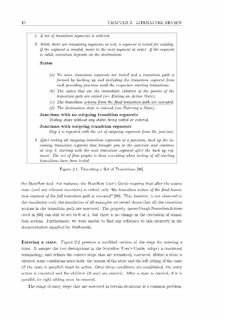
10 CHAPTER 2. LITERATURE REVIEW
1. A set of transition segments is ordered.
2. While there are remaining segments to test, a segment is tested for validity.If the segment is invalid, move to the next segment in order. If the segmentis valid, execution depends on the destination:
States
(a) No more transition segments are tested and a transition path isformed by backing up and including the transition segment fromeach preceding junction until the respective starting transitions.
(b) The states that are the immediate children of the parent of thetransition path are exited (see Exiting an Active State).
(c) The transition actions from the �nal transition path are executed.
(d) The destination state is entered (see Entering a State).
Junctions with no outgoing transition segmentsTesting stops without any states being exited or entered.
Junctions with outgoing transition segmentsStep 1 is repeated with the set of outgoing segments from the junction.
3. After testing all outgoing transition segments at a junction, back up the in-coming transition segment that brought you to the junction and continueat step 2, starting with the next transition segment after the back up seg-ment. The set of �ow graphs is done executing when testing of all startingtransitions have been tested.
Figure 2.1: Executing a Set of Transitions [98].
the State�ow tool. For instance, the State�ow User's Guide requires that after the source
state (and any relevant ancestors) is exited, only �the transition action of the �nal transi-
tion segment of the full transition path is executed" [98]. This, however, is not observed in
the simulation tool; the simulation of all examples we tested shows that all the transition
actions in the transition path are executed. The property ignoreUnsafeTransitionActions
cited in [68] can still be set to 0 or 1, but there is no change in the execution of transi-
tion actions. Furthermore, we were unable to �nd any reference to this property in the
documentation supplied by Mathworks.
Entering a state. Figure 2.2 presents a modi�ed version of the steps for entering a
state. It merges the two descriptions in the State�ow User's Guide, adopts a consistent
terminology, and de�nes the correct steps that are recursively executed. Before a state is
entered, some conditions must hold: the parent of the state and the left sibling of the state
(if the state is parallel) must be active. Once these conditions are established, the entry
action is executed and the children (if any) are entered. After a state is entered, if it is
parallel, its right sibling must be entered.
The range of entry steps that are executed in certain situations is a common problem.

2.1. STATEFLOW 11
1. If the parent of the state is not active, perform steps 1-4 for the parent.
2. If this is a parallel state, check the immediate sibling with a higher (i.e., ear-lier) entry order is active. If not, perform entry steps 1-5 for this state �rst.
3. Mark the state active.
4. Perform any entry actions.
5. Enter children, if needed:
(a) If the state contains a history junction and there was an active childof this state at some point after the most recent chart initialisation,perform entry steps 1-5 for that child. Otherwise, execute the default�ow paths for the state.
(b) If this state has parallel decomposition, i.e., has children that are paral-lel states, perform entry steps 1-5 for each state according to its entryorder.
6. If this is a parallel state, perform all entry steps for the sibling state next inentry order if one exists.
7. Else, if the transition path parent is not the same as the parent of the currentstate, perform entry steps 6 and 7 for the immediate parent of this state.
Figure 2.2: Entering a State [98].
For instance, when entering a parallel state, the User's Guide states "check that all siblings
with a higher (i.e., earlier) entry order are active. If not, perform all entry steps for these
states �rst" [98]. In fact, only the immediate left sibling is checked and entered if necessary.
Moreover, not all entry steps are executed, only the steps from 1 to 5 are executed for that
state. This fact has been con�rmed independently in [20].
Both descriptions in the User's Guide require that if the history junction in a state
points to one particular substate, the entry action of that state is executed. This would
imply that the substates of that child state are not entered because the entry steps are not
executed on it. This, however, is not the observed behaviour of the simulator. In this case,
we observe that, in fact, the entry steps from 1 to 5 are executed on that child. Step 6
can be ignored because the state is sequential, and step 7 is not executed because the
immediate parent of the child is already active, as it triggered the entering of this state.
This type of inconsistency can also be found in the description of the process of exiting
a state in the main body of the User's Guide; however, it was corrected in the appendix.
Our experiments suggest that step 7 is only executed if the condition of step 6 fails,
that is, if the state is not a parallel state, or if it does not have a right sibling. Since step 6
requires the execution of all entry steps to the right sibling, the step 7 is accumulated for
each parallel state entered, and is therefore executed multiple times. It is our understanding
that step 7 should only be executed once in a sequence of parallel states. If we require that
step 7 is only executed when step 6 fails, it should be executed exactly when the state is
12 CHAPTER 2. LITERATURE REVIEW
sequential, or when (it is parallel and) the last sibling has been entered.
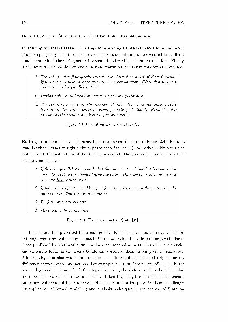
Executing an active state. The steps for executing a state are described in Figure 2.3.
These steps specify that the outer transitions of the state must be executed �rst. If the
state is not exited, the during action is executed, followed by the inner transitions. Finally,
if the inner transitions do not lead to a state transition, the active children are executed.
1. The set of outer �ow graphs execute (see Executing a Set of Flow Graphs).If this action causes a state transition, execution stops. (Note that this stepnever occurs for parallel states.)
2. During actions and valid on-event actions are performed.
3. The set of inner �ow graphs execute. If this action does not cause a statetransition, the active children execute, starting at step 1. Parallel statesexecute in the same order that they become active.
Figure 2.3: Executing an active State [98].
Exiting an active state. There are four steps for exiting a state (Figure 2.4). Before a
state is exited, its active right siblings (if the state is parallel) and active children must be
exited. Next, the exit actions of the state are executed. The process concludes by marking
the state as inactive.
1. If this is a parallel state, check that the immediate sibling that became activeafter this state have already become inactive. Otherwise, perform all exitingsteps on that sibling state.
2. If there are any active children, perform the exit steps on these states in thereverse order that they became active.
3. Perform any exit actions.
4. Mark the state as inactive.
Figure 2.4: Exiting an active State [98].
This section has presented the semantic rules for executing transitions as well as for
entering, executing and exiting a state in State�ow. While the rules are largely similar to
those published by Mathworks [98], we have commented on a number of inconsistencies
and omissions found in the User's Guide and corrected those in our presentation above.
Additionally, it is also worth pointing out that the Guide does not clearly de�ne the
di�erence between steps and actions. For example, the term "entry action" is used in the
text ambiguously to denote both the steps of entering the state as well as the action that
must be executed when a state is entered. Taken together, the various inconsistencies,
omissions and errors of the Mathworks o�cial documentation pose signi�cant challenges
for application of formal modelling and analysis techniques in the context of State�ow

2.1. STATEFLOW 13
Figure 2.5: Early return logic example.
diagram; their detection and resolution can therefore be seen as one of the contributions
of this thesis.
2.1.3 Early return logic
Early return logic occurs when a recursive execution (triggered by a local event broadcast)
activates (or deactivates) states that should not be active (or, respectively, inactive) after
the event broadcast. It interrupts part of the execution of the chart to avoid reaching an
inconsistent state (e.g. a state with sequential decomposition and two active substates).
It is worth mentioning that early return logic does not necessarily interrupt the execu-
tion of the whole chart. For example, if the chart has two parallel states and the execution
of the substates of the �rst parallel state is interrupted (in a consistent state) by early
return logic, the execution of the second parallel state may continue, as the inconsistency
was avoided.
Local event broadcasts may occur in entry, during, exit, condition, transition and on
actions. Bind actions do not lead to local event broadcasts. The User's Guide [98] speci�es
the early return conditions for each type of action (on actions are considered as during
actions).
For local event broadcast originating from the execution of the entry actions of state s,
if s is inactive after the broadcast, the process of entering state s is interrupted. The
instructions for during and exit actions are similar, but the processes of executing and
existing, respectively, are interrupted. For condition actions, if the source of the transi-
tion path is inactive after the local event broadcast, the execution of the transitions is
interrupted.
The case of local event broadcasts from transition actions is slightly di�erent. For all
the previous cases, some state that is active before the broadcast, must be active after it.
Since transition actions are executed after the source state (and any necessary ancestor
state) is exited, and before the destination state is entered, all substates of the parent of
the transition path must be inactive before and after the broadcast. If any of them is
active after the broadcast, the execution of the transitions is interrupted.
By way of illustration, we consider the simple chart in Figure 2.5 adapted from an
14 CHAPTER 2. LITERATURE REVIEW
example in [98]. This example shows a situation where an event (E) triggers the execution
of a transition, which raises a di�erent event (F). This event then triggers a di�erent
transition, and since the �rst one was not completed before the event F was raised, it
is abandoned and the simulation proceeds with the second transition. The �rst time this
chart receives an input event E, the state A is entered. When the second event E is received,
the �rst outer transition from A is attempted. Since its trigger is true, the transition is
valid, and consequently the condition action is executed. This broadcasts the local event
F, which triggers the reexecution of the chart under F. The reexecution considers the outer
transitions of the active state, A. The �rst outer transition is not possible because the
trigger does not contain F, but the second transition is possible. It is taken, A is exited,
and the state C is entered. The reexecution �nishes, but the execution of the chart cannot
proceed because the transition from A to B can no longer be executed, since A is not active
anymore. In this case, the original execution is interrupted, the assignment data=1 is not
executed, and the step of execution �nishes.
The User's Guide [98] is not clear about exactly which portions of the execution must be
interrupted. For example, in the case of entry actions, it simply says that "any remaining
steps in entering a state are not performed". We have veri�ed using the simulation tool
that when a local event is broadcast from the entry action of a state s, in certain cases
only the remaining steps for entering s are interrupted, while in other cases the steps for
entering some of the parents are also interrupted.
For example, Step 1 in Figure 2.2 activates the parent state. It is expected therefore
that Step 2 can only continue if the parent is active. Assume that the parent p has a
sequential decomposition, if its entry action exits p (for instance, by executing an outer
transition), Step 3 would mark the substate active, and we would end up with an active
state whose parent is inactive, which is an inconsistency. We believe that early return
conditions should be checked not only after local event broadcasts, but after each step
with respect to the appropriate state (the parent state in the case of Step 1). This is the
approach we took to model the semantics of State�ow charts as presented in Chapter 3 of
this thesis.
2.2 Formal models of state diagram notations
In order to achieve the objective of this thesis, we need some formal account of the nota-
tion. In the literature on veri�cation and analysis of state diagrams, we can �nd di�erent
approaches that can be divided into two types according to how the formalisation is carried
out: formal semantics and translation strategies to a formal notation. Another distinction
can be made with respect to the objectives of this formalisation: veri�cation (of properties
and implementations) and automatic code generation.
Works that establish the formal semantics of a notation allow for the analysis and
veri�cation of diagrams and can be used to de�ne simulation and compilation procedures.
Those that de�ne a translation strategy can achieve the same results, but are able to re-use

2.2. FORMAL MODELS 15
existing technologies for the formal notation to which the state diagrams are translated.
In what follows, we discuss some of the formal approaches to state diagram notations.
We divide them into two groups according to the objectives: veri�cation (Section 2.2.1)
and automatic code generation (Section 2.2.2). Within these groups, we will �nd works
that can be classi�ed according to the formalisation techniques.
2.2.1 Veri�cation approaches
A formal semantics of statecharts was �rst introduced in [40] in an operational style using
a notion of micro-steps to de�ne a step of execution of the chart. Pnueli and Shalev
[82] revise the operational semantics described in [40], and propose a declarative semantics
consistent with the revised operational semantics. It relies on a notion of global consistency
in order to show that both the declarative and operational semantics are consistent with
each other. The execution step of statecharts is de�ned by the set of enabled transitions
at a particular con�guration, which are execute to calculate the next con�guration. This
semantics limits the number of times a transition may be executed in a step, and di�ers
quite signi�cantly from State�ow in the treatment of event broadcasts.
In statecharts, events can be generated only by the transitions, and the transitions
that are enabled by events generated by enabled transitions are restricted to be consistent
with each other, therefore a transition cannot enable, for instance, another transition
originating in the same source state. In State�ow, local events can be broadcast both from
transitions and states, thus the calculation of the set of enabled transitions would depend
on the states being entered, executed and exited as well as the possible transitions. In
addition, the transitions that can be triggered by a local event broadcast in State�ow are
not restricted as in statecharts. This generates the possibility of inconsistency, which is
treated by early return logic. Since the consistency check is performed after the treatment
of the local event broadcast, some actions (that would not occur otherwise) take place. For
this reason, the approach in [82] cannot be applied directly to the semantics of State�ow.
In [38], the semantics implemented in the STATEMATE system [39] is presented, but
again in an informal fashion. Mikk et al. [60] give a formal account of the simulation of the
semantics implemented in STATEMATE; it uses the Z notation to de�ne the semantics.
Given the syntactic and semantic di�erences of STATEMATE statecharts and State�ow
charts, it is not possible to use these results to verify implementations of State�ow charts,
and although Z has a re�nement calculus, it is not clear how this could be used to verify
parallel implementations of such charts. One possibility would be to specify the reactive
behaviour of the chart in Z as described in [26].
The semantics of State�ow charts is given in two forms: an informal description con-
tained in the User's Guide [98] and a simulation semantics implemented in the State�ow
simulator. In [35], an operational semantics for State�ow charts is proposed; however,
it does not cover some features of the notation, e.g. history junctions, and also imposes
restrictions on the use of local events and transitions. It is not clear, however, how to use

16 CHAPTER 2. LITERATURE REVIEW
this semantics in the context of program veri�cation, and how to integrate this semantics
with a semantics of Simulink diagrams. Hamon [34] proposes a denotational semantics
that overcomes some of the limitations of [35]. It claims to models the "the full local event
mechanism" [34], but there is no discussion about the issue of inconsistent states arising
from local event broadcasts, which is treated by early return logic.
The denotational and operational semantics proposed in [35] and [34] can be used to
verify properties and implementations, and automatically generate code; however, because
of the formalism in which the semantics is given, new theories and tools would need to be
developed in order to support such goals.
Whalen [108] proposes a structural operational semantics for three dialects of state-
charts (State�ow, UML Statecharts and Rhapsody [37]) based on [34]. It lifts some of
the restrictions previously imposed, and corrects some aspects of the semantics. However,
history junctions are not covered, and the treatment of local event broadcasts is not clear.
The formal rules for the treatment of local events seem to correctly model the semantics
of local event broadcast, except that early return logic is not treated.
Chen [20] speci�es the semantics of State�ow in a version of CSP accepted by the
model checker PAT [96]. Some of the problems with the informal semantics of State�ow
discussed in [68] were independently observed and corrected. The proposed treatment of
interlevel transitions requires exiting "the highest superstate (in terms of hierarchy) of the
source state", but this requirement is incomplete because the highest substate may be the
parent of the source and destination states, and this state should not be exited. The User's
Guide [98] description requires that the substates of the parent of the transition path are
exited. Our model of State�ow charts de�nes this state as the least upper bound of the
source and destination states with respect to an ancestry relation. The treatment of input
and local events is brie�y mentioned in [20]. Multiple input events are treated using a
notion of priority of transitions, when, in fact, State�ow executes the chart for each input
event that occurs in the same time step. Local event broadcasts are modelled, but early
return logic is not mentioned. It is not clear how the models are obtained, and what is
necessary to support automatic generation.
Boström and Morel [10] propose an approach to support the application of mode-
automata [58] in an industrial setting, while maintaining its formal aspect. The approach
identi�es the subset of Simulink/State�ow necessary to de�ne mode-automata, and gives
a formal semantics to this subset. This semantics is to be used as the basis for the ver-
i�cation of properties of the models, but the veri�cation aspect is not developed further.
The restrictions imposed on Simulink/State�ow are so strong, that the proposed seman-
tics cannot be used as a basis for the veri�cation of implementations of State�ow charts.
Moreover, these restrictions yield a very simple semantics that cannot be easily extended
to include the excluded features of the notation.
Sekerinski and Zurob [90] translate statecharts to the B notation, but impose some
limitations on the structure of valid diagrams. The translation strategy is implemented
in the iState tool that can also generate code in other languages. The choice of the B
2.2. FORMAL MODELS 17
notation as a target language is due to its support of non-determinism and suitability for
safety analysis. Although the B notation supports veri�cation of implementations, this
aspect is not mentioned by the authors. Moreover, using this approach as a basis for
our work would be rather di�cult, given the syntactic and semantic di�erences between
statecharts and State�ow charts.
Latella et al. [53] propose an operational semantics of extended hierarchical automata
and a translation strategy from UML state machines to this formalism. However, the
subset of the language that is formalised is small. This work is signi�cantly extended
in [107]. The extensions include a treatment of the history mechanism, and entry and exit
actions. Lilius and Paltor [55] translate UML state machines to PROMELA [44] and use
the model checker SPIN [45] to analyse the diagrams. None of these works contemplate
the veri�cation of implementations.
Ng and Butler [75] de�ne a translation from UML state machines to CSP speci�cations
by translating UML states to CSP processes and UML events to CSP events. This work
presents an elegant model of UML state machines, but data aspects are not covered.
Furthermore, aspects of statecharts that make the semantics of State�ow charts challenging
(e.g. inter-level transitions) are not discussed. CSP is used primarily for its tool support
for the veri�cation of properties and re�nement of UML state machines.
The approach presented in [84] extends that of Ng and Butler [75] by translating UML
statecharts to Circus speci�cations, covering more aspects of the notation. A state is trans-
lated into a Circus action, and as in the previous work, a UML event is mapped to a
Circus event. None of these works formalise aspects that render the semantics of State-
�ow charts challenging, e.g. local event broadcast, connective and history junctions, etc.
Therefore, formalisations of UML statecharts do not shed much light into the formalisation
of State�ow charts.
Snook et al. [95] propose a strategy for the veri�cation of properties of UML models.
The strategy is based on a translation from UML to UML-B [94] (a graphical notation
similar to UML based on Event-B [2]) and applies the tools and techniques associated with
UML-B and Event-B to verify both the internal consistency of the UML model and the
target properties. This work di�ers from our approach both in the notation covered (UML)
and in the objectives.
Banphawatthanarak and Krogh [6] propose a translation from State�ow charts to the
input notation of the SMV symbolic model checker, thus allowing for the veri�cation of
properties of the charts [7]; they impose restrictions on the types of input signals, number
of transitions reaching a junctions, output signals and transition actions. Tiwari [101]
translates State�ow charts to a formalism called communicating push-down automata and
uses the Symbolic Analysis Laboratory (SAL) framework to analyse the models; this work
contemplates the main aspects of the State�ow notation (parallel and sequential states,
connective and history junctions, transitions, etc), but it is not clear what elements are
not treated.
Scaife et al. [87] translate State�ow models to the synchronous language Lustre [33],

18 CHAPTER 2. LITERATURE REVIEW
allowing for the model checking of the models; the subset treated imposes some limitations
on features such as inter-level transitions. This work extends previous work that de�nes a
translation strategy from discrete-time Simulink to Lustre [12]. Chen [20], Banphawattha-
narak et al. [7], Tiwari [101] and Scaife et al. [87] focus on veri�cation of properties, and
the latter approach could be used for automatic code generation; the veri�cation of imple-
mentations of State�ow charts is not supported by these works or by the notations used
to formalise State�ow charts.
In [104], State�ow charts are formalised in the Z notation. Assumptions that record
the requirements on the states of the chart are then combined with the chart using the
Practical Formal Speci�cation method [59] producing a set of healthiness conditions. These
conditions are veri�ed by the Simulink/State�ow Analyser [103] in order to validate the
State�ow model. While we are interested in verifying that a program correctly implements
a State�ow chart, Toyn and Galloway [104] are interested on whether the chart is the
intended model of the system. Moreover, the Simulink/State�ow Analyser does not support
some of the features of the State�ow notation, such as parallel states and junctions.
Cavalcanti et al. [19] present the most similar work with respect to our objectives; it
describes an approach for translating Simulink diagrams to Circus speci�cations. It uses
extended versions of the ClawZ [4] and ClaSP tools developed by QinetiQ to translate
control law diagrams to Z and CSP, respectively, and to generate a Circus speci�cation.
This allows the veri�cation of functional and concurrent aspects in an integrated manner,
as well as the veri�cation of implementations of control law diagrams.
ClawZ comprises a library of block de�nitions and a translation strategy that maps a
diagram into a Z schema that declares all the input and output signals, and constants;
the predicate of the schema establishes the relationship between inputs and outputs. The
translation strategy also includes in the speci�cation the schemas corresponding to the
blocks used in the diagram.
ClaSP does not produce CSP speci�cations of the control law diagrams, but rather
generates a set of pairs that relate inputs and outputs. For each block A in the diagram,
the pair (x , y), where x is the set of inputs of block A, and y is the sequence of outputs of
block A, is included in this set.
ClawZ and ClaSP are extended to produce more information about the diagrams, so
that it is possible to merge both speci�cations (from ClawZ and ClaSP) into one Cir-
cus speci�cation [19]. For that purpose, ClawZ is extended to include action and enabled
subsystems, as well as merge blocks (i.e, block that output the last input received), whereas
ClaSP is modi�ed so that it includes, for a particular diagram, its name, inputs, outputs
and blocks; the blocks are characterised by their sequence of inputs, sequence of outputs
and �ows of execution.
A translation strategy is de�ned to merge these extended speci�cations. It de�nes the
signals as channels and de�nes a channel called end cycle. The strategy includes the ClawZ
library and translates the diagram into a Circus process called clasp.spec that consists of
the parallel execution of all the blocks in the diagram. The parallel execution of two blocks
2.2. FORMAL MODELS 19
synchronises over the intersection of their alphabets, i.e. the set that contains a block's
input and output channels, determining the order of execution of the blocks. The blocks
also synchronise over the channel end cycle, determining the end of the execution of each
block and marking the end of the execution of a cycle of the diagram.
In [16], an initial Circus semantics of State�ow charts is proposed using a denotational
style, and, while many of the most interesting aspects of the semantics of State�ow are
discussed, they are not formalised. Also, the denotational style used in this work proved
di�cult to extend for the most complex aspects of State�ow (e.g. early return logic), and
hard to validate with respect to the informal semantics.
2.2.2 Code generation approaches
Caspi et al. [13] propose a code generation approach for obtaining embedded software
implemented in a distributed architecture called Time-Triggered Architecture (TTA) [106].
This approach consists of using Simulink for designing control systems, SCADE/Lustre [24]
for designing software and TTA as the distributed platform for the generated code. The
three tools are widely used in avionics and automotive domains.
The decision to use SCADE/Lustre as an intermediate level between Simulink and
TTA is due to a series of features of SCADE/Lustre. The latter has an automatic code
generator quali�ed to SIL-A of the DO-178b standard and is suitable for the development
of high integrity applications; it is supported by analysis tools (model checkers and test
case generators) and presents some features that distinguish it as a programming language,
rather then a simulation tool such as Simulink.
The approach consists, �rst, of translating a Simulink diagram to SCADE/Lustre [24],
and then producing an implementation with the aid of the certi�ed automatic code gen-
erator. This work extends [12] focusing on automatic code generation, but it does not
cover the State�ow notation. However, the fact that the work in [12] was extended to
contemplate the State�ow notation [87] suggests that this approach can also be extended.
Toom et al. [102] and Rugina et al. [86] report on work done in the context of the
Gene-Auto ITEA European project. The goals of this project are to develop a code gen-
erator for Simulink/State�ow and Scicos and to qualify the code generator through formal
approaches. Izerrouken et al. [49] account for the validation and veri�cation of the code
generator. Since this work is based on automatic code generation, the only implementa-
tions that can be deemed correct are those generated by the tool. For this reason, the
implementations cannot be modi�ed. With an approach based on the veri�cation of im-
plementations, modi�ed implementations can be individually assessed; thus allowing, for
example, for manual code optimisation.

20 CHAPTER 2. LITERATURE REVIEW
2.3 Speci�cation languages
In order to verify implementations of State�ow charts, we need to formalise them in a
suitable notation. In this section, we survey speci�cation languages that allow for this
kind of veri�cation and could be used for this formalisation.
Two aspects that can be used to distinguish speci�cation languages are the capability
of representing state on the one hand, and communication on the other. State based
notations, such as Z [109], VDM [51] and B [1], are used mainly to specify sequential
systems with complex data structures. In contrast, process algebras, such as CCS [61],
CSP [85, 88, 41], ACP [9] and LOTOS [23], can specify reactive and concurrent systems.
Arthan et al. [4] and Adams and Clayton [3] use Z to verify implementations of Simulink
diagrams. However, Z is not su�cient to describe all the aspects of such diagrams and
programs. For that reason, CSP is used to describe the concurrent aspects. Given that
State�ow charts can have complex data types, for example arrays and matrices [98], and
complex reactive behaviour, it is convenient to use a speci�cation language that can tackle
both of those aspects.
Fischer [28] and Smith [91] provide an integration of CSP and Object-Z [92], an object-
oriented extension of the Z notation, by de�ning a failures-divergence semantics for Object-
Z classes. Mahony and Dong [56] and Hoenicke and Olderog [43] also integrate CSP and
Object-Z, but add a temporal aspect. Mahony and Dong [56] use Timed-CSP [89] for this,
whereas Hoenicke and Olderog [43] use the duration calculus [112].
Butler and Leuschel [11] and Treharne and Schneider [105] use CSP and the B notation
to provide an integrated notation. The former approach [11] identi�es B operations and
CSP channels. Treharne and Schneider [105] de�ne a compatibility criteria between a B
machine and a CSP speci�cation that allows the CSP speci�cation to direct the B machine
execution.
Taguchi and Araki [97] integrate Z and CCS [61] by providing a state-based semantics
of CCS, and then composing it with the semantics of Z in terms of labelled transition
systems. It also introduces a logic for the speci�cation of properties of systems described
in this formalism.
Woodcock and Cavalcanti [110] de�ne Circus as a combination of Z, CSP, the re�ne-
ment calculus and Dijkstra's language of guarded commands. The semantics of Circus [79]
is de�ned using the UTP [42], and its main advantage is the existence of a re�nement
calculus [78] that supports the veri�cation of implementations of Circus speci�cations.
In the next section, we present a brief description of Circus. We chose Circus as the
basis for our formalisation of State�ow charts because of the existing work on formalisation
of Simulink diagrams and on veri�cation of implementations of such diagrams, as well
as because Circus supports the speci�cation of both the static and dynamic behaviour
and provides a re�nement calculus that supports the veri�cation of implementations of
speci�cations.
While other combinations of state base notations and process algebra (e.g, CSP ‖ B ,
2.4. REFINEMENT CALCULUS 21
CSP-OZ, Event-B) have similar expressive power as Circus to the best of our knowledge,
Circus is the only one that provides a re�nement calculus that supports the veri�cation of
implementations in a calculational fashion. The latter aspects is particularly relevant to
us because the potential automation allowed by the calculational style is fundamental for
the successful adoption of our technique in industrial settings.
2.4 Re�nement calculus
In this thesis, we are concerned with re�nement based veri�cation of implementations of
State�ow charts. In particular, we are interested in the approach known as the re�nement
calculus [5, 73, 74]. In the re�nement calculus an abstract speci�cation is transformed into
a (possibly more concrete) speci�cation by means of sound re�nement laws.
In our approach, we favour the re�nement calculus as it supports a high degree of
automation. The automation derives from the fact that once a re�nement law is selected, its
applicability can, in general, be checked by simple provisos (mostly syntactic). This allows
us to focus on strategies for the selection of re�nement laws that support the veri�cation
of a speci�c implementation.
As previously mentioned, Circus combines the re�nement calculus with Z, CSP and
guarded commands. Besides supporting step-wise development (and veri�cation), the re-
�nement calculus in the context of Circus also support the reasoning about concurrency. In
particular, it allows us to derive (and verify) a concurrent implementation from a centralised
speci�cation. Veri�cation of implementations with respect to speci�cations is carried out
by re�ning the speci�cation into the implementation.
The soundness of the development (or veri�cation) derives from the soundness of the
re�nement laws, which must be proved correct with respect to the semantics of Circus [79].
2.5 Circus
In this section, we present some of the Circus features using a simple Circus process (Fig-
ure 2.6) that models a systems of image transmitters and receivers as an example1. A de-
tailed presentation of Circus can be found in Oliveira et al. [79].
A Circus speci�cation is a sequence of paragraphs: Z paragraphs (axiomatic de�ni-
tions, schemas, and so on), channel and channel set declarations, and process de�nitions
(Appendix A presents the syntax of Circus). The �rst few paragraphs of our example (Fig-
ure 2.6) de�ne the horizontal coordinates as the set HORIZONTAL (of numbers from 1 to
800), the vertical coordinates as the set VERTICAL, the set of colours COLOUR, and the
set of images IMAGE . An image is de�ned as a total function from the horizontal and ver-
tical coordinates to colours. Next, an axiomatic de�nition declares the maximum number
(maxbu� ) of images that can be held in the transmitters and receivers as a constant.
1This example has been previously published in [70] and extends the example presented in [18]

22 CHAPTER 2. LITERATURE REVIEW
HORIZONTAL == 1..800VERTICAL == 1..600COLOUR == 0..255IMAGE == HORIZONTAL×VERTICAL→ COLOUR
maxbu� : N1
channel read ,write : IMAGE
processBu�er =̂ begin
stateS == [image : seq IMAGE | # image < maxbu� ]InitState == [S ′ | image ′ = 〈〉]Read =̂ (# image < maxbu� )N read?x −→ image := image a 〈x 〉Write =̂ (# image > 0)N write!(head image)−→ image := tail image
• InitState ; (µX • (Read @Write) ; X )end
Figure 2.6: The Bu�er process
A channel declaration introduces channel names and the types of the values that they
communicate. A channel with no type does not communicate any values; it is used for
synchronisation only. Our model declares two channels read and write of type IMAGE .
A basic process de�nition provides the name of a process, its state, local actions, and a
main action. The state is de�ned by a schema expression. In Figure 2.6, we de�ne a process
Bu�er whose state is given by the schema S . The state contains a single component: the
sequence image of the elements stored in the bu�er. The state invariant de�nes that the
maximum size of the bu�er is given by maxbu� .
A Circus action can freely combine schema expressions, CSP constructs, guarded com-
mands, and speci�cation statements. The bu�er must be initialised before it is used; for
that, we specify the action InitState as an operation schema that establishes that image is
the empty sequence.
The Bu�er can read new information only if there is space to store it. Thus the action
Read has the condition # image < maxbu� as a guard. This requires the size of the image
bu�er to be smaller than maxbu� . If the guard is true, Bu�er can receive a value through
the read channel, and store it in image by concatenating it to the end of this sequence.
Similarly, writing is only enabled if there is some value stored in the bu�er. If the guard
# image > 0 is true, the action Write can send the �rst value of the sequence (head bu�er)
through the channel write, and remove it from the bu�er by rede�ning it as the rest of the
sequence (tail bu�er).
The main action de�nes the behaviour of the process. In the case of Bu�er , it initialises
the state, and recursively o�ers the (external) choice (@) of Read or Write. A recursion is
de�ned in the form µX • A(X ) where A(X ) is an action that contains recursive calls X .
The state of a process is local and encapsulated. Interaction with a process is only possible
via communication through the channels that it uses.
2.5. CIRCUS 23
Processes can also be de�ned through process operators. For example, we can de�ne
a new process by composing two other processes in parallel (JK). Other process operatorsare interleave (9), internal choice (u), external choice (@), and sequential composition (; ).
Like in CSP, processes can be parametrised, have their components renamed, havetheir channels hidden, and so on. For instance, we can specialise the Bu�er process as atransmitter that reads images from an antenna and sends them through a radio-frequencychannel rfchannel . For that, we de�ne a new process Transmitter by renaming the channelsread and write of the process Bu�er to re�ect this change:
processTransmitter =̂ Bu�er [read ,write := antenna, rfchannel ]
The new channels antenna and rfchannel are implicitly declared by the renaming to havethe same type as the corresponding channels read and write. We can de�ne receivers inthe same fashion:
processReceiver1 =̂ Bu�er [read ,write := rfchannel , tv ]
processReceiver2 =̂ Bu�er [read ,write := rfchannel , vcr ]
Both receivers run in parallel and share the reception through rfchannel . We specify this bycomposing them with synchronisation set {| rfchannel |} to de�ne a process called Receivers
as shown below.
processReceivers =̂ Receiver1 J {| rfchannel |} K Receiver2
Finally, the system is de�ned by composing the receivers and the transmitter in parallel.They communicate through rfchannel , which is hidden. Thus, interactions with the systemuse only tv , vcr and antenna.
processSystem =̂ Receivers J {| rfchannel |} K Transmitter \ {| rfchannel |}
Actions can also be composed in parallel. In this case, not only the synchronisation channel
set must be explicit, but also the sets of state components (and local variables in scope)
to which each action writes. Interleaving does not require a synchronisation channel, but
needs the sets of components that are modi�ed. Actions can also be composed in sequence
or in internal choice.
We present a much larger example of a Circus speci�cation and the re�nement calculus,
as we describe our State�ow models in Chapter 3, and our re�nement strategy in Chapter 5.
Finally, Circus o�ers some tool support. A parser and a type checker have been devel-
oped and incorporated in the CZT toolkit [57]. An encoding of Circus in the theorem prover
ProofPower is available [111], and a re�nement tool called CRe�ne [80] are available. The
latter, however, requires further development to fully support the application of re�nement
strategies such as the one proposed in this thesis. A translator from Circus to Java has
been developed for an early version of Circus [31], but is currently not compatible with the
version of Circus used in this thesis. A prototype model checker [32] was developed, but
not made publicly available.
24 CHAPTER 2. LITERATURE REVIEW
2.6 Final considerations
None of the works on formal modelling and veri�cation of state diagram notations cover all
desired features we discussed in Section 1.1. The work in [87] deals in an integrated way
with models of State�ow charts and Simulink diagrams, but does not cover veri�cation of
implementations because the code generated is supposedly correct by construction.
Most of the works on translation of State�ow charts to formal notations focus on veri-
�cation of properties, except, perhaps, [75] and [84], which translate UML state machines
into CSP and Circus, languages that provide means for the veri�cation of implementations.
However, these works are concerned with UML state machines, which do not present the
same complexities as State�ow charts. Also, these works deal only with a well-behaved
subset of UML state machines. For that reason, they do not give much insight into the
formal treatment of more complicated aspects of statechart-like notations.
One approach that can be used in order to formalise State�ow charts is the extension of
the work presented in [19]. This is especially suitable because, in order to model Simulink
function, we need a model of Simulink diagrams, and State�ow charts are always part of
a Simulink diagram.
Although most of the combined notations mentioned in section 2.3 present the features
necessary to formalise State�ow charts, since we are interested in the veri�cation of im-
plementations of such charts, we also need a notation that has a theory that allows us to
verify implementations (for instance, a re�nement theory). Smith and Derrick [93] discuss
the re�nement of speci�cations written in the combination proposed in [91], and Oliveira
et al. [78] propose a re�nement calculus for Circus. Both combinations have re�nement
theories, but Circus is the only one known to support the veri�cation of executable code in
a calculational style [17]. Moreover, Circus is unique in that it supports the speci�cation of
data-rich complex distributed systems, and the re�nement calculus supports the de�nition
of re�nement strategies that can potentially reach a high degree of automation.
The semantics of State�ow presented in this thesis stems from this initial work done
in [16]. However, we took a completely di�erent approach, favouring an operational style
of speci�cation, and a higher degree of connection with the informal semantics to facilitate
the validation.
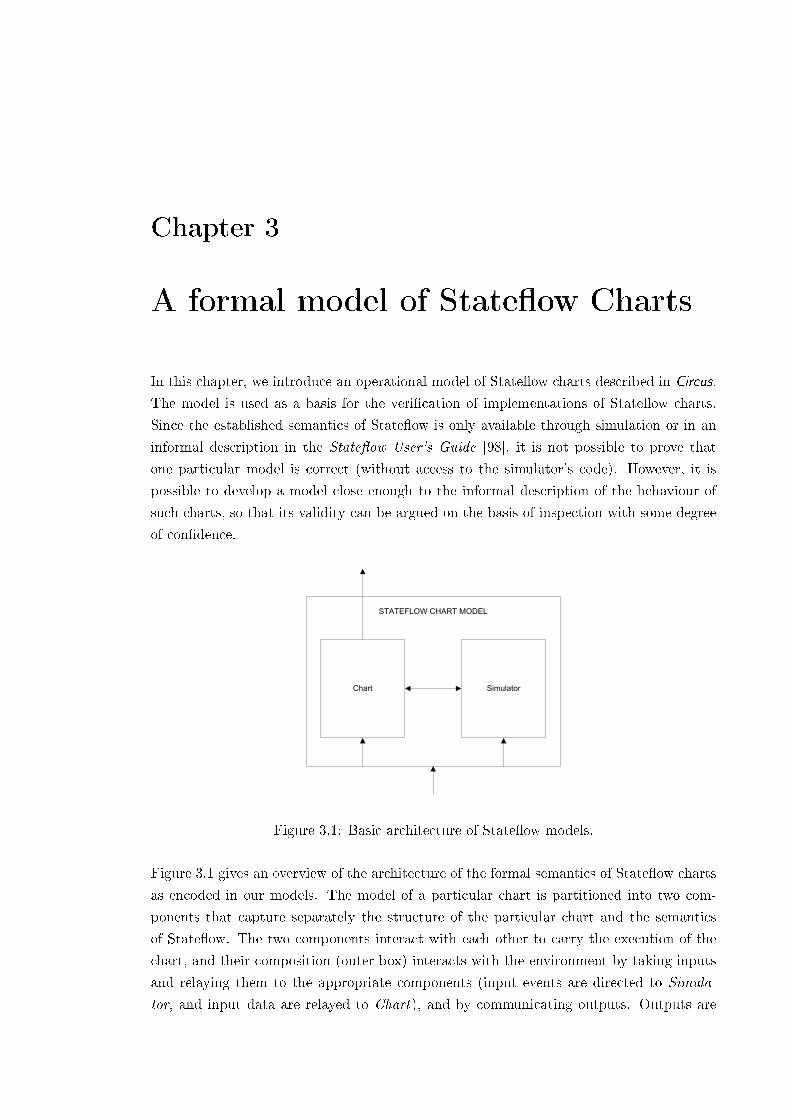
Chapter 3
A formal model of State�ow Charts
In this chapter, we introduce an operational model of State�ow charts described in Circus.
The model is used as a basis for the veri�cation of implementations of State�ow charts.
Since the established semantics of State�ow is only available through simulation or in an
informal description in the State�ow User's Guide [98], it is not possible to prove that
one particular model is correct (without access to the simulator's code). However, it is
possible to develop a model close enough to the informal description of the behaviour of
such charts, so that its validity can be argued on the basis of inspection with some degree
of con�dence.
STATEFLOW CHART MODEL
Chart Simulator
Figure 3.1: Basic architecture of State�ow models.
Figure 3.1 gives an overview of the architecture of the formal semantics of State�ow charts
as encoded in our models. The model of a particular chart is partitioned into two com-
ponents that capture separately the structure of the particular chart and the semantics
of State�ow. The two components interact with each other to carry the execution of the
chart, and their composition (outer box) interacts with the environment by taking inputs
and relaying them to the appropriate components (input events are directed to Simula-
tor, and input data are relayed to Chart), and by communicating outputs. Outputs are

26 CHAPTER 3. FORMAL MODEL
communicated by the component Chart.
The decomposition of the model into two components allows us to isolate the semantics
of State�ow from chart dependent aspects such as its structure and actions. Since the se-
mantics is independent of a particular chart, only the component Chart must be generated
to obtain a complete model. Moreover, changes to certain parts of the semantics (e.g.,
transition execution) can be contained within the component Simulator.
It is worth mentioning that this decomposition is not commonly used when formalising
the semantics of a language with the goal of veri�cation of implementations. Traditionally,
a more denotational approach is favoured. However, a denotational approach embeds in the
translation rules assumptions and simpli�cations that are not necessarily correct and must
be veri�ed. In our approach, no simpli�cation is performed during the translation process,
and the simpli�cation is tackled by the veri�cation strategy. Besides eliminating the (often
unveri�ed) simpli�cations from the translation process, our operational style yields simpler
translation rules that can be more easily validated against the informal description of the
semantics of State�ow chart, which is given in an operational fashion.
One drawback of our choice of semantic style is that the generated models can be bulky
and contain unnecessary complexity. Additionally, the veri�cation of implementations is
not as directs as in a more denotational setting. These hindrances are formally treated by
our veri�cation strategy which eliminates the unnecessary complexity and transforms the
model into a format more amenable to veri�cation. Our veri�cation strategy is presented
in Chapter 5.
In Section 3.1, we provide an overview of the model, its main components and how
they interact. Section 3.2 presents the formal speci�cation of the simulator process based
on the informal description previously shown in Section 2.1.2. Section 3.3 explains the
part of the model that is speci�c to a particular chart. Finally, Section 3.4 discusses the
validation of our models, and Section 3.5 summarises and discusses our results.
3.1 Overview of the model
We describe and illustrate our models using the chart in Figure 3.2 which was adapted
from a State�ow model called "Modelling an Automatic Transmission Controller" [98].
This chart contains two parallel states gear state and selection state; each of
them has a set of sequential substates. The state gear state comprises sequential states
first, second, third and fourth; the transitions between these states are controlled by
local events (UP and DOWN) that are broadcast by the state selection state. The choice
of which event to broadcast, if any at all, is made according to the relation between the
input variable speed and the local variables up th and down th. These local variables
are updated by the Simulink function calc th that takes variables gear and speed as
parameters every time the state selection state is executed. The chart has a single
output variable gear.
Our models of State�ow charts consist of two Circus processes in parallel: the simula-
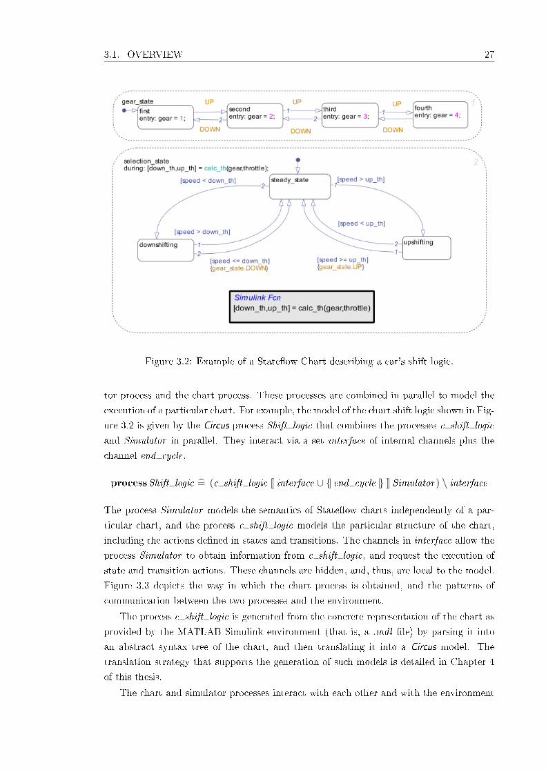
3.1. OVERVIEW 27
Figure 3.2: Example of a State�ow Chart describing a car's shift logic.
tor process and the chart process. These processes are combined in parallel to model the
execution of a particular chart. For example, the model of the chart shift logic shown in Fig-
ure 3.2 is given by the Circus process Shift logic that combines the processes c shift logic
and Simulator in parallel. They interact via a set interface of internal channels plus the
channel end cycle.
processShift logic =̂ (c shift logic J interface ∪ {| end cycle |} K Simulator) \ interface
The process Simulator models the semantics of State�ow charts independently of a par-
ticular chart, and the process c shift logic models the particular structure of the chart,
including the actions de�ned in states and transitions. The channels in interface allow the
process Simulator to obtain information from c shift logic, and request the execution of
state and transition actions. These channels are hidden, and, thus, are local to the model.
Figure 3.3 depicts the way in which the chart process is obtained, and the patterns of
communication between the two processes and the environment.
The process c shift logic is generated from the concrete representation of the chart as
provided by the MATLAB Simulink environment (that is, a .mdl �le) by parsing it into
an abstract syntax tree of the chart, and then translating it into a Circus model. The
translation strategy that supports the generation of such models is detailed in Chapter 4
of this thesis.
The chart and simulator processes interact with each other and with the environment
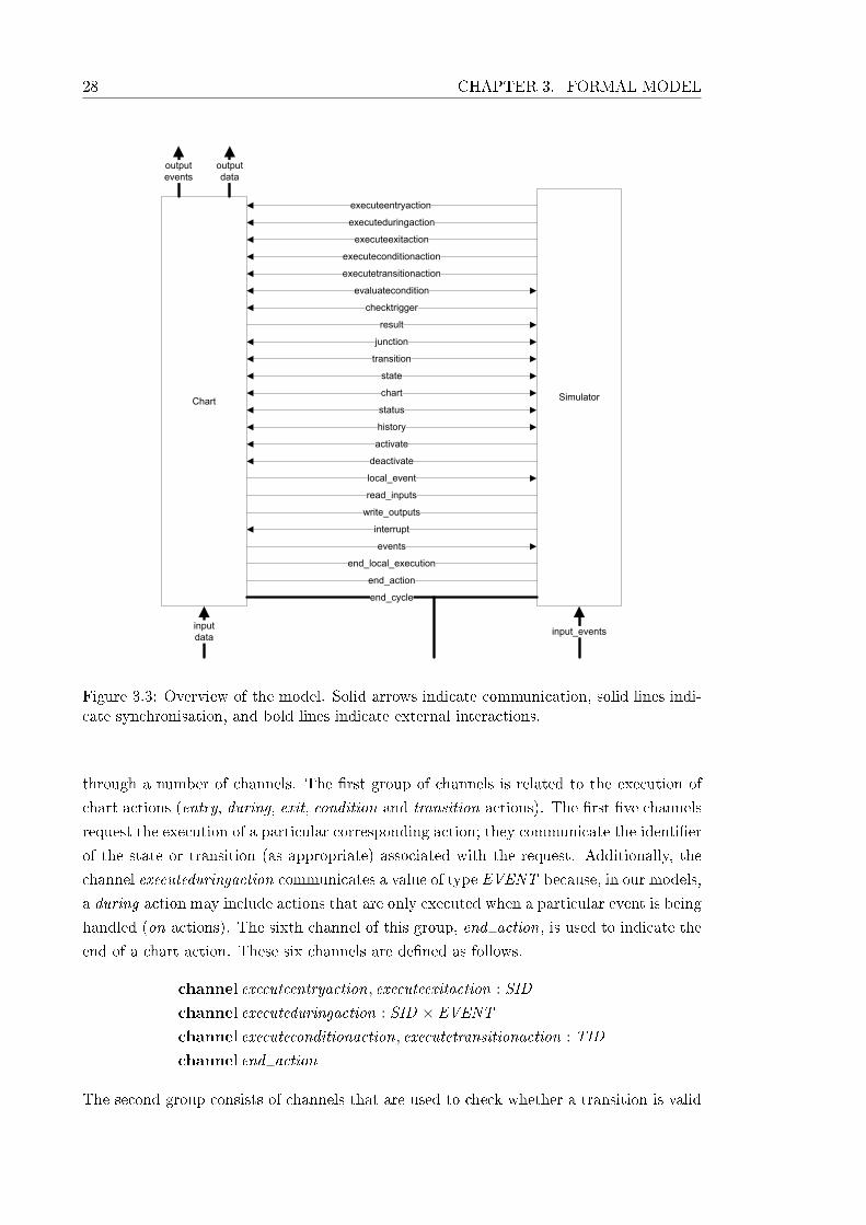
28 CHAPTER 3. FORMAL MODEL
Chart Simulator
executeentryaction
executeduringaction
executeexitaction
executeconditionaction
executetransitionaction
evaluatecondition
checktrigger
result
junction
transition
state
chart
status
history
activate
deactivate
local_event
read_inputs
output
events
output
data
input_eventsinput
data
write_outputs
interrupt
events
end_local_execution
end_action
end_cycle
Figure 3.3: Overview of the model. Solid arrows indicate communication, solid lines indi-cate synchronisation, and bold lines indicate external interactions.
through a number of channels. The �rst group of channels is related to the execution of
chart actions (entry, during, exit, condition and transition actions). The �rst �ve channels
request the execution of a particular corresponding action; they communicate the identi�er
of the state or transition (as appropriate) associated with the request. Additionally, the
channel executeduringaction communicates a value of type EVENT because, in our models,
a during action may include actions that are only executed when a particular event is being
handled (on actions). The sixth channel of this group, end action, is used to indicate the
end of a chart action. These six channels are de�ned as follows.
channel executeentryaction, executeexitaction : SID
channel executeduringaction : SID × EVENT
channel executeconditionaction, executetransitionaction : TID
channel end action
The second group consists of channels that are used to check whether a transition is valid

3.1. OVERVIEW 29
or not. The channel evaluatecondition, used to evaluate the conditions of a transitions,
communicates a transition identi�er and a boolean value. The channels checktrigger and
result are used to check whether a transition has been triggered. The former communicates
a transition identi�er and an event, whereas the latter communicates the same information
plus a boolean value.
channel evaluatecondition : TID × Bchannel checktrigger : TID × EVENT
channel result : TID × EVENT × B
The third group contains channels used to recover instances of elements contained in the
chart from their identi�ers.
channel junction : JID × Junction
channel transition : TID × Transition
channel state : SID × State
channel chart : State
In general, these channels communicate an identi�er (of one of the types: state, junction or
transition) and an element of the same type. For example, the communication state!sid?s
is used to recover the state whose identi�er is sid . The channel chart simply communicates
the binding that represents the chart; it does not require an identi�er because the identi�er
of a chart is unique.
The channels in the fourth group are used to request information about the status
and history of particular states, and to request the activation and deactivation of states.
They all communicate a state identi�er. The status channel also communicates a boolean
value that represents whether the state is active or not. Finally, the history channel
communicates the additional state identi�er of the last activated substate.
channel status : SID × Bchannel history : SID × SID
channel activate, deactivate : SID
The �fth group consists of channels related to local event broadcasts. The channel local event
communicates the event being broadcast along with the state that is the target of the
broadcast. The local event broadcast triggers a local execution (of the chart or of a state)
whose end is marked by a synchronisation on the channel end local execution. Finally, the
channel interrupt communicates a boolean value, and indicates whether or not an early
return logic condition has arisen; it controls the execution of the rest of a chart action after
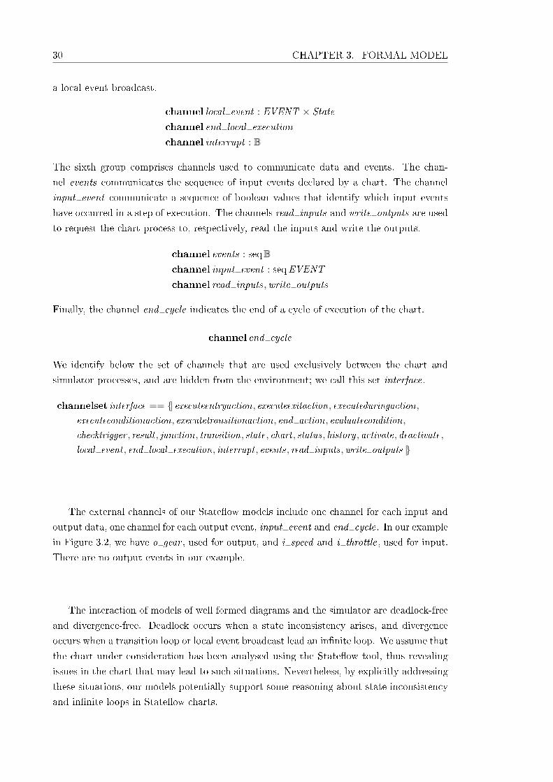
30 CHAPTER 3. FORMAL MODEL
a local event broadcast.
channel local event : EVENT × State
channel end local execution
channel interrupt : B
The sixth group comprises channels used to communicate data and events. The chan-
nel events communicates the sequence of input events declared by a chart. The channel
input event communicate a sequence of boolean values that identify which input events
have occurred in a step of execution. The channels read inputs and write outputs are used
to request the chart process to, respectively, read the inputs and write the outputs.
channel events : seqBchannel input event : seqEVENT
channel read inputs,write outputs
Finally, the channel end cycle indicates the end of a cycle of execution of the chart.
channel end cycle
We identify below the set of channels that are used exclusively between the chart and
simulator processes, and are hidden from the environment; we call this set interface.
channelset interface == {| executeentryaction, executeexitaction, executeduringaction,executeconditionaction, executetransitionaction, end action, evaluatecondition,
checktrigger , result , junction, transition, state, chart , status, history , activate, deactivate,
local event , end local execution, interrupt , events, read inputs,write outputs |}
The external channels of our State�ow models include one channel for each input and
output data, one channel for each output event, input event and end cycle. In our example
in Figure 3.2, we have o gear , used for output, and i speed and i throttle, used for input.
There are no output events in our example.
The interaction of models of well formed diagrams and the simulator are deadlock-free
and divergence-free. Deadlock occurs when a state inconsistency arises, and divergence
occurs when a transition loop or local event broadcast lead an in�nite loop. We assume that
the chart under consideration has been analysed using the State�ow tool, thus revealing
issues in the chart that may lead to such situations. Nevertheless, by explicitly addressing
these situations, our models potentially support some reasoning about state inconsistency
and in�nite loops in State�ow charts.
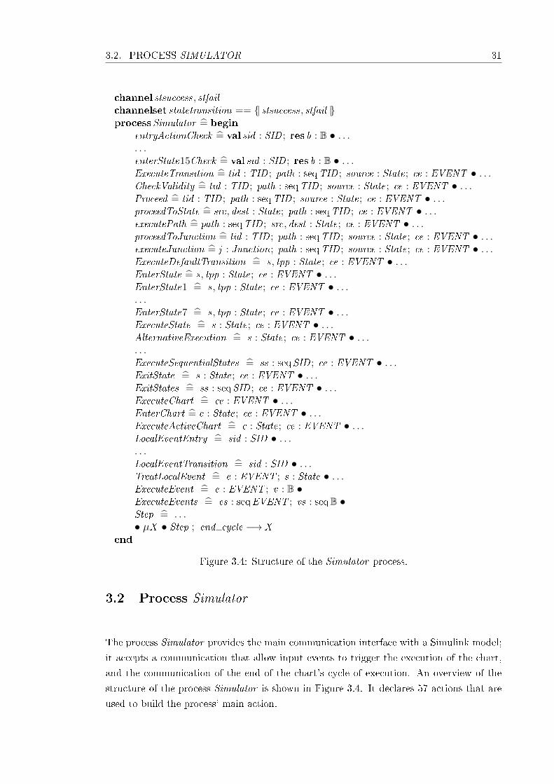
3.2. PROCESS SIMULATOR 31
channel stsuccess, stfailchannelset statetransition == {| stsuccess, stfail |}processSimulator =̂ begin
entryActionCheck =̂ val sid : SID ; res b : B • . . .. . .enterState15Check =̂ val sid : SID ; res b : B • . . .ExecuteTransition =̂ tid : TID ; path : seqTID ; source : State; ce : EVENT • . . .CheckValidity =̂ tid : TID ; path : seqTID ; source : State; ce : EVENT • . . .Proceed =̂ tid : TID ; path : seqTID ; source : State; ce : EVENT • . . .proceedToState =̂ src, dest : State; path : seqTID ; ce : EVENT • . . .executePath =̂ path : seqTID ; src, dest : State; ce : EVENT • . . .proceedToJunction =̂ tid : TID ; path : seqTID ; source : State; ce : EVENT • . . .executeJunction =̂ j : Junction; path : seqTID ; source : State; ce : EVENT • . . .ExecuteDefaultTransition =̂ s, tpp : State; ce : EVENT • . . .EnterState =̂ s, tpp : State; ce : EVENT • . . .EnterState1 =̂ s, tpp : State; ce : EVENT • . . .. . .EnterState7 =̂ s, tpp : State; ce : EVENT • . . .ExecuteState =̂ s : State; ce : EVENT • . . .AlternativeExecution =̂ s : State; ce : EVENT • . . .. . .ExecuteSequentialStates =̂ ss : seqSID ; ce : EVENT • . . .ExitState =̂ s : State; ce : EVENT • . . .ExitStates =̂ ss : seqSID ; ce : EVENT • . . .ExecuteChart =̂ ce : EVENT • . . .EnterChart =̂ c : State; ce : EVENT • . . .ExecuteActiveChart =̂ c : State; ce : EVENT • . . .LocalEventEntry =̂ sid : SID • . . .. . .LocalEventTransition =̂ sid : SID • . . .TreatLocalEvent =̂ e : EVENT ; s : State • . . .ExecuteEvent =̂ e : EVENT ; v : B •ExecuteEvents =̂ es : seqEVENT ; vs : seqB •Step =̂ . . .• µX • Step ; end cycle −→ X
end
Figure 3.4: Structure of the Simulator process.
3.2 Process Simulator
The process Simulator provides the main communication interface with a Simulink model;
it accepts a communication that allow input events to trigger the execution of the chart,
and the communication of the end of the chart's cycle of execution. An overview of the
structure of the process Simulator is shown in Figure 3.4. It declares 57 actions that are
used to build the process' main action.
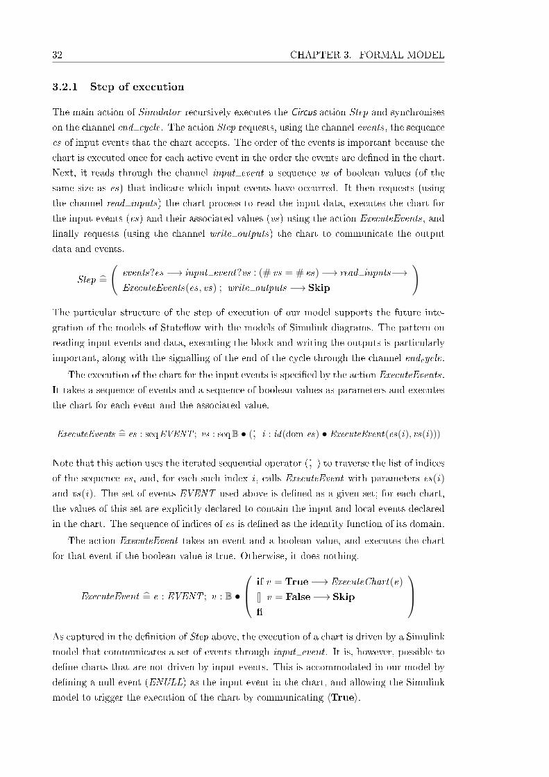
32 CHAPTER 3. FORMAL MODEL
3.2.1 Step of execution
The main action of Simulator recursively executes the Circus action Step and synchronises
on the channel end cycle. The action Step requests, using the channel events, the sequence
es of input events that the chart accepts. The order of the events is important because the
chart is executed once for each active event in the order the events are de�ned in the chart.
Next, it reads through the channel input event a sequence vs of boolean values (of the
same size as es) that indicate which input events have occurred. It then requests (using
the channel read inputs) the chart process to read the input data, executes the chart for
the input events (es) and their associated values (vs) using the action ExecuteEvents, and
�nally requests (using the channel write outputs) the chart to communicate the output
data and events.
Step =̂
(events?es −→ input event?vs : (# vs = # es)−→ read inputs−→ExecuteEvents(es, vs) ; write outputs −→ Skip
)
The particular structure of the step of execution of our model supports the future inte-
gration of the models of State�ow with the models of Simulink diagrams. The pattern on
reading input events and data, executing the block and writing the outputs is particularly
important, along with the signalling of the end of the cycle through the channel endcycle.
The execution of the chart for the input events is speci�ed by the action ExecuteEvents.
It takes a sequence of events and a sequence of boolean values as parameters and executes
the chart for each event and the associated value.
ExecuteEvents =̂ es : seqEVENT ; vs : seqB • (; i : id(dom es) • ExecuteEvent(es(i), vs(i)))
Note that this action uses the iterated sequential operator (; ) to traverse the list of indicesof the sequence es, and, for each such index i , calls ExecuteEvent with parameters es(i)
and vs(i). The set of events EVENT used above is de�ned as a given set; for each chart,
the values of this set are explicitly declared to contain the input and local events declared
in the chart. The sequence of indices of es is de�ned as the identity function of its domain.
The action ExecuteEvent takes an event and a boolean value, and executes the chart
for that event if the boolean value is true. Otherwise, it does nothing.
ExecuteEvent =̂ e : EVENT ; v : B •
if v = True−→ ExecuteChart(e)
8 v = False−→ Skip
�
As captured in the de�nition of Step above, the execution of a chart is driven by a Simulink
model that communicates a set of events through input event . It is, however, possible to
de�ne charts that are not driven by input events. This is accommodated in our model by
de�ning a null event (ENULL) as the input event in the chart, and allowing the Simulink
model to trigger the execution of the chart by communicating 〈True〉.

3.2. PROCESS SIMULATOR 33
The execution of a chart depends on whether it is active or inactive; it is modelled by
the action ExecuteChart .
ExecuteChart =̂ ce : EVENT • chart?c −→ status!(c.identi�er)?active−→ if active = True−→ ExecuteActiveChart(c, ce)
8active = False−→ ExecuteInactiveChart(c, ce)
�
This action receives an event as a parameter, and, �rstly, requests the chart c through
channel chart . It then requests the status of the chart by communicating the identi�er of
the chart (c.identi�er) through channel status and receiving the value in active. Finally,
if the chart is active (active = True), ExecuteChart calls the action ExecuteActiveChart ;
otherwise, it calls the action ExecuteInactiveChart .
ExecuteActiveChart =̂ c : State; ce : EVENT •
if c.substates = ∅−→ ExecuteInactiveChart(c, ce)
8c.substates 6= ∅−→ ExecuteSubstates(c, ce)
�
If the chart has substates, ExecuteActiveChart calls the action ExecuteSubstates to execute
them. Otherwise, it executes the chart as if it were inactive. ExecuteActiveChart receives
a parameter whose type is the schema State.
State
identi�er : SID
default , inner , outer : TID
parent , left , right : SID
substates : seqSID
decomposition : DECOMPOSITION
type : TYPE ; history : B
This schema records the identi�er of the state, the identi�ers of its �rst (if any) default,
inner and outer transitions, the identi�er of its parent state (or chart), left and right
siblings, the sequence of the identi�ers of its substates, its decomposition type, its type,
and whether or not it has a history junction. Identi�ers for states and transitions are
drawn from the sets SID and TID (respectively), which together with the set JID of
junction identi�ers, are de�ned as disjoint given sets. The sets DECOMPOSITION and
TYPE are de�ned by free types. In State�ow, substates in both parallel and sequential
decompositions are ordered. In the case of parallel decomposition, this order determines
the order in which the states are entered, executed and exited. In the case of sequential
decomposition, the order establishes the order in which the states are queried for their
34 CHAPTER 3. FORMAL MODEL
statuses.
TYPE ::= AND | OR | CHARTDECOMPOSITION ::= SET | CLUSTER
A state must be of type AND or OR, and have decomposition of type SET or CLUSTER.
Only a chart (represented as a state in our models) has type CHART .
ExecuteInactiveChart =̂ c : State; ce : EVENT • activate!(c.identi�er)−→
if c.default 6= nulltransition.identi�er ∨ c.decomposition = CLUSTER−→ExecuteDefaultTransition(c, c, ce)
8c.default = nulltransition.identi�er ∧ c.decomposition = SET−→ if c.substates = 〈〉−→ Skip
8c.substates 6= 〈〉−→ state!(head(c.substates))?�rst −→ EnterState(�rst , c, ce)
�
�
The execution of an inactive chart c triggers the activation of the state denoted by
c.identi�er , which represents the chart as a whole. ExecuteInactiveChart uses the channel
activate to request that the chart process carry out this activation. Afterwards, if the
chart has a default transition (c.default 6= nulltransition.identi�er) or if it has a sequential
decomposition (c.decomposition = CLUSTER), ExecuteInactiveChart executes the default
transition using ExecuteDefaultTransition. If the chart has a parallel decomposition and
no default transitions, ExecuteInactiveChart checks if the chart has any substates. If it
does, ExecuteInactiveChart recovers the binding of the state whose identi�er is the �rst
substate using channel state, and enters it using action EnterState.
ExecuteDefaultTransition =̂ s, tpp : State; ce : EVENT •
if s.default 6= nulltransition.identi�er−→(var success : B • ExecuteTransition(s.default , 〈〉, s, ce, success);
(if success = True−→ Skip 8 success = False−→ Stop�)
)8 s.default = nulltransition.identi�er−→
if # s.substates = 0−→ Skip
8 # s.substates = 1−→(
state!(head s.substates)?saux−→EnterState(saux , tpp, ce)
)8 # s.substates > 1−→ Stop
�
�
The action ExecuteDefaultTransition receives two states (s and tpp) and an event (ce) as
parameters. The parameter s corresponds to the state whose default transitions are to be
executed, tpp is the parent of the transition path being executed, and ce is the current
event. The parent of the transition path is the state lowest in the hierarchy that contains
3.2. PROCESS SIMULATOR 35
both ends of a transition path. This information is necessary for the proper treatment of
interlevel transitions (discussed in Section 3.2.2).
If the state has a default transition, we declare a local variable success of type boolean
and call action ExecuteTransition on the default transitions passing the variable success
as a value-result parameter. This variable is used to monitor the success or failure of the
execution of the default transitions. If the execution is successful, ExecuteDefaultTransition
terminates. Otherwise, it deadlocks (Stop), indicating a chart error. This error occurs
because default transitions cannot fail to lead to a state being entered. Chart errors that
lead to deadlock are detected by the State�ow tool, and are modelled in our semantics for
completeness.
If the state does not have a default transition, ExecuteDefaultTransition must identify
the unique state that can be entered (if any). This is only possible if the state has exactly
one substate. If there are no substates, the action terminates successfully. If there is more
than one substate, the action deadlocks. As previously mentioned, the model of a well
formed State�ow chart should never lead to a deadlock.
3.2.2 Transition
The execution of a transition is one of the most complicated aspects of the semantics of
State�ow charts. It is modelled by the action ExecuteTransition that attempts to execute
a sequence of transitions. This sequence is formed by all the transitions that must be
tried. For example, when executing the state steady state (Figure 3.2), there are two outer
transitions to be executed; they are ordered and their execution consists of attempting to
follow the �rst, and, if that fails, trying the second.
ExecuteTransition takes as parameters the identi�er tid of the �rst transition, the
sequence path of identi�ers of the transitions that have been successfully executed, the
source state of the transition path, the current event ce, and a value-result parameter
success. The parameter path is needed in cases where there are junctions in the path of
the transitions and backtracking occurs, and success is used to indicate whether or not the
execution of the transition caused a state to be entered.
ExecuteTransition =̂
val tid : TID ; val path : seqTID ; val source : State; val ce : EVENT ; vres success : B •
if tid = nulltransition.identi�er−→if path = ∅−→ success := False
8 path 6= ∅−→(
transition!(last path)?lt−→ExecuteTransition(lt .next , (front path), source, ce, success)
)�
8 tid 6= nulltransition.identi�er−→CheckValidity(tid , path, source, ce, success)
�
The backtracking mechanism of transitions has been modelled by means of continuations
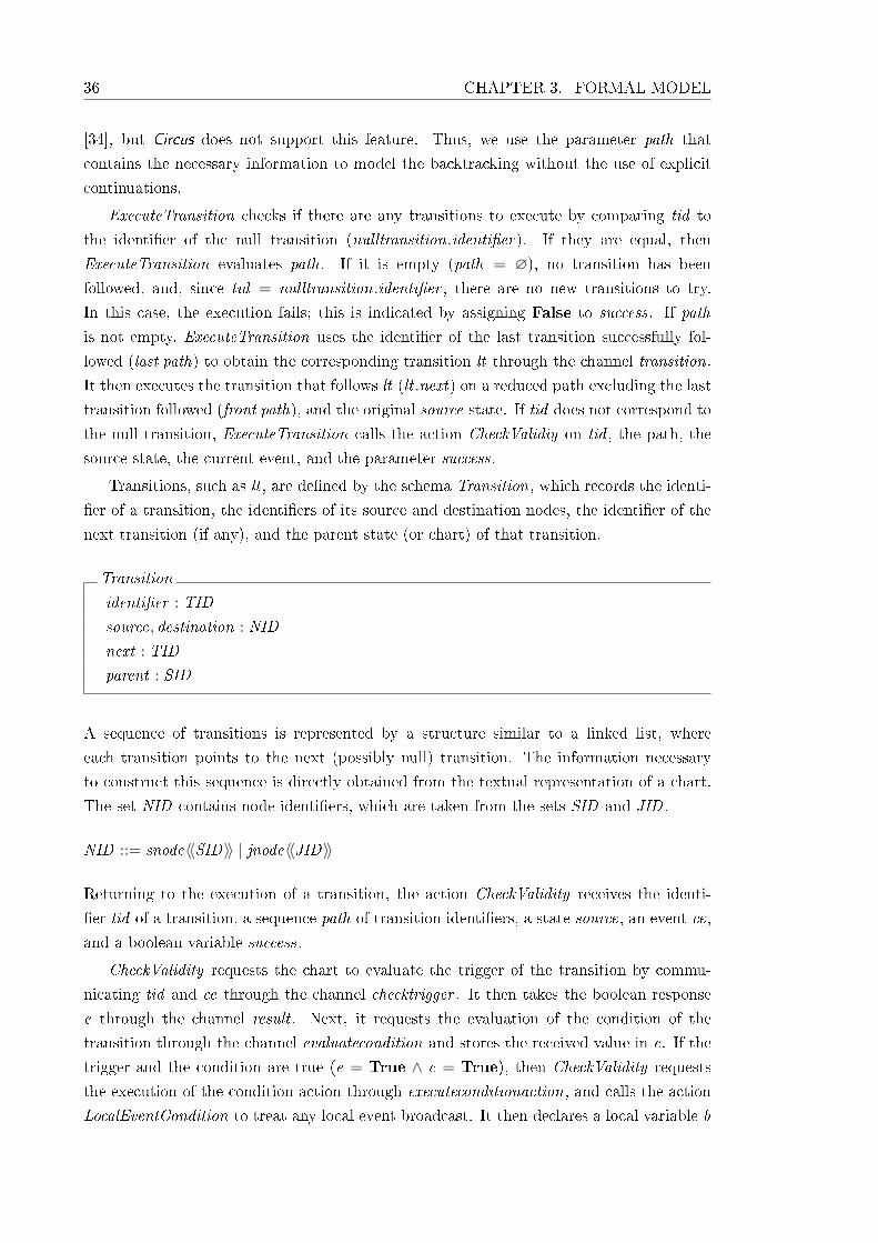
36 CHAPTER 3. FORMAL MODEL
[34], but Circus does not support this feature. Thus, we use the parameter path that
contains the necessary information to model the backtracking without the use of explicit
continuations.
ExecuteTransition checks if there are any transitions to execute by comparing tid to
the identi�er of the null transition (nulltransition.identi�er). If they are equal, then
ExecuteTransition evaluates path. If it is empty (path = ∅), no transition has been
followed, and, since tid = nulltransition.identi�er , there are no new transitions to try.
In this case, the execution fails; this is indicated by assigning False to success. If path
is not empty, ExecuteTransition uses the identi�er of the last transition successfully fol-
lowed (last path) to obtain the corresponding transition lt through the channel transition.
It then executes the transition that follows lt (lt .next) on a reduced path excluding the last
transition followed (front path), and the original source state. If tid does not correspond to
the null transition, ExecuteTransition calls the action CheckValidiy on tid , the path, the
source state, the current event, and the parameter success.
Transitions, such as lt , are de�ned by the schema Transition, which records the identi-
�er of a transition, the identi�ers of its source and destination nodes, the identi�er of the
next transition (if any), and the parent state (or chart) of that transition.
Transition
identi�er : TID
source, destination : NID
next : TID
parent : SID
A sequence of transitions is represented by a structure similar to a linked list, where
each transition points to the next (possibly null) transition. The information necessary
to construct this sequence is directly obtained from the textual representation of a chart.
The set NID contains node identi�ers, which are taken from the sets SID and JID .
NID ::= snode〈〈SID〉〉 | jnode〈〈JID〉〉
Returning to the execution of a transition, the action CheckValidity receives the identi-
�er tid of a transition, a sequence path of transition identi�ers, a state source, an event ce,
and a boolean variable success.
CheckValidity requests the chart to evaluate the trigger of the transition by commu-
nicating tid and ce through the channel checktrigger . It then takes the boolean response
e through the channel result . Next, it requests the evaluation of the condition of the
transition through the channel evaluatecondition and stores the received value in c. If the
trigger and the condition are true (e = True ∧ c = True), then CheckValidity requests
the execution of the condition action through executeconditionaction, and calls the action
LocalEventCondition to treat any local event broadcast. It then declares a local variable b
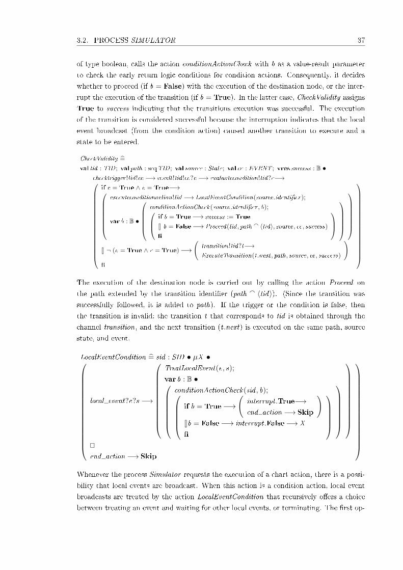
3.2. PROCESS SIMULATOR 37
of type boolean, calls the action conditionActionCheck with b as a value-result parameter
to check the early return logic conditions for condition actions. Consequently, it decides
whether to proceed (if b = False) with the execution of the destination node, or the inter-
rupt the execution of the transition (if b = True). In the latter case, CheckValidity assigns
True to success indicating that the transitions execution was successful. The execution
of the transition is considered successful because the interruption indicates that the local
event broadcast (from the condition action) caused another transition to execute and a
state to be entered.
CheckValidity =̂
val tid : TID ; val path : seqTID ; val source : State; val ce : EVENT ; vres success : B •checktrigger !tid !ce −→ result !tid !ce?e −→ evaluatecondition!tid?c−→
if e = True ∧ c = True−→executeconditionaction!tid −→ LocalEventCondition(source.identi�er);
var b : B •
conditionActionCheck(source.identi�er , b); if b = True−→ success := True
8 b = False−→ Proceed(tid , path a 〈tid〉, source, ce, success)
�
8 ¬ (e = True ∧ c = True)−→
(transition!tid?t−→ExecuteTransition(t .next , path, source, ce, success)
)�
The execution of the destination node is carried out by calling the action Proceed on
the path extended by the transition identi�er (path a 〈tid〉). (Since the transition was
successfully followed, it is added to path). If the trigger or the condition is false, then
the transition is invalid: the transition t that corresponds to tid is obtained through the
channel transition, and the next transition (t .next) is executed on the same path, source
state, and event.
LocalEventCondition =̂ sid : SID • µX •
local event?e?s −→
TreatLocalEvent(e, s);
var b : B •conditionActionCheck(sid , b);
if b = True−→(
interrupt .True−→end action −→ Skip
)8b = False−→ interrupt .False−→ X
�
@end action −→ Skip
Whenever the process Simulator requests the execution of a chart action, there is a possi-
bility that local events are broadcast. When this action is a condition action, local event
broadcasts are treated by the action LocalEventCondition that recursively o�ers a choice
between treating an event and waiting for other local events, or terminating. The �rst op-
38 CHAPTER 3. FORMAL MODEL
tion is modelled by an action that waits for a communication on the channel local event .
If it occurs, the action TreatLocalEvent is called, and the action conditionActionCheck is
called to check the appropriate early return logic conditions. If the early return logic con-
ditions are true, the action interrupts the chart action by communicating true through the
interrupt channel and waits for the end of the chart action on the channel end action. In
contrast, if the early return logic conditions are false, LocalEventCondition indicates that
the chart action can continue by communicating False through interrupt , and recurses.
The second option waits for a synchronisation on end action; the chart process agrees
on that when a state or transition action terminates. In this case, LocalEventCondition
terminates.
The action TreatLocalEvent takes an event e and a destination state s. If s has type
CHART (s.type = CHART ), it executes the chart, as de�ned by ExecuteChart , on e.
Otherwise, TreatLocalEvent executes s using ExecuteState again on the new event. Finally,
it signals the end of the local execution on the channel end local execution, thus, allowing
the broadcasting action of the chart (discussed in the next section) to terminate.
TreatLocalEvent =̂ e : EVENT ; s : State • if s.type = CHART −→ ExecuteChart(e)
8 s.type 6= CHART −→ ExecuteState(s, e)
�
; end local execution −→ Skip
This treatment of local events uni�es the notions of event broadcast, directed and quali�ed
event broadcasts. The form of broadcast modelled is the directed form. A simple broad-
casting is a directed broadcast to the chart. A quali�ed broadcast is a directed broadcast
to the qualifying state.
Whenever a local event broadcast occurs, the appropriate early return logic conditions
must be checked to avoid the possibility of reaching an inconsistent state 1. In the action
LocalEventCondition, this is achieved by a call to conditionActionCheck , which checks
whether the source of the transition path (source) is still active after the execution of the
condition action. If it is, the execution proceeds as expected. Otherwise, it is halted.
In CheckValidity , the check takes place after the condition action has been completely
executed. In contrast, in LocalEventCondition, conditionActionCheck checks the early
return logic conditions after each local event broadcast (because the same action might
have more than one broadcast).
Local event broadcasts and early return logic are two aspects of State�ow charts that
complicate the semantics. They are particularly di�cult because they are not well doc-
umented. Additionally, in our case, these aspects complicate the model because they do
not respect the separation between chart structure and the simulator as enforced by our
modelling approach. Our solution models a communication protocol that supports the re-
cursive execution of chart (or states) and the interruption of speci�c parts of the execution1An inconsistency occurs when, for instance, two sequential states are active at the same time, or the
parent of an active state is inactive.
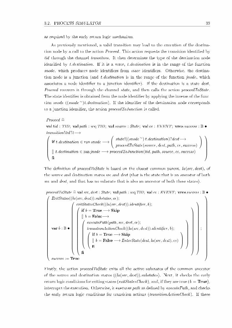
3.2. PROCESS SIMULATOR 39
as required by the early return logic mechanism.
As previously mentioned, a valid transition may lead to the execution of the destina-
tion node by a call to the action Proceed . This action requests the transition identi�ed by
tid through the channel transition. It then determines the type of the destination node
identi�ed by t .destination. If it is a state, t .destination is in the range of the function
snode, which produces node identi�ers from state identi�ers. Otherwise, the destina-
tion node is a junction (and t .destination is in the range of the function jnode, which
associates a node identi�er to a junction identi�er). If the destination is a state dest ,
Proceed recovers it through the channel state, and then calls the action proceedToState.
The state identi�er is obtained from the node identi�er by applying the inverse of the func-
tion snode ((snode ∼)t .destination). If the identi�er of the destination node corresponds
to a junction identi�er, the action proceedToJunction is called.
Proceed =̂
val tid : TID ; val path : seqTID ; val source : State; val ce : EVENT ; vres success : B •transition!tid?t−→
if t .destination ∈ ran snode −→(
state!((snode ∼) t .destination)?dest−→proceedToState(source, dest , path, ce, success)
)8 t .destination ∈ ran jnode −→ proceedToJunction(tid , path, source, ce, success)
�
The de�nition of proceedToState is based on the closest common parent, la(src, dest), of
the source and destination states src and dest (that is the state that is an ancestor of both
src and dest , and that has no substate that is also an ancestor of both these states).
proceedToState =̂ val src, dest : State; val path : seqTID ; val ce : EVENT ; vres success : B •
ExitStates((la(src, dest)).substates, ce);
var b : B •
exitStatesCheck((la(src, dest)).identi�er , b);
if b = True−→ Skip
8 b = False−→executePath(path, src, dest , ce);
transitionActionCheck((la(src, dest)).identi�er , b); if b = True−→ Skip
8 b = False−→ EnterState(dest , la(src, dest), ce)
�
�
;
success := True
Firstly, the action proceedToState exits all the active substates of the common ancestor
of the source and destination states ((la(src, dest)).substates). Next, it checks the early
return logic conditions for exiting states (exitStatesCheck), and, if they are true (b = True),
interrupts the execution. Otherwise, it executes path as de�ned by executePath, and checks
the early return logic conditions for transition actions (transitionActionCheck). If these
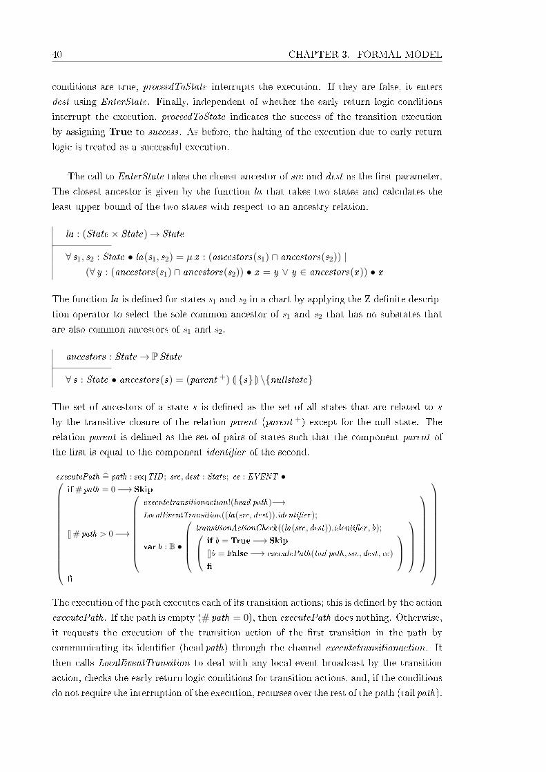
40 CHAPTER 3. FORMAL MODEL
conditions are true, proceedToState interrupts the execution. If they are false, it enters
dest using EnterState. Finally, independent of whether the early return logic conditions
interrupt the execution, proceedToState indicates the success of the transition execution
by assigning True to success. As before, the halting of the execution due to early return
logic is treated as a successful execution.
The call to EnterState takes the closest ancestor of src and dest as the �rst parameter.
The closest ancestor is given by the function la that takes two states and calculates the
least upper bound of the two states with respect to an ancestry relation.
la : (State × State)→ State
∀ s1, s2 : State • la(s1, s2) = µ x : (ancestors(s1) ∩ ancestors(s2)) |(∀ y : (ancestors(s1) ∩ ancestors(s2)) • x = y ∨ y ∈ ancestors(x )) • x
The function la is de�ned for states s1 and s2 in a chart by applying the Z de�nite descrip-
tion operator to select the sole common ancestor of s1 and s2 that has no substates that
are also common ancestors of s1 and s2.
ancestors : State→ PState
∀ s : State • ancestors(s) = (parent +) L {s} M \{nullstate}
The set of ancestors of a state s is de�ned as the set of all states that are related to s
by the transitive closure of the relation parent (parent +) except for the null state. The
relation parent is de�ned as the set of pairs of states such that the component parent of
the �rst is equal to the component identi�er of the second.
executePath =̂ path : seqTID ; src, dest : State; ce : EVENT •
if # path = 0−→ Skip
8 # path > 0−→
executetransitionaction!(head path)−→LocalEventTransition((la(src, dest)).identi�er);
var b : B •
transitionActionCheck((la(src, dest)).identi�er , b); if b = True−→ Skip
8b = False−→ executePath(tail path, src, dest , ce)
�
�
The execution of the path executes each of its transition actions; this is de�ned by the action
executePath. If the path is empty (# path = 0), then executePath does nothing. Otherwise,
it requests the execution of the transition action of the �rst transition in the path by
communicating its identi�er (head path) through the channel executetransitionaction. It
then calls LocalEventTransition to deal with any local event broadcast by the transition
action, checks the early return logic conditions for transition actions, and, if the conditions
do not require the interruption of the execution, recurses over the rest of the path (tail path).

3.2. PROCESS SIMULATOR 41
The de�nition of LocalEventTransition is similar to that of LocalEventCondition (above),
except that the early return logic conditions checked are those for transition actions.
Action transitionActionCheck checks that the substates of the closest common ancestor,
la(src, dest), are not active, as they had just been exited before the execution of the path 2.
If the destination of the transition is a junction, proceedToJunction is called. It obtains
the transition t with identi�er tid through the channel transition, and then the destination
junction dj of t by communicating its identi�er (jnode ∼) t .destination through junction.
If dj is not a history junction, it calls executeJunction on dj , the sequence path, the state
source, and the event ce. Otherwise, it obtains the state identi�er lsid that is stored in the
history junction by communicating the identi�er of the parent of the junction (dj .parent)
through history . If lsid is the identi�er of the null state (lsid = nullstate.identi�er), the
default transitions of the state are executed using ExecuteDefaultTransition, and success
is assigned True. Otherwise, proceedToJunction recovers the state ls identi�ed by lsid
through state, and calls proceedToState with ls as the destination state.
proceedToJunction =̂
val tid : TID ; val path : seqTID ; val source : State; val ce : EVENT ; vres success : B •transition!tid?t −→ junction!((jnode ∼) t .destination)?dj−→
if dj .history = False−→ executeJunction(dj , path, source, ce, success)
8 dj .history = True−→ history !(dj .parent)?lsid−→
if lsid = nullstate.identi�er −→
state!(dj .parent)?s−→ExecuteDefaultTransition(s, s, ce);
success := True
8 lsid 6= nullstate.identi�er −→
(state!lsid?ls−→proceedToState(source, ls, path, ce, success)
)�
�
The State�ow User's Guide discusses inner transitions to history junctions, but outer and
default transitions are not mentioned. Our experiments show that outer transitions to
history junctions have a behaviour similar to that of inner transitions. On the other
hand, default transitions to history junctions may lead to inconsistencies. In our model,
this may lead to divergence: the �rst time a default transition to a history junction is
followed, it observes nullstate.identi�er , and the default transitions are attempted again
in a potentially in�nite loop. Moreover, inner transitions to history junctions can lead to
an attempt to enter an already active state; in this case, the state is exited, and reentered.
This is captured in proceedToState. As previously explained, this action calls ExitStates
on the substates of the closest common parent of the source and destination states. In this
case, they are the substates of the state with the inner transition. At least one of them is
active, and is deactivated before any attempt at entering is made.
A junction is de�ned by the schema Junction, which records the identi�er of a junc-
2The de�nition of LocalEventTransition and transitionActionCheck can be found in Appendix B.

42 CHAPTER 3. FORMAL MODEL
tion, the identi�er of the �rst (if any) transition leaving it, the identi�er of its parent
state (or chart), and a boolean component indicating whether or not the junction is a
history junction.
Junction
identi�er : JID ; transition : TID ; parent : SID ; history : B
The execution of a junction consists of executing its outgoing transitions. If there are none,
the transition path fails. The action executeJunction compares the identi�er of the �rst
outgoing transition (j .transition) to the identi�er of the null transition. If they are the
same, there are no transitions out of the junction, and the execution failure is indicated
by assigning False to success. Otherwise, executeJunction calls ExecuteTransition.
executeJunction =̂
val j : Junction; val path : seqTID ; val source : State; val ce : EVENT ; vres success : B •if j .transition = nulltransition.identi�er −→ success := False
8 j .transition 6= nulltransition.identi�er−→ExecuteTransition(j .transition, path, source, ce, success)
�
The key actions that model the execution of transitions are ExecuteTransition, which
we presented above, and ExecuteDefaultTransition. ExecuteDefaultTransition extends
ExecuteTransition by treating the possibility that there are no default transitions to follow,
but the choice of which state to enter is deterministic. This is the case when, for example,
there is only one substate.
The informal description of the execution of a set of transitions is shown in Figure 2.1,
which is repeated in Figure 3.5 for convenience. These steps describe the execution of a set
of transitions as an iterative procedure, where each iteration starts with step 2 and ends
with step 3. ExecuteTransition corresponds to the �rst sentence of step 2 in conjunction
with step 3. CheckValidity corresponds to the rest of step 2, Proceed to the selection
between state and junction destinations speci�ed in the end of step 2, proceedToState to
the four steps under the label States, and executeJunction to the steps under the labels
Junctions with no outgoing transition segments and Junctions with outgoing
transition segments. The action proceedToJunction does not correspond to any step in
the informal description; it extends the execution of transition by modelling the case when
a transition leads to a history junction.
3.2.3 Entering a state
To keep close to the informal description previously shown in Figure 2.2, we preserve the
structure and granularity of the steps in the actions that model the simulation semantics.
For convenience, we repeat in Figure 3.6 the steps for entering a state.
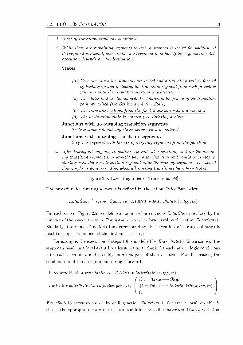
3.2. PROCESS SIMULATOR 43
1. A set of transition segments is ordered.
2. While there are remaining segments to test, a segment is tested for validity. Ifthe segment is invalid, move to the next segment in order. If the segment is valid,execution depends on the destination:
States
(a) No more transition segments are tested and a transition path is formedby backing up and including the transition segment from each precedingjunction until the respective starting transitions.
(b) The states that are the immediate children of the parent of the transitionpath are exited (see Exiting an Active State).
(c) The transition actions from the �nal transition path are executed.
(d) The destination state is entered (see Entering a State).
Junctions with no outgoing transition segmentsTesting stops without any states being exited or entered.
Junctions with outgoing transition segmentsStep 1 is repeated with the set of outgoing segments from the junction.
3. After testing all outgoing transition segments at a junction, back up the incom-ing transition segment that brought you to the junction and continue at step 2,starting with the next transition segment after the back up segment. The set of�ow graphs is done executing when all starting transitions have been tested.
Figure 3.5: Executing a Set of Transitions [98]
The procedure for entering a state s is de�ned by the action EnterState below.
EnterState =̂ s, tpp : State; ce : EVENT • EnterState16(s, tpp, ce)
For each step in Figure 2.2, we de�ne an action whose name is EnterState post�xed by the
number of the associated step. For instance, step 1 is formalised by the action EnterState1.
Similarly, the name of actions that correspond to the execution of a range of steps is
post�xed by the numbers of the �rst and last steps.
For example, the execution of steps 1-6 is modelled by EnterState16. Since some of the
steps can result in a local event broadcast, we must check the early return logic conditions
after each such step, and possibly interrupt part of the execution. For this reason, the
combination of these steps is not straightforward.
EnterState16 =̂ s, tpp : State; ce : EVENT • EnterState1(s, tpp, ce);
var b : B • enterState1Check(s.identi�er , b) ;
if b = True−→ Skip
8b = False−→ EnterState26(s, tpp, ce)
�
EnterState16 executes step 1 by calling action EnterState1, declares a local variable b,
checks the appropriate early return logic condition by calling enterState1Check with b as
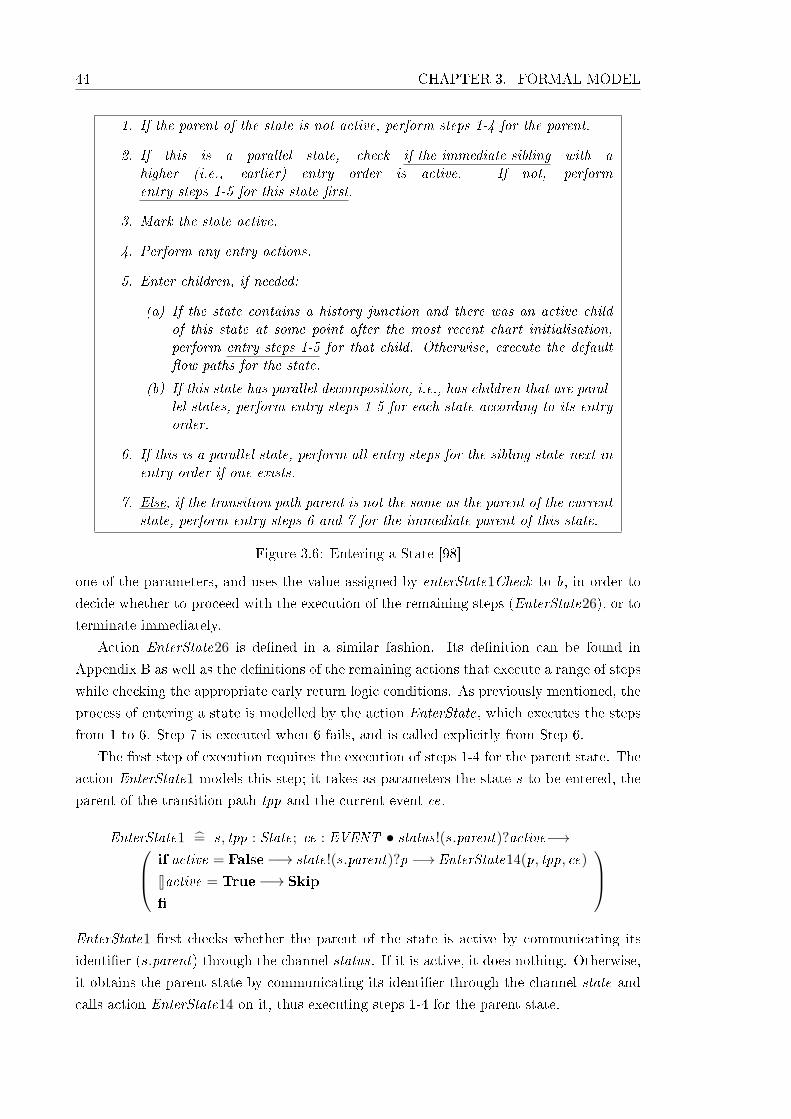
44 CHAPTER 3. FORMAL MODEL
1. If the parent of the state is not active, perform steps 1-4 for the parent.
2. If this is a parallel state, check if the immediate sibling with ahigher (i.e., earlier) entry order is active. If not, performentry steps 1-5 for this state �rst.
3. Mark the state active.
4. Perform any entry actions.
5. Enter children, if needed:
(a) If the state contains a history junction and there was an active childof this state at some point after the most recent chart initialisation,perform entry steps 1-5 for that child. Otherwise, execute the default�ow paths for the state.
(b) If this state has parallel decomposition, i.e., has children that are paral-lel states, perform entry steps 1-5 for each state according to its entryorder.
6. If this is a parallel state, perform all entry steps for the sibling state next inentry order if one exists.
7. Else, if the transition path parent is not the same as the parent of the currentstate, perform entry steps 6 and 7 for the immediate parent of this state.
Figure 3.6: Entering a State [98]
one of the parameters, and uses the value assigned by enterState1Check to b, in order to
decide whether to proceed with the execution of the remaining steps (EnterState26), or to
terminate immediately.
Action EnterState26 is de�ned in a similar fashion. Its de�nition can be found in
Appendix B as well as the de�nitions of the remaining actions that execute a range of steps
while checking the appropriate early return logic conditions. As previously mentioned, the
process of entering a state is modelled by the action EnterState, which executes the steps
from 1 to 6. Step 7 is executed when 6 fails, and is called explicitly from Step 6.
The �rst step of execution requires the execution of steps 1-4 for the parent state. The
action EnterState1 models this step; it takes as parameters the state s to be entered, the
parent of the transition path tpp and the current event ce.
EnterState1 =̂ s, tpp : State; ce : EVENT • status!(s.parent)?active−→ if active = False−→ state!(s.parent)?p −→ EnterState14(p, tpp, ce)
8active = True−→ Skip
�
EnterState1 �rst checks whether the parent of the state is active by communicating its
identi�er (s.parent) through the channel status. If it is active, it does nothing. Otherwise,
it obtains the parent state by communicating its identi�er through the channel state and
calls action EnterState14 on it, thus executing steps 1-4 for the parent state.
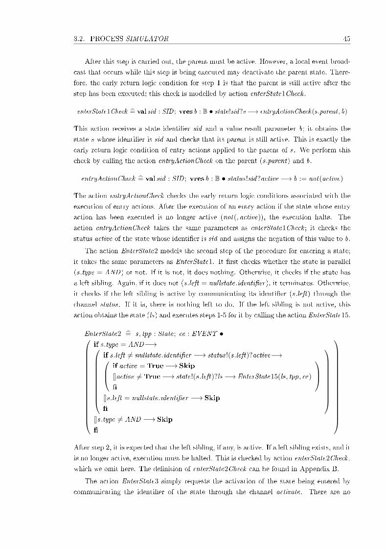
3.2. PROCESS SIMULATOR 45
After this step is carried out, the parent must be active. However, a local event broad-
cast that occurs while this step is being executed may deactivate the parent state. There-
fore, the early return logic condition for step 1 is that the parent is still active after the
step has been executed; this check is modelled by action enterState1Check .
enterState1Check =̂ val sid : SID ; vres b : B • state!sid?s −→ entryActionCheck(s.parent , b)
This action receives a state identi�er sid and a value-result parameter b; it obtains the
state s whose identi�er is sid and checks that its parent is still active. This is exactly the
early return logic condition of entry actions applied to the parent of s. We perform this
check by calling the action entryActionCheck on the parent (s.parent) and b.
entryActionCheck =̂ val sid : SID ; vres b : B • status!sid?active −→ b := not(active)
The action entryActionCheck checks the early return logic conditions associated with the
execution of entry actions. After the execution of an entry action if the state whose entry
action has been executed is no longer active (not(, active)), the execution halts. The
action entryActionCheck takes the same parameters as enterState1Check ; it checks the
status active of the state whose identi�er is sid and assigns the negation of this value to b.
The action EnterState2 models the second step of the procedure for entering a state;
it takes the same parameters as EnterState1. It �rst checks whether the state is parallel
(s.type = AND) or not. If it is not, it does nothing. Otherwise, it checks if the state has
a left sibling. Again, if it does not (s.left = nullstate.identi�er), it terminates. Otherwise,
it checks if the left sibling is active by communicating its identi�er (s.left) through the
channel status. If it is, there is nothing left to do. If the left sibling is not active, this
action obtains the state (ls) and executes steps 1-5 for it by calling the action EnterState15.
EnterState2 =̂ s, tpp : State; ce : EVENT •
if s.type = AND−→
if s.left 6= nullstate.identi�er −→ status!(s.left)?active−→ if active = True−→ Skip
8active 6= True−→ state!(s.left)?ls −→ EnterState15(ls, tpp, ce)
�
8s.left = nullstate.identi�er −→ Skip
�
8s.type 6= AND −→ Skip
�
After step 2, it is expected that the left sibling, if any, is active. If a left sibling exists, and it
is no longer active, execution must be halted. This is checked by action enterState2Check ,
which we omit here. The de�nition of enterState2Check can be found in Appendix B.
The action EnterState3 simply requests the activation of the state being entered by
communicating the identi�er of the state through the channel activate. There are no
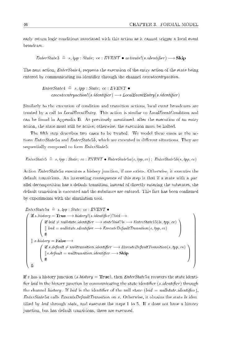
46 CHAPTER 3. FORMAL MODEL
early return logic conditions associated with this action as it cannot trigger a local event
broadcast.
EnterState3 =̂ s, tpp : State; ce : EVENT • activate!(s.identi�er)−→ Skip
The next action, EnterState4, requests the execution of the entry action of the state being
entered by communicating its identi�er through the channel executeentryaction.
EnterState4 =̂ s, tpp : State; ce : EVENT •executeentryaction!(s.identi�er)−→ LocalEventEntry(s.identi�er)
Similarly to the execution of condition and transition actions, local event broadcasts are
treated by a call to LocalEventEntry . This action is similar to LocalEventCondition and
can be found in Appendix B. As previously mentioned, after the execution of an entry
action, the state must still be active; otherwise, the execution must be halted.
The �fth step describes two cases to be treated. We model these cases as the ac-
tions EnterState5a and EnterState5b, which are executed in di�erent situations. They are
sequentially composed to form EnterState5.
EnterState5 =̂ s, tpp : State; ce : EVENT • EnterState5a(s, tpp, ce) ; EnterState5b(s, tpp, ce)
Action EnterState5a executes a history junction, if one exists. Otherwise, it executes the
default transitions. An interesting consequence of this step is that if a state with a par-
allel decomposition has a default transition, instead of directly entering the substates, the
default transition is executed and the substates are entered. This fact has been con�rmed
by experiments with the simulation tool.
EnterState5a =̂ s, tpp : State; ce : EVENT •
if s.history = True−→ history !(s.identi�er)?lsid−→ if lsid 6= nullstate.identi�er −→ state!lsid?ls −→ EnterState15(ls, tpp, ce)
8 lsid = nullstate.identi�er −→ ExecuteDefaultTransition(s, tpp, ce)
�
8 s.history = False−→ if s.default 6= nulltransition.identi�er −→ ExecuteDefaultTransition(s, tpp, ce)
8s.default = nulltransition.identi�er −→ Skip
�
�
If s has a history junction (s.history = True), then EnterState5a recovers the state identi-
�er lsid in the history junction by communicating the state identi�er (s.identi�er) through
the channel history . If lsid is the identi�er of the null state (lsid = nullstate.identi�er),
EnterState5a calls ExecuteDefaultTransition on s. Otherwise, it obtains the state ls iden-
ti�ed by lsid through state, and executes the steps 1 to 5. If s does not have a history
junction, but has default transitions, these are executed.
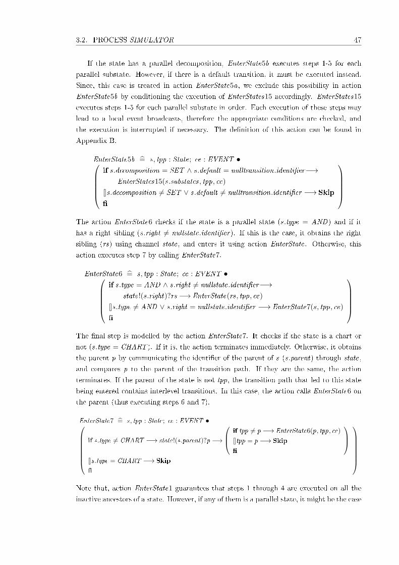
3.2. PROCESS SIMULATOR 47
If the state has a parallel decomposition, EnterState5b executes steps 1-5 for each
parallel substate. However, if there is a default transition, it must be executed instead.
Since, this case is treated in action EnterState5a, we exclude this possibility in action
EnterState5b by conditioning the execution of EnterStates15 accordingly. EnterStates15
executes steps 1-5 for each parallel substate in order. Each execution of these steps may
lead to a local event broadcasts, therefore the appropriate conditions are checked, and
the execution is interrupted if necessary. The de�nition of this action can be found in
Appendix B.
EnterState5b =̂ s, tpp : State; ce : EVENT •if s.decomposition = SET ∧ s.default = nulltransition.identi�er−→
EnterStates15(s.substates, tpp, ce)
8s.decomposition 6= SET ∨ s.default 6= nulltransition.identi�er −→ Skip
�
The action EnterState6 checks if the state is a parallel state (s.type = AND) and if it
has a right sibling (s.right 6= nullstate.identi�er). If this is the case, it obtains the right
sibling (rs) using channel state, and enters it using action EnterState. Otherwise, this
action executes step 7 by calling EnterState7.
EnterState6 =̂ s, tpp : State; ce : EVENT •if s.type = AND ∧ s.right 6= nullstate.identi�er−→
state!(s.right)?rs −→ EnterState(rs, tpp, ce)
8s.type 6= AND ∨ s.right = nullstate.identi�er −→ EnterState7(s, tpp, ce)
�
The �nal step is modelled by the action EnterState7. It checks if the state is a chart or
not (s.type = CHART ). If it is, the action terminates immediately. Otherwise, it obtains
the parent p by communicating the identi�er of the parent of s (s.parent) through state,
and compares p to the parent of the transition path. If they are the same, the action
terminates. If the parent of the state is not tpp, the transition path that led to this state
being entered contains interlevel transitions. In this case, the action calls EnterState6 on
the parent (thus executing steps 6 and 7).
EnterState7 =̂ s, tpp : State; ce : EVENT •if s.type 6= CHART −→ state!(s.parent)?p −→
if tpp 6= p −→ EnterState6(p, tpp, ce)
8tpp = p −→ Skip
�
8s.type = CHART −→ Skip
�
Note that, action EnterState1 guarantees that steps 1 through 4 are executed on all the
inactive ancestors of a state. However, if any of them is a parallel state, it might be the case

48 CHAPTER 3. FORMAL MODEL
that its right siblings are not entered. The action EnterState7 takes care of this scenario,
by recursively applying the action EnterState6 to the necessary states.
3.2.4 Executing and exiting a state
The processes of executing and exiting active states are simple compared to entering a
state or executing transitions. As before, we repeat in this section the informal description
in Figures 3.7 and 3.8.
The action ExecuteState takes a state s and the current event as parameters.
ExecuteState =̂ s : State; ce : EVENT • status!(s.identi�er)?active−→
if active = True−→
var success : B •ExecuteTransition(s.outer , 〈〉, s, ce, success);
if success = True−→ Skip
8 success = False−→
executeduringaction!(s.identi�er)!ce−→LocalEventDuring(s.identi�er);
var b : B •duringActionCheck(s.identi�er , b); if b = True−→ Skip
8 b = False−→ AlternativeExecution(s, ce)
�
�
8active = False−→ Skip
�
ExecuteState �rst checks whether or not the state is active by communicating the identi�er
of the state through the channel status. If the state is not active, ExecuteState terminates
immediately. Otherwise, ExecuteState declares a boolean variable success and calls the
action ExecuteTransition on the outer transitions passing success as a parameter. The call
to ExecuteTransition then updates success to indicate whether or not the execution of the
outer transitions was successful. If it is (success = True), then ExecuteState terminates im-
mediately. Otherwise, it requests the execution of the during and on actions of the state by
communicating the state identi�er and the current event ce through executeduringaction.
Since the execution of a during action can lead to local event broadcasts, ExecuteState
treats such broadcasts (LocalEventDuring), checks the appropriate early return logic con-
ditions (duringActionCheck), and, if necessary, terminates immediately. Otherwise, it calls
the action AlternativeExecution on the state to execute its inner transitions.
AlternativeExecution attempts to execute the inner transitions of the state s in the
same fashion as ExecuteState. The local variable success is used to indicate the success or
failure of the execution, and the alternation controls the remaining execution according to
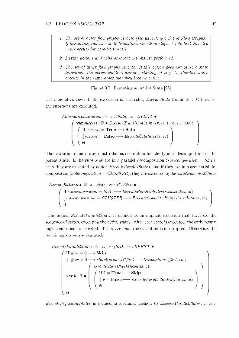
3.2. PROCESS SIMULATOR 49
1. The set of outer �ow graphs execute (see Executing a Set of Flow Graphs).If this action causes a state transition, execution stops. (Note that this stepnever occurs for parallel states.)
2. During actions and valid on-event actions are performed.
3. The set of inner �ow graphs execute. If this action does not cause a statetransition, the active children execute, starting at step 1. Parallel statesexecute in the same order that they become active.
Figure 3.7: Executing an active State [98]
the value of success. If the execution is successful, ExecuteState terminates. Otherwise,
the substates are executed.
AlternativeExecution =̂ s : State; ce : EVENT •var success : B • ExecuteTransition(s.inner , 〈〉, s, ce, success); if success = True−→ Skip
8success = False−→ ExecuteSubstates(s, ce)
�
The execution of substates must take into consideration the type of decomposition of the
parent state. If the substates are in a parallel decomposition (s.decomposition = SET ),
then they are executed by action ExecuteParallelStates, and if they are in a sequential de-
composition (s.decomposition = CLUSTER), they are executed by ExecuteSequentialStates.
ExecuteSubstates =̂ s : State; ce : EVENT • if s.decomposition = SET −→ ExecuteParallelStates(s.substates, ce)
8s.decomposition = CLUSTER −→ ExecuteSequentialStates(s.substates, ce)
�
The action ExecuteParallelStates is de�ned as an implicit recursion that traverses the
sequence of states, executing the active states. After each state is executed, the early return
logic conditions are checked. If they are true, the execution is interrupted. Otherwise, the
remaining states are executed.
ExecuteParallelStates =̂ ss : seqSID ; ce : EVENT •
if # ss = 0−→ Skip
8 # ss > 0−→ state!(head ss)?�rst −→ ExecuteState(�rst , ce);
var b : B •
executeStateCheck(head ss, b); if b = True−→ Skip
8 b = False−→ ExecuteParallelStates(tail ss, ce)
�
�
ExecuteSequentialStates is de�ned in a similar fashion to ExecuteParallelStates; it is a
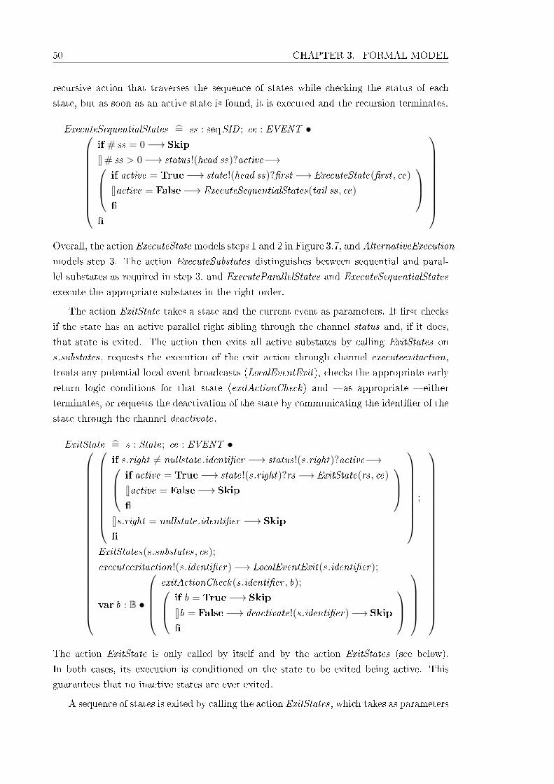
50 CHAPTER 3. FORMAL MODEL
recursive action that traverses the sequence of states while checking the status of each
state, but as soon as an active state is found, it is executed and the recursion terminates.
ExecuteSequentialStates =̂ ss : seqSID ; ce : EVENT •
if # ss = 0−→ Skip
8 # ss > 0−→ status!(head ss)?active−→ if active = True−→ state!(head ss)?�rst −→ ExecuteState(�rst , ce)
8active = False−→ ExecuteSequentialStates(tail ss, ce)
�
�
Overall, the action ExecuteState models steps 1 and 2 in Figure 3.7, and AlternativeExecution
models step 3. The action ExecuteSubstates distinguishes between sequential and paral-
lel substates as required in step 3, and ExecuteParallelStates and ExecuteSequentialStates
execute the appropriate substates in the right order.
The action ExitState takes a state and the current event as parameters. It �rst checks
if the state has an active parallel right sibling through the channel status and, if it does,
that state is exited. The action then exits all active substates by calling ExitStates on
s.substates, requests the execution of the exit action through channel executeexitaction,
treats any potential local event broadcasts (LocalEventExit), checks the appropriate early
return logic conditions for that state (exitActionCheck) and � as appropriate � either
terminates, or requests the deactivation of the state by communicating the identi�er of the
state through the channel deactivate.
ExitState =̂ s : State; ce : EVENT •
if s.right 6= nullstate.identi�er −→ status!(s.right)?active−→ if active = True−→ state!(s.right)?rs −→ ExitState(rs, ce)
8active = False−→ Skip
�
8s.right = nullstate.identi�er −→ Skip
�
;
ExitStates(s.substates, ce);
executeexitaction!(s.identi�er)−→ LocalEventExit(s.identi�er);
var b : B •
exitActionCheck(s.identi�er , b); if b = True−→ Skip
8b = False−→ deactivate!(s.identi�er)−→ Skip
�
The action ExitState is only called by itself and by the action ExitStates (see below).
In both cases, its execution is conditioned on the state to be exited being active. This
guarantees that no inactive states are ever exited.
A sequence of states is exited by calling the action ExitStates, which takes as parameters

3.2. PROCESS SIMULATOR 51
1. If this is a parallel state, check that the immediate sibling that became activeafter this state have already become inactive. Otherwise, perform all exitingsteps on that sibling state.
2. If there are any active children, perform the exit steps on these states in thereverse order that they became active.
3. Perform any exit actions.
4. Mark the state as inactive.
Figure 3.8: Exiting a State [98]
a sequence of state identi�ers, and the current event. If the sequence is empty nothing is
done. If the sequence is empty, ExitStates terminates. If the sequence has one or more state
identi�ers, ExitStates checks the status of the state that corresponds to the last identi�er
in the sequence, and, if the state is active, exits it. Next, ExitStates checks the early
return logic conditions for exiting a state, and, if they are true, terminates. Otherwise, it
recursively exits the remaining states.
ExitStates =̂ ss : seqSID ; ce : EVENT •
if # ss = 0−→ Skip
8 # ss > 0−→ status!(last ss)?active−→ if active = True−→ state!(last ss)?l −→ ExitState(l , ce)
8 active = False−→ Skip
�
;
var b : B •
exitStateCheck(head ss, b); if b = True−→ Skip
8 b = False−→ ExitStates(front ss, ce)
�
�
The action ExitState models steps 1, 3 and 4 of the process of exiting a state shown in
Figure 3.8. Step 2 is modelled by a call to ExitStates.
This concludes the process Simulator that models the semantics of State�ow charts
independently of any particular instance of State�ow charts. An advantage of this separa-
tion is that changes and extensions to the semantics of the main components of State�ow
are restricted to this process. Furthermore, since this process is the same for every chart,
the e�ort require to generate the chart speci�c model is reduced signi�cantly.
In the next section, we describe the process that represents the structure of a particular
chart and complements the Simulator process in order to model the execution of the chart.

52 CHAPTER 3. FORMAL MODEL
3.3 Chart process
The chart process records the structure of the chart (state, transitions, and junctions) using
constants, as this information does not change throughout the execution of the chart. The
process state records the data declared in the chart, and information particular to its
execution. For instance, the chart process c shift logic (Figure 3.9) corresponds to our
example in Figure 3.2.
A schema State�owChart captures the general structure of a State�ow chart. It is
de�ned outside of the scope of the chart process, since it is the same for every chart.
State�owChart
identi�er : SID
states : SID 7 7→ State
transitions : TID 7 7→ Transition
junctions : JID 7 7→ Junction
nullstate 6∈ ran statesnulltransition 6∈ ran transitionsnulljunction 6∈ ran junctions#{s : ran states | s.type = CHART} = 1
(states(identi�er)).type = CHART
∀n : SID | n ∈ dom states • (states(n)).identi�er = n
∀n : JID | n ∈ dom junctions • (junctions(n)).identi�er = n
∀n : TID | n ∈ dom transitions • (transitions(n)).identi�er = n
The component identi�er identi�es the state that represents the chart. The sets State,
Transition and Junction are de�ned by the schemas described in the previous section. The
components states, transitions and junctions are, therefore, �nite functions from identi�ers
to bindings. The invariant de�nes basic structural constraints enforced by the State�ow
notation:
• each of the states, transitions, and junctions components must not contain the null
object (of the appropriate type);
• the range of states must contain a single state of type CHART , that is indicated by
identi�er ; and
• the application of each of the functions states, transitions, and junctions to an iden-
ti�er n in its domain must yield a binding whose component identi�er is equal to n.
In the chart process (see Figure 3.9), an axiomatic de�nition includes State�owChart ,
promoting its components to process constants, and identifying their values. For our shift
logic example, the axiomatic de�nition states that identi�er = c shift logic and that states
includes the pairs (s downshifting ,S downshifting), (s gear state,S gear state) and so

3.3. CHART PROCESS 53
process c shift logic =̂ begin
State�owChart
. . .
SimulationData == [state status : SID 7 7→ B; state history : SID 7 7→ SID | . . .]InitSimulationData == [SimulationData ′ | . . .]SimulationInstance == [v gear , v speed , v throttle, v up th, v down th : R]InitSimulationInstance == [SimulationInstance ′ | . . .]InitState == (InitSimulationInstance) ∧ (InitSimulationData). . .Activate == (ActivateWithHistory ∨ ActivateNoHistory) ∧ ΞSimulationInstance. . .Deactivate == [ΞSimulationInstance; ∆SimulationData | . . .]state shift logic state == SimulationInstance ∧ SimulationDataentryaction downshifting =̂ executeentryaction.(s downshifting)−→ Skip
. . .entryactions =̂ entryaction downshifting @ . . . @ entryaction steady state
duringaction downshifting =̂ executeduringaction.(s downshifting)?ce −→ Skip
. . .duringactions =̂ duringaction downshifting @ . . . @ duringaction steady state
exitaction downshifting =̂ executeexitaction.(s downshifting)−→ Skip
. . .exitactions =̂ exitaction downshifting @ . . . @ exitaction steady state
conditionaction third fourth =̂ executeconditionaction.(t third fourth)−→ Skip
. . .conditionactions =̂ conditionaction third fourth @ . . . @ conditionaction default steady state
transitionaction third fourth =̂ executetransitionaction.(t third fourth)−→ Skip
. . .transitionactions =̂ transitionaction third fourth @ . . . transitionaction steady state upshifting
condition third fourth =̂ evaluatecondition.(t third fourth)!(True)−→ Skip
. . .conditions =̂ condition third fourth @ . . . condition steady state upshifting
trigger default �rst =̂ checktrigger .(t default �rst)?e −→ result .(t default �rst).(e)!(True)−→ Skip
. . .triggers =̂ trigger third fourth @ . . . @ trigger upshifting steady state26getevents =̂ events!(〈ENULL〉)−→ Skip
getstate =̂ state?x : (x ∈ dom(states))!(states(x))−→ Skip
getjunction =̂ junction?x : (x ∈ dom(junctions))!(junctions(x))−→ Skip
gettransition =̂ transition?x : (x ∈ dom(transitions))!(transitions(x))−→ Skip
getchart =̂ chart !(states(identi�er))−→ Skip
status =̂ status?x : (x ∈ dom(state status))!(state status(x))−→ Skip
history =̂ history?x : (x ∈ dom(state history))!(state history(x))−→ Skip
activation =̂ activate?x −→Activate
deactivation =̂ deactivate?x −→Deactivate
ChartActions =̂ . . .InterfaceActions =̂ . . .Inputs =̂ . . .Outputs =̂ . . .AllActions =̂ . . .broadcast =̂ e : EVENT ; dest : SID • . . .check =̂ res erl : B • . . .
• InitState ; µX •
µY
AllActions ; Y
@end cycle −→ Skip
; X
end
Figure 3.9: Structure of the c shift logic process.
on, where s downshifting and s gear state are state identi�ers, and S downshifting and
S gear state are bindings of the schema State.
These identi�ers and binding are constants that are de�ned outside the process and
model the main objects of the State�ow notation: states, transitions, junctions and events.
For instance, for each state in the diagram, we de�ne a constant of type State and a constant

54 CHAPTER 3. FORMAL MODEL
of type SID ; the name of the �rst is the name of the state pre�xed by a capital S , and the
name of the second is created in the same fashion, but pre�xed by a lower case s. For state
gear state, the constant S gear state has type State and the value of its components are
de�ned by the following binding.
S gear state : State
S gear state = 〈|identi�er == s gear state, default == default �rst ,
inner == nulltransition.identi�er , outer == nulltransition.identi�er ,
parent == s shift logic, left == nullstate.identi�er ,
right == s selection state, substates == 〈s �rst , s second , s third , s fourth〉,decomposition == CLUSTER, type == AND , history == False|〉
This state's identi�er is s gear state. It has a default transition whose identi�er is
default �rst . It has no inner or outer transitions, no left sibling, but has a right sib-
ling that has identi�er s selection state. It has a sequence of substates and sequential
decomposition (CLUSTER). It is a parallel (AND) state and has no history junction.
Identi�ers and binding of transitions and junctions are de�ned in a similar way. The
remaining identi�er and binding de�nitions for our example can be found in Appendix C.1.
Input and local events are de�ned as constants of type EVENT . For our example, the event
identi�ers are de�ned as follows.
e UP , e DOWN ,ENULL : EVENT
As discussed in the previous section, at each cycle, the process Simulator executes the
chart once for each input event that has occurred. If the chart does not have any input
events, we declare the dummy event ENULL to allow the Simulator to execute the chart.
The de�nition of the schema SimulationData is independent of a particular chart. It
declares the state components of the chart process that record the status of each state
in the chart (state status), and the last active substate for those with a history junc-
tion (state history). If state status n is true, the state n is active; state history is a
function from state identi�ers to state identi�ers.
SimulationData
state status : SID 7 7→ Bstate history : SID 7 7→ SID
dom state status = dom states
dom state history = {j : ran junctions | j .history = True • j .parent}∀ s : ran states | s.decomposition = CLUSTER •
#{ss : ran s.substates | state status(ss) = True} ≤ 1
The predicate of SimulationData states that the domain of state status contains the iden-
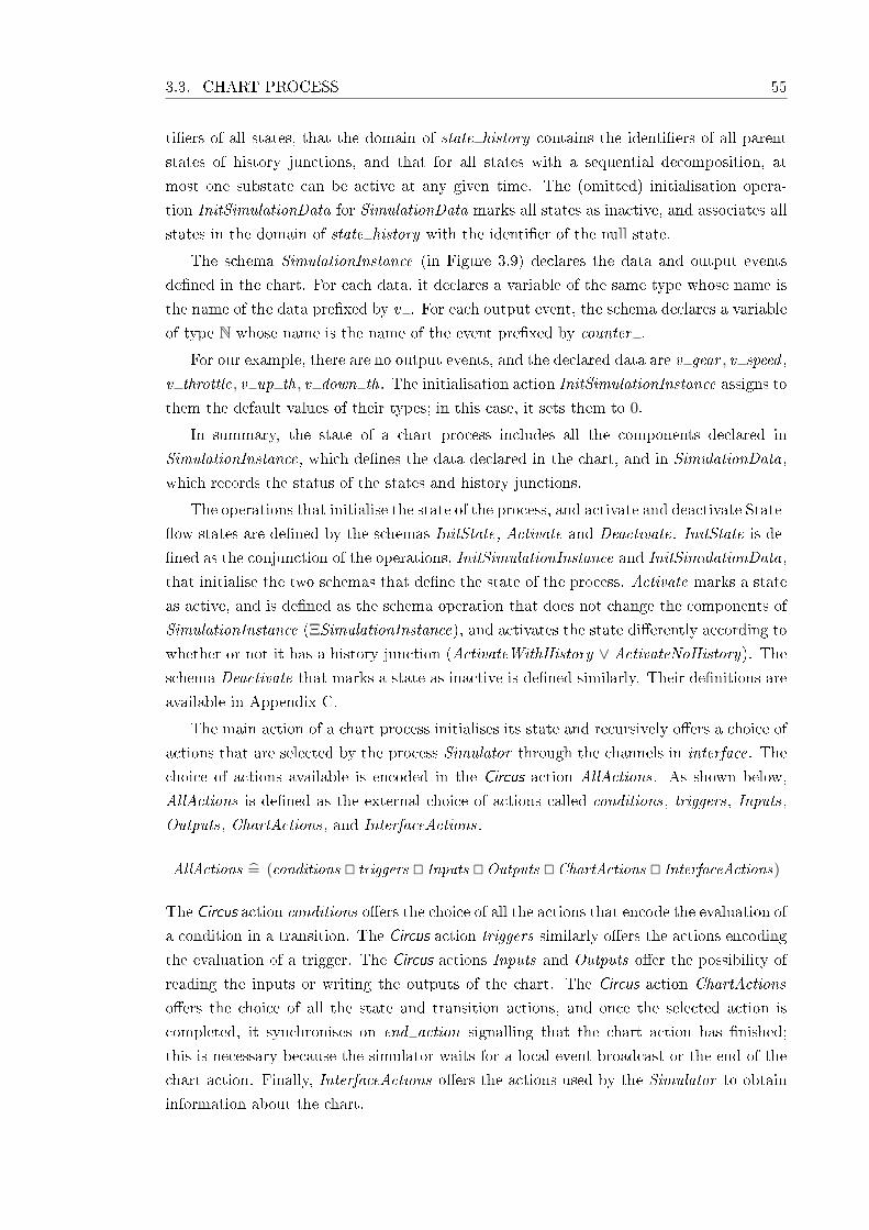
3.3. CHART PROCESS 55
ti�ers of all states, that the domain of state history contains the identi�ers of all parent
states of history junctions, and that for all states with a sequential decomposition, at
most one substate can be active at any given time. The (omitted) initialisation opera-
tion InitSimulationData for SimulationData marks all states as inactive, and associates all
states in the domain of state history with the identi�er of the null state.
The schema SimulationInstance (in Figure 3.9) declares the data and output events
de�ned in the chart. For each data, it declares a variable of the same type whose name is
the name of the data pre�xed by v . For each output event, the schema declares a variable
of type N whose name is the name of the event pre�xed by counter .
For our example, there are no output events, and the declared data are v gear , v speed ,
v throttle, v up th, v down th. The initialisation action InitSimulationInstance assigns to
them the default values of their types; in this case, it sets them to 0.
In summary, the state of a chart process includes all the components declared in
SimulationInstance, which de�nes the data declared in the chart, and in SimulationData,
which records the status of the states and history junctions.
The operations that initialise the state of the process, and activate and deactivate State-
�ow states are de�ned by the schemas InitState, Activate and Deactivate. InitState is de-
�ned as the conjunction of the operations, InitSimulationInstance and InitSimulationData,
that initialise the two schemas that de�ne the state of the process. Activate marks a state
as active, and is de�ned as the schema operation that does not change the components of
SimulationInstance (ΞSimulationInstance), and activates the state di�erently according to
whether or not it has a history junction (ActivateWithHistory ∨ ActivateNoHistory). The
schema Deactivate that marks a state as inactive is de�ned similarly. Their de�nitions are
available in Appendix C.
The main action of a chart process initialises its state and recursively o�ers a choice of
actions that are selected by the process Simulator through the channels in interface. The
choice of actions available is encoded in the Circus action AllActions. As shown below,
AllActions is de�ned as the external choice of actions called conditions, triggers, Inputs,
Outputs, ChartActions, and InterfaceActions.
AllActions =̂ (conditions @ triggers @ Inputs @ Outputs @ ChartActions @ InterfaceActions)
The Circus action conditions o�ers the choice of all the actions that encode the evaluation of
a condition in a transition. The Circus action triggers similarly o�ers the actions encoding
the evaluation of a trigger. The Circus actions Inputs and Outputs o�er the possibility of
reading the inputs or writing the outputs of the chart. The Circus action ChartActions
o�ers the choice of all the state and transition actions, and once the selected action is
completed, it synchronises on end action signalling that the chart action has �nished;
this is necessary because the simulator waits for a local event broadcast or the end of the
chart action. Finally, InterfaceActions o�ers the actions used by the Simulator to obtain
information about the chart.

56 CHAPTER 3. FORMAL MODEL
The evaluation of a condition is speci�ed as a Circus action that communicates true
through the channel evaluatecondition if the condition holds, and false otherwise. For
example, the condition of the transition between the states steady state and downshift-
ing (of Figure 3.2) is de�ned as follows.
condition steady state downshifting =̂if (v speed<Av down th) 6= 0−→
evaluatecondition.t steady state downshifting !True−→ Skip
8 ¬ ((v speed<Av down th) 6= 0)−→evaluatecondition.t steady state downshifting !False−→ Skip
�
First, the predicate (v speed<Av down th) 6= 0 is evaluated; if it is true, the action of-
fers a synchronisation on evaluatecondition with the identi�er of the condition's transition
(t steady state downshifting) and the boolean value True. Otherwise, it o�ers a commu-
nication with False. The operation <A returns 0 if the �rst operand is not less than the
second operand, otherwise, it returns a number di�erent than 0.
The evaluation of a transition trigger is de�ned by a Circus action that waits for the
communication of an event e along with the transition identi�er through checktrigger , and
then evaluates the trigger with respect to e. Afterwards, it communicates the identi�er,
the event, and the boolean result of the evaluation through result . For the trigger of the
transition between the states �rst and second, we have the following action.
trigger �rst second =̂ checktrigger .t �rst second?e−→ if e = e UP −→ result .t �rst second .e!True−→ Skip
8 ¬ (e = e UP)−→ result .t �rst second .e!False−→ Skip
�
This action communicates True if the event received through the channel checktrigger is
e UP , and False otherwise.
The Circus action Inputs waits for a synchronisation on read inputs and reads the
values of the input variables in interleaving. A channel of the appropriate type is declared
for each input and output data, as well as for each output event. In our example, there are
two input variables, v speed and v throttle, and their values are communicated through
the channels i speed and i throttle.
Inputs =̂ read inputs −→
i speed?x −→ v speed := x
||[{v speed} | {v throttle}]||i throttle?x −→ v throttle := x
The interleaving requires the partitioning of the state components that are written to by
each parallel action to avoid race conditions. This interleaving terminates when all the
input variables are read and recorded in the appropriate state component.

3.3. CHART PROCESS 57
The Circus action Outputs is also de�ned by a communication followed by an interleav-
ing (if necessary). Each interleaved action communicates an output variable or an output
event. For each output event, the action that communicates it �rst checks the counter
associated to that event. If the counter is positive, the actions decrements it, and commu-
nicates True through the appropriate channel. If the counter is zero, the value False is
communicated. For our example, there are no output events, and the only output variable
in the example is v gear ; therefore there is no need for an interleaving. The action Output ,
for our example, is as follows.
Outputs =̂ write outputs −→ o gear !(v gear)−→ Skip
The action ChartActions o�ers a choice between the actions entryactions, duringactions,
exitactions, conditionactions, and transitionactions, which are all de�ned as the external
choice of all the actions of the appropriate type. For example, entryactions is de�ned by
an external choice of all the Circus actions that model the execution of an entry action. In
our example, the state �rst, for instance, has an entry action that consists of assigning the
value 1 to the variable gear; this is modelled by the following Circus action.
entryaction �rst =̂ executeentryaction.(s �rst)−→ v gear := 1
This action waits for the communication of the state's identi�er on executeentryaction, and
assigns the value 1 to the state component v gear . As previously discussed, the execution
of during actions requires information about the current event. This is supplied to the
chart process as an additional value communicated by the channel executeduringaction.
The same approach is taken for the other types of actions. For example, the condition
action of the �rst transition from upshifting to steady state is modelled as follows.
conditionaction upshifting steady state26 =̂
executeconditionaction.(t upshifting steady state26)−→var b : B • broadcast(e UP , s gear state) ; check(b); if b = True−→ Skip
8¬ (b = True)−→ Skip
�
The number post�xed to the transition name uniquely identi�es it, as there are two transi-
tions with the same source and destination states. The action waits for the communication
of the transition identi�er through executeconditionaction, broadcasts the event e UP to
the state s gear state, and waits for the simulator to check the appropriate early return
logic conditions by calling the action check . The local variable b is used to store the result
of the early return logic condition. Finally, an alternation decides to proceed (b = False)
or terminate (b = True). In our example, there are no actions after the broadcast, and
the alternation immediately terminates in both cases. The action check , therefore, must

58 CHAPTER 3. FORMAL MODEL
always be called after a call to broadcast as it o�ers the process Simulator the information
necessary to perform the veri�cation of the early return logic conditions.
A local event broadcast can be directed at the whole chart or speci�c states. In the
shift logic example, the local event broadcasts are used to trigger a change of state within
the parallel state gear state.
The Circus action broadcast that speci�es the broadcasting mechanism takes two pa-
rameters: the local event e and the identi�er of the destination state dest .
broadcast =̂ e : EVENT ; dest : SID •
local event !(e, states(dest))−→ µX •
(AllActions ; X )
@(end local execution −→ Skip)
First, the action broadcast communicates e and the destination state states(dest) through
the channel local event . Next, it recursively o�ers a choice between AllActions followed
by a recursive call to X , and a terminating action that waits for a synchronisation on the
channel end local execution, and terminates the recursion.
Every call to broadcast is followed by a call to the action check that takes a result param-
eter erl of type boolean, and recursively o�ers the option either to execute InterfaceActions
and recurse, or to terminate the recursion by reading a value on interrupt and assigning
it to erl . The actions in InterfaceActions are o�ered to allow the simulator to inspect the
state of the chart and decide whether the early return logic conditions hold or not. Once
the simulator has �nished checking the conditions, it communicates True or False on the
channel interrupt , thus, terminating the recursion.
check =̂ res erl : B • µX • (InterfaceAction ; X @ interrupt?x −→ erl := x )
Whenever the local event broadcast is followed by another action, an alternation decides
whether to proceed with the execution or not based on the value assigned by check to a
local variable b.
The only during action in the chart in Figure 3.2 involves the use of the Simulink
function calc th. This is speci�ed as the application of a Z function with the same name
whose de�nition must be provided in a separate Z library. The Circus action that models
these during action waits for the communication of the state identi�er, s selection state,
through executeduringaction and executes the assignment.
duringaction selection state =̂ executeduringaction.(s selection state)?ce−→var aux : R× R •( aux := calc th(v gear , v throttle) ; v down th := aux .1 ; v up th := aux .2)
Since calc th returns a pair whose elements are assigned to a vector formed by two compo-
nents of the process state, we de�ne an auxiliary variable aux , assign the pair to it, and
then assign the values in aux to the appropriate state components. More precisely, the
3.4. VALIDATION 59
�rst value of aux , that is, aux .1 is assigned to v down th, and the second value ( aux .2)
is assigned to v up th.
The action InterfaceActions o�ers a choice of actions that are the same for every chart.
InterfaceActions =̂
(getevents @ getchart @ getstate @ getjunction @ gettransition
@status @ history @ activation @ deactivation
)
These Circus actions allow the Simulator to recover the bindings that specify objects of
the chart using their identi�ers, obtain information about the status of a state, or about
the history junction of a state, and activate and deactivate a state.
The action getstate, for example, receives a state identi�er and outputs the correspond-
ing state, and the action getevents outputs the sequence of input events of the chart. The
order of the input events is important because the simulator executes the chart once for
each input event that has occurred in a time step, in the order speci�ed in the chart and
recorded in the textual representation of the chart.
Finally, the main action of the chart process consists of two nested recursions. The
inner recursion repeatedly o�ers a choice between AllActions and a synchronisation on
end cycle, which terminates the inner recursion, and marks the end of an execution step.
In this section, we presented a brief overview of the model of the chart process of the
shift logic example. The complete model of this example can be found in Appendix C.1.
3.4 Validation
As previously mentioned in Chapter 1, we identify three main avenues for evaluating and
validating our models: inspection, testing and re�nement.
The model of the simulator presented in Section 3.2 was developed with evaluation by
inspection in mind. We maintained in our speci�cation the granularity of the informal
description, associating the Circus actions of the process Simulator to steps or clearly
identi�ed parts of steps in the informal description by means of naming conventions. For
instance, in the speci�cation of the process of entering a state, this correspondence is made
explicit by post�xing the name of the action with the number of the step it models.
The second form of validation was carried by simulating our models. Since there is no
simulation tool for Circus we have translated the Circus models of State�ow charts to CSP,
and used tools such as ProBE [29], ProB [54] and FDR2 [30] to simulate and analyse the
models.
State components are modelled in CSP as one one-place bu�ers: every assignment is
converted to a communication, and every use of a state component must be preceded by
a communication that reads the value of the state component and puts it in scope. This
signi�cantly increases the amount of communication in the model, restricting further the
complexity of models that can be simulated using the available tools.
While the translation of simple models is straightforward, it does not scale for more

60 CHAPTER 3. FORMAL MODEL
complex models, and the (informal) link between the speci�cation and the informal se-
mantics is lost in the translation. Because of this and due to the support of veri�cation of
implementations, as well as the availability of a re�nement calculus, Circus is still a better
choice for modelling State�ow charts. Nevertheless, better tool support is necessary.
We used ProBE and ProB to simulate the models and compare the results of the simu-
lation to the execution of the chart in the State�ow toolbox; FDR2 and ProB were used to
model check our models for interesting properties such as deadlock-freedom, divergence-
freedom and determinism. It is worth mentioning, that for larger examples, ProB performed
signi�cantly better than ProBE and FDR2 both when executing the model and verifying
properties.
Finally, the third form of validation was performed by applying the re�nement calculus
to the veri�cation of the implementation of small examples, and describing a re�nement
strategy for the veri�cation of parallel implementation of State�ow charts (presented in
Chapter 5). With the support of appropriate tools3 this validation can be strengthened by
applying our re�nement strategy to larger examples and industrial case-studies.
The evaluation of our models (and similar models) can be performed using either of the
three approaches mentioned. However, the easiest method is the inspections of the models.
For this reason, it is important that any formalisation that follows our approach take this
into consideration and document the link between the formal and informal descriptions.
3.5 Final considerations
In this chapter, we gave an overview of our models of State�ow chart, and discussed in
further details the two main components of these models: the simulator process and the
chart process. These processes are composed in parallel to obtain a process that represents
the simulation of the given chart. The main action of the chart process o�ers the structure
and the actions of the chart, and the main action of the process Simulator waits for an
event and executes a step of the simulation.
As previously mentioned, the external channels of our State�ow models include one
channel for each input and output data, one channel for each output event, input event
and end cycle. The channel input event triggers the execution of a cycle of the chart, and
the channel end cycle marks the end of a cycle.
The separation between the execution of charts, and the structure of a particular
chart (including its actions) leads to a simpler set of translation rules since the com-
plex semantics of State�ow charts is almost completely isolated in the process Simulator .
Moreover, when updating our models to re�ect changes in the semantics of State�ow, these
changes can potentially be restricted to the process Simulator and have minimal impact
on the translation rules.
3We have developed a (incomplete) prototype tool to support the application of basic re�nement laws.While this was helpful in the beginning of the validation process, it soon became clear that for any practicalapplication, a more complete and robust tool is necessary.

3.5. FINAL CONSIDERATIONS 61
Since it is not possible to formally verify our models with respect to the simulator
embedded in State�ow, we have to rely partially on inspection and peer-reviewing to
validate the models. In this context, it is important to manage the complexity of our
models to facilitate the validation. The separation between chart and simulator is intuitive
and supports a divide-and-conquer approach to validation.
The model described in this chapter extends those presented in [68, 69, 70]. In partic-
ular, it provides a more complete account for the possibility of early return logic in local
event broadcasts. This model covers aspect that were left untreated on other works, such
as history junctions, local events and inter-level transitions. Other aspects, in particular
the interaction with Simulink blocks, are not yet formalised. The complete speci�cation
of the process Simulator and the supporting de�nitions can be found in Appendix B. The
complete model of the chart in Figure 3.2 can be found in Appendix C.1.
In the next chapter, we discuss the formalisation of a translation strategy that auto-
matically generates models of State�ow charts, such as the one presented in Section 3.3.


Chapter 4
Translation strategy: from State�ow
charts to Circus
Having presented a formal model of State�ow charts in the previous chapter, we now
turn to the formalisation and implementation of a translation strategy. Since the model
presented in Chapter 3 segregates the chart-speci�c information from the general encoding
of the semantics of State�ow (modelled in the process Simulator), we only need to concern
ourselves with the translation of the former. Furthermore, since most of the complexity of
the semantics of State�ow is isolated in the process Simulator , the translation of State�ow
chart can be described by means of simpler rules, which can be more easily validated. As
a means for further validation, we have formalised the translation rules in the Z notation.
While the chart process is simpler than the process Simulator , the translation rules
are by no means trivial. In the interest of conciseness, we present an overview of the
translation strategy, and focus on the most interesting aspects of the formalisation. The
complete formalisation of the translation rules can be found in [67].
Circus
Formal
syntax of
Circus
and Z
Formal
syntax of
Stateflow
.mdl file
ASCII text
Java Java
LaTeXParser RenderingTranslation Rules
s2c tool
Figure 4.1: Translation strategy: overview.
In this chapter, we explain and formalise the algebraic strategy devised in order to
translate a State�ow chart into a Circus model. The translation process is implemented
by the s2c tool, which re�ects the steps of the formalised strategy and is depicted in

64 CHAPTER 4. TRANSLATION STRATEGY
Figure 4.1. The translation starts with a textual representation of the chart (in the form
of a .mdl �le), which is parsed to produce an intermediate representation of the chart
(based on our formalisation of the syntax of State�ow). Next, our formal translation rules
(as implemented in the tool) are applied to the intermediate representation to produce
a Circus model (encoded in our formalisation of the syntax of Circus and Z). Finally, the
Circus model is rendered in LATEX by direct translation.
The choice of Z as the notations for the speci�cation of the translation rules stems from
our familiarity with the notation and the availability of tools that support parsing, type
checking and veri�cation. While we did not perform any veri�cation beyond type checking,
the formal nature of the speci�cation opens the possibility for the veri�cation of properties
of the veri�cation strategy. It is worth noting that other (perhaps more) suitable notations
exist, but for the purposes of this work, we believe any bene�ts would be overshadowed by
the e�ort of re-speci�cation and re-validation.
This chapter is organised as follows. The �rst three sections discuss the formalisation of
the translation strategy: Section 4.1 introduces the formal syntax of State�ow charts that
is used as a basis for formalisation of the translation rules, Section 4.2 discusses the well-
formedness conditions that characterise valid charts and Section 4.3 presents the translation
rules used to produce the Circus models of charts. Section 4.4 discusses the implementation
of the translation rules previously presented, and in Section 4.5, we discuss the evaluation
and validation of the translation rules and s2c tool (Section 4.5) before concluding the
chapter with a discussion of results and limitations (Section 4.6).
4.1 Syntax of State�ow charts
In this section, we explain the formalisation of the syntax of State�ow charts that is used
as a basis for the de�nition of the translation rules and implementation of the translation
tool. The syntax is formalised in Z [109], and basic knowledge of the Z notation is assumed.
The syntax of State�ow charts is captured by seven main groups of objects: charts,
states, junctions, transitions, functions, events and data. Supporting the de�nition of some
of these objects are identi�ers, names, expressions and actions. Section 4.1.1 discusses
names and identi�ers, Section 4.1.2 presents the syntax of expressions and actions, and
Section 4.1.3 describes the syntax of the main objects previously mentioned.
4.1.1 Names and Identi�ers
Every State�ow object contains an identi�er that makes it unique among all objects de�ned
in a .mdl �le. Moreover, some objects contain names that are used as references in actions
and expressions. The objects that are named are charts, states, functions, events and data.
We de�ne the set NAME of names (as a given set) as well as �ve subsets that correspond
to each group of objects that are given names in State�ow. The set of names of charts,
states, functions, events and data are disjoint sets of names.

4.1. SYNTAX OF STATEFLOW CHARTS 65
CNAME ,SNAME ,FNAME ,ENAME ,DNAME : PNAME
disjoint〈CNAME ,SNAME ,FNAME ,ENAME ,DNAME 〉
We de�ne the sets of identi�ers of each of the groups of objects in the same way we de�ned
the sets of names. We must also include sets of identi�ers of junctions and transitions
(which, while having an identi�er, have no name).
CID ,SID , JID ,TID ,EID ,DID ,FID : PN
disjoint〈CID ,SID , JID ,TID ,EID ,DID ,FID〉
Names and identi�ers play an important role in allowing references to be made both in the
encoding in the .mdl �le and in the expressions and actions used within certain objects.
For example, in a .mdl �le, the chart associated with a state is referred to by its identi�er,
while a piece of data is referred to by its name in an action or expression.
4.1.2 Expressions and Actions
One of the most basic elements of the State�ow notation are expressions, which are elements
of the notation that are associated with a value. An expression can be a variable name, a
scalar value, a vector, a matrix, a function application, an operator applied to one or more
expressions, or a temporal expression.
The set EXPR of expressions is de�ned as a free type � a Z construct that supports the
de�nition of a set by specifying its elements in terms of constants and constructor functions.
Free types and schemas are the constructs of Z commonly used to model syntax. The free
type de�nition of the set EXPR is partially shown below. The constructors not , and , and
or are used to build logical expressions from other expressions or pairs of expressions.
EXPR ::= . . . | not〈〈EXPR〉〉 | and〈〈EXPR × EXPR〉〉 | or〈〈EXPR × EXPR〉〉 | . . .
It is worth noticing that expressions which refer to State�ow objects always do so by name,
rather than by identi�er. For example, the constructor in builds an expression from a state
name which returns 1 if the state referred by the expression is active, and 0 otherwise.
in〈〈SNAME 〉〉
There is a special set of expressions called temporal expressions; they are built by the
following constructors:
after〈〈EXPR × ENAME 〉〉 | before〈〈EXPR × ENAME 〉〉 | at〈〈EXPR × ENAME 〉〉 |
every〈〈EXPR × ENAME 〉〉 | tempCount〈〈ENAME 〉〉 |
66 CHAPTER 4. TRANSLATION STRATEGY
The set of temporal expressions is the range of the constructors of those expressions.
TEXPR == ran after ∪ ran before ∪ ran at ∪ ran every ∪ ran tempCount
The complete de�nition of the set EXPR can be found in [65].
Actions, in general, alter the state of the system and do not have an associated value.
A State�ow action can be the broadcasting of an event, the execution of an expression, the
assignment of an expression to a variable, or the assignment of an expression to a vector
of variables.
ACTION ::= bcast〈〈ENAME 〉〉 |
expr〈〈EXPR〉〉 |
assign〈〈DNAME × seqEXPR × EXPR〉〉 |
massign〈〈seqDNAME × EXPR〉〉
Multiple assignment actions, represented above using the constructor massign, only occur
when assigning the return value of a function with multiple output data.
In general, an expression being used as an action can be ignored, since it does not
a�ect the state of the chart. However, the evaluation of certain expressions can trigger
changes to the chart. In particular, a function can be de�ned to alter the value of data
in the chart that contains the function. In this case, we cannot ignore the evaluation of
the expression, as this could change the behaviour of the chart. Our current treatment
of functions does not cover the modelling of functions which change data values because
they are speci�ed externally to the chart process, and therefore do not have access to its
variables. In Chapter 6, we discuss how this limitation can be overcome.
A derived type of action is an on action, which associates an action to an event name.
ONACTION == ENAME × seqACTION
As already mentioned, expressions and actions are used in the de�nition of the main objects
of State�ow, which are discussed next.
4.1.3 State�ow objects
The main objects of the language of State�ow charts are states, junctions, transitions,
events, data, functions and charts. These are the objects used to build charts; the expres-
sions and actions (previously de�ned) are used to complement the behaviour of some of
these objects (states and transitions).
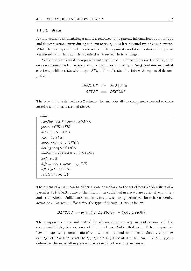
4.1. SYNTAX OF STATEFLOW CHARTS 67
4.1.3.1 State
A state contains an identi�er, a name, a reference to its parent, information about its type
and decomposition, entry, during and exit actions, and a list of bound variables and events.
While the decomposition of a state refers to the organisation of its sub-states, the type of
a state refers to the way it is organised with respect to its siblings.
While the terms used to represent both type and decompositions are the same, they
encode di�erent facts. A state with a decomposition of type SEQ contains sequential
substates, while a state with a type SEQ is the substate of a state with sequential decom-
position.
DECOMP ::= SEQ | PAR
STYPE == DECOMP
The type State is de�ned as a Z schema that includes all the components needed to char-
acterise a state as described above.
State
identi�er : SID ; name : SNAME
parent : CID ∪ SIDdecomp : DECOMP
type : STYPE
entry , exit : seqACTION
during : seqDACTION
binding : seq(ENAME ∪DNAME )
history : Bdefault , inner , outer : optTID
left , right : optSID
substates : seqSID
The parent of a state can be either a state or a chart, so the set of possible identi�ers of a
parent is CID ∪SID . Some of the information contained in a state are optional, e.g. entry
and exit actions. Unlike entry and exit actions, a during action can be either a regular
action or an on action. We de�ne the type of during actions as follows.
DACTION ::= action〈〈seqACTION 〉〉 | on〈〈ONACTION 〉〉
The components entry and exit of the schema State are sequences of actions, and the
component during is a sequence of during actions. Notice that some of the components
have an opt type; components of this type are optional components, that is, they may
or may not have a value (of the appropriate set) associated with them. The opt type is
de�ned as the set of all sequences of size one plus the empty sequence.

68 CHAPTER 4. TRANSLATION STRATEGY
4.1.3.2 Junction
A junction has an identi�er, a reference to its parent and the �rst outgoing transition, and
an indication of whether or not it is a history junction.
Junction
identi�er : JID
parent : CID ∪ SIDtransition : optTID
history : B
The schema Junction represents two types of junctions: connective junctions and history
junctions; this di�erence is established by the component history . If the parent of a junction
is the chart or a state with parallel decomposition, then it should not be a history junction.
Well-formedness conditions like this are formalised in [65] and are discussed in Section 4.2.
4.1.3.3 Transition
A transition has a sequence of triggers, a condition, a condition action and a transition
action.
Transition
identi�er : TID ; parent : CID ∪ SIDsource : opt (SID ∪ JID)
destination : SID ∪ JIDtrigger : seqTRIGGER
condition : optEXPR
condact , transact : seqACTION
next : optTID
Default transitions do not have source states, thus, the component source takes an op-
tional value ranging over the set of state and junction identi�ers. A trigger is either an
event (which must be an input or local event) or a temporal expression.
TRIGGER ::= e〈〈ENAME 〉〉 | t〈〈TEXPR〉〉
As in the case of states, condition and transition actions are recorded as sequences of
actions. Finally, the component next points to the next transition in a list of transitions.
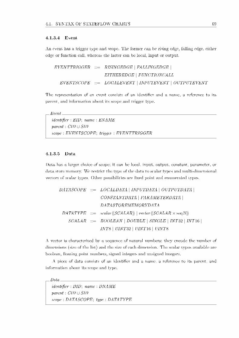
4.1. SYNTAX OF STATEFLOW CHARTS 69
4.1.3.4 Event
An event has a trigger type and scope. The former can be rising edge, falling edge, either
edge or function call, whereas the latter can be local, input or output.
EVENTTRIGGER ::= RISINGEDGE | FALLINGEDGE |
EITHEREDGE | FUNCTIONCALL
EVENTSCOPE ::= LOCALEVENT | INPUTEVENT | OUTPUTEVENT
The representation of an event consists of an identi�er and a name, a reference to its
parent, and information about its scope and trigger type.
Event
identi�er : EID ; name : ENAME
parent : CID ∪ SIDscope : EVENTSCOPE ; trigger : EVENTTRIGGER
4.1.3.5 Data
Data has a larger choice of scope; it can be local, input, output, constant, parameter, or
data store memory. We restrict the type of the data to scalar types and multi-dimensional
vectors of scalar types. Other possibilities are �xed-point and enumerated types.
DATASCOPE ::= LOCALDATA | INPUTDATA | OUTPUTDATA |
CONSTANTDATA | PARAMETERDATA |
DATASTOREMEMORYDATA
DATATYPE ::= scalar〈〈SCALAR〉〉 | vector〈〈SCALAR × seqN〉〉
SCALAR ::= BOOLEAN | DOUBLE | SINGLE | INT32 | INT16 |
INT8 | UINT32 | UINT16 | UINT8
A vector is characterised by a sequence of natural numbers; they encode the number of
dimensions (size of the list) and the size of each dimension. The scalar types available are
boolean, �oating point numbers, signed integers and unsigned integers.
A piece of data consists of an identi�er and a name, a reference to its parent, and
information about its scope and type.
Data
identi�er : DID ; name : DNAME
parent : CID ∪ SIDscope : DATASCOPE ; type : DATATYPE

70 CHAPTER 4. TRANSLATION STRATEGY
4.1.3.6 Functions
A Simulink function consists of an identi�er and a name, a sequence of names of input
variables, a sequence of names of output variables, a reference to its parent, and the name
of the Simulink block that de�nes the function.
SimulinkFunction
identi�er : FID ; name : FNAME
inputs, outputs : seqDNAME
parent : CID ∪ SIDblock : NAME
A graphical function is similar to a Simulink function, but instead of a block name, it
includes an identi�er of a chart as a component. The chart to which the function refers is
obtained from the �owchart that de�nes the function. The schema GraphicalFunction can
be found in [65].
4.1.3.7 Chart
The top object of a State�ow model is a chart. It contains an identi�er, a name, the
identi�er of the �rst default transition (if one exists), a sequence of state identi�ers, its
decomposition, and partial functions from identi�er to the objects contained in the chart.
Chart
identi�er : CID
name : CNAME
default : optTID
substates : seqSID
decomp : DECOMP
states : SID 7→ State
junctions : JID 7→ Junction
transitions : TID 7→ Transition
events : EID 7→ Event
data : DID 7→Data
sfunctions : FID 7→ SimulinkFunction; gfunctions : FID 7→GraphicalFunction
The default component is a reference to the �rst default transition of the chart; its type is
optTID since this reference is optional because a chart with parallel decomposition or an
unambiguous start point does not need to de�ne a default transition.
There are two levels of representation in a chart: the chart as a container, and a chart
as an object in itself. The latter perspective is associated with the �rst �ve components,
whereas the former is associated with the remaining components.

4.2. WELL-FORMEDNESS CONDITIONS 71
4.2 Well-formedness conditions
In this section, we brie�y discuss the well-formedness conditions for the syntax of the
State�ow notation. These conditions are characterised by the de�nition of sets of well
formed expressions and objects, culminating in the de�nition of the set of well formed
charts. The well-formedness conditions are by no mean complete; they simply characterise
the minimal properties that must hold for the translation rules to applied successfully.
The translation strategy assumes that the chart is accepted by the State�ow tool as a
valid chart.
The functions snames, dnames, enames, sfnames and gfnames are used to extract
information about names of states, data, events, Simulink functions and graphical functions
from a chart. They are de�ned in [65].
We further de�ne three sets, unary , binary and tempbinary , of expressions that repre-
sent, respectively, unary expression, binary expressions, and temporal binary expressions.
The well-formedness conditions over expressions are de�ned in terms of these sets in order
to simplify the speci�cation.
Well-formedness of expressions is characterised inductively over the constructors of
expressions, and always depends on a chart. For instance, a name expression is well formed
with respect to a chart if, and only if, its name component corresponds to a piece of data
in the chart, and the expressions in the index sequence are well formed with respect to the
chart.
WF EXPR : Chart ↔ EXPR
∀ c : Chart ; n : DNAME ; s : seqEXPR • (c,name(n, s)) ∈WF EXPR ⇔n ∈ dnames(c) ∧ (∀ e : ran s • (c, e) ∈WF EXPR)
∀ c : Chart ; n : NAME ; s : seqEXPR • (c, fun(n, s)) ∈WF EXPR ⇔n ∈ sfnames(c) ∪ gfnames(c) ∧ (∀ e : ran s • (c, e) ∈WF EXPR)
∀ c : Chart ; a : A • (c, value(a)) ∈WF EXPR
∀ c : Chart ; s : seq1 A | # s > 1 • (c, array(s)) ∈WF EXPR
∀ c : Chart ; s : seq1 seq1 A | # s > 1 •(c,matrix (s)) ∈WF EXPR ⇔ ∃n : N | n > 1 • ∀ row : ran s • # row = n
∀ c : Chart ; e : EXPR; op : unary • (c, op(e)) ∈WF EXPR ⇔ (c, e) ∈WF EXPR
∀ c : Chart ; e1, e2 : EXPR; op : binary •(c, op(e1, e2)) ∈WF EXPR ⇔ (c, e1) ∈WF EXPR ∧ (c, e2) ∈WF EXPR
∀ c : Chart ; s : SNAME • (c, in(s)) ∈WF EXPR ⇔ s ∈ snames(c)
∀ c : Chart ; e : EXPR; n : ENAME ; op : tempbinary •(c, op(e,n)) ∈WF EXPR ⇔ (c, e) ∈WF EXPR ∧ n ∈ enames(c)
∀ c : Chart ; n : ENAME • (c, tempCount(n)) ∈WF EXPR ⇔ n ∈ enames(c)∀
A function application is well formed if, and only if, the name corresponds to a Simulink
or graphical function in the chart, and the expressions that form the sequence of indexes
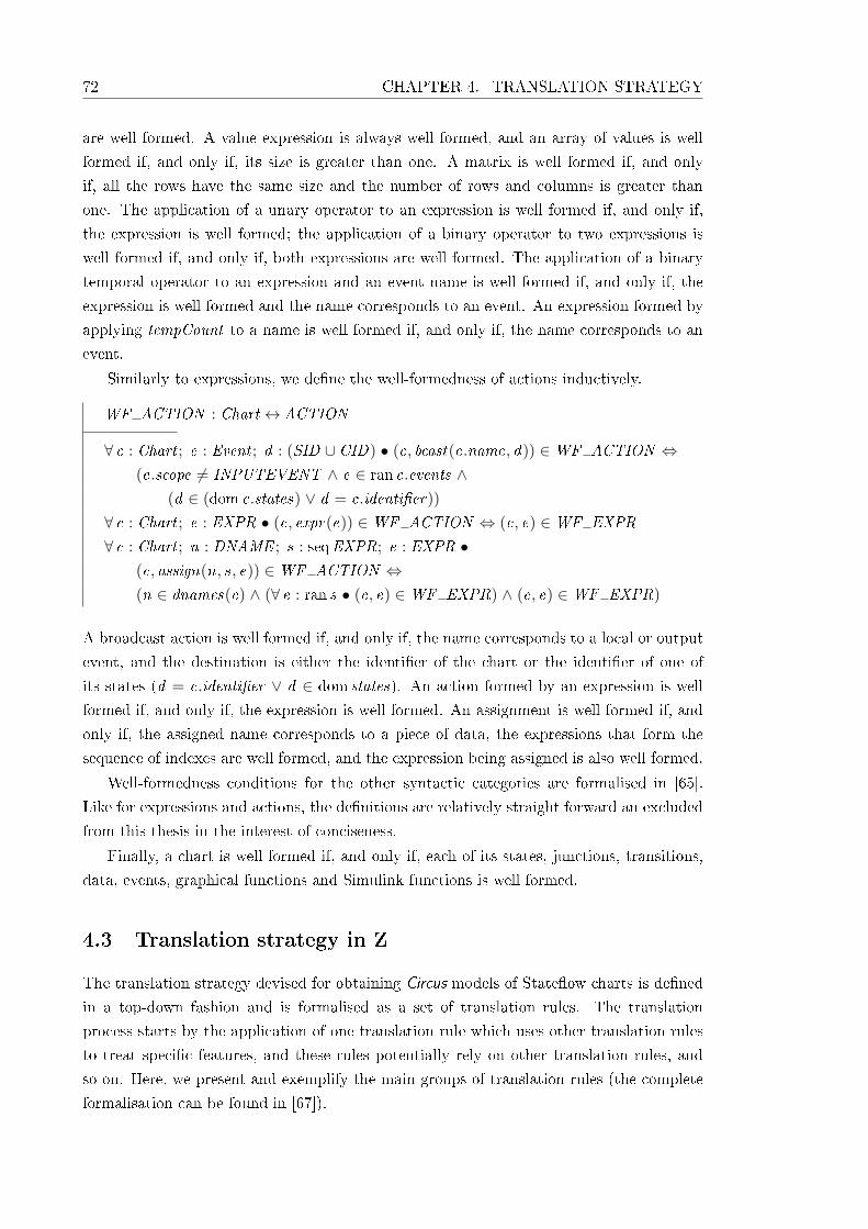
72 CHAPTER 4. TRANSLATION STRATEGY
are well formed. A value expression is always well formed, and an array of values is well
formed if, and only if, its size is greater than one. A matrix is well formed if, and only
if, all the rows have the same size and the number of rows and columns is greater than
one. The application of a unary operator to an expression is well formed if, and only if,
the expression is well formed; the application of a binary operator to two expressions is
well formed if, and only if, both expressions are well formed. The application of a binary
temporal operator to an expression and an event name is well formed if, and only if, the
expression is well formed and the name corresponds to an event. An expression formed by
applying tempCount to a name is well formed if, and only if, the name corresponds to an
event.
Similarly to expressions, we de�ne the well-formedness of actions inductively.
WF ACTION : Chart ↔ ACTION
∀ c : Chart ; e : Event ; d : (SID ∪ CID) • (c, bcast(e.name, d)) ∈WF ACTION ⇔(e.scope 6= INPUTEVENT ∧ e ∈ ran c.events ∧
(d ∈ (dom c.states) ∨ d = c.identi�er))
∀ c : Chart ; e : EXPR • (c, expr(e)) ∈WF ACTION ⇔ (c, e) ∈WF EXPR
∀ c : Chart ; n : DNAME ; s : seqEXPR; e : EXPR •(c, assign(n, s, e)) ∈WF ACTION ⇔(n ∈ dnames(c) ∧ (∀ e : ran s • (c, e) ∈WF EXPR) ∧ (c, e) ∈WF EXPR)
A broadcast action is well formed if, and only if, the name corresponds to a local or output
event, and the destination is either the identi�er of the chart or the identi�er of one of
its states (d = c.identi�er ∨ d ∈ dom states). An action formed by an expression is well
formed if, and only if, the expression is well formed. An assignment is well formed if, and
only if, the assigned name corresponds to a piece of data, the expressions that form the
sequence of indexes are well formed, and the expression being assigned is also well formed.
Well-formedness conditions for the other syntactic categories are formalised in [65].
Like for expressions and actions, the de�nitions are relatively straight forward an excluded
from this thesis in the interest of conciseness.
Finally, a chart is well formed if, and only if, each of its states, junctions, transitions,
data, events, graphical functions and Simulink functions is well formed.
4.3 Translation strategy in Z
The translation strategy devised for obtaining Circus models of State�ow charts is de�ned
in a top-down fashion and is formalised as a set of translation rules. The translation
process starts by the application of one translation rule which uses other translation rules
to treat speci�c features, and these rules potentially rely on other translation rules, and
so on. Here, we present and exemplify the main groups of translation rules (the complete
formalisation can be found in [67]).
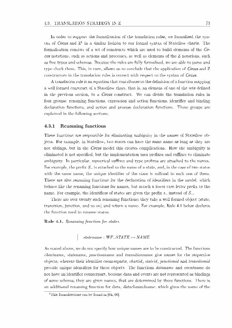
4.3. TRANSLATION STRATEGY IN Z 73
In order to support the formalisation of the translation rules, we formalised the syn-
tax of Circus and Z1 in a similar fashion to our formal syntax of State�ow charts. The
formalisation consists of a set of constructs which are used to build elements of the Cir-
cus notations, such as actions and processes, as well as elements of the Z notations, such
as free types and schemas. Because the rules are fully formalised, we are able to parse and
type check them. This, in turn, allows us to conclude that the application of Circus and Z
constructors in the translation rules is correct with respect to the syntax of Circus.
A translation rule is an equation that contributes to the de�nition of a function mapping
a well formed construct of a State�ow chart, that is, an element of one of the sets de�ned
in the previous section, to a Circus construct. We can divide the translation rules in
four groups: renaming functions, expression and action functions, identi�er and binding
declaration functions, and action and process declaration functions. These groups are
explained in the following sections.
4.3.1 Renaming functions
These functions are responsible for eliminating ambiguity in the names of State�ow ob-
jects. For example, in State�ow, two states can have the same name as long as they are
not siblings, but in the Circus model this creates complications. How the ambiguity is
eliminated is not speci�ed, but the implementation uses pre�xes and su�xes to eliminate
ambiguity. In particular, numerical su�xes and type pre�xes are attached to the names.
For example, the pre�x S is attached to the name of a state, and, in the case of two states
with the same name, the unique identi�er of the state is su�xed to each one of them.
There are also renaming functions for the declaration of identi�ers in the model, which
behave like the renaming functions for names, but attach a lower case letter pre�x to the
name. For example, the identi�ers of states are given the pre�x s instead of S .
There are over twenty such renaming functions; they take a well formed object (state,
transition, junction, and so on) and return a name. For example, Rule 4.1 below declares
the function used to rename states.
Rule 4.1. Renaming function for states.
statename : WF STATE � NAME
As stated above, we do not specify how unique names are to be constructed. The functions
chartname, statename, junctionname and transitionname give names for the respective
objects, whereas their identi�er counterparts, chartid , stateid , junctionid and transitionid
provide unique identi�ers for these objects. The functions dataname and eventname do
not have an identi�er counterpart, because data and events are not represented as bindings
of some schema; they are given names, that are determined by these functions. There is
an additional renaming function for data, datachannelname, which gives the name of the1This formalisations can be found in [64, 66].

74 CHAPTER 4. TRANSLATION STRATEGY
channel used to communicate the values of the variables to the environment. The renaming
functions for output events give the name of the counter variable associated with the event
(eventcountername), and the name of the output channel for communicating such events
(outputeventchannelname).
The functions processname and processstatename de�ne, respectively, the name of the
process that models the chart, and the name of the schema that represents that chart
(and is part of the process' state). The functions entryactionname, duringactionname
and exitactionname de�ne the name of the action that models entry, during and exit
actions, respectively. The functions conditionactionname and transitionactionname name
condition and transition actions after the corresponding transition, whereas conditionname
and triggername name the Circus actions that specify the conditions and triggers of a
transition. The range of all the renaming functions is speci�ed to be disjoint. The same
holds for the functions that provide identi�ers.
4.3.2 Expression and Action functions
The second group of functions translates expressions, actions, on actions, during ac-
tions, predicates, triggers, and sequences of these objects. It consists of translateExpr ,
translateExprs , translateAct , translateActs , translateONAct , translateDAct , translateDActs ,
translatePred , translateTrigger and translateTriggers . The complete de�nition of these func-
tions can be found in [67]; below, we discuss a selection of the rules that we consider most
interesting.
Variable expression The translation of this type of expression is separated into two
cases: simple variable and vector position. A simple variable is translated by obtaining the
corresponding data and calculating the appropriate name through the renaming function
dataname. A vector position requires us to �rst translate the expressions that are used as
indexes, calculate the appropriate name of the variable (as in the case of simple variables)
and apply this name to the translated expressions. Rule 4.2 (F) presents the formal
translation rule for variable expressions.
Rule 4.2 (F). Formal translation rule for variable expressions.
∀n : DNAME ; es : seqEXPR; c : WF CHART | (c,name(n, es)) ∈WF EXPR •
translateExpr (c,name(n, es)) =
if # es = 0
then reference(ref (dataname(c, getdatabyname(c,n))))
else functionapplication(
app(dataname(c, getdatabyname(c,n)),
translateExprs(c, es)))
As mentioned above, the domain of translateExpr is the set of well formed expressions.
We apply the function to a well formed chart c, and a well formed variable expression
formed by a name n and a sequence of vector indexes es. If the sequence es is empty
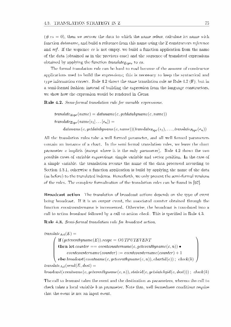
4.3. TRANSLATION STRATEGY IN Z 75
(# es = 0), then we recover the data to which the name refers, calculate its name with
function dataname, and build a reference from this name using the Z constructors reference
and ref . If the sequence es is not empty, we build a function application from the name
of the data (obtained as in the previous case) and the sequence of translated expressions
obtained by applying the function translateExprs to es.
The formal translation rule can be hard to read because of the amount of constructor
applications used to build the expressions; this is necessary to keep the syntactical and
type information correct. Rule 4.2 shows the same translation rule as Rule 4.2 (F), but in
a semi-formal fashion; instead of building the expression from the language constructors,
we show how the expression would be rendered in Circus.
Rule 4.2. Semi-formal translation rule for variable expressions.
translateExpr (name) = dataname(c, getdatabyname(c,name))
translateExpr (name[e1] . . . [en ]) =
dataname(c, getdatabyname(c,name))(translateExpr (e1), . . . , translateExpr (en))
All the translation rules take a well formed parameter, and all well formed parameters
contain an instance of a chart. In the semi-formal translation rules, we leave the chart
parameter c implicit (except where it is the only parameter). Rule 4.2 shows the two
possible cases of variable expressions: simple variable and vector position. In the case of
a simple variable, the translation returns the name of the data processed according to
Section 4.3.1, otherwise a function application is build by applying the name of the data
(as before) to the translated indexes. Henceforth, we only present the semi-formal versions
of the rules. The complete formalisation of the translation rules can be found in [67].
Broadcast action The translation of broadcast actions depends on the type of event
being broadcast. If it is an output event, the associated counter obtained through the
function eventcountername is incremented. Otherwise, the broadcast is translated into a
call to action broadcast followed by a call to action check . This is speci�ed in Rule 4.3.
Rule 4.3. Semi-formal translation rule for broadcast action.
translateAct(E ) =if (geteventbyname(E )).scope = OUTPUTEVENT
then let counter == eventcountername(c, geteventbyname(c,n)) •eventcountername(counter) := eventcountername(counter) + 1
else broadcast(eventname(c, geteventbyname(c,n)), chartid(c)) ; check(b)
translateAct(send(E , dest) =
broadcast(eventname(c, geteventbyname(c,n)), stateid(c, getstatebyid(c, dest))) ; check(b)
The call to broacast takes the event and the destination as parameters, whereas the call to
check takes a local variable b as parameter. Note that, well-formedness conditions require
that the event is not an input event.

76 CHAPTER 4. TRANSLATION STRATEGY
Assignment action The translation of assignment is also separated into the two cases
depending on whether the variable being assigned is a simple variable or a vector posi-
tion. The simple variable case is trivial, and consists of renaming the variable (as previ-
ously discussed), and building the Circus assignment expression. The vector position case
n[e1] . . . [em ] is more interesting. Namely, because multi-dimensional vectors are speci�ed
as �nite functions, the assignment of a value to one position needs to alter the function
only in that position. This is achieved by overriding (⊕) the function with the mapping
(indexes) 7→ value and assigning the result to the function variable. Rule 4.4 formalises
this translation rule.
Rule 4.4. Semi-formal translation rule for assignment actions.
translateAct(name = e) =
dataname(getdatabyname(name)) := translateExpr (e)
translateAct(name[e1] . . . [en ] = e) =
dataname(getdatabyname(name)) :=
dataname(getdatabyname(name))⊕
{(translateExpr (e1), . . . , translateExpr (en)) 7→ translateExpr (e)}
The translation rule is de�ned for the two cases previously mentioned. If the variable
being assigned is simple (name = e), we recover the data to which name refers, calculate
its name with function dataname, and use this name together with the translation of the
expression e to build an assignment. If the variable being assigned is a vector position, we
�rst obtain the name of the data in the same way as in the previous case. We then build
an assignment from this name and from an expression obtained by applying the override
operator to the name of the variable and a mapping that speci�es the change to the vector
position. This mapping is composed by the translated indexes of the vector position and
the translated expression that is being assigned.
On action These actions are conditionally executed according to the current event being
processed. Rule 4.5 shows the semi-formal translation rule for on actions.
Rule 4.5. Semi-formal translation rule for on action.
translateONAct(onn : a1, . . . an) =
if E = eventname(geteventbyname(n))−→
translateActs(〈a1, . . . , an〉)8E 6= eventname(geteventbyname(n))−→
Skip
�
On actions are translated to an alternation that executes the associated action if the current
event is the one speci�ed by the on action, otherwise it terminates immediately.
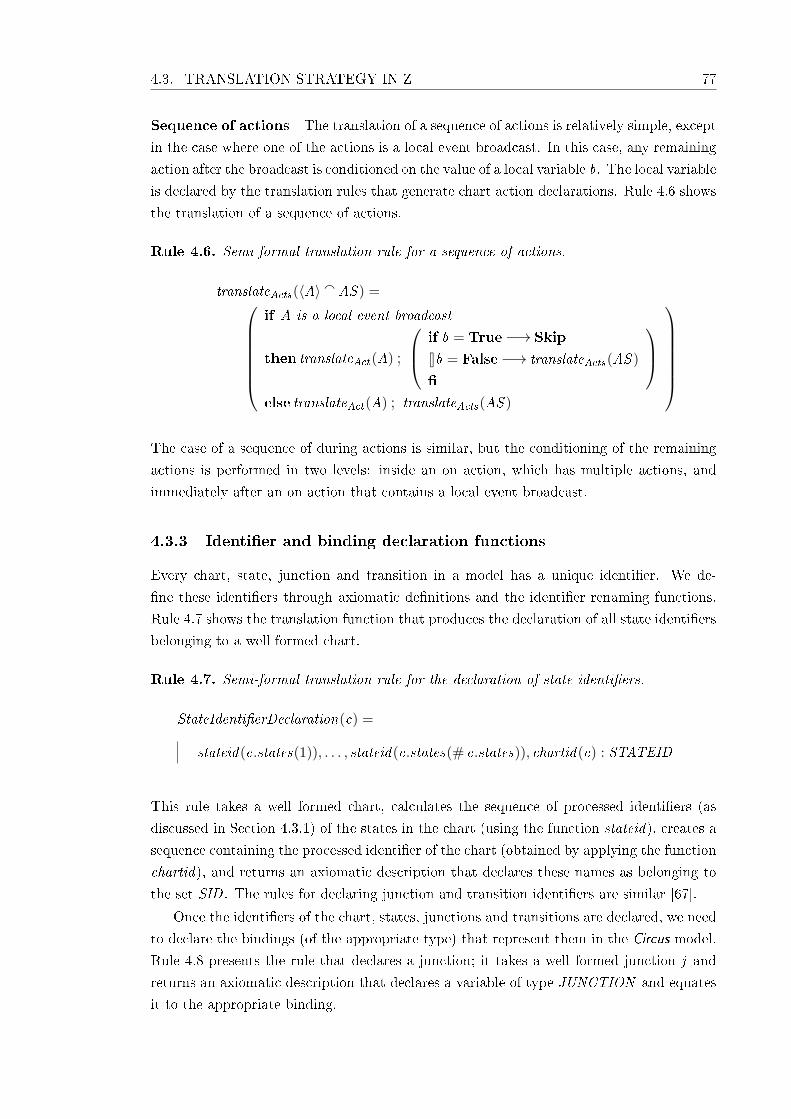
4.3. TRANSLATION STRATEGY IN Z 77
Sequence of actions The translation of a sequence of actions is relatively simple, except
in the case where one of the actions is a local event broadcast. In this case, any remaining
action after the broadcast is conditioned on the value of a local variable b. The local variable
is declared by the translation rules that generate chart action declarations. Rule 4.6 shows
the translation of a sequence of actions.
Rule 4.6. Semi-formal translation rule for a sequence of actions.
translateActs(〈A〉a AS ) =if A is a local event broadcast
then translateAct(A) ;
if b = True−→ Skip
8b = False−→ translateActs(AS )
�
else translateAct(A) ; translateActs(AS )
The case of a sequence of during actions is similar, but the conditioning of the remaining
actions is performed in two levels: inside an on action, which has multiple actions, and
immediately after an on action that contains a local event broadcast.
4.3.3 Identi�er and binding declaration functions
Every chart, state, junction and transition in a model has a unique identi�er. We de-
�ne these identi�ers through axiomatic de�nitions and the identi�er renaming functions.
Rule 4.7 shows the translation function that produces the declaration of all state identi�ers
belonging to a well formed chart.
Rule 4.7. Semi-formal translation rule for the declaration of state identi�ers.
StateIdenti�erDeclaration(c) =
stateid(c.states(1)), . . . , stateid(c.states(# c.states)), chartid(c) : STATEID
This rule takes a well formed chart, calculates the sequence of processed identi�ers (as
discussed in Section 4.3.1) of the states in the chart (using the function stateid), creates a
sequence containing the processed identi�er of the chart (obtained by applying the function
chartid), and returns an axiomatic description that declares these names as belonging to
the set SID . The rules for declaring junction and transition identi�ers are similar [67].
Once the identi�ers of the chart, states, junctions and transitions are declared, we need
to declare the bindings (of the appropriate type) that represent them in the Circus model.
Rule 4.8 presents the rule that declares a junction; it takes a well formed junction j and
returns an axiomatic description that declares a variable of type JUNCTION and equates
it to the appropriate binding.
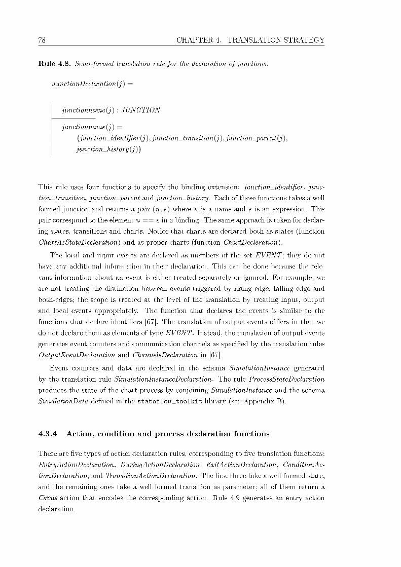
78 CHAPTER 4. TRANSLATION STRATEGY
Rule 4.8. Semi-formal translation rule for the declaration of junctions.
JunctionDeclaration(j ) =
junctionname(j ) : JUNCTION
junctionname(j ) =
〈|junction identi�er(j ), junction transition(j ), junction parent(j ),
junction history(j )|〉
This rule uses four functions to specify the binding extension: junction identi�er , junc-
tion transition, junction parent and junction history . Each of these functions takes a well
formed junction and returns a pair (n, e) where n is a name and e is an expression. This
pair correspond to the element n == e in a binding. The same approach is taken for declar-
ing states, transitions and charts. Notice that charts are declared both as states (function
ChartAsStateDeclaration) and as proper charts (function ChartDeclaration).
The local and input events are declared as members of the set EVENT ; they do not
have any additional information in their declaration. This can be done because the rele-
vant information about an event is either treated separately or ignored. For example, we
are not treating the distinction between events triggered by rising edge, falling edge and
both-edges; the scope is treated at the level of the translation by treating input, output
and local events appropriately. The function that declares the events is similar to the
functions that declare identi�ers [67]. The translation of output events di�ers in that we
do not declare them as elements of type EVENT . Instead, the translation of output events
generates event counters and communication channels as speci�ed by the translation rules
OutputEventDeclaration and ChannelsDeclaration in [67].
Event counters and data are declared in the schema SimulationInstance generated
by the translation rule SimulationInstanceDeclaration. The rule ProcessStateDeclaration
produces the state of the chart process by conjoining SimulationInstance and the schema
SimulationData de�ned in the stateflow toolkit library (see Appendix B).
4.3.4 Action, condition and process declaration functions
There are �ve types of action declaration rules, corresponding to �ve translation functions:
EntryActionDeclaration, DuringActionDeclaration, ExitActionDeclaration, ConditionAc-
tionDeclaration, and TransitionActionDeclaration. The �rst three take a well formed state,
and the remaining ones take a well formed transition as parameter; all of them return a
Circus action that encodes the corresponding action. Rule 4.9 generates an entry action
declaration.
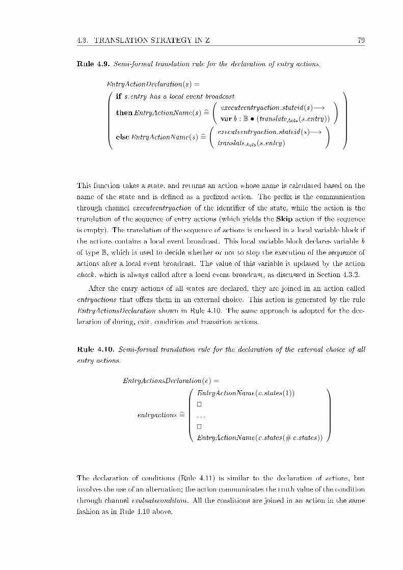
4.3. TRANSLATION STRATEGY IN Z 79
Rule 4.9. Semi-formal translation rule for the declaration of entry actions.
EntryActionDeclaration(s) =
if s.entry has a local event broadcast
thenEntryActionName(s) =̂
(executeentryaction.stateid(s)−→var b : B • (translateActs(s.entry))
)
elseEntryActionName(s) =̂
(executeentryaction.stateid(s)−→translateActs(s.entry)
)
This function takes a state, and returns an action whose name is calculated based on the
name of the state and is de�ned as a pre�xed action. The pre�x is the communication
through channel executeentryaction of the identi�er of the state, while the action is the
translation of the sequence of entry actions (which yields the Skip action if the sequence
is empty). The translation of the sequence of actions is enclosed in a local variable block if
the actions contains a local event broadcast. This local variable block declares variable b
of type B, which is used to decide whether or not to stop the execution of the sequence of
actions after a local event broadcast. The value of this variable is updated by the action
check , which is always called after a local event broadcast, as discussed in Section 4.3.2.
After the entry actions of all states are declared, they are joined in an action called
entryactions that o�ers them in an external choice. This action is generated by the rule
EntryActionsDeclaration shown in Rule 4.10. The same approach is adopted for the dec-
laration of during, exit, condition and transition actions.
Rule 4.10. Semi-formal translation rule for the declaration of the external choice of all
entry actions.
EntryActionsDeclaration(c) =
entryactions =̂
EntryActionName(c.states(1))
@. . .
@EntryActionName(c.states(# c.states))
The declaration of conditions (Rule 4.11) is similar to the declaration of actions, but
involves the use of an alternation; the action communicates the truth value of the condition
through channel evaluatecondition. All the conditions are joined in an action in the same
fashion as in Rule 4.10 above.

80 CHAPTER 4. TRANSLATION STRATEGY
Rule 4.11. Semi-formal translation rule for the declaration of conditions.
if # t .condition = 0
then ConditionDeclaration(t) =
ConditionName(t) =̂ evaluatecondition.transitionid(t).True−→ Skip
else ConditionDeclaration(t) =
ConditionName(t) =̂
if translatePred (head t .condition)−→
evaluatecondition.transitionid(t).True−→ Skip
8¬ translatePred (head t .condition)−→evaluatecondition.transitionid(t).False−→ Skip
�
The condition declaration translation rule takes a transition as parameter and builds a Cir-
cus action, named after the transition, through the function ConditionName. Since a condi-
tion is optional, it is recorded in the transition t as a sequence of size at most 1. If there is no
condition, this action is de�ned as a communication over the channel evaluatecondition of
the identi�er of the transition and the valueTrue. If there is a condition (head t .condition),
this action is de�ned as an alternation. The �rst guard checks if the translated condition
is di�erent than zero; the associated action communicates the identi�er of the transition
and the value True through channel evaluatecondition. The second guard checks if the
translated condition is equal to zero; the associated action then communicates the iden-
ti�er of the transition and the value False through the same channel as in the �rst case.
Note that State�ow conditions yield integer values; zero corresponds to false, and values
di�erent than zero correspond to true.
Trigger declarations are speci�ed to evaluate the triggers of a transition; they use two
communication channels checktrigger and result to, respectively, prompt the evaluation of
the trigger and to obtain the result of the evaluation. The declaration consists of two cases:
if there is no trigger, the action returns True as a default value, otherwise, it calculates
the truth value and returns it. Rule 4.12 speci�es the declaration of triggers.
Rule 4.12. Semi-formal translation rule for the declaration of triggers.
if # t .trigger = 0 then TriggerDeclaration(t) =
(TriggerName(t) =̂ checktrigger .transitionid(t)?E−→
result .transitionid(t).E !True−→ Skip)
elseTriggerDeclaration(t) = TriggerName(t) =̂ checktrigger .transitionid(t)?E−→ if translateTriggers(t .trigger)−→ result .transitionid(t).E !True−→ Skip
8¬ translateTriggers(t .trigger)−→ result .transitionid(t).E !False−→ Skip
�
This translation rule takes a transition as parameter and generates a Circus action whose
name is the result of the function TriggerName, and whose behaviour depends on whether

4.3. TRANSLATION STRATEGY IN Z 81
the transitions has a trigger or not. If there is no trigger, the action uses channel checktrigger
to synchronise on the transition identi�er and receive the current event E . It then uses
channel result to synchronise on the transition identi�er and event, and output the value
True. If there is a trigger, the action communicates through channel checktrigger in the
same way as before, and uses an if-statement to o�er two di�erent communications. If the
translation of the trigger is true, the channel result is used to synchronise on the transition
identi�er and current event, and output the value True; otherwise, instead of True, the
value False is communicated through the channel result .
The process declaration rule takes a well formed chart and produces a Circus pro-
cess that encloses the appropriate paragraphs produced by other functions; it is shown in
Rule 4.13. Because of the size of the rule, some parts are omitted for clarity.
Rule 4.13. Semi-formal translation rule for the declaration of chart processes.
ProcessDeclaration(c) =
process processname(c) =̂ begin
ChartDeclaration(c))
SimulationInstanceDeclaration(c)
InitSimulationInstanceDeclaration(c)
ProcessStateDeclaration(c)
EntryActionDeclaration(s1)
. . .
EntryActionDeclaration(sn)
EntryActionsDeclaration(c)
. . .
ConditionActionsDeclaration(c)
. . .
ConditionsDeclaration(c) . . .
TriggersDeclaration(c)
GetStateDeclaration
. . .
• MainActionDeclaration
end
This rule takes a chart c and returns a Circus process whose name is the result of applying
processname to c. The body of the process consists of a series of schema and action
declarations which are obtained by applying the appropriate translation functions. For
instance, the axiomatic de�nition that represents the chart is part of the process, this is
speci�ed in the rule by the application of the translation rule ChartDeclaration.
Rule 4.13 includes in the body of the process the declarations of the chart, the schemas
SimulationInstance and SimulationData, the initialisation and operation schemas, the state
82 CHAPTER 4. TRANSLATION STRATEGY
of the process, and all the actions. It completes the process by declaring the main action
through the function MainActionDeclaration.
The root translation rule, translate, takes a well formed chart and outputs a Circus spec-
i�cation. This rule is structured in the same way as the process declaration rule. It declares
the paragraphs external to the process (e.g. identi�er declarations) and the process through
previously de�ned translation rules.
4.4 Automation of the translation strategy
The manual translation process is extremely error prone, a mechanisation of such process
is clearly bene�cial. Moreover, when the translation of very simple charts (6 states and 7
transitions) generates more than ten pages of speci�cation, the translation of larger charts
is prohibitively costly. For example, one of our experiments on an industrial case study
yielded a 180-page speci�cation.
A mechanisation of the translation process can reduce the cost of the translation,
thus increasing the viability of any task that depends on a Circus model. In addition,
mechanising the translation provides extra validation of the model (and translation rules),
uncovering potential errors and inconsistencies. Since the Circus models are meant to
be used in the formal veri�cation of implementations of State�ow charts, the mechanical
translation increases the number and size of charts that can be tackled, and minimises the
possibility that translation errors occur.
In this section, we describe the tool s2c which implements the translation rules discussed
in the previous sections. s2c takes a .mdl �le and produces a Circus speci�cation containing
the processes that model the charts contained in the �le.
The translation of State�ow charts into Circus processes is de�ned in a manner that
makes it suitable for mechanisation; namely, by using formal and yet concrete transla-
tion rules. Since the implementation of s2c resembles the formal speci�cation, it can be
inspected and compared to the formalisation.
The implementation of s2c is guided by one main principle: to keep a close relationship
between the implementation and the formalisation of the translation rules. The advantage
of an implementation based on this principle is that it is easy to identify how components
of the code map to the formal rules, thus, facilitating the validation of the implementation
with respect to the formalisation.
Section 4.4.1 discusses the architecture of the tool, and Section 4.4.2 discusses the
implementation of the translation rules.
4.4.1 Architecture
The architecture of s2c is organised in �ve main packages: parser, stateflow abstract
syntax, Circus syntax, Z syntax and translator (Figure 4.2). The translator package
is the main one, and uses all the other packages to perform the translation. We now discuss
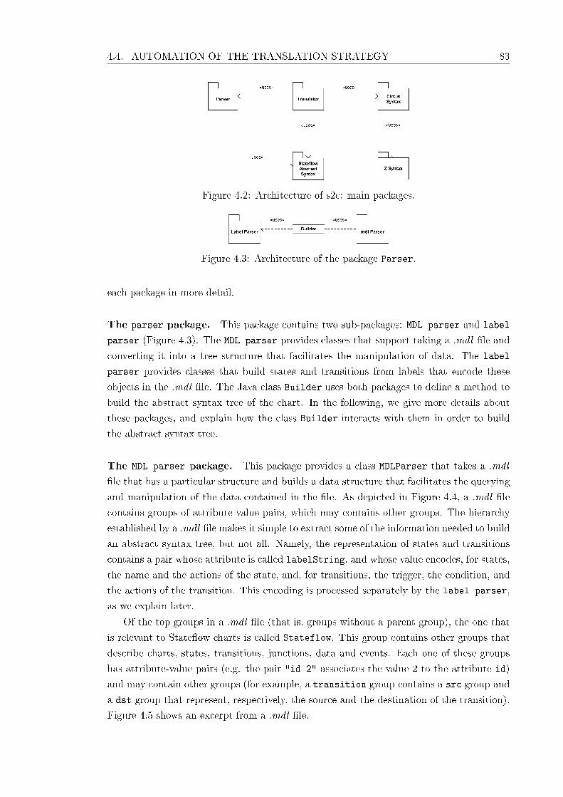
4.4. AUTOMATION OF THE TRANSLATION STRATEGY 83
Figure 4.2: Architecture of s2c: main packages.
Figure 4.3: Architecture of the package Parser.
each package in more detail.
The parser package. This package contains two sub-packages: MDL parser and label
parser (Figure 4.3). The MDL parser provides classes that support taking a .mdl �le and
converting it into a tree structure that facilitates the manipulation of data. The label
parser provides classes that build states and transitions from labels that encode these
objects in the .mdl �le. The Java class Builder uses both packages to de�ne a method to
build the abstract syntax tree of the chart. In the following, we give more details about
these packages, and explain how the class Builder interacts with them in order to build
the abstract syntax tree.
The MDL parser package. This package provides a class MDLParser that takes a .mdl
�le that has a particular structure and builds a data structure that facilitates the querying
and manipulation of the data contained in the �le. As depicted in Figure 4.4, a .mdl �le
contains groups of attribute-value pairs, which may contains other groups. The hierarchy
established by a .mdl �le makes it simple to extract some of the information needed to build
an abstract syntax tree, but not all. Namely, the representation of states and transitions
contains a pair whose attribute is called labelString, and whose value encodes, for states,
the name and the actions of the state, and, for transitions, the trigger, the condition, and
the actions of the transition. This encoding is processed separately by the label parser,
as we explain later.
Of the top groups in a .mdl �le (that is, groups without a parent group), the one that
is relevant to State�ow charts is called Stateflow. This group contains other groups that
describe charts, states, transitions, junctions, data and events. Each one of these groups
has attribute-value pairs (e.g. the pair "id 2" associates the value 2 to the attribute id)
and may contain other groups (for example, a transition group contains a src group and
a dst group that represent, respectively, the source and the destination of the transition).
Figure 4.5 shows an excerpt from a .mdl �le.

84 CHAPTER 4. TRANSLATION STRATEGY
Figure 4.4: Structure of a .mdl �le.
Stateflow {
chart {
id 2
name "Chart"
decomposition CLUSTER_CHART
...
}
state {
id 3
labelString "State1"
type OR_STATE
decomposition CLUSTER_STATE
...
}
transition {
id 9
labelString "{Data = Data+1;}"
src {
}
dst {
id 3
}
chart 2
...
}
...
}
Figure 4.5: Excerpt from a .mdl �le.
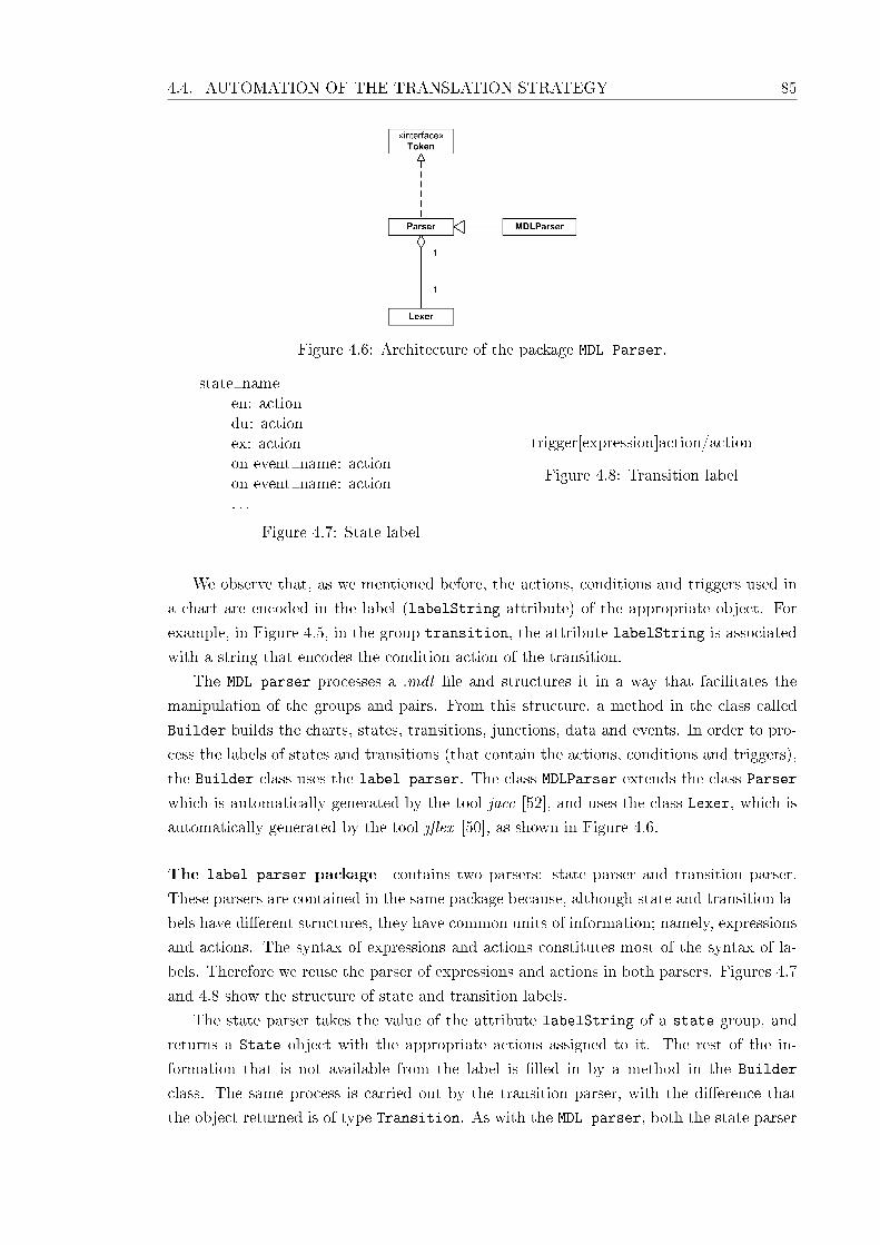
4.4. AUTOMATION OF THE TRANSLATION STRATEGY 85
Figure 4.6: Architecture of the package MDL Parser.
state nameen: actiondu: actionex: actionon event name: actionon event name: action. . .
Figure 4.7: State label
trigger[expression]action/action
Figure 4.8: Transition label
We observe that, as we mentioned before, the actions, conditions and triggers used in
a chart are encoded in the label (labelString attribute) of the appropriate object. For
example, in Figure 4.5, in the group transition, the attribute labelString is associated
with a string that encodes the condition action of the transition.
The MDL parser processes a .mdl �le and structures it in a way that facilitates the
manipulation of the groups and pairs. From this structure, a method in the class called
Builder builds the charts, states, transitions, junctions, data and events. In order to pro-
cess the labels of states and transitions (that contain the actions, conditions and triggers),
the Builder class uses the label parser. The class MDLParser extends the class Parser
which is automatically generated by the tool jacc [52], and uses the class Lexer, which is
automatically generated by the tool j�ex [50], as shown in Figure 4.6.
The label parser package contains two parsers: state parser and transition parser.
These parsers are contained in the same package because, although state and transition la-
bels have di�erent structures, they have common units of information; namely, expressions
and actions. The syntax of expressions and actions constitutes most of the syntax of la-
bels. Therefore we reuse the parser of expressions and actions in both parsers. Figures 4.7
and 4.8 show the structure of state and transition labels.
The state parser takes the value of the attribute labelString of a state group, and
returns a State object with the appropriate actions assigned to it. The rest of the in-
formation that is not available from the label is �lled in by a method in the Builder
class. The same process is carried out by the transition parser, with the di�erence that
the object returned is of type Transition. As with the MDL parser, both the state parser
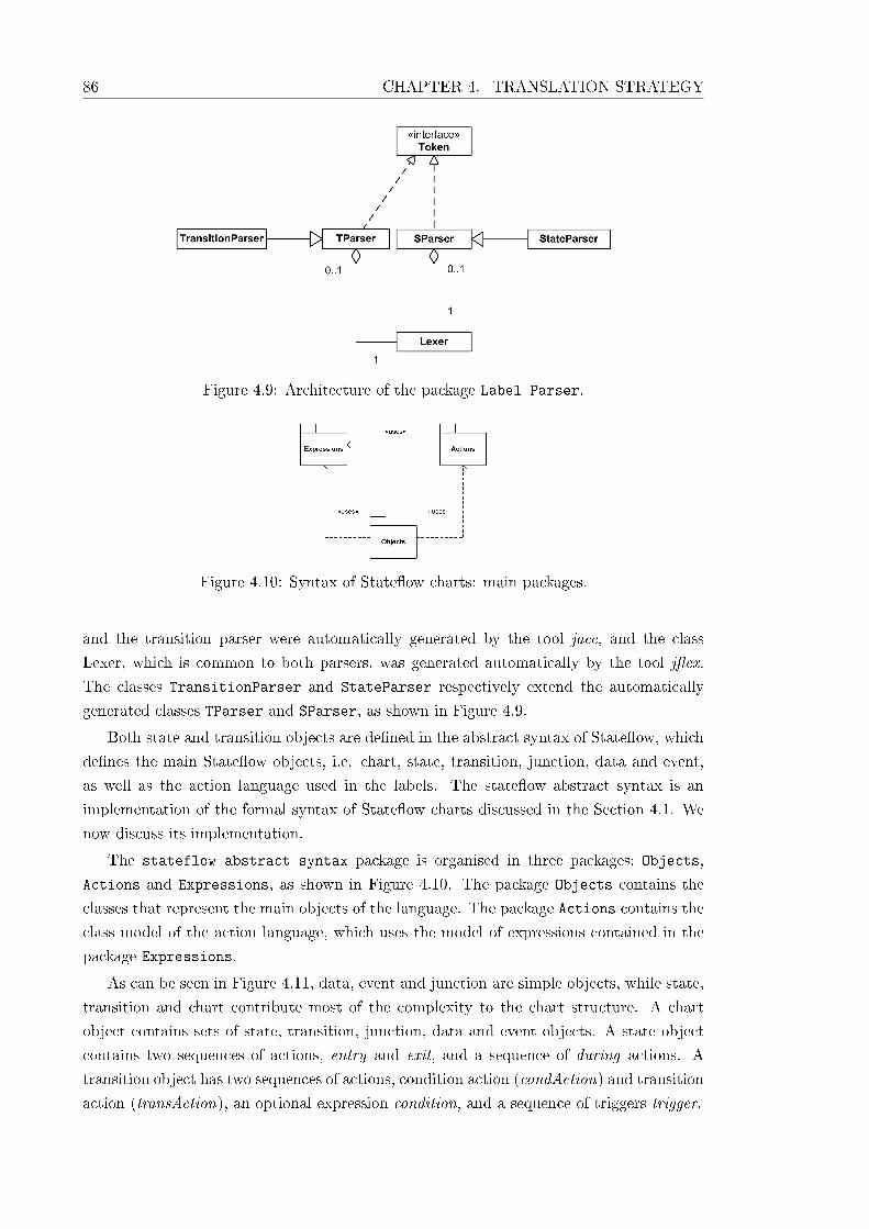
86 CHAPTER 4. TRANSLATION STRATEGY
Figure 4.9: Architecture of the package Label Parser.
Figure 4.10: Syntax of State�ow charts: main packages.
and the transition parser were automatically generated by the tool jacc, and the class
Lexer, which is common to both parsers, was generated automatically by the tool j�ex.
The classes TransitionParser and StateParser respectively extend the automatically
generated classes TParser and SParser, as shown in Figure 4.9.
Both state and transition objects are de�ned in the abstract syntax of State�ow, which
de�nes the main State�ow objects, i.e. chart, state, transition, junction, data and event,
as well as the action language used in the labels. The state�ow abstract syntax is an
implementation of the formal syntax of State�ow charts discussed in the Section 4.1. We
now discuss its implementation.
The stateflow abstract syntax package is organised in three packages: Objects,
Actions and Expressions, as shown in Figure 4.10. The package Objects contains the
classes that represent the main objects of the language. The package Actions contains the
class model of the action language, which uses the model of expressions contained in the
package Expressions.
As can be seen in Figure 4.11, data, event and junction are simple objects, while state,
transition and chart contribute most of the complexity to the chart structure. A chart
object contains sets of state, transition, junction, data and event objects. A state object
contains two sequences of actions, entry and exit, and a sequence of during actions. A
transition object has two sequences of actions, condition action (condAction) and transition
action (transAction), an optional expression condition, and a sequence of triggers trigger.
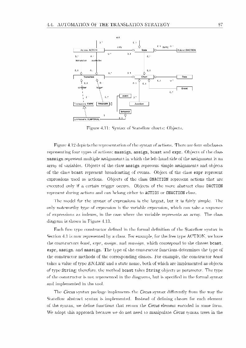
4.4. AUTOMATION OF THE TRANSLATION STRATEGY 87
Figure 4.11: Syntax of State�ow charts: Objects.
Figure 4.12 depicts the representation of the syntax of actions. There are four subclasses
representing four types of actions: massign, assign, bcast and expr. Objects of the class
massign represent multiple assignments in which the left-hand side of the assignment is an
array of variables. Objects of the class assign represent simple assignments and objects
of the class bcast represent broadcasting of events. Object of the class expr represent
expressions used as actions. Objects of the class ONACTION represent actions that are
executed only if a certain trigger occurs. Objects of the more abstract class DACTION
represent during actions and can belong either to ACTION or ONACTION class.
The model for the syntax of expressions is the largest, but it is fairly simple. The
only noteworthy type of expression is the variable expression, which can take a sequence
of expressions as indexes, in the case where the variable represents an array. The class
diagram is shown in Figure 4.13.
Each free type constructor de�ned in the formal de�nition of the State�ow syntax in
Section 4.1 is now represented by a class. For example, for the free type ACTION, we have
the constructors bcast , expr , assign, and massign, which correspond to the classes bcast,
expr, assign, and massign. The type of the constructor functions determines the type of
the constructor methods of the corresponding classes. For example, the constructor bcast
takes a value of type ENAME and a state name, both of which are implemented as objects
of type String; therefore, the method bcast takes String objects as parameter. The type
of the constructor is not represented in the diagrams, but is speci�ed in the formal syntax
and implemented in the tool.
The Circus syntax package implements the Circus syntax di�erently from the way the
State�ow abstract syntax is implemented. Instead of de�ning classes for each element
of the syntax, we de�ne functions that return the Circus element encoded in some form.
We adopt this approach because we do not need to manipulate Circus syntax trees in the
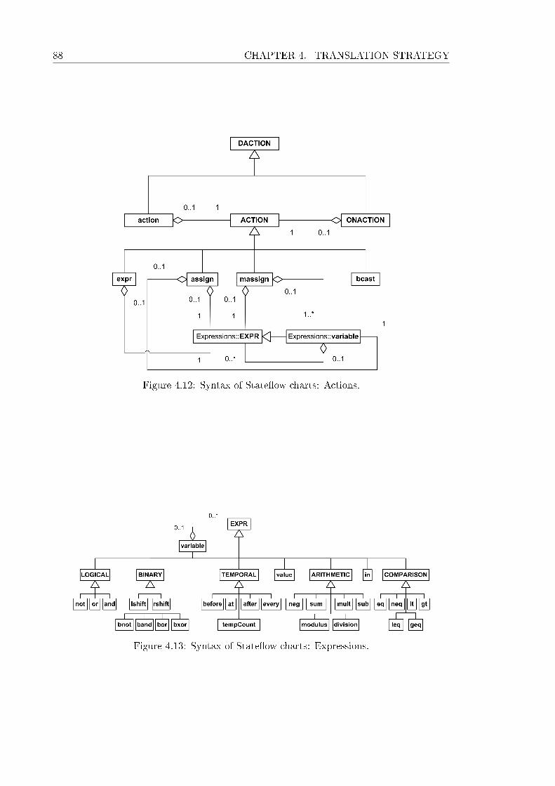
88 CHAPTER 4. TRANSLATION STRATEGY
Figure 4.12: Syntax of State�ow charts: Actions.
Figure 4.13: Syntax of State�ow charts: Expressions.

4.4. AUTOMATION OF THE TRANSLATION STRATEGY 89
Figure 4.14: Syntax of Circus.
Figure 4.15: Architecture of s2c: the Translator package.
tool. Moreover, the use of functions to build Circus speci�cations makes the resulting code
resemble the formal speci�cation more closely. We de�ne an interface that contains the
functions that can be used to build Circus statements and provide an implementation of
this interface that produces LATEX code. Note that it is simple to implement the interface
to generate speci�cations suitable for other tools.
The Z syntax package is structured in exactly the same fashion. The Circus syntax
interface and implementation extend, respectively, the interface and implementation of the
Z syntax, as shown in Figure 4.14.
Finally, the Translator class contains a method translate that takes a State�ow chart
represented in the abstract syntax and produces the Circus speci�cation of the chart. The
translator uses an implementation of the Circus syntax interface and a name generator to
produce the speci�cations. The name generator is responsible for taking State�ow objects
and returning their names in an appropriate format. For example, we disambiguate state
names (when needed) by su�xing the unique identi�er of the state. State identi�ers are
obtained by pre�xing the (disambiguated) name of the state with a lower case "s", while
state names are obtained by pre�xing the name with a capital "S". Figure 4.15 shows the
architecture of the translator package.
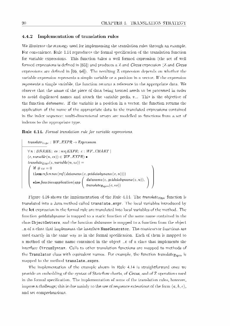
90 CHAPTER 4. TRANSLATION STRATEGY
4.4.2 Implementation of translation rules
We illustrate the strategy used for implementing the translation rules through an example.
For convenience, Rule 4.14 reproduces the formal speci�cation of the translation function
for variable expressions. This function takes a well formed expression (the set of well
formed expressions is de�ned in [65]) and produces a Z and Circus expression (Z and Circus
expressions are de�ned in [66, 64]). The resulting Z expression depends on whether the
variable expression represents a simple variable or a position in a vector. If the expression
represents a simple variable, the function returns a reference to the appropriate data. We
observe that the name of the piece of data being treated needs to be processed in order
to avoid duplicated names and attach the variable pre�x v . This is the objective of
the function dataname. If the variable is a position in a vector, the function returns the
application of the name of the appropriate data to the translated expressions contained
in the index sequence; multi-dimensional arrays are modelled as functions from a set of
indexes to the appropriate type.
Rule 4.14. Formal translation rule for variable expressions.
translateExpr : WF EXPR→ Expression
∀n : DNAME ; es : seqEXPR; c : WF CHART |(c, variable(n, es)) ∈WF EXPR) •translateExpr (c, variable(n, es)) =
if # es = 0
then reference(ref (dataname(c, getdatabyname(c,n))))
else functionapplication(app
(dataname(c, getdatabyname(c,n)),
translateExprs(c, es))
)
Figure 4.16 shows the implementation of the Rule 4.14. The translateExpr function is
translated into a Java method called translate expr. The local variables introduced by
the let expression in the formal rule are translated into local variables of the method. The
function getdatabyname is mapped to a static function of the same name contained in the
class ObjectGetters, and the function dataname is mapped to a function from the object
n of a class that implements the interface NameGenerator. The constructor functions are
used exactly in the same way as in the formal speci�cation. Each of them is mapped to
a method of the same name contained in the object c of a class that implements the
interface CircusSyntax. Calls to other translation functions are mapped to methods of
the Translator class with equivalent names. For example, the function translateExprs is
mapped to the method translate exprs.
The implementation of the example shown in Rule 4.14 is straightforward once we
provide an embedding of the syntax of State�ow charts, of Circus, and of Z operations used
in the formal speci�cation. The implementation of some of the translation rules, however,
impose a challenge; this is due mainly to the use of sequence extensions of the form 〈a, b, c〉,and set comprehensions.
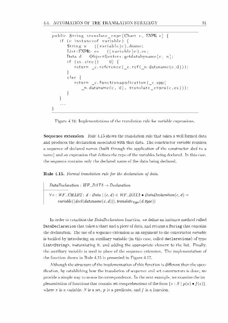
4.4. AUTOMATION OF THE TRANSLATION STRATEGY 91
pub l i c S t r ing t rans la te_expr ( Chart c , EXPR e ) {i f ( e i n s t an c e o f v a r i a b l e ) {
St r ing n = ( ( va r i a b l e ) e ) . dname ;Li s t<EXPR> es = ( ( va r i a b l e ) e ) . e s ;Data d = ObjectGetters . getdatabyname ( c , n ) ;i f ( e s . s i z e ( ) == 0) {
return _c . r e f e r e n c e (_c . r e f (_n. dataname ( c , d ) ) ) ;}e l s e {
re turn _c . f un c t i o n app l i c a t i o n (_c . app (_n. dataname ( c , d ) , t rans la t e_exprs ( c , e s ) ) ) ;
}}. . .
}
Figure 4.16: Implementations of the translation rule for variable expressions.
Sequence extension Rule 4.15 shows the translation rule that takes a well formed data
and produces the declaration associated with that data. The constructor variable requires
a sequence of declared names (built through the application of the constructor decl to a
name) and an expression that de�nes the type of the variables being declared. In this case,
the sequence contains only the declared name of the data being declared.
Rule 4.15. Formal translation rule for the declaration of data.
DataDeclaration : WF DATA→Declaration
∀ c : WF CHART ; d : Data | (c, d) ∈WF DATA • DataDeclaration(c, d) =
variable(〈decl(dataname(c, d))〉, translateType(d .type))
In order to translate the DataDeclaration function, we de�ne an instance method called
DataDeclaration that takes a chart and a piece of data, and returns a String that contains
the declaration. The use of a sequence extension as an argument to the constructor variable
is tackled by introducing an auxiliary variable (in this case, called declarations) of type
List<String>, instantiating it, and adding the appropriate element to the list. Finally,
the auxiliary variable is used in place of the sequence extension. The implementation of
the function shown in Rule 4.15 is presented in Figure 4.17.
Although the structure of the implementation of this function is di�erent than the spec-
i�cation, by establishing how the translation of sequence and set constructors is done, we
provide a simple way to assess its correspondence. In the next example, we examine the im-
plementation of functions that contain set comprehensions of the form {x : S | p(x ) • f (x )},where x is a variable, S is a set, p is a predicate, and f is a function.

92 CHAPTER 4. TRANSLATION STRATEGY
pub l i c S t r ing DataDeclarat ion ( Chart c , Data d) {List<Str ing> de c l a r a t i o n s = new LinkedList<Str ing >() ;d e c l a r a t i o n s . add (_c . dec l (_n. dataname ( c , d ) ) ) ;r e turn _c . v a r i a b l e ( d e c l a r a t i on s , t rans la te_type (d . type ) ) ;
}
Figure 4.17: Implementations of the translation rule for the declaration of data.
pub l i c S t r ing S imu la t i on In s tanceDec l a ra t i on ( Chart c ) {Lis t<Str ing> va r i a b l e s = new LinkedList<Str ing >() ;f o r ( In t eg e r i : c . data . keySet ( ) ) {
v a r i a b l e s . add ( DataDeclarat ion ( c , c . data . get ( i ) ) ) ;}Li s t<Str ing> outputevents = new LinkedList<Str ing >() ;f o r ( In t eg e r i : c . events . keySet ( ) ) {
i f ( c . events . get ( i ) . scope == EVENTSCOPE.OUTPUTEVENT) {outputevents . add ( OutputEventDeclaration ( c , c . events . get ( i ) ) ) ;
}}v a r i a b l e s . addAll ( outputevents ) ;S t r ing dec l = _c . d e c l p a r t_ve r t i c a l ( v a r i a b l e s ) ;r e turn _c . s chemade f in i t i on (
_n.SIMULATIONINSTANCE( ) ,_c . schematext_vert i ca l (
new Opt<Str ing >(dec l ) ,new LinkedList<Str ing >( ) ) ) ;
}
Figure 4.18: Implementations of the translation rule for the declaration of the simulationinstance.
Set comprehension Rule 4.16 shows a function that declares a schema used as part of
the state of the chart process. The function takes a well formed chart and produces a Z
paragraph. Notice that the local variable variables is de�ned as a sequence by applying the
function squash to a set comprehension. The set comprehension takes the indexes of the
sequence c.data and produces a partial function from natural numbers to data declarations
by applying a translation function to the data contained in c.data.
Rule 4.16. Formal translation rules for the declaration of the simulation instance.
SimulationInstanceDeclaration : WF CHART → Paragraph
∀ c : WF CHART • SimulationInstanceDeclaration(c) = let
variables == squash{i : dom c.data • i 7→DataDeclaration(c, c.data(i))};outputevents == squash{i : dom c.events | (c.events(i)).scope = OUTPUTEVENT •
i 7→OutputEventDeclaration(c, c.events(i))} • letdecl == declpart(variables a outputevents) •
schemade�nition(SimulationInstance, schematext(〈decl〉, 〈〉))
As shown in Figure 4.18, the set comprehension is translated into the instantiation of a list
4.5. EVALUATION 93
(because the function squash applied to the set comprehension, in this example, de�nes a
list) which is assigned to the variable variables. The list is then �lled in with all the data
declarations obtained from the data in the list c.data. The same is done for the list of
output events, and the two lists are joined together before the declaration is built. Note
that we use the class Opt which implements the type Opt de�ned in the speci�cation to
obtain, more easily, lists of size zero or one.
Set comprehensions could be implemented by the Java class Set, but, in most cases,
the sets de�ned in the speci�cation are transformed into sequences. Since a sequence can
be seen as an ordered set, we do not lose information by using sequences instead of sets.
In some of the rules, we use a function set2seq which takes a set and produces a
sequence with the same objects. The de�nition of this function is underspeci�ed, stating
only that the range of the sequence obtained from the application of the function to a set S
must be equal to S . Since the order of the elements in the list is clearly not important, we
add them directly to a list, instead of a set, thus rendering the use of the function set2seq
unnecessary in the implementation.
The implementation of s2c2 has approximately 19000 lines of code, 75% of which im-
plements the various parsers and is automatically generated. In the next section, we will
discuss the usage and evaluation of the tool s2c.
4.5 Evaluation
The tool s2c takes a .mdl �le that contains the de�nition of a number of charts, and pro-
duces a Circus process for each chart; each process and associated de�nitions are enclosed
in a Z section. The tool ignores de�nitions of Simulink and graphical functions, truth
tables, as well as Simulink blocks. The existence of functions implies that there are data
de�nitions of the input and output variables of the function; these are also ignored.
Since Simulink and graphical functions are not translated, but are widely used in charts
along with matlab and C functions, we adopt a strategy for dealing with functions whereby
the user is required to supply the formal de�nition of the functions being used in the form
of libraries. Each library is speci�ed in a separate �le within a named Z section which is
inherited by the section that contains the model of the chart that uses the library.
Our evaluation strategy consists of testing the tool on three distinct sets of examples:
basic charts, complete examples, and industrial case studies. The group of basic charts
contains models that exercise speci�c features of the State�ow notation, for example, for
each type of action a, we have a chart formed by a single state whose entry action is a.
The group of complete examples is formed by those charts (or collections of charts) that
model a simpli�ed system (usually "toy-examples"), but whose complexity is larger. For
example, we have used the shift logic chart of the Automatic Transmission Control example
supplied with State�ow and used in Chapter 3. The third group consists of models supplied
by industrial collaborators. These models usually describe the whole system. For example,
2The tool can be downloaded from http://www-users.cs.york.ac.uk/~alvarohm/s2c/tool/
94 CHAPTER 4. TRANSLATION STRATEGY
one of the case studies with which we have tested s2c was supplied by Airbus Operations
and describes a generic Fuel Management Control System.
By testing basic charts, we can easily track any errors in the tool to the speci�c feature
being tested. Moreover, since these models are very small, it is possible to check the gen-
erated speci�cation and notice any potential errors. With this approach, while validating
the tool, we also validate the translation strategy and the model presented in Chapter 3.
On the other hand, the complete examples allow us to test the interaction between dif-
ferent features of the notation, and while their size makes it di�cult to manually check
the generated speci�cation, it is still feasible to track errors in the translation process to
features of the State�ow model. The speci�cation generated by industrial case-studies can
be extremely large, and, therefore, not tractable manually, and, while it is possible to track
translation errors to pieces of the model, it is a demanding task. Nevertheless, testing in-
dustrial case-studies allows us to evaluate the correctness, robustness and e�ciency of the
tool.
We now turn to the results of testing the tool with all three groups. Due to the number
of examples in the �rst group, we only give an overview of how they were built, and discuss
the main �ndings.
We have tested the tool with the basic charts in di�erent stages of development, and
errors found during the development were corrected. The main problems found during test-
ing were concerned with the handling of elements not treated by the translation strategy,
and simple programming errors (such as index out of bound errors, un-initialised variables
etc). The latter errors were easily �xed, while the former required us either to treat the
features in the translation strategy, or �nd a way to overcome the features when they
appear in a chart.
The testing of the tool has highlighted two features that were not treated, one known
and the other unknown. The former is the treatment of functions, and the latter is the use
of the time symbol t .
The treatment of functions is not a simple issue, because the functions that can be used
in charts are not restricted to the types of functions that can be de�ned within a chart �
MATLAB and even C function can be used. The complete treatment of function would
require us to formalise all the possible functions (including the MATLAB and C ones). Our
approach to this issue was to assume that the user of the tool has a library of de�nition of
the functions being used in the chart. It is worth mentioning that this approach is limited in
the sense that it does not allow the speci�cation of graphical functions with side-e�ects (i.e.,
graphical functions that change the state of the chart). However, if a separate translation
strategy is de�ned for graphical functions, it can be easily incorporated to the tool, thus,
eliminating this limitation.
The proper treatment of the time symbol t was delegated to the Simulink diagram and
referenced by a process variable which is updated through a channel time. The reason why
the treatment of t can be delegated to the Simulink diagram is that this symbol represents
the "absolute time inherited from a Simulink signal" [98].
4.6. FINAL CONSIDERATIONS 95
The two industrial case studies we use to test the tool were provided, respectively,
by Embraer S.A and Airbus Operations. The example from Embraer is fairly simple and
the translation, although laborious, is trivial. This example uses the abs function, which
reinforced the need to reconsider our treatment of functions, and motivated the use of
libraries for specifying functions.
The case study from Airbus is larger, and the translation of four charts found in one
of the �les resulted in a 180-page speci�cation. It also required the treatment of functions
and the symbol t . We observe that the charts contained in both case studies extensively
used functions (MATLAB functions and graphical functions), and that the approach to
the treatment of general function by use of Z libraries has proved successful so far.
In its current version, the tool translates, without errors, all the tested examples, and
the speci�cations generated by the tool are all correctly parsed and type checked by the
Circus CZT toolkit [57].
4.6 Final considerations
In this chapter, we discussed the syntax of State�ow charts, the conditions that establish
the well-formedness of charts, the translation rules that guide the translation process, and
the automation of the translation strategy implemented in the tool s2c. The syntax, well-
formedness conditions and translation rules, as well as their automation, cover a large
portion of the State�ow notation, including many aspects that, as far as we know, are not
covered in other approaches presented in the literature.
To the best of our knowledge, no other work has treated history junctions, unrestricted
transitions and early return logic. Moreover, as far as we know, no one has provided
a partial (or complete) treatment of functions. The main features that are usually not
treated by other approaches to veri�cation of State�ow charts are: during actions, inter-
level transitions, local event broadcast, �ow-charts, and in expressions.
It is worth noticing, however, that some features that are speci�ed in the syntax are not
treated by the translation rules. They are temporal expressions, bind actions, function-
call events, and constant, parameter and data store memory data. Graphical and Simulink
functions are only partially treated. Our models can be easily extended to cover such
function by integrating it with the existing models of Simulink diagrams. The reason the
syntax covers features not treated by the translation rules is that this will allow us to
extend the translation rules to cover such features in the future.
Our translation has been evaluated through a number of case studies that ranged in
scale and complexity (from small feature-focused examples to case studies supplied by
industrial collaborators). These experiments not only validated the translation strategy
and the rules implemented by the s2c tool, but also provided additional con�dence in the
correctness of our model of the semantics of State�ow presented in Chapter 3.
Furthermore, the use of the models generated by the tool as the basis for the veri�cation
of implementations described in the next chapter provided an additional validation of both
96 CHAPTER 4. TRANSLATION STRATEGY
the tool and the translation rules implemented in it.
It is worth noting that while the choice of Z as the basis for the formalisation of the
translation strategy proved suitable, a notation that supports automatic code generation
might be more appropriate. The main disadvantage of the approach we have taken is
that the translation strategy has to be implemented separately. In retrospect, since the
formality of Z was not fully explored, our choice of notation for the translation rules should
have favoured automatic code generation more heavily.
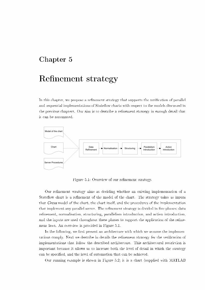
Chapter 5
Re�nement strategy
In this chapter, we propose a re�nement strategy that supports the veri�cation of parallel
and sequential implementations of State�ow charts with respect to the models discussed in
the previous chapters. Our aim is to describe a re�nement strategy in enough detail that
it can be automated.
StructuringParallelism
Introduction
Action
Introduction
Data
RefinementNormalisation
Model of the chart
Server Procedures
Chart
Figure 5.1: Overview of our re�nement strategy.
Our re�nement strategy aims at deciding whether an existing implementation of a
State�ow chart is a re�nement of the model of the chart. The strategy takes as inputs
that Circus model of the chart, the chart itself, and the procedures of the implementation
that implement any parallel server. The re�nement strategy is divided in �ve phases: data
re�nement, normalisation, structuring, parallelism introduction, and action introduction,
and the inputs are used throughout these phases to support the application of the re�ne-
ment laws. An overview is provided in Figure 5.1.
In the following, we �rst present an architecture with which we assume the implemen-
tations comply. Next we describe in details the re�nement strategy for the veri�cation of
implementations that follow the described architecture. This architectural restriction is
important because it allows us to increase both the level of detail in which the strategy
can be speci�ed, and the level of automation that can be achieved.
Our running example is shown in Figure 5.2; it is a chart (supplied with MATLAB

98 CHAPTER 5. REFINEMENT STRATEGY
PowerOn
FAN1 1On
Off
FAN2 2On
Off
SpeedValue
du: airflow = in(FAN1.On) + in(FAN2.On);
3
PowerOffen:airflow = 0;
SWITCH SWITCH
[temp < 120 ]
[temp >= 120 ]
[temp< 150 ]
[temp>= 150 ]
Figure 5.2: Air controller chart: supplied with State�ow.
State�ow) that models a temperature controller for a ventilation system. The chart has one
input variable temp, one output variable airflow, and is triggered by two events: SWITCH
and CLOCK. The event CLOCK is not shown in Figure 5.2; it is part of the Simulink diagram
that includes the State�ow block de�ned by this chart. In every step of the Simulink
diagram, the State�ow block is executed if SWITCH or CLOCK occurs. In the execution of
the block, the chart is executed once for each of the events that occurred. This is recorded
in the properties of the State�ow block de�ned by the chart (even though it is not included
in its diagrammatic description).
The Circus model of this example is obtained through the application of the translation
rules described in the previous chapter and follows the structure detailed in Chapter 3.
The complete model of this chart is in Appendix C.2
Section 5.1 describes the architecture of the implementations we consider, Section 5.2
discusses the Circus models of implementations, Section 5.3 presents the re�nement strat-
egy that supports the veri�cation of implementations of State�ow charts, and Section 5.4
summarises and discusses our results. In the sequel, we illustrate our approach using an
implementation of the chart in Figure 5.2, and the Circus models of the chart and of the
implementation. The implementation can be found in [63], and its model is in Appendix D.
5.1 Implementations of State�ow charts
Our re�nement strategy focuses on the implementations of State�ow charts that may be
generated by the Realtime Workshop [100] in association with the State�ow Coder [98],
but also covers programs that, perhaps, result from modi�cations of such implementations,
but preserve speci�c architectural patterns. In particular, we are interested in parallel im-

5.1. IMPLEMENTATIONS OF STATEFLOW CHARTS 99
Program
BlockIO D_Work ExternalInputs ExternalOutputs
Server: parallel states
state1
stateN
Client
MdlInitialize
calculate_output
calculate_step
Iterate up to the number of input events
Figure 5.3: Architecture of implementations of State�ow charts.
plementations of State�ow charts, and while sequential implementations can be obtained
automatically through the use of code generators, the same is not true for parallel ones.
We propose a pattern for the introduction of parallelism in a sequential implementation,
and equip our strategy with the means for verifying both sequential and parallel imple-
mentations.
The programming language used by State�ow Coder, and that we adopt in examples, is
a subset of C. Our strategy, however, is in no way restricted to C, but to the architectural
pattern described here, which can be realised by programs written in other languages, like
SPARK Ada [8], for instance.
Figure 5.3 gives an overview of the pattern. We distinguish two major aspects of the
architecture: data types (represented by slanted boxes in Figure 5.3) and control �ow (rect-
angular boxes). The �rst determines how information regarding the status of the states,
history junctions, input, output and local data, and events are represented. The second
de�nes how states and transitions are executed, and includes patterns for parallel execu-
tion of states. Section 5.1.1 discusses the data patterns, and Section 5.1.2 the execution
patterns.
5.1.1 Architecture: data patterns
An implementation of a State�ow chart uses a number of variables to record input, output
and local data, input, output and local events, and execution data used to determine the
state of the chart. The variables that store these values are grouped in records represented
by the slanted boxes in Figure 5.3. They are used as types of global variables used to control
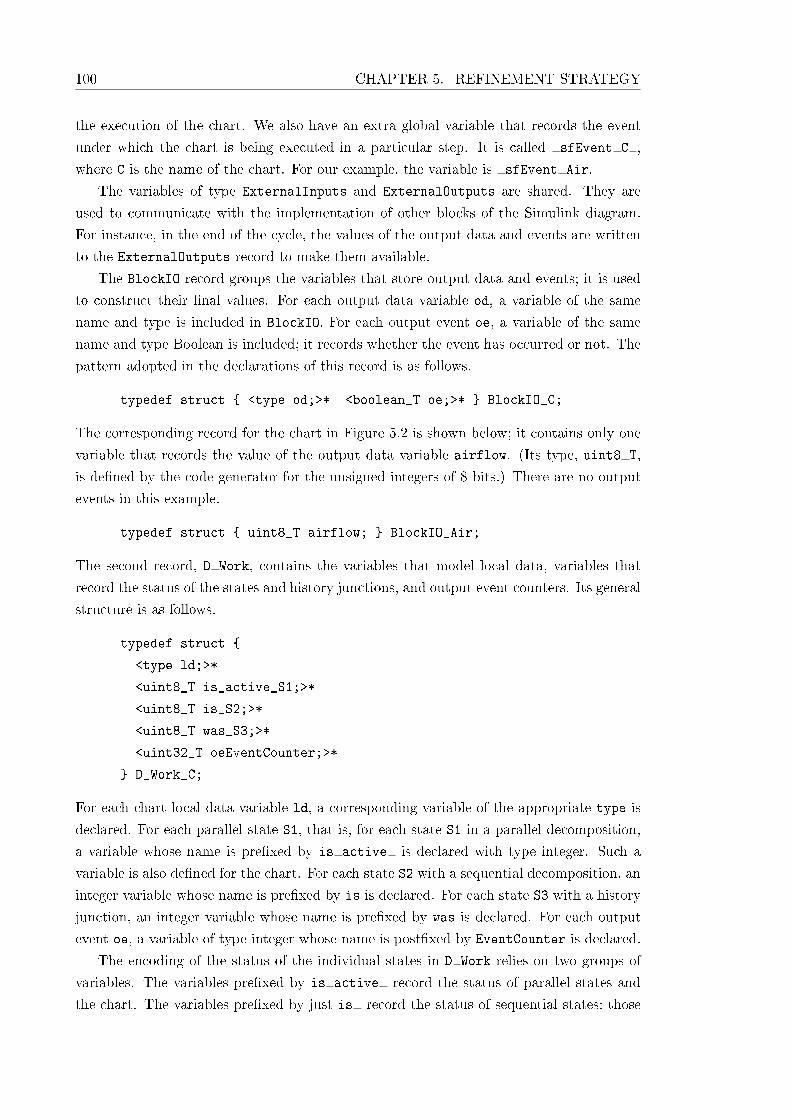
100 CHAPTER 5. REFINEMENT STRATEGY
the execution of the chart. We also have an extra global variable that records the event
under which the chart is being executed in a particular step. It is called sfEvent C ,
where C is the name of the chart. For our example, the variable is sfEvent Air.
The variables of type ExternalInputs and ExternalOutputs are shared. They are
used to communicate with the implementation of other blocks of the Simulink diagram.
For instance, in the end of the cycle, the values of the output data and events are written
to the ExternalOutputs record to make them available.
The BlockIO record groups the variables that store output data and events; it is used
to construct their �nal values. For each output data variable od, a variable of the same
name and type is included in BlockIO. For each output event oe, a variable of the same
name and type Boolean is included; it records whether the event has occurred or not. The
pattern adopted in the declarations of this record is as follows.
typedef struct { <type od;>* <boolean_T oe;>* } BlockIO_C;
The corresponding record for the chart in Figure 5.2 is shown below; it contains only one
variable that records the value of the output data variable airflow. (Its type, uint8 T,
is de�ned by the code generator for the unsigned integers of 8 bits.) There are no output
events in this example.
typedef struct { uint8_T airflow; } BlockIO_Air;
The second record, D Work, contains the variables that model local data, variables that
record the status of the states and history junctions, and output event counters. Its general
structure is as follows.
typedef struct {
<type ld;>*
<uint8_T is_active_S1;>*
<uint8_T is_S2;>*
<uint8_T was_S3;>*
<uint32_T oeEventCounter;>*
} D_Work_C;
For each chart local data variable ld, a corresponding variable of the appropriate type is
declared. For each parallel state S1, that is, for each state S1 in a parallel decomposition,
a variable whose name is pre�xed by is active is declared with type integer. Such a
variable is also de�ned for the chart. For each state S2 with a sequential decomposition, an
integer variable whose name is pre�xed by is is declared. For each state S3 with a history
junction, an integer variable whose name is pre�xed by was is declared. For each output
event oe, a variable of type integer whose name is post�xed by EventCounter is declared.
The encoding of the status of the individual states in D Work relies on two groups of
variables. The variables pre�xed by is active record the status of parallel states and
the chart. The variables pre�xed by just is record the status of sequential states: those
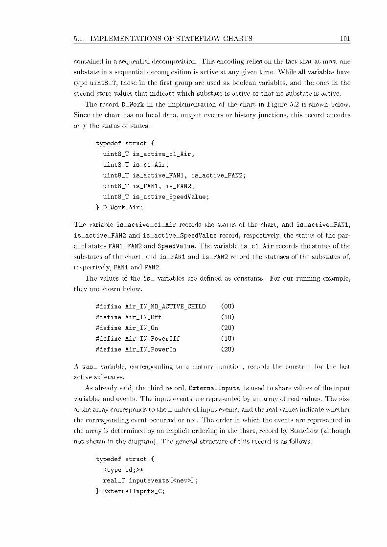
5.1. IMPLEMENTATIONS OF STATEFLOW CHARTS 101
contained in a sequential decomposition. This encoding relies on the fact that at most one
substate in a sequential decomposition is active at any given time. While all variables have
type uint8 T, those in the �rst group are used as boolean variables, and the ones in the
second store values that indicate which substate is active or that no substate is active.
The record D Work in the implementation of the chart in Figure 5.2 is shown below.
Since the chart has no local data, output events or history junctions, this record encodes
only the status of states.
typedef struct {
uint8_T is_active_c1_Air;
uint8_T is_c1_Air;
uint8_T is_active_FAN1, is_active_FAN2;
uint8_T is_FAN1, is_FAN2;
uint8_T is_active_SpeedValue;
} D_Work_Air;
The variable is active c1 Air records the status of the chart, and is active FAN1,
is active FAN2 and is active SpeedValue record, respectively, the status of the par-
allel states FAN1, FAN2 and SpeedValue. The variable is c1 Air records the status of the
substates of the chart, and is FAN1 and is FAN2 record the statuses of the substates of,
respectively, FAN1 and FAN2.
The values of the is variables are de�ned as constants. For our running example,
they are shown below.
#define Air_IN_NO_ACTIVE_CHILD (0U)
#define Air_IN_Off (1U)
#define Air_IN_On (2U)
#define Air_IN_PowerOff (1U)
#define Air_IN_PowerOn (2U)
A was variable, corresponding to a history junction, records the constant for the last
active substates.
As already said, the third record, ExternalInputs, is used to share values of the input
variables and events. The input events are represented by an array of real values. The size
of the array corresponds to the number of input events, and the real values indicate whether
the corresponding event occurred or not. The order in which the events are represented in
the array is determined by an implicit ordering in the chart, record by State�ow (although
not shown in the diagram). The general structure of this record is as follows.
typedef struct {
<type id;>*
real_T inputevents[<nev>];
} ExternalInputs_C;
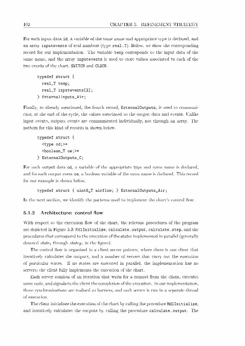
102 CHAPTER 5. REFINEMENT STRATEGY
For each input data id, a variable of the same name and appropriate type is declared, and
an array inputevents of real numbers (type real T). Below, we show the corresponding
record for our implementation. The variable temp corresponds to the input data of the
same name, and the array inputevents is used to store values associated to each of the
two events of the chart, SWITCH and CLOCK.
typedef struct {
real_T temp;
real_T inputevents[2];
} ExternalInputs_Air;
Finally, as already mentioned, the fourth record, ExternalOutputs, is used to communi-
cate, at the end of the cycle, the values associated to the output data and events. Unlike
input events, outputs events are communicated individually, not through an array. The
pattern for this kind of records is shown below.
typedef struct {
<type od;>*
<boolean_T oe;>*
} ExternalOutputs_C;
For each output data od, a variable of the appropriate type and same name is declared,
and for each output event oe, a boolean variable of the same name is declared. This record
for our example is shown below.
typedef struct { uint8_T airflow; } ExternalOutputs_Air;
In the next section, we identify the patterns used to implement the chart's control �ow.
5.1.2 Architecture: control �ow
With respect to the execution �ow of the chart, the relevant procedures of the program
are depicted in Figure 5.3: MdlInitialize, calculate output, calculate step, and the
procedures that correspond to the execution of the states implemented in parallel (generally
denoted state1 through stateN , in the �gure).
The control �ow is organised in a client-server pattern, where there is one client that
iteratively calculates the outputs, and a number of servers that carry out the execution
of particular states. If no states are executed in parallel, the implementation has no
servers: the client fully implements the execution of the chart.
Each server consists of an iteration that waits for a request from the client, executes
some code, and signals to the client the completion of the execution. In our implementation,
these synchronisations are realised as barriers, and each server is run in a separate thread
of execution.
The client initialises the execution of the chart by calling the procedure MdlInitialize,
and iteratively calculates the outputs by calling the procedure calculate output. The
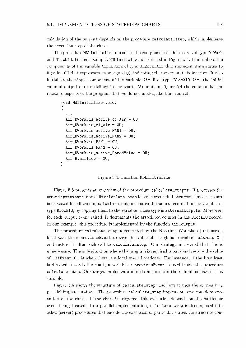
5.1. IMPLEMENTATIONS OF STATEFLOW CHARTS 103
calculation of the outputs depends on the procedure calculate step, which implements
the execution step of the chart.
The procedure MDLInitialize initialises the components of the records of type D Work
and BlockIO. For our example, MDLInitialize is sketched in Figure 5.4. It initialises the
components of the variable Air DWork of type D Work Air that represent state status to
0 (value 0U that represents an unsigned 0), indicating that every state is inactive. It also
initialises the single component of the variable Air B of type BlockIO Air; the initial
value of output data is de�ned in the chart. We omit in Figure 5.4 the commands that
relate to aspects of the program that we do not model, like time control.
void MdlInitialize(void)
{
...
Air_DWork.is_active_c1_Air = 0U;
Air_DWork.is_c1_Air = 0U;
Air_DWork.is_active_FAN1 = 0U;
Air_DWork.is_active_FAN2 = 0U;
Air_DWork.is_FAN1 = 0U;
Air_DWork.is_FAN2 = 0U;
Air_DWork.is_active_SpeedValue = 0U;
Air_B.airflow = 0U;
}
Figure 5.4: Function MDLInitialize.
Figure 5.5 presents an overview of the procedure calculate output. It processes the
array inputevents, and calls calculate step for each event that occurred. Once the chart
is executed for all events, calculate output shares the values recorded in the variable of
type BlockIO, by copying them to the variable whose type is ExternalOutputs. Moreover,
for each output event raised, it decrements the associated counter in the BlockIO record.
In our example, this procedure is implemented by the function Air output.
The procedure calculate output generated by the Realtime Workshop [100] uses a
local variable c previousEvent to save the value of the global variable sfEvent C ,
and restore it after each call to calculate step. Our strategy uncovered that this is
unnecessary. The only situation where the program is required to save and restore the value
of sfEvent C is when there is a local event broadcast. For instance, if the broadcast
is directed towards the chart, a variable c previousEvent is used inside the procedure
calculate step. Our target implementations do not contain the redundant uses of this
variable.
Figure 5.6 shows the structure of calculate step, and how it uses the servers in a
parallel implementation. The procedure calculate step implements one complete exe-
cution of the chart. If the chart is triggered, this execution depends on the particular
event being treated. In a parallel implementation, calculate step is decomposed into
other (server) procedures that encode the execution of particular states. Its structure con-
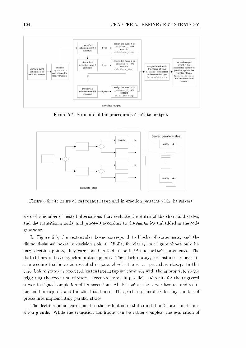
104 CHAPTER 5. REFINEMENT STRATEGY
calculate_output
analyse
inputevents
and update the
local variables.
define a local
variable eN for
each input event.
check if e1
indicates event 1
occurred.
assign the event 1 to
_sfEvent_C_ and
execute
calculate_step.
if yes
check if eN
indicates event N
occurred.
assign the event N to
_sfEvent_C_ and
execute
calculate_step.
check if e2
indicates event 2
occurred.
assign the event 2 to
_sfEvent_C_ and
execute
calculate_step.
if yes
if yes
assign the values in
the record of type
BlockIO to variables
of the record of type
ExternalOutputs.
for each output
event, if the
associated counter is
positive, update the
variable of type
ExternalOutputs
and decrement the
counter.
Figure 5.5: Structure of the procedure calculate output.
Server: parallel states
state1
stateN
calculate_step
stateA
Figure 5.6: Structure of calculate step and interaction patterns with the servers.
sists of a number of nested alternations that evaluate the status of the chart and states,
and the transition guards, and proceeds according to the semantics embedded in the code
generator.
In Figure 5.6, the rectangular boxes correspond to blocks of statements, and the
diamond-shaped boxes to decision points. While, for clarity, our �gure shows only bi-
nary decision points, they correspond in fact to both if and switch statements. The
dotted lines indicate synchronisation points. The block stateA, for instance, represents
a procedure that is to be executed in parallel with the server procedure state1. In this
case, before stateA is executed, calculate step synchronises with the appropriate server
triggering the execution of state1, executes stateA in parallel, and waits for the triggered
server to signal completion of its execution. At this point, the server iterates and waits
for another request, and the client continues. This pattern generalises for any number of
procedures implementing parallel states.
The decision points correspond to the evaluation of state (and chart) status, and tran-
sition guards. While the transition conditions can be rather complex, the evaluation of
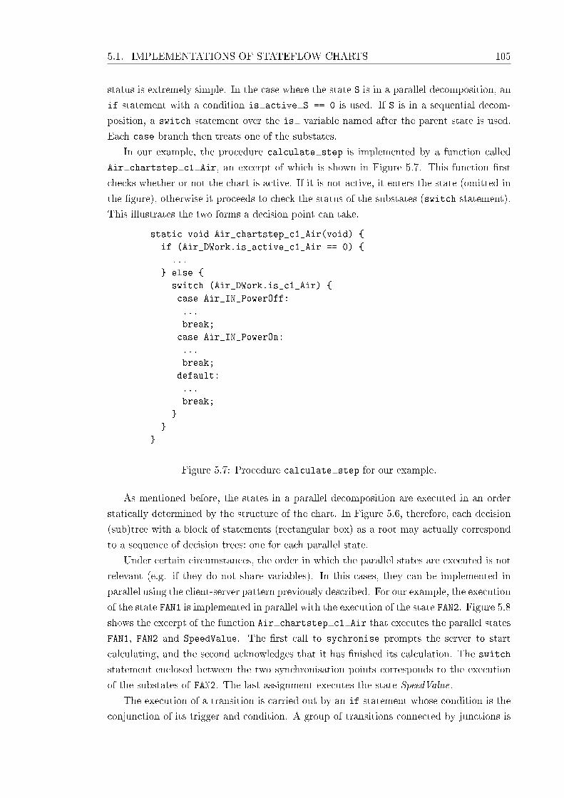
5.1. IMPLEMENTATIONS OF STATEFLOW CHARTS 105
status is extremely simple. In the case where the state S is in a parallel decomposition, an
if statement with a condition is active S == 0 is used. If S is in a sequential decom-
position, a switch statement over the is variable named after the parent state is used.
Each case branch then treats one of the substates.
In our example, the procedure calculate step is implemented by a function called
Air chartstep c1 Air, an excerpt of which is shown in Figure 5.7. This function �rst
checks whether or not the chart is active. If it is not active, it enters the state (omitted in
the �gure), otherwise it proceeds to check the status of the substates (switch statement).
This illustrates the two forms a decision point can take.
static void Air_chartstep_c1_Air(void) {
if (Air_DWork.is_active_c1_Air == 0) {
...
} else {
switch (Air_DWork.is_c1_Air) {
case Air_IN_PowerOff:
...
break;
case Air_IN_PowerOn:
...
break;
default:
...
break;
}
}
}
Figure 5.7: Procedure calculate step for our example.
As mentioned before, the states in a parallel decomposition are executed in an order
statically determined by the structure of the chart. In Figure 5.6, therefore, each decision
(sub)tree with a block of statements (rectangular box) as a root may actually correspond
to a sequence of decision trees: one for each parallel state.
Under certain circumstances, the order in which the parallel states are executed is not
relevant (e.g. if they do not share variables). In this cases, they can be implemented in
parallel using the client-server pattern previously described. For our example, the execution
of the state FAN1 is implemented in parallel with the execution of the state FAN2. Figure 5.8
shows the excerpt of the function Air chartstep c1 Air that executes the parallel states
FAN1, FAN2 and SpeedValue. The �rst call to sychronise prompts the server to start
calculating, and the second acknowledges that it has �nished its calculation. The switch
statement enclosed between the two synchronisation points corresponds to the execution
of the substates of FAN2. The last assignment executes the state SpeedValue.
The execution of a transition is carried out by an if statement whose condition is the
conjunction of its trigger and condition. A group of transitions connected by junctions is
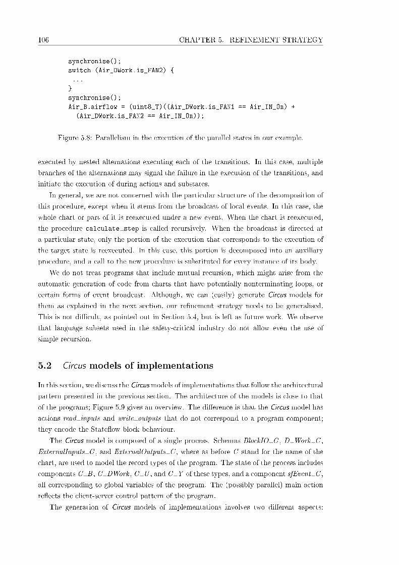
106 CHAPTER 5. REFINEMENT STRATEGY
synchronise();
switch (Air_DWork.is_FAN2) {
...
}
synchronise();
Air_B.airflow = (uint8_T)((Air_DWork.is_FAN1 == Air_IN_On) +
(Air_DWork.is_FAN2 == Air_IN_On));
Figure 5.8: Parallelism in the execution of the parallel states in our example.
executed by nested alternations executing each of the transitions. In this case, multiple
branches of the alternations may signal the failure in the execution of the transitions, and
initiate the execution of during actions and substates.
In general, we are not concerned with the particular structure of the decomposition of
this procedure, except when it stems from the broadcast of local events. In this case, the
whole chart or part of it is reexecuted under a new event. When the chart is reexecuted,
the procedure calculate step is called recursively. When the broadcast is directed at
a particular state, only the portion of the execution that corresponds to the execution of
the target state is reexecuted. In this case, this portion is decomposed into an auxiliary
procedure, and a call to the new procedure is substituted for every instance of its body.
We do not treat programs that include mutual recursion, which might arise from the
automatic generation of code from charts that have potentially nonterminating loops, or
certain forms of event broadcast. Although, we can (easily) generate Circus models for
them as explained in the next section, our re�nement strategy needs to be generalised.
This is not di�cult, as pointed out in Section 5.4, but is left as future work. We observe
that language subsets used in the safety-critical industry do not allow even the use of
simple recursion.
5.2 Circus models of implementations
In this section, we discuss the Circusmodels of implementations that follow the architectural
pattern presented in the previous section. The architecture of the models is close to that
of the programs; Figure 5.9 gives an overview. The di�erence is that the Circus model has
actions read inputs and write outputs that do not correspond to a program component;
they encode the State�ow block behaviour.
The Circus model is composed of a single process. Schemas BlockIO C , D Work C ,
ExternalInputs C , and ExternalOutputs C , where as before C stand for the name of the
chart, are used to model the record types of the program. The state of the process includes
components C B , C DWork , C U , and C Y of these types, and a component sfEvent C ,
all corresponding to global variables of the program. The (possibly parallel) main action
re�ects the client-server control pattern of the program.
The generation of Circus models of implementations involves two di�erent aspects:

5.2. CIRCUS MODELS OF IMPLEMENTATIONS 107
process ProgramModel
Server: parallel states
state1
stateN
Client
MdlInitialize
calculate_outputs
calculate_stepread_inputs
write_outputs
BlockIO D_Work ExternalInputs ExternalOutputs
Figure 5.9: Overview of the models of implementations of State�ow charts.
Client =̂ MdlInitialize ;
µX •
input events?s −→ C U .inputevents := s;read inputs ; calculate output ;write outputs ; end cycle −→ X
Figure 5.10: Action Client in implementation models.
translation and abstraction. The programming language statements are translated into
Circus actions, and aspects of the program that are not covered by our models of State�ow
chart (for instance, time control) are abstracted.
The calculations of the time steps that determine the execution of a chart are abstracted
by synchronisations over the channels input event and end cycle that mark, respectively,
the start and end of a cycle (step). The way in which these channels are used to abstract
time is shown in Figure 5.10, which presents the action Client . It initialises the state,
and recursively reads input events, reads input data, calculates outputs, writes outputs,
and signals the end of the cycle. (As an aside, we observe that the name of the action
calculate output is speci�c to each example; for our example, it is Air output . Moreover,
in the code generated by Realtime Workshop, the procedure Air output has a parameter
tid, probably for uniformity with programs generated for the Simulink diagram. Our
strategy shows that this parameter is not needed, and we simplify the code and the model
to avoid useless features. This is in line with guidelines adopted in the development of
safety-critical systems.)
As illustrated in (the �rst two boxes of) Figure 5.5, the treatment of input events in
the implementation involves calculations that identify which events occurred according

108 CHAPTER 5. REFINEMENT STRATEGY
to values supplied by the Simulink model in an array inputevents. In our models, we
abstract from this calculation by assuming that this is an array of booleans that indicate
the occurrence of each event, not its associated value. As a consequence, we cannot reason
about di�erent types of input events (rising, falling, or either edge trigger).
Finally, sharing is modelled as communication. For instance, the use of a global shared
variable of type ExternalInputs is modelled by an action that reads in interleaving the
input variables and the array of events modelled as a sequence of boolean values, and writes
them to the state component of type ExternalInputs. Similarly, the use of a global shared
variable of type ExternalOutputs is modelled by an action that communicates the values
of the components of the state component of type ExternalOutputs in interleaving. The
channels used to read inputs and write outputs, and the channel used to communicate input
and output events are the same channels used in the model of the chart being implemented.
This ensures that the Circus models of the chart and of the program can be compared by
re�nement.
Another aspect of the implementations that involves sharing is the client-server pattern
of parallel implementations. In our models, the di�erent threads are modelled as Circus
parallel actions Client and Servers. The state of the process is handled by Client , and
Servers is itself the parallel composition of actions that model the procedures that execute
parallel states. As for interleaving, the state needs to be partitioned between parallel
actions to avoid racing conditions. We, therefore, model the initial synchronisation between
Client and a server action as a communication that sends the complete state from the
client to the server. The �nal synchronisations are modelled as a number of interleaved
communications that send the components modi�ed by each server to the client. Once all
the values are received by Client , it updates the state.
Except for the aspects discussed above, the Circus models of the implementations are,
in general, obtained by direct translation. Circus includes constructs that map directly
into imperative programming languages. Records are translated into schemas, loops into
recursive actions, if and switch statements are mapped to alternations, and procedures
are mapped to named Circus actions.
5.3 Re�nement strategy
In this section, we present a new re�nement strategy suited for the veri�cation of (par-
allel) implementations of State�ow charts that follow the architectural pattern presented
in Section 5.1. It is a tactic of re�nement, which we de�ne as a procedure for systematic
application of re�nement laws.
As previously mentioned, our re�nement strategy is organised in �ve phases: data
re�nement, normalisation, structuring, parallelism introduction, and action introduction;
an overview is provided in Figure 5.1. The main input is the model of the State�ow chart,
which as already explained, can be automatically generated. We also use the chart itself,
for instance, to guide our calculation of a concrete state, and of a retrieve relation between
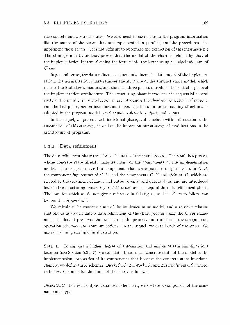
5.3. REFINEMENT STRATEGY 109
the concrete and abstract states. We also need to extract from the program information
like the names of the states that are implemented in parallel, and the procedures that
implement these states. (It is not di�cult to automate the extraction of this information.)
The strategy is a tactic that proves that the model of the chart is re�ned by that of
the implementation by transforming the former into the latter using the algebraic laws of
Circus.
In general terms, the data re�nement phase introduces the data model of the implemen-
tation, the normalisation phase removes the structure of the abstract chart model, which
re�ects the State�ow semantics, and the next three phases introduce the control aspects of
the implementation architecture. The structuring phase introduces the sequential control
pattern, the parallelism introduction phase introduces the client-server pattern, if present,
and the last phase, action introduction, introduces the appropriate naming of actions as
adopted in the program model (read inputs, calculate output , and so on).
In the sequel, we present each individual phase, and conclude with a discussion of the
automation of this strategy, as well as the impact on our strategy of modi�cations to the
architecture of programs.
5.3.1 Data re�nement
The data re�nement phase transforms the state of the chart process. The result is a process
whose concrete state already includes many of the components of the implementation
model. The exceptions are the components that correspond to output events in C B ,
the component inputevents of C U , and the components C Y and sfEvent C , which are
related to the treatment of input and output events, and output data, and are introduced
later in the structuring phase. Figure 5.11 describes the steps of the data re�nement phase.
The laws for which we do not give a reference in this �gure, and in others to follow, can
be found in Appendix E.
We calculate the concrete state of the implementation model, and a retrieve relation
that allows us to calculate a data re�nement of the chart process using the Circus re�ne-
ment calculus. It preserves the structure of the process, and transforms the assignments,
operation schemas, and communications. In the sequel, we detail each of the steps. We
use our running example for illustration.
Step 1. To support a higher degree of automation and enable certain simpli�cations
later on (see Section 5.3.3.7), we calculate, besides the concrete state of the model of the
implementation, properties of its components that become the concrete state invariant.
Namely, we de�ne three schemas: BlockIO C , D Work C , and ExternalInputs C , where,
as before, C stands for the name of the chart, as follows.
BlockIO C For each output variable in the chart, we declare a component of the same
name and type.

110 CHAPTER 5. REFINEMENT STRATEGY
1. Calculate the concrete state. Use the provided templates.
2. Calculate the retrieve relation. Use the provided template.
Transform the chart process as follows.
3. Introduce the abstract state invariant as an assumption after theinitialisation. Apply Law C.29 [76] to the initialisation schema in themain action, and distribute the assumption towards the assignments (applyLaws C.37-C.54 [76] exhaustively until all assignments are reached).
4. Convert any actions of the form {inv} ; v := e. Apply Law assign-schema-conv to all of them.
5. Calculate the simulation. Apply the Circus laws of action simulation tothe chart process (Laws C.1-C.25 [76]).
Figure 5.11: Re�nement strategy: data re�nement phase.
D Work C To characterise the general form of D Work C , we consider the unique
identi�ers LV1, . . . ,LVm for the chart local variables of types T1, . . . ,Tm , the identi�ers
PS1, . . . ,PSn for the parallel states and for the chart, the identi�ers SS1, . . . ,SSo of the
states that have a sequential decomposition, possibly including the chart, and the identi�ers
HS1, . . . ,HSp of the states that contain a history junction. Additionally, we consider the
names OE1, . . . ,OEq of the output events. To specify the invariant of D Work C , we
also use substates, a function that associates (the identi�er of) each state to the set of
(identi�ers of) its substates. With these, we can specify that D Work C is to be de�ned
as follows.
D Work C
LV1 : T1; . . . ; LVm : Tm
is active PS1, . . . , is active PSn : Nis SS1, . . . , is SSo : Nwas HS1, . . . ,was HSp : NOE1EventCounter , . . . ,OEqEventCounter : N
∀ i : 1 . . o • is SSi ∈ {C IN NO ACTIVE CHILD} ∪ {s : substates(SSi) • C IN s}∀ i : 1 . . p •
was HSi ∈ {C IN NO ACTIVE CHILD} ∪ {s : substates(HSi) • C IN s}
For each chart local variable, we declare a component of the same name and type. All
the remaining components are of type N. We also declare, for each parallel state S and
the chart, a component is active S . For each S with a sequential decomposition, we
declare is S . For each history junction within a state S , we declare was S , and for each

5.3. REFINEMENT STRATEGY 111
D Work Airis active c1 Air : Nis c1 Air : Nis active FAN 1, is active FAN 2 : Nis FAN 1, is FAN 2 : Nis active Speedvalue : N
is c1 Air ∈ {Air IN NO ACTIVE CHILD ,Air IN PowerOn,Air IN PowerO� }is FAN 1 ∈ {Air IN NO ACTIVE CHILD ,Air IN O� ,Air IN On}is FAN 2 ∈ {Air IN NO ACTIVE CHILD ,Air IN O� ,Air IN On}
Figure 5.12: Schema D Work Air .
output event e, we declare a component eEventCounter . For each state S with a sequential
decomposition, possibly including the chart, the invariant requires that the value of is S is
restricted to one of the identi�ers of the substates of S , or C IN NO ACTIVE CHILD ,
when none of them are active. Similarly, the value of a was S variable is restricted to
the substates of S , or C IN NO ACTIVE CHILD , if none of them have been active yet.
Figure 5.12 shows the D Work C schema for our example.
ExternalInputs C For each input data, we declare a component of the same name and
type. In the case of our example, we have a schema ExternalInputs Air with a single
component v temp : R.
The concrete state is de�ned by a schema ConcreteState with three components C B ,
C DWork , and C U , whose types are the schemas de�ned above. In our example, we
have Air B , Air DWork , and Air U .
Step 2. The retrieve relation maps the components of BlockIO C (that correspond to
input and output variables) and the components of D Work C that correspond to lo-
cal variables to components of SimulationInstance. The eEventCounter components of
D Work C are mapped to the counters in the schema SimulationInstance. The com-
ponents of D Work C that record the status of the states and the history junctions,
precisely, those whose names are pre�xed with is active , is or was , are mapped to the
components state status and state history of SimulationData.
The correspondence between variables is trivial. It is obtained by equating each of the
concrete variables to the corresponding abstract variable whose name is the same except
for a pre�x v . For event counters, we also have a simple mapping: each eEventCounter
component is equated to the corresponding counter e.
The speci�cation of the relation between the is active and is pre�xed variables and
the function state status in SimulationData is de�ned by equating state status to a set
comprehension that speci�es the status of the states using the is active and is variables.
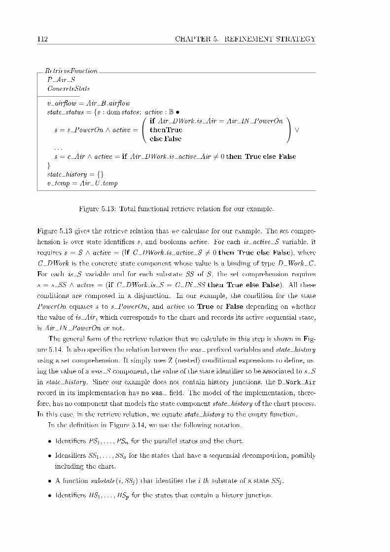
112 CHAPTER 5. REFINEMENT STRATEGY
RetrieveFunctionP Air SConcreteState
v air�ow = Air B .air�owstate status = {s : dom states; active : B •
s = s PowerOn ∧ active =
if Air DWork .is Air = Air IN PowerOnthenTrueelseFalse
∨. . .s = c Air ∧ active = if Air DWork .is active Air 6= 0 then True else False}state history = {}v temp = Air U .temp
Figure 5.13: Total functional retrieve relation for our example.
Figure 5.13 gives the retrieve relation that we calculate for our example. The set compre-
hension is over state identi�ers s, and booleans active. For each is active S variable, it
requires s = S ∧ active = (if C DWork .is active S 6= 0 then True else False), where
C DWork is the concrete state component whose value is a binding of type D Work C .
For each is S variable and for each substate SS of S , the set comprehension requires
s = s SS ∧ active = (if C DWork .is S = C IN SS then True else False). All these
conditions are composed in a disjunction. In our example, the condition for the state
PowerOn equates s to s PowerOn, and active to True or False depending on whether
the value of is Air , which corresponds to the chart and records its active sequential state,
is Air IN PowerOn or not.
The general form of the retrieve relation that we calculate in this step is shown in Fig-
ure 5.14. It also speci�es the relation between the was pre�xed variables and state history
using a set comprehension. It simply uses Z (nested) conditional expressions to de�ne, us-
ing the value of a was S component, the value of the state identi�er to be associated to s S
in state history . Since our example does not contain history junctions, the D Work Air
record in its implementation has no was �eld. The model of the implementation, there-
fore, has no component that models the state component state history of the chart process.
In this case, in the retrieve relation, we equate state history to the empty function.
In the de�nition in Figure 5.14, we use the following notation.
• Identi�ers PS1, . . . ,PSn for the parallel states and the chart.
• Identi�ers SS1, . . . ,SSo for the states that have a sequential decomposition, possibly
including the chart.
• A function substate(i ,SSj ) that identi�es the i-th substate of a state SSj .
• Identi�ers HS1, . . . ,HSp for the states that contain a history junction.

5.3. REFINEMENT STRATEGY 113
• The number ri of substates of SSi .
• Identi�ers LV1, . . . ,LVm for the local variables.
• Identi�ers IV1, . . . , IVs for the input variables, and OV1, . . . ,OVt for the output
variables.
• Names OE1, . . . ,OEq of the output events.
The retrieve relation is always a total function because it is speci�ed by a set of equations
that de�nes each abstract state component as a total function of the concrete components.
Steps 3 and 4. Some of the assignments in the chart, and therefore, in the (abstract)
chart process are implemented as assignments to components of records. In the implemen-
tation model, they become assignments to records themselves. For instance, the assignment
v air�ow := 0 in the action entryaction PowerO� in the chart process corresponds to an
assignment Air B := 〈|air�ow == 0|〉 in the model of the implementation. The simulation
law for assignment, however, does not handle records directly, and therefore, in these steps
we transform the assignments to schema operations.
For that, in Step 3, we introduce the abstract state invariant after the initialisation
operation in the main action of the chart process, and distribute it to just before each of
the assignments in AllActions. The application of the distribution laws raises no proof
obligations because all data operations in the chart process preserve its state invariant. In
Step 4, we convert the assumptions followed by the assignments into schema operations.
For the assignment v air�ow := 0, we get the schema below.
Assign1
∆P Air S
state status ′ = state status ∧ state history ′ = state history
v temp′ = v temp ∧ v air�ow ′ = 0
Step 4 uses a novel, but very simple Law assign-schema-conv. It is de�ned in Appendix E.
Step 5. This is a standard data re�nement step. Using the retrieve relation, we apply
the Circus laws of simulation [76] to obtain a Circus process C P Air Controller by data
re�nement of the process P Air Controller . The state of the new process contains three
components Air B , Air DWork , and Air U .
5.3.2 Normalisation
The objective of this phase is to remove the top (parallel) structure of the chart model,
which re�ects the operational semantics of the State�ow notation (see Chapter 3). This
results in a model whose monolithic, but simple, process structure is adequate as a starting
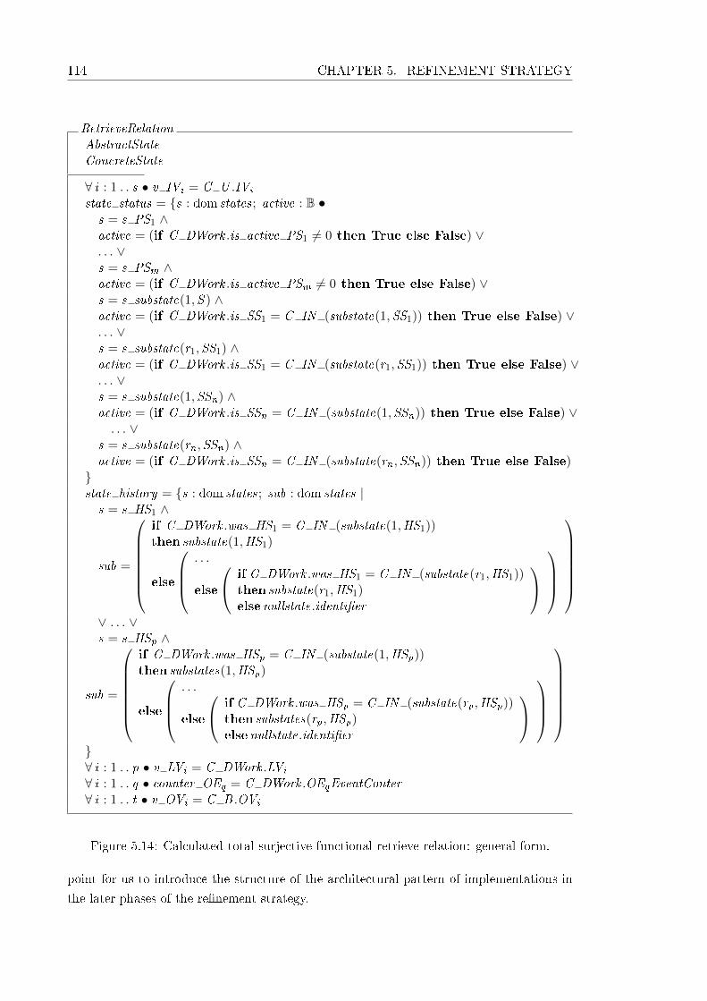
114 CHAPTER 5. REFINEMENT STRATEGY
RetrieveRelationAbstractStateConcreteState
∀ i : 1 . . s • v IVi = C U .IVi
state status = {s : dom states; active : B •s = s PS1 ∧active = (if C DWork .is active PS1 6= 0 then True else False) ∨. . . ∨s = s PSm ∧active = (if C DWork .is active PSm 6= 0 then True else False) ∨s = s substate(1,S ) ∧active = (if C DWork .is SS1 = C IN (substate(1,SS1)) then True else False) ∨. . . ∨s = s substate(r1,SS1) ∧active = (if C DWork .is SS1 = C IN (substate(r1,SS1)) then True else False) ∨. . . ∨s = s substate(1,SSn) ∧active = (if C DWork .is SSn = C IN (substate(1,SSn)) then True else False) ∨. . . ∨
s = s substate(rn ,SSn) ∧active = (if C DWork .is SSn = C IN (substate(rn ,SSn)) then True else False)}state history = {s : dom states; sub : dom states |s = s HS1 ∧
sub =
if C DWork .was HS1 = C IN (substate(1,HS1))then substate(1,HS1)
else
. . .
else
if C DWork .was HS1 = C IN (substate(r1,HS1))then substate(r1,HS1)elsenullstate.identi�er
∨ . . . ∨s = s HSp ∧
sub =
if C DWork .was HSp = C IN (substate(1,HSp))then substates(1,HSp)
else
. . .
else
if C DWork .was HSp = C IN (substate(rp ,HSp))then substates(rp ,HSp)elsenullstate.identi�er
}∀ i : 1 . . p • v LVi = C DWork .LVi
∀ i : 1 . . q • counter OEq = C DWork .OEqEventConter∀ i : 1 . . t • v OVi = C B .OVi
Figure 5.14: Calculated total surjective functional retrieve relation: general form.
point for us to introduce the structure of the architectural pattern of implementations in
the later phases of the re�nement strategy.
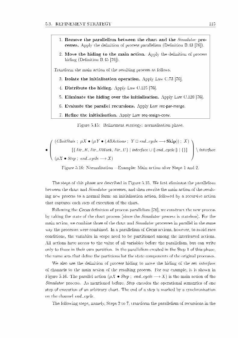
5.3. REFINEMENT STRATEGY 115
1. Remove the parallelism between the chart and the Simulator pro-cesses. Apply the de�nition of process parallelism (De�nition B.43 [76]).
2. Move the hiding to the main action. Apply the de�nition of processhiding (De�nition B.45 [76]).
Transform the main action of the resulting process as follows.
3. Isolate the initialisation operation. Apply Law C.73 [76].
4. Distribute the hiding. Apply Law C.125 [76].
5. Eliminate the hiding over the initialisation. Apply Law C.120 [76].
6. Evaluate the parallel recursions. Apply Law rec-par-merge.
7. Re�ne the initialisation. Apply Law seq-assign-conv.
Figure 5.15: Re�nement strategy: normalisation phase.
•
(CInitState ; µX • (µY • (AllActions ; Y @ end cycle −→ Skip)) ; X )
J{Air B ,Air DWork ,Air U } | interface ∪ {| end cycle |} | {}K
(µX • Step ; end cycle −→ X )
\ interfaceFigure 5.16: Normalisation � Example: Main action after Steps 1 and 2.
The steps of this phase are described in Figure 5.15. We �rst eliminate the parallelism
between the chart and Simulator processes, and then rewrite the main action of the result-
ing new process to a normal form: an initialisation action, followed by a recursive action
that captures each step of execution of the chart.
Following the Circus de�nition of process parallelism [76], we construct the new process
by taking the state of the chart process (since the Simulator process is stateless). For the
main action, we combine those of the chart and Simulator processes in parallel in the same
way the processes were combined. In a parallelism of Circus actions, however, to avoid race
conditions, the variables in scope need to be partitioned among the interleaved actions.
All actions have access to the value of all variables before the parallelism, but can write
only to those in their own partition. In the parallelism created in the Step 1 of this phase,
the name sets that de�ne the partitions list the state components of the original processes.
We also use the de�nition of process hiding to move the hiding of the set interface
of channels to the main action of the resulting process. For our example, it is shown in
Figure 5.16. The parallel action (µX • Step ; end cycle −→ X ) is the main action of the
Simulator process. As mentioned before, Step encodes the operational semantics of one
step of execution of an arbitrary chart. The end of a step is marked by a synchronisation
on the channel end cycle.
The following steps, namely, Steps 2 to 7, transform the parallelism of recursions in the
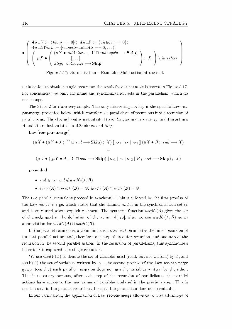
116 CHAPTER 5. REFINEMENT STRATEGY
•
Air U := 〈|temp == 0|〉 ; Air B := 〈|air�ow == 0|〉;Air DWork := 〈|is active c1 Air == 0, . . . |〉; µX •
(µY • AllActions ; Y @ end cycle −→ Skip)J . . . K
Step; end cycle −→ Skip
; X
\ interface
Figure 5.17: Normalisation � Example: Main action at the end.
main action to obtain a single recursion; the result for our example is shown in Figure 5.17.
For conciseness, we omit the name and synchronisation sets in the parallelism, which do
not change.
The Steps 2 to 7 are very simple. The only interesting novelty is the speci�c Law rec-
par-merge, presented below, which transforms a parallelism of recursions into a recursion of
parallelisms. The channel end is instantiated to end cycle in our strategy, and the actions
A and B are instantiated to AllActions and Step.
Law[rec-par-merge]
(µX • (µY • A ; Y @ end −→ Skip) ; X ) J ns1 | cs | ns2 K (µX • B ; end −→ X )
=
(µX • ((µY • A ; Y @ end −→ Skip) J ns1 | cs | ns2 K B ; end −→ Skip) ; X )
provided
• end ∈ cs; end 6∈ usedC (A,B)
• wrtV (A) ∩ usedV (B) = ∅; usedV (A) ∩ wrtV (B) = ∅
The two parallel recursions proceed in synchrony. This is enforced by the �rst proviso of
the Law rec-par-merge, which states that the channel end is in the synchronisation set cs
and is only used where explicitly shown. The syntactic function usedC (A) gives the set
of channels used in the de�nition of the action A [76]; also, we use usedC (A,B) as an
abbreviation for usedC (A) ∪ usedC (B).
In the parallel recursions, a communication over end terminates the inner recursion of
the �rst parallel action, and, therefore, one step of its outer recursion, and one step of the
recursion in the second parallel action. In the recursion of parallelisms, this synchronous
behaviour is captured as a single recursion.
We use usedV (A) to denote the set of variables used (read, but not written) by A, and
wrtV (A) the set of variables written by A. The second proviso of the Law rec-par-merge
guarantees that each parallel recursion does not use the variables written by the other.
This is necessary because, after each step of the recursion of parallelisms, the parallel
actions have access to the new values of variables updated in the previous step. This is
not the case in the parallel recursions, because the parallelism does not terminate.
In our veri�cation, the application of Law rec-par-merge allows us to take advantage of

5.3. REFINEMENT STRATEGY 117
MdlInitialize; µX •
µY • AllActions ; Y @ end cycle −→ SkipJns1 | interface ∪ {| end cycle |} | ns2K
Step; end cycle −→ Skip
; X
\ interface
Figure 5.18: Structuring starting point.
the fact that, in both the chart and the Simulator process, each step of execution of the
chart is marked by a synchronisation on end cycle. For each of the steps of the simulator,
an arbitrary number of executions of AllActions may be necessary to provide and update
information about the chart components.
The other new law used in Figure 5.15 are very simple and are listed in Appendix E as
usual.
5.3.3 Structuring
In this phase, we introduce the sequential control structure of the implementation: the
structure of the client in Figure 5.9. For parallel implementations, the next phase (paral-
lelism introduction) introduces the servers.
Starting point The steps of this phase are to be applied to the normalised process
obtained in the previous phase. The general form of its main action is illustrated in
Figure 5.17 and described in Figure 5.18, where MdlInitialize stands for a sequence of
assignments that initialise the state. The action Step of the Simulator process is de�ned
as shown and explained below. A detailed description is in Chapter 3.
Step =̂
events?es −→ input event?vs : (# vs = # es)−→ read inputs−→ExecuteEvents(es, vs);
write outputs −→ Skip
ExecuteEvents =̂ es : seqEVENT ; vs : seqB • (; i : id(1 . .# es) • ExecuteEvent(es(i), vs(i)))
ExecuteEvent =̂ e : EVENT ; v : B •
if v = True−→ ExecuteChart(e)
8 v = False−→ Skip
�
Step requests from the chart a sequence es of input events, reads a sequence vs (of the
same size) of boolean values associated to these events, requests the chart to read the input
data, executes the chart for each event by calling another action ExecuteEvents(es, vs), and
requests the chart to write its outputs.
ExecuteEvents is de�ned by an iterated sequence of calls ExecuteEvent(es(i), vs(i))
that execute the chart for each of the events in es (and their associated values in vs).
ExecuteEvent(e, v) models the execution of the chart for the event e; the boolean parameter
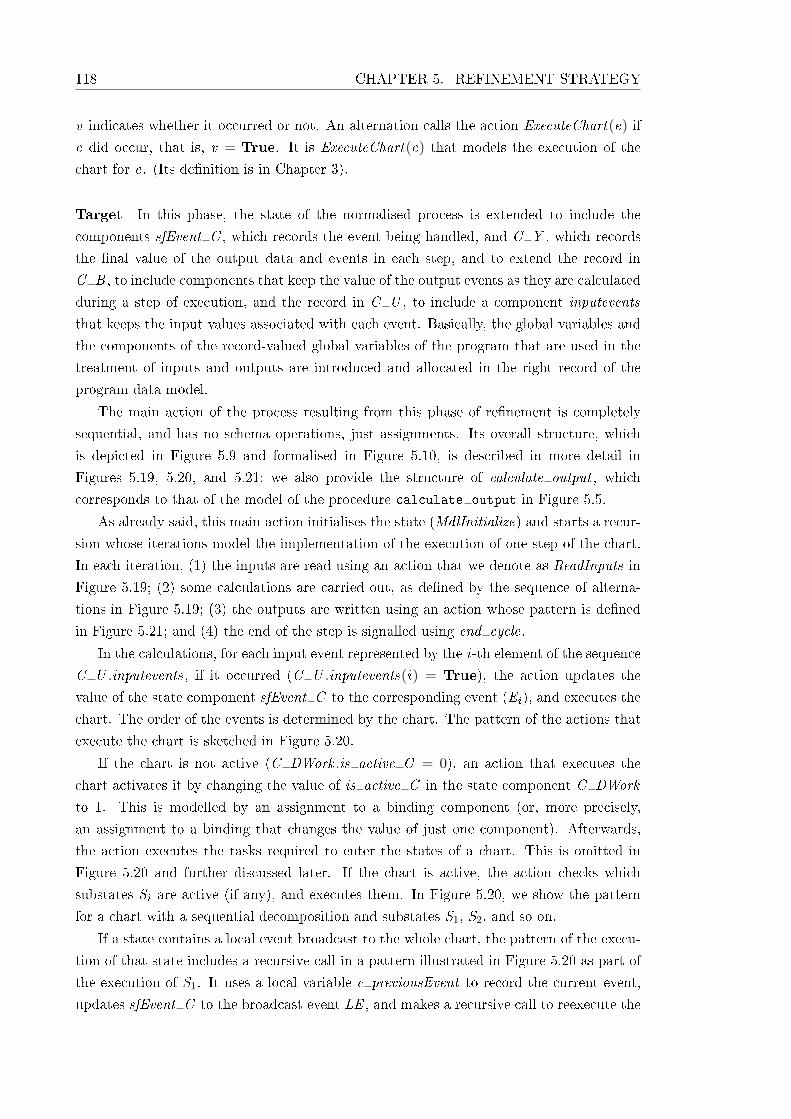
118 CHAPTER 5. REFINEMENT STRATEGY
v indicates whether it occurred or not. An alternation calls the action ExecuteChart(e) if
e did occur, that is, v = True. It is ExecuteChart(e) that models the execution of the
chart for e. (Its de�nition is in Chapter 3).
Target In this phase, the state of the normalised process is extended to include the
components sfEvent C , which records the event being handled, and C Y , which records
the �nal value of the output data and events in each step, and to extend the record in
C B , to include components that keep the value of the output events as they are calculated
during a step of execution, and the record in C U , to include a component inputevents
that keeps the input values associated with each event. Basically, the global variables and
the components of the record-valued global variables of the program that are used in the
treatment of inputs and outputs are introduced and allocated in the right record of the
program data model.
The main action of the process resulting from this phase of re�nement is completely
sequential, and has no schema operations, just assignments. Its overall structure, which
is depicted in Figure 5.9 and formalised in Figure 5.10, is described in more detail in
Figures 5.19, 5.20, and 5.21: we also provide the structure of calculate output , which
corresponds to that of the model of the procedure calculate output in Figure 5.5.
As already said, this main action initialises the state (MdlInitialize) and starts a recur-
sion whose iterations model the implementation of the execution of one step of the chart.
In each iteration, (1) the inputs are read using an action that we denote as ReadInputs in
Figure 5.19; (2) some calculations are carried out, as de�ned by the sequence of alterna-
tions in Figure 5.19; (3) the outputs are written using an action whose pattern is de�ned
in Figure 5.21; and (4) the end of the step is signalled using end cycle.
In the calculations, for each input event represented by the i-th element of the sequence
C U .inputevents, if it occurred (C U .inputevents(i) = True), the action updates the
value of the state component sfEvent C to the corresponding event (Ei), and executes the
chart. The order of the events is determined by the chart. The pattern of the actions that
execute the chart is sketched in Figure 5.20.
If the chart is not active (C DWork .is active C = 0), an action that executes the
chart activates it by changing the value of is active C in the state component C DWork
to 1. This is modelled by an assignment to a binding component (or, more precisely,
an assignment to a binding that changes the value of just one component). Afterwards,
the action executes the tasks required to enter the states of a chart. This is omitted in
Figure 5.20 and further discussed later. If the chart is active, the action checks which
substates Si are active (if any), and executes them. In Figure 5.20, we show the pattern
for a chart with a sequential decomposition and substates S1, S2, and so on.
If a state contains a local event broadcast to the whole chart, the pattern of the execu-
tion of that state includes a recursive call in a pattern illustrated in Figure 5.20 as part of
the execution of S1. It uses a local variable c previousEvent to record the current event,
updates sfEvent C to the broadcast event LE , and makes a recursive call to reexecute the

5.3. REFINEMENT STRATEGY 119
MdlInitialize;
µX •
ReadInputs;
if C U .inputevents(1) = True−→sfEvent C := E1 ; . . . (Figure 5.20)
8 C U .inputevents(1) = False−→ Skip�
;
. . . ;if C U .inputevents(n) = True−→sfEvent C := En ; . . . (Figure 5.20)
8 C U .inputevents(n) = False−→ Skip�
;
(Figure 5.21); end cycle −→ X
Figure 5.19: Structuring target.
µY •
var c previousEvent : N •
if C DWork .is active C = 0−→C DWork := 〈|is active C == 1, . . . |〉 ; . . .
8 C DWork .is active C > 0−→
if C DWork .is C = C IN S1−→
. . .
c previousEvent := sfEvent C ;sfEvent C := LE ;Y ;sfEvent C := c previousEvent ;
; . . .
8 C DWork .is C = C IN S2−→
. . .
µZ •
if ct −→ . . .Z8 ¬ ct −→ Skip�
; . . .
8 . . .�
�
Figure 5.20: Structuring target - chart execution.
if C DWork .counter E > 0−→
C DWork := 〈|counter E == (C DWork .counter E − 1), . . . |〉 ; C B .E := True8 C DWork .counter E = 0−→ E := False�
;
. . . ;C Y := C B ;o E !(C Y .E )−→ Skip 9 . . . 9 o v !(C Y .v)−→ Skip 9 . . .
Figure 5.21: Structuring target - writing the outputs.
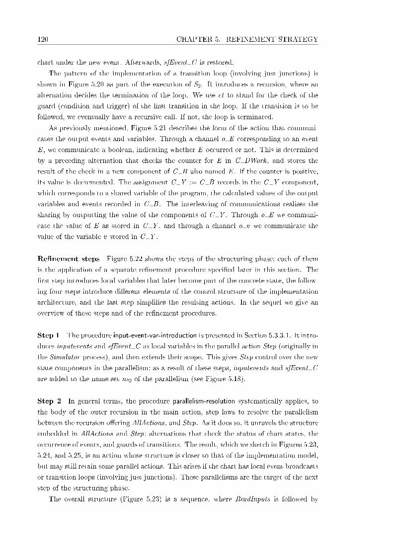
120 CHAPTER 5. REFINEMENT STRATEGY
chart under the new event. Afterwards, sfEvent C is restored.
The pattern of the implementation of a transition loop (involving just junctions) is
shown in Figure 5.20 as part of the execution of S2. It introduces a recursion, where an
alternation decides the termination of the loop. We use ct to stand for the check of the
guard (condition and trigger) of the �rst transition in the loop. If the transition is to be
followed, we eventually have a recursive call. If not, the loop is terminated.
As previously mentioned, Figure 5.21 describes the form of the action that communi-
cates the output events and variables. Through a channel o E corresponding to an event
E , we communicate a boolean, indicating whether E occurred or not. This is determined
by a preceding alternation that checks the counter for E in C DWork , and stores the
result of the check in a new component of C B also named E . If the counter is positive,
its value is decremented. The assignment C Y := C B records in the C Y component,
which corresponds to a shared variable of the program, the calculated values of the output
variables and events recorded in C B . The interleaving of communications realises the
sharing by outputting the value of the components of C Y . Through o E we communi-
cate the value of E as stored in C Y , and through a channel o v we communicate the
value of the variable v stored in C Y .
Re�nement steps Figure 5.22 shows the steps of the structuring phase; each of them
is the application of a separate re�nement procedure speci�ed later in this section. The
�rst step introduces local variables that later become part of the concrete state, the follow-
ing four steps introduce di�erent elements of the control structure of the implementation
architecture, and the last step simpli�es the resulting actions. In the sequel we give an
overview of these steps and of the re�nement procedures.
Step 1 The procedure input-event-var-introduction is presented in Section 5.3.3.1. It intro-
duces inputevents and sfEvent C as local variables in the parallel action Step (originally in
the Simulator process), and then extends their scope. This gives Step control over the new
state components in the parallelism: as a result of these steps, inputevents and sfEvent C
are added to the name set ns2 of the parallelism (see Figure 5.18).
Step 2 In general terms, the procedure parallelism-resolution systematically applies, to
the body of the outer recursion in the main action, step laws to resolve the parallelism
between the recursion o�ering AllActions, and Step. As it does so, it unravels the structure
embedded in AllActions and Step: alternations that check the status of chart states, the
occurrence of events, and guards of transitions. The result, which we sketch in Figures 5.23,
5.24, and 5.25, is an action whose structure is closer to that of the implementation model,
but may still retain some parallel actions. This arises if the chart has local event broadcasts
or transition loops (involving just junctions). These parallelisms are the target of the next
step of the structuring phase.
The overall structure (Figure 5.23) is a sequence, where ReadInputs is followed by

5.3. REFINEMENT STRATEGY 121
1. Introduce input event variables. Apply procedure input-event-var-introduction.
2. Introduce alternations in calculate output. Apply the procedureparallelism-resolution to the body of the outer recursion in the main action.
3. Introduce recursions that implement event broadcast and transi-tion loops. Apply the procedure recursion-introduction to the body of theoutmost recursion in the main action.
4. Introduce assignments. Apply procedure assignment-introduction to thebody of the outmost recursion in the main action.
5. Introduce update of outputs. Apply procedure update-output to thesecond action in the sequence that de�nes body of the outmost recursion inthe main action.
6. Simplify. Apply the procedure simpli�cation to the recursion in the mainaction.
Figure 5.22: Re�nement strategy: structuring phase
ReadInputs;
if C U .inputevents(1) = True−→ sfEvent C := E1 ; . . . ; (Figure 5.24)8 C U .inputevents(1) = False−→
. . .if C U .inputevents(n) = True−→sfEvent C := En ; . . . ; (Figure 5.24)
8 C U .inputevents(n) = False−→ end cycle −→ Skip�
�
Figure 5.23: Structuring: body of the outmost recursion in the main action after Step 2.
nested alternations that check the value of each of the input events in order. If the
i-th event occurred (C U .inputevents(i) = True), then Ei is recorded as the current
event (sfEvent C := Ei), and the chart is executed. This involves internal communica-
tions (omitted in Figure 5.23 and eliminated in Step 6), followed by a variable block as in
Figure 5.24.
The body of the variable block also contains internal communications followed by an-
other group of nested alternations that check for the active states and valid transitions. It
is as part of executing a state or following a transition that there may remain parallelisms.
Those that are sketched in Figure 5.24 correspond to a local event broadcast (as part of
executing S1) and a transition loop involving just junctions (as part of executing S2). Once
all the checks and executions are carried out, further alternations (similar to those in Fig-
ure 5.23) check whether the remaining events, if any, have occurred. When all events have
been considered, the outputs are produced, and a synchronisation on end cycle signals the
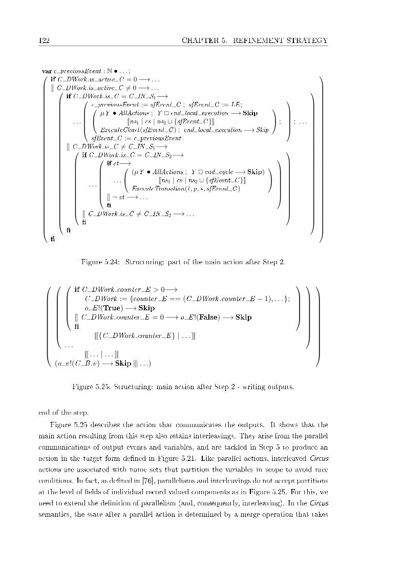
122 CHAPTER 5. REFINEMENT STRATEGY
var c previousEvent : N • . . . ;
if C DWork .is active C = 0−→ . . .8 C DWork .is active C 6= 0−→ . . .
if C DWork .is C = C IN S1−→
. . .
c previousEvent := sfEvent C ; sfEvent C := LE ; µY • AllActions ; Y @ end local execution −→ Skip
Jns1 | cs | ns2 ∪ {sfEvent C}KExecuteChart(sfEvent C ) ; end local execution −→ Skip
;
sfEvent C := c previousEvent
; . . .
8 C DWork .is C 6= C IN S1−→
if C DWork .is C = C IN S2−→
. . .
if ct−→
. . .
(µY • AllActions ; Y @ end cycle −→ Skip)Jns1 | cs | ns2 ∪ {sfEvent C}K
ExecuteTransition(t , p, s, sfEvent C )
8 ¬ ct −→ . . .�
8 C DWork .is C 6= C IN S2 −→ . . .�
�
�
Figure 5.24: Structuring: part of the main action after Step 2.
if C DWork .counter E > 0−→
C DWork := 〈|counter E == (C DWork .counter E − 1), . . . |〉;o E !(True)−→ Skip
8 C DWork .counter E = 0−→ o E !(False)−→ Skip�
||[{C DWork .counter E} | . . . ]||
. . .
||[ . . . | . . . ]||
(o v !(C B .v)−→ Skip 9 . . .)
Figure 5.25: Structuring: main action after Step 2 - writing outputs.
end of the step.
Figure 5.25 describes the action that communicates the outputs. It shows that the
main action resulting from this step also retains interleavings. They arise from the parallel
communications of output events and variables, and are tackled in Step 5 to produce an
action in the target form de�ned in Figure 5.21. Like parallel actions, interleaved Circus
actions are associated with name sets that partition the variables in scope to avoid race
conditions. In fact, as de�ned in [76], parallelisms and interleavings do not accept partitions
at the level of �elds of individual record-valued components as in Figure 5.25. For this, we
need to extend the de�nition of parallelism (and, consequently, interleaving). In the Circus
semantics, the state after a parallel action is determined by a merge operation that takes
5.3. REFINEMENT STRATEGY 123
µY •
var c previousEvent : N • . . . ;
if C DWork .is active C = 0−→ . . .8 C DWork .is active C 6= 0−→ . . .
if C DWork .is C = C IN S1−→
. . .
c previousEvent := sfEvent C ;sfEvent C := LE ;Y ;sfEvent C := c previousEvent
; . . .
8 C DWork .is C 6= C IN S1−→
if C DWork .is C = C IN S2−→
. . .
µZ •
if ct −→ . . .Z8 ¬ ct −→ . . .�
8 C DWork .is C 6= C IN S2 −→ . . .�
�
�
Figure 5.26: Structuring: body of the outmost recursion in the main action after Step 3.
into account the partition. So it is enough to change this merge operation to support the
kind of partitioning that we are using.
The details of the procedure parallelism-resolution are presented in Section 5.3.3.2. It is
rather extensive, as it has to consider the several forms of parallelism that can arise from
the application of the step laws.
Step 3 This deals with the parallelisms left in the previous step, if any. The procedure
recursion-introduction de�nes new recursive actions and proves their equivalence to the
existing parallel actions. The result of this step transforms the main action so that variable
blocks like those in Figure 5.24 change: in the case illustrated, where we have a local event
broadcast to the chart as a whole, the block itself becomes a recursive action as sketched
in Figure 5.26. We present recursion-introduction in Section 5.3.3.4.
Step 4 This step re�nes the main action so that all calls to actions de�ned by schema
operations are re�ned to assignments, by applying the procedure assignment-introduction.
It is presented in Section 5.3.3.5. After this step, we have no abstract speci�cation of data
operations left, just assignments.
Step 5 As already mentioned, as a result of Step 2, output events and data are commu-
nicated in interleaving (see Figure 5.25). The objective of this step is to gather together
the construction of the values to be output, before making all outputs available (still in
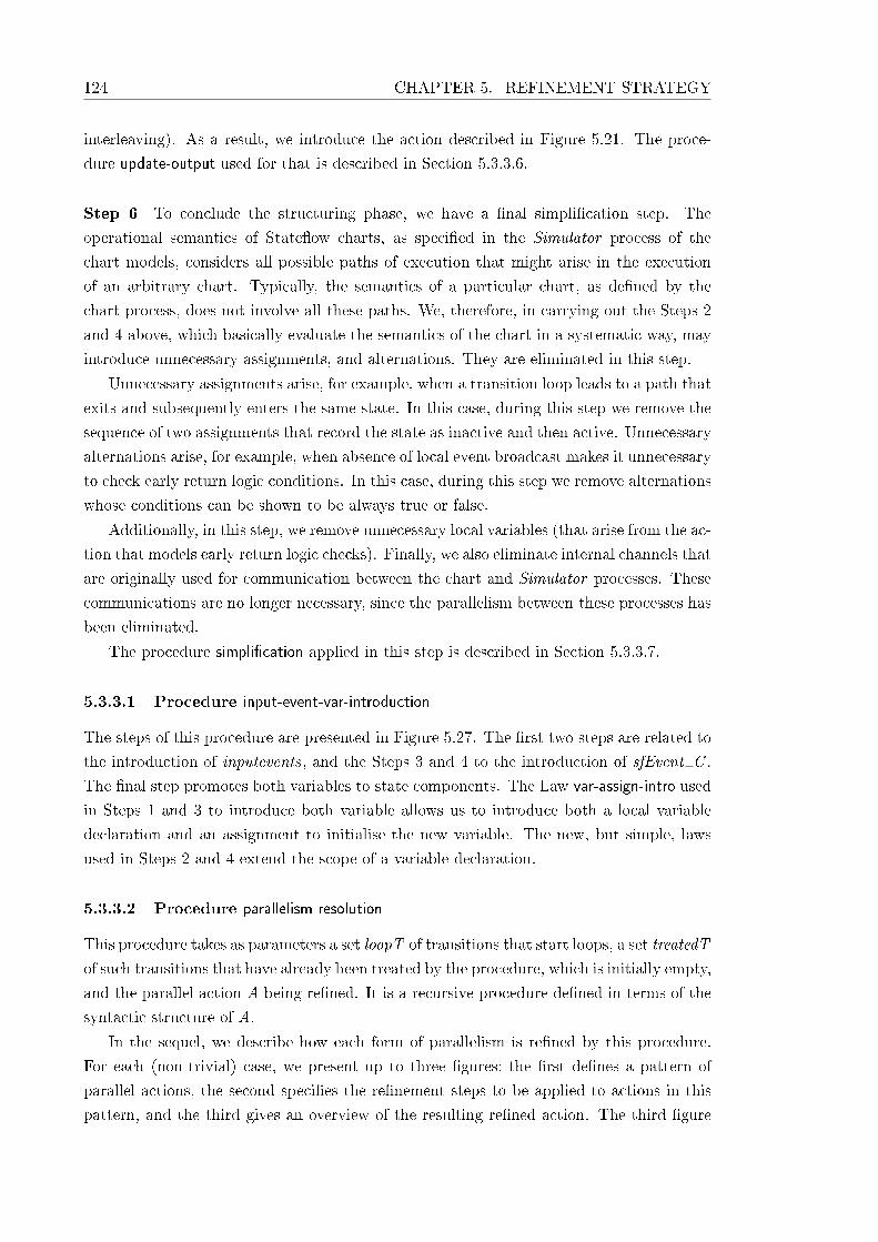
124 CHAPTER 5. REFINEMENT STRATEGY
interleaving). As a result, we introduce the action described in Figure 5.21. The proce-
dure update-output used for that is described in Section 5.3.3.6.
Step 6 To conclude the structuring phase, we have a �nal simpli�cation step. The
operational semantics of State�ow charts, as speci�ed in the Simulator process of the
chart models, considers all possible paths of execution that might arise in the execution
of an arbitrary chart. Typically, the semantics of a particular chart, as de�ned by the
chart process, does not involve all these paths. We, therefore, in carrying out the Steps 2
and 4 above, which basically evaluate the semantics of the chart in a systematic way, may
introduce unnecessary assignments, and alternations. They are eliminated in this step.
Unnecessary assignments arise, for example, when a transition loop leads to a path that
exits and subsequently enters the same state. In this case, during this step we remove the
sequence of two assignments that record the state as inactive and then active. Unnecessary
alternations arise, for example, when absence of local event broadcast makes it unnecessary
to check early return logic conditions. In this case, during this step we remove alternations
whose conditions can be shown to be always true or false.
Additionally, in this step, we remove unnecessary local variables (that arise from the ac-
tion that models early return logic checks). Finally, we also eliminate internal channels that
are originally used for communication between the chart and Simulator processes. These
communications are no longer necessary, since the parallelism between these processes has
been eliminated.
The procedure simpli�cation applied in this step is described in Section 5.3.3.7.
5.3.3.1 Procedure input-event-var-introduction
The steps of this procedure are presented in Figure 5.27. The �rst two steps are related to
the introduction of inputevents, and the Steps 3 and 4 to the introduction of sfEvent C .
The �nal step promotes both variables to state components. The Law var-assign-intro used
in Steps 1 and 3 to introduce both variable allows us to introduce both a local variable
declaration and an assignment to initialise the new variable. The new, but simple, laws
used in Steps 2 and 4 extend the scope of a variable declaration.
5.3.3.2 Procedure parallelism-resolution
This procedure takes as parameters a set loopT of transitions that start loops, a set treatedT
of such transitions that have already been treated by the procedure, which is initially empty,
and the parallel action A being re�ned. It is a recursive procedure de�ned in terms of the
syntactic structure of A.
In the sequel, we describe how each form of parallelism is re�ned by this procedure.
For each (non-trivial) case, we present up to three �gures: the �rst de�nes a pattern of
parallel actions, the second speci�es the re�nement steps to be applied to actions in this
pattern, and the third gives an overview of the resulting re�ned action. The third �gure
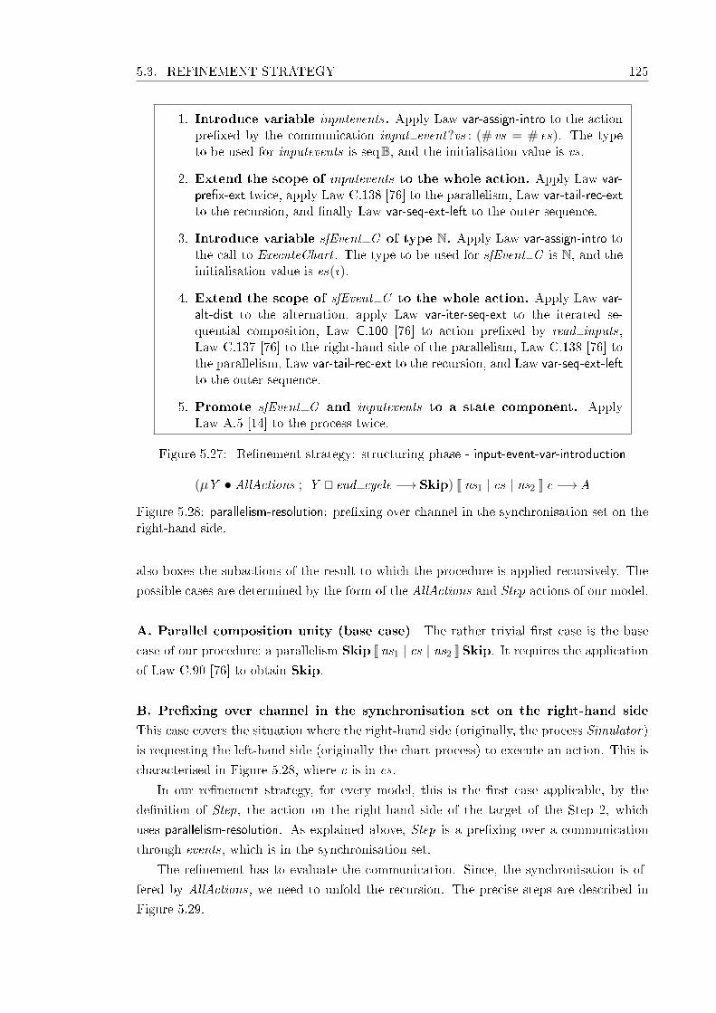
5.3. REFINEMENT STRATEGY 125
1. Introduce variable inputevents. Apply Law var-assign-intro to the actionpre�xed by the communication input event?vs : (# vs = # es). The typeto be used for inputevents is seqB, and the initialisation value is vs.
2. Extend the scope of inputevents to the whole action. Apply Law var-pre�x-ext twice, apply Law C.138 [76] to the parallelism, Law var-tail-rec-extto the recursion, and �nally Law var-seq-ext-left to the outer sequence.
3. Introduce variable sfEvent C of type N. Apply Law var-assign-intro tothe call to ExecuteChart . The type to be used for sfEvent C is N, and theinitialisation value is es(i).
4. Extend the scope of sfEvent C to the whole action. Apply Law var-alt-dist to the alternation, apply Law var-iter-seq-ext to the iterated se-quential composition, Law C.100 [76] to action pre�xed by read inputs,Law C.137 [76] to the right-hand side of the parallelism, Law C.138 [76] tothe parallelism, Law var-tail-rec-ext to the recursion, and Law var-seq-ext-leftto the outer sequence.
5. Promote sfEvent C and inputevents to a state component. ApplyLaw A.5 [14] to the process twice.
Figure 5.27: Re�nement strategy: structuring phase - input-event-var-introduction
(µY • AllActions ; Y @ end cycle −→ Skip) J ns1 | cs | ns2 K c −→ A
Figure 5.28: parallelism-resolution: pre�xing over channel in the synchronisation set on theright-hand side.
also boxes the subactions of the result to which the procedure is applied recursively. The
possible cases are determined by the form of the AllActions and Step actions of our model.
A. Parallel composition unity (base case) The rather trivial �rst case is the base
case of our procedure: a parallelism Skip J ns1 | cs | ns2 KSkip. It requires the applicationof Law C.90 [76] to obtain Skip.
B. Pre�xing over channel in the synchronisation set on the right-hand side
This case covers the situation where the right-hand side (originally, the process Simulator)
is requesting the left-hand side (originally the chart process) to execute an action. This is
characterised in Figure 5.28, where c is in cs.
In our re�nement strategy, for every model, this is the �rst case applicable, by the
de�nition of Step, the action on the right-hand side of the target of the Step 2, which
uses parallelism-resolution. As explained above, Step is a pre�xing over a communication
through events, which is in the synchronisation set.
The re�nement has to evaluate the communication. Since, the synchronisation is of-
fered by AllActions, we need to unfold the recursion. The precise steps are described in
Figure 5.29.

126 CHAPTER 5. REFINEMENT STRATEGY
1. Unfold recursion. Apply Law C.128 [76] to the left-hand side of theparallelism.
2. Expand action calls. Apply to the outermost occurrence of AllActionsthe copy rule exhaustively, except to calls to broadcast .
3. Distribute sequence. Apply Law C.112 [76].
4. Distribute parallelism. Apply Law C.87 [76] from right to left.
5. Introduce deadlocks. Apply Law C.92 [76] exhaustively.
6. Eliminate deadlocks. Apply Law C.114 [76] exhaustively.
7. Recurse. Apply the procedure parallelism-resolution.
Figure 5.29: parallelism-resolution: steps for pre�xing over channel in the synchronisationset on the right-hand side.
c −→ B ; (µY • AllActions ; Y @ end cycle −→ Skip) J ns1 | cs | ns2 K c −→ A
Figure 5.30: parallelism-resolution: result for pre�xing over channel in the synchronisationset on the right-hand side.
In the �rst step, we unfold the recursion on the left-hand side of the parallelism to
obtain an external choice between AllActions and end cycle−→Skip. In the second step,
we expand the de�nition of AllActions and all its subactions (except for the chart action
broadcast , since this is not needed and would lead to nontermination, due to recursive calls
to AllActions itself). The result is of the following form.
(((c1 −→ . . . @ . . . @ cn −→ . . .) ; (µY • AllActions . . .)) @ end cycle −→ Skip) J ns1 | cs | ns2 K c −→ A
It is an external choice, which is sequentially composed with the original recursion; this
sequence is itself in choice with end cycle −→ Skip, and this external choice is in parallel
with the right-hand actions. Steps 3 and 4 distribute the sequential composition over the
external choice, and then the parallel composition over the resulting external choice, to
obtain an external choice of parallel actions. Each parallel action so obtained is pre�xed
by a single communication. Step 5 evaluates the deadlocked parallelisms to Stop, and
Step 6 eliminates them from the choice (using the unit law of external choice). Because
for each possible request c there is necessarily a unique matching initial communication
in AllActions, we are guaranteed to have exactly one non-deadlocked parallelism after
Step 4. Finally, we recursively apply parallelism-resolution to the remaining parallel action.
The parameters of the recursive call are loopT and treatedT unchanged, and the boxed
action in Figure 5.30, which gives the form of the action resulting in this case.
For our example, when this case is applied, we obtain the action below (before recurs-
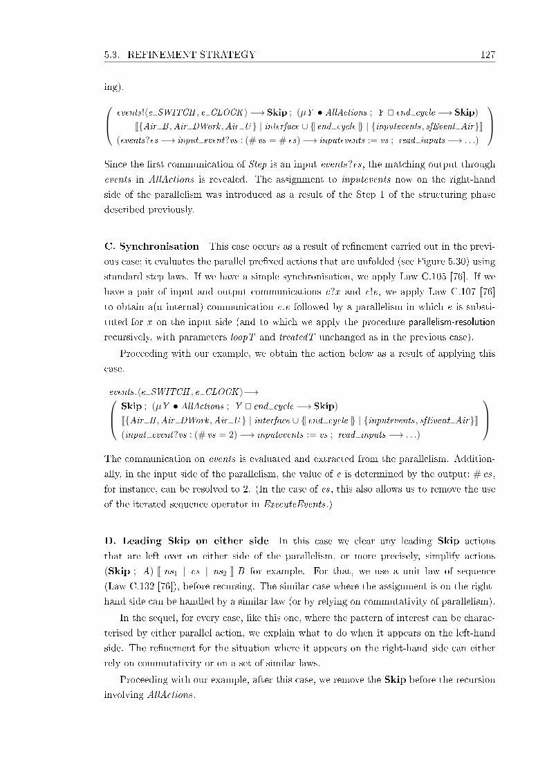
5.3. REFINEMENT STRATEGY 127
ing).
events!〈e SWITCH , e CLOCK 〉 −→ Skip ; (µY • AllActions ; Y @ end cycle −→ Skip)
J{Air B ,Air DWork ,Air U } | interface ∪ {| end cycle |} | {inputevents, sfEvent Air}K(events?es −→ input event?vs : (# vs = # es)−→ inputevents := vs ; read inputs −→ . . .)
Since the �rst communication of Step is an input events?es, the matching output through
events in AllActions is revealed. The assignment to inputevents now on the right-hand
side of the parallelism was introduced as a result of the Step 1 of the structuring phase
described previously.
C. Synchronisation This case occurs as a result of re�nement carried out in the previ-
ous case; it evaluates the parallel pre�xed actions that are unfolded (see Figure 5.30) using
standard step laws. If we have a simple synchronisation, we apply Law C.105 [76]. If we
have a pair of input and output communications c?x and c!e, we apply Law C.107 [76]
to obtain a(n internal) communication c.e followed by a parallelism in which e is substi-
tuted for x on the input side (and to which we apply the procedure parallelism-resolution
recursively, with parameters loopT and treatedT unchanged as in the previous case).
Proceeding with our example, we obtain the action below as a result of applying this
case.
events.〈e SWITCH , e CLOCK 〉−→ Skip ; (µY • AllActions ; Y @ end cycle −→ Skip)
J{Air B ,Air DWork ,Air U } | interface ∪ {| end cycle |} | {inputevents, sfEvent Air}K(input event?vs : (# vs = 2)−→ inputevents := vs ; read inputs −→ . . .)
The communication on events is evaluated and extracted from the parallelism. Addition-
ally, in the input side of the parallelism, the value of e is determined by the output: # es,
for instance, can be resolved to 2. (In the case of es, this also allows us to remove the use
of the iterated sequence operator in ExecuteEvents.)
D. Leading Skip on either side In this case we clear any leading Skip actions
that are left over on either side of the parallelism, or more precisely, simplify actions
(Skip ; A) J ns1 | cs | ns2 K B for example. For that, we use a unit law of sequence
(Law C.132 [76]), before recursing. The similar case where the assignment is on the right-
hand side can be handled by a similar law (or by relying on commutativity of parallelism).
In the sequel, for every case, like this one, where the pattern of interest can be charac-
terised by either parallel action, we explain what to do when it appears on the left-hand
side. The re�nement for the situation where it appears on the right-hand side can either
rely on commutativity or on a set of similar laws.
Proceeding with our example, after this case, we remove the Skip before the recursion
involving AllActions.

128 CHAPTER 5. REFINEMENT STRATEGY
(c −→ A) J ns1 | cs | ns2 K B or A J ns1 | cs | ns2 K (c −→ B)
Figure 5.31: parallelism-resolution: pre�xing over channel not in the synchronisation set oneither side.
E. Pre�xing over channel not in the synchronisation set on either side This
case deals with the communications with the environment. The relevant channels are the
input and output channels (used in the left parallel action) and input event (used in the
right action). In general, this case covers parallelisms as shown in Figure 5.31. A simple
step law pre�x-parallelism-dist-2 carries out the re�nement to extract the communication
from the parallelism. We can show that its provisos always hold, since the structure of
the process we are re�ning is quite restricted. For instance, it is easy to show that for
all communications that are relevant to this case, the �rst possible communication on the
opposite side of the parallel composition is over a channel in the synchronisation set. (On
the left, we have communications on input and output channels; according to the de�nition
of Simulator , at these points Step is always waiting for an internal communication. On the
right, we have a communication on input events, and the de�nition of AllActions shows
that its initials only contains communications in the synchronisation set.)
Proceeding with our example, we obtain the action below.
events.〈e SWITCH , e CLOCK 〉 −→ input event?vs : (# vs = 2)−→ µY • AllActions ; Y @ end cycle −→ Skip
J{Air B ,Air DWork ,Air U } | interface ∪ {| end cycle |} | {inputevents, sfEvent Air}K(inputevents := vs ; read inputs −→ . . .)
The communication with the environment on input events is extracted from the paral-
lelism.
F. Leading assignment on either side This case covers parallel actions of the form
(v := e ; A) J ns1 | cs | ns2 K B or AJns1 | cs | ns2 K (v := e ; B). Basically, we use
our simple law assign-par-dist to extract the assignment from the parallelism. Its provisos
require that the assigned variables are in the name set of the parallelism, and are not
used by the other parallel action. These always hold by construction, since assignments
result from the re�nement of schema operations in the normalisation phase, or from the
introduction of local variables in the Step 1 of the structuring phase. In the �rst case, the
assignments change state components, which are always used exclusively by the left-hand
side of the parallelism, and whose names are in the appropriate name set by construction
of the model. In the second case, the local variable and the assignment are introduced in
one side of the parallelism, thus the other side does not use them, and when the scope of
the local variable is expanded over the parallelism on the other side, the variable name is
included in the appropriate name set. Therefore, in both cases, the provisos raised by this
case are satis�ed.
Proceeding with our example, the re�nement in this case extracts the assignment

5.3. REFINEMENT STRATEGY 129
A1
||[ns1 |⋃i : 2 . . n • nsi ]||
(. . . ||[ nsn−1 | nsn ]|| An)
; B
J nsx | cs | nsy K C
Figure 5.32: parallelism-resolution: leading interleaving on the left-hand side. A1
||[ns1 |⋃i : 2 . . n • nsi ]||
(. . . ||[ nsn−1 | nsn ]|| An)
; (B J nsx | cs | nsy K C )
Figure 5.33: parallelism-resolution: result for leading interleaving on the left-hand side.
inputevents := vs from the parallelism. Moreover, further recursive applications of previous
cases extract the internal communication read inputs, and the external communication in
AllActions over the channel i temp corresponding to the input variable temp. In general,
however, there may be several input variables and, consequently, several input communi-
cations in interleaving. This is the object of the next case.
G. Leading interleaving on the left-hand side This case covers actions characterised
as shown in Figure 5.32. We have on the left an interleaving of actions A1, . . .An , followed
by an action B , all in parallel with another action C . Each Ai is associated in the inter-
leaving with a name set nsi , so that the name set of the interleaving of actions Ai to An
is the union of the sets nsi to nsn .
In this case, we simply apply the step law C.84 [76] to extract the interleaving from the
parallelism (and recursively call the parallelism-resolution procedure). The result is shown
in Figure 5.33.
The provisos of Law C.84 always hold by the construction of the model. This case only
arises after the re�nement related to communications over read inputs and write outputs.
In the �rst case, the �rst communication on the right-hand side is over the channel chart in
the synchronisation set, and in the second case, the �rst communication is over end cycle,
which is also in the synchronisation set. All the communications in the interleaving are
over channels not in the synchronisation set because they communicate inputs and outputs
of the chart. The variables written by the interleaving are not used by the right-hand side
of the parallelism. In the case the interleaving preceded by read inputs, the variables
written by the interleaving are the input variables, and in the case of the interleaving
preceded by write outputs, the written variables correspond to event counters. In both
cases, these variables are only written by the action on the left-hand side of the parallelism,
which originates from the chart process, and are contained in its name set. Moreover, both
parallel actions are divergence free, also by construction of the model and its re�nement.
H. Alternation followed by sequence, on either side As already mentioned, the
structure of AllActions and Step involves a number of alternations. This case covers their
treatment, considering actions of the form shown in Figure 5.34 or the similar cases where

130 CHAPTER 5. REFINEMENT STRATEGY
if g −→ A1
8¬ g −→ A2
�
; B
J ns1 | cs | ns2 K C
Figure 5.34: parallelism-resolution: alternation followed by sequence, on either side.
the alternation is on the right-hand side of the parallelism. All alternations have mutually
exclusive guards g and ¬ g .
Proceeding with our example, at this stage, we have the action below, where the alter-
nations now shown on the right parallel action are originally part of ExecuteEvent .
events.〈e SWITCH , e CLOCK 〉 −→ input event?vs : (# vs = 2)−→ inputevents := vs;
read inputs−→
µY • AllActions ; Y @ end cycle −→ Skip
J{Air B ,Air DWork ,Air U } | interface ∪ {| end cycle |} | {inputevents, sfEvent Air}K
if inputevents(1) = True−→
sfEvent Air := e SWITCH ; ExecuteChart(sfEvent Air)
8 inputevents(1) = False−→ Skip
�
;
if inputevents(2) = True−→
sfEvent Air := e CLOCK ; ExecuteChart(sfEvent Air)
8 inputevents(2) = False−→ Skip
�
;
write outputs −→ end cycle −→ Skip
In general, the alternations can involve checks that depend on the current state of the
chart, for instance, the veri�cation of the guard of a transition, or can decide how to
proceed based solely on the structure of the chart. These arise from the generality of the
semantics encoded in the process Simulator . The two types of alternation can be easily
distinguished by the names used in the guards. If a guards refers to state components,
it is of the �rst type. If not, it is of the second type, and can be eliminated using the
static information that de�nes the structure of the chart. This is achieved in this step. In
our example above, the alternation refers to the state component inputevents and is not
eliminated.
The re�nement steps to be carried out in this case are shown in Figure 5.35, and the
possible outcomes of this case are shown in Figure 5.36. We �rst distribute the sequential
composition over the alternation, and then the parallelism using the fact that the guards
of the alternation are mutually exclusive. Next, if the guard refers to state components, we
recursively apply the procedure parallelism-resolution to the actions in each branch. If the
guard does not refer to state components, we remove the alternation using the de�nitions
of constants like s O� 3, states, and transitions (see Appendix C). Finally, we recursively
apply this procedure to the remaining action with the remaining parameters unchanged.
The result depends on whether the alternation is eliminated or not: both option are

5.3. REFINEMENT STRATEGY 131
1. Apply Law alt-seq-dist.
2. Distribute parallelism. Apply Law alt-par-dist.
3. If g refers to a state component, recursively apply parallelism-resolution toeach branch. Otherwise, apply Law alt-elim, before recursing.
Figure 5.35: parallelism-resolution: steps for alternation followed by sequence, on eitherside.
if g −→ (A J ns1 | cs | ns2 K B1)
8 ¬ g −→ (A J ns1 | cs | ns2 K B2)
�
or (A J ns1 | cs | ns2 K B)
Figure 5.36: parallelism-resolution: possible results for alternation followed by sequence, oneither side.
shown in Figure 5.36.
If we proceed with our example, we obtain the following action.
events.〈e SWITCH , e CLOCK 〉 −→ input event?vs : (# vs = 2)−→ inputevents := vs ; read inputs−→
if inputevents(1) = True−→
µY • AllActions ; Y @ end cycle −→ Skip
J . . . K
sfEvent Air := e SWITCH ; ExecuteChart(sfEvent Air);if inputevents(2) = True−→
sfEvent Air := e CLOCK ; ExecuteChart(sfEvent Air)
8 inputevents(2) = False−→ Skip
�
;
write outputs −→ end cycle −→ Skip
8 inputevents(1) = False−→
µY • AllActions ; Y @ end cycle −→ Skip
J . . . K
if inputevents(2) = True−→
sfEvent Air := e CLOCK ; ExecuteChart(sfEvent Air)
8 inputevents(2) = False−→ Skip
�
;
write outputs −→ end cycle −→ Skip
�
At this stage, recursive calls to parallelism-resolution lead to a number of applications of
the previous cases, until we reach a parallelism whose right-hand parallel action is a call
to ExecuteChart .
I. Call action on either side Whenever a call action is the leading action in one of the
sides of the parallelism, and none of the other cases apply, we expand it using a procedure
copy. This simply replaces a call to an action with its de�nition, with the appropriate
parameters substituted. This procedure is described in Section 5.3.3.3. It basically applies
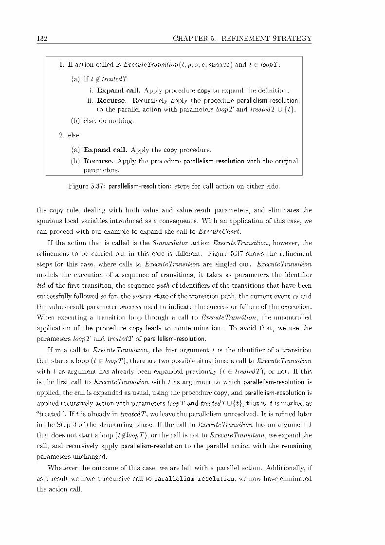
132 CHAPTER 5. REFINEMENT STRATEGY
1. If action called is ExecuteTransition(t , p, s, e, success) and t ∈ loopT .
(a) If t 6∈ treatedTi. Expand call. Apply procedure copy to expand the de�nition.ii. Recurse. Recursively apply the procedure parallelism-resolution
to the parallel action with parameters loopT and treatedT ∪ {t}.(b) else, do nothing.
2. else
(a) Expand call. Apply the copy procedure.
(b) Recurse. Apply the procedure parallelism-resolution with the originalparameters.
Figure 5.37: parallelism-resolution: steps for call action on either side.
the copy rule, dealing with both value and value-result parameters, and eliminates the
spurious local variables introduced as a consequence. With an application of this case, we
can proceed with our example to expand the call to ExecuteChart .
If the action that is called is the Simmulator action ExecuteTransition, however, the
re�nement to be carried out in this case is di�erent. Figure 5.37 shows the re�nement
steps for this case, where calls to ExecuteTransition are singled out. ExecuteTransition
models the execution of a sequence of transitions; it takes as parameters the identi�er
tid of the �rst transition, the sequence path of identi�ers of the transitions that have been
successfully followed so far, the source state of the transition path, the current event ce and
the value-result parameter success used to indicate the success or failure of the execution.
When executing a transition loop through a call to ExecuteTransition, the uncontrolled
application of the procedure copy leads to nontermination. To avoid that, we use the
parameters loopT and treatedT of parallelism-resolution.
If in a call to ExecuteTransition, the �rst argument t is the identi�er of a transition
that starts a loop (t ∈ loopT ), there are two possible situations: a call to ExecuteTransition
with t as argument has already been expanded previously (t ∈ treatedT ), or not. If this
is the �rst call to ExecuteTransition with t as argument to which parallelism-resolution is
applied, the call is expanded as usual, using the procedure copy, and parallelism-resolution is
applied recursively action with parameters loopT and treatedT ∪{t}, that is, t is marked as�treated". If t is already in treatedT , we leave the parallelism unresolved. It is re�ned later
in the Step 3 of the structuring phase. If the call to ExecuteTransition has an argument t
that does not start a loop (t 6∈loopT ), or the call is not to ExecuteTransition, we expand the
call, and recursively apply parallelism-resolution to the parallel action with the remaining
parameters unchanged.
Whatever the outcome of this case, we are left with a parallel action. Additionally, if
as a result we have a recursive call to parallelism-resolution, we now have eliminated
the action call.

5.3. REFINEMENT STRATEGY 133
(SchAct ; (µY • AllActions ; Y @ end cycle −→ Skip)) J ns1 | cs | ns2 K A
Figure 5.38: parallelism-resolution: leading schema operation on the left-hand side.
SchAct ; ((µY • AllActions ; Y @ end cycle −→ Skip) J ns1 | cs | ns2 K A)
Figure 5.39: parallelism-resolution: result for leading schema operation on the left-handside.
A J ns1 | cs | ns2 K (µX • B [X ])
Figure 5.40: parallelism-resolution: explicit recursion on the right-hand side.
A J ns1 | cs | ns2 K B [(µX • B [X ])]
Figure 5.41: parallelism-resolution: result for explicit recursion on the right-hand side.
J. Leading schema operation on the left-hand side In our example, after expanding
ExecuteChart , several of the previous cases apply. Eventually, we reach a parallelism where
on the left-hand side we have a schema operation. The process Simulator does not have
schema operations, and so this kind of action can only appear on the left. They are used to
model chart actions (entry, during, and so on) and activation and deactivation operations.
Just like assignments, these schemas are extracted from the parallelism.
Figure 5.38 shows the general pattern covered in this case; as said above, it arises
from applications of the previous cases to unfold the recursion on AllActions. Figure 5.39
presents the result of this step of the procedure, which is just an application of Law C.73 [76].
The provisos require that the variables modi�ed by the schema are in the name set of the
parallelism, and are not used by the other parallel action. These always hold by construc-
tion of the model. (The Simulator process does not change or use the state of the chart
process.) As usual, we recursively apply the procedure to the remaining parallel action as
indicated in Figure 5.39. The other parameters of the recursive application are loopT and
treatedT (both unchanged).
K. Explicit recursion on the right-hand side The action ExecuteChart involves
communication that request the execution of a chart action. These are speci�ed as se-
quences of Circus actions, some of which may correspond to local event broadcasts. In Step,
at this point, we have, therefore, a call to one of the Simulator actions LocalEventEntry ,
LocalEventDuring , LocalEventExit , LocalEventCondition or LocalEventTransition, depend-
ing on the type of chart action. These Simulator actions are all recursions (that o�er a
choice between treating a local event and recursing, or signalling the end of the chart
action). Additionally, at several points in Step, we have a call to transitionActionCheck ,
which is also a recursion (that checks the status of the substates of another state as part
of the modelling of the check of early return logic condition).
In this case, we unfold the recursions. It applies to actions of the form shown in

134 CHAPTER 5. REFINEMENT STRATEGY
1. Distribute sequence. Apply Law C.112 [76].
2. Distribute parallelism. Apply Law C.87 [76].
3. Introduce deadlocks. Apply Law C.92 [76].
4. Eliminate deadlocks. Apply Law C.114 [76].
5. Recurse. Apply the procedure parallelism-resolution.
Figure 5.42: parallelism-resolution: steps for leading pre�xing over channel in the synchro-nisation set on the left-hand side.
Figure 5.40, applies Law C.128 [76], and produces the action in Figure 5.41, to which
parallelism-resolution is applied recursively. This does not lead to nontermination because
any chart action involves only a �nite number of local event broadcasts, and every state
has a �nite number of substates.
L. Leading pre�xing over channel in the synchronisation set on the left-hand
side A Circus action that models a local event broadcast uses internal channels (local event
and end action, both in the synchronisation set) to control the Simulator . In this case, we
consider a parallelism where the left-hand action is a communication on such a channel. In
the right-hand action, at these points, Step always o�ers a(n external) choice that accepts
the communication, followed by some other action. The general pattern that is covered is
c −→ A J ns1 | cs | ns2 K (c −→ B1 @ d −→ B2) ; C , where both c and d are in cs.
In this step, re�nement resolves the external choice. The particular re�nement steps to
be carried out are shown in Figure 5.42. We distribute the sequence and the parallelism
over the external choice, eliminate the deadlocked parallel actions. The provisos of the
laws applied follow from the fact that c and d are both in the synchronisation set, and
are di�erent. The result is the action c −→ A J ns1 | cs | ns2 K c −→ (B1 ; C ); a recursive
application of parallelism-resolution to it solves the synchronisation.
M. Local event broadcast In the Simulator actions LocalEventEntry , LocalEventExit ,
LocalEventDuring , LocalEventCondition or LocalEventTransition, we have a call to the
action TreatLocalEvent . It decides whether to reexecute the whole chart or a speci�c chart
state, depending on the kind of broadcast.
This call to TreatLocalEvent cannot be expanded indiscriminately (as in the case call
action on either side, for instance) because the resulting action can involve a recursive
call to ExecuteChart , or to ExecuteState, the Simulator action that models the execution
of a chart state. The situation is similar to that of calls to ExecuteTransition, which are
singled out in the case call action on either side. Here, however, we have a di�erent
pattern because we do not have a tail recursion.
Calls to TreatLocalEvent occur in parallel with the Circus actions of the chart process
that model local event broadcasts. In those, we have recursions, which provide the services
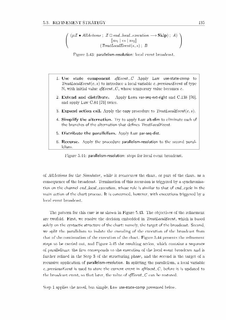
5.3. REFINEMENT STRATEGY 135
(µZ • AllActions ; Z @ end local execution −→ Skip) ; A)Jns1 | cs | ns2K
(TreatLocalEvent(e, s) ; B
Figure 5.43: parallelism-resolution: local event broadcast.
1. Use state component sfEvent C Apply Law use-state-comp toTreatLocalEvent(e, s) to introduce a local variable c previousEvent of typeN, with initial value sfEvent C , whose temporary value becomes e.
2. Extend and distribute. Apply Laws var-seq-ext-right and C.138 [76],and apply Law C.84 [76] twice.
3. Expand action call. Apply the copy procedure to TreatLocalEvent(e, s).
4. Simplify the alternation. Try to apply Law alt-elim to eliminate each ofthe branches of the alternation that de�nes TreatLocalEvent .
5. Distribute the parallelism. Apply Law par-seq-dist.
6. Recurse. Apply the procedure parallelism-resolution to the second paral-lelism.
Figure 5.44: parallelism-resolution: steps for local event broadcast.
of AllActions for the Simulator , while it reexecutes the chart, or part of the chart, as a
consequence of the broadcast. Termination of this recursion is triggered by a synchronisa-
tion on the channel end local execution, whose role is similar to that of end cycle in the
main action of the chart process. It is concerned, however, with executions triggered by a
local event broadcast.
The pattern for this case is as shown in Figure 5.43. The objectives of the re�nement
are twofold. First, we resolve the decision embedded in TreatLocalEvent , which is based
solely on the syntactic structure of the chart: namely, the target of the broadcast. Second,
we split the parallelism to isolate the encoding of the execution of the broadcast from
that of the continuation of the execution of the chart. Figure 5.44 presents the re�nement
steps to be carried out, and Figure 5.45 the resulting action, which contains a sequence
of parallelisms: the �rst corresponds to the execution of the local event broadcast and is
further re�ned in the Step 3 of the structuring phase, and the second is the target of a
recursive application of parallelism-resolution. In splitting the parallelism, a local variable
c previousEvent is used to store the current event in sfEvent C , before it is updated to
the broadcast event, so that later, the value of sfEvent C can be restored.
Step 1 applies the novel, but simple, Law use-state-comp presented below.
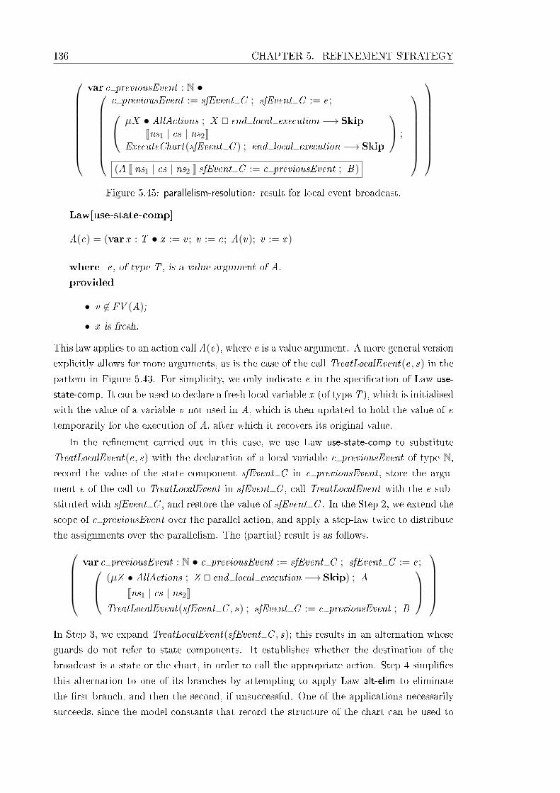
136 CHAPTER 5. REFINEMENT STRATEGY
var c previousEvent : N •
c previousEvent := sfEvent C ; sfEvent C := e; µX • AllActions ; X @ end local execution −→ SkipJns1 | cs | ns2K
ExecuteChart(sfEvent C ) ; end local execution −→ Skip
;
(A J ns1 | cs | ns2 K sfEvent C := c previousEvent ; B)
Figure 5.45: parallelism-resolution: result for local event broadcast.
Law[use-state-comp]
A(e) = (var x : T • x := v ; v := e; A(v); v := x )
where e, of type T , is a value argument of A.
provided
• v 6∈ FV (A);
• x is fresh.
This law applies to an action call A(e), where e is a value argument. A more general version
explicitly allows for more arguments, as is the case of the call TreatLocalEvent(e, s) in the
pattern in Figure 5.43. For simplicity, we only indicate e in the speci�cation of Law use-
state-comp. It can be used to declare a fresh local variable x (of type T ), which is initialised
with the value of a variable v not used in A, which is then updated to hold the value of e
temporarily for the execution of A, after which it recovers its original value.
In the re�nement carried out in this case, we use Law use-state-comp to substitute
TreatLocalEvent(e, s) with the declaration of a local variable c previousEvent of type N,record the value of the state component sfEvent C in c previousEvent , store the argu-
ment e of the call to TreatLocalEvent in sfEvent C , call TreatLocalEvent with the e sub-
stituted with sfEvent C , and restore the value of sfEvent C . In the Step 2, we extend the
scope of c previousEvent over the parallel action, and apply a step-law twice to distribute
the assignments over the parallelism. The (partial) result is as follows.var c previousEvent : N • c previousEvent := sfEvent C ; sfEvent C := e; (µZ • AllActions ; Z @ end local execution −→ Skip) ; A
Jns1 | cs | ns2KTreatLocalEvent(sfEvent C , s) ; sfEvent C := c previousEvent ; B
In Step 3, we expand TreatLocalEvent(sfEvent C , s); this results in an alternation whose
guards do not refer to state components. It establishes whether the destination of the
broadcast is a state or the chart, in order to call the appropriate action. Step 4 simpli�es
this alternation to one of its branches by attempting to apply Law alt-elim to eliminate
the �rst branch, and then the second, if unsuccessful. One of the applications necessarily
succeeds, since the model constants that record the structure of the chart can be used to

5.3. REFINEMENT STRATEGY 137
determine that one of the guards of the alternation is True and the other is False. For
the sake of example, we assume that the alternation simpli�es to the �rst branch, and we
obtain the result below.var c previousEvent : N • c previousEvent := sfEvent C ; sfEvent C := e; (µZ • AllActions ; Z @ end local execution −→ Skip) ; A
Jns1 | cs | ns2KExecuteChart(sfEvent C ) ; end local execution −→ Skip ; sfEvent C := c previousEvent ; B
Finally, Step 5 applies the novel Law par-seq-dist to separate the parallelism into a sequence
of two parallel compositions. It considers a parallelism of sequences (and relates it to a
sequence of parallelisms). The action of the left-hand side of the parallelism is the second
component of a pair (M ,N ) of actions de�ned by mutual recursion. The �rst component
M may o�er a communication over a channel l and start the second component N , and N
o�ers a choice between calling M and recursing on N or synchronising on a channel el and
terminating. The �rst action of the sequence on the right-hand side of the parallelism is
a simple recursion that communicates on l , conditionally recurses, and synchronises on el
afterwards. The second action of the right-hand side starts with a synchronisation on el .
In our application of this law as part of our strategy, N is the recursion o�ering
AllActions with el as end local execution. The action M is AllActions itself, which ac-
cepts communications on a channel local event and then starts a new recursion identical
to the one that called it. So, l is the channel local event . The actions ExecuteChart and
ExecuteState are both recursions: they treat local event broadcasts themselves, and that
involves recursive calls to either ExecuteChart or ExecuteState. For example, ExecuteChart
can be written as a parametrised explicit recursion as follows.
µX • ce : EVENT • chart?c −→ status!(c.identi�er)?active−→
if active = True−→ . . .
8 active = False−→ activate!(c.identi�er)−→
if c.default 6= nulltransition.identi�er ∨ c.decomposition = CLUSTER −→ . . .
8 c.default = nulltransition.identi�er ∧ c.decomposition = SET−→
if c.substates = 〈〉−→ Skip
8 c.substates 6= 〈〉−→ . . . ; executeentryaction!(�rst .identi�er)−→
local event?e?s−→ if s.type = CHART −→ X (e)
8 s.type 6= CHART −→ ExecuteState(s, e)
�
;
end local execution −→ . . .
@end action −→ Skip
; . . .
�
�
�
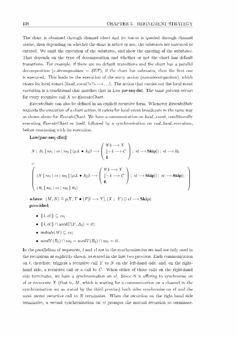
138 CHAPTER 5. REFINEMENT STRATEGY
The chart is obtained through channel chart and its status is queried through channel
status, then depending on whether the chart is active or not, the substates are executed or
entered. We omit the execution of the substates, and show the entering of the substates.
That depends on the type of decomposition and whether or not the chart has default
transitions. For example, if there are no default transitions and the chart has a parallel
decomposition (c.decomposition = SET ), if the chart has substates, then the �rst one
is executed. This leads to the execution of the entry action (executeentryaction), which
caters for local events (local event?e?s−→ . . .). The action that carries out the local event
execution is a conditional that matches that in Law par-seq-dist. The same pattern occurs
for every recursive call X to ExecuteChart .
ExecuteState can also be de�ned in an explicit recursive form. Whenever ExecuteState
requests the execution of a chart action, it caters for local event broadcasts in the same way
as shown above for ExecuteChart . We have a communication on local event , conditionally
executing ExecuteChart or itself, followed by a synchronisation on end local execution,
before continuing with its execution.
Law[par-seq-dist]
N ; B1 J ns1 | cs | ns2 K (µX • A2[l −→
if b −→ X
8¬ b −→ C
�
; el −→ Skip]) ; el −→ B2
= (N J ns1 | cs | ns2 K (µX • A2[l −→
if b −→ X
8¬ b −→ C
�
; el −→ Skip]) ; el −→ Skip);
(B1 J ns1 | cs | ns2 K B2)
where (M ,N ) =̂ µX ,Y • (F [l −→ Y ], (X ; Y ) @ el −→ Skip)
provided
• {| l , el |} ⊆ cs;
• {| l , el |} ∩ usedC (F ,A2) = ∅;
• initials(M ) ⊆ cs;
• usedV (B1) ∩ ns2 = usedV (B2) ∩ ns1 = ∅.
In the parallelism of sequences, l and el are in the synchronisation set and are only used in
the recursions as explicitly shown, as stated in the �rst two provisos. Each communication
on l , therefore, triggers a recursive call Y to N on the left-hand side, and, on the right-
hand side, a recursive call or a call to C . When either of those calls on the right-hand
side terminates, we have a synchronisation on el . Since N is o�ering to synchronise on
el or reexecute X (that is, M , which is waiting for a communication on a channel in the
synchronisation set as stated by the third proviso) both sides synchronise on el and the
most recent recursive call to N terminates. When the recursion on the right-hand side
terminates, a second synchronisation on el prompts the mutual recursion to terminate.

5.3. REFINEMENT STRATEGY 139
Since there is no possibility of B2 communicating with the mutual recursion or B1 commu-
nicating with the simple recursion because both recursions terminate synchronously, and
B2 does not use variables written by the mutual recursion and B1 does not use variables
written by the simple recursion (last proviso), we can separate the parallel action in two
parallel actions in sequence.
As already mentioned, we apply this Law par-seq-dist to the action obtained from
step 4, with the recursion on the left-hand side as N , ExecuteChart(sfEvent C ) as the
recursion on the right-hand side, local event as l and end local execution as el . Since
local event , end local execution and initials(AllActions) are all in the synchronisation set,
each parallel action does not use the variables written by the other, and local event and
end local execution are, respectively, only used immediately before and after a recursive
call in both AllActions and ExecuteChart , the application is successful. For our example,
we have the following result.var c previousEvent : N • c previousEvent := sfEvent C ; sfEvent C := e;
(µZ • AllActions ; Z @ end local execution −→ Skip)
Jns1 | cs | ns2KExecuteChart(sfEvent C ) ; end local execution −→ Skip
;
A J ns1 | cs | ns2 K sfEvent C := c previousEvent ; B
Step 6 applies the procedure parallelism-resolution to the second parallel action.
The resulting action shown in Figure 5.45 is for a local event broadcast directed at the
whole chart, as is the example shown above. The same steps apply for broadcasts directed
at particular states. The resulting action di�ers solely on the action call that executes the
state: instead of ExecuteChart(sfEvent C ), we have ExecuteState(s, sfEvent C ), where s
is the target state.
N. Leading local variable declaration on either side Following the execution of a
local event broadcast, both the chart and the Simulator processes carry out early return
logic checks. For that, they use a local boolean variable b that records the result of the
check. In our example, the action B above is such a variable block. In this case, therefore,
we consider parallelisms A J ns1 | cs | ns2 K (var b : B • B). We apply Laws var-rename
and C.138 [76] to give b a fresh name and expand its scope out of the parallelism, before
recursing. The result is a block like var bi : B • (A J ns1 | cs | ns2 ∪ {bi} K B [bi/b]), where
bi is a fresh name.
Since parallelism-resolution is recursive, termination is an issue. In the sequel, we present
a detailed argument based on the structure of the parallel actions found in our chart models.
Termination of parallelism-resolution Since parallelism-resolution is recursive, we now
address the issue of its termination. Our argument is based on the structure of the right-
hand parallel action.

140 CHAPTER 5. REFINEMENT STRATEGY
There are two base cases: A, and I. The other cases can be divided into three groups: those
that do not change the right-hand action, those that reduce its structure, and those that
expand it. The cases in the �rst group can be applied only a �nite number of times: they
do not lead to an in�nite sequence of steps that do not reduce the right-hand action. As we
explain next, this is due to the structure of the left-hand parallel action: after applications
of such cases, we eventually apply a case in another group.
The cases in this �rst group are: B, D, E, F, G, H, I, J, N. Case B simpli�es the
left-hand action to allow the pre�x on the right-hand action to be addressed by case C.
Cases D, E, F, G and N remove an action on the left to apply the other cases to the
remaining action to resolve the parallelism. Any sequence of applications of these cases
must be followed by an application of case C, or case B followed by C, which reduce
the structure of the right-hand action. Case H simpli�es the structure on the left-hand
action to allow the other cases to handle the actions in each branch of the alternation.
Finally, case I for the left-hand action only expands the de�nition of broadcast , which is
not expanded by case B. Each occurrence of this case must necessarily be followed by an
application of case L, which reduces the structure of the right-hand action.
For cases in the second group, since each application reduces the structure of the right-
hand parallel action to that of one of its components, eventually we reach end cycle−→Skip.Re�nement, using cases B and C, leads to the application of the base case A, which elim-
inates the parallelism and terminates the procedure. This group contains the cases C, D,
E, F, H, L, and N.
The cases in the third group, that is, I, K, and M, expand the right parallel action.
Case I could potentially expand calls to recursive actions. If such an action allowed a non-
terminating recursion, then the procedure parallelism-resolution would not terminate due to
successive indiscriminate applications of I. The right parallel actions, however, come from
the Simulator process, so we know exactly to which actions case I is applied. The only
recursive action as above is ExecuteTransition, when executing a transition that starts a
loop. Case I treats it as a special case, only expanding once the execution of a transition
that starts a loop.
Case M is applied to each local event broadcast. Since there is only a �nite number
of broadcasts in a chart, and recursions introduced by local event broadcasts are not
unfolded, this case only expands the right-hand action a �xed number of times. All the
actions introduced in this expansion can be treated by the remaining cases.
Case K, similarly to case I, unfolds the recursion, but in the recursive application of
parallelism-resolution, case F is applied to extract the assignment to sfEvent C , and then
case N is applied to the right-hand side to treat the local variable declaration that always
follows a call to TreatLocalEvent . In any case, any such recursion can be unfolded up to
a �nite number of times (number of local event broadcasts in an action). Eventually, an
application of case C, resolving a synchronisation over channel end action) will terminate
the recursion. The channel end action signals the end of a chart action.
Finally, case K unfolds a recursion on the right hand side, this recursions are associated
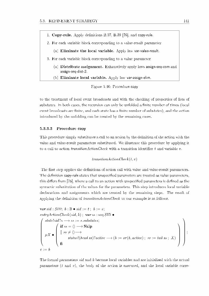
5.3. REFINEMENT STRATEGY 141
1. Copy-rule. Apply de�nitions B.37, B.39 [76], and copy-rule.
2. For each variable block corresponding to a value-result parameter
(a) Eliminate the local variable. Apply law var-value-result.
3. For each variable block corresponding to a value parameter
(a) Distribute assignment. Exhaustively apply laws assign-seq-com andassign-seq-dist-2.
(b) Eliminate local variable. Apply law var-assign-elim.
Figure 5.46: Procedure copy
to the treatment of local event broadcasts and with the checking of properties of lists of
substates. In both cases, the recursion can only be unfolded a �nite number of times (local
event broadcasts are �nite, and each state has a �nite number of substates), and the action
introduced by the unfolding can be treated by the remaining cases.
5.3.3.3 Procedure copy
This procedure simply substitutes a call to an action by the de�nition of the action with the
value and value-result parameters substituted. We illustrate this procedure by applying it
to a call to action transitionActionCheck with a transition identi�er t and variable v .
transitionActionCheck(t , v)
The �rst step applies the de�nitions of action call with value and value-result parameters.
The de�nition copy-rule states that unspeci�ed parameters are treated as value parameters,
this di�ers from [76], where a call to an action with unspeci�ed parameters is de�ned as the
syntactic substitution of the values for the parameters. This step introduces local variable
declarations and assignments which are treated by the remaining steps. The result of
applying the de�nition of transitionActionCheck to our example is as follows.
var sid : SID ; b : B • sid := t ; b := v ;
entryActionCheck(sid , b) ; var ss : seqSID •state!sid?s −→ ss := s.substates;
µX •
if ss = 〈〉−→ Skip
8 ss 6= 〈〉−→status!(head ss)?active −→ (b := or(b, active) ; ss := tail ss ; X )
�
;
v := b
The formal parameters sid and b become local variables and are initialised with the actual
parameters (t and v), the body of the action is executed, and the local variable corre-

142 CHAPTER 5. REFINEMENT STRATEGY
sponding to the value-result parameter is assigned to the actual parameter v .
For each blocks var x : T • x := y ; A ; y := x introduced by de�nition B.39 [76],
Step 2(a) removes the local variable. In our example, this step applies to the parameter b; it
is eliminated by an application of the law var-value-result that substitutes the local variable
by the actual parameter, provided the actual parameter is not used in the de�nition of the
action, resulting in the following action.
var sid : SID • sid := t ;
entryActionCheck(sid , v) ; var ss : seqSID •state!sid?s −→ ss := s.substates;
µX •
if ss = 〈〉−→ Skip
8 ss 6= 〈〉−→status!(head ss)?active −→ (v := or(v , active) ; ss := tail ss ; X )
�
In step 3, for each local variable introduced in step 1 by de�nition B.37 [76], we distribute
the assignment over the variable block, and eliminate it. In our example, the result of this
step is the action below.
entryActionCheck(t , v) ; var ss : seqSID •state!t?s −→ ss := s.substates;
µX •
if ss = 〈〉−→ Skip
8 ss 6= 〈〉−→status!(head ss)?active −→ (v := or(v , active) ; ss := tail ss ; X )
�
The assignment to sid is distributed over the sequential composition towards the end of
the local variable block, and the local variable is eliminated.
5.3.3.4 Procedure recursion-introduction
This procedure is used in Step 3 of the structuring phase. It receives the same parameters
loopT and treatedT as parallelism-resolution, which it uses to call that procedure. It acts on
the body of the outermost recursion in the main action to transform the remaining parallel
actions into recursions.
So far, in resolving the parallelism between the chart and Simulator processes and
actions, the re�nement has basically instantiated the generic operational semantics de�ned
by Simulator to the speci�c chart de�ned in the chart process. This unravels a sequential
structure of conditionals that establish the paths of execution available in the chart. Where,
however, we have loops in these paths, we need to introduce recursions. (Some of them
become loops in the program.) For that, we calculate the recursive actions, and then show
that they re�ne the parallel actions. Figure 5.47 shows the re�nement steps.
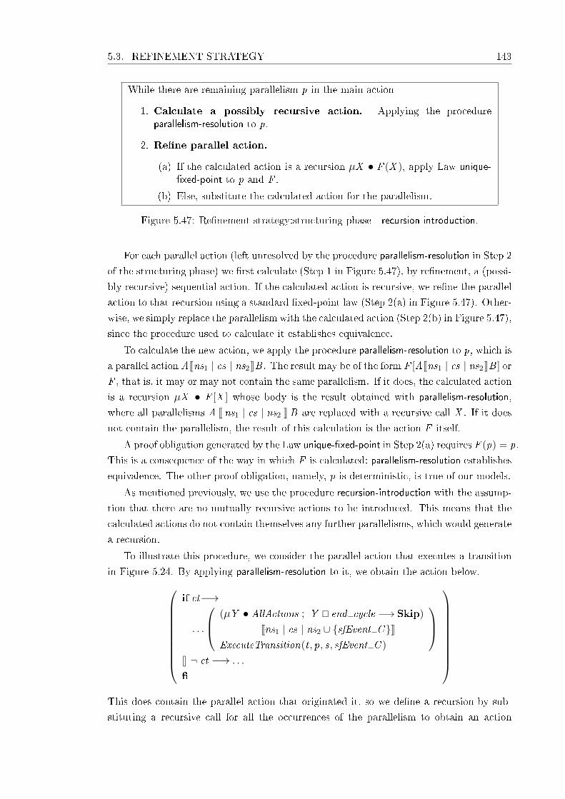
5.3. REFINEMENT STRATEGY 143
While there are remaining parallelism p in the main action
1. Calculate a possibly recursive action. Applying the procedureparallelism-resolution to p.
2. Re�ne parallel action.
(a) If the calculated action is a recursion µX • F (X ), apply Law unique-�xed-point to p and F .
(b) Else, substitute the calculated action for the parallelism.
Figure 5.47: Re�nement strategy:structuring phase - recursion-introduction.
For each parallel action (left unresolved by the procedure parallelism-resolution in Step 2
of the structuring phase) we �rst calculate (Step 1 in Figure 5.47), by re�nement, a (possi-
bly recursive) sequential action. If the calculated action is recursive, we re�ne the parallel
action to that recursion using a standard �xed-point law (Step 2(a) in Figure 5.47). Other-
wise, we simply replace the parallelism with the calculated action (Step 2(b) in Figure 5.47),
since the procedure used to calculate it establishes equivalence.
To calculate the new action, we apply the procedure parallelism-resolution to p, which is
a parallel action AJns1 | cs | ns2KB . The result may be of the form F [AJns1 | cs | ns2KB ] or
F , that is, it may or may not contain the same parallelism. If it does, the calculated action
is a recursion µX • F [X ] whose body is the result obtained with parallelism-resolution,
where all parallelisms A J ns1 | cs | ns2 K B are replaced with a recursive call X . If it does
not contain the parallelism, the result of this calculation is the action F itself.
A proof obligation generated by the Law unique-�xed-point in Step 2(a) requires F (p) = p.
This is a consequence of the way in which F is calculated: parallelism-resolution establishes
equivalence. The other proof obligation, namely, p is deterministic, is true of our models.
As mentioned previously, we use the procedure recursion-introduction with the assump-
tion that there are no mutually recursive actions to be introduced. This means that the
calculated actions do not contain themselves any further parallelisms, which would generate
a recursion.
To illustrate this procedure, we consider the parallel action that executes a transition
in Figure 5.24. By applying parallelism-resolution to it, we obtain the action below.
if ct−→
. . .
(µY • AllActions ; Y @ end cycle −→ Skip)
Jns1 | cs | ns2 ∪ {sfEvent C}KExecuteTransition(t , p, s, sfEvent C )
8 ¬ ct −→ . . .
�
This does contain the parallel action that originated it, so we de�ne a recursion by sub-
stituting a recursive call for all the occurrences of the parallelism to obtain an action
144 CHAPTER 5. REFINEMENT STRATEGY
µX • if ct −→ . . .X 8 ¬ ct −→ . . .�.
Finally, we re�ne the parallelism in Figure 5.24 to the calculated action, by applying
Law unique-�xed-point. This generates two provisos: the body of the recursion is determin-
istic, which follows from the de�nition of our models, and the parallelism is a �xed point
of the recursion. This last proviso is shown below.
if ct −→ . . . (µY • AllActions ; Y @ end cycle −→ Skip)
Jns1 | cs | ns2 ∪ {sfEvent C}KExecuteTransition(t , p, s, sfEvent C )
8 ¬ ct −→ . . .
�
=
(µY • AllActions ; Y @ end cycle −→ Skip)
Jns1 | cs | ns2 ∪ {sfEvent C}KExecuteTransition(t , p, s, sfEvent C )
This is exactly the result of applying the procedure parallelism-resolution to the right-hand
side of the equation.
Figure 5.26 shows the result of applying recursion-introduction to both parallelisms in
Figure 5.24.
5.3.3.5 Procedure assignment-introduction
Figure 5.48 presents the procedure assignment-introduction. As indicated previously, it
re�nes to assignments all schema operations. We distinguish two types of schema opera-
tions: (1) those that activate or deactivate a particular state, and (2) those introduced in
the data re�nement phase plus the initialisation schema.
The operations in the �rst group are speci�ed by a renaming of the schema Activate
or Deactivate, which are originally de�ned in the chart process. They specify data oper-
ations that record an input state x? as active or inactive. Renamings Activate[s S/x?]
and Deactivate[s S/x?] are used in the main action at this stage to de�ne (data re�ned)
operations that activate or deactivate a speci�c state S .
All assignments introduced are of bindings to the state component C DWork , which
records the status of states and history junctions. The predicates in the schemas of the
second group are conjunctions of equalities, and so we convert them into assignments
directly (using a Z re�nement law). The schemas in the �rst group do not enjoy such
property, so we �rst convert them to speci�cation statements (also using a Z law).
The actual assignments are determined by the kind of schema operation, by the type of
the state being activated or deactivated (parallel or sequential), and by whether the parent
P of a sequential state being activated has a history junction or not. These conditions
identify the components of C DWork that are to be modi�ed. The identi�cation is based on
the naming conventions described in Section 5.3.1. For instance, activation or deactivation
of a parallel state S modi�es the component is active S of C DWork . In the steps shown
in Figure 5.48, the ellipses in the bindings on the right-hand side of the assignments
indicate that all other components of the binding that de�nes the value of C DWork are
left unchanged.

5.3. REFINEMENT STRATEGY 145
For each call to a schema operation
1. Convert schema. If it is of the form Activate[s S/x?] or Deactivate[s S/x?],apply the Law bC [15].
2. Introduce assignment.
(a) If it is of the form Activate[s S/x?]
• If S is a parallel state, apply Law assigI [15] to introduceC DWork := 〈|is active S == 1, . . . |〉.• else, if the parent P of S has a history junction, apply Law assigI [15] tointroduce C DWork := 〈|is P == C IN S ,was P == C IN S . . . |〉.• else, apply Law assigI [15] to introduceC DWork := 〈|is P == C IN S , . . . |〉.
(b) If it is of the form Deactivate[s S/x?]
• If S is a parallel state, apply Law assigI [15] to introduceC DWork := 〈|is active S == 0, . . . |〉.• else, if the parent P of S has a history junction, apply Law assigI [15] tointroduce
C DWork := 〈| is P == C IN NO ACTIVE CHILD ,was P == C IN NO ACTIVE CHILD . . . |〉
• else, apply Law assigI [15] to introduce
C DWork := 〈|is P == C IN NO ACTIVE CHILD , . . . |〉
(c) If it is not of the form Activate[s S/x?] or Deactivate[s S/x?], applyLaw assC [15].
Figure 5.48: Re�nement strategy: structuring phase - assignment-introduction
5.3.3.6 Procedure update-output
This procedure data re�nes the process to introduce a new state component, namely, C Y ,
which, as previously explained, records the values of the output variables and events to
be communicated at the end of the step. The procedure update-output also expands the
de�nition of the schema type of C B , to include boolean components that record whether
the output events have occurred or not.
As a parameter, update-output takes the sequence output events of output events in
the order in which they are de�ned in the chart. The starting point of update-output is
the second action in the sequence that de�nes the body of the outmost recursion in the
main action: this is the whole body, except ReadInputs. It has the general form shown in
Figure 5.26, and contains a number of interleavings (omitted in Figure 5.26) repeated at
the end of the innermost branches of the nested alternations. These interleavings have the
general form shown in Figure 5.49; each is an interleaving of alternations communicating
events, and communications of output variables. In Figure 5.49, the interleaved actions
shown are an alternation that communicates an output event E , and a pre�xing that
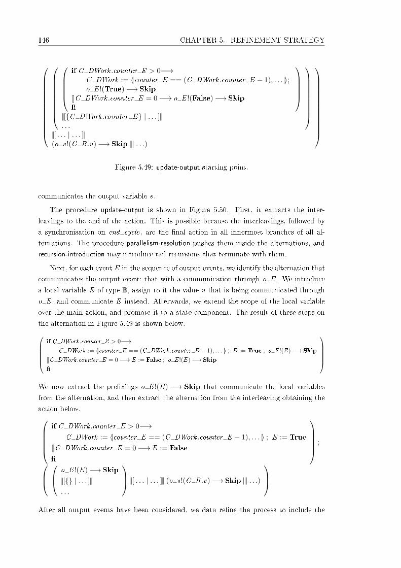
146 CHAPTER 5. REFINEMENT STRATEGY
if C DWork .counter E > 0−→
C DWork := 〈|counter E == (C DWork .counter E − 1), . . . |〉;o E !(True)−→ Skip
8C DWork .counter E = 0−→ o E !(False)−→ Skip�
||[{C DWork .counter E} | . . . ]||. . .
||[ . . . | . . . ]||(o v !(C B .v)−→ Skip 9 . . .)
Figure 5.49: update-output starting point.
communicates the output variable v .
The procedure update-output is shown in Figure 5.50. First, it extracts the inter-
leavings to the end of the action. This is possible because the interleavings, followed by
a synchronisation on end cycle, are the �nal action in all innermost branches of all al-
ternations. The procedure parallelism-resolution pushes them inside the alternations, and
recursion-introduction may introduce tail recursions that terminate with them.
Next, for each event E in the sequence of output events, we identify the alternation that
communicates the output event: that with a communication through o E . We introduce
a local variable E of type B, assign to it the value v that is being communicated through
o E , and communicate E instead. Afterwards, we extend the scope of the local variable
over the main action, and promote it to a state component. The result of these steps on
the alternation in Figure 5.49 is shown below.if C DWork .counter E > 0−→
C DWork := 〈|counter E == (C DWork .counter E − 1), . . . |〉 ; E := True ; o E !(E )−→ Skip
8C DWork .counter E = 0−→ E := False ; o E !(E )−→ Skip
�
We now extract the pre�xings o E !(E ) −→ Skip that communicate the local variables
from the alternation, and then extract the alternation from the interleaving obtaining the
action below.if C DWork .counter E > 0−→
C DWork := 〈|counter E == (C DWork .counter E − 1), . . . |〉 ; E := True
8C DWork .counter E = 0−→ E := False
�
;
o E !(E )−→ Skip
||[{} | . . . ]||. . .
||[ . . . | . . . ]|| (o v !(C B .v)−→ Skip 9 . . .)
After all output events have been considered, we data re�ne the process to include the

5.3. REFINEMENT STRATEGY 147
1. Isolate outputs. Exhaustively apply Laws alt-seq-dist and tail-rec-seq-dist to thewhole action.
2. For each output event E in output events
(a) Introduce local variable. Apply Law var-assign-intro to pre�xing actionsof the form o E !v −→ Skip to introduce a fresh local variable E of type Band initialise it with v , and then apply Law assign-seq-dist to the assignmentfollowed by the pre�xing.
(b) Extend scope. Apply Laws var-seq-ext-left to the branch of the alternationthat initialises E with True, var-alt-dist-both to the alternation, var-int-distto the interleaving, C.137 [76] to the body of the outmost recursion, var-tail-rec-ext to the recursion, and var-seq-ext-left to the outer sequence.
(c) Promote to state component. Apply Law A.5 [14] to the process.
(d) Extract communication. Apply Law alt-seq-dist to the alternation withthe communications over o E .
(e) Step-law. Apply Law int-seq-dist to the interleaving, with A as the alter-nation.
3. Data re�nement. Apply Laws C.1-C.25 [76] to the whole process (to includethe new state components in C B).
4. Introduce local variable. Apply Law var-assign-intro to the interleaving in-troduce a local variable C Y of type ExternalOutputs C and initialise it withC B .
5. Substitute variable for value. Apply Law assign-seq-dist to the sequence con-taining the new assignment and the interleaving.
6. Extend scope. Apply Law C.137 [76] to the body of the outmost recursion toextend the scope of C Y , Law var-tail-rec-ext to the recursion and var-seq-ext-leftto the outer sequence.
7. Promote to state component. Apply Law A.5 [14] to the process.
Figure 5.50: Re�nement strategy: structuring phase - update-output
newly added state components in the component C B . This is achieved by �rst de�ning a
new concrete state identical to the current state, except that the variables that were just
promoted are components of the schema BlockIO C . The retrieve relation equates each
promoted variable to the corresponding variable of the component of type BlockIO C of the
new concrete state. The laws of action simulation determine the required data re�nement.
After the data re�nement, we apply Law var-assign-intro to the remaining interleaving
to introduce the variable C Y and initialise it with C B . (This is now possible because
the bindings of ExternalOutputs C and BlockIO have the same components). Next, we
substitute C Y for C B in the interleaved communications, and distribute the local vari-
able over the main action. Finally, we promote it to a state component. The result, as
probably expected, is the action shown in Figure 5.21.

148 CHAPTER 5. REFINEMENT STRATEGY
5.3.3.7 Procedure simpli�cation
This procedure, which is applied in the last step of the structuring phase, eliminates
redundant code, simpli�es the control structure, and adds inputevents to the record C U .
It is applied to the whole of the main action, and basically, this aligns its speci�cation with
the code of the implementation.
Figure 5.51 shows the steps of simpli�cation. Step 1 distributes the hiding of the channel
set interface over the whole action, thus eliminating the internal communications and the
hidings themselves. This is possible because of the sequential and deterministic structure
of the starting action.
Before the application of this procedure, the action may contain assignments deactivat-
ing a state, followed by the activation of the same state or a sequential sibling. The second
step of simpli�cation removes such redundant assignments. It applies to sequences where
the �rst action is a deactivation assignment: an assignment DWork C .is active S := 0
or is S := C IN NO ACTIVE CHILD , for some chart state S . It moves such assign-
ments forward as far a possible, and then eliminates redundancy if it arises. For exam-
ple, is S := C IN NO ACTIVE CHILD ; A ; is S := C IN Sp may be re�ned to
A ; is S := C IN Sp , if A does not use is S . This is an optimisation frequently used to
avoid unnecessary assignments.
The only local variables that should remain in the model of the implementation are
those that record the current event when a local event broadcast occurs, namely the local
variables c previousEvent . In the third step, we remove all other (spurious) local variables
by moving them over sequential compositions (using Laws assign-seq-com and assign-seq-
col), extracting them from alternations (using Law alt-seq-dist from right to left), and
eliminating them using Laws C.136 [76], from right to left, and var-assign-elim.
The procedure simpli�cation uses three other procedures that we present later on in
this section. The procedure early-return-simpli�cation, used in the fourth step, attempts to
simplify alternations that verify early return logic conditions. It introduces and distributes
assertions about the status of the states, and uses them to eliminate some of these alterna-
tions. The �fth step uses the procedure parallel-state-simpli�cation to simplify alternations
that model the entering, executing, and exiting of parallel states, whenever possible. It
relies on two facts: (1) whenever a state is inactive, all its substates are inactive too; and
(2) in most cases, whenever an active state with a parallel decomposition is being exe-
cuted, all its substates are also active. (The latter is not necessarily true when there is
local event broadcast; in this case the alternation cannot be simpli�ed.) The sixth step
�attens the alternations that execute sequential states using sequential-state-simpli�cation.
It relies on the fact that at any point at most one sequential substate may be active, and
that the values of a component C DWork .is S are in a one-to-one correspondence with
the substates of S .
The execution of transitions may result in nested alternations, the �rst checking the
trigger of the transitions and the second evaluating its condition, and in tail recursions
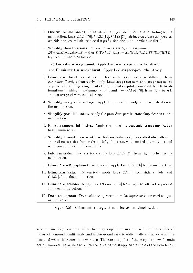
5.3. REFINEMENT STRATEGY 149
1. Distribute the hiding. Exhaustively apply distribution laws for hiding to themain action: Laws C.120 [76], C.122 [76], C.125 [76], alt-hide-dist, var-rec-hide-dist,rec-hide-dist, var-tail-alt-rec-hide-dist,pre�x-hide-dist-1, and pre�x-hide-dist-2.
2. Simplify deactivations. For each chart state S , and assignmentDWork C .is active S := 0 or DWork C .is S := S IN NO ACTIVE CHILD ,try to eliminate it as follows.
(a) Distribute assignment. Apply Law assign-seq-comp exhaustively.
(b) Eliminate the assignment. Apply Law assign-seq-col exhaustively.
3. Eliminate local variables. For each local variable di�erent fromc previousEvent , exhaustively apply Laws assign-seq-com and assign-seq-col tosequences containing assignments to it, Law alt-seq-dist from right to left to al-ternations �nishing in assignments to it, and Laws C.136 [76], from right to left,and var-assign-elim to its declaration.
4. Simplify early return logic. Apply the procedure early-return-simpli�cation tothe main action.
5. Simplify parallel states. Apply the procedure parallel-state-simpli�cation to themain action.
6. Flatten sequential states. Apply the procedure sequential-state-simpli�cationto the main action.
7. Simplify transition executions. Exhaustively apply Laws alt-alt-dist, alt-simp,and tail-rec-seq-dist from right to left, if necessary, to nested alternations andrecursions that execute transitions.
8. Fold recursion. Exhaustively apply Law C.128 [76] from right to left to themain action.
9. Eliminate assumptions. Exhaustively apply Law C.35 [76] to the main action.
10. Eliminate Skip. Exhaustively apply Laws C.100, from right to left, andC.132 [76] to the main action.
11. Eliminate actions. Apply Law action-intr [14] from right to left to the processand each of its actions.
12. Data re�nement. Data re�ne the process to make inputevents a record compo-nent of C U .
Figure 5.51: Re�nement strategy: structuring phase - simpli�cation
whose main body is a alternation that may stop the recursion. In the �rst case, Step 7
�attens the nested conditionals, and in the second case, it additionally extracts the actions
executed when the recursion terminates. The starting point of this step is the whole main
action, however the actions to which the law alt-alt-dist applies are those of the form below.
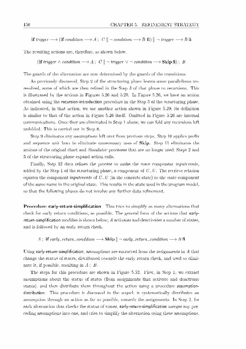
150 CHAPTER 5. REFINEMENT STRATEGY
if trigger −→ (if condition −→ A ; C 8 ¬ condition −→ B �) 8 ¬ trigger −→ B �
The resulting actions are, therefore, as shown below.
(if trigger ∧ condition −→ A ; C 8 ¬ trigger ∨ ¬ condition −→ Skip�) ; B
The guards of the alternation are now determined by the guards of the transitions.
As previously discussed, Step 2 of the structuring phase leaves some parallelisms un-
resolved, some of which are then re�ned in the Step 3 of that phase to recursions. This
is illustrated by the actions in Figures 5.26 and 5.20. In Figure 5.26, we have an action
obtained using the recursion-introduction procedure in the Step 3 of the structuring phase.
As indicated, in that action, we use another action shown in Figure 5.20; its de�nition
is similar to that of the action in Figure 5.26 itself. Omitted in Figure 5.26 are internal
communications. Once they are eliminated in Step 1 above, we can fold any recursions left
unfolded. This is carried out in Step 8.
Step 9 eliminates any assumptions left over from previous steps. Step 10 applies pre�x
and sequence unit laws to eliminate unnecessary uses of Skip. Step 11 eliminates the
actions of the original chart and Simulator processes that are no longer used: Steps 2 and
3 of the structuring phase expand action calls.
Finally, Step 12 data re�nes the process to make the state component inputevents,
added by the Step 1 of the structuring phase, a component of C U . The retrieve relation
equates the component inputevents of C U (in the concrete state) to the state component
of the same name in the original state. This results in the state used in the program model,
so that the following phases do not involve any further data re�nement.
Procedure early-return-simpli�cation This tries to simplify as many alternations that
check for early return conditions, as possible. The general form of the actions that early-
return-simpli�cationmodi�es is shown below; A activates and deactivates a number of states,
and is followed by an early return check.
A ; if early return condition −→ Skip 8 ¬ early return condition −→ B �
Using early-return-simpli�cation, assumptions are extracted from the assignments in A that
change the status of states, distributed towards the early return check, and used to elimi-
nate it, if possible, resulting in A ; B .
The steps for this procedure are shown in Figure 5.52. First, in Step 1, we extract
assumptions about the status of states (from assignments that activate and deactivate
states), and then distribute them throughout the action using a procedure assumption-
distribution. This procedure is discussed in the sequel; it systematically distributes an
assumption through an action as far as possible, towards the assignments. In Step 2, for
each alternation that checks the status of states, early-return-simpli�cation merges any pre-
ceding assumptions into one, and tries to simplify the alternation using these assumptions.
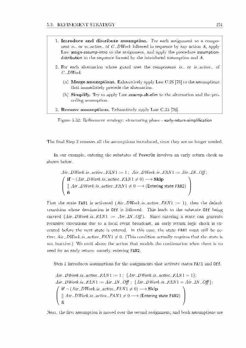
5.3. REFINEMENT STRATEGY 151
1. Introduce and distribute assumption. For each assignment to a compo-nent is or is active of C DWork followed in sequence by any action A, applyLaw assign-assump-intro to the assignment, and apply the procedure assumption-distribution to the sequence formed by the introduced assumption and A.
2. For each alternation whose guard uses the components is or is active ofC DWork
(a) Merge assumptions. Exhaustively apply Law C.26 [76] to the assumptionsthat immediately precede the alternation.
(b) Simplify. Try to apply Law assump-alt-elim to the alternation and the pre-ceding assumption.
3. Remove assumptions. Exhaustively apply Law C.35 [76].
Figure 5.52: Re�nement strategy: structuring phase - early-return-simpli�cation
The �nal Step 3 removes all the assumptions introduced, since they are no longer needed.
In our example, entering the substates of PowerOn involves an early return check as
shown below.
Air DWork .is active FAN 1 := 1 ; Air DWork .is FAN 1 := Air IN O� ; if ¬ (Air DWork .is active FAN 1 6= 0)−→ Skip
8 Air DWork .is active FAN 1 6= 0−→ (Entering state FAN2)
�
First the state FAN1 is activated (Air DWork .is active FAN 1 := 1), then the default
transition whose destination is Off is followed. This leads to the substate Off being
entered (Air DWork .is FAN 1 := Air IN O� ). Since entering a state can generate
recursive executions due to a local event broadcast, an early return logic check is ex-
ecuted before the next state is entered. In this case, the state FAN1 must still be ac-
tive: Air DWork .is active FAN 1 6= 0. (This condition actually requires that the state is
not inactive.) We omit above the action that models the continuation when there is no
need for an early return: namely, entering FAN2.
Step 1 introduces assumptions for the assignments that activate states FAN1 and Off.
Air DWork .is active FAN 1 := 1 ; {Air DWork .is active FAN 1 = 1};Air DWork .is FAN 1 := Air IN O� ; {Air DWork .is FAN 1 = Air IN O� }; if ¬ (Air DWork .is active FAN 1 6= 0)−→ Skip
8 Air DWork .is active FAN 1 6= 0−→ (Entering state FAN2)
�
Next, the �rst assumption is moved over the second assignment, and both assumptions are
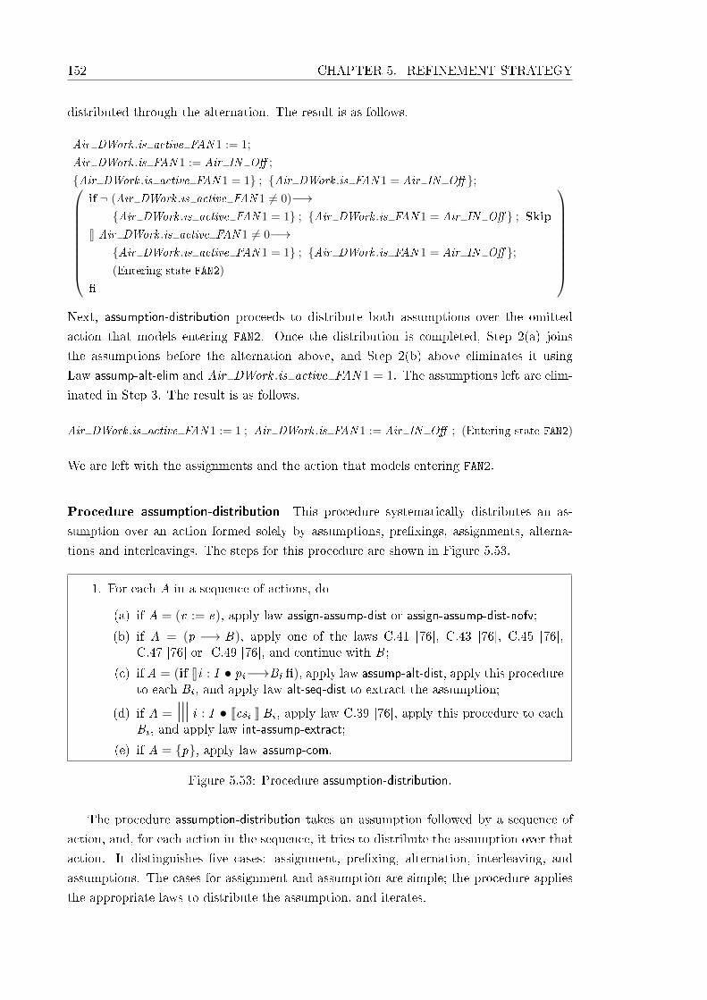
152 CHAPTER 5. REFINEMENT STRATEGY
distributed through the alternation. The result is as follows.
Air DWork .is active FAN 1 := 1;
Air DWork .is FAN 1 := Air IN O� ;
{Air DWork .is active FAN 1 = 1} ; {Air DWork .is FAN 1 = Air IN O� };
if ¬ (Air DWork .is active FAN 1 6= 0)−→{Air DWork .is active FAN 1 = 1} ; {Air DWork .is FAN 1 = Air IN O� } ; Skip
8 Air DWork .is active FAN 1 6= 0−→{Air DWork .is active FAN 1 = 1} ; {Air DWork .is FAN 1 = Air IN O� };(Entering state FAN2)
�
Next, assumption-distribution proceeds to distribute both assumptions over the omitted
action that models entering FAN2. Once the distribution is completed, Step 2(a) joins
the assumptions before the alternation above, and Step 2(b) above eliminates it using
Law assump-alt-elim and Air DWork .is active FAN 1 = 1. The assumptions left are elim-
inated in Step 3. The result is as follows.
Air DWork .is active FAN 1 := 1 ; Air DWork .is FAN 1 := Air IN O� ; (Entering state FAN2)
We are left with the assignments and the action that models entering FAN2.
Procedure assumption-distribution This procedure systematically distributes an as-
sumption over an action formed solely by assumptions, pre�xings, assignments, alterna-
tions and interleavings. The steps for this procedure are shown in Figure 5.53.
1. For each A in a sequence of actions, do
(a) if A = (v := e), apply law assign-assump-dist or assign-assump-dist-nofv;
(b) if A = (p −→ B), apply one of the laws C.41 [76], C.43 [76], C.45 [76],C.47 [76] or C.49 [76], and continue with B ;
(c) if A = (if 8i : I • pi−→Bi �), apply law assump-alt-dist, apply this procedureto each Bi , and apply law alt-seq-dist to extract the assumption;
(d) if A = 9 i : I • Jcsi K Bi , apply law C.39 [76], apply this procedure to eachBi , and apply law int-assump-extract;
(e) if A = {p}, apply law assump-com.
Figure 5.53: Procedure assumption-distribution.
The procedure assumption-distribution takes an assumption followed by a sequence of
action, and, for each action in the sequence, it tries to distribute the assumption over that
action. It distinguishes �ve cases: assignment, pre�xing, alternation, interleaving, and
assumptions. The cases for assignment and assumption are simple; the procedure applies
the appropriate laws to distribute the assumption, and iterates.
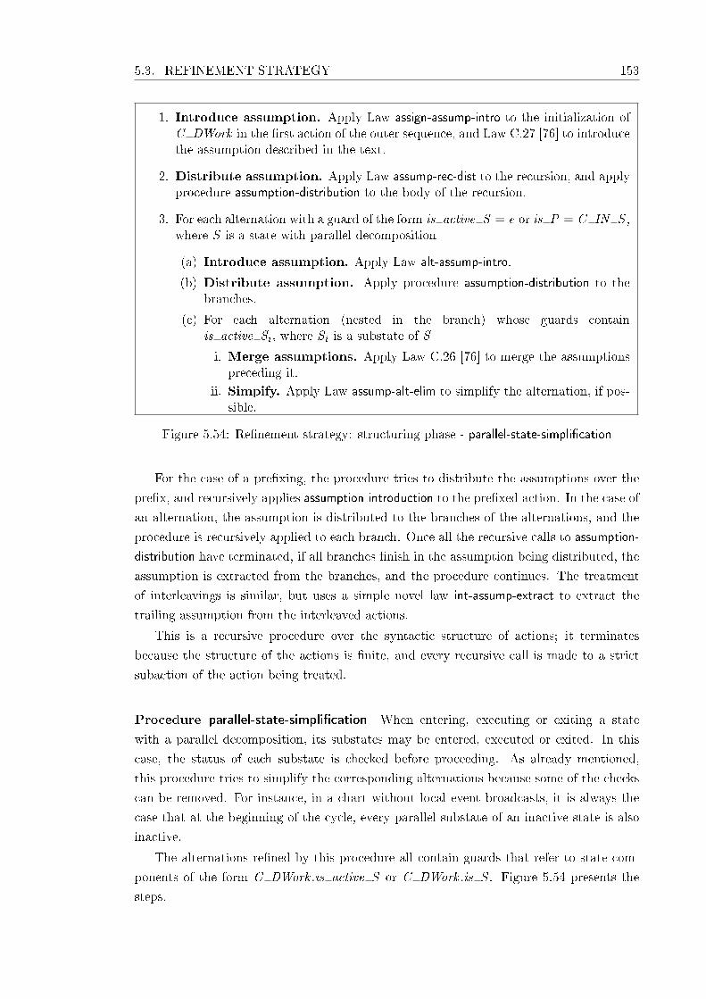
5.3. REFINEMENT STRATEGY 153
1. Introduce assumption. Apply Law assign-assump-intro to the initialization ofC DWork in the �rst action of the outer sequence, and Law C.27 [76] to introducethe assumption described in the text.
2. Distribute assumption. Apply Law assump-rec-dist to the recursion, and applyprocedure assumption-distribution to the body of the recursion.
3. For each alternation with a guard of the form is active S = e or is P = C IN S ,where S is a state with parallel decomposition
(a) Introduce assumption. Apply Law alt-assump-intro.
(b) Distribute assumption. Apply procedure assumption-distribution to thebranches.
(c) For each alternation (nested in the branch) whose guards containis active Si , where Si is a substate of S
i. Merge assumptions. Apply Law C.26 [76] to merge the assumptionspreceding it.
ii. Simpify. Apply Law assump-alt-elim to simplify the alternation, if pos-sible.
Figure 5.54: Re�nement strategy: structuring phase - parallel-state-simpli�cation
For the case of a pre�xing, the procedure tries to distribute the assumptions over the
pre�x, and recursively applies assumption-introduction to the pre�xed action. In the case of
an alternation, the assumption is distributed to the branches of the alternations, and the
procedure is recursively applied to each branch. Once all the recursive calls to assumption-
distribution have terminated, if all branches �nish in the assumption being distributed, the
assumption is extracted from the branches, and the procedure continues. The treatment
of interleavings is similar, but uses a simple novel law int-assump-extract to extract the
trailing assumption from the interleaved actions.
This is a recursive procedure over the syntactic structure of actions; it terminates
because the structure of the actions is �nite, and every recursive call is made to a strict
subaction of the action being treated.
Procedure parallel-state-simpli�cation When entering, executing or exiting a state
with a parallel decomposition, its substates may be entered, executed or exited. In this
case, the status of each substate is checked before proceeding. As already mentioned,
this procedure tries to simplify the corresponding alternations because some of the checks
can be removed. For instance, in a chart without local event broadcasts, it is always the
case that at the beginning of the cycle, every parallel substate of an inactive state is also
inactive.
The alternations re�ned by this procedure all contain guards that refer to state com-
ponents of the form C DWork .is active S or C DWork .is S . Figure 5.54 presents the
steps.
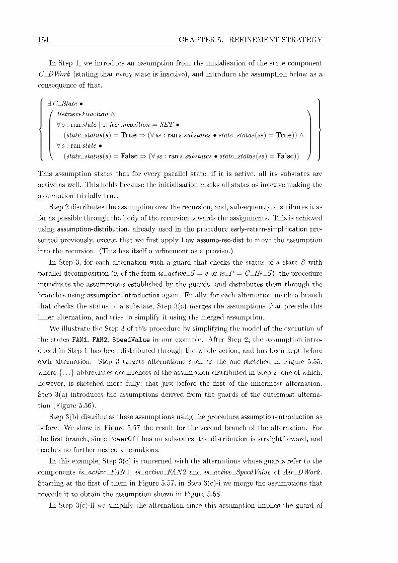
154 CHAPTER 5. REFINEMENT STRATEGY
In Step 1, we introduce an assumption from the initialisation of the state component
C DWork (stating that every state is inactive), and introduce the assumption below as a
consequence of that.
∃C State •RetrieveFunction ∧∀ s : ran state | s.decomposition = SET •
(state status(s) = True⇒ (∀ ss : ran s.substates • state status(ss) = True)) ∧∀ s : ran state •
(state status(s) = False⇒ (∀ ss : ran s.substates • state status(ss) = False))
This assumption states that for every parallel state, if it is active, all its substates are
active as well. This holds because the initialisation marks all states as inactive making the
assumption trivially true.
Step 2 distributes the assumption over the recursion, and, subsequently, distributes it as
far as possible through the body of the recursion towards the assignments. This is achieved
using assumption-distribution, already used in the procedure early-return-simpli�cation pre-
sented previously, except that we �rst apply Law assump-rec-dist to move the assumption
into the recursion. (This has itself a re�nement as a proviso.)
In Step 3, for each alternation with a guard that checks the status of a state S with
parallel decomposition (is of the form is active S = e or is P = C IN S ), the procedure
introduces the assumptions established by the guards, and distributes them through the
branches using assumption-introduction again. Finally, for each alternation inside a branch
that checks the status of a substate, Step 3(c) merges the assumptions that precede this
inner alternation, and tries to simplify it using the merged assumption.
We illustrate the Step 3 of this procedure by simplifying the model of the execution of
the states FAN1, FAN2, SpeedValue in our example. After Step 2, the assumption intro-
duced in Step 1 has been distributed through the whole action, and has been kept before
each alternation. Step 3 targets alternations such as the one sketched in Figure 5.55,
where {. . .} abbreviates occurrences of the assumption distributed in Step 2, one of which,
however, is sketched more fully: that just before the �rst of the innermost alternation.
Step 3(a) introduces the assumptions derived from the guards of the outermost alterna-
tion (Figure 5.56).
Step 3(b) distributes these assumptions using the procedure assumption-introduction as
before. We show in Figure 5.57 the result for the second branch of the alternation. For
the �rst branch, since PowerOff has no substates, the distribution is straightforward, and
reaches no further nested alternations.
In this example, Step 3(c) is concerned with the alternations whose guards refer to the
components is active FAN 1, is active FAN 2 and is active SpeedValue of Air DWork .
Starting at the �rst of them in Figure 5.57, in Step 3(c)-i we merge the assumptions that
precede it to obtain the assumption shown in Figure 5.58.
In Step 3(c)-ii we simplify the alternation since this assumption implies the guard of

5.3. REFINEMENT STRATEGY 155
{. . .} ;
if Air DWork .is c1 Air = Air IN PowerO� −→ . . .8 Air DWork .is c1 Air = Air IN PowerOn −→ {. . .};
if sfEvent Air = Air event SWITCH −→ . . .8 ¬ ( sfEvent Air = Air event SWITCH )−→
. . . ∧Air DWork .is c1 Air = Air IN PowerOn ⇒ Air DWork .is active FAN 1 = 1 ∧
Air DWork .is active FAN 2 = 1 ∧Air DWork .is active SpeedValue = 1
;
if Air DWork .is active FAN 1 = 1−→ (FAN1)8 ¬ (Air DWork .is active FAN 1 = 1)−→ Skip�
;
{. . .}; if Air DWork .is active FAN 2 = 1−→ (FAN2)8¬ (Air DWork .is active FAN 2 = 1)−→ Skip�
;
{. . .}; if Air DWork .is active SpeedValue = 1−→ (SpeedValue)8 ¬ (Air DWork .is active SpeedValue = 1)−→ Skip�
�
�
Figure 5.55: parallel-state-simpli�cation: example after step 2.
{. . .} ;
if Air DWork .is c1 Air = Air IN PowerO�−→{Air DWork .is c1 Air = Air IN PowerO� } ; . . .
8 Air DWork .is c1 Air = Air IN PowerOn−→{Air DWork .is c1 Air = Air IN PowerOn} ; {. . .} ; . . .
�
Figure 5.56: parallel-state-simpli�cation: example after step 3(a).
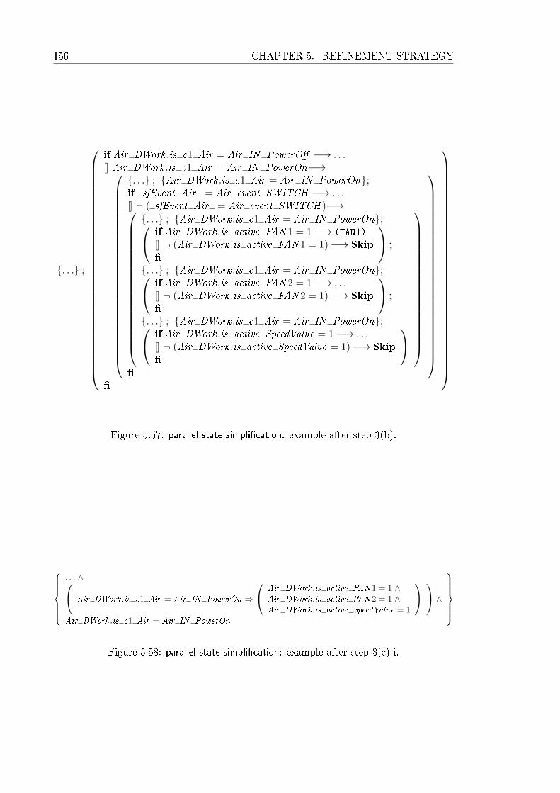
156 CHAPTER 5. REFINEMENT STRATEGY
{. . .} ;
if Air DWork .is c1 Air = Air IN PowerO� −→ . . .8 Air DWork .is c1 Air = Air IN PowerOn−→
{. . .} ; {Air DWork .is c1 Air = Air IN PowerOn};if sfEvent Air = Air event SWITCH −→ . . .8 ¬ ( sfEvent Air = Air event SWITCH )−→
{. . .} ; {Air DWork .is c1 Air = Air IN PowerOn}; if Air DWork .is active FAN 1 = 1−→ (FAN1)
8 ¬ (Air DWork .is active FAN 1 = 1)−→ Skip�
;
{. . .} ; {Air DWork .is c1 Air = Air IN PowerOn}; if Air DWork .is active FAN 2 = 1−→ . . .8 ¬ (Air DWork .is active FAN 2 = 1)−→ Skip�
;
{. . .} ; {Air DWork .is c1 Air = Air IN PowerOn}; if Air DWork .is active SpeedValue = 1−→ . . .8 ¬ (Air DWork .is active SpeedValue = 1)−→ Skip�
�
�
Figure 5.57: parallel-state-simpli�cation: example after step 3(b).
. . . ∧ Air DWork .is c1 Air = Air IN PowerOn ⇒
Air DWork .is active FAN 1 = 1 ∧Air DWork .is active FAN 2 = 1 ∧Air DWork .is active SpeedValue = 1
∧Air DWork .is c1 Air = Air IN PowerOn
Figure 5.58: parallel-state-simpli�cation: example after step 3(c)-i.
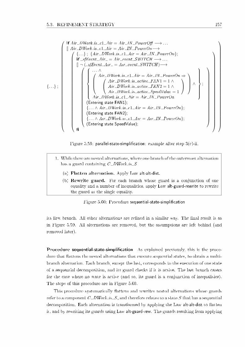
5.3. REFINEMENT STRATEGY 157
{. . .} ;
if Air DWork .is c1 Air = Air IN PowerO� −→ . . .8 Air DWork .is c1 Air = Air IN PowerOn−→
{. . .} ; {Air DWork .is c1 Air = Air IN PowerOn};if sfEvent Air = Air event SWITCH −→ . . .8 ¬ ( sfEvent Air = Air event SWITCH )−→
. . . ∧Air DWork .is c1 Air = Air IN PowerOn ⇒ Air DWork .is active FAN 1 = 1 ∧
Air DWork .is active FAN 2 = 1 ∧Air DWork .is active SpeedValue = 1
∧
Air DWork .is c1 Air = Air IN PowerOn
;
(Entering state FAN1);{. . . ∧ Air DWork .is c1 Air = Air IN PowerOn};(Entering state FAN2);{. . . ∧ Air DWork .is c1 Air = Air IN PowerOn};(Entering state SpeedValue);
�
Figure 5.59: parallel-state-simpli�cation: example after step 3(c)-ii.
1. While there are nested alternations, where one branch of the outermost alternationhas a guard containing C DWork .is S
(a) Flatten alternation. Apply Law alt-alt-dist.
(b) Rewrite guard. For each branch whose guard is a conjunction of oneequality and a number of inequalities, apply Law alt-guard-rewrite to rewritethe guard as the single equality.
Figure 5.60: Procedure sequential-state-simpli�cation
its �rst branch. All other alternations are re�ned in a similar way. The �nal result is as
in Figure 5.59. All alternations are removed, but the assumptions are left behind (and
removed later).
Procedure sequential-state-simpli�cation As explained previously, this is the proce-
dure that �attens the nested alternations that execute sequential states, to obtain a multi-
branch alternation. Each branch, except the last, corresponds to the execution of one state
of a sequential decomposition, and its guard checks if it is active. The last branch caters
for the case where no state is active (and so, its guard is a conjunction of inequalities).
The steps of this procedure are in Figure 5.60.
This procedure systematically �attens and rewrites nested alternations whose guards
refer to a component C DWork .is S , and therefore relates to a state S that has a sequential
decomposition. Each alternation is transformed by applying the Law alt-alt-dist to �atten
it, and by rewriting its guards using Law alt-guard-rew. The guards resulting from applying
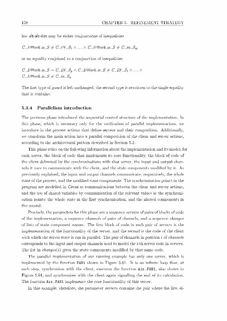
158 CHAPTER 5. REFINEMENT STRATEGY
law alt-alt-dist may be either conjunctions of inequalities
C DWork .is S 6= C IN S1 ∧ . . . ∧ C DWork .is S 6= C in Sm
or an equality conjoined to a conjunction of inequalities
C DWork .is S = C IN Sp ∧ C DWork .is S 6= C IN S1 ∧ . . . ∧C DWork .is S 6= C in Sn
The �rst type of guard is left unchanged; the second type is rewritten to the single equality
that it contains.
5.3.4 Parallelism introduction
The previous phase introduced the sequential control structure of the implementation. In
this phase, which is necessary only for the veri�cation of parallel implementations, we
introduce in the process actions that de�ne servers and their composition. Additionally,
we transform the main action into a parallel composition of the client and server actions,
according to the architectural pattern described in Section 5.2.
This phase relies on the following information about the implementation and its model: for
each server, the block of code that implements its core functionality, the block of code of
the client delimited by the synchronisations with that server, the input and output chan-
nels it uses to communicate with the client, and the state components modi�ed by it. As
previously explained, the input and output channels communicate, respectively, the whole
state of the process, and the modi�ed state components. The synchronisation points in the
program are modelled in Circus as communications between the client and server actions,
and the use of shared variables by communication of the relevant values at the synchroni-
sation points: the whole state in the �rst synchronisation, and the altered components in
the second.
Precisely, the parameters for this phase are a sequence servers of pairs of blocks of code
of the implementation, a sequence channels of pairs of channels, and a sequence changes
of lists of state component names. The �rst block of code in each pair of servers is the
implementation of the functionality of the server, and the second is the code of the client
with which the server state is run in parallel. The pair of channels in position i of channels
corresponds to the input and output channels used to model the i-th server code in servers.
The list in changes(i) gives the state components modi�ed by that same code.
The parallel implementation of our running example has only one server, which is
implemented by the function FAN1 shown in Figure 5.61. It is an in�nite loop that, at
each step, synchronises with the client, executes the function Air FAN1, also shown in
Figure 5.61, and synchronises with the client again signalling the end of its calculation.
The function Air FAN1 implements the core functionality of this server.
In this example, therefore, the parameter servers contains the pair where the �rst el-
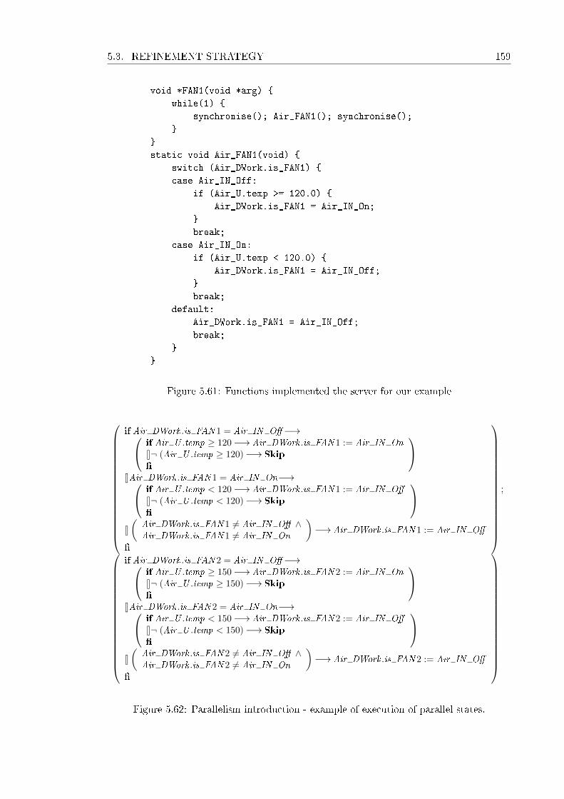
5.3. REFINEMENT STRATEGY 159
void *FAN1(void *arg) {
while(1) {
synchronise(); Air_FAN1(); synchronise();
}
}
static void Air_FAN1(void) {
switch (Air_DWork.is_FAN1) {
case Air_IN_Off:
if (Air_U.temp >= 120.0) {
Air_DWork.is_FAN1 = Air_IN_On;
}
break;
case Air_IN_On:
if (Air_U.temp < 120.0) {
Air_DWork.is_FAN1 = Air_IN_Off;
}
break;
default:
Air_DWork.is_FAN1 = Air_IN_Off;
break;
}
}
Figure 5.61: Functions implemented the server for our example
if Air DWork .is FAN 1 = Air IN O�−→ if Air U .temp ≥ 120−→ Air DWork .is FAN 1 := Air IN On8¬ (Air U .temp ≥ 120)−→ Skip�
8Air DWork .is FAN 1 = Air IN On−→ if Air U .temp < 120−→ Air DWork .is FAN 1 := Air IN O�
8¬ (Air U .temp < 120)−→ Skip�
8(
Air DWork .is FAN 1 6= Air IN O� ∧Air DWork .is FAN 1 6= Air IN On
)−→ Air DWork .is FAN 1 := Air IN O�
�
;
if Air DWork .is FAN 2 = Air IN O�−→ if Air U .temp ≥ 150−→ Air DWork .is FAN 2 := Air IN On8¬ (Air U .temp ≥ 150)−→ Skip�
8Air DWork .is FAN 2 = Air IN On−→ if Air U .temp < 150−→ Air DWork .is FAN 2 := Air IN O�
8¬ (Air U .temp < 150)−→ Skip�
8(
Air DWork .is FAN 2 6= Air IN O� ∧Air DWork .is FAN 2 6= Air IN On
)−→ Air DWork .is FAN 2 := Air IN O�
�
Figure 5.62: Parallelism introduction - example of execution of parallel states.
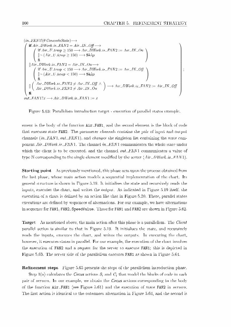
160 CHAPTER 5. REFINEMENT STRATEGY
(in FAN 1!(θConcreteState)−→
if Air DWork .is FAN 2 = Air IN O�−→ if Air U .temp ≥ 150−→ Air DWork .is FAN 2 := Air IN On8¬ (Air U .temp ≥ 150)−→ Skip�
8Air DWork .is FAN 2 = Air IN On−→ if Air U .temp < 150−→ Air DWork .is FAN 2 := Air IN O�
8¬ (Air U .temp < 150)−→ Skip�
8(
Air DWork .is FAN 2 6= Air IN O� ∧Air DWork .is FAN 2 6= Air IN On
)−→ Air DWork .is FAN 2 := Air IN O�
�
;
out FAN 1?x −→ Air DWork .is FAN 1 := x
Figure 5.63: Parallelism introduction target - execution of parallel states example.
ement is the body of the function Air FAN1, and the second element is the block of code
that executes state FAN2. The parameter channels contains the pair of input and output
channels (in FAN 1, out FAN 1), and changes the singleton list containing the state com-
ponent Air DWork .is FAN 1. The channel in FAN 1 communicates the whole state under
which the client is to be executed, and the channel out FAN 1 communicates a value of
type N corresponding to the single element modi�ed by the server (Air DWork .is FAN 1).
Starting point As previously mentioned, this phase acts upon the process obtained from
the last phase, whose main action models a sequential implementation of the chart. Its
general structure is shown in Figure 5.19. It initialises the state and recursively reads the
inputs, executes the chart, and writes the output. As indicated in Figure 5.19 itself, the
execution of a chart is de�ned by an action like that in Figure 5.20. There, parallel states
executions are de�ned by sequences of alternations. For our example, we have alternations
in sequence for FAN1, FAN2, SpeedValue. Those for FAN1 and FAN2 are shown in Figure 5.62.
Target As mentioned above, the main action after this phase is a parallelism. The Client
parallel action is similar to that in Figure 5.19. It initialises the state, and recursively
reads the inputs, executes the chart, and writes the outputs. In executing the chart,
however, it executes states in parallel. For our example, the execution of the chart involves
the execution of FAN2 and a request for the server to execute FAN1; this is depicted in
Figure 5.63. The server side of the parallelism executes FAN1 as shown in Figure 5.64.
Re�nement steps Figure 5.65 presents the steps of the parallelism introduction phase.
Step 1(a) calculates the Circus actions Si and Ci that model the blocks of code in each
pair of servers. In our example, we obtain the Circus actions corresponding to the body
of the function Air FAN1 (see Figure 5.61) and the execution of state FAN2 in servers.
The �rst action is identical to the outermost alternation in Figure 5.64, and the second is
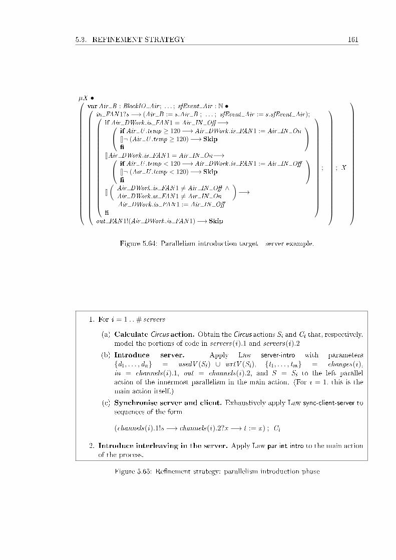
5.3. REFINEMENT STRATEGY 161
µX •
varAir B : BlockIO Air ; . . . ; sfEvent Air : N •
in FAN 1?s −→ (Air B := s.Air B ; . . . ; sfEvent Air := s.sfEvent Air);
if Air DWork .is FAN 1 = Air IN O�−→ if Air U .temp ≥ 120−→ Air DWork .is FAN 1 := Air IN On8¬ (Air U .temp ≥ 120)−→ Skip�
8Air DWork .is FAN 1 = Air IN On−→ if Air U .temp < 120−→ Air DWork .is FAN 1 := Air IN O�
8¬ (Air U .temp < 120)−→ Skip�
8(
Air DWork .is FAN 1 6= Air IN O� ∧Air DWork .is FAN 1 6= Air IN On
)−→
Air DWork .is FAN 1 := Air IN O��
;
out FAN 1!(Air DWork .is FAN 1)−→ Skip
; X
Figure 5.64: Parallelism introduction target - server example.
1. For i = 1 . .# servers
(a) Calculate Circus action. Obtain the Circus actions Si and Ci that, respectively,model the portions of code in servers(i).1 and servers(i).2
(b) Introduce server. Apply Law server-intro with parameters{d1, . . . , dn} = usedV (Si) ∪ wrtV (Si), {t1, . . . , tm} = changes(i),in = channels(i).1, out = channels(i).2, and S = Si to the left parallelaction of the innermost parallelism in the main action. (For i = 1, this is themain action itself.)
(c) Synchronise server and client. Exhaustively apply Law sync-client-server tosequences of the form
(channels(i).1!s −→ channels(i).2?x −→ t := x ) ; Ci
2. Introduce interleaving in the server. Apply Law par-int-intro to the main actionof the process.
Figure 5.65: Re�nement strategy: parallelism introduction phase
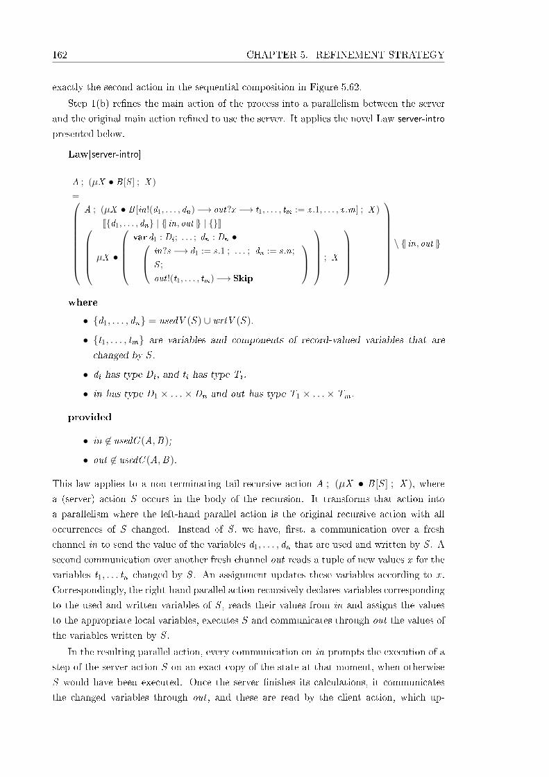
162 CHAPTER 5. REFINEMENT STRATEGY
exactly the second action in the sequential composition in Figure 5.62.
Step 1(b) re�nes the main action of the process into a parallelism between the server
and the original main action re�ned to use the server. It applies the novel Law server-intro
presented below.
Law[server-intro]
A ; (µX • B [S ] ; X )
=
A ; (µX • B [in!(d1, . . . , dn)−→ out?x −→ t1, . . . , tm := x .1, . . . , x .m] ; X )
J{d1, . . . , dn} | {| in, out |} | {}K µX •
var d1 : Di ; . . . ; dn : Dn • in?s −→ d1 := s.1 ; . . . ; dn := s.n;
S ;
out !(t1, . . . , tm)−→ Skip
; X
\ {| in, out |}
where
• {d1, . . . , dn} = usedV (S ) ∪ wrtV (S ).
• {t1, . . . , tm} are variables and components of record-valued variables that are
changed by S .
• di has type Di , and ti has type Ti .
• in has type D1 × . . .×Dn and out has type T1 × . . .× Tm .
provided
• in 6∈ usedC (A,B);
• out 6∈ usedC (A,B).
This law applies to a non-terminating tail-recursive action A ; (µX • B [S ] ; X ), where
a (server) action S occurs in the body of the recursion. It transforms that action into
a parallelism where the left-hand parallel action is the original recursive action with all
occurrences of S changed. Instead of S , we have, �rst, a communication over a fresh
channel in to send the value of the variables d1, . . . , dn that are used and written by S . A
second communication over another fresh channel out reads a tuple of new values x for the
variables t1, . . . tn changed by S . An assignment updates these variables according to x .
Correspondingly, the right-hand parallel action recursively declares variables corresponding
to the used and written variables of S , reads their values from in and assigns the values
to the appropriate local variables, executes S and communicates through out the values of
the variables written by S .
In the resulting parallel action, every communication on in prompts the execution of a
step of the server action S on an exact copy of the state at that moment, when otherwise
S would have been executed. Once the server �nishes its calculations, it communicates
the changed variables through out , and these are read by the client action, which up-
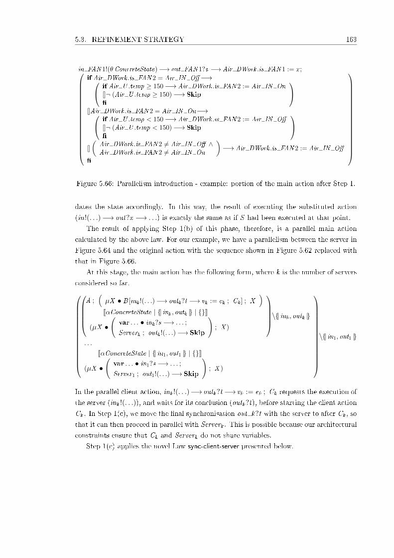
5.3. REFINEMENT STRATEGY 163
in FAN 1!(θConcreteState)−→ out FAN 1?x −→ Air DWork .is FAN 1 := x ;
if Air DWork .is FAN 2 = Air IN O�−→ if Air U .temp ≥ 150−→ Air DWork .is FAN 2 := Air IN On8¬ (Air U .temp ≥ 150)−→ Skip�
8Air DWork .is FAN 2 = Air IN On−→ if Air U .temp < 150−→ Air DWork .is FAN 2 := Air IN O�
8¬ (Air U .temp < 150)−→ Skip�
8(
Air DWork .is FAN 2 6= Air IN O� ∧Air DWork .is FAN 2 6= Air IN On
)−→ Air DWork .is FAN 2 := Air IN O�
�
Figure 5.66: Parallelism introduction - example: portion of the main action after Step 1.
dates the state accordingly. In this way, the result of executing the substituted action
(in!(. . .)−→ out?x −→ . . .) is exactly the same as if S had been executed at that point.
The result of applying Step 1(b) of this phase, therefore, is a parallel main action
calculated by the above law. For our example, we have a parallelism between the server in
Figure 5.64 and the original action with the sequence shown in Figure 5.62 replaced with
that in Figure 5.66.
At this stage, the main action has the following form, where k is the number of servers
considered so far.
A ;
(µX • B [ink !(. . .)−→ outk?t −→ vk := ek ; Ck ] ; X
)JαConcreteState | {| ink , outk |} | {}K
(µX •(var . . . • ink?s −→ . . . ;
Serverk ; outk !(. . .)−→ Skip
); X )
\{| ink , outk |}. . .
JαConcreteState | {| in1, out1 |} | {}K
(µX •(var . . . • in1?s −→ . . . ;
Server1 ; out1!(. . .)−→ Skip
); X )
\{| in1, out1 |}
In the parallel client action, ink !(. . .)−→outk?t −→ vk := ek ; Ck requests the execution of
the server (ink !(. . .)), and waits for its conclusion (outk?t), before starting the client action
Ck . In Step 1(c), we move the �nal synchronisation out k?t with the server to after Ck , so
that it can then proceed in parallel with Serverk . This is possible because our architectural
constraints ensure that Ck and Serverk do not share variables.
Step 1(c) applies the novel Law sync-client-server presented below.
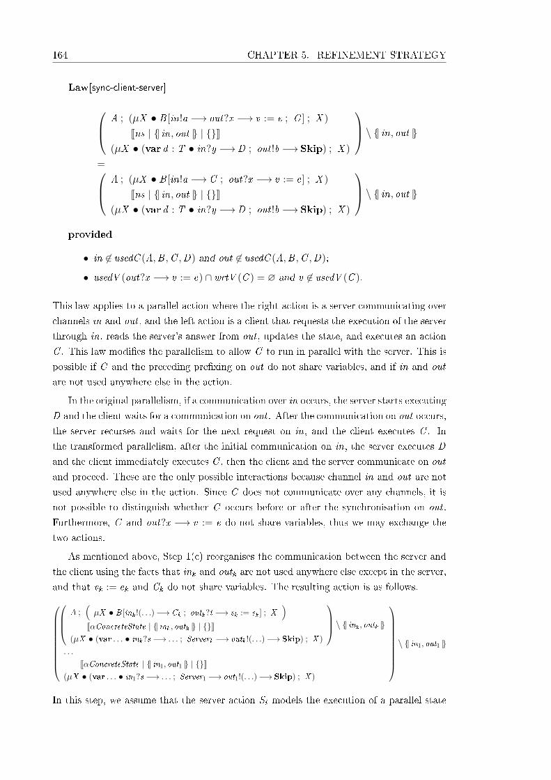
164 CHAPTER 5. REFINEMENT STRATEGY
Law[sync-client-server]
A ; (µX • B [in!a −→ out?x −→ v := e ; C ] ; X )
Jns | {| in, out |} | {}K(µX • (var d : T • in?y −→D ; out !b −→ Skip) ; X )
\ {| in, out |}= A ; (µX • B [in!a −→ C ; out?x −→ v := e] ; X )
Jns | {| in, out |} | {}K(µX • (var d : T • in?y −→D ; out !b −→ Skip) ; X )
\ {| in, out |}provided
• in 6∈ usedC (A,B ,C ,D) and out 6∈ usedC (A,B ,C ,D);
• usedV (out?x −→ v := e) ∩ wrtV (C ) = ∅ and v 6∈ usedV (C ).
This law applies to a parallel action where the right action is a server communicating over
channels in and out , and the left action is a client that requests the execution of the server
through in, reads the server's answer from out , updates the state, and executes an action
C . This law modi�es the parallelism to allow C to run in parallel with the server. This is
possible if C and the preceding pre�xing on out do not share variables, and if in and out
are not used anywhere else in the action.
In the original parallelism, if a communication over in occurs, the server starts executing
D and the client waits for a communication on out . After the communication on out occurs,
the server recurses and waits for the next request on in, and the client executes C . In
the transformed parallelism, after the initial communication on in, the server executes D
and the client immediately executes C , then the client and the server communicate on out
and proceed. These are the only possible interactions because channel in and out are not
used anywhere else in the action. Since C does not communicate over any channels, it is
not possible to distinguish whether C occurs before or after the synchronisation on out .
Furthermore, C and out?x −→ v := e do not share variables, thus we may exchange the
two actions.
As mentioned above, Step 1(c) reorganises the communication between the server and
the client using the facts that ink and outk are not used anywhere else except in the server,
and that vk := ek and Ck do not share variables. The resulting action is as follows.
A ;
(µX • B [ink !(. . .)−→ Ck ; outk?t −→ vk := ek ] ; X
)JαConcreteState | {| ink , outk |} | {}K
(µX • (var . . . • ink?s −→ . . . ; Serverk −→ outk !(. . .)−→ Skip) ; X )
\ {| ink , outk |}. . .
JαConcreteState | {| in1, out1 |} | {}K(µX • (var . . . • in1?s −→ . . . ; Server1 −→ out1!(. . .)−→ Skip) ; X )
\ {| in1, out1 |}
In this step, we assume that the server action Si models the execution of a parallel state
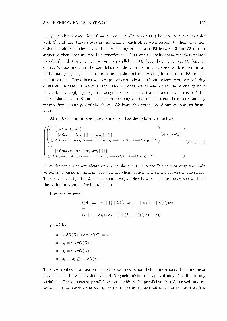
5.3. REFINEMENT STRATEGY 165
S, Ci models the execution of one or more parallel states CS (that do not share variables
with S) and that these states are adjacent to each other with respect to their execution
order as de�ned in the chart. If there are any other states PS between S and CS in that
sequence, there are three possible situations: (1) S, PS and CS are independent (do not share
variables) and, thus, can all be put in parallel, (2) PS depends on S, or (3) CS depends
on PS. We assume that the parallelism of the chart is fully explored at least within an
individual group of parallel states, thus, in the �rst case we require the states PS are also
put in parallel. The other two cases present complications because they require reordering
of states. In case (2), we must show that CS does not depend on PS and exchange both
blocks before applying Step 1(c) to synchronise the client and the server. In case (3), the
blocks that execute S and PS must be exchanged. We do not treat these cases as they
require further analysis of the chart. We leave this extension of our strategy as future
work.
After Step 1 terminates, the main action has the following structure.
A ;
(µX • B ; X
)JαConcreteState | {| inn , outn |} | {}K
(µX • (var . . . • inn?s −→ . . . ; Servern −→ outn !(. . .)−→ Skip) ; X )
\{| inn , outn |}. . .
JαConcreteState | {| in1, out1 |} | {}K(µX • (var . . . • in1?s −→ . . . ; Server1 −→ out1!(. . .)−→ Skip) ; X )
\{| in1, out1 |}
Since the servers communicate only with the client, it is possible to rearrange the main
action as a single parallelism between the client action and all the servers in interleave.
This is achieved by Step 2, which exhaustively applies Law par-int-intro below to transform
the action into the desired parallelism.
Law[par-int-intro]
((A J ns | cs1 | {} K B) \ cs1 J ns | cs2 | {} K C ) \ cs2=
(A J ns | cs1 ∪ cs2 | {} K (B 9 C )) \ cs1 ∪ cs2
provided
• usedC (B) ∩ usedC (C ) = ∅;
• cs1 = usedC (B);
• cs2 = usedC (C );
• cs1 ∪ cs2 ⊆ usedC (A).
This law applies to an action formed by two nested parallel compositions. The innermost
parallelism is between actions A and B synchronising on cs1, and only A writes to any
variables. The outermost parallel action combines the parallelism just described, and an
action C ; they synchronise on cs2, and only the inner parallelism writes to variables (be-
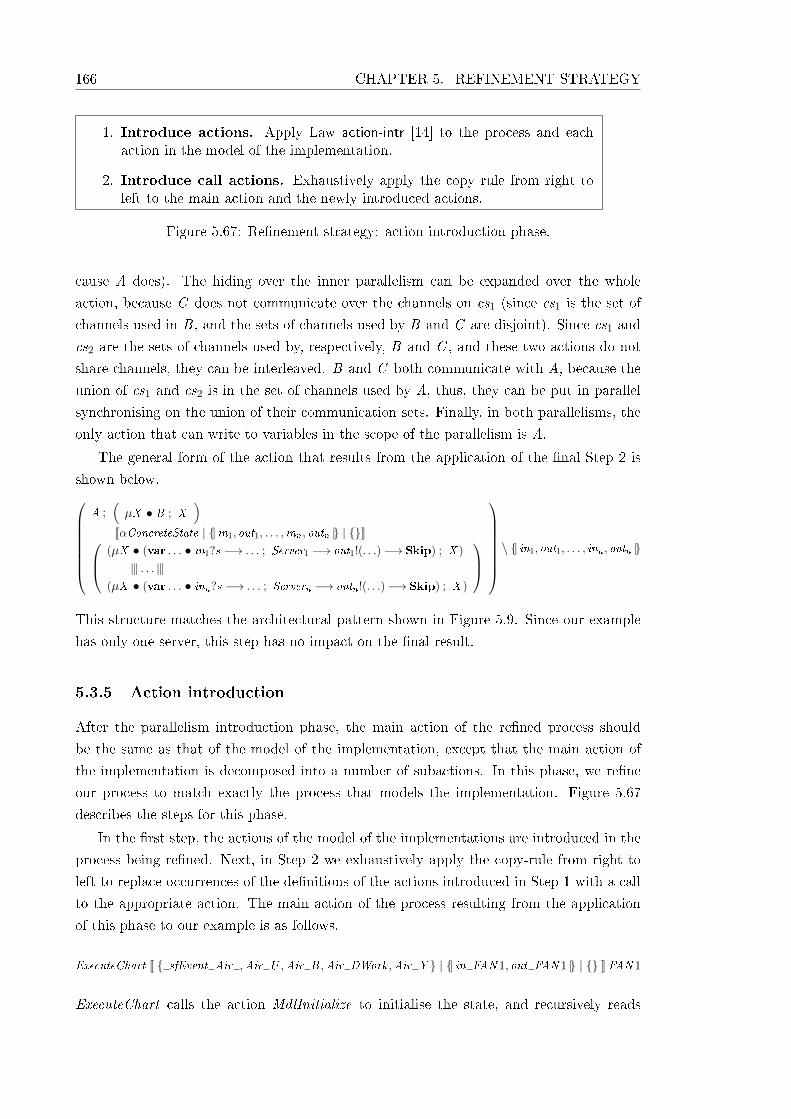
166 CHAPTER 5. REFINEMENT STRATEGY
1. Introduce actions. Apply Law action-intr [14] to the process and eachaction in the model of the implementation.
2. Introduce call actions. Exhaustively apply the copy rule from right toleft to the main action and the newly introduced actions.
Figure 5.67: Re�nement strategy: action introduction phase.
cause A does). The hiding over the inner parallelism can be expanded over the whole
action, because C does not communicate over the channels on cs1 (since cs1 is the set of
channels used in B , and the sets of channels used by B and C are disjoint). Since cs1 and
cs2 are the sets of channels used by, respectively, B and C , and these two actions do not
share channels, they can be interleaved. B and C both communicate with A, because the
union of cs1 and cs2 is in the set of channels used by A, thus, they can be put in parallel
synchronising on the union of their communication sets. Finally, in both parallelisms, the
only action that can write to variables in the scope of the parallelism is A.
The general form of the action that results from the application of the �nal Step 2 is
shown below.
A ;(µX • B ; X
)JαConcreteState | {| in1, out1, . . . , inn , outn |} | {}K (µX • (var . . . • in1?s −→ . . . ; Server1 −→ out1!(. . .)−→ Skip) ; X )
9 . . .9(µX • (var . . . • inn?s −→ . . . ; Servern −→ outn !(. . .)−→ Skip) ; X )
\ {| in1, out1, . . . , inn , outn |}
This structure matches the architectural pattern shown in Figure 5.9. Since our example
has only one server, this step has no impact on the �nal result.
5.3.5 Action introduction
After the parallelism introduction phase, the main action of the re�ned process should
be the same as that of the model of the implementation, except that the main action of
the implementation is decomposed into a number of subactions. In this phase, we re�ne
our process to match exactly the process that models the implementation. Figure 5.67
describes the steps for this phase.
In the �rst step, the actions of the model of the implementations are introduced in the
process being re�ned. Next, in Step 2 we exhaustively apply the copy-rule from right to
left to replace occurrences of the de�nitions of the actions introduced in Step 1 with a call
to the appropriate action. The main action of the process resulting from the application
of this phase to our example is as follows.
ExecuteChart J { sfEvent Air ,Air U ,Air B ,Air DWork ,Air Y } | {| in FAN 1, out FAN 1 |} | {} K FAN 1
ExecuteChart calls the action MdlInitialize to initialise the state, and recursively reads
5.4. FINAL CONSIDERATIONS 167
the inputs using the action read inputs, executes the chart using Air output , writes the
outputs using write outputs, and signals the end of the step by synchronising on end cycle.
The action FAN 1 is that in Figure 5.64.
This completes the veri�cation of our example.
5.4 Final considerations
In this chapter, we have identi�ed a simple, but general architectural pattern for the par-
allel implementation of State�ow charts, based on the sequential architecture implemented
by MATLAB's automatic code generator [98, 100]. Based on this pattern, we have pro-
posed a re�nement strategy for the veri�cation of implementations. While parts of the
strategy are dependent on the architecture of the implementation (namely, data re�ne-
ment, structuring (except steps 2 and 3) and parallelism introduction phases), other parts
can be reused in strategies that target di�erent architectures.
In particular, the normalisation phase and the procedure parallelism-resolution are cen-
tral to any strategy that deals with our models as they support the collapsing of the process
parallelism. The procedure parallelism-resolution is particularly important as it supports the
use of our modelling approach, where the core of the semantics is separated from structural
aspects of the notation.
Additionally, the architecture-dependent procedures can also be a starting point for
other strategies. While their details may require revision, the fundamental underlying
principles are bound to remain the same. For instance, procedures similar to those used
in the structuring phase, where appropriate assumptions are introduced and distributed
through the action to simplify the structure, are likely to be widely applicable.
Our re�nement strategy makes a number of assumptions about the automatically gen-
erated models of State�ow chart: deadlock free, divergence free, and deterministic. All of
these properties can be checked with a model checker, but they are also evident from the
structure of the model. It is not inconceivable that it is possible to prove that every model
of a well formed chart satis�es these properties. The strategy uses the Circus re�nement
calculus and derives its soundness from the soundness of the re�nement laws.
Our re�nement strategy should produce the process that models the implementation.
If this is not true, then either the implementation is incorrect, or it does not follow the
architectural patterns veri�ed by this strategy. In the �rst case, the comparison between
the two process may shed some light into what is the actual problem. Although the issue
of error traceability is interesting one, we leave it as future work. In the latter case, we can
directly apply the re�nement calculus to the model, or identify the architectural patterns
used in the implementation, and adapt our re�nement strategy to explore them.
Additionally, as already mentioned, we do not treat programs that include mutual
recursions. Our strategy, however, can be extended to treat mutual recursions by modifying
the procedure recursion-introduction to extract information about mutual recursions from
the implementation, calculate the appropriate recursive action, and apply a version of the
168 CHAPTER 5. REFINEMENT STRATEGY
law unique-�xed-point that re�nes actions to mutual recursions.
In general, the provisos generated by the re�nement laws are simple and can be dis-
charged using a theorem prover, except for the proviso of the law assump-rec-dist, which
requires that the assumption holds before and after the body of the recursion. It is used
to distribute an assumption through the recursion that characterises the step of execution
of the chart. For charts without recursions originating from local event broadcasts, it is
possible to describe a re�nement strategy that discharges this proviso, and we leave this
as future work. For cases where local event broadcast leads to recursive behaviour in the
chart, the occurrence of early return logic may leave the chart in a state that violates some
of the assumptions. In this case, the proviso does not hold, and the model is not further
simpli�ed. It is important to note, however, that the State�ow code generator does not
simplify the implementation in these cases either.
The re�nement strategy we propose shows that our choice of a more operational model
can be easily treated by a appropriately designed veri�cation strategy. The veri�cation
of implementation through re�nement has its advantages and disadvantages. It support a
higher degree of automation and possibly scales better to larger cases studies1 as it does
not rely so strongly on theorem proving. The main disadvantage of our approach is that
the veri�able implementations are very restricted, and, for more general implementations,
new re�nement strategies need to be developed.
For any similar treatments of the problem of veri�cation of implementations, it is
extremely important that the assumptions about the implementation are well understood
and delimited because this facilitates the de�nition of the re�nement strategy.
Overall, our strategy is a general approach for the veri�cation of, possibly parallel,
implementations of State�ow charts. Moreover, it is a substantial starting point for the
development of other re�nement strategies, tailored for other architectural patterns, as it
tackles aspects of the re�nement process that are fundamental to any veri�cation based on
our automated technique for generation of chart models.
1This point is speculative, and needs further investigation

Chapter 6
Conclusions
In this chapter, we discuss the main contributions of our work, compare it with the closely
related results in the literature, and provide directions for future work.
6.1 Thesis contributions
The use of graphical notations in general, and more speci�cally Simulink and State�ow, is
widespread in industry for the speci�cation of a variety of systems. Furthermore, some of
the systems modelled in such notations are safety critical, and thus require a higher level
of assurance of correctness. At present, the use of formal methods in this context is almost
exclusively restricted to the veri�cation of properties of the models [20, 7, 101, 87]. While
there has been some work on the veri�cation of code generators [102, 86], and veri�cation of
implementations of Simulink diagrams [19], we are not aware of any proposed approaches
for the veri�cation of implementations of State�ow charts. Our work stands as a di�erent
direction for the use of formal speci�cation and re�nement for graphical notations. The
main contributions of the work presented in this thesis can be divided in �ve areas.
A new approach to semantic description. Traditionally, models of graphical nota-
tions that are tailored for veri�cation of properties and implementations follow a denota-
tional style, where each component of the notation is associated with some complete and
independent element of the model. We adopt a completely di�erent approach, in which we
prioritise comprehensive coverage of the notation, and support for validation by inspection
of the informal description, over the particular scenarios in which the models are to be
used.
Our approach yields a number of advantages. Firstly, it provides a better support for
the formalisation of the semantics of inherently non-compositional notations such as State-
�ow. Secondly, it allows us to separate the semantics of the notation from the structure
of particular charts, reducing the size of the chart-speci�c model. Finally, our approach
does not embed simpli�cations of the semantics based on the particular chart structures,
as such simpli�cations may introduce errors in the semantics of the charts.
170 CHAPTER 6. CONCLUSIONS
A comprehensive modelling approach for State�ow charts. Most of the formali-
sation of State�ow charts (and other varieties of state diagram notations) identify a well-
behaved subset of the notation, and restrict the de�ned semantics to this subset. In
particular, as far as we know, there has not been a formalisation of State�ow charts that
completely treat local event broadcasts and early return logic. Our models provide a
thorough treatment of these features, and describes without restrictions most of the core
elements of the notation.
We have validated our models through:
• Translation of the models of some examples into CSP;
• Analysis and simulation of the CSP models;
• Comparison of the results of simulations to the expected behaviour;
• Translation of large industrial case-studies.
Formalisation and implementation of a technique for automatic generation of
models. We have formalised the translation rules that characterise our models of State-
�ow charts and de�ne a technique for the automatic generation of these models. While
most of the literature on formal semantics of State�ow charts either does not give an ac-
count of the translation process, or provide rather informal translation rules, we formalise
in Z the syntax of State�ow and Circus, and the translation rules for each element of
State�ow that we cover in our models. Furthermore, frequently the translation of smaller
aspects of the notation are overlooked (e.g. action language). Our translation rules cover
these aspects as well. We provide an implementation of the translation rules in the tool
s2c. We have thoroughly validated this tool and the models it generates by means of a
number of examples, including industrial case-studies. The tool was further validated by
parsing and type checking the generated models.
Architecture for implementations. We described an architecturals pattern for (par-
allel) implementations of State�ow charts based on the architecture enforced by State�ow
code generator, extended with a client-server pattern for the execution of parallel states.
This architecture identi�es the main aspects of implementations that are required to sup-
port the automation of a re�nement strategy. As far as we know, this is the �rst approach
to parallel implementations of State�ow charts.
Re�nement strategy. We propose a re�nement strategy that supports the veri�cation
of implementations of State�ow charts with respect to our models. This strategy relies
on the identi�ed architecture to support a high degree of automation, and its soundness
is derived from the soundness of the re�nement laws used to de�ne it. The motivation
for a highly specialised veri�cation strategies is that they are necessary to support a high
6.1. THESIS CONTRIBUTIONS 171
degree of automation in the veri�cation task, which is a key requirement for the adoption
of formal techniques by industry.
The strategy is structured in �ve phases: data re�nement, normalisation, structuring,
parallelism introduction and action introduction. The normalisation and action introduc-
tion phases are completely independent of the architecture of the implementations.
The structuring phase describes how to systematically collapse the parallelism between
the process that models the semantics of State�ow and the process that models the chart's
structure. It also determines how to carry out simpli�cations in the nested structure of
alternations that characterise the execution of the chart. This phase is key to the success
of our approach to the description of graphical notations using an operational style, as it
produces simpler, correct by construction, models of the chart by eliminating the unneces-
sary aspects of the semantics, which in other approaches are simpli�ed in the translation
strategy. While the portion of this phase that resolves the parallelism of the model is
completely independent of the implementation, the portion that simpli�es the structure of
the model depends on the particular architectural patterns of the implementation.
The data re�nement phase depends heavily on the state of the implementation. Simple
restructuring of the state of implementations, however, can easily be re�ected in this phase,
provided the data patterns are equivalent. More sophisticated changes to the state of
implementations can be incorporated provided the appropriate retrieve relation is de�ned.
The parallelism introduction phase relies on the client-server pattern used in our parallel
implementations of State�ow charts. In general, it can be adapted to di�erent patterns
of parallelism based on synchronisation. The use of explicit schedulers may require some
changes to this phase, but we note that it has been previously treated in Circus for Simulink
diagrams [14].
Our re�nement strategy is extremely general in that it supports a wide range of State-
�ow features as well as a number of architectural choices for the implementations. Fur-
thermore, it can be extended to cover new architectural patterns and State�ow features.
The failure of the re�nement strategy indicates either that the implementation is in-
correct or that it does not follow the associated architecture. In the latter case, the archi-
tectural patterns can be identi�ed, and we can de�ne a new strategy potentially reusing
parts of the strategy proposed in this thesis. In the former, knowledge of the exact point
of failure may help correct the program, as the phases and procedures of the re�nement
strategy target speci�c aspects of the implementation.
While the semantics of State�ow is rather cumbersome in some points (e.g., local event
broadcast), it is undeniably a notation that is actively used in industry. Most approaches
to the veri�cation of State�ow tend to restrict the subset of the notation that is allowed,
however, it is our belief that such a restriction should come from the users of the notation.
If di�cult aspects of the notation such as early return logic are used in industry, the
issue of veri�cation of this aspect is relevant and cannot be simply ignored if veri�cation
approaches are to have a chance of industrial adoption.
Our approach aims at minimising the need for expert guidance during the veri�cation

172 CHAPTER 6. CONCLUSIONS
process, this limits the robustness of our veri�cation strategy, but increases the chances of
industrial adoption. We believe that this is a reasonable trade-o�.
6.2 Related Work
Our approach combines a direct semantic formulation of State�ow charts, and a specialised
re�nement strategy to verify implementations. It partially follows the approach proposed
for Simulink diagrams presented in [19, 17], but diverges mainly on the style of the proposed
semantics and the complexity of the required re�nement strategy. The technique used to
de�ne the semantics of Simulink diagrams in [19] does not translate well for the task of
de�ning a semantics for State�ow charts because the behaviour of State�ow charts is not
as compositional as that of Simulink diagrams.
Hamon and Rushby [35] propose an operational semantics of State�ow, but it does
not cover history junctions and imposes restrictions on transitions. Hamon [34] describes
a denotational semantics heavily based on the notion of continuations. They claim to
cover most of the notation, but Simulink functions and events of type function-call are not
mentioned, and early return logic is not taken into consideration in the treatment of local
event broadcast.
While we do not use continuations in our models, our treatment of transition backtrack-
ing and state execution is similar to that of [34]. For transition backtracking, we keep a
record of the transitions that have been successfully executed, which upon failure allows us
to recover the last executed transition and attempt the next transition. This behaviour is
modelled in [34] by passing a continuation that executes the appropriate transition in case
of failure. The same continuation scheme is used to execute outer and inner transitions,
during actions and substates when executing a state. We use a value-result parameter to
assess the success or failure of a transition (in causing a state transition), and decide how
to proceed based on this parameter.
Banphawatthanarak et al. [7] restrict input signals to boolean values, and do not cal-
culate output signals. It also imposes restrictions on the number of transitions reaching a
junction, and the types of actions supported.
The work in [87] imposes a series of restrictions on the charts it treats. It does not allow
multi-segment transition paths that represent loops. Variable assignment on transitions
must be made solely on transition actions or the condition action of the last segment.
It avoids backtracking of transitions by requiring that conditions of outgoing transitions
from junctions form a cover, that is, the disjunction of the conditions is true. It also
avoids relying on orderings determined by position of elements in the diagram by requiring
that transitions leaving a node have disjunct conditions, for instance. Toyn and Galloway
[104] impose even stronger restrictions; they do not cover parallel states, junctions, local
variables, and so on.
In contrast to the above, in de�ning our models of State�ow charts, we provide an
extensive coverage of the notation. Our models cover edge-triggered input and output

6.3. FUTURE WORK 173
events, local events, input and output data, entry, during, exit, condition, transition and
on actions, parallel and sequential states, connective and history junctions, and transitions
without imposing restrictions other that those already imposed by the State�ow notation.
The features that distinguish these models are the unrestricted treatment of states, junc-
tions and transitions, and the thorough account of local event broadcasts and early return
logic. Simulink and graphical functions are partially supported, but function-call events,
temporal expressions, �xed-point and enumeration types are not supported.
There are few approaches to the veri�cation of implementations of graphical notations.
Arthan et al. [4] and Adams and Clayton [3] describe ClawZ, a tool for translating Simulink
diagrams into Z [109] in order to formally verify implementations in Ada. This approach
does not cover the State�ow notation and can only deal with sequential implementations.
To overcome the latter limitation, concurrent aspects were speci�ed in CSP [85] and anal-
ysed through the model checker FDR2 [30].
Cavalcanti and Clayton [17] de�ne the semantics of control law diagrams in the Circus
notation [79]. This semantics reuses ClawZ and the CSP approach to concurrency, and
extends these works to cover a larger subset of the Simulink notation, but it still does not
cover the State�ow notation. The Circus model of State�ow charts presented in this thesis
is a natural extension of previous work, allowing for the veri�cation of a broader variety
of control law diagrams.
Cavalcanti et al. [14] proposes a re�nement strategy that supports the veri�cation of
parallel implementations of Simulink diagrams. It builds upon the models proposed in
[17], therefore it does not consider State�ow blocks. Our work is a natural extension of
[17, 14], but di�ers in the approach to the de�nition of the semantics of State�ow, and, as
a consequence of this, the requirements of the re�nement strategy.
6.3 Future work
Due to the complexity of the semantics of State�ow charts and the size of our models,
the manual application of the re�nement strategy to the smallest of charts is already an
extremely time consuming task. We have rigourously applied the re�nement calculus to
verify a simple example, and selectively applied speci�c phases to simple examples. The
complete veri�cation of most State�ow charts requires tool support that is currently un-
available, and the complete veri�cation of industrial case studies requires the automation
of the re�nement strategy. Currently, even the task of simulating our models is not pos-
sible. Therefore, it is indispensable that better tool support is developed. In particular,
simulation and re�nement tools are of extreme importance to the approach proposed in
this thesis.
Our models of State�ow chart do not model the interaction between the chart and other
Simulink blocks. Since a State�ow chart is always de�ned in the context of a Simulink
diagram, a model that integrates both notations is essential, but goes beyond the scope of
this thesis. To solve this drawback, we must �rst re�ne the treatment of input events to

174 CHAPTER 6. CONCLUSIONS
accept Simulink signals. Next, the treatment of type in the translation of State�ow chart
and Simulink diagrams must be harmonised, and the translation strategy for Simulink
diagrams must be extended to include State�ow blocks.
When considered in the context of a Simulink diagram, the current treatment of events
is not su�ciently detailed. Our current treatment of events must be extended to distinguish
di�erent types of triggered events and to include function-call events. Di�erent types of
edge-triggered events can be supported by extending the de�nition of events to include
type, and by re�ning the treatment of input events to accept Simulink signals.
Function-call events require some further modi�cations. The Simulink models must
be extended to support enabled subsystems, and the step of execution of Simulink blocks
needs to be revised to allow multiple executions of a block in the same step of the diagram.
Furthermore, the models of State�ow charts must also be updated to re�ect these changes.
Our models do not treat bind actions, which in general specify scope properties that can
be checked statically, but, in the special case of function-call events, may yield a behaviour
similar to that of enabled subsystems. A complete treatment of bind actions must start by
integrating the models of Simulink diagrams and State�ow charts, and by extending both
models to support function-call events.
Temporal expressions are not treated; they can be supported by re�ning the de�nition
of events in order to record information about the number of times an event has been
broadcast. Simulink and graphical functions can be fully supported by integrating our
models to the models of Simulink diagrams: Simulink functions are Simulink diagrams,
and graphical functions are State�ow charts containing only junctions and transitions.
While the operational style adopted proved suitable for most of the semantics of State-
�ow charts, the di�culties faced in modelling local event broadcasts and early return logic
raise the question of whether a denotational approach would be better suited. As future
work, we would like to further develop the denotational model that inspired this work
[16] and compare the treatment of local event broadcast and early return logic in the two
models.
The current re�nement strategy targets parallel implementations that follow a fairly
restrictive architecture. In particular, only parallel states that do not share variables can
be run in parallel. As future work, we would like to relax some of the restrictions and de�ne
new re�nement strategies to support the veri�cation of a wider variety of implementations.
Furthermore, once an integration of the models of State�ow charts and Simulink diagrams
exists, a natural development is the integration of the available re�nement strategies to
support the veri�cation of Simulink diagrams that contain State�ow charts.
Currently, our re�nement strategy must be thoroughly validated with large industrial
case-studies. As previously discussed, two industrial case studies were used to validate the
translation strategy, but they are too large to be manually veri�ed using our re�nement
strategy. In order to support semi-automatic veri�cation, we must �rst formalise the strat-
egy in a tactic language for re�nement, such as ArcAngel [77], and then use a re�nement
tool like CRefine [80] to verify larger examples. However, in its current state CRefine
6.3. FUTURE WORK 175
does not fully support the application of a re�nement strategy such as the one proposed
in this thesis. Thus, as previously mentioned, a more robust re�nement tool needs to be
developed to fully support our veri�cation approach.
Finally, since the re�nement strategy derives its soundness from the re�nement laws
used, providing mechanised proofs for all the re�nement laws is a requirement for any
practical use of the strategy. Since Circus has theorem proving support [111], these law can
be formalised in ProofPowerZ and veri�ed. This task, however, is not simple, and requires
deep understanding of the semantics of Circus and of the theorem prover.
It is still the case that the use of formal methods in industry is limited, and in order
to change this, both communities must bridge the gap between academic and industrial
practice. Our work contributes to this goal by providing a formal treatment of the problem
of correctness of software in the context of a graphical notation widely used in industry.


Appendix A
Syntax of Circus
The syntax presented in this appendix is based on that published in [76].
Program ::= CircusPar∗
CircusPar ::= Par | channelCDecl | channelsetN == CSExp | ProcDecl
CDecl ::= SimpleCDecl | SimpleCDecl ; CDecl
SimpleCDecl ::= N+ | N+ : Exp | [N+]N+ : Exp | SchemaExp
CSExp ::= {| |} | {|N+ |} | N | CSExp ∪ CSExp | CSExp ∩ CSExp | CSExp \ CSExp
ProcDecl ::= processN =̂ ProcDef | processN [N+] =̂ ProcDef
ProcDef ::= Decl • ProcDef | Decl � ProcDef | Proc
Proc ::= beginPPar ∗ stateSchemaExpPPar∗ • Action end
| Proc ; Proc | Proc @ Proc | Proc u Proc | Proc J CSExpr K Proc |
| Proc 9 Proc | Proc \ CSExpr | (Decl • ProcDef )(Exp+) | N (Exp+) | N
| (Decl � ProcDef )bExp+c | N bExp+c | Proc[N+ := N+] | N [Exp+]
| ; Decl • Proc |@Decl • Proc |uDecl • Proc | JCSExpr K Decl • Proc
| 9Dec • Proc
NSExp ::= {} | {N+} | N | NSExp ∪ NSExp | NSExp ∩ NSExp | NSExp \ NSExp
PPar ::= Par | N =̂ ParAction | namesetN == NSExp
ParAction ::= Action | Decl • ParAction
Action ::= (SchemaExp) | Command | N | CSPAction | Action[N+ := N+]
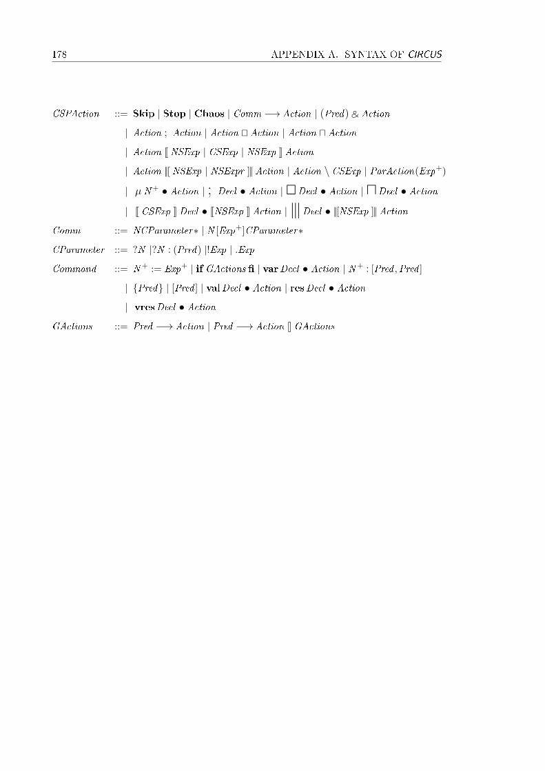
178 APPENDIX A. SYNTAX OF CIRCUS
CSPAction ::= Skip | Stop | Chaos | Comm −→ Action | (Pred) N Action
| Action ; Action | Action @ Action | Action u Action
| Action J NSExp | CSExp | NSExp K Action
| Action ||[ NSExp | NSExpr ]|| Action | Action \ CSExp | ParAction(Exp+)
| µ N+ • Action | ; Decl • Action |@Decl • Action |uDecl • Action
| J CSExp K Decl • JNSExp K Action |9Decl • ||[NSExp ]|| Action
Comm ::= NCParameter∗ | N [Exp+]CParameter∗
CParameter ::= ?N |?N : (Pred) |!Exp | .Exp
Command ::= N+ := Exp+ | if GActions � | varDecl • Action | N+ : [Pred ,Pred ]
| {Pred} | [Pred ] | valDecl • Action | resDecl • Action
| vresDecl • Action
GActions ::= Pred −→ Action | Pred −→ Action 8 GActions
Appendix B
Circus model of State�ow semantics
B.1 Basic de�nitions
section basic toolkit parents circus toolkit
[NAME ]
R : PA
r : Z× N→ R
generic( opt )
optX == {s : seqX | # s ≤ 1}
b2r : B→ R
∀ v : B • b2r(v) = (if v = True then 1 else 0)
truthvalue : A→ B
∀ x : A | x > 0 • truthvalue(x ) = True
∀ x : A | x ≤ 0 • truthvalue(x ) = False
180 APPENDIX B. CIRCUS MODEL OF STATEFLOW SEMANTICS
B.2 State�ow semantics
section state�ow toolkit parents circus toolkit , basic toolkit
function 40 leftassoc ( ∧A )
function 40 leftassoc ( ∨A )
function(¬ A )
function 40 leftassoc ( ∧B )
function 40 leftassoc ( ∨B )
function 40 leftassoc ( ⊕B )
function(¬ B )
function 40 leftassoc ( << )
function 40 leftassoc ( >> )
function 40 leftassoc ( <A )
function 40 leftassoc ( >A )
function 40 leftassoc ( ≤A )
function 40 leftassoc ( ≥A )
function 40 leftassoc ( =A )
function 40 leftassoc ( 6=A )
∧A : A× A→ A∨A : A× A→ A¬ A : A→ A∧B : A× A→ A∨B : A× A→ A⊕B : A× A→ A¬ B : A→ A<< : A× A→ A>> : A× A→ A<A : A× A→ A>A : A× A→ A≤A : A× A→ A≥A : A× A→ A=A : A× A→ A6=A : A× A→ A
∀ x , y : A • x ∧A y = ¬ A(¬ Ax ∨A ¬ Ay)
∀ x , y : A • x ∧B y = ¬ B(¬ Bx ∨B ¬ By)
∀ x , y : A • x ⊕B y = (x ∧B ¬ By) ∨B (¬ Bx ∧B y)
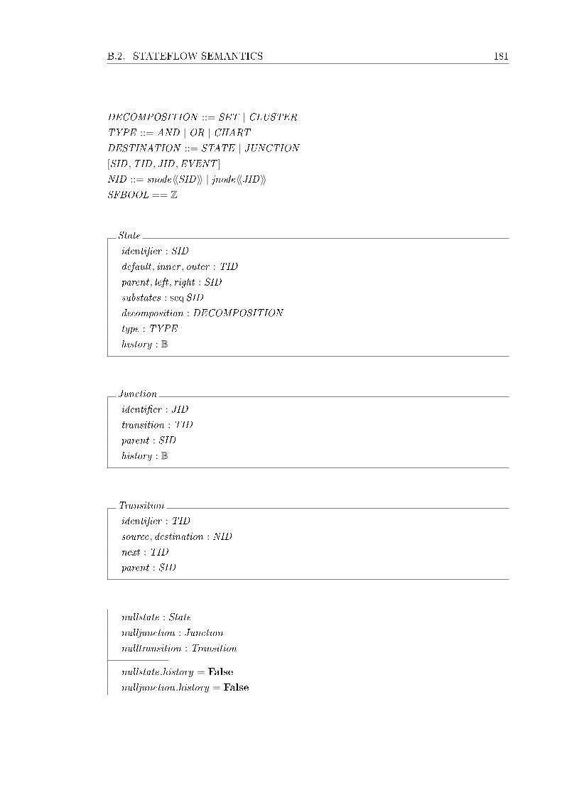
B.2. STATEFLOW SEMANTICS 181
DECOMPOSITION ::= SET | CLUSTERTYPE ::= AND | OR | CHARTDESTINATION ::= STATE | JUNCTION[SID ,TID , JID ,EVENT ]
NID ::= snode〈〈SID〉〉 | jnode〈〈JID〉〉SFBOOL == Z
State
identi�er : SID
default , inner , outer : TID
parent , left , right : SID
substates : seqSID
decomposition : DECOMPOSITION
type : TYPE
history : B
Junction
identi�er : JID
transition : TID
parent : SID
history : B
Transition
identi�er : TID
source, destination : NID
next : TID
parent : SID
nullstate : State
nulljunction : Junction
nulltransition : Transition
nullstate.history = False
nulljunction.history = False
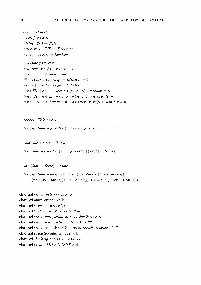
182 APPENDIX B. CIRCUS MODEL OF STATEFLOW SEMANTICS
State�owChart
identi�er : SID
states : SID 7 7→ State
transitions : TID 7 7→ Transition
junctions : JID 7 7→ Junction
nullstate 6∈ ran statesnulltransition 6∈ ran transitionsnulljunction 6∈ ran junctions#{s : ran states | s.type = CHART} = 1
(states(identi�er)).type = CHART
∀n : SID | n ∈ dom states • (states(n)).identi�er = n
∀n : JID | n ∈ dom junctions • (junctions(n)).identi�er = n
∀n : TID | n ∈ dom transitions • (transitions(n)).identi�er = n
parent : State↔ State
∀ s1, s2 : State • parent(s1) = s2 ⇔ s1.parent = s2.identi�er
ancestors : State→ PState
∀ s : State • ancestors(s) = (parent +) L {s} M \{nullstate}
la : (State × State)→ State
∀ s1, s2 : State • la(s1, s2) = µ x : (ancestors(s1) ∩ ancestors(s2)) |(∀ y : (ancestors(s1) ∩ ancestors(s2)) • x = y ∨ y ∈ ancestors(x )) • x
channel read inputs,write outputs
channel input event : seqBchannel events : seqEVENT
channel local event : EVENT × State
channel executeentryaction, executeexitaction : SID
channel executeduringaction : SID × EVENT
channel executeconditionaction, executetransitionaction : TID
channel evaluatecondition : TID × Bchannel checktrigger : TID × EVENT
channel result : TID × EVENT × B
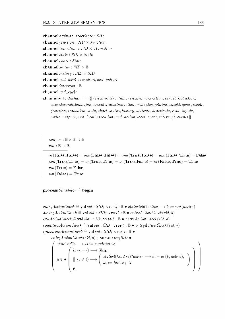
B.2. STATEFLOW SEMANTICS 183
channel activate, deactivate : SID
channel junction : JID × Junction
channel transition : TID × Transition
channel state : SID × State
channel chart : State
channel status : SID × Bchannel history : SID × SID
channel end local execution, end action
channel interrupt : Bchannel end cycle
channelset interface == {| executeentryaction, executeduringaction, executeexitaction,executeconditionaction, executetransitionaction, evaluatecondition, checktrigger , result ,
junction, transition, state, chart , status, history , activate, deactivate, read inputs,
write outputs, end local execution, end action, local event , interrupt , events |}
and , or : B× B→ Bnot : B→ B
or(False,False) = and(False,False) = and(True,False) = and(False,True) = False
and(True,True) = or(True,True) = or(True,False) = or(False,True) = True
not(True) = False
not(False) = True
processSimulator =̂ begin
entryActionCheck =̂ val sid : SID ; vres b : B • status!sid?active −→ b := not(active)
duringActionCheck =̂ val sid : SID ; vres b : B • entryActionCheck(sid , b)
exitActionCheck =̂ val sid : SID ; vres b : B • entryActionCheck(sid , b)
conditionActionCheck =̂ val sid : SID ; vres b : B • entryActionCheck(sid , b)
transitionActionCheck =̂ val sid : SID ; vres b : B •entryActionCheck(sid , b) ; var ss : seqSID •
state!sid?s −→ ss := s.substates;
µX •
if ss = 〈〉−→ Skip
8 ss 6= 〈〉−→(
status!(head ss)?active −→ b := or(b, active);
ss := tail ss ; X
)�
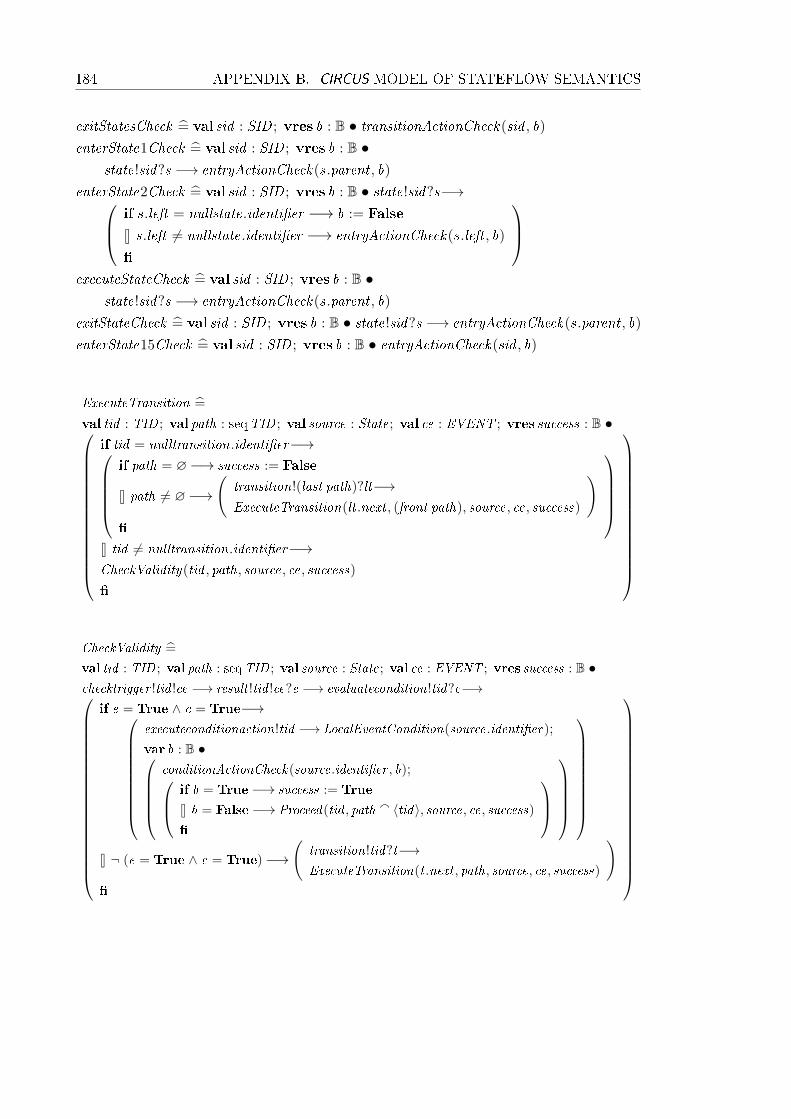
184 APPENDIX B. CIRCUS MODEL OF STATEFLOW SEMANTICS
exitStatesCheck =̂ val sid : SID ; vres b : B • transitionActionCheck(sid , b)
enterState1Check =̂ val sid : SID ; vres b : B •state!sid?s −→ entryActionCheck(s.parent , b)
enterState2Check =̂ val sid : SID ; vres b : B • state!sid?s−→ if s.left = nullstate.identi�er −→ b := False
8 s.left 6= nullstate.identi�er −→ entryActionCheck(s.left , b)
�
executeStateCheck =̂ val sid : SID ; vres b : B •
state!sid?s −→ entryActionCheck(s.parent , b)
exitStateCheck =̂ val sid : SID ; vres b : B • state!sid?s −→ entryActionCheck(s.parent , b)
enterState15Check =̂ val sid : SID ; vres b : B • entryActionCheck(sid , b)
ExecuteTransition =̂
val tid : TID ; val path : seqTID ; val source : State; val ce : EVENT ; vres success : B •
if tid = nulltransition.identi�er−→if path = ∅−→ success := False
8 path 6= ∅−→(
transition!(last path)?lt−→ExecuteTransition(lt .next , (front path), source, ce, success)
)�
8 tid 6= nulltransition.identi�er−→CheckValidity(tid , path, source, ce, success)
�
CheckValidity =̂
val tid : TID ; val path : seqTID ; val source : State; val ce : EVENT ; vres success : B •checktrigger !tid !ce −→ result !tid !ce?e −→ evaluatecondition!tid?c−→
if e = True ∧ c = True−→
executeconditionaction!tid −→ LocalEventCondition(source.identi�er);
var b : B •conditionActionCheck(source.identi�er , b); if b = True−→ success := True
8 b = False−→ Proceed(tid , path a 〈tid〉, source, ce, success)
�
8 ¬ (e = True ∧ c = True)−→
(transition!tid?t−→ExecuteTransition(t .next , path, source, ce, success)
)�

B.2. STATEFLOW SEMANTICS 185
Proceed =̂
val tid : TID ; val path : seqTID ; val source : State; val ce : EVENT ; vres success : B •transition!tid?t−→
if t .destination ∈ ran snode −→(
state!((snode ∼) t .destination)?dest−→proceedToState(source, dest , path, ce, success)
)8 t .destination ∈ ran jnode −→ proceedToJunction(tid , path, source, ce, success)
�
proceedToState =̂
val src, dest : State; val path : seqTID ; val ce : EVENT ; vres success : B •
ExitStates((la(src, dest)).substates, ce);
var b : B •
exitStatesCheck((la(src, dest)).identi�er , b);
if b = True−→ Skip
8 b = False−→executePath(path, src, dest , ce);
transitionActionCheck((la(src, dest)).identi�er , b); if b = True−→ Skip
8 b = False−→ EnterState(dest , la(src, dest), ce)
�
�
;
success := True
executePath =̂ path : seqTID ; src, dest : State; ce : EVENT •
if # path = 0−→ Skip
8 # path > 0−→
executetransitionaction!(head path)−→LocalEventTransition((la(src, dest)).identi�er);
var b : B •transitionActionCheck((la(src, dest)).identi�er , b); if b = True−→ Skip
8 b = False−→ executePath(tail path, src, dest , ce)
�
�
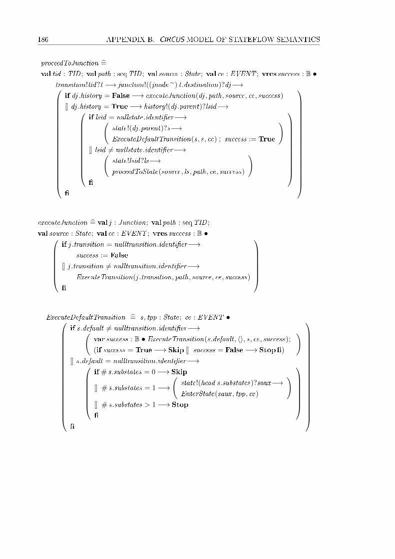
186 APPENDIX B. CIRCUS MODEL OF STATEFLOW SEMANTICS
proceedToJunction =̂
val tid : TID ; val path : seqTID ; val source : State; val ce : EVENT ; vres success : B •transition!tid?t −→ junction!((jnode ∼) t .destination)?dj−→
if dj .history = False−→ executeJunction(dj , path, source, ce, success)
8 dj .history = True−→ history !(dj .parent)?lsid−→
if lsid = nullstate.identi�er−→(state!(dj .parent)?s−→ExecuteDefaultTransition(s, s, ce) ; success := True
)8 lsid 6= nullstate.identi�er−→(
state!lsid?ls−→proceedToState(source, ls, path, ce, success)
)�
�
executeJunction =̂ val j : Junction; val path : seqTID ;
val source : State; val ce : EVENT ; vres success : B •if j .transition = nulltransition.identi�er−→
success := False
8 j .transition 6= nulltransition.identi�er−→ExecuteTransition(j .transition, path, source, ce, success)
�
ExecuteDefaultTransition =̂ s, tpp : State; ce : EVENT •
if s.default 6= nulltransition.identi�er−→(var success : B • ExecuteTransition(s.default , 〈〉, s, ce, success);
(if success = True−→ Skip 8 success = False−→ Stop�)
)8 s.default = nulltransition.identi�er−→
if # s.substates = 0−→ Skip
8 # s.substates = 1−→(
state!(head s.substates)?saux−→EnterState(saux , tpp, ce)
)8 # s.substates > 1−→ Stop
�
�
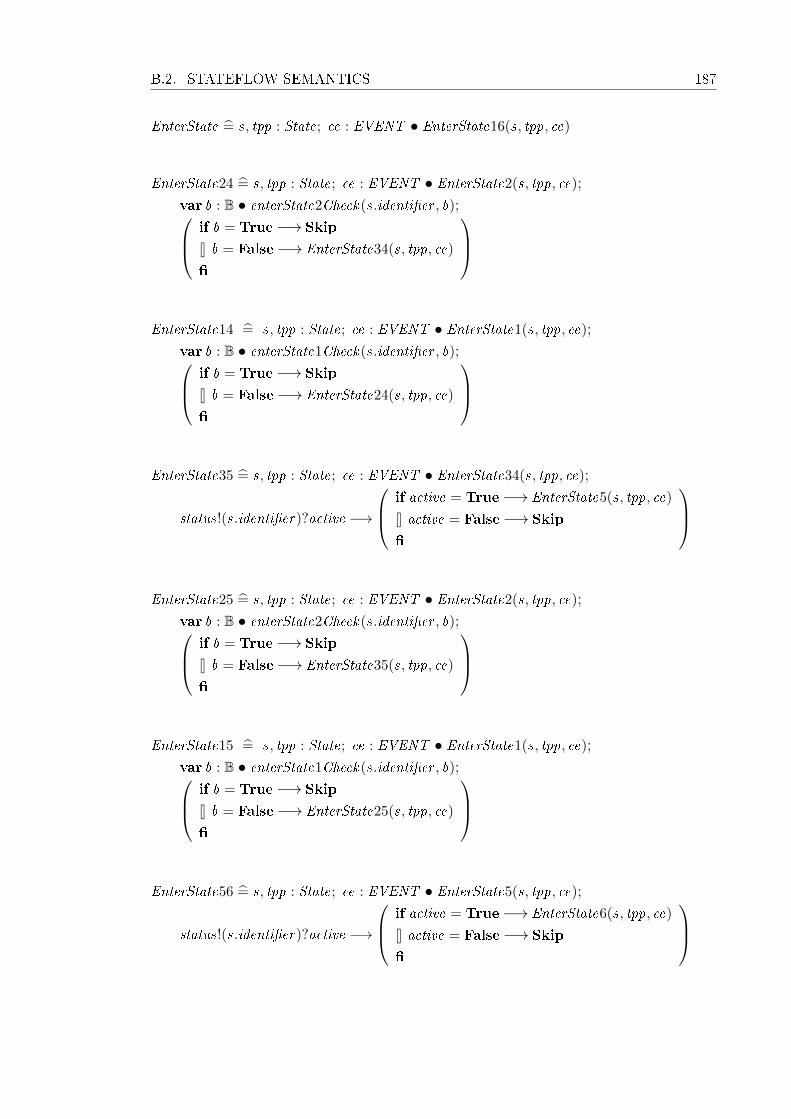
B.2. STATEFLOW SEMANTICS 187
EnterState =̂ s, tpp : State; ce : EVENT • EnterState16(s, tpp, ce)
EnterState24 =̂ s, tpp : State; ce : EVENT • EnterState2(s, tpp, ce);
var b : B • enterState2Check(s.identi�er , b); if b = True−→ Skip
8 b = False−→ EnterState34(s, tpp, ce)
�
EnterState14 =̂ s, tpp : State; ce : EVENT • EnterState1(s, tpp, ce);
var b : B • enterState1Check(s.identi�er , b); if b = True−→ Skip
8 b = False−→ EnterState24(s, tpp, ce)
�
EnterState35 =̂ s, tpp : State; ce : EVENT • EnterState34(s, tpp, ce);
status!(s.identi�er)?active −→
if active = True−→ EnterState5(s, tpp, ce)
8 active = False−→ Skip
�
EnterState25 =̂ s, tpp : State; ce : EVENT • EnterState2(s, tpp, ce);
var b : B • enterState2Check(s.identi�er , b); if b = True−→ Skip
8 b = False−→ EnterState35(s, tpp, ce)
�
EnterState15 =̂ s, tpp : State; ce : EVENT • EnterState1(s, tpp, ce);
var b : B • enterState1Check(s.identi�er , b); if b = True−→ Skip
8 b = False−→ EnterState25(s, tpp, ce)
�
EnterState56 =̂ s, tpp : State; ce : EVENT • EnterState5(s, tpp, ce);
status!(s.identi�er)?active −→
if active = True−→ EnterState6(s, tpp, ce)
8 active = False−→ Skip
�
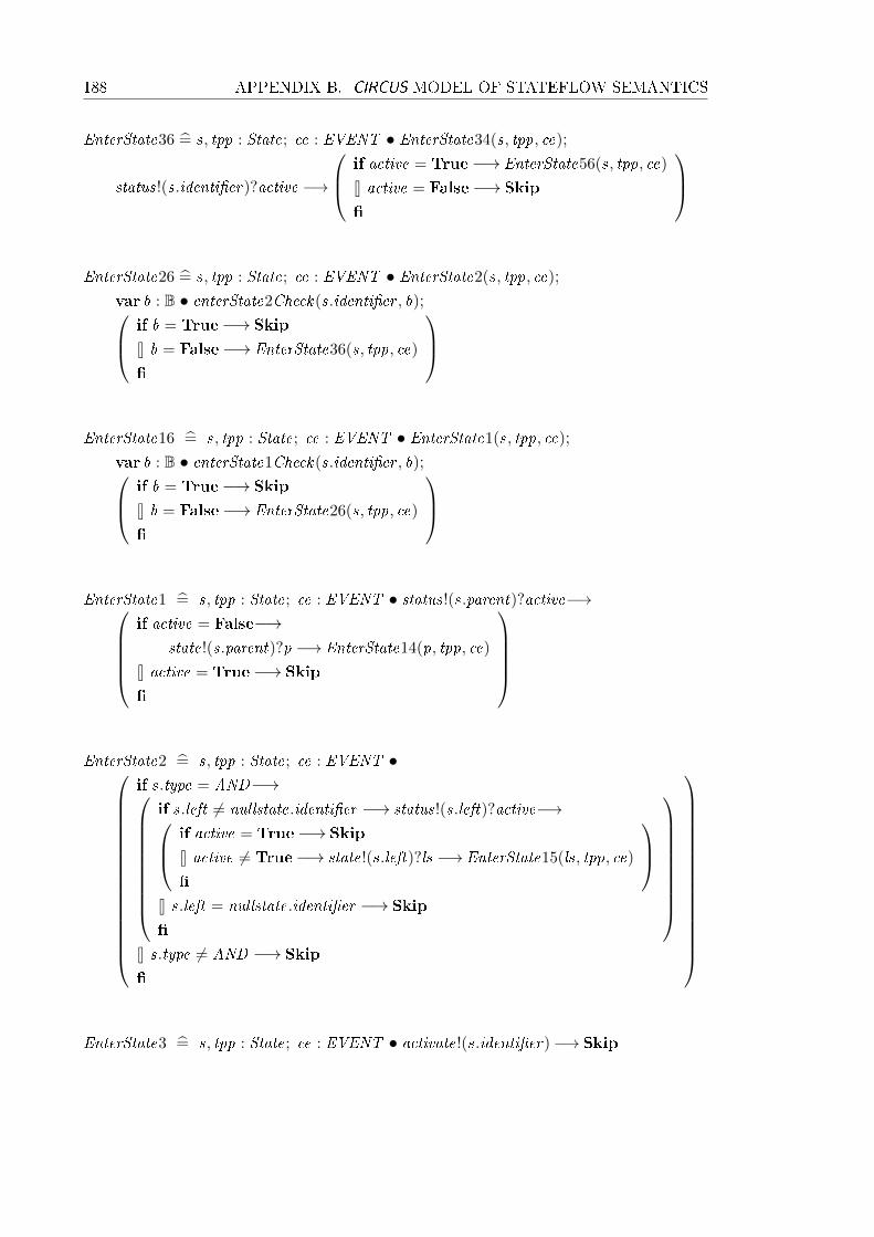
188 APPENDIX B. CIRCUS MODEL OF STATEFLOW SEMANTICS
EnterState36 =̂ s, tpp : State; ce : EVENT • EnterState34(s, tpp, ce);
status!(s.identi�er)?active −→
if active = True−→ EnterState56(s, tpp, ce)
8 active = False−→ Skip
�
EnterState26 =̂ s, tpp : State; ce : EVENT • EnterState2(s, tpp, ce);
var b : B • enterState2Check(s.identi�er , b); if b = True−→ Skip
8 b = False−→ EnterState36(s, tpp, ce)
�
EnterState16 =̂ s, tpp : State; ce : EVENT • EnterState1(s, tpp, ce);
var b : B • enterState1Check(s.identi�er , b); if b = True−→ Skip
8 b = False−→ EnterState26(s, tpp, ce)
�
EnterState1 =̂ s, tpp : State; ce : EVENT • status!(s.parent)?active−→if active = False−→
state!(s.parent)?p −→ EnterState14(p, tpp, ce)
8 active = True−→ Skip
�
EnterState2 =̂ s, tpp : State; ce : EVENT •
if s.type = AND−→
if s.left 6= nullstate.identi�er −→ status!(s.left)?active−→ if active = True−→ Skip
8 active 6= True−→ state!(s.left)?ls −→ EnterState15(ls, tpp, ce)
�
8 s.left = nullstate.identi�er −→ Skip
�
8 s.type 6= AND −→ Skip
�
EnterState3 =̂ s, tpp : State; ce : EVENT • activate!(s.identi�er)−→ Skip

B.2. STATEFLOW SEMANTICS 189
EnterState4 =̂ s, tpp : State; ce : EVENT •executeentryaction!(s.identi�er)−→ LocalEventEntry(s.identi�er)
EnterState34 =̂ s, tpp : State; ce : EVENT • status.(s.identi�er)?active−→ if active = True−→ Skip
8 active = False−→ EnterState3(s, tpp, ce) ; EnterState4(s, tpp, ce)
�
EnterState5 =̂ s, tpp : State; ce : EVENT •EnterState5a(s, tpp, ce) ; EnterState5b(s, tpp, ce)
EnterState5a =̂ s, tpp : State; ce : EVENT •
if s.history = True−→ history !(s.identi�er)?lsid−→ if lsid 6= nullstate.identi�er −→ state!lsid?ls −→ EnterState15(ls, tpp, ce)
8 lsid = nullstate.identi�er −→ ExecuteDefaultTransition(s, tpp, ce)
�
8 s.history = False−→ if s.default 6= nulltransition.identi�er −→ ExecuteDefaultTransition(s, tpp, ce)
8s.default = nulltransition.identi�er −→ Skip
�
�
EnterState5b =̂ s, tpp : State; ce : EVENT •if s.decomposition = SET ∧ s.default = nulltransition.identi�er−→
EnterStates15(s.substates, tpp, ce)
8 s.decomposition 6= SET ∨ s.default 6= nulltransition.identi�er −→ Skip
�
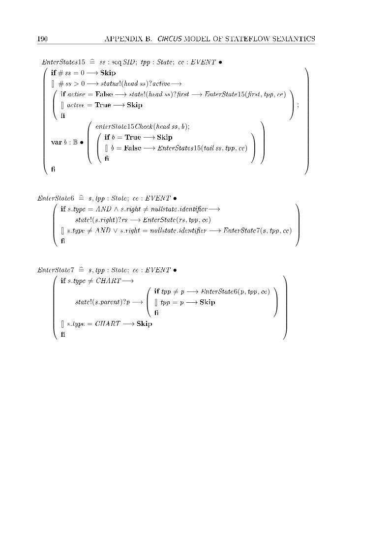
190 APPENDIX B. CIRCUS MODEL OF STATEFLOW SEMANTICS
EnterStates15 =̂ ss : seqSID ; tpp : State; ce : EVENT •
if # ss = 0−→ Skip
8 # ss > 0−→ status!(head ss)?active−→ if active = False−→ state!(head ss)?�rst −→ EnterState15(�rst , tpp, ce)
8 active = True−→ Skip
�
;
var b : B •
enterState15Check(head ss, b); if b = True−→ Skip
8 b = False−→ EnterStates15(tail ss, tpp, ce)
�
�
EnterState6 =̂ s, tpp : State; ce : EVENT •if s.type = AND ∧ s.right 6= nullstate.identi�er−→
state!(s.right)?rs −→ EnterState(rs, tpp, ce)
8 s.type 6= AND ∨ s.right = nullstate.identi�er −→ EnterState7(s, tpp, ce)
�
EnterState7 =̂ s, tpp : State; ce : EVENT •
if s.type 6= CHART−→
state!(s.parent)?p −→
if tpp 6= p −→ EnterState6(p, tpp, ce)
8 tpp = p −→ Skip
�
8 s.type = CHART −→ Skip
�

B.2. STATEFLOW SEMANTICS 191
ExecuteState =̂ s : State; ce : EVENT • status!(s.identi�er)?active−→
if active = True−→
var success : B •ExecuteTransition(s.outer , 〈〉, s, ce, success);
if success = True−→ Skip
8 success = False−→
executeduringaction!(s.identi�er)!ce−→LocalEventDuring(s.identi�er);
var b : B •duringActionCheck(s.identi�er , b); if b = True−→ Skip
8 b = False−→ AlternativeExecution(s, ce)
�
�
8active = False−→ Skip
�
AlternativeExecution =̂ s : State; ce : EVENT •var success : B • ExecuteTransition(s.inner , 〈〉, s, ce, success); if success = True−→ Skip
8success = False−→ ExecuteSubstates(s, ce)
�
ExecuteSubstates =̂ s : State; ce : EVENT • if s.decomposition = SET −→ ExecuteParallelStates(s.substates, ce)
8 s.decomposition = CLUSTER −→ ExecuteSequentialStates(s.substates, ce)
�
ExecuteParallelStates =̂ ss : seqSID ; ce : EVENT •
if # ss = 0−→ Skip
8 # ss > 0−→ state!(head ss)?�rst −→ ExecuteState(�rst , ce);
var b : B •
executeStateCheck(head ss, b); if b = True−→ Skip
8 b = False−→ ExecuteParallelStates(tail ss, ce)
�
�

192 APPENDIX B. CIRCUS MODEL OF STATEFLOW SEMANTICS
ExecuteSequentialStates =̂ ss : seqSID ; ce : EVENT •
if # ss = 0−→ Skip
8 # ss > 0−→ status!(head ss)?active−→ if active = True−→ state!(head ss)?�rst −→ ExecuteState(�rst , ce)
8 active = False−→ ExecuteSequentialStates(tail ss, ce)
�
�
ExitState =̂ s : State; ce : EVENT •
if s.right 6= nullstate.identi�er −→ status!(s.right)?active−→ if active = True−→ state!(s.right)?rs −→ ExitState(rs, ce)
8 active = False−→ Skip
�
8 s.right = nullstate.identi�er −→ Skip
�
;
ExitStates(s.substates, ce);
executeexitaction!(s.identi�er)−→ LocalEventExit(s.identi�er);
var b : B •
exitActionCheck(s.identi�er , b); if b = True−→ Skip
8 b = False−→ deactivate!(s.identi�er)−→ Skip
�
ExitStates =̂ ss : seqSID ; ce : EVENT •
if # ss = 0−→ Skip
8 # ss > 0−→ status!(last ss)?active−→ if active = True−→ state!(last ss)?l −→ ExitState(l , ce)
8 active = False−→ Skip
�
;
var b : B •
exitStateCheck(head ss, b); if b = True−→ Skip
8 b = False−→ ExitStates(front ss, ce)
�
�
ExecuteChart =̂ ce : EVENT • chart?c −→ status!(c.identi�er)?active−→ if active = True−→ ExecuteActiveChart(c, ce)
8 active = False−→ ExecuteInactiveChart(c, ce)
�

B.2. STATEFLOW SEMANTICS 193
ExecuteInactiveChart =̂ c : State; ce : EVENT • activate!(c.identi�er)−→
if c.default 6= nulltransition.identi�er ∨ c.decomposition = CLUSTER−→ExecuteDefaultTransition(c, c, ce)
8 c.default = nulltransition.identi�er ∧ c.decomposition = SET−→if c.substates = 〈〉−→ Skip
8 c.substates 6= 〈〉−→state!(head(c.substates))?�rst −→ EnterState(�rst , c, ce)
�
�
ExecuteActiveChart =̂ c : State; ce : EVENT • if c.substates = ∅−→ ExecuteInactiveChart(c, ce)
8 c.substates 6= ∅−→ ExecuteSubstates(c, ce)
�
LocalEventEntry =̂ sid : SID • µX •
local event?e?s −→
TreatLocalEvent(e, s);
var b : B •entryActionCheck(sid , b);
if b = True−→interrupt .True−→ end action −→ Skip
8 b = False−→ interrupt .False−→ X
�
@end action −→ Skip
LocalEventDuring =̂ sid : SID • µX •
local event?e?s −→
TreatLocalEvent(e, s);
var b : B
•
duringActionCheck(sid , b);
if b = True−→interrupt .True−→ end action −→ Skip
8 b = False−→ interrupt .False−→ X
�
@end action −→ Skip
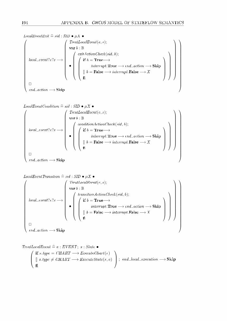
194 APPENDIX B. CIRCUS MODEL OF STATEFLOW SEMANTICS
LocalEventExit =̂ sid : SID • µX •
local event?e?s −→
TreatLocalEvent(e, s);
var b : B
•
exitActionCheck(sid , b);
if b = True−→interrupt .True−→ end action −→ Skip
8 b = False−→ interrupt .False−→ X
�
@end action −→ Skip
LocalEventCondition =̂ sid : SID • µX •
local event?e?s −→
TreatLocalEvent(e, s);
var b : B
•
conditionActionCheck(sid , b);
if b = True−→interrupt .True−→ end action −→ Skip
8 b = False−→ interrupt .False−→ X
�
@end action −→ Skip
LocalEventTransition =̂ sid : SID • µX •
local event?e?s −→
TreatLocalEvent(e, s);
var b : B
•
transitionActionCheck(sid , b);
if b = True−→interrupt .True−→ end action −→ Skip
8 b = False−→ interrupt .False−→ X
�
@end action −→ Skip
TreatLocalEvent =̂ e : EVENT ; s : State • if s.type = CHART −→ ExecuteChart(e)
8 s.type 6= CHART −→ ExecuteState(s, e)
�
; end local execution −→ Skip

B.2. STATEFLOW SEMANTICS 195
ExecuteEvent =̂ e : EVENT ; v : B •
if v = True−→ ExecuteChart(e)
8 v = False−→ Skip
�
ExecuteEvents =̂ es : seqEVENT ; vs : seqB • (; i : id(1 . .# es) • ExecuteEvent(es(i), vs(i)))
• (µX • Step ; end cycle −→ X )
end

Appendix C
Circus models of State�ow charts
C.1 Circus model of Shift Logic Chart
section calc th parents basic toolkit
calc th : (R× R)→ (R× R)
section sf car shift logic parents state�ow toolkit , calc th
s downshifting , s gear state, s fourth, s second , s third , s �rst ,
s selection state, s upshifting , s steady state, c shift logic : SID
t third fourth, t second third , t �rst second , t fourth third , t default �rst ,
t second �rst , t third second , t steady state upshifting , t default steady state,
t upshifting steady state23, t steady state downshifting ,
t downshifting steady state25, t downshifting steady state24,
t upshifting steady state26 : TID

198 APPENDIX C. CIRCUS MODELS OF STATEFLOW CHARTS
C shift logic : State
C shift logic =〈|identi�er == c shift logic, default == nulltransition.identi�er ,
inner == nulltransition.identi�er , outer == nulltransition.identi�er ,
parent == nullstate.identi�er , left == nullstate.identi�er ,
right == nullstate.identi�er , substates == 〈s gear state, s selection state〉,decomposition == SET , type == CHART , history == False|〉
S downshifting : State
S downshifting =〈|identi�er == s downshifting , default == nulltransition.identi�er ,
inner == nulltransition.identi�er , outer == t downshifting steady state24,
parent == s selection state, left == nullstate.identi�er ,
right == nullstate.identi�er , substates == 〈〉,decomposition == CLUSTER, type == OR, history == False|〉
S gear state : State
S gear state =〈|identi�er == s gear state, default == t default �rst ,
inner == nulltransition.identi�er , outer == nulltransition.identi�er ,
parent == c shift logic, left == nullstate.identi�er ,
right == s selection state, substates == 〈s fourth, s third , s �rst , s second〉,decomposition == CLUSTER, type == AND , history == False|〉
S fourth : State
S fourth =
〈|identi�er == s fourth, default == nulltransition.identi�er ,
inner == nulltransition.identi�er , outer == t fourth third ,
parent == s gear state, left == nullstate.identi�er ,
right == nullstate.identi�er , substates == 〈〉,decomposition == CLUSTER, type == OR, history == False|〉

C.1. CIRCUS MODEL OF SHIFT LOGIC CHART 199
S second : State
S second =
〈|identi�er == s second , default == nulltransition.identi�er ,
inner == nulltransition.identi�er , outer == t second third ,
parent == s gear state, left == nullstate.identi�er ,
right == nullstate.identi�er , substates == 〈〉,decomposition == CLUSTER, type == OR, history == False|〉
S third : State
S third =
〈|identi�er == s third , default == nulltransition.identi�er ,
inner == nulltransition.identi�er , outer == t third fourth,
parent == s gear state, left == nullstate.identi�er ,
right == nullstate.identi�er , substates == 〈〉,decomposition == CLUSTER, type == OR, history == False|〉
S �rst : State
S �rst =〈|identi�er == s �rst , default == nulltransition.identi�er ,
inner == nulltransition.identi�er , outer == t �rst second ,
parent == s gear state, left == nullstate.identi�er ,
right == nullstate.identi�er , substates == 〈〉,decomposition == CLUSTER, type == OR, history == False|〉
S selection state : State
S selection state =〈|identi�er == s selection state, default == t default steady state,
inner == nulltransition.identi�er , outer == nulltransition.identi�er ,
parent == c shift logic, left == s gear state, right == nullstate.identi�er ,
substates == 〈s upshifting , s downshifting , s steady state〉,decomposition == CLUSTER, type == AND , history == False|〉
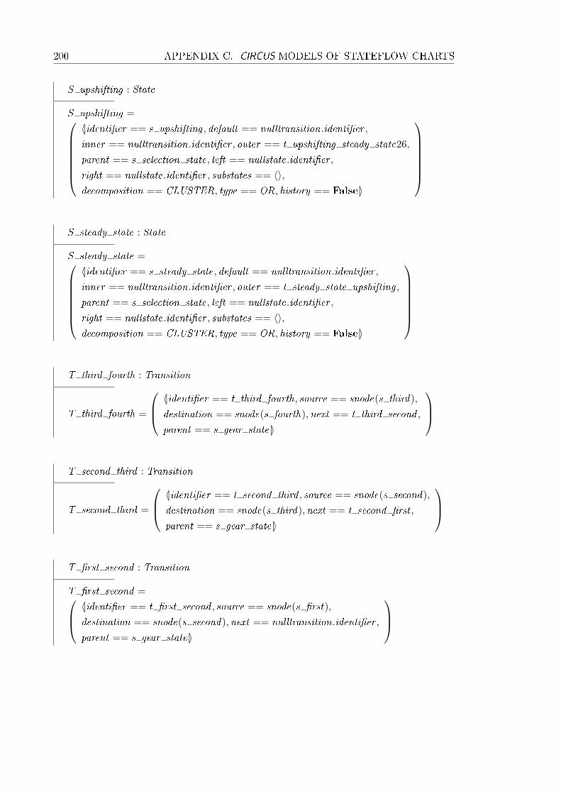
200 APPENDIX C. CIRCUS MODELS OF STATEFLOW CHARTS
S upshifting : State
S upshifting =〈|identi�er == s upshifting , default == nulltransition.identi�er ,
inner == nulltransition.identi�er , outer == t upshifting steady state26,
parent == s selection state, left == nullstate.identi�er ,
right == nullstate.identi�er , substates == 〈〉,decomposition == CLUSTER, type == OR, history == False|〉
S steady state : State
S steady state =〈|identi�er == s steady state, default == nulltransition.identi�er ,
inner == nulltransition.identi�er , outer == t steady state upshifting ,
parent == s selection state, left == nullstate.identi�er ,
right == nullstate.identi�er , substates == 〈〉,decomposition == CLUSTER, type == OR, history == False|〉
T third fourth : Transition
T third fourth =
〈|identi�er == t third fourth, source == snode(s third),
destination == snode(s fourth),next == t third second ,
parent == s gear state|〉
T second third : Transition
T second third =
〈|identi�er == t second third , source == snode(s second),
destination == snode(s third),next == t second �rst ,
parent == s gear state|〉
T �rst second : Transition
T �rst second = 〈|identi�er == t �rst second , source == snode(s �rst),
destination == snode(s second),next == nulltransition.identi�er ,
parent == s gear state|〉

C.1. CIRCUS MODEL OF SHIFT LOGIC CHART 201
T fourth third : Transition
T fourth third = 〈|identi�er == t fourth third , source == snode(s fourth),
destination == snode(s third),next == nulltransition.identi�er ,
parent == s gear state|〉
T default �rst : Transition
T default �rst = 〈|identi�er == t default �rst , source == snode(nullstate.identi�er),
destination == snode(s �rst),next == nulltransition.identi�er ,
parent == s gear state|〉
T second �rst : Transition
T second �rst = 〈|identi�er == t second �rst , source == snode(s second),
destination == snode(s �rst),next == nulltransition.identi�er ,
parent == s gear state|〉
T third second : Transition
T third second = 〈|identi�er == t third second , source == snode(s third),
destination == snode(s second),next == nulltransition.identi�er ,
parent == s gear state|〉
T steady state upshifting : Transition
T steady state upshifting = 〈|identi�er == t steady state upshifting , source == snode(s steady state),
destination == snode(s upshifting),next == t steady state downshifting ,
parent == s selection state|〉
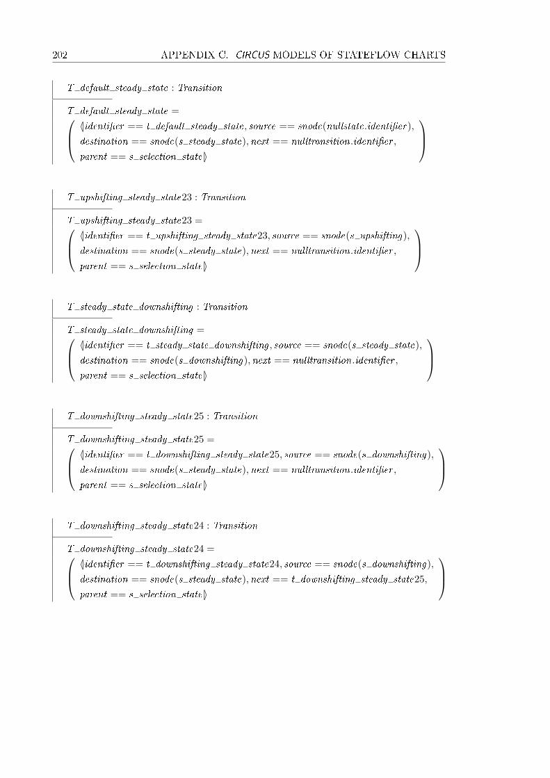
202 APPENDIX C. CIRCUS MODELS OF STATEFLOW CHARTS
T default steady state : Transition
T default steady state = 〈|identi�er == t default steady state, source == snode(nullstate.identi�er),
destination == snode(s steady state),next == nulltransition.identi�er ,
parent == s selection state|〉
T upshifting steady state23 : Transition
T upshifting steady state23 = 〈|identi�er == t upshifting steady state23, source == snode(s upshifting),
destination == snode(s steady state),next == nulltransition.identi�er ,
parent == s selection state|〉
T steady state downshifting : Transition
T steady state downshifting = 〈|identi�er == t steady state downshifting , source == snode(s steady state),
destination == snode(s downshifting),next == nulltransition.identi�er ,
parent == s selection state|〉
T downshifting steady state25 : Transition
T downshifting steady state25 = 〈|identi�er == t downshifting steady state25, source == snode(s downshifting),
destination == snode(s steady state),next == nulltransition.identi�er ,
parent == s selection state|〉
T downshifting steady state24 : Transition
T downshifting steady state24 = 〈|identi�er == t downshifting steady state24, source == snode(s downshifting),
destination == snode(s steady state),next == t downshifting steady state25,
parent == s selection state|〉
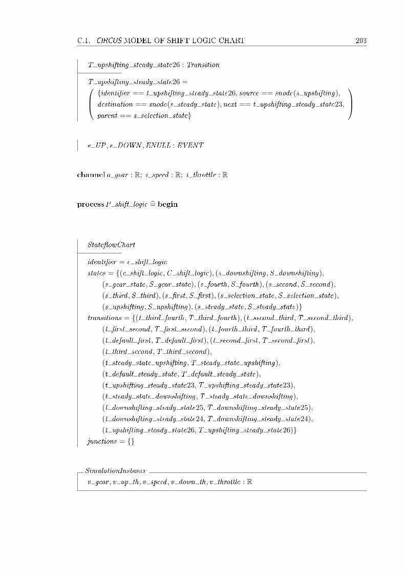
C.1. CIRCUS MODEL OF SHIFT LOGIC CHART 203
T upshifting steady state26 : Transition
T upshifting steady state26 = 〈|identi�er == t upshifting steady state26, source == snode(s upshifting),
destination == snode(s steady state),next == t upshifting steady state23,
parent == s selection state|〉
e UP , e DOWN ,ENULL : EVENT
channel o gear : R; i speed : R; i throttle : R
processP shift logic =̂ begin
State�owChart
identi�er = c shift logic
states = {(c shift logic,C shift logic), (s downshifting ,S downshifting),
(s gear state,S gear state), (s fourth,S fourth), (s second ,S second),
(s third ,S third), (s �rst ,S �rst), (s selection state,S selection state),
(s upshifting ,S upshifting), (s steady state,S steady state)}transitions = {(t third fourth,T third fourth), (t second third ,T second third),
(t �rst second ,T �rst second), (t fourth third ,T fourth third),
(t default �rst ,T default �rst), (t second �rst ,T second �rst),
(t third second ,T third second),
(t steady state upshifting ,T steady state upshifting),
(t default steady state,T default steady state),
(t upshifting steady state23,T upshifting steady state23),
(t steady state downshifting ,T steady state downshifting),
(t downshifting steady state25,T downshifting steady state25),
(t downshifting steady state24,T downshifting steady state24),
(t upshifting steady state26,T upshifting steady state26)}junctions = {}
SimulationInstance
v gear , v up th, v speed , v down th, v throttle : R

204 APPENDIX C. CIRCUS MODELS OF STATEFLOW CHARTS
InitSimulationInstance
SimulationInstance ′
v gear ′ = 0
v up th ′ = 0
v speed ′ = 0
v down th ′ = 0
v throttle ′ = 0
SimulationData
state status : SID 7→ Bstate history : SID 7→ SID
dom state status = dom states
dom state history = {j : ran junctions | j .history = True • j .parent}∀ s : ran states | s.decomposition = CLUSTER •
#{ss : ran s.substates | state status(ss) = True} ≤ 1
InitSimulationData
SimulationData ′
state status ′ = {n : dom states • n 7→ False}state history ′ = {n : dom state history ′ • n 7→ nullstate.identi�er}
ActivateNoHistory
∆SimulationData
x? : SID
x? ∈ dom state status
(parent (states x?)).history = False
state history ′ = state history
state status ′ = state status ⊕ {x? 7→True}
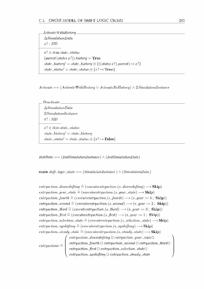
C.1. CIRCUS MODEL OF SHIFT LOGIC CHART 205
ActivateWithHistory
∆SimulationData
x? : SID
x? ∈ dom state status
(parent (states x?)).history = True
state history ′ = state history ⊕ {((states x?).parent) 7→ x?}state status ′ = state status ⊕ {x? 7→True}
Activate == (ActivateWithHistory ∨ ActivateNoHistory) ∧ ΞSimulationInstance
Deactivate
∆SimulationData
ΞSimulationInstance
x? : SID
x? ∈ dom state status
state history ′ = state history
state status ′ = state status ⊕ {x? 7→ False}
InitState == (InitSimulationInstance) ∧ (InitSimulationData)
state shift logic state == (SimulationInstance ) ∧ (SimulationData )
entryaction downshifting =̂ (executeentryaction.(s downshifting)−→ Skip)
entryaction gear state =̂ (executeentryaction.(s gear state)−→ Skip)
entryaction fourth =̂ (executeentryaction.(s fourth)−→ (v gear := 4 ; Skip))
entryaction second =̂ (executeentryaction.(s second)−→ (v gear := 2 ; Skip))
entryaction third =̂ (executeentryaction.(s third)−→ (v gear := 3 ; Skip))
entryaction �rst =̂ (executeentryaction.(s �rst)−→ (v gear := 1 ; Skip))
entryaction selection state =̂ (executeentryaction.(s selection state)−→ Skip)
entryaction upshifting =̂ (executeentryaction.(s upshifting)−→ Skip)
entryaction steady state =̂ (executeentryaction.(s steady state)−→ Skip)
entryactions =̂
entryaction downshifting @ entryaction gear state@entryaction fourth @ entryaction second @ entryaction third@entryaction �rst @ entryaction selection state@entryaction upshifting @ entryaction steady state

206 APPENDIX C. CIRCUS MODELS OF STATEFLOW CHARTS
duringaction downshifting =̂ (executeduringaction.(s downshifting)?ce −→ Skip)
duringaction gear state =̂ (executeduringaction.(s gear state)?ce −→ Skip)
duringaction fourth =̂ (executeduringaction.(s fourth)?ce −→ Skip)
duringaction second =̂ (executeduringaction.(s second)?ce −→ Skip)
duringaction third =̂ (executeduringaction.(s third)?ce −→ Skip)
duringaction �rst =̂ (executeduringaction.(s �rst)?ce −→ Skip)
duringaction selection state =̂ executeduringaction.(s selection state)?ce−→(var aux : R× R • aux := calc th(v gear , v throttle);
v down th := aux .1 ; v up th := aux .2
)duringaction upshifting =̂ (executeduringaction.(s upshifting)?ce −→ Skip)
duringaction steady state =̂ (executeduringaction.(s steady state)?ce −→ Skip)
duringactions =̂
duringaction downshifting @ duringaction gear state@duringaction fourth @ duringaction second@duringaction third @ duringaction �rst@duringaction selection state @ duringaction upshifting@duringaction steady state
exitaction downshifting =̂ (executeexitaction.(s downshifting)−→ Skip)
exitaction gear state =̂ (executeexitaction.(s gear state)−→ Skip)
exitaction fourth =̂ (executeexitaction.(s fourth)−→ Skip)
exitaction second =̂ (executeexitaction.(s second)−→ Skip)
exitaction third =̂ (executeexitaction.(s third)−→ Skip)
exitaction �rst =̂ (executeexitaction.(s �rst)−→ Skip)
exitaction selection state =̂ (executeexitaction.(s selection state)−→ Skip)
exitaction upshifting =̂ (executeexitaction.(s upshifting)−→ Skip)
exitaction steady state =̂ (executeexitaction.(s steady state)−→ Skip)
exitactions =̂
exitaction downshifting @ exitaction gear state@exitaction fourth @ exitaction second@exitaction third @ exitaction �rst@exitaction selection state @ exitaction upshifting@exitaction steady state
conditionaction third fourth =̂ (executeconditionaction.(t third fourth)−→ Skip)
conditionaction second third =̂ (executeconditionaction.(t second third)−→ Skip)
conditionaction �rst second =̂ (executeconditionaction.(t �rst second)−→ Skip)
conditionaction fourth third =̂ (executeconditionaction.(t fourth third)−→ Skip)
conditionaction default �rst =̂ (executeconditionaction.(t default �rst)−→ Skip)
conditionaction second �rst =̂ (executeconditionaction.(t second �rst)−→ Skip)
conditionaction third second =̂ (executeconditionaction.(t third second)−→ Skip)
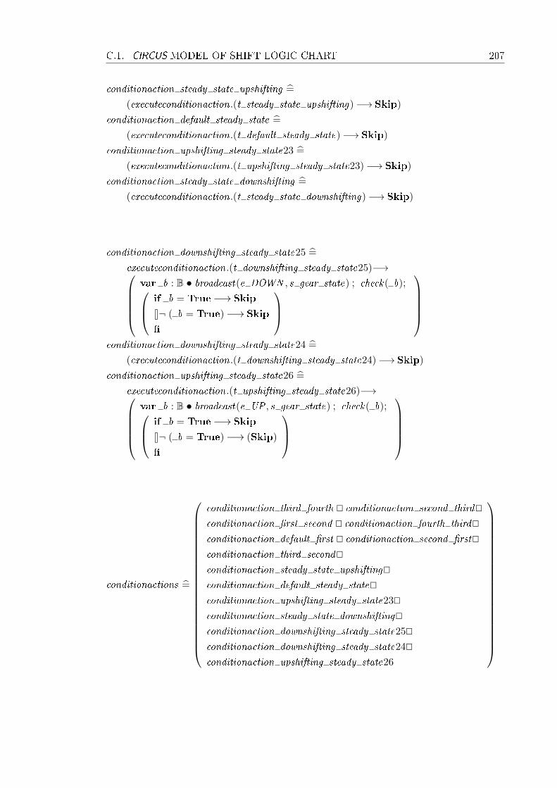
C.1. CIRCUS MODEL OF SHIFT LOGIC CHART 207
conditionaction steady state upshifting =̂
(executeconditionaction.(t steady state upshifting)−→ Skip)
conditionaction default steady state =̂
(executeconditionaction.(t default steady state)−→ Skip)
conditionaction upshifting steady state23 =̂
(executeconditionaction.(t upshifting steady state23)−→ Skip)
conditionaction steady state downshifting =̂
(executeconditionaction.(t steady state downshifting)−→ Skip)
conditionaction downshifting steady state25 =̂
executeconditionaction.(t downshifting steady state25)−→var b : B • broadcast(e DOWN , s gear state) ; check( b); if b = True−→ Skip
8¬ ( b = True)−→ Skip
�
conditionaction downshifting steady state24 =̂
(executeconditionaction.(t downshifting steady state24)−→ Skip)
conditionaction upshifting steady state26 =̂
executeconditionaction.(t upshifting steady state26)−→var b : B • broadcast(e UP , s gear state) ; check( b); if b = True−→ Skip
8¬ ( b = True)−→ (Skip)
�
conditionactions =̂
conditionaction third fourth @ conditionaction second third@conditionaction �rst second @ conditionaction fourth third@conditionaction default �rst @ conditionaction second �rst@conditionaction third second@conditionaction steady state upshifting@conditionaction default steady state@conditionaction upshifting steady state23@conditionaction steady state downshifting@conditionaction downshifting steady state25@conditionaction downshifting steady state24@conditionaction upshifting steady state26

208 APPENDIX C. CIRCUS MODELS OF STATEFLOW CHARTS
transitionaction third fourth =̂ (executetransitionaction.(t third fourth)−→ Skip)
transitionaction second third =̂ (executetransitionaction.(t second third)−→ Skip)
transitionaction �rst second =̂ (executetransitionaction.(t �rst second)−→ Skip)
transitionaction fourth third =̂ (executetransitionaction.(t fourth third)−→ Skip)
transitionaction default �rst =̂ (executetransitionaction.(t default �rst)−→ Skip)
transitionaction second �rst =̂ (executetransitionaction.(t second �rst)−→ Skip)
transitionaction third second =̂ (executetransitionaction.(t third second)−→ Skip)
transitionaction steady state upshifting =̂
(executetransitionaction.(t steady state upshifting)−→ Skip)
transitionaction default steady state =̂
(executetransitionaction.(t default steady state)−→ Skip)
transitionaction upshifting steady state23 =̂
(executetransitionaction.(t upshifting steady state23)−→ Skip)
transitionaction steady state downshifting =̂
(executetransitionaction.(t steady state downshifting)−→ Skip)
transitionaction downshifting steady state25 =̂
(executetransitionaction.(t downshifting steady state25)−→ Skip)
transitionaction downshifting steady state24 =̂
(executetransitionaction.(t downshifting steady state24)−→ Skip)
transitionaction upshifting steady state26 =̂
(executetransitionaction.(t upshifting steady state26)−→ Skip)
transitionactions =̂
transitionaction third fourth @ transitionaction second third@transitionaction �rst second @ transitionaction fourth third@transitionaction default �rst @ transitionaction second �rst@transitionaction third second@transitionaction steady state upshifting@transitionaction default steady state@transitionaction upshifting steady state23@transitionaction steady state downshifting@transitionaction downshifting steady state25@transitionaction downshifting steady state24@transitionaction upshifting steady state26

C.1. CIRCUS MODEL OF SHIFT LOGIC CHART 209
condition third fourth =̂ (evaluatecondition.(t third fourth)!(True)−→ Skip)
condition second third =̂ (evaluatecondition.(t second third)!(True)−→ Skip)
condition �rst second =̂ (evaluatecondition.(t �rst second)!(True)−→ Skip)
condition fourth third =̂ (evaluatecondition.(t fourth third)!(True)−→ Skip)
condition default �rst =̂ (evaluatecondition.(t default �rst)!(True)−→ Skip)
condition second �rst =̂ (evaluatecondition.(t second �rst)!(True)−→ Skip)
condition third second =̂ (evaluatecondition.(t third second)!(True)−→ Skip)
condition steady state upshifting =̂if((v speed>Av up th) 6= 0)−→
evaluatecondition.(t steady state upshifting)!(True)−→ Skip
8¬ (((v speed>Av up th) 6= 0))−→evaluatecondition.(t steady state upshifting)!(False)−→ Skip
�
condition default steady state =̂
(evaluatecondition.(t default steady state)!(True)−→ Skip)
condition upshifting steady state23 =̂if((v speed<Av up th) 6= 0)−→
evaluatecondition.(t upshifting steady state23)!(True)−→ Skip
8¬ (((v speed<Av up th) 6= 0))−→evaluatecondition.(t upshifting steady state23)!(False)−→ Skip
�
condition steady state downshifting =̂
if((v speed<Av down th) 6= 0)−→evaluatecondition.(t steady state downshifting)!(True)−→ Skip
8¬ (((v speed<Av down th) 6= 0))−→evaluatecondition.(t steady state downshifting)!(False)−→ Skip
�
condition downshifting steady state25 =̂
if((v speed≤Av down th) 6= 0)−→evaluatecondition.(t downshifting steady state25)!(True)−→ Skip
8¬ (((v speed≤Av down th) 6= 0))−→evaluatecondition.(t downshifting steady state25)!(False)−→ Skip
�
condition downshifting steady state24 =̂
if((v speed>Av down th) 6= 0)−→evaluatecondition.(t downshifting steady state24)!(True)−→ Skip
8¬ (((v speed>Av down th) 6= 0))−→evaluatecondition.(t downshifting steady state24)!(False)−→ Skip
�

210 APPENDIX C. CIRCUS MODELS OF STATEFLOW CHARTS
condition upshifting steady state26 =̂if((v speed≥Av up th) 6= 0)−→
evaluatecondition.(t upshifting steady state26)!(True)−→ Skip
8¬ (((v speed≥Av up th) 6= 0))−→evaluatecondition.(t upshifting steady state26)!(False)−→ Skip
�
conditions =̂
condition third fourth @ condition second third@condition �rst second @ condition fourth third@condition default �rst @ condition second �rst@condition third second@condition steady state upshifting@condition default steady state@condition upshifting steady state23@condition steady state downshifting@condition downshifting steady state25@condition downshifting steady state24@condition upshifting steady state26
trigger third fourth =̂ checktrigger .(t third fourth)?e−→ if e = e UP −→ result .(t third fourth).(e)!(True)−→ Skip
8¬ (e = e UP)−→ result .(t third fourth).(e)!(False)−→ Skip
�
trigger second third =̂ checktrigger .(t second third)?e−→ if e = e UP −→ result .(t second third).(e)!(True)−→ Skip
8¬ (e = e UP)−→ result .(t second third).(e)!(False)−→ Skip
�
trigger �rst second =̂ checktrigger .(t �rst second)?e−→ if e = e UP −→ result .(t �rst second).(e)!(True)−→ Skip
8¬ (e = e UP)−→ result .(t �rst second).(e)!(False)−→ Skip
�
trigger fourth third =̂ checktrigger .(t fourth third)?e−→ if e = e DOWN −→ result .(t fourth third).(e)!(True)−→ Skip
8¬ (e = e DOWN )−→ result .(t fourth third).(e)!(False)−→ Skip
�
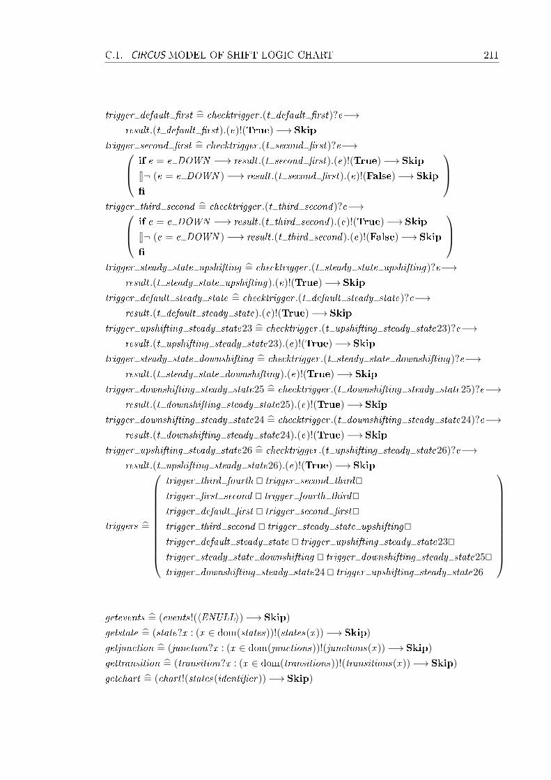
C.1. CIRCUS MODEL OF SHIFT LOGIC CHART 211
trigger default �rst =̂ checktrigger .(t default �rst)?e−→result .(t default �rst).(e)!(True)−→ Skip
trigger second �rst =̂ checktrigger .(t second �rst)?e−→ if e = e DOWN −→ result .(t second �rst).(e)!(True)−→ Skip
8¬ (e = e DOWN )−→ result .(t second �rst).(e)!(False)−→ Skip
�
trigger third second =̂ checktrigger .(t third second)?e−→ if e = e DOWN −→ result .(t third second).(e)!(True)−→ Skip
8¬ (e = e DOWN )−→ result .(t third second).(e)!(False)−→ Skip
�
trigger steady state upshifting =̂ checktrigger .(t steady state upshifting)?e−→
result .(t steady state upshifting).(e)!(True)−→ Skip
trigger default steady state =̂ checktrigger .(t default steady state)?e−→result .(t default steady state).(e)!(True)−→ Skip
trigger upshifting steady state23 =̂ checktrigger .(t upshifting steady state23)?e−→result .(t upshifting steady state23).(e)!(True)−→ Skip
trigger steady state downshifting =̂ checktrigger .(t steady state downshifting)?e−→result .(t steady state downshifting).(e)!(True)−→ Skip
trigger downshifting steady state25 =̂ checktrigger .(t downshifting steady state25)?e−→result .(t downshifting steady state25).(e)!(True)−→ Skip
trigger downshifting steady state24 =̂ checktrigger .(t downshifting steady state24)?e−→result .(t downshifting steady state24).(e)!(True)−→ Skip
trigger upshifting steady state26 =̂ checktrigger .(t upshifting steady state26)?e−→result .(t upshifting steady state26).(e)!(True)−→ Skip
triggers =̂
trigger third fourth @ trigger second third@trigger �rst second @ trigger fourth third@trigger default �rst @ trigger second �rst@trigger third second @ trigger steady state upshifting@trigger default steady state @ trigger upshifting steady state23@trigger steady state downshifting @ trigger downshifting steady state25@trigger downshifting steady state24 @ trigger upshifting steady state26
getevents =̂ (events!(〈ENULL〉)−→ Skip)
getstate =̂ (state?x : (x ∈ dom(states))!(states(x ))−→ Skip)
getjunction =̂ (junction?x : (x ∈ dom(junctions))!(junctions(x ))−→ Skip)
gettransition =̂ (transition?x : (x ∈ dom(transitions))!(transitions(x ))−→ Skip)
getchart =̂ (chart !(states(identi�er))−→ Skip)

212 APPENDIX C. CIRCUS MODELS OF STATEFLOW CHARTS
broadcast =̂ e : EVENT ; dest : SID • local event !(e, states(dest))−→µX • (AllActions ; X @ end local execution −→ Skip)
check =̂ res erl : B • µX • (InterfaceActions ; X @ interrupt?x −→ erl := x )
status =̂ (status?x : (x ∈ dom(state status))!(state status(x ))−→ Skip)
history =̂ (history?x : (x ∈ dom(state history))!(state history(x ))−→ Skip)
activation =̂ (activate?x −→ (Activate))deactivation =̂ (deactivate?x −→ (Deactivate))
ChartActions =̂
entryactions @ duringactions@exitactions @ conditionactions@transitionactions
; end action −→ Skip
InterfaceActions =̂
(getevents @ getchart @ getstate @ getjunction @ gettransition@status @ history @ activation @ deactivation
)
Inputs =̂ read inputs −→
i speed?x −→ v speed := x
||[{v speed} | {v throttle}]||i throttle?x −→ v throttle := x
Outputs =̂ write outputs −→ o gear !(v gear)−→ Skip
AllActions =̂
(conditionactions @ triggers @ Inputs @ Outputs@ChartActions @ InterfaceActions
)
• (InitState) ;
µX •
µY •
AllActions ; Y
@end cycle −→ Skip
; X
end
process shift logic =̂ (P shift logic J interface ∪ {| end cycle |} K Simulator) \ interface
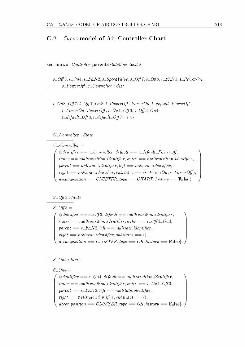
C.2. CIRCUS MODEL OF AIR CONTROLLER CHART 213
C.2 Circus model of Air Controller Chart
section air Controller parents state�ow toolkit
s O� 3, s On4, s FAN 2, s SpeedValue, s O� 7, s On8, s FAN 1, s PowerOn,
s PowerO� , c Controller : SID
t On8 O� 7, t O� 7 On8, t PowerO� PowerOn, t default PowerO� ,
t PowerOn PowerO� , t On4 O� 3, t O� 3 On4,
t default O� 3, t default O� 7 : TID
C Controller : State
C Controller =〈|identi�er == c Controller , default == t default PowerO� ,
inner == nulltransition.identi�er , outer == nulltransition.identi�er ,
parent == nullstate.identi�er , left == nullstate.identi�er ,
right == nullstate.identi�er , substates == 〈s PowerOn, s PowerO� 〉,decomposition == CLUSTER, type == CHART , history == False|〉
S O� 3 : State
S O� 3 =〈|identi�er == s O� 3, default == nulltransition.identi�er ,
inner == nulltransition.identi�er , outer == t O� 3 On4,
parent == s FAN 2, left == nullstate.identi�er ,
right == nullstate.identi�er , substates == 〈〉,decomposition == CLUSTER, type == OR, history == False|〉
S On4 : State
S On4 =〈|identi�er == s On4, default == nulltransition.identi�er ,
inner == nulltransition.identi�er , outer == t On4 O� 3,
parent == s FAN 2, left == nullstate.identi�er ,
right == nullstate.identi�er , substates == 〈〉,decomposition == CLUSTER, type == OR, history == False|〉

214 APPENDIX C. CIRCUS MODELS OF STATEFLOW CHARTS
S FAN 2 : State
S FAN 2 =〈|identi�er == s FAN 2, default == t default O� 3,
inner == nulltransition.identi�er , outer == nulltransition.identi�er ,
parent == s PowerOn, left == s FAN 1,
right == s SpeedValue, substates == 〈s O� 3, s On4〉,decomposition == CLUSTER, type == AND , history == False|〉
S SpeedValue : State
S SpeedValue =〈|identi�er == s SpeedValue, default == nulltransition.identi�er ,
inner == nulltransition.identi�er , outer == nulltransition.identi�er ,
parent == s PowerOn, left == s FAN 2,
right == nullstate.identi�er , substates == 〈〉,decomposition == CLUSTER, type == AND , history == False|〉
S O� 7 : State
S O� 7 =〈|identi�er == s O� 7, default == nulltransition.identi�er ,
inner == nulltransition.identi�er , outer == t O� 7 On8,
parent == s FAN 1, left == nullstate.identi�er ,
right == nullstate.identi�er , substates == 〈〉,decomposition == CLUSTER, type == OR, history == False|〉
S On8 : State
S On8 =〈|identi�er == s On8, default == nulltransition.identi�er ,
inner == nulltransition.identi�er , outer == t On8 O� 7,
parent == s FAN 1, left == nullstate.identi�er ,
right == nullstate.identi�er , substates == 〈〉,decomposition == CLUSTER, type == OR, history == False|〉
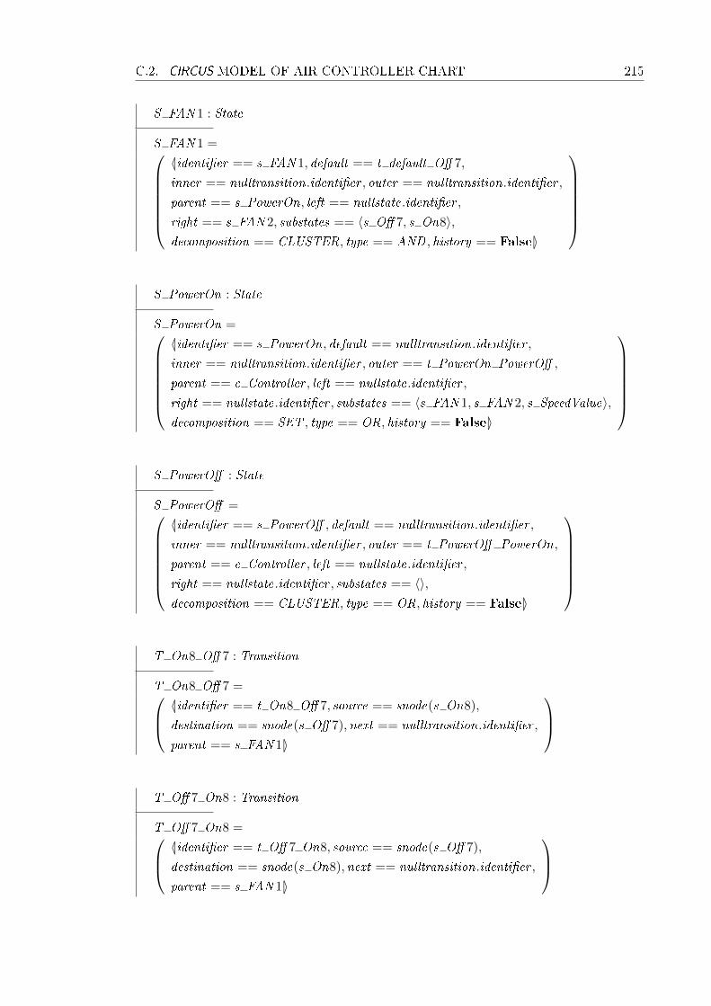
C.2. CIRCUS MODEL OF AIR CONTROLLER CHART 215
S FAN 1 : State
S FAN 1 =〈|identi�er == s FAN 1, default == t default O� 7,
inner == nulltransition.identi�er , outer == nulltransition.identi�er ,
parent == s PowerOn, left == nullstate.identi�er ,
right == s FAN 2, substates == 〈s O� 7, s On8〉,decomposition == CLUSTER, type == AND , history == False|〉
S PowerOn : State
S PowerOn =〈|identi�er == s PowerOn, default == nulltransition.identi�er ,
inner == nulltransition.identi�er , outer == t PowerOn PowerO� ,
parent == c Controller , left == nullstate.identi�er ,
right == nullstate.identi�er , substates == 〈s FAN 1, s FAN 2, s SpeedValue〉,decomposition == SET , type == OR, history == False|〉
S PowerO� : State
S PowerO� =〈|identi�er == s PowerO� , default == nulltransition.identi�er ,
inner == nulltransition.identi�er , outer == t PowerO� PowerOn,
parent == c Controller , left == nullstate.identi�er ,
right == nullstate.identi�er , substates == 〈〉,decomposition == CLUSTER, type == OR, history == False|〉
T On8 O� 7 : Transition
T On8 O� 7 = 〈|identi�er == t On8 O� 7, source == snode(s On8),
destination == snode(s O� 7),next == nulltransition.identi�er ,
parent == s FAN 1|〉
T O� 7 On8 : Transition
T O� 7 On8 = 〈|identi�er == t O� 7 On8, source == snode(s O� 7),
destination == snode(s On8),next == nulltransition.identi�er ,
parent == s FAN 1|〉
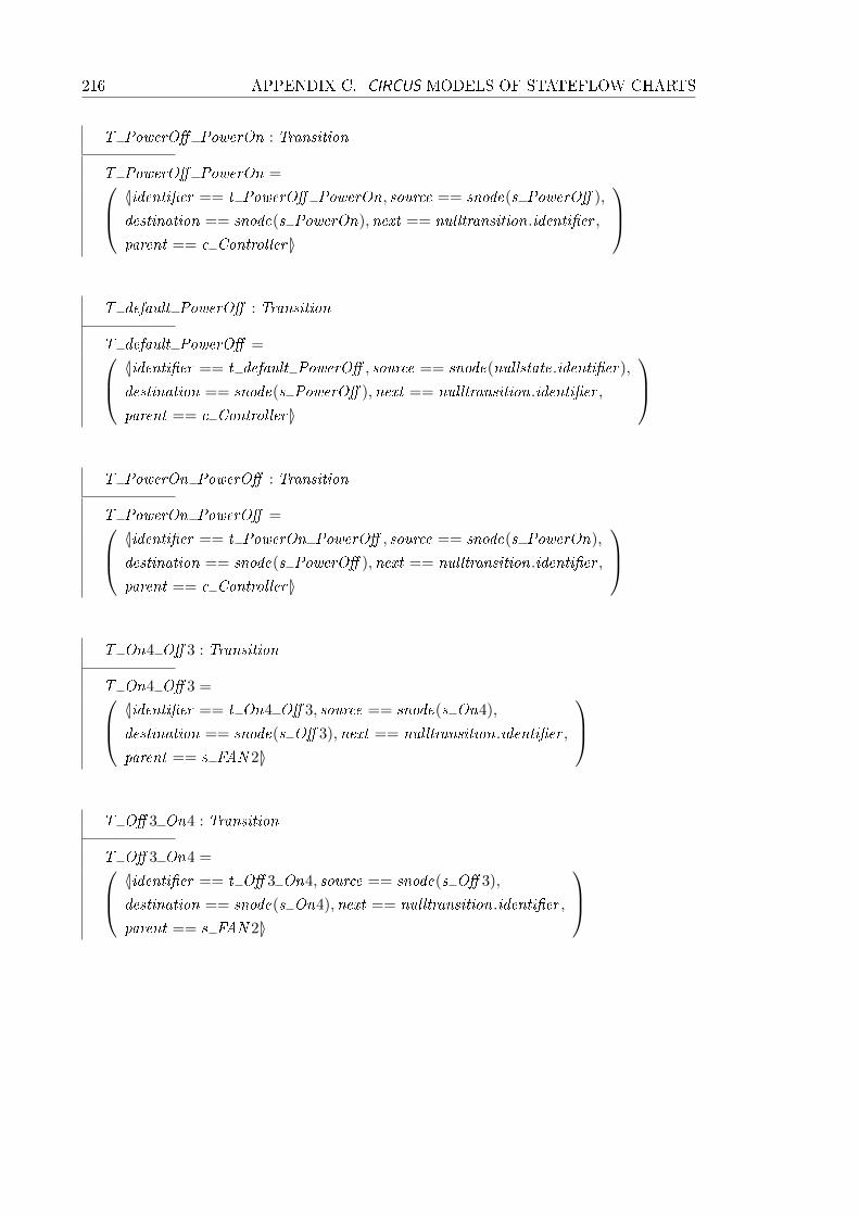
216 APPENDIX C. CIRCUS MODELS OF STATEFLOW CHARTS
T PowerO� PowerOn : Transition
T PowerO� PowerOn = 〈|identi�er == t PowerO� PowerOn, source == snode(s PowerO� ),
destination == snode(s PowerOn),next == nulltransition.identi�er ,
parent == c Controller |〉
T default PowerO� : Transition
T default PowerO� = 〈|identi�er == t default PowerO� , source == snode(nullstate.identi�er),
destination == snode(s PowerO� ),next == nulltransition.identi�er ,
parent == c Controller |〉
T PowerOn PowerO� : Transition
T PowerOn PowerO� = 〈|identi�er == t PowerOn PowerO� , source == snode(s PowerOn),
destination == snode(s PowerO� ),next == nulltransition.identi�er ,
parent == c Controller |〉
T On4 O� 3 : Transition
T On4 O� 3 = 〈|identi�er == t On4 O� 3, source == snode(s On4),
destination == snode(s O� 3),next == nulltransition.identi�er ,
parent == s FAN 2|〉
T O� 3 On4 : Transition
T O� 3 On4 = 〈|identi�er == t O� 3 On4, source == snode(s O� 3),
destination == snode(s On4),next == nulltransition.identi�er ,
parent == s FAN 2|〉

C.2. CIRCUS MODEL OF AIR CONTROLLER CHART 217
T default O� 3 : Transition
T default O� 3 = 〈|identi�er == t default O� 3, source == snode(nullstate.identi�er),
destination == snode(s O� 3),next == nulltransition.identi�er ,
parent == s FAN 2|〉
T default O� 7 : Transition
T default O� 7 = 〈|identi�er == t default O� 7, source == snode(nullstate.identi�er),
destination == snode(s O� 7),next == nulltransition.identi�er ,
parent == s FAN 1|〉
e SWITCH , e CLOCK : EVENT
channel o air�ow : N; i temp : R
processP Controller =̂ begin
State�owChart
identi�er = c Controller
states = {(c Controller ,C Controller), (s O� 3,S O� 3), (s On4,S On4),
(s FAN 2,S FAN 2), (s SpeedValue,S SpeedValue), (s O� 7,S O� 7),
(s On8,S On8), (s FAN 1,S FAN 1), (s PowerOn,S PowerOn),
(s PowerO� ,S PowerO� )}transitions = {(t On8 O� 7,T On8 O� 7), (t O� 7 On8,T O� 7 On8),
(t PowerO� PowerOn,T PowerO� PowerOn),
(t default PowerO� ,T default PowerO� ),
(t PowerOn PowerO� ,T PowerOn PowerO� ), (t On4 O� 3,T On4 O� 3),
(t O� 3 On4,T O� 3 On4), (t default O� 3,T default O� 3),
(t default O� 7,T default O� 7)}junctions = {}
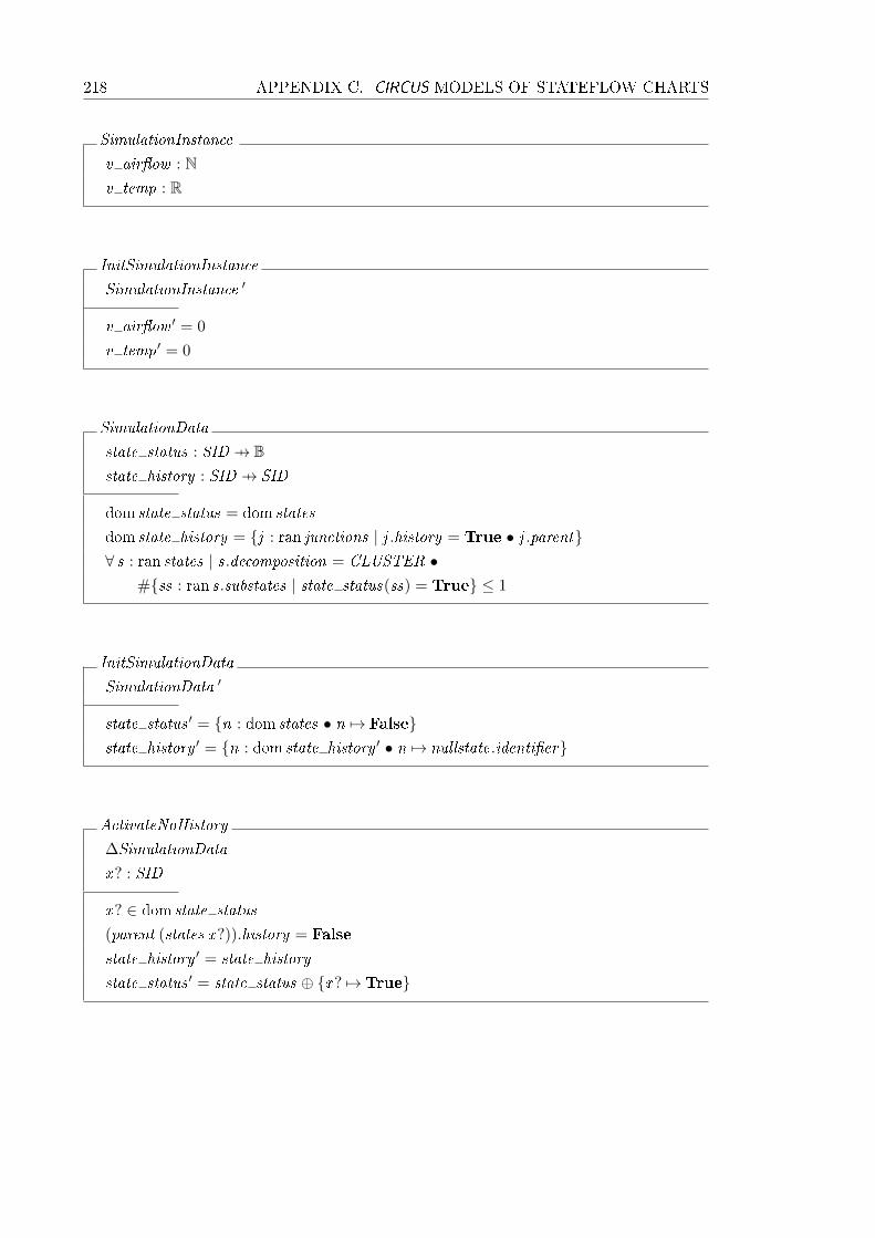
218 APPENDIX C. CIRCUS MODELS OF STATEFLOW CHARTS
SimulationInstance
v air�ow : Nv temp : R
InitSimulationInstance
SimulationInstance ′
v air�ow ′ = 0
v temp′ = 0
SimulationData
state status : SID 7→ Bstate history : SID 7→ SID
dom state status = dom states
dom state history = {j : ran junctions | j .history = True • j .parent}∀ s : ran states | s.decomposition = CLUSTER •
#{ss : ran s.substates | state status(ss) = True} ≤ 1
InitSimulationData
SimulationData ′
state status ′ = {n : dom states • n 7→ False}state history ′ = {n : dom state history ′ • n 7→ nullstate.identi�er}
ActivateNoHistory
∆SimulationData
x? : SID
x? ∈ dom state status
(parent (states x?)).history = False
state history ′ = state history
state status ′ = state status ⊕ {x? 7→True}

C.2. CIRCUS MODEL OF AIR CONTROLLER CHART 219
ActivateWithHistory
∆SimulationData
x? : SID
x? ∈ dom state status
(parent (states x?)).history = True
state history ′ = state history ⊕ {((states x?).parent) 7→ x?}state status ′ = state status ⊕ {x? 7→True}
Activate == (ActivateWithHistory ∨ ActivateNoHistory) ∧ ΞSimulationInstance
Deactivate
∆SimulationData
ΞSimulationInstance
x? : SID
x? ∈ dom state status
state history ′ = state history
state status ′ = state status ⊕ {x? 7→ False}
InitState == (InitSimulationInstance) ∧ (InitSimulationData)
stateController state == (SimulationInstance ) ∧ (SimulationData )
entryaction O� 3 =̂ (executeentryaction.(s O� 3)−→ Skip)
entryaction On4 =̂ (executeentryaction.(s On4)−→ Skip)
entryaction FAN 2 =̂ (executeentryaction.(s FAN 2)−→ Skip)
entryaction SpeedValue =̂ (executeentryaction.(s SpeedValue)−→ Skip)
entryaction O� 7 =̂ (executeentryaction.(s O� 7)−→ Skip)
entryaction On8 =̂ (executeentryaction.(s On8)−→ Skip)
entryaction FAN 1 =̂ (executeentryaction.(s FAN 1)−→ Skip)
entryaction PowerOn =̂ (executeentryaction.(s PowerOn)−→ Skip)
entryaction PowerO� =̂ (executeentryaction.(s PowerO� )−→ v air�ow := 0)
entryactions =̂
entryaction O� 3 @ entryaction On4 @ entryaction FAN 2@entryaction SpeedValue @ entryaction O� 7 @ entryaction On8@entryaction FAN 1 @ entryaction PowerOn @ entryaction PowerO�
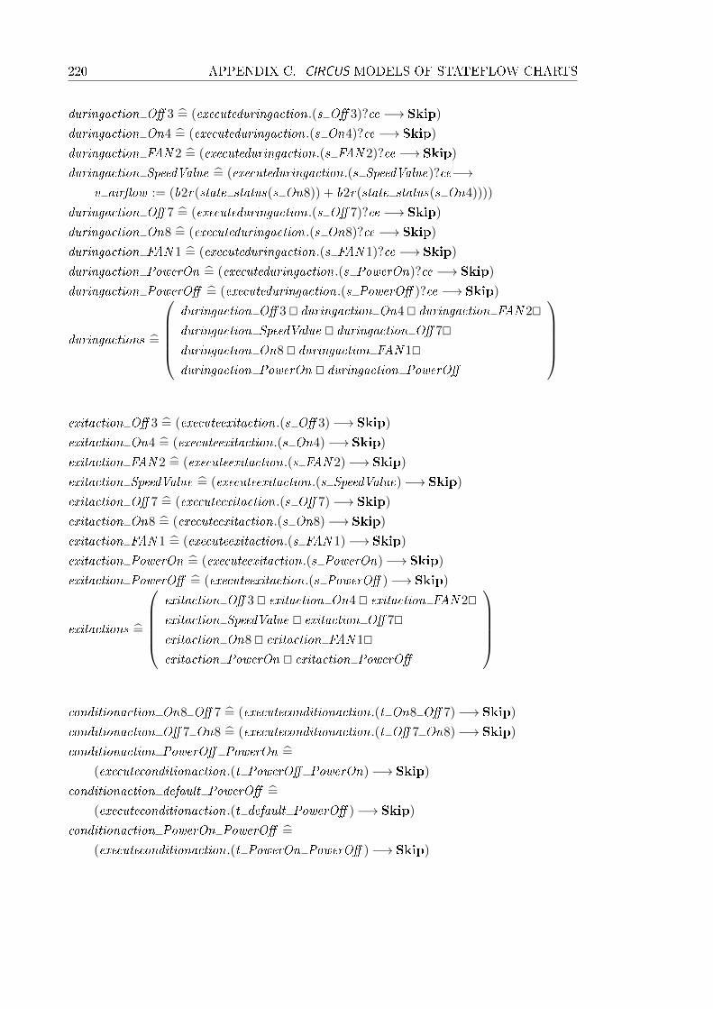
220 APPENDIX C. CIRCUS MODELS OF STATEFLOW CHARTS
duringaction O� 3 =̂ (executeduringaction.(s O� 3)?ce −→ Skip)
duringaction On4 =̂ (executeduringaction.(s On4)?ce −→ Skip)
duringaction FAN 2 =̂ (executeduringaction.(s FAN 2)?ce −→ Skip)
duringaction SpeedValue =̂ (executeduringaction.(s SpeedValue)?ce−→v air�ow := (b2r(state status(s On8)) + b2r(state status(s On4))))
duringaction O� 7 =̂ (executeduringaction.(s O� 7)?ce −→ Skip)
duringaction On8 =̂ (executeduringaction.(s On8)?ce −→ Skip)
duringaction FAN 1 =̂ (executeduringaction.(s FAN 1)?ce −→ Skip)
duringaction PowerOn =̂ (executeduringaction.(s PowerOn)?ce −→ Skip)
duringaction PowerO� =̂ (executeduringaction.(s PowerO� )?ce −→ Skip)
duringactions =̂
duringaction O� 3 @ duringaction On4 @ duringaction FAN 2@duringaction SpeedValue @ duringaction O� 7@duringaction On8 @ duringaction FAN 1@duringaction PowerOn @ duringaction PowerO�
exitaction O� 3 =̂ (executeexitaction.(s O� 3)−→ Skip)
exitaction On4 =̂ (executeexitaction.(s On4)−→ Skip)
exitaction FAN 2 =̂ (executeexitaction.(s FAN 2)−→ Skip)
exitaction SpeedValue =̂ (executeexitaction.(s SpeedValue)−→ Skip)
exitaction O� 7 =̂ (executeexitaction.(s O� 7)−→ Skip)
exitaction On8 =̂ (executeexitaction.(s On8)−→ Skip)
exitaction FAN 1 =̂ (executeexitaction.(s FAN 1)−→ Skip)
exitaction PowerOn =̂ (executeexitaction.(s PowerOn)−→ Skip)
exitaction PowerO� =̂ (executeexitaction.(s PowerO� )−→ Skip)
exitactions =̂
exitaction O� 3 @ exitaction On4 @ exitaction FAN 2@exitaction SpeedValue @ exitaction O� 7@exitaction On8 @ exitaction FAN 1@exitaction PowerOn @ exitaction PowerO�
conditionaction On8 O� 7 =̂ (executeconditionaction.(t On8 O� 7)−→ Skip)
conditionaction O� 7 On8 =̂ (executeconditionaction.(t O� 7 On8)−→ Skip)
conditionaction PowerO� PowerOn =̂
(executeconditionaction.(t PowerO� PowerOn)−→ Skip)
conditionaction default PowerO� =̂
(executeconditionaction.(t default PowerO� )−→ Skip)
conditionaction PowerOn PowerO� =̂
(executeconditionaction.(t PowerOn PowerO� )−→ Skip)
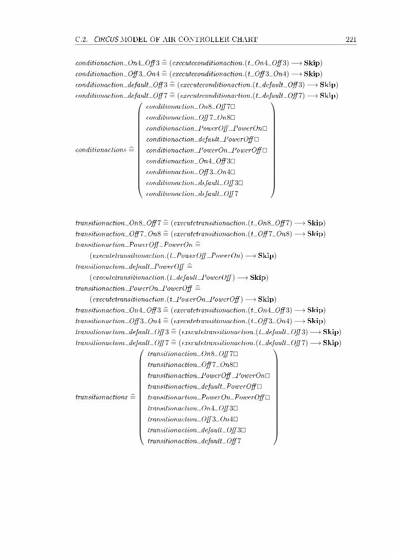
C.2. CIRCUS MODEL OF AIR CONTROLLER CHART 221
conditionaction On4 O� 3 =̂ (executeconditionaction.(t On4 O� 3)−→ Skip)
conditionaction O� 3 On4 =̂ (executeconditionaction.(t O� 3 On4)−→ Skip)
conditionaction default O� 3 =̂ (executeconditionaction.(t default O� 3)−→ Skip)
conditionaction default O� 7 =̂ (executeconditionaction.(t default O� 7)−→ Skip)
conditionactions =̂
conditionaction On8 O� 7@conditionaction O� 7 On8@conditionaction PowerO� PowerOn@conditionaction default PowerO� @conditionaction PowerOn PowerO� @conditionaction On4 O� 3@conditionaction O� 3 On4@conditionaction default O� 3@conditionaction default O� 7
transitionaction On8 O� 7 =̂ (executetransitionaction.(t On8 O� 7)−→ Skip)
transitionaction O� 7 On8 =̂ (executetransitionaction.(t O� 7 On8)−→ Skip)
transitionaction PowerO� PowerOn =̂
(executetransitionaction.(t PowerO� PowerOn)−→ Skip)
transitionaction default PowerO� =̂
(executetransitionaction.(t default PowerO� )−→ Skip)
transitionaction PowerOn PowerO� =̂
(executetransitionaction.(t PowerOn PowerO� )−→ Skip)
transitionaction On4 O� 3 =̂ (executetransitionaction.(t On4 O� 3)−→ Skip)
transitionaction O� 3 On4 =̂ (executetransitionaction.(t O� 3 On4)−→ Skip)
transitionaction default O� 3 =̂ (executetransitionaction.(t default O� 3)−→ Skip)
transitionaction default O� 7 =̂ (executetransitionaction.(t default O� 7)−→ Skip)
transitionactions =̂
transitionaction On8 O� 7@transitionaction O� 7 On8@transitionaction PowerO� PowerOn@transitionaction default PowerO� @transitionaction PowerOn PowerO� @transitionaction On4 O� 3@transitionaction O� 3 On4@transitionaction default O� 3@transitionaction default O� 7

222 APPENDIX C. CIRCUS MODELS OF STATEFLOW CHARTS
condition On8 O� 7 =̂ if(v temp<A120) 6= 0−→ evaluatecondition.(t On8 O� 7)!(True)−→ Skip
8¬ ((v temp<A120) 6= 0)−→ evaluatecondition.(t On8 O� 7)!(False)−→ Skip
�
condition O� 7 On8 =̂ if(v temp≥A120) 6= 0−→ evaluatecondition.(t O� 7 On8)!(True)−→ Skip
8¬ ((v temp≥A120) 6= 0)−→ evaluatecondition.(t O� 7 On8)!(False)−→ Skip
�
condition PowerO� PowerOn =̂
(evaluatecondition.(t PowerO� PowerOn)!(True)−→ Skip)
condition default PowerO� =̂
(evaluatecondition.(t default PowerO� )!(True)−→ Skip)
condition PowerOn PowerO� =̂
(evaluatecondition.(t PowerOn PowerO� )!(True)−→ Skip)
condition On4 O� 3 =̂ if((v temp<A150) 6= 0)−→ evaluatecondition.(t On4 O� 3)!(True)−→ Skip
8¬ ((v temp<A150) 6= 0)−→ evaluatecondition.(t On4 O� 3)!(False)−→ Skip
�
condition O� 3 On4 =̂ if((v temp≥A150) 6= 0)−→ evaluatecondition.(t O� 3 On4)!(True)−→ Skip
8¬ ((v temp≥A150) 6= 0)−→ evaluatecondition.(t O� 3 On4)!(False)−→ Skip
�
condition default O� 3 =̂ (evaluatecondition.(t default O� 3)!(True)−→ Skip)
condition default O� 7 =̂ (evaluatecondition.(t default O� 7)!(True)−→ Skip)
conditions =̂
condition On8 O� 7 @ condition O� 7 On8@condition PowerO� PowerOn @ condition default PowerO� @condition PowerOn PowerO� @ condition On4 O� 3@condition O� 3 On4 @ condition default O� 3@condition default O� 7
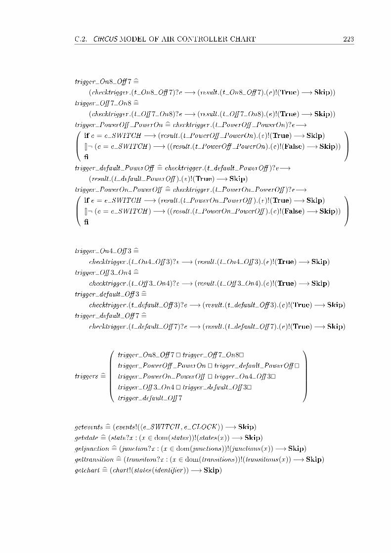
C.2. CIRCUS MODEL OF AIR CONTROLLER CHART 223
trigger On8 O� 7 =̂
(checktrigger .(t On8 O� 7)?e −→ (result .(t On8 O� 7).(e)!(True)−→ Skip))
trigger O� 7 On8 =̂
(checktrigger .(t O� 7 On8)?e −→ (result .(t O� 7 On8).(e)!(True)−→ Skip))
trigger PowerO� PowerOn =̂ checktrigger .(t PowerO� PowerOn)?e−→ if e = e SWITCH −→ (result .(t PowerO� PowerOn).(e)!(True)−→ Skip)
8¬ (e = e SWITCH )−→ ((result .(t PowerO� PowerOn).(e)!(False)−→ Skip))
�
trigger default PowerO� =̂ checktrigger .(t default PowerO� )?e−→
(result .(t default PowerO� ).(e)!(True)−→ Skip)
trigger PowerOn PowerO� =̂ checktrigger .(t PowerOn PowerO� )?e−→ if e = e SWITCH −→ (result .(t PowerOn PowerO� ).(e)!(True)−→ Skip)
8¬ (e = e SWITCH )−→ ((result .(t PowerOn PowerO� ).(e)!(False)−→ Skip))
�
trigger On4 O� 3 =̂
checktrigger .(t On4 O� 3)?e −→ (result .(t On4 O� 3).(e)!(True)−→ Skip)
trigger O� 3 On4 =̂
checktrigger .(t O� 3 On4)?e −→ (result .(t O� 3 On4).(e)!(True)−→ Skip)
trigger default O� 3 =̂
checktrigger .(t default O� 3)?e −→ (result .(t default O� 3).(e)!(True)−→ Skip)
trigger default O� 7 =̂
checktrigger .(t default O� 7)?e −→ (result .(t default O� 7).(e)!(True)−→ Skip)
triggers =̂
trigger On8 O� 7 @ trigger O� 7 On8@trigger PowerO� PowerOn @ trigger default PowerO� @trigger PowerOn PowerO� @ trigger On4 O� 3@trigger O� 3 On4 @ trigger default O� 3@trigger default O� 7
getevents =̂ (events!(〈e SWITCH , e CLOCK 〉)−→ Skip)
getstate =̂ (state?x : (x ∈ dom(states))!(states(x ))−→ Skip)
getjunction =̂ (junction?x : (x ∈ dom(junctions))!(junctions(x ))−→ Skip)
gettransition =̂ (transition?x : (x ∈ dom(transitions))!(transitions(x ))−→ Skip)
getchart =̂ (chart !(states(identi�er))−→ Skip)
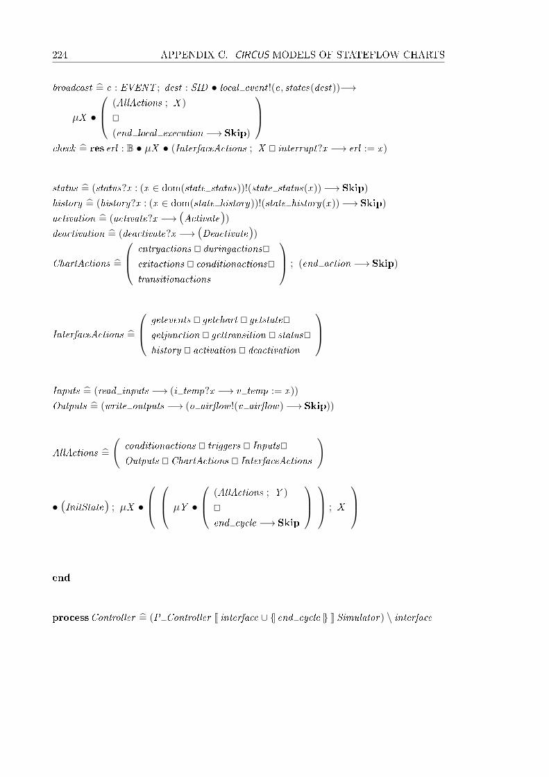
224 APPENDIX C. CIRCUS MODELS OF STATEFLOW CHARTS
broadcast =̂ e : EVENT ; dest : SID • local event !(e, states(dest))−→
µX •
(AllActions ; X )
@(end local execution −→ Skip)
check =̂ res erl : B • µX • (InterfaceActions ; X @ interrupt?x −→ erl := x )
status =̂ (status?x : (x ∈ dom(state status))!(state status(x ))−→ Skip)
history =̂ (history?x : (x ∈ dom(state history))!(state history(x ))−→ Skip)
activation =̂ (activate?x −→ (Activate))deactivation =̂ (deactivate?x −→ (Deactivate))
ChartActions =̂
entryactions @ duringactions@exitactions @ conditionactions@transitionactions
; (end action −→ Skip)
InterfaceActions =̂
getevents @ getchart @ getstate@getjunction @ gettransition @ status@history @ activation @ deactivation
Inputs =̂ (read inputs −→ (i temp?x −→ v temp := x ))
Outputs =̂ (write outputs −→ (o air�ow !(v air�ow)−→ Skip))
AllActions =̂
(conditionactions @ triggers @ Inputs@Outputs @ ChartActions @ InterfaceActions
)
• (InitState) ; µX •
µY •
(AllActions ; Y )
@end cycle −→ Skip
; X
end
processController =̂ (P Controller J interface ∪ {| end cycle |} K Simulator) \ interface
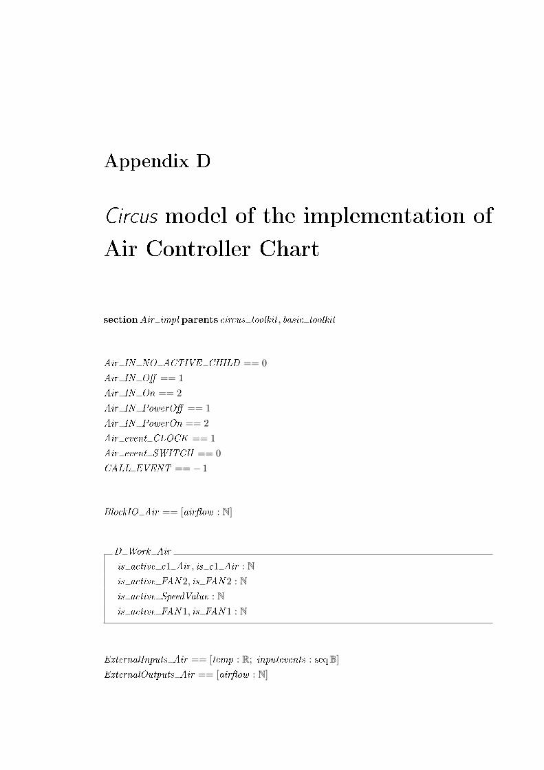
Appendix D
Circus model of the implementation of
Air Controller Chart
sectionAir impl parents circus toolkit , basic toolkit
Air IN NO ACTIVE CHILD == 0
Air IN O� == 1
Air IN On == 2
Air IN PowerO� == 1
Air IN PowerOn == 2
Air event CLOCK == 1
Air event SWITCH == 0
CALL EVENT == − 1
BlockIO Air == [air�ow : N]
D Work Air
is active c1 Air , is c1 Air : Nis active FAN 2, is FAN 2 : Nis active SpeedValue : Nis active FAN 1, is FAN 1 : N
ExternalInputs Air == [temp : R; inputevents : seqB]
ExternalOutputs Air == [air�ow : N]
226APPENDIX D. CIRCUS MODEL OF THE IMPLEMENTATION OF AIR
CONTROLLER CHART
is active c1 Air : D Work Air × N→D Work Air
∀ b : D Work Air ; v : N • is active c1 Air(b, v) =
〈|is active c1 Air == v , is c1 Air == b.is c1 Air ,
is active FAN 2 == b.is active FAN 2, is FAN 2 == b.is FAN 2,
is active SpeedValue == b.is active SpeedValue,
is active FAN 1 == b.is active FAN 1, is FAN 1 == b.is FAN 1|〉
is c1 Air : D Work Air × N→D Work Air
∀ b : D Work Air ; v : N • is c1 Air(b, v) =
〈|is active c1 Air == b.is active c1 Air ,
is c1 Air == v , is active FAN 2 == b.is active FAN 2,
is FAN 2 == b.is FAN 2, is active SpeedValue == b.is active SpeedValue,
is active FAN 1 == b.is active FAN 1, is FAN 1 == b.is FAN 1|〉
is active FAN 2 : D Work Air × N→D Work Air
∀ b : D Work Air ; v : N • is active FAN 2(b, v) =
〈|is active c1 Air == b.is active c1 Air ,
is c1 Air == b.is c1 Air , is active FAN 2 == v ,
is FAN 2 == b.is FAN 2, is active SpeedValue == b.is active SpeedValue,
is active FAN 1 == b.is active FAN 1, is FAN 1 == b.is FAN 1|〉
is FAN 2 : D Work Air × N→D Work Air
∀ b : D Work Air ; v : N • is FAN 2(b, v) =
〈|is active c1 Air == b.is active c1 Air ,
is c1 Air == b.is c1 Air , is active FAN 2 == b.is active FAN 2,
is FAN 2 == v , is active SpeedValue == b.is active SpeedValue,
is active FAN 1 == b.is active FAN 1, is FAN 1 == b.is FAN 1|〉
is active SpeedValue : D Work Air × N→D Work Air
∀ b : D Work Air ; v : N • is active SpeedValue(b, v) =
〈|is active c1 Air == b.is active c1 Air ,
is c1 Air == b.is c1 Air , is active FAN 2 == b.is active FAN 2,
is FAN 2 == b.is FAN 2, is active SpeedValue == v ,
is active FAN 1 == b.is active FAN 1, is FAN 1 == b.is FAN 1|〉
227
is active FAN 1 : D Work Air × N→D Work Air
∀ b : D Work Air ; v : N • is active FAN 1(b, v) =
〈|is active c1 Air == b.is active c1 Air ,
is c1 Air == b.is c1 Air , is active FAN 2 == b.is active FAN 2,
is FAN 2 == b.is FAN 2, is active SpeedValue == b.is active SpeedValue,
is active FAN 1 == v , is FAN 1 == b.is FAN 1|〉
is FAN 1 : D Work Air × N→D Work Air
∀ b : D Work Air ; v : N • is FAN 1(b, v) =
〈|is active c1 Air == b.is active c1 Air ,
is c1 Air == b.is c1 Air , is active FAN 2 == b.is active FAN 2,
is FAN 2 == b.is FAN 2, is active SpeedValue == b.is active SpeedValue,
is active FAN 1 == b.is active FAN 1, is FAN 1 == v |〉
air�ow : BlockIO Air × N→ BlockIO Air
∀ b : BlockIO Air ; v : N • air�ow(b, v) =
〈|air�ow == v |〉
temp : ExternalInputs Air × R→ ExternalInputs Air
∀ b : ExternalInputs Air ; v : R • temp(b, v) =
〈|temp == v , inputevents == b.inputevents|〉
inputevents : ExternalInputs Air × (seqB)→ ExternalInputs Air
∀ b : ExternalInputs Air ; v : seqB • inputevents(b, v) =
〈|temp == b.temp, inputevents == v |〉
Air state
sfEvent Air : ZAir B : BlockIO Air
Air DWork : D Work Air
Air U : ExternalInputs Air
Air Y : ExternalOutputs Air
228APPENDIX D. CIRCUS MODEL OF THE IMPLEMENTATION OF AIR
CONTROLLER CHART
channel in FAN 1 : Air state
channel out FAN 1 : Nchannel input event : (seqB)
channel i temp : Rchannel o air�ow : N
processAir =̂ begin
stateAir state
Air FAN 1 =̂
varAir B : BlockIO Air ; Air DWork : D Work Air ; Air U : ExternalInputs Air ;
Air Y : ExternalOutputs Air ; sfEvent Air : Z •in FAN 1?s −→ Air B ,Air DWork ,Air U ,Air Y , sfEvent Air :=
s.Air B , s.Air DWork , s.Air U , s.Air Y , s. sfEvent Air ;
if Air DWork .is FAN 1 = Air IN O�−→ if Air U .temp ≥ 120−→ Air DWork := is FAN 1(Air DWork ,Air IN On)
8¬ (Air U .temp ≥ 120)−→ Skip
�
8Air DWork .is FAN 1 = Air IN On−→ if Air U .temp < 120−→ Air DWork := is FAN 1(Air DWork ,Air IN O� )
8¬ (Air U .temp < 120)−→ Skip
�
8¬ (Air DWork .is FAN 1 = Air IN O� ∨ Air DWork .is FAN 1 = Air IN On)−→
Air DWork := is FAN 1(Air DWork ,Air IN O� )
�
;
out FAN 1!(Air DWork .is FAN 1)−→ Skip
FAN 2 =̂
if Air DWork .is FAN 2 = Air IN O�−→ if Air U .temp ≥ 150−→ Air DWork := is FAN 2(Air DWork ,Air IN On)
8¬ (Air U .temp ≥ 150)−→ Skip
�
8Air DWork .is FAN 2 = Air IN On−→ if Air U .temp < 150−→ Air DWork := is FAN 2(Air DWork ,Air IN O� )
8¬ (Air U .temp < 150)−→ Skip
�
8¬ (Air DWork .is FAN 2 = Air IN O� ∨ Air DWork .is FAN 2 = Air IN On)−→
Air DWork := is FAN 2(Air DWork ,Air IN O� )
�
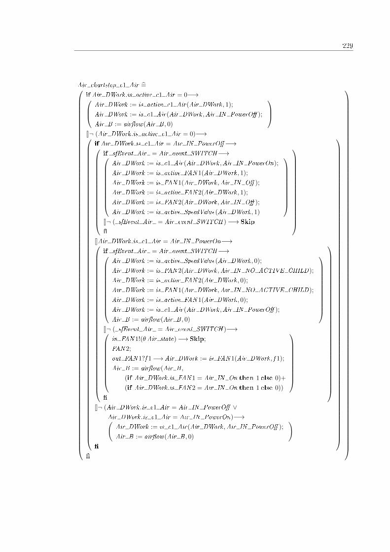
229
Air chartstep c1 Air =̂
if Air DWork .is active c1 Air = 0−→ Air DWork := is active c1 Air(Air DWork , 1);
Air DWork := is c1 Air(Air DWork ,Air IN PowerO� );
Air B := air�ow(Air B , 0)
8¬ (Air DWork .is active c1 Air = 0)−→
if Air DWork .is c1 Air = Air IN PowerO�−→
if sfEvent Air = Air event SWITCH−→
Air DWork := is c1 Air(Air DWork ,Air IN PowerOn);
Air DWork := is active FAN 1(Air DWork , 1);
Air DWork := is FAN 1(Air DWork ,Air IN O� );
Air DWork := is active FAN 2(Air DWork , 1);
Air DWork := is FAN 2(Air DWork ,Air IN O� );
Air DWork := is active SpeedValue(Air DWork , 1)
8¬ ( sfEvent Air = Air event SWITCH )−→ Skip
�
8Air DWork .is c1 Air = Air IN PowerOn−→
if sfEvent Air = Air event SWITCH−→
Air DWork := is active SpeedValue(Air DWork , 0);
Air DWork := is FAN 2(Air DWork ,Air IN NO ACTIVE CHILD);
Air DWork := is active FAN 2(Air DWork , 0);
Air DWork := is FAN 1(Air DWork ,Air IN NO ACTIVE CHILD);
Air DWork := is active FAN 1(Air DWork , 0);
Air DWork := is c1 Air(Air DWork ,Air IN PowerO� );
Air B := air�ow(Air B , 0)
8¬ ( sfEvent Air = Air event SWITCH )−→
in FAN 1!(θAir state)−→ Skip;
FAN 2;
out FAN 1?f 1−→ Air DWork := is FAN 1(Air DWork , f 1);
Air B := air�ow(Air B ,
(if Air DWork .is FAN 1 = Air IN On then 1 else 0)+
(if Air DWork .is FAN 2 = Air IN On then 1 else 0))
�
8¬ (Air DWork .is c1 Air = Air IN PowerO� ∨
Air DWork .is c1 Air = Air IN PowerOn)−→(Air DWork := is c1 Air(Air DWork ,Air IN PowerO� );
Air B := air�ow(Air B , 0)
)�
�
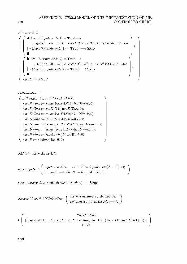
230APPENDIX D. CIRCUS MODEL OF THE IMPLEMENTATION OF AIR
CONTROLLER CHART
Air output =̂
if Air U .inputevents(1) = True−→
sfEvent Air := Air event SWITCH ; Air chartstep c1 Air
8¬ (Air U .inputevents(1) = True)−→ Skip
�
;
if Air U .inputevents(2) = True−→
sfEvent Air := Air event CLOCK ; Air chartstep c1 Air
8¬ (Air U .inputevents(2) = True)−→ Skip
�
;
Air Y := Air B
MdlInitialize =̂
sfEvent Air := CALL EVENT ;
Air DWork := is active FAN 1(Air DWork , 0);
Air DWork := is FAN 1(Air DWork , 0);
Air DWork := is active FAN 2(Air DWork , 0);
Air DWork := is FAN 2(Air DWork , 0);
Air DWork := is active SpeedValue(Air DWork , 0);
Air DWork := is active c1 Air(Air DWork , 0);
Air DWork := is c1 Air(Air DWork , 0);
Air B := air�ow(Air B , 0)
FAN 1 =̂ µX • Air FAN 1
read inputs =̂
(input event?es −→ Air U := inputevents(Air U , es);
i temp?v −→ Air U := temp(Air U , v)
)
write outputs =̂ o air�ow !(Air Y .air�ow)−→ Skip
ExecuteChart =̂ MdlInitialize ;
(µX • read inputs ; Air output ;
write outputs ; end cycle −→ X
)
•
ExecuteChart
J{ sfEvent Air ,Air U ,Air B ,Air DWork ,Air Y } | {| in FAN 1, out FAN 1 |} | {}KFAN 1
end

Appendix E
Novel re�nement laws
We present here, in alphabetical order, the novel re�nement laws of Circus that we need.
Law[alt-alt-dist]
if g1 −→ A1
8 g2 −→
if g3 −→ A2
8 g4 −→ A3
�
�
=
if g1 −→ A1
8 g2 ∧ g3 −→ A2
8 g2 ∧ g4 −→ A3
�
provided
• g1 ∨ g2;
• g1 ⇒ ¬ g2;
• g3 ∨ g4;
• g3 ⇒ ¬ g4.
Law[alt-assump-intro]
(if b1 −→ A1 8 b2 −→ A2 �) = (if b1 −→ {b1} ; A1 8 b2 −→ {b2} ; A2 �)
provided
• b1 ∨ b2;
• b1 ⇒ ¬ b2.
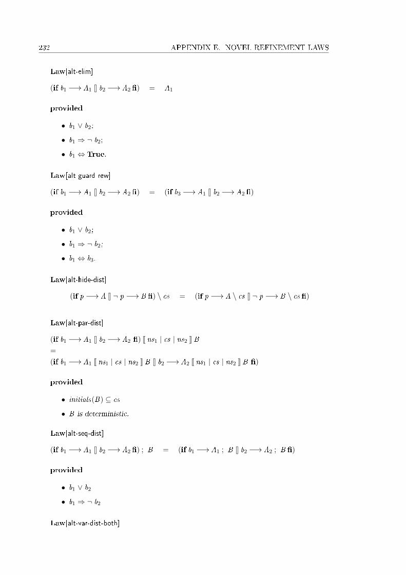
232 APPENDIX E. NOVEL REFINEMENT LAWS
Law[alt-elim]
(if b1 −→ A1 8 b2 −→ A2 �) = A1
provided
• b1 ∨ b2;
• b1 ⇒ ¬ b2;
• b1 ⇔ True.
Law[alt-guard-rew]
(if b1 −→ A1 8 b2 −→ A2 �) = (if b3 −→ A1 8 b2 −→ A2 �)
provided
• b1 ∨ b2;
• b1 ⇒ ¬ b2;
• b1 ⇔ b3.
Law[alt-hide-dist]
(if p −→ A 8 ¬ p −→ B �) \ cs = (if p −→ A \ cs 8 ¬ p −→ B \ cs �)
Law[alt-par-dist]
(if b1 −→ A1 8 b2 −→ A2 �) J ns1 | cs | ns2 K B=
(if b1 −→ A1 J ns1 | cs | ns2 K B 8 b2 −→ A2 J ns1 | cs | ns2 K B �)
provided
• initials(B) ⊆ cs
• B is deterministic.
Law[alt-seq-dist]
(if b1 −→ A1 8 b2 −→ A2 �) ; B = (if b1 −→ A1 ; B 8 b2 −→ A2 ; B �)
provided
• b1 ∨ b2
• b1 ⇒ ¬ b2
Law[alt-var-dist-both]
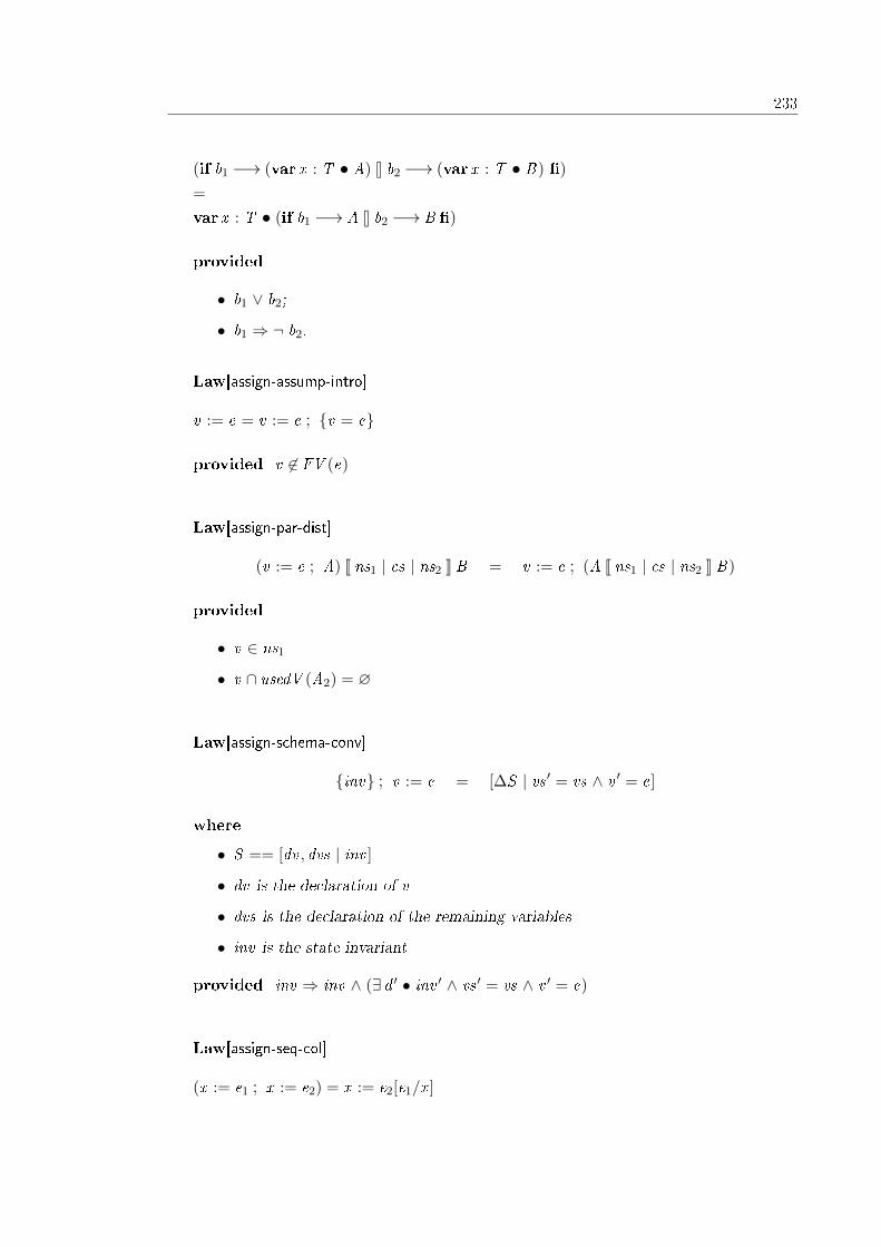
233
(if b1 −→ (var x : T • A) 8 b2 −→ (var x : T • B) �)
=
var x : T • (if b1 −→ A 8 b2 −→ B �)
provided
• b1 ∨ b2;
• b1 ⇒ ¬ b2.
Law[assign-assump-intro]
v := e = v := e ; {v = e}
provided v 6∈ FV (e)
Law[assign-par-dist]
(v := e ; A) J ns1 | cs | ns2 K B = v := e ; (A J ns1 | cs | ns2 K B)
provided
• v ∈ ns1
• v ∩ usedV (A2) = ∅
Law[assign-schema-conv]
{inv} ; v := e = [∆S | vs ′ = vs ∧ v ′ = e]
where
• S == [dv , dvs | inv ]
• dv is the declaration of v
• dvs is the declaration of the remaining variables
• inv is the state invariant
provided inv ⇒ inv ∧ (∃ d ′ • inv ′ ∧ vs ′ = vs ∧ v ′ = e)
Law[assign-seq-col]
(x := e1 ; x := e2) = x := e2[e1/x ]
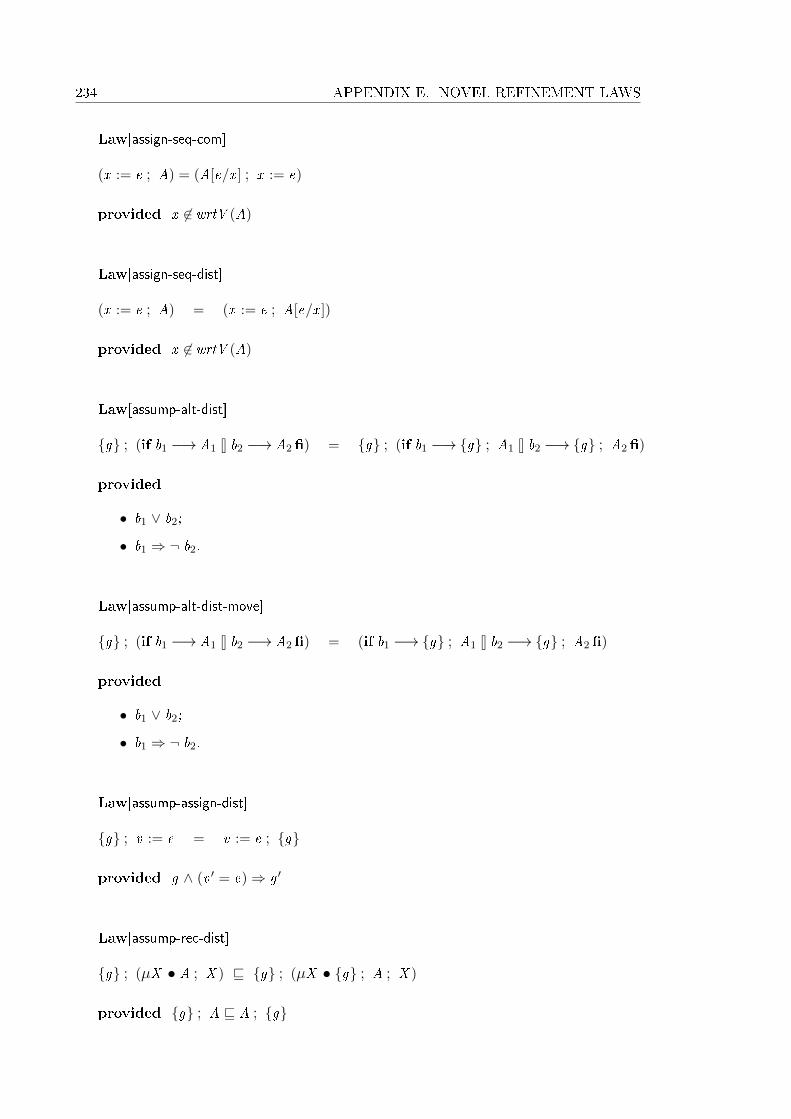
234 APPENDIX E. NOVEL REFINEMENT LAWS
Law[assign-seq-com]
(x := e ; A) = (A[e/x ] ; x := e)
provided x 6∈ wrtV (A)
Law[assign-seq-dist]
(x := e ; A) = (x := e ; A[e/x ])
provided x 6∈ wrtV (A)
Law[assump-alt-dist]
{g} ; (if b1 −→ A1 8 b2 −→ A2 �) = {g} ; (if b1 −→ {g} ; A1 8 b2 −→ {g} ; A2 �)
provided
• b1 ∨ b2;
• b1 ⇒ ¬ b2.
Law[assump-alt-dist-move]
{g} ; (if b1 −→ A1 8 b2 −→ A2 �) = (if b1 −→ {g} ; A1 8 b2 −→ {g} ; A2 �)
provided
• b1 ∨ b2;
• b1 ⇒ ¬ b2.
Law[assump-assign-dist]
{g} ; v := e = v := e ; {g}
provided g ∧ (v ′ = e)⇒ g ′
Law[assump-rec-dist]
{g} ; (µX • A ; X ) v {g} ; (µX • {g} ; A ; X )
provided {g} ; A v A ; {g}

235
Law[int-seq-dist]
(A ; B) ||[ ns1 | ns2 ]|| C = A ; (B ||[ ns1 | ns2 ]|| C )
provided
• usedC (A) = ∅;
• wrtV (A) ⊆ ns1;
• wrtV (A) ∩ usedV (C ) = ∅.
Law[pre�x-hide-dist-1]
(c −→ A) \ cs = c −→ (A \ cs)
provided c 6∈ cs
Law[pre�x-hide-dist-2]
(c −→ A) \ cs = A \ cs
provided c ∈ cs
Law[pre�x-par-dist]
((c −→ A) J ns1 | cs | ns2 K B) = c −→ (A J ns1 | cs | ns2 K B)
((c?x −→ A) J ns1 | cs | ns2 K B) = c?x −→ (A J ns1 | cs | ns2 K B)
((c.e −→ A) J ns1 | cs | ns2 K B) = c.e −→ (A J ns1 | cs | ns2 K B)
provided
• c 6∈ cs
• x 6∈ usedV (B)
• initials(B) ⊆ cs
• B is deterministic
Law[seq-assign-conv]
[∆S | c′1 = e1 ∧ . . . ∧ c′m = em ∧ c′m+1 = cm+1 ∧ . . . ∧ c′n = cn ] v c1 := e1 ; . . . ; cm := em
where
• S = [d | inv ]
• c1, . . . , cn are state components (elements of αd)
syntactic restriction αd and αd ′ are not free in e1, . . . , en .
provided inv [e1, . . . , em/c1, . . . , cm ]
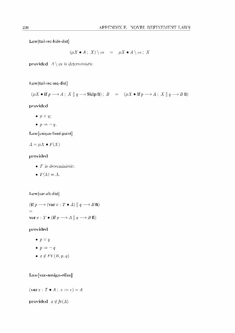
236 APPENDIX E. NOVEL REFINEMENT LAWS
Law[tail-rec-hide-dist]
(µX • A ; X ) \ cs = µX • A \ cs ; X
provided A \ cs is deterministic
Law[tail-rec-seq-dist]
(µX • if p −→ A ; X 8 q −→ Skip�) ; B = (µX • if p −→ A ; X 8 q −→ B �)
provided
• p ∨ q ;
• p ⇒ ¬ q .
Law[unique-�xed-point]
A = µX • F (X )
provided
• F is deterministic;
• F(A) = A.
Law[var-alt-dist]
(if p −→ (var x : T • A) 8 q −→ B �)
=
var x : T • (if p −→ A 8 q −→ B �)
provided
• p ∨ q
• p ⇒ ¬ q
• x 6∈ FV (B , p, q)
Law[var-assign-elim]
(var x : T • A ; x := e) = A
provided x 6∈ fv(A)
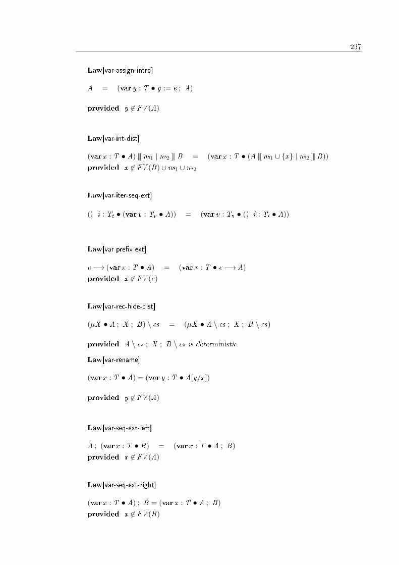
237
Law[var-assign-intro]
A = (var y : T • y := e ; A)
provided y 6∈ FV (A)
Law[var-int-dist]
(var x : T • A) ||[ ns1 | ns2 ]|| B = (var x : T • (A ||[ ns1 ∪ {x} | ns2 ]|| B))
provided x 6∈ FV (B) ∪ ns1 ∪ ns2
Law[var-iter-seq-ext]
(; i : Ti • (var v : Tv • A)) = (var v : Tv • (; i : Ti • A))
Law[var-pre�x-ext]
c −→ (var x : T • A) = (var x : T • c −→ A)
provided x 6∈ FV (c)
Law[var-rec-hide-dist]
(µX • A ; X ; B) \ cs = (µX • A \ cs ; X ; B \ cs)
provided A \ cs ; X ; B \ cs is deterministic
Law[var-rename]
(var x : T • A) = (var y : T • A[y/x ])
provided y 6∈ FV (A)
Law[var-seq-ext-left]
A ; (var x : T • B) = (var x : T • A ; B)
provided x 6∈ FV (A)
Law[var-seq-ext-right]
(var x : T • A) ; B = (var x : T • A ; B)
provided x 6∈ FV (B)
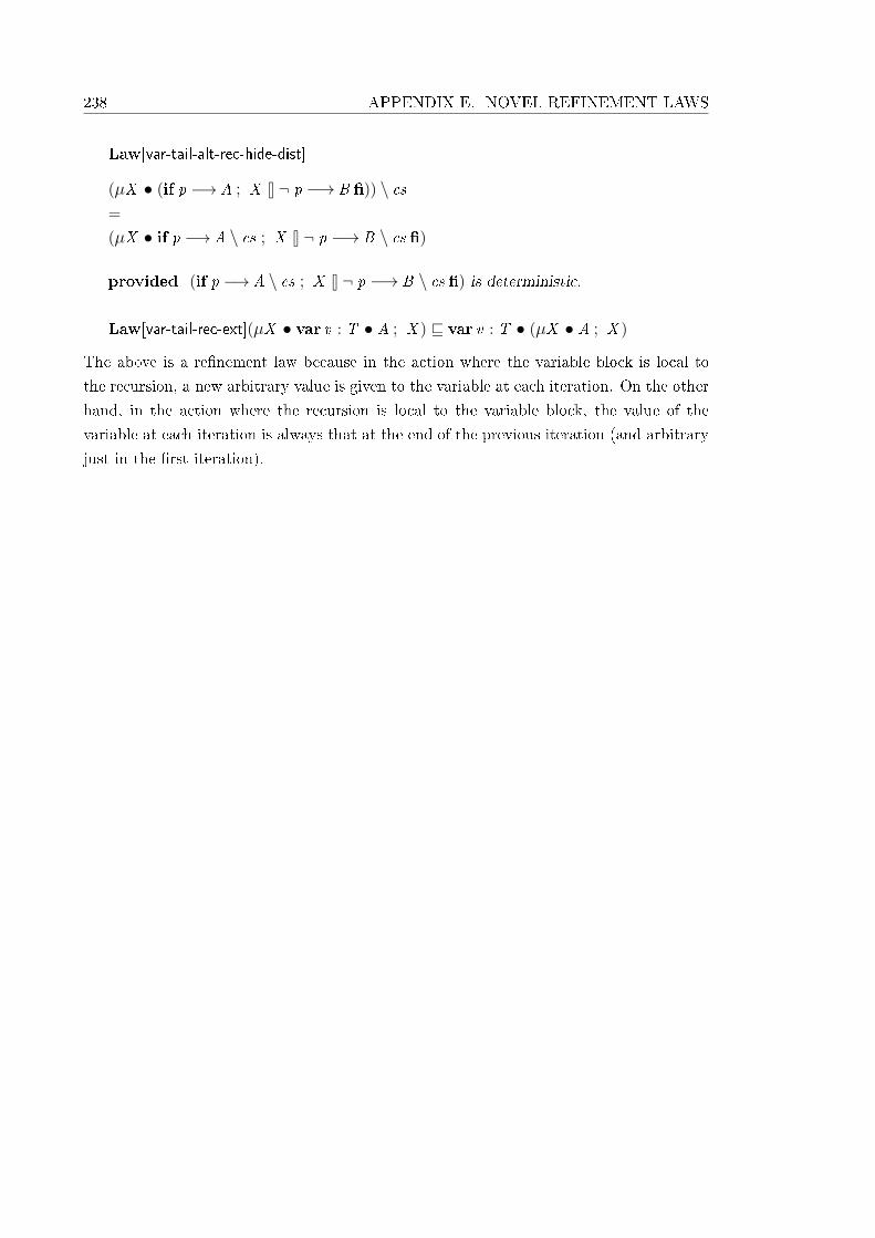
238 APPENDIX E. NOVEL REFINEMENT LAWS
Law[var-tail-alt-rec-hide-dist]
(µX • (if p −→ A ; X 8 ¬ p −→ B �)) \ cs=
(µX • if p −→ A \ cs ; X 8 ¬ p −→ B \ cs �)
provided (if p −→ A \ cs ; X 8 ¬ p −→ B \ cs �) is deterministic.
Law[var-tail-rec-ext](µX • var v : T • A ; X ) v var v : T • (µX • A ; X )
The above is a re�nement law because in the action where the variable block is local to
the recursion, a new arbitrary value is given to the variable at each iteration. On the other
hand, in the action where the recursion is local to the variable block, the value of the
variable at each iteration is always that at the end of the previous iteration (and arbitrary
just in the �rst iteration).
Bibliography
[1] J.-R. Abrial. The B-book: assigning programs to meanings. Cambridge University
Press, New York, NY, USA, 1996. ISBN 0-521-49619-5.
[2] J.-R. Abrial. Modeling in Event-B - System and Software Engineering. Cambridge
University Press, 2010. ISBN 978-0-521-89556-9.
[3] M. M. Adams and P. B. Clayton. ClawZ: Cost-E�ective Formal Veri�cation for
Control Systems. In K.-K. Lau and R. Banach, editors, ICFEM, volume 3785 of
LNCS. Springer-Verlag, 2005. ISBN 3-540-29797-9. doi: 10.1007/11576280_32.
[4] R. Arthan, P. Caseley, C. O'Halloran, and A. Smith. ClawZ: control laws in Z. In
ICFEM, 2000. pp. 169.
[5] R.-J. Back. On the Correctness of Re�nement Steps in Program Development. PhD
thesis, Åbo Akademi, Department of Computer Science, Helsinki, Finland, 1978.
Report A�1978�4.
[6] C. Banphawatthanarak and B. H. Krogh. Veri�cation of state�ow diagrams using
smv: sf2smv 2.0. Technical Report CMU-ECE-2000-020, Carnegie Mellon University,
2000.
[7] C. Banphawatthanarak, B. Krogh, and K. Butts. Symbolic veri�cation of executable
control speci�cations. In Proceedings of the 1999 IEEE International Symposium on
Computer Aided Control System Design, pages 581�586, August 1999.
[8] J. Barnes. High Integrity Software: The SPARK Approach to Safety and Security.
Addison-Wesley Longman Publishing Co., Inc., Boston, MA, USA, 2003. ISBN
0321136160.
[9] J. A. Bergstra and J. W. Klop. Algebra of communicating processes with abstraction.
Theoretical Computer Science, 37(1):77�121, 1985.
[10] P. Boström and L. Morel. Mode-Automata in Simulink/State�ow. Technical Report
772, Turku Centre for Computer Science, 2006.
[11] M. Butler and M. Leuschel. Combining CSP and B for Speci�cation and Property
Veri�cation. In J. Fitzgerald, I. Hayes, and A. Tarlecki, editors, Formal Methods
240 BIBLIOGRAPHY
2005, number LNCS 3582, pages 221�236. Springer-Verlag, January 2005. URL
http://eprints.ecs.soton.ac.uk/10388/.
[12] P. Caspi, A. Curic, A. Maignan, C. Sofronis, and S. Tripakis. Translating discrete-
time Simulink to Lustre. In R. Alur and I. Lee, editors, EMSOFT'03 LNCS. Springer-
Verlag, 2003.
[13] P. Caspi, A. Curic, A. Maignan, C. Sofronis, S. Tripakis, and P. Niebert. From
simulink to SCADE/lustre to TTA: a layered approach for distributed embedded
applications. ACM SIGPLAN Notices, 38(7):153�162, 2003. ISSN 0362-1340. doi:
10.1145/780731.780754.
[14] A. Cavalcanti, P. Clayton, and C. O'Halloran. From control law diagrams to Ada
via Circus. Formal Aspects of Computing, pages 1�48, 2011. ISSN 0934-5043. doi:
10.1007/s00165-010-0170-3.
[15] A. L. C. Cavalcanti. A re�nement calculus for Z. PhD thesis, Oxford University
Computing Laboratory, 1997.
[16] A. L. C. Cavalcanti. State�ow Diagrams in Circus. Electronic Notes in Theoretical
Computer Science, 240:23�41, 2009. ISSN 1571-0661. doi: 10.1016/j.entcs.2009.05.
043.
[17] A. L. C. Cavalcanti and P. Clayton. Veri�cation of Control Systems using Circus. In
Proceedings of the 11th IEEE International Conference on Engineering of Complex
Computer Systems, pages 269 � 278. IEEE Computer Society, 2006.
[18] A. L. C. Cavalcanti, A. C. A. Sampaio, and J. C. P. Woodcock. A Re�nement
Strategy for Circus. Formal Aspects of Computing, 15(2 - 3):146 � 181, 2003.
[19] A. L. C. Cavalcanti, P. Clayton, and C. O'Halloran. Control Law Diagrams in Circus.
In J. Fitzgerald, I. J. Hayes, and A. Tarlecki, editors, FM 2005: Formal Methods,
volume 3582 of LNCS, pages 253 � 268. Springer-Verlag, 2005.
[20] C. Chen. Formal Analysis for State�ow Diagrams. In Proceedings of the Fourth
International Conference on Secure Software Integration and Reliability Improvement
Companion (SSIRI-C), pages 102 �109, june 2010. doi: 10.1109/SSIRI-C.2010.29.
[21] M. L. Crane and J. Dingel. UML Vs. Classical Vs. Rhapsody Statecharts: Not All
Models Are Created Equal. Software and Systems Modeling, 6, 2007. doi: 10.1007/
s10270-006-0042-8.
[22] E. W. Dijkstra. Guarded commands, nondeterminacy and formal derivation of pro-
grams. Commun. ACM, 18(8):453�457, 1975. ISSN 0001-0782. doi: 10.1145/360933.
360975.
BIBLIOGRAPHY 241
[23] P. V. Eijk and M. Diaz, editors. Formal Description Technique Lotos: Results of
the Esprit Sedos Project. Elsevier Science Inc., New York, NY, USA, 1989. ISBN
0444872671.
[24] Esterel Technologies, Inc. Scade suiteTM. http://www.esterel-technologies.com/.
[25] European Committee for Electrotechnical Standardization (CENELEC). Railway
applications � Communications, signalling and processing systems � Software for
railway control and protection systems, March 2001.
[26] A. Evans. An Improved Recipe for Specifying Reactive Systems in Z. In ZUM
'97: Proceedings of the 10th International Conference of Z Users on The Z Formal
Speci�cation Notationes, pages 275�294, London, UK, 1997. Springer-Verlag. ISBN
3-540-62717-0.
[27] H. Fecher, J. Schönborn, M. Kyas, and W. P. de Roever. 29 New Unclarities in the
Semantics of UML 2.0 State Machines. In ICFEM, pages 52�65, 2005.
[28] C. Fischer. CSP-OZ: a combination of Object-Z and CSP. In FMOODS '97: Pro-
ceedings of the IFIP TC6 WG6.1 international workshop on Formal methods for open
object-based distributed systems, pages 423�438, London, UK, UK, 1997. Chapman
& Hall, Ltd. ISBN 0-412-82040-4.
[29] Formal Systems (Europe) Ltd. Process Behaviour Explorer, 2003. www.fsel.com.
[30] Formal Systems (Europe) Ltd. Failures-Divergence Re�nement, 2010. www.fsel.com.
[31] A. F. Freitas and A. L. C. Cavalcanti. Automatic Translation from Circus to Java. In
J. Misra, T. Nipkow, and E. Sekerinski, editors, FM 2006: Formal Methods, volume
4085 of Lecture Notes in Computer Science, pages 115 � 130. Springer-Verlag, 2006.
[32] L. Freitas. Model-checking Circus. PhD thesis, Department of Computer Science,
The University of York, UK, 2005. YCST-2005/11.
[33] N. Halbwachs, P. Caspi, P. Raymond, and D. Pilaud. The synchronous data-�ow
programming language LUSTRE. In Proceedings of the IEEE, volume 79, pages 1305
� 1320, 1991.
[34] G. Hamon. A denotational semantics for State�ow. In W. Wolf, editor, EMSOFT,
pages 164�172. ACM, 2005. ISBN 1-59593-091-4. doi: 10.1145/1086228.1086260.
[35] G. Hamon and J. Rushby. An operational semantics for State�ow. In M. Wermelinger
and T. Margaria-Ste�en, editors, Fundamental Approaches to Software Engineer-
ing:7th International Conference (FASE), volume 2984 of LNCS, pages 229�243,
Barcelona, Spain, 2004. Springer-Verlag.
[36] D. Harel. Statecharts: A visual formalism for complex systems. Science of Computer
Programming, 8(3):231�274, 1987.

242 BIBLIOGRAPHY
[37] D. Harel and H. Kugler. The Rhapsody Semantics of Statecharts (or, On the Ex-
ecutable Core of the UML) - Preliminary Version. In SoftSpez Final Report, pages
325�354, 2004.
[38] D. Harel and A. Naamad. The STATEMATE semantics of statecharts. ACM Trans-
actions on Software Engineering and Methodology, 5(4):293�333, Oct. 1996. ISSN
1049-331X.
[39] D. Harel and M. Politi. Modeling Reactive Systems with Statecharts: The Statemate
Approach. McGraw-Hill, Inc., New York, NY, USA, 1998. ISBN 0070262055.
[40] D. Harel, A. Pnueli, J. P. Schmidt, and R. Sherman. On the formal semantics
of statecharts. In Proceedings of the 2nd IEEE Symposium on Logic in Computer
Science, pages 54�64, New York, 1987. IEEE Press.
[41] C. A. R. Hoare. Communicating sequential processes. Prentice-Hall, Inc., Upper
Saddle River, NJ, USA, 1985. ISBN 0-13-153271-5.
[42] C. A. R. Hoare and H. Jifeng. Unifying Theories of Programming. Prentice Hall,
1998.
[43] J. Hoenicke and E.-R. Olderog. Combining speci�cation techniques for processes,
data and time. In IFM '02: Proceedings of the Third International Conference on
Integrated Formal Methods, pages 245�266, London, UK, 2002. Springer-Verlag. ISBN
3-540-43703-7.
[44] G. J. Holtzmann. Design and Validation of Computer Protocols. Prentice Hall, 1991.
[45] G. J. Holtzmann. The model checker SPIN. In IEEE Transactions on Software
Engineering, volume 23, May 1997.
[46] J. E. Hopcroft, R. Motwani, and J. D. Ullman. Introduction to Automata Theory,
Languages, and Computation (3rd Edition). Addison-Wesley Longman Publishing
Co., Inc., Boston, MA, USA, 2006. ISBN 0321455363.
[47] International Electrotechnical Commission (IEC). Functional safety of electrical/-
electronic/programmable electronic safety related systems � Part 1: General require-
ments (IEC 61508-1), 1997.
[48] ISO. Road vehicles � Funcional safety (ISO 26262), 2011.
[49] N. Izerrouken, X. Thirioux, M. Pantel, and M. Strecker. Certifying an Automated
Code Generator Using Formal Tools. In ERTS'08, 4th European symposium on Real
Time Systems, 2008.
[50] JFlex. JFlex - The Fast Scanner Generator for Java, 2009. http://jflex.de/ [Last
accessed 2009].
BIBLIOGRAPHY 243
[51] C. B. Jones. Systematic Software Development Using VDM. Prentice-Hall Interna-
tional, 1986.
[52] M. P. Jones. jacc: just another compiler compiler for Java, 2004. http://web.cecs.
pdx.edu/~mpj/jacc/ [Last accessed 2009].
[53] D. Latella, I. Majzik, and M. Massink. Towards a formal operational semantics of
uml statechart diagrams. In Proceedings of the IFIP TC6/WG6.1 Third Interna-
tional Conference on Formal Methods for Open Object-Based Distributed Systems
(FMOODS), page 465, Deventer, The Netherlands, The Netherlands, 1999. Kluwer,
B.V. ISBN 0-7923-8429-6.
[54] M. Leuschel and M. Butler. ProB: A Model Checker for B. In A. Keijiro, S. Gnesi,
and M. Dino, editors, Formal Methods Europe 2003, volume 2805, pages 855�874.
Springer-Verlag, LNCS, 2003. URL http://eprints.ecs.soton.ac.uk/8341/.
[55] J. Lilius and I. P. Paltor. The Semantics Of UML State Machines. Technical Report
273, Turku Centre and Computer Science, May 1999.
[56] B. Mahony and J. S. Dong. Blending Object-Z and Timed CSP: an introduction to
TCOZ. In ICSE '98: Proceedings of the 20th international conference on Software
engineering, pages 95�104, Washington, DC, USA, 1998. IEEE Computer Society.
ISBN 0-8186-8368-6.
[57] P. Malik and M. Utting. CZT: A Framework for Z Tools. In ZB. Lecture, pages
65�84. Springer-Verlag, 2005.
[58] F. Maraninchi and Y. Rémond. Mode-automata: a new domain-speci�c construct
for the development of safe critical systems. Science of Computer Programming, 46:
219�254, March 2003. ISSN 0167-6423. doi: 10.1016/S0167-6423(02)00093-X.
[59] J. McDermid, A. Galloway, S. Burton, J. Clark, I. Toyn, N. Tracey, and S. Valentine.
Towards industrially applicable formal methods: Three small steps, and one giant
leap. In Proceedings of the International Conference on Formal Engineering Methods,
pages 76�88. Press, 1998.
[60] E. Mikk, Y. Lakhnech, C. Petersohn, and M. Siegel. On formal semantics of state-
charts as supported by statemate. In In Second BCS-FACS Northern Formal Methods
Workshop. Springer-Verlag, 1997.
[61] R. Milner. A Calculus of Communicating Systems. Springer-Verlag New York, Inc.,
Secaucus, NJ, USA, 1982. ISBN 0387102353.
[62] Ministry of Defence. Requirements for safety related software in defence equipment
(Def Stan 00-55), 1997.

244 BIBLIOGRAPHY
[63] A. Miyazawa. Source �les for a parallel implementation of the State�ow chart
in air.mdl , 2012. Available from http://www-users.cs.york.ac.uk/~alvarohm/
thesis/.
[64] A. Miyazawa. Formal syntax of Circus, 2012. Available from http://www-users.
cs.york.ac.uk/~alvarohm/thesis/.
[65] A. Miyazawa. Formal syntax of State�ow charts, 2012. Available from http://
www-users.cs.york.ac.uk/~alvarohm/thesis/.
[66] A. Miyazawa. Formal syntax of Z, 2012. Available from http://www-users.cs.
york.ac.uk/~alvarohm/thesis/.
[67] A. Miyazawa. Formal translation rules for State�ow charts, 2012. Available from
http://www-users.cs.york.ac.uk/~alvarohm/thesis/.
[68] A. Miyazawa and A. L. C. Cavalcanti. Towards the formal veri�cation of implemen-
tations of State�ow Diagrams. Technical Report YCS-2010-449, University of York,
2010.
[69] A. Miyazawa and A. L. C. Cavalcanti. A formal semantics of State�ow charts.
Technical Report YCS-2011-461, University of York, 2011.
[70] A. Miyazawa and A. L. C. Cavalcanti. Re�nement-oriented models of State�ow
charts. Science of Computer Programming, 2011. doi: 10.1016/j.scico.2011.07.007.
[71] A. Miyazawa and A. L. C. Cavalcanti. Re�nement-based veri�cation of sequential
implementations of State�ow charts. In J. Derrick, E. Boiten, and S. Reeves, edi-
tors, Proceedings 15th International Re�nement Workshop, volume 55, pages 65�83.
EPTCS, 2011. doi: 10.4204/EPTCS.55.5.
[72] A. Miyazawa and A. L. C. Cavalcanti. Re�nement-based veri�cations of implemen-
tations of State�ow charts. 2012. (to be submitted).
[73] C. C. Morgan. Programming from Speci�cations. Prentice-Hall, 2nd edition, 1994.
[74] J. M. Morris. A theoretical basis for stepwise re�nement and the programming
calculus. Sci. Comput. Program., 9(3):287�306, 1987.
[75] M. Y. Ng and M. J. Butler. Towards formalizing UML state diagrams in CSP. In
SEFM, page 138. IEEE Computer Society, 2003. ISBN 0-7695-1949-0.
[76] M. V. M. Oliveira. Formal Derivation of State-Rich Reactive Programs using Circus.
PhD thesis, Department of Computer Science - University of York, UK, 2006. YCST-
2006-02.
BIBLIOGRAPHY 245
[77] M. V. M. Oliveira and A. L. C. Cavalcanti. ArcAngelC: a Re�nement Tactic Language
for Circus. Electronic Notes in Theoretical Computer Science, 214C:203 � 229, 2008.
doi: 10.1016/j.entcs.2008.06.010. c© Elsevier B. V.
[78] M. V. M. Oliveira, A. L. C. Cavalcanti, and J. C. P. Woodcock. Formal development
of industrial-scale systems. Innovations in Systems and Software Engineering, 1(2):
125 � 146, 2005.
[79] M. V. M. Oliveira, A. L. C. Cavalcanti, and J. C. P. Woodcock. A UTP Se-
mantics for Circus. Formal Aspects of Computing, 21(1):3 � 32, 2007. doi:
10.1007/s00165-007-0052-5.
[80] M. V. M. Oliveira, A. C. Gurgel, and C. G. de Castro. CRe�ne: Support for the Circus
Re�nement Calculus. In A. Cerone and S. Gruner, editors, 6th IEEE International
Conferences on Software Engineering and Formal Methods, pages 281�290. IEEE
Computer Society Press, 2008. ISBN 978-0-7695-3437-4.
[81] OMG. UML 2.0 Superstructure Speci�cation. Technical report, Object Management
Group (OMG), August 2005.
[82] A. Pnueli and M. Shalev. What is in a step: On the semantics of statecharts. In
Theoretical Aspects of Computer Software. Springer-Verlag, 1991.
[83] Radio Technical Commission for Aeronautics (RTCA). Software Considerations in
Airborne Systems and Equipment Certi�cation (DO-178B), 1992.
[84] R. Ramos, A. Sampaio, and A. Mota. A semantics for UML-RT active classes via
mapping into Circus. In M. Ste�en and G. Zavattaro, editors, FMOODS, volume
3535 of LNCS, pages 99�114. Springer-Verlag, 2005. ISBN 3-540-26181-8. doi: 10.
1007/11494881_7.
[85] A. W. Roscoe. The Theory and Practice of Concurrency. Prentice-Hall Series in
Computer Science. Prentice-Hall, New York, 1998. ISBN 0-13-674409-5. Oxford.
[86] A. E. Rugina, D. Thomas, X. Olive, and G. Veran. Gene-Auto: Automatic software
code generation for real-time embedded systems. In DASIA 2008, the International
Space System Engineering Conference, 2008.
[87] N. Scaife, C. Sofronis, P. Caspi, S. Tripakis, and F. Maraninchi. De�ning and
translating a "safe" subset of simulink/state�ow into lustre. In G. C. But-
tazzo, editor, EMSOFT, pages 259�268. ACM, 2004. ISBN 1-58113-860-1. doi:
10.1145/1017753.1017795.
[88] S. Schneider. Concurrent and Real Time Systems: The CSP Approach. John Wiley
& Sons, Inc., New York, NY, USA, 1999. ISBN 0471623733.
246 BIBLIOGRAPHY
[89] S. Schneider and J. Davies. A brief history of Timed CSP. Theoretical Computer
Science. 1995.
[90] E. Sekerinski and R. Zurob. Translating Statecharts to B. In Springer-Verlag, editor,
IFM 2002, volume 2335 of LNCS, pages 128�144, 2002.
[91] G. Smith. A Semantic Integration of Object-Z and CSP for the Speci�cation of
Concurrent Systems. In FME '97: Proceedings of the 4th International Symposium
of Formal Methods Europe on Industrial Applications and Strengthened Foundations
of Formal Methods, pages 62�81, London, UK, 1997. Springer-Verlag. ISBN 3-540-
63533-5.
[92] G. Smith. The Object-Z Speci�cation Language. Kluwer Academic Publishers, Nor-
well, MA, USA, 2000. ISBN 0-7923-8684-1.
[93] G. Smith and J. Derrick. Speci�cation, Re�nement and Veri�cation of Concur-
rent Systems�An Integration of Object-Z and CSP. Formal Methods in System
Design, 18(3):249�284, 2001. ISSN 0925-9856. doi: http://dx.doi.org/10.1023/A:
1011269103179.
[94] C. Snook and M. Butler. UML-B: Formal modelling and design aided by UML. ACM
Transactions on Software Engineering and Methodology, 15(1):92�122, January 2006.
URL http://eprints.ecs.soton.ac.uk/10169/.
[95] C. Snook, V. Savicks, and M. Butler. Veri�cation of UML models by translation to
UML-B. LNCS, 6957:251, 2011. URL http://eprints.ecs.soton.ac.uk/22921/.
[96] J. Sun, Y. Liu, J. S. Dong, and J. Pang. Pat: Towards �exible veri�cation under
fairness. In CAV, pages 709�714, 2009.
[97] K. Taguchi and K. Araki. The state-based CCS semantics for concurrent Z speci�-
cation. In ICFEM '97: Proceedings of the 1st International Conference on Formal
Engineering Methods, page 283, Washington, DC, USA, 1997. IEEE Computer Soci-
ety. ISBN 0-8186-8002-4.
[98] The MathWorks,Inc. State�ow and State�ow Coder 7 User's Guide, October 2008.
Available at http://www.mathworks.com/products/stateflow [Last accessed Oc-
tober 2008].
[99] The MathWorks,Inc. Simulink, October 2009. Available at http://www.mathworks.
com/products/simulink [Last accessed October 2008].
[100] The MathWorks,Inc. Real-Time Workshop 7 User's Guide, March 2010. Available
at http://www.mathworks.com/products/rtw [Last accessed March 2010].
BIBLIOGRAPHY 247
[101] A. Tiwari. Formal semantics and analysis methods for Simulink State�ow models.
Technical report, SRI International, 2002. URL http://www.csl.sri.com/users/
tiwari/html/stateflow.html.
[102] A. Toom, T. Naks, M. Panter, M. Grandriau, and I. Wati. Gene-Auto: an Automatic
Code Generator for a safe subset of Simulink/State�ow and Scicos. In ERTS'08, 4th
European symposium on Real Time Systems, 2008.
[103] I. Toyn. Simulink/State�ow Analyser user's manual. Technical report, Department
of Computer Science, University of York, 2005.
[104] I. Toyn and A. Galloway. Proving properties of State�ow models using ISO Standard
Z and CADiZ. In In ZB-2005, vol. 3455 of LNCS, pages 104�123, 2005.
[105] H. Treharne and S. Schneider. Using a process algebra to control B OPERATIONS.
In IFM'99 1st International Conference on Integrated Formal Methods, pages 437�
457, York, June 1999. Springer-Verlag. URL http://www.cs.rhbnc.ac.uk/~helent.
[106] TTA-Group. TTA � A Dependable Real-Time Communication Platform for Safety-
Relevant Applications, 2007. URL http://www.ttagroup.org/technology/tta.
htm.
[107] M. von der Beeck. A structured operational semantics for UML-statecharts. Software
and Systems Modeling, V1:130�141, 2002.
[108] M. W. Whalen. A Parametric Structural Operational Semantics for State�ow, UML
Statecharts, and Rhapsody. Technical Report 2010-1, University of Minnesota Soft-
ware Engineering Center, 200 Union St., Minneapolis, MN 55455, August 2010.
[109] J. Woodcock and J. Davies. Using Z: speci�cation, re�nement, and proof. Prentice-
Hall, Inc., Upper Saddle River, NJ, USA, 1996. ISBN 0-13-948472-8.
[110] J. C. P. Woodcock and A. L. C. Cavalcanti. The Semantics of Circus. In D. Bert, J. P.
Bowen, M. C. Henson, and K. Robinson, editors, ZB 2002: Formal Speci�cation and
Development in Z and B, volume 2272 of LNCS, pages 184�203. Springer-Verlag,
2002.
[111] F. Zeyda and A. Cavalcanti. Encoding Circus Programs in ProofPowerZ. LNCS.
Springer-Verlag, 2009. Awaiting publication.
[112] C. Zhou, C. A. R. Hoare, and A. P. Ravn. A calculus of durations. In Information
Processing Letters, volume 40, pages 269�276, 1991.