form postponement: a decision-making perspective

1

007-0323

Form Postponement: a Decision-Making Perspective

Alessio Trentin Dipartimento di Tecnica e Gestione dei sistemi industriali,

Università di Padova, Stradella S. Nicola, 3, 36100 Vicenza, Italy

Tel. +39-0444-998817 Email: [email protected]

Fabrizio Salvador

Department of Operations and Technology Management, Instituto de Empresa,

Maria de Molina, 12-5, 28006 Madrid, Spain Tel. +34-91-5689600

Email: [email protected]

Cipriano Forza Dipartimento di Tecnica e Gestione dei sistemi industriali,

Università di Padova, Stradella S. Nicola, 3, 36100 Vicenza, Italy

Tel. +39-0444-998817 Email: [email protected]

M. Johnny Rungtusanatham

Operations & Management Science Department Curtis L. Carlson School of Management

University of Minnesota - Twin Cities 321 Nineteenth Avenue South Minneapolis, MN 55455-9940, USA

Tel. (612) 626-6965 Email: [email protected]

POMS 18th Annual Conference Dallas, Texas, U.S.A. May 4 to May 7, 2007

2

Form Postponement: a Decision-Making Perspective

Abstract

Operations management literature defines form postponement as the deferment of product

differentiation activities through changes in the architecture and/or the manufacturing and

distribution process of a product family. We contend that when form postponement is meant to

reduce the risk and associated costs of specifying the wrong mix of product variants, it is more

appropriately defined as the deferment of production planning decisions. We elaborate on this

concept, proposing a notion of form postponement from a decision-making perspective, and

develop an operational procedure to identify and quantify all opportunities for form

postponement relative to a given product family. We demonstrate that each potential for form

postponement can be divided in two components, one related to the forecasting and master

scheduling process and the other related to product and/or process redesign. We empirically

illustrate the fact that the former component, usually neglected in the literature, can account for

more than 50% of the total potential for form postponement within a product family. We

conclude by setting directions for future decision-making research on form postponement.

Keywords:

Form postponement, product variety management, production planning and control.

3

1. Introduction

Form Postponement (FP) is commonly defined as deferring the timing of one or more product

differentiation activities (PDAs) that specialize the work-in-progress into specific product

variants along a manufacturing and distribution process (e.g., Zinn and Bowersox 1988, Garg

and Tang 1997, Van Hoek 2001, Hsu and Wang 2004). FP, by this definition, is achieved

through changes in the product family architecture and/or the manufacturing and distribution

process (Lee and Billington 1994, Lee and Tang 1997, Gupta and Krishnan 1998, Swaminathan

and Lee 2003).

To date, the majority of research on FP, based on this definition, assumes that decisions

driving PDAs, namely decisions specifying the mix of products the company is going to make at

a given time in the future, are triggered by a priori-defined inventory replenishment rules (e.g.,

Lee 1996, Lee and Tang 1997, Brown et al. 2000, Aviv and Federgruen 2001a, 2001b, Ma et al.

2002). Under this assumption, deferring a PDA automatically leads to the deferment of the

corresponding decision, so that FP reduces the risk of making forecast errors in estimating

demand mix (Whang and Lee 1998, Aviv and Federgruen 2001b).

We argue, however, that when decisions pertaining to product mix are not put on triggers,

FP defined as deferment of PDAs is no longer an appropriate perspective if the essential purpose

of FP is that of reducing the risk and associated costs of specifying the wrong mix of product

variants. Instead, we demonstrate that in this context, FP should be more appropriately defined

in terms of the deferment of production planning decisions. This complementary definitional

perspective has, in fact, been echoed as early as in Alderson (1950) and, more recently, by

researchers in logistics management (e.g., Heskett 1977, Mather 1986, Cooper 1993, Pagh and

Cooper 1998, Yang et al. 2004).

4

In this paper, we define FP as the deferment of forecast-driven production planning

decisions pertaining to product mix and provide a measurement procedure to identify and

quantify all opportunities for deferring these decisions. Formalizing FP from a decision-making

perspective we demonstrate how this definitional perspective complements and completes the

extant definition of FP. We also discuss and illustrate the relevance of this definitional

perspective for decision-making through three real examples. We conclude by discussing future

research opportunities motivated by this definitional perspective.

2. Defining Form Postponement from a “Decision-Making” Perspective

2.1 Setting the Stage

Consider, for the purpose of illustration, the case of a Z, batch manufacturer producing and

selling a single product family with 10 product variants in a make-to-order environment. Z as

documented in Figure 1: BASELINE can be described as follows:

• Making the end items for this product family (i.e., product variants) requires execution of a

transformation process involving K=7 sourcing or manufacturing activities.

• For the purpose of production planning, each kth activity has an associated planned lead time

lk and must start no later than at time TActitity k. The planned lead time represents an estimate

of the time that will elapse between when an order is released for each kth activity and when

the corresponding activity is completed (Orlicky 1975, Kanet 1986, Enns 2001). Planned

lead times are generally kept as quantity-invariant, since they mainly comprise elements,

such as queue time and setup time, which are independent of lot size (Vollmann et al. 2005).

• The cumulative lead time for the entire process (CLT) is, therefore, given by CLT = ∑lk = 9.4

weeks and the transformation process must start no later than at time TActitity 1.

5

• All sourcing and manufacturing activities are initiated by purchase or work orders planned

through a Materials Requirements Planning (MRP) system that is run weekly. All orders

planned by MRP in a given week are launched contemporarily at the beginning of the same

week. This means that the order launching process, which converts planned orders into

scheduled receipts (Vollmann et al. 2005), is performed on a weekly basis as opposed to a

continuous basis. Consequently, there is a time lag, δk≥0, between the timing of order release

for an Activity k (k

TActivityOR ) and TActitity k.

• For Z, Activity 3 is a Mix Composition Differentiation Activity (MCDA). Mix is the set of

different final product variants; mix composition is defined as the quantity of each final

product variant to be produced. An MCDA, therefore, is an activity whose execution creates

the mix and mix composition or whose execution simply modifies the mix composition for

the end of the process. When an MCDA creates the mix, an MCDA is, therefore, a PDA. In

fact, an MCDA, as defined here, extends the concept of what a PDA is to include an activity

that changes the mix composition of a previously specified mix. The number of MCDAs

along a product family’s transformation process is denoted as I, the ith MCDA is denoted as

MCDAi, and the number of different possible outcomes of MCDAi is denoted as Mi. In the

case of Z, Activity 3 is MCDA1, and M1=10.

• Any kth>3 manufacturing activity, once started, must process all work-in-progress to which it

has been fed by the kth–1 activity. This, in essence, constrains the baseline situation to have

only one MCDA, as mix composition cannot be altered after Activity 3. In the case of Z,

therefore, I=1.

• TCODP= –2 denotes the point in time when Z has perfect information about market demand

requirements (i.e., mix composition) that Z must be able to satisfy at TCOMPLETION (≡0), where

6

TCOMPLETION = TCODP + ∆ and ∆≥0 is the average time that a customer is willing to wait after

order placement and net of shipping time. Since all decisions taken prior to TCODP are

forecast-driven and all decisions taken after TCODP are order-driven, the definition of

Customer Order Decoupling Point offered here is consistent with that in literature (Giesberts

and Van der Tang 1992, Brown et al. 2000, Wikner and Rudberg 2005).

• Given the CLT constraint and the weekly frequency with which planned orders are launched,

to satisfy mix composition requirements at TCOMPLETION Z releases the order to start Activity

1 at time 1ActivityOR

T = –10.

• Since purchase and work orders are planned through an MRP system and the MRP requires

input from the Master Production Schedule (MPS), Z must specify, in this example, an MPS

prior to 1ActivityOR

T , and precisely at time TMPS= –11.

• In the case of Z, the MPS comprises two logically-related but distinct decision components –

one component concerning total production volume (MPSVOL) and one component that splits

(differentiates) the total production volume into the quantities of the various possible

outcomes of MCDA1 (MPSMIX1). MPSMIX1 consists of M1 elementary decisions, where the jth

elementary decision (MPSMIX1, j) specifies the quantity of the jth possible outcome of MCDA1

to be produced (j=1,…, M1).

• The MPSVOL affects all activities starting with Activity 1, while the MPSMIX1 affects only

MCDA1. Consequently, MPSVOL and MPSMIX1 can theoretically be decoupled in time. Z

shows the case when these two decision components of the MPS are taken contemporarily

(i.e., TMPS=VOL

TMPS =1MIX

TMPS ).

7

• Given TMPS and TCODP, the time span between the two defines the Forecast Window for the

MPS ( MPSFW ) such that MPSFW =TCODP–TMPS= –2–(–11) = 9 weeks. Since

TMPS=VOL

TMPS =1MIX

TMPS in the example of Z, the Forecast Windows for the respective MPS

decision components (i.e., VOL

FWMPS and 1MIX

FWMPS ) are also 9 weeks (i.e., MPSFW =

VOLFWMPS =

1MIXFWMPS ).

Together, the salient characteristics of the product family (i.e., number of product

variants), the transformation process (i.e., the K sourcing and manufacturing activities and

associated TActivity k ’s), the MPS process (i.e., the MPSFW , VOL

FWMPS , 1MIX

FWMPS , TMPS, VOL

TMPS ,

and 1MIX

TMPS for the production planning decisions MPSVOL and MPSMIX1), and the MRP and order

launching process (i.e., the k

TActivityOR ’s) can be said to establish the state s for Z.

8

A1

time (wks)

BASELINEFWMPS= FWMPSVOL= FWMPSMIX1

= [UFPDM]

A2 A3 A4 A5 A6 A7

MPSMPSVOL MPSMIX1

-1-5-7-8-9-10-11 -6

TCODP

-3 -2

TCOMPLETION

-4 0

TACTIVITY 1TMPS =TMPSVOL= TMPSMIX1

∆TORMCDA1

TRA

NS

FOR

MAT

ION

PR

OC

ES

SM

RP

PR

OC

ESS

MP

S P

RO

CE

SS

FORECAST-DRIVENDECISIONS

ORDER-DRIVENDECISIONS

Time when market demand for T=0 is

known in mix

[uFPDM]MPSMIX

[uFPDM]TRANS+MRP

A1

time (wks)

A2 A3A4 A5 A6 A7

MPSMPSVOL MPSMIX1

-1-5-7-8-9-10-11 -6

TCODP

-3 -2

TCOMPLETION

-4 0


∆TOR, 1 TORMCDA1

MCDA1

MRP

FP TRANSFORMATION

MCDA1

MRP

SITUATION A

Lead time of k-th activity

k

TOR, 1 TMCDA1

δ1 δMCDA1

A1

time (wks)


= [UFPDM]

A2 A3 A4 A5 A6 A7

MPSMPSVOL MPSMIX1MPSVOL MPSMIX1

-1-5-7-8-9-10-11 -6

TCODP

-3 -2

TCOMPLETION

-4 0


∆TORMCDA1

TRA

NS

FOR

MAT

ION

PR

OC

ES

SM

RP

PR

OC

ESS

MP

S P

RO

CE

SS




known in mix

[uFPDM]MPSMIX

[uFPDM]TRANS+MRP

A1

time (wks)

A2 A3A4 A5 A6 A7


-1-5-7-8-9-10-11 -6

TCODP

-3 -2

TCOMPLETION

-4 0


∆TOR, 1 TORMCDA1

MCDA1

MRP

FP TRANSFORMATION

MCDA1

MRP

SITUATION A


k

TOR, 1 TMCDA1

δ1 δMCDA1

Figure 1: FP as commonly defined in the literature

9

2.2 Relating Form Postponement to Forecast Window Reduction

Suppose Z implements FP, consistent with the common definition, by deferring the timing of

MCDA1 (i.e., TMCDA1) along the transformation process, as shown in Figure 1: SITUATION A.

To defer MCDA1, changes to the transformation process would be required, which may or may

not require changes to the product family design (Lee and Billington 1994, Lee and Tang 1997,

Gupta and Krishnan 1998, Swaminathan and Lee 2003). Doing so allows Z to enjoy such

benefits as reduced safety stock for a given customer service level due to inventory risk-pooling

(Whang and Lee 1998, Lin et al. 2000, Aviv and Federgruen 2001b) and lower processing costs

and overhead due to reduced variety of components and processes within the system (Lee and

Billington 1994, Garg and Tang 1997). Notice, however, that deferring TMCDA1 does not

automatically reduce the risk and associated costs of specifying the wrong mix of end products.

For Z, given that TMPS= –11, no different than in Figure 1: BASELINE, there is no change to the

MPSFW and, hence, no changes to the VOL

FWMPS and the 1MIX

FWMPS .

In contrast, the accuracy of the forecast pertaining to the mix composition requirements

known at time TCODP could be improved without pursuing FP in terms of deferring TMCDA1.

Instead, Z could focus on reducing the 1MIX

FWMPS by decoupling the MPSMIX1 from the MPSVOL

and deferring the timing of MPSMIX1 (i.e., 1MIX

TMPS ) closer to time TCODP (Alderson 1950, Mather

1986, Yang et al. 2004). As shown in Figure 2: SITUATION B, Z can defer 1MIX

TMPS from

1MIXTMPS = –11 weeks to

1MIXTMPS = –7 weeks.

10

A1

time (wks)


= [UFPDM]

A2 A3 A4 A5 A6 A7

MPSMPSVOL MPSMIX1

-1-5-7-8-9-10-11 -6

TCODP

-3 -2

TCOMPLETION

-4 0


∆TORMCDA1

TRA

NS

FOR

MAT

ION

PR

OC

ES

SM

RP

PR

OC

ES

SM

PS

PR

OC

ES

S




known in mix

[uFPDM]MPSMIX

[uFPDM]TRANS+MRP

time (wks)

MCDA1

MRP

SITUATION B


k

TOR, 1 TMCDA1

δ1 δMCDA1

A1 A2 A3 A4 A5 A6 A7

-1-5-7-8-9-10-11 -6

TCODP

-3 -2

TCOMPLETION

-4 0


∆TORMCDA1

MCDA1

TOR, 1 TMCDA1

δ1 δMCDA1

FP DECISION-MAKING

MPSVOL MPSMIX1

MRP

A1

time (wks)


= [UFPDM]

A2 A3 A4 A5 A6 A7


-1-5-7-8-9-10-11 -6

TCODP

-3 -2

TCOMPLETION

-4 0


∆TORMCDA1

TRA

NS

FOR

MAT

ION

PR

OC

ES

SM

RP

PR

OC

ES

SM

PS

PR

OC

ES

S




known in mix

[uFPDM]MPSMIX

[uFPDM]TRANS+MRP

time (wks)

MCDA1

MRP

SITUATION B


k

TOR, 1 TMCDA1

δ1 δMCDA1

A1 A2 A3 A4 A5 A6 A7

-1-5-7-8-9-10-11 -6

TCODP

-3 -2

TCOMPLETION

-4 0


∆TORMCDA1

MCDA1

TOR, 1 TMCDA1

δ1 δMCDA1

FP DECISION-MAKING

MPSVOL MPSMIX1

MRP

Figure 2: FP from a decision-making perspective

11

To summarize, interpreting Figure 1: SITUATION A and Figure 2: SITUATION B

concurrently, we can observe that:

(i) The 1MIX

FWMPS cannot be reduced by simply deferring TMCDA1,

(ii) The 1MIX

FWMPS can be reduced by deferring 1MIX

TMPS without deferring TMCDA1 but

the maximum reduction achievable is constrained by 1MCDAORT , and

(iii) The 1MIX

FWMPS can be completely eliminated by deferring 1MIX

TMPS , 1MCDAORT , and

TMCDA1 such that eventually 1MIX

TMPS = TCODP.

2.3 Formalizing Form Postponement from a “Decision-Making” Perspective

Thus far, we have assumed, for the sake of illustration, that the planned lead time for the sole

MCDA (i.e., MCDA1) is invariant across the product variants. In a more realistic environment,

the planned lead time for MCDA1 may vary across its M1 possible different outcomes. This may

happen, for example, because different outcomes of MCDA1 are produced at different locations

or because different outcomes require different processes with different cycle times. Regardless

of the reason for which more than one planned lead times are associated to MCDA1, let

jT ,MCDA1 = timing of MCDA1 when its outcome is j (j=1,…, Mi)

j,T

1MCDAOR = timing of order release for MCDA1 when its outcome is j

(j=1,…, M1)

12

j,MIXT

1MPS = timing of the elementary decision specifying the quantity of

the jth outcome of MCDA1 to be produced (i.e., MPSMIX1, j)

j ,MIXFW

1MPS = CODPT – j,MIX

T1MPS

= forecast window for the MPSMIX1, j.

The length of the j ,MIX

FW1MPS for state s is the maximum amount of time that the forecast-

driven MPSMIX1, j can be deferred. For each MPSMIX1, j (j=1,…, M1), therefore, j ,MIX

FW1MPS can be

considered as the “potential” for pursuing FP from a “decision-making” perspective or simply

FPDM. Consistent with the established notation in the physical sciences, we can re-label:

[ ]( )j

sDM

U,FP 1

= FPDM “potential” for the MPSMIX1, j in state s

This “potential” for FPDM can, in fact, be split into two constituent components:

[ ]jMPS

sDM

U,

FPMIX 1

⎟⎠

⎞⎜⎝

⎛ = s

j,T

1MCDAOR –s

j,MIXT

1MPS

= Maximum possible deferment of the MPSMIX1, j that can be

achieved without having to defer s

j,T

1MCDAOR

[ ]j

sDM

U,MRPTRANS

FP1⎟⎠⎞⎜

⎝⎛

+ =

sTCODP –

sj,

T1MCDAOR

13

= Maximum additional deferment of the MPSMIX1, j that can

only be achieved by deferring S

jT ,MCDA1 to

sTCODP , and then

by zeroing δMCDA1 (i.e., the time lag between s

j,T

1MCDAOR and

S

jT ,MCDA1) so that

S

jT ,MCDA1 =

sj,

T1MCDAOR .

Therefore, we can express [ ]( )j

sDM

U,FP 1

as follows:

[ ]( )j

sDM

U,FP 1

= [ ]jMPS

sDM

U,

FPMIX 1

⎟⎠

⎞⎜⎝

⎛ + [ ]j

sDM

U,MRPTRANS

FP1⎟⎠⎞⎜

⎝⎛

+ [1]

Equation [1], to summarize, makes a theoretical contribution. It formalizes the argument

as to why it is insufficient to define and implement FP simply as commonly understood (i.e., to

defer S

jT ,MCDA1, j=1,…, M1), particularly if the purpose of implementing FP is to reduce the risk

and associated costs of forecasting an incorrect mix composition. Rather, given such a purpose,

it is more appropriate to define and implement FP from a “decision-making” perspective (i.e., to

defer s

j,MIXT

1MPS , j=1,…, M1). In fact, while s

j,MIXT

1MPS can be deferred without deferring S

jT ,MCDA1,

the complete elimination of the risk and associated costs of forecasting an incorrect mix

composition requires both deferring S

jT ,MCDA1 and deferring

sj,MIX

T1MPS (i.e., both terms on the right-

hand side of Equation [1]).

Equation [1], moreover, makes a measurement contribution. It allows for the

quantification of the amount of deferment of the MPSMIX1, j (j=1,…, M1) resulting from

14

implementing FPDM. This quantification arises from comparing state s (i.e., before FPDM

implementation) to state s+1 (i.e., after FPDM implementation) to computej

DM

ss,FP

,1

1⎟⎠⎞⎜

⎝⎛ +

as follows:

j

DM

ss,FP

,1

1⎟⎠⎞⎜

⎝⎛ +

=

[ ] [ ] [ ] [ ]

⎪⎪⎪

⎩

⎪⎪⎪

⎨

⎧ >⎟⎠⎞⎜

⎝⎛ −⎟

⎠⎞⎜

⎝⎛ −

++

otherwise

for,

FPFP,

FPFP

UUUUjj

ssssDMDMDMDM

0

01

1

1

1

= –neg [ ] [ ]j

ssDMDM

UU,

FPFP

1

1

⎟⎟⎠

⎞⎜⎜⎝

⎛−

+ [2]

While the preceding discussion is based on only one MCDA for the sake of illustration,

the results are readily extended to the case of multiple MCDAs. Without derivation, we can

show that with 1<I≤K MCDAs, where the ith MCDA (i=1,…, I) has Mi possible different

outcomes (j=1,…, Mi), Equation [1] can be stated as the following Nx1 vector:

[ ]sDM

U FP =

[ ] [ ]

[ ] [ ] ⎟⎟⎟⎟⎟⎟

⎠

⎞

⎜⎜⎜⎜⎜⎜

⎝

⎛

⎟⎠⎞⎜

⎝⎛

⎟⎠⎞⎜

⎝⎛

+

+

+

+

IDMDM

DMDM

MIMRPTRANSMPS

MRPTRANSMPS

ss

ss

UU

UU

,FPFP

,FPFP

MIX

MIX

M

11

[3]

where ∑=

=

=Ii

i

MN1

i , and Equation [2] can be subsequently computed for each element of

the Nx1 vector as follows:

1+ ss,

DMFP =

[ ] [ ]( )

[ ] [ ]( ) ⎟⎟⎟⎟⎟

⎠

⎞

⎜⎜⎜⎜⎜

⎝

⎛

−

−

−

−

+

+

IDMDM

DMDM

M,I

ss

ss

UUneg

UUneg

FPFP

,FPFP

1

111

M [4]

15

3. A Measurement Procedure for Computing FPDM Potentials

To quantify Equation [3], we need to obtain the values for s

j,iT

MCDAOR , s

j,iMIXTMPS , and

sTCODP

(i=1,…, I; j=1,…, Mi). In order to do so, we design and illustrate, by means of an example, a

measurement procedure comprising the following six tasks:

Task 1: Identify all the sourcing and manufacturing activities for the product

family of interest, their precedence relationships, and retain only the K

activities that are driven by the MPS.

This task serves to specify all sourcing and manufacturing activities and their execution

sequence that need to be completed in order to produce the product variants within the product

family. Moreover, activities whose executions are not driven by MPS decisions (e.g., activities

that are triggered by some stationary inventory control policies such as the order-point inventory

control system) are eliminated from further consideration.

Consider, for the example, a batch manufacturer of bird-cages who makes eight different

bird-cage variants in a make-to-stock environment. The process for making bird-cages involves

11 sourcing and manufacturing activities and is depicted as the digraph in Figure 3(a). The six

sourcing activities, in this example, are non-MPS driven activities and are consequently depicted

as “black boxes.” The MPS-driven activities are Activities {B–E, H}.

16

Coilsourcing

Rawplastic

sourcing

Gridfabrication

Master sourcing

Raw cagefabrication

VarnishingPackaging

Plasticbottommolding

Plasticaccessories

moldingPackagingmaterialssourcing

A B C

D

E

G H

I L

M

Coatingmaterialssourcing

Brass-plating

Coating

N

Fig. 3(a) – Sourcing and manufacturing process for a product family

Activity not driven by the MPSActivity driven by the MPSKEY:

Fig. 3(c) – Order release times for the various MCDAi

-4 0-1-2-3-5-6-7-8-9-10-11-12-13-14-15-16-17-18-19-20

B1B2

H1H2H3H4

D1D2D3D4

E1E2E3E4E5E6E7E8

time (days)

B1B2

H1H2H3H4D1D2D3D4

E1E2E3E4E5E6E7E8

Fig. 3(e) – FPDM potentials for the various MPSMIXi , j

0-1-2-3-4-5-6-7-8-9-10-11-12-13-14-15-16-17-18-19-20 time (days)

Fig. 3(b) – Product family Operations Setback Chart and order release times

0-1-2-3-4-5-6-7-8-9-10-11-12-13-14-15-16-17-18-19-20 time (days)

B1: #L gridB2: #S grid

C1: #L housingC2: #S housing

D1: #L blue cageD2: #L brass-plated cageD3: #S blue cageD4: #S brass-plated cage

S

BOR jT

H1: #L blue bottomH2: #L gold bottomH3: #S blue bottomH4: #S gold bottom

S

COR jT

S

DOR jT

E1: #L blue cage w/ bathE2: #L blue cage w/o bathE3: #L brass-pl. cage w/ bathE4: #L brass-pl. cage w/o bathE5: #S blue cage w/ bathE6: #S blue cage w/o bathE7: #S brass-pl. cage w/ bathE8: #S brass-pl. cage w/o bath

S

EOR jT

S

HOR jT=

MPS cycles0-1-2-3-4-5-6-7-8-9-10-11-12-13-14-15-16-17-18-19-20

-1-2-3 0-4time (days)

B1B2

H1H2H3H4

D1D2D3D4

E1E2E3E4E5E6E7E8

S

,BMPS jMIXT S

EMPS j,MIXT

Fig. 3(d) – Timing of the various MPSMIXi , j

S

HMPS j,MIXT

S

DMPS j,MIXT=

Coilsourcing

Rawplastic

sourcing

Gridfabrication

Master sourcing

Raw cagefabrication

VarnishingPackaging


Plasticaccessories


A B C

D

E

G H

I L

M


Brass-plating

Coating

N

Coilsourcing

Rawplastic

sourcing

Gridfabrication

Master sourcing

Raw cagefabrication

VarnishingPackaging


Plasticaccessories


A B C

D

E

G H

I L

M


Brass-plating

Coating

N

Fig. 3(a) – Sourcing and manufacturing process for a product family

Activity not driven by the MPSActivity not driven by the MPSActivity driven by the MPSActivity driven by the MPSKEY:

Fig. 3(c) – Order release times for the various MCDAi

-4 0-1-2-3-5-6-7-8-9-10-11-12-13-14-15-16-17-18-19-20

B1B2

H1H2H3H4

D1D2D3D4

E1E2E3E4E5E6E7E8

time (days)-4 0-1-2-3-5-6-7-8-9-10-11-12-13-14-15-16-17-18-19-20

B1B2

H1H2H3H4

D1D2D3D4

E1E2E3E4E5E6E7E8

time (days)

B1B2

H1H2H3H4D1D2D3D4

E1E2E3E4E5E6E7E8


0-1-2-3-4-5-6-7-8-9-10-11-12-13-14-15-16-17-18-19-20 time (days)

B1B2

H1H2H3H4D1D2D3D4

E1E2E3E4E5E6E7E8

B1B2

H1H2H3H4D1D2D3D4

E1E2E3E4E5E6E7E8


0-1-2-3-4-5-6-7-8-9-10-11-12-13-14-15-16-17-18-19-20 time (days)


0-1-2-3-4-5-6-7-8-9-10-11-12-13-14-15-16-17-18-19-20 time (days)




S

BOR jT


S

COR jT

S

DOR jT


S

EOR jT

S

HOR jT=


0-1-2-3-4-5-6-7-8-9-10-11-12-13-14-15-16-17-18-19-20 time (days)




S

BOR jT


S

COR jT

S

DOR jT


S

EOR jT

S

HOR jT=

0-1-2-3-4-5-6-7-8-9-10-11-12-13-14-15-16-17-18-19-20 time (days)




S

BOR jT


S

COR jT

S

DOR jT


S

EOR jT

S

HOR jT=

MPS cycles0-1-2-3-4-5-6-7-8-9-10-11-12-13-14-15-16-17-18-19-20

-1-2-3 0-4time (days)

B1B2

H1H2H3H4

D1D2D3D4

E1E2E3E4E5E6E7E8

S

,BMPS jMIXT S

EMPS j,MIXT


S

HMPS j,MIXT

S

DMPS j,MIXT=

MPS cycles0-1-2-3-4-5-6-7-8-9-10-11-12-13-14-15-16-17-18-19-20

-1-2-3 0-4time (days)

B1B2

H1H2H3H4

D1D2D3D4

E1E2E3E4E5E6E7E8

B1B2

H1H2H3H4

D1D2D3D4

E1E2E3E4E5E6E7E8

S

,BMPS jMIXT S

EMPS j,MIXT


S

HMPS j,MIXT

S

DMPS j,MIXT=

17

Task 2: Draw the Operations Setback Chart, set the end time of the last activity

or the production completion time to zero, and identify the order release

times for all K activities with respect to zero.

This task creates the Operations Setback Chart based on each activity’s planned lead

times so as to determine the timing of order releases for the K MPS-driven activities with respect

to the end time of the last activity (set equal to zero). The Operations Setback Chart indicates the

latest possible times when orders for each jth possible outcome of each kth activity are to be

released for production to be completed at time zero, namely S

jk,TActivity ’s (Vollmann et al. 2005).

By time-phasing S

jk,TActivity ’s with the order launching cycle, all the order release times

(S

jk, T

ActivityOR ’s ) are finally identified relative to zero.

For the bird-cage batch manufacturer, the Operations Setback Chart is shown in Figure

3(b). Notice that one branch of the Operations Setback Chart contains Activities {B–E}, while a

separate and parallel branch contains Activity H. For the sake of illustration, we assume that

planned lead times for Activities {B–E, H} are invariant across product variants, so that for

example sT1,B

= sT2,B

= sj

T,B

, and orders are released on a daily basis, so that for example

sj

T,B

= sj,

TBOR

= 0–14 = –14 days (= sT1B,OR

= sT2B,OR

).

In a more realistic environment, the planned lead times across product variants for a

given activity could vary. Suppose, for instance, that packaging lead time is greater for

varnished cages than for brass-plated cages, as the former require a more careful handling due to

more easy-to-damage coating. If this would be the case, distinct Operations Setback Charts

should be drawn for varnished cages and brass-plated cages. By superimposing these two charts,

18

we could derive the Operations Setback Chart for the entire product family and, finally,

determine the timing of order releases for the individual outcomes of each activity. For example,

because of the different planned lead times associated to Activity E according to what its

outcome is, sT1E,OR

(= sT2E,OR

= sT5E,OR

= sT6E,OR

) would be lesser than sT3E,OR

(= sT4E,OR

= sT7E,OR

= sT8E,OR

).

Task 3: Sequence the order release times for the K activities in increasing order,

determine whether or not a kth activity is an MCDA, and, if not, eliminate

it from further consideration.

This task effectively identifies the MCDAs by asking whether or not a kth activity tied to

a given set of order release times (S

j,k T

ActivityOR ’s) is creating the mix or modifying the mix

composition. Answering this question for each activity pares the K set of activities down to I

relevant MCDAs.

In the example of the bird-cage batch manufacturer, notice that Activity B, whose

sj,

TBOR

= –14 is first in the sequence according to Figure 3(b), creates the mix and mix

composition in terms of fabricating large and small grids for bird cages and is consequently an

MCDA. Activity C, whose sj,

TCOR

= –9 is sequenced next according to Figure 3(b), is not an

MCDA since it has to process all the large grids and all the small grids from Activity B to form

respective bird-cage housings (i.e., bird cage without the bottom); this is consistent with the

description of the baseline situation for Z in Section 2. Activity H ( sj,

THOR

= –9), which is on a

19

different branch of the Operations Setback Chair, is also an MCDA since it creates the mix and

mix composition in terms of colors (blue and gold) of the bottoms for the cages and allows the

blue (or gold) bottoms to be combined with both large and small bird-cage housings. Activity D

is like Activity C in that it does not affect the mix, since the coated colors of the bird-cage

housings must match the colors of the bottoms. However, for Activity D ( sj ,

TDOR

= –6), there is

the possibility to not process all the housings from Activity C, so that some large bird-cage

housings and some small bird-cage housings can remain in inventory in their pre-colored forms.

Activity D, in this regard, alters the mix composition and is, therefore, an MCDA as well.

Finally, Activity E ( sj ,

TEOR

= –4) is also an MCDA because it creates the mix in terms of final

packaging options (i.e., whether or not a bird bath is included). Figure 3(c) restates Figure 3(b)

without Activity C since it is not an MCDA and shows both the order release times and the

number of possible outcomes (Mi) for each MCDAi.

Task 4: Identify the timing of each MPSMIXi, j (j=1,…, Mi) tied to each MCDAi

(i=1,…, I), s

j,iMIXTMPS .

This task identifies when the MPSMIXi, j for each possible outcome of each MCDAi are

taken without violating s

j,iT

MCDAOR . To do so, two parameters for the MPS are required – the

replanning periodicity and the freezing policy (Sridharan et al. 1987, Sridharan and Berry 1990,

Xie et al. 2003). The replanning periodicity (RPS) is the time span between two successive

replannings (i.e., the time between successive specifications of the MPS). The freezing policy

20

defines the latest point in time, relative to production completion time, beyond which no changes

to the created MPS are allowed, effectively setting the frozen interval per Task 2 to [S

FrozenT , 0].

The following rules are then applied to determines

j,iMIXTMPS :

Rule 1: For S

FrozenT ≤ s

j,iT

MCDAOR < 0, set s

j,iMIXTMPS =

S

FrozenT

Rule 2: For s

j,iT

MCDAOR < S

FrozenT , set s

j,iMIXTMPS =

S

Sj,i RP

RP

Ts

×⎟⎟⎟

⎠

⎞

⎜⎜⎜

⎝

⎛−

⎥⎥

⎥

⎤

⎢⎢

⎢

⎡1MCDAOR

The logic of Rule 1 is simple, in that the MPSMIXi, j for all activities whose order release

times fall within the frozen interval must be taken no later than the start of the frozen interval. In

turn, Rule 2 requires that the MPSMIXi, j for all activities whose order release times fall outside the

frozen interval be time-phased with MPS cycles.

For the bird-cage batch manufacturer, Figure 3(d) shows how these two rules applied to

sj,

TBOR

, sj ,

TDOR

, sj ,

TEOR

, and sj,

THOR

translate s

j,iT

MCDAOR into the corresponding s

j,iMIXTMPS , given

RPS = 5 days and S

FrozenT = -5.

Task 5: Identify the Customer Order Decoupling Point, s

TCODP .

This task identifies the s

TCODP before applying Equation [3] to compute the [ ]( )ji,

sDM

UFP for

the various MCDAi. In a make-to-stock environment, such as the bird-cage batch manufacturer

in this example, s

TCODP = 0 by definition (i.e. ∆=0 and s

TCODP = COMPLETIONT ).

21

In any other environment (e.g., assemble-to-order), to determines

TCODP , the average time

that a customer is willing to wait after order placement and net of shipping time (∆≥0) would

have to be computed. Once ∆ is known, then set s

TCODP = 0–∆, adjust the s

j,iT

MCDAOR by ∆ (Adjusted

sj,i

TMCDAOR =

sj,i

TMCDAOR +∆), eliminate Adjusted

sj,i

TMCDAOR ≥0, and based on the remaining Adjusted

sj,i

TMCDAOR , repeat Task 4 and go to Task 6.

Task 6: Apply Equation [3].

Figure 3(e) shows the identification of the various FPDM potentials for the MPSMIXi, j

decisions of all the MCDAs in the bird-cage example. The splitting of the FPDM potentials into

the two respective components, according to Equation [1], can be presented in either tabular

form (see Figure 4(a)) or graphical representation (see Figure 4(b)).

22

0-1-2-3-4-5-6-7-8-9-10-11-12-13-14-15-16 days

Number of MPSMIXi , j

0

5

10

15

20

Bi

Hi

Di

Ei

[ ]( )ji,

sDM

U FP

[ ]ji,

sDM

U ⎟⎠⎞⎜

⎝⎛

+MRPTRANSFP[ ]

ji,MPS

sDM

U ⎟⎠

⎞⎜⎝

⎛MIX

FP

[ ]ji,

sDM

U ⎟⎠⎞⎜

⎝⎛

+MRPTRANSFP

4(a) 4(b)

T U

# MPSMIXi , j ID MPSMIXi , j s

j,iMIXTMPS

sj,i

TMCDAOR [ ]( )

ji,

sDM

UFP [ ]ji,

sDM

U ⎟⎠⎞⎜

⎝⎛

+MRPTRANSFP

1 B1 -15 -14 15 14 2 B2 -15 -14 15 14 3 H1 -10 -9 10 9 4 H2 -10 -9 10 9 5 H3 -10 -9 10 9 6 H4 -10 -9 10 9 7 D1 -10 -6 10 6 8 D2 -10 -6 10 6 9 D3 -10 -6 10 6

10 D4 -10 -6 10 6 11 E1 -5 -4 5 4 12 E2 -5 -4 5 4 13 E3 -5 -4 5 4 14 E4 -5 -4 5 4 15 E5 -5 -4 5 4 16 E6 -5 -4 5 4 17 E7 -5 -4 5 4 18 E8 -5 -4 5 4

0-1-2-3-4-5-6-7-8-9-10-11-12-13-14-15-16 days


0

5

10

15

20

Bi

Hi

Di

Ei

[ ]( )ji,

sDM

U FP

[ ]ji,

sDM

U ⎟⎠⎞⎜

⎝⎛

+MRPTRANSFP[ ]

ji,MPS

sDM

U ⎟⎠

⎞⎜⎝

⎛MIX

FP

[ ]ji,

sDM

U ⎟⎠⎞⎜

⎝⎛

+MRPTRANSFP

0-1-2-3-4-5-6-7-8-9-10-11-12-13-14-15-16 days


0

5

10

15

20

BiBi

HiHi

DiDi

EiEi

[ ]( )ji,

sDM

U FP

[ ]ji,

sDM

U ⎟⎠⎞⎜

⎝⎛

+MRPTRANSFP[ ]

ji,MPS

sDM

U ⎟⎠

⎞⎜⎝

⎛MIX

FP

[ ]ji,

sDM

U ⎟⎠⎞⎜

⎝⎛

+MRPTRANSFP

4(a) 4(b)

T U

# MPSMIXi , j ID MPSMIXi , j s

j,iMIXTMPS

sj,i

TMCDAOR [ ]( )

ji,

sDM

UFP [ ]ji,

sDM

U ⎟⎠⎞⎜

⎝⎛

+MRPTRANSFP

1 B1 -15 -14 15 14 2 B2 -15 -14 15 14 3 H1 -10 -9 10 9 4 H2 -10 -9 10 9 5 H3 -10 -9 10 9 6 H4 -10 -9 10 9 7 D1 -10 -6 10 6 8 D2 -10 -6 10 6 9 D3 -10 -6 10 6

10 D4 -10 -6 10 6 11 E1 -5 -4 5 4 12 E2 -5 -4 5 4 13 E3 -5 -4 5 4 14 E4 -5 -4 5 4 15 E5 -5 -4 5 4 16 E6 -5 -4 5 4 17 E7 -5 -4 5 4 18 E8 -5 -4 5 4

Figura 4: FPDM potentials and their components for the bird-cage example in tabular form (4(a)) and diagram (4(b))

23

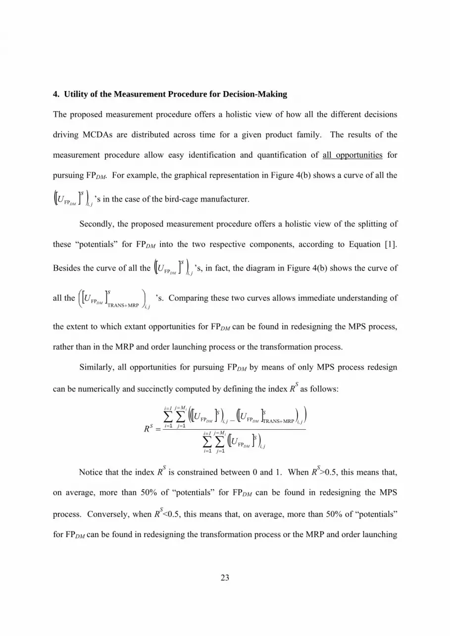
4. Utility of the Measurement Procedure for Decision-Making

The proposed measurement procedure offers a holistic view of how all the different decisions

driving MCDAs are distributed across time for a given product family. The results of the

measurement procedure allow easy identification and quantification of all opportunities for

pursuing FPDM. For example, the graphical representation in Figure 4(b) shows a curve of all the

[ ]( )ji,

sDM

UFP ’s in the case of the bird-cage manufacturer.

Secondly, the proposed measurement procedure offers a holistic view of the splitting of

these “potentials” for FPDM into the two respective components, according to Equation [1].

Besides the curve of all the [ ]( )ji,

sDM

UFP ’s, in fact, the diagram in Figure 4(b) shows the curve of

all the [ ]ji,

sDM

U ⎟⎠⎞⎜

⎝⎛

+MRPTRANSFP ’s. Comparing these two curves allows immediate understanding of

the extent to which extant opportunities for FPDM can be found in redesigning the MPS process,

rather than in the MRP and order launching process or the transformation process.

Similarly, all opportunities for pursuing FPDM by means of only MPS process redesign

can be numerically and succinctly computed by defining the index RS as follows:

[ ]( ) [ ]( )( )[ ]( )∑ ∑

∑ ∑=

=

=

=

=

=

=

=+

=Ii

i

Mj

jji,

S

Ii

i

Mj

jji,

S

ji,

S

Si

DM

i

DMDM

U

UUR

1 1

1 1

FP

MRPTRANSFPFP _

Notice that the index RS is constrained between 0 and 1. When RS>0.5, this means that,

on average, more than 50% of “potentials” for FPDM can be found in redesigning the MPS

process. Conversely, when RS<0.5, this means that, on average, more than 50% of “potentials”

for FPDM can be found in redesigning the transformation process or the MRP and order launching

24

process. For RS=0, no opportunities of FPDM can be found in redesigning the MPS process

without first redesigning the transformation process or the MRP and order launching process.

Finally, caution should be exercised when using the RS index. Like any numerical ratio,

RS ignores the magnitude of the denominator or the numerator and, as such, does not inform

about the absolute value of the “potentials” for FPDM that can be found in redesigning only the

MPS process. Such absolute values, instead, are clearly communicated in the visualization in

Figure 4(b).

5. Empirical Illustrations

We successfully applied the proposed measurement procedure to a number of product families

across several different companies. Through this field research, we discovered that high values

of the RS index are empirically quite common. To illustrate this and the associated insights, we

present and discuss, in Figure 5, the graphical results (following the convention of Figure 4(b))

and the RS index values of applying the measurement procedure to three product families in the

machinery industry: a submersible pump for evacuating domestic wastewater (CASE A), a pump

for industrial use (CASE B), and an electric generator for industrial use (CASE C).

For CASE A (Figure 5(a)), RS=0.56. The dashed curve shows all the timing of actual

order releases for various activities (i.e., all the [ ]ji,

sDM

U ⎟⎠⎞⎜

⎝⎛

+MRPTRANSFP ) and the solid curve shows

the timing of the MPS decisions driving the various MCDAs (i.e., all the [ ]( )ji,

sDM

UFP ). Notice

that there are only 2 decision points for all the MCDAs, shown on the solid curve at time T= –20

and at time T= –8. The first denotes timing of the MPSMIX decisions tied to purchase orders for

critical, long lead-time materials, such as ferromagnetic steel coil and stainless steel rods. The

25

latter denotes the MPSMIX decisions tied to all remaining purchase and work orders. RS=0.56 is a

concise representation of the gap between the two curves. Interestingly, for the MPSMIX

decisions taken at time T= –20, the associated gap is explained by the company policy to freeze

the purchasing plan for critical materials five months before production completion. Likewise,

for the MPSMIX decisions taken at time T= –8, the gap exists to accommodate a two-months

frozen interval policy. This policy, while designed to ensure a disciplined execution of

production plans, actually prevents the company from revising the MPS at time T= –4, which

would allow a reduction in the forecast errors for the many work orders that are released at time

T= –4 and later. The same logic can be applied to the first gap.

RS = 0.17

# MPSMIXi , j

RS = 0.56

0

-12 -8 -4 0-24 -20 -16-36 -32 -28

30

20

10

50

40

70

60

90

80

100

110

120

130

140

10

7

9

4

4

22

4

8

53

333

1

weeks

5(a) 5(b) 5(c)

12

6

12

16

47

17

9

5

11

23

7

20

1 0

-12 -8 -4 0-24 -20 -16-36 -32 -28

30

20

10

50

40

70

60

90

80

100

110

120

130

140

31

60

230

150

160

170

weeks

180

190

200

210

220

5

240

RS = 0.50

25

0

-12 -8 -4 0-24 -20 -16-36 -32 -28

30

20

1010

10

40

weeks

# MPSMIXi , j

# MPSMIXi , j

RS = 0.17

# MPSMIXi , j

RS = 0.56

0

-12 -8 -4 0-24 -20 -16-36 -32 -28

30

20

10

50

40

70

60

90

80

100

110

120

130

140

10

7

9

4

4

22

4

8

53

333

1

weeks0

-12 -8 -4 0-24 -20 -16-36 -32 -28

30

20

10

50

40

70

60

90

80

100

110

120

130

140

10

7

9

4

4

22

4

8

53

333

1

weeks

5(a) 5(b) 5(c)

12

6

12

16

47

17

9

5

11

23

7

20

1 0

-12 -8 -4 0-24 -20 -16-36 -32 -28

30

20

10

50

40

70

60

90

80

100

110

120

130

140

31

60

230

150

160

170

weeks

180

190

200

210

220

5

240

RS = 0.50

25

0

-12 -8 -4 0-24 -20 -16-36 -32 -28

30

20

1010

10

40

weeks

# MPSMIXi , j

# MPSMIXi , j

Figure 5: FPDM potentials and their components in three case examples

26

Not all companies can find significant opportunities for FPDM in the redesign of the MPS

process – see Figure 5(b) for CASE B as an example. In this instance, RS=0.17 and the time

lapse between the MPSMIX decisions and the associated timing of the work order releases is

always less than three weeks. This is due to the fact that the MPSMIX decisions are revised on a

monthly basis, with a frozen interval of only one month. Hence, the only avenue to effect

substantial reductions in the forecasting windows associated to MPSMIX decisions is to first

redesign the industrial pump architecture and/or the transformation process so as to push the

dashed curve closer to the right of the diagram.

Finally, there are companies for which the opportunities for FPDM are relatively slim.

Consider, for example, CASE C – see Figure 5(c). Although CASE C reports a high RS=0.50,

higher than in CASE B, the opportunity for pursuing FPDM is actually moderate, since the longest

forecasting window is only five weeks. The company in CASE C has, in fact, successfully

pursued FPDM in the past such that most MCDAs (for various couplings, connectors, etc.) are

now deferred to the Customer Order Decoupling Point, allowing all finished product variants to

be configured-to-order.

6. Conclusions

Conceptualizing FP formally as the deferment of forecast-driven decisions in the MPS process,

we complement the prevailing conception of FP as the deferment of PDAs achieved via redesign

of the product family architecture and/or the transformation process. This complementary

definitional perspective explicitly links FP to the reduction of forecast errors and applies directly

to contexts in which product mix decisions are not determined by triggers. Moreover, we

formalized a measurement procedure for identification and quantification of all opportunities for

27

postponing forecast-driven MPS decisions and provided a graphical means of depicting these

opportunities.

A fundamental insight of the proposed “decision-making” perspective of FP is that

forecast errors can be reduced by deferring product mix decisions through a redesign of the MPS

process, without necessarily redesigning the product family architecture and/or the

transformation process. This is due to the fact that time lags exist between when the MPS

decisions are taken and when the corresponding purchase or work orders are released to drive

activities across the supply chain. The proposed measurement procedure provides a succinct

quantification of these time lags by means of the RS index. These time lags are often substantial

in practice. Therefore, redesigning the MPS process may offer comparable advantages to those

obtained through product and/or transformation process redesign. This insight, as a matter of

fact, challenges the prevailing wisdom in industry – one implicitly equating the reduction of

forecast windows associated with product mix decisions to FP, defined as the deferment of

physical activities.

A second contribution stems directly from the proposed measurement procedure. From a

human cognition perspective, the graphical and numerical outputs of the proposed measurement

procedure offer a tool to overcome the limitations set by bounded rationality in high level

decision-making processes in manufacturing firms. These outputs, if fact, easily express an

otherwise complex-to-communicate set of characteristics of production planning relative to a

product family, such as all planned lead times, forecasting windows’ length, etc. This may be

important to convey complex but critical operations-related information to the upper

management echelons of a manufacturing company, thus making top management more aware of

28

the FP potentials associated to a given product family and guiding them in the process of

identifying candidates for a FP initiative.

By taking a fresh look at FP, the present paper opens at least two research opportunities.

Firstly, it would be useful and interesting to understand why some companies allow themselves

to make product mix decisions so much in advance, compared to when these decisions are

required by the factory. Is this a consequence of bounded rationality, meaning that the company

is not aware of the “potentials” for FP that can be found in the redesign of the MPS process or,

instead, is it a consequence of a deliberate decision of not pursuing FP? Moreover, assuming

that such FP initiatives are economically profitable, what organizational factors can inhibit or

catalyze the pursuit of FP, given the fact that neither transformation process redesign nor product

architecture redesign would be required? As some managers suggested, for example, the

cognitive complexity of the task of production planning could play a role in explaining missed

opportunities for FP. Postponing product mix decisions to the latest possible point in time, in

fact, prevents the production planner from dealing with these decisions all at once, in a batch-like

fashion. The need to make product mix decisions at numerous points in time may conflict with

other production planner’s tasks, or may subdue him/her to unduly cognitive load due to multiple

“mental set-ups” (Pentland 2003), thus ultimately inhibiting the pursuit of FP.

Second and last, it would be interesting and useful to elaborate on our measurement

procedure drawing from decision theory, in order to quantify how reductions of FP potentials

turn into reductions of the risk and associated costs of forecasting the wrong mix composition.

This could require, for example, weighing FP potentials associated to product mix decisions with

such factors as volatility of demand for the individual product options within a product family or

unit inventory holding cost and unit shortage cost of each possible outcome of each MCDA.

29

References

Alderson, W. 1950. Marketing efficiency and the principle of postponement. Cost and Profit

Outlook 3(4) 15-18.

Aviv, Y., A. Federgruen. 2001a. Capacitated multi-item inventory systems with random and

seasonally fluctuating demands: Implications for postponement strategies. Management

Sci. 47(4) 512-531.

Aviv, Y., A. Federgruen. 2001a. Design for postponement: A comprehensive characterization of

its benefits under unknown demand distributions. Oper. Res. 49(4) 578-598.

Brown, A. O., H. L. Lee, R. Petrakian. 2000. Xilinx improves its semiconductor supply chain

using product and process postponement. Interfaces 30(4) 65-80.

Cooper, J.C. 1993. Logistics strategies for global businesses. Int. J. of Physical Distribution and

Logist. Management 23(4) 12-23.

Enns, S. T. 2001. MRP performance effects due to lot size and planned lead time settings. Int. J.

of Production Res. 39(3) 461-480.

Garg, A., C. S. Tang. 1997. On postponement strategies for product families with multiple points

of differentiation. IIE Trans. 29(8) 641-650.

Giesberts, P. M. J., L. Van der Tang. 1992. Dynamics of the customer order decoupling point:

Impact on information systems for production control. Production Planning and Control

3(3) 300–313.

Gupta, S., V. Krishnan. 1998. Product family-based assembly sequence design methodology. IIE

Trans. 30(10) 933-945.

Heskett, J. L. 1977. Logistics – essential to strategy. Harvard Bus. Rev. 55(6) 119-126.

30

Hsu, H., W. Wang. 2004. Dynamic programming for delayed product differentiation. Eur. J. of

Oper. Res. 156(1) 183-193.

Kanet, J. J. 1986. Toward a better understanding of lead times in MRP systems. J. of Oper.

Management 6(3) 305-315.

Lee, H. L. 1996. Effective inventory and service management through product and process

redesign. Oper. Res. 44(1) 151-159.

Lee, H. L., C. Billington. 1994. Designing products and processes for postponement. S. Dasu, C.

Eastman, eds. Management of design: Engineering and management perspectives.

Kluwer Academic Publishers, Boston, MA, 105-122.

Lee, H. L., C. S. Tang. 1997. Modeling the costs and benefits of delayed product differentiation.

Management Sci. 43(1) 40-53.

Lin, G. Y., R. Breitwieser, F. Cheng, J. T. Eagen, M. Ettl. 2000. Product hardware complexity

and its impact on inventory and customer on-time delivery. The Int. J. of Flexible

Manufacturing Systems 12(2-3) 145-63.

Ma, S., W. Wang, L. Liu. 2002. Commonality and postponement in multistage assembly

systems. Eur. J. of Oper. Res. 142(3) 523-538.

Mather, H. F. 1986. Design, bills of materials, and forecasting - the inseparable threesome.

Production and Inventory Management J. 27(1) 90-107.

Orlicky, J. A. 1975. Materials Requirements Planning. McGraw-Hill, New York, NY.

Pagh, J. D., M. C. Cooper. 1998. Supply chain postponement and speculation strategies: How to

choose the right strategy. J. of Bus. Logist. 19(2) 13-33.

Pentland, B. T. 2003. Conceptualizing and measuring variety in the execution of organizational

work processes. Management Sci. 49(7) 857-870.

31

Sridharan, S. V., W. L. Berry. 1990. Freezing the master production schedule under demand

uncertainty. Decision Sci. 21(1) 97–120.

Sridharan, S. V., W. L. Berry, V. Udayabhanu. 1987. Freezing the master production schedule

under rolling planning horizons. Management Sci. 33(9) 1137-1149.

Swaminathan, J. M., H. L. Lee. 2003. Design for postponement. S. C. Graves, A. G. de Kok, eds.

Supply chain management: Design, coordination and operation – Handbooks in OR/MS,

Vol. 11. North-Holland, Amsterdam, The Netherlands, 199-228.

Van Hoek, R. I. 2001. The rediscovery of postponement: A literature review and directions for

research. J. of Oper. Management 19(2) 161-184.

Vollmann, T. E., W. L. Berry, D. C. Whybark, F. R. Jacobs. 2005. Manufacturing planning and

control systems for supply chain management. McGraw-Hill, New York, NY.

Whang, S., H. L. Lee. 1998. Value of postponement. T.-H. Ho, C. S. Tang, eds. Product variety

management: Research advances. Kluwer Academic Publishers, Norwell, MA, 65-84.

Wikner, J., M. Rudberg. 2005. Introducing a customer order decoupling zone in logistics

decision-making. Int. J. of Logist. 8(3) 211-224.

Xie, J., X. Zhao, T. S. Lee. 2003. Freezing the master production schedule under single resource

constraint and demand uncertainty. Int. J. of Production Economics 83(1) 65-84.

Yang, B., N. D. Burns, C. J. Backhouse. 2004. Management of uncertainty through

postponement. Int. J. of Production Res. 42(6) 1049-1064.

Zinn, W., D. J. Bowersox. 1988. Planning physical distribution with the principle of

postponement. J. of Bus. Logist. 9(2) 117-137.

32

APPENDIX A: ACRONYMS AND SYMBOLS

FP Form postponement

FPDM Form postponement from a decision-making perspective

MCDA Mix composition differentiation activity

MPS Master production schedule

MPSMIXi Decision component of the MPS that drives the ith MCDA

MPSMIXi, j Elementary decision that specifies the quantity of the jth outcome of the

ith MCDA to be produced

MPSVOL Decision component of the MPS that specifies the total production

volume for the product family

MRP Material requirements planning

PDA Production differentiation activity

33

APPENDIX B: VARIABLES AND FUNCTIONS

CLT Cumulative lead time for the entire transformation process of the

product family

1+ ss,DMFP =

[ ] [ ]( )

[ ] [ ]( ) ⎟⎟⎟⎟⎟

⎠

⎞

⎜⎜⎜⎜⎜

⎝

⎛

−

−

−

−

+

+

IDMDM

DMDM

M,I

ss

ss

UUneg

UUneg

FPFP

,FPFP

1

111

M

MPSFW Forecast window for the MPS

j ,iMIXFWMPS Forecast window for the MPSMIXi, j

VOLFWMPS Forecast window for the MPSVOL

I Number of MCDAs along the product family’s transformation process

K Number of MPS-driven activities along the product family’s

transformation process

lk, j Planned lead time for the kth activity when its outcome is j

Mi Number of possible different outcomes of the ith MCDA

neg(x) =

⎪⎪⎩

⎪⎪⎨

⎧ <

otherwise

for

xx

0

0

R [ ]( ) [ ]( )( )

[ ]( )∑ ∑

∑ ∑=

=

=

=

=

=

=

=+

=Ii

i

Mj

jji,

Ii

i

Mj

jji,ji,

i

DM

i

DMDM

U

UU

1 1

1 1

FP

MRPTRANSFPFP _

RP Replanning periodicity in the MPS process

34

jk,TActivity Latest possible time at which the kth activity must start, for production to

be completed at time T=0, when the activity’s outcome is j

CODPT Customer order decoupling point

TCOMPLETION Timing of production completion (set equal to zero)

FrozenT Latest point in time, relative to production completion time, beyond

which no changes to the created MPS are allowed

j,iTMCDA see jk,TActivity , where Activity k is the ith MCDAi

TMPS Timing of the MPS

j,iMIXTMPS Timing of the elementary decision specifying the quantity of the jth

outcome of MCDAi to be produced (i.e., MPSMIXi, j)

VOLTMPS Timing of the MPSVOL

jk, T

ActivityOR Timing of order release for the kth activity when its outcome is j

j,iT

MCDAOR see jk,

TActivityOR , where Activity k is the ith MCDAi

[ ]( )ji,DM

UFP FPDM “potential” for the MPSMIXi, j

[ ]ji,MIX

DMU ⎟

⎠⎞

⎜⎝⎛

MPSFP Maximum possible deferment of the MPSMIXi, j that can be achieved

without having to defer j,i

TMCDAOR

[ ]ji,

DMU ⎟

⎠⎞⎜

⎝⎛

+MRPTRANSFP Maximum additional deferment of the MPSMIXi, j that can only be

achieved by deferring j,iTMCDA to CODPT , and then by zeroing δMCDAi, j

35

(i.e., the time lag between j,i

TMCDAOR and j,i

TMCDA ) so that j,iTMCDA =

j,iT

MCDAOR

δk, j Timing offset between jk,

TActivityOR and

jk, T

ActivityOR

δMCDAi, j see δk, j, where Activity k is the ith MCDAi

∆ Average time that a customer is willing to wait after order placement

and net of shipping time

(i.e., time at which demand information is perfectly known relative to

production completion time)

form postponement: a decision-making perspective

Documents