The Dynamic and Stochastic Knapsack Problem with

Homogeneous-Sized items and Postponement Options

Tianke Feng and Joseph C. Hartman

Industrial and Systems Engineering, University of Florida

May 4, 2015

Abstract

This paper generalizes the Dynamic and Stochastic Knapsack Problem (DSKP) by allowing

the decision-maker to postpone the accept/reject decision for an item and maintain a queue of

waiting items to be considered later. Postponed decisions are penalized with delay costs, while

idle capacity incurs a holding cost. This generalization addresses applications where requests

of scarce resources can be delayed, e.g., dispatching in logistics and allocation of funding to

investments. We model the problem as a Markov decision process (MDP) and analyze it through

Dynamic Programming (DP). We show that the optimal policy with homogeneous-sized items

possesses a bi-threshold structure, despite the high dimensionality of the decision space. Finally,

the value (or price) of postponement is illustrated through numerical examples.

Keywords: Primary: Sequential Decisions, Dynamic Programming; Secondary: Markov pro-

cesses, Stochastic model applications

1 Introduction

The classical knapsack problem, which addresses the allocation of limited capacity to items with

known size to maximize expected profit, has been extensively studied in the literature (Kellerer

and Pisinger [18]). One extension is the Dynamic and Stochastic Knapsack Problem (DSKP), as

defined in Papastavrou et al. [29], which assumes that items arrive according to a Poisson process

with the reward (referred to as “revenue” in this paper) and resource requirement for each item

being made known upon arrival. The decision-maker must then accept or reject the item. This

problem has many applications in transportation, scheduling, and finance.

In this paper, we explicitly analyze the situation where a decision-maker may delay the ac-

cept/reject decision in a DSKP. Specifically, the decision-maker may postpone the decision, whereby

items form a queue and the decision for each item may be revisited at a later time. It should be

clear that if a decision-maker has the ability to hold an arriving item, then a more informed ac-

1

cept/reject decision can be made later, albeit at some cost, as more items may arrive during the

delay period.

In practice, there are many situations in which delaying the accept/reject decision is feasible,

although possibly for a fee. In logistics, a dispatcher may delay accepting a capacity reservation

request that is not very attractive in hopes of receiving a better offer within some time frame

(Spivey and Powell [36]). In finance, an angel investor may entertain a number of “pitches” from

entrepreneurs before deciding which investments to make. In human resources, a firm may interview

dozens or even hundreds of applicants before making offers to hire a certain subset. Essentially, any

resource allocation decision that must not be made immediately inherently allows for the decision

to delay.

To our knowledge, little research has been published on the postponement, or delay, option in

operational settings. Spivey and Powell [36] point out the potential benefit of postponing assign-

ments. Feng and Hartman [11] study the Stochastic Sequential Assignment problem (SSAP) with

the ability to delay. Real options analysis generally evaluates the delay option in investment analysis

(McDonald and Siegel [23]), but only when considering a single investment decision. In this paper,

we study the DSKP model with homogeneous-sized items when the decision-maker can postpone

the accept/reject decision. It should be noted that the postponement option greatly complicates

the analysis, as items that have arrived but are yet to be accepted or rejected form a queue, which

enlarges the decision space. Furthermore, the decision-maker can accept/reject any queued item at

any time. Surprisingly, we found that the optimal policy of the new model possesses a threshold

structure. Specifically, we make the following contributions to the literature:

1. Model the finite horizon DSKP with the postponement option and homogeneous-sized items,

considering finite/infinite number of arriving items, holding cost, delay cost, and the option

to terminate the process early;

2. Derive an optimal policy defined by a revenue threshold and a time threshold, such that the

decision-maker should first immediately reject the queued items below the revenue threshold

and then postpone the acceptance of the remaining queued items until the time threshold is

reached;

3. Generalize the DSKP, allowing to recall the rejected items at a cost;

4. Illustrate the benefits and costs of postponement through numerical experiments.

This paper is organized as follows. In Section 3, we introduce notation, assumptions and our

model. In Section 4, we examine the DSKP model with holding costs for unallocated resources.

The optimal policy and the associated structural properties of the finite horizon DSKP with

homogeneous-sized items are developed through induction. In Section 5, we investigate how to

incorporate other costs and the option to terminate into the model and identify conditions for the

threshold optimal policy and the associated structural properties to hold. The benefits of post-

ponement are illustrated through numerical examples in Section 5. In the following section, we

2

review the related literature.

2 Related Research

The seminal work on the DSKP was performed by Papastavrou et al. [29] in which items arrive

over a finite number of time periods. Kleywegt and Papastavrou [20] study the version of the

DSKP with homogeneous-sized items in continuous time. Moreover, they introduce holding costs

for unallocated resources, a penalty for rejected items, and an option to stop receiving items. A

threshold optimal policy was developed. This model and the threshold optimal policy are extended

to the case of randomly sized items by Kleywegt and Papastavrou [21]. Nikolaev and Jacobson [27]

further extend the model to the case where the number of items to arrive is random. McLay et al.

[24] apply the optimal policy of the DSKP to the allocation of screening resources to passengers.

Papastavrou et al. [29] note that recalling rejected items is a possible extension of the DSKP model.

This is in essence equivalent to delaying the accept/reject decisions and is the basis of this paper.

Closely related to the DSKP is the sequential and stochastic assignment problem (SSAP). By

appropriately setting the costs introduced by Kleywegt and Papastavrou [20] and forbidding the

decision-maker to terminate decisions before the deadline, the infinite horizon DSKP with homogeneous-

sized items reduces to the SSAP with homogeneous resources and infinitely many arriving items.

In the seminal work of Derman et al. [8], the authors study the case when there are equally many

items and resources. Albright [1] studies the case of infinite item arrivals and discounting. Exten-

sions on the arrival process include Sakaguchi [34], Sakaguchi [35], Nakai [26] and Nakai [25]. Other

extensions include Albright [2], Kennedy [19] and Righter [31]. Feng and Hartman [11] study the

model with postponement options.

There are several other problems related to the DSKP. In general, the stochastic knapsack problem

(e.g., Dean et al. [7]) considers the situation where the sizes and/or rewards of items are unknown

until they are inserted into the knapsack. The sequential selection problem is defined as follows.

An i.i.d. sequence of non-negative random variables with known distribution is to be inspected.

Upon inspection, the value of the random variable is made known and the decision-maker must

immediately decide whether to accept or reject the variable. The objective is to maximize the

number of accepted variables with the summation of these variables being less than some specified

amount. This problem corresponds to a special case of the DSKP with random sized items, ho-

mogeneous revenues and no costs or stop options. Coffman et al. [5] propose a threshold optimal

policy. Rhee and Talagrand [30] discuss the asymptotic behavior of the problem. Lu et al. [22]

propose a time-constrained capital-budgeting problem, which can be viewed as a generalized version

of the sequential selection problem or a special case of the DSKP. In this problem, project proposals

of different types arrive at a funding agency randomly. Each type is characterized by a distinctive

cost and a random benefit. Upon arrival of a project, the decision-maker must immediately decide

whether to accept and fund the proposal. Given a limited amount of budget and a finite time

3

horizon, the decision-maker selects projects to maximize the expected profit. Herbots et al. [15]

discussed a dynamic order acceptance problem, in which project proposals arrive sequentially with

deterministic inter-arrival times, while project characteristics are revealed upon arrival. Papadaki

and Powell [28] tackled the batch dispatch problem with random arriving requests by approximate

dynamic programming.

Postponement naturally arises as an option in finance (e.g., Trigeorgis [39] and Amram and

Kulatilaka [3]) and operations management (Hoek [16]). In finance, it usually appears in the context

of real options, as stated by Triantis [38]. In operations management, the concept of postponement

has been studied in marketing channels (Bucklin [4]), mass customization (Feitzinger and Lee [10]),

capacity allocation (Ding et al. [9]), and R&D management (Huchzermeier and Loch [17]). These

decision settings differ greatly from the DSKP, as the postponement mentioned here is generally

over a longer time frame (months, quarters, or years) than in our applications. Also, this literature

mainly focuses on case studies or qualitative analysis. Mathematical models on postponement

options are relatively rare.

Of the mathematical models, two are quite typical. McDonald and Siegel [23] study the optimal

timing of investing in a project, with the benefits and costs following a Brownian motion. Our

research also studies the best time to accept or reject an item, but we consider the arrivals of

a number of items (or projects) and the reward and costs, once made known, do not vary over

time. Grenadier and Weiss [13] model the optimal investment strategy for a firm confronted with

technological innovations. In this research, technological innovations arrive sequentially, with the

arrival time and the value of the innovation uncertain to the firm. Each innovation connects to other

innovations that arrive in the future at different costs. The objective of the firm is to determine

the right time to invest in order to adopt innovations at lower cost, while keeping a competitive

advantage. This problem resembles our research in terms of stochastic arrivals and the ability of

the decision-maker to delay decisions. However, the authors consider in their model two innovation

arrivals (the current innovation and the future innovation), while the DSKP can consider an infinite

number of arrivals, complicating the analysis as delayed decisions (items) are queued.

In our model, arriving items may form a queue, such that the model closely resembles an online

bin packing problem. In the bin packing problem (see Coffman and Stolyar [6]), fractions of a single

resource are allocated to a set of streams of requests. Each stream is characterized by a distinct

value of resource requests and is governed by a Poisson process. The system operates in discrete

units of time. Each fulfilled request occupies the allocated resource for a unit of time and releases

it thereafter, leaving the system. Unfulfilled requests form queues. Gamarnik and Squillante [12]

provide new methods to analyze the problem under a general class of scheduling policies, and obtain

stability conditions and stationary distributions. Gyorgy et al. [14] study the case where there is

more than one bin.

4

3 Model and Assumptions

We model the DSKP as a Markov Decision Process in Section 3.1. Then, we introduce assumptions

to simplify the analysis in 3.2 and develop the principle of optimality. The notation to be introduced

in this paper is summarized in Table 1. In our model, we use bold letters to represent a multivariate

variable or a set. Also, functions are mainly denoted by lowercase letters, except for widely accepted

conventions in literature. Finally, E(·) represents the mathematical expectation.

3.1 Model Definitions

Items arrive according to a Poisson process, each requiring one unit of resource, with a random

revenue (we use the term revenue rather than reward in this paper). Upon the arrival of a new

item, the revenue value of the item is known and the decision-maker has three options:

(1) Immediately reject the item;

(2) Immediately accept and load the item, fulfilling its resource requirement;

(3) Postpone the accept/reject decision.

For convenience, we abbreviate “accept and load” in (2) as “accept”. If the decision-maker chooses

(1), the item is discarded and cannot be recalled in the future. If the decision-maker chooses (2),

one unit of resource is consumed by the item and its revenue is received instantaneously. If the

decision-maker chooses (3), both (1) and (2) are available at any time in the future. A consequence

of the postponement option is that the arriving items yet to be accepted or rejected form a queue;

termed the postponement queue.

The postponement queue results in increased complexity in decisions. Arriving items join the

postponement queue, and the decision-maker can accept or reject any queued items at any point

in time. Moreover, costs are incurred for holding resources, postponing, and rejecting items, and

the revenues are discounted over time. The problem ends when resources are depleted, there is

no remaining item to arrive, or when the deadline is reached. The objective is to maximize the

expected discounted profit. Next, we formally define the DSKP model.

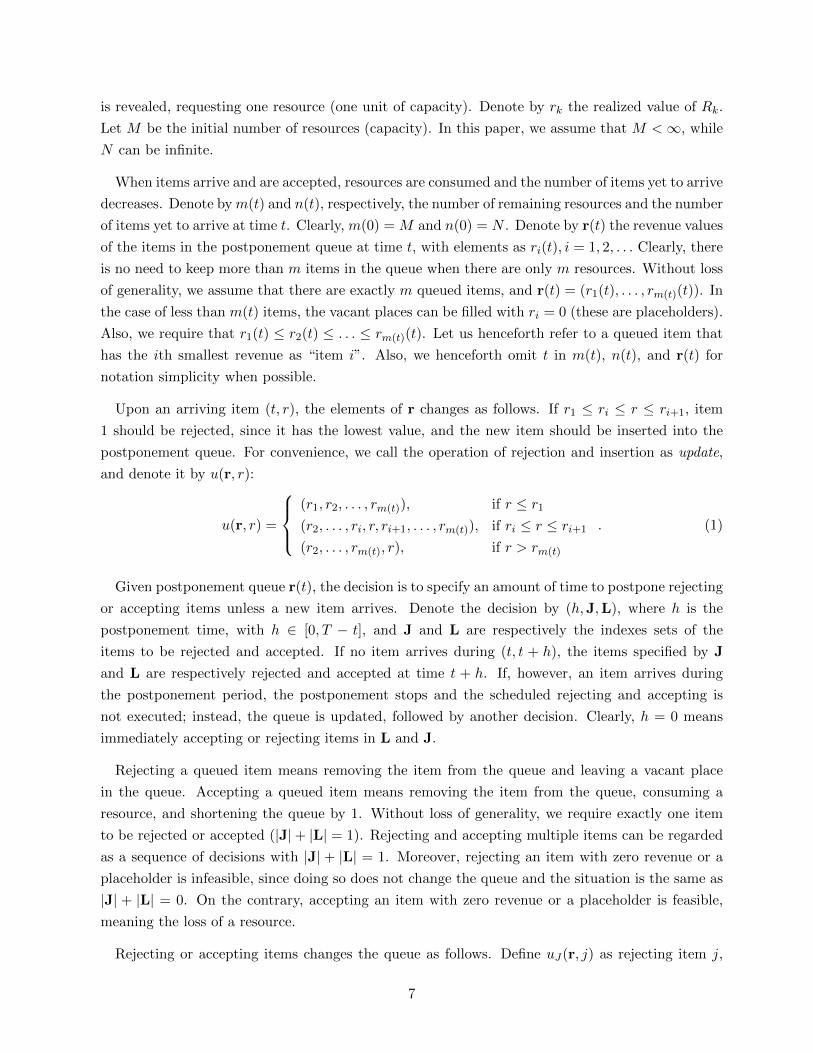
3.1.1 Problem Description: Arrivals, Capacity, Queue, and Decisions

First, we define the arrival process of items. Define T ∈ (0,∞) as the deadline and N as the limit on

the number of items to arrive. An arriving item, say item k, is characterized by its arrival time and

revenue, (Ak, Rk). Assume that {Ak}Nk=1 are the arrival times of a Poisson process on (0, T ) with

rate λ ∈ (0,∞), and {Rk}Nk=1 as an i.i.d. sequence, with Rk as the revenue of item k, independent

of Ak. Let FR and R be the probability distribution and support of R, respectively. Assume that

E[R] <∞ and R ⊆ [0, rmax], where rmax <∞ is a constant. When arriving, the revenue of item k

5

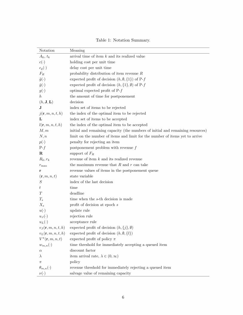
Table 1: Notation Summary.

Notation Meaning

Ak, tk arrival time of item k and its realized value

c(·) holding cost per unit time

cq(·) delay cost per unit time

FR probability distribution of item revenue R

g(·) expected profit of decision (h, ∅, {1}) of P-f

g(·) expected profit of decision (h, {1}, ∅) of P-f

g(·) optimal expected profit of P-f

h the amount of time for postponement

(h,J,L) decision

J index set of items to be rejected

j(r,m, n, t, h) the index of the optimal item to be rejected

L index set of items to be accepted

l(r,m, n, t, h) the index of the optimal item to be accepted

M,m initial and remaining capacity (the numbers of initial and remaining resources)

N,n limit on the number of items and limit for the number of items yet to arrive

p(·) penalty for rejecting an item

P-f postponement problem with revenue f

R support of FR

Rk, rk revenue of item k and its realized revenue

rmax the maximum revenue that R and r can take

r revenue values of items in the postponement queue

(r,m, n, t) state variable

S index of the last decision

t time

T deadline

Ts time when the s-th decision is made

Xs profit of decision at epoch s

u(·) update rule

uJ(·) rejection rule

uL(·) acceptance rule

vJ(r,m, n, t, h) expected profit of decision (h, {j}, ∅)vL(r,m, n, t, h) expected profit of decision (h, ∅, {l})V π(r,m, n, t) expected profit of policy π

wm,n(·) time threshold for immediately accepting a queued item

α discount factor

λ item arrival rate, λ ∈ (0,∞)

π policy

θm,n(·) revenue threshold for immediately rejecting a queued item

ν(·) salvage value of remaining capacity

6

is revealed, requesting one resource (one unit of capacity). Denote by rk the realized value of Rk.

Let M be the initial number of resources (capacity). In this paper, we assume that M <∞, while

N can be infinite.

When items arrive and are accepted, resources are consumed and the number of items yet to arrive

decreases. Denote bym(t) and n(t), respectively, the number of remaining resources and the number

of items yet to arrive at time t. Clearly, m(0) = M and n(0) = N . Denote by r(t) the revenue values

of the items in the postponement queue at time t, with elements as ri(t), i = 1, 2, . . . Clearly, there

is no need to keep more than m items in the queue when there are only m resources. Without loss

of generality, we assume that there are exactly m queued items, and r(t) = (r1(t), . . . , rm(t)(t)). In

the case of less than m(t) items, the vacant places can be filled with ri = 0 (these are placeholders).

Also, we require that r1(t) ≤ r2(t) ≤ . . . ≤ rm(t)(t). Let us henceforth refer to a queued item that

has the ith smallest revenue as “item i”. Also, we henceforth omit t in m(t), n(t), and r(t) for

notation simplicity when possible.

Upon an arriving item (t, r), the elements of r changes as follows. If r1 ≤ ri ≤ r ≤ ri+1, item

1 should be rejected, since it has the lowest value, and the new item should be inserted into the

postponement queue. For convenience, we call the operation of rejection and insertion as update,

and denote it by u(r, r):

u(r, r) =

(r1, r2, . . . , rm(t)), if r ≤ r1

(r2, . . . , ri, r, ri+1, . . . , rm(t)), if ri ≤ r ≤ ri+1

(r2, . . . , rm(t), r), if r > rm(t)

. (1)

Given postponement queue r(t), the decision is to specify an amount of time to postpone rejecting

or accepting items unless a new item arrives. Denote the decision by (h,J,L), where h is the

postponement time, with h ∈ [0, T − t], and J and L are respectively the indexes sets of the

items to be rejected and accepted. If no item arrives during (t, t + h), the items specified by J

and L are respectively rejected and accepted at time t + h. If, however, an item arrives during

the postponement period, the postponement stops and the scheduled rejecting and accepting is

not executed; instead, the queue is updated, followed by another decision. Clearly, h = 0 means

immediately accepting or rejecting items in L and J.

Rejecting a queued item means removing the item from the queue and leaving a vacant place

in the queue. Accepting a queued item means removing the item from the queue, consuming a

resource, and shortening the queue by 1. Without loss of generality, we require exactly one item

to be rejected or accepted (|J|+ |L| = 1). Rejecting and accepting multiple items can be regarded

as a sequence of decisions with |J| + |L| = 1. Moreover, rejecting an item with zero revenue or a

placeholder is infeasible, since doing so does not change the queue and the situation is the same as

|J| + |L| = 0. On the contrary, accepting an item with zero revenue or a placeholder is feasible,

meaning the loss of a resource.

Rejecting or accepting items changes the queue as follows. Define uJ(r, j) as rejecting item j,

7

where rj > 0 and:

uJ(r, j) =

(0, r2, . . . , rm(t)), if j = 1

(0, r1, . . . , rj−1, rj+1, . . . , rm(t)), if 1 < j < m(t)

(0, r1, . . . , rm(t)−1), if j = m(t)

. (2)

Define uL(r, l) as accepting item l, where:

uL(r, l) =

(r2, . . . , rm(t)), if l = 1

(r1, . . . , rl−1, rl+1, . . . , rm(t)), if 1 < l < m(t)

(r1, . . . , rm(t)−1), if l = m

. (3)

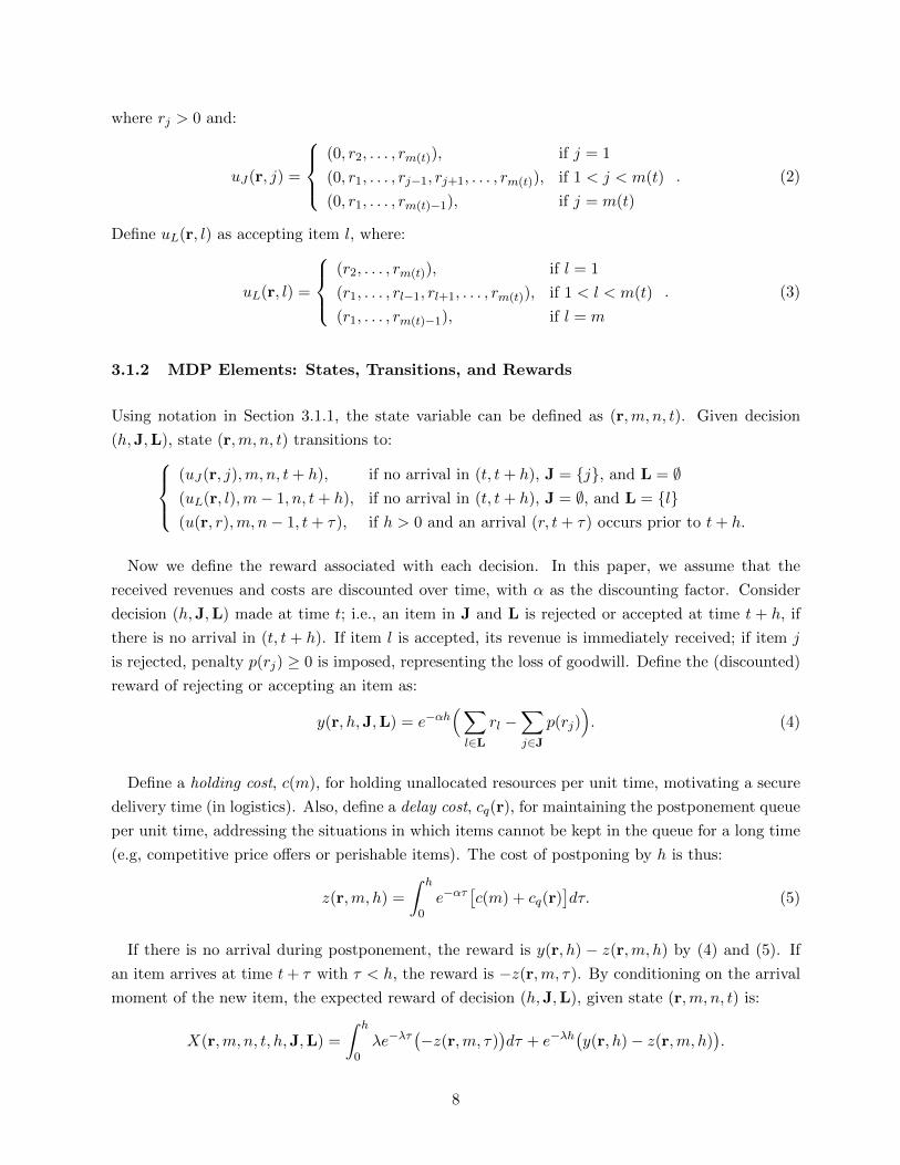
3.1.2 MDP Elements: States, Transitions, and Rewards

Using notation in Section 3.1.1, the state variable can be defined as (r,m, n, t). Given decision

(h,J,L), state (r,m, n, t) transitions to:(uJ(r, j),m, n, t+ h), if no arrival in (t, t+ h), J = {j}, and L = ∅(uL(r, l),m− 1, n, t+ h), if no arrival in (t, t+ h), J = ∅, and L = {l}(u(r, r),m, n− 1, t+ τ), if h > 0 and an arrival (r, t+ τ) occurs prior to t+ h.

Now we define the reward associated with each decision. In this paper, we assume that the

received revenues and costs are discounted over time, with α as the discounting factor. Consider

decision (h,J,L) made at time t; i.e., an item in J and L is rejected or accepted at time t + h, if

there is no arrival in (t, t+ h). If item l is accepted, its revenue is immediately received; if item j

is rejected, penalty p(rj) ≥ 0 is imposed, representing the loss of goodwill. Define the (discounted)

reward of rejecting or accepting an item as:

y(r, h,J,L) = e−αh(∑l∈L

rl −∑j∈J

p(rj)). (4)

Define a holding cost, c(m), for holding unallocated resources per unit time, motivating a secure

delivery time (in logistics). Also, define a delay cost, cq(r), for maintaining the postponement queue

per unit time, addressing the situations in which items cannot be kept in the queue for a long time

(e.g, competitive price offers or perishable items). The cost of postponing by h is thus:

z(r,m, h) =

∫ h

0e−ατ

[c(m) + cq(r)

]dτ. (5)

If there is no arrival during postponement, the reward is y(r, h) − z(r,m, h) by (4) and (5). If

an item arrives at time t+ τ with τ < h, the reward is −z(r,m, τ). By conditioning on the arrival

moment of the new item, the expected reward of decision (h,J,L), given state (r,m, n, t) is:

X(r,m, n, t, h,J,L) =

∫ h

0λe−λτ

(−z(r,m, τ)

)dτ + e−λh

(y(r, h)− z(r,m, h)

).

8

3.1.3 MDP Model: Policies and Decision Processes

Decisions immediately follow queue updating upon an arrival, accepting an item, and rejecting an

item. These time moments define decision epochs. Let Ts be the time when the s-th decision is

made, or decision epoch, and S be the index of the last decision. Clearly, TS is the moment when

m = 0 or T . Let π be the policy mapping states to decisions. Let ΠDSKP be the set of policies

that are memoryless and satisfy non-anticipatory conditions (all policies only utilize information

available up to the decision epoch).

Let Sπ be the number of decision epochs under policy π. Similarly, denote by T πs and Xπs ,

s = 1, . . . , Sπ, respectively the decision epochs and expected rewards following policy π. At time

t = 0, the queue is vacant, denoted by r0 = (0, . . . , 0). The expected profit of π can be defined as:

V πDSKP(r0,M,N, 0) = E

[ Sπ∑s=1

e−αTπs Xπ

s

]. (6)

The objective is to find the policy π∗ maximizing the expected profit:

V π∗(r0,M,N, 0) = maxπ∈ΠDSKP

V πDSKP(r0,M,N, 0). (7)

3.2 Assumptions and Simplifications

To solve the DSKP model, we introduce the following assumptions:

(1) p(r, t) = 0;

(2) c(m) = cm, where c is a constant;

(3) cq(r) =∑m

i=1 cqri, where cq is a constant.

Compared with DSKP models in the literature, our model relies on assumptions (1) and (2), and

does not explicitly consider the option of stopping and salvaging remaining resources. However, our

model incorporates the postponement option, which is not considered in those models. Moreover,

as will be shown in Section 4.4, the stop and salvage option can be addressed implicitly.

We analyze π∗ through the principle of optimality of dynamic programming. Consider all feasible

decisions given state (r,m, n, t). For a postponement time h, an item is either accepted or rejected.

Let l and j be the best item to be accepted and rejected in each case, respectively:

l(r,m, n, t, h) = arg max0≤i≤m

{ri + V π∗

(uL(r, i),m− 1, n, t+ h

)},

j(r,m, n, t, h) = arg max0≤i≤m

{V π∗

(uJ(r, i),m, n, t+ h

)}. (8)

For convenience, we henceforth refer to (h, ∅, {l}) and (h, {j}, ∅) as the “acceptance decision” and

the “rejection decision”, respectively. We use “immediate/postponed acceptance” and “immedi-

9

ate/postponed rejection” to differentiate acceptance and rejection decisions with h = 0 and h > 0,

respectively.

The expected profit of applying decision (h, ∅, {l}) and π∗ thereafter can be defined as:

vL(r,m, n, t, h) =

∫ h

0

{e−ατ

∫RV π∗

(u(r, r),m, n− 1, t+ τ

)dFR(r)− z(r,m, τ)

}λe−λτdτ

+ e−λh{e−αh

[rl + V π∗

(uL(r, l),m− 1, n, t+ h

)]− z(r,m, h)

}, (9)

where the terms in the curly brackets denote the expected profits of the cases with and without

an arrival during postponement, respectively. Similarly, the expected profit of applying decision

(h, {j}, ∅) and following π∗ thereafter can be defined as:

vJ(r,m, n, t, h) =

∫ h

0

{e−ατ

∫RV π∗

(u(r, r),m, n− 1, t+ τ

)dFR(r)− z(r,m, τ)

}λe−λτdτ

+ e−λh{e−αhV π∗

(uJ(r, j),m, n, t+ h

)− z(r,m, h)

}. (10)

Denote the expected profits of optimal acceptance and optimal rejection by:

v∗J(r,m, n, t) = maxh∈[0,T−t]

vJ(r,m, n, t, h),

v∗L(r,m, n, t) = maxh∈[0,T−t]

vL(r,m, n, t, h),

respectively. By the optimality principle,

V π∗(r,m, n, t) =

{max{v∗J(r,m, n, t), v∗L(r,m, n, t)}, r 6= r0

v∗L(r,m, n, t), r = r0

, (11)

where the case of r = r0 follows, since rejection is infeasible for vacant queue (Section 3.1.1).

Moreover, V π∗(r,m, n, t) =∑

i ri for n = 0 and t = T , since no items will arrive.

4 Optimal Policies of DSKP with Postponement Options

In this section, we study the finite horizon DSKP with postponement options. For convenience, we

refer to the DSKP with postponement options as “DSKP”. An interesting result is that the DSKP

is closely related to a decision problem, called the postponement problem ( Section 4.1). In Sections

4.1 and 4.2, we develop the optimal policies of the DSKP by bundling the postponement problems.

In Section 4.3, we illustrate the optimal decisions and the resulting decision process through an

example. In Section 4.4, we explain how to incorporate the stop and salvage option into our model.

In section 4.5, we discuss the difficulty of including the rejection penalty in our model.

10

4.1 DSKP with m = 1

The postponement problem is similar to the DSKP with M = N = 1, except that the revenue

of the arriving item is dependent on the arrival time and the revenue of the queued item. Below,

we first show its relationship with the DSKP (Section 4.1.1). Then, we introduce its properties

(Section 4.1.2), based on which, we develop the optimal policies of the DSKP (Section 4.1.3).

4.1.1 Relationship with Postponement Problem

Definition 1. The postponement problem is a DSKP defined in Section 3 with M = N = 1, except

that given state (r1, 1, 1, t) and the arrival time of the (only) arriving item t + τ , the revenue of

this arriving item is a function of r1 and t + τ . If this function is f(r1, t + τ), the postponement

problem is denoted by P-f .

It can be shown (see Theorem 2) that the optimal policy of P-f possesses a threshold structure,

if f satisfies the following conditions:

(a) r ≤ f(r, t) ≤ rmax and is non-increasing in t;

(b) (∂/∂r)f(r, t) ∈ [0, 1] and is non-decreasing in r;

(c) (∂/∂r)f(r, t) is non-decreasing in t.

Based on Theorem 1 below, the optimal policy of the DSKP with m = 1 can be readily developed.

Theorem 1. Given (r1, 1, n, t) and function f1,n defined as:

f1,n(r1, t+ τ) =

∫RV π∗

(u(r1, r

), 1, n− 1, t+ τ

)dFR(r),

the optimal policy of P-f1,n is optimal to the DSKP with 1 resource and n item yet to arrive.

Proof. For P-f1,n and state (r1, 1, 1, t), denote by g1,n(r1, t, h) and g1,n(r1, t, h) the expected profits

of decisions (h, ∅, {1}) and (h, {1}, ∅), respectively. We establish the conclusion by showing that

g1,n(r1, t, h) = vL(r1, 1, n, t, h) and g1,n(r1, t, h) = vJ(r1, 1, n, t, h).

First, consider the DSKP with m = 1. As stated in Section 3.2, the decision is to specify an

amount of time to postpone rejecting or accepting an item, together with the item to be accepted

or rejected. Also, the chosen item will be accepted or rejected at the end of the postponement

period unless a new item arrives during postponement.

Since m = 1, there is only one item in the queue to be accepted or rejected. As a result,

l(r, 1, n, t, h) = j(r, 1, n, t, h) = 1.

11

Then, (9) and (10) respectively reduce to:

vL(r1, 1, n, t, h) =

∫ h

0

{e−ατf1,n(r1, t+ τ)− z(r1, 1, τ)

}λe−λτdτ

+ e−λh{e−αhr1 − z(r1, 1, h)

},

vJ(r1, 1, n, t, h) =

∫ h

0

{e−ατf1,n(r1, t+ τ)− z(r1, 1, τ)

}λe−λτdτ

+ e−λh{e−αhv∗L(0, 1, n, t+ h)− z(r1, 1, h)

}.

Note the term in the second curly brackets of vJ(r1, 1, n, t, h) is v∗L(0, 1, n, t+h), since v∗L(0, 1, n, t+

h) = V π∗(0, 1, n, t+ h), as a result of (11). Moreover, f1,n(r1, t+ τ) ≥ r1, since π∗ is optimal.

Next, consider P-f1,n, the decisions of which are shown in Figure 4.1.1. As shown in the figure,

nodes L and J respectively denote the decisions of (postponed/immediate) acceptance and rejection;

nodes La, L0, Ja, J0 denote the corresponding states after transitions. Note that if the arrival occurs

during postponement (i.e., the arrival occurs at time t+ τ with τ < h), the revenue of the arriving

item is f1,n(r1, t + τ). Since f1,n(r1, t + τ) ≥ r1, the update rule u replaces the originally queued

item with the arriving item.

In the case with the arrival at t + τ , the arriving item is accepted, with revenue f1,n(r1, t +

τ) received. In the case without an arrival during postponement, the originally queued item is

accepted, with revenue r1 received. By conditioning on the arrival,

g1,n(r1, t, h) =

∫ h

0

{e−ατf1,n(r1, t+ τ)− z(r1, 1, τ)

}λe−λτdτ + e−λh

{e−αhr1 − z(r1, 1, h)

},

which is exactly vL(r1, 1, n, t, h).

It can be verified in a similar way that g1,n(r1, t, h) = vJ(r1, 1, n, t, h).

4.1.2 Properties of Postponement Problem

We show that the optimal policy of P-f possesses a threshold structure, if f satisfies (a) - (c). The

analysis is long and not straightforward, and is thus presented in Appendix B. Below, we use the

key results and intuitions to illustrate the basic ideas.

For convenience, we denote by (r, 1, 1, t) the state of P-f and define g, g∗, g, g∗, and g the

12

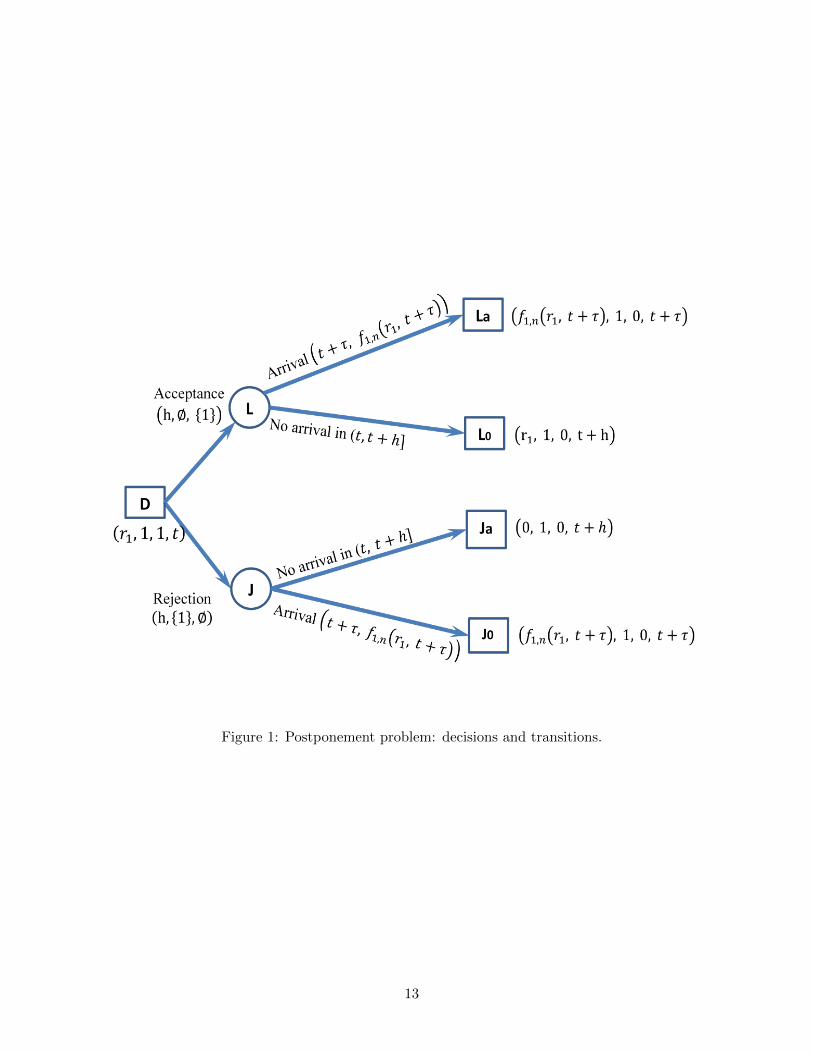
Figure 1: Postponement problem: decisions and transitions.

13

counterparts of vL, v∗L, vJ , v∗J , and V π∗ , respectively:

g(r, t, h) =

∫ h

0

{e−ατf(r, t+ τ)− z(r, 1, τ)

}λe−λτdτ + e−λh

{e−αhr − z(r, 1, h)

}, (12)

g(r, t, h) =

∫ h

0

{e−ατf(r, t+ τ)− z(r, 1, τ)

}λe−λτdτ + e−λh

{e−αhg∗(0, t+ h)− z(r, 1, h)

}(13)

g∗(r, t) = maxh∈[0,T−t]

g(r, t, h), (14)

g∗(r, t) = maxh∈[0,T−t]

g(0, t, h), (15)

g(r, t) =

{max

{g∗(r, t), g∗(r, t)

}, r > 0

g∗(0, t), r = 0. (16)

First, we analyze g. In Lemma 1, we show that (12) can be rewritten as (17), the second term

of which is the benefit of postponed acceptance over immediate acceptance. In particular, term

λf(r, t+ h)− (α+ λ+ cq)r − c is non-increasing in α, λ, c, and cq.

Lemma 1. Equation (12) can be simplified as:

g(r, t, h) = r +

∫ h

0e−(α+λ)τ

[λf(r, t+ τ)− (α+ λ+ cq)r − c

]dτ. (17)

Proof. For the second term of (12),

re−(α+λ)h = r + r

∫ h

0de−(α+λ)τ ,

e−λhz(r, 1, t+ h) =

∫ h

0e−(α+λ)τdz(r, 1, t+ τ)−

∫ h

0λe−λτz(r, 1, t+ τ)dτ

=

∫ h

0e−(α+λ)τ (c+ cqr)dτ −

∫ h

0λe−λτz(r, 1, t+ τ)dτ.

The conclusion follows by substituting the above two equations into the right hand side of g.

Clearly, the sign of (∂/∂h)g(r, t, h) is determined by λf(r, t+h)− (α+λ+ cq)r− c. If f satisfies

(a), this expression is non-increasing in h. Thus, g(r, t, h) may either be monotone or first increase

and then decrease in h, implying a threshold w(r) such that postponed acceptance is worthwhile

only if t < w(r).

Lemma 2. With fixed r and t, if f satisfies (a), g∗(r, t) = g(r, t, [w(r)− t]+), where

w(r) =

0, if (∂/∂h)g(r, 0, 0) < 0

T, if (∂/∂h)g(r, 0, T ) > 0

min{h : (∂/∂h)g(r, 0, h) = 0}, otherwise

. (18)

Proof. See Appendix B.

14

Second, Lemma 3 states that g∗ is convex and may not be monotone in the revenue of the queued

item. In particular, if the delay cost is positive (cq > 0), g∗ may first decrease and then increase in

the revenue of the queued item. Thus, g∗(r, t) ≤ g∗(0, t) if r > 0 is below a threshold:

θ(t) = max{r : g

(r, t, [w(r)− t]+

)≤ g(0, t, [w(0)− t]+

)}. (19)

Clearly, 0 ≤ θ(t) ≤ rmax, since 0 ≤ f ≤ rmax.

Lemma 3. If f satisfies (a) and (b), the following conclusions hold:

(i) w(r) is non-increasing in r;

(ii) if cq = 0, (∂/∂r)g∗(r, t) ≥ 0;

(iii) g∗(r, t) is convex in r.

Proof. See Appendix B.

Finally, postponed rejection (i.e.,(h, {1}, ∅) with h > 0) is always dominated (Lemma 4), such

that g∗ ≤ g∗. Alternatively, the optimal decision of P-f could either be immediate/postponed ac-

ceptance, or immediate rejection. Given state (r, 1, 1, t), the expected profit of immediate rejection

should be g∗(0, t). Thus, g(r, t) = max{g∗(r, t), g∗(0, t)}.

Lemma 4. If f satisfies (a) and (b), for any h > 0,

g(r, t, h) ≤ max{g∗(r, t), g∗(0, t)

},

and g(r, t) = max{g∗(r, t), g∗(0, t)

}.

Proof. See Appendix B.

These lead to an optimal policy with threshold structure for P-f .

Theorem 2. For P-f with f satisfying (a) - (c), there exist thresholds θ(t) and w(r), defining an

optimal policy as:

• if 0 < r < θ(t), reject the queued item.

• if r ≥ θ(t) and t ≥ w(r), or r = 0 and t ≥ w(0), immediately accept the queued item;

• if r ≥ θ(t) and t < w(r), or r = 0 and t < w(0), postpone accepting until w(r),

where θ and w can be written as (18) and (19). The optimal profit is equal to g, as defined in (16).

Moreover, θ(t), w(r), and g(r, t) satisfies:

(i) w(r) is non-increasing in r and θ(t) is non-increasing in t;

(ii) g(r, t) satisfies (a) - (c).

15

Proof. See Appendix B.

Theorem 2 serves as the building block to the analysis of the DSKP with m = 1. To establish

the optimal policies for the DSKP, it remains proving that f1,n satisfies (a)-(c), which requires the

following property (Lemma 5) of the postponement problem.

For convenience, we introduce an operator T , defined as follows.

Definition 2. Given functions gi : [0, rmax]× [0, T ] 7→ [0, rmax], i = 1, 2:(T (g1, g2)

)(r, t) =

∫Rg2(max(r, x), t)dFR(x) +

∫x>r

[g1(r, t)− g1(x, t)

]dFR(x), (20)

If g1 = rmax, the second term in (20) disappears; in this case, we write T g2 instead.

Lemma 5. Given functions gi : [0, rmax] × [0, T ] 7→ [0, rmax], i = 1, 2, which satisfy (a)-(c), if

(∂/∂r)(g2 − g1) ≥ 0, T (g1, g2) satisfies (a)-(c).

Proof. See Appendix B.

4.1.3 Optimal Policy

By Theorem 1 and Theorem 2, there exists a threshold optimal policy for the DSKP with m = 1,

if f1,n satisfies (a) - (c). Next, we illustrate that this is indeed the case. Consider the case of n = 1

as an example:

f1,1(r1, t+ τ) =

∫RV π∗

(u(r1, r

), 1, 0, t+ τ

)dFR(r) = E[max(r1, R)].

It is not hard to verify that f1,1 satisfies (a)-(c). By Theorem 2, there exists an optimal policy with

threshold structure for the postponement problem P-f1,1, or the DSKP with m = 1 and n = 1.

Denote by g1,1 the optimal expected profit of P-f1,1. Moreover, g1,1 or V π∗(r1, 1, 1, t

)satisfies

(a)-(c).

Next, consider the case of n = 2. It can be verified that:

f1,2(r1, t+ τ) =

∫RV π∗

(u(r1, r

), 1, 1, t+ τ

)dFR(r) =

(T g1,1

)(r1, t+ τ).

By Lemma 5, f1,2 also satisfies (a) - (c). The analysis of the case of n = 2 is similar as above.

In general, for P-f1,n, we use g1,n, w1,n, θ1,n, and g1,n to denote the counterparts of g, w, θ,

and g in P-f . For n ≥ 2, f1,n = T g1,n−1, and the optimal policy of P-f1,n is determined by two

thresholds:

w1,n(r1) =

0, if (∂/∂h)g1,n(r1, 0, 0) < 0

T, if (∂/∂h)g1,n(r1, 0, T ) > 0

min{h : (∂/∂h)g1,n(r1, 0, h) = 0}, otherwise

(21)

θ1,n(t) = max{r : g1,n

(r, t, [w1,n(r)− t]+

)≤ g1,n

(0, t, [w1,n(0)− t]+

)}, (22)

16

where

g1,n(r1, t, h) = r1 +

∫ h

0e−(α+λ)τ

[λf1,n(r1, t+ τ)− (α+ λ+ cq)r1 − c

]dτ.

And the optimal profit is:

g1,n(r1, t) =

{g1,n

(r1, t, [w1,n(r1)− t]+

), r1 ≥ θ1,n(t)

g1,n

(0, t, [w1,n(0)− t]+

), r1 < θ1,n(t)

. (23)

Note that (∂/∂r1)g1,n(r1, t) may not exist at r1 = θ1,n(t), leading to technical inconvenience

when arguing the monotonicity of g1,n. In this paper, we instead use the sign of the right first-

order derivative to argue the monotonicity of functions, based on a property of real functions

introduced in Feng and Hartman [11] (see Appendix A). For convenience, we henceforth do not

differentiate the right derivatives and the derivatives.

Formally, we have the following theorem.

Theorem 3. For (r1, 1, n, t) with n ≥ 1, there exists an optimal policy with thresholds defined by

(21) and (22):

• if r1 ∈ (0, θ1,n(t)), immediately reject item 1;

• if r1 6∈ (0, θ1,n(t)) and t ≥ w1,n(r1), immediately accept item 1;

• if r1 6∈ (0, θ1,n(t)) and t < w1,n(r1), postpone accepting item 1 until w1,n(r1) if no item arrives.

And the optimal expected profit is V π∗(r1, 1, n, t) = g1,n(r1, t).

Also, w1,n(r1), θ1,n(t), and g1,n(r1, t) satisfy:

(i) w1,n(r1) is non-increasing in r1 and θ1,n(t) is non-increasing in t;

(ii) g1,n(r1, t) ≥ r1 and is non-increasing in t;

(iii) (∂/∂r1)g1,n(r1, t) ∈ [0, 1] and is non-decreasing in r1 and t;

(iv) w1,n(r1), θ1,n(t), and g1,n(r1, t) are non-decreasing in n;

(v) (∂/∂r1)g1,n(r1, t) is non-increasing n.

Proof. See Appendix C.

By Lemma 3, if cq = 0, g∗1,n(r1, t) is non-decreasing in r1 and θ1,n(t) = 0. Thus, there is no

need to consider rejection in decisions; instead, rejection is achieved through queue updates upon

arrivals. In this case, the optimal policy stated by Theorem 3 can be simplified: there exists a

threshold r1 such that immediate acceptance is optimal if r1 is larger than r1, and otherwise, it is

optimal to postpone acceptance until T if no arrival occurs.

17

Corollary 1. If cq = 0, θ1,n = 0 and there exists r1, defined as:

r1 = min{r : λE[max(r,R)] ≤ (α+ λ)r + c

},

such that w1,n(r1) = 0 for r1 ≥ r1, and w1,n(r1) = T for r1 < r1.

Proof. See Appendix D.

Intuitively, E[max(r,R)] is the expected revenue of the queued item upon an arrival together

with the subsequent update. And λE[max(r,R)] − (α + λ)r − c is the reward difference between

postponement and immediate acceptance per unit time. Postponement is beneficial only when this

value is positive.

Next, we discuss the case when n→∞. In this case, n can be removed from the state variable,

and there is a result similar to Theorem 3.

Corollary 2. As n→∞, w1,n, θ1,n, and g1,n, respectively converge to w1, θ1, and g1. For (r1, 1, t),

there exists an optimal policy with thresholds w1 and θ1:

• if r1 ∈ (0, θ1(t)), immediately reject item 1;

• if r1 6∈ (0, θ1(t)) and t ≥ w1(r1), immediately accept item 1;

• if r1 6∈ (0, θ1(t)) and t < w1(r1), postpone accepting item 1 until w1(r1) if no item arrives.

And the optimal expected profit is V π∗(r1, 1, t) = g1(r1, t). Also, w1(r1), θ1(t), and g1(r1, t) satisfy:

(i) w1(r1) is non-increasing in r1 and θ1(t) is non-increasing in t;

(ii) g1(r1, t) ≥ r1 and is non-increasing in t;

(iii) (∂/∂r1)g1(r1, t) ∈ [0, 1] and is non-decreasing in r1 and t;

Proof. See Appendix E.

4.2 DSKP with m ≥ 2

The optimal policy of the DSKP with m ≥ 2 is established by bundling m postponement problems,

such that for each item i in the queue, there is a postponement problem, P-fi,n, and the optimal

policy of the DSKP is determined by the optimal policies of individual P-fi,n’s. The analysis is

long and not straightforward, and is thus presented in Appendix F. Below, we use the key results

and intuitions to illustrate the basic ideas.

For P-fi,n, we use gi,n, wi,n, θi,n, and gi,n to denote the counterparts of g, w, θ, and g in P-f .

With the aid of Theorem 2 and Lemma 5, it is possible to recursively construct fi,n, wi,n(ri),

18

θi,n(t), and gi,n(ri, t). For i ≥ 2 and i > n, fi,n(ri, t) = ri, such that wi,n(ri) = 0, θi,n(t) = 0, and

gi,n(ri, t) = ri. For i ≥ 2 and i ≤ n, fi,n = T(gi−1,n−1, gi,n−1

), such that:

gi,n(ri, t, h) = ri +

∫ h

0e−(α+λ)τ

[λfi,n(ri, t+ τ)− (α+ λ+ cq)ri − c

]dτ, (24)

w(i,n)(ri) =

0, if (∂/∂h)gi,n(ri, 0, 0) < 0

T, if (∂/∂h)gi,n(ri, 0, T ) > 0

min{h : (∂/∂h)gi,n(ri, 0, h) = 0)

}, otherwise

, (25)

θi,n(t) = max{r : gi,n

(r, t, [wi,n(r)− t]+

)≤ gi,n(0, t, [wi,n(0)− t]+

)}, (26)

gi,n(ri, t) =

{gi,n(ri, t, [wi,n(ri)− t]+

), ri ≥ θi,n(t)

gi,n(0, t, [wi,n(0)− t]+

), ri < θi,n(t)

. (27)

Moreover, wi,n’s and θi,n’s are non-increasing in i.

The key result shown in Appendix F is a generalization on Theorem 1:

vL(r,m, n, t, h) = gm,n(rm, t, h) +∑i 6=m

φi,n(ri, t, h),

vJ(r,m, n, t, h

)= gj,n(rj , t, h) +

∑i 6=j

φi,n(ri, t, h),

where j is the smallest index of the queued items with positive revenue (i.e., ri = 0 for i < j) and

φi,n(ri, t) is the expected profit of a (sub)optimal policy of P-fi,n: postpone applying the optimal

policy for P-fi,n by h. Clearly, this policy is optimal to P-fi,n only if h = 0 or if t + h ≤ wi,n(ri)

and ri 6∈ (0, θi,n(t)). With these results, the optimal policies of the DSKP can be determined by

the optimal policies of individual P-fi,n’s.

If rj < θj,n(t), immediate rejection is optimal to P-fj,n and gj,n(rj , t, 0) = gj,n(rj , t) by (13) and

(27), respectively. It follows that:

vJ(r,m, n, t, 0) = gj,n(rj , t) +∑i 6=j

φi,n(ri, t, 0) =∑i

gi,n(ri, t).

Note that∑

i gi,n is the upperbound for both vJ and vL. Thus, V π∗(r,m, n, t) =∑

i gi,n(ri, t) and

the optimal decision of P-fj,n is optimal to the DSKP.

If rj ≥ θj,n(t), rk ≥ θi,n(t) for any i > j, since θi,n is non-increasing in i. Thus, the optimal de-

cisions are immediate/postponed acceptance for all P-fi,n’s. Moreover, since wi,n is non-increasing

in i as stated above, for any i < m, φi,n(ri, t, h) = gi,n(ri, t) at h = [wm,n(rm)− t]+ and thus

vL(r,m, n, t, [wm,n(rm)− t]+) =∑i

gi,n(ri, t) = V π∗(r,m, n, t).

In other words, the optimal decision of P-fm,n is optimal to the DSKP.

Theorem 4. For (r,m, n, t) with m ≥ 2 and n ≥ 1, the optimal policy is:

19

• if ri ∈ (0, θi,n(t)) for any 1 ≤ i ≤ m, immediately reject item i;

• if ri 6∈ (0, θi,n(t)) for any 1 ≤ i ≤ m and t ≥ wm,n(rm), immediately accept item m;

• if ri 6∈ (0, θi,n(t)) for any 1 ≤ i ≤ m and t < wm,n(rm), postpone until wm,n(rm).

The corresponding expected profit is V π∗(r,m, n, t) =∑m

i=1 gi,n(ri, t).

Additionally, wi,n(ri), θi,n(t), and gi,n(ri, t) satisfy the following properties:

(i) wi,n(ri) is non-increasing in ri and θi,n(t) is non-increasing in t;

(ii) gi,n(ri, t) ≥ ri and is non-increasing in t;

(iii) (∂/∂ri)gi,n(ri, t) ∈ [0, 1] and is non-decreasing in ri and t;

(iv) wi,n(ri), θi,n(t), and gi,n(ri, t) are non-decreasing in n;

(v) (∂/∂r)gi,n(ri, t) is non-increasing in n;

(vi) wi,n(ri), θi,n(t), and gi,n(ri, t) are non-increasing in i;

(vii) (∂/∂ri)gi,n(ri, t) is non-decreasing in i.

Proof. See Appendix F.

The number of items yet to arrive, n, determines the rewards that can be earned in the future.

Thus, gm,n(rm, t) and wm,n(rm) increase in n. The number of available resources, m, dilutes the

effect of n. With more items to be accepted, there are more discounting and holding costs, and thus

the decision-maker is less picky when accepting an item. We illustrate the optimal policy stated in

Theorem 4 through an algorithm. Given state (r,m, n, t), the optimal decision is:

Algorithm 1 Optimal Policy

i← 1

while i ≤ m and not 0 < ri < θi,n(ri, t) do

i← i+ 1

if i ≤ m then

Decision ← (0, {i}, ∅)else

if t < wm,n(rm) then

Decision ← (wm,n(rm)− t, ∅, {m})else

Decision ← (0, ∅, {m})

We next discuss the case of n → ∞. Similar to Section 4.1, we remove n from the state, such

that the state now is represented as (r,m, t).

Corollary 3. As n→∞, wi,n, θi,n, and gi,n respectively converge to wi, θi, and gi, for i = 1, . . . ,m.

For (r,m, t) with m ≥ 2 and n ≥ 1, the optimal policy is:

20

• if ri ∈ (0, θi(t)) for any 1 ≤ i ≤ m, immediately reject item i;

• if ri 6∈ (0, θi(t)) for any 1 ≤ i ≤ m and t ≥ wm(rm), immediately accept item m;

• if ri 6∈ (0, θi(t)) for any 1 ≤ i ≤ m and t < wm(rm), postpone until wm(rm).

The corresponding expected profit is V π∗(r,m, t) =∑m

i=1 gi(ri, t). Additionally, wi(ri), θi(t), and

gi(ri, t) satisfy the following properties:

(i) wi(ri) is non-increasing in ri and θi(t) is non-increasing in t;

(ii) gi(ri, t) ≥ ri and is non-increasing in t;

(iii) (∂/∂ri)gi(ri, t) ∈ [0, 1] and is non-decreasing in ri and t;

(iv) wi(ri), θi(t), and gi(ri, t) are non-increasing in i;

(v) (∂/∂ri)gi(ri, t) is non-decreasing in i.

Proof. See Appendix G.

Clearly, the optimal policy π∗ developed here significantly differs from the policies of the DSKP

models in the literature. In those models, no postponement queue exists and the decision-maker

accepts or rejects an arriving item by checking its revenue against a single threshold, while there

are multiple thresholds in our model. For comparison, consider state (r,m, n, t), where r =

(0, . . . , 0, rm) and rm > 0. Let w−1m,n(t) be the minimum r such that gm,n(r, t) = r; i.e., w−1

m,n(·) is

the inverse function of wm,n(·). If w−1m,n(t) > θm,n(t), w−1

m,n(t) and θm,n(t) will divide the support of

R into three intervals such that the optimal decision is:

• if rm ∈ [w−1m,n(t), rmax], immediately accept item m;

• if rm ∈ [θm,n(t), w−1m,n(t)), postpone accepting item m until wm,n(rm) unless new item arrives;

• if rm ∈ [0, θm,n(t)), immediately reject item m.

In other words, there is an interval on the support of R, where postponement is optimal.

Intuitively, this interval where postponement is optimal will shrink as cq increases. When cq = 0,

θ1,n(t) = 0 (Corolary 1), and thus θm,n(t) ≤ θ1,n(t) = 0 (Theorem 4). In this case, there is no need

to immediately reject a queued item. As cq increases, the second term of (17) or the benefit of

postponement decreases. When cq > 1, for any P-f with f satisfying (a)-(c),

(∂/∂h)g(r, t, h) = e−(α+λ)h[λf(r, t+ h)− (α+ λ+ cq)r − c

]< 0,

thus there is no need for postponement. As a result, w1,n = 0 (Theorem 3) and wm,n ≤ w1,n = 0

(Theorem 4). In this case, the decision-maker only needs to consider immediate acceptance and

immediate rejection, which is similar to the DSKP models in the literature.

In particular, our model addresses the second potential extension pointed out in Papastavrou

et al. [29]: allow rejected items to be recalled. In that paper, the items (e.g., customers requesting

21

the capacity of a truck) that are not immediately accepted, are rejected and cannot be recalled. Put

in the context of our model, these items first enter the postponement queue and may be accepted

later with the revenue values of the queued items listed as r = (r1, . . . , rm). At time t, if ri ∈(0, θi(t)), the item will never be recalled; if ri ≥ θi(t) and t ≥ wi(ri), i.e., ri ≥ max{θi(t), w−1

i (t)},the item should be recalled.

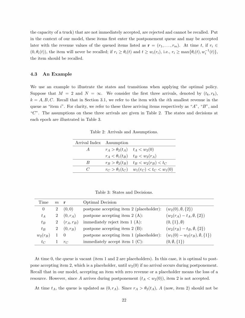
4.3 An Example

We use an example to illustrate the states and transitions when applying the optimal policy.

Suppose that M = 2 and N = ∞. We consider the first three arrivals, denoted by (tk, rk),

k = A,B,C. Recall that in Section 3.1, we refer to the item with the ith smallest revenue in the

queue as “item i”. For clarity, we refer to these three arriving items respectively as “A”, “B”, and

“C”. The assumptions on these three arrivals are given in Table 2. The states and decisions at

each epoch are illustrated in Table 3.

Table 2: Arrivals and Assumptions.

Arrival Index Assumption

A rA > θ2(tA) tA < w2(0)

rA < θ1(tB) tB < w2(rA)

B rB > θ2(tB) tB < w2(rB) < tC

C rC > θ1(tC) w1(rC) < tC < w1(0)

Table 3: States and Decisions.

Time m r Optimal Decision

0 2 (0, 0) postpone accepting item 2 (placeholder): (w2(0), ∅, {2})tA 2 (0, rA) postpone accepting item 2 (A): (w2(rA)− tA, ∅, {2})tB 2 (rA, rB) immediately reject item 1 (A): (0, {1}, ∅)tB 2 (0, rB) postpone accepting item 2 (B): (w2(rB)− tB, ∅, {2})

w2(rB) 1 0 postpone accepting item 1 (placeholder): (w1(0)− w2(rB), ∅, {1})tC 1 rC immediately accept item 1 (C): (0, ∅, {1})

At time 0, the queue is vacant (item 1 and 2 are placeholders). In this case, it is optimal to post-

pone accepting item 2, which is a placeholder, until w2(0) if no arrival occurs during postponement.

Recall that in our model, accepting an item with zero revenue or a placeholder means the loss of a

resource. However, since A arrives during postponement (tA < w2(0)), item 2 is not accepted.

At time tA, the queue is updated as (0, rA). Since rA > θ2(tA), A (now, item 2) should not be

22

rejected. Instead, since tA < tB < w2(rA), it is optimal to postpone accepting A until w2(rA) if no

item arrives during postponement. However, since B arrives during postponement (tB < w2(rA)),

A is neither accepted nor rejected.

At time tB, the queue is updated as (rA, rB). Since rA < θ1(tB), A (now, item 1) should be

immediately rejected. The queue then changes from (rA, rB) to (0, rB), followed by a new decision.

Since rB > θ2(tB) and tB < w2(rB), it is optimal to postpone accepting B until w2(rB) if no item

arrives during postponement. Unlike the case of A, B is accepted, since w2(rB) < tC and no item

arrives during postponement.

At time w2(rB), the queue goes vacant after B is accepted, followed by a new decision. Since

w2(rB) < tC < w1(0), it is optimal to postpone accepting item 1, which is a placeholder, until

w1(0) if no item arrives during postponement. Item 1 is not accepted, since tC < w1(0) and C

arrives during postponement.

At time tC , C is the only queued item. Since rC > θ1(tC) and tC > w1(rC), C should be

immediately accepted, and the process stops.

Note that the optimal decisions tend to accept both A and B, respectively at time tA and tB.

However, A is not accepted due to the arrival of B during postponement, while B is accepted,

since no item arrives during postponement. Moreover, A arrives at time tA and is rejected at

time tB, though optimal decisions listed in Table 3 do not postpone rejecting it. This happens

because A changes its position in the queue; at time tA, A is item 2, while at time tB, it is item 1.

Since θ2(tA) < rA < θ1(tB), though A should not be immediately rejected at time tA, it should be

immediately rejected at tB.

4.4 Stop and Salvage Option

In this section, we discuss the feasibility of incorporating the option of stopping and salvaging

resources, as it better addresses the concerns in applications (Kleywegt and Papastavrou [20]).

Specifically, this option enables the flexibility of stopping the decision process and salvaging all

remaining resources, with rewards defined as ν(m). Though our model does not directly consider

this option, it can be added to our model with three assumptions: (1) salvaging can be done at

any time, (2) a subset of the available resources can be salvaged, and (3) ν(m) = νm.

Note that if the revenue of an item is not higher than ν, the item should be immediately rejected

since it is not worth allocating a resource to it, while keeping the item in the queue merely causes

delay costs. It should be enough to limit the arrival rate to those items with revenue higher than ν.

Moreover, resources are similar to items; salvaging a resource and accepting an item both lead to

rewards and the queue being shortened. With these observations, we can require that all elements

in r be at least ν; ri > ν denotes the revenue of an item, while ri = ν denotes a vacant place; i.e.,

r0 = (ν, . . . , ν).

23

In fact, the analysis in earlier sections does not rely on whether a vacant place in the queue is

denoted by an item with zero revenue. With slight modifications to the model and the postponement

problem, it is possible to use the framework developed in this paper to establish the optimal policy

for the DSKP with the stop and salvage option. In brief, we modify θ in the postponement problem

as follows:

θ(t) = max{r : g

(r, t, [w(r)− t]+

)≤ g(ν, t, [w(ν)− t]+

)},

where:

g(ν, t, h) = ν +

∫ h

0e−(α+λ)τ

[λf(ν, t+ τ)− (α+ λ)ν − c

]dτ.

And

g(r, t) =

{g(r, t, [w(r)− t]+

), r ≥ θ(t)

g(ν, t, [w(ν)− t]+

), r < θ(t)

.

With an argument analogous to those in Section 4.1 through 4.2, it should not be difficult to develop

similar optimal policies.

Implicitly included in the models from the literature are two assumptions. First, it is possible to

salvage the unallocated resources at any time (e.g., in Kleywegt and Papastavrou [20]), the salvage

function ν(·) is independent of time. Second, all resources that have not been allocated must be

salvaged simultaneously. As a comparison, the first assumption is the same as ours. However, we

do not require that all resources to be salvaged at the same time and we need ν(m) = νm.

Our approach of modeling the salvage option entails more flexibility in salvaging resources. By

regarding salvaging resources as accepting items, our model allows the decision-maker to salvage a

subset of the remaining resources and the decision process continues with the resources that are not

salvaged. As a comparison, in the DSKP models in the literature, salvaging resources terminates

the decision process. The additional flexibility achieved by our model may lead to better decisions.

4.5 Rejection Penalty

Unfortunately, it is not possible to accommodate the rejection penalty into the model. Given r = 0,

the queue consists of items with revenue 0. When a new item arrives and is added into the queue,

then one item with zero revenue is to be removed from the queue. However, the queuing model

presented in this paper can hardly distinguish whether an item removed from the queue has zero

revenue or merely a placeholder. We would argue that this does not affect the applicability of our

model in practice. For many applications, the rejection penalty represents the loss of goodwill,

which typically does not apply when requests compete for limited resources.

24

5 Numerical Examples: Benefits of Postponement

In this section, numerical experiments illustrate the benefits of postponement by comparing the

model developed in this paper with the model developed by Kleywegt and Papastavrou [20]. For

the sake of convenience, we call their model the “traditional DSKP model”, and the model devel-

oped in this paper the “new model”. Moreover, we study the factors that affect the benefits of

postponement.

In the experiments, we compute the thresholds and expected profits of the new model recursively.

When computing gi,n(r, t), the support of R is divided into intervals with homogeneous length 0.4.

On the other hand, the time horizon is divided into intervals with lengths ranging from 0.2 to 2;

specifically, the first interval starts from t = 0 and ends at t = 2, with the remaining intervals

having a fractional length of the previous interval. The break points of the support of R and time

horizon compose a grid of points, which we will refer as “grid points”.

For each m and n, the procedure to compute the optimal policy of our model is:

(1) compute fm,n’s value based on gm,n−1 and gm−1,n−1 over the grid points as described above;

(2) compute gm,n’s value based on fm,n over the grid points;

(3) compute wm,n(rm) based on gm,n over the grid points;

(4) compute θm,n(t) based on gm,n and wm,n over grid points;

(5) compute gm,n’s value over the grid points.

Here, we elaborate how the thresholds are computed. First, consider wm,n. For every grid point

(r, t) and any h, (∂/∂h)gm,n can be evaluated. Thus, wm,n(r) can be determined according to (27)

for any (r, t). Then, g∗m,n(r, t) can be computed. Finally, θm,n(t) is determined: if g∗m,n(0, t) >

g∗m,n(ε, t), θm,n(t) is taken such that:

g∗m,n(θm,n(t), t) ≥ g∗m,n(0, t),

g∗m,n(θm,n(t)− ε, t) < g∗m,n(0, t),

where ε = 0.4 in our experiment; otherwise, θm,n(t) is taken as 0.

When N → ∞, we increase n until the summation of the difference between gm,n and gm,n−1

over all grid points is smaller than 0.1. Compared with the traditional DSKP, which relies on

solving differential equations, this computational procedure requires more time. For a DSKP with

M = 20 and infinite N , it takes minutes to compute the optimal policy for our model with C++

implementation of the above procedure, while only seconds for MATLAB to solve the traditional

DSKP. We argue that the potential gain in profits justifies the additional computation time.

25

5.1 Comparison with Traditional DSKP

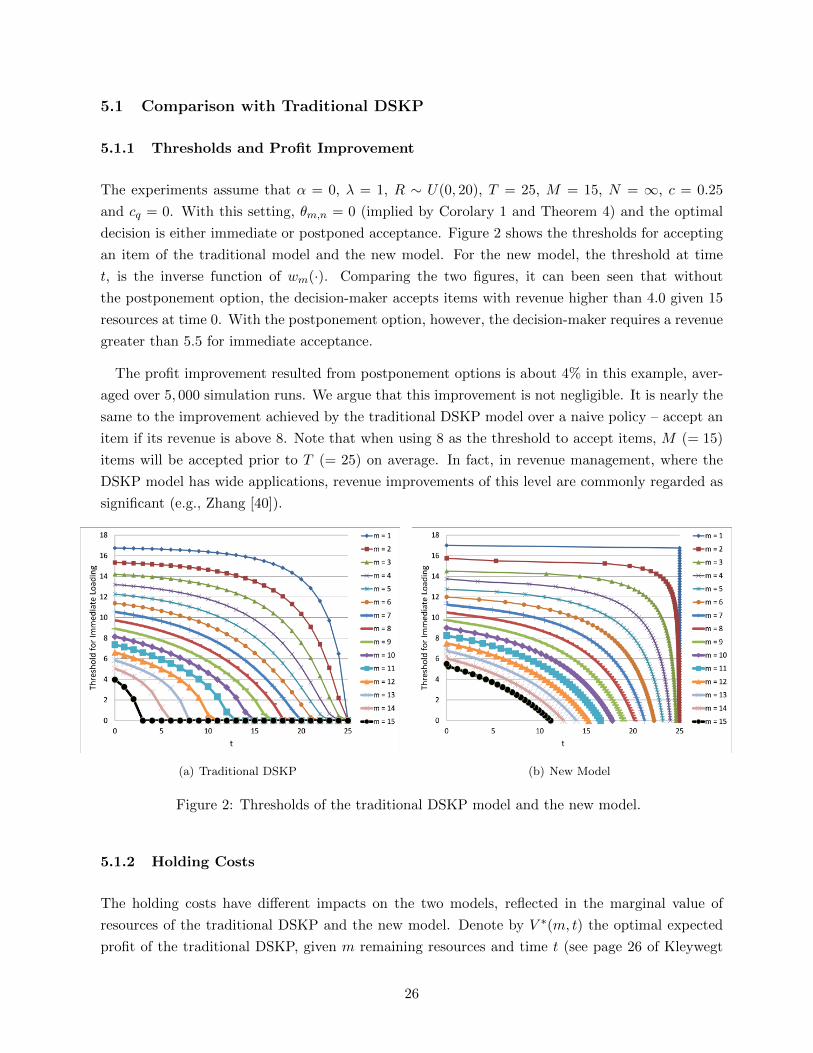
5.1.1 Thresholds and Profit Improvement

The experiments assume that α = 0, λ = 1, R ∼ U(0, 20), T = 25, M = 15, N = ∞, c = 0.25

and cq = 0. With this setting, θm,n = 0 (implied by Corolary 1 and Theorem 4) and the optimal

decision is either immediate or postponed acceptance. Figure 2 shows the thresholds for accepting

an item of the traditional model and the new model. For the new model, the threshold at time

t, is the inverse function of wm(·). Comparing the two figures, it can been seen that without

the postponement option, the decision-maker accepts items with revenue higher than 4.0 given 15

resources at time 0. With the postponement option, however, the decision-maker requires a revenue

greater than 5.5 for immediate acceptance.

The profit improvement resulted from postponement options is about 4% in this example, aver-

aged over 5, 000 simulation runs. We argue that this improvement is not negligible. It is nearly the

same to the improvement achieved by the traditional DSKP model over a naive policy – accept an

item if its revenue is above 8. Note that when using 8 as the threshold to accept items, M (= 15)

items will be accepted prior to T (= 25) on average. In fact, in revenue management, where the

DSKP model has wide applications, revenue improvements of this level are commonly regarded as

significant (e.g., Zhang [40]).

(a) Traditional DSKP (b) New Model

Figure 2: Thresholds of the traditional DSKP model and the new model.

5.1.2 Holding Costs

The holding costs have different impacts on the two models, reflected in the marginal value of

resources of the traditional DSKP and the new model. Denote by V ∗(m, t) the optimal expected

profit of the traditional DSKP, given m remaining resources and time t (see page 26 of Kleywegt

26

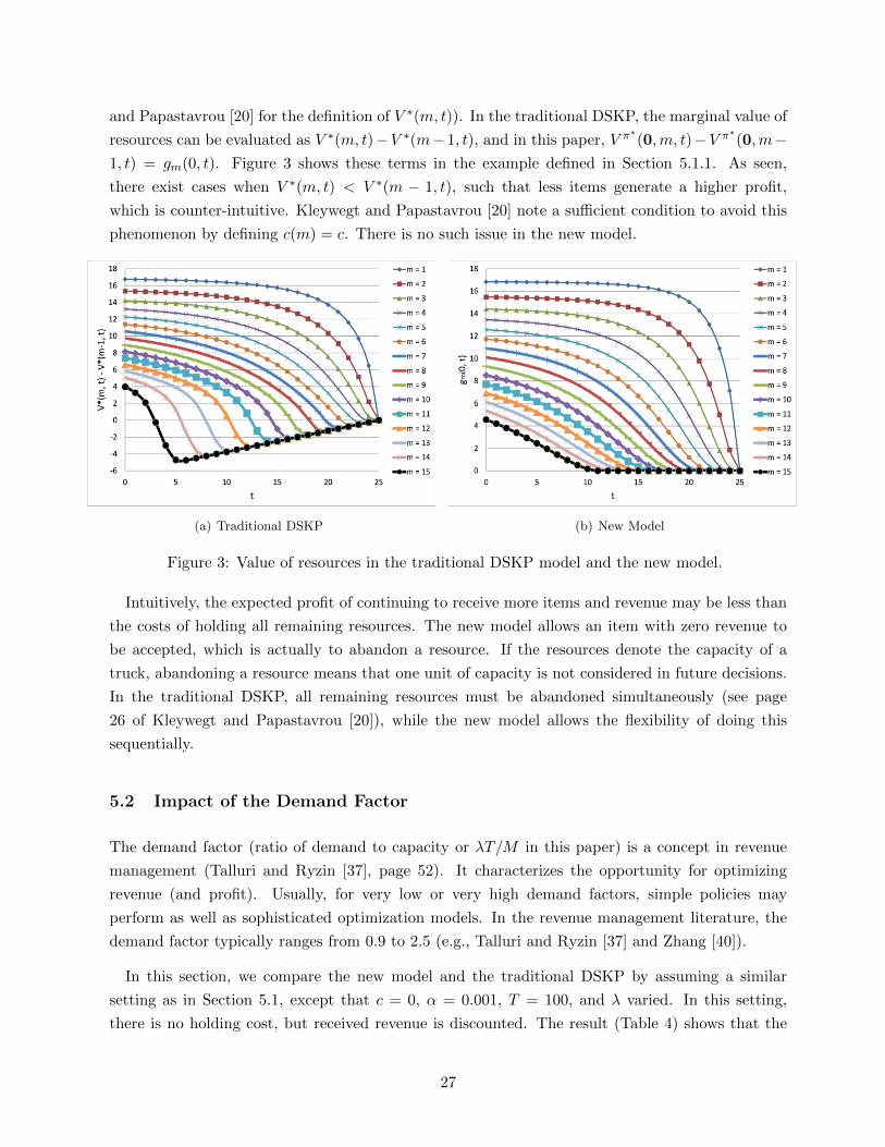
and Papastavrou [20] for the definition of V ∗(m, t)). In the traditional DSKP, the marginal value of

resources can be evaluated as V ∗(m, t)−V ∗(m− 1, t), and in this paper, V π∗(0,m, t)−V π∗(0,m−1, t) = gm(0, t). Figure 3 shows these terms in the example defined in Section 5.1.1. As seen,

there exist cases when V ∗(m, t) < V ∗(m − 1, t), such that less items generate a higher profit,

which is counter-intuitive. Kleywegt and Papastavrou [20] note a sufficient condition to avoid this

phenomenon by defining c(m) = c. There is no such issue in the new model.

(a) Traditional DSKP (b) New Model

Figure 3: Value of resources in the traditional DSKP model and the new model.

Intuitively, the expected profit of continuing to receive more items and revenue may be less than

the costs of holding all remaining resources. The new model allows an item with zero revenue to

be accepted, which is actually to abandon a resource. If the resources denote the capacity of a

truck, abandoning a resource means that one unit of capacity is not considered in future decisions.

In the traditional DSKP, all remaining resources must be abandoned simultaneously (see page

26 of Kleywegt and Papastavrou [20]), while the new model allows the flexibility of doing this

sequentially.

5.2 Impact of the Demand Factor

The demand factor (ratio of demand to capacity or λT/M in this paper) is a concept in revenue

management (Talluri and Ryzin [37], page 52). It characterizes the opportunity for optimizing

revenue (and profit). Usually, for very low or very high demand factors, simple policies may

perform as well as sophisticated optimization models. In the revenue management literature, the

demand factor typically ranges from 0.9 to 2.5 (e.g., Talluri and Ryzin [37] and Zhang [40]).

In this section, we compare the new model and the traditional DSKP by assuming a similar

setting as in Section 5.1, except that c = 0, α = 0.001, T = 100, and λ varied. In this setting,

there is no holding cost, but received revenue is discounted. The result (Table 4) shows that the

27

new model outperforms when the demand is moderately larger than capacity.

Table 4: Impact of Demand Factor.

Case λ Demand Factor Profit Improvement (%)

1 0.15 1.00 2.09%

2 0.20 1.33 4.01%

3 0.25 1.67 4.29%

4 0.30 2.00 3.70%

5 0.35 2.33 3.07%

6 0.50 3.33 2.10%

Intuitively, postponement is beneficial because the held items hedge against the risk that revenue

of the items yet to arrive are less than expected. This risk decreases as T and λ increase, since with

more items yet to arrive, the probability of all these items being inferior to the held item approach

zero and thus the benefit of postponement declines. On the other hand, when the time horizon is

quite short, only a few items may arrive before T , which also reduces the benefit of postponement.

5.3 Impact of Holding Cost

Intuitively, the holding cost c discourages the options of postponement and rejection. In this

section, we illustrate its impact by varying the distribution of R, and the value of c. Due to

the issue mentioned in Section 5.1.2, we do not use the traditional DSKP as the case “without

the postponement option”. Instead, we use our model with very large cq (= 20) to disable the

postponement option.

We fix parameters α = 0.001, λ = 0.25, M = 20, cq = 0, and T = 200, and vary FR and c.

Specifically, c takes the values of 0, 0.01, 0.02, 0.03, and 0.04; R assumes a scaled Beta distribution,

R = 20ξ, with two parameter settings, ξ ∼ Beta(1.0, 1.0) and ξ ∼ Beta(1.0, 3.0). With the first

setting, R is uniformly distributed. With the second setting, the p.d.f. of R is left leaning; in this

case, the postponement option should benefit more, since the risk of encountering the items with

inferior revenue is higher. In this experiment, we illustrate the benefit of the postponement option

through the percentage of profit improvement:

V π∗(0, 20, t)|cq=0

V π∗(0, 20, t)|cq=20− 1.

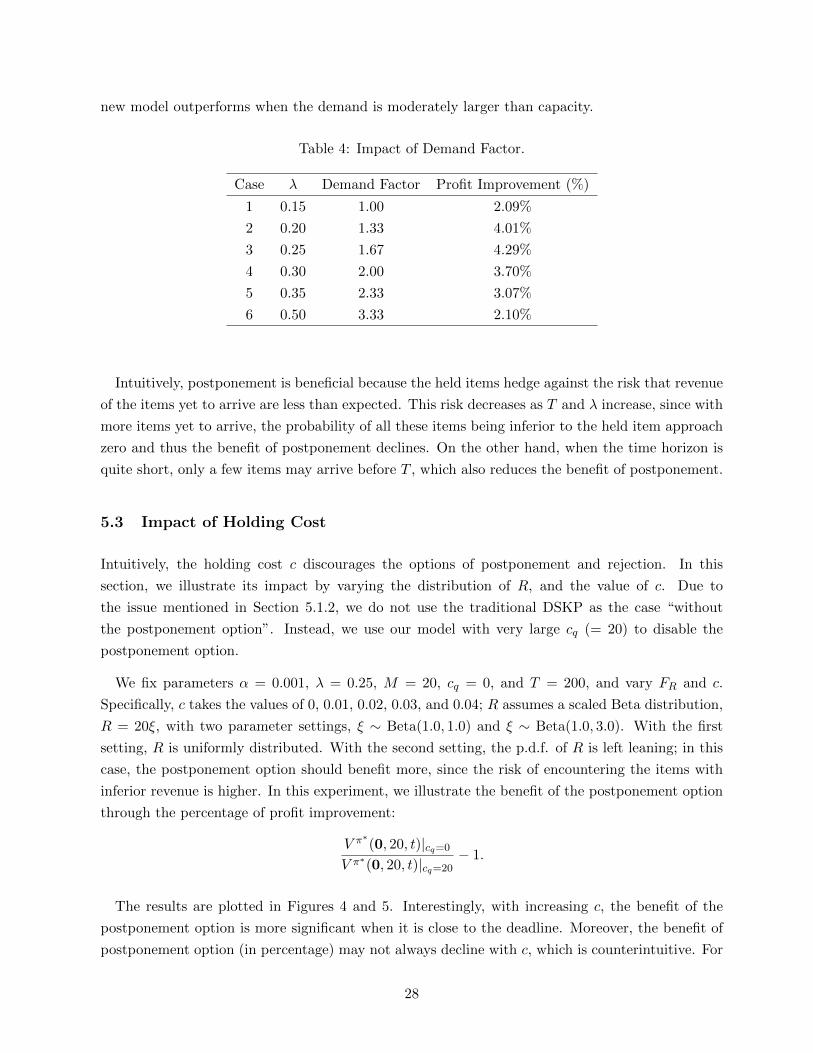
The results are plotted in Figures 4 and 5. Interestingly, with increasing c, the benefit of the

postponement option is more significant when it is close to the deadline. Moreover, the benefit of

postponement option (in percentage) may not always decline with c, which is counterintuitive. For

28

example, prior to t = 80 in Figure 4 the curve of c = 0.00 is above that of c = 0.04, but the order

reverses at t = 140. Also, postponement is more beneficial more in the case of ξ ∼ Beta(1.0, 3.0),

when there is no holding cost (c = 0); however, the benefit declines quickly in c.

Figure 4: Impact of holding cost onV π∗

(0,20,t)|cq=0

V π∗ (0,20,t)|cq=20− 1 (ξ ∼ Beta(1.0, 1.0)).

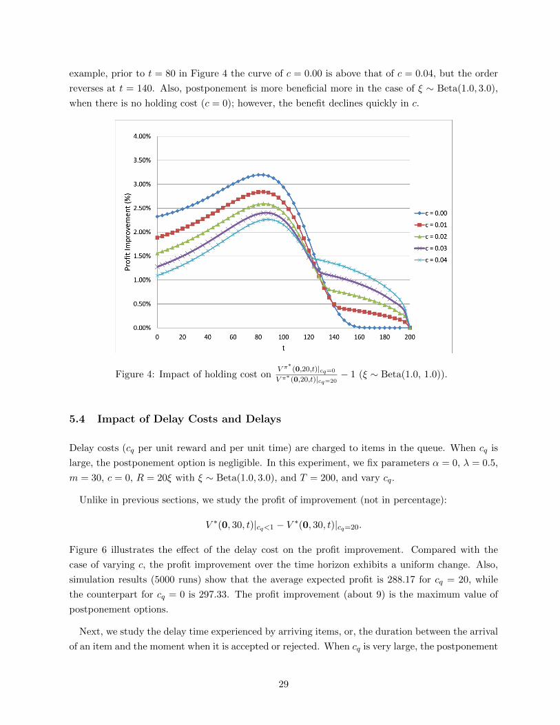
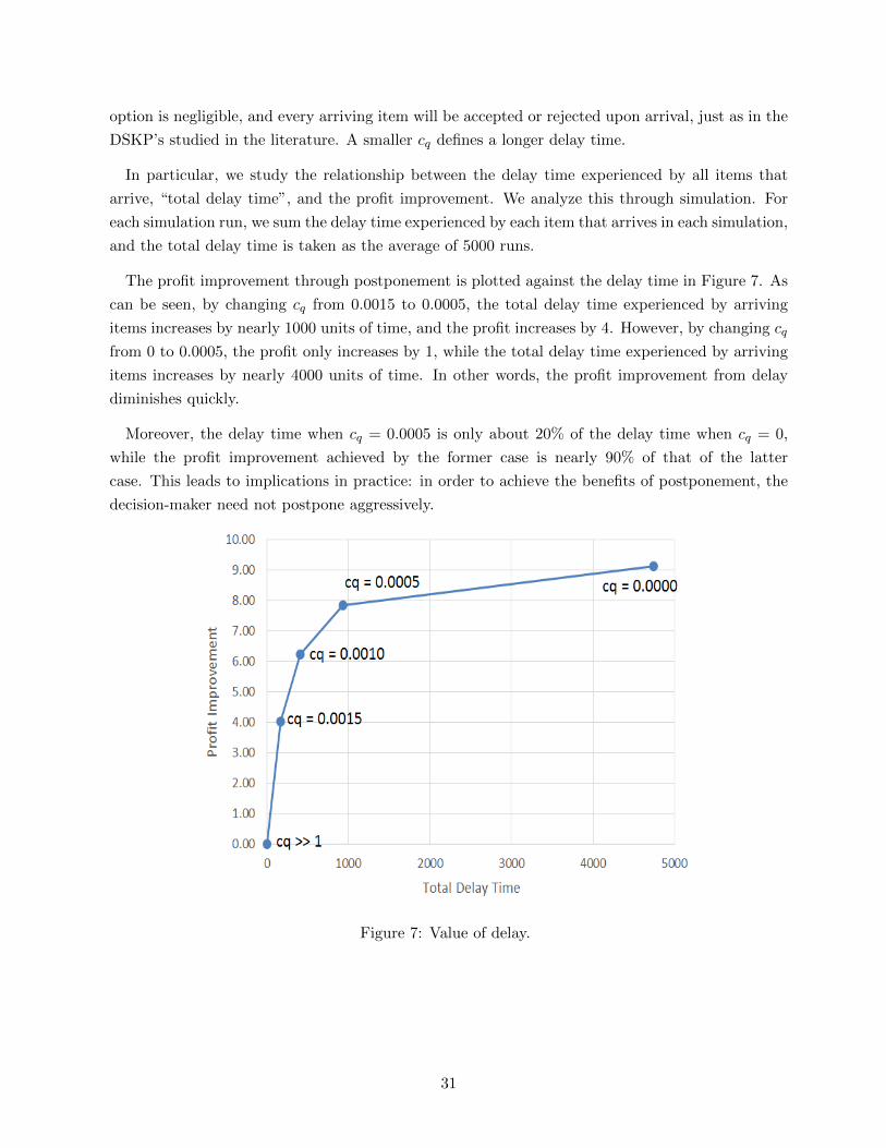
5.4 Impact of Delay Costs and Delays

Delay costs (cq per unit reward and per unit time) are charged to items in the queue. When cq is

large, the postponement option is negligible. In this experiment, we fix parameters α = 0, λ = 0.5,

m = 30, c = 0, R = 20ξ with ξ ∼ Beta(1.0, 3.0), and T = 200, and vary cq.

Unlike in previous sections, we study the profit of improvement (not in percentage):

V ∗(0, 30, t)|cq<1 − V ∗(0, 30, t)|cq=20.

Figure 6 illustrates the effect of the delay cost on the profit improvement. Compared with the

case of varying c, the profit improvement over the time horizon exhibits a uniform change. Also,

simulation results (5000 runs) show that the average expected profit is 288.17 for cq = 20, while

the counterpart for cq = 0 is 297.33. The profit improvement (about 9) is the maximum value of

postponement options.

Next, we study the delay time experienced by arriving items, or, the duration between the arrival

of an item and the moment when it is accepted or rejected. When cq is very large, the postponement

29

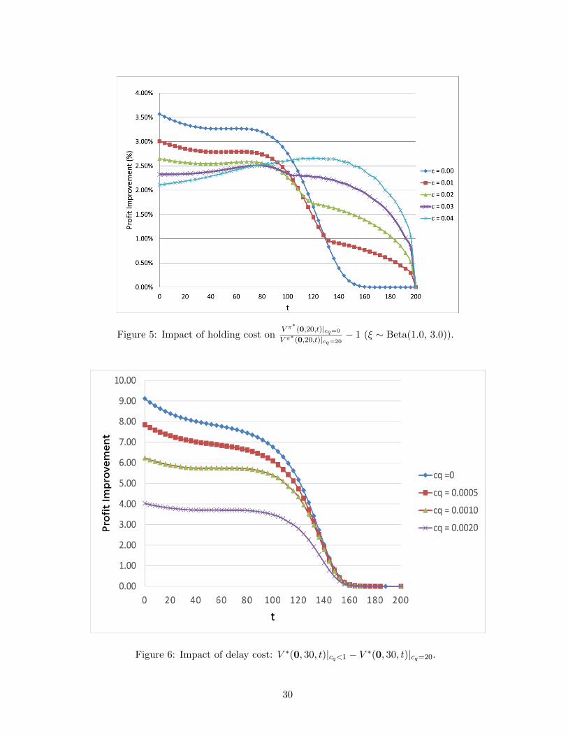
Figure 5: Impact of holding cost onV π∗

(0,20,t)|cq=0

V π∗ (0,20,t)|cq=20− 1 (ξ ∼ Beta(1.0, 3.0)).

Figure 6: Impact of delay cost: V ∗(0, 30, t)|cq<1 − V ∗(0, 30, t)|cq=20.

30

option is negligible, and every arriving item will be accepted or rejected upon arrival, just as in the

DSKP’s studied in the literature. A smaller cq defines a longer delay time.

In particular, we study the relationship between the delay time experienced by all items that

arrive, “total delay time”, and the profit improvement. We analyze this through simulation. For

each simulation run, we sum the delay time experienced by each item that arrives in each simulation,

and the total delay time is taken as the average of 5000 runs.

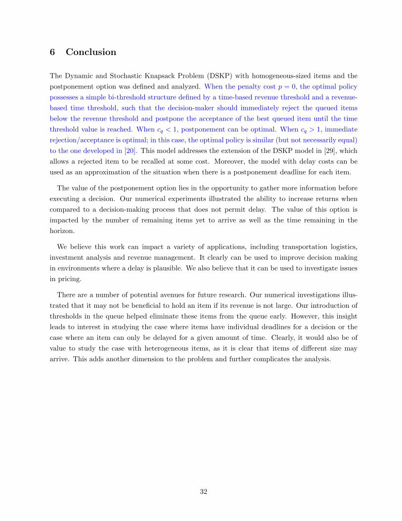
The profit improvement through postponement is plotted against the delay time in Figure 7. As

can be seen, by changing cq from 0.0015 to 0.0005, the total delay time experienced by arriving

items increases by nearly 1000 units of time, and the profit increases by 4. However, by changing cq

from 0 to 0.0005, the profit only increases by 1, while the total delay time experienced by arriving

items increases by nearly 4000 units of time. In other words, the profit improvement from delay

diminishes quickly.

Moreover, the delay time when cq = 0.0005 is only about 20% of the delay time when cq = 0,

while the profit improvement achieved by the former case is nearly 90% of that of the latter

case. This leads to implications in practice: in order to achieve the benefits of postponement, the

decision-maker need not postpone aggressively.

Figure 7: Value of delay.

31

6 Conclusion

The Dynamic and Stochastic Knapsack Problem (DSKP) with homogeneous-sized items and the

postponement option was defined and analyzed. When the penalty cost p = 0, the optimal policy

possesses a simple bi-threshold structure defined by a time-based revenue threshold and a revenue-

based time threshold, such that the decision-maker should immediately reject the queued items

below the revenue threshold and postpone the acceptance of the best queued item until the time

threshold value is reached. When cq < 1, postponement can be optimal. When cq > 1, immediate

rejection/acceptance is optimal; in this case, the optimal policy is similar (but not necessarily equal)

to the one developed in [20]. This model addresses the extension of the DSKP model in [29], which

allows a rejected item to be recalled at some cost. Moreover, the model with delay costs can be

used as an approximation of the situation when there is a postponement deadline for each item.

The value of the postponement option lies in the opportunity to gather more information before

executing a decision. Our numerical experiments illustrated the ability to increase returns when

compared to a decision-making process that does not permit delay. The value of this option is

impacted by the number of remaining items yet to arrive as well as the time remaining in the

horizon.

We believe this work can impact a variety of applications, including transportation logistics,

investment analysis and revenue management. It clearly can be used to improve decision making

in environments where a delay is plausible. We also believe that it can be used to investigate issues

in pricing.

There are a number of potential avenues for future research. Our numerical investigations illus-

trated that it may not be beneficial to hold an item if its revenue is not large. Our introduction of

thresholds in the queue helped eliminate these items from the queue early. However, this insight

leads to interest in studying the case where items have individual deadlines for a decision or the

case where an item can only be delayed for a given amount of time. Clearly, it would also be of

value to study the case with heterogeneous items, as it is clear that items of different size may

arrive. This adds another dimension to the problem and further complicates the analysis.

32

References

[1] Albright, S. C. (1974). Optimal sequential assignments with random arrival times. Management Sci. 21(1), 60–67.

[2] Albright, S. C. (1977). A bayesian approach to a generalized house selling problem. Management Sci. 24(4),

432–440.

[3] Amram, M. and N. Kulatilaka (1999). Real Options: Managing Strategic Investment in an Uncertain World.

Boston: Harvard Business School Press.

[4] Bucklin, L. P. (1965). Postponement, speculation and the structure of distribution channels. Journal of Marketing

Research 2(2), 26–31.

[5] Coffman, E. G., L. Flatto, and R. R. Weber (1987). Optimal selection of stochastic intervals under a sum

constraint. Adv. Appl. Prob. 19, 454–473.

[6] Coffman, E. G. and A. L. Stolyar (1999). Bandwidth packing. Algorithmica. 29, 70–88.

[7] Dean, B. C., M. X. Goemans, and J. Vondrak. (2008). Approximating the stochastic knapsack problem: The

benefit of adaptivity. Math. Oper. Res. 33(4), 945–964.

[8] Derman, C., G. J. Lieberman, and S. M. Ross (1972). Stochastic assignment problem. Management Sci. 18(7),

349–355.

[9] Ding, Q., L. Dong, and P. Kouvelis (2007). On the interaction of production and financial hedging decisions in

global markets. Oper. Res. 55(3), 470–489.

[10] Feitzinger, E. and H. L. Lee (1997). Mass customization at hewlett packard: the power of postponement. Harvard

Business Review 75, 116–121.

[11] Feng, T. and J. Hartman (2013). Sequential stochastic assignment problem with the postponement option.

Probabilities in Engineering and Informational Sciences. 27(1)., 25–51.

[12] Gamarnik, D. and M. S. Squillante (2005). Analysis of stochastic online bin packing processes. Stoch. Models. 21,

401–425.

[13] Grenadier, S. R. and A. Weiss (1997). Investment in technological innovations: An option pricing approach.

Journal of Financial Economics 44, 397–416.

[14] Gyorgy, A., G. Lugosi, and G. Ottuscak (2010). Online sequential bin packing. J. Mach. Learn. Res. 11, 89–109.

[15] Herbots, J., W. Herroelen, and R. Leus (2007). Dynamic order acceptance and capacity planning on a single

bottleneck resource. Naval Res. Logist. 54(8), 874–889.

[16] Hoek, R. I. V. (2001). The rediscovery of postponement a literature review and directions for research. Journal

of Operations Management 19(2), 161–184.

[17] Huchzermeier, A. and C. H. Loch (2001). Project management under risk. Management Sci. 47(1), 85–101.

[18] Kellerer, H., U. P. and D. Pisinger (2004). Knapsack Problems. Berlin, Germany: Springer.

[19] Kennedy, D. P. (1986). Optimal sequential assignment. Math. Oper. Res. 11(4), 619–626.

[20] Kleywegt, A. J. and J. D. Papastavrou (1998). The dynamic and stochastic knapsack problem. Oper. Res. 46(1),

17–35.

33

[21] Kleywegt, A. J. and J. D. Papastavrou (2001). The dynamic and stochastic knapsack problem with random

sized items. Oper. Res. 49(1), 26–41.

[22] Lu, L. L., S. Y. Chiu, and L. A. C. Jr (1999). Optimal project selection: Stochastic knapsack with finite time

horizon. J. Oper. Res. Soc. 50(6), 645–650.

[23] McDonald, R. and D. Siegel (1986). The value of waiting to invest. Quarterly Journal of Economics 101,

707–727.

[24] McLay, L. A., S. H. Jacobson, and A. G. Nikolaev (2009). A sequential stochastic passenger screening problem

for aviation security. IIE Transactions 41(6), 575–591.

[25] Nakai, T. (1986a). A sequential stochastic assignment problem in a partially observable markov chain. Math.

Oper. Res. 11, 230–240.

[26] Nakai, T. (1986b). A sequential stochastic assignment problem in a stationary markov chain. Mathematica

Japonica 31, 741–757.

[27] Nikolaev, A. G. and S. H. Jacobson (2010). Technical note – stochastic sequential decision-making with a random

number of jobs. Oper. Res. 58(4), 1023–1027.

[28] Papadaki, K. and W. Powell (2003). An adaptive dynamic programming algorithm for a stochastic multiproduct

batch dispatch problem. Naval Res. Logist. 50(7), 742–769.

[29] Papastavrou, J. D., S. Rajagopalan, and A. Kleywegt (1996). The dynamic and stochastic knapsack problem

with deadlines. Management Sci. 42(12), 1706–1718.

[30] Rhee, W. and M. Talagrand (1991). A note on the selection of random variables under a sum constraint. J.

Appl. Prob. 28, 919–923.

[31] Righter, R. L. (1989). A resource allocation problem in a random environment. Oper. Res. 37(2), 329–337.

[32] Rudin, W. (1976). Principles of Mathematical Analysis. New York: McGraw-Hill.

[33] Rudin, W. (1987). Real and Complex Analysis. New York: McGraw-Hill.

[34] Sakaguchi, M. (1984a). A sequential stochastic assignment problem associated with a non-homogeneous makov

process. Mathematica Japonica 29(1), 13–22.

[35] Sakaguchi, M. (1984b). A sequential stochastic assignment problem associated with unknown number of jobs.

Mathematica Japonica 29(2), 141–152.

[36] Spivey, M. Z. and W. B. Powell (2004). The dynamic assignment problem. Transportation Sci. 38(4), 399–419.

[37] Talluri, K. and G. J. V. Ryzin (2005). The Theory and Practice of Revenue Management. New York: Springer.

[38] Triantis, A. J. (2000). Real options and corporate risk management. Journal of Applied Corporate Finance 13(2),

64–73.

[39] Trigeorgis, L. (1996). Real Options: Managerial Flexibility and Strategy in Resource Allocation. Cambridge,

MA: MIT Press.

[40] Zhang, D. (2009). An improved dynamic programming decomposition approach for network revenue manage-

ment. Manufacturing & Service Operations Management 13(1), 35–52.

34

Appendices

A Right Derivatives and An Alternative Expression of Costs

The theorems developed in this paper rely on some technical results. To better streamline the

paper, we present these results as lemmas in this section.

To avoid technical inconveniences, we use the sign of the right first-order derivative to argue

monotonicity of functions in this paper. This, however, requires a property of real functions, which

is rarely mentioned in standard mathematical analysis texts but introduced in Feng and Hartman

Feng and Hartman [11]. We reiterate this property in the following lemma and henceforth do not

distinguish right derivatives and derivatives.

Lemma A.1. Let f(x) be a continuous function on [b, c] and for every x ∈ [b, c), the right derivative

exists and is nonnegative:

f ′(x+) := limh↓0

f(x+ h)− f(x)

h≥ 0.

Then f is non-decreasing on [b, c]. Moreover, f is strictly increasing on [b, c] if f ′(x+) > 0 for

every x ∈ [b, c).

In this section, we derive a compact expression of the costs (Section 3.1) given state (r,m, n, t)

and decision (h,J,L): ∫ h

0λe−λτz(r,m, t+ τ)dτ + e−λhz(r,m, t+ h).

Lemma A.2. The costs of state (r,m, n, t) and decision (J,L, h) can be alternatively written as:∫ h

0e−(α+λ)τ (c+ cq

m∑i=1

ri)dτ.

Proof. By (5) and the assumptions introduced in Section 3.2,∫ h

0e−(α+λ)τ (c+ cq

m∑i=1

ri)dτ =

∫ h

0e−λτ

∂

∂τz(r,m, t+ τ)dτ

= e−λτz(r,m, t+ τ)|h0 +

∫ h

0λe−λτz(r,m, t+ τ)dτ

= e−λhz(r,m, t+ h) +

∫ h

0λe−λτz(r,m, t+ τ)dτ.

35

B Postponement Problem

The analysis on postponement problem relies on conditions conditions (a) - (c). For convenience,

Denote by F the collection of real-valued functions from [0, rmax] × [0, T ] to [0, rmax] that satisfy

conditions (a) - (c).

Lemma B.1 (Lemma 2). With fixed r and t, if f satisfies (a), g∗(r, t) = g(r, t, [w(r)− t]+), where

w(r) =

0, if (∂/∂h)g(r, 0, 0) < 0

T, if (∂/∂h)g(r, 0, T ) > 0

min{h : (∂/∂h)g(r, 0, h) = 0}, otherwise

.

Proof. By Lemma 1,

g(r, t, h) = r +

∫ h

0e−(α+λ)τ

[λf(r, t+ τ)− (α+ λ+ cq)r − c

]dτ.

Take the derivative of g with respect to h:

(∂/∂h)g(r, t, h) = e−(α+λ)h[λf(r, t+ h)− (α+ λ+ cq)r − c

].

Since f(r, t) is non-increasing in t by (a), the terms in the square brackets are non-increasing in h.

As a result, if (∂/∂h)g(r, 0, 0) < 0, g(r, 0, h) is non-increasing in h; if (∂/∂h)g(r, 0, T ) > 0, g(r, 0, h)

is non-decreasing in h; otherwise, g(r, 0, h) is unimodal. The conclusion readily follows.

Lemma B.2 (Lemma 3). If f ∈ F , the following conclusions hold:

(i) w(r) is non-increasing in r;

(ii) if cq = 0, (∂/∂r)g∗(r, t) ≥ 0;

(iii) g∗(r, t) is convex in r.

Proof. First, we show (i): w(r) is non-increasing in r. With (a), Lemma 2 holds and w(r) can be

determined as (18). For r′ < r,

(∂/∂h)g(r, t, h)− (∂/∂h)g(r′, t, h) = e−(α+λ)h{λ[f(r, t+ h)− f(r′, t+ h)

]− (α+ λ+ cq)(r − r′)

}= e−(α+λ)h

∫ r

r′

[λ(∂/∂x)f(x, t+ h)− (α+ λ+ cq)x

]dx ≤ 0,

since (∂/∂x)f(x, t + h) ≤ 1 according to (b). This indicates that w(r) ≤ w(r′) according to (18).

Thus, (i) holds.

We next show (ii): if cq = 0, (d/dr)g∗ ≥ 0. Note that:

g∗(r, t) =

{g(r, t, w(r)− t), t < w(r)

r, t ≥ w(r).

36

For t < w(r), take the derivative of g∗:

dg∗(r, t)

dr=∂g(r, t, h)

∂r|h=w(r)−t +

dw(r)

dr

∂g(r, t, h)

∂h|h=w(r)−t

=∂g(r, t, h)

∂r|h=w(r)−t,

where the second equality follows since either ∂g(r,t,h)∂h |h=w(r)−t or (d/dr)w(r) equals to zero, as

implied by (18). Thus,

dg∗(r, t)

dr= 1 +

∫ w(r)−t

0e−(α+λ)τ

[λ∂f(r, t+ τ)

∂r− (α+ λ+ cq)

]dτ (28)

=

∫ w(r)−t

0e−(α+λ)τ

[λ∂f(r, t+ τ)

∂r− cq

]dτ + e−(α+λ)(w(r)−t),

If cq = 0, (d/dr)g∗ ≥ 0, since (∂/∂r)f ≥ 0 by (b). This establishes (ii).

Finally, (c) indicates that the term in the square brackets of (28) is non-positive and non-

decreasing in r. Since w(r) is non-increasing in r, (d/dr)g∗ is non-decreasing in r and (iii) follows.

Lemma B.3 (Lemma 4). If f ∈ F , for any h > 0,

g(r, t, h) ≤ max(g∗(r, t), g∗(0, t)),

and g(r, t) = max(g∗(r, t), g∗(0, t)).

Proof. With condition (a) and (b), Lemma 2 and 3 hold; w(r) can thus be determined and:

g∗(r, t) =

{g(r, t, w(r)− t), t < w(r)

r, t ≥ w(r).

For any h ≥ 0 such that t+ h < w(0),

g∗(0, t) =

∫ h

0e−(α+λ)τ

[λf(0, t+ τ)− c

]dτ + e−(α+λ)hg∗(0, t+ h).

Consider the gap between g(r, t, h) and g∗(0, t):

g(r, t, h)− g∗(0, t) =

∫ h

0e−(α+λ)τ

[λ(f(r, t+ τ)− f(0, t+ τ)

)− cqr

]dτ.

Taking the derivative with respect to h on both sides, we have:

(∂/∂h)g(r, t, h) = e−(α+λ)h[λ(f(r, t+ h)− f(0, t+ h)

)− cqr

].

Note that the the derivative of g∗(0, t) with respect to h is zero. By (c), (∂/∂x)f(x, t + h) is

non-decreasing in h, and so is f(r, t+ h)− f(0, t+ h). Therefore, (∂/∂h)g(r, t, h) increases in h.

37

Consider the case of λf(r, t) ≥ λf(0, t) + cqr. For t + h < w(0), (∂/∂h)g(r, t, h) ≥ 0; g(r, t, h)

increases in h. For t+ h ≥ w(0), g∗(0, t+ h) = 0 and:

g(r, t, h)− g(r, t, h) = e−λh{e−αhr − z(r, 1, t+ h)

}− e−λh

{e−αhg∗(0, t+ h)− z(r, 1, t+ h)

}= e−(α+λ)h

{g∗(0, t+ h)− r

}≤ 0.

Therefore, for λf(r, t) ≥ λf(0, t) + cqr,

g(r, t, h) ≤ g(r, t, h) ≤ g∗(r, t).

Consider the case of λf(r, t) < λf(0, t) + cqr. For h small enough, g(r, t, h) decreases in h and:

g(r, t, h) ≤ g(r, t, 0) = g∗(0, t).

For h large enough such that (∂/∂h)g(r, t, h) switches its sign, g(r, t, h) ≤ g∗(r, t), as discussed

already.

With the convexity of g∗ in r (Lemma 3), it is clear that g∗(r, t) ≤ g∗(0, t) if r > 0 is below a

threshold:

θ(t) = max{r : g

(r, t, (w(r)− t)+

)≤ g(0, t, (w(0)− t)+

)}.

Clearly, θ(t) ≤ rmax, since f ≤ rmax.

Lemma B.4. If f ∈ F , θ(t) is non-increasing in t.

Proof. Recalling (28), (∂/∂r)g∗(r, t) is non-decreasing in t due to condition (c). Thus, for any

t < t′,

g∗(θ(t), t′)− g∗(0, t′) ≥ g∗(θ(t), t)− g∗(0, t) ≥ 0.

Thus, θ(t′) ≤ θ(t).

Lemma B.5. For P-f , if f ∈ F , its optimal expected profit g satisfies g ∈ F .

Proof. We first show that g satisfies (a): r ≤ g(r, t) ≤ rmax and g(r, t) is non-increasing in t. It

is obvious that r ≤ g(r, t) ≤ rmax. Note that w(r) is independent of t. By (17), g(r, t, w(r) − t)clearly decreases in t. Consider t′ > t. First, for r ≥ θ(t) ≥ θ(t′),

g(r, t) = g(r, t, w(r)− t) ≥ g(r, t′, w(r)− t′) = g(r, t′).

Also, for r ≤ θ(t′) ≤ θ(t),

g(r, t) = g(0, t, w(0)− t) ≥ g(0, t′, w(0)− t′) = g(r, t′).

38

Finally, for r ∈ (θ(t′), θ(t)),

g(r, t) = g(0, t, w(0)− t) ≥ g(r, t, w(r)− t) ≥ g(r, t′, w(r)− t′) = g(r, t′).

The conclusions follows.

We next show that g satisfies (b): (∂/∂r)g(r, t) ∈ [0, 1] and is non-decreasing in r. For r ≥ θ(t),g(r, t) = g(r, t, [w(r) − t]+) = g∗(r, t) and the conclusion follows by the definition of θ(t) and the

convexity of g∗(r, t) in r (by Lemma 3). For r < θ(t), g(r, t) does not change in r. The conclusion

follows.

We finally show that g satisfies (c): (∂/∂r)g(r, t) is non-decreasing in t. For the case of r < θ(t)

and the case of r ≥ θ(t) and t ≥ w(r), the conclusion is obvious. For the case of r ≥ θ(t) and

t < w(r), (∂/∂r)g(r, t) = (∂/∂r)g∗. The terms in the square brackets of (28) is non-decreasing in

t, since (c) holds for f . The conclusion follows.

Theorem B.1 (Theorem 2). For P-f with f satisfying (a) - (c), there exist thresholds θ(t) and

w(r), defining an optimal policy as:

• if 0 < r < θ(t), reject the queued item.

• if r ≥ θ(t) and t ≥ w(r), or r = 0 and t ≥ w(0), immediately accept the queued item;

• if r ≥ θ(t) and t < w(r), or r = 0 and t < w(0), postpone accepting until w(r),

where θ and w can be written as (18) and (19). The optimal profit is equal to g, as defined in (16).

Moreover, θ(t), w(r), and g(r, t) satisfies:

(i) w(r) is non-increasing in r and θ(t) is non-increasing in t;

(ii) g(r, t) satisfies (a) - (c).

Proof. First of all, Lemma 4 states that decision (h, {1}, ∅) with h > 0 is always dominated. There-

fore, the optimal decision can either be immediate/postponed acceptance or immediate rejection.

Moreover, note in (13) that with immediate rejection or decision (0, {1}, ∅) leads to revenue g∗(0, t).

As a result,

g(r, t) = max{g∗(0, t), g∗(r, t)

}.

Secondly, Lemma 3 indicates that g∗(r, t) is convex in r when t is fixed. This implies a threshold

θ(t), such that:

g(r, t) =

{g∗(r, t), r ≥ θ(t)g∗(0, t), r < θ(t)

.

Therefore, if the revenue of the queued item is below θ(t), it is better to immediately reject it.

Finally, Lemma 2 implies that it is worth of postponing accepting the queued item only if

t < w(r). These lead to the optimal policy with thresholds w and θ. The remaining follows by

Lemma 2, Lemma B.4, and Lemma B.5.

39

Lemma B.6. Consider P-fi for i = 1, 2, with fi ∈ F . Let gi, wi, and θi be functions defined as in

(12), (18), and (19), respectively. If f1 ≤ f2 and (∂/∂r)f1 ≥ (∂/∂r)f2, the following conclusions

hold:

(i) w1 ≤ w2;

(ii) θ1 ≤ θ2;

(iii) g1 ≤ g2;

(iv) (∂/∂r)g1 ≥ (∂/∂r)g2.

Proof. We first show (i): w1 ≤ w2. According to (18), wi is determined by (∂/∂h)gi. Recall that

by definition (17),

gi(r, t, h) = r +

∫ h

0e−(α+λ)τ

[λfi(r, t+ τ)− (α+ λ+ cq)r − c

]dτ,

for i = 1, 2. Thus, f1 ≤ f2 indicates that (∂/∂h)g1 ≤ (∂/∂h)g2. The conclusion follows.

Second, we show (ii): θ1 ≤ θ2. For t < wi(r),

(∂/∂r)gi(r, t, wi(r)− t) = 1 +

∫ wi(r)−t

0e−(α+λ)τ

[(∂/∂r)fi(r, t+ τ)− (α+ λ+ cq)

]dτ,

for i = 1, 2. Since (b) holds for fi, the integral of the above equality is non-positive. Also, since

w1 ≤ w2 and (∂/∂r)f1 ≥ (∂/∂r)f2,

(∂/∂r)g1

(r, t, (w1(r)− t)+

)≥ (∂/∂r)g2

(r, t, (w2(r)− t)+

).

Recall that:

θi(t) = max{x : gi

(x, t, (wi(x)− t)+

)≤ gi

(0, t, (wi(0)− t)+

), x ≥ 0

}.

The conclusion follows.

Next, we show (iii): g1 ≤ g2. Note that:

g1(r, t)− g2(r, t) =

g1

(r, t, (w1(r)− t)+

)− g2

(r, t, (w2(r)− t)+

), θ2(t) ≤ r

g1

(r, t, (w1(r)− t)+

)− g2

(0, t, (w2(0)− t)+

), θ1(t) ≤ r < θ2(t)

g1

(0, t, (w1(0)− t)+

)− g2

(0, t, (w2(0)− t)+

), r < θ1(t)

.

Since w1 ≤ w2 and f1 ≤ f2, the case of θ2(t) ≤ r is easy to verify. Moreover, for θ1(t) ≤ r < θ2(t),

g2

(r, t, (w1(r)− t)+

)≤ g2

(0, t, (w1(0)− t)+

),

by the definition of θ2(t). The remaining case is straightforward. Thus, (iii) holds.

Finally, we show (iv): (∂/∂r)g1 ≥ (∂/∂r)g2. Following the arguments for (iii),

(∂/∂r)(g1(r, t)− g2(r, t)) =

(∂/∂r)

(g1(r, t, (w1(r)− t)+

)− g2

(r, t, (w2(r)− t)+

)), θ2(t) ≤ r

(∂/∂r)g1(r, t, (w1(r)− t)+

), θ1(t) ≤ r < θ2(t)

0, r < θ1(t)

.

40

Recalling the arguments when establishing (ii), the case of θ2(t) ≤ r can be easily verified. The

remaining cases are straightforward. This establishes (iv).

Lemma B.7 (Lemma 5). Consider gi ∈ F , i = 1, 2. If (∂/∂r)(g2 − g1) ≥ 0, T (g1, g2) ∈ F .

Proof. We first show f satisfies (a): r ≤ f(r, t) ≤ rmax and f(r, t) is non-increasing in t. Note that:

f(r, t) =

∫Rg2(max(r, x), t)dFR(x) +

∫x>r

[g1(r, t)− g1(x, t)

]dFR(x)

=[g2(r, t)FR(r) +

∫x>r

g2(x, t)dFR(x)]−∫x>r

[g1(x, t)− g1(r, t)

]dFR(x)

=[g2(r, t)FR(r) +

∫x>r

g2(x, t)dFR(x)]−∫x>r

∫ x

r(∂/∂y)g1(y, t)dydFR(x),

where the second equality follows since g2(r, t) is non-decreasing in r, according to (b). Since (a)

holds for g2 and (c) holds for g1, it follows that f is non-increasing in t. Since (∂/∂r)(g2− g1) ≥ 0,

f(r, t) ≥[g2(r, t)FR(r) +

∫x>r

g2(x, t)dFR(x)]−∫x>r

∫ x

r(∂/∂y)g2(y, t)dydFR(x)

=[g2(r, t)FR(r) +

∫x>r

g2(x, t)dFR(x)]−∫x>r

[g2(x, t)− g2(r, t)

]dFR(x) = g2(r, t) ≥ r.

Finally,

f(r, t) ≤[g2(rmax, t)FR(r) +

∫x>r

g2(rmax, t)dFR(x)]

= rmax.

Therefore, (a) holds.

We next show f satisfies (b): (∂/∂r)f(r, t) ∈ [0, 1] and is non-decreasing in r. Take the derivative

of f with respect to r:

(∂/∂r)f(r, t) = (∂/∂r)g2(r, t)FR(r) + (∂/∂r)g1(r, t)FR(r).

Since (b) holds for g1 and g2, (∂/∂r)f(r, t) ∈ [0, 1]; moreover, since (∂/∂r)(g2−g1) ≥ 0, (∂/∂r)f(r, t)

is non-decreasing in r.

We finally show f satisfies (c): (∂/∂r)f(r, t) is non-decreasing in t. Since (c) holds for g1 and g2,

the result is immediate.

Lemma B.8. Consider P-fi, where fi = T (gi, gi+2) for i = 1, 2 and gi ∈ F for i = 1, 2, 3, 4.

If g3 ≤ g4 and for i = 1, 2, (∂/∂r)(gi+2 − gi) ≥ 0, and (∂/∂r)g2i−1 ≥ (∂/∂r)g2i, the following

conclusions hold:

(i) f1 ≤ f2;

(ii) (∂/∂r)f1 ≥ (∂/∂r)f2.

41

Proof. We first show (i): f1 ≥ f2. Since (b) holds for g2 and g4,

f1(r, t) =[g3(r, t)FR(r) +

∫x>r

g3(x, t)dFR(x)]−∫x>r

∫ x

r(∂/∂y)g1(y, t)dydFR(x),

f2(r, t) =[g4(r, t)FR(r) +

∫x>r

g4(x, t)dFR(x)]−∫x>r

∫ x

r(∂/∂y)g2(y, t)dydFR(x).

Thus,

f1(r, t)− f2(r, t) =[(g3(r, t)− g4(r, t)

)FR(r) +

∫x>r

(g3(x, t)− g4(x, t)

)dFR(x)

]−∫x>r

∫ x

r(∂/∂y)

(g1(y, t)− g2(y, t)

)dydFR(x).

Since g3 ≤ g4 and (∂/∂y)g1(y, t) ≥ (∂/∂y)g2(y, t), f1 ≤ f2 and (i) is established.

We next show (ii): (∂/∂r)f1 ≥ (∂/∂r)f2. It is not hard to verify that:

(∂/∂r)(f1(r, t)− f2(r, t)

)= (∂/∂r)

(g3(r, t)− g4(r, t)

)FR(r) + (∂/∂r)

(g1(r, t)− g2(r, t)

)FR(r).

Since (∂/∂r)g2i−1 ≥ (∂/∂r)g2i for i = 1, 2, the conclusion is obvious.

Lemma B.9. For P-f with f ∈ F ,

g(r, t) ≥ g(r, t, h) + e−(α+λ)h(g(r, t+ h)− ri

).

If h = 0, the equality holds. If h > 0, the equality holds when r 6∈ (0, θ(t)) and t+ h ≤ w(r).

Proof. Consider the right hand side of the inequality. By Lemma 2 and (12),

g(r, t, h) + e−(α+λ)h{g(r, t+ h)− r

}=

∫ h

0

{e−ατf(r, t+ τ)− z(r, 1, τ)

}λe−λτdτ + e−λh

{e−αhr − z(r, 1, h)

}+ e−λh

{e−αhg(r, t+ h)− e−αhr

}=

∫ h

0

{e−ατf(r, t+ τ)− z(r, 1, τ)

}λe−λτdτ + e−λh

{e−αh(r, t+ h)− z(r, 1, h)

},

which is the expected profit of the following policy: postpone applying the optimal policy by h for

P-f . This policy is (sub)optimal and conclusions follow.

C Proof of Theorem 3

Proof. Given state (r, 1, n, t) and decision (h, {1}, ∅) or (h, ∅, {1}), an item may arrive during post-

ponement. Consider the expected profits of these two decisions, as defined in (9) and (10). By

definition ((1) and (2)), u and uJ reduce to:

u(r1, r) = max(r1, r), uJ(r1, 1) = 0.

42

Thus, (9) and (10) can be reduced to:

vL(r1, 1, n, t, h) =

∫ h

0

{e−ατf1,n(r1, t+ τ)− z(r1, 1, τ)

}λe−λτdτ + e−λh

{e−αhr1 − z(r1, 1, h)

},

vJ(r1, 1, n, t, h) =

∫ h

0

{e−ατf1,n(r1, t+ τ)− z(r1, 1, τ)

}λe−λτdτ + e−λh

{e−αhV π

∗(0, 1, n, t+ h)− z(r1, 1, h)

},

where:

f1,n(r1, t) =

∫RV π∗

(u(r1, r

), 1, n− 1, t

)dFR(r),

V π∗(0, 1, n, t) = v∗L(0, 1, n, t).

Clearly, the right hand sides of vL(r1, 1, n, t, h) and vJ(r1, 1, n, t, h) are equivalent to those of (12)

and (13), respectively. If f1,n(r1, t) satisfies conditions (a) - (c), the optimal policy, equation

V π∗(r1, 1, n, t) = g1,n(r1, t), and (i) - (iii), are immediate results of Theorem 2, with V π∗(r1, 1, n, t) =

g1,n(r1, t).

We show these by induction. Clearly, f1,1 satisfies (a) - (c). The conclusions hold for the case

of n = 1, according to Theorem 2. Suppose that f1,n−1 satisfies conditions (a) - (c), V π∗(r1, 1, n−1, t) = g1,n−1(r1, t), and (i) - (iii) hold for the case of n− 1. Lemma B.5 indicates that g1,n−1(r1, t)

defined as (23) satisfies (a) - (c), since f1,n−1(r1, t) does. Lemma 5 ensures that f1,n also satisfies

them (by replacing g1 and g2 in this lemma with rmax and g1,n−1, respectively). The conclusions

thus follow.

Finally, we show (iv) and (v). Note that f1,1 and f1,2 are defined as in (20), respectively with

r1 and g1,1(r1, t). Since r1 ≤ g1,1(r1, t) and 1 ≥ (∂/∂r1)g1,1(r1, t), it follows by Lemma B.8 that

f1,1(r1, t) ≤ f1,2(r1, t) and (∂/∂r1)f1,1(r1, t) ≥ (∂/∂r1)f1,2(r1, t). Then, (iv) and (v) can be obtained

by applying Lemma B.6 for the case of n = 1, 2. By repeating the above argument, it is easy to

establish (iv) and (v) for the general case.

D Proof of Corollary 1

Proof. First, by Lemma 3, if cq = 0, g∗1,n(r1, t) is non-decreasing in r1, and thus θ1,n = 0.

Next, we show that r1 exists. Consider the equation:

λE[max(r,R)] = (α+ λ)r + c.

Denote by q1(r) and q2(r) the left hand side and right hand side of the above equation, respectively.

It can be verified that for any r ≤ rmax:

(d/dr)q1(r) = λFR(r) < α+ λ = (d/dr)q2(r),

q1(0)− q2(0) = λE[R]− c.

43

If λE[R] ≤ c, q1(r) ≤ q2(r) for any r ≥ 0; in this case, define r1 = 0. Otherwise, q1(r) − q2(r) is

strictly decreasing in r and q1(rmax) ≤ q2(rmax); in this case, define r1 = min{r : q1(r) ≤ q2(r)}.

Finally, we show the relationship between r1 and w1,n(r1). Recall that f1,1(r1, t) = E[max(r1, R)].

It follows by (21) that w1,1(r1) = 0 for r1 ≥ r1 and w1,1(r1) = T for r1 < r1.

If 0 ≤ r1 < r1,

f1,n(r1, t) = E[g1,n−1

(max(r,R), t

)]≥ E

[max(r,R)

]= f1,1(r1, t),

since g1,n−1(r1, t) ≥ r1 according to Theorem 3. It follows that λf1,n(r1, t) ≥ (α+λ)r1 + c and thus

w1,n = T .

If r ≥ r1, it is easy to verify that f1,2(r1, t) = f1,1(r1, t) and thus w1,2(r1) = 0. By repeating this

argument, w1,n(r1) = 0.

E Proof of Corollary 2

Proof. By Theorem 4, w1,n is non-decreasing in n and w1,n ≤ T , thus w1,n converges as n → ∞(3.14 of Rudin [32]); denote the limit by w1(r1). Clearly, w1(r1) is non-increasing in r1. Since θ1,n

is non-decreasing in n and θ1,n ≤ rmax, θ1,n(t) converges as n → ∞; denote the limit by θ1(t).

Clearly, θ1(t) is non-increasing in t. Therefore, (i) holds.

For each t, g1,n(r1, t) is a continuous convex function of r1, with (∂/∂r1)g1,n(r1, t) ∈ [0, 1],

according to Theorem 4. It follows by Arzela-Ascoli Theorem (11.28 of Rudin [33]) that g1,n(r1, t)

uniformly converges to a continuous function; denote the limit by g1(r1, t). Clearly, g1(r1, t) is

non-decreasing in r1 and non-increasing in t. Therefore, (ii) holds.

We next show that (iii) holds. If r1 6∈ [0, θ1(t)) and t ≥ w1(r), g1(r1, t) = r1. If r1 ∈ (0, θ1(t)),

g1(r1, t) does not depend on r1. The conclusion holds for these two cases. If r1 ≥ θ1(t) and t <

w1(r1), the conclusion can be established by showing (∂/∂r1)g1(r1, t) = limn→∞(∂/∂r1)g1,n(r1, t).

Note that in this case,

g1(r1, t) = r1 +

∫ w1(r1)−t

0e−(α+λ)τ

{λE[g1

(max(r1, R), t+ τ

)]− (α+ λ+ cq)r1 − c

}dτ.

Clearly, w1(r1) is continuous for r1 > θ1(t) and t < w1(r1); otherwise, g1(r1, t) is discontinuous.

Moreover, for r1 > θ1(t) and t < w1(r1),

limn→∞

(∂/∂r1)g1,n(r1, t) = 1 + limn→∞

∫ w1(r1)−t

0

e−(α+λ)τ{λ[(∂/∂r1)g1,n−1(r1, t+ τ)FR(r1)

+

∫r>r1

(∂/∂r)g1,n−1(r, t+ τ)dFR(r)]

− (α+ λ+ cq)r1 − c}dτ.

44

By Theorem 3, (∂/∂r1)g1,n(r1, t) is non-increasing in n. It follows by monotone convergence theorem

(11.28 of Rudin [32]) that:

limn→∞

(∂/∂r1)g1,n(r1, t) = 1 +

∫ w1(r1)−t

0

e−(α+λ)τ{λ[

limn→∞

(∂/∂r1)g1,n−1(r1, t+ τ)FR(r1)

+

∫r>r1

limn→∞

(∂/∂r)g1,n−1(r, t+ τ)dFR(r)]

− (α+ λ+ cq)r1 − c}dτ.

Clearly, the limit of (∂/∂r1)g1,n(r1, t) is continuous in r1; otherwise, w1(r1) is discontinuous, con-

tradicting to the continuity of g1,n in r1 for r1 > θ1(t) and t < w1(r1). Therefore, (∂/∂r1)g1,n(r1, t)

uniformly converges (7.13 of Rudin [32]), and the conclusion follows (7.17 of Rudin [32]).

Finally, the decision problem is similar to P-f1, where:

f1(r1, t) = E[g1

(max(r1, R), t

)].

Clearly, f1 satisfies (a) - (c). Thus, π∗ holds by Theorem 2.

F Proof of Theorem 4

Proof. We first show that fm,n satisfy (a) - (c), and that (i) - (vii) hold. Then, we establish the

optimal policy.

1. Function fm,n ∈ F and properties (i) - (vii) hold.

The case of m = 1 has been shown in Theorem 3. We establish the results through induction,

with the base step as the case of m = 2 and n = 2. In each step of the induction, we use Lemma 5

to establish the conclusion for fm,n. As a result, Theorem 2 leads to (i) - (iii). Properties (iv) and

(vii) can be established by Lemma B.6 and B.8

By definition, f2,1(r2, t) = r2 and thus f2,1 ∈ F , implying w2,1 = 0, θ2,1 = 0, and g2,1(r2, t) =

r2. By definition, f2,2 = Tg(g1,1, g2,1), where g1,1, g2,1 ∈ F . Lemma 5 indicates that f2,2 ∈ F .

Therefore, g2,2 ∈ F and (i) - (iii) hold, according to Theorem 2.

By the definition of f2,1(r, t),

f2,1(r, t) = r ≤ f2,2(r, t),

(∂/∂r)f2,1(r, t) = 1 ≥ (∂/∂r)f2,2(r, t),

where the inequalities hold since f2,2 ∈ F . By Lemma B.6, w2,1 ≤ w2,2, θ2,1 ≤ θ2,2, g2,1 ≤ g2,2, and

(∂/∂r)g2,1 ≥ (∂/∂r)g2,2; i.e., (iv) and (v) hold.

We finish the base step of the induction by showing (vi) and (vii), which are obviously true for

the case of m ≤ 2 and n = 1. Note that f2,2 is defined as in (20) with g2,1 and g1,1, while f1,2 is

45

defined with g1,1. Clearly,

g2,1(r, t) = r ≤ g1,1(r, t),

(∂/∂r)g2,1(r, t) = 1 ≥ (∂/∂r)g1,1(r, t).

Then, f2,2 ≤ f1,2 and (∂/∂r)f2,2 ≥ (∂/∂r)f1,2 by Lemma B.8, and (vi) - (vii) hold by Lemma B.6.

Now, suppose that fm,n ∈ F and (i) - (vii) hold for m+n = k−1 with k ≥ 5, m > 1, and n > 1.

We show that these conclusions hold form+n = k. By induction hypotheses, gm,n−1, gm−1,n−1 ∈ F ,

and thus fm,n = T (gm−1,n−1, gm,n−1) ∈ F by Lemma 5. It follows by Theorem 2 that (i) - (iii)

hold for m+ n = k.

To establish (iv) and (v) for m+ n = k, we compare fm,n and fm−1,n and show that:

fm,n−1 ≤ fm,n, (∂/∂r)fm,n−1 ≥ (∂/∂r)fm,n.

For m > n − 1, fm,n−1(rm, t) = rm by definition and the conclusion is obvious. For m ≤ n − 1,

note that fm,n−1 = T (gm−1,n−2, gm,n−2) and fm,n = T (gm−1,n−1, gm,n−1), respectively. Induction

hypotheses imply that:

gm,n−2 ≤ gm,n−1 , gm−1,n−2 ≤ gm−1,n−1,

(∂/∂r)gm,n−1 ≥ (∂/∂r)gm−1,n−1, (∂/∂r)gm,n−2 ≥ (∂/∂r)gm−1,n−2,

(∂/∂r)gm,n−2 ≥ (∂/∂r)gm,n−1 , (∂/∂r)gm−1,n−2 ≥ (∂/∂r)gm−1,n−1.

The conclusion follows by Lemma B.8. Thus, (iv) and (v) follow by Lemma B.6.

To establish (vi) and (vii) for m + n = k, we compare fm,n and fm−1,n. Note that fm,n =

T (gm−1,n−1, gm,n−1) and fm−1,n = T (gm−2,n−1, gm−1,n−1). Induction hypotheses imply that:

gm,n−1 ≤ gm−1,n−1 ≤ gm−2,n−1,

(∂/∂r)gm,n−1 ≥ (∂/∂r)gm−1,n−1 ≥ (∂/∂r)gm−2,n−1.

It follows by Lemma B.8 that:

fm,n ≤ fm−1,n,

(∂/∂r)fm,n ≥ (∂/∂r)fm−1,n.

Thus, (vi) and (vii) follow by Lemma B.6.

Below, we show that the policy stated in this theorem is optimal through induction, with the

base as the case of n = 1.

2. The policy stated in this theorem is optimal for n = 1, and V π∗(r,m, 1, t) =∑m

i=1 gi,1(ri, t).

Even if n items yet to arrive are high in revenues, the queued items with the m − n largest

revenues should be immediately accepted. For m = 2 and n = 1, the optimal policy accepts item

46

2, since r2 ≥ θ2,1 = 0 and w2,1 = 0. As a result, V π∗(r, 2, 1, t) = g1,1(r1, t) + g2,1(r2, t). By using

the same argument, V π∗(r,m, 1, t) =∑m

i=1 gi,1(ri, t).

Next, suppose that the conclusions hold for the case of m + n < k with m > 1 and n > 1. We

show that these conclusions hold for the case of m+ n = k.

3. The policy stated in this theorem is optimal for finite n, and V π∗(r,m, n, t) =∑mi=1 gi,n(ri, t).

First, we develop two useful equations based on induction hypotheses. Then, we use them to

analyze vL and vJ , respectively.

3.1 Connection between the DSKP and P-fi,n’s.

We show two equations connecting the DSKP and P-fi,n’s:∫RV π∗

(u(r, r),m, n− 1, t

)dFR(r) =

m∑i=1

fi,n(ri, t), (29)

vL(r,m, n, t, h) = gm,n(rm, t, h)

+m−1∑i=1

[gi,n(ri, t, h) + e−(α+λ)h

(gi,n(ri, t+ h)− ri

)], (30)

where gi,n is defined in (24), respectively. Recall that the terms in the square brackets are the profit

of postponing applying optimal policy to P-fi,n (Lemma B.9).

We show (29) by decomposing its left hand side. For convenience, let r′ be the queue by removing

the m-th element from r; i.e., if r = (r1, . . . , rm), r′ = (r1, . . . , rm−1). Compare u(r, r)

and u(r′, r

):

u(r, r)

=

(r2, . . . , rm−2, rm−1, rm, r), if rm ≤ r(r2, . . . , rm−2, rm−1, r, rm), if rm−1 ≤ r < rm

...

(r1, . . . , rm−2, rm−1, rm), if r < r1

,

u(r′, r

)=

(r2, . . . , rm−2, rm−1, r), if rm−1 ≤ r

...

(r1, . . . , rm−2, rm−1), if r < r1

.

If r ≤ rm, the first m− 1 elements of u(r, r) are exactly u(r′, r); if rm < r, the first m− 2 elements

of u(r, r) are exactly those of u(r′, r). Also, by the hypothesis of induction,

V π∗(r,m, n, t

)=

m∑i=1

gi,n(ri, t), (31)

47

for m+ n < k (with m > 1 and n > 1). Thus,∫r≤rm

V π∗(u(r, r),m, n− 1, t

)dFR(r) =

∫r≤rm

gm,n(rm, t)

+

∫r≤rm

V π∗(u(r′, r

),m− 1, n− 1, t

)dFR(r),∫

rm<rV π∗

(u(r, r),m, n− 1, t

)dFR(r) =

∫rm<r

gm,n(r, t)dFR(r)

+

∫rm<r

[gm−1,n−1(rm, t)− gm−1,n−1(r, t)

]dFR(r)

+

∫rm<r

V π∗(u(r′, r

),m− 1, n− 1, t

)dFR(r).

Summing up the above two equations yields:

fm,n(rm, t) =

∫RV π∗

(u(r, r),m, n− 1, t

)dFR(r)−

∫RV π∗

(u(r′, r

),m− 1, n− 1, t

)dFR(r),

which results in (29).

Next, we show (30). First, we resolve l in (8):

l(r,m, n, t, h) = arg max0≤i≤m

{ri + V π∗

(uL(r, i),m− 1, n, t+ h

)}= m.

In other words, for acceptance decisions, the optimal item to be accepted is the one with the highest

revenue, regardless of h.

To see this, we compare accepting item κ and κ− 1 at time t+ h by their difference in profit:{rκ + V π∗

(uL(r, κ),m− 1, n, t+ h

)}−{rκ−1 + V π∗

(uL(r, κ− 1),m− 1, n, t+ h

)},

where:

uL(r, κ) = (r1, . . . , rκ−2, rκ−1, rκ+1, . . . , rm),

uL(r, κ− 1) = (r1, . . . , rκ−2, rκ, rκ+1, . . . , rm).

By (31), the profit difference reduces to:{rκ − rκ−1

}+{gκ−1,n(rκ−1, t+ h)− gκ−1,n(rκ, t+ h)

}≥ 0,

where the inequality holds since (∂/∂r)gκ−1,n ≤ 1. Therefore, l(r,m, n, t, h) = m.

Then, (9) reduces to:

vL(r,m, n, t, h) =

∫ h

0

{e−ατ

∫RV π∗

(u(r, r),m, n− 1, t+ τ

)dFR(r)− z(r,m, τ)

}λe−λτdτ

+ e−λh{e−αh

[rm + V π∗

(uL(r,m),m− 1, n, t+ h

)]− z(r,m, h)

}.

48

Note that z(r,m, h

)=∑m

i=1 z(ri, 1, h) by definition. Together with (29) and (31),

vL(r,m, n, t, h) =

∫ h

0

{e−ατ

m∑i=1

fi,n(ri, t+ τ)−m∑i=1

z(ri, 1, h)

}λe−λτdτ

+ e−λh{e−αh

[rm +

m−1∑i=1

gi,n(ri, t+ h)]−

m∑i=1

z(ri, 1, h)

}.

By interchanging integration and summation,

vL(r,m, n, t, h) =

{∫ h

0

[e−ατfm,n(rm, t+ τ)− z(rm, 1, τ)

]λe−λτdτ + e−λh

[e−αhrm − z(rm, 1, h)

]}+

m−1∑i=1

{∫ h

0

[e−ατfi,n(ri, t+ τ)− z(ri, 1, τ)

]λe−λτdτ + e−λh

[e−αhgi,n(ri, t+ h)− z(ri, 1, h)

]}.

The terms in the first curly brackets are the profit of acceptance (h, ∅, {1}) of P-fm,n. The terms

in the remaining curly brackets are the profit of postponing applying the optimal policy for P-fi,n

(Appendix B). This establishes (30).

Next, we study v∗L and v∗J in sequel.

3.2 If ri 6∈ (0, θi,n(t)) for i < m, vL(r,m, n, t, h) achieves the optimum at h = (wm,n(rm)−t)+.

Consider h such that t+ h < wm−1,n(rm). It follows by (i) and (vi) that:

t+ h < wm−1,n(rm−1) ≤ . . . ≤ w1,n(r1),

since ri ≤ ri+1. Moreover, (i) implies that θi,n(t + h) is non-increasing in h. Therefore, for P-f1,n

with i < m,

gi,n(ri, t, h) + e−(α+λ)h(gi,n(ri, t+ h)− ri

),

equals to gi,n(ri, t) if t+ h < wi,n(ri) and is non-increasing in h otherwise.

As a result, for t+h < wm−1,n(rm) ≤ wm−1,n(rm−1), the only term changing with h on the right

hand side of (30) is gm,n(rm, t, h). Thus, if t < wm−1,n(rm), vL(r,m, n, t, h) reaches the maximum

at t+ h = wm,n(rm); otherwise, h should take 0. The conclusion follows.

Following the analysis above, for ri 6∈ (0, θi,n(ri)), i = 1, 2, . . . ,m,

v∗L(r,m, n, t) =m∑i=1

gi,n(ri, t).

3.3 Postponed rejection is not optimal and V π∗(r,m, n, t) =∑m

i=1 gi,n(ri, t) for m+n = k.

Recall that by (7) and (27),

V π∗(r0,m, n, t) = v∗L(r0,m, n, t) =m∑i=1

gi,n(0, t).

49

Define r0,q as the queue with the first q elements being placeholders; i.e., ri = 0 for i ≤ q and

ri > 0 for i > q. We establish the conclusions through induction on q with the base step q = m

already obtained. We henceforth refer to this new induction as “q-induction” and the original

induction as “k-induction”.

Suppose that the conclusions hold for r0,q+1: decision (h, {κ}, ∅) with h > 0 is suboptimal for

κ = q + 2, . . . ,m, and:

V π∗(r0,q+1,m, n, t) =

q+1∑i=1

gi,n(ri, t) +

m∑i=q+2

gi,n(ri, t). (32)

We show these conclusions hold for r0,q.

Similar to the case of vL, the key step is to establish the connection between vJ and P-fi,n:

vJ(r0,q,m, n, t, h

)= gq+1,n(rq+1, t, h) +

∑i 6=q+1

[gi,n(ri, t, h) + e−(α+λ)h

(gi,n(ri, t+ h)− ri

)]. (33)

Recall that gq+1,n is the expected profit of postponed rejection for P-fq+1,n (Appendix B). The

terms in the square brackets are the profit of postponing applying optimal policy of P-fi,n (Lemma

B.9).

We first resolve j in (8):

j(r0,q,m, n, t, h) = arg maxq+1≤i≤m

{V π∗

(uJ(r0,q, i),m, n, t+ h

)}= q + 1.

In other words, for rejection decisions, the optimal item to be rejected is the one with the smallest

non-zero revenue, regardless of h.

To see this, we compare rejecting item q + 1 and κ (> q + 1) by their difference in profit:

V π∗(uJ(r0,q, q + 1),m, n, t+ h

)− V π∗

(uJ(r0,q, κ),m, n, t+ h

),

where

uJ(r0,q, q + 1) = (0, . . . , 0, rq+2, . . . , rκ−1, rκ, rκ+1, . . . , rm),

uJ(r0,q, κ) = (0, . . . , 0, rq+1, . . . , rκ−2, rκ−1, rκ+1, . . . , rm)

By (32), the profit difference is:

κ∑i=q+2

{gi,n(ri, t+ h)− gi,n(ri−1, t+ h)

}≥ 0.

Therefore, j(r0,q,m, n, t, h) = q + 1.

Substituting j = q + 1 into (10) yields:

vJ(r0,q,m, n, t, h) =

∫ h

0

{e−ατ

∫RV π∗

(u(r0,q, r

),m, n− 1, t+ τ

)dFR(r)− z(r0,q,m, τ)

}λe−λτdτ

+e−λh{e−αh

[V π∗

(uJ(r0,q, q + 1),m, n, t+ h

)]− z(r0,q,m, h)

}.

50

Note that z(r0,q,m, h

)=∑

i≤q z(ri, 1, h) +∑

i>q z(ri, 1, h). With (29) and (32),

vJ(r0,q,m, n, t, h) =

∫ h

0

{e−ατ

m∑i=1

fi,n(ri, t+ τ)−m∑i=1

z(ri, 1, τ)

}λe−λτdτ

+e−λh{e−αh

[gq+1,n(0, t+ h) +

∑i 6=q+1

gi,n(ri, t+ h)]−

m∑i=1

z(ri, 1, h)

}.

By interchanging integration and summation in the first term,

vJ(r0,q,m, n, t, h

)=

{∫ h

0

[e−ατfq+1,n(rq+1, t+ τ)− z(rq+1, 1, τ)

]λe−λτdτ

+ e−λh[e−αhgq+1,n(0, t+ h)− z(rq+1, 1, h)

]}∑i 6=q+1

{∫ h

0

[e−ατfi,n(ri, t+ τ)− z(ri, 1, τ)

]λe−λτdτ

− e−λh[e−αhgi,n(ri, t+ h)− z(ri, 1, h)

]}.

By (13), the terms in the first curly bracket are the profit of rejection for P-fq+1,n. And the terms in

the remaining curly brackets are the profit of postponing applying optimal policy of P-fi,n. Thus,

(33) is established.

Next, we show that decision (h, {q + 1}, ∅) with h > 0 is suboptimal. Consider the case of the

case of rq+1 ≥ θq+1,n(t). In this case, ri ≥ rq+1 ≥ θq+1,n(t) ≥ θi,n(t), for i > q + 1. As we have

shown earlier in 3.2, in this case,

v∗L(r0,q,m, n, t) =m∑i=1

gi,n(ri, t).

In other words, v∗L(r0,q,m, n, t) is the sum of optimal profits of P-fi,n. Clearly, this is greater than

or equal to that vJ(r0,q,m, n, t, h

)with h > 0, since by (33), vJ

(r0,q,m, n, t, h

)is the sum of profits

when suboptimal policies are applied to P-fi,n.

Consider the case of rq+1 < θq+1,n(t). Note that the profit of immediately rejecting item q+ 1 is:

vJ(r0,q,m, n, t, 0

)= V π∗

(r0,q+1,m, n, t

)= gq+1,n(0, t) +

∑i 6=q+1

gi,n(ri, t),

where the second equality holds by (32). Also, in this case, gq+1,n(rq+1, t) = gq+1,n(0, t) by defini-

tion. Thus,

vJ(r0,q,m, n, t, 0

)=

m∑i=1

gi,n(ri, t) ≥ vJ(r0,q,m, n, t, h

).

Therefore, postponed rejection is suboptimal.

51

To complete induction q, we show

V π∗(r0,q,m, n, t) =

m∑i=1

gi,n(ri, t).

Without postponed rejection,

V π∗(r0,q,m, n, t) = max{v∗L(r0,q,m, n, t

), V π∗

(rq+1,m, n, t

)}.

First, consider the case of rq+1 ≥ θq+1,n(t). In this case, ri ≥ rq+1 ≥ θq+1,n(t) ≥ θi,n(t), for

i > q + 1. This reduces to the case discussed in 3.2. Moreover, since gq+1(rq+1, t) ≥ gq+1(0, t) for

rq+1 ≥ θq+1,n(t),

v∗L(r,m, n, t) =m∑i=1

gi,n(ri, t) ≥q+1∑i=1

gi,n(0, t) +m∑

i=q+2

gi,n(ri, t) = V π∗(rq+1,m, n, t

),

where the second equality follows by the hypotheses of induction q. This completes induction q for

the case of rq+1 ≥ θq+1,n(t).

Next, consider the case of rq+1 ∈ (0, θq+1,n(t)). Recall that by (30),

vL(r0,q,m, n, t, h) = gm,n(rm, t, h) +

m−1∑i=q+1

[gi,n(ri, t, h) + e−(α+λ)h

(gi,n(ri, t+ h)− ri

)]+

q∑i=1

{gi,n(0, t, h) + e−(α+λ)hgi,n(0, t+ h)

}(34)

Recall that the terms in the square and the curly brackets are the expected profits of the following

policy for stopping problem i: postponing applying the optimal policy for P-f1,n by h. This is no

larger than gi,n(ri, t) for i < m. Therefore,

vL(r0,q,m, n, t, h) ≤q∑i=1

gi,n(0, t) +

m∑i=q+1

gi,n(ri, t) = V π∗(r0,q+1,m, n, t).

where the equality follows since gq+1,n(0, t) = gq+1,n(rq+1, t) for rq+1 ∈ (0, θq+1,n(t)). Induction q

is established for rq+1 ∈ (0, θq+1,n(t)).

With the arguments in 3.2 and 3.3, the optimal policy follows.

G Proof of Corollary 3

Proof. The convergences of wi,n, θi,n, and gi,n can be established with the same argument as in

Corollary 2; denote the limits by wi, θi, and gi, respectively. In particular, gi,n uniformly converges

and is continuous. Also, (i) and (ii) can be established as n→∞.

52

We next show that (iii) holds as n → ∞. If ri 6∈ (0, θi(t)) and t ≥ wi(ri), gi(ri, t) = ri. If

ri ∈ (0, θi(t)), gi(ri, t) does not depend on ri. In these two cases, (iii) clearly holds. If ri ≥ θi(t)

and t < wi(ri),

gi(ri, t) = ri +

∫ wi(ri)−t

0e−(α+λ)τ

{λE[gi(

max(ri, R), t+ τ)]− (α+ λ+ cq)ri − c

}dτ.

This indicates that wi(r) is continuous for ri ≥ θi(t) and t < wi(ri); otherwise, gi(ri, t) is discon-

tinuous. Following an argument analogous to the proof of Corollary 2, it can be shown that:

(∂/∂ri)gi(ri, t) = limn→∞

(∂/∂ri)gi,n(ri, t).

Thus, (∂/∂ri)gi(ri, t) satisfies (iii), since (∂/∂ri)gi,n(ri, t) satisfies (iii). It is straightforward to

verify (vi) and (vii).

Finally, the optimal policy for the case of m ≥ 2 and n→∞ can be established by following an

argument analogous to the proof of Theorem 4.

53