foreign reserves, crises and growth
TRANSCRIPT
Institut d’Etudes Politiques de Paris
ECOLE DOCTORALE DE SCIENCES PO
Programme doctoral en économie
Département d’économie
Doctorat en Sciences économiques
Foreign Reserves, Crises and Growth
Gong Cheng
Thèse dirigée par
M. Philippe Martin
Soutenue à Paris le 21 février 2014
Jury :
M. Yann Algan, Professeur des universités, IEP de Paris
Mme. Agnès Bénassy-Quéré, Professeur des universités, Université Paris 1 Panthéon
Sorbonne - Rapporteur
M. Matthieu Bussière, Directeur adjoint, Direction des études et des relations inter-
nationales et européennes, Banque de France
M. Jean Imbs, Professor of Economics, Ecole d’économie de Paris, Directeur de re-
cherche CNRS - Rapporteur
M. Philippe Martin, Professeur des universités, IEP de Paris

A Keyou, à mes parents et à mes compagnons de route

Copyright c© 2014 Gong Cheng
Acknowledgements
First and foremost, I would like to express my sincere gratitude to my thesis
advisor, Professor Philippe Martin, for having accepted to supervise my research
and for his valuable advice and guidance throughout my years as his Ph.D
student. Without his continuous support and encouragement, it is unimaginable
for me to complete this challenging long journey towards my thesis defense. His
great scientific rigor, intellectual openness, and willingness to give his time so
generously have been particularly appreciated.
In addition to my thesis advisor, I would like to offer my special thanks to Dr.
Matthieu Bussière, my second supervisor during my three-year fellowship at the
Banque de France. Thanks to Matthieu, I have learned not only technical skills
to conduct empirical research in international finance, but also indispensable
qualities to be a good professional economist. Matthieu introduced me to the
real word of policy making and taught me how to transform academic research
into policy recommendations. With this respect, I consider him as my mentor
and still follow his example in my current work.
I am indebted to Professors Yann Algan, Agnès Bénassy-Quéré and Jean
Imbs for having accepted to participate in the jury of my thesis defense. I am
deeply grateful to all members of the jury for taking their time to read this work.
My special thanks are also extended to other faculty members of the De-
partment of Economics at Sciences Po and professors with whom I have worked
during my stay in the United State. Nicolas Coeurdacier provided me with great
help for the revision of my job market paper. Menzie Chinn who has been an
inspiring co-author taught me a lot about how to conduct policy relevant applied
research. I would also like to thank Joshua Aizenman, Barry Eichengreen and

Maury Obstfeld to whom I extensively discussed my research.
I need to thank the Banque de France and the ANRT for granting me with
a three-year CIFRE fellowship. I really appreciated my three-year working
experience in the International Macroeconomics Division at the Banque de
France and need to thank all my former colleagues. They made my daily work
enjoyable and helped me a lot for my research. Special thanks goes to Claude
Lopez and Pascal Towbin who have read carefully my works and have given me
valuable advice for improvement.
I cannot forget my CIFRE fellows and other friends I met in the Banque de
France: Clément, Mohamed, Noëmie, Marie-Louise, Dilyara, Pauline, Ludovic,
Lilia, Majdi, etc. I really appreciated their help and support through all kinds
of activities we did together: macroeconomic study group, doctoral brown bag
seminars and beyond the work. Many of them have become my closest friends.
I would like to thank my colleagues and the staff of the Department of
Economics at Sciences Po, in particular Dilan, Thomas, Lisa, Camille, Gabriel
and Etienne, for all fruitful discussions we had together.
Finally, I own very much to my family. My parents, even back in China, are
always the source of my strength. I thank them for letting me follow my dreams -
even though this means endless years of separation with their only son. Needless
to say, I am deeply indebted to my dear fiancée, for her love and encouragement
through these past years. She has made life so easy for me to concentrate on
my research with the promise of a lovely future together. I love you all immensely.
The list of people I need to say thanks is endless. The names of many more
people go unmentioned in these limited pages. However, please believe, professors,
colleagues, friends and family, without you I would never be able to accomplish
this hard task. I am indebted to you all!
Abstract
This thesis includes three essays on foreign reserves, crises and growth. The
first one proposes a theoretical model to look at foreign reserve accumulation in
a fast-growing developing economy. The second chapter is a joint empirical work
with Matthieu Bussière, Menzie Chinn and Noëmie Lisack on the role of foreign
reserves during the global financial crisis. Based on a stylized model, the final
chapter takes a political economy stance and shows how reserves can be used to
stabilize the domestic economy when the private sector faces credit constraint
and currency mismatch.
Based on a dynamic open-economy macroeconomic model, chapter 1 analyzes
the motive for foreign reserve accumulation in fast-growing emerging economies.
The demand for foreign reserves stems from the interaction between productivity
growth and underdevelopment of the domestic financial market. As domestic
firms are credit-constrained, domestic saving instruments are necessary to
increase their retained earnings so as to invest in capital. The central bank
plays the role of financial intermediary and provides liquid public bonds while
investing the bond proceeds abroad in the form of foreign reserves. Foreign
reserve accumulation is thus part of a catching-up strategy in an economy facing
financial frictions. During economic transition, foreign reserve accumulation is
proved to be welfare improving as long as private capital flows are controlled.
This joint strategy enables the central bank to channel sufficient external funding
to the domestic economy while keeping domestic interest rates under control to
cope with positive shocks on productivity growth.
Based on a dataset of 112 emerging economies and developing countries,
chapter 2 addresses two key questions regarding the accumulation of international
reserves: first, has the accumulation of reserves effectively protected countries
during the 2008-09 financial crisis? And second, what explains the patterns of
reserve accumulation observed during and after the crisis? More specifically, this
chapter investigates the relation between international reserves and the existence
of capital controls. It is found that the level of reserves matters: countries with
high reserves relative to short-term debt suffered less from the crisis, particularly
if associated with a less open capital account. In the immediate aftermath of the
crisis, countries that depleted foreign reserves during the crisis quickly rebuilt
their stocks. This rapid rebuilding has, however, been followed by a deceleration
in the pace of accumulation. The timing of this deceleration roughly coincides
with the point when reserves reached their pre-crisis level and may be related
to the fact that short-term debt accumulation has also decelerated in most
countries over this period.
Using a simple theoretical framework of the ‘third-generation’ crisis models
with multiple equilibria, chapter 3 studies how foreign reserves, accumulated be-
fore the onset of the crisis, were useful to enhance countries’ resilience to balance
sheet effects during the recent economic turbulence. It is argued that both a tar-
geted lending in foreign currency or a fiscal spending financed by foreign reserves
help remove the bad equilibrium represented by a largely depreciated domestic
currency and a very low level of domestic investment. Nevertheless, these two
policy tools differ in the mechanism through which they stabilize the domestic
economy and in terms of the amount of foreign reserves needed. A targeted lend-
ing is at work by altering investors’ expectation on firms’ net worth, thus exerts
an influence on domestic investment and exchange rate. As long as foreign re-
serves are sufficient to cover the economy’s external debt, the bad equilibrium is
removed even without an actual depletion of reserves. On the contrary, a fiscal
spending increases the demand for domestic goods and thus virtually appreciates
the domestic exchange rate. An appreciated currency increases firms’ net worth
and facilitates investment.
Contents
Contents vii
Introduction 1
1 Faits stylisés . . . . . . . . . . . . . . . . . . . . . . . . . . . . . . 1
2 Problématiques et enjeux du sujet . . . . . . . . . . . . . . . . . . 6
3 Contribution de la thèse . . . . . . . . . . . . . . . . . . . . . . . 15
Bibliographie . . . . . . . . . . . . . . . . . . . . . . . . . . . . . . . . 21
1 A Growth Perspective on Foreign Reserve Accumulation 25
1.1 Introduction . . . . . . . . . . . . . . . . . . . . . . . . . . . . . . 25
1.2 Model setting . . . . . . . . . . . . . . . . . . . . . . . . . . . . . 29
1.2.1 The private sector . . . . . . . . . . . . . . . . . . . . . . . 29
1.2.2 The central bank . . . . . . . . . . . . . . . . . . . . . . . 33
1.3 Competitive market equilibrium . . . . . . . . . . . . . . . . . . . 35
1.3.1 Uniqueness in steady state . . . . . . . . . . . . . . . . . . 38
1.3.2 Capital formation . . . . . . . . . . . . . . . . . . . . . . . 41
1.4 The central bank’s optimal policy . . . . . . . . . . . . . . . . . . 43
1.4.1 Ramsey problem . . . . . . . . . . . . . . . . . . . . . . . 44
1.4.2 Numerical results . . . . . . . . . . . . . . . . . . . . . . . 45
1.5 Conclusion . . . . . . . . . . . . . . . . . . . . . . . . . . . . . . . 50
Bibliography . . . . . . . . . . . . . . . . . . . . . . . . . . . . . . . . 53
1.A Proof of Proposition 1 . . . . . . . . . . . . . . . . . . . . . . . . 56
1.B Deriving the threshold value of ψ . . . . . . . . . . . . . . . . . . 57
1.C Proof of Proposition 2 . . . . . . . . . . . . . . . . . . . . . . . . 58
1.D Details of the Ramsey program . . . . . . . . . . . . . . . . . . . 59
vii
CONTENTS
2 For a Few Dollars More: Reserves and Growth in Times of Crises 61
2.1 Introduction . . . . . . . . . . . . . . . . . . . . . . . . . . . . . . 61
2.2 Data and specification . . . . . . . . . . . . . . . . . . . . . . . . 68
2.2.1 Data and key variables . . . . . . . . . . . . . . . . . . . . 68
2.2.2 Specification . . . . . . . . . . . . . . . . . . . . . . . . . . 72
2.3 Econometric analysis: the role of pre-crisis reserve adequacy during
the GFC . . . . . . . . . . . . . . . . . . . . . . . . . . . . . . . . 74
2.3.1 Reserve adequacy ratios: which one works better? . . . . . 74
2.3.2 Do reserves matter for economic growth during the GFC? . 76
2.3.3 Controlling for the interaction between reserves and capital
controls . . . . . . . . . . . . . . . . . . . . . . . . . . . . 77
2.3.4 Accounting for endogeneity . . . . . . . . . . . . . . . . . 83
2.3.5 Foreign reserves: gunpowder or nuclear weapons? . . . . . 89
2.4 Foreign reserve accumulation after the global financial crisis . . . 91
2.4.1 Reserve rebuilding in the immediate aftermath of the crisis 92
2.4.2 Foreign reserve accumulation: a recent deceleration . . . . 97
2.5 Conclusion . . . . . . . . . . . . . . . . . . . . . . . . . . . . . . . 100
Bibliography . . . . . . . . . . . . . . . . . . . . . . . . . . . . . . . . 103
2.A Country sample . . . . . . . . . . . . . . . . . . . . . . . . . . . . 106
2.B Variables used for econometric analysis . . . . . . . . . . . . . . . 109
2.C Complementary results for Section 2.3.1 . . . . . . . . . . . . . . 111
2.D Complementary results for Section 2.3.2 . . . . . . . . . . . . . . 114
2.E Complementary results for Section 2.3.3 . . . . . . . . . . . . . . 116
2.F Complementary results for Section 2.3.4 . . . . . . . . . . . . . . 117
3 Balance Sheet Effects, Foreign Reserves and Public Policies 121
3.1 Introduction . . . . . . . . . . . . . . . . . . . . . . . . . . . . . . 121
3.2 The model . . . . . . . . . . . . . . . . . . . . . . . . . . . . . . . 129
3.2.1 Workers . . . . . . . . . . . . . . . . . . . . . . . . . . . . 129
3.2.2 Entrepreneurs . . . . . . . . . . . . . . . . . . . . . . . . . 130
3.2.3 Government and the good market clearing . . . . . . . . . 134
3.3 Multiple equilibria in a decentralized economy . . . . . . . . . . . 135
3.3.1 Market equilibrium . . . . . . . . . . . . . . . . . . . . . . 135
viii
CONTENTS
3.3.2 Conditions for the existence of multiple equilibria . . . . . 137
3.4 Public policies . . . . . . . . . . . . . . . . . . . . . . . . . . . . . 139
3.4.1 Targeted lending to the private sector . . . . . . . . . . . . 139
3.4.2 Fiscal spending . . . . . . . . . . . . . . . . . . . . . . . . 143
3.4.3 Differences between targeted lending and fiscal spending . 148
3.5 Conclusion . . . . . . . . . . . . . . . . . . . . . . . . . . . . . . . 150
Bibliography . . . . . . . . . . . . . . . . . . . . . . . . . . . . . . . . 151
3.A Unstable middle intersection point . . . . . . . . . . . . . . . . . . 154
Conclusion 155
ix

Introduction
Cette thèse de doctorat comporte trois chapitres traitant de la question de
l’accumulation de réserves de change dans les pays émergents, un phénomène qui
tend à s’amplifier depuis la fin des années 1990. Sous différents angles, théorique
comme empirique, les trois travaux présentés dans cette thèse analysent les mo-
tivations d’accumulation de réserves de change et testent l’utilité de ces avoirs en
devises étrangères pendant la crise financière mondiale de 2009.
Avant d’introduire les nouveautés de chacun des trois chapitres (partie 3), je
présente tout d’abord les faits stylisés (partie 1) et les principaux problématiques
à l’égard de l’accumulation de réserves de change (partie 2) afin d’illustrer l’im-
portance du sujet, tant pour la recherche académique que pour la décision des
politiques économiques.
1 Faits stylisés
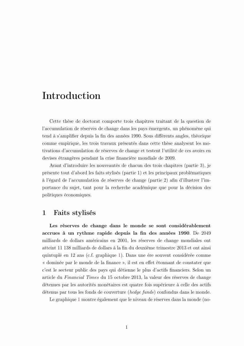
Les réserves de change dans le monde se sont considérablement
accrues à un rythme rapide depuis la fin des années 1990. De 2049
milliards de dollars américains en 2001, les réserves de change mondiales ont
atteint 11 138 milliards de dollars à la fin du deuxième trimestre 2013 et ont ainsi
quintuplé en 12 ans (c.f. graphique 1). Dans une ère souvent considérée comme
« dominée par le monde de la finance », il est en effet étonnant de constater que
c’est le secteur public des pays qui détienne le plus d’actifs financiers. Selon un
article du Financial Times du 15 octobre 2013, la valeur des réserves de change
détenues par les autorités monétaires est quatre fois supérieure à celle des actifs
détenus par tous les fonds de couverture (hedge funds) confondus dans le monde.
Le graphique 1 montre également que le niveau de réserves dans la monde (no-
1
INTRODUCTION
Figure 1 – Évolution des réserves de change dans le monde
tamment dans les pays en voie de développement) s’est infléchi pendant la crise
financière mondiale de 2009. En effet, comme le soulignent Bianchi et collab.
(2013) et Broner et collab. (2013), l’achat des actifs étrangers par des résidents
nationaux ou par les autorités publiques d’un pays présente une tendance procy-
clique et s’effondre ainsi pendant les crises.
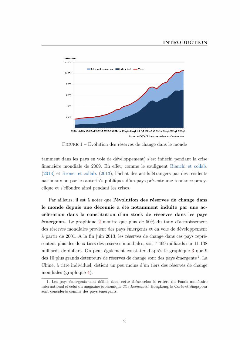
Par ailleurs, il est à noter que l’évolution des réserves de change dans
le monde depuis une décennie a été notamment induite par une ac-
célération dans la constitution d’un stock de réserves dans les pays
émergents. Le graphique 2 montre que plus de 50% du taux d’accroissement
des réserves mondiales provient des pays émergents et en voie de développement
à partir de 2001. A la fin juin 2013, les réserves de change dans ces pays repré-
sentent plus des deux tiers des réserves mondiales, soit 7 469 milliards sur 11 138
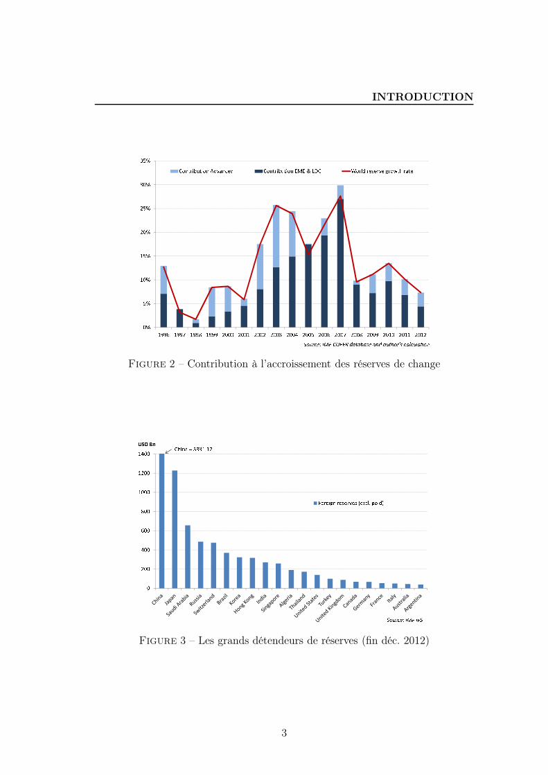
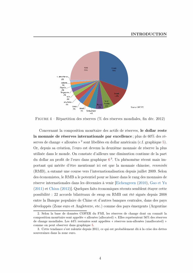
milliards de dollars. On peut également constater d’après le graphique 3 que 9
des 10 plus grands détenteurs de réserves de change sont des pays émergents 1. La
Chine, à titre individuel, détient un peu moins d’un tiers des réserves de change
mondiales (graphique 4).
1. Les pays émergents sont définis dans cette thèse selon le critère du Fonds monétaireinternational et celui du magazine économique The Economist. Hongkong, la Corée et Singapoursont considérés comme des pays émergents.
2
INTRODUCTION
Figure 2 – Contribution à l’accroissement des réserves de change
Figure 3 – Les grands détendeurs de réserves (fin déc. 2012)
3
INTRODUCTION
Figure 4 – Répartition des réserves (% des réserves mondiales, fin déc. 2012)
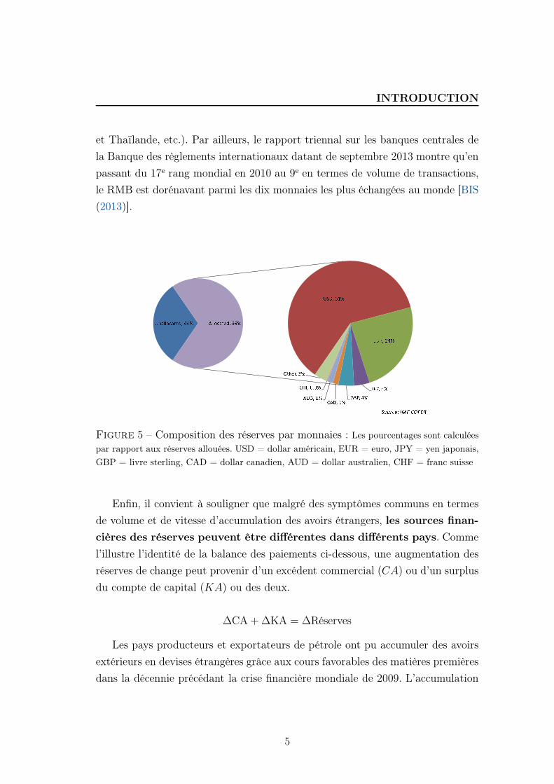
Concernant la composition monétaire des actifs de réserves, le dollar reste
la monnaie de réserves internationale par excellence ; plus de 60% des ré-
serves de change « allouées » 2 sont libellées en dollar américain (c.f. graphique 5).
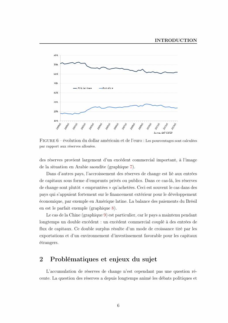
Or, depuis sa création, l’euro est devenu la deuxième monnaie de réserve la plus
utilisée dans le monde. On constate d’ailleurs une diminution continue de la part
du dollar au profit de l’euro dans graphique 6 3. Un phénomène récent mais im-
portant qui mérite d’être mentionné ici est que la monnaie chinoise, renminbi
(RMB), a entamé une course vers l’internationalisation depuis juillet 2009. Selon
des économistes, le RMB a le potentiel pour se hisser dans le rang des monnaies de
réserve internationales dans les décennies à venir [Eichengreen (2010), Gao et Yu
(2011) et Chinn (2012)]. Quelques faits économiques récents semblent étayer cette
possibilité : 22 accords bilatéraux de swap en RMB ont été signés depuis 2008
entre la Banque populaire de Chine et d’autres banques centrales, dans des pays
développés (Zone euro et Angleterre, etc.) comme des pays émergents (Argentine
2. Selon la base de données COFER du FMI, les réserves de change dont on connaît lacomposition monétaire sont appelée « allouées (allocated) ». Elles représentent 56% des réservesde change mondiales. Les 44% restantes sont appelées « réserves non-allouées (unallocated) »comme on peut observer dans graphique 5.
3. Cette tendance s’est ralentie depuis 2011, ce qui est probablement dû à la crise des dettessouveraines dans la zone euro.
4
INTRODUCTION
et Thaïlande, etc.). Par ailleurs, le rapport triennal sur les banques centrales de
la Banque des règlements internationaux datant de septembre 2013 montre qu’en
passant du 17e rang mondial en 2010 au 9e en termes de volume de transactions,
le RMB est dorénavant parmi les dix monnaies les plus échangées au monde [BIS
(2013)].
Figure 5 – Composition des réserves par monnaies : Les pourcentages sont calculées
par rapport aux réserves allouées. USD = dollar américain, EUR = euro, JPY = yen japonais,
GBP = livre sterling, CAD = dollar canadien, AUD = dollar australien, CHF = franc suisse
Enfin, il convient à souligner que malgré des symptômes communs en termes
de volume et de vitesse d’accumulation des avoirs étrangers, les sources finan-
cières des réserves peuvent être différentes dans différents pays. Comme
l’illustre l’identité de la balance des paiements ci-dessous, une augmentation des
réserves de change peut provenir d’un excédent commercial (CA) ou d’un surplus
du compte de capital (KA) ou des deux.
∆CA +∆KA = ∆Réserves
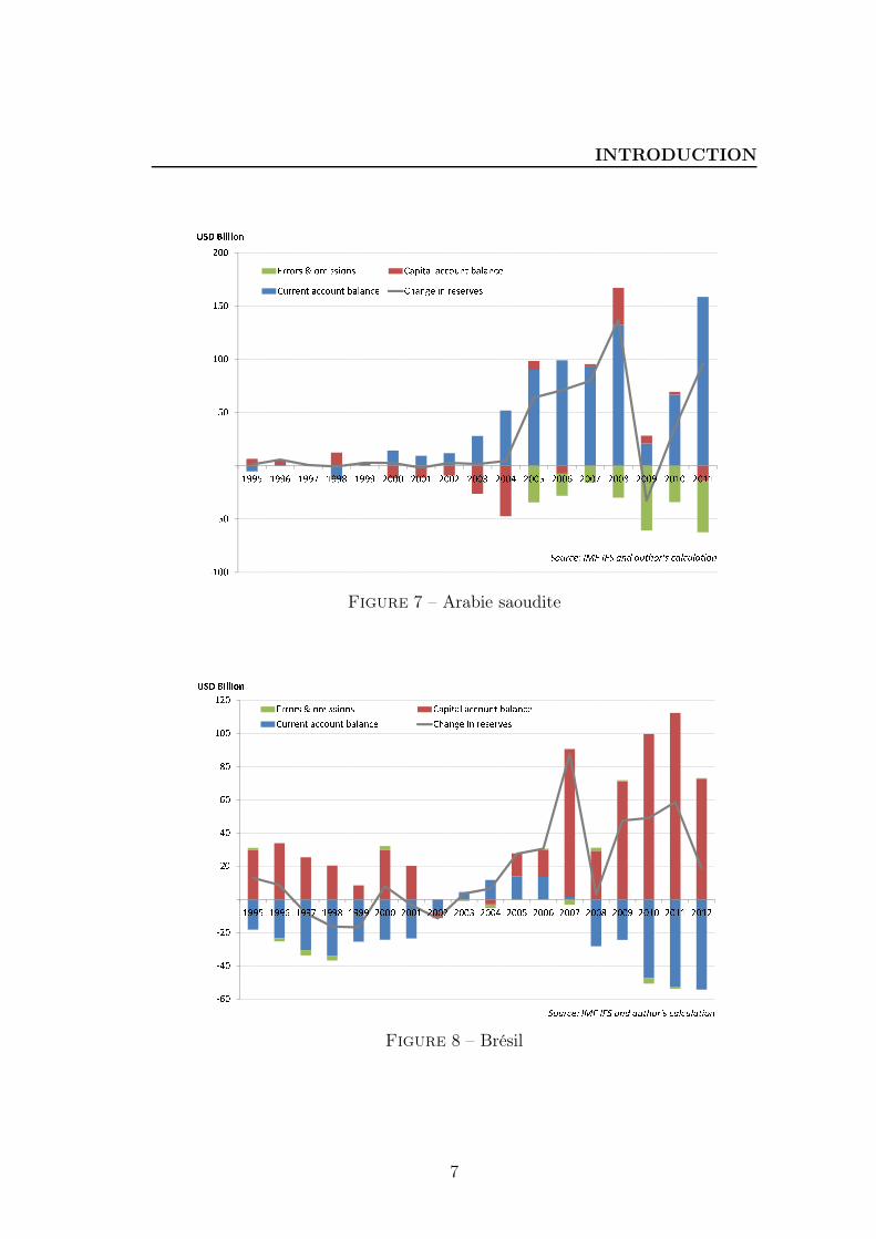
Les pays producteurs et exportateurs de pétrole ont pu accumuler des avoirs
extérieurs en devises étrangères grâce aux cours favorables des matières premières
dans la décennie précédant la crise financière mondiale de 2009. L’accumulation
5
INTRODUCTION
Figure 6 – évolution du dollar américain et de l’euro : Les pourcentages sont calculées
par rapport aux réserves allouées.
des réserves provient largement d’un excédent commercial important, à l’image
de la situation en Arabie saoudite (graphique 7).
Dans d’autres pays, l’accroissement des réserves de change est lié aux entrées
de capitaux sous forme d’emprunts privés ou publics. Dans ce cas-là, les réserves
de change sont plutôt « empruntées » qu’achetées. Ceci est souvent le cas dans des
pays qui s’appuient fortement sur le financement extérieur pour le développement
économique, par exemple en Amérique latine. La balance des paiements du Brésil
en est le parfait exemple (graphique 8).
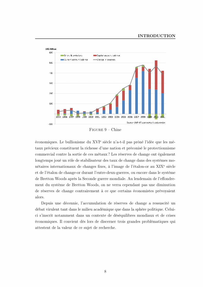
Le cas de la Chine (graphique 9) est particulier, car le pays a maintenu pendant
longtemps un double excédent : un excédent commercial couplé à des entrées de
flux de capitaux. Ce double surplus résulte d’un mode de croissance tiré par les
exportations et d’un environnement d’investissement favorable pour les capitaux
étrangers.
2 Problématiques et enjeux du sujet
L’accumulation de réserves de change n’est cependant pas une question ré-
cente. La question des réserves a depuis longtemps animé les débats politiques et
6
INTRODUCTION
Figure 7 – Arabie saoudite
Figure 8 – Brésil
7
INTRODUCTION
Figure 9 – Chine
économiques. Le bullionisme du XVIe siècle n’a-t-il pas prôné l’idée que les mé-
taux précieux constituent la richesse d’une nation et préconisé le protectionnisme
commercial contre la sortie de ces métaux ? Les réserves de change ont également
longtemps joué un rôle de stabilisateur des taux de change dans des systèmes mo-
nétaires internationaux de changes fixes, à l’image de l’étalon-or au XIXe siècle
et de l’étalon de change-or durant l’entre-deux-guerres, ou encore dans le système
de Bretton Woods après la Seconde guerre mondiale. Au lendemain de l’effondre-
ment du système de Bretton Woods, on ne verra cependant pas une diminution
de réserves de change contrairement à ce que certains économistes prévoyaient
alors.
Depuis une décennie, l’accumulation de réserves de change a ressuscité un
débat virulent tant dans le milieu académique que dans la sphère politique. Celui-
ci s’inscrit notamment dans un contexte de déséquilibres mondiaux et de crises
économiques. Il convient dès lors de discerner trois grandes problématiques qui
attestent de la valeur de ce sujet de recherche.
8
INTRODUCTION
Pour quelles raisons les réserves de change sont-elles néces-
saires dans un monde qui est de plus en plus intégré finan-
cièrement ?
L’accumulation de réserves de change est un phénomène aux multiples facettes
dont les motivations peuvent être multiples. Le Fonds monétaire international
(FMI) définit cinq grands objectifs dans le management des réserves de change
[IMF (2013)] :
– « Susciter et maintenir la confiance dans la politique monétaire et la poli-
tique de change en assurant la capacité à effectuer des interventions sur le
marché des changes » ;
– « Limiter la vulnérabilité externe par le maintien des liquidités en devises
étrangères afin d’absorber les chocs en temps de crise ou lorsque l’accès au
financement extérieur est restreint » ;
– « Donner aux marchés l’assurance que le pays est en mesure de remplir ses
obligations extérieures » ;
– « Démontrer le soutien à la monnaie nationale par des avoirs extérieurs de
réserve ; et aider le gouvernement à satisfaire à son besoin de financement
en devises étrangères et à s’acquitter de ses dettes extérieure » ;
– « Maintenir des réserves en cas de catastrophes ou d’urgences nationales ».
En fonction de ces objectifs, la motivation première pour avoir suffisamment
d’actifs liquides en devises étrangères dans un pays est d’assurer la liquidité en
cas de crise de balance des paiements ou de revirement des capitaux étrangers. Il
s’agit de la motivation de précaution. Un stock de réserves suffisant pourrait
garantir le paiement des importations ou le financement du secteur privé dans
le cas où aucun financement extérieur n’est possible. Les pays asiatiques, comme
Thaïlande et Indonésie, ont ainsi fortement augmenté leurs réserves de change
dans le sillage de la crise asiatique de 1997-1998. Cette « auto-assurance » permet
également aux pays de ne pas recourir à un renflouement par le FMI, souvent
considéré comme très contraignant. Le rôle d’assurance des réserves pourrait aussi
être envisagé comme un élément de dissuasion contre les attaques spéculatives.
Un niveau de réserves suffisant réduit la probabilité d’un revirement des flux
9
INTRODUCTION
de capitaux étrangers [Jeanne et Rancière (2011)] ou d’une attaque spéculative
contre la monnaie locale [Krugman (1999)]. Le deuxième et troisième chapitres
de cette thèse abordent en effet ce pouvoir dissuasif des réserves de change sous
deux différents angles.
Selon d’autres économistes [Dooley et collab. (2003)], l’achat des réserves
pourrait également être incité par une stratégie de croissance liée à un com-
merce extérieur excédentaire. Dans cette perspective, les réserves de change sont
accumulées pour déprécier la monnaie locale afin de soutenir les exportations. La
détention des réserves de change pourrait être ainsi considérée comme une forme
déguisée de subvention au secteur exportateur [Jeanne (2012)]. Cette motivation
d’accumulation de réserves est souvent appelée motivation néo-mercantiliste.
Si accumuler des réserves de change génère un coût financier à court terme, le pays
pourra bénéficier des gains de productivité à travers les exportations (« learning
by exporting ») à long terme [Korinek et Serven (2010)].
Enfin, outre les objectifs définis par le FMI, l’accumulation de réserves
pourrait aussi provenir d’un écart entre l’épargne et l’investissement
au sein d’une économie. Comme l’équation ci-dessous le montre, dans une éco-
nomie où les flux de capitaux privés sont contrôlés (c’est-à-dire les résidents ne
peuvent pas investir facilement à l’étranger ou vice versa pour les non-résidents),
l’écart entre l’épargne (S) et l’investissement (I) se traduit par une augmentation
du niveau de réserves de change. Autrement dit, l’excédent de l’épargne natio-
nale est exporté à l’étranger. Dans cette perspective, l’accumulation de réserves
de change est liée aux motifs qui sont à l’origine d’une abondante épargne dans
certains pays émergents et au mécanisme selon lequel l’épargne privée se retrouve
dans les bilans des banques centrales. Ce mécanisme a été exploré dans la littéra-
ture par Caballero et collab. (2008), Dominguez (2010), Bénassy-Quéré et collab.
(2011), Song et collab. (2011), Wen (2011) and Bacchetta et collab. (2013) etc. Le
premier chapitre de cette thèse propose une nouvelle lecture de ce mécanisme en
mettant en avant l’interaction entre un marché financier national sous-développé
et un taux de croissance économique élevé basé sur l’investissement du capital.
10
INTRODUCTION
∆Réserves = ∆CA +∆KA
= ∆CA
= ∆S −∆I
De récentes études empiriques [Delatte et Fouquau (2012) et Ghosh et collab.
(2012)] montrent clairement la multiplicité des motifs derrière l’accumulation de
réserves de change et l’évolution de leur poids relatif dans le temps. Delatte et
Fouquau (2012) trouvent que la motivation néo-mercantiliste devient plus im-
portante après 2000 tandis que Ghosh et collab. (2012) mettent en avant une
évolution en faveur des déterminants de la demande des réserves liés au compte
de capital (risques de revirement de capitaux et ouverture financière etc.).
Les réserves de change sont-elles « excédentaires » ?
Une seconde problématique est de savoir si le niveau de réserves observé dans
un bon nombre de pays émergents est excessif.
Pour répondre à cette question, il faut définir le niveau optimal de réserves
selon différentes approches. Issus d’une littérature qui date des années 1970 4,
plusieurs ratios d’adéquation de réserves de change ont été développés et par
ailleurs souvent utilisés dans la prise de décision politique en matière de réserves
de change. Dans une perspective d’équilibre de la balance des paiements, le niveau
des réserves de change doit couvrir trois mois d’importation. Avec l’intégration
financière des pays en voie de développement, notamment suite à des événements
de tarissement de flux de capitaux étrangers [« sudden Stops », terme défini par
Calvo (1998)], la règle « Greenspan-Guidotti » recommande que les réserves de
change couvrent l’intégralité de la dette extérieure à court terme afin d’assurer
la capacité de remboursement à court-terme des pays en crises. Plus récemment,
s’inscrivant dans une idée de crise de change déclenchée par une ruée vers les
devises étrangères fortes, Obstfeld et collab. (2010) recommandent de calculer
le ratio de réserves de change sur l’agrégat monétaire M2 comme un facteur
4. c.f. Heller (1966), Clark (1970b) and Clark (1970a), etc. Bahmani-Oskooee et Brown(2002) présentent une synthèse de cette littérature historique.
11
INTRODUCTION
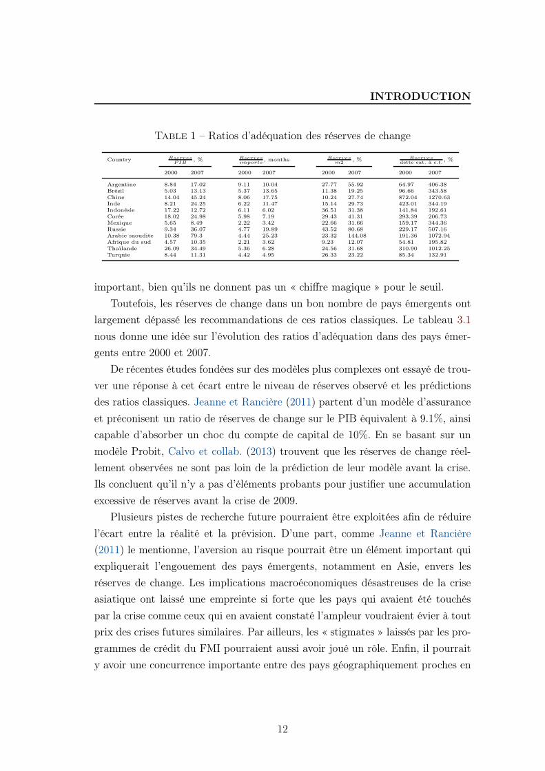
Table 1 – Ratios d’adéquation des réserves de change
Country RservesPIB
, % Rservesimports
, months Rservesm2
, % Rservesdette ext. à c.t.
, %
2000 2007 2000 2007 2000 2007 2000 2007
Argentine 8.84 17.02 9.11 10.04 27.77 55.92 64.97 406.38Brésil 5.03 13.13 5.37 13.65 11.38 19.25 96.66 343.58Chine 14.04 45.24 8.06 17.75 10.24 27.74 872.04 1270.63Inde 8.21 24.25 6.22 11.47 15.14 29.73 423.01 344.19Indonésie 17.22 12.72 6.11 6.02 36.51 31.38 141.84 192.61Corée 18.02 24.98 5.98 7.19 29.43 41.31 293.39 206.73Mexique 5.65 8.49 2.22 3.42 22.66 31.66 159.17 344.36Russie 9.34 36.07 4.77 19.89 43.52 80.68 229.17 507.16Arabie saoudite 10.38 79.3 4.44 25.23 23.32 144.08 191.36 1072.94Afrique du sud 4.57 10.35 2.21 3.62 9.23 12.07 54.81 195.82Thaïlande 26.09 34.49 5.36 6.28 24.56 31.68 310.90 1012.25Turquie 8.44 11.31 4.42 4.95 26.33 23.22 85.34 132.91
important, bien qu’ils ne donnent pas un « chiffre magique » pour le seuil.
Toutefois, les réserves de change dans un bon nombre de pays émergents ont
largement dépassé les recommandations de ces ratios classiques. Le tableau 3.1
nous donne une idée sur l’évolution des ratios d’adéquation dans des pays émer-
gents entre 2000 et 2007.
De récentes études fondées sur des modèles plus complexes ont essayé de trou-
ver une réponse à cet écart entre le niveau de réserves observé et les prédictions
des ratios classiques. Jeanne et Rancière (2011) partent d’un modèle d’assurance
et préconisent un ratio de réserves de change sur le PIB équivalent à 9.1%, ainsi
capable d’absorber un choc du compte de capital de 10%. En se basant sur un
modèle Probit, Calvo et collab. (2013) trouvent que les réserves de change réel-
lement observées ne sont pas loin de la prédiction de leur modèle avant la crise.
Ils concluent qu’il n’y a pas d’éléments probants pour justifier une accumulation
excessive de réserves avant la crise de 2009.
Plusieurs pistes de recherche future pourraient être exploitées afin de réduire
l’écart entre la réalité et la prévision. D’une part, comme Jeanne et Rancière
(2011) le mentionne, l’aversion au risque pourrait être un élément important qui
expliquerait l’engouement des pays émergents, notamment en Asie, envers les
réserves de change. Les implications macroéconomiques désastreuses de la crise
asiatique ont laissé une empreinte si forte que les pays qui avaient été touchés
par la crise comme ceux qui en avaient constaté l’ampleur voudraient évier à tout
prix des crises futures similaires. Par ailleurs, les « stigmates » laissés par les pro-
grammes de crédit du FMI pourraient aussi avoir joué un rôle. Enfin, il pourrait
y avoir une concurrence importante entre des pays géographiquement proches en
12
INTRODUCTION
termes d’accumulation de réserves. Cette émulation pourrait être incitée par un
grand besoin de financement extérieur 5 [le cas dans des pays de l’Amérique la-
tine ; c.f. Cheung et Sengupta (2011)] ou par un besoin de maintenir un taux de
change faible 6 (le cas des pays asiatiques).
Enfin, si l’excédent des réserves de change est confirmé, il faut trouver des
moyens pour réduire le niveau de réserves de change dans des pays émergents.
Une réponse possible serait de déterminer des alternatives aux réserves de change.
Sous l’angle dit « de précaution », par exemple, est-il possible de remplacer une
auto-assurance par un filet de sécurité global (« global safety net » à l’image des
lignes de crédit du FMI) ou/et par les filets de sécurité régionaux (« regional safety
net », tels que l’Initiative de Chiang Mai (CMI) ou le Fonds de stabilité européen
(ESM)). Pour réduire la partie de réserves liées à la motivation mercantiliste, il
faut que les pays en excédent commercial réorientent leur mode de croissance vers
la consommation interne plutôt que la demande extérieure.
L’accumulation des réserves de change alimente-t-elle les
déséquilibres mondiaux ?
L’accumulation de réserves de change n’est pas un phénomène qui se confine
uniquement à l’intérieur des frontières d’un pays. Elle constitue une question
d’envergure internationale en raison de ses retombées sur le niveau des taux d’in-
térêt, la croissance économique et la stabilité économique et financière à l’échelle
mondiale.
Tout d’abord, selon la théorie de l’« excès d’épargne mondiale » [« global sa-
ving glut », théorie développée par Bernanke (2005)], la capacité des États-Unis
à financer le déficit de leur balance des paiements courants a été favorisée par les
achats massifs d’obligations du Trésor américain et de titres d’agences américaines
par des banques centrales des pays émergents sous forme de réserves de change.
Autrement dit, une accumulation de réserves de change dans des pays émergents
5. Les réserves de change pourraient être considérées comme une assurance sur la capacitéde remboursement vis-à-vis des investisseurs étrangers. Pour arbitrer entre deux destinationsde perspective économique similaire, les investisseurs pourraient préférer celle qui s’avère plusrobuste financièrement avec un niveau de réserves élevé.
6. Cette émulation est justifiée par la volonté de déprécier la monnaie locale afin de favoriserune croissance tirée par exportations.
13
INTRODUCTION
ont comme conséquence (volontaire ou involontaire) de déprécier la monnaie lo-
cale et d’engendrer ainsi un excédent commercial persistent. En contrepartie, le
surplus de la balance commerciale dans les pays émergents et en voie de dévelop-
pement est compensé par le déficit commercial des pays industrialisés.
Par ailleurs, l’achat massif des titres gouvernementaux américains par des
pays émergents fait baisser le rendement de ces titres publics, c’est-à-dire le taux
d’intérêt mondial à long-terme 7. Autrement dit, la politique monétaire accommo-
dante aux États-Unis avant la crise des subprimes aurait été financée par des pays
émergents. En effet, selon Bernanke (2005), « [c]ette offre grandissante d’épargne
[internationale] a fait prospéré les valeurs des actions américaines pendant l’eu-
phorie du marché boursier et a aidé à accroître la valeur des immobiliers dans
une plus récente période. Ainsi, l’épargne nationale aux États-Unis diminue et le
déficit commercial du pays se creuse. » Sous cet angle, l’accumulation de réserves
de change contribue directement à l’éclatement de la crise financière mondiale de
2009 car cette dernière partagent « des causes communes » avec les déséquilibres
mondiaux avant la crise [Obstfeld et Rogoff (2009)].
Enfin, dans une perspective de croissance incertaine dans des pays avancés et
de ralentissement économique dans des pays émergents, une émulation en termes
d’accumulation des réserves entre pays, notamment incitée par des intérêts dans
le commerce international, pourrait entrainer une guerre des monnaies et une spi-
rale protectionniste dans le monde. Dès 2008, Aizenman (2008) a mis en exergue
ce risque : « dans un monde où des économies émergentes symétriques se font
concurrence sur des secteurs d’activité comparables, l’accumulation compétitive
[de réserves] tend à annuler l’essentiel des gains de compétitivité, entraînant l’ap-
pauvrissement de ces économies ».
7. Les taux de rendement des bons du Trésor américains servent souvent de taux directeursans risque à long-terme.
14
INTRODUCTION
3 Contribution de la thèse
Chapitre 1
Le premier chapitre de cette thèse 8 est une véritable contribution à la littéra-
ture traitant de la relation entre les réserves de change et l’écart entre l’épargne et
l’investissement dans une économie en forte croissance. En comparaison avec des
articles considérant que les réserves sont un résidu de la politique de change dans
une économie où le coût de stérilisation reste faible, cette étude soutient la thèse
que la banque centrale dans un pays en voie de développement peut avoir une
politique de réserves optimale dans le but d’accélérer le rattrapage économique.
En effet, l’accumulation de réserves résulte de l’interaction entre une forte crois-
sance de la productivité et des frictions sur le marché financier qui restreignent le
financement des investissements dans le capital physique. En effet, lorsqu’un pays
connaît des chocs positifs sur le taux de croissance des productivités, les entre-
prises sont incitées à investir dans le capital dont le produit marginal augmente
avec les gains des productivités. En revanche, la capacité des firmes à financer
de nouveaux investissements est limitée par leur capacité d’endettement à cause
des frictions sur le marché financier national. Face à ces frictions financières, les
autorités publiques, en l’occurrence la banque centrale, peuvent fournir des titres
publics avec lesquels les entreprises peuvent épargner davantage. Ce qui a comme
conséquence de réduire les frictions du marché financier liées aux contraintes de
crédit. Dans une économie où il y a un réel manque d’actifs financiers nationaux,
la banque centrale ne peux compenser l’émission des titres publiques nationaux
par une augmentation des ses avoirs en devises étrangères.
Par ailleurs, ce chapitre de thèse entend définir les conditions dans lesquelles
une accumulation de réserves de change issue du mécanisme décrit au-dessus peut
être une politique optimale en termes de bien-être social. A l’aide d’un problème
de Ramsey, il est prouvé que l’accumulation de réserves de change est d’autant
plus efficace que les flux de capitaux privés sont contrôlés, c’est-à-dire, une éco-
nomie avec des contrôles de capitaux est plus efficace qu’une économie financiè-
rement ouverte pour atteindre l’état stationnaire de long terme. Deux raisons
8. L’article de recherche sur lequel est basé ce premier chapitre de thèse a été accepté pourpublication dans Macroeconomic Dynamics, numéro de juillet 2014.
15
INTRODUCTION
justifient ce résultat. Premièrement, la banque centrale, en tant que représentant
de l’économie nationale, peut obtenir autant de financements étrangers qu’une
économie financièrement ouverte. En second lieu, le compte de capital étant fermé
pour le secteur privé, la banque centrale garde la mainmise sur les taux d’intérêt
nationaux car les agents privés ne peuvent se contenter que des titres publics
nationaux dont les taux d’intérêt sont fixés par l’état. En conséquence, la banque
centrale pourrait ajuster les taux d’intérêt nationaux à la hausse face à un choc
de productivité temporaire afin d’inciter les agents privés à épargner davantage
et à investir plus dans le stock de capital par la suite.
Ce chapitre met en avant trois résultats dont la portée politique est particu-
lièrement intéressante. Tout d’abord, selon cette approche que j’analyse, l’accu-
mulation de réserves de change est un phénomène propre aux pays en phase de
rattrapage économique. Même sans tenir compte des préoccupations de change
ou d’assurance, les autorités monétaires de ces pays peuvent être amenés à ache-
ter des réserves pour répondre aux chocs de productivité positifs et à la capacité
insuffisante du secteur privé à s’endetter. De surcroît, pendant la phase de transi-
tion, l’accumulation de réserves de change, combinée à des contrôles de capitaux
sur les flux privés constitue une politique optimale en termes de bien-être so-
cial. Cette politique conjointe permet en effet non seulement à l’économie tout
entière d’avoir suffisamment de ressources financières par rapport à une écono-
mie financièrement ouverte, mais aussi d’ajuster les taux d’intérêt nationaux si
besoin. Enfin, l’utilisation de contrôles de capitaux et de réserves n’a de réelles
conséquences que temporaires ; les gains du bien-être issus d’une utilisation com-
binée de réserves et de contrôles de capitaux diminuent avec le développement
des marchés financiers. Dès lors qu’il n’y a plus de contraintes financières, il suffit
d’ouvrir complètement le compte de capital afin que l’économie atteigne l’équi-
libre du « first-best ». Ainsi, l’accumulation de réserves de change et l’utilisation
des contrôles sur les flux de capitaux ne doivent pas empêcher les réformes struc-
turelles nécessaires sur le marché financier national.
16
INTRODUCTION
Chapitre 2
De nature empirique, ce chapitre 9 propose une analyse du rôle d’assurance
des réserves de change pendant la crise financière mondiale de 2009. Malgré une
riche littérature théorique soulignant la motivation de précaution, la littérature
empirique n’a pas trouvé de résultats univoques à l’égard du rôle des réserves
pendant la dernière crise financière mondiale.
A l’aide d’une base de données comprenant 112 pays émergents et en voie
de développement, ce travail examine d’abord la relation entre l’accumulation de
réserves avant la crise et la performance économique pendant la crise, à savoir si
les pays qui avaient accumulé plus de réserves de change se sont mieux sortis de
la crise. La performance économique d’un pays se mesure par la perte de niveau
de Produit Intérieur Brut (PIB) par rapport à une moyenne historique ou à un
niveau de PIB contrefactuel (si la crise n’avait pas eu lieu). Un aspect particu-
lier qui est analysé dans cette étude est l’interaction entre le niveau de réserves
de change et les contrôles de capitaux. Dans la littérature en macroéconomie et
finance internationales, les réserves de change et les contrôles de capitaux sont
considérés tantôt comme des substituts, tantôt comme des compléments. En ef-
fet, un pays dont le compte de capital est ouvert s’expose plus à la volatilité des
flux de capitaux étrangers et est ainsi incité à accumuler plus de réserves pour se
prémunir contre des revirements des capitaux étrangers. Dans cette perspective,
les contrôles de capitaux et les réserves de change peuvent être considérés comme
des substituts ces deux politiques réduisant le risque lié à la volatilité des ca-
pitaux étrangers. Or, ces deux instruments peuvent aussi être complémentaires,
comme le souligne ce chapitre de thèse. Autrement dit, leur effet marginal sur la
croissance se renforce mutuellement : les réserves de change sont d’autant plus
efficaces comme moyen d’assurance que le compte de capital est fermé. Enfin, par
rapport à la littérature empirique sur les réserves de change, notre étude instru-
ment les réserves de changes, car ces dernières pourraient avoir un effet sur la
croissance via des variables omises (« biais de variables omises »). Il est possible
qu’un pays qui est structurellement vulnérable (par exemple, à cause d’institu-
9. Ce chapitre fait partie d’un travail de recherche en collaboration avec Matthieu Bussière(Banque de France), Menzie Chinn (Université de Wisconsin, Madison) et Noëmie Lisack (Ins-titut universitaire européen). Il est publié en tant que document de travail du NBER WP19791.
17
INTRODUCTION
tions inadéquates) accumule plus de réserves de change par anticipation. Dans
ce cas-là, des régressions estimées par la méthode des moindres carrés génèrent
des résultats biaisés. Pour corriger ce problème, ce chapitre propose plusieurs
variables instrumentales potentielles.
Trois résultats sur le rôle des réserves pendant la crise peuvent être dégagés
de cette étude. Tout d’abord, lorsque le ratio d’adéquation de réserves de change
est calculé en point de pourcentage par rapport à la dette extérieure à court-
terme, la performance économique d’un pays pendant la crise est positivement
corrélée avec les réserves de change d’avant la crise. Ce résultat reste robuste
même si on change la définition de la performance économique, utilise différents
sous-échantillons ou rajoute d’autres variables de contrôle. Il suggère également
que la dette extérieure à court terme pourrait être un objectif sous-jacent qu’un
État peut avoir à l’esprit lors d’une prise de décision sur la politique de réserves.
On observe également que le coefficient de régression illustrant l’interaction entre
les réserves de change et les contrôles de capitaux est significatif. Autrement dit,
l’effet de réserves de change sur la performance économique d’un pays dépend de
l’ouverture financière de celui-ci : un pays ayant un compte de capital moins ou-
vert voit l’effet marginal des réserves augmenter. Il est à noter que l’effet marginal
des réserves (pondérées par la dette extérieure à court terme) se renforce lorsque
l’on élimine les observations « aberrantes » 10 et les petits pays. Enfin, cette étude
essaie d’apporter une réponse à un débat récent : les réserves de change doivent-
elles être réellement déployées pour jouer le rôle d’assurance ? En effet, il se peut
que l’utilisation des réserves pendant la crise (pour défendre la monnaie locale)
atténue le détresse économique ou que l’existence même d’un stock régulateur
décourage les attaques spéculative. Ce chapitre est en faveur du pouvoir dissuasif
des réserves. Il montre que si une variable indicatrice de l’utilisation de réserves
est ajoutée à la régression le ratio de réserves sur la dette extérieure à court
terme d’avant la crise reste statistiquement significative tandis que la variable
indicatrice ne l’est pas.
En outre, grâce à des données récentes après la crise, ce chapitre met en
avant les nouvelles tendances dans le comportement d’accumulation des réserves
de change que l’on peut observer dans un bon nombre de pays. D’une part,
10. Définies en détails dans le chapitre en question.
18
INTRODUCTION
les pays qui avaient largement utilisé des réserves de change pendant la crise
financière de 2009 en ont reconstitué un stock dès leur sortie de crise. D’autre part,
la vitesse d’accumulation des réserves s’est ralentie depuis deux ans. Plusieurs
facteurs pourraient être à l’origine de cette évolution. Basé sur un modèle à
correction d’erreur (VECM), cette étude montre que cette récente décélération
dans l’accumulation des réserves est corrélée avec la stabilisation du niveau de la
dette extérieure à court terme. Cette dernière étant une variable d’objectif que
les réserves doivent entièrement couvrir afin d’éviter des risques liés à la volatilité
des flux de capitaux étrangers.
Chapitre 3
Le troisième chapitre revient sur un facteur déstabilisateur qui a lourdement
affecté les pays émergents pendant les crises de la fin des années 1990 et qui est
beaucoup moins étudié dans le contexte de la crise financière de 2009 : l’asymétrie
de devises dans le passif et l’actif du bilan (« currency mismatch ») et l’effet
d’une dépréciation sur les bilans du secteur privé (« balance sheet effect ») qui en
résulte. En effet, si le secteur privé s’expose à la dette extérieure libellée en devises
étrangères, une dépréciation de la monnaie locale, anticipée ou réalisée, accroîtra
le passif du bilan du secteur privé et entraînera une insolvabilité de ce secteur,
ce qui déclenchera par la suite une sortie de capitaux étrangers qui confirmera
une fois de plus la pression baissière sur le cours de change. Ainsi, comme le
montre Krugman (1999), deux équilibres de marché peuvent exister : un équilibre
défavorable caractérisé par une dépréciation importante de la monnaie locale et
un niveau d’investissement faible ; un équilibre favorable avec un taux de change
apprécié et un niveau d’investissement élevé.
Le travail effectué dans ce chapitre de thèse montre qu’en accumulant des
réserves de change, le gouvernement est en mesure d’améliorer les anticipations
des investisseurs et d’éliminer l’équilibre défavorable. D’une part, le gouverne-
ment peut promettre une recapitalisation du secteur privé en réduisant la dette
extérieure de ce dernier ou s’endetter auprès des investisseurs étrangers pour le
secteur privé national. Pour ce faire, le gouvernement doit avoir un stock suffisant
d’actifs libellés en devises étrangères. Hormis pour des raisons dites de « précau-
19
INTRODUCTION
tion », la valeur en monnaie locale des réserves de change augmente dans le cas où
la monnaie locale subit une pression de dépréciation. Ainsi, une perte de richesse
du secteur privé en cas de choc négatif sera compensée par une augmentation de
la valeur des actifs étrangers détenus par le gouvernement. L’équilibre défavorable
est ainsi écarté du fait que la richesse du secteur privé est garantie par le gou-
vernement en cas de choc. Les réserves de change peuvent ainsi être considérées
comme une forme d’assurance contingente dépendant du taux de change.
D’autre part, le gouvernement peut également mener une politique de relance
fiscale afin d’accroître la demande des biens produits à l’intérieur du pays, ce qui
apprécie le taux de change, réduit la charge financière des entreprises et garantit
leur richesse qui sert de collatéral pour le financement des entreprises.
En termes de ressources utilisées, ce travail montre que la politique de reca-
pitalisation demande moins de réserves que la politique de relance budgétaire.
En effet, la politique de recapitalisation change les anticipations des investisseurs
tandis que la politique de relance budgétaire doit réellement changer le taux de
change afin d’assurer la capacité de financement des entreprises.
20
BIBLIOGRAPHIE
Bibliographie
Aizenman, J. 2008, «Large hoarding of international reserves and the emerging glo-
bal economic architecture», The Manchester School, vol. 76, no 5, p. 487–503. URL
http://ideas.repec.org/a/bla/manchs/v76y2008i5p487-503.html.
Bacchetta, P., K. Benhima et Y. Kalantzis. 2013, «Capital controls with international reserve
accumulation : Can this be optimal ?», American Economic Journal : Macroeconomics, vol. 5,
no 3, p. 229–62. URL http://ideas.repec.org/a/aea/aejmac/v5y2013i3p229-62.html.
Bahmani-Oskooee, M. et F. Brown. 2002, «Demand for international reserves :
a review article», Applied Economics, vol. 34, no 10, p. 1209–1226. URL
http://ideas.repec.org/a/taf/applec/v34y2002i10p1209-1226.html.
Bénassy-Quéré, A., B. Carton et L. Gauvin. 2011, «Rebalancing growth in China :
An international perspective», Working Papers 2011-08, CEPII research center. URL
http://ideas.repec.org/p/cii/cepidt/2011-08.html.
Bernanke, B. S. 2005, «The global saving glut and the u.s. current account deficit», cahier de
recherche.
Bianchi, J., J. C. Hatchondo et L. Martinez. 2013, «International reserves and
rollover risk», IMF Working Papers 13/33, International Monetary Fund. URL
http://ideas.repec.org/p/imf/imfwpa/13-33.html.
BIS. 2013, «Triennial central bank survey : Foreign exchange turnover in april 2013», cahier de
recherche, Bank of International Settlements.
Broner, F., T. Didier, A. Erce et S. L. Schmukler. 2013, «Gross capital flows : Dyna-
mics and crises», Journal of Monetary Economics, vol. 60, no 1, p. 113–133. URL
http://ideas.repec.org/a/eee/moneco/v60y2013i1p113-133.html.
Caballero, R. J., E. Farhi et P.-O. Gourinchas. 2008, «An equilibrium model of “global
imbalances” and low interest rates», American Economic Review, vol. 98, no 1. URL
http://ideas.repec.org/p/nbr/nberwo/11996.html.
Calvo, G., A. Izquierdo et R. Loo-Kung. 2013, «Optimal holdings of international re-
serves : Self-insurance against sudden stops», Monetaria, , no 1, p. 1–35. URL
http://ideas.repec.org/a/cml/moneta/vxxxvy2013i1p1-35.html.
Calvo, G. A. 1998, «Capital flows and capital-market crises : The simple econo-
mics of sudden stops», Journal of Applied Economics, vol. 0, p. 35–54. URL
http://ideas.repec.org/a/cem/jaecon/v1y1998n1p35-54.html.
21
BIBLIOGRAPHIE
Cheung, Y.-W. et R. Sengupta. 2011, «Accumulation of reserves and keeping up with the jo-
neses : The case of latam economies», International Review of Economics & Finance, vol. 20,
no 1, p. 19–31. URL http://ideas.repec.org/a/eee/reveco/v20y2011i1p19-31.html.
Chinn, M. 2012, «A note on reserve currencies with special reference to the G20 countries»,
cahier de recherche, University of Wisconsin, Madison.
Clark, P. B. 1970a, «Demand for international reserves : A cross-country analysis», The Cana-
dian Journal of Economics.
Clark, P. B. 1970b, «Optimum international reserves and the speed of ad-
justment», Journal of Political Economy, vol. 78, no 2, p. 356–76. URL
http://ideas.repec.org/a/ucp/jpolec/v78y1970i2p356-76.html.
Delatte, A.-L. et J. Fouquau. 2012, «What drove the massive hoarding of
international reserves in emerging economies ? a time-varying approach»,
Review of International Economics, vol. 20, no 1, p. 164–176. URL
http://ideas.repec.org/a/bla/reviec/v20y2012i1p164-176.html.
Dominguez, K. M. E. 2010, «International reserves and underdeveloped capi-
tal markets», dans NBER International Seminar on Macroeconomics 2009,
NBER Chapters, National Bureau of Economic Research, Inc, p. 193–221. URL
http://ideas.repec.org/h/nbr/nberch/11915.html.
Dooley, M., D. Folkerts-Landau et P. M. Garber. 2003, «An essay on the revived Bretton Woods
system», NBER Working Papers 9971, National Bureau of Economic Research.
Eichengreen, B. 2010, «The renminbi as an international currency», cahier de recherche, UC
Berkeley.
Gao, H. et Y. Yu. 2011, «Internationalisation of the renminbi», dans Currency in-
ternationalisation : lessons from the global financial crisis and prospects for the fu-
ture in Asia and the Pacific, BIS Papers chapters, vol. 61, édité par B. for
International Settlements, Bank for International Settlements, p. 105–124. URL
http://ideas.repec.org/h/bis/bisbpc/61-09.html.
Ghosh, A. R., J. D. Ostry et C. G. Tsangarides. 2012, «Shifting motives : Explaining the
buildup in official reserves in emerging markets since the 1980s», IMF Working Papers 12/34,
International Monetary Fund. URL http://ideas.repec.org/p/imf/imfwpa/12-34.html.
Heller, R. 1966, «Optimal international reserves», The Economic Journal, vol. 76, no 302, p.
296–311.
22
BIBLIOGRAPHIE
IMF. 2013, «Revised guidelines for foreign exchange reserve management», cahier de recherche,
International Monetary Fund.
Jeanne, O. 2012, «Capital account policies and the real exchange rate», dans NBER Interna-
tional Seminar on Macroeconomics 2012, NBER Chapters, National Bureau of Economic
Research, Inc. URL http://ideas.repec.org/h/nbr/nberch/12768.html.
Jeanne, O. et R. Rancière. 2011, «The optimal level of international reserves for emerging
market countries : A new formula and some applications», Economic Journal, vol. 121, no
555, p. 905–930.
Korinek, A. et L. Serven. 2010, «Undervaluation through foreign reserve accumulation : Static
losses, dynamic gains», Policy Research Working Paper Series 5250, The World Bank. URL
http://ideas.repec.org/p/wbk/wbrwps/5250.html.
Krugman, P. 1999, «Balance sheets, the transfer problem, and financial crises»,
International Tax and Public Finance, vol. 6, no 4, p. 459–472. URL
http://ideas.repec.org/a/kap/itaxpf/v6y1999i4p459-472.html.
Obstfeld, M. et K. Rogoff. 2009, «Global imbalances and the finan-
cial crisis : products of common causes», Proceedings, p. 131–172. URL
http://ideas.repec.org/a/fip/fedfpr/y2009p131-172.html.
Obstfeld, M., J. C. Shambaugh et A. M. Taylor. 2010, «Financial stability, the trilemma, and
international reserves», American Economic Journal : Macroeconomics, vol. 2, no 2, p. 57–94.
URL http://ideas.repec.org/a/aea/aejmac/v2y2010i2p57-94.html.
Song, Z., K. Storesletten et F. Zilibotti. 2011, «Growing like China»,
American Economic Review, vol. 101, no 1, p. 196–233. URL
http://ideas.repec.org/a/aea/aecrev/v101y2011i1p196-233.html.
Wen, Y. 2011, «Making sense of China’s excessive foreign reserves»,
Working paper series, Federal Reserve Bank of St. Louis. URL
http://ideas.repec.org/p/fip/fedlwp/2011-006.html.
23

Chapter 1
A Growth Perspective on Foreign
Reserve Accumulation
The work presented in this chapter is accepted for publication in Macroeconommic
Dynamics (Cambridge University Press), forthcoming in July 2014.
1.1 Introduction
Since the beginning of the 21st century, the fast accumulation of international
reserves in emerging market economies and developing countries has driven the
world total international reserves to an unprecedented high level. This recent
phenomenon has reignited the debate on the reasons motivating the demand for
reserve assets among academics and policymakers.
Inspired by the situation in China, I propose in this paper a theory of for-
eign reserve accumulation in fast-growing emerging economies. The focal point
of the theory resides in the interaction between productivity growth and financial
frictions, two features commonly observed in emerging market economies. Posi-
tive shocks on productivity growth induce the private sector to invest in capital
while financial frictions constrain the private sector’s borrowing ability. In this
context, domestic capital formation needs to rely on firms’ retained earnings. In
order to push capital formation to its first-best level - defined as the steady state
level without financial frictions - the central bank intervenes by providing the pri-
25
FOREIGN RESERVES AND GROWTH
vate sector with domestic assets which are in turn financed by the central bank’s
investment in foreign reserves. Foreign reserve accumulation is thus motivated
by a strong demand for domestic liquid assets, especially when the domestic fi-
nancial market lacks alternative investment opportunities to absorb the central
bank’s bond proceeds. By comparing with a situation of financial autarky, it is
shown that the central bank’s intervention by channeling external funding to the
domestic economy relaxes the credit constraint and raises the domestic interest
rate. Altogether, this generates higher retained earnings for the private sector
and accelerates domestic capital formation to reach the first-best level.
Using a Ramsey problem, this paper goes one step further to examine condi-
tions under which the central bank’s reserve policy is optimal in terms of social
welfare. In comparison with a financially open economy, an economy where only
the central bank can get access to international financial markets while private
capital flows are controlled is proved to raise social welfare provided binding fi-
nancial constraints. The reason is that with foreign reserve accumulation and
capital controls the central bank can not only channel as much external funding
as in a financially open economy - the central bank is merely a financial interme-
diary between the domestic economy and the rest of the world - it has also the
domestic interest rate under control. As a result, it can increase it to encourage
domestic firms to save more facing positive productivity shocks.
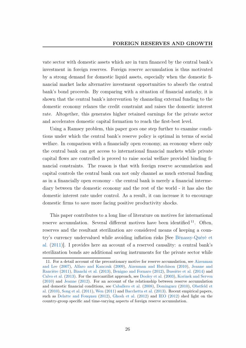
This paper contributes to a long line of literature on motives for international
reserve accumulation. Several different motives have been identified 11. Often,
reserves and the resultant sterilization are considered means of keeping a coun-
try’s currency undervalued while avoiding inflation risks [See Bénassy-Quéré et
al. (2011)]. I provides here an account of a reserved causality: a central bank’s
sterilization bonds are additional saving instruments for the private sector while
11. For a detail account of the precautionary motive for reserve accumulation, see Aizenmanand Lee (2007), Alfaro and Kanczuk (2009), Aizenman and Hutchison (2010), Jeanne andRancière (2011), Bianchi et al. (2013), Benigno and Fornaro (2012), Bussière et al. (2014) andCalvo et al. (2013). For the mercantilist approach, see Dooley et al. (2003), Korinek and Serven(2010) and Jeanne (2012). For an account of the relationship between reserve accumulationand domestic financial conditions, see Caballero et al. (2008), Dominguez (2010), Obstfeld etal. (2010), Song et al. (2011), Wen (2011) and Bacchetta et al. (2013). Recent empirical papers,such as Delatte and Fouquau (2012), Ghosh et al. (2012) and IEO (2012) shed light on thecountry-group specific and time-varying aspects of foreign reserve accumulation.
26

FOREIGN RESERVES AND GROWTH
reserves are the counterpart used to finance these domestic bonds. My paper
complements the strand of the literature arguing that foreign reserves can be ac-
cumulated because of domestic financial frictions. Song et al. (2011), Wen (2011),
Coeurdacier et al. (2012) and Bacchetta and Benhima (2012) have studied this
relationship in a standard open economy setting. They all document that in an
open economy domestic credit frictions generate a wedge between domestic sav-
ings and investment, thus lead to a structural surplus of the balance of payments
and capital outflows. As these models study the open economy, they only focus
on the overall position of net foreign assets of a country; official foreign reserves
held by the country’s monetary authorities and private foreign assets cannot be
discriminated. By introducing capital controls 12, my model focuses on the cen-
tral bank’s reserve assets 13 and allows a scrutiny of its optimal reserve policy.
Moreover, my paper argues that it is through domestic public bond provision
that the central bank, as a financial intermediary, reduces the wedge between do-
mestic savings and investment and transfers external financing into the domestic
economy. This is also a missing aspect in the existing literature.
With respect to a joint analysis of foreign reserve accumulation and capital
controls, this paper is directly comparable with Bacchetta et al. (2013) but differs
in several aspects. First, I nest foreign reserve accumulation in a growth model
so as to examine the relationship between reserve holding and economic growth.
Second, whereas Bacchetta et al. (2013) present an endowment economy, I focus
on the contribution of reserves to domestic capital formation, driver of economic
catch-up in emerging market economies. The introduction of capital is crucial
for three main reasons. It introduces a feedback loop 14 in the credit constraint
12. Benigno and Fornaro (2012) also look at the imperfect substitutability between publicand private flows. Instead of imposing capital controls as this current article does, they chooseto impose an external borrowing constraint on private firms. Also, they study different motivesof reserve accumulation.
13. In this paper, international reserves comprise foreign exchange reserves [‘official claims onnonresidents in the form of foreign banknotes, bank deposits, treasury bills, short- and long-term government securities and other claims usable in the event of balance of payments need’(IFS Yearbook 2012)], reserve position in the Fund, the U.S. dollar value of SDR holdings andgold holdings. As foreign exchange reserves are the major component, I will use ‘internationalreserves’ and ‘foreign (exchange) reserves’ interchangeably.
14. Future output produced with the capital invested today serves as a collateral. Thus, themore capital invested, the less binding the constraint and more capital can be further invested.
27
FOREIGN RESERVES AND GROWTH
and allows a better understanding of how the public intervention relaxes the
constraint facing domestic firms. It also enables me to examine gains from capital
formation instead of redistributive effects and consumption smoothing gains in
the welfare analysis. Ultimately, this makes the model more relevant to fast-
growing economies, such as China. The economic growth in these countries is
largely driven by strong productivity growth and resultant capital accumulation
[see Nelson and Pack (1999), Bond et al. (2010) and Ahuja and Nabar (2012)] 15.
The theory that I develop is also related to the seminal contribution of Wood-
ford (1990) who argues that issuing public bonds promotes domestic capital in-
vestment and is welfare improving when the private sector faces borrowing con-
straints. My paper can be regarded as an extension to Woodford’s framework
in an open economy context with possibilities of imposing capital controls; it ex-
plains how official foreign reserves can be complementary to domestic bonds so
as to ease domestic financial frictions.
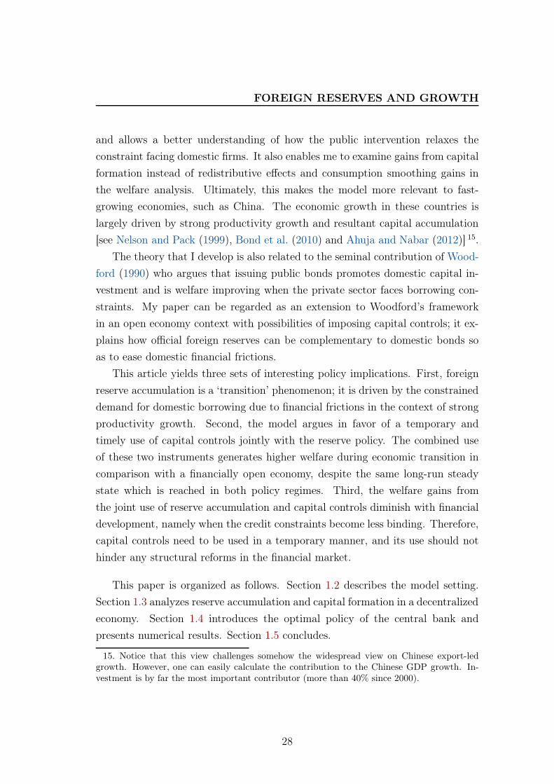
This article yields three sets of interesting policy implications. First, foreign
reserve accumulation is a ‘transition’ phenomenon; it is driven by the constrained
demand for domestic borrowing due to financial frictions in the context of strong
productivity growth. Second, the model argues in favor of a temporary and
timely use of capital controls jointly with the reserve policy. The combined use
of these two instruments generates higher welfare during economic transition in
comparison with a financially open economy, despite the same long-run steady
state which is reached in both policy regimes. Third, the welfare gains from
the joint use of reserve accumulation and capital controls diminish with financial
development, namely when the credit constraints become less binding. Therefore,
capital controls need to be used in a temporary manner, and its use should not
hinder any structural reforms in the financial market.
This paper is organized as follows. Section 1.2 describes the model setting.
Section 1.3 analyzes reserve accumulation and capital formation in a decentralized
economy. Section 1.4 introduces the optimal policy of the central bank and
presents numerical results. Section 1.5 concludes.
15. Notice that this view challenges somehow the widespread view on Chinese export-ledgrowth. However, one can easily calculate the contribution to the Chinese GDP growth. In-vestment is by far the most important contributor (more than 40% since 2000).
28
FOREIGN RESERVES AND GROWTH
1.2 Model setting
The model that I develop is inspired by Bacchetta and Benhima (2012) to
which I explicitly add a central bank 16.
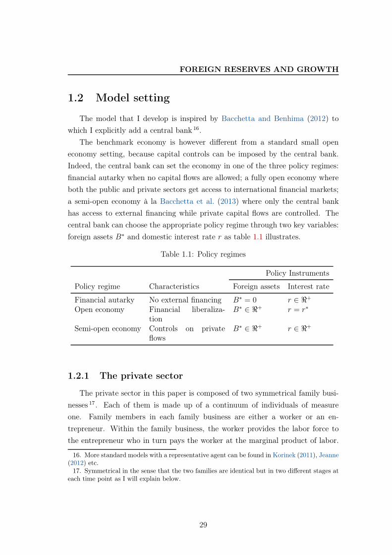
The benchmark economy is however different from a standard small open
economy setting, because capital controls can be imposed by the central bank.
Indeed, the central bank can set the economy in one of the three policy regimes:
financial autarky when no capital flows are allowed; a fully open economy where
both the public and private sectors get access to international financial markets;
a semi-open economy à la Bacchetta et al. (2013) where only the central bank
has access to external financing while private capital flows are controlled. The
central bank can choose the appropriate policy regime through two key variables:
foreign assets B∗ and domestic interest rate r as table 1.1 illustrates.
Table 1.1: Policy regimes
Policy Instruments
Policy regime Characteristics Foreign assets Interest rate
Financial autarky No external financing B∗ = 0 r ∈ ℜ+
Open economy Financial liberaliza-tion
B∗ ∈ ℜ+ r = r∗
Semi-open economy Controls on privateflows
B∗ ∈ ℜ+ r ∈ ℜ+
1.2.1 The private sector
The private sector in this paper is composed of two symmetrical family busi-
nesses 17. Each of them is made up of a continuum of individuals of measure
one. Family members in each family business are either a worker or an en-
trepreneur. Within the family business, the worker provides the labor force to
the entrepreneur who in turn pays the worker at the marginal product of labor.
16. More standard models with a representative agent can be found in Korinek (2011), Jeanne(2012) etc.
17. Symmetrical in the sense that the two families are identical but in two different stages ateach time point as I will explain below.
29
FOREIGN RESERVES AND GROWTH
Importantly, I assume that the family business pools together the incomes of both
family members and optimally makes consumption and investment decisions at
the family level 18. This is a parsimonious way to model households and firms all
combined. The advantage of doing so is twofold: it simplifies the program of the
private sector and renders the Ramsey problem neater; it also allows both the
worker and the entrepreneur to save and to contribute to physical capital invest-
ment, in contrast with Bacchetta and Benhima (2012) where only the corporate
sector is allowed to save (as the worker in their model is ‘hand-to-month’ and
consumes all the labor income every period).
I assume that each family business is infinitely lived and capital is invested
every two periods. As a result, any family produces in one period and invests in
the other and so on so forth; that is, each of the two families changes its status
every two periods, alternating between a ‘producing-saving’ period (denoted S)
and an ‘investing-borrowing’ period (denoted I). The assumption of two sym-
metrical family businesses is to guarantee that in each period there is always one
family in the ‘producing-saving’ stage and the other in the ‘investing-borrowing’
stage, so that there is always a family (‘investing-borrowing’) which faces the
borrowing constraint.
Family businesses’ program
As the family businesses are symmetrical, it is sufficient to look at the program
of one of them. Let’s consider the family who starts at time t in the ‘producing-
saving’ period. It faces a standard intertemporal utility function with a discount
factor β:
∞∑
t=0
βt[U(cSt ) + βU(cIt+1)
](1.1)
18. There are other papers which adopt this strategy of modeling a family business (or ‘rep-resentative family’) composed of two types of members, such as Merz (1995) or Ljungqvist andSargent (2007).
30
FOREIGN RESERVES AND GROWTH
It has the following alternating budget constraints every two periods:
At t : F (At, Kt, Nt)− rtLt = cSt + St+1 +Tt2
(1.2)
At t+1 : rt+1St+1 + Lt+2 = cIt+1 +Kt+2 +Tt+1
2(1.3)
The family business which starts with the ‘investing-producing’ period at time
t has similar budget constraints: at time t, rtSt + Lt+1 = cIt +Kt+1 +Tt2; at time
t + 1, F (At+1, Kt+1, Nt+1)− rt+1Lt+1 = cSt+1 + St+2 +Tt+1
2.
From (1.2) and (1.3), a typical family business in its ‘producing-saving’ period
harvests an output F (At, Kt, Nt) (produced with inputsKt andNt chosen a period
earlier), and makes the decision between current consumption cSt and savings St+1.
The willingness to save is explained by the fact that the output is only harvested
every two periods. Namely, at t+1 the family will be in its ‘investing-borrowing’
period and will rely on retained earnings rt+1St+1 as well as domestic borrowing
Lt+2 to invest in physical capital Kt+2 and to consume cIt+1. If the ‘producing-
saving’ family is able to save, it is because the other symmetrical family is in the
‘investing-borrowing’ period and demands for loans (or because additional saving
instruments, such as central bank bonds or foreign assets, are available) 19. rt
denotes the sequence of the domestic gross interest rate (rt > 1, for all t). Tt
denotes lump-sum taxes (transfers) to (from) an implicit government.
The production function F (At, Kt, Nt) is a standard neoclassical production
function: increasing in all arguments, concave and homogeneous of degree one.
FK,t and FN,t denote the marginal product of capital and that of labor respectively.
At stands for a production technology which is the only source of shocks in the
model. The wage payment does not appear in the above budget constraints. This
is because the wage payment between the worker and the entrepreneur is carried
out internally with wt = FN,t while consumption and investment decisions are
made by the head of the family at the family level. It is further assumed that the
labor supply is inelastic with Nt = 1.
19. In the current setting, families lend to each other directly and the banking sector isabsent. However, the results that I derive in the subsequent sections will not change even if acompetitive banking sector is introduced. Therefore, to keep the model tractable, I decide toleave the financial sector aside.
31
FOREIGN RESERVES AND GROWTH
Credit constraint and demand for liquid assets
Most importantly, there is a credit constraint facing the family in its ‘investing-
borrowing’ period:
Lt+1 ≤ψF (At+1, Kt+1)
rt+1
(1.4)
The maximum amount of loans that an investing family can get is conditional
on the discounted value of its next period output, thus negatively correlated with
the domestic interest rate and positively related to the production technology
and to the contemporaneous capital investment. ψ denotes the tightness of the
credit constraint with ψ ∈ [0, 1]. The smaller the value of ψ, the tighter the
constraint 20.
Whenever the credit constraint is binding, the demand for domestic bor-
rowing is reduced, generating a wedge between savings and borrowing, namely
St+1 − Lt+1 > 0. In equilibrium, this leads either to a lower supply of savings
and a repressed domestic interest rate - as savings St+1 are pinned down by the
constrained borrowing Lt+1 - or calls for supplementary liquid assets for saving.
The demand for supplementary liquid assets is thus motivated in this paper
by the interaction between a fast productivity growth which generates strong
incentives to invest and a borrowing constraint which confines both domestic
savings and borrowing in a suboptimal level. The motive of the demand for liquid
assets is thus different from Bacchetta and Benhima (2012) where the liquidity
demand is induced by the need to pay the labor force in advance.
Finally, it is assumed that the credit constraint is institutional and cannot be
removed in the short run. It is very common to observe obstacles to domestic
financing in various emerging and developing countries: direct lending is costly
or banks have preference biases in selecting firms to which they grant loans, etc.
For example, in China, households have a large level of savings that they are
willing to lend to firms in need but fail to do so short of a developed financial
market [see Chamon and Prasad (2010)]. In addition, being mostly state-owned,
commercial banks in China prefer (and sometimes are obliged) to lend to state-
20. The form of the credit constraint can be micro-founded based on the contract enforcementargument [e.g. Bernanke et al. (1999)].
32
FOREIGN RESERVES AND GROWTH
owned enterprises; domestic private firms, notwithstanding more productive, are
unable to get enough loans from commercial banks [see Song et al. (2011)]. To
remove the credit frictions, many structural reforms 21 need to be implemented
and this takes time.
1.2.2 The central bank
The central bank issues domestic saving bonds, Bt+1, which aim at filling out
the gap between domestic savings and borrowing. Due to the limited scope of the
domestic financial market, the central bank then invests domestic bond proceeds
in foreign assets, B∗t+1. The central bank’s flow budget constraint is described as
follows:
r∗tB∗t +Bt+1 + Tt = rtBt +B∗
t+1 (1.5)
r∗t is the world interest rate; it is assumed that the world interest rate is
constant and equals to the inverse of the discount factor β, namely r∗β = 1
(assuming the same time preference in the domestic economy and abroad). Tt
is a lump-sum transfer from the government which taxes households to pay this
transfer (this can be a transfer to the government as well if T < 0). To focus on
the central bank’s policy, it is assumed that the transfer from (to) the government
is exogenous, used only to balance the central bank’s flow budget constraint each
period; it captures the financial gains or losses from the central bank’s investment,
which are transfered to the government as the latter can be regarded as the central
bank’s stakeholder.
The supply of liquid bonds by the central bank is determined by the demand
on the domestic market (difference between domestic savings and borrowing):
Bt+1︸︷︷︸supply of liquid bonds
= St+1 − Lt+1︸ ︷︷ ︸demand for liquid bonds
(1.6)
In a financially open economy, B∗ and B are perfect substitutes; the
‘producing-saving’ family is indifferent between investing in domestic public
21. One may especially think of fiscal reforms (reinforcing domestic firms’ financial situation)or standardization of accounting principles, etc.
33
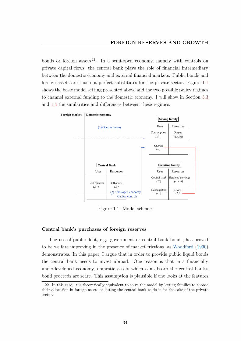
FOREIGN RESERVES AND GROWTH
bonds or foreign assets 22. In a semi-open economy, namely with controls on
private capital flows, the central bank plays the role of financial intermediary
between the domestic economy and external financial markets. Public bonds and
foreign assets are thus not perfect substitutes for the private sector. Figure 1.1
shows the basic model setting presented above and the two possible policy regimes
to channel external funding to the domestic economy. I will show in Section 3.3
and 1.4 the similarities and differences between these regimes.
CB bondsFX reserves
Uses Resources
(B)(B∗)
Output
Uses Resources
(F(K,N))
Consumption
(cS)
Savings(S)
Retained earnings
Uses Resources
(r × S)Capital stock
(K)
Loans(L)
Consumption(cL)
Saving family
Investing familyCentral Bank
Foreign market
(1) Open economy
(2) Semi-open economyCapital controls
Domestic economy
Figure 1.1: Model scheme
Central bank’s purchases of foreign reserves
The use of public debt, e.g. government or central bank bonds, has proved
to be welfare improving in the presence of market frictions, as Woodford (1990)
demonstrates. In this paper, I argue that in order to provide public liquid bonds
the central bank needs to invest abroad. One reason is that in a financially
underdeveloped economy, domestic assets which can absorb the central bank’s
bond proceeds are scare. This assumption is plausible if one looks at the features
22. In this case, it is theoretically equivalent to solve the model by letting families to choosetheir allocation in foreign assets or letting the central bank to do it for the sake of the privatesector.
34
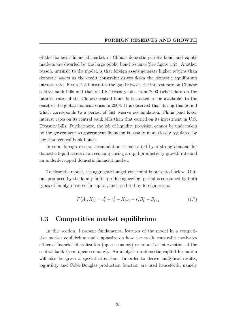
FOREIGN RESERVES AND GROWTH
of the domestic financial market in China: domestic private bond and equity
markets are dwarfed by the large public bond issuance(See figure 1.2). Another
reason, intrinsic to the model, is that foreign assets generate higher returns than
domestic assets as the credit constraint drives down the domestic equilibrium
interest rate. Figure 1.3 illustrates the gap between the interest rate on Chinese
central bank bills and that on US Treasury bills from 2003 (when data on the
interest rates of the Chinese central bank bills started to be available) to the
onset of the global financial crisis in 2008. It is observed that during this period
which corresponds to a period of fast reserve accumulation, China paid lower
interest rates on its central bank bills than that earned on its investment in U.S.
Treasury bills. Furthermore, the job of liquidity provision cannot be undertaken
by the government as government financing is usually more closely regulated by
law than central bank bonds.
In sum, foreign reserve accumulation is motivated by a strong demand for
domestic liquid assets in an economy facing a rapid productivity growth rate and
an underdeveloped domestic financial market.
To close the model, the aggregate budget constraint is presented below. Out-
put produced by the family in its ‘producing-saving’ period is consumed by both
types of family, invested in capital, and used to buy foreign assets.
F (At, Kt) = cSt + cIt +Kt+1 − r∗tB∗t +B∗
t+1 (1.7)
1.3 Competitive market equilibrium
In this section, I present fundamental features of the model in a competi-
tive market equilibrium and emphasize on how the credit constraint motivates
either a financial liberalization (open economy) or an active intervention of the
central bank (semi-open economy). An analysis on domestic capital formation
will also be given a special attention. In order to derive analytical results,
log-utility and Cobb-Douglas production function are used henceforth, namely
35
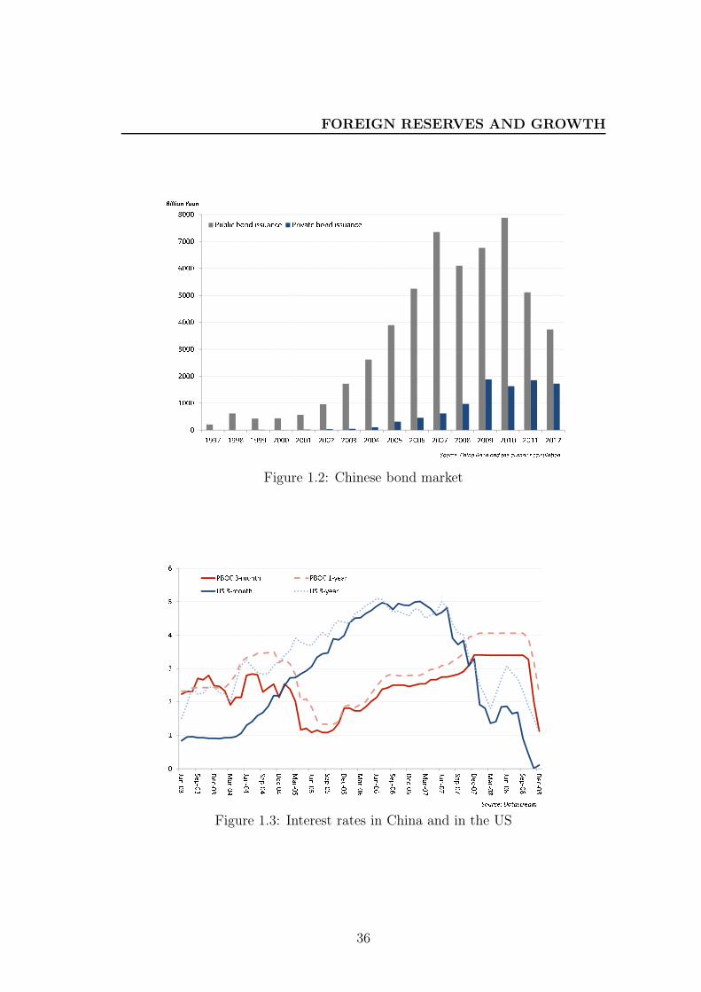
FOREIGN RESERVES AND GROWTH
Figure 1.2: Chinese bond market
Figure 1.3: Interest rates in China and in the US
36
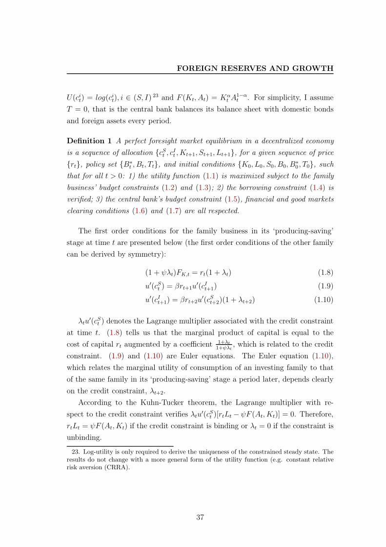
FOREIGN RESERVES AND GROWTH
U(cit) = log(cit), i ∈ (S, I) 23 and F (Kt, At) = Kαt A
1−αt . For simplicity, I assume
T = 0, that is the central bank balances its balance sheet with domestic bonds
and foreign assets every period.
Definition 1 A perfect foresight market equilibrium in a decentralized economy
is a sequence of allocation {cSt , cIt , Kt+1, St+1, Lt+1}, for a given sequence of price
{rt}, policy set {B∗t , Bt, Tt}, and initial conditions {K0, L0, S0, B0, B
∗0 , T0}, such
that for all t > 0: 1) the utility function (1.1) is maximized subject to the family
business’ budget constraints (1.2) and (1.3); 2) the borrowing constraint (1.4) is
verified; 3) the central bank’s budget constraint (1.5), financial and good markets
clearing conditions (1.6) and (1.7) are all respected.
The first order conditions for the family business in its ‘producing-saving’
stage at time t are presented below (the first order conditions of the other family
can be derived by symmetry):
(1 + ψλt)FK,t = rt(1 + λt) (1.8)
u′(cSt ) = βrt+1u′(cIt+1) (1.9)
u′(cIt+1) = βrt+2u′(cSt+2)(1 + λt+2) (1.10)
λtu′(cSt ) denotes the Lagrange multiplier associated with the credit constraint
at time t. (1.8) tells us that the marginal product of capital is equal to the
cost of capital rt augmented by a coefficient 1+λt1+ψλt
, which is related to the credit
constraint. (1.9) and (1.10) are Euler equations. The Euler equation (1.10),
which relates the marginal utility of consumption of an investing family to that
of the same family in its ‘producing-saving’ stage a period later, depends clearly
on the credit constraint, λt+2.
According to the Kuhn-Tucker theorem, the Lagrange multiplier with re-
spect to the credit constraint verifies λtu′(cSt )[rtLt−ψF (At, Kt)] = 0. Therefore,
rtLt = ψF (At, Kt) if the credit constraint is binding or λt = 0 if the constraint is
unbinding.
23. Log-utility is only required to derive the uniqueness of the constrained steady state. Theresults do not change with a more general form of the utility function (e.g. constant relativerisk aversion (CRRA).
37
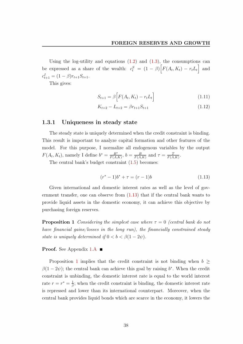
FOREIGN RESERVES AND GROWTH
Using the log-utility and equations (1.2) and (1.3), the consumptions can
be expressed as a share of the wealth: cSt = (1 − β)[F (At, Kt) − rtLt
]and
cIt+1 = (1− β)rt+1St+1.
This gives:
St+1 = β[F (At, Kt)− rtLt
](1.11)
Kt+2 − Lt+2 = βrt+1St+1 (1.12)
1.3.1 Uniqueness in steady state
The steady state is uniquely determined when the credit constraint is binding.
This result is important to analyze capital formation and other features of the
model. For this purpose, I normalize all endogenous variables by the output
F (At, Kt), namely I define b∗ = B∗
F (A,K), b = B
F (A,K)and τ = T
F (A,K).
The central bank’s budget constraint (1.5) becomes:
(r∗ − 1)b∗ + τ = (r − 1)b (1.13)
Given international and domestic interest rates as well as the level of gov-
ernment transfer, one can observe from (1.13) that if the central bank wants to
provide liquid assets in the domestic economy, it can achieve this objective by
purchasing foreign reserves.
Proposition 1 Considering the simplest case where τ = 0 (central bank do not
have financial gains/losses in the long run), the financially constrained steady
state is uniquely determined if 0 < b < β(1− 2ψ).
Proof. See Appendix 1.A
Proposition 1 implies that the credit constraint is not binding when b ≥
β(1− 2ψ); the central bank can achieve this goal by raising b∗. When the credit
constraint is unbinding, the domestic interest rate is equal to the world interest
rate r = r∗ = 1β; when the credit constraint is binding, the domestic interest rate
is repressed and lower than its international counterpart. Moreover, when the
central bank provides liquid bonds which are scarce in the economy, it lowers the
38
FOREIGN RESERVES AND GROWTH
price of the liquid bonds and pushes the domestic interest rate up to the world
interest rate level. r is indeed increasing in b: r = ψ
β(1−ψ)−b.
We can further look at the steady state in different policy regimes.
Financial autarky In a closed economy where B∗ = 0, if ψ ≥ 1/2, the credit
constraint does not bind in the steady state (the critical value of ψ is derived in
Appendix 1.B). In this case, βr = 1, namely, the domestic interest rate is equal
to the world interest rate. K = A(αβ)1
1−α , the capital stock achieves its first-
best level (i.e. the long-run steady state with an unbinding credit constraint).
Consumptions are perfectly smoothed, namely the consumption in the saving
stage and that in the investing stage are equalized cS = cI .
If ψ < 1/2, the credit constraint binds in the steady state. The Lagrange
multiplier associated with the credit constraint is thus positive, λ = 1β2r2
−1 > 0.
The domestic interest rate is lower than the world interest rate, namely βr =
ψ
1−ψ< 1. The capital stock, K = A
{α[(1−ψ)β2r+ ψ
r
]} 1
1−α
, cannot achieve the
first-best level. As for consumptions, that of the investing stage is always smaller
than that of the saving stage, cI
cS= ψ
1−ψ< 1.
In fact, in a financial autarky, with positive productivity growth, the more
capital invested the better. There is thus a strong demand for capital investment.
However, the investing family is financially constrained and the aggregate econ-
omy does not have sufficient resources to finance the investment as no external
financing is available. The left panel in figure 1.4 shows that in case of a decrease
in ψ, the credit constraint becomes more binding and the demand for domestic
assets increases while the supply remains fixed (due to the financial autarky).
This results in a sharp decrease in the domestic interest rate. This is undesirable
both for capital investment and domestic consumptions.
Open economy One big difference here in comparison with the financial au-
tarky is that the economy has access to external financing. It results in the equal-
ization between the domestic interest rate and the world interest rate, r = r∗ = 1β.
There is an unlimited supply of external financing. In this case, the credit con-
straint is never binding, leading to b = b∗ = β(1 − 2ψ). In an open economy,
39
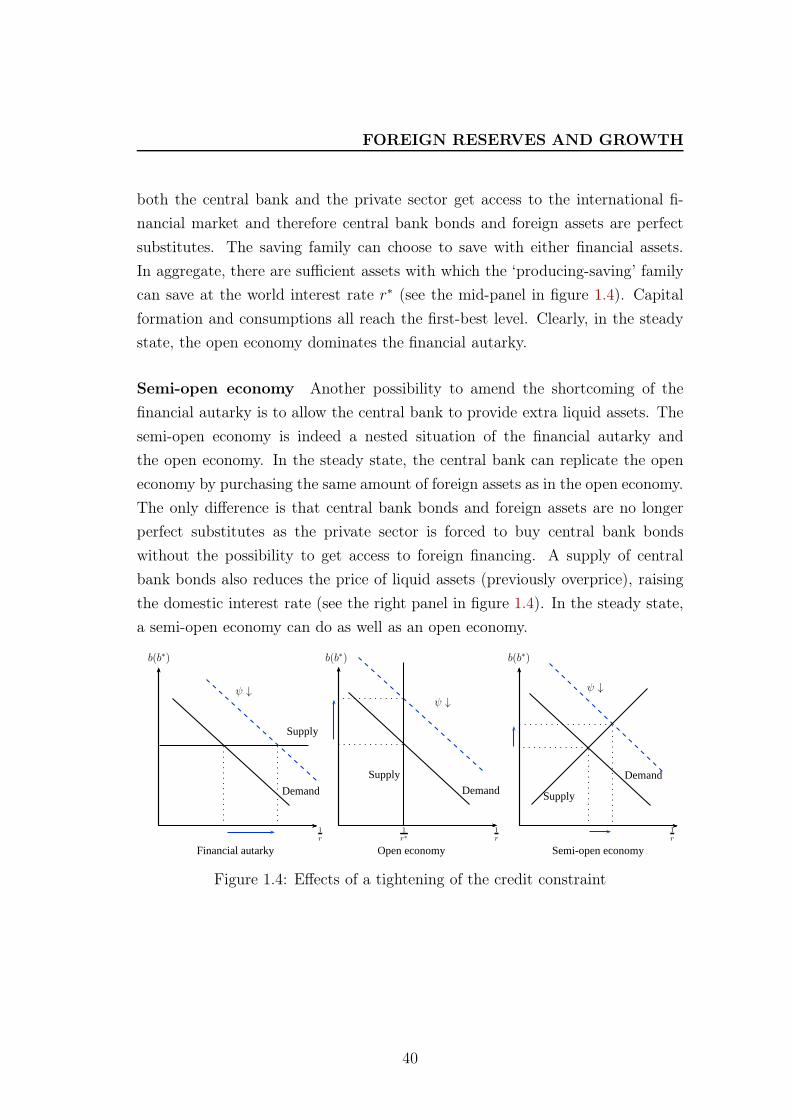
FOREIGN RESERVES AND GROWTH
both the central bank and the private sector get access to the international fi-
nancial market and therefore central bank bonds and foreign assets are perfect
substitutes. The saving family can choose to save with either financial assets.
In aggregate, there are sufficient assets with which the ‘producing-saving’ family
can save at the world interest rate r∗ (see the mid-panel in figure 1.4). Capital
formation and consumptions all reach the first-best level. Clearly, in the steady
state, the open economy dominates the financial autarky.
Semi-open economy Another possibility to amend the shortcoming of the
financial autarky is to allow the central bank to provide extra liquid assets. The
semi-open economy is indeed a nested situation of the financial autarky and
the open economy. In the steady state, the central bank can replicate the open
economy by purchasing the same amount of foreign assets as in the open economy.
The only difference is that central bank bonds and foreign assets are no longer
perfect substitutes as the private sector is forced to buy central bank bonds
without the possibility to get access to foreign financing. A supply of central
bank bonds also reduces the price of liquid assets (previously overprice), raising
the domestic interest rate (see the right panel in figure 1.4). In the steady state,
a semi-open economy can do as well as an open economy.
b(b∗)
1r
Supply
Demand
ψ ↓
Demand
Supply
ψ ↓
Demand
Supply
ψ ↓
1r
1r
b(b∗) b(b∗)
1r∗
Financial autarky Open economy Semi-open economy
Figure 1.4: Effects of a tightening of the credit constraint
40
FOREIGN RESERVES AND GROWTH
1.3.2 Capital formation
How does the capital stock evolve over time? From (1.11) and (1.12), capi-
tal accumulation which is consistent with optimal consumptions in a financially
constrained economy satisfies:
Kt+2 = βrt+1St+1︸ ︷︷ ︸retained earnings
+Lt+2︸︷︷︸loans
= β2rt+1(1− ψ)F (At, Kt) +ψF (At+2, Kt+2)
rt+2
(1.14)
Notice that retained earnings and loans are affected by the interest rate in
two opposite ways. An increase in the domestic interest rate raises the retained
earnings of the saving family (revenue effect) but reduces the loans that the
same family may make next period during its investing period (borrowing effect).
Whether capital stock increases or decreases depends on which effect dominates.
A feedback loop effect can be observed through capital investment in (1.14).
Namely, more capital invested (Kt+2) provides a stronger collateral (as the capital
enters in the production function), allowing the investing family to borrow more
(Lt+2) during the investing stage and relaxing the credit constraint. This further
pushes up capital investment. For example, an initial positive shock on retained
earnings (e.g. an increase in rt+1, an increase in the initial capital stock Kt or a
productivity shock at time t) will lead to an increase in capital formation at t+2
(through the revenue effect), which in turn drives loans up (through the feedback
loop). Capital formation Kt+2 further increases, generating a virtuous cycle.
To better understand the impact of the interest rate on domestic capital for-
mation, (1.15) can be derived in the steady state using (1.8)-(1.10). Three distinct
effects on capital stock can be identified: 1) opportunity cost of capital, 2) revenue
effect, (βr)2 = 11+λ
, 3) borrowing effect, ψ[1− (βr)2].
FK =r
(βr)2 + ψ[1− (βr)2](1.15)
The first effect, the opportunity cost of capital, is standard: the higher r, the
higher the cost of investing in capital stock, the less capital is demanded. The
41
FOREIGN RESERVES AND GROWTH
other two effects are specific to this model.
The second term (βr)2 is related to families’ saving revenues. As families are
occasionally credit-constrained, they have incentives to rely on retained earnings
to invest in capital. As the retained earnings are increasing in the interest rate,
the revenue effect has a positive impact on capital stock. Notice that the square
appears as the capital is invested every two periods. In an extreme case, when
ψ = 0 (i.e. no borrowing is possible), families rely entirely on retained earnings
for capital investment. The revenue effect clearly dominates the opportunity cost.
As a result, a higher supply of liquid bonds leads to a higher domestic interest rate
and higher retained earnings. This unambiguously increases the capital stock.
The third effect stems from the fact that the loans that an investing family
can ask are conditional on the discounted value of the future production. An
increase in r lowers the borrowing capacity of the investing family, as it reduces
the discounted value of the collateral. The interest rate has thus a negative
borrowing effect on capital stock.
Proposition 2 Capital stock represents a U-shape curve as a function of βr in
the steady state. Purchasing foreign reserves, which leads to a higher supply of
domestic liquid assets and thus a higher interest rate, increase capital stock and
output production in the economy.
Proof. See Appendix 1.C
From figure 1.5, the capital stock achieves the first-best level if βr = 1 (i.e.
in an open economy steady state) or βr = ψ
1−ψ. However, the latter case is ruled
out by the uniqueness of the binding steady state (see Appendix 1.A).
When ψ
1−ψ< βr ≤
√ψ
1−ψ, the curve is decreasing. That is, when the financial
constraint is stringent, the initial domestic interest rate is very low, any increase
in the interest rate decreases the value of the collateral, leading to a decrease
in borrowing. The initial domestic savings are also very low short of saving
instruments, an increase in retained earnings (due to a raise of interest rate)
cannot offset the decrease in borrowing. Therefore, on this part of the curve,
the borrowing effect of the interest rate dominates the revenue effect, leading to
a decrease in capital stock. The initial steady state (before the realization of
42
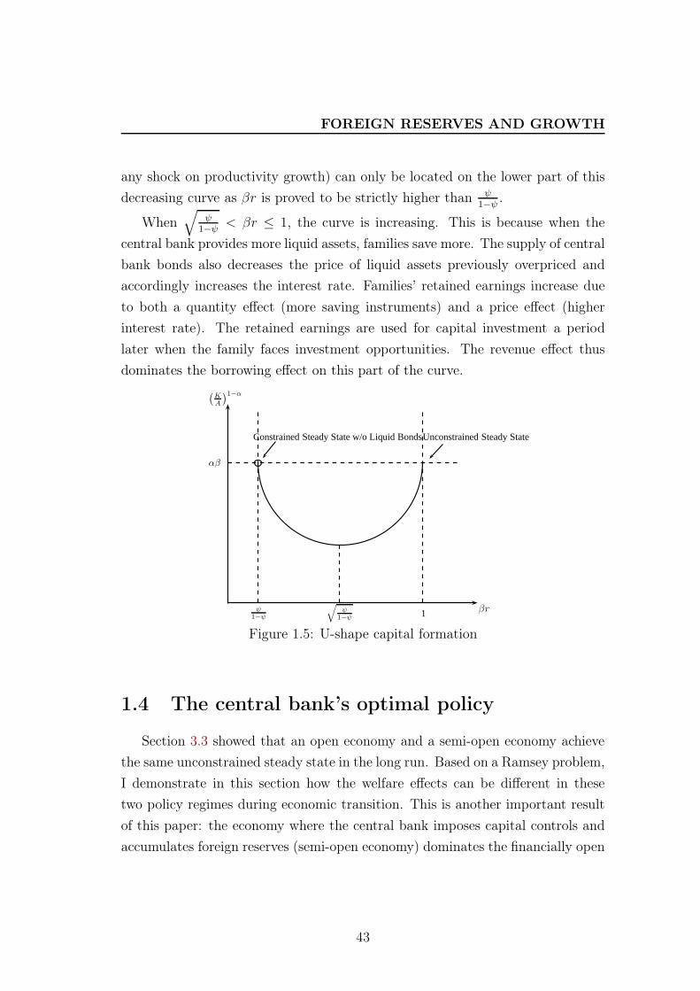
FOREIGN RESERVES AND GROWTH
any shock on productivity growth) can only be located on the lower part of this
decreasing curve as βr is proved to be strictly higher than ψ
1−ψ.
When√
ψ
1−ψ< βr ≤ 1, the curve is increasing. This is because when the
central bank provides more liquid assets, families save more. The supply of central
bank bonds also decreases the price of liquid assets previously overpriced and
accordingly increases the interest rate. Families’ retained earnings increase due
to both a quantity effect (more saving instruments) and a price effect (higher
interest rate). The retained earnings are used for capital investment a period
later when the family faces investment opportunities. The revenue effect thus
dominates the borrowing effect on this part of the curve.
βr
(KA
)1−α
1ψ1−ψ
√ψ
1−ψ
αβ
Unconstrained Steady StateConstrained Steady State w/o Liquid Bonds
Figure 1.5: U-shape capital formation
1.4 The central bank’s optimal policy
Section 3.3 showed that an open economy and a semi-open economy achieve
the same unconstrained steady state in the long run. Based on a Ramsey problem,
I demonstrate in this section how the welfare effects can be different in these
two policy regimes during economic transition. This is another important result
of this paper: the economy where the central bank imposes capital controls and
accumulates foreign reserves (semi-open economy) dominates the financially open
43
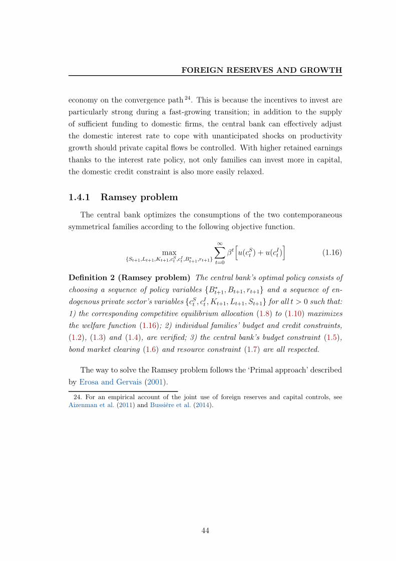
FOREIGN RESERVES AND GROWTH
economy on the convergence path 24. This is because the incentives to invest are
particularly strong during a fast-growing transition; in addition to the supply
of sufficient funding to domestic firms, the central bank can effectively adjust
the domestic interest rate to cope with unanticipated shocks on productivity
growth should private capital flows be controlled. With higher retained earnings
thanks to the interest rate policy, not only families can invest more in capital,
the domestic credit constraint is also more easily relaxed.
1.4.1 Ramsey problem
The central bank optimizes the consumptions of the two contemporaneous
symmetrical families according to the following objective function.
max{St+1,Lt+1,Kt+1,c
St ,c
It ,B
∗
t+1,rt+1}
∞∑
t=0
βt[u(cSt ) + u(cIt )
](1.16)
Definition 2 (Ramsey problem) The central bank’s optimal policy consists of
choosing a sequence of policy variables {B∗t+1, Bt+1, rt+1} and a sequence of en-
dogenous private sector’s variables {cSt , cIt , Kt+1, Lt+1, St+1} for all t > 0 such that:
1) the corresponding competitive equilibrium allocation (1.8) to (1.10) maximizes
the welfare function (1.16); 2) individual families’ budget and credit constraints,
(1.2), (1.3) and (1.4), are verified; 3) the central bank’s budget constraint (1.5),
bond market clearing (1.6) and resource constraint (1.7) are all respected.
The way to solve the Ramsey problem follows the ‘Primal approach’ described
by Erosa and Gervais (2001).
24. For an empirical account of the joint use of foreign reserves and capital controls, seeAizenman et al. (2011) and Bussière et al. (2014).
44
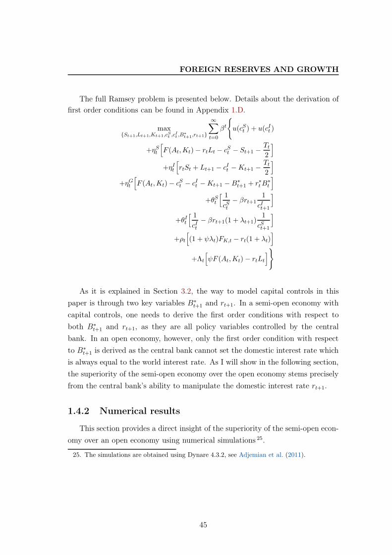
FOREIGN RESERVES AND GROWTH
The full Ramsey problem is presented below. Details about the derivation of
first order conditions can be found in Appendix 1.D.
max{St+1,Lt+1,Kt+1,c
St ,c
It ,B
∗
t+1,rt+1}
∞∑
t=0
βt
{u(cSt ) + u(cIt )
+ηSt
[F (At,Kt)− rtLt − cSt − St+1 −
Tt
2
]
+ηIt
[rtSt + Lt+1 − cIt −Kt+1 −
Tt
2
]
+ηGt
[F (At,Kt)− cSt − cIt −Kt+1 −B∗
t+1 + r∗tB∗t
]
+θSt
[ 1
cSt− βrt+1
1
cIt+1
]
+θIt
[ 1cIt
− βrt+1(1 + λt+1)1
cSt+1
]
+ρt
[(1 + ψλt)FK,t − rt(1 + λt)
]
+Λt
[ψF (At,Kt)− rtLt
]}
As it is explained in Section 3.2, the way to model capital controls in this
paper is through two key variables B∗t+1 and rt+1. In a semi-open economy with
capital controls, one needs to derive the first order conditions with respect to
both B∗t+1 and rt+1, as they are all policy variables controlled by the central
bank. In an open economy, however, only the first order condition with respect
to B∗t+1 is derived as the central bank cannot set the domestic interest rate which
is always equal to the world interest rate. As I will show in the following section,
the superiority of the semi-open economy over the open economy stems precisely
from the central bank’s ability to manipulate the domestic interest rate rt+1.
1.4.2 Numerical results
This section provides a direct insight of the superiority of the semi-open econ-
omy over an open economy using numerical simulations 25.
25. The simulations are obtained using Dynare 4.3.2, see Adjemian et al. (2011).
45

FOREIGN RESERVES AND GROWTH
Calibration
The productivity growth is assumed to follow an AR(1) process: At = (1 +
gt)At−1 and the growth rate of the productivity is determined by gt = µgt−1 + ǫ.
µ stands for the persistence of the productivity growth which is less than 1 and
ǫ is an unanticipated shock. I simulate the model by setting a positive shock
of 10% on the productivity growth rate at the beginning of the period 1. The
productivity process and the shock are used to mimic the fast economic catch-up
in emerging economies.
The discount factor β is calibrated to match the average yields of the one-
year US Treasury bills 26. This gives β = 1r∗
= 11.05
= 0.95. The capital share
is set to α = 0.5, consistent with Bai et al. (2006) and also used by Song et al.
(2011) which is the most recent and influential quantitative work on the Chinese
economic growth. I choose the value of the key parameter ψ, tightness of the
credit constraint, so as to match the savings-to-output ratio in the initial steady
state of simulations with China’s average gross saving rate (as a percentage of
the national income) 27. This gives ψ = 0.12. A summary of parameter values
can be found in table 1.2.
Notice that due to the parsimony of the model, the numerical results that
I present below only aim at illustrating the qualitative results derived from the
model.
Table 1.2: Calibrated parameters
Parameter Description Value
α Share of capital in the production 0.50β Discount factor 0.95ψ Credit constraint tightness 0.12ǫ Initial shock on productivity growth 0.10µ Persistence of productivity shock 0.50
26. The average rate of return on one-year US Treasury bills amounts to 5% between 1998and 2005. This rate can be regarded as a proxy to measure the world interest rate in this paper.Data source: Datastream.
27. This amounts to 42% between 1998 and 2005. Data source: World Bank WDI database.
46
FOREIGN RESERVES AND GROWTH
Superiority of the semi-open economy during economic transition
Figure 1.6 presents the impulse responses from the numerical exercise. Unless
otherwise notified (i.e. for the current account balance which is expressed in
absolute change), all impulse responses are expressed in terms of the percentage
deviation from the initial steady state (period 0). The solid lines represent the
results in a semi-open economy while the dashed lines represent that in an open
economy.
It has been analytically demonstrated in Section 3.3 that a semi-open econ-
omy and an open-economy can both achieve the long-run steady state with an
unbinding credit constraint (first-best situation). In fact, figure 1.6 shows that
all variables achieve the same final steady state regardless of the policy regime.
Recall that a semi-open economy is an economy where only the central bank gets
access to foreign financial markets while private capital flows are strictly con-
trolled; an open economy is on the contrary an economy with a fully liberalized
capital account. In steady state, accumulating foreign reserves while keeping the
capital account closed do not allow the central bank to do better than in a fully
open economy. This is because the central bank in the steady state accumulates
sufficient foreign assets so that the domestic interest rate catches with the world
interest rate.
However, during economic transition, especially when the productivity growth
becomes suddenly higher, the combined use of foreign reserves and capital controls
allows a faster convergence to the final steady state than in a fully open economy
(the solid lines are in general higher than the dashed lines during transition).
This is precisely due to the autonomy of the central bank to set the domestic
interest rate in a semi-open economy. Facing the same shock on productivity
growth at the beginning of the period 1, the central bank raises immediately the
domestic interest rate in a semi-open economy while the interest rate is fixed in
an open economy [Panel (a)]. To achieve this, the central bank provides more
saving instruments [Panel (b)] with which the ‘producing-saving’ family can save
to overcome the credit constraint. The private sector has indeed incentives to save
more in a semi-open economy [Panel (c)]. On the one hand, this is because it is
financially more interesting for the private sector to save with a higher interest
47
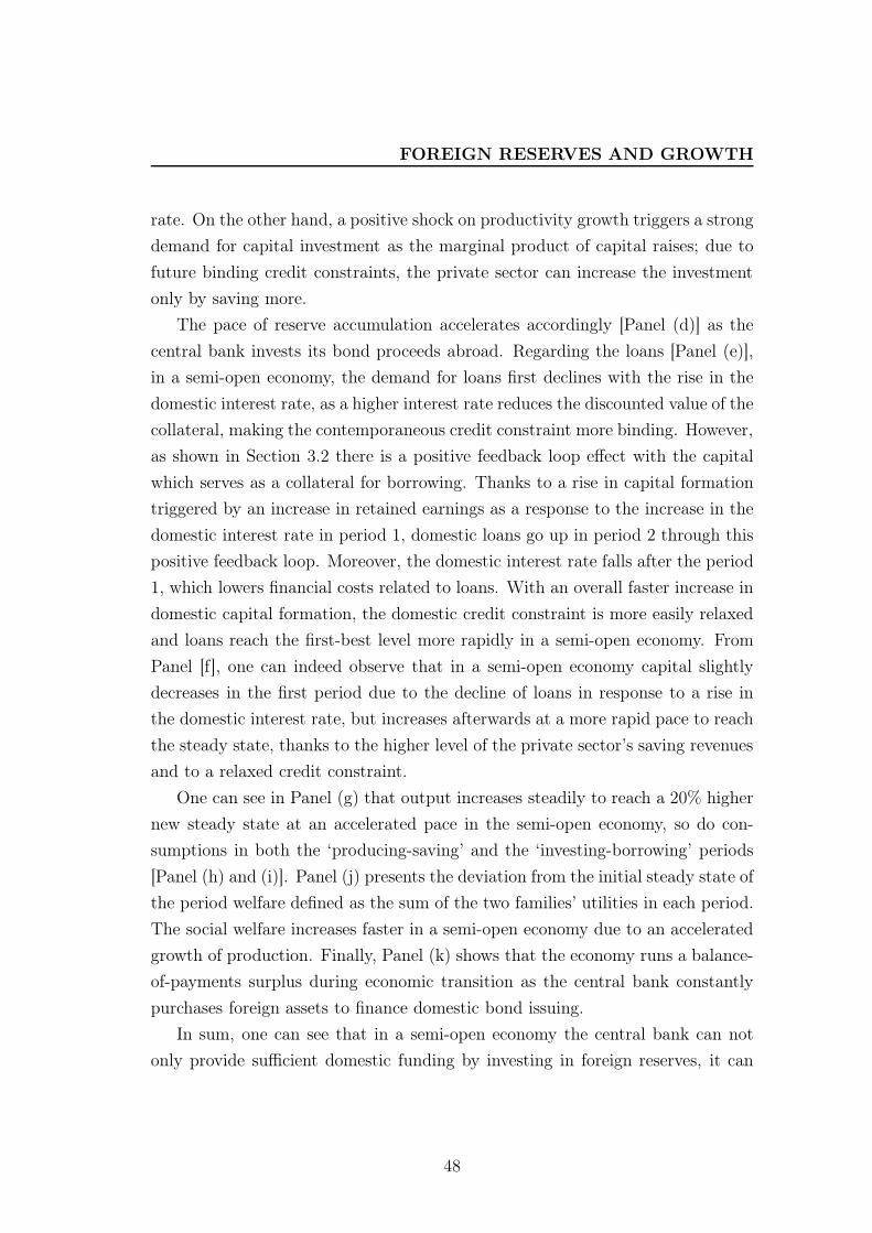
FOREIGN RESERVES AND GROWTH
rate. On the other hand, a positive shock on productivity growth triggers a strong
demand for capital investment as the marginal product of capital raises; due to
future binding credit constraints, the private sector can increase the investment
only by saving more.
The pace of reserve accumulation accelerates accordingly [Panel (d)] as the
central bank invests its bond proceeds abroad. Regarding the loans [Panel (e)],
in a semi-open economy, the demand for loans first declines with the rise in the
domestic interest rate, as a higher interest rate reduces the discounted value of the
collateral, making the contemporaneous credit constraint more binding. However,
as shown in Section 3.2 there is a positive feedback loop effect with the capital
which serves as a collateral for borrowing. Thanks to a rise in capital formation
triggered by an increase in retained earnings as a response to the increase in the
domestic interest rate in period 1, domestic loans go up in period 2 through this
positive feedback loop. Moreover, the domestic interest rate falls after the period
1, which lowers financial costs related to loans. With an overall faster increase in
domestic capital formation, the domestic credit constraint is more easily relaxed
and loans reach the first-best level more rapidly in a semi-open economy. From
Panel [f], one can indeed observe that in a semi-open economy capital slightly
decreases in the first period due to the decline of loans in response to a rise in
the domestic interest rate, but increases afterwards at a more rapid pace to reach
the steady state, thanks to the higher level of the private sector’s saving revenues
and to a relaxed credit constraint.
One can see in Panel (g) that output increases steadily to reach a 20% higher
new steady state at an accelerated pace in the semi-open economy, so do con-
sumptions in both the ‘producing-saving’ and the ‘investing-borrowing’ periods
[Panel (h) and (i)]. Panel (j) presents the deviation from the initial steady state of
the period welfare defined as the sum of the two families’ utilities in each period.
The social welfare increases faster in a semi-open economy due to an accelerated
growth of production. Finally, Panel (k) shows that the economy runs a balance-
of-payments surplus during economic transition as the central bank constantly
purchases foreign assets to finance domestic bond issuing.
In sum, one can see that in a semi-open economy the central bank can not
only provide sufficient domestic funding by investing in foreign reserves, it can
48
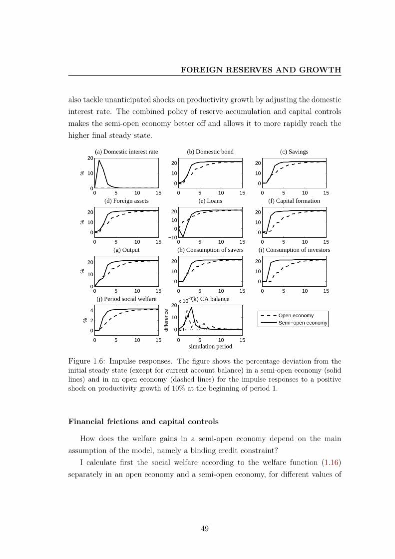
FOREIGN RESERVES AND GROWTH
also tackle unanticipated shocks on productivity growth by adjusting the domestic
interest rate. The combined policy of reserve accumulation and capital controls
makes the semi-open economy better off and allows it to more rapidly reach the
higher final steady state.
0 5 10 150
10
20(a) Domestic interest rate
%
0 5 10 15
0
10
20
(b) Domestic bond
0 5 10 15
0
10
20
(c) Savings
0 5 10 15
0
10
20
%
(d) Foreign assets
0 5 10 15−10
0
10
20
(e) Loans
0 5 10 15
0
10
20
(f) Capital formation
0 5 10 150
10
20
%
(g) Output
0 5 10 15
0
10
20
(h) Consumption of savers
0 5 10 15
0
10
20
(i) Consumption of investors
0 5 10 15
0
2
4
%
(j) Period social welfare
0 5 10 15
0
10
20x 10
−3
diffe
renc
e
simulation period
(k) CA balance
Open economySemi−open economy
Figure 1.6: Impulse responses. The figure shows the percentage deviation from theinitial steady state (except for current account balance) in a semi-open economy (solidlines) and in an open economy (dashed lines) for the impulse responses to a positiveshock on productivity growth of 10% at the beginning of period 1.
Financial frictions and capital controls
How does the welfare gains in a semi-open economy depend on the main
assumption of the model, namely a binding credit constraint?
I calculate first the social welfare according to the welfare function (1.16)
separately in an open economy and a semi-open economy, for different values of
49
FOREIGN RESERVES AND GROWTH
the credit constraint tightness ψ. Then, I calculate the welfare gains in a semi-
open economy compared to an open economy and present it as a function of the
parameter ψ. The result is shown in figure 1.7.
One can observe that the bigger ψ - the credit constraint less binding - the
lower the welfare gains of a semi-open economy over an open economy. Moreover,
the closer ψ gets to the threshold value 0.5, the sharper the decline in the welfare
gains. This is because when ψ gets bigger and close to 0.5, the demand for loans of
the ‘investing-borrowing’ family is close to the unbinding level and almost absorbs
the maximum savings that the ‘producing-saving’ family is willing to provide. In
the extreme case where there is no more credit constraint, a semi-open economy
can do no better than an open economy; the welfare gains associated with capital
controls and foreign reserve accumulation vanish. Put it in another way, in an
economy with little financial frictions, liberalizing the capital account is the first-
best strategy.
This result sheds light on the temporary character of the benefits from the
use of capital controls. In fact, capital controls are welfare improving and need
to be maintained only if there are strong imperfections on the domestic financial
market. Once appropriate financial reforms eliminate financial frictions, there is
no more reason for imposing capital controls.
1.5 Conclusion
Based on the model presented in this paper, I can partly attribute the rapid
accumulation of foreign exchange reserves in fast-growing emerging economies to
the joint force of fast productivity growth and domestic financial market frictions.
In fact, facing a rapid economic catch-up, the private sector in these countries has
a strong demand for liquid assets to support capital investment. In the absence
of a sound financial market with sufficient domestic assets, the central bank has
to serve as a financial intermediary to provide domestic liquid assets by investing
abroad in foreign exchange reserves short of domestic investment opportunities.
This paper also proves that during economic transition characterized by posi-
tive shocks on productivity growth it is welfare improving to let the central bank
accumulate foreign reserves and supply domestic liquid assets instead of letting
50
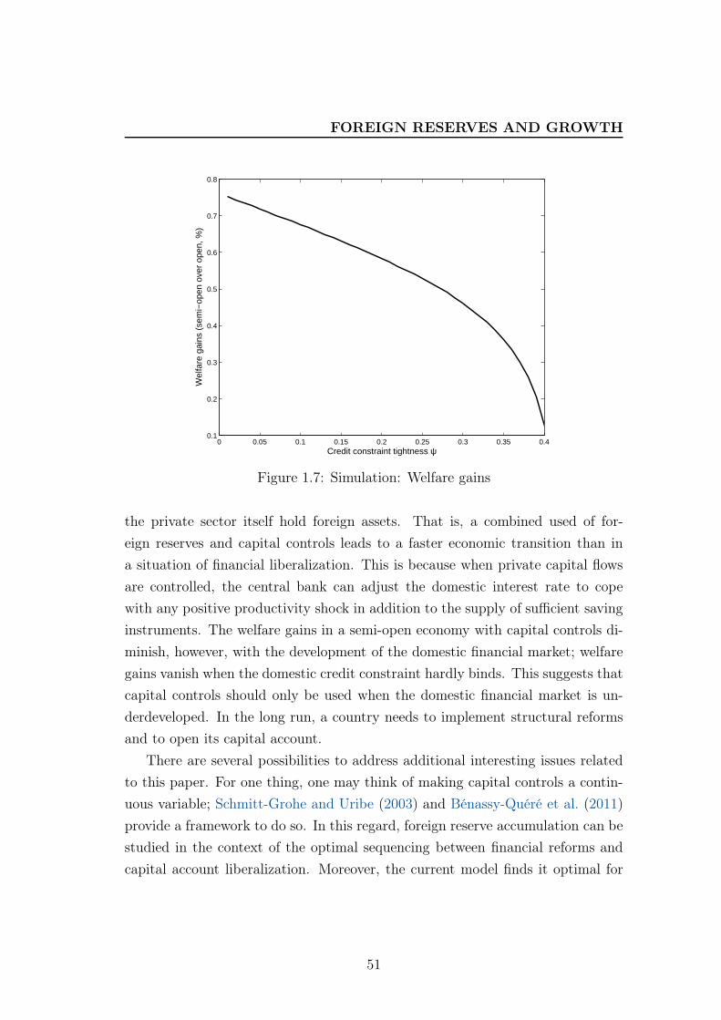
FOREIGN RESERVES AND GROWTH
0 0.05 0.1 0.15 0.2 0.25 0.3 0.35 0.40.1
0.2
0.3
0.4
0.5
0.6
0.7
0.8
Wel
fare
gai
ns (
sem
i−op
en o
ver
open
, %)
Credit constraint tightness ψ
Figure 1.7: Simulation: Welfare gains
the private sector itself hold foreign assets. That is, a combined used of for-
eign reserves and capital controls leads to a faster economic transition than in
a situation of financial liberalization. This is because when private capital flows
are controlled, the central bank can adjust the domestic interest rate to cope
with any positive productivity shock in addition to the supply of sufficient saving
instruments. The welfare gains in a semi-open economy with capital controls di-
minish, however, with the development of the domestic financial market; welfare
gains vanish when the domestic credit constraint hardly binds. This suggests that
capital controls should only be used when the domestic financial market is un-
derdeveloped. In the long run, a country needs to implement structural reforms
and to open its capital account.
There are several possibilities to address additional interesting issues related
to this paper. For one thing, one may think of making capital controls a contin-
uous variable; Schmitt-Grohe and Uribe (2003) and Bénassy-Quéré et al. (2011)
provide a framework to do so. In this regard, foreign reserve accumulation can be
studied in the context of the optimal sequencing between financial reforms and
capital account liberalization. Moreover, the current model finds it optimal for
51
FOREIGN RESERVES AND GROWTH
the domestic economy to accumulate reserves and set capital controls, it might
not be the case if cross-country spillover effects are taken into account. It would
be interesting to study the same question in an international context by extending
the model into a two-country framework 28.
28. There are a couple of new papers studying the impact of foreign reserves using a two-country model in the context of bilateral relations between China and the United States [e.g.Bonatti and Fracasso (2013)].
52
BIBLIOGRAPHY
Bibliography
Adjemian, Stéphane, Houtan Bastani, Michel Juillard, Ferhat Mihoubi, George Perendia, Marco
Ratto, and Sébastien Villemot (2011) Dynare: Reference manual, version 4. Dynare Working
Papers 1, CEPREMAP, April
Ahuja, Ashvin, and Malhar Nabar (2012) Investment-led growth in China: Global spillovers.
IMF Working Papers 12/267, International Monetary Fund, November
Aizenman, Joshua, and Jaewoo Lee (2007) International reserves: Precautionary versus mer-
cantilist views, theory and evidence. Open Economies Review 18(2), 191–214
Aizenman, Joshua, and Michael M. Hutchison (2010) Exchange market pressure and absorption
by international reserves: Emerging markets and fear of reserve loss during the 2008-09 crisis.
NBER Working Papers 16260, National Bureau of Economic Research, Inc, September
Aizenman, Joshua, Menzie Chinn, and Hiro Ito (2011) Surfing the waves of globalization: Asia
and financial globalization in the context of the trilemma. Journal of the Japanese and
International Economies 25(3), 290–320
Alfaro, Laura, and Fabio Kanczuk (2009) Optimal reserve management and sovereign debt.
Journal of International Economics 77(1), 23–36
Bacchetta, Philippe, and Kenza Benhima (2012) The demand for liquid assets, corporate sav-
ing, and global imbalances. CEPR Discussion Papers 9268, C.E.P.R. Discussion Papers,
December
Bacchetta, Philippe, Kenza Benhima, and Yannick Kalantzis (2013) Capital controls with inter-
national reserve accumulation: Can this be optimal? American Economic Journal: Macroe-
conomics 5(3), 229–62
Bai, Chong-En, Chang-Tai Hsieh, and Yingyi Qian (2006) The return to capital in China.
Brookings Papers on Economic Activity 37(2), 61–102
Bénassy-Quéré, Agnes, Benjamin Carton, and Ludovic Gauvin (2011) Rebalancing growth in
China: An international perspective. Working Papers 2011-08, CEPII research center, March
Benigno, Gianluca, and Luca Fornaro (2012) Reserve accumulation, growth and financial crises.
CEPR Discussion Papers 9224, C.E.P.R. Discussion Papers, November
Bernanke, Ben S., Mark Gertler, and Simon Gilchrist (1999) The financial accelerator in a quan-
titative business cycle framework. In John B. Taylor and Michael Woodford (ed.), Handbook
of Macroeconomics, pp. 1341–1393
53
BIBLIOGRAPHY
Bianchi, Javier, Juan Carlos Hatchondo, and Leonardo Martinez (2013) International reserves
and rollover risk. IMF Working Papers 13/33, International Monetary Fund, January
Bonatti, Luigi, and Andrea Fracasso (2013) Hoarding of international reserves in China: Mer-
cantilism, domestic consumption and us monetary policy. Journal of International Money
and Finance 32(C), 1044–1078
Bond, Steve, Asli Leblebicioglu, and Fabio Schiantarelli (2010) Capital accumulation and
growth: a new look at the empirical evidence. Journal of Applied Econometrics 25(7), 1073–
1099
Bussière, Matthieu, Gong Cheng, Menzie D. Chinn, and Noemie Lisack (2014) For a few dollars
more: Reserves and growth in times of crises. Working Paper 19791, National Bureau of
Economic Research, January
Caballero, Ricardo J., Emmanuel Farhi, and Pierre-Olivier Gourinchas (2008) An equilibrium
model of ‘Global imbalances’ and low interest rates. American Economic Review
Calvo, Guillermo, Alejandro Izquierdo, and Rudy Loo-Kung (2013) Optimal holdings of inter-
national reserves: Self-insurance against sudden stops. Monetaria (1), 1–35
Chamon, Marcos D., and Eswar S. Prasad (2010) Why are saving rates of urban households in
China rising? American Economic Journal: Macroeconomics 2(1), 93–130
Coeurdacier, Nicolas, Stéphane Guibaud, and Keyu Jin (2012) Credit constraints and growth
in a global economy. CEPR Discussion Papers 9109, C.E.P.R. Discussion Papers, August
Delatte, Anne-Laure, and Julien Fouquau (2012) What drove the massive hoarding of inter-
national reserves in emerging economies? A time-varying approach. Review of International
Economics 20(1), 164–176
Dominguez, Kathryn M. E. (2010) International reserves and underdeveloped capital markets.
In Lucrezia Reichlin and Kenneth D. West (ed.), NBER International Seminar on Macroe-
conomics 2009, National Bureau of Economic Research, Inc
Dooley, Michael, David Folkerts-Landau, and Peter M. Garber (2003) An essay on the revived
Bretton Woods system. NBER Working Papers 9971, National Bureau of Economic Research
Erosa, Andres, and Martin Gervais (2001) Optimal taxation in infinitely-lived agent and over-
lapping generations models : A review. Economic Quarterly (Spr), 23–44
Ghosh, Atish R., Jonathan David Ostry, and Charalambos G. Tsangarides (2012) Shifting
motives: Explaining the buildup in official reserves in emerging markets since the 1980s.
IMF Working Papers 12/34, International Monetary Fund, January
54
BIBLIOGRAPHY
IEO (2012) International reserves: IMF concerns and country perspectives. Evaluation reports
of the Independent Evaluation Office, International Monetary Fund
Jeanne, Olivier (2012) Capital account policies and the real exchange rate. In Francesco Giavazzi
and Kenneth D. West (ed.), NBER International Seminar on Macroeconomics 2012, National
Bureau of Economic Research, Inc
Jeanne, Olivier, and Romain Rancière (2011) The optimal level of international reserves
for emerging market countries: A new formula and some applications. Economic Journal
121(555), 905–930
Korinek, Anton (2011) The new economics of prudential capital controls: A research agenda.
IMF Economic Review 59(3), 523–561
Korinek, Anton, and Luis Serven (2010) Undervaluation through foreign reserve accumulation:
Static losses, dynamic gains. Policy Research Working Paper Series 5250, The World Bank,
March
Ljungqvist, Lars, and Thomas J. Sargent (2007) Understanding European unemployment with
a representative family model. Journal of Monetary Economics 54(8), 2180–2204
Merz, Monika (1995) Search in the labor market and the real business cycle. Journal of Monetary
Economics 36(2), 269–300
Nelson, Richard R, and Howard Pack (1999) The Asian miracle and modern growth theory.
Economic Journal 109(457), 416–36
Obstfeld, Maurice, Jay C. Shambaugh, and Alan M. Taylor (2010) Financial stability,
the trilemma, and international reserves. American Economic Journal: Macroeconomics
2(2), 57–94
Schmitt-Grohe, Stephanie, and Martin Uribe (2003) Closing small open economy models. Jour-
nal of International Economics 61(1), 163–185
Song, Zheng, Kjetil Storesletten, and Fabrizio Zilibotti (2011) Growing like China. American
Economic Review 101(1), 196–233
Wen, Yi (2011) Making sense of China’s excessive foreign reserves. Working Paper Series, Fed-
eral Reserve Bank of St. Louis
Woodford, Michael (1990) Public debt as private liquidity. American Economic Review
80(2), 382–88
55
APPENDIX
1.A Proof of Proposition 1
Proof. The central bank has to have a balanced budget (1.5) and the financial
market has to be cleared (1.6). The steady state of the model with a binding
credit constraint is determined by these two conditions:
– Central Bank’s budget balance
– Financial market clearing
Using the binding credit constraint (1.4), (1.6), (1.11) as well as normalized
policy variable, one can derive:
B = S − L
⇒ B = β[F (A,K)− rL]− L
⇒ B = β(1− ψ)F (A,K)−ψF (A,K)
r
⇒ b = β(1− ψ)−ψ
r
The financial market clearing shows a negative linear relationship between b
and 1r.
Moreover, in the simplest case without any government transfer, using (1.13)
gives,
(r − 1)b = (r∗ − 1)b∗
⇒ b =1
r − 1(r∗ − 1)b∗
⇒ b =
(1
1− 1r
− 1
)(r∗ − 1)b∗
The balanced central bank’s budget shows a non-linear and positive relation-
ship between b and 1r.
The uniqueness of the steady state can be thus demonstrated graphically
(figure 1.8).
56
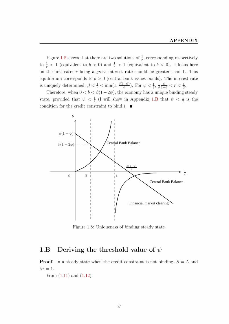
APPENDIX
Figure 1.8 shows that there are two solutions of 1r, corresponding respectively
to 1r< 1 (equivalent to b > 0) and 1
r> 1 (equivalent to b < 0). I focus here
on the first case; r being a gross interest rate should be greater than 1. This
equilibrium corresponds to b > 0 (central bank issues bonds). The interest rate
is uniquely determined, β < 1r< min(1, β(1−ψ)
ψ). For ψ < 1
2, 1β
ψ
1−ψ< r < 1
β.
Therefore, when 0 < b < β(1−2ψ), the economy has a unique binding steady
state, provided that ψ < 12
(I will show in Appendix 1.B that ψ < 12
is the
condition for the credit constraint to bind.).
β 10
b
1r
β(1 − ψ)
β(1− 2ψ)
β(1−ψ)ψ
Financial market clearing
Central Bank Balance
Central Bank Balance
Figure 1.8: Uniqueness of binding steady state
1.B Deriving the threshold value of ψ
Proof. In a steady state when the credit constraint is not binding, S = L and
βr = 1.
From (1.11) and (1.12):
57
APPENDIX
S = β[F (A,K)− rL]
⇒S = L =1
2βF (A,K)
When the credit constraint is not binding, rL ≤ ψF (A,K), namely12rβF (A,K) ≤ ψF (A,K).
Therefore, in a steady state with an unbinding credit constraint, I obtain:
ψ ≥1
2
Accordingly, the steady state is binding if ψ < 12
1.C Proof of Proposition 2
Proof. In a constrained state steady, (1.9) and (1.10) generate:
1 + λ =1
β2r2(1.17)
Using this result, along with the first order condition of capital (1.8), gives
equation (1.15):
FK = r1 + λ
1 + ψλ
=r
(βr)2 + ψ[1− (βr)2]
Graphically, K first decreases in βr then increases to go back to the first-best
level (figure 1.5).
58
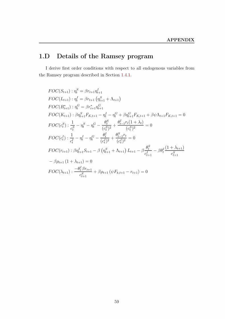
APPENDIX
1.D Details of the Ramsey program
I derive first order conditions with respect to all endogenous variables from
the Ramsey program described in Section 1.4.1.
FOC(St+1) : ηSt = βrt+1η
It+1
FOC(Lt+1) : ηIt = βrt+1
(ηSt+1 + Λt+1
)
FOC(B∗t+1) : η
Gt = βr∗t+1η
Gt+1
FOC(Kt+1) : βηSt+1FK,t+1 − ηIt − ηGt + βηGt+1FK,t+1 + βψΛt+1FK,t+1 = 0
FOC(cSt ) :1
cSt− ηSt − ηGt −
θSt(cSt )
2+θIt−1rt(1 + λt)
(cSt )2
= 0
FOC(cIt ) :1
cIt− ηIt − ηGt −
θIt(cIt )
2+θSt−1rt(cIt )
2= 0
FOC(rt+1) : βηIt+1St+1 − β
(ηSt+1 + Λt+1
)Lt+1 − β
θStcIt+1
− βθIt(1 + λt+1)
cSt+1
− βρt+1 (1 + λt+1) = 0
FOC(λt+1) :−θIt βrt+1
cSt+1
+ βρt+1 (ψFk,t+1 − rt+1) = 0
59

Chapter 2
For a Few Dollars More: Reserves
and Growth in Times of Crises
This chapter is a paper written with Matthieu Bussière (Banque de France), Menzie
Chinn (University of Wisconsin, Madison) and Noëmie Lisack (European University
Institute). It is published in the NBER Working Paper Series no.19791 in January
2014.
2.1 Introduction
In the decade preceding the 2008 global financial crisis (GFC), emerging mar-
ket economies accumulated large stocks of international reserves (figure 2.1). The
unprecedented pace of reserve accumulation was, at least partly, a response to
the lessons drawn from previous financial crises which predominantly affected
emerging markets. Most research on emerging market crises suggests that coun-
tries with an insufficient level of reserves, measured against appropriately chosen
benchmarks, suffered more from crises in the 1990s 29. A natural question arising
from this observation is to what extent the accumulation of international reserves
has protected countries from the negative shock of the latest crisis: have coun-
tries with more reserves fared better, in terms of output growth performance,
29. For a detailed review of this literature, see Flood and Marion (1999), Berg and Pattillo(1999), Reinhart and Kaminsky (1999), Bussière and Mulder (1999), Gourinchas and Obstfeld(2012), Catao and Milesi-Ferretti (2013) and Obstfeld (2013).
61
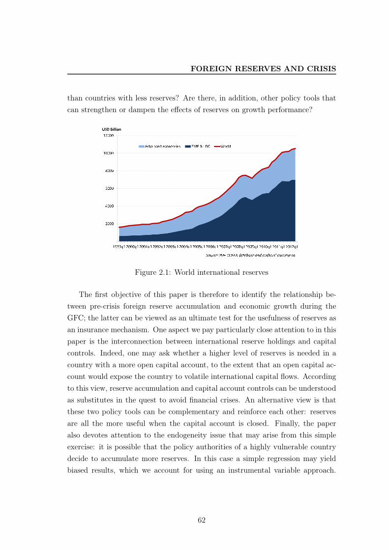
FOREIGN RESERVES AND CRISIS
than countries with less reserves? Are there, in addition, other policy tools that
can strengthen or dampen the effects of reserves on growth performance?
Figure 2.1: World international reserves
The first objective of this paper is therefore to identify the relationship be-
tween pre-crisis foreign reserve accumulation and economic growth during the
GFC; the latter can be viewed as an ultimate test for the usefulness of reserves as
an insurance mechanism. One aspect we pay particularly close attention to in this
paper is the interconnection between international reserve holdings and capital
controls. Indeed, one may ask whether a higher level of reserves is needed in a
country with a more open capital account, to the extent that an open capital ac-
count would expose the country to volatile international capital flows. According
to this view, reserve accumulation and capital account controls can be understood
as substitutes in the quest to avoid financial crises. An alternative view is that
these two policy tools can be complementary and reinforce each other: reserves
are all the more useful when the capital account is closed. Finally, the paper
also devotes attention to the endogeneity issue that may arise from this simple
exercise: it is possible that the policy authorities of a highly vulnerable country
decide to accumulate more reserves. In this case a simple regression may yield
biased results, which we account for using an instrumental variable approach.
62
FOREIGN RESERVES AND CRISIS
Aside from this first objective, which focuses on the initial stage of the crisis, the
paper also investigates the patterns of reserve accumulation in the subsequent
periods. Indeed, the finding that more reserves before the crisis have indeed
benefited countries during the GFC may have prompted countries to accumulate
even more reserves after the crisis. We therefore seek to uncover the patterns of
reserve accumulation after the GFC, distinguishing between the immediate after-
math of the crisis, which recorded a strong rebound, and the following period,
during which the pace of reserve accumulation decelerated.
Against this background, the paper presents three sets of findings. First, we
test the hypothesis that international reserves fulfill the protective role they are
often assigned to, by testing whether the extent of the crisis (proxied here by two
different measures of output collapse, which control for idiosyncratic factors) are
related to the level of reserves before the crisis. More specifically, given the de-
bate on what constitutes the most appropriate metrics for international reserves,
we construct a set of reserve ratios, expressing reserves as a percentage of GDP,
imports, M2 and short-term debt. The results indicate that when reserves are
measured as a percentage of short-term debt, there is a statistically significant
relationship with the dependent variable, but not for the other reserve adequacy
ratios (i.e. reserves/M2, reserves/imports and reserves/GDP). This result is ro-
bust to using alternative definitions of the crisis variable, different sub-samples
(emerging market countries only or combined with developing countries) or intro-
ducing additional control variables such as trade openness, dummy variables for
oil exporting countries or financial centers, and so forth. In this set of regressions
we also use an instrumental variable approach to account for a potential endo-
geneity bias. We develop two main instruments for our reserve ratio, focusing
on reserve accumulation in neighboring countries as an alternative accumulation
motive.
Second, we focus on the interaction between international reserves and cap-
ital account openness by introducing an interaction term involving these two
variables. We find that the coefficient of the interacted term is sometimes sig-
nificantly different from zero. The magnitude of the marginal effects of reserves
depends on the degree of capital controls; that is, a less open capital account
63
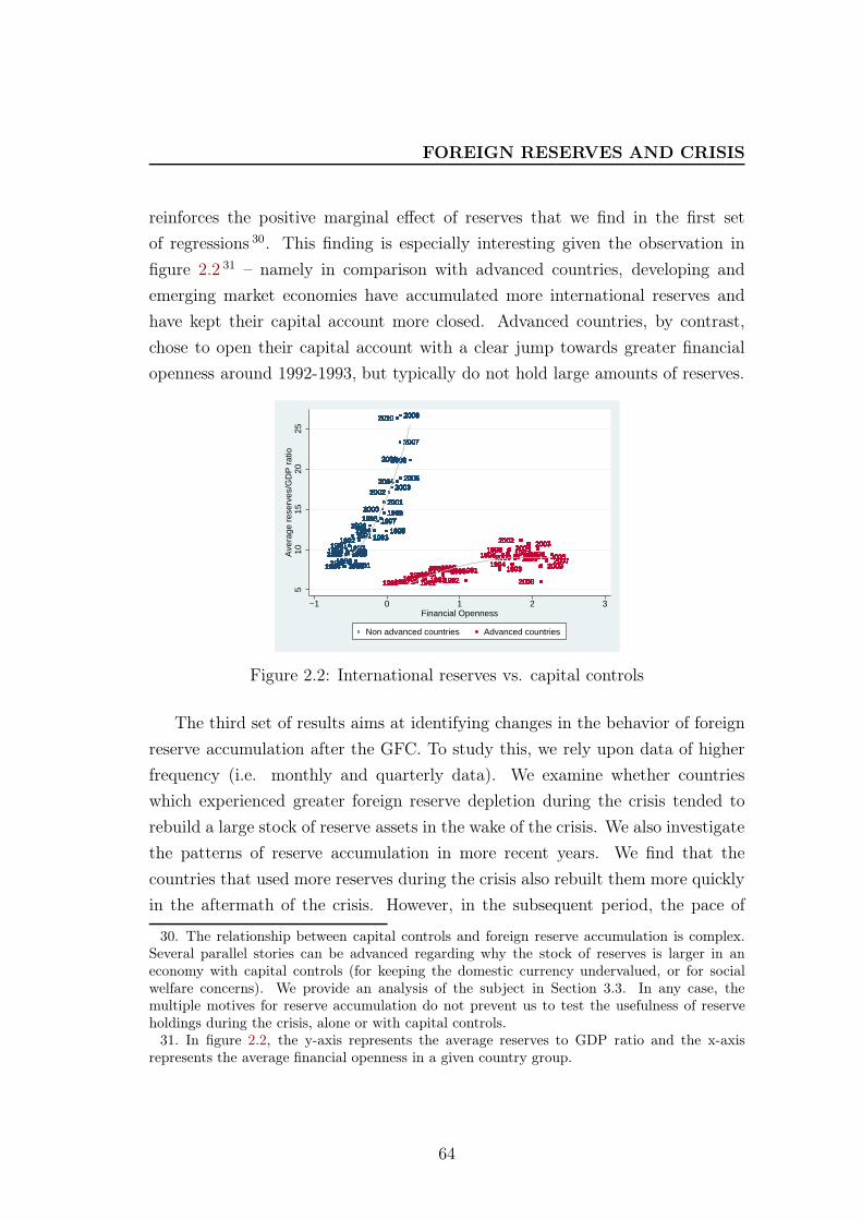
FOREIGN RESERVES AND CRISIS
reinforces the positive marginal effect of reserves that we find in the first set
of regressions 30. This finding is especially interesting given the observation in
figure 2.2 31 – namely in comparison with advanced countries, developing and
emerging market economies have accumulated more international reserves and
have kept their capital account more closed. Advanced countries, by contrast,
chose to open their capital account with a clear jump towards greater financial
openness around 1992-1993, but typically do not hold large amounts of reserves.
1980 19811982 19831984
19851986 19871988 19891990
19911992 1993
1994 19951996
19971998199920002001
20022003
2004 2005
2006
2007
2008
20092010
1980 19811982 19831984
19851986 19871988 19891990
19911992 1993
1994 19951996
19971998199920002001
20022003
2004 2005
2006
2007
2008
20092010
1980 19811982 19831984
19851986 19871988 19891990
19911992 1993
1994 19951996
19971998199920002001
20022003
2004 2005
2006
2007
2008
20092010
1980 19811982 19831984
19851986 19871988 19891990
19911992 1993
1994 19951996
19971998199920002001
20022003
2004 2005
2006
2007
2008
20092010
1980 19811982 19831984
19851986 19871988 19891990
19911992 1993
1994 19951996
19971998199920002001
20022003
2004 2005
2006
2007
2008
20092010
1980 19811982 19831984
19851986 19871988 19891990
19911992 1993
1994 19951996
19971998199920002001
20022003
2004 2005
2006
2007
2008
20092010
1980 19811982 19831984
19851986 19871988 19891990
19911992 1993
1994 19951996
19971998199920002001
20022003
2004 2005
2006
2007
2008
20092010
1980 19811982 19831984
19851986 19871988 19891990
19911992 1993
1994 19951996
19971998199920002001
20022003
2004 2005
2006
2007
2008
20092010
1980 19811982 19831984
19851986 19871988 19891990
19911992 1993
1994 19951996
19971998199920002001
20022003
2004 2005
2006
2007
2008
20092010
1980 19811982 19831984
19851986 19871988 19891990
19911992 1993
1994 19951996
19971998199920002001
20022003
2004 2005
2006
2007
2008
20092010
1980 19811982 19831984
19851986 19871988 19891990
19911992 1993
1994 19951996
19971998199920002001
20022003
2004 2005
2006
2007
2008
20092010
1980 19811982 19831984
19851986 19871988 19891990
19911992 1993
1994 19951996
19971998199920002001
20022003
2004 2005
2006
2007
2008
20092010
1980 19811982 19831984
19851986 19871988 19891990
19911992 1993
1994 19951996
19971998199920002001
20022003
2004 2005
2006
2007
2008
20092010
1980 19811982 19831984
19851986 19871988 19891990
19911992 1993
1994 19951996
19971998199920002001
20022003
2004 2005
2006
2007
2008
20092010
1980 19811982 19831984
19851986 19871988 19891990
19911992 1993
1994 19951996
19971998199920002001
20022003
2004 2005
2006
2007
2008
20092010
1980 19811982 19831984
19851986 19871988 19891990
19911992 1993
1994 19951996
19971998199920002001
20022003
2004 2005
2006
2007
2008
20092010
1980 19811982 19831984
19851986 19871988 19891990
19911992 1993
1994 19951996
19971998199920002001
20022003
2004 2005
2006
2007
2008
20092010
1980 19811982 19831984
19851986 19871988 19891990
19911992 1993
1994 19951996
19971998199920002001
20022003
2004 2005
2006
2007
2008
20092010
1980 19811982 19831984
19851986 19871988 19891990
19911992 1993
1994 19951996
19971998199920002001
20022003
2004 2005
2006
2007
2008
20092010
1980 19811982 19831984
19851986 19871988 19891990
19911992 1993
1994 19951996
19971998199920002001
20022003
2004 2005
2006
2007
2008
20092010
1980 19811982 19831984
19851986 19871988 19891990
19911992 1993
1994 19951996
19971998199920002001
20022003
2004 2005
2006
2007
2008
20092010
1980 19811982 19831984
19851986 19871988 19891990
19911992 1993
1994 19951996
19971998199920002001
20022003
2004 2005
2006
2007
2008
20092010
1980 19811982 19831984
19851986 19871988 19891990
19911992 1993
1994 19951996
19971998199920002001
20022003
2004 2005
2006
2007
2008
20092010
1980 19811982 19831984
19851986 19871988 19891990
19911992 1993
1994 19951996
19971998199920002001
20022003
2004 2005
2006
2007
2008
20092010
1980 19811982 19831984
19851986 19871988 19891990
19911992 1993
1994 19951996
19971998199920002001
20022003
2004 2005
2006
2007
2008
20092010
1980 19811982 19831984
19851986 19871988 19891990
19911992 1993
1994 19951996
19971998199920002001
20022003
2004 2005
2006
2007
2008
20092010
1980 19811982 19831984
19851986 19871988 19891990
19911992 1993
1994 19951996
19971998199920002001
20022003
2004 2005
2006
2007
2008
20092010
1980 19811982 19831984
19851986 19871988 19891990
19911992 1993
1994 19951996
19971998199920002001
20022003
2004 2005
2006
2007
2008
20092010
1980 19811982 19831984
19851986 19871988 19891990
19911992 1993
1994 19951996
19971998199920002001
20022003
2004 2005
2006
2007
2008
20092010
1980 19811982 19831984
19851986 19871988 19891990
19911992 1993
1994 19951996
19971998199920002001
20022003
2004 2005
2006
2007
2008
20092010
1980 19811982 19831984
19851986 19871988 19891990
19911992 1993
1994 19951996
19971998199920002001
20022003
2004 2005
2006
2007
2008
20092010
1980 19811982 19831984
19851986 19871988 19891990
19911992 1993
1994 19951996
19971998199920002001
20022003
2004 2005
2006
2007
2008
20092010
1980 19811982 19831984
19851986 19871988 19891990
19911992 1993
1994 19951996
19971998199920002001
20022003
2004 2005
2006
2007
2008
20092010
1980 19811982 19831984
19851986 19871988 19891990
19911992 1993
1994 19951996
19971998199920002001
20022003
2004 2005
2006
2007
2008
20092010
1980 19811982 19831984
19851986 19871988 19891990
19911992 1993
1994 19951996
19971998199920002001
20022003
2004 2005
2006
2007
2008
20092010
1980 19811982 19831984
19851986 19871988 19891990
19911992 1993
1994 19951996
19971998199920002001
20022003
2004 2005
2006
2007
2008
20092010
1980 19811982 19831984
19851986 19871988 19891990
19911992 1993
1994 19951996
19971998199920002001
20022003
2004 2005
2006
2007
2008
20092010
1980 19811982 19831984
19851986 19871988 19891990
19911992 1993
1994 19951996
19971998199920002001
20022003
2004 2005
2006
2007
2008
20092010
1980 19811982 19831984
19851986 19871988 19891990
19911992 1993
1994 19951996
19971998199920002001
20022003
2004 2005
2006
2007
2008
20092010
1980 19811982 19831984
19851986 19871988 19891990
19911992 1993
1994 19951996
19971998199920002001
20022003
2004 2005
2006
2007
2008
20092010
1980 19811982 19831984
19851986 19871988 19891990
19911992 1993
1994 19951996
19971998199920002001
20022003
2004 2005
2006
2007
2008
20092010
1980 19811982 19831984
19851986 19871988 19891990
19911992 1993
1994 19951996
19971998199920002001
20022003
2004 2005
2006
2007
2008
20092010
1980 19811982 19831984
19851986 19871988 19891990
19911992 1993
1994 19951996
19971998199920002001
20022003
2004 2005
2006
2007
2008
20092010
1980 19811982 19831984
19851986 19871988 19891990
19911992 1993
1994 19951996
19971998199920002001
20022003
2004 2005
2006
2007
2008
20092010
1980 19811982 19831984
19851986 19871988 19891990
19911992 1993
1994 19951996
19971998199920002001
20022003
2004 2005
2006
2007
2008
20092010
1980 19811982 19831984
19851986 19871988 19891990
19911992 1993
1994 19951996
19971998199920002001
20022003
2004 2005
2006
2007
2008
20092010
1980 19811982 19831984
19851986 19871988 19891990
19911992 1993
1994 19951996
19971998199920002001
20022003
2004 2005
2006
2007
2008
20092010
1980 19811982 19831984
19851986 19871988 19891990
19911992 1993
1994 19951996
19971998199920002001
20022003
2004 2005
2006
2007
2008
20092010
1980 19811982 19831984
19851986 19871988 19891990
19911992 1993
1994 19951996
19971998199920002001
20022003
2004 2005
2006
2007
2008
20092010
1980 19811982 19831984
19851986 19871988 19891990
19911992 1993
1994 19951996
19971998199920002001
20022003
2004 2005
2006
2007
2008
20092010
1980 19811982 19831984
19851986 19871988 19891990
19911992 1993
1994 19951996
19971998199920002001
20022003
2004 2005
2006
2007
2008
20092010
1980 19811982 19831984
19851986 19871988 19891990
19911992 1993
1994 19951996
19971998199920002001
20022003
2004 2005
2006
2007
2008
20092010
1980 19811982 19831984
19851986 19871988 19891990
19911992 1993
1994 19951996
19971998199920002001
20022003
2004 2005
2006
2007
2008
20092010
1980 19811982 19831984
19851986 19871988 19891990
19911992 1993
1994 19951996
19971998199920002001
20022003
2004 2005
2006
2007
2008
20092010
1980 19811982 19831984
19851986 19871988 19891990
19911992 1993
1994 19951996
19971998199920002001
20022003
2004 2005
2006
2007
2008
20092010
1980 19811982 19831984
19851986 19871988 19891990
19911992 1993
1994 19951996
19971998199920002001
20022003
2004 2005
2006
2007
2008
20092010
1980 19811982 19831984
19851986 19871988 19891990
19911992 1993
1994 19951996
19971998199920002001
20022003
2004 2005
2006
2007
2008
20092010
1980 19811982 19831984
19851986 19871988 19891990
19911992 1993
1994 19951996
19971998199920002001
20022003
2004 2005
2006
2007
2008
20092010
1980 19811982 19831984
19851986 19871988 19891990
19911992 1993
1994 19951996
19971998199920002001
20022003
2004 2005
2006
2007
2008
20092010
1980 19811982 19831984
19851986 19871988 19891990
19911992 1993
1994 19951996
19971998199920002001
20022003
2004 2005
2006
2007
2008
20092010
1980 19811982 19831984
19851986 19871988 19891990
19911992 1993
1994 19951996
19971998199920002001
20022003
2004 2005
2006
2007
2008
20092010
1980 19811982 19831984
19851986 19871988 19891990
19911992 1993
1994 19951996
19971998199920002001
20022003
2004 2005
2006
2007
2008
20092010
1980 19811982 19831984
19851986 19871988 19891990
19911992 1993
1994 19951996
19971998199920002001
20022003
2004 2005
2006
2007
2008
20092010
1980 19811982 19831984
19851986 19871988 19891990
19911992 1993
1994 19951996
19971998199920002001
20022003
2004 2005
2006
2007
2008
20092010
1980 19811982 19831984
19851986 19871988 19891990
19911992 1993
1994 19951996
19971998199920002001
20022003
2004 2005
2006
2007
2008
20092010
1980 19811982 19831984
19851986 19871988 19891990
19911992 1993
1994 19951996
19971998199920002001
20022003
2004 2005
2006
2007
2008
20092010
1980 19811982 19831984
19851986 19871988 19891990
19911992 1993
1994 19951996
19971998199920002001
20022003
2004 2005
2006
2007
2008
20092010
1980 19811982 19831984
19851986 19871988 19891990
19911992 1993
1994 19951996
19971998199920002001
20022003
2004 2005
2006
2007
2008
20092010
1980 19811982 19831984
19851986 19871988 19891990
19911992 1993
1994 19951996
19971998199920002001
20022003
2004 2005
2006
2007
2008
20092010
1980 19811982 19831984
19851986 19871988 19891990
19911992 1993
1994 19951996
19971998199920002001
20022003
2004 2005
2006
2007
2008
20092010
1980 19811982 19831984
19851986 19871988 19891990
19911992 1993
1994 19951996
19971998199920002001
20022003
2004 2005
2006
2007
2008
20092010
1980 19811982 19831984
19851986 19871988 19891990
19911992 1993
1994 19951996
19971998199920002001
20022003
2004 2005
2006
2007
2008
20092010
1980 19811982 19831984
19851986 19871988 19891990
19911992 1993
1994 19951996
19971998199920002001
20022003
2004 2005
2006
2007
2008
20092010
1980 19811982 19831984
19851986 19871988 19891990
19911992 1993
1994 19951996
19971998199920002001
20022003
2004 2005
2006
2007
2008
20092010
1980 19811982 19831984
19851986 19871988 19891990
19911992 1993
1994 19951996
19971998199920002001
20022003
2004 2005
2006
2007
2008
20092010
1980 19811982 19831984
19851986 19871988 19891990
19911992 1993
1994 19951996
19971998199920002001
20022003
2004 2005
2006
2007
2008
20092010
1980 19811982 19831984
19851986 19871988 19891990
19911992 1993
1994 19951996
19971998199920002001
20022003
2004 2005
2006
2007
2008
20092010
1980 19811982 19831984
19851986 19871988 19891990
19911992 1993
1994 19951996
19971998199920002001
20022003
2004 2005
2006
2007
2008
20092010
1980 19811982 19831984
19851986 19871988 19891990
19911992 1993
1994 19951996
19971998199920002001
20022003
2004 2005
2006
2007
2008
20092010
1980 19811982 19831984
19851986 19871988 19891990
19911992 1993
1994 19951996
19971998199920002001
20022003
2004 2005
2006
2007
2008
20092010
1980 19811982 19831984
19851986 19871988 19891990
19911992 1993
1994 19951996
19971998199920002001
20022003
2004 2005
2006
2007
2008
20092010
1980 19811982 19831984
19851986 19871988 19891990
19911992 1993
1994 19951996
19971998199920002001
20022003
2004 2005
2006
2007
2008
20092010
1980 19811982 19831984
19851986 19871988 19891990
19911992 1993
1994 19951996
19971998199920002001
20022003
2004 2005
2006
2007
2008
20092010
1980 19811982 19831984
19851986 19871988 19891990
19911992 1993
1994 19951996
19971998199920002001
20022003
2004 2005
2006
2007
2008
20092010
1980 19811982 19831984
19851986 19871988 19891990
19911992 1993
1994 19951996
19971998199920002001
20022003
2004 2005
2006
2007
2008
20092010
1980 19811982 19831984
19851986 19871988 19891990
19911992 1993
1994 19951996
19971998199920002001
20022003
2004 2005
2006
2007
2008
20092010
1980 19811982 19831984
19851986 19871988 19891990
19911992 1993
1994 19951996
19971998199920002001
20022003
2004 2005
2006
2007
2008
20092010
1980 19811982 19831984
19851986 19871988 19891990
19911992 1993
1994 19951996
19971998199920002001
20022003
2004 2005
2006
2007
2008
20092010
1980 19811982 19831984
19851986 19871988 19891990
19911992 1993
1994 19951996
19971998199920002001
20022003
2004 2005
2006
2007
2008
20092010
1980 19811982 19831984
19851986 19871988 19891990
19911992 1993
1994 19951996
19971998199920002001
20022003
2004 2005
2006
2007
2008
20092010
1980 19811982 19831984
19851986 19871988 19891990
19911992 1993
1994 19951996
19971998199920002001
20022003
2004 2005
2006
2007
2008
20092010
1980 19811982 19831984
19851986 19871988 19891990
19911992 1993
1994 19951996
19971998199920002001
20022003
2004 2005
2006
2007
2008
20092010
1980 19811982 19831984
19851986 19871988 19891990
19911992 1993
1994 19951996
19971998199920002001
20022003
2004 2005
2006
2007
2008
20092010
1980 19811982 19831984
19851986 19871988 19891990
19911992 1993
1994 19951996
19971998199920002001
20022003
2004 2005
2006
2007
2008
20092010
1980 19811982 19831984
19851986 19871988 19891990
19911992 1993
1994 19951996
19971998199920002001
20022003
2004 2005
2006
2007
2008
20092010
1980 19811982 19831984
19851986 19871988 19891990
19911992 1993
1994 19951996
19971998199920002001
20022003
2004 2005
2006
2007
2008
20092010
1980 19811982 19831984
19851986 19871988 19891990
19911992 1993
1994 19951996
19971998199920002001
20022003
2004 2005
2006
2007
2008
20092010
1980 19811982 19831984
19851986 19871988 19891990
19911992 1993
1994 19951996
19971998199920002001
20022003
2004 2005
2006
2007
2008
20092010
1980 19811982 19831984
19851986 19871988 19891990
19911992 1993
1994 19951996
19971998199920002001
20022003
2004 2005
2006
2007
2008
20092010
1980 19811982 19831984
19851986 19871988 19891990
19911992 1993
1994 19951996
19971998199920002001
20022003
2004 2005
2006
2007
2008
20092010
1980 19811982 19831984
19851986 19871988 19891990
19911992 1993
1994 19951996
19971998199920002001
20022003
2004 2005
2006
2007
2008
20092010
1980 19811982 19831984
19851986 19871988 19891990
19911992 1993
1994 19951996
19971998199920002001
20022003
2004 2005
2006
2007
2008
20092010
1980 19811982 19831984
19851986 19871988 19891990
19911992 1993
1994 19951996
19971998199920002001
20022003
2004 2005
2006
2007
2008
20092010
1980 19811982 19831984
19851986 19871988 19891990
19911992 1993
1994 19951996
19971998199920002001
20022003
2004 2005
2006
2007
2008
20092010
1980 19811982 19831984
19851986 19871988 19891990
19911992 1993
1994 19951996
19971998199920002001
20022003
2004 2005
2006
2007
2008
20092010
1980 19811982 19831984
19851986 19871988 19891990
19911992 1993
1994 19951996
19971998199920002001
20022003
2004 2005
2006
2007
2008
20092010
1980 19811982 19831984
19851986 19871988 19891990
19911992 1993
1994 19951996
19971998199920002001
20022003
2004 2005
2006
2007
2008
20092010
1980 19811982 19831984
19851986 19871988 19891990
19911992 1993
1994 19951996
19971998199920002001
20022003
2004 2005
2006
2007
2008
20092010
1980 19811982 19831984
19851986 19871988 19891990
19911992 1993
1994 19951996
19971998199920002001
20022003
2004 2005
2006
2007
2008
20092010
1980 19811982 19831984
19851986 19871988 19891990
19911992 1993
1994 19951996
19971998199920002001
20022003
2004 2005
2006
2007
2008
20092010
1980 19811982 19831984
19851986 19871988 19891990
19911992 1993
1994 19951996
19971998199920002001
20022003
2004 2005
2006
2007
2008
20092010
1980 19811982 19831984
19851986 19871988 19891990
19911992 1993
1994 19951996
19971998199920002001
20022003
2004 2005
2006
2007
2008
20092010
1980 19811982 19831984
19851986 19871988 19891990
19911992 1993
1994 19951996
19971998199920002001
20022003
2004 2005
2006
2007
2008
20092010
1980 19811982 19831984
19851986 19871988 19891990
19911992 1993
1994 19951996
19971998199920002001
20022003
2004 2005
2006
2007
2008
20092010
1980 19811982 19831984
19851986 19871988 19891990
19911992 1993
1994 19951996
19971998199920002001
20022003
2004 2005
2006
2007
2008
20092010
1980 19811982 19831984
19851986 19871988 19891990
19911992 1993
1994 19951996
19971998199920002001
20022003
2004 2005
2006
2007
2008
20092010
1980 19811982 19831984
19851986 19871988 19891990
19911992 1993
1994 19951996
19971998199920002001
20022003
2004 2005
2006
2007
2008
20092010
1980 19811982 19831984
19851986 19871988 19891990
19911992 1993
1994 19951996
19971998199920002001
20022003
2004 2005
2006
2007
2008
20092010
1980 19811982 19831984
19851986 19871988 19891990
19911992 1993
1994 19951996
19971998199920002001
20022003
2004 2005
2006
2007
2008
20092010
1980 19811982 19831984
19851986 19871988 19891990
19911992 1993
1994 19951996
19971998199920002001
20022003
2004 2005
2006
2007
2008
20092010
1980 19811982 19831984
19851986 19871988 19891990
19911992 1993
1994 19951996
19971998199920002001
20022003
2004 2005
2006
2007
2008
20092010
1980 19811982 19831984
19851986 19871988 19891990
19911992 1993
1994 19951996
19971998199920002001
20022003
2004 2005
2006
2007
2008
20092010
1980 19811982 19831984
19851986 19871988 19891990
19911992 1993
1994 19951996
19971998199920002001
20022003
2004 2005
2006
2007
2008
20092010
1980 19811982 19831984
19851986 19871988 19891990
19911992 1993
1994 19951996
19971998199920002001
20022003
2004 2005
2006
2007
2008
20092010
1980 19811982 19831984
19851986 19871988 19891990
19911992 1993
1994 19951996
19971998199920002001
20022003
2004 2005
2006
2007
2008
20092010
1980 19811982 19831984
19851986 19871988 19891990
19911992 1993
1994 19951996
19971998199920002001
20022003
2004 2005
2006
2007
2008
20092010
1980 19811982 19831984
19851986 19871988 19891990
19911992 1993
1994 19951996
19971998199920002001
20022003
2004 2005
2006
2007
2008
20092010
1980 19811982 19831984
19851986 19871988 19891990
19911992 1993
1994 19951996
19971998199920002001
20022003
2004 2005
2006
2007
2008
20092010
1980 19811982 19831984
19851986 19871988 19891990
19911992 1993
1994 19951996
19971998199920002001
20022003
2004 2005
2006
2007
2008
20092010
1980 19811982 19831984
19851986 19871988 19891990
19911992 1993
1994 19951996
19971998199920002001
20022003
2004 2005
2006
2007
2008
20092010
1980 19811982 19831984
19851986 19871988 19891990
19911992 1993
1994 19951996
19971998199920002001
20022003
2004 2005
2006
2007
2008
20092010
1980 19811982 19831984
19851986 19871988 19891990
19911992 1993
1994 19951996
19971998199920002001
20022003
2004 2005
2006
2007
2008
20092010
1980 19811982 19831984
19851986 19871988 19891990
19911992 1993
1994 19951996
19971998199920002001
20022003
2004 2005
2006
2007
2008
20092010
1980 19811982 19831984
19851986 19871988 19891990
19911992 1993
1994 19951996
19971998199920002001
20022003
2004 2005
2006
2007
2008
20092010
1980 19811982 19831984
19851986 19871988 19891990
19911992 1993
1994 19951996
19971998199920002001
20022003
2004 2005
2006
2007
2008
20092010
1980 19811982 19831984
19851986 19871988 19891990
19911992 1993
1994 19951996
19971998199920002001
20022003
2004 2005
2006
2007
2008
20092010
1980 19811982 19831984
19851986 19871988 19891990
19911992 1993
1994 19951996
19971998199920002001
20022003
2004 2005
2006
2007
2008
20092010
1980 19811982 19831984
19851986 19871988 19891990
19911992 1993
1994 19951996
19971998199920002001
20022003
2004 2005
2006
2007
2008
20092010
1980 19811982 19831984
19851986 19871988 19891990
19911992 1993
1994 19951996
19971998199920002001
20022003
2004 2005
2006
2007
2008
20092010
1980 19811982 19831984
19851986 19871988 19891990
19911992 1993
1994 19951996
19971998199920002001
20022003
2004 2005
2006
2007
2008
20092010
1980 19811982 19831984
19851986 19871988 19891990
19911992 1993
1994 19951996
19971998199920002001
20022003
2004 2005
2006
2007
2008
20092010
1980 19811982 19831984
19851986 19871988 19891990
19911992 1993
1994 19951996
19971998199920002001
20022003
2004 2005
2006
2007
2008
20092010
1980 19811982 19831984
19851986 19871988 19891990
19911992 1993
1994 19951996
19971998199920002001
20022003
2004 2005
2006
2007
2008
20092010
1980 19811982 19831984
19851986 19871988 19891990
19911992 1993
1994 19951996
19971998199920002001
20022003
2004 2005
2006
2007
2008
20092010
1980 19811982 19831984
19851986 19871988 19891990
19911992 1993
1994 19951996
19971998199920002001
20022003
2004 2005
2006
2007
2008
20092010
1980 19811982 19831984
19851986 19871988 19891990
19911992 1993
1994 19951996
19971998199920002001
20022003
2004 2005
2006
2007
2008
20092010
1980 19811982 19831984
19851986 19871988 19891990
19911992 1993
1994 19951996
19971998199920002001
20022003
2004 2005
2006
2007
2008
20092010
1980 19811982 19831984
19851986 19871988 19891990
19911992 1993
1994 19951996
19971998199920002001
20022003
2004 2005
2006
2007
2008
20092010
1980 19811982 19831984
19851986 19871988 19891990
19911992 1993
1994 19951996
19971998199920002001
20022003
2004 2005
2006
2007
2008
20092010
1980 19811982 19831984
19851986 19871988 19891990
19911992 1993
1994 19951996
19971998199920002001
20022003
2004 2005
2006
2007
2008
20092010
1980 19811982 19831984
19851986 19871988 19891990
19911992 1993
1994 19951996
19971998199920002001
20022003
2004 2005
2006
2007
2008
20092010
1980 19811982 19831984
19851986 19871988 19891990
19911992 1993
1994 19951996
19971998199920002001
20022003
2004 2005
2006
2007
2008
20092010
1980 19811982 19831984
19851986 19871988 19891990
19911992 1993
1994 19951996
19971998199920002001
20022003
2004 2005
2006
2007
2008
20092010
1980 19811982 19831984
19851986 19871988 19891990
19911992 1993
1994 19951996
19971998199920002001
20022003
2004 2005
2006
2007
2008
20092010
1980 19811982 19831984
19851986 19871988 19891990
19911992 1993
1994 19951996
19971998199920002001
20022003
2004 2005
2006
2007
2008
20092010
1980 19811982 19831984
19851986 19871988 19891990
19911992 1993
1994 19951996
19971998199920002001
20022003
2004 2005
2006
2007
2008
20092010
1980 19811982 19831984
19851986 19871988 19891990
19911992 1993
1994 19951996
19971998199920002001
20022003
2004 2005
2006
2007
2008
20092010
1980 19811982 19831984
19851986 19871988 19891990
19911992 1993
1994 19951996
19971998199920002001
20022003
2004 2005
2006
2007
2008
20092010
1980 19811982 19831984
19851986 19871988 19891990
19911992 1993
1994 19951996
19971998199920002001
20022003
2004 2005
2006
2007
2008
20092010
1980 19811982 19831984
19851986 19871988 19891990
19911992 1993
1994 19951996
19971998199920002001
20022003
2004 2005
2006
2007
2008
20092010
1980 19811982 19831984
19851986 19871988 19891990
19911992 1993
1994 19951996
19971998199920002001
20022003
2004 2005
2006
2007
2008
20092010
1980 19811982 198319841985
19861987
1988 19891990 1991
1992
19931994
19951996 1997199819992000 2001
2002 20032004
200520062007
2008
20092010
1980 19811982 198319841985
19861987
1988 19891990 1991
1992
19931994
19951996 1997199819992000 2001
2002 20032004
200520062007
2008
20092010
1980 19811982 198319841985
19861987
1988 19891990 1991
1992
19931994
19951996 1997199819992000 2001
2002 20032004
200520062007
2008
20092010
1980 19811982 198319841985
19861987
1988 19891990 1991
1992
19931994
19951996 1997199819992000 2001
2002 20032004
200520062007
2008
20092010
1980 19811982 198319841985
19861987
1988 19891990 1991
1992
19931994
19951996 1997199819992000 2001
2002 20032004
200520062007
2008
20092010
1980 19811982 198319841985
19861987
1988 19891990 1991
1992
19931994
19951996 1997199819992000 2001
2002 20032004
200520062007
2008
20092010
1980 19811982 198319841985
19861987
1988 19891990 1991
1992
19931994
19951996 1997199819992000 2001
2002 20032004
200520062007
2008
20092010
1980 19811982 198319841985
19861987
1988 19891990 1991
1992
19931994
19951996 1997199819992000 2001
2002 20032004
200520062007
2008
20092010
1980 19811982 198319841985
19861987
1988 19891990 1991
1992
19931994
19951996 1997199819992000 2001
2002 20032004
200520062007
2008
20092010
1980 19811982 198319841985
19861987
1988 19891990 1991
1992
19931994
19951996 1997199819992000 2001
2002 20032004
200520062007
2008
20092010
1980 19811982 198319841985
19861987
1988 19891990 1991
1992
19931994
19951996 1997199819992000 2001
2002 20032004
200520062007
2008
20092010
1980 19811982 198319841985
19861987
1988 19891990 1991
1992
19931994
19951996 1997199819992000 2001
2002 20032004
200520062007
2008
20092010
1980 19811982 198319841985
19861987
1988 19891990 1991
1992
19931994
19951996 1997199819992000 2001
2002 20032004
200520062007
2008
20092010
1980 19811982 198319841985
19861987
1988 19891990 1991
1992
19931994
19951996 1997199819992000 2001
2002 20032004
200520062007
2008
20092010
1980 19811982 198319841985
19861987
1988 19891990 1991
1992
19931994
19951996 1997199819992000 2001
2002 20032004
200520062007
2008
20092010
1980 19811982 198319841985
19861987
1988 19891990 1991
1992
19931994
19951996 1997199819992000 2001
2002 20032004
200520062007
2008
20092010
1980 19811982 198319841985
19861987
1988 19891990 1991
1992
19931994
19951996 1997199819992000 2001
2002 20032004
200520062007
2008
20092010
1980 19811982 198319841985
19861987
1988 19891990 1991
1992
19931994
19951996 1997199819992000 2001
2002 20032004
200520062007
2008
20092010
1980 19811982 198319841985
19861987
1988 19891990 1991
1992
19931994
19951996 1997199819992000 2001
2002 20032004
200520062007
2008
20092010
1980 19811982 198319841985
19861987
1988 19891990 1991
1992
19931994
19951996 1997199819992000 2001
2002 20032004
200520062007
2008
20092010
1980 19811982 198319841985
19861987
1988 19891990 1991
1992
19931994
19951996 1997199819992000 2001
2002 20032004
200520062007
2008
20092010
1980 19811982 198319841985
19861987
1988 19891990 1991
1992
19931994
19951996 1997199819992000 2001
2002 20032004
200520062007
2008
20092010
1980 19811982 198319841985
19861987
1988 19891990 1991
1992
19931994
19951996 1997199819992000 2001
2002 20032004
200520062007
2008
20092010
1980 19811982 198319841985
19861987
1988 19891990 1991
1992
19931994
19951996 1997199819992000 2001
2002 20032004
200520062007
2008
20092010
1980 19811982 198319841985
19861987
1988 19891990 1991
1992
19931994
19951996 1997199819992000 2001
2002 20032004
200520062007
2008
20092010
1980 19811982 198319841985
19861987
1988 19891990 1991
1992
19931994
19951996 1997199819992000 2001
2002 20032004
200520062007
2008
20092010
1980 19811982 198319841985
19861987
1988 19891990 1991
1992
19931994
19951996 1997199819992000 2001
2002 20032004
200520062007
2008
20092010
1980 19811982 198319841985
19861987
1988 19891990 1991
1992
19931994
19951996 1997199819992000 2001
2002 20032004
200520062007
2008
20092010
1980 19811982 198319841985
19861987
1988 19891990 1991
1992
19931994
19951996 1997199819992000 2001
2002 20032004
200520062007
2008
20092010
1980 19811982 198319841985
19861987
1988 19891990 1991
1992
19931994
19951996 1997199819992000 2001
2002 20032004
200520062007
2008
20092010
1980 19811982 198319841985
19861987
1988 19891990 1991
1992
19931994
19951996 1997199819992000 2001
2002 20032004
200520062007
2008
20092010
1980 19811982 198319841985
19861987
1988 19891990 1991
1992
19931994
19951996 1997199819992000 2001
2002 20032004
200520062007
2008
20092010
510
1520
25A
vera
ge r
eser
ves/
GD
P r
atio
−1 0 1 2 3Financial Openness
Non advanced countries Advanced countries
Figure 2.2: International reserves vs. capital controls
The third set of results aims at identifying changes in the behavior of foreign
reserve accumulation after the GFC. To study this, we rely upon data of higher
frequency (i.e. monthly and quarterly data). We examine whether countries
which experienced greater foreign reserve depletion during the crisis tended to
rebuild a large stock of reserve assets in the wake of the crisis. We also investigate
the patterns of reserve accumulation in more recent years. We find that the
countries that used more reserves during the crisis also rebuilt them more quickly
in the aftermath of the crisis. However, in the subsequent period, the pace of
30. The relationship between capital controls and foreign reserve accumulation is complex.Several parallel stories can be advanced regarding why the stock of reserves is larger in aneconomy with capital controls (for keeping the domestic currency undervalued, or for socialwelfare concerns). We provide an analysis of the subject in Section 3.3. In any case, themultiple motives for reserve accumulation do not prevent us to test the usefulness of reserveholdings during the crisis, alone or with capital controls.
31. In figure 2.2, the y-axis represents the average reserves to GDP ratio and the x-axisrepresents the average financial openness in a given country group.
64
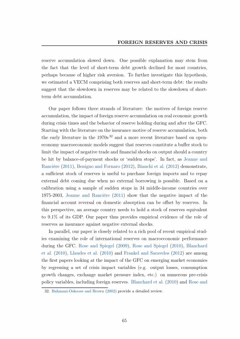
FOREIGN RESERVES AND CRISIS
reserve accumulation slowed down. One possible explanation may stem from
the fact that the level of short-term debt growth declined for most countries,
perhaps because of higher risk aversion. To further investigate this hypothesis,
we estimated a VECM comprising both reserves and short-term debt: the results
suggest that the slowdown in reserves may be related to the slowdown of short-
term debt accumulation.
Our paper follows three strands of literature: the motives of foreign reserve
accumulation, the impact of foreign reserve accumulation on real economic growth
during crisis times and the behavior of reserve holding during and after the GFC.
Starting with the literature on the insurance motive of reserve accumulation, both
the early literature in the 1970s 32 and a more recent literature based on open-
economy macroeconomic models suggest that reserves constitute a buffer stock to
limit the impact of negative trade and financial shocks on output should a country
be hit by balance-of-payment shocks or ‘sudden stops’. In fact, as Jeanne and
Rancière (2011), Benigno and Fornaro (2012), Bianchi et al. (2012) demonstrate,
a sufficient stock of reserves is useful to purchase foreign imports and to repay
external debt coming due when no external borrowing is possible. Based on a
calibration using a sample of sudden stops in 34 middle-income countries over
1975-2003, Jeanne and Rancière (2011) show that the negative impact of the
financial account reversal on domestic absorption can be offset by reserves. In
this perspective, an average country needs to hold a stock of reserves equivalent
to 9.1% of its GDP. Our paper thus provides empirical evidence of the role of
reserves as insurance against negative external shocks.
In parallel, our paper is closely related to a rich pool of recent empirical stud-
ies examining the role of international reserves on macroeconomic performance
during the GFC. Rose and Spiegel (2009), Rose and Spiegel (2010), Blanchard
et al. (2010), Llaudes et al. (2010) and Frankel and Saravelos (2012) are among
the first papers looking at the impact of the GFC on emerging market economies
by regressing a set of crisis impact variables (e.g. output losses, consumption
growth changes, exchange market pressure index, etc.) on numerous pre-crisis
policy variables, including foreign reserves. Blanchard et al. (2010) and Rose and
32. Bahmani-Oskooee and Brown (2002) provide a detailed review.
65
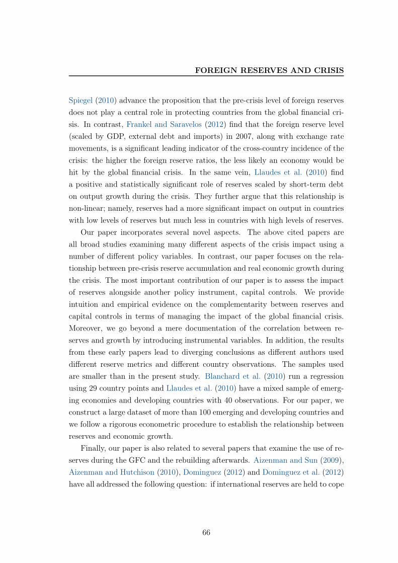
FOREIGN RESERVES AND CRISIS
Spiegel (2010) advance the proposition that the pre-crisis level of foreign reserves
does not play a central role in protecting countries from the global financial cri-
sis. In contrast, Frankel and Saravelos (2012) find that the foreign reserve level
(scaled by GDP, external debt and imports) in 2007, along with exchange rate
movements, is a significant leading indicator of the cross-country incidence of the
crisis: the higher the foreign reserve ratios, the less likely an economy would be
hit by the global financial crisis. In the same vein, Llaudes et al. (2010) find
a positive and statistically significant role of reserves scaled by short-term debt
on output growth during the crisis. They further argue that this relationship is
non-linear; namely, reserves had a more significant impact on output in countries
with low levels of reserves but much less in countries with high levels of reserves.
Our paper incorporates several novel aspects. The above cited papers are
all broad studies examining many different aspects of the crisis impact using a
number of different policy variables. In contrast, our paper focuses on the rela-
tionship between pre-crisis reserve accumulation and real economic growth during
the crisis. The most important contribution of our paper is to assess the impact
of reserves alongside another policy instrument, capital controls. We provide
intuition and empirical evidence on the complementarity between reserves and
capital controls in terms of managing the impact of the global financial crisis.
Moreover, we go beyond a mere documentation of the correlation between re-
serves and growth by introducing instrumental variables. In addition, the results
from these early papers lead to diverging conclusions as different authors used
different reserve metrics and different country observations. The samples used
are smaller than in the present study. Blanchard et al. (2010) run a regression
using 29 country points and Llaudes et al. (2010) have a mixed sample of emerg-
ing economies and developing countries with 40 observations. For our paper, we
construct a large dataset of more than 100 emerging and developing countries and
we follow a rigorous econometric procedure to establish the relationship between
reserves and economic growth.
Finally, our paper is also related to several papers that examine the use of re-
serves during the GFC and the rebuilding afterwards. Aizenman and Sun (2009),
Aizenman and Hutchison (2010), Dominguez (2012) and Dominguez et al. (2012)
have all addressed the following question: if international reserves are held to cope
66
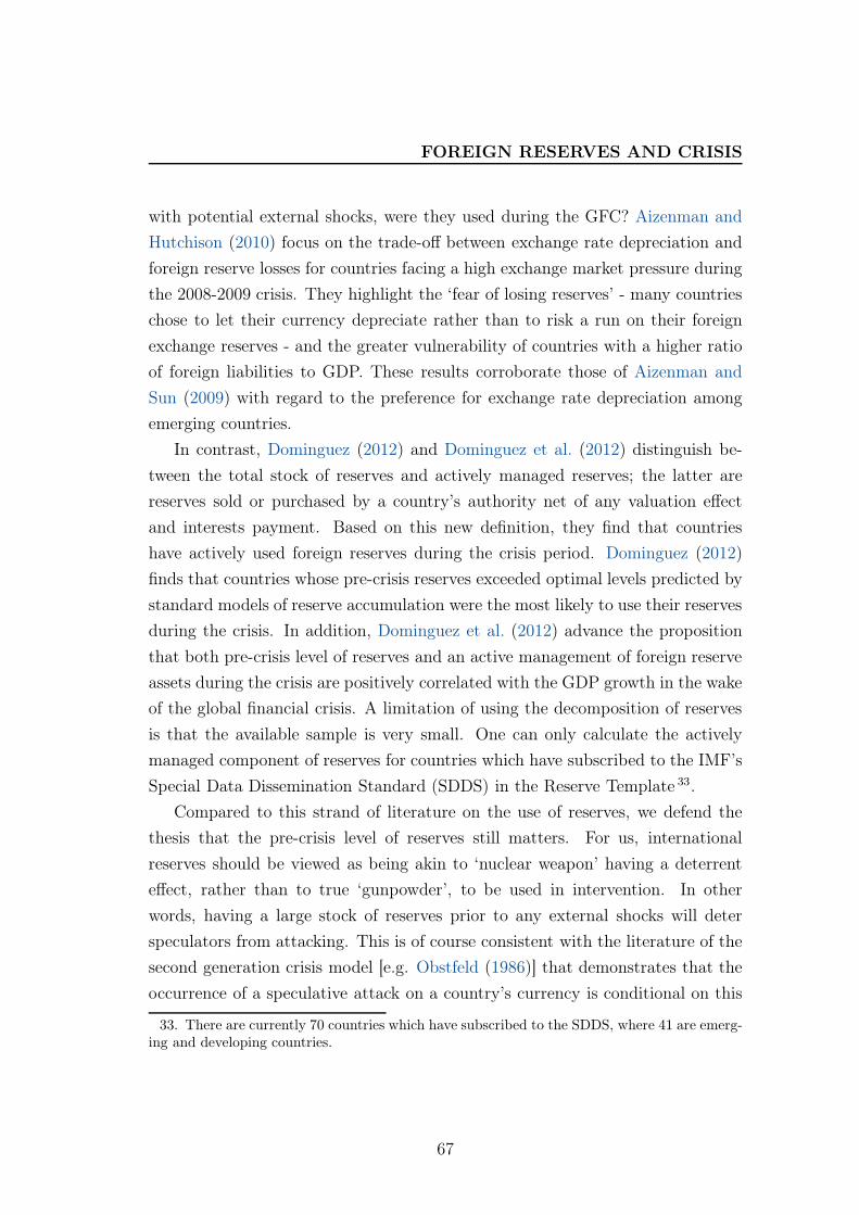
FOREIGN RESERVES AND CRISIS
with potential external shocks, were they used during the GFC? Aizenman and
Hutchison (2010) focus on the trade-off between exchange rate depreciation and
foreign reserve losses for countries facing a high exchange market pressure during
the 2008-2009 crisis. They highlight the ‘fear of losing reserves’ - many countries
chose to let their currency depreciate rather than to risk a run on their foreign
exchange reserves - and the greater vulnerability of countries with a higher ratio
of foreign liabilities to GDP. These results corroborate those of Aizenman and
Sun (2009) with regard to the preference for exchange rate depreciation among
emerging countries.
In contrast, Dominguez (2012) and Dominguez et al. (2012) distinguish be-
tween the total stock of reserves and actively managed reserves; the latter are
reserves sold or purchased by a country’s authority net of any valuation effect
and interests payment. Based on this new definition, they find that countries
have actively used foreign reserves during the crisis period. Dominguez (2012)
finds that countries whose pre-crisis reserves exceeded optimal levels predicted by
standard models of reserve accumulation were the most likely to use their reserves
during the crisis. In addition, Dominguez et al. (2012) advance the proposition
that both pre-crisis level of reserves and an active management of foreign reserve
assets during the crisis are positively correlated with the GDP growth in the wake
of the global financial crisis. A limitation of using the decomposition of reserves
is that the available sample is very small. One can only calculate the actively
managed component of reserves for countries which have subscribed to the IMF’s
Special Data Dissemination Standard (SDDS) in the Reserve Template 33.
Compared to this strand of literature on the use of reserves, we defend the
thesis that the pre-crisis level of reserves still matters. For us, international
reserves should be viewed as being akin to ‘nuclear weapon’ having a deterrent
effect, rather than to true ‘gunpowder’, to be used in intervention. In other
words, having a large stock of reserves prior to any external shocks will deter
speculators from attacking. This is of course consistent with the literature of the
second generation crisis model [e.g. Obstfeld (1986)] that demonstrates that the
occurrence of a speculative attack on a country’s currency is conditional on this
33. There are currently 70 countries which have subscribed to the SDDS, where 41 are emerg-ing and developing countries.
67
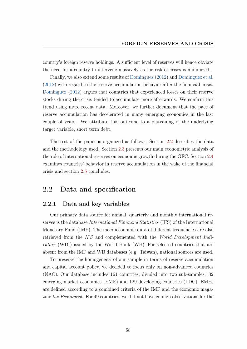
FOREIGN RESERVES AND CRISIS
country’s foreign reserve holdings. A sufficient level of reserves will hence obviate
the need for a country to intervene massively as the risk of crises is minimized.
Finally, we also extend some results of Dominguez (2012) and Dominguez et al.
(2012) with regard to the reserve accumulation behavior after the financial crisis.
Dominguez (2012) argues that countries that experienced losses on their reserve
stocks during the crisis tended to accumulate more afterwards. We confirm this
trend using more recent data. Moreover, we further document that the pace of
reserve accumulation has decelerated in many emerging economies in the last
couple of years. We attribute this outcome to a plateauing of the underlying
target variable, short term debt.
The rest of the paper is organized as follows. Section 2.2 describes the data
and the methodology used. Section 2.3 presents our main econometric analysis of
the role of international reserves on economic growth during the GFC. Section 2.4
examines countries’ behavior in reserve accumulation in the wake of the financial
crisis and section 2.5 concludes.
2.2 Data and specification
2.2.1 Data and key variables
Our primary data source for annual, quarterly and monthly international re-
serves is the database International Financial Statistics (IFS) of the International
Monetary Fund (IMF). The macroeconomic data of different frequencies are also
retrieved from the IFS and complemented with the World Development Indi-
cators (WDI) issued by the World Bank (WB). For selected countries that are
absent from the IMF and WB databases (e.g. Taiwan), national sources are used.
To preserve the homogeneity of our sample in terms of reserve accumulation
and capital account policy, we decided to focus only on non-advanced countries
(NAC). Our database includes 161 countries, divided into two sub-samples: 32
emerging market economies (EME) and 129 developing countries (LDC). EMEs
are defined according to a combined criteria of the IMF and the economic maga-
zine the Economist. For 49 countries, we did not have enough observations for the
68
FOREIGN RESERVES AND CRISIS
key independent variables including control variables; therefore, 112 countries are
effectively used in our main regressions. The details about our country coverage
can be found in Appendix 2.A.
International reserves
Several important features of the reserve data we use in this paper need to be
highlighted.
Which assets are included in reserves? International reserves can be defined as
the immediately available external assets denominated in foreign currencies that a
country’s government or monetary authority effectively holds. According to the
IFS, total international reserves comprise foreign exchange reserves 34, reserve
position in the Fund, the U.S. dollar value of SDR holdings and gold holdings 35.
Except gold holdings, all the other assets are included in the reserve data we use
in the scope of this paper. The reason to exclude gold holdings is that the gold
share is very small in non-advanced countries and gold holdings are less liquid
than other reserve assets. As foreign reserves constitute the major component of
international reserves (reserve position in the Fund and SDR holdings are also
very small), we will interchangeably use the terms international reserves and
foreign reserves in this paper.
Similarly, external assets held by sovereign wealth funds are not included in
our reserve data. Foreign assets held by a sovereign wealth fund and that under
control of a central bank are indeed managed under very different principles.
While higher returns and strategic value are the objective of reserve management
in a sovereign wealth fund, the liquidity and security of foreign assets are the
guidelines for reserve management in a central bank. As we focus on the insurance
role of foreign reserves, we only consider those foreign assets managed under the
liquidity and security motives.
Moreover, the IMF credit facilities (e.g. Precautionary and liquidity line,
34. This includes ‘official claims on nonresidents in the form of foreign banknotes, bank de-posits, treasury bills, short- and long-term government securities and other claims usable in theevent of balance of payments need’ (IFS Yearbook 2012).
35. Gold holdings are expressed in millions of fine troy ounces and valued in U.S. dollar byeach country.
69
FOREIGN RESERVES AND CRISIS
Flexible credit line, Stand-by facility, etc.) and bilateral swap lines between
countries are not included in foreign reserves defined by the IFS and used in
this paper 36. There are fundamental differences between the self-owned stock
of foreign reserves and ad hoc contingent facility instruments which are short-
term in nature. A few papers examine the substitutability between swap lines
and foreign reserves [see Aizenman et al. (2011), Obstfeld et al. (2009)]; this is
however out of the scope of this paper.
Finally, it is very important to notice that there is an issuance of 183 billion
of Special Drawing Rights by the IMF in August 2009 (equivalent to 283 billion
of U.S. dollars). This is in part due to the requirements of reforming the inter-
national monetary system under the G20 negotiations. This new issuance can be
regarded as an exogenous increase of member countries’ SDRs, thus of their stock
of foreign reserves; it leads to an unexpected jump in the reserve data from 2009
and constitutes an issue when we examine the after-crisis behavior of reserve ac-
cumulation. Therefore, in order to concentrate on a given country’s own decision
of holding foreign reserves, we subtract this newly issued SDR in 2009 from our
monthly and quarterly data on foreign reserves which is used in Section 2.4.
How to incorporate reserve data into our analysis? In this paper, we will
use reserve adequacy ratios (in log 37) instead of the absolute level of reserves.
The reasons are two-fold. First, a reserve adequacy ratio facilitates cross-country
comparison; the heterogeneity in the stock of reserves is tremendous, for example
between China, which holds more than a third of the world foreign reserves, and
small African countries. Second, the absolute level of reserves does not provide
useful information about the robustness and resilience of a country facing shocks;
36. However, we used a dummy variable for the Fed swap lines. This only concerns Koreaand Mexico in our non-advanced country sample. The introduction of this dummy does notchange our results. Details are available upon request.
37. We use the log ratio in our regressions for several reasons. First, it is commonly used inthe existing literature regarding the role of foreign reserves during crises in emerging marketeconomies. Second, the evolution of international reserves, especially in non-advanced countries,is non-linear, displaying an exponential pattern. Third, based on our analysis, the effect of ex
ante holding of reserves on economic growth is non-linear; it exhibits positive and concavepatterns, meaning that the marginal contribution of the reserve adequacy ratio on growth isdiminishing. The effect is more pronounced for countries with low values of reserves to short-term debt ratio. Llaudes et al. (2010) provides a more detailed account on the non-linearity ofthis effect.
70
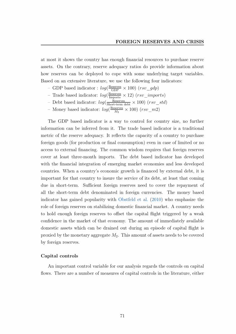
FOREIGN RESERVES AND CRISIS
at most it shows the country has enough financial resources to purchase reserve
assets. On the contrary, reserve adequacy ratios do provide information about
how reserves can be deployed to cope with some underlying target variables.
Based on an extensive literature, we use the following four indicators:
– GDP based indicator : log(ReservesGDP
× 100) (rsv_gdp)
– Trade based indicator: log(ReservesImports
× 12) (rsv_imports)
– Debt based indicator: log( ReservesShort-term debt
× 100) (rsv_std)
– Money based indicator: log(ReservesM2
× 100) (rsv_m2)
The GDP based indicator is a way to control for country size, no further
information can be inferred from it. The trade based indicator is a traditional
metric of the reserve adequacy. It reflects the capacity of a country to purchase
foreign goods (for production or final consumption) even in case of limited or no
access to external financing. The common wisdom requires that foreign reserves
cover at least three-month imports. The debt based indicator has developed
with the financial integration of emerging market economies and less developed
countries. When a country’s economic growth is financed by external debt, it is
important for that country to insure the service of its debt, at least that coming
due in short-term. Sufficient foreign reserves need to cover the repayment of
all the short-term debt denominated in foreign currencies. The money based
indicator has gained popularity with Obstfeld et al. (2010) who emphasize the
role of foreign reserves on stabilizing domestic financial market. A country needs
to hold enough foreign reserves to offset the capital flight triggered by a weak
confidence in the market of that economy. The amount of immediately available
domestic assets which can be drained out during an episode of capital flight is
proxied by the monetary aggregateM2. This amount of assets needs to be covered
by foreign reserves.
Capital controls
An important control variable for our analysis regards the controls on capital
flows. There are a number of measures of capital controls in the literature, either
71
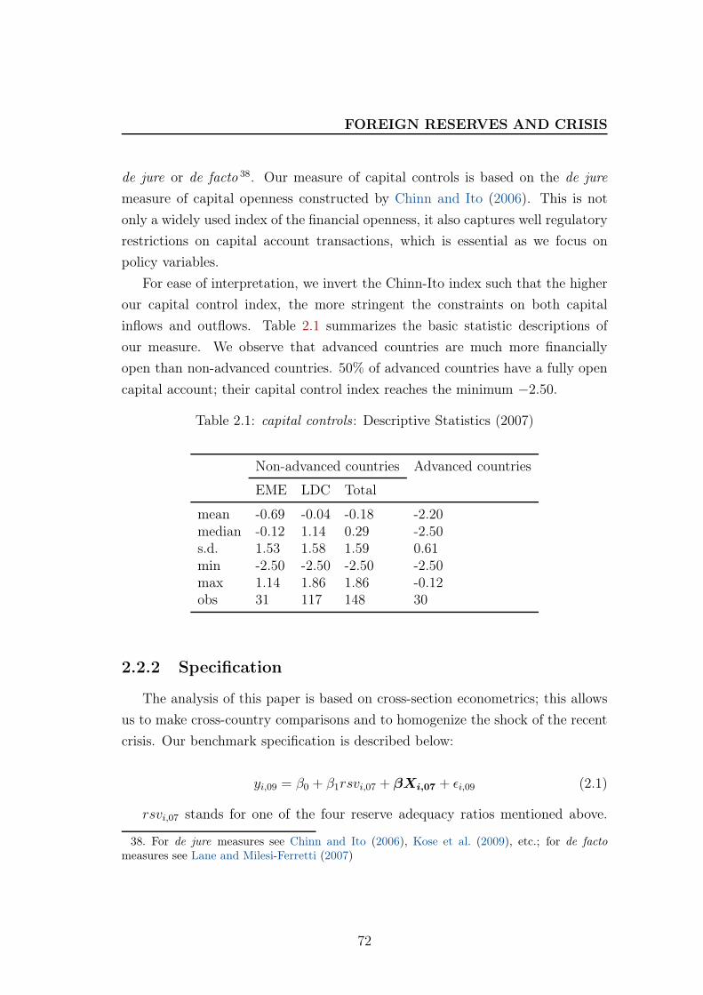
FOREIGN RESERVES AND CRISIS
de jure or de facto 38. Our measure of capital controls is based on the de jure
measure of capital openness constructed by Chinn and Ito (2006). This is not
only a widely used index of the financial openness, it also captures well regulatory
restrictions on capital account transactions, which is essential as we focus on
policy variables.
For ease of interpretation, we invert the Chinn-Ito index such that the higher
our capital control index, the more stringent the constraints on both capital
inflows and outflows. Table 2.1 summarizes the basic statistic descriptions of
our measure. We observe that advanced countries are much more financially
open than non-advanced countries. 50% of advanced countries have a fully open
capital account; their capital control index reaches the minimum −2.50.
Table 2.1: capital controls: Descriptive Statistics (2007)
Non-advanced countries Advanced countries
EME LDC Total
mean -0.69 -0.04 -0.18 -2.20median -0.12 1.14 0.29 -2.50s.d. 1.53 1.58 1.59 0.61min -2.50 -2.50 -2.50 -2.50max 1.14 1.86 1.86 -0.12obs 31 117 148 30
2.2.2 Specification
The analysis of this paper is based on cross-section econometrics; this allows
us to make cross-country comparisons and to homogenize the shock of the recent
crisis. Our benchmark specification is described below:
yi,09 = β0 + β1rsvi,07 + βXi,07 + ǫi,09 (2.1)
rsvi,07 stands for one of the four reserve adequacy ratios mentioned above.
38. For de jure measures see Chinn and Ito (2006), Kose et al. (2009), etc.; for de facto
measures see Lane and Milesi-Ferretti (2007)
72
FOREIGN RESERVES AND CRISIS
Xi,07 corresponds to additional control variables. Note that all the independent
variables (except for dummies) are lagged two periods 39. Taking lagged indepen-
dent variables allows us to have a snapshot of the situation of the country before
the start of the crisis, and to use this picture to explain its performance during
the crisis. Using later values for reserves and other controls would be problem-
atic, since countries may already have changed their reserve holdings by the end
of 2008 due to the start of the crisis. Yet, this does not solve endogeneity issues,
which we will tackle in Section 2.3.4.
Construction of the dependent variable yi,09
To assess the role of foreign reserves in mitigating the crisis impact on real
economic growth in 2009, we need to construct appropriate measures of the GFC
impact. Based on the above-cited literature on this issue, we use two measures
that aim at capturing the gap between the actual real economic growth rate and
a counterfactual growth rate should the crisis have not occurred.
The first method calculates the difference between the realized real economic
growth rate and a linear prediction from a historical mean. We call this dependent
variable ‘purged real GDP growth’, and denote it rgdp_residual in our equations
and tables. It is obtained as follows:
rgdp_residuali,09 = ∆ryi,09 − ∆ryi,09
∆ryi,09 = α0 + α1∆ryi,03−08
The coefficients α0 and α1 are estimated using a preliminary regression:
∆ryi,09 = α0 + α1∆ryi,03−08 + ǫi,09
This preliminary regression assumes constant coefficients across countries,
namely the contribution of the historical trend to real economic growth rate at a
given time t being identical for all countries in our sample.
39. As a robustness test, we have also used independent variables lagged three periods. Theresults remain very similar to that presented in the paper. Details can be provided upon request.
73
FOREIGN RESERVES AND CRISIS
Our alternative dependent variable follows Blanchard et al. (2010) and Berk-
men et al. (2012) and captures the change between the actual real GDP growth
in 2009 and the IMF World Economic Outlook (WEO) forecast in the first quar-
ter of 2008 (before the Lehman collapse in September of the same year). This
variable measures the real output losses due to the unexpected magnitude of the
financial crisis. We call it ‘unexpected real GDP growth’ and denote it rgdp_fe.
One caveat about this variable is that there might be estimation errors associated
with the forecast model that the IMF adopts. We assume that these errors are
not time-varying and consistent over time.
We have also tried another potential dependent variable: the difference be-
tween actual real GDP growth and a historical mean, over 2003-2008. We find
consistent results using this different dependent variable 40.
In Appendix 2.B, figures 2.11 and 2.12 illustrate the ranking of a few big
emerging market economies (belonging to the G20) in terms of our two dependent
variables rgdp_residual or rgdp_fe. In the same appendix, a list of the main
variables used in our econometric analysis is also available.
2.3 Econometric analysis: the role of pre-crisis re-
serve adequacy during the GFC
2.3.1 Reserve adequacy ratios: which one works better?
Based on the 2008-2009 global financial crisis, we first try to examine whether
ex ante foreign reserve accumulation has played any role in preventing output
losses during the crisis. We pay a particular attention to the distinct explanatory
power of each of the above-mentioned four reserve metrics.
We find that the reserves to short-term debt ratio is the most useful indicator
to explain the real output growth during the crisis. The stock of foreign reserves
scaled by the level of short-term debt two years prior to the crisis is positively
and significantly correlated with the real GDP growth deviation from the trend.
We illustrate this result using the full sample and the ‘purged real GDP growth’
40. The results using this third variable as dependent variable are available upon request.
74
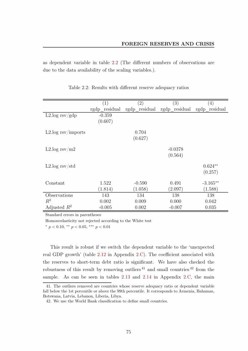
FOREIGN RESERVES AND CRISIS
as dependent variable in table 2.2 (The different numbers of observations are
due to the data availability of the scaling variables.).
Table 2.2: Results with different reserve adequacy ratios
(1) (2) (3) (4)rgdp_residual rgdp_residual rgdp_residual rgdp_residual
L2.log rsv/gdp -0.359(0.607)
L2.log rsv/imports 0.704(0.627)
L2.log rsv/m2 -0.0378(0.564)
L2.log rsv/std 0.624∗∗
(0.257)
Constant 1.522 -0.590 0.491 -3.165∗∗
(1.814) (1.058) (2.097) (1.588)Observations 143 134 138 138R2 0.002 0.009 0.000 0.042Adjusted R2 -0.005 0.002 -0.007 0.035
Standard errors in parentheses
Homoscedasticity not rejected according to the White test∗ p < 0.10, ∗∗ p < 0.05, ∗∗∗ p < 0.01
This result is robust if we switch the dependent variable to the ‘unexpected
real GDP growth’ (table 2.12 in Appendix 2.C). The coefficient associated with
the reserves to short-term debt ratio is significant. We have also checked the
robustness of this result by removing outliers 41 and small countries 42 from the
sample. As can be seen in tables 2.13 and 2.14 in Appendix 2.C, the main
41. The outliers removed are countries whose reserve adequacy ratio or dependent variablefall below the 1st percentile or above the 99th percentile. It corresponds to Armenia, Bahamas,Botswana, Latvia, Lebanon, Liberia, Libya.
42. We use the World Bank classification to define small countries.
75
FOREIGN RESERVES AND CRISIS
conclusions remain unchanged. Given that China has a very specific behavior in
terms of reserve accumulation, we also removed this country from the sample,
and obtained largely unchanged results 43.
2.3.2 Do reserves matter for economic growth during the
GFC?
In order to better understand the influence of reserve holdings on output
growth, we add control variables and estimate the full specification of our regres-
sion equation (2.1). The control variables Xi,07 include capital controls, trade
openness, an exchange rate regime dummy 44 and an oil exporter dummy 45.
After controlling for further specific characteristics of different countries, we
still find that the accumulation of foreign reserves prior to the crisis positively
and significantly contributes to the real GDP growth during the crisis. The
significance and magnitude of the coefficient associated with the reserve adequacy
ratio remain similar when adding controls, for both of our dependent variables
(columns (1) and (2) in table 2.3).
43. As these findings are obtained with a ratio, a natural question to ask is which term in theratio drives the results. However, this is a complex question: testing both terms separately maynot be conclusive if what really matters is the ratio of the two. Bearing this caveat in mind, weran two additional sets of regressions. First, when using log( reserves
STD) and log( reserves
GDP), both
are significant with rgdp_residual as dependent variable, but only the first term is significantwith rgdp_fe as dependent variable. Second, when using log( reserves
STD) and log( STD
GDP), only
the second term is significant with rgdp_residual as dependent variable, and nothing is signif-icant with rgdp_fe as dependent variable (with a collinearity issue). Third, log( reserves
GDP) and
log( STDGDP
) have also been used to replace the reserve adequacy ratio. Only the second termturns out to be significant; but this result cannot validate the hypothesis that short-term debtmatters more than foreign reserves, as log( reserves
GDP) is not a significant regressor even in a bi-
variate regression with our two dependent variables (table 2.2). These complementary results,which are available upon request, are therefore mixed, such that it is hard to conclude whetherone of the two terms is predominantly driving the main result.
44. Our exchange rate regime dummy is constructed based on the classification by Reinhartand Rogoff (2004). It takes the value 1 when a country has a ‘crawling peg’ or more controlledexchange rate regime; it takes the value 0 when a country has a ‘managed floating’ or ‘freefloating’ regime.
45. The countries classified as oil exporters/producers are the following: Algeria, Angola,Bahrain, Cameroon, Chad, Congo, Ecuador, Equatorial Guinea, Gabon, Iran, Iraq, Kaza-khstan, Kuwait, Libya, Mexico, Nigeria, Oman, Qatar, Russia, Saudi Arabia, Sudan, Timor-Leste, Trinidad and Tobago, Turkmenistan, United Arab Emirates, Uzbekistan, Venezuela,Yemen.
76
FOREIGN RESERVES AND CRISIS
We further test the robustness of our results by estimating the same regres-
sions using trimmed samples. Appendix 2.D provides the results obtained after
outliers 46 or/and small countries are ruled out. The coefficients have the same
signs as in table 2.3 but have larger magnitude and stronger significance. One
additional control variable, trade openness, turns out to be significant and has
a negative sign as expected when rgdp_residual is used as dependent variable.
The goodness of fit, in terms of R2 and adjusted R2, also becomes larger. Hence,
our results can be regarded as robust and do not depend on the inclusion of
outliers and small countries.
For robustness, we tested our results with additional control variables (i.e. net
foreign assets and current account balance); the results are qualitatively similar.
More restrictively trimmed samples have also been used throughout the paper 47;
the estimates of interest (reserves to short-term debt ratio and capital controls)
become even larger and more significant. These results are available upon request.
2.3.3 Controlling for the interaction between reserves and
capital controls
The introduction of an interacted term between foreign reserves and capital
controls as a further control variable can help us check the robustness of our re-
sults, and shed light on the complementarity between foreign reserves and capital
controls.
We show how the role of foreign reserves on economic growth may depend
on other relevant policies, in particular capital account management, and then
present the specification we adopt to estimate the interacted term.
46. Defined in the same line as in footnote 12, namely all observations which fall below the1st percentile or above the 99th percentile of any continuous variables (i.e. dependent variable,reserve ratio and trade openness). This criteria will apply in the subsequent sections whenoutliers are eliminated. As a result we further drop Brazil, Hong Kong, Rwanda and Singaporefrom the sample (no financial centers in this case).
47. In these regressions, we have removed the top and bottom 5% observations of any continu-ous variables, or countries whose reserves to short-term debt ratio exceeds 1000 (75th percentile)in 2007.
77
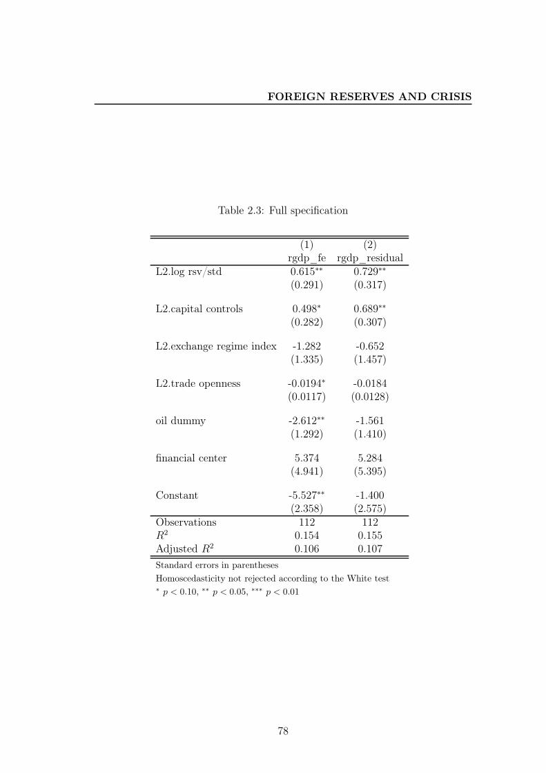
FOREIGN RESERVES AND CRISIS
Table 2.3: Full specification
(1) (2)rgdp_fe rgdp_residual
L2.log rsv/std 0.615∗∗ 0.729∗∗
(0.291) (0.317)
L2.capital controls 0.498∗ 0.689∗∗
(0.282) (0.307)
L2.exchange regime index -1.282 -0.652(1.335) (1.457)
L2.trade openness -0.0194∗ -0.0184(0.0117) (0.0128)
oil dummy -2.612∗∗ -1.561(1.292) (1.410)
financial center 5.374 5.284(4.941) (5.395)
Constant -5.527∗∗ -1.400(2.358) (2.575)
Observations 112 112R2 0.154 0.155Adjusted R2 0.106 0.107
Standard errors in parentheses
Homoscedasticity not rejected according to the White test∗ p < 0.10, ∗∗ p < 0.05, ∗∗∗ p < 0.01
78
FOREIGN RESERVES AND CRISIS
Intuition
Our empirical results suggest that foreign reserves and capital controls are
complements with regard to their impact on economic growth during the GFC.
We provide here an intuition which supports this particular relationship. In fact,
if foreign reserves can be seen as munitions of liquidity that can be deployed when
a country is cut off from external financial markets, a closed capital account can
be interpreted as a neutralized playing field for the impact of reserves to be effec-
tive. Indeed, capital controls insure that public capital outflows (foreign reserve
purchasing) are not completely offset by private capital inflows (accumulation of
private foreign liabilities). As a matter of fact, foreign reserves can be used to
provide an aggregate insurance to the economy, but the moral hazard associated
with foreign reserve accumulation might incite the private sector, firms and banks,
to take extra risks given that the government will provide foreign currency liq-
uidity when it is necessary. Therefore, the insurance provided by foreign reserves
can be offset by private capital inflows should the capital account be completely
open. There are a few recent theoretical works which support our intuition and
empirical finding. For example, Benigno and Fornaro (2012), Bacchetta et al.
(2013) and Cheng (2013) all argue that the imperfect substitutability between
public and private capital flows is crucial for foreign reserves to play a role. Ac-
cording to this strand of literature, foreign reserve accumulation and a closed
capital account are complements rather than substitutes.
Specification
There are several ways to introduce an interactive term. To facilitate interpre-
tation, we use a demeaned interacted term: (rsv_stdi − rsv_stdi) × (cci − cci)
as stated in equation (2.2). Using this setting, the coefficient before rsv_stdi(respectively cci) refers to the marginal effect of that variable when cci (respec-
tively rsv_stdi) is valued at its mean. Note that xi,07 refers to the set of control
variables we used in Section 2.3.2 except capital controls.
79
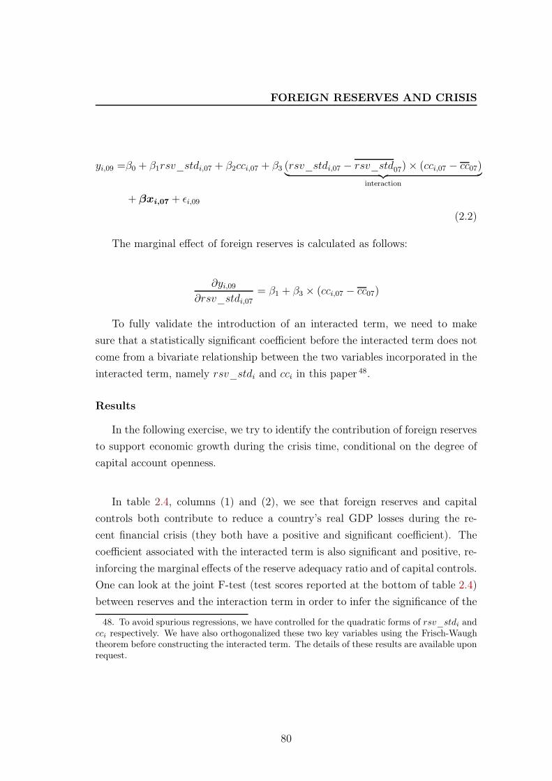
FOREIGN RESERVES AND CRISIS
yi,09 =β0 + β1rsv_stdi,07 + β2cci,07 + β3 (rsv_stdi,07 − rsv_std07)× (cci,07 − cc07)︸ ︷︷ ︸interaction
+ βxi,07 + ǫi,09
(2.2)
The marginal effect of foreign reserves is calculated as follows:
∂yi,09∂rsv_stdi,07
= β1 + β3 × (cci,07 − cc07)
To fully validate the introduction of an interacted term, we need to make
sure that a statistically significant coefficient before the interacted term does not
come from a bivariate relationship between the two variables incorporated in the
interacted term, namely rsv_stdi and cci in this paper 48.
Results
In the following exercise, we try to identify the contribution of foreign reserves
to support economic growth during the crisis time, conditional on the degree of
capital account openness.
In table 2.4, columns (1) and (2), we see that foreign reserves and capital
controls both contribute to reduce a country’s real GDP losses during the re-
cent financial crisis (they both have a positive and significant coefficient). The
coefficient associated with the interacted term is also significant and positive, re-
inforcing the marginal effects of the reserve adequacy ratio and of capital controls.
One can look at the joint F-test (test scores reported at the bottom of table 2.4)
between reserves and the interaction term in order to infer the significance of the
48. To avoid spurious regressions, we have controlled for the quadratic forms of rsv_stdi andcci respectively. We have also orthogonalized these two key variables using the Frisch-Waughtheorem before constructing the interacted term. The details of these results are available uponrequest.
80
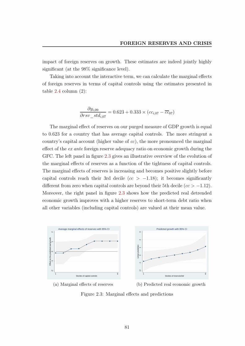
FOREIGN RESERVES AND CRISIS
impact of foreign reserves on growth. These estimates are indeed jointly highly
significant (at the 98% significance level).
Taking into account the interactive term, we can calculate the marginal effects
of foreign reserves in terms of capital controls using the estimates presented in
table 2.4 column (2):
∂yi,09∂rsv_stdi,07
= 0.623 + 0.333× (cci,07 − cc07)
The marginal effect of reserves on our purged measure of GDP growth is equal
to 0.623 for a country that has average capital controls. The more stringent a
country’s capital account (higher value of cc), the more pronounced the marginal
effect of the ex ante foreign reserve adequacy ratio on economic growth during the
GFC. The left panel in figure 2.3 gives an illustrative overview of the evolution of
the marginal effects of reserves as a function of the tightness of capital controls.
The marginal effects of reserves is increasing and becomes positive slightly before
capital controls reach their 3rd decile (cc > −1.18); it becomes significantly
different from zero when capital controls are beyond their 5th decile (cc > −1.12).
Moreover, the right panel in figure 2.3 shows how the predicted real detrended
economic growth improves with a higher reserves to short-term debt ratio when
all other variables (including capital controls) are valued at their mean value.
−2
−1
01
2E
ffect
on
the
pred
icte
d re
al g
row
th
1 9Deciles of capital controls
Average marginal effects of reserves with 95% CI
(a) Marginal effects of reserves
−2
−1
01
23
Line
ar p
redi
ctio
n
1 9Deciles of reserves/std
Predicted growth with 95% CI
(b) Predicted real economic growth
Figure 2.3: Marginal effects and predictions
81
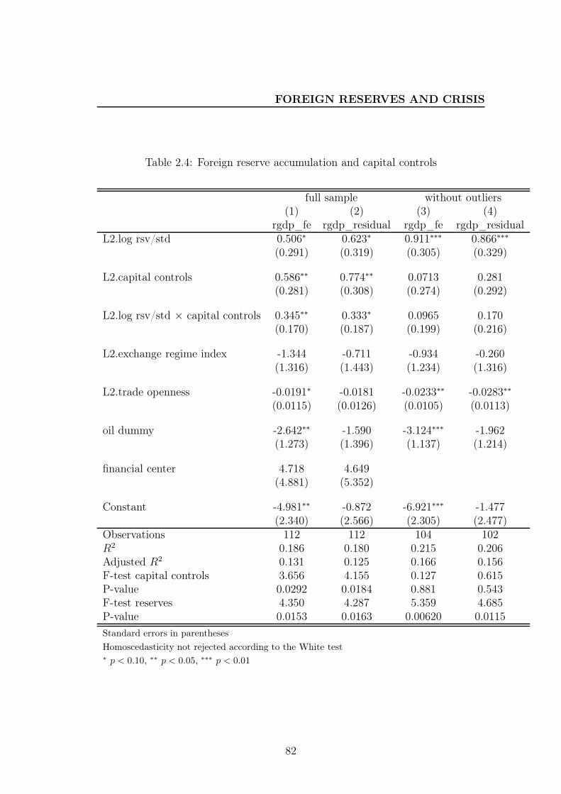
FOREIGN RESERVES AND CRISIS
Table 2.4: Foreign reserve accumulation and capital controls
full sample without outliers(1) (2) (3) (4)
rgdp_fe rgdp_residual rgdp_fe rgdp_residualL2.log rsv/std 0.506∗ 0.623∗ 0.911∗∗∗ 0.866∗∗∗
(0.291) (0.319) (0.305) (0.329)
L2.capital controls 0.586∗∗ 0.774∗∗ 0.0713 0.281(0.281) (0.308) (0.274) (0.292)
L2.log rsv/std × capital controls 0.345∗∗ 0.333∗ 0.0965 0.170(0.170) (0.187) (0.199) (0.216)
L2.exchange regime index -1.344 -0.711 -0.934 -0.260(1.316) (1.443) (1.234) (1.316)
L2.trade openness -0.0191∗ -0.0181 -0.0233∗∗ -0.0283∗∗
(0.0115) (0.0126) (0.0105) (0.0113)
oil dummy -2.642∗∗ -1.590 -3.124∗∗∗ -1.962(1.273) (1.396) (1.137) (1.214)
financial center 4.718 4.649(4.881) (5.352)
Constant -4.981∗∗ -0.872 -6.921∗∗∗ -1.477(2.340) (2.566) (2.305) (2.477)
Observations 112 112 104 102R2 0.186 0.180 0.215 0.206Adjusted R2 0.131 0.125 0.166 0.156F-test capital controls 3.656 4.155 0.127 0.615P-value 0.0292 0.0184 0.881 0.543F-test reserves 4.350 4.287 5.359 4.685P-value 0.0153 0.0163 0.00620 0.0115
Standard errors in parentheses
Homoscedasticity not rejected according to the White test∗ p < 0.10, ∗∗ p < 0.05, ∗∗∗ p < 0.01
82
FOREIGN RESERVES AND CRISIS
Here again, we check for robustness by dropping outliers 49. Whereas the pre-
vious results (without the interaction term between reserves and capital controls)
were fairly robust to this change of sample, here both the coefficients of capital
controls and of the interaction term lose significance when we control for outliers,
as one can see in columns (3) and (4) of table 2.4 50. However, the coefficient
associated with the reserves to short-term debt ratio is highly significant and in-
creases in magnitude. From this, we can conclude that the impact of the reserve
adequacy ratio itself is still fairly robust, even after we drop outliers from our
sample. Finally, as regards the magnitude of the coefficient associated with the
reserve adequacy ratio, it seems that the estimate we obtained in our benchmark
regression (table 2.3) is rather a minimal value, since the associated coefficient
tends to increase when excluding outliers.
2.3.4 Accounting for endogeneity
As mentioned above, using foreign reserves as an explanatory variable to ex-
plain real economic growth can cause endogeneity issues. Foreign reserves might
be held by a central bank as in anticipation of a future negative shock to the
national economy; foreign reserves and higher GDP growth might also both be
by-products of a mercantilist exchange rate policy. So far, we have been us-
ing lagged metrics of foreign reserves as our main explanatory variable without
controlling for endogeneity; this is also the method adopted by most existing
empirical papers on foreign reserves. This may induce a bias in our coefficient
estimates, the direction of which is however ambiguous. On the one hand, if we
consider that fragile countries accumulate more reserves for precautionary rea-
sons, and are more likely to be affected in a crisis (because of the idiosyncratic
fragility), we can argue that the OLS coefficient associated to reserves may be bi-
ased downwards. On the other hand, reserve accumulation can be a buy-product
of an undervalued domestic currency which stimulates economic growth through
49. Results are similar when excluding both small countries and outliers. They are presentedin Appendix 2.E table 2.17. Results using more restrictively trimmed samples are availableupon request.
50. Note that by dropping outliers (top and bottom 1% of observations of each continuousvariable), we drop all financial centers from our sample, which explains the absence of thefinancial center dummy in columns (3) and (4) of table 2.4.
83
FOREIGN RESERVES AND CRISIS
strong exports. This mechanism implies an upward bias of our OLS coefficient. It
is therefore difficult to predict the direction of the bias altogether. We go one step
further to account for endogeneity and reverse causality by choosing appropriate
instrumental variables for foreign reserve metrics.
Construction of instrumental variables
Finding an instrumental variable for reserves is not an easy task. An appro-
priate instrumental variable needs to fulfill two conditions: first, it needs to be
correlated with the instrumented variable; second, it must be uncorrelated with
the error term in the original OLS regression (equation (2.1)). We have thought
of various candidates, including a dummy for the occurrence of currency crises
in the 1970’s and 1980’s, a measure of the severity of past crises, real GDP per
capita expressed in purchasing power parity, or metrics of regional peer pressure
for reserves accumulation. After carefully examining different possibilities, we
conclude that the regional peer pressure is the best suited instrumental variable
with respect to our analysis.
Regional peer pressure for reserve accumulation captures the idea of ‘keeping
up with the Joneses’, namely a country might be motivated to hold foreign re-
serves as its neighbors do so. In many empirical papers 51, this idea of regional
peer pressure is introduced to study the demand function of foreign reserves.
Therefore, it should be highly correlated with foreign reserve accumulation per
se. Furthermore, these instrumental variables allow us to focus on reserves accu-
mulated for ‘neighborhood’ motives, and disregard those related to precautionary
or mercantilist motives, which are related to the economic performance of a coun-
try and therefore endogenous.
As for our instrumental variables, we propose two proxies to measure the
regional peer pressure:
– IDW06i: An inverse distance weighted mean for country i measures the
average of the reserves to GDP ratio of all other countries in the world
(j 6= i) weighted by the inverse distance between country i and country
j (so that country i’s neighbors matter more than remoter countries). We
51. See Bastourre et al. (2009), Cheung and Sengupta (2011), etc.
84
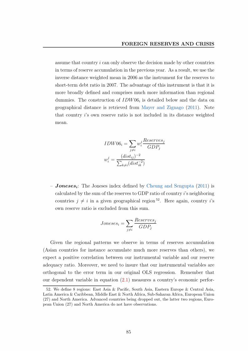
FOREIGN RESERVES AND CRISIS
assume that country i can only observe the decision made by other countries
in terms of reserve accumulation in the previous year. As a result, we use the
inverse distance weighted mean in 2006 as the instrument for the reserves to
short-term debt ratio in 2007. The advantage of this instrument is that it is
more broadly defined and comprises much more information than regional
dummies. The construction of IDW06i is detailed below and the data on
geographical distance is retrieved from Mayer and Zignago (2011). Note
that country i’s own reserve ratio is not included in its distance weighted
mean.
IDW06i =∑
j 6=i
wjiReservesjGDPj
wji =(distij)
−2
∑k 6=i(dist
−2ik )
– Jonesesi: The Joneses index defined by Cheung and Sengupta (2011) is
calculated by the sum of the reserves to GDP ratio of country i’s neighboring
countries j 6= i in a given geographical region 52. Here again, country i’s
own reserve ratio is excluded from this sum.
Jonesesi =∑
j 6=i
ReservesjGDPj
Given the regional patterns we observe in terms of reserves accumulation
(Asian countries for instance accumulate much more reserves than others), we
expect a positive correlation between our instrumental variable and our reserve
adequacy ratio. Moreover, we need to insure that our instrumental variables are
orthogonal to the error term in our original OLS regression. Remember that
our dependent variable in equation (2.1) measures a country’s economic perfor-
52. We define 8 regions: East Asia & Pacific, South Asia, Eastern Europe & Central Asia,Latin America & Caribbean, Middle East & North Africa, Sub-Saharan Africa, European Union(27) and North America. Advanced countries being dropped out, the latter two regions, Euro-pean Union (27) and North America do not have observations.
85
FOREIGN RESERVES AND CRISIS
mance during the global financial crisis compared to non-crisis times, namely a
‘detrended’ real GDP growth rate. This is thus a measure of short-term eco-
nomic growth, mainly affected by circumstantial factors (i.e. temporary external
shocks). The importance of reserve holdings of a country’s neighbors in 2006
should not be directly related to the impact of the 2009 financial crisis on eco-
nomic growth.
Hence, the reserve accumulation behavior of neighbor countries before the
crisis has no clear relationship with residuals of our OLS regression (which cor-
respond to the crisis impact that is not explained by reserves, capital controls,
trade openness, exchange rate regime, and financial centers) 53.
We provide the results of the first-stage regressions using our candidate in-
strumental variables, in table 2.18 in Appendix 2.F. Column (1) shows the results
using the distance-weighted index, column (2) uses the Joneses index, while col-
umn (3) uses both variables as joint instruments. In all three cases we find
a significant correlation with the instrumented variable, reserves to short-term
debt ratio, and obtain signs consistent with our expectation, namely the stronger
regional pressure, the higher reserve adequacy ratio. The R2 is also reasonably
large, around 14% in all three cases. These findings confirm our choice of instru-
mental variables. The sign and goodness of fit of the distance-weighted index
remain stable when we drop outliers; that of the Joneses index is slightly weaker
(see table 2.19 in Appendix 2.F).
Two-stage least square regressions
We present in table 2.5 the results of the second stage regression when the
reserve adequacy ratio is instrumented. To facilitate interpretation, we repeat our
OLS results in column (1). Columns (2), (3) and (4) respectively show the final
results of the two-stage least square procedure (2SLS) using the distance-weighted
index, the Joneses index and both.
53. One caveat: one may argue that countries in a given region have similar trade and financialflows, therefore the pattern of their reserve accumulation may have a common componentrelated to common growth expectations in the region. This would weaken the exogeneity of ourinstruments.
86
FOREIGN RESERVES AND CRISIS
Using instrumental variables, the coefficients of interest in our regressions
are not significant any more. This result is not very surprising, since we know
that the 2SLS procedure usually yields larger standard errors, driving down the
significance of the 2SLS estimates. For this reason, it is hard to conclude anything
in terms of bias correction and magnitude. The signs of the 2SLS estimates are
consistent with the OLS estimates, although the magnitude of the 2SLS estimates
are higher, but none of the coefficients estimated through 2SLS are significantly
different from zero 54.
For robustness checks, table 2.20 in Appendix 2.F presents similar results when
dropping outliers from the sample. We also instrumented the reserve adequacy
ratio when adding the interaction term between reserves and capital controls in
the regression; results are fairly similar to that presented above and are available
upon request.
54. Considering that the corresponding Hausman test fails to reject the null hypothesis ofexogenous right-hand-side variables, we feel more confident on relying on our OLS estimates.
87
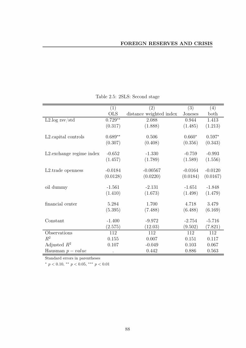
FOREIGN RESERVES AND CRISIS
Table 2.5: 2SLS: Second stage
(1) (2) (3) (4)OLS distance weighted index Joneses both
L2.log rsv/std 0.729∗∗ 2.088 0.944 1.413(0.317) (1.888) (1.485) (1.213)
L2.capital controls 0.689∗∗ 0.506 0.660∗ 0.597∗
(0.307) (0.408) (0.356) (0.343)
L2.exchange regime index -0.652 -1.330 -0.759 -0.993(1.457) (1.789) (1.589) (1.556)
L2.trade openness -0.0184 -0.00567 -0.0164 -0.0120(0.0128) (0.0220) (0.0184) (0.0167)
oil dummy -1.561 -2.131 -1.651 -1.848(1.410) (1.673) (1.498) (1.479)
financial center 5.284 1.700 4.718 3.479(5.395) (7.488) (6.488) (6.169)
Constant -1.400 -9.972 -2.754 -5.716(2.575) (12.03) (9.502) (7.821)
Observations 112 112 112 112R2 0.155 0.007 0.151 0.117Adjusted R2 0.107 -0.049 0.103 0.067Hausman p− value . 0.442 0.886 0.563
Standard errors in parentheses∗ p < 0.10, ∗∗ p < 0.05, ∗∗∗ p < 0.01
88
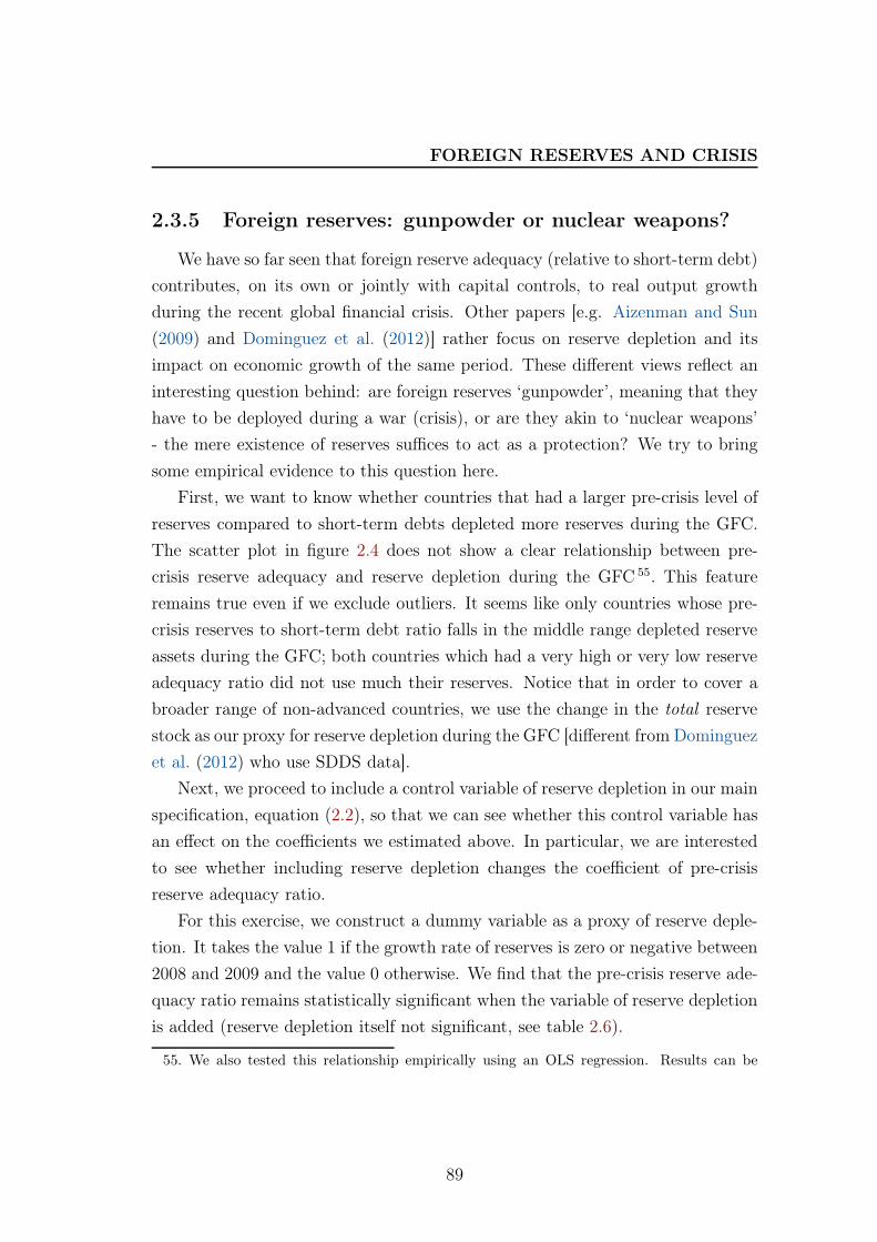
FOREIGN RESERVES AND CRISIS
2.3.5 Foreign reserves: gunpowder or nuclear weapons?
We have so far seen that foreign reserve adequacy (relative to short-term debt)
contributes, on its own or jointly with capital controls, to real output growth
during the recent global financial crisis. Other papers [e.g. Aizenman and Sun
(2009) and Dominguez et al. (2012)] rather focus on reserve depletion and its
impact on economic growth of the same period. These different views reflect an
interesting question behind: are foreign reserves ‘gunpowder’, meaning that they
have to be deployed during a war (crisis), or are they akin to ‘nuclear weapons’
- the mere existence of reserves suffices to act as a protection? We try to bring
some empirical evidence to this question here.
First, we want to know whether countries that had a larger pre-crisis level of
reserves compared to short-term debts depleted more reserves during the GFC.
The scatter plot in figure 2.4 does not show a clear relationship between pre-
crisis reserve adequacy and reserve depletion during the GFC 55. This feature
remains true even if we exclude outliers. It seems like only countries whose pre-
crisis reserves to short-term debt ratio falls in the middle range depleted reserve
assets during the GFC; both countries which had a very high or very low reserve
adequacy ratio did not use much their reserves. Notice that in order to cover a
broader range of non-advanced countries, we use the change in the total reserve
stock as our proxy for reserve depletion during the GFC [different from Dominguez
et al. (2012) who use SDDS data].
Next, we proceed to include a control variable of reserve depletion in our main
specification, equation (2.2), so that we can see whether this control variable has
an effect on the coefficients we estimated above. In particular, we are interested
to see whether including reserve depletion changes the coefficient of pre-crisis
reserve adequacy ratio.
For this exercise, we construct a dummy variable as a proxy of reserve deple-
tion. It takes the value 1 if the growth rate of reserves is zero or negative between
2008 and 2009 and the value 0 otherwise. We find that the pre-crisis reserve ade-
quacy ratio remains statistically significant when the variable of reserve depletion
is added (reserve depletion itself not significant, see table 2.6).
55. We also tested this relationship empirically using an OLS regression. Results can be
89
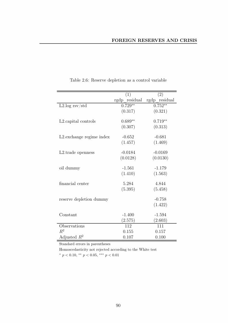
FOREIGN RESERVES AND CRISIS
Table 2.6: Reserve depletion as a control variable
(1) (2)rgdp_residual rgdp_residual
L2.log rsv/std 0.729∗∗ 0.752∗∗
(0.317) (0.321)
L2.capital controls 0.689∗∗ 0.719∗∗
(0.307) (0.313)
L2.exchange regime index -0.652 -0.681(1.457) (1.469)
L2.trade openness -0.0184 -0.0169(0.0128) (0.0130)
oil dummy -1.561 -1.179(1.410) (1.563)
financial center 5.284 4.844(5.395) (5.458)
reserve depletion dummy -0.758(1.422)
Constant -1.400 -1.594(2.575) (2.603)
Observations 112 111R2 0.155 0.157Adjusted R2 0.107 0.100
Standard errors in parentheses
Homoscedasticity not rejected according to the White test∗ p < 0.10, ∗∗ p < 0.05, ∗∗∗ p < 0.01
90
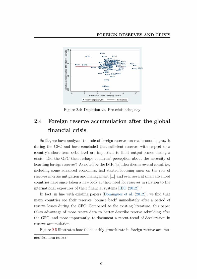
FOREIGN RESERVES AND CRISIS
ALBDZAARG
ARM
BHSBRB
BLRBOL
BIHBWA
BRA
BGR
CHLCHN
COL
CRI
HRV
CZE
DOM
ECU
EGY
SLV
GNQ
GAB
GEOGTMGUYHTIHND
HKG
HUN
IND
IDN
JAM
JOR
KAZKOR
KWT
KGZ
LVA
LBN
LBYLTU
MAC
MYSMUS MEX
MNG
MNE
MAR
NAMOMN
PAKPAN
PNG
PRYPER
PHL
POL
QAT
ROM
RUS
SAU
SRB
SYC SGPZAF
LKA
SWZTWNTHA
TTOTUN
TUR
UKR
ARE
URY
VEN
VNMYEM
−10
0−
500
50V
aria
tion
in r
eser
ves(
log
diff)
08m
09 −
09m
03
0 2 4 6 8 10Reserves/S.t.Debt ratio (log) 07m12
reserve depletion, L9 Fitted values
Figure 2.4: Depletion vs. Pre-crisis adequacy
2.4 Foreign reserve accumulation after the global
financial crisis
So far, we have analyzed the role of foreign reserves on real economic growth
during the GFC and have concluded that sufficient reserves with respect to a
country’s short-term debt level are important to limit output losses during a
crisis. Did the GFC then reshape countries’ perception about the necessity of
hoarding foreign reserves? As noted by the IMF, ‘[a]uthorities in several countries,
including some advanced economies, had started focusing anew on the role of
reserves in crisis mitigation and management [...] and even several small advanced
countries have since taken a new look at their need for reserves in relation to the
international exposures of their financial systems [IEO (2012)].’
In fact, in line with existing papers [Dominguez et al. (2012)], we find that
many countries see their reserves ‘bounce back’ immediately after a period of
reserve losses during the GFC. Compared to the existing literature, this paper
takes advantage of more recent data to better describe reserve rebuilding after
the GFC, and more importantly, to document a recent trend of deceleration in
reserve accumulation.
Figure 2.5 illustrates how the monthly growth rate in foreign reserve accumu-
provided upon request.
91
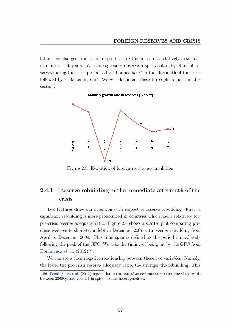
FOREIGN RESERVES AND CRISIS
lation has changed from a high speed before the crisis to a relatively slow pace
in more recent years. We can especially observe a spectacular depletion of re-
serves during the crisis period, a fast ‘bounce-back’ in the aftermath of the crisis
followed by a ‘flattening-out’. We will document these three phenomena in this
section.
Figure 2.5: Evolution of foreign reserve accumulation
2.4.1 Reserve rebuilding in the immediate aftermath of the
crisis
Two features draw our attention with respect to reserve rebuilding. First, a
significant rebuilding is more pronounced in countries which had a relatively low
pre-crisis reserve adequacy ratio. Figure 2.6 shows a scatter plot comparing pre-
crisis reserves to short-term debt in December 2007 with reserve rebuilding from
April to December 2009. This time span is defined as the period immediately
following the peak of the GFC. We take the timing of being hit by the GFC from
Dominguez et al. (2012) 56.
We can see a clear negative relationship between these two variables. Namely,
the lower the pre-crisis reserve adequacy ratio, the stronger the rebuilding. This
56. Dominguez et al. (2012) report that most non-advanced countries experienced the crisisbetween 2008Q4 and 2009Q1 in spite of some heterogeneities.
92
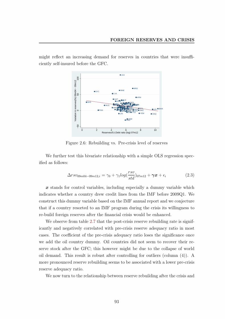
FOREIGN RESERVES AND CRISIS
might reflect an increasing demand for reserves in countries that were insuffi-
ciently self-insured before the GFC.
ARG
ARM
BHS
BRB
BLR
BOL BWA
BRA
BGRCHL
CHN
COL
CRI
HRV
CZE
DOM
ECU EGYSLV
GNQGAB
GEO
GTM
GUYHTI
HND
HUN
INDIDNJAM
JORKAZ
KOR
KWT
LVA
LBN
LBY
LTU
MYS
MUS MEX
MNGMNE
MAR
NAM
OMN
PAK
PAN
PNGPRY
PERPHL
POL
QAT
ROMRUS
SAU
SRB
SYC
SGPZAF
LKA
SWZ
THA
TTO
TUN
TURUKR
AREURY
VEN
VNM
YEM
−50
050
100
Var
iatio
n in
res
erve
s(%
) 09
m04
− 0
9m12
0 2 4 6 8 10Reserves/S.t.Debt ratio (log) 07m12
Figure 2.6: Rebuilding vs. Pre-crisis level of reserves
We further test this bivariate relationship with a simple OLS regression spec-
ified as follows:
∆rsv09m04−09m12,i = γ0 + γ1log(rsv
std)07m12 + γx+ ǫi (2.3)
x stands for control variables, including especially a dummy variable which
indicates whether a country drew credit lines from the IMF before 2009Q1. We
construct this dummy variable based on the IMF annual report and we conjecture
that if a country resorted to an IMF program during the crisis its willingness to
re-build foreign reserves after the financial crisis would be enhanced.
We observe from table 2.7 that the post-crisis reserve rebuilding rate is signif-
icantly and negatively correlated with pre-crisis reserve adequacy ratio in most
cases. The coefficient of the pre-crisis adequacy ratio loses the significance once
we add the oil country dummy. Oil countries did not seem to recover their re-
serve stock after the GFC; this however might be due to the collapse of world
oil demand. This result is robust after controlling for outliers (column (4)). A
more pronounced reserve rebuilding seems to be associated with a lower pre-crisis
reserve adequacy ratio.
We now turn to the relationship between reserve rebuilding after the crisis and
93
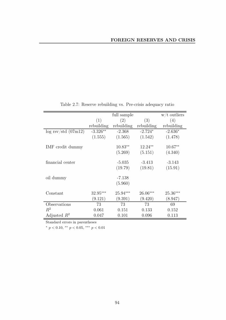
FOREIGN RESERVES AND CRISIS
Table 2.7: Reserve rebuilding vs. Pre-crisis adequacy ratio
full sample w/t outliers(1) (2) (3) (4)
rebuilding rebuilding rebuilding rebuildinglog rsv/std (07m12) -3.326∗∗ -2.368 -2.724∗ -2.636∗
(1.555) (1.565) (1.542) (1.478)
IMF credit dummy 10.83∗∗ 12.24∗∗ 10.67∗∗
(5.269) (5.151) (4.340)
financial center -5.035 -3.413 -3.143(19.79) (19.81) (15.91)
oil dummy -7.138(5.960)
Constant 32.95∗∗∗ 25.94∗∗∗ 26.06∗∗∗ 25.36∗∗∗
(9.121) (9.391) (9.420) (8.947)Observations 73 73 73 69R2 0.061 0.151 0.133 0.152Adjusted R2 0.047 0.101 0.096 0.113
Standard errors in parentheses∗ p < 0.10, ∗∗ p < 0.05, ∗∗∗ p < 0.01
94
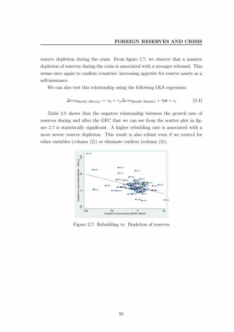
FOREIGN RESERVES AND CRISIS
reserve depletion during the crisis. From figure 2.7, we observe that a massive
depletion of reserves during the crisis is associated with a stronger rebound. This
seems once again to confirm countries’ increasing appetite for reserve assets as a
self-insurance.
We can also test this relationship using the following OLS regression:
∆rsv09m04−09m12,i = γ0 + γ1∆rsv08m09−09m03,i + γx+ ǫi (2.4)
Table 2.8 shows that the negative relationship between the growth rate of
reserves during and after the GFC that we can see from the scatter plot in fig-
ure 2.7 is statistically significant. A higher rebuilding rate is associated with a
more severe reserve depletion. This result is also robust even if we control for
other variables (column (2)) or eliminate outliers (column (3)).
ARG
ARM
BHS
BHR
BRB
BLR
BOLBWA
BRA
BGRCHL
CHN
COL
CRI
HRV
CZE
DOM
ECU EGY SLV
GNQGAB
GEO
GTM
GUYHTI
HND
HUN
INDIDNJAM
JORKAZ
KOR
KWT
LVA
LBN
LBY
LTU
MKD
MYS
MUSMEX
MNGMNE
MAR
NAM
OMN
PAK
PAN
PNGPRY
PERPHL
POL
QAT
ROMRUS
SAU
SRB
SYC
SGPZAF
LKA
KNA
SWZ
THA
TTO
TUN
TURUKR
AREURY
VEN
VNM
YEM
−50
050
100
Var
iatio
n in
res
erve
s(%
) 09
m04
− 0
9m12
−100 −50 0 50Variation in reserves(%) 08m09−09m03
Figure 2.7: Rebuilding vs. Depletion of reserves
95
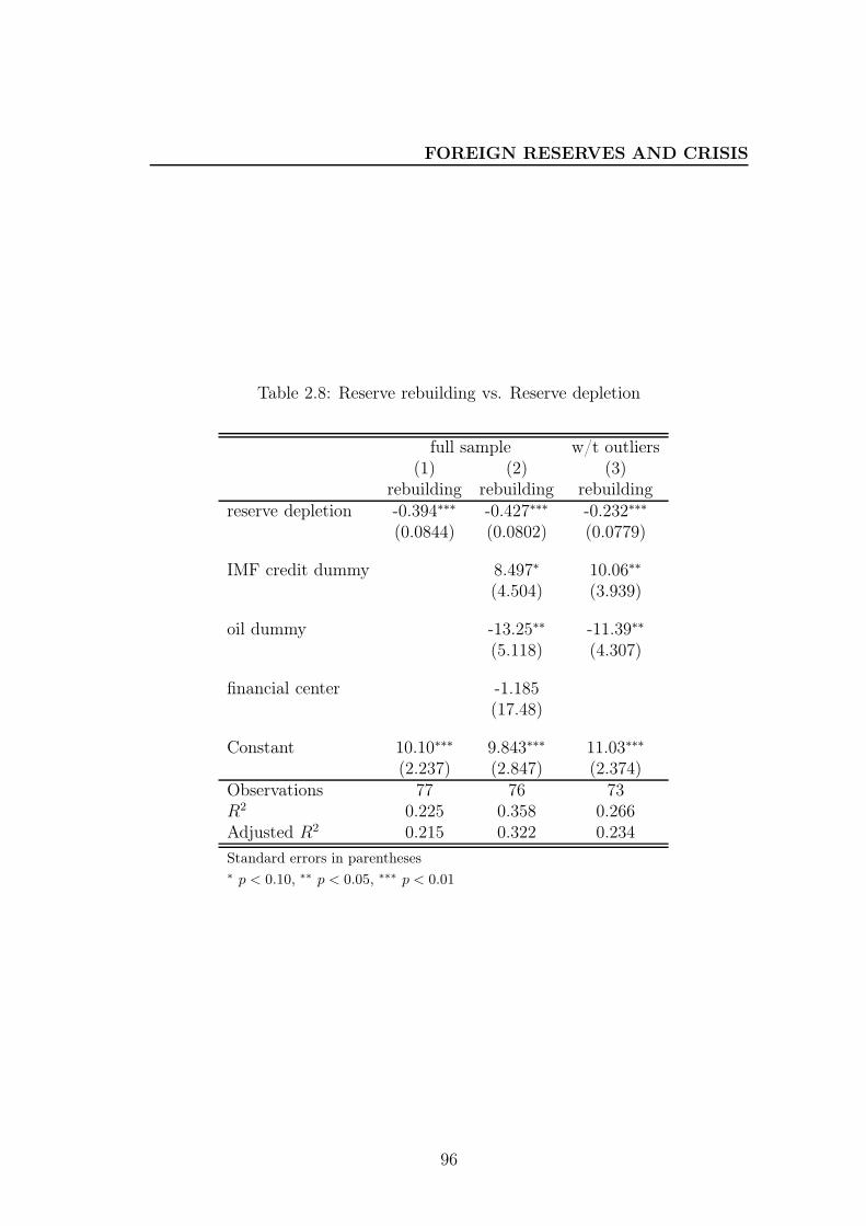
FOREIGN RESERVES AND CRISIS
Table 2.8: Reserve rebuilding vs. Reserve depletion
full sample w/t outliers(1) (2) (3)
rebuilding rebuilding rebuildingreserve depletion -0.394∗∗∗ -0.427∗∗∗ -0.232∗∗∗
(0.0844) (0.0802) (0.0779)
IMF credit dummy 8.497∗ 10.06∗∗
(4.504) (3.939)
oil dummy -13.25∗∗ -11.39∗∗
(5.118) (4.307)
financial center -1.185(17.48)
Constant 10.10∗∗∗ 9.843∗∗∗ 11.03∗∗∗
(2.237) (2.847) (2.374)Observations 77 76 73R2 0.225 0.358 0.266Adjusted R2 0.215 0.322 0.234
Standard errors in parentheses∗ p < 0.10, ∗∗ p < 0.05, ∗∗∗ p < 0.01
96
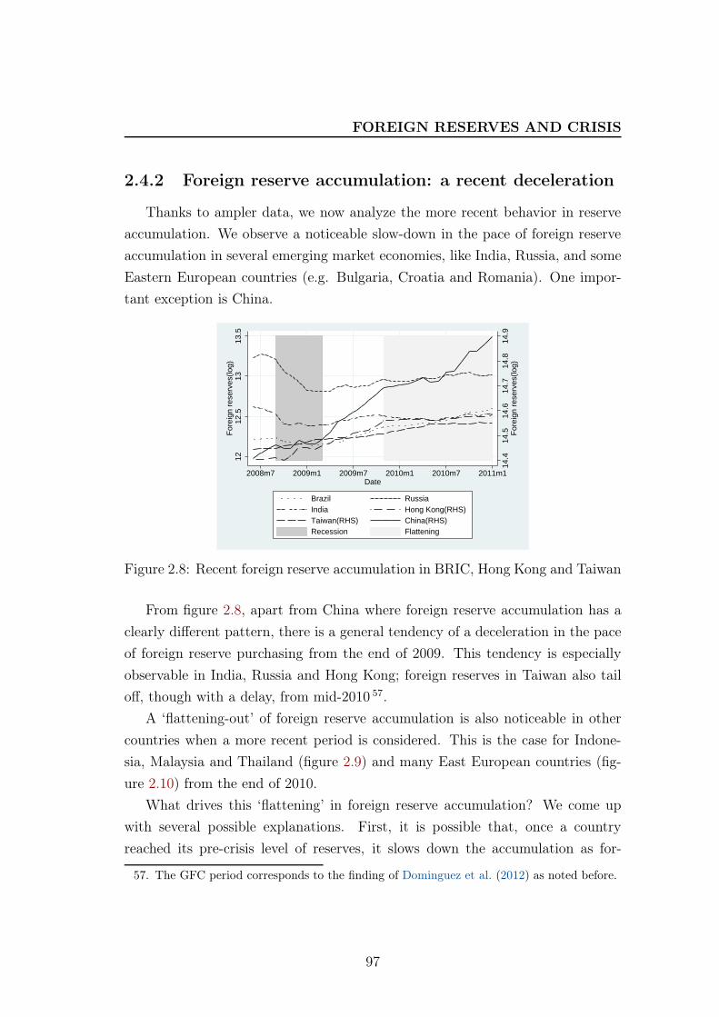
FOREIGN RESERVES AND CRISIS
2.4.2 Foreign reserve accumulation: a recent deceleration
Thanks to ampler data, we now analyze the more recent behavior in reserve
accumulation. We observe a noticeable slow-down in the pace of foreign reserve
accumulation in several emerging market economies, like India, Russia, and some
Eastern European countries (e.g. Bulgaria, Croatia and Romania). One impor-
tant exception is China.
14.4
14.5
14.6
14.7
14.8
14.9
For
eign
res
erve
s(lo
g)
1212
.513
13.5
For
eign
res
erve
s(lo
g)
2008m7 2009m1 2009m7 2010m1 2010m7 2011m1Date
Brazil RussiaIndia Hong Kong(RHS)Taiwan(RHS) China(RHS)Recession Flattening
Figure 2.8: Recent foreign reserve accumulation in BRIC, Hong Kong and Taiwan
From figure 2.8, apart from China where foreign reserve accumulation has a
clearly different pattern, there is a general tendency of a deceleration in the pace
of foreign reserve purchasing from the end of 2009. This tendency is especially
observable in India, Russia and Hong Kong; foreign reserves in Taiwan also tail
off, though with a delay, from mid-2010 57.
A ‘flattening-out’ of foreign reserve accumulation is also noticeable in other
countries when a more recent period is considered. This is the case for Indone-
sia, Malaysia and Thailand (figure 2.9) and many East European countries (fig-
ure 2.10) from the end of 2010.
What drives this ‘flattening’ in foreign reserve accumulation? We come up
with several possible explanations. First, it is possible that, once a country
reached its pre-crisis level of reserves, it slows down the accumulation as for-
57. The GFC period corresponds to the finding of Dominguez et al. (2012) as noted before.
97
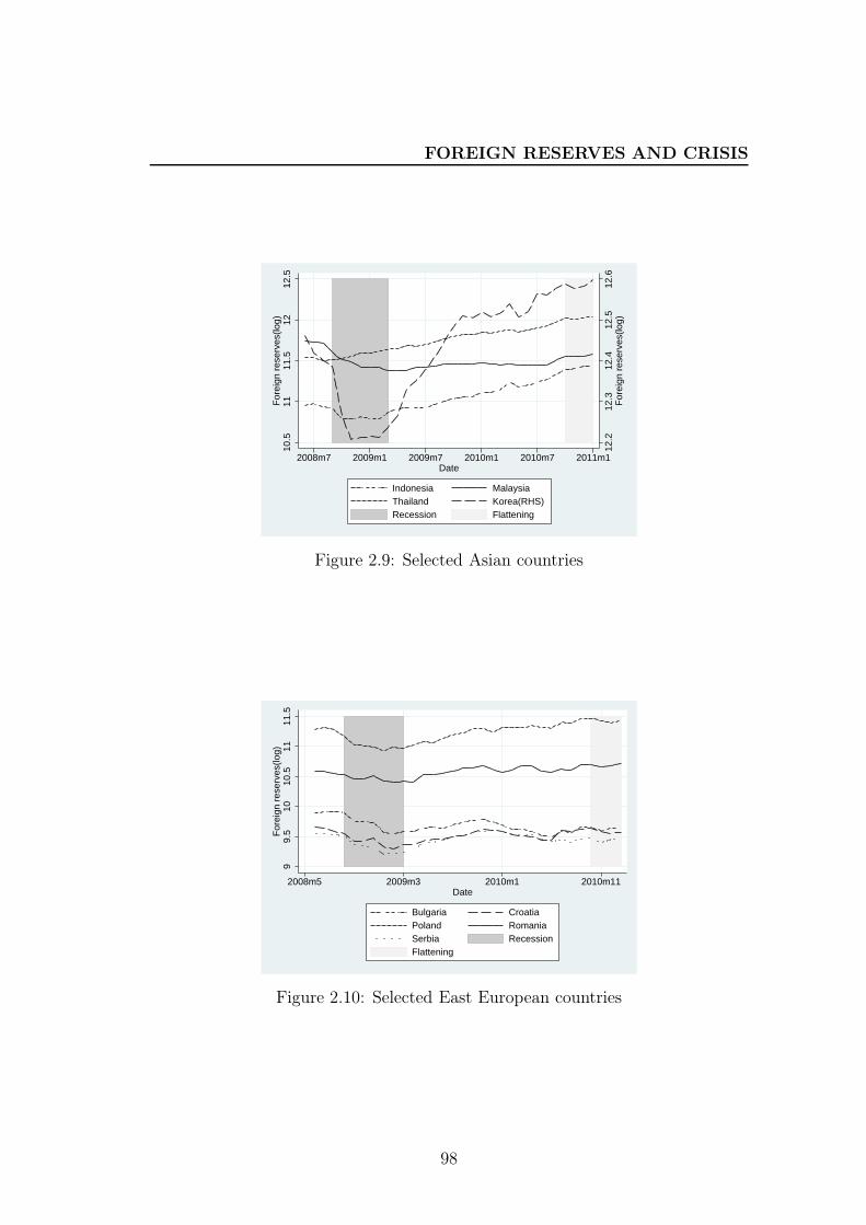
FOREIGN RESERVES AND CRISIS
12.2
12.3
12.4
12.5
12.6
For
eign
res
erve
s(lo
g)
10.5
1111
.512
12.5
For
eign
res
erve
s(lo
g)
2008m7 2009m1 2009m7 2010m1 2010m7 2011m1Date
Indonesia MalaysiaThailand Korea(RHS)Recession Flattening
Figure 2.9: Selected Asian countries
99.
510
10.5
1111
.5F
orei
gn r
eser
ves(
log)
2008m5 2009m3 2010m1 2010m11Date
Bulgaria CroatiaPoland RomaniaSerbia RecessionFlattening
Figure 2.10: Selected East European countries
98
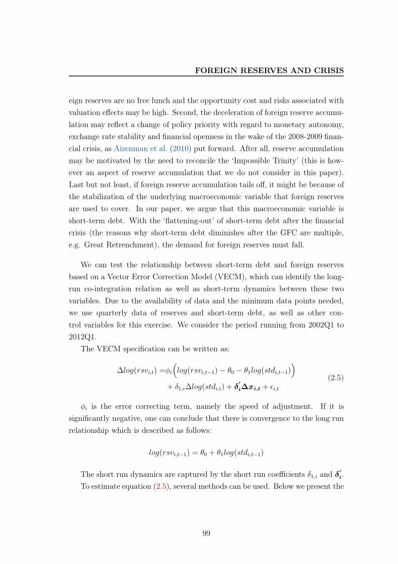
FOREIGN RESERVES AND CRISIS
eign reserves are no free lunch and the opportunity cost and risks associated with
valuation effects may be high. Second, the deceleration of foreign reserve accumu-
lation may reflect a change of policy priority with regard to monetary autonomy,
exchange rate stability and financial openness in the wake of the 2008-2009 finan-
cial crisis, as Aizenman et al. (2010) put forward. After all, reserve accumulation
may be motivated by the need to reconcile the ‘Impossible Trinity’ (this is how-
ever an aspect of reserve accumulation that we do not consider in this paper).
Last but not least, if foreign reserve accumulation tails off, it might be because of
the stabilization of the underlying macroeconomic variable that foreign reserves
are used to cover. In our paper, we argue that this macroeconomic variable is
short-term debt. With the ‘flattening-out’ of short-term debt after the financial
crisis (the reasons why short-term debt diminishes after the GFC are multiple,
e.g. Great Retrenchment), the demand for foreign reserves must fall.
We can test the relationship between short-term debt and foreign reserves
based on a Vector Error Correction Model (VECM), which can identify the long-
run co-integration relation as well as short-term dynamics between these two
variables. Due to the availability of data and the minimum data points needed,
we use quarterly data of reserves and short-term debt, as well as other con-
trol variables for this exercise. We consider the period running from 2002Q1 to
2012Q1.
The VECM specification can be written as:
∆log(rsvi,t) =φi
(log(rsvi,t−1)− θ0 − θ1log(stdi,t−1)
)
+ δ1,i∆log(stdi,t) + δ′
i∆xi,t + ǫi,t
(2.5)
φi is the error correcting term, namely the speed of adjustment. If it is
significantly negative, one can conclude that there is convergence to the long run
relationship which is described as follows:
log(rsvi,t−1) = θ0 + θ1log(stdi,t−1)
The short run dynamics are captured by the short run coefficients δ1,i and δ′
i.
To estimate equation (2.5), several methods can be used. Below we present the
99
FOREIGN RESERVES AND CRISIS
estimation results using pooled mean group estimates, which assume a common
long-run coefficient across countries but heterogeneous short-term adjustment.
From table 2.9, we observe that there is a clear positive long-run relationship
between foreign reserves and short-term debt both expressed in logarithm. In the
baseline case (column (1)), log(rsvi,t) = 0.436log(stdi,t). In the short-term, the
error correction coefficient (-0.0743) is significant and negative, meaning that if
foreign reserves exceed the long-run equilibrium level a country reduces its foreign
reserve accumulation with an adjustment rate of 7% in the baseline case.
As a robustness check, we also tried different estimation methods and used
additional control variables. The main coefficients presented in table 2.9 do not
change in signs nor in magnitude.
The VECM confirms our initial guess on why foreign reserve accumulation
tails off in recent years. It is likely that the underlying target variable for foreign
reserves, namely short-term debt, stabilizes after the financial crisis; this, in turn,
may be associated with the global liquidity crunch and Great Retrenchment?
[Milesi-Ferretti and Tille (2011)] in international capital flows that took place in
the wake of the GFC.
2.5 Conclusion
In the late 1990s and early 2000s, a consensus developed that reserves were
useful in averting, or at least mitigating, the occurrence of crises in emerging
market and developing countries. Policy makers from these countries have ap-
parently absorbed the lessons from this literature, as the level of international
reserves dramatically increased in the 2000s (even accepting that other motives
have played a role). The results presented in this paper suggest that the Great
Financial Crisis has further demonstrated the usefulness of reserves: empirically,
the countries that held more reserves as a percentage of short-term debt have
been less negatively impacted than others, ceteris paribus. The results also sug-
gest that this effect is especially strong when the capital account is less open.
Given that reserves seem to have played a role in offsetting the effect of the
crisis, it is not surprising that the countries that depleted reserves to a greater
100
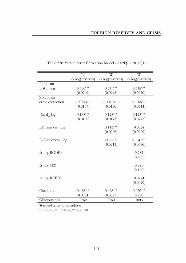
FOREIGN RESERVES AND CRISIS
Table 2.9: Vector Error Correction Model (2002Q1 - 2012Q1)
(1) (2) (3)∆ log(reserves) ∆ log(reserves) ∆ log(reserves)
Long-runL.std_log 0.436∗∗∗ 0.445∗∗∗ 0.448∗∗∗
(0.0249) (0.0243) (0.0270)Short-runerror correction -0.0743∗∗∗ -0.0815∗∗∗ -0.186∗∗∗
(0.0107) (0.0130) (0.0514)
D.std_log 0.138∗∗∗ 0.128∗∗∗ 0.148∗∗∗
(0.0188) (0.0173) (0.0277)
LD.reserves_log 0.113∗∗∗ 0.0338(0.0296) (0.0399)
L2D.reserves_log -0.0357∗ -0.131∗∗∗
(0.0213) (0.0436)
∆ log(RGDP) 0.282(0.485)
∆ log(M2) 0.225(0.199)
∆ log(REER) 0.0474(0.0920)
Constant 0.438∗∗∗ 0.468∗∗∗ 0.950∗∗∗
(0.0584) (0.0697) (0.230)Observations 2752 2750 1093
Standard errors in parentheses∗ p < 0.10, ∗∗ p < 0.05, ∗∗∗ p < 0.01
101
FOREIGN RESERVES AND CRISIS
extent are also the ones that rebuilt them more quickly in the direct aftermath
of the crisis, as shown in the paper. One possible factor is that policy makers in
emerging market and developing countries have concluded from the experience
of the GFC that reserves are indeed very useful in protecting countries against
crises. Nonetheless, we also find that in the most recent period, the pace of reserve
accumulation has slowed down, in line with the deceleration in the pace of short-
term debt. This outcome suggests that countries target the level of short-term
debt: if, for whatever reason, short-term debt accumulation decelerates, then
reserves are likely to follow the same course.
102
BIBLIOGRAPHY
Bibliography
Aizenman, J., Chinn, M. D., and Ito, H. (2010). The emerging global financial architecture:
Tracing and evaluating new patterns of the trilemma configuration. Journal of International
Money and Finance, 29(4):615–641.
Aizenman, J. and Hutchison, M. M. (2010). Exchange market pressure and absorption by
international reserves: Emerging markets and fear of reserve loss during the 2008-09 crisis.
NBER Working Papers 16260, National Bureau of Economic Research, Inc.
Aizenman, J., Jinjarak, Y., and Park, D. (2011). International reserves and swap lines: Substi-
tutes or complements? International Review of Economics & Finance, 20(1):5–18.
Aizenman, J. and Sun, Y. (2009). The financial crisis and sizable international reserves deple-
tion: From ‘fear of floating’ to the ‘fear of losing international reserves’? NBER Working
Papers 15308, National Bureau of Economic Research, Inc.
Bacchetta, P., Benhima, K., and Kalantzis, Y. (2013). Capital controls with international
reserve accumulation: Can this be optimal? American Economic Journal: Macroeconomics,
5(3):229–62.
Bahmani-Oskooee, M. and Brown, F. (2002). Demand for international reserves: a review
article. Applied Economics, 34(10):1209–1226.
Bastourre, D., Carrera, J., and Ibarlucia, J. (2009). What is driving reserve accumulation? A
dynamic panel data approach. Review of International Economics, 17(4):861–877.
Benigno, G. and Fornaro, L. (2012). Reserve accumulation, growth and financial crises. CEP
Discussion Papers dp1161, Centre for Economic Performance, LSE.
Berg, A. and Pattillo, C. (1999). Are currency crises predictable? A test. IMF Staff Papers,
46(2):1.
Berkmen, S. P., Gelos, G., Rennhack, R., and Walsh, J. P. (2012). The global financial crisis:
Explaining cross-country differences in the output impact. Journal of International Money
and Finance, 31(1):42–59.
Bianchi, J., Hatchondo, J. C., and Martinez, L. (2012). International reserves and rollover risk.
NBER Working Papers 18628, National Bureau of Economic Research, Inc.
Blanchard, O. J., Das, M., and Faruqee, H. (2010). The initial impact of the crisis on emerging
market countries. Brookings Papers on Economic Activity, 41(1 (Spring):263–323.
103
BIBLIOGRAPHY
Bussière, M. and Mulder, C. B. (1999). External vulnerability in emerging market economies -
how high liquidity can offset weak fundamentals and the effects of contagion. IMF Working
Papers 99/88, International Monetary Fund.
Catao, L. and Milesi-Ferretti, G.-M. (2013). External liabilities and crises. IMF Working Papers
13/113, International Monetary Fund.
Cheng, G. (2013). A growth perspective on foreign reserve accumulation. Working papers 443,
Banque de France.
Cheung, Y.-W. and Sengupta, R. (2011). Accumulation of reserves and keeping up with the
joneses: The case of LATAM economies. International Review of Economics & Finance,
20(1):19–31.
Chinn, M. and Ito, H. (2006). What matters for financial development? Capital controls,
institutions, and interactions. Journal of Development Economics, 81(1):163–192.
Dominguez, K. M. (2012). Foreign reserve management during the global financial crisis. Jour-
nal of International Money and Finance, 31(8):2017–2037.
Dominguez, K. M., Hashimoto, Y., and Ito, T. (2012). International reserves and the global
financial crisis. Journal of International Economics, 88(2):388 – 406.
Flood, R. and Marion, N. (1999). Perspectives on the recent currency crisis literature. Inter-
national Journal of Finance & Economics, 4(1):1–26.
Frankel, J. and Saravelos, G. (2012). Can leading indicators assess country vulnerability? Evi-
dence from the 2008-09 global financial crisis. Journal of International Economics, 87(2):216–
231.
Gourinchas, P.-O. and Obstfeld, M. (2012). Stories of the twentieth century for the twenty-first.
American Economic Journal: Macroeconomics, 4(1):226–65.
IEO (2012). International reserves: IMF concerns and country perspectives. In IEO report.
International Monetary Fund.
Jeanne, O. and Rancière, R. (2011). The optimal level of international reserves for emerging
market countries: A new formula and some applications. Economic Journal, 121(555):905–
930.
Kose, M. A., Prasad, E., Rogoff, K., and Wei, S.-J. (2009). Financial globalization: A reap-
praisal. IMF Staff Papers, 56(1):8–62.
104
BIBLIOGRAPHY
Lane, P. R. and Milesi-Ferretti, G. M. (2007). The external wealth of nations mark II: Revised
and extended estimates of foreign assets and liabilities, 1970-2004. Journal of International
Economics, 73(2):223–250.
Llaudes, R., Salman, F., and Chivakul, M. (2010). The impact of the great recession on emerging
markets. IMF Working Papers 10/237, International Monetary Fund.
Mayer, T. and Zignago, S. (2011). Notes on CEPII’s distances measures: The geodist database.
Working Papers 2011-25, CEPII research center.
Milesi-Ferretti, G.-M. and Tille, C. (2011). The great retrenchment: International capital flows
during the global financial crisis. Economic Policy, 26(66):285–342.
Obstfeld, M. (1986). Rational and self-fulfilling balance-of-payments crises. American Economic
Review, 76(1):72–81.
Obstfeld, M. (2013). Never say never: commentary on a policymaker’s reflections. Manuscript,
UC Berkeley.
Obstfeld, M., Shambaugh, J. C., and Taylor, A. M. (2009). Financial instability, reserves, and
central bank swap lines in the panic of 2008. American Economic Review, 99(2):480–86.
Obstfeld, M., Shambaugh, J. C., and Taylor, A. M. (2010). Financial stability, the trilemma,
and international reserves. American Economic Journal: Macroeconomics, 2(2):57–94.
Reinhart, C. M. and Kaminsky, G. L. (1999). The twin crises: The causes of banking and
balance-of-payments problems. American Economic Review, 89(3):473–500.
Reinhart, C. M. and Rogoff, K. S. (2004). The modern history of exchange rate arrangements:
A reinterpretation. The Quarterly Journal of Economics, 119(1):1–48.
Rose, A. K. and Spiegel, M. M. (2009). Cross-country causes and consequences of the 2008
crisis: Early warning. CEPR Discussion Papers 7354, C.E.P.R. Discussion Papers.
Rose, A. K. and Spiegel, M. M. (2010). Cross-country causes and consequences of the 2008 crisis:
International linkages and American exposure. Pacific Economic Review, 15(3):340–363.
105
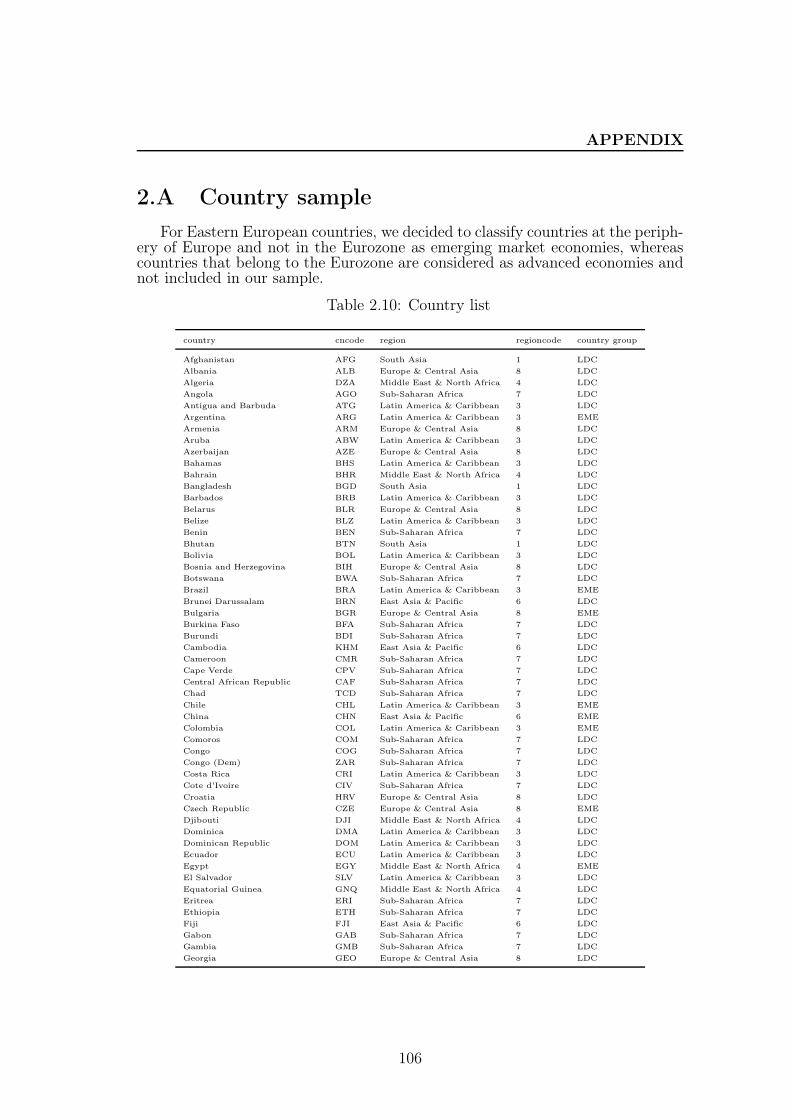
APPENDIX
2.A Country sample
For Eastern European countries, we decided to classify countries at the periph-ery of Europe and not in the Eurozone as emerging market economies, whereascountries that belong to the Eurozone are considered as advanced economies andnot included in our sample.
Table 2.10: Country list
country cncode region regioncode country group
Afghanistan AFG South Asia 1 LDC
Albania ALB Europe & Central Asia 8 LDC
Algeria DZA Middle East & North Africa 4 LDC
Angola AGO Sub-Saharan Africa 7 LDC
Antigua and Barbuda ATG Latin America & Caribbean 3 LDC
Argentina ARG Latin America & Caribbean 3 EME
Armenia ARM Europe & Central Asia 8 LDC
Aruba ABW Latin America & Caribbean 3 LDC
Azerbaijan AZE Europe & Central Asia 8 LDC
Bahamas BHS Latin America & Caribbean 3 LDC
Bahrain BHR Middle East & North Africa 4 LDC
Bangladesh BGD South Asia 1 LDC
Barbados BRB Latin America & Caribbean 3 LDC
Belarus BLR Europe & Central Asia 8 LDC
Belize BLZ Latin America & Caribbean 3 LDC
Benin BEN Sub-Saharan Africa 7 LDC
Bhutan BTN South Asia 1 LDC
Bolivia BOL Latin America & Caribbean 3 LDC
Bosnia and Herzegovina BIH Europe & Central Asia 8 LDC
Botswana BWA Sub-Saharan Africa 7 LDC
Brazil BRA Latin America & Caribbean 3 EME
Brunei Darussalam BRN East Asia & Pacific 6 LDC
Bulgaria BGR Europe & Central Asia 8 EME
Burkina Faso BFA Sub-Saharan Africa 7 LDC
Burundi BDI Sub-Saharan Africa 7 LDC
Cambodia KHM East Asia & Pacific 6 LDC
Cameroon CMR Sub-Saharan Africa 7 LDC
Cape Verde CPV Sub-Saharan Africa 7 LDC
Central African Republic CAF Sub-Saharan Africa 7 LDC
Chad TCD Sub-Saharan Africa 7 LDC
Chile CHL Latin America & Caribbean 3 EME
China CHN East Asia & Pacific 6 EME
Colombia COL Latin America & Caribbean 3 EME
Comoros COM Sub-Saharan Africa 7 LDC
Congo COG Sub-Saharan Africa 7 LDC
Congo (Dem) ZAR Sub-Saharan Africa 7 LDC
Costa Rica CRI Latin America & Caribbean 3 LDC
Cote d’Ivoire CIV Sub-Saharan Africa 7 LDC
Croatia HRV Europe & Central Asia 8 LDC
Czech Republic CZE Europe & Central Asia 8 EME
Djibouti DJI Middle East & North Africa 4 LDC
Dominica DMA Latin America & Caribbean 3 LDC
Dominican Republic DOM Latin America & Caribbean 3 LDC
Ecuador ECU Latin America & Caribbean 3 LDC
Egypt EGY Middle East & North Africa 4 EME
El Salvador SLV Latin America & Caribbean 3 LDC
Equatorial Guinea GNQ Middle East & North Africa 4 LDC
Eritrea ERI Sub-Saharan Africa 7 LDC
Ethiopia ETH Sub-Saharan Africa 7 LDC
Fiji FJI East Asia & Pacific 6 LDC
Gabon GAB Sub-Saharan Africa 7 LDC
Gambia GMB Sub-Saharan Africa 7 LDC
Georgia GEO Europe & Central Asia 8 LDC
106
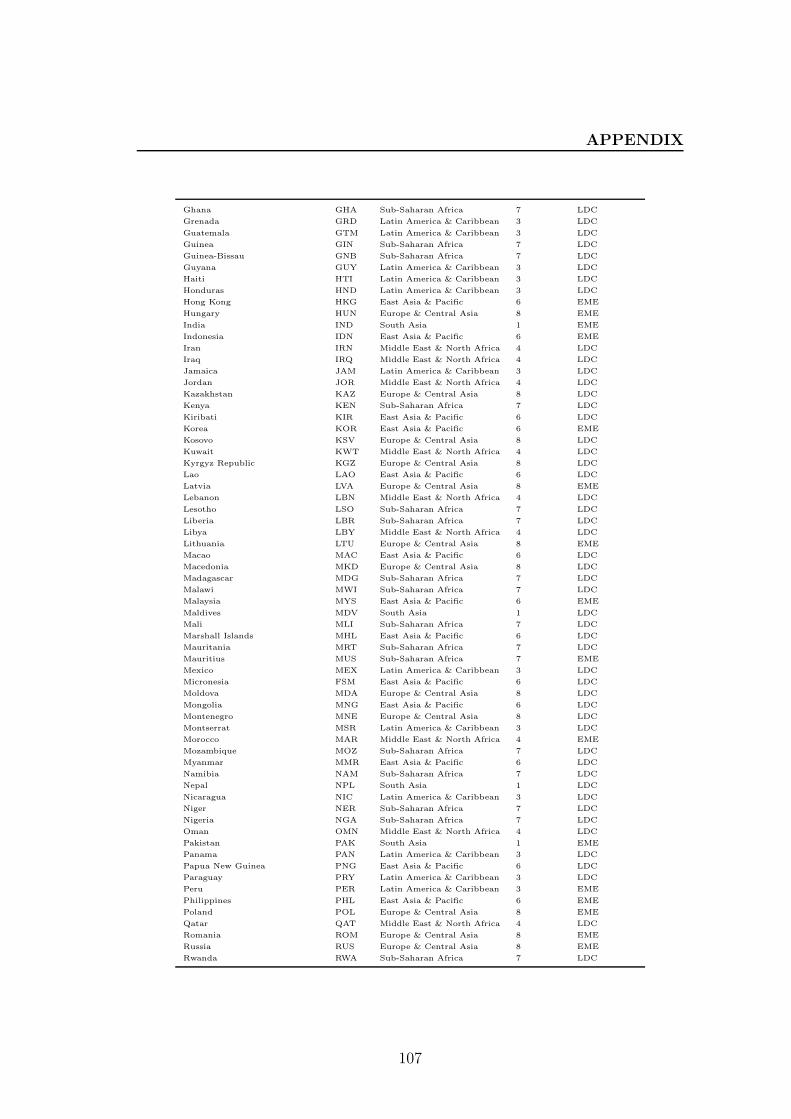
APPENDIX
Ghana GHA Sub-Saharan Africa 7 LDC
Grenada GRD Latin America & Caribbean 3 LDC
Guatemala GTM Latin America & Caribbean 3 LDC
Guinea GIN Sub-Saharan Africa 7 LDC
Guinea-Bissau GNB Sub-Saharan Africa 7 LDC
Guyana GUY Latin America & Caribbean 3 LDC
Haiti HTI Latin America & Caribbean 3 LDC
Honduras HND Latin America & Caribbean 3 LDC
Hong Kong HKG East Asia & Pacific 6 EME
Hungary HUN Europe & Central Asia 8 EME
India IND South Asia 1 EME
Indonesia IDN East Asia & Pacific 6 EME
Iran IRN Middle East & North Africa 4 LDC
Iraq IRQ Middle East & North Africa 4 LDC
Jamaica JAM Latin America & Caribbean 3 LDC
Jordan JOR Middle East & North Africa 4 LDC
Kazakhstan KAZ Europe & Central Asia 8 LDC
Kenya KEN Sub-Saharan Africa 7 LDC
Kiribati KIR East Asia & Pacific 6 LDC
Korea KOR East Asia & Pacific 6 EME
Kosovo KSV Europe & Central Asia 8 LDC
Kuwait KWT Middle East & North Africa 4 LDC
Kyrgyz Republic KGZ Europe & Central Asia 8 LDC
Lao LAO East Asia & Pacific 6 LDC
Latvia LVA Europe & Central Asia 8 EME
Lebanon LBN Middle East & North Africa 4 LDC
Lesotho LSO Sub-Saharan Africa 7 LDC
Liberia LBR Sub-Saharan Africa 7 LDC
Libya LBY Middle East & North Africa 4 LDC
Lithuania LTU Europe & Central Asia 8 EME
Macao MAC East Asia & Pacific 6 LDC
Macedonia MKD Europe & Central Asia 8 LDC
Madagascar MDG Sub-Saharan Africa 7 LDC
Malawi MWI Sub-Saharan Africa 7 LDC
Malaysia MYS East Asia & Pacific 6 EME
Maldives MDV South Asia 1 LDC
Mali MLI Sub-Saharan Africa 7 LDC
Marshall Islands MHL East Asia & Pacific 6 LDC
Mauritania MRT Sub-Saharan Africa 7 LDC
Mauritius MUS Sub-Saharan Africa 7 EME
Mexico MEX Latin America & Caribbean 3 LDC
Micronesia FSM East Asia & Pacific 6 LDC
Moldova MDA Europe & Central Asia 8 LDC
Mongolia MNG East Asia & Pacific 6 LDC
Montenegro MNE Europe & Central Asia 8 LDC
Montserrat MSR Latin America & Caribbean 3 LDC
Morocco MAR Middle East & North Africa 4 EME
Mozambique MOZ Sub-Saharan Africa 7 LDC
Myanmar MMR East Asia & Pacific 6 LDC
Namibia NAM Sub-Saharan Africa 7 LDC
Nepal NPL South Asia 1 LDC
Nicaragua NIC Latin America & Caribbean 3 LDC
Niger NER Sub-Saharan Africa 7 LDC
Nigeria NGA Sub-Saharan Africa 7 LDC
Oman OMN Middle East & North Africa 4 LDC
Pakistan PAK South Asia 1 EME
Panama PAN Latin America & Caribbean 3 LDC
Papua New Guinea PNG East Asia & Pacific 6 LDC
Paraguay PRY Latin America & Caribbean 3 LDC
Peru PER Latin America & Caribbean 3 EME
Philippines PHL East Asia & Pacific 6 EME
Poland POL Europe & Central Asia 8 EME
Qatar QAT Middle East & North Africa 4 LDC
Romania ROM Europe & Central Asia 8 EME
Russia RUS Europe & Central Asia 8 EME
Rwanda RWA Sub-Saharan Africa 7 LDC
107
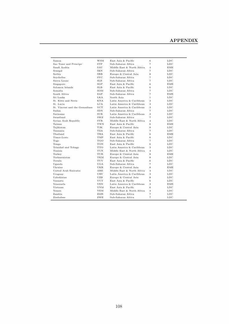
APPENDIX
Samoa WSM East Asia & Pacific 6 LDC
Sao Tome and Principe STP Sub-Saharan Africa 7 LDC
Saudi Arabia SAU Middle East & North Africa 4 EME
Senegal SEN Sub-Saharan Africa 7 LDC
Serbia SRB Europe & Central Asia 8 LDC
Seychelles SYC Sub-Saharan Africa 7 LDC
Sierra Leone SLE Sub-Saharan Africa 7 LDC
Singapore SGP East Asia & Pacific 6 EME
Solomon Islands SLB East Asia & Pacific 6 LDC
Somalia SOM Sub-Saharan Africa 7 LDC
South Africa ZAF Sub-Saharan Africa 7 EME
Sri Lanka LKA South Asia 1 LDC
St. Kitts and Nevis KNA Latin America & Caribbean 3 LDC
St. Lucia LCA Latin America & Caribbean 3 LDC
St. Vincent and the Grenadines VCT Latin America & Caribbean 3 LDC
Sudan SDN Sub-Saharan Africa 7 LDC
Suriname SUR Latin America & Caribbean 3 LDC
Swaziland SWZ Sub-Saharan Africa 7 LDC
Syrian Arab Republic SYR Middle East & North Africa 4 LDC
Taiwan TWN East Asia & Pacific 6 EME
Tajikistan TJK Europe & Central Asia 8 LDC
Tanzania TZA Sub-Saharan Africa 7 LDC
Thailand THA East Asia & Pacific 6 EME
Timor-Leste TMP East Asia & Pacific 6 LDC
Togo TGO Sub-Saharan Africa 7 LDC
Tonga TON East Asia & Pacific 6 LDC
Trinidad and Tobago TTO Latin America & Caribbean 3 LDC
Tunisia TUN Middle East & North Africa 4 LDC
Turkey TUR Europe & Central Asia 8 EME
Turkmenistan TKM Europe & Central Asia 8 LDC
Tuvalu TUV East Asia & Pacific 6 LDC
Uganda UGA Sub-Saharan Africa 7 LDC
Ukraine UKR Europe & Central Asia 8 EME
United Arab Emirates ARE Middle East & North Africa 4 LDC
Uruguay URY Latin America & Caribbean 3 LDC
Uzbekistan UZB Europe & Central Asia 8 LDC
Vanuatu VUT East Asia & Pacific 6 LDC
Venezuela VEN Latin America & Caribbean 3 EME
Vietnam VNM East Asia & Pacific 6 LDC
Yemen YEM Middle East & North Africa 4 LDC
Zambia ZMB Sub-Saharan Africa 7 LDC
Zimbabwe ZWE Sub-Saharan Africa 7 LDC
108
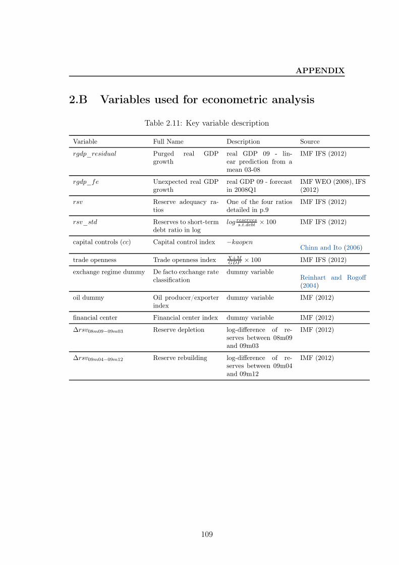
APPENDIX
2.B Variables used for econometric analysis
Table 2.11: Key variable description
Variable Full Name Description Source
rgdp_residual Purged real GDPgrowth
real GDP 09 - lin-ear prediction from amean 03-08
IMF IFS (2012)
rgdp_fe Unexpected real GDPgrowth
real GDP 09 - forecastin 2008Q1
IMF WEO (2008), IFS(2012)
rsv Reserve adequacy ra-tios
One of the four ratiosdetailed in p.9
IMF IFS (2012)
rsv_std Reserves to short-termdebt ratio in log
log reservess.t.debt
× 100 IMF IFS (2012)
capital controls (cc) Capital control index −kaopenChinn and Ito (2006)
trade openness Trade openness index X+MGDP
× 100 IMF IFS (2012)
exchange regime dummy De facto exchange rateclassification
dummy variableReinhart and Rogoff(2004)
oil dummy Oil producer/exporterindex
dummy variable IMF (2012)
financial center Financial center index dummy variable IMF (2012)
∆rsv08m09−09m03 Reserve depletion log-difference of re-serves between 08m09and 09m03
IMF (2012)
∆rsv09m04−09m12 Reserve rebuilding log-difference of re-serves between 09m04and 09m12
IMF (2012)
109
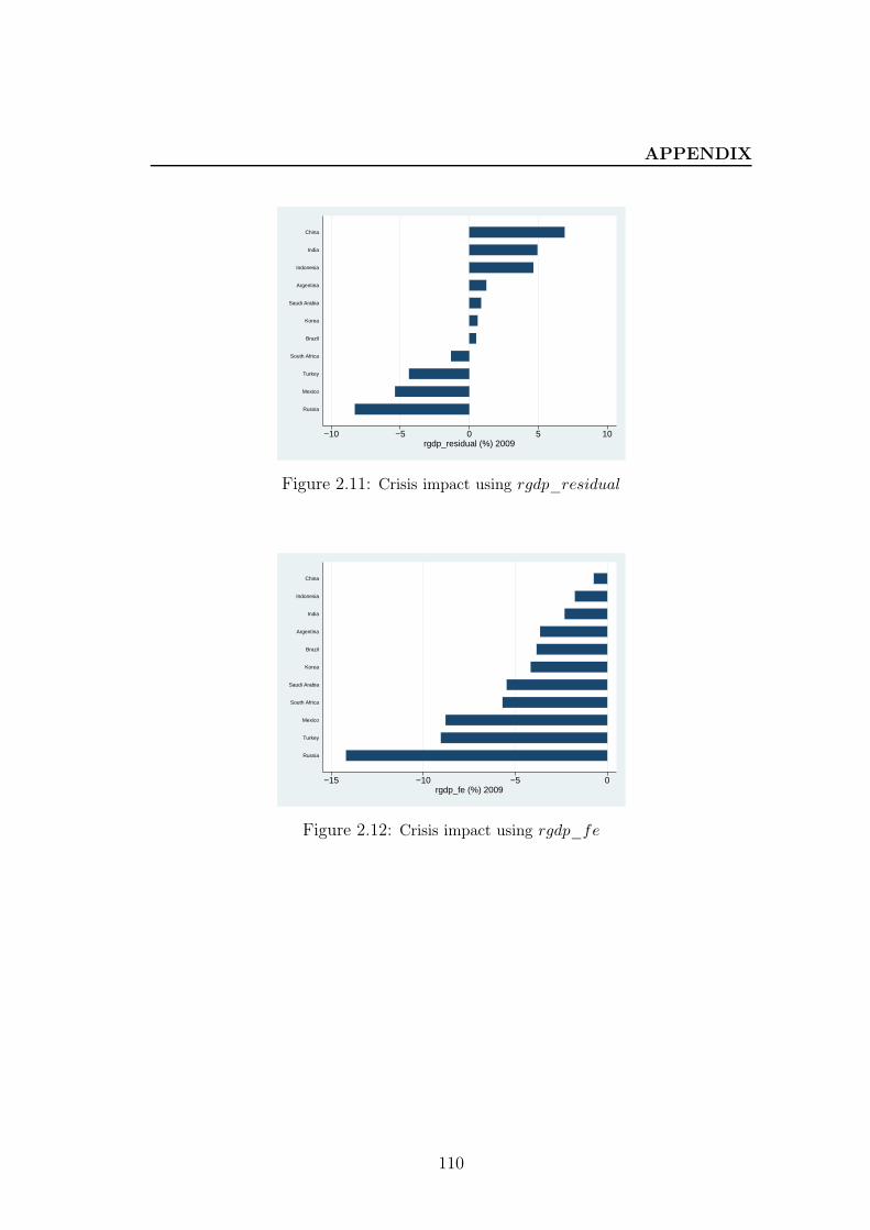
APPENDIX
−10 −5 0 5 10rgdp_residual (%) 2009
Russia
Mexico
Turkey
South Africa
Brazil
Korea
Saudi Arabia
Argentina
Indonesia
India
China
Figure 2.11: Crisis impact using rgdp_residual
−15 −10 −5 0rgdp_fe (%) 2009
Russia
Turkey
Mexico
South Africa
Saudi Arabia
Korea
Brazil
Argentina
India
Indonesia
China
Figure 2.12: Crisis impact using rgdp_fe
110
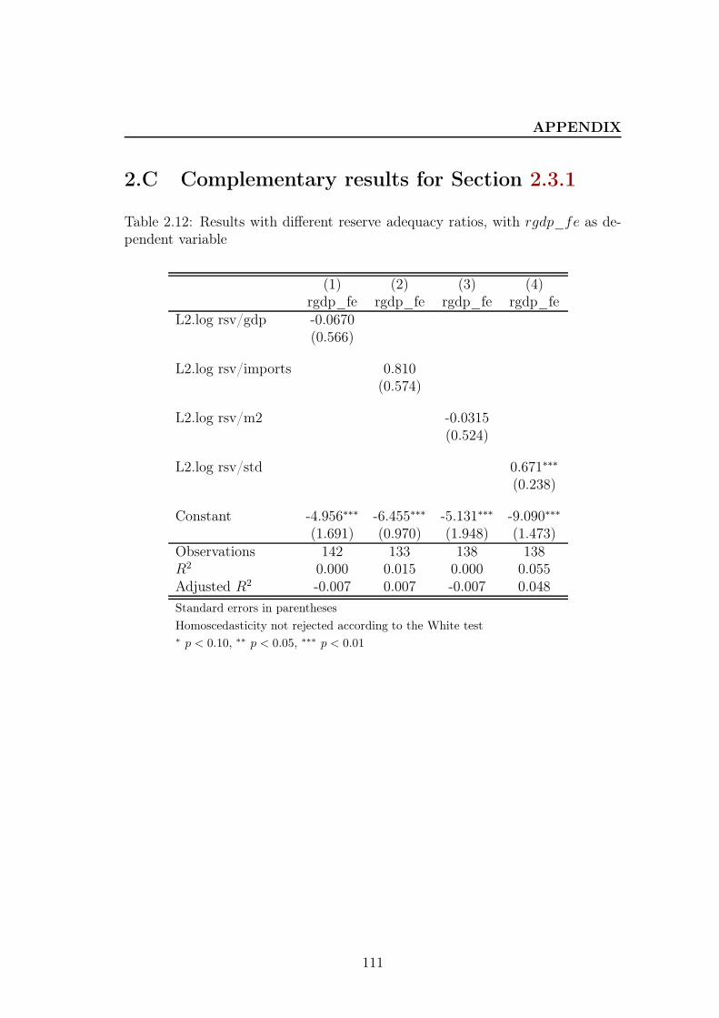
APPENDIX
2.C Complementary results for Section 2.3.1
Table 2.12: Results with different reserve adequacy ratios, with rgdp_fe as de-pendent variable
(1) (2) (3) (4)rgdp_fe rgdp_fe rgdp_fe rgdp_fe
L2.log rsv/gdp -0.0670(0.566)
L2.log rsv/imports 0.810(0.574)
L2.log rsv/m2 -0.0315(0.524)
L2.log rsv/std 0.671∗∗∗
(0.238)
Constant -4.956∗∗∗ -6.455∗∗∗ -5.131∗∗∗ -9.090∗∗∗
(1.691) (0.970) (1.948) (1.473)Observations 142 133 138 138R2 0.000 0.015 0.000 0.055Adjusted R2 -0.007 0.007 -0.007 0.048
Standard errors in parentheses
Homoscedasticity not rejected according to the White test∗ p < 0.10, ∗∗ p < 0.05, ∗∗∗ p < 0.01
111
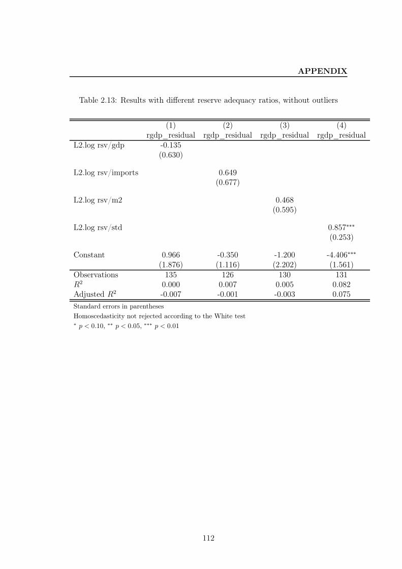
APPENDIX
Table 2.13: Results with different reserve adequacy ratios, without outliers
(1) (2) (3) (4)rgdp_residual rgdp_residual rgdp_residual rgdp_residual
L2.log rsv/gdp -0.135(0.630)
L2.log rsv/imports 0.649(0.677)
L2.log rsv/m2 0.468(0.595)
L2.log rsv/std 0.857∗∗∗
(0.253)
Constant 0.966 -0.350 -1.200 -4.406∗∗∗
(1.876) (1.116) (2.202) (1.561)Observations 135 126 130 131R2 0.000 0.007 0.005 0.082Adjusted R2 -0.007 -0.001 -0.003 0.075
Standard errors in parentheses
Homoscedasticity not rejected according to the White test∗ p < 0.10, ∗∗ p < 0.05, ∗∗∗ p < 0.01
112
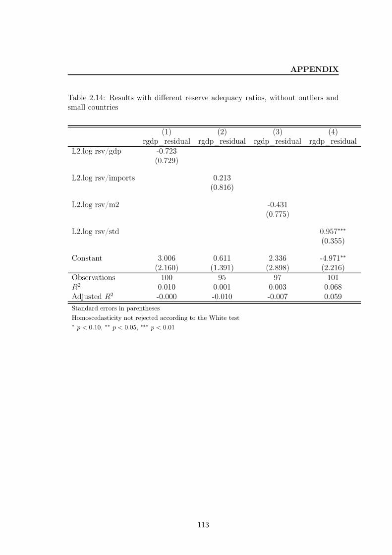
APPENDIX
Table 2.14: Results with different reserve adequacy ratios, without outliers andsmall countries
(1) (2) (3) (4)rgdp_residual rgdp_residual rgdp_residual rgdp_residual
L2.log rsv/gdp -0.723(0.729)
L2.log rsv/imports 0.213(0.816)
L2.log rsv/m2 -0.431(0.775)
L2.log rsv/std 0.957∗∗∗
(0.355)
Constant 3.006 0.611 2.336 -4.971∗∗
(2.160) (1.391) (2.898) (2.216)Observations 100 95 97 101R2 0.010 0.001 0.003 0.068Adjusted R2 -0.000 -0.010 -0.007 0.059
Standard errors in parentheses
Homoscedasticity not rejected according to the White test∗ p < 0.10, ∗∗ p < 0.05, ∗∗∗ p < 0.01
113

APPENDIX
2.D Complementary results for Section 2.3.2
Table 2.15: Full specification without outliers
(1) (2)rgdp_fe rgdp_residual
L2.log rsv/std 0.951∗∗∗ 0.937∗∗∗
(0.292) (0.316)
L2.capital controls 0.0352 0.220(0.263) (0.281)
L2.exchange regime index -0.892 -0.196(1.226) (1.311)
L2.trade openness -0.0235∗∗ -0.0286∗∗
(0.0104) (0.0113)
oil dummy -3.142∗∗∗ -1.987(1.132) (1.211)
Constant -7.111∗∗∗ -1.830(2.263) (2.431)
Observations 104 102R2 0.213 0.201Adjusted R2 0.173 0.159
Standard errors in parentheses
Homoscedasticity not rejected according to the White test∗ p < 0.10, ∗∗ p < 0.05, ∗∗∗ p < 0.01
114
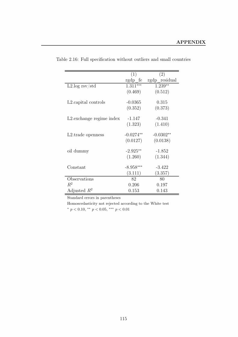
APPENDIX
Table 2.16: Full specification without outliers and small countries
(1) (2)rgdp_fe rgdp_residual
L2.log rsv/std 1.311∗∗∗ 1.239∗∗
(0.469) (0.512)
L2.capital controls -0.0365 0.315(0.352) (0.373)
L2.exchange regime index -1.147 -0.341(1.323) (1.410)
L2.trade openness -0.0274∗∗ -0.0302∗∗
(0.0127) (0.0138)
oil dummy -2.925∗∗ -1.852(1.260) (1.344)
Constant -8.958∗∗∗ -3.422(3.111) (3.357)
Observations 82 80R2 0.206 0.197Adjusted R2 0.153 0.143
Standard errors in parentheses
Homoscedasticity not rejected according to the White test∗ p < 0.10, ∗∗ p < 0.05, ∗∗∗ p < 0.01
115
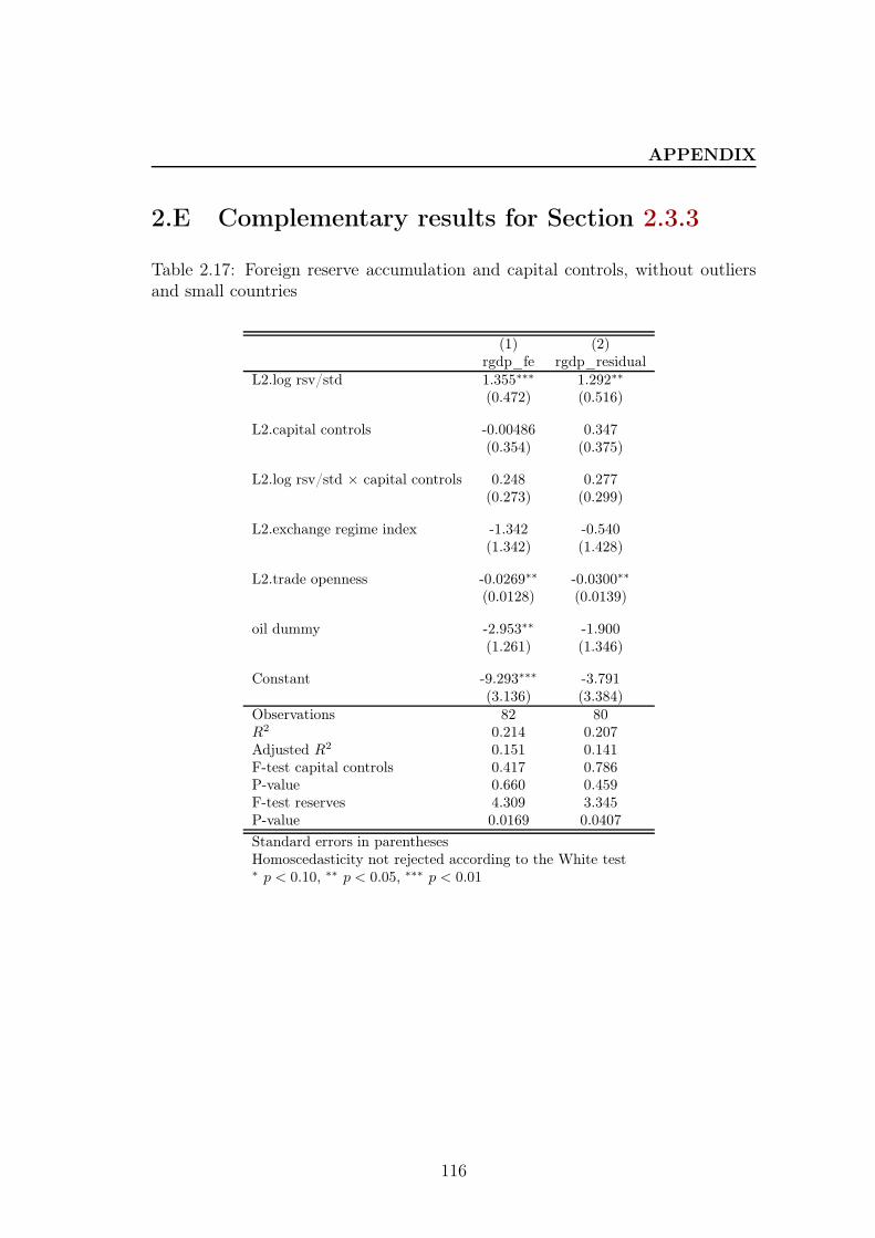
APPENDIX
2.E Complementary results for Section 2.3.3
Table 2.17: Foreign reserve accumulation and capital controls, without outliersand small countries
(1) (2)rgdp_fe rgdp_residual
L2.log rsv/std 1.355∗∗∗ 1.292∗∗
(0.472) (0.516)
L2.capital controls -0.00486 0.347(0.354) (0.375)
L2.log rsv/std × capital controls 0.248 0.277(0.273) (0.299)
L2.exchange regime index -1.342 -0.540(1.342) (1.428)
L2.trade openness -0.0269∗∗ -0.0300∗∗
(0.0128) (0.0139)
oil dummy -2.953∗∗ -1.900(1.261) (1.346)
Constant -9.293∗∗∗ -3.791(3.136) (3.384)
Observations 82 80R2 0.214 0.207Adjusted R2 0.151 0.141F-test capital controls 0.417 0.786P-value 0.660 0.459F-test reserves 4.309 3.345P-value 0.0169 0.0407
Standard errors in parenthesesHomoscedasticity not rejected according to the White test∗ p < 0.10, ∗∗ p < 0.05, ∗∗∗ p < 0.01
116
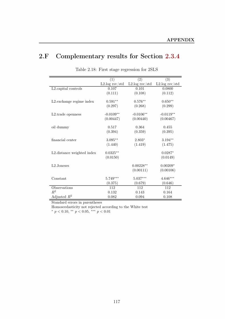
APPENDIX
2.F Complementary results for Section 2.3.4
Table 2.18: First stage regression for 2SLS
(1) (2) (3)L2.log rsv/std L2.log rsv/std L2.log rsv/std
L2.capital controls 0.107 0.101 0.0800(0.111) (0.108) (0.112)
L2.exchange regime index 0.591∗∗ 0.576∗∗ 0.650∗∗
(0.297) (0.268) (0.299)
L2.trade openness -0.0109∗∗ -0.0106∗∗ -0.0119∗∗
(0.00447) (0.00440) (0.00467)
oil dummy 0.517 0.364 0.455(0.394) (0.359) (0.395)
financial center 3.095∗∗ 2.803∗ 3.194∗∗
(1.440) (1.419) (1.475)
L2.distance weighted index 0.0325∗∗ 0.0287∗
(0.0150) (0.0149)
L2.Joneses 0.00228∗∗ 0.00209∗
(0.00111) (0.00106)
Constant 5.749∗∗∗ 5.037∗∗∗ 4.646∗∗∗
(0.375) (0.679) (0.646)Observations 112 112 112R2 0.132 0.143 0.164Adjusted R2 0.082 0.094 0.108
Standard errors in parenthesesHomoscedasticity not rejected according to the White test∗ p < 0.10, ∗∗ p < 0.05, ∗∗∗ p < 0.01
117
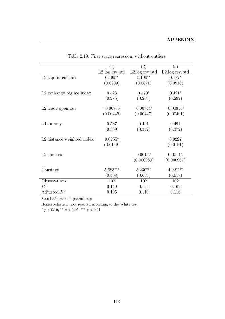
APPENDIX
Table 2.19: First stage regression, without outliers
(1) (2) (3)L2.log rsv/std L2.log rsv/std L2.log rsv/std
L2.capital controls 0.199∗∗ 0.196∗∗ 0.177∗
(0.0909) (0.0871) (0.0918)
L2.exchange regime index 0.423 0.470∗ 0.491∗
(0.286) (0.269) (0.292)
L2.trade openness -0.00735 -0.00744∗ -0.00815∗
(0.00445) (0.00447) (0.00461)
oil dummy 0.537 0.421 0.491(0.369) (0.342) (0.372)
L2.distance weighted index 0.0255∗ 0.0227(0.0149) (0.0151)
L2.Joneses 0.00157 0.00144(0.000989) (0.000967)
Constant 5.683∗∗∗ 5.230∗∗∗ 4.921∗∗∗
(0.408) (0.659) (0.617)Observations 102 102 102R2 0.149 0.154 0.169Adjusted R2 0.105 0.110 0.116
Standard errors in parentheses
Homoscedasticity not rejected according to the White test∗ p < 0.10, ∗∗ p < 0.05, ∗∗∗ p < 0.01
118
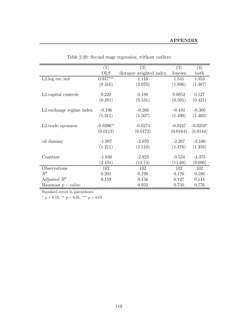
APPENDIX
Table 2.20: Second stage regression, without outliers
(1) (2) (3) (4)OLS distance weighted index Joneses both
L2.log rsv/std 0.937∗∗∗ 1.116 1.541 1.353(0.316) (2.070) (1.896) (1.467)
L2.capital controls 0.220 0.180 0.0852 0.127(0.281) (0.531) (0.501) (0.421)
L2.exchange regime index -0.196 -0.266 -0.434 -0.360(1.311) (1.507) (1.490) (1.402)
L2.trade openness -0.0286∗∗ -0.0274 -0.0247 -0.0259∗
(0.0113) (0.0172) (0.0164) (0.0144)
oil dummy -1.987 -2.070 -2.267 -2.180(1.211) (1.510) (1.476) (1.358)
Constant -1.830 -2.923 -5.524 -4.375(2.431) (12.74) (11.68) (9.086)
Observations 102 102 102 102R2 0.201 0.198 0.170 0.186Adjusted R2 0.159 0.156 0.127 0.144Hausman p− value . 0.932 0.750 0.776
Standard errors in parentheses∗ p < 0.10, ∗∗ p < 0.05, ∗∗∗ p < 0.01
119

Chapter 3
Balance Sheet Effects, Foreign
Reserves and Public Policies
3.1 Introduction
The global economic turmoil which started with a local crisis in 2007 in the
United States has quickly become a widespread global financial crisis (GFC) of
a magnitude never seen since the Great Depression in 1929. One particular phe-
nomenon which can be observed in recent years is that emerging market economies
(EMEs), which seemed most vulnerable during the last waves of financial crises
in the 1990s, fared much better than advanced economies during the GFC.
As a matter of fact, figure 3.1 presents two crisis impact indicators 58 in terms
of real GDP losses in the G20 countries (excluding the European Uinon); one
can see that many EMEs, such as China, Indonesia, India and Argentina, suf-
fered less output losses than developed industrial economies. Moreover, figure 3.2
shows that some EMEs, such as Argentina, Indonesia and Thailand which had
experienced large currency depreciation in previous crisis periods demonstrated
58. Both indicators are calculated by Bussière et al. (2014). The detrended real GDP growthmeasures the difference between the actual annual real GDP growth rate in 2009 and a six-yearhistorical mean before the crisis. The forecast errors capture the difference between the actualreal GDP growth in 2009 and the IMF World Economic Outlook (WEO) forecast in the firstquarter of 2008 (before the Lehman collapse in September of the same year).
121
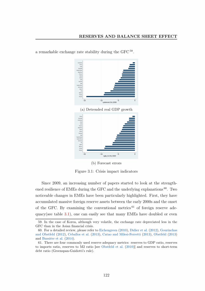
RESERVES AND BALANCE SHEET EFFECT
a remarkable exchange rate stability during the GFC 59.
−15 −10 −5 0rydetrend (%) 2009
Russia
Turkey
Mexico
UK
Japan
Germany
South Africa
Italy
Canada
USA
Korea
Brazil
France
Argentina
Saudi Arabia
Australia
India
China
Indonesia
(a) Detrended real GDP growth
−15 −10 −5 0rgdp_fe (%) 2009
Russia
Turkey
Mexico
Japan
UK
Germany
South Africa
Saudi Arabia
Italy
Canada
Korea
Brazil
Argentina
France
USA
India
Indonesia
Australia
China
(b) Forecast errors
Figure 3.1: Crisis impact indicators
Since 2009, an increasing number of papers started to look at the strength-
ened resilience of EMEs during the GFC and the underlying explanations 60. Two
noticeable changes in EMEs have been particularly highlighted. First, they have
accumulated massive foreign reserve assets between the early 2000s and the onset
of the GFC. By examining the conventional metrics 61 of foreign reserve ade-
quacy(see table 3.1), one can easily see that many EMEs have doubled or even
59. In the case of Korea, although very volatile, the exchange rate depreciated less in theGFC than in the Asian financial crisis.
60. For a detailed review, please refer to Eichengreen (2010), Didier et al. (2012), Gourinchasand Obstfeld (2012), Ceballos et al. (2013), Catao and Milesi-Ferretti (2013), Obstfeld (2013)and Bussière et al. (2014).
61. There are four commonly used reserve adequacy metrics: reserves to GDP ratio, reservesto imports ratio, reserves to M2 ratio [see Obstfeld et al. (2010)] and reserves to short-termdebt ratio (Greenspan-Guidotti’s rule).
122
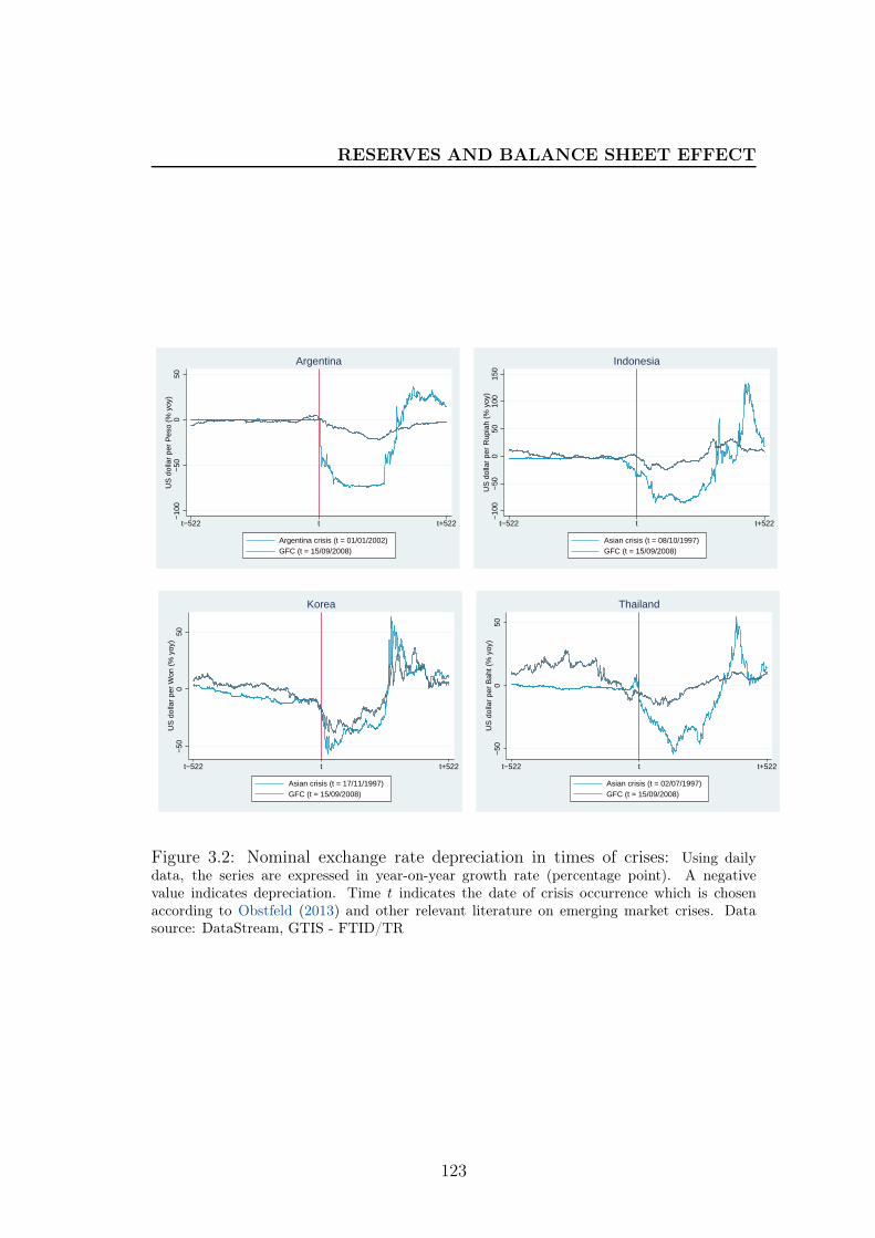
RESERVES AND BALANCE SHEET EFFECT−
100
−50
050
US
dol
lar
per
Pes
o (%
yoy
)
t−522 t t+522
Argentina crisis (t = 01/01/2002)GFC (t = 15/09/2008)
Argentina
−10
0−
500
5010
015
0U
S d
olla
r pe
r R
upia
h (%
yoy
)
t−522 t t+522
Asian crisis (t = 08/10/1997)GFC (t = 15/09/2008)
Indonesia
−50
050
US
dol
lar
per
Won
(%
yoy
)
t−522 t t+522
Asian crisis (t = 17/11/1997)GFC (t = 15/09/2008)
Korea
−50
050
US
dol
lar
per
Bah
t (%
yoy
)
t−522 t t+522
Asian crisis (t = 02/07/1997)GFC (t = 15/09/2008)
Thailand
Figure 3.2: Nominal exchange rate depreciation in times of crises: Using dailydata, the series are expressed in year-on-year growth rate (percentage point). A negativevalue indicates depreciation. Time t indicates the date of crisis occurrence which is chosenaccording to Obstfeld (2013) and other relevant literature on emerging market crises. Datasource: DataStream, GTIS - FTID/TR
123
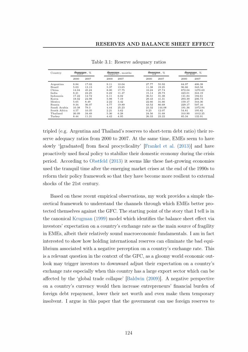
RESERVES AND BALANCE SHEET EFFECT
Table 3.1: Reserve adequacy ratios
Country ReservesGDP
, % Reservesimports
, months Reservesm2
, % Reservesst.debt
, %
2000 2007 2000 2007 2000 2007 2000 2007
Argentina 8.84 17.02 9.11 10.04 27.77 55.92 64.97 406.38Brazil 5.03 13.13 5.37 13.65 11.38 19.25 96.66 343.58China 14.04 45.24 8.06 17.75 10.24 27.74 872.04 1270.63India 8.21 24.25 6.22 11.47 15.14 29.73 423.01 344.19Indonesia 17.22 12.72 6.11 6.02 36.51 31.38 141.84 192.61Korea 18.02 24.98 5.98 7.19 29.43 41.31 293.39 206.73Mexico 5.65 8.49 2.22 3.42 22.66 31.66 159.17 344.36Russia 9.34 36.07 4.77 19.89 43.52 80.68 229.17 507.16Saudi Arabia 10.38 79.3 4.44 25.23 23.32 144.08 191.36 1072.94South Africa 4.57 10.35 2.21 3.62 9.23 12.07 54.81 195.82Thailand 26.09 34.49 5.36 6.28 24.56 31.68 310.90 1012.25Turkey 8.44 11.31 4.42 4.95 26.33 23.22 85.34 132.91
tripled (e.g. Argentina and Thailand’s reserves to short-term debt ratio) their re-
serve adequacy ratios from 2000 to 2007. At the same time, EMEs seem to have
slowly ‘[graduated] from fiscal procyclicality’ [Frankel et al. (2013)] and have
proactively used fiscal policy to stabilize their domestic economy during the crisis
period. According to Obstfeld (2013) it seems like these fast-growing economies
used the tranquil time after the emerging market crises at the end of the 1990s to
reform their policy framework so that they have become more resilient to external
shocks of the 21st century.
Based on these recent empirical observations, my work provides a simple the-
oretical framework to understand the channels through which EMEs better pro-
tected themselves against the GFC. The starting point of the story that I tell is in
the canonical Krugman (1999) model which identifies the balance sheet effect via
investors’ expectation on a country’s exchange rate as the main source of fragility
in EMEs, albeit their relatively sound macroeconomic fundamentals. I am in fact
interested to show how holding international reserves can eliminate the bad equi-
librium associated with a negative perception on a country’s exchange rate. This
is a relevant question in the context of the GFC, as a gloomy world economic out-
look may trigger investors to downward adjust their expectation on a country’s
exchange rate especially when this country has a large export sector which can be
affected by the ‘global trade collapse’ [Baldwin (2009)]. A negative perspective
on a country’s currency would then increase entrepreneurs’ financial burden of
foreign debt repayment, lower their net worth and even make them temporary
insolvent. I argue in this paper that the government can use foreign reserves to
124
RESERVES AND BALANCE SHEET EFFECT
restore lenders’ confidence on the country’s currency. There are however several
ways regarding how reserves work to eliminate the unfavorable equilibrium. One
the one hand, the government can use its previously accumulated foreign reserves
as a targeted lending to the private sector; namely the government writes off
the private sector’s foreign-currency liabilities or provides extra foreign-currency
liquidities when any other external funding is cut off. This is equivalent to give
lenders’ a government guarantee on the loans they grant private entrepreneurs or
to let the government borrow abroad for the sake of the private sector. On the
other hand, the country’s authorities can also choose to stabilize domestic ab-
sorption via an increase in government spending. This expansionary fiscal policy
can be financed by foreign reserves (expenditure switching policy) for example.
Comparing the targeted lending with fiscal spending, it is shown in this paper
that although both policies eliminate the bad equilibrium (i.e. a very depreci-
ated exchange rate and a zero domestic investment) they stabilize the economy
through two different mechanisms. In the case of targeted lending, foreign reserves
can be regarded as a state-contingent insurance. Its value expressed in domes-
tic terms increases with domestic depreciation while the latter lowers firms’ net
worth. Therefore, a targeted lending mainly affects lenders’ expectation on do-
mestic entrepreneurs’ wealth which is used as collateral for borrowing. The bad
equilibrium can be removed even without an actual depletion of reserves as long
as the stock of reserves in the economy is sufficient with respect to entrepreneurs’
foreign debt. However, a fiscal spending affects entrepreneurs’ wealth via a vir-
tual change in the domestic exchange rate. This is achieved by an increase in
demand for domestic goods on the good market. The need for reserves depends
on the magnitude of the domestic depreciation. Therefore, it is not surprising to
see that the minimum amount of reserves needed for a targeted lending policy is
lower than for fiscal spending. In both cases, the stock of reserves matters.
This paper is closely related to three strands of literature: foreign reserve
accumulation, ‘third-generation’ crisis models and currency mismatch, as well as
the countercyclical fiscal policies in EMEs during the GFC.
As for the motives of foreign reserve accumulation, my work fits well in the
125
RESERVES AND BALANCE SHEET EFFECT
works on the precautionary motive of reserve holding 62. In the literature, studies
on the precautionary role of reserves have been mainly focusing on how holding
reserves can smooth domestic output or/and consumption when the economy is
hit by ‘sudden stops’ [Jeanne and Rancière (2011)] 63 or when the government
faces increasing costs of external financing or default risks [Bianchi et al. (2012)].
In contrast, I rather study how reserves are useful in the context of currency
mismatch and of the resultant balance sheet effect. In fact, reserves can not
only be used to provide foreign-currency liquidity in case of ‘sudden stops’ [Calvo
(1998)], they can also alter investors’ expectations on the net worth of a country’s
private sector and on the country’s domestic exchange rate, thus insulating the
domestic economy from balance sheet effects. This is the focal point of my current
work. After all, the last wave of emerging market crises, especially in Asia,
is largely explained by balance sheet effects and curiously, this aspect of the
insurance role of reserves has not been thoroughly analyzed. My current work
can also be regarded as a theoretical underpinning to a few recent empirical
papers 64 which point out that the reserves to (short-term) external debt ratio 65
is the most relevant metric to predict countries’ economic performance during the
GFC. Moreover, I argue that depending on the policy tool used, foreign reserves
need to be or not to be virtually depleted. This is related to the empirical finding
of Bussière et al. (2014) who document that reserves are rather ‘nuclear power’
than real ‘gunpowder’. Finally, my work does not only focus on the motives
of reserve accumulation, it also analyzes and compares different ways of ‘using’
reserves. This is a new angle of studying foreign reserves.
My current work is also closely related to the literature on the ‘third-
generation’ crisis. In the aftermath of the Asian financial crisis, Krugman (1999)
62. For a detailed review, see Aizenman and Lee (2007), Alfaro and Kanczuk (2009), Aizen-man and Hutchison (2010), Obstfeld et al. (2010), Jeanne and Rancière (2011), Bianchi et al.(2012), Benigno and Fornaro (2012), Calvo et al. (2013) and Bussière et al. (2014).
63. Based on a calibration using a sample of sudden stops in 34 middle-income countries over1975-2003, Jeanne and Rancière (2011) show that the negative impact of the financial accountreversal on domestic absorption can be offset by a depletion of reserves; a 10% fall in capitalinflows leads to less than 3% of GDP collapse if there is a buffer stock of reserves.
64. See Llaudes et al. (2010), Catao and Milesi-Ferretti (2013) and Bussière et al. (2014)65. In the case of emerging market economies, their short-term debts are mostly denominated
in foreign currency due to the ‘Original sin’ [Eichengreen et al. (2007)]
126
RESERVES AND BALANCE SHEET EFFECT
demonstrates that multiple equilibria exist when the private sector in a country
faces credit constraint (where the net worth serves as collateral) and is exposed
to large foreign-currency debt. While Krugman (1999) aims at proving the ex-
istence of multiple equilibria, I propose concrete policy choices to eliminate the
bad one. Moreover, I add a government sector into Krugman (1999)’s frame-
work. By doing so, lenders’ expectation concerns not only entrepreneurs’ wealth
but also the strength and the willingness of the government to stabilize domestic
economy whenever it is necessary. My paper is also inspired by Aghion et al.
(2000) and Aghion et al. (2004) who provide a micro-founded version of Krug-
man’s model. While these two papers focus on how a monetary policy affects the
multiple equilibria, I study fiscal policies and targeted lending in foreign currency.
The currency mismatch is a key assumption for the balance sheet effect to
work. In the scope of this paper, as I aim at illustrating how different public
policies may be used to stabilize the domestic economy rather than at explaining
why entrepreneurs want to hold foreign-currency liabilities ex ante, I take cur-
rency mismatch as given. There are nevertheless various well-founded motivations
in the literature explaining the demand for foreign-currency liabilities. Burnside
et al. (1999) and Schneider and Tornell (2004) argue that foreign-currency bor-
rowing results from a risk-overtaking behavior of domestic firms when they know
that the government will bail out domestic banks in case of default. Jeanne
(2000) and Jeanne (2003) point to the signaling and commitment effect of bor-
rowing in foreign currency. Namely, by allowing the private sector to hold foreign
debt which is subject to exchange rate fluctuations, the government sends to the
market a signal about its commitment not to inflate the economy or depreciate
the currency. The need for foreign funding can also be explained by the fact that
the domestic financial market is underdeveloped; there is no sufficient domestic
savings to be channeled to firms. This is the assumption pointed out by Aghion
et al. (2000) that I follow in my analysis.
Regarding how to reduce the impact of the currency mismatch, Jeanne and
Zettelmeyer (2002) compare the pros and cons of the monetary policy and of
the choice of exchange rate. They conclude that the monetary policy is contra-
dictory in dealing with balance sheet effects. With perfect capital mobility, the
country where the private sector is hit by negative expectations on the exchange
127
RESERVES AND BALANCE SHEET EFFECT
rate should increase the interest rate to prevent depreciation. However, a rise in
interest rates is detrimental to domestic investment. I explore in this paper a pol-
icy choice that has been mentioned but not analyzed in Jeanne and Zettelmeyer
(2002): how fiscal policies can play a role when the monetary policy is not ef-
fective in dealing with the multiple equilibria. Two different fiscal policy tools
- targeted lending or fiscal spending - are analyzed in the subsequent sections.
Jeanne and Wyplosz (2003) take a different angle to analyze how an international
lender-of-last-resort can be useful in dealing with the issue of currency mismatch.
The GFC has unfortunately demonstrated that an international coordination in
the matter of crisis management is far from developed nowadays. Many countries
might prefer to constitute a buffer stock for self-insurance instead of resort to the
assistance of international financial institutions.
Finally, my paper is related to some recent empirical works on how EMEs
used countercyclical fiscal policies to tackle the GFC. As Crowe et al. (2009),
Eichengreen (2010) and Didier et al. (2012) point out, in the past, fiscal policy
in emerging market countries used to be procyclical because EME business cy-
cles tend to be driven by capital flows [see Kaminsky et al. (2005)]. This strand
of literature has emphasized the role of countercyclical fiscal policies to smooth
domestic production. I rather study to what extend these policies can help alle-
viate the balance sheet effect in the private sector. Prasad (2011), Didier et al.
(2012) and Obstfeld (2013) argue that many EMEs have reduced the external
debt denominated in foreign currency and the external financing is oriented to-
wards equity (which have advantages of being denominated in local currency
and state-contingent) and foreign direct investment. However, as Llaudes et al.
(2010) points out ‘large increases in reserves played a more important role than
any change in the currency denomination of external debt’ in reducing a country’s
exposure to external liabilities. The private sector might still have net foreign
liabilities in its balance sheet and is thus vulnerable to valuation losses in case
of domestic currency depreciation. Indeed, as Eichengreen (2010) states, ‘[w]hile
on-balance sheet foreign currency mismatches had been reduced, corporations [...]
had increased their off-balance sheet foreign currency exposure through derivative
positions.’
128
RESERVES AND BALANCE SHEET EFFECT
This paper is organized as follows. Section 3.2 describes the model setting.
Section 3.3 analyzes and derives conditions for the existence of multiple equilibria
in absence of government intervention. Section 3.4 studies and compares two
policy tools used to stabilize the domestic economy. Section 3.5 concludes.
3.2 The model
The aim of this paper is to provide a theoretical framework showing the ways
through which foreign reserves can be useful in stabilizing the domestic economy.
In the paper, I especially focus on the risks associated with the currency mismatch
and the resultant balance sheet effect in the private sector. For this purpose, the
analysis in this paper is based on a stylized model with multiple equilibria similar
to Krugman (1999). Although very simple, it is enough to demonstrate the
different ways the government can stabilize the domestic economy using foreign
reserves. This is a real-economy model with three types of agents: ‘hand-to-
mouth’ workers, entrepreneurs 66 and a government. Capital is supposed to be
perfectly mobile across borders and all prices are flexible.
3.2.1 Workers
As in Krugman (1999), the role played by workers is completely passive. They
provide the labor force to entrepreneurs and get paid at the marginal product of
labor. They do not have access to financial market so that they consume all
the labor income every period (so called ‘hand-to-mouth’ labor). The choice
of passive labor force is motivated by the fact that the main mechanism of the
balance sheet effect goes through entrepreneurs’ investment decision to which the
attention of this paper is paid. It is further assumed that the labor supply is
inelastic and the total mass of labor is equal to one.
The workers consume both domestic goods, CHt , and foreign goods, CF
t . The
domestic goods are regarded as the numéraire with an unitary price. Therefore,
66. In this paper I focus on the balance sheet of entrepreneurs. But the analysis can also beapplied to banks which are exposed to foreign liabilities, like in Jeanne and Zettelmeyer (2002).There are no fundamental differences between firms and banks with regard to the balance sheeteffect.
129
RESERVES AND BALANCE SHEET EFFECT
the price of foreign goods in terms of domestic goods, pt, denotes the real exchange
rate in the domestic economy. An increase in pt means a depreciation of the price
of the domestic goods (depreciation of the local currency, loosely speaking.). For
simplicity, I assume that the elasticity of substitution between domestic goods
and foreign goods is one. The workers maximize their utility subject to the budget
constraint as described below:
MaxCHt ,C
Ft
U(CHt , C
Ft ) = (CH
t )1−µ(CFt )
µ
such that CHt + ptC
Ft = Ct
Ct refers to the total consumption by domestic workers, expressed in terms of
domestic goods. The workers’ maximization program yields the following results:
CHt = (1− µ)Ct
CFt =
µCtpt
The consumption of domestic goods is thus a constant share (1 − µ) of the
total consumption C.
3.2.2 Entrepreneurs
The economy is populated by identical entrepreneurs who face credit con-
straints which prevent them from borrowing and investing more than a multiple
of their current real wealth (Wt). Entrepreneurs’ wealth is therefore the funda-
mental variable that determines investment and output.
In fact, entrepreneurs use labor (Nt) and capital (Kt) to produce an output.
The labor supply being perfectly inelastic with Nt = 1. The capital is chosen
a period earlier through investment and fully depreciates every period, namely
Kt = It−1. As one can see later, entrepreneurs’ capacity to invest is precisely
constrained, depending on their real wealth.
The production function is a standard neoclassical production function.
Namely, the production is increasing in both inputs with decreasing marginal
returns and is homogeneous of degree one. Yt = F (Kt, Nt) = Kαt N
1−αt .
130
RESERVES AND BALANCE SHEET EFFECT
For private investment, it is assumed that entrepreneurs need both foreign and
domestic goods. They spend a constant share µ of total investment on imported
goods, and thus a constant share 1−µ in domestic goods. Namely IHt = (1−µ)It
and IFt = µItpt
.
In each period, the only important decision that entrepreneurs need to make is
how much to invest in capital which is financed by borrowing from both domestic
lenders and foreign lenders. The timing of events can be summarized as follows:
investors (those who lend to entrepreneurs) enter the period t with an expectation
on the exchange rate which affects the expected value of entrepreneurs’ wealth
and thus the collateral value for borrowing. An expectation on the investment is
thus formed and it will feed back the expectation on the exchange rate through the
domestic good market clearing. Everything is thus simultaneously determined.
In rational expectation equilibrium, the expected values coincide with the actual
values.
Two important assumptions characterize entrepreneurs’ investment behavior:
entrepreneurs face credit constraint on the one hand and they have foreign-good
denominated liabilities on the other.
First, the assumption on the credit constraint stipulates that the maximum
amount of credit that entrepreneurs may obtain in period t depends on their real
net worth. Namely, from lenders’ viewpoint, they would only lend up to a share ψ
of entrepreneurs’ net worth, namely Let ≤ ψW et . L
et denotes expected credit that
lenders are willing to grant entrepreneurs. W et refers to entrepreneurs’ expected
wealth. ψ is a parameter of the tightness of the credit market. The higher ψ 67,
the higher leverage entrepreneurs have. Entrepreneurs’ investment at time t can
be written as:
67. The value of ψ depends on the stage of development in a country. ψ = 0 when noborrowing (especially external borrowing) is possible. This can be the case in less developedcountries where the financial market is far from developed. In this extreme case, the balancesheet effect is not at work as there is no foreign borrowing at all. In an advanced economy, ψ isexpected to be high, the private sector mainly replies on borrowing to finance the investment.As Aghion et al. (2000) argue, the financial market is mature in advanced economies, there issufficient domestic credit available such that the balance sheet effect may or may not apply.The emerging market economies (middle-income countries) that I focus on in this paper shouldhave a ψ in between the two former cases and have a strong demand for foreign credit.
131
RESERVES AND BALANCE SHEET EFFECT
Iet = W et + Let ≤ (1 + ψ)W e
t (3.1)
The functional form of the credit constraint is well-founded in the litera-
ture on financial accelerator [see Bernanke et al. (1999)], based on the idea of
contract enforcement. The investment constraint (3.1) can be binding or unbind-
ing depending on the value of the collateral. When this constraint is binding,
Iet = (1 + ψ)W et . When the constraint is unbinding, the amount of investment is
determined by the equalization between marginal product of capital and marginal
cost. As the economy is fully open, the marginal cost is ultimately equal to the
world gross interest rate R∗. Namely, Fk(Kt+1, Nt+1) = R∗, where Fk(·) denotes
the marginal product of capital. This gives It = I =(αR∗
) 1
1−α
when the credit
constraint is not binding.
The second assumption that entrepreneurs have foreign-good denominated
liabilities is crucial to trigger balance sheet effects that this paper wants to study.
As entrepreneurs have foreign-good denominated liabilities, their real wealth Wt
is subject to the valuation effect of the exchange rate. As in Krugman (1999), I
take the currency mismatch as given in order to concentrate on the link between
the domestic exchange rate and entrepreneurs’ wealth and investment. There
are several ways to endogenize the currency mismatch as I summarized in the
literature review. A nature extension of my current work is to endogenously
determine entrepreneurs’ portfolio choice.
Entrepreneurs’ wealth function can thus be written as follows:
W et = αYt −Dt − petD
∗t (3.2)
Notice that Yt is predetermined in period t as both inputs of production are
chosen a period earlier. αYt is the output accruing to entrepreneurs (equivalent
to entrepreneurs’ earnings after paying the labor force). Dt and D∗t respectively
denote the domestic-good denominated and foreign-good denominated net debts.
132
RESERVES AND BALANCE SHEET EFFECT
They are both exogenously given. Therefore, the expectation on entrepreneurs’
wealth in period t only depends on the expectation on the exchange rate pet .
Clearly, if lenders thought the domestic exchange rate would depreciate (namely
a rise in pet), they would expect an increase in entrepreneurs’ burden of foreign debt
repayment, thus a decrease in entrepreneurs’ net worth. As a result, lenders would
cut down their investment, driving down the next-period production (period t+1)
through equation (3.1).
Combining equations (3.1) and (3.2), the demand for investment of en-
trepreneurs can be derived below; it is a truncated function of the expected
exchange rate.
It =
0 pt > pt
(1 + ψ)(αYt −Dt − petD∗t ) pt < pet < pt
I =(αR∗
) 1
1−α
pt < pt
(3.3)
pt = αYt−DtD∗
tdenotes the threshold value of exchange rate beyond which
entrepreneurs’ wealth is reduced to zero or beneath. On the contrary, pt =αYt−Dt−
I1+ψ
D∗
tdenotes the threshold value of exchange rate below which en-
trepreneurs’ wealth is high enough that the credit constraint (3.1) does not bind.
In between these two threshold values, the investment is a negative function of
the expected exchange rate.
In sum, as the red cycle in figure 3.3 illustrates, the mechanism of the model
goes through lenders’ expectation on the domestic exchange rate which affects
entrepreneurs’ expected wealth via foreign debt repayment. The expected invest-
ment in the economy will ultimately determine the actual level of the domestic
exchange rate on the good market as I will detail in the next subsection. There-
fore, the only endogenous variables in this model that are important in period t
are domestic investment It, domestic exchange rate pt and entrepreneurs’ wealth
Wt. As a matter of timing, all the decisions are made within the period t. The
impact of the period t decisions on the future economy only goes through domes-
tic investment which will be entirely used for the next-period production. From
133
RESERVES AND BALANCE SHEET EFFECT
Section 3.3 and on, I will drop the time subscripts as we only need to focus on
period t variables.
3.2.3 Government and the good market clearing
I introduce a government in the model economy. Entering period t, the gov-
ernment has some resources in hands in the form of foreign reserve assets B∗ that
have been accumulated beforehand. The following sections of the paper will focus
on how the government should use its resources to stabilize the domestic econ-
omy whenever it is necessary. For purposes of analysis, the costs of accumulating
reserves ex ante are not incorporated into the analysis.
To close the model, I present the clearing condition on the domestic good mar-
ket. It is also assumed that the domestic economy exports part of domestic output
abroad. I denote X∗t units of domestic goods exported abroad and expressed in
terms of foreign goods. I assume that the foreign elasticity of substitution is also
one 68.
The aggregate demand for the domestic goods can be written below:
Yt = (1− µ)Ct + (1− µ)It + ptX∗t
= (1− µ)(1− α)Yt + (1− µ)It + ptX∗t
(3.4)
This is actually the equation which determines the real exchange rate given
a level of investment. Bear in mind that the production is predetermined and
the foreign demand is exogenously given. Therefore, equation (3.4) gives an
unambiguous negative relationship between exchange rate and investment, as
described below:
pt =Yt[µ+ (1− µ)α]− (1− µ)It
X∗t
(3.5)
68. Allowing the elasticity of substitution to be bigger than one does not change the qualitativeresults of the model. It is easy to extend the current model using a CES trade framework withmonopolistic competition.
134
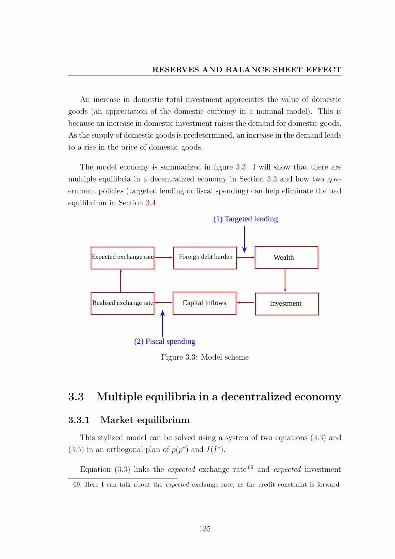
RESERVES AND BALANCE SHEET EFFECT
An increase in domestic total investment appreciates the value of domestic
goods (an appreciation of the domestic currency in a nominal model). This is
because an increase in domestic investment raises the demand for domestic goods.
As the supply of domestic goods is predetermined, an increase in the demand leads
to a rise in the price of domestic goods.
The model economy is summarized in figure 3.3. I will show that there are
multiple equilibria in a decentralized economy in Section 3.3 and how two gov-
ernment policies (targeted lending or fiscal spending) can help eliminate the bad
equilibrium in Section 3.4.
Expected exchange rate WealthForeign debt burden
Realised exchange rate InvestmentCapital inflows
(1) Targeted lending
(2) Fiscal spending
Figure 3.3: Model scheme
3.3 Multiple equilibria in a decentralized economy
3.3.1 Market equilibrium
This stylized model can be solved using a system of two equations (3.3) and
(3.5) in an orthogonal plan of p(pe) and I(Ie).
Equation (3.3) links the expected exchange rate 69 and expected investment
69. Here I can talk about the expected exchange rate, as the credit constraint is forward-
135
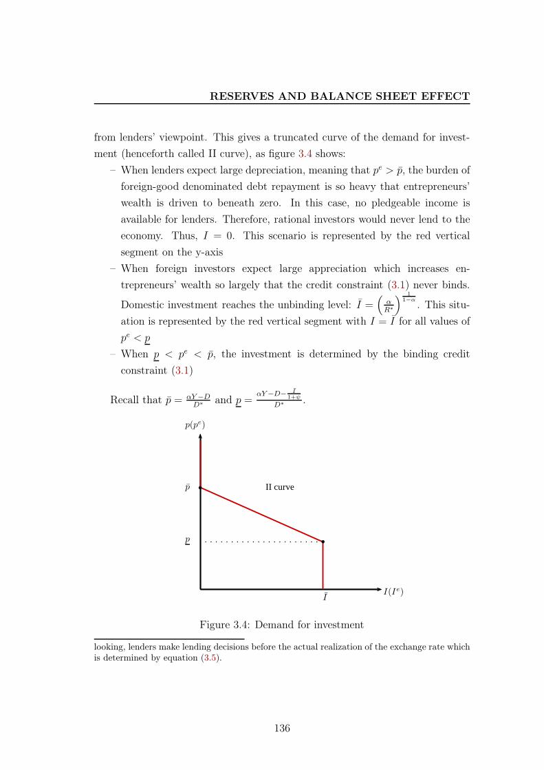
RESERVES AND BALANCE SHEET EFFECT
from lenders’ viewpoint. This gives a truncated curve of the demand for invest-
ment (henceforth called II curve), as figure 3.4 shows:
– When lenders expect large depreciation, meaning that pe > p, the burden of
foreign-good denominated debt repayment is so heavy that entrepreneurs’
wealth is driven to beneath zero. In this case, no pledgeable income is
available for lenders. Therefore, rational investors would never lend to the
economy. Thus, I = 0. This scenario is represented by the red vertical
segment on the y-axis
– When foreign investors expect large appreciation which increases en-
trepreneurs’ wealth so largely that the credit constraint (3.1) never binds.
Domestic investment reaches the unbinding level: I =(αR∗
) 1
1−α
. This situ-
ation is represented by the red vertical segment with I = I for all values of
pe < p
– When p < pe < p, the investment is determined by the binding credit
constraint (3.1)
Recall that p = αY−DD∗
and p =αY−D− I
1+ψ
D∗.
p(pe)
I(Ie)
p
p
I
II curveb
b
Figure 3.4: Demand for investment
looking, lenders make lending decisions before the actual realization of the exchange rate whichis determined by equation (3.5).
136
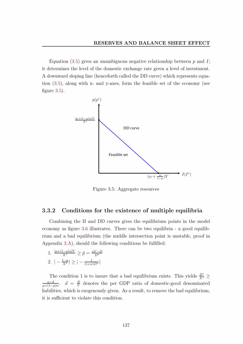
RESERVES AND BALANCE SHEET EFFECT
Equation (3.5) gives an unambiguous negative relationship between p and I;
it determines the level of the domestic exchange rate given a level of investment.
A downward sloping line (henceforth called the DD curve) which represents equa-
tion (3.5), along with x- and y-axes, form the feasible set of the economy (see
figure 3.5).
Feasible set
[µ+(1−µ)α]YX∗
(α+ µ1−µ )Y
p(pe)
I(Ie)
DD curve
b
b
Figure 3.5: Aggregate resources
3.3.2 Conditions for the existence of multiple equilibria
Combining the II and DD curves gives the equilibrium points in the model
economy as figure 3.6 illustrates. There can be two equilibria - a good equilib-
rium and a bad equilibrium (the middle intersection point is unstable, proof in
Appendix 3.A), should the following conditions be fulfilled:
1. [µ+(1−µ)α]YX∗
≥ p = αY−DD∗
2. | − 1−µX∗
| ≥ | − 1(1+ψ)D∗
|
The condition 1 is to insure that a bad equilibrium exists. This yields D∗
X∗≥
α−dµ+(1−µ)α
. d = DY
denotes the per GDP ratio of domestic-good denominated
liabilities, which is exogenously given. As a result, to remove the bad equilibrium,
it is sufficient to violate this condition.
137
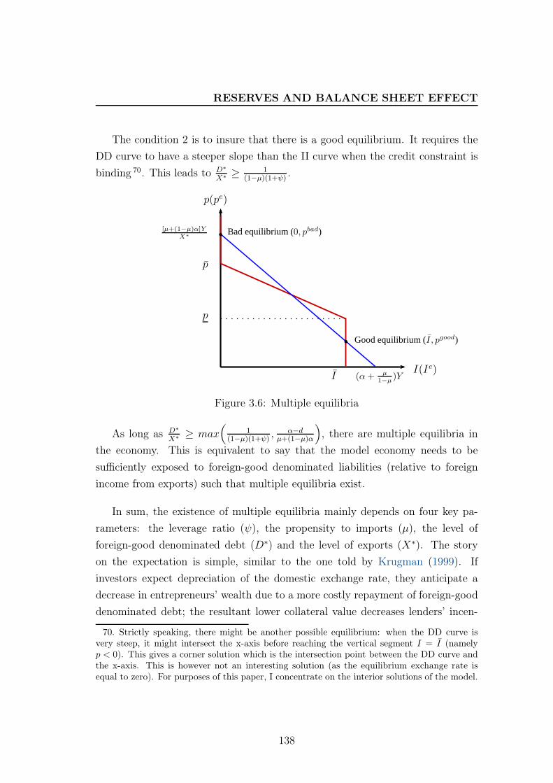
RESERVES AND BALANCE SHEET EFFECT
The condition 2 is to insure that there is a good equilibrium. It requires the
DD curve to have a steeper slope than the II curve when the credit constraint is
binding 70. This leads to D∗
X∗≥ 1
(1−µ)(1+ψ).
p(pe)
I(Ie)
p
p
I
b
b Bad equilibrium (0, pbad)
Good equilibrium (I, pgood)
[µ+(1−µ)α]YX∗
(α + µ1−µ )Y
Figure 3.6: Multiple equilibria
As long as D∗
X∗≥ max
(1
(1−µ)(1+ψ), α−dµ+(1−µ)α
), there are multiple equilibria in
the economy. This is equivalent to say that the model economy needs to be
sufficiently exposed to foreign-good denominated liabilities (relative to foreign
income from exports) such that multiple equilibria exist.
In sum, the existence of multiple equilibria mainly depends on four key pa-
rameters: the leverage ratio (ψ), the propensity to imports (µ), the level of
foreign-good denominated debt (D∗) and the level of exports (X∗). The story
on the expectation is simple, similar to the one told by Krugman (1999). If
investors expect depreciation of the domestic exchange rate, they anticipate a
decrease in entrepreneurs’ wealth due to a more costly repayment of foreign-good
denominated debt; the resultant lower collateral value decreases lenders’ incen-
70. Strictly speaking, there might be another possible equilibrium: when the DD curve isvery steep, it might intersect the x-axis before reaching the vertical segment I = I (namelyp < 0). This gives a corner solution which is the intersection point between the DD curve andthe x-axis. This is however not an interesting solution (as the equilibrium exchange rate isequal to zero). For purposes of this paper, I concentrate on the interior solutions of the model.
138
RESERVES AND BALANCE SHEET EFFECT
tives to invest in the economy. A reduction in capital inflows is thus expected,
driving down the price of domestic goods and further confirms investors’ expecta-
tion. This unambiguously leads to the bad equilibrium (0, pbad). On the contrary,
an optimistic expectation on the price of domestic goods will lead to the good
equilibrium.
I will show in the next section to what extent appropriate public policies can
eliminate the bad equilibrium and stabilize the domestic economy, especially in
the context of unfavorable international economic environment.
3.4 Public policies
To understand how the government can use foreign reserves to stabilize domes-
tic economy, suppose we are in the context of the GFC. Lenders form a negative
expectation on exporting countries’ exchange rate due to a gloomy perspective
on foreign demand [e.g. a decrease in foreign demand X∗ due to the ‘global trade
collapse Baldwin (2009)’]. Without any government intervention, a domestic de-
preciation is foreseeable through the resource constraint (3.4).
The objective of the government is to eliminate the bad equilibrium associated
with the scenario of depreciation and a low level of investment. This requires
sustaining entrepreneurs’ wealth which is the key variable linking exchange rate
perspective and domestic investment. Several ways of public intervention can be
considered: a targeted lending denominated in foreign goods to entrepreneurs or
an increase in public spending which restores the value of the domestic exchange
rate. I will show these different policy tools in the following sections.
3.4.1 Targeted lending to the private sector
As the government has previously accumulated foreign reserves, one policy
choice is to lend directly foreign goods to the private sector so as to insulate
entrepreneurs’ net worth from potential exchange rate depreciation. As a conse-
quence, the impact of the exchange rate on entrepreneurs’ balance sheets would
be largely minimized. Under this vision, foreign reserves can be regarded as a
state-contingent insurance, as its value increases with potential depreciation of
139
RESERVES AND BALANCE SHEET EFFECT
the domestic exchange rate. One the one hand, depreciation increases the foreign
debt repayment and thus lowers entrepreneurs’ net wealth. On the other hand,
it increases the value of reserves held by the government which are used for the
targeted lending policy, all expressed in terms of domestic goods. This policy
is similar to the idea of setting an ‘international banking fund’ which provides
liquid foreign-good assets to ‘truly solvent banks’ [Jeanne and Wyplosz (2003)].
The difference here is that the targeted lending is provided by a national govern-
ment 71. As long as foreign reserves cover the foreign liabilities in the domestic
economy, there will be a full insurance. Concretely, the promise of the govern-
ment to strengthen entrepreneurs’ wealth by targeted lending changes the wealth
function (3.2). It alters the lenders’ perspectives on entrepreneurs’ wealth, thus
on the value of collateral for their lending. The new wealth function is written:
W e = αY −D − peD∗ + peB∗ (3.6)
The aggregate resource function (3.4) which determines the actual level of ex-
change rate does not change, as nothing changes the demand for domestic goods.
As a result, the DD curve remains the same while the II curve shifts upward (with
the unbinding level of demand for investment I unchanged which only depends
on the international interest rate). Figure 3.7 shows the new equilibrium and
compares it with the multiple equilibria in a decentralized economy.
Figure 3.7 clearly shows that when the government lends foreign goods to the
private sector, it eliminates the bad equilibrium (0, pbad), where pbad = Y [µ+(1−µ)α]X∗
,
as it is derived in Section 3.3. The good equilibrium is the same as in the decen-
tralized market equilibrium. Put it in another way, the government’s commitment
to lend foreign goods to entrepreneurs whenever it is necessary is equivalent to
give lenders a government guarantee on their loans. This immediately eliminate
the bad equilibrium. In theory, if the government has enough foreign reserves to
cover foreign-good denominated liabilities, it does even not need to actually use
71. Clearly, the ‘international banking fund’ has never be founded since Jeanne and Wyplosz’spaper in 2003. One argument in this model in favor of holding international reserves at thenational level is that the stock of reserves gives a positive signal to the market on the economy’sfinancial capacity to conduct appropriate policies in the times of crises. Moreover, nationalauthorities should know better their domestic private institutions and can be more easily toselect ‘truly solvent’ banks or firms to which the lending in foreign goods should be granted.
140
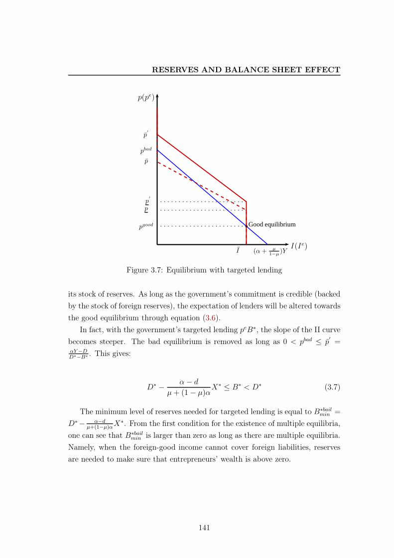
RESERVES AND BALANCE SHEET EFFECT
p(pe)
I(Ie)
p′
p
I
b Good equilibrium
pbad
(α + µ1−µ )Y
pgood
p′
p
Figure 3.7: Equilibrium with targeted lending
its stock of reserves. As long as the government’s commitment is credible (backed
by the stock of foreign reserves), the expectation of lenders will be altered towards
the good equilibrium through equation (3.6).
In fact, with the government’s targeted lending peB∗, the slope of the II curve
becomes steeper. The bad equilibrium is removed as long as 0 < pbad ≤ p′
=αY−DD∗−B∗
. This gives:
D∗ −α− d
µ+ (1− µ)αX∗ ≤ B∗ < D∗ (3.7)
The minimum level of reserves needed for targeted lending is equal to B∗bailmin =
D∗− α−dµ+(1−µ)α
X∗. From the first condition for the existence of multiple equilibria,
one can see that B∗bailmin is larger than zero as long as there are multiple equilibria.
Namely, when the foreign-good income cannot cover foreign liabilities, reserves
are needed to make sure that entrepreneurs’ wealth is above zero.
141
RESERVES AND BALANCE SHEET EFFECT
The amount of reserves needed 72 depends on the private sector’s exposure to
foreign-good debt (D∗). The higher foreign debt, the higher reserves are needed
for targeted lending policy. It is negatively correlated with foreign-good income
earned through exports. If at time t, the flow of exports exceeds that of foreign li-
abilities, B∗ might become negative, namely there is an accumulation of reserves
instead of depletion. The amount of reserves for targeted lending policy also
depends on the marginal propensity to imports and the share of domestic lend-
ing per GDP. The higher µ, the more foreign goods are demanded, thus higher
reserves are needed to pay out imported goods.
Notice that the targeted lending policy can be replicated in a situation where
the government commits to borrow externally for the sake of the national econ-
omy, using its own net worth along with entrepreneurs’ net worth as collateral,
when private entrepreneurs are excluded from external financial markets (mainly
because of their negative net worth for example). The good thing about holding
reserves is that there is a valuation effect which increases the government’s net
worth in case of depreciation. Put it in a formal way, the government enters
period t with a net worth equal to WG = peB∗, pe being the expected exchange
rate in period t. In case of domestic deprecation, WG increases, allowing the
government to borrow for the sake of the private sector whose net worth W is
driven to negative due to higher repayment of foreign debt (equation (3.2)). If
the government uses its own net worth as collateral to borrow externally, the
investment function (3.1) becomes:
Ie ≤ (1 + ψ)(W e +WG)
= (1 + ψ)(αY −D − peD∗ + peB∗)
This is exactly the equation (3.6) in the case of a targeted lending policy.
In reality, during the GFC, some emerging economies which were seriously
hit by the balance sheet effect during the last wave of emerging economy crises
72. This is a flow variable which refers to the amount of reserves required to conduct a certainpublic policy. This is different from the stock of reserves which is a stock variable.
142
RESERVES AND BALANCE SHEET EFFECT
experienced rather an exchange rate stability. This is the case in Thailand for
example (see figure 3.2). Obstfeld (2013) attributes this exchange rate stability to
the ample level of reserves in Thailand compared to its external debt. In the case
of Korea, albeit a large absolute level (sixth largest reserve holder), the reserves
to short-term debt ratio is less impressive there in comparison with other EMEs
(see table 3.1). If reserves are scaled by total external debt of different maturities,
they can only cover 70% of the entire exposure of the Korean private sector to
foreign-currency debt [Cho (2012)]. According to Cho, the Korean government
depleted its foreign reserves to supply foreign currency liquidity required to reduce
the accumulated leverage in the private banking sector; ‘[i]t was not a sheer
coincidence that the amount of decrease in foreign reserves during the crisis period
from September to December 2008, approximately US$40 billion, was almost the
same as that of short-term foreign debts [Cho (2012)].’ Based on the implications
of the current model, the market may think Korea do not hold enough foreign
reserves to rule out the bad equilibrium. As a result one observes in figure 3.2
that the exchange rate of Korean won was still very volatile during the GFC
compared to other EMEs’ currencies.
3.4.2 Fiscal spending
The second policy choice of the government is to increase public spending.
Bearing in mind that in the framework of Krugman (1999), a fiscal spending
should not be understood in the Keynesian sense, as prices are fully flexible in this
stylized model and the supply of domestic goods is predetermined at the beginning
of each period. Therefore, an expansionary fiscal policy affects entrepreneurs’
wealth as well as their investment through a pure price effect. Namely, a fiscal
expansion would raise domestic demand and appreciate the domestic exchange
rate given a fixed level of good supply.
Different from the targeted lending policy, a fiscal spending affects the ex-
change rate through the aggregate resource constraint. Suppose the fiscal spend-
ing is financed by previously accumulated foreign reserves, the aggregate resource
constraint (3.4) becomes:
143
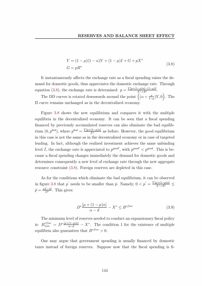
RESERVES AND BALANCE SHEET EFFECT
Y = (1− µ)(1− α)Y + (1− µ)I +G+ pX∗
G = pB∗(3.8)
It instantaneously affects the exchange rate as a fiscal spending raises the de-
mand for domestic goods, thus appreciates the domestic exchange rate. Through
equation (3.8), the exchange rate is determined: p = Y [µ+(1−µ)α]−(1−µ)IX∗+B∗
.
The DD curves is rotated downwards around the point((α+ µ
1−µ)Y, 0
). The
II curve remains unchanged as in the decentralized economy.
Figure 3.8 shows the new equilibrium and compares it with the multiple
equilibria in the decentralized economy. It can be seen that a fiscal spending
financed by previously accumulated reserves can also eliminate the bad equilib-
rium (0, pbad), where pbad = Y [µ+(1−µ)α]X∗
as before. However, the good equilibrium
in this case is not the same as in the decentralized economy or in case of targeted
lending. In fact, although the realized investment achieves the same unbinding
level I, the exchange rate is appreciated to pgood′
, with pgood′
< pgood. This is be-
cause a fiscal spending changes immediately the demand for domestic goods and
determines consequently a new level of exchange rate through the new aggregate
resource constraint (3.8). Foreign reserves are depleted in this case.
As for the conditions which eliminate the bad equilibrium, it can be observed
in figure 3.8 that p′
needs to be smaller than p. Namely, 0 < p′
= Y [µ+(1−µ)α]X∗+B∗
≤
p = αY−DD∗
. This gives:
D∗ [µ+ (1− µ)α]
α− d−X∗ ≤ B∗fisc (3.9)
The minimum level of reserves needed to conduct an expansionary fiscal policy
is: B∗fiscmin = D∗ [µ+(1−µ)α]
α−d− X∗. The condition 1 for the existence of multiple
equilibria also guarantees that B∗fisc > 0.
One may argue that government spending is usually financed by domestic
taxes instead of foreign reserves. Suppose now that the fiscal spending is fi-
144
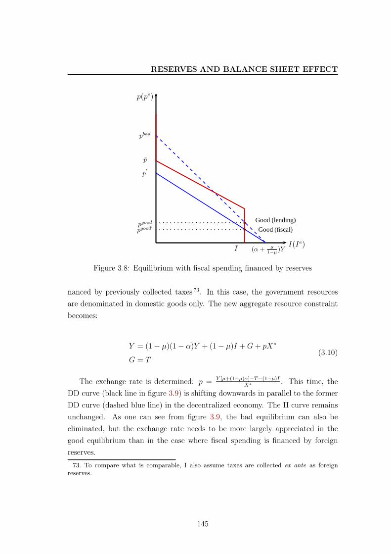
RESERVES AND BALANCE SHEET EFFECT
p(pe)
I(Ie)
p
I
b
b Good (lending)
Good (fiscal)
pbad
(α + µ1−µ )Y
pgood
pgood′
p′
Figure 3.8: Equilibrium with fiscal spending financed by reserves
nanced by previously collected taxes 73. In this case, the government resources
are denominated in domestic goods only. The new aggregate resource constraint
becomes:
Y = (1− µ)(1− α)Y + (1− µ)I +G+ pX∗
G = T(3.10)
The exchange rate is determined: p = Y [µ+(1−µ)α]−T−(1−µ)IX∗
. This time, the
DD curve (black line in figure 3.9) is shifting downwards in parallel to the former
DD curve (dashed blue line) in the decentralized economy. The II curve remains
unchanged. As one can see from figure 3.9, the bad equilibrium can also be
eliminated, but the exchange rate needs to be more largely appreciated in the
good equilibrium than in the case where fiscal spending is financed by foreign
reserves.
73. To compare what is comparable, I also assume taxes are collected ex ante as foreignreserves.
145
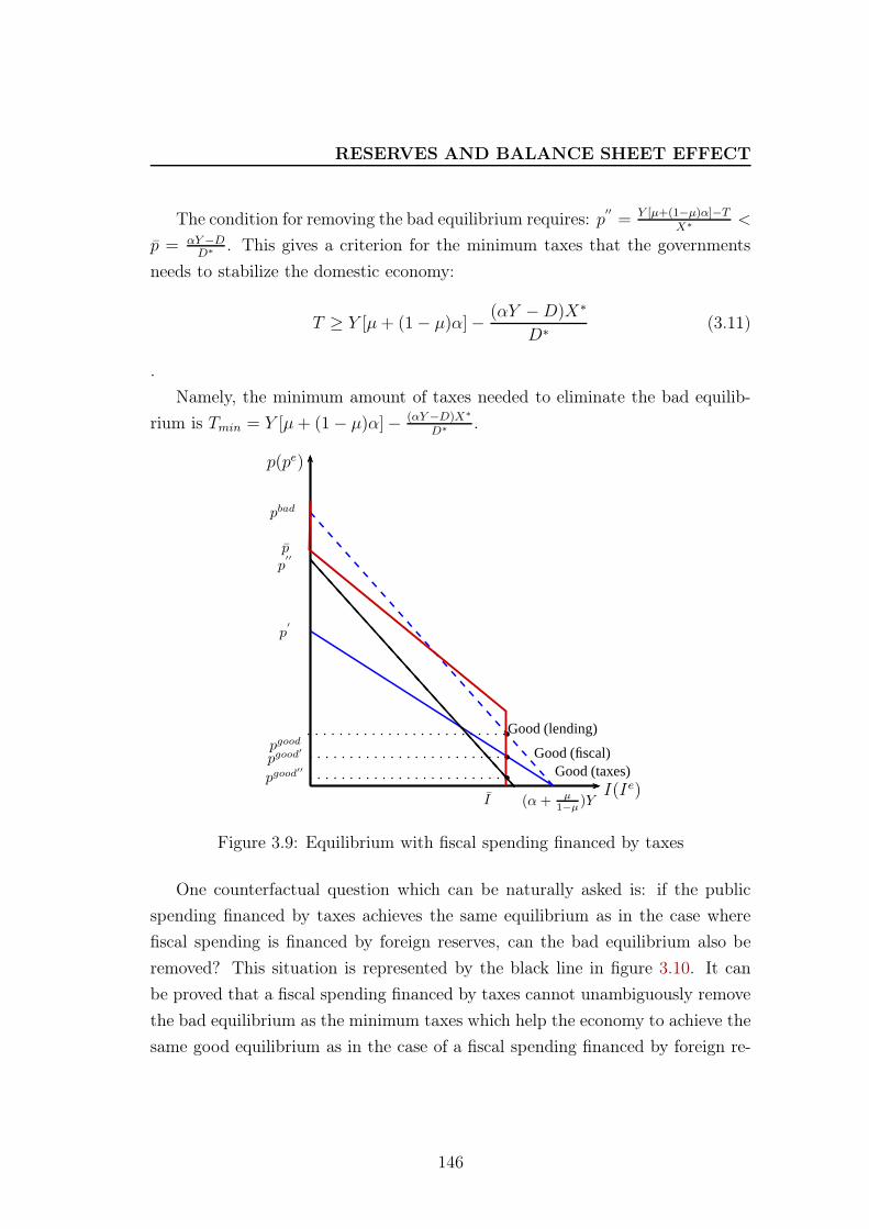
RESERVES AND BALANCE SHEET EFFECT
The condition for removing the bad equilibrium requires: p′′
= Y [µ+(1−µ)α]−TX∗
<
p = αY−DD∗
. This gives a criterion for the minimum taxes that the governments
needs to stabilize the domestic economy:
T ≥ Y [µ+ (1− µ)α]−(αY −D)X∗
D∗(3.11)
.
Namely, the minimum amount of taxes needed to eliminate the bad equilib-
rium is Tmin = Y [µ+ (1− µ)α]− (αY−D)X∗
D∗.
p(pe)
I(Ie)
p
p′′
I
b
b
b
Good (lending)
Good (fiscal)
pbad
(α+ µ1−µ )Y
pgood
pgood′
p′
Good (taxes)pgood′′
Figure 3.9: Equilibrium with fiscal spending financed by taxes
One counterfactual question which can be naturally asked is: if the public
spending financed by taxes achieves the same equilibrium as in the case where
fiscal spending is financed by foreign reserves, can the bad equilibrium also be
removed? This situation is represented by the black line in figure 3.10. It can
be proved that a fiscal spending financed by taxes cannot unambiguously remove
the bad equilibrium as the minimum taxes which help the economy to achieve the
same good equilibrium as in the case of a fiscal spending financed by foreign re-
146
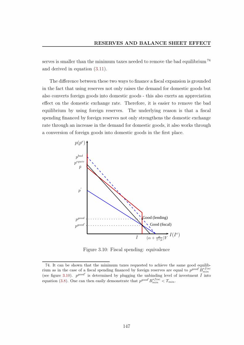
RESERVES AND BALANCE SHEET EFFECT
serves is smaller than the minimum taxes needed to remove the bad equilibrium 74
and derived in equation (3.11).
The difference between these two ways to finance a fiscal expansion is grounded
in the fact that using reserves not only raises the demand for domestic goods but
also converts foreign goods into domestic goods - this also exerts an appreciation
effect on the domestic exchange rate. Therefore, it is easier to remove the bad
equilibrium by using foreign reserves. The underlying reason is that a fiscal
spending financed by foreign reserves not only strengthens the domestic exchange
rate through an increase in the demand for domestic goods, it also works through
a conversion of foreign goods into domestic goods in the first place.
p(pe)
I(Ie)
p
I
b
bGood (lending)
Good (fiscal)
pbad
(α+ µ1−µ )Y
pgood
pgood′
p′
pequiv
Figure 3.10: Fiscal spending: equivalence
74. It can be shown that the minimum taxes requested to achieve the same good equilib-rium as in the case of a fiscal spending financed by foreign reserves are equal to pgood
′
B∗fiscmin
(see figure 3.10). pgood′
is determined by plugging the unbinding level of investment I into
equation (3.8). One can then easily demonstrate that pgood′
B∗fiscmin < Tmin.
147
RESERVES AND BALANCE SHEET EFFECT
3.4.3 Differences between targeted lending and fiscal
spending
A targeted lending policy and a public spending policy, although both can
remove the bad equilibrium, work through two different mechanisms. They also
differ in terms of the amount of reserves needed. I discuss these differences in
this section.
First, a targeted lending policy can be at work through lenders’ expecta-
tion while a fiscal spending virtually shifts the demand for domestic goods and
raises the real exchange rate. In fact, the targeted lending policy affects en-
trepreneurs’ wealth function. As one can see in figure 3.7, what changes with the
announced targeted lending is to increase the threshold exchange rate for which
entrepreneurs’ wealth falls beneath zero (p′
> p). Similarly, this policy makes
it easier for the credit constraint not to bind (p′
> p). As a result, lenders will
believe that entrepreneurs’ wealth is positive and is kept as high as possible; so is
the collateral for borrowing. Therefore, lenders will be willing to provide funding
to this economy. With the targeted lending, the government only needs to hold
sufficient foreign reserves to cover the private sector’s foreign liabilities so as to
eliminate the bad equilibrium. Foreign reserves will need to be deployed only if
a shock on foreign demand X∗ materializes.
This theoretical funding is in line with the empirical literature on the role of
foreign reserves in the GFC. Bussière et al. (2014) find that the pre-crisis reserves
to short term debt ratio is the most significant reserve adequacy ratio when
assessing the role of reserves on the real GDP growth across different emerging
and developing economies during the GFC. Moreover, their paper finds that it is
rather the level of foreign reserves which matters than the active use.
As for the fiscal spending, the mechanism is different. An increase in gov-
ernment spending will unambiguously change the exchange rate through the ag-
gregate demand for domestic goods. To insure the same amount of investment
(when the credit constraint is unbinding), the government needs to appreciate the
price of domestic goods by increasing government consumption so as to maintain
entrepreneurs’ wealth. If the insurance provided by a targeted lending policy
148
RESERVES AND BALANCE SHEET EFFECT
works through entrepreneurs’ wealth directly, the fiscal spending affects the level
of domestic exchange rate and affects entrepreneurs’ wealth indirectly. I have
also shown that the funding of fiscal spending matters. For the same amount
of resources (denominated in domestic goods, T = pgood′
B∗fiscmin ), a fiscal spend-
ing financed by foreign reserves can eliminate the bad equilibrium while a fiscal
spending financed by taxes cannot unambiguously remove it. More resources
need to be deployed in the latter case.
I can also compare the minimum levels of reserves needed to implement the
targeted lending or fiscal spending financed by reserves. In fact, accumulating
foreign reserves is not costless, the less reserves needed to achieve the same policy
objective the better.
Let us denote Γ = B∗bailmin − B∗fisc
min .
Γ = D∗ −(α− d)X∗
µ+ (1− µ)α− [D∗ [µ+ (1− µ)α]
α− d−X∗]
=[d+ (1− α)µ
][ X∗
µ+ (1− µ)α−
D∗
α− d
]
= −[d+ (1− α)µ
]X∗ 1
α− d
[D∗
X∗−
α− d
µ+ (1− µ)α
]
Γ < 0 unambiguously as long as there are multiple equilibria, namely D∗
X∗≥
max
(1
(1−µ)(1+ψ), α−dµ+(1−µ)α
).
As a result, B∗fiscmin > B∗bail
min . To increase government spending requires a
higher level of reserves than a direct lending in foreign goods. The reason behind
is that a lending policy can be regarded as a direct write-off of the private sector’s
foreign-good debt or an official government guarantee on the private sector’s debt.
The need in terms of foreign goods is capped by the total amount of external debt
facing the economy. However, for an expansionary fiscal policy to stabilize the
domestic exchange rate, the amount of foreign reserves that the government needs
to sell and with which it buys domestic goods depends on the magnitude of the
depreciation. The more severe the depreciation, the more reserves are needed.
149
RESERVES AND BALANCE SHEET EFFECT
Therefore, in terms of the level of reserves needed, a targeted lending uses less
resources than an expansionary fiscal policy.
In sum, a lending policy or an increase in government spending can both
stabilize an economy where the private sector faces balance sheet effects due to
the level of foreign-good denominated debt in the economy. In terms of foreign
reserves needed, a lending policy uses fewer resources than a fiscal spending.
3.5 Conclusion
This work provides a simple theoretical framework to study different mech-
anisms through which foreign reserves can be useful in an economy where the
private sector faces credit constraints and currency mismatch. It is shown that
foreign reserves can be considered as a state-contingent insurance when the ex-
change rate valuation effect is taken into account. This is an aspect which has
not yet been emphasized in the literature on foreign reserves. In fact, when there
is a negative shock or a negative expectation on a country’s currency, the do-
mestic value of foreign reserves increases such that they can be used to stabilize
the domestic economy, either through a targeted lending to the private sector
or through an expansionary fiscal policy. The former channel works through in-
vestors’ expectation and requires less foreign reserves than in the second case.
The underlying reason is that a targeted lending is equivalent to give investors’ a
governmental guarantee on the private sector’s liabilities (especially foreign liabil-
ities). Having sufficient foreign reserves alters investors’ expectation and pushes
the economy towards the good equilibrium as it is defined in Krugman (1999).
The current framework remains a bit too simple. A more comprehensive
theoretical framework is needed to endogenize entrepreneurs’ portfolio choice and
different costs related to ex ante foreign reserve purchases.
150
BIBLIOGRAPHY
Bibliography
Aghion, P., Bacchetta, P., and Banerjee, A. (2000). A simple model of monetary policy and
currency crises. European Economic Review, 44(4-6):728–738.
Aghion, P., Bacchetta, P., and Banerjee, A. (2004). A corporate balance-sheet approach to
currency crises. Journal of Economic Theory, 119(1):6–30.
Aizenman, J. and Hutchison, M. M. (2010). Exchange market pressure and absorption by
international reserves: Emerging markets and fear of reserve loss during the 2008-09 crisis.
NBER Working Papers 16260, National Bureau of Economic Research, Inc.
Aizenman, J. and Lee, J. (2007). International reserves: Precautionary versus mercantilist
views, theory and evidence. Open Economies Review, 18(2):191–214.
Alfaro, L. and Kanczuk, F. (2009). Optimal reserve management and sovereign debt. Journal
of International Economics, 77(1):23–36.
Baldwin, R., editor (2009). The Great Trade Collapse: Causes, Consequences and Prospects.
CEPR.
Benigno, G. and Fornaro, L. (2012). Reserve accumulation, growth and financial crises. CEP
Discussion Papers dp1161, Centre for Economic Performance, LSE.
Bernanke, B. S., Gertler, M., and Gilchrist, S. (1999). The financial accelerator in a quanti-
tative business cycle framework. In Taylor, J. B. and Woodford, M., editors, Handbook of
Macroeconomics, volume 1 of Handbook of Macroeconomics, chapter 21, pages 1341–1393.
Elsevier.
Bianchi, J., Hatchondo, J. C., and Martinez, L. (2012). International reserves and rollover risk.
Technical report, University of Wisconsin.
Burnside, C., Eichenbaum, M., and Rebelo, S. (1999). Hedging and financial fragilities in fixed
exchange rate regimes. Technical report.
Bussière, M., Cheng, G., Chinn, M. D., and Lisack, N. (2014). For a few dollars more: Reserves
and growth in times of crises. Working Paper 19791, National Bureau of Economic Research.
Calvo, G., Izquierdo, A., and Loo-Kung, R. (2013). Optimal holdings of international reserves:
Self-insurance against sudden stops. Monetaria, (1):1–35.
Calvo, G. A. (1998). Capital flows and capital-market crises: The simple economics of sudden
stops. Journal of Applied Economics, pages 35–54.
151
BIBLIOGRAPHY
Catao, L. and Milesi-Ferretti, G.-M. (2013). External liabilities and crises. IMF Working Papers
13/113, International Monetary Fund.
Ceballos, F., Didier, T., Hevia, C., and Schmukler, S. (2013). Policy responses to the global
financial crisis: What did emerging economies do differently? Working Papers 2013-002,
Banco Central de Reserva del Perú.
Cho, D. (2012). Responses of the Korean economy to the global economic crisis: Another
currency crisis? In Maurice Obstfeld, Dongchul Cho, A. M., editor, Global economic crisis:
Impacts, transmission, and recovery. Cheltenham UK: Edward Elgar.
Crowe, C. W., Ostry, J. D., Kim, J. I., Chamon, M., and Ghosh, A. R. (2009). Coping with
the crisis: Policy options for emerging market countries. IMF Staff Position Notes 2009/08,
International Monetary Fund.
Didier, T., Hevia, C., and Schmukler, S. L. (2012). How resilient and countercyclical were
emerging economies during the global financial crisis? Journal of International Money and
Finance, 31(8):2052–2077.
Eichengreen, B. (2010). Lessons of the crisis for emerging markets. International Economics
and Economic Policy, 7(1):49–62.
Eichengreen, B., Hausmann, R., and Panizza, U. (2007). Currency mismatches, debt intol-
erance, and the original sin: Why they are not the same and why it matters. In Capital
Controls and Capital Flows in Emerging Economies: Policies, Practices and Consequences,
NBER Chapters, pages 121–170. National Bureau of Economic Research, Inc.
Frankel, J. A., Vegh, C. A., and Vuletin, G. (2013). On graduation from fiscal procyclicality.
Journal of Development Economics, 100(1):32–47.
Gourinchas, P.-O. and Obstfeld, M. (2012). Stories of the twentieth century for the twenty-first.
American Economic Journal: Macroeconomics, 4(1):226–65.
Jeanne, O. (2000). Foreign currency debt and the global financial architecture. European
Economic Review, 44(4-6):719–727.
Jeanne, O. (2003). Why do emerging economies borrow in foreign currency? IMF Working
Papers 03/177, International Monetary Fund.
Jeanne, O. and Rancière, R. (2011). The optimal level of international reserves for emerging
market countries: A new formula and some applications. Economic Journal, 121(555):905–
930.
152

BIBLIOGRAPHY
Jeanne, O. and Wyplosz, C. (2003). The international lender of last resort. How large is large
enough? In Managing Currency Crises in Emerging Markets, NBER Chapters, pages 89–124.
National Bureau of Economic Research, Inc.
Jeanne, O. and Zettelmeyer, J. (2002). “Original sin”, balance sheet crises, and the roles of
international lending. IMF Working Papers 02/234, International Monetary Fund.
Kaminsky, G. L., Reinhart, C. M., and Végh, C. A. (2005). When it rains, it pours: Procyclical
capital flows and macroeconomic policies. In NBER Macroeconomics Annual 2004, Volume
19, NBER Chapters, pages 11–82. National Bureau of Economic Research, Inc.
Krugman, P. (1999). Balance sheets, the transfer problem, and financial crises. International
Tax and Public Finance, 6(4):459–472.
Llaudes, R., Salman, F., and Chivakul, M. (2010). The impact of the great recession on emerging
markets. IMF Working Papers 10/237, International Monetary Fund.
Obstfeld, M. (2013). Never say never: commentary on a policymaker’s reflections. Manuscript,
UC Berkeley.
Obstfeld, M., Shambaugh, J. C., and Taylor, A. M. (2010). Financial stability, the trilemma,
and international reserves. American Economic Journal: Macroeconomics, 2(2):57–94.
Prasad, E. S. (2011). Role reversal in global finance. Proceedings, The 2011 Jackson Hole
Symposium:339–390.
Schneider, M. and Tornell, A. (2004). Balance sheet effects, bailout guarantees and financial
crises. Review of Economic Studies, 71:883–913.
153
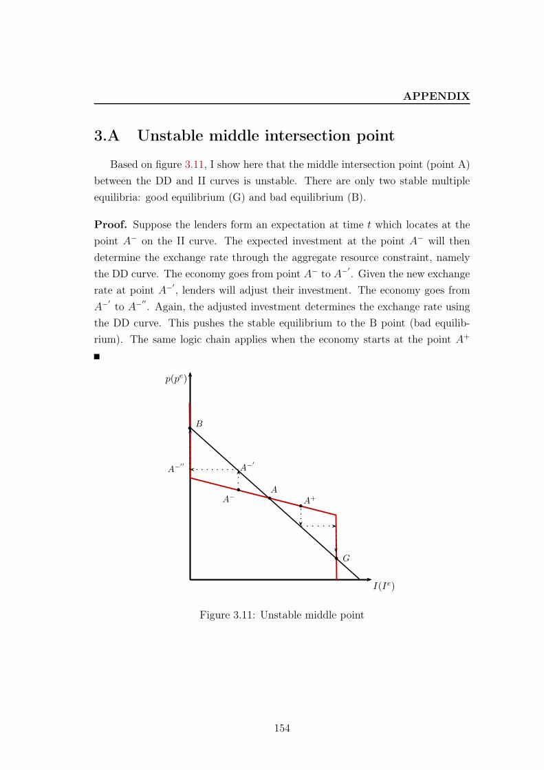
APPENDIX
3.A Unstable middle intersection point
Based on figure 3.11, I show here that the middle intersection point (point A)
between the DD and II curves is unstable. There are only two stable multiple
equilibria: good equilibrium (G) and bad equilibrium (B).
Proof. Suppose the lenders form an expectation at time t which locates at the
point A− on the II curve. The expected investment at the point A− will then
determine the exchange rate through the aggregate resource constraint, namely
the DD curve. The economy goes from point A− to A−′
. Given the new exchange
rate at point A−′
, lenders will adjust their investment. The economy goes from
A−′
to A−′′
. Again, the adjusted investment determines the exchange rate using
the DD curve. This pushes the stable equilibrium to the B point (bad equilib-
rium). The same logic chain applies when the economy starts at the point A+
p(pe)
I(Ie)
b
bb
b
b G
B
A
A+A−
A−′
A−′′
Figure 3.11: Unstable middle point
154
Conclusion
At the end of the journey, I hope I have conveyed some thoughtful messages on
foreign reserve accumulation in emerging market economies and have convinced
the reader that there is a promising avenue for future research. In chapter 1, I have
showed that foreign reserve accumulation is a ‘transition’ phenomenon; it is driven
by the constrained demand for domestic borrowing due to financial frictions in
the context of strong productivity growth. Moreover, this chapter provides some
simulated results in favor of a temporary and timely use of capital controls jointly
with the reserve policy. The combined use of these two instruments generates
higher welfare during economic transition in comparison with a financially open
economy. However, the welfare gains from the joint use of reserve accumulation
and capital controls diminish with financial development, namely when the credit
constraints become less binding. Therefore, capital controls need to be used
in a temporary manner, and should not hinder any structural reforms in the
financial market. In the future, I should incorporate more ingredients in this
model so as to provide a more comprehensive cost-benefit analysis of foreign
reserve accumulation, both within a growing economy and at the international
level.
Chapter 2 finds a significant positive relationship between pre-crisis reserves to
short-term debt ratio and economic performance during the global financial crisis.
Namely, countries with high reserves relative to short-term debt suffered less from
the crisis, particularly if associated with a less open capital account. Moreover,
in the immediate aftermath of the crisis, countries that depleted foreign reserves
during the crisis quickly rebuilt their stocks. This rapid rebuilding has, however,
been followed by a deceleration in the pace of accumulation. For a future research
155
CONCLUSION
agenda, with my co-authors we are trying to find more relevant instruments
for foreign reserves on the one hand and dig into the reasons explaining the
more recent behavior of reserves accumulation in emerging economies, namely
the factors behind this ‘flattening-out’ of reserve accumulation.
Chapter 3 analyzes the effective use of reserves to tackle balance sheet effects
in an economy where the private sector is exposed to foreign liabilities and faces
credit constraints. It is argued that both a targeted lending in foreign currency
and a fiscal spending financed by foreign reserves help remove the bad equilibrium
represented by a largely depreciated domestic currency and a very low level of
domestic investment. It is also showed that the mechanisms through which these
two policy tools stabilize the domestic economy are different. While targeted
lending works through investors’ expectation on the domestic exchange rate and
on firms’ net worth, fiscal spending affects the investment through a direct change
of the value of domestic exchange rate. This framework needs to be enriched in
the future so as to incorporate firms’ portfolio choice and costs related to reserve
accumulation in the analysis.
In conclusion, foreign reserve accumulation has received much attention in
the past decade. The topic is closely related to many key issues in economic de-
bates around the world, including discussions on exchange rate alignments, global
imbalances and growth strategies, capital account management as well as the re-
forms in the international monetary and financial system. Will global or regional
financial safety nets be well-functioning so as to substitute foreign reserves held
by individual countries? What will be the future reserve currencies? Will China
reduce its reserve holdings with the internationalization of its currency and re-
cent financial reforms? Many questions regarding foreign reserve accumulation
are already in the future agenda of academics and policymakers.
156
