foraging behaviour of brown trout in wild populations: can population density cause...

Animal Biology 63 (2013) 425–450 brill.com/ab

Foraging behaviour of brown trout in wild populations:can population density cause behaviourally-mediated

foraging specializations?

Javier Sánchez-Hernández1,2,∗ and Fernando Cobo1,2

1 Department of Zoology and Physical Anthropology, Faculty of Biology, University ofSantiago de Compostela, Campus Sur s/n, 15782 Santiago de Compostela, Spain

2 Station of Hydrobiology “Encoro do Con”, Castroagudín s/n,36617 Vilagarcía de Arousa, Pontevedra, Spain

Submitted: June 19, 2013. Final revision received: October 11, 2013. Accepted: October 11, 2013

AbstractBrown trout is considered as a territorial fish, in which negative density effects on growth and survivalrates can be mediated through competition mechanisms. Here, in order to examine whether competi-tion mechanisms can affect the foraging behaviour of wild Salmo trutta with respect to active-bottom,benthic-drift or surface-drift foraging, three neighbouring populations under different levels of fishdensity (high, intermediate and low) were studied. We analysed the foraging behaviour of each popu-lation according to niche breadth, prey preferences, the modified Costello graphical method and preytrait analysis. The results revealed a remarkable similarity in the feeding behaviour among these feralfish populations, suggesting a foraging behaviour convergence in response to site-specific prey ac-cessibility. A generalist foraging behaviour was the prevailing feeding strategy, independent of fishdensity. Hence, this study offered evidence for the occurrence of density-independent individual for-aging behaviour when food is abundant and available; however, density-dependent foraging behaviourmight occur when resource limitation exists. Studies under natural conditions like the present studyare needed to increase ecological realism, and indeed this study opens promising research directionsfor future feeding studies in territorial fish species.

KeywordsDensity-dependent; diet; foraging behaviour; prey accessibility; prey trait analysis; trout

∗) Corresponding author; e-mail: [email protected]

© Koninklijke Brill NV, Leiden, 2013 DOI 10.1163/15707563-00002423

426 J. Sánchez-Hernández and F. Cobo / Animal Biology 63 (2013) 425–450

Introduction

During recent decades, special attention has been given to the interaction betweenbiological and physical factors with respect to the ecology of brown trout popula-tions (e.g., Elliott, 1994; Alonso-González et al., 2008; Ayllón et al., 2012). Amongthese factors, population density is considered one of the most influential in Salmotrutta Linnaeus, 1758 (e.g., Lobón-Cerviá, 2007, 2010; Parra et al., 2012). Densityeffects can in particular be mediated through competition mechanisms, especiallyat the intraspecific level (Elliott, 1994), resulting in negative effects on growth andsurvival rates (e.g., Elliott, 1994; Lobón-Cerviá, 2007, 2010).

Traditionally, brown trout has been considered as a territorial fish (Burnet, 1969)and individual trout can change their tactics of foraging behaviour according tochanges in both the food availability and environment characteristics (Shustov etal., 2008). Moreover, much of the intraspecific variation among brown trout indi-viduals in foraging behaviour is attributable to differences in age, sex or body size(e.g., Steingrimsson & Gislason, 2002; Montori et al., 2006; Sánchez-Hernández& Cobo, 2012a). However, the foraging behaviour of fishes often exhibits consid-erable intraspecific variation that cannot be accounted for by these variables, butrather may be related to conspecific densities (Schindler et al., 1997). In this re-spect, territoriality and density-dependence are closely linked in such a way thatthe former is a resolution of resource competition between individuals, and the lat-ter is the consequence of this competition at the population level (Both & Visser,2003).

Regardless of the mechanisms involved in the competition and although sal-monids are able to coexist in streams by food and habitat resources partition-ing (Alanärä et al., 2001; Ayllón et al., 2010; Sánchez-Hernández et al., 2011b;Sánchez-Hernández & Cobo, 2012a), several studies have demonstrated that ag-gressive interactions in salmonids increase in accordance with increasing fish den-sity or reduced food density (Cole & Noakes, 1890; Dunbrack et al., 1996; Blanchetet al., 2006). In this context, Fortier & Harris (1989) have found evidence fordensity-dependence of foraging behaviour in marine fish larvae, concluding thatthe density-dependent competition for food suggested by the observed patterns ofpostlarval distribution only could be generated at the level of the entire assem-blage of planktonic predators. In the literature, there is an increasing number ofstudies under controlled laboratory conditions addressing the effects of food rationand social context (e.g., Ryer & Olla, 1995; Grant et al., 2002; Imre et al., 2004).These controlled studies provide invaluable preliminary information on the effectsof population density, but further studies under natural conditions are needed to in-crease the ecological realism. Recently, Martinussen et al. (2011) found that dietbreadth of young-of-the-year (YOY) Atlantic salmon Salmo salar Linnaeus, 1758in three small tributaries of the River Conon (northern Scotland) increased withincreasing population density. Hence, it is reasonable to expect that the effects ofdensity dependence may influence the feeding behaviour of fishes. In this respect,the main objective of the present investigation was to explore whether competi-

J. Sánchez-Hernández and F. Cobo / Animal Biology 63 (2013) 425–450 427

tion mechanisms can affect the foraging behaviour of wild Salmo trutta in threeneighbouring populations with different levels of fish density. We hypothesised thatfish density influences (i) the behavioural feeding habits of brown trout in termsof active-bottom, benthic-drift or surface-drift foraging, (ii) the niche breadth, and(iii) the individual feeding strategy (specialization versus generalization).

Material and methods

Study area

Sampling sites (SS) were established in three neighbouring rivers of Galicia (NWSpain) (fig. 1). The entire river basin selected in this study includes a mixture ofagricultural and relatively undisturbed areas in which watercourses are generallyoligotrophic, acid and very soft (Martínez-Ansemil & Membiela, 1992). To avoidpossible differences in feeding behaviour among populations due to differences inhabitat complexity among sampling sites, samples were collected in three wadeableriffle sections with similar environmental characteristics (table 1). Sampling wascarried out during three consecutive days in September 2007.

The River Lengüelle (SS1, UTM: 29T 543882 4758938) is a tributary of RiverTambre, and is 36 km in length (Río-Barja & Rodríguez-Lestegás, 1992). At thesampling site the river was about 10 m wide, and water-crowfoot (Ranunculus spp.)and hemlock water-dropwort (Oenanthe crocata) were abundant aquatic plants. Thedeciduous riparian vegetation was principally composed of alder (Alnus glutinosa),and the bottom substrate was composed mainly of boulders and gravel.

The River Tambre (SS2) is 139 km long, drains an area of 1530 km2 (Río-Barja& Rodríguez-Lestegás, 1992) and flows into the Atlantic Ocean. At the sampling

Figure 1. Maps of Europe and north-western Spain showing the sampling sites. SS1: River Lengüelle;SS2: River Tambre; SS3: River Anllóns.


Table 1.Physical and environmental characteristics of sampling sites.

SS1 SS2 SS3(high density) (normal density) (low density)

Stream width (m) 10.4 15.9 16.2Water depth (m) 0.35 0.48 0.45Current velocity (cm/s) 4.1 6.5 3.6Boulders (%) 86.6 91.6 97Gravel (%) 12.3 7.2 2.8Sand (%) 1.1 1.2 0.2Water temperature (°C) 18.6 21.3 18.6pH 7 7.1 7.5Conductivity (μS/cm) 160.3 66.6 151.3O2 (mg/l) 8.4 8.4 7.8Percent of O2 saturation (%) 91.8 93.7 95.9

site (UTM: 29T: 556103 4760391), the deciduous riparian vegetation was princi-pally composed of alder (Alnus glutinosa) and Pyrenean oak (Quercus pyrenaica),and the bottom substrate was composed mainly of boulders. The sampling site wasabout 16 m wide and aquatic plants were present, mainly water-crowfoot (Ranun-culus spp.).

The River Anllóns (SS3) flows into the Atlantic Ocean and has a catchment areaof 516.35 km2 and a total length of 54.4 km (Río-Barja & Rodríguez-Lestegás,1992). Deciduous riparian vegetation in the sampling site (UTM: 29T 5093344786497) was principally composed of alder (Alnus glutinosa) and willow (Salixspp.), and hemlock water-dropwort (Oenanthe crocata) and sedges (Carex spp.)were abundant aquatic plants. Channel width was about 16 m, and the bottom sub-strate was composed mainly of boulders.

Samples collection

Prior to electrofishing, samples of potential prey (benthic and drifting invertebrates)were collected to study the prey availability in the environment. Benthic inverte-brates were collected from riffles using a 0.1 m2 Surber sampler (n = 3). Brundinnets (250 μm mesh size, 1 m long, 30 cm mouth diameter) were used to collecttwo drifting samples (one at the water surface and the other on the bottom). Driftnets were set at sunrise (8:00 a.m.) and retrieved after at least 2.5 hours (rangingbetween 179 min at SS1 and 200 min at SS3). After collection, we fixed samplesusing 4% formalin and stored them for later processing. We estimated drift den-sity per 100 m3 of water using the following equation provided by Allan & Russek(1985): Drift density = 100 × [(number of organisms per net hour)/(m3 filtered pernet hour)].


Brown trout were collected using pulsed D.C. backpack electrofishing equipment(Hans Grassl GmbH, ELT60II). Three-pass removal electrofishing was conductedin each sampling site following the standardised electric fishing procedures de-scribed by the CEN directive Water analysis-fishing with electricity (CEN, 2003)for wadeable rivers. Fish were anaesthetized with benzocaine (6 ml diluted in 20litres of water), measured to the nearest 1 mm and weighed to the nearest 0.01 g.Scales were taken only in individuals > 10 cm. Estimates of fish age were madeby scale examination and by using Petersen’s length-frequency method (Bagenal& Tesch, 1978). After manipulation, all fishes were returned to the river exceptfor some trout (ranging between 31 at SS2 and 38 at SS1) that were immediatelykilled by an overdose of anaesthetics (benzocaine) and transported in cooler boxes(approx. 4°C) to the laboratory, where they were frozen at −30°C until process-ing.

Fish density

In the laboratory the age was determined in all specimens, and the estimated density(fish/m2) of each age-class was calculated using the Zippin multiple-pass deple-tion method (Zippin, 1958; Zamora et al., 2009) and the corresponding solutionproposed by Seber (1982) for three removals assuming constant-capture effort.The population density at each sampling site was classified according to the den-sity categories established for salmonid populations of Galicia (NW Spain) bySánchez-Hernández et al. (2012b), which include five reference categories: low(<0.07 trout/m2), poor (0.07-0.17 trout/m2), normal (0.17-0.35 trout/m2), high(0.35-0.56 trout/m2) and very high (>0.56 trout/m2).

Diet analysis

In order to standardise the dietary study among brown trout populations and avoidany effects of possible differences in the feeding behaviour among age classes(Sánchez-Hernández & Cobo, 2012a; Sánchez-Hernández et al., 2013), only 1+individuals were selected for the diet analysis. The number of analyzed 1+ troutwas 12 at SS1, 25 at SS2 and 18 at SS3.

The fish were dissected and the stomachs were removed for diet analysis. Noempty stomachs were observed. The degree of stomach fullness (f ) was calculatedfor each trout as f = (Ws/W) × 100, where Ws is the total stomach content wetweight (mg) and W is the trout wet weight (mg). Prey items were identified tothe lowest taxonomic level possible, and counted. When fragmented or partiallydigested, the number of items was estimated by counting body parts resistant to di-gestion. For the description of the diet, data are presented as the relative abundanceof prey items (Ai = (

∑Si/

∑St )× 100, where Si is the stomach content (number)

composed by prey i, and St the total stomach content of all stomachs in the entiresample) and frequency of occurrence of prey (Fi = (Ni/N) × 100, where Ni is the


number of fishes with prey i in their stomach and N is the total number of fisheswith stomach contents of any kind).

Feeding selectivity of S. trutta was measured using the Savage index (Savage,1931): Wi = Ai/Di, where Ai is the relative abundance of prey i in the alimentarytract content, and Di is the relative availability of this resource in the river. TheSavage index varies from zero (maximum negative selection) to infinity (maximumpositive selection). As a descriptor of diet width, the Shannon diversity index wascalculated using the following equation: H ′ = −∑

Pi log2 Pi , where Pi is the pro-portion of the prey item i among the total number of prey. Additionally, the Levinsmeasure of niche breadth (B) was calculated using Levin’s index: B = 1/

∑P 2

i

(Levins, 1968), where Pi is the proportion of each prey type i in the diet expressedas fraction rather than percentage (Amundsen et al., 2010). Moreover, in order toevaluate diet specialization, the evenness index (E = H ′/H ′max) was used, andaccording to Oscoz et al. (2005), values close to zero were considered to indicate astenophagous diet (i.e., individuals eat a limited range of prey) and those closer toone a more euryphagous diet (i.e., individuals eat a diverse range of prey).

To assess the feeding strategy among brown trout populations, the modifiedCostello (1990) graphical method (Amundsen et al., 1996) was used. In this methodbased on a two-dimensional representation, the prey-specific abundance (Pi) (y-axis) was plotted against the frequency of occurrence (Fi) (x-axis). Prey-specificabundance is defined as the percentage a prey taxon comprised of all prey items inonly those predators in which the actual prey occurs (Pi = (

∑Si/

∑Sti) × 100,

where Si is the stomach content (number) comprised of prey i, and Sti the totalstomach content in only those predators with prey i in their stomach. According toAmundsen et al. (1996), the interpretation of the diagram (prey importance, feedingstrategy and niche breadth) can be obtained by examining the distribution of pointsalong the diagonals and axes of the graph (fig. 2).

Prey trait analysis has been proposed as a functional approach to understandmechanisms involved in predator-prey relationships (de Crespin de Billy, 2001; deCrespin de Billy & Usseglio-Polatera, 2002), providing extremely valuable ecolog-ical information on the feeding habits (Sánchez-Hernández et al., 2011b, 2012a).To evaluate the potential vulnerability of invertebrates to fish predation, de Crespinde Billy & Usseglio-Polatera (2002) created a total of 71 different categories for17 invertebrate traits (see trait categories used in this study in table 2). Informationwas structured using a ‘fuzzy coding’ procedure (Chevenet et al., 1994). A scorewas assigned to every taxon describing its affinity for each trait category, with ‘0’indicating ‘no affinity’ to ‘5’ indicating ‘high affinity’. It is important to note thatthe advantages of this coding methodology are: (1) the inclusion of trait variationfound within a species, (2) the standardized coding of information coming fromdiverse sources or concerning very distinct taxa and (3) the potential for statisti-cal analysis by ordination methods like correspondence analysis (Chevenet et al.,


Figure 2. Feeding strategy diagram of the modified Costello method according to Amundsen etal. (1996). Uppermost left diagram: Explanatory diagram for the modified Costello method; WPC:within-phenotype component, and BPC: between-phenotype component. The feeding strategy isshown for each sampling site (SS1: River Lengüelle, SS2: River Tambre, and SS3: River Anllóns).

1994). The taxonomic resolution (order, family or genus) used in the classifica-tion process corresponded to the lowest possible level of determination of taxa infish stomach contents. When the identification to genus was not possible or in thecase of missing information for a certain genus, the value assigned for a trait wasthat of the family level, using the average profile of all other genus of the samefamily, as recommended by de Crespin de Billy & Usseglio-Polatera (2002) andRodrígues-Capítulo et al. (2009). In the present study, four macroinvertebrate eco-logical traits were used to study if the behavioural feeding habits of brown trout (i.e.,active-bottom, benthic-drift or surface-drift foraging) vary among populations. Forthis purpose ‘current velocity’, ‘macrohabitat’, ‘surface drift behaviour’ and ‘wa-ter drift behaviour’ traits were chosen; the categories for these traits can be seenin the table 2. The same prey trait database as de Crespin de Billy (2001) and deCrespin de Billy & Usseglio-Polatera (2002) has been used to make prey trait anal-yses; the complete list of taxa and scores used in the prey trait analysis are providedas supplementary material (see supplementary table S1). In our case, Ostracoda,Aeshnidae, Calopterygidae, Cordulegasteridae, Gomphidae, Gyrinidae, Hydrophil-idae and Leptoceridae were not included in the analysis because trait values are stillnot available. Finally, the affinity of each taxon for each trait category was multi-plied by the taxon abundance (see Chevenet et al., 1994).


Table 2.Traits, categories and codes used in analyses and graphics. Based on de Crespin de Billy & Usseglio-Polatera (2002).

Trait Categories Code

Current velocity (cm/s) Still (0-5) 0-5Slow (5-25) 5-25Moderate (25-75) 25-75Fast (> 75) > 75

Macrohabitat Hyporheic ‘burrower’ hypo-bHyporheic ‘interstitial’ hypo-iEpibenthic depositional epi-dEpibenthic erosional epi-eWater column water

Tendency to drift at the water surface None noneWeak weakMedium medHigh high

Tendency to drift in the water column None noneWeak weakMedium medHigh high

Statistical analysis

Prior to the statistical analyses, all data were tested for normality of distributionusing the Kolmogornov-Smirnov test. The non-parametric Kruskal-Wallis tests fornon-normal data were used for detecting differences in the proportion of aquaticinvertebrates (%), proportion of terrestrial invertebrates (%), stomach fullness (f ),Shannon diversity index (H ′), Levin’s index (B) and Evenness index (E) amongpopulations. These tests were carried out in IBM SPSS Statistics 20 software (IBMCorporation, Armonk, NY, USA). All tests were considered statistically significantat P level < 0.05.

Similarity analyses carried out on abundance data were performed using the pro-gramme Primer statistical package version 6.0 to assess the degree of similarityin the diets between brown trout populations from Bray-Curtis similarity, using acluster mode of group average and Log(x + 1) transformation (Clarke & Gorley,2001).

The fuzzy principal component analysis (FPCA) required for the prey trait anal-yses were performed in the free software R (version 2.11.1). FPCA is a methodfor robust estimation of principal components that has been described in detailsby, e.g., Cundari et al. (2002), who found that this method diminishes the influ-ence of outliers. In the present study, multivariate analysis and graphical outputswere computed with the ADE4 library implemented in R freeware (Ihaka & Gen-tleman, 1996). The ADE4 library (see Thioulouse et al., 1997) can be freely ob-


tained at http://cran.es.r-projet.org/. More detail about trait analysis procedure canbe found, for example, in Rodrígues-Capítulo et al. (2009) or Sánchez-Hernándezet al. (2011b).

Results

Benthos and drift

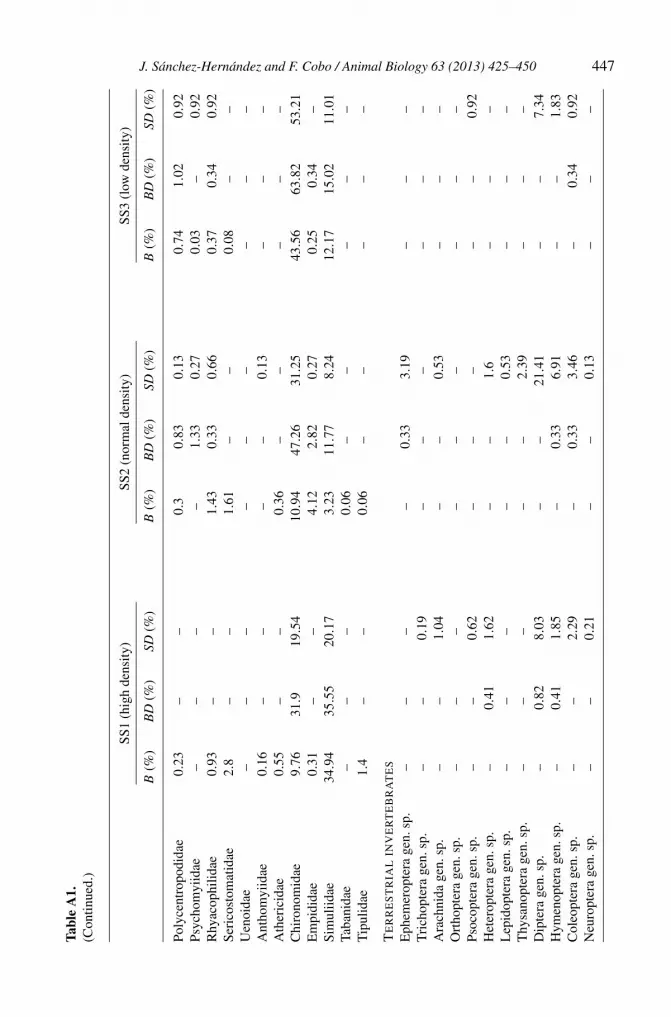
Benthic invertebrate densities varied widely among sampling sites (3841 ind/m2 inSS2 to 8111 ind/m2 in SS3). Simuliidae was the most abundant taxon in SS1 andrepresented 34.94% of the total number of individuals. Conversely, Chironomidaeand Elmidae were the most abundant taxa in SS3 and SS2 respectively. Less nu-merous in the benthos of all sampling sites, although very important in trout dietin other studies, were families such as Baetidae or Gammaridae (see Appendix,table A1).

Both aquatic and terrestrial invertebrates were found in the drift samples and thetotal composition for each category is given as in the Appendix (table A1). Aquaticinvertebrates were taken in large numbers at each station and formed a considerableproportion of the surface drift. Only in SS2, the terrestrial invertebrates constituted>40% of the surface drift samples (table 3), whereas the terrestrial component ofthe surface drift was less important at the other sampling sites (11% in SS3 and16% in SS1). Also the drift densities varied among sampling sites (table 3). Ingeneral, spatial differences in the proportions of each taxon between the benthos anddrift were found; for example the percentage of chironomid larvae in the benthoswas 43.56%, 9.76% and 10.94% for SS3, SS1 and SS2, respectively. Similarly, theabundance observed of this same prey item was 63.82%, 31.9% and 47.27%, in thebenthic drift compared to 53.21%, 19.54% and 31.25% in the surface drift for therespective three sampling sites (table A1).

Table 3.Food availability (benthos and drift) for each sampling site.

SS1 SS2 SS3(high density) (normal density) (low density)

Benthos density (ind/m2) 4086 3841 8111Surface drift density 764.1 563.41 336.5

(ind/100 m3 ∗ hour)Benthic drift density 307.6 431.48 890.9

(ind/100 m3 ∗ hour)Terrestrial invertebrates 15.85 40.16 11

in the surface drift (%)

http://cran.es.r-projet.org/

http://cran.es.r-projet.org/


Brown trout densities

The brown trout density showed large variations between sites (0.05 trout/m2 inSS3, 0.17 trout/m2 in SS2 and 0.56 trout/m2 in SS1). Using the data of the presentwork and the reference categories of Sánchez-Hernández et al. (2012b), the reporteddensities corresponded to the high category in SS1, normal category in SS2 and lowcategory in SS3.

Diet

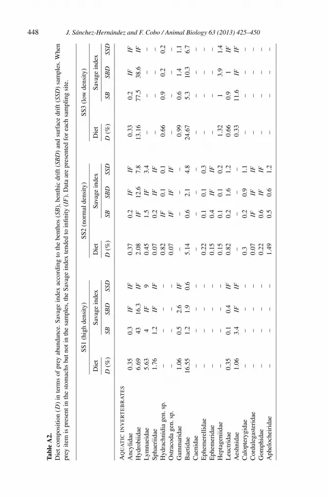
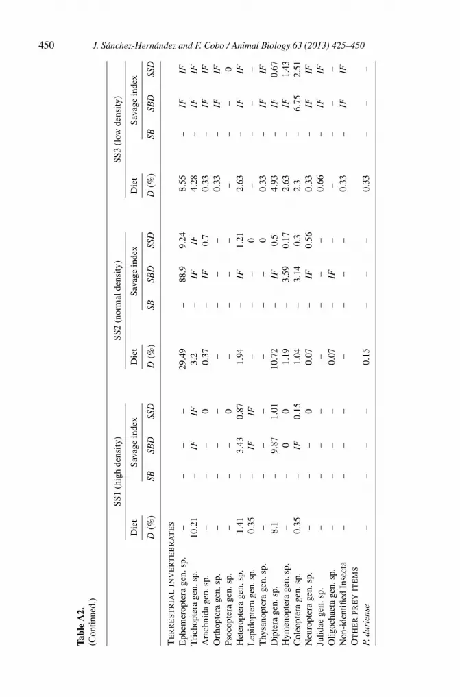
The diet composition of the three populations is provided as supplementary material(see Appendix, table A2). Baetidae was the most abundant taxon in SS3 (24.67% ofthe total diet), ephemeroptera imagoes dominated the diet of trout in SS2 (29.49%),whereas Simuliidae was the most abundant prey item in SS1 (21.48%). Aquaticinvertebrates constituted an important food source in all brown trout populations,and no significant differences were found among the populations (table 4). Also,the analysis of the niche breadth of the populations using different indices likeShannon diversity, evenness and Levin’s indices revealed a large similarity in theseparameters among populations, and no significant differences were found (table 4).Piscivorous behaviour was found in the normal (SS2) and low density categories(SS3) but not in SS1 (high category). According to the cluster analysis, the min-imum Bray-Curtis similarity between the populations was 59.3% for SS1 versusSS2, followed by 60.7% for SS3 versus SS1, and 63.8% for the most similar group(SS3 versus SS2).

A comparison of macroinvertebrate availability in the environment (drift andbenthos) and prey selectivity using Savage index shows that brown trout selectedcertain prey types, in particular Hydrobiidae and Leptoceridae in the benthos andterrestrial invertebrates in the drift, positively (table A2). Despite the high abun-dance in the benthos of Simuliidae in SS1, Elmiidae in SS2 and Chironomidae in

Table 4.Diet analyses. Data are presented for each sampling site (mean ± SE).

SS1 SS2 SS3 Kruskal-Wallis test(high density) (normal density) (low density)

Aquatic 79.3 ± 5.22 58.29 ± 5.66 74.0 ± 7.05 H = 5.41, P = 0.067invertebrates (%)

Terrestrial 20.7 ± 5.22 40.9 ± 5.78 25.3 ± 6.82 H = 4.52, P = 0.104invertebrates (%)

Fullness index 1.02 ± 0.128 0.79 ± 0.105 0.71 ± 0.920 H = 3.63, P = 0.163Shannon diversity 0.71 ± 0.032 0.68 ± 0.066 0.60 ± 0.055 H = 1.37, P = 0.503

index (H ′)Levin’s index (B) 4.1 ± 0.34 5.0 ± 0.63 3.6 ± 0.44 H = 2.24, P = 0.326Evenness index (E) 0.62 ± 0.028 0.60 ± 0.058 0.60 ± 0.055 H = 0.09, P = 0.954


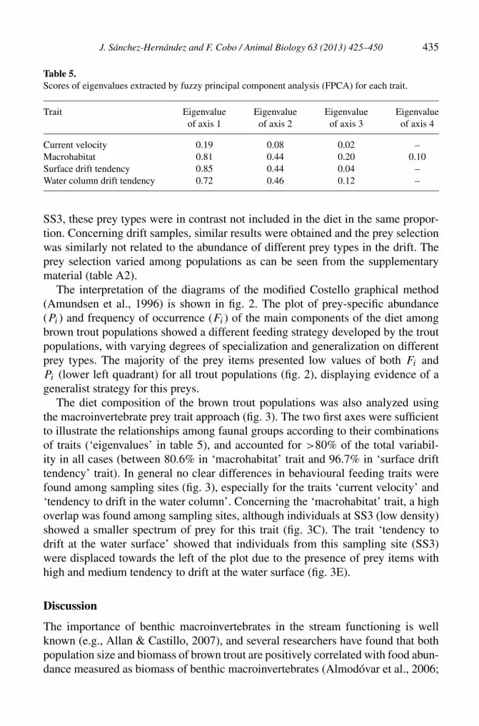
Table 5.Scores of eigenvalues extracted by fuzzy principal component analysis (FPCA) for each trait.

Trait Eigenvalue Eigenvalue Eigenvalue Eigenvalueof axis 1 of axis 2 of axis 3 of axis 4

Current velocity 0.19 0.08 0.02 –Macrohabitat 0.81 0.44 0.20 0.10Surface drift tendency 0.85 0.44 0.04 –Water column drift tendency 0.72 0.46 0.12 –

SS3, these prey types were in contrast not included in the diet in the same propor-tion. Concerning drift samples, similar results were obtained and the prey selectionwas similarly not related to the abundance of different prey types in the drift. Theprey selection varied among populations as can be seen from the supplementarymaterial (table A2).

The interpretation of the diagrams of the modified Costello graphical method(Amundsen et al., 1996) is shown in fig. 2. The plot of prey-specific abundance(Pi) and frequency of occurrence (Fi) of the main components of the diet amongbrown trout populations showed a different feeding strategy developed by the troutpopulations, with varying degrees of specialization and generalization on differentprey types. The majority of the prey items presented low values of both Fi andPi (lower left quadrant) for all trout populations (fig. 2), displaying evidence of ageneralist strategy for this preys.

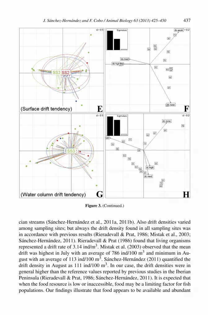
The diet composition of the brown trout populations was also analyzed usingthe macroinvertebrate prey trait approach (fig. 3). The two first axes were sufficientto illustrate the relationships among faunal groups according to their combinationsof traits (‘eigenvalues’ in table 5), and accounted for >80% of the total variabil-ity in all cases (between 80.6% in ‘macrohabitat’ trait and 96.7% in ‘surface drifttendency’ trait). In general no clear differences in behavioural feeding traits werefound among sampling sites (fig. 3), especially for the traits ‘current velocity’ and‘tendency to drift in the water column’. Concerning the ‘macrohabitat’ trait, a highoverlap was found among sampling sites, although individuals at SS3 (low density)showed a smaller spectrum of prey for this trait (fig. 3C). The trait ‘tendency todrift at the water surface’ showed that individuals from this sampling site (SS3)were displaced towards the left of the plot due to the presence of prey items withhigh and medium tendency to drift at the water surface (fig. 3E).

Discussion

The importance of benthic macroinvertebrates in the stream functioning is wellknown (e.g., Allan & Castillo, 2007), and several researchers have found that bothpopulation size and biomass of brown trout are positively correlated with food abun-dance measured as biomass of benthic macroinvertebrates (Almodóvar et al., 2006;


Figure 3. Biplots of macroinvertebrate ecological traits (current velocity, macrohabitat, surface driftbehaviour, and water drift behaviour) obtained from a fuzzy principal component analysis (FPCA).Position of sampling sites depending on the prey present in gut contents (A, C, E, G) and axes in-terpretation, including the histogram of eigenvalues (B, D, F, H). Ellipses envelop weighted-averageof prey-taxa positions consumed by each brown-trout population; labels (SS1: River Lengüelle, SS2:River Tambre, and SS3: River Anllóns) indicate the gravity centre of the ellipses. Filled lines link preyfamilies (represented by a point) to their corresponding predator locality, but are only 80% of theirtotal length for readability. Dotted lines represent the width and height of ellipses. Details and dataneeded for the elaboration of graphics can be found in the Materials and methods section.

Morante et al., 2012). Indeed, direct competition between fishes occurs when theirhabitat is restricted or when food is scarce due to low densities of benthic inverte-brates (Elliott, 2006 and references therein). Benthic invertebrate densities reportedin this study varied widely among sampling sites, but were within or even higherthan the density ranges (2030-4559 ind/m2) reported from other studies in Gali-


Figure 3. (Continued.)

cian streams (Sánchez-Hernández et al., 2011a, 2011b). Also drift densities variedamong sampling sites; but always the drift density found in all sampling sites wasin accordance with previous results (Rieradevall & Prat, 1986; Mistak et al., 2003;Sánchez-Hernández, 2011). Rieradevall & Prat (1986) found that living organismsrepresented a drift rate of 3.14 ind/m3. Mistak et al. (2003) observed that the meandrift was highest in July with an average of 786 ind/100 m3 and minimum in Au-gust with an average of 113 ind/100 m3. Sánchez-Hernández (2011) quantified thedrift density in August as 111 ind/100 m3. In our case, the drift densities were ingeneral higher than the reference values reported by previous studies in the IberianPeninsula (Rieradevall & Prat, 1986; Sánchez-Hernández, 2011). It is expected thatwhen the food resource is low or inaccessible, food may be a limiting factor for fishpopulations. Our findings illustrate that food appears to be available and abundant


in the environment, and a priori none of the three studied sampling sites seems tobe under food-limitation phenomena.

As predicted by optimal foraging theory (OFT), the fish should select those preyitems that maximize their net rate of energy gain (MacArthur & Pianka, 1966; Pykeet al., 1977; Gerking, 1994). It has been demonstrated that prey selection in fishes isrelated to prey characteristics (e.g., size, locomotor abilities, accessibility, or anti-predator behaviour), fish characteristics (e.g., prior experience, locomotor abilities,stomach fullness, mouth gape, sensory capabilities, and fish size) and physical habi-tat characteristics (e.g., flow patterns and structural complexity of habitat) (Gerking,1994 and references therein). Our results are in good agreement with those ob-tained in other studies of different fish species, demonstrating that fishes do notalways consume the most abundant taxa in the environment (de Crespin de Billy& Usseglio-Polatera, 2002; Sánchez-Hernández et al., 2011a, 2011b). Hence, preyabundance could not be the most important factor determining the food selectivity,and the results of this study rather support the hypothesis that the preference orrejection of prey items might be related to site-specific prey accessibility as demon-strated by other researchers (Johnson et al., 2007; Sánchez-Hernández et al., 2011a;Sánchez-Hernández & Cobo, 2012b).

As noted in the introduction, the importance of competitive or density-dependentmechanisms on growth and survival rates is well known in brown trout (e.g.,Lobón-Cerviá, 2007, 2010; Einum et al., 2011). Salmonids in running waters areconsidered as drift feeders (Rader, 1997 and references therein), and aggressiveterritory defence is an important component for the habitat uses in streams (Chap-man, 1962; Keenleyside & Yamamoto, 1962). Stewart et al. (2005) found that aspopulation density increases, intraspecific competition for these optimal resourcesalso intensifies. Therefore, the variety of resources or habitats used by a populationshould increase with increasing population density and the niche breadth shouldincrease (Pianka, 1988). Martinussen et al. (2011) accordingly demonstrated thatdiet breadth of YOY Atlantic salmon increases with increasing population den-sity. Previous studies of largemouth bass (Micropterus salmoides Lacépède, 1802)demonstrated in contrast that diet breadth did not change with population size, andfishes tended to have more consistent diets during periods with high conspecificdensities (Schindler et al., 1997). In our case, according to the diet indices employedin this study, no differences were found among populations similar to Schindler etal.’s findings (1997), but in contrast to the observations of Martinussen et al. (2011).On the other hand, Shustov et al. (2012) found that Atlantic salmon parr is able tofeed more intensively in the tributaries than in the main river channel where thedensities of juveniles normally are lower, suggesting that the frequency of emptystomachs could be related to fish density. In our case, no differences among rivershave been found either in the stomachs fullness or in the percentage of empty stom-achs, however this needs to be tested more firmly as more data from other studiesbecome available.


Several researchers have demonstrated that brown trout shows a generalist feed-ing strategy in lotic water systems (Oscoz et al., 2005, 2008; Sánchez-Hernández& Cobo, 2012a), whereas field studies carried out in reservoirs and lochs suggesteda dietary specialization rather than opportunistic feeding of some individuals (e.g.,Grey, 2001; Encina et al., 2004). Our analyses, based on the modified Costellographical method, are in agreement with previous studies that have demonstratedthat brown trout shows a generalist feeding strategy in running waters (Oscoz etal., 2005, 2008; Sánchez-Hernández & Cobo, 2012a), and suggest that the potentialmechanism underlying such foraging behaviour of brown trout is a generalisation inresource use independent of fish density or spatial heterogeneity in food resources.

Recent experiments have demonstrated that social interactions among fishes canaffect their feeding behaviour (Kooijman, 2009). In this respect, increases in thepopulation density may lead to a decrease in territory qualities due to an increas-ing use of suboptimal feeding territories (Nislow et al., 2000; Ward et al., 2007).Moreover, although Brännäs et al. (2003) have demonstrated that there was nosignificant relationship between food abundance and the number of territorial in-dividuals in brown trout; previous studies in salmonids have demonstrated that highfish densities (Cole & Noakes, 1890; Blanchet et al., 2006) or low food density(Berejikian et al., 1996; Dunbrack et al., 1996) lead to an increase in agonistic in-teractions. Thus, when no density-dependent competition occurs, each individualis free to forage in the zone of highest food availability, whereas, in contrast, whendensity-dependent competition does occur, the fish should redistribute in proportionto the percentage of the total resource available at a given depth (Fretwell & Lu-cas, 1970; Fortier & Harris, 1989). Hence, it may be expected that the acquisitionof a specific foraging behaviour can be closely related to the population densityof trout as well as the abundance and availability of prey. However, despite thefact that diet composition was not exactly the same among sampling sites (sim-ilarity between 59.3% and 60.7%) and there were differences in prey preferencesamong populations (table A2), the modified Costello graphical method and the preytrait analysis confirmed that no remarkable differences in the foraging behaviour ofbrown trout exist among the populations. Therefore, in contrast to previous expec-tations, the present study exemplifies the possibility of a foraging convergence ofpopulations in response to spatial availability in food resources regardless of thefish population density. For example, we have found that when terrestrial inverte-brates in the surface drift are available, their abundance in the diet is high, and alsowhen the benthic drift density is high, the feeding on aquatic invertebrates is hightoo. A similar convergence in the feeding mechanics has been demonstrated amongecomorphologically similar fish species (e.g., Lazzaro, 1991; Norton & Brainerd,1993). Recently, Cucherousset et al. (2007) demonstrated that dietary convergenceamong salmonids species is more likely to be due to behavioural interactions thanto other factors like, e.g., variations in food availability or fish displacements. In ourcase, the foraging convergence observed among neighbouring populations might bedue to low food competition as the food resources in the three rivers appear to be


abundant and available. As a consequence, the adaptive decision making of indi-viduals for the development of the foraging behaviour in streams is characterizedby a generalist or opportunist strategy regardless of the population density level,although the acquisition of the diet seems to be influenced by site-specific preyaccessibility.

Acknowledgements

The authors thank the staff of the Station of Hydrobiology of the USC ‘Encorodo Con’ due their participation in the surveys. Dr. Per-Arne Amundsen is acknowl-edged for valuable comments and corrections on the manuscript. We also appreciatethe constructive comments on the manuscript given by two anonymous referees.This work has been partially supported by the project 10PXIB2111059PR of theXunta de Galicia and the project MIGRANET of the Interreg IV B SUDOE (South-West Europe) Territorial Cooperation Programme (SOE2/P2/E288).

References

Alanärä, A., Burns, M.D. & Metcalfe, N.B. (2001) Intraspecific resource partitioning in brown trout:the temporal distribution of foraging is determined by social rank. J. Anim. Ecol., 70, 980-986.

Allan, J.D. & Castillo, M.M. (2007) Stream Ecology. Structure and Function of Running Waters. 2nded. Springer, Dordrecht (The Netherlands).

Allan, J.D. & Russek, E. (1985) The quantification of stream drift. Can. J. Fish. Aquat. Sci., 42, 210-215.

Almodóvar, A., Nicola, G.G. & Elvira, B. (2006) Spatial variation of brown trout production: the roleof environmental factors. Trans. Am. Fish. Soc., 135, 1348-1360.

Alonso-González, C., Gortázar, J., Baeza Sanz, D. & García de Jalón, D. (2008) Dam functionrules based on brown trout flow requirements: design of environmental flow regimes in regulatedstreams. Hydrobiologia, 609, 253-262.

Amundsen, P.-A., Gabler, H.-M. & Staldvik, F.J. (1996) A new approach to graphical analysis offeeding strategy from stomach contents data – modification of the Costello (1990) method. J. FishBiol., 48, 607-614.

Amundsen, P.-A., Knudsen, R. & Bryhni, H. (2010) Niche use and resource partitioning of Arcticcharr, European whitefish and grayling in a subarctic lake. Hydrobiologia, 650, 3-14.

Ayllón, D., Almodóvar, A., Nicola, G.G. & Elvira, B. (2010) Ontogenetic and spatial variations inbrown trout habitat selection. Ecol. Freshwat. Fish., 19, 420-432.

Ayllón, D., Almodóvar, A., Nicola, G.G., Parra, I. & Elvira, B. (2012) A new biological indicator toassess the ecological status of Mediterranean trout type streams. Ecol. Indicat., 20, 295-303.

Bagenal, T.B. & Tesch, F.W. (1978) Age and growth. In: T.B. Bagenal (Ed.) Methods for Assessmentof Fish Production in Fresh Waters. 3rd ed., pp. 101-136. Blackwell Science Publications, Oxford.

Berejikian, B.A., Mathews, S.B. & Quinn, T.P. (1996) Effects of hatchery and wild ancestry andrearing environments on the development of agonistic behavior in steelhead trout (Oncorhynchusmykiss) fry. Can. J. Fish. Aquat. Sci., 53, 2004-2014.

Blanchet, S., Dodson, J.J. & Brosse, S. (2006) Influence of habitat structure and fish density on At-lantic salmon Salmo salar L. territorial behaviour. J. Fish Biol., 68, 951-957.


Both, C. & Visser, M.E. (2003) Density dependence, territoriality and divisibility of resources: fromoptimality models to population processes. Am. Nat., 161, 326-336.

Brännäs, E., Jonsson, S. & Lundqvist, H. (2003) Influence of food abundance on individual behaviourstrategy and growth rate in juvenile brown trout (Salmo trutta). Can. J. Zool., 81, 684-691.

Burnet, A.M.R. (1969) Territorial behaviour in brown trout (Salmo trutta L.). New. Zeal. J. Mar,Freshwat. Res., 3, 385-388.

CEN (2003) Water quality – sampling of fish with electricity. European standard – EN 14011: 2003.European Committee for Standardization, Brussels.

Chapman, D.W. (1962) Aggressive behaviour in juvenile coho salmon as a cause of emigration.J. Fish. Res. Board. Can., 19, 1047-1079.

Chevenet, F., Dolédec, S. & Chessel, D. (1994) A fuzzy coding approach for the analysis of long-termecological data. Freshwat Biol., 31, 295-309.

Clarke, K.R. & Gorley, R.N. (2001) Primer v6: User Manual/Tutorial. Primer-E, Plymouth, UK.Cole, K.S. & Noakes, D.L.G. (1980) Development of early social behavior of rainbow trout, Salmo

gairdneri (Pisces, salmonidae). Behav. Proc., 5, 97-112.Costello, M.J. (1990) Predator feeding strategy and prey importance: a new graphical analysis. J. Fish

Biol., 36, 261-263.Cucherousset, J., Aymes, J.C., Santoul, F. & Céréghino, R. (2007) Stable isotope evidence of trophic

interactions between introduced brook trout Salvelinus fontinalis and native brown trout Salmotrutta in a mountain stream of south-west France. J. Fish Biol., 71, 210-223.

Cundari, T.R., Sârbu, C. & Pop, H.F. (2002) Robust fuzzy principal component analysis (FPCA).A comparative study concerning interaction of carbon-hydrogen bonds with molybdenum-oxobonds. J. Chem. Inf. Comp. Sci., 42, 1363-1369.

de Crespin de Billy, V. (2001) Régime alimentaire de la truite (Salmo trutta L.) en eaux courantes:rôles de lh́abitat physique des traits des macroinvertébrés. Thesis. Lúniversité Claude Bernard,Lyon.

de Crespin de Billy, V. & Usseglio-Polatera, P. (2002) Traits of brown trout prey in relation to habitatcharacteristics and benthic invertebrate communities. J. Fish Biol., 60, 687-714.

Dunbrack, R.L., Clarke, L. & Bassler, C. (1996) Population level differences in aggressiveness andtheir relationship to food density in a stream salmonid (Salvelinus fontinalis). J. Fish Biol., 48,615-622.

Einum, S., Robertsen, G., Nislow, K.H., McKelvey, S. & Armstrong, J.D. (2011) The spatial scale ofdensity-dependent growth and implications for dispersal from nests in juvenile Atlantic salmon.Oecologia, 165, 959-969.

Elliott, J.M. (1994) Quantitative Ecology and the Brown Trout. Oxford University Press, Oxford.Elliott, J.M. (2006) Periodic habitat loss alters the competitive coexistence between brown trout and

bullheads in a small stream over 34 years. J. Anim. Ecol., 75, 54-63.Encina, L., Rodríguez-Ruiz, A. & Granado-Lorencio, C. (2004) Trophic habits of the fish assemblage

in an artificial freshwater ecosystem: the Joaquin Costa reservoir, Spain. Fol. Zool., 3, 437-449.Fortier, L. & Harris, R.P. (1989) Optimal foraging and density-dependent competition in marine fish

larvae. Mar. Ecol. Prog. Ser., 51, 19-33.Fretwell, S.D. & Lucas, H.L. Jr. (1970) On territorial behavior and other factors influencing habitat

distribution in birds. Acta Biotheor., 19, 16-36.Gerking, S.D. (1994) Feeding Ecology of Fish. Academic Press, San Diego.Grant, J.W.A., Girard, I.L., Breau, C. & Weir, L.K. (2002) Influence of food abundance on aggression

in juvenile convict cichlids. Anim. Behav., 63, 323-330.


Grey, J. (2001) Ontogeny and dietary specialization on brown trout (Salmo trutta L.) from Loch Ness,Scotland, examined using stable isotopes of carbon and nitrogen. Ecol. Freshwat. Fish, 10, 168-176.

Ihaka, R. & Gentleman, R. (1996) R: a language for data analysis and graphics. J. Comput. Graph.Stat., 5, 299-314.

Imre, I., Grant, J.W.A. & Keeley, E.R. (2004) The effect of food abundance on territory size andpopulation density of juvenile steelhead trout (Oncorhynchus mykiss). Oecologia, 138, 371-378.

Johnson, R.L., Coghlan, S.M. & Harmon, T. (2007) Spatial and temporal variation in prey selectionof brown trout in a cold Arkansas tailwater. Ecol. Freshwat. Fish, 16, 373-384.

Keenleyside, M.H. & Yamamoto, F.T. (1962) Territorial behavior of juvenile Atlantic salmon (Salmosalar L.). Behaviour, 19, 139-169.

Kooijman, S.A.L.M. (2009) Social interactions can affect feeding behaviour of fish in tanks. J. SeaRes., 62, 175-178.

Lazzaro, X. (1991) Feeding convergence in South American and African zooplanktivorous cichlidsGeophagus brasiliensis and Tilapia rendalli. Environ. Biol. Fish., 31, 283-294.

Levins, R. (1968) Evolution in Changing Environments: Some Theoretical Explorations. PrincetonUniversity Press, Princeton.

Lobón-Cerviá, J. (2007) Density-dependent growth in stream-living brown trout Salmo trutta L. FunctEcol., 21, 117-124.

Lobón-Cerviá, J. (2010) Density dependence constrains mean growth rate while enhancing individualsize variation in stream salmonids. Oecologia, 164, 109-115.

MacArthur, R.H. & Pianka, E.R. (1996) On optimal use of a patchy environment. Amer. Naturalist.,100, 603-609.

Martínez-Ansemil, E. & Membiela, P. (1992) The low mineralized and fast turnover watercourses ofGalicia. Limnetica, 8, 125-130.

Martinussen, P.A., Robertsen, G. & Einum, S. (2011) Density-dependent diet composition of juvenileAtlantic salmon (Salmo salar). Ecol. Freshwat. Fish, 20, 384-392.

Mistak, J., Hayes, D.B. & Bremigan, M.T. (2003) Food habits of coexisting salmonines above andbelow Stronach Dam in the Pine River, Michigan. Environ. Biol. Fish., 67, 179-190.

Montori, A., Tierno de Figueroa, J.M. & Santos, X. (2006) The diet of the brown trout Salmo trutta(L.) during the reproductive period: size-related and sexual effects. Internat. Rev. Hydrobiol., 91,438-450.

Morante, T., García-Arberas, L., Antón, A. & Rallo, A. (2012) Macroinvertebrate biomass estimatesin Cantabrian streams and relationship with brown trout (Salmo trutta) populations. Limnetica, 31,85-94.

Nislow, K.H., Folt, C.L. & Parrish, D.L. (2000) Spatially explicit bioenergetic analysis of habitatquality for age-0 Atlantic salmon. Trans. Am. Fish. Soc., 129, 1067-1081.

Norton, S.F. & Brainerd, E.L. (1993) Convergence in the feeding mechanics of ecomorphologicallysimilar species in the Centrarchidae and Cichlidae. J. Exp. Biol., 176, 11-29.

Oscoz, J., Leunda, P.M., Campos, F., Escala, M.C. & Miranda, R. (2005) Diet of 0+ brown trout(Salmo trutta L., 1758) from the river Erro (Navarra, North of Spain). Limnetica, 24, 319-326.

Oscoz, J., Leunda, P.M., Escala, M.C. & Miranda, R. (2008) Summer feeding relationships of theco-occurring hatchling brown trout Salmo trutta and Ebro minnows Phoxinus bigerri in an Iberianriver. Acta Zool. Sin., 54, 675-685.

Parra, I., Almodóvar, A., Ayllón, D., Nicola, G.G. & Elvira, B. (2012) Unravelling the effects of watertemperature and density dependence on the spatial variation of brown trout body size. Can. J. Fish.Aquat. Sci., 69, 1-12.


Pianka, E.R. (1988) Evolutionary ecology. 4th ed. Harper and Row Publishers, New York.Pyke, G.H., Pulliam, H.R. & Charnov, E.L. (1977) Optimal foraging: a selective review of theory and

tests. Q. Rev. Biol., 52, 137-154.Rader, R.B. (1997) A functional classification of the drift: traits that influence invertebrate availability

to salmonids. Can. J. Fish. Aquat. Sci., 54, 1211-1234.Rieradevall, M. & Prat, N. (1986) Deriva nictemeral de macroinvertebrados en el Río Llobregat

(Barcelona). Limnetica, 2, 147-156.Río-Barja, F.J. & Rodríguez-Lestegás, F. (1992) Os Ríos Galegos. Morfoloxía e Réxime. Concello da

Cultura Galega, Santiago de Compostela.Rodrígues-Capítulo, A., Muñoz, I., Bonada, N., Gaudés, A. & Tomanova, S. (2009) La biota de los

ríos: los invertebrados. In: A. Elosegi & S. Sabater (Eds.) Conceptos y técnicas en ecología fluvial,pp. 253-270. Fundación BBVA, Bilbao.

Ryer, C.H. & Olla, B.L. (1995) The influence of food distribution upon the development of aggressiveand competitive behaviour in juvenile chum salmon, Oncorhynchus keta. J. Fish Biol., 46, 264-272.

Sánchez-Hernández, J. (2011) Biological and ecological traits of the macroinvertebrates in a hy-porhitron sector of the River Tormes (Central Spain). Zool. Baetica, 22, 51-67 (in Spanish withEnglish summary).

Sánchez-Hernández, J. & Cobo, F. (2012a) Summer differences in behavioural feeding habits and useof feeding habitat among brown trout (Pisces) age classes in a temperate area. Ital. J. Zool., 79,468-478.

Sánchez-Hernández, J. & Cobo, F. (2012b) Ontogenetic dietary shifts and food selection of endemicSqualius carolitertii (Actinopterygii: Cypriniformes: Cyprinidae) in River Tormes, Central Spain,in summer. Acta Ichthyol. Piscat., 42, 101-111.

Sánchez-Hernández, J., Servia, M.J., Vieira-Lanero, R. & Cobo, F. (2012a) Application of the analysisof prey ecological characteristics (traits) for the study of the feeding behaviour of bottom-feederfishes: the example of the stickleback (Gasterosteus gymnurus Cuvier, 1829). Limnetica, 31, 59-76(in Spanish with English summary).

Sánchez-Hernández, J., Servia, M.J., Vieira-Lanero, R., Barca-Bravo, S. & Cobo, F. (2012b) Refer-ences data on the growth and population parameters of brown trout in the siliceous rivers of Galicia(NW Spain). Limnetica, 31, 273-288.

Sánchez-Hernández, J., Servia, M.J., Vieira-Lanero, R. & Cobo, F. (2013) Ontogenetic dietary shiftsin a predatory freshwater fish species: the brown trout as an example of a dynamic fish species. In:H. Türker (Ed.) New Advances and Contributions to Fish Biology, pp. 271-298. InTech, Croatia.

Sánchez-Hernández, J., Vieira-Lanero, R., Servia, M.J. & Cobo, F. (2011a) First feeding diet of youngbrown trout fry in a temperate area: disentangling constraints and food selection. Hydrobiologia,663, 109-119.

Sánchez-Hernández, J., Vieira-Lanero, R., Servia, M.J. & Cobo, F. (2011b) Feeding habits of foursympatric fish species in the Iberian Peninsula: keys to understanding coexistence using prey trais.Hydrobiologia, 667, 119-132.

Savage, R.E. (1931) The relation between the feeding of the herring off the cast coast of England andthe plankton of the surrounding waters. Fish. Invest. II, 12, 1-88.

Schindler, D., Hodgson, J.R. & Kitchell, J.F. (1997) Density-dependent changes in individual foragingspecialization of largemouth bass. Oecologia, 110, 592-600.

Seber, G.A.F. (1982) The Estimation of Animal Abundance and Related Parameters. Charles GriffinPublications, London.


Shustov, Yu.A., Baryshev, I.A. & Belyakova, E.E. (2012) Specific features of the feeding of juvenileAtlantic salmon (Salmo salar L.) in the subarctic Varzuga River and its small tributaries (KolaPeninsula). Inland Water Biol., 5, 288-292.

Shustov, Yu.A., Veselov, A.E. & Baryshev, I.A. (2008) The diet of juvenile lake trout Salmo trutta L.in rivers of the Onega basin in autumn. Russ. J. Ecol., 39, 119-122.

Steingrimsson, S.O. & Gislason, G.M. (2002) Body size, diet and growth of landlocked brown trout,Salmo trutta, in the subarctic River Laxa, North-East Iceland. Environ. Biol. Fish., 63, 417-426.

Stewart, K.M., Bowyer, R.T., Dick, B.L., Johnson, B.K. & Kie, J.G. (2005) Density-dependent effectson physical condition and reproduction in North American elk: an experimental test. Oecologia,143, 85-93.

Thioulouse, J., Chessel, D., Dolédec, S. & Olivier, J.M. (1997) ADE-4: a multivariate analysis andgraphical display software. Stat. Comput., 7, 75-83.

Ward, D.M., Nislow, K.H., Armstrong, J.D., Einum, S. & Folt, C.L. (2007) Is the shape of thedensity-growth relationship for stream salmonids evidence for exploitative rather than interferencecompetition? J. Anim. Ecol., 76, 135-138.

Zamora, L., Vila, A. & Naspleda, J. (2009) La biota de los ríos: los peces. In: A. Elosegi & S. Sabater(Eds.) Conceptos y técnicas en ecología fluvial, pp. 271-291. Fundación BBVA, Bilbao.

Zippin, C. (1958) The removal method population and estimation. J. Wildl. Manage., 22, 82-90.

J. Sánchez-Hernández and F. Cobo / Animal Biology 63 (2013) 425–450 445A

ppen

dix

Tabl

eA

1.Fo

odav

aila

bilit

yin

the

envi

ronm

ent.

Ben

thos

(B),

bent

hic

drif

t(B

D)

and

surf

ace

drif

t(SD

).D

ata

are

pres

ente

dfo

rea

chsa

mpl

ing

site

.

SS1

(hig

hde

nsity

)SS

2(n

orm

alde

nsity

)SS

3(l

owde

nsity

)

B(%

)B

D(%

)SD

(%)

B(%

)B

D(%

)SD

(%)

B(%

)B

D(%

)SD

(%)

AQ

UA

TIC

INV

ER

TE

BR

AT

ES

Plan

ariid

ae0.

23–

0.19

0.18

––

0.2

––

Olig

ocha

eta

gen.

sp.

2.13

0.92

0.19

1.49

––

0.45

––

Erp

obde

llida

e0.

62–

–1.

79–

–0.

060.

34–

Glo

ssip

honi

idae

––

–0.

24–

––

––

Hir

udid

ae–

––

––

––

––

Anc

ylid

ae1.

14–

–2.

21–

–1.

44–

–H

ydro

biid

ae0.

160.

41–

–0.

170.

270.

170.

34–

Lym

naei

dae

1.4

–0.

620.

3–

0.13

0.03

––

Spha

eriid

ae1.

51–

–0.

3–

–0.

08–

–H

ydra

chni

dia

gen.

sp.

0.31

10.4

97.

28–

9.29

5.85

0.71

3.41

–G

amm

arid

ae2.

230.

41–

0.06

0.17

0.13

1.7

0.68

–O

stra

coda

gen.

sp.

––

––

––

––

–D

aphn

iasp

.–

––

–0.

17–

–0.

34–

Bae

tidae

13.4

58.

6626

.47.

952.

491.

064.

642.

39–

Cae

nida

e1.

820.

920.

62–

0.33

1.06

0.06

––

Eph

emer

ellid

ae1.

30.

454.

571.

493.

980.

661.

591.

711.

83E

phem

erid

ae0.

86–

–0.

36–

––

––

Hep

tage

niid

ae0.

31–

–2.

871

0.93

1.27

0.34

0.92

Lep

toph

lebi

idae

0.16

–0.

211.

140.

170.

130.

2–

–L

euct

rida

e2.

960.

92–

3.35

0.5

0.66

0.74

0.68

–N

emou

rida

e–

––

––

–0.

06–

–Pe

rlid

ae–

––

1.32

––

––

–A

eshn

idae

0.31

––

0.3

0.17

–0.

03–

–

446 J. Sánchez-Hernández and F. Cobo / Animal Biology 63 (2013) 425–450Ta

ble

A1.

(Con

tinue

d.)

SS1

(hig

hde

nsity

)SS

2(n

orm

alde

nsity

)SS

3(l

owde

nsity

)

B(%

)B

D(%

)SD

(%)

B(%

)B

D(%

)SD

(%)

B(%

)B

D(%

)SD

(%)

Cal

opte

rygi

dae

1.35

–1.

041.

430.

330.

270.

08–

–C

oena

grio

nida

e0.

62–

––

0.33

0.13

–0.

34–

Cor

dule

gast

erid

ae–

––

––

––

––

Gom

phid

ae0.

16–

–0.

36–

–0.

03–

–Pl

atyc

nem

idid

ae–

––

––

0.13

––

–A

phel

oche

irid

ae0.

160.

45–

2.81

2.32

1.2

0.59

0.68

0.92

Ger

rida

e–

–0.

42–

0.66

0.53

––

–N

epid

ae–

––

––

––

––

Sial

idae

0.31

––

0.12

––

––

–D

ryop

idae

––

0.21

––

––

––

Dyt

isci

dae

0.16

––

0.06

––

––

–E

lmid

ae5.

976.

391.

4528

.63

6.97

2.39

15.9

94.

13.

67G

yrin

idae

0.31

––

0.36

0.66

0.27

0.65

0.68

0.92

Hyd

raen

idae

0.16

–0.

210.

420.

170.

270.

25–

–H

ydro

chid

ae–

––

––

0.4

––

–H

ydro

phili

dae

––

––

––

––

–B

erae

idae

––

––

––

–1.

37–

Bra

chyc

entr

idae

0.23

0.45

0.21

0.48

0.17

––

––

Goe

rida

e0.

16–

––

––

––

–G

loss

osom

atid

ae–

––

––

–0.

03–

–H

ydro

psyc

hida

e5.

710.

450.

4217

.14.

312.

3911

.52

1.37

0.92

Hyd

ropt

ilida

e–

–0.

21–

––

Lep

idos

tom

atid

ae–

––

0.42

––

0.14

––

Lep

toce

rida

e–

––

0.06

––

––

–L

imne

phili

dae

1.01

––

0.12

––

0.03

–0.

92Ph

ilopo

tam

idae

1.71

–0.

210.

180.

33–

0.06

0.34

–

J. Sánchez-Hernández and F. Cobo / Animal Biology 63 (2013) 425–450 447Ta

ble

A1.

(Con

tinue

d.)

SS1

(hig

hde

nsity

)SS

2(n

orm

alde

nsity

)SS

3(l

owde

nsity

)

B(%

)B

D(%

)SD

(%)

B(%

)B

D(%

)SD

(%)

B(%

)B

D(%

)SD

(%)

Poly

cent

ropo

dida

e0.

23–

–0.

30.

830.

130.

741.

020.

92Ps

ycho

myi

idae

––

––

1.33

0.27

0.03

–0.

92R

hyac

ophi

lidae

0.93

––

1.43

0.33

0.66

0.37

0.34

0.92

Seri

cost

omat

idae

2.8

––

1.61

––

0.08

––

Uen

oida

e–

––

––

––

––

Ant

hom

yiid

ae0.

16–

––

–0.

13–

––

Ath

eric

idae

0.55

––

0.36

––

––

–C

hiro

nom

idae

9.76

31.9

19.5

410

.94

47.2

631

.25

43.5

663

.82

53.2

1E

mpi

dida

e0.

31–

–4.

122.

820.

270.

250.

34–

Sim

uliid

ae34

.94

35.5

520

.17

3.23

11.7

78.

2412

.17

15.0

211

.01

Taba

nida

e–

––

0.06

––

––

–T

ipul

idae

1.4

––

0.06

––

––

–

TE

RR

ES

TR

IAL

INV

ER

TE

BR

AT

ES

Eph

emer

opte

rage

n.sp

.–

––

–0.

333.

19–

––

Tri

chop

tera

gen.

sp.

––

0.19

––

––

––

Ara

chni

dage

n.sp

.–

–1.

04–

–0.

53–

––

Ort

hopt

era

gen.

sp.

––

––

––

––

–Ps

ocop

tera

gen.

sp.

––

0.62

––

––

–0.

92H

eter

opte

rage

n.sp

.–

0.41

1.62

––

1.6

––

–L

epid

opte

rage

n.sp

.–

––

––

0.53

––

–T

hysa

nopt

era

gen.

sp.

––

––

–2.

39–

––

Dip

tera

gen.

sp.

–0.

828.

03–

–21

.41

––

7.34

Hym

enop

tera

gen.

sp.

–0.

411.

85–

0.33

6.91

––

1.83

Col

eopt

era

gen.

sp.

––

2.29

–0.

333.

46–

0.34

0.92

Neu

ropt

era

gen.

sp.

––

0.21

––

0.13

––

–


Tabl

eA

2.D

ietc

ompo

sitio

n(D

)in

term

sof

prey

abun

danc

e.Sa

vage

inde

xac

cord

ing

toth

ebe

ntho

s(S

B),

bent

hic

drif

t(SB

D)

and

surf

ace

drif

t(SS

D)

sam

ples

.Whe

npr

eyite

mis

pres

enti

nth

est

omac

hsbu

tnot

inth

esa

mpl

es,t

heSa

vage

inde

xte

nded

toin

finity

(IF

).D

ata

are

pres

ente

dfo

rea

chsa

mpl

ing

site

.

SS1

(hig

hde

nsity

)SS

2(n

orm

alde

nsity

)SS

3(l

owde

nsity

)

Die

tSa

vage

inde

xD

iet

Sava

gein

dex

Die

tSa

vage

inde

x

D(%

)SB

SBD

SSD

D(%

)SB

SBD

SSD

D(%

)SB

SBD

SSD

AQ

UA

TIC

INV

ER

TE

BR

AT

ES

Anc

ylid

ae0.

350.

3IF

IF0.

370.

2IF

IF0.

330.

2IF

IFH

ydro

biid

ae6.

6943

16.3

IF2.

08IF

12.6

7.8

13.1

677

.538

.6IF

Lym

naei

dae

5.63

4IF

90.

451.

5IF

3.4

––

––

Spha

eriid

ae1.

761.

2IF

IF0.

070.

2IF

IF–

––

–H

ydra

chni

dia

gen.

sp.

––

––

0.82

IF0.

10.

10.

660.

90.

20.

2O

stra

coda

gen.

sp.

––

––

0.07

IFIF

IF–

––

–G

amm

arid

ae1.

060.

52.

6IF

––

––

0.99

0.6

1.4

1.1

Bae

tidae

16.5

51.

21.

90.

65.

140.

62.

14.

824

.67

5.3

10.3

6.7

Cae

nida

e–

––

––

––

––

––

–E

phem

erel

lidae

––

––

0.22

0.1

0.1

0.3

––

––

Eph

emer

idae

––

––

0.15

0.4

IFIF

––

––

Hep

tage

niid

ae–

––

–0.

150.

10.

10.

21.

321

3.9

1.4

Leu

ctri

dae

0.35

0.1

0.4

IF0.

820.

21.

61.

20.

660.

91

IFA

eshn

idae

1.06

3.4

IFIF

––

––

0.33

11.6

IFIF

Cal

opte

rygi

dae

––

––

0.3

0.2

0.9

1.1

––

––

Cor

dule

gast

erid

ae–

––

–0.

07IF

IFIF

––

––

Gom

phid

ae–

––

–0.

220.

6IF

IF–

––

–A

phel

oche

irid

ae–

––

–1.

490.

50.

61.

2–

––

–


Tabl

eA

2.(C

ontin

ued.

)

SS1

(hig

hde

nsity

)SS

2(n

orm

alde

nsity

)SS

3(l

owde

nsity

)

Die

tSa

vage

inde

xD

iet

Sava

gein

dex

Die

tSa

vage

inde

x

D(%

)SB

SBD

SSD

D(%

)SB

SBD

SSD

D(%

)SB

SBD

SSD

Ger

rida

e–

––

–0.

22IF

0.3

0.4

––

––

Nep

idae

––

––

0.22

IFIF

IF–

––

–Si

alid

ae–

––

––

––

––

––

–D

ytis

cida

e1.

419

IFIF

––

––

––

––

Elm

idae

0.7

0.1

0.1

0.5

0.3

0.01

0.04

0.1

0.99

0.1

0.2

0.3

Gyr

inid

ae1.

063.

4IF

IF0.

070.

20.

10.

3–

––

–H

ydro

phili

dae

––

––

0.07

IFIF

IF–

––

–B

rach

ycen

trid

ae–

––

––

00

–0.

33IF

IFIF

Hyd

rops

ychi

dae

3.87

0.7

8.6

9.3

1.86

0.1

0.4

0.8

3.62

0.3

2.7

3.9

Lep

toce

rida

e1.

06IF

IFIF

––

––

3.62

IFIF

IFL

imne

phili

dae

0.7

0.7

IFIF

0.45

3.7

IFIF

1.32

46.5

IF1.

4Po

lyce

ntro

podi

dae

0.35

1.5

IFIF

0.15

0.5

0.2

1.1

0.66

0.9

0.6

0.7

Psyc

hom

yiid

ae0.

35IF

IFIF

0.3

IF0.

21.

1–

––

–R

hyac

ophi

lidae

2.11

2.3

IFIF

0.45

0.3

1.3

0.7

0.33

0.9

10.

4Se

rico

stom

atid

ae0.

350.

1IF

IF0.

670.

4IF

IF1.

6419

.4IF

IFC

hiro

nom

idae

12.3

21.

30.

40.

611

.32

10.

20.

410

.86

0.2

0.2

0.2

Em

pidi

dae

0.35

1.1

IFIF

0.22

0.1

0.1

0.8

––

––

Sim

uliid

ae21

.48

0.6

0.6

1.1

22.9

37.

11.

92.

86.

580.

50.

40.

6T

ipul

idae

––

––

0.07

1.25

IFIF

––

––


Tabl

eA

2.(C

ontin

ued.

)

SS1

(hig

hde

nsity

)SS

2(n

orm

alde

nsity

)SS

3(l

owde

nsity

)

Die

tSa

vage

inde

xD

iet

Sava

gein

dex

Die

tSa

vage

inde

x

D(%

)SB

SBD

SSD

D(%

)SB

SBD

SSD

D(%

)SB

SBD

SSD

TE

RR

ES

TR

IAL

INV

ER

TE

BR

AT

ES

Eph

emer

opte

rage

n.sp

.–

––

–29

.49

–88

.99.

248.

55–

IFIF

Tri

chop

tera

gen.

sp.

10.2

1–

IFIF

3.2

–IF

IF4.

28–

IFIF

Ara

chni

dage

n.sp

.–

––

00.

37–

IF0.

70.

33–

IFIF

Ort

hopt

era

gen.

sp.

––

––

––

––

0.33

–IF

IFPs

ocop

tera

gen.

sp.

––

–0

––

––

––

–0

Het

erop

tera

gen.

sp.

1.41

–3.

430.

871.

94–

IF1.

212.

63–

IFIF

Lep

idop

tera

gen.

sp.

0.35

–IF

IF–

––

0–

––

–T

hysa

nopt

era

gen.

sp.

––

––

––

–0

0.33

–IF

IFD

ipte

rage

n.sp

.8.

1–

9.87

1.01

10.7

2–

IF0.

54.

93–

IF0.

67H

ymen

opte

rage

n.sp

.–

–0

01.

19–

3.59

0.17

2.63

–IF

1.43

Col

eopt

era

gen.

sp.

0.35

–IF

0.15

1.04

–3.

140.

32.

3–

6.75

2.51

Neu

ropt

era

gen.

sp.

––

–0

0.07

–IF

0.56

0.33

–IF

IFJu

lidae

gen.

sp.

––

––

––

––

0.66

–IF

IFO

ligoc

haet

age

n.sp

.–

––

–0.

07–

IF–

––

––

Non

-ide

ntifi

edIn

sect

a–

––

––

––

–0.

33–

IFIF

OT

HE

RP

RE

YIT

EM

S

P.du

rien

se–

––

–0.

15–

––

0.33

––

–

foraging behaviour of brown trout in wild populations: can population density cause...

Documents