Title:

Student:

Supervisor:

Study program:

Branch / specialization:

Department:

Validity:

Assignment of bachelor’s thesis

Flow modelling around airfoil with graph neural networks

David Horský

Mgr. Vojtěch Rybář

Informatics

Knowledge Engineering

Department of Applied Mathematics

until the end of summer semester 2022/2023

Instructions

Machine learning is gradually becoming a core technology used in scientific computing.

In computational fluid dynamics (CFD), it allows to accelerate numerical simulations and

improve turbulence modelling.

The aim of this work is to review current machine learning methods available to support

CFD simulations and apply graph neural networks to simulate flow around an airfoil

using selected graph neural network library. Then to explore the possibility to predict

flow around different types of airfoil and investigating effect of minor changes in the

graph neural network architecture.

Electronically approved by Ing. Karel Klouda, Ph.D. on 27 January 2022 in Prague.

Bachelor’s thesis

Flow Modelling Around Airfoil with GraphNeural Networks

David Horský

Department of Applied MathematicsSupervisor: Mgr. Vojtěch Rybář

May 12, 2022

Declaration

I hereby declare that the presented thesis is my own work and that I havecited all sources of information in accordance with the Guideline for adheringto ethical principles when elaborating an academic final thesis.

I acknowledge that my thesis is subject to the rights and obligations stipu-lated by the Act No. 121/2000 Coll., the Copyright Act, as amended. In accor-dance with Article 46 (6) of the Act, I hereby grant a nonexclusive authoriza-tion (license) to utilize this thesis, including any and all computer programsincorporated therein or attached thereto and all corresponding documentation(hereinafter collectively referred to as the “Work”), to any and all persons thatwish to utilize the Work. Such persons are entitled to use the Work in anyway (including for-profit purposes) that does not detract from its value. Thisauthorization is not limited in terms of time, location and quantity. However,all persons that makes use of the above license shall be obliged to grant alicense at least in the same scope as defined above with respect to each andevery work that is created (wholly or in part) based on the Work, by modi-fying the Work, by combining the Work with another work, by including theWork in a collection of works or by adapting the Work (including translation),and at the same time make available the source code of such work at least in away and scope that are comparable to the way and scope in which the sourcecode of the Work is made available.

In Prague on May 12, 2022 . . .. . .. . .. . .. . .. . .. . .

Czech Technical University in PragueFaculty of Information Technology© 2022 David Horský. All rights reserved.This thesis is school work as defined by Copyright Act of the Czech Republic.It has been submitted at Czech Technical University in Prague, Faculty ofInformation Technology. The thesis is protected by the Copyright Act and itsusage without author’s permission is prohibited (with exceptions defined by theCopyright Act).

Citation of this thesisHorský, David. Flow Modelling Around Airfoil with Graph Neural Networks.Bachelor’s thesis. Czech Technical University in Prague, Faculty of Informa-tion Technology, 2022.

Abstrakt

V bakalářské práci podáváme přehled využití strojového učení ve výpočetnídynamice tekutin. Implementovali jsme nejmodernější grafovou neuronovousíť pro simulaci proudění vzduchu kolem profilu křídla ve 2D. Trénujeme mo-del na nižších rychlostech a úhlech náběhu, následně extrapolujeme na vyšší.Natrénovali jsme model, který extrapoluje s malou chybou přesnosti a zůstávástabilní po dlouhý počet simulačních kroků.

Klíčová slova strojové učení, grafové neuronové sítě, message passing neuralnetwork, výpočetní dynamika tekutin, profil křídla

v

Abstract

In this thesis we reviewed uses of machine learning in computational fluiddynamics. We then implemented a state-of-the-art graph neural network tosimulate the flow around an airfoil in 2D. We train the model at lower speedsand angles of attack and then extrapolate to higher ones. We trained a modelthat extrapolates with a small precision error and remains stable on longrollouts.

Keywords machine learning, graph neural network, message passing neuralnetwork, Computational fluid dynamics, Airfoil

vi

Contents

Introduction 3Aim of the Thesis . . . . . . . . . . . . . . . . . . . . . . . . . . . . 4

1 Aerodynamics 51.1 Equations of Aerodynamics . . . . . . . . . . . . . . . . . . . . 71.2 Conservation of mass . . . . . . . . . . . . . . . . . . . . . . . . 81.3 Navier-Stokes Equations . . . . . . . . . . . . . . . . . . . . . . 10

2 Computational Fluid Dynamics 132.1 Direct Numerical Solution . . . . . . . . . . . . . . . . . . . . . 142.2 Reynolds-averaged Navier–Stokes model . . . . . . . . . . . . . 142.3 Large Eddy Simulation . . . . . . . . . . . . . . . . . . . . . . . 15

3 Machine Learning 173.1 Neuron . . . . . . . . . . . . . . . . . . . . . . . . . . . . . . . . 173.2 Multilayer Perceptron . . . . . . . . . . . . . . . . . . . . . . . 173.3 Residual connection . . . . . . . . . . . . . . . . . . . . . . . . 173.4 Recurrent neural network . . . . . . . . . . . . . . . . . . . . . 183.5 Graph . . . . . . . . . . . . . . . . . . . . . . . . . . . . . . . . 183.6 Graph Neural Network . . . . . . . . . . . . . . . . . . . . . . . 193.7 Message Passing Neural Network . . . . . . . . . . . . . . . . . 20

4 Revue of ML for CFD 23

5 MeshGraphNets 255.1 Introduction . . . . . . . . . . . . . . . . . . . . . . . . . . . . . 255.2 Model Design . . . . . . . . . . . . . . . . . . . . . . . . . . . . 255.3 Training . . . . . . . . . . . . . . . . . . . . . . . . . . . . . . . 27

6 Implementation 29

vii

6.1 Technologies . . . . . . . . . . . . . . . . . . . . . . . . . . . . . 296.2 Architecture . . . . . . . . . . . . . . . . . . . . . . . . . . . . . 306.3 Hyperparameters . . . . . . . . . . . . . . . . . . . . . . . . . . 306.4 Hardware . . . . . . . . . . . . . . . . . . . . . . . . . . . . . . 30

7 Experiments 337.1 Default hyperparameters . . . . . . . . . . . . . . . . . . . . . . 337.2 Dataset . . . . . . . . . . . . . . . . . . . . . . . . . . . . . . . 337.3 Effect of number of message passing steps . . . . . . . . . . . . 347.4 Effect of noise change . . . . . . . . . . . . . . . . . . . . . . . 347.5 Effect of moving simulation start on prediction . . . . . . . . . 367.6 Predicting multiple variables . . . . . . . . . . . . . . . . . . . 37

8 Results 398.1 Result comparison . . . . . . . . . . . . . . . . . . . . . . . . . 42

Conclusion 43

Bibliography 45

A Content of attached medium 49

viii

List of Figures

0.1 Use of CFD in plane design . . . . . . . . . . . . . . . . . . . . . . 4

1.1 Forces on aircraft . . . . . . . . . . . . . . . . . . . . . . . . . . . . 61.2 Flow trajectories on wing . . . . . . . . . . . . . . . . . . . . . . . 61.3 Airfoil description . . . . . . . . . . . . . . . . . . . . . . . . . . . 71.4 Laminar and turbulent flow . . . . . . . . . . . . . . . . . . . . . . 81.5 Control volume . . . . . . . . . . . . . . . . . . . . . . . . . . . . . 91.6 Control volume mass flow . . . . . . . . . . . . . . . . . . . . . . . 10

2.1 Mesh example . . . . . . . . . . . . . . . . . . . . . . . . . . . . . . 14

3.1 Neural network layout . . . . . . . . . . . . . . . . . . . . . . . . . 183.2 GNN graph example . . . . . . . . . . . . . . . . . . . . . . . . . . 203.3 GNN graph encoding . . . . . . . . . . . . . . . . . . . . . . . . . . 21

4.1 U-net architecture example . . . . . . . . . . . . . . . . . . . . . . 24

5.1 MeshGraphNets . . . . . . . . . . . . . . . . . . . . . . . . . . . . 26

7.1 Loss and errors of models m-12 and m-15 . . . . . . . . . . . . . . 357.2 Loss and error of models m-12 and m-15 . . . . . . . . . . . . . . . 357.3 Loss and errors of models m-18 . . . . . . . . . . . . . . . . . . . . 357.4 Loss and error of model m-12n . . . . . . . . . . . . . . . . . . . . 367.5 Second derivation of velocity dependent on rollout . . . . . . . . . 377.6 Dependence of error on starting point . . . . . . . . . . . . . . . . 37

8.1 Simulation . . . . . . . . . . . . . . . . . . . . . . . . . . . . . . . . 408.2 Simulation lower velocity . . . . . . . . . . . . . . . . . . . . . . . 41

ix

List of Tables

7.1 Results of first experiment . . . . . . . . . . . . . . . . . . . . . . . 367.2 Results of second experiment . . . . . . . . . . . . . . . . . . . . . 36

8.1 Results of all models . . . . . . . . . . . . . . . . . . . . . . . . . . 39

xi

Used abbreviations

API Application Programming Interface

CFD Computational Fluid Dynamics

CV Control Volume

DNS Direct Numerical Solution

GNN Graph Neural Network

GPU Graphics Processing Unit

LES Large Eddy Simulation

ML Machine learning

MLP Multilayer Perceptron

MPNN Message Passing Neural Networks

MSE Mean Square Error

RANS Reynolds-averaged Navier–Stokes Model

1

Introduction

Humans were always inspired by flying. We can see this inspiration, for ex-ample, from Greek mythology, specifically the legend of Icarus and Daedalus.In China around 400 BC kites were used for religious and testing weatherconditions. The first studies of flight were done by Leonardo da Vinci, andeven though he did not achieve successful human flight, modern helicoptersare based on one of his designs [1]. The first human flight was performed ina hot air balloon designed by Joseph and Jacques Montgolfier in 1783. Latergliders where developed, and at the end of the 19th century first tests of addingpower to these gliders took place but were unsuccessful. In 1903 the Wrightbrothers achieved the first flight in an aircraft heavier than air. Since then,the evolution of aircrafts has accelerated.

It is difficult to attach all the necessary testing equipment to an aircraft;therefore, testing on the ground was developed. The first test machine wasa Whirling Arm designed by Benjamin Robins in the first half of the 18thcentury. The model was placed on the end of a spinning arm and spun. Thishad a few problems with turbulence and it was hard to precisely measureforces acting on the model. In 1871 Frank H. Wenham designed the first windtunnel [2]. The model was placed in a tube and a steam engine-powered fanblows air to the model.

In the first half of the nineteenth century, the Navier-Stokes equations weredeveloped. These equations describe the motion of fluids. In the first half ofthe twentieth century, methods using these equations were computed in 2Dwith mixed results. In the 1950s and 1960s, a research group in Los AlamosNational Laboratory led by Francis H. Harlow developed numerical methodsfor computers and performed the first simulations. Since then many newmethods have been developed and a new field of studies called ComputationalFluid Dynamics (CFD) focuses on improving and applying these methods. [3]

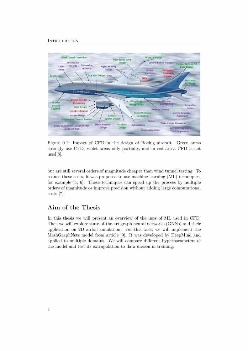
Today, in the aviation industry, thousands of CFD simulations are per-formed every year [4] and are used in many parts of aircraft design, as shownin Figure 0.1. These simulations are costly in terms of time and resources,

3

Introduction

Figure 0.1: Impact of CFD in the design of Boeing aircraft. Green areasstrongly use CFD, violet areas only partially, and in red areas CFD is notused[8].

but are still several orders of magnitude cheaper than wind tunnel testing. Toreduce these costs, it was proposed to use machine learning (ML) techniques,for example [5, 6]. These techniques can speed up the process by multipleorders of magnitude or improve precision without adding large computationalcosts [7].

Aim of the ThesisIn this thesis we will present an overview of the uses of ML used in CFD.Then we will explore state-of-the-art graph neural networks (GNNs) and theirapplication on 2D airfoil simulation. For this task, we will implement theMeshGraphNets model from article [9]. It was developed by DeepMind andapplied to multiple domains. We will compare different hyperparameters ofthe model and test its extrapolation to data unseen in training.

4

Chapter 1Aerodynamics

In this chapter, we will introduce forces acting on an airplane. Then we willintroduce an airfoil, describe it and present why it is useful in aircraft design.Then we explore the Navier-Stokes equations, the governing equations of fluid.

Aerodynamics is the study of forces and the resulting motion of objectsthrough the air. [10] When an airplane fly, there are four main forces actingon it: weight, trust, lift and drag [11].

Weight is a force that is generated by the gravitational force of the Earthand is acting in direction towards it’s center.

Trust is a force generated by the airplane engines. It acts forwards in therelative to the plane.

Lift is part of the force, that acts upwards normal to the line of flight,generated by the flow of air around the airplane. It is generated mainly aroundwings.

Drag is the other part of this force that act backwards along the line offlight.

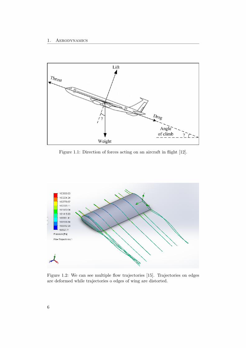
All these forces are shown in Figure 1.1. We will concern ourselves onlywith aerodynamic forces, meaning lift and drag, and only on the wing of theaircraft, since that is where most of the lift and drag is generated.

If we look at Figure 1.2, we can see trajectories deformed on the edges. Forthese trajectories we need full 3D simulation, but if we look at the center of thewing, we can see that the trajectories are the same. If we expected that theairfoil shape is not changing and has an infinite length we could calculate thesimulation in 2D, since the airflow is not impacted by the third dimension [13].In engineering applications the third dimension is often ignored for design ofthe middle section of wing [14].

The front of an airfoil is called leading edge and the furthest end is calledtrailing edge. These two edges are connected by a line called chord line. Thesurfaces of the airfoil are called upper and lower surface. The camber line isa line where each point is the same distance from the nearest points of upperand lower surface. The thickness of an airfoil differs along the airfoil and is

5

1. Aerodynamics

Figure 1.1: Direction of forces acting on an aircraft in flight [12].

Figure 1.2: We can see multiple flow trajectories [15]. Trajectories on edgesare deformed while trajectories o edges of wing are distorted.

6

1.1. Equations of Aerodynamics

chord lineα

trailing edge

leading edge

upper surface

lower surface

camber line

max. camber

relative wind

angle of attack

max. thickness

Figure 1.3: We can see the airfoil and its description [16].

measured perpendicularly to the camber line. An airfoil can be described bythe shape of the camber, thickness and length of the cord line. When airmoves around and airfoil the angle between the camber line and the directionof the wind is called angle of attack. We can see all of the above definedconcepts in Figure 1.3.

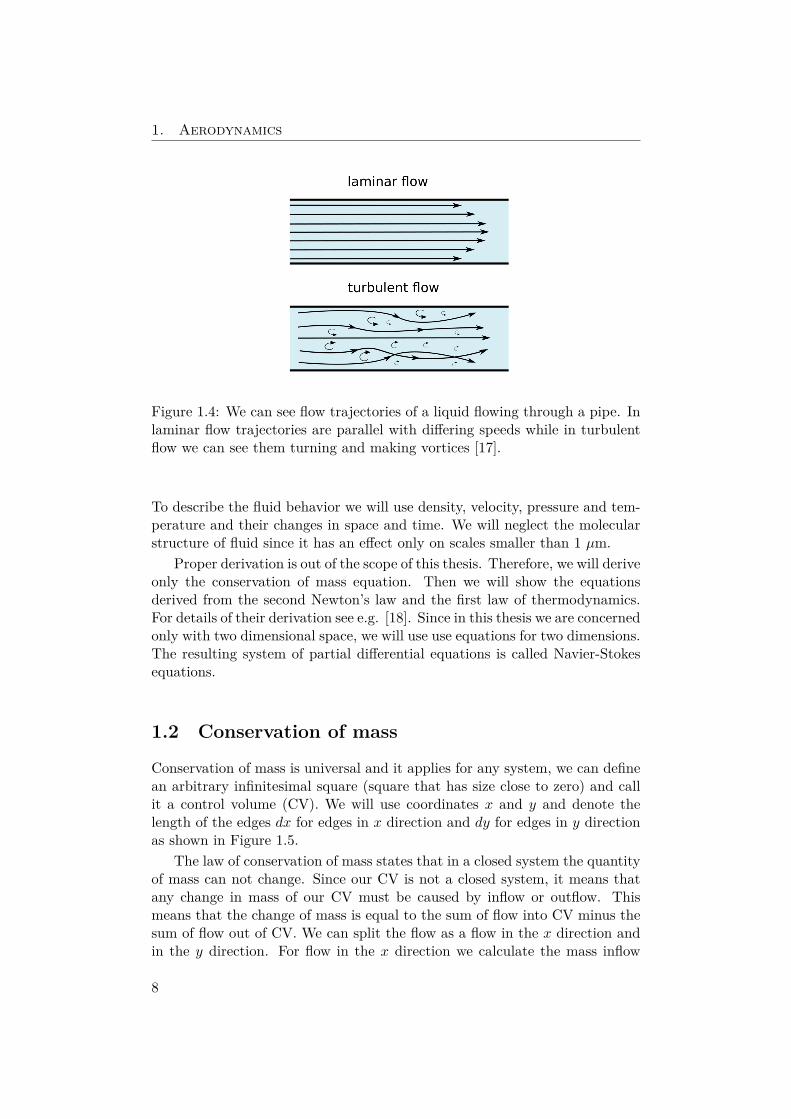
We can separate the movement of air into two categories, laminar andturbulent flow. Laminar flow is when air particles are moving smoothly inlayers and these layers are not mixing in contrast to turbulent flow wherethe particles irregularly mix. We can see illustration of these two flows inFigure 1.4. We can describe the flow of the fluid by Navier-Stokes equationsdeveloped in 19th century by Claude-Louis Navier and improved by GeorgeGabriel Stokes.

1.1 Equations of AerodynamicsTo introduce equations governing fluid flow we will follow [18] here and infollowing sections.

Equations describing the flow represent the mathematical formulation ofthe conservation laws of physics:

• The mass of the fluid is conserved,

• The rate of change of momentum equals the sum of the forces on a fluid,i.e. Newton’s second law,

• The rate of change of energy is equal to the sum of the rate of heataddition to and the rate of work done on a fluid, i.e. the first law ofthermodynamics.

7

1. Aerodynamics

Figure 1.4: We can see flow trajectories of a liquid flowing through a pipe. Inlaminar flow trajectories are parallel with differing speeds while in turbulentflow we can see them turning and making vortices [17].

To describe the fluid behavior we will use density, velocity, pressure and tem-perature and their changes in space and time. We will neglect the molecularstructure of fluid since it has an effect only on scales smaller than 1 µm.

Proper derivation is out of the scope of this thesis. Therefore, we will deriveonly the conservation of mass equation. Then we will show the equationsderived from the second Newton’s law and the first law of thermodynamics.For details of their derivation see e.g. [18]. Since in this thesis we are concernedonly with two dimensional space, we will use use equations for two dimensions.The resulting system of partial differential equations is called Navier-Stokesequations.

1.2 Conservation of mass

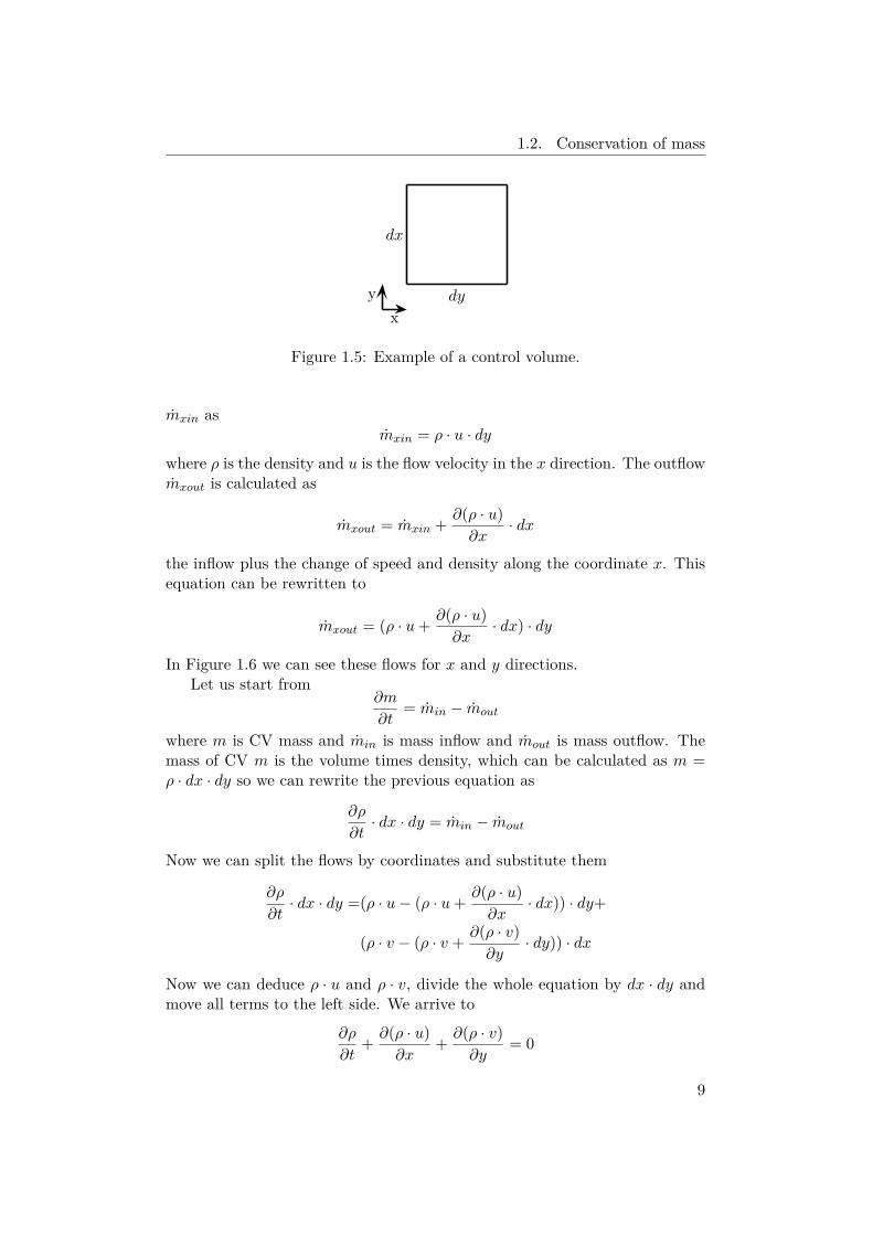
Conservation of mass is universal and it applies for any system, we can definean arbitrary infinitesimal square (square that has size close to zero) and callit a control volume (CV). We will use coordinates x and y and denote thelength of the edges dx for edges in x direction and dy for edges in y directionas shown in Figure 1.5.

The law of conservation of mass states that in a closed system the quantityof mass can not change. Since our CV is not a closed system, it means thatany change in mass of our CV must be caused by inflow or outflow. Thismeans that the change of mass is equal to the sum of flow into CV minus thesum of flow out of CV. We can split the flow as a flow in the x direction andin the y direction. For flow in the x direction we calculate the mass inflow

8

1.2. Conservation of mass

dx

dyyx

Figure 1.5: Example of a control volume.

mxin asmxin = ρ · u · dy

where ρ is the density and u is the flow velocity in the x direction. The outflowmxout is calculated as

mxout = mxin + ∂(ρ · u)∂x

· dx

the inflow plus the change of speed and density along the coordinate x. Thisequation can be rewritten to

mxout = (ρ · u + ∂(ρ · u)∂x

· dx) · dy

In Figure 1.6 we can see these flows for x and y directions.Let us start from

∂m

∂t= min − mout

where m is CV mass and min is mass inflow and mout is mass outflow. Themass of CV m is the volume times density, which can be calculated as m =ρ · dx · dy so we can rewrite the previous equation as

∂ρ

∂t· dx · dy = min − mout

Now we can split the flows by coordinates and substitute them

∂ρ

∂t· dx · dy =(ρ · u − (ρ · u + ∂(ρ · u)

∂x· dx)) · dy+

(ρ · v − (ρ · v + ∂(ρ · v)∂y

· dy)) · dx

Now we can deduce ρ · u and ρ · v, divide the whole equation by dx · dy andmove all terms to the left side. We arrive to

∂ρ

∂t+ ∂(ρ · u)

∂x+ ∂(ρ · v)

∂y= 0

9

1. Aerodynamics

y

x

ρ · u · dy (ρ · u + ∂(ρ·u)∂x · dx) · dy

ρ · v · dx

(ρ · v + ∂(ρ·v)∂y · dy) · dx

Figure 1.6: Control volume with equations for mass flow.

This equation can be rewritten in a more compact form with the divergenceoperator divu = ∂u1

∂x + ∂u2∂y for vector u = (u1, u2) as

∂ρ

∂t+ div(ρu) = 0

for u = (u, v).This equation tells us that the change in density over time plus the change

in density and the speed of flow in the x and y directions must be equal to zeroand is called the mass equation and is the first of the Navier-Stokes equations.

1.3 Navier-Stokes EquationsIf we perform a similar procedure based on Newton’s second law and the firstlaw of thermodynamics, we will obtain the full set of Navier-Stokes equations:

∂ρ

∂t+ div(ρu) = 0 (1.1)

∂(ρu)∂t

+ div(ρuu) = − ∂p

∂x+ div(µ grad u) + SMx (1.2)

∂(ρv)∂t

+ div(ρvu) = −∂p

∂y+ div(µ grad v) + SMy (1.3)

∂(ρi)∂t

+ div(ρiu) = −p div u + div(k grad T ) + Φ + Si. (1.4)

10

1.3. Navier-Stokes Equations

The operator grad is defined as grad u = (∂u∂x , ∂u

∂y ).Equation (1.1) is derived from the conservation of momentum. In equation

ρ stands for density, t for time and u for the vector of velocities. The first termrepresents the change in density over time and the second term the change indensity and flow velocity.

Equations 1.2 and 1.3 are derived from Newton’s second law. In theseequations, u and v represent the velocity in the x and y directions respec-tively, p represents pressure, µ is the proportionality factor and indicates theeffect of the change in velocity on viscosity and SMx and SMy are externalforces acting in the x and y directions respectively. Equation (1.2) representsthe momentum in the x direction, while Equation (1.3) represents the y direc-tion. We will describe the terms of Equation (1.2) and for Equation (1.3) thedirections x and y are flipped. On the left side of the equation, the first thermrepresents the change in velocity and density in the x direction dependent ontime and the second term represents the change in speed and direction de-pendent on the place. The left side is the mass times the acceleration, whereρ stands for the mass and the changes in velocity are the acceleration. Onthe right side, the first term is the change in pressure in the x direction, thesecond is the force of internal stress (effects of viscosity), and the last are theexternal forces acting in the x direction. This part of the equation representsthe force in Newton’s second law.

Equation (1.4) is derived from the first law of thermodynamics. In theequation i stands for internal energy, k is thermal conductivity, T is tempera-ture, Φ is a dissipation function that represents the effects of viscous stresses,and St is the external energy source. On the left side, the first term standsfor the change of internal energy over time and the second for the change indensity,internal energy and velocity dependent on place. On the right side,the first term stands for change of pressure dependent on velocity, the sec-ond term represents thermal exchange, the third term represents the effect ofviscous stresses and the last term represents an external source of energy.

The existence and uniqueness of a solution to the Navier-Stokes equationsis still an open problem and there is no way to derive an analytical solution.Since these equations are the best description of the behavior of a fluid thatwe have, we would like to use them in simulation. Therefore, we can use anumerical approximation.

11

Chapter 2Computational Fluid Dynamics

In this chapter we will introduce computational fluid dynamics and explainthe steps involved in simulation. We will then introduce three types of solvers.

Computational Fluid Dynamics (CFD) simulates fluid flows and their in-teraction with surfaces. These simulations originate from attempts to solvethe Navier-Srokes equations. To be able to solve these equations, the simu-lation space is divided into small cells, similar to the CV from the previouschapter, creating a mesh. When we have an exact time, it is possible to checkif the actual condition meets the equations. Then, if we take a small time step,we can calculate the inflows and outflows of each cell and update the condi-tions to match the equations. This is called spatial and time discretizationand it is the first step of a CDF simulation.

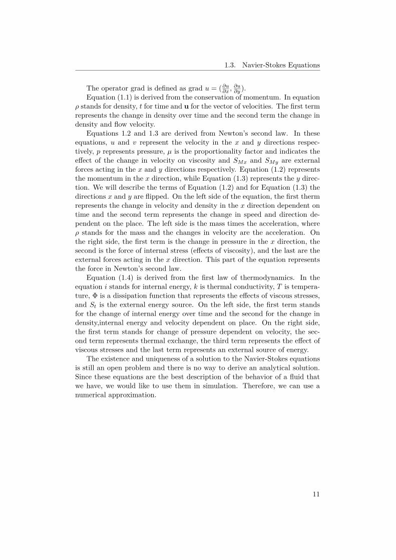
A mesh is an artificial division of the simulation space into small cells, ascan be seen in Figure 2.1. These cells can have different sizes and shapes. Theshape of the cells depends on the geometry of the mesh. The size of the celldepends on the density of the mesh. The density of the mesh depends on theprecision required and the expected flow velocity gradient.[19]

After we select a mesh for our simulation and select the time step, we takethe initial conditions and take their averages in each cell. Then we computethe transport equations.

The transport equations in CFD are the equations that describe the move-ment of the flow in the mesh and the time. They are calculated from theNavier-Strokes equations and are a localized version of them [21]. As men-tioned in the previous chapter, to solve them we use a numerical approxima-tion. The process of finding the matching approximation is called interpola-tion.

There are many methods of interpolation, but the most common is finite-volume interpolation [22]. The idea behind this method is that the volume thatflows into a cell is the same as that that flows out of the cell. The equationsdescribing these flows are then approximated by polynomial functions. Theresult is a system of algebraic equations. We fit these equations to our grid so

13

2. Computational Fluid Dynamics

Figure 2.1: We can see a triangular mesh around an airfoil, far view andzoomed in view. There are dense areas near the airfoil where the biggestchanges are expected [20].

that each cell is represented by one equation.To calculate these equations, we transform them into a linear version and

iterate to obtain the solution. We start by taking a guess, calculating the resultand updating our guess until our solution converges [23]. For this processalgorithms such as SIMPLE, SIMPLEC or PISO are used.

These solutions solve these simulations for laminar flow. For turbulentflows, we need to take into account turbulence on a smaller scale than thedimensions of the mesh cells [24]. We will discuss three different ways oftaking into account these turbulences.

2.1 Direct Numerical SolutionDirect numerical solution (DNS) resolves turbulence near the atomic scale andwith an extremely small time step [25]. This method is used, for example, inparticle dissolution [26], but for larger domains, it is incalculable [24].

2.2 Reynolds-averaged Navier–Stokes modelReynolds-averaged Navier–Stokes model (RANS) is a model derived from theReynolds-averaged Navier-Stokes equations. The idea behind these equationsis to decompose the Navier-Stokes equations into a time-averaged flow (lam-inar) and a fluctuating flow (turbulence). RANS then averages the effect ofthe turbulence and adds to the result. To calculate the average, we use tur-

14

2.3. Large Eddy Simulation

bulence models such as k-ϵ and k-ω. This is the most widely used model inCFD because it is precise and easier to calculate than DNS [24].

2.3 Large Eddy SimulationLarge Eddy Simulation (LES) is a combination of DNS and RANS. LES cal-culates only larger turbulence, and for smaller turbulence, use the turbulencemodel [24]. It has better resolution than RANS, but usually takes about twiceas much resources as RANS [26].

15

Chapter 3Machine Learning

In this chapter we will introduce the basics of ML. Then we will introducethe basic concepts of graph theory and combine it to introduce graph neuralnetworks and message passing neural networks. The purpose of this chapteris to lay the foundation for MeshGraphNets.

3.1 Neuron

Neuron is a small computation unit that has many inputs k1, k2 . . . , kn, anactivation function f , and an output o. The output is calculated as

o = f(n∑

i=1ki)

3.2 Multilayer Perceptron

Multilayer Perceptron (MLP) is a type of neural network. MLP is composedof connected neurons. They are arranged in layers where the inputs of eachneuron are the outputs of the previous layer and bias, multiplied by weights[27], as can be seen in Figure 3.1.

3.3 Residual connection

Residual connection is a type of connection that adds input of a neural networkto its output. This connection is added if output is expected to be similar toinput, because it is easier to learn the small change than near identity [29].

17

3. Machine Learning

Figure 3.1: Neural network layout [28].

3.4 Recurrent neural network

Recurrent neural network (RNN) is a neural network which output zt is notonly dependent on the observed state x but also on the previous state ht−1[30]. We can represent ht as ht = f(ht−1, x) and the result zt as zt = g(ht).Functions f and g are usually implemented as MLP. The connection of ht−1 toinput of function f is called external connection while the connection throughf is called internal [31].

This kind of network is useful for data that are ordered and have strongrelation with previous examples. Good example of such data can be stock costover time.

3.5 Graph

Graph is an ordered pair (V, E) where V is a finite set of nodes and E is finiteset of edges. Edge is an unordered connection of two nodes.

Directed graph differs from graph in that edges are ordered and thereforedirected.

Neighbors of a node v are nodes that are connected by an edge to the nodev. We will note them ne[v].

Incidence in graph is an connection between an edge and a node. A nodev is incident with edge e = (x, y) if v equals x or v equals y. We will note alledges incident to a node v as co[v]. [32]

18

3.6. Graph Neural Network

3.6 Graph Neural NetworkGraph Neural Network (GNN) is a model,defined in [31], extending neuralnetworks for use on data represented in graphs. ”For example, a chemicalcompound can be modeled by a graph G, the nodes of which stand for atoms(or chemical groups) and the edges of which represent chemical bonds linkingtogether some of the atoms.”[31]

The learning set for this model can be defined as

L = (Gi, ni, ti); 1 ≤ i ≤ p

where Gi is the ith graph, ni is the initial state and ti is the target state of ithexample and p is the number of learning examples. This can be simplified toL = (G, T ) where G is a disconnected graph that includes all Gi graphs andT is set of pairs T = (ni, ti); 1 ≤ i ≤ p.

”The intuitive idea underlining the proposed approach is that nodes ina graph represent objects or concepts, and edges represent their relation-ships.”[31] Concepts are therefore defined by there features types of theirrelations and related concepts. Therefore we attach state xn to each noden and a label le to each edge e. The xn represents the state of node n, there-fore it is possible to produce the output on from it. We define l(e1,e2...en) as(le1, le2 . . . len) and the same way for x(e1,e2...en) as (xe1, xe2 . . . xen).

”Let fw be a parametric function, called local transition function, thatexpresses the dependence of a node n on its neighborhood and let gw be thelocal output function that describes how the output is produced.”[31] Then, xn

the new value of xn, and on are defined as

xn = fw(xn, lco[n], xne[n])on = gw(xn)

(3.1)

In Figure 3.2 you can see the use of the local transition function fw.For easier calculation, it is possible to stack their parameters and results

and gain global transition and output functions as

x = Fw(x, lx)o = Gw(x)

(3.2)

where x is stacked xn, x is stacked xn, o is stacked on and lx is stacked lco[n]and xne[n]. Since the number of node’s neighbors may differ, there are manypossibilities of solving this issue. If the order of neighbors is influential, wecan add padding with null values. If not, we can replace the function fw fromequation 3.1 with

xn =∑

u∈ne[n]hw(xn, l(n,u), xu) (3.3)

19

3. Machine Learning

x4

x2

x3

x1

x5

x6

l7

l6

l1

l2

l5

l4

l3

l8

l9

x1 = fw( x1︸︷︷︸xn

l1, l2, l3, l4︸ ︷︷ ︸lco[n]

, x3, x4, x5, x6︸ ︷︷ ︸xne[n]

)

Figure 3.2: Graph example and update of node state.

where l(n,u) represents the edge between n and u. From (3.1), we can computethe next state and the next output by iterating:

xn(t + 1) = fw(xn(t), lco[n], xne[n](t))o(t) = gw(xn(t))

(3.4)

These equations can be represented by the network shown in Figure 3.3. Ifwe implement the function fw and gw as MLP. We get an RNN with internaland external connections, where the internal connections are determined bythe MLP, and the external connections are determined by the initial graphedges. We can rewrite the equations to match the RNN equations as follows:

x(t) = Fw(tw(x(t − 1)), lx)o(t) = Gw(x(t))

(3.5)

where tw is the external connection that rearranges the states according tothe initial edges of the graph.

3.7 Message Passing Neural NetworkMessage Passing Neural Network (MPNN) is a special type of GNN proposedin [33]. MPNN defines the transition function (marked fw) in much more

20

3.7. Message Passing Neural Network

x1

x2

x3

l1

l2

fw

fw

fw

gw

gw

gw

o1(t)

o2(t)

o3(t)

x3(t)

x1(t)

x2(t)

x1(t)

x1(t)

x2(t)

x3(t)

fw

fw

fw

fw

fw

fw

fw

fw

fw

. . .

. . .

. . .

gw

gw

gw

o1(t)

o2(t)

o3(t)t0t1tntime

Figure 3.3: Graph (on top) gets encoded (in the middle) and then unfoldedto network (bottom). The network layers are connected the same way as inthe graph.

21

3. Machine Learning

detail and on depends not only on neighbors, but also on nodes farther away.This allows MPNN to pass information further into the graph.

MPNN consists of T message passing steps that are followed by a read-outphase. In the message passing step, a message mt+1

v is calculated for eachnode v as

mt+1v =

∑u∈ne[n]

hw(xv, l(v,u), xu) (3.6)

This equation is similar to (3.3) but does not update the node directly. Nodev is updated by the second function uw as

xt+1v = uw(xt

v, mt+1v ) (3.7)

After T steps a readout function R is used to extract the results per node as

o = R({xn|n ∈ G}) (3.8)

22

Chapter 4Revue of ML for CFD

In this chapter we will review the application of ML in CFD.Machine learning in CFD is used to achieve two main goals, simulation

acceleration and improving physical understanding [7]. We can divide ML inCFD into two main categories. The complete replacement of a CFD solverby a ML model and CFD solvers assisted by a ML model. When a CFDsolver is completely replaced, the results are generally worse and many modelshave problems generalizing, but can perform up to three orders of magnitudefaster [34]. When ML helps a CFD model, it is usually used to replace someapproximations in the model. This improves precision, which can be tradedfor a coarser grid and increases the speed of the solver.

In article [35] ML is used in DNS to more precisely interpolate partialdifferential equations; therefore, allowing for a coarser grid and speeding upthe simulation. Multiple equations were tested, for example, Burger’s equation(movement of shock information in 1D) or the Kuramoto-Sivashinsky equation(evolution of flame). The drawbacks of this method are the need for DNStraining data, which can be calculated only for really small problems, and inthis article it is used only in 1D.

In article [7] a convolutional network is used to accelerate DNS and LES.This is achieved by using a coarser grid. The network is trained to replace thepolynomial approximation in the interpolation step in CFD. The network istrained on the difference between a DNS solution on a dense grid and a DNS orLES on a coarser grid. Therefore, the network learns not only to interpolate,but also to reduce the error created by the coarser grid. It is shown that thiscan outperform an 8-time denser grid (in 2D, an 8-time denser grid has 64times more cells) and is up to 80 times faster with the same resolution.

In article [36] MLP is used to replace finite-volume interpolation. Thismethod speeds up the solution and decreases the one-step error; the draw-back of this method is that it accumulates errors in the rollouts. To solvethis problem, this method was proposed in conjunction with basic CFD so-lutions, where once in n steps, the CFD solution calculates the finite-volume

23

4. Revue of ML for CFD

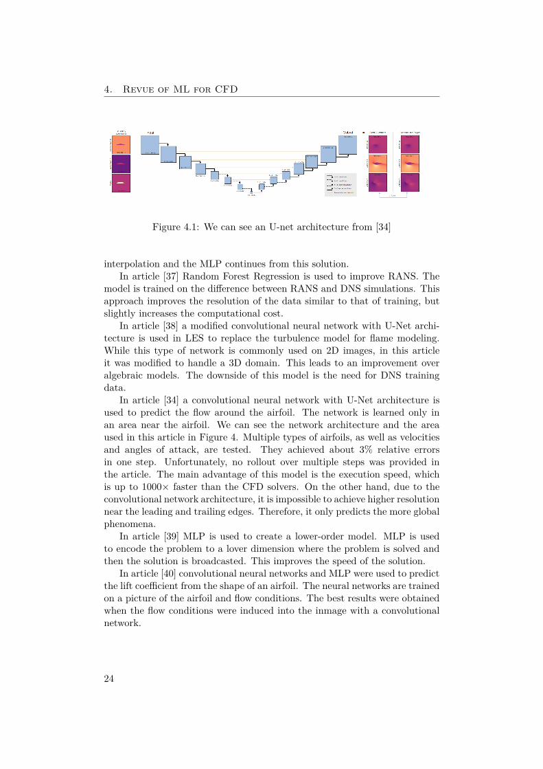
Figure 4.1: We can see an U-net architecture from [34]

interpolation and the MLP continues from this solution.In article [37] Random Forest Regression is used to improve RANS. The

model is trained on the difference between RANS and DNS simulations. Thisapproach improves the resolution of the data similar to that of training, butslightly increases the computational cost.

In article [38] a modified convolutional neural network with U-Net archi-tecture is used in LES to replace the turbulence model for flame modeling.While this type of network is commonly used on 2D images, in this articleit was modified to handle a 3D domain. This leads to an improvement overalgebraic models. The downside of this model is the need for DNS trainingdata.

In article [34] a convolutional neural network with U-Net architecture isused to predict the flow around the airfoil. The network is learned only inan area near the airfoil. We can see the network architecture and the areaused in this article in Figure 4. Multiple types of airfoils, as well as velocitiesand angles of attack, are tested. They achieved about 3% relative errorsin one step. Unfortunately, no rollout over multiple steps was provided inthe article. The main advantage of this model is the execution speed, whichis up to 1000× faster than the CFD solvers. On the other hand, due to theconvolutional network architecture, it is impossible to achieve higher resolutionnear the leading and trailing edges. Therefore, it only predicts the more globalphenomena.

In article [39] MLP is used to create a lower-order model. MLP is usedto encode the problem to a lover dimension where the problem is solved andthen the solution is broadcasted. This improves the speed of the solution.

In article [40] convolutional neural networks and MLP were used to predictthe lift coefficient from the shape of an airfoil. The neural networks are trainedon a picture of the airfoil and flow conditions. The best results were obtainedwhen the flow conditions were induced into the inmage with a convolutionalnetwork.

24

Chapter 5MeshGraphNets

In this chapter we will introduce MeshGraphNets, describe its design andintroduce a special training trick that achieves stability in rollouts.

5.1 IntroductionMeshGraphNets are state-of-the-art GNN models for physics modeling from[9]. It was developed by DeepMind in 2020. It is used for physics simulationson meshes. In the article, they demonstrated its use to model compressibleand incompressible flows, structural mechanics, and the interaction of clothswith the wind.

5.2 Model DesignThe model is a special type of MPNN. In this model, we have features not onlyin nodes, but also at edges and the edges are oriented. This model consists ofan encoder, processor and decoder. The input of this model is the state st ofthe simulation at time t and the result rt is the change in state between timest and t + 1. To obtain the state at t + 1, we add the result to the previousstate as follows:

st+1 = st + rt.

Before using the model, we modify the input state. Each edge of the meshis converted into two edges connecting the same nodes in opposite directions.For each edge eij = (ui, uj) we add relative positional features, it’s displace-ment vector uij = ui − uj and it’s length |uij |. For each node vi we use asubset of dynamical characteristics (velocity, pressure, density,temperature)and one hot encoding the type of node (inflow, normal and airfoil). Then westandardize all edge and node features according to the following:

X ′ = X − µ

σ(5.1)

25

5. MeshGraphNets

Encoder

Input

Processor

Decoder

+

Output

Message passing step 1

Message passing step 2

Message passing step n

···

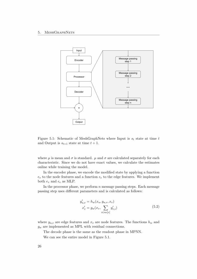
Figure 5.1: Schematic of MeshGraphNets where Input is st state at time tand Output is st+1 state at time t + 1.

where µ is mean and σ is standard. µ and σ are calculated separately for eachcharacteristic. Since we do not have exact values, we calculate the estimatesonline while training the model.

In the encoder phase, we encode the modified state by applying a functionev to the node features and a function ee to the edge features. We implementboth ev and ee as MLP.

In the processor phase, we perform n message passing steps. Each messagepassing step uses different parameters and is calculated as follows:

y′u,v = hw(xu, yu,v, xv)

x′v = gw(xv,

∑i∈ne[v]

y′v,i) (5.2)

where yu,v are edge features and xv are node features. The functions hw andgw are implemented as MPL with residual connections.

The decode phase is the same as the readout phase in MPNN.We can see the entire model in Figure 5.1.

26

5.3. Training

5.3 TrainingFor training we use the state at time t as the input state and the state attime t + 1 as the ground truth. This presents a problem when we run thesimulation. In each step, the model may predict a small error that our modeldid not encounter when training and this error can accumulate. Therefore,if we could add this type of inaccuracy to our training, we could reduce thisaccumulation of errors. We do this by adding small random values to ourinput and result data. This approach was proposed in [41] and used in [9] andhad a huge positive effect in removing this error. The authors of both articlesdo not fully understand this phenomenon and will investigate it further.

27

Chapter 6Implementation

In this chapter we will describe our implementation of MeshGraphNets andintroduce the main libraries used in the implementation. Later, we will discussthe hyperparameters of the model and mention where we trained our models.

In article [9] an implementation was provided. Unfortunately, this imple-mentation was not complete, for example, predicting different features thenvelocity was not possible. Also, we did not have a training environment forTensorFlow 1 that their implementation used. Therefore, we decided to com-pletely reimplement the MeshGraphNets. The reimplementation also provideda good ground for further research.

6.1 Technologies

For the practical part of this thesis, we chose Python1 as the programminglanguage due to its prevalence and available libraries.

We use the Google-developed TensorFlow2 machine learning framework.It provides the ability to run our code on GPU, which improves the speed ofoperations, as well as tensor manipulation functions, that we used for datamanipulation and calculation of training metrics.

Sonnet3 is a DeepMind-developed machine learning library built on top ofTensorFlow. Sonnet provides a high-level object-oriented API. We used it todefine and train our model.

Graph Nets4 is another DeepMind-developed library. It is used to buildgraph networks in Tensorflow and Sonnet. This library provides us with agraph net block, a class that updates one of the types of features by the

1python.org2tensorflow.org3deepmind.com/open-source/deepmind-sonnet4deepmind.com/open-source/graph-nets

29

6. Implementation

corresponding features, which can be used to build almost any type of graphneural network.

We also used Matplotlib5, a visualization library to plot data in human-readable form. It was used for visualization of results and for monitoringpurposes.

6.2 ArchitectureArchitecture of my implementation was directly inspired by the implemen-tation provided in [9]. EncodeProcessDecode is a class that represents themodel, and each message passing step is represented as an instance of theOnePass class. This class is composed of two graph net blocks. The first isfor updating the edge features and the second is for updating the node fea-tures. EncodeProcessDecode also implements the encoding and decoding ofthe graph. Normalization with online training is implemented by the Normal-izer class.

6.3 HyperparametersThere is a large number of hyperparameters for this model. In the encodephase, the size of encoded node and edge features and the number and sizeof layers in the encoding MLPs. In the process phase, the number of messagepassing steps and the shape of MLPs that implement node and edge functions.In the decoder phase, the shape of the MLP that implements the readout func-tion is the only hyperparameter. To decrease the number of hyperparameters,we decided to use the same shape of MLPs in all their uses and the same sizeof the encoded node and edge features, since according to [9] it has a smalleffect on the result.

For training, the hyperparameters are the amount of noise added as well asthe selection of predicted variables, in our case a subset of velocity, pressure,density and temperature. Other hyperparameters for training are the batchsize, learning rate, number of iterations and optimizer.

6.4 HardwareWe trained our model on a server provided by the faculty. This server has fourx Tesla V100-DGXS-32GB GPUs, 20 core m Intel(R) Xeon(R) CPU E5-2698v4 and 256 GB of RAM. This server is shared with other students; therefore,for training, we used one GPU and there were other processes sharing thisGPU. For less computationally difficult processes, we used Google colabora-tory and local environment for development. Although we had access to such

5matplotlib.org

30

6.4. Hardware

computationally strong hardware, the average training time of one model was15 days.

31

Chapter 7Experiments

We will start by introducing the default hyperparameters for the model anddescribe the dataset used in the experiments. We will then conduct experi-ments to tune our model. We will do several experiments to understand ourmodel and the effects of its hyperparameters.

7.1 Default hyperparametersIn experiments we decided to use the default hyperparameters from the [9]implementation and modify them. The default hyperparameters are:

• predicted variables - speed

• training noise - 0.02

• batch size - 2

• learning steps - 107

• learning rate - decreasing from 10−4 to 2 · 10−6 over 107 learning steps

• optimizer - Adam

• MLP shape - two layers with 128 neurons

• node and edge features size - 128

• message passing steps - 15

7.2 DatasetIn this thesis, we use the dataset from article [9]. The dataset is generated bySU2 using RANS. SU2 is open source software for solving partial differential

33

7. Experiments

equations [42]. In the dataset there are 1000 training, 100 validation, and100 test trajectories with different angles of attack and velocity, but the sameairfoil. Each trajectory has 600 steps and each time step is equal to 0.008 s.The solver used compressible Navier-Stock equations. In the simulation, anirregular triangular 2D mesh with 5233 nodes and 15449 edges was used. Theairfoil is symmetric and is 2 m long with a maximum width of 12 cm. Themesh is a circle around this airfoil with a diameter of 40 m. The longest edgesin the mesh are 3.5 m, on the edges of the mesh, and the shortest are 0.25 mm,at the trailing edge of the airfoil. In the training part, there are trajectorieswith an angle of attack between −25◦ and 25◦ and a velocity between 0.2Mand 0.7M (M mach number). In the validation and test datasets, there aretrajectories with angle of attack between −35◦ and 35◦ and velocity between0.2M and 0.9M .

7.3 Effect of number of message passing stepsIn this experiment we decided to compare the effect of the number of messagepassing steps on the model. Regarding the number of message passing stepsthat will be tested, we decided on 12, 15 and 18. We chose this based on [9]where 15 message passing steps were selected and 12 and 18 message passingsteps were selected to observe the change in both directions and to allow thechange to be large enough to have an effect. We call these models m-12, m-15and m-18.

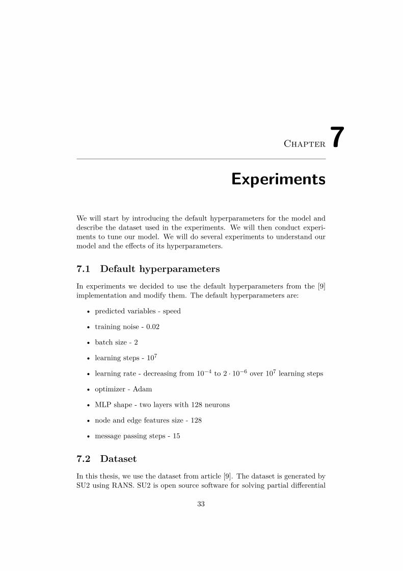
We start with models m-12 and m-15. In Figure 7.1 we can see the devel-opment of loss and error. We can see that the one-step error is larger thanthe averaged error over multiple steps. Since we are trying to obtain the bestresult over multiple steps, we will choose the best iteration based on the meanMSE in 20 steps, as can be seen in Figure 7.2. The exact selected iterationscan be seen in Table 7.1.

For the m-18 model, we can see in Figure 7.3 that its loss does not de-crease. This is an unexpected behavior, and we are not sure why this behavioroccurred for this model and not for the others.

We compared the model on the full development set. As we can see inTable 7.1, model m-15 outperforms model m-12 by approximately 33% on theentire trajectory. Interestingly, model m-12 is slightly better over 10 and 20steps.

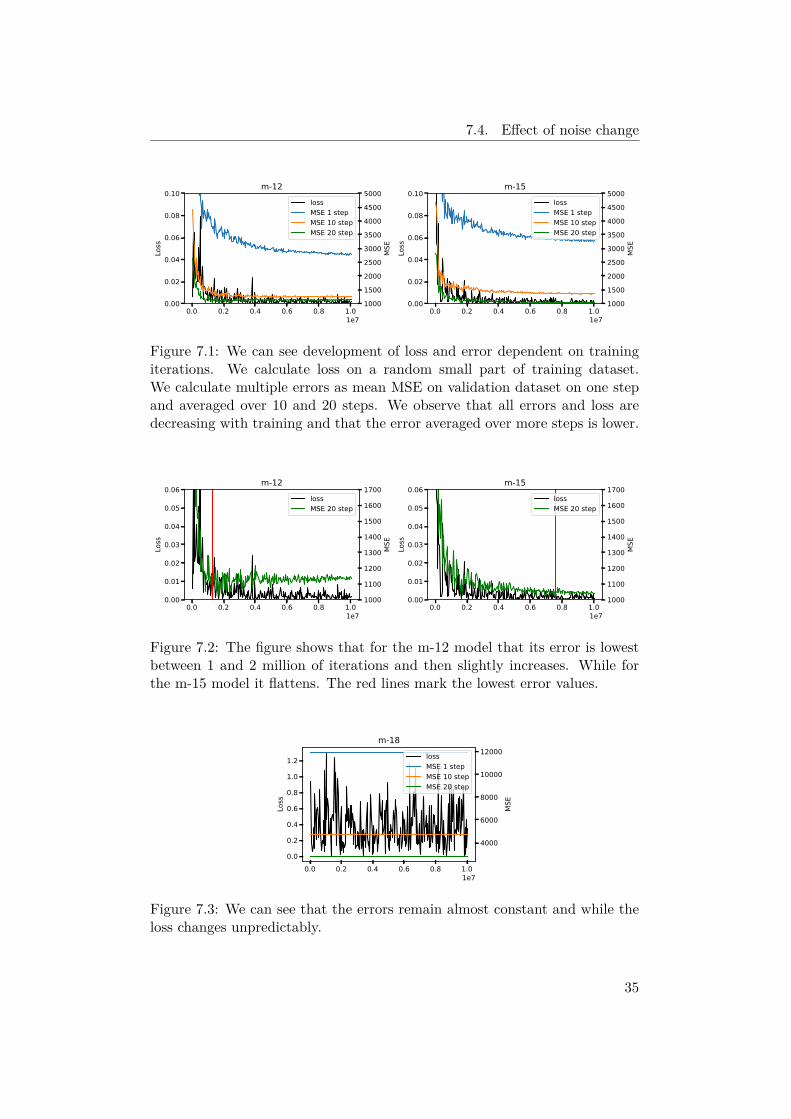
7.4 Effect of noise changeWe noticed that the default value from implementation is 0.02 while in thearticle the value is 1. Therefore, we decided to test which training noise levelgives us a better result. We used the model with 12 message passing stepsfrom the previous experiment and trained a model m-12n with 12 message

34

7.4. Effect of noise change

0.0 0.2 0.4 0.6 0.8 1.01e7

0.00

0.02

0.04

0.06

0.08

0.10

Loss

m-12

0.0 0.2 0.4 0.6 0.8 1.01e7

0.00

0.02

0.04

0.06

0.08

0.10

Loss

m-15

100015002000250030003500400045005000

MSE

lossMSE 1 stepMSE 10 stepMSE 20 step

100015002000250030003500400045005000

MSE

lossMSE 1 stepMSE 10 stepMSE 20 step

Figure 7.1: We can see development of loss and error dependent on trainingiterations. We calculate loss on a random small part of training dataset.We calculate multiple errors as mean MSE on validation dataset on one stepand averaged over 10 and 20 steps. We observe that all errors and loss aredecreasing with training and that the error averaged over more steps is lower.

0.0 0.2 0.4 0.6 0.8 1.01e7

0.00

0.01

0.02

0.03

0.04

0.05

0.06

Loss

m-12

0.0 0.2 0.4 0.6 0.8 1.01e7

0.00

0.01

0.02

0.03

0.04

0.05

0.06

Loss

m-15

1000

1100

1200

1300

1400

1500

1600

1700

MSE

lossMSE 20 step

1000

1100

1200

1300

1400

1500

1600

1700

MSE

lossMSE 20 step

Figure 7.2: The figure shows that for the m-12 model that its error is lowestbetween 1 and 2 million of iterations and then slightly increases. While forthe m-15 model it flattens. The red lines mark the lowest error values.

0.0 0.2 0.4 0.6 0.8 1.01e7

0.0

0.2

0.4

0.6

0.8

1.0

1.2

Loss

m-18

4000

6000

8000

10000

12000

MSE

lossMSE 1 stepMSE 10 stepMSE 20 step

Figure 7.3: We can see that the errors remain almost constant and while theloss changes unpredictably.

35

7. Experiments

Table 7.1: Comparison of models on full trajectory on validation data as wellas over one, then and twenty steps.

Model Iteration MSE over MSE over MSE over MSE overname 1-step 10-steps 20-steps full trajectorym-12 1240000 3797 13165 20438 22,554,182m-15 7520000 3308 13561 20485 14,803,762

0.0 0.5 1.0 1.5 2.01e6

0.00

0.02

0.04

0.06

0.08

0.10

Loss

m-12n

0.0 0.5 1.0 1.5 2.01e6

0.00

0.02

0.04

0.06

0.08

0.10

Loss

m-12n

2000

4000

6000

8000

10000

MSE

lossMSE 1 stepMSE 10 stepMSE 20 step

7501000125015001750200022502500

MSE

lossMSE 20 step

Figure 7.4: We can see how the second derivation of velocity summed overall nodes dependent on the step in rollout. The left shows this change on fullrollout while the right one only for the start.

Table 7.2: Comparison of models on full trajectory on validation data as wellas over one, the and twenty steps.

Model Iteration MSE over MSE over MSE over MSE overname 1-step 10-steps 20-steps full trajectorym-12 1240000 3797 13165 20438 22,554,182m-12n 1960000 1817 9076 15434 3,323,552

passing steps and noise value of 1. Because for the m-12 model, we selectedlow iteration and due to time constraints, we decided to decrease the learningsteps to 2.3 × 106 steps. We can see the development of loss and errors inFigure 7.4, as well as the selection of iteration.

From Table 7.2 we can see that increasing the noise decreased the MSEin all steps and on the entire trajectory approximately 7 times compared totraining without noise.

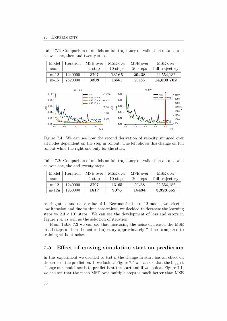
7.5 Effect of moving simulation start on predictionIn this experiment we decided to test if the change in start has an effect onthe error of the prediction. If we look at Figure 7.5 we can see that the biggestchange our model needs to predict is at the start and if we look at Figure 7.1,we can see that the mean MSE over multiple steps is much better than MSE

36

7.6. Predicting multiple variables

0 100 200 300 400 500 600Rollout step

0

2000

4000

6000

8000

Seco

nd d

eriv

atio

n of

vel

ocity

0 5 10 15Rollout step

0

2000

4000

6000

8000

Figure 7.5: We can see how the second derivation of velocity summed overall nodes dependent on the step in rollout. The left shows this change on fullrollout while the right one only for the start.

0 25 50 75 100 125 150 175 2000

2500

5000

7500

10000

12500

15000

MSE

Start at 0Start at 5Start at 10Start at 20Start at 30Start at 50Start at 100

0 5 10 15 20 25 300

200

400

600

800

MSE

Start at 0Start at 5Start at 10Start at 20Start at 30Start at 50Start at 100

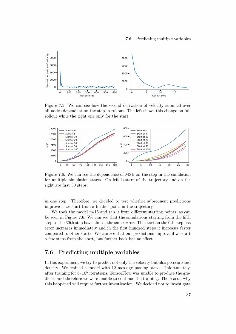
Figure 7.6: We can see the dependence of MSE on the step in the simulationfor multiple simulation starts. On left is start of the trajectory and on theright are first 30 steps.

in one step. Therefore, we decided to test whether subsequent predictionsimprove if we start from a further point in the trajectory.

We took the model m-15 and ran it from different starting points, as canbe seen in Figure 7.6. We can see that the simulations starting from the fifthstep to the 30th step have almost the same error. The start on the 0th step haserror increases immediately and in the first hundred steps it increases fastercompared to other starts. We can see that our predictions improve if we starta few steps from the start, but further back has no effect.

7.6 Predicting multiple variablesIn this experiment we try to predict not only the velocity but also pressure anddensity. We trained a model with 12 message passing steps. Unfortunately,after training for 6 ·105 iterations, TensorFlow was unable to produce the gra-dient, and therefore we were unable to continue the training. The reason whythis happened will require further investigation. We decided not to investigate

37

7. Experiments

further due to time constraints and we prioritized other experiments. We willexplain this in more detail in the conclusion.

38

Chapter 8Results

In this chapter we will compare the models from the previous chapter andpresent results of our simulations and compare our model to model from [9].

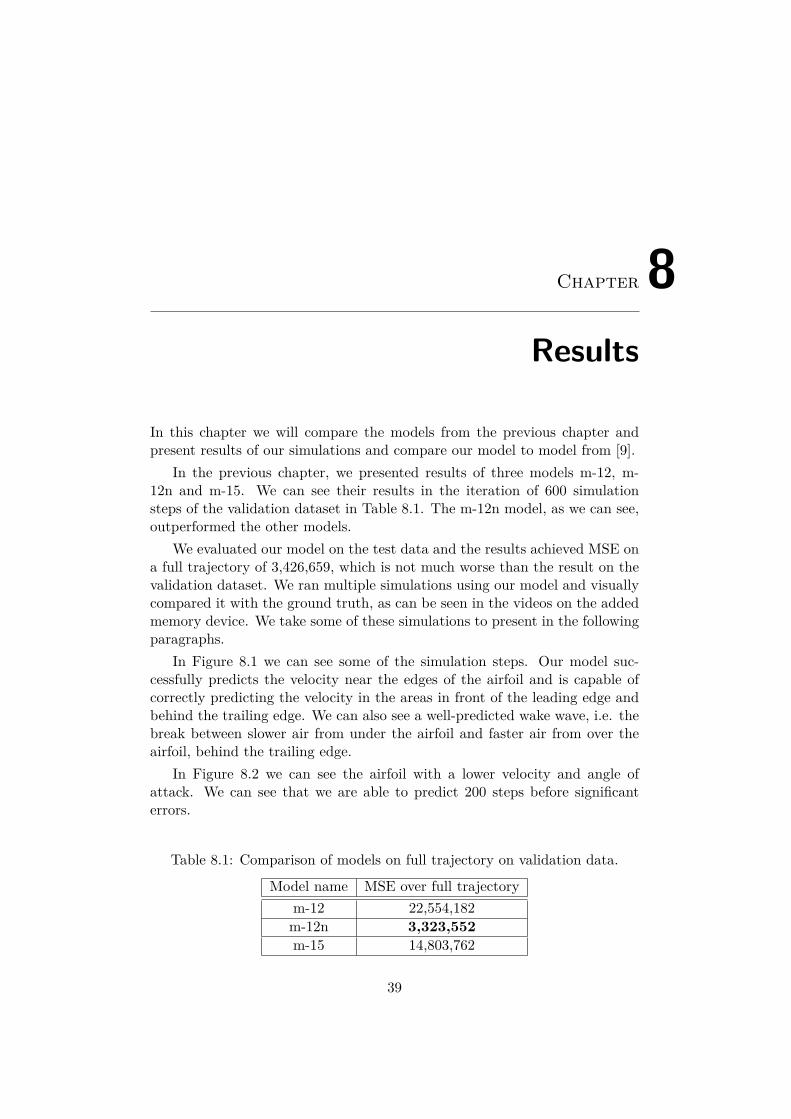
In the previous chapter, we presented results of three models m-12, m-12n and m-15. We can see their results in the iteration of 600 simulationsteps of the validation dataset in Table 8.1. The m-12n model, as we can see,outperformed the other models.

We evaluated our model on the test data and the results achieved MSE ona full trajectory of 3,426,659, which is not much worse than the result on thevalidation dataset. We ran multiple simulations using our model and visuallycompared it with the ground truth, as can be seen in the videos on the addedmemory device. We take some of these simulations to present in the followingparagraphs.

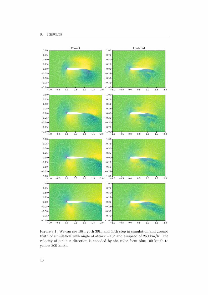
In Figure 8.1 we can see some of the simulation steps. Our model suc-cessfully predicts the velocity near the edges of the airfoil and is capable ofcorrectly predicting the velocity in the areas in front of the leading edge andbehind the trailing edge. We can also see a well-predicted wake wave, i.e. thebreak between slower air from under the airfoil and faster air from over theairfoil, behind the trailing edge.

In Figure 8.2 we can see the airfoil with a lower velocity and angle ofattack. We can see that we are able to predict 200 steps before significanterrors.

Table 8.1: Comparison of models on full trajectory on validation data.

Model name MSE over full trajectorym-12 22,554,182m-12n 3,323,552m-15 14,803,762

39

8. Results

1.0 0.5 0.0 0.5 1.0 1.5 2.01.00

0.75

0.50

0.25

0.00

0.25

0.50

0.75

1.00Correct

1.0 0.5 0.0 0.5 1.0 1.5 2.01.00

0.75

0.50

0.25

0.00

0.25

0.50

0.75

1.00Predicted

1.0 0.5 0.0 0.5 1.0 1.5 2.01.00

0.75

0.50

0.25

0.00

0.25

0.50

0.75

1.00

1.0 0.5 0.0 0.5 1.0 1.5 2.01.00

0.75

0.50

0.25

0.00

0.25

0.50

0.75

1.00

1.0 0.5 0.0 0.5 1.0 1.5 2.01.00

0.75

0.50

0.25

0.00

0.25

0.50

0.75

1.00

1.0 0.5 0.0 0.5 1.0 1.5 2.01.00

0.75

0.50

0.25

0.00

0.25

0.50

0.75

1.00

1.0 0.5 0.0 0.5 1.0 1.5 2.01.00

0.75

0.50

0.25

0.00

0.25

0.50

0.75

1.00

1.0 0.5 0.0 0.5 1.0 1.5 2.01.00

0.75

0.50

0.25

0.00

0.25

0.50

0.75

1.00

Figure 8.1: We can see 10th 20th 30th and 40th step in simulation and groundtruth of simulation with angle of attack −13◦ and airspeed of 260 km/h. Thevelocity of air in x direction is encoded by the color form blue 100 km/h toyellow 300 km/h.

40

1.0 0.5 0.0 0.5 1.0 1.5 2.01.00

0.75

0.50

0.25

0.00

0.25

0.50

0.75

1.00Correct

1.0 0.5 0.0 0.5 1.0 1.5 2.01.00

0.75

0.50

0.25

0.00

0.25

0.50

0.75

1.00Predicted

1.0 0.5 0.0 0.5 1.0 1.5 2.01.00

0.75

0.50

0.25

0.00

0.25

0.50

0.75

1.00

1.0 0.5 0.0 0.5 1.0 1.5 2.01.00

0.75

0.50

0.25

0.00

0.25

0.50

0.75

1.00

1.0 0.5 0.0 0.5 1.0 1.5 2.01.00

0.75

0.50

0.25

0.00

0.25

0.50

0.75

1.00

1.0 0.5 0.0 0.5 1.0 1.5 2.01.00

0.75

0.50

0.25

0.00

0.25

0.50

0.75

1.00

1.0 0.5 0.0 0.5 1.0 1.5 2.01.00

0.75

0.50

0.25

0.00

0.25

0.50

0.75

1.00

1.0 0.5 0.0 0.5 1.0 1.5 2.01.00

0.75

0.50

0.25

0.00

0.25

0.50

0.75

1.00

Figure 8.2: We can see 50th 100th 150th and 200th step in simulation andground truth of simulation with angle of attack −10◦ and airspeed of 170km/h.The velocity of air in x direction is encoded by the color form blue 100km/h to yellow 300 km/h.

41

8. Results

8.1 Result comparisonUnfortunately we were not able to compare our model exactly with the resultsfrom [9]. The reason is that they calculated the metric only on a rectangularcutout and did not provide its dimensions in the article. From visual compar-ison of produced video simulations, we can see that our model’s predictionsare similar. In some simulations, after close inspection, we can see slight in-consistencies, but if we use more message passing steps, we expect to achievethe same or better results.

42

Conclusion

In this thesis, we introduced concepts to understant how ML can be appliedto CFD. We reviewed many uses of ML in CFD, from CFD solvers aidedby ML to fully ML approaches and present work that uses machine learningnot only to speed up the simulation, but also to improve the precision ofused models. We then introduced MeshGraphNets, a state-of-the-art messagepassing neural network. We reimplemented it and tested the effect of changingthe number of message passing steps within the model architecture. We foundthat a model with 15 message passing steps is better than with 12 while at18 the model is not able to learn with our implementation. Then we testedthe effect of noise applied to training data and found that it is better to usetraining noise with a standard deviation of 1 rather than 0.02. In our nextexperiment, we compare the effect of starting our model at a later step ofthe simulation. We found that it influences the simulation only in the firstfew steps, where the changes in velocity are the greatest. Then we tried totrain the model using more variables than velocity, but were unable to trainit successfully so far. We compared all our models and found that the modelwith 12 message passing steps and training noise with a standard deviationof 1 has at least four times lower MSE than our other models. We comparedthis model with the results provided in the original article and found that ourmodel provides similar results.

Compared to the initial plan, we did not test the ability of the model toextrapolate to different airfoils because we did not expect to reimplement themodel and it proved more complex than initially expected. It was a directionthat we wanted to explore further, but the authors of the original articlealready used this model on airfoils with different shapes in [43] and therefore,after consultations with the authors, we changed the direction of our research.

In future work, we plan to explore different ways to iterate over time.This would increase precision when large changes are expected, such as at thebeginning of the simulation. we plan to publish this as part of the VýLetprogram. Another interesting path to explore would be to scale to velocities

43

Conclusion

over Mach 1, where shock waves begin to form, or to investigate the trainingnoise and why it has such a big effect on the model.

44

Bibliography

[1] Benson, T. How Did We Learn to Fly Like the Birds? [online], ac-cessed: 2022-04-30. Available from: https://www.grc.nasa.gov/www/k-12/UEET/StudentSite/historyofflight.html

[2] Baals, D. D. Wind tunnels of NASA, volume 440. Scientific and TechnicalInformation Branch, National Aeronautics and Space …, 1981.

[3] AMWEL Enterprises. A Brief History of CFD. [online], accessed: 2022-04-21. Available from: http://www.amwel.com/history.html

[4] Johnson, F. T.; Tinoco, E. N.; et al. Thirty years of development andapplication of CFD at Boeing Commercial Airplanes, Seattle. Computers& Fluids, volume 34, no. 10, 2005: pp. 1115–1151.

[5] Tracey, B. D.; Duraisamy, K.; et al. A machine learning strategy to assistturbulence model development. In 53rd AIAA aerospace sciences meeting,2015, p. 1287.

[6] Zhang, Z. J.; Duraisamy, K. Machine learning methods for data-driventurbulence modeling. In 22nd AIAA Computational Fluid Dynamics Con-ference, 2015, p. 2460.

[7] Kochkov, D.; Smith, J. A.; et al. Machine learning–accelerated computa-tional fluid dynamics. Proceedings of the National Academy of Sciences,volume 118, no. 21, 2021.

[8] Spalart, P. R.; Venkatakrishnan, V. On the role and challenges of CFD inthe aerospace industry. The Aeronautical Journal, volume 120, no. 1223,2016: pp. 209–232.

[9] Pfaff, T.; Fortunato, M.; et al. Learning mesh-based simulation withgraph networks. arXiv preprint arXiv:2010.03409, 2020.

45

Bibliography

[10] NASA. Beginner’s Guide to Aerodynamics. [online], accessed: 2010-09-30. Available from: https://www.grc.nasa.gov/WWW/K-12/airplane/bga.html

[11] Talay, T. A. Introduction to the Aerodynamics of Flight. Technical report,NASA, 1975.

[12] Murrieta Mendoza, A. Vertical and lateral flight optimization algorithmand missed approach cost calculation. Dissertation thesis, Mémoire demaîtrise électronique, Montréal, École de technologie supérieure., 06 2013.

[13] Flandro, G. A.; McMahon, H. M.; et al. Basic aerodynamics: incom-pressible flow, volume 31. Cambridge University Press, 2011.

[14] Jonsson, E.; Leifsson, L. T.; et al. Trawl-door Performance Analysis andDesign Optimization with CFD. In SIMULTECH, 2012, pp. 479–488.

[15] Keane, P. Tutorial: Performing Flow Simulation of an Aero-foil. [online], 2018, accessed: 2022-04-12. Available from:https://www.engineersrule.com/tutorial-performing-flow-simulation-aerofoil/

[16] Unknown. Airfoil. [online], accessed: 2022-04-28. Available from: https://en.wikipedia.org/wiki/Airfoil

[17] CFD support. Laminar vs. Turbulent Flow. [online], accessed: 2022-04-28. Available from: https://www.cfdsupport.com/openfoam-training-by-cfd-support/node334.html

[18] Versteeg, H. K.; Malalasekera, W. An introduction to computational fluiddynamics: the finite volume method. Pearson education, 2007.

[19] CFD, C. CFD Meshing Methods. [online], 2021, accessed: 2022-04-08.Available from: https://resources.system-analysis.cadence.com/blog/msa2021-cfd-meshing-methods

[20] SU2. Quick Start. [online], accessed: 2022-05-02. Available from: https://su2code.github.io/docs_v7/Quick-Start/

[21] DMS Marine Consultant. GUTS OF CFD: TransportEquations. [online], 2019, accessed: 2022-04-08. Availablefrom: https://www.youtube.com/watch?v=NaEfgRO59xk&list=PLhupav37c1P96025AWMashika9JvGCgEr&index=8

[22] DMS Marine Consultant. GUTS OF CFD: InterpolationEquations. [online], 2019, accessed: 2022-04-08. Availablefrom: https://www.youtube.com/watch?v=KYAWl8o5TQc&list=PLhupav37c1P96025AWMashika9JvGCgEr&index=10

46

Bibliography

[23] DMS Marine Consultant. GUTS OF CFD: Linear Solver.[online], 2019, accessed: 2022-04-08. Available from:https://www.youtube.com/watch?v=XW0dU7Pjoe0&list=PLhupav37c1P96025AWMashika9JvGCgEr&index=11

[24] DMS Marine Consultant. GUTS OF CFD: Turbulence.[online], 2019, accessed: 2022-04-08. Available from:https://www.youtube.com/watch?v=_eXzSZPprkQ&list=PLhupav37c1P96025AWMashika9JvGCgEr&index=12

[25] Cao, H.; Jia, X.; et al. CFD-DNS simulation of irregular-shaped particledissolution. Particuology, volume 50, 2020: pp. 144–155.

[26] DMS Marine Consultant. CFD METHODS: Overview of CFDTechniques. [online], 2019, accessed: 2022-04-08. Availablefrom: https://www.youtube.com/watch?v=x-pbe3S6YSo&list=PLhupav37c1P96025AWMashika9JvGCgEr&index=2

[27] Goodfellow, I.; Bengio, Y.; et al. Deep learning. MIT press, 2016.

[28] Bahra, G.; Wiese, L. Parameterizing neural networks for disease classifi-cation. Expert Systems, volume 37, 02 2020, doi:10.1111/exsy.12465.

[29] He, K.; Zhang, X.; et al. Deep residual learning for image recognition.In Proceedings of the IEEE conference on computer vision and patternrecognition, 2016, pp. 770–778.

[30] Chen, G. A gentle tutorial of recurrent neural network with error back-propagation. arXiv preprint arXiv:1610.02583, 2016.

[31] Scarselli, F.; Gori, M.; et al. The Graph Neural Network Model. IEEETransactions on Neural Networks, volume 20, no. 1, 2009: pp. 61–80,doi:10.1109/TNN.2008.2005605.

[32] Biggs, N.; Lloyd, E. K.; et al. Graph Theory, 1736-1936. Oxford Univer-sity Press, 1986.

[33] Battaglia, P. W.; Hamrick, J. B.; et al. Relational inductive biases, deeplearning, and graph networks. arXiv preprint arXiv:1806.01261, 2018.

[34] Thuerey, N.; Weißenow, K.; et al. Deep learning methods for Reynolds-averaged Navier–Stokes simulations of airfoil flows. AIAA Journal, vol-ume 58, no. 1, 2020: pp. 25–36.

[35] Bar-Sinai, Y.; Hoyer, S.; et al. Learning data-driven discretizations forpartial differential equations. Proceedings of the National Academy ofSciences, volume 116, no. 31, 2019: pp. 15344–15349, ISSN 0027-8424,doi:10.1073/pnas.1814058116, https://www.pnas.org/content/116/31/

47

Bibliography

15344.full.pdf. Available from: https://www.pnas.org/content/116/31/15344

[36] Jeon, J.; Kim, S. J. FVM Network to reduce computational cost of CFDsimulation. arXiv preprint arXiv:2105.03332, 2021.

[37] Wang, J.-X.; Wu, J.-L.; et al. Physics-informed machine learning ap-proach for reconstructing Reynolds stress modeling discrepancies basedon DNS data. Physical Review Fluids, volume 2, no. 3, 2017: p. 034603.

[38] Lapeyre, C. J.; Misdariis, A.; et al. Training convolutional neural net-works to estimate turbulent sub-grid scale reaction rates. Combustionand Flame, volume 203, 2019: pp. 255–264.

[39] Renganathan, S. A.; Maulik, R.; et al. Machine learning for nonintrusivemodel order reduction of the parametric inviscid transonic flow past anairfoil. Physics of Fluids, volume 32, no. 4, 2020: p. 047110.

[40] Zhang, Y.; Sung, W. J.; et al. Application of convolutional neural net-work to predict airfoil lift coefficient. In 2018 AIAA/ASCE/AHS/ASCstructures, structural dynamics, and materials conference, 2018, p. 1903.

[41] Sanchez-Gonzalez, A.; Godwin, J.; et al. Learning to simulate complexphysics with graph networks. In International Conference on MachineLearning, PMLR, 2020, pp. 8459–8468.

[42] Economon, T. D.; Palacios, F.; et al. SU2: An open-source suite formultiphysics simulation and design. Aiaa Journal, volume 54, no. 3, 2016:pp. 828–846.

[43] Allen, K. R.; Lopez-Guevara, T.; et al. Physical Design using Differen-tiable Learned Simulators. arXiv preprint arXiv:2202.00728, 2022.

48

Appendix AContent of attached medium

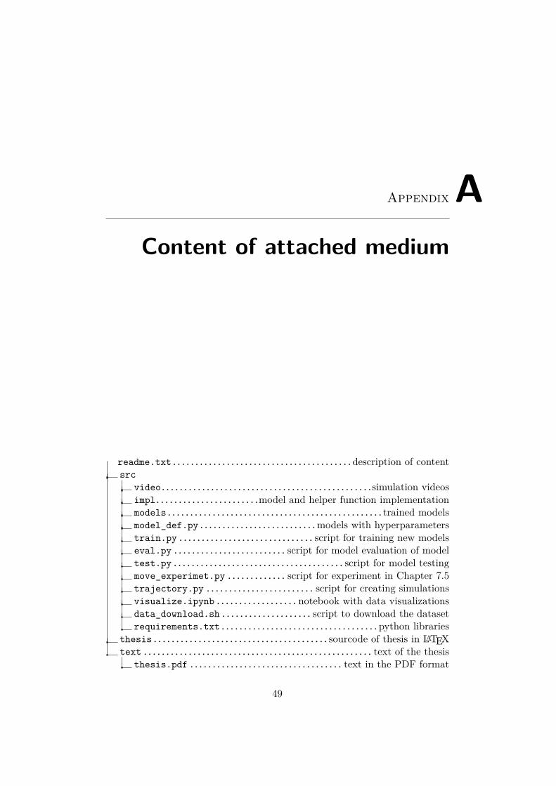
readme.txt........................................description of contentsrc

video...............................................simulation videosimpl.......................model and helper function implementationmodels................................................trained modelsmodel_def.py..........................models with hyperparameterstrain.py..............................script for training new modelseval.py......................... script for model evaluation of modeltest.py......................................script for model testingmove_experimet.py ............. script for experiment in Chapter 7.5trajectory.py ........................ script for creating simulationsvisualize.ipynb..................notebook with data visualizationsdata_download.sh.................... script to download the datasetrequirements.txt...................................python libraries

thesis.......................................sourcode of thesis in LATEXtext................................................... text of the thesis

thesis.pdf.................................. text in the PDF format

49