flight regime mapping for aircraft engine fault diagnosis
TRANSCRIPT

FLIGHT REGIME MAPPING FOR AIRCRAFT ENGINE FAULT DIAGNOSIS
Weizhong Yan *, C. James Li +, Kai F. Goebel *
* Information & Decision Technologies
GE Global Research Center One Research Circle, Niskayuna, NY
12309
{yan, goebelk} @ crd.ge.com
+ Department of MANE Rensselaer Polytechnic Institute
Troy, NY 12181
Abstract: One of the issues that impair the performance of aircraft engine fault diagnosis is the flight
regime. When an aircraft travels from one point to another in flight regime, engine performance
parameters that are used for fault diagnosing change and such changes mask the parameter changes
caused by engine faults, thus make the engine fault diagnosis much more difficult. Properly addressing the
flight regime issue is the key in achieving good aircraft engine fault diagnosis. Currently, the flight regime
issue is typically addressed by flight regime partitioning. That is, the flight regime is partitioned into
several smaller regions and each of the regions is assigned a classifier that is appropriate just for that
region. There are several drawbacks associated with this approach. The fundamental one is that it requires
the design and implementation of a large number of classifiers, which result in a significant increase of the
costs and complexity. In this paper, a novel approach – flight regime mapping - is introduced for tackling
the flight regime issue in aircraft engine fault diagnosis. The proposed flight regime mapping essentially
compensates for flight regime induced parameter changes, thus accentuates the engine condition related
changes, by mapping the engine parameter values from the actual flight regime to sea level static
equivalent. The mapping enables classifiers that are designed for the sea level static condition to work over
the entire flight regime without using multiple classifiers for different regions of flight regime. More
importantly, the mapping is able to improve the performance of aircraft engine fault diagnosis. Empirical
studies are conducted to demonstrate the effectiveness of the flight regime mapping approach in tackling
the flight regime issue in the design of aircraft engine fault diagnostic systems.
Keywords: Aircraft engines; Classification; Diagnostics; Flight regime; Mapping; Neural
networks;
1. Introduction: Aircraft engine fault diagnostic (AEFD) systems are the core of the modern
condition-based maintenance strategy for aircraft engines. The benefits of AEFD systems
may include the following aspects [1]:
• Increasing flight safety by early detection of engine malfunctions.
• Preventing costly component damage and/or catastrophic failure.
• Reducing turnaround time by providing maintenance personnel with information on fault
locations (by reducing time for manual fault isolation).
• Reducing delays and cancellations by facilitating more on-wing maintenance.
• Increasing engine on-wing time by minimizing scheduled and unscheduled engine removal.
Aircraft engine fault diagnosis is a difficult task due to the following intrinsic characteristics
related to aircraft engines:
• There exist engine initial quality variations. Engine initial quality variation is the results of
the variation of fabricating and assembling. The engine initial quality varies from engine to
engine even within the same engine models.

• Engine quality deteriorates over time. Engine deterioration is caused by many effects, such
as, tip clearance changes in the rotating components, seal wear, blade fouling, blade erosion,
blade warping, foreign object damage, actuator wear, and blocked fuel nozzles [2]. Engine
deterioration results in engine performance parameter changes over time (time-varying).
• Aircraft engines are operated at different points in flight regime. When an aircraft travels
from one point to another in flight regime, the engine performance parameters change
following the principles of thermodynamics and aerodynamics.
Due to the importance and the challenges, aircraft engine fault diagnosis has drawn tremendous
amount of research interests. With advances in modern aircraft engines, designing a reliable and
cost-effective AEFD system continues to be the most interesting research topic in fault diagnosis.
This paper is concerned with the flight regime issue in the design of AEFD system. Engines when
operating at different points in flight regime result in changes of engine performance parameters.
Such “inherent” or not-fault-related changes may resemble the changes caused by engine
faults/abnormality and therefore “confuse” the engine fault diagnostic system. Properly
addressing such flight regime issue is the key to improving the performance of AEFD systems. In
this paper, we propose an innovative method, flight regime mapping, to tackle the flight regime
issues so that a more accurate and reliable AEFD system can be achieved.
The rest of this paper is organized as follows. Section 2 presents the flight regime problem and
the related work in addressing the flight regime problem. Section 3 details proposed flight regime
mapping method. Section 4 describes an AEFD system design example that is used to
demonstrate the effectiveness of flight regime mapping. The classification performance of the
AEFD system designed using flight regime mapping is given in Section 5. Section 6 concludes
the paper.
2. Flight regime problem and related work: One of the inherent characteristics of aircraft
engines is that they need to be operated at various points of flight regime (different altitudes and
Mach numbers), more broadly
at various operating points in
the operating space typically
defined by four dimensions:
the altitude, the Mach number,
the ambient temperature, and
the TRA value (the power
setting). When aircraft travels
from one point to another in
flight regime, or from one
operating point to another, the
engine performance parameters
that are used for fault
diagnosing change and such
changes mask the parameter
changes caused by engine
faults, thus makes the engine
fault diagnosis much more
difficult. To illustrate this
masking effect, let’s look at Figure 1: Flight regime effects on engine parameters

Figure 1, where histograms of the compressor exit temperature, one of the engine performance
parameters, for three engine conditions are shown.
While Figure 1.A shows the compressor exit temperature at sea level static (S.L.S), Figure 1.B is
for the same engine parameter over entire flight regime. Under S.L.S. condition (Figure 1.A), the
difference of this engine parameter among the three engine conditions is noticeable although
some overlapping does exist. The variation of this engine parameter within each engine condition
under SLS condition is due to the engine-to-engine variation and different levels of engine
deterioration. However, over entire flight regime (Figure 1.B), the histograms of this engine
parameter for three engine conditions are almost completely overlapped, i.e., inseparable among
the three engine conditions, due to the significantly increased variation resulted from flight
regime. From Figure 1, we can see that flight regime causes a significant amount of reduction in
class separability. As a result, most aircraft engine fault diagnostic systems that perform
reasonably well within a small region in flight regime usually perform poorly over entire flight
regime.
Currently, the flight regime issues are typically addressed by flight regime partitioning. That is,
the entire flight regime is partitioned into several smaller regions. Each of the regions is assigned
a classifier that is trained just for that region. A scheduling algorithm is used to switch between
appropriate classifiers based on the operating condition. For example, this approach was used in
the study of Mast et al [3] for aircraft engine fault identification and in the study of Embrechts et
al [4] for turbofan engine parameter modeling. This flight regime partitioning approach is
conceptually simple and intuitive. However, it bears the following drawbacks:
• The overall performance of the fault diagnostics system designed depends on how the flight
regime is partitioned. Since there is no systematic method to guide the partitioning, the
partitioning is usually empirical. As a result, the number of sub-regions tends to be large,
e.g., 63 models were used in Embrechts’ work, which demands significant resource in terms
of design time and efforts, and that in turn increases the design costs.
• The partition boundary is crisp. Two similar operating conditions that are represented by two
adjacent points in the flight regime may be assigned to different classifiers simply because
the two points are located in different sides of the boundary. As a result, classification
discontinuity may occur in the neighborhood of the partition boundary.
3. Flight regime mapping using neural networks: In this paper, the flight regime issue
encountered in design of aircraft engine fault diagnosis is tackled through an innovative approach
– flight regime mapping. As discussed before, engine performance parameters change as engine
travels from one point to another in flight regime. It has also been illustrated in Section 2 that
such flight regime induced parameter changes mask the parameter changes caused by engine
faults, thus greatly increase the difficulties of engine fault diagnosis. Imaging somehow we can
eliminate the flight regime induced disturbance from engine parameter values and design the
AEFD system based on these corrected parameters, we would expect an improved performance in
terms of accuracy and reliability of the AEFD system. Flight regime mapping proposed in this
paper does just that.
Flight regime mapping is essentially to map engine performance parameters from the actual flight
regime to a common point (e.g., sea level static) in the engine operating space. At this common
point, any engine parameter differences will be primarily due to engine faults, thus results in a
higher AEFD performance.

The mapping idea is natural and intuitive since engines have to follow physics laws of
thermodynamics and aerodynamics over entire flight regime all the time. The physics laws
constitute a fixed functional relation of engine performance parameter values between any two
points in flight regime if engine condition is assumed unchanged. Obviously for a real engine,
however, such functional relation will be highly nonlinear and complex. Explicitly expressing the
functional relation would almost be impossible considering the nonlinear and dynamic nature of
engine and noisy environment. In this paper, the use of neural networks to represent the
functional relation for flight regime mapping is investigated. Neural networks are universal
function approximators that can approximate every bounded continuous function with arbitrarily
small error [5 & 6]. The data-driven character makes neural networks more powerful than other
methods for complex function relation identification.
Figure 2 (a) illustrates the architecture of flight regime mapping. To reduce the model complexity
and to increase the mapping accuracy as well, one-map-per-parameter mapping scheme is used.
Each mapping takes inputs including the four engine operating space descriptors (altitude, Mach
number, ambient temperature, and TRA) and the specific engine performance parameter to be
mapped. The mapping targets are the engine performance parameter values for the same engine
condition, but at sea level static (SLS). That is, the mapping outputs the equivalent engine
parameter values at SLS. Mathematically, the mapping for ith
parameter pi can be expressed as:
),,,,(@
i
i
i
SLSpTRADTXnAltFf =
(a) (b)
Figure 2: (a) Flight regime mapping architecture; (b) Flight regime mapping NN structure
Neural network structure that represents this mapping function is shown in Figure 2 (b). The
network is a two-layer (one hidden layer) feed-forward type and has sigmoid activation functions
in the hidden layer and linear transfer functions in the output layer.
The flight regime mapping seems to be a fairly straightforward concept for dealing with the flight
regime problem. However, to make it work effectively, there are issues to be resolved. Take a
closer look at the mapping function shown in Equation 1. It may resemble a typical prediction
function, where Alt, Xn, DT, TRA, and pi can be thought of as the independent variables while
iSLSf@ is the dependent variable. However, there is a unique characteristic associated with flight
Alt
Xn
DT
TRA
i
SLSf@
…
pi
Alt
Xn
DT
TRA
i
SLSf@
…
pi
p1 mapping1
Alt
Xn
DT
TRA
p2 mapping2
pn mappingn
f1
f2
fn
: : :
At SLS
Par
amet
ers
at
any p
oin
t in
the
op
erat
ing s
pac
e
(1)
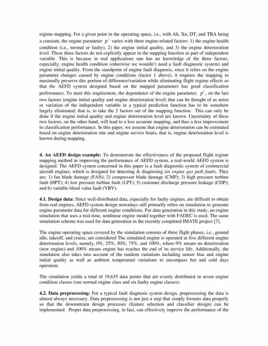
regime mapping. For a given point in the operating space, i.e., with Alt, Xn, DT, and TRA being
a constant, the engine parameter ip varies with three engine-related factors: 1) the engine health
condition (i.e., normal or faulty), 2) the engine initial quality, and 3) the engine deterioration
level. These three factors do not explicitly appear in the mapping function as part of independent
variable. This is because in real applications one has no knowledge of the three factors,
especially, engine health condition (otherwise we wouldn’t need a fault diagnostic system) and
engine initial quality. From the standpoint of engine fault diagnosis, since it relies on the engine
parameter changes caused by engine conditions (factor 1 above), it requires the mapping to
maximally preserve this portion of difference/variation while eliminating flight regime effects so
that the AEFD system designed based on the mapped parameters has good classification
performance. To meet this requirement, the dependence of the engine parameter, ip , on the last
two factors (engine initial quality and engine deterioration level) that can be thought of as noise
or variation of the independent variable in a typical prediction function has to be somehow
largely eliminated, that is, to take the 2 factors out of the mapping function. This can only be
done if the engine initial quality and engine deterioration level are known. Uncertainty of these
two factors, on the other hand, will lead to a less accurate mapping, and thus a less improvement
in classification performance. In this paper, we assume that engine deterioration can be estimated
based on engine deterioration rate and engine service hours, that is, engine deterioration level is
known during mapping.
4. An AEFD design example: To demonstrate the effectiveness of the proposed flight regime
mapping method in improving the performance of AEFD system, a real-world AEFD system is
designed. The AEFD system concerned in this paper is a fault diagnostic system of commercial
aircraft engines, which is designed for detecting & diagnosing six engine gas path faults. They
are: 1) fan blade damage (FAN); 2) compressor blade damage (CMP); 3) high pressure turbine
fault (HPT); 4) low pressure turbine fault (LPT); 5) customer discharge pressure leakage (CDP);
and 6) variable bleed value fault (VBV).
4.1. Design data: Since well-distributed data, especially for faulty engines, are difficult to obtain
from real engines, AEFD system design nowadays still primarily relies on simulation to generate
engine parameter data for different engine conditions. For data generation in this study, an engine
simulation that uses a real-time, nonlinear engine model together with FADEC is used. The same
simulation scheme was used for data generation in the recently completed IMATE project [7].
The engine operating space covered by the simulation consists of three flight phases, i.e., ground
idle, takeoff, and cruise, are considered The simulated engine is operated at five different engine
deterioration levels, namely, 0%, 25%, 50%, 75%, and 100%, where 0% means no deterioration
(new engine) and 100% means engine has reaches the end of its service life. Additionally, the
simulation also takes into account of the random variations including sensor bias and engine
initial quality as well as ambient temperature variations to encompass hot and cold days
operation.
The simulation yields a total of 19,635 data points that are evenly distributed in seven engine
condition classes (one normal engine class and six faulty engine classes).
4.2. Data preprocessing: For a typical fault diagnosis system design, preprocessing the data is
almost always necessary. Data preprocessing is not just a step that simply formats data properly
so that the downstream design processes (feature selection and classifier design) can be
implemented. Proper data preprocessing, in fact, can effectively improve the performance of the

diagnostic system designed. In that sense, data preprocessing is an important sub-task in fault
diagnosis design. Typical data preprocessing include steps like data formatting, data scrubbing,
and missing data handling, etc. In this study, since the data is generated from the simulation, data
formatting and cleaning become unnecessary. Our focus, hence, is on TRA effects removal and
data normalization. Our preliminary study shows both processes are effective in improving the
performance of the AEFD system.
After examining the engine performance parameters through visualization, we observed that the
values of the sensed engine performance parameters are highly correlated with the throttle
resolver angle (TRA) values. To illustrate the correlation, the “compressor exit pressure”
parameter, as an example, is plotted against TRAs in Figure 3.a, where different colors represent
data points from
different engine
condition classes. It is
clear that the
compressor exit pressure
value increases almost
linearly with the TRAs.
The strong dependence
of the sensed parameters
on the TRA degrades
the classifier
performance. From
Figure 3.a one can see
that different engine
faults do introduce
certain noticeable
changes in compressor
exit pressure values
(different color bars in
each cluster in Figure
3.a). However, changes
of the compressor exit
pressure due to different levels of TRAs are much more significant (from one cluster to another in
Figure 3.a). Significant changes of the parameter values due to TRA “mask” the subtle changes of
the parameter values introduced by engine faults. As a result, diagnosing the engine faults
becomes more difficult since the degree of difficulty of a classification task increases as the
magnitude of the within-class variability increases with respect to among-class differences [8].
To remove the TRA effects, the mean of the feature values for all classes at each TRA level are
subtracted from the feature values. Graphically, this is to bring the center of each cluster of data
in Figure 3.a to the zero level.
The compressor exit pressure is again plotted against TRAs in Figure 3.b after the TRA effects
are removed. Comparing Figure 3.b with Figure 3.a, it is clear that removing the TRA effects
accentuates the difference of the feature values between classes, i.e., more separable.
Normalization for pattern classification problems is typically to scale all features to a common
range so that effects due to arbitrary feature representation (e.g., different units) can be eliminated
Figure 3: Compressor exit pressure –vs- TRA:
(a) Before TRA removal; (b) After TRA removal

[8]. There are different methods for normalization. In this paper, the range normalization, the
most common one, is used.
5. Results: Followings are the results of the flight regime mapping and of the classification for
the AEFD systems concerned.
5.1. Flight regime mapping: Each of the mapping neural networks is a 3-layer feed-forward
network, i.e., is of [5, 15, 1] structure. The network is trained using the Levenberg-Marquardt
learning algorithm.
To show the effectiveness
of the mapping, the mapped
engine parameters are
compared with those before
mapping and those at SLS
(the mapping targets).
Figure 4 illustrates such
comparison for compressor
exit pressure - one of the
sensed engine parameters.
Different colors in Figure 6
represent different engine
condition classes and the
parameter values are
normalized into a range of
[0,1]. Figure 4 (a) shows
the distribution of
compressor exit pressure
before flight regime
mapping, while Figure 4
(b) shows the same
parameter after flight regime mapping. By comparing Figures 4 (b) with 4 (a), one can see that
flight regime mapping significantly reduces the variation of the engine parameter within each
engine condition class and increases the class separability between classes, thus improves the
classification performance. Figures 4 (c) shows the distribution of the same engine parameter at
sea level static, which is used as the targets for training the mapping neural networks. The
similarity between Figures 4 (b) and 4 (c) is significant, which indicates that the NN mapping
performs reasonably well.
To mathematically quantify how well the flight regime mapping performs, the R2 value [9], a
statistical index for measuring goodness of fit is used. The R2 has a range between 0 and 1, where
1 indicates a perfect fit and a zero means no match at all. The calculated R2 values for all sensed
engine performance parameters are shown in Table I. The numbers in Table I indicate that the
NN mapping performs well in mapping the engine parameter values from different points in flight
regime to SLS.
Table I - R2 values of flight regime mapping
Engine performance parameters
N1 N2 PS3 PS13 P25 T25 T3 T495 T5
R2 0.999 0.992 0.994 0.994 0.988 0.987 0.991 0.984 0.967
Figure 4: Mapping results
5.2. Classification: The mapped engine performance parameters are then used for classifier
development (training and testing). Since our focus in this paper is on the innovative flight regime
mapping method, specifically on demonstrating the effectiveness of the flight regime mapping in
improving classifier performance, we will not try to explore the best classification system for
AEFD. Rather, we only use one type of classifier, namely neural network classifier for
demonstration. It is our belief that using neural networks as a classifier can serve our purpose of
demonstrating effectiveness of flight regime mapping without loss of generality. Exploring the
best design of classification system for AEFD will be the topic of a separate paper.
The classifier: As we can see from section 4, the AEFD system concerned in this paper involves
diagnosing 7 different engine conditions (1 normal condition and 6 different types of faults). That
is, the classifier to be designed has 7 different outputs, which is typically referred as a multi-class
classification problem [10]. For NN classifiers, the multi-class classification can be handled
directly, i.e., to structure network such that the number of output nodes equal to the number of
classes. However, studies have proved that performance can be improved if the multiclass
problem is decomposed into a series of binary classification ones [11]. There are several ways to
decompose the multiclass classification problem into a series of binary classification ones in
order to achieve better performance [12]. In this study, we take “one-vs-other” method to
decompose the AEFD classification problem into 7 binary classifiers. Each of the seven
classifiers is trained to distinguish between patterns belonging to a class (i
C ) and its complement
(i
C ) (combining all data not belonging to class i
C ). To classify an unknown input x, the outputs
of the 7 binary classifiers form a 7-component vector and are combined to arrive at a final
classification decision.
Each binary classifier is a 3-layer feed-forward neural network, where the number of input nodes
is 11 (9 sensed engine parameters plus 2 manufactured features), and the output node is always
one. The activation functions for all layers are of the same type, i.e., the hyperbolic tangent
sigmoidal function. The network is trained using the Levenberg-Marquardt learning algorithm,
which has the fastest convergence. Additionally, to prevent saturation, the target values are scaled
to +0.9 for positive cases and to –0.9 for negative cases. The error on a separate validation set is
monitored during the training process as a measure to stop the training, thus to prevent
overfitting.
The performance indices: Three performance indices (overall accuracy, false positive rate, and
false negative rate) extracted from a confusion matrix are used for classifier performance
comparison/evaluation. For multiclass classification, the three performance indices are defined as
follows.
Let 1,...C ji, ),,( =jiCM be the confusion matrix, where C is the number of classes. And assume
Class 1 represents normal (fault-free) engine condition.
Overall accuracy: ∑∑===
C
ji
C
i
jiCMiiCMOAC1,1
),(),(
False positive rate: ∑∑===
C
j
C
j
jCMjCMFPR12
),1(),1(
False negative rate: ∑∑====
C
ji
C
i
jiCMiCMFNR1,22
),()1,(
(2)
(3)
(4)

The classifier is evaluated by 5-fold stratified cross-validation [13]. The classification results
shown in this section are actually the average of the classification results of the 5-fold cross-
validation.
The results: To demonstrate the effectiveness of flight regime mapping in improving
classification performance, the classification results of the AEFD system concerned are shown
here for two different designs. They are: 1) the baseline design, where the original engine
performance values over all flight regimes are directly used for designing the AEFD; and 2) the
design with flight regime mapping, under which the parameter values are first mapped from
actual flight regime onto sea level static (SLS) before they are used for classifier design. The
flight regime mapping here is designed with engine deterioration level being assumed known (see
section 3 for discussion)
The confusion matrices and the extracted performance indices for the two designs are listed in
Tables II and III, respectively.
From Tables II and III, we can see that flight regime mapping (Table III) increases the overall
accuracy by more than 13 percentage points, reduces the false positive error by more than 17
percentage points, and reduces the false negative error by approximately 7 percentage points,
comparing to the those from baseline design (Table II).
It is worthwhile to point out that the relatively low performance of the three designs shown in this
section is due to the facts of 1) the classifier used is not the optimal and 2) the AEFD system
design is a model-free method, which typically shows lower performance than model-based
methods. However, model-free method deprives the model-based method of the requirement of
an accurate engine model, which is difficult to obtain in real-world applications.
Table II: Classification results for baseline design
Predicted Classes Per Class Performance
NF FAN CMP HPT LPT CDP VBV Accuracy Indices
NF 1656 7 195 90 620 182 55 59.04
FAN 2 2777 13 11 0 1 1 99.00
CMP 475 84 1678 98 347 110 13 59.82 OAC= 70.39
HPT 317 103 67 1733 527 25 33 61.78 FPR= 40.96
LPT 625 22 98 311 1547 180 22 55.15 FNR= 12.01
CDP 546 11 129 8 323 1749 39 62.35 Tru
e C
lasse
s
VBV 57 5 9 3 28 21 2682 95.61
Table III: Classification results for design with flight regime mapping
Predicted Classes Per Class Performance
NF FAN CMP HPT LPT CDP VBV Accuracy Indices
NF 2139 7 106 150 197 70 136 76.26
FAN 0 2786 13 0 2 0 4 99.32
CMP 118 7 2454 62 94 57 13 87.49 OAC= 83.65
HPT 188 2 76 2210 291 16 22 78.79 FPR= 23.74
LPT 288 2 81 317 1893 177 47 67.49 FNR= 5.19
CDP 202 1 86 7 190 2292 27 81.71 Tru
e C
lasse
s
VBV 77 1 4 8 37 28 2650 94.47

6. Conclusions: Several issues make aircraft engine fault diagnosis one of the most difficult
diagnostic problems. One of such issues is related to flight regime. When an aircraft travels from
one point to another in flight regime, engine performance parameters that are used for fault
diagnosing change and such changes mask the parameter changes caused by engine faults, thus
make the engine fault diagnosis much more difficult. To tackle the flight regime issues, an
innovative flight regime mapping using neural networks is proposed in this paper. The mapping
reduces the disturbance caused by change of flight regime to engine performance parameter
changes and thus accentuates the engine fault induced parameter changes. As the result,
classifiers designed based on the mapped engine performance parameters yield a much better
performance. In this paper, we have demonstrated the effectiveness of the flight regime mapping
in improving classification performance of AEFD through designing a real-world AEFD system.
REFERENCES:
[1] Yan, W.Z. (2003), “Diagnostic system configuration optimization and its application to
aircraft engine fault diagnosis”, PhD Dissertation, Department of Mechanical Engineering,
Rensselaer Polytechnic Institute
[2] Merrington, G., Kwon, O-K, Goodwin, G., and Carlsson, B. (1991), “Fault detection and
diagnosis in gas turbines”, ASME Journal of Engineering for Gas Turbines and Power, Vol. 113,
No. 4.
[3] Mast, T.A., Reed, A.T. & Yurkovich, S. (1999), “Bayesian belief networks for fault
identification in aircraft gas turbine engines”, Proceedings of the 1999 IEEE International
Conference on Control Application, Kohala-Coast Island of Hawaii, August 22-27, 1999, Vol. X,
pp39-44
[4] Embrechts, M.J., Schweizerhof, A.L., Bushman, M. and Sabatella, M.H., (2000), “Neural
network modeling of turbofan parameters”, Proceedings of ASME TurboExpo 2000, Munich,
German, May 8-11, Technical Paper No: 2000-GT-0036
[5] Cybenko, G. (1989), “Approximation by superpositions of a sigmoidal function”,
Mathematics of Control, Signals, and Systems, 2:303-314
[6] Hornik, K. M., Stinchcombe, M. and White, H. (1989), “Multilayer feedforward networks are
universal approximators”, Neural Networks, Vol.2, No. 5, pp359-366.
[7] Ashby, M. J. and Scheuren, W. J. (2000), “Intelligent maintenance advisor for turbine
engines”, Proceedings of 2000 IEEE Aerospace Conference, Big Sky, MT, USA, March 18-25,
Vol.6, pp211-219
[8] Duda, R. O., Hart, P. E., and Stork, D. G. (2000), Pattern Classification, John Wiley & Sons,
Inc., New York, NY
[9] Stamatics, D.H. (2003), Six Sigma and Beyond – statistics and probability, CRC Press LLC,
Boca Raton, Florida
[10] Breiman, L, Friedman, J.H., Olshen, R.A., and Stone, C.J., (1984), Classification and
regression trees, Chapman & Hall/CRC, Florida
[11] Hastie, T. & Tibshirani, R. (1998), “Classification by pairwise coupling”, The Annals of
Statistics, Vol. 26, Issue 2, pp451-471.
[12] Dietterich, T.G. & Bakiri, G. (1995), “Solving multiclass learning problems via error-
correcting output codes”, Journal of Artificial Intelligence Research, 2, pp263-286.
[13] Friedman, J. H. (1996), “Another approach to polychotomous classification”, Technical
Report, Department of Statistics, Stanford University