finite volume and pseudo-spectral schemes for the fully nonlinear 1d serre equations
TRANSCRIPT

arX
iv:1
104.
4456
v1 [
phys
ics.
flu-
dyn]
22
Apr
201
1
AN IMPLICIT-EXPLICIT FINITE VOLUME SCHEME FOR THE
FULLY NONLINEAR SERRE SYSTEM OF EQUATIONS
DENYS DUTYKH∗, DIDIER CLAMOND, PAUL MILEWSKI, AND DIMITRIOS MITSOTAKIS
Abstract. After we derive the Serre system of equations of water wave theory from ageneralized variational principle, we present some of its structural properties. We alsopropose a robust and accurate numerical scheme to solve these equations based on thefinite volume method. The numerical discretization is validated by comparisons withanalytical, experimental data or other numerical solutions obtained by a highly accuratepseudo-spectral method.
Contents
1. Introduction 12. Mathematical model 22.1. Derivation of the Serre equations 42.2. Invariants of the Serre equations 63. Finite volume scheme and numerical results 73.1. High order reconstruction 93.2. Treatment of the dispersive terms 104. Pseudo-spectral Fourier-type method for Serre equations 115. Numerical results 135.1. Convergence test and invariants preservation 135.2. Solitary wave interaction 145.3. Experimental validation 166. Conclusions 18Acknowledgements 20References 21
1. Introduction
The full water wave problem consisting of the Euler equations with free surface stillis a very difficult problem to study theoretically and even numerically. Consequently,the water wave theory has always been developed through the derivation, analysis andcomprehension of various approximate models (see the historical review of Craik [15] for
Key words and phrases. Serre equations; finite volumes; UNO scheme; IMEX scheme; spectral methods.∗ Corresponding author.
1
2 D. DUTYKH, D. CLAMOND, P. MILEWSKI, AND D. MITSOTAKIS
more information). For this reason a plethora of approximate models have been derivedunder various physical assumptions. In this family, the Serre equations have a particularplace and they are the subject of the present study. The Serre equations can be derivedfrom the Euler equations, contrary to Boussinesq systems or the shallow water system,without the small amplitude or the hydrostatic assumptions respectively.
The Serre equations are named after Francois Serre, an engineer at Ecole Nationale desPonts et Chaussees, who derived this model for the first time in 1953 in his prominent paperentitled “Contribution a l’etude des ecoulements permanents et variables dans les canaux”(see [44]). Later, these equations have been independently rediscovered by Su and Gardner[48] and by Green, Laws and Naghdi [25]. The extension of Serre equations for generaluneven bathymetries was derived by Seabra-Santos et al. [43]. For some generalizationsand new results we refer to recent studies by Barthelemy [7] and by Dias & Milewski [16].
A variety of numerical methods have been applied to discretize dispersive wave modelsand, more specifically, the Serre equations. A pseudo-spectral method was applied in[16], an implicit finite difference scheme in [38, 7] and a compact higher-order scheme in[10, 11]. Some Galerkin and Finite Element type methods have been successfully appliedto Boussinesq-type equations [17, 39, 4, 3].
Recently, efficient high-order explicit or implicit-explicit finite volume schemes for dis-persive wave equations have been developed [20, 19]. The robustness of the proposednumerical schemes allowed also the run-up of long waves on a beach with high accuracy[20]. The present study is a further extension of the finite volume method to the practicallyimportant case of the Serre equations.
The present paper is organized as follows. In Section 2 we provide a derivation of theSerre equations from a relaxed Lagrangian principle and discuss some structural propertiesof the governing equations. The rationale on the employed finite volume scheme are givenin Section 3. A very accurate pseudo-spectral method for the numerical solution of theSerre equations is presented in Section 4. In Section 5, we present convergence tests andnumerical experiments validating the model and the numerical schemes. Finally, the lastSection 6 contains main conclusions of this study.
2. Mathematical model
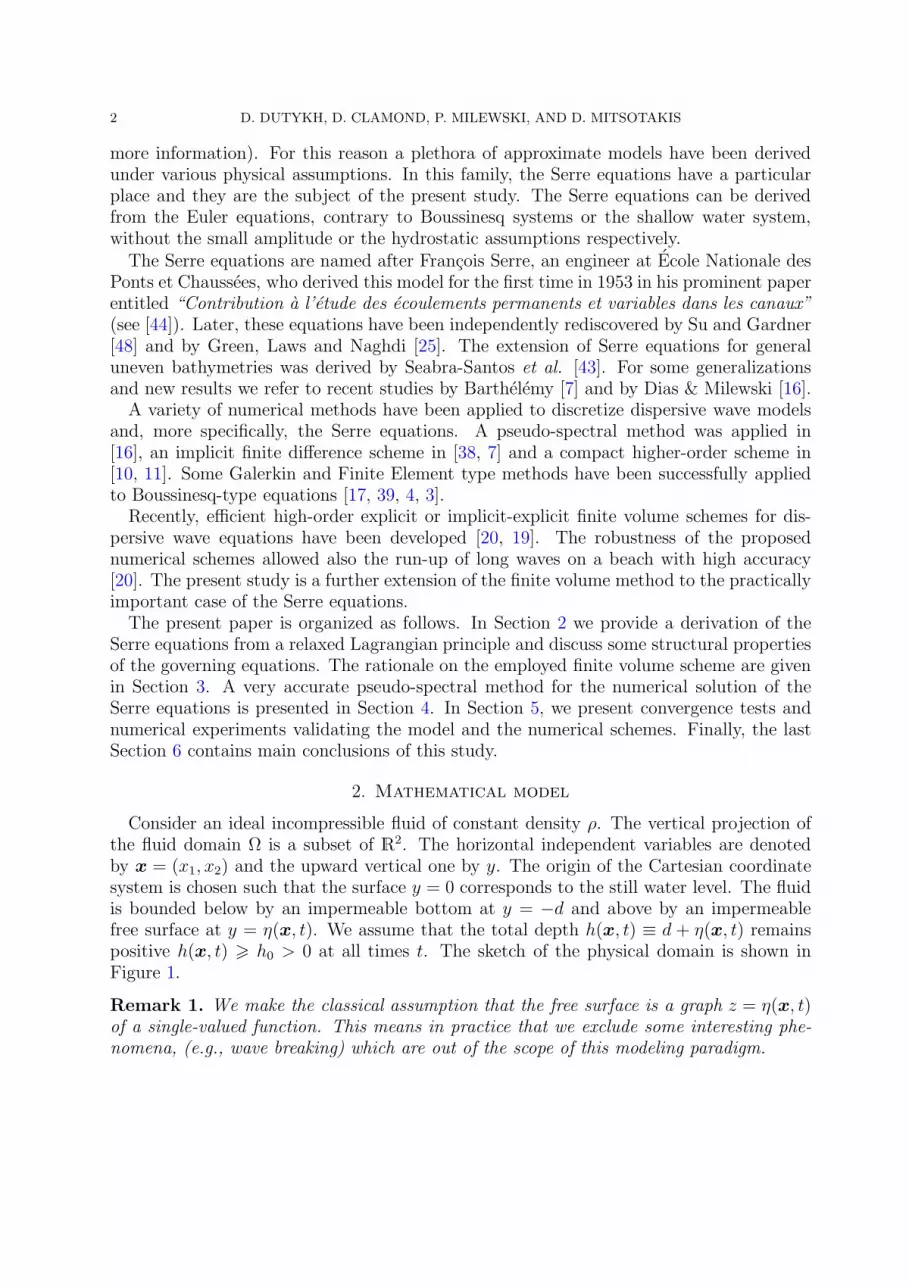
Consider an ideal incompressible fluid of constant density ρ. The vertical projection ofthe fluid domain Ω is a subset of R2. The horizontal independent variables are denotedby x = (x1, x2) and the upward vertical one by y. The origin of the Cartesian coordinatesystem is chosen such that the surface y = 0 corresponds to the still water level. The fluidis bounded below by an impermeable bottom at y = −d and above by an impermeablefree surface at y = η(x, t). We assume that the total depth h(x, t) ≡ d + η(x, t) remainspositive h(x, t) > h0 > 0 at all times t. The sketch of the physical domain is shown inFigure 1.
Remark 1. We make the classical assumption that the free surface is a graph z = η(x, t)of a single-valued function. This means in practice that we exclude some interesting phe-nomena, (e.g., wave breaking) which are out of the scope of this modeling paradigm.

A FINITE VOLUME SCHEME FOR THE SERRE EQUATIONS 3
x
y
O
dh(x, t)
η(x, t)
Figure 1. Sketch of the physical domain.
Assuming that the flow is incompressible and irrotational, the governing equations ofthe classical water wave problem are the following [30, 47, 35, 54]
∇2φ + ∂ 2
y φ = 0 − d(x, t) 6 y 6 η(x, t), (2.1)
∂tη + (∇φ) · (∇η) − ∂y φ = 0 y = η(x, t), (2.2)
∂tφ + 12(∇φ)2 + 1
2(∂yφ)
2 + g η = 0 y = η(x, t), (2.3)
dt + (∇d) · (∇φ) + ∂y φ = 0 y = −d(x, t), (2.4)
with φ being the velocity potential (by definition, the irrotational velocity field (u, v) =(∇φ, ∂yφ), g the acceleration due to gravity force and ∇ = (∂x1
, ∂x2) denotes the gradient
operator in horizontal Cartesian coordinates.The incompressibility condition leads to the Laplace equation for φ. The main difficulty
of the water wave problem lies on the nonlinear free boundary conditions and that the freesurface shape is unknown. Equations (2.2) and (2.4) express the free-surface kinematiccondition and bottom impermeability respectively, while the dynamic condition (2.3) ex-presses the free surface isobarity.
The water wave problem possesses several variational structures [40, 53, 33, 56]. Inthe present study, we will focus mainly on the Lagrangian variational formalism but notexclusively. Surface gravity wave equations (2.1)–(2.4) can be derived by minimizing thefollowing functional proposed by Luke [33]:
L =
∫ t2
t1
∫
Ω
L ρ d2x dt, L = −∫ η
−d
[g y + ∂t φ + 1
2(∇φ)2 + 1
2(∂y φ)
2]dy. (2.5)
4 D. DUTYKH, D. CLAMOND, P. MILEWSKI, AND D. MITSOTAKIS
In a recent study, Clamond and Dutykh [12] proposed to use Luke’s Lagrangian (2.5) inthe following relaxed form
L = (ηt + µ ·∇η − ν) φ + (dt + µ ·∇d+ ν) φ − 12g η2
+
∫ η
−d
[µ · u− 1
2u2 + νv − 1
2v2 + (∇ · µ+ νy)φ
]dy, (2.6)
where u, v,µ, ν are the horizontal, vertical velocities and associated Lagrange multipliers,respectively. The additional variables µ, ν (Lagrange multipliers) are called pseudo-velocities. The over ‘tildes’ and ‘wedges’ denote, respectively, a quantity computed at thefree surface y = η(x, t) and at the bottom y = −d(x, t). We shall also denote below with‘bars’ the quantities averaged over the water depth.
While the original Lagrangian (2.5) incorporates only two variables (η and φ), the relaxedLagrangian density (2.6) involves six variables η, φ,u, v,µ, ν. These additional degreesof freedom provide us with more flexibility in constructing various approximations. Formore details, explanations and examples we refer to [12].
2.1. Derivation of the Serre equations. Now we are going to illustrate the practicaluse of the variational principle (2.6) on an example borrowed from [12]. First of all, wechoose a simple shallow water ansatz, which is a zeroth-order polynomial in y for φ andfor u, and a first-order one for v, i.e., we approximate flows that are nearly uniform alongthe vertical direction
φ ≈ φ(x, t), u ≈ u(x, t), v ≈ (y + d) (η + d)−1 v(x, t). (2.7)
We have also to introduce suitable ansatz for the Lagrange multiplier µ and ν
µ ≈ µ(x, t), ν ≈ (y + d) (η + d)−1 ν(x, t).
In the remainder of this paper, we will assume for simplicity the bottom to be flat d(x, t) =d = Cst. With this ansatz the Lagrangian density (2.6) becomes
L = (ηt + µ · ∇η) φ − 12g η2
+ (η + d)[µ · u − 1
2u2 + 1
3ν v − 1
6v2 + φ∇ · µ
]. (2.8)
Finally, we impose a constraint of the free surface impermeability, i.e.
ν = ηt + µ · ∇η.
After substituting the last relation into the Lagrangian density (2.8), the minimizationprocedure leads to the following equations:
ht + ∇ · [ h u ] = 0, (2.9)
ut + u · ∇u + g∇h + 13h−1
∇[ h2 γ ] = (u · ∇h)∇(h∇ · u)
− [ u · ∇(h∇ · u) ]∇h, (2.10)
where we eliminated φ, µ and v and where
γ ≡ vt + u · ∇v = h(∇ · u)2 − ∇ · ut − u · ∇ [∇ · u ]
, (2.11)

A FINITE VOLUME SCHEME FOR THE SERRE EQUATIONS 5
is the fluid vertical acceleration at the free surface. The vertical velocity at the free surfacev can be expressed in terms of other variables as well, i.e.,
v =ηt + (∇φ) · (∇η)
1 + 13|∇η|2 .
In two dimensions (one horizontal dimension), the two terms on the right hand side of(2.10) vanish and the system (2.9), (2.10) reduces to the classical Serre equations [44].
Remark 2. In the publication by Clamond and Dutykh [12] it is explained why equations(2.9), (2.10) cannot be obtained from the classical Luke’s Lagrangian. Thus, a relaxed formof the Lagrangian density (2.6) is necessary for the variational derivation of the Serreequations (2.9), (2.10) (see also [28] & [36]).
2.1.1. Generalized Serre equations. A further generalization of the Serre equations can beobtained if we modify slightly the shallow water ansatz (2.7) following again the ideas from[12]:
φ ≈ φ(x, t), u ≈ u(x, t), v ≈[y + d
η + d
]λ
v(x, t).
In the following we consider for simplicity the two-dimensional case and pose µ = u andν = v together with the constraint v = ηt + uηx (free surface impermeability). Thus, theLagrangian desnity (2.6) becomes
L = (ht + [ h u ]x) φ − 12g η2 + 1
2h u2 + 1
2β h ( ηt + u ηx )
2 . (2.12)
where β = (2λ + 1)−1. After some algebra, the Euler–Lagrange equations lead to thefollowing equations
ht + [ h u ]x = 0, (2.13)
ut + u ux + g hx + β h−1 [ h2 γ ]x = 0, (2.14)
where γ is defined as above (2.11). If β = 13(or equivalently λ = 1) the classical Serre
equations (2.9), (2.10) are recovered.Using equations (2.13) and (2.14) one can show that the following relations hold
[ h u ]t +[h u2 + 1
2g h2 + β h2 γ
]
x= 0,
[ u − β h−1(h3ux)x ]t +[
12u2 + g h − 1
2h2 u2x − β uh−1 (h3ux)x
]
x= 0,
[ h u − β (h3ux)x ]t +[h u2 + 1
2g h2 − 2 β h3 u2x − β h3 u uxx − h2 hx u ux
]
x= 0,
[12h u2 + 1
2β h3 u2x + 1
2g h2
]
t+
[ (12u2 + 1
2β h2 u2x + g h + β h γ
)h u
]
x= 0.
Physically, these relations represent conservations of the momentum, potential vorticity[36], potential vorticity flux and energy, respectivelyy. Moreover, the Serre equations areinvariant under the Galilean transformation. This property is naturally inherited fromthe full water wave problem since our ansatz does not destroy this symmetry [8] and thederivation is made according variational principles.

6 D. DUTYKH, D. CLAMOND, P. MILEWSKI, AND D. MITSOTAKIS
−40 −30 −20 −10 0 10 20 30 40−0.03
−0.02
−0.01
0
0.01
0.02
0.03
0.04
0.05
0.06
x
η(x,
0)
(a) Solitary wave
−40 −30 −20 −10 0 10 20 30 40−0.03
−0.02
−0.01
0
0.01
0.02
0.03
0.04
0.05
0.06
x
η(x,
0)
(b) Cnoidal wave
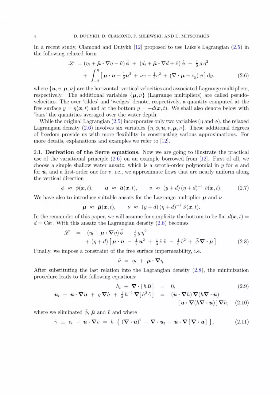
Figure 2. Two exact solutions to Serre equations. For the cnoidal waveparameters m and a are equal to 0.99 and 0.05 respectively.
Equations (2.13)–(2.14) admit a (2π/k)-periodic cnoidal traveling wave solution
u =c η
d+ η, (2.15)
η = adn2
(12κ(x− ct)|m
)− E/K
1−E/K= a − H sn2
(12κ(x− ct)|m
), (2.16)
where dn and sn are the Jacobian elliptic functions with parameter m (0 6 m 6 1), andwhere K = K(m) and E = E(m) are the complete ellipic integrals of the first and secondkind, respectively [1]. The wave parameters are given by the relations
k =π κ
2K, H =
maK
K −E, (κd)2 =
g H
mβ c2, (2.17)
m =g H (d+ a) (d+ a−H)
g (d+ a)2 (d+ a−H) − d2 c2. (2.18)
However, in the present study, we are interested in the classical solitary wave solutionwhich is recovered in the limiting case m→ 1
η = a sech2 12k(x− ct), u =
c η
d+ η, c2 = g(d+ a), (kd)2 =
a
β(d+ a). (2.19)
For illustrative purposes, some free surface elevations are depicted on Figure 2.
2.2. Invariants of the Serre equations. Henceforth we consider only the two-dimensionalcase. As pointed out by Yi Li (2002) [31], the classical Serre equations possess a non-canonical Hamiltonian structure which can be easily generalized for the model (2.13),

A FINITE VOLUME SCHEME FOR THE SERRE EQUATIONS 7
(2.14)(htqt
)
= J ·
(δH / δqδH / δh
)
,
where the Hamiltonian functional H and the symplectic operator J are defined as
H = 12
∫
R
[
h u2 + β h3 u2x + g η2]
dx, J = −(
hx 0qx + q∂x h∂x
)
.
The variable q is sometimes referred to as the potential vorticity flux and is defined by
q ≡ h u − β [ h3 ux ]x.
According to [31], one-parameter symmetry groups of Serre equations include the spacetranslation (x + ε, t, h, u), the time translation (x, t + ε, h, u), the Galilean boost (x +εt, t, h, u+ ε) and the scaling eε(eεx, t, eεh, u). Using the first three symmetry groups andthe symplectic operator J, one may recover the following invariants:
Q =
∫
R
η q
d + ηdx, H,
∫
R
[t q − x η
]dx. (2.20)
Obviously, the equation (2.13) leads to an invariant closely related to the mass conservationproperty
∫
Rη dx. The scaling does not yield any conserved quantity with respect to the
symplectic operator J. Below, we are going to use extensively the generalized energy Hand the generalized momentum Q conservation to assess the accuracy of the numericalschemes additionally to the exact analytical solution (2.19).
3. Finite volume scheme and numerical results
In the present study, we propose a finite volume discretization procedure [5, 6] for thefollowing Serre equations
ht + [ h u ]x = 0, (3.1)
ut +[
12u2 + g h
]
x= β h−1
[h3 (uxt + u uxx − u 2
x)]
x, (3.2)
where the overlines have been omitted for brevity. (In this section, overlines denote quan-tities averaged over a cell, as explained below.)
We begin our presentation by a discretization of the hyperbolic part of the equations(which are simply the classical Saint-Venant equations) and then discuss the treatment ofdispersive terms. The Serre equations can be formally put under the quasilinear form
V t + [F (V ) ]x = S(V ), (3.3)
where V , F (V ) are the conservative variables and the advective flux function, respectively
V ≡(hu
)
, F (V ) ≡(
h u12u2 + g h
)
.
The source term S(V ) denotes the right-hand side of (3.1), (3.2) and thus, depends alsoon space and time derivatives of V .
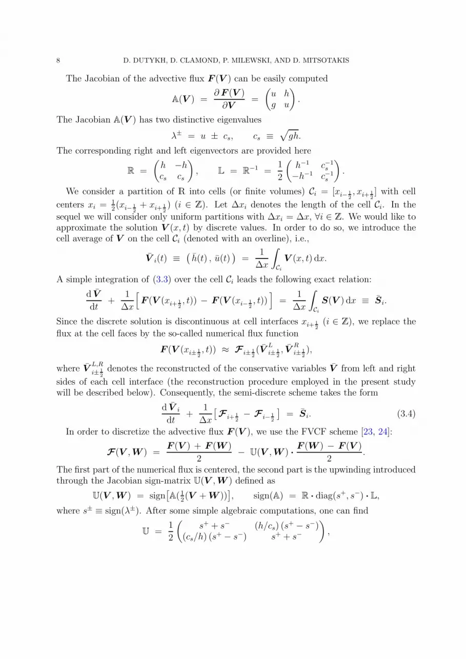
8 D. DUTYKH, D. CLAMOND, P. MILEWSKI, AND D. MITSOTAKIS
The Jacobian of the advective flux F (V ) can be easily computed
A(V ) =∂ F (V )
∂V=
(u hg u
)
.
The Jacobian A(V ) has two distinctive eigenvalues
λ± = u ± cs, cs ≡√
gh.
The corresponding right and left eigenvectors are provided here
R =
(h −hcs cs
)
, L = R−1 =
1
2
(h−1 c−1
s
−h−1 c−1s
)
.
We consider a partition of R into cells (or finite volumes) Ci = [xi− 1
2
, xi+ 1
2
] with cell
centers xi =12(xi− 1
2
+ xi+ 1
2
) (i ∈ Z). Let ∆xi denotes the length of the cell Ci. In the
sequel we will consider only uniform partitions with ∆xi = ∆x, ∀i ∈ Z. We would like toapproximate the solution V (x, t) by discrete values. In order to do so, we introduce thecell average of V on the cell Ci (denoted with an overline), i.e.,
V i(t) ≡(h(t) , u(t)
)=
1
∆x
∫
Ci
V (x, t) dx.
A simple integration of (3.3) over the cell Ci leads the following exact relation:
d V
dt+
1
∆x
[
F (V (xi+ 1
2
, t)) − F (V (xi− 1
2
, t))]
=1
∆x
∫
Ci
S(V ) dx ≡ Si.
Since the discrete solution is discontinuous at cell interfaces xi+ 1
2
(i ∈ Z), we replace the
flux at the cell faces by the so-called numerical flux function
F (V (xi± 1
2
, t)) ≈ F i± 1
2
(VLi± 1
2
, VRi± 1
2
),
where VL,R
i± 1
2
denotes the reconstructed of the conservative variables V from left and right
sides of each cell interface (the reconstruction procedure employed in the present studywill be described below). Consequently, the semi-discrete scheme takes the form
d V i
dt+
1
∆x
[F i+ 1
2
− F i− 1
2
]= Si. (3.4)
In order to discretize the advective flux F (V ), we use the FVCF scheme [23, 24]:
F(V ,W ) =F (V ) + F (W )
2− U(V ,W ) ·
F (W ) − F (V )
2.
The first part of the numerical flux is centered, the second part is the upwinding introducedthrough the Jacobian sign-matrix U(V ,W ) defined as
U(V ,W ) = sign[A(1
2(V +W ))
], sign(A) = R · diag(s+, s−) · L,
where s± ≡ sign(λ±). After some simple algebraic computations, one can find
U =1
2
(s+ + s− (h/cs) (s
+ − s−)(cs/h) (s
+ − s−) s+ + s−
)
,
A FINITE VOLUME SCHEME FOR THE SERRE EQUATIONS 9
the sign-matrix U being evaluated at the average state of left and right values.
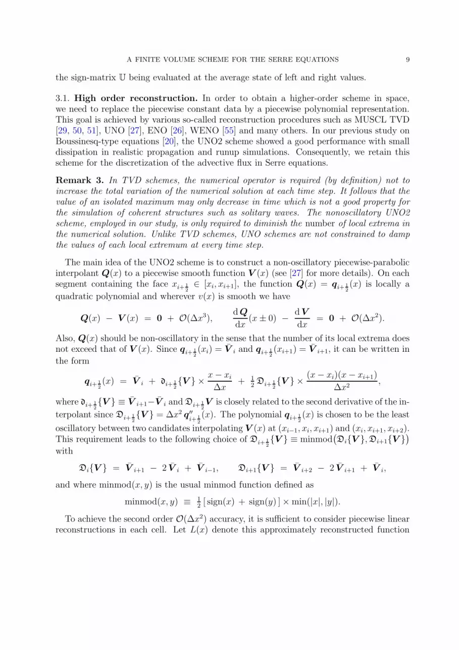
3.1. High order reconstruction. In order to obtain a higher-order scheme in space,we need to replace the piecewise constant data by a piecewise polynomial representation.This goal is achieved by various so-called reconstruction procedures such as MUSCL TVD[29, 50, 51], UNO [27], ENO [26], WENO [55] and many others. In our previous study onBoussinesq-type equations [20], the UNO2 scheme showed a good performance with smalldissipation in realistic propagation and runup simulations. Consequently, we retain thisscheme for the discretization of the advective flux in Serre equations.
Remark 3. In TVD schemes, the numerical operator is required (by definition) not toincrease the total variation of the numerical solution at each time step. It follows that thevalue of an isolated maximum may only decrease in time which is not a good property forthe simulation of coherent structures such as solitary waves. The nonoscillatory UNO2scheme, employed in our study, is only required to diminish the number of local extrema inthe numerical solution. Unlike TVD schemes, UNO schemes are not constrained to dampthe values of each local extremum at every time step.
The main idea of the UNO2 scheme is to construct a non-oscillatory piecewise-parabolicinterpolant Q(x) to a piecewise smooth function V (x) (see [27] for more details). On eachsegment containing the face xi+ 1
2
∈ [xi, xi+1], the function Q(x) = qi+ 1
2
(x) is locally a
quadratic polynomial and wherever v(x) is smooth we have
Q(x) − V (x) = 0 + O(∆x3),dQ
dx(x± 0) − dV
dx= 0 + O(∆x2).
Also, Q(x) should be non-oscillatory in the sense that the number of its local extrema doesnot exceed that of V (x). Since qi+ 1
2
(xi) = V i and qi+ 1
2
(xi+1) = V i+1, it can be written in
the form
qi+ 1
2
(x) = V i + di+ 1
2
V × x− xi∆x
+ 12Di+ 1
2
V × (x− xi)(x− xi+1)
∆x2,
where di+ 1
2
V ≡ V i+1−V i andDi+ 1
2
V is closely related to the second derivative of the in-
terpolant since Di+ 1
2
V = ∆x2 q′′
i+ 1
2
(x). The polynomial qi+ 1
2
(x) is chosen to be the least
oscillatory between two candidates interpolating V (x) at (xi−1, xi, xi+1) and (xi, xi+1, xi+2).This requirement leads to the following choice of Di+ 1
2
V ≡ minmod(DiV ,Di+1V
)
with
DiV = V i+1 − 2 V i + V i−1, Di+1V = V i+2 − 2 V i+1 + V i,
and where minmod(x, y) is the usual minmod function defined as
minmod(x, y) ≡ 12[ sign(x) + sign(y) ]×min(|x|, |y|).
To achieve the second order O(∆x2) accuracy, it is sufficient to consider piecewise linearreconstructions in each cell. Let L(x) denote this approximately reconstructed function

10 D. DUTYKH, D. CLAMOND, P. MILEWSKI, AND D. MITSOTAKIS
which can be written in this form
L(x) = V i + Si ·x− xi∆x
, x ∈ [xi− 1
2
, xi+ 1
2
].
In order to L(x) be a non-oscillatory approximation, we use the parabolic interpolationQ(x) constructed below to estimate the slopes Si within each cell
Si = ∆x×minmod(dQ
dx(xi − 0),
dQ
dx(xi + 0)
)
.
In other words, the solution is reconstructed on the cells while the solution gradient isestimated on the dual mesh as it is often performed in more modern schemes [5, 6]. A briefsummary of the UNO2 reconstruction can be also found in [20].
3.2. Treatment of the dispersive terms. In this section, we explain how we treat thedispersive terms of Serre equations (3.1), (3.2). We begin the exposition by discussing thespace discretization and then, we propose a way to remove the intrinsic stiffness of thedispersion by partial implicitation.
For the sake of simplicity, we split the dispersive terms into three parts:
M(V ) ≡ β h−1[h3 uxt
]
x, D1(V ) ≡ β h−1
[h3 u uxx
]
x, D2(V ) ≡ β h−1
[h3 u 2
x
]
x.
We propose the following approximations in space (which are all of the second orderO(∆x2)to be consistent with UNO2 advective flux discretization presented above)
Mi(V ) = β h−1i
h3i+1 (uxt)i+1 − h
3i−1 (uxt)i−1
2∆x
=β h
−1i
2∆x
[
h3i+1
(ut)i+2 − (ut)i2∆x
− h3i−1
(ut)i − (ut)i−2
2∆x
]
=β h
−1i
4∆x2[h
3i+1 (ut)i+2 − (h
3i+1 + h
3i−1) (ut)i + h
3i−1 (ut)i−2
].
The last relation can be rewritten in a short-hand form if we introduce the matrix M(V )such that the i-th component of the product M(V )·V t gives exactly the expression Mi(V ).
In a similar way, we discretize the other dispersive terms without giving here the inter-mediate steps
D1i(V ) =β h
−1i
2∆x2[h
3i+1 ui+1 (ui+2 − 2ui+1 + ui) − h
3i−1 ui−1 (ui − 2ui−1 + ui−2)
],
D2i(V ) =βh
−1i
8∆x3[h
3i+1 (ui+2 − ui)
2 − h3i−1 (ui − ui−2)
2].
If we denote by I the identity matrix, we can rewrite the semi-discrete scheme (3.4) byexpanding the right-hand side Si
d h
dt+
1
∆x
[F (1)
+ (V ) − F (1)− (V )
]= 0,
(I−M) · d udt
+1
∆x
[F (2)
+ (V ) − F (2)− (V )
]= D(V ) · u,

A FINITE VOLUME SCHEME FOR THE SERRE EQUATIONS 11
where F (1,2)± (V ) are the two components of the advective numerical flux vector F at the
right (+) and left (−) faces correspondingly and D(V ) ≡ D1(V )− D2(V ).Finally, in order to describe the fully discrete scheme, we need to specify how we distrib-
ute the nonlinear terms in expressions D1,2(v) on time layers tn and tn+1. We will performit in an economical way so that on each time step we have only one linear system to solve
[D1(V
(n)) · u(n+1)
]
i=
β
2 h(n)i ∆x2
[(h
(n)i+1)
3 u(n)i+1 (u
(n+1)i+2 − 2u
(n+1)i+1 + u
(n+1)i )
− (h(n)i−1)
3 u(n)i−1 (u
(n+1)i − 2u
(n+1)i−1 + u
(n+1)i−2 )
],
[D2(V
(n)) · u(n+1)
]
i=
β
8 h(n)i ∆x3
[(h
(n)i+1)
3 (u(n)i+2 − u
(n)i )(u
(n+1)i+2 − u
(n+1)i )
− (h(n)i−1)
3 (u(n)i − u
(n)i−2)(u
(n+1)i − u
(n+1)i−2 )
].
In our numerical scheme, the advective terms will be treated in the explicit way since thereconstruction procedure is relatively complex and, therefore, highly nonlinear. Conse-quently, the fully discrete scheme takes the following form:
h(n+1)
= h(n) − ∆t
∆x
[F (1)
+ (V(n)
) − F (1)− (V
(n))], (3.5)
( I − M − ∆tD ) · u(n+1) = ( I − M ) · u(n) − ∆t
∆x
[F (2)
+ (V(n)
) − F (2)− (V
(n))], (3.6)
where ∆t is the chosen time step and the matrix D ≡ D1 − D2 as above.
Remark 4. It is possible to enhance the time discretization accuracy by applying theRichardson extrapolation technique [21], for example. Let us briefly recall the main idea. Itconsists in approximating the solution v(t) with two time steps v∆t and v∆t/2. Since the fullydiscrete scheme (3.5), (3.6) is locally second order accurate, the Richardson extrapolationtechnique aims to cancel the leading error term by taking the following combination:
v(t) ≈ 43v∆t/2 − 1
3v∆t.
4. Pseudo-spectral Fourier-type method for Serre equations
In this Section we describe a pseudo-spectral solver to integrate numerically the Serreequations in periodic domains. In spectral methods it is more convenient to work invariables free surface elevation η(x, t) and potential vorticity q(x, t)
ηt + [ (d+ η) u ]x = 0, (4.1)
qt +[q u − 1
2u2 + g η − 1
2(d+ η)2 u2x
]
x= 0, (4.2)
q − u + 13(d+ η)2uxx + (d+ η)ηxux = 0. (4.3)
The first two equations (4.1), (4.2) are of evolution type, while the third one (4.3) relatesthe potential vorticity q to the primitive variables: the free surface elevation η and the

12 D. DUTYKH, D. CLAMOND, P. MILEWSKI, AND D. MITSOTAKIS
velocity u. In order to solve relation (4.3) with respect to the velocity u, we extract thelinear part as
u − 13d2 uxx − q = 1
3(2dη + η2) uxx + (d+ η) ηx ux
︸ ︷︷ ︸
N(η,u)
.
Then, we apply to the last relation the following fixed point type iteration in Fourier space
ˆuj+1 =q
1 + 13(kd)2
+FN(η, uj)
1 + 13(kd)2
j = 0, 1, 2, · · · , (4.4)
where ψ ≡ Fψ denotes the Fourier transform of a quantity ψ. The last iterationcontinues until the desired convergence. For example, for moderate amplitude solitarywaves (≈ 0.2), the accuracy 10−16 is attained in approximatively 20 iterations if the velocityu0 is initialized from the previous time step. We note that the usual 4-half rule is appliedto the nonlinear terms for anti-aliasing [49, 13, 22].
In order to improve the numerical stability of the time stepping method, we will integrateexactly the linear terms in evolution equations
ηt + d ux = −[ η u ]x,
qt + g ηx =[
12u2 + 1
2(d+ η)2 u2x − q u
]
x.
Taking the Fourier transform and using the relation (4.3) between u and q, we obtain thefollowing system of ODEs:
ηt +ikd
1 + 13(kd)2
q = − ikFηu − ikdFN(η, uj)
1 + 13(kd)2
,
qt + ikg η = ikF
12u2 + 1
2(d+ η)2u2x − qu
.
The next step consists in introducing the vector of dimensionless variables in Fourier space
V ≡ (ikη,iω
gq), where ω2 =
gk2d
1 + 13(kd)2
is the dispersion relation of the linearized Serre
equations. With unscaled variables in vectorial form, the last system becomes
V t + L · V = N(V ), L ≡(0 iωiω 0
)
.
On the right-hand side, we put all the nonlinear terms
N (V ) =
(k2Fηu + dk2F
N(η, uj)
/(1 + 1
3(kd)2)
−(kω/g)F
12u2 + 1
2(d+ η)2u2x − qu
)
.
In order to integrate the linear terms, we make the last change of variables [37, 22]:
W t = e(t−t0)L ·N
e−(t−t0)L · W
, W (t) ≡ e−(t−t0)L · V (t), W (t0) = V (t0).
Finally, the last system of ODEs is discretized in time by Verner’s embedded adaptive 9(8)Runge–Kutta scheme [52]. The time step is chosen adaptively using the so-called H211b

A FINITE VOLUME SCHEME FOR THE SERRE EQUATIONS 13
Undisturbed water depth: d 1Gravity acceleration: g 1Solitary wave amplitude: a 0.05Final simulation time: T 2Free parameter: β 1/3
Table 1. Values of various parameters used in convergence tests.
digital filter [45, 46] to meet some estimated error tolerance (generally of the same orderof the fixed point iteration (4.4) precision).
5. Numerical results
In the present section we present some numerical results the new finite volume scheme.First, we validate the discretization and check the convergence of the scheme using ananalytical solution. Then we demonstrate the ability of the scheme to simulate the prac-tically important solitary wave interaction problem. Throughout this section we considerthe initial value problem with periodic boundary conditions.
5.1. Convergence test and invariants preservation. Consider the Serre equations(3.1), (3.2) posed in the periodic domain [−40, 40]. We solve numerically the initial-periodic boundary value problem with an exact solitary wave solution (2.19) posed as aninitial condition. Then, this specific initial disturbance will be translated in space withknown celerity under the system dynamics. This particular class of solutions plays animportant role in water wave theory and it will allow us to assess the accuracy of theproposed fully discrete scheme (3.5), (3.6). The values of the various physical parametersused in the simulation are given in Table 1.
The error is measured using the discrete L∞ norm for various successively refined dis-cretizations. The result is shown on Figure 3. Without any surprise, the finite volumescheme (blue line with circles) shows a fairly good second order convergence (with esti-mated slope ≈ 2.02). For illustrative purposes we show also the error measured for thepseudo-spectral method (red line with crosses) which exhibits an exponential convergencerate.
During all the numerical tests, the mass conservation was satisfied with accuracy ofthe order ≈ 10−14. This impressive result is due to excellent local conservative propertiesof the finite volume method. We also investigate the numerical behaviour of the schemewith respect to the less obvious invariants H and Q defined in (2.20). These invariantscan be computed exactly for solitary waves. However, we do not provide them to avoidcumbersome expressions. For the solitary wave with parameters given in Table 1, the

14 D. DUTYKH, D. CLAMOND, P. MILEWSKI, AND D. MITSOTAKIS
101
102
10−7
10−6
10−5
10−4
10−3
10−2
10−1
100
N
ε ∞
FV UNO2
N−2
Spectral method
Figure 3. Convergence test for the finite volume and spectral methods.
generalized energy and momentum are given by the following expressions:
H0 =21√7
100+
7√3
10log
√21− 1√21 + 1
≈ 0.0178098463,
Q0 =62√15
225+
2√35
5log
√21− 1√21 + 1
≈ 0.017548002.
These values are used to measure the error on these quantities at the end of the simulation.Convergence of this error under the mesh refinement is shown on Figure 4. One can observea super-convergence phenomenon since apparently we are accurate far beyond the secondorder that was expected.
5.2. Solitary wave interaction. Solitary wave interactions are an important phenomenain nonlinear dispersive waves which have been studied by numerical and analytical methodsand results have been compared to experimental evidence. They also often serve as oneof the only robust nonlinear benchmark test cases for numerical methods. We mentiononly a few works among the existing literature. For example, in [34, 41, 14] solitarywave interactions were studied experimentally. The head-on collision of solitary waveswas studied in the framework of full Euler equations in [14, 9]. Studies of solitary wavesin various approximate models can be found in [32, 18, 2, 20, 19]. To our knowledge,solitary wave collisions for the Serre equations were studied numerically for the first timein the PhD thesis of Seabra-Santos [42]. Finally, there are also a few studies devoted tosimulations with full Euler equations [32, 22, 14].

A FINITE VOLUME SCHEME FOR THE SERRE EQUATIONS 15
101
102
103
10−6
10−5
10−4
10−3
10−2
N
H(T
)
|H−Hex
|
N−2
(a) Hamiltonian H
101
102
103
10−6
10−5
10−4
10−3
10−2
N
Q(T
)
|Q−Qex
|
N−2
(b) Momentum Q
Figure 4. Hamiltonian and generalized momentum conservation conver-gence of the finite volume method under the mesh refinement measured atthe end of the simulation.
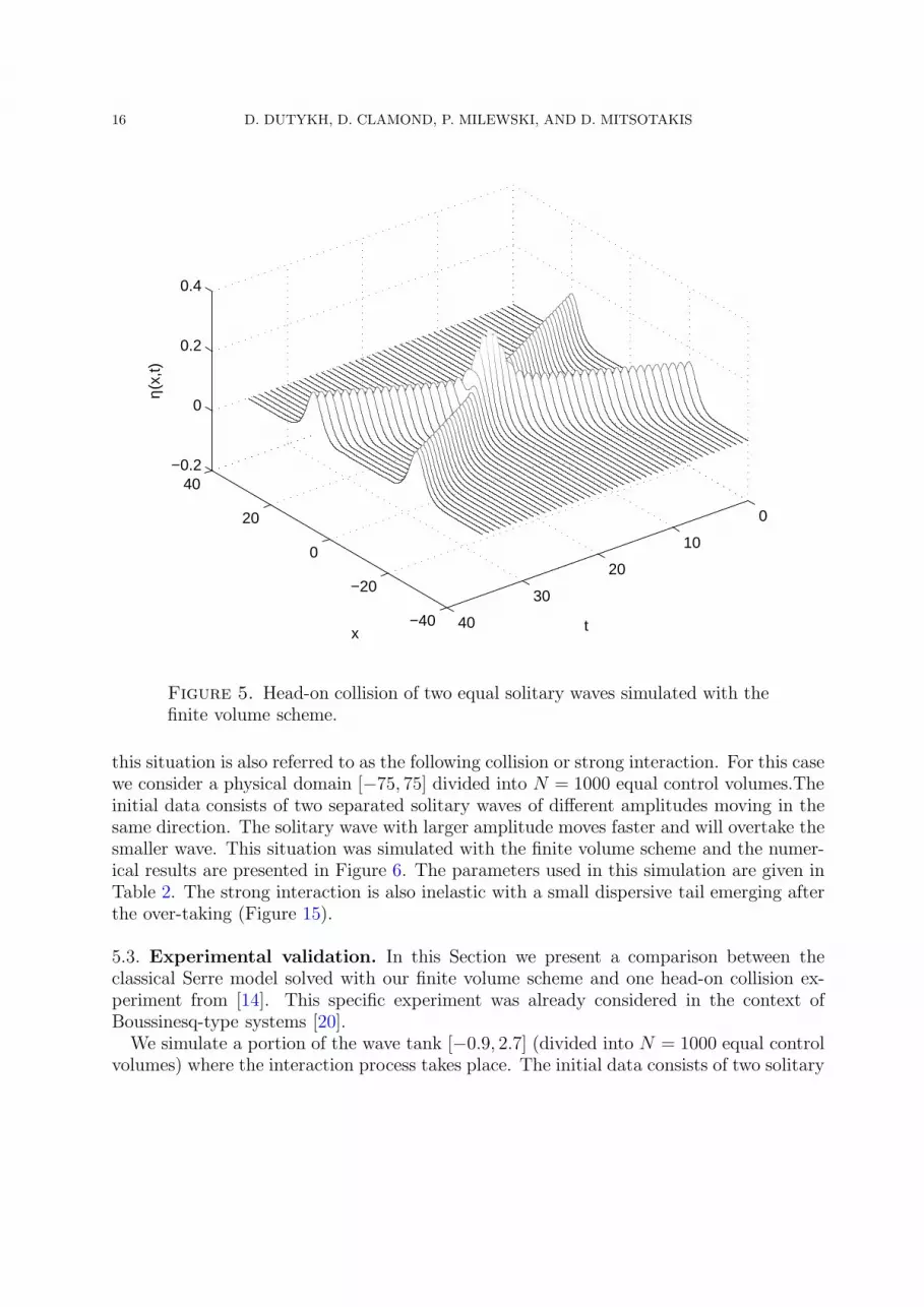
First, we study the head-on collision (weak interaction) of two solitary waves of equalamplitude moving in opposite directions. Consider the Serre equations posed in the domain[−40, 40] with periodic boundary conditions. In the present section, we study the head-oncollision (weak interaction) of two solitary waves of equal amplitude moving in oppositedirections. Initially, two solitary waves of amplitude a = 0.15 are located at x0 = ±20(other parameters can be found in Table 1). The computational domain is divided intoN = 1000 intervals (finite volumes in 1D) of the uniform length ∆x = 0.08. The timestep in the fully discrete scheme (3.5), (3.6) is chosen to be ∆t ≈ 3 × 10⁻⁴. The processis simulated up to time T = 36. The numerical results are presented in Figure 5. Asexpected, the solitary waves collide quasi-elastically and continue to propagate in oppositedirections after the interaction. The value of importance is the maximum amplitude duringthe interaction process, sometimes referred to as the runup. Usually, it is larger than thesum of the amplitudes of the two initial solitary waves. In this case, we obtain a runup of0.3130 > 2a = 0.3.
In order to validate the finite volume simulation, we performed the same computationwith the pseudo-spectral method presented briefly in Section 4. We used a fine grid of 1024nodes and adaptive time stepping. The overall interaction process is visually identical tothe finite volume result shown in Figure 5. The runup value according to the spectralmethod is 0.3127439 showing again the accuracy of our simulation.
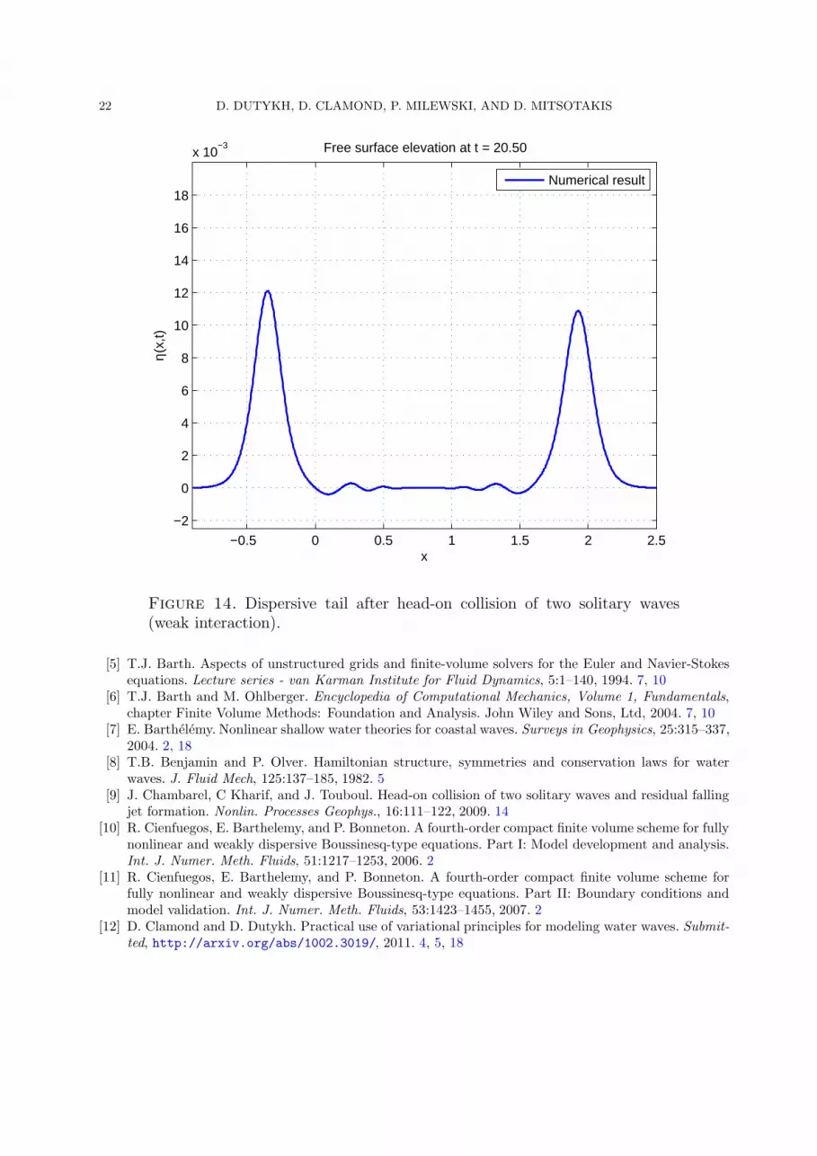
The small inelasticity is evident from the small dispersive wave train emerging after theinteraction (for an example in a slightly different setting described below, see Figure 14,as first found numerically and experimentally by Seabra-Santos [42].
A second type of solitary wave interaction is the overtaking collision (or strong interac-tion) of two solitary waves of different amplitudes moving in the same direction. Sometimes
16 D. DUTYKH, D. CLAMOND, P. MILEWSKI, AND D. MITSOTAKIS
−40
−20
0
20
40
0
10
20
30
40
−0.2
0
0.2
0.4
tx
η(x,
t)
Figure 5. Head-on collision of two equal solitary waves simulated with thefinite volume scheme.
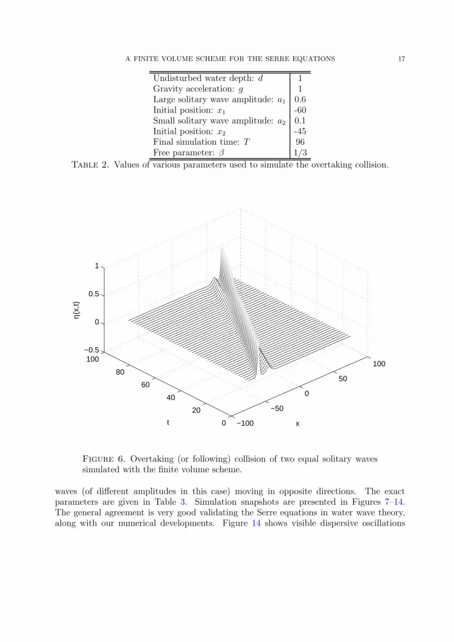
this situation is also referred to as the following collision or strong interaction. For this casewe consider a physical domain [−75, 75] divided into N = 1000 equal control volumes.Theinitial data consists of two separated solitary waves of different amplitudes moving in thesame direction. The solitary wave with larger amplitude moves faster and will overtake thesmaller wave. This situation was simulated with the finite volume scheme and the numer-ical results are presented in Figure 6. The parameters used in this simulation are given inTable 2. The strong interaction is also inelastic with a small dispersive tail emerging afterthe over-taking (Figure 15).
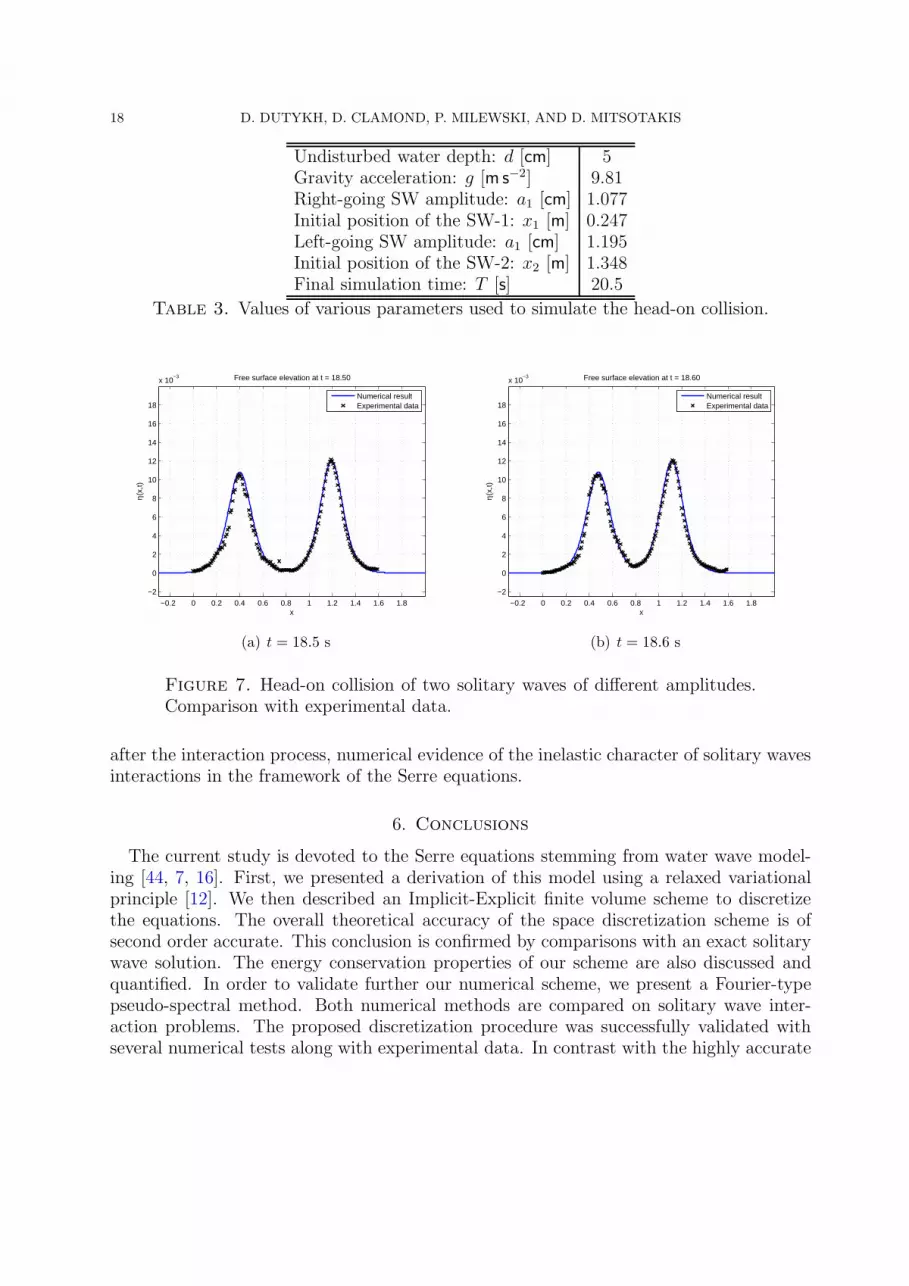
5.3. Experimental validation. In this Section we present a comparison between theclassical Serre model solved with our finite volume scheme and one head-on collision ex-periment from [14]. This specific experiment was already considered in the context ofBoussinesq-type systems [20].
We simulate a portion of the wave tank [−0.9, 2.7] (divided into N = 1000 equal controlvolumes) where the interaction process takes place. The initial data consists of two solitary
A FINITE VOLUME SCHEME FOR THE SERRE EQUATIONS 17
Undisturbed water depth: d 1Gravity acceleration: g 1Large solitary wave amplitude: a1 0.6Initial position: x1 -60Small solitary wave amplitude: a2 0.1Initial position: x2 -45Final simulation time: T 96Free parameter: β 1/3
Table 2. Values of various parameters used to simulate the overtaking collision.
−100
−50
0
50
100
0
20
40
60
80
100−0.5
0
0.5
1
xt
η(x,
t)
Figure 6. Overtaking (or following) collision of two equal solitary wavessimulated with the finite volume scheme.
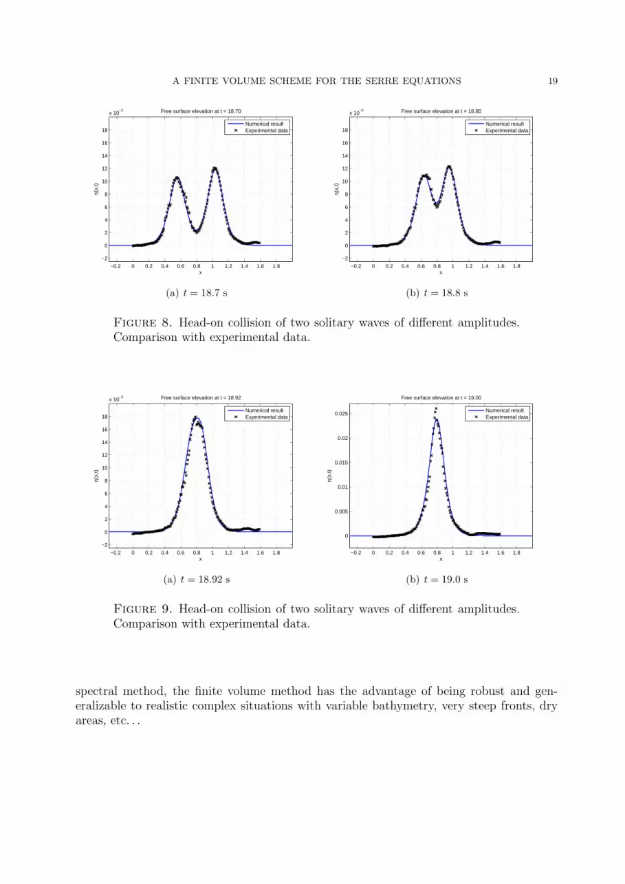
waves (of different amplitudes in this case) moving in opposite directions. The exactparameters are given in Table 3. Simulation snapshots are presented in Figures 7–14.The general agreement is very good validating the Serre equations in water wave theory,along with our numerical developments. Figure 14 shows visible dispersive oscillations
18 D. DUTYKH, D. CLAMOND, P. MILEWSKI, AND D. MITSOTAKIS
Undisturbed water depth: d [cm] 5Gravity acceleration: g [ms
−2] 9.81Right-going SW amplitude: a1 [cm] 1.077Initial position of the SW-1: x1 [m] 0.247Left-going SW amplitude: a1 [cm] 1.195Initial position of the SW-2: x2 [m] 1.348Final simulation time: T [s] 20.5
Table 3. Values of various parameters used to simulate the head-on collision.
−0.2 0 0.2 0.4 0.6 0.8 1 1.2 1.4 1.6 1.8
−2
0
2
4
6
8
10
12
14
16
18
x 10−3 Free surface elevation at t = 18.50
x
η(x,
t)
Numerical resultExperimental data
(a) t = 18.5 s
−0.2 0 0.2 0.4 0.6 0.8 1 1.2 1.4 1.6 1.8
−2
0
2
4
6
8
10
12
14
16
18
x 10−3 Free surface elevation at t = 18.60
x
η(x,
t)
Numerical resultExperimental data
(b) t = 18.6 s
Figure 7. Head-on collision of two solitary waves of different amplitudes.Comparison with experimental data.
after the interaction process, numerical evidence of the inelastic character of solitary wavesinteractions in the framework of the Serre equations.
6. Conclusions
The current study is devoted to the Serre equations stemming from water wave model-ing [44, 7, 16]. First, we presented a derivation of this model using a relaxed variationalprinciple [12]. We then described an Implicit-Explicit finite volume scheme to discretizethe equations. The overall theoretical accuracy of the space discretization scheme is ofsecond order accurate. This conclusion is confirmed by comparisons with an exact solitarywave solution. The energy conservation properties of our scheme are also discussed andquantified. In order to validate further our numerical scheme, we present a Fourier-typepseudo-spectral method. Both numerical methods are compared on solitary wave inter-action problems. The proposed discretization procedure was successfully validated withseveral numerical tests along with experimental data. In contrast with the highly accurate
A FINITE VOLUME SCHEME FOR THE SERRE EQUATIONS 19
−0.2 0 0.2 0.4 0.6 0.8 1 1.2 1.4 1.6 1.8
−2
0
2
4
6
8
10
12
14
16
18
x 10−3 Free surface elevation at t = 18.70
x
η(x,
t)
Numerical resultExperimental data
(a) t = 18.7 s
−0.2 0 0.2 0.4 0.6 0.8 1 1.2 1.4 1.6 1.8
−2
0
2
4
6
8
10
12
14
16
18
x 10−3 Free surface elevation at t = 18.80
x
η(x,
t)
Numerical resultExperimental data
(b) t = 18.8 s
Figure 8. Head-on collision of two solitary waves of different amplitudes.Comparison with experimental data.
−0.2 0 0.2 0.4 0.6 0.8 1 1.2 1.4 1.6 1.8
−2
0
2
4
6
8
10
12
14
16
18
x 10−3 Free surface elevation at t = 18.92
x
η(x,
t)
Numerical resultExperimental data
(a) t = 18.92 s
−0.2 0 0.2 0.4 0.6 0.8 1 1.2 1.4 1.6 1.8
0
0.005
0.01
0.015
0.02
0.025
Free surface elevation at t = 19.00
x
η(x,
t)
Numerical resultExperimental data
(b) t = 19.0 s
Figure 9. Head-on collision of two solitary waves of different amplitudes.Comparison with experimental data.
spectral method, the finite volume method has the advantage of being robust and gen-eralizable to realistic complex situations with variable bathymetry, very steep fronts, dryareas, etc. . .

20 D. DUTYKH, D. CLAMOND, P. MILEWSKI, AND D. MITSOTAKIS
−0.2 0 0.2 0.4 0.6 0.8 1 1.2 1.4 1.6 1.8
0
0.005
0.01
0.015
0.02
0.025
Free surface elevation at t = 19.05
x
η(x,
t)
Numerical resultExperimental data
(a) t = 19.05 s
−0.2 0 0.2 0.4 0.6 0.8 1 1.2 1.4 1.6 1.8
0
0.005
0.01
0.015
0.02
0.025
Free surface elevation at t = 19.10
x
η(x,
t)
Numerical resultExperimental data
(b) t = 19.1 s
Figure 10. Head-on collision of two solitary waves of different amplitudes.Comparison with experimental data.
−0.2 0 0.2 0.4 0.6 0.8 1 1.2 1.4 1.6 1.8
−2
0
2
4
6
8
10
12
14
16
18
x 10−3 Free surface elevation at t = 19.15
x
η(x,
t)
Numerical resultExperimental data
(a) t = 19.15 s
−0.2 0 0.2 0.4 0.6 0.8 1 1.2 1.4 1.6 1.8
−2
0
2
4
6
8
10
12
14
16
18
x 10−3 Free surface elevation at t = 19.19
x
η(x,
t)
Numerical resultExperimental data
(b) t = 19.19 s
Figure 11. Head-on collision of two solitary waves of different amplitudes.Comparison with experimental data.
Acknowledgements
D. Dutykh acknowledges the support from French Agence Nationale de la Recherche,project MathOcean (Grant ANR-08-BLAN-0301-01). P. Milewski acknowledges the sup-port of the University of Savoie which made this joint work possible.
We would like also to thank Brice Eichwald for helpful discussions on spectral methods.

A FINITE VOLUME SCHEME FOR THE SERRE EQUATIONS 21
−0.2 0 0.2 0.4 0.6 0.8 1 1.2 1.4 1.6 1.8
−2
0
2
4
6
8
10
12
14
16
18
x 10−3 Free surface elevation at t = 19.33
x
η(x,
t)
Numerical resultExperimental data
(a) t = 19.33 s
−0.2 0 0.2 0.4 0.6 0.8 1 1.2 1.4 1.6 1.8
−2
0
2
4
6
8
10
12
14
16
18
x 10−3 Free surface elevation at t = 19.50
x
η(x,
t)
Numerical resultExperimental data
(b) t = 19.5 s
Figure 12. Head-on collision of two solitary waves of different amplitudes.Comparison with experimental data.
−0.2 0 0.2 0.4 0.6 0.8 1 1.2 1.4 1.6 1.8
−2
0
2
4
6
8
10
12
14
16
18
x 10−3 Free surface elevation at t = 19.85
x
η(x,
t)
Numerical resultExperimental data
(a) t = 19.85 s
−0.2 0 0.2 0.4 0.6 0.8 1 1.2 1.4 1.6 1.8
−2
0
2
4
6
8
10
12
14
16
18
x 10−3 Free surface elevation at t = 20.00
x
η(x,
t)
Numerical resultExperimental data
(b) t = 20.0 s
Figure 13. Head-on collision of two solitary waves of different amplitudes.Comparison with experimental data.
References
[1] M. Abramowitz and I. A. Stegun. Handbook of Mathematical Functions. Dover, 1965. 6[2] D. C. Antonopoulos, V. A. Dougalis, and D. E. Mitsotakis. Initial-boundary-value problems for the
Bona-Smith family of Boussinesq systems. Advances in Differential Equations, 14:27–53, 2009. 14[3] D. C. Antonopoulos, V. A. Dougalis, and D. E. Mitsotakis. Numerical solution of Boussinesq systems
of the Bona-Smith family. Appl. Numer. Math., 30:314–336, 2010. 2[4] P. Avilez-Valente and F.J. Seabra-Santos. A high-order Petrov-Galerkin finite element method for the
classical Boussinesq wave model. Int. J. Numer. Meth. Fluids, 59:969–1010, 2009. 2
22 D. DUTYKH, D. CLAMOND, P. MILEWSKI, AND D. MITSOTAKIS
−0.5 0 0.5 1 1.5 2 2.5
−2
0
2
4
6
8
10
12
14
16
18
x 10−3 Free surface elevation at t = 20.50
x
η(x,
t)
Numerical result
Figure 14. Dispersive tail after head-on collision of two solitary waves(weak interaction).
[5] T.J. Barth. Aspects of unstructured grids and finite-volume solvers for the Euler and Navier-Stokesequations. Lecture series - van Karman Institute for Fluid Dynamics, 5:1–140, 1994. 7, 10
[6] T.J. Barth and M. Ohlberger. Encyclopedia of Computational Mechanics, Volume 1, Fundamentals,chapter Finite Volume Methods: Foundation and Analysis. John Wiley and Sons, Ltd, 2004. 7, 10
[7] E. Barthelemy. Nonlinear shallow water theories for coastal waves. Surveys in Geophysics, 25:315–337,2004. 2, 18
[8] T.B. Benjamin and P. Olver. Hamiltonian structure, symmetries and conservation laws for waterwaves. J. Fluid Mech, 125:137–185, 1982. 5
[9] J. Chambarel, C Kharif, and J. Touboul. Head-on collision of two solitary waves and residual fallingjet formation. Nonlin. Processes Geophys., 16:111–122, 2009. 14
[10] R. Cienfuegos, E. Barthelemy, and P. Bonneton. A fourth-order compact finite volume scheme for fullynonlinear and weakly dispersive Boussinesq-type equations. Part I: Model development and analysis.Int. J. Numer. Meth. Fluids, 51:1217–1253, 2006. 2
[11] R. Cienfuegos, E. Barthelemy, and P. Bonneton. A fourth-order compact finite volume scheme forfully nonlinear and weakly dispersive Boussinesq-type equations. Part II: Boundary conditions andmodel validation. Int. J. Numer. Meth. Fluids, 53:1423–1455, 2007. 2
[12] D. Clamond and D. Dutykh. Practical use of variational principles for modeling water waves. Submit-ted, http://arxiv.org/abs/1002.3019/, 2011. 4, 5, 18

A FINITE VOLUME SCHEME FOR THE SERRE EQUATIONS 23
30 40 50 60 70 80 90 100 110−0.01
−0.005
0
0.005
0.01
0.015
0.02
0.025
0.03
0.035
0.04
x
η(x,
t)Zoom on the free surface at t = 120
Figure 15. Dispersive tail after overtaking collision of two solitary waves(strong interaction).
[13] D. Clamond and J. Grue. A fast method for fully nonlinear water-wave computations. J. Fluid. Mech.,447:337–355, 2001. 12
[14] W. Craig, P. Guyenne, J. Hammack, D. Henderson, and C. Sulem. Solitary water wave interactions.Phys. Fluids, 18:57–106, 2006. 14, 16
[15] A.D.D. Craik. The origins of water wave theory. Ann. Rev. Fluid Mech., 36:1–28, 2004. 1[16] F. Dias and P. Milewski. On the fully-nonlinear shallow-water generalized Serre equations. Physics
Letters A, 374(8):1049–1053, 2010. 2, 18[17] V. A. Dougalis and D. E. Mitsotakis. Theory and numerical analysis of Boussinesq systems: A review.
In N. A. Kampanis, V. A. Dougalis, and J. A. Ekaterinaris, editors, Effective Computational Methodsin Wave Propagation, pages 63–110. CRC Press, 2008. 2
[18] V.A. Dougalis and D.E. Mitsotakis. Advances in scattering theory and biomedical engineering, chapterSolitary waves of the Bona-Smith system, pages 286–294. World Scientific, New Jersey, 2004. 14
[19] D. Dutykh, Th. Katsaounis, and D. Mitsotakis. Finite volume methods for unidirectional dispersivewave models. Submitted, http://hal.archives-ouvertes.fr/hal-00538043/, 2010. 2, 14
[20] D. Dutykh, Th. Katsaounis, and D. Mitsotakis. Finite volume schemes for dispersive wave propagationand runup. Journal of Computational Physics, 230:3035–3061, 2011. 2, 9, 10, 14, 16
[21] W.F. Ford and A. Sidi. An algorithm for a generalization of the Richardson extrapolation process.SIAM Journal on Numerical Analysis, 24(5):1212–1232, 1987. 11

24 D. DUTYKH, D. CLAMOND, P. MILEWSKI, AND D. MITSOTAKIS
[22] D. Fructus, D. Clamond, O. Kristiansen, and J. Grue. An efficient model for threedimensional surfacewave simulations. Part i: Free space problems. J. Comput. Phys., 205:665–685, 2005. 12, 14
[23] J.-M. Ghidaglia, A. Kumbaro, and G. Le Coq. Une methode volumes-finis a flux caracteristiquespour la resolution numerique des systemes hyperboliques de lois de conservation. C. R. Acad. Sci. I,322:981–988, 1996. 8
[24] J.-M. Ghidaglia, A. Kumbaro, and G. Le Coq. On the numerical solution to two fluid models via cellcentered finite volume method. Eur. J. Mech. B/Fluids, 20:841–867, 2001. 8
[25] A. E. Green, N. Laws, and P. M. Naghdi. On the theory of water waves. Proc. R. Soc. Lond. A,338:43–55, 1974. 2
[26] A. Harten. ENO schemes with subcell resolution. J. Comput. Phys, 83:148–184, 1989. 9[27] A. Harten and S. Osher. Uniformly high-order accurate nonscillatory schemes, I. SIAM J. Numer.
Anal., 24:279–309, 1987. 9[28] J.W. Kim, K.J. Bai, R.C. Ertekin, and W.C. Webster. A derivation of the Green-Naghdi equations
for irrotational flows. Journal of Engineering Mathematics, 40(1):17–42, 2001. 5[29] N.E. Kolgan. Finite-difference schemes for computation of three dimensional solutions of gas dynamics
and calculation of a flow over a body under an angle of attack. Uchenye Zapiski TsaGI [Sci. NotesCentral Inst. Aerodyn], 6(2):1–6, 1975. 9
[30] H. Lamb. Hydrodynamics. Cambridge University Press, 1932. 3[31] Y.A. Li. Hamiltonian structure and linear stability of solitary waves of the Green-Naghdi equations.
J. Nonlin. Math. Phys., 9, 1:99–105, 2002. 6, 7[32] Y.A. Li, J.M. Hyman, and W. Choi. A numerical study of the exact evolution equations for surface
waves in water of finite depth. Stud. Appl. Maths., 113:303–324, 2004. 14[33] J.C. Luke. A variational principle for a fluid with a free surface. J. Fluid Mech., 27:375–397, 1967. 3[34] T. Maxworthy. Experiments on collisions between solitary waves. J Fluid Mech, 76:177–185, 1976. 14[35] C.C. Mei. The applied dynamics of ocean surface waves. World Scientific, 1994. 3[36] J.W. Miles and R. Salmon. Weakly dispersive nonlinear gravity waves. J. Fluid Mech., 157:519–531,
1985. 5[37] P. Milewski and E. Tabak. A pseudospectral procedure for the solution of nonlinear wave equations
with examples from free-surface flows. SIAM J. Sci. Comput., 21(3):1102–1114, 1999. 12[38] S.M. Mirie and C.H. Su. Collision between two solitary waves. Part 2. A numerical study. J. Fluid
Mech, 115:475–492, 1982. 2[39] D.E. Mitsotakis. Boussinesq systems in two space dimensions over a variable bottom for the generation
and propagation of tsunami waves. Math. Comp. Simul., 80:860–873, 2009. 2[40] A.A. Petrov. Variational statement of the problem of liquid motion in a container of finite dimensions.
PMM, 28(4):917–922, 1964. 3[41] D.P. Renouard, F.J. Seabra-Santos, and A.M. Temperville. Experimental study of the generation,
damping, and reflexion of a solitary wave. Dynamics of Atmospheres and Oceans, 9(4):341–358, 1985.14
[42] F.J. Seabra-Santos. Contribution a l’etude des ondes de gravite bidimensionnelles en eau peu profonde.PhD thesis, Institut National Polytechnique de Grenoble, 1985. 14, 15
[43] F.J. Seabra-Santos, D.P. Renouard, and A.M. Temperville. Numerical and experimental study of thetransformation of a solitary wave over a shelf or isolated obstacle. J. Fluid Mech, 176:117–134, 1987.2
[44] F. Serre. Contribution a l’etude des ecoulements permanents et variables dans les canaux. La Houilleblanche, 8:374–388 & 830–872, 1953. 2, 5, 18
[45] G. Soderlind. Digital filters in adaptive time-stepping. ACM Trans. Math. Software, 29:1–26, 2003. 13[46] G. Soderlind and L. Wang. Adaptive time-stepping and computational stability. Journal of Compu-
tational and Applied Mathematics, 185(2):225–243, 2006. 13[47] J.J. Stoker. Water waves, the mathematical theory with applications. Wiley, 1958. 3
A FINITE VOLUME SCHEME FOR THE SERRE EQUATIONS 25
[48] C.H. Su and C.S. Gardner. Korteweg-de Vries equation and generalizations. III. Derivation of theKorteweg-de Vries equation and Burgers equation. J. Math. Phys., 10:536–539, 1969. 2
[49] Lloyd N. Trefethen. Spectral methods in MatLab. Society for Industrial and Applied Mathematics,Philadelphia, PA, USA, 2000. 12
[50] B. van Leer. Towards the ultimate conservative difference scheme V: a second order sequel to Godunov’method. J. Comput. Phys., 32:101–136, 1979. 9
[51] B. van Leer. Upwind and high-resolution methods for compressible flow: From donor cell to residual-distribution schemes. Communications in Computational Physics, 1:192–206, 2006. 9
[52] J.H. Verner. Explicit Runge–Kutta methods with estimates of the local truncation error. SIAM J.Num. Anal., 15(4):772–790, 1978. 12
[53] G. B. Whitham. A general approach to linear and non-linear dispersive waves using a Lagrangian. J.Fluid Mech., 22:273–283, 1965. 3
[54] G.B. Whitham. Linear and nonlinear waves. John Wiley & Sons Inc., New York, 1999. 3[55] Y. Xing and C.-W. Shu. High order finite difference weno schemes with the exact conservation property
for the shallow water equations. J. Comput. Phys., 208:206–227, 2005. 9[56] V.E. Zakharov. Stability of periodic waves of finite amplitude on the surface of a deep fluid. J. Appl.
Mech. Tech. Phys., 9:1990–1994, 1968. 3
LAMA, UMR 5127 CNRS, Universite de Savoie, Campus Scientifique, 73376 Le Bourget-
du-Lac Cedex, France
E-mail address : [email protected]: http://www.lama.univ-savoie.fr/~dutykh/
Laboratoire J.-A. Dieudonne, Universite de Nice – Sophia Antipolis, Parc Valrose, 06108
Nice cedex 2, France
E-mail address : [email protected]: http://math.unice.fr/~didierc/
University of Wisconsin, Dept. of Mathematics, 480 Lincoln Dr. Madison, WI 53706,
USA
E-mail address : [email protected]: http://www.math.wisc.edu/~milewski/
IMA, University of Minnesota, 114 Lind Hall and 207 Church Street SE, Minneapolis
MN 55455, USA
E-mail address : [email protected]: http://sites.google.com/site/dmitsot/