final grade project - upcommons

FINAL GRADE PROJECT

TITLE FGP : Performance Evaluation of Frame Slotted Aloha with Diversity and Interference Cancellation TITULATION: Telecommunications technical engineering, specializing in Telecommunication Systems AUTHOR: Marc Rietti Fernández DIRECTORS: Joan Bas y Francisco Vázquez Gallego TUTORS: Luis Alonso Zárate DATA: February 6, 2014

Title: Performance Evaluation of Frame Slotted Aloha with Diversity and Interference Cancellation Author: Marc Rietti Fernández Directors: Joan Bas y Francisco Vázquez Gallego Tutor: Luis Alonso Zárate Date: February 6, 2014

Abstract

Since 1995, Machine to Machine (M2M) networks are spreading very quickly. These technologies allow both wired and wireless system communicating with other devices of the same type. Regardless of the type of machine or data, information usually is distributed in the same way, from a machine to a network, and then through a gateway to a system where it can be reviewed. This type of communications require new protocols and optimizations to minimize the energy consumption of the devices of the network to extent their battery life-times. The M2M network considered in this work is composed of a group of devices that are collecting data and, periodically, transmit this data to a coordinator upon request. Once each device is able to transmit the information correctly, passes into a sleep mode for saving energy. Generally, the use of random access protocols such as Aloha provides good results due to its low complexity. On the contrary, its performance is degraded drastically when the data traffic load increases or the number of devices is huge, which is the case in dense M2M networks. For that reason, new versions of the Aloha protocol were developed, such as Slotted-Aloha, which doubles the throughput of classical Aloha. Based on Slotted-Aloha, a new access protocol called Successive Interference Cancellation Frame Slotted Aloha (SICFSA) has been proposed in recent works. In SICFSA, the transmitter devices send multiple copies (replicas) of a data packet in different time slots. Each data packet indicates the time slots where the other replicas are transmitted. At the receiver side, i.e., the coordinator, it tries to recover the data from the transmitters by means of a Successive Interference Cancellation (SIC) algorithm. In order to successfully decode the transmitted packets, the coordinator has to identify the time-slots free of collisions. In this way, this information can be reused in the time-slots with collisions to decode data packets that have collided in the access to the channel.

This work evaluates, by means of computer-based simulations using MATLAB and C, the delay and energy performance of a data-collection M2M network that uses SICFSA. The performance of SICFSA is compared with the one of conventional FSA. Results show that SICFSA outperforms FSA in about 50% in terms of delay and coordinator energy consumption, and in terms of devices energy consumption outperforms FSA in about 5%.

Título: Evaluación de la eficiencia del protocolo Frame Slotted Aloha con diversidad y cancelación de interferencias. Autor: Marc Rietti Fernández Directores: Joan Bas y Francisco Vázquez Gallego Tutor: Luis Alonso Zárate Data: 04 de febrero de 2014

Resumen

Desde 1995, las tecnologías máquina a la máquina (M2M) se están extendiendo muy rápidamente. Estas tecnologías permiten que tanto sistemas por cable o inalámbricos puedan comunicarse con otros dispositivos del mismo tipo. Independientemente del tipo de máquina o datos, por lo general la información se distribuye de la misma manera, a partir de una máquina a una red, y luego a través de una puerta de entrada a un sistema en el que pueda ser revisado. Este tipo de comunicación requiere de nuevos protocolos y optimizaciones para minimizar el consumo de energía de los dispositivos de la red para extender la vida de sus baterías. La red de M2M considerada en este trabajo se compone de un grupo de dispositivos que están recogiendo datos y, periódicamente, transmiten estos datos a un coordinador bajo petición. Una vez que cada dispositivo es capaz de transmitir la información correctamente, pasa a un modo de reposo para ahorrar energía. En general, el uso de protocolos de acceso aleatorio tales como Aloha, proporciona buenos resultados, debido a su baja complejidad. Por el contrario, su rendimiento se ve reducido drásticamente cuando aumenta la carga de tráfico de datos o el número de dispositivos es enorme, que es el caso en redes M2M densas. Por esa razón, se desarrollaron nuevas versiones del protocolo Aloha, tales como Aloha ranurado, que duplica el rendimiento de procesamiento del clásico Aloha.

Basado en el Aloha ranurado, un nuevo protocolo llamado (SICFSA) es propuesto en este trabajo. En SICFSA, los dispositivos transmisores envían varias copias de la información en diferentes ranuras de tiempo. Cada paquete de datos indica las ranuras de tiempo donde las otras replicas son transmitidas .En el lado del receptor, es decir, el coordinador, intenta recuperar la información de los transmisores por medio de un algoritmo SIC. Para decodificar con éxito los paquetes transmitidos, el coordinador tiene que identificar los intervalos de tiempo libres de colisiones. De esta manera, esta información puede ser reutilizada en los intervalos de tiempo con colisiones para decodificar paquetes de datos que han colisionado en el acceso al canal. En este trabajo se evalúa por medio de simulaciones por computadora utilizando MATLAB y C, el rendimiento de retardo y la energía de una red M2M de recopilación de datos que utiliza SICFSA. El rendimiento del SICFSA es comparado con un FSA convencional. Los resultados muestran que SICFSA supera a la FSA en aproximadamente 50% en términos de retardo y el consumo de energía coordinador, en términos de dispositivos de consumo de energía sólo supera a la FSA en aproximadamente 5%.

INDEX

1 INTRODUCTION ........................................................................................ 1

1.1. Motivation ........................................................................................................................... 1

1.2. Objectives ........................................................................................................................... 2

1.3. Document structure .......................................................................................................... 2

2 OVERVIEW OF MACHINE-TO-MACHINE AREA NETWORKS ............... 3

3 ALOHA-BASED ACCESS PROTOCOLS FOR M2M ................................ 5

3.1. Pure ALOHA ....................................................................................................................... 5

3.2. Slotted ALOHA ................................................................................................................... 6

3.3. Frame Slotted ALOHA ....................................................................................................... 8

3.4. Successive Interference Cancellation Frame Slotted ALOHA ...................................... 9

3.5. Diversity Frame Slotted ALOHA ..................................................................................... 11

4 SYSTEM MODEL ..................................................................................... 12

5 DEVELOPMENT OF THE MATLAB SIMULATION CODE ..................... 14

5.1. Slot selection function .................................................................................................... 14

5.2. SICFSA function .............................................................................................................. 15

5.3. D-FSA function ................................................................................................................. 18

5.4. Interface between functions ........................................................................................... 19

5.5. Computation of delay and energy consumption .......................................................... 20 5.5.1. Average delay ....................................................................................................... 20 5.5.2. Average energy consumption of the coordinator .................................................. 22 5.5.3. Average energy consumption of a device ............................................................ 22

6 PERFORMANCE EVALUATION ............................................................. 24

6.2. Average Delay and Energy Consumption over the Diversity Order ........................... 25 6.2.1. Average delay ....................................................................................................... 25 6.2.2. Average number of frames ................................................................................... 27 6.2.3. Average energy consumption of the coordinator .................................................. 28 6.2.4. Average energy consumption of a devices .......................................................... 29

6.3. Average Delay and Energy Consumption over the Number of Devices .................... 31 6.3.1. Average delay ....................................................................................................... 31 6.3.2. Average Frames ................................................................................................... 33 6.3.3. Average energy consumption of the coordinator .................................................. 34 6.3.4. Average energy consumption of one devices ...................................................... 35

6.4. Throughput, delay and energy saving and energy efficiency .................................... 36 6.4.1. Throughput ........................................................................................................... 36 6.4.2. Delay saving ......................................................................................................... 37 6.4.3. Coordinator energy saving ................................................................................... 38 6.4.4. Devices energy saving ......................................................................................... 39 6.4.5. Energy efficiency .................................................................................................. 40

7 CONCLUSIONS ....................................................................................... 42

8 FUTURE LINES OF RESEARCH ............................................................ 43

9 BIBLIOGRAPHY ...................................................................................... 43

Introduction 1

1 Introduction

1.1. Motivation Machine-to-Machine (M2M) communications is the emerging paradigm that boosts future communication technologies and applications. This new communication paradigm requires minimizing the energy consumption of devices in order to prolong the autonomous operation of M2M networks. For that reason, M2M networks have to optimize the protocol stack to extend the battery life of the devices in the network. These technologies allow both wired and wireless devices to communicate with other devices of the same type. Regardless of the type of machine or data, information usually is distributed in the same way, from a machine to a network, and then through a gateway to an M2M application server. We have considered an M2M data-collection application where a set of devices are collecting data and, periodically, transmit this data to a coordinator (i.e., gateway) upon request. Since the number of devices that may attempt to transmit data to an M2M gateway in a given time instant can be large, a Medium Access Control (MAC) protocol is needed in order to solve the contention in an efficient manner. In this work, we focus on random access protocols because they have a low implementation complexity and are suitable for simple and energy-constrained M2M devices. Within random access, we choose Frame Slotted ALOHA (FSA), which is typically used in similar applications such as Radio Frequency Identification (RFID), where a group of tags transmit their identification (ID) to a reader upon request. In FSA, the transmission of data from the devices is performed in a sequence of time frames, which are divided into time slots. Thus, the devices transmit at the beginning of the slot and not at any time instant as happens in ALOHA. The works in [1] and [2] propose the Successive Interference Cancellation FSA (SICFSA) protocol as an enhancement of FSA that improves the performance of FSA in terms of throughput for RFID and satellite applications. In SICFSA, each device sends multiples copies of each data packet in different time-slots instead of one, and the coordinator performs a SIC algorithm to cancel interferences and extract the data packets which collided in the same frame. The work in [1] uses the RFID Gen2 standard to identify a large number of tags by a reader, and modifies the MAC protocol used in the Gen2 RFID standard to improve its throughput. It uses inter-frame successive interference cancelation (ISIC). When the reader decodes with success a tag, the reader can identify the slot positions where the same ID was transmitted in all past frames, and therefore cancel it from all slots. Each tag only transmits its ID in one slot per frame.

2 Performance Evaluation of Frame Slotted Aloha with Diversity and Interference Cancellation

A similar work is presented in [2] for short packet transmissions in satellite networks over a shared medium. This work introduces a new scheme called Contention Resolution Diversity Slotted Aloha (CRDSA), in which each device sends two copies of the same data packet, also called twin bursts, to try cancel the interference that generate one of them in case that the other one is successfully retrieved. All the existing works in SICFSA, or similar, evaluate throughput’s performance in steady state conditions. That means that all devices generate data packets according to a random distribution (e.g., Poison). However, as far as author’s knowledge, none of the existing works on interference cancellation evaluates the delay and energy performance when there is an abrupt change in the traffic conditions from idle to saturation. This is the main motivation of this work, where we aim at evaluating under which conditions we can minimize the delay and energy consumption of an M2M network using SICFSA under idle-to-saturation transitions.

1.2. Objectives The objectives for this final grade project are:

1) To study the state of the art in slotted Aloha protocols.

2) To develop code in MATLAB to simulate SICFSA.

3) To generate performance results, in terms of delay and energy consumption, and compare the performance between SICFSA and FSA.

1.3. Document structure The rest of this document is organized as follows. In Section 2, we describe M2M networks and introduce the MAC protocols ALOHA, FSA, SICFSA and D-FSA. Section 3 presents the system model considered in this work. Section 4 describes the structure of the MATLAB simulation code designed to evaluate the performance of SICFSA and D-FSA. In Section 5, we discuss the results obtained from simulation. In Section 6, we present the main conclusions of this work.

Overview of Machine-to-Machine Area Networks 3

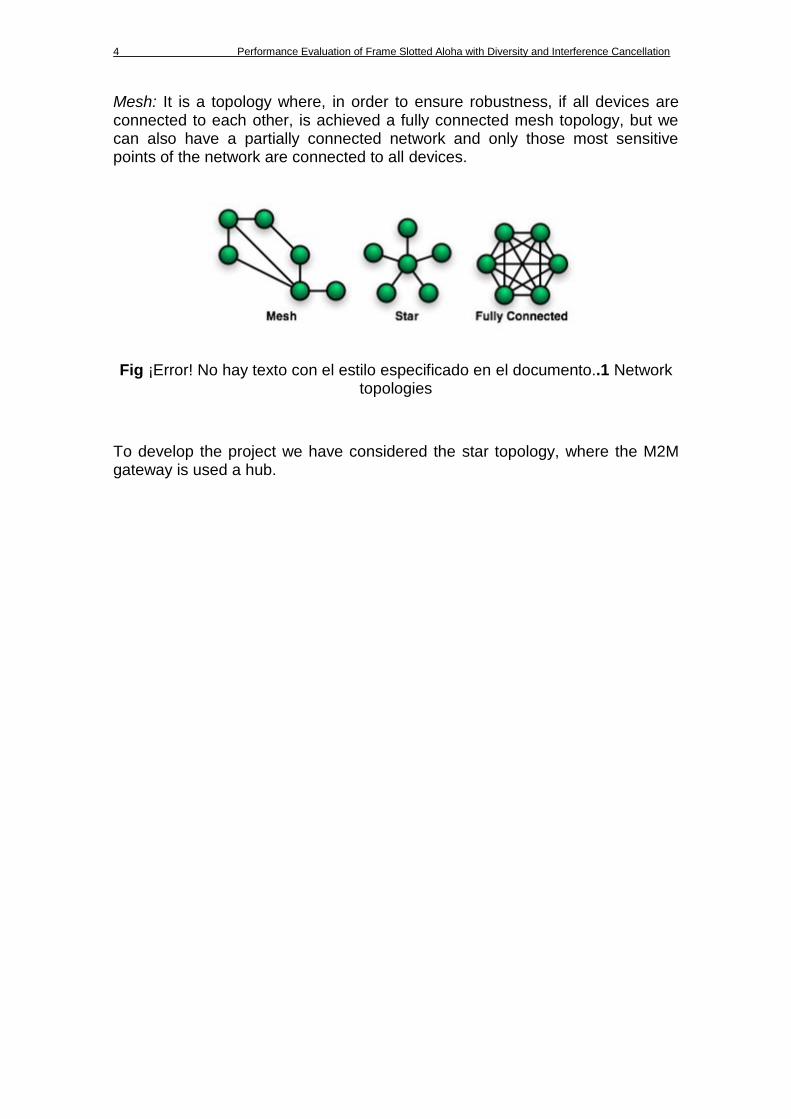
2 Overview of Machine-to-Machine Area Networks The term M2M can be used to describe any technology that enables networked devices exchange information and perform actions without human intervention. A few examples are a vending machine that warns the distributor when a particular item is running low, a medical device that periodically sends the results of a patient to the doctor, a light counter that sends their data without the need that an operator take data so the customer can know his consumption in real time, or a panel that indicates how many free parking spaces are on a plant. M2M allows a wide variety of machines to become nodes of personal wireless networks, and enables to develop monitoring and remote control applications. In this way, the quality of service will increase providing more data to the information centers in which diary-decisions are taken. M2M networks are composed of devices (sensor, RFID tags, etc.) that capture ‘events’ (temperature, inventory level, etc.), which are relayed through a network (wireless, wired or hybrid) to an application (software program), that translates the captured events into meaningful information to be stored and processed in remote M2M servers. An M2M area network consists of one M2M gateway or coordinator and many devices. The gateway is required to interconnect all the network devices with M2M servers. M2M area networks can implement different communication protocols, such as Zigbee (IEEE 802.15.4), the IEEE 802.15.4f or IEEE 802.15.6 standards. ZigBee is used in applications that require long battery life, low data rate, and secure networking. ZigBee has a rate of 250 Kbit/s, this rate is optimal for periodic or intermittent data, and is also suitable for transmission of a single signal from a device. The technology defined by the ZigBee specification intends to be simpler and less expensive than Bluetooth or Wi-Fi. The 802.15.4f version was defined as a standard for real-time locating systems (RTLS) applications such as active radio frequency identification (RFID) whereas IEEE 802.15.6 is the standard for sensing medical application. There are several network topologies to implement a M2M area network. The network topology defines the paths that information has to travel to get from one point to another. The topologies used in M2M area networks are star and mesh topology. Star: In Star topology every device is connected to central device called hub or switch (i.e., gateway). All traffic that traverses the network passes through the central hub. An advantage of the star topology is the simplicity of adding additional devices. The primary disadvantage of the star topology is that if the hub fails then all the communications through the network breaks down.


Mesh: It is a topology where, in order to ensure robustness, if all devices are connected to each other, is achieved a fully connected mesh topology, but we can also have a partially connected network and only those most sensitive points of the network are connected to all devices.

Fig ¡Error! No hay texto con el estilo especificado en el documento..1 Network topologies

To develop the project we have considered the star topology, where the M2M gateway is used a hub.

ALOHA-based Access Protocols for M2M 5

3 ALOHA-based Access Protocols for M2M

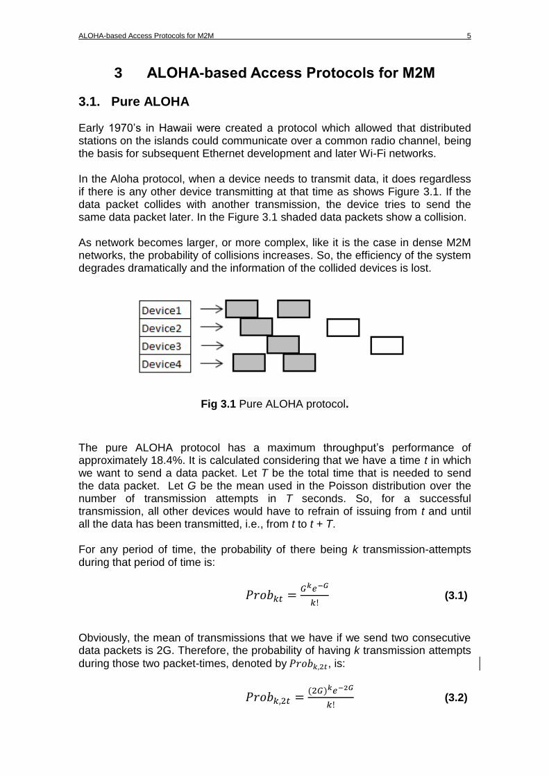
3.1. Pure ALOHA Early 1970’s in Hawaii were created a protocol which allowed that distributed stations on the islands could communicate over a common radio channel, being the basis for subsequent Ethernet development and later Wi-Fi networks. In the Aloha protocol, when a device needs to transmit data, it does regardless if there is any other device transmitting at that time as shows Figure 3.1. If the data packet collides with another transmission, the device tries to send the same data packet later. In the Figure 3.1 shaded data packets show a collision. As network becomes larger, or more complex, like it is the case in dense M2M networks, the probability of collisions increases. So, the efficiency of the system degrades dramatically and the information of the collided devices is lost.

Fig 3.1 Pure ALOHA protocol.

The pure ALOHA protocol has a maximum throughput’s performance of approximately 18.4%. It is calculated considering that we have a time t in which we want to send a data packet. Let T be the total time that is needed to send the data packet. Let G be the mean used in the Poisson distribution over the number of transmission attempts in T seconds. So, for a successful transmission, all other devices would have to refrain of issuing from t and until all the data has been transmitted, i.e., from t to t + T. For any period of time, the probability of there being k transmission-attempts during that period of time is:

(3.1)

Obviously, the mean of transmissions that we have if we send two consecutive data packets is 2G. Therefore, the probability of having k transmission attempts

during those two packet-times, denoted by , is:

(3.2)


Thus, the probability of having a successful transmission, or in other words that

the value of k is 0, denoted by , is:

(3.3)

So, if we consider that the throughput of the ALOHA protocol, , is

calculated multiplying the ratio of transmission attempts by their probabilities of success, then the throughput can be expressed as:

(3.4)

From the formula (3.4) we see that a value of G = 0.5 gives us a maximum throughput of 18.4%. This means that 81.6% of the total available time for accessing to the channel is lost due to the collisions of multiple devices accessing to the same channel simultaneously.

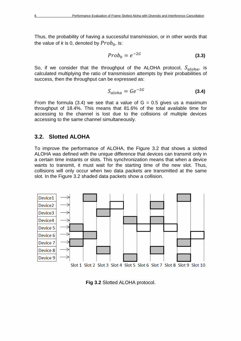
3.2. Slotted ALOHA To improve the performance of ALOHA, the Figure 3.2 that shows a slotted ALOHA was defined with the unique difference that devices can transmit only in a certain time instants or slots. This synchronization means that when a device wants to transmit, it must wait for the starting time of the new slot. Thus, collisions will only occur when two data packets are transmitted at the same slot. In the Figure 3.2 shaded data packets show a collision.

Fig 3.2 Slotted ALOHA protocol.


As explained before, the main concern of the devices is the number of transmission attempts within the period of a single slot and not 2 consecutives, since collisions can only occur during every slot. Then, the probability of there

being k transmission attempts in a single slot, denoted by , is:

(3.5)

Therefore, the probability of having a successful transmission, denoted by

, is:

(3.6)

Finally, following the same steps as in pure ALOHA, the throughput of slotted-

ALOHA, denoted by , can be expressed as:

(3.7)

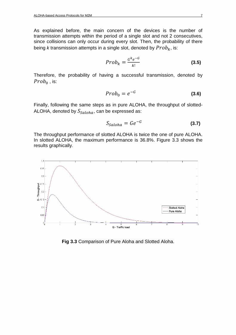
The throughput performance of slotted ALOHA is twice the one of pure ALOHA. In slotted ALOHA, the maximum performance is 36.8%. Figure 3.3 shows the results graphically.

Fig 3.3 Comparison of Pure Aloha and Slotted Aloha.


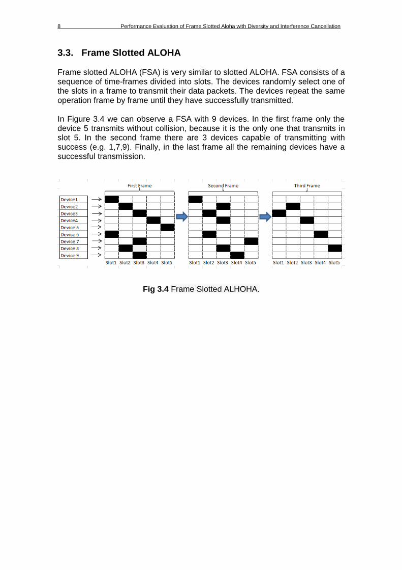
3.3. Frame Slotted ALOHA Frame slotted ALOHA (FSA) is very similar to slotted ALOHA. FSA consists of a sequence of time-frames divided into slots. The devices randomly select one of the slots in a frame to transmit their data packets. The devices repeat the same operation frame by frame until they have successfully transmitted. In Figure 3.4 we can observe a FSA with 9 devices. In the first frame only the device 5 transmits without collision, because it is the only one that transmits in slot 5. In the second frame there are 3 devices capable of transmitting with success (e.g. 1,7,9). Finally, in the last frame all the remaining devices have a successful transmission.

Fig 3.4 Frame Slotted ALHOHA.


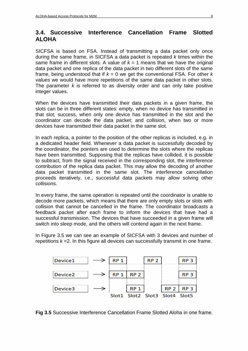
3.4. Successive Interference Cancellation Frame Slotted ALOHA SICFSA is based on FSA. Instead of transmitting a data packet only once during the same frame, in SICFSA a data packet is repeated k times within the same frame in different slots. A value of k = 1 means that we have the original data packet and one replica of the data packet in two different slots of the same frame, being understood that if k = 0 we get the conventional FSA. For other k values we would have more repetitions of the same data packet in other slots. The parameter k is referred to as diversity order and can only take positive integer values. When the devices have transmitted their data packets in a given frame, the slots can be in three different states: empty, when no device has transmitted in that slot; success, when only one device has transmitted in the slot and the coordinator can decode the data packet; and collision, when two or more devices have transmitted their data packet in the same slot. In each replica, a pointer to the position of the other replicas is included, e.g. in a dedicated header field. Whenever a data packet is successfully decoded by the coordinator, the pointers are used to determine the slots where the replicas have been transmitted. Supposing that the replicas have collided, it is possible to subtract, from the signal received in the corresponding slot, the interference contribution of the replica data packet. This may allow the decoding of another data packet transmitted in the same slot. The interference cancellation proceeds iteratively, i.e., successful data packets may allow solving other collisions. In every frame, the same operation is repeated until the coordinator is unable to decode more packets, which means that there are only empty slots or slots with collision that cannot be cancelled in the frame. The coordinator broadcasts a feedback packet after each frame to inform the devices that have had a successful transmission. The devices that have succeeded in a given frame will switch into sleep mode, and the others will contend again in the next frame. In Figure 3.5 we can see an example of SICFSA with 3 devices and number of repetitions k =2. In this figure all devices can successfully transmit in one frame.

Fig 3.5 Successive Interference Cancellation Frame Slotted Aloha in one frame.


In Figure 3.5, we can observe that 3 slots have a collision as in the case of slot 1, in which devices 1 and 2 collide, slot 2 in which devices 2 and 3 collide, and slot 5 where the 3 devices collide. The coordinator identifies the first successful replica in slot 3. This data packet belongs to device 1, and thus the coordinator can cancel the replicas of the data packet of device 1 in slots 1 and 5. This cancellation allows decoding the data packet of device 2 in slot 1. Therefore, the coordinator can cancel the replica of the data packets of device 2 in slots 2 and 5. Finally, thanks to the previous cancellations all the slots where device 3 had sent the replicas of its data packet now are success slots and not only the slot 4.

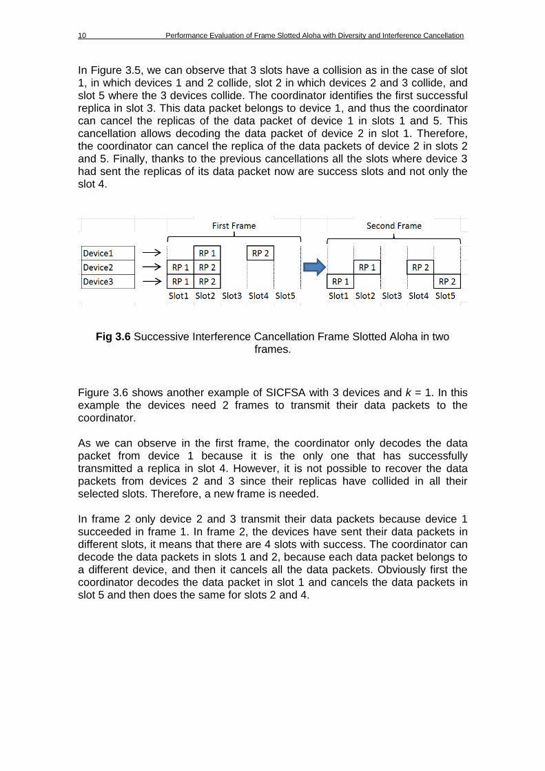
Fig 3.6 Successive Interference Cancellation Frame Slotted Aloha in two frames.

Figure 3.6 shows another example of SICFSA with 3 devices and k = 1. In this example the devices need 2 frames to transmit their data packets to the coordinator. As we can observe in the first frame, the coordinator only decodes the data packet from device 1 because it is the only one that has successfully transmitted a replica in slot 4. However, it is not possible to recover the data packets from devices 2 and 3 since their replicas have collided in all their selected slots. Therefore, a new frame is needed. In frame 2 only device 2 and 3 transmit their data packets because device 1 succeeded in frame 1. In frame 2, the devices have sent their data packets in different slots, it means that there are 4 slots with success. The coordinator can decode the data packets in slots 1 and 2, because each data packet belongs to a different device, and then it cancels all the data packets. Obviously first the coordinator decodes the data packet in slot 1 and cancels the data packets in slot 5 and then does the same for slots 2 and 4.


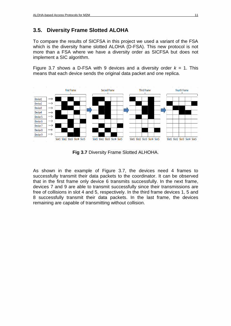
3.5. Diversity Frame Slotted ALOHA To compare the results of SICFSA in this project we used a variant of the FSA which is the diversity frame slotted ALOHA (D-FSA). This new protocol is not more than a FSA where we have a diversity order as SICFSA but does not implement a SIC algorithm. Figure 3.7 shows a D-FSA with 9 devices and a diversity order k = 1. This means that each device sends the original data packet and one replica.

Fig 3.7 Diversity Frame Slotted ALHOHA.

As shown in the example of Figure 3.7, the devices need 4 frames to successfully transmit their data packets to the coordinator. It can be observed that in the first frame only device 6 transmits successfully. In the next frame, devices 7 and 9 are able to transmit successfully since their transmissions are free of collisions in slot 4 and 5, respectively. In the third frame devices 1, 5 and 8 successfully transmit their data packets. In the last frame, the devices remaining are capable of transmitting without collision.


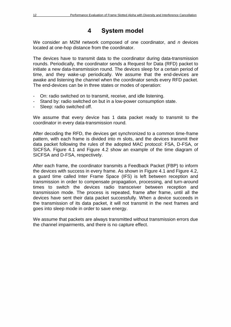
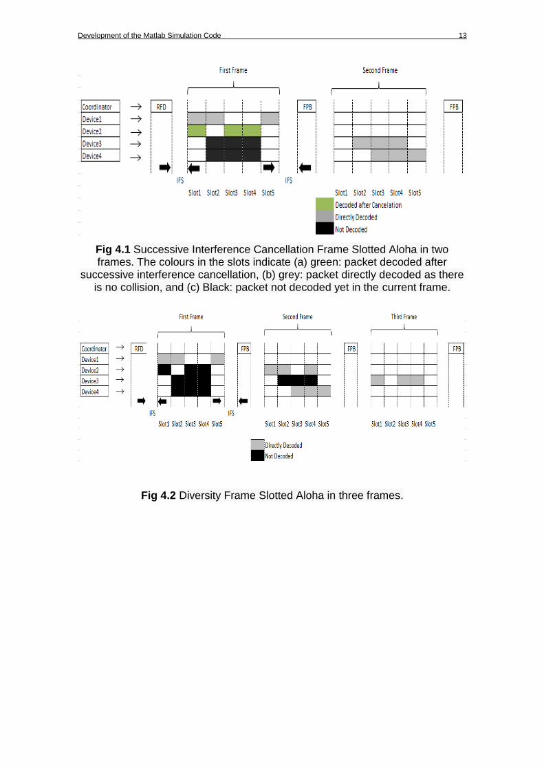
4 System model We consider an M2M network composed of one coordinator, and n devices located at one-hop distance from the coordinator. The devices have to transmit data to the coordinator during data-transmission rounds. Periodically, the coordinator sends a Request for Data (RFD) packet to initiate a new data-transmission round. The devices sleep for a certain period of time, and they wake-up periodically. We assume that the end-devices are awake and listening the channel when the coordinator sends every RFD packet. The end-devices can be in three states or modes of operation: - On: radio switched on to transmit, receive, and idle listening. - Stand by: radio switched on but in a low-power consumption state. - Sleep: radio switched off. We assume that every device has 1 data packet ready to transmit to the coordinator in every data-transmission round. After decoding the RFD, the devices get synchronized to a common time-frame pattern, with each frame is divided into m slots, and the devices transmit their data packet following the rules of the adopted MAC protocol: FSA, D-FSA, or SICFSA. Figure 4.1 and Figure 4.2 show an example of the time diagram of SICFSA and D-FSA, respectively.

After each frame, the coordinator transmits a Feedback Packet (FBP) to inform the devices with success in every frame. As shown in Figure 4.1 and Figure 4.2, a guard time called Inter Frame Space (IFS) is left between reception and transmission in order to compensate propagation, processing, and turn-around times to switch the devices radio transceiver between reception and transmission mode. The process is repeated, frame after frame, until all the devices have sent their data packet successfully. When a device succeeds in the transmission of its data packet, it will not transmit in the next frames and goes into sleep mode in order to save energy. We assume that packets are always transmitted without transmission errors due the channel impairments, and there is no capture effect.

Development of the Matlab Simulation Code 13

Fig 4.1 Successive Interference Cancellation Frame Slotted Aloha in two frames. The colours in the slots indicate (a) green: packet decoded after

successive interference cancellation, (b) grey: packet directly decoded as there is no collision, and (c) Black: packet not decoded yet in the current frame.

Fig 4.2 Diversity Frame Slotted Aloha in three frames.


5 Development of the Matlab Simulation Code This section describes the algorithms of the various functions that we used for the development of SICFSA and D-FSA in Matlab. Sections 5.1, 5.2 and 5.3 show the operation of ‘slot selection’ function, ‘SICFSA’ function, and ‘D-FSA’ function, respectively. Section 5.4 describes the variables passed between the ‘slot selection’ function, ‘SICFSA’ function and ‘D-FSA’ function. Finally, section 5.5 shows the computation of delay and energy consumption.

5.1. Slot selection function

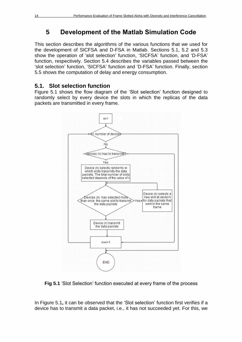
Figure 5.1 shows the flow diagram of the ‘Slot selection’ function designed to randomly select by every device the slots in which the replicas of the data packets are transmitted in every frame.

Fig 5.1 ‘Slot Selection’ function executed at every frame of the process

In Figure 5.1, it can be observed that the ‘Slot selection’ function first verifies if a device has to transmit a data packet, i.e., it has not succeeded yet. For this, we


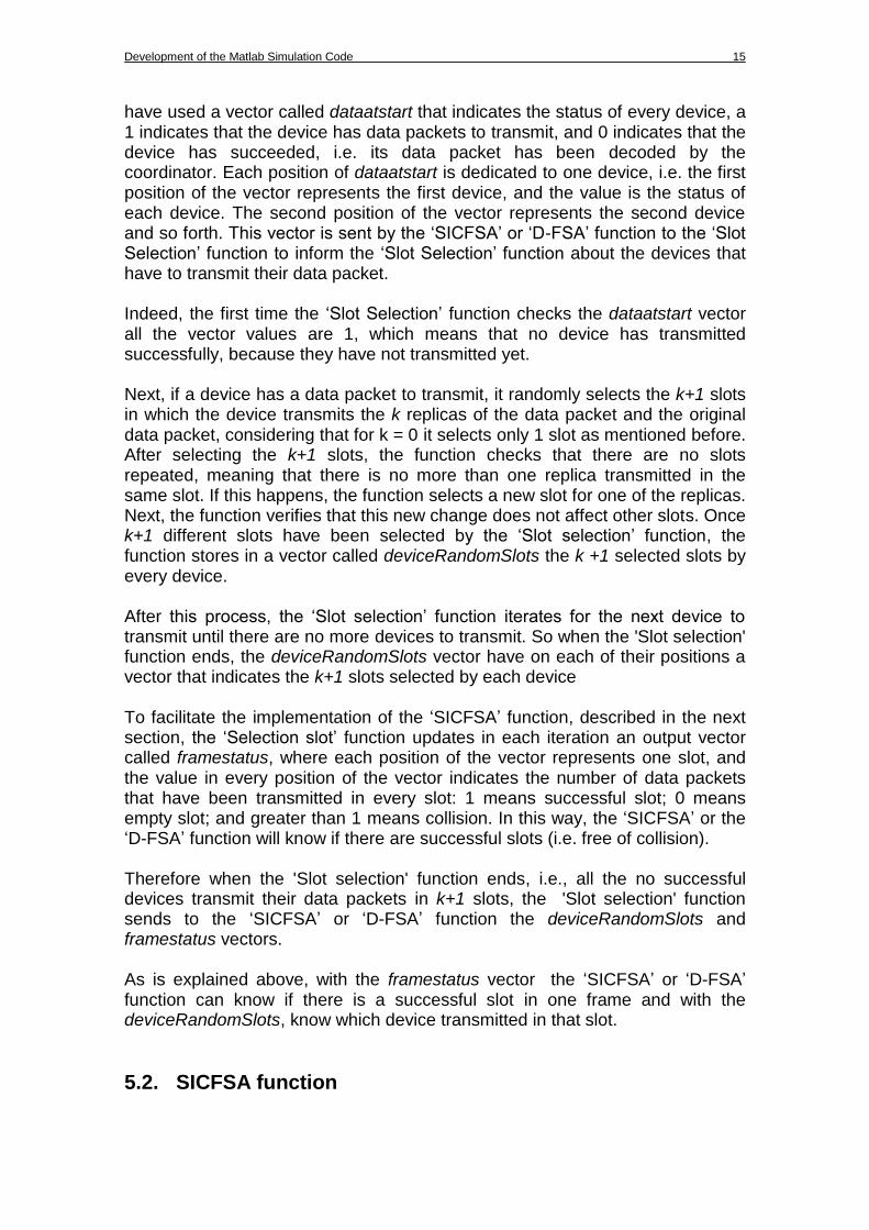
have used a vector called dataatstart that indicates the status of every device, a 1 indicates that the device has data packets to transmit, and 0 indicates that the device has succeeded, i.e. its data packet has been decoded by the coordinator. Each position of dataatstart is dedicated to one device, i.e. the first position of the vector represents the first device, and the value is the status of each device. The second position of the vector represents the second device and so forth. This vector is sent by the ‘SICFSA’ or ‘D-FSA’ function to the ‘Slot Selection’ function to inform the ‘Slot Selection’ function about the devices that have to transmit their data packet. Indeed, the first time the ‘Slot Selection’ function checks the dataatstart vector all the vector values are 1, which means that no device has transmitted successfully, because they have not transmitted yet. Next, if a device has a data packet to transmit, it randomly selects the k+1 slots in which the device transmits the k replicas of the data packet and the original data packet, considering that for k = 0 it selects only 1 slot as mentioned before. After selecting the k+1 slots, the function checks that there are no slots repeated, meaning that there is no more than one replica transmitted in the same slot. If this happens, the function selects a new slot for one of the replicas. Next, the function verifies that this new change does not affect other slots. Once k+1 different slots have been selected by the ‘Slot selection’ function, the function stores in a vector called deviceRandomSlots the k +1 selected slots by every device. After this process, the ‘Slot selection’ function iterates for the next device to transmit until there are no more devices to transmit. So when the 'Slot selection' function ends, the deviceRandomSlots vector have on each of their positions a vector that indicates the k+1 slots selected by each device To facilitate the implementation of the ‘SICFSA’ function, described in the next section, the ‘Selection slot’ function updates in each iteration an output vector called framestatus, where each position of the vector represents one slot, and the value in every position of the vector indicates the number of data packets that have been transmitted in every slot: 1 means successful slot; 0 means empty slot; and greater than 1 means collision. In this way, the ‘SICFSA’ or the ‘D-FSA’ function will know if there are successful slots (i.e. free of collision). Therefore when the 'Slot selection' function ends, i.e., all the no successful devices transmit their data packets in k+1 slots, the 'Slot selection' function sends to the ‘SICFSA’ or ‘D-FSA’ function the deviceRandomSlots and framestatus vectors. As is explained above, with the framestatus vector the ‘SICFSA’ or ‘D-FSA’ function can know if there is a successful slot in one frame and with the deviceRandomSlots, know which device transmitted in that slot.

5.2. SICFSA function


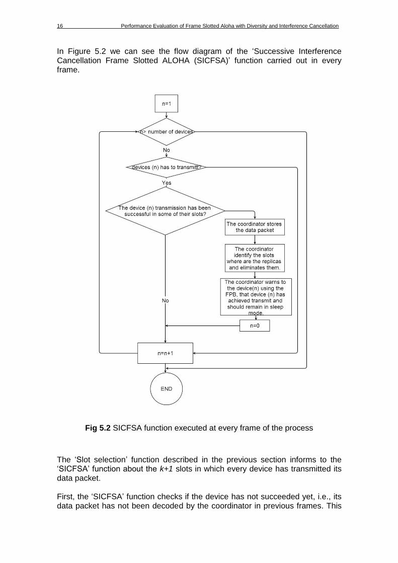
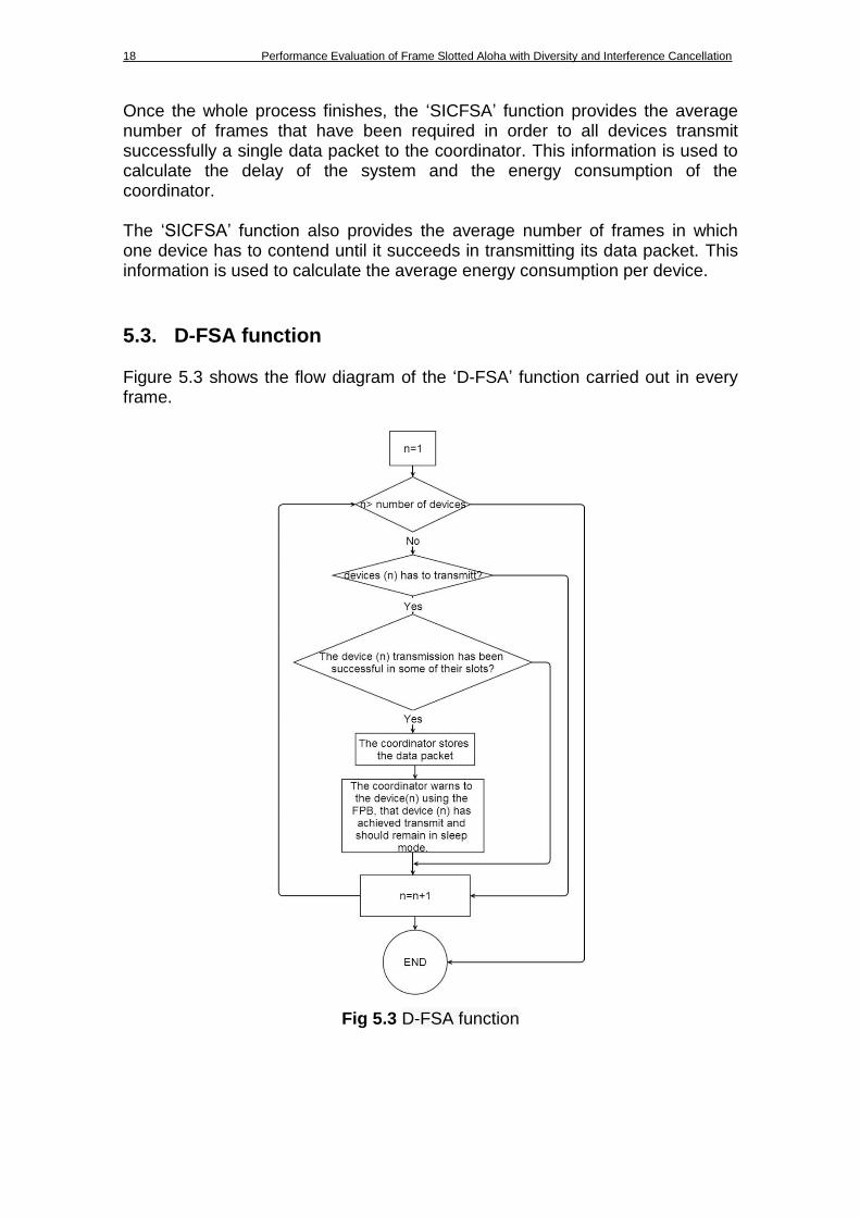
In Figure 5.2 we can see the flow diagram of the ‘Successive Interference Cancellation Frame Slotted ALOHA (SICFSA)’ function carried out in every frame.

Fig 5.2 SICFSA function executed at every frame of the process

The ‘Slot selection’ function described in the previous section informs to the ‘SICFSA’ function about the k+1 slots in which every device has transmitted its data packet. First, the ‘SICFSA’ function checks if the device has not succeeded yet, i.e., its data packet has not been decoded by the coordinator in previous frames. This


is verified by checking the corresponding position of the vector dataatstart. If the device has transmitted in the current frame, the ‘SICFSA’ function checks if any of the k+1 slots where the device has transmitted its data packet is a successful slot, i.e., the value in any of the positions of the framestatus vector corresponding to the slots where the device has transmitted is 1. If the ‘SICFSA’ function finds a successful slot, it stores the data packet of the device, i.e., the coordinator has decoded the data packet successfully. This is represented with a vector called success_device, where each position indicates a device number, and the values that of each position of success_device can be 1 or 0: 1 indicates that the data packet from the device has already been decoded successfully, whereas 0 means that there is still no data packet successfully decoded from the device. Therefore, when the ‘SICFSA’ function finds a successful slot, it changes the value of the corresponding position of success_device to 1. Then, it decrements by 1 all the positions of the framestatus vector that correspond to the slots where the device has transmitted the replicas of its data packet, this simulates the interference cancelation. The ‘SICFSA’ function knows the slots that contain the replicas by checking the deviceRandomSlots vector which provides such information. It is worth to note that the decrement by 1 in a position of the framestatus vector in which there is a value of 2 (i.e., 2 different devices transmitted in that slot), now it would be 1 and therefore a new data packet from another device can be successfully decoded as there is only one data packet in that slot after cancelling the interference. Then, the ‘SICFSA’ function changes the value of the corresponding value of the dataatstart vector to 0 indicating that the device has succeeded (i.e., it enters into sleep mode in subsequent frames). This is equivalent to the FPB packet sent by the coordinator to inform the devices whether they transmitted successfully or not. Once the vector variables success_device, framestatus, and dataatstart have been updated, the ‘SICFSA’ function checks again (starting from the first device) all slots where the devices have transmitted replicas of their data packets looking for new successful slots. When a new position of the framestatus vector is 1 (i.e., another data packet from other device can be decoded by the coordinator), the ‘SICFSA’ function executes again the interference cancellation by decrementing by 1 all the positions of framestatus that correspond to the slots where the new successful device has transmitted the replicas of its data packet. The ‘SICFSA’ function finishes in a frame when it finds that there are no more data packets to be successfully decoded by the coordinator. Once the ‘SICFSA’ function finishes, the ‘Selection slot’ function is executed again so that those devices that have not successfully transmitted yet can select again new slots for transmitting replicas of their data packet in the next frame. Thus, the ‘Selection slot’ function and ‘SICFSA’ function are executed sequentially frame by frame until one data packet from every device has been successfully decoded.


Once the whole process finishes, the ‘SICFSA’ function provides the average number of frames that have been required in order to all devices transmit successfully a single data packet to the coordinator. This information is used to calculate the delay of the system and the energy consumption of the coordinator. The ‘SICFSA’ function also provides the average number of frames in which one device has to contend until it succeeds in transmitting its data packet. This information is used to calculate the average energy consumption per device.

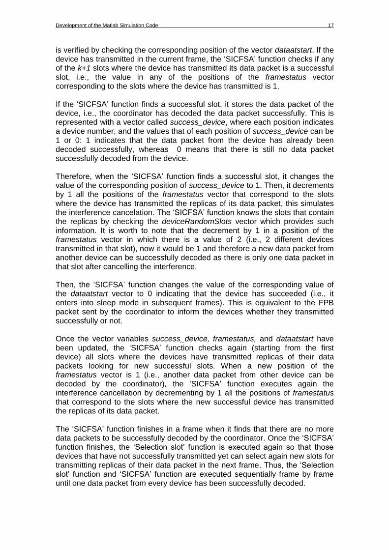
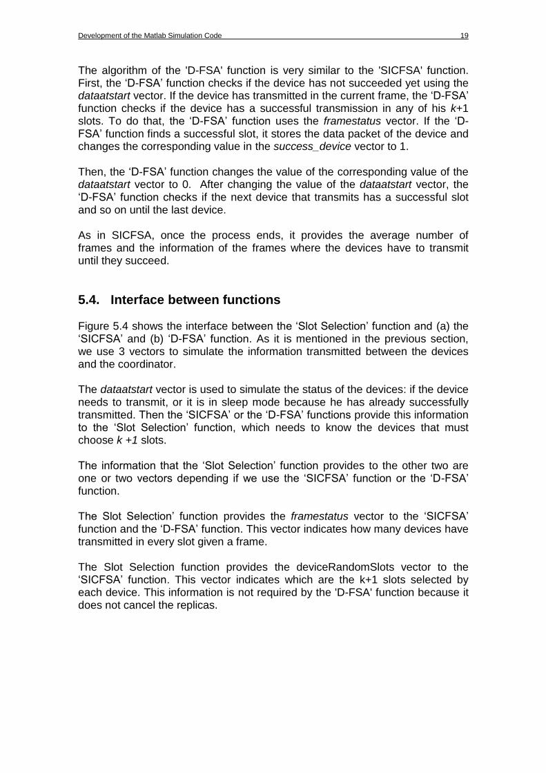
5.3. D-FSA function Figure 5.3 shows the flow diagram of the ‘D-FSA’ function carried out in every frame.

Fig 5.3 D-FSA function


The algorithm of the 'D-FSA' function is very similar to the 'SICFSA' function. First, the ‘D-FSA’ function checks if the device has not succeeded yet using the dataatstart vector. If the device has transmitted in the current frame, the ‘D-FSA’ function checks if the device has a successful transmission in any of his k+1 slots. To do that, the ‘D-FSA’ function uses the framestatus vector. If the ‘D-FSA’ function finds a successful slot, it stores the data packet of the device and changes the corresponding value in the success_device vector to 1. Then, the ‘D-FSA’ function changes the value of the corresponding value of the dataatstart vector to 0. After changing the value of the dataatstart vector, the ‘D-FSA’ function checks if the next device that transmits has a successful slot and so on until the last device. As in SICFSA, once the process ends, it provides the average number of frames and the information of the frames where the devices have to transmit until they succeed.

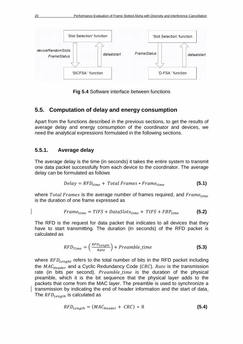
5.4. Interface between functions Figure 5.4 shows the interface between the ‘Slot Selection’ function and (a) the ‘SICFSA’ and (b) ‘D-FSA’ function. As it is mentioned in the previous section, we use 3 vectors to simulate the information transmitted between the devices and the coordinator. The dataatstart vector is used to simulate the status of the devices: if the device needs to transmit, or it is in sleep mode because he has already successfully transmitted. Then the ‘SICFSA’ or the ‘D-FSA’ functions provide this information to the ‘Slot Selection’ function, which needs to know the devices that must choose k +1 slots. The information that the ‘Slot Selection’ function provides to the other two are one or two vectors depending if we use the ‘SICFSA’ function or the ‘D-FSA’ function. The Slot Selection’ function provides the framestatus vector to the ‘SICFSA’ function and the ‘D-FSA’ function. This vector indicates how many devices have transmitted in every slot given a frame. The Slot Selection function provides the deviceRandomSlots vector to the ‘SICFSA’ function. This vector indicates which are the k+1 slots selected by each device. This information is not required by the 'D-FSA' function because it does not cancel the replicas.


Fig 5.4 Software interface between functions

5.5. Computation of delay and energy consumption Apart from the functions described in the previous sections, to get the results of average delay and energy consumption of the coordinator and devices, we need the analytical expressions formulated in the following sections.

5.5.1. Average delay The average delay is the time (in seconds) it takes the entire system to transmit one data packet successfully from each device to the coordinator. The average delay can be formulated as follows

(5.1)

where is the average number of frames required, and is the duration of one frame expressed as

(5.2)

The RFD is the request for data packet that indicates to all devices that they have to start transmitting. The duration (in seconds) of the RFD packet is calculated as

(

) (5.3)

where refers to the total number of bits in the RFD packet including

the and a Cyclic Redundancy Code ( ). is the transmission rate (in bits per second). is the duration of the physical preamble, which it is the bit sequence that the physical layer adds to the packets that come from the MAC layer. The preamble is used to synchronize a transmission by indicating the end of header information and the start of data. The is calculated as

(5.4)


The contains all the information needed to send the RFD packet

to the devices. The contains a broadcast address that allows to all the devices receive the RFD packet. CRC (in bytes) is a Cyclic Redundancy Check (CRC) code used to detect errors in transmission due to channel impairments.

The , indicated in (5.2), is the time (in seconds) of the Inter Frame Space. The , indicated in the same (5.2), refers to the time (in seconds) of all slots in the frame, which is calculated as

(5.5) where m is the total number of slots per frame, and is the duration (in seconds) of a single slot. All the slots have the same duration. The maximum

duration of a slot is time of transmission of a data packet. The is calculated as

(

) (5.6)

where refers to the total number of bits of the data

packet. can be formulated as follows

( ) (5.7)

is the total number of data bits contained in the payload of a data

packet. The FPB packet is sent by the coordinator at the end of each frame. The FPB informs to the devices if some data packet has been decoded successfully by

the coordinator. The duration (in seconds) of the FPB packet, , indicated in (5.2) is calculated as

(5.8)

where means the total length of the FPB packet including the

, the payload, and The is calculated as,

(5.9)

is the total number of bits in the payload of the FPB packet, which

can be calculated as

(5.10)

where m is the number of slots and 16 is the number of bits used to encode the MAC address (or identification) of the device that has succeeded in a slot.


5.5.2. Average energy consumption of the coordinator The average energy consumption of the coordinator is the energy (in joules) consumed by the coordinator since the process starts until all devices successfully transmit one data packet to the coordinator. The average coordinator energy consumption can be expressed as

)} * (5.11)

where is the energy (in joules) needed by the coordinator to transmit the RFD packet and is formulated as

(5.12)

the was formulated in (5.3) and the is the power (in watts) consumption of the radio transceiver of the coordinator in transmission mode. The is the energy (in joules) spent by the coordinator in a TIFS. The

expression for calculating is the next

(5.13)

During a TIFS the coordinator must not receive or transmit, therefore the coordinator remains in a standby mode and the power (in watts) is

.

refers to the energy (in joules) used by the coordinator to receive a data packet in a slot, the expression of the is,

(5.14)

where the is the power (in watts) consumption of the radio transceiver of the coordinator in reception mode.

is the average number of frames necessary so that all devices successfully transmit one data packet to the coordinator.

5.5.3. Average energy consumption of a device The average energy consumption of one device is the energy that needs to use a device to successfully transmit a data packet to the coordinator and it can be formulated as follows (5.15)

is the energy (in joules) needed by a device to receive the RFD packet and can be formulated as


(5.16)

As the radio transceiver is the same for coordinator and a device, the is the same as in (5.14). is the energy (in joules) consumed by a device to transmit the k+1 replicas of a data packets in one frame, is the average number of frames where the device has to transmit the k+1 replicas of the data packet until it is successfully decoded by the coordinator. The expression of is,

( )

(5.17)

where is the energy (in joules) consumed by a device in the transmission of a replica of a data packet, indicates the total number of slots in which device transmits the data packet. The energy (in joules) consumed by a device in those slots in which it does not transmit any replica of the data packet is and is the total number of slots where the device does

not transmit. The expressions of is,

(5.18)

where is formulated in (5.6) and is the power consumption (in watts) of the radio transceiver of a device in transmission mode. The formula of indicated in (5.17) is,

(5.19)

where is the power (in watts) consumption of the radio transceiver of the device when it is in standby mode, i.e., it does not transmit in one slot. indicated in (5.15) is the energy (in joules) consumed by one device

that remains in sleep mode during a frame once it has succeeded.

indicates the average number of frames in which one device remains in sleep mode after succeeding in the transmission of its data packet to the coordinator. The expression of is,

(5.20)

where is the power consumption of the radio transceiver of the device in sleep mode.


6 Performance Evaluation

6.1. System Parameters

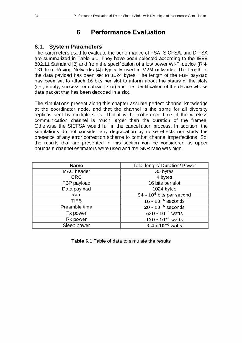
The parameters used to evaluate the performance of FSA, SICFSA, and D-FSA are summarized in Table 6.1. They have been selected according to the IEEE 802.11 Standard [3] and from the specification of a low power Wi-Fi device (RN-131 from Roving Networks [4]) typically used in M2M networks. The length of the data payload has been set to 1024 bytes. The length of the FBP payload has been set to attach 16 bits per slot to inform about the status of the slots (i.e., empty, success, or collision slot) and the identification of the device whose data packet that has been decoded in a slot. The simulations present along this chapter assume perfect channel knowledge at the coordinator node, and that the channel is the same for all diversity replicas sent by multiple slots. That it is the coherence time of the wireless communication channel is much larger than the duration of the frames. Otherwise the SICFSA would fail in the cancellation process. In addition, the simulations do not consider any degradation by noise effects nor study the presence of any error correction scheme to combat channel imperfections. So, the results that are presented in this section can be considered as upper bounds if channel estimators were used and the SNR ratio was high.

Name Total length/ Duration/ Power

MAC header 30 bytes

CRC 4 bytes

FBP payload 16 bits per slot

Data payload 1024 bytes

Rate bits per second

TIFS seconds

Preamble time seconds

Tx power watts

Rx power watts

Sleep power watts

Table 6.1 Table of data to simulate the results

Conclusions 25

6.2. Average Delay and Energy Consumption over the Diversity Order In order to study the performance of the SICFSA and D-FSA protocols, we first set the number of devices to 50 and 100 devices and we evaluate the protocols’ performance as a function of the diversity order (k). In order to have representative measures, we have averaged the results of 400 simulation samples.

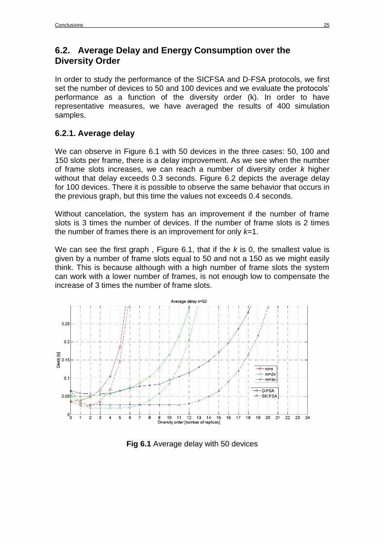
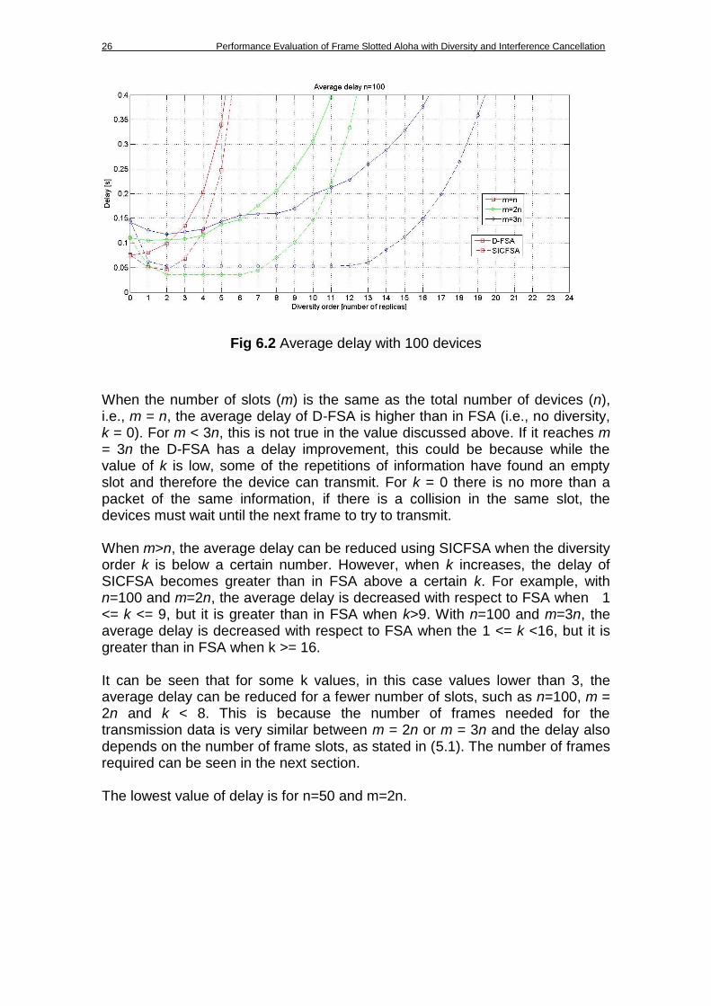
6.2.1. Average delay We can observe in Figure 6.1 with 50 devices in the three cases: 50, 100 and 150 slots per frame, there is a delay improvement. As we see when the number of frame slots increases, we can reach a number of diversity order k higher without that delay exceeds 0.3 seconds. Figure 6.2 depicts the average delay for 100 devices. There it is possible to observe the same behavior that occurs in the previous graph, but this time the values not exceeds 0.4 seconds. Without cancelation, the system has an improvement if the number of frame slots is 3 times the number of devices. If the number of frame slots is 2 times the number of frames there is an improvement for only k=1. We can see the first graph , Figure 6.1, that if the k is 0, the smallest value is given by a number of frame slots equal to 50 and not a 150 as we might easily think. This is because although with a high number of frame slots the system can work with a lower number of frames, is not enough low to compensate the increase of 3 times the number of frame slots.

Fig 6.1 Average delay with 50 devices


Fig 6.2 Average delay with 100 devices

When the number of slots (m) is the same as the total number of devices (n), i.e., m = n, the average delay of D-FSA is higher than in FSA (i.e., no diversity, k = 0). For m < 3n, this is not true in the value discussed above. If it reaches m = 3n the D-FSA has a delay improvement, this could be because while the value of k is low, some of the repetitions of information have found an empty slot and therefore the device can transmit. For k = 0 there is no more than a packet of the same information, if there is a collision in the same slot, the devices must wait until the next frame to try to transmit. When m>n, the average delay can be reduced using SICFSA when the diversity order k is below a certain number. However, when k increases, the delay of SICFSA becomes greater than in FSA above a certain k. For example, with n=100 and m=2n, the average delay is decreased with respect to FSA when 1 <= k <= 9, but it is greater than in FSA when k>9. With n=100 and m=3n, the average delay is decreased with respect to FSA when the 1 <= k <16, but it is greater than in FSA when k >= 16. It can be seen that for some k values, in this case values lower than 3, the average delay can be reduced for a fewer number of slots, such as n=100, m = 2n and k < 8. This is because the number of frames needed for the transmission data is very similar between m = 2n or m = 3n and the delay also depends on the number of frame slots, as stated in (5.1). The number of frames required can be seen in the next section. The lowest value of delay is for n=50 and m=2n.

Conclusions 27

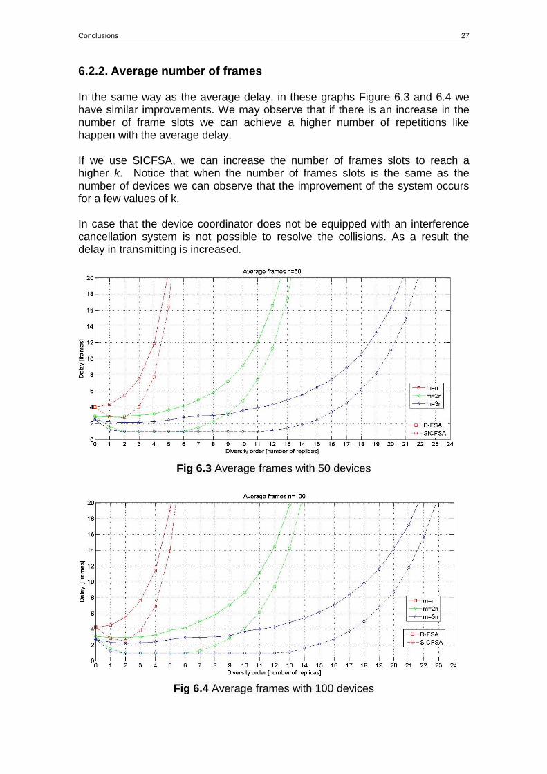
6.2.2. Average number of frames In the same way as the average delay, in these graphs Figure 6.3 and 6.4 we have similar improvements. We may observe that if there is an increase in the number of frame slots we can achieve a higher number of repetitions like happen with the average delay. If we use SICFSA, we can increase the number of frames slots to reach a higher k. Notice that when the number of frames slots is the same as the number of devices we can observe that the improvement of the system occurs for a few values of k. In case that the device coordinator does not be equipped with an interference cancellation system is not possible to resolve the collisions. As a result the delay in transmitting is increased.

Fig 6.3 Average frames with 50 devices

Fig 6.4 Average frames with 100 devices


As stated in the previous section can be seen for a value of k = 0, the lowest value of frames is for m = 3n, but this is not 3 times less than for m = n and therefore in Figure 6.1 or Figure 6.2 appears the changed result. As said above also shows that for k >= 2 and k <= 6 use the same number of frames, in this case 1, for m = 2n and m = 3n. Then during this interval will be less the delay for m = 2n that for m = 3n as is evident. We must also take into account that for m = 3n resolve in one frame is maintained in 2 <= k <= 12. As mentioned in the previous section, there is a little improvement in the D-FSA with m = 3n, for 0 < k <=4. This same improvement appears for m = 2n and k=1 or 2. So it seems that if the number of frame slots is sufficiently large can get an improvement even without cancellation.

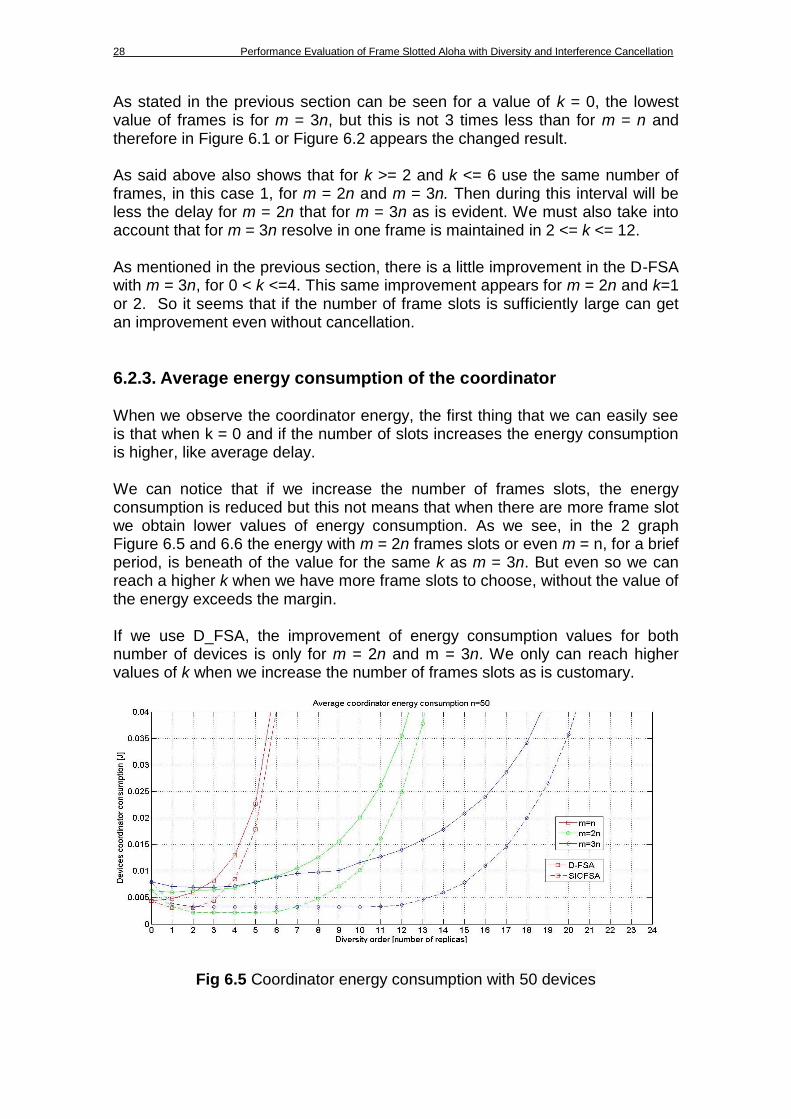
6.2.3. Average energy consumption of the coordinator When we observe the coordinator energy, the first thing that we can easily see is that when k = 0 and if the number of slots increases the energy consumption is higher, like average delay. We can notice that if we increase the number of frames slots, the energy consumption is reduced but this not means that when there are more frame slot we obtain lower values of energy consumption. As we see, in the 2 graph Figure 6.5 and 6.6 the energy with m = 2n frames slots or even m = n, for a brief period, is beneath of the value for the same k as m = 3n. But even so we can reach a higher k when we have more frame slots to choose, without the value of the energy exceeds the margin. If we use D_FSA, the improvement of energy consumption values for both number of devices is only for m = 2n and m = 3n. We only can reach higher values of k when we increase the number of frames slots as is customary.

Fig 6.5 Coordinator energy consumption with 50 devices

Conclusions 29

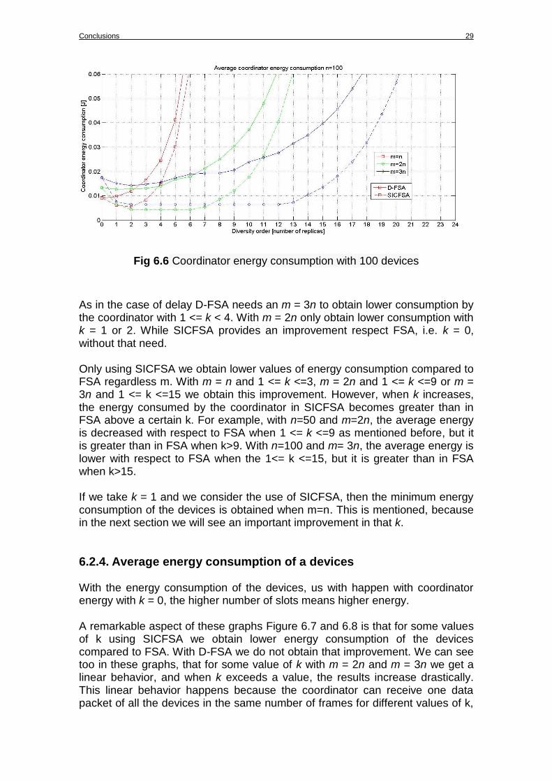
Fig 6.6 Coordinator energy consumption with 100 devices

As in the case of delay D-FSA needs an m = 3n to obtain lower consumption by the coordinator with 1 <= k < 4. With m = 2n only obtain lower consumption with k = 1 or 2. While SICFSA provides an improvement respect FSA, i.e. k = 0, without that need. Only using SICFSA we obtain lower values of energy consumption compared to FSA regardless m. With m = n and 1 <= k <=3, m = 2n and 1 <= k <=9 or m = 3n and 1 <= k <=15 we obtain this improvement. However, when k increases, the energy consumed by the coordinator in SICFSA becomes greater than in FSA above a certain k. For example, with n=50 and m=2n, the average energy is decreased with respect to FSA when 1 <= k <=9 as mentioned before, but it is greater than in FSA when k>9. With n=100 and m= 3n, the average energy is lower with respect to FSA when the 1<= k <=15, but it is greater than in FSA when k>15. If we take k = 1 and we consider the use of SICFSA, then the minimum energy consumption of the devices is obtained when m=n. This is mentioned, because in the next section we will see an important improvement in that k.

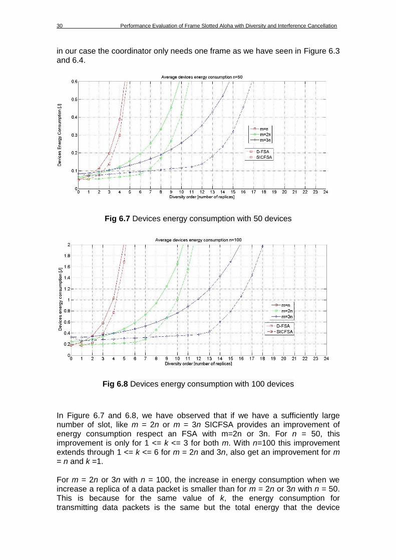
6.2.4. Average energy consumption of a devices With the energy consumption of the devices, us with happen with coordinator energy with k = 0, the higher number of slots means higher energy. A remarkable aspect of these graphs Figure 6.7 and 6.8 is that for some values of k using SICFSA we obtain lower energy consumption of the devices compared to FSA. With D-FSA we do not obtain that improvement. We can see too in these graphs, that for some value of k with m = 2n and m = 3n we get a linear behavior, and when k exceeds a value, the results increase drastically. This linear behavior happens because the coordinator can receive one data packet of all the devices in the same number of frames for different values of k,


in our case the coordinator only needs one frame as we have seen in Figure 6.3 and 6.4.

Fig 6.7 Devices energy consumption with 50 devices

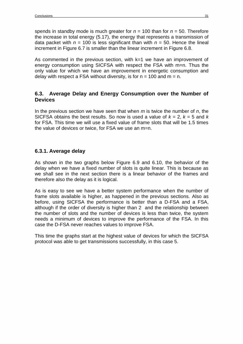
Fig 6.8 Devices energy consumption with 100 devices

In Figure 6.7 and 6.8, we have observed that if we have a sufficiently large number of slot, like m = 2n or m = 3n SICFSA provides an improvement of energy consumption respect an FSA with m=2n or 3n. For n = 50, this improvement is only for 1 <= k <= 3 for both m. With n=100 this improvement extends through 1 <= k <= 6 for m = 2n and 3n, also get an improvement for m = n and k =1. For m = 2n or 3n with n = 100, the increase in energy consumption when we increase a replica of a data packet is smaller than for m = 2n or 3n with n = 50. This is because for the same value of k, the energy consumption for transmitting data packets is the same but the total energy that the device

Conclusions 31

spends in standby mode is much greater for n = 100 than for n = 50. Therefore the increase in total energy (5.17), the energy that represents a transmission of data packet with n = 100 is less significant than with n = 50. Hence the lineal increment in Figure 6.7 is smaller than the linear increment in Figure 6.8. As commented in the previous section, with k=1 we have an improvement of energy consumption using SICFSA with respect the FSA with m=n. Thus the only value for which we have an improvement in energetic consumption and delay with respect a FSA without diversity, is for n = 100 and m = n.

6.3. Average Delay and Energy Consumption over the Number of Devices In the previous section we have seen that when m is twice the number of n, the SICFSA obtains the best results. So now is used a value of k = 2, k = 5 and k for FSA. This time we will use a fixed value of frame slots that will be 1.5 times the value of devices or twice, for FSA we use an m=n.

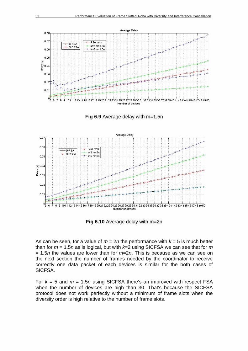
6.3.1. Average delay As shown in the two graphs below Figure 6.9 and 6.10, the behavior of the delay when we have a fixed number of slots is quite linear. This is because as we shall see in the next section there is a linear behavior of the frames and therefore also the delay as it is logical. As is easy to see we have a better system performance when the number of frame slots available is higher, as happened in the previous sections. Also as before, using SICFSA the performance is better than a D-FSA and a FSA, although if the order of diversity is higher than 2 and the relationship between the number of slots and the number of devices is less than twice, the system needs a minimum of devices to improve the performance of the FSA. In this case the D-FSA never reaches values to improve FSA. This time the graphs start at the highest value of devices for which the SICFSA protocol was able to get transmissions successfully, in this case 5.


Fig 6.9 Average delay with m=1.5n

Fig 6.10 Average delay with m=2n

As can be seen, for a value of m = 2n the performance with k = 5 is much better than for m = 1.5n as is logical, but with k=2 using SICFSA we can see that for m = 1.5n the values are lower than for m=2n. This is because as we can see on the next section the number of frames needed by the coordinator to receive correctly one data packet of each devices is similar for the both cases of SICFSA.

For k = 5 and m = 1.5n using SICFSA there's an improved with respect FSA when the number of devices are high than 30. That's because the SICFSA protocol does not work perfectly without a minimum of frame slots when the diversity order is high relative to the number of frame slots.

Conclusions 33

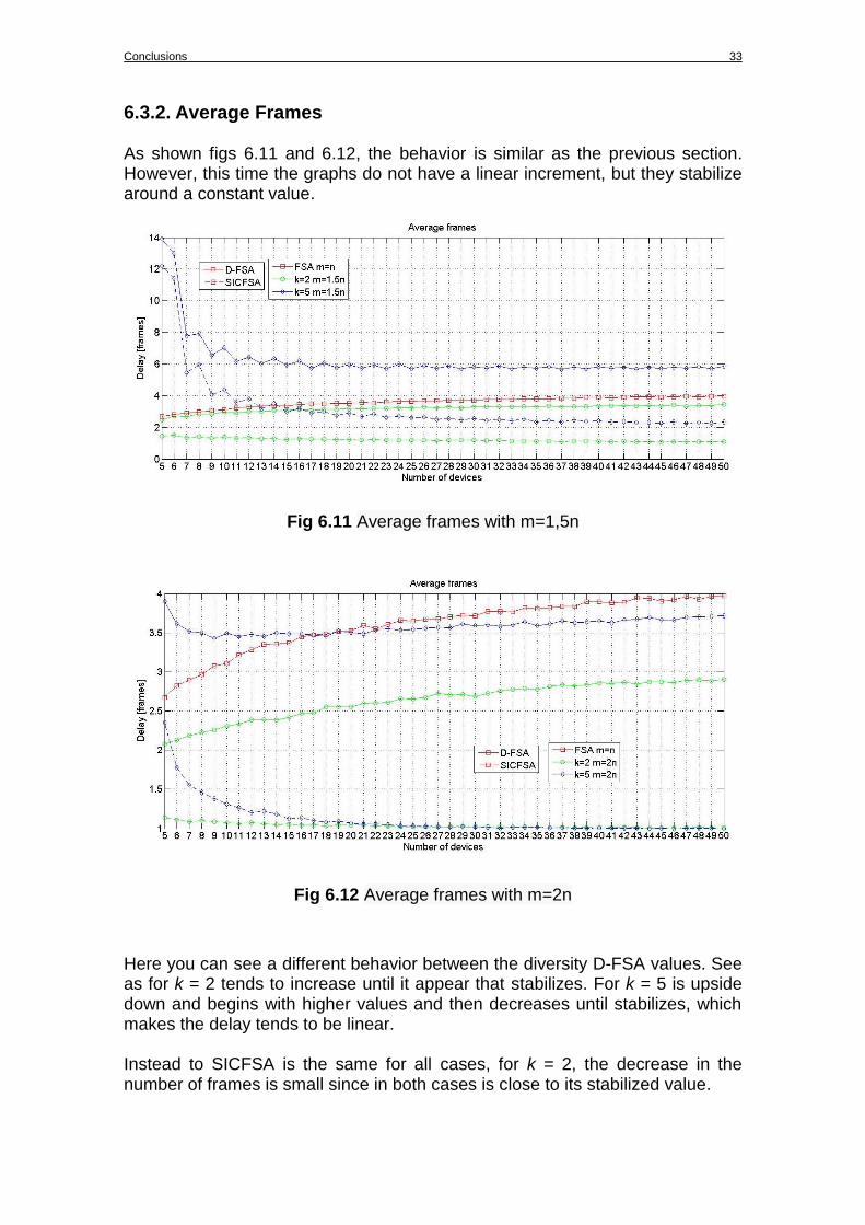
6.3.2. Average Frames As shown figs 6.11 and 6.12, the behavior is similar as the previous section. However, this time the graphs do not have a linear increment, but they stabilize around a constant value.

Fig 6.11 Average frames with m=1,5n

Fig 6.12 Average frames with m=2n

Here you can see a different behavior between the diversity D-FSA values. See as for k = 2 tends to increase until it appear that stabilizes. For k = 5 is upside down and begins with higher values and then decreases until stabilizes, which makes the delay tends to be linear. Instead to SICFSA is the same for all cases, for k = 2, the decrease in the number of frames is small since in both cases is close to its stabilized value.


Can see that for both slot numbers, for k = 2 using SICFSA the result is practically the same. Not so with k = 5 because for m = 1.5n, SICFSA needs n > 14 to improve FSA values.

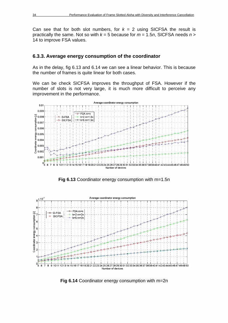
6.3.3. Average energy consumption of the coordinator As in the delay, fig 6.13 and 6.14 we can see a linear behavior. This is because the number of frames is quite linear for both cases. We can be check SICFSA improves the throughput of FSA. However if the number of slots is not very large, it is much more difficult to perceive any improvement in the performance.

Fig 6.13 Coordinator energy consumption with m=1.5n

Fig 6.14 Coordinator energy consumption with m=2n

Conclusions 35

As you can see from the graphs above, the performance in terms of consume of energy of the coordinator is best for m = 2n, as has been explaining for the last points. While it is true that for m = 1.5n SICFSA obtain better results than FSA, this improvement does not reach until n > 30 for k = 5. For k = 2, we get better results than FSA from the first device value.

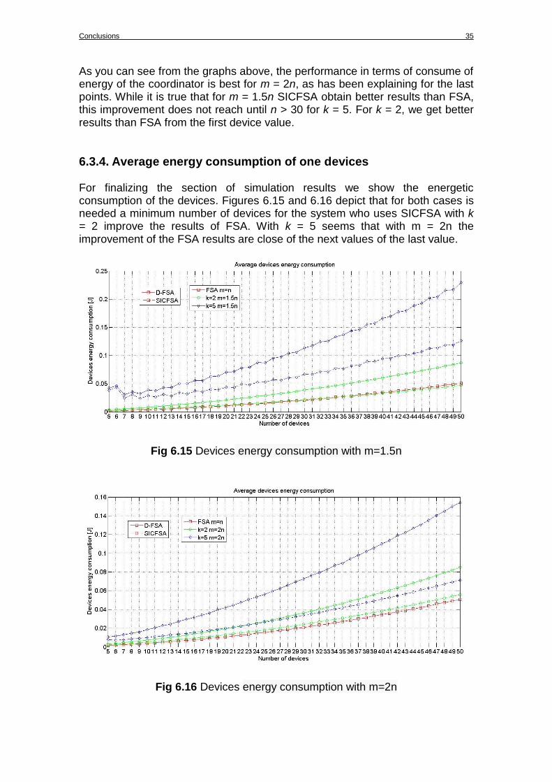
6.3.4. Average energy consumption of one devices For finalizing the section of simulation results we show the energetic consumption of the devices. Figures 6.15 and 6.16 depict that for both cases is needed a minimum number of devices for the system who uses SICFSA with k = 2 improve the results of FSA. With k = 5 seems that with m = 2n the improvement of the FSA results are close of the next values of the last value.

Fig 6.15 Devices energy consumption with m=1.5n

Fig 6.16 Devices energy consumption with m=2n


For m = 1.5n only with k = 2 and n >33 SICFSA improves the FSA values. For m = 2n we can see that we can’t reach the improvement of values for any value of device. This results, agrees with the results shown in Figures 6.7 and 6.8, when only for m=n and n=100 devices we can obtain better results using SICFSA than FSA. But with these new graphs we can see that if we increase the number of frame slots in only one half we can still obtain better results using SICFSA than FSA.

6.4. Throughput, delay and energy saving and energy efficiency Once seen the SICFSA protocol behavior for two values of devices, now is examined the throughput of the system, the saving of energy and delay that the system have when we increase the diversity order. For this purpose we have focused on the results for 25, 50 and 100 devices. This time we will focus only on the SICFSA protocol.

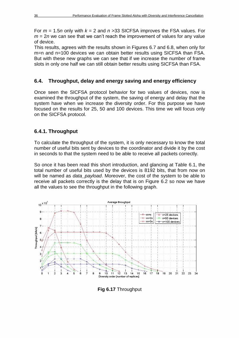
6.4.1. Throughput To calculate the throughput of the system, it is only necessary to know the total number of useful bits sent by devices to the coordinator and divide it by the cost in seconds to that the system need to be able to receive all packets correctly. So once it has been read this short introduction, and glancing at Table 6.1, the total number of useful bits used by the devices is 8192 bits, that from now on will be named as data_payload. Moreover, the cost of the system to be able to receive all packets correctly is the delay that is on Figure 6.2 so now we have all the values to see the throughput in the following graph.

Fig 6.17 Throughput

Conclusions 37

As can be seen, the highest value of throughput, which is approximately 920 Kbits / s, is obtained for m = 2n with 2 < k < 5 and n = 25 devices. As shown in the Figure 6.17, the behavior for the three devices values is quite similar, getting higher throughput values for m = 2n. Also shows that if we need higher diversity order value and a throughput not very low should be used an m = 3n for any number of devices. For m = n only have better throughput for k = 1, 2 respect FSA.

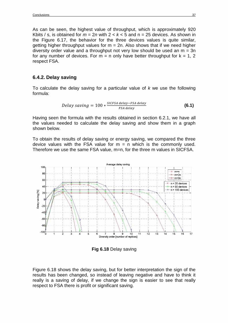
6.4.2. Delay saving To calculate the delay saving for a particular value of k we use the following formula:

(6.1)

Having seen the formula with the results obtained in section 6.2.1, we have all the values needed to calculate the delay saving and show them in a graph shown below. To obtain the results of delay saving or energy saving, we compared the three device values with the FSA value for m = n which is the commonly used. Therefore we use the same FSA value, m=n, for the three m values in SICFSA.

Fig 6.18 Delay saving

Figure 6.18 shows the delay saving, but for better interpretation the sign of the results has been changed, so instead of leaving negative and have to think it really is a saving of delay, if we change the sign is easier to see that really respect to FSA there is profit or significant saving.


So seeing the graph, we can say we have the greater delay saving when we use m = 2n. The greater delay saving is using 100 devices and is higher than the 50% with 2 < k < = 6. As we can observe behavior for any number of device is quite similar, as with the throughput. The best values are obtained for m = 2n. With m = n only improves the FSA value with k = 1 or 2, also for k = 3 with 100 devices. If we use m = 3n we can use k <11 and we continue obtaining better values than FSA, but no values as high as m = 2n. But according to the value of m, once the diversity order reaches certain values the delay saving falls sharply. We can see this phenomenon to m = n with k > 4 which already have a delay saving less than -100 %, i.e. FSA would need less of half of time to transmit all packets successfully, compared to SICFSA protocol with m = n and k = 5. Therefore it is necessary to take into account the value of diversity order given to our system because could have the opposite effect. One can see that for m = 2n or 3n the graph does not start at 0%. As mentioned before showing the Figure 6.18 the values shown in it are related to the value of FSA for m = n. As we have shown in Figure 6.1 or 6.2 the delay is greater when m increase in FSA. Therefore it is normal for k = 0 and m > n the values are negatives because as mentioned the graph is inverted.

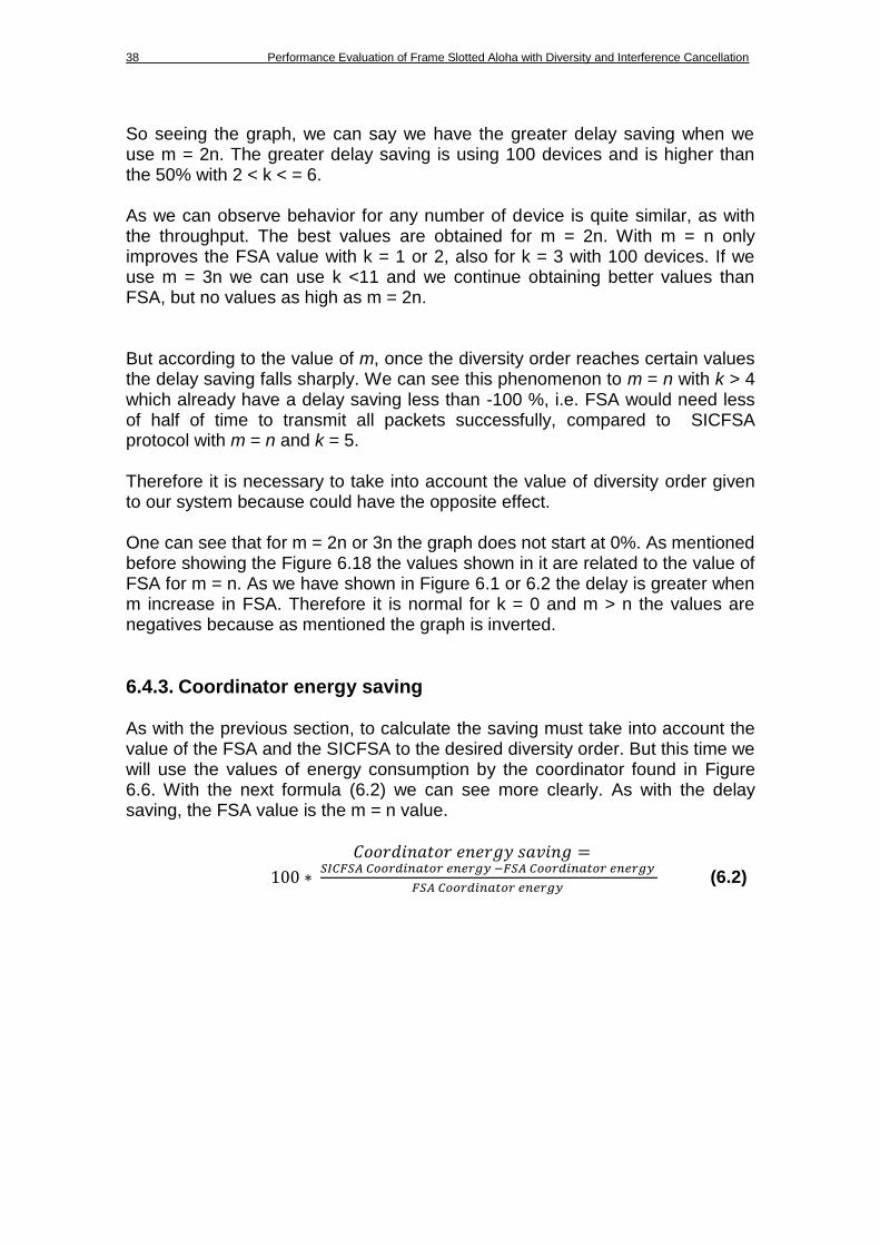
6.4.3. Coordinator energy saving As with the previous section, to calculate the saving must take into account the value of the FSA and the SICFSA to the desired diversity order. But this time we will use the values of energy consumption by the coordinator found in Figure 6.6. With the next formula (6.2) we can see more clearly. As with the delay saving, the FSA value is the m = n value.

(6.2)

Conclusions 39

Fig 6.19 Coordinator energy saving

As can be seen in Figure 6.19, we have the same results as with the delay saving, since as we have seen in the calculations section, to know the energy consumption of the coordinator, is needed to multiply the total number of frames used per the energy consumed in one frame (5.11). This is the same as for the delay (5.1), but multiplies the total number of frames for the time to finish one i.e. both are the multiplication of a different value by one common. Since saving is a relationship between values of the same type at the end we get the same result for delay that for the energy consumption of the coordinator. This means we have more than 50% savings on regarding FSA with m= 2n and n = 100 devices and after a certain value of k the saving plummets.

6.4.4. Devices energy saving As with the coordinator energy saving, to calculate the saving we need the values of energy consumption by the devices. These values can be founded in Figure 6.8. With the follow formula (6.3) we calculate the saving and is,

(6.3)

Remember again that the value of FSA is the value for m = n, which is used for the three values of m.


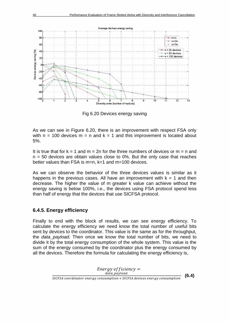
Fig 6.20 Devices energy saving

As we can see in Figure 6.20, there is an improvement with respect FSA only with n = 100 devices m = n and k = 1 and this improvement is located about 5%. It is true that for k = 1 and m = 2n for the three numbers of devices or m = n and n = 50 devices are obtain values close to 0%. But the only case that reaches better values than FSA is m=n, k=1 and m=100 devices. As we can observe the behavior of the three devices values is similar as it happens in the previous cases. All have an improvement with k = 1 and then decrease. The higher the value of m greater k value can achieve without the energy saving is below 100%, i.e., the devices using FSA protocol spend less than half of energy that the devices that use SICFSA protocol.

6.4.5. Energy efficiency Finally to end with the block of results, we can see energy efficiency. To calculate the energy efficiency we need know the total number of useful bits sent by devices to the coordinator. This value is the same as for the throughput, the data_payload. Then once we know the total number of bits, we need to divide it by the total energy consumption of the whole system. This value is the sum of the energy consumed by the coordinator plus the energy consumed by all the devices. Therefore the formula for calculating the energy efficiency is,

(6.4)

Conclusions 41

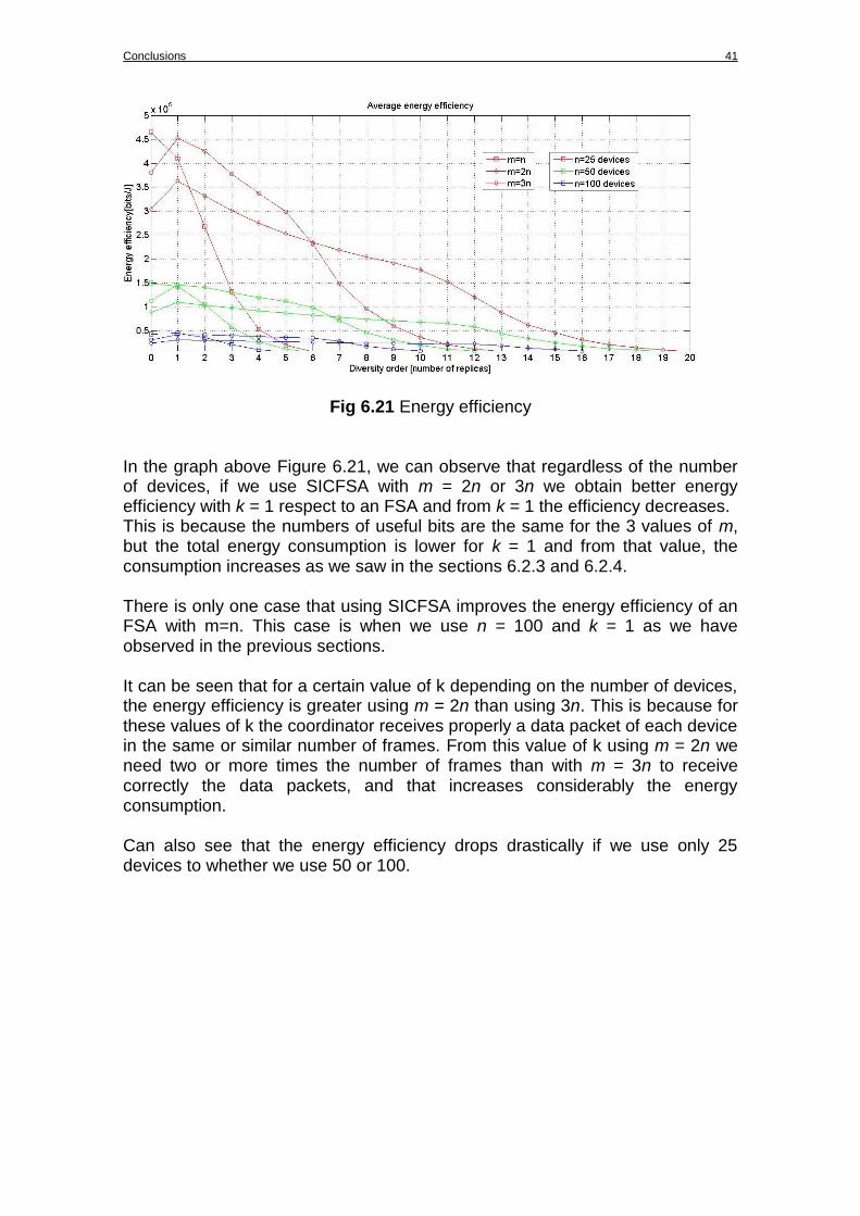
Fig 6.21 Energy efficiency In the graph above Figure 6.21, we can observe that regardless of the number of devices, if we use SICFSA with m = 2n or 3n we obtain better energy efficiency with k = 1 respect to an FSA and from k = 1 the efficiency decreases. This is because the numbers of useful bits are the same for the 3 values of m, but the total energy consumption is lower for k = 1 and from that value, the consumption increases as we saw in the sections 6.2.3 and 6.2.4. There is only one case that using SICFSA improves the energy efficiency of an FSA with m=n. This case is when we use n = 100 and k = 1 as we have observed in the previous sections. It can be seen that for a certain value of k depending on the number of devices, the energy efficiency is greater using m = 2n than using 3n. This is because for these values of k the coordinator receives properly a data packet of each device in the same or similar number of frames. From this value of k using m = 2n we need two or more times the number of frames than with m = 3n to receive correctly the data packets, and that increases considerably the energy consumption. Can also see that the energy efficiency drops drastically if we use only 25 devices to whether we use 50 or 100.


7 Conclusions

Machine-to-Machine (M2M) communications is the emerging paradigm that boosts future communication technologies and applications. We have considered an M2M data-collection application where a set of devices are collecting data and, periodically, transmit their data to a coordinator (i.e., gateway) upon request. The channel is constant and the noise signal is very small during the monitoring process. Once a device is able to transmit its data to the coordinator successfully, the device switches into sleep mode in order to save energy. Since the number of devices that may attempt to transmit data to an M2M gateway in a given time can be large, a Medium Access Control (MAC) protocol is needed in order to solve the contention in an efficient manner. In this work, we focus on random access protocols. Within random access, we choose Frame Slotted ALOHA (FSA). In FSA, the transmission of data from the devices is performed in a sequence of time frames, which are divided into time slots. The devices only can transmit one time on the beginning of a time slot in a frame. Based on the operation of the FSA we have tested the performance of an existing protocol called Successive Interference Cancellation Framed Slotted ALOHA (SICFSA). The idea is the same as for FSA, but instead of transmitting a data packet only once during the same frame, a data packet is repeated k times, called diversity order, within the same frame in different time slots. Each data packet has a field that informs in which time slots are the data packets repeated. When all data packets have been transmitted the coordinator decodes the received data packets free of collision and cancels their replicas in other time slots to try to resolve devices in collided time slots. In this work, we also use a protocol called Diversity Frame Slotted ALOHA (D-FSA). D-FSA is the same as SICFSA but does not cancel the replicas of the data packet. To evaluate FSA, SICFSA and D-FSA, we used MATLAB and different functions in C language to simulate the protocols and obtain performance results. After evaluating all results, we can draw several conclusions that are shown below. If we analyze the average number of frames that SICFSA uses, we can see as SICFSA has an improvement with regard FSA using only one replica of data packet. With this improvement, for some values of the diversity order, SICFSA only uses one frame for the coordinator receives correctly one data packet from each device. But if we increase too much the diversity order, the number of frames needed by SICFSA becomes much larger than for FSA. If we compare the transmission delay of SICFSA and FSA, then we conclude that SICFSA improves by more than 50% the FSA. This result is shown in Figure 6.18 and is obtained when the number of slots per frame is 2 times the number of devices and the diversity order is between 2 to 6 using 100 devices. If we use a smaller number of devices as may be 25 or 50, also is improved the FSA results in almost 50% using m = 2n, but not reach values as high as with 100 devices.

Conclusions 43

In terms of energy consumption, SICFSA provides lower energy consumption for the coordinator and for the devices compared to that of FSA. Energy saving for the coordinator reaches 50% of saving with respect to FSA. The result for the coordinator consumption is obtained using the same specifications as for the delay and is shown in Figure 6.19. With energy savings regarding to devices only with 100 devices, using a replica of the data packet and using the same number of frame slots that devices, we obtain an improvement about 5% with respect to the FSA standard protocol as we can see in Figure 6.20. If we observe the behavior of SICFSA in terms of energy efficiency, we can see in Figure 6.21 that if we use one replica of the data packet we obtain better efficiency using SICFSA than FSA for m = 2n or 3n. If we increase the number of replicas, the improvement that gives us SICFSA begins to fall drastically. As with the energy saving the only case that improves a FSA standard protocol is using 100 devices and m = n.

8 Future lines of research

Analysis of SICFSA to evaluate the results theoretically.

Evaluate the performance of SICFSA when there are channel and noise impairments. Considerations of coherence time in order to modify SICFSA for constraining the available time slots in which a device can allocate the diversity information.

Study of requirements of a wireless physical layer allowing implement the SIC to configure the physical layer to use a SIC.

9 Bibliography [1] Fabio Ricciato and Paolo Castiglione, “Pseudo-Random ALOHA for Enhanced Collision-Recovery in RFID”, (2013). [2] Enrico Casini, Riccardo De Gaudenzi and Oscar del Rio Herrero, “Contention Resolution Diversity Slotted ALOHA CRDSA An Enhanced Random Access Scheme for satellite”, (2007). [3] IEEE Std. 802.11, “Wireless LAN Medium Access Control (MAC) and Physical Layer (PHY) Specification,” 1999. [4] http://ww1.microchip.com/downloads/en/DeviceDoc/rn-131-ds-v3.2r.pdf [5] http://www.seas.upenn.edu/~kassam/tcom370/n99_12.pdf [6] http://www.laynetworks.com/ALOHA%20PROTOCOL.htm [7] http://www.m2mcomm.com/about/what-is-m2m/

final grade project - upcommons

Documents