fault diagnosis of photovoltaic modules through image processing and canny edge detection on field...

This article was downloaded by: [Mr Antonios Gasteratos]On: 28 August 2013, At: 02:09Publisher: Taylor & FrancisInforma Ltd Registered in England and Wales Registered Number: 1072954 Registeredoffice: Mortimer House, 37-41 Mortimer Street, London W1T 3JH, UK

International Journal of SustainableEnergyPublication details, including instructions for authors andsubscription information:http://www.tandfonline.com/loi/gsol20

Fault diagnosis of photovoltaic modulesthrough image processing and Cannyedge detection on field thermographicmeasurementsJ. A. Tsanakas a , D. Chrysostomou b , P. N. Botsaris a & A.Gasteratos ba Faculty of Materials, Processes and Engineering, Department ofProduction Engineering and Management , School of Engineering,Democritus University of Thrace , Thrace , Greeceb Faculty of Production Systems, Department of ProductionEngineering and Management , School of Engineering, DemocritusUniversity of Thrace , Thrace , GreecePublished online: 14 Aug 2013.

To cite this article: International Journal of Sustainable Energy (2013): Fault diagnosis ofphotovoltaic modules through image processing and Canny edge detection on field thermographicmeasurements, International Journal of Sustainable Energy, DOI: 10.1080/14786451.2013.826223

To link to this article: http://dx.doi.org/10.1080/14786451.2013.826223

PLEASE SCROLL DOWN FOR ARTICLE

Taylor & Francis makes every effort to ensure the accuracy of all the information (the“Content”) contained in the publications on our platform. However, Taylor & Francis,our agents, and our licensors make no representations or warranties whatsoever as tothe accuracy, completeness, or suitability for any purpose of the Content. Any opinionsand views expressed in this publication are the opinions and views of the authors,and are not the views of or endorsed by Taylor & Francis. The accuracy of the Contentshould not be relied upon and should be independently verified with primary sourcesof information. Taylor and Francis shall not be liable for any losses, actions, claims,proceedings, demands, costs, expenses, damages, and other liabilities whatsoever orhowsoever caused arising directly or indirectly in connection with, in relation to or arisingout of the use of the Content.

http://www.tandfonline.com/loi/gsol20

http://dx.doi.org/10.1080/14786451.2013.826223

This article may be used for research, teaching, and private study purposes. Anysubstantial or systematic reproduction, redistribution, reselling, loan, sub-licensing,systematic supply, or distribution in any form to anyone is expressly forbidden. Terms &Conditions of access and use can be found at http://www.tandfonline.com/page/terms-and-conditions

Dow

nloa

ded

by [

Mr

Ant

onio

s G

aste

rato

s] a

t 02:

09 2

8 A

ugus

t 201

3

http://www.tandfonline.com/page/terms-and-conditions

http://www.tandfonline.com/page/terms-and-conditions

International Journal of Sustainable Energy, 2013http://dx.doi.org/10.1080/14786451.2013.826223

Fault diagnosis of photovoltaic modules through imageprocessing and Canny edge detection on field thermographic

measurements

J.A. Tsanakasa*, D. Chrysostomoub, P.N. Botsarisa and A. Gasteratosb

aFaculty of Materials, Processes and Engineering, Department of Production Engineering andManagement, School of Engineering, Democritus University of Thrace, Thrace, Greece; bFaculty of

Production Systems, Department of Production Engineering and Management, School of Engineering,Democritus University of Thrace, Thrace, Greece

(Received 31 January 2013; final version received 3 June 2013)

Today, conventional condition monitoring of installed, operating photovoltaic (PV) modules is mainlybased on electrical measurements and performance evaluation. However, such practices exhibit restrictedfault-detection ability. This study proposes the use of standard thermal image processing and the Canny edgedetection operator as diagnostic tools for module-related faults that lead to hot-spot heating effects. Theintended techniques were applied on thermal images of defective PV modules, from several field infraredthermographic measurements conducted during this study. The whole approach provided promising resultswith the detection of hot-spot formations that were diagnosed to specific defective cells in each inspectedmodule. These evolving hot spots lead to abnormally low performance of the PV modules, a fact that isalso validated by the manufacturer’s standard electrical tests.

Keywords: infrared thermography; photovoltaic modules; hot-spot detection; condition monitoring;thermal image processing; Canny edge detection

1. Introduction

With the advent of the twenty-first century’s early decades, the world awareness of revising theenergy policies has stimulated an increasing interest for sustainable development and researchin renewable energies, such as solar energy via photovoltaic (PV) systems (Ahuja and Tatsutani2008). Towards this new global energy policy, PV industry is already rapidly growing to addressthe increasing demand for PV systems. On the other hand, current PV research focuses on achiev-ing high utilisation factors and optimum performance of a PV system, in order to improve thefuture competitiveness of such investments. In principle, around 50% of the capital costs for PVsystems refer to PV modules, while the payback time of any grid-connected PV system is mainlydetermined by the ratio between electricity price, feed-in tariffs and total system cost (EPIAand Greenpeace 2011). Meanwhile, performance and lifetime of a PV module are influenced bydefects (faults) originated either in the module’s manufacturing processes (assembling) or in thefield (installation and operation). In fact, there is a strong need for establishing the long-term

*Corresponding author. Email: [email protected]

© 2013 Taylor & Francis

Dow

nloa

ded

by [

Mr

Ant

onio

s G

aste

rato

s] a

t 02:

09 2

8 A

ugus

t 201

3

2 J.A. Tsanakas et al.

efficiency of each PV module by applying responsible, non-destructive condition monitoring(CM) to both of the above stages (Tsanakas and Botsaris 2011a).

Generally, CM of an equipment appears as part of a typical condition-based maintenance sched-ule and comprises three main steps; the monitoring method(s), the signal-processing technique(s)and the diagnosis/classification. In principle, a monitoring method can be characterised as eitherdirect or indirect. Direct methods give an actual representation of the monitored equipment, usingoptical or vision-based approaches, such as computer vision, infrared (IR) imaging or electrolu-minescence (EL), while indirect methods monitor a parameter (e.g. temperature, current, etc.) as afunction of the equipment’s condition. In the next step of a CM approach, the acquired raw signalfrom the monitoring method is analysed using common signal/image processing techniques suchas Fourier transforms, time domain or statistical parameters analysis, wavelet transforms, his-togram analysis or edge detection. The meaningful information that is extracted from the appliedprocessing technique is then used, in the third step of a CM approach, to accomplish a faultdiagnosis and classify the equipment’s status.

Today, the assembled PV modules are rated during the quality-control stage using characteristiccurrent–voltage (I–V) measurements under standard test conditions (STC). However, operatingconditions typically encountered in the field rarely emulate STC (del Cueto 2002; Kurtz et al.2009). It is also a fact that although some standardised accelerated tests (e.g. ASTM E1171-01or IEC 61215:2005/IEC 61646:2008) for extreme outdoor environment are used for qualifica-tion tests procedures, failures in crystalline-Si modules or cells still occur (Simon and Meyer2010). Hence, the module’s efficiency must be either explicitly modelled or monitored. Further-more, conventional CM of installed PV modules is mainly based on electrical measurements andperformance monitoring, which are applied to the whole PV system installation. Unfortunately,such practices appear inefficient to detect and/or isolate possible defects in the modules. Directmonitoring of operating PV modules, with the use of IR thermography, comprises a method ableto indicate the ‘signature’ of a potential fault to a thermal image pattern, witnessing its physicallocation within the defective module (Tsanakas and Botsaris 2011b). In addition, effective, thoughusually simple, techniques for thermal image processing can provide a comprehensive diagnosiswith regard to the condition, performance and, ultimately, efficiency of each module.

To summarise, according to the current status in the field of CM for PV modules, there is achallenging need for a direct monitoring method, such as IR thermography, capable of detectingand diagnosing defective PV modules, both during the assembling stage and under real-fieldconditions. In this paper, standard thermal image processing and the Canny edge detection operatorare experimentally assessed for their applicability to a CM approach upon fault diagnosis inPV modules. The intended techniques are applied to thermal images of defective PV modules,from several field IR thermographic measurements conducted during this study. The impetus foradopting a temperature-monitoring method for this investigation lies upon the strong interrelationbetween the evolving surface temperature of a PV module and its ‘health’ in terms of efficiency.Before presenting the experimental set-up and results of this study, the following section givesa thorough literature review of commonly reported techniques for thermal image processing aswell as a theoretical background with regard to Canny edge detection and hot-spot heating anddegradation mechanisms in PV modules.

2. Literature research and theoretical background

2.1. Thermal image processing techniques

IR thermography is a non-destructive technique of temperature measurement that provides imagesof a specific temperature pattern utilising the IR radiation which is emitted by all objects

Dow

nloa

ded

by [

Mr

Ant

onio

s G

aste

rato

s] a

t 02:

09 2

8 A

ugus

t 201

3

International Journal of Sustainable Energy 3

proportionally to their temperatures. By this way, the analysis of thermal images gives usefulinformation about the surface temperature, while further image processing can reveal possibleabnormalities to the thermal signature of the inspected equipment. These data, along with theknowledge of the equipment’s physical construction and thermodynamic state, are used to evalu-ate the degree of deterioration. There is an interesting field of global research, through the relatedliterature, in techniques for thermal image processing. The majority of the reported techniques arecommon, simple and well-established methods and algorithms, the effectiveness of which has beenproved through the last decades in computer vision and image processing of conventional images.

In Ibarra-Castanedo et al. (2004), Vergura and Falcone (2011) and Kosikowski, Suszynski,and Bednarek (2011), tools for preprocessing and processing IR images are proposed, when theacquired images cannot give satisfactory information about the condition of the inspected objects.Particularly, Ibarra-Castanedo et al. (2004) suggest noise smoothing by means of, e.g. median orGaussian filtering, as the most common preprocessing procedures. Moreover, the authors proposesimple subtraction techniques, such as spatial reference and temporal reference techniques, whichallow removing of unwanted effects present in cases of nonuniform heating as well as smooth-ing operators, high-pass filtering and Sobel operators (for edge extraction). In the same paper,various techniques for the enhancement of the subtle thermal signatures are proposed, includ-ing: (i) thermal contrast computation, (ii) normalisation, (iii) pulsed phase thermography (PPT),(iv) principal component thermography, (v) first and second derivatives, (vi) quantitative pro-cessing; defect detection algorithms and thresholding, and (vii) statistical behaviour of regions ofinterest (ROIs). Vergura and Falcone (2011) propose the application of both median and Gaussianfilters and then edge detection to IR images with poor or insufficient information about the health ofPV modules. On the other hand, Kosikowski et al. (2011) propose methods based on both discreteand continuous wavelet transforms. In the same work, the space-scale representation of thermalimage was used for the detection of thermal non-uniformities in the layered objects examined.

In Abdel-Qader et al. (2008), the objective of the study was to automate the detection ofsubsurface defects in concrete bridge decks using IR thermography. The algorithm, developed byAbdel-Qader et al. for this purpose, was based on the region growing approach, which segmentsthe image into defective and good regions using an integrated method of adaptive thresholdingand fully automated seed selection. In most cases in the same study, the acquired raw IR imageswere preprocessed using a 3 × 3 Gaussian filter, in order to smooth out isolated bright pixels,thus avoiding false seeds. Another interesting approach is found in Chou and Yao (2009), whereChou et al. propose a system known as Infrared Thermography Anomaly Detection Algorithm,the implementation of which was based on the principle of Otsu’s statistical threshold selectionalgorithm (Otsu 1979) using grey-level histograms.

Plotnikov and Winfree (1998) attempt a comparison between thermal contrast, time derivativeand phase analysis methods for defect visualisation. A defect edge extraction procedure basedon an image gradient computation has been applied to phase images of the same work. Theauthors concluded that the thermal contrast is the most suitable parameter for the task of defectedge extraction. On the other hand, time of the peak slope was found to be a good characteristicmeasure of defect depth, while PPT has also been shown to be an effective method for edgeextraction. Bai et al. (2000) present a technique that combines time domain and space domainanalysis; an interframe comparison denoise process and an adaptive mode filter were used tosuppress the thermal images’ noise. Savelyev and Sugumaran (2008) apply georeferencing andmosaicing together with automated statistical analysis to thermal images that were acquired inorder to map the surface temperature of a university campus. In the same study, the authors alsoperformed histogram stretching with boundary values according to the Chebyshev’s inequality,in order to improve the visual contrast of the images.

Thermal image processing is also widely reported in medical applications. For instance, inScales, Herry, and Frize (2004), Wiecek et al. (2008) and Wiecek (2005), techniques such as

Dow

nloa

ded

by [

Mr

Ant

onio

s G

aste

rato

s] a

t 02:

09 2

8 A

ugus

t 201

3


filtering, data compression, false colour contrast enhancement, histograms and ROI analysis aretypically used for preliminary processing. Moreover, feature calculations based on first- andsecond-order statistical parameters, principal component analysis, linear discriminant analysis,neural networks (NNs), nearest neighbour classification as well as nearest neighbour algorithmsand edge detection are successfully used in more advanced approaches for passive thermography.Especially for edge detection, Scales, Herry, and Frize (2004) suggest an approach with a sequenceof Canny edge detectors, due to their robustness to noise and their equal treatment of false positivesand false negatives. For active dynamic thermography, transform methods are widely used, i.e.fast Fourier or wavelet ones. Last but not least, according to Wiecek (2005), multispectral analysisis under the scientific interest for processing sequences of thermal images.

Apart from the aforementioned studies, there are specific book chapters in Maldague (2001),Vollmer and Mollmann (2010) and Hardy (1997) where several aspects of thermal image process-ing are described, e.g. frequency/spatial domain image enhancement, defect detection algorithms,NNs, statistical methods, PPT, wavelets, image fusion/subtraction, segmentation and patternrecognition.

2.2. Canny edge detection

Canny edge detection is considered as a well-established and reliable tool, upon fault detectionand diagnosis of structures or equipment, in various research fields such as computer vision,computer-aided medical diagnostics, IR thermography and digital radiography (Scales, Herry,and Frize 2004; Vergura and Falcone 2011; Wang et al. 2011). Edge detection treats the locali-sation of significant variations of a grey level in an image and the identification of the physicaland geometrical properties of objects in a scene. Variations of a grey-level image commonlyinclude discontinuities (step edges), local extrema (line edges) and junctions. Especially in ther-mal imaging, such variations might be indicative of abnormalities in the temperature pattern ofthe equipment under inspection. Contemporary, multi-scale edge detectors possess three mainprocessing steps, viz. smoothing, differentiation and labelling.

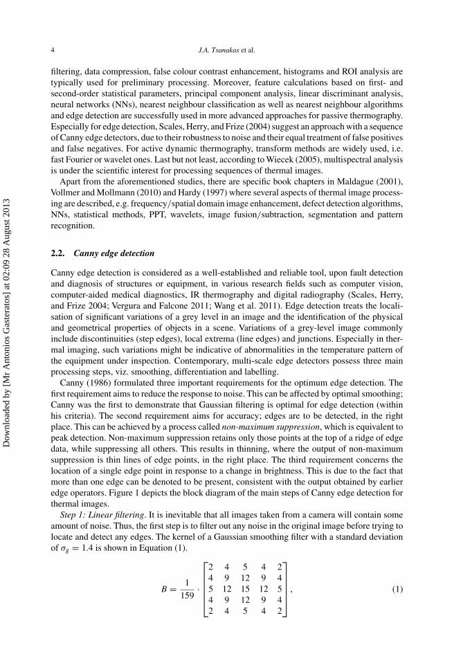
Canny (1986) formulated three important requirements for the optimum edge detection. Thefirst requirement aims to reduce the response to noise. This can be affected by optimal smoothing;Canny was the first to demonstrate that Gaussian filtering is optimal for edge detection (withinhis criteria). The second requirement aims for accuracy; edges are to be detected, in the rightplace. This can be achieved by a process called non-maximum suppression, which is equivalent topeak detection. Non-maximum suppression retains only those points at the top of a ridge of edgedata, while suppressing all others. This results in thinning, where the output of non-maximumsuppression is thin lines of edge points, in the right place. The third requirement concerns thelocation of a single edge point in response to a change in brightness. This is due to the fact thatmore than one edge can be denoted to be present, consistent with the output obtained by earlieredge operators. Figure 1 depicts the block diagram of the main steps of Canny edge detection forthermal images.

Step 1: Linear filtering. It is inevitable that all images taken from a camera will contain someamount of noise. Thus, the first step is to filter out any noise in the original image before trying tolocate and detect any edges. The kernel of a Gaussian smoothing filter with a standard deviationof σg = 1.4 is shown in Equation (1).

B = 1

159·

⎡⎢⎢⎢⎢⎣

2 4 5 4 24 9 12 9 45 12 15 12 54 9 12 9 42 4 5 4 2

⎤⎥⎥⎥⎥⎦ , (1)

Dow

nloa

ded

by [

Mr

Ant

onio

s G

aste

rato

s] a

t 02:

09 2

8 A

ugus

t 201

3


Figure 1. Block diagram of edge detection for thermal images, using the Canny algorithm.

while the Gaussian operator is given by:

Gσ = 1√2πσ 2

g

· exp

[−x2 + y2

2σ 2g

], (2)

where x is the distance from the origin in the horizontal axis, y is the distance from the origin inthe vertical axis and σ is the standard deviation of the Gaussian distribution.

Step 2: Intensity gradient computation. After smoothing the image and eliminating the noise,the next step is to estimate the edge strength by computing the 2-D gradient of the image. TheSobel operator performs a 2-D partial gradient measurement on an image. Then, the approximateabsolute gradient magnitude (edge strength) at each point is found. The Sobel operator uses a pairof 3 × 3 convolution masks, to approximate the gradient in the x- and y-directions, respectively,by applying the following kernels:

Kernelgx =⎡⎣−1 0 1

−2 0 2−1 0 1

⎤⎦

Kernelgy =⎡⎣ 1 2 1

0 0 0−1 2 −1

⎤⎦ .

(3)

The magnitude M, or edge strength, of the gradient is then approximated using the formula:

M(x, y) =√

g2x(x, y) + g2

y(x, y), (4)

where gx and gy operators stand for the gradient in the x- and y-directions, respectively. In caseswhere gx takes a large value, the pixel normally has a large gradient in the x-direction andconsequently favours a vertical edge. On the other hand, in cases where gy has a large gradient inthe y-direction, a horizontal edge is most likely to occur.

Typically, the edges are already indicated by this step but are still quite broad and, thus, do notcharacterise their position clearly. To make this determination possible, the direction of the edgesmust be calculated using Equation (5).

θ(x, y) = tan−1

[gy(x, y)

gx(x, y)

]. (5)

Step 3: Non-maximum suppression. The purpose of this step is to convert the ‘blurred’ edges inthe image of the gradient magnitudes to ‘sharp’ edges. Therefore, all local maxima in the gradient

Dow

nloa

ded

by [

Mr

Ant

onio

s G

aste

rato

s] a

t 02:

09 2

8 A

ugus

t 201

3


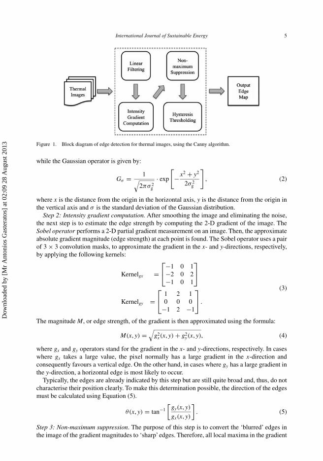
Figure 2. Typical cases of cracked solar cells.

image are preserved, while removing everything else. Non-maximum suppression is used to tracealong the edge in the edge direction and suppress any pixel value that is not considered to be anedge. For each pixel in the linear window, edge strength of the neighbours is compared; if thepixels are not part of the local maxima, they are set to zero.

Step 4: Hysteresis thresholding. The edge pixels remaining after the non-maximum suppressionstep are (still) marked with their strength pixel-by-pixel. Many of these will probably be true edgesin the image, but some may appear due to noise or colour variations, e.g. owing to rough surfaces.The simplest way to discern between these would be to use a threshold, so that only the strongestedges are to be preserved. The Canny edge detection algorithm uses hysteresis thresholding. Edgepixels stronger than the high threshold are marked as ‘strong’, while edge pixels weaker than thelow threshold are suppressed and edge pixels between the two thresholds are marked as ‘weak’.Strong edges are interpreted as ‘certain edges’, and can immediately be included in the final edgeimage. Weak edges are included only if they are connected to strong edges, given that noise andother small variations are unlikely to result in a strong edge. Thus, strong edges will only be dueto real edges in the original image. The weak edges can either be due to true edges or noise/colourvariations. The latter type will probably be distributed independently of edges on the entire image,and thus only a small amount will be located adjacent to strong edges. Weak edges due to trueedges are much more likely to be connected directly to strong edges.

2.3. The hot-spot heating effect

Defects such as cracks or interconnection mismatches in solar cells are a genuine problem for PVmodules (Figure 2). They are hard to avoid and, up to now, it is basically impossible to quantify theirimpact on the module’s performance during its lifetime (Kontges et al. 2010). Ideally, defectivecells or cell strings are identified and rejected during the early stages of a module’s manufacturingprocess, using, e.g. ultrasonic methods (Dallas, Polupan, and Ostapenko 2007), thermal fluxthermography (Breitenstein et al. 2005; Gupta and Breitenstein 2007; Krenzinger and de Andrade2007; Van der Borg and Burgers 2003) or EL imaging (Fuyuky et al. 2005; Kasemann et al. 2006).However, even if this is performed in a coherent and effective manner, new defects may occureither within the stage of string/module assembling or during the lifetime of an operating module.

Practically, the presence of a crack may have only a marginal effect on a new module’s operation,as long as the different parts of the defective cell remain electrically connected. However, as themodule ages and is subjected to thermal and mechanical stresses, the repeated relative movementof the cracked cell parts usually results in a complete electrical separation and, inevitably, in

Dow

nloa

ded

by [

Mr

Ant

onio

s G

aste

rato

s] a

t 02:

09 2

8 A

ugus

t 201

3


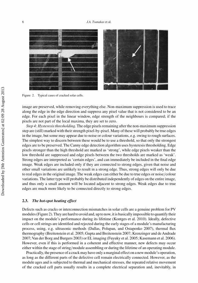
Figure 3. Electrical power dissipation in a shaded cell due to hot-spot effect (Designation ASTM E2481-08 2008).

inactive cell parts and significant hot-spot heating effects. Hot-spot heating is existent when thereis at least one solar cell within an illuminated module, which presents a short-circuit currentabnormally much smaller than the rest of the cells in the module’s series string. This occurswhen the cell is totally or partially shaded, cracked or electrically mismatched. In such cases, thedefective cell is forced to pass a current higher than its generation capabilities, becomes reversebiased, even enters the breakdown regime and subsequently sinks power instead of sourcing it.Figure 3 illustrates the hot-spot effect in a module of a series string of cells, one of which, cellY, is defective (shaded). The amount of electrical power dissipated in Y is equal to the product ofthe module’s current and the reverse voltage developed across Y.

From a heat-transfer point of view, on the basis of the Stefan–Boltzmann law, the relationbetween the additional dissipated power and the consequent temperature rise in the defective cellcan be given by the following equation (Hoyer et al. 2009):

�Pconv = h · A · (T2 − T1), (6)

where �Pconv is the additional dissipated power (in W), A is the area (i.e. the cell) in directcontact with air, h stands for the heat-transfer convection coefficient that can be considered of10 W/m2K, for the air with null velocity, T1 is the initial temperature of the cell (in K) and T2

is the increased cell’s temperature (in K) due to hot-spot heating. That is, the reverse-biased celldissipates power, in the form of heat, leading to excessive efficiency degradation of the relatedPV module (Hoyer et al. 2009; Luque and Hegedus 2003; Wohlgemuth and Herrmann 2005). Theseverity of this degradation directly correlates with the heat dissipated under reverse bias and,consequently, with the cell’s temperature increment; typically, a 10◦C increase in the cell’s surfacetemperature causes about 4% power loss (light hot spot) while an 18◦C increase reduces the powerabout 10% (strong hot spot) (Acciani, Falcone, and Vergura 2010). As a large PV system or aPV plant cannot be investigated cell-to-cell through a thermometer, a CM system, by means ofthermography, emerges as a potential solution.

3. Experimental set-up

3.1. Hardware and software

The experimental part of this study included three daily sets of several in situ thermo-graphic measurements regarding two PV arrays (PV-1 and PV-2) installed on the rooftop of a

Dow

nloa

ded

by [

Mr

Ant

onio

s G

aste

rato

s] a

t 02:

09 2

8 A

ugus

t 201

3


laboratorial facility building in the School of Engineering Campus of Democritus Universityof Thrace (DUTh), Xanthi (41◦8′N, 24◦53′E), Greece. PV-1 consists of four mono-crystallinesilicon (mono-Si) modules, type Siemens SP75. Each module in this array features a max-imum power rating Pmax of 75 Wp, short-circuit current ISC of 4.8A, rated current IMPP of4A, open-circuit voltage VOC of 21.7V and rated voltage VMPP of 17.1V, under STC. PV-2 consists of four poly-crystalline silicon (poly-Si) modules, type ExelSolar ESP Series60,each one with a maximum power rating Pmax of 240 Wp, short-circuit current ISC of 8.66A,rated current IMPP of 8.04A, open-circuit voltage VOC of 37.3V and rated voltage VMPP of29.84V, under STC. Electrical tests in a QuickSun solar simulator, which included ISC andVOC measurements in STC, were applied to each and every module of the two arrays, priorto any thermographic measurement of this study. The tests have witnessed a total 9.5% and9.8% performance deterioration of PV-1 and PV-2, respectively, due to possible hot spots ordefects.

The thermal camera (portable thermal imager) employed for the performed measurements was aLumasense/Impac IVN 780-P that features a 320 × 240 uncooled focal plane array microbolome-ter detector with a spectral range of 8–14 μm long. The specific model has a temperature rangeof −40 to +1000◦C with a measurement uncertainty factor of 2◦C or 2% of reading and animage update rate of 8.5 frames per second. All strings of series connected solar cells, withineach module of the PV arrays, were in principle considered as linear and orthogonal ROIs. Basicprocessing of the obtained thermal images was performed with the use of Lumasense/MikronMikroSpec 4.0 software, including filtering, ROI analysis, 3-D profile, line profile and his-togram analysis. Further processing and fault diagnosis, by means of Canny edge detection,was implemented applying thresholding and a multi-stage algorithm to raw thermal images, inMathworks Matlab R2009a environment. Although the thermal imager provides image signalsboth in greyscale and pseudo-colour mode (such as rainbow scale), the overall raw data wereprocessed in greyscale. In cases of black/white reproduction, rainbow colour maps appear tobe confusing due to their lack of perceptual ordering and misleadingly interpreted through theintroduction of non-data-dependent gradients (Borland and Taylor 2007). Moreover, processingof greyscale images requires a significantly lower computational burden.

3.2. Experimental outline

The thermographic measurements took place in the city of Xanthi (Thrace region, north-easternGreece, latitude: 41.14◦, mean elevation: 40 m), by three daily sets, i.e. 8, 9 and 10 August 2011,under clear-sky conditions. Each set included three instant measurements, according to the time;06:00 (transient conditions – sunrise), 13:00 (steady-state conditions) and 20:00 (transient condi-tions – sunset) for each module. The environmental conditions, such as ambient air temperature,humidity, mean value of solar irradiance flux GT and wind velocity were taken into account forthe initial set-up of the thermal camera, before each set of measurements. Ambient air temper-ature, wind velocity and humidity data were obtained by a local weather station and a portabletemperature/humidity recorder. Solar irradiance flux values were measured with the use of aconventional pyranometer (solarimeter). An overview of the recorded environmental conditionsis given in Table 1.

The inspected PV arrays, installed at a fixed angle θ ≈ 32◦, were set under short-circuit con-ditions. It should be noticed that, according to the European Commission’s PV GeographicalInformation System, for Xanthi/Greece, the overall optimum inclination value for a PV mod-ule is, indeed, approximately θopt ≈ 32◦. However, for the period of these measurements, i.e.during the first days of August, the optimum inclination value ranges between 17◦ and 22◦.Since the performed measurements aim to reveal possible defects on the modules’ surface

Dow

nloa

ded

by [

Mr

Ant

onio

s G

aste

rato

s] a

t 02:

09 2

8 A

ugus

t 201

3


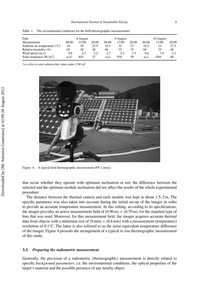
Table 1. The environmental conditions for the field thermographic measurements.

Date 8 August 9 August 10 AugustMeasurement 06:00 13:00 20:00 06:00 13:00 20:00 06:00 13:00 20:00Ambient air temperature (◦C) 18 30 25.5 18.5 32 27 18.5 33 27.5Relative humidity (%) 65 30 40 60 35 35 60 25 40Wind speed (m/s) 0.8 4.5 2.2 2.7 2.5 1.5 0.6 1.9 2.1Solar irradiance (W/m2) n/aa 845 37 n/a 930 59 n/a 1001 60

an/a refers to solar radiation flux values under 15 W/m2.

Figure 4. A typical field thermographic measurement (PV-1 array).

that occur whether they operate with optimum inclination or not, the difference between theselected and the optimum module inclination did not affect the results of the whole experimentalprocedure.

The distance between the thermal camera and each module was kept at about 1.5–2 m. Thespecific parameter was also taken into account during the initial set-up of the imager in orderto provide an accurate temperature measurement. At this setting, according to its specifications,the imager provides an active measurement field of (0.96 m) × (0.70 m), for the standard type oflens that was used. Moreover, for this measurement field, the imager acquires accurate thermaldata from objects with a minimum size of (9 mm) × (8.8 mm) with a measurement (temperature)resolution of 0.1◦C. The latter is also referred to as the noise-equivalent temperature differenceof the imager. Figure 4 presents the arrangement of a typical in situ thermographic measurementof this study.

3.3. Preparing the radiometric measurement

Generally, the precision of a radiometric (thermographic) measurement is directly related tospecific background parameters, i.e. the environmental conditions, the optical properties of thetarget’s material and the possible presence of any nearby object.

Dow

nloa

ded

by [

Mr

Ant

onio

s G

aste

rato

s] a

t 02:

09 2

8 A

ugus

t 201

3


As mentioned above, the values of air temperature, humidity, solar irradiance flux GT andwind velocity were used as inputs for the initial set-up (ambient compensation value (ACV)) ofthe thermal imager. For instance, for the environmental conditions of 8 August at 13:00, the IRmeasurement was obtained with anACV equal to 0.98, as it was calculated by the imager’s built-inalgorithm/software.

Moreover, a similar algorithm provides the proper background correction, in order to compen-sate the influence of objects, with known temperature, nearby the measured target. This featureis called reflected temperature compensation (RTC). RTC is used to achieve accurate radiometricmeasurements when, due to a significantly high uniform background temperature, IR energy isreflected off the target surface to the thermal imager. In principle, this reflected thermal radiantenergy induces an apparent change to the target’s measured temperature, proportional to: (i) apower of the temperature difference between the actual target and that of the nearby object thatacts as an external heat source, (ii) the reflectance (1.0 minus the emissivity value) of the targetand (iii) the emissivity of the external heat source (Zayicek 2002). This apparent change is not theresult of a real temperature change at the target surface and, practically, occurs when the target’smaterial is characterised by low emissivity. For the present case study, the described effect canbe assumed as negligible; the target surface’s material (front cover of the PV modules) is glasswith a relatively high emissivity; besides, there is no significant temperature difference betweenthe target and surrounding objects. However, a value of 43◦C was set as input for the RTC of thethermal imager with the use of a built-in algorithm, similarly to ACV. According to the user’smanual of the thermal imager, during RTC activation, the temperature of the background objects(which may influence the measurement) should be estimated. On this basis, the aforementionedvalue of 43◦C was calculated as the mean temperature of the background/surrounding objectsduring the measurements, i.e. nearby installed solar collectors and other PV arrays and the roof’smaterial under the inspected PV array.

Last but not least, the optical properties of glass (i.e. the target’s material) are taken intoaccount in order to provide a radiometric measurement as precise as possible. According totheir optical properties, all objects reflect, transmit and emit energy. However, only the emittedenergy is indicative of the object’s temperature. An IR radiometer (thermal imager) measuresthe sum of the emitted (We), reflected (Wr) and transmitted (Wt) energies coming from the tar-get of interest. The sum of We + Wr + Wt is called exitance or radiosity (Zayicek 2002). Thus,the thermal imager has to be adjusted to the actual emissivity value for each measured target’smaterial, in order to ‘read’ only the emitted energy and, consequently, the actual temperatureof the target. If the emissivity of the target surface changes, or if the wrong emissivity value isassumed for the target, the apparent temperature reading will be erroneous and different fromthe target’s actual temperature. For each measurement of the present study, the emissivity ε

for the front glass of the inspected PV modules was set to 0.85, a value that was validatedby performing identical IR (radiometric) measurements to a similar glass target at a knowntemperature. In particular, the measurements were taken under the same conditions (environ-mental and ambient/background parameters, distance-to-target value, target material) and thetemperature of the test-target was measured using a conventional thermometer; it was thennoticed that, for an emissivity value of around ε = 0.85, the thermal imager was measuringthe same test-target temperature as the thermometer. It should be mentioned that IR measure-ments to glass-coated surfaces often lead to undesirable specular reflection (‘self-detection’ or‘Narcissus’) effects. The latter must be avoided by keeping the proper distance and/or anglebetween the target and the thermal imager. Although a clearly visible specular reflection isoften an indicator of a highly reflective surface, high specularity is not always the same ashigh reflectivity; for instance, in the case of the inspected modules’ glass covers, reflectivitycan be assumed to be quite low (ρ = 0.15), in contrast with the significantly high specularity ofthe glass.

Dow

nloa

ded

by [

Mr

Ant

onio

s G

aste

rato

s] a

t 02:

09 2

8 A

ugus

t 201

3


4. Results and discussion

4.1. ROI and line profile analysis

According to Skoplaki, Boudouvis, and Palyvos (2008), the operating temperature of a ‘healthy’cell in a PV module can be fairly estimated by the following semi-empirical equation:

Tcell = Tamb +(

0.32

8.91 + 2 · Vf

)· GT (Vf > 0), (7)

where Tcell is the cell’s operating temperature (in ◦C), Tamb is the ambient air temperature (in ◦C),Vf is the air velocity (in m/s) and GT is the incident solar irradiance flux (in W/m2). At first,the acquired thermal images from the inspected PV arrays were analysed in order to generatea simple and fast correlation between the expected temperatures (Tcell) of each solar cell ofthe module, estimated by Equation (7), and the measured ones (Tcell,m) obtained from the fieldthermographic inspection. In practice, a �T > 5◦C between Tcell and Tcell,m induces an abnormaloverall temperature pattern, witnessing a potential hot spot (Maldague 2001). If it is assumed thatTcell is approximately equal to the module’s temperature (Tmodule), then the knowledge of the latterhelps in assessing the module’s overall efficiency (Tsanakas and Botsaris 2011a).

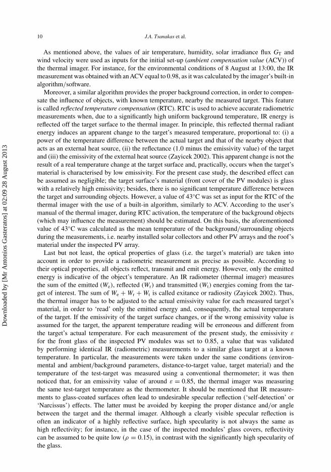
Figures 5 and 6 illustrate the thermal images and the relative 3-D thermal profiles of the fourmodules of PV-1, on 8 August at 13:00, under clear-sky conditions. A basic ROI analysis wasapplied to quantify the needed thermal data from each solar cell, which can be examined as asingle orthogonal ROI. For instance, in the thermal image of Figure 5, the performed analysisfor the two cells of ROI 3 gave an average cell temperature Tcell,m = 53.2◦C. At the same time,an apparently ‘healthy’ cell, i.e. the one between ROI 2 and 3, features a Tcell,m = 44.5◦C. Onthe other hand, applying Equation (7) for the environmental parameters of this measurement (seeTable 1), the expected cell temperature is estimated to Tcell = 45.1◦C. Thus, the ‘healthy’ cell,here, is operating at a temperature very close to the ‘normal’ Tcell, in contrast to the cells of ROI3 that present an abnormal operating temperature, higher than the normal one by a �T = 8.1◦C.Similarly, a significant �T was observed in the operating temperatures of several cells within allfour modules of this array.According to the complete ROI analysis, 14 hot spots, where �T > 5◦C,have been detected among the total number of 144 solar cells of the inspected array’s modules.These ‘suspicious’ cells (or groups of cells) may relate to implicit defects and, consequently, to adeteriorated performance of the PV array.

The described ROI analysis was also applied to the thermal data of the PV-2 array and, sugges-tively, the thermal images of modules 1 and 2, on 8 August at 13:00, are given in Figures 7 and 8,respectively. For the needs of this study, all four modules of this array were deliberately purchased

Figure 5. Thermal image and 3-D profile of modules 1–2 of PV-1, on 8 August, at 13:00.

Dow

nloa

ded

by [

Mr

Ant

onio

s G

aste

rato

s] a

t 02:

09 2

8 A

ugus

t 201

3


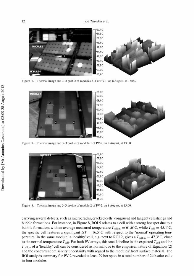
Figure 6. Thermal image and 3-D profile of modules 3–4 of PV-1, on 8 August, at 13:00.

Figure 7. Thermal image and 3-D profile of module 1 of PV-2, on 8 August, at 13:00.

Figure 8. Thermal image and 3-D profile of module 2 of PV-2, on 8 August, at 13:00.

carrying several defects, such as microcracks, cracked cells, congruent and tangent cell strings andbubble formations. For instance, in Figure 8, ROI 5 relates to a cell with a strong hot spot due to abubble formation; with an average measured temperature Tcell,m = 61.6◦C, while Tcell = 45.1◦C,the specific cell features a significant �T = 16.5◦C with respect to the ‘normal’ operating tem-perature. In the same module, a ‘healthy’ cell, e.g. next to ROI 2, gives a Tcell,m = 47.3◦C, closeto the normal temperature Tcell. For both PV arrays, this small decline in the expected Tcell and theTcell,m of a ‘healthy’ cell can be considered as normal due to the empirical nature of Equation (2)and the concurrent emissivity uncertainty with regard to the modules’ front surface material. TheROI analysis summary for PV-2 revealed at least 29 hot spots in a total number of 240 solar cellsin four modules.

Dow

nloa

ded

by [

Mr

Ant

onio

s G

aste

rato

s] a

t 02:

09 2

8 A

ugus

t 201

3


Figure 9. LPA for ROI 1 and 2 of module 1 of PV-1, on 8 August, at 13:00.

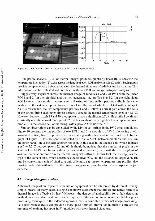
Line profile analysis (LPA) of thermal images produces graphs by linear ROIs, showing thetemperature fluctuation (Y -axis) across the length of each ROI in pixels scale (X-axis). Such graphsprovide complementary information about the thermal signature of a defect and its location. Thisinformation can be evaluated and correlated with both ROI and image histogram analysis.

Suggestively, Figure 9 shows the thermal image of modules 1 and 2 of PV-1 with the linearROI 1 and 2 (on the left side) and the two generated line profiles 1 and 2 (on the right side).ROI 1 extends, in module 1, across a vertical string of 4 normally operating cells. In the samemodule, ROI 2 extends representing a string of 4 cells, one of which is related with a hot spot.As it is reasonable, the two temperature profiles 1 and 2 follow a normal path across the cellsof the string, fitting each other almost perfectly around the normal temperature level of 44.5◦C.However, between pixels 13 and 30, they appear to have a significant �T ; while profile 1 continuesconstantly near the normal level, profile 2 reaches an abnormally high level of temperature overprofile 1, in the second cell of the string, with a peak �T value of 5.6◦C.

Similar observations can be concluded by the LPA of cell strings in the PV-2 array’s modules.Figure 10 presents the line profiles of two ROI 1 and 2 in module 1 of PV-2. Following a left-to-right direction, line 1 represents a six-cell string with a hot spot in the fourth cell. In thegraph of Figure 10, this hot spot is indicated by a �T = 5.6◦C between pixels 89 and 127. Onthe other hand, line 2 includes another hot spot, in this case in the second cell, which inducesa �T = 5.2◦C between pixels 22 and 60. It should be noticed that the number of pixels in theX-axis of each LPA graph can be directly converted to distance (in m), with the use of a physicaldistance calculation tool from the thermal imager’s software. In this tool, the user applies thetype of the camera lens, which determines the relative FOV, and the distance-to-target value (inm). By converting a unit of pixel to a unit of length, e.g. metre, temperature line profiles alsoprovide useful data with regard to the dimensions, geometry and location of any inspected objector defect.

4.2. Image histogram analysis

A thermal image of an inspected structure or equipment can be interpreted by different, usuallysimple, means. In many cases, a single qualitative assessment that utilises the native form of athermal image is effective by itself. However, the degree of applicability for a fault-detectingmethod under variable conditions can be improved if the method incorporates a reliable signal-processing technique. In the indented approach, even a basic step of thermal image processing,i.e. a histogram analysis, can provide a more ‘pure’ form of information in order to correlate thepresence of evolving hot spots in PV modules with their thermal signature.

Dow

nloa

ded

by [

Mr

Ant

onio

s G

aste

rato

s] a

t 02:

09 2

8 A

ugus

t 201

3


Figure 10. LPA for ROI 1 and 2 of module 1 of PV-2, on 8 August, at 13:00.

A thermal image histogram acts as a graphical representation of the tonal or colour distributionin the image. Since tonal distribution in such images refers to discrete temperature values, theanalysis of specific histogram features, in a thermal image, is a practical and potent tool indetecting abnormal temperature patterns and, thus, defective equipment. Mean value, variance,standard deviation and skew are the most common statistical-based features that characterise thetonal distribution of an image. For any grey-level image, the first-order histogram probability P(g)

is given by Younus, Widodo, and Yang (2009):

P(g) = L(g)

M, (8)

where L(g) is the number of grey levels g and Mis the total number of pixels in the image. Whilein a typical grey-level image the total number of available L integer grey levels spans into [0,256],the relative range for a thermal image extends from minimum to maximum temperature value.As the tonal distribution varies on temperature, a thermal image can be classified according to itscolour/tonal intensities. The mean is the average value which expresses some information aboutthe general brightness of the image and, thus, it can be expressed as:

g =L−1∑g=0

g · P(g). (9)

Variance is defined as a measure of the dispersion of a set of data points around their mean valueand is given by the following equation:

σ 2g =

L−1∑g=0

(g − g)2 · P(g). (10)

Moreover, the square root of the variance gives the standard deviation, which is informative aboutthe contrast of an image. In other words, it describes the spread in the image data; a high-contrastthermal image will have a high temperature distribution. In the majority of thermal-image-baseddiagnostics, standard deviation is a key index of possible defects. Last, skew S measures theasymmetry around the mean in the grey-level distribution and is defined as:

S = 1

σ 3g

√√√√L−1∑g=0

(g − g)3 · P(g). (11)

Dow

nloa

ded

by [

Mr

Ant

onio

s G

aste

rato

s] a

t 02:

09 2

8 A

ugus

t 201

3


Figure 11. Image histogram for the polygon ROI 1 of module 1 of PV-1, on 8 August, at 13:00.


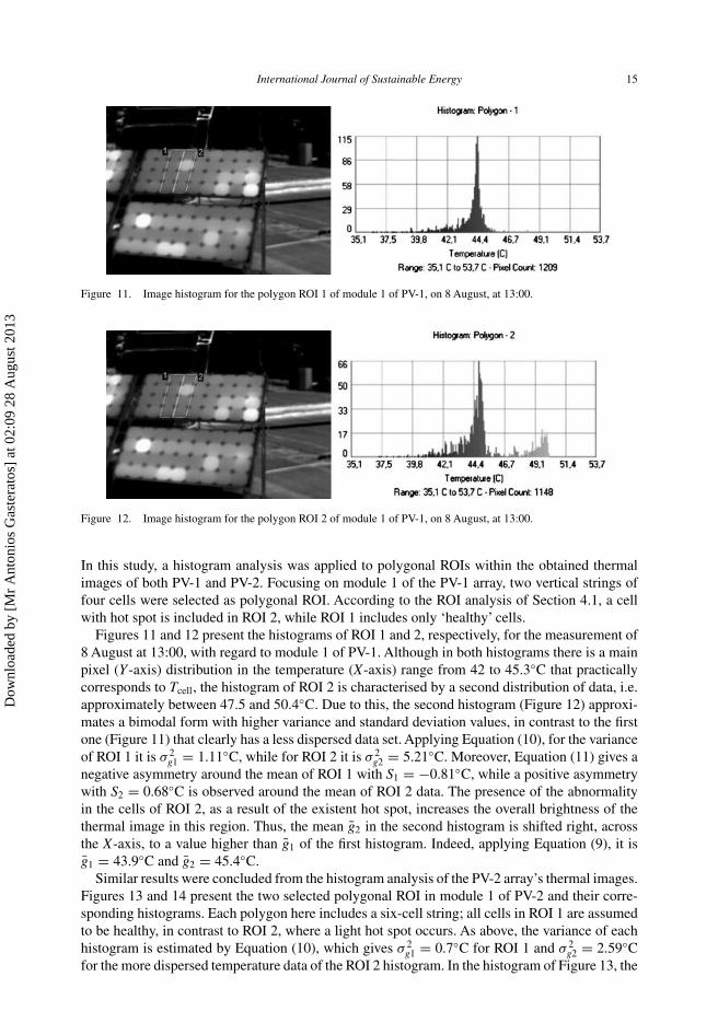
In this study, a histogram analysis was applied to polygonal ROIs within the obtained thermalimages of both PV-1 and PV-2. Focusing on module 1 of the PV-1 array, two vertical strings offour cells were selected as polygonal ROI. According to the ROI analysis of Section 4.1, a cellwith hot spot is included in ROI 2, while ROI 1 includes only ‘healthy’ cells.

Figures 11 and 12 present the histograms of ROI 1 and 2, respectively, for the measurement of8 August at 13:00, with regard to module 1 of PV-1. Although in both histograms there is a mainpixel (Y -axis) distribution in the temperature (X-axis) range from 42 to 45.3◦C that practicallycorresponds to Tcell, the histogram of ROI 2 is characterised by a second distribution of data, i.e.approximately between 47.5 and 50.4◦C. Due to this, the second histogram (Figure 12) approxi-mates a bimodal form with higher variance and standard deviation values, in contrast to the firstone (Figure 11) that clearly has a less dispersed data set. Applying Equation (10), for the varianceof ROI 1 it is σ 2

g1 = 1.11◦C, while for ROI 2 it is σ 2g2 = 5.21◦C. Moreover, Equation (11) gives a

negative asymmetry around the mean of ROI 1 with S1 = −0.81◦C, while a positive asymmetrywith S2 = 0.68◦C is observed around the mean of ROI 2 data. The presence of the abnormalityin the cells of ROI 2, as a result of the existent hot spot, increases the overall brightness of thethermal image in this region. Thus, the mean g2 in the second histogram is shifted right, acrossthe X-axis, to a value higher than g1 of the first histogram. Indeed, applying Equation (9), it isg1 = 43.9◦C and g2 = 45.4◦C.

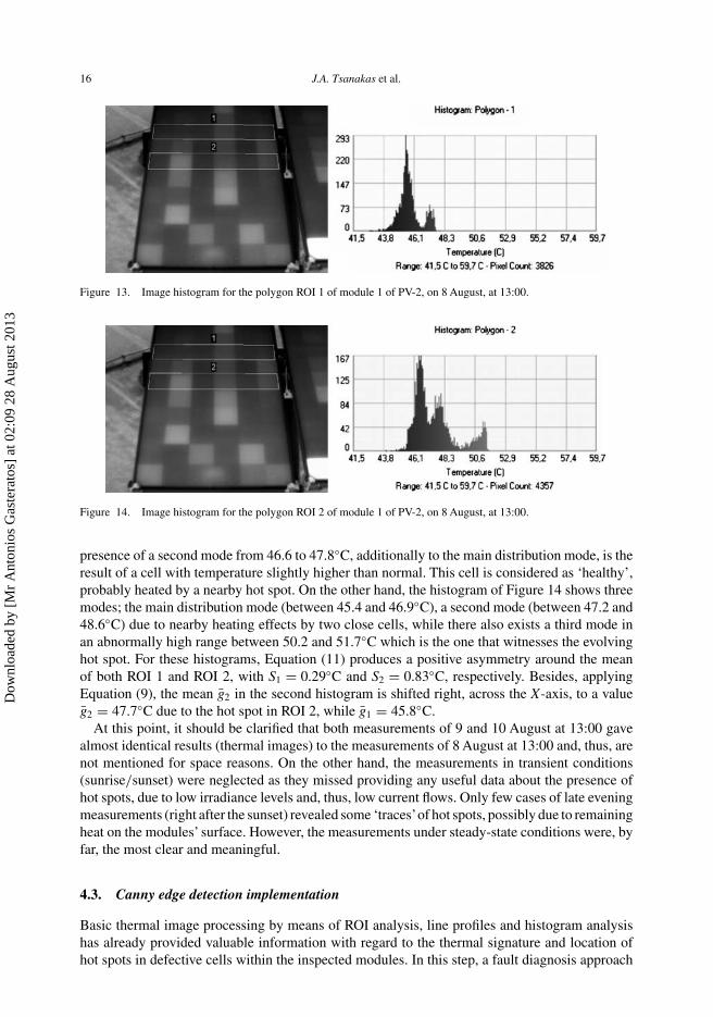
Similar results were concluded from the histogram analysis of the PV-2 array’s thermal images.Figures 13 and 14 present the two selected polygonal ROI in module 1 of PV-2 and their corre-sponding histograms. Each polygon here includes a six-cell string; all cells in ROI 1 are assumedto be healthy, in contrast to ROI 2, where a light hot spot occurs. As above, the variance of eachhistogram is estimated by Equation (10), which gives σ 2

g1 = 0.7◦C for ROI 1 and σ 2g2 = 2.59◦C

for the more dispersed temperature data of the ROI 2 histogram. In the histogram of Figure 13, the

Dow

nloa

ded

by [

Mr

Ant

onio

s G

aste

rato

s] a

t 02:

09 2

8 A

ugus

t 201

3




presence of a second mode from 46.6 to 47.8◦C, additionally to the main distribution mode, is theresult of a cell with temperature slightly higher than normal. This cell is considered as ‘healthy’,probably heated by a nearby hot spot. On the other hand, the histogram of Figure 14 shows threemodes; the main distribution mode (between 45.4 and 46.9◦C), a second mode (between 47.2 and48.6◦C) due to nearby heating effects by two close cells, while there also exists a third mode inan abnormally high range between 50.2 and 51.7◦C which is the one that witnesses the evolvinghot spot. For these histograms, Equation (11) produces a positive asymmetry around the meanof both ROI 1 and ROI 2, with S1 = 0.29◦C and S2 = 0.83◦C, respectively. Besides, applyingEquation (9), the mean g2 in the second histogram is shifted right, across the X-axis, to a valueg2 = 47.7◦C due to the hot spot in ROI 2, while g1 = 45.8◦C.

At this point, it should be clarified that both measurements of 9 and 10 August at 13:00 gavealmost identical results (thermal images) to the measurements of 8 August at 13:00 and, thus, arenot mentioned for space reasons. On the other hand, the measurements in transient conditions(sunrise/sunset) were neglected as they missed providing any useful data about the presence ofhot spots, due to low irradiance levels and, thus, low current flows. Only few cases of late eveningmeasurements (right after the sunset) revealed some ‘traces’of hot spots, possibly due to remainingheat on the modules’ surface. However, the measurements under steady-state conditions were, byfar, the most clear and meaningful.

4.3. Canny edge detection implementation

Basic thermal image processing by means of ROI analysis, line profiles and histogram analysishas already provided valuable information with regard to the thermal signature and location ofhot spots in defective cells within the inspected modules. In this step, a fault diagnosis approach

Dow

nloa

ded

by [

Mr

Ant

onio

s G

aste

rato

s] a

t 02:

09 2

8 A

ugus

t 201

3


by means of Canny edge detection was applied to the obtained raw thermal images. As describedin Section 2.2, edge detectors are used to localise significant variations of a grey-level image andidentify the physical and geometrical properties of objects in a scene. In the case of the thermalimages of this study, hot spots induce abnormal operating cell temperatures and, consequently,variations and discontinuities to each grey-level image pattern. Thus, an approach based on Cannyedge detection could be an effective tool for the diagnosis of hot spots in PV modules, in the formof edges. Following the described steps of Canny edge detection (Figure 1), the tasks of themulti-stage algorithm applied to the thermal images are as follows:

Step 1: Read the thermal image I;Step 2: Smooth I using convolution by a 1D Gaussian G mask;Step 3: Create a 1D mask for the first derivative of the Gaussian in the x- and y-directions;Step 4: Convolve I with G along the rows to obtain Ix and down the columns to obtain Iy;Step 5: Convolve Ix with Gx to have gx and Iy with Gy to have gy;Step 6: Find the magnitude M and the angle θ of the result at each pixel (x,y);Step 7: Preserve all local maxima in the gradient image and mark them as edges;Step 8: Apply hysteresis thresholding; Edge pixels stronger than the upper threshold aremarked as ‘strong’, edge pixels weaker than the lower threshold are suppressed and edgepixels between the two thresholds are marked as weak;Step 9: Final edges are determined by suppressing all edges that are not connected to a strongedge.

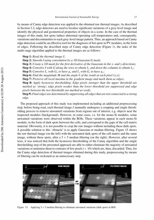
The proposed approach of this study was implemented including an additional preprocessingstep; before being read, each thermal image I manually undergoes a cropping and single thresh-olding process to remove unwanted variations from regions out of interest, e.g. objects near theinspected modules (background). However, in some cases, i.e. for the mono-Si modules, someunwanted variations were observed within the ROIs. These variations appear in each mono-Simodule, in the form of dark spots between the cells, and correspond to the gaps of the cell matrixmaterial. Obviously, it is not possible to crop the raw images without including these dark spots.A possible solution to this ‘obstacle’ is to apply Gaussian or median filtering. Figure 15 showsthe raw thermal image (on the left) with the unwanted dark spots of the cell matrix and the sameimage, without these spots, after a 5 × 5 median filtering (on the right). However, after severaltests, it was noticed that both the hysteresis thresholding of the Canny algorithm and the singlethresholding step of the presented approach are able to either eliminate the majority of unwantedvariations or minimise them to contours of few pixels (< 10) which are, then, discarded. Thus, forthe Canny edge detection of thermal images obtained during this study, preprocessing by meansof filtering can be reckoned as an unnecessary step.

Figure 15. Applying 5 × 5 median filtering to eliminate unwanted variations (dark spots) in ROI.

Dow

nloa

ded

by [

Mr

Ant

onio

s G

aste

rato

s] a

t 02:

09 2

8 A

ugus

t 201

3


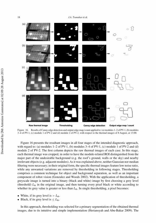
Figure 16. Results of Canny edge detection and output edge map/count applied to: (a) modules 1–2 of PV-1, (b) modules3–4 of PV-1, (c) module 1 of PV-2 and (d) module 2 of PV-2, with respect to the thermal images of 8 August, at 13:00.

Figure 16 presents the resultant images in all four stages of the intended diagnostic approach,with regard to: (a) modules 1–2 of PV-1, (b) modules 3–4 of PV-1, (c) module 1 of PV-2 and (d)module 2 of PV-2. The first column depicts the raw thermal images of each case. In this stage,each thermal image was cropped, in order to have the module-related ROI distinguished from themajor part of the undesirable background (e.g. the roof’s ground, walls or the sky) and nearbyirrelevant objects (e.g. adjacent modules). As it was explained above, neither Gaussian nor medianfiltering were necessary; in their original form, the specific thermal images feature low noise ratio,while any unwanted variations are removed by thresholding in following stages. Thresholdingcomprises a common technique for object and background separation, as well as an importantcomponent of robot vision (Gonzalez and Woods 2002). With the application of thresholding, agreyscale image is turned into a binary (black and white) image by first choosing a grey level(threshold) Lth in the original image, and then turning every pixel black or white according towhether its grey value is greater or less than Lth. In single thresholding, a pixel becomes:

• White, if its grey level is > Lth.• Black, if its grey level is ≤ Lth.

In this approach, thresholding was selected for a primary segmentation of the obtained thermalimages, due to its intuitive and simple implementation (Heriansyah and Abu-Bakar 2009). The

Dow

nloa

ded

by [

Mr

Ant

onio

s G

aste

rato

s] a

t 02:

09 2

8 A

ugus

t 201

3


second column of Figure 16 illustrates the output images from a single thresholding process thatwas provided in Matlab R2009a environment, with a threshold Lth = 160. The latter was selected,after several trials, as the optimum threshold value that accomplishes a fair separation of unwantedregions in the majority of the tested thermal images, without cutting out any ROI. The resultantimages from this stage provide a valuable sum of binary data, overly clear from possible erroneousvariations. These data, in the form of images with hot-spot-related ROI, constitute the inputs forthe Canny edge detection stage.

The last two columns of Figure 16 present the results from the applied edge detection of theCanny algorithm. For the thermal image of modules 1–2 of the PV-1 array, the Canny operator, withhysteresis thresholds 0.8 (lower) and 0.9 (upper) and smoothing parameter sigma = 1 detected atotal number of 6 edges. Then, in the last column, the output edge image is displayed with randomcolours, as an edge map. Each fitted line segment in such maps is stored in a so-called seglist. Itcan be noticed that in the final edge map, one detected edge was excluded, due to small contourlength. A simple count step was added to the algorithm of the presented approach, in order toprovide the final size of the ‘seglist’stores and, thus, the number of the diagnosed defective regionswithin the modules. In this case, a defective region is characterised as a hot-spot formation, whichmay include either a single cell or a group of cells. A total number of 5 hot-spot formations werediagnosed, representing 7 out of 8 defective cells in modules 1–2 of PV-1. The algorithm missed toconfirm one defective cell, the one that was related to the discarded edge contour. For the thermalimage of the other two modules of the PV-1 array, with hysteresis thresholds 0.7 and 0.8 andsmoothing parameter sigma = 1, the Canny operator detected a total number of 5 edges. Similarto the previous case, an edge with small contour length was excluded from the final edge map. Asa result, a total number of 4 hot-spot formations were diagnosed, confirming all 6 defective cellsin modules 3–4 of PV-1. The discarded edge contour was, in this case, correctly considered asnegligible; in the original thermal image, the specific edge corresponds to a background object,on the left side of module 4. However, the smallest of the four segments in the final edge map hasbeen erroneously assumed to be a hot spot. As it can be noticed in the original thermal image, thespecific edge was detected due to a grey-level variation between the two modules.

Canny edge detection was also applied to the thermal images of the PV-2 array. In particular, theCanny operator was applied to the thermal image of both module 1 and module 2, with hysteresisthresholds 0.1 and 0.2 and smoothing parameter sigma = 1. The algorithm detected a total numberof 7 and 10 edges, respectively. Due to their negligible size, two edges in the first module andfour edges in the second one were excluded from the output edge map, in the last stage of thealgorithm. According to each ‘seglist’ count, the overall diagnosis revealed a total number of 11hot-spot formations, which represent and confirm all 20 defective cells within these two modules.

5. Concluding remarks

A CM approach based on IR thermography was proposed and experimentally assessed, in thisstudy, for its potential upon fault diagnosis of PV modules. In particular, the main objectivewas to investigate the applicability of standard thermal image processing and edge detection tothermal images of defective PV modules. Such thermal images were obtained from several fieldIR thermographic measurements performed on two commercial PV arrays installed on the rooftopof a laboratory building in the School of Engineering Campus of DUTh, Greece.

Standard processing of the temperature data from the acquired thermal images, by means of ROIanalysis, line profile and image histogram analysis, showed an evident correlation between theabnormalities to the temperature pattern of a module and existent hot spots through its surface. Onthe other hand, the proposed diagnostic approach, which combines image segmentation and Canny

Dow

nloa

ded

by [

Mr

Ant

onio

s G

aste

rato

s] a

t 02:

09 2

8 A

ugus

t 201

3


edge detection, gave fairly promising results, succeeding to diagnose 13 out of 14 defective cells inPV-1 and 27 out of 29 defective cells in PV-2, in the form of hot-spot formations within the resultantedge maps. The diagnosed hot spots have verified the standard electrical tests applied to each andevery module, prior to the experiments, indicating a total 9.5% and 9.7% performance deteriorationfor PV-1 and PV-2, respectively. In conclusion, IR thermography with the combination of suitable(not necessarily sophisticated) thermal image processing techniques was proved to be a potentialand reliable method for CM, performance evaluation and fault diagnosis of PV modules. Thepresented approach gave easily interpreted results and fast detection and diagnosis of hot spots inPV modules, utilising both qualitative and quantitative data from the processed thermal imagesfrom the two PV arrays.

Probably the most serious limitation of field radiometric measurements combined with thepresented edge detection algorithm is the lack of fault (defect) classification ability, an issue thatis under investigation by Vergura, Acciani, and Falcone (2012). Another serious limitation of theused edge detection algorithm is the fact that any specular object present in the background couldcause unwanted grey-level variations that may be conflicting with the actual variations related tohot spots and, thus, cause ‘false alarms’. Thus, in order to eliminate any case of erroneous edgedetections or missing edges, each IR measurement should be performed (if possible) perpendicu-larly to the target and with the less possible interference from the background scenery or objects.Unfortunately, there are further limitations referring to emissivity uncertainties, the presence ofglass in front of the solar cells and the undesirable dependency on the environmental (ambientand background) conditions that have to be always taken into account for field measurements.Additional investigation in characterising cell/module defects, e.g. ohmic losses, shunts, micro-cracks, etc. can be based on a micro-scale analysis combining the current experience with activethermography approaches. Besides, a more thorough understanding of degradation mechanismsand failure modes in PV modules is critical to improvements in PV modules’ design and relia-bility. Large-scale CM of PV modules, i.e. aerial thermography, as well as the implementationof standardised accelerated aging tests to the defective PV modules, are of further interest to thecurrent research team.

Acknowledgements

The authors would like to thank ExelSolar Division of ExelGroup Green Technologies SA and, especially, Mr NikolaosPitsokos and Mr CharalamposAmanatidis, for providing the specific poly-Si PV modules of the PV-2 array, as well for theirvaluable information and contribution to the standard electrical/performance tests on the PV modules. The authors wouldalso like to thank Dr Georgios Bakos, Associate Professor of DUTh, School of Engineering, Department of Electrical andComputer Engineering, Faculty of Electric Energy Systems, for his assistance in providing the mono-Si PV modules ofthe PV-1 array. This work has been partially funded by the TSMEDE-2009 project titled ‘Fault diagnosis in renewableenergy systems with the use of IR thermography – case study: PV modules’.

References

Abdel-Qader, I., S. Yohali, O. Abudayyeh, and S. Yehia. 2008. “Segmentation of Thermal Images for Non-destructiveEvaluation of Bridge Deck”. NDT & E International 41 (5): 395–405.

Acciani, G., O. Falcone, and S. Vergura. 2010. “Typical Defects of PV-Cells”. Proceedings of IEEE internationalsymposium on industrial electronics (ISIE), Bari, Italy, July 4–7.

Ahuja, D., and M. Tatsutani. 2008. Sustainable Energy for Developing Countries. A report to the Academy of Sciencesfor the Developing World (TWAS), Trieste, Italy.

Bai, L., Q. Chen, C. Lei, and B. Zhang. 2000. “New Technique for Infrared Thermal Image Processing Combining TimeDomain and Space Domain”. Proceedings of infrared technology and applications XXVI, SPIE 4130, San Diego,CA, USA, July 30.

Borland, D., and R. M. Taylor. 2007. “Rainbow Color Map (Still) Considered Harmful”. IEEE Computer Graphics andApplications 27 (2): 14–17.

Dow

nloa

ded

by [

Mr

Ant

onio

s G

aste

rato

s] a

t 02:

09 2

8 A

ugus

t 201

3


Breitenstein, O., J. P. Rakotoniaina, M. Kaes, S. Seren, T. Pernau, G. Hahn, W. Warta, and J. Isenberg. 2005. “Lock-inThermography – A Universal Tool for Local Analysis of Solar Cells”. Proceedings of 20th European photovoltaicsolar energy conference and exhibition (EUPVSEC), Barcelona, Spain, June 6–10.

Canny, J. 1986. “A Computational Approach to Edge Detection”. IEEE Transactions on Pattern Analysis and MachineIntelligence (PAMI) 8 (6): 679–698.

Chou, Y.-C., and L. Yao. 2009. “Automatic Diagnosis System of Electrical Equipment Using Infrared Thermography”.Proceedings of international conference of soft computing and pattern recognition (SoCPar’09), Malacca, Malaysia,December 4–7.

del Cueto, J. A. 2002. “Comparison of Energy Production and Performance from Flat-Plate Photovoltaic Module Tech-nologies Deployed at Fixed Tilt”. Proceedings of 29th IEEE PV specialists conference, New Orleans, LA, May20–24. NREL/CP-520-31444.

Dallas, W., O. Polupan, and S. Ostapenko. 2007. “Resonance Ultrasonic Vibrations for Crack Detection in PhotovoltaicSilicon Wafers”. Measurement Science and Technology 18 (3): 852–858.

Designation ASTM E2481-08. 2008. Standard Test Method for Hot Spot Protection Testing of Photovoltaic Modules. ICSNumber Code 27.160 (Solar energy engineering). doi:10.1520/E2481-08.

EPIA (European Photovoltaic Industry Association) and Greenpeace. 2011. Solar Generation 6: Solar PhotovoltaicElectricity Empowering the World (Report). Amsterdam/Brussels, Netherlands/Belgium.

Fuyuky, T., H. Kondo, T. Yamazaki, Y. Takahaschi, and Y. Uraoka. 2005. “Photographic Surveying of Minority CarrierDiffusion Length in Polycrystalline Silicon Solar Cells by Electroluminescence”. Applied Physics Letters 86 (26):262108.

Gonzalez, R. C., and R. E. Woods. 2002. “Image Segmentation”. Chap. 10 in Digital Image Processing. Upper SaddleRiver, NJ: Prentice-Hall.

Gupta, R., and O. Breitenstein. 2007. “Unsteady-state Lock-in Thermography – Application to Shunts in Solar Cells”.Quantitative InfraRed Thermography Journal 4 (1): 85–105.

Hardy, G. 1997. “Thermal Inspection.” Chap. 22 in ASM Handbook – Nondestructive Evaluation and Quality Control.Vol. 17, 5th ed. Materials Park, OH: ASM International.

Heriansyah, R., and S. A. R. Abu-Bakar. 2009. “Defect Detection in Thermal Image for Nondestructive Evaluation ofPetrochemical Equipments”. NDT & E International 42 (8): 729–740.

Hoyer, U., A. Burkert, R. Auer, and C. Buerhop-Lutz. 2009. “Analysis of PV Modules by Electroluminescence and IRThermography”. Proceedings of 24th European photovoltaic solar energy conference and exhibition (EUPVSEC),Hamburg, Germany, September 21–25.

Ibarra-Castanedo, C., D. Gonzalez, M. Klein, M. Pilla, S. Vallerand, and X. Maldague. 2004. “Infrared Image Processingand Data Analysis”. Infrared Physics & Technology 46 (1–2): 75–83.

Kasemann, M., M. C. Schubert, M. The, M. Kober, M. Hermle, and W. Warta. 2006. “Comparison of LuminescenceImaging and Illuminated Lock-in Thermography on Silicon Solar Cells”. Applied Physics Letters 89 (22): 224102.

Kontges, M., I. Kunze, S. Kajari-Schroder, X. Breitenmoser, and B. Bjorneklett. 2010. “Quantifying the Risk of PowerLoss in PV Modules due to Micro Cracks”. Proceedings of 25th European photovoltaic solar energy conference(EUPVSEC), Valencia, Spain, September 6–10.

Kosikowski, M., Z. Suszynski, and M. Bednarek. 2011. “Processing and Recognition of the Thermal Images Using WaveletTransforms”. Microelectronics Reliability 51 (7): 1271–1275.

Krenzinger, A., and A. C. de Andrade. 2007. “Accurate Outdoor Glass Thermographic Thermometry Applied to SolarEnergy Devices”. Solar Energy 81 (8): 1025–1034.

Kurtz, S., D. Miller, M. Kempe, N. Bosco, K. Whitefield, J. Wohlgemuth, N. Dhere, and T. Zgonena. 2009. “Evalua-tion of High-Temperature Exposure of Photovoltaic Modules”. Proceedings of 34th IEEE photovoltaic specialistsconference, Philadelphia, PA, USA, June 7–12. NREL/CP-520-45986.

Luque, A., and S. Hegedus. 2003. “Crystalline Silicon Solar Cells and Modules”. Chap. 7 in Handbook of PhotovoltaicScience and Engineering. Chichester: Wiley-Interscience.

Maldague, X. P.V. 2001. “Getting Started with Thermography for Nondestructive Testing”. Chap. 1 in Theory and Practiceof Infrared Technology for Nondestructive Testing. 1st ed. New York: Wiley-Interscience.

Otsu, N. 1979. “A Threshold Selection Method from Gray-Level Histograms”. IEEE Transactions on Systems, Man, andCybernetics 9 (1): 62–66.

Plotnikov, Y. A., and W. P. Winfree. 1998. “Advanced Image Processing for Defect Visualization in InfraredThermography”. Proceedings of Thermosense XX, SPIE 3361, Orlando, FL, USA, March 26.

Savelyev, A., and R. Sugumaran. 2008. “Surface Temperature Mapping of the University of Northern Iowa Campus UsingHigh Resolution Thermal Infrared Aerial Imageries”. Sensors 8 (8): 5055–5068.

Scales, N., C. Herry, and M. Frize. 2004. “Automated Image Segmentation for Breast Analysis Using Infrared Images”.Proceedings of 26th annual international conference of the IEEE EMBS, San Francisco, CA, USA, September 1–4.

Simon, M., and E. L. Meyer. 2010. “Detection and Analysis of Hot-spot Formation in Solar Cells”. Solar Energy Materialsand Solar Cells 94 (2): 106–113.

Skoplaki, E., A. G. Boudouvis, and J. A. Palyvos. 2008. “A Simple Correlation for the Operating Temperature ofPhotovoltaic Modules of Arbitrary Mounting”. Solar Energy Materials and Solar Cells 92 (11): 1393–1402.

Tsanakas, J. A., and P. N. Botsaris. 2011a. “Passive and Active Thermographic Assessment as a Tool for Condition-basedPerformance Monitoring of Photovoltaic Modules”. Journal of Solar Energy Engineering 133(2): 021012.

Tsanakas, J. A., and P. N. Botsaris. 2011b. “Quantifying the Impact of Hot Spots on the Performance of PhotovoltaicModules by Infrared Thermography and a Simulation Model”. Proceedings of 2nd international exergy, life cycleassessment, and sustainability workshop & symposium (ELCAS-2), Nisyros, Greece, June 19–21.

Dow

nloa

ded

by [

Mr

Ant

onio

s G

aste

rato

s] a

t 02:

09 2

8 A

ugus

t 201

3


Van der Borg, N. J. C. M., and A. R. Burgers. 2003. “Thermography: Quality Control for Module Manufacturing”.Proceedings of 3rd world conference on photovoltaic energy conversion, Osaka, Japan, May 11–18.

Vergura, S., and O. Falcone. 2011. “Filtering and Processing IR Images of PV Modules”. Proceedings of internationalconference on renewable energies and power quality (ICREPQ’11), Las Palmas de Gran Canaria, Spain, April 13–15.

Vergura, S., G. Acciani, and O. Falcone. 2012. “A Finite-Element Approach to Analyze the Thermal Effect of Defects onSilicon-Based PV Cells”. IEEE Transactions on Industrial Electronics 59 (10): 3860–3867.

Vollmer, M., and K.-P. Mollmann. 2010. “Advanced Methods in IR Imaging”. Chap. 3. in Infrared Thermal Imaging:Fundamentals, Research and Applications. Weinheim, Germany: Wiley-VCH Verlag.

Wang, X., B. S. Wong, C. Tan, and C. G. Tui. 2011. “Automated Crack Detection for Digital Radiography Aircraft WingInspection”. Research in Nondestructive Evaluation 22 (2): 105–127.

Wiecek, B. 2005. “Review on Thermal Image Processing for Passive and Active Thermography”. Proceedings of 27thannual conference IEEE engineering in medicine and biology, Shanghai, China, September 1–4.

Wiecek, M., R. Strakowski, T. Jakubowska, and B. Wiecek. 2008. “Chosen Aspects of Thermal Image Processing –A New Software for Medical Applications”. Proceedings of 9th international conference on quantitative infraredthermography (QIRT), Krakow, Poland, July 2–5.

Wohlgemuth, J., and W. Herrmann. 2005. “Hot Spot Tests for Crystalline Silicon Modules”. Proceedings of 31st IEEEphotovoltaic specialists conference, Orlando, FL, USA, January 3–7.

Younus, A. M., A. Widodo, and B. S. Yang. 2009. “Image Histogram Features Based Thermal Image Retrieval to PatternRecognition of Machine Condition”. Proceedings of 4th world congress on engineering asset management, Athens,Greece, September 28–30.

Zayicek, P. 2002. Infrared Thermography Guide (Revision 3). Palo Alto, CA: Electric Power Research Institute (EPRI).

Dow

nloa

ded

by [

Mr

Ant

onio

s G

aste

rato

s] a

t 02:

09 2

8 A

ugus

t 201

3

fault diagnosis of photovoltaic modules through image processing and canny edge detection on field...

Documents