Fast Frequency Sweep Technique for E�cient Analysisof Dielectric Waveguides1Sergey V. Polstyanko2 Romanus Dyczij-Edlinger3 Jin-Fa Lee2AbstractThis paper describes a new approach to spectral response computation of an arbi-trary 2D waveguide. This technique is based on the Tangential Vector Finite ElementMethod (TVFEM) in conjunction with the Asymptotic Waveform Evaluation (AWE)technique. The former is used to obtain modes characteristics for a central frequency,whereas the latter employs an e�cient algorithm to compute frequency moments foreach mode. These moments are then matched via Pad�e approximation to a reduced-order rational polynomial which can be used to interpolate mode over a frequencyband with a high degree of accuracy. Furthermore, the moments computations andsubsequent interpolation for a given set of frequency points can be done much morerapidly than just simple simulations for each frequency point.1 IntroductionCOMPUTER{AIDED numerical analysis has become a necessary tool for designing mi-crowave and optical wave-guiding structures such as microstrip line, optical channel guideand optical �ber. Di�erent numerical techniques have been presented in the past to solvea wide variety of dielectric waveguide problems [1, 2, 3, 4, 5]. Among them, the FiniteElement Method (FEM) is probably the most versatile [6, 3, 7, 8]. By discretizing thewaveguide cross-section into a number of triangles and employing the variational technique,the FEM can be used to predict the propagation characteristics of any arbitrary waveguideaccurately.It has been shown by previous researchers, that by using the Tangential Vector Finite Ele-ment Method (TVFEM) electromagnetic characteristics of propagating modes in waveguidescan be obtained without the occurrences of so-called spurious solutions [9, 8, 10]. However,these spurious solutions are not completely eliminated, they are reduced to a set of identi-�able non-physical solutions corresponding to the null-space of the generalized eigenmatrixequation. Consequently, they can slow down the convergence of desirable modes during thesolution process and cause additional complications. In this paper, we have introduced anadditional set of constraint equations for the generalized eigenmatrix equation. By using1This work was sponsored by Hewlett-Packard Inc.2The authors are with the ECE Department, WPI, Worcester, MA 01609 USA3Currently with Motorola Inc., Schaumburg, IL 1

this set of constraint equations, the non-physical solutions can be completely suppressedand the solution space is limited only to physical modes.Previously, we have implemented a H10(curl) Tangential Vector Finite Element Method(TVFEM) to perform a full-wave analysis of an anisotropic waveguide which is characterizedsimultaneously by both o�-diagonal second rank symmetric [�] and [�] tensors [11]. But ifone wants to compute a dispersion curve with the propagation constant versus frequencyover a given frequency band, this analysis has to be repeated for many sampling frequencypoints. Consequently, the entire process can become very time consuming, especially whenthe number of frequency points becomes large and the number of unknowns is signi�cant.To avoid this di�culty a new approach based on the Asymptotic Waveform Evaluation(AWE) [12] has been developed. Starting with the known modes characteristics for a cen-tral frequency, the AWE technique employs an e�cient algorithm to compute frequencymoments for each mode. These moments are then matched via Pad�e approximation to areduced-order rational polynomial with a high degree of accuracy. Furthermore, the mo-ments computations and subsequent interpolation for a given set of frequency points canbe done more rapidly than just simple simulations for each frequency point. To verify theproposed approach, the method has been implemented and tested for sample wave-guidingstructures and the resultant dispersion curves are compared with those obtained by theH10(curl) TVFEM. The details of the formulation, error estimation, and sample numericalresults will be discussed in the following sections.2 Formulation2.1 Time Harmonic Maxwell's EquationsShown in Fig. 1 is a general wave-guiding structure that is uniform in the z direction withan arbitrary cross-section in the xy plane and the boundary of consists of either perfectelectric conductor (PEC) or perfect magnetic conductor (PMC). Assuming time-harmonicexcitations, Maxwell's equations can be written asr� ~E = �j!�0[�r] ~Hr� ~H = j!�0[�r] ~E + [�] ~Er � [�r] ~H = 0r � [�r] ~E = 0 (1)where [�r] and [�r] are the relative permittivity and permeability,respectively, and [�] isthe conductivity tensor. In the present study, they are assumed to be diagonal tensors.Furthermore, in the frequency domain, [�r] and [�] can be combined to de�ne a complexe�ective relative permittivity [�r] as [�r] = [�r]� j!�0 [�] (2)2

To solve for the wave propagation characteristics, we start by expressing the �elds as~E(~r; t) = ~E(x; y)e� zej!t~H(~r; t) = ~H(x; y)e� zej!t (3)where =� +j � is the propagation constant with �, � being the attenuation and phaseconstant, respectively; and ~r = (x; y; z) denotes the position vector of a point in the wave-guide.2.2 A-V FormulationIn the current formulation, we use a vector potential ~A and a scalar potential ' as ourunknown variables. They are de�ned through the �elds as~B = r� ~A~E = �j! ~A� cr' (4)Also, it is well known that the vector potential ~A de�ned by (4) is not unique withoutimposing a gauge condition. Instead of using the conventional Coulomb or Lorenz gauge wechoose Az = 0. This condition will greatly simplify the formulation. By using Eqs. (1)-(4)and the gauge condition Az = 0, Maxwell's equations becomer� [�]r� ~A� � k20[�r] ~A� + jk0[�r]r' = 0�jk0r � [�r] ~A� �r � [�r]r' = 0 (5)where k0 = !2�0�0 is the free-space wavenumber and [�] = [�r]�1 denotes the inverse matrixof [�r] . Taking into account that r = r� - z, equations (5) can be rewritten asr� � ��1zz r� � ~A� � 2[�]� ~A� � k20[�r]� ~A� + jk0[�r]�r�' = 0 (6)� r� � [�]� ~A� � jk0 �zz' = 0 (7)�jk0r� � [�r]� ~A� �r� � [�r]�r�'� 2�zz' = 0 (8)where [�r]� = " �xx 00 �yy # [�]� = " �yy 00 �xx # (9)Equation (7) can be obtained by subtracting equation (8) from (6). Subsequently, in thecurrent formulation, we focus on solving Eqs. (6) and (8) simultaneously. Furthermore,boundary conditions associated with this formulation are:on PEC s ( ~n� ~A� = 0' = 0 (10)on PMC s ( ~n� ([�]r� ~A� ) = 0[�r]� (jk0 ~A� +r�') � ~n = 0 (11)where ~n is the normal vector to the boundary.3

3 Finite Element Implementation3.1 The Bilinear FormEquations (6), (8) and boundary conditions (10), (11) describe a well de�ned boundary valueproblem (BVP) and are ready for the application of the �nite element method. Applicationof the Galerkin's method for the current BVP results in the following bilinear formB(~�;~a) = Zf��1zz (r� � ~��) � (r� � ~a� )� k20~�� � [�r]�~a� +r��z � [�r]�r�az+ jk0~�� � [�r]�r�az + jk0r��z � [�r]�~a�gd� 2 Zf~�� � [�]�~a� + �zz�zazgd (12)where ~�;~a are the testing and trial �elds, respectively. Notice that in an e�ort to balance thesmoothness requirements on both the trial and testing �elds, we have adopted the Green'stheorems to derive Eq. (12). Moreover, to facilitate our discussion, we have also employeda vector notation for the potentials as~a = " ~a�az # = " ~A�' # (13)Judging from the bilinear form (12), a vector �eld ~a is admissible in the bilinear form if andonly if ~a 2 V = n~v : ~v� 2 (L2())2; r� � ~v� � z 2 L2(); vz 2 C0()o (14)where L2(), C0() are the sets of square integrable functions and continuous functions in, respectively.3.2 Two-dimensional H10(curl) TVFEMIn the Galerkin's process, we need to �nd a complex number and a vector function~a 2 V , such that B(~�;~a) = 0 for every ~� in the in�nite dimensional space V . The �niteelement method is nothing but replacing V by a sequence of �nite dimensional subspacesV h contained in V . In the present approach, we have chosen V h to be spanned by theH10(curl) TVFEM basis functions. Mathematically, we de�ne a �nite dimensional vectorspace Hk(curl; h), for a two-dimensional discretization h asHk(curl; h) = (Pk(h))2 � Sk+1(h) (15)where Pk(h) is the set of piece-wise polynomials in h with order complete to k. Thefunction space Sk+1(h) can be de�ned simply bySk(h) = n~v h� j ~v h� 2 ( ~Pk(h))2; < ~v h� ;r��h >= 0; 8� 2 ~Pk+1(h)o (16)and ~Pk(h) is the set of piece-wise homogeneous kth order polynomials in h. And thefunction space Hk0(curl; h) is further de�ned byHk0(curl; h) = n~v h� j ~v h� 2 Hk(curl; h); n� ~v� h = 0 on �PECo (17)4

Henceforth, the �nite dimensional space V h that is used in the current FEM formulation isV h = n~v h j ~v� h 2 H10(curl; h); vhz 2 P2(h); vhz = 0 on �PECo (18)Note that in choosing the FEM space as in (18), the following statement is valid: 8~v h 2V h we have rvhz 2 H10(curl; h). Explicitly, for a tetrahedral element there are 8 vectorbasis functions and 6 scalar basis functions for the �nite element space V h (Fig. 2). Eachtrial/testing function ~ah 2 V h can now be written as~a� h = 7Xi=0 ah�i ~W hi ahz = 5Xi=0 ahzi hi (19)where the 6 scalar basis functions i are the usual second order FEM basis functions, namely 0 = 2�0(�0 � 1=2); 3 = 4�1�2; 1 = 2�1(�1 � 1=2); 4 = 4�0�2; 2 = 2�2(�2 � 1=2); 5 = 4�0�1;and the 8 vector basis functions are given by~W0 = �1r�2 � �2r�1;~W1 = �1r�2 + �2r�1;~W2 = �2r�0 � �0r�2; ~W6 = 4�1(�2r�0 � �0r�2);~W3 = �2r�0 + �0r�2; ~W7 = 4�2(�0r�1 � �1r�0);~W4 = �0r�1 � �1r�0;~W5 = �0r�1 + �1r�0;where �i is the Lagrangian interpolation polynomial or simplex coordinate at vertex i [13].3.3 Generalized Eigenmatrix EquationFinally, a generalized eigenmatrix equation can be obtained by setting B(~�;~a) = 0 for every~� h 2 V h. The result isXe " [A]e [C]e[C]Te [D]e #! " a�az # = 2Xe " [B]e 00 [E]e #! " a�az # (20)wherePe means the summation over the contributions from each element and a� ; az are thecorresponding coe�cient vector for the �nite dimensional approximation of ~ah. Moreover,the element matrices in Eq. (20) are given by[A]e = Zef��1zz (r� � ~Wi) � (r� � ~Wj)� k20 ~Wi � [�r]� ~Wjgd[B]e = Zef ~Wi � [�]� ~Wjgd[C]e = jk0 Zef ~Wi � [�r]�r� jgd[D]e = Zefr� i � [�r]�r� jgd[E]e = Zef�zz i jgd (21)5

The integrations in (21) are performed on triangular regions. To make computation fasterwe rearrange the matrix equation (20) into" [B] 00 [E] # " a�az # = 1 2 + �2 " [A] [C][C]t [D] #+ �2 " [B] 00 [E] #! " a�az # (22)where [A] = Pe [A]e and so on, and �2 = k20 � �max � �max is an educated guess, which canbe obtained by a quasi-TEM approximation for an isotropic medium. The reason for thistransformation is as follows: in a lossless dielectric waveguide, a more dominant mode corre-sponds to smaller 2 value and as a result, the 1=( 2+ �2) ratio will be larger. It turns out,that although the Lanczos algorithm can compute both the smallest and the largest eigen-values, the latter almost always converges faster than the former one. Furthermore, from(21)and (22), we can conclude that for an anisotropic waveguide, characterized by diagonalpermittivity and permeability tensors, the generalized eigenmatrix equation involves twocomplex but symmetric matrices. Subsequently, savings in computational time and storagecan be realized by taking advantage of this symmetry.3.4 Constraint EquationsThe eigenpair solutions < i;~a i > to Eq. (22) can be divided into three groups. This canbe seen as follows: Our bilinear form (12) and subsequently the generalized eigenmatrixequation (22) are derived based on Eqs. (6) and (8). The solutions of (6) and (8) areguaranteed to be nontrivial solutions of Maxwell's equations only if 6= 0. When = 0,there are two possibilities: the cuto� modes which are still solutions of Maxwell's equations;and the trivial solutions : ~a = " ~A�' # 6= 0, but ~E = �j! ~A� � cr' = 0. To summarize, theeigenpairs < i;~a i > can be divided into 3 groupsgroup 1 (physical modes): i 6= 0, ~Ei = �j! ~A i� � cr'i 6= 0;group 2 (cuto� modes): i = 0, ~Ei = �j! ~A i� � cr'i 6= 0;group 3 (trivial modes): i = 0, ~Ei = �j! ~A i� � cr'i = 0.Our objective is to develop a constrained Lanczos algorithm which will solve for solutionsin group 1 and 2 without the occurrences of group 3. To achieve this goal, we �rst noticethat the group 3 solutions form a vector function space V hNULL de�ned asV hNULL = ( " ~���z # : ~�� = jk0r��z ) (23)and obviously V hNULL � V h. Furthermore, the number of trivial modes, or the dimension ofV hNULL equals the number of free nodes in the second order discretization. Although thesetrivial solutions can be easily identi�ed and disregarded at the post-processing stage, theirpresence can signi�cantly degrade the performance of the Lanczos algorithm. Therefore, aconstrained Lanczos algorithm which completely suppresses the occurrence of these trivialmodes will enhance the numerical e�ciency and stability.6

3.5 Orthogonality RelationsFrom Eq. (12), the following orthonormal property exists for the eigensolutions:Z(~a i� � [�]�~a j� + �zzaizajz) = �ij (24)where �ij is the Kronecker delta-function. Equation (24) is the basis for the constraintequation that will be used in the constrained Lanczos algorithm. Since a physical solution~a j from group 1 or group 2 must be orthogonal to any ~a i 2 V hNULL through Eq. (24), theconstraint equation for the physical solutions readsZf jk0r��z � [�]�~a� + �zz�zazgd = 0 8vz 2 P2(); vz = 0 on �PEC (25)In discretized form equation (25) reduces to the following matrix equationaz = �[E]�1[F ]a� (26)where matrices [E] and [F ] are given by[E]e = Zef�zz i jgd[F ]e = jk0 Zefr� i � [�]� ~Wjgd (27)Equation (26) can be used as a set of additional constraints to restrict the solution space togroup 1 and 2 solutions in the Lanczos algorithm.3.6 Constrained Lanczos AlgorithmBy incorporating the constraint equation (26) into the generalized algorithm, the followingalgorithm can be used to �nd N eigenpairs of the generalized eigenmatrix equation [A]x =�[B]x without the occurrences of group 3 solutions1. Input the number of desired modes N.2. Input an initial guess x0, and(a) �x 0� = x 0� , �x 0z = �[E]�1[F ]�x 0� ;(b) g0 = [B]�x 0.3. Orthogonalize g0 to previously converged vectors Xi(i = 1; :::n),�g0 = g0 � nXi ciXi; ci = XTi g0 (28)4. Solve [B]x1 = �g0 and normalize x1 to obtain v1 = x1kx1k (m = 1).7

5. f = [A]vm � hm;m[B]vm � hm�1;m[B]vm�1, wherehm;m = vTm[A]vmvTm[B]vm ; hm�1;m = vTm�1[A]vmvTm�1[B]vm�1 :6. Orthogonalize f to previously converged vectors Xi(i = 1; :::n), namely�f = f � nXi=1 diXi; di = XTi f (29)7. Solve for xm+1 from [B]xm+1 = �f , and(a) �xm+1� = xm+1� , �xm+1z = �[E]�1[F ]�xm+1� ;(b) hm+1;m = k�xm+1k; vm+1 = �xm+1k�xm+1k .8. Calculate (�(m); y(m)) of the triangular matrix Hm whereHm = 26666664 h1;1 h1;2h2;1 h2;2 h2;3h3;2 h3;3 ::: hm;m�1 hm;m37777775 (30)

9. Check the residual norm = hm+1;m y(m)m for convergence; if not converged, incrementm by 1 and go to step 4.10. Increment n by 1. If all desired modes have converged (n = N) then stop, otherwisego to step 1.We would like to comment here that theoretically if the initial vector is constructed in sucha way that it satis�es equation (26) our solution becomes orthogonal to the subspace oftrivial solutions. The purpose of step 7(a) is simply to avoid the accumulation of roundingerror. Practically, step 7(a) can be performed selectively.4 Asymptotic Waveform EvaluationIt has been shown previously that the FEM formulation for the electromagnetic wave prop-agation in 2D wave-guiding structures leads to the matrix equation of the formP(f)x(f) = �(f)Q(f)x(f) (31)where P(f) and Q(f) are the square complex matrices, f is a given frequency, x representsthe unknown �eld components, and � is related to the propagation constant itself. Equation(31) can be solved directly for the unknown eigenpairs < �i; xi > by using the constrained8

Lanczos algorithm described above. However, if we are looking for the solution over agiven frequency band [f 0; f 1] the entire process has to be repeated for a set of frequenciesffigi=Ni=0 such that f 0 = f0 < f1 < � � � < fN = f 1 to �nd eigenpairs < �i; xi >. Afterthat the eigenpair < �(f); x(f) > for any arbitrary frequency f within the interval [f 0; f 1]can be determined based on an interpolation technique such as linear, quadratic or splineapproximation.However, if we deal with a big problem or the number of sampling points N is large, thenthe entire analysis can become very time consuming. Consequently, our goal is to developan alternative method for which the spectral responses over a given frequency range can bedetermined e�ciently.To achieve the above goal, a Fast Frequency Sweep (FFS) technique is proposed andimplemented in this work. The FFS approach proposed herein is a combination of theTVFEM, described in previous sections, and the Asymptotic Waveform Evaluation (AWE)technique. The latter has been successfully used for the analysis/simulation of 2D/3Dinterconnect structures on integrated circuits and has recently gained much attention fromthe CAD community [12, 14, 15, 16]. A number of papers have devoted to AWE as themethod for computing an approximation of the response of a linear circuit from circuit'slow-order moments. Furthermore, the method has been proven by many researchers to be ane�cient and accurate technique for simulating lumped, linear circuit of arbitrary topologies.Recently, several attempts have also been made to apply the AWE technique for electo-magnetic problems and the validity of the approach has been shown [17, 18]. In this paperwe extend the AWE method, based on the rational function approximation, for modelingwave propagation in 2D wave-guiding structures. Furthermore, we will compare the powerseries expansion and rational function approximation and present the results of our accuracystudy.4.1 Taylor ExpansionWe start our discussion with the following generalized eigenmatrix equation that was ob-tained previously " [A] [C][C]T [D] # " ~A�'z # = 2 " [B] 00 [E] # " ~A�'z # (32)where the element matrices are the same as those given by Eq. (21). To facilitate ourdiscussion, we simply rewrite (32) asP(k)x(k) = �(k)Q(k)x(k) (33)where matrices P(k), Q(k) and eigenpairs < �(k); x(k) > are in general functions of thewavenumber k,P(k) = " [A] [C][C]T [D] # ; Q(k) = " [B] 00 [E] # ; x(k) = " ~A�'z # (34)9

Let us �rst expand these quantities by Taylor series around k = k0. Namely,P(k) = NXi=0Pi(k � k0)i Q(k) = NXi=0Qi(k � k0)i�(k) = NXi=0 �i(k � k0)i x(k) = NXi=0 xi(k � k0)i (35)Furthermore, from Eq. (21) it can be seen that matrix Q(k) has only the Q0 component,whereas matrix calP (k) has contributions from P0;P1;P2. Substituting equations (35) into(33) and matching the coe�cients of corresponding power of (k � k0) we end up with thefollowing recursive system of equations to solve1 : (P0 � �0Q0)x1 = Q0�1x0 � P1x0� � � � � � � � � � � � � � � � � � � � � � � � � � � � � �i : (P0 � �0Q0)xi = Q0(�ix0 + � � �+ �1xi�1)� P2xi�2 � P1xi�1 (36)� � � � � � � � � � � � � � � � � � � � � � � � � � � � � �N : (P0 � �0Q0)xN = Q0(�Nx0 + � � �+ �1xN�1)� P2xN�2 � P1xN�1Taking into account that x0 is the eigenvector of (33) and multiplying (36) by xT0 , �i andconsequently xi can be found. In this process, we have to solve the symmetric eigenmatrixequation (32) only once for the central frequency point. After that the corresponding Taylorseries expansion is found by solving (36) with the same matrix (P0 � �0Q0) but di�erentright-hand sides. This process can be performed e�ciently once the factorization of matrix(P0 � �0Q0) becomes available.4.2 Pad�e ExpansionIn many cases, the Taylor series expansion for the solution of eigenmatrix equation (32) givesfairly good results. However the situation is di�erent if one wants to �nd an approximatesolution in the proximity of a pole or some other singularity of the desirable function. In suchcases, Taylor expansion fails to converge, whereas rational interpolation may still providesatisfactory results. Subsequently, we may want to replace the Taylor expansion by theso-called Pad�e expansion to improve the accuracy of our numerical solution. In this sectionwe explain how to construct a rational function for the eigenvalue �(k). The extension ofthis approach to the eigenvector is straight-forward and is not given here. Using the Taylorexpansion we can express an eigenvalue �(k) as�(k) = NXi=0 �i(k � k0)i (37)whereas in the Pad�e expansion we employ a rational polynomial � to interpolate �(k) as,�(k) = LXi=0 pi(k � k0)i1 + MXi=1 qi(k � k0)i (38)10

The rational function � is de�ned by its L+M + 1 coe�cients to be determined later. Fora given amount of computational e�ort, one can usually construct a rational approximationthat has a smaller error than a polynomial approximation. Furthermore, for a �xed valueof L +M the error is the smallest when PL(k) and QM (k) have the same degree or PL(k)has a degree one higher than QM(k). We construct the rational polynomial �(k) in such away that it agrees with �(k) at k0 and their derivative up to L+M degree at k = k0. Theseconditions result in a system of L+M + 1 linear equations to solve. Namely,�0 � p0 = 0q1�0 + �1 � p1 = 0q2�0 + q1�1 + �2 � p2 = 0� � � � � � � � � � � � � � � � � � � � � � � � � � �qM�L�M + qM�1�L�M+1 + � � �+ �L � pL = 0 (39)and qM�L�M+1 + qM�1�L�M+2 + � � �+ q1�L + �L+1 = 0qM�L�M+2 + qM�1�L�M+3 + � � �+ q1�L+1 + �L+2 = 0� � � � � � � � � � � � � � � � � � � � � � � � � � � � � � � � �qM�L + qM�1�L+1 + � � �+ q1�L+M�1 + �L+M = 0 (40)The M equations in (40) involve only the unknowns q1; : : : ; qM and thus must be solved�rst. Then equations in (39) are used to �nd p0; : : : ; pL. Once q1; : : : ; qM and p0; : : : ; pLare determined Eq. (38) can be used to compute the propagation constant at any fre-quency. The described above procedure can be repeated to interpolate each component ofthe eigenvector x(k).5 Numerical ResultsTo validate the proposed approach several examples have been studied. In our �rst examplewe applied the Fast Frequency Sweep (FFS) method to a partially �lled isotropic waveguide.Then, the method was tested on an anisotropic waveguide. Finally, a shielded microstrip lineand a coplanar waveguide were considered. For each example a dispersion curve with thepropagation constant versus frequency has been computed. The results were compared withthe solution obtained by using the TVFEM for di�erent frequency points. Furthermore, toperform an accuracy study of the proposed method over a frequency range we de�ne theerror by error = jP(k)x(k)� �(k)Q(k)x(k)jjx(k)j (41)where P(k), Q(k) are the exact matrices from equation (33) and �(k), x(k) are our ap-proximate solutions. To compare the performance of Taylor and Pad�e expansions, we haveplotted the error versus frequency for each example and comparisons have also been made.11

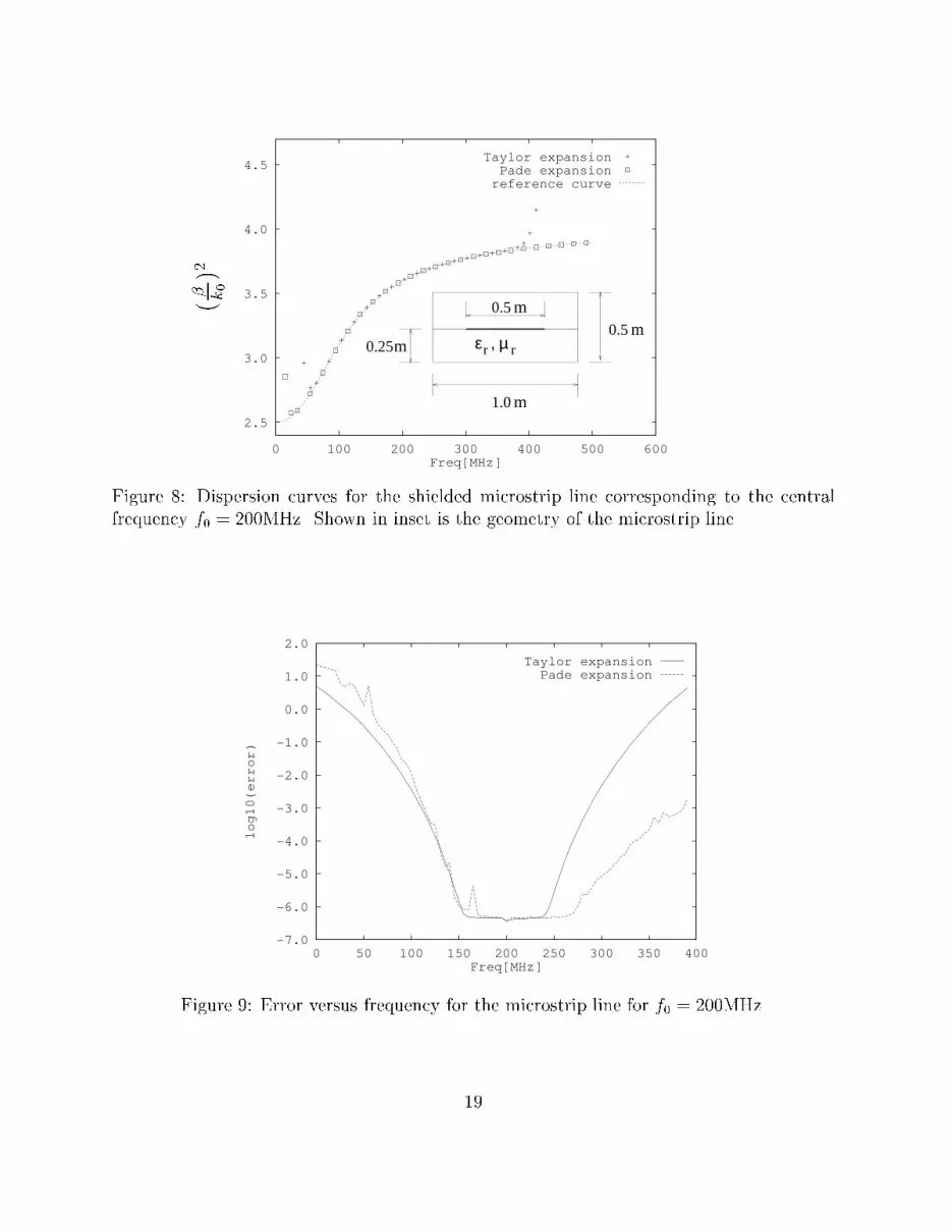
5.1 Partially Filled WaveguideTo verify the proposed FFS method we have studied �rst a rectangular waveguide partiallyloaded with a dielectric, which is a well-known example that has been analyzed by manyresearchers. For the geometry shown in the inset of Fig. 3 the cuto� frequency of thedominant mode equals 31MHz. Our objective was to demonstrate that the FFS methodcan predict correctly mode characteristics below the cuto� frequency.First, we have used the H10(curl) method to plot the reference dispersion curve for thedominant mode over the frequency interval from 1MHz to 140MHz (Fig. 3). After that,the FFS technique have been applied for the dominant mode starting with the known modecharacteristics for f0 = 70MHz. Two dispersion curves, computed by Taylor and Pad�eexpansions, have been obtained and plotted in Fig. 3 for f 2 [1MHz; 140MHz]. FromFig. 3 one can conclude that for frequencies smaller than 31MHz the dominant solutionbecomes an attenuating mode, but still Pad�e approximation has a good agreement withthe reference curve. On the other hand, power series expansion fails for frequencies smallerthan the cuto�. Error analysis, based on Eq. (41), only con�rms the above conclusionand suggests that in general Pad�e expansion may have a potential advantage over Taylorexpansion for physical problems with complex zeros and poles.5.2 Anisotropic WaveguideIn this example we study a rectangular waveguide, which is loaded with an anisotropicrectangular insert (Fig. 5). The dielectric is made of T iO2, a material having a very highpermittivity �rx = 170 and �ry = �rz = 85. The interest in this problem arose in connectionwith the realization of maser ampli�ers in the high frequency region.Our objective for this example was to demonstrate that the FFS technique proposedherein is able to predict multi-modes characteristics based on one central frequency point.Reference solutions for this structure have been obtained by using the H10(curl) TVFEM(Fig. 5). The FFS approach has been applied to the waveguide for the central frequencyf0 = 36MHz, and solutions have been plotted in Fig. 5 and compared with reference results.Furthermore, the error analysis for the �rst two dominant modes is presented in Figs. 6-7and again Pad�e expansion results in a better approximation over the entire frequency range.5.3 Shielded Microstrip LineThe next example in this paper is a shielded microstrip transmission line. Figure 8 shows asample microstrip line with strip which is assumed to be an in�nitely-thin perfect electricconductor. The dominant mode, which is used for transmission purposes, is the one havinga zero cuto� frequency. At cuto�, it reduces to a transverse electric and magnetic mode.The solution procedure starts by solving for the normalized propagation constant byusing the H10(curl) TVFEM. After that the FFS analysis was carried out for the central12

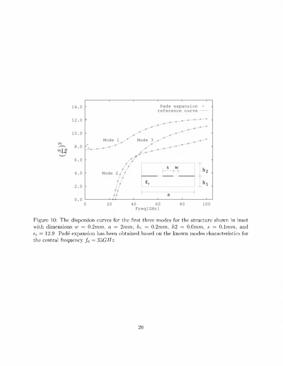
frequency f0 = 200MHz. Both Taylor and Pad�e expansions have been obtained from 1MHzto 500MHz, and results are plotted in Fig. 8. Shown results as well as the error analysis inFig. 9 prove that the rational polynomial approximation is more accurate than the powerseries expansion. For example, even though both approachers fail near DC, Pad�e expansionagrees very well for high frequencies, whereas Taylor expansion does not. Moreover, at thelower frequency end, although Pad�e expansion fails eventually, its validity extends muchfurther than for the power series expansions.5.4 Coplanar WaveguideCoplanar waveguide (CPW) structures have been attracting considerable attention becauseof their suitability for broad-band microwave integrated circuits (MIC's) and microwavemonolithic integrated circuits (MMIC'c) as well as the ease of incorporation of series andshunt elements. In the last example in this paper, we study the dispersion characteristicsof a conductor-backed coplanar waveguide (CBCPW) in a metal enclosure. The dispersioncharacteristics are computed for three modes using the proposed FFS procedure.The structure is enclosed in a perfectly conducting channel and assumed to be uniformand in�nite in the z direction. Both the ground plane and central strips are assumed tobe perfectly conducting and in�nitely thin, and the dielectric substrate is assumed to belossless. For this example the comparison between the reference solutions and FFS solutions,for the central frequency f0 = 35MHz, is presented in Fig. 10. In Fig. 10 we include onlyresults of Pad�e expansion since they are much more accurate than those of Taylor expansion.From all examples in this section we can conclude that, in general, the FFS procedureprovides a good approximation for mode characteristics and may be used in the future fore�cient computations of waveguide modes.6 Concluding RemarksIn this paper we have described a novel approach to e�ciently compute the spectral re-sponses of arbitrary waveguides. The proposed technique is based on the Tangential VectorFinite Element Method in conjunction with the Asymptotic Waveform Evaluation approach.In the FEM computation, we have also developed a modi�ed Lanczos algorithm with anadditional set of constraint equations to completely eliminate non-physical solutions duringthe iteration process. This algorithm was combined with the H10(curl) TVFEM to obtainelectromagnetic characteristics of propagating modes in waveguides for any given frequencypoint. To result in a frequency response for a given frequency range, the frequency momentsfor each mode are computed through a recursive procedure. Note that, in this recursive pro-cedure, the matrix does not change only the right-hand side has to be updated. Thus, themoments calculations become inexpensive when the factorization of the matrix is available.These moments are then matched via Pad�e approximation to a reduced-order rational poly-nomial which can be used to interpolate mode over a frequency band with a high degree ofaccuracy. Numerical results have shown that theH10(curl) TVFEM when used together withAWE provides an e�cient procedure for modeling two-dimensional wave-guiding structures.13

References[1] K. S. Kunz, and K. M. Lee. "A Three Dimensional Finite Di�erence Solution of theExternal Response of an Aircraft to a Complex Transient EM Enviroment: Part I{ The method and its Implementation". IEEE Trans. Electromagn. Compat., 20:pp.328{333, 1978.[2] E. Schwig and W. B. Bridges. "Computer Analysis of Dielectric Waveguides: A FiniteDi�erence Method". IEEE Trans. Microwave Theory Tech., 32(5):pp. 531{541, 1984.[3] B. M. A. Rahman, and J. B. Davies. "Finite-Element Analysis of Optical and MicrowaveProblems". IEEE Trans. Microwave Theory Tech., 32:pp. 20{28, 1984.[4] K. S. Yee. "Numerical Solution of Initial Boundary Value Problems Involving Maxwell'sEquations in Isotropic Media". IEEE Trans. Antennas Prop., 14:pp. 302{307, 1966.[5] M. D. Feit and J. A. Fleck. "Light Propagation in Graded-Index Optical Fibers". Appl.Opt., 17:pp. 3990{3998, 1978.[6] B. Dillon, A. Gibson, J. Webb. "Cut-o� and Phase Constant of Partially Filled Axi-ally Magnetized, Gyromagnetic Waveguide Using Finite Elements". IEEE Trans. Mi-crowave Theory Tech., 41(5):pp. 803{807, 1993.[7] P. Vandenbulcke and P. E. Lagasse. "Eigenmode Analysis of Anisotropic Optical Fibersor Integrated Optical Waveguides". Electronics letters, 12(5):pp. 120{121, 1976.[8] J. Lee, D. Sun, Z. Cendes. "Full-Wave Analysis of Dielectric Waveguides Using Tan-gential Vector Finite Elements". IEEE Trans. Microwave Theory Tech., 39(8):pp.1262{1271, 1991.[9] Jin-Fa Lee. "Finite Element Analysis of Lossy Dielectric Waveguide". IEEE Trans.Microwave Theory Tech., 42(6):pp. 1025{1031, 1994.[10] S. H. Wong and Z. J. Cendes. "Combined Finite Element-Modal Solution of Three-Dimensional Eddy Current Problems". IEEE Trans. on Mag., 24(6):pp. 2685{2687,1988.[11] S. V. Polstyanko and J.-F. Lee. "H1(curl) Tangential Vector Finite Element Method forModeling Anisotropic Optical Fibers". J. Lightwave Technol., 13(11):pp. 2290{2295,1995.[12] J. E. Bracken, V. Raghvan and R. A. Rohrer. "Interconnect Simulation with Asymp-totic Waveform Evaluation (AWE)". IEEE Trans. on Circuits and Systems, 39(11):pp.869{878, 1992.[13] J. Jin. The Finite Element Method in Electromagnetics. John Wiley & Sons, Inc, 1993.14

[14] R. Kao, and M. Horowitz. "Eliminating Redundant DC Equations for AsymptoticWaveform Evaluation". IEEE Trans. Computer-Aided Design, 13(3):pp. 396{397, 1994.[15] S. Kumashiro, R .A. Rohrer, and A. J. Strojwas. "Asymptotic Waveform Evaluationfor Transient Analysis of 3-d Interconnect Structures". IEEE Trans. Computer-AidedDesign, 12(7):pp. 988{996, 1993.[16] L. T. Pillage, and R. A. Rohrer. "Asymptotic Waveform Evaluation for Timing Anal-ysis". IEEE Trans. Computer-Aided Design, 9(4):pp. 352{366, 1990.[17] M. Kuzuoglu, R. Mittra, J. Brauer, and G. Lizalek. "An E�cient Scheme for FiniteElement Analysis in the Frequency Domain". volume 2, pages pp. 1210{1219, 1996.[18] E. K. Miller. "Model{Based Parameter Estimation in Electromagnetics: II{App-lications to EM Observables". ACES Newsletter, 11(1):pp. 35{56, 1996.

15

r

[µ ]r

[ε ][σ]

X

ZY Figure 1: General anisotropic optical waveguide

0

21

~W7 0

1 2 3 4 5

~W0 ~W1 ~W2~W3~W4~W5 ~W6Figure 2: Two dimensional H10(curl) tangential vector element.

0.0

1.0

2.0

3.0

4.0

5.0

0 20 40 60 80 100 120 140Freq[MHz]

Taylor expansionPade expansionreference curve

j j � �εµ

== 1.0

3.0

2

4

2

m

mm

mm

m 1rr

Figure 3: Dispersion curve of the fundamental mode for the partially �lled waveguide.Central frequency has been chosen to be f0 = 70[MHz]. Inset shows a dielectric waveguide�lled with an isotropic material. 16

-7.0

-6.0

-5.0

-4.0

-3.0

-2.0

-1.0

0.0

1.0

2.0

0 20 40 60 80 100 120 140

log10(error)

Freq[MHz]

Taylor expansionPade expansion

Figure 4: Error versus frequency for the central frequency f0 = 70[MHz].

1.0

2.0

3.0

4.0

5.0

6.0

7.0

8.0

9.0

10.0

25 30 35 40 45Freq[MHz]

Mode 1 Mode 2

Taylor expansionPade expansion

reference curve�

0.55

0.821.60

1.30

m

m

m

m

Figure 5: Dispersion curves for the �rst two modes of the anisotropic waveguide. Shown ininset is the geometry of the anisotropic dielectric waveguide, �rx = 170, �ry = �rz = 85.17

-7.0

-6.0

-5.0

-4.0

-3.0

-2.0

-1.0

0.0

1.0

25 30 35 40

log10(error)

Freq[MHz]

Taylor expansionPade expansion

Figure 6: Error versus frequency for the dominant mode of the anisotropic waveguide forthe central frequency f0 = 36[MHz].

-7.0

-6.0

-5.0

-4.0

-3.0

-2.0

-1.0

0.0

1.0

2.0

32 34 36 38 40 42 44

log10(error)

Freq[MHz]

Taylor expansionPade expansion

Figure 7: Error versus frequency for the second mode of the anisotropic waveguide for thecentral frequency f0 = 36[MHz]. 18

2.5

3.0

3.5

4.0

4.5

0 100 200 300 400 500 600Freq[MHz]

Taylor expansionPade expansion

reference curve

(� k 0)21.0

0.50.25

0.5

m

m

m

m ε , µr r

Figure 8: Dispersion curves for the shielded microstrip line corresponding to the centralfrequency f0 = 200MHz. Shown in inset is the geometry of the microstrip line.

-7.0

-6.0

-5.0

-4.0

-3.0

-2.0

-1.0

0.0

1.0

2.0

0 50 100 150 200 250 300 350 400

log10(error)

Freq[MHz]

Taylor expansionPade expansion

Figure 9: Error versus frequency for the microstrip line for f0 = 200MHz.19

0.0

2.0

4.0

6.0

8.0

10.0

12.0

14.0

0 20 40 60 80 100Freq[GHz]

Mode 1

Mode 2

Mode 3

Pade expansionreference curve

(� k 0)2s

a

h

h

1

2

εr

w

Figure 10: The dispersion curves for the �rst three modes for the structure shown in insetwith dimensions w = 0:2mm, a = 2mm, h1 = 0:2mm, h2 = 0:6mm, s = 0:1mm, and�r = 12:9. Pad�e expansion has been obtained based on the known modes characteristics forthe central frequency f0 = 35GHz.

20