CODEN:LUTEDX/(TEAT-7026)/1-24/(1993)

Revision No. 4: August 1995

Transient Electromagnetic WavePropagation in Waveguides

Gerhard Kristensson

Department of ElectroscienceElectromagnetic TheoryLund Institute of TechnologySweden

Gerhard Kristensson

Department of Electromagnetic TheoryLund Institute of TechnologyP.O. Box 118SE-221 00 LundSweden

Editor: Gerhard Kristenssonc© Gerhard Kristensson, Lund, August 2, 1995

1

Abstract

This paper focuses on propagation of transient electromagnetic waves in wave-guides of general cross section with perfectly conducting walls. The solution ofthe transient wave propagation problem relies on a wave splitting technique,which has been frequently used in direct and inverse scattering problems dur-ing the last decade. The field in the waveguide is represented as a timeconvolution of a Green function and the excitation. Some numerical compu-tations illustrate the method. A new way of calculating the first precursorin a Lorentz medium is presented. This method, which is not based uponthe classical asymptotic methods, gives an expression of the first precursor atall depths in the medium. The excitation of the waveguide modes for timedependent sources is also addressed.

1 Introduction

Modern information and communication technologies rely on propagation of tran-sient electromagnetic waves, e.g., short pulses. Electromagnetic wave propagationproblems in waveguides have traditionally been analyzed using fixed frequency meth-ods. A large body of results has been collected in this field, see, e.g., Ref [2] for asurvey of these results. The transient wave propagation phenomena have then beensynthesized by Fourier transform techniques [5]. However, modern applications askfor a more effective method, which does not rely on Fourier transform techniques.Specifically, wave front behavior and pulse broadening due to waveguide dispersionare important quantities.

This paper takes a fresh look at the propagation of transient electromagneticwave in waveguides by using time domain techniques. More explicitly, the transientwave propagation problem is solved using a wave splitting technique. This techniquehas frequently been used to solve direct and inverse scattering problems in the lastdecade and was first introduced in one-dimensional scattering problems [3]. In recentyears the three-dimensional wave splitting has been developed by Weston [18–21].For a collection of applications of this theory the reader is referred to Ref [4].

The bounding surface is assumed to be perfectly conducting, but no other as-sumptions on the cross section of the waveguide have to be made (except mildsmoothness requirements). The modal structure, similar to the concept used forfixed frequency, is retained. This concept introduces a set of basis functions inwhich the transverse field components can be expanded. The propagation of tran-sient electromagnetic waves is systematically treated by means of the wave splittingtechnique, and for each mode the transient field is expressed as a time convolutionof the excitation and a Green function. The TEM-modes are not analyzed in thispaper, since these waves propagate as if the medium were free space and they aretherefore already covered by previous analyses, see Refs. [10–12].

The first precursor for the propagation of an electromagnetic wave in a slab isalso addressed. This result is obtained as a special result in the analysis of thewaveguide problem. Explicit expression of the first precursor is given that holds

2

at all depths in the medium. In this respect, it is a generalization of the classicalprecursor results.

In Section 2 the basic underlying equations of the problem and the decompositionof the fields are outlined. The canonical problems are stated in Section 3 and thewave splitting of the field is presented in Section 4. The Green functions that mapan excitation to the response at an interior point are introduced in Section 5, whichalso contains the exact solution to this problem, the precursor problem, and somenumerical illustrations showing the versatility of the method. In Section 6, thepower flux of the split waves is analyzed. The appropriate expansion functions areintroduced in Section 7 and in Section 8 the excitation of modes from a given sourcedistribution is calculated.

2 Basic equations

In this section, the decomposition of the field and the basic equations are developed.Several of the results are found elsewhere, see, e.g., Refs. [8, 17], but to properly in-troduce the notation and for the convenience of the reader these results are presentedhere.

The Maxwell equations are the basic underlying equations that model the fields.∇×E(r, t) = −∂B(r, t)

∂t

∇×H(r, t) = J(r, t) +∂D(r, t)

∂t

(2.1)

All fields in this paper are assumed to be quiescent before a fixed time. This propertyguarantees that all fields vanish at t→ −∞.

The medium in the waveguide is assumed to be non-dispersive and homogeneous,i.e.,

D(r, t) = ε0εE(r, t)

B(r, t) = µ0µH(r, t)

The (relative) permittivity and permeability of the medium are denoted ε and µ,respectively, and are assumed to be constants. The phase velocity c and the waveimpedance η are

c =1√

ε0εµ0µ, η =

√µ0µ

ε0ε

respectively.The Maxwell equations (2.1) in a source free region and the constitutive relations

imply

∇2E(r, t)− 1

c2

∂2

∂t2E(r, t) = 0 (2.2)

for the electric field E and

∇2H(r, t)− 1

c2

∂2

∂t2H(r, t) = 0

for the magnetic field H .

3

2.1 Decomposition of the field

The decomposition of the fields in a transverse part and a z-component is, of course,not new. It is a well established technique to handle fixed frequency problems, see,e.g., Ref [8], and even for time domain problems similar decompositions are foundelsewhere, see, e.g., Ref [17].

The nabla-operator and a general vector field F (r, t) are decomposed with re-spect to a fixed direction, here taken as the positive z-direction.

∇ = ∇T + z∂

∂zF (r, t) = F T (r, t) + zFz(r, t)

The space vector r is also decomposed as

r = xx + yy + zz = ρ+ zz

For a general vector field F the following identities hold:

z · (∇× F (r, t)) = −∇T · (z × F T (r, t)) = z · (∇T × F T (r, t))

∇× F (r, t)− z (z · (∇× F (r, t))) = z × ∂

∂zF T (r, t)− z ×∇TFz(r, t)

Apply this decomposition to the source-free Maxwell equations (2.1). The resultfor the z-component is

z · (∇T ×ET (r, t)) = −1

c

∂

∂tηHz(r, t)

z · (∇T × ηHT (r, t)) =1

c

∂

∂tEz(r, t)

(2.3)

and for the transverse components the result is

1

c

∂

∂tηHT (r, t) + z × ∂

∂zET (r, t) = z ×∇TEz(r, t)

1

c

∂

∂tET (r, t)− z × ∂

∂zηHT (r, t) = −z ×∇TηHz(r, t)

(2.4)

These equations can also be combined so that the magnetic or the electric transversefields are eliminated. The transverse fields satisfy the one-dimensional wave equationwith source terms.

(∂2

∂z2− 1

c2

∂2

∂t2

)ET (r, t) =

1

c

∂

∂t(z ×∇TηHz(r, t)) +

∂

∂z∇TEz(r, t)(

∂2

∂z2− 1

c2

∂2

∂t2

)ηHT (r, t) = −1

c

∂

∂t(z ×∇TEz(r, t)) +

∂

∂z∇TηHz(r, t)

The z-components of the electric and the magnetic fields act as sources of the trans-verse fields. The z-components of the fields therefore generate the correspondingtransverse components.

4

S∂Ω Ω

n

z

Figure 1: Geometry of the waveguide.

2.2 Boundary conditions

The geometry of the waveguide is depicted in Figure 1. The surface S is the outerbounding surface of the waveguide and n is the outward normal to S. The crosssection of the waveguide is denoted Ω and ∂Ω is its bounding curve in the xy-plane.This curve is assumed to be smooth and the domain Ω is simply connected (nointerior conductor is present).

The boundary conditions on the perfectly conducting wall of the waveguide aren×E = 0,

n ·H = 0,r ∈ S (2.5)

Since n is independent of z, these boundary conditions are equivalent to

Ez = 0,

∂Hz

∂n= 0,

r ∈ S

For a waveguide with perfectly conducting walls, the wave propagation phenom-ena in the waveguide separate into two different classes—the TE- and the TM-modes. This is completely analogous to the fixed frequency case. The TEM-modesare excluded in this presentation due to the absence of an inner conductor in thewaveguide.

3 The canonical problems

The z-components of the electric and the magnetic field satisfy the three-dimensionalwave equation (see (2.2)).

∇2

(Ez(r, t)ηHz(r, t)

)− 1

c2

∂2

∂t2

(Ez(r, t)ηHz(r, t)

)= 0

5

The method of separation of variables is now applied to this equation. Themethod is, however, not applied to each coordinate but with respect to the pairs(x, y) and (z, t). The ansatz for z-components in the TM- and the TE-cases istherefore

Ez(r, t) = v(ρ)a(z, t)

Hz(r, t) = 0(TM-case)

Ez(r, t) = 0

Hz(r, t) = w(ρ)b(z, t)(TE-case)

respectively. The functions v and w determine the transverse behavior of the fieldsand satisfy an eigenvalue problem. These eigenvalue problems are

∇2Tv(ρ) + λ2v(ρ) = 0, ρ ∈ Ω

v(ρ) = 0, ρ ∈ ∂Ω

and ∇2Tw(ρ) + λ2w(ρ) = 0, ρ ∈ Ω

n · ∇Tw(ρ) = 0, ρ ∈ ∂Ω

The positive real constant λ is here the eigenvalue for the waveguide listed with dueregard to multiplicity.

λ = λn, n = 1, 2, 3, . . .

All fields depend on the index n, but to avoid complicated notation this index isoften omitted in this paper. Furthermore, the same notation for the eigenvalue ofthe Dirichlet (TM) and the Neumann problem (TE) is used. From the context it isalways obvious what problem λ refers to.

The TEM-case corresponds to the eigenvalue λ = 0. In this paper it is assumedthat no such mode exists and thus the eigenfunctions form a complete orthogonalset in Ω [16, p. 138].

The functions a(z, t) and b(z, t) determine the wave propagation along the waveguide and satisfy the one-dimensional Klein-Gordon equation.

∂2

∂z2u(z, t)− 1

c2

∂2

∂t2u(z, t)− λ2u(z, t) = 0

The transverse fields are determined by the z-components of the field. TheTM-modes satisfy (see (2.3) and (2.4))

z · (∇T ×ET (r, t)) = 0

z · (∇T × ηHT (r, t)) =1

c

∂

∂tEz(r, t)

1

c

∂

∂tηHT (r, t) + z × ∂

∂zET (r, t) = z ×∇TEz(r, t)

1

c

∂

∂tET (r, t)− z × ∂

∂zηHT (r, t) = 0

(TM-case) (3.1)

6

and the transverse field of the TE-modes satisfies (see (2.3) and (2.4))

z · (∇T ×ET (r, t)) = −1

c

∂

∂tηHz(r, t)

z · (∇T × ηHT (r, t)) = 0

1

c

∂

∂tηHT (r, t) + z × ∂

∂zET (r, t) = 0

1

c

∂

∂tET (r, t)− z × ∂

∂zηHT (r, t) = −z ×∇TηHz(r, t)

(TE-case) (3.2)

From these equations it is seen that the transverse components have the formET (r, t) = ∇Tv(ρ)ψ1(z, t)

ηHT (r, t) = [z ×∇Tv(ρ)]φ1(z, t)(TM-case)

ET (r, t) = − [z ×∇Tw(ρ)]φ2(z, t)

ηHT (r, t) = ∇Tw(ρ)ψ2(z, t)(TE-case)

(3.3)

where ψi and φi satisfy (see (3.1) and (3.2))

λ2φ1 = −1

c

∂a

∂t1

c

∂φ1

∂t+

∂ψ1

∂z= a

1

c

∂ψ1

∂t+

∂φ1

∂z= 0

(TM-case)

λ2φ2 = −1

c

∂b

∂t1

c

∂φ2

∂t+

∂ψ2

∂z= b

1

c

∂ψ2

∂t+

∂φ2

∂z= 0

(TE-case)

These equations imply that the functions ψi and φi can be expressed in terms ofthe functions a and b as follows, since all fields are assumed to vanish at sufficientlylarge negative time:

λ2φ1 = −1

c

∂a

∂t

λ2ψ1 =∂a

∂z

λ2φ2 = −1

c

∂b

∂t

λ2ψ2 =∂b

∂z

(3.4)

The functions a and b can also be eliminated. The result is that the functionsψi and φi satisfy the same kind of one-dimensional Klein-Gordon equations that aand b do, i.e.,

∂φ2

i

∂z2− 1

c2

∂φ2i

∂t2− λ2φi = 0

∂ψ2i

∂z2− 1

c2

∂ψ2i

∂t2− λ2ψi = 0

From this it is seen that the (z, t)-dependence of all field components (a, b, φi andψi) satisfy the one-dimensional Klein-Gordon equation. Furthermore, the transversecomponents have (z, t)-dependence that is either the z- or the t-derivative of the cor-responding (z, t)-dependence of the z-component of the field, see (3.4). It thereforesuffices to study the z-component of the field.

7

4 Wave splitting

In recent years, a new technique for solving direct and inverse scattering problems inthe time domain has been developed. For a collection of results, see Ref [4]. In thissection, this technique is adapted to the electromagnetic wave propagation problemin a waveguide.

The one-dimensional Klein-Gordon equation is the starting point for this method.

∂2

∂z2u(z, t)− 1

c2

∂2

∂t2u(z, t)− λ2u(z, t) = 0 (4.1)

This equation is conveniently rewritten as a system of first order equations

∂

∂z

(u∂zu

)=

(0 1

1c2∂2t + λ2 0

) (u∂zu

)(4.2)

The purpose of the wave spitting is to change the dependent variables u and∂zu to another set more suited for investigating the propagation problem in thewaveguide. The aim is to construct a set of variables, u+ and u−, such that theequation for these variables is diagonal. Crudely speaking, the matrix in (4.2) isdiagonalized. As is seen below in (4.8), the following change of variables gives adiagonal equation [7]:

u±(z, t) =1

2[u(z, t)∓ c(K∂zu(z, ·))(t)]

where the operator K has the integral representation

(Kf)(t) =

∫ t

−∞J0(cλ(t− t′))f(t′) dt′

Formally, the splitting can be written in matrix notation as(u+

u−

)=

1

2

(1 −cK1 cK

) (u∂zu

)(4.3)

This operation defines the wave splitting used in this paper. Even though the TEM-case is not addressed in this paper, it corresponds to λ = 0 and has the same splittingas in free space, see Ref [3], i.e.,

limλ→0

(Kf)(t) =

∫ t

−∞f(t′) dt′

The operator K has a inverse K−1, with

KK−1f = f, K−1Kf = f

The fields u and ∂zu are therefore expressed in u± as(u∂zu

)=

(1 1

−1cK−1 1

cK−1

) (u+

u−

)(4.4)

8

The inverse operator K−1 has the explicit integral representation

(K−1f)(t) =∂f

∂t+ cλ

∫ t

−∞

J1(cλ(t− t′))

t− t′f(t′) dt′ =

∂f

∂t+ (L(·) ∗ f(·)) (t) (4.5)

where

L(t) = H(t)cλJ1(cλt)

t(4.6)

and H(t) is Heaviside’s step function. Time convolutions are defined as

(L(·) ∗ f(·)) (t) =

∫ ∞

−∞L(t− t′)f(t′) dt′

The integral representation of the inverse in (4.5) is proved by the identity [6, p. 698]∫ x

0

J1(x− y)

x− yJ0(y) dy = J1(x)

Another useful identity, found by integration by parts, is

K∂f 2

∂t2= K−1f − c2λ2Kf (4.7)

The new fields u±(z, t) satisfy a system of first order equations, which is obtainedfrom (4.3), (4.4) and (4.2).

∂

∂z

(u+

u−

)=

1

2

(1 −cK1 cK

) (0 1

1c2∂2t + λ2 0

) (1 1

−1cK−1 1

cK−1

) (u+

u−

)

=

(−1cK−1 00 1

cK−1

) (u+

u−

) (4.8)

The effect of the splitting in (4.3) is now obvious. The transformation K factorizesthe Klein-Gordon equation in (4.1), such that no coupling between the two com-ponents u+ and u− occurs. The field u+ or u− expresses the part of the field thatpropagates power in the +z- or −z-direction in the waveguide, respectively. Using(4.7), it is clear that u+- and u−-waves both satisfy the Klein-Gordon equation (4.1).

Finally, the concept of a right- and left-going wave is defined. A field u(z, t) iscalled right-going if u(z, t) satisfies

u(z, t) = −c (K∂zu(z, ·)) (t)

The field, cf. first line in (4.3),

w(z, t) =1

2[u(z, t)− c(K∂zu(z, ·))(t)]

is right-going since

w + cK∂zw =1

2

[u− c2K2uzz

]=

1

2

[u− c2K2(c−2utt + λ2u)

]=

1

2

[u−KK−1u)

]= 0

9

where (4.7) is used. Similarly, a field u(z, t) is called left-going if u(z, t) satisfies

u(z, t) = c (K∂zu(z, ·)) (t)

To summarize, the condition for right- and left-going fields are

u(z, t) = ∓c (K∂zu(z, ·)) (t)

or by taking the inverse

∂

∂zu(z, t) = ∓1

c

(K−1u(z, ·)

)(t) (4.9)

5 Green functions

The Green functions represent the mapping of the excitation at the boundary of asection of the waveguide, say z = 0, to some point z > 0 in the interior. These Greenfunctions were first introduced by Krueger and Ochs [12] in the non-dispersive caseand Kristensson [9] for dispersive media.

The case of propagation in the positive z-direction is first considered. The Greenfunctions G±(z, t) for this case are defined as

u−(z, t + z/c) =(G−(z, ·) ∗ u+(0, ·)

)(t)

u+(z, t + z/c) = u+(0, t) +(G+(z, ·) ∗ u+(0, ·)

)(t)

, z > 0 (5.1)

where, as before, time convolutions are defined by a star (∗). The field u+(z, t)at some point z > 0 consists of two parts—one due to the direct transmission ofthe incident field u+(0, t) and one due to scattering effects represented by a timeconvolution of the incident field u+(0, t) with the Green function G+(z, t). In thisway, the Green function G+(z, t) represents the mapping of a right-going field atz = 0 to a right-going field at some point z > 0. The other Green function G−(z, t)represents the corresponding mapping of a right-going field at z = 0 to a left-goingfield at z > 0. Due to causality, G±(z, t) = 0 for t < 0, and from the definition ofG+(z, t) in (5.1) it follows that

G+(0, t) = 0

The Green functions G±(z, t) satisfy differential equations, which are found bydifferentiating (5.1) with respect to z and using (4.8) (see also Ref [7]). The differ-entiation gives

∓(K−1u±(z, ·)

)(t + z/c) + ∂tu

±(z, t + z/c) = c(∂zG

±(z, ·) ∗ u+(0, ·))(t)

Inserting the explicit integral representation for K−1 yields−

(L(·) ∗ u+(z, ·)

)(t + z/c) = c

(∂zG

+(z, ·) ∗ u+(0, ·))(t)

2∂tu−(z, t + z/c) +

(L(·) ∗ u−(z, ·)

)(t + z/c) = c

(∂zG

−(z, ·) ∗ u+(0, ·))(t)

10

where L is defined in (4.6). Apply (5.1) once more. This gives

c(∂zG

+(z, ·) ∗ u+(0, ·))(t)

= −(L(·) ∗ u+(0, ·)

)(t)−

(L(·) ∗G+(z, ·) ∗ u+(0, ·)

)(t)

and

c(∂zG

−(z, ·) ∗ u+(0, ·))(t) = 2

(∂tG

−(z, ·) ∗ u+(0, ·))(t)

+ 2G−(z, 0+)u+(0, t) +(L(·) ∗G−(z, ·) ∗ u+(0, ·)

)(t)

These expressions hold for all excitations u+(0, t). This implies thatc∂zG

+(z, t) = −L(t)−(L(·) ∗G+(z, ·)

)(t)

G+(0, t) = 0(5.2)

and c∂zG

−(z, t) = 2∂tG−(z, t) +

(L(·) ∗G−(z, ·)

)(t)

G−(z, 0+) = 0(5.3)

The corresponding mapping of an excitation at z = 0 to some interior pointz < 0 is obtained by changing sign of the z-coordinate, i.e., z → −z. This mappingdescribes the propagation of waves in the negative z-direction.

5.1 Exact solutions

The Green function G−(z, t) is identically zero in this splitting (unique solubility),as can be seen from (5.3) by rewriting the equation as an initial value problem alongthe characteristic direction of the equation.

G−(z, t) = 0

This fact implies that a right-going wave, the way it is defined by the wave splittingin (4.3), continues to propagate as a right-going wave in the region z > 0. Similarly,a left-going wave continues to propagate as a left-going wave in the region z < 0.

The other Green function, G+(z, t), is solved from (5.2) with Laplace transformtechniques. The solution is

G+(z, t) = −cλzH(t)J1

(λ√c2t2 + 2zct

)√c2t2 + 2zct

This solution is equivalent to the following complicated identity of Bessel functions:

J1(x) =d

dz

[z

∫ x

0

J1(√

y2 + 2zy)√y2 + 2zy

J0(x− y) dy

]+ z

∫ x

0

J1(√

y2 + 2zy)√y2 + 2zy

J1(x− y) dy

for all x and z.

11

The Green function G+(z, t) represents the propagation of an excitation at z = 0in the positive z-direction. The propagation in the negative z-direction is obtainedby replacing z by −z. It is therefore natural to a define propagator kernel G(z, t)

G(z, t) = −cλ|z|H(t)J1

(λ√

c2t2 + 2|z|ct)

√c2t2 + 2|z|ct

(5.4)

which propagates an excitation at z = 0 in the positive or the negative z-directiondepending on the sign of z. This propagator kernel is closely related to the Greenfunction of the Klein-Gordon equation. For further reference, see Refs. [13, 22].

5.2 Fundamental solutions

For any excitation u±(0, t) at z = 0, the response u±(z, t) is therefore found as

u±(z, t± z/c) = u±(0, t) +

∫ t

−∞G(z, t− t′)u±(0, t′) dt′ (5.5)

where the plus sign holds in the region z > 0 and the negative sign in the regionz < 0. Notice that the time parameter t is the time measured from the wave front,which propagates with speed c. An alternative way of writing this expression usingreal time is

u±(z, t) = u±(0, t− |z|/c)− cλ|z|∫ t−|z|/c

−∞

J1

(λ√

c2(t− t′)2 − z2)

√c2(t− t′)2 − z2

u±(0, t′) dt′

By construction, these wave are right-going (z > 0) or left-going (z < 0) waves.Note that different modes (different λ) basically is a scaling in the space and timevariables. The dimensionless variables, in which the scaling is performed, are

x = λz

s = λct

5.3 First precursor of the slab problem

Related to the wave propagation problem in the waveguide, is the propagation of aelectromagnetic wave in a homogeneous Lorentz medium. This propagation prob-lem and the related precursor (forerunner) analysis (early arrival of the signal) isanalyzed in, e.g., Refs. [8, Sect. 7.11] and [1]. In a Lorentz medium the (transverselypolarized) electric field E(z, t) satisfies

∂2

∂z2E(z, t)− µ

c20

∂2

∂t2[εE(z, t) + (χ(·) ∗ E(z, ·)) (t)] = 0 (5.6)

where c0 is the speed of light in vacuum, ε and µ are the permittivity and thepermeability of the medium, respectively, and χ(t) the susceptibility kernel of themedium given by [8]

χ(t) = H(t)ω2p

ν0

e−νt/2 sin ν0t

12

The plasma and the collision frequencies are ωp and ν, respectively. The frequencyν0 is defined in terms of the resonance frequency ω0 as

ν0 =√

ω20 − ν2/4

The short time behavior of χ(t) is

χ(t) ≈ ω2pt, t→ 0+

If the medium is characterized by several resonances, this expression is modified suchthat the short time behavior of χ is t times a sum of the squares of the correspondingplasma frequencies.

The approximate behavior of the convolution term in (5.6) evaluated at shorttimes is

∂2

∂t2(χ(·) ∗ E(z, ·)) (t) ≈ ω2

pE(z, t), t→ 0+

The wave propagating problem in a Lorentz medium at short times after the ar-rival of the wave front is therefore formally identical to the waveguide propagationproblem treated in this paper if λ is identified as

λ =ωp√µ

c0

The propagator kernel G+(z, t) in (5.4) is therefore the appropriate propagator ofthe electric field in the slab for short times t (from the wave front). The field E(z, t)at a point z > 0 in the slab is related to the excitation E(0, t), see (5.5).

E(z, t + z/c) = E(0, t)− 2ξ

∫ t

−∞

J1

(√λ2c2(t− t′)2 + 4ξ(t− t′)

)√

λ2c2(t− t′)2 + 4ξ(t− t′)E(0, t′) dt′ (5.7)

where

ξ =cλ2z

2=

ω2pz

2c0

õ

ε=

ω2pz

2cε

At large distances z, the integrand in (5.7) can be approximated as (t > 0)

E(z, t + z/c) =tm

m!− 2ξ

m!

∫ t

0

J1

(2√

ξ(t− t′))

2√

ξ(t− t′)t′mdt′

where the excitation at z = 0 is assumed to have the explicit form

E(0, t) = H(t)tm

m!, m ≥ 0

The integral can be evaluated by using [14]∫ a

0

J1(x)(a2 − x2

)mdx = a2m − (2a)mm!Jm(a)

13

-1.0

-0.5

0.0

0.5

1.0

Am

pli

tud

e

14121086420Time

x=0, x=2 x=5, x=10

Figure 2: The amplitude of the z-component of the field in the waveguide as afunction of the time t, measured from the wave front, i.e., the real time is t + |z|/c.The input is given by (5.8), where T = 2. The time scale is given in units of (cλn)

−1

and the parameter x = λn|z|.

and the field at large distances is (t > 0)

E(z, t + z/c) =

(t

ξ

)m/2

Jm

(2√

ξt)

which is in agreement with the result in Ref. [8]. However, the solution to theprecursor problem, see (5.7), is not restricted to the special excitation which is usedhere to illustrate the result. Furthermore, it is not restricted to large values of z,but holds for all values of z, provided the time t (from the wave front) is small. Inthis sense, it is a generalization of the classical precursor results.

5.4 Numerical illustrations

The response of a pulse excitation

u+(0, t) = H(t)H(T − t) (5.8)

is depicted in Figure 2. The transient behavior of the field at increasing distancealong the waveguide is clearly illustrated for this excitation. At larger distancesdown the waveguide the pulse gets broadened and more oscillations occur.

In Figures 3 and 4 the shape of the wave is depicted at different positions alongthe waveguide. In these examples the exciting field is the modulated sine wave.

u+(0, t) = H(t)H(π/ωm − t) sinωmt sinωct (5.9)

In Figures 5, 6 and 7 the transient behavior of a sinusoidal excitation is shownat different positions along the waveguide. The exciting field in these plots is

u+(0, t) = H(t) sinωt

14

-1.0

-0.5

0.0

0.5

1.0

Am

pli

tud

e

6543210Time

x=0 x=20 x=50

Figure 3: The amplitude of the z-component of the field in the waveguide as afunction of the time t, measured from the wave front, i.e., the real time is t + |z|/c.The input is given by (5.9), where the carrier frequency is ωc = 10 and the pulseis modulation frequency ωm = 1. The time scale is given in units of (cλn)

−1, thefrequency scale in units of cλn and the parameter x = λn|z|.

-1.0

-0.5

0.0

0.5

1.0

Am

pli

tud

e

14121086420Time

x=0 x=20 x=50

Figure 4: The amplitude of the z-component of the field in the waveguide as afunction of the time t, measured from the wave front, i.e., the real time is t + |z|/c.The input is given by (5.9), where the carrier frequency is ωc = 5 and the pulseis modulation frequency ωm = .3. The time scale is given in units of (cλn)

−1, thefrequency scale in units of cλn and the parameter x = λn|z|.

15

1.0

0.5

0.0

-0.5

-1.0

Am

pli

tud

e

1086420Time

x=0, x=15, x=30

Figure 5: The amplitude of the z-component of the field in the waveguide as afunction of the time t, measured from the wave front, i.e., the real time is t + |z|/c.The input is given by u+(0, t) = H(t) sinωt, where ω = 5. The time scale is givenin units of (cλn)

−1, the frequency scale in units of cλn and the parameter x = λn|z|.

1.0

0.5

0.0

-0.5

-1.0

Am

pli

tud

e

302520151050Time

x=0, x=1, x=2, x=5

Figure 6: The amplitude of the z-component of the field in the waveguide as afunction of the time t, measured from the wave front, i.e., the real time is t + |z|/c.The input is given by u+(0, t) = H(t) sinωt, where ω = 1. The time scale is givenin units of (cλn)

−1, the frequency scale in units of cλn and the parameter x = λn|z|.

16

-1.0

-0.5

0.0

0.5

1.0

Am

pli

tud

e

140120100806040200Time

x=0, x=0.3, x=1, x=5

Figure 7: The amplitude of the z-component of the field in the waveguide as afunction of the time t, measured from the wave front, i.e., the real time is t + |z|/c.The input is given by u+(0, t) = H(t) sinωt, where ω = .3. The time scale is givenin units of (cλn)

−1, the frequency scale in units of cλn and the parameter x = λn|z|.

The cutoff frequency for the stationary wave in these examples is ω = 1. Figure 5shows the transient behavior for a propagating wave (ω = 5). Figure 6 shows theeffects for a wave at cutoff (ω = 1) and Figure 7 for a wave below cutoff (ω = .3).Below cutoff the wave is rapidly attenuating.

6 Power flux

From the definition of the split fields u+ and u−, it is not obvious that these wavesgive energy transport in the positive and the negative z-direction, respectively. Inthis section, the energy flow of each such wave is analyzed.

The power flux is

S = E ×H = (ET + zEz)× (HT + zHz) = ET ×HT + Ez z ×HT +ET × zHz

The longitudinal power flux S · z is

S · z = (E ×H) · z = (ET ×HT ) · z =

1η|∇Tv|2ψ1φ1 (TM-case)

1η|∇Tw|2ψ2φ2 (TE-case)

where equation (3.3) has been used. The direction of the power flow is determinedby the factor ψiφi. From (3.4) and the wave splitting, it is easy to use (4.5) to obtain(u is either a or b depending upon the mode)

λ4ψiφi = −1

c

∂u

∂t

∂u

∂z= ± 1

c2

∂u

∂tK−1u = ± 1

c2

∂u

∂t

∂u

∂t+ (L(·) ∗ u(·)) (t)

17

where the upper (lower) sign holds for a right-(left-)going field. With the convenientchange of variable, x = cλt, the previous expression is equivalent to analyzing

F (x) = ±f ′(x)

f ′(x) +

∫ x

−∞

J1(x− y)

x− yf(y) dy

This is, in general, not a function of a definite sign (compare with a superpositionof a propagating and a non-propagating mode for fixed frequency).

The total energy up to time τ is∫ τ

−∞F (x) dx = ±

∫ τ

−∞(f ′(x))

2dx±

∫ τ

−∞f ′(x)

∫ x

−∞

J1(x− y)

x− yf(y) dy dx

Define an even function g(x)

g(x) =

∫ |x|

0

J1(y)

ydy

Then limx→∞ g(x) = 1 (see [6, p. 684]) and∫ τ

−∞F (x) dx = ±

∫ τ

−∞(f ′(x))

2dx±

∫ τ

−∞f ′(x)

∫ x

−∞g(x− y)f ′(y) dy dx

= ±∫ τ

−∞

∫ τ

−∞f ′(x)G(x− y)f ′(y) dy dx

where

G(x) = δ(x) +1

2

∫ |x|

0

J1(y)

ydy

which is even in x.It is straightforward to prove that

∫ ∞

−∞G(x) cos ξx dx = πδ(ξ) + H(|ξ| − 1)

√ξ2 − 1

|ξ|

which is an even, positive function (distribution) of ξ. This implies that G(x) is afunction (distribution) of positive type (Bochner-Schwartz’s theorem, see [15, p. 14])and therefore ∫ τ

−∞

∫ τ

−∞f ′(x)G(x− y)f ′(y) dy dx ≥ 0

for all functions f(x).This inequality implies that the total energy∫ τ

−∞S(r, t) · z dt

in the waveguide up to time τ is positive for a right-going wave and negative for aleft-going wave, irrespective of the excitation and the time τ .

18

7 Expansion functions

To tackle the excitation of the field inside the waveguide and to determine the ampli-tude of each mode, expansion functions are needed. In this section, the appropriateexpansion functions for transient waves are developed.

7.1 Orthogonal modes for transverse fields

In this section, the index n is used on the eigenfunctions v and w. An additionalindex ν is appended to indicate which mode it is.

Define for ν=TMenν(ρ) = ∇Tvn(ρ)

hnν(ρ) = z ×∇Tvn(ρ) = z × enν(ρ)(TM-case)

and for ν=TE enν(ρ) = −z ×∇Twn(ρ)

hnν(ρ) = ∇Twn(ρ) = z × enν(ρ)(TE-case)

Notice that enν(ρ) and hnν(ρ) both have the same units. The functions vn and wnsatisfy

∇2Tvn(ρ) + λ2

nvn(ρ) = 0, ρ ∈ Ω

vn(ρ) = 0, ρ ∈ ∂Ω

and ∇2Twn(ρ) + λ2

nwn(ρ) = 0, ρ ∈ Ω

n · ∇Twn(ρ) = 0, ρ ∈ ∂Ω

respectively.The functions vn and wn can always be normalized such that (λn = 0)∫∫

Ω

vn(ρ)vm(ρ) dS =

∫∫Ω

wn(ρ)wm(ρ) dS = λ−2n δn,m

By doing so, it is easy to see that the vector functions enν and hnν are orthonormal.∫∫Ω

enν(ρ) · en′ν′(ρ) dS =

∫∫Ω

hnν(ρ) · hn′ν′(ρ) dS = δn,n′δν,ν′

and ∫∫Ω

[enν(ρ)× hn′ν′(ρ)] · z dS = δn,n′δν,ν′ (7.1)

The sequences enν∞n=1 and hnν∞n=1, ν=TM, TE form a complete orthonormalset of vector-valued functions in the plane.

19

7.2 Expansion functions

Let fnν(z, t) be any function satisfying

∂2

∂z2fnν(z, t)−

1

c2

∂2

∂t2fnν(z, t)− λ2

nfnν(z, t) = 0

and define for ν=TMEnν(r, t) = enν(ρ)λ−2

n

∂

∂zfnν(z, t) + zvn(ρ)fnν(z, t)

Hnν(r, t) = −1

chnν(ρ)λ−2

n

∂

∂tfnν(z, t)

(TM-case)

and for ν=TEEnν(r, t) = −1

cenν(ρ)λ−2

n

∂

∂tfnν(z, t)

Hnν(r, t) = hnν(ρ)λ−2n

∂

∂zfnν(z, t) + zwn(ρ)fnν(z, t)

(TE-case)

Then these vector-valued functions satisfy∇×Enν(r, t) = −1

c

∂

∂tHnν(r, t)

∇×Hnν(r, t) =1

c

∂

∂tEnν(r, t)

(7.2)

and ∇ ·Enν(r, t) = 0

∇ ·Hnν(r, t) = 0

and the boundary condition on S

n×Enν(r, t) = 0, r ∈ S (7.3)

Notice also that both fields Enν(r, t) and Hnν(r, t) have the same units.

7.3 Right- and left-going basis functions

The eigenfunctions Enν and Hnν defined in Section 7.2 are, in general, superpo-sitions of both right- and left-going waves. The right- and left-going eigenmodesE±nν(ρ, z, t) and H±nν(ρ, z, t) are obtained by taking an appropriate choice of thefunction fnν(z, t). The obvious choice here is u(z, t) defined in (5.5). From thedefinition of right- and left-going waves, see (4.9), the spatial differentiation withrespect to z is replaced by the K−1-operator, with the appropriate sign dependingon whether the wave is right- or left-going. This operation guarantees that right-and left-going wave are constructed. The definition of E±nν(ρ, z, t) and H±nν(ρ, z, t)for ν=TM is thereforeE±nν(ρ, z, t) =∓ 1

cenν(ρ)λ−2

n

[K−1∆n(z, ·)

](t− |z|/c) + zvn(ρ)∆n(z, t− |z|/c)

H±nν(ρ, z, t) =− 1

chnν(ρ)λ−2

n

∂

∂t∆n(z, t− |z|/c)

20

S z

Vz+

z−

J

Ω+

Ω−

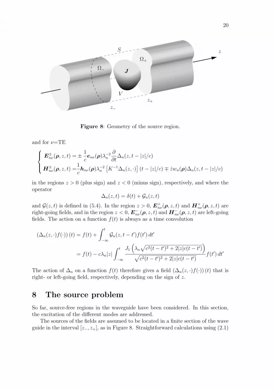
Figure 8: Geometry of the source region.

and for ν=TEE±nν(ρ, z, t) =± 1

cenν(ρ)λ−2

n

∂

∂t∆n(z, t− |z|/c)

H±nν(ρ, z, t) =1

chnν(ρ)λ−2

n

[K−1∆n(z, ·)

](t− |z|/c)∓ zwn(ρ)∆n(z, t− |z|/c)

in the regions z > 0 (plus sign) and z < 0 (minus sign), respectively, and where theoperator

∆n(z, t) = δ(t) + Gn(z, t)and G(z, t) is defined in (5.4). In the region z > 0, E+

nν(ρ, z, t) and H+nν(ρ, z, t) are

right-going fields, and in the region z < 0, E−nν(ρ, z, t) andH−nν(ρ, z, t) are left-goingfields. The action on a function f(t) is always as a time convolution

(∆n(z, ·)f(·)) (t) = f(t) +

∫ t

−∞Gn(z, t− t′)f(t′) dt′

= f(t)− cλn|z|∫ t

−∞

J1

(λn

√c2(t− t′)2 + 2|z|c(t− t′)

)√

c2(t− t′)2 + 2|z|c(t− t′)f(t′) dt′

The action of ∆n on a function f(t) therefore gives a field (∆n(z, ·)f(·)) (t) that isright- or left-going field, respectively, depending on the sign of z.

8 The source problem

So far, source-free regions in the waveguide have been considered. In this section,the excitation of the different modes are addressed.

The sources of the fields are assumed to be located in a finite section of the waveguide in the interval [z−, z+], as in Figure 8. Straightforward calculations using (2.1)

21

and (7.2) yield∫ ∞

−∞∇ ·

[E(r, t− t′)×H±nν(ρ, z − z∓, t

′) + ηH(r, t− t′)×E±nν(ρ, z − z∓, t′)]dt′

= η

∫ ∞

−∞J(r, t− t′) ·E±nν(ρ, z − z∓, t

′) dt′, z ∈ [z−, z+]

since all fields are assumed to vanish as t → −∞. Integrate this expression overthe volume V bounded by the surfaces S, Ω− and Ω+, see Figure 8, and use Gauss’theorem. Due to the boundary conditions (2.5) and (7.3), there is no contributionfrom S.

η

∫ ∞

−∞

∫∫∫V

J(r, t− t′) ·E±nν(ρ, z − z∓, t′) dv dt′

=

∫ ∞

−∞

∫∫Ω+

[E(r, t− t′)×H±nν(ρ, z − z∓, t

′)

+ ηH(r, t− t′)×E±nν(ρ, z − z∓, t′)]· z dS dt′

−∫ ∞

−∞

∫∫Ω−

[E(r, t− t′)×H±nν(ρ, z − z∓, t

′)

+ ηH(r, t− t′)×E±nν(ρ, z − z∓, t′)]· z dS dt′

In a region to the left of the sources, z < z−, the fields are assumed to be asuperposition of left-going waves.

E(r, t) =

∑nν

(F−nν(·) ∗E−nν(ρ, z − z−, ·)

)(t),

ηH(r, t) =∑nν

(F−nν(·) ∗H−nν(ρ, z − z−, ·)

)(t),

z < z−

and the fields in the region to the right of the sources, z > z+, are right-going wavesE(r, t) =

∑nν

(F+nν(·) ∗E+

nν(ρ, z − z+, ·))(t),

ηH(r, t) =∑nν

(F+nν(·) ∗H+

nν(ρ, z − z+, ·))(t),

z > z+

where the functions F±nν(t) are unknown expansion functions depending only on time.The plus and the minus signs correspond to right- and left-going fields, respectively.

22

The explicit expansions in the region z > z+ for the ν=TM mode are

E(r, t) =− 1

c

∑nν

enν(ρ)λ−2n

[K−1F+

nν

](t− (z − z+)/c)

− 1

c

∑nν

enν(ρ)λ−2n

[K−1

(G(z − z+, ·) ∗ F+

nν(·))]

(t− (z − z+)/c)

+ z∑nν

vn(ρ)[F+nν(t− (z − z+)/c)

+(G(z − z+, ·) ∗ F+

nν(·))(t− (z − z+)/c)

]H(r, t) =− 1

c

∑nν

hnν(ρ)λ−2n

∂

∂t

[F+nν(t− (z − z+)/c)

+(G(z − z+, ·) ∗ F+

nν(·))(t− (z − z+)/c)

]Orthogonality implies (see (7.1)) that∫ ∞

−∞

∫∫Ω±

[E(r, t− t′)×H±nν(ρ, z − z∓, t

′)

+ ηH(r, t− t′)×E±nν(ρ, z − z∓, t′)]· z dS dt′ = 0

and∫ ∞

−∞

∫∫Ω∓

[E(r, t− t′)×H±nν(ρ, z − z∓, t

′)

+ ηH(r, t− t′)×E±nν(ρ, z − z∓, t′)]· z dS dt′

= ∓ 2

c2λ4n

∂

∂t

∂

∂tF∓nν(t) +

(L(·) ∗ F∓nν(·)

)(t)

= ∓ 2

c2λ4n

∂

∂t

(K−1F∓nν

)(t)

where the upper (lower) sign of the expansion functions should be read with upper(lower) sign of the integration domain. The expansion functions F±n (t) therefore are

F±nν(t) =ηc2λ4

n

2K∂−1

t

∫ ∞

−∞

∫∫∫V

J(r, t− t′) ·E∓nν(ρ, z − z±, t′) dv dt′

=ηc2λ4

n

2

∫ t

−∞

∫ t′

−∞J0 (cλ(t′ − t′′))

∫ ∞

−∞∫∫∫V

J(r, t′′ − t′′′) ·E∓nν(ρ, z − z±, t′′′) dv dt′′′ dt′′ dt′

which are explicit expressions of the unknown functions F±nν . From these expressionsthe unknown functions F±nν(t) and the expansion of the fields in the regions outsidethe source are determined if the current density J is known.

23

Acknowledgment

The author likes to thank Dr. Anders Karlsson for constructive discussions concern-ing the precursor problem.

References

[1] L. Brillouin. Wave propagation and group velocity. Academic Press, New York,1960.

[2] R.E. Collin. Field Theory of Guided Waves. IEEE Press, New York, secondedition, 1991.

[3] J.P. Corones, M.E. Davison, and R.J. Krueger. Direct and inverse scatteringin the time domain via invariant imbedding equations. J. Acoust. Soc. Am.,74(5), 1535–1541, 1983.

[4] J.P. Corones, G. Kristensson, P. Nelson, and D.L. Seth, editors. InvariantImbedding and Inverse Problems. SIAM, 1992.

[5] M. Cotte. Propagation of a pulse in a waveguide. Onde Elec., 34, 143–146,1954.

[6] I.S. Gradshteyn and I.M. Ryzhik. Table of Integrals, Series, and Products.Academic Press, New York, fourth edition, 1965.

[7] S. He and A. Karlsson. Time domain Green functions technique for a pointsource over a dissipative stratified half-space. Radio Science, 28(4), 513–526,1993.

[8] J.D. Jackson. Classical Electrodynamics. John Wiley & sons, New York, secondedition, 1975.

[9] G. Kristensson. Direct and inverse scattering problems in dispersive media—Green’s functions and invariant imbedding techniques. In Kleinman R., KressR., and Martensen E., editors, Direct and Inverse Boundary Value Problems,Methoden und Verfahren der Mathematischen Physik, Band 37, pages 105–119,Mathematisches Forschungsinstitut Oberwolfach, FRG, 1991.

[10] G. Kristensson and R.J. Krueger. Direct and inverse scattering in the timedomain for a dissipative wave equation. Part 1: Scattering operators. J. Math.Phys., 27(6), 1667–1682, 1986.

[11] G. Kristensson and R.J. Krueger. Direct and inverse scattering in the timedomain for a dissipative wave equation. Part 2: Simultaneous reconstructionof dissipation and phase velocity profiles. J. Math. Phys., 27(6), 1683–1693,1986.

24

[12] R.J. Krueger and R.L. Ochs, Jr. A Green’s function approach to the determi-nation of internal fields. Wave Motion, 11, 525–543, 1989.

[13] P.M. Morse and H. Feshbach. Methods of Theoretical Physics, volume 1.McGraw-Hill Book Company, New York, 1953.

[14] A.P. Prudnikov, Y.A. Brychkov, and O.I. Marichev. Integrals and Series, vol-ume 2: Special functions. Gordon and Breach Science Publishers, New York,1986.

[15] M. Reed and B. Simon. Methods of modern mathematical physics, volume II:Fourier analysis, Self-adjointness. Academic Press, New York, 1975.

[16] I. Stakgold. Boundary Value Problems of Mathematical Physics, volume 2.MacMillan, New York, 1968.

[17] J. Van Bladel. Electromagnetic Fields. Hemisphere Publication Corporation,New York, 1986. Revised Printing.

[18] V.H. Weston. Factorization of the wave equation in higher dimensions. J.Math. Phys., 28, 1061–1068, 1987.

[19] V.H. Weston. Invariant imbedding for the wave equation in three dimensionsand the applications to the direct and inverse problems. Inverse Problems, 6,1075–1105, 1990.

[20] V.H. Weston. Invariant imbedding and wave splitting in R3: II. The Greenfunction approach to inverse scattering. Inverse Problems, 8, 919–947, 1992.

[21] V.H. Weston. Time-domain wave-splitting of Maxwell’s equations. J. Math.Phys., 34(4), 1370–1392, 1993.

[22] E. Zauderer. Partial Differential Equations of Applied Mathematics. Wiley,New York, second edition, 1989.