fast biases in monsoon rainfall over southern and central

Fast Biases in Monsoon Rainfall over Southern and Central India in theMet Office Unified Model

RICHARD J. KEANE

Met Office, Exeter, and School of Earth and Environment, University of Leeds, Leeds, United Kingdom

KEITH D. WILLIAMS, ALISON J. STIRLING, AND GILL M. MARTIN

Met Office, Exeter, United Kingdom

CATHRYN E. BIRCH AND DOUGLAS J. PARKER

School of Earth and Environment, University of Leeds, Leeds, United Kingdom

(Manuscript received 28 September 2018, in final form 21 June 2019)

ABSTRACT

TheMet Office UnifiedModel (MetUM) is known to produce too little total rainfall on average over India

during the summer monsoon period, when assessed for multiyear climate simulations. We investigate how

quickly this dry bias appears by assessing the 5-day operational forecasts produced by the MetUM for six

different years. It is found that theMetUM shows a drying tendency across the five days of the forecasts, for all

of the six years (which correspond to two different model versions). We then calculate each term in the

moisture budget, for a region covering southern and central India, where the dry bias is worst in both climate

simulations and weather forecasts. By looking at how the terms vary with forecast lead time, we are able to

identify biases in the weather forecasts that have been previously identified in climate simulations using the

samemodel, and we attempt to quantify how these biases lead to a reduction in total rainfall. In particular, an

anticyclonic bias develops to the east of India throughout the forecast, and it has a complex effect on the

moisture available over the peninsula, and a reduction in the wind speed into the west of the region appears

after about 3 days, indicative of upstream effects. In addition, we find a new bias that the air advected from the

west is too dry from very early in the forecast, and this has an important effect on the rainfall.

1. Introduction

The Indian summer monsoon is one of the most im-

portant weather systems in the world, producing a large

majority of the annual rainfall for over a billion people. It

is also one of the most difficult for general circulation

models (GCMs) to simulate on a range of spatial and

temporal scales. Although there is significant interannual

variability in themonsoon, one of the largest difficulties is

in simulating the correct amount of total monsoon rain-

fall on average over an extended period of many years.

Most GCMs exhibit a significant climatological June–

September dry bias when compared with observations,

while several others conversely produce toomuch rainfall

(Sperber et al. 2013).

The Met Office Unified Model (MetUM) is one of

many GCMs with a dry bias over India in the summer

months (Walters et al. 2017). Levine and Turner (2012)

showed that a significant contribution to this dry bias

comes from sea surface temperature (SST) biases in the

coupled model version of the MetUM (these biases

being themselves caused by biases in the atmospheric

component) and, indeed, coupled rainfall and SST bia-

ses play an important part in Indian summer monsoon

errors for GCMs generally (Levine et al. 2013). How-

ever, Levine and Turner (2012) also conducted an

experiment with an atmosphere-only version of the

MetUM forced with SSTs derived from observations,

and here some aspects of the dry bias were improved,

but a significant part of it remained. Similar results have

been obtained in various other studies (Ringer et al.

2006; Martin et al. 2010; Martin and Levine 2012; Bush

et al. 2015; Johnson et al. 2016, 2017; Levine and Martin

2018), so it is clear that deficiencies in the atmospheric

component of the MetUM play a significant part. Al-

though the situation has improved as recent versions ofCorresponding author: Richard J. Keane, [email protected]

1 OCTOBER 2019 KEANE ET AL . 6385

DOI: 10.1175/JCLI-D-18-0650.1

� 2019 American Meteorological Society. For information regarding reuse of this content and general copyright information, consult the AMS CopyrightPolicy (www.ametsoc.org/PUBSReuseLicenses).

Unauthenticated | Downloaded 02/12/22 05:44 AM UTC

mailto:[email protected]

http://www.ametsoc.org/PUBSReuseLicenses



the MetUM have been released, the Indian dry bias re-

mains one of the most significant biases in the configura-

tion in current operational use (Walters et al. 2017).

The nature of the MetUM Indian monsoon dry bias

has been studied extensively, and various mechanisms

have been put forward as potential causes. For example,

Bush et al. (2015) showed that the dry bias is related to a

wet bias over the equatorial Indian Ocean: when they

increased the convective entrainment over this latter re-

gion, suppressing the rainfall there, it led to an increase in

rainfall over the Indian Peninsula. Levine and Martin

(2018) showed that an inability to correctly simulate low

pressure systems leads to a reduction in rainfall over In-

dia, and that this effect is mitigated when running a re-

gional simulation over India, with the boundary forcing

(including remote precursors to low pressure systems)

provided by analyses. However, in both of these studies

the dry bias was not explained entirely by the phenome-

non investigated, and it is clear that in its totality it is due

to an interplay of various remote and local effects and a

range of temporal and spatial scales.

The aforementioned studies refer to longer climate

simulations, but forecasting the Indian summer mon-

soon is also challenging at shorter time scales appro-

priate to numerical weather prediction (NWP) (Ranade

et al. 2014; Gadgil and Srinivasan 2012), and theMetUM

also shows rainfall biases at NWP scales (Prakash et al.

2016; Mitra et al. 2013). Categorical yes/no forecasts of

rainfall are generally good, but it is rather more difficult

to produce good forecasts of rainfall amount (Joshi and

Kar 2016; Kumar et al. 2017). Although it is possible to

improve forecasts by combining models or using post-

processing such as bias correction (Joshi and Kar 2016;

Mitra et al. 2011), it is still desirable for NWP to use an

underlyingGCM that captures the physics and dynamics

of the monsoon as well as possible, for example, in order

to continue to produce good forecasts as the climate

changes.

Mitra et al. (2013) showed that the MetUM produces

too little rainfall over much of India on a time scale of a

few days for summer 2012, although this bias is still

smaller than the day-to-day variability in rainfall being

predicted. One aim of the present study is to evalu-

ate NWP forecasts produced operationally using the

MetUM for multiple years, and to investigate to what

extent these forecasts exhibit the dry bias seen in longer

climate runs with the same underlying GCM. This will

give insight into whether the bias is caused by fast pro-

cesses such as convection, or processes that evolve more

slowly, such as the global-scale circulation, without re-

quiring lengthy climate simulations or, indeed, any

simulations beyond those that have been produced for

operational purposes.

Such an investigation is made possible by the fact that

the Met Office applies a ‘‘seamless’’ approach to pre-

dicting the weather and climate, whereby a single GCM

is developed for all weather and climate time scales

(Brown et al. 2012;Mitra et al. 2013). This has previously

been exploited by Birch et al. (2014), to study the water

cycle of the West African monsoon, and by Martin et al.

(2010), who showed that two long-standing systematic

errors (including in the Asian monsoon region), present

in longer climate runs, appear during the first few days of

NWP forecasts. Additionally, Bush et al. (2015) traced

the influence of changing the entrainment parameter

over the equatorial Indian Ocean region from the first

few days of a simulation to the climate time scale. NWP

techniques have also been used to assess climate models

by Rodwell and Palmer (2007) and Klocke and Rodwell

(2014), who used temporally averaged tendencies from

the data assimilation system to represent fast errors in

the model, and investigated their sensitivity to changes

in model parameters.

In this paper we investigate how the MetUM dry bias

develops within the first five days of the forecast, and

carry out a detailed investigation of the moisture budget

for a region covering southern and central India, within

which the dry bias seems to look similar after 5 days to

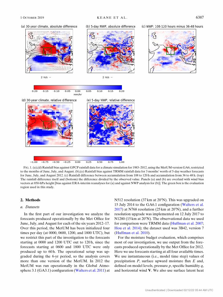
that after 30 years. This is shown in Fig. 1, which shows

the rainfall bias for a 30-yr climate simulation against

GPCP data (Adler et al. 2003) and for a series of NWP

forecasts, of accumulation between 4.5 and 5 days

(where forecasts were initialized every 12 h, so the full

diurnal cycle is captured here) against Tropical Rainfall

Measuring Mission (TRMM) data (Huffman et al.

2007). As well as the dry bias within the green box, the

significant wet bias over the equatorial Indian Ocean

seen in the climate run is also seen in the weather

forecasts, although the dry bias over northern India seen

in the climate run is not seen in the weather forecasts.

We investigate the operational forecasts for the period

2012–17 and show that, while the bias against obser-

vations is not always dry at early (1–2 day) forecast

ranges, every year has a drying tendency from the start

of the forecast such that the model is always too dry at

five days. For the remainder of the paper, we therefore

carry out a more detailed investigation of how the

different terms in the moisture budget develop, in

comparison with their values at analysis time. By con-

fining this study to the drying tendency between the end

and beginning of the forecast, we can make a direct

comparison between later and earlier forecasts. This

removes the need to provide observed values of the

horizontal flux terms, which would require wind speed

and humidity profile measurements at a large number

of locations.

6386 JOURNAL OF CL IMATE VOLUME 32


2. Methods

a. Datasets

In the first part of our investigation we analyze the

forecasts produced operationally by the Met Office for

June, July, and August for each of the six years 2012–17.

Over this period, the MetUM has been initialized four

times per day (at 0000, 0600, 1200, and 1800 UTC), but

we restrict this part of the investigation to the forecasts

starting at 0000 and 1200 UTC out to 120 h, since the

forecasts starting at 0600 and 1800 UTC were only

produced up to 60h. The operational setup was up-

graded during the 6-yr period, so the analysis covers

more than one version of the MetUM. In 2012 the

MetUM was run operationally in the Global Atmo-

sphere 3.1 (GA3.1) configuration (Walters et al. 2011) at

N512 resolution (37km at 208N). This was upgraded on

15 July 2014 to the GA6.1 configuration (Walters et al.

2017) at N768 resolution (25km at 208N), and a further

resolution upgrade was implemented on 12 July 2017 to

N1280 (15km at 208N). The observational data we used

for comparison were TRMM data (Huffman et al. 2007;

Hou et al. 2014); the dataset used was 3B42, version 7

(Huffman et al. 2010).

For the moisture budget evaluation, which comprises

most of our investigation, we use output from the fore-

casts produced operationally by theMet Office for 2012.

Here we use forecasts starting at all four available times.

We use instantaneous (i.e., model time step) values of

precipitation P, surface upward moisture flux E and,

defined on model levels, pressure p, specific humidity q,

and horizontal wind V. We also use surface latent heat

FIG. 1. (a),(d) Rainfall bias againstGPCP rainfall data for a climate simulation for 1983–2012, using theMetUMversionGA6, restricted

to the months of June, July, and August. (b),(e) Rainfall bias against TRMM rainfall data for 3 months’ worth of 5-day weather forecasts

for June, July, and August 2012. (c) Rainfall difference between accumulation from 108 to 120 h and accumulation from 36 to 48 h. (top)

The rainfall difference itself and (bottom) the difference divided by the observed value. Panels (a) and (b) are overlaid with wind bias

vectors at 850-hPa height [bias against ERA-interim reanalyses for (a) and against NWP analysis for (b)]. The green box is the evaluation

region used in this study.



flux h, defined as a 6-h mean, to calibrate the surface

upward moisture flux (see appendix).

For both investigations, quantities have been aver-

aged over forecasts initialized in June, July, and August.

We have restricted to valid times from 6 June until

31 August—constant for each forecast lead time—so

that for a perfect forecast each term should be in-

dependent of lead time. The evolution of the quantities

with forecast lead time therefore gives an indication as

to how quantities change as the forecast develops.

b. Moisture budget calculation

FollowingYanai et al. (1973), Zangvil et al. (2001), and

Zangvil et al. (2004) we write the moisture budget as

1

g

›

›t

ðððqd2Adp52

1

g

ðþA

qV � dl dp1ðð

(E2P)d2A ,

(1)

where g is the acceleration due to gravity, t is time, A is

an arbitrary horizontal area, and dl is an element along

the edge of A. Note that we do not define quantities as

area averages, but apply an extra area integral compared

with Zangvil et al. (2004). Note also that this budget

applies to water vapor, so that storage of moisture in

clouds, and horizontal transport of clouds, is neglected.

Applying this to a box region over India, bounded by

latitudes (u1, u2) (here equal to 9.028 and 21.458N) and

longitudes (f1, f2) (here equal to 71.898 and 85.968E),the first term on the right-hand side of Eq. (1) can be

written

2

ðþA

qV � dl dp5"ðp5psurface

p50

ðu5u2

u5u1

qurEdudp

#f5f1

f5f2

1

"ðp5psurface

p50

ðf5f2

f5f1

qyrEcosudf dp

#u5u1

u5u2

,

(2)

and for an arbitrary quantity x:

ððxd2A5

ðu5u2

u5u1

ðf5f2

f5f1

xr2E cosudu df (3)

[hxi3 r2E(sinu2 2 sinu1)(f

22f

1) , (4)

where the angle brackets represent an area-weighted

mean of the values at each grid box and rE is the radius

of Earth.

We define the fluxes into the box on the western, east-

ern, southern and northern sides as, respectively,

MW5

rE

g

ðp5psurface

p50

ðu5u2

u5u1

qu dudpjf5f1

, (5)

ME52

rE

g

ðp5psurface

p50

ðu5u2

u5u1

qu dudpjf5f2

, (6)

MS5

rE

g

ðp5psurface

p50

ðf5f2

f5f1

qy cosudf dpju5u1

, and (7)

MN52

rE

g

ðp5psurface

p50

ðf5f2

f5f1

qy cosudf dpju5u2

. (8)

We define the total flux E of moisture entering the box

from the surface and the total flux P of moisture leaving

the box due to precipitation as

(E,P)5

ðð(E,P)d2A. (9)

So Eq. (1) can be rewritten as

Qt5M

W1M

E1M

S1M

N1E2P , (10)

where

Qt5

1

g

›

›t

ðððqd2Adp (11)

is the rate of change of total moisture in the box.We also

define MA 5MW 1ME 1MS 1MN 1E as the total net

moisture flux entering the box, which is ‘‘available’’ for

rainfall. We have multiplied each term in kilograms per

second (kg s21) by 3600 s h21/ÐÐd2A and assumed awater

density of 103 kgm23, to obtain a value that represents

the amount of rainfall in millimeters per hour (mmh21)

that would be produced in the box if all the moisture

from that term were converted into rainfall.

The moisture conservation of the MetUM can be

tested by comparing Qt and MA 2P, since both can be

calculated directly from different model outputs. We

take Qt[t(n21)/2]’ [Q(tn)2Q(tn21)]/Dt, where n repre-

sents the individual forecast lead times separated by

Dt 5 12h, and Q5 1/gÐÐÐ

qd2Adp. Any discrepancies

betweenQt andMA 2Pwould suggest a lack ofmoisture

conservation, although could also be caused by the some-

what coarse temporal discretization used to define Qt.

c. Separation into moisture and wind effects

The variation in the terms MWESN could be due to

variations in the humidity, variations in the wind ad-

vecting the moisture, or a combination of the two. Here

we separate the effects of the humidity field and of the

wind field, by alternately only allowing one of the two to



vary with forecast lead time. First, we define the terms in

general as a function of forecast lead time t:

Mftg[l

�ðMftgdp

�F,t

[l

g

�ðqftgVftgdp

�F,t

, (12)

where the angle brackets are here an average over

forecast valid time, and the relevant latitude or longi-

tude lineF (representing u or f as appropriate), and l is

the length of this line. The quantity V represents the

appropriate horizontal wind u or y. Any changes in M

could be due to changes inmoisture q or wind speedV or

the interaction thereof. It is interesting to isolate the

effects of changing only q or only V, and this is accom-

plished by defining

Hftg[ l

�ðHftgdp

�F,t

[l

g

�ðqftgVf0gdp

�F,t

, and

(13)

Sftg[ l

�ðSftgdp

�F,t

[l

g

�ðqf0gVftgdp

�F,t

. (14)

In this way,H represents how the moisture flux develops

with forecast lead time, based only on variation in hu-

midity (i.e., holding wind speed constant), and S repre-

sents how the moisture flux develops with forecast lead

time based only on variation in wind speed (i.e., holding

humidity constant).

In practice, quantities are defined on model levels, so

we use the pressure field to define dp/dz and integrate

with respect to height z, from the surface up to ap-

proximately 18 km. We take dp/dz to vary with forecast

lead time in the definition ofH and to be constant in the

definition of S. The physical justification for this is that

dp/dz ’ 2rg, where r is air density, so that

Hftg’ l

�ðrftgqftgVf0gdz

�F,t

, and (15)

Sftg’ l

�ðrf0gqf0gVftgdz

�F,t

, (16)

with the integration limits suitably reversed. The quan-

tity rq is the actual moisture content, so that H repre-

sents the variation in M, varying only the moisture

content, and S represents the variation in M, varying

only the wind speed.

3. Results

As mentioned in section 1, there are similarities and

differences in the rainfall bias between the climate

simulation and weather forecasts produced using the

MetUM, as shown in Fig. 1. In this study, we focus on

southern India, since both biases look similar here, so

analyzing the bias in the weather forecasts could also

provide insights into the bias in the climate simulation.

Figure 1 also shows vectors for the bias in wind speed

at 850-hPa height. These were calculated by taking a

temporal mean over June, July, and August (for 1983–

2012 for the climate simulations and 2012 for the NWP

forecasts) and comparing with a reference dataset. The

reference dataset for the climate simulations is ERA-

Interim (Dee et al. 2011) and for the NWP forecasts is

the NWP analysis field.

Also shown in Fig. 1 is the relative difference in

rainfall between model and observations, for both the

weather forecasts and climate simulations. This is simply

the actual difference divided by the relevant observed

value (GPCP data for the climate simulation and

TRMM data for the weather forecasts). This shows that

the relative bias is somewhat lower for the weather

forecasts than for the climate simulations. However,

over the region chosen for this study, the dry bias is

significant for both setups.

It is interesting to note that the dry bias in the weather

forecasts does not seem to extend as far north as that in

the climate simulation (cf. Figs. 1a and 1b). On further

investigation, it was found that the rainfall over northern

India increases during the first two days of the weather

forecast and then decreases steadily thereafter. This can

be seen from Fig. 1c, where there is a clear drying over

northern India between two and five days, similar to that

seen over southern India over the full five days. It may

be the case, then, that the behavior over northern India

after an initial two-day adjustment is similar to that over

southern India. However, because this study attempts to

use the first five days of the weather forecast to better

understand the climate bias, we concentrate on the region

in the green box shown in Fig. 1 for the rest of this study.

Although the region of India to the north of the box is

socioeconomically very important, and accounts for a large

part of the total monsoon rainfall over India, we concen-

trate here on southern and central India so as to obtain a

clearmonotonic drying that develops over the full five days

of the operational forecast being considered.

a. General rainfall climatology

Figure 2 shows the evolution of the total rainfall,

within the green box in Fig. 1, as a function of forecast

lead time, for the years 2012–17. The values are 12-h

accumulations, and each accumulation is plotted against

the whole period to which it applies. Also plotted is the

observed rainfall for the same area, for which there is a

single value independent of forecast lead time since the

forecast valid time does not change.



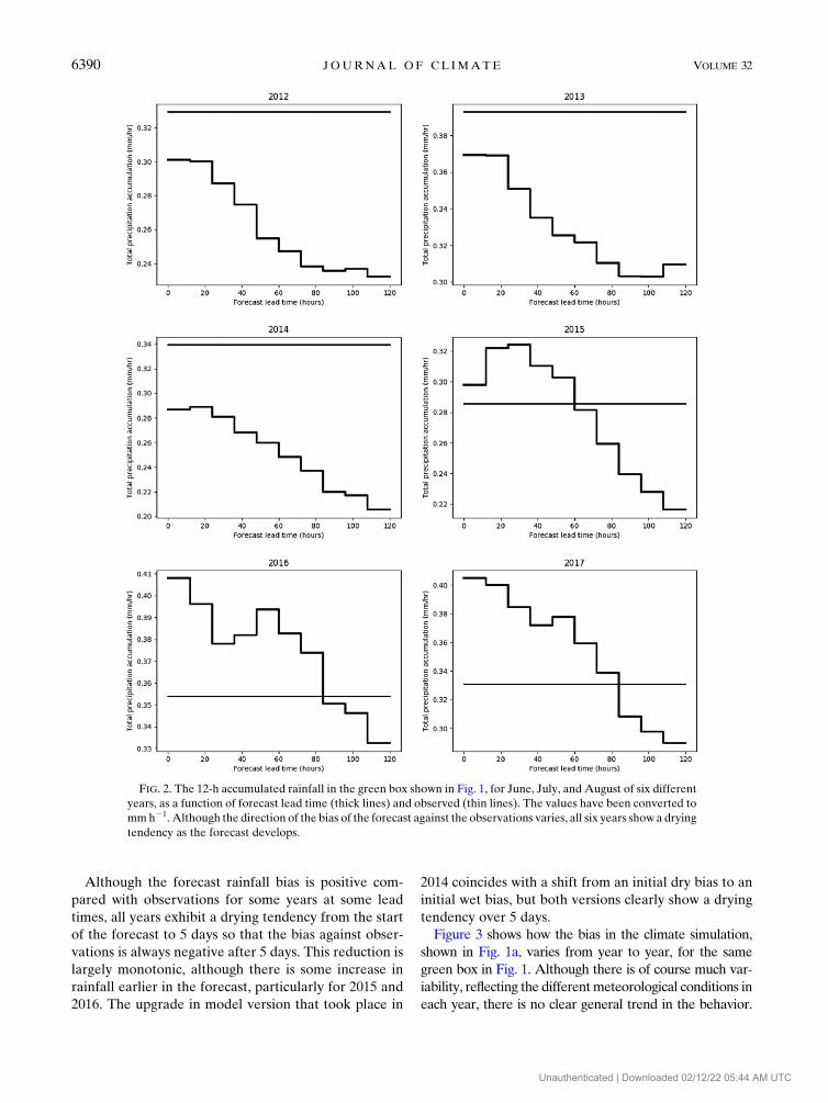
Although the forecast rainfall bias is positive com-

pared with observations for some years at some lead

times, all years exhibit a drying tendency from the start

of the forecast to 5 days so that the bias against obser-

vations is always negative after 5 days. This reduction is

largely monotonic, although there is some increase in

rainfall earlier in the forecast, particularly for 2015 and

2016. The upgrade in model version that took place in

2014 coincides with a shift from an initial dry bias to an

initial wet bias, but both versions clearly show a drying

tendency over 5 days.

Figure 3 shows how the bias in the climate simulation,

shown in Fig. 1a, varies from year to year, for the same

green box in Fig. 1. Although there is of course much var-

iability, reflecting the differentmeteorological conditions in

each year, there is no clear general trend in the behavior.

FIG. 2. The 12-h accumulated rainfall in the green box shown in Fig. 1, for June, July, and August of six different

years, as a function of forecast lead time (thick lines) and observed (thin lines). The values have been converted to

mmh21. Although the direction of the bias of the forecast against the observations varies, all six years show a drying

tendency as the forecast develops.



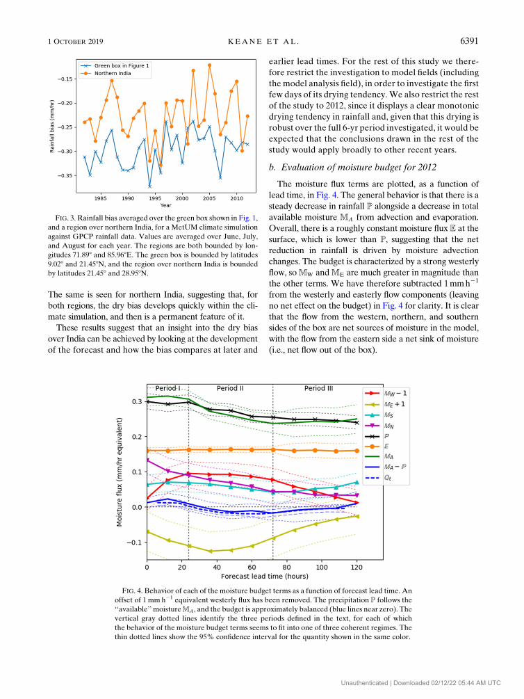
The same is seen for northern India, suggesting that, for

both regions, the dry bias develops quickly within the cli-

mate simulation, and then is a permanent feature of it.

These results suggest that an insight into the dry bias

over India can be achieved by looking at the development

of the forecast and how the bias compares at later and

earlier lead times. For the rest of this study we there-

fore restrict the investigation to model fields (including

the model analysis field), in order to investigate the first

few days of its drying tendency.We also restrict the rest

of the study to 2012, since it displays a clear monotonic

drying tendency in rainfall and, given that this drying is

robust over the full 6-yr period investigated, it would be

expected that the conclusions drawn in the rest of the

study would apply broadly to other recent years.

b. Evaluation of moisture budget for 2012

The moisture flux terms are plotted, as a function of

lead time, in Fig. 4. The general behavior is that there is a

steady decrease in rainfall P alongside a decrease in total

available moisture MA from advection and evaporation.

Overall, there is a roughly constant moisture flux E at the

surface, which is lower than P, suggesting that the net

reduction in rainfall is driven by moisture advection

changes. The budget is characterized by a strong westerly

flow, soMW andME are much greater in magnitude than

the other terms. We have therefore subtracted 1mmh21

from the westerly and easterly flow components (leaving

no net effect on the budget) in Fig. 4 for clarity. It is clear

that the flow from the western, northern, and southern

sides of the box are net sources of moisture in the model,

with the flow from the eastern side a net sink of moisture

(i.e., net flow out of the box).

FIG. 3. Rainfall bias averaged over the green box shown in Fig. 1,

and a region over northern India, for a MetUM climate simulation

against GPCP rainfall data. Values are averaged over June, July,

and August for each year. The regions are both bounded by lon-

gitudes 71.898 and 85.968E. The green box is bounded by latitudes

9.028 and 21.458N, and the region over northern India is bounded

by latitudes 21.458 and 28.958N.

FIG. 4. Behavior of each of the moisture budget terms as a function of forecast lead time. An

offset of 1mmh21 equivalent westerly flux has been removed. The precipitation P follows the

‘‘available’’ moistureMA, and the budget is approximately balanced (blue lines near zero). The

vertical gray dotted lines identify the three periods defined in the text, for each of which

the behavior of the moisture budget terms seems to fit into one of three coherent regimes. The

thin dotted lines show the 95% confidence interval for the quantity shown in the same color.



The actual values ofQt andMA 2P are approximately

zero at t 5 0 (although significantly above, rather than

below, zero), indicating that the moisture in the box is

fairly constant from one analysis to the next over the

3-month period. They are also approximately equal to

each other, suggesting that the MetUM keeps an ap-

proximately balanced moisture budget (relative to the

magnitude of the tendencies) for the duration of the

forecast. The variation in MA, P, and Qt can be broadly

divided into three stages. During the first day of the

forecast (which we define as period I), MA and P are

approximately constant, with MA slightly larger than P

so that there is a moistening of the box during this pe-

riod; although the significance interval allows for some

possibility of P being larger than MA, Qt is significantly

positive. From days 1 to 3 (period II), both quantities

decrease, but MA decreases rather faster. Again, the

significance intervals suggest that this will vary depend-

ing on the precise period used for the calculation, but Qt

is significantly negative, suggesting a drying of the box

during this period. From days 3 to 5 (period III), MA

levels off and even increases slightly, whileP continues to

decrease so that the box continues to dry but at a slower

and slower rate, until at day 5 the budget becomes ap-

proximately balanced (hereQt is significantly negative at

the start of the period, but approaches zero toward the

end of the period).

The zonal moisture advection also seems to follow a

three-stage pattern, as MW and ME both increase in

magnitude during period I, start to reduce slowly in

magnitude during period II, and then reduce more

quickly inmagnitude during period III. The flow into the

south of the box MS varies rather less (following a sim-

ilar pattern toQt), and the flow into the north of the box

MN decreases monotonically throughout the forecast,

although this decrease is slower during period III than

during the other periods.

Figure 4 suggests that the fastest processes during the

first day of the forecast do not contribute immediately to

the reduction in rainfall, and are likely due tomodel spinup

and adjustment to analysis, but that the processes on time

scales of a few days do make a significant contribution.

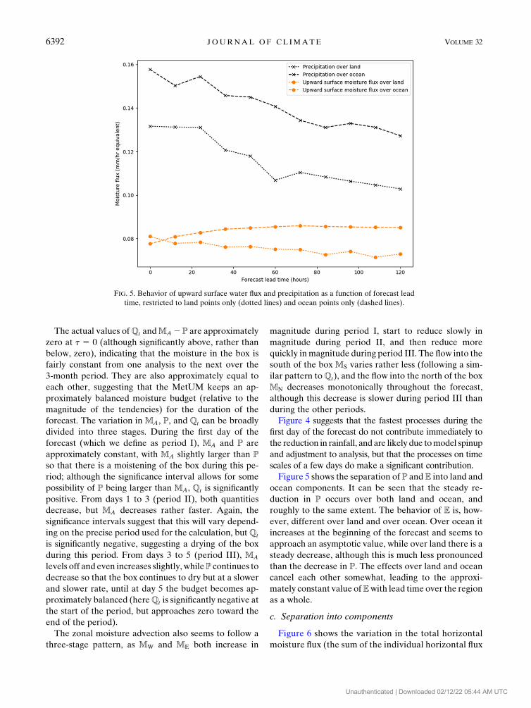
Figure 5 shows the separation of P and E into land and

ocean components. It can be seen that the steady re-

duction in P occurs over both land and ocean, and

roughly to the same extent. The behavior of E is, how-

ever, different over land and over ocean. Over ocean it

increases at the beginning of the forecast and seems to

approach an asymptotic value, while over land there is a

steady decrease, although this is much less pronounced

than the decrease in P. The effects over land and ocean

cancel each other somewhat, leading to the approxi-

mately constant value ofEwith lead time over the region

as a whole.

c. Separation into components

Figure 6 shows the variation in the total horizontal

moisture flux (the sum of the individual horizontal flux

FIG. 5. Behavior of upward surface water flux and precipitation as a function of forecast lead

time, restricted to land points only (dotted lines) and ocean points only (dashed lines).



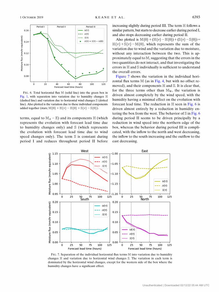
terms, equal to MA 2E) and its components H (which

represents the evolution with forecast lead time due

to humidity changes only) and S (which represents

the evolution with forecast lead time due to wind

speed changes only). The term S is constant during

period I and reduces throughout period II before

increasing slightly during period III. The term H follows a

similar pattern, but starts to decrease earlier during period I,

and also stops decreasing earlier during period II.

Also plotted is Mf0g1(Hftg2Hf0g)1(Sftg2Sf0g)5Hftg1Sftg2Mf0g, which represents the sum of the

variation due to wind and the variation due to moisture,

without any interaction between the two. This is ap-

proximately equal toM, suggesting that the errors in the

two quantities do not interact, and that investigating the

errors inH and S individually is sufficient to understand

the overall errors.

Figure 7 shows the variation in the individual hori-

zontal flux terms M (as in Fig. 4, but with no offset re-

moved), and their components H and S. It is clear that,

for the three terms other than MW, the variation is

driven almost completely by the wind speed, with the

humidity having a minimal effect on the evolution with

forecast lead time. The reduction in H seen in Fig. 6 is

driven almost entirely by a reduction in humidity en-

tering the box from the west. The behavior of S in Fig. 6

during period II seems to be driven principally by a

reduction in wind speed into the northern edge of the

box, whereas the behavior during period III is compli-

cated, with the inflow to the north and west decreasing,

the inflow to the south increasing and the outflow to the

east decreasing.

FIG. 6. Total horizontal flux M (solid line) into the green box in

Fig. 1, with separation into variation due to humidity changes H

(dashed line) and variation due to horizontal wind changes S (dotted

line). Also plotted is the variation due to these individual components

added together (stars; Mf0g1Hftg2Hf0g1Sftg2Sf0g).

FIG. 7. Separation of the individual horizontal flux terms M into variation due to humidity

changes H and variation due to horizontal wind changes S. The variation in each term is

dominated by the horizontal wind changes, except for the western side of the box where the

humidity changes have a significant effect.



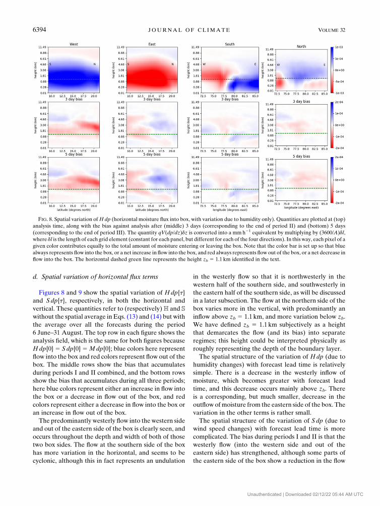
d. Spatial variation of horizontal flux terms

Figures 8 and 9 show the spatial variation of Hdp{t}

and Sdp{t}, respectively, in both the horizontal and

vertical. These quantities refer to (respectively)H and S

without the spatial average in Eqs. (13) and (14) but with

the average over all the forecasts during the period

6 June–31 August. The top row in each figure shows the

analysis field, which is the same for both figures because

Hdp{0}5 Sdp{0}5Mdp{0}; blue colors here represent

flow into the box and red colors represent flow out of the

box. The middle rows show the bias that accumulates

during periods I and II combined, and the bottom rows

show the bias that accumulates during all three periods;

here blue colors represent either an increase in flow into

the box or a decrease in flow out of the box, and red

colors represent either a decrease in flow into the box or

an increase in flow out of the box.

The predominantly westerly flow into the western side

and out of the eastern side of the box is clearly seen, and

occurs throughout the depth and width of both of those

two box sides. The flow at the southern side of the box

has more variation in the horizontal, and seems to be

cyclonic, although this in fact represents an undulation

in the westerly flow so that it is northwesterly in the

western half of the southern side, and southwesterly in

the eastern half of the southern side, as will be discussed

in a later subsection. The flow at the northern side of the

box varies more in the vertical, with predominantly an

inflow above zb 5 1.1 km, and more variation below zb.

We have defined zb 5 1.1 km subjectively as a height

that demarcates the flow (and its bias) into separate

regimes; this height could be interpreted physically as

roughly representing the depth of the boundary layer.

The spatial structure of the variation of Hdp (due to

humidity changes) with forecast lead time is relatively

simple. There is a decrease in the westerly inflow of

moisture, which becomes greater with forecast lead

time, and this decrease occurs mainly above zb. There

is a corresponding, but much smaller, decrease in the

outflow ofmoisture from the eastern side of the box. The

variation in the other terms is rather small.

The spatial structure of the variation of Sdp (due to

wind speed changes) with forecast lead time is more

complicated. The bias during periods I and II is that the

westerly flow (into the western side and out of the

eastern side) has strengthened, although some parts of

the eastern side of the box show a reduction in the flow

FIG. 8. Spatial variation ofHdp (horizontal moisture flux into box, with variation due to humidity only). Quantities are plotted at (top)

analysis time, along with the bias against analysis after (middle) 3 days (corresponding to the end of period II) and (bottom) 5 days

(corresponding to the end of period III). The quantity qV(dp/dz)dz is converted into a mmh21 equivalent by multiplying by (3600/A)dl,

where dl is the length of each grid element (constant for each panel, but different for each of the four directions). In this way, each pixel of a

given color contributes equally to the total amount of moisture entering or leaving the box. Note that the color bar is set up so that blue

always represents flow into the box, or a net increase in flow into the box, and red always represents flow out of the box, or a net decrease in

flow into the box. The horizontal dashed green line represents the height zb 5 1.1 km identified in the text.



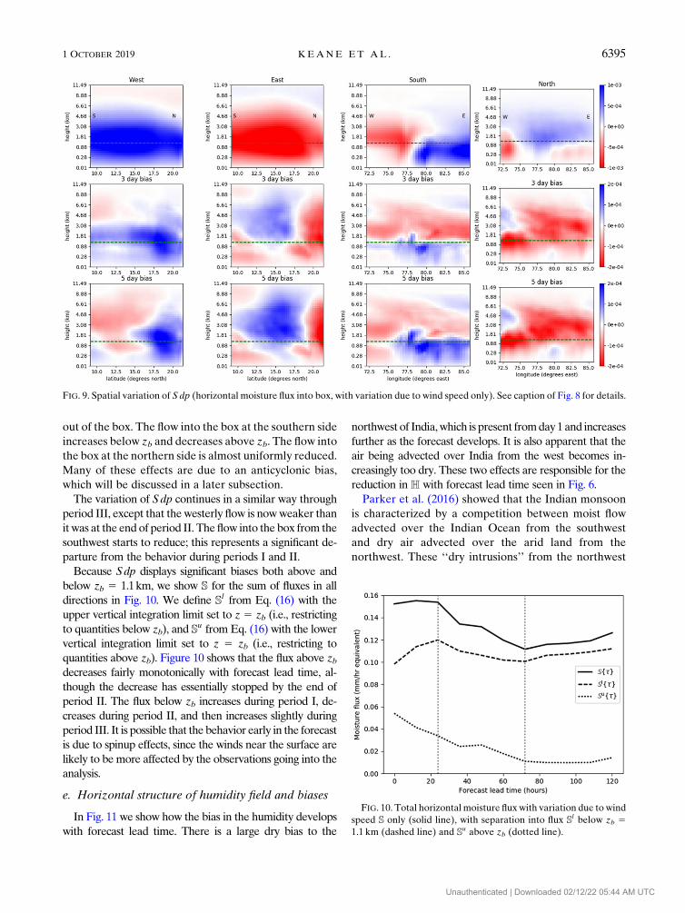
out of the box. The flow into the box at the southern side

increases below zb and decreases above zb. The flow into

the box at the northern side is almost uniformly reduced.

Many of these effects are due to an anticyclonic bias,

which will be discussed in a later subsection.

The variation of Sdp continues in a similar way through

period III, except that thewesterly flow is nowweaker than

it was at the end of period II. The flow into the box from the

southwest starts to reduce; this represents a significant de-

parture from the behavior during periods I and II.

Because Sdp displays significant biases both above and

below zb 5 1.1km, we show S for the sum of fluxes in all

directions in Fig. 10. We define Sl from Eq. (16) with the

upper vertical integration limit set to z5 zb (i.e., restricting

to quantities below zb), and Su from Eq. (16) with the lower

vertical integration limit set to z 5 zb (i.e., restricting to

quantities above zb). Figure 10 shows that the flux above zbdecreases fairly monotonically with forecast lead time, al-

though the decrease has essentially stopped by the end of

period II. The flux below zb increases during period I, de-

creases during period II, and then increases slightly during

period III. It is possible that the behavior early in the forecast

is due to spinup effects, since the winds near the surface are

likely to be more affected by the observations going into the

analysis.

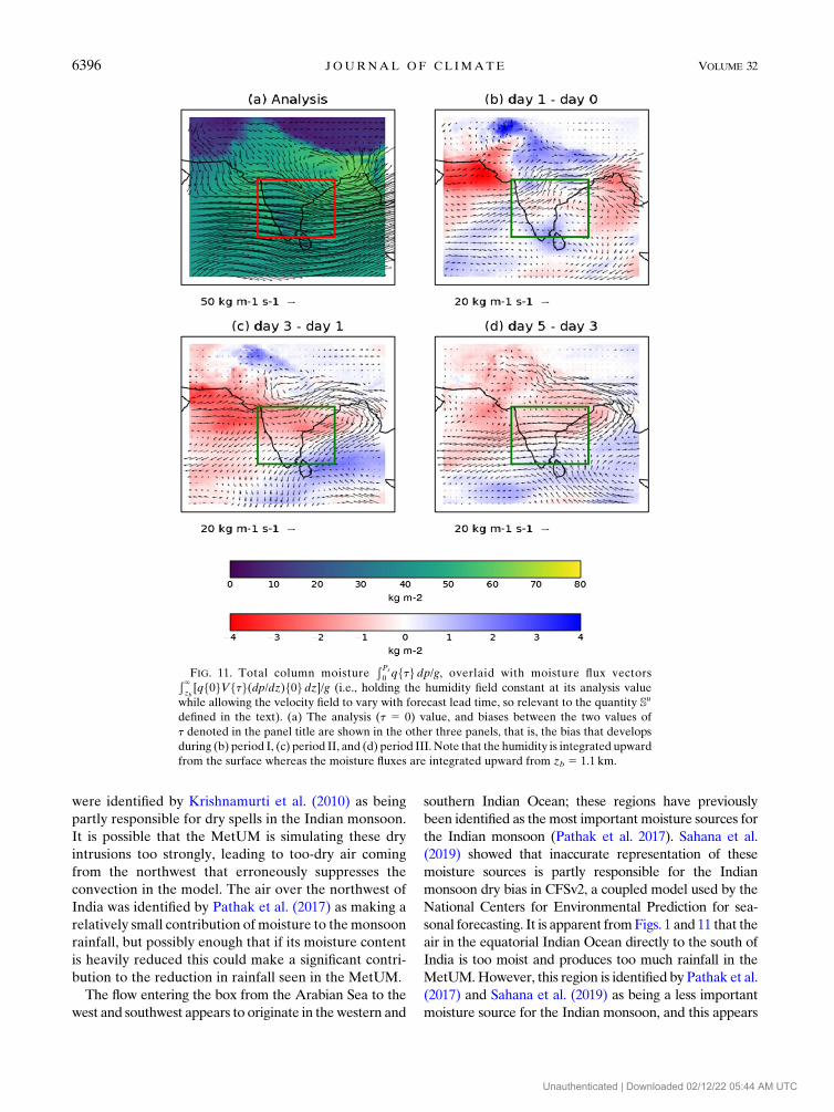
e. Horizontal structure of humidity field and biases

In Fig. 11 we show how the bias in the humidity develops

with forecast lead time. There is a large dry bias to the

northwest of India,which is present fromday1and increases

further as the forecast develops. It is also apparent that the

air being advected over India from the west becomes in-

creasingly too dry. These two effects are responsible for the

reduction in H with forecast lead time seen in Fig. 6.

Parker et al. (2016) showed that the Indian monsoon

is characterized by a competition between moist flow

advected over the Indian Ocean from the southwest

and dry air advected over the arid land from the

northwest. These ‘‘dry intrusions’’ from the northwest

FIG. 9. Spatial variation of S dp (horizontal moisture flux into box, with variation due to wind speed only). See caption of Fig. 8 for details.

FIG. 10. Total horizontal moisture flux with variation due to wind

speed S only (solid line), with separation into flux Sl below zb 51.1 km (dashed line) and Su above zb (dotted line).



were identified by Krishnamurti et al. (2010) as being

partly responsible for dry spells in the Indian monsoon.

It is possible that the MetUM is simulating these dry

intrusions too strongly, leading to too-dry air coming

from the northwest that erroneously suppresses the

convection in the model. The air over the northwest of

India was identified by Pathak et al. (2017) as making a

relatively small contribution of moisture to themonsoon

rainfall, but possibly enough that if its moisture content

is heavily reduced this could make a significant contri-

bution to the reduction in rainfall seen in the MetUM.

The flow entering the box from the Arabian Sea to the

west and southwest appears to originate in thewestern and

southern Indian Ocean; these regions have previously

been identified as the most important moisture sources for

the Indian monsoon (Pathak et al. 2017). Sahana et al.

(2019) showed that inaccurate representation of these

moisture sources is partly responsible for the Indian

monsoon dry bias in CFSv2, a coupled model used by the

National Centers for Environmental Prediction for sea-

sonal forecasting. It is apparent fromFigs. 1 and 11 that the

air in the equatorial Indian Ocean directly to the south of

India is too moist and produces too much rainfall in the

MetUM.However, this region is identified by Pathak et al.

(2017) and Sahana et al. (2019) as being a less important

moisture source for the Indian monsoon, and this appears

FIG. 11. Total column moistureÐ Ps

0qftgdp/g, overlaid with moisture flux vectorsÐ ‘

zb[qf0gVftg(dp/dz)f0g dz]/g (i.e., holding the humidity field constant at its analysis value

while allowing the velocity field to vary with forecast lead time, so relevant to the quantity Su

defined in the text). (a) The analysis (t 5 0) value, and biases between the two values of

t denoted in the panel title are shown in the other three panels, that is, the bias that develops

during (b) period I, (c) period II, and (d) period III. Note that the humidity is integrated upward

from the surface whereas the moisture fluxes are integrated upward from zb 5 1.1 km.



from Figs. 1 and 11 to be also the case for shorter time

scales. Indeed, there is some evidence that moistening in

this region is related tomoisture being diverted away from

the peninsular region, at least during period II.

f. Horizontal structure of wind speed field and biases

The variation ofmoisture flux vectors due to wind speed

(ÐSdp) is also shown in Fig. 11. These were calculated by

taking the wind velocity at a given forecast lead time,

multiplying by the humidity field at analysis time and in-

tegrating vertically above zb. In this way, they are relevant

to the quantity Su. Another physical interpretation is that

Fig. 11 shows the evolution of the wind vectors, but

weighted toward air that is more humid at analysis time.

The westerly flow is clear to see in Fig. 11a, and the effect

of this flow is to transport moisture into the box from the

west and out of the box to the east. As discussed in the

previous subsection, this moisture comes from two sources:

air coming from the southwest of the box (which would be

expected to bemoister), and air coming from the northwest

of the box (which would be expected to be drier). The

westerly flow also undulates, and the effect of this on the

southern side of the box is that it transports moisture out of

the box farther west and back into the box farther east. The

moisture flux is also characterized by cyclonic flow to the

northeast of India, which may be associated with the mon-

soon trough or the passage of monsoon depressions.

The reduction in wind flow from the western side of the

box also makes an important contribution to the drying of

the box leading to reduced rainfall in the NWP forecast.

This only manifests itself after approximately 3 days (i.e.,

during period III), suggesting that it could be due to errors

farther upstream, over the Arabian Sea. This connection

has been presented in previous work on longer time scales.

Levine and Martin (2018) used a set of regional climate

model simulations with differing lateral boundary locations

to show that themost significant regions of influence on the

biases around the Indian Peninsula were those to the south

and to the west. Further, it was shown by Bush et al. (2015)

that increasing the entrainment rate in theMetUMover the

equatorial Indian Ocean (and thereby suppressing con-

vection and alleviating the moist bias over that region)

leads to an enhanced southwesterly flow (i.e., reducing the

wind bias) and a reduction in the dry bias over India.

Willetts et al. (2017) also showed that rainfall over India

could be increased by using a convection-permittingmodel,

and that this is partly achieved by increasing the flow of

moist air from theArabian Sea into India, andChakraborty

and Agrawal (2017) showed that an earlier monsoon onset

tends to coincide with a stronger low-level jet over the

Arabian Sea. Roxy et al. (2017) showed that extreme

rainfall events are often related to variability in moisture

from the Arabian Sea.

The moisture flux exhibits an anticyclonic bias centered

near the eastern edge of the box, which is present for all

three periods but shifts northward as the forecast develops.

Its effect near the beginning of the forecast is to advect less

air in through the northern side of the box, while later in the

forecast its effect is to advect less air out through the eastern

side of the box. It is possible that this anticyclonic bias cor-

responds to a weaker monsoon trough, which would lead

to a reduction in rainfall overall. A climatological anticy-

clonic bias was identified by Martin and Levine (2012) and

Levine and Martin (2018) in climate simulations, although

the positioning of the bias was not the same as in our in-

vestigation. Indeed, we have shown that the location of this

bias changes as the forecast develops; it also is possible that

it would be in a different location in a different monsoon

year. Bush et al. (2015) showed that this anticyclonic bias

could be reduced by increasing the entrainment rate over

the equatorial Indian Ocean, a change that, as mentioned

above, also reduced the dry bias over India.

There is a northerly bias during period II on the south-

ern side of the box, which could be indicative of divergent

flow toward the equatorial IndianOcean, where themodel

produces too much rainfall (Fig. 1). During period III the

southern side of the box is near a saddle point in a some-

what complex bias flow, and the northerly bias here seems

to be contingent on the precise location of the saddle point.

This suggests that correctly simulating smaller-scale fea-

tures of the flow is important for capturing the flux through

the southern edge of the box correctly.

4. Conclusions

We have demonstrated in this study that the long-

standing summer dry bias over India, seen in climate sim-

ulations using the Met Office Unified Model (MetUM), is

also partially present in NWP forecasts using the same

model. Although there is sometimes more rainfall in the

NWP forecasts than observations up to a few days, the

NWP forecasts always exhibit a drying tendency over their

5-day length, and this is the case for both the GA3 config-

uration and the GA6 configuration.

We have analyzed the moisture budget in the NWP

forecasts for 2012, focusing on a region over southern India

for which the dry bias is worst in both climate simulations

and NWP forecasts. Its development with forecast lead

time can be separated into three distinct periods:

d During the first day (period I), the moisture flux

entering the region and the rainfall are roughly

constant, but the individual budget terms vary consid-

erably, as the forecast ‘‘spins up’’ from its analysis.d During days 1–3 (period II), a steady reduction in the

moisture flux coincides with a steady, but slightlymore



gradual, reduction in precipitation, so that the region

dries slightly during this period.d During days 3–5 (period III), the reduction in mois-

ture flux entering the box tails off, while the rainfall

continues to decrease at a similar rate to in period II,

so that the drying of the box continues but slows down.

In this study we have identified and quantified different

sources of Indian monsoon negative rainfall bias inMetUM

NWP forecasts, some of which relate to biases previously

identified for longer time scale simulations. In particular:

d A reduction in the moisture-carrying wind speed into

the west of the region appears from day 3 of the

forecast. This provides further evidence that improv-

ing the simulation over the Arabian Sea would help to

increase rainfall over India.d The air entering the region from the west is also too

dry, and this is the case from very early in the forecast.

This is associated with a drying of the air over the

northern Arabian Sea. It is not clear what causes this

drying initially but it is made worse by a reduction in

the flow ofmoist air from farther south andwest, as the

forecast develops.d This drying also applies to already very dry air entering

the region from the northwest of India. Improving how

the MetUM handles dry intrusions from the northwest

may therefore contribute to reducing the dry bias over

India, although it is not clear whether this error would

continue to be significant in longer model simulations.

This may be the same phenomenon as the previous

error, with the drying simply spreading southward. Note

that this dry air to the northwest of India is advected into

the region considered in this study (i.e., southward then

eastward) and not directly eastward into northern India

(see Fig. 11). This could help to explain why a reduction

in rainfall is seen over southern India during the first two

days of the forecast, but not over northern India.d We have provided further evidence of an anticyclonic

bias in the wind flow over India. This has a mixed effect

on the overall moisture budget, but correcting this

would certainly have scope for improving the dry bias.

In general, the errors seem to be more important above the

boundary layer than within it, suggesting that improvements

to how the MetUM convection scheme handles convective

plumes may have a significant impact on the simulated

rainfall over India. This has previously been suggested by

Bush et al. (2015), who showed that modifying the entrain-

ment rate in the MetUM convection scheme can lead to

increased rainfall over India over longer time scales. It is also

clear that the short-term drying is not driven significantly by

errors in the land surface, as the upward moisture flux at the

surface does not change significantly with forecast lead time.

However, there is a small but steady reduction in this

quantity when the calculation is restricted to land points,

which is offset by an initial, but shorter-lived, increase over

ocean points, so feedbacks involving surface evaporation

may become more important at longer time scales if this

reduction over land points continues further into the fore-

cast. Indeed, Devanand et al. (2018) showed that improving

the representation of the Himalayas and land surface pro-

cesses was effective in improving a similar dry bias seen in

theCFSv2model (see also section3eandSahanaet al. 2019).

Suggestions for future work

We have confined this study to looking at the mean flux

terms over most of the monsoon season as a whole, and fu-

ture work will investigate how these terms vary as the mon-

soon progresses. In particular, we shall determine whether it

is possible to identify relatively short periods within the

monsoon, which account for a relatively large amount of the

overall negative rainfall bias. If this is the case, then it will be

possible to run relatively inexpensive further simulations for

just these short periods, and to test the likely effects ofmodel

changes on the dry bias in the MetUM. Similarly, we have

been careful to eliminate the effects of the diurnal cycle on

our overall budget, but it would also be interesting to carry

out an analysis on shorter time scales and to investigate how

the diurnal cycle varies as the forecast progresses.

Having shown that the drying tendency is common to all

years of a 6-yr period, we have focused on a single year as

representative of the recent past. We are currently working

on repeating the full analysis for all the years 2011–18, in

order to investigate towhat extent conclusions hold for other

years (inparticular thosewithadifferentmodel version), and

to enable an enhanced significance testing of the conclusions

arrived at in this study. Initial results suggest that the de-

crease inmoisture flux into the region from around day 3, as

well as the drying of the air to the west and northwest of the

region, is seen in other recent years. Some other years show

evidence of an anticyclonic bias, although in varying loca-

tions meaning it has a varying effect on the moisture fluxes,

particularly into the northern side of the region.

The detailedmoisture budget investigation, carried out in

this study for weather forecasts, could also be applied to

climate simulations. This would involve a somewhat dif-

ferent approach, since there would only be a single simu-

lation for the whole period, rather than several shorter,

overlapping simulations, and the simulations would have to

be compared with, for example, reanalysis datasets, instead

of against the same model analysis. However, it would be

useful to investigate how the dry bias, and the moisture

budget terms, develop on the longer time scales of a climate

simulation, and this might further inform the discussion of

similarities and differences in the dry bias between climate

simulations and weather forecasts using the MetUM.



It will be interesting to carry out a similar analysis for

other regions, particularly that to the south of India, where

there is a wet bias, and over northern India, where the

biases in the weather and climate simulations are different.

For northern India, initial analysis suggests that there is a

similar steady decrease in total moisture flux into the re-

gion (to that for southern India), but that the rainfall in-

creases initially before steadily decreasing later in the

forecast. This rainfall behavior is also seen over southern

India in other recent years (see Fig. 2), so extending the

analysis to these yearsmay clarify the comparison between

the climate simulations and weather forecasts.

The effects of initial conditions on the dry bias should

also be considered. It is possible that a model captures the

monsoon system correctly, but incorrect initial conditions

cause it to develop toward an equilibriumstate that produces

less rainfall than the real atmosphere. We have conducted

forecast experiments for 2012, similar to those analyzed in

this study, with different initial conditions, and analysis of

these experiments will also form the basis of a future study.

Acknowledgments. We thank Prince Xavier, Sean Mil-

ton, Mike Cullen, and John Marsham for discussion and

comments on the manuscript. The 30-yr climate simula-

tions using the MetUM at GA6 were carried out by Paul

Ernshaw. R. J. Keane was funded by the INCOMPASS

project (Interaction of Convective Organization and

Monsoon Precipitation, Atmosphere, Surface and Sea).

D. J. Parkerwas fundedby INCOMPASS (NE/L013843/1).

The work of D. J. Parker was also supported by a Royal

Society Wolfson Research Merit Award (2014–18). G. M.

Martin was supported by the Met Office Hadley Centre

Climate Programme funded by BEIS and DEFRA. We

thank three anonymous reviewers, whose suggestions have

greatly improved the quality and clarity of the manuscript.

APPENDIX

Technical Details

a. Correction factors

We use four forecasts per day in order to sample the

diurnal cycle sufficiently. These are initiated at 0000, 0600,

1200, and 1800 UTC. However, two of the forecasts are

only available out to 60h, which means that after this time,

any averaged quantity x will be evaluated using only the

two remaining forecasts and this could introduce a bias into

the forecast average since only two points in the diurnal

cycle are sampled. To correct for this, we use the forecasts

up to 60h to seewhat biaskwould be introduced if the 0600

and 1800UTC forecasts had been unavailable and only the

0000 and 1200 UTC forecasts were used.We define xXXXX

as the average of all forecasts initialized at XXXXUTC, x4as the estimate of x based on using all available forecasts,

and x2 as the estimate of x based on only using the 0000 and

1200 UTC forecasts. Then x2 5 x4 1 k, with

x2[ (x

00001 x

1200)/2, and (A1)

x4[ (x

00001 x

06001 x

12001 x

1800)/4: (A2)

In practice k varies with forecast lead time t, but it is a

reasonable approximation to treat it as a constant. This

is demonstrated by Fig. A1, where we have plotted various

moisture flux terms calculated using only the 0000 and

1200UTC forecasts and using only the 0600 and 1800UTC

forecasts. It is clear that, although the difference between

each pair is not constant, each pair does follow a very

similar variation with forecast lead time and assuming a

constant offset is valid. We therefore estimate k as

k’ (x0000

1 x1200

)/22 (x0000

1 x0600

1 x1200

1 x1800

)/4 ,

(A3)

where the bar denotes an average over the period be-

tween 0 and t60 5 60h. This is then subtracted off the

later forecasts to estimate what the quantity would have

been had all four forecasts been available. In summary:

x(t# t60)5 x

45 (x

00001 x

06001 x

12001 x

1800)/4, and

(A4)

x(t. t60)5 x

22 k

5 (x0000

1 x1200

)/2

2 (x0000

1 x1200

2 x0600

2 x1800

)/4 . (A5)

The exception to this was the surface upward moisture

flux E, which was not available at all after 60 h. Instead,

we used the surface latent heat flux h (which is available

averaged over the previous 6h) to define

L5

ððh

ld2A , (A6)

where l is the latent heat of vaporization of water. Then

E(t# t60) was defined as in Eq. (A4) up to 60h, and

after 60 h was defined as

E(t. t60)5 (L

00001L

1200)/2

2 (L0000

1L1200

)/22 (E0000

1E0600

1E1200

1E1800

)/4. (A7)



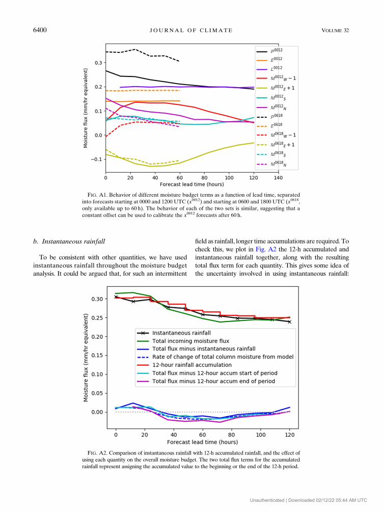
b. Instantaneous rainfall

To be consistent with other quantities, we have used

instantaneous rainfall throughout the moisture budget

analysis. It could be argued that, for such an intermittent

field as rainfall, longer time accumulations are required. To

check this, we plot in Fig. A2 the 12-h accumulated and

instantaneous rainfall together, along with the resulting

total flux term for each quantity. This gives some idea of

the uncertainty involved in using instantaneous rainfall:

FIG. A1. Behavior of different moisture budget terms as a function of lead time, separated

into forecasts starting at 0000 and 1200 UTC (x0012) and starting at 0600 and 1800 UTC (x0618,

only available up to 60 h). The behavior of each of the two sets is similar, suggesting that a

constant offset can be used to calibrate the x0012 forecasts after 60 h.

FIG. A2. Comparison of instantaneous rainfall with 12-h accumulated rainfall, and the effect of

using each quantity on the overall moisture budget. The two total flux terms for the accumulated

rainfall represent assigning the accumulated value to the beginning or the end of the 12-h period.



note that the 12-h accumulation is not a better quantity to

use because it samples parts of the diurnal cycle that are not

sampled by the other quantities in themoisture budget. It is

clear from Fig. A2 that the overall conclusions from this

study, relating to the rainfall field,would not be affected if a

longer accumulated period was used for the rainfall.

c. Calculation of significance intervals

The significance intervals were calculated using a sim-

ple bootstrapping method, based on determining the

sensitivity of the calculation to the precise period used.

For each spatially averaged quantity x, the data were

divided into pairs of forecasts, one starting at 0000 or

1200 UTC (lasting the full 120h) and the other 6h later

(lasting 60h). Equations (A4), (A5), and (A7) were then

applied, with the 0000 or 1200 UTC forecast taking the

role of (x0000 1 x1200)/2 and the 0600 or 1800 UTC fore-

cast taking the role of (x12001 x1800)/2, to produce a set of

172 forecasts, for each quantity and for each lead time.

The bootstrapping was applied by constructing, for

each lead time, 10 000 sequences of 172 forecasts, each

randomly selected from the 172 values available (i.e.,

with replacement, so it was possible to select the same

forecast more than once in any given sequence). The

mean value of x was then taken over each of the 10 000

sequences, to produce 10 000 estimates of x. These es-

timates were sorted and the 250th-highest estimate was

taken as the upper bound and the 9750th-highest esti-

mate as the lower bound. In this way, an estimate of the

95% significance interval was produced.

REFERENCES

Adler, R. F., andCoauthors, 2003: TheVersion-2Global Precipitation

Climatology Project (GPCP) monthly precipitation analysis

(1979–present). J. Hydrometeor., 4, 1147–1167, https://doi.org/

10.1175/1525-7541(2003)004,1147:TVGPCP.2.0.CO;2.

Birch, C. E., D. J. Parker, J. H. Marsham, D. Copsey, and L. Garcia-

Carreras, 2014: A seamless assessment of the role of convection

in the water cycle of the west Africanmonsoon. J.Geophys. Res.

Atmos., 119, 2890–2912, https://doi.org/10.1002/2013JD020887.

Brown, A., S. Milton, M. Cullen, B. Golding, J. Mitchell, and

A. Shelly, 2012: Unified modeling and prediction of weather

and climate: A 25-year journey. Bull. Amer. Meteor. Soc., 93,

1865–1877, https://doi.org/10.1175/BAMS-D-12-00018.1.

Bush, S. J., A. G. Turner, S. J. Woolnough, G. M. Martin, and N. P.

Klingaman, 2015: The effect of increased convective entrainment

on Asian monsoon biases in the MetUM general circulation

model. Quart. J. Roy. Meteor. Soc., 141, 311–326, https://doi.org/

10.1002/qj.2371.

Chakraborty, A., and S. Agrawal, 2017: Role of west Asian surface

pressure in summer monsoon onset over central India. Environ.

Res. Lett., 12, 074002, https://doi.org/10.1088/1748-9326/aa76ca.

Dee, D. P., and Coauthors, 2011: The ERA-Interim reanalysis: Con-

figuration and performance of the data assimilation system.Quart.

J. Roy. Meteor. Soc., 137, 553–597, https://doi.org/10.1002/qj.828.

Devanand, A., M. K. Roxy, and S. Ghosh, 2018: Coupled land–

atmosphere regional model reduces dry bias in Indian summer

monsoon rainfall simulated by CFSv2.Geophys. Res. Lett., 45,

2476–2486, https://doi.org/10.1002/2018GL077218.

Gadgil, S., and J. Srinivasan, 2012: Monsoon prediction: Are dy-

namical models getting better than statistical models. Curr.

Sci., 103, 257–259.

Hou, A. Y., and Coauthors, 2014: The Global Precipitation Mea-

surement Mission. Bull. Amer. Meteor. Soc., 95, 701–722, https://

doi.org/10.1175/BAMS-D-13-00164.1.

Huffman, G. J., and Coauthors, 2007: The TRMM Multisatellite Pre-

cipitation Analysis (TMPA): Quasi-global, multiyear, combined-

sensor precipitation estimates at fine scales. J. Hydrometeor., 8,

38–55, https://doi.org/10.1175/JHM560.1.

——, R. F. Adler, D. T. Bolvin, and E. J. Nelkin, 2010: The TRMM

Multi-Satellite Precipitation Analysis (TMPA). Satellite Rainfall

Applications for Surface Hydrology, Springer, 3–22, https://

doi.org/10.1007/978-90-481-2915-7_1.

Johnson, S. J., and Coauthors, 2016: The resolution sensitivity of

the South Asian monsoon and Indo-Pacific in a global 0.358AGCM. Climate Dyn., 46, 807–831, https://doi.org/10.1007/

s00382-015-2614-1.

——, A. Turner, S. Woolnough, G. Martin, and C. MacLachlan,

2017: An assessment of Indian monsoon seasonal forecasts

and mechanisms underlying monsoon interannual variability

in the Met Office GloSea5-GC2 system. Climate Dyn., 48,

1447–1465, https://doi.org/10.1007/s00382-016-3151-2.

Joshi, M., and S. C. Kar, 2016: Value-added quantitative medium-

range rainfall forecasts for the BIMSTEC region. Meteor.

Appl., 23, 491–502, https://doi.org/10.1002/met.1573.

Klocke,D., andM. J.Rodwell, 2014:A comparison of two numerical

weather prediction methods for diagnosing fast-physics errors

in climate models. Quart. J. Roy. Meteor. Soc., 140, 517–524,

https://doi.org/10.1002/qj.2172.

Krishnamurti, T. N., A. Thomas, A. Simon, and V. Kumar, 2010:

Desert air incursions, an overlooked aspect, for the dry spells

of the Indian summer monsoon. J. Atmos. Sci., 67, 3423–3441,

https://doi.org/10.1175/2010JAS3440.1.

Kumar, A., and Coauthors, 2017: Block level weather forecast

using direct model output from NWPmodels during monsoon

season in India. Mausam, 68, 23–40.

Levine, R. C., and A. G. Turner, 2012: Dependence of Indian

monsoon rainfall on moisture fluxes across the Arabian Sea

and the impact of coupled model sea surface temperature

biases. Climate Dyn., 38, 2167–2190, https://doi.org/10.1007/

s00382-011-1096-z.

——, and G. M. Martin, 2018: On the climate model simulation of

Indian monsoon low pressure systems and the effect of remote

disturbances and systematic biases. Climate Dyn, 50, 4721–

4743, https://doi.org/10.1007/s00382-017-3900-x.

——, A. G. Turner, D. Marathayil, and G. M. Martin, 2013: The

role of northern Arabian Sea surface temperature biases in

CMIP5 model simulations and future projections of Indian

summer monsoon rainfall. Climate Dyn., 41, 155–172, https://

doi.org/10.1007/s00382-012-1656-x.

Martin, G. M., and R. C. Levine, 2012: The influence of dynamic

vegetation on the present-day simulation and future pro-

jections of the South Asian summer monsoon in the

HadGEM2 family. Earth Syst. Dyn., 3, 245–261, https://

doi.org/10.5194/esd-3-245-2012.

——, S. F. Milton, C. A. Senior, M. E. Brooks, S. Ineson,

T. Reichler, and J. Kim, 2010: Analysis and reduction of sys-

tematic errors through a seamless approach to modeling



https://doi.org/10.1175/1525-7541(2003)004<1147:TVGPCP>2.0.CO;2

https://doi.org/10.1175/1525-7541(2003)004<1147:TVGPCP>2.0.CO;2

https://doi.org/10.1002/2013JD020887

https://doi.org/10.1175/BAMS-D-12-00018.1

https://doi.org/10.1002/qj.2371


https://doi.org/10.1088/1748-9326/aa76ca


https://doi.org/10.1002/2018GL077218



https://doi.org/10.1175/JHM560.1

https://doi.org/10.1007/978-90-481-2915-7_1

https://doi.org/10.1007/978-90-481-2915-7_1

https://doi.org/10.1007/s00382-015-2614-1

https://doi.org/10.1007/s00382-015-2614-1

https://doi.org/10.1007/s00382-016-3151-2

https://doi.org/10.1002/met.1573


https://doi.org/10.1175/2010JAS3440.1

https://doi.org/10.1007/s00382-011-1096-z

https://doi.org/10.1007/s00382-011-1096-z

https://doi.org/10.1007/s00382-017-3900-x

https://doi.org/10.1007/s00382-012-1656-x

https://doi.org/10.1007/s00382-012-1656-x

https://doi.org/10.5194/esd-3-245-2012

https://doi.org/10.5194/esd-3-245-2012

weather and climate. J. Climate, 23, 5933–5957, https://doi.org/

10.1175/2010JCLI3541.1.

Mitra, A. K., G. R. Iyengar, V. R. Durai, J. Sanjay, T. N.

Krishnamurti, A.Mishra, andD. R. Sikka, 2011: Experimental

real-time multi-model ensemble (MME) prediction of rainfall

during monsoon 2008: Large-scale medium-range aspects.

J. Earth Syst. Sci., 120, 27–52, https://doi.org/10.1007/s12040-

011-0013-5.

——, andCoauthors, 2013: Prediction of monsoon using a seamless

coupled modelling system. Curr. Sci., 104, 1369–1379.

Parker, D. J., P. Willetts, C. Birch, A. G. Turner, J. H. Marsham,

C. M. Taylor, S. Kolusu, and G. M. Martin, 2016: The in-

teraction of moist convection and mid-level dry air in the ad-

vance of the onset of the Indian monsoon. Quart. J. Roy.

Meteor. Soc., 142, 2256–2272, https://doi.org/10.1002/qj.2815.Pathak, A., S. Ghosh, J. A.Martinez, F. Dominguez, and P. Kumar,

2017: Role of oceanic and land moisture sources and transport

in the seasonal and interannual variability of summer mon-

soon in India. J. Climate, 30, 1839–1859, https://doi.org/10.1175/JCLI-D-16-0156.1.

Prakash, S., A. K. Mitra, I. M. Momin, E. N. Rajagopal, S. F.

Milton, and G. M. Martin, 2016: Skill of short- to medium-

range monsoon rainfall forecasts from two global models over

India for hydro-meteorological applications. Meteor. Appl.,

23, 574–586, https://doi.org/10.1002/met.1579.

Ranade, A., A.Mitra, N. Singh, and S. Basu, 2014: A verification of

spatio-temporal monsoon rainfall variability across Indian

region using NWP model output. Meteor. Atmos. Phys., 125,

43–61, https://doi.org/10.1007/S00703-014-0317-5.

Ringer, M. A., and Coauthors, 2006: Global mean cloud feedbacks

in idealized climate change experiments. Geophys. Res. Lett.,

33, L07718, https://doi.org/10.1029/2005GL025370.

Rodwell, M. J., and T. N. Palmer, 2007: Using numerical weather

prediction to assess climate models. Quart. J. Roy. Meteor.

Soc., 133, 129–146, https://doi.org/10.1002/qj.23.

Roxy, M. K., S. Ghosh, A. Pathak, R. Athulya, M. Mujumdar,

R. Murtugudde, P. Terray, andM. Rajeevan, 2017: A threefold

rise in widespread extreme rain events over central India. Nat.

Commun., 8, 708, https://doi.org/10.1038/S41467-017-00744-9.

Sahana, A. S., A. Pathak, M. K. Roxy, and S. Ghosh, 2019: Un-

derstanding the role of moisture transport on the dry bias in

Indian monsoon simulations by CFSv2.Climate Dyn., 52, 637–

651, https://doi.org/10.1007/S00382-018-4154-Y.

Sperber, K. R., H. Annamalai, I.-S. Kang, A. Kitoh, A. Moise,

A. Turner, B. Wang, and T. Zhou, 2013: The Asian summer

monsoon: An intercomparison of CMIP5 vs. CMIP3 simula-

tions of the late 20th century. Climate Dyn., 41, 2711–2744,https://doi.org/10.1007/s00382-012-1607-6.

Walters, D. N., and Coauthors, 2011: The Met Office Unified

Model Global Atmosphere 3.0/3.1 and JULES Global Land

3.0/3.1 configurations.Geosci. Model Dev., 4, 919–941, https://doi.org/10.5194/gmd-4-919-2011.

——, and Coauthors, 2017: The Met Office Unified Model Global

Atmosphere 6.0/6.1 and JULES Global Land 6.0/6.1 configu-

rations. Geosci. Model Dev., 10, 1487–1520, https://doi.org/

10.5194/gmd-10-1487-2017.

Willetts, P. D., J. H.Marsham,C. E. Birch,D. J. Parker, S.Webster,

and J. Petch, 2017: Moist convection and its upscale effects in

simulations of the Indian monsoon with explicit and parame-

trized convection.Quart. J. Roy. Meteor. Soc., 143, 1073–1085,

https://doi.org/10.1002/qj.2991.

Yanai, M., S. Esbensen, and J.-H. Chu, 1973: Determination of bulk

properties of tropical cloud clusters from large-scale heat and

moisture budgets. J. Atmos. Sci., 30, 611–627, https://doi.org/

10.1175/1520-0469(1973)030,0611:DOBPOT.2.0.CO;2.

Zangvil, A., D. H. Portis, and P. J. Lamb, 2001: Investigation

of the large-scale atmospheric moisture field over the

midwestern United States in relation to summer pre-

cipitation. Part I: Relationships between moisture budget

components on different timescales. J. Climate, 14, 582–

597, https://doi.org/10.1175/1520-0442(2001)014,0582:

IOTLSA.2.0.CO;2.

——, ——, and ——, 2004: Investigation of the large-scale atmo-

spheric moisture field over the midwestern United States in

relation to summer precipitation. Part II: Recycling of local

evapotranspiration and association with soil moisture and

crop yields. J. Climate, 17, 3283–3301, https://doi.org/10.1175/

1520-0442(2004)017,3283:IOTLAM.2.0.CO;2.



https://doi.org/10.1175/2010JCLI3541.1

https://doi.org/10.1175/2010JCLI3541.1

https://doi.org/10.1007/s12040-011-0013-5

https://doi.org/10.1007/s12040-011-0013-5


https://doi.org/10.1175/JCLI-D-16-0156.1

https://doi.org/10.1175/JCLI-D-16-0156.1

https://doi.org/10.1002/met.1579

https://doi.org/10.1007/S00703-014-0317-5

https://doi.org/10.1029/2005GL025370


https://doi.org/10.1038/S41467-017-00744-9

https://doi.org/10.1007/S00382-018-4154-Y

https://doi.org/10.1007/s00382-012-1607-6

https://doi.org/10.5194/gmd-4-919-2011

https://doi.org/10.5194/gmd-4-919-2011

https://doi.org/10.5194/gmd-10-1487-2017

https://doi.org/10.5194/gmd-10-1487-2017


https://doi.org/10.1175/1520-0469(1973)030<0611:DOBPOT>2.0.CO;2

https://doi.org/10.1175/1520-0469(1973)030<0611:DOBPOT>2.0.CO;2

https://doi.org/10.1175/1520-0442(2001)014<0582:IOTLSA>2.0.CO;2

https://doi.org/10.1175/1520-0442(2001)014<0582:IOTLSA>2.0.CO;2

https://doi.org/10.1175/1520-0442(2004)017<3283:IOTLAM>2.0.CO;2

https://doi.org/10.1175/1520-0442(2004)017<3283:IOTLAM>2.0.CO;2

fast biases in monsoon rainfall over southern and central

Documents