econstor www.econstor.eu

Der Open-Access-Publikationsserver der ZBW – Leibniz-Informationszentrum WirtschaftThe Open Access Publication Server of the ZBW – Leibniz Information Centre for Economics

Nutzungsbedingungen:Die ZBW räumt Ihnen als Nutzerin/Nutzer das unentgeltliche,räumlich unbeschränkte und zeitlich auf die Dauer des Schutzrechtsbeschränkte einfache Recht ein, das ausgewählte Werk im Rahmender unter→ http://www.econstor.eu/dspace/Nutzungsbedingungennachzulesenden vollständigen Nutzungsbedingungen zuvervielfältigen, mit denen die Nutzerin/der Nutzer sich durch dieerste Nutzung einverstanden erklärt.

Terms of use:The ZBW grants you, the user, the non-exclusive right to usethe selected work free of charge, territorially unrestricted andwithin the time limit of the term of the property rights accordingto the terms specified at→ http://www.econstor.eu/dspace/NutzungsbedingungenBy the first use of the selected work the user agrees anddeclares to comply with these terms of use.

zbw Leibniz-Informationszentrum WirtschaftLeibniz Information Centre for Economics

Rahim, Fazeer; Tavares, José

Conference Paper

Family matters: endogenous gender discrimination ineconomic development

Proceedings of the German Development Economics Conference, Berlin 2011, No. 69

Provided in Cooperation with:Research Committee on Development Economics (AEL), GermanEconomic Association

Suggested Citation: Rahim, Fazeer; Tavares, José (2011) : Family matters: endogenous genderdiscrimination in economic development, Proceedings of the German Development EconomicsConference, Berlin 2011, No. 69

This Version is available at:http://hdl.handle.net/10419/48315

Family matters: endogenous gender discrimination

in economic development∗

Fazeer Rahim† Jose Tavares‡

June 2010

Abstract

We present a growth model where savings, fertility, labour forceparticipation and gender wage discrimination are endogenously deter-mined. Households consist of husband and wife, who disagree on howto allocate resources to their individual consumption. Household deci-sions are made by bargaining and the bargaining power of each spousedepends on the market income he/she brings home. This providesthe basis for the reluctance of men to grant women equal access tolabour markets despite the fact that this hurts them in terms of re-duced family income. Economic development makes discriminationcostlier, initiating a positive cycle of high female participation, lowfertility and high growth. Our empirical study is in two parts. Firstly,we use cross-country micro data to test the hypothesis that develop-ment is negatively related to male ‘preference for discrimination’. Weshow that men’s views converge to those of women over the develop-ment process and that, for low levels of income, a large majority ofmen have discriminatory views. Our conclusion is that a turning pointoccurs at an annual per capita GDP of around $15000. Secondly, weexploit the National Longitudinal Survey of Youth 1979 to find outwhat cause individuals to change their discriminatory preferences overtime.

JEL Codes: D13, J7, J13, J16, 015Keywords: Economic Development, Fertility, Female Labor Force

Participation, Gender Discrimination

1 Introduction

Economic development and the role and rights of women in society are in-terconnected. In particular, economic development appears to be associated∗This paper has benefited from the financial support of the Fundacao para a Ciencia e

Tecnologia(FCT). We thank Colin Cameron and participants at a seminar at UniversidadeNova de Lisboa for useful comments.†Faculdade de Economia, Universidade Nova de Lisboa; email: fsrahim@fe.unl.pt‡Corresponding Author: Jose Tavares, Universidade Nova de Lisboa and Center for

Economic Policy Research (CEPR). Address: Faculdade de Economia, Universidade Novade Lisboa, Campus de Campolide, Lisboa, Portugal 1099-032. Tel.: +351-21-380-1669;fax: +351-21-388-6078; email: jtavares@fe.unl.pt

1

with high levels of female labor force participation (FLP) and lower genderwage gaps.

Galor and Weil (1996) offer a theory of rising female labor force partic-ipation and declining fertility in economic development. It is based on thepositive feedback on capital accumulation and the gender wage gap. Casualobservation suggests that, although declining, the gender wage gap remainssizable even in advanced economies1. Our proposition is that the genderwage gap is not just the result of physical differences between men andwomen, but it is also caused by a gender bias in the workplace. We suggestthat this bias is rooted in a family conflict regarding resource allocation andwe show how economic development influences this conflict.

More precisely, we introduce a collective model of the family where hus-band and wife bargain on resource allocation. Essential in our analysis isthe assumption that the husband loses some bargaining power when thewife’s contribution to family income increases. This provides the basis forthe reluctance of men to grant women equal access to labour markets despitethe fact that this hurts family income. For low levels of development, menwould forgo the increased income from women earning the market wage theydeserve in favor of having more bargaining power at home. Increased capitalaccumulation makes it financially costlier for them to stick to their genderbias. Support for discrimination wanes out, initiating a positive cycle ofhigh female participation, low fertility and high growth.

The idea that dominant groups can choose to give up some of their priv-ileges for purely selfish considerations can be found in a variety of contexts,such as the abolition of slavery (Wright 2006), the spread of public educa-tion to the masses (Galor and Moav 2006) or the extension of voting rights(Acemoglu and Robinson 2000, Lizzeri and Persico 2004). More specifically,there is a growing literature on the extension of voting and legal rights towomen. Bertocchi (2007) attribute the extension of voting rights to womenas the consequence of a falling gender wage gap, which reduces the divergencebetween men and women on the size and scope of government2. Geddes andLueck (2002) claim that, when the returns to human capital are sufficientlyhigh, it is in the interest of men to loosen their control over women as an in-centive for the latter to invest more in education. They support their claimby showing that the cross-state variations in the timing at which propertyrights were granted to women in the 19th century in the U.S. are relatedto differences in female human capital. Doepke and Tertilt (2009) offer amodel where men are torn between having the upper hand at home withtheir wives and the welfare of their daughters. An important implication isthat, when fertility falls and wealth is accumulated, men are faced with anincreasing welfare gap between their sons and daughters since the financial

1According to O’Neill (2003), at least 10% of the gender wage gap in the U.S. isunaccounted for by differences in schooling, tenure and occupational choice

2There is a growing literature on the consequences of the extension of voting rightsto women on government size and policy (Lott and Kenny 1999, Aidt, Dutta, andLoukoianova 2006, Funk and Gathmann 2006). More generally, Cavalcanti and Tavares(2003) show how increasing FLP alters government size.

2

transfers made to their daughters are captured by sons-in-laws. This com-pels them to commit to better women rights. Fernandez (2009) supportsthis claim by showing that states that had lower levels of fertility reformedearlier in the U.S. Our paper builds on this literature but we instead focuson what can be termed as the ‘right to equal pay’. Unlike in Doepke andTertilt (2009) and Fernandez (2009) in which there a discrete shift from aso-called ‘patriarchal’ regime to an ‘egalitarian’ one, our approach considerschanges in household bargaining as a gradual, continuous process.

Attributing the root cause of a gender bias in the workplace to the fam-ily, as we do, is not uncommon in the literature. In Becker (1985), divisionof labor within the family, which leaves effort-intensive tasks (such as childcare and household chores) to women, forces them to expend less effort thanmen in the market place or to select into less-demanding occupations. Alongthe same lines, Albanesi and Olivetti (2006) present a model in which thereis division of labor at home and utility cost of work is increasing in homehours. They show that, under imperfect information about effort, employerspay women less as they expect women to exert less effort than men at work.This reinforces further household division of labor, making employers’ ex-pectations self-fulfilling. Economic development, by improving the relativereturn to market work, may break this cycle. Others have emphasized tech-nological improvements as key factors that led women into the labor force(e.g. in the form of time-saving home goods (Greenwood, Seshadri, andYorukoglu 2005), contraceptive methods Goldin and Katz (2002) or medicalimprovements in childbearing (Albanesi and Olivetti 2007)). In Fernandez,Fogli, and Olivetti (2004), intergenerational transmission of values is keyto understanding changes in gender bias: men who grew up with workingmothers have more progressive attitudes towards FLP and housework.

Finally, our work is related to the literature which consider how changesin the economic, legal or technological environment alter bargaining withinthe household. Chiappori and Oreffice (2008) model the impact of techno-logical improvements in birth control on the empowerment of women, whileAkerlof, Yellen, and Katz (1996) and Oreffice (2007) assess on the impactof legalization of abortion on married women’s bargaining position.

2 Model

2.1 The Environment

Production technology: Consider the following production function withthree factors of production, physical capital (K), mental labor (Lm) andphysical labor (Lp). Mental labor is a complement to physical capital whilephysical labor is neither a complement nor a substitute to physical capital.

Yt = Kαt (AtLmt )1−α +BAtL

pt (1)

where At = (1 + µ)t , B > 0

3

The returns to the factors of production are

wpt = AtB (2)wmt = (1− α)Atkαt m

−αt (3)

rt = αkα−1t m1−α

t (4)

where kt = Kt/(AtLpt ) and mt = Lmt /L

pt

As in Galor and Weil (1996), it is assumed that men are endowed withboth physical and mental labor while women are endowed with mental laboronly. As the return to mental labor is increasing in physical capital, a highercapital stock leads, ceteris paribus, to a lower gender gap.

Discrimination: It is assumed that a fraction of what women earn frommarket work is “melted” away due to discrimination. Thus, women earn afraction φt of their mental wage.

Individual preferences: Agents have equal probabilities of being bornmale or female and they live for three periods. During childhood, an agent israised by father and mother. During adulthood, which also correspond to theproductive years of the agent both in terms of production and fertility, twoagents of opposite sexes form a couple, make choices regarding labour supply,fertility and savings and decide on the allocation of old-age savings betweenthe two. During old age, each consumes income saved during adulthood.

Husband and wife have the following utility functions (respectively uhtand uwt ), valuing their own old-age consumption (respectively dht+1 and dwt+1)and the number of children (nt).

uht = ln dht+1 + γ lnntuwt = ln dwt+1 + γ lnnt

where γ ∈ (0, 1)

Fertility: The household labor supply is lt and as in Greenwood, Seshadri,and Vandenbroucke (2005), children are assumed to be costly in terms ofparental time only.

nt = D(2− lt)θ (5)

where D > 0; θ > 0; lt ∈ (0, 2)

Household preferences: Following Chiappori (1988), we consider a col-lective utility function of the household which takes the following form

ut = η(φt) ln dht+1 + (1− η(φt)) ln dwt+1 + γ lnnt (6)

where η(φt) is the husband’s Pareto weight; η′(·) < 0

4

2.2 Household maximisation

Budget Constraints: We note that since the opportunity cost of raisingchildren is always higher for the husband than for the wife, husbands onlyget involved in raising children if lt < 1.

dht+1 + dwt+1 ≤{

(1 + rt+1)(wpt + wmt )lt if lt ≤ 1(1 + rt+1)(wpt + wmt + (lt − 1)φtwmt ) if lt > 1

(7)

Thus, the household problem reduces to choosing its collective labor supply,lt and the husband’s old-age consumption, dht+1.

In order to allow for women to participate in the labor force, we assumethat the utility from children is low enough and raising children is costlyenough in time that the household chooses a fertility level that is compatiblewith the husband devoting all his time endowment to market work.

Assumption 1. γθ ≤ 1

Choices: The chosen level of FLP and male old-age consumption are thus

lt = max{

1, 2− γθ

1 + γθ

(1 + φtφt

+wptφtwmt

)}(8)

dht+1 = (1 + rt+1) · η(φt) · st (9)

st ={wpt + wmt if lt = 1

11+γθ · (w

pt + (1 + φt)wmt ) if lt > 1 (10)

2.3 Endogenous discrimination

At a household level, gender wage discrimination is taken as given. It re-duces the amount of time spent by women in the labor force (consequentlyincreasing fertility) and it also increases the share of household savings thatgoes to the husband. At the economy-wide level, men are called upon tochoose the coefficient φt. For the sake of simplicity, they are given the choicebetween two 2 possible values: φl and φh, where φh > φl.

Male utilities in the two possible configurations are

uht ={

ln η(φl) + ln(1 + rt+1) + ln st(φl) + γ lnD + γθ ln(2− lt(φl)) if φ = φlln η(φh) + ln(1 + rt+1) + ln st(φh) + γ lnD + γθ ln(2− lt(φh)) if φ = φh

Men benefit from high discrimination as this increases their share ofhousehold resources. However, high discrimination is costly in terms oftotal earnings of the family. When FLP is zero, the cost of discrimination tomen is also zero, meaning that they will vote always choose φl. We thereforefocus on the case where lt > 1. Define umt as the utility difference for menbetween choosing low discrimination and choosing high discrimination:

uht = uht (φh)− uht (φl) = ln

((1 + (1 + φh)ωt)

1+γθ φγθl ηh

(1 + (1 + φl)ωt)1+γθφγθh ηl

)

5

where ωt = wmt /wpt

Note that

∂uh

∂ωt=

((1 + γθ)(φh − φl)

(1 + (1 + φl)ωt)(1 + (1 + φh)ωt)

)> 0

Denote the ratio mental wage - physical wage for which men are indif-ferent between high and low discrimination as ω:

ω =

(φγθh ηl

φγθl ηh

)1/(1+γθ)

− 1

1 + φh −(φγθh ηl

φγθl ηh

)1/(1+γθ)

(1 + φl)

2.4 Equilibrium

Equilibrium in the market for mental labour: In the market for men-tal labor: Lmt = Lpt lt. Using this equilibrium condition, replacing equations2 and 3 into 8 yields

l(kt) = max{

1, 2− γθ

1 + γθ

(1 + φ(kt)φ(kt)

+B

φ(kt)(1− α)kαt l(kt)−α

)}(11)

where

φ(kt) ={φl for B−1(1− α)kαt l(kt)

−α ≤ ωφh for B−1(1− α)kαt l(kt)

−α ≥ ω (12)

Proposition 1. lt is increasing with kt. There exists k such that

φ(kt) ={φl for kt ≤ kφh for kt ≥ k

Proof. Using the Implicit Function Theorem on equation 11, we have3

∂lt∂kt

=

Bγαk−1

t lt

(1+γθ)φl(1−α)kαt l1−αt +Bγα

> 0 if B−1(1− α)kαt l−αt < ω

Bγαk−1t lt

(1+γθ)φh(1−α)kαt l1−αt +Bγα

> 0 if B−1(1− α)kαt l−αt > ω

Using the above and the fact that ωt = B−1(1− α)kαt l(kt)−α, we have

∂ωt∂kt

=

α(1+γθ)φlω

2t ltk

−1t

(1+γθ)φlωtlt+γα> 0 if kt < k

α(1+γθ)φhω2t ltk

−1t

(1+γθ)φhωtlt+γα> 0 if kt > k

where k =(Bωl(k)α

1−α

)1/α

3Note that l(kt) is not differentiable for B−1(1− α)kαt l−αt = ω

6

Capital Market Equilibrium: The condition that equilibrates the cap-ital market is

Kt+1 = Lpt st (13)

This gives us

kt+1 =st

(1 + µ)AthθtD

We first identify the value of kt after which FLP is positive:

k =(

Bγθ

(1− α) (φl − γθ)

)1/α

We can deduce that for k < k,

kt+1 =

B+(1−α)kαt

(1+µ)D if kt ≤ k(φl(1−α)kαt l(kt)

−α)θ((1+φl)(1−α)kαt l(kt)−α+B)1−θ

D(1+µ)(γθ)θ(1+γθ)1−θif k < kt < k

(φh(1−α)kαt l(kt)−α)θ((1+φh)(1−α)kαt l(kt)

−α+B)1−θ

D(1+µ)(γθ)θ(1+γθ)1−θif kt > k

(14)

In the above situation, FLP is zero until kt reaches k. On entering thelabor market, women face high discrimination, until k is reaches at whichpoint the economy switches to low discrimination. We can also envisage asituation where k is reached before k, in which case the dynamics of kt is asfollows

kt+1 =

B+(1−α)kαt

(1+µ)D if kt ≤ k(φh(1−α)kαt l(kt)

−α)θ((1+φh)(1−α)kαt l(kt)−α+B)1−θ

D(1+µ)(γθ)θ(1+γθ)1−θif kt > k

(15)

Using the fact that for kt < k, l(k) = 1, we can find the condition underwhich k > k:

ηlηh

<

(1 + γθφhφl

1 + γθ

)1+γθ (φlφh

)γθ(16)

Figure 1 shows two different configurations depending on condition 16. Thefirst (figure i) is when the male share of household income does not varymuch from the high discrimination regime to the low discrimination one(i.e. ηl/ηh is low). In this case, the switch to low discrimination occursearly, at a time when women are not yet participating in the labor force.The second (figure ii) is when men stand to lose significantly from the switchfrom high discrimination to low discrimination (i.e. ηl/ηh is high). In thiscase, when women join the labor force, they face high discrimination andonly later does the regime switch occur. Casual empiricism suggests thatthe first configuration is not the norm as rising FLP usually precedes fallinggender wage gaps.4

4For instance, in the case of the U.S., the gender wage gap started falling in the 1970swhile FLP rose substantially from the 1940s onwards.

7

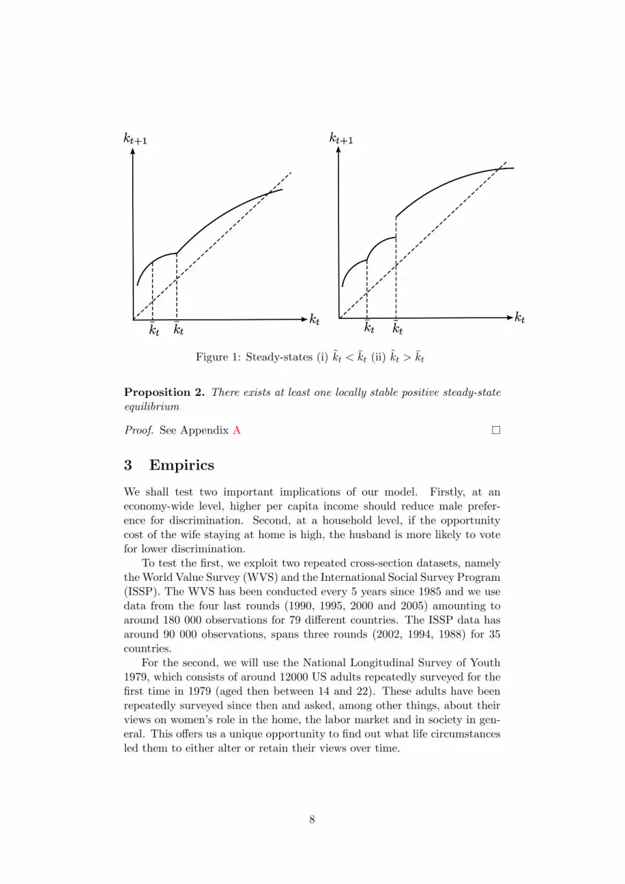
Figure 1: Steady-states (i) kt < kt (ii) kt > kt

Proposition 2. There exists at least one locally stable positive steady-stateequilibrium

Proof. See Appendix A

3 Empirics

We shall test two important implications of our model. Firstly, at aneconomy-wide level, higher per capita income should reduce male prefer-ence for discrimination. Second, at a household level, if the opportunitycost of the wife staying at home is high, the husband is more likely to votefor lower discrimination.

To test the first, we exploit two repeated cross-section datasets, namelythe World Value Survey (WVS) and the International Social Survey Program(ISSP). The WVS has been conducted every 5 years since 1985 and we usedata from the four last rounds (1990, 1995, 2000 and 2005) amounting toaround 180 000 observations for 79 different countries. The ISSP data hasaround 90 000 observations, spans three rounds (2002, 1994, 1988) for 35countries.

For the second, we will use the National Longitudinal Survey of Youth1979, which consists of around 12000 US adults repeatedly surveyed for thefirst time in 1979 (aged then between 14 and 22). These adults have beenrepeatedly surveyed since then and asked, among other things, about theirviews on women’s role in the home, the labor market and in society in gen-eral. This offers us a unique opportunity to find out what life circumstancesled them to either alter or retain their views over time.

8

3.1 Cross-Country Differences

3.1.1 Methodology

From the WVS and the ISSP datasets, we identify 6 variables which cancapture individual ‘preference for discrimination’. All variables are set in away that a higher value represents a higher preference for discrimination.

1. JBPRIOR: “When jobs are scarce, men should have more right to ajob than women”. 1 - disagree, 2 - neither, 3 - agree. (Source: WVS)

2. HMEKIDS: “What women really want is home and kids”. 1 - stronglydisagree, 2 - disagree, 3 - neither, 4 - agree, 5 - strongly agree. (Source:ISSP)

3. HSEWORK: “Housework satisfies as much as paid work”. 1 - stronglydisagree, 2 - disagree, 3 - neither, 4 - agree, 5 - strongly agree. (Source:ISSP)

4. INDEP: “Work is best for women’s independence”. 1 - strongly agree,2 - agree, 3 - neither, 4 - disagree, 5 - strongly disagree.(Source: ISSP)

5. CONTRIB: “Both husband and wife should contribute to householdincome”. 1 - strongly agree, 2 - agree, 3 - neither, 4 - disagree, 5 -strongly disagree. (Source: ISSP)

6. PLACEHOME: “Men’s job is at work and women’s job is in the house-hold”. 1 - strongly disagree, 2 - disagree, 3 - neither, 4 - agree, 5 -strongly agree. (Source: ISSP)

Repeated cross-section: We estimate the following model

Yi = β0 + β1Mi + β2logGDPi + β3Mi ∗ logGDPi + β4X′i + β5D

′i + εi (17)

where Yi is the ordered response of individual i to the above questions; Mi

is an indicator variable which takes a value of 1 if the respondent is male;logGDP is the log of GDP of the country of residence of the respondent; X ′iis a vector of controls which varies according to the chosen specification; Di

is a set of dummy variables.For variable JBPRIOR, the controls variables, Xi consist of the age of

the respondent (AGE), his/her marital status (MARRIED), his/her edu-cation level (EDUC), his/her marital status the number of children he/shehas (CHILD), the size of the town he/she lives in (TOWNSIZE), his/herreported degree of religiosity (RELIGIOSITY). The set of dummy variablesconsists of (1) country dummies, i.e. the respondent’s country of residence,(2) cultural dummies, i.e. the cultural group to which the country is asso-ciated with (based on Inglehart-Welzel Cultural Map of the World) and (3)the occupation type of the respondent.

For variables (2) - (6), the control variables consist of the age of therespondent (AGE), his/her marital status (MARRIED), his/her education

9

level (EDUC) and whether he/she lives in urban or rural areas (URBAN).The set of dummy variables consists of (1) country dummies and (2) religiondummies, i.e. the respondent’s religion.

For dependent variables (1) -(6), probit regressions are carried out. Fromvariables (2) - (6), a latent variable is generated from factor analysis and isdenoted Index, for which OLS regressions are carried out. We are particu-larly aware of the fact that clustering in repeated cross-section data leads togrossly under-estimated standard errors (see Moulton 1990, Bertrand, Du-flo, and Mullainathan 2004, Kezdi 2004). In addition to the usual standarderror estimates, we therefore report “cluster-robust” standard errors thatcluster by country. We also report “cluster-robust” standard errors thatcluster by country and time following the estimator developed by Cameron,Gelbach, and Miller (2010).5

Pseudo panel: From the repeated cross-section WVS and ISSP data, weconstruct pseudo-panel data, according to the method proposed by Deaton(1985). We build our cohorts around 4 birth-year bands (before 1939, 1940-1954, 1955-1969, after 1970), 4 education groups (primary education, sec-ondary education, higher education), 2 sex groups and 80 countries for WVS/ 38 countries for ISSP, giving 2560 cohort-year observations for the WVSdata and 1216 cohort-year observations for the ISSP data. We run bothfixed-effect and random-effect regressions and run Hausman test to choosebetween them.

Yit = β0 + β1Mi + β2logGDPit + β3Mi ∗ logGDPit + β4X′i + εi (18)

where Yi is the average response of cohort i; Mi is an indicator variablewhich takes a value of 1 if the cohort is male; logGDP is the log of GDPof the country of residence of the cohort; X ′i is a vector of time-invariantcontrols.

3.1.2 Results

Repeated cross-section: Figure 2 shows the inverse relationship betweenthe variables that characterize preference for gender discrimination and logGDP. Controlling for individual-specific characteristics such as education,age, religiosity, number of children, respondent’s town size, tables 3 and4 confirm this relationship. Additionally, we can see that although menare more discriminatory than women (the negative coefficient on the maledummy), their views converge to those of women (as shown by the negativecoefficient on the interaction variable LOGGDP*MALE), which is line withour model.

Accounting for potential clustering in the data (i.e. models (2) and (3)in tables 3 and 4) increases considerably the standard errors, as expected

5The code used for the ordered probit regressions is adapted from Mitchell Petersen’sStata routine that allows for two-way clustering. Code available upon request.

10

(up to a ten-fold increase in some cases). Nevertheless, all the coefficientsremain significant.

The coefficients on the control variables suggest that (i) older people, lesseducated people, people with more children, people living in smaller towns,and religious people tend to have more discriminatory views. Although notreported here, all regressions have also been carried out without the dummyvariables, and the results do not change.

Pseudo panel data: From table 5, we are led to conclude that an increasein GDP leads to a reduction in the ”preference for discrimination”.

3.1.3 Predicted probabilities

Figure 6(a) shows the predicted probabilities of the respondent agreeing thatjob priority be given to men when jobs are scarce, conditional on the genderand on the country GDP of the respondents. Both men and women becomeless discriminatory as GDP increases, but the decline is more significantfor men. Figures 6(b) to 6(f) show predicted probabilities from the ISSPvariables. Again, men become less discriminatory as GDP increases and thegap between men and women declines with GDP.

3.2 Changes in preferences

The National Longitudinal Survey of Youth 1979 enables us to understandhow life circumstances influence people’s attitude to gender roles. In fouroccasions (1979, 1982, 1987 and 2004), the same adults (aged between 14and 22 in 1979) are asked whether they strongly agree, agree, disagree orstrongly disagree with the following statements:

1. “A woman’s place is at home, not in the office” (PLACEHOME)

2. “It is much better for everyone if the man is the achiever outside thehome and the woman takes care of the home and family” (TRAD-ROLE)

3. “Women are much happier if they stay at home and take care of chil-dren” (HAPPIER).

We regroup responses into two categories, agree (consisting of those whoagree and those who strongly agree with the given statement) and disagree(consisting of those who agree and those who strongly agree). For eachvariable, we construct the following latent variable:

W =

0 for Y1987 = agree & Y2004 = agree1 for Y1987 = disagree & Y2004 = agree2 for Y1987 = agree & Y2004 = disagree3 for Y1987 = disagree & Y2004 = disagree

where Y1987 and Y2004 represent variables PLACEHOME, TRADROLE andHAPPIER as observed in 1987 and 2004.

11

Table 7 summarizes the proportion of respondent who fall in the differentcategories.

We restrict our analysis to married men and women and consider poten-tial explanatory variables which can lead respondents to alter or keep theiropinion from 1987 to 2004: race (given by HISP and BLACK), the levelof education (EDUC) and the ratio of spouse’s income to respondent’s ownincome (RATIOINCOME).

We consider a multinomial probit model, using 0 as a base (table 8).Firstly, we find out that both for men and women, the level of education pos-itively influences the probability of keeping non-discriminatory views from1987 to 2004 (i.e. the respondent disagreed with the given statement bothin 1987 and 2004). Secondly, the spouse-respondent income ratio also posi-tively influences (1) the probability of keeping non-discriminatory views from1987 to 2004, (2) the probability of switching from discriminatory views in1987 to non-discriminatory views in 2004, in the case of men only. Thisratio has no role in women’s decision to keep or alter their views. This pro-vides a foundation for the following statement: that, controlling for theirown level of education, men married to high-income women tend to improvetheir attitude towards working women over time.

4 Conclusion

12

A Proof of Proposition 2

1. For k ≤ k, kt+1, as given by equation 15, is continuous.

• When kt < k we have

∂kt+1

∂kt=

(1− α)αkα−1t

(1 + µ)D> 0

∂2kt+1

∂k2t

=−(1− α)2αkα−2

t

(1 + µ)D< 0

limkt→0

∂kt+1

∂kt= lim

kt→0

(1− α)αkα−1t

(1 + µ)D=∞

• When kt > k,

∂kt+1

∂kt=

kt+1

kt·((1 + γθ)φh(1− α)kαt l

1−αt

(1 + γθ)φh(1− α)kαt l1−αt +Bγα

)·(

(1− θ)α(1 + φh)(1− α)kαt l−αt + θα

(1 + φh)(1− α)kαt l−αt +B

)> 0

∂kt+1

∂kt=

(φh(1− α)kαt lt)−α)θ

((1 + φh)(1− α)kαt l

−αt +B

)1−θD(1 + µ) (γθ)θ (1 + γθ)1−θkt

·((1 + γθ)φh(1− α)kαt l

1−αt

(1 + γθ)φh(1− α)kαt l1−αt +Bγα

)·(

(1− θ)α(1 + φh)(1− α)kαt l−αt + θα

(1 + φh)(1− α)kαt l−αt +B

)> 0

limkt→∞

∂kt+1

∂kt= 0

2. For k ≥ k, kt+1, as given by equation 14, is not continuous.

B Alternative specifications

We check the robustness of the theoretical results by allowing for alternativespecifications.

B.1 Bargaining power depends on female wage income

Following Chiappori (1988), we consider a collective utility function of thehousehold which takes the following form

ut = η(max(0, )) ln dht+1 + (1− η(max(0, )) ln dwt+1 + γ lnnt (19)

where η(φt) is the husband’s Pareto weight; η′(·) < 0

13

B.2 Disutility from home production

We assume here that there is a home good that needs to be produced (e.g.washing up, cooking) and this requires time. Both men and women getdisutility from time spent producing this household good

uh = ln dt + γ lnnt − ρ(2− lt)δ (20)

ut = ln dt + γ lnnt − ρ(2− lt)δ (21)

References

Acemoglu, D., and J. A. Robinson (2000): “Why Did the West Extendthe Franchise? Democracy, Inequality, and Growth in Historical Perspec-tive,” The Quarterly Journal of Economics, 115(4), 1167–1199. 2

Aidt, T. S., J. Dutta, and E. Loukoianova (2006): “Democracy comesto Europe: Franchise extension and fiscal outcomes 1830-1938,” EuropeanEconomic Review, 50(2), 249–283. 2

Akerlof, G. A., J. L. Yellen, and M. L. Katz (1996): “An Analysisof Out-of-Wedlock Childbearing in the United States,” The QuarterlyJournal of Economics, 111(2), 277–317. 3

Albanesi, S., and C. Olivetti (2006): “Home Production, Market Pro-duction and the Gender Wage Gap: Incentives and Expectations,” NBERWorking Paper No. 12212. 3

(2007): “Gender Roles and Technological Progress,” National Bu-reau of Economic Research Working Paper No. 13179. 3

Becker, G. S. (1985): “Human Capital, Effort, and the Sexual Divisionof Labor,” Journal of Labor Economics, 3(1), S33–S58. 3

Bertocchi, G. (2007): “The Enfranchisement of Women and the WelfareState,” IZA Discussion Paper No. 2922. 2

Bertrand, M., E. Duflo, and S. Mullainathan (2004): “How MuchShould We Trust Differences-in-Differences Estimates?,” The QuarterlyJournal of Economics, 119(1), 249–275. 10

Cameron, A. C., J. B. Gelbach, and D. L. Miller (2010): “RobustInference with Multi-way Clustering,” Journal of Business and EconomicStatistics, forthcoming. 10

Cavalcanti, T. V. d. V., and J. Tavares (2003): “Women Prefer LargerGovernments: Female Labour Supply and Public Spending,” mimeo, Uni-versidade Nova de Lisboa. 2

14

ALB

ARG

ARM

AUS

AZE

BFA

BGD

BGRBIH

BLR

BRA

CANCHE

CHL

CHN

COL

CYPCZE

DEUDMA

DZA

EGY

ESP

EST

ETHFIN FRAGBR

GEOGHA

GTM HKG

HUN

IDNIND

IRN

ITA

JOR

JPN

KGZ

KORLTU

LVA

MAR

MDA

MEX

MKD

MLI

MNE

MYSNGA

NLDNORNZL

PAK

PER

PHL

POLROM

RUS

RWA

SAU

SER

SGP

SLV

SRBSVK

SVN

SWE

THA

TTO

TUR

TZA

UGA

UKR

URY

USA

VENVMN

VNM

ZAFZMB

0.2

.4.6

.81

% o

f m

en w

ho a

gre

eth

at jo

bs p

riority

should

be g

iven to m

en

6 7 8 9 10 11Log per capita GDP

AUSAUT

BGR

BRA

CAN

CHE

CHL

CYP

CZE

DEU

DNK

ESPFINFRA

GBR

HUN

IRL

ISR

ITAJPNLVA

MEX

NLD

NORNZL

PHL

POL

PRT

RUS

SVK

SVN

SWE

USA

.2.4

.6.8

% o

f m

en w

ho a

gre

eth

at w

hat w

om

en r

eally

want is

hom

e a

nd k

ids

7 8 9 10 11Log per capita GDP

AUSAUT

BGR

BRA

CAN

CHECHL

CYP

CZE

DEU

DNK

ESP

FINFRAGBR

HUN

IRL

ISR

ITA

JPN

LVA

MEX

NLDNOR

NZL

PHL

POLPRT

RUS

SVKSVN

SWE

USA

0.2

.4.6

.8

% o

f m

en w

ho a

gre

eth

at household

satisfies

as m

uch a

s p

aid

job

7 8 9 10 11Log per capita GDP

AUS

AUT

BGR

BRA

CAN

CHECHL CYP

CZE

DEU

DNKESP

FIN

FRA

GBR

HUN

IRLISR

ITA

JPN

LVA

MEX

NLD

NOR

NZL

PHL

POL

PRT

RUS

SVK

SVNSWE

USA

.4.5

.6.7

.8

% o

f m

en w

ho d

isagre

eth

at w

ork

is b

est fo

rw

om

en independence

7 8 9 10 11Log per capita GDP

AUS

AUT

BGR

BRA

CANCHE

CHLCYP

CZE

DEU

DNK

ESP

FINFRA

GBR

HUN

IRL

ISR

ITA

JPN

LVAMEX

NLD

NOR

NZL

PHL

POL

PRT

RUS

SVK

SVN

SWE

USA

.2.4

.6.8

1

% o

f m

en w

ho d

isagre

e that

both

men a

nd w

om

en s

hould

contr

ibute

to h

ousehold

incom

e

7 8 9 10 11Log per capita GDP

AUS

AUT

BGRBRA

CAN

CHE

CHL

CYP

CZE

DEU

DNK

ESP

FIN

FRAGBR

HUN

IRLISR

ITA JPN

LVAMEX

NLD

NOR

NZL

PHL

POL

PRT

RUS

SVK

SVN

SWE

USA

0.2

.4.6

.8

% o

f m

en w

hic

h a

gre

eth

at household

is w

ife’s

job

7 8 9 10 11Log per capita GDP

Figure 2: Male preference for discrimination and GDP

15

Chiappori, P.-A. (1988): “Rational Household Labour Supply,” Econo-metrica, 56(1), 63–90. 4, 13

Chiappori, P.-A., and S. Oreffice (2008): “Birth Control and FemaleEmpowerment: An Equilibrium Analysis,” The Journal of Political Econ-omy, 116(1), 113–140. 3

Deaton, A. (1985): “Panel Data from Time Series of Cross-Sections,”Journal of Econometrics, 30, 109–126. 10

Doepke, M., and M. Tertilt (2009): “Women’s Liberation: What’s inIt for Men?,” The Quarterly Journal of Economics, 124(4). 2, 3

Fernandez, R. (2009): “Women’s Rights and Development,” NBER Work-ing Paper 15355. 3

Fernandez, R., A. Fogli, and C. Olivetti (2004): “Mothers and Sons:Preference Formation and Female Labour Force Dynamics,” QuarterlyJournal of Economics, 119(4), 1249–1299. 3

Funk, P., and C. Gathmann (2006): “What Women Want: Suffrage,Gender Gaps in Voter Preferences and Government Expenditures,” Work-ing Paper. 2

Galor, O., and O. Moav (2006): “Das Human-Kapital: A Theory ofthe Demise of the Class Structure,” Review of Economic Studies, 73(1),85–117. 2

Galor, O., and D. N. Weil (1996): “The Gender Gap, Fertility, andGrowth,” The American Economic Review, 86(3), 374–387. 2, 4

Geddes, R., and D. Lueck (2002): “The Gains from Self-Ownership andthe Expansion of Women’s Rights,” The American Economic Review,92(4), 1079–1092. 2

Goldin, C., and L. F. Katz (2002): “The Power of the Pill: Oral Con-traceptives and Women’s Career and Marriage Decisions,” The Journalof Political Economy, 110(4), 730–770. 3

Greenwood, J., A. Seshadri, and G. Vandenbroucke (2005): “TheBaby Boom and Baby Bust,” The American Economic Review, 95(1),183–207. 4

Greenwood, J., A. Seshadri, and M. Yorukoglu (2005): “Engines ofLiberation,” The Review of Economic Studies, 72(1), 109–133. 3

Kezdi, G. (2004): “Robust Standard Error Estimation in Fixed-EffectsPanel Models,” Hungarian Statistical Review, 9, 95–116. 10

16

Lizzeri, A., and N. Persico (2004): “Why Did the Elites Extend theSuffrage? Democracy and the Scope of Government, With an Applica-tion to Britain’s ¨Age of Reform¨,” The Quarterly Journal of Economics,119(2), 705–763. 2

Lott, John R., J., and L. W. Kenny (1999): “Did Women’s SuffrageChange the Size and Scope of Government?,” The Journal of PoliticalEconomy, 107(6), 1163–1198. 2

Moulton, B. R. (1990): “An Illustration of a Pitfall in Estimating theEffects of Aggregate Variables on Micro Units,” The Review of Economicsand Statistics, 72(2), 334–338. 10

O’Neill, J. (2003): “The Gender Gap in Wages, circa 2000,” The AmericanEconomic Review, 93(2), 309–314. 2

Oreffice, S. (2007): “Did the Legalization of Abortion Increase Women’sHousehold Bargaining Power? Evidene from Labour Supply?,” Review ofthe Economics of the Household, 5(2), 181–207. 3

Wright, G. (2006): Slavery and American Economic Development.Louisiana State University Press, Baton Rouge. 2

17

JBP

RIO

RJB

PR

IOR

JBP

RIO

RJB

PR

IOR

JBP

RIO

RJB

PR

IOR

JBP

RIO

RJB

PR

IOR

JBP

RIO

R(1

)(1

)(1

)(2

)(2

)(2

)(3

)(3

)(3

)v4

4M

ain

Eff

ects

:L

OG

GD

P-0

.237

∗∗∗

-0.2

09∗∗∗

-0.2

34∗∗∗

-0.2

37∗∗

-0.2

09∗∗

-0.2

34∗∗

-0.2

37∗∗

-0.2

09∗∗

-0.2

34∗

(0.0

141)

(0.0

145)

(0.0

169)

(0.0

960)

(0.0

949)

(0.1

159)

(0.1

010)

(0.0

981)

(0.1

239)

MA

LE

0.93

3∗∗∗

1.00

5∗∗∗

0.93

3∗∗∗

1.00

5∗∗∗

0.93

3∗∗∗

1.00

5∗∗∗

(0.0

519)

(0.0

550)

(0.1

409)

(0.1

476)

(0.1

194)

(0.1

045)

LO

GG

DP

*MA

LE

-0.0

72∗∗∗

-0.0

75∗∗∗

-0.0

72∗∗∗

-0.0

75∗∗∗

-0.0

72∗∗∗

-0.0

75∗∗∗

(0.0

060)

(0.0

064)

(0.0

157)

(0.0

166)

(0.0

153)

(0.0

126)

Con

trol

s:M

AR

RIE

D-0

.016

∗∗∗

-0.0

16∗∗∗

-0.0

16∗∗∗

(0.0

018)

(0.0

037)

(0.0

059)

AG

E0.

005∗

∗∗0.

005∗

∗∗0.

005∗

∗∗

(0.0

003)

(0.0

009)

(0.0

008)

ED

UC

-0.0

60∗∗∗

-0.0

60∗∗∗

-0.0

60∗∗∗

(0.0

018)

(0.0

053)

(0.0

062)

CH

ILD

0.01

0∗∗∗

0.01

0∗∗∗

0.01

0∗∗∗

(0.0

022)

(0.0

031)

(0.0

039)

TO

WN

SIZ

E-0

.016

∗∗∗

-0.0

16∗

-0.0

16∗∗

(0.0

013)

(0.0

088)

(0.0

070)

RE

LIG

IOSI

TY

0.09

2∗∗∗

0.09

2∗∗∗

0.09

2∗∗∗

(0.0

041)

(0.0

138)

(0.0

107)

Cou

ntry

dum

mie

sY

esY

esY

esY

esY

esY

esY

esY

esY

esC

ultu

ral

dum

mie

sY

esY

esY

esY

esY

esY

esY

esY

esY

esO

ccup

atio

ndu

mm

ies

Yes

Yes

Yes

Yes

Yes

Yes

Yes

Yes

Yes

Pse

udoR

-squ

are

0.10

20.

109

0.12

10.

102

0.10

90.

121

Log

Lik

elih

ood

-141

676

-140

448

-124

903

-141

676

-140

448

-124

903

-141

676

-140

448

-124

903

Obs

.15

2321

1522

8713

7552

1523

2115

2287

1375

5215

2321

1522

8713

7552

∗p<

0.1

0,∗∗p<

0.0

5,∗∗∗p<

0.0

1

Fig

ure

3:O

rder

edpr

obit

regr

essi

ons

usin

g4

roun

dsof

WV

S-

1990

,19

95,

2000

,20

05(A

llre

spon

dent

s).

All

regr

essi

ons

incl

ude

aco

nsta

nt.

*si

gnifi

canc

eat

10%

,**

sign

ifica

nce

at5%

,**

*si

gnifi

canc

eat

1%.

Stan

dard

erro

rsin

pare

nthe

sis:

(1)

robu

stst

anda

rder

rors

wit

hno

clus

teri

ng,

(2)

clus

tere

dst

anda

rder

rors

inco

untr

ydi

men

sion

,(3

)cl

uste

red

stan

dard

erro

rsin

coun

try

and

tim

edi

men

sion

s)

18

HM

EK

IDS

HSW

OR

KIN

DE

PH

ME

KID

SH

SWO

RK

IND

EP

HM

EK

IDS

HSW

OR

KIN

DE

P(1

)(1

)(1

)(2

)(2

)(2

)(3

)(3

)(3

)m

ain

LO

GG

DP

-0.3

16∗∗∗

-0.3

29∗∗∗

-0.1

77∗∗∗

-0.3

16∗∗

-0.3

29∗∗∗

-0.1

77∗∗

-0.3

16∗∗∗

-0.3

29∗∗∗

-0.1

77∗∗∗

(0.0

267)

(0.0

267)

(0.0

269)

(0.1

340)

(0.0

786)

(0.0

702)

(0.0

110)

(0.0

277)

(0.0

269)

MA

LE

0.14

5∗∗∗

0.08

6∗∗∗

0.11

5∗∗∗

0.14

5∗∗∗

0.08

6∗∗∗

0.11

5∗∗∗

0.14

5∗∗∗

0.08

6∗∗∗

0.11

5∗∗∗

(0.0

098)

(0.0

098)

(0.0

100)

(0.0

180)

(0.0

198)

(0.0

207)

(0.0

098)

(0.0

227)

(0.0

100)

ED

UC

-0.2

94∗∗∗

-0.1

66∗∗∗

-0.0

31∗∗∗

-0.2

94∗∗∗

-0.1

66∗∗∗

-0.0

31∗

-0.2

94∗∗∗

-0.1

66∗∗∗

-0.0

31∗∗∗

(0.0

075)

(0.0

075)

(0.0

077)

(0.0

175)

(0.0

184)

(0.0

179)

(0.0

085)

(0.0

116)

(0.0

077)

AG

E0.

013∗

∗∗0.

009∗

∗∗-0

.003

∗∗∗

0.01

3∗∗∗

0.00

9∗∗∗

-0.0

03∗∗∗

0.01

3∗∗∗

0.00

9∗∗∗

-0.0

03∗∗∗

(0.0

003)

(0.0

003)

(0.0

003)

(0.0

010)

(0.0

010)

(0.0

012)

(0.0

017)

(0.0

013)

(0.0

003)

UR

BA

N0.

030∗

∗∗0.

029∗

∗∗0.

013∗

∗∗0.

030∗

0.02

9∗∗

0.01

3∗∗∗

0.03

0∗∗∗

0.02

9∗∗∗

0.01

3∗∗∗

(0.0

036)

(0.0

036)

(0.0

037)

(0.0

172)

(0.0

113)

(0.0

045)

(0.0

039)

(0.0

050)

(0.0

037)

Cou

ntry

dum

mie

sY

esY

esY

esY

esY

esY

esY

esY

esR

elig

ion

dum

mie

sY

esY

esY

esY

esY

esY

esY

esY

esL

ogL

ikel

ihoo

d-5

8868

-597

09-5

4655

-588

68-5

9709

-546

55-5

8868

-597

09-5

4655

Obs

.62

155

6179

363

032

6215

561

793

6303

262

155

6179

363

032

∗p<

0.1

0,∗∗p<

0.0

5,∗∗∗p<

0.0

1

CO

NT

RIB

PL

AC

EH

OM

EIN

DE

XC

ON

TR

IBP

LA

CE

HO

ME

IND

EX

CO

NT

RIB

PL

AC

EH

OM

EIN

DE

X(1

)(1

)(1

)(2

)(2

)(2

)(3

)(3

)(3

)m

ain

LO

GG

DP

-0.4

08∗∗∗

-0.5

30∗∗∗

-0.3

54∗∗∗

-0.4

08∗∗∗

-0.5

30∗∗∗

-0.3

54∗∗∗

-0.4

08∗∗∗

-0.5

30∗∗∗

-0.3

54∗∗∗

(0.0

282)

(0.0

271)

(0.0

166)

(0.0

952)

(0.1

296)

(0.0

877)

(0.0

282)

(0.1

021)

(0.0

384)

MA

LE

0.11

2∗∗∗

0.27

3∗∗∗

0.15

6∗∗∗

0.11

2∗∗∗

0.27

3∗∗∗

0.15

6∗∗∗

0.11

2∗∗∗

0.27

3∗∗∗

0.15

6∗∗∗

(0.0

106)

(0.0

099)

(0.0

061)

(0.0

209)

(0.0

166)

(0.0

108)

(0.0

106)

(0.0

100)

(0.0

059)

ED

UC

0.03

4∗∗∗

-0.3

51∗∗∗

-0.2

18∗∗∗

0.03

4-0

.351

∗∗∗

-0.2

18∗∗∗

0.03

4∗∗∗

-0.3

51∗∗∗

-0.2

18∗∗∗

(0.0

081)

(0.0

078)

(0.0

047)

(0.0

251)

(0.0

186)

(0.0

130)

(0.0

081)

(0.0

102)

(0.0

078)

AG

E0.

002∗

∗∗0.

019∗

∗∗0.

011∗

∗∗0.

002∗

∗0.

019∗

∗∗0.

011∗

∗∗0.

002∗

∗∗0.

019∗

∗∗0.

011∗

∗∗

(0.0

003)

(0.0

003)

(0.0

002)

(0.0

011)

(0.0

014)

(0.0

010)

(0.0

003)

(0.0

016)

(0.0

014)

UR

BA

N0.

019∗

∗∗0.

040∗

∗∗0.

028∗

∗∗0.

019∗

∗∗0.

040∗

∗∗0.

028∗

∗0.

019∗

∗∗0.

040

0.02

8(0

.003

8)(0

.003

6)(0

.002

2)(0

.006

0)(0

.013

8)(0

.011

5)(0

.003

8)(.

)(.

)C

ount

rydu

mm

ies

Yes

Yes

Yes

Yes

Yes

Yes

Yes

Yes

Rel

igio

ndu

mm

ies

Yes

Yes

Yes

Yes

Yes

Yes

Yes

Yes

Log

Lik

elih

ood

-464

74-5

6198

-624

83-4

6474

-561

98-6

2483

-464

74-5

6198

-624

83O

bs.

6411

664

329

5771

664

116

6432

957

716

6411

664

329

5771

6∗p<

0.1

0,∗∗p<

0.0

5,∗∗∗p<

0.0

1

Fig

ure

4:R

egre

ssio

ns(O

rder

edP

robi

tfo

rco

lum

nsH

meK

ids,

Hsw

ork,

Pla

ceH

ome

and

OL

Sfo

rIn

dex)

usin

g3

roun

dsof

ISSP

-19

88,

1994

,200

2.St

anda

rder

rors

inpa

rent

hesi

s.*

sign

ifica

nce

at10

%,*

*si

gnifi

canc

eat

5%,*

**si

gnifi

canc

eat

1%(1

)no

clus

teri

ng,(

2)cl

uste

red

stan

dard

erro

rsin

coun

try

dim

ensi

on,

(3)

clus

tere

dst

anda

rder

rors

inco

untr

yan

dti

me

dim

ensi

ons.

19

JBP

RIO

RIT

YH

ME

KID

SH

SWO

RK

IND

EP

CO

NT

RIB

PL

AC

EH

OM

EIN

DE

X(R

.E.)

(F.E

.)(R

.E.)

(F.E

.)(F

.E.)

(F.E

.)(F

.E.)

LO

GG

DP

-0.1

18∗∗∗

-0.4

07∗∗∗

-0.2

80∗∗∗

-0.2

80∗∗∗

-0.1

76∗∗

-0.3

23∗∗∗

-0.2

94∗∗∗

(0.0

110)

(0.0

599)

(0.0

343)

(0.0

750)

(0.0

797)

(0.0

474)

(0.0

389)

LO

GG

DP

*MA

LE

-0.0

51∗∗∗

0.09

30.

022

0.06

8-0

.072

0.04

20.

012

(0.0

152)

(0.0

795)

(0.0

463)

(0.1

034)

(0.1

082)

(0.0

672)

(0.0

517)

MA

LE

-0.6

58∗∗∗

0.07

3(0

.135

7)(0

.449

6)E

DU

C-0

.137

∗∗∗

-0.1

69∗∗∗

(0.0

084)

(0.0

193)

cons

tant

4.54

4∗∗∗

6.54

2∗∗∗

5.80

0∗∗∗

4.74

9∗∗∗

4.19

7∗∗∗

5.57

1∗∗∗

2.71

3∗∗∗

(0.2

115)

(0.3

852)

(0.6

907)

(0.5

006)

(0.5

240)

(0.3

250)

(0.2

502)

Obs

.40

9213

7513

7313

7513

7513

7513

73∗p<

0.1

0,∗∗p<

0.0

5,∗∗∗p<

0.0

1

Fig

ure

5:F

ixed

Effe

cts

(F.E

.)an

dR

ando

mE

ffect

s(R

.E.)

regr

essi

ons

usin

gps

eudo

-pan

elda

ta.

Rob

ust

stan

dard

erro

rsin

pare

nthe

sis.

20

Figure 6: Predicted probabilities by gender

0.1

.2.3

.4.5

.6.7

.8.9

1P

r(Y

| ge

nder

)

600 6000 14000 25000 35000 45000Per capita GDP

men

lower/upper limits (95%)

women

0.0

5.1

.15

.2.2

5.3

.35

.4.4

5.5

Pr(

Y |

man

) −

Pr

(Y |

wom

an)

600 6000 14000 25000 35000 45000Per capita GDP

(a) JobPriority

0.1

.2.3

.4.5

.6.7

.8.9

Pro

b(y

| gen

der)

1500 8000 17000 25000 35000Per capita GDP

men

lower/upper limits (95%)

women

.01

.02

.03

.04

.05

.06

.07

.08

.09

Pr(

y | m

en)

− P

r(y

| wom

en)

1500 8000 17000 25000 35000Per capita GDP

ISSP

(b) HmeKids

0.1

.2.3

.4.5

.6.7

.8.9

Pro

b(y

| gen

der)

1500 8000 17000 25000 35000Per capita GDP

men

lower/upper limits (95%)

women

.01

.02

.03

.04

.05

.06

.07

.08

.09

Pr(

y | m

en)

− P

r(y

| wom

en)

1500 8000 17000 25000 35000Per capita GDP

ISSP

(c) Hsework

0.1

.2.3

.4.5

.6.7

.8.9

Pro

b(y

| gen

der)

1500 8000 17000 25000 35000Per capita GDP

men

lower/upper limits (95%)

women

.01

.02

.03

.04

.05

.06

.07

.08

.09

Pr(

y | m

en)

− P

r(y

| wom

en)

1500 8000 17000 25000 35000Per capita GDP

ISSP

(d) Indep

0.1

.2.3

.4.5

.6.7

.8.9

Pro

b(y

| gen

der)

1500 8000 17000 25000 35000Per capita GDP

men

lower/upper limits (95%)

women

.01

.02

.03

.04

.05

.06

.07

.08

.09

Pr(

y | m

en)

− P

r(y

| wom

en)

1500 8000 17000 25000 35000Per capita GDP

ISSP

(e) Contrib

0.1

.2.3

.4.5

.6.7

.8.9

Pro

b(y

| gen

der)

1500 8000 17000 25000 35000Per capita GDP

men

lower/upper limits (95%)

women

.01

.02

.03

.04

.05

.06

.07

.08

.09

Pr(

y | m

en)

− P

r(y

| wom

en)

1500 8000 17000 25000 35000Per capita GDP

ISSP

(f) PlaceHome

21

PlaceHome TradRole HomeChildren WorkUseful1987→ 2004 Agree Disagree Agree Disagree Agree Disagree Agree DisagreeAgree 256 508 814 1008 859 1060 981 1749Disagree 415 5887 964 4153 778 3611 2342 1629

Figure 7: Transition from 1987 to 2004

PlaceHome PlaceHome TradRole TradRole Happier Happier(1) (2) (3) (4) (5) (6)

Men Women Men Women Men WomenDisagree → AgreeHispanic -0.123 -0.610 -0.394 0.109 -0.546∗ -0.520

(-0.28) (-1.26) (-1.54) (0.37) (-2.33) (-1.73)Black -0.549 0.270 0.122 0.143 0.145 0.075

(-1.04) (0.46) (0.44) (0.50) (0.55) (0.24)Education 0.203 0.383 0.208 0.183 0.314∗ 0.256

(0.90) (1.40) (1.58) (1.23) (2.55) (1.67)spouse incomeown income -0.002 0.014 0.012 -0.032 0.015 -0.007

(-0.02) (0.12) (0.16) (-0.47) (0.23) (-0.11)Agree → DisagreeHispanic 0.594 -0.657 -0.194 -0.026 -0.428 -0.187

(1.48) (-1.38) (-0.77) (-0.09) (-1.60) (-0.61)Black 0.147 -0.779 0.059 -0.368 0.422 -0.017

(0.32) (-1.18) (0.21) (-1.16) (1.50) (-0.05)Education 0.123 0.449 0.007 0.041 0.187 0.124

(0.56) (1.64) (0.05) (0.26) (1.34) (0.76)spouse incomeown income 0.411∗∗∗ -0.209 0.389∗∗∗ -0.053 0.178∗ 0.036

(3.57) (-1.78) (5.44) (-0.75) (2.47) (0.50)Disagree → DisagreeHispanic -0.014 -0.547 -0.499∗ -0.192 -0.751∗∗∗ -0.389

(-0.04) (-1.46) (-2.43) (-0.77) (-3.82) (-1.60)Black 0.314 0.251 -0.010 -0.312 0.156 -0.064

(0.82) (0.50) (-0.04) (-1.27) (0.69) (-0.24)Education 0.574∗∗ 0.719∗∗ 0.357∗∗ 0.469∗∗∗ 0.321∗∗ 0.464∗∗∗

(3.14) (3.10) (3.27) (3.74) (3.01) (3.54)spouse incomeown income 0.429∗∗∗ -0.120 0.328∗∗∗ -0.119∗ 0.252∗∗∗ -0.012

(4.40) (-1.21) (5.61) (-2.12) (4.58) (-0.21)PseudoR-square 0.046 0.023 0.029 0.016 0.021 0.010LogLikelihood -917 -735 -1624 -1397 -1574 -1330LRchi2 89 35 98 46 69 28Obs. 1514 1384 1495 1352 1343 1274

Figure 8: Multinomial logit using NLSY79. z statistics in parenthesis.

22