external shocks and banking crises in developing countries: does the exchange rate regime matter?
TRANSCRIPT
EXTERNAL SHOCKS AND BANKING CRISES
IN DEVELOPING COUNTRIES: DOES THE
EXCHANGE RATE REGIME MATTER?
CHANDIMA MENDIS
CESIFO WORKING PAPER NO. 759CATEGORY 6: MONETARY POLICY AND INTERNATIONAL FINANCE
AUGUST 2002
An electronic version of the paper may be downloaded• from the SSRN website: www.SSRN.com• from the CESifo website: www.CESifo.de
CESifo Working Paper No. 759
EXTERAL SHOCKS AND BANKING CRISES IN
DEVELOPING COUNTRIES: DOES THE
EXCHANGE RATE REGIME MATTER?
Abstract
This paper examines some determinants of banking crises in developingeconomies. Specifically, the effects of terms of trade shocks and capital flows areanalyzed. The choice of the nominal exchange rate regime is found to be a crucialfactor in the way various shocks are transmitted through the monetary sector. Alogit model is used on panel data and preliminary results indicate that countrieswith flexible regimes were able to lessen the impact of external shocks on thedomestic economy. This in turn reduced the likelihood of banking crises.
JEL Classification: E42, E51, G21.
Keywords: banking crises, shocks, exchange rates.
Chandima Mendis1601 18th St, NW, Apt. 1007
Washington DC 20009U.S.A.
1
1. Introduction
The causes and consequences of banking crises have regained prominence after the
recent wave of financial and banking crises in emerging economies. A number of internal
and external factors, such as capital flows, terms of trade shocks, institutional strength and
appreciations of exchange rates have been identified in the literature as contributory factors.
While factors such as interest rates, stock market crashes and public confidence could
seriously affect the performance of a banking system, the type of exchange rate regime could
also be a major determining factor in the way external shocks are transmitted to the banking
sector. This is particularly important in small open developing economies, which are heavily
dependent on volatile primary product exports and foreign capital and where large negative
shocks have the potential to create banking crises.
This paper empirically focuses on the link between external factors and the incidence
of banking crises in developing small open economies, (SOEs). Major banking crises over
the 1970 to 1992 period are identified from existing case studies. Using theoretical priors
from the literature, principal factors that may lead to banking crises in these economies are
modeled in a logistic framework. Particular emphasis is placed on the occurrence of terms of
trade shocks, capital flows, bank lending and how they affect economies under different
nominal exchange rate regimes.
The remainder of the paper is organized as follows. Section II discusses the
theoretical literature. Section III analyzes case studies from the literature and the
2
methodology used to define crisis episodes. Section IV explains the econometric model and
Section V conducts the estimation. Section VI concludes the analysis.
II. Literature on Banking Crisis
We begin by defining a banking crisis, with some commonly cited examples:
“..liquidation of credits that have been built up in a boom. '' Veblen [1904]
`”.. a sharp reduction in the value of banks' assets, resulting in the apparent or realinsolvency of many banks and accompanied by some bank collapse and possiblysome runs.'' Federal Reserve Bank of San Francisco [1985]
''... situation in which a significant group of financial institutions have liabilitiesexceeding the market value of their assets, leading to runs and other portfolio shifts,collapse of some financial firms, and government intervention.'' Sundararajan andBalino [1991]
“.. a non-linear disruption to financial markets in which adverse selection and moralhazard problems become much worse, so that financial markets are unable toefficiently channel funds to those who have the most productive investmentopportunities. '' Frederic Mishkin [1996]
These definitions imply that banking crises have both micro and macro economic
origins. In fact, the interaction of microeconomic and macroeconomic factors could explain a
large number of banking crises in SOEs. Macroeconomic factors such as negative terms of
trade shocks, level and composition of foreign debt, changes in interest rates, recessions and
sudden capital outflows have been suggested as major determinants of crises. Some of these
factors are also conditioned by the nature of the policy environment in place, such as
institutional strength, confidence in government and the type of the nominal exchange rate
regime in operation prior to the occurrence of a crisis. On the microeconomic front,
3
institutional factors relating to bank supervision and regulation, adequate legal and judicial
framework with regard to bankruptcy, law enforcement as well as internationally recognized
accounting standards could also have a bearing on the performance and soundness of a
banking system. In fact, the combination of several of these factors have the potential to
trigger a banking crises.
The theoretical literature for analyzing banking crises is reflective of these numerous
contributory factors, with different models and theories explaining various aspects of banking
crises. While it is impossible to discuss all models pertinent to banking crises, a brief
overview of the main explanations will be conducted. These will be discussed under the
monetary approach to financial crises, asymmetric information and micro theories and the
business cycle view of banking crises. We start with the monetary view and the role played
by exchange rates.
1. Monetary approach and exchange rates
The monetary approach emphasizes the role of money growth and its variability as
the principal determinant of a crisis, Friedman and Schwartz [1963]. A financial crisis need
not occur at any particular stage of the business cycle, but could result from a change in the
monetary base, such as a sudden and erratic tightening of reserve money, or a foreign inflow
which may force financial enterprises to sell assets to meet reserve obligations. This may
reduce asset prices, raise interest rates and threaten solvency. The exchange rate regime is
one of the factors which may affect the way external shocks impact on monetary base and
banking sector. This arises works through the demand for money and the supply of supply.
4
The demand for money is affected through two elements. First there is the
conventional change in the transactions demand component. Second, agents also hold money
as a store of value. The process by which the supply of money is altered depends on the type
of exchange rate regime, i.e. if it is fixed or flexible. If the currency is freely floating, then
the supply of money is determined by the central bank. When the exchange rate is fixed, the
supply of base money is determined by the balance of payments. The Neary [1985] model
analyzes the adjustment process under fixed and floating exchange rates.
The level of real money balances is determined by a conventional money demand
function:
(1) iyPm δα −=−
where i is the domestic interest rate and m, P and y are the logarithms of nominal
money demand, the price level and the level of income. This equation is related to the
nominal exchange rate in two ways. First, the domestic price level P is a weighted average of
the prices of trade and non-traded goods:
(2) .)1( ePP nnn ββ −+=
Secondly, the expected changes in the exchange rate influence the link between the
domestic interest rate i and the world interest rate i* (which the home country is too small to
5
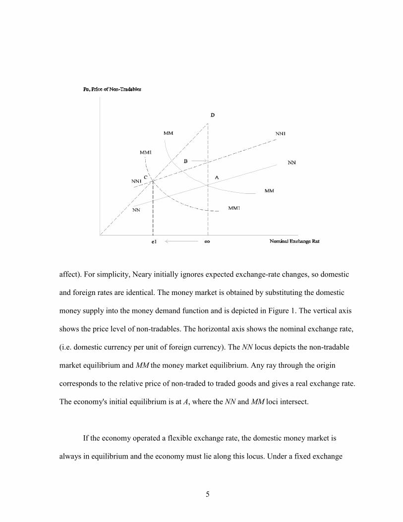
affect). For simplicity, Neary initially ignores expected exchange-rate changes, so domestic
and foreign rates are identical. The money market is obtained by substituting the domestic
money supply into the money demand function and is depicted in Figure 1. The vertical axis
shows the price level of non-tradables. The horizontal axis shows the nominal exchange rate,
(i.e. domestic currency per unit of foreign currency). The NN locus depicts the non-tradable
market equilibrium and MM the money market equilibrium. Any ray through the origin
corresponds to the relative price of non-traded to traded goods and gives a real exchange rate.
The economy's initial equilibrium is at A, where the NN and MM loci intersect.
If the economy operated a flexible exchange rate, the domestic money market is
always in equilibrium and the economy must lie along this locus. Under a fixed exchange
6
rate on the other hand, the economy could be, for example, at a point above the MM locus,
reflecting a shortfall of actual holdings of real money balances below desired holdings. This
disequilibrium must be offset by a buildup of foreign exchange reserves to augment domestic
money supply. Therefore, all points above the MM locus depict situations of balance of
payments surplus and all points below reflect deficits.
The model can be used to analyze the effects of a boom. With a pre-boom equilibrium
A, the increased demand for non-tradables shifts the NN locus upwards to NN1. The increase
in real income also raises demand and if domestic money supply is unchanged, the price level
must fall to restore money market equilibrium. The liquidity effect shifts the MM locus to
MM1. The nominal exchange rate appreciates from e0 to e1, and a new equilibrium C is
reached. The greater slope of OC relative to OA implies a fall in the real exchange rate. This
combined with the nominal appreciation means that the price of domestic tradable goods
unambiguously falls while the price of non-tradables may rise or fall.
Now consider the case when the exchange rate is fixed at e0 . The price of non-
tradables moves the economy to B, and since desired money balances are greater than actual,
the equilibrium at this point cannot be maintained indefinitely. Instead the trade surplus leads
to a build-up of foreign reserves and in the absence of sterilization, money supply gradually
rises. This causes both the MM1 and NN1 curves to shift upwards. This process can only end
when the post-boom equilibrium real exchange rate is attained at point D where the surplus is
eliminated and the economy reaches its new long run equilibrium. In this Neary framework, a
fixed exchange rate increases the real and monetary effects of a boom and gives rise to
7
inflationary pressures as the rise in the price of non-traded goods is brought about by a rise in
the nominal price rather than a fall in the price of tradables. If a large part of this monetary
expansion is transmitted through the banking system in the form of bank credit, a large debt
overhang may result. A slowdown in growth or a recession in subsequent years, may
deteriorate the loan portfolio. A negative shock, such as sudden capital outflows would also
adversely affect the banking sector. Lower foreign reserves and bank liquidity would result in
higher interest rates and subsequently a decline in output and employment. These factors
would increase debt servicing burden of borrowers and increase the potential for default. If
this is systematic across the financial sector, a banking crisis may result.
The situation may be less acute under a floating regime, if most of the debt is
domestic, as capital outflows and reduced demand for real money balances would depreciate
the currency and raise domestic prices. This in turn would reduce the real value of assets of
the banking system (including loans given to the private sector). Furthermore, the real value
of bank liabilities would also fall, lessening the impact of the negative outflow on banks.
Floating exchange rates would also accommodate downward wage rigidity through a
nominal depreciation, after a negative shock or economic slowdown, easing competitive
pressures. The key difference between the fixed and flexible exchange rate scenarios is that
the adjustment in the fixed case mainly affects the supply side and the price level while under
flexible regimes, the adjustment largely takes place through cahnges in the nominal exchange
rate and relative prices.
8
While the transmission of external shocks through different exchange rate regimes
could play a leading role in causing crises, the interaction of various other internal
disturbances and institutional factors could also important in determining banking crises.
These relate to institutional strength with regard to supervision, prudential regulation relating
to connected lending, accounting standards affecting the disclosure of financial information
and an adequate legal environment. Some of these micro theoretic factors are discussed
below.
2. Micro theoretic explanations
The micro view comes from asymmetric information and credit market analysis. The
most commonly discussed approach is the credit rationing situation resulting from various
market failures, Stiglitz and Weiss [1981]. Due to asymmetric information and adverse
selection, banks may ration credit, creating problems for non-financial firms. According to
Mishkin [1996], the problems of moral hazard and adverse selection rise after stock market
crashes. As the value of net worth declines, the moral hazard problem increases as borrowers
have less to lose by making a more risky investment. Demirguc-Kunt and Detragiache,
hereafter DKD [1997], have argued that these problems of moral hazard and adverse
selection are attenuated after financial liberalization in developing countries. While the
benefits of financial liberalization have been well documented in theoretical and empirical
work, hasty liberalization of often weak financial sectors have known to create financial
crises in subsequent years, Diaz-Alexandro [1985]. DKD [1997] address this issue using
cross country data and shows that countries which liberalized with weak institutional and
regulatory frameworks were more susceptible to financial crises in subsequent years.
9
3. Business cycle explanations of banking crises
The business cycle approach looks at the vulnerability of a financial sector over the
business cycle. The financial sector responds endogenously to movements in the business
cycle, see Minsky [1977], Taylor and O'Connell [1985]. A crisis may develop due to
systematic forces near the peak of the cycle as interest rates rise. Reduced lending by banks
and high interest payments may adversely affect non-financial firms, increasing the
likelihood of default. The entire financial sector may suffer after a surprise shock, such as
news of a major bankruptcy. Studies by Calomiris and Garton [1991], Greenwald and Stiglitz
[1988] and Bernanke and Gertler [1988] show that unanticipated shocks such as stock market
crashes could lead to financial crises through the impact on the balance sheets of financial
institutions.
External conditions could also affect assets of the banking sector. Terms of trade
shocks could profoundly affect the profitability of firms and households in primary product
exporting economies. Unanticipated changes in the terms of trade could make debtors unable
to discharge their debts, deteriorating bank balance sheets. Sachs, Tornell and Velasco [1996]
argue that countries with a high proportion of short term debt may end up with a maturity
mismatch due to sudden changes in interest rates and debt service requirements. Eichengreen
and Rose [1998] make the point that this maturity mismatch is attenuated in developing
countries where the average length of maturity is much shorter than in developed countries.
Aligned to this is the problem of currency mismatch, where a large proportion of loans is
denominated in foreign currency, as an exchange rate depreciation may severely increase the
debt service requirement.
10
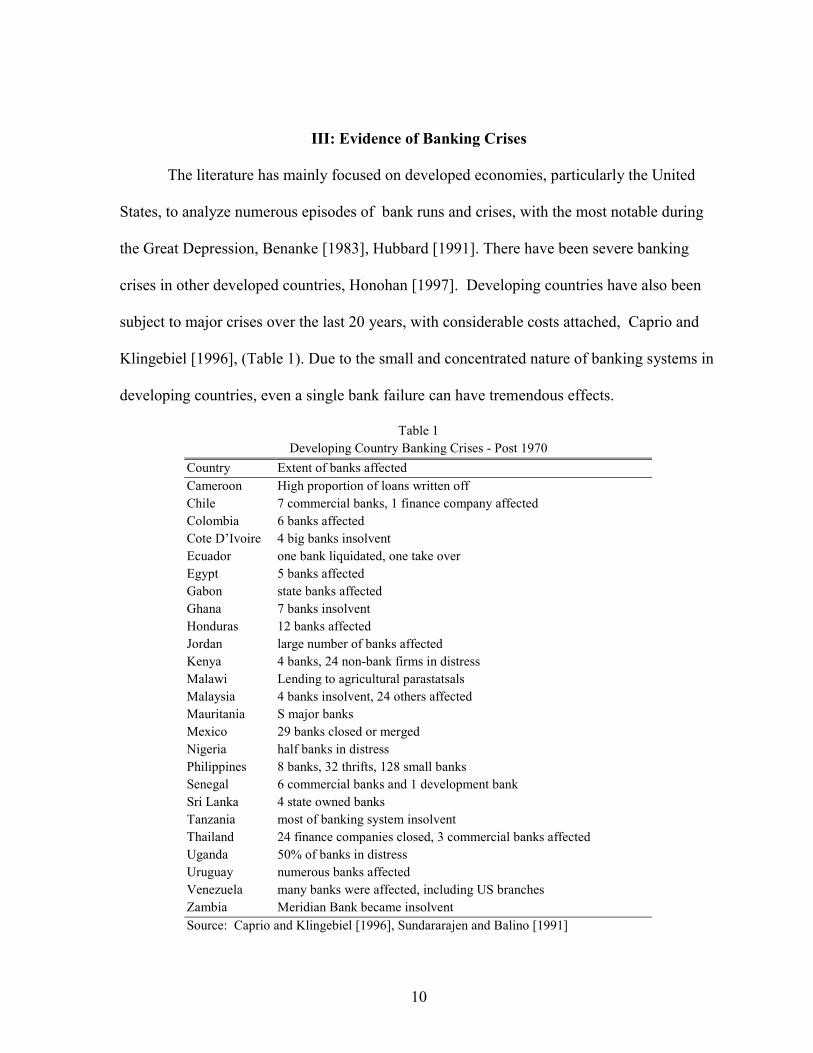
III: Evidence of Banking Crises
The literature has mainly focused on developed economies, particularly the United
States, to analyze numerous episodes of bank runs and crises, with the most notable during
the Great Depression, Benanke [1983], Hubbard [1991]. There have been severe banking
crises in other developed countries, Honohan [1997]. Developing countries have also been
subject to major crises over the last 20 years, with considerable costs attached, Caprio and
Klingebiel [1996], (Table 1). Due to the small and concentrated nature of banking systems in
developing countries, even a single bank failure can have tremendous effects.
Table 1Developing Country Banking Crises - Post 1970
Country Extent of banks affectedCameroon High proportion of loans written offChile 7 commercial banks, 1 finance company affectedColombia 6 banks affectedCote D’Ivoire 4 big banks insolventEcuador one bank liquidated, one take overEgypt 5 banks affectedGabon state banks affectedGhana 7 banks insolventHonduras 12 banks affectedJordan large number of banks affectedKenya 4 banks, 24 non-bank firms in distressMalawi Lending to agricultural parastatsalsMalaysia 4 banks insolvent, 24 others affectedMauritania S major banksMexico 29 banks closed or mergedNigeria half banks in distressPhilippines 8 banks, 32 thrifts, 128 small banksSenegal 6 commercial banks and 1 development bankSri Lanka 4 state owned banksTanzania most of banking system insolventThailand 24 finance companies closed, 3 commercial banks affectedUganda 50% of banks in distressUruguay numerous banks affectedVenezuela many banks were affected, including US branchesZambia Meridian Bank became insolvent
Source: Caprio and Klingebiel [1996], Sundararajen and Balino [1991]
11
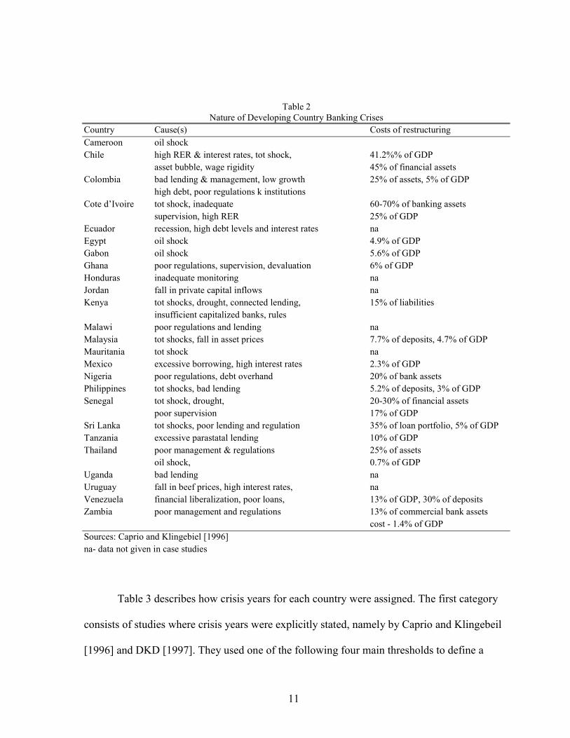
Table 2Nature of Developing Country Banking Crises
Country Cause(s) Costs of restructuring
Cameroon oil shockChile high RER & interest rates, tot shock, 41.2%% of GDP
asset bubble, wage rigidity 45% of financial assetsColombia bad lending & management, low growth 25% of assets, 5% of GDP
high debt, poor regulations k institutionsCote d’Ivoire tot shock, inadequate 60-70% of banking assets
supervision, high RER 25% of GDPEcuador recession, high debt levels and interest rates naEgypt oil shock 4.9% of GDPGabon oil shock 5.6% of GDPGhana poor regulations, supervision, devaluation 6% of GDPHonduras inadequate monitoring naJordan fall in private capital inflows naKenya tot shocks, drought, connected lending, 15% of liabilities
insufficient capitalized banks, rulesMalawi poor regulations and lending naMalaysia tot shocks, fall in asset prices 7.7% of deposits, 4.7% of GDPMauritania tot shock naMexico excessive borrowing, high interest rates 2.3% of GDPNigeria poor regulations, debt overhand 20% of bank assetsPhilippines tot shocks, bad lending 5.2% of deposits, 3% of GDPSenegal tot shock, drought, 20-30% of financial assets
poor supervision 17% of GDPSri Lanka tot shocks, poor lending and regulation 35% of loan portfolio, 5% of GDPTanzania excessive parastatal lending 10% of GDPThailand poor management & regulations 25% of assets
oil shock, 0.7% of GDPUganda bad lending naUruguay fall in beef prices, high interest rates, naVenezuela financial liberalization, poor loans, 13% of GDP, 30% of depositsZambia poor management and regulations 13% of commercial bank assets
cost - 1.4% of GDP
Sources: Caprio and Klingebiel [1996]na- data not given in case studies
Table 3 describes how crisis years for each country were assigned. The first category
consists of studies where crisis years were explicitly stated, namely by Caprio and Klingebeil
[1996] and DKD [1997]. They used one of the following four main thresholds to define a
12
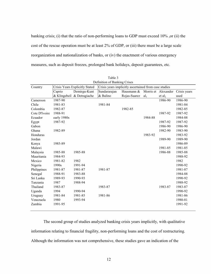
banking crisis; (i) that the ratio of non-performing loans to GDP must exceed 10% ,or (ii) the
cost of the rescue operation must be at least 2% of GDP, or (iii) there must be a large scale
reorganization and nationalization of banks, or (iv) the enactment of various emergency
measures, such as deposit freezes, prolonged bank holidays, deposit guarantees, etc.
Table 3Definition of Banking Crises
Country Crisis Years Explicitly Stated Crisis years implicitly ascertained from case studiesCaprio Demirgu-Kunt Sundararajan Hausmann & Morris et Alexander Crisis years& Klingebeil & Detragiache & Balino Rojas-Suarez al1 et al2 used
Cameroon 1987-90 1986-90 1986-90Chile 1981-83 1981-84 1981-84Colombia 1982-87 1982-85 1982-85Cote D'Ivoire 1988-91 1987-92 1987-92Ecuador early 1980s 1984-88 1984-88Egypt 1987-92 1987-92 1987-92Gabon 1986-90 1986-90Ghana 1982-89 1982-90 1983-90Honduras 1983-92 1983-92Jordan 1989-90 1989-90Kenya 1985-89 1986-89Malawi 1981-85 1981-85Malaysia 1985-88 1985-88 1986-88 1985-88Mauritania 1984-93 1988-92Mexico 1981-82 1982 1982Nigeria 1990s 1991-94 1990-92Philippines 1981-87 1981-87 1981-87 1981-87Senegal 1988-91 1983-88 1984-88Sri Lanka 1989-93 1990-93 1990-92Tanzania 1987 1988-94 1988-92Thailand 1983-87 1983-87 1983-87 1983-87Uganda 1994 1990-94 1990-92Uruguay 1981-84 1981-85 1981-86 1981-86Venezuela 1980 1993-94 1980-81Zambia 1991-95 1991-92
The second group of studies analyzed banking crisis years implicitly, with qualitative
information relating to financial fragility, non-performing loans and the cost of restructuring.
Although the information was not comprehensive, these studies gave an indication of the
13
severity of crises. For the purposes of this paper, common crisis periods were identified from
all six studies. When the crisis periods differed, information from the studies discussing the
crises implicitly were used as they had more detailed in-depth information.
IV: Empirical Estimation
1. Econometric model
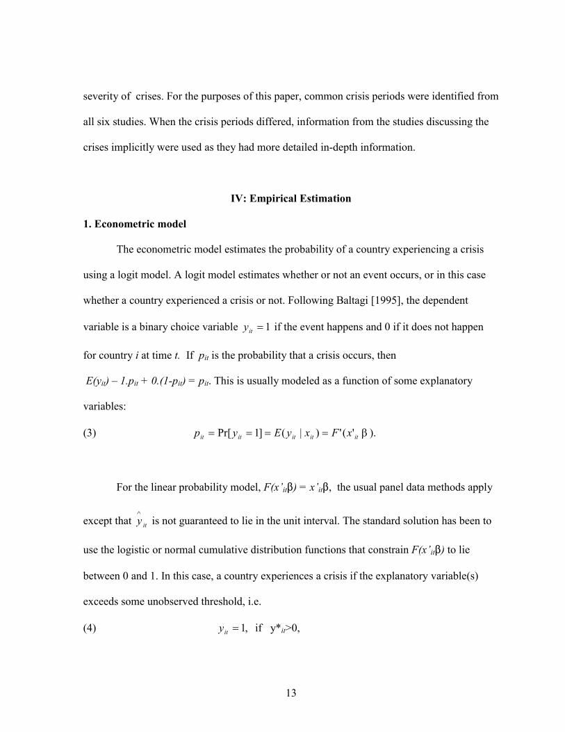
The econometric model estimates the probability of a country experiencing a crisis
using a logit model. A logit model estimates whether or not an event occurs, or in this case
whether a country experienced a crisis or not. Following Baltagi [1995], the dependent
variable is a binary choice variable 1=ity if the event happens and 0 if it does not happen
for country i at time t. If pit is the probability that a crisis occurs, then
E(yit) – 1.pit + 0.(1-pit) = pit. This is usually modeled as a function of some explanatory
variables:
(3) ).'(')|(]1Pr[ βititititit xFxyEyp ====
For the linear probability model, F(x’it$) = x’it$, the usual panel data methods apply
except that ity∧
is not guaranteed to lie in the unit interval. The standard solution has been to
use the logistic or normal cumulative distribution functions that constrain F(x’it$) to lie
between 0 and 1. In this case, a country experiences a crisis if the explanatory variable(s)
exceeds some unobserved threshold, i.e.
(4) ,1=ity if y*it>0,
14
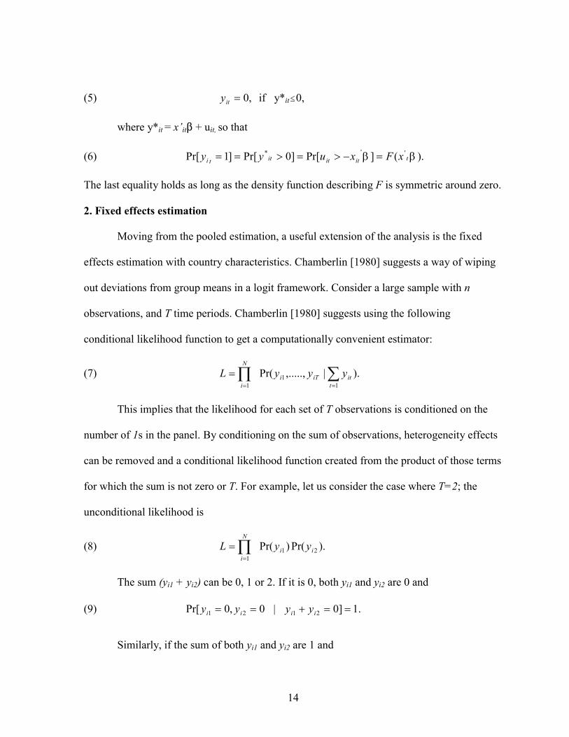
(5) ,0=ity if y*it#0,
where y*it = x’it$ + uit, so that
(6) ).(]Pr[]0Pr[]1Pr[ ''* ββ titititti xFxuyy =−>=>==
The last equality holds as long as the density function describing F is symmetric around zero.
2. Fixed effects estimation
Moving from the pooled estimation, a useful extension of the analysis is the fixed
effects estimation with country characteristics. Chamberlin [1980] suggests a way of wiping
out deviations from group means in a logit framework. Consider a large sample with n
observations, and T time periods. Chamberlin [1980] suggests using the following
conditional likelihood function to get a computationally convenient estimator:
(7) ).|,.....,Pr(1
11
∑∏==
=t
itiTi
N
i
yyyL
This implies that the likelihood for each set of T observations is conditioned on the
number of 1s in the panel. By conditioning on the sum of observations, heterogeneity effects
can be removed and a conditional likelihood function created from the product of those terms
for which the sum is not zero or T. For example, let us consider the case where T=2; the
unconditional likelihood is
(8) ).Pr()Pr( 211
ii
N
i
yyL ∏=
=
The sum (yi1 + yi2) can be 0, 1 or 2. If it is 0, both yi1 and yi2 are 0 and
(9) .1]0|0,0Pr[ 2121 ==+== iiii yyyy
Similarly, if the sum of both yi1 and yi2 are 1 and
15
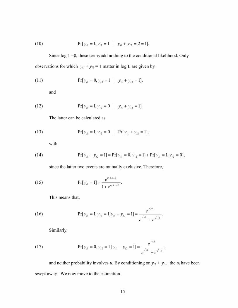
(10) ].12|1,1Pr[ 2121 ==+== iiii yyyy
Since log 1 =0, these terms add nothing to the conditional likelihood. Only
observations for which yi1 + yi2 = 1 matter in log L are given by
(11) ],1|1,0Pr[ 2121 =+== iiii yyyy
and
(12) ].1|0,1Pr[ 2121 =+== iiii yyyy
The latter can be calculated as
(13) ],1Pr[|0,1Pr[ 2121 =+== iiii yyyy
with
(14) ],0,1Pr[]1,0Pr[]1Pr[ 212121 ==+====+ iiiiii yyyyyy
since the latter two events are mutually exclusive. Therefore,
(15) .1
]1Pr['
'
1 β
β
iti
iti
xu
xu
ie
ey+
+
+==
This means that,
(16) .]1]1,1Pr[2
''
'
2121ββ
β
iitx
itx
xiiii
ee
eyyyy+
==+==
Similarly,
(17) ,]1|1,0Pr[2
''
2'
2121ββ
β
iitx
ix
xiiii
ee
eyyyy+
==+==
and neither probability involves u. By conditioning on yi1 + yi2, the ui have been
swept away. We now move to the estimation.
16
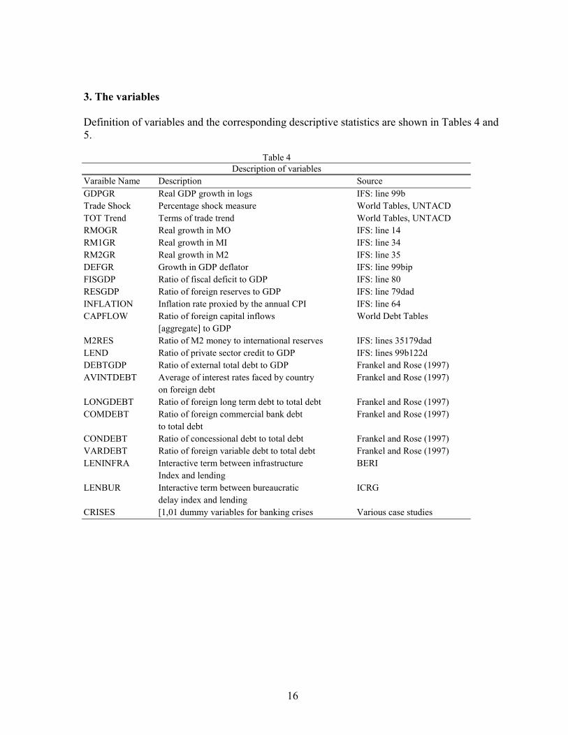
3. The variables
Definition of variables and the corresponding descriptive statistics are shown in Tables 4 and5.
Table 4Description of variables
Varaible Name Description SourceGDPGR Real GDP growth in logs IFS: line 99bTrade Shock Percentage shock measure World Tables, UNTACDTOT Trend Terms of trade trend World Tables, UNTACDRMOGR Real growth in MO IFS: line 14RM1GR Real growth in MI IFS: line 34RM2GR Real growth in M2 IFS: line 35DEFGR Growth in GDP deflator IFS: line 99bipFISGDP Ratio of fiscal deficit to GDP IFS: line 80RESGDP Ratio of foreign reserves to GDP IFS: line 79dadINFLATION Inflation rate proxied by the annual CPI IFS: line 64CAPFLOW Ratio of foreign capital inflows World Debt Tables
[aggregate] to GDPM2RES Ratio of M2 money to international reserves IFS: lines 35179dadLEND Ratio of private sector credit to GDP IFS: lines 99b122dDEBTGDP Ratio of external total debt to GDP Frankel and Rose (1997)AVINTDEBT Average of interest rates faced by country Frankel and Rose (1997)
on foreign debtLONGDEBT Ratio of foreign long term debt to total debt Frankel and Rose (1997)COMDEBT Ratio of foreign commercial bank debt Frankel and Rose (1997)
to total debtCONDEBT Ratio of concessional debt to total debt Frankel and Rose (1997)VARDEBT Ratio of foreign variable debt to total debt Frankel and Rose (1997)LENINFRA Interactive term between infrastructure BERI
Index and lendingLENBUR Interactive term between bureaucratic ICRG
delay index and lendingCRISES [1,01 dummy variables for banking crises Various case studies
17
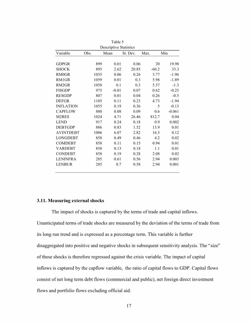
Table 5Descriptive Statistics
Variable Obs. Mean St. Dev. Max. Min
GDPGR 899 0.01 0.06 20 19.98SHOCK 895 2.62 20.85 -60.2 33.3RM0GR 1035 0.06 0.26 3.77 -1.96RM1GR 1059 0.01 0.3 5.98 -1.89RM2GR 1058 0.1 0.3 5.37 -1.3FISGDP 975 -0.01 0.07 0.62 -0.25RESGDP 807 0.01 0.04 0.26 -0.5DEFGR 1105 0.11 0.23 4.73 -1.94INFLATION 1055 0.19 0.36 5 -0.13CAPFLOW 880 0.08 0.09 0.6 -0.061M2RES 1024 4.71 26.46 812.7 0.04LEND 917 0.24 0.18 0.9 0.002DEBTGDP 886 0.83 1.52 13.9 0.01AVINTDEBT 1006 6.07 2.82 16.5 0.12LONGDEBT 858 0.49 0.46 4.2 0.02COMDEBT 858 0.11 0.15 0.94 0.01VARDEBT 858 0.13 0.18 1.1 0.01CONDEBT 858 0.19 0.28 2.08 0.02LENINFRA 285 0.61 0.56 2.94 0.003LENBUR 285 0.7 0.58 2.94 0.001
3.11. Measuring external shocks
The impact of shocks is captured by the terms of trade and capital inflows.
Unanticipated terms of trade shocks are measured by the deviation of the terms of trade from
its long run trend and is expressed as a percentage term. This variable is further
disaggregated into positive and negative shocks in subsequent sensitivity analysis. The “size”
of these shocks is therefore regressed against the crisis variable. The impact of capital
inflows is captured by the capflow variable, the ratio of capital flows to GDP. Capital flows
consist of net long term debt flows (commercial and public), net foreign direct investment
flows and portfolio flows excluding official aid.
18
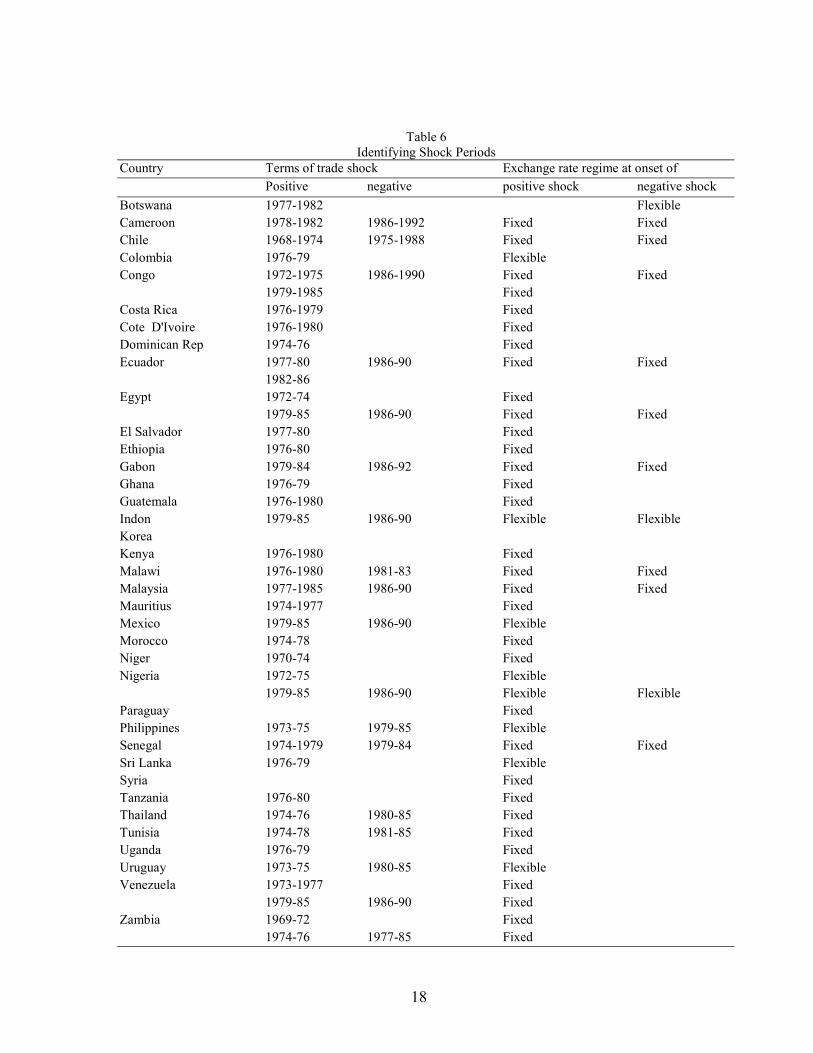
Table 6Identifying Shock Periods
Country Terms of trade shock Exchange rate regime at onset of
Positive negative positive shock negative shock
Botswana 1977-1982 FlexibleCameroon 1978-1982 1986-1992 Fixed FixedChile 1968-1974 1975-1988 Fixed FixedColombia 1976-79 FlexibleCongo 1972-1975 1986-1990 Fixed Fixed
1979-1985 FixedCosta Rica 1976-1979 FixedCote D'Ivoire 1976-1980 FixedDominican Rep 1974-76 FixedEcuador 1977-80 1986-90 Fixed Fixed
1982-86Egypt 1972-74 Fixed
1979-85 1986-90 Fixed FixedEl Salvador 1977-80 FixedEthiopia 1976-80 FixedGabon 1979-84 1986-92 Fixed FixedGhana 1976-79 FixedGuatemala 1976-1980 FixedIndon 1979-85 1986-90 Flexible FlexibleKoreaKenya 1976-1980 FixedMalawi 1976-1980 1981-83 Fixed FixedMalaysia 1977-1985 1986-90 Fixed FixedMauritius 1974-1977 FixedMexico 1979-85 1986-90 FlexibleMorocco 1974-78 FixedNiger 1970-74 FixedNigeria 1972-75 Flexible
1979-85 1986-90 Flexible FlexibleParaguay FixedPhilippines 1973-75 1979-85 FlexibleSenegal 1974-1979 1979-84 Fixed FixedSri Lanka 1976-79 FlexibleSyria FixedTanzania 1976-80 FixedThailand 1974-76 1980-85 FixedTunisia 1974-78 1981-85 FixedUganda 1976-79 FixedUruguay 1973-75 1980-85 FlexibleVenezuela 1973-1977 Fixed
1979-85 1986-90 FixedZambia 1969-72 Fixed
1974-76 1977-85 Fixed
19
3.12. Financial variables
With the lifting of controls on interest rates and directed credit, evidence from case
studies points to lending booms with the proliferation of new banks. A corollary of this may
be a worsening of financial fragility, especially if undertaken without adequate institutional
development, DKD [1997]. The literature uses a number of variables to proxy for financial
liberalization. An obvious choice is lending itself (Lend), which is private sector credit from
the banking sector expressed as a percentage of GDP. To test whether sudden capital
outflows lead to liquidity crises, the ratio of M2 money to foreign reserves is introduced,
(M2reserves). The composition of debt, in terms of maturity and creditor has received much
attention, Sachs et al [1996]. This may be important for countries with a high proportion of
short term foreign commercial debt with variable interest rates.
3.13. Macroeconomic variables
Inflation was introduced as it is normally associated with mismanagement of the
economy. Other macroeconomic variables include the fiscal deficit and various measures of
nominal exchange rate in the sensitivity analysis. The real exchange rate (Reer) was used to
test for overvaluation. Real GDP growth was used to investigate the impact of banking crises
on real income . In order to establish the causality between real income growth and crises,
lagged values of the real GDP variable were used in the predictive model. Finally, to test for
sensitivity of crisis year definitions, different years of banking crises were introduced.
V. Econometric Results
1. Baseline model
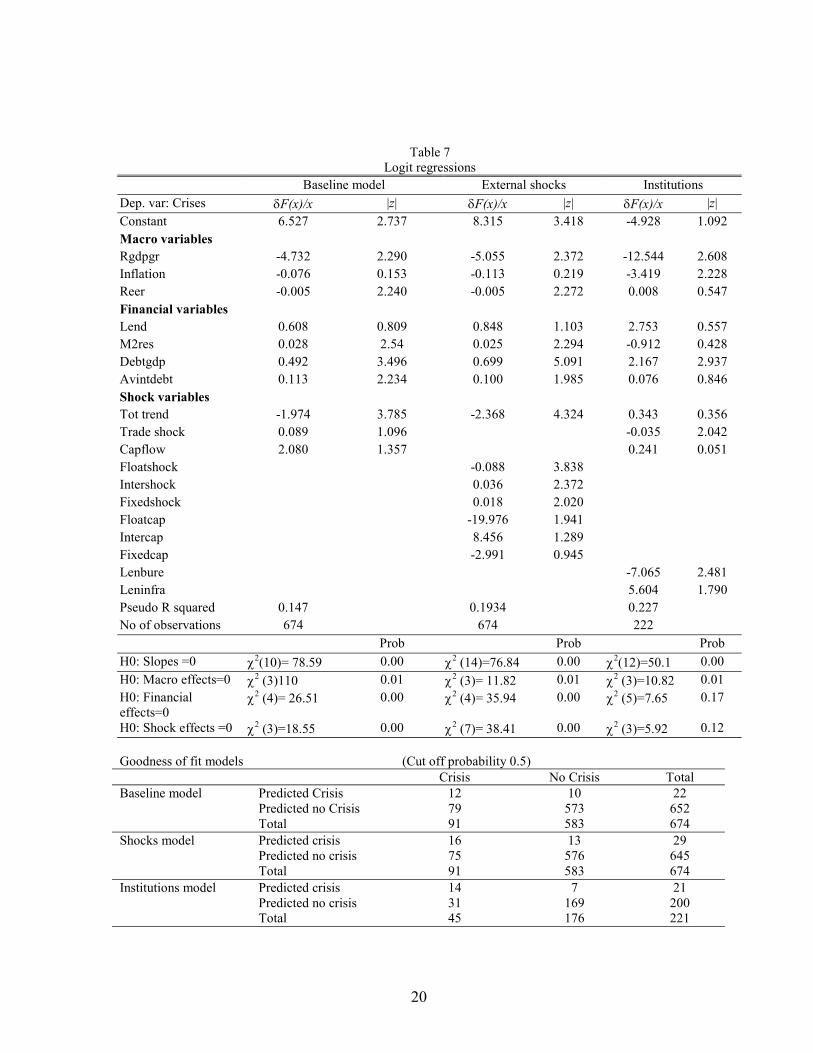
Table 7 shows the results from the baseline case, using Stata (5).
20
Table 7Logit regressions
Baseline model External shocks Institutions
Dep. var: Crises δF(x)/x |z| δF(x)/x |z| δF(x)/x |z|
Constant 6.527 2.737 8.315 3.418 -4.928 1.092Macro variablesRgdpgr -4.732 2.290 -5.055 2.372 -12.544 2.608Inflation -0.076 0.153 -0.113 0.219 -3.419 2.228Reer -0.005 2.240 -0.005 2.272 0.008 0.547Financial variablesLend 0.608 0.809 0.848 1.103 2.753 0.557M2res 0.028 2.54 0.025 2.294 -0.912 0.428Debtgdp 0.492 3.496 0.699 5.091 2.167 2.937Avintdebt 0.113 2.234 0.100 1.985 0.076 0.846Shock variablesTot trend -1.974 3.785 -2.368 4.324 0.343 0.356Trade shock 0.089 1.096 -0.035 2.042Capflow 2.080 1.357 0.241 0.051Floatshock -0.088 3.838Intershock 0.036 2.372Fixedshock 0.018 2.020Floatcap -19.976 1.941Intercap 8.456 1.289Fixedcap -2.991 0.945Lenbure -7.065 2.481Leninfra 5.604 1.790Pseudo R squared 0.147 0.1934 0.227No of observations 674 674 222
Prob Prob Prob
H0: Slopes =0 χ2(10)= 78.59 0.00 χ2 (14)=76.84 0.00 χ2(12)=50.1 0.00
H0: Macro effects=0 χ2 (3)110 0.01 χ2 (3)= 11.82 0.01 χ2 (3)=10.82 0.01H0: Financialeffects=0
χ2 (4)= 26.51 0.00 χ2 (4)= 35.94 0.00 χ2 (5)=7.65 0.17
H0: Shock effects =0 χ2 (3)=18.55 0.00 χ2 (7)= 38.41 0.00 χ2 (3)=5.92 0.12
Goodness of fit models (Cut off probability 0.5)Crisis No Crisis Total
Baseline model Predicted CrisisPredicted no CrisisTotal
127991
10573583
22652674
Shocks model Predicted crisisPredicted no crisisTotal
167591
13576583
29645674
Institutions model Predicted crisisPredicted no crisisTotal
143145
7169176
21200221
21
The coefficients and associated z-statistics are shown in the first two columns.
Diagnostic tests are shown at the bottom of the table together with joint hypothesis tests for
the shock, macro and financial effects. Finally, tabulations of actual and predicted values are
reported for each regression. Overall, the pooled results have a low explanatory power.
However, the levels are similar to those found in the literature, for example Eichengreen and
Rose [1998]. Of the macro variables, the contemporaneous growth rate is highly significant,
implying that negative real income shocks could lead to a banking crisis. However, as
causality may run from the banking sector to the real economy, a predictive model with
lagged values is tested in the next section.
Coming to the other macro variables, the inflation term was not significant, while the
real exchange rate (Reer) term was significant and negatively associated with crises. This
implies that real exchange rate appreciations increases the probability of banking crises. The
ratio of foreign debt to GDP was highly significant. Furthermore, the average interest rate
faced by a country on its foreign debt (Avindebtgdp), was also significant. Sudden increases
in debt service requirements strongly increased the probability of banking crises, supporting
Sachs et al. [1996], that debt maturity mismatches could generate banking crises. Although
DKD [1997] also find real interest rates to be significant, the interest rate used in this study
applies to the debt stock outstanding for that particular country, as changes in this variable
are a more appropriate indicator of a crisis than a general interest rate. The trade shock
variable was positive, but insignificant, though the trend term was significant. Capital
inflows were also not significant. The other significant variable is the ratio of M2 money to
international reserves. The results suggest that the probability of a crisis is significantly
22
enhanced with a low level of reserves, i.e. a sudden capital outflow could seriously
undermine the banking system. Looking at the diagnostic statistics, the test for joint
significance for the aggregate effects was jointly significant in the baseline model. From the
table of actual and predicted outcomes, at a cut-off probability of 0.5%, 12 out of 22 cases
were correctly predicted as having crises and 573 out of 652 cases were correctly predicted
as not having crises in the baseline model, i.e. in total 86% of the cases were correctly
classified.
2. Shocks and choice of exchange regime
The relationships between nominal exchange rate regimes and shocks was analyzed
to investigate the nature of the monetary transmission channel. Nominal regimes were
broadly classified into fixed pegs, intermediate regimes and floating rates. Dummy variables
were created for each year for the three types of regime. These in turn were interacted with
the shock variables. For example, if Kenya experienced a positive external shock in 1979,
and the exchange rate regime in operation was a fixed peg, then the interactive dummy for
the fixed exchange rate and the external trade shock, (Fixshock), took a value of one
multiplied by the shock variables, and zero for other years. This differs from the Eichengreen
and Rose study, which employs [1,0] dummy variables for each regime. The question posed
in this study is more specific, investigating how different regimes interact with external
shocks.
23
The results in the second regression in Table 7 also support the priors on the effects of
trade shocks on the macro economy. Terms of trade shocks that enter through floating
exchange rate regimes decrease the probability of banking crises. For both intermediate and
pegged regimes, the results are diametrically opposite, where shocks significantly increase
the probability of crises. The results are less conclusive for capital inflows, though the
interactive variable on the floating exchange rate term is negative and significant. An
interpretation could be that capital flows entering through floating exchange rate regimes are
less likely to cause crises. These results again support the assertions made in the theory
regarding the transmission of external inflows and their monetary consequences. It was
suggested that under fixed exchange rate regimes, external inflows would have a greater
effect on monetary growth, particularly on the supply side. Shocks and capital inflows going
though floating regimes had a lower probability of creating a crisis in subsequent years (with
a negative sign), than shocks that went through more rigid regimes, which had a positive sign
on the coefficients. Coming to the diagnostics, the combined macro, shock and financial
effects were jointly significant. In the goodness-of-fit table, 576 out of the 645 cases were
correctly predicted as not having a crisis, and 16 out of the 29 cases were predicted as having
crises, i.e. (87%) of the case were correctly classified.
3. Role of institutions
Since theoretical foundations concerning asymmetric information and moral hazard
are linked to institutional structure, the level of “financial institutional development'” could
significantly affect banking crises. Unfortunately, data on institutional development, such as
connected lending, corruption, bureaucracy, prudential regulations and supervision, are non-
24
existent across countries. The closest proxies available were the Bureaucratic Delay Index
from the Business Environmental Risk Intelligence (BERI) organization, and the
International Country Risk Guide (ICRG) measures on infrastructure.
These variables consist of indices specifying infrastructure quality, on a 0 to 4 scale.
Higher values imply low infrastructure quality. However, complete data for all the countries
were not available, with data missing for most of the 1970s and for the entire period for some
countries. This reduced the sample size to 222 observations. The infrastructure index was
interacted with the lending variable to yield (Leninfra), to proxy how poor levels of
institutions such as prudential regulation and banking supervision might have led to
excessive lending. The signs on the coefficient imply that the level of infrastructure
development could affect the probability of banking crises through bank lending, i.e. lending
booms associated with low quality institutions increased the likelihood of crises. Interacting
the bureaucratic variable with lending, (Lenbur), did not yield significant results. The signs
on the other key variables such as real income, and shock variables were significant for the
institutions equation. The other significant variable is the lagged ratio of M2 money to
international reserves. DKD [1997] also use an institutional variable in their study, where a
law and order variable measuring the quality of law enforcement, i.e. measures of effective
legal and judiciary systems, (proxying corruption) was highly significant, i.e. a higher value
in the index implies a higher level of law and order which decreases the probability of crises.
From the table of predictions, 14 out of the 21 cases were correctly predicted as
having a crisis, while 169 out of the 200 cases were correctly predicted as not having crises,
25
implying in total that 83% of all the cases were correctly called. However, these results must
be treated with caution due to the small sample size. The models were then subjected to a
range of robustness and sensitivity tests.
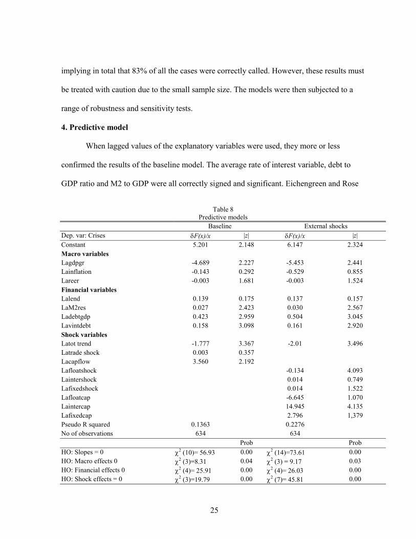
4. Predictive model
When lagged values of the explanatory variables were used, they more or less
confirmed the results of the baseline model. The average rate of interest variable, debt to
GDP ratio and M2 to GDP were all correctly signed and significant. Eichengreen and Rose
Table 8Predictive models
Baseline External shocks
Dep. var: Crises δF(x)/x |z| δF(x)/x |z|
Constant 5.201 2.148 6.147 2.324Macro variablesLagdpgr -4.689 2.227 -5.453 2.441Lainflation -0.143 0.292 -0.529 0.855Lareer -0.003 1.681 -0.003 1.524Financial variablesLalend 0.139 0.175 0.137 0.157LaM2res 0.027 2.423 0.030 2.567Ladebtgdp 0.423 2.959 0.504 3.045Lavintdebt 0.158 3.098 0.161 2.920Shock variablesLatot trend -1.777 3.367 -2.01 3.496Latrade shock 0.003 0.357Lacapflow 3.560 2.192Lafloatshock -0.134 4.093Laintershock 0.014 0.749Lafixedshock 0.014 1.522Lafloatcap -6.645 1.070Laintercap 14.945 4.135Lafixedcap 2.796 1,379Pseudo R squared 0.1363 0.2276No of observations 634 634
Prob Prob
HO: Slopes = 0 χ2 (10)= 56.93 0.00 χ2 (14)=73.61 0.00HO: Macro effects 0 χ2 (3)=8.31 0.04 χ2 (3) = 9.17 0.03HO: Financial effects 0 χ2 (4)= 25.91 0.00 χ2 (4)= 26.03 0.00HO: Shock effects = 0 χ2 (3)=19.79 0.00 χ2 (7)= 45.81 0.00
26
Goodness of fit models (Cut off probability 0.5)Crisis No Crisis Total
Predictive model Predicted CrisisPredicted no CrisisTotal
117889
12533545
23611634
Shocks model Predicted crisisPredicted no crisisTotal
236689
12533545
35599634
[1998] also find high debt to GDP ratios and high foreign interest rates to be significant
predictors of crises. The lagged value of capital flows is a significant predictor of impending
problems. In the disaggregated shocks model, the effects of shocks transmitted through
floating exchange rate regimes reduced the likelihood of a crisis. While the lagged floatcap
term became insignificant, the value of the intermediate interactive term became highly
significant. Coming to the test of joint significance, only the macro effects were rejected at
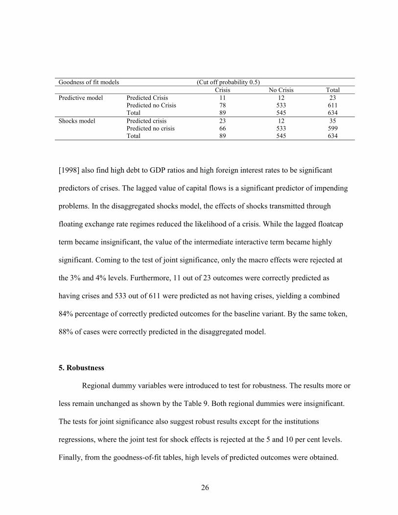
the 3% and 4% levels. Furthermore, 11 out of 23 outcomes were correctly predicted as
having crises and 533 out of 611 were predicted as not having crises, yielding a combined
84% percentage of correctly predicted outcomes for the baseline variant. By the same token,
88% of cases were correctly predicted in the disaggregated model.
5. Robustness
Regional dummy variables were introduced to test for robustness. The results more or
less remain unchanged as shown by the Table 9. Both regional dummies were insignificant.
The tests for joint significance also suggest robust results except for the institutions
regressions, where the joint test for shock effects is rejected at the 5 and 10 per cent levels.
Finally, from the goodness-of-fit tables, high levels of predicted outcomes were obtained.
27
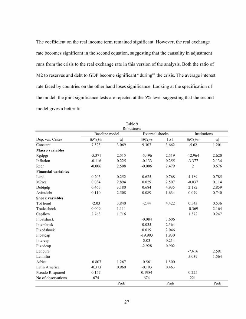
The coefficient on the real income term remained significant. However, the real exchange
rate becomes significant in the second equation, suggesting that the causality in adjustment
runs from the crisis to the real exchange rate in this version of the analysis. Both the ratio of
M2 to reserves and debt to GDP become significant “during'” the crisis. The average interest
rate faced by countries on the other hand loses significance. Looking at the specification of
the model, the joint significance tests are rejected at the 5% level suggesting that the second
model gives a better fit.
Table 9Robustness
Baseline model External shocks Institutions
Dep. var: Crises δF(x)/x |z| δF(x)/x I z I δF(x)/x |z|
Constant 7.523 3.069 9.307 3.662 -5.62 1.201Macro variablesRgdpgr -5.371 2.515 -5.496 2.519 -12.964 2.620Inflation -0.116 0.225 -0.133 0.255 -3.377 2.134Reer -0.006 2.508 -0.006 2.479 2 0.676Financial variablesLend 0.203 0.252 0.625 0.768 4.189 0.785M2res 0.034 2.894 0.029 2.507 -0.037 0.114Debtgdp 0.465 3.180 0.684 4.935 2.182 2.859Avintdebt 0.110 2.508 0.089 1.634 0.079 0.740Shock variablesTot trend -2.03 3.840 -2.44 4.422 0.543 0.536Trade shock 0.009 1.111 -0.369 2.164Capflow 2.763 1.716 1.372 0.247Floatshock -0.084 3.606Intershock 0.035 2.364Fixedshock 0.019 2.046Floatcap -19.993 1.930Intercap 8.03 0.214Fixedcap -2.928 0.902Lenbure -7.616 2.591Leninfra 5.039 1.564Africa -0.807 1.267 -0.561 1.500Latin America -0.373 0.960 -0.193 0.463Pseudo R squared 0.157 0.1984 0.225No of observations 674 674 221
Prob Prob Prob
28
HO: Slopes = 0 χ2 (12)= 66.48 0.00 χ2 (14)=77.42 0.00 χ2 (14)=35.01 0.00HO: Macro effects 0 χ2 (3) = 13.2 0.00 χ2 (3)= 13.34 0.00 χ2 (3)=10.56 0.01HO: Financial effects 0 χ2 (4) = 24.81 0.00 χ2 (4)= 37.14 0.00 χ2 (4)=13.31 0.01HO: Shock effects = 0 χ2 (3) = 19.92 0.00 χ2 (7)= 34.29 0.00 χ2 (3) =6.02 0.11HO: Institu. effects = 0 χ2 (2) =6.73 0.03
Goodness-of-fit: (cut-off probability 0.5) Crisis No crisis Total
8 20575 674583 674
Baseline Crisis Predicted crisis Predicted no crisis Total
127991
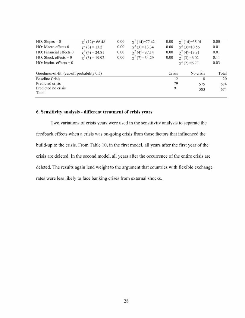
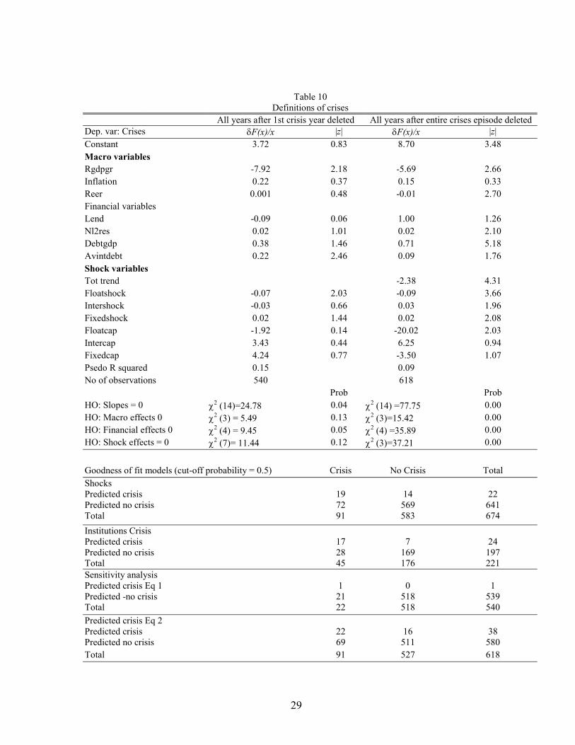
6. Sensitivity analysis - different treatment of crisis years
Two variations of crisis years were used in the sensitivity analysis to separate the
feedback effects when a crisis was on-going crisis from those factors that influenced the
build-up to the crisis. From Table 10, in the first model, all years after the first year of the
crisis are deleted. In the second model, all years after the occurrence of the entire crisis are
deleted. The results again lend weight to the argument that countries with flexible exchange
rates were less likely to face banking crises from external shocks.
29
Table 10Definitions of crises
All years after 1st crisis year deleted All years after entire crises episode deletedDep. var: Crises δF(x)/x |z| δF(x)/x |z|
Constant 3.72 0.83 8.70 3.48Macro variablesRgdpgr -7.92 2.18 -5.69 2.66Inflation 0.22 0.37 0.15 0.33Reer 0.001 0.48 -0.01 2.70Financial variablesLend -0.09 0.06 1.00 1.26Nl2res 0.02 1.01 0.02 2.10Debtgdp 0.38 1.46 0.71 5.18Avintdebt 0.22 2.46 0.09 1.76Shock variablesTot trend -2.38 4.31Floatshock -0.07 2.03 -0.09 3.66Intershock -0.03 0.66 0.03 1.96Fixedshock 0.02 1.44 0.02 2.08Floatcap -1.92 0.14 -20.02 2.03Intercap 3.43 0.44 6.25 0.94Fixedcap 4.24 0.77 -3.50 1.07Psedo R squared 0.15 0.09No of observations 540 618
Prob ProbHO: Slopes = 0 χ2 (14)=24.78 0.04 χ2 (14) =77.75 0.00HO: Macro effects 0 χ2 (3) = 5.49 0.13 χ2 (3)=15.42 0.00HO: Financial effects 0 χ2 (4) = 9.45 0.05 χ2 (4) =35.89 0.00HO: Shock effects = 0 χ2 (7)= 11.44 0.12 χ2 (3)=37.21 0.00
Goodness of fit models (cut-off probability = 0.5) Crisis No Crisis Total
ShocksPredicted crisis 19 14 22Predicted no crisis Total
7291
569583
641674
Institutions Crisis Predicted crisisPredicted no crisisTotal
172845
7169176
24197221
Sensitivity analysis Predicted crisis Eq 1Predicted -no crisis Total
12122
0518518
1539540
Predicted crisis Eq 2Predicted crisis 22 16 38Predicted no crisis 69 511 580Total 91 527 618
30
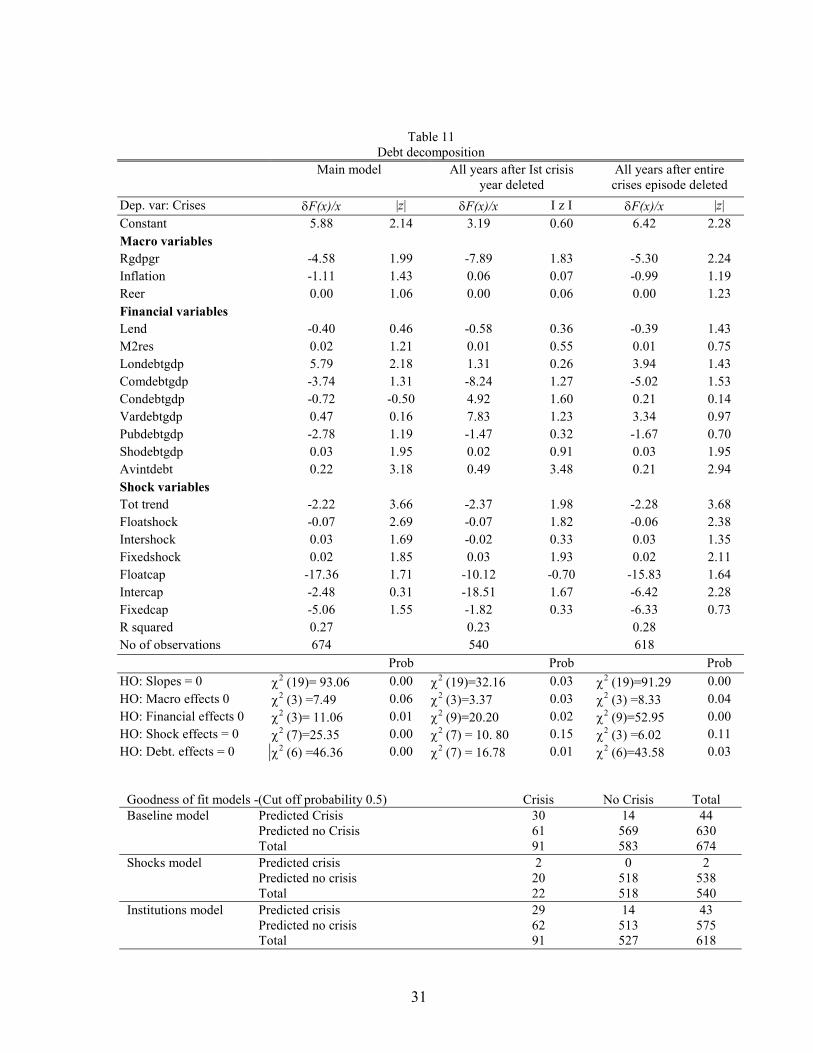
7. Foreign Debt composition
Using the Frankel and Rose [1996] database, the aggregate debt variable was
decomposed into long term debt to GDP (Longdebtgdp), commercial debt to GDP,
(Comdebtgdp), concessional debt to GDP, (Condebtgdp), variable interest debt to GDP
(Vardebt), public debt to GDP, (Pubdebtgdp) and the ratio of short term debt to GDP,
(Shodebtgdp). Results are shown in Table 8, starting with the main model.
As seen, only the long term and short term debt definitions were important. They had
the expected sign and support the view that excessive levels of debt, especially short term
debt, led to problems in the banking sector, while concessional debt was unlikely to have
induced crises. These results again corroborate results from the literature, for example by
Sachs et al. [1996] and Eichengreen and Rose. The signs on the interacted terms of trade
shock variables exhibited the expected signs in the first equation, where more flexible
regimes lessened the likelihood of a crisis. The other two equations use different definitions
of the crisis periods. Again the results support the underlying story looking at the first and
last equation. When all the post-crisis years were deleted in the last equation, the signs on the
interacted shock variables remained unchanged. Only the interaction between capital flows
and fixed regimes had a sign contrary to what was expected.
31
Table 11Debt decomposition
Main model All years after Ist crisisyear deleted
All years after entirecrises episode deleted
Dep. var: Crises δF(x)/x |z| δF(x)/x I z I δF(x)/x |z|
Constant 5.88 2.14 3.19 0.60 6.42 2.28Macro variablesRgdpgr -4.58 1.99 -7.89 1.83 -5.30 2.24Inflation -1.11 1.43 0.06 0.07 -0.99 1.19Reer 0.00 1.06 0.00 0.06 0.00 1.23Financial variablesLend -0.40 0.46 -0.58 0.36 -0.39 1.43M2res 0.02 1.21 0.01 0.55 0.01 0.75Londebtgdp 5.79 2.18 1.31 0.26 3.94 1.43Comdebtgdp -3.74 1.31 -8.24 1.27 -5.02 1.53Condebtgdp -0.72 -0.50 4.92 1.60 0.21 0.14Vardebtgdp 0.47 0.16 7.83 1.23 3.34 0.97Pubdebtgdp -2.78 1.19 -1.47 0.32 -1.67 0.70Shodebtgdp 0.03 1.95 0.02 0.91 0.03 1.95Avintdebt 0.22 3.18 0.49 3.48 0.21 2.94Shock variablesTot trend -2.22 3.66 -2.37 1.98 -2.28 3.68Floatshock -0.07 2.69 -0.07 1.82 -0.06 2.38Intershock 0.03 1.69 -0.02 0.33 0.03 1.35Fixedshock 0.02 1.85 0.03 1.93 0.02 2.11Floatcap -17.36 1.71 -10.12 -0.70 -15.83 1.64Intercap -2.48 0.31 -18.51 1.67 -6.42 2.28Fixedcap -5.06 1.55 -1.82 0.33 -6.33 0.73R squared 0.27 0.23 0.28No of observations 674 540 618
Prob Prob Prob
HO: Slopes = 0 χ2 (19)= 93.06 0.00 χ2 (19)=32.16 0.03 χ2 (19)=91.29 0.00HO: Macro effects 0 χ2 (3) =7.49 0.06 χ2 (3)=3.37 0.03 χ2 (3) =8.33 0.04HO: Financial effects 0 χ2 (3)= 11.06 0.01 χ2 (9)=20.20 0.02 χ2 (9)=52.95 0.00HO: Shock effects = 0 χ2 (7)=25.35 0.00 χ2 (7) = 10. 80 0.15 χ2 (3) =6.02 0.11HO: Debt. effects = 0 χ2 (6) =46.36 0.00 χ2 (7) = 16.78 0.01 χ2 (6)=43.58 0.03
Goodness of fit models -(Cut off probability 0.5) Crisis No Crisis TotalBaseline model Predicted Crisis
Predicted no CrisisTotal
306191
14569583
44630674
Shocks model Predicted crisisPredicted no crisisTotal
22022
0518518
2538540
Institutions model Predicted crisisPredicted no crisisTotal
296291
14513527
43575618
32
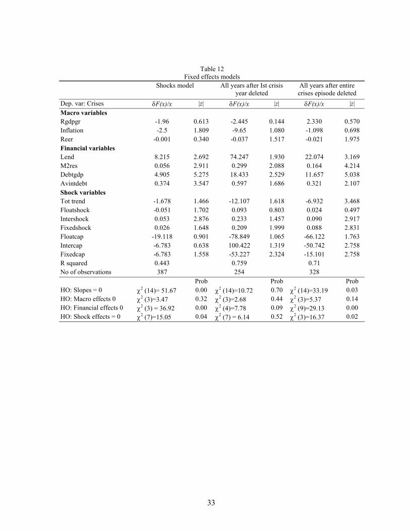
8. Fixed effects specification
In the fixed effects version, only those countries which experienced crises were
included. The first equation interacted the shocks model with exchange rate regimes.
Sensitivity analysis of the crisis variable was carried out following the definitions used
previously. The fixed effects results are reported in Table 12 and corroborate some of the
findings from the pooled results. The interactive shock terms survives the fixed effects
estimation. The capital flow variable is significant but negative in sign. The effects on the
financial variables all have robust effects on the fixed effects estimation. However, the
significance of the real income growth term diminishes. Of the test for joint significance,
only the effects of the macro variables were rejected in the shocks model. Coming to the
other two models, all the tests of joint significance are rejected when the first definition of
crisis was used, while only the financial effects mattered in the second definition.
33
Table 12Fixed effects models
Shocks model All years after Ist crisisyear deleted
All years after entirecrises episode deleted
Dep. var: Crises δF(x)/x |z| δF(x)/x |z| δF(x)/x |z|
Macro variablesRgdpgr -1.96 0.613 -2.445 0.144 2.330 0.570Inflation -2.5 1.809 -9.65 1.080 -1.098 0.698Reer -0.001 0.340 -0.037 1.517 -0.021 1.975Financial variablesLend 8.215 2.692 74.247 1.930 22.074 3.169M2res 0.056 2.911 0.299 2.088 0.164 4.214Debtgdp 4.905 5.275 18.433 2.529 11.657 5.038Avintdebt 0.374 3.547 0.597 1.686 0.321 2.107Shock variablesTot trend -1.678 1.466 -12.107 1.618 -6.932 3.468Floatshock -0.051 1.702 0.093 0.803 0.024 0.497Intershock 0.053 2.876 0.233 1.457 0.090 2.917Fixedshock 0.026 1.648 0.209 1.999 0.088 2.831Floatcap -19.118 0.901 -78.849 1.065 -66.122 1.763Intercap -6.783 0.638 100.422 1.319 -50.742 2.758Fixedcap -6.783 1.558 -53.227 2.324 -15.101 2.758R squared 0.443 0.759 0.71No of observations 387 254 328
Prob Prob ProbHO: Slopes = 0 χ2 (14)= 51.67 0.00 χ2 (14)=10.72 0.70 χ2 (14)=33.19 0.03HO: Macro effects 0 χ2 (3)=3.47 0.32 χ2 (3)=2.68 0.44 χ2 (3)=5.37 0.14HO: Financial effects 0 χ2 (3) = 36.92 0.00 χ2 (4)=7.78 0.09 χ2 (9)=29.13 0.00HO: Shock effects = 0 χ2 (7)=15.05 0.04 χ2 (7) = 6.14 0.52 χ2 (3)=16.37 0.02
34
V1: Conclusion
This paper examined various determinants of banking crises. The results point to a
strong association between the incidence of external shocks and the occurrence of banking
crises in SOEs. Key macroeconomic factors such as negative income shocks, level of debt
and the real exchange rate were decisive determinants of crises. Countries with high levels of
external debt, particularly short term debt were more likely to have banking crises than
countries which relied on concessional borrowing. Both terms of trade shocks and capital
flows were significant predictors of crises. Some of these factors were also conditioned by
the nature of the policy environment in place, in particular the exchange rate regime. This
was more profound in cases where external inflows were channeled through fixed or rigid
exchange rate regimes. In particular, negative trade shocks, were responsible for a large
number of banking crises in the sample. Shocks that were transmitted through more flexible
exchange rate regimes caused less problems to the banking sector.
While externally driven factors played a leading role in this process, various other internal
disturbances and institutional factors also led to banking crises in SOEs. When low levels of
infrastructure and bureaucratic delay were interacted with bank lending, the likelihood of
banking crises increased. Again the problem was more acute under rigid exchange rate
regimes.
35
Bibliography
Alexander, W., J. Davis, L. Ebrill, and C. Lindgren [1997] Systematic Bank Restructuring and MacroeconomicPolicy , International Monetary Fund, Washington DC.
Baltagi, B. [1995], Econometric Analysis of Panel Data, John Wiley & Sons, Chichester.
Bernanke, B. [1983] “Nonmonetary Effects of the Financial Crisis in the Propagation of the Banking Crisis'”,American Economic Review, vol. 73, 257-276.
Bernanke, B. and M. Gertler [1989] “Financial Fragility and Economic Performance,” Quarterly Journal ofEconomics, vol. 105, 87-114.
Calomiris, C. and G. Garton [1991] “The Origins of Bank Panics: Models, Facts and Bank Regulation,'' in R.Hubbard, [ed.], Financial Market and Financial Crises, University of Chicago Press, Chicago.
Caprio, G. and D. Klingebiel [1996] “Bank Insolvencies: Cross-Country Experience”, World Bank PolicyResearch Working Paper, No. 1620, Washington DC.
Choudhri, E and L. Kochin [1980] “The Exchange Rate and the International Transmission of the BusinessCycle Disturbances”, Journal of Money, Credit and Banking, vol. 12, 565-574.
Demirguc-Kunt, A. and E. Detragiache [1997] “The Determinants of Banking Crises: Evidence fromDeveloping and Developed Countries”, International Monetary Fund Working Paper, WP/97/106, WashingtonDC.
Diaz-Alejandro, C. [1985] “Good-Bye Financial Repression, Hello Financial Crash”, Journal of DevelopmentEconomics, vol. 19, 1-24.
Eastwood, R. and A. Venables [1982] “The Macroeconomic Implications of a Resource Discovery in an OpenEconomy”, Economic Journal, vol. 92, pp. 285-299.
Eichengreen, B. and A. Rose [1998] “Staying Afloat when the Wind Shifts: External Factors and Emerging-Market Banking Crises”, Working Paper No. 6370, Cambridge.
Federal Reserves Bank of San Francisco [1985] “The Search for Financial Stability: the Past Fifty Years”,conference proceedings, June 23-25.
Frankel, J. and A. Rose [1997] “Currency Crashes in Emerging Markets; Empirical Indicators”, NationalBureau of Economic Research Working Paper No 543, Cambridge.
Friedman, M. and A. Schwartz [1963], A Monetary History of the United States, 1867-1960}, PrincetonUniversity Press, Princeton.
Greenwald, B. and J. Stiglitz [1988] “Information, Financial Constraints, and Business Fluctuations”, in Khan,M. and S. Tsiang, [eds], Expectations and Macroeconomics, Oxford University Press, Oxford.
Hausmann, R. and L. Rojas-Suarez [1996] Banking Crises in Latin America, Inter American Bank, Washington
Honohan, P. [1997] “Banking System Failures in Developing and Transition Countries”, Bank for InternationalSettlements Working Paper, Basle.
36
Hubbard, R. [1991] Financial Markets and Financial Crises, University of Chicago Press, Chicago.
Kindleberger, C. [1978] Manias, Panics and Crashes, Basic Books, New York.
Minsky, P. [1977] John Maynard Keynes, Colombia University Press, New York.
Mishkin, F. [1996] “Understanding Financial; Crises”, National Bureau of Economic Research Working PaperNo. 5600, Cambridge.
Morris, F., M. Dorfman, J. Ortiz, and M. Franco [1990] ‘Latin America's Banking Systems in the 1980s”,World Bank Discussion Papers, No 81, Washington DC.
Neary, P. [1985] “Real and Monetary Aspects of Dutch Disease”, in Jungfeld, K. and D. Hague (eds),Structural Adjustment in Developed Open Economies, Macmillan, London.
Sachs, J., A. Tornell, and A. Velasco [1996] “Financial Crises in Emerging Markets”, Brookings Papers onEconomic Activity, Washington DC.
Stiglitz, J. and A. Weiss [1981] “Credit Rationing in Market with Imperfect Information'', American EconomicReview, vol. 72, 393-410.
Sundararajan, V. and T. Balino [1991] Banking Crises; Cases and Issues, International Monetary Fund,Washington DC.
Taylor, L. and S. O'Connell [1985] “A Minsky Crisis”, Quarterly Journal of Economics, vol. 100, 871-885.
Temin, P. [1976] Did Monetary Forces cause the Great Depression? N. Norton, New York.
Veblen, T. [1904] The Theory of Business Enterprise, Charles Scribner, New York.
CESifo Working Paper Series
___________________________________________________________________________
689 Amihai Glazer and Vesa Kanniainen, The Effects of Employment Protection on theChoice of Risky Projects, March 2002
690 Michael Funke and Annekatrin Niebuhr, Threshold Effects and Regional EconomicGrowth – Evidence from West Germany, March 2002
691 George Economides, Apostolis Philippopoulos, and Simon Price, Elections, FiscalPolicy and Growth: Revisiting the Mechanism, March 2002
692 Amihai Glazer, Vesa Kanniainen, and Mikko Mustonen, Innovation of Network Goods:A Non-Innovating Firm Will Gain, March 2002
693 Helmuth Cremer, Jean-Marie Lozachmeur, and Pierre Pestieau, Social Security,Retirement Age and Optimal Income Taxation, April 2002
694 Rafael Lalive and Josef Zweimüller, Benefit Entitlement and the Labor Market:Evidence from a Large-Scale Policy Change, April 2002
695 Hans Gersbach, Financial Intermediation and the Creation of Macroeconomic Risks,April 2002
696 James M. Malcomson, James W. Maw, and Barry McCormick, General Training byFirms, Apprentice Contracts, and Public Policy, April 2002
697 Simon Gächter and Arno Riedl, Moral Property Rights in Bargaining, April 2002
698 Kai A. Konrad, Investment in the Absence of Property Rights: The Role of IncumbencyAdvantages, April 2002
699 Campbell Leith and Jim Malley, Estimated General Equilibrium Models for theEvaluation of Monetary Policy in the US and Europe, April 2002
700 Yin-Wong Cheung and Jude Yuen, Effects of U.S. Inflation on Hong Kong andSingapore, April 2002
701 Henry Tulkens, On Cooperation in Musgravian Models of Externalities within aFederation, April 2002
702 Ralph Chami and Gregory D. Hess, For Better or For Worse? State-Level MaritalFormation and Risk Sharing, April 2002
703 Fredrik Andersson and Kai A. Konrad, Human Capital Investment and Globalization inExtortionary States, April 2002
704 Antonis Adam and Thomas Moutos, The Political Economy of EU Enlargement: Or,Why Japan is not a Candidate Country?, April 2002
705 Daniel Gros and Carsten Hefeker, Common Monetary Policy with Asymmetric Shocks,April 2002
706 Dirk Kiesewetter and Rainer Niemann, Neutral and Equitable Taxation of Pensions asCapital Income, April 2002
707 Robert S. Chirinko, Corporate Taxation, Capital Formation, and the SubstitutionElasticity between Labor and Capital, April 2002
708 Frode Meland and Gaute Torsvik, Structural Adjustment and Endogenous WorkerRecall Probabilities, April 2002
709 Rainer Niemann and Caren Sureth, Taxation under Uncertainty – Problems of DynamicProgramming and Contingent Claims Analysis in Real Option Theory, April 2002
710 Thomas Moutos and William Scarth, Technical Change and Unemployment: PolicyResponses and Distributional Considerations, April 2002
711 Günther Rehme, (Re-)Distribution of Personal Incomes, Education and EconomicPerformance Across Countries, April 2002
712 Thorvaldur Gylfason and Gylfi Zoega, Inequality and Economic Growth: Do NaturalResources Matter?, April 2002
713 Wolfgang Leininger, Contests over Public Goods: Evolutionary Stability and the Free-Rider Problem, April 2002
714 Ernst Fehr and Armin Falk, Psychological Foundations of Incentives, April 2002
715 Giorgio Brunello, Maria Laura Parisi, and Daniela Sonedda, Labor Taxes and Wages:Evidence from Italy, May 2002
716 Marta Aloi and Huw Dixon, Entry Dynamics, Capacity Utilisation and Productivity in aDynamic Open Economy, May 2002
717 Paolo M. Panteghini, Asymmetric Taxation under Incremental and SequentialInvestment, May 2002
718 Ben J. Heijdra, Christian Keuschnigg, and Wilhelm Kohler, Eastern Enlargement of theEU: Jobs, Investment and Welfare in Present Member Countries, May 2002
719 Tapio Palokangas, The Political Economy of Collective Bargaining, May 2002
720 Gilles Saint-Paul, Some Evolutionary Foundations for Price Level Rigidity, May 2002
721 Giorgio Brunello and Daniela Sonedda, Labor Tax Progressivity, Wage Determination,and the Relative Wage Effect, May 2002
722 Eric van Damme, The Dutch UMTS-Auction, May 2002
723 Paolo M. Panteghini, Endogenous Timing and the Taxation of Discrete InvestmentChoices, May 2002
724 Achim Wambach, Collusion in Beauty Contests, May 2002
725 Dominique Demougin and Claude Fluet, Preponderance of Evidence, May 2002
726 Gilles Saint-Paul, Growth Effects of Non Proprietary Innovation, May 2002
727 Subir Bose, Gerhard O. Orosel, and Lise Vesterlund, Optimal Pricing and EndogenousHerding, May 2002
728 Erik Leertouwer and Jakob de Haan, How to Use Indicators for ‘Corporatism’ inEmpirical Applications, May 2002
729 Matthias Wrede, Small States, Large Unitary States and Federations, May 2002
730 Christian Schultz, Transparency and Tacit Collusion in a Differentiated Market, May2002
731 Volker Grossmann, Income Inequality, Voting Over the Size of Public Consumption,and Growth, May 2002
732 Yu-Fu Chen and Michael Funke, Working Time and Employment under Uncertainty,May 2002
733 Kjell Erik Lommerud, Odd Rune Straume, and Lars Sørgard, Downstream Merger withOligopolistic Input Suppliers, May 2002
734 Saku Aura, Does the Balance of Power Within a Family Matter? The Case of theRetirement Equity Act, May 2002
735 Sandro Brusco and Fausto Panunzi, Reallocation of Corporate Resources andManagerial Incentives in Internal Capital Markets, May 2002
736 Stefan Napel and Mika Widgrén, Strategic Power Revisited, May 2002
737 Martin W. Cripps, Godfrey Keller, and Sven Rady, Strategic Experimentation: TheCase of Poisson Bandits, May 2002
738 Pierre André Chiappori and Bernard Salanié, Testing Contract Theory: A Survey ofSome Recent Work, June 2002
739 Robert J. Gary-Bobo and Sophie Larribeau, A Structural Econometric Model of PriceDiscrimination in the Mortgage Lending Industry, June 2002
740 Laurent Linnemer, When Backward Integration by a Dominant Firm Improves Welfare,June 2002
741 Gebhard Kirchgässner and Friedrich Schneider, On the Political Economy ofEnvironmental Policy, June 2002
742 Christian Keuschnigg and Soren Bo Nielsen, Start-ups, Venture Capitalits, and theCapital Gains Tax, June 2002
743 Robert Fenge, Silke Uebelmesser, and Martin Werding, Second-best Properties ofImplicit Social Security Taxes: Theory and Evidence, June 2002
744 Wendell Fleming and Jerome Stein, Stochastic Optimal Control, International Financeand Debt, June 2002
745 Gene M. Grossman, The Distribution of Talent and the Pattern and Consequences ofInternational Trade, June 2002
746 Oleksiy Ivaschenko, Growth and Inequality: Evidence from Transitional Economies,June 2002
747 Burkhard Heer, Should Unemployment Benefits be Related to Previous Earnings?, July2002
748 Bas van Aarle, Giovanni Di Bartolomeo, Jacob Engwerda, and Joseph Plasmans,Staying Together or Breaking Apart: Policy-makers’ Endogenous Coalitions Formationin the European Economic and Monetary Union, July 2002
749 Hans Gersbach, Democratic Mechanisms: Double Majority Rules and Flexible AgendaCosts, July 2002
750 Bruno S. Frey and Stephan Meier, Pro-Social Behavior, Reciprocity or Both?, July 2002
751 Jonas Agell and Helge Bennmarker, Wage Policy and Endogenous Wage Rigidity: ARepresentative View From the Inside, July 2002
752 Edward Castronova, On Virtual Economies, July 2002
753 Rebecca M. Blank, U.S. Welfare Reform: What’s Relevant for Europe?, July 2002
754 Ruslan Lukach and Joseph Plasmans, Measuring Knowledge Spillovers Using PatentCitations: Evidence from the Belgian Firm’s Data, July 2002
755 Aaron Tornell and Frank Westermann, Boom-Bust Cycles in Middle Income Countries:Facts and Explanation, July 2002
756 Jan K. Brueckner, Internalization of Airport Congestion: A Network Analysis, July2002
757 Lawrence M. Kahn, The Impact of Wage-Setting Institutions on the Incidence of PublicEmployment in the OECD: 1960-98, July 2002
758 Sijbren Cnossen, Tax Policy in the European Union, August 2002
759 Chandima Mendis, External Shocks and Banking Crises in Developing Countries: Doesthe Exchange Rate Regime Matter?, August 2002