ColecciónBanca Central y Sociedad

BANCO CENTRAL DE VENEZUELA

4444455555Serie Documentos de Trabajo

Oficina de Investigaciones Económicas

Inconsistency of policiesand oil shocks:

dynamics accordingto the monetary regime

Harold Zavarceand Luis A. Sosa

Abril 2003

Las ideas y opiniones contenidas en el presenteDocumento de Trabajo son de la exclusiva

responsabilidad de sus autores y se correspondencon un contexto de libertad de opinión en el cualresulta más productiva la discusión de los temas

abordados en la serie.

Inconsistency of Policies and Oil Shocks:Dynamics According to the Monetary Regime

Harold Zavarcea and Luis A. Sosab

aBanco Central de Venezuela, Caracas, Venezuela

bDivision of Economics and Business, Colorado School of Mines, Golden, CO, USA

E-mail addresses: hzavarce@bcv.org.ve (H. Zavarce); luissosa@mines.edu (L. Sosa)_____________________________________________________________

AbstractThe main goal of this paper is to analyze the inconsistency between monetary and fiscalpolicy for an oil economy. In particular, we study the dynamics caused by a permanent oilrevenue reduction when fiscal corrections are not implemented and the respectiveintermediate monetary policy variable is maintained at its original level. We examine theeffects of a permanent oil shock under two alternative monetary regimes. These regimes are,according to the election of the intermediate variable, a monetary rule and the exchange rateanchor. For the purposes of our study, we assume a small open economy for which oilconstitutes an important source of public revenue. Also, we assume perfect capital mobility,perfect foresight, full employment, and flexible prices. The inconsistency arises with apermanent reduction in oil revenues. In this paper, we offer the following two contributions.First, we show that, under any of the previous monetary regimes, keeping policies at pre-shock levels generates an unstable growth of government indebtedness. This unstable growthcauses both the abandonment of the monetary regime and higher future inflation rates.Second, we demonstrate that delaying the implementation of an adjustment program causesincreasing inflationary and indebtedness costs.

JEL Classification: E42, E52, E61, F34,E63

Keywords: Consistency, monetary and fiscal policy, rules, debt_____________________________________________________________

Abril 2003

2

1. Introduction

This work analyzes the macroeconomic dynamics originated by the inconsistency betweenmonetary policy and fiscal policy in an economy where oil constitutes an important source ofpublic income. In particular, we study the dynamics generated by a permanent reduction ofoil revenue when the required fiscal corrections are not implemented and the central bankmaintains the trajectory of its intermediate variable at levels that are compatible with pre-shock oil revenue. The monetary strategies that we included, according to the election of theintermediate variable, are the monetary rule and the exchange rate anchor. We simplify theanalysis by using a simple neoclassic model with full employment and flexible prices for asmall open economy with capital mobility. This simplification is made to focus on the effectof inconsistent policies on the dynamics of inflation, debt, and real money balances.

Zavarce (1998) studies the case of the exchange rate as an intermediate variable andconsiders the implementation of capital account controls in an oil economy. He shows thatkeeping the exchange rule at pre-shock levels in order to maintain a stable rate of inflation,leads to unstable growth of public debt that in turn produces a speculative attack as explainedby Krugman (1979).

Our study draws heavily on the work of Auernheimer (1987). He studies the failure ofstabilization programs based on exchange rate or monetary anchors considering the key roleof the consolidated budgetary restriction of government with the central bank on the processof formation of expectations. Basically, the results that we obtain for the case of an oileconomy are variations of the results from Auernheimer (1987). In a small open economypopulated with agents with perfect foresight, obtaining an inflation rate smaller than thatrequired to maintain a stable level of national debt, by adopting an exchange rate rule or amonetary rule, can be achieved only temporarily and at a greater rate of future inflation. Thisresult shows that some unpleasant monetarist arithmetic characterizes the dynamicsgenerated by inconsistent stabilization programs for a small open economy, as in Sargent andWallace (1981) and the later works of Liviatan (1984) and Drazen (1985). This result is alsopresent in the case that we examine. Regardless of the monetary regime, fiscal and monetarystrategies that are not adjusted after oil shocks bring unstable growth of government net debt.This situation causes the abandonment of the intermediate monetary policy variable resultingin an inflation rate higher than the forecasted one.

We examine the effects of a permanent reduction of oil revenue under unchanged levels ofthe intermediate monetary policy variable. We study the dynamics of the country’s net debt,real money balances, inflation and the price level. Two main conclusions emerge from ourstudy. First, keeping policies at the pre-shock levels to generate a stable inflation rate leads tounstable growth of the indebted position of the public sector that produces both theabandonment of the monetary regime and higher future inflation rates, regardless of themonetary policy regime. Second, delaying necessary changes of the intermediate monetarypolicy variable causes increasing indebtedness and higher costs of inflation in order tostabilize the debt dynamic.

3

This paper is organized as follows. Section 2 describes the model and the closings accordingto the election of the intermediate variable. Section 3 examines the dynamics of theexchange rate and monetary aggregates as intermediate monetary policy variables. Section 4concludes and offers suggestions for further research.

2. The model

Assume a small open economy that is inhabited by a continuum of identical private agents.Population is normalized to the [0, 1] interval. Time is continuous and all the individuals liveforever and have perfect foresight.

There are two types of goods. A constant flow of oil that emerges from the ground, denotedby Xg, is property of the government. Oil, Xg, is not consumed within the economy but istraded with the rest of the world, without restrictions, at a price Pg. Also, private agentsproduce a constant flow of good y, which also is internationally traded without restrictions ata constant price Py. For simplicity, Py is normalized to one. Because of the effects ofarbitrage, the exchange rate E equals the price level P, and the rate of inflation π equals therate of depreciation / .E E&

For simplicity we assume that the government is a net debtor with a real debt stock b at anytime. Private agents are net creditors. They save in real non-monetary financial assets, a, andin real monetary balances, m. The total of the country’s net debt, b-a, is represented by Ω .

Both private agents and the government can lend and borrow without restrictions in theinternational financial market at the same interest rate r. However, this interest rate r issubject to the country-risk level that positively depends on ,Ω the country’s total net debt.Thus, in spite of being a small open economy, the aggregate economy faces a variable realinterest rate. However, given the competitive character of the economy, private agentsconsider that the interest rate is exogenously given when they allocate their disposableincome into their portfolio of assets. Thus, private agents tend to excessively borrow becausethey ignore the effects of their portfolio decisions on the real interest rate.

Following Auernheimer (1987) and Garcia-Saltos (1998), we assume that the real interestrate depends positively on total level of net debt and on the exogenous world interest rate r*,which is assumed constant. Thus,

*( , )r r r= Ω , where 1 0r > and 2 0r > . (1)

The government spends g, receives income from selling Xg, charges a lump-sum tax T, andpays interests on its debt br. The fiscal deficit, including these payments of interests, isfinanced by borrowing b& and the use of seignorage / .M P& Consequently, the governmentbudget constraint cum the central bank can be written as

4

..

g yg

y

P EP Mg T X br b

P P P− − + = + . (2)

Equation (2) indicates that the amount of income resulting from oil sales depends upon boththe terms of trade g yP / P and the real exchange rate g yEP / P . To simplify matters, we assumethat all private production is freely traded with the rest of the world. Thus we ignore theeffect of the real exchange rate on oil revenues in terms of domestic goods. The dynamics ofseignorage is given by

Mm m m

Pπ µ= + =

&& . (3)

Equation (3) contains the dynamics of real money balances. Using (3) and (2), we have thatthe dynamic of government debt is given by

*( , )b d br r mµ= + Ω −& . (4)

Where d represent the primary deficit. That is .g yg

y

P EPd g T X

P P= − −

As usual, households obtain utility from consumption (c) and real money balances (m). Weassume an instantaneous utility function that is additively separable in c and m. That is,

( , ) ( ) ( )U c m u c v m= + . Both u(c) and v(m) are strictly concave, twice differentiable, andsatisfy the usual Inada conditions. Also, we assume a constant rate of time preference, ? .

Every period, individuals decide how to allocate their disposable income betweenconsumption and assets accumulation, for a given level of private wealth constituted bymonetary assets (m) and non-monetary assets (a). The problem of the representativeindividual is to maximize the present value of utility. That is,

( ) ( ) ( ) ( )[ ]∫

∞−+

0,

dtemvcumax t

tmtc

ρ (5)

subject to( )π+−−−+= rmTcwryw& , (6)

,w a m≡ + (7)

0(0) , a a= (8)and

lim 0rt

twe−

→∞= . (9)

5

Note that condition (9) rules out the possibility of unlimited wealth accumulation. Appendix1 contains a detailed solution for the representative individual’s maximization problem.

Aggregating across individuals, and considering the assumption of an additively separableutility function, the first order conditions for maximization are reduced to

( )'.

*" ,

uc r r

uρ = − Ω (10)

and

( ) ( ) ( )' ' *,v m u c r r π = Ω + . (11)

From equation (11), we derive the money demand function, which plays a fundamental rolein our analysis. Thus, assuming that the money market clears instantaneously, we have

( ), , m l c i= (12)

where i is the nominal interest rate defined as i r π≡ + and 1 2 0 and 0.l l> <

In addition, by using equations (2), (3), and (6), we obtain the following expression thatshows the country’s balance of payments identity,

( ) ( ).

*,g gc g y X P r rΩ = + − − + Ω Ω . (13)

Note that the right hand side of (6) constitutes the current account deficit whereas the firstterm in parenthesis shows the trade balance deficit. Thus, current account deficits increasethe aggregate of the country’s net debt.

The solution to the overall aggregate system is obtained as follows. First, equations (10) and(13) determine consumption and the aggregate of the country’s net debt. Second, thebehavior of inflation, the rate of monetary expansion, and the rate of growth of real moneybalances are obtained from equations (3) and (11), considering both the monetary regime andmaximum level of sustainable debt. Third, the path of government debt is obtained fromequation (4) after determining the path of π , the rate of monetary expansion, and the rate ofgrowth of real money balances.

In the three following subsections, we describe completely the behavior of the economy. Inthese sub-sections, we examine the dynamics of consumption and the country’s net debt andexplain the existence of a maximum level of sustainable debt. In addition, we defineinconsistency of policies and study the behavior of key monetary variables under each of thetwo alternative regimes that are considered.

6

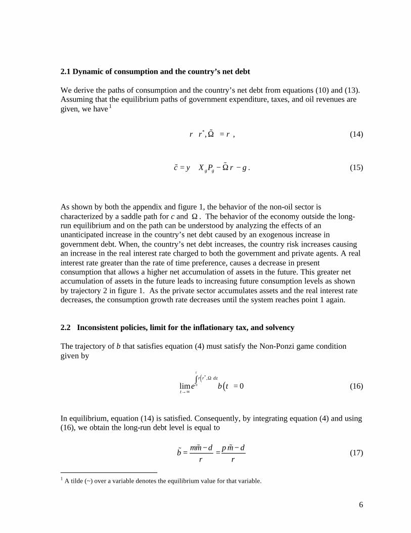
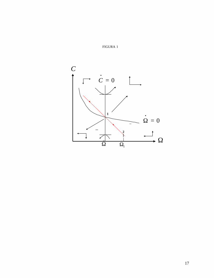
2.1 Dynamic of consumption and the country’s net debt

We derive the paths of consumption and the country’s net debt from equations (10) and (13).Assuming that the equilibrium paths of government expenditure, taxes, and oil revenues aregiven, we have 1

*,r r ρ

Ω =

% , (14)

g gc y X P gρ= + − Ω −%% . (15)

As shown by both the appendix and figure 1, the behavior of the non-oil sector ischaracterized by a saddle path for c and Ω . The behavior of the economy outside the long-run equilibrium and on the path can be understood by analyzing the effects of anunanticipated increase in the country’s net debt caused by an exogenous increase ingovernment debt. When, the country’s net debt increases, the country risk increases causingan increase in the real interest rate charged to both the government and private agents. A realinterest rate greater than the rate of time preference, causes a decrease in presentconsumption that allows a higher net accumulation of assets in the future. This greater netaccumulation of assets in the future leads to increasing future consumption levels as shownby trajectory 2 in figure 1. As the private sector accumulates assets and the real interest ratedecreases, the consumption growth rate decreases until the system reaches point 1 again.

2.2 Inconsistent policies, limit for the inflationary tax, and solvency

The trajectory of b that satisfies equation (4) must satisfy the Non-Ponzi game conditiongiven by

( )( )

*

0

,

lim 0

t

r r dz

te b t

Ω

→∞

∫= (16)

In equilibrium, equation (14) is satisfied. Consequently, by integrating equation (4) and using(16), we obtain the long-run debt level is equal to

m d m db

µ πρ ρ− −

= =% %% (17)

1 A tilde (~) over a variable denotes the equilibrium value for that variable.

7

where m~ and b~

represent the equilibrium levels of real money balances and government netdebt, respectively. Equation (17) establishes that the long-run debt level is equal to thepresent value of the government surpluses including revenue from the inflationary tax πmthat equals the level of seigniorage in equilibrium. Therefore, fiscal solvency exists if thetrajectory of b that satisfies equation (4) also satisfies equation (17) with a finite value oflong-run debt that satisfies equation (17) too. After defining fiscal solvency, we can defineinconsistent policies. The mix of fiscal and monetary policy is inconsistent if thegovernment net debt grows without limits given a monetary strategy that determines both theinflationary tax π and the exogenous components of the primary fiscal deficit.

Note that a permanent increase in the primary deficit that increases government net debtwithout limits is inconsistent with the monetary strategy. This is because it is impossible tofinance the fiscal deficit and the interests on the debt, d + br, with inflationary tax income inthe long run. A government indebtedness crisis emerges when a maximum level of debtconstraints the explosive trajectory of b.

How can the indebtedness crisis be solved?

Assuming that the instantaneous utility function u + v allows for a maximum level ofinflationary tax income 2, the central bank abandons the monetary strategy by changing orredefining the intermediate variable when b reaches a maximum level b so that themaximum level of inflationary tax income satisfies equation (17). The following expressionshows this situation formally:

( ) ( )( )1max [max , ]b t b l c d

ππ π ρ

ρ= = + −% . (18)

At the time when the central bank modifies the monetary strategy, government debt isstabilized at max b. The rate of monetary expansion equals the inflation rate that maximizesthe inflationary tax collections, that is commonly called Cagan’s revenue-maximizinginflation rate. In this manner, adjusting the inflation tax solves the indebtedness crisis.

3. Inconsistency of policies

For our analysis of the outcome of inconsistent policies, we assume that in a neighborhood ofthe initial equilibrium the inflation rate is lower than Cagan’s revenue-maximizing inflationrate. Later in this section, we will see that a permanent reduction in oil revenues causes a

2 In general, the class of utility functions that has a Cagan maximum level of revenues are of type

[ ] ( )1

"' donde 0,1 o ln

1m m

v v v m mv

σ

σ α βσ

−

= = − ∈ = −−

8

reduction in the demand for money. This reduction in the money demand can be produced bytwo different sets of circumstances. First, the reduction can be due to a fall in consumptionand a discrete decrease in real money balances via capital flight or foreign exchange sales bythe central bank.That is, a discrete fall in b when the exchange rate is the intermediatevariable. Second, the money demand reduction can be due to a decrease in consumption anda jump in the price level when the exchange rate is flexible and M is continuous. Since inboth of the previous cases, seigniorage mµ falls, government debt increases without limits tofinance the after-shock fiscal deficit level. This unlimited government debt growth makes themonetary program inconsistent with the fiscal stance. Under these circumstances, we say thatthe monetary and fiscal policies are incompatible and that coordinating them is not feasible.

Finally, note that each monetary policy regime is constituted by a particular set of equationsthat determines the dynamics of the relevant monetary variables. In the next section, westudy the inconsistency of policies under two alternative monetary regimes: the exchange raterule and a monetary rule.

3.1 Inconsistency of policies under the exchange rate rule

Under this monetary regime, the exchange rate is the variable controlled by the monetaryauthority. The central bank announces at t = 0 that it will intervene in the exchange market tomaintain a continuous path of the exchange rate, such as

( ) ( )0 tE t E eπ= . (19)

Note that π is the rate of devaluation of the exchange rate that is equal to the inflation rate inthis model. Remember that because of the effects of arbitration in the market for goods, theexchange rate equals the price level and the inflation rate equals the rate of devaluation.Also, remember that under the exchange rate rule, the behavior of the nominal money stockis endogenous. Notice that for a given rate of devaluation, the commitment to keep acontinuous path of the exchange rate prevents the monetary authority from implementingonce-and-for-all devaluation or any other discretionary exchange rate adjustments.Devaluations may eliminate the problem of inconsistent policies since they may reduce thelevel of government indebtedness. Auernheimer (1987) argues that the implementation of theexchange rule is vulnerable to credibility/reputation problems, as explained by the literatureon time inconsistency.

The behavior of inflation, real money balances, and government debt

In aggregation, real money balances are piecewise continuous since both consumption andthe real interest rate are piecewise continuous. Thus, the equations describing the behavior ofinflation, real money balances, and government debt are the following:

.

EE

π = , (20)

9

( ) ( ) ( )' ' *,v m u c r r π = Ω + , (21)

.

0m = , (22)

( ).

* ,b d br r mπ= + Ω − (23)

The effects of a permanent oil revenue reduction

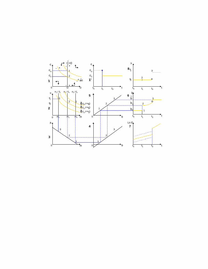
Let us assume that the system is initially in steady state equilibrium where 0 0, r ρ µ π= = , allthe state variables are in equilibrium, and the level of government net debt satisfies equation(17). Assume now that oil revenues fall permanently and, at that time, the monetary authorityannounces that the exchange rule will be maintained at the pre-shock level and that discretechanges in the level of the exchange rate will not be allowed. These results are shown inFigure 3. At the time of the shock, consumption falls from c0 to c1. At the new equilibrium,the country’s net debt level remains unchanged. This is because the reduction of consumptionproduces an increase in the amount of assets held by private individuals, that matches theincrease in government indebtedness. In addition, expression (12) shows that the fall inconsumption causes a discrete reduction in the demand for real money balances, which, inturn, affects the money market equilibrium at t=0. This new level of real money balanceswill remain unchanged as long as the central bank does not abandon the exchange rule.

If continuity prevails, the disequilibrium in the monetary market will be restored via loss ofinternational reserves. The loss of international reserves causes an equilibrating contractionof the monetary base as shown in Graph 3, panel 3. Also, panel 6 of the same graph showsthat this loss of international reserves generates a discreet jump in government net debt frombo to b1. Panel 6 also shows that if fiscal corrections necessary to face the permanent oilrevenue reduction are not implemented, government net debt increases without limits anddoes not converge to an equilibrium path.

In addition to the permanent fall in oil revenues, there are two other elements that cause theseunlimited increasing levels of government debt. One, the reduction in real money balancesdecreases inflationary tax income for any given inflation rate. Two, the higher level ofgovernment debt produces higher debt-service payments.

Public sector indebtedness is limited by the government repayment capacity. This capacity isdetermined by the present value of fiscal surpluses that included income from seigniorage. Inour model, this indebtedness limit is determined by equation (18), whereas equation (4)determines the path of government debt. Panel 6 from Graph 3 illustrates the path ofgovernment debt for the period during which the central bank maintains the exchange rule.This is the period between t0 and t3, where t3 is the time when the speculative attack occursand the central bank abandons the exchange rules and switches to a monetary rule. Note thatboth the path of government debt and the indebtedness limit determine t3.

10

At t3, the central bank adopts a monetary rule that satisfies ( )( )*arg max , ,l c r rπ

µ π π= + Ω%%

and avoids further increases in government indebtedness by fixing government debt at max bfor every t ≥ t3. In addition, note that the exchange rate does not jump at time t3 since agentshave perfect foresight. Consequently, the price level does not jump either. If the exchangerule jumped, individuals would obtain unlimited gains because of the perfect capital mobilityassumption. Therefore, there is a sudden lost of foreign reserves when the crisis occurs. Themagnitude of this loss of foreign reserves is high enough to stabilize government debt at itsmaximum sustainable level in line with the higher inflationary tax income. This is alsoshown in panel 6.

As in Krugman (1979), a speculative attack leads to the abandonment of the fixed exchangerate regime. Also, it is important to highlight the possibility that an autonomous decrease inmoney demand due to changes in consumer preferences might be another source of policyinconsistency, as noted by Auernheimer (1987). Furthermore, a decrease in money demand,may cause a sudden speculative attack that changes the distribution of assets betweengovernment and private causing, in turn, a balance of payments crisis.

3.2 Inconsistency of policies under a monetary rule

Under this monetary regime, a monetary aggregate is the variable controlled by the monetaryauthority. The central bank announces at t = 0 that it will allow the exchange rate to float andintervene in the exchange market to maintain a continuous path of monetary aggregate, suchas

( ) ( )0 tM t M eµ= , (24)

where µ is the constant rate of monetary expansion.

Under a monetary rule, both the exchange rate and the price level are not determined by thedevaluation rate. Now, the exchange rate and, consequently, the price level are endogenouslydetermined by the money market equilibrium.

Also, note that for a given rate of monetary expansion the commitment to keep a continuouspath of the monetary aggregate prevents the monetary authority from implementing openmarket operations to change the level of the monetary aggregate. As before, the possibility ofinconsistent policies may be ruled out by an open market operation that simultaneouslydecreases both the level of the monetary aggregate and government indebtedness. Thisoperation produces capital gains that are not transferred to private agents via a price levelreduction. Instead, the government appropriates these capital gains through accumulation ofassets. This means, as in the case of the exchange rate rule, that a monetary rule is alsovulnerable to the time inconsistency problem if the commitment of the monetary authority isnot perfectly credible.

11

The behavior of inflation, real money balances, and government debt

Since inflation is endogenous under a monetary rule, the path of real money balances isobtained by substituting equation (11) in equation (3). Thus, the equations describing thebehavior of real money balances, inflation, and government debt are

( )( )

'

'

v mr

u cπ = − , (25)

( )( )

'.

'

v mm m r

u cµ

= + −

, (26)

and.b d br mµ= + − , (27)

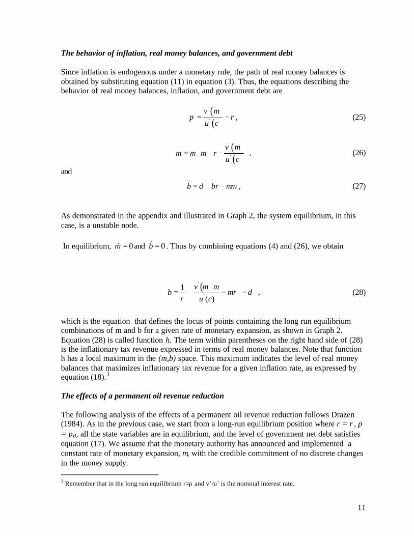
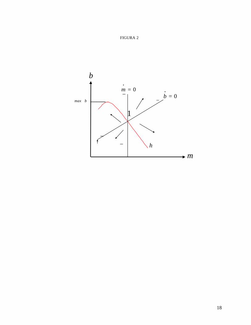
As demonstrated in the appendix and illustrated in Graph 2, the system equilibrium, in thiscase, is a unstable node.

In equilibrium, 0=m& and 0=b& . Thus by combining equations (4) and (26), we obtain

( )'

'

1( )

v m mb mr d

r u c

= − −

, (28)

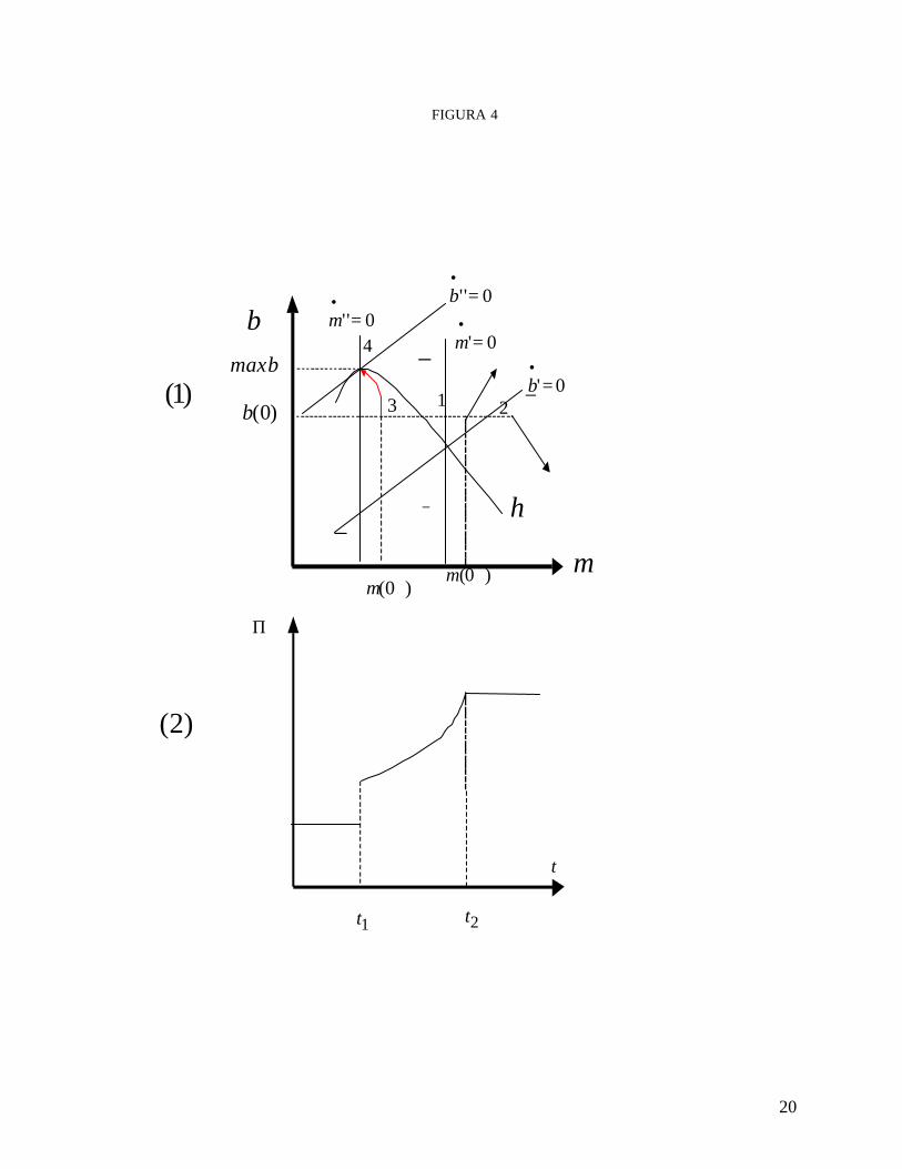
which is the equation that defines the locus of points containing the long run equilibriumcombinations of m and b for a given rate of monetary expansion, as shown in Graph 2.Equation (28) is called function h. The term within parentheses on the right hand side of (28)is the inflationary tax revenue expressed in terms of real money balances. Note that functionh has a local maximum in the (m,b) space. This maximum indicates the level of real moneybalances that maximizes inflationary tax revenue for a given inflation rate, as expressed byequation (18).3

The effects of a permanent oil revenue reduction

The following analysis of the effects of a permanent oil revenue reduction follows Drazen(1984). As in the previous case, we start from a long-run equilibrium position where r = ρ, π= π0, all the state variables are in equilibrium, and the level of government net debt satisfiesequation (17). We assume that the monetary authority has announced and implemented aconstant rate of monetary expansion, µ, with the credible commitment of no discrete changesin the money supply. 3 Remember that in the long run equilibrium r=ρ and v’/u’ is the nominal interest rate.

12

Now, we assume that oil revenue falls permanently at t0 and the central bank reacts byannouncing that the monetary rule will be maintained at the pre-shock level and that discretechanges in the monetary aggregate will not be allowed. As the result of the permanent oilrevenue reduction, private consumption decreases at the time of the shock and the country’snet debt level remains unchanged at the new equilibrium as in the case of the exchange raterule. The decrease in consumption causes a decrease in the demand for real money balances,as before. This lesser money demand and the permanent increase of the fiscal deficit levelgenerate the expectation that the central bank will adopt a higher rate of monetary expansionto restore fiscal equilibrium, after government debt reaches max b. This expectation of ahigher money supply growth rate contributes further to the reduction of the real moneybalances. Consequently, both the path of m and d are shifted. The path of real moneybalances shifts to the left while the path of government net debt shifts to the right. Theseshifts lead the economy to a point such as 1 in panel 1 of Graph 4. At the time of the shock,real money balances jump to point 3 that is on a path that will take them, within a finiteperiod, to point 4. At point 4, b reaches its maximum sustainable level, max b, and the rate ofmonetary expansion increases to µ2, as it is illustrated by the leftward shift experienced bythe demarcation curve m& . The initial decrease of real money balances is offset by a discreteincrease in both the exchange rate and the price level. Panel 1 of Graph 4 shows thisadjustment process.

In sum, if fiscal corrections necessary to face the permanent oil revenue reduction are notimplemented, government net debt grows until it reaches its maximum sustainable level maxb. In turn, real money balances fall continuously until they reach the level that maximizesinflationary tax revenue. Equation (25) shows that inflation increases until the time in whichthe central bank abandons the monetary rule. This behavior of inflation differs from the onethat we obtained under the exchange rate rule. Also, it is important to note that the path ofinflation becomes unstable, during the adjustment period, only under the monetary rule.

5. Concluding Remarks

Following Auernheimer (1987), we provide a simple neoclassical dynamic model as thestarting point to analyze the inconsistency between monetary and fiscal policy for an oileconomy. We assume the existence of identical private agents with rational expectations insmall open economy, for which oil constitutes a significant source of public income. Also,we assume perfect capital mobility, full employment, and flexible prices. Within thistheoretical framework, we examine the dynamics caused by a permanent oil revenuereduction when fiscal corrections are not implemented and the respective intermediatemonetary policy variable is maintained at its original level.

In particular, we examine the effects of a permanent oil shock under two alternative monetaryregimes. These regimes are, according to the election of the intermediate variable, theexchange rate rule and a monetary rule. Policy inconsistency arises when government netdebt grows without limits, given a monetary strategy that determines both the inflationary taxand the exogenous components of the fiscal deficit.

13

Two important conclusions emerge from our work. First, keeping policies at the levelprevious to the permanent decrease in oil revenue generates an unstable growth ofgovernment indebtedness, under any of the monetary regimes that were examined. Thisunstable growth causes both the abandonment of the monetary regime and higher futureinflation rates. Second, maintaining the monetary regime after the oil shock in order tostabilize the path of debt causes increasing inflationary and indebtedness costs.

Intuitively, the adverse oil shock implies greater discounted values of future fiscal deficits.Consequently, private agents forecast that the government will use higher seigniorage tomeet future higher fiscal deficit levels. At some later point, the central bank would modifythe monetary strategy by either replacing the intermediate variable or redefining it to a levelconsistent with a greater fiscal deficit. Thus, the ultimate results are higher inflation, agreater level of public indebtedness, and higher debt-service expenses.

These previous results do not consider the rationale that might explain why the central bankmaintains the monetary regime after an adverse oil shock. On this topic, Auernheimer (1987)suggests that the central bank could overestimate the government’s ability to restore theequilibrium deficit. Also, he argues that monetary discipline could either motivate or forcethe government to implement the necessary fiscal adjustments. Further research will analyzethe reasons that motivate the central bank decision to maintain its monetary program after apermanent oil revenue reduction.

Another interesting opportunity for future research is to extend our analysis by including aninflation targeting monetary regime. We can use two alternative approaches for this task. Wecan either include the case of Taylor’s rules or consider the case of an optimal rule explicitlyderived from the monetary authority’s maximization problem.

14

Appendix

In this appendix some of the technical derivations employed in the work are discussed.

1. First order conditions of the individual problem

In order to solve the problem of individual optimization we applied the maximum principlein terms of the current value of the Hamiltonian:

( ) ( ).

H u c v m wλ= + + (A1)

The conditions of first order are

( )' 0cH u c λ= − = (A2)

( )' ( ) 0mH v m rλ π= − + = (A3)

( ).

wH rλ ρλ λ ρ= − = − (A4)

( )'lim 0t

twu c e ρ−

→∞= (A5)

to which we added the restriction (3b) in the text. Differentiating (A2) with respect to timeand replacing in (A4) we obtain the equation (7a) in the text. Also, replacing (A2) in (A3)we obtain the equation (7b).

2. Dynamics of c and W

Linearizing (6) and (7a) in the neighborhood of an initial equilibrium, we have:

.

.J

c cc

Ω Ω − Ω = −

%

%(A6)

( )( )

' "2 ,

/ 1/ 0

c

rJ

r u uΩ

∂ Ω Ω = − % %

(0.1)

15

where J is the Jacobian.

Because (TrJ)2-4detJ>0 and TrJ>0 by hypothesis, dynamics exhibits a saddle path, which,given to the initial conditions of the state variables and the characteristics of the problem,determines a unique rational expectations solution.

2. Dynamics of m y b

Linealizing (4) y (17) in the neighborhood of a long term initial equilibrium we have:

m mmJ

b b b

− = −

%&& % (A7)

where

( ),

''( ) / '( ) 0

m b

mv m u cJ

rµ

− = − %%

Because detJ > 0, (TrJ)2 > 0, y (TrJ)2-4detJ > 0 by hipothesis, this equilibrium is an unstablenode. In this case, we have an unique rational expetation equilibrium as in Drezen (1984).

16

References

Auernheimer, Leonardo, “The honest government's guide to the revenue from the creation ofmoney”, Journal of Political Economy, 82, (19xx), pp. 598-606.

Auernheimer, Leonardo, “On the outcome of inconsistent programs under exchange rate andmonetary rules, or ‘Allowing the market to compensate for government mistakes’ ”, Journalof Monetary Economics, Vol. 19, (March 1987), pp. 279-305.

Auernheimer, Leonardo and Michael Ellis, “Stabilization under capital controls”, Journal ofInternational Money and Finance, Vol. 15, (August 1996), pp. 523-533.

Auernheimer, Leonardo and Roberto Garcia Saltos, “International debt and the price ofdomestic assets” IMF Working Paper, No. 00/177, (October 2000).

Calvo, Guillermo, “Devaluation: levels versus rates”, Journal of International Economics,11 (1981), pp. 165-72.

Calvo, Guillermo, “Staggered prices in a utility maximizing framework”, Journal ofMonetary Economics, Vol 12 (September 1983), pp.383-98.

Calvo, Guillermo, “Macroeconomic implications of the government budget constraint: somebasic considerations”, Journal of Monetary Economics, Vol 15 (1985), pp. 95-112.

Drazen, Allan, “Tight money and inflation: further results”, Journal of Monetary Economics,Vol. 15 (1984), pp. 113-120.

Drazen, Allan and Elhanan Helpman, “Stabilization with exchange rate management”,Quarterly Journal of Economics, Vol. 52 (November 1987), pp. 835-855.

Krugman, Paul, “A model of balance of payments crisis”, Journal of Money, Credit andBanking, 11 (1979), pp. 311-325.

Liviatan, Nissan, “Tight money and inflation”, Journal of Monetary Economics, Vol. 13(1984), pp. 5-15.

Sargent, Thomas and Neil Wallace, “Some unpleasant monetarist arithmetic”, FederalReserve Bank of Minneapolis Quarterly Review, Vol. 1 (1981), pp. 1-17.

Zavarce, Harold, “Fiscal inconsistency and oil shocks: The case of the exchange rule”,Central Bank of Venezuela, Mimeo, (Julio 1998).

17

FIGURA 1

1Ω)

Ω)

C

Ω

0=•

C

0=Ω•+

−

+− 2

1

18

FIGURA 2

bmax

b

m

0=•

m− +

+

−0=

•b

h

1

+

+

−−

•C=0

+

+

+

+

-

-

-

-c

2b1

2 c1c1

0 Ω Ω

Ω=0•

π0

π

m

a

m

0

0 0 b

0 b t1 t3

(c1,r+π0)

2

m1

m1 / E0

2 2

2

t0 t

b0

b

Ln E

t0 t1 t3 t

t1 t3t0 tt1 t3t0 t

co

c π

co

1

1

1

1

1

(c0,r+π0)

m0

m0 / E0

b~

π1

1

π0

3

m2

m2 / E1

(c1,r+π1)

π1 33

3 3

3

2

3

2

1

4

5

1’

7

6

8

20

FIGURA 4

bbmax

m

)0(b)1(

1t 2t

Π

t

)2(

0'' =•b

0'' =•m

4

)0( +m

3

)0( −m

1

0'=•m

− +

+

− 0'=•b

h

+

+ −

−

2