Naivete and sophistication in dynamic inconsistency

Zsombor Z. Medera, Janos Fleschb, Ronald Peetersa

aDepartment of Economics, Maastricht University, The NetherlandsbDepartment of Quantitative Economics, Maastricht University, The Netherlands

Abstract

This paper introduces a general framework for dealing with dynamic inconsistency in

the context of Markov decision problems. It carefully decouples and examines concepts

that are often entwined in the literature: it distinguishes between the decision maker

and its various temporal agents, and between the beliefs and intentions of the agents.

Classical examples of naivete and sophistication are modeled and contrasted based on

this new language. We show that naive and sophisticated decision makers can form

optimal strategies at each possible history, and provide welfare comparisons for a class

of decision problems including procrastination, impulsiveness, underinvestment, binges

and indulgence. The creation of a unified formalism to deal with dynamic inconsistency

allows for the introduction of a hybrid decision maker, who is naive sometimes, sophis-

ticated at others. Such a hybrid decision maker can be used to model situations where

type determination is endogenous. Interestingly, the analysis of hybrid types indicates

that self-deception can be optimal.

Keywords: dynamic inconsistency; naivete; sophistication; Markov decision problem;quasi-hyperbolic discountingJEL: C70, D11, D91

Email addresses:z.meder@maastrichtuniversity.nl (Zsombor Z. Meder),j.flesch@maastrichtuniversity.nl (Janos Flesch),r.peeters@maastrichtuniversity.nl (Ronald Peeters)

Job market paper October 5, 2014

1. Introduction

Imagine that you are sitting with a few friends, drinking beer. You have just finishedyour second glass, and your friends want to order a new round. You think to yourself:“well, I could deal with one or two more, but then I really should go home.” However,from previous experience, you are also acutely aware that after your third beer yourmindset is likely to change. You will start fooling yourself, repeating over and overin the course of the evening: “just one more beer, and then I am really going home”.This would lead to an undesirable outcome, getting drunk and having a hangover thenext morning. So you wisely leave your friends after just your second beer. What ishappening here? The framework that we propose in this paper makes it possible tomodel this and similar scenarios.1

Traditionally, there are three main ways to portray decision makers under timeinconsistency. The first one regards decision makers as naifs (Akerlof, 1991; O’Donoghueand Rabin, 1999b), the second attributes sophistication to them (Laibson, 1997; Fischer,1999; Harris and Laibson, 2001), while the third argues that even resolute behavior ispossible (McClennen, 1990). A common assumption of these models in the classicpapers on dynamic inconsistency is regarding the decision maker as falling entirelyinto one of the above three categories, treating his type as exogeneously given. Morerecently, mainly building on the work of O’Donoghue and Rabin (2001), hybrid decisionmakers have been considered, in models of so-called “partial naivete”. However, thesemodels still treat this type as exogeneous to the decision problem.

One way to interpret our example above is that you are sophisticated after finish-ing the first two beers, but as you drink more, you expect to become naive later on.The story indicates that in certain situations, a decision maker could cause his typeto change; moreover, he might even be able to reason about such changes. Any per-spective that assumes a fixed type is unable to capture such situations. In order to fixthis shortcoming, we attempt a general interpretation of naivete and sophistication fordynamic inconsistency. The language we develop allows the introduction of hybrid-typedecision makers such as the one in our example.

Following a review of the relevant literature, we start building a formalism thatallows for precise definitions of the two most commonly discussed types of decisionmakers, naifs and sophisticates. We work in discrete time, assuming that the situationof the decision maker can be captured as a Markov decision problem. Adopting theterminology of multiple self models, we distinguish between the agent level and the levelof the decision maker. Starting on the agent level, we introduce the notion of a strategy,which contains information about the intentions and beliefs of the individual agentat one particular history. Next, the properties of strategies (coherence, stationarity,consistency) are discussed. Moving to the level of the decision maker (i.e., the collectionof all agents), we define the concept of a frame, and consider its properties. In twotheorems, we link the properties of strategies to the properties of frames. Frames are

1The model of this situation is presented in Section 7.

2

a novel concept that provide all the relevant information on a decision maker facingdynamic inconsistency.

After clarifying our assumptions on utility functions, we define and introduce thetwo pure types of decision making, naivete and sophistication. We provide existenceresults for optimal frames of both types, and discuss various properties of such frames.In the main text body, we then expand the framework to include decision makers witha hybrid type, also providing an existence theorem, and discuss two examples of hybriddecision making in detail. In the concluding section, we point towards further extensionsof the model. The appendix gives a minimalist summary of classical decision problemsof the literature on dynamic inconsistency, and compares naively and sophisticatedlyoptimal frames for these problems. It also serves as an illustration for the applicabilityof our approach.

The contributions of this paper are thus threefold. First, it provides new conceptsand distinctions for problems of dynamic inconsistency. In particular, the representationof the decision maker through a frame, the distinction between a stationary strategyand frame, and the theorems relating consistency and stationarity should prove useful(Section 3.6). Second, it provides definitions for naivete and sophistication, and showsthe existence of naively and sophisticatedly optimal frames. Third, it introduces hybridnaive-sophisticated types, expanding the scope of dynamic inconsistency models. As acorollary, the analysis of hybrid types shows that self-deception can be optimal.

2. Related literature

Modelling approaches to dynamic inconsistency come in two varieties (Asheim,2007). Dual-self planner-doer models bear a close analogy to principal-agent models(Thaler and Shefrin, 1981). A (single) planner, endowed with dynamically consistentpreferences formulates plans; a present-biased doer can execute them or deviate fromthem. The conceptual background of planner-doer models is multifold: they sometimesrely on the hot-cold empathy gap (Loewenstein, 2005), on recent findings of neuro-science, or even the Freudian distinction between the id and the ego. Fudenberg andLevine (2006) argues in favor of dual-self model as being more simple analytically, morein line with findings in neuroscience, and nevertheless being able to explain a large num-ber of empirical phenomena. An important advantage of this approach is that welfarecomparisons are relatively straightforward: the preferences of the planner are generallyadopted to be normatively relevant. Recent models allow for the planner to learn aboutthe doer’s type through costly experimentation (Ali, 2011), or can include self-control(Gul and Pesendorfer, 2001; Benabou and Pycia, 2002; Fudenberg and Levine, 2012).

Despite all their advantages, dual-self models make the strong assumption thatindividuals have long-run, time-consistent preferences, and that these preferences canbe identified. In this paper we avoid this assumption, and instead adopt the multiple-self approach.2 Our primary focus is on naive and sophisticated decision makers, and

2Bach and Heilmann (2011) link multiple-self models to the philosophical literature on personal

3

hybrid types. Multiple-self models have analyzed pure types of decision makers ina variety of settings. For instance, Laibson (1994); Fischer (1999); Laibson (1997);Angeletos et al. (2001) work with sophisticates, while Akerlof (1991) and O’Donoghueand Rabin (1999b) assume naivete. In a generial equilibrium setting, Herings and Rohde(2006, 2008) deal with both naifs and sophisticates. For us, a crucial precursor paper isO’Donoghue and Rabin (1999a), who systematically compare naivete and sophisticationfor the case of quasi-hyperbolic discounting, with so-called immediate costs and rewards.

The first model of hybrid naive-sophisticated types is in O’Donoghue and Rabin(2001). They use quasi-hyperbolic (β − δ-)discounting to define partial naivete. Whilenaifs think their β is 1, the actual β is fully known to sophisticates, while partially naiveagents think they have a β that is larger than their actual one. Partially naive agentsthus entertain false beliefs about the future (just like naifs). This approach has provenits fruitfulness especially in the contract design literature (DellaVigna and Malmendier,2004; Eliaz and Spiegler, 2006; Gilpatric, 2008); while DellaVigna and Malmendier(2006) focus on a monopolistic firm facing a mixed population of consumers. Heidhuesand Koszegi (2009) generalize the distributional assumptions on beliefs, but still in thecontext of quasi-hyperbolic discounting.

An important aspect of the O’Donoghue and Rabin (2001) approach is that – com-pared to sophistication – any degree of partial naivete can generate arbitrarily largelosses in efficiency for a decision maker. In this sense, the limit of partial naivete (asthe perceived present-biasedness approaches the real parameter) is not sophistication.

There were a few other attempts to treat hybrid decision makers. In Asheim (2007),agents have a perceived preference persistence, i.e., a probability (between 0 and 1)with which they think their preferences will be identical in the next period. However,this belief is always incorrect, as their preferences will change with probability 1. InJehiel and Lilico (2010) agents endowed with exponential discounting have access toinformation about a number of future periods (“foresight”). They find that improvingthe length of foresight always improves welfare.

This paper expands on the existing literature by providing the foundations of ahybrid model that is independent of the quasi-hyperbolic assumption of O’Donoghueand Rabin (2001), and where type determination is an endogenous part of the decisionproblem, as in our motivating example.

In the appendix, we provide stylized models of a few standard problems often dis-cussed in the context of dynamic inconsistency: procrastination (Akerlof, 1991; Fischer,1999; Ariely and Wertenbroch, 2002; Steel, 2007), impulsiveness (Ainslie, 1974, 1975),underinvestment (Laibson et al., 1998; Angeletos et al., 2001; DellaVigna and Mal-mendier, 2004) and binging behavior/addiction (Gruber and Koszegi, 2001; Ainslie andMonterosso, 2003). Indulgence is a particular type of timing problem, where the issue iswhen to consume a certain good. We adopt the latter model directly from O’Donoghueand Rabin (1999a). For all of these problems, we compare the welfare of naive and

identity.

4

sophisticated decision makers. The appendix also serves as a means of illustrating thepotential use of our framework.

3. Basic concepts

In this section, we introduce our framework and notations. Standard definitionsare provided for the notions of “decision problem” and “history”. However, beforeintroducing strategies, we argue in Section 3.3 for a new way of defining strategies thatincludes both beliefs and intentions. We then proceed by defining strategies and frames,which correspond to two different levels of analysis. Towards the end of the section, wepresent some results on the relationship between consistency and stationarity.

3.1. Markov decision problem

We start with a decision maker facing a finite Markov decision problem on an infinitehorizon.3

Definition 1. A finite Markov decision problem is given by:

• the set of time periods T = 0, 1, 2, . . . ;

• a finite set of states Ω, with ω ∈ Ω as the initial state;

• a finite and non-empty set of pure actions Aω that the decision maker can choosefrom in state ω;

• a payoff function uω : Aω → R that assigns a payoff to every action in state ω;

• transition probabilities mω : Aω → ∆(Ω), with mω (ω′|aω) denoting the probabil-ity to transit from state ω to state ω′ when action aω is chosen.

This definition excludes the possibility of randomization over actions, although in somecases such an extension is needed to obtain existence of a stationary optimal strategy(see Section Appendix A.2). Nevertheless, in order to keep the presentation simpler,for the moment we only consider pure actions.

3.2. History

To capture all the informational aspects on which an action choice can be condi-tioned, we introduce the notion of a history:

Definition 2. A history h has the form h =(ω0, aω0 , . . . , ωt−1, aωt−1 , ωt

), with:

• ωi ∈ Ω, for i ∈ 0, 1, . . . , t, and ω0 = ω;

3The latter is not a restrictive requirement, since it is easy to rewrite a decision problem on a finitehorizon to one on an infinite horizon.

5

• aωi ∈ Aωi , for i ∈ 0, 1, . . . , t− 1;

• mωi (ωi+1|aωi) > 0, for i ∈ 0, 1, . . . , t− 1.

The length of h or current time at h is denoted by t = t(h), and the function ω(h) = ωt(h)

indicates the current or end state at history h. We use H to refer to the set of allhistories.

If history h′ begins with h, we say that h′ succeeds h, or equivalently, that h precedesh′; and denote this with h 4 h′, or equivalently, with h′ < h.4 The subset of H thatconsists of all histories that succeed h is denoted by H<h:

H<h = h′ ∈ H| h′ < h.

We refer to h0 = (ω0) as the “root history”. To shorten notation, when specifying ahistory, we sometimes omit the commas separating states and actions, and also theenclosing parentheses. Thus, history h = (ω0, aω0 , ω1) will be occasionally written ash = ω0aω0ω1.

3.3. Conceptual foundations

The fundamental entities in our model are agents :5 they are the ones with theultimate power of choosing an action and executing it. We assume a one-to-one corre-spondence between histories and agents. Our agents form beliefs and intentions aboutthe future, and have the ability to choose an action in the present.6 To refer to thecollection of all agents, we use the notion of decision maker.

We keep the general assumption that past actions have no effect on the well-beinggenerated by current and future actions of the agents, i.e., “bygones are bygones”. Ouragents have full control over their current actions.7

Using the distinction between experienced and decision utility (Kahneman et al.,1997), we can delimit two senses of “expected utility from taking action a”. Let usdisregard the immediate payoff for taking the action, and consider only future payoff.In one sense, the phrase could mean “experienced utility from expectation”, i.e., utilitythat is actually experienced by the agent due to expecting a certain stream of futurepayoffs. Think of a student that decides to study for an upcoming exam instead ofwatching his favorite TV show. He might, in fact, already enjoy the benefits of thedecision to study (he is already less anxious for the exam, maybe he relishes the ideathat he is doing “the right thing” etc.). The other sense of “expected utility” could

4Obviously, h′ 4 h & h 4 h′ ⇔ h = h′.5Others in the multiple-selves approach refer to them as “selves”.6We follow Cowen (1991), who identifies a self “with a set of preferences linked to certain cognitive

and volitional capacities.”7To see that this choice is not so obvious, see Jehiel and Lilico (2010). Similarly, Elster’s interpre-

tation of the Ulysses story is an example of a model where control over current action is essentiallyeliminated (Elster, 1979).

6

be rendered as “the expected present value of various streams of payoffs” that theagent’s current decision can lead to. In this sense, the agent is not experiencing anyactual change in utility by choosing one or other course of action; he is merely able tocalculate with these future payoffs. This distinction between the two senses of expectedutility will be used in Section 4, and in our conceptual interpretations of naivete andsophistication in subsequent sections.

3.4. Intentions, beliefs, strategy

We attempt to give a full description for the two most prevalent decision maker types(naifs and sophisticates) and the hybrid types that we introduce later in the paper. Forthis purpose, we define a strategy as having three components: the current action, theintended future actions, and the belief on what future agents will in fact do. There isno special reason for assuming that the latter two coincide for future actions, althoughwith our definitions, they coincide for pure, but not for hybrid decision makers. Tosimplify notation, we reduce this triadic framework to just intentions and beliefs, andassume that for the current action, these two have to coincide: no agent can be wrongabout which action he takes, and each agent takes the action that he intends to.

The basic building blocks of our model are all functions from the set of historiesthat succeed the agent to the set of available actions at those histories.

Definition 3. The intentions of an agent at history h assign an intended action toeach history that succeeds the present:

ih : h ∈ H<h 7→ Aω(h).

Definition 4. The beliefs of an agent at history h assign an action to each history thatsucceeds the present:

bh : h ∈ H<h 7→ Aω(h).

Note that intentions and beliefs are defined at all succeeding histories, even at thosethat the agent does not intend to reach or believes will not be reached.

We now proceed to define strategies as the pair of intentions and beliefs for an agent.This practice is not common: beliefs are usually separated from the strategy. However,it turns out to be very convenient to include them as part of the strategy.

Definition 5. A strategy of an agent at history h is a pair of intentions and beliefs forthat agent, with the added property that the belief and intention for the current actioncoincide:

sh =(ih, bh

),with ih

(h)

= bh(h).

The set of all strategies for this agent is denoted by Sh.

For an agent at h, ih (h) refers to the intention, while bh (h) refers to the belief compo-nent of the strategy sh about the future agent at h. For example, bh (h) = a should be

7

read as such: “The agent at h who holds strategy sh believes the agent at h will chooseaction a.”

We emphasize that our definition of a strategy in terms of an intention-belief pairis not standard. In fact, the most common practice is to conflate the two concepts. Onthe other hand, in epistemic game theory, beliefs are strictly seperated from actions. Ifour usage seems awkward, it might be convenient for the reader to think of the term“strategy” simply as an abbreviation for “intention-belief pair”.

We can now define two properties of strategies, stationarity and coherence, as wellas a relation over the set of strategies, consistency.

Definition 6. The intentions (or beliefs) of an agent at h are stationary whenever theintended (believed) actions depend only on the end-state. Thus, ih or bh is called sta-tionary if, for all h, h′ ∈ H<h with ω(h) = ω (h′), we have ih (h) = ih (h′) or respectively,bh (h) = bh (h′). A strategy sh is stationary if both its constituent intentions ih andbeliefs bh are stationary.

For example, if each day of the week can be modeled as a single state, the strategy ofan agent who intends and believes eating in a restaurant every second Saturday, butstaying home on every other one is not stationary.

Definition 7. An agent at h is said to hold a coherent strategy, if his intention andbeliefs about future actions coincide for all future histories. Formally, a strategy sh =(ih, bh) of an agent at h is coherent if ih(h) = bh(h) for all h ∈ H<h.

For example, a strategy of an agent who intends to stop drinking, but believes he willbe unable to do so is not coherent.

Definition 8. The strategies of two agents at h and h′ are said to be consistent if theyassign the same intentions and beliefs to each history that succeeds both agents, i.e.,sh and sh

′are consistent, if sh (h′′) = sh

′(h′′) for all h′′ ∈ H<h ∩H<h′ .8

For example, a strategy formulated yesterday which intended eating apples for todayas desert and a strategy formulated today that intends eating cookies instead are notconsistent.

Whereas coherence concerns the relationship between the intentions and beliefs ofthe same strategy, i.e., belonging to one agent, consistency compares strategies of twodistinct agents. In other words, coherence is an intrinsic property, whereas consistencyis an extrinsic (relational) property of a strategy.

A natural question is whether consistency of strategies is transitive, i.e., whether if sh

and sh′are consistent, and sh

′and sh

′′are also consistent, for some h 4 h′ 4 h′′, implies

that sh and sh′′

are also consistent. However, without this constraint, consistency is nottransitive in general – it is not even transitive within the set of stationary strategies.

8So, if two strategies are defined at histories that neither succeed nor preceed each other, then theyare consistent, as there are no histories that succeed both.

8

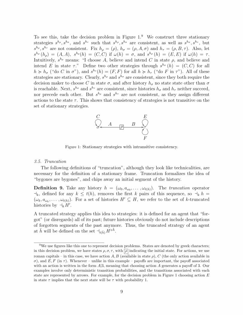
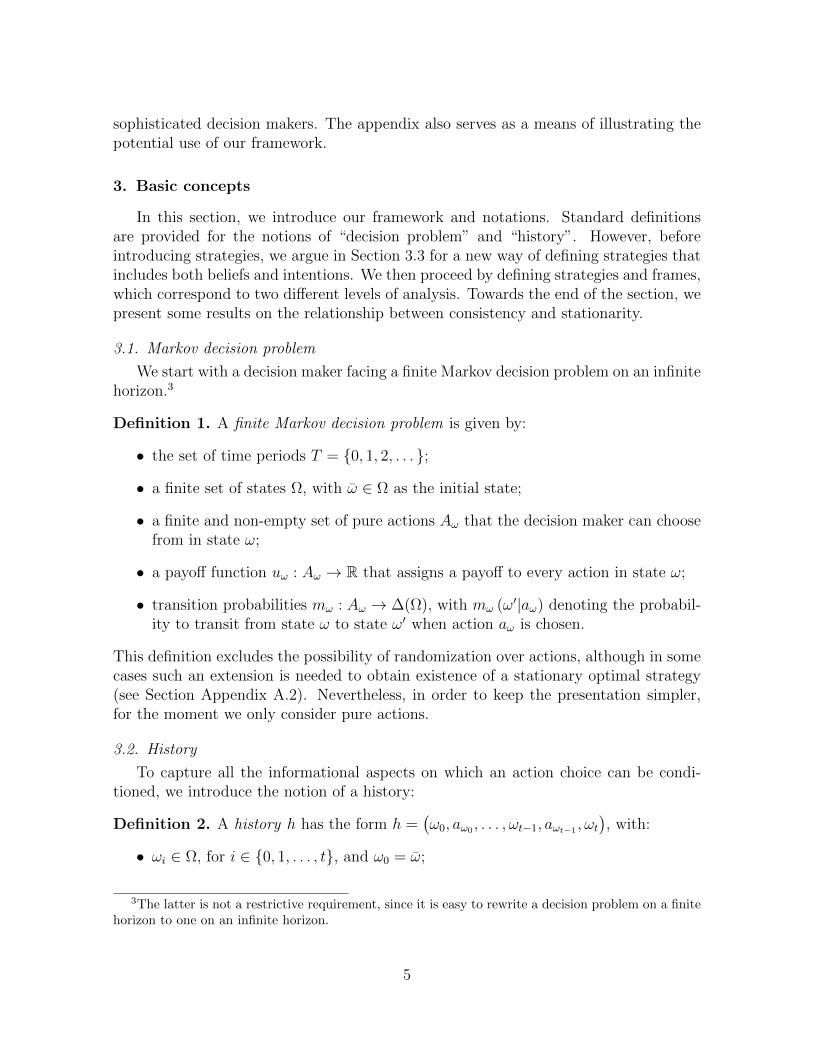
To see this, take the decision problem in Figure 1.9 We construct three stationarystrategies shρ , shσ , and shτ such that shρ , shσ are consistent, as well as shσ , shτ , butshρ , shτ are not consistent. Fix hρ = (ρ), hσ = (ρ,A, σ) and hτ = (ρ,B, τ). Also, letshρ (hρ) = (A,A), shρ(h) = (C,C) if ω(h) = σ, and shρ (h) = (E,E) if ω(h) = τ .Intuitively, shρ means: “I choose A, believe and intend C in state ρ, and believe andintend E in state τ .” Define two other strategies through shσ (h) = (C,C) for allh < hσ (“do C in σ”), and shτ (h) = (F, F ) for all h < hτ (“do F in τ”). All of thesestrategies are stationary. Clearly, shρ and shσ are consistent, since they both require thedecision maker to choose C in state σ, and after history hσ no state state other than σis reachable. Next, shσ and shτ are consistent, since histories hσ and hτ neither succeed,nor precede each other. But shρ and shτ are not consistent, as they assign differentactions to the state τ . This shows that consistency of strategies is not transitive on theset of stationary strategies.

σ

C

ρAoo B //τ

E

F

CC

Figure 1: Stationary strategies with intransitive consistency.

3.5. Truncation

The following definitions of “truncation”, although they look like technicalities, arenecessary for the definition of a stationary frame. Truncation formalizes the idea of“bygones are bygones”, and chips away an initial segment of the history.

Definition 9. Take any history h = (ω0, aω0 , . . . , ωt(h)). The truncation operatorak, defined for any k ≤ t(h), removes the first k pairs of this sequence, so ak h =(ωk, aωk , . . . , ωt(h)). For a set of histories H ′ ⊆ H, we refer to the set of k-truncatedhistories by akH ′.

A truncated strategy applies this idea to strategies: it is defined for an agent that “for-got” (or disregards) all of its past; future histories obviously do not include descriptionsof forgotten segments of the past anymore. Thus, the truncated strategy of an agentat h will be defined on the set at(h)H

<h.

9We use figures like this one to represent decision problems. States are denoted by greek characters;in this decision problem, we have states ρ, σ, τ , with ρ indicating the initial state. For actions, we use

roman capitals – in this case, we have action A,B (available in state ρ), C (the only action available inσ), and E,F (in τ). Whenever – unlike in this example – payoffs are important, the payoff associatedwith an action is written in the form A|3, meaning that choosing action A generates a payoff of 3. Ourexamples involve only deterministic transition probabilities, and the transitions associated with eachstate are represented by arrows. For example, for the decision problem in Figure 1 choosing action Ein state τ implies that the next state will be τ with probability 1.

9

Definition 10. For any strategy sh, the truncated strategy ash : h ∈at(h)H<h 7→ Aω(h)

denotes the function for which ash(at(h)h

)= sh(h), for all h ∈ H<h.

We note that while truncated histories are defined for truncations of arbitrary length(ak), for strategies we only need truncations of length t(h) for a strategy sh of an agentat history h.

To see this definition at work, think of the decision to stop smoking on the firstday of the next month. Take an agent who resolves on July 24th: “I will stop smokingfrom August 1st” and then fails. On August 24th, he makes another decision: “I willstop smoking from September 1st”. If we interpret each statement as a strategy, itis easy to see that they are not consistent: they prescribe different smoking behaviorfor instance, for August 28th – the first strategy forbids it, while the second allows it.However, there is an intuitive sense in which they are very similar. Indeed, they mapthem into the same resolve that uses indexicals instead of precise dates: “I can smokefor one more week, and then I will stop”.10 Truncating the present history highlightsthis similarity by getting rid of the past. In our example, the original strategies are notidentical or consistent; but their truncated versions are identical.

3.6. Frames

We now move from the agent level to the level of the decision maker. Since thereis no a priori reason for the agents to have consistent strategies, different agents canform different intentions and entertain different beliefs about any certain future agent.To have an “external” overview of all agents, we introduce the concept of a frame.In our terminology, a frame is an auxiliary tool for representing the strategies of allpossible agents, and not something that is intentionally put together by the decisionmaker. Whereas each agent chooses a strategy, the decision maker does not choose aframe. Instead, a frame contains a full description of the intentions and beliefs in allcontingencies, i.e., at all histories.

Definition 11. A frame a frame assigns a strategy to each agent. That is, a frame isa function f : h ∈ H 7→ Sh.

• Each agent has a strategy.

• The collection of all agents, i.e., the decision maker, is described through a frame.

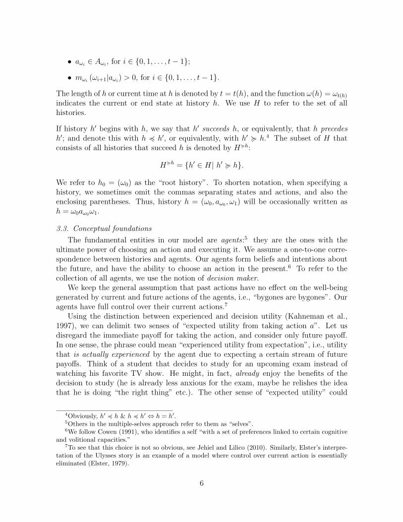
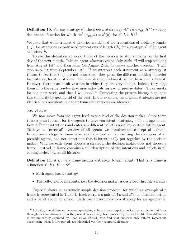
Figure 2 shows an extremely simple decision problem, for which an example of aframe is represented in Table 1. Each entry is a pair of A’s and B’s, an intended actionand a belief about an action. Each row corresponds to a strategy for an agent at h,

10Actually, the difference between specifying a future consumption period by a calendar date orthrough its time distance from the present has already been noticed by Strotz (1956). This differenceis experimentally explored by Read et al. (2005), who find that subjects only exhibit hyperbolicdiscounting when future periods are identified via their temporal distance.

10

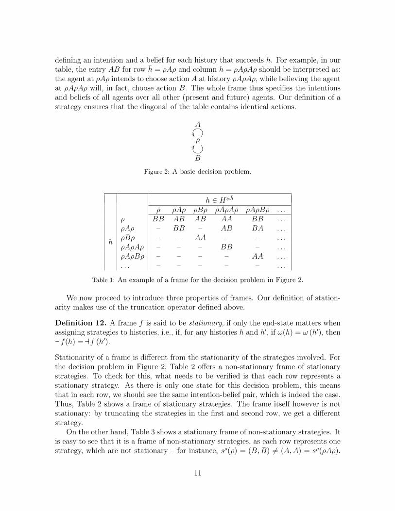
defining an intention and a belief for each history that succeeds h. For example, in ourtable, the entry AB for row h = ρAρ and column h = ρAρAρ should be interpreted as:the agent at ρAρ intends to choose action A at history ρAρAρ, while believing the agentat ρAρAρ will, in fact, choose action B. The whole frame thus specifies the intentionsand beliefs of all agents over all other (present and future) agents. Our definition of astrategy ensures that the diagonal of the table contains identical actions.

ρ

A

B

FF

Figure 2: A basic decision problem.

h ∈ H<h

ρ ρAρ ρBρ ρAρAρ ρAρBρ . . .

h

ρ BB AB AB AA BB . . .ρAρ – BB – AB BA . . .ρBρ – – AA – – . . .ρAρAρ – – – BB – . . .ρAρBρ – – – – AA . . .. . . – – – – – . . .

Table 1: An example of a frame for the decision problem in Figure 2.

We now proceed to introduce three properties of frames. Our definition of station-arity makes use of the truncation operator defined above.

Definition 12. A frame f is said to be stationary, if only the end-state matters whenassigning strategies to histories, i.e., if, for any histories h and h′, if ω(h) = ω (h′), thenaf(h) =af (h′).

Stationarity of a frame is different from the stationarity of the strategies involved. Forthe decision problem in Figure 2, Table 2 offers a non-stationary frame of stationarystrategies. To check for this, what needs to be verified is that each row represents astationary strategy. As there is only one state for this decision problem, this meansthat in each row, we should see the same intention-belief pair, which is indeed the case.Thus, Table 2 shows a frame of stationary strategies. The frame itself however is notstationary: by truncating the strategies in the first and second row, we get a differentstrategy.

On the other hand, Table 3 shows a stationary frame of non-stationary strategies. Itis easy to see that it is a frame of non-stationary strategies, as each row represents onestrategy, which are not stationary – for instance, sρ(ρ) = (B,B) 6= (A,A) = sρ(ρAρ).

11

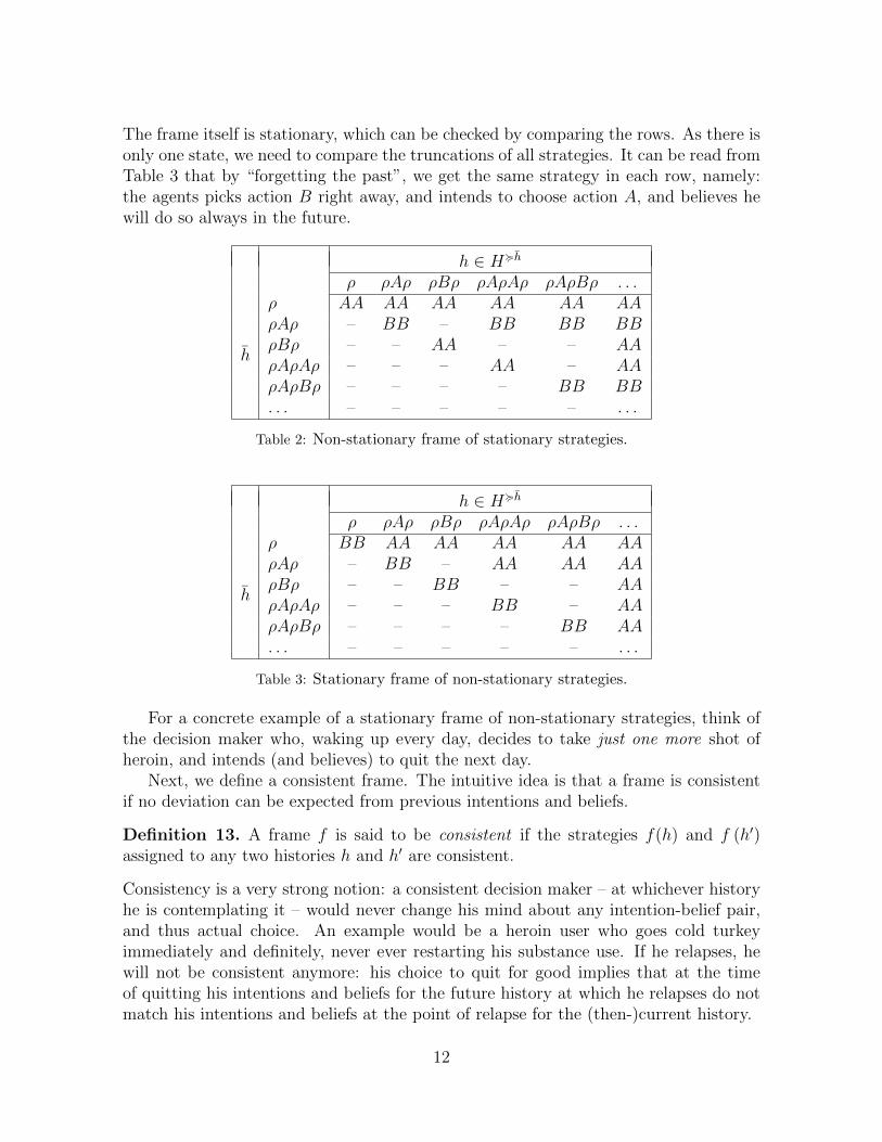
The frame itself is stationary, which can be checked by comparing the rows. As there isonly one state, we need to compare the truncations of all strategies. It can be read fromTable 3 that by “forgetting the past”, we get the same strategy in each row, namely:the agents picks action B right away, and intends to choose action A, and believes hewill do so always in the future.

h ∈ H<h

ρ ρAρ ρBρ ρAρAρ ρAρBρ . . .

h

ρ AA AA AA AA AA AAρAρ – BB – BB BB BBρBρ – – AA – – AAρAρAρ – – – AA – AAρAρBρ – – – – BB BB. . . – – – – – . . .

Table 2: Non-stationary frame of stationary strategies.

h ∈ H<h

ρ ρAρ ρBρ ρAρAρ ρAρBρ . . .

h

ρ BB AA AA AA AA AAρAρ – BB – AA AA AAρBρ – – BB – – AAρAρAρ – – – BB – AAρAρBρ – – – – BB AA. . . – – – – – . . .

Table 3: Stationary frame of non-stationary strategies.

For a concrete example of a stationary frame of non-stationary strategies, think ofthe decision maker who, waking up every day, decides to take just one more shot ofheroin, and intends (and believes) to quit the next day.

Next, we define a consistent frame. The intuitive idea is that a frame is consistentif no deviation can be expected from previous intentions and beliefs.

Definition 13. A frame f is said to be consistent if the strategies f(h) and f (h′)assigned to any two histories h and h′ are consistent.

Consistency is a very strong notion: a consistent decision maker – at whichever historyhe is contemplating it – would never change his mind about any intention-belief pair,and thus actual choice. An example would be a heroin user who goes cold turkeyimmediately and definitely, never ever restarting his substance use. If he relapses, hewill not be consistent anymore: his choice to quit for good implies that at the timeof quitting his intentions and beliefs for the future history at which he relapses do notmatch his intentions and beliefs at the point of relapse for the (then-)current history.

12

According to this definition, if f is a consistent frame, then we get f(h) (h′′) =f (h′) (h′′) whenever h′′ ∈ H<h ∩ H<h′ , and either h′ ∈ H<h, or h ∈ H<h′ . Note that,since for a consistent frame, f(h)(h) = f(h′)(h) for all h′ and h ∈ H<h′ ; and ourrequirement for strategies that ih(h) = bh(h), a consistent frame is necessarily made upby coherent strategies. This implies that a choice of an action for all histories uniquelydetermines a consistent frame. Similarly, a choice of an action for all states uniquelydetermines a consistent frame of stationary strategies.

Theorem 1. A consistent, stationary frame consists of stationary strategies.

Proof. Take any histories h, h′ and h′′ for which ω(h′) = ω(h′′). We have to show thatf(h) (h′) = f(h) (h′′). For this, see that:

f(h) (h′) = f (h′) (h′) =af (h′)(at(h′)h′

)=af (h′′)

(at(h′′)h′′

)= f (h′′) (h′′) = f(h) (h′′) .

For the respective equations, we use, in order, consistency, definition of truncation,stationarity of the frame, definition of truncation and consistency again.

Theorem 2. A consistent frame of stationary strategies is a stationary frame.

Proof. Take histories h, h′, h′′, h′′′ with ω(h) = ω (h′). We have to show that

(af(h)) (at(h)h′′) = (af(h′)) (at(h′)h′′′)

if at(h)h′′ =at(h′)h′′′. Note that such h′′, h′′′ exist, because the end-state in h and h′ is

identical. Using the fact that ω(h′′) = ω(at(h)h′′) = ω(at(h′)h′′′) = ω(h′′′), we get:

(af(h)) (at(h)h′′) = f(h)(h′′) = f(h0)(h′′) = f(h0)(h′′′) = f(h′)(h′′′) = (af(h′)) (at(h′)h′′′).

We use, in turn, the definitions of truncation, consistency, stationarity of the strategies,consistency, and finally, truncation again. (We make use of the root strategy h0 as ahistory which is surely succeeded by both h′′ and h′′′.)

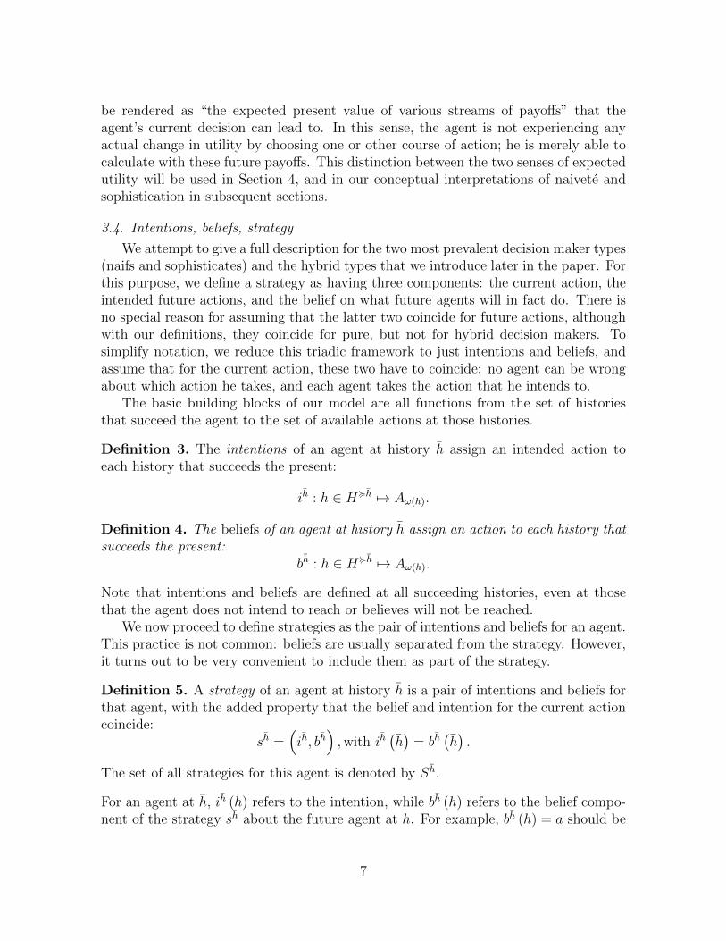
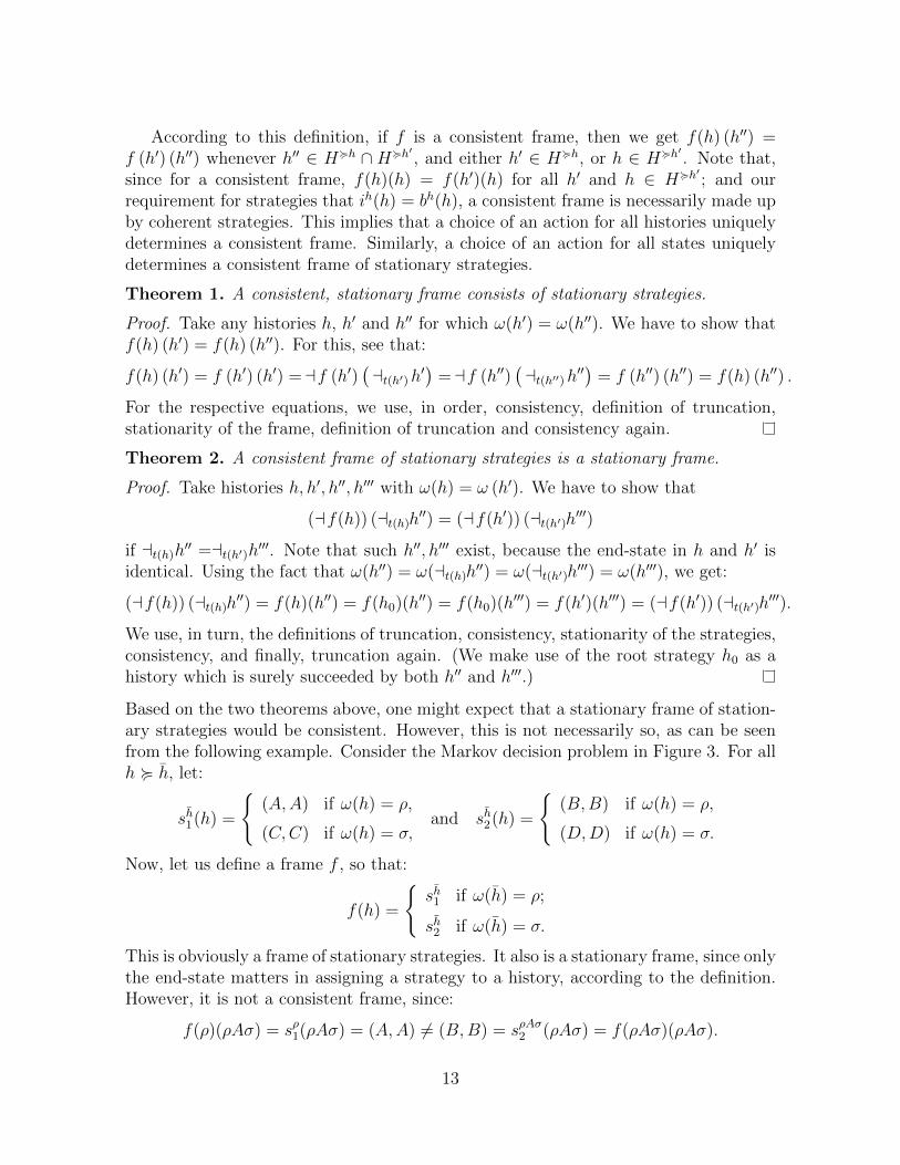
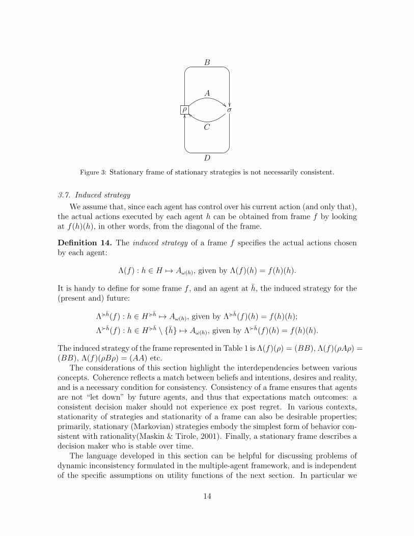
Based on the two theorems above, one might expect that a stationary frame of station-ary strategies would be consistent. However, this is not necessarily so, as can be seenfrom the following example. Consider the Markov decision problem in Figure 3. For allh < h, let:

sh1(h) =

(A,A) if ω(h) = ρ,

(C,C) if ω(h) = σ,and sh2(h) =

(B,B) if ω(h) = ρ,

(D,D) if ω(h) = σ.

Now, let us define a frame f , so that:

f(h) =

sh1 if ω(h) = ρ;

sh2 if ω(h) = σ.

This is obviously a frame of stationary strategies. It also is a stationary frame, since onlythe end-state matters in assigning a strategy to a history, according to the definition.However, it is not a consistent frame, since:

f(ρ)(ρAσ) = sρ1(ρAσ) = (A,A) 6= (B,B) = sρAσ2 (ρAσ) = f(ρAσ)(ρAσ).

13

ρ

A

!!

B

σ

C

aa

D

OO

Figure 3: Stationary frame of stationary strategies is not necessarily consistent.

3.7. Induced strategy

We assume that, since each agent has control over his current action (and only that),the actual actions executed by each agent h can be obtained from frame f by lookingat f(h)(h), in other words, from the diagonal of the frame.

Definition 14. The induced strategy of a frame f specifies the actual actions chosenby each agent:

Λ(f) : h ∈ H 7→ Aω(h), given by Λ(f)(h) = f(h)(h).

It is handy to define for some frame f , and an agent at h, the induced strategy for the(present and) future:

Λ<h(f) : h ∈ H<h 7→ Aω(h), given by Λ<h(f)(h) = f(h)(h);

Λh(f) : h ∈ H<h \ h 7→ Aω(h), given by Λh(f)(h) = f(h)(h).

The induced strategy of the frame represented in Table 1 is Λ(f)(ρ) = (BB), Λ(f)(ρAρ) =(BB), Λ(f)(ρBρ) = (AA) etc.

The considerations of this section highlight the interdependencies between variousconcepts. Coherence reflects a match between beliefs and intentions, desires and reality,and is a necessary condition for consistency. Consistency of a frame ensures that agentsare not “let down” by future agents, and thus that expectations match outcomes: aconsistent decision maker should not experience ex post regret. In various contexts,stationarity of strategies and stationarity of a frame can also be desirable properties;primarily, stationary (Markovian) strategies embody the simplest form of behavior con-sistent with rationality(Maskin & Tirole, 2001). Finally, a stationary frame describes adecision maker who is stable over time.

The language developed in this section can be helpful for discussing problems ofdynamic inconsistency formulated in the multiple-agent framework, and is independentof the specific assumptions on utility functions of the next section. In particular we

14

believe that our (conceptual) distinction between beliefs and intentions, the agent (andits strategy) and the decision maker (and the frame used to describe him), and ourmethod of representing frames through tables should prove useful. To see the latter inuse, we refer the reader to the appendix. Moreover, the distinction between stationarystrategies and stationary frames is, as far as we are aware, entirely new in the literature.

4. Utility and discounting

The term payoff, introduced in Definition 1, refers to the immediate gains or lossesresulting from an action. Formally, a payoff gained in period t is denoted by ut, anda stream of payoffs starting at period t by ut→ = (ut, ut+1, . . . ). We say that a streamof payoffs ut→ starting at period t coincides with a stream of payoffs u′t′→ starting atperiod t′ if ut = u′t′ and ut+1 = u′t′+1, and so on.

Payoffs are fully determined by the decision problem, the state and the action taken.However, time preference implies that identical payoffs might be regarded differentlyby various agents. Throughout the paper, we make two assumptions on the utilityfunctions Uh(u) that integrates a stream of future payoffs into a single number. Thefirst assumption says that Uh is continuous at infinity for every h.

Assumption 1. Uh is continuous at infinity for every h, i.e., for any ε, there is ahorizon T (h) – possibly depending on h – such that the total variation of utility aftert(h) + T (h) is less than ε. This is the same assumption as in Fudenberg and Levine(1983).

Another crucial assumption that we use is that agents are identical in the way theyevaluate streams of payoffs.

Assumption 2. For any two agents at histories h and h′, and coinciding streamsof payoffs ut(h)→, u

′t(h′)→, the utilities of the two agents are equal, i.e., Uh(ut(h)→) =

Uh′(u′t(h′)→) .

If the utility functions satisfy First and Second Order separability (Lapied and Renault,2012), then the discount factor for a future payoff ut can only depend on the timedistance t(h)− t. In our examples in Section 7 and the appendix, we use a discountedutility function of a particular form, namely, quasi-hyperbolic discounting:

Uh(ut(h)→) = ut(h) + β

∞∑t=t(h)+1

δt−t(h) ut,

with 0 ≤ β ≤ 1 and 0 ≤ δ < 1.In Section 3.3, we distinguished between two senses of the term “expected util-

ity”: utility actually experienced from expecting a future payoff stream; and “expected

15

utility” as simply a means of calculating with various future courses of action. Thisdistinction is formally nailed down and further refined by the following definitions.11

Definition 15. The expected utility based on intentions of playing strategy sh for anagent at h is:

Uhi

(sh)

= E[ih] (Uh).

On the other hand, whenever an agent is reflecting on how much utility he can reason-ably expect, he will calculate his utility based on his beliefs.

Definition 16. The expected utility based on beliefs of playing strategy sh for an agentat h is:

Uhb

(sh)

= E[bh] (Uh).

Disregarding mere expectations, to calculate the utility gained by an agent, we have toconsider which actions future agents will actually implement under various eventualities.The definition of induced strategy captures just this, and can thus be used to defineinduced utility :

Definition 17. Given a frame f , the (ex post) induced utility of the root agent at h0

is:Ur (f) = E

[Λ<h0(f)

] (Uh0).

We will use the notion of induced utility for welfare comparisons between various frames,especially in the appendix, when contrasting naive and sophisticated decision makersin particular decision problems. Implicitly, this means picking the perspective of theroot agent for welfare comparisons of frames. We do so in order to avoid any normativeassumptions on the agent’s long-run preferences.12

Notice that traditionally, the above three meanings of the term “expected utility”coincide. The reason is that where dynamic inconsistency does not pose a problem,intentions and beliefs on future actions coincide; moreover, the decision maker alwaysexecutes the intentions of past agents.

5. Naivete

At first sight, it is not even clear whether naivete is a property of the decisionmaker or that of an agent. In this and the following section, we define naivete andsophistication primarily for agents, assuming that the decision maker is always naive

11Saez-Martı and Weibull (2005) connect discounting with altruism towards future selves. Theynote that “[c]urrent welfare or ‘total utility’, so defined, does not stem only from current instantaneousutility but also from (the anticipation of) the stream of future instantaneous utilities”. Our distinctionhighlights exactly this: is it the actual future stream, or the anticipation of that stream that is reallyimportant?

12One alternative would be using a Pareto criterion, as for instance, in Herings and Rohde (2006).

16

(or sophisticated). We return to the issue presented in Section 1 after analysing andcontrasting these base cases.

Naivete has been characterized in several ways in the literature; a naif is aware orunaware of different things, depending on the particular interpretation. A naif is saidto:

• choose at each stage an option which seems currently the best (Strotz, 1956;Hammond, 1976);

• fail to realize that future selves will have different preferences (O’Donoghue andRabin, 2001; Sarafidis, 2004; DellaVigna and Malmendier, 2006; Herings and Ro-hde, 2006; Heidhues and Koszegi, 2009);

• believe that – though his preferences might change – he has perfect self-controlabout the future, allowing him to commit to a strategy (O’Donoghue and Rabin,1999a; Gruber and Koszegi, 2001; Ali, 2011).

It is easy to see that these are genuinely alternative interpretations of naivete. Acommon aspect is that something is wrong with the beliefs held by the agent. Weargue that these troubles arise from the way the naif determines his beliefs: particularly,that for a naive agent, his current preferences determine his intentions, which in turndetermine his beliefs on future actions. Thus, it does not matter whether the agentholds an explicit belief on the lack of change in his preferences, or whether he believeshe will simply fail to act on such changes, or that he has strong beliefs in his ownwill- or pre-commitment power. The essential features of naivete are the directions ofdetermination seen in Figure 4. All the above cases are described by this model.

Preferences → intentions → beliefs → strategy.

Figure 4: The forming of intentions and beliefs by a naif.

Definition 18. A strategy sh of an agent at h is naively optimal, if it maximizesexpected utility based on intentions:

sh ∈ arg maxs∈Sh

Uhi (s) ,

and it is coherent:bh (h′) = ih (h′) , for all h′ ∈ H<h.

A frame f is naively optimal if the strategy f(h) is naively optimal at each history h.

Working in a continuous-time discounted utility framework, Strotz (1956) showsthat only when the discount function is exponential does the decision maker possessa consistent naively optimal frame for all decision problems. For any non-exponentialdiscount functions there are decision problems for which there is no consistent naivelyoptimal frame.

17

Theorem 3. For any decision problem, there exists a stationary naively optimal frame.

Proof. For each h, the set arg maxs∈Sh Uhi (s) is non-empty, because Sh is non-empty

and closed for pointwise limits, and Uhi is continuous (Assumption 1). Therefore, the

set of strategies where the maximum is, in fact, reached is non-empty. But note that theoptimality condition in the definition of naively optimal strategies only determines theintention-component of strategies, thus, beliefs can be constructed freely. This meansthat we can ensure coherence, i.e., we can choose a naively optimal strategy at each h.

Now, to guarantee that the generated frame is stationary, we need to choose thesame truncated strategy for each set of histories where the end-state is identical. Thisis always possible, since whenever the final state is identical for two histories, both thetruncated strategy set and the utility function defined at those histories are identical(Assumption 2), and therefore so are the set of truncated optimal strategies.

Is the stationary naively optimal frame unique? For a naive decision maker, this dependson whether for each history, there is a unique naively optimal strategy; this latterproblem can be reduced to whether for each state that can be reached, there is aunique naively optimal strategy (defined at any history where the current state is thatstate). For generic decision problems, it seems likely that this is indeed the case,though the scope of this proof is beyond this paper. Now, if there is a unique naivelyoptimal strategy for each history, then there is only one naively optimal frame – andit is stationary, too. In degenerate cases, where multiple naively optimal strategiescan be assigned to at least one state, we get stationary naively optimal frames, alongwith non-stationary ones. It should also be noted that – because of the possibility ofinconsistency – multiplicity of naively optimal frames also leads to a multiplicity ofinduced utilities. In particular, the agents facing multiple naively optimal strategiesbelieve it does not matter which strategy they choose, as they expect they will stick tothose strategies – but they can be wrong.

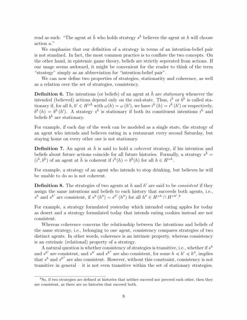
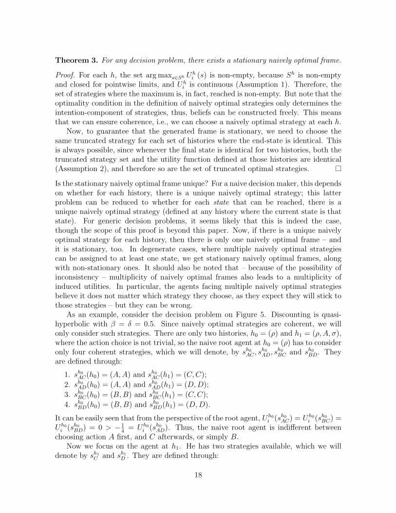
As an example, consider the decision problem on Figure 5. Discounting is quasi-hyperbolic with β = δ = 0.5. Since naively optimal strategies are coherent, we willonly consider such strategies. There are only two histories, h0 = (ρ) and h1 = (ρ,A, σ),where the action choice is not trivial, so the naive root agent at h0 = (ρ) has to consideronly four coherent strategies, which we will denote, by sh0AC , s

h0AD, s

h0BC and sh0BD. They

are defined through:

1. sh0AC(h0) = (A,A) and sh0AC(h1) = (C,C);

2. sh0AD(h0) = (A,A) and sh0AD(h1) = (D,D);

3. sh0BC(h0) = (B,B) and sh0BC(h1) = (C,C);

4. sh0BD(h0) = (B,B) and sh0BD(h1) = (D,D).

It can be easily seen that from the perspective of the root agent, Uh0i (sh0AC) = Uh0

i (sh0BC) =Uh0i (sh0BD) = 0 > −1

4= Uh0

i (sh0AD). Thus, the naive root agent is indifferent betweenchoosing action A first, and C afterwards, or simply B.

Now we focus on the agent at h1. He has two strategies available, which we willdenote by sh1C and sh1D . They are defined through:

18

ρA | 0~~

B | 0

σC | 0~~

D | 2

τ2

E2 | 0

GG

τ0

E0 | 0

GG τ1

E1 | − 3

GG

β = 0.5, δ = 0.5

Figure 5: Multiplicity of induced utility for naively optimal frames.

1. sh1C (h1) = C;

2. sh1D (h1) = D.

For the agent at h1, Uh1i (sh1D ) = 0.5 > 0 = Uh1

i (sh1C ). Therefore, the naive agent at h1

prefers to choose action D. Now, consider the two naively optimal frames fBCD andfACD, defined through:

• fBCD(h0) = sh0BC and fBCD(h1) = sh1D ;

• fACD(h0) = sh0AC and fACD(h1) = sh1D ;

From the previous calculations, we see that both fBCD and fACD are naively optimalframes. However, the induced utilities are not equal: Ur(fBCD) = 0 and Ur(fACD) =−1

4. The underlying reason is the following: when an agent picks a naively optimal

strategy in h0, he expects to earn 0 by either choosing strategy sh0BC or sh0AC . But ifhe chooses sh0AC , after getting to history h1 – on account of being present-biased – hewill not stick to his previous strategy, which would prescribe him choosing action C;instead, he chooses D, which leads to a decrease in his induced utility.

To sum up our discussion of naivete: if we interpret an optimal frame as predictivefor a naive decision maker’s behavior, then in the generic case, we get a unique predictionof actions, intentions and belief for each history; and we expect stationary behavior inrealization, and a single prediction for the induced utility. On the other hand, indegenerate cases we can get multiple predictions of actions, intentions and beliefs forsome agents; we do not necessarily expect stationary behavior; and we do not necessarilyget a unique expectation for induced utility.

6. Sophistication

Similar to naivete, there are several definitions of sophistication:

• optimality under a credibility constraint: following a feasible optimal strategy, ora plan that he will actually follow (Strotz, 1956; Yaari, 1978);

19

• game-theoretic notion: an intra-personal subgame-perfect equilibrium, sometimesalso referred to as Strotz-Pollak equilibrium (Kocherlakota, 1996; Vieille andWeibull, 2009);

• rational expectations: perfectly anticipating future behavior (O’Donoghue andRabin, 2001; Gilpatric, 2008);

• self-awareness: being aware of future changes in discount rates and preferences(Hammond, 1976; Heidhues and Koszegi, 2009; Ali, 2011).

These definitions do not match precisely. For instance, the notion of sophistication as anintra-personal equilibrium does not guarantee the satisfaction of rational expectationsin case when multiple such equilibria exist. Just like for naivete, we would like to offer anew interpretation of sophistication. We regard sophistication as primarily a propertyof agents. In our framework, the defining characteristic of sophisticated agents is thatthey first consider their beliefs about the future, and only then do they form intentions.For now, our sophisticated agents assume that all future agents will be sophisticated,too – we will relax this assumption for hybrid agents in Section 7.

A sophisticatedly optimal strategy is made up, first, by beliefs about future agents’choices: he believes each future agent will pick a best response to future agent’s choices.So we implicitly have to consider second-order beliefs, the beliefs of each agent aboutthe beliefs of agents about the future. However, we assume that in a sophisticatedstrategy, the second-order beliefs coincide with first-order beliefs.13 Thus, the currentagent believes that future agents will believe what he currently believes.

Beliefs and preferences → intentions → action → strategy.

Figure 6: The forming of intentions and beliefs by a sophisticated.

The second component of a sophisticatedly optimal strategy concerns the intentions,which are set to match the beliefs; as the agent knows he has no control over his futureselves, he can just as well intend future actions that they are choosing anyway.

Finally, the current action is chosen to be a best response to future actions.

Definition 19. A strategy sh of an agent at h is sophisticatedly optimal, if:

bh (h′) ∈ arg maxa∈Aω(h′)

Uh′

b

(sh [a : h′]

), for all h′ ∈ H<h,

and it is coherent:ih (h′) = bh (h′) , for all h′ ∈ H<h,

13O’Donoghue and Rabin (2001) makes the assumption on second-order beliefs explicit for partiallynaive agents.

20

where sh [a : h′] denotes the strategy where the action taken at h′ is replaced with actiona in strategy sh.14

A frame f is sophisticatedly optimal if the strategy f (h) is sophisticatedly optimalat each history h.

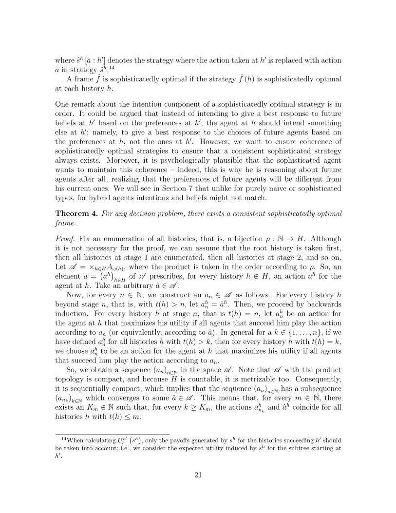
One remark about the intention component of a sophisticatedly optimal strategy is inorder. It could be argued that instead of intending to give a best response to futurebeliefs at h′ based on the preferences at h′, the agent at h should intend somethingelse at h′; namely, to give a best response to the choices of future agents based onthe preferences at h, not the ones at h′. However, we want to ensure coherence ofsophisticatedly optimal strategies to ensure that a consistent sophisticated strategyalways exists. Moreover, it is psychologically plausible that the sophisticated agentwants to maintain this coherence – indeed, this is why he is reasoning about futureagents after all, realizing that the preferences of future agents will be different fromhis current ones. We will see in Section 7 that unlike for purely naive or sophisticatedtypes, for hybrid agents intentions and beliefs might not match.

Theorem 4. For any decision problem, there exists a consistent sophisticatedly optimalframe.

Proof. Fix an enumeration of all histories, that is, a bijection ρ : N → H. Althoughit is not necessary for the proof, we can assume that the root history is taken first,then all histories at stage 1 are enumerated, then all histories at stage 2, and so on.Let A = ×h∈HAω(h), where the product is taken in the order according to ρ. So, anelement a =

(ah)h∈H of A prescribes, for every history h ∈ H, an action ah for the

agent at h. Take an arbitrary a ∈ A .Now, for every n ∈ N, we construct an an ∈ A as follows. For every history h

beyond stage n, that is, with t(h) > n, let ahn = ah. Then, we proceed by backwardsinduction. For every history h at stage n, that is t(h) = n, let ahn be an action forthe agent at h that maximizes his utility if all agents that succeed him play the actionaccording to an (or equivalently, according to a). In general for a k ∈ 1, . . . , n, if wehave defined ahn for all histories h with t(h) > k, then for every history h with t(h) = k,we choose ahn to be an action for the agent at h that maximizes his utility if all agentsthat succeed him play the action according to an.

So, we obtain a sequence (an)n∈N in the space A . Note that A with the producttopology is compact, and because H is countable, it is metrizable too. Consequently,it is sequentially compact, which implies that the sequence (an)n∈N has a subsequence(ank)k∈N which converges to some a ∈ A . This means that, for every m ∈ N, thereexists an Km ∈ N such that, for every k ≥ Km, the actions ahnk and ah coincide for allhistories h with t(h) ≤ m.

14When calculating Uh′

b

(sh), only the payoffs generated by sh for the histories succeeding h′ should

be taken into account; i.e., we consider the expected utility induced by sh for the subtree starting ath′.

21

Let shn be the strategy of the agent at history h which intends to play the action ah′n

at all histories h′ h and believes that these actions will be played – thus, a coherentstrategy. Similarly, we define the strategy sh with respect to a. Now consider the framef that assigns strategy sh to the agent at h, for every history h.

First, we show that f is consistent. Take any h, h′, the corresponding strategies sh

and sh′

and some history h′′ with h′′ < h and h′′ < h′. Then

sh (h′′) =(ah′′, ah

′′)

= sh′(h′′) .

Thus, f is a consistent frame.We now prove that f is sophisticatedly optimal. For this purpose, consider an

arbitrary agent, say at history h, and an agent at a history h′ h. By construction,for every n ≥ t (h′), the action ah

′n maximizes the utility of the agent at h′ if all agents

that succeed him play the action according to an. Thus,

bhn (h′) = ah′

n ∈ arg maxa∈Aω(h′)

Uh′

b

(shn [a : h′]

)and as we have seen, shn is coherent:

ihn (h′) = bhn (h′) .

By taking the limit along the subsequence (nk)k∈N and using continuity, we obtain

bh (h′) = ah′ ∈ arg max

a∈Aω(h′)

Uh′

b

(sh [a : h′]

)and

ih (h′) = bh (h′) .

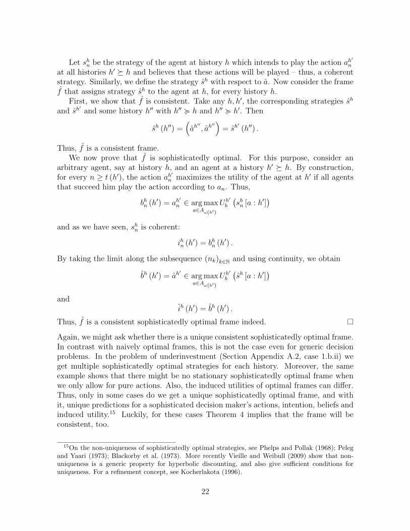
Thus, f is a consistent sophisticatedly optimal frame indeed.

Again, we might ask whether there is a unique consistent sophisticatedly optimal frame.In contrast with naively optimal frames, this is not the case even for generic decisionproblems. In the problem of underinvestment (Section Appendix A.2, case 1.b.ii) weget multiple sophisticatedly optimal strategies for each history. Moreover, the sameexample shows that there might be no stationary sophisticatedly optimal frame whenwe only allow for pure actions. Also, the induced utilities of optimal frames can differ.Thus, only in some cases do we get a unique sophisticatedly optimal frame, and withit, unique predictions for a sophisticated decision maker’s actions, intention, beliefs andinduced utility.15 Luckily, for these cases Theorem 4 implies that the frame will beconsistent, too.

15On the non-uniqueness of sophisticatedly optimal strategies, see Phelps and Pollak (1968); Pelegand Yaari (1973); Blackorby et al. (1973). More recently Vieille and Weibull (2009) show that non-uniqueness is a generic property for hyperbolic discounting, and also give sufficient conditions foruniqueness. For a refinement concept, see Kocherlakota (1996).

22

Overall, our understanding of sophistication in terms of sophisticated agents firstworking through their beliefs, then deriving their intentions is closest to the self-awareness interpretation. However, sophisticated optimality can indeed be regarded asa notion of intra-personal subgame-perfection.16 As there might be several such equilib-ria, agents at various histories might pick actions corresponding to different equilibria;thus, there is no a priori guarantee for the satisfaction of rational expectations, orthat the subgame-perfect equilibrium chosen by the root agent will actually be followedthrough. Thus, the equilibrium aspect of sophisticated optimality on the strategy leveldoes not imply consistency or stationarity for the sophisticated frame. However, theabove theorem shows that a consistent sophisticatedly optimal frame exists.

The next natural question concerns the relative advantages of sophistication againstnaivete.17 The most commonly analyzed examples in the literature of dynamic incon-sistency are stories of procrastination, impulsiveness, underinvestment, addiction andbinging behavior. We can classify these problems into two groups: in the first group,there are decisions that concern the execution of a single task, like finishing an aca-demic paper or ending a marriage in a sudden burst of anger (procrastination andimpulsiveness). In the other conceptual box, we put problems concerning the repeatedexecution of a task, like not saving enough for retirement, or drug addiction (underin-vestment and binging). It turns out that we can model all of these as Markov decisionproblems with only two states (Figures A.9 and A.10), if we assume a decision makerthat uses quasi-hyperbolic discounting, arguably the simplest form of non-exponentialdiscounting.

In the appendix, we derive conditions for the payoffs, the discount factor, and thepresent-biasedness parameter to classify these problems. We find that in some decisionproblems involving either a single or a repeated task, namely, impulsivity and bingingproblems, sophisticates commit the same mistake as naifs, and sophistication brings nobenefits. This should not come as a surprise, as we cannot expect a notion of intra-personal subgame-perfect equilibrium to solve all welfare problems of decision makers.In some single and also in some repeated decision problems, however sophisticationbrings clear benefits, and from the perspective of the root agent, the induced utilityof a sophisticatedly optimal frame can be strictly higher than that of naively optimalone. Again, this is something to be expected – sophistication would hardly deserve theattention it receives if it never brought any improvement over naivete.

Coincidentally, among our examples, decision problems in which sophistication isbeneficial are also the ones where there exists no sophisticated frame of stationarystrategies. Thus, these cases serve as examples to the point that a sophisticated agentsmight be forced to use non-stationary strategies when mixed actions are disallowed. For

16This also highlights why in Definition 5 we defined a strategy as an intention-belief pair for allfuture histories, since – as in subgame-perfection – the actions of agents at histories off the optimalpath are relevant.

17For a the detailed comparison and the calculations, we refer the reader to the appendix. Here wesummarize the main findings of the analysis contained therein.

23

the underinvestment problem, we also analyze the possibility of using mixed actions,and calculate the mixing probability that leads to a consistent sophisticated frame instationary strategies.

The final section of the appendix presents the indulgence problem, discovered byO’Donoghue and Rabin (1999a). This is the simplest known decision problem wherenaivete outperforms sophistication from the perspective of the root agent. Thus, the ad-vantages of sophistication are shown not be equivocal across all decision problems, andchanging to sophistication might harm the decision maker. We make use of this findingin constructing our final example of hybridity decision making in the next section.

7. Hybrid decision makers

This section introduces a new type of decision maker. So far, a naive decisionmaker is always naive, a sophisticated is always sophisticated. However, such purity isquite rare, perhaps even nonexistent in the real world. Even the most naive individualrealizes after a while that his intentions might not be credible; and even the mostconsistently sophisticated individual can slip into wishful thinking about his futureactions. Therefore, we try to model this duality of an individual through hybrid types.In contrast to the partially naifs of O’Donoghue and Rabin (2001) who (in the context ofquasi-hyperbolic discounting) are aware of future present-biasedness, but underestimateits magnitude, our hybrid decision maker flip-flops between being sophisticated andnaive, like Ulysses before arriving to the sirens and while listening to them.

We now extend our model to capture hybrid types. Our type space includes naifsand sophisticates.

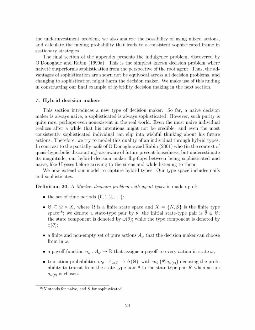
Definition 20. A Markov decision problem with agent types is made up of:

• the set of time periods 0, 1, 2, . . . ;

• Θ ⊆ Ω × X, where Ω is a finite state space and X = N,S is the finite typespace18; we denote a state-type pair by θ; the initial state-type pair is θ ∈ Θ;the state component is denoted by ω(θ); while the type component is denoted byx(θ);

• a finite and non-empty set of pure actions Aω that the decision maker can choosefrom in ω;

• a payoff function uω : Aω → R that assigns a payoff to every action in state ω;

• transition probabilities mθ : Aω(θ) → ∆(Θ), with mθ

(θ′|aω(θ)

)denoting the prob-

ability to transit from the state-type pair θ to the state-type pair θ′ when actionaω(θ) is chosen.

18N stands for naive, and S for sophisticated.

24

This definition keeps the Markovian properties of the original model, and adds a speci-fication of naivete or sophistication to each state. Also, Θ is common knowledge amongthe agents.

Our model is quite general. Before moving on to illustrate its use in detail for ourmotivating example from Section 1, we list a few kinds of decision problems for whichit could be used:

• exogeneous types: all state-type combinations are allowed (Θ = Ω × X). More-over, in each new state, the agent is naive (or sophisticated) with the same prob-ability: mθ((ω

′, x)|aω(θ)) = mθ((ω′′, x)|a′ω(θ)) for all θ, ω, ω′, x. Such a model re-

quires there being no correlation between state and type.

• fixed type for each state: here, we have (ω, x), (ω, x′) ∈ Θ ⇒ x = x′. This is theopposite of the previous scenario, as there is perfect correlation between state andtype. It can be easily seen that any Markov decision problem with agent typescan be reformulated in this manner by expanding the state space; however, it canmake the model less illuminating, possibly hiding structural similarities betweenthe problems faced by a naive and a sophisticated agent.

• deterministic type determination: this requires that for all θ, aω(θ), there is somex ∈ X, such that

∑ω′mθ((ω

′, x)|aω(θ)) = 1. This means that whatever theagent chooses, his type (but not necessarily his state) in the next period is fullydetermined.

• full control over type: for all θ, x ∈ X, there is some aω(θ) so that∑

ω′mθ((ω′, x)|aω(θ)) =

1. Each agent can always ensure his type to be whatever he wants for the nextperiod.

Of course, these are merely edge cases, and many interesting situations lie in the mid-dle, having some, but imperfect correlation between state and type; and giving some,but less than total control for agents over their future types. Indeed, it could be ar-gued that the drinking problem we present below should involve stochastic, instead ofdeterministic type determination. However, for simplicity of analysis, we abstract fromsuch complications.

To understand optimal strategies for hybrid agents, we first have to re-define thenotion of a history:

Definition 21. A type-dependent history h has the form h =(θ0, aω(θ0), . . . , θt−1, aω(θt−1), θt

),

with:

• θi ∈ Θ, for i ∈ 0, 1, . . . , t, and θ0 = θ;

• aω(θi) ∈ Aωi , for i ∈ 0, 1, . . . , t− 1;

• mθi

(θi+1|aω(θi)

)> 0, for i ∈ 0, 1, . . . , t− 1.

25

Extending the previous notation, x(h) refers to the current type. We keep the associ-ation between histories and agents – each history now corresponds to an agent, and italso includes the agent’s type.

Next, we define optimal type-dependent strategies for the Markov decision problemwith agent types. We make use of Definitions 18 and 19 for naively and sophisticatedlyoptimal strategies. We first present the formal definition, and then explain the intuitionsbelow.

Definition 22. A type-dependent strategy sh for a Markov decision problem with agenttypes is optimal at history h, if it satisfies the following conditions:

• for x(h) = N :sh ∈ arg max

s∈ShUhi (s) ,

andbh (h′) = ih (h′) , for all h′ ∈ H<h.

• for x(h) = S:

bh (h′) ∈ [arg maxs∈Sh′

Uh′

i (s)] (h′) , for all h′ ∈ H<h with x (h′) = N ;

bh (h′) ∈ arg maxa∈Aω(h′)

Uh′

b

(sh′[a : h′]

), for all h′ ∈ H<h with x (h′) = S;

and

ih (h′) ∈ arg maxa∈Aω(h′)

Uh′

b

(sh′[a : h′]

), for all h′ ∈ H<h with x (h′) = N ;

ih (h′) = bh (h′) , for all h′ ∈ H<h with x (h′) = S.

A type-dependent frame f is optimal, if f(h) is an optimal type-dependent strategy forall h.

Although this definition is rather lengthy, it captures our basic intuitions for the twotypes. A naive agent at h does not reason about future agents, as his intentions deter-mine his beliefs, and thus, his whole optimal strategy in the standard way. However, asophisticated agent at h is able to reason about future agents in the following manner:if a future agent at h′ is naive, then the agent at h believes the agent at h′ will act in anaive way, maximizing his expected utility based on intentions. If, on the other hand,a future agent at h′ is sophisticated, then the agent at h (correctly) believes that theagent at h′ will act in a sophisticated way, being able to reason about future agentsjust as well as h himself does. So a sophisticated agent at h intends to choose in a so-phisticated manner at all nodes, giving a best response to the choices of future agents.This implies that the intention and belief component of an optimal type-dependent

26

strategy match for all future histories where the agent is sophisticated, but they mightnot match for future histories where the agent is naive. Coherence is therefore not aproperty of optimal type-dependent strategies.

Since naively optimal strategies are, in general, not made up of stationary strategies,the belief-component of an optimal type-dependent frame can also be non-stationary.Moreover, it is easy to see that such a frame is not consistent: the intentions of sophis-ticated agents will not, in general, correspond to the actions taken by naive agents. Inboth examples of hybrid decision making we present below, we will see such inconsisten-cies.19 The lack of coherence, stationarity and consistency represent the inner conflictsthat arise within a hybrid decision maker.

Theorem 5. For any decision problem, there exists a type-dependent optimal frame.

Proof. First, start with determining the intentions and beliefs of naive agents, i.e., thoseat histories where x(h) = N . For these, we can simply use the first part of the proof ofTheorem 3. So, we have sh = (ih, bh) defined for all h with x(h) = N . Let f(h) = sh

for all such h.Moving now to histories where the agent is sophisticated, our construction is analo-

gous to that of Theorem 4. Let A = ×h∈HAω(h), and take an arbitrary a = (ah)h∈H ∈ Athat assigns an action to each history.

Recall that a type-dependent optimal frame will not necessarily be coherent. There-fore, both intentions and beliefs have to be constructed; we start with beliefs. First,transform a into a by fixing actions assigned to histories where the agent is naive, i.e.,where x(h) = N , so that they are actions corresponding to those agents acting in anaive way:

ah = ih(h) if x(h) = N ;

ah = ah if x(h) = S.

Let an ∈ A be defined as follows: ahn = ah for all h with t(h) > n, or with t(h) ≤ n,and x(h) = N . For the remaining histories with t(h) ≤ N and x(h) = S, we move bybackwards induction from n to 0, and let ahn be the best response to the future actions,which are already all defined.

Thus, we obtain a sequence (an)n∈N in A . Since A is sequentially compact (seethe proof of Theorem 4), the sequence an has a subsequence ank converging to somea ∈ A .20 Thus, for all possible choices of a horizon m, we can find a Km such thatah = ahnk for all k ≥ Km and h with t(h) ≤ m.

Now, let the beliefs of a sophisticated agent – i.e., at a history h with x(h) = S –be bh(h′) = ah

′.

19Recall that when an action is actually taken by an agent, it is both believed and intended by theagent for the current history.

20There might be multiple subsequences converging to different a-s; in that case, we can select anyone of them.

27

Finally, we construct the intentions of sophisticated agents. Set sophisticated agents’beliefs about future nodes as: ih(h′) = bh(h′) for all h′ with x(h) = x(h′). For sophisti-cated agents’ intentions assigned to future naive nodes, we construct a by modifying ain a way that whenever x(h) = N , ah is a best response to the future actions in a. Wekeep actions at other, sophisticated histories unchanged: a = a. We set the intentionsof a sophisticated agent to be ih(h′) = ah

′.

We have thus defined both bh and ih for sophisticated agents. Let sh = (ih, bh) andfinally, f(h) = sh for all x(h) = S. This completes our construction of a type-dependentoptimal frame, as we have provided the strategies assigned to histories where the agentis naive, and also to the ones where he is sophisticated.

We will now review our construction again to confirm that f is indeed a type-dependent optimal frame. For x(h) = N , this is immediate. For x(h) = S, we will firstcheck the beliefs, and then the intentions.

First, suppose that x(h′) = N . We have:

bh(h′) = ah′= ih

′(h′) ∈ arg max

s∈Sh′Uh′

i (s)(h′),

which is what is required in the definition of f . For the other case, take x(h′) = S.Now, from our construction of ah

′n , for all n ≥ t(h′):

bhn(h′) = ah′

n ∈ arg maxa∈Aω(h′)

Uh′

b (bhn[a : h′]).

Taking the limit along the subsequence nk, using continuity, we get:

bh(h′) = ah′ ∈ arg max

a∈Aω(h′)Uh′

b (bh[a : h′]).

For the intentions of sophisticated agents for future sophisticated nodes, we set thesedirectly to be ih(h′) = bh(h′). The last thing we need to check is the intentions ofsophisticated agents for future naive agents. These were defined as:

ih(h′) = ah′ ∈ arg max

a∈Aω(h′)

Uh′

b (bh′[a : h′]).

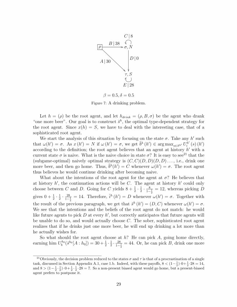
We now return to the problem raised in the introduction, displayed in Figure 7. Thedecision maker is sitting in the pub, having finished his second beer (in state ρ), andis of type S (sophisticated). He can either go home directly, by choosing action A,transiting to state τ , where he does not need to make any more decisions. Alternatively,he can drink “one more beer” by choosing action B. This, however, transitions himto a “drunken” state σ, where he becomes type N (naive). In this drunken state,he can choose between drinking one more beer by choosing C (thus, maintaining hisdrunkenness and staying at σ), or going home to state τ by choosing D.

28

ρB | 38

//

A | 30

σ,N

D | 0

C | 8

τ, S

E | 28

GG

β = 0.5, δ = 0.5

Figure 7: A drinking problem.

Let h = (ρ) be the root agent, and let hdrink = (ρ,B, σ) be the agent who drank“one more beer”. Our goal is to construct sh, the optimal type-dependent strategy forthe root agent. Since x(h) = S, we have to deal with the interesting case, that of asophisticated root agent.

We start the analysis of this situation by focusing on the state σ. Take any h′ suchthat ω(h′) = σ. As x (h′) = N if ω (h′) = σ, we get bh (h′) ∈ arg maxs∈Sh′ U

h′i (s) (h′)

according to the definition; the root agent believes that an agent at history h′ with acurrent state σ is naive. What is the naive choice in state σ? It is easy to see21 that the(subgame-optimal) naively optimal strategy is (C,C)(D,D)(D,D) . . . , i.e., drink onemore beer, and then go home. Thus, bh(h′) = C whenever ω(h′) = σ. The root agentthus believes he would continue drinking after becoming naive.

What about the intentions of the root agent for the agent at σ? He believes thatat history h′, the continuation actions will be C. The agent at history h′ could onlychoose between C and D. Going for C yields 8 + 1

2· 1

2· 8

1− 12

= 12, whereas picking D

gives 0 + 12· 1

2· 28

1− 12

= 14. Therefore, ih (h′) = D whenever ω(h′) = σ. Together with

the result of the previous paragraph, we get that sh (h′) = (D,C) whenever ω(h′) = σ.We see that the intentions and the beliefs of the root agent do not match: he wouldlike future agents to pick D at every h′, but correctly anticipates that future agents willbe unable to do so, and would actually choose C. The sober, sophisticated root agentrealizes that if he drinks just one more beer, he will end up drinking a lot more thanhe actually wishes for.

So what should the root agent choose at h? He can pick A, going home directly,earning him Uh0

b (sh0 [A : h0]) = 30 + 12· 1

2· 28

1− 12

= 44. Or, he can pick B, drink one more

21Obviously, the decision problem reduced to the states σ and τ is that of a procrastination of a singletask, discussed in Section Appendix A.1, case 1.b. Indeed, with these payoffs, 8 < (1− 1

2 )·0+ 12 ·28 = 14,

and 8 > (1− 12 ·

12 ) ·0+ 1

2 ·12 ·28 = 7. So a non-present biased agent would go home, but a present-biased

agent prefers to postpone it.

29

beer, and end up in the pub. This would earn him Uh0b (sh0 [B : h0]) = 38+ 1

2· 1

2· 8

1− 12

= 42.

Going home seems best. Thus, sh (h) = (A,A). The optimal type-dependent strategyis thus:

sh(h) = (A,A),

sh(h′) = (D,C), whenever ω (h′) = σ,

sh(h′) = (E,E), whenever ω (h′) = τ.

Note that a fully naive root agent would expect that he can resist the temptation ofadditional beers, and would expect a utility of 38 + 1

2· 1

2· 0 + 1

2· 1

2

2 · 281− 1

2

= 45. The

sophisticated root agent realizes that this is unachievable, as the incentives and thetype of the agents changes by transiting to σ. So in the drinking problem, the sober,sophisticated root agent avoids becoming naive, and thus is better off. Sophisticationthus can help avoiding the trap of naivete. But can sophistication help in avoiding thepitfalls of sophistication?

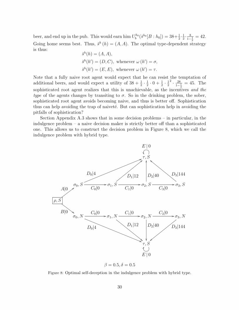
Section Appendix A.3 shows that in some decision problems – in particular, in theindulgence problem – a naive decision maker is strictly better off than a sophisticatedone. This allows us to construct the decision problem in Figure 8, which we call theindulgence problem with hybrid type.

τ, S

E | 0

σ0, SC0|0

//

D0|4

55

σ1, SC1|0

//

D1|12

<<

σ2, SC3|0

//

D2|40

OO

σ3, S

D3|144

bb

ρ, S

B|0 ##

A|0 ;;

σ0, NC0|0 //

D0|4

))

σ1, NC1|0 //

D1|12

""

σ2, NC2|0 //

D2|40

σ3, N

D3|144

||τ, S

E | 0

GG

β = 0.5, δ = 0.5

Figure 8: Optimal self-deception in the indulgence problem with hybrid type.

30

The agent at the root history h0 = ((ρ, S)) is sophisticated. Therefore, he is ableto reason about future agents in the following way: at history h1 = ((ρ, S), A, (σ0, S)),and at all succeeding histories, he will be sophisticated. Thus, he concludes – after ananalysis similar to the one in Section Appendix A.3 – that he will choose the action D0.On the other hand, at history h′1 = ((ρ, S), B, (σ0, N)), and at all succeeding histories,he will be naive. Thus, he concludes that in the subgame starting at h′1, he will chooseaction D2. From the perspective of the root agent:

Uh0b (sh0 [A : h0]) = 1

2· 1

2· 4 = 1 < 2.5 = 1

2·(

12

)3 · 40 = Uh0b (sh0 [B : h0]).

Therefore, the best response of the root agent is to choose action B. Notice thatthis means that a sophisticated agent chooses to face the indulgence problem as a naif,thereby intentionally causing the agent at h′1 to have wrong beliefs. In particular, thenaive agent at h′1 believes that he will be able to wait until the wine fully matures, andtake action D3. The sophisticated agent at the preceeding history h0 knows that thisis not the case, that in fact, action D2 will be taken. Thus, when choosing an optimaltype-dependent strategy, the root agent realizes that he is better off with false beliefs,and decides to deceive himself.

By what means such self-deception might be effectively achieved, or whether it canbe achieved intentionally at all is, of course, a difficult problem. But it seems likeself-deception has its virtues, which might, in itself, challenge ethical arguments on theinherent immorality of self-deception.22

8. Concluding remarks and future research

This paper attempts to play a foundational role for future discourse in multi-selfmodels of dynamic inconsistency. It attempts to establish that the basic epistemicconcepts to be considered are beliefs and intentions, and the main levels of analysisshould be those of strategies and frames. We would now like to provide some remarksand outline some directions for follow-up research in this area.

An obvious limitation of the current framework is that it only allows for pure actions.This limitation is introduced to ease the presentation, but the technical adaptationsrequired for dealing with mixed actions can be accomplished rather straightforwardly.Mixed actions should play a particularly important role when moving from decision-theoretic models to a game setting.

One might wonder how flexible this model is with regards to increasing the stateor action space of the decision problem. Countably infinite states and actions can beallowed for without much difficulty, as long as the set of payoffs for each action remainscompact (and hence, bounded). However, handling continuous time would require afundamentally different framework, along with a reinterpretation of the notion of an“agent”.

22For an overview on the philosophical problems of self-deception, see Deweese-Boyd (2012).

31

Whereas our focus was the two most common types of decision makers facing dy-namic inconsistency, naifs and sophisticates, there have been arguments in the literaturefor taking seriously other types as well. In particular, McClennen (1990) argues for thepossibility of resolute decision making. In fact, resoluteness can easily be incorporatedinto our framework. It would be interesting to expand the type space in Markov decisionproblems with hybrid types to include resolutes.

The horizon of sophisticated decision makers requires further investigation. If agentshave only a finite horizon, reasoning about future agents can be based on two assump-tions: either the length, or the endpoint of the horizon of that future agent is the sameas that of the current agent. In the former case, we are talking about a moving, inthe latter, about a fixed horizon. The implications of these two assumptions on theoptimal strategies (generated, for instance, through a backward induction reasoning)are not yet understood. For example, it seems that a moving horizons approach mightbe more appropriate to capture the consistent stationary sophisticated strategy that iscomposed of mixed actions of Section Appendix A.2.

Finally, the most interesting application of the framework presented above will befor game theory. How can players reason about the intentions and beliefs of otherplayers, as well as their types? How can one exploit the naivete (or sophistication) ofothers? What kind of equilibria are generated when (pure, or hybrid) players are pittedagainst each other? We hope that through this paper, we have broken the ground forsuch questions.

Appendix A. Comparison of naive and sophisticated decision makers insome classical decision problems

This appendix discusses a few particular decision problems to compare naive andsophisticated decision makers. In Sections Appendix A.1 and Appendix A.2, our analy-sis involves simple decision problems with only two states. We show that many classicalexamples of inconsistent behavior can already be formulated with such decision prob-lems. In Section Appendix A.1, we tackle a class of decision problems where the decisionmaker faces the choice between executing an action eventually or never. We find thatin the procrastination, but not in the impulsiveness problem, sophisticates might out-perform naifs, depending on the exact parameters. In Section Appendix A.2 we focuson problems where an action can be chosen an arbitrary number of times, and it hasboth short- and long-term effects. Here, we find similar results: sophisticates can bebetter off than naifs in the underinvestment, but not in the binge problem. Althougha lot of ground can be covered with just two states, in each of these cases sophisticatesare at least as well off as naifs. To show that this is not the case for all decision prob-lems, Section Appendix A.3 reviews a decision problem adapted from O’Donoghue andRabin (1999a) with five states where naivete dominates sophistication from a welfareperspective.

Common to the analyses is the choice of quasi-hyperbolic discounting for the utility

32

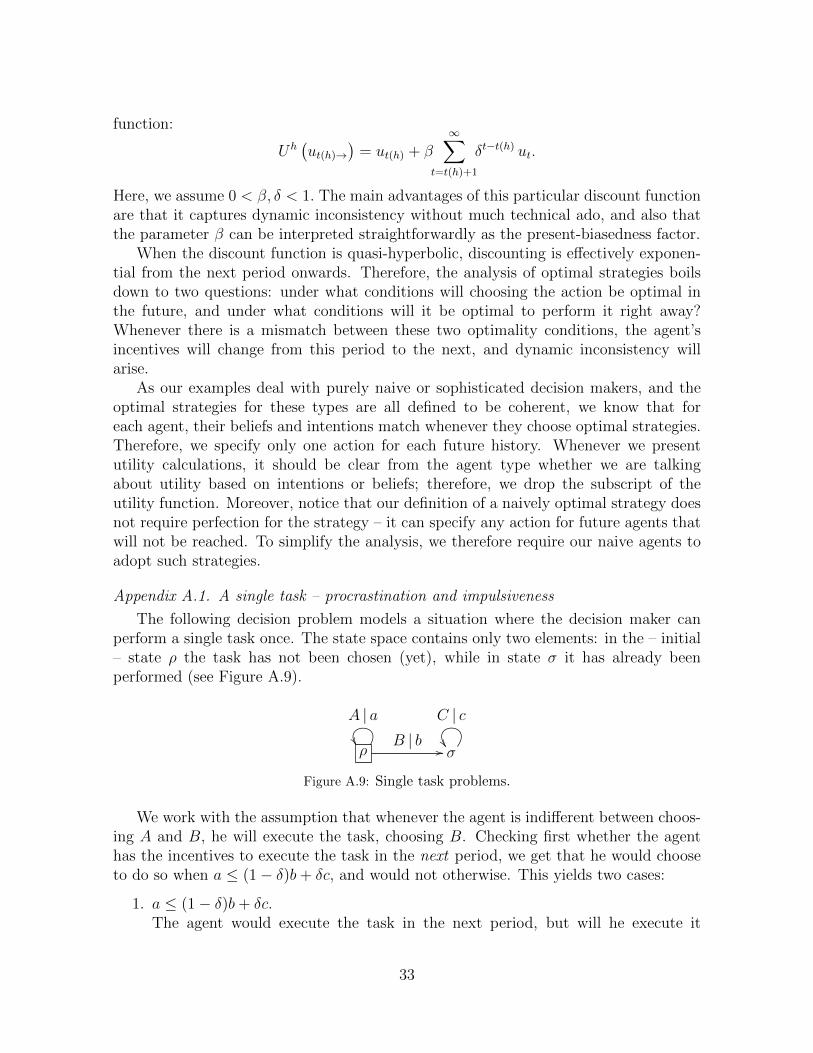
function:

Uh(ut(h)→

)= ut(h) + β

∞∑t=t(h)+1

δt−t(h) ut.

Here, we assume 0 < β, δ < 1. The main advantages of this particular discount functionare that it captures dynamic inconsistency without much technical ado, and also thatthe parameter β can be interpreted straightforwardly as the present-biasedness factor.

When the discount function is quasi-hyperbolic, discounting is effectively exponen-tial from the next period onwards. Therefore, the analysis of optimal strategies boilsdown to two questions: under what conditions will choosing the action be optimal inthe future, and under what conditions will it be optimal to perform it right away?Whenever there is a mismatch between these two optimality conditions, the agent’sincentives will change from this period to the next, and dynamic inconsistency willarise.

As our examples deal with purely naive or sophisticated decision makers, and theoptimal strategies for these types are all defined to be coherent, we know that foreach agent, their beliefs and intentions match whenever they choose optimal strategies.Therefore, we specify only one action for each future history. Whenever we presentutility calculations, it should be clear from the agent type whether we are talkingabout utility based on intentions or beliefs; therefore, we drop the subscript of theutility function. Moreover, notice that our definition of a naively optimal strategy doesnot require perfection for the strategy – it can specify any action for future agents thatwill not be reached. To simplify the analysis, we therefore require our naive agents toadopt such strategies.

Appendix A.1. A single task – procrastination and impulsiveness

The following decision problem models a situation where the decision maker canperform a single task once. The state space contains only two elements: in the – initial– state ρ the task has not been chosen (yet), while in state σ it has already beenperformed (see Figure A.9).

ρB | b

//

A | a

σ

C | c

Figure A.9: Single task problems.

We work with the assumption that whenever the agent is indifferent between choos-ing A and B, he will execute the task, choosing B. Checking first whether the agenthas the incentives to execute the task in the next period, we get that he would chooseto do so when a ≤ (1− δ)b+ δc, and would not otherwise. This yields two cases:

1. a ≤ (1− δ)b+ δc.The agent would execute the task in the next period, but will he execute it

33

immediately? If he does, he gains b+β δ1−δc; if he does not, he gains a+βδb+β δ2

1−δc.This again generates two cases, where after some algebra we get:

(a) a ≤ (1− βδ)b+ βδc.23

Here, executing the task is the optimal immediate choice, as well as the op-timal choice for all future periods. Both naively and sophisticatedly optimalstrategies prescribe choosing B at all histories where the end-state is ρ; thereis no dynamic inconsistency.

(b) a > (1− βδ)b+ βδc.24

In this case, executing the task is optimal in the next period, but not imme-diately. This is the situation of procrastinating a single task.A naively optimal strategy prescribes postponing B one period by choosingA first. A naively optimal frame would involve choosing such a strategy atevery history. This implies that in the induced strategy, action B is in factnever chosen, as each naive agent keeps postponing B by one period. Theinduced utility over the naive frame f is thus: Ur(f) = a+ β δ

1−δa.Although the decision problem looks simple enough, finding the sophisticat-edly optimal strategy is not straightforward. Suppose that the sophisticatedagent at h believes that no future agent will choose B. If he chooses to alsonot do B himself, he gains U h(AAA . . . ) = a + β δ

1−δa. On the other hand,

if he takes on B, he gains U h(B . . . ) = b + β δ1−δc. It so happens that our

two conditions thus far do not determine which of these values is larger.25

Therefore, we need two more subcases:

i. a+ β δ1−δa ≥ b+ β δ

1−δc.This means that choosing B is a best response to the belief that nofuture agent would choose A. Condition 1.b implies that choosing Ais also a best response to the belief that in the next period B will bechosen. Furthermore, we will now show that choosing A is also a bestreply to the belief that any future agent chooses B. Suppose the agentat h believes that k is the earliest period when an agent would chooseB. Then, we get:

U h(AA . . . AB . . . ) = a+ β δ(1−δk−1)

1−δ a+ βδkb+ β δk+1

1−δ c

= a+ β δ1−δa+ β δk

1−δ (−a+ (1− δ)b+ δc)

≥ a+ β δ1−δa ≥ b+ β δ

1−δc = U h(B . . . ).

Note that we only get equality if both conditions 1 and 1.b.ii are satisfied

23e.g. a = 4, b = 0, c = 20, β = δ = 0.5.24e.g. a = 4, b = 0, c = 10, β = δ = 0.5.25For instance, take a = −1, b = −1, c = 4, δ = 0.5, β = 0.5. These values satisfy conditions 1:

a ≤ (1−δ)b+δc, 1.b: a > (1−βδ)b+βδc, with a+β δ1−δa > b+β δ

1−δ c. Changing only the assignment

of c to c = 6, the parameters still satisfy conditions 1 and 1.b, but now a+ β δ1−δa < b+ β δ

1−δ c. Thusconditions 1.b.i/1.b.ii are independent from 1 and 1.b

34

with equality. It can be derived that such a scenario is impossible, givenconditions 1.b and β < 1. Therefore, at least one of them is a strictinequality. This implies that A is a best response to any belief aboutthe future, and the only sophisticatedly optimal strategy for an agent isbelieving and intending A for every future history. Thus, in this case,there is no difference between the induced strategy of the naively andsophisticatedly optimal frame, and the induced utilities are equal.

ii. a+ β δ1−δa < b+ β δ

1−δc.26

Choosing B is the best response for an agent that believes all futureagents will choose A, and thus the strategy “all-A” is not sophisticatedlyoptimal. In what follows, we show that if the moment at whichB is takenin the future is sufficiently far, it is optimal to choose B immediately.Take the strategies shk and shk+1, where the index k ≥ 1 indicates thefirst period in which action B is taken.27 For the utilities generated bythese two strategies, we get that:

∆k = U h(shk

)− U h

(shk+1

)=

(a+ β δ

1−δ

(1− δk−1

)a+ βδkb+ β δ

k+1

1−δ c)

−(a+ βδ

1−δ

(1− δk

)a+ βδk+1b+ β δ

k+2

1−δ c)

= βδk (−a+ (1− δ)b+ δc) ≥ 0.

So we find, by condition 1, that U h(shk

)is decreasing in k. Taking the

difference between the utility generated by strategy sh1 = AB . . . and anarbitrary strategy with k > 1, we get:

U h(sh1

)− U h

(shk

)=

k−1∑i=1

∆i = βδ 1−δk−1

1−δ (−a+ (1− δ)b+ δc) .

Hence, we obtain:

limk→∞

U h(shk

)= U h

(sh1

)− lim

k→∞

(U h(sh1

)− U h

(shk

))= a+ βδb+ β δ2

1−δc− βδ

1−δ (−a+ (1− δ)b+ δc)

= a+ β δ1−δa.

We know from condition 1.b that U h(sh1

)= U h (AB . . . ) > U h (B . . . ) =

U h(sh0

). However, we see that limk→∞ U

h(shk

)= a + β δ

1−δa < b +

26We ignore the possibility of mixed actions here, and instead choose to discuss it only for theunderinvestment problem. Moreover, we assume that when a sophisticated decision maker can attainconsistency, he will do so. For both issues, see Section Appendix A.2 condition 1.b.ii below.

27E.g., sh1 = AB . . . , sh2 = AAB . . .

35

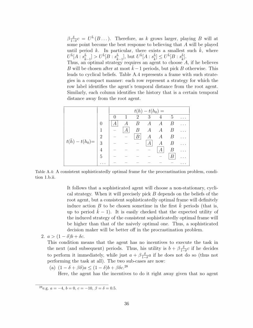
β δ1−δc = U h (B . . . ). Therefore, as k grows larger, playing B will at

some point become the best response to believing that A will be playeduntil period k. In particular, there exists a smallest such k, whereU h[A : sh

k−1] > U h[B : sh

k−1], but U h[A : sh

k] ≤ U h[B : sh

k].

Thus, an optimal strategy requires an agent to choose A, if he believesB will be chosen after at most k−1 periods, but pick B otherwise. Thisleads to cyclical beliefs. Table A.4 represents a frame with such strate-gies in a compact manner: each row represent a strategy for which therow label identifies the agent’s temporal distance from the root agent.Similarly, each column identifies the history that is a certain temporaldistance away from the root agent.

t(h)− t(h0) =0 1 2 3 4 5 . . .

t(h)− t(h0)=

0 A A B A A B . . .

1 – A B A A B . . .

2 – – B A A B . . .

3 – – – A A B . . .

4 – – – – A B . . .

5 – – – – – B . . .. . . – – – – – – . . .

Table A.4: A consistent sophisticatedly optimal frame for the procrastination problem, condi-tion 1.b.ii.

It follows that a sophisticated agent will choose a non-stationary, cycli-cal strategy. When it will precisely pick B depends on the beliefs of theroot agent, but a consistent sophisticatedly optimal frame will definitelyinduce action B to be chosen sometime in the first k periods (that is,up to period k − 1). It is easily checked that the expected utility ofthe induced strategy of the consistent sophisticatedly optimal frame willbe higher than that of the naively optimal one. Thus, a sophisticateddecision maker will be better off in the procrastination problem.

2. a > (1− δ)b+ δc.This condition means that the agent has no incentives to execute the task inthe next (and subsequent) periods. Thus, his utility is b + β δ

1−δc if he decides

to perform it immediately, while just a + β δ1−δa if he does not do so (thus not

performing the task at all). The two sub-cases are now:

(a) (1− δ + βδ)a ≤ (1− δ)b+ βδc.28

Here, the agent has the incentives to do it right away given that no agent

28e.g. a = −4, b = 0, c = −10, β = δ = 0.5.

36

would execute the task in a later period. A naively optimal strategy simplyprescribes choosing B right away, generating a utility of U = b + β δ

1−δc forthe naive agent.The sophisticatedly optimal strategy depends on the beliefs of the agent.Because of condition 2.a, choosing B right away is optimal if the agentbelieves that no future agent will take it. Now, suppose the sophisticatedagent at h believes that some future agent will pick B. Let k be the earliestfuture period in which B will be taken, according to the strategy sh. We getthat:

U h[B : sh] = b+ βδ1−δc ≥

1−δ+βδ1−δ a = a+ βδ

1−δ (a− δk−1a+ δk−1a)

> a+ βδ1−δ

((1− δk−1)a+ (1− δ)δk−1b+ δkc

)= U h[A : sh]

We conclude that taking B right away is optimal, whatever the agent’s be-liefs. This means that the sophisticated decision maker cannot avoid im-pulsivity, and that there is no difference between the utility gained by naifsand sophisticates. In either case, if the decision maker later reflects on thisdecision from a non-present-biased perspective, he will regret taking B.

(b) (1− δ + βδ)a > (1− δ)b+ βδc.29

Now, picking A and staying in ρ is always optimal both for naifs and sophis-ticates, and dynamic inconsistency does not arise.

This shows that for single task problems, there is no difference in the behavior ofsophisticated and naive agents for the problem of impulsiveness. In the procrastinationproblem, it can happen that sophistication brings no benefits, but – depending on theparameters of the problem – it might also be the case that it overperforms naivete.

The asymmetry found between problems of impulsiveness and procrastination mightlook counter-intuitive at first, as the structure of the Markov decision problem looksquite similar. However, our finding is consistent with Thaler (1981), who presents somebehavioral evidence that implicit discount rates are much higher for gains than for losses.If we interpret taking an impulsive action as a choice of an immediate reward, whereastaking the action that is to be procrastinated as accepting an immediate loss, our resultthat sophisticated decision makers can overcome the problem of procrastination are inline with their findings.

Appendix A.2. A repeated task – underinvestment and binges

The following decision problems are very similar to the previous ones in that thereare two states, with only one of them requiring a decision, whether to perform a taskor not. The main difference is that the task can be executed repeatedly, as the decisionmaker always returns to the initial state. Figure A.10 presents the parametrized versionof the repeated task problem.

29e.g. a = 4, b = 0, c = 0, β = δ = 0.5.

37

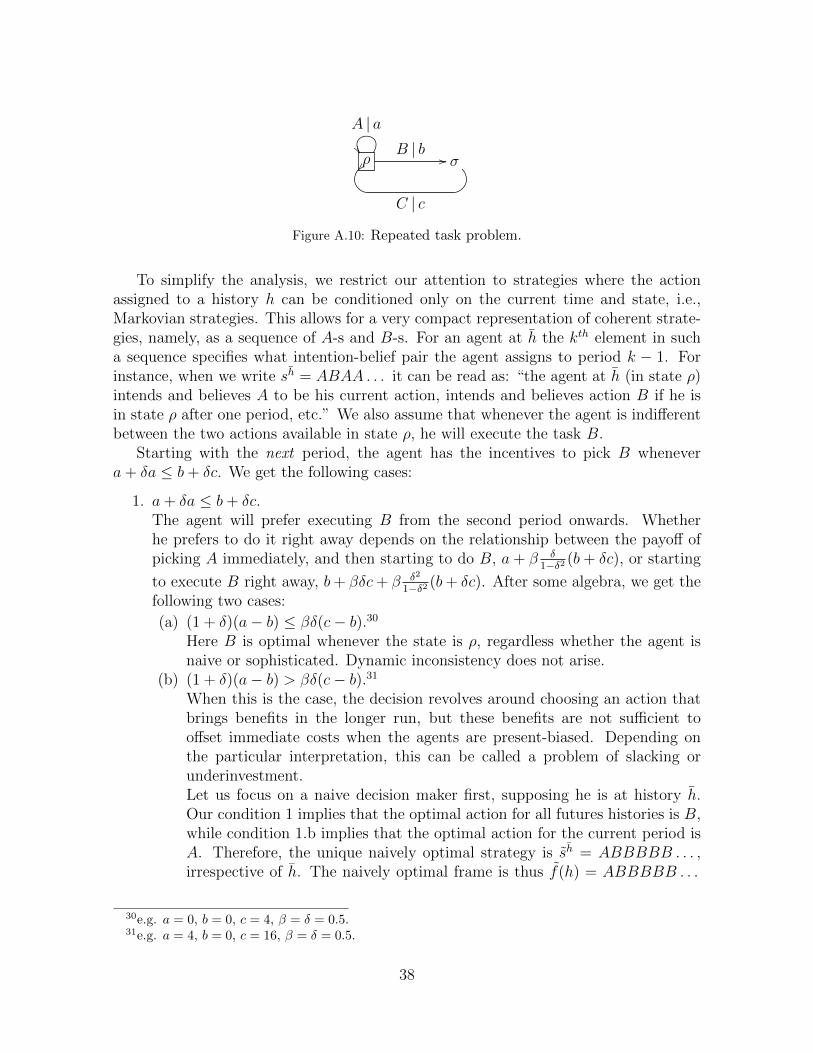
ρB | b

//

A | a

σ

C | c

Figure A.10: Repeated task problem.

To simplify the analysis, we restrict our attention to strategies where the actionassigned to a history h can be conditioned only on the current time and state, i.e.,Markovian strategies. This allows for a very compact representation of coherent strate-gies, namely, as a sequence of A-s and B-s. For an agent at h the kth element in sucha sequence specifies what intention-belief pair the agent assigns to period k − 1. Forinstance, when we write sh = ABAA . . . it can be read as: “the agent at h (in state ρ)intends and believes A to be his current action, intends and believes action B if he isin state ρ after one period, etc.” We also assume that whenever the agent is indifferentbetween the two actions available in state ρ, he will execute the task B.

Starting with the next period, the agent has the incentives to pick B whenevera+ δa ≤ b+ δc. We get the following cases:

1. a+ δa ≤ b+ δc.The agent will prefer executing B from the second period onwards. Whetherhe prefers to do it right away depends on the relationship between the payoff ofpicking A immediately, and then starting to do B, a+ β δ

1−δ2 (b+ δc), or starting

to execute B right away, b+ βδc+ β δ2

1−δ2 (b+ δc). After some algebra, we get thefollowing two cases:

(a) (1 + δ)(a− b) ≤ βδ(c− b).30

Here B is optimal whenever the state is ρ, regardless whether the agent isnaive or sophisticated. Dynamic inconsistency does not arise.

(b) (1 + δ)(a− b) > βδ(c− b).31

When this is the case, the decision revolves around choosing an action thatbrings benefits in the longer run, but these benefits are not sufficient tooffset immediate costs when the agents are present-biased. Depending onthe particular interpretation, this can be called a problem of slacking orunderinvestment.Let us focus on a naive decision maker first, supposing he is at history h.Our condition 1 implies that the optimal action for all futures histories is B,while condition 1.b implies that the optimal action for the current period isA. Therefore, the unique naively optimal strategy is sh = ABBBBB . . . ,irrespective of h. The naively optimal frame is thus f(h) = ABBBBB . . .

30e.g. a = 0, b = 0, c = 4, β = δ = 0.5.31e.g. a = 4, b = 0, c = 16, β = δ = 0.5.

38

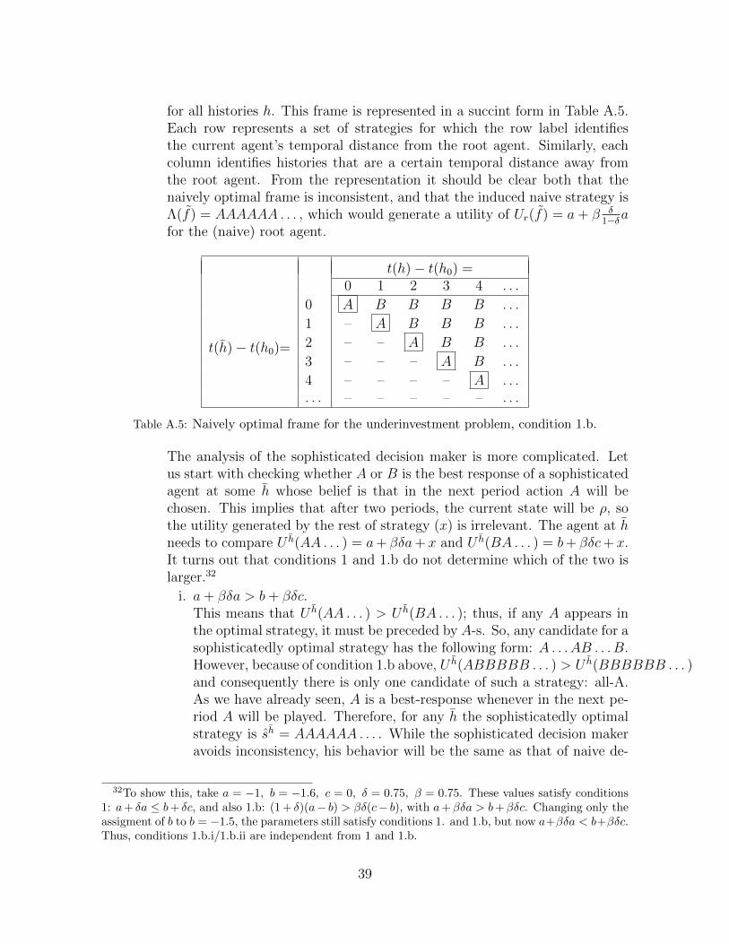
for all histories h. This frame is represented in a succint form in Table A.5.Each row represents a set of strategies for which the row label identifiesthe current agent’s temporal distance from the root agent. Similarly, eachcolumn identifies histories that are a certain temporal distance away fromthe root agent. From the representation it should be clear both that thenaively optimal frame is inconsistent, and that the induced naive strategy isΛ(f) = AAAAAA . . . , which would generate a utility of Ur(f) = a+ β δ

1−δafor the (naive) root agent.

t(h)− t(h0) =0 1 2 3 4 . . .

t(h)− t(h0)=

0 A B B B B . . .

1 – A B B B . . .

2 – – A B B . . .

3 – – – A B . . .

4 – – – – A . . .. . . – – – – – . . .

Table A.5: Naively optimal frame for the underinvestment problem, condition 1.b.

The analysis of the sophisticated decision maker is more complicated. Letus start with checking whether A or B is the best response of a sophisticatedagent at some h whose belief is that in the next period action A will bechosen. This implies that after two periods, the current state will be ρ, sothe utility generated by the rest of strategy (x) is irrelevant. The agent at hneeds to compare U h(AA . . . ) = a+ βδa+ x and U h(BA . . . ) = b+ βδc+ x.It turns out that conditions 1 and 1.b do not determine which of the two islarger.32

i. a+ βδa > b+ βδc.This means that U h(AA . . . ) > U h(BA . . . ); thus, if any A appears inthe optimal strategy, it must be preceded by A-s. So, any candidate for asophisticatedly optimal strategy has the following form: A . . . AB . . . B.However, because of condition 1.b above, U h(ABBBBB . . . ) > U h(BBBBBB . . . )and consequently there is only one candidate of such a strategy: all-A.As we have already seen, A is a best-response whenever in the next pe-riod A will be played. Therefore, for any h the sophisticatedly optimalstrategy is sh = AAAAAA . . . . While the sophisticated decision makeravoids inconsistency, his behavior will be the same as that of naive de-

32To show this, take a = −1, b = −1.6, c = 0, δ = 0.75, β = 0.75. These values satisfy conditions1: a+ δa ≤ b+ δc, and also 1.b: (1 + δ)(a− b) > βδ(c− b), with a+βδa > b+βδc. Changing only theassigment of b to b = −1.5, the parameters still satisfy conditions 1. and 1.b, but now a+βδa < b+βδc.Thus, conditions 1.b.i/1.b.ii are independent from 1 and 1.b.

39

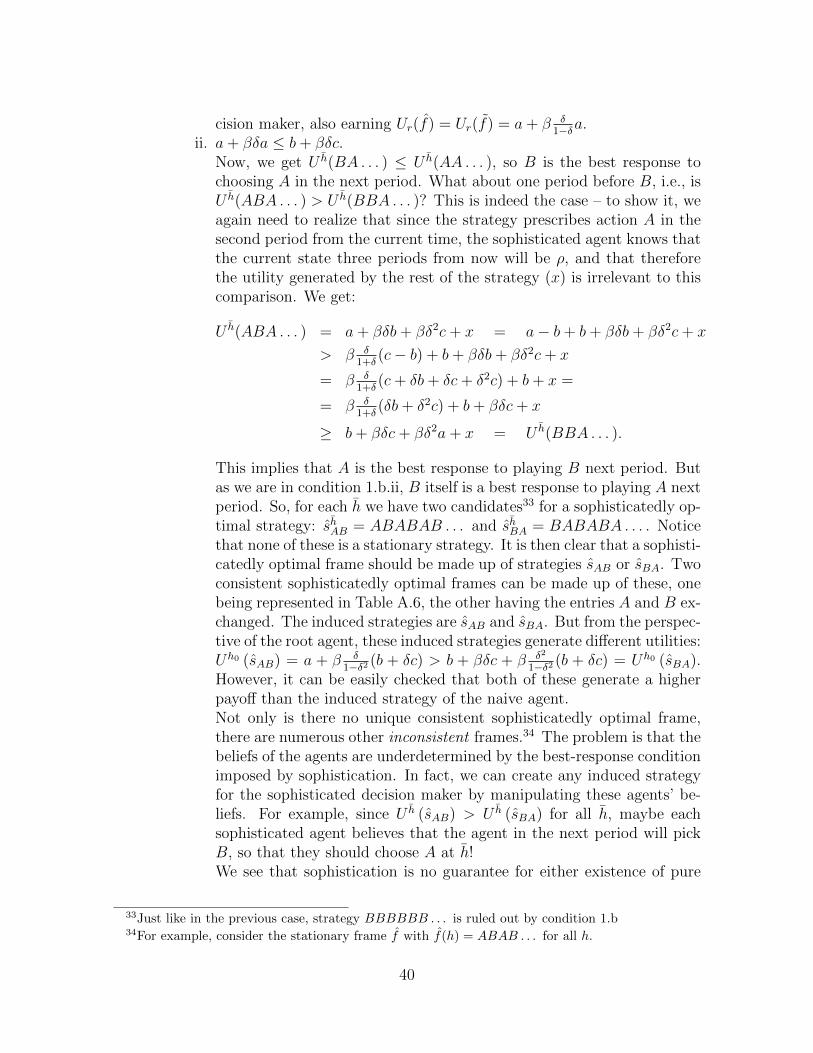
cision maker, also earning Ur(f) = Ur(f) = a+ β δ1−δa.

ii. a+ βδa ≤ b+ βδc.Now, we get U h(BA . . . ) ≤ U h(AA . . . ), so B is the best response tochoosing A in the next period. What about one period before B, i.e., isU h(ABA . . . ) > U h(BBA . . . )? This is indeed the case – to show it, weagain need to realize that since the strategy prescribes action A in thesecond period from the current time, the sophisticated agent knows thatthe current state three periods from now will be ρ, and that thereforethe utility generated by the rest of the strategy (x) is irrelevant to thiscomparison. We get:

U h(ABA . . . ) = a+ βδb+ βδ2c+ x = a− b+ b+ βδb+ βδ2c+ x

> β δ1+δ

(c− b) + b+ βδb+ βδ2c+ x

= β δ1+δ

(c+ δb+ δc+ δ2c) + b+ x =

= β δ1+δ

(δb+ δ2c) + b+ βδc+ x

≥ b+ βδc+ βδ2a+ x = U h(BBA . . . ).

This implies that A is the best response to playing B next period. Butas we are in condition 1.b.ii, B itself is a best response to playing A nextperiod. So, for each h we have two candidates33 for a sophisticatedly op-timal strategy: shAB = ABABAB . . . and shBA = BABABA . . . . Noticethat none of these is a stationary strategy. It is then clear that a sophisti-catedly optimal frame should be made up of strategies sAB or sBA. Twoconsistent sophisticatedly optimal frames can be made up of these, onebeing represented in Table A.6, the other having the entries A and B ex-changed. The induced strategies are sAB and sBA. But from the perspec-tive of the root agent, these induced strategies generate different utilities:Uh0 (sAB) = a + β δ

1−δ2 (b + δc) > b + βδc + β δ2

1−δ2 (b + δc) = Uh0 (sBA).However, it can be easily checked that both of these generate a higherpayoff than the induced strategy of the naive agent.Not only is there no unique consistent sophisticatedly optimal frame,there are numerous other inconsistent frames.34 The problem is that thebeliefs of the agents are underdetermined by the best-response conditionimposed by sophistication. In fact, we can create any induced strategyfor the sophisticated decision maker by manipulating these agents’ be-liefs. For example, since U h (sAB) > U h (sBA) for all h, maybe eachsophisticated agent believes that the agent in the next period will pickB, so that they should choose A at h!We see that sophistication is no guarantee for either existence of pure

33Just like in the previous case, strategy BBBBBB . . . is ruled out by condition 1.b34For example, consider the stationary frame f with f(h) = ABAB . . . for all h.

40

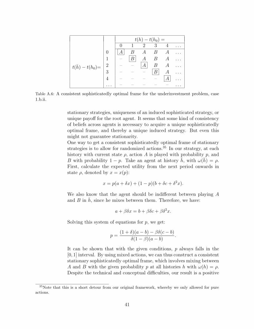
t(h)− t(h0) =0 1 2 3 4 . . .

t(h)− t(h0)=

0 A B A B A . . .

1 – B A B A . . .

2 – – A B A . . .

3 – – – B A . . .

4 – – – – A . . .. . . – – – – – . . .

Table A.6: A consistent sophisticatedly optimal frame for the underinvestment problem, case1.b.ii.

stationary strategies, uniqueness of an induced sophisticated strategy, orunique payoff for the root agent. It seems that some kind of consistencyof beliefs across agents is necessary to acquire a unique sophisticatedlyoptimal frame, and thereby a unique induced strategy. But even thismight not guarantee stationarity.One way to get a consistent sophisticatedly optimal frame of stationarystrategies is to allow for randomized actions.35 In our strategy, at eachhistory with current state ρ, action A is played with probability p, andB with probability 1 − p. Take an agent at history h, with ω(h) = ρ.First, calculate the expected utility from the next period onwards instate ρ, denoted by x = x(p):

x = p(a+ δx) + (1− p)(b+ δc+ δ2x).

We also know that the agent should be indifferent between playing Aand B in h, since he mixes between them. Therefore, we have:

a+ βδx = b+ βδc+ βδ2x.

Solving this system of equations for p, we get:

p =(1 + δ)(a− b)− βδ(c− b)

δ(1− β)(a− b).

It can be shown that with the given conditions, p always falls in the[0, 1] interval. By using mixed actions, we can thus construct a consistentstationary sophisticatedly optimal frame, which involves mixing betweenA and B with the given probability p at all histories h with ω(h) = ρ.Despite the technical and conceptual difficulties, our result is a positive

35Note that this is a short detour from our original framework, whereby we only allowed for pureactions.

41

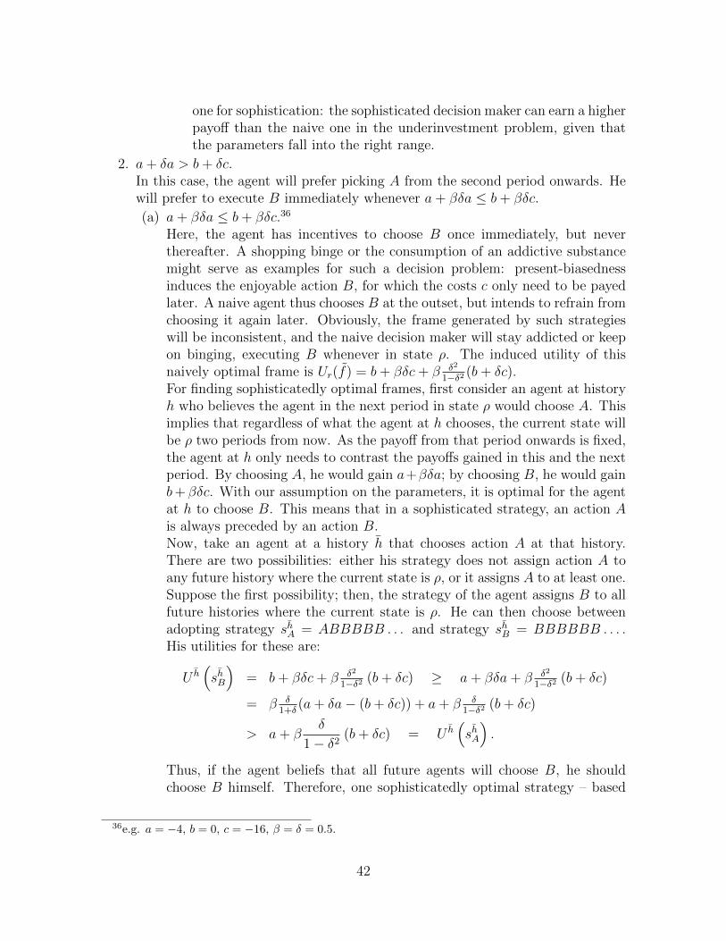
one for sophistication: the sophisticated decision maker can earn a higherpayoff than the naive one in the underinvestment problem, given thatthe parameters fall into the right range.

2. a+ δa > b+ δc.In this case, the agent will prefer picking A from the second period onwards. Hewill prefer to execute B immediately whenever a+ βδa ≤ b+ βδc.

(a) a+ βδa ≤ b+ βδc.36

Here, the agent has incentives to choose B once immediately, but neverthereafter. A shopping binge or the consumption of an addictive substancemight serve as examples for such a decision problem: present-biasednessinduces the enjoyable action B, for which the costs c only need to be payedlater. A naive agent thus chooses B at the outset, but intends to refrain fromchoosing it again later. Obviously, the frame generated by such strategieswill be inconsistent, and the naive decision maker will stay addicted or keepon binging, executing B whenever in state ρ. The induced utility of thisnaively optimal frame is Ur(f) = b+ βδc+ β δ2

1−δ2 (b+ δc).For finding sophisticatedly optimal frames, first consider an agent at historyh who believes the agent in the next period in state ρ would choose A. Thisimplies that regardless of what the agent at h chooses, the current state willbe ρ two periods from now. As the payoff from that period onwards is fixed,the agent at h only needs to contrast the payoffs gained in this and the nextperiod. By choosing A, he would gain a+βδa; by choosing B, he would gainb+ βδc. With our assumption on the parameters, it is optimal for the agentat h to choose B. This means that in a sophisticated strategy, an action Ais always preceded by an action B.Now, take an agent at a history h that chooses action A at that history.There are two possibilities: either his strategy does not assign action A toany future history where the current state is ρ, or it assigns A to at least one.Suppose the first possibility; then, the strategy of the agent assigns B to allfuture histories where the current state is ρ. He can then choose betweenadopting strategy shA = ABBBBB . . . and strategy shB = BBBBBB . . . .His utilities for these are:

U h(shB

)= b+ βδc+ β δ2

1−δ2 (b+ δc) ≥ a+ βδa+ β δ2

1−δ2 (b+ δc)

= β δ1+δ

(a+ δa− (b+ δc)) + a+ β δ1−δ2 (b+ δc)

> a+ βδ

1− δ2(b+ δc) = U h

(shA

).

Thus, if the agent beliefs that all future agents will choose B, he shouldchoose B himself. Therefore, one sophisticatedly optimal strategy – based

36e.g. a = −4, b = 0, c = −16, β = δ = 0.5.

42

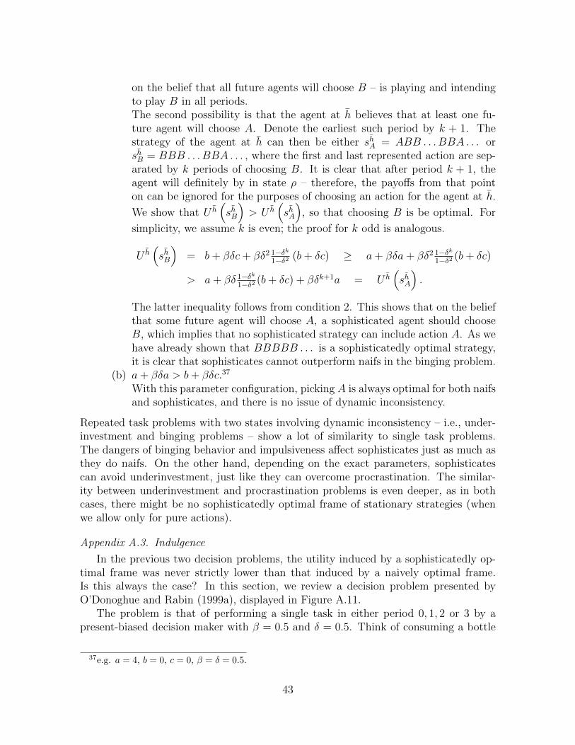
on the belief that all future agents will choose B – is playing and intendingto play B in all periods.The second possibility is that the agent at h believes that at least one fu-ture agent will choose A. Denote the earliest such period by k + 1. Thestrategy of the agent at h can then be either shA = ABB . . . BBA . . . orshB = BBB . . . BBA . . . , where the first and last represented action are sep-arated by k periods of choosing B. It is clear that after period k + 1, theagent will definitely by in state ρ – therefore, the payoffs from that pointon can be ignored for the purposes of choosing an action for the agent at h.

We show that U h(shB

)> U h

(shA

), so that choosing B is be optimal. For

simplicity, we assume k is even; the proof for k odd is analogous.

U h(shB

)= b+ βδc+ βδ2 1−δk

1−δ2 (b+ δc) ≥ a+ βδa+ βδ2 1−δk1−δ2 (b+ δc)

> a+ βδ 1−δk1−δ2 (b+ δc) + βδk+1a = U h

(shA

).

The latter inequality follows from condition 2. This shows that on the beliefthat some future agent will choose A, a sophisticated agent should chooseB, which implies that no sophisticated strategy can include action A. As wehave already shown that BBBBB . . . is a sophisticatedly optimal strategy,it is clear that sophisticates cannot outperform naifs in the binging problem.

(b) a+ βδa > b+ βδc.37

With this parameter configuration, picking A is always optimal for both naifsand sophisticates, and there is no issue of dynamic inconsistency.

Repeated task problems with two states involving dynamic inconsistency – i.e., under-investment and binging problems – show a lot of similarity to single task problems.The dangers of binging behavior and impulsiveness affect sophisticates just as much asthey do naifs. On the other hand, depending on the exact parameters, sophisticatescan avoid underinvestment, just like they can overcome procrastination. The similar-ity between underinvestment and procrastination problems is even deeper, as in bothcases, there might be no sophisticatedly optimal frame of stationary strategies (whenwe allow only for pure actions).

Appendix A.3. Indulgence

In the previous two decision problems, the utility induced by a sophisticatedly op-timal frame was never strictly lower than that induced by a naively optimal frame.Is this always the case? In this section, we review a decision problem presented byO’Donoghue and Rabin (1999a), displayed in Figure A.11.

The problem is that of performing a single task in either period 0, 1, 2 or 3 by apresent-biased decision maker with β = 0.5 and δ = 0.5. Think of consuming a bottle

37e.g. a = 4, b = 0, c = 0, β = δ = 0.5.

43

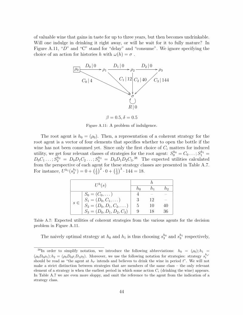
of valuable wine that gains in taste for up to three years, but then becomes undrinkable.Will one indulge in drinking it right away, or will he wait for it to fully mature? InFigure A.11, “D” and “C” stand for “delay” and “consume”. We ignore specifying thechoice of an action for histories h with ω(h) = σ .

ρ0D0 | 0 //

C0 | 4

''

ρ1

D1 | 0 //

C1 | 12

ρ2

D2 | 0 //

C2 | 40

ρ3

C3 | 144

~~σ

R | 0

EE

β = 0.5, δ = 0.5

Figure A.11: A problem of indulgence.

The root agent is h0 = (ρ0). Then, a representation of a coherent strategy for theroot agent is a vector of four elements that specifies whether to open the bottle if thewine has not been consumed yet. Since only the first choice of Ci matters for inducedutility, we get four relevant classes of strategies for the root agent: Sh00 = C0 . . . ;S

h11 =

D0C1 . . . ;Sh22 = D0D1C2 . . . ;S

h33 = D0D1D2C3.38 The expected utilities calculated

from the perspective of each agent for these strategy classes are presented in Table A.7.

For instance, Uh1(sh13 ) = 0 +(

12

)2 · 0 +(

12

)3 · 144 = 18.

Uh(s)h

h0 h1 h2

s ∈

S0 = (C0, . . . ) 4 – –S1 = (D0, C1, . . . ) 3 12 –S2 = (D0, D1, C2, . . . ) 5 10 40S3 = (D0, D1, D2, C3) 9 18 36

Table A.7: Expected utilities of coherent strategies from the various agents for the decisionproblem in Figure A.11.

The naively optimal strategy at h0 and h1 is thus choosing sh03 and sh13 respectively,

38In order to simplify notation, we introduce the following abbreviations: h0 = (ρ0);h1 =

(ρ0D0ρ1);h2 = (ρ0D0ρ,D1ρ2). Moreover, we use the following notation for strategies: strategy sht′t

should be read as “the agent at ht′ intends and believes to drink the wine in period t”. We will notmake a strict distinction between strategies that are members of the same class – the only relevantelement of a strategy is when the earliest period in which some action Ci (drinking the wine) appears.In Table A.7 we are even more sloppy, and omit the reference to the agent from the indication of astrategy class.

44

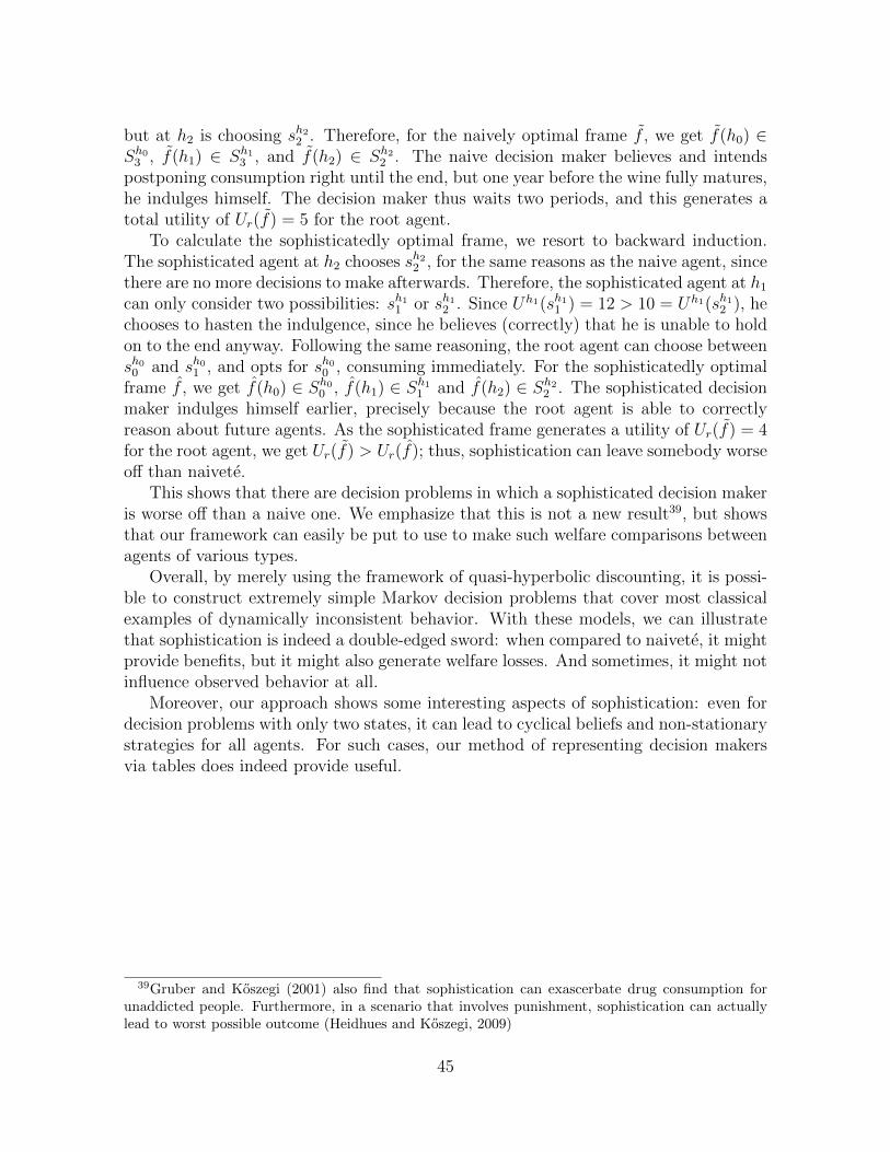
but at h2 is choosing sh22 . Therefore, for the naively optimal frame f , we get f(h0) ∈Sh03 , f(h1) ∈ Sh13 , and f(h2) ∈ Sh22 . The naive decision maker believes and intendspostponing consumption right until the end, but one year before the wine fully matures,he indulges himself. The decision maker thus waits two periods, and this generates atotal utility of Ur(f) = 5 for the root agent.

To calculate the sophisticatedly optimal frame, we resort to backward induction.The sophisticated agent at h2 chooses sh22 , for the same reasons as the naive agent, sincethere are no more decisions to make afterwards. Therefore, the sophisticated agent at h1

can only consider two possibilities: sh11 or sh12 . Since Uh1(sh11 ) = 12 > 10 = Uh1(sh12 ), hechooses to hasten the indulgence, since he believes (correctly) that he is unable to holdon to the end anyway. Following the same reasoning, the root agent can choose betweensh00 and sh01 , and opts for sh00 , consuming immediately. For the sophisticatedly optimalframe f , we get f(h0) ∈ Sh00 , f(h1) ∈ Sh11 and f(h2) ∈ Sh22 . The sophisticated decisionmaker indulges himself earlier, precisely because the root agent is able to correctlyreason about future agents. As the sophisticated frame generates a utility of Ur(f) = 4for the root agent, we get Ur(f) > Ur(f); thus, sophistication can leave somebody worseoff than naivete.

This shows that there are decision problems in which a sophisticated decision makeris worse off than a naive one. We emphasize that this is not a new result39, but showsthat our framework can easily be put to use to make such welfare comparisons betweenagents of various types.

Overall, by merely using the framework of quasi-hyperbolic discounting, it is possi-ble to construct extremely simple Markov decision problems that cover most classicalexamples of dynamically inconsistent behavior. With these models, we can illustratethat sophistication is indeed a double-edged sword: when compared to naivete, it mightprovide benefits, but it might also generate welfare losses. And sometimes, it might notinfluence observed behavior at all.

Moreover, our approach shows some interesting aspects of sophistication: even fordecision problems with only two states, it can lead to cyclical beliefs and non-stationarystrategies for all agents. For such cases, our method of representing decision makersvia tables does indeed provide useful.

39Gruber and Koszegi (2001) also find that sophistication can exascerbate drug consumption forunaddicted people. Furthermore, in a scenario that involves punishment, sophistication can actuallylead to worst possible outcome (Heidhues and Koszegi, 2009)

45

References

Ainslie, G. W. (1974). Impulse control in pigeons. Journal of the Experimental Analysisof Behavior, 21(3), 485–489.

Ainslie, G. W. (1975). Specious reward: a behavioral theory of impulsiveness and im-pulse control. Psychological Bulletin, 82(4), 463.

Ainslie, G. W., and Monterosso, J. (2003). Hyperbolic discounting as a factor in addic-tion: A critical analysis. Choice, Behavioral Economics and Addiction, 35–61.

Akerlof, G. A. (1991). Procrastination and obedience. The American Economic Review,81(2), 1–19.

Ali, S. N. (2011). Learning self-control. The Quarterly Journal of Economics 126(2),857–893.

Angeletos, G. M., Laibson, D. I., Repetto, A., Tobacman, J., and Weinberg, S. (2001).The hyperbolic consumption model: Calibration, simulation, and empirical evalua-tion. The Journal of Economic Perspectives, 15(3), 47–68.

Ariely, D., and Wertenbroch, K. (2002). Procrastination, deadlines, and performance:Self-control by precommitment. Psychological Science, 13(3), 219–224.

Asheim, G. B. (2007). Procrastination, partial naivete, and behavioral welfare analysis.No. 2007, 02. Memorandum, Department of Economics, University of Oslo.

Bach, C. W., and Heilmann, C. (2011). Agent connectedness and backward induction.International Game Theory Review, 13(02), 195–208.

Benabou, R., and Pycia, M. (2002). Dynamic inconsistency and self-control: A planner-doer interpretation. Economics Letters, 77(3), 419–424.

Blackorby, C., Nissen, D., Primont, D., and Russell, R. R. (1973). Consistent intertem-poral decision making. The Review of Economic Studies, 40(2), 239–248.

Cowen, T. (1991). Self-constraint versus self-liberation. Ethics, 101(2), 360–373.

DellaVigna, S., and Malmendier, U. (2004). Contract design and self-control: Theoryand evidence. The Quarterly Journal of Economics, 119(2), 353–402.

DellaVigna, S., and Malmendier, U. (2006). Paying not to go to the gym. The AmericanEconomic Review, 694–719.

Deweese-Boyd, I. (2012). Self-deception. The Stanford Encyclopedia of Phi-losophy (Spring 2012 Edition), Edward N. Zalta (ed.), Retrieved fromhttp://plato.stanford.edu/archives/spr2012/entries/self-deception.

46

Eliaz, K., and Spiegler, R. (2006). Contracting with diversely naive agents. The Reviewof Economic Studies, 73(3), 689–714.

Elster, J. (1979). Ulysses and the sirens: Studies in rationality and irrationality. Cam-bridge: Cambridge University Press.

Fischer, C. (1999). Read this paper even later: Procrastination with time-inconsistentpreferences. Discussion Paper 99-20, Resources for the Future.

Fudenberg, D. and Levine, D. K. (1983). Subgame-perfect equilibria of finite- andinfinite-horizon games. Journal of Economic Theory 31(2), 251–268.

Fudenberg, D., and Levine, D. K. (2006). A dual-self model of impulse control. TheAmerican Economic Review 96(5), 1449–1476.

Fudenberg, D., and Levine, D. K. (2012). Timing and self-control. Econometrica, 80(1),1–42.

Gilpatric, S. M. (2008). Present-biased preferences, self-awareness and shirking. Journalof Economic Behavior & Organization, 67(3), 735–754.

Gruber, J., and Koszegi, B. (2001). Is addiction “rational”? Theory and evidence. TheQuarterly Journal of Economics, 116(4), 1261–1303.

Gul, F., and Pesendorfer, W. (2001). Temptation and self-control. Econometrica, 69(6),1403–1435.

Hammond, P. J. (1976). Changing tastes and coherent dynamic choice. The Review ofEconomic Studies, 43(1), 159–173.

Harris, C., and Laibson, D. I. (2001). Dynamic choices of hyperbolic consumers. Econo-metrica, 69(4), 935–957.

Heidhues, P., and Koszegi, B. (2009). Futile attempts at self-control. Journal of theEuropean Economic Association 7(2-3), 423–434.

Herings, P. J. J., and Rohde, K. I. (2006). Time-inconsistent preferences in a generalequilibrium model. Economic Theory, 29(3), 591–619.

Herings, P. J. J., and Rohde, K. I. (2008). On the completeness of complete markets.Economic Theory, 37(2), 171–201.

Jehiel, P., and Lilico, A. (2010). Smoking today and stopping tomorrow: a limitedforesight perspective. CESifo Economic Studies 56(2), 141–164.

Kahneman, D., Wakker, P. P., and Sarin, R. (1997). Back to Bentham? Explorationsof experienced utility. The Quarterly Journal of Economics, 112(2), 375–406.

47

Kocherlakota, N. R. (1996). Reconsideration-proofness: A refinement for infinite horizontime inconsistency. Games and Economic Behavior, 15(1), 33–54.

Laibson, D. I. (1994). Hyperbolic discounting and consumption. Doctoral dissertation,Massachusetts Institute of Technology.

Laibson, D. I. (1997). Golden eggs and hyperbolic discounting. The Quarterly Journalof Economics, 112(2), 443–478.

Laibson, D. I., Repetto, A., Tobacman, J., Hall, R. E., Gale, W. G., and Akerlof, G. A.(1998). Self-control and saving for retirement. Brookings Papers on Economic Activ-ity, 1998(1), 91–196.

Lapied, A., and Renault, O. (2012). A subjective discounted utility model. EconomicsBulletin, 32(2), 1171–1179.

Loewenstein, G. (2005). Hot-cold empathy gaps and medical decision making. HealthPsychology, 24(4S), S49–S56.

Maskin, E., and Tirole, J. (2001). Markov perfect equilibrium: I. Observable actions.Journal of Economic Theory, 100(2), 191–219.

McClennen, E. F. (1990). Rationality and dynamic choice. Cambridge: Cambridge Uni-versity Press.

O’Donoghue, T., and Rabin, M. (1999a). Doing it now or later. American EconomicReview, 89(1), 103–124.

O’Donoghue, T., and Rabin, M. (1999b). Incentives for procrastinators. The QuarterlyJournal of Economics, 114(3), 769–816.

O’Donoghue, T., and Rabin, M. (2001). Choice and procrastination. The QuarterlyJournal of Economics, 16(1), 121–160.

Peleg, B., and Yaari, M. E. (1973). On the existence of a consistent course of actionwhen tastes are changing. The Review of Economic Studies, 40(3), 391–401.

Phelps, E. S., and Pollak, R A. (1968). On second-best national saving and game-equilibrium growth. The Review of Economic Studies, 35(2), 185–199.

Read, D., Frederick, S., Orsel, B., and Rahman, J. (2005). Four score and seven yearsfrom now: The date/delay effect in temporal discounting. Management Science,51(9), 1326–1335.

Saez-Martı, M., and Weibull, J. W. (2005). Discounting and altruism to future decision-makers. Journal of Economic Theory, 122(2), 254–266.

48

Sarafidis, Y. (2004). Inter-temporal price discrimination with time inconsistent con-sumers. In: Econometric Society 2004 North American Summer Meetings (No. 479).Econometric Society.

Steel, P. (2007). The nature of procrastination: a meta-analytic and theoretical reviewof quintessential self-regulatory failure. Psychological bulletin, 133(1), 65–94.

Strotz, R. H. (1956). Myopia and inconsistency in dynamic utility maximization. TheReview of Economic Studies, 23(3), 165–180.

Thaler, R. (1981). Some empirical evidence on dynamic inconsistency. Economics Let-ters, 8(3), 201–207.

Thaler, R. H., and Shefrin, H. M. (1981). An economic theory of self-control. The Jour-nal of Political Economy, 89(2), 392–406.

Vieille, N., and Weibull, J. W. (2009). Multiple solutions under quasi-exponential dis-counting. Economic Theory, 39(3), 513–526.

Yaari, M. E. (1978). Endogenous changes in tastes: A philosophical discussion. in: Eber-lein, G. and Leinfellner, W.[eds.]: Decision theory and Social Ethics. Springer Nether-lands, 59–98.

49