Department of Economics School of Business, Economics and Law at University of Gothenburg Vasagatan 1, PO Box 640, SE 405 30 Göteborg, Sweden +46 31 786 0000, +46 31 786 1326 (fax) www.handels.gu.se info@handels.gu.se

WORKING PAPERS IN ECONOMICS

No 430

Strategic Sophistication of Individuals and

Teams in Experimental Normal-Form Games

Matthias Sutter

Simon Czermak

Francesco Feri

January 2010

ISSN 1403-2473 (print) ISSN 1403-2465 (online)

Strategic sophistication of individuals and teams in experimental

normal-form games*

Matthias Sutter# University of Innsbruck and University of Gothenburg and IZA Bonn

Simon Czermak University of Innsbruck

Francesco Feri University of Innsbruck

Abstract

We present an experiment on strategic thinking and behavior of individuals and teams in one-

shot normal-form games. Besides making choices, decision makers have to state their first-

and second-order beliefs. We find that teams play the Nash strategy significantly more often,

and their choices are more often consistent by being a best reply to first order beliefs. We

identify the complexity of a game and the payoffs in equilibrium as determining the

likelihood of consistent behavior according to textbook rationality. Using a mixture model,

the estimated probability to play strategically is 62% for teams, but only 40% for individuals.

JEL-classification: C72, C91, C92

Keywords: Strategic sophistication, beliefs, experiment, team decision making,

individual decision making

This version: 29 January 2010

* We would like to thank Loukas Balafoutas, Jordi Brandts, Gary Charness, David Cooper, Vince Crawford,

Martin Dufwenberg, Simon Gächter, Uri Gneezy, Nagore Iriberri, Martin Kocher, Dorothea Kübler, John List, Pedro Rey-Biel and audiences at the University of California at San Diego, the University of Paderborn, the AEA-Meeting in Atlanta, the ESA-European Meeting in Innsbruck, the EWEBE4-Meeting in Barcelona, and the Spring Meeting of Young Economists in Lille for helpful comments. Financial support from the Max Planck Institute of Economics in Jena and the Austrian Science Foundation (through FWF-project P16617) is gratefully acknowledged.

# Corresponding author. Address: Department of Public Finance, University of Innsbruck, Universitaetsstrasse 15, A-6020 Innsbruck, Austria. e-mail: matthias.sutter@uibk.ac.at

1

1. Introduction

Strategic sophistication refers to the extent to which players consider the structure of a

game and the other players’ incentives in the game before deciding on their strategy. There is

a large literature that examines the strategic sophistication of individuals by means of

experimental normal-form games (see, e.g., Stahl and Wilson, 1994, 1995; Haruvy, Stahl and

Wilson, 1999; Costa-Gomes, Crawford and Broseta, 2001; Weizsäcker, 2003; Bhatt and

Camerer, 2005; Crawford and Iriberri, 2007a; Costa-Gomes and Weizsäcker, 2008; Fehr,

Kübler and Danz, 2008; Rey-Biel, 2009). In a nutshell, the main insight from this literature is

the fact that strategic sophistication is often limited, such that many subjects ignore the

incentives and the rationality of the other players (e.g., Costa-Gomes et al., 2001, Weizsäcker,

2003) or fail to best reply with their choices to their own stated beliefs (Costa-Gomes and

Weizsäcker, 2008).

In this paper, we present an experiment in which we examine the strategic sophistication

of teams (of three subjects each) and compare team decision making with individual

decisions. Generally speaking, investigating team decision making seems interesting and

important because many economically important decisions are taken by teams rather than by

individuals. One can think of company boards, management teams, committees, or central

bank boards as relevant economic agents in a variety of contexts where strategic

sophistication plays a role, such as in decisions on market entry, technology races, company

takeovers, or how to optimally intervene through monetary policy instruments in financial

markets during a crisis. In addition to this genuine relevance of team decision making, our

paper contributes to the literature on strategic sophistication and the literature on team

decision-making in the following ways.

We let teams and individuals make choices in 18 different, one-shot normal-form games

that have been designed by Costa-Gomes et al. (2001) to study the strategic sophistication of

individuals. In addition to asking for choices of individuals and teams, we elicit their first

order beliefs about their opponent’s choice, and their second-order beliefs about the

opponent’s first order belief. We examine the differences between individual and team

decision making by analyzing the following aspects of strategic sophistication: (i) the relative

frequency of equilibrium play and beliefs about equilibrium play, (ii) the degree of a decision

maker’s consistency and the consistency expected from the opponent, where consistency

means that choices are a best reply to beliefs, (iii) the determinants of standard textbook-

rationality by which a decision maker plays the equilibrium strategy and expects the opponent

to do so as well, and (iv) the distribution of eight different strategic and non-strategic types

2

which is estimated separately for teams and individuals by a mixture model in which each

decision maker’s type is drawn from a common prior distribution over the eight types and

remains constant for all 18 games.

Our estimations on the determinants of textbook-rationality examine how the complexity

of a game and how the distribution of payoffs in equilibrium affect the likelihood of a

decision maker playing Nash and expecting the opponent to do the same. This adds to the

literature on strategic sophistication by shedding more light on which factors of a game

promote or hinder equilibrium choices and beliefs. A recent paper by Rey-Biel (2009) has

investigated the influence of constant-sum games versus variable-sum games on the

predictive power of Nash equilibrium, finding that the likelihood of observing Nash

equilibrium choices is higher in constant-sum games than variable-sum games. We contribute

to this issue by focusing on the role of the decision maker (being either an individual or a

team). By considering not only first-order, but also second-order expectations we are also able

to investigate how rational a decision maker expects his opponent to be, something which has

not been explored in detail in the literature on strategic sophistication.

We also contribute to the flourishing research on team decision making. While the basic

bottom-line of team decision making-research seems to be that teams are “more rational” than

individuals in strategic games – meaning that team behavior is in the aggregate typically

closer to standard game theoretic predictions than individual behavior (see, e.g., Bornstein

and Yaniv, 1998; Bornstein, Kugler and Ziegelmeyer, 2004; Cooper and Kagel, 2005; Kocher

and Sutter, 2005; Charness and Jackson, 2007)1 – we are not aware of any research on team

decision making that classifies single teams as of a particular strategic or non-strategic type

and compares the distribution of different types across individuals and teams. The closest

paper with respect to classifying teams as more or less strategic is by Cooper and Kagel

(2005) who investigate individual and team decision-making in a signaling game where a

market incumbent has to decide on a production quantity (as a signal for its type) before a

potential market entrant decides on whether or not to enter the market. Cooper and Kagel

(2005) find that teams are more frequently playing strategically by choosing higher

production levels to signal a low-cost type market incumbent, thus making it less likely for

outsiders to enter the market. While their study – in particular the excellent analysis of chat

communication in the two-person teams – adds valuable insights about the strategic thinking

1 The paper by Cason and Mui (1997) is often misinterpreted as showing that teams are more generous than individuals in a dictator game. However, Cason and Mui (1997) did not find that teams in general are more generous than individuals, but only reported more other-regarding team choices when team members differed in their individual dictator game choices.

3

of teams, it does not provide a detailed classification of types on the level of single teams as

will be done in our paper. Furthermore, Cooper and Kagel (2005) have not elicited higher-

order beliefs, leaving open the question if the different behavior of individuals and teams is

due either to differences in choice behavior or to different beliefs which then influence

choices. We will analyze the strategic sophistication of teams by considering not only

choices, but also their first- and second-order beliefs. Eliciting beliefs will allow us to check

whether teams are more likely to best reply to their own first-order beliefs, and whether teams

expect their opponents to be best responding as well (by matching first-order beliefs with

second-order beliefs). None of this has been studied systematically and in depth in the team

decision-making literature before.2 Our paper can therefore provide a fine-grained picture of

the (bounded) rationality and strategic sophistication of teams and how this compares to

individual decision making.

Based on a total of 192 experimental participants, we find that teams play Nash-strategies

significantly more often, and their choices are more often a best reply to their first order

beliefs. Hence, teams are more often consistent than individuals.3 Teams also expect their

opponents to be more consistent, i.e. first-order beliefs are more often a best reply to second-

order beliefs. Neither teams nor individuals are found to discriminate in their behavior and

beliefs with respect to the type of decision-maker in the opponent’s role. This is most likely

due to our experimental setup which does not allow for learning.4 This finding implies that

teams expect (mistakenly) their opponents to be more consistent in general, and not only in

situations where a team faces another team in the opponent’s role. Addressing the

determinants of textbook-rationality (by playing and expecting equilibrium strategies) we find

that the complexity of a game has a considerable impact on textbook-rationality, as has the

distribution of payoffs in equilibrium. Using a mixture model, the estimated probability for

teams to play strategically is 62%. The modal type of team decision making is a strategic D1-

2 Second-order beliefs in normal-form games have been studied with individuals as decision makers by Bhatt and Camerer (2005) and Costa-Gomes and Weizsäcker (2008). The latter authors mention to have run some treatments where they had asked for second-order beliefs, but they do not report these treatments and their results in the paper. The role of second-order beliefs on actual behavior (of individuals) in extensive form games (such as a lost wallet-game or a trust game) is studied in Dufwenberg and Gneezy (2000) or Charness and Dufwenberg (2006), for instance.

3 The degree of consistency – by choices being a best reply to first-order beliefs – that we find for individuals is remarkably similar to the level reported in Costa-Gomes and Weizsäcker (2008) or found in the early phases of the experiment of Fehr et al. (2008) where they had feedback. The level of consistency reported in these studies and in ours is somewhat lower than in Rey-Biel’s (2009) study, which might be caused by the fact that Rey-Biel (2009) also included games with weak dominance relationships (which should make consistent behavior more likely) and constant-sum games.

4 We are not interested in the issue of learning in team decision making here, since this has been studied elsewhere. The interested reader is referred to Kocher and Sutter (2005) or Feri, Irlenbusch and Sutter (forthcoming) on how teams learn (in beauty-contest games and coordination games, respectively).

4

type which applies one step of deleting strategies that are dominated by pure strategies and

then plays best reply to a uniform prior over the opponent’s remaining strategies. Individuals

are classified as strategic significantly less often, i.e., in only 40% of cases. Their modal type

is a non-strategic optimistic type (which chooses the strategy that maximizes the maximum

possible payoff).

The rest of the paper is organized as follows. In section 2 we present the experimental

design, covering the normal-form games used in the experiment, the experimental treatments

and procedures. Section 3 reports the experimental results. It starts with an aggregate analysis

of choices, first- and second-order beliefs of individuals and teams. Then we examine the

consistency of players’ choices with own first-order beliefs, and the expected consistency of

their opponents by matching players’ first- and second-order beliefs. We continue with a

probit regression that determines the factors that lead players to play the Nash strategy and to

expect their opponent to play Nash as well. In the final subsection we use a maximum-

likelihood error-rate model to classify individuals and teams into either of eight different

strategic and non-strategic types. Section 4 discusses our results and concludes the paper.

2. Experimental design

2.1. The 18 normal-form games

Figure 1 presents the 18 normal-form games that we used in our experiment. They are

taken from Costa-Gomes et al. (2001), because these games are very well designed to study

strategic thinking and behavior. Out of the 18 games, 16 games are pairs of isomorphic games

(which are identical for row and column players except for transformation of player roles and

small, uniform payoff shifts). We applied the same order of games as in Costa-Gomes et al.

(2001). This is indicated in Figure 1 as “game # x”, with x ∈ {1, …, 18}. In brackets after the

game number we refer to two different types of games. “D”-games (“ND”-games) are those in

which one (none) of the two players has a strictly dominant strategy. In total, there are 10 D-

games and 8 ND-games. Note that in all games the unique, pure strategy Nash equilibrium is

Pareto-dominated by another strategy combination of row and column players.

Figure 1 about here

5

The number of rows (columns) indicates the number of available strategies for row

(column) players. The 18 games have different levels of complexity, interpreted as the

required number of rounds of iterated pure-strategy dominance a row or column player needs

to identify the own equilibrium choice. The notation [xR, yR] refers to the number of rounds

needed for the row (x) and column player (y). In D-games, we have x, y ∈ {1, 2}, while in

ND-games x, y ∈ {2, 3, ∞}, where [∞R, ∞R] denotes non-dominance solvable games.

2.2. Treatments, decisions and payments

We have implemented three different treatments which are distinguished by which types

of decision makers are interacting with each other in the normal-form games. Note that the

treatment – and thus the type of decision maker in the opponent’s role – was common

knowledge in the experiment (see the experimental instructions in the Supplementary

Material).

• Ind: In the individual treatment both row and column players were individuals.

• Team: In the team treatment both row and column players were teams of three subjects

each. Team members sat together in a sound-proof cabin and could communicate with

each other in order to reach a team-decision. There were no restrictions on

communication and no regulations how a team should reach an agreement, except that

only one decision could be entered by a team on the computer.

• Mixed: In the mixed treatment a team of three subjects was interacting with an

individual. In half of the Mixed-sessions the team was in the role of the row-player and

the individual in the role of the column-player, while the reverse order applied in the

other half of sessions.

The Mixed treatment has been included because it allows examining whether individuals

and teams condition their choices and beliefs on the type of decision maker (individual or

team) in the opponent’s role. To avoid any influence of the kind of presentation on the data,

we presented all games to all players in a way that they saw themselves as a row player. In

each single game each player (either individual or team) had to make three different

decisions:

• Choice: This was a player’s choice of a row in a given game.

6

• First-order belief (FOB): Each player had to indicate the action expected from the

opponent. From the viewpoint of the player this meant to select a column as the expected

choice of the opponent.

• Second-order belief (SOB): Players stated a belief about their opponent’s first-order

belief. This meant to indicate a row that matches the player’s belief about the opponent’s

expectation of the player’s choice.

Each player had to make all three decisions in each of the 18 games, yielding a total of 54

decisions to be taken during the experiment. We proceeded game by game with all three

decisions, but the order of the three decisions for a given game was randomly determined.5 In

order to suppress learning, partners changed after each game (random matching) and there

was no feedback until the experiment was finished. All details of this procedure were

common knowledge to participants.

In order to keep the per-capita incentives constant for individuals and teams the payoffs

described in the following were paid to each member of a team, and participants knew this. At

the end of the experiment each player needed to draw a card from a deck of cards which were

showing numbers from 1 to 18. This card determined the game that was relevant for payment.

Players then received full information about their own and their opponent’s choices and

beliefs in this game. After that players were asked to draw another card from a deck of cards

showing numbers 1 (for choice), 2 (for first-order belief), or 3 (for second-order belief). If a

player was paid for her choice, the player received 30 Euro Cents for each experimental point

earned in the game as a consequence from the own and the opponent’s choice (as shown in

Figure 1). Players who were paid for their first-order or second-order belief received 15 Euros

if their belief was correct, but nothing if it was wrong. The all-or-nothing feature for paying

beliefs was intended to make the decisions on first- and second-order beliefs as salient as

possible. Our approach with respect to eliciting and paying beliefs was also chosen for

practical reasons, though. Given the relatively high number of decisions (54) to be taken in

the experiment we opted for eliciting point beliefs rather than asking for a probability

distribution of beliefs over all available strategies. In particular asking teams for a probability

distribution would have been very time-consuming and would probably have exhausted

5 Note that Costa-Gomes and Weizsäcker (2008) do not find order effects depending on whether to elicit

beliefs before choices or the other way round.

7

participants’ attention and patience in an experiment that already took on average 2 hours

with our procedure.6

2.3. Experimental procedure

In each treatment we conducted four sessions that were run in the video-lab of the Max

Planck Institute of Economics in Jena.7 This lab has eight sound-proof cabins which are

connected via a computer network (using z-Tree by Fischbacher, 2007). Hence, we could

invite eight decision makers for each session. Four decision makers were row players and four

decision makers were column players. Depending upon the treatment, a decision maker was

either an individual subject or a team of three subjects. When recruiting subjects with the help

of ORSEE (Greiner, 2004), assignment to treatments was randomly determined. In the

treatments with team decision making, subjects were randomly assigned to a particular team

at the beginning of the experiment. Teams stayed together for the entire experiment. The

matching of row and column players was random and changed after each game. Note that for

a particular game (with its three decisions) the matching was kept constant. To make sure that

participants understood the instructions and the experimental tasks, they needed to answer

individually a questionnaire before the experiment in which they were tested how choices and

first- and second-order beliefs mapped into outcomes and payoffs. All participants were able

to answer all questions correctly.

In sum, we had a total of 192 participants, recruited from undergraduate students of the

University of Jena. For each game in each treatment we obtained 32 different observations.

No subject was allowed to participate in more than one session. On average, a session lasted 2

hours and subjects earned 16.5 Euro, including a show-up fee of 4 Euro.

6 Haruvy (2002), Costa-Gomes and Weizsäcker (2008) or Rey-Biel (2009) elicited (more informative)

probability distributions of the opponent’s choices (i.e., a player’s first-order beliefs). While in the study of Haruvy (2002) the computer then calculated the best response for the player’s first order belief and implemented the best response automatically as the choice of the player, the subjects in the studies of Costa-Gomes and Weizsäcker (2008) and Rey-Biel (2009) could make their choices and state their first-order beliefs independently. Our approach of asking for a single strategy as a belief and rewarding beliefs if they are exactly right induces subjects to report the mode of their (implicit) distribution of probabilities for the different available strategies.

7 Participants were not videotaped and they were told so. Individual decision makers were also seated alone in soundproof cabins in order to keep the conditions of individual and team decision making as identical as possible. We decided not to videotape team discussions because we wanted to minimize the possibility that differences between individuals and teams might be driven by the fact that teams were taped and thus observed.

8

3. Experimental results

3.1. Pooling of data

In the following analysis we pool the data of row and column players, because 16 out of

18 games are isomorphic games which are practically identical for row and column players

expect for small payoff shifts and the transformation of player roles (see Costa-Gomes et al.,

2001, for details). All analyses presented below are based on all 18 games.

We have also examined whether players’ choices and beliefs depend on the type of

decision maker they face as their opponent. In other words, we tested whether the distribution

of choices and first- and second-order beliefs differs for individuals between treatments Ind

and Mixed, respectively for teams between treatments Team and Mixed. In none of these

distribution tests we find any significant difference. This result indicates that decision makers

do not condition their behavior and their beliefs on the type of decision maker in the opponent

role. This is most likely due to giving no feedback until the end of the experiment, which

prevents teams or individuals to learn about the decision patterns of their opponents and thus

calibrate their decisions on the experienced decision patterns of their opponents. We

summarize as our first result:

Result 1: Neither individuals nor teams condition their choices and beliefs on the type of

decision maker (individual or team) in the opponent role.

This result allows us to pool individual decisions from the treatments Ind and Mixed, as

well as the team decisions taken in either Team or Mixed. Hence, when we talk of individual

(team) decisions in the following, we refer to all decisions made by individuals (teams) in the

different treatments. Whether individuals and teams make different choices and state different

beliefs (independent of the type of opponent they are facing) is subject of the following

analysis.

3.2. Choices, first- and second-order beliefs of individuals and teams

In Table 1 we report the relative frequency of different strategies – chosen either by

teams or individuals – across all games, and separately for D-games and ND-games.8 We

consider the strategy that leads to the Nash-equilibrium (“Nash”), the strategy that could yield

an outcome that Pareto-dominates the Nash-equilibrium (“Pareto”), and other strategies

8 Tables S1 to S6 in the supplementary material present the relative frequencies of each single strategy in

each single game, both for individuals and teams, and for choices, first- and second-order beliefs.

9

(“Other”). The upper panel reports relative frequencies for own choices, the middle and lower

panel for first-order, respectively second-order, beliefs.

Table 1 about here

We compare the relative frequencies of the different strategies chosen by individuals and

teams by considering for each single decision maker the relative frequency of choosing a

particular strategy across all games (or across D- and ND-games separately) and then apply a

two-sided Mann-Whitney U-test to the resulting data. We see from the upper panel of Table 1

that teams are significantly more often playing the Nash-strategy than individuals (49.30% vs.

40.97%; p < 0.05).9 Individuals choose more often what we call the “Pareto”-strategy of

trying to improve on the Nash-equilibrium choice (53.47% vs. 45.72%; p < 0.05). These

differences between individuals and teams are mainly driven by the 10 games with a

dominant strategy. Only in D-games teams are significantly more often playing Nash, and less

often playing Pareto, while there is no significant difference between individuals and teams in

the games where neither player has a dominant strategy. This is a first indication that the

complexity of a game has an impact on how the type of decision maker influences behavior.

Table 2 below will shed more light on this issue.

The middle panel in Table 1 considers first-order beliefs. Although teams expect their

opponents to play Nash more often, respectively Pareto less often, than individuals, none of

these differences is significant according to conventional levels. Only when considering

second-order beliefs (in the lower panel) we find for the set of D-games again the same type

of differences between individuals and teams as we do for choice-data.10 Actually, teams

think that their opponents expect them to play Nash more often, respectively Pareto less often,

than individual decision makers think about their opponents’ expectations.

9 If players chose their strategies randomly, then the expected relative frequency of observing Nash

equilibrium choices would be 43%. In Figure F1 of the supplementary material we show that players’ choices of both individuals and teams are significantly different from random, though. In this Figure F1 we plot the relative frequency of playing Nash in x out of 18 games (with x ranging on the horizontal axis from zero to 18) and compare the distributions of actually observed relative frequencies and theoretically expected ones in case of random play. The upper row of Figure F1 plots choices, first- and second-order beliefs for individuals, and the lower row for teams. In all six cases we find that the actually observed distribution is significantly different from a random one (Kolmogorov-Smirnov one sample test, p < 0.05 in all cases).

10 In the supplementary material we provide in Tables S7 to S10 the relative frequency with which individuals and teams were correct in their first- and second-order beliefs. On average, teams were marginally more often correct in their beliefs (62.7% vs. 61.0% for first-order beliefs; 69.1% vs. 68.6% for second-order beliefs), but the difference is far from being significant.

10

Comparing across panels in Table 1, while holding the type of decision maker constant,

we find that the relative frequency of playing Nash decreases from top to bottom, i.e. is

highest for own choices, intermediate for first-order beliefs and lowest for second-order

beliefs. This holds true both for individuals and teams and the descending order is significant

for both types of decision makers (p < 0.05; Page tests). Hence, equilibrium play is less likely

according to beliefs than according to own choices and less likely the higher the order of

beliefs. 11 The reverse pattern applies for (potentially) Pareto improving strategies which

increase from choices to first-order beliefs, and from first-order to second-order beliefs.

Table 2 about here

In Table 2 we examine the influence of a game’s complexity on choices and beliefs in

more detail. We present the relative frequencies of chosen strategies separately for games

with and without a dominant strategy (D- vs. ND-games) and for each type of game we report

data contingent on the number of rounds of iterated pure-strategy dominance a player needs to

identify the own equilibrium choice. The first column shows that in games with a dominant

strategy those players with the dominant strategy play Nash in about 80% of cases. There is

no significant difference between individuals and teams, neither for choices nor for first- or

second-order beliefs.

However, the second column reveals a very strong difference between individuals and

teams when they are in the role of the player without the dominant strategy (when the

opponent has one). While teams choose the Nash-strategy in almost 60% of cases then,

individuals play Nash in less than 40%. The reverse holds true for the Pareto strategy. Given

the high probability of players with a dominant strategy who actually choose the dominant

strategy (see first column), the behavior of teams in column 2R(D) can be judged as more

rational, since playing what we call the Pareto strategy when the opponent plays Nash would

lead to lower payoffs than playing Nash. These differences in choices between individuals

and teams (when they need two rounds of iterated pure-strategy dominance to identify the

own equilibrium choice) is again mirrored in second-order beliefs. Teams also think that their

opponents expect them to play Nash almost double as often as individuals think of their

opponents (25.42% vs. 13.75%). The differences in first-order beliefs are qualitatively

similar, but fail significance at conventional levels.

11 This pattern is consistent with a model of noisy introspection by Goeree and Holt (2004) in which they

predict more noise (and less equilibrium play) the higher the order of beliefs.

11

The third column in Table 2 considers games without a dominant strategy for either of

the players, and it clearly confirms the findings from the second column. When two rounds of

iterated dominance are needed, teams play significantly more often Nash – and less often

Pareto – than individuals. The same pattern is found for first- and second-order beliefs (with

the differences being weakly significant for first-order beliefs). The final two columns in

Table 2 show that for more complex situations (with more than two rounds of iterated

dominance) there are no significant differences in strategy choices between individuals and

teams. Thus, the evidence from Table 2 suggests that for very straightforward decisions

(when a player has a dominant strategy) and for more complex decisions (with more than 2

rounds of iterated dominance) there are no differences between individuals and teams. Yet,

for decisions with 2 rounds of iterated dominance teams choose (and think that they are

expected to choose) more often the equilibrium-strategy.

Table 3 about here

The pattern observed in Table 2 is reflected from a different perspective in Table 3 which

reports the relative frequency of equilibrium play in the different types of games, classified in

Table 3 by the available number of strategies for row and column players and the presence or

absence of a dominant strategy for a player or its opponent. Table 3 reveals the most

prominent differences between individuals and teams in the games where the opponent has a

dominant strategy. We summarize the findings from Table 2 and Table 3 in our second result:

Result 2: Overall, teams play the equilibrium strategy significantly more often than

individuals. Taking a game’s complexity into account we find that individuals and teams do

not differ in the likelihood of playing equilibrium when they have a dominant strategy or need

more than two steps of iterated dominance. In situations where two steps are required,

though, teams play equilibrium much more often. These differences in choice-patterns of

individuals and teams are also reflected in their beliefs, in particular in second-order beliefs.

3.3. Consistency of choices and beliefs

We classify a player’s choice as consistent with beliefs if the choice is a best reply to the

player’s own first-order belief. Likewise, we define the opponent’s expected consistency as to

whether the first-order belief is a best reply to a player’s second-order belief. The latter

determines basically a player’s first-order belief about the opponent’s consistency.

12

Table 4 about here

Table 4 reports in the upper part the players’ own consistency and in the lower part the

expected consistency of the opponent player.12 Consistent with earlier findings by Costa-

Gomes and Weizsäcker (2008) or Fehr et al. (2008) we find that only about one half of the

individual decisions (55.79%) are a best-reply to the individual’s own first-order (point)

belief.13 However, we find that teams play best-reply significantly more often (65.86%; p <

0.05, two-sided Mann-Whitney U-test). Again we see from the column “D-games” that this

difference is predominantly driven by the games where one party has a dominant strategy

(and where the main difference is again due to the player who does not have the dominant

strategy). The lower part of Table 4 indicates that teams also expect their opponents to be

more often consistent by playing best reply. However, this difference is not significant. We

summarize these results in

Result 3: Teams make more often consistent choices than individuals, such that the

choices of a team are more frequently a best reply to their first-order beliefs about the

opponent’s behavior. The level of consistency observed for individuals confirms earlier

experimental findings. Hence, team decision making is a means for inducing more consistent

behavior.

3.4. A closer look at the consistency of choices and beliefs

In this subsection we examine the consistency of choices and beliefs in more detail by

having a look at the two most frequent types of consistency. One type is a straightforward

combination of playing Nash and expecting the opponent to play Nash as well. We call this

the “Nash-consistency” (Nash-CON). The other type is when the combination of a player’s

choice and first-order belief would yield the maximal payoff that is available for the player in

a specific game. We call this the “Maximax-consistency” (Max-CON). Note that Max-CON

12 In Figure F2 of the supplementary material we plot the theoretically expected relative frequency of being

consistent in x out of 18 games under the assumption of random play (with x ranging from zero to 18 on the horizontal axis) versus the actually observed relative frequency of being consistent. We note a clear rightward shift – in particular for teams – of the actually observed distribution, clearly rejecting the null-hypothesis of randomness in consistency (p < 0.01 for individuals and teams, both for own consistency and the opponent’s expected consistency; Kolmogorov-Smirnov one-sample tests).

13 Fehr et al. (2008) show that the relative frequency of best responses to own beliefs increases with repetition if feedback is given after each game. However, in their study it also starts out with slightly more than 50% in the first round – which is comparable to the level we observe without feedback – and converges to only around 75% in the final round of their experiment.

13

cannot coincide with the Nash-equilibrium in our games. The relative frequency of these two

consistency types can be examined for a player himself, but also for the player’s expectation

about the opponent’s consistency type.

Table 5 about here

Table 5 reports the relative frequency of Nash-CON and Max-CON. For the player’s own

consistency (see upper part) we find a very strong difference between individuals and teams

with respect to Nash-CON. Again, the difference is mainly driven by our D-games. While

only 27% of individual choices and beliefs can be classified as Nash-CON, it is 45% of team

choices and beliefs in the 10 D-games where one player has a dominant strategy (p < 0.05,

two-sided Mann-Whitney U-test). Interestingly, for individuals it is even the case that Max-

CON is (marginally) more frequent than Nash-CON, while for teams the ratio is around 2:3.

From the lower part of Table 5 we note that teams expect their opponents significantly more

often to be of the Nash-CON-type than individuals, while individuals expect opponents more

often to be of the Max-CON-type.14

Result 4: Teams play the Nash-strategy with the expectation that the opponent also plays

Nash much more often than individuals do. Individuals’ choices and beliefs more often focus

(optimistically) on the maximum available payoff in a given game. Teams also expect their

opponents more often to play and expect Nash (first- and second-order beliefs) than

individuals do.

3.5. The determinants of consistency-type Nash-CON

As a final step in analyzing the consistency of decisions we examine the determinants

that increase the likelihood of the “Nash-consistency”. Note that this is precisely the type of

consistency standard game theory would predict for rational and payoff-maximizing decision

makers. Hence, estimating the factors that make “Nash-consistency” more likely does not

only reveal which factors promote this type of consistency, but also which ones prevent

decision makers from playing the equilibrium strategy and expecting their opponent to do the

same. In Table 6 we report a probit estimation of a player’s Nash-CON on various factors that

14 In Figure F3 of the supplementary material we compare the relative frequency of Nash-consistency if players’ choices were random to the actually observed relative frequencies. Again, the actually observed distributions are significantly different from random both for individuals and teams as well as for the own Nash-consistency and the opponent’s expected Nash-consistency (p < 0.01; Kolmogorov-Smirnov one-sample tests).

14

are explained in the following. Since each decision maker had to make decisions in 18

different games, we cluster the standard errors on the decision maker.

Table 6 about here

Panel [A] of Table 6 shows that the consistency type Nash-CON is more likely if players

have a dominant strategy themselves (“dominant strategy”) or if their opponent has one

(“opponent dominant strategy”). The next three independent variables are all insignificant.

Making decisions in a team (“team player”), having a team as opponent player (“opponent =

team”) or playing as a team against another team (“team * opponent = team”) does not

influence the likelihood of “Nash-consistency”. The latter two terms confirm that the type of

decision maker in the opponent role does not matter for decision making. However, the

interaction of team decision making and having a dominant strategy (“team * dominant

strategy”) or the opponent having a dominant strategy (“team * opponent dominant strategy”)

has a significantly positive effect each. This is in line with our previous findings that

decisions in the D-games mainly drive the differences between individuals and teams. The

latter two independent variables show that team decision making in games where a dominant

strategy is available increases the likelihood of decisions and beliefs to be in accordance with

standard game theoretic predictions.

The final four variables in panel [A] of Table 6 consider the magnitude and distribution

of payoffs in a game in different ways. The variable “risk with maxstrategy” measures the

absolute difference between the decision maker’s payoff in the Nash-equilibrium and the

decision maker’s payoff in case he chose the strategy in which the game’s highest payoff is

possible while the opponent played Nash. In other words, this variable indicates how much

money is at risk when a decision maker tries (unsuccessfully) to reach his maximal possible

payoff instead of playing Nash. The estimation shows that Nash-CON gets weakly

significantly more likely the more money is at risk if a player wants to deviate to the strategy

that could maximize his payoff. 15 The variable “risk with maxstrategy opponent” is

constructed like “risk with maxstrategy”, but measures the opponent’s potential losses from

15 The estimation presented in Table 6 remains qualitatively identical if we used the relative – rather than the

absolute – losses from deviating from the Nash strategy. In fact, “risk with maxstrategy” becomes significant even at the 5%-level, while all other significant variables in Table 6 keep their significance level with the alternative specification. We have opted for absolute losses since this fits better to the final two independent variables.

15

deviating from Nash. This variable has no significant influence on a player’s likelihood to be

Nash-consistent.

The final two variables examine the influence of inequality aversion in the Nash

equilibrium on the consistency of decisions. Since subjects have been shown to respond

differently to advantageous and disadvantageous inequality (Fehr and Schmidt, 1999), we

distinguish between “advantageous inequality in Nash” (defined as max {own payoff –

opponent’s payoff in Nash, 0}) and “disadvantageous inequality in Nash” (defined as max

{opponent’s payoff – own payoff in Nash, 0}). Table 6 shows that advantageous inequality

does not influence a player’s likelihood to be Nash-CON. However, if disadvantageous

inequality increases in the Nash equilibrium, a player is less likely of the Nash-CON-type.

Hence, distributional preferences such as inequality aversion have a significant influence on

consistent behavior in our experiment. It is important to note that interacting any of the final

four variables in Table 6 with the variable “team player” does not yield any significant

effects. Hence, payoff distributions affect the Nash-consistency of individuals and teams to

the same extent.

Panel [B] of Table 6 reports the marginal effects of team decision making (compared to

individual decision making) for specific combinations of the binary variables from panel [A],

evaluated at the means of the four ultimate variables in panel [A]. If a decision maker has no

dominant strategy, while the opponent has one, the likelihood of observing Nash-consistency

is more than 20 percentage points higher when teams instead of individuals make choices and

state their first-order beliefs. If a decision maker has a dominant strategy, while the opponent

doesn’t, then teams are also more likely to be Nash-consistent, however the effect fails

significance.

Table 7 about here

Table 7 reports a similar probit regression as Table 6, but takes as the dependent variable

a player’s expectation about the opponent being a Nash-CON-type. The variables used in

Table 7 are defined from the point of view of the player who states first- and second-order

beliefs. Basically, we find very similar results as in Table 6, with a few noteworthy exceptions

though. Most strikingly, “opponent dominant strategy” is not significant in itself. However,

“teams * opponent dominant strategy” is significantly positive. Taken together, this shows

that individuals fail to recognize that if an opponent has a dominant strategy then the

opponent is more likely to be Nash-consistent (as it has become clear from Table 6). Teams,

16

however, expect (correctly) opponents who have a dominant strategy to be more often Nash-

consistent. These implications are fully in line with our previous findings on the differences

between individuals and teams when the degree of complexity is intermediate (i.e., requiring

two steps of reasoning). Finally, both “advantageous inequality in Nash” and

“disadvantageous inequality in Nash” are significantly negative in Table 7, indicating that

players expect their opponents to be less often consistent even when the Nash-equilibrium

would be to their (i.e., the opponent’s) advantage – which is something which players

themselves do not consider as far as their own consistency is concerned (see Table 6). It is

noteworthy that the latter four variables again show no significant interaction effect with the

decision maker being either a team or an individual. Panel [B] of Table 7 reports the marginal

effects of team decision making (compared to individual decision making) on the the

likelihood of expecting the opponent to be Nash-consistent. The results are very similar to

those discussed above for Table 6 and hence we dispense with a detailed discussion. We

summarize the findings in this subsection as follows:

Result 5: Teams are more likely than individuals to be a Nash-consistency type – and

expect their opponents to be of this type also more often – when the game has a dominant

strategy. Inequality in payoffs in the Nash equilibrium makes consistent decisions (of choices

and first-order beliefs, respectively of first- and second-order beliefs) less likely. Hence,

distributional preferences affect the degree of standard game-theoretic rationality.

3.6. Estimation of strategic and non-strategic types

In the final subsection we present a maximum likelihood error-rate analysis of players’

choices following the econometric model used in Costa-Gomes et al (2001). This econometric

model is a mixture model in which each player’s type is drawn from a common prior

distribution over eight types and remains constant for all 18 games. The eight types that we

consider can be classified into non-strategic and strategic types and they are defined as

follows:16

Non-strategic types: (1) An altruistic type tries to maximize the sum of payoffs to

himself and the opponent, implicitly assuming that the opponent is also altruistic.17 (2) A

16 We follow Costa-Gomes et al. (2001) in the selection of types to be considered. As they indicate, the

definition of types is largely based on earlier work by Stahl and Wilson (1994, 1995). 17 In keeping with the literature (see Costa-Gomes et al., 2001) we denote this type altruistic, although

efficiency-loving would probably be a more appropriate term. Note that efficiency-loving has been identified to

17

pessimistic type chooses the strategy that secures the best of all worst outcomes. Hence, a

pessimistic type plays maximin. (3) An optimistic type chooses the strategy that maximizes

the maximum possible payoff, thus ignoring the incentives of the opponent player.18

Strategic types: (4) Type L2 plays best response to optimistic (naïve) types. (5) Type D1

applies one step of deleting strategies that are dominated by pure strategies and then plays

best reply to a uniform prior over the opponent’s remaining strategies. (6) Type D2 applies

two steps of deleting dominated strategies and then best responds to the opponent’s remaining

strategies. (7) An equilibrium type makes equilibrium choices (which are unique in our

games). (8) A sophisticated type plays best reply to the probability distribution of opponents’

strategies by taking the actually observed distribution of strategies in the experiment’s subject

pool as the estimated probability distribution.19

For the estimation of the mixture model let i = 1, . . . , N index the different players

(individuals or teams), let k = 1, . . . , K index our types, and let c = 2, 3, or 4 be the number of

a player’s possible decisions in a given game. We assume that a type-k player normally makes

a type k decision, but in each game he makes an error with probability [ ]1,0∈kε , type k’s

error rate, in which case he makes each of his c decisions with probability 1/c. For a type-k

player, the probability of a type k decision is then kcc ε)1(1 −

− . Hence, the probability of any

single non-type k decision is ckε . We assume errors are independently and identically

distributed across games and players.

The likelihood function can be constructed as follows. Let Tc denote the total number of

games in which players have c decisions; in our design we have T2 = 11, T3 = 6, and T4 = 1.

Then let ickx denote the number of player i’s decisions that equal type k’s in games in which

he has c decisions with ),,( 432 ik

ik

ik

ik xxxx = , ),...,( 1

iK

ii xxx = , and ),...,( Ni xxx = . Let kp

denote players’ common prior k-type probability, and ∑ ==

K

k kp1

1 and ),...,( 1 Kppp = . Let

be important in shaping subjects’ behavior in non-strategic allocation tasks (Charness and Rabin, 2002). Hence, it seems interesting to study how efficiency-loving influences behavior in a strategic game.

18 As noted by Costa-Gomes et al. (2001), it is impossible to distinguish an optimistic type from a naïve type in the 18 games. A naïve type assigns equal probabilities to the opponent’s strategies and best responds to this naïve belief. While a naïve type might reflect strategic decision making with diffuse beliefs, Costa-Gomes et al. (2001) describe naive types as non-strategic. We follow their approach, but talk about optimistic types, which are non-strategic for sure.

19 The best responses in each game for each type are indicated in Figure F4 in the supplementary material. Note that the sophisticated type may have different strategies as best response, dependent on whether a player plays against an individual (denoted as SI in Figure F4) or against a team (ST). Types D1 and D2 may yield the same prediction, which is indicated as D in Figure F4.

18

kε denote the k-type error rate and ),...,( 1 Kεεε = . Given that a game has one type-k decision

and c-1 non-type-k decisions, the probability of observing a particular sample with ikx type-k

decisions when player i is type k can be written as:

ick

cick xT

kx

kcikk

ik cc

cxL−

= ⎥⎦⎤

⎢⎣⎡

⎥⎦⎤

⎢⎣⎡ −−∏=

εεε )1(1)|( 4,3,2 (1)

Weighting the right-hand side by kp , summing over k, taking logarithms, and summing

over i yields the log-likelihood function for the entire sample:

∑ ∑= ==

n

i

K

kikk

ikk xLpxpL

1 1)(ln)|,(ln εε (2)

We provide two separate estimations of equation (2), one with individuals as decision

makers and one with teams. Table 8 presents the main estimation results for individual

choices (left-hand side) and team choices (right-hand side).20

Table 8 about here

In the analysis of the results we interpret the estimated probability pk as the probability to

find a player of type k in the population under observation. From the bottom row of Table 8

we can see that individuals are estimated as strategic types in only 40% of cases, while 62%

of teams are classified under any of the strategic types, and the difference is significant.21

There are three types with a significantly positive probability both for individuals and teams,

and a fourth type which is only significant for teams. The three significant types common to

both types of decision makers are the non-strategic types altruistic and optimistic, and the

strategic type D1. While the probability to find an altruistic type does not differ significantly

20 We have also run estimations with five types only where types (4), (5) and (6) introduced above have been

dropped (like Costa-Gomes et al., 2001, did in their initial approach). The results with respect to the estimated frequencies of strategic, respectively non-strategic, play remain practically the same as those presented in Table 8. First- and second-order beliefs are noisier than choices, which makes estimating standard errors in some cases impossible when we use eight types. With five types, we can show that first-order and second-order beliefs are more often strategic for teams than for individuals. Additional results are available upon request.

21 At first sight it might seem surprising why the equilibrium type is so rare, while Table 1 has shown about 50% of equilibrium play by teams across all games. For the classification of types it is important what a decision maker chooses when, for example, D1 and equilibrium do not suggest the same choice (as is the case in 6 of our games). In these games, the large majority of teams opt for the D1-strategy rather than the equilibrium-choice.

19

between individuals and teams, there are clear differences concerning the other two types.

Individuals are significantly more often of the non-strategic optimistic type than teams.

Teams, however, are significantly more likely to be of the strategic D1-type. The fourth

(weakly) significant type – which applies only to teams – is the strategic type L2. We

summarize the findings in this subsection in our final result.

Result 6: The likelihood of teams to be of any of five different strategic types

(equilibrium, sophisticated, D1, D2, L2) is about 62%, while it is only 40% for individuals.

The latter are predominantly acting non-strategically (as altruistic, pessimistic, or in

particular optimistic types).

4. Conclusion

In this paper we have studied the strategic sophistication of individuals and teams in 18

different normal-form games taken from Costa-Gomes et al. (2001). We have found that

teams are more likely than individuals to play these games strategically – meaning that teams

consider more often the structure of the game and the incentives of their opponents when

making decisions. We have estimated the likelihood of strategic play for teams to be 62%,

while it is only 40% for individuals. The modal type of team decision making is a strategic

D1-type which applies one step of deleting strategies that are dominated by pure strategies

and then plays best reply to a uniform prior over the opponent’s remaining strategies. On the

contrary, the modal type of individual decision making is a non-strategic optimistic type

which picks the strategy that maximizes the maximum possible payoff.

A detailed analysis of individual and team behavior has shown that teams play the Nash

equilibrium significantly more often than individuals. Interestingly, this difference between

individuals and teams is mainly driven by games with an intermediate degree of complexity.

When games are very straightforward (when the decision maker has a dominant strategy) or

when they are relatively complex (by requiring three or more steps of iterated dominance to

figure out the equilibrium choice) there is no significant difference between individuals and

teams.

Matching choices and first-order beliefs we have found that teams are more likely to play

a best reply with their choices to their own first-order beliefs. While this kind of consistency

of choices and beliefs is only found in 56% of individual decisions, it prevails in 66% of team

decisions. It seems noteworthy that the relative frequency of consistency of individual

decisions is very similar to the one reported in a recent study by Costa-Gomes and

20

Weizsäcker (2008). Our findings, however, indicate that this relatively low level of

consistency can be significantly improved through team decision making. This is our first

main contribution to the flourishing literature on strategic sophistication.

Another important feature of our paper is our consideration of how first- and second-

order beliefs are related. This yields insights into how individuals or teams perceive the

consistency of their opponents. Similar to the findings for the relation between choices and

first-order beliefs, we find also a difference between individuals and teams with respect to

how consistent are first- and second-order beliefs. Teams expect their opponents –

irrespective of whether this is an individual or a team – to play and expect the Nash strategy

more often than individuals expect that from their opponents. Obviously, this insight

contributes to a deeper understanding of why individuals and teams differ already with

respect to how own choices relate to first-order beliefs. If a decision maker expects his

opponent to be someone who is likely to play optimally by best responding to his beliefs –

and in particular to play the Nash equilibrium and expect it from the other player – then such

a decision maker has a stronger incentive to play Nash (and expect it from the opponent) than

a decision maker who perceives the opponent as less consistent.

Our paper also adds to the literature on strategic sophistication through our analysis of the

determinants of “Nash-consistency”, which we consider a novel approach in this literature.

The term Nash-consistency refers to a situation where a decision maker plays Nash and

expects the opponent to play Nash. While our analysis has shown that team decision making –

in situations where a dominant strategy for any of the players is available – makes Nash-

consistency more likely, our analysis also sheds light on the reasons for the surprisingly low

level of Nash-consistency in the first place. In particular, we find that Nash-consistency also

depends on the potential monetary losses if a player deviates from Nash and on the

distribution of payoffs in the Nash equilibrium. If payoffs in the equilibrium are too much

different then consistency between choices and first-order beliefs becomes less likely. It is

easily conceivable, for instance, that inequality averse subjects (Fehr and Schmidt, 1999;

Bolton and Ockenfels, 2000) might expect their opponent to play the equilibrium strategy

(which can be a rational expectation), but nevertheless refrain from their equilibrium choice

for reasons of payoff asymmetry. Our analysis has also revealed an influence of what we have

called the risk of not picking the equilibrium choice. If there is more money at risk when a

decision maker tries to reach his maximal possible payoff instead of playing Nash, then Nash-

consistency becomes more likely to be observed. It seems noteworthy that the effects of

distributional preferences and the money at risk when deviating from Nash are important both

21

for individual and team decision making. Accordingly, our findings add to the explanation of

Costa-Gomes and Weizsäcker (2008) for the low levels of consistency of choices and first-

order beliefs. They have shown that subjects perceive a game differently when making

choices than when stating beliefs (with stated beliefs revealing deeper strategic thinking than

subjects’ actions). In addition to addressing the issue of the consistency of choices in relation

to first-order beliefs, our approach of eliciting also second-order beliefs allows to assess the

expected level of consistency of the opponent player. This analysis has largely revealed the

same general patterns as the analysis of a player’s own consistency, meaning that teams

expect others to be more often consistent.

Given that our paper addresses differences between individuals and teams it is also

important to consider this paper’s contribution to the literature on team decision making. First

of all, it offers a classification of teams according to eight different strategic and non-strategic

types of decision making. While the existing literature on team decision making has mainly

focused on whether or not teams play equilibrium strategies more often than individuals (see,

e.g., Bornstein et al., 2004; Cooper and Kagel, 2005), our experiment can also answer this

question (affirmatively), but goes one step further by showing the distributional differences

between individuals and teams with respect to different types of strategic and non-strategic

behavior. In particular, the main difference (with respect to strategic types) originates from

teams being more likely a D1-type, as explained above. This is an important difference as it

shows that the higher strategic sophistication of teams is particularly driven by teams thinking

one step further than individuals. This is in line with the findings of Kocher and Sutter (2005)

where they have found in experimental guessing games that the modal depth of reasoning of

teams is one level higher than the one of individuals.22 Second, we do not only elicit actual

choices, but also first- and second-order beliefs. This has not been done in the team decision

making literature before. Our approach allows checking the consistency of choices and first-

order beliefs, respectively the expected consistency of one’s opponent (by relating first- and

second-order beliefs). We have found that teams are more consistent than individuals in this

respect, and that they also expect their opponents to be more consistent than individuals

expect their opponents to be. The latter feature of team behavior reinforces the consistency of

teams, as it makes it more profitable for teams to be consistent themselves, because not

playing Nash against an opponent who picks the equilibrium strategy leads to smaller gains

22 On the limited depths of reasoning (of individuals) in guessing games, information cascade experiments or

auctions see, e.g., Kübler and Weizsäcker (2004), Gneezy (2005), Costa-Gomes and Crawford (2006), or Crawford and Iriberri (2007b).

22

than choosing the equilibrium strategy. In fact, we find that teams earn significantly more

money than individuals in all games where one player has a dominant strategy (i.e., the D-

games).

Previous studies on team decision making shed light on the possible reasons for our

findings of higher strategic sophistication of teams. Cooper and Kagel (2005), for instance,

have shown that putting oneself into the shoes of the opponent in a signaling game increases

the likelihood of strategic play (being defined in their game as the relative frequency with

which an incumbent monopolist chooses a larger quantity than a myopic best reply to the

threat of market entry by an opponent would require). It seems very likely that our teams have

also been influenced by such perspective taking, as suggested by the differences in higher-

order beliefs between individuals and teams. Once such perspective taking is proposed, it

seems hard to ignore it subsequently (as has been shown in the analysis of Cooper and Kagel,

2005).23 For example, imagine that one team member draws the others’ attention to how the

opponent perceives the game, then the team might think more carefully about how to react

optimally to the expected choice of the opponent, making it more likely that the strategic

types prevail in a team.

Summing up, our paper has provided compelling evidence that teams are more

sophisticated, i.e., more strategic in playing normal-form games than individuals. Given the

surprisingly low level of strategic sophistication of individuals reported in previous papers –

and replicated in this one – we consider the finding that team decision making increases the

relative frequency of equilibrium play and the level of consistency in best responding to own

beliefs an important contribution to the literature on strategic sophistication. Additionally, our

paper is the first in the team decision making literature that provides a fine-grained

classification of teams into eight different strategic and non-strategic types of decision

makers, thereby adding important details to the bottom-line emerging from the team decision

making literature that “teams are more rational” than individuals.

23 The issue of perspective taking is related to the sharing and aggregating of information in teams. For a

theoretical treatment of information aggregation in groups see Sobel (2006).

23

References Bhatt, M., Camerer, C. F. (2005), Self-referential thinking and equilibrium as states of mind

in games: fMRI evidence. Games and Economic Behavior 52: 424-459.

Bolton, G. E., Ockenfels, A. (2000), ERC – A theory of equity, reciprocity and competition.

American Economic Review 90: 166-193.

Bornstein, G., Kugler, T., Ziegelmeyer, A. (2004). Individual and groups decisions in the

centipede game: are groups more rational players? Journal of Experimental Social

Psychology 40: 599-605.

Bornstein, G., Yaniv, I. (1998), Individual and group behavior in the ultimatum game: are

groups more “rational” players? Experimental Economics 1: 101-108.

Cason, T., Mui, V.-L. (1997), A laboratory study of group polarization in the team dictator

game. Economic Journal 107: 1465-1483.

Charness, G., Dufwenberg, M. (2006), Promises and partnership. Econometrica 74: 1579-

1601.

Charness, G., Jackson, M. (2007), Group play in games and the role of consent in network

formation. Journal of Economic Theory 136: 417-445.

Charness, G., Rabin, M. (2002), Understanding social preferences with simple tests. Quarterly

Journal of Economics 117: 817-869.

Cooper, D. J., Kagel, J. H. (2005). Are two heads better than one? Team versus individual

play in signaling games. American Economic Review 95: 477-509.

Costa-Gomes, M., Crawford, V. (2006), Cognition and behavior in guessing games: An

experimental study. American Economic Review 96: 1737-1768.

Costa-Gomes, M., Crawford, V., Broseta, B. (2001), Cognition and behavior in normal-form

games: An experimental study. Econometrica 69: 1193-1235.

Costa-Gomes, M., Weizsäcker, G. (2008), Stated beliefs and play in normal-form games. The

Review of Economic Studies 75: 729-762.

Crawford, V., Iriberri, N. (2007a), Fatal attraction: Salience, naiveté, and sophistication in

experimental “Hide-and-Seek” games. American Economic Review 97: 1731-1750.

Crawford, V., Iriberri, N. (2007b), Level-k auctions: Can a nonequilibrium model of strategic

thinking explain the winner’s curse and overbidding in private-value auctions?

Econometrica 75: 1721-1770.

Dufwenberg, M., Gneezy, U. (2000), Measuring beliefs in an experimental lost wallet game.

Games and Economic Behavior 30: 163-182.

24

Fehr, D., Kübler, D., Danz, D. (2008), Information and beliefs in a repeated normal-form

game. Working Paper, Technical University of Berlin.

Fehr, E., Schmidt, K. (1999), A Theory of fairness, competition, and cooperation. Quarterly

Journal of Economics 114: 817-868.

Feri, F., Irlenbusch, B., Sutter, M. (forthcoming), Efficiency gains from team-based

coordination – Large-scale experimental evidence. American Economic Review.

Fischbacher, U. (2007), z-Tree: Zurich Toolbox for Ready-Made Economic Experiments.

Experimental Economics 10: 171-178.

Gneezy, U. (2005), Step-level reasoning and bidding in auctions. Management Science 51:

1633-1642.

Goeree, J., Holt, C. (2004), A model of noisy introspection. Games and Economic Behavior

46: 365-382.

Greiner, B. (2004), An Online Recruiting System for Economic Experiments. In: Kremer, K.,

Macho, V. (eds.), Forschung und wissenschaftliches Rechnen 2003. GWDG Bericht 63,

Goettingen, Gesellschaft fuer wissenschaftliche Datenverarbeitung: 79-93.

Haruvy, E. (2002), Identification and testing of modes in beliefs. Journal of Mathematical

Psychology 46: 88-109.

Haruvy, E., Stahl, D., Wilson, P. (1999), Evidence for optimistic and pessimistic behavior in

normal-form games. Economic Letters 63: 255-259.

Kocher, M., Sutter, M. (2005), The decision maker matters: Individual versus group

behaviour in experimental beauty contest games. The Economic Journal 115: 200-223.

Kübler, D., Weizsäcker, G. (2004), Limited depths of reasoning and failure of cascade

formation in the laboratory. Review of Economic Studies 71: 425-441.

Rey-Biel, P. (2009), Equilibrium play and best response to (stated) beliefs in normal form

games. Games and Economic Behavior 65: 572-585.

Sobel, J. (2006), Information aggregation and group decisions. Working Paper, University of

California at San Diego.

Stahl, D., Wilson, P. (1994), Experimental evidence of players’ models of other players.

Journal of Economic Behavior and Organziation 25: 309-327.

Stahl, D., Wilson, P. (1995), On players’ models of other players: theory and experimental

evidence. Games and Economic Behavior 10: 213-254.

Weizsäcker, G. (2003), Ignoring the rationality of others: evidence from experimental normal-

form games. Games and Economic Behavior 44: 145-171.

25

Tables and Figures

Table 1: Choices and beliefs of individuals and teams (relative frequencies in %)

All games D-games ND-games

Individuals 40.97 ** 57.71 ** 20.05 Nash Teams 49.30 70.42 22.92

Individuals 53.47 ** 41.25 ** 68.75 Pareto Teams 45.72 28.96 66.67

Individuals 5.56 1.04 11.20

Cho

ice

Other Teams 4.98 0.62 10.41

Individuals 37.26 55.63 14.32 Nash Teams 40.04 60.62 14.32

Individuals 57.06 43.33 74.22 Pareto Teams 55.21 38.75 75.78

Individuals 5.68 1.04 11.46 F

irst

-ord

er b

elie

fs

Other Teams 4.75 0.63 9.90

Individuals 30.55 47.71 ** 9.11 Nash Teams 33.79 53.96 8.59

Individuals 62.62 50.21 * 78.13 Pareto Teams 61.11 45.42 80.73

Individuals 6.83 2.08 * 12.76

Seco

nd-o

rder

bel

iefs

Other Teams 5.10 0.62 10.68 ** (*) significant difference between individuals (in a given row) and teams (in the next

row) at p < 0.05 (p < 0.1); two-sided Mann-Whitney U-test.

26

Table 2: Complexity of the game, choices and beliefs (relative frequencies in %)

Complexity

(game type)a 1R (D) 2R (D) 2R (ND) 3R (ND) ∞R (ND)

Individuals 76.67 38.75 ** 31.25 * 14.58 17.19 Nash Teams 81.67 59.17 44.79 10.42 18.23

Individuals 22.50 60.00 ** 68.75 * 56.25 75.00 Pareto Teams 17.91 40.00 55.21 57.29 77.08

Individuals 0.83 1.25 0.00 29.17 7.81

Cho

ice

Other Teams 0.42 0.83 0.00 32.29 4.69

Individuals 88.75 22.50 21.87 * 7.29 14.06 Nash Teams 87.92 33.33 33.33 6.25 8.86

Individuals 10.42 76.25 78.13 * 56.25 81.25 * Pareto Teams 10.83 66.67 66.67 57.29 89.58

Individuals 0.83 * 1.25 * 0.00 36.46 4.69 F

irst

-ord

er b

elie

fs

Other Teams 1.25 0.00 0.00 36.46 1.56

Individuals 81.67 13.75 ** 9.37 9.37 8.85 Nash Teams 82.50 25.42 17.71 4.17 6.25

Individuals 16.25 84.17 ** 90.63 50.00 85.94 Pareto Teams 17.08 73.75 82.29 57.29 91.67

Individuals 2.08 * 2.08 * 0.00 40.63 5.21

Seco

nd-o

rder

bel

iefs

Other Teams 0.42 * 0.83 0.00 38.54 2.08 ** (*) significant difference between individuals and teams at p < 0.05 (p < 0.1); two-

sided Mann-Whitney U-test. a The columns separate behavior according to (i) the different number of rounds (R) of

iterated pure-strategy dominance a player needs to identify the own equilibrium choice,

and (ii) the presence (D) or absence (ND) of a dominant strategy in the game.

27

Table 3: Percentages of decisions that comply with equilibrium, contingent on game-type Complexity (game # for rows // game # for columns) Individuals Teams

1 round of dominance to identify own equilibrium choice 2x2 with dominant decision (#3, #13 // #1, #12)

78.13

78.13

2x3 with dominant decision (#16 // #11) 75.00 83.33 3x2 with dominant decision (#9 // #7) 81.25 79.17 4x2 with dominant decision (#17 // #18) 70.83** 89.58 2 rounds of dominance 2x2, partner has dominant decision (#1, #12 // #3, #13)

39.58**

60.42

2x3, partner has dominant decision (#7 // #9) 27.08* 45.83 3x2, partner has dominant decision (#11 // #16) 37.50** 66.67 2x4, partner has dominant decision (#18 // #17) 50.00 62.50 2x3 with 2 rounds of dominance (#2, #14 // #6, # 15) 31.25* 44.79 3 rounds of dominance 3x2 with 3 rounds of dominance (#6, #15 // #2, #14)

14.58

10.42

No dominance 2x3, unique equilibrium, no dominance (#8, #10 // # 4, #5)

18.75

22.92

Cho

ice

3x2, unique equilibrium, no dominance (#4, #5 // #8, #10) 15.63 13.54

1 round of dominance to identify own equilibrium choice 2x2 with dominant decision (#3, #13 // #1, #12)

87.50

89.58

2x3 with dominant decision (#16 // #11) 91.67 93.75 3x2 with dominant decision (#9 // #7) 91.67 83.33 4x2 with dominant decision (#17 // #18) 85.42 83.33 2 rounds of dominance 2x2, partner has dominant decision (#1, #12 // #3, #13)

22.92

30.21

2x3, partner has dominant decision (#7 // #9) 29.17 25.00 3x2, partner has dominant decision (#11 // #16) 14.58** 35.42 2x4, partner has dominant decision (#18 // #17) 22.92** 45.83 2x3 with 2 rounds of dominance (#2, #14 // #6, # 15) 21.87* 33.33 3 rounds of dominance 3x2 with 3 rounds of dominance (#6, #15 // #2, #14)

7.29

6.25

No dominance 2x3, unique equilibrium, no dominance (#8, #10 // # 4, #5)

19.79

14.58

Fir

st o

rder

bel

iefs

3x2, unique equilibrium, no dominance (#4, #5 // #8, #10) 8.33 3.13

1 round of dominance to identify own equilibrium choice 2x2 with dominant decision (#3, #13 // #1, #12)

85.42

85.42

2x3 with dominant decision (#16 // #11) 85.42 83.33 3x2 with dominant decision (#9 // #7) 79.17 75.00 4x2 with dominant decision (#17 // #18) 72.92 83.33 2 rounds of dominance 2x2, partner has dominant decision (#1, #12 // #3, #13)

18.75

27.08

2x3, partner has dominant decision (#7 // #9) 6.25 16.67 3x2, partner has dominant decision (#11 // #16) 6.25** 27.08 2x4, partner has dominant decision (#18 // #17) 18.75 29.17 2x3 with 2 rounds of dominance (#2, #14 // #6, # 15) 9.37 17.71 3 rounds of dominance 3x2 with 3 rounds of dominance (#6, #15 // #2, #14)

9.37

4.17

No dominance 2x3, unique equilibrium, no dominance (#8, #10 // # 4, #5)

8.33

8.33

Seco

nd o

rder

bel

iefs

3x2, unique equilibrium, no dominance (#4, #5 // #8, #10) 9.37 4.17 ** (*) significant difference between individuals and teams for a given game type at p < 0.05

(p < 0.1); two-sided Mann-Whitney U-test.

28

Table 4: Consistency of decisions (relative frequency of best reply in %) All games D-games ND-games Choice is best reply to first- Individuals 55.79** 59.79 ** 50.78 order belief Teams 65.86 75.21 54.17 First-order belief is best Individuals 59.26 61.67 56.25 reply to second-order belief Teams 62.73 67.08 57.29

** (*) significant difference between individuals and teams at p < 0.05 (p < 0.1); two-sided Mann-Whitney U-

test.

29

Table 5: Relative frequency of consistency-types Nash-CON and Max-CON all games D-games ND-games Individuals 18.75** 27.71** 7.55 Player’s

Nash-CON Teams 27.66 45.00 5.99

own consistency Individuals 32.41 31.46 33.59 Max-CON Teams 31.37 29.58 33.59

Individuals 10.53** 15.42** 4.43 Expected Nash-CON Teams 17.36 28.75 3.13 consistency of opponent Individuals 44.56* 44.79** 44.27 Max-CON Teams 40.16 37.71 43.23

** (*) significant difference between individuals and teams at p < 0.05 (p < 0.1); two-sided Mann-

Whitney U-test.

30

Table 6: Determinants of a player’s consistency-type Nash-CON [A] Probit regression

Variable Coefficient Std. error p-value dominant strategy 1.313 0.281 0.000 opponent dominant strategy 0.935 0.257 0.000 team player -0.145 0.287 0.614 opponent = team -0.053 0.242 0.826 team * opponent = team 0.053 0.329 0.873 team * dominant strategy 0.508 0.209 0.015 team * opponent dominant strategy 0.703 0.221 0.001 risk with maxstrategy 0.011 0.007 0.092 risk with maxstrategy opponent 0.000 0.007 0.970 advantageous inequality in Nash -0.013 0.012 0.292 disadvantageous inequality in Nash -0.038 0.013 0.003 Constant -1.339 0.405 0.001

N = 1.728; standard errors clustered for the 96 decision makers (48 individuals, 48 teams).

[B] Marginal effects of team decision making contingent on binary independent variables

Dominant strategy

Opponent domi-nant strategy

Opponent = Team

Marginal effect Std. error p-value

Yes No Yes 0.163 0.100 0.105 Yes No No 0.143 0.102 0.162 No Yes Yes 0.221 0.089 0.013 No Yes No 0.204 0.090 0.023 No No Yes -0.009 0.025 0.728 No No No -0.014 0.029 0.628

Marginal effects evaluated at the mean of independent variables (risk with maxstrategy, risk with

maxstrategy opponent, advantageous inequality in Nash, disadvantageous inequality in Nash) and

contingent on the three binary variables indicated in the top row (and their interaction effect with

team decision making).

31

Table 7: Determinants of the opponent’s expected consistency-type being Nash-CON [A] Probit regression

Variable Coefficient Std. error p-value dominant strategy 1.594 0.369 0.000 opponent dominant strategy 0.414 0.289 0.152 team player -0.196 0.364 0.589 opponent =team -0.023 0.256 0.930 team * opponent = team 0.045 0.340 0.895 team * dominant strategy 0.581 0.269 0.031 team * opponent dominant strategy 0.720 0.229 0.002 risk with maxstrategy 0.020 0.007 0.007 risk with maxstrategy opponent -0.007 0.006 0.239 advantageous inequality in Nash -0.036 0.013 0.008 disadvantageous inequality in Nash -0.037 0.014 0.010 Constant -1.465 0.417 0.000

N = 1.728; standard errors clustered for the 96 decision makers (48 individuals, 48 teams).

[B] Marginal effects of team decision making contingent on binary independent variables

Dominant strategy

Opponent domi-nant strategy

Opponent = Team

Marginal effect Std. error p-value

Yes No Yes 0.108 0.048 0.024 Yes No No 0.099 0.052 0.059 No Yes Yes 0.169 0.095 0.077 No Yes No 0.151 0.107 0.158 No No Yes -0.008 0.015 0.599 No No No -0.011 0.022 0.630

Marginal effects evaluated at the mean of independent variables (risk with maxstrategy, risk with

maxstrategy opponent, advantageous inequality in Nash, disadvantageous inequality in Nash) and

contingent on the three binary variables indicated in the top row (and their interaction effect with

team decision making).

32

Table 8: Estimated types of individuals and teams – Own choices Individuals Teams

Type pk εk pk εk

Altruistic .122

(.051)**

.232

(.073)***

.121

(.066)*

.445

(.158)***

Pessimistic .070

(.047)

.553

(.128)***

.005

(.212)

.999

(.000)***

Optimistic .407

(.082)***

.220

(.044)***

.252

(.067)***

.208

(.048)***

Equilibrium .021

(.021)

.097

(.094)

.020

(.028)

.318

(.171)*

Sophisticated .058

(.051)

.311

(.117)***

.020

(.021)

.000

(.000)

D1 .223

(.080)***

.504

(.065)***

.472

(.087)***

.315

(.038)***

D2 .062

(.042)

.242

(.101)**

.002

(.201)

.999

(.001)***

L2 .038

(.049)

.376

(.147)**

.108

(.060)*

.270

(.076)***

Sum Strategic .402

(.076)***

.622

(.221)***

(standard errors in parenthesis, *** significant at 1% level, ** significant at 5% level, * significant at 10% level)

33

Figure 1. The 18 normal-form games

game # 3 (D) [1R, 2R] game # 13 (D) [1R, 2R] 1 2 1 2

1 72, 93 31, 46 1 94, 23 38, 57 2 84, 52 55, 79 2 45, 89 14, 18

game # 1 (D) [2R, 1R] game # 12 (D) [2R, 1R] 1 2 1 2

1 75, 51 42, 27 1 21, 92 87, 43 2 48, 80 89, 68 2 55, 36 16, 12

game # 7 (D) [2R, 1R] game # 11 (D) [2R, 1R] 1 2 3 1 2

1 59, 58 46, 83 85, 61 1 31, 32 68, 46 2 38, 29 70, 52 37, 23 2 72, 43 47, 61

3 91, 65 43, 84

game # 9 (D) [1R, 2R] game # 16 (D) [1R, 2R] 1 2 1 2 3

1 28, 37 57, 58 1 42, 64 57, 43 80, 39 2 22, 36 60, 84 2 28, 27 39, 68 61, 87 3 51, 69 82, 45

game # 6 (ND) [3R, 2R] game # 15 (ND) [3R, 2R] 1 2 1 2

1 53, 86 24, 19 1 76, 93 25, 12 2 79, 57 42, 73 2 43, 40 74, 62 3 28, 23 71, 50 3 94, 16 59, 37

game # 14 (ND) [2R, 3R) game # 2 (ND) [2R, 3R] 1 2 3 1 2 3

1 21, 26 52, 73 75, 44 1 42, 45 95, 78 18, 96 2 88, 55 25, 30 59, 81 2 64, 76 14, 27 39, 61

game # 8 (ND) [∞R, ∞R] game # 10 (ND) [∞R, ∞R] 1 2 3 1 2 3

1 87, 32 18, 37 63, 76 1 67, 91 95, 64 31, 35 2 65, 89 96, 63 24, 30 2 89, 49 23, 53 56, 78

game # 5 (ND) [∞R, ∞R] game # 4 (ND) [∞R, ∞R] 1 2 1 2

1 72, 59 26, 20 1 46, 16 57, 88 2 33, 14 59, 92 2 71, 49 28, 24 3 28, 83 85, 61 3 42, 82 84, 60

game # 17 (D) [1R, 2R] game # 18 (D) [2R, 1R] 1 2 1 2 3 4

1 22, 14 57, 55 1 56, 58 38, 29 89, 62 32, 86 2 30, 42 28, 37 2 15, 23 43, 31 61, 16 67, 46 3 15, 60 61, 88 4 45, 66 82, 31

1

Supplementary material

to

“Strategic sophistication of individuals and teams in experimental

normal-form games”

• Tables S1 to S10 (pages 2 to 11)

• Figures F1 to F4 (pages 12 to 15)

• Experimental instructions and control questionnaire (pages 16 to 21)

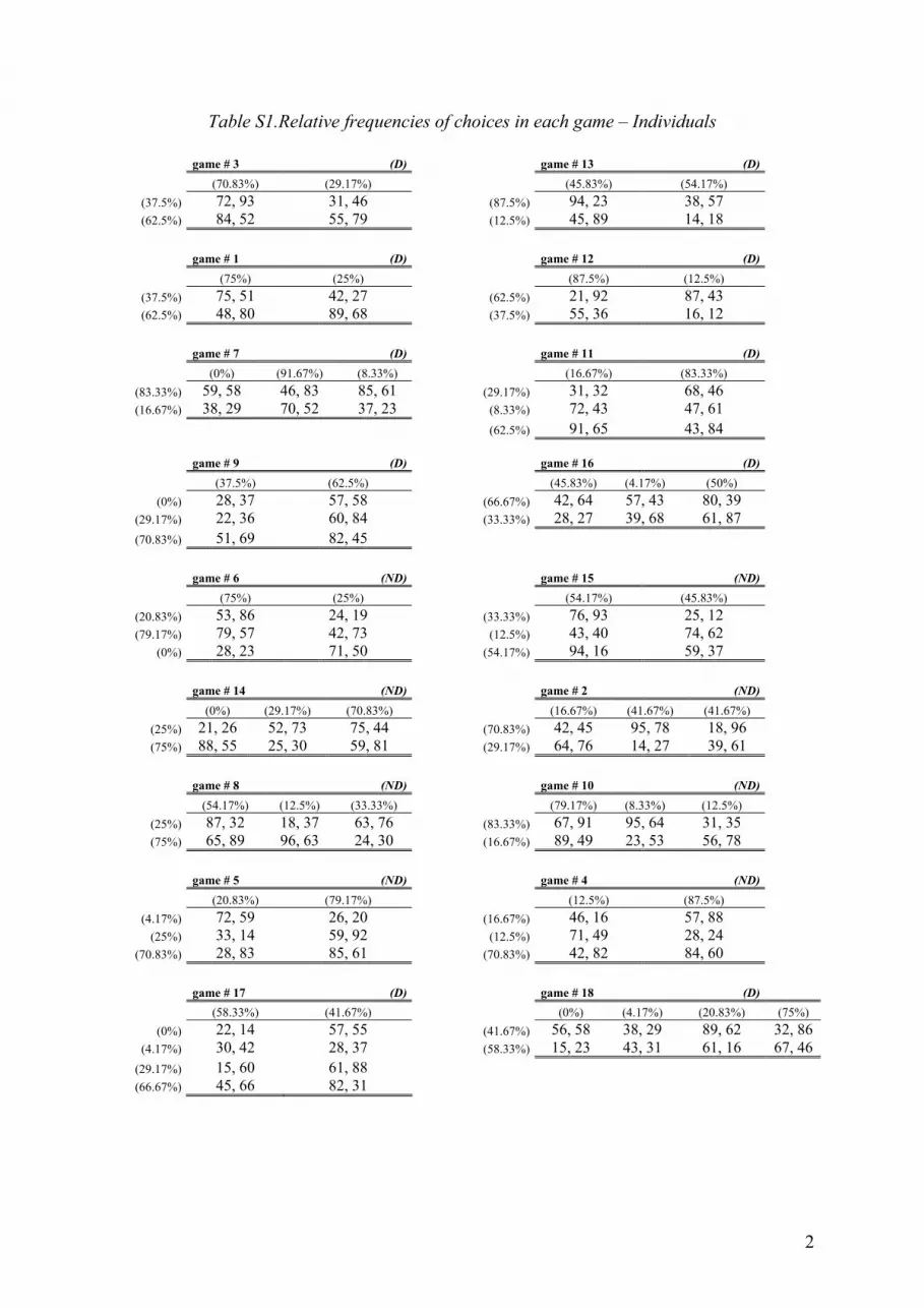
2

Table S1.Relative frequencies of choices in each game – Individuals

game # 3 (D) game # 13 (D) (70.83%) (29.17%) (45.83%) (54.17%)

(37.5%) 72, 93 31, 46 (87.5%) 94, 23 38, 57 (62.5%) 84, 52 55, 79 (12.5%) 45, 89 14, 18

game # 1 (D) game # 12 (D) (75%) (25%) (87.5%) (12.5%)

(37.5%) 75, 51 42, 27 (62.5%) 21, 92 87, 43 (62.5%) 48, 80 89, 68 (37.5%) 55, 36 16, 12

game # 7 (D) game # 11 (D) (0%) (91.67%) (8.33%) (16.67%) (83.33%)

(83.33%) 59, 58 46, 83 85, 61 (29.17%) 31, 32 68, 46 (16.67%) 38, 29 70, 52 37, 23 (8.33%) 72, 43 47, 61

(62.5%) 91, 65 43, 84

game # 9 (D) game # 16 (D) (37.5%) (62.5%) (45.83%) (4.17%) (50%)

(0%) 28, 37 57, 58 (66.67%) 42, 64 57, 43 80, 39 (29.17%) 22, 36 60, 84 (33.33%) 28, 27 39, 68 61, 87 (70.83%) 51, 69 82, 45

game # 6 (ND) game # 15 (ND) (75%) (25%) (54.17%) (45.83%)

(20.83%) 53, 86 24, 19 (33.33%) 76, 93 25, 12 (79.17%) 79, 57 42, 73 (12.5%) 43, 40 74, 62

(0%) 28, 23 71, 50 (54.17%) 94, 16 59, 37

game # 14 (ND) game # 2 (ND) (0%) (29.17%) (70.83%) (16.67%) (41.67%) (41.67%)

(25%) 21, 26 52, 73 75, 44 (70.83%) 42, 45 95, 78 18, 96 (75%) 88, 55 25, 30 59, 81 (29.17%) 64, 76 14, 27 39, 61

game # 8 (ND) game # 10 (ND) (54.17%) (12.5%) (33.33%) (79.17%) (8.33%) (12.5%)

(25%) 87, 32 18, 37 63, 76 (83.33%) 67, 91 95, 64 31, 35 (75%) 65, 89 96, 63 24, 30 (16.67%) 89, 49 23, 53 56, 78

game # 5 (ND) game # 4 (ND) (20.83%) (79.17%) (12.5%) (87.5%)

(4.17%) 72, 59 26, 20 (16.67%) 46, 16 57, 88 (25%) 33, 14 59, 92 (12.5%) 71, 49 28, 24

(70.83%) 28, 83 85, 61 (70.83%) 42, 82 84, 60

game # 17 (D) game # 18 (D) (58.33%) (41.67%) (0%) (4.17%) (20.83%) (75%)

(0%) 22, 14 57, 55 (41.67%) 56, 58 38, 29 89, 62 32, 86 (4.17%) 30, 42 28, 37 (58.33%) 15, 23 43, 31 61, 16 67, 46

(29.17%) 15, 60 61, 88 (66.67%) 45, 66 82, 31

3

Table S2.Relative frequencies of choices in each game – Teams

game # 3 (D) game # 13 (D) (58.33%) (41.67%) (25%) (75%)

(33.33%) 72, 93 31, 46 (91.67%) 94, 23 38, 57 (66.67%) 84, 52 55, 79 (8.33%) 45, 89 14, 18

game # 1 (D) game # 12 (D) (66.67%) (33.33%) (87.5%) (12.5%)

(54.17%) 75, 51 42, 27 (29.17%) 21, 92 87, 43 (45.83%) 48, 80 89, 68 (70.83%) 55, 36 16, 12

game # 7 (D) game # 11 (D) (4.17%) (83.33%) (12.5%) (20.83%) (79.17%)

(54.17%) 59, 58 46, 83 85, 61 (62.5%) 31, 32 68, 46 (45.83%) 38, 29 70, 52 37, 23 (4.17%) 72, 43 47, 61

(33.33%) 91, 65 43, 84

game # 9 (D) game # 16 (D) (45.83%) (54.17%) (70.83%) (4.17%) (25%)

(0%) 28, 37 57, 58 (87.5%) 42, 64 57, 43 80, 39 (25%) 22, 36 60, 84 (12.5%) 28, 27 39, 68 61, 87 (75%) 51, 69 82, 45

game # 6 (ND) game # 15 (ND) (58.33%) (41.67%) (29.17%) (70.83%)

(0%) 53, 86 24, 19 (25%) 76, 93 25, 12 (83.33%) 79, 57 42, 73 (8.33%) 43, 40 74, 62 (16.67%) 28, 23 71, 50 (66.67%) 94, 16 59, 37

game # 14 (ND) game # 2 (ND) (0%) (8.33%) (91.67%) (8.33%) (29.17%) (62.5%)

(25%) 21, 26 52, 73 75, 44 (58.33%) 42, 45 95, 78 18, 96 (75%) 88, 55 25, 30 59, 81 (41.67%) 64, 76 14, 27 39, 61

game # 8 (ND) game # 10 (ND) (75%) (8.33%) (16.67%) (79.17%) (12.5%) (8.33%)

(25%) 87, 32 18, 37 63, 76 (79.17%) 67, 91 95, 64 31, 35 (75%) 65, 89 96, 63 24, 30 (20.83%) 89, 49 23, 53 56, 78

game # 5 (ND) game # 4 (ND) (20.83%) (79.17%) (25%) (75%)

(16.67%) 72, 59 26, 20 (4.17%) 46, 16 57, 88 (12.5%) 33, 14 59, 92 (12.5%) 71, 49 28, 24

(70.83%) 28, 83 85, 61 (83.33%) 42, 82 84, 60

game # 17 (D) game # 18 (D) (66.67%) (33.33%) (0%) (0%) (20.83%) (79.17%)

(0%) 22, 14 57, 55 (41.67%) 56, 58 38, 29 89, 62 32, 86 (0%) 30, 42 28, 37 (58.33%) 15, 23 43, 31 61, 16 67, 46 (0%) 15, 60 61, 88

(100%) 45, 66 82, 31

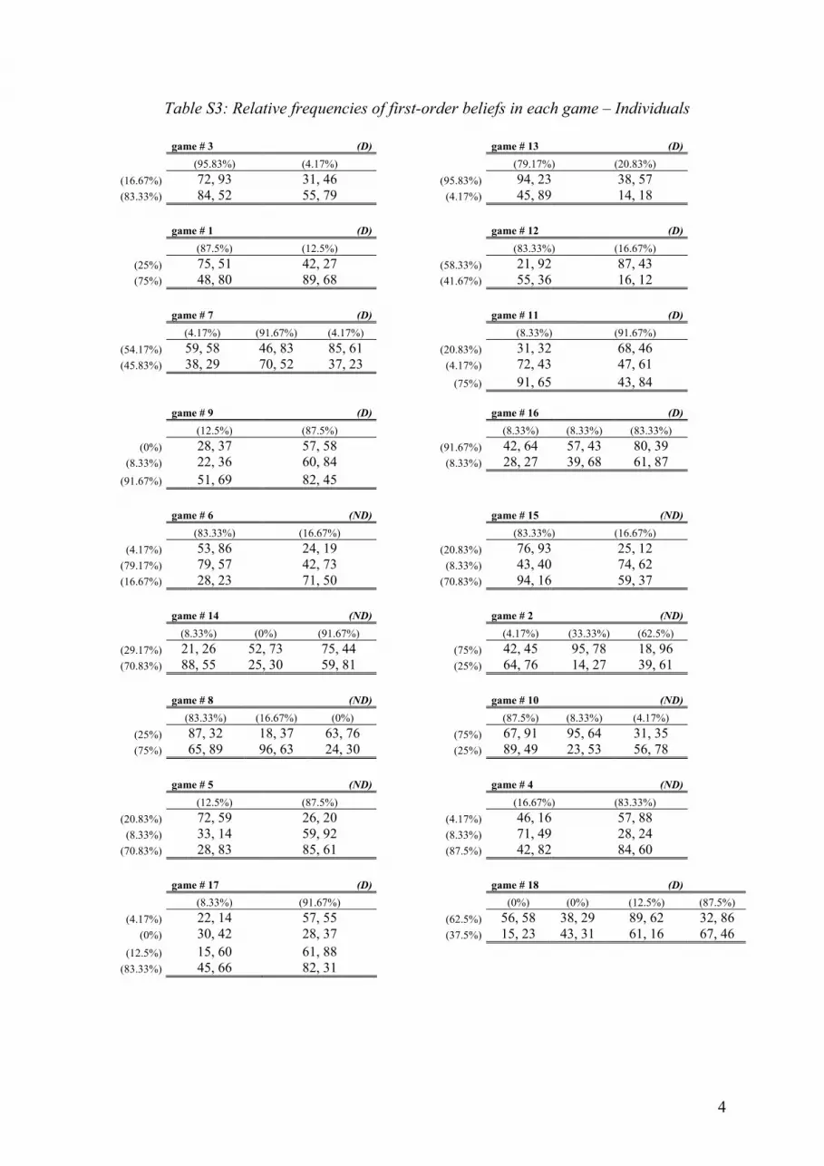
4

Table S3: Relative frequencies of first-order beliefs in each game – Individuals

game # 3 (D) game # 13 (D) (95.83%) (4.17%) (79.17%) (20.83%)

(16.67%) 72, 93 31, 46 (95.83%) 94, 23 38, 57 (83.33%) 84, 52 55, 79 (4.17%) 45, 89 14, 18

game # 1 (D) game # 12 (D) (87.5%) (12.5%) (83.33%) (16.67%)

(25%) 75, 51 42, 27 (58.33%) 21, 92 87, 43 (75%) 48, 80 89, 68 (41.67%) 55, 36 16, 12

game # 7 (D) game # 11 (D) (4.17%) (91.67%) (4.17%) (8.33%) (91.67%)

(54.17%) 59, 58 46, 83 85, 61 (20.83%) 31, 32 68, 46 (45.83%) 38, 29 70, 52 37, 23 (4.17%) 72, 43 47, 61

(75%) 91, 65 43, 84

game # 9 (D) game # 16 (D) (12.5%) (87.5%) (8.33%) (8.33%) (83.33%)

(0%) 28, 37 57, 58 (91.67%) 42, 64 57, 43 80, 39 (8.33%) 22, 36 60, 84 (8.33%) 28, 27 39, 68 61, 87

(91.67%) 51, 69 82, 45

game # 6 (ND) game # 15 (ND) (83.33%) (16.67%) (83.33%) (16.67%)

(4.17%) 53, 86 24, 19 (20.83%) 76, 93 25, 12 (79.17%) 79, 57 42, 73 (8.33%) 43, 40 74, 62 (16.67%) 28, 23 71, 50 (70.83%) 94, 16 59, 37

game # 14 (ND) game # 2 (ND) (8.33%) (0%) (91.67%) (4.17%) (33.33%) (62.5%)

(29.17%) 21, 26 52, 73 75, 44 (75%) 42, 45 95, 78 18, 96 (70.83%) 88, 55 25, 30 59, 81 (25%) 64, 76 14, 27 39, 61

game # 8 (ND) game # 10 (ND) (83.33%) (16.67%) (0%) (87.5%) (8.33%) (4.17%)

(25%) 87, 32 18, 37 63, 76 (75%) 67, 91 95, 64 31, 35 (75%) 65, 89 96, 63 24, 30 (25%) 89, 49 23, 53 56, 78

game # 5 (ND) game # 4 (ND) (12.5%) (87.5%) (16.67%) (83.33%)

(20.83%) 72, 59 26, 20 (4.17%) 46, 16 57, 88 (8.33%) 33, 14 59, 92 (8.33%) 71, 49 28, 24

(70.83%) 28, 83 85, 61 (87.5%) 42, 82 84, 60

game # 17 (D) game # 18 (D) (8.33%) (91.67%) (0%) (0%) (12.5%) (87.5%)

(4.17%) 22, 14 57, 55 (62.5%) 56, 58 38, 29 89, 62 32, 86 (0%) 30, 42 28, 37 (37.5%) 15, 23 43, 31 61, 16 67, 46

(12.5%) 15, 60 61, 88 (83.33%) 45, 66 82, 31

5

Table S4: Relative frequencies of first-order beliefs in each game – Teams

game # 3 (D) game # 13 (D) (75%) (25%) (54.17%) (45.83%)

(16.67%) 72, 93 31, 46 (91.67%) 94, 23 38, 57 (83.33%) 84, 52 55, 79 (8.33%) 45, 89 14, 18

game # 1 (D) game # 12 (D) (75%) (25%) (100%) (0%)

(37.5%) 75, 51 42, 27 (75%) 21, 92 87, 43 (62.5%) 48, 80 89, 68 (25%) 55, 36 16, 12

game # 7 (D) game # 11 (D) (8.33%) (83.33%) (8.33%) (4.17%) (95.83%)

(70.83%) 59, 58 46, 83 85, 61 (20.83%) 31, 32 68, 46 (29.17%) 38, 29 70, 52 37, 23 (0%) 72, 43 47, 61

(79.17%) 91, 65 43, 84

game # 9 (D) game # 16 (D) (20.83%) (79.17%) (50%) (0%) (50%)

(0%) 28, 37 57, 58 (91.67%) 42, 64 57, 43 80, 39 (16.67%) 22, 36 60, 84 (8.33%) 28, 27 39, 68 61, 87 (83.33%) 51, 69 82, 45

game # 6 (ND) game # 15 (ND) (54.17%) (45.83%) (66.67%) (33.33%)

(0%) 53, 86 24, 19 (12.5%) 76, 93 25, 12 (91.67%) 79, 57 42, 73 (8.33%) 43, 40 74, 62

(8.33%) 28, 23 71, 50 (79.17%) 94, 16 59, 37

game # 14 (ND) game # 2 (ND) (0%) (4.17%) (95.83%) (4.17%) (29.17%) (66.67%)

(25%) 21, 26 52, 73 75, 44 (70.83%) 42, 45 95, 78 18, 96 (75%) 88, 55 25, 30 59, 81 (29.17%) 64, 76 14, 27 39, 61

game # 8 (ND) game # 10 (ND) (95.83%) (4.17%) (0%) (100%) (0%) (0%)

(8.33%) 87, 32 18, 37 63, 76 (91.67%) 67, 91 95, 64 31, 35 (91.67%) 65, 89 96, 63 24, 30 (8.33%) 89, 49 23, 53 56, 78

game # 5 (ND) game # 4 (ND) (16.67%) (83.33%) (25%) (75%)

(12.5%) 72, 59 26, 20 (0%) 46, 16 57, 88 (8.33%) 33, 14 59, 92 (0%) 71, 49 28, 24

(79.17%) 28, 83 85, 61 (100%) 42, 82 84, 60

game # 17 (D) game # 18 (D) (54.17%) (45.83%) (0%) (0%) (12.5%) (87.5%)

(4.17%) 22, 14 57, 55 (62.5%) 56, 58 38, 29 89, 62 32, 86 (0%) 30, 42 28, 37 (37.5%) 15, 23 43, 31 61, 16 67, 46

(16.67%) 15, 60 61, 88 (79.17%) 45, 66 82, 31

6

Table S5: Relative frequencies of second-order beliefs in each game – Individuals

game # 3 (D) game # 13 (D) (87.5%) (12.5%) (70.83%) (29.17%)

(20.83%) 72, 93 31, 46 (91.67%) 94, 23 38, 57 (79.17%) 84, 52 55, 79 (8.33%) 45, 89 14, 18

game # 1 (D) game # 12 (D) (83.33%) (16.67%) (87.5%) (12.5%)

(8.33%) 75, 51 42, 27 (75%) 21, 92 87, 43 (91.67%) 48, 80 89, 68 (25%) 55, 36 16, 12

game # 7 (D) game # 11 (D) (8.33%) (83.33%) (8.33%) (8.33%) (91.67%)

(100%) 59, 58 46, 83 85, 61 (4.17%) 31, 32 68, 46 (0%) 38, 29 70, 52 37, 23 (4.17%) 72, 43 47, 61

(91.67%) 91, 65 43, 84

game # 9 (D) game # 16 (D) (12.5%) (87.5%) (8.33%) (16.67%) (75%)

(0%) 28, 37 57, 58 (79.17%) 42, 64 57, 43 80, 39 (25%) 22, 36 60, 84 (20.83%) 28, 27 39, 68 61, 87 (75%) 51, 69 82, 45

game # 6 (ND) game # 15 (ND) (87.5%) (12.5%) (83.33%) (16.67%)

(20.83%) 53, 86 24, 19 (25%) 76, 93 25, 12 (79.17%) 79, 57 42, 73 (4.17%) 43, 40 74, 62

(0%) 28, 23 71, 50 (70.83%) 94, 16 59, 37

game # 14 (ND) game # 2 (ND) (8.33%) (16.67%) (75%) (16.67%) (20.83%) (62.5%)

(4.17%) 21, 26 52, 73 75, 44 (95.83%) 42, 45 95, 78 18, 96 (95.83%) 88, 55 25, 30 59, 81 (4.17%) 64, 76 14, 27 39, 61

game # 8 (ND) game # 10 (ND) (75%) (8.33%) (16.67%) (79.17%) (8.33%) (12.5%)

(0%) 87, 32 18, 37 63, 76 (87.5%) 67, 91 95, 64 31, 35 (100%) 65, 89 96, 63 24, 30 (12.5%) 89, 49 23, 53 56, 78

game # 5 (ND) game # 4 (ND) (8.33%) (91.67%) (12.5%) (87.5%)

(4.17%) 72, 59 26, 20 (8.33%) 46, 16 57, 88 (16.67%) 33, 14 59, 92 (4.17%) 71, 49 28, 24 (79.17%) 28, 83 85, 61 (87.5%) 42, 82 84, 60

game # 17 (D) game # 18 (D) (25%) (75%) (8.33%) (0%) (16.67%) (75%)

(4.17%) 22, 14 57, 55 (87.5%) 56, 58 38, 29 89, 62 32, 86 (0%) 30, 42 28, 37 (12.5%) 15, 23 43, 31 61, 16 67, 46

(25%) 15, 60 61, 88 (70.83%) 45, 66 82, 31

7

Table S6: Relative frequencies of second-order beliefs in each game – Teams

game # 3 (D) game # 13 (D) (91.67%) (8.33%) (62.5%) (37.5%)

(25%) 72, 93 31, 46 (95.83%) 94, 23 38, 57 (75%) 84, 52 55, 79 (4.17%) 45, 89 14, 18

game # 1 (D) game # 12 (D) (83.33%) (16.67%) (87.5%) (12.5%)

(8.33%) 75, 51 42, 27 (45.83%) 21, 92 87, 43 (91.67%) 48, 80 89, 68 (54.17%) 55, 36 16, 12

game # 7 (D) game # 11 (D) (4.17%) (79.17%) (16.67%) (20.83%) (79.17%)

(87.5%) 59, 58 46, 83 85, 61 (25%) 31, 32 68, 46 (12.5%) 38, 29 70, 52 37, 23 (4.17%) 72, 43 47, 61

(70.83%) 91, 65 43, 84

game # 9 (D) game # 16 (D) (20.83%) (79.17%) (29.17%) (4.17%) (66.67%)

(0%) 28, 37 57, 58 (87.5%) 42, 64 57, 43 80, 39 (29.17%) 22, 36 60, 84 (12.5%) 28, 27 39, 68 61, 87 (70.83%) 51, 69 82, 45

game # 6 (ND) game # 15 (ND) (87.5%) (12.5%) (75%) (25%)

(4.17%) 53, 86 24, 19 (25%) 76, 93 25, 12 (87.5%) 79, 57 42, 73 (0%) 43, 40 74, 62 (8.33%) 28, 23 71, 50 (75%) 94, 16 59, 37

game # 14 (ND) game # 2 (ND) (0%) (4.17%) (95.83%) (4.17%) (20.83%) (75%)

(12.5%) 21, 26 52, 73 75, 44 (79.17%) 42, 45 95, 78 18, 96 (87.5%) 88, 55 25, 30 59, 81 (20.83%) 64, 76 14, 27 39, 61

game # 8 (ND) game # 10 (ND) (91.67%) (0%) (8.33%) (91.67%) (8.33%) (0%)

(8.33%) 87, 32 18, 37 63, 76 (87.5%) 67, 91 95, 64 31, 35 (91.67%) 65, 89 96, 63 24, 30 (12.5%) 89, 49 23, 53 56, 78

game # 5 (ND) game # 4 (ND) (8.33%) (91.67%) (4.17%) (95.83%)

(4.17%) 72, 59 26, 20 (4.17%) 46, 16 57, 88 (4.17%) 33, 14 59, 92 (4.17%) 71, 49 28, 24

(91.67%) 28, 83 85, 61 (91.67%) 42, 82 84, 60

game # 17 (D) game # 18 (D) (20.83%) (79.17%) (0%) (0%) (29.17%) (70.83%)

(0%) 22, 14 57, 55 (62.5%) 56, 58 38, 29 89, 62 32, 86 (0%) 30, 42 28, 37 (37.5%) 15, 23 43, 31 61, 16 67, 46

(4.17%) 15, 60 61, 88 (95.83%) 45, 66 82, 31

8

Table S7: Relative frequency of correct higher order beliefs (%) – Individuals (row players)

First – order beliefs Second – order beliefs

game correct incorrect correct incorrect

game #1 62.5 37.5 62.50 37.50

game #2 54.17 45.83 62.50 37.50

game #3 70.83 29.17 75.00 25.00

game #4 62.5 37.5 75.00 25.00

game #5 83.33 16.67 62.50 37.50

game #6 70.83 29.17 66.67 33.33

game #7 70.83 29.17 58.33 41.67

game #8 41.67 58.33 62.50 37.50

game #9 62.50 37.50 70.83 29.17

game #10 75.00 25.00 70.83 29.17

game #11 66.67 33.33 66.67 33.33

game #12 79.17 20.83 50.00 50.00

game #13 45.83 54.17 87.50 12.50

game #14 70.83 29.17 70.83 29.17

game #15 50.00 50.00 62.50 37.50

game #16 37.50 62.50 62.50 37.50

game #17 50.00 50.00 75.00 25.00

game #18 54.17 45.83 58.33 41.67

all games 61.57 38.43 66.67 33.33

9

Table S8: Relative frequency of correct higher order beliefs (%) –

Individuals (column players)

First – order beliefs Second – order beliefs

game correct incorrect correct incorrect

game #1 58.33 41.67 70.83 29.17

game #2 54.17 45.83 37.50 62.50

game #3 58.33 41.67 79.17 20.83

game #4 66.67 33.33 62.50 37.50

game #5 50.00 50.00 83.33 16.67

game #6 66.67 33.33 83.33 16.67

game #7 45.83 54.17 66.67 33.33

game #8 66.67 33.33 75.00 25.00

game #9 62.50 37.50 75.00 25.00

game #10 79.17 20.83 75.00 25.00

game #11 33.33 66.67 87.50 12.50

game #12 54.17 45.83 79.17 20.83

game #13 83.33 16.67 70.83 29.17

game #14 70.83 29.17 70.83 29.17

game #15 50.00 50.00 70.83 29.17

game #16 70.83 29.17 54.17 45.83

game #17 70.83 29.17 70.83 29.17

game #18 45.83 54.17 58.33 41.67

all games 60.42 39.58 70.60 29.40

10

Table S9: Relative frequency of correct higher order beliefs (%) – Teams (row players)

First – order beliefs Second – order beliefs

game correct incorrect correct incorrect

game #1 66.67 33.33 70.83 29.17

game #2 62.50 37.50 66.67 33.33

game #3 45.83 54.17 66.67 33.33

game #4 79.17 20.83 83.33 16.67

game #5 62.50 37.50 70.83 29.17

game #6 62.50 37.50 75.00 25.00

game #7 58.33 41.67 75.00 25.00

game #8 62.50 37.50 87.50 12.50

game #9 45.83 54.17 58.33 41.67

game #10 79.17 20.83 83.33 16.67

game #11 83.33 16.67 62.50 37.50

game #12 70.83 29.17 58.33 41.67

game #13 41.67 58.33 87.50 12.50

game #14 79.17 20.83 66.67 33.33

game #15 37.50 62.50 58.33 41.67

game #16 66.67 33.33 70.83 29.17

game #17 62.50 37.50 83.33 16.67

game #18 70.83 29.17 58.33 41.67

all games 63.19 36.81 71.30 28.70

11

Table S10: Relative frequency of correct higher order beliefs (%) – Teams (column players)

First – order beliefs Second – order beliefs

game correct incorrect correct incorrect

game #1 58.33 41.67 75.00 25.00

game #2 54.17 45.83 70.83 29.17

game #3 54.17 45.83 70.83 29.17

game #4 79.17 20.83 79.17 20.83

game #5 54.17 45.83 70.83 29.17

game #6 75.00 25.00 54.17 45.83

game #7 50.00 50.00 70.83 29.17

game #8 58.33 41.67 79.17 20.83

game #9 83.33 16.67 58.33 41.67

game #10 66.67 33.33 83.33 16.67

game #11 50.00 50.00 70.83 29.17

game #12 37.50 62.50 79.17 20.83

game #13 83.33 16.67 29.17 70.83

game #14 66.67 33.33 87.50 12.50

game #15 41.67 58.33 45.83 54.17

game #16 75.00 25.00 45.83 54.17

game #17 70.83 29.17 62.50 37.50

game #18 62.50 37.50 70.83 29.17

all games 62.27 37.73 66.90 33.10

12

Figure F1: Frequency of Nash strategy in the 18 games (choices, first- and second-order

beliefs) – actually observed versus random play

0.1

.2.3

.4re

lativ

e fre

quen

cy

0.1

.2.3

.4re

lativ

e fre

quen

cy

0 6 12 18frequency of playing Nash

0 6 12 18frequency of playing Nash

0 6 12 18frequency of playing Nash

0 6 12 18frequency of playing Nash

0 6 12 18frequency of playing Nash

0 6 12 18frequency of playing Nash

choices (individuals) FOB's (individuals) SOB's (individuals)

choices (teams) FOB's (teams) SOB's (teams)

observed expected (random play)

13

Figure F2: Frequency of consistency in the 18 games (own consistency, expected consistency

of opponent) – actually observed versus random play

0.1

.2.3

rela

tive

frequ

ency

0.1

.2.3

rela

tive

frequ

ency

0 6 12 18frequency of best reply

0 6 12 18frequency of best reply

0 6 12 18frequency of best reply

0 6 12 18frequency of best reply

choice best reply to FOB (individuals) FOB best reply to SOB (individuals)

choice best reply to FOB (teams) FOB best reply to SOB (teams)

observed expected (random play)

14

Figure F3: Frequency of Nash-consistency in the 18 games (own consistency, expected

consistency of opponent) – actually observed versus random play

0.2

.4re

lativ

e fre

quen

cy0

.2.4

rela

tive

frequ

ency

0 6 12 18frequency of Nash-CON

0 6 12 18frequency of Nash-CON

0 6 12 18frequency of Nash-CON

0 6 12 18frequency of Nash-CON

own Nash-CON (individuals) expected Nash-CON (individuals)

own Nash-CON (teams) expected Nash-CON (teams)

observed expected (random play)

15

Figure F4: Best responses of different strategic and non-strategic types

game # 3 (D) [1R, 2R] game # 13 (D) [1R, 2R] A, P, O, Si D12, L2, E, St A, P, O D12, L2, E, S

A 72, 93 31, 46 D 94, 23 38, 57 D 84, 52 55, 79 A 45, 89 14, 18

game # 1 (D) [2R, 1R] game # 12 (D) [2R, 1R] D A D A

D12, L2, E, S 75, 51 42, 27 A, P, O 21, 92 87, 43 A, P, O 48, 80 89, 68 D12, L2, E, S 55, 36 16, 12

game # 7 (D) [2R, 1R] game # 11 (D) [2R, 1R] D A A D

A, P, O 59, 58 46, 83 85, 61 D12, L2, E, S 31, 32 68, 46 D12, L2, E, S 38, 29 70, 52 37, 23 P 72, 43 47, 61

A, O 91, 65 43, 84

game # 9 (D) [1R, 2R] game # 16 (D) [1R, 2R] D12, L2, E, S A, P, O D12, L2, E, St P A, O, Si 28, 37 57, 58 D 42, 64 57, 43 80, 39

A 22, 36 60, 84 A 28, 27 39, 68 61, 87 D 51, 69 82, 45

game # 6 (ND) [3R, 2R] game # 15 (ND) [3R, 2R] A, P, O, Si D12, L2, E, St A, P, O, St D12, L2, E, Si

A 53, 86 24, 19 A 76, 93 25, 12 P, O, D1, L2, S 79, 57 42, 73 D2, E 43, 40 74, 62

D2, E 28, 23 71, 50 P, O, D1, L2, S 94, 16 59, 37

game # 14 (ND) [2R, 3R) game # 2 (ND) [2R, 3R] A D2, E P, O, D1, D2, S D2, E A P, O, D1, D2, S

D12, L2, E, S 21, 26 52, 73 75, 44 A, P, O, S 42, 45 95, 78 18, 96 A, P, O 88, 55 25, 30 59, 81 D12, L2, E 64, 76 14, 27 39, 61

game # 8 (ND) [∞R, ∞R] game # 10 (ND) [∞R, ∞R] O, D12, L2, S A, P E O, D12, L2, S A, P E

L2, E, S 87, 32 18, 37 63, 76 A, P, O, D12 67, 91 95, 64 31, 35 A, P, O, D12 65, 89 96, 63 24, 30 L2, E, S 89, 49 23, 53 56, 78

game # 5 (ND) [∞R, ∞R] game # 4 (ND) [∞R, ∞R] L2, E, St A, P, O, D12, Si L2, E, S A, P, O, D12

E 72, 59 26, 20 A, P 46, 16 57, 88 A, P 33, 14 59, 92 E 71, 49 28, 24

O, D12, L2, S 28, 83 85, 61 O, D12, L2, S 42, 82 84, 60

game # 17 (D) [1R, 2R] game # 18 (D) [2R, 1R] D12, L2, E, S A, P, O A D

22, 14 57, 55 A, P, O 56, 58 38, 29 89, 62 32, 86 30, 42 28, 37 D12, L2, E, S 15, 23 43, 31 61, 16 67, 46

A 15, 60 61, 88 D 45, 66 82, 31

A … altruistic; P … pessimistic; O … optimistic; L2, D1, D2 … strategic types (see section 3.6 in paper);

E … equilibrium; S … sophisticated (SI … sophisticated against individuals; ST … sophisticated against teams);

D12 = D1 and D2.

16

Experimental instructions In the following we present the instructions for the individual treatment as a baseline and

indicate parts which were used for the team treatment by underlined letters and parts which

were used for the mixed treatment by italic letters.

18 games in which two randomly chosen cabins are interacting with each other

In this experiment you will make decisions in 18 different “matrix-games”. In each „matrix-

game“ two different cabins are interacting with each other. From a total of eight cabins, in

every game two cabins are randomly selected to interact with each other. Out of those two

cabins there is always one cabin with three participants and one cabin with one participant.

This means in this experiment interaction takes place between teams of three participants and

single players. It is randomly selected whether you are a member of a team or a single player

by drawing cards at the beginning of the experiment.

In each “matrix game” both cabins have up to four choices. In most games the quantity of

choices is two or three. All choices in your own cabin are indicated with the following signs:

§

%

@

µ

Choices in the other cabin are indicated with the following signs:

§§

%%

@@

µµ

The combination of choices of both randomly selected cabins decides about your potential

payment in the experiment.

Three types of screens in each game (three decisions in each game)

For each of the 18 games you will be randomly matched with another cabin. Within each

game you need to make three different choices on three different screen types. For those three

decisions the matching of the cabins remains constant.

17

Please take care of the fact that the sequence of those three decisions is randomly determined.

Because of this you always need to pay attention to the upper row placed above the matrices.

On the following three pages you will find examples of the three different screen-types

(decisions). Note that the numbers within the matrices are just examples.

Payment

During the experiment you will have to make 18 * 3 decisions. At the end of the experiment

one of the 18 games and one of the corresponding three decisions will be randomly assigned

to be relevant for your payment.

This random selection is done by a draw from a deck of cards showing numbers from 1 to 18

(to select one of the 18 games) and from a deck of cards showing numbers 1 to 3 (to select

one of the three decisions). You will draw the card by yourself. In the following you will find

an explanation how much you can earn.

Independently from your decisions you will receive a show up fee of 4 Euros.

Feedback

Until the end of period 18 you will not get any feedback about the choices of the other cabins.

As soon as the game and the screen-type (decision) which will be relevant for payment are

selected, you will get detailed information about the corresponding decisions and the payment

resulting from these decisions.

Teams in cabins

In the case that there are three participants in your cabin you need to agree on one common

team decision. At the end of the experiment each team member gets the payment as

explained in the instructions.

Teams in cabins

In this experiment there is a team consisting of three members in each cabin. The team

members are required to agree on one common team decision. At the end of the experiment

each team member gets the payment as explained in the instructions.

18

Screen type A. What is your choice?

On the left hand side of the screen you can find your potential profit, depending on your own choice (in this example „§“ oder „%“) and on the choice of the cabin that is matched with you in a certain period (in this example „§§“ oder „%%“). Lets assume that you choose the option „%“, while the other cabin chooses the option „§§“, in this particular case you would earn 58 experimental points while the other cabin earns 80 experimental points. (Please take care that the screen for the other cabin is transposed (looks contrariwise). If you have any questions about this, please ask the instructor of the experiment) In the case that at the end of the experiment screen type A is randomly selected to be relevant for your payment, your profit (measured in experimental points) will be determined by the combination of your own choice and the choice of the other cabin. The relevant exchange rate between experimental points and Euros is:

1 experimental point = 0.30 Euros In the example illustrated above this would result in a payoff of 14.4 Euros (plus show up fee) for yourself and 24 Euros (plus show up fee) for the other cabin.

Please take care of this first row to identify the screen type and the kind of decision you need to make.

Here you can see the actual period.

In this column you can see your options. In the case that there are only “x-signs” in a certain row, this row cannot be selected.

In this row you can see the options of the other cabin.

In this box you can find your potential profits.

In this box you can find the potential profits of the other cabin.

19

Screen type B. According to your opinion, which option will be chosen by the other cabin?

In the case of screen type B you need to correctly predict the decision of the other cabin. In order to do that you need to select the choice which you expect from the other cabin in the screen-area as explained above. In the case that at the end of the experiment screen type B is randomly selected to be relevant for your payment, your profit will be 15 Euros if your guess was correct. To assess whether your guess was correct we will compare your expectation indicated on this screen with the real choice of the other cabin.

Please take care of this first row to identify the screen type and the kind of decision you need to make.

Here you need to indicate your opinion regarding the other cabin’s choice.

20

Screen type C. What is the choice that the other player expects from you?

In the case of screen type C you need to correctly predict the other cabin’s expectation regarding your own choice. On screen type B (which is explained on the previous page) you need to correctly predict the decision of the other cabin. For each game the other cabin needs to make the same prediction which means that the other cabin needs to state an expectation regarding your own choice. On screen type C you need to indicate which choice the other cabin expects from you. In the case that at the end of the experiment screen type C is randomly selected to be relevant for payment, your profit will be 15 Euros if your guess regarding the expectation of the other cabin was correct. To assess whether your guess was correct we will compare your decision on this screen (which is your guess regarding the expectation of the other cabin) with the real expectation of the other cabin.

Please take care of this first row to identify the screen type and the kind of decision you need to make.

Here you need to indicate your guess about the expectation of the other cabin regarding your own choice.

21

Control questions

Please answer the following questions which are all related to the matrices of the three screen-

types explained before.

Screen-type A.

1) Let’s assume you choose option „§“ and the other cabin chooses option „%%“:

a. How many experimental points do you earn? ______________

b. How many experimental points does the other cabin earn? _______________

2) Let’s assume you choose option „%“ and the other cabin chooses option „§§“:

a. How many experimental points do you earn? ______________

b. How many experimental points does the other cabin earn? _______________

Screen-type B.

3) Let’s assume you expect the other cabin to choose option „%%“ and the other cabin

chooses option „§§“.

a. How much do you earn (show up fee excluded), if this screen-type (decision)

is selected to be relevant for payment? _________________

4) Let’s assume you expect the other cabin to choose option „§§“ and the other cabin

chooses option „§§“.

a. How much do you earn (show up fee excluded), if this screen-type (decision)

is selected to be relevant for payment? _________________

Screen-type C.

5) Let’s assume the other cabin expects you to choose option „%“ and let’s assume you

select option „%“ on screen-type C.

a. How much do you earn (show up fee excluded), if this screen-type (decision)

is selected to be relevant for payment? _________________

6) Let’s assume the other cabin expects you to choose option „§“and let’s assume you

select option „%“ on screen-type C.

a. How much do you earn (show up fee excluded), if this screen-type (decision)

is selected to be relevant for payment? _________________