EXPERIMENTAL RESULTS OF GUIDED WAVE TRAVEL TIME

TOMOGRAPHY

Arno Volker, Arjan Mast and Joost Bloom

TNO Science & Industry, Stieltjes weg 1, 2600 AD, Delft, The Netherlands

ABSTRACT. Corrosion is one of the industries major issues regarding the integrity of assets.

Currently inspections are conducted at regular intervals to ensure a sufficient integrity level of these

assets. Both economical and social requirements are pushing the industry to even higher levels of

availability, reliability and safety of installations. The concept of predictive maintenance using

permanent sensors that monitor the integrity of an installation is an interesting addition to the current

method of periodic inspections reducing uncertainty and extending inspection intervals. Guided wave

travel time tomography is a promising method to monitor the wall thickness quantitatively over large

area’s.

Obviously the robustness and reliability of such a monitoring system is of paramount importance.

Laboratory experiments have been carried out on a 10” pipe with an nominal wall thickness of 8 mm.

Multiple, inline defects have been created with a realistic morphology. The depth of the defects was

increased stepwise from 0.5 mm to 2 mm. Additionally the influences of the presence of liquid inside

the pipe and surface roughness have been evaluated as well. Experimental results show that this

method is capable of providing quantitative wall thickness information over a distance of 4 meter,

with a sufficient accuracy such that results can be used for trending. The method has no problems

imaging multiple defects.

Keywords: Ultrasonic, Tomography, Inversion, Guided wave, Corrosion monitoring, Travel time,

Parameterization, Dispersion

PACS: 43.35.+d, 81.70.Cv, 81.70.Tx, 46.40.Cd, 43.35.Wa, 81.40.Np, 81.65.Kn, 43.60.Rw, 81.70.Tx

INTRODUCTION

Corrosion is one of the most important mechanisms of structural damage. There are

various reasons why corrosion is such an issue. First of all, its behavior strongly depends on

operating and environmental conditions. Also, it can occur in many forms from the formation

of clusters of small cracks to large patches of wall thickness loss. The parameters driving the

corrosion growth and appearance are not well understood and are often based on expert

opinion. This way corrosion can strike unexpectedly and due to possible high grow rates it can

lead to incidents before regular inspections are carried out.

Therefore periodic inspections can never be a cost effective solution for corrosion

monitoring. More promising are permanent monitoring systems that can measure the integrity

of the installation at any moment in time. The ideal permanent monitoring system for corrosion

management should have the following properties. First of all, the coverage of the system

should be 100% of the inside as well as the outside surface of the object. It should also be able

Copyright © 2010 American Institute of Physics. This article may be downloaded for personal use only.

Any other use requires prior permission of the author and the American Institute of Physics.

The following article appeared in AIP Conference Proceedings Volume 1211,

Review of Progress in Quantitative Nondestructive Evaluation and may be found at http://link.aip.org/link/?apc/1211/2052

to measure the corrosion rate, in order for optimal replacement or repair planning. Finally, the

system should be able to work without interference with the production process.

GUIDED WAVE CORROSION MAPPING

We describe a method to monitor the wall thickness of an arbitrary object using guided

waves. It uses the fact that the phase velocity of certain ultrasonic guided wave modes depends

on the thickness of the wave guide (see Figure 1). In a plate symmetrical and anti-symmetrical

modes exist. The zero-order modes (S0/A0) are attractive to use, since these modes always

exist. There are several reasons for using the symmetrical zero-order mode S0, these include

the low attenuation and the fact that this is the fastest mode, which makes it easier to

distinguish this wave mode from other possible modes. Similar wave modes exist in a pipe.

FIGURE 1 The left graph shows the dispersion curves for a steel plate. The shown modes are the

fundamental and first order symmetric and asymmetric Lamb wave modes. The right graph shows the

attenuation due to leakage of the same modes for a steel plate of 8 mm thick water loaded on one side.

So if a source and a receiver are placed at a known distance from each other, the time it

takes a guided wave mode to travel from the source to the receiver is a direct measure of the

integral thickness of the waveguide. However, the wave only contains information of the part

of the waveguide it traversed and the travel time only measures the integral wall thickness.

Therefore, the local properties of the thickness profile can not be retrieved from a single travel

time measurement. To obtain this information, it is needed to measure the travel time along

different paths over the object. Non-linear inversion of all the different travel times then yields

the wall thickness map.

Different approaches to guided wave tomography were discussed in by other authors

papers [1]-[3]. In most cases a back-projection approach is used, which essentially requires an

enclosed area to avoid a lot of artifacts. Leonard and Hinders [4] describe a method for pipes,

using a dense parameterization of the pipe surface to reconstruct the velocity profile

The method described in this paper could for example be applied to monitor the wall

thickness in pipes, bends or plates but uses an adaptive parameterizations and hence requires

much less transducers.. For a schematic depiction of the sensor setup on a pipe see Figure 2.

One ring array of sources is placed on the pipe. At a certain distance L further along the pipe a

ring array of receivers is placed. This way a large number of travel times can be measured

using direct arrivals and higher order circumferential paths. The time window in which higher

order modes can be used is limited by the arrival of other (slower) wave modes. Typically three

to four orders of circumferential passes can be used. The number of orders that can be used

determines the spatial resolution that can be achieved in the axial direction.

The larger the distance between the two arrays the larger the area covered and the more

useful the method is in practice. The goal is to maximize this distance, while maintaining

sufficient resolution for the detection of corrosion defects.

The resolution of this system depends on several factors, apart from the already

mentioned number of circumferential passes. It also depends strongly on the sensitivity of the

wave mode to wall thickness differences. This sensitivity determines the amount of time delay

for a given volume loss. The sensitivity of a certain mode on the thickness can be derived from

the dispersion curve. A final important factor is the parameterization of the surface that is used

to describe the wall thickness of the plate. A fine regular sampling would lead to a very large

number of parameters to be estimated. Only a local dense sampling is used, where the data

indicates that a defect is present.

FIGURE 2 The top image shows a schematic depiction of the setup used to measure the wall-thickness loss

of the area between the single source and receiver. The bottom image shows the schematic depiction of the

setup used the measure the absolute wall thickness of the pipe using two linear arrays around the

circumference.

TOMOGRAPHIC INVERSION

The non-linear inversion scheme is shown in Figure 3. We start by performing a

dispersion correction on the raw data and extracting the travel time of a specific Lamb wave

arrival for several higher orders of circumferential waves. In the dispersion correction

refraction effects are also included, i.e., no straight rays are used. A reference frequency is

defined and after dispersion correction the arrival will have an arrival time that corresponds to

the phase velocity for the reference frequency. Based on an initial guess of the thickness profile

the travel times are forward modeled using a ray tracing algorithm using the velocity profile

that corresponds to the reference frequency. Normally this initial guess is simply the nominal

wall thickness of the pipe.

Then a cost function is defined based on the difference between the modeled and

measured travel time and a sparseness constraint [7] to improve the resolution and avoid

oscillations in the solution. This cost function is minimized in an iterative way by updating the

initial guessed wall thickness, refining the mesh and redoing the dispersion correction.

Figure 4 illustrates the mesh refinement; only at the nodes of the mesh a parameter is

defined that describes the local wall thickness. During the interactive inversion nodes can be

added or removed from the grid automatically, such that only a fine mesh is obtained where

needed. The final number of used support point is 100, whereas 6240 support points would

have been needed on a uniform grid with the same resolution.

After one or a few iterations a new dispersion correction is performed on the measured

data. A locally changing velocity causes changes in travel time and refraction effect. This

Source Receiver

Source array Receiver array

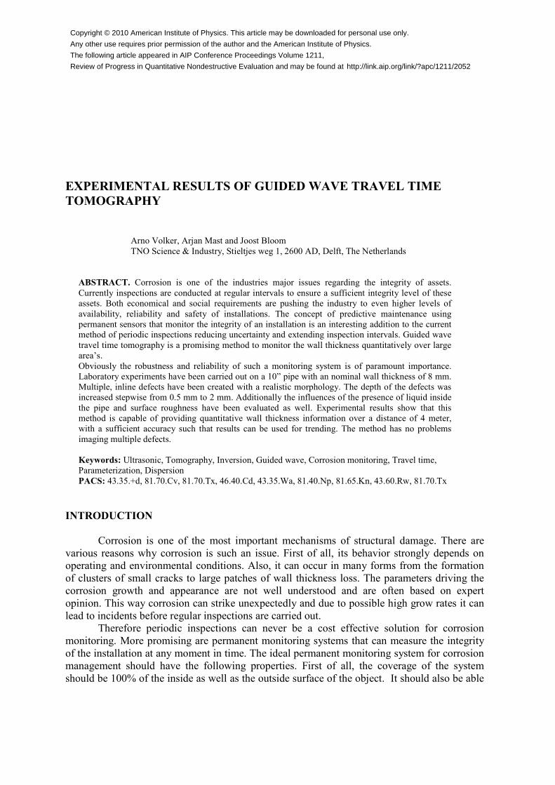
means that a straight ray-path approach cannot be used. This is illustrated very clearly in

Figure 5 for the A0-mode in a plate. Due to the presence of a defect a local low velocity area

exists. The low velocity zone will focus the rays, clearly illustrating that a straight ray approach

is not valid. This behavior is characteristic for the A0-mode. A wall thickness loss increases the

phase velocity for S0-mode and no focusing effects occur.

When the travel time difference between the measurements and the forward model data

is sufficiently small the inversion process is complete. Normally this occurs within ten

iterations.

FIGURE 3 Inversion scheme of the travel times to obtain the wall thickness image.

FIGURE 4 The top image shows the progress of the inversion process after two more iterations. Newly added

support points are again denoted by white crosses. The bottom image shows the final result of 10 iterations. Many

support points are used to describe the defects with high resolution and a limited number of support points is used

to describe the rest of the surface.

initial wall thickness guess

evaluation of objective function

Yes

adjust wall thickness profile

No

forward modeling travel times

dispersion correction +

travel time picking

convergence?

mesh refinement

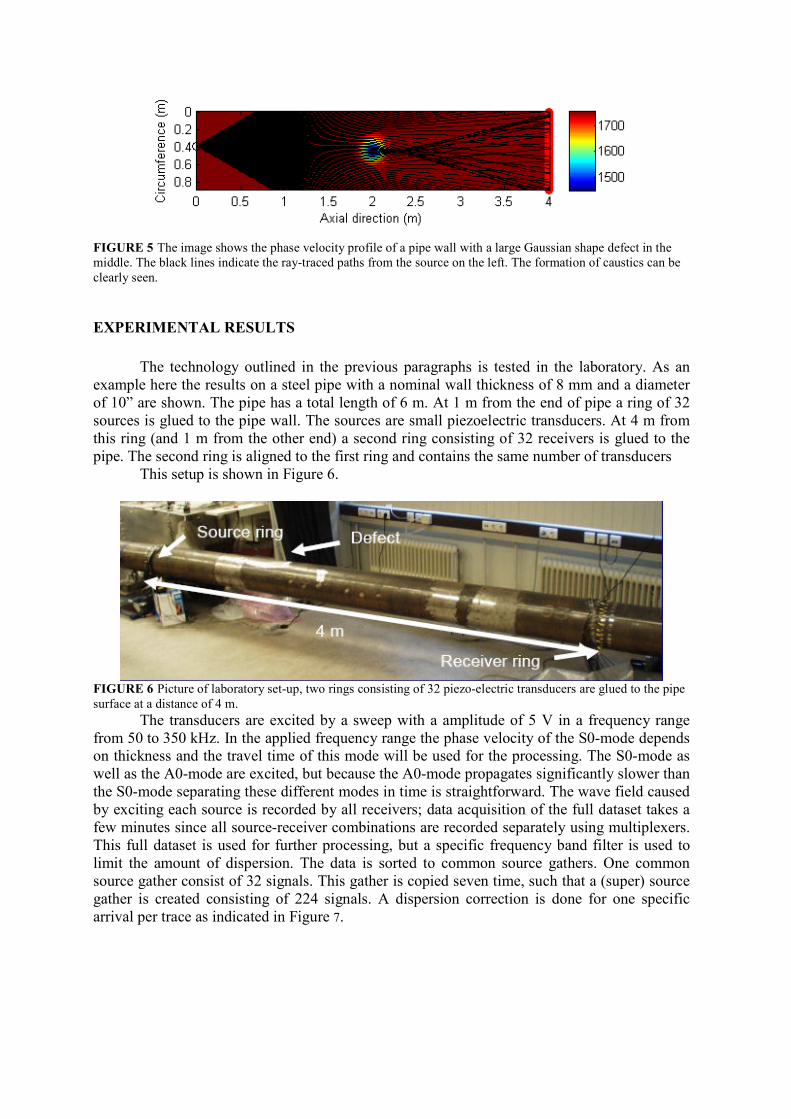
FIGURE 5 The image shows the phase velocity profile of a pipe wall with a large Gaussian shape defect in the

middle. The black lines indicate the ray-traced paths from the source on the left. The formation of caustics can be

clearly seen.

EXPERIMENTAL RESULTS

The technology outlined in the previous paragraphs is tested in the laboratory. As an

example here the results on a steel pipe with a nominal wall thickness of 8 mm and a diameter

of 10” are shown. The pipe has a total length of 6 m. At 1 m from the end of pipe a ring of 32

sources is glued to the pipe wall. The sources are small piezoelectric transducers. At 4 m from

this ring (and 1 m from the other end) a second ring consisting of 32 receivers is glued to the

pipe. The second ring is aligned to the first ring and contains the same number of transducers

This setup is shown in Figure 6.

FIGURE 6 Picture of laboratory set-up, two rings consisting of 32 piezo-electric transducers are glued to the pipe surface at a distance of 4 m.

The transducers are excited by a sweep with a amplitude of 5 V in a frequency range

from 50 to 350 kHz. In the applied frequency range the phase velocity of the S0-mode depends

on thickness and the travel time of this mode will be used for the processing. The S0-mode as

well as the A0-mode are excited, but because the A0-mode propagates significantly slower than

the S0-mode separating these different modes in time is straightforward. The wave field caused

by exciting each source is recorded by all receivers; data acquisition of the full dataset takes a

few minutes since all source-receiver combinations are recorded separately using multiplexers.

This full dataset is used for further processing, but a specific frequency band filter is used to

limit the amount of dispersion. The data is sorted to common source gathers. One common

source gather consist of 32 signals. This gather is copied seven time, such that a (super) source

gather is created consisting of 224 signals. A dispersion correction is done for one specific

arrival per trace as indicated in Figure 7.

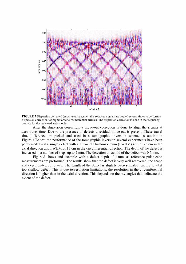
FIGURE 7 Dispersion corrected (super) source gather, this received signals are copied several times to perform a

dispersion correction for higher order circumferential arrivals. The dispersion correction is done in the frequency

domain for the indicated arrival only. After the dispersion correction, a move-out correction is done to align the signals at

zero-travel time. Due to the presence of defects a residual move-out is present. These travel

time difference are picked and used in a tomographic inversion scheme as outline in

Figure 3.To test the performance of the tomographic inversion several experiments have been

performed: First a single defect with a full-width half-maximum (FWHM) size of 25 cm in the

axial direction and FWHM of 13 cm in the circumferential direction. The depth of the defect is

increased in a number of steps up to 2 mm. The detection threshold of the defect was 0.5 mm.

Figure 8 shows and example with a defect depth of 1 mm, as reference pulse-echo

measurements are preformed. The results show that the defect is very well recovered; the shape

and depth match quite well. The length of the defect is slightly overestimated leading to a bit

too shallow defect. This is due to resolution limitations; the resolution in the circumferential

direction is higher than in the axial direction. This depends on the ray-angles that delineate the

extent of the defect.

FIGURE 8 Tomographic inversion result on a 1 mm deep defect, a reference pulse echo measurements are

preformed showing an accurate match with the inversion result. A typical configuration for corrosion under insulation is the presence of multiple defects

at the same circumferential location. With this configuration, we can evaluate whether the

tomography is capable of recovering two defects located behind each other in the axial

direction. The shape of the defects is different; one is more rounded, while the second one is

more elongated. Both have the same depth of nearly 2 mm. The tomographic inversion result is

shown in Figure 9. Both defects are recovered at the correct location, again slightly

overestimating the defect length at the expense of the defect depth. Overall the sizing accuracy

is typically better than 0.7 mm. Similar results where obtained with a liquid filled pipe.

FIGURE 9 Tomographic inversion result of two defects behind each other in the circumferential direction.

CONCLUSIONS AND FUTURE RESEARCH

This paper demonstrated a new technique to determine the wall thickness of large

structures such as plates, pipes and bends using the inversion of the travel times of dispersive

guided waves. It is a promising technique for the monitoring of large area’s using permanently

attached sensors. The full area of the pipe can be covered, with no zones of reduced sensitivity

by using several orders of waves that traveled around the circumference of the pipe. Key

factors that determine the performance of the tomography are the objective function and the

adaptive meshing.

By choosing the optimal wave mode this method also works on liquid filled pipes.

Experimental results show that the tomographic inversion is capable in resolving multiple

defects at the same circumferential location.

reference measurement

x [m]

r [m

]

x [m]

r [m

]

Future work will focus on improving the resolution, extending the distance between the

transducer rings and handling more complex geometries like bends. Additionally field test will

be carried out under operational conditions.

REFERENCES

1. J.L. Rose, J. Press. Ves. Techn. – Trans. ASME 124, 273-282 (2002). 2. M.J.S. Lowe, D.N. Alleyne, P. Cawley, Ultrasonics 36, 147-154 (1998).

3. G. Instanes, M. Toppe, B. Lakshminarayan, P.B. Nagy, Advanced Ultrasonic Methods

for Material and Structure Inspection, 115-157 (2006).

4. K. R. Leonard and M. K. Hinders, “Guided wave helical ultrasonic tomography of

pipes”, J. Acoust. Soc. Am. 114 (2), August 2003.

5. J. Li and J.L. Rose, Ultrasonics 44, 35-45 (2006). 6. P. Belanger, P. Cawley, Review of Progress in Quantitative NDE 27, 1290-1297 (2008). 7. P.M. Zwartjes, “Fourier reconstruction with sparse inversion”, Ph.D Thesis, Delft

University of Technology, 2005.