experimental polycrystal stress mapping using raman

UNLV Theses, Dissertations, Professional Papers, and Capstones

8-1-2020

Experimental Polycrystal Stress Mapping Using Raman Experimental Polycrystal Stress Mapping Using Raman

Spectroscopy Spectroscopy

Genevieve C. Kidman

Follow this and additional works at: https://digitalscholarship.unlv.edu/thesesdissertations

Part of the Geology Commons, and the Geophysics and Seismology Commons

Repository Citation Repository Citation Kidman, Genevieve C., "Experimental Polycrystal Stress Mapping Using Raman Spectroscopy" (2020). UNLV Theses, Dissertations, Professional Papers, and Capstones. 4005. http://dx.doi.org/10.34917/22110068

This Thesis is protected by copyright and/or related rights. It has been brought to you by Digital Scholarship@UNLV with permission from the rights-holder(s). You are free to use this Thesis in any way that is permitted by the copyright and related rights legislation that applies to your use. For other uses you need to obtain permission from the rights-holder(s) directly, unless additional rights are indicated by a Creative Commons license in the record and/or on the work itself. This Thesis has been accepted for inclusion in UNLV Theses, Dissertations, Professional Papers, and Capstones by an authorized administrator of Digital Scholarship@UNLV. For more information, please contact [email protected].

http://library.unlv.edu/

http://library.unlv.edu/

https://digitalscholarship.unlv.edu/thesesdissertations

https://digitalscholarship.unlv.edu/thesesdissertations?utm_source=digitalscholarship.unlv.edu%2Fthesesdissertations%2F4005&utm_medium=PDF&utm_campaign=PDFCoverPages

http://network.bepress.com/hgg/discipline/156?utm_source=digitalscholarship.unlv.edu%2Fthesesdissertations%2F4005&utm_medium=PDF&utm_campaign=PDFCoverPages

http://network.bepress.com/hgg/discipline/158?utm_source=digitalscholarship.unlv.edu%2Fthesesdissertations%2F4005&utm_medium=PDF&utm_campaign=PDFCoverPages

http://dx.doi.org/10.34917/22110068

mailto:[email protected]

EXPERIMENTAL POLYCRYSTAL STRESS MAPPING USING RAMAN SPECTROSCOPY

By

Genevieve C. Kidman

Bachelor of Science – Geology

Southern Utah University

2015

A thesis submitted in partial fulfillment

of the requirements for the

Master of Science – Geoscience

Department of Geoscience

College of Sciences

The Graduate College

University of Nevada, Las Vegas

August 2020

Copyright by Genevieve C. Kidman, 2020

All Rights Reserved

ii

Thesis Approval

The Graduate College

The University of Nevada, Las Vegas

July 9, 2020

This thesis prepared by

Genevieve C. Kidman

entitled

Experimental Polycrystal Stress Mapping Using Raman Spectroscopy

is approved in partial fulfillment of the requirements for the degree of

Master of Science – Geoscience

Department of Geoscience

Pamela Burnley, Ph.D. Kathryn Hausbeck Korgan, Ph.D. Examination Committee Chair Graduate College Dean

Michael Wells, Ph.D. Examination Committee Member

Wanda Taylor, Ph.D. Examination Committee Member

Ashkan Salamat, Ph.D. Graduate College Faculty Representative

iii

Abstract

Stress conditions leading to rock deformation influence how a rock will ultimately deform.

However, the internal distribution of stress in an elastically anisotropic rock under load, a

precursor to rock deformation, is not well understood. Two models that may describe the

distribution of stress in polycrystals include the Reuss bound and stress percolation. The Reuss

bound, when applied to a polycrystal, describes isostress on each grain resulting in homogeneous

intragranular strain and heterogeneous intergranular strain. The stress percolation model involves

a network of strong contacts or force chains containing domains of high stress interwoven

through areas of lower stress that are heterogeneous at an intragranular and intergranular scale.

An experiment has been devised to measure the intragranular stress state of a polycrystal to

understand rock deformation. Experimentally measuring stress is possible through Raman

spectroscopy, which is capable of quantifying elastic strain changes in a crystal lattice by looking

at a change in spectral peak position between a non-loaded and loaded polycrystal. A

megapascal load was applied through a uniaxial hand vice equipped with a load cell on a

millimeter-sized rectangular parallelepiped consisting of quartz Tiger’s Eye. Spectra were

measured on the surface at specific locations on the sample in a loaded and non-loaded state.

Stress was calculated at each location, and a stress raster was created to show the stress state of

the polycrystalline rock. A grain orientation map using EBSD was collected on the surface of the

sample, then overlain with the stress raster, creating the stress map. In several large quartz

grains, the map shows an intergranular heterogeneous stress distribution. An interconnecting

pattern of raster cells classified as high stress, as well as groups of raster cells classified as low

stress, show evidence of an intergranular stress percolation pattern. Results show that the stress

distribution in a polycrystalline rock is best modeled by stress percolation.

iv

Acknowledgments

The National Nuclear Security Administration has supported this research under the Stewardship

Science Academic Alliances program through DOE Cooperative Agreement #DE-NA0003896.

Support has also been provided through the National Science Foundation EAR – 1417218.

I would like to give many thanks to Dr. Pamela Burnley for her wisdom and guidance through

this project. I have been fortunate to have an advisor who is not only a brilliant scientist but one

of kindness and thoughtfulness. I have learned how to be a better scientist through her example

and I am honored to count Dr. Burnley as a role model and friend. I would also like to give

thanks to my committee members, Dr. Ashkan Salamat, Dr. Wanda Taylor, and Dr. Michael

Wells, for their positivity, hallway pep talks, and never-ending encouragement. This project has

been enriched by their unique points of view and expertise, and I will be forever grateful to them.

This project has been greatly impacted by the fellow students that I have had the opportunity to

work alongside. I would like to thank past and present NeRD Lab students Carrie Clark, Vy

Nguyen, Jessica Butanda, and Devon Scheg for their tireless contribution in sample preparation.

I would also like to thank Taryn Traylor, Christian Childs, Jasmine Hinton, Joshua Sacket, Dawn

Reynoso, and Shirin Kaboli for their thoughtful discussions and brilliant ideas.

Finally, I would like to acknowledge and thank my family for their love and support during this

project. I am grateful to have the support and love of my best friend and husband, Sam Kidman.

Sam has been my favorite rock of support and kept me sane in countless ways through the ups

and downs of this process. Lastly, to Charlie and Inga, whose insistence on going to the dog park

each night gave me time to breathe fresh air, reflect, and refresh my imagination.

v

Table of Contents

Abstract ........................................................................................................................................ iii

Acknowledgments ....................................................................................................................... iv

Table of Contents ......................................................................................................................... iv

List of Tables .............................................................................................................................. iv

List of Figures ............................................................................................................................. iv

Chapter 1: Introduction and Background ..................................................................................... 1

1.1 Introduction ....................................................................................................................... 1

1.2 Experimental Summary ..................................................................................................... 2

1.3 Background ....................................................................................................................... 3

1.4 Chapter 1 Figures ............................................................................................................ 15

1.5 Chapter 1 Tables ............................................................................................................. 21

Chapter 2: Experimental Methods ............................................................................................. 23

2.1 Experimental Samples ..................................................................................................... 23

2.2 Uniaxial Vice and Load Cell ........................................................................................... 29

2.3 Break Tests ...................................................................................................................... 30

2.4 Fiduciary Marks .............................................................................................................. 31

2.5 High-Resolution Micrographs ......................................................................................... 32

vi

2.6 Raman Methods .............................................................................................................. 32

2.7 Data Processing ............................................................................................................... 36

2.8 Calcite tests ..................................................................................................................... 38

2.9 Single crystal Quartz Tests .............................................................................................. 39

2.10 Tiger’s Eye Tests ........................................................................................................... 41

2.11 Stress Map ..................................................................................................................... 44

2.12 Chapter 2 Figures .......................................................................................................... 46

2.13 Chapter 2 Table ............................................................................................................. 77

Chapter 3: Raman Experimental Results ................................................................................... 78

3.1 Single Crystal Tests ........................................................................................................ 78

3.2 Raman Stress Shift Factors ............................................................................................. 80

3.3 Polycrystal Tests ............................................................................................................. 81

3.4 Chapter 3 Figures ............................................................................................................ 86

3.5 Chapter 3 Tables ............................................................................................................. 97

Chapter 4: Discussion and Conclusion .................................................................................... 103

4.1 Single-Crystals .............................................................................................................. 103

4.2 Polycrystals ................................................................................................................... 107

4.3 Stress Percolation .......................................................................................................... 109

vii

4.4 Conclusion .................................................................................................................... 110

4.5 Future Work .................................................................................................................. 111

4.6 Chapter 4 Figures .......................................................................................................... 113

4.7 Chapter 4 Tables ........................................................................................................... 120

Appendix .................................................................................................................................. 121

2.1 Sample Preparation Equipment List .............................................................................. 121

2.2 Raman File Separation Fortran Code ............................................................................ 123

2.3 Fityk Batch Processing Lua Code ................................................................................. 127

3.1 Tig01 Raman Data ........................................................................................................ 131

3.2 Tig03 Raman Data ........................................................................................................ 135

Bibliography ............................................................................................................................ 139

Curriculum Vitae ..................................................................................................................... 146

viii

List of Tables

Table 1.1 Raman stress shift factors for calcite .......................................................................... 21

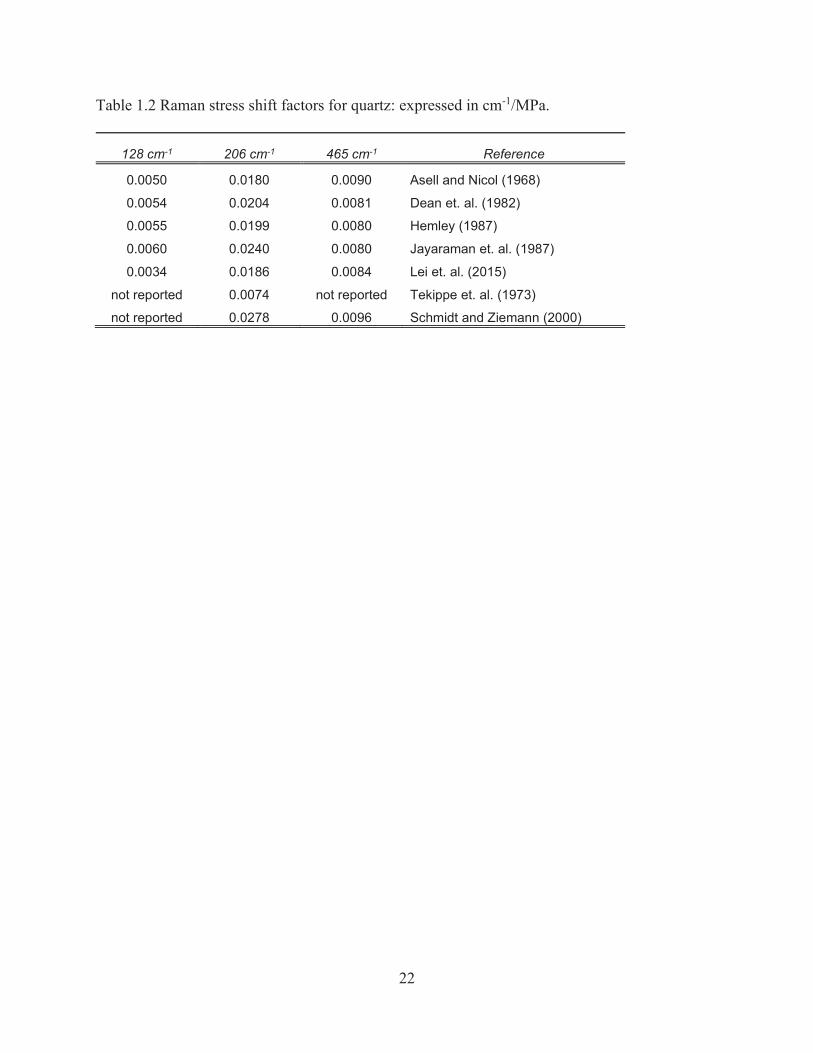
Table 1.2 Raman stress shift factors for quartz ........................................................................... 22

Table 2.1 Sample break tests ..................................................................................................... 77

Table 3.1 Single-crystal calcite test 1 ........................................................................................ 97

Table 3.2 Experimental test data ................................................................................................ 98

Table 3.3 Single-crystal quartz tests .......................................................................................... 99

Table 3.4: RQa peak position standard deviation .................................................................... 100

Table 3.5: Raman stress shift factor for single-crystal calcite and quartz tests ....................... 101

Table 3.6: Carrara Marble Test 7 corrected peak positions ..................................................... 102

Table 4.1 RSSF’s for quartz ..................................................................................................... 120

ix

List of Figures

Figure 1.1 Anisotropy in Crystals .............................................................................................. 15

Figure 1.2 Voigt upper bound elastic model .............................................................................. 16

Figure 1.3 Reuss lower bound elastic model ............................................................................. 17

Figure 1.4 Finite Element Model of Stress Percolation ............................................................. 18

Figure 1.5 Raman Spectra Mechanics ....................................................................................... 19

Figure 1.6 Sample surface effects with optical depth of field ................................................... 20

Figure 2.1 Tiger’s Eye micrograph with grain boundaries ........................................................ 46

Figure 2.2 Schematic of the rectangular parallelepiped samples ............................................... 47

Figure 2.3 Rhombohedral cleavage for calcite .......................................................................... 48

Figure 2.4 Cartoon of Tiger’s Eye crystals orientation relative to the sample’s cut plane ........ 49

Figure 2.5 Sample height problems in the vice and on the Raman spectrometer ...................... 50

Figure 2.6 Sample preparation method ...................................................................................... 51

Figure 2.7 Sample polishing process ......................................................................................... 52

Figure 2.8 Fine polish on Carrara Marble .................................................................................. 53

Figure 2.9 VibroMet puck modification .................................................................................... 54

Figure 2.10 Hand Vice ............................................................................................................... 55

Figure 2.11 Load Cell Standard Deviation ................................................................................ 56

x

Figure 2.12 Carrara Marble Break Test 3 .................................................................................. 57

Figure 2.13 Tigers Eye Break Test 1 ......................................................................................... 58

Figure 2.14: Fiducial marks on quartz samples ......................................................................... 59

Figure 2.15 The T64000 Horiba Jobin Yvon Raman system .................................................... 60

Figure 2.16 Laser path schematic of the Horiba Jobin-Yvon T64000 Raman spectrometer in a

triple configuration ..................................................................................................................... 61

Figure 2.17 Czerny Turner Monochromator .............................................................................. 62

Figure 2.18 Raman spectra of calcite at 488 nm laser wavelength ............................................ 63

Figure 2.19 Raman spectra of quartz at 488 nm laser wavelength ............................................ 64

Figure 2.20 Raman spectra of quartz at 514 nm laser wavelength ............................................ 65

Figure 2.21 Quartz spectra signal to noise ratios ....................................................................... 66

Figure 2.22 Linear extrapolation example for datapoint 100, 100 from test RQa3 ................... 67

Figure 2.23 Carrara marble spectrum ........................................................................................ 68

Figure 2.24: Schematic of the spectra positions on the surface of the RQa samples ................ 69

Figure 2.25 Tig01 micrograph ................................................................................................... 70

Figure 2.26 Tig01 load cell and mean stress log ....................................................................... 71

Figure 2.27 Mosaiced screenshots of the spectral data points on loaded Tig03 ........................ 72

Figure 2.28 Mosaiced screenshots of the spectral data points on unloaded Tig03 .................... 73

Figure 2.29 Esri ArcMap natural breaks histogram for Tig03 ................................................... 74

xi

Figure 2.30 High-resolution micrograph of the unloaded surface of Tig03 .............................. 75

Figure 2.31 Georeferenced stress raster and Tig03 micrograph ................................................ 76

Figure 3.1: Histogram of Single-crystal calcite and Carrara marble test 7 ................................ 86

Figure 3.2 RQa peak position histogram ................................................................................... 87

Figure 3.3 Tig01 peak position histogram ................................................................................. 88

Figure 3.4 Spectra misalignment ............................................................................................... 89

Figure 3.5 Tig03 peak position histogram ................................................................................. 90

Figure 3.6 EBSD grain orientation map .................................................................................... 91

Figure 3.7 Grain boundary map ................................................................................................. 92

Figure 3.8 Stress map on Tig03 ................................................................................................. 93

Figure 3.9 Raman stress shift histogram of Tig03 ..................................................................... 94

Figure 3.10 Intergranular stress in Tig03 ................................................................................... 95

Figure 3.11 Intragranular heterogeneous stress in Tig03 ........................................................... 96

Figure 4.1 Range of Raman quartz peak positions for single-crystal and polycrystal tests .... 113

Figure 4.2 Diagram for single-crystal uncertainty calculation ................................................. 114

Figure 4.3 Iron oxide inclusion map for unloaded test Tig03 .................................................. 115

Figure 4.4: Histogram of iron oxide proximity unloaded Tig03 peak positions ..................... 116

Figure 4.5: Orientation and wavenumber map for unloaded Test Tig03 ................................. 117

xii

Figure 4.6 Histogram of unloaded peak positions for different grain orientations .................. 118

Figure 4.7 Tig03 stress magnitudes with single-crystal uncertainty ........................................ 119

1

Chapter 1: Introduction and Background

1.1 Introduction

It is well understood how single crystals deform, but what is less understood is how an aggregate

of crystals with different orientations will deform. A single crystal has an arrangement of atoms

assembled in a long-range three-dimensional pattern. The pattern of atoms can be described by

several point, and translational symmetry operations, which are characterized relative to their

position in a convenient coordinate system with the principal axes labeled a, b, and c. The

arrangement of atoms in a non-isometric crystal along the a-axis will be different from that of the

b, or c-axis, leading to elastic and mechanical properties that are orientation-dependent. An

example of elastic anisotropy can be seen in the a- and c-axes of quartz. The a-axis is

approximately 50% more compressible than the c-axis (Hazen, 1989; Angel, 1997). When a

boundary condition of uniaxial stress is imposed on a single crystal, the first reaction in the

lattice is elastic. As stress increases, the crystal eventually plastically deforms via well-

understood deformation mechanisms. A single crystal with an imposed boundary condition will

strain predictably via its intrinsic elastically anisotropic properties if nothing surrounds the single

crystal to impede the strain (Figure 1.1a). A single crystal amid other neighboring crystals will

not be able to have the same intrinsic reaction to stress due to the limitations of the crystal's

neighbors and their orientation-dependent anisotropic properties. The reaction of a crystal grain

within a polycrystal must be compatible with each neighbor’s reaction. The outer boundary

condition of uniaxial stress that was initially imposed upon the polycrystal would be very

different from the boundary condition imposed on the individual crystal grain by its crystal

neighbors (Figure 1.1b). What is not understood in anisotropic materials is how the external

2

boundary conditions placed on the aggregate is related to the inner boundary conditions that are

unique to every single crystal within the aggregate (Burnley, 2013).

The commonality of anisotropic minerals in the Earth creates an underlying problem for

comprehending stress and strain. The Voigt (1928) iso-strain, and Reuss (1929) iso-stress, are

mathematical upper and lower bounds defining the stress and strain distribution in a polycrystal

(Hirsekorn 1988). These models do not account for the assortment of strain heterogeneity in the

bulk of Earth materials. To test stress distribution in a polycrystal, Burnley (2013) created a two-

dimensional finite element model consisting of hexagonal ‘grains’ with a variety of elastic and

mechanical properties. When the model was compressed, a stress percolation pattern emerged.

The stress percolation model is proposed as an alternative to the Reuss model in understanding

the distribution of stress in a polycrystal (Burnley, 2013). The goal for these series of

experiments is to observe the magnitude of stress in natural polycrystalline materials using

experimental methods to discover if the distribution of stress follows a Reuss iso-stress model, or

if there could be a new paradigm for stress distribution. Measuring stress distributions in natural

polycrystalline rock will set the groundwork for understanding the development of micro and

macro-deformation patterns such as shear localization, deformational rock fabrics, foliation, and

fractures (Burnley 2013).

1.2 Experimental Summary

This experiment tested the elastic response of single-crystal and polycrystal samples to an

imposed uniaxial load to determine the nature of stress distribution. Raman spectroscopy was

used to measure characteristic pressure-dependent spectral peaks of single-crystal and

polycrystalline calcite and quartz samples. Spectra were collected on samples with no imposed

3

stress; then, the measurement was repeated using the same samples at the same locations with an

imposed uniaxial load. The change in peak positions between the two spectrums showed the

elastic strain response of the crystal. Spectra were mapped across the surface of single-crystal

samples, as well as polycrystalline samples. Single crystal samples were used as a control for the

polycrystal tests based on the assumption that a single boundary condition applied to a single

relatively flawless crystalline lattice should produce a single strain at all points in the crystal,

which would produce a uniform Raman stress shift. Polycrystal tests were conducted at a scale

that intragranular and intergranular relationships could be observed. The peak positions of the

no-load spectrum would then be subtracted from the peak positions from loaded spectrum

resulting in a Raman stress shift that was then converted to stress. Stress at individual

measurement locations were mapped for polycrystal tests using Esri ArcMap software. A

polycrystal stress map was then be analyzed through direct observation to determine the nature

of stress distribution in the sample. I hypothesized that the stress percolation model better

represents the stress distribution in a polycrystal over a Reuss state of iso-stress.

1.3 Background

These experiments draw from many scientific concepts that are different but interconnected in a

way that enables stress to be measured and mapped across the surface of a polycrystalline

material. A brief overview of stress, strain, and elasticity is described, followed by traditional

elastic models that describe stress and strain in a polycrystal, and a brief overview of stress

percolation. A background on Raman spectroscopy is then addressed, followed by an overview

of the experimental materials used in the experiment.

1.3.1 Stress, Strain, and Elasticity

4

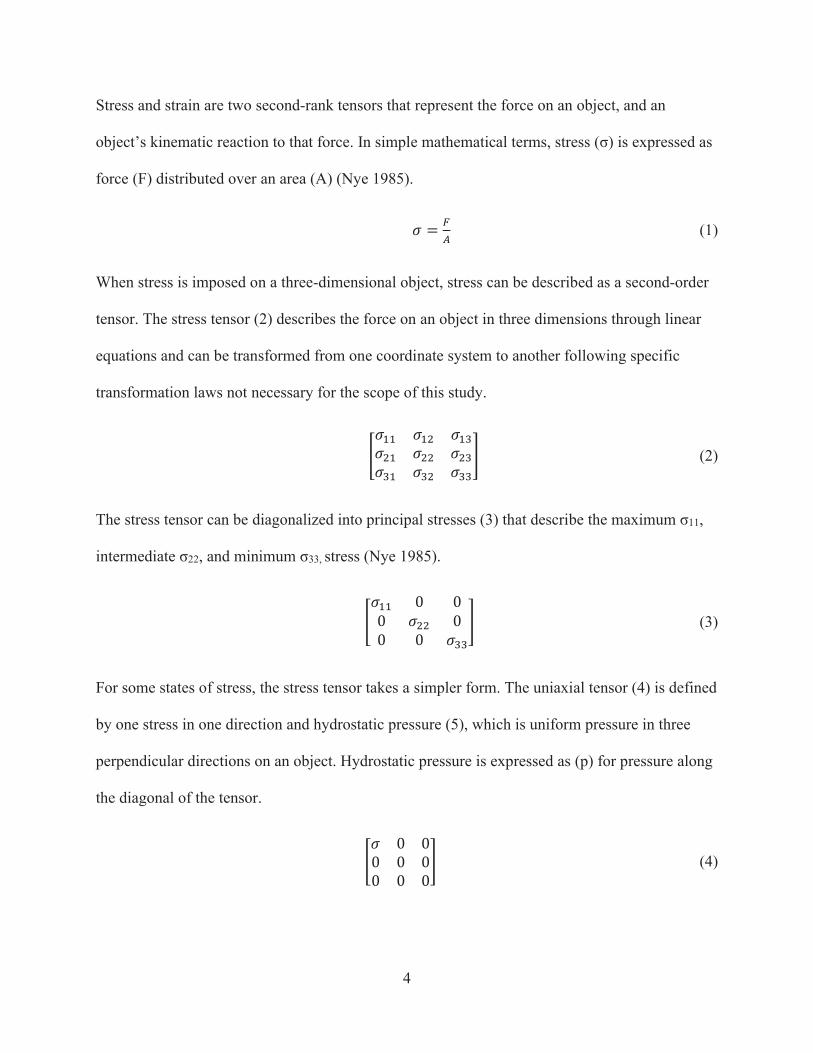
Stress and strain are two second-rank tensors that represent the force on an object, and an

force (F) distributed over an area (A) (Nye 1985).

= (1)

When stress is imposed on a three-dimensional object, stress can be described as a second-order

tensor. The stress tensor (2) describes the force on an object in three dimensions through linear

equations and can be transformed from one coordinate system to another following specific

transformation laws not necessary for the scope of this study.

(2)

The stress tensor can be diagonalized into principal stresses (3) 11,

22 33, stress (Nye 1985).

0 00 00 0 (3)

For some states of stress, the stress tensor takes a simpler form. The uniaxial tensor (4) is defined

by one stress in one direction and hydrostatic pressure (5), which is uniform pressure in three

perpendicular directions on an object. Hydrostatic pressure is expressed as (p) for pressure along

the diagonal of the tensor.

0 00 0 00 0 0 (4)

5

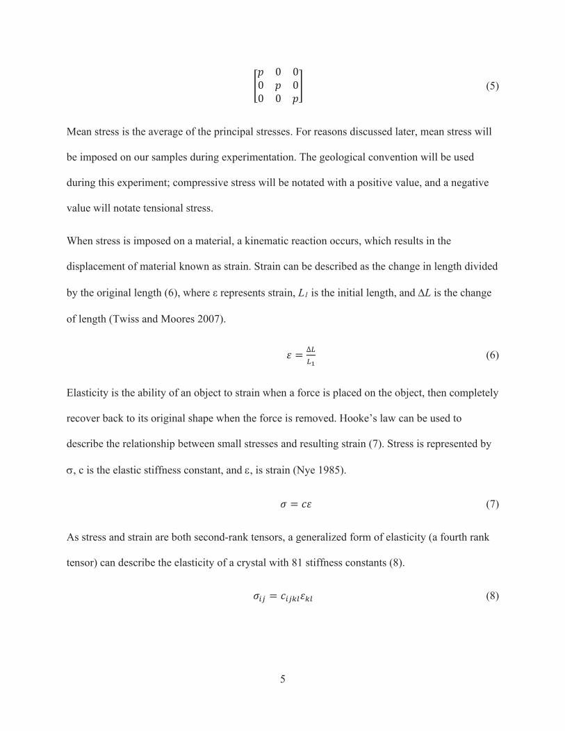
0 00 00 0 (5)

Mean stress is the average of the principal stresses. For reasons discussed later, mean stress will

be imposed on our samples during experimentation. The geological convention will be used

during this experiment; compressive stress will be notated with a positive value, and a negative

value will notate tensional stress.

When stress is imposed on a material, a kinematic reaction occurs, which results in the

displacement of material known as strain. Strain can be described as the change in length divided

by the original length (6) L1 is the initial length, and L is the change

of length (Twiss and Moores 2007).

= (6)

Elasticity is the ability of an object to strain when a force is placed on the object, then completely

recover back to its original shape when the force is removed. Hooke’s law can be used to

describe the relationship between small stresses and resulting strain (7). Stress is represented by

, c is the elastic stiffness constant, and , is strain (Nye 1985).

= (7)

As stress and strain are both second-rank tensors, a generalized form of elasticity (a fourth rank

tensor) can describe the elasticity of a crystal with 81 stiffness constants (8).

= (8)

6

Although the stiffness constants are beyond the scope of this study, it is important to note that

there can be substantial variations between the elastic response of a crystal in different

directions.

1.3.2 Traditional Elastic Homogenization Models

Models describing the bulk elastic reaction of polycrystalline material to stress have been

developed since the early 20th century. To ascertain the value for elastic moduli of a polycrystal,

the Voigt, Reuss, and Hill models were developed. The Voigt approximation (Figure 1.2)

proposes heterogeneous stress in a polycrystal, which results in a homogeneous strain (Voigt

1928). The Reuss approximation (Figure 1.3) proposes homogeneous stress in a polycrystal

leading to heterogeneous strain (Reuss 1929). The Hill model uses the mean values of the Voigt

and Reuss approximations and proposes that the value of the elastic moduli lies between the two

with a higher weight towards the Voigt bound (Hirsekorn 1988, Hill 1952).

Historically, it has been mathematically theorized that the Reuss state is a predominant factor in

mechanical and thermodynamic stress states of aggregates, while Young’s modulus was most

accurately measured using the Hill average (Kumazawa 1969). It is now standard practice in

geophysics to use the Voigt and Reuss model along with Voigt-Reuss-Hill (VRH) average in

calculating elastic moduli of aggregates (Kieffer 1979; Sone and Zoback 2013; Ikehata et al.

2004; Sab 1992).

1.3.3 Stress Percolation

Anisotropy is a material’s directionally dependent reaction to a physical phenomenon and is an

important aspect of stress percolation. A few examples of anisotropic physical characteristics in a

7

crystal include; electrical conductivity, thermal conductivity, piezoelectricity, and elasticity (Nye

1985). For this study, I focused on elastic anisotropy.

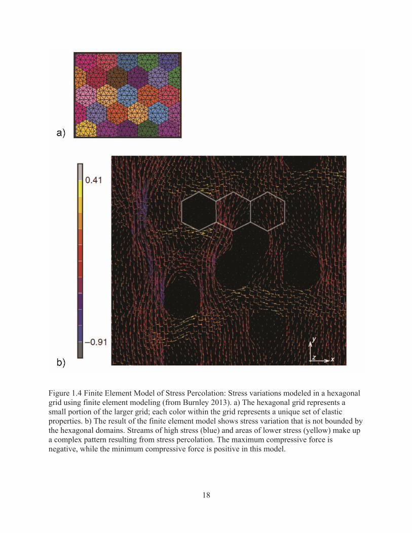
The concept of stress percolation in a polycrystal was proposed by Burnley (2013) using finite

element modeling to examine the distribution of stress states in an elastically heterogeneous

material at an intergranular and intergranular scale. A two-dimensional virtual polycrystal was

created using hexagons, each randomly assigned with elastic properties from a set of 25

possibilities (Figure 1.4a). When a uniaxial boundary condition was placed on the model, regions

containing low and high-stress states emerged independently of grain domains (Figure 1.4b). As

the uniaxial stress increased, the stress state intensified until the material yielded locally, and

plastic deformation became predominant, redistributing the stress states (Burnley 2013). Stress

percolation was first proposed in granular materials based on the observation of strong and weak

granular contacts forming strong subnetworks that result in force chains (Walker 2011). The

results from the finite element model from Burnley (2013) showed that force chain patterns are

the underlying mechanism for shear localization, which can lead to plastic or brittle deformation.

Experimentally measuring the stress distribution on a polycrystal would test whether the stress

percolation hypothesis is an appropriate way to model stress in a polycrystal.

1.3.4 Raman Spectroscopy

Raman spectroscopy is a non-destructive method that can measure crystal lattice vibrations from

the interaction of inelastically scattered photons (Ismail 2015; Neuville, de Ligny, and

Henderson 2014). Photons, generated from a light source such as a laser, are quantization

packets of energy that consists in the form of an electromagnetic wave. When an incident photon

interacts with a crystal lattice, one of two interactions can occur. The vibrating bonds in the

8

crystal lattice can oscillate in resonance with the frequency of the incident photon resulting in no

energy loss or gain by the interaction. This type of scattering that has no change in energy or

wavelength between incident photon and the resultant photon is known as Rayleigh scattering.

Inelastic scattering begins in the same manner as elastic scattering, an incident photon

approaches, and interacts with a crystal lattice. The difference is that the electrons oscillating in

the crystal lattice react with the incident photon’s energy in a way that changes the molecular

polarizability of the crystal lattice. Materials can be defined as Raman active when there is a

temporary change in polarizability of their structure in response to the presence of a photon.

Through this change in polarizability, energy is lost or gained by the resultant scattered photon.

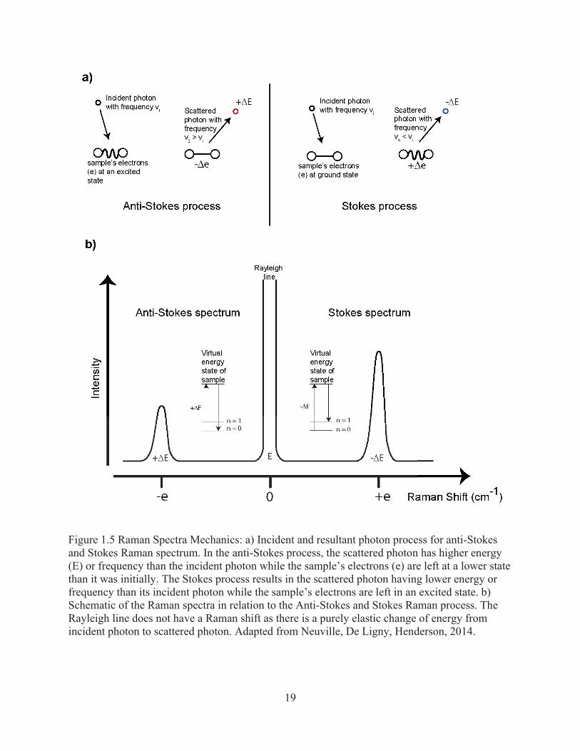
A resultant photon that has less energy than its incident photon, leaving the energy in the crystal

lattice higher than when it began, is known as Stokes scattering (Figure 1.5a). These resultant

inelastic Stokes photons have a longer wavelength than the elastically scattered Rayleigh

photons. The resultant photon that has more energy than its incident photon, leaving the energy

in the crystal lattice lower than when it began, is known as anti-Stokes scattering.

The anti-Stokes scattered photons have a higher wavelength than the elastically scattered

Rayleigh photons. The difference in wavelength for inelastic scattering is the Raman shift.

Figure 1.5b shows a simplified spectrum containing the Stokes, Rayleigh, and anti-Stokes

features. The Rayleigh scattered photons are centered at zero on the x-axis of the graph,

measured in relative wavenumber. Inelastic scattering has a significantly lower probability of

occurrence than elastic scattering, with one in ten million incident photons that interact with a

crystal lattice result in inelastic scatter (Neuville, de Ligny, and Henderson 2014). Elastic

scattering of the Rayleigh peak is common, resulting in an intense signal at zero wavenumber on

the Raman spectrum. With inelastically scattered photons, a material has a higher probability of

9

starting at a ground energy state and being excited to a higher energy state than starting at an

already excited state. Due to this, the Stokes peaks have a stronger intensity than the anti-Stokes

peaks. This study observed the more common Stokes spectrum.

The amount of Raman scattering intensity is dependent on several factors, including laser

wavelength and laser power density. Equation 9 shows that the frequency (v) or wavelength (1/ )

of the laser source is exponentially proportional to Raman scattering intensity (IR), while the

power density of the laser (I0) is linearly proportional to Raman scattering (Larkin 2011).

(9)

The number of scattering molecules that the laser interacts with (N) as well as the polarizability

of the molecules ( and the vibrational amplitude (Q) are also factors that influence the amount

of Raman scatter from a material (Larkin 2011). The amount of Raman scattering is proportional

to the frequency (9) while frequency is inversely proportional to wavelength, the resulting

relationship is that Raman scattering is inversely proportional to wavelength. Using a shorter

laser wavelength ( will increase the Raman scatter by a power of 4.

Increasing the spatial Raman spectroscopy probe in relation to the surface of the sample can be

achieved by reducing the FWHM of the laser foci and increasing the number of data points in a

given area. Equation 10 shows that the spatial resolution of the laser spot size on the sample is

the result of laser wavelength ( ), and the numerical aperture of the objective lens (NA)

multiplied by a constant (Adar 2010).

= 1.22 (10)

10

A change in laser wavelength will be directly proportional to changing spot size, changing the

numerical aperture of the optical objective in the confocal microscope will be inversely

proportional to the laser spot size. This theoretical calculation gives an approximate minimum

spot size as there are other factors such as non-uniform illumination on the sample surface by the

optical objective that will distort the spot size diameter (Adar 2010).

For transparent materials such as calcite and quartz, the Raman depth resolution is controlled by

the restricted collection of light through optical focusing on the sample surface and the confocal

microscope (Meyer 2013). In transparent materials such as quartz and calcite, the excitation

laser will cause scattering across a large 3-dimensional region of the sample. The confocality of

the microscope restricts the collection of scattered light to be recorded from within a defined

optical depth of field. The depth of field can be described using (11) (Spring and Davidson

2019). The depth of field is calculated from the wavelength of the excitation laser , the

numerical aperture NA, the refractive index of the matter between the sample and lense n, the

magnification M, and the smallest resolvable dimension across the sample surface e, seen

through the optical objective.

= + (11)

The depth of field calculations for laser wavelengths 488 and 514nm is 0.1134 and 0.1180

microns using an MPlanN 50x/.75 NA optical objective with the refractive index value of air (1)

and the smallest resolvable distance on the sample as seen through the microscope as 1 micron.

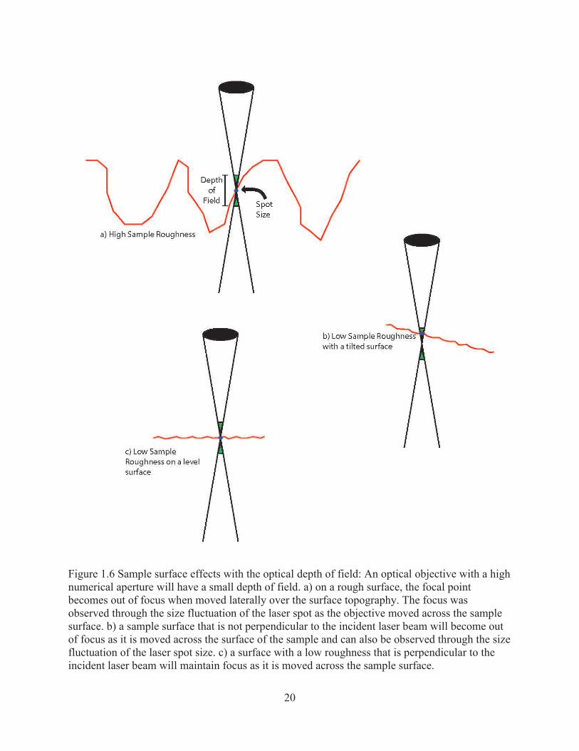
Obtaining a quality spectrum from a sample using Raman spectroscopy is, in part dependant on

the sample surface roughness. The shallow depth of field will result in the need for constant

refocusing on a sample with high surface roughness (Figure 1.6a), or uneven surface (Figure

11

1.6b). A level and well-polished sample surface were needed to stay within the focal depth of

field as the sample is moved (Figure 1.6c).

For Raman active materials, spectral peaks that are characteristic of each material contain

information about the type of motions that are happening within a crystal lattice. The bonds in a

crystal lattice can vibrate in unique ways such as stretching, bending, torsion, and liberation

(Gouadec and Colomban 2007); these movements are classified through group theory. Group

theory includes the study of the symmetry that describes the organization of vibrational modes

categorized by vibrational symmetry in the molecule or crystal lattice (Tuschel 2014). Each point

group for a molecule or crystal lattice can be broken down into different types of symmetry

species, denoted with a Mulliken symbol, that describes the specific symmetry that a unit cell

displays. The Mulliken symbol of A represents a vibrational movement that is symmetrical

around the principal axis of the molecule. Doubly degenerate modes represent two states in the

molecule that have the same energy and are represented with the Mulliken symbol of E (Tuschel

2014). Although this study will not be classifying the different vibrational modes of Raman

spectra for experimental materials, it is useful for understanding Raman spectra.

Piezospectroscopy is the measurement of stress through spectrographic methods; using Raman

piezospectroscopy, the elastic strain response of a crystal lattice can be measured. Specific

vibrational modes in Raman spectra are stress-dependent. When the atomic bonds of a crystal

lattice are strained elastically, the resultant photons in a stress-sensitive Raman mode will exhibit

a Raman stress shift different than Raman shift of the non-strained crystal lattice. The Raman

stress shift measured under elastic strain will be proportional to stress within the crystal lattice

(Gouadec and Colomban 2007). Therefore, it is possible to define the Raman stress shift v) as

the change in wavenumber from a Raman shift due to stress ( ), to a Raman shift ( ). Equation

12

12 shows that the Raman stress shift is proportional to mean stress using the Raman shift factor

as a proxy for the stress state within a crystal (Pezzotti 1999, Lei, et al.

2018).

= = (12)

A compressional stress shift results in an increase of wavenumber for the spectrum’s peak

position, in general, as the length in the atomic bonds of a crystal lattice, shortens, the stiffness in

the bonds increase. A tensional stress shift decreases the wavenumber value for the spectrum’s

peak position as the stiffness in the bonds decrease (Gouadec and Colomban 2007).

The Raman stress shift has been used in many different fields but is relatively new to geology.

Examples of recent Raman stress and strain mapping investigated in other scientific fields have

measured the stress response of various materials; Aluminum Indium Gallium Phosphide films

(Guo, et al. 2020), silicon wafers (Wang, et al. 2019), Kevlar 49 yarn (Lei, et al. 2018), ceramic

composites (Jannotti, et al. 2017), GaN film (Jiang, et al. 2017), graphene monolayer

nanocomposites (Young, et al. 2011).

Raman spectra can have a strong temperature dependency that affects the position and width of

spectral peaks (Gouadec and Colomban 2007). As a crystal lattice is heated, thermal expansion

in the bond length between atoms can change the position of a Raman shift. Changes in bond

lengths from temperature changes result in a Raman temperature shift. The wavenumbers of the

peak position will increase with decreased temperature and decrease with increasing temperature

(Hibbert, et al. 2015; Kolesov 2016; Asell and Nicol 1968; Gillet, et al. 1993) resulting in a

Raman temperature shift that can mimic a Raman stress shift. Raman modes that are stress-

dependent are commonly temperature-dependent (Jayaraman, et al. 1987).

13

1.3.5 Raman Active Materials

Calcite and quartz were selected for this experiment based on their Raman active spectrographic

characteristics and measurable Raman stress shifts. Calcite and quartz are easily obtainable

Raman active materials whose spectra contain several different stress-dependent peaks. Five

distinctive calcite peaks result from different (CO3)-2 vibrational modes, with approximate peak

positions at E 156, E 281, E 711, A 1085, and E 1434 (Gillet, et al. 1993; Liu and Mernagh 1990;

Liu, et al. 2016; Rutt and Nicola 1974; Sun, et al. 2014). The calcite modes vary between

stretching and external vibration in CO3-2. The E-1434 calcite mode is attributed to asymmetric

stretching, A-1085, and E-711 modes are attributed to symmetric stretching, and the E-156 and

E-281 modes are attributed to external vibration (Sun, Wu, Cheng, Zhang, Frost, 2014). Raman

spectra for alpha quartz include A-1082, A-467, A-356, A-207, E-1162, E-1072, E-795, E-697,

E-450, E-394, E-265, E-128 (Etchepare, et. al. 1974). The motion of quartz vibrations has been

modeled using first-principle calculations and involves the bending of the Si-O-Si angle (Lei,

Chao-Jia, Chun-Qiang, Li, Hong and Jian-Guo 2015). Calcite and quartz peak positions

generally agree amongst published works with small variations.

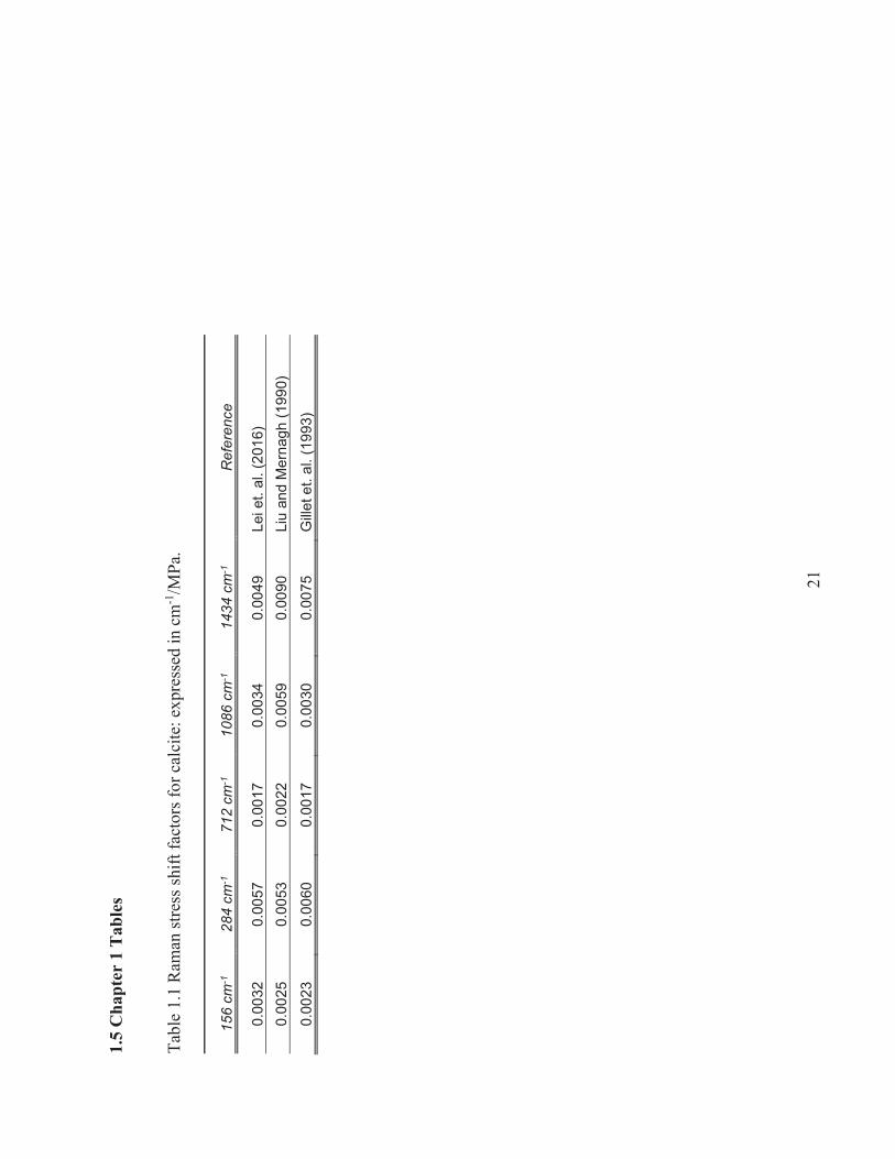
Raman stress shift factors for calcite and quartz are well documented through experimental and

first-principle calculations (Table 1 and 2). Experimental methods for measuring the Raman

stress factor in calcite included hydrostatic compression in a diamond anvil cell (Gillet, et al.

1993; Liu and Mernagh 1990) and mathematical calculation using density functional

perturbation theory and the planewave pseudopotential method (Lei, et al. 2015). The Raman

stress shift factors experimentally and mathematically calculated for calcite agree that the most

significant pressure-dependent Raman shift occurs at the 1434 cm-1 peak, followed by the 284

cm-1 peak. Methods for measuring the Raman stress factor in quartz included a two-stage

14

hydrostatic high-pressure Raman cell (Dean, Sherman, and Wilkinson 1982), high pressure

hydrostatic optical cell (Asell and Nicol 1968), hydrostatic compression in a diamond anvil cell

(Hemley 1987; Jayaraman, Wood, and Maines 1987), and a hydrothermal diamond anvil cell

(Schmidt and Ziemann 2000). The most considerable quartz Raman stress shift occurs within the

206 cm-1 peak, followed by the 464 cm-1 peak, then the 128 cm-1 peak. For this experiment, the

Quartz 464 cm-1 peak, and the Calcite 1434 cm-1 peak were used based on their high-stress

dependencies.

15

1.4 Chapter 1 Figures

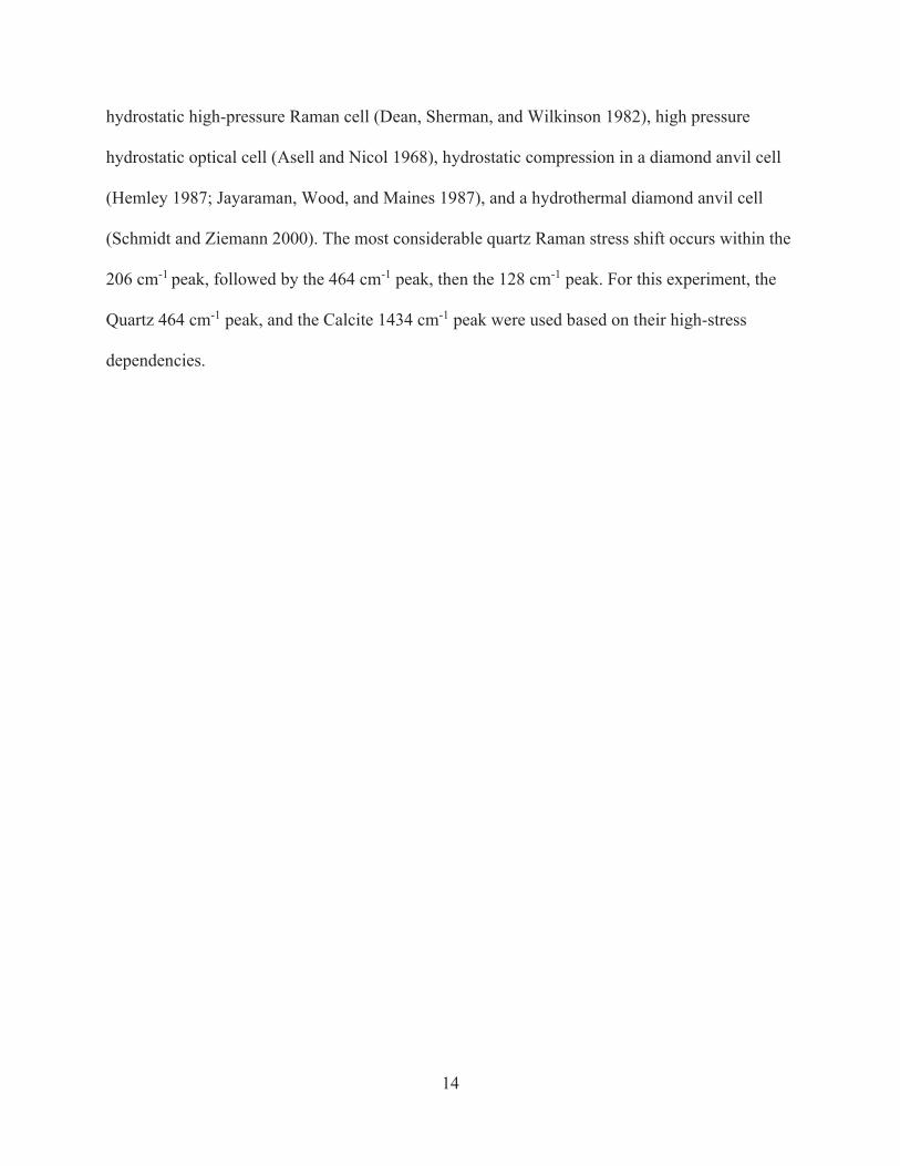
Figure 1.1 Anisotropy in Crystals: The stress state of an elastically anisotropic single crystal (a) and a polycrystal (b). a) Two different springs with different stiffnesses inside a crystal represent an elastically anisotropic crystal lattice. Uniaxial stress imposed on the outside of the single crystal (represented by the purple arrows) affects the internal elastic response of the crystal, and the elastic response across the crystal is directly proportional to the stress distribution across the crystal. The stress distribution of the single crystal lattice would be the same at each point (assuming a perfect crystal) and dependent on the orientation of the crystal lattice to the imposed uniaxial stress. b) In comparison with the single crystal, the stress distribution in a polycrystal with varying crystal orientations from grain to grain is likely to be complicated. The elastic response of each grain in a polycrystal is not only different depending on orientation, but would also feel an effect from neighboring, crystals. It is experimentally unknown what type of stress distribution would be present in a stressed elastically anisotropic polycrystal.

16

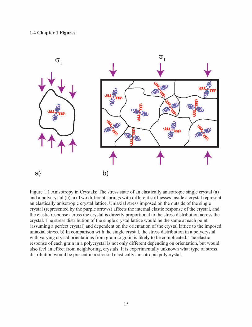
Figure 1.2 Voigt upper bound elastic model: (a) and (b) represent two different materials with unique elasticity. As uniaxial force imposes on the materials, the stress in the model differs while elastic strain in the materials stays the same.

17

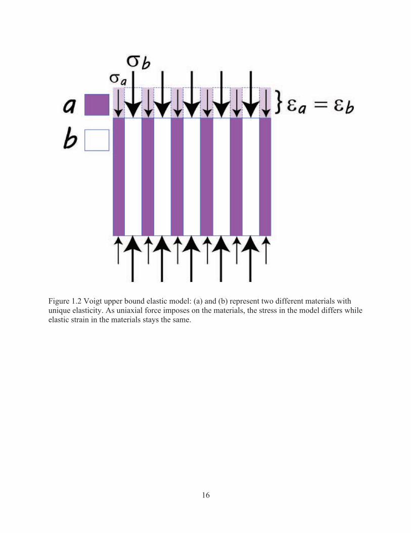
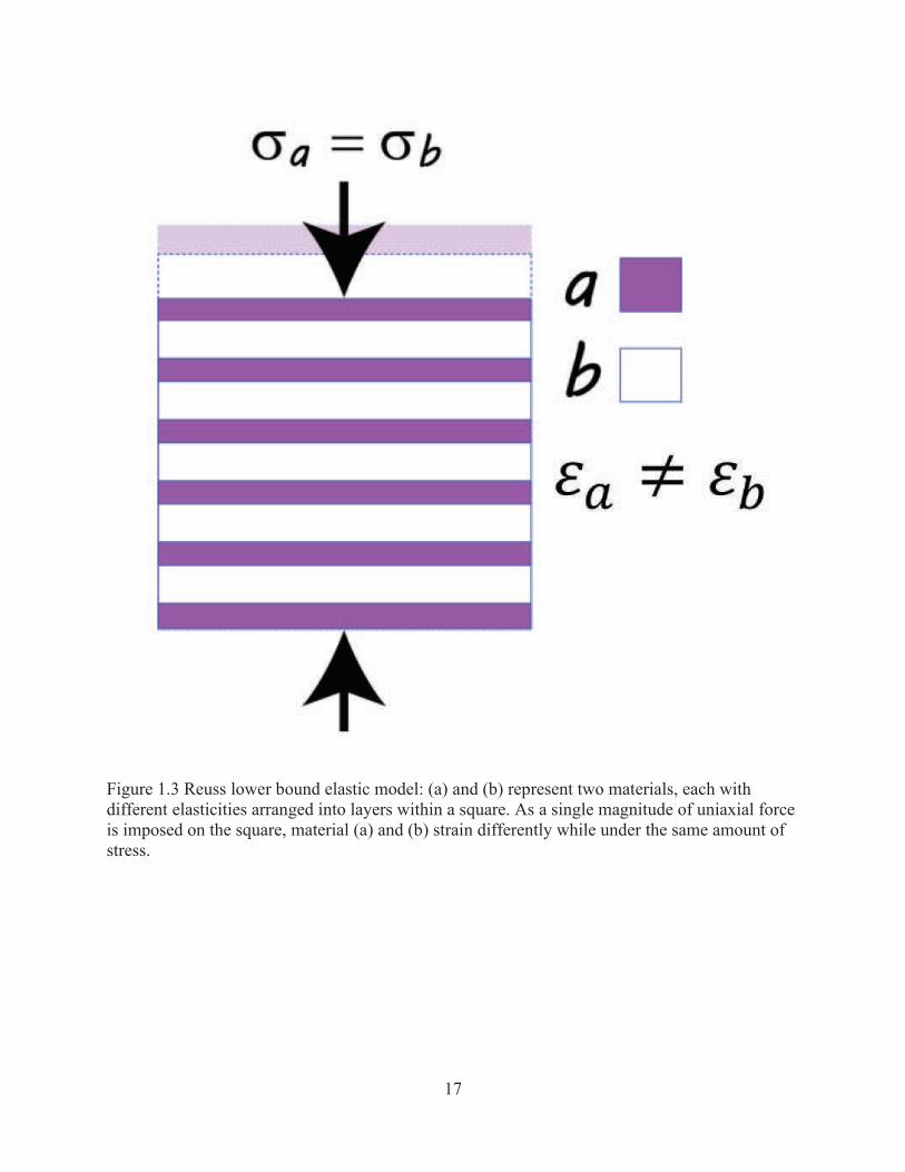
Figure 1.3 Reuss lower bound elastic model: (a) and (b) represent two materials, each with different elasticities arranged into layers within a square. As a single magnitude of uniaxial force is imposed on the square, material (a) and (b) strain differently while under the same amount of stress.

18

Figure 1.4 Finite Element Model of Stress Percolation: Stress variations modeled in a hexagonal grid using finite element modeling (from Burnley 2013). a) The hexagonal grid represents a small portion of the larger grid; each color within the grid represents a unique set of elastic properties. b) The result of the finite element model shows stress variation that is not bounded by the hexagonal domains. Streams of high stress (blue) and areas of lower stress (yellow) make up a complex pattern resulting from stress percolation. The maximum compressive force is negative, while the minimum compressive force is positive in this model.

19

Figure 1.5 Raman Spectra Mechanics: a) Incident and resultant photon process for anti-Stokes and Stokes Raman spectrum. In the anti-Stokes process, the scattered photon has higher energy (E) or frequency than the incident photon while the sample’s electrons (e) are left at a lower state than it was initially. The Stokes process results in the scattered photon having lower energy or frequency than its incident photon while the sample’s electrons are left in an excited state. b) Schematic of the Raman spectra in relation to the Anti-Stokes and Stokes Raman process. The Rayleigh line does not have a Raman shift as there is a purely elastic change of energy from incident photon to scattered photon. Adapted from Neuville, De Ligny, Henderson, 2014.

20

Figure 1.6 Sample surface effects with the optical depth of field: An optical objective with a high numerical aperture will have a small depth of field. a) on a rough surface, the focal point becomes out of focus when moved laterally over the surface topography. The focus was observed through the size fluctuation of the laser spot as the objective moved across the sample surface. b) a sample surface that is not perpendicular to the incident laser beam will become out of focus as it is moved across the surface of the sample and can also be observed through the size fluctuation of the laser spot size. c) a surface with a low roughness that is perpendicular to the incident laser beam will maintain focus as it is moved across the sample surface.

21

1.5

Cha

pter

1 T

able

s

Tabl

e 1.

1 R

aman

stre

ss sh

ift fa

ctor

s for

cal

cite

: exp

ress

ed in

cm

-1/M

Pa.

156

cm-1

28

4 cm

-1

712

cm-1

10

86 c

m-1

14

34 c

m-1

R

efer

ence

0.00

32

0.00

57

0.00

17

0.00

34

0.00

49

Lei e

t. al

. (20

16)

0.00

25

0.00

53

0.00

22

0.00

59

0.00

90

Liu

and

Mer

nagh

(199

0)

0.00

23

0.00

60

0.00

17

0.00

30

0.00

75

Gille

t et.

al. (

1993

)

22

Table 1.2 Raman stress shift factors for quartz: expressed in cm-1/MPa.

128 cm-1 206 cm-1 465 cm-1 Reference

0.0050 0.0180 0.0090 Asell and Nicol (1968)

0.0054 0.0204 0.0081 Dean et. al. (1982)

0.0055 0.0199 0.0080 Hemley (1987)

0.0060 0.0240 0.0080 Jayaraman et. al. (1987)

0.0034 0.0186 0.0084 Lei et. al. (2015)

not reported 0.0074 not reported Tekippe et. al. (1973)

not reported 0.0278 0.0096 Schmidt and Ziemann (2000)

23

Chapter 2: Experimental Methods

2.1 Experimental Samples

2.1.1 Sample Selection

Natural single crystal and polycrystal samples of calcite and quartz were selected for this

experiment based on several criteria. 1) the samples were monomineralic, which will reduce the

number of variables during experimentation and data interpretation. 2) If possible, polycrystals

were found in a columnar habit to mimic a two-dimensional space. 3) Individual grains in the

polycrystal were easily identifiable to assist with mapping.

The calcite and quartz polycrystals selected for the experiment are predominantly

monomineralic. The variability in elastic properties between different minerals in a polycrystal is

simplified by limiting the samples to monomineralic species. By reducing the variables in the

experiment, we can gain a clearer picture of the stress distribution on the surface of the sample.

Both Carrara marble and Tiger’s Eye are known for their high degree of chemical homogeneity.

Carrara Marble consists o 99 % calcite (Backers, et al. 2004; Howarth and Rowlands 1987),

while Tigers Eye has been reported to be > 99 weight percent in quartz with iron

oxide/hydroxide crystallite inclusions (Heaney and Fisher 2003).

The geometric arrangement of crystals in the fabric of a polycrystal was considered during

sample selection to simplify boundary conditions for crystals present on the surface of the

specimen. Polycrystals consisting of an aggregate of randomly oriented crystals arranged in a

three-dimensional fabric will contain crystals on the surface of the sample that would be

influenced by its neighboring crystals to the sides and below, all imposing their unique boundary

24

conditions on each other. A sample with a columnar habit was preferable as each crystal grain

might extend from one side of the sample to the other, simplifying the imposed stress on each

grain from three-dimensional boundary conditions to two-dimensional boundary conditions. A

suitable calcite sample with a columnar habit was not identified, so preliminary Raman

measurements were made with Carrara marble, which has a random orientation of anhedral

crystals approximately 300 microns in size with easily identifiable grain boundaries. Later

Raman measurements were taken with Tiger’s Eye quartz, which has a columnar habit with the

c-axis oriented parallel to the quartz columnar growth pattern (Heaney and Fisher 2003). Tiger’s

Eye quartz grains were easily identifiable when the sample height was less than 1.5 millimeters;

the average grain size was estimated at 30 microns (Figure 2.1).

2.1.2 Sample Preparation

Single-crystal and polycrystal calcite and quartz samples were cut into small rectangular prisms

oriented relative to crystallographic axes or mineral fabrics. Figure 2.2 describes the convention

used to label the different sides of the samples. Samples were attached to aluminum sample

plates using crystal bond and cut into rectangular prisms shapes using a Buehler IsoMet low-

speed diamond wheel saw. Calcite, a soft mineral with a Mohs hardness of three, has rhombic

cleavage planes that break easily in response to small forces placed upon the sample. The low

tenacity of calcite was problematic when cubic shaped samples were cut as the cleavage planes

do not lie in the directions of the crystallographic axes. One cleavage plane in single-crystal

calcite formed sides 3 and 6 while the other sides were cut with the IsoMet saw. The cut of the

single-crystal calcite samples resulted in the crystallographic c-axis being oriented diagonally

through the body of the sample (Figure 2.3). Carrara marble was easily cut into rectangular

prisms as it has a polycrystalline granoblastic texture. Quartz samples were cut from two

25

varieties that included colorless transparent single crystal quartz and Tiger’s Eye quartz. The

process of orienting the sample cuts relative to the crystallographic axes of the crystal was not

difficult due to the high tenacity of quartz. Single-crystal quartz specimens were cut

perpendicular to the c-axis and parallel to the a-axis so that the a-axis would be parallel to

compression, and the c-axis would be perpendicular to the surface that data would be collected

on. Tiger’s Eye was cut perpendicular to the columnar habit (Figure 2.4), the c-axis runs parallel

to the columnar habit (Heaney and Fisher 2003) while the a-axis is perpendicular to the columnar

habit.

The uniaxial hand vice used to compress the samples limited the sample dimensions to no greater

than 6.24 mm in length, 2 mm in height, and width around 4 mm. The sample sat between two

sample holder plates that have a 2 mm step machined into their edges. Sides 1 and 4 needed to sit

flush against the vice’s metal plate with the height of the sample being no higher or lower than

the 2 mm step. If the sample were too high, only a portion of the area of the sample would have

been under uniaxial stress, which could lead to more complicated boundary conditions on the

sample (Figure 2.5a). If the sample were short of reaching the top of the 2 mm step on the

sample holder, the Raman microscope objective lens would be unable to focus on the surface of

the sample, which would lead to poor spectra quality (Figure 2.5b).

Each sample side was roughly polished so that adjacent sides were orthogonal to one another,

and opposing sides were parallel to each other, resulting in a rectangular parallelepiped. If sides

1 and 4 were not parallel to each other, force across the area of sides 1 and 4 would be uneven,

resulting in premature brittle failure. Without parallel faces on sides 3 and 6, the automated

Raman mapping function would lose focus as the stage moved the sample under the optical

objective. The process to prepare each sample (Figure 2.6) into a rectangular parallelepiped was

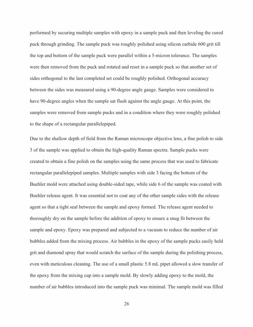
26

performed by securing multiple samples with epoxy in a sample puck and then leveling the cured

puck through grinding. The sample puck was roughly polished using silicon carbide 600 grit till

the top and bottom of the sample puck were parallel within a 5-micron tolerance. The samples

were then removed from the puck and rotated and reset in a sample puck so that another set of

sides orthogonal to the last completed set could be roughly polished. Orthogonal accuracy

between the sides was measured using a 90-degree angle gauge. Samples were considered to

have 90-degree angles when the sample sat flush against the angle gauge. At this point, the

samples were removed from sample pucks and in a condition where they were roughly polished

to the shape of a rectangular parallelepiped.

Due to the shallow depth of field from the Raman microscope objective lens, a fine polish to side

3 of the sample was applied to obtain the high-quality Raman spectra. Sample pucks were

created to obtain a fine polish on the samples using the same process that was used to fabricate

rectangular parallelepiped samples. Multiple samples with side 3 facing the bottom of the

Buehler mold were attached using double-sided tape, while side 6 of the sample was coated with

Buehler release agent. It was essential not to coat any of the other sample sides with the release

agent so that a tight seal between the sample and epoxy formed. The release agent needed to

thoroughly dry on the sample before the addition of epoxy to ensure a snug fit between the

sample and epoxy. Epoxy was prepared and subjected to a vacuum to reduce the number of air

bubbles added from the mixing process. Air bubbles in the epoxy of the sample pucks easily held

grit and diamond spray that would scratch the surface of the sample during the polishing process,

even with meticulous cleaning. The use of a small plastic 5.8 mL pipet allowed a slow transfer of

the epoxy from the mixing cup into a sample mold. By slowly adding epoxy to the mold, the

number of air bubbles introduced into the sample puck was minimal. The sample mold was filled

27

with epoxy to the top of the glass ring and allowed to cure for 12 hours. The bottom portion of

the mold was removed, resulting in a sample puck surrounded by a glass ring. The glass ring

helped to keep the puck level during hand polishing, as glass is harder than the epoxy puck. A

silicon carbide 600 grit was applied to the bottom of the puck to smooth out any residual epoxy

that possibly came between the glass ring and the base of the puck. The result was a sample puck

that contained a maximum of 6 samples.

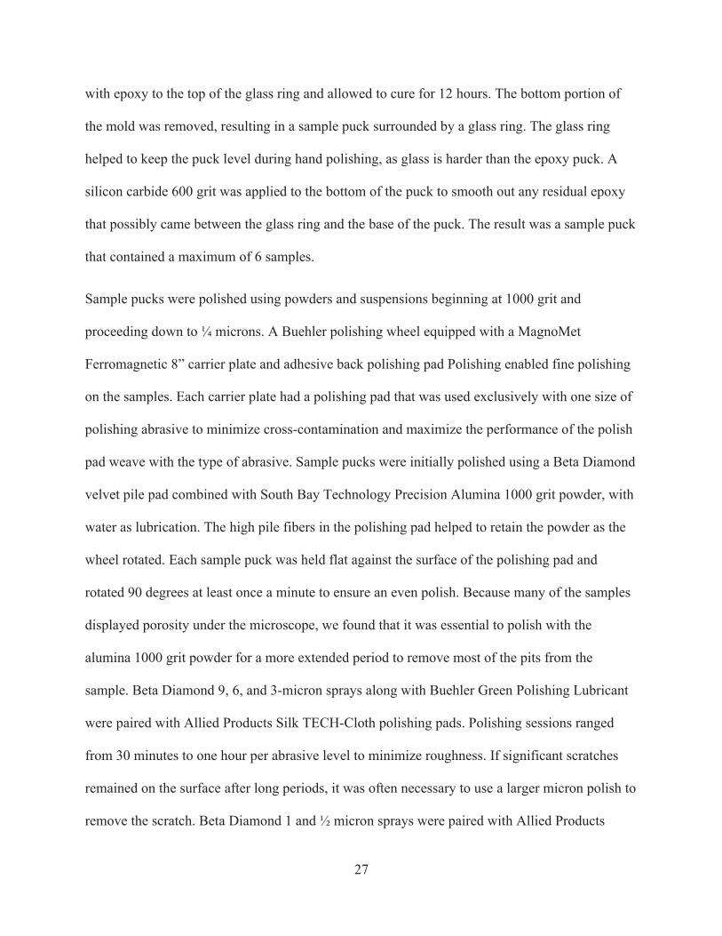
Sample pucks were polished using powders and suspensions beginning at 1000 grit and

proceeding down to ¼ microns. A Buehler polishing wheel equipped with a MagnoMet

Ferromagnetic 8” carrier plate and adhesive back polishing pad Polishing enabled fine polishing

on the samples. Each carrier plate had a polishing pad that was used exclusively with one size of

polishing abrasive to minimize cross-contamination and maximize the performance of the polish

pad weave with the type of abrasive. Sample pucks were initially polished using a Beta Diamond

velvet pile pad combined with South Bay Technology Precision Alumina 1000 grit powder, with

water as lubrication. The high pile fibers in the polishing pad helped to retain the powder as the

wheel rotated. Each sample puck was held flat against the surface of the polishing pad and

rotated 90 degrees at least once a minute to ensure an even polish. Because many of the samples

displayed porosity under the microscope, we found that it was essential to polish with the

alumina 1000 grit powder for a more extended period to remove most of the pits from the

sample. Beta Diamond 9, 6, and 3-micron sprays along with Buehler Green Polishing Lubricant

were paired with Allied Products Silk TECH-Cloth polishing pads. Polishing sessions ranged

from 30 minutes to one hour per abrasive level to minimize roughness. If significant scratches

remained on the surface after long periods, it was often necessary to use a larger micron polish to

remove the scratch. Beta Diamond 1 and ½ micron sprays were paired with Allied Products

28

White Label silk polishing pads while a high pile Beta Diamond pad was used for the final ¼

micron Beta Diamond polish spray. Polishing the samples at a reduced speed during the final ¼

micron level resulted in a high-quality polished surface.

At any point in the polishing process, the glass ring could become separated from the epoxy

puck, which would damage the samples at lower micron polishes. When this happened, it was

essential to remove the glass ring as the sample puck was not able to be adequately cleaned.

After each level of polish, the sample puck was cleaned using soap and water. High water

pressure was useful in rinsing the remaining residue off the puck surface. The ultrasonic cleaner

removed residual oils and abrasives off the sample pucks then the pucks were dried with

compressed air. The samples in the puck were then observed under the microscope for polish

quality and checked for any residual residue. If residue remained on the sample, a second

cleaning was then performed. As finer polishes were achieved on the sample puck, it became

increasingly important to minimize physically touching the polished sample surface to prevent

damage to the surface. Figure 2.7 shows the surface polish of Carrara Marble from incremental

polishes ranging from 1000 grit to 9 - 0.25 microns through the Olympus SZ-STB1 boom stand

microscope.

Select sample pucks were given a final polish with Allied High Tech 0.05-micron colloidal silica

suspension using a Buehler VibroMet2 Vibratory Polisher. The VibroMet was able to remove

0.25-micron scratches and made a significant difference in the final product polish (Figure 2.8).

The sample pucks then needed to be altered in a way so that they could fit inside the VibroMet

polishing puck. The polished side of the sample puck was covered with a protective layer of

clear masking tape to protect the polished surface. A ring of masking tape applied to the

perimeter of the puck created a mold for epoxy that would increase the sample puck height.

29

Epoxy was poured into the top of the puck, filling the mold till it reached the appropriate height

to fit into the VibroMet sample holder and then left to cure for 24 hours. When the epoxy cured,

the tape on the perimeter of the puck was removed, and the top was given a polish using silicon

carbide 600 grit powder to level the puck. The sample puck and VibroMet puck were then

cleaned without removing the tape from the polished surface of the sample puck. Macor rod was

placed inside the VibroMet puck to center the sample puck if needed; then, the sample puck was

aligned and secured inside the VibroMet puck (Figure 2.9). After a final rinse, the bottom

masking tape protecting the polished surface was removed, and polishing was then performed

following the Buehler VibroMet user instructions. Calcite samples were polished for 2 hours,

and quartz samples were polished for 6 hours. After polishing, samples were cut from the sample

puck, and a final wash of acetone was applied to the samples to clean the surfaces. The sample's

height varied from one end of the sample to the other by a maximum of 50 microns by the time

sample preparation was finished, most samples varied below 10 microns. Samples were then

stored in a small plastic box secured with double-sided tape for easy access and sample

protection. Appendix 2.1 contains a list of all equipment used for sample preparation.

2.2 Uniaxial Vice and Load Cell

The uniaxial vice used for the experiment was the Brown and Sharpe 752 Toolmakers Vise

equipped with movable steel plates that slid in-line to apply force to the sample. The load on the

sample was measured with a calibrated load cell gauge that sat in-line with the metal plates of

the vice. An Arduino SparkFun HX711 board read the load cell with a USB connector. The vice

was later modified by the removal of the front nose portion, which allowed easier access for the

optical objective on the Raman spectrometer to reach the sample (Figure 2.10).

30

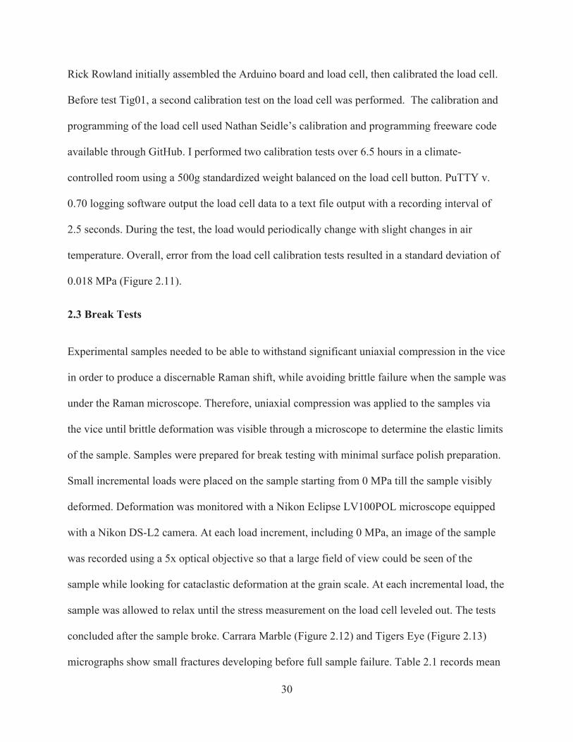
Rick Rowland initially assembled the Arduino board and load cell, then calibrated the load cell.

Before test Tig01, a second calibration test on the load cell was performed. The calibration and

programming of the load cell used Nathan Seidle’s calibration and programming freeware code

available through GitHub. I performed two calibration tests over 6.5 hours in a climate-

controlled room using a 500g standardized weight balanced on the load cell button. PuTTY v.

0.70 logging software output the load cell data to a text file output with a recording interval of

2.5 seconds. During the test, the load would periodically change with slight changes in air

temperature. Overall, error from the load cell calibration tests resulted in a standard deviation of

0.018 MPa (Figure 2.11).

2.3 Break Tests

Experimental samples needed to be able to withstand significant uniaxial compression in the vice

in order to produce a discernable Raman shift, while avoiding brittle failure when the sample was

under the Raman microscope. Therefore, uniaxial compression was applied to the samples via

the vice until brittle deformation was visible through a microscope to determine the elastic limits

of the sample. Samples were prepared for break testing with minimal surface polish preparation.

Small incremental loads were placed on the sample starting from 0 MPa till the sample visibly

deformed. Deformation was monitored with a Nikon Eclipse LV100POL microscope equipped

with a Nikon DS-L2 camera. At each load increment, including 0 MPa, an image of the sample

was recorded using a 5x optical objective so that a large field of view could be seen of the

sample while looking for cataclastic deformation at the grain scale. At each incremental load, the

sample was allowed to relax until the stress measurement on the load cell leveled out. The tests

concluded after the sample broke. Carrara Marble (Figure 2.12) and Tigers Eye (Figure 2.13)

micrographs show small fractures developing before full sample failure. Table 2.1 records mean

31

stress at the first brittle deformation event observable on the samples. The average value of the

uniaxial break tests was a benchmark to gauge how much pressure to apply to the samples

without brittle deformation during Raman testing.

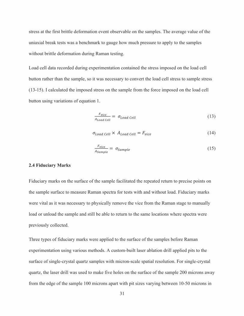
Load cell data recorded during experimentation contained the stress imposed on the load cell

button rather than the sample, so it was necessary to convert the load cell stress to sample stress

(13-15). I calculated the imposed stress on the sample from the force imposed on the load cell

button using variations of equation 1.

= (13)

× = (14)

= (15)

2.4 Fiduciary Marks

Fiduciary marks on the surface of the sample facilitated the repeated return to precise points on

the sample surface to measure Raman spectra for tests with and without load. Fiduciary marks

were vital as it was necessary to physically remove the vice from the Raman stage to manually

load or unload the sample and still be able to return to the same locations where spectra were

previously collected.

Three types of fiduciary marks were applied to the surface of the samples before Raman

experimentation using various methods. A custom-built laser ablation drill applied pits to the

surface of single-crystal quartz samples with micron-scale spatial resolution. For single-crystal

quartz, the laser drill was used to make five holes on the surface of the sample 200 microns away

from the edge of the sample 100 microns apart with pit sizes varying between 10-50 microns in

32

diameter (Figure 2.14a). Quartz Tiger's Eye was challenging to ablate at the time as the laser drill

was not yet powerful enough to affect the polycrystal. Fiduciary marks were drilled on the

sample using a miniature drill press equipped with a diamond drill bit. Three holes were drilled

that were approximately 400 microns in diameter and 650 microns apart (Figure 2.14b). The

final fiduciary method used was a custom cut aluminum sticker that was placed on the sample

enclosing the mapping area. The laser drill was used to cut the aluminum sticker into a

rectangular frame with an opening of 100 x 600 microns and an outer size of 2000 x 2000

microns (Figure 2.14c).

2.5 High-Resolution Micrographs

The Nikon Eclipse LV100POL microscope equipped with a Nikon DS-L2 camera equipped with

a 5x optical objective was used to take high-resolution micrographs of samples before or after

Raman data collection. Each micrograph was made from several high-resolution micrographs

and merged using the photo merge tool in Adobe Photoshop version 20.0.4. A scale was then

added to the images using ImageJ version 1.52a. For successful Raman stress maps, the

micrograph was used to display the location of the stress map on the sample surface.

2.6 Raman Methods

2.6.1 System Setup

The T64000 Horiba Jobin Yvon Raman system, located in the Salamat Lab at the University of

Las Vegas Nevada Physics and Astronomy Department, was used to measure spectra for all

experiments. The Raman system consists of an argon-krypton laser, a Nikon Eclipse LV100POL

integrated confocal microscope equipped with a mapping stage, a triple spectrometer, a charge-

coupled device (CCD detector), and computer (Figure 2.15). The features of the system that

33

controlled experimentation were the sample stage and confocal microscope, the laser path and

monochromators, and a bandpass filter.

The automated stage moved the sample under the confocal microscope through pre-programmed

points or manually. The confocal microscope is not equipped with an autofocus feature,

therefore, the sample surfaces needed to be level below 1 micron for the microscope to stay

focused on the sample surface due to the short depth of field from the MplanN 50x/.75NA

objective. Because the height of the samples varied by up to 50 microns from one end of the

sample to the other, it was usually not viable to use the automated navigation.

Spectra for stress mapping was measured using the Raman high-resolution additive mode

configuration. The Raman spectrometer uses monochromatic, collimated, low divergent light

provided by a tunable krypton-argon laser (Figure 2.16). Laser light travels to the confocal

microscope, which focuses it onto the surface of the sample. The scattered light then goes back

through the confocal microscope and is diffracted and focused by three Czerny-Turner

monochromators (https://www.horiba.com/en_en/technology/measurement-and-control-

techniques/spectroscopy/spectrometers-and-monochromators/spectrometer-monochromator/).

Depending on the arrangement of concave mirrors, gratings, and slits in the monochromators, the

spectrum can be measured in either subtractive mode (low spectral resolution) or additive mode

(high spectral resolution). In additive mode, gratings and mirrors in the monochromator spread

the scattered light (Figure 2.17), resulting in a small range of wavenumbers with high spectral

resolution. Raman subtractive mode uses the first monochromator to spread scattered light,

condense the light in the second, and then separate the light in the third monochromator. The use

of subtractive mode results in a lower spectral resolution but allows for a larger spectral range.

The average spectral resolution in additive mode is 0.11 cm-1, while the average spectral

34

resolution in subtractive mode is 0.35 cm-1. The scattered light is then detected by the CCD and

recorded by a computer using Labspec version 5.78.24 where the Raman data is saved as text

files.

Typically a bandpass filter is used to remove the argon-krypton plasma emission lines inherent in

the laser light. For these experiments, we did not use a bandpass filter so that the plasma

emission lines could be used as an internal calibrant to correct any systematic error inherent to

the Raman spectrometer. Plasma emission lines originating from the laser are located at very

precise, fixed positions in the electromagnetic spectrum with each plasma emission line

originating from either argon or krypton plasma in the laser. A low-resolution spectrum of calcite

was taken at 488 nm wavelength (Figure 2.18), quartz at 488 nm (Figure 2.19), and 514 nm

wavelengths (Figure 2.20) to catalog and identify the spectral peaks. The argon-krypton plasma

emission lines values in the spectra were cataloged using the absolute values of the plasma

emission lines from the National Institute of Standards and Technology (NIST) database

(https://www.nist.gov/pml/atomic-spectra-database). The NIST plasma emission line values were

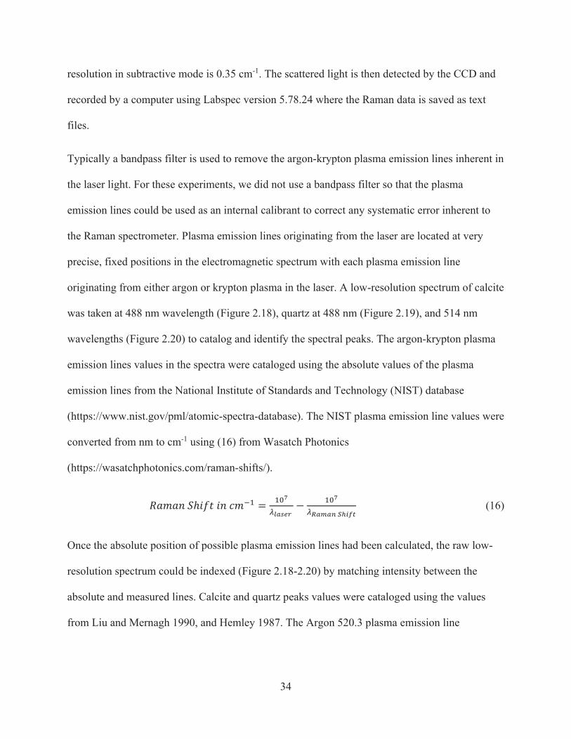
converted from nm to cm-1 using (16) from Wasatch Photonics

(https://wasatchphotonics.com/raman-shifts/).

= (16)

Once the absolute position of possible plasma emission lines had been calculated, the raw low-

resolution spectrum could be indexed (Figure 2.18-2.20) by matching intensity between the

absolute and measured lines. Calcite and quartz peaks values were cataloged using the values

from Liu and Mernagh 1990, and Hemley 1987. The Argon 520.3 plasma emission line

35

measured at a 514 nm wavelength is documented by Craig and Levin (1979) and used as a

calibration line in Tiger’s Eye experiments.

2.6.2 Raman Experimental Testing

The Raman system required an initial preparation before each experiment. The CCD is cooled

using liquid nitrogen, and each of the monochromators required alignment before spectra were

collected as multiple scientists commonly use the Raman. The laser power density was measured

using a Thorlabs PM100D power meter placed below the optical objective. The laser power

density was then adjusted using an optical laser filter located along the laser beam path.

Before each experiment, Raman settings were tuned to maximize a high signal to noise ratio

while minimizing spectrum acquisition time. Different Raman settings that impacted the signal

to noise ratio of a spectrum; these settings include laser power density, laser wavelength, the

amount of time the laser is exposed to the sample (exposure), and the number of exposures taken

for the spectrum (acquisition). An increase in laser power density proportionally increases the

Raman signal (Equation 11); however, a high laser power density can heat the sample and cause

a thermal Raman shift. The laser wavelength is inversely proportional to Raman scattering, so a

lower laser wavelength will result in a higher signal. Both the 488 nm and 514 nm laser

wavelengths were used during experimentation; however, a lower laser wavelength such as blue

488 nm was preferable over 514 nm as it has a higher amount of Raman scatter and a smaller

spot size. Acquisition and exposure times affected the S/N ratio as increased exposure time

allowed for the collection of more photons, which increased the signal, while many acquisitions

reduced the noise through subtractive algorithms in the Raman software. For quartz, the

optimum result was 12 acquisitions, at 10-second exposures, and a laser power density of 9 mW

36

(figure 2.21). These settings were used as baseline settings that could then be adjusted at the start

of each Raman session to maximize the signal to noise ratio. Testing the signal to noise ratio at

the beginning of each test was necessary as small changes to the laser power density, laser

wavelength, exposure, and acquisition times, could change the signal to noise ratio significantly.

Signal to noise testing was done for calcite but to a lesser extent. After the signal to noise testing

was completed before each experiment, Raman spectra were then collected on each sample, and

spectra were saved as a text file containing wavenumber and intensity after each test.

2.7 Data Processing

2.7.1 Peak Fitting

For Raman tests that used the automated stage mapping function, the output consisted of a single

text file containing spatial coordinates and their corresponding spectrum. To peak fit each

datapoint’s spectrum, a Fortran code separated the single file into individual files. Each

individual file contained the spectrum of one datapoint and was named after the coordinate of

that datapoint (Appendix 2.2).

Fityk curve fitting and data analysis software version 1.2.9 was chosen to fit the Raman spectra

due to its intuitive interface, and its large library of peak fitting functions. I used the data range

mode in Fityk to select a portion of the spectrum that contained the plasma emission lines and

calcite or quartz peaks. The selected range in the spectrum could be applied to the remainder of

the spectra using a Lua code within Fityk (Appendix 2.3). Lua is the programming code for

Fityk. The background was modeled with a spline function and then applied to the other spectra.

A pseudo-Voight or a split pseudo-Voight function was then used to model each peak. The

pseudo-Voigt function was used for symmetrical calcite peaks while the split pseudo-Voigt

37

function better modeled the slightly asymmetrical quartz peaks. Peak fits were determined to be

acceptable when their standard error was no higher than +/- 0.05 wavenumbers. A Lua code was

then used to output the peak center fit, peak height, FWHM, and area into a text file.

2.7.2 Calculating Absolute Peak Positions

Peak fits for each experiment were imported into Excel, where the peak positions and plasma

emission line positions could be calibrated using the previously cataloged plasma emission lines.

Using Excel, the calcite or quartz peak positions were corrected using linear interpolation or

extrapolation to the plasma emission lines. The correction was applied individually to every

spectrum. Figure 2.22 shows a linear extrapolation example from single-crystal quartz test RQa3.

The observed quartz peak is not located on the trendline of the plasma emission line values,

when corrected through linear extrapolation, the absolute value of the data point lies on the

trendline. This linear interpolation or extrapolation was performed for all Raman peak positions.

2.7.3 Calculating v, and

The Raman stress shift, Raman stress shift factor, and mean stress was calculated using

combinations of experimentally measured Raman peak positions and load cell data. Equation 12

was used to calculate the different variables. The Raman stress shift ( v) was calculated using

the difference in peak position between loaded and non-loaded spectra. The single-crystal calcite,

Carrara Marble, and Tig01 experiments used loaded and non-loaded peak positions to obtain an

average Raman stress shift. An average was taken because the locations of the spectra were not

in the same places between loaded and non-loaded tests. In single-crystal quartz and Tig03 tests,

the locations of loaded and non-loaded spectra were located in the same place on the sample,

which resulted in a unique Raman stress shift value for each spectrum location on the sample.

38

The Raman stress shift factor ( was calculated in single-crystal tests so that it could be used in

calculating stress at each unique spectrum location in polycrystal tests. The average Raman stress

shift was used along with the mean stress on the single-crystal sample to calculate the Raman

stress shift factor. Mean stress was used to compare the experimentally derived Raman stress

shift factors to published Raman stress shift factors, which used mean stress because their

experiments were conducted using hydrostatic pressure. By comparing the experimentally

derived Raman stress shift factor to published Raman stress shift factors, it was possible to gauge

the success of the single-crystal experiments. Mean stress was also used because the Raman

spectrometer was not configured to output data in a way to measure the different stress tensor

components. By using mean stress, it was possible to express stress only as a scalar in the stress

map. Stress was calculated for each Raman stress shift value in test Tig03 using the single-

crystal quartz Raman shift factor.

2.8 Calcite Tests

The methods used during calcite testing varied from methods on quartz as the experimental

methods were continually improved based on the previous testing. Single-crystal calcite was cut

and polished into a 4.445 x 3.738 x 2.077 mm rectangular parallelepiped with a .05 m surface

polish while the Carrara marble sample was cut and polished into a rectangular parallelepiped

with dimensions of 7.66 x 5.93 x 2.21 mm with a ¼ m polish.

Raman additive mode measurements were collected on a loaded and non-loaded sample at

predetermined points. Data was collected on samples with no-load conditions first, then loaded

conditions. Raman spectra were collected at the center of the surface of the sample for both

single-crystal calcite and Carrara marble using Labspec automated mapping software. The length

39

and width of side 3 of each sample were each measured then divided in half to give the center

coordinates. The center coordinates were used as a starting point to measure spectra at the same

loaded, and no-load locations on the calcite samples as fiduciary marks were not in use yet.

Single-crystal calcite was mapped in a 4 x 5 array consisting of 20 points with 10 m spacing. In

contrast, Carrara marble’s mapping array contained 36 points in a 6x6 grid with a 40 m spacing

to produce multiple points per grain as the grain size of Carrara marble averaged around 300 m.

The laser power density for both samples was set to 27.5 mW at a wavelength of 488 nm. The

optical objective used was a MplanN 50x/.75NA objective. Eight acquisitions with 30-second

exposures were used. These Raman settings achieved a signal to noise ratio of 7.5/1 for the 1434

cm-1 calcite peak.

The Raman data was separated through a Fortran code, and then peak fit using a pseudo-Voigt

function on Fityk. Two plasma emission lines located in the uncorrected spectra at 1430 cm-1 and

1471 cm-1 were included in the spectrum (Figure 2.23) and identified through NIST as the Argon

1427 cm-1 and Krypton 1468 cm-1. Peak positions for single-crystal calcite and Carrara marble

were corrected using linear interpolation. Stress maps were not developed from these tests as the

reproducibility of the locations of the data points from the loaded to the unloaded sample was

uncertain.

2.9 Single Crystal Quartz Test

Two single-crystal quartz samples Qa3 and Qa4 were prepared for Raman stress shift

experiments RQa3 and RQa4. Both samples Qa3 and Qa4 were ground and polished using the

sample puck method. The orientation of the a-axis was parallel to the compression direction.

After preparation, the shapes of the samples were rectangular parallelepipeds with final

40

dimensions of 6.007 mm length, 3.207 mm width, and 2.087 mm in height for Qa3 and 5.659

mm length, 3.442 mm width, and 2.024 mm height for Qa4. Laser drilling was used to ablate a

line of 5 fiduciary pits at 200-micron intervals orientated parallel to the direction of compression.

Raman additive mode measurements were each manually collected on a loaded and non-loaded

sample at predetermined points. Spectra were collected on samples with no load conditions first,

then loaded conditions. Although the samples had been prepared using the puck method, enough

variation across the surface of the sample existed that intensity variations in the spectra resulted

as the sample surface moved out of the focal point of the laser and optical objective. Two lines of

spectra were collected across the surface of the sample (Figure 2.24). One line of spectra located

parallel to the fiduciary marks in a line offset 200 microns on the y-axis from the fiduciary holes

to avoid any residual stress variation that might radiate from the holes while under stress. The

second line of spectra located perpendicular to the direction of compression was acquired,

starting 200 microns from the center fiduciary hole to observe any stress variations that might

occur perpendicular to the axis of compression.

Raman settings for the RQa tests were tuned to acquire the 464 cm-1 Raman peak due to its

spectral intensity and shape. Although the 206 cm-1 Raman quartz peak is reported to be the most

pressure-dependent (Table 1.2), the 464 cm-1 peak was less challenging to measure as it was far

from the Rayleigh line and had a well-defined peak shape. Raman test settings for RQa3 and

RQa4 were set for an exposure of 15 seconds with a total of 13 acquisitions using a laser

wavelength of 488 nm at 9.5mW laser power density. These settings resulted in a signal to noise

ratio of 36/1 for the 464 cm-1 quartz peak in additive mode. The spot size was visually measured

at 1 micron through the Raman microscope using a MplanN 50x/.75NA objective.

41

Tests RQa3 and RQa4 were collected in a similar manner, the difference between the two tests

being the amount of load placed on the sample. RQa3 was loaded to a load cell stress of 210

MPa with a sample mean stress of 52 MPa. Test RQa4 was loaded to a load cell stress of 286

MPa with a sample mean stress of 68 MPa.

Quartz spectra were modeled using a split pseudo-Voigt function as the quartz spectrum had

asymmetrical peaks. The measured, uncorrected spectrum of single-crystal quartz contained a

quartz peak at 466 cm-1 and two plasma emission lines, argon located at 531 cm-1 and krypton

located at 547 cm-1. A linear extrapolation was used to correct the RQa3 and RQa4 data using

absolute NIST plasma emission line values of argon 529 cm-1 and krypton 544 cm-1.

2.10 Tiger’s Eye Tests

2.10.1 Tig01

Tiger’s Eye samples were prepared for Raman testing using the puck procedure to achieve flat

surfaces with orthogonal sides. Sample Tig01 was selected for its light color resulting from a low

amount of iron oxide impurities. The sample was then ground and polished to ¼ microns on side

3 using Beta Diamond spray. At that time, laser ablation was ineffective in adding fiduciary

holes to the surface of the sample; as a solution, three holes were drilled into the sample surface

using a miniature drill press. Before Raman testing, sample Tig01 had dimensions of 5.651 mm

length, 3.006 mm width, and 1.901 mm height.

The Raman spectrometer was tuned to measure the 464 cm-1 quartz peak in additive mode. The

laser wavelength was changed to 514 nm for this experiment due to a systematic drift in Raman

spectra detected at the 488 nm wavelength. A signal to noise ratio of 64/1 was achieved using a

laser exposure time of 12 seconds with 12 acquisitions with a laser power density of 29 mW.

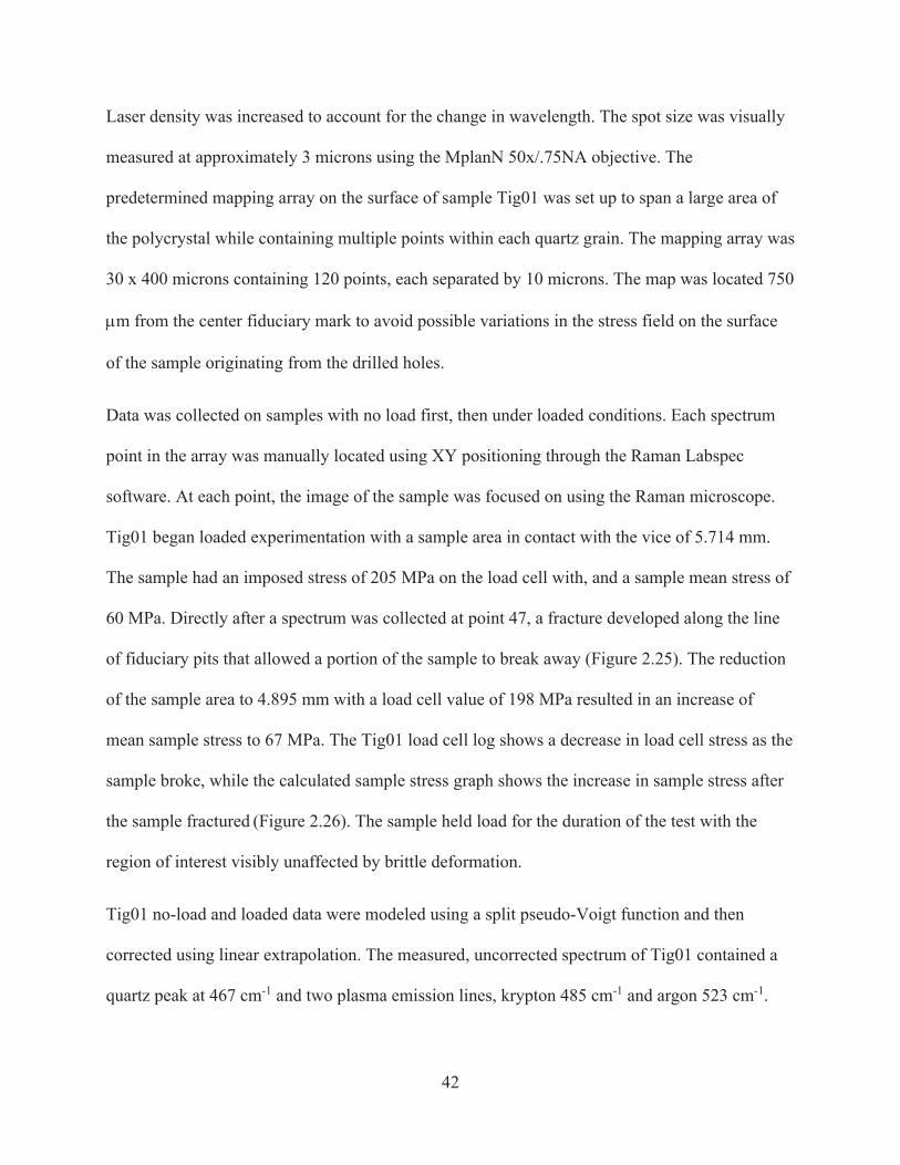
42

Laser density was increased to account for the change in wavelength. The spot size was visually

measured at approximately 3 microns using the MplanN 50x/.75NA objective. The

predetermined mapping array on the surface of sample Tig01 was set up to span a large area of

the polycrystal while containing multiple points within each quartz grain. The mapping array was

30 x 400 microns containing 120 points, each separated by 10 microns. The map was located 750

m from the center fiduciary mark to avoid possible variations in the stress field on the surface

of the sample originating from the drilled holes.

Data was collected on samples with no load first, then under loaded conditions. Each spectrum

point in the array was manually located using XY positioning through the Raman Labspec

software. At each point, the image of the sample was focused on using the Raman microscope.

Tig01 began loaded experimentation with a sample area in contact with the vice of 5.714 mm.

The sample had an imposed stress of 205 MPa on the load cell with, and a sample mean stress of

60 MPa. Directly after a spectrum was collected at point 47, a fracture developed along the line

of fiduciary pits that allowed a portion of the sample to break away (Figure 2.25). The reduction

of the sample area to 4.895 mm with a load cell value of 198 MPa resulted in an increase of

mean sample stress to 67 MPa. The Tig01 load cell log shows a decrease in load cell stress as the

sample broke, while the calculated sample stress graph shows the increase in sample stress after

the sample fractured (Figure 2.26). The sample held load for the duration of the test with the

region of interest visibly unaffected by brittle deformation.

Tig01 no-load and loaded data were modeled using a split pseudo-Voigt function and then

corrected using linear extrapolation. The measured, uncorrected spectrum of Tig01 contained a

quartz peak at 467 cm-1 and two plasma emission lines, krypton 485 cm-1 and argon 523 cm-1.

43

NIST plasma line values for krypton at 483 cm-1 and argon at 520 cm-1 were used to correct the

quartz peak values through linear extrapolation.

2.10.2 Tig03

The Tiger’s Eye polycrystal used for test Tig03 was prepared similarly to Tig01, using the puck

method for grinding and polishing. Before Raman testing, the sample areas in contact with the

vice was measured to calculate the sample stress and its associated error. The variation in height

(distance between sides 3 and 6 on opposite ends) was 2.078 +/- 0.015 mm. The variation in

width (between sides 2 and 5) was 3.206 +/- .008 mm. A length of 6.199 mm separated the two

sides that were in contact with the vice. The sample was polished to 0.05 microns using the

Buhler vibromet polisher. A fiduciary sticker was applied to Tig03 to minimize the chance of the

sample fracturing during uniaxial compression. The 2000 x 2000 micron square fiduciary sticker

framed a 100 x 600-micron region of interest in the middle of the sample.

Raman settings for test Tig03 did not vary much from test Tig01. Test Tig03 measured the 464

cm-1 peak of quartz using a laser power density of 29.5 mW at a wavelength of 514 nm with an

exposure time of 12 seconds at 12 acquisitions. The MplanN 50x/.75NA optical objective was

used, and the laser spot size was measured at 1 m. The spectrum was measured with a signal to

noise ratio of 26/1, which possibly resulted from the reflective fiduciary sticker and/or amount of

iron oxide constituents in the sample.

Test Tig03 employed new improvements in testing methods that resulted in the current

methodology for obtaining a Raman stress map. For Tig03, the Raman spectrum was first

measured for loaded spectra then unloaded spectra to save experimental time in case of sample

failures during the loading process. Tig03 was loaded to an average load cell value of 187 MPa

44

across a surface area of 6.663 +/- .066 mm. The spectra map array on the sample Tig03 was

changed from a 3 x 40 array to a 4 x 30 array to measure a wider width across the sample.

Screenshots from the Labspec program at each spectrum position were recorded, which showed

the laser spot and the surface of the sample. The micrographs were used as a location reference

to ensure that the same place was being measured from loaded to unloaded tests. The images in

each loaded or unloaded experiment were then stitched together using Adobe Illustrator by

aligning the bright iron oxide inclusions. The results were mosaiced micrographs that showed the

exact locations of each spectrum point on the sample surface during the loaded test (Figure 2.27)

and the unloaded test (Figure 2.28).

The plasma emission lines and quartz peak for Test Tig03 were modeled using a split pseudo-

Voigt function then corrected using linear extrapolation. The NIST values used to correct the

data were the krypton 483 cm-1 and argon 520 cm-1 plasma emission lines. The quartz peak was

then corrected using linear extrapolation. The Raman stress shift was calculated for each point by

subtracting the loaded peak position from the unloaded peak position. Stress was calculated for

each point using the change in peak position and the calculated single-crystal RQa Raman shift

factor.

2.11 Stress Map

A raster stress map was made from Tig03 data using Esri ArcMap 10.3.1. Tig03 stress values

and their corresponding coordinates were organized into an XYZ format with XY corresponding

to the spectrum coordinates and Z corresponding to the stress value. A text file was created

containing the XYZ data and imported into an ArcMap geodatabase. The table was converted

into spatial point data through the display XY data function. The point to raster tool converted

45

the spatial point data into 10-micron raster cells. The stress raster was classified using the

Natural Breaks (Jenks) method, which looks for natural groupings within the data. Natural Jenks

was selected to classify the data as it would adequately display the difference between a

heterogeneous and homogeneous stress map. Natural Jenks was classified into four total

categories; too many categories would lose the pattern of stress variation to static while too few

categories would homogenize the subtleties in the stress variation (Figure 2.29).

Electron backscatter diffraction was used to make an orientation image map of the sample using

the JSM6700F Field Emission SEM in UNLV's EMiL. The map was made using an accelerating

voltage of 20 kv and a step size of 4 microns. EBSD data were analyzed using MTEX. Data

points with a MAD of greater than 1.2 were removed. Grains were modeled using a grain

segmentation angle of 2 degrees; non-indexed points were removed as were grains containing

fewer than 9 pixels.

The stress map is a georeferenced compilation of layers that create a picture of the state of stress

on sample Tig03. Points were added to each laser point in the unloaded mosaiced screenshots

from Tig03 that represent individual spectrum points. The high-resolution micrograph was then

registered to the mosaiced spectrum point image using iron oxide impurities that show up as

bright, unique shapes in both micrographs. The points from the mosaiced image were then added

to the high-resolution micrograph resulting in a high-resolution micrograph with point positions

(Figure 2.30). The raster stress map and the high-resolution micrograph with spectral points were

georeferenced with the center of each spectrum point referenced to the center of each corner

raster cell (Figure 2.31).

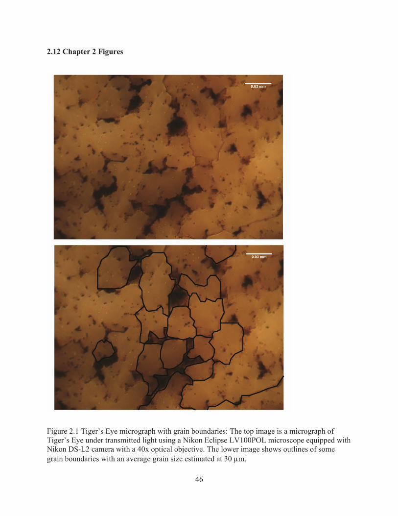
46


Figure 2.1 Tiger’s Eye micrograph with grain boundaries: The top image is a micrograph of Tiger’s Eye under transmitted light using a Nikon Eclipse LV100POL microscope equipped with Nikon DS-L2 camera with a 40x optical objective. The lower image shows outlines of some grain boundaries with an average grain size estimated at 30 m.

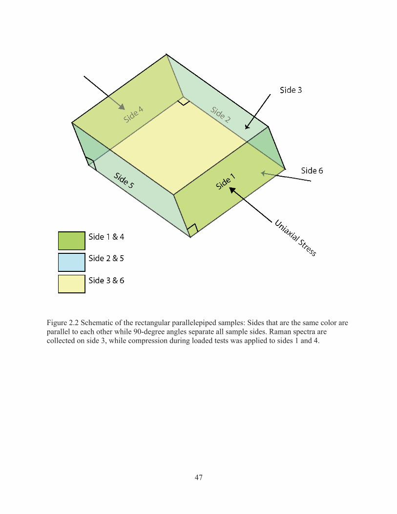
47

Figure 2.2 Schematic of the rectangular parallelepiped samples: Sides that are the same color are parallel to each other while 90-degree angles separate all sample sides. Raman spectra are collected on side 3, while compression during loaded tests was applied to sides 1 and 4.

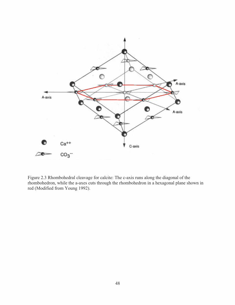
48

Figure 2.3 Rhombohedral cleavage for calcite: The c-axis runs along the diagonal of the rhombohedron, while the a-axes cuts through the rhombohedron in a hexagonal plane shown in red (Modified from Young 1992).

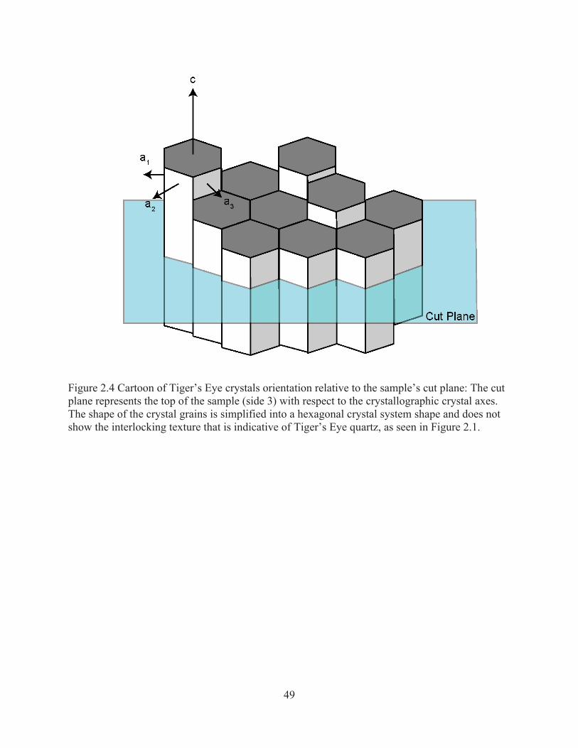
49

Figure 2.4 Cartoon of Tiger’s Eye crystals orientation relative to the sample’s cut plane: The cut plane represents the top of the sample (side 3) with respect to the crystallographic crystal axes. The shape of the crystal grains is simplified into a hexagonal crystal system shape and does not show the interlocking texture that is indicative of Tiger’s Eye quartz, as seen in Figure 2.1.

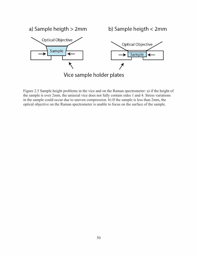
50

Figure 2.5 Sample height problems in the vice and on the Raman spectrometer: a) if the height of the sample is over 2mm, the uniaxial vice does not fully contain sides 1 and 4. Stress variations in the sample could occur due to uneven compression. b) If the sample is less than 2mm, the optical objective on the Raman spectrometer is unable to focus on the surface of the sample.

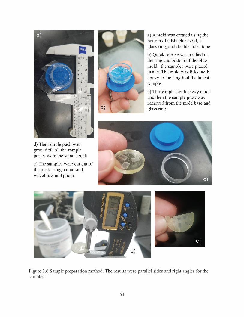
51

Figure 2.6 Sample preparation method. The results were parallel sides and right angles for the samples.

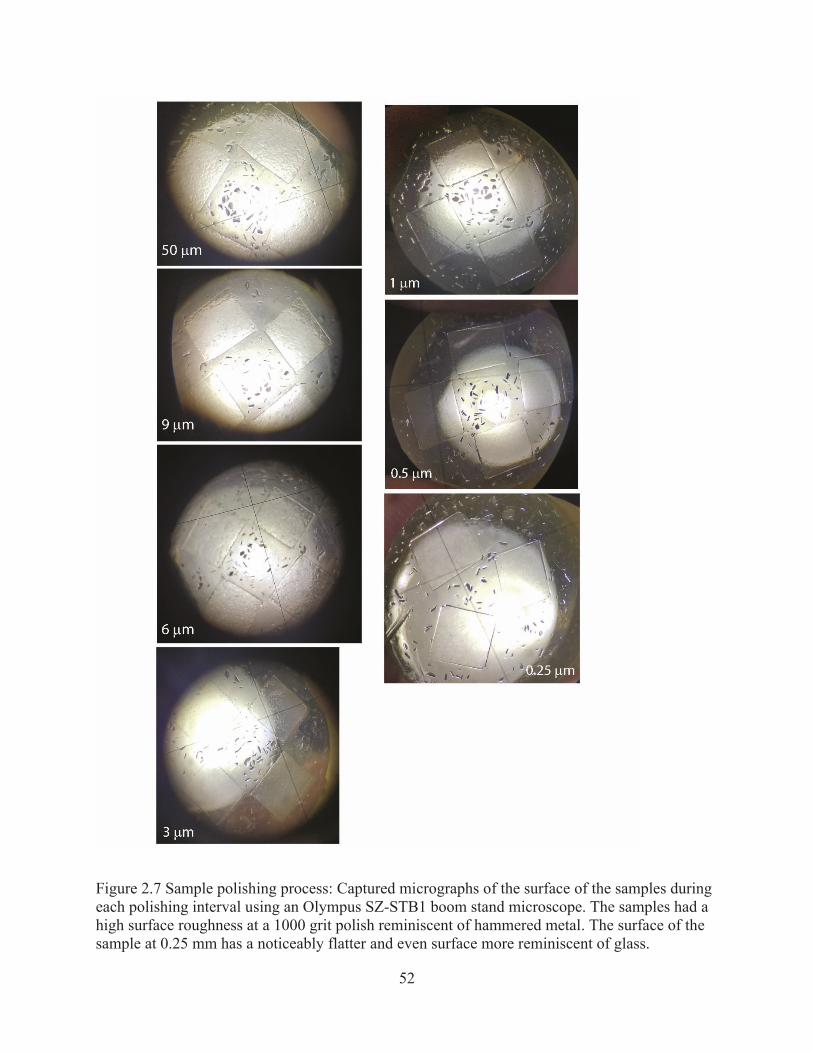
52

Figure 2.7 Sample polishing process: Captured micrographs of the surface of the samples during each polishing interval using an Olympus SZ-STB1 boom stand microscope. The samples had a high surface roughness at a 1000 grit polish reminiscent of hammered metal. The surface of the sample at 0.25 mm has a noticeably flatter and even surface more reminiscent of glass.

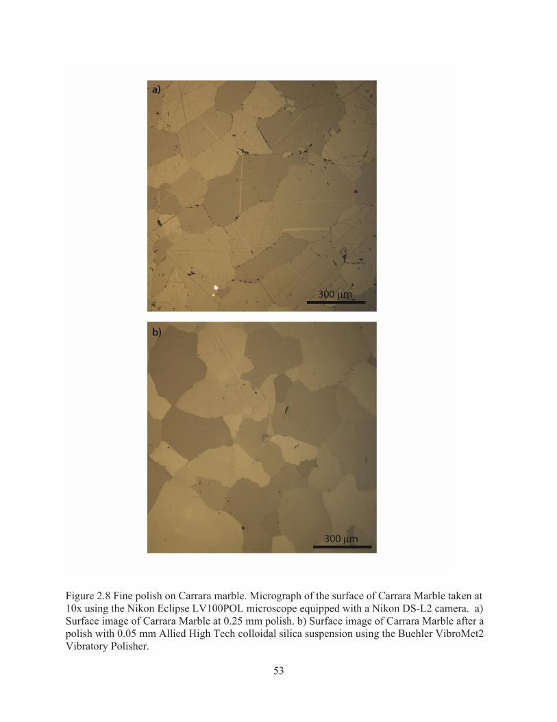
53

Figure 2.8 Fine polish on Carrara marble. Micrograph of the surface of Carrara Marble taken at 10x using the Nikon Eclipse LV100POL microscope equipped with a Nikon DS-L2 camera. a) Surface image of Carrara Marble at 0.25 mm polish. b) Surface image of Carrara Marble after a polish with 0.05 mm Allied High Tech colloidal silica suspension using the Buehler VibroMet2 Vibratory Polisher.

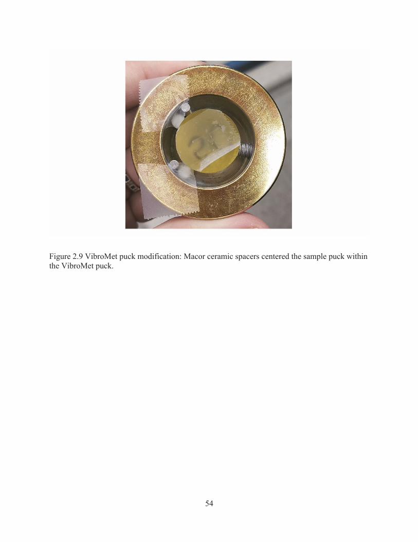
54

Figure 2.9 VibroMet puck modification: Macor ceramic spacers centered the sample puck within the VibroMet puck.

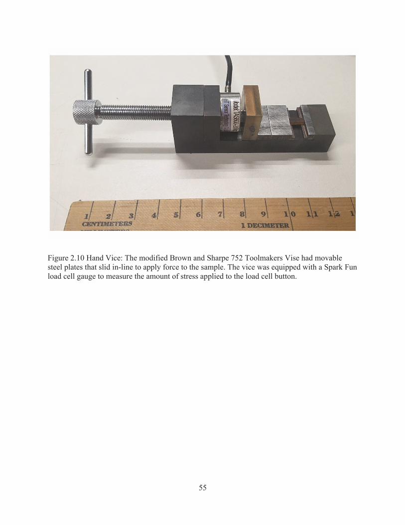
55

Figure 2.10 Hand Vice: The modified Brown and Sharpe 752 Toolmakers Vise had movable steel plates that slid in-line to apply force to the sample. The vice was equipped with a Spark Fun load cell gauge to measure the amount of stress applied to the load cell button.

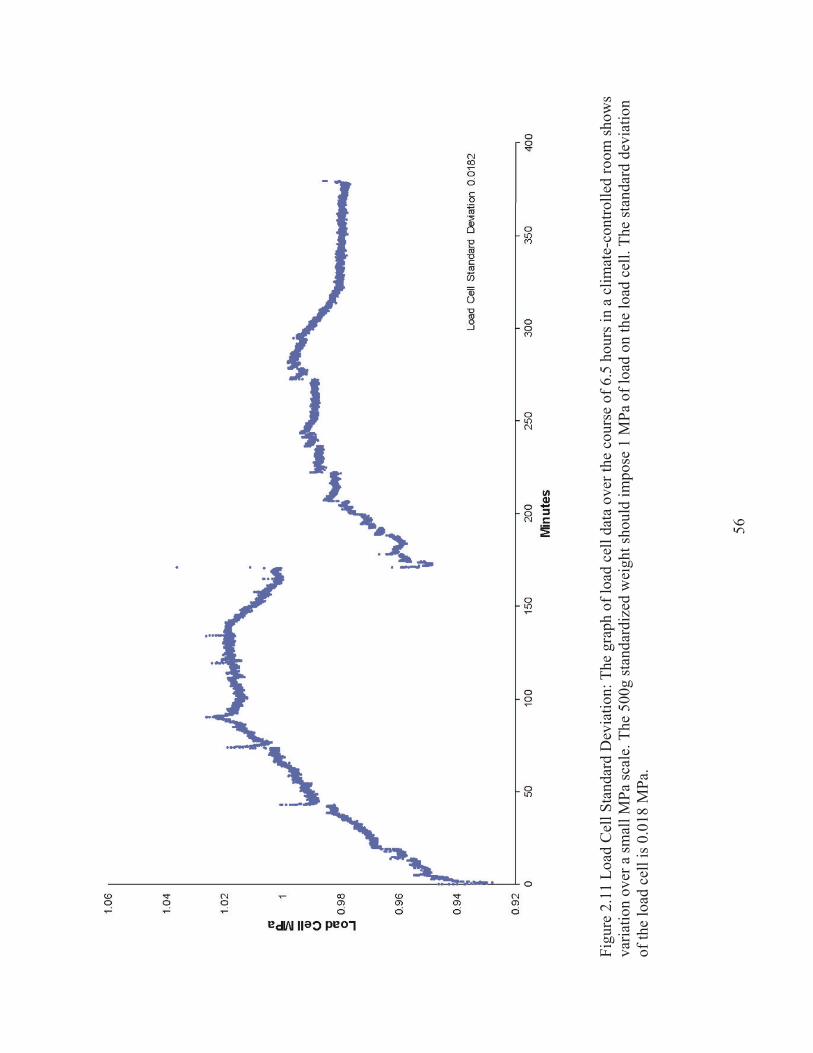
56

Figu

re 2

.11

Load

Cel

l Sta

ndar

d D

evia

tion:

The

gra

ph o

f loa

d ce

ll da

ta o

ver t

he c

ours

e of

6.5

hou

rs in

a c

limat

e-co

ntro

lled

room

show

s va

riatio

n ov

er a

smal

l MPa

scal

e. T

he 5

00g

stan

dard

ized

wei

ght s

houl

d im

pose

1 M

Pa o

f loa

d on

the

load

cel

l. Th

e st

anda

rd d

evia

tion

of th

e lo

ad c

ell i

s 0.0

18 M

Pa.

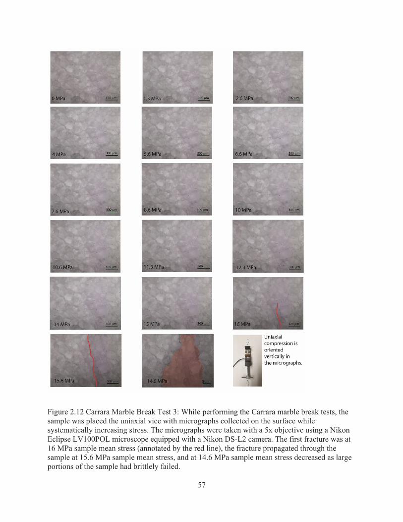
57

Figure 2.12 Carrara Marble Break Test 3: While performing the Carrara marble break tests, the sample was placed the uniaxial vice with micrographs collected on the surface while systematically increasing stress. The micrographs were taken with a 5x objective using a Nikon Eclipse LV100POL microscope equipped with a Nikon DS-L2 camera. The first fracture was at 16 MPa sample mean stress (annotated by the red line), the fracture propagated through the sample at 15.6 MPa sample mean stress, and at 14.6 MPa sample mean stress decreased as large portions of the sample had brittlely failed.

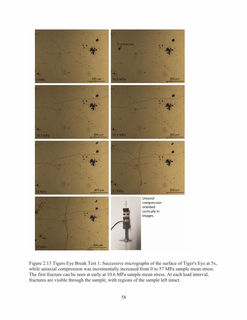
58

Figure 2.13 Tigers Eye Break Test 1: Successive micrographs of the surface of Tiger's Eye at 5x, while uniaxial compression was incrementally increased from 0 to 57 MPa sample mean stress. The first fracture can be seen at early at 10.6 MPa sample mean stress. At each load interval, fractures are visible through the sample, with regions of the sample left intact.

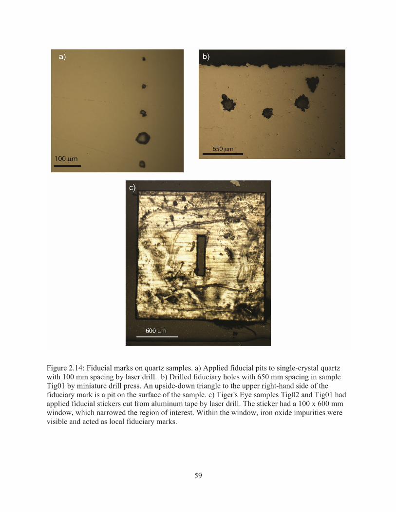
59

Figure 2.14: Fiducial marks on quartz samples. a) Applied fiducial pits to single-crystal quartz with 100 mm spacing by laser drill. b) Drilled fiduciary holes with 650 mm spacing in sample Tig01 by miniature drill press. An upside-down triangle to the upper right-hand side of the fiduciary mark is a pit on the surface of the sample. c) Tiger's Eye samples Tig02 and Tig01 had applied fiducial stickers cut from aluminum tape by laser drill. The sticker had a 100 x 600 mm window, which narrowed the region of interest. Within the window, iron oxide impurities were visible and acted as local fiduciary marks.

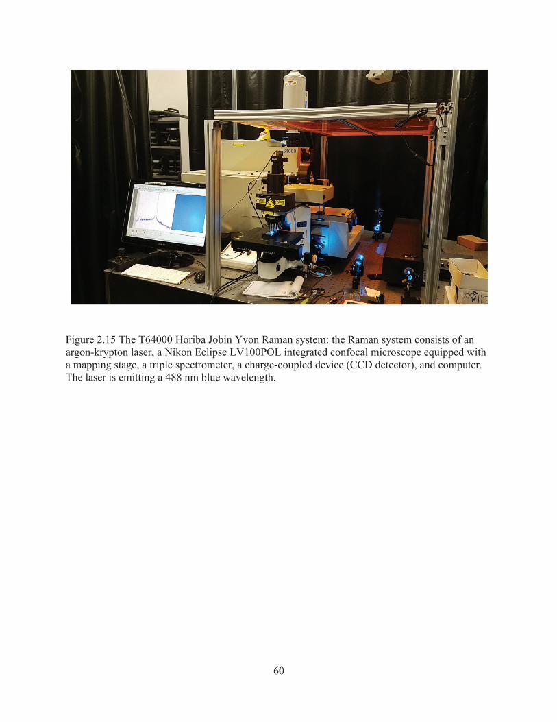
60

Figure 2.15 The T64000 Horiba Jobin Yvon Raman system: the Raman system consists of an argon-krypton laser, a Nikon Eclipse LV100POL integrated confocal microscope equipped with a mapping stage, a triple spectrometer, a charge-coupled device (CCD detector), and computer. The laser is emitting a 488 nm blue wavelength.

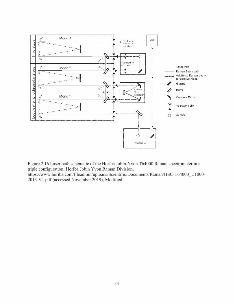
61

Figure 2.16 Laser path schematic of the Horiba Jobin-Yvon T64000 Raman spectrometer in a triple configuration: Horiba Jobin Yvon Raman Division, https://www.horiba.com/fileadmin/uploads/Scientific/Documents/Raman/HSC-T64000_U1000-2013-V1.pdf (accessed November 2019), Modified.

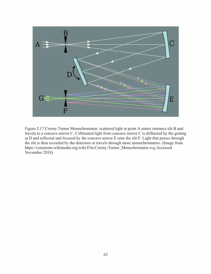
62

Figure 2.17 Czerny Turner Monochromator: scattered light at point A enters entrance slit B and travels to a concave mirror C. Collimated light from concave mirror C is diffracted by the grating at D and reflected and focused by the concave mirror E onto the slit F. Light that passes through the slit is then recorded by the detectors or travels through more monochromators. (Image from https://commons.wikimedia.org/wiki/File:Czerny-Turner_Monochromator.svg Accessed November 2018)

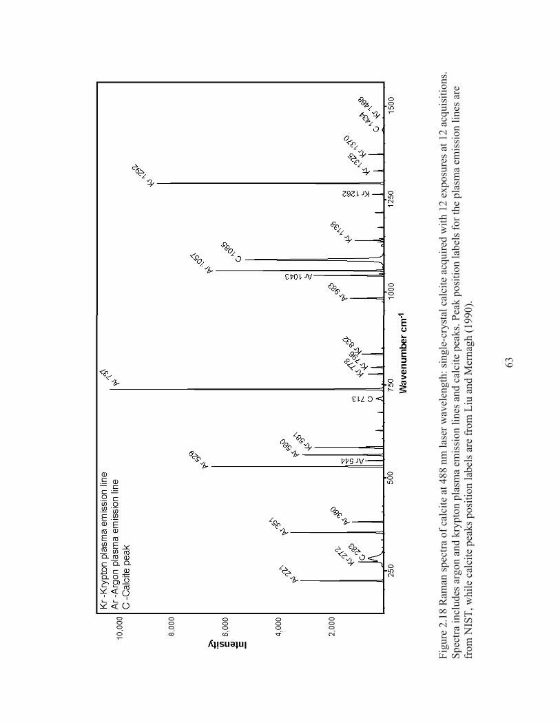
63

Figu

re 2

.18

Ram

an sp

ectra

of c

alci

te a

t 488

nm

lase

r wav

elen

gth:

sing

le-c

ryst

al c

alci

te a

cqui

red

with

12

expo

sure

s at 1

2 ac

quis

ition

s. Sp

ectra

incl

udes

arg

on a

nd k

rypt

on p

lasm

a em

issio

n lin

es a

nd c

alci

te p

eaks

. Pea

k po

sitio

n la

bels

for t

he p

lasm

a em

issi

on li

nes a

re

from

NIS

T, w

hile

cal

cite

pea

ks p

ositi

on la

bels

are

from

Liu

and

Mer

nagh

(199

0).

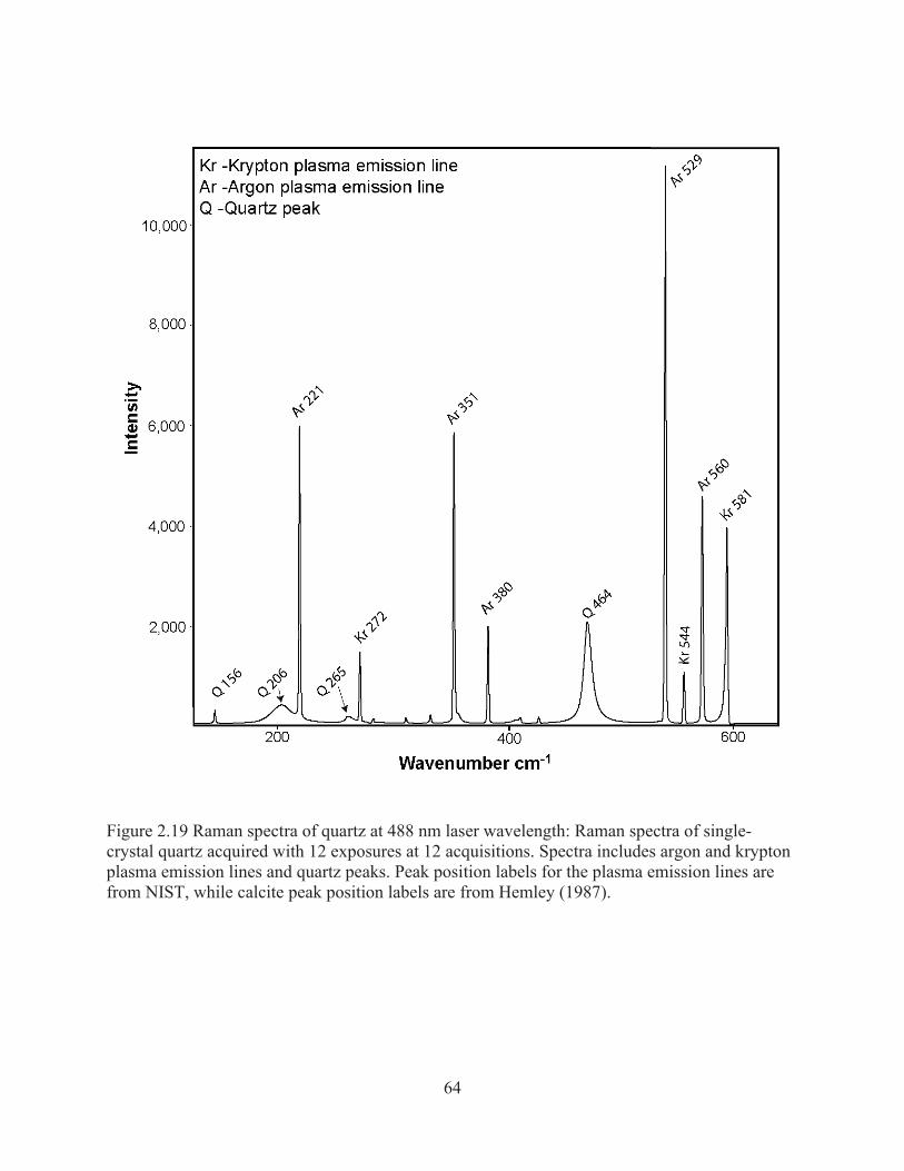
64

Figure 2.19 Raman spectra of quartz at 488 nm laser wavelength: Raman spectra of single-crystal quartz acquired with 12 exposures at 12 acquisitions. Spectra includes argon and krypton plasma emission lines and quartz peaks. Peak position labels for the plasma emission lines are from NIST, while calcite peak position labels are from Hemley (1987).

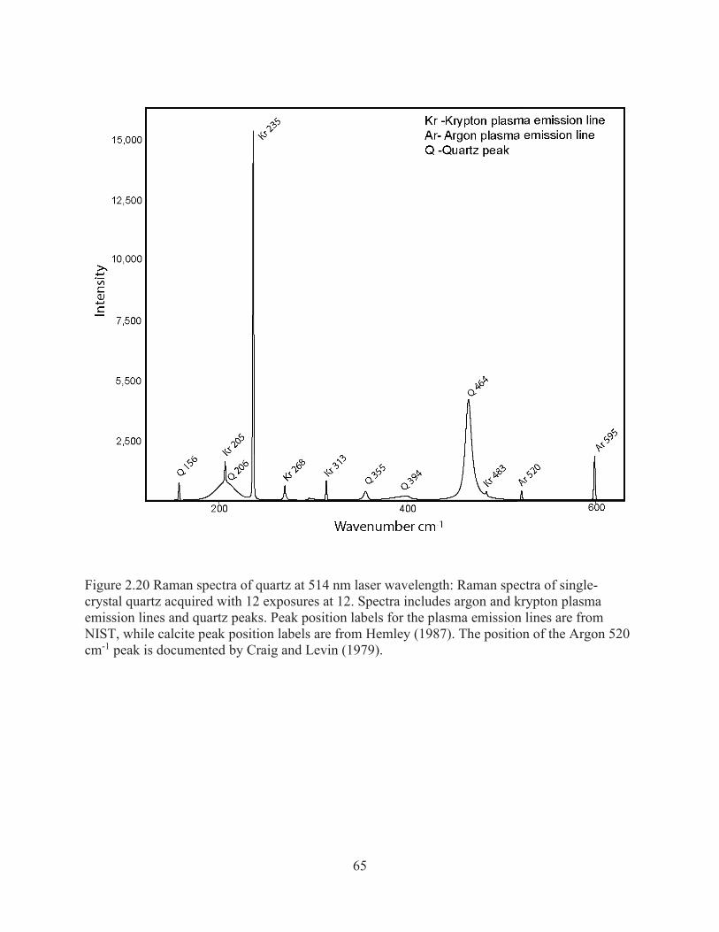
65

Figure 2.20 Raman spectra of quartz at 514 nm laser wavelength: Raman spectra of single-crystal quartz acquired with 12 exposures at 12. Spectra includes argon and krypton plasma emission lines and quartz peaks. Peak position labels for the plasma emission lines are from NIST, while calcite peak position labels are from Hemley (1987). The position of the Argon 520 cm-1 peak is documented by Craig and Levin (1979).

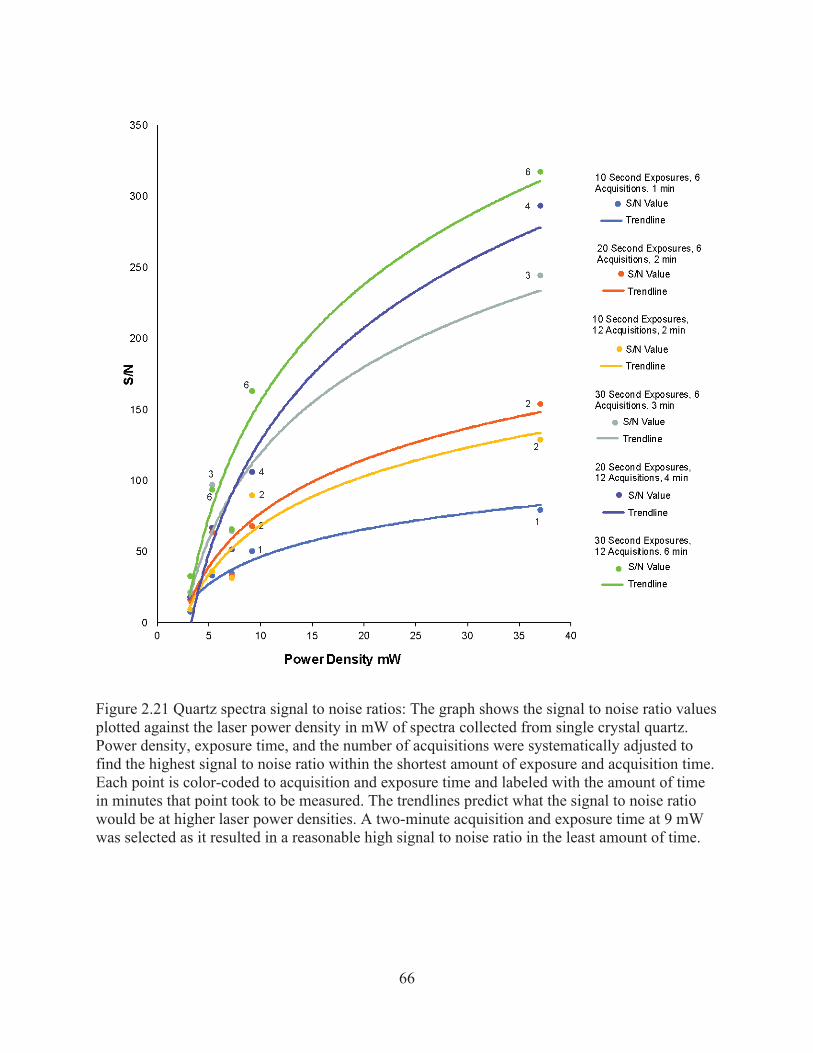
66

Figure 2.21 Quartz spectra signal to noise ratios: The graph shows the signal to noise ratio values plotted against the laser power density in mW of spectra collected from single crystal quartz. Power density, exposure time, and the number of acquisitions were systematically adjusted to find the highest signal to noise ratio within the shortest amount of exposure and acquisition time. Each point is color-coded to acquisition and exposure time and labeled with the amount of time in minutes that point took to be measured. The trendlines predict what the signal to noise ratio would be at higher laser power densities. A two-minute acquisition and exposure time at 9 mW was selected as it resulted in a reasonable high signal to noise ratio in the least amount of time.

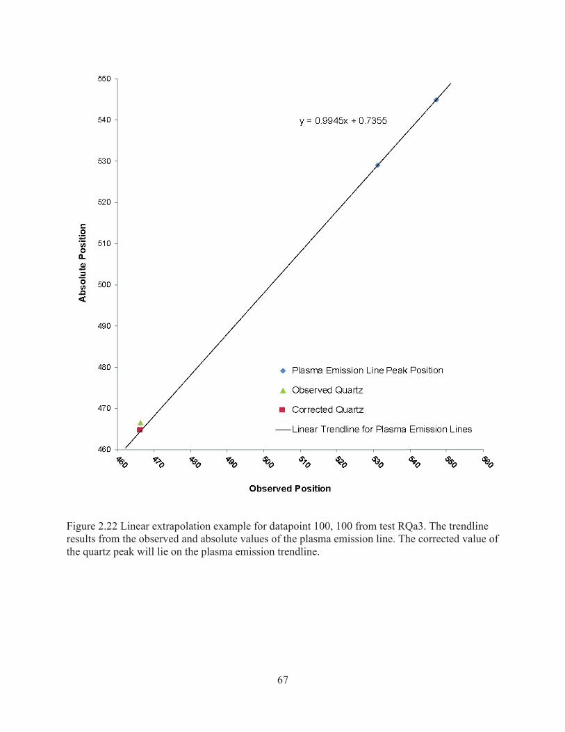
67

Figure 2.22 Linear extrapolation example for datapoint 100, 100 from test RQa3. The trendline results from the observed and absolute values of the plasma emission line. The corrected value of the quartz peak will lie on the plasma emission trendline.

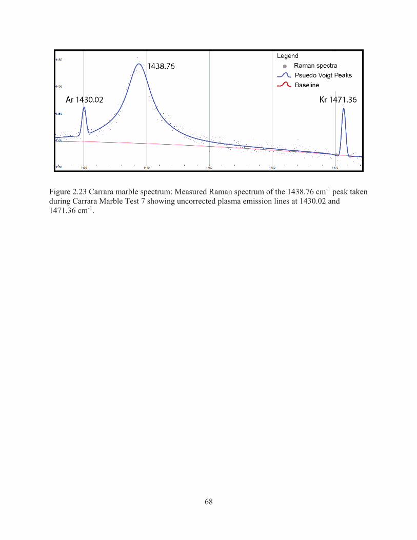
68

Figure 2.23 Carrara marble spectrum: Measured Raman spectrum of the 1438.76 cm-1 peak taken during Carrara Marble Test 7 showing uncorrected plasma emission lines at 1430.02 and 1471.36 cm-1.

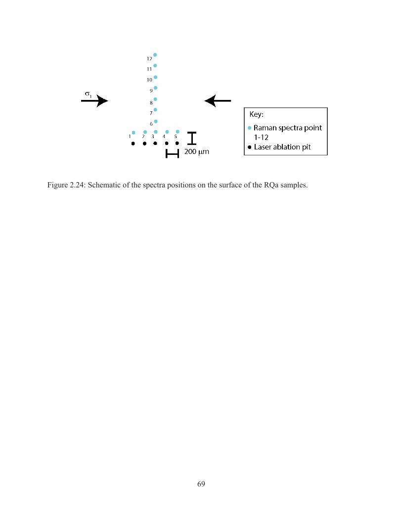
69

Figure 2.24: Schematic of the spectra positions on the surface of the RQa samples.

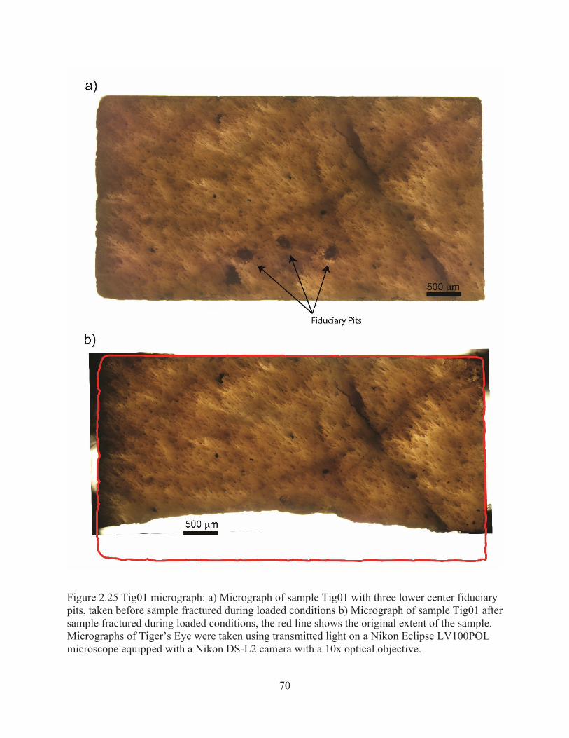
70

Figure 2.25 Tig01 micrograph: a) Micrograph of sample Tig01 with three lower center fiduciary pits, taken before sample fractured during loaded conditions b) Micrograph of sample Tig01 after sample fractured during loaded conditions, the red line shows the original extent of the sample. Micrographs of Tiger’s Eye were taken using transmitted light on a Nikon Eclipse LV100POL microscope equipped with a Nikon DS-L2 camera with a 10x optical objective.

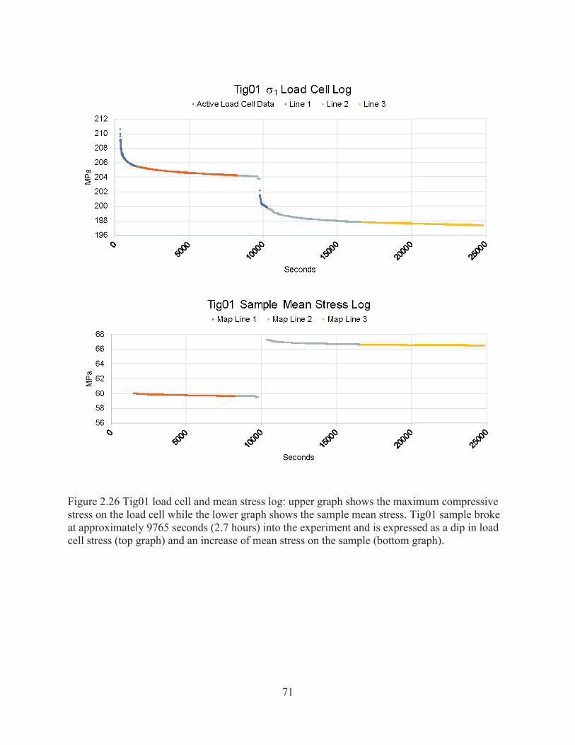
71

Figure 2.26 Tig01 load cell and mean stress log: upper graph shows the maximum compressive stress on the load cell while the lower graph shows the sample mean stress. Tig01 sample broke at approximately 9765 seconds (2.7 hours) into the experiment and is expressed as a dip in load cell stress (top graph) and an increase of mean stress on the sample (bottom graph).

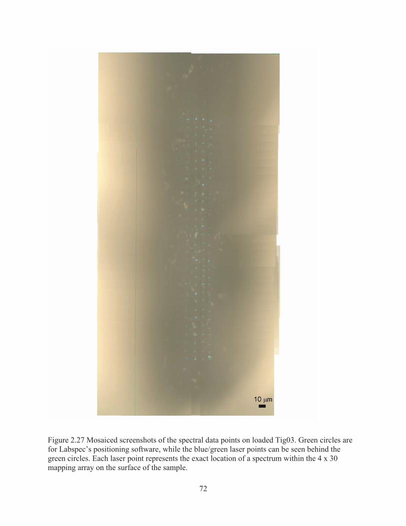
72

Figure 2.27 Mosaiced screenshots of the spectral data points on loaded Tig03. Green circles are for Labspec’s positioning software, while the blue/green laser points can be seen behind the green circles. Each laser point represents the exact location of a spectrum within the 4 x 30 mapping array on the surface of the sample.

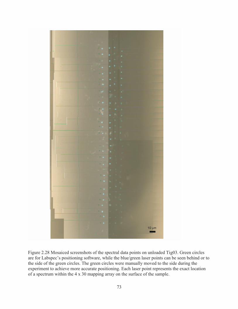
73

Figure 2.28 Mosaiced screenshots of the spectral data points on unloaded Tig03. Green circles are for Labspec’s positioning software, while the blue/green laser points can be seen behind or to the side of the green circles. The green circles were manually moved to the side during the experiment to achieve more accurate positioning. Each laser point represents the exact location of a spectrum within the 4 x 30 mapping array on the surface of the sample.

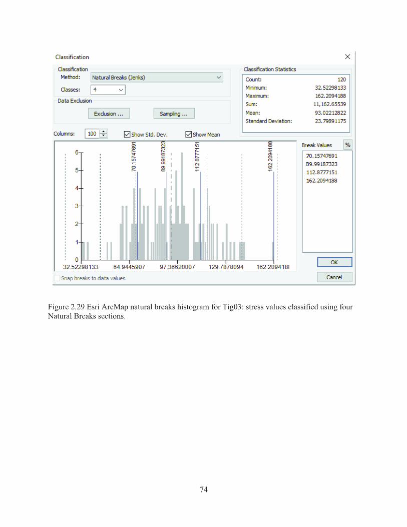
74

Figure 2.29 Esri ArcMap natural breaks histogram for Tig03: stress values classified using four Natural Breaks sections.

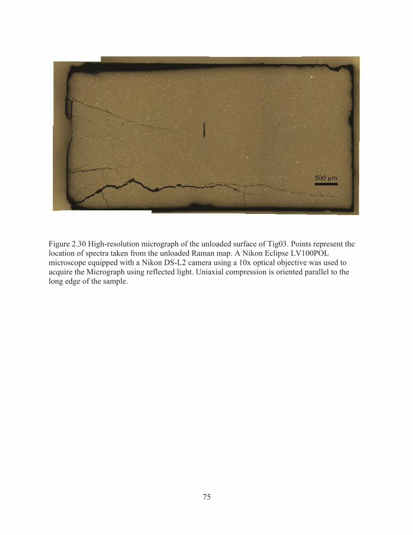
75

Figure 2.30 High-resolution micrograph of the unloaded surface of Tig03. Points represent the location of spectra taken from the unloaded Raman map. A Nikon Eclipse LV100POL microscope equipped with a Nikon DS-L2 camera using a 10x optical objective was used to acquire the Micrograph using reflected light. Uniaxial compression is oriented parallel to the long edge of the sample.

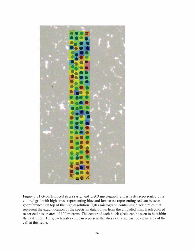
76

Figure 2.31 Georeferenced stress raster and Tig03 micrograph. Stress raster represented by a colored grid with high stress representing blue and low stress representing red can be seen georeferenced on top of the high-resolution Tig03 micrograph containing black circles that represent the exact location of the spectrum data points from the unloaded map. Each colored raster cell has an area of 100 microns. The center of each black circle can be seen to be within the raster cell. Thus, each raster cell can represent the stress value across the entire area of the cell at this scale.

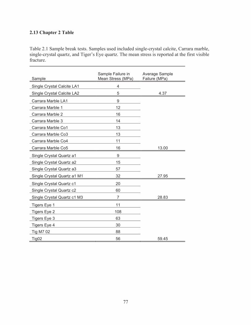
77

2.13 Chapter 2 Table

Table 2.1 Sample break tests. Samples used included single-crystal calcite, Carrara marble, single-crystal quartz, and Tiger’s Eye quartz. The mean stress is reported at the first visible fracture.

Sample Sample Failure in Mean Stress (MPa)

Average Sample Failure (MPa)

Single Crystal Calcite LA1 4 Single Crystal Calcite LA2 5 4.37

Carrara Marble LA1 9 Carrara Marble 1 12 Carrara Marble 2 16 Carrara Marble 3 14 Carrara Marble Co1 13 Carrara Marble Co3 13 Carrara Marble Co4 11 Carrara Marble Co5 16 13.00

Single Crystal Quartz a1 9 Single Crystal Quartz a2 15 Single Crystal Quartz a3 57 Single Crystal Quartz a1 M1 32 27.95

Single Crystal Quartz c1 20 Single Crystal Quartz c2 60 Single Crystal Quartz c1 M3 7 28.83

Tigers Eye 1 11 Tigers Eye 2 108 Tigers Eye 3 63 Tigers Eye 4 30 Tig M7 02 88 Tig02 56 59.45

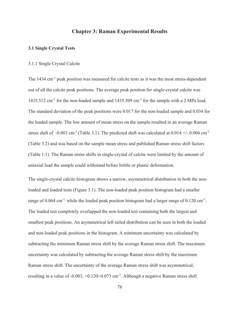
78

Chapter 3: Raman Experimental Results

3.1 Single Crystal Tests

3.1.1 Single Crystal Calcite

The 1434 cm-1 peak position was measured for calcite tests as it was the most stress-dependent

out of all the calcite peak positions. The average peak position for single-crystal calcite was

1435.512 cm-1 for the non-loaded sample and 1435.509 cm-1 for the sample with a 2 MPa load.

The standard deviation of the peak positions were 0.017 for the non-loaded sample and 0.034 for

the loaded sample. The low amount of mean stress on the sample resulted in an average Raman

stress shift of -0.003 cm-1 (Table 3.1). The predicted shift was calculated at 0.014 +/- 0.004 cm-1

(Table 3.2) and was based on the sample mean stress and published Raman stress shift factors

(Table 1.1). The Raman stress shifts in single-crystal of calcite were limited by the amount of

uniaxial load the sample could withstand before brittle or plastic deformation.

The single-crystal calcite histogram shows a narrow, asymmetrical distribution in both the non-

loaded and loaded tests (Figure 3.1). The non-loaded peak position histogram had a smaller

range of 0.064 cm-1, while the loaded peak position histogram had a larger range of 0.120 cm-1.

The loaded test completely overlapped the non-loaded test containing both the largest and

smallest peak positions. An asymmetrical left tailed distribution can be seen in both the loaded

and non-loaded peak positions in the histogram. A minimum uncertainty was calculated by

subtracting the minimum Raman stress shift by the average Raman stress shift. The maximum

uncertainty was calculated by subtracting the average Raman stress shift by the maximum

Raman stress shift. The uncertainty of the average Raman stress shift was asymmetrical,

resulting in a value of -0.003, +0.120/-0.073 cm-1. Although a negative Raman stress shift

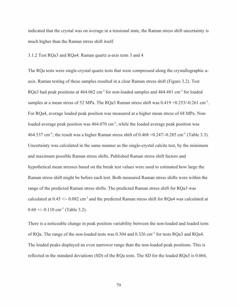
79

indicated that the crystal was on average in a tensional state, the Raman stress shift uncertainty is

much higher than the Raman stress shift itself.

3.1.2 Test RQa3 and RQa4: Raman quartz a-axis tests 3 and 4

The RQa tests were single-crystal quartz tests that were compressed along the crystallographic a-

axis. Raman testing of these samples resulted in a clear Raman stress shift (Figure 3.2). Test

RQa3 had peak positions at 464.062 cm-1 for non-loaded samples and 464.481 cm-1 for loaded

samples at a mean stress of 52 MPa. The RQa3 Raman stress shift was 0.419 +0.253/-0.261 cm-1.

For RQa4, average loaded peak position was measured at a higher mean stress of 68 MPa. Non-

loaded average peak position was 464.070 cm-1, while the loaded average peak position was

464.537 cm-1; the result was a higher Raman stress shift of 0.468 +0.247/-0.285 cm-1 (Table 3.3).

Uncertainty was calculated in the same manner as the single-crystal calcite test, by the minimum

and maximum possible Raman stress shifts. Published Raman stress shift factors and

hypothetical mean stresses based on the break test values were used to estimated how large the

Raman stress shift might be before each test. Both measured Raman stress shifts were within the

range of the predicted Raman stress shifts. The predicted Raman stress shift for RQa3 was

calculated at 0.45 +/- 0.082 cm-1 and the predicted Raman stress shift for RQa4 was calculated at

0.60 +/- 0.110 cm-1 (Table 3.2).

There is a noticeable change in peak position variability between the non-loaded and loaded tests

of RQa. The range of the non-loaded tests was 0.304 and 0.326 cm-1 for tests RQa3 and RQa4.

The loaded peaks displayed an even narrower range than the non-loaded peak positions. This is

reflected in the standard deviations (SD) of the RQa tests. The SD for the loaded RQa3 is 0.064,

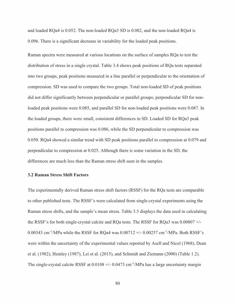
80

and loaded RQa4 is 0.052. The non-loaded RQa3 SD is 0.082, and the non-loaded RQa4 is

0.096. There is a significant decrease in variability for the loaded peak positions.

Raman spectra were measured at various locations on the surface of samples RQa to test the

distribution of stress in a single crystal. Table 3.4 shows peak positions of RQa tests separated

into two groups, peak positions measured in a line parallel or perpendicular to the orientation of

compression. SD was used to compare the two groups. Total non-loaded SD of peak positions

did not differ significantly between perpendicular or parallel groups; perpendicular SD for non-

loaded peak positions were 0.085, and parallel SD for non-loaded peak positions were 0.087. In

the loaded groups, there were small, consistent differences in SD. Loaded SD for RQa3 peak

positions parallel to compression was 0.086, while the SD perpendicular to compression was

0.050. RQa4 showed a similar trend with SD peak positions parallel to compression at 0.079 and

perpendicular to compression at 0.025. Although there is some variation in the SD, the

differences are much less than the Raman stress shift seen in the samples.

3.2 Raman Stress Shift Factors

The experimentally derived Raman stress shift factors (RSSF) for the RQa tests are comparable

to other published tests. The RSSF’s were calculated from single-crystal experiments using the

Raman stress shifts, and the sample’s mean stress. Table 3.5 displays the data used in calculating

the RSSF’s for both single-crystal calcite and RQa tests. The RSSF for RQa3 was 0.00807 +/-

0.00343 cm-1/MPa while the RSSF for RQa4 was 0.00712 +/- 0.00257 cm-1/MPa. Both RSSF’s

were within the uncertainty of the experimental values reported by Asell and Nicol (1968), Dean

et al. (1982), Hemley (1987), Lei et al. (2015), and Schmidt and Ziemann (2000) (Table 1.2).

The single-crystal calcite RSSF at 0.0108 +/- 0.0473 cm-1/MPa has a large uncertainty margin

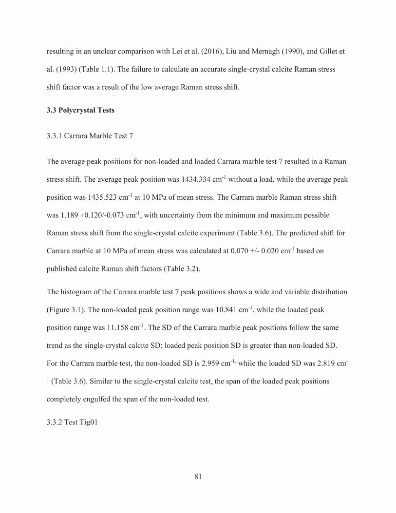
81

resulting in an unclear comparison with Lei et al. (2016), Liu and Mernagh (1990), and Gillet et

al. (1993) (Table 1.1). The failure to calculate an accurate single-crystal calcite Raman stress

shift factor was a result of the low average Raman stress shift.

3.3 Polycrystal Tests

3.3.1 Carrara Marble Test 7

The average peak positions for non-loaded and loaded Carrara marble test 7 resulted in a Raman

stress shift. The average peak position was 1434.334 cm-1 without a load, while the average peak

position was 1435.523 cm-1 at 10 MPa of mean stress. The Carrara marble Raman stress shift

was 1.189 +0.120/-0.073 cm-1, with uncertainty from the minimum and maximum possible

Raman stress shift from the single-crystal calcite experiment (Table 3.6). The predicted shift for

Carrara marble at 10 MPa of mean stress was calculated at 0.070 +/- 0.020 cm-1 based on

published calcite Raman shift factors (Table 3.2).

The histogram of the Carrara marble test 7 peak positions shows a wide and variable distribution

(Figure 3.1). The non-loaded peak position range was 10.841 cm-1, while the loaded peak

position range was 11.158 cm-1. The SD of the Carrara marble peak positions follow the same

trend as the single-crystal calcite SD; loaded peak position SD is greater than non-loaded SD.

For the Carrara marble test, the non-loaded SD is 2.959 cm-1, while the loaded SD was 2.819 cm-

1 (Table 3.6). Similar to the single-crystal calcite test, the span of the loaded peak positions

completely engulfed the span of the non-loaded test.

3.3.2 Test Tig01

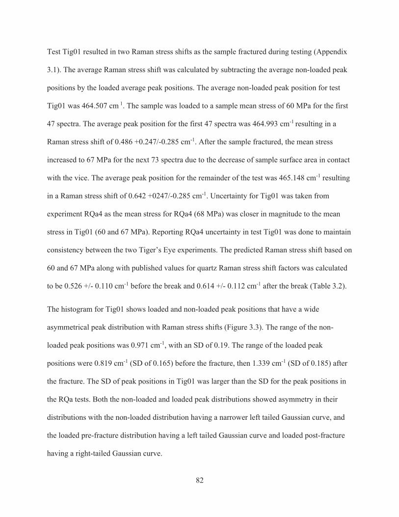
82

Test Tig01 resulted in two Raman stress shifts as the sample fractured during testing (Appendix

3.1). The average Raman stress shift was calculated by subtracting the average non-loaded peak

positions by the loaded average peak positions. The average non-loaded peak position for test

Tig01 was 464.507 cm 1. The sample was loaded to a sample mean stress of 60 MPa for the first

47 spectra. The average peak position for the first 47 spectra was 464.993 cm-1 resulting in a

Raman stress shift of 0.486 +0.247/-0.285 cm-1. After the sample fractured, the mean stress

increased to 67 MPa for the next 73 spectra due to the decrease of sample surface area in contact

with the vice. The average peak position for the remainder of the test was 465.148 cm-1 resulting

in a Raman stress shift of 0.642 +0247/-0.285 cm-1. Uncertainty for Tig01 was taken from

experiment RQa4 as the mean stress for RQa4 (68 MPa) was closer in magnitude to the mean

stress in Tig01 (60 and 67 MPa). Reporting RQa4 uncertainty in test Tig01 was done to maintain

consistency between the two Tiger’s Eye experiments. The predicted Raman stress shift based on

60 and 67 MPa along with published values for quartz Raman stress shift factors was calculated

to be 0.526 +/- 0.110 cm-1 before the break and 0.614 +/- 0.112 cm-1 after the break (Table 3.2).

The histogram for Tig01 shows loaded and non-loaded peak positions that have a wide

asymmetrical peak distribution with Raman stress shifts (Figure 3.3). The range of the non-

loaded peak positions was 0.971 cm-1, with an SD of 0.19. The range of the loaded peak

positions were 0.819 cm-1 (SD of 0.165) before the fracture, then 1.339 cm-1 (SD of 0.185) after

the fracture. The SD of peak positions in Tig01 was larger than the SD for the peak positions in

the RQa tests. Both the non-loaded and loaded peak distributions showed asymmetry in their

distributions with the non-loaded distribution having a narrower left tailed Gaussian curve, and

the loaded pre-fracture distribution having a left tailed Gaussian curve and loaded post-fracture

having a right-tailed Gaussian curve.

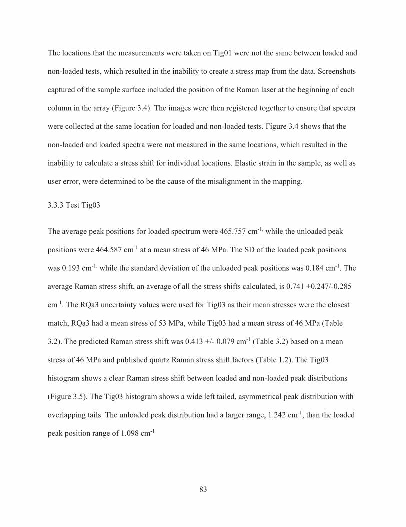
83

The locations that the measurements were taken on Tig01 were not the same between loaded and

non-loaded tests, which resulted in the inability to create a stress map from the data. Screenshots

captured of the sample surface included the position of the Raman laser at the beginning of each

column in the array (Figure 3.4). The images were then registered together to ensure that spectra

were collected at the same location for loaded and non-loaded tests. Figure 3.4 shows that the

non-loaded and loaded spectra were not measured in the same locations, which resulted in the

inability to calculate a stress shift for individual locations. Elastic strain in the sample, as well as

user error, were determined to be the cause of the misalignment in the mapping.

3.3.3 Test Tig03

The average peak positions for loaded spectrum were 465.757 cm-1, while the unloaded peak

positions were 464.587 cm-1 at a mean stress of 46 MPa. The SD of the loaded peak positions

was 0.193 cm-1, while the standard deviation of the unloaded peak positions was 0.184 cm-1. The

average Raman stress shift, an average of all the stress shifts calculated, is 0.741 +0.247/-0.285

cm-1. The RQa3 uncertainty values were used for Tig03 as their mean stresses were the closest

match, RQa3 had a mean stress of 53 MPa, while Tig03 had a mean stress of 46 MPa (Table

3.2). The predicted Raman stress shift was 0.413 +/- 0.079 cm-1 (Table 3.2) based on a mean

stress of 46 MPa and published quartz Raman stress shift factors (Table 1.2). The Tig03

histogram shows a clear Raman stress shift between loaded and non-loaded peak distributions

(Figure 3.5). The Tig03 histogram shows a wide left tailed, asymmetrical peak distribution with

overlapping tails. The unloaded peak distribution had a larger range, 1.242 cm-1, than the loaded

peak position range of 1.098 cm-1

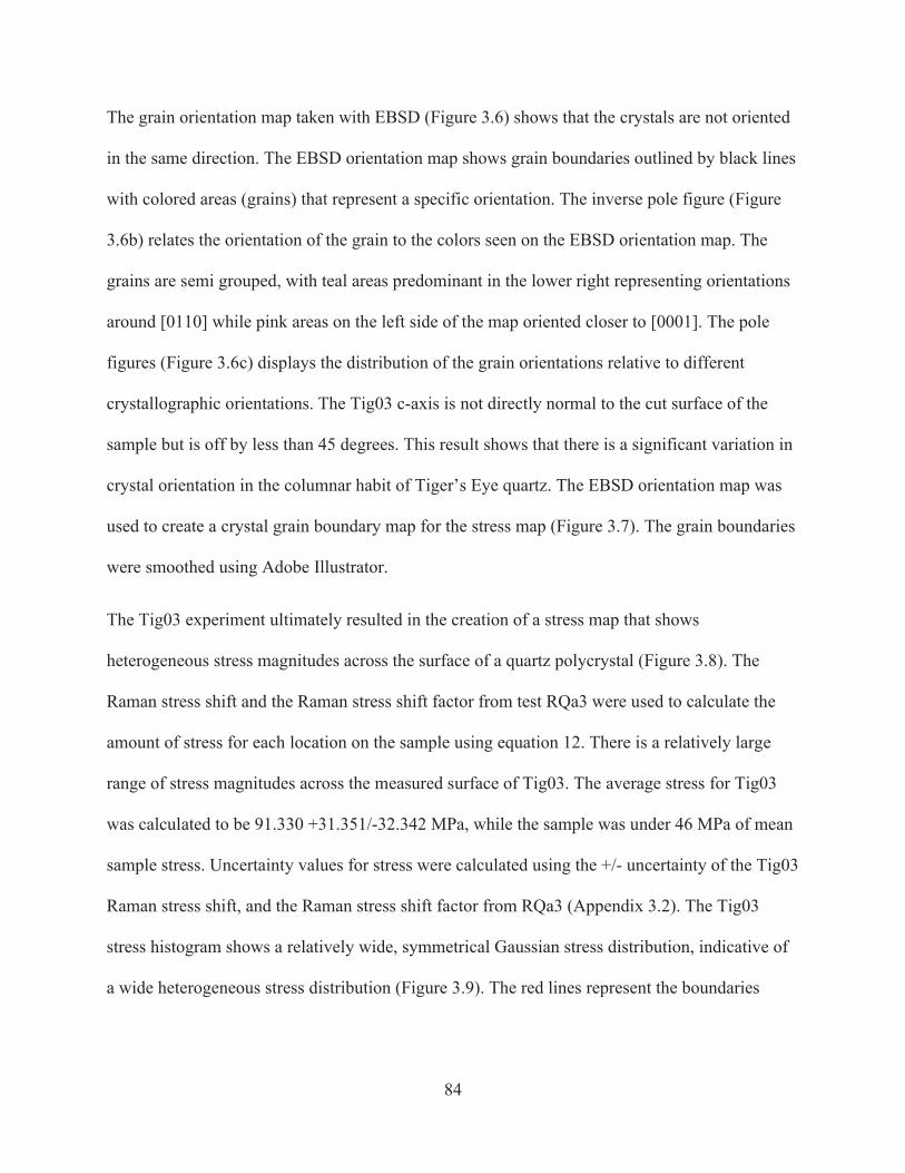
84

The grain orientation map taken with EBSD (Figure 3.6) shows that the crystals are not oriented

in the same direction. The EBSD orientation map shows grain boundaries outlined by black lines

with colored areas (grains) that represent a specific orientation. The inverse pole figure (Figure

3.6b) relates the orientation of the grain to the colors seen on the EBSD orientation map. The

grains are semi grouped, with teal areas predominant in the lower right representing orientations

around [0110] while pink areas on the left side of the map oriented closer to [0001]. The pole

figures (Figure 3.6c) displays the distribution of the grain orientations relative to different

crystallographic orientations. The Tig03 c-axis is not directly normal to the cut surface of the

sample but is off by less than 45 degrees. This result shows that there is a significant variation in

crystal orientation in the columnar habit of Tiger’s Eye quartz. The EBSD orientation map was

used to create a crystal grain boundary map for the stress map (Figure 3.7). The grain boundaries

were smoothed using Adobe Illustrator.

The Tig03 experiment ultimately resulted in the creation of a stress map that shows

heterogeneous stress magnitudes across the surface of a quartz polycrystal (Figure 3.8). The

Raman stress shift and the Raman stress shift factor from test RQa3 were used to calculate the

amount of stress for each location on the sample using equation 12. There is a relatively large

range of stress magnitudes across the measured surface of Tig03. The average stress for Tig03

was calculated to be 91.330 +31.351/-32.342 MPa, while the sample was under 46 MPa of mean

sample stress. Uncertainty values for stress were calculated using the +/- uncertainty of the Tig03

Raman stress shift, and the Raman stress shift factor from RQa3 (Appendix 3.2). The Tig03

stress histogram shows a relatively wide, symmetrical Gaussian stress distribution, indicative of

a wide heterogeneous stress distribution (Figure 3.9). The red lines represent the boundaries

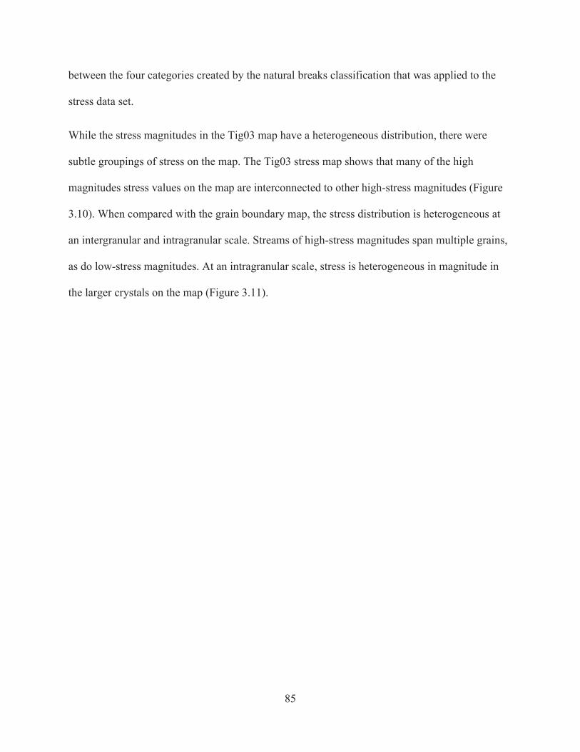
85

between the four categories created by the natural breaks classification that was applied to the

stress data set.

While the stress magnitudes in the Tig03 map have a heterogeneous distribution, there were

subtle groupings of stress on the map. The Tig03 stress map shows that many of the high

magnitudes stress values on the map are interconnected to other high-stress magnitudes (Figure

3.10). When compared with the grain boundary map, the stress distribution is heterogeneous at

an intergranular and intragranular scale. Streams of high-stress magnitudes span multiple grains,

as do low-stress magnitudes. At an intragranular scale, stress is heterogeneous in magnitude in

the larger crystals on the map (Figure 3.11).

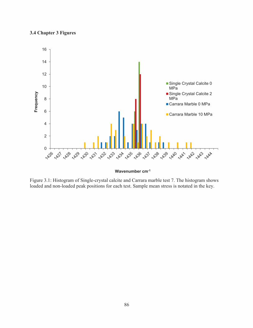
86


Figure 3.1: Histogram of Single-crystal calcite and Carrara marble test 7. The histogram shows loaded and non-loaded peak positions for each test. Sample mean stress is notated in the key.

0

2

4

6

8

10

12

14

16

Freq

uenc

y

Wavenumber cm-1

Single Crystal Calcite 0MPaSingle Crystal Calcite 2MPaCarrara Marble 0 MPa

Carrara Marble 10 MPa

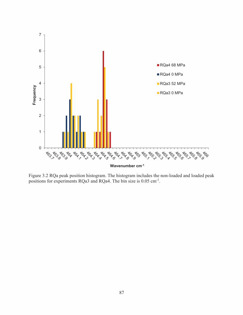
87

Figure 3.2 RQa peak position histogram. The histogram includes the non-loaded and loaded peak positions for experiments RQa3 and RQa4. The bin size is 0.05 cm-1.

0

1

2

3

4

5

6

7Fr

eque

ncy

Wavenumber cm-1

RQa4 68 MPa

RQa4 0 MPa

RQa3 52 MPa

RQa3 0 MPa

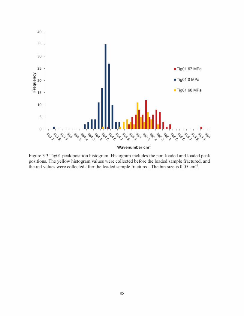
88

Figure 3.3 Tig01 peak position histogram. Histogram includes the non-loaded and loaded peak positions. The yellow histogram values were collected before the loaded sample fractured, and the red values were collected after the loaded sample fractured. The bin size is 0.05 cm-1.

0

5

10

15

20

25

30

35

40Fr

eque

ncy

Wavenumber cm-1

Tig01 67 MPa

Tig01 0 MPa

Tig01 60 MPa

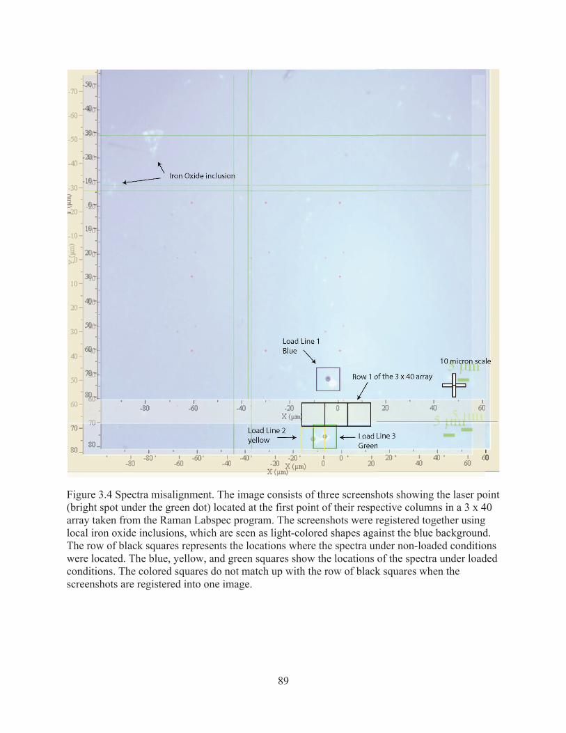
89

Figure 3.4 Spectra misalignment. The image consists of three screenshots showing the laser point (bright spot under the green dot) located at the first point of their respective columns in a 3 x 40 array taken from the Raman Labspec program. The screenshots were registered together using local iron oxide inclusions, which are seen as light-colored shapes against the blue background. The row of black squares represents the locations where the spectra under non-loaded conditions were located. The blue, yellow, and green squares show the locations of the spectra under loaded conditions. The colored squares do not match up with the row of black squares when the screenshots are registered into one image.

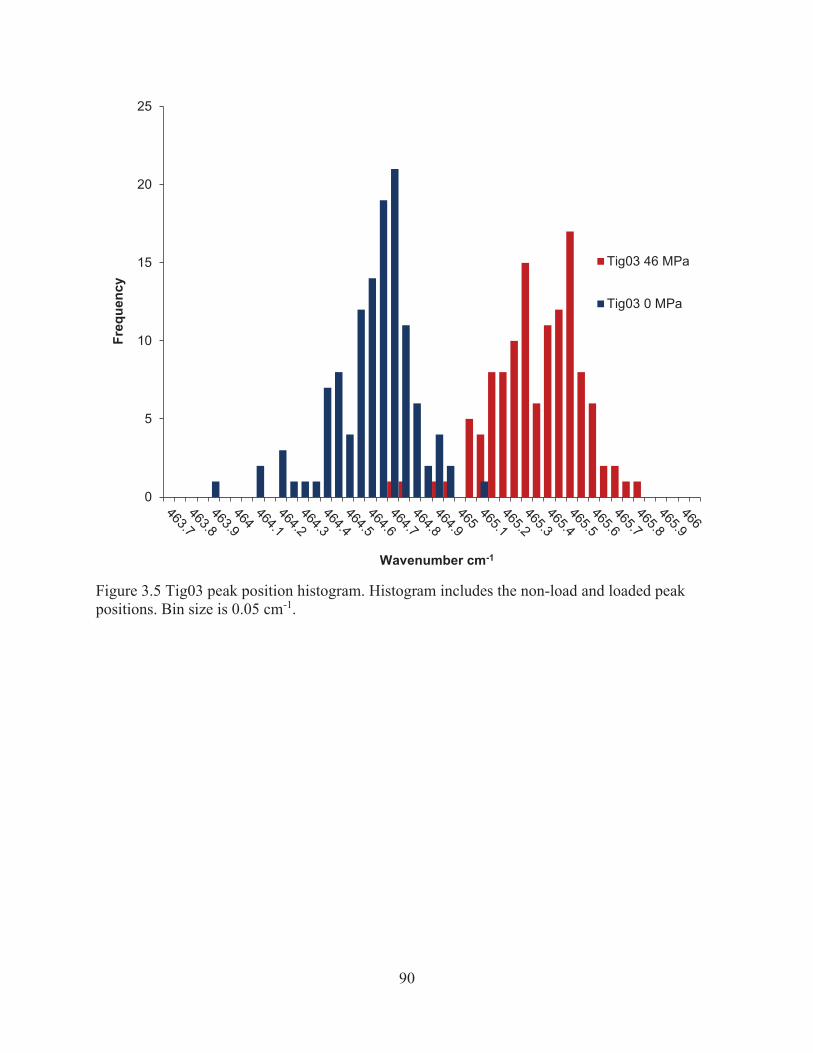
90

Figure 3.5 Tig03 peak position histogram. Histogram includes the non-load and loaded peak positions. Bin size is 0.05 cm-1.

0

5

10

15

20

25Fr

eque

ncy

Wavenumber cm-1

Tig03 46 MPa

Tig03 0 MPa

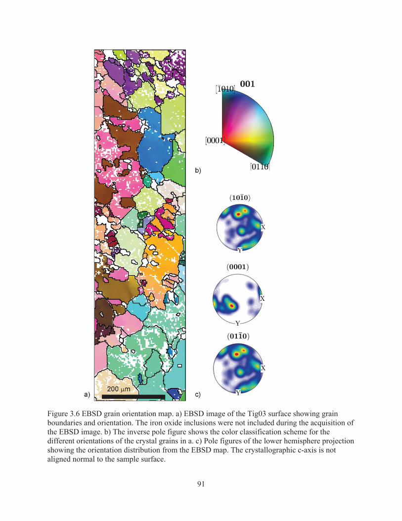
91

Figure 3.6 EBSD grain orientation map. a) EBSD image of the Tig03 surface showing grain boundaries and orientation. The iron oxide inclusions were not included during the acquisition of the EBSD image. b) The inverse pole figure shows the color classification scheme for the different orientations of the crystal grains in a. c) Pole figures of the lower hemisphere projection showing the orientation distribution from the EBSD map. The crystallographic c-axis is not aligned normal to the sample surface.

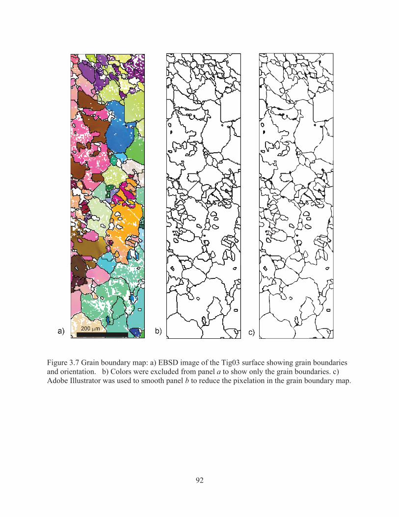
92

Figure 3.7 Grain boundary map: a) EBSD image of the Tig03 surface showing grain boundaries and orientation. b) Colors were excluded from panel a to show only the grain boundaries. c) Adobe Illustrator was used to smooth panel b to reduce the pixelation in the grain boundary map.

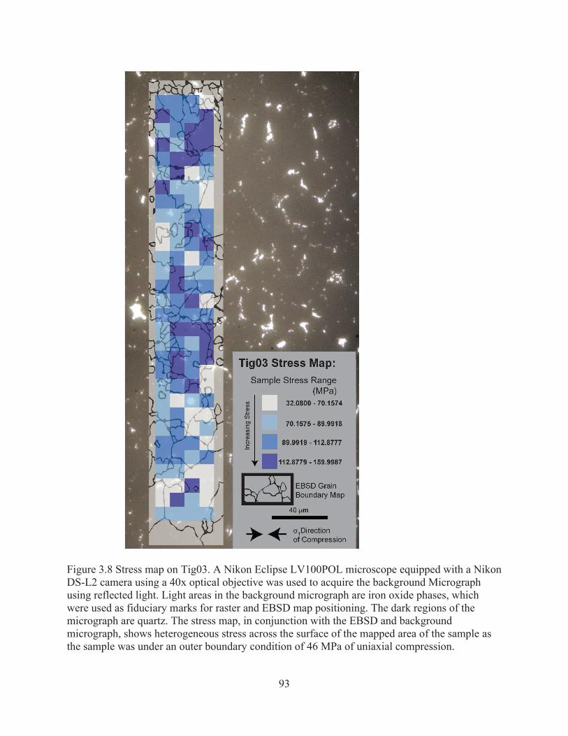
93

Figure 3.8 Stress map on Tig03. A Nikon Eclipse LV100POL microscope equipped with a Nikon DS-L2 camera using a 40x optical objective was used to acquire the background Micrograph using reflected light. Light areas in the background micrograph are iron oxide phases, which were used as fiduciary marks for raster and EBSD map positioning. The dark regions of the micrograph are quartz. The stress map, in conjunction with the EBSD and background micrograph, shows heterogeneous stress across the surface of the mapped area of the sample as the sample was under an outer boundary condition of 46 MPa of uniaxial compression.

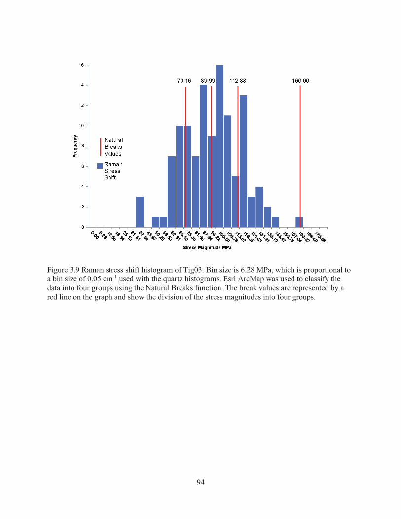
94

Figure 3.9 Raman stress shift histogram of Tig03. Bin size is 6.28 MPa, which is proportional to a bin size of 0.05 cm-1 used with the quartz histograms. Esri ArcMap was used to classify the data into four groups using the Natural Breaks function. The break values are represented by a red line on the graph and show the division of the stress magnitudes into four groups.

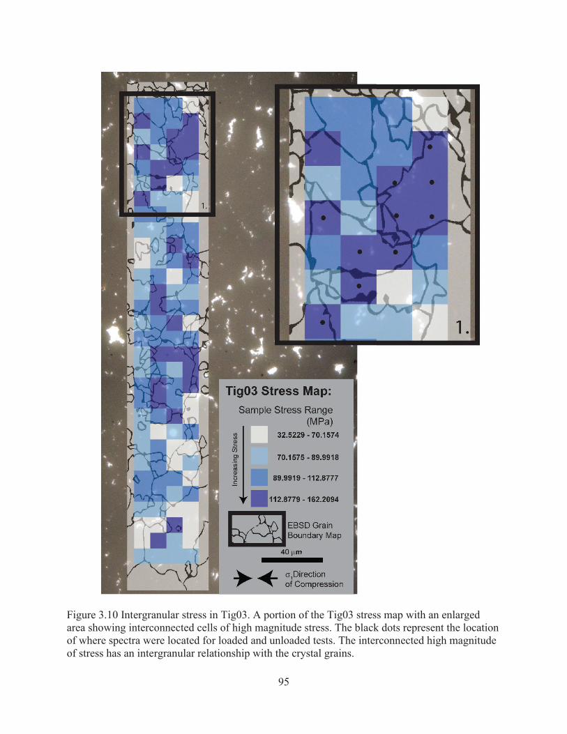
95

Figure 3.10 Intergranular stress in Tig03. A portion of the Tig03 stress map with an enlarged area showing interconnected cells of high magnitude stress. The black dots represent the location of where spectra were located for loaded and unloaded tests. The interconnected high magnitude of stress has an intergranular relationship with the crystal grains.

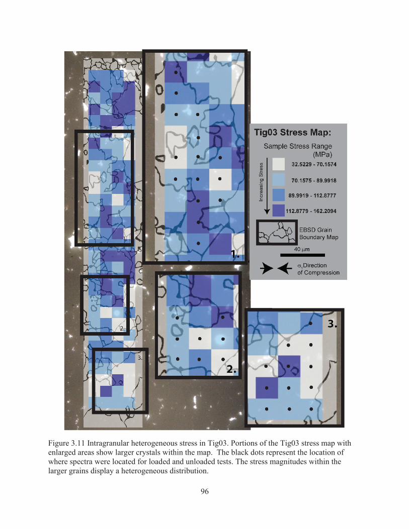
96

Figure 3.11 Intragranular heterogeneous stress in Tig03. Portions of the Tig03 stress map with enlarged areas show larger crystals within the map. The black dots represent the location of where spectra were located for loaded and unloaded tests. The stress magnitudes within the larger grains display a heterogeneous distribution.

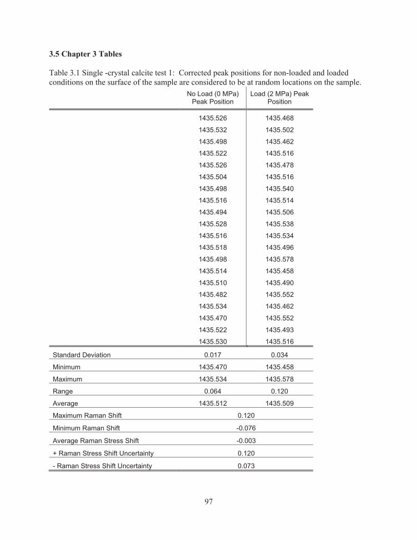
97

3.5 Chapter 3 Tables

Table 3.1 Single -crystal calcite test 1: Corrected peak positions for non-loaded and loaded conditions on the surface of the sample are considered to be at random locations on the sample. No Load (0 MPa)

Peak Position Load (2 MPa) Peak

Position 1435.526 1435.468

1435.532 1435.502 1435.498 1435.462 1435.522 1435.516 1435.526 1435.478 1435.504 1435.516 1435.498 1435.540 1435.516 1435.514 1435.494 1435.506 1435.528 1435.538 1435.516 1435.534 1435.518 1435.496 1435.498 1435.578 1435.514 1435.458 1435.510 1435.490 1435.482 1435.552 1435.534 1435.462 1435.470 1435.552 1435.522 1435.493

1435.530 1435.516

Standard Deviation 0.017 0.034

Minimum 1435.470 1435.458

Maximum 1435.534 1435.578

Range 0.064 0.120

Average 1435.512 1435.509

Maximum Raman Shift 0.120

Minimum Raman Shift -0.076

Average Raman Stress Shift -0.003

+ Raman Stress Shift Uncertainty 0.120

- Raman Stress Shift Uncertainty 0.073

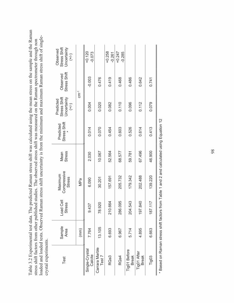
98

Tabl

e 3.

2 Ex

perim

enta

l tes

t dat

a. T

he p

redi

cted

Ram

an st

ress

shift

was

cal

cula

ted

usin

g th

e m

ean

stre

ss o

n th

e sa

mpl

e an

d th

e R

aman

st

ress

shift

fact

ors f

rom

oth

er p

ublis

hed

stud

ies.

The

obse

rved

stre

ss sh

ift w

as m

easu

red

on th

e R

aman

spec

trom

eter

thro

ugh

non

load

ed a

nd lo

aded

test

s. O

bser

ved

Ram

an st

ress

shift

unc

erta

inty

is fr

om th

e m

inim

um a

nd m

axim

um R

aman

stre

ss sh

ift o

f sin

gle-

crys

tal e

xper

imen

ts.

Test

Sa

mpl

e Ar

ea

Load

Cel

l St

ress

Max

imum

C

ompr

essi

ve

Stre

ss

Mea

n St

ress

Pred

icte

d St

ress

Shi

ft *

Pred

icte

d St

ress

Shi

ft U

ncer

tain

ty

(+/-)

Obs

erve

d St

ress

Shi

ft

Obs

erve

d St

ress

Shi

ft U

ncer

tain

ty

(+/-)

(mm

) M

Pa

cm-1

Sing

le-C

ryst

al

Cal

cite

7.

764

9.43

7 6.

090

2.03

0 0.

014

0.00

4 -0

.003

+0

.120

-0

.073

C

arra

ra M

arbl

e Te

st 7

13

.105

78

.920

30

.201

10

.067

0.

070

0.02

0 0.

476

RQ

a3

6.69

3 21

0.66

4 15

7.69

1 52

.564

0.

454

0.08

2 0.

419

+0.2

58

-0.2

61

RQ

a4

6.96

7 28

6.09

5 20

5.73

2 68

.577

0.

603

0.11

0 0.

468

+0.2

47

-0.2

85

Tig0

1 Be

fore

Br

eak

5.71

4 20

4.54

3 17

9.34

2 59

.781

0.

526

0.09

6 0.

486

Ti

g01

Afte

r Br

eak

4.89

5 19

7.84

0 20

2.48

8 67

.496

0.

614

0.11

2 0.

642

Tig0

3 6.

663

187.

117

139.

220

46.9

00

0.41

3 0.

079

0.74

1

* Bas

ed o

n R

aman

stre

ss s

hift

fact

ors

from

Tab

le 1

and

2 a

nd c

alcu

late

d us

ing

Equa

tion

12

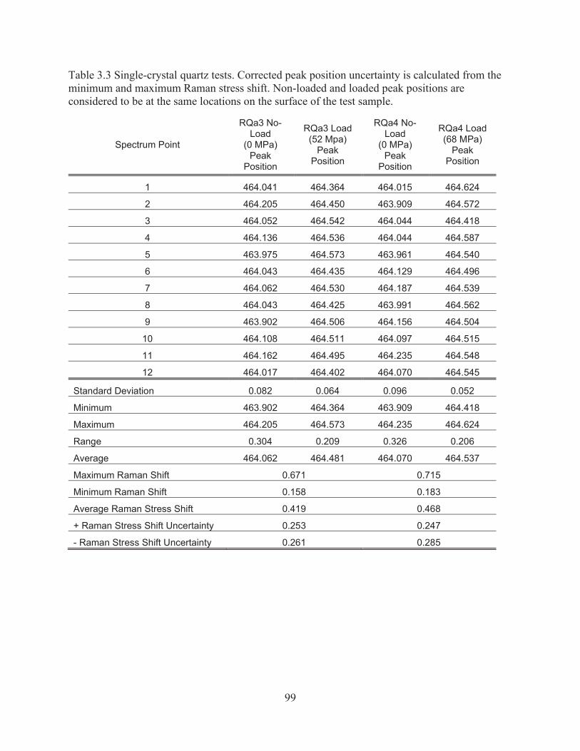
99

Table 3.3 Single-crystal quartz tests. Corrected peak position uncertainty is calculated from the minimum and maximum Raman stress shift. Non-loaded and loaded peak positions are considered to be at the same locations on the surface of the test sample.

Spectrum Point

RQa3 No-Load

(0 MPa) Peak

Position

RQa3 Load (52 Mpa)

Peak Position

RQa4 No-Load

(0 MPa) Peak

Position

RQa4 Load (68 MPa)

Peak Position

1 464.041 464.364 464.015 464.624

2 464.205 464.450 463.909 464.572

3 464.052 464.542 464.044 464.418

4 464.136 464.536 464.044 464.587

5 463.975 464.573 463.961 464.540

6 464.043 464.435 464.129 464.496

7 464.062 464.530 464.187 464.539

8 464.043 464.425 463.991 464.562

9 463.902 464.506 464.156 464.504

10 464.108 464.511 464.097 464.515

11 464.162 464.495 464.235 464.548

12 464.017 464.402 464.070 464.545

Standard Deviation 0.082 0.064 0.096 0.052

Minimum 463.902 464.364 463.909 464.418

Maximum 464.205 464.573 464.235 464.624

Range 0.304 0.209 0.326 0.206

Average 464.062 464.481 464.070 464.537

Maximum Raman Shift 0.671 0.715

Minimum Raman Shift 0.158 0.183

Average Raman Stress Shift 0.419 0.468

+ Raman Stress Shift Uncertainty 0.253 0.247

- Raman Stress Shift Uncertainty 0.261 0.285

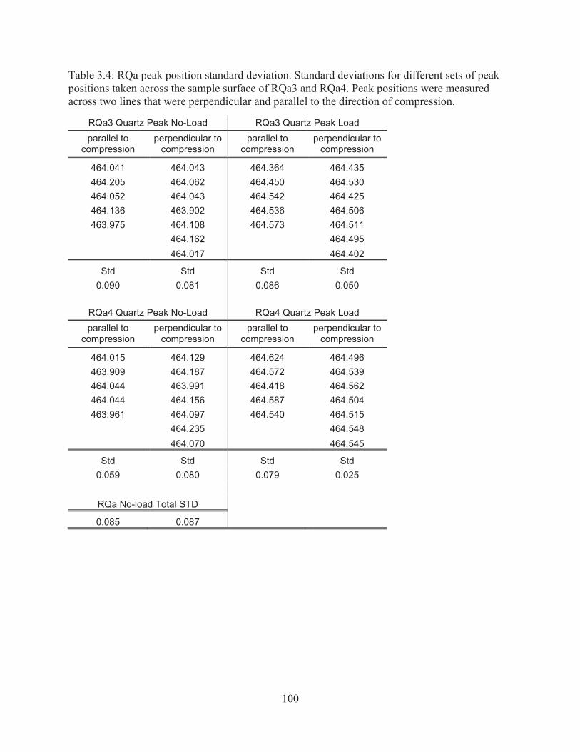
100

Table 3.4: RQa peak position standard deviation. Standard deviations for different sets of peak positions taken across the sample surface of RQa3 and RQa4. Peak positions were measured across two lines that were perpendicular and parallel to the direction of compression.

RQa3 Quartz Peak No-Load RQa3 Quartz Peak Load parallel to

compression perpendicular to

compression parallel to


compression

464.041 464.043 464.364 464.435 464.205 464.062 464.450 464.530 464.052 464.043 464.542 464.425 464.136 463.902 464.536 464.506 463.975 464.108 464.573 464.511

464.162 464.495 464.017 464.402

Std Std Std Std 0.090 0.081 0.086 0.050

RQa4 Quartz Peak No-Load RQa4 Quartz Peak Load parallel to


compression parallel to


compression

464.015 464.129 464.624 464.496 463.909 464.187 464.572 464.539 464.044 463.991 464.418 464.562 464.044 464.156 464.587 464.504 463.961 464.097 464.540 464.515

464.235 464.548 464.070 464.545

Std Std Std Std 0.059 0.080 0.079 0.025

RQa No-load Total STD 0.085 0.087

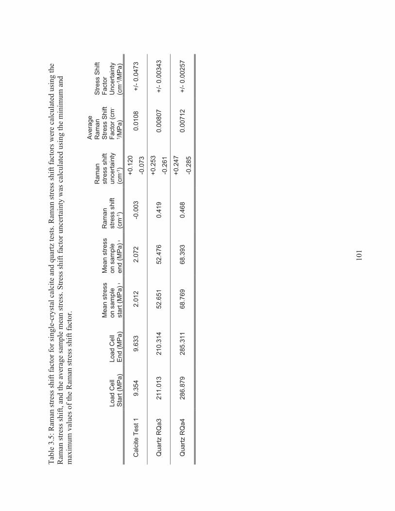
101

Tabl

e 3.

5: R

aman

stre

ss sh

ift fa

ctor

for s

ingl

e-cr

ysta

l cal

cite

and

qua

rtz te

sts.

Ram

an st

ress

shift

fact

ors w

ere

calc

ulat

ed u

sing

the

Ram

an st

ress

shift

, and

the

aver

age

sam

ple

mea

n st

ress

. Stre

ss sh

ift fa

ctor

unc

erta

inty

was

cal

cula

ted

usin

g th

e m

inim

um a

nd

max

imum

val

ues o

f the

Ram

an st

ress

shift

fact

or.

Lo

ad C

ell

Star

t (M

Pa)

Load

Cel

l En

d (M

Pa)

Mea

n st

ress

on

sam

ple

Mea

n st

ress

on

sam

ple

Ram

an

stre

ss s

hift

(cm

-1)

Ram

an

stre

ss s

hift

unce

rtain

ty

(cm

-1)

Aver

age

Ram

an

Stre

ss S

hift

Fact

or (c

m-

1 /MPa

)

Stre

ss S

hift

Fact

or

Unc

erta

inty

(c

m-1

/MPa

)

Cal

cite

Tes

t 1

9.35

4 9.

633

2.01

2 2.

072

-0.0

03

+0.1

20

0.01

08

+/- 0

.047

3 -0

.073

Qua

rtz R

Qa3

21

1.01

3 21

0.31

4 52

.651

52

.476

0.

419

+0.2

53

0.00

807

+/- 0

.003

43

-0.2

61

Qua

rtz R

Qa4

28

6.87

9 28

5.31

1 68

.769

68

.393

0.

468

+0.2

47

0.00

712

+/- 0

.002

57

-0.2

85

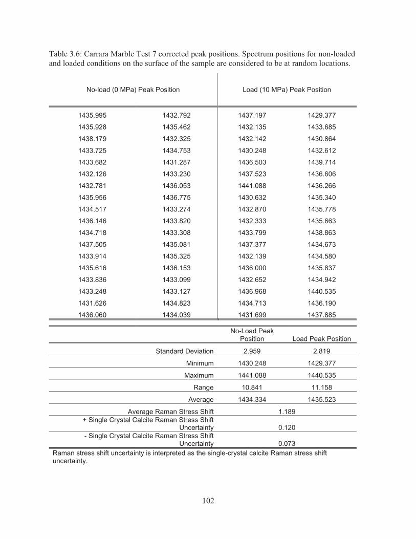
102

Table 3.6: Carrara Marble Test 7 corrected peak positions. Spectrum positions for non-loaded and loaded conditions on the surface of the sample are considered to be at random locations.

No-load (0 MPa) Peak Position Load (10 MPa) Peak Position

1435.995 1432.792 1437.197 1429.377

1435.928 1435.462 1432.135 1433.685

1438.179 1432.325 1432.142 1430.864

1433.725 1434.753 1430.248 1432.612

1433.682 1431.287 1436.503 1439.714

1432.126 1433.230 1437.523 1436.606

1432.781 1436.053 1441.088 1436.266

1435.956 1436.775 1430.632 1435.340

1434.517 1433.274 1432.870 1435.778

1436.146 1433.820 1432.333 1435.663

1434.718 1433.308 1433.799 1438.863

1437.505 1435.081 1437.377 1434.673

1433.914 1435.325 1432.139 1434.580

1435.616 1436.153 1436.000 1435.837

1433.836 1433.099 1432.652 1434.942

1433.248 1433.127 1436.968 1440.535

1431.626 1434.823 1434.713 1436.190

1436.060 1434.039 1431.699 1437.885

No-Load Peak

Position Load Peak Position

Standard Deviation 2.959 2.819

Minimum 1430.248 1429.377

Maximum 1441.088 1440.535

Range 10.841 11.158

Average 1434.334 1435.523

Average Raman Stress Shift 1.189 + Single Crystal Calcite Raman Stress Shift

Uncertainty 0.120 - Single Crystal Calcite Raman Stress Shift

Uncertainty 0.073 Raman stress shift uncertainty is interpreted as the single-crystal calcite Raman stress shift uncertainty.

103

Chapter 4: Discussion and Conclusion

Experimental goals were to discover the type of stress distribution that is prominent in a natural

polycrystal sample using calcite and quartz. While calcite results were unsuccessful,

experimental testing of single-crystal quartz resulted in a reasonable Raman stress shift, a Raman

stress shift factor (RSSF), and a level of uncertainty sufficient to be used in interpreting the

quartz polycrystal tests. The RSSF from the RQa3 test was applied to the polycrystal experiment

Tig03, where the Raman stress shifts were converted to a stress map showing a heterogeneous

stress distribution. The proposed hypothesis is that stress percolation will be the best model that

describes stress distribution in a natural polycrystal.

4.1 Single Crystals

4.1.1 Homogeneous Stress in Single Crystals

An assumption made in this experiment is that a single crystal will homogeneously react to an

external boundary condition. A uniform reaction to stress would result in a narrow distribution of

Raman peak positions. Figure 4.1 shows a comparison between the ranges of quartz single-

crystal and polycrystal Raman peak positions. The non-loaded RQa tests show narrow ranges in

peak position compared with the ranges of the polycrystal peak positions. The standard

deviations (SD) of the peak positions reflect this as well. Furthermore, the SD of the loaded RQa

peak positions is smaller than the unloaded SD of the RQa peak positions. This suggests that

there is a relatively uniform reaction to stress at all measured points on the crystal and supports

the assumption that the stress state in a single crystal is homogeneous.

104

Single crystal calcite did not produce a discernable Raman stress shift at a mean stress of 2 MPa.

Single crystal test failure resulted in the inability to calculate the Raman stress shift factor

(RSSF) and test uncertainty for polycrystal calcite. Uniaxially compressing the single-crystal

calcite to a higher mean stress is not probable as the sample has very low tenacity, because of

this, single-crystal calcite is not a viable material for this experiment.

4.1.2 Raman stress shift factors

The single-crystal quartz RQa tests resulted in RSSFs that were comparable to other published

RSSFs (Table 4.1). Published RSSFs were obtained through hydrostatic diamond anvil testing,

while the RSSFs from the RQa experiments were obtained through uniaxial testing. The different

methods for testing could explain why the RSSF from the RQa tests is slightly lower than the

values from other published studies. In a uniaxial configuration, friction between the sample and

the metal plates of the vice will result from the different Poisson’s ratios of the two materials; as

one seeks to expand more than the other in the transverse direction. Friction at the interface

between sample and metal could be large enough to reduce the amount of compressional strain in

the sample, which would yield a lower Raman stress shift than what would be seen in a

hydrostatic experiment. As a result, the RSSF could be lower. The RQa RSSF was used to

calculate the stress in the Tig03 experiment rather than the published RSSFs since it was

measured using the same experimental geometry.

4.1.3 Test Uncertainty

Accurately measuring the test uncertainty is vital for assessing whether the results for the

polycrystal map are meaningful. It is essential to have a method for accurately calculating

uncertainty that can distinguish between the two possible models proposed in this study, the

105

Reuss iso-stress and stress percolation model. In the Reuss model, stress should be the same

value at each measured point in the polycrystal. As a result, the variation in peak position would

be an appropriate measure of uncertainty for a Reuss model. The stress percolation model

requires a different approach to calculating uncertainty in a polycrystal. In a stress percolation

model, a considerable variation of stress magnitude would be expected and not erroneous.

Residual stress possibly present in the polycrystal samples would also skew uncertainty

comparisons between loaded and non-loaded experiments. As a result, it was necessary to use

uncertainty from single-crystal experiments and apply them to their polycrystal counterparts.

Uncertainty from single-crystal experiments also provides a method to measure uncertainty that

accommodates both possible models.

4.1.4 Uncertainty in Single-crystal Tests

Test uncertainty for the single-crystal Raman stress shift experiments comes from several

sources. There is uncertainty inherent from the Raman spectrometer. Some of this uncertainty is

dealt with by using the plasma emission lines as calibration standards and correcting every

measured spectrum through linear interpolation or extrapolation. The load cell used to measure

the stress in loaded experiments also has uncertainty, a standard deviation of 0.018. Uncertainty

is inherent in the peak fitting process; a standard error of less than 0.05 cm-1 was considered an

acceptable fit for the model. Measurement uncertainty also originates from the single-crystal

samples. The samples used are naturally occurring, with imperfections such as fluid inclusions,

dislocations, and twin boundaries. Any of these imperfections could easily affect the stress

distribution measured in the crystals.

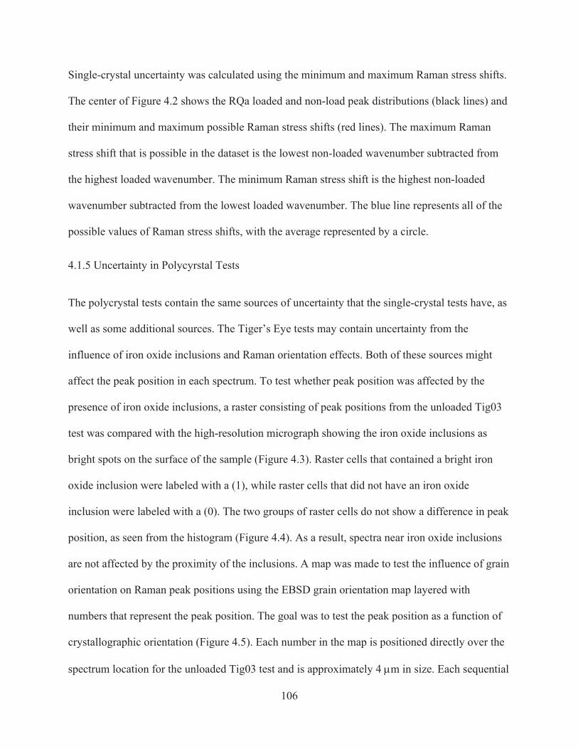
106

Single-crystal uncertainty was calculated using the minimum and maximum Raman stress shifts.

The center of Figure 4.2 shows the RQa loaded and non-load peak distributions (black lines) and

their minimum and maximum possible Raman stress shifts (red lines). The maximum Raman

stress shift that is possible in the dataset is the lowest non-loaded wavenumber subtracted from

the highest loaded wavenumber. The minimum Raman stress shift is the highest non-loaded

wavenumber subtracted from the lowest loaded wavenumber. The blue line represents all of the

possible values of Raman stress shifts, with the average represented by a circle.

4.1.5 Uncertainty in Polycyrstal Tests

The polycrystal tests contain the same sources of uncertainty that the single-crystal tests have, as

well as some additional sources. The Tiger’s Eye tests may contain uncertainty from the

influence of iron oxide inclusions and Raman orientation effects. Both of these sources might

affect the peak position in each spectrum. To test whether peak position was affected by the

presence of iron oxide inclusions, a raster consisting of peak positions from the unloaded Tig03

test was compared with the high-resolution micrograph showing the iron oxide inclusions as

bright spots on the surface of the sample (Figure 4.3). Raster cells that contained a bright iron

oxide inclusion were labeled with a (1), while raster cells that did not have an iron oxide

inclusion were labeled with a (0). The two groups of raster cells do not show a difference in peak

position, as seen from the histogram (Figure 4.4). As a result, spectra near iron oxide inclusions

are not affected by the proximity of the inclusions. A map was made to test the influence of grain

orientation on Raman peak positions using the EBSD grain orientation map layered with

numbers that represent the peak position. The goal was to test the peak position as a function of

crystallographic orientation (Figure 4.5). Each number in the map is positioned directly over the

spectrum location for the unloaded Tig03 test and is approximately 4 m in size. Each sequential

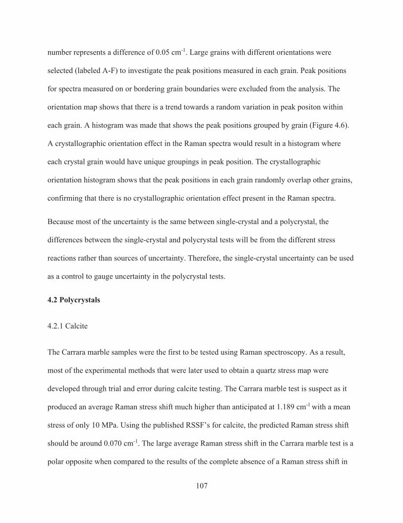
107

number represents a difference of 0.05 cm-1. Large grains with different orientations were

selected (labeled A-F) to investigate the peak positions measured in each grain. Peak positions

for spectra measured on or bordering grain boundaries were excluded from the analysis. The

orientation map shows that there is a trend towards a random variation in peak positon within

each grain. A histogram was made that shows the peak positions grouped by grain (Figure 4.6).

A crystallographic orientation effect in the Raman spectra would result in a histogram where

each crystal grain would have unique groupings in peak position. The crystallographic

orientation histogram shows that the peak positions in each grain randomly overlap other grains,

confirming that there is no crystallographic orientation effect present in the Raman spectra.

Because most of the uncertainty is the same between single-crystal and a polycrystal, the

differences between the single-crystal and polycrystal tests will be from the different stress

reactions rather than sources of uncertainty. Therefore, the single-crystal uncertainty can be used

as a control to gauge uncertainty in the polycrystal tests.

4.2 Polycrystals

4.2.1 Calcite

The Carrara marble samples were the first to be tested using Raman spectroscopy. As a result,

most of the experimental methods that were later used to obtain a quartz stress map were

developed through trial and error during calcite testing. The Carrara marble test is suspect as it

produced an average Raman stress shift much higher than anticipated at 1.189 cm-1 with a mean

stress of only 10 MPa. Using the published RSSF’s for calcite, the predicted Raman stress shift

should be around 0.070 cm-1. The large average Raman stress shift in the Carrara marble test is a

polar opposite when compared to the results of the complete absence of a Raman stress shift in

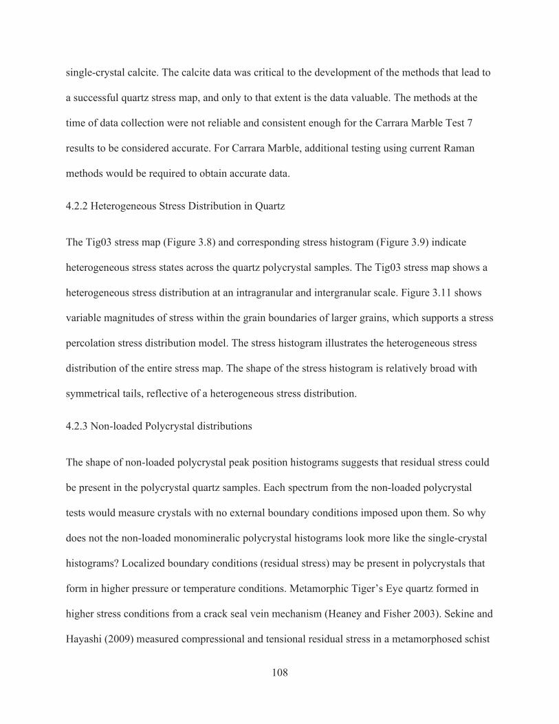
108

single-crystal calcite. The calcite data was critical to the development of the methods that lead to

a successful quartz stress map, and only to that extent is the data valuable. The methods at the

time of data collection were not reliable and consistent enough for the Carrara Marble Test 7

results to be considered accurate. For Carrara Marble, additional testing using current Raman

methods would be required to obtain accurate data.

4.2.2 Heterogeneous Stress Distribution in Quartz

The Tig03 stress map (Figure 3.8) and corresponding stress histogram (Figure 3.9) indicate

heterogeneous stress states across the quartz polycrystal samples. The Tig03 stress map shows a

heterogeneous stress distribution at an intragranular and intergranular scale. Figure 3.11 shows

variable magnitudes of stress within the grain boundaries of larger grains, which supports a stress

percolation stress distribution model. The stress histogram illustrates the heterogeneous stress

distribution of the entire stress map. The shape of the stress histogram is relatively broad with

symmetrical tails, reflective of a heterogeneous stress distribution.

4.2.3 Non-loaded Polycrystal distributions

The shape of non-loaded polycrystal peak position histograms suggests that residual stress could

be present in the polycrystal quartz samples. Each spectrum from the non-loaded polycrystal

tests would measure crystals with no external boundary conditions imposed upon them. So why

does not the non-loaded monomineralic polycrystal histograms look more like the single-crystal

histograms? Localized boundary conditions (residual stress) may be present in polycrystals that

form in higher pressure or temperature conditions. Metamorphic Tiger’s Eye quartz formed in

higher stress conditions from a crack seal vein mechanism (Heaney and Fisher 2003). Sekine and

Hayashi (2009) measured compressional and tensional residual stress in a metamorphosed schist

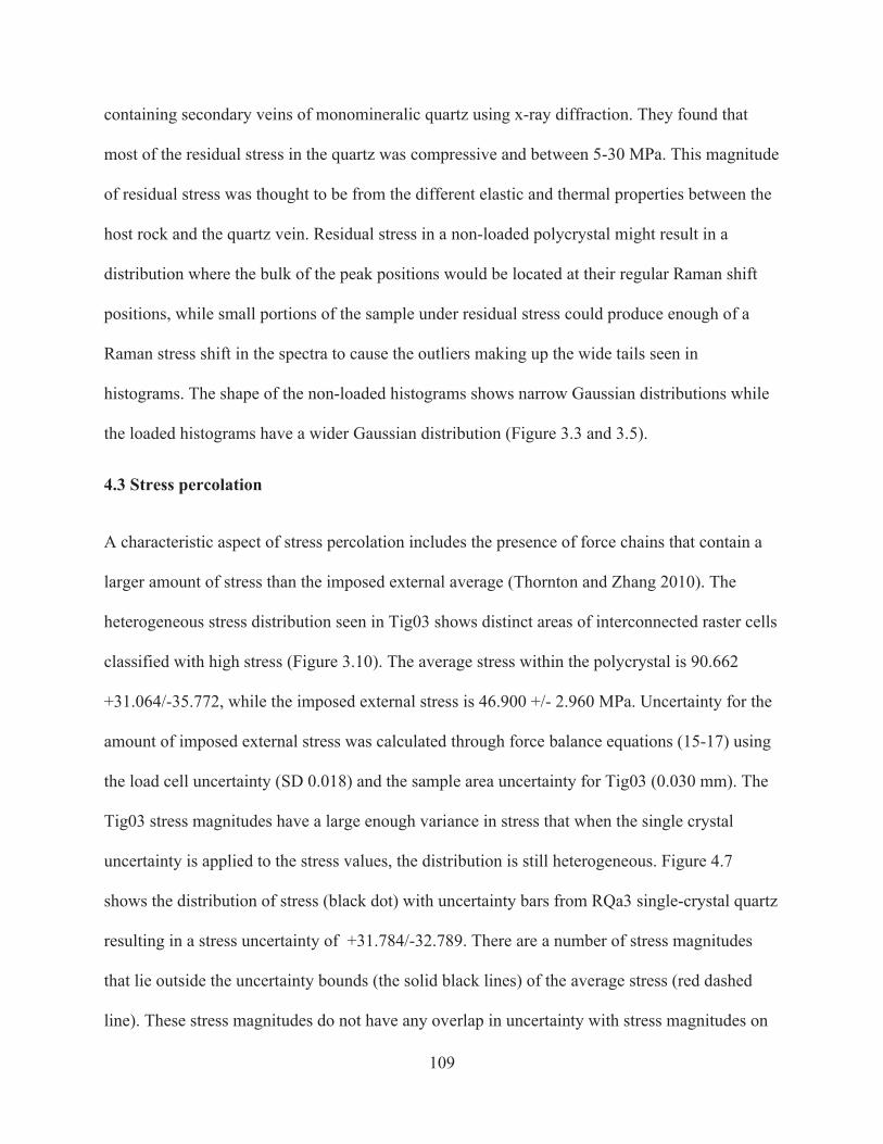
109

containing secondary veins of monomineralic quartz using x-ray diffraction. They found that

most of the residual stress in the quartz was compressive and between 5-30 MPa. This magnitude

of residual stress was thought to be from the different elastic and thermal properties between the

host rock and the quartz vein. Residual stress in a non-loaded polycrystal might result in a

distribution where the bulk of the peak positions would be located at their regular Raman shift

positions, while small portions of the sample under residual stress could produce enough of a

Raman stress shift in the spectra to cause the outliers making up the wide tails seen in

histograms. The shape of the non-loaded histograms shows narrow Gaussian distributions while

the loaded histograms have a wider Gaussian distribution (Figure 3.3 and 3.5).

4.3 Stress percolation

A characteristic aspect of stress percolation includes the presence of force chains that contain a

larger amount of stress than the imposed external average (Thornton and Zhang 2010). The

heterogeneous stress distribution seen in Tig03 shows distinct areas of interconnected raster cells

classified with high stress (Figure 3.10). The average stress within the polycrystal is 90.662

+31.064/-35.772, while the imposed external stress is 46.900 +/- 2.960 MPa. Uncertainty for the

amount of imposed external stress was calculated through force balance equations (15-17) using

the load cell uncertainty (SD 0.018) and the sample area uncertainty for Tig03 (0.030 mm). The

Tig03 stress magnitudes have a large enough variance in stress that when the single crystal

uncertainty is applied to the stress values, the distribution is still heterogeneous. Figure 4.7

shows the distribution of stress (black dot) with uncertainty bars from RQa3 single-crystal quartz

resulting in a stress uncertainty of +31.784/-32.789. There are a number of stress magnitudes

that lie outside the uncertainty bounds (the solid black lines) of the average stress (red dashed

line). These stress magnitudes do not have any overlap in uncertainty with stress magnitudes on

110

the opposite side of the graph. This supports that the overall stress state is still heterogeneous in

nature, with the single crystal uncertainty applied.

Interconnected regions of low magnitude stress are also present in the map and are often near the

high magnitude areas. Some raster cells classified with high magnitude show evidence of linear

patterning, which resembles strong contacts or force chain patterns produced by stress

percolation. The patterns of stress do not show clear evidence of being controlled by grain

boundaries or grain orientations.

4.4 Conclusion

A method has been presented that allows for the measurement of stress on the surface of single-

crystal and polycrystalline materials using Raman spectroscopy. The resultant stress map of

polycrystalline Tiger’s Eye quartz shows 1) intergranular streams of high magnitude stress that

are greater than the amount of average externally imposed stress on the sample, 2) intergranular

regions of low stress that is equal to or lower than the amount of average externally imposed

stress on the sample, 3) large polycrystal grains in the map showing heterogenous intragranular

stress states and, 4) stress patterning not visibly controlled by grain boundaries or grain

orientations.

Experimentation that did not result in a stress map also yielded useful results. The narrow

distributions of peak positions for the quartz data confirm the assumption that a single boundary

condition imposed on a single crystal results in homogeneous stress across the crystal. The clear

Raman stress shift in the single crystal quartz tests resulted in RSSF’s that were within the error

of other published experiments. The magnitudes of the Raman stress shifts measured for single-

crystal quartz were comparable with the quartz polycrystal tests.

111

The calcite tests did not yield quality data due to the inconsistencies in the methods used to

obtain the data. The single-crystal calcite test was ultimately unable to hold enough of a load to

produce a discernable Raman shift, while an experimentally derived Carrara marble Raman

stress shift was far above the predicted Ramans stress shift using the RSSF from other published

experiments.

The experimental results have implications that could change the way we think of stress in the

field of deformation. The experiments support stress percolation as the model that describes the

stress distribution in a polycrystal. The traditional Reuss approximation, used as a foundation in

many deformation studies, contains well known unreasonable assumptions. Individual grains

need to be free to strain without the limitations of their neighboring grains to maintain a Reuss

stress state in a polycrystal. This ultimately creates a space problem, as in reality, the interlocked

grains have neighbors that influence the possible reactions of each grain. The stress percolation

model allows a polycrystal to react to an external boundary condition with a heterogeneous

elastic strain that maintains force balance with localized heterogeneous stress at an intergranular

and intragranular scale. The Tiger’s Eye stress map confirms the heterogeneous distribution of

stress in a polycrystal with a single external boundary condition and is best modeled by stress

percolation. Stress percolation as the mechanism for stress distribution in rocks is important for

deformational science as it unifies micro and macro deformation.

4.5 Future Work

Additional work would be helpful to confirm the results of Tig03 and obtain a larger map with

higher spatial resolution. A larger Raman stress shift map could show a complete picture of a

stress percolation network while taking spectra at closer XY increments would allow for more

112

data points inside crystal grains. Adapting both of these for future testing would give a more

visually intuitive picture for discerning stress percolation. Two experimental problems at the

moment are keeping this from happening. The sample surface needs to be oriented perpendicular

to the laser, so that focus of the Raman beam is not lost as the sample is translated. With better

accuracy in parallel sides, automated Raman mapping can be utilized for either a loaded or

unloaded test, which would significantly reduce the amount of labor-intensive work involved in

collecting spectra. The other problem that would need to be resolved for automated mapping is

the accommodation of strain between the spectra positions between a loaded and unloaded

sample. Elastic strain in Tig03 between the non-loaded and loaded spectrum positions was great

enough that a pre-programmed array would not cover the same points between a loaded and

unloaded sample (Figures 2.27-28). An adaptive mapping program would need to be used that

could adjust points in the array to be in the same locations between loaded and unloaded tests.

Currently, the automated mapping program does not spatially adjust between the original

unstrained location of collected spectra and the new strained location of collected spectra. As

spatial resolution increases on the sample surface, this problem becomes more of an issue.

Additional improvements can also be made to the map by measuring individual components of

the stress tensor at each point. Measurement of the individual stress tensor components would

give a more definitive picture of what is happening inside the stress map.

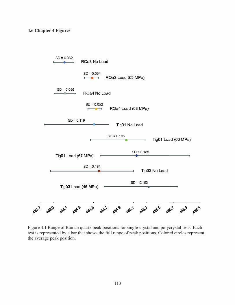
113


Figure 4.1 Range of Raman quartz peak positions for single-crystal and polycrystal tests. Each test is represented by a bar that shows the full range of peak positions. Colored circles represent the average peak position.

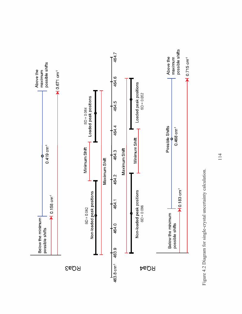
114

Figu

re 4

.2 D

iagr

am fo

r sin

gle-

crys

tal u

ncer

tain

ty c

alcu

latio

n.

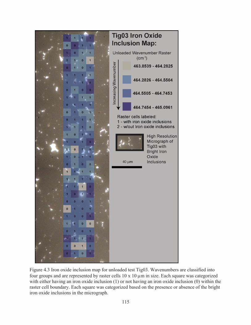
115

Figure 4.3 Iron oxide inclusion map for unloaded test Tig03. Wavenumbers are classified into four groups and are represented by raster cells 10 x 10 m in size. Each square was categorized with either having an iron oxide inclusion (1) or not having an iron oxide inclusion (0) within the raster cell boundary. Each square was categorized based on the presence or absence of the bright iron oxide inclusions in the micrograph.

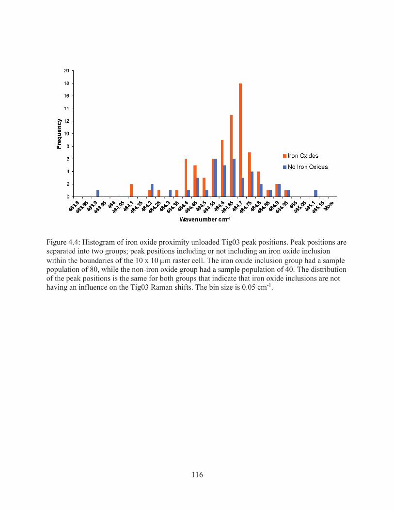
116

Figure 4.4: Histogram of iron oxide proximity unloaded Tig03 peak positions. Peak positions are separated into two groups; peak positions including or not including an iron oxide inclusion within the boundaries of the 10 x 10 m raster cell. The iron oxide inclusion group had a sample population of 80, while the non-iron oxide group had a sample population of 40. The distribution of the peak positions is the same for both groups that indicate that iron oxide inclusions are not having an influence on the Tig03 Raman shifts. The bin size is 0.05 cm-1.

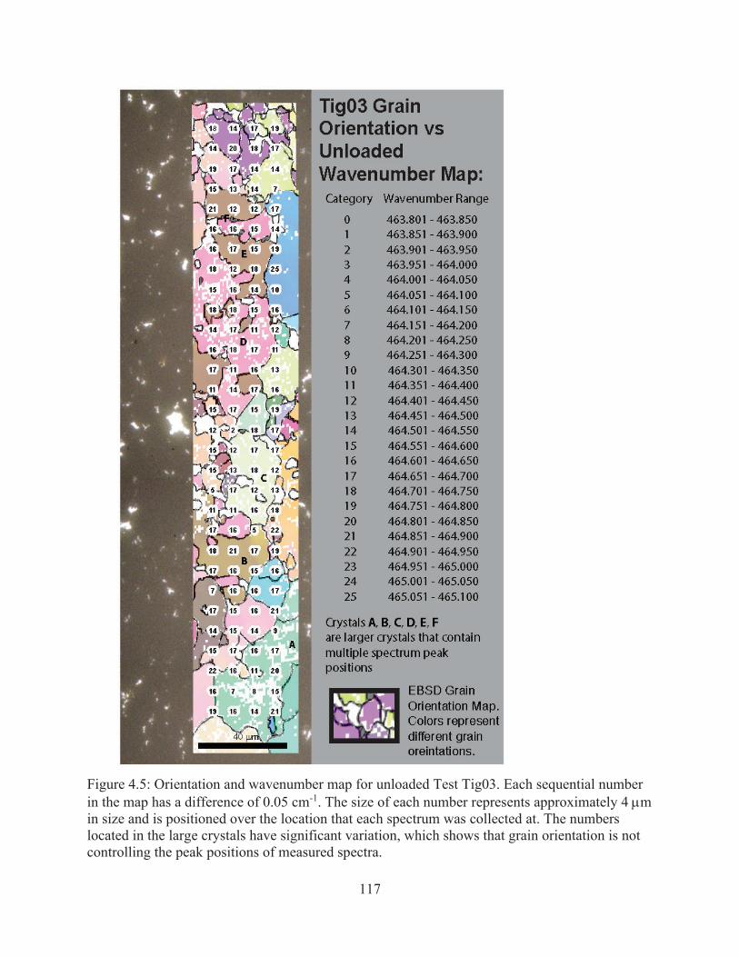
117

Figure 4.5: Orientation and wavenumber map for unloaded Test Tig03. Each sequential number in the map has a difference of 0.05 cm-1. The size of each number represents approximately 4 m in size and is positioned over the location that each spectrum was collected at. The numbers located in the large crystals have significant variation, which shows that grain orientation is not controlling the peak positions of measured spectra.

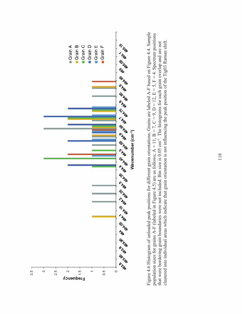
118

Figu

re 4

.6 H

isto

gram

of u

nloa

ded

peak

pos

ition

s for

diff

eren

t gra

in o

rient

atio

ns. G

rain

s are

labe

led

A-F

bas

ed o

n Fi

gure

4.4

. Sam

ple

popu

latio

n si

zes f

orgr

ains

A-F

(lab

eled

in F

igur

e 4.

5) a

re a

s fol

low

s; A

= 1

1, B

= 7

, C =

9, D

= 1

2, E

= 5

, F =

4. S

pect

rum

pos

ition

s th

at w

ere

bord

erin

g gr

ain

boun

darie

s wer

e no

t inc

lude

d. B

in si

ze is

0.0

5 cm

-1. T

he h

isto

gram

s for

eac

h gr

ain

over

lap

and

are

not

clus

tere

d in

to in

divi

dual

are

as w

hich

indi

cate

that

gra

in o

rient

atio

n is

not

influ

enci

ng th

e pe

ak p

ositi

on o

f the

Tig

03 R

aman

shift

.

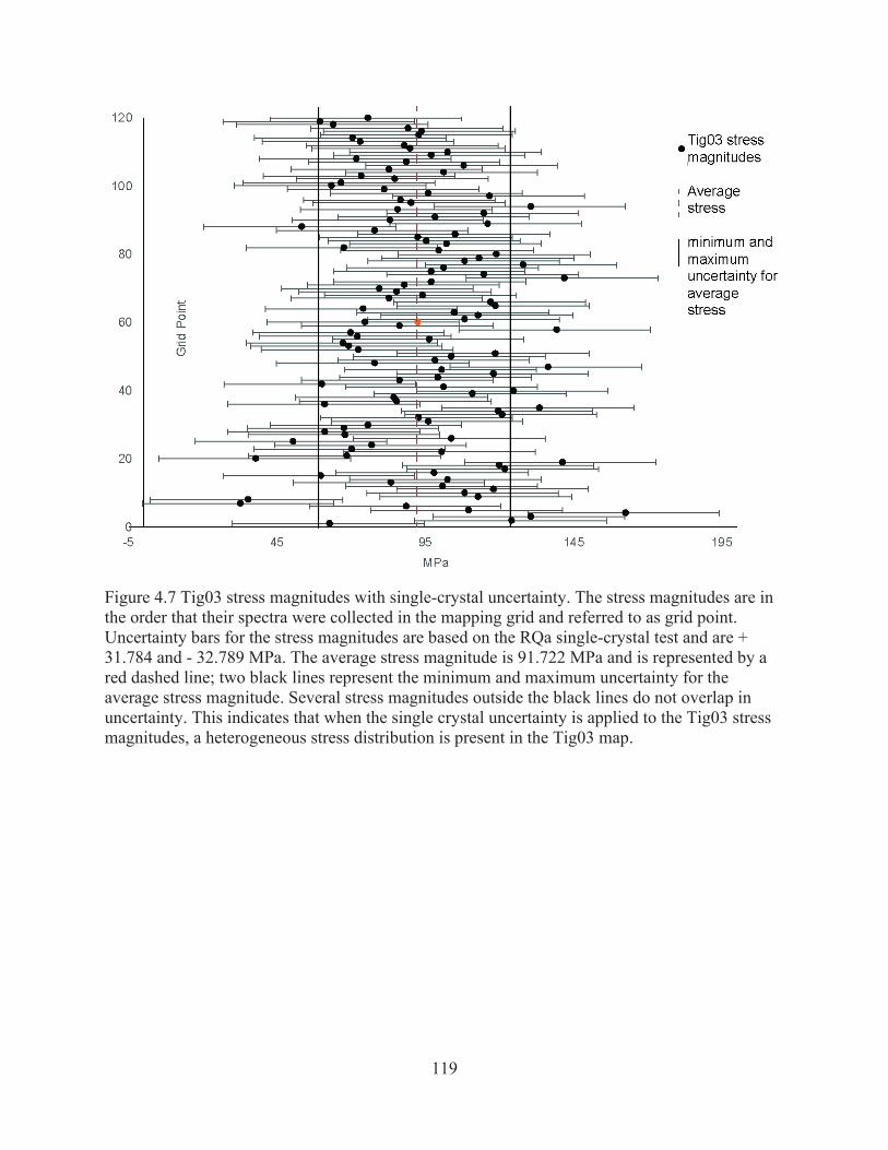
119

Figure 4.7 Tig03 stress magnitudes with single-crystal uncertainty. The stress magnitudes are in the order that their spectra were collected in the mapping grid and referred to as grid point. Uncertainty bars for the stress magnitudes are based on the RQa single-crystal test and are + 31.784 and - 32.789 MPa. The average stress magnitude is 91.722 MPa and is represented by a red dashed line; two black lines represent the minimum and maximum uncertainty for the average stress magnitude. Several stress magnitudes outside the black lines do not overlap in uncertainty. This indicates that when the single crystal uncertainty is applied to the Tig03 stress magnitudes, a heterogeneous stress distribution is present in the Tig03 map.

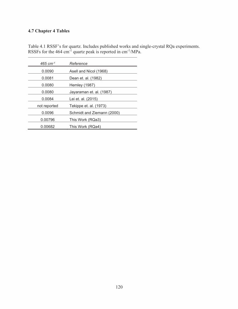
120

4.7 Chapter 4 Tables

Table 4.1 RSSF’s for quartz. Includes published works and single-crystal RQa experiments. RSSFs for the 464 cm-1 quartz peak is reported in cm-1/MPa.

465 cm-1 Reference

0.0090 Asell and Nicol (1968)

0.0081 Dean et. al. (1982)

0.0080 Hemley (1987)

0.0080 Jayaraman et. al. (1987)

0.0084 Lei et. al. (2015)

not reported Tekippe et. al. (1973)

0.0096 Schmidt and Ziemann (2000)

0.00796 This Work (RQa3)

0.00682 This Work (RQa4)

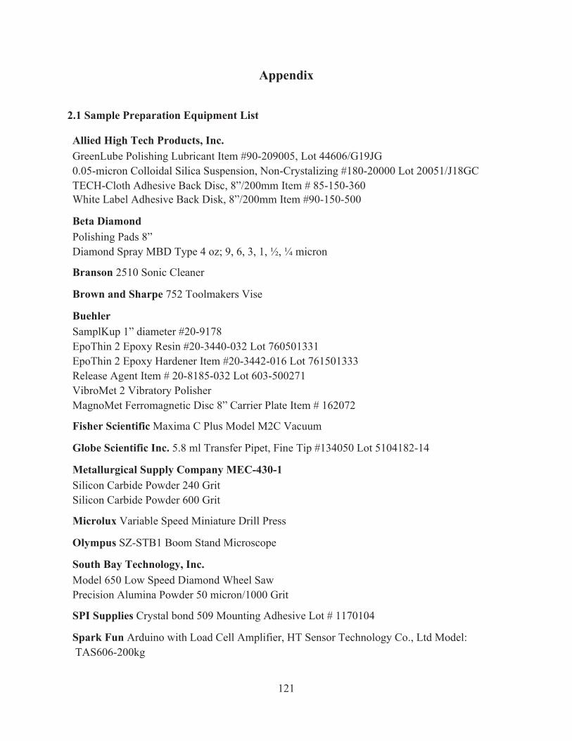
121

Appendix

2.1 Sample Preparation Equipment List

Allied High Tech Products, Inc. GreenLube Polishing Lubricant Item #90-209005, Lot 44606/G19JG 0.05-micron Colloidal Silica Suspension, Non-Crystalizing #180-20000 Lot 20051/J18GC TECH-Cloth Adhesive Back Disc, 8”/200mm Item # 85-150-360 White Label Adhesive Back Disk, 8”/200mm Item #90-150-500 Beta Diamond Polishing Pads 8” Diamond Spray MBD Type 4 oz; 9, 6, 3, 1, ½, ¼ micron Branson 2510 Sonic Cleaner Brown and Sharpe 752 Toolmakers Vise Buehler SamplKup 1” diameter #20-9178 EpoThin 2 Epoxy Resin #20-3440-032 Lot 760501331 EpoThin 2 Epoxy Hardener Item #20-3442-016 Lot 761501333 Release Agent Item # 20-8185-032 Lot 603-500271 VibroMet 2 Vibratory Polisher MagnoMet Ferromagnetic Disc 8” Carrier Plate Item # 162072 Fisher Scientific Maxima C Plus Model M2C Vacuum Globe Scientific Inc. 5.8 ml Transfer Pipet, Fine Tip #134050 Lot 5104182-14 Metallurgical Supply Company MEC-430-1 Silicon Carbide Powder 240 Grit Silicon Carbide Powder 600 Grit Microlux Variable Speed Miniature Drill Press Olympus SZ-STB1 Boom Stand Microscope South Bay Technology, Inc. Model 650 Low Speed Diamond Wheel Saw Precision Alumina Powder 50 micron/1000 Grit SPI Supplies Crystal bond 509 Mounting Adhesive Lot # 1170104 Spark Fun Arduino with Load Cell Amplifier, HT Sensor Technology Co., Ltd Model: TAS606-200kg

122

Ted Pella, Inc. 3M Aluminum Conductive Tape 12.7mm x 16.4m. Product number 16071-1

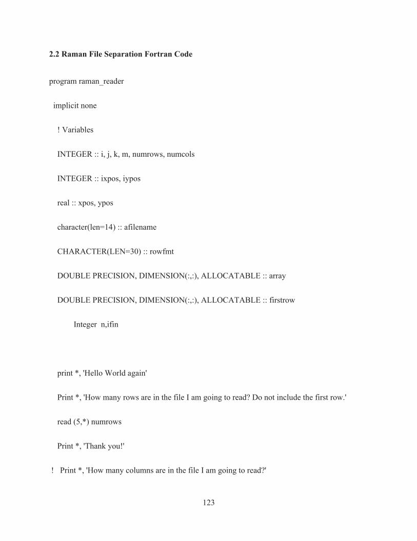
123

2.2 Raman File Separation Fortran Code

program raman_reader

implicit none

! Variables

INTEGER :: i, j, k, m, numrows, numcols

INTEGER :: ixpos, iypos

real :: xpos, ypos

character(len=14) :: afilename

CHARACTER(LEN=30) :: rowfmt

DOUBLE PRECISION, DIMENSION(:,:), ALLOCATABLE :: array

DOUBLE PRECISION, DIMENSION(:,:), ALLOCATABLE :: firstrow

Integer n,ifin

print *, 'Hello World again'

Print *, 'How many rows are in the file I am going to read? Do not include the first row.'

read (5,*) numrows

Print *, 'Thank you!'

! Print *, 'How many columns are in the file I am going to read?'

124

Print *, 'Currently the program is set to read files with the first two columns x and y and then

2050 columns of spectra'

Print *, 'If the file has more we need to revise the program'

! Read (5,*) numcols

! numrows=196

numcols=2050 !PUT IN THE NUMBER OF TOTAL COLUMNS

ALLOCATE(array(numrows,numcols))

ALLOCATE(firstrow(1,numcols))

WRITE(rowfmt,'(A,I4,A)') '(',numcols,'(1X,I6))'

OPEN (UNIT=21,file='ramandata',status='OLD',err=300)

read(21,*) (firstrow(1,k),k=1,2048) !PUT IN THE NUMBER OF TOTAL COLUMNS -2

read(21,*)((array(i,j),j=1,2050),i=1,numrows) !PUT IN THE NUMBER OF TOTAL

COLUMNS

Do 200 m=1,numrows

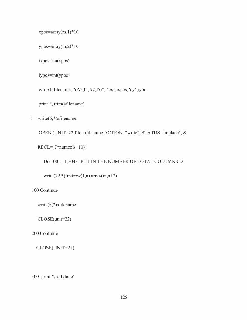
125

xpos=array(m,1)*10

ypos=array(m,2)*10

ixpos=int(xpos)

iypos=int(ypos)

write (afilename, "(A2,I5,A2,I5)") "cx",ixpos,"cy",iypos

print *, trim(afilename)

! write(6,*)afilename

OPEN (UNIT=22,file=afilename,ACTION="write", STATUS="replace", &

RECL=(7*numcols+10))

Do 100 n=1,2048 !PUT IN THE NUMBER OF TOTAL COLUMNS -2

write(22,*)firstrow(1,n),array(m,n+2)

100 Continue

write(6,*)afilename

CLOSE(unit=22)

200 Continue

CLOSE(UNIT=21)

300 print *, 'all done'

126

301 Continue

end program raman_reader

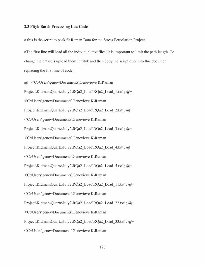
127

2.3 Fityk Batch Processing Lua Code

# this is the script to peak fit Raman Data for the Stress Percolation Project.

#The first line will load all the individual text files. It is important to limit the path length. To

change the datasets upload them in fityk and then copy the script over into this document

replacing the first line of code.

@+ <'C:\Users\genev\Documents\Genevieve K\Raman

Project\Kidman\Quartz\July2\RQa2_Load\RQa2_Load_1.txt' ; @+

<'C:\Users\genev\Documents\Genevieve K\Raman















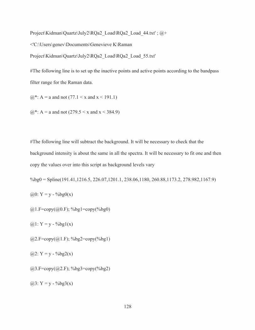
128



Project\Kidman\Quartz\July2\RQa2_Load\RQa2_Load_55.txt'

#The following line is to set up the inactive points and active points according to the bandpass

filter range for the Raman data.

@*: A = a and not (77.1 < x and x < 191.1)

@*: A = a and not (279.5 < x and x < 384.9)

#The following line will subtract the background. It will be necessary to check that the

background intensity is about the same in all the spectra. It will be necessary to fit one and then

copy the values over into this script as background levels vary

%bg0 = Spline(191.41,1216.5, 226.07,1201.1, 238.06,1180, 260.88,1173.2, 278.982,1167.9)

@0: Y = y - %bg0(x)

@1.F=copy(@0.F); %bg1=copy(%bg0)

@1: Y = y - %bg1(x)


@2: Y = y - %bg2(x)


@3: Y = y - %bg3(x)

129


@4: Y = y - %bg4(x)


@5: Y = y - %bg5(x)


@6: Y = y - %bg6(x)


@7: Y = y - %bg7(x)


@8: Y = y - %bg8(x)


@9: Y = y - %bg9(x)

#The following line will fit the three desired peaks, if the peak guessing does not work, it will be

necessary to manually place a peak and then fit that to the rest of the spectra. This will depend on

the intensity of the peak as fityk will fit the most intense followed by the second most intense,

etc...

@*.F += PseudoVoigt(height=~96, center=~206.74, area=~1476.48, hwhm=~7.69)


130


#The final line will export all the peak information and file name into one text file. It is

necessary that the location and name of the text file is set at the end of the pathname. It will

create this file when the script is run successfully.

@*: info filename, peaks >> 'C:\Users\genev\Desktop\Results.txt'

#The best way to make this script work is to fit one dataset and copy and paste the command line

into this script

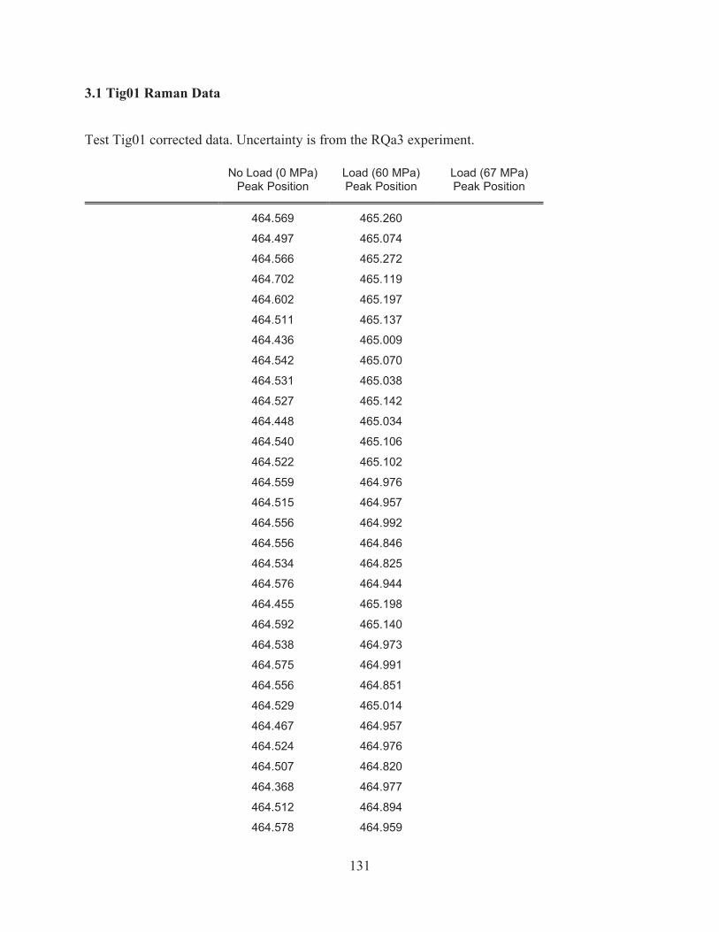
131

3.1 Tig01 Raman Data

Test Tig01 corrected data. Uncertainty is from the RQa3 experiment.

No Load (0 MPa) Peak Position

Load (60 MPa) Peak Position


464.569 465.260

464.497 465.074

464.566 465.272

464.702 465.119

464.602 465.197

464.511 465.137

464.436 465.009

464.542 465.070

464.531 465.038

464.527 465.142

464.448 465.034

464.540 465.106

464.522 465.102

464.559 464.976

464.515 464.957

464.556 464.992

464.556 464.846

464.534 464.825

464.576 464.944

464.455 465.198

464.592 465.140

464.538 464.973

464.575 464.991

464.556 464.851

464.529 465.014

464.467 464.957

464.524 464.976

464.507 464.820

464.368 464.977

464.512 464.894

464.578 464.959

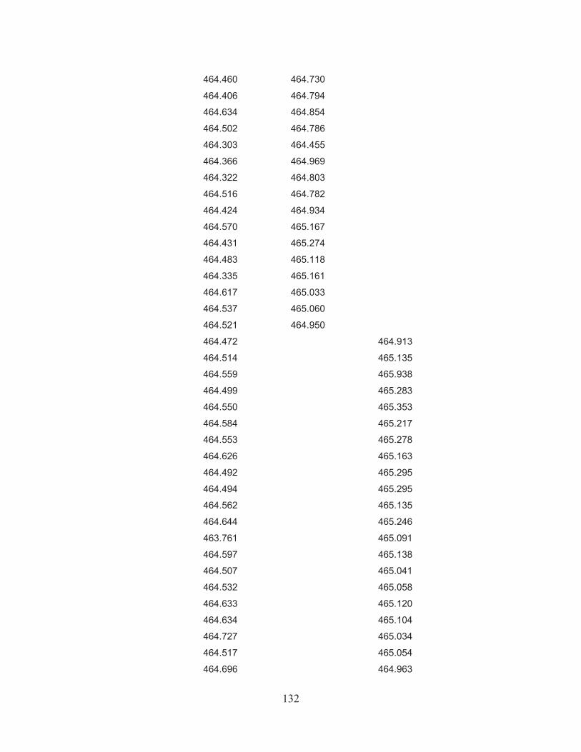
132

464.460 464.730

464.406 464.794

464.634 464.854

464.502 464.786

464.303 464.455

464.366 464.969

464.322 464.803

464.516 464.782

464.424 464.934

464.570 465.167

464.431 465.274

464.483 465.118

464.335 465.161

464.617 465.033

464.537 465.060

464.521 464.950

464.472 464.913

464.514 465.135

464.559 465.938

464.499 465.283

464.550 465.353

464.584 465.217

464.553 465.278

464.626 465.163

464.492 465.295

464.494 465.295

464.562 465.135

464.644 465.246

463.761 465.091

464.597 465.138

464.507 465.041

464.532 465.058

464.633 465.120

464.634 465.104

464.727 465.034

464.517 465.054

464.696 464.963

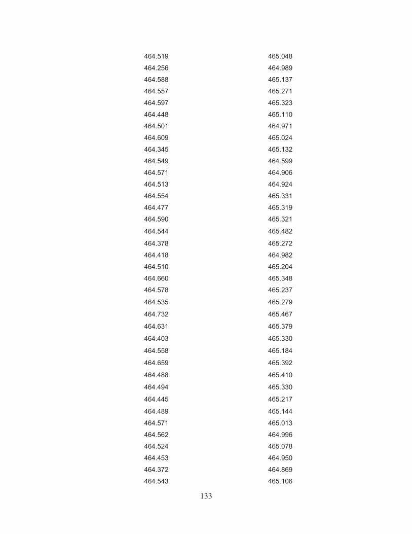
133

464.519 465.048

464.256 464.989

464.588 465.137

464.557 465.271

464.597 465.323

464.448 465.110

464.501 464.971

464.609 465.024

464.345 465.132

464.549 464.599

464.571 464.906

464.513 464.924

464.554 465.331

464.477 465.319

464.590 465.321

464.544 465.482

464.378 465.272

464.418 464.982

464.510 465.204

464.660 465.348

464.578 465.237

464.535 465.279

464.732 465.467

464.631 465.379

464.403 465.330

464.558 465.184

464.659 465.392

464.488 465.410

464.494 465.330

464.445 465.217

464.489 465.144

464.571 465.013

464.562 464.996

464.524 465.078

464.453 464.950

464.372 464.869

464.543 465.106

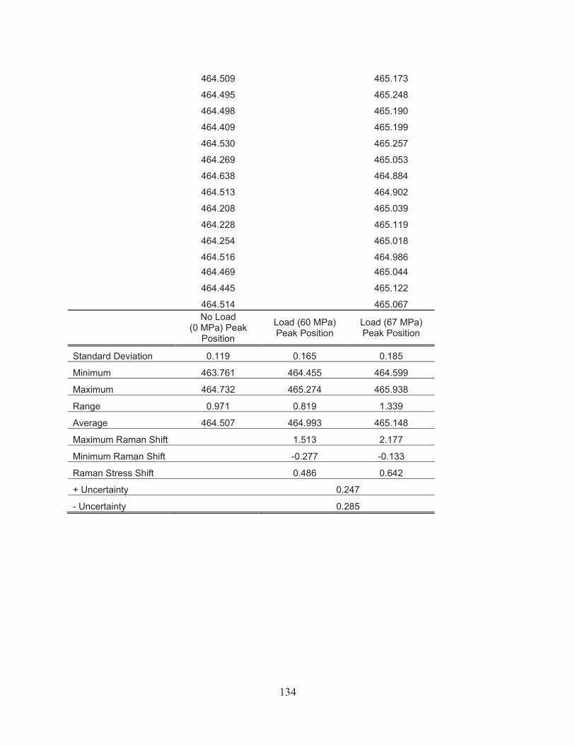
134

464.509 465.173

464.495 465.248

464.498 465.190

464.409 465.199

464.530 465.257

464.269 465.053

464.638 464.884

464.513 464.902

464.208 465.039

464.228 465.119

464.254 465.018

464.516 464.986

464.469 465.044

464.445 465.122

464.514 465.067

No Load (0 MPa) Peak

Position



Standard Deviation 0.119 0.165 0.185

Minimum 463.761 464.455 464.599

Maximum 464.732 465.274 465.938

Range 0.971 0.819 1.339

Average 464.507 464.993 465.148

Maximum Raman Shift 1.513 2.177

Minimum Raman Shift -0.277 -0.133

Raman Stress Shift 0.486 0.642

+ Uncertainty 0.247

- Uncertainty 0.285

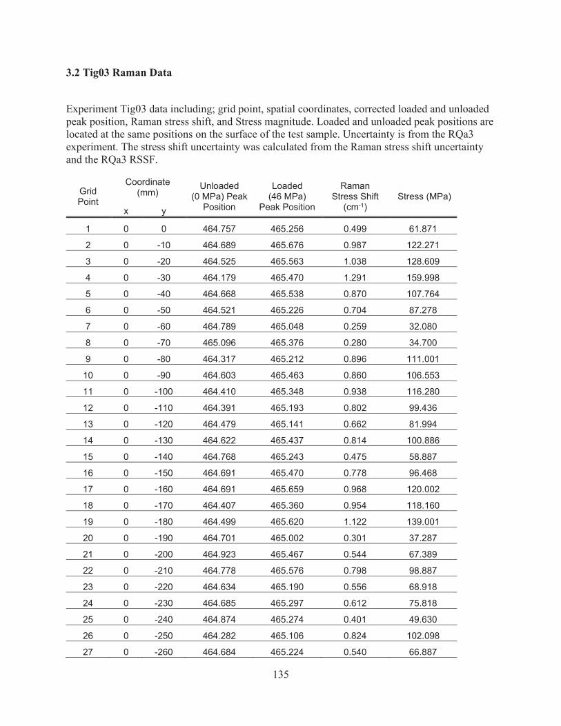
135

3.2 Tig03 Raman Data

Experiment Tig03 data including; grid point, spatial coordinates, corrected loaded and unloaded peak position, Raman stress shift, and Stress magnitude. Loaded and unloaded peak positions are located at the same positions on the surface of the test sample. Uncertainty is from the RQa3 experiment. The stress shift uncertainty was calculated from the Raman stress shift uncertainty and the RQa3 RSSF.

Grid Point

Coordinate (mm)

Unloaded (0 MPa) Peak

Position

Loaded (46 MPa)

Peak Position

Raman Stress Shift

(cm-1) Stress (MPa)

x y

1 0 0 464.757 465.256 0.499 61.871

2 0 -10 464.689 465.676 0.987 122.271

3 0 -20 464.525 465.563 1.038 128.609

4 0 -30 464.179 465.470 1.291 159.998

5 0 -40 464.668 465.538 0.870 107.764

6 0 -50 464.521 465.226 0.704 87.278

7 0 -60 464.789 465.048 0.259 32.080

8 0 -70 465.096 465.376 0.280 34.700

9 0 -80 464.317 465.212 0.896 111.001

10 0 -90 464.603 465.463 0.860 106.553

11 0 -100 464.410 465.348 0.938 116.280

12 0 -110 464.391 465.193 0.802 99.436

13 0 -120 464.479 465.141 0.662 81.994

14 0 -130 464.622 465.437 0.814 100.886

15 0 -140 464.768 465.243 0.475 58.887

16 0 -150 464.691 465.470 0.778 96.468

17 0 -160 464.691 465.659 0.968 120.002

18 0 -170 464.407 465.360 0.954 118.160

19 0 -180 464.499 465.620 1.122 139.001

20 0 -190 464.701 465.002 0.301 37.287

21 0 -200 464.923 465.467 0.544 67.389

22 0 -210 464.778 465.576 0.798 98.887

23 0 -220 464.634 465.190 0.556 68.918

24 0 -230 464.685 465.297 0.612 75.818

25 0 -240 464.874 465.274 0.401 49.630

26 0 -250 464.282 465.106 0.824 102.098

27 0 -260 464.684 465.224 0.540 66.887

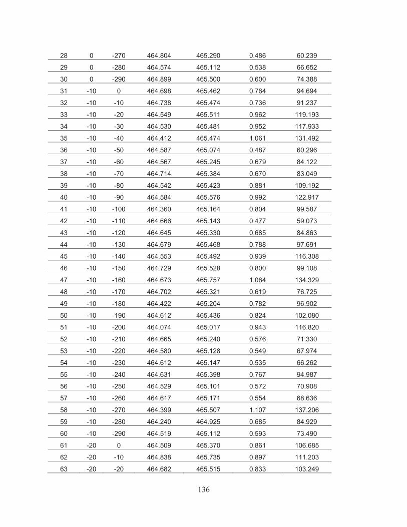
136

28 0 -270 464.804 465.290 0.486 60.239

29 0 -280 464.574 465.112 0.538 66.652

30 0 -290 464.899 465.500 0.600 74.388

31 -10 0 464.698 465.462 0.764 94.694

32 -10 -10 464.738 465.474 0.736 91.237

33 -10 -20 464.549 465.511 0.962 119.193

34 -10 -30 464.530 465.481 0.952 117.933

35 -10 -40 464.412 465.474 1.061 131.492

36 -10 -50 464.587 465.074 0.487 60.296

37 -10 -60 464.567 465.245 0.679 84.122

38 -10 -70 464.714 465.384 0.670 83.049

39 -10 -80 464.542 465.423 0.881 109.192

40 -10 -90 464.584 465.576 0.992 122.917

41 -10 -100 464.360 465.164 0.804 99.587

42 -10 -110 464.666 465.143 0.477 59.073

43 -10 -120 464.645 465.330 0.685 84.863

44 -10 -130 464.679 465.468 0.788 97.691

45 -10 -140 464.553 465.492 0.939 116.308

46 -10 -150 464.729 465.528 0.800 99.108

47 -10 -160 464.673 465.757 1.084 134.329

48 -10 -170 464.702 465.321 0.619 76.725

49 -10 -180 464.422 465.204 0.782 96.902

50 -10 -190 464.612 465.436 0.824 102.080

51 -10 -200 464.074 465.017 0.943 116.820

52 -10 -210 464.665 465.240 0.576 71.330

53 -10 -220 464.580 465.128 0.549 67.974

54 -10 -230 464.612 465.147 0.535 66.262

55 -10 -240 464.631 465.398 0.767 94.987

56 -10 -250 464.529 465.101 0.572 70.908

57 -10 -260 464.617 465.171 0.554 68.636

58 -10 -270 464.399 465.507 1.107 137.206

59 -10 -280 464.240 464.925 0.685 84.929

60 -10 -290 464.519 465.112 0.593 73.490

61 -20 0 464.509 465.370 0.861 106.685

62 -20 -10 464.838 465.735 0.897 111.203

63 -20 -20 464.682 465.515 0.833 103.249

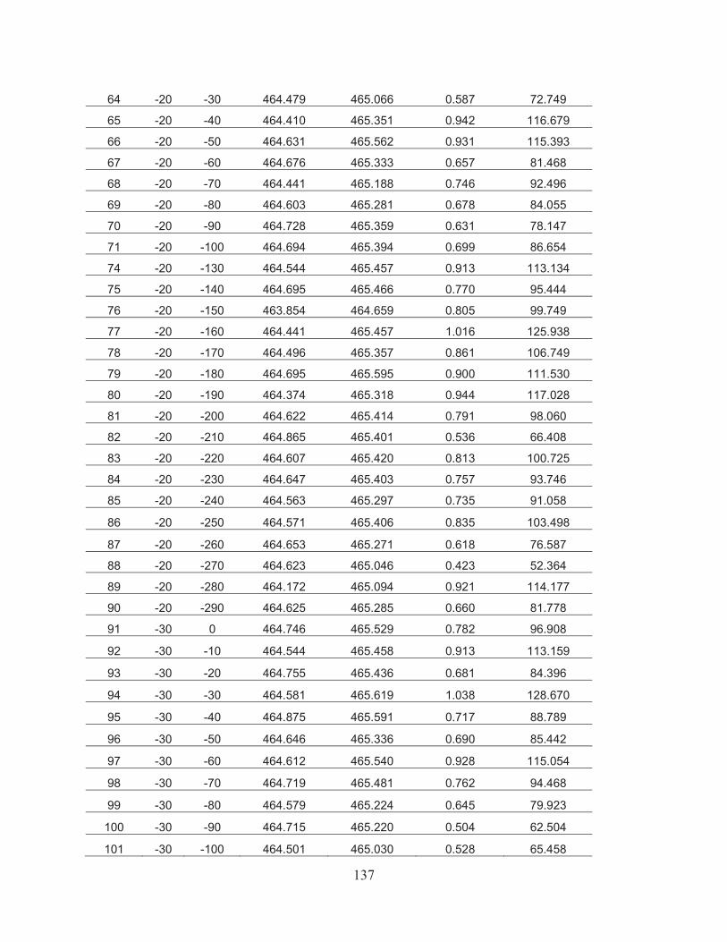
137

64 -20 -30 464.479 465.066 0.587 72.749

65 -20 -40 464.410 465.351 0.942 116.679

66 -20 -50 464.631 465.562 0.931 115.393

67 -20 -60 464.676 465.333 0.657 81.468

68 -20 -70 464.441 465.188 0.746 92.496

69 -20 -80 464.603 465.281 0.678 84.055

70 -20 -90 464.728 465.359 0.631 78.147

71 -20 -100 464.694 465.394 0.699 86.654

74 -20 -130 464.544 465.457 0.913 113.134

75 -20 -140 464.695 465.466 0.770 95.444

76 -20 -150 463.854 464.659 0.805 99.749

77 -20 -160 464.441 465.457 1.016 125.938

78 -20 -170 464.496 465.357 0.861 106.749

79 -20 -180 464.695 465.595 0.900 111.530

80 -20 -190 464.374 465.318 0.944 117.028

81 -20 -200 464.622 465.414 0.791 98.060

82 -20 -210 464.865 465.401 0.536 66.408

83 -20 -220 464.607 465.420 0.813 100.725

84 -20 -230 464.647 465.403 0.757 93.746

85 -20 -240 464.563 465.297 0.735 91.058

86 -20 -250 464.571 465.406 0.835 103.498

87 -20 -260 464.653 465.271 0.618 76.587

88 -20 -270 464.623 465.046 0.423 52.364

89 -20 -280 464.172 465.094 0.921 114.177

90 -20 -290 464.625 465.285 0.660 81.778

91 -30 0 464.746 465.529 0.782 96.908

92 -30 -10 464.544 465.458 0.913 113.159

93 -30 -20 464.755 465.436 0.681 84.396

94 -30 -30 464.581 465.619 1.038 128.670

95 -30 -40 464.875 465.591 0.717 88.789

96 -30 -50 464.646 465.336 0.690 85.442

97 -30 -60 464.612 465.540 0.928 115.054

98 -30 -70 464.719 465.481 0.762 94.468

99 -30 -80 464.579 465.224 0.645 79.923

100 -30 -90 464.715 465.220 0.504 62.504

101 -30 -100 464.501 465.030 0.528 65.458

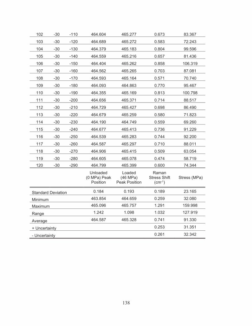
138

102 -30 -110 464.604 465.277 0.673 83.367

103 -30 -120 464.689 465.272 0.583 72.243

104 -30 -130 464.379 465.183 0.804 99.596

105 -30 -140 464.559 465.216 0.657 81.436

106 -30 -150 464.404 465.262 0.858 106.319

107 -30 -160 464.562 465.265 0.703 87.081

108 -30 -170 464.593 465.164 0.571 70.740

109 -30 -180 464.093 464.863 0.770 95.467

110 -30 -190 464.355 465.169 0.813 100.798

111 -30 -200 464.656 465.371 0.714 88.517

112 -30 -210 464.729 465.427 0.698 86.490

113 -30 -220 464.679 465.259 0.580 71.823

114 -30 -230 464.190 464.749 0.559 69.260

115 -30 -240 464.677 465.413 0.736 91.229

116 -30 -250 464.539 465.283 0.744 92.200

117 -30 -260 464.587 465.297 0.710 88.011

118 -30 -270 464.906 465.415 0.509 63.054

119 -30 -280 464.605 465.078 0.474 58.719 120 -30 -290 464.799 465.399 0.600 74.344

Unloaded (0 MPa) Peak

Position

Loaded (46 MPa)

Peak Position

Raman Stress Shift

(cm-1) Stress (MPa)

Standard Deviation 0.184 0.193 0.189 23.165

Minimum 463.854 464.659 0.259 32.080

Maximum 465.096 465.757 1.291 159.998

Range 1.242 1.098 1.032 127.919

Average 464.587 465.328 0.741 91.330

+ Uncertainty 0.253 31.351

- Uncertainty 0.261 32.342

139

Bibliography

Angel, R.J., Allan, D.R., Miletich, R., Finger, LW, 1997, The Use of Quartz as an Internal

Pressure Standard in High -Pressure Crystallography: Journal of Applied Crystallography, v. 30,

p. 461-466.

Adar, F., 2010, Depth Resolution of the Raman Microscope: Optical Limitations and Sample

Characteristics, Spectroscopy Online, http://www.spectroscopyonline.com/depth-resolution-

raman-microscope-optical-limitations-and-sample-characteristics (accessed 9/20/2019).

Asell, J.F., Nicol, M., 1968, Raman Spectrum of Alpha Quartz at High Pressures: The Journal of

Chemical Physics 49, 5396, doi: 10.1063/1.1670064.

Backers, T., Dresen, G., Rybacki, E., Stephansson, O., 2004, New Data on Mode II Fracture

Toughness of Rock from the Punch-Through Shear Test: International Journal of Rock

Mechanics Min. Sci., v. 41, n. 3.

Burnley, P.C., 2013, The Importance of Stress Percolation Patterns in Rocks and other

Polycrystalline Materials: Nature Communications, doi: 10.1038/ncomms3117.

Craig, N.C., Levin, I.W., 1979, Calibrating Raman Spectrometers with Plasma Lines from the

Argon Ion Laser: Applied Spectroscopy, v. 33, n. 5.

Dean, K.J., Sherman, W.F., Wilkinson, G.R., 1982, Temperature and Pressure Dependence of

the Raman Active Modes of Vibration of Alpha Quartz: Spectrochimica Acta, v. 38A, n. 10, p.

1105-1108.

Etchepare, J., Merian, M., Smetankine, L., 1974, Vibrational Normal Modes of SiO2 alpha and

beta Quartz: The Journal of Chemical Physics, v. 60, 1873, doi: 10.1063/1.1681287.

140

Ferraro, J.R., and Nakamoto, K., 2002, Introductory Raman Spectroscopy: Burlington, Elsevier

Science.

Gillet, P., Biellmann, C., Reynard, B., McMillan, P., 1992, Raman Spectroscopic Studies of

Carbonates Part I: High-Pressure and High-Temperature Behavior of Calcite, Magnesite,

Dolomite and Aragonite: Physics and Chemistry of Minerals, v. 20, p. 1-18

Gouadec, G., Coomban, P., 2007, Raman Spectroscopy of Nanomaterials: How Spectra Relate to

Disorder, Particle Size and Mechanical Properties: Progress in Crystal Growth and

Characterization of Materials, 53, 1-56.

Guo, X., Mughal, A., Dunphy, D., Stone, G., Miller, D., Huh, S., 2020, Ambient Temperature-

Corrected Mechanical Stress Mapping of Gallium Nitride and Aluminum Indium Gallium

Phosphide Films by Raman Scattering Spectroscopy for Characterization of Light-Emitting

Diodes: Physics Status Solidi A, doi: 10.1002/pssa.201900776.

Hazen, R.M., Finger, LW, Hemley, R.J., Mao, H.K., 1989, High-Pressure Crystal Chemistry and

Amorphization of alpha Quartz: Solid State Communications, v. 72, n. 5, p. 507-511.

Heaney, P.J., Fisher, D.M., 2003, New Interpretation of the Origin of Tiger’s-Eye: Geology, v.

31, n. 4, p. 323-326.

Hemley, RJ, 1987, Pressure Dependence of Raman Spectra of SiO2 Polymorphs: Alpha Quartz,

Coesite, and Stishovite: High-Pressure Research in Mineral Physics, p. 347-359.

Hibbert, R., Price, M.C., Kinnear, T.M., Cole, J.M., Burchell, M.J., 2015, The Effects of

Temperature on the Raman Spectrum of High Purity Quartz Crystals: 46th Lunar and Planetary

Science Conference, 1826.pdf.

141

Hill, R., 1952, The Elastic Behavior of a Crystalline Aggregate: Proceedings of the Physical

Society Section A, v. 65, p. 349.

Hirsekorn, S., 1990, Elastic Properties of Polycrystals A Review: Textures and Microstructures,

v. 12, p. 1-14.

Howarth, D.F., Rowlands, J.C., 1987, Quantitative Assessment of Rock Texture and Correlation

with Drillability and Strength Properties: Rock Mechanics and Rock Engineering, v. 20, p. 57-

85.

Ikehata, H., Nagasako, N., Furuta, T., Fukumoto, A., Miwa, K., Saito, T., 2004, First-Principles

Calculations for Development of Low Elastic Modulus Ti Alloys: Physical Review B, 70,

174113, doi: 10.1103/PhysRevB.70.174113.

Ismail, K., 2015, Fabrication and Characterization of SERS Substrates Through Photo-

Deposition of Gold Nanoparticles [Ph.D. thesis]:The Abdus Salam International Center for

Theoretical Physics, section 1.5 doi: 10.13140/RG.2.1.4401.0963.

Jannotti, P., Subhash, G., Zheng, J., Halls, V., 2017, Measurement of Microscale Residual

Stresses in Multi-Phase Ceramic Composites using Raman Spectroscopy: Acta Materialia, doi:

10.1016/j.actamat.2017.03.015.

Jayaraman, A., Wood, D.L., Maines, R.G. Sr., 1987, High-pressure Raman Study of the

Vibrational modes in AlPO4 and SiO2: Physical Review B, v. 35, n. 16.

Jiang, T., Lin, Z., Zhang, J., Xu, S., Huang, J., Niu, M., Gao, X., Guo, L., Hao, Y., 2017, Raman

Mapping of Hexagonal Hillocks in N-Polar GaN Grown on c-plane Sapphire: Superlattice and

Microstructures,

142

Kieffer, S.W., 1979, Thermodynamics and Lattice Vibrations of Minerals: Lattice Dynamics and

an Approximation for Minerals with Application to Simple Substances and Framework Silicates:

Reviews of Geophysics and Space Physics, v. 17, n. 1.

Kolesov, B.A., 2016 How the Vibrational Frequency Varies with Temperature: Journal of

Raman Spectroscopy, doi: 10.1002/jrs.5009.

Kumazawa, M., 1969, The elastic constant of polycrystalline rocks and nonelastic behavior

inherent to them: Journal of Geophysical Research, v. 74, p. 5311–5320, doi:

10.1029/jb074i022p05311.

Larkin, P., 2011, Infrared and Raman Spectroscopy Principals and Spectral Interpretation:

Elsevier Science.

Lei, L., Chao-Jia, L., Chun-Qiang, Z., Li, Y., Hong, L., Jian-Guo, D., 2015, First-principles

Simulation of Raman Spectra and Structural Properties of Quartz up to 5 GPa: Chinese Physics

B, 24 127401, doi: 10.1088/1674-1056/24/12/127401.

Lei, Z.K., Qin, F.Y., Fang, Q.C., Bai, R.X., Qiu, W., Chen, X., 2018, Full-Field Fabric Stress

Mapping by Micro Raman Spectroscopy in a Yarn Push-out Test: Applied Optics, v. 57, n. 4 doi:

10.1364/AO.57.000924.

Liu, L., Lv, C., Zhuang, C., Yi, L., Liu, H., Du, J., 2016 Effects of Differential Stress on the

Structure and Raman Spectra of Calcite from First-principles Calculations: American

Mineralogist, v. 101, p. 1892-1897, doi: 10.2138/am-2016-5558.

Liu, L., Mernagh, T.P., 1990, Phase Transitions and Raman Spectra of Calcite at High Pressures

and Room Temperature: American Mineralogist, v. 75, p. 801-806.

143

Logan, J.M., Hastedt, M., Lehnert, D., Denton, M., 1993, A Case Study of the Properties of

Marble as Building Veneer: International Journal of Rock Mechanics, v. 30, n. 7, p. 1531-1537.

Meyer, M.W., 2013, Scanning Angle Raman Spectroscopy: Investigation of Raman Scatter

Enhancement Techniques for Chemical Analysis [Ph.D. thesis]: Iowa State University.

Molli, G., Conti, P., Giorgetti, G., Meccheri, M., Oesterling, N., 2000, Microfabric Study on the

Deformational and Thermal History of the Alpi Apuane Marbles (Carrara Marbles), Italy:

Journal of Structural Geology, v. 22, p. 1809-1825.

Neuville, D., De Ligny, D., Henderson, G.S., 2014, Advances in Raman Spectroscopy Applied to

Earth and Material Sciences: Reviews in Mineralogy and Geochemistry, v. 78, p. 509-541, doi:

10.2138/rmg.2013.78.13.

Nye, J.F., 1985, Physical Properties of Crystals, Their Representation by Tensors and Matrices:

New York, Oxford University Press, p. 329.

Pezzotti, G., 1999, In situ Study of Fracture Mechanisms in Advanced Ceramics using

Fluorescence and Raman Microprobe Spectroscopy: Journal of Raman Spectroscopy, v. 30, p.

867-875.

Reuss, A., 1929, Berechnung der Fließgrenze von Mischkristallen auf Grund der

Plastizitätsbedingung für Einkristalle: Z. Angew, Math. Mech. 9, 49-58.

Rutt, H.N., Nicola, J.H., 1974, Raman Spectra of Carbonates of Calcite Structure: Journal of

Physics C: Solid State Physics, 7 4522.

Sab, K., 1992, On the Homogenization and the Simulation of Random Materials: European

Journal of Mechanics. A, Solids: v. 11, i. 5, p. 585-607.

144

Schmidt, C., Ziemann, M., 2000, In-situ Raman Spectroscopy of Quartz: A Pressure Sensor for

Hydrothermal Diamond-anvil cell Experiments at Elevated Temperatures: American

Mineralogist, v. 85, p. 1725-1734.

Sekine, K., Hayashi, K., 2009, Residual Stress Measurements on a Quartz Vein: A Constraint on

Paleostress Magnitude: Journal of Geophysical Research, v. 114, doi: 10.1029/2007JB005295.

Siegesmund, S., Ruedrich, J., Koch, A., 2008, Marble Bowing: Comparative Studies of Three

Different Public Building Facades: Environmental Geology, v. 56, p. 473-494, doi:

10.1007/s00254-008-1307-z.

Sone, H., Zoback, D., 2013, Mechanical Properties of Shale-gas Reservoir Rocks -Part 1: Static

and Dynamic Elastic Properties and Anisotropy: Geophysics, v. 78, n. 5, doi:10.1190/GEO2013-

0050.1.

Spring, K.R., Davidson, M.W., 2019, Depth of Field and Depth of Focus:

https://www.microscopyu.com/microscopy-basics/depth-of-field-and-depth-of-focus, (accessed

9/20/2019).

Sun, J., Wu, Z., Cheng, H., Zhang, Z., Frost, R.L., 2014, A Raman Spectroscopic Comparison of

Calcite and Dolomite: Spectrochimica Acta Part A: Molecular and biomolecular Spectroscopy,

117, p. 158-162, doi: 10.1016/j.saa.2013.08.014.

Tekippe, VJ, Ramdas, A.K., Rodriguez, S., 1973, Piezospectroscopic Study of the Raman

Spectrum of Alpha Quartz: Physical Review B, v. 8, n. 2.

145

Thornton, C., Zhang, L., 2010, On the Evolution of Stress and Microstructure during General 3D

Deviatoric Straining of Granular Media: Geotechnique, v. 60, n. 5, p. 333-341 doi:

10.1680/geot.2010.60.5.333.

Tullis, T.E., 1980, The Use of Mechanical Twinning in Materials as a Measure of Shear Stress

Magnitudes: Journal of Geophysical Research, v. 85, n. B11, p. 6263-6268.

Tuschel, D., 2014, Practical Group Theory and Raman Spectroscopy, Part I: Normal Vibrational

Modes: Spectroscopy, 29, 14.

Twiss, R.J., and Moores, E.M., 2007, Structural geology: New York, W.H. Freeman.

Voigt, W., 1928, Lehrbuch der Kristallphysik. Leipzig: Teubner-Verlag.

Walker, D.M., Tordesillas, A., Thorton, C., Behringer, R.P., Zhang, J., Peters, J.F., 2011,

Percolating Contact Subnetworks on the Edge of Isostaticity: Granular Matter, 13, p. 233-240,

doi: 10.1007/s20035-011-0250-y.

Wang, Z., Si, B., Chen, S., Jiao, B., Yan, X., 2019, A Nondestructive Raman Spectra Stress 2D

Analysis for the Pressure Sensor Sensitive Silicon Membrane; Engineering Failure Analysis,

105, doi: 10.1016/j.engfailanal.2019.06.089.

Young, R.J., Gong, L.G., Kinloch, I.A., Riaz, I., Jalil, R., Novoselov, K.S. 2011, Strain Mapping

in a Graphene Monolayer Nanocomposite: American Chemical Society, v. 5, n. 4, doi: 10

1031/nn2002079.

Zuddas, P., Salvi, S., Lopez, O., DeGiudici, G., Censi, P., 2018, Rapid Migration of CO2 rich

Microfluids in Calcite Matrices: Nature Scientific Reports, doi: 10.1038/s41598-018-32461-8.

146

Curriculum Vitae

Genevieve C. Kidman [email protected]

Education

Southern Utah University -Geology Professional Bachelors with GIS Certificate, May 2015 College of Southern Nevada -General Science Associate’s, May 2004

Recent Professional Experience University of Las Vegas Nevada -Graduate Assistant

Research Assistant 2017-2020 Teaching Assistant Spring 2020

Southern Utah University -Adjunct Professor Dec 2016 – June 2017

Lecture and Lab -Geo 1050/1055 Geology of the National Parks Lecture and Field Trips to Zion National Park and Great Basin National Park. Created entirely new course content and lesson plans.

Online Lecture and Lab -Geo 1090/1095 How the Earth Works. Created entirely new lesson plans and content.

Field Co-Instructor -Geo 4960 Field Camp. Assisted in the development of new course content while teaching established lesson plans.

Field Co-Instructor -Geo 4000 Structural geology of Arches National Park Field Trip Honors Society Advisor to the Southern Utah University Sigma Gamma Epsilon

Chapter 2016-17 Southern Utah University -Teaching Assistant January 2013 – April 2015

Classes included: Environmental Geology, Sedimentology Stratigraphy, Structural Geology, Physical Geology

lead lecture discussions, geology labs, the development and application of GIS labs, and grading coursework.

U.S. Geological Survey, Montana Water Science Center -Intern May 2014 – August 2014 National Rivers and Stream Assessment through the EPA to sample and evaluate the conditions of the rivers and streams for the state of Montana.

CS Mining -Intern October 2013

Soil sampling project to find a copper ore vein.

Additional Job History Available Upon Request

Educational Volunteer Work Inclusions Rocks Community Outreach Program November 2018-May 2019

147

UNLV Geology Community Outreach May 2019-2020 North Elementary Geology Club Director 2013-2015

Affiliations

American Geophysical Union, 2019 Association of Women Geoscientists, 2019 Member of the Geological Society of America, September 2013 Member of High-Pressure Science and Engineering Center, UNLV, June 2017- June

2018 Member of Sigma Gamma Epsilon, Geological Honors Society, February 2012 – June

2017

Accomplishments

Sigma Gamma Epsilon Tarr Award May 2014 National Science Foundation S-Stem Scholarship 2012-2015 2014 Best Student Paper Award from the Geology and Society Division of the

Geological Society of America Southern Utah University Department of Physical Science Outstanding Research Student

2015

Conference Presentations

Oral Presentation - Measuring Stress States in Polycrystalline Quartz using Raman Spectroscopy.

UNLV Department of Geoscience 15th annual Geo-Symposium 2020. Poster Presentation - Measuring Stress States in Polycrystalline Quartz using Raman

Spectroscopy. National Nuclear Security Administration SSAP Annual Review 2020. American Geophysical Union Fall 2019 Meeting. UNLV Department of Geoscience 14th annual Geo-Symposium 2019. UNLV Department of Geoscience 13th annual Geo-Symposium 2018.

Poster Presentation - New Kinematic Model of the Southern Utah Virgin Anticline Through

New 3-D Stereoscopic and Traditional Field Methods.

Geological Society of America 2015 Poster Presentation - An Analysis of Stereoscopic 3D Geological Mapping Methods Using Cardinal and Esri Systems.

Digital Mapping Techniques, National Geologic Map Database 2015 Southern Utah University Festival of Excellence 2015.

Oral Presentation - Lessons From my Summer Internship: National Rivers and Streams Assessment with the NAGT and USGS.

148

Geological Society of America 2014 Poster Presentation - Evidence of Large-Scale Tectonic Processes on the Tharsis Rise. Mars.

45th Annual Binghamton Geomorphology Symposium, Planetary Geomorphology: University of Tennessee, Knoxville 2014.

Southern Utah University Festival of Excellence 2014. Geological Society of America 2013 WMG COSE Undergraduate Research Symposium 2013.

Publications Cleveland, C, Gerrard, R.M., McLemore, D.M., Yon, J.C.E., Kidman, G.C., and MacLean, J.S.,

2014, Strain Accommodation in the Footwall of the Ruby’s Inn Thrust Fault, Hillsdale Canyon, Southern Utah: The Compass: Earth Science Journal of Sigma Gamma Epsilon: vol. 86: iss. 4, article 2. p. 102-117. http://digitalcommons.csbsju.edu/compass/vol86/iss4/2/

Kidman, G., MacLean, J.S., and Maxwell, D., 2014, Evidence of Large-Scale Tectonic

Processes on the Tharsis Rise, Mars: The Compass: Earth Science Journal of Sigma Gamma Epsilon: vol. 86: iss. 2, article 1, p. 36-52.http://digitalcommons.csbsju.edu/compass/vol86/iss2/1/