ECE 417 c©2018 Bruno Korst CommLab

Experiment # 3

Baseband Pulse Transmission

• Name: Experiment Date:

• Student No.: Day of the week: Time:

• Grade: / 10

RX FilterMATCHED

TX Filter

BIT SOURCE

CHANNEL

EYE DIAGRAM

1 Purpose

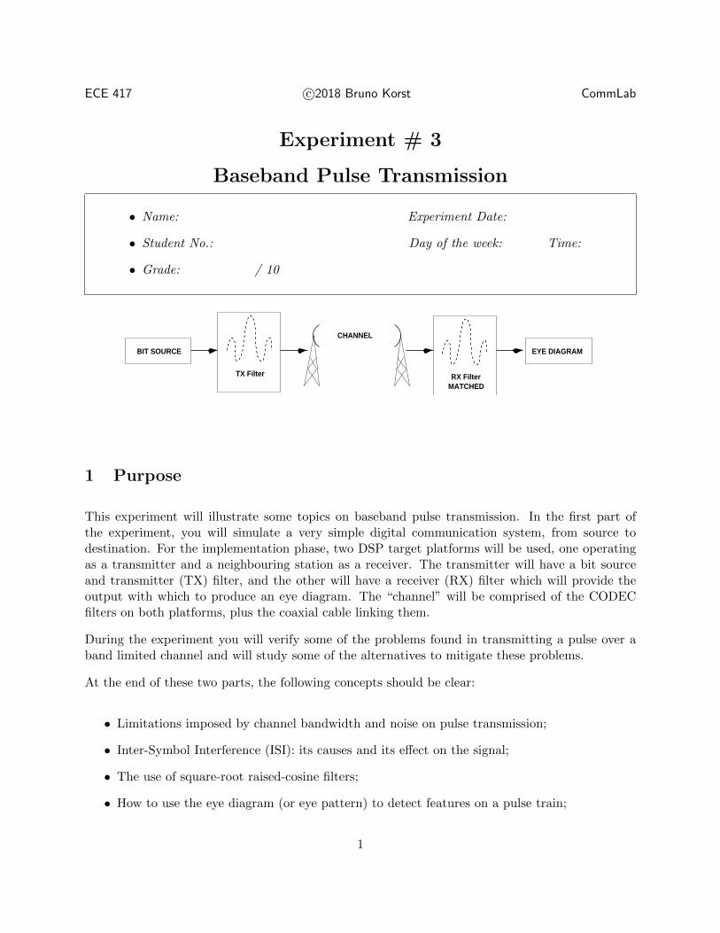
This experiment will illustrate some topics on baseband pulse transmission. In the first part ofthe experiment, you will simulate a very simple digital communication system, from source todestination. For the implementation phase, two DSP target platforms will be used, one operatingas a transmitter and a neighbouring station as a receiver. The transmitter will have a bit sourceand transmitter (TX) filter, and the other will have a receiver (RX) filter which will provide theoutput with which to produce an eye diagram. The “channel” will be comprised of the CODECfilters on both platforms, plus the coaxial cable linking them.

During the experiment you will verify some of the problems found in transmitting a pulse over aband limited channel and will study some of the alternatives to mitigate these problems.

At the end of these two parts, the following concepts should be clear:

• Limitations imposed by channel bandwidth and noise on pulse transmission;

• Inter-Symbol Interference (ISI): its causes and its effect on the signal;

• The use of square-root raised-cosine filters;

• How to use the eye diagram (or eye pattern) to detect features on a pulse train;

1

2 Background Reading and Preparation

Though there are many very good references on digital communications, throughout the lab portionof this course you may find useful to refer to [1], [2], [3] and [4] in addition to the course notes. It ismost advantageous for you to read different authors discussing the same topic, as they will provideyou with different points of view. This will help you to create a meaningful mental representationof the individual topics, and will lead to a very good understanding of the subject.

3 Experiment

There are two parts for this experiment, as usual: simulation and implementation. You will firstsimulate the complete transmitter (TX), channel, and receiver (RX) system using Simulink to seehow different pulse shapes and channel bandwidths will affect the data at the receiving end. Onthe second part, you will run a program on the DSP that generates pulses, shapes them via asquare-root raised cosine filters, passes them through a channel with noise, and then ”receives” thedata using a matched filter. You will be required to use concepts from Signals and Systems, DSPand Communication Systems, in addition to the knowledge gained in ECE417.

3.1 Simulation of Baseband Pulse Transmission

From Simulink, open the model relative to the first portion of the experiment, found in www.comm.

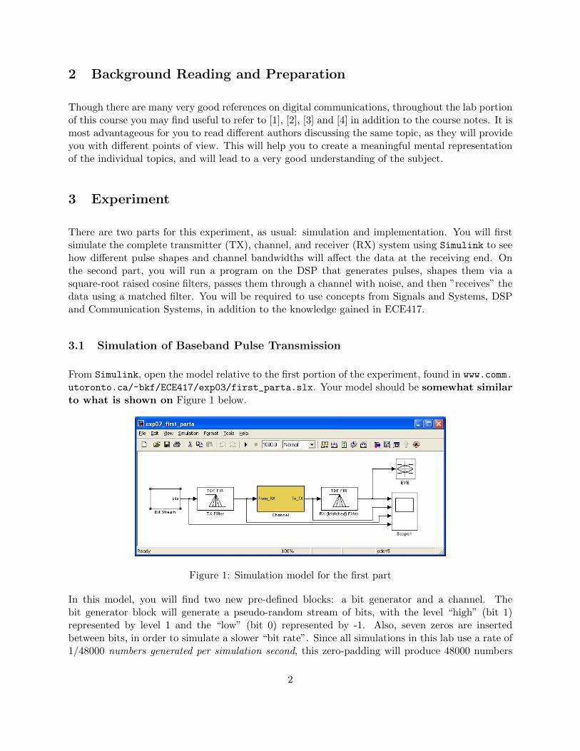
utoronto.ca/~bkf/ECE417/exp03/first_parta.slx. Your model should be somewhat similarto what is shown on Figure 1 below.

Figure 1: Simulation model for the first part

In this model, you will find two new pre-defined blocks: a bit generator and a channel. Thebit generator block will generate a pseudo-random stream of bits, with the level “high” (bit 1)represented by level 1 and the “low” (bit 0) represented by -1. Also, seven zeros are insertedbetween bits, in order to simulate a slower “bit rate”. Since all simulations in this lab use a rate of1/48000 numbers generated per simulation second, this zero-padding will produce 48000 numbers

2

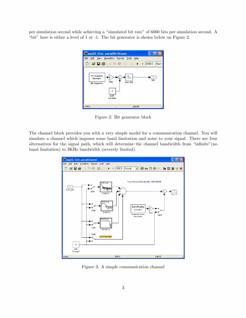
per simulation second while achieving a “simulated bit rate” of 6000 bits per simulation second. A“bit” here is either a level of 1 or -1. The bit generator is shown below on Figure 2.

Figure 2: Bit generator block

The channel block provides you with a very simple model for a communication channel. You willsimulate a channel which imposes some band limitation and noise to your signal. There are fouralternatives for the signal path, which will determine the channel bandwidth from “infinite”(noband limitation) to 3KHz bandwidth (severely limited).

Figure 3: A simple communication channel

3

For obvious reasons, only one path should be used at a time; do not forget to disable all otherpaths when you enable one of them. Also, there is a switch for the simulation of noise added bythe channel. By double clicking on the switch icon you toggle the switch. The channel model ispresented on Figure 3 below. You may be required to redesign the filter(s) using the FDAtool.

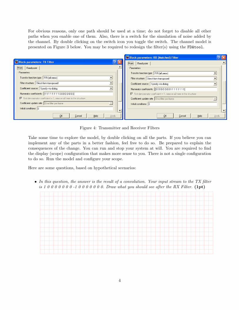
Figure 4: Transmitter and Receiver Filters

Take some time to explore the model, by double clicking on all the parts. If you believe you canimplement any of the parts in a better fashion, feel free to do so. Be prepared to explain theconsequences of the change. You can run and stop your system at will. You are required to findthe display (scope) configuration that makes more sense to you. There is not a single configurationto do so. Run the model and configure your scope.

Here are some questions, based on hypothetical scenarios:

• In this question, the answer is the result of a convolution. Your input stream to the TX filteris 1 0 0 0 0 0 0 0 -1 0 0 0 0 0 0 0. Draw what you should see after the RX Filter. (1pt)

4

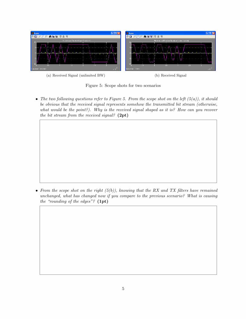
(a) Received Signal (unlimited BW) (b) Received Signal

Figure 5: Scope shots for two scenarios

• The two following questions refer to Figure 5. From the scope shot on the left (5(a)), it shouldbe obvious that the received signal represents somehow the transmitted bit stream (otherwise,what would be the point?). Why is the received signal shaped as it is? How can you recoverthe bit stream from the received signal? (2pt)

• From the scope shot on the right (5(b)), knowing that the RX and TX filters have remainedunchanged, what has changed now if you compare to the previous scenario? What is causingthe “rounding of the edges”? (1pt)

5

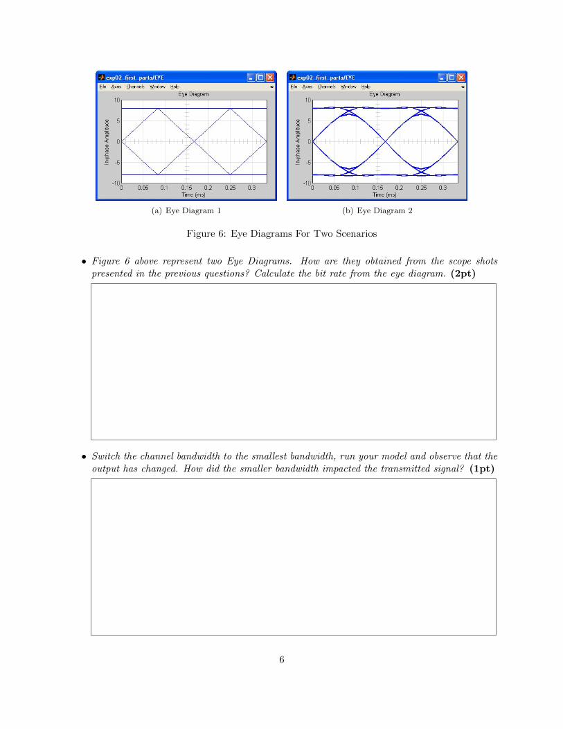
(a) Eye Diagram 1 (b) Eye Diagram 2

Figure 6: Eye Diagrams For Two Scenarios

• Figure 6 above represent two Eye Diagrams. How are they obtained from the scope shotspresented in the previous questions? Calculate the bit rate from the eye diagram. (2pt)

• Switch the channel bandwidth to the smallest bandwidth, run your model and observe that theoutput has changed. How did the smaller bandwidth impacted the transmitted signal? (1pt)

6

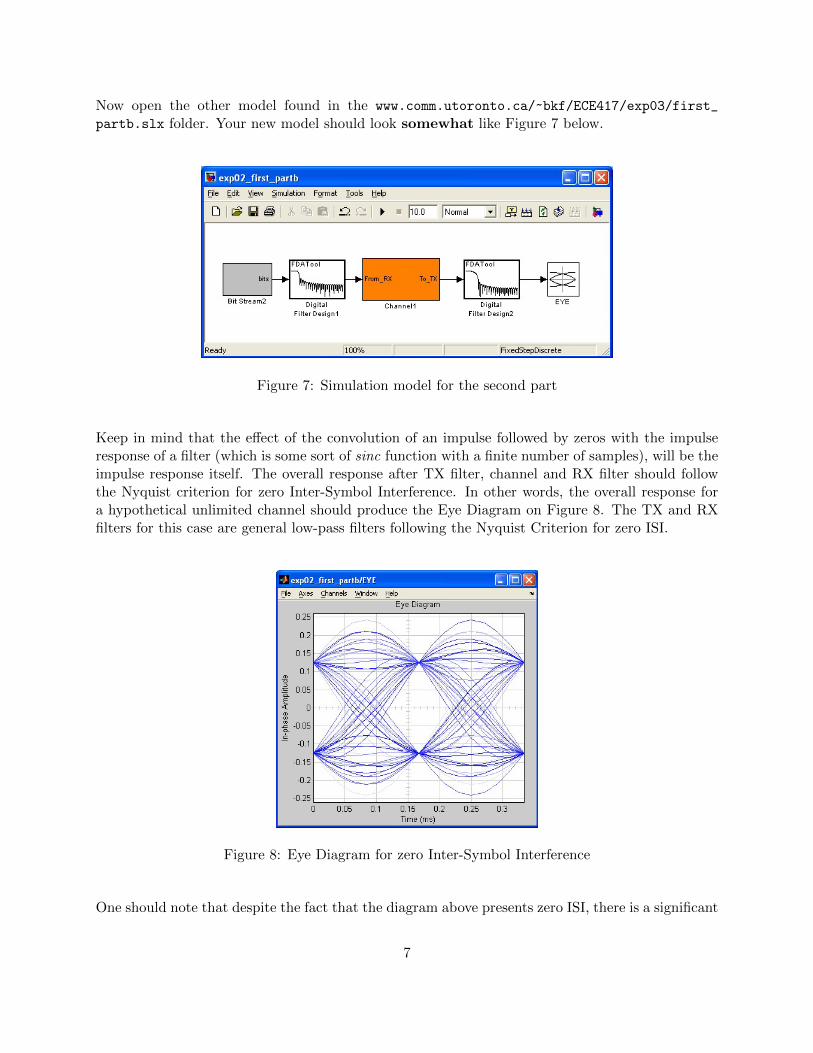
Now open the other model found in the www.comm.utoronto.ca/~bkf/ECE417/exp03/first_

partb.slx folder. Your new model should look somewhat like Figure 7 below.

Figure 7: Simulation model for the second part

Keep in mind that the effect of the convolution of an impulse followed by zeros with the impulseresponse of a filter (which is some sort of sinc function with a finite number of samples), will be theimpulse response itself. The overall response after TX filter, channel and RX filter should followthe Nyquist criterion for zero Inter-Symbol Interference. In other words, the overall response fora hypothetical unlimited channel should produce the Eye Diagram on Figure 8. The TX and RXfilters for this case are general low-pass filters following the Nyquist Criterion for zero ISI.

Figure 8: Eye Diagram for zero Inter-Symbol Interference

One should note that despite the fact that the diagram above presents zero ISI, there is a significant

7

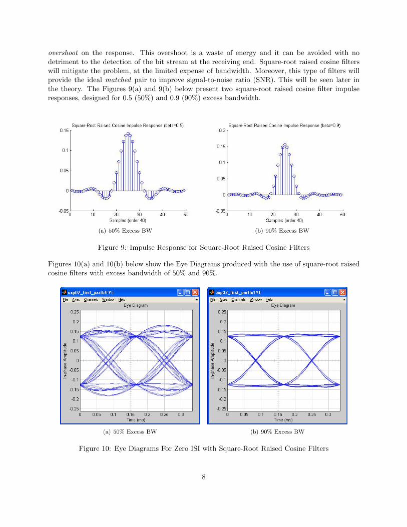
overshoot on the response. This overshoot is a waste of energy and it can be avoided with nodetriment to the detection of the bit stream at the receiving end. Square-root raised cosine filterswill mitigate the problem, at the limited expense of bandwidth. Moreover, this type of filters willprovide the ideal matched pair to improve signal-to-noise ratio (SNR). This will be seen later inthe theory. The Figures 9(a) and 9(b) below present two square-root raised cosine filter impulseresponses, designed for 0.5 (50%) and 0.9 (90%) excess bandwidth.

(a) 50% Excess BW (b) 90% Excess BW

Figure 9: Impulse Response for Square-Root Raised Cosine Filters

Figures 10(a) and 10(b) below show the Eye Diagrams produced with the use of square-root raisedcosine filters with excess bandwidth of 50% and 90%.

(a) 50% Excess BW (b) 90% Excess BW

Figure 10: Eye Diagrams For Zero ISI with Square-Root Raised Cosine Filters

8

Next you will experiment with some of the parameters closer to the real world.

For your new model, design TX and RX filters following the Nyquist Criterion of zero ISI. Use anorder 48 square-root raised cosine filter with 50% (beta = 0.5) excess bandwidth. Run the system,starting with a straight through channel. Note that, again, you will have to find the appropriatedisplay configuration that will produce meaningful plots. Play with the given model to find theright configuration. Once you understand what the eye diagram represents, you will find it easierto configure the real oscilloscope during the implementation phase below.

• Show how you determined the cutoff frequency. (1pt)

3.2 Transmitter and Receiver Implementation

In this part, you will implement a transmitter/receiver system, by running a program on theDSP target hardware. Open Code Composer Studio, and select (click on) the project calledECE417 Exp05 Pulse Transmission. This will make the project active.

Compile the project now. Before you run the executable, you will need to load a script so thatyou can select the excess bandwidth of the matched filters using a slider, as well as switch noise onand off and choose noise levels. At his point, your project should be compiled without errors, andready to run. Follow this procedure in order to load the script:

1. In the CCS Debug environment, choose the menu Tools -- Gel Files. This will open apane (likely on the bottom right corner);

2. Under Script, right-click on an blank cell and choose Load GEL. The GEL file is the actualscript that will run and change parameters on the code in real-time;

3. Load the file called noise.gel, which is found within the same directory where your main ccode is located;

4. Now go back to the top menu, and click on the menu item Scripts. You should see threeitems: Noise Switch, Noise Level and Filter. Use the mouse to open all three of thesesliders.

5. Set Filter to 1, set Switch Noise to 0 and Noise to 0.

9

Since your project has been compiled and it is ready to run, run it. Connect all appropriate cablesbetween the board output and the oscilloscope. The output produced will be displayed on onechannel only. When you see it running, turn your attention to the c code.

Look at the c program called pulse trans.c. The individual parts of the code are commented.You will see what the transmitter, channel and receiver are doing.

The transmitter implements a bit generator based on a Pseudo-noise sequence generator, and itproduces positive and negative values interpolated by a number of zeros (seven). This sequence ispassed through a transmitter filter, which can be selected by the user via the Filter slider. Theresulting value is sent to the “outside world”(the channel) scaled appropriately.

The receiver, then, collects samples from the “outside world” and passes them through a receiverfilter (matched to the transmitter filter). This filtered value is sent to a D/A converter to beviewed in the oscilloscope. The ”channel” on the code adds scaling and noise to the output of thetransmitter. No bandwidth limitation is imposed by the channel on the code.

Now that you have the code understood and running, let us see how to obtain the eye diagram.

4 Obtaining the Eye Diagram for Different Scenarios

4.1 For Different Matched Filters

The eye diagram, or eye pattern, is a common method utilized to observe the features on a receivedpulse train. In this part of the experiment, you will use channel noise and modify the TX and RXfilters so that you can observe the effects on the eye diagram.

However, one needs to recall a special oscilloscope feature called the Lissajous Figure. You may haveused this feature to measure phase differences between two channels of the oscilloscope (typicallydone in power electronics). This figure is obtained with the waveform on one input channel drivingthe horizontal sweep and the one on the other input channel driving the vertical sweep. Theoscilloscope must be set to X-Y mode. This mode is obtained via the Display -- Format menu.Now that you have the right display mode, make th

For the eye diagram, you must use the output of the DSP target on one channel of the oscilloscope,and a saw-tooth signal (2.0 Vpp) coming directly from the signal generator on the other channel.You will have to adjust the frequency of the saw-tooth wave to generate a meaningful eye diagram.According to your knowledge of the pulse rate and cutoff frequency, what should the saw-toothfrequency be? That is, what is the period determined by the crossing points on the opening ofthe eye? After you find the right frequency, make the display steady (that is, without using therun/stop button).

Now let us look at the filter options. Option 1 selects a square-root raised-cosine filter with 50%excess bandwidth, with a 3KHz cutoff frequency. This is to say that if you have the square-root onRX and on TX, your overall response will be a raised-cosine filter cutting at 3KHz, which is whatyou would desire. Option 2, then, selects the 99% excess bandwidth filter.

10

As the system runs, choose different filters and observe the result on the eye diagram display.When you are ready, show your impressive result to the TA and have the TA sign the box. (1pt)

4.2 With Noise

After you try the different types of filters, add noise to your system by using the appropriate slider.You have to switch the noise on first using the switch slider. After you do that, change the noisegain up and down and observe the effect on the “closing” of the eye. Then you can do all this foreach of the pulse shaping filter.

When you are ready, show it to the TA and have the TA sign the box. (1pt)

5 Accomplishments

The main objective of this experiment was to show how pulse shaping and the limitation on channelbandwidth will affect the transmission of a bit sequence generated at a certain rate. In orderfor you to observe that, you have simulated a basic digital communication system and modifiedthe channel bandwidth, as well as the transmitter and receiver filters. You also implemented atransmitter/receiver system running in real time, and modified some of its parameters using slidersin real-time. You have also learned how to utilize the eye diagram to observe features on a signalrepresenting a sequence of bits received by a digital communication system.

References

[1] S. Haykin and M. Moher Introduction to Analog and Digital Communications, 2nd Ed. - Wiley,2007

[2] B. P. Lathi, Modern Digital and Analog Communication Systems, 3rd Edition. New York: Ox-ford University Press, 1998.

[3] S. Haykin Communication Systems, 4th Edition. Toronto: John Wiley & Sons, Inc., 2001.

[4] I.A. Glover and P.M. Grant, Digital Communications, Prentice Hall, 1998.

11

Preparation - Baseband Pulse Transmission

• Name: Experiment Date:

• Student No.: Grade: / 10

1. Draw a high-level block diagram of a “complete” digital communication sytem, from sourceto destination. Itentify the transmitter portion, the channel and the receiver portion of yoursystem, and some of the relevant subsystems of each of these portions. Point out where noisecould be added to the signal. (look at [1], p.232, Figure 6.1(a)) (2pt)

2. Explain what is the advantage brought by the use of a “matched” filter in a communicationsystem. Explain how the matched filter is designed and detail its location in the communica-tion system drawn above. (2pt)

3. Explain how an “eye diagram” or “eye pattern” is obtained, and what information about thetransmitted/received data can be drawn from it. (2pt)

12

4. Explain inter-symbol interference (ISI): what causes it, how it is observed in the “eye diagram”and briefly describe the trade-offs involved in mitigating it. (2pt)

5. How is noise observed in the Eye Diagram? How will it affect the recovery of the transmitteddata? (2pt)

13