MPRAMunich Personal RePEc Archive

Existence of optimal strategies in linearmultisector models with severalconsumption goods

Freni, Giuseppe; Gozzi, Fausto and Salvadori, Neri

University Partenope, Naples (Italy), University LUISS,

Rome (Italy), University of Pisa, Pisa (Italy)

01. April 2010

Online at http://mpra.ub.uni-muenchen.de/21809/

MPRA Paper No. 21809, posted 01. April 2010 / 18:35

Giuseppe Freni · Fausto Gozzi · Neri Salvadori

Existence of optimal strategies in linear multisector models with several con-sumption goods

Abstract. In this paper we give a sufficient and almost necessary condition for the existence ofoptimal strategies in linear multisector models when time is continuous and the the instantaneousutility function of the representative agent has two properties: (a) the intertemporal elasticityof substitution is constant over time and (b) preferences are concave and homothetic.

Key words: Endogenous growth, optimal control with mixed constraints, von Neumann growthmodel.

JEL Classification Numbers: C62, O41.

Giuseppe FreniDipartimento di Studi Economici, Facolta di Economia, Universita Parthenope,via Medina 40, 80133 Napoli, Italy.E-mail: giuseppe.freni@uninav.it

Fausto GozziDipartimento di Scienze Economiche ed Aziendali, Facolta di Economia, Universita LUISS - Guido Carli,vial Pola 12, 00198 Roma, Italy.E-mail: fgozzi@luiss.it

Neri SalvadoriDipartimento di Scienze Economiche, Facolta di Economia, Universita di Pisa,via Ridolfi 10, 56124 Pisa, Italy.E-mail: nerisal@ec.unipi.it

1

1 Introduction

In 1981 Magill [12] explored existence of optimal strategies in linear multisector modelswhen time is continuous and the preferences of the representative agent are characterizedby two parameters: the rate of time discount ρ and the constant elasticity of substitutionσ > 0, within a more general formulation in which technology is not necessarily linear.He proved ([12], Theorem 9.15, p. 703) that in a von Neumann technology with constantreturns if

Γ0 >Γ0 − ρσ

,

then an optimal strategy exists, where Γ0 is the maximum rate of growth (Magill [12] didnot provide any non-existence results; but see [13]). However Magill used an assumptionon ”regularity” ([12], Assumption T.2, p. 703) justified on the basis of the Gale [9] inde-composability assumption implying that the upper bound of the uniform over time ratesof reproduction of any commodity equals the maximum rate of growth.

In a more recent paper, Freni et alii [7] analyzed in greater depth the existence ofoptimal strategies in linear multisector models when time is continuous and proved, onthe assumption that only one commodity is consumed, that if

Γ1 >Γ1 − ρσ

,

then an optimal strategy exists, whereas if

Γ1 <Γ1 − ρσ

,

then no optimal strategy exists, where Γ1 is the upper bound of the uniform over timerate of reproduction of commodity 1, which is the only commodity which is consumed.Freni et alii [7] also considered the case in which

Γ1 =Γ1 − ρσ

,

and provided further results of the existence or non existence according to the size of σ.Therefore what matters is not the maximum rate of growth, but the upper bound of theuniform over time rates of reproduction of the consumption good if only one commodityis consumed. In this paper we aim to generalize this result to the case in which severalconsumption goods exist. More precisely we will prove that if

Γν >Γν − ρσ

, (1)

then an optimal strategy exists, whereas if

Γν <Γν − ρσ

, (2)

then no optimal strategy exists, where Γν is an average of the upper bounds of the uniformover time rates of reproduction of consumption commodities. Finding the right definition

2

of the average Γν and studying its properties was indeed the main technical difficultyof the paper. The average Γν is defined by the instantaneous utility function only andis totally independent of technology whereas the upper bound of the uniform over timerate of reproduction of a commodity depends only on technology and is independent ofconsumer preferences.1

Our result depends on the fact that the instantaneous utility function has two prop-erties: (a) the intertemporal elasticity of substitution is constant over time and (b) pref-erences are concave and homothetic. Hence the instantaneous utility function uσ dependson a parameter σ > 0 (the elasticity of substitution) and is given by

uσ (ν) = ν1−σ−11−σ for σ > 0, σ 6= 1

u1 (ν) = log ν for σ = 1

(3)

(with the agreement that uσ(0) = −∞ for σ ≥ 1), where ν : Rk+ → R is continuous,

increasing on every component, concave, and homogeneous. With no loss of generality weassume that ν is homogeneous of degree 1. The assumption of homothetic preferences isjustified by the fact that otherwise income distribution among consumers matters and, asa consequence, it would be appropriate to avoid an analysis in terms of a representativeagent. However, if nonhomothetic preferences are modelled through Stone-Geary utilityfunctions, as in Kongsamut et al. [11], then results similar to those presented here can beobtained.

The analysis presented here is most relevant when the upper bound of the uniformover-time rates of reproduction of different consumption goods are not equal (because ofdecomposability of technology). This analysis introduces the possibility of investigatingstructural change in relation to the different growth rates Γi and their average Γν foundhere. Structural change, mainly in exogenous growth models, is an increasingly widelystudied issue in the literature: see [17] and [1]. The fact that the average defined hereΓν depends on the instantaneous utility function alone and is wholly independent oftechnology suggests that such an average should emerge even in different analytic contextsin which technology is not linear and inequalities among growth rates are not related tothe decomposability of technology.

From the technical point of view the results obtained in this paper can be seen asgeneralizations of those obtained elsewhere [7]. Indeed, while some preliminary Lemmas(see e.g. Lemma 4.1) are straightforward extensions of results contained in [7], the technicalcore of the present paper needs new ideas and techniques to be dealt with. The mainreason is the fact that as we want to find “sharp” results (i.e. existence when (1) holdsand nonexistence when (2) holds), we have to understand precisely the role of the functionν in the existence of optimal trajectories. It would be very easy to extend the result ofthe paper [7] and find only rough sufficient conditions for the existence (e.g. substitutingΓν with the maximum of the Γi’s) and for the non-existence (e.g. substituting Γν withthe minimum of the Γi’s). But to get our sharp results we need to understand what is

1We consider also the case in which Γν = Γν−ρσ , and provide further results of existence or non

existence.

3

the right average, and then carefully prove all the various estimates needed for existenceand nonexistence. For this reason these estimates, as happens for all sharp estimates, arestructurally different from those needed when there is only one consumption good.

The paper is structured as follows: first we describe the model and assess the mainassumptions in Section 2. In Section 3 we enunciate the main results and provide examplesto show the complexity of the limiting cases. Section 4 is devoted to proving the mainresults. Finally the Appendix aims to prove some useful results concerning the averageΓν .

2 The Model

There are n ≥ 1 commodities, and k of them are consumed, say commodities 1, . . . , k.Preferences with respect to consumption over time are such that they can be described bya single intertemporal utility function Uσ, which is the usual C.E.S. (Constant Elasticityof Substitution) function: for a given consumption path c : [0,+∞) → Rk, (ct ≥ 0 a.e.),we set

Uσ (c (·)) =

∫ +∞

0

e−ρtuσ (ν(c (t))) dt (4)

where ρ ∈ R is the rate of time discount of the representative agent, and the instantaneousutility function uσ : [0,+∞)→ R∪{−∞} has the form (3) and ν : Rk

+ → R is continuous,increasing on every component, concave, and homogeneous of degree 1. Possible examplesof function ν are the following:

ν(c) = cα11 c

α22 · · · c

αkk , αi ∈ (0, 1), i = 1, . . . k,

k∑i=1

αi = 1 (5)

ν(c) = min {α1c1, α2c2, . . . , αkck} , αi ∈ (0, 1), i = 1, . . . k,k∑i=1

αi = 1 (6)

ν(c) = α1c1 + α2c2 + · · ·+ αkck, αi ∈ (0, 1), i = 1, . . . k,k∑i=1

αi = 1 (7)

ν(c) = {α1cq1 +α2c

q2 + · · ·+αkc

qk}

1/q, αi ∈ (0, 1), i = 1, . . . k,k∑i=1

αi = 1, q < 1. (8)

In the first case preferences are Cobb-Douglas, in the second consumed commodities areperfect complements, in the third consumed commodities are perfect substitutes, in thefourth preferences are CES.

For the sake of simplicity we will drop the additive constant − (1− σ)−1 in the fol-lowing since this will not affect the optimal paths.

Technology is fully described by a pair of nonnegative matrices (the m× n materialinput matrix A and the m× n material output matrix B, m ≥ 0) and by a uniform rateof depreciation δx of capital goods used for production. The rate of depreciation for goods

4

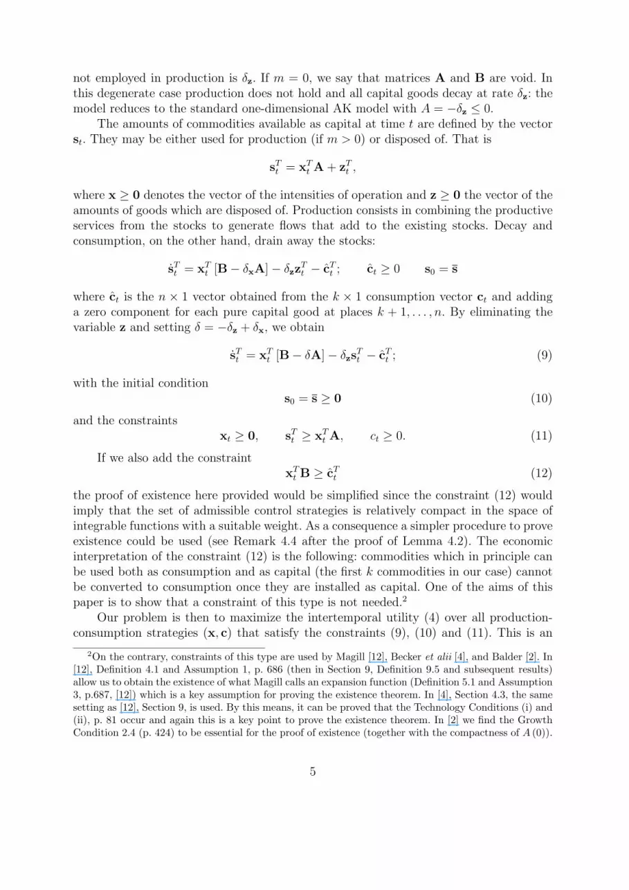
not employed in production is δz. If m = 0, we say that matrices A and B are void. Inthis degenerate case production does not hold and all capital goods decay at rate δz: themodel reduces to the standard one-dimensional AK model with A = −δz ≤ 0.

The amounts of commodities available as capital at time t are defined by the vectorst. They may be either used for production (if m > 0) or disposed of. That is

sTt = xTt A + zTt ,

where x ≥ 0 denotes the vector of the intensities of operation and z ≥ 0 the vector of theamounts of goods which are disposed of. Production consists in combining the productiveservices from the stocks to generate flows that add to the existing stocks. Decay andconsumption, on the other hand, drain away the stocks:

sTt = xTt [B− δxA]− δzzTt − cTt ; ct ≥ 0 s0 = s

where ct is the n × 1 vector obtained from the k × 1 consumption vector ct and addinga zero component for each pure capital good at places k + 1, . . . , n. By eliminating thevariable z and setting δ = −δz + δx, we obtain

sTt = xTt [B− δA]− δzsTt − cTt ; (9)

with the initial conditions0 = s ≥ 0 (10)

and the constraintsxt ≥ 0, sTt ≥ xTt A, ct ≥ 0. (11)

If we also add the constraintxTt B ≥ cTt (12)

the proof of existence here provided would be simplified since the constraint (12) wouldimply that the set of admissible control strategies is relatively compact in the space ofintegrable functions with a suitable weight. As a consequence a simpler procedure to proveexistence could be used (see Remark 4.4 after the proof of Lemma 4.2). The economicinterpretation of the constraint (12) is the following: commodities which in principle canbe used both as consumption and as capital (the first k commodities in our case) cannotbe converted to consumption once they are installed as capital. One of the aims of thispaper is to show that a constraint of this type is not needed.2

Our problem is then to maximize the intertemporal utility (4) over all production-consumption strategies (x, c) that satisfy the constraints (9), (10) and (11). This is an

2On the contrary, constraints of this type are used by Magill [12], Becker et alii [4], and Balder [2]. In[12], Definition 4.1 and Assumption 1, p. 686 (then in Section 9, Definition 9.5 and subsequent results)allow us to obtain the existence of what Magill calls an expansion function (Definition 5.1 and Assumption3, p.687, [12]) which is a key assumption for proving the existence theorem. In [4], Section 4.3, the samesetting as [12], Section 9, is used. By this means, it can be proved that the Technology Conditions (i) and(ii), p. 81 occur and again this is a key point to prove the existence theorem. In [2] we find the GrowthCondition 2.4 (p. 424) to be essential for the proof of existence (together with the compactness of A (0)).

5

optimal control problem where s is the state variable and x and c are the control variables.We now describe this problem more formally.

A production-consumption strategy (x, c) is defined as a measurable and locally inte-grable function of t : R+ →Rm×Rk (we will denote by L1

loc

(0,+∞; Rm+k

)the set of such

functions). Then the differential equation (9) has a unique solution : R+ 7→Rn which isabsolutely continuous (we will denote by W 1,1

loc (0,+∞; Rn) the set of such functions). Asthis solution clearly depends on the initial datum s and on the production-consumptionstrategy (x, c), it will be denoted by the symbol st;s,(x,c), omitting the subscript s, (x, c)when it is clear from the context.

Given an initial endowment s we will say that a strategy (x, c) is admissible from sif the triple

(x, c, st;s,(x,c)

)satisfies the constraints (11) and U1 (c) is well defined3. The

set of admissible control strategies starting at s will be denoted by A(s). We adopt thefollowing definition of optimal strategies.

Definition 2.1 A strategy (x∗, c∗) ∈ A(s) will be called optimal if we have Uσ(c∗) > −∞and

+∞ > Uσ(c∗) ≥ Uσ(c)

for every admissible control pair (x, c) ∈ A(s).

We now comment on a set of assumptions that will be used throughout the paper.

Assumption 2.2 Each row of matrix A is semipositive.

This assumption means that no commodity can be produced without using somecommodity as an input.

Assumption 2.3 Each row of matrix B is semipositive.

This assumption means that each process produces something: i.e. that pure destruc-tion processes are not dealt with as production processes.

Assumption 2.4 The initial datum s ≥ 0 and the matrices A and B are such that thereis an admissible strategy (x∗, c∗) ∈ A(s) and a time t∗ > 0 such that ν

(st∗ ;s,(x∗,c∗)

)> 0,

where s is the subvector of vector s consisting of the first k elements.

If this assumption does not hold, then every admissible strategy starting from s musthave ν(ct) = 0 a.e. This case holds little interest for investigation purposes.

3The condition on U1 (c) is relevant only when σ = 1. Note that for σ ∈ (0, 1) the function t →e−ρtuσ (ν(ct)) is always nonnegative so it is always semiintegrable (with the integral eventually +∞).On the other hand for σ > 1 the function t → e−ρtuσ (ν(ct)) is always negative (and may be −∞ whenν(c)t = 0) and again it is always semiintegrable (with the integral eventually −∞). This means that theintertemporal utility Uσ is always well defined for σ 6= 1. For σ = 1 the function t→ e−ρtuσ (ν(ct)) maychange sign so it may be not semiintegrable on [0,+∞). This is the reason why we need to require thatU1 (c) is well defined in order to define the admissibility of c.

6

Assumption 2.5 The initial datum s ≥ 0 and the matrices A and B are such that thereis an admissible strategy (x∗, c∗) ∈ A(s) and a time t∗ such that st∗ ;s,(x∗,c∗) is positive.

Assumption 2.5 implies that all commodities are available at any time t > 0 and,in particular, that Assumption 2.4 is satisfied. Moreover Assumptions 2.4 and 2.5 couldbe stated in terms of the zero components of the initial datum s and of the structureof matrices A and B. On this point, see Appendix D of [8]. Further, it can be shownthat Assumption 2.5 is not really restrictive, provided that Assumption 2.4 holds, in thesense that when it does not hold, matrices A and B, vector s, and consumption goodscan be redefined in order to obtain an equivalent model in which Assumption 2.5 holds.Assume, in fact, that Assumption 2.5 does not hold. Then there is a commodity j whichis not available at any time t ≥ 0 (sTt ej = 0 for every t ≥ 0). In this case any productionprocess i in which commodity j is employed (aij > 0) cannot be used. The model isthen equivalent to one in which matrices B and A and vector s, in the state equation(9), are substituted with matrices D and C and vector s′, respectively, where matrix C isobtained from A by deleting the j-th column and all rows which on the j-th column have apositive element, matrix D is obtained from matrix B by deleting the corresponding rowsand the j-th column, and vector s′ is obtained from vector s by deleting the j-th element.(If commodity j is a consumption good, it is also deleted from the list of consumptiongoods.) Note that if in the new equivalent model the Assumption 2.5 does not hold andmatrices C and D are not void, the argument can be iterated. If matrices C and Dare void, then an equivalent model satisfying Assumption 2.5 is obtained by deleting thenought elements of vector s′. In any case the algorithm is able to determine an equivalentmodel in which Assumption 2.5 does hold. We will refer to the equivalent model foundin this way as the truncated model and to the corresponding technology as the truncatedtechnology, which then depends on s. It can easily be proved that if Assumptions 2.2, 2.3,2.4 hold in the original technology, then they hold in the truncated technology too (seeAppendix D of [8]). If not otherwise mentioned, all the following assumptions refer to thetruncated technology.

Let us define

G0 :={γ|∃x ∈ Rm : x ≥ 0,x 6= 0,xT [B− (γ + δx) A] ≥0

}, Γ0 = maxG0

and, for i = 1, . . . , k,

Gi :={γ|∃x ∈ Rm : x ≥ 0,xT [B− (γ + δx) A] ≥ eTi

}, Γi = supGi

Γ0 is clearly the maximum among the uniform over time rates of growth feasible forthis economy and corresponds to what von Neumann [16] found both as growth rate andas rate of profit. Γi is the upper bound of the uniform over time rates of reproduction ofthe i−th consumption good. Obviously Γi ≤ Γ0 for every i = 1, . . . , k.

Magill [12], Assumption T.2, p. 703, assumed that if x ∈ X , then xTB > 0T , where

X ={x|x ≥ 0,x 6= 0,xT [B− (Γ0 + δx) A] ≥ 0T

}It is easily checked that, under this assumption, if x ∈ X and xTAei = 0, then there isα > 0 such that

xT [B− (Γ0 + δx) A] ≥ αeTi

7

whereas if x ∈ X and xTAei > 0, then for any ε > 0 there is α > 0 such that

xT [B− (Γ0 − ε+ δx) A] ≥ αeTi

In any case

sup{γ|∃x ∈ Rm : x ≥ 0,x 6= 0,xT [B− (γ + δx) A] ≥ eTi

}= Γ0

that is, the upper bound of the uniform over time rates of reproduction of any commodityequals the maximum rate of growth. In this paper we will not make any assumption onindecomposability.

It is easily proved that the Γi’s relative to the truncated technology are not greaterthan the corresponding Γi’s relative to the original one. If either Bei = Aei = 0 ormatrices A and B are void, then Γi = −∞. Moreover if Bei = 0 and Aei 6= 0 thenΓi = −δx. Finally, if Bei 6= 0 and if commodity j is available at time 0 (sTej > 0) andis essential to the reproduction of the i−th consumption good, then Γi = −δx.4 (see [8]Proposition 4.4).

Assumption 2.6 Bei 6= 0 for each consumption good i and δz < δx.

Assumption 2.6 is not necessary, but it helps in simplifying the exposition sinceit implies that Γi > −δz for each consumption good i. The first part means that allconsumption goods are technologically producible. The second part implies that usingcommodities in production dominates their storing; i.e. it is not convenient to producesomething just in order to dispose something else.

We callΓmax := max

i=1,...,kΓi, Γmin := min

i=1,...,kΓi > 0

Moreover we introduce the following number

Γν = inf

{η ∈ R : lim

t→+∞e−ηtν

(eΓ1t, eΓ2t, . . . , eΓkt

)= 0

}

= sup

{η ∈ R : lim

t→+∞e−ηtν

(eΓ1t, eΓ2t, . . . , eΓkt

)= +∞

}Since, from the homogeneity of degree 1 and the monotonicity of ν, we have

eΓmintν(1, 1, . . . , 1) ≤ ν(eΓ1t, eΓ2t, . . . , eΓkt

)≤ eΓmaxtν(1, 1, . . . , 1)

then it is easy to see that Γmin ≤ Γν ≤ Γmax.It is also easy to check that, for the four examples given in (5), (6), (7), and (8),we

have:

4We say that commodity j is essential to the reproduction of the i−th consumption good when(x ≥ 0, ε > 0,xT [B− εA] ≥ ei

)⇒ xTAej 6= 0.

8

• in the example (5), Γν =∑k

i=1 αiΓi,

• in the example (6), Γν = Γmin,

• in the example (7), Γν = Γmax,

• in the example (8), Γν = Γmax if 0 < q < 1 whereas Γν = Γmin if q < 0.

As mentioned in the introduction, this paper is mainly devoted to showing the role thatthe following assumption plays in the existence of optimal strategies of the problem underanalysis.

Assumption 2.7

Γν >Γν − ρσ

The reader will have noticed that we used the convoluted expression “the upperbound of the uniform over time rates of reproduction of the i−th consumption good”instead of the more straightforward “the upper bound of the rates of reproduction of thei−th consumption good”. This is because, for particular forms of matrices, growth ratesof consumption might be found which are higher, but not uniform over time. In [7] weprovided the following example, with details, to clarify this point.

Example 2.8 k = 1, δx = δz ∈ (0, 1) and

A =

[0 1 00 0 1

], B =

[1 1 00 1 1

].

It is immediately recognized that Γ1 = 1 − δx > 0. Nevertheless, consumption can growat the rate

c

c= Γ1 +

β

α + βt> Γ1

where α and β are positive constants.

We finally observe that, from the definition of Γν the value of the limit

limt→+∞

e−Γνtν(eΓ1t, . . . , eΓkt

),

may be any L ∈ [0,+∞]. However, as shown in the Appendix when the law of thefunction ν is made only by a finite number of sums, products, powers, and/or max/minover a finite number of terms - which is e.g. the case of the examples (5), (6), (7), (8)above - then L ∈ (0,+∞). In the same appendix we provide examples in which eitherL = 0 or L = +∞. The relevance of these two cases is explored in Theorem 3.3.

9

3 The main results

The main goal of this paper is to show that in the general context outlined by Assumptions2.2, 2.3, 2.5, 2.6, we have substantially an if and only if condition for the existence ofoptimal strategies. In this paper we will prove the following results:

Theorem 3.1 If Assumptions 2.2, 2.3, 2.5, 2.6 and 2.7 hold, then there is an optimalstrategy (x, c) for problem (Pσ) starting at s. Moreover this strategy is unique in the sensethat if (x, c) is another optimal strategy, then ν(c) ≡ ν(c). If ν is strictly concave, thenwe also have c ≡ c.

Theorem 3.2 Let Assumptions 2.2, 2.3, 2.5, 2.6 hold. If

Γν <Γν − ρσ

then no optimal strategy exists for problem (Pσ) starting at s.

Theorem 3.3 Let Assumptions 2.2, 2.3, 2.5, 2.6 hold. Let

Γν =Γν − ρσ

.

Then we have the following:

1. Let σ = 1.

• If Γν < 0, then all strategies have value −∞ and so no optimal strategy existsfor problem (P1) starting at s.

• If Γν > 0 there exists an admissible strategy with value +∞ and so no optimalstrategy exists for problem (P1) starting at s.

• If Γν = 0, each Γi is not a maximum and

limt→+∞

e−Γνtν(eΓ1t, . . . , eΓkt

)< +∞, (13)

then all strategies have value −∞ and so no optimal strategy exists for problem(P1) starting at s.

• If Γν = 0, each Γi is a maximum,

limt→+∞

e−Γνtν(eΓ1t, . . . , eΓkt

)> 0, (14)

and s satisfy5

sTej >k∑i=1

xTi Aej, j = 1, . . . n.

(where xi is the maximum point of Gi), then there exists an admissible strategywith value +∞ and so no optimal strategy exists for problem (P1) starting ats.

5Note that this is always true if all components of s are very large.

10

2. Let σ ∈ (0, 1). If each Γi is a maximum and (14) holds then there exists an admissiblestrategy with value +∞ and so no optimal strategy exists for problem (Pσ) startingat s.

3. Let σ > 1. If each Γi is not a maximum and (13) holds, then all strategies havevalue −∞ and so no optimal strategy exists for problem (Pσ) starting at s.

The limit cases where Γν = Γν−ρσ

and

1. σ = 1, Γν = 0, and at least one Γi is a maximum or (13) does not hold;

2. σ = 1, Γν = 0, and at least one Γi is not a maximum or (14) does not hold or s isnot big enough;

3. σ ∈ (0, 1) and at least one Γi is not a maximum or (14) does not hold;

4. σ > 1 and at least one Γi is a maximum or (13) does not hold;

are intrinsically more complex than the others. Indeed in such cases we can have existenceor nonexistence depending on the value of σ. In our paper [7] (see also [8] for details) weprovided two examples of matrices A and B and scalars ρ, δx, δz showing counterexampleswhen k = 1 and Γν = Γ1 > 0. Here we provide an example of the case when σ = 1, k = 1,Γν = Γ1 = 0 is a maximum, and (14) holds, showing what happens for different values ofs.

Example 3.4 k = 1, δx = δz = 1 and

A =

[1 00 1

], B =

[1 01 1

].

It is immediately recognized that Γν = Γ1 = 0 and that it is a maximum. The maximumpoint in the definition of Γ1 is (x1, 1) for every x1 ≥ 0. The constant strategy xt = α(0, 1),ct = α, for any α > 0, is admissible if and only if s2 ≥ α. So, if s1 ≥ 0 and s2 ≥ 1, thensuch an admissible strategy has value +∞. On the other hand, the state control constraintsimply that s′1 ≤ s2 − c and s′2 ≤ 0 so. Hence, by integrating, we get, for t ≥ 0,∫ t

0

csds ≤ s1 + ts2

which implies ∫ t

0

ln csds ≤ t ln[ s1

t+ s2

].

The above implies that, when s2 < 1 then U(c) = −∞ for every admissible strategy.Moreover, when s2 = 1, then the strategy above has value zero and U(c) ≤ s1 for everyadmissible strategy. In this last case there exists an optimal strategy.

Remark 3.5 If Γν is invariant to a small change in Γi, consumption good i is said to bemarginally inessential to the definition of Γν; otherwise it is marginally essential. In theabove Theorem 3.3, each time all Γi’s are required to be maximum or not, this requirementcan be restricted to the goods that are marginally essential to the definition of Γν.

11

4 Proofs of the main results

In this section, we provide the proofs of the main results stated in section 3. The proofsrequire a set of preliminary results which we discuss in Subsection 4.1. In Subsection 4.2we prove the existence and nonexistence results stated above as Theorems 3.1, 3.2 and3.3.

Throughout this section we will assume that Assumptions 2.2, 2.3, 2.5, 2.6 holdwithout explicitly mentioning them. We observe that some results hold in the more generalframework when Assumption 2.6 does not hold; on this point see also Appendix A and Bof [8].

4.1 Preliminary lemmata

The following Lemma provides the basis for estimates of the state and control trajectories.

Lemma 4.1 Let i ∈ {1, . . . , k}. If Γi is not a maximum

γ ≥ Γi ⇐⇒ ∃viF≥ 0 : (B− (γ + δx) A) viF≤ 0, eTi viF=1. (15)

If Γi is a maximum

γ > Γi ⇐⇒ ∃viF≥ 0 : (B− (γ + δx) A) viF≤ 0, eTi viF = 1, (16)

Moreover∃viS≥ 0 : (B− (Γi + δx) A) viS≤ 0,viS 6= 0, (17)

andeTi viS = yT [B− (Γi + δx) A] viS = 0, (18)

wherey ∈

{x|x ≥ 0,xT [B− (Γi + δx) A] ≥ eTi

}.

Proof. Statements (15) and (16) are obvious applications of the Farkas Lemma (seefor instance Gale’s theorem for linear inequalities; [10] or [14], pp. 33-34). Assume nowthat statement (17) does not hold and obtain, once again from the Farkas Lemma (seefor instance Motzkin’s theorem of the alternative; [15] or [14], pp. 28-29), that

∃w ≥ 0 : wT [B− (Γi + δx) A] > 0T .

Hence there is φ > 0 so large and η > 0 so small that

φwT [B− (Γi + δx) A] ≥ eTi + ηφwTA

Hence a contradiction since Γi = supGi. By remarking that

0 ≥ yT [B− (Γi + δx) A] viS ≥ eTi viS ≥ 0

the proof is completed.

12

The next lemma and the subsequent corollary give various estimates for the state andcontrol variables that will be the basis for the proof of existence and nonexistence. Notethat for the case σ ∈ (0, 1) we are interested in an estimate from above of the integral∫ t

0e−ρsν(cs)

1−σds giving finiteness of the value function for ρ − Γν(1 − σ) > 0 (so weneed terms that remain bounded when t→ +∞), while for the case σ ∈ (1,+∞) we areinterested in an estimate from below of the same integral to show that the value functionis equal to −∞ when ρ− Γν(1− σ) < 0, (so we need terms that explode when t→ +∞).These different targets require the use of different estimates with different methods ofproof. Of course, both methods can be applied to both cases, albeit yielding estimatesthat are not useful for our target. In order to simplify notation we will set, for ε ≥ 0,

Γi := max{−δz,Γi} (19)

Γi,ε := max{−δz,Γi + ε} (20)

ai,ε = ρ− Γi,ε(1− σ) (21)

aν,ε = ρ− (Γν + ε) (1− σ). (22)

Obviously, if Assumption 2.6 holds, Γi = Γi and Γi,ε := Γi + ε.

Lemma 4.2 Let i ∈ {1, . . . , k} and σ > 0. Fix ε > 0 when Γi is a maximum andε = 0 when Γi is not a maximum; call viF,ε the vector given by Lemma 4.1. For every0 ≤ t < +∞, s ∈ Rn, s ≥ 0 we have, for every admissible control strategy (x, c) ∈ A(s),

sTt viF,ε ≤ eΓi,εtsTviF,ε, (23)

and, for η ∈ R ∫ t0e−ηssTs viF,εds ≤ sTviF,ε

e(Γi,ε−η)t−1Γi,ε−η

; η 6= Γi,ε;∫ t0e−ηssTs viF,εds ≤ sTviF,εt; η = Γi,ε;

(24)

and, setting Ii,ε(t) :=∫ t

0e−Γi,εscTs viF,εds,

Ii,ε(t) + e−Γi,εtxTt AviF,ε ≤ sTviF,ε. (25)

Moreover, for 0 ≤ τ ≤ t < +∞, and η ∈ R,

xTt AviF,εe−ηt +

∫ t

τ

e−ηscTs viF,εds ≤ e−ητ sTτ viF,εe(Γi,ε−η)

+(t−τ). (26)

Finally there exists a constant λ > 0 (depending only on the matrices A and B) suchthat, for every t ≥ 0 ∣∣∣∣xTt A

∣∣∣∣≤ ||st|| ≤ eλt ||s|| , ||xt|| ≤ Ceλt ||s|| (27)

for suitable real number C > 0 (depending only on the matrix A).

13

Proof. We prove the five inequalities (23)–(27) in order of presentation. We give onlya sketch. To avoid heavy notation we will write viF for viF,ε along this proof.

(1) Let i ∈ {1, . . . , k}. First we observe that, by multiplying the state equation (9) byviF we obtain

sTt viF = −δzsTt viF + xTt [B−δA] viF − cTt viF t ∈ (0,+∞),

sT0 viF = sTviF ≥ 0.

Now for every x and ε,

xT [B−δA] = xT [B− (Γi+ε+ δx) A] + (Γi + ε+ δz) xTA

Moreover for x ≥ 0 we have by (15) and (16) xT [B− (Γi + ε+ δx) A] viF ≤ 0 withthe agreement that ε = 0 when Γi is not a maximum. Then

sTt viF = −δzsTt viF + xTt [B− (Γi + ε+ δx) A] viF + (Γi + ε+ δz) xTt AviF − cTt viF≤ −δzsTt viF + (Γi + ε+ δz) xTAviF − cTt viF

If Γi + ε ≥ −δz, from the constraint sTt ≥ xTt A and from the non-negativity of ct,we get

sTt viF ≤ (Γi + ε) sTt viF − cTt viF ≤ (Γi + ε) sTt viF t ∈ (0,+∞), (28)

and so, by integrating on [0, t] and using the Gronwall lemma (see e.g. [3, p. 218])we get the first claim (23).

Take now Γi + ε < −δz in this case we have (Γi + ε+ δz) xTAviF ≤ 0 which gives

sTt viF ≤ −δzsTt viF − cTt viF ≤ −δzsTt viF , t ∈ (0,+∞), (29)

and so the claim (in this case we clearly can take ε = 0).

(2) Inequalities (24) are proved by multiplying the inequality (23) by e−ηs and integrat-ing on [0, t].

(3) From (28) (taking ε = 0 when allowed)

sTs vF ≤ Γi,εsTs viF − cTs viF ∀s ∈ [0, t] (30)

so that, by the comparison theorem for ODE’s

sTt viF ≤ sTviF eΓi,εt −

∫ t

0

eΓi,ε(t−s)cTs viFds

From the inequality xTt AviF≤ sTt viF we get inequality (25) by rearranging the terms.

14

(4) For simplicity we take the case τ = 0. Inequality (26) easily follows by multiplyingboth sides of (30) by e−ηs and then integrating. Indeed we have

0 ≤ e−ηscTs viF ≤ e−ηs[Γi,εs

Ts viF − sTs viF

]∀s ∈ [0, t]

Now we integrate the above expression, then we integrate by parts and use thatxTt AviF≤ sTt viF :∫ t

0

e−ηscTs viFds ≤∫ t

0

e−ηs[Γi,εs

Ts viF − sTs viF

]ds

=

∫ t

0

e−ηsΓi,εsTs viFds− e−ηtsTt viF + sTviF − η

∫ t

0

e−ηssTs viFds

≤ sTviF − e−ηtxTt AviF +(Γi,ε − η

) ∫ t

0

e−ηssTs viFds

Now, if η ≥ Γi,ε the above inequality gives the claim immediately. If η < Γi,ε we getthe claim by using (24).

(5) The inequality (27) comes as follows. By Assumption 2.2 for every i there exists jsuch that aij > 0 so that

xTei ≤ a−1ij sTej

and we can find a nonnegative matrix n ×m C with exactly one positive elementfor every column such that xT ≤ sTC. Consequently we have, for xTA ≤ sT ,

xTB ≤ sTCB.

Now the matrix D = CB is n × n and has only positive elements. From the stateequation (9) it follows that for every admissible strategy we have

sTt ≤ sTt D− δzsTt − cTt .

Since the control c is positive and D has only positive elements one gets

sTt ≤ sT et[D−δzI]

so the claim easily follows taking any λ > max {Reµ,µ eigenvalue of D} − δz

For η ∈ R define, for every 0 ≤ s < +∞, s ∈ Rn, s ≥ 0 and (x, c) ∈ A(s), thequantity

Iη(s) :=

∫ s

0

e−ηrν (c1r, c2r, . . . , ckr) dr. (31)

The following estimates hold.

15

Lemma 4.3 Let t ≥ 0, s ∈ Rn, s ≥ 0 and (x, c) ∈ A(s). We have, for σ ∈ (0, 1),∫ t

0

e−ρsν (c1s, c2s, . . . , cks)1−σ ds ≤ tσ

[I ρ

1−σ(t)]1−σ

(32)

while, for σ ∈ (1,+∞),∫ t

0

e−ρsν (c1s, c2s, . . . , cks)1−σ ds ≥ tσ

[I ρ

1−σ(t)]1−σ

. (33)

Moreover let η ∈ R. Then, for σ = 1 we have∫ t

0

e−ρs log [ν (c1s, c2s, . . . , cks)] ds ≤ te−ρt[η

2t+ log

(Iη(t)

t

)](34)

+[ρ]+∫ t

0

se−ρs[η

2s+ log

(Iη(s)

s

)]ds

while, for σ ∈ (0, 1),∫ t

0

e−ρsν (c1s, c2s, . . . , cks)1−σ ds (35)

≤ Iη(t)1−σtσe−(ρ−η(1−σ))t + [ρ− η(1− σ)]+

∫ t

0

Iη(s)1−σsσe−(ρ−η(1−σ))sds

and, for σ > 1, and ρ > η(1− σ),∫ t

0

e−ρsν (c1s, c2s, . . . , cks)1−σ ds (36)

≥ Iη(t)1−σtσe−(ρ−η(1−σ))t + (ρ− η(1− σ))

∫ t

0

Iη(s)1−σsσe−(ρ−η(1−σ))sds

Proof.

(1) Concerning inequality (35) we take η ∈ R. Setting

hη(s) :=

∫ s

0

[e−ηrν (c1s, c2s, . . . , cks)

]1−σdr

we have, by Jensen’s inequality, for σ ∈ (0, 1)

hη(s) ≤ s

[1

s

∫ s

0

e−ηrν (c1s, c2s, . . . , cks) dr

]1−σ

= sσIη(s)1−σ (37)

Now integrating by parts we obtain∫ t

0

e−ρsν (c1s, c2s, . . . , cks)1−σ ds =

∫ t

0

e−(ρ−η(1−σ))s[e−ηsν (c1s, c2s, . . . , cks)

]1−σds

= e−(ρ−η(1−σ))thη(t) +

∫ t

0

(ρ− η (1− σ)) e−(ρ−η(1−σ))shη(s)ds (38)

≤ e−(ρ−η(1−σ))tsσIη(t)1−σ + [ρ− η (1− σ)]+

∫ t

0

e−(ρ−η(1−σ))ssσIη(s)1−σds.

16

which gives the claim. Inequality (32) follows observing that∫ t

0

e−ρsν (c1s, c2s, . . . , cks)1−σ ds = h ρ

1−σ(t) (39)

and using inequality (37).

(2) To prove inequality (33) dealing with the case when σ ∈ (1,+∞) we still observethat (39) holds and then apply the Jensen inequality. Since the power functionx→ x1−σ is convex we get the inequality (37) with ≥ and so the claim.

Similarly inequality (36) follows integrating by part exactly as for proving (35) andthen applying the reversed Jensen inequality.

(3) Inequality (34) follows by similar arguments. In fact, calling, for η ∈ R

h(s) :=

∫ s

0

log ν(cr)dr =

∫ s

0

ηrdr +

∫ s

0

log(e−ηrν(cr)

)dr

we have, because of Jensen’s inequality

h(s) ≤ ηs2

2+ s log

[Iη(s)

s

]. (40)

Now, integrating by parts as in (38), we obtain∫ t

0

e−ρs log ν(cs)ds = e−ρth(t) +

∫ t

0

ρe−ρsh(s)ds. (41)

which, together with (40) and (25), gives the claim.

Remark 4.4 We observe that, if the constraint (12) is assumed to hold then the proofof the above lemma would be simpler. Indeed all estimates on the integrals containing theconsumption strategy (25)–(34) would be immediately true since, thanks to (23) and (27)we would have an estimate of the type ct ≤ Ceλt ||s||.

Moreover an estimate of this kind would allow us to prove the existence result moresimply, using the technique of proof of the existence Theorem 2.8 of [2] (see also [4, 12]),based on the compactness of the derivatives of the stock (Theorem 4.2) in the space of ab-solutely continuous functions (which, in our model, would be equivalent to the compactnessof the set of admissible strategies in a suitable weighted space of integrable functions).

Since we do not have this property we employ a different technique that exploits thestructure of our problem. In the case when σ ∈ (0, 1), we change variables to get compact-ness in the new variable and then we go back to the old variable; in the other cases we usea result that strongly exploits the structure of the problem, in particular the monotonicityof the functions involved.

17

4.2 Proof of existence and nonexistence theorems

We now prove the above Theorem 3.1 about existence and Theorems 3.2, 3.3 aboutnonexistence of optimal strategies. The proof of nonexistence consists in providing suitableestimates for the value of admissible strategies; the proof of existence requires a “dual”version of such estimates and then uses compactness arguments. Due to the complexity ofthe problem (that combines the difficulties of solving inequalities for positive matrices withthe dynamic optimization problem), to our knowledge the results given in the literaturecannot apply to this case (see [5] and [19] for similar results). For this reason we give acomplete proof.

The structure of the proof is a little complex since various cases need to be analyzed.To be precise, for existence we need to prove that:

1 the admissible strategies always have the value < +∞ (this is obvious for σ > 1 asuσ ≥ 0, but nontrivial for σ ≤ 1)

2 at least one admissible strategy has the value > −∞ (this is obvious for σ < 1 asuσ > 0, but nontrivial for σ ≥ 1);

3 suitable compactness arguments can be applied.

For the nonexistence proof we need to prove that

1′ in the case when σ < 1 (or σ = 1 and Γν > 0) either at least one admissible strategyhas the value = +∞ or there exists a sequence of admissible strategies with valuesconverging to +∞;

2′ in the case σ > 1 (or σ = 1 and Γν ≤ 0), all admissible strategies have the value= −∞.

The techniques needed to prove points 1 and 2′ are very similar. Moreover, the tech-niques needed to prove points 2 and 1′ are also very similar. So we give first Proposition4.5 where points 1 and 2′ are dealt with. Then in Proposition 4.7 points 2 and 1′ aretreated. These two Propositions prove the nonexistence Theorems 3.2, 3.3 and provideelements for the proof of Theorem 3.1. In order to complete the proof of the existenceTheorem 3.1 we still have to tackle point 3 which is the aim of Proposition 4.9. In thestatement below we denote by ΓE the Euler Gamma function.

Proposition 4.5 Given any s ≥ 0, satisfying Assumption 2.5 the following hold.

1. Let σ ∈ (0, 1). Fix ε > 0 (ε = 0 when Γi is not a maximum for every i = 1, . . . , k)such that ρ

1−σ > Γν+ε. Then for any (x, c) ∈ A(s) and η such that ρ1−σ > η > Γν+ε

we have

0 ≤ Uσ(c) ≤ ρ− η(1− σ)

1− σ· ΓE(1 + σ)

(ρ− η(1− σ))1+σ

[Cε

k∑i=1

sTviF,ε

]1−σ

< +∞ (42)

for a suitable Cε independent of the initial datum and of the control strategy.

18

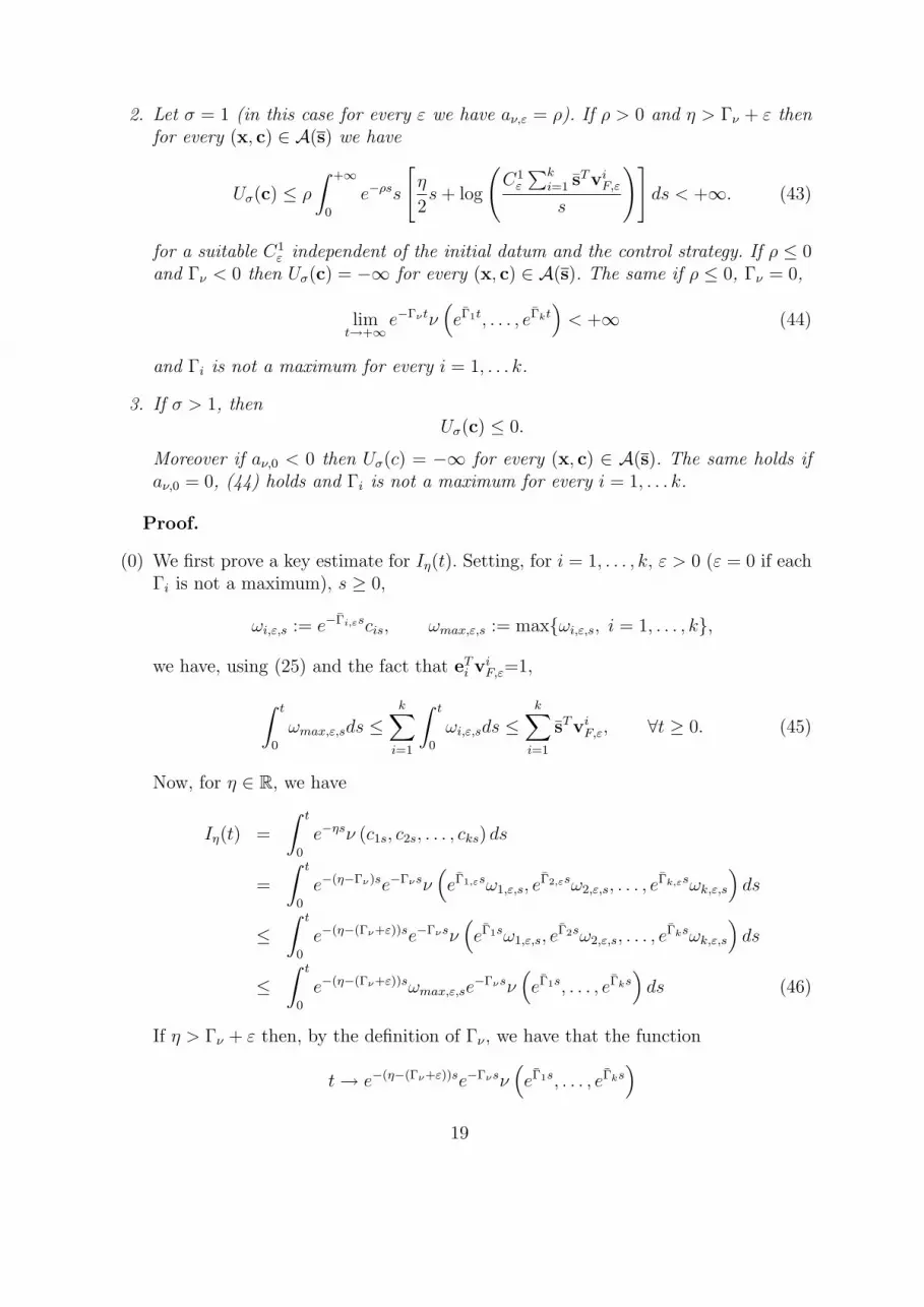
2. Let σ = 1 (in this case for every ε we have aν,ε = ρ). If ρ > 0 and η > Γν + ε thenfor every (x, c) ∈ A(s) we have

Uσ(c) ≤ ρ

∫ +∞

0

e−ρss

[η

2s+ log

(C1ε

∑ki=1 sTviF,εs

)]ds < +∞. (43)

for a suitable C1ε independent of the initial datum and the control strategy. If ρ ≤ 0

and Γν < 0 then Uσ(c) = −∞ for every (x, c) ∈ A(s). The same if ρ ≤ 0, Γν = 0,

limt→+∞

e−Γνtν(eΓ1t, . . . , eΓkt

)< +∞ (44)

and Γi is not a maximum for every i = 1, . . . k.

3. If σ > 1, thenUσ(c) ≤ 0.

Moreover if aν,0 < 0 then Uσ(c) = −∞ for every (x, c) ∈ A(s). The same holds ifaν,0 = 0, (44) holds and Γi is not a maximum for every i = 1, . . . k.

Proof.

(0) We first prove a key estimate for Iη(t). Setting, for i = 1, . . . , k, ε > 0 (ε = 0 if eachΓi is not a maximum), s ≥ 0,

ωi,ε,s := e−Γi,εscis, ωmax,ε,s := max{ωi,ε,s, i = 1, . . . , k},

we have, using (25) and the fact that eTi viF,ε=1,

∫ t

0

ωmax,ε,sds ≤k∑i=1

∫ t

0

ωi,ε,sds ≤k∑i=1

sTviF,ε, ∀t ≥ 0. (45)

Now, for η ∈ R, we have

Iη(t) =

∫ t

0

e−ηsν (c1s, c2s, . . . , cks) ds

=

∫ t

0

e−(η−Γν)se−Γνsν(eΓ1,εsω1,ε,s, e

Γ2,εsω2,ε,s, . . . , eΓk,εsωk,ε,s

)ds

≤∫ t

0

e−(η−(Γν+ε))se−Γνsν(eΓ1sω1,ε,s, e

Γ2sω2,ε,s, . . . , eΓksωk,ε,s

)ds

≤∫ t

0

e−(η−(Γν+ε))sωmax,ε,se−Γνsν

(eΓ1s, . . . , eΓks

)ds (46)

If η > Γν + ε then, by the definition of Γν , we have that the function

t→ e−(η−(Γν+ε))se−Γνsν(eΓ1s, . . . , eΓks

)19

is bounded on [0,+∞) (say by a constant Cε independent of the initial datum andon the control strategy) and so, by putting (45) into (46) we get

Iη(t) ≤ Cε

k∑i=1

sTviF,ε, ∀t ≥ 0. (47)

Similarly, if

limt→+∞

e−Γνtν(eΓ1t, . . . , eΓkt

)< +∞

and Γi is not a maximum for every i = 1, . . . k, then we can choose ε = 0 and η = Γνin (46) and still get (47) with ε = 0, η = Γν .

(1) Now we prove estimate (42) using (35). Take η < ρ1−σ , put the estimate (47) into

(35) and let t→ +∞. We get

Uσ(c) ≤ ρ− η(1− σ)

1− σ

[Cε

k∑i=1

sTviF,ε

]1−σ ∫ +∞

0

sσe−(ρ−η(1−σ))sds

≤ ρ− η(1− σ)

1− σ· ΓE(1 + σ)

(ρ− η(1− σ))1+σ

[Cε

k∑i=1

sTviF,ε

]1−σ

so the claim (42) follows.

(2) If σ = 1 and ρ > 0 we get (43) taking η > Γν + ε, putting (47) into (34) and lettingt→ +∞.

If ρ = 0, then from (34) and (47) we get, for η > Γν + ε∫ t

0

log ν(cs)ds ≤ t

[tη

2+ log

(Cε∑k

i=1 sTviF,εt

)]so if Γν < 0 we take ε > 0, η < 0 such that η > Γν + ε. Then we get, in the limitfor t→ +∞, that U1(c) = −∞.

Let finally Γν = 0,

limt→+∞

e−Γνtν(eΓ1t, . . . , eΓkt

)< +∞

and Γi is not a maximum for every i = 1, . . . k. Then by part (0) of this proof wecan take η = Γν = 0 and ε = 0 in (47) so the estimate (34) becomes∫ t

0

log ν(cs)ds ≤ t log

(C0

∑ki=1 sTviF,0t

)so, in the limit for t→ +∞, we still get that U1(c) = −∞. If ρ < 0 and Γν < 0 (orΓν = 0 when possible) then∫ t

0

e−ρs log ν(cs)ds =

∫ t

0

e−ρs [log ν(cs)]+ ds+

∫ t

0

e−ρs [log ν(cs)]− ds.

20

Now, thanks to the nonpositivity of the negative part and to the fact that e−ρs ≥ 1,∫ t

0

e−ρs [log ν(cs)]− ds ≤

∫ t

0

[log ν(cs)]− ds.

Since the right hand side goes to −∞ as t → +∞ (thanks to the case ρ = 0) wehave

∫ +∞0

e−ρs [log ν(cs)]− ds = −∞. By admissibility this implies that the integral

of the positive part is finite and so U1(c) = −∞.

(3) When σ > 1 it is obvious that Uσ(c) ≤ 0 by construction. Moreover using (33) and(47) with η = ρ

1−σ > Γν + ε we get

1

1− σ

∫ t

0

e−ρsν(c1s, c2s, . . . , cks)1−σds ≤ tσ

1− σ

(Cε

k∑i=1

sTviF,ε

)1−σ

and letting t → +∞ we get Uσ(c) = −∞ for every admissible strategy. Finallyif aν,0 = 0, (44) holds and Γi is not a maximum for every i = 1, . . . k, we knowfrom part (0) of this proof that (47) still holds so we can still let t → +∞ and getUσ(c) = −∞ for every admissible strategy.

Remark 4.6 The above result shows in particular that, when aν,0 > 0 and σ ∈ (0, 1), theintertemporal utility functional Uσ(c) is finite and uniformly bounded for every admissibleproduction-consumption strategy (while for σ ≥ 1 it is only bounded from above). In thecases when

1. σ = 1, ρ ≤ 0, Γν < 0;

2. σ = 1, ρ ≤ 0 and Γν = 0, each Γi is not a maximum and (44) holds;

3. σ > 1, aν,0 < 0;

4. σ > 1, aν,0 = 0, each Γi is not a maximum and (44) holds;

Proposition 4.5 shows that there are no optimal strategies in the sense of Definition 2.1since all strategies have utility −∞.

Proposition 4.7 Let s ≥ 0.

1. Let σ ∈ (0, 1) and, either aν,0 < 0, or aν,0 = 0, each Γi is a maximum for i = 1, . . . , kand

limt→+∞

e−Γνtν(eΓ1t, . . . , eΓkt

)> 0. (48)

Then there exists an admissible strategy (x, c) ∈ A(s) such that Uσ(c) = +∞.

21

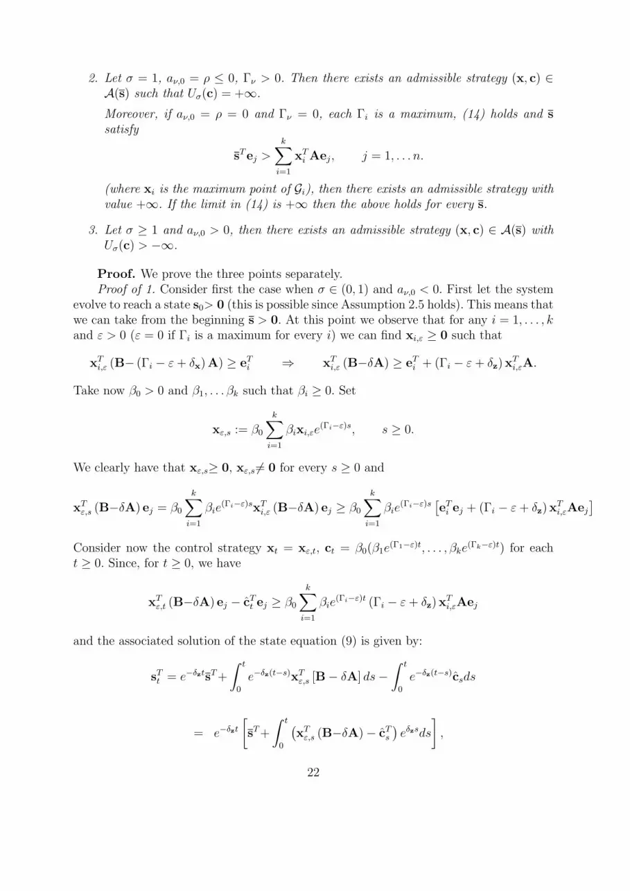
2. Let σ = 1, aν,0 = ρ ≤ 0, Γν > 0. Then there exists an admissible strategy (x, c) ∈A(s) such that Uσ(c) = +∞.

Moreover, if aν,0 = ρ = 0 and Γν = 0, each Γi is a maximum, (14) holds and ssatisfy

sTej >k∑i=1

xTi Aej, j = 1, . . . n.

(where xi is the maximum point of Gi), then there exists an admissible strategy withvalue +∞. If the limit in (14) is +∞ then the above holds for every s.

3. Let σ ≥ 1 and aν,0 > 0, then there exists an admissible strategy (x, c) ∈ A(s) withUσ(c) > −∞.

Proof. We prove the three points separately.Proof of 1. Consider first the case when σ ∈ (0, 1) and aν,0 < 0. First let the system

evolve to reach a state s0> 0 (this is possible since Assumption 2.5 holds). This means thatwe can take from the beginning s > 0. At this point we observe that for any i = 1, . . . , kand ε > 0 (ε = 0 if Γi is a maximum for every i) we can find xi,ε ≥ 0 such that

xTi,ε (B− (Γi − ε+ δx) A) ≥ eTi ⇒ xTi,ε (B−δA) ≥ eTi + (Γi − ε+ δz) xTi,εA.

Take now β0 > 0 and β1, . . . βk such that βi ≥ 0. Set

xε,s := β0

k∑i=1

βixi,εe(Γi−ε)s, s ≥ 0.

We clearly have that xε,s≥ 0, xε,s 6= 0 for every s ≥ 0 and

xTε,s (B−δA) ej = β0

k∑i=1

βie(Γi−ε)sxTi,ε (B−δA) ej ≥ β0

k∑i=1

βie(Γi−ε)s

[eTi ej + (Γi − ε+ δz) xTi,εAej

]Consider now the control strategy xt = xε,t, ct = β0(β1e

(Γ1−ε)t, . . . , βke(Γk−ε)t) for each

t ≥ 0. Since, for t ≥ 0, we have

xTε,t (B−δA) ej − cTt ej ≥ β0

k∑i=1

βie(Γi−ε)t (Γi − ε+ δz) xTi,εAej

and the associated solution of the state equation (9) is given by:

sTt = e−δztsT+

∫ t

0

e−δz(t−s)xTε,s [B− δA] ds−∫ t

0

e−δz(t−s)csds

= e−δzt[sT+

∫ t

0

(xTε,s (B−δA)− cTs

)eδzsds

],

22

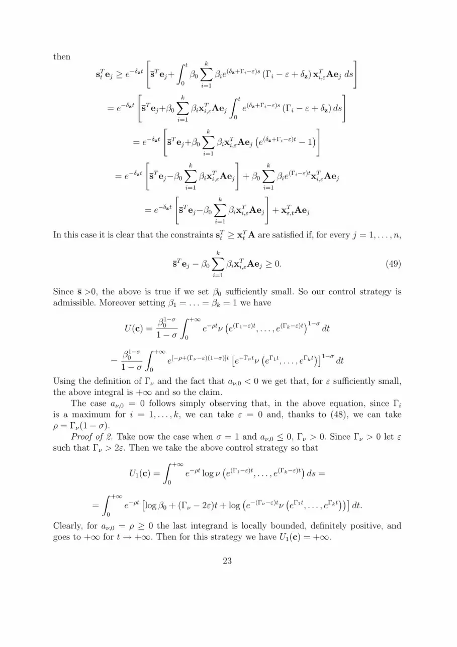
then

sTt ej ≥ e−δzt

[sTej+

∫ t

0

β0

k∑i=1

βie(δz+Γi−ε)s (Γi − ε+ δz) xTi,εAej ds

]

= e−δzt

[sTej+β0

k∑i=1

βixTi,εAej

∫ t

0

e(δz+Γi−ε)s (Γi − ε+ δz) ds

]

= e−δzt

[sTej+β0

k∑i=1

βixTi,εAej

(e(δz+Γi−ε)t − 1

)]

= e−δzt

[sTej−β0

k∑i=1

βixTi,εAej

]+ β0

k∑i=1

βie(Γi−ε)txTi,εAej

= e−δzt

[sTej−β0

k∑i=1

βixTi,εAej

]+ xTε,tAej

In this case it is clear that the constraints sTt ≥ xTt A are satisfied if, for every j = 1, . . . , n,

sTej − β0

k∑i=1

βixTi,εAej ≥ 0. (49)

Since s >0, the above is true if we set β0 sufficiently small. So our control strategy isadmissible. Moreover setting β1 = . . . = βk = 1 we have

U(c) =β1−σ

0

1− σ

∫ +∞

0

e−ρtν(e(Γ1−ε)t, . . . , e(Γk−ε)t

)1−σdt

=β1−σ

0

1− σ

∫ +∞

0

e[−ρ+(Γν−ε)(1−σ)]t[e−Γνtν

(eΓ1t, . . . , eΓkt

)]1−σdt

Using the definition of Γν and the fact that aν,0 < 0 we get that, for ε sufficiently small,the above integral is +∞ and so the claim.

The case aν,0 = 0 follows simply observing that, in the above equation, since Γiis a maximum for i = 1, . . . , k, we can take ε = 0 and, thanks to (48), we can takeρ = Γν(1− σ).

Proof of 2. Take now the case when σ = 1 and aν,0 ≤ 0, Γν > 0. Since Γν > 0 let εsuch that Γν > 2ε. Then we take the above control strategy so that

U1(c) =

∫ +∞

0

e−ρt log ν(e(Γ1−ε)t, . . . , e(Γk−ε)t

)ds =

=

∫ +∞

0

e−ρt[log β0 + (Γν − 2ε)t+ log

(e−(Γν−ε)tν

(eΓ1t, . . . , eΓkt

))]dt.

Clearly, for aν,0 = ρ ≥ 0 the last integrand is locally bounded, definitely positive, andgoes to +∞ for t→ +∞. Then for this strategy we have U1(c) = +∞.

23

In the case when σ = 1, aν,0 = ρ = 0, Γν = 0, each Γi is a maximum, and (14) holds,the strategy defined in the proof of point 1 above is still admissible. However it has value+∞ only if β0 is big enough (i.e. β0L > 1, where L is defined at the end of Section 2).This means that also s must be big enough so (49) is verified. In particular, if L = +∞,again for every s the claim holds.

Proof of 3. Let aν,0 > 0 and σ ∈ [1,+∞). We observe that (since admissibility doesnot depend on the value of σ) the strategy found in point 1 above is admissible. We thenhave, for σ ∈ (1,+∞)

U(c) =β1−σ

0

1− σ

∫ +∞

0

e[−ρ+(Γν−ε)(1−σ)]t[e−Γνtν

(eΓ1t, . . . , eΓkt

)]1−σdt

so, if ε > 0 is such that −ρ+ (Γν − ε)(1− σ) < 0 we get the claim.For σ = 1 we have

U1(c) =

∫ +∞

0

e−ρt log ν(e(Γ1−ε)t, . . . , e(Γk−ε)t

)ds =

=

∫ +∞

0

e−ρt[log β0 + Γνt+ log

(e−(Γν+ε)tν

(eΓ1t, . . . , eΓkt

))]dt.

Since the last integrand is less than polynomially growing and ρ = aν,0 > 0 then theintegral above is finite, so U1(c) > −∞.

Remark 4.8 The above result shows in particular that, when aν,0 > 0 and σ ∈ [1,+∞),the intertemporal utility functional Uσ(c) is not always −∞ so it is bounded from below(recall that from Proposition 4.5 we already know that in these case Uσ(c) is bounded fromabove). Moreover in the cases when

1. σ ∈ (0, 1) and aν,0 < 0;

2. σ ∈ (0, 1), aν,0 = 0, each Γi is a maximum and (48) holds;

3. σ = 1, aν,0 ≤ 0 and Γν > 0;

4. σ = 1, aν,0 = 0, Γν = 0, each Γi is a maximum (48) holds and s is big enough;

Proposition 4.7 shows that there are no optimal strategies in the sense of Definition 2.1since the supremum of the utility is +∞.

Summing up the informations taken from Propositions 4.5 and 4.7 we can say thefollowing.

• In the cases when aν,0 > 0 we know that the functional is uniformly bounded (caseσ ∈ (0, 1)) or bounded from from above and not identically −∞ (case σ ≥ 1);

24

• In the cases when aν,0 ≤ 0 we have nonexistence when

1. σ ∈ (0, 1) and aν,0 < 0;

2. σ ∈ (0, 1), aν,0 = 0, each Γi is a maximum and (48) holds;

3. σ = 1, aν,0 ≤ 0, Γν 6= 0

4. σ = 1, aν,0 ≤ 0, Γν = 0, each Γi is not a maximum and (44) holds;

5. σ = 1, aν,0 = 0, Γν = 0, each Γi is a maximum (48) holds and s is big enough;

6. σ > 1 and aν,0 < 0

7. σ > 1, aν,0 = 0, each Γi is not a maximum and (44) holds.

We observe that, to end the treatment of nonexistence result one should deal with acomplete treatment of the following limiting cases:

• σ ∈ (0, 1) and aν,0 = 0;

• σ = 1, aν,0 ≤ 0, Γν = 0;

• σ > 1 and aν,0 = 0

Proof of Theorem 3.2. It follows directly from Proposition 4.5, Proposition 4.7and the remarks above.

Now we come to prove existence when aν,0 > 0 using compactness arguments. To dothis we need first to prove suitable properties of the set A (s) which are given in the nextproposition. First we recall a simple definition: given a measurable function g1 : R+→ Rwe denote by L∞g1

(0,+∞; Rm) the set of measurable functions f : R+→ Rm such that the

product f · g1 is bounded on R+. Moreover given a measurable function g2 : R+→ Rk

we denote by L1g2

(0,+∞; Rk

)the set of measurable functions f : R+→ Rk such that the

product fi · g2,i is integrable on R+ for each i = 1, . . . , k. We set g1 (t) = eλt (λ is givenby (27) of Lemma 4.2) and g2 (t) = (e(Γ1+ε)t, . . . , e(Γk+ε)t) for ε > 0 such that aν,ε > 0.

Proposition 4.9 Let Assumptions 2.2 and 2.3 be verified. Let also σ ∈ (0, 1)∪ (1,+∞).Given any s ≥ 0 the set A (s) of admissible control strategies starting at s is a closed,bounded, convex subset of the space L∞g1

(0,+∞; Rm)× L1g2

(0,+∞; Rk

). Moreover

(x,c) ∈ A (s) , λ ∈ [0, 1]⇒ (λx,λc) ∈ A (s) (50)

Finally, if ν is strictly concave the functional Uσ is strictly concave with respect to theargument c. The same holds when σ = 1 and ρ > 0.

25

Proof. Convexity. Let i = 1, 2 and let (xi,ci) ∈ A (s), and λ ∈ [0, 1]. Calling

(xλ,cλ) = λ (x1,c1) + (1− λ) (x2,c2)

then due to the linearity of the state equation (9)

st,s,(xλ,cλ) = λst,s,(x1,c1) + (1− λ) st,s,(x2,c2).

Since all constraints on (s, (x, c)) (i.e. x ≥ 0, c ≥ 0, xTA ≤ sT ) are linear it follows that,since (xi,ci) (i = 1, 2) satisfy them, then so does (xλ,cλ). This yields (xλ,cλ) ∈ A (s) whenσ ∈ (0, 1) ∪ (1,+∞). If σ = 1 we also have to prove that (xλ,cλ) is semiintegrable. Thisfollows from point (2) of Proposition 4.5. Indeed if ρ > 0, thanks to estimate (43) we knowall admissible strategies are upper semiintegrable, so also their convex combinations areupper semiintegrable. Boundedness follows from the estimates of Lemma 4.2.

Closedness follows from the fact that all constraints are linear so all of them preservein the limit in the topology of L∞g1

(0,+∞; Rm) × L1g2

(0,+∞; Rk

). For σ = 1 we need to

know that the limit of semiintegrable sequences is again semiintegrable. For ρ > 0 thisfollows from the estimate (43).

Homogeneity (50) follows from convexity and from the fact that the strategy (0,0)is always admissible.

Strict concavity of the functional Uσ is a standard result (see e.g. [6]) and we omitthe proof.

Now we move on to the proof of Theorem 3.1.

Proof of Theorem 3.1. The uniqueness property follows from the strict concavity ofUσ proved in Proposition 4.9. The existence result follows applying a suitable modificationof Theorems 21 and 22 in [19, p. 406] (see also [18]). We divide it into three cases dependingon the value of σ.

Case σ > 1.Here we can apply directly Theorem 22 and note 26 of [19, p. 406] plus [19, note 20,

p.137]. In fact this theorem asks the following:

1. the set U where the controls take values is closed (in our case U is Rm+ ×Rk

+ i.e. thepositive orthant of Rm+k);

2. the functions defining the running utility ((s, (x,c) , t)→ e−ρtuσ (ν(c))), the dynam-ics of the state equation ((s, (x,c) , t)→ −δzsT +xT (B−δA)−c) and the constraints((s, (x,c) , t)→ sT − xTA) are defined on the set

S ={

(s, (x,c) , t) ∈ Rn+ ×

[Rm

+ × Rk+

]× R+ : sT − xTA ≥ 0

},

are linear (or sum of linear and nondecreasing) in the variable s and continuous onthe set

S ′ ={

(s, (x,c) , t) ∈ Rn+ ×

[Rm

+ × Rk+

]× R+ : sT − xTA ≥ 0

};

26

3. for each t ≥ 0 the set

S ′ (t) ={

(s, (x,c)) ∈ Rn+ ×

[Rm

+ × Rk+

]: sT − xTA ≥ 0

}is contained in the closure S0 (t) of the set

S0 (t) ={

(s, (x,c)) ∈ Rn+ × U : sT − xTA > 0

};

4. for each n ∈ N and t ≥ 0 the set

Γnt ={

(s, (x,c)) : sT − xTA ≥ 0, (x,c) ∈ U,∣∣∣∣(e−ρtuσ (ν(c)) ,−δzsT + xT (B−δA)− c)∣∣∣∣ ≤ n,

}is closed and is contained in S ′ (t). The same for the set

Γn = {s : (s, (x,c)) ∈ Γnt } ;

5. there exists an admissible strategy with finite value;

6. the set

N (s,U, t) ={(e−ρtuσ (ν(c)) + γ,−δzs + xT (B−δA)− c + γ

):

(γ, γ) ≤ 0, s− xTA ≥ 0, (x,c) ∈ U}

is convex for all (s,t) ∈ Rn × [0,+∞) ;

7. the set N (s,U, t) has closed graph for each t as a function of s ∈ Γn. Closed graphmeans that

sn ∈ Γn,vn ∈ N (s,U, t) , sn → s,vn → v⇒ s ∈ Γn.

8. there exists q′ ∈ Rn+1, q′ ≥ 0 such that for every q ≥ q′ (q = (q0, q1, ..., qn) =(q0,q1)) there exists locally integrable functions φq and ψq defined for t ∈ [0,+∞)such that

e−ρtuσ (ν(c)) q0+(−δzsT + xT (B−δA)− c

)q1 ≤ φq (t)+ψq (t)·max

[0, sTe1, ..., s

Ten]

for every (s, (x,c) , t) ∈ S.

9. for every i = 1, ..., n and every admissible state trajectory st, we have sTt ei ≥ 0 forevery t ≥ 0. Moreover for every q0∈R, q0 ≥ 0, there exists an integrable function νq0defined for t ∈ [0,+∞) such that, ,

e−ρtuσ (ν(ct)) (1 + q0) ≤ νq0 (t) ,

for every admissible strategy (x,c) ∈ A (s).

27

All points 1-4 and 6-7 are easily checked in our case thanks to the linearity of thestate equation and of the constraints. We omit the verification of them for brevity. Point5 is known from previous results (Proposition 4.5 and Proposition 4.7). Point 9 comessimply recalling that for σ > 1 the utility is negative and so one can choose νq0 (t) = 0for every t ≥ 0. Point 8 is more delicate. Setting

g (c) = e−ρtuσ (ν(c)) q0 − cTq1

we haveg (c) ≤ 0

Moreover

−δzsT + xT (B−δA) = −δz(sT − xTA

)+ xT (B−δxA) ≤ xTB.

Now, recalling the proof of (27) we have that

xTB ≤ sTD ≤M max[0, sTe1, ..., s

Ten]

whereM depends only on the coefficient of D. Setting, for t ≥ 0, φq (t) = 0 and ψq (t) = Mwe see that φq and ψq are locally integrable functions and satisfy point 8.

Case σ = 1 and σ ∈ (0, 1).Also this case goes applying Theorem 22 and note 26 of [19, p. 406] (see also [18] or

[19, Exercise 6.8.3, p.410]). In fact this theorem asks the following:

1. the set U where the controls take values is closed (in our case U is Rm+ ×Rk

+ i.e. thepositive orthant of Rm+k);

2. the functions defining the running utility ((s, (x,c) , t) → e−ρtuσ (c)), the dynamicsof the state equation ((s, (x,c) , t)→ −δzsT + xT (B−δA)− c) and the constraints((s, (x,c) , t)→ sT − xTA) are defined on the set

S ={

(s, (x,c) , t) ∈ Rn+ × U × R+ : sT − xTA ≥ 0

}are linear (or sum of linear and nondecreasing) in the variable s and continuous onthe set

S ′ ={

(s, (x,c) , t) ∈ Rn+ × U × R+ : sT − xTA ≥ 0

};

3. for each t ≥ 0 the set

S ′ (t) ={

(s, (x,c)) ∈ Rn+ × U : sT − xTA ≥ 0

}is contained in the closure S0 (t) of the set

S0 (t) ={

(s, (x,c)) ∈ Rn+ × U : sT − xTA > 0

};

28

4. for each n ∈ N and t ≥ 0 the set

Γnt ={

(s, (x,c)) : sT − xTA ≥ 0, (x,c) ∈ U,∣∣∣∣(e−ρtuσ (ν(c)) ,−δzsT + xT (B−δA)− c)∣∣∣∣ ≤ n,

}is closed and is contained in S ′ (t). The same for the set

Γn = {s : (s, (x,c)) ∈ Γnt } ;

5. there exists an admissible strategy with finite value;

6. the set

N (s,U, t) ={(e−ρtuσ (ν(c)) + γ,−δzs + xT (B−δA)− cT + γ

):

(γ, γ) ≤ 0, s− xTA ≥ 0, (x,c) ∈ U}

is convex for all (s,t) ∈ Rn × [0,+∞);

7. the set N (s,U, t) has closed graph for each t as a function of s ∈ Γn. Closed graphmeans that

sn ∈ Γn,vn ∈ N (s,U, t) , sn → s,vn → v⇒ s ∈ Γn.

8. there exists q′ ∈ Rn+1, q′ ≥ 0 such that for every q ≥ q′ (q = (q0, q1, ..., qn) =(q0,q1)) there exists locally integrable functions φq and ψq defined for t ∈ [0,+∞)such that

e−ρtuσ (ν(c)) q0+(−δzsT + xT (B−δA)− cT

)q1 ≤ φq (t)+ψq (t)·max

[0, sTe1, ..., s

Ten]

for every (s, (x,c) , t) ∈ S.

9. for every i = 1, ..., n and every admissible state trajectory st, we have sTt ei ≥ 0 forevery t ≥ 0. Moreover for every q0∈R, q0 ≥ 0, there exists an integrable functionνq0 , continuous functions χiq0 and θiq0 (i = 1, ..., n) defined for t ∈ [0,+∞) such that,for every admissible strategy (x,c) ∈ A (s),

e−ρtuσ(ν(ct) (1 + q0) +n∑i=1

χiq0 (t)(−δzsTt + xTt (B−δA)− cTt

)ei ≤ νq0 (t) , (51)

and

−∫ +∞

s

χiq0 (t)(−δzsTt + xTt (B−δA)− cTt

)eidt ≤ θiq0 (s) (52)

where lims→+∞ θiq0

(s) = 0.

29

All points 1-4 and 6-7 are easily checked in our case thanks to the linearity of thestate equation and of the constraints. We omit the verification of them for brevity. Point5 is known from previous results (Proposition 4.5 and Proposition 4.7). Point 8 followsarguing exactly as in the case σ > 1 except for the estimate of the function g(c) which isdone as follows. First observe that g(c) goes to −∞ as any ci → +∞, then observe thatg is positive on a compact set depending on q and t which is bounded uniformly when qand t belong to a bounded set. This is enough to guarantee that g has a maximum pointand that the value of the maximum is uniformly bounded for q and t on bounded sets.

Point 9 is more delicate. Take first the case σ ∈ (0, 1). Set, for i = 1, . . . , n, χiq0 (t) =

eTi

(∑kj=1 vjF e

−djt)

where dj = Γj + ε0 for suitable ε0 to choose later. First consider, in

(51), the terms containing ct. They are

e−ρtuσ(ν(ct)) (1 + q0)−n∑i=1

cTt eiχiq0

(t) .

Since we haven∑i=1

cTt eiχiq0

(t) =k∑j=1

cTt vjF e−djt ≥

k∑j=1

cTt eje−djt

(using Lemma 4.1 to get the last inequality) then, setting

g (t, c) := e−ρtuσ(ν(c)) (1 + q0)−n∑i=1

cTeiχiq0

(t) .

we have

g (t, c) ≤ e−ρtuσ(ν(c)) (1 + q0)−k∑j=1

e−djtcTej.

Setting ωj = e−djtcTej we have that

e−ρtuσ(ν(c)) (1 + q0)−k∑j=1

e−djtcTej = e−ρtuσ(ν(ω1ed1t, . . . , ωke

dkt)) (1 + q0)−k∑j=1

ωj.

So, calling

g1(t, ω) = e−ρtuσ(ν(ω1ed1t, . . . , ωke

dkt)) (1 + q0)−k∑j=1

ωj,

we havesupc≥0

g(t, c) ≤ supω≥0

g1(t, ω)

Now, setting ωmax = max{ω1, . . . , ωk}

ν(ω1ed1t, . . . , ωke

dkt) ≤ ωmaxν(ed1t, . . . , edkt) = ωmaxeε0tν(eΓ1t, . . . , eΓkt) = ωmaxe

ε0tν(eΓ1t, . . . , eΓkt)

30

So, calling, for ε > 0

Cε = supt≥0{e−(Γν+ε)tν(eΓ1t, . . . , eΓkt)} < +∞

we haveν(ω1e

d1t, . . . , ωkedkt) ≤ Cεωmaxe

(Γν+ε+ε0)t.

It follows

g1(t, ω) ≤ C1−σε ω1−σ

max

1 + q0

1− σe−[ρ−(Γν+ε+ε0)(1−σ)]t −

k∑j=1

ωj.

Since

ω1−σmax ≤

k∑j=1

ω1−σj

we have

g1(t, ω) ≤k∑j=1

C1−σε

1 + q0

1− σe−[ρ−(Γν+ε+ε0)(1−σ)]tω1−σ

j − ωj.

The maximum value of the left hand side can be easily calculated and is

σ

1− σC

1σ−1

ε (1 + q0)1σ e−[ρ−(Γν+ε+ε0)(1−σ)]t

So if we take ε and ε0 such that ρ > (Γν + ε + ε0)(1 − σ) we have integrability ofsupc≥0 g(t, c) and so also of g(t, ct) for every admissible consumption strategy ct.

Now consider the terms without ct in (51)

−δzsTt + xTt (B−δA) = −δz(sTt − xTt A

)+ xTt (B−δxA) ≤ xTt (B−δxA) .

Then

n∑i=1

χiq0 (t)(−δzsTt + xTt (B−δA)

)ei ≤

n∑i=1

χiq0 (t)(xTt (B−δxA)

)ei =

k∑j=1

(xTt (B−δxA)

)vjF e

−djt

From Lemma 4.1 we have, for every ε > 0(xTt (B−δxA)

)vjF e

−djt ≤ xTt AvjF (Γj + ε) e−djt ≤ e(−dj+Γj+ε)tsTvjF (Γj + ε) .

So, taking ε < ε0 the first part of point 9 is true.

Now we go to (52) observing that

−∫ +∞

s

χiq0 (t) ·(−δzsTt + xTt (B−δA)− cTt

)eidt

≤∫ +∞

s

χiq0 (t) ·(δzs

Tt + δxxTt A + cTt

)eidt.

31

From the estimates (23) and (25) we get, for every j = 1, . . . , k,

eTi vjF ·(δzs

Tt + δxxTt A

)ei ≤ (δz + δx) sTt vjF ≤ (δz + δx) sTvjF e

(Γj+ε)t

so that ∫ +∞

s

χiq0 (t) ·(δzs

Tt + δxxTt A

)eidt ≤

e−(ε0−ε)s

ε0 − ε(δz + δx)

k∑j=1

sTvjF ,

which goes to zero as t → +∞ if ε < ε0. Finally, arguing as above, thanks to (23)-(26)we get, for ε < ε0 ∫ +∞

s

χiq0 (t) · cTt eidt ≤ e−(ε0−ε)sk∑j=1

sTvjF

and this completes the proof.Case σ = 1. The proof of (52) and of the estimate for the part not containing c of

(52) is the same as in the case σ ∈ (0, 1). Concerning the remaining estimate we set

g (t, c) := e−ρt log(ν(c)) (1 + q0)−n∑i=1

cTeiχiq0

(t) .

Again we observe thatsupc≥0

g(t, c) ≤ supω≥0

g1(t, ω)

where

g1(t, ω) = e−ρt log(ν(ω1ed1t, . . . , ωke

dkt)) (1 + q0)−k∑j=1

ωj,

and, arguing as above we get

g1(t, ω) ≤ e−ρt (1 + q0) log(Cεωmaxe(Γν+ε+ε0)t)−

k∑j=1

ωj,

and from now on we estimate g1(t, ω) as above getting the claim.

5 Appendix

In this Appendix we study the limit

limt→+∞

e−Γνtν(eΓ1t, . . . , eΓkt

)=: Lν , (53)

First of all we prove the following result.

Proposition 5.1 Assume that the law of ν contains a finite number of sums, products,powers and min operation. Then L ∈ (0,+∞).

32

Proof. We prove the result by induction on the number of elementary operations (sums,products, power, min). If there is only one elementary operation the claim is obvious.Assume now that the the claim is true when ν is done by n elementary operations. Considerthen ν with the law done by n+ 1 elementary operations. This means, in particular, thatwe can write, either

ν(c) = f(ν1(c), ν2(c)) ∀c ∈ Rk+,

where f(a, b) = a+ b, ab, a ∧ b and ν1, ν2 are done by n elementary operations; or

ν(c) = [ν0(c)]α ∀c ∈ Rk+,

for some α ∈ R− {0} and ν0 done by n elementary operations.First case: f(a, b) = a+ b. In this case we have

limt→+∞

e−Γνtν(eΓ1t, . . . , eΓkt

)= lim

t→+∞e−Γνt

[ν1

(eΓ1t, . . . , eΓkt

)+ ν2

(eΓ1t, . . . , eΓkt

)]By the positivity of ν1, ν2 we have

limt→+∞

e−Γνtν1

(eΓ1t, . . . , eΓkt

)+ lim

t→+∞e−Γνtν2

(eΓ1t, . . . , eΓkt

)and the same when we substitute Γν with Γν ± ε. So we have

Γν = Γν1 ∨ Γν2 .

So we must have either Lν = Lν1 , or Lν = Lν2 , or Lν = Lν1 + Lν2 .

Second case: f(a, b) = ab. In this case we have that both ν1, ν2 must be homogeneousof constant degree η and 1− η, respectively. Then

ν1 · ν2 =[ν

1/η1

]η·[ν

1/(1−η)2

]1−η=: νη1 · ν

1−η2

Moreover arguing as above we observe that it must be

Γν = ηΓν1 + (1− η)Γν2

so

limt→+∞

e−Γνtν(eΓ1t, . . . , eΓkt

)= lim

t→+∞

[e−Γν1 tν1

(eΓ1t, . . . , eΓkt

)]η·[e−Γν2 tν2

(eΓ1t, . . . , eΓkt

)]1−ηand the claim follows as in the first case.

Third case: f(a, b) = a ∧ b. One argues as in the first case using that here

Γν = Γν1 ∧ Γν2 .

So we must have Lν = Lν1 ∧ Lν2 .

Fourth case: the power. One argues as in the second case.

Now we provide two examples where L = 0 and L = +∞.

33

Example 5.2 Let k = 2 and let {αi}i∈N be a sequence such that αi ∈ (0, 1) for everyi ∈ N and limi→+∞ αi = 0. Assume that 0 < Γ1 < Γ2 and let

ν(c1, c2) =+∞∑i=1

cαi1 c1−αi2

It is easy to check that Γν = Γ2 and that L = 0.

Example 5.3 Let k = 2 and let αi = 1− 1i+1

for i ∈ N. Assume that 0 < Γ1 < Γ2 and let

ν(c1, c2) = infi∈N

{icαi1 c

1−αi2

}It is easy to check that Γν = Γ1 and that L = +∞.

References

[1] Acemoglu, D. and Guerrieri, V.: Capital Deepening and Nonbalanced EconomicGrowth. Journal of Political Economy, 116(3), 467-498 (2008)

[2] Balder, E. J.: Existence of Optimal Solutions for Control and Variational Problemswith Recursive Objectives. Journal of Mathematical Analysis and Applications, 178,418-437 (1993)

[3] Bardi, M., Capuzzo Dolcetta, I.: Optimal Control and Viscosity Solutions ofHamilton-Jacobi-Bellman Equations. Boston, Birkhauser, 1997.

[4] Becker, R. A., Boyd III, J. H., Sung, B. Y.: Recursive Utility and Optimal CapitalAccumulationI: Existence. Journal of Economic Theory, 47, 76-100 (1989)

[5] Cesari, L.: Optimization Theory and Applications. New York, Springer–Verlag, 1983

[6] Freni, G., Gozzi, F., Pignotti, C.: A Multisector AK Model with Endogenous Growth:Value Function and Optimality Conditions. J. Math. Ec., 2008.

[7] Freni, G., Gozzi, F., Salvadori, N.: Existence of Optimal Strategies in linear multi-sector models. Economic Theory, 29 25-48, 2006.

[8] Freni, G., Gozzi, F., Salvadori, N.: Existence of Optimal Strategies in linear Multi-sector Models. Discussion papers, Collana di E-papers del Dipartimento di ScienzeEconomiche - Universita di Pisa, No. 29, 2004. http://www-dse.ec.unipi.it/discussion-papers/lavori/freniGozziSalvadori.pdf

[9] Gale, D.: The Closed Linear Model of Production. Paper 18 in Kuhn, H., and A. W.Tucker, eds., Linear Inequalities and Related Systems. Princeton U. Press, 1956

[10] Gale, D.: The Theory of Linear Economic Models. New York, McGraw-Hill, 1960

34

[11] Kongsamut, P., Rebelo, S., and Xie, D.; Beyond Balanced Growth. Review of Eco-nomic Studies, 68(4), 869-82 (2001).

[12] Magill, M. J. P.: Infinite Horizon Programs. Econometrica, 49, 679-711 (1981).

[13] Magill, M. J. P.: On a Class of Variational Problems Arising in Mathematical Eco-nomics. J. Math. Anal. Appl., 82, 66-74 (1981).

[14] Mangasarian, O. L.: Nonlinear Programming. Bombay-New Delhi: Tata McGrawHill, reprinted as vol. 16 of the series Classics in Applied Mathematics, Philadelphia:SIAM, 1994.

[15] Motzkin, T. S.: Beitrage zur Theorie der Linearen Ungleichungen. Inaugural Disser-tation, Jerusalem, Base, 1936.

[16] von Neumann, J.: A Model of General Economic Equilibrium. Review of EconomicStudies 13, 1-9 (1945)

[17] Ngai, L.R. and Pissarides, A.: Structural Change in a Multisector Model of Growth.American Economic Review, 97(1), 429-443 (2007).

[18] Seierstad, A.: Nontrivial Multipliers and Necessary Conditions for Optimal ControlProblems with Infinite Horizon and Time Path Restrictions. Memorandum from De-partment of Economics, University of Oslo, 24, (1986).

[19] Seierstad, A., Sydsaeter, K.: Optimal Control Theory with Economic Applications.Amsterdam, North Holland, 1987.

35