arX

iv:1

405.

1687

v2 [

mat

h.C

O]

8 M

ay 2

014

EXISTENCE OF UNIMODULAR TRIANGULATIONS

—

POSITIVE RESULTS

CHRISTIAN HAASE, ANDREAS PAFFENHOLZ, LINDSAY C. PIECHNIK,AND FRANCISCO SANTOS

Abstract. Unimodular triangulations of lattice polytopes and theirrelatives arise in algebraic geometry, commutative algebra, integer pro-gramming and, of course, combinatorics.

Presumably, “most” lattice polytopes do not admit a unimodulartriangulation. In this article, we survey which classes of polytopesare known to have unimodular triangulations; among them some newclasses, and some not so new which have not been published elsewhere.

We include a new proof of the classical result by Knudsen-Munford-Waterman stating that every lattice polytope has a dilation that admitsa unimodular triangulation. Our proof yields an explicit (although dou-bly exponential) bound for the dilation factor.

Contents

1. Introduction 21.1. What? 31.2. Why? Who? 51.3. What’s new? 101.4. What’s not here 111.5. What’s left? 112. Methods 122.1. Pulling Triangulations 122.2. Push-forward subdivisions and pull-back subdivisions 172.3. Joins and (Fiber) Products 212.4. Toric Grobner Bases 293. Examples 333.1. Polytopes cut out by roots 343.2. Polytopes spanned by roots 393.3. Other Graph Polytopes 473.4. Smooth Polytopes 503.5. The Grobner fan and the toric Hilbert scheme 534. Dilations and the KMW Theorem 57

Date: May 9, 2014.Work of the first author was supported in part by NSF grant DMS-0200740, and by

Emmy Noether HA 4383/1 and Heisenberg HA 4383/4 fellowships of the German ResearchCouncil (DFG).

Work of the second author was supported by a Priority Program (DFG/SPP 1489) ofthe German Research Council (DFG).

Work of the fourth author is supported in part by the Spanish Ministry of Sciencethrough grants MTM2008-04699-C03-02 and MTM2011-22792, and by a Research Awardfrom the Alexander von Humboldt Foundation.

1

2 HAASE, PAFFENHOLZ, PIECHNIK, AND SANTOS

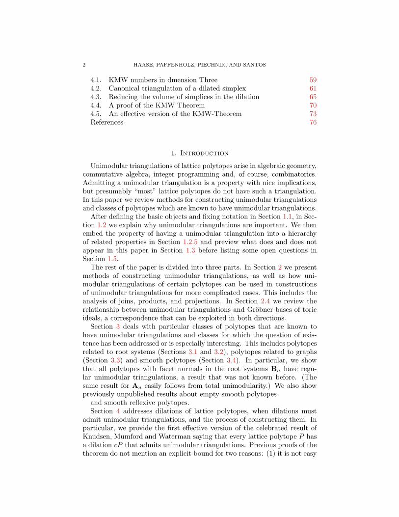
4.1. KMW numbers in dmension Three 594.2. Canonical triangulation of a dilated simplex 614.3. Reducing the volume of simplices in the dilation 654.4. A proof of the KMW Theorem 704.5. An effective version of the KMW-Theorem 73References 76

1. Introduction

Unimodular triangulations of lattice polytopes arise in algebraic geometry,commutative algebra, integer programming and, of course, combinatorics.Admitting a unimodular triangulation is a property with nice implications,but presumably “most” lattice polytopes do not have such a triangulation.In this paper we review methods for constructing unimodular triangulationsand classes of polytopes which are known to have unimodular triangulations.

After defining the basic objects and fixing notation in Section 1.1, in Sec-tion 1.2 we explain why unimodular triangulations are important. We thenembed the property of having a unimodular triangulation into a hierarchyof related properties in Section 1.2.5 and preview what does and does notappear in this paper in Section 1.3 before listing some open questions inSection 1.5.

The rest of the paper is divided into three parts. In Section 2 we presentmethods of constructing unimodular triangulations, as well as how uni-modular triangulations of certain polytopes can be used in constructionsof unimodular triangulations for more complicated cases. This includes theanalysis of joins, products, and projections. In Section 2.4 we review therelationship between unimodular triangulations and Grobner bases of toricideals, a correspondence that can be exploited in both directions.

Section 3 deals with particular classes of polytopes that are known tohave unimodular triangulations and classes for which the question of exis-tence has been addressed or is especially interesting. This includes polytopesrelated to root systems (Sections 3.1 and 3.2), polytopes related to graphs(Section 3.3) and smooth polytopes (Section 3.4). In particular, we showthat all polytopes with facet normals in the root systems Bn have regu-lar unimodular triangulations, a result that was not known before. (Thesame result for An easily follows from total unimodularity.) We also showpreviously unpublished results about empty smooth polytopes

and smooth reflexive polytopes.Section 4 addresses dilations of lattice polytopes, when dilations must

admit unimodular triangulations, and the process of constructing them. Inparticular, we provide the first effective version of the celebrated result ofKnudsen, Mumford and Waterman saying that every lattice polytope P hasa dilation cP that admits unimodular triangulations. Previous proofs of thetheorem do not mention an explicit bound for two reasons: (1) it is not easy

UNIMODULAR TRIANGULATIONS 3

Figure 1.1. A non-unimodular triangulation and two unimodular ones.They are all regular, but only the last is quadratic. (See Sec-tion 2.4.2).

to derive a bound from the algorithm, (2) the bound obtained would containarbitrarily long towers of exponentials. Our bound, instead, is “only” doublyexponential:

Theorem 4.4. If P is a lattice polytope of dimension d and (lattice) volumevol(P ), then the dilation

d!vol(P )!dd2 vol(P )

P

has a regular unimodular triangulation.More precisely, if P has a triangulation into N d-simplices, of volumes

V1, . . . , VN , then the dilation

d!∑

N

i=1 Vi!((d+1)!(d!)d)Vi−1

T

has a regular unimodular refinement.

1.1. What? A lattice polytope in Rd is the convex hull of finitely manypoints in the lattice Zd. We identify two lattice polytopes if they are relatedby a lattice preserving affine map. Up to this lattice equivalence, we canalways assume that our polytope is d-dimensional. (For more on convexpolytopes and lattices we refer to [7].)

A unimodular simplex is a lattice polytope which is lattice equivalent tothe standard simplex ∆d, the convex hull of the origin 0 together with thestandard unit vectors ei (1 ≤ i ≤ d). Equivalently, unimodular simplicesare characterized as the d-dimensional lattice polytopes of minimal possibleEuclidean volume, 1/d! .

For the purposes of this paper, a (lattice) subdivision of a d-dimensionallattice polytope P is a finite collection of (lattice) polytopes S such that

(1) every face of a member of S is in S,(2) any two elements of S intersect in a common (possibly empty) face,

and(3) the union of the polytopes in S is P .

The maximal (d-dimensional) polytopes in S are called cells of S.A triangulation is a subdivision of a polytope for which each cell of the

subdivision is a simplex. The triangulation is unimodular if every cell is.

4 HAASE, PAFFENHOLZ, PIECHNIK, AND SANTOS

reeve(q) := conv[0 0 0 q0 0 1 10 1 0 1

]

Figure 1.2. Reeve’s tetrahedra reeve(q) for integral non-negative q.

Figure 1.1 depicts three triangulations of the 9-point square. The first is notunimodular, while the other two are.

A full triangulation is a lattice triangulation which uses all the latticepoints in P . The triangulation on the left in Figure 1.1 is not full. Everysubdivision has a refinement to a full triangulation, for example the oneresulting from the strong pulling procedure discussed in Section 2.1. Also,every unimodular triangulation is full, and in dimension at most two the con-verse is true as well. Depending on one’s perspective, this is a consequenceof, or the reason for, Pick’s formula, which says that the area a polygon is oneless than its number of interior lattice points plus half the number of latticepoints on its boundary [93]. The formula yields the following proposition.

Proposition 1.1. Every lattice polygon has a unimodular triangulation.

However, there are 3 dimensional polytopes for which a unimodular tri-angulation does not exist.

Example 1.2 (John Reeve [97]). For q ∈ Z>0, the tetrahedron in Figure 1.2contains only four lattice points — the vertices. Its only lattice triangulationis the trivial one. As the Euclidean volume is equal to q/6, this simplex doesnot have a unimodular triangulation for q > 1.

A subdivision is regular if cells are the domains of linearity of a convexpiecewise linear function. (Compare [68, Section 14.3], [34].) Less formally,a regular triangulation can be thought of as a triangulation that can berealized as a “convex folding” of the polytope (Figure 1.3 on the left). Allthree triangulations in Figure 1.1 are regular while the triangulation on theright in Figure 1.3 is not.

A particular method for constructing regular full triangulations for anarbitrary lattice polytope is given in Lemma 2.1. However, in general, toconstruct a regular subdivision of P one specifies weights/heights ω ∈ RA,where A = P ∩Zd is the set of lattice points in P , and defines a subdivisionSω of P as follows. A set F is a face of Sω if there is an ηF ∈ RA and aζF ∈ R such that

(1.1) ωa ≥ 〈ηF ,a〉+ ζF for all a ∈ A

and

(1.2) F = conv {a ∈ A : ωa = 〈ηF ,a〉+ ζF } .

UNIMODULAR TRIANGULATIONS 5

Figure 1.3. Regular vs. non-regular subdivisions.

Geometrically, consider the polyhedron P = conv(a× [ωa,∞) : a ∈ A) in

Rd+1. The bounded/lower faces of P project to the faces of Sω. The latterare the domains of linearity of the function

x 7→ min{h : (x, h) ∈ P

}= max

{〈ηF ,x〉+ ζF : F ∈ Sω

}.

We do not change the function or the subdivision if, for all a ∈ A, we dropωa to the value of that function at a, so that

(1.3) a ∈ F ⇐⇒ ωa = 〈ηF ,a〉+ ζF .

If these equalities hold, we call the pair (Sω,ω) tight. If all a ∈ A arevertices of Sω, then (Sω,ω) is automatically tight.

A non-face of a triangulation is a set of points whose convex hull doesnot form a face. Particularly important are the minimal non-faces, which donot form faces but for which every proper subset does. The list of minimalnon-faces completely characterizes a triangulation, as does the list of (setsof points that form) cells. A triangulation for which all minimal non-facescontain only two elements is called flag. Putting these properties together, aquadratic triangulation is defined as a regular unimodular flag triangulation.The triangulation on the right in Figure 1.1 is quadratic. However, the threewhite vertices of the triangulation in the middle form a minimal non-face.So that triangulation is not quadratic.

1.2. Why? Who? In this section, we present some applications of uni-modular triangulations and closely related objects (“Why?”), arranged bymathematical discipline (“Who?”).

1.2.1. Enumerative combinatorics. Many counting problems can be phrasedas counting lattice points in (dilates) of polytopes or polyhedral complexes [11,31]. By a fundamental result of Ehrhart, the number of lattice points in pos-itive dilates kP of P is a polynomial function of degree d in k ∈ Z>0 [11,36].

6 HAASE, PAFFENHOLZ, PIECHNIK, AND SANTOS

Consequently, the generating function has the special form:∑

k≥0

#(kP ∩ Zd) tk =h∗(t)

(1− t)d+1,

where h∗(t) is a polynomial of degree ≤ d. If P has a unimodular triangu-lation, h∗ equals the combinatorial h-polynomial of that triangulation [15].This means if different unimodular triangulations exist they have the samef -vector.

For example, the chromatic polynomial of a graph can be interpreted asthe Ehrhart polynomial of the complement of a hyperplane arrangementin the 0/1-cube [12]. This hyperplane arrangement is compatible with thestandard unimodular triangulation of the cube as the order polytope of ananti-chain (see Section 3.1.1). This can be used to compute the chromaticpolynomial in terms of Steingrımsson’s coloring complex [111]. Hersh andSwartz used this to derive rather strong conditions for a polynomial to be achromatic polynomial of a graph [53]. A very similar argument applies forpolynomials counting nowhere-zero flows or nowhere-zero tensions [16] andeven for the Tutte polynomial of a graph [17].

In combinatorial representation theory, Littlewood-Richardson coefficientsin type A, and more general Clebsch Gordan coefficients in other types, canbe represented as the number of lattice points in specific polytopes ( [13,14]and [26, 67]). In type A, Knutson and Tao prove the Saturation Theoremthat implies Horn’s Conjecture by showing that the hives polytope has anintegral vertex whenever it is non-empty. This result would also follow fromDe Loera and McAllister’s conjecture [33, Conj. 4.5] that the so called ho-mogenized hive matrix has a unimodular triangulation, which they havevalidated up to A6.

Other well known enumerative results involving unimodular triangula-tions include the proof of the hook-length formula by Pak [90] and Stanley’sobservation that Eulerian numbers are volumes of hypersimplices [108] (seealso Section 3.1.1).

1.2.2. Integer programming. Embedding a polytope at height one as P ×{1} ⊂ Rd+1 generates a pointed polyhedral cone σP ⊂ Rd+1. The Hilbertbasis, H, of this cone is the minimal generating set for the semigroup σP ∩Zd+1. H clearly contains the set of lattice points in P ×{1}. If the converseholds then P is called integrally closed. A sufficient condition for this tohappen is that P has a unimodular triangulation or, more generally, thatP can be covered by unimodular simplices. In fact, there is a hierarchyof covering properties interpolating between integrally closed polytopes andpolytopes with unimodular triangulations (see Section 1.2.5).

This Hilbert basis hierarchy appears in integer programming in two guises:test sets and TDI systems. For the first, suppose we want to solve, for afixed matrix A ∈ Zd×n, the family of integer programs IP(b; c;u) given by

min { 〈c,x〉 : x ∈ Zn, Ax = b, 0 ≤ x ≤ u }

UNIMODULAR TRIANGULATIONS 7

for varying b ∈ Zd, u ∈ Zn, c ∈ (Zn)∗. For every sign pattern ε ∈ {±1}n

consider the pointed polyhedral cone

σε = {x ∈ Rn : Ax = 0, εixi ≥ 0 for i = 1, . . . , n }

together with its Hilbert basis Hε. Then the Graver basis⋃Hε is a test set

for our family of IPs in the sense that for every feasible non-optimal pointwe find an improving vector in our finite test set [4, 32,52,105].

TDI systems are closely related [103, §22]. A system of inequalities Ax ≤b is called totally dual integral (TDI ) if for every c such that the dual linearprogram (LP) min{ 〈y, b〉 : yA = c, y ≥ 0 } is bounded, there exists anintegral dual optimal solution.

This property is equivalent to the condition that the active constraintsfor every face of the feasible polyhedron P = {x : Ax ≤ b } form a Hilbertbasis of the normal cone [103, §22.3]. This is guaranteed, for example, if thenormal fan of P has a unimodular triangulation using the rows of A.

A particularly nice special class of TDI systems are those with a totallyunimodular constraint matrix A. A matrix A ∈ Rm×n is unimodular if ev-ery maximal minor is in {0,±1}, and it is totally unimodular if this holdsfor all minors. Note that negating columns or rows and adding unit vec-tors to the matrix does not change total unimodularity. A system Ax ≤ b

is TDI for every integral right hand side b if and only if A is totally uni-modular. Surprisingly, many families of polytopes satisfy this. In fact, in-cidence matrices of bipartite graphs, incidence matrices of directed graphs,and sub-configurations of the root system An−1 are all totally unimodular(see Sections 3.1.1 and 3.2.3).

Suppose we want to minimize a linear functional c ∈ Rn subject to con-straints Ax = b, and x ≥ 0. We can interpret the columns of the d × nmatrix A as vectors in Rd. Clearly, the system is (LP-)feasible if and onlyif b belongs to the cone generated by these columns of A. If we assumethat this cone is pointed, then we can consider ci as a weight of the i-thvector so that c induces a regular subdivision of the cone. If this subdivi-sion happens to be a unimodular triangulation, then the LP-optimum equalsthe IP-optimum for any b. This is because a feasible b has a non-negativeintegral representation in “its” cone, and the PL function induced by c isconvex.

1.2.3. Commutative algebra. Many properties of combinatorial objects havedirect translations to algebraic objects like semigroup algebras, monomialideals, toric varieties, and singularities, via the correspondence

lattice point Laurent monomial

a = (a1, . . . , ad) ∈ Zd ←→ xa := xa11 · . . . · xadd ∈ k[x±1

1 , . . . , x±1d ]

Commutative algebraists are interested in the properties of the gradedsemigroup ring RP = k[σP ∩ Zd+1]. For example, P is integrally closed ifand only if the domain RP is generated in degree one.

8 HAASE, PAFFENHOLZ, PIECHNIK, AND SANTOS

Normality is a closely related notion. Consider the subring RP ⊆ RP

generated by the degree one piece. P is called normal if RP is normal(integrally closed in its quotient field). That is, P is normal if k[σP ∩ Λ]is generated in degree one, where Λ ⊆ Zd+1 is the sublattice generated by(P × {1}) ∩ Zd+1 [19, Def. 2.59].

Further, there is a close connection between the Grobner bases of thedefining ideal IP of RP = k[x1 . . . xn]/IP (n = |P ∩ Zd|) and regular trian-gulations of P . In particular, if P has a regular unimodular triangulationT , then RP = RP and, moreover, there is a Grobner consisting of binomialsand with leading terms given by the minimal non-faces of T (this correspon-dence is demonstrated in Section 2.4). The degree of each binomial in theGrobner basis is equal to the size of the corresponding non-face. So, trian-gulations provide degree bounds for Grobner bases. This makes the searchfor quadratic triangulations of particular interest, as the existence of such atriangulation guarantees the existence of a quadratic Grobner basis whichin turn shows that the algebra RP = RP is Koszul (i.e. k has a linear freeresolution as an RP -module) [22,37].

1.2.4. Algebraic geometry. Algebraic geometry associates two objects with P[39, 43,77]. First there is the affine Gorenstein toric variety

UP = Speck[σ∨P ∩ Zd+1],

where σ∨P is the cone dual to σP . Here a unimodular triangulation of P

corresponds to a crepant desingularization of UP , which is projective if andonly if the triangulation is regular. These crepant birational morphismshave been used to reduce canonical singularities to Q-factorial terminal sin-gularities, and to treat minimal models in high dimensions. They appear inthe high-dimensional McKay correspondence [56,98] for Gorenstein quotientsingularities Cd/G, proven by Batyrev [8]. Moreover, a one-to-one corre-spondence of McKay-type also holds for triangulation induced resolutionsof UP [9].

One of the earliest, and to this day one of the most striking, results in-volving unimodular triangulations is the stable reduction theorem of Kempf,Knudsen, Mumford and Saint-Donat [64]. They showed that in characteris-tic zero, every one-dimensional family can be resolved so that the exceptionallocus is a normal crossing divisor. They achieved this by reducing the state-ment to the case of “toroidal” singularities. The combinatorial core of theargument is in [66], which we discuss in detail in Section 4.

The other algebraic geometric object associated with P is the projectivelyembedded toric variety

XP = Projk[σP ∩ Zd+1] = ProjRP .

Here the polytope P specifies an ample line bundle LP on XP . (see [43,Section 3.4].) If XP is smooth (i.e., the normal fan of P is unimodular),then LP is very ample, and provides an embedding XP → Pn−1, wheren = #(P ∩ Zd). The two following questions about the defining equations

UNIMODULAR TRIANGULATIONS 9

of a smooth XP ⊂ Pn−1 have been around for quite a while, but the originsare hard to track.

First, if P is a lattice polytope whose corresponding projective toric vari-ety is smooth, is the defining ideal IP generated by quadrics? And secondly,is the embedding XP → Pn−1 of a smooth XP projectively normal (i.e. isRP generated in degree one)?

Both questions have a positive answer for polytopes with a quadratictriangulation (see Section 2.4.2), both questions have a negative answerwithout the smoothness assumption. (See Knutson’s section in [10] for ahistorical discussion and partial results.)

1.2.5. The hierarchy. The property of admitting a unimodular triangulationembeds into a large hierarchy of algebraic and convex geometric properties.We list some of the more combinatorial ones in decreasing strength. Com-pare [1, p. 2097f] and [2, p. 2313ff].

(1) P ∩ Zd is totally unimodular(2) P is compressed (see Section 2.1)(3) P has a regular unimodular triangulation(4) P has a unimodular triangulation(5) P has a unimodular binary cover (a cycle generating Hd(P, ∂P ;Z2)

formed by unimodular simplices)(6) P has a unimodular cover(7) σP is integrally closed and has a free Hilbert cover (every lattice point

is a Z≥0-linear combination of linearly independent lattice points inP × {1})

(8) P is integrally closed

All the implications (i) ⇒ (i+ 1) are strict [18]. See [40] for other coveringproperties.

Property (7) is known to be equivalent to σP being integrally closed andsatisfying the integral Caratheodory property [18]: every lattice point is aZ≥0-linear combination of dimC many lattice points in P × {1}).

Most of this hierarchy’s properties have direct translations into an al-gebraic language about RP and IP . However, there are a few additionalalgebraic properties which do not quite fit and have their own shorter hier-archy.

(1’) P has a quadratic triangulation (see §2.4.2)(2’) IP has a quadratic Grobner basis(3’) RP is a Koszul algebra (k has a linear free resolution as an RP -

module)(4’) IP is generated by quadrics

The two hierarchies are linked by the fact that a quadratic triangulation isa regular unimodular triangulation.

10 HAASE, PAFFENHOLZ, PIECHNIK, AND SANTOS

1.3. What’s new? In this section we will give a brief summary of theresults contained in this paper that have not appeared elsewhere, or notappeared in this form.

1.3.1. Section 2. In Section 2.1 we clarify the relationship between two no-tions of pulling that have been used in the literature, and sometimes confusedwith one another. We also show a general procedure for obtaining regular,unimodular and/or flag triangulations of (some) lattice polytopes, by firstdicing by hyperplanes and then refining. We show that all polytopes withunimodular facet matrices have regular, unimodular triangulations. How-ever, the (3× 3)-Birkhoff polytope shows that not all have quadratic ones.

Section 2.2 introduces pull-back and push-forward techniques for con-structing unimodular triangulations. These methods were announced in [50].Here we give extended versions of the constructions with full proofs. Weuse this to construct regular unimodular triangulations for smooth reflexivepolytopes. An update on these results is given in Section 3.4.2.

We prove that (regular and unimodular) triangulations of polytopes canbe extended to give (regular and unimodular) triangulations of their prod-ucts, joins, and some other constructions (Section 2.3). In particular, werework and extend to the case of non regular triangulations a result ofOhsugi and Hibi about nested configurations, for which we introduce thenotion of a semidirect product of polytopes [88]. We also extend a result ofSullivant [118] on toric fiber products to the case of positive codimension.

Section 2.4 contains a direct proof of the correspondence between regu-lar unimodular triangulations and square-free initial ideals. Finally, in Sec-tion 3.5 we briefly recall the relation between toric Hilbert schemes, Grobnerbases and unimodular triangulations. We reproduce the example of a dis-connected toric Hilbert scheme by Santos, based in the root configurationof type F4.

1.3.2. Section 3. We also give several new examples of families of polytopesthat do (or do not) have regular unimodular triangulations, and some withadditional properties.

We start by considering polytopes whose facet normals belong to a rootsystem (Section 3.1). Those of type A can be triangulated via hyperplanedicing, which implies that they have quadratic triangulations. For type Bn

we show that the hyperplane subdivision by short roots can be extended toproduce a regular unimodular triangulation (but not necessarily a quadraticone). In contrast, we show examples of polytopes cut out by hyperplanes oftype E8 and F4 and which do not have unimodular triangulations. In fact,these examples are not even integrally closed.

Section 3.2 compiles several results about polytopes whose vertices belongto a root system, giving a unified approach to and sometimes shorter proofsof known results.

Smooth (3× 3)-transportation polytopes have been studied in [51] usinghyperplane subdivision. Here we extend this with a theorem of Lenz proving

UNIMODULAR TRIANGULATIONS 11

that all simple 3× 4 transportation polytopes have quadratic triangulations(Proposition 3.26). In Section 3.4.1 we show that smooth empty latticepolytopes are products of unimodular simplices.

1.3.3. Section 4. This section revolves around dilations of lattice polytopes,including the proof of our effective version of the Knudsen-Mumford-WatermanTheorem (Theorem 4.4). As the original one, our proof is based on inductionon the maximum volume of a simplex in an initial triangulation of P

Before that, in Section 4.2 we study refinements of dilations of unimodulartriangulations. In particular, we show a new procedure to quadraticallyrefine a dilation of a quadratic triangulation (Theorem 4.7).

1.4. What’s not here. Although we try to give a thorough overview ofmethods for obtaining unimodular triangulations, we cannot cover every-thing in this paper. In particular, we restrict our attention to (geometric)triangulations of lattice polytopes. We do not cover subdivisions of conesor combinatorial abstractions via oriented matroids. We also don’t considermethods for modifying a triangulation via flips.

There are a number of computational tools available to test for and ex-plore triangulations, secondary fans, etc. Among the prominent tools arethe software package normaliz2 of Bruns, Ichim, and Soger [23, 25] for thecomputation of normalizations of cones; 4ti2 of Hemmecke, Koppe, and De-Loera [3] for the computation of generating sets of integer points in polyhe-dra, Hilbert and Grobner bases; TOPCOM by Rambau [96] for various types oftriangulations; LattE Integrale by De Loera et al. for computing Ehrhartseries; The software polymake [44,94] offers fast enumeration of lattice pointsand extensive computations with polyhedra, fans, and triangulations. Forthe toric methods explained in Section 2.4 one should also consider the com-puter algebra packages Singular [35], Macaulay2 [47], and CoCoA [30]. Thesoftware polymake offers many computations for toric ideals and varietiesvia extensions [62,63].

Finally, this survey also does not comment on connections between theemerging field of tropical geometry and lattice polytopes, their subdivisions,and the secondary fan. For this, see for example [57].

1.5. What’s left? We close this introduction by noting some importantopen questions on (regular, unimodular, or flag) triangulations. A veryprominent open problem is the question of whether all smooth polytopeshave regular and unimodular triangulations. Various results have beenproved in this direction (see [2, 48, 51, 69], and computational approachesin [49,71]), but the general question is still open.

Also, although we have considerably extended the results on triangula-tions of polytopes cut out by root systems in Section 3.1, some cases are stillopen. In particular, it is not known whether polytopes whose facet normalsare contained in Cn or Dn have unimodular triangulations (we expect thatthey do), and whether those with facet normals in E7 or E6 do (we expect

12 HAASE, PAFFENHOLZ, PIECHNIK, AND SANTOS

that they are not in general even integrally closed). Further, although weshow that Bn-polytopes have a regular and unimodular triangulation, wedon’t know whether our triangulations are quadratic in all cases.

Finally, there are several open questions concerning existence of unimod-ular triangulations in dilated polytopes. Among them we can mention thefollowing:

(1) Is it true that if cP has a (regular, flag) unimodular triangulationthen (c+ 1)P must have one too? Is it true at least that if c1P andc2P have one, then (c1 + c2)P has one? The latter is known to holdfor empty simplices in dimension three, but not in general. Bothstatements are trivially true if we ask for unimodular covers ratherthan triangulations.

(2) The bound in Theorem 4.4 is doubly exponential both in the di-mension and the volume of the starting polytope. Is there a singlyexponential one? Is there a bound depending on dimension but noton volume (a bound “constant in fixed dimension”)? Is the lattertrue at least in dimension four?

Concerning the last question, the authors do not believe a constant bound(in fixed dimension) exists for d ≥ 5. However, given a triangulation of ad-polytope P in which no simplex has volume greater than V , we believethat a dilation factor of about c ≃ dV would be sufficient for cP to have aunimodular triangulation.

2. Methods

2.1. Pulling Triangulations. Pulling refinements are a useful tool for con-structing regular triangulations. Two distinct versions of pulling refinementsappear in the literature. We will call them weak pulling and strong pulling.

2.1.1. Weak and Strong Pulling. We first discuss strong pulling. If S is asubdivision of P and m ∈ P ∩ Zd is a lattice point in P , the strong pullingrefinement pullm S is obtained by replacing every face F ∈ S containing m

by the pyramids conv(m, F ′), for each face F ′ of F which does not containm.

Here are some facts about the structure of pulling subdivisions.

Lemma 2.1. Let P be a lattice polytope with a subdivision S.

(1) Strong pulling preserves regularity.(2) Strongly pulling all lattice points of P in any order results in a full

triangulation.(3) If only vertices of P are pulled, then every maximal cell of the re-

finement will be the join of the first pulled vertex v1 with a maximalcell in the pulling subdivisions of the facets not containing v1.

In particular, this Lemma guarantees that every (regular) lattice subdi-vision of a lattice polytope has a (regular) refinement which is a full trian-gulation.

UNIMODULAR TRIANGULATIONS 13

m3

m1 m2

m3

m1 m2

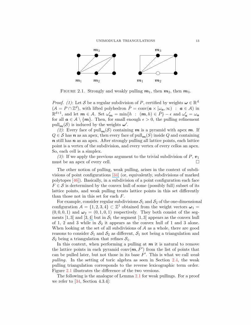
Figure 2.1. Strongly and weakly pulling m1, then m2, then m3.

Proof. (1): Let S be a regular subdivision of P , certified by weights ω ∈ RA

(A = P ∩ Zd), with lifted polyhedron P = conv(a × [ωa,∞) : a ∈ A) in

Rd+1, and let m ∈ A. Set ω′m = min{h : (m, h) ∈ P} − ǫ and ω′

a = ωa

for all a ∈ A \ {m}. Then, for small enough ǫ > 0, the pulling refinementpullm(S) is induced by the weights ω′.

(2): Every face of pullm(S) containing m is a pyramid with apex m. IfQ ∈ S has n as an apex, then every face of pullm(S) inside Q and containingn still has n as an apex. After strongly pulling all lattice points, each latticepoint is a vertex of the subdivision, and every vertex of every cellos an apex.So, each cell is a simplex.

(3): If we apply the previous argument to the trivial subdivision of P , v1

must be an apex of every cell. �

The other notion of pulling, weak pulling, arises in the context of subdi-visions of point configurations [34] (or, equivalently, subdivisions of markedpolytopes [46]). Basically, in a subdivision of a point configuration each faceF ∈ S is dertermined by the convex hull of some (possibly full) subset of itslattice points, and weak pulling treats lattice points in this set differentlythan those not in this set for each F .

For example, consider regular subdivisions S1 and S2 of the one-dimensionalconfiguration A = {1, 2, 3, 4} ⊂ Z1 obtained from the weight vectors ω1 =(0, 0, 0, 1) and ω2 = (0, 1, 0, 1) respectively. They both consist of the seg-ments [1, 3] and [3, 4] but in S1 the segment [1, 3] appears as the convex hullof 1, 2 and 3 while in S2 it appears as the convex hull of 1 and 3 alone.When looking at the set of all subdivisions of A as a whole, there are goodreasons to consider S1 and S2 as different, S1 not being a triangulation andS2 being a triangulation that refines S1.

In this context, when performing a pulling at m it is natural to removethe lattice points in each pyramid conv(m, F ′) from the list of points thatcan be pulled later, but not those in its base F ′. This is what we call weakpulling . In the setting of toric algebra as seen in Section 2.4, the weakpulling triangulation corresponds to the reverse lexicographic term order.Figure 2.1 illustrates the difference of the two versions.

The following is the analogue of Lemma 2.1 for weak pullings. For a proofwe refer to [34, Section 4.3.4]:

14 HAASE, PAFFENHOLZ, PIECHNIK, AND SANTOS

Lemma 2.2. Let P be a lattice polytope with a subdivision S.(1) Weak pulling preserves regularity.(2) Weakly pulling all lattice points of P in any order yields a triangu-

lation.

In this article, we will only use pulling refinements in cases where alllattice points in the polytope P are vertices of the subdivision S. Withthis assumption, strong and weak pulling subdivisions agree, so there is noambiguity when referring to pulling subdivisions.

2.1.2. Compressed Polytopes. Stanley calls a polytope compressed if all itsweak pulling triangulations are unimodular [109]. This clearly implies thatthe only lattice points in P are its vertices.

Surprisingly many well-known polytopes fall into this category. Examplesof compressed polytopes include the Birkhoff polytope (Section 3.3.1), orderpolytopes and hypersimplices (Section 3.1.1), stable set polytopes of perfectgraphs (Section 3.3.2). Athanasiadis was even able to use the fact that theBirkhoff polytope is compressed to prove unimodality of its h∗-vector [6](see also [24]).

There are several characterizations of compressed polytopes. Here wepresent one based on width with respect to facets. If P is a lattice polytopeand 〈yi,x〉 ≥ ci for i = 1, . . . , n are the facet defining inequalities withprimitive integral yi, the width of P with respect to the i-th facet (or withrespect to the direction of yi) is the difference

max〈yi, P 〉 − min〈yi, P 〉.

In particular, P has width 1 with respect to a facet if it lies between thehyperplane spanned by this facet and the next parallel lattice hyperplane.

The main implication of the following theorem is due to the fourth author.The proof we present here is the original one (MSRI 1997, unpublished). Itwas subsequently also proven by Ohsugi and Hibi [84] and by Sullivant [117].

Theorem 2.3. Let P be a lattice polytope. Then the following are equiva-lent:

(1) P is compressed.(2) P has width one with respect to all its facets.(3) P is lattice equivalent to the intersection of a unit cube with an affine

space.

Proof. (2) =⇒ (1): By decreasing induction on the dimension one sees thatevery face of P has width 1 with respect to all facets. The restriction ofa pulling triangulation to any face is a pulling triangulation itself and thusunimodular (by another induction). Hence, every maximal simplex in thetriangulation of P is the join of a unimodular simplex in some facet withthe first lattice point that was pulled.

The other implications are easy. �

UNIMODULAR TRIANGULATIONS 15

2.1.3. Hyperplane Arrangements. In this section, we apply the above char-acterization of compressed polytopes to triangulate “bigger” polytopes usinghyperplane arrangements.

Let A := {n1, . . . ,nr} ⊂ Zd be a collection of vectors that span Rd andform a unimodular matrix, (i.e. such that all (d× d)–minors of A are either0, 1 or −1). Such a collection induces an infinite arrangement of hyperplanes

{x ∈ Rd : 〈ni,x〉 = k} for i = 1, . . . , r and k ∈ Z ,

which subdivide Rd regularly into lattice polytopes. These subdivisions arereferred to in the literature as lattice dicings [38].

A lattice polytope P whose collection of primitive facet normals forms aunimodular matrix is called facet unimodular . Every face of a facet unimod-ular polytope is also facet unimodular in its own lattice. The lattice dicinghyperplane arrangement slices P into dicing cells. This is called the canon-ical subdivision of a facet unimodular polytope. The canonical subdivisionsubdivides faces canonically.

Theorem 2.4. Suppose that P ⊂ Rd is a facet unimodular lattice polytope.Then:

(1) The canonical subdivision of P is regular, and all the cells are com-pressed.

(2) P has a regular unimodular triangulation.

Proof. The dicing cells have width 1 with respect to all their facets by con-struction. This proves part 1 except for regularity. Regularity of the canon-ical subdivision follows from considering weights given by the restriction ofthe following quadratic function to the lattice points in P :

f(x) =

r∑

i=1

〈ni,x〉2.

Since every lattice point in each cell of the canonical subdivision is containedin two consecutive hyperplanes in each direction ni, the corresponding sum-mand of f is equal, on those lattice points, to an affine map. Therefore, fis affine on each cell. But any two adyacent cells contain lattice points inthree hyperplanes for some direction, so f is not affine on the union.

For part 2 recall that any pulling refinement of a regular subdivisionis regular. Since the cells in the canonical subdivision are compressed, atriangulation obtained by pulling will be regular and unimodular �

As a direct application of Theorem 2.4, flow polytopes (Section 3.3.1) aswell as polytopes with facets in the root system of type A have regular uni-modular triangulations (Section 3.1.1). This dicing method also shows thatevery dilation cP of a polytope P with a (regular) unimodular triangulationitself admits a (regular) unimodular triangulation (Theorem 4.7).

This approach to finding (regular) unimodular triangulations can be ap-plied whenever there is a lattice dicing that cuts P into lattice polytopes.

16 HAASE, PAFFENHOLZ, PIECHNIK, AND SANTOS

However in this more general case, the cells do not automatically have width1 with respect to the facets given by P . This must be checked separately.Polytopes with facet normals in the root system of type B are an examplewhere this approach was successful (Section 3.1.2).

2.1.4. Circuits. A circuit of a point configuration A is a minimal affine de-pendent subset C. A circuit C comes with a unique (up to a constant) affinedependence ∑

a∈C

λaa = 0,∑

a∈C

λa = 0.

It is well-known that a configuration that is itself a circuit, or that hasa unique circuit, has exactly two triangulations. Having a unique circuitis equivalent to the configuration having exactly two points more than itsdimension. The following is essentially Lemma 2.4.2 in [34].

Lemma 2.5. Let A be a configuration of d+2 points spanning a d-dimensionalaffine space. Let λ ∈ RA be its unique (up to a constant) affine dependence.Call

A+ := {a ∈ A : λa > 0}, A

0 := {a ∈ A : λa = 0}, A− := {a ∈ A : λa < 0}.

Then, A has exactly two triangulations, namely:

T + = {F ⊂ A : A+ 6⊂ F}, T − = {F ⊂ A : A− 6⊂ F},

Both triangulations are regular.

Put differently, T + (resp. T −) has A+ (resp. A

−) as its only minimalnon-face. Observe that the points of A0 lie in every maximal simplex ofboth T + and T −. This reflects the fact that for a a ∈ A

0, a is not in theaffine span of A \ a.

It is easy to specify when these triangulations are flag and/or unimodular:

Lemma 2.6. Let A be a configuration of d+2 points spanning a d-dimensionalaffine space with its two triangulations T + and T −.

(1) T + (resp. T −) is flag if, and only if, |A+| ≤ 2 (resp. |A−| ≤ 2).(2) Suppose A is a lattice point set and that λ is normalized to have

integer entries with no common factor. Let ΛA be the affine latticegenerated by A. Then, T + (resp. T −) is unimodular in ΛA if, andonly if, all positive (resp. negative) coefficients in λ are equal to ±1.

Proof. For part (1), observe that A+ is the unique minimal non-face in T +.For part (2), observe that the coefficient λa of a point a ∈ A equals ±1if, and only if, a is an integer affine combination of the rest of the points.Since the maximal simplices of T + are precisely {A\a : a ∈ A

+}, the resultfollows. �

In particular, for T + to be quadratic we need A+ to have at most two

elements and those elements have coefficient 1 in the dependence. Since∑a∈A λa = 0, A− has also at most two elements and there are only the

following two possibilities:

UNIMODULAR TRIANGULATIONS 17

l

u

P

π

Q

Figure 2.2. An example of the chimney construction. Here l ≡ 0 andu(x) = 3− x on Q = [0, 2].

• A+ = {a, b} and A

− = {c,d} with a+ b = c+ d, or• A

+ = {a, b} and A− = {c} with a+ b = 2c.

The circuit consists of the four vertices of a parallelogram in the first caseand of three collinear and equally spaced points in the second case.

Finally, let us mention that T + (resp. T −) is the weak pulling of A fromany a ∈ A

− (resp. from any a ∈ A+). It agrees with what strong pulling

would give unless A− (resp. A+) has a single element a. (In this case, a isnot a vertex of A).

2.2. Push-forward subdivisions and pull-back subdivisions. In somecases the search for triangulations can be simplified via projection. This isdone via push-forward and pull-back subdivisions.

2.2.1. Chimney polytopes and pull-back subdivisions. In this section we de-scribe a method for recursively constructing unimodular triangulations ofcertain lattice polytopes. The process yields (regular) unimodular trian-gluations of generalized prisms over polytopes with a (regular) unimodulartriangulation. In particular, this section extends results announced in [50].

We must first define chimney polytopes. Given a lattice polytope Q ⊂ Rd,consider two integral linear functionals l and u, such that l ≤ u along Q.We define the the chimney polytope associated to Q, l and u as

Chim(Q, l,u) := {(x, y) ∈ Rd × R | x ∈ Q, l(x) ≤ y ≤ u(x)} .

We call Q the base of the chimney. Chim(Q, l,u) is itself a lattice polytope(see Figure 2.2).

We will show that a chimney polytope has a unimodular triangulation ifits base has one. For this we introduce the general concept of a pull-backsubdivision.

Given a lattice polytope P in Rd and a projection π : Rd → Rd′ , letQ := π(P ) and let S ′ be a subdivision of Q. The pull-back subdivision π∗S ′

18 HAASE, PAFFENHOLZ, PIECHNIK, AND SANTOS

of P is obtained from S ′ by intersecting P with the infinite prisms π−1(F )for each cell F ∈ S ′.

Observe that the cells in the pull-back subdivision may in principle notbe lattice polytopes. A simple example is the projection of the triangle{(x, y) : 0 ≤ 2y ≤ x ≤ 2} to the segment [0, 2]. The pull-back of {[0, 1], [1, 2]}produces cells with a non-integer vertex, (1, 1/2). (Observe that this triangleis not a chimney polytope over the segment, because the functional u(x) =x/2 is not integral).

We want to show that in the case when the pull-back is integral and theprojection drops only one dimension, it can be refined to a triangulationwith nice properties. To show that the construction preserves degree of thetriangulation we need the following property:

Lemma 2.7. Let T be a simplicial ball whose dual graph is a tree. Then Tis flag.

Proof. We use induction on the number of maximal simplices in T .Let F be a maximal simplex that corresponds to a leaf in the tree. F has

a common facet with some other simplex in the triangulation, and a singlevertex a not in that facet. Then, T ′ = T \ F is also a triangulation whosedual graph is a tree, so we assume it is flag.

Let now N be a non-face of T . If a 6∈ N then N is also a non-face in T ′

hence it has size two. If a ∈ N then pick any vertex b ∈ N \F (which existssince N 6⊂ F ) and observe that N ′ = {a, b} is a non-face. �

Theorem 2.8. Let P ⊂ Rd be a lattice polytope and let π : Rd → Rd−1 be aprojection such that π(Zd) = Zd−1. Let T be a unimodular triangulation ofQ := π(P ) and suppose π∗T is integral, then

• Any full refinement T ′ of π∗T is a unimodular triangulation of P .• T ′ does not have minimal non-faces of cardinality larger than thoseof T .• If T is regular, T ′ is regular as well.

Proof. To show that regularity can be preserved, recall that if T is regular,a full pulling refinement of π∗T will be regular as well.

For the unimodularity, it is enough to consider the chimneys π−1(G) ∩P for each simplex G ∈ T individually. They are equivalent to someChim(∆d−1,0,u). Any d-simplex F in a full triangulation of Chim(∆d−1,0,u)has two vertices above one vertex of ∆d−1 and one vertex above every othervertex of ∆d−1. Since F is part of a full triangulation T ′, the heights of thetwo vertices with the same projection differ by 1. Hence, F is unimodular.

Let N ⊆ P ∩ Zd be a non-face of T ′. Then either π(N) spans a faceof T or not. If π(N) is a non-face then N contains a non-face N ′ withπ(N ′) = π(N) on which π is injective.

If π(N) is a face we can, again, restrict our attention to a single chimneyof the form Chim(∆d−1,0,u). The dual graph in a triangulation of such a

UNIMODULAR TRIANGULATIONS 19

3

1

4

5

2

Figure 2.3. Ordering of maximal simplices in a simplex chimney.

chimney is a path (cf. Figure 2.3) and Lemma 2.7 shows that N contains anon-face of cardinality two. �

This method of pull-back subdivisions and induction on dimension worksnicely on the class of recursively defined polytopes known as Nakajima. Alattice polytope is a Nakajima polytope if it is a single lattice point or it is ofthe form Chim(Q,0,u) for a Nakajima polytopeQ. These are precisely thosepolytopes P for which the singularity UP is a local complete intersection (seeSection 1.2.4).

Corollary 2.9. Every Nakajima polytope has a quadratic triangulation. (Atriangulation which is regular, unimodular and flag.)

Proof. For a polytope Chim(Q, l,u), the pull back of every lattice subdivi-sion of Q is lattice. Hence, we can apply Theorem 2.8 recursively. �

2.2.2. Push-forward subdivision. To apply the chimney Theorem 2.8 in acase where P has more than one functional bounding P from below or fromabove, we need the subdivision of the projected polytope Q to respect theintersections of the multiple upper and lower facets. To this end we definethe push-forward of a subdivision.

Given a subdivision S of a lattice polytope P in Rd and a projectionπ : Rd → Rd′ , the push-forward subdivision π∗S of Q := π(P ) is the commonrefinement of the projections of all faces of S (including low-dimensionalfaces).

The following theorem tells us under what conditions we can still applyTheorem 2.8.

Theorem 2.10. Let P ⊂ Rd be a lattice polytope and π : Rd → Rd−1 be theprojection which forgets the last coordinate. If S is a (regular) subdivisionof P such that every cell F of S has a description

F = {(x, y) ∈ π(F )× R : li(x) ≤ y ≤ uj(x), for 1 ≤ i ≤ r, 1 ≤ j ≤ s}

with integral linear functionals l1, . . . , lr and u1, . . . ,us such that li ≤ uj for1 ≤ i ≤ r, 1 ≤ j ≤ s along the lattice polytope Q, and that the push-forward

20 HAASE, PAFFENHOLZ, PIECHNIK, AND SANTOS

x

y

z

x

y

Figure 2.4. The projections Pxyz and Pxy

π∗S of S to Q has a (regular) unimodular refinement, then S has a (regular)unimodular refinement. The degree of minimal non-faces will be preserved.

This theorem provides a heuristic for finding regular unimodular trian-gulations of a lattice polytopes. Namely, given a lattice polytope P : searchfor unimodular transformations Φ of P such that Φ(P ) has the above form;project to Q and check whether Q has a regular unimodular refinementof the push-forward subdivision; iterate. The push-forward and pull-backmethods are implemented in an extension to polymake [89] and have beenused for triangulating smooth reflexive polytopes (see Section 3.4.2).

Here is an example. Consider the following polytope given by eight in-equalities in variables x, y, z, w.

(2.1)

0 ≤ x0 ≤ y ≤ 3− x0 ≤ z

x− 1 ≤ z0 ≤ w ≤ 2 + x− z

w ≤ 4− y − z

We have ordered the inequalities so that each variable is bounded above orbelow by integral linear functionals in the previous variables. We want toproject P to x-y-z-space. This projection Pxyz has the representation (seeFigure 2.4 on the left)

0 ≤ x0 ≤ y ≤ 3− x0 ≤ z ≤ 2 + x

x− 1 ≤ z ≤ 4− y .

Observe that Pxyz has facets z ≤ 2+x and z ≤ 4−y whose pull-backs are notfacets of P . They are implied by the inequalities 0 ≤ w and w ≤ 2 + x− z,respectively w ≤ 4− y − z.

UNIMODULAR TRIANGULATIONS 21

The push-forward of the trivial subdivision of P divides Pxyz along theplane x+y = 2, the projection of the ridge formed by the two upper boundson w in (2.1),

0 ≤ w ≤ 2 + x− zw ≤ 4− y − z

}x+ y = 2 .

This is a lattice subdivision, as the intersection of this hyperplane with Pxyz

is the convex hull of the lattice points (1, 1, 0), (0, 2, 0), (0, 2, 2), (2, 0, 4), and(2, 0, 1).

We can project this again to obtain a subdivided polytope Pxy in the x-y-plane given by the inequalities 0 ≤ x and 0 ≤ y ≤ 3−x (see Figure 2.4 onthe right). Any (regular and unimodular) triangulation of this subdivisioncan be used to construct a triangulation of P .

2.3. Joins and (Fiber) Products.

2.3.1. Products. Let T and T ′ be subdivisions of P and P ′ respectively.Then

T × T ′ :={F × F ′ : F ∈ T , F ′ ∈ T ′

}

is the product subdivision of P × P ′. Unfortunately, the product of twotriangulations is not a triangulation. It is a subdivision into products ofsimplices. The product of two unimodular simplices is totally unimodular(see [115, p.72, Ex.(9)], [68, p. 282], or [34, Section 6.2.2]; alternatively, thinkof it as the undirected edge polytope of a complete bipartite graph and applyLemma 3.17(2)). In particular, all its triangulations are unimodular.

There is a particularly nice triangulation of a product of simplices ∆d×∆d′

(compare [68, p. 282], [34, Section 6.2.3]). To define it, order the vertices ofthe factors a0 ≺ . . . ≺ ad and a′

0 ≺ . . . ≺ a′d′ . This induces a componentwise

partial order on the vertices of ∆d × ∆d′ . The family of totally orderedsubsets yields a quadratic triangulation, called the staircase triangulation.One geometric way to construct this triangulation is to pull the vertices of∆d ×∆d′ in the lexicographic order.

Proposition 2.11. Let P and P ′ be lattice polytopes. If both admit regularunimodular triangulations T and T ′, then so does P × P ′.

The set of minimal non–faces consists of lifts of minimal non–faces fromP and P ′ together with non–faces of cardinality two.

Proof. If T and T ′ are regular, then the subdivision T × T ′ of P × P ′

into products of unimodular simplices is regular, and any triangulation thatrefines it is unimodular. In order to control the non–faces, order the latticepoints p1 ≺ . . . ≺ pr in P and p′

1 ≺ . . . ≺ p′s in P ′. Then pull the lattice

points (pi,p′j) in P × P ′ lexicographically.

Consider a non–face N . If both its projections to P or P ′ are faces, N isa non–face in a staircase triangulation. �

22 HAASE, PAFFENHOLZ, PIECHNIK, AND SANTOS

Proposition 2.11 can be extended to non-regular triangulations. Thisextension is at the heart of the counter-examples constructed by Santosin [99,100] (see also [34, Ch. 7]) which we will return to in Section 3.5. Themain idea is that if we do not care about the regularity of the unimodulartriangulation of P × P ′ we do not need to refine T × T ′ by pulling vertices.Any refinement of the individual cells of T × T ′ is unimodular, and theonly concern is that the different refinements agree on common faces. Usingstaircase refinements of each product of simplices will still accomplish this.It does not require a globally defined ordering of all the vertices of T andof T ′, but only a local ordering of the vertices in each individual simplex.These local orderings can be represented via an acyclic orientation of the1-skeleton of each simplex, as follows. Let T be a triangulation of a pointconfiguration. A locally acyclic orientation of the 1-skeleton of T (or alocally acyclic orientation of T ) is an assignment of a direction to each edgesuch that no simplex contains a directed cycle (equivalently, no triangle inT is a directed 3-cycle).

Proposition 2.12. Let T1 and T2 be triangulations of P1 and P2 with locallyacyclic orientations. Refining each product of simplices in T1 × T2 in thestaircase manner indicated by the orientations produces a triangulation T ofP1 × P2 with the following properties:

(1) T is unimodular if and only if T1 and T2 are both unimodular.(2) T is regular if and only if T1 and T2 are both regular and the orien-

tations are globally acyclic.(3) T is flag if and only if T1 and T2 are both flag.

The triangulation of Proposition 2.12 is called the staircase refinement ofT1 × T2 with respect to the corresponding locally acyclic orientations.

Proof. We made it clear above that the triangulation is well-defined. For(1) the refinement is unimodular if the factors are unimodular since everytriangulation of the product of two simplices is unimodular. Conversely, if asimplex in one of the factors is not unimodular, then the staircase refinementdoes not give product cells using that simplex unimodular refinements. For(2), observe that the restriction of T to every {a1} × P2 or P1 × {a2} forvertices a1 of P1 or a2 of P2 is affinely isomorphic to T2 or T1, respectively.So, both must be regular for T to be regular. If the locally acyclic orientationof, say, T1, has a cycle a0,a1, . . . ,ak = a0 then for every (oriented) edgeb1b2 in T2 the edges (ai, b1)(ai+1, b2) , i = 0, . . . , k are in T , which impliesT is not regular. Indeed, the curcuit

(ai, b1) + (ai+1, b2) = (ai, b2)(ai+1, b1)

implies that if the edge (ai, b1)(ai+1, b2) appears the following inequalitymust hold for the weight vector ω:

ω(ai, b1) + ω(ai+1, b2) < ω(ai, b2)ω(ai+1, b1).

UNIMODULAR TRIANGULATIONS 23

Summing this over all i yields the impossible equation∑

i

ω(ai, b1) +∑

i

ω(ai, b2) <∑

i

ω(ai, b2)∑

i

ω(ai, b1).

This proves it is necessary for T1 and T2 to be regular. For sufficiency,note that if T1 and T2 are regular, T1 × T2 is a regular subdivision. Nowif the orientations of T1 and T2’s 1-skeletons are globally acyclic, they canbe extended to give total orderings on the vertices of T1 and T2, and ourstaircase refinement can be obtained by pulling the vertices of T1 × T2 withrespect to the lexicographic ordering, which yeilds a regular triangulation.

For (3), flagness follows from the characterization of minimal non-faces ofthe staircase refinement stated in Proposition 2.11. �

2.3.2. Joins. Let P and P ′ be polytopes of dimension d and d′, and 0k theorigin in Rk. The join P ⋆ P ′ of P and P ′ is the convex hull of

P × {0d′} × {0} ∪ {0d} × P ′ × {1}.

This gives a (d + d′ + 1)-dimensional polytope. The join of two simplices,

∆r ⋆∆r′ is a simplex ∆r+r′+1. Any subdivisions S and S ′ of P and P ′ lift toa subdivision T of P ⋆ P ′ by taking all joins of cells in S and S ′, and everysubdivision of P ⋆P ′ can be obtained this way. In particular, if S and S ′ are(regular, unimodular, flag) triangulations of P and P ′, then T is a (regular,unimodular, flag) triangulation of P ⋆ P ′.

The toric ring of the join is the tensor product of the components: RP⋆P ′ =RP ⊗RP ′ (compare Section 1.2.3).

The facets of P ⋆ P ′ are joins of P with facets of P ′ and joins of P ′ withfacets of P . Hence P ⋆ P ′ is compressed if and only if both P and P ′ arecompressed.

The join can be defined for more than two factors in a similar way, andis associative. Just as P ⋆ P ′ has a canonical projection to ∆1 — the lastcoordinate, P0 ⋆ . . . ⋆ Pr has a canonical projection to ∆r.

2.3.3. Fiber Products. Suppose two lattice polytopes project linearly, re-

specting their lattices, to the same lattice polytope: Pπ→ Q

π′

← P ′. Thenthe polyhedral fiber product, also known as the multigraded Segre productP ×Q P ′ is the polytope

{(p,p′) ∈ P × P ′ : π(p) = π′(p′)

}.

This construction was first used by Buczynska and Wisniewski in the studyof statistical models of binary symmetric phylogenetic trees [27]. A closelyrelated toric fiber product

conv{(p,p′) ∈ (P ∩ Zd)× (P ′ ∩ Zd′) : π(p) = π′(p′)

}

was defined by Sullivant [118].Under the assumptions of the following theorem (which includes the phy-

logenetic case) P ×Q P ′ is a lattice polytope, so the two notions agree.

24 HAASE, PAFFENHOLZ, PIECHNIK, AND SANTOS

Theorem 2.13. Let Pπ→ Q

π′

← P ′ be lattice preserving projections. IfQ admits a unimodular triangulation T , and P and P ′ have unimodulartriangulations S and S ′, which refine the pull-back subdivisions π∗T andπ′∗T respectively, then P ×Q P ′ admits a unimodular triangulation.

Further, regularity and the degree of minimal non-faces can be preserved.

Before proving this theorem, let us state as a corollary a slight gener-alization of a result of Sullivant [118, Cor. 15] for the case where Q is aunimodular simplex. In this case, the pull-back subdivision is trivial.

Corollary 2.14. If Pπ→ ∆r π′

← P ′ are lattice preserving projections suchthat both P and P ′ admit unimodular triangulations, then P ×∆r P ′ admitsa unimodular triangulation.

Regularity and degree of minimal non-faces can be preserved.

A lattice polytope projecting to a unimodular simplex is known in the lit-erature as a Cayley sum of the fibers of the simplex vertices [46, Ch.9, eq.(1.2)].The fiber product in the above corollary is the Cayley sum of the productsof the fibers.

The proof of Theorem 2.13 requires the following lemma.

Lemma 2.15. Given lattice preserving projections ∆d π→ ∆r π′

← ∆d′, thefiber product ∆d ×∆r ∆d′ is a lattice polytope.

Proof. For ν = 1, . . . , r + 1 let Iν := { i : π(ei) = eν} and I ′ν := { j :π′(ej) = eν}. With this notation, the fiber product has the inequalitydescription

(p,p′) ≥ 0 ,

d+1∑

i=1

pi =

d′+1∑

j=1

p′j = 1 ,

∑

i∈Iν

pi =∑

j∈I′ν

p′j for 1 ≤ ν ≤ r + 1 .

The equation matrix is (after omission of repeated columns) of the form1 · · · 1 0 · · · 00 · · · 0 1 · · · 1idr+1 − idr+1

which is a totally unimodular matrix. �

Proof of Theorem 2.13. Let T , S and S ′ be as in the statement. S and S ′

give a subdivision S × S ′ of P × P ′ into products of unimodular simplices.We claim that intersecting S ×S ′ with P ×QP ′ gives a lattice subdivision ofP×QP

′. Indeed, consider a cell in this subdivision (F×F ′)∩(P×QP′) a cell

in this subdivision, for some unimodular simplices F and F ′. Since π andπ′ map simplices of S and S ′ to simplices in T , πF and πF ′ are simplices

UNIMODULAR TRIANGULATIONS 25

in T and, in fact, (assuming F × F ′ is the minimal product of simplicescontaining our cell) they are the same simplex G. Then

(F × F ′) ∩ (P ×Q P ′) = F ×G F ′

which, by Lemma 2.15, is a lattice polytope.Thus, we have a lattice regular subdivision of P ×Q P ′ into totally uni-

modular cells. (For regularity, observe that the intersection of a regularsubdivision with an affine subspace is regular). Any refinement of it intoa triangulation of P ×Q P ′ is unimodular. If the refinement is done, forexample, pulling all the lattice points in P ×Q P ′ lexicographically as in theproof of Proposition 2.11, it will also be regular. The non–face statementfollows as in Proposition 2.11. �

Note that Theorem 2.13 can be proved for more than two factors, viainduction, since the triangulation obtained refines the pull-back of P×QP

′ →Q.

2.3.4. Nested Configurations. Motivated by a construction in algebraic sta-tistics, Aoki, Hibi, Ohsugi and Takemura introduced nested configurations.Given lattice polytopes Q ⊆ k∆d

and Pi ⊂ Rdi for i = 1, . . . , d+1, the nested polytope NP(Q;P1, . . . , Pd+1)is the convex hull, in Rd ×

∏Rdi of the polytopes {a} ×

∏aiPi, where a

runs over the vertices of Q. Here and in what follows, ∆d = {(x1, . . . , xd+1) :x ≥ 0,

∑xi = 1} denotes the homogeneous unimodular d-simplex in Rd+1.

The following is an equivalent definition in terms of joins.

NP(Q;P1, . . . , Pd+1) = k · (P1 ⋆ · · · ⋆ Pd+1) ∩ π−1(Q),

where π : Rd+1 ×∏

Rdi → Rd+1 is the natural projection.In [88], Hibi and Ohsugi show that many properties of the input polytopes

can be inherited by nested polytopes. These include normality and theexistence of regular unimodular triangulations as well as degrees of Grobnerbases (or generators). Their proof uses the algebraic-geometric machineryfrom section 2.4, so no statements about non-regular triangulations canbe concluded from it. Here we offer a purely combinatorial proof. (Thedefinition in [5] takes more general configurations as input, but if one is onlyinterested in the normal case, no generality is lost by taking our definition.)

We first introduce the following alternative way of looking at nested con-figurations. Given lattice polytopes Q ⊂ Rd and Pi ⊂ Rdi for i = 1, . . . , nand an integer affine map, φ : Zd → Zn, that is nonnegative on Q, thesemidirect product of Q and the tuple (P1, . . . , Pn) along the map φ is de-fined as

Q⋉φ (P1, . . . , Pn) := conva∈Q

({a} ×

∏φi(a)Pi

),

where (φ1, . . . , φn) are the coordinates of φ.If n = d + 1, Q ⊂ k∆d, and φ is the identity map, we recover the defi-

nition of nested configuration. Conversely, every semidirect product can be

26 HAASE, PAFFENHOLZ, PIECHNIK, AND SANTOS

rewritten as a nested configuration as follows. If φ is injective, unimodular(meaning that φ(Zd) = aff(φ(Zd)) ∩ Zn)) and homogeneous (meaning thatφ(Zd) ⊂ {

∑xi = k} for some k ∈ N) then

Q⋉φ (P1, . . . , Pn) ∼= NP(φ(Q);P1, . . . , Pn).

If φ is not injective, not unimodular, or not homogeneous, consider the

modified map φ = (φ, Id, f) : Rd → Rn × Rd × R, where f(x) = k −∑i φ(x)i −

∑j xj for a sufficiently large k, take Pi to be a single point for

all i > n and observe that

Q⋉φ (P1, . . . , Pn) ∼= NP(φ(Q);P1, . . . , Pn,pt, . . . ,pt).

So, semidirect products are really an equivalent operation to nested con-figurations. But we find them conceptually easier to handle. They generalizethe following constructions:

• ∆d ⋉Id (P0, . . . , Pd) is the join of P0, . . . , Pd,• {pt}⋉1(P0, . . . , Pd) is the product of P0, . . . , Pd, as is P0⋉1(P1, . . . , Pd).In both cases 1 denotes the constant map with image (1, . . . , 1).• {pt}⋉k (P ) is the k-th dilation of P and {pt}⋉(k1,...,kd) (P1, . . . , Pd)is the product

∏kiPi.

• The chimney Chim(Q, l,u) associated to two integer functionals l ≤u on Q is equivalent to the semidirect product Q ⋉u−l I, where Iis a unimodular segment. In particular, a Nakajima polytope is onethat can be obtained as

(. . . ({pt⋉φ1 I) . . . )⋉φdI,

for certain choice of functionals φi.

There are two ways of relating any semidirect product with several factorsto semidirect products with only two factors at a time. One is as a specialcase of fiber products, taking into account that every semidirect productcomes with a canonical projection Q ⋉φ (P1, . . . , Pn) → Q. The other is aspecial associativity property:

Lemma 2.16. As in the definition of the semidirect product, let φ1, . . . , φn

denote the coordinates of φ : Rd → Rn. Then:

Q⋉φ (P1, . . . , Pd) = (Q⋉φ1 P1)×Q · · · ×Q (Q⋉φnPn)

= (. . . (Q⋉φ1

P1)⋉φ2· · · ⋉

φd

Pd),

where φi denotes the composition of the natural projection Zd×Zd1+···+di−1 →Zd with φi : Z

d → Z. �

We are going to prove that

Theorem 2.17. Suppose Q and P admit unimodular triangulations S andT . Then, the semidirect product Q⋉φ P admits a unimodular triangulationthat refines the pull-back π∗S of S by the projection π : Q⋉φ P → Q.

UNIMODULAR TRIANGULATIONS 27

Corollary 2.18. If Q,P1, . . . ,and Pn admit unimodular triangulations, thenevery semidirect product Q⋉φ (P1, . . . , Pn) admits one too.

Proof. Lemma 2.16 gives two different ways to derive the corollary fromTheorem 2.17. One is by associativity, using induction on n. The other isvia the relation to fiber products, using Theorem 2.13. �

The key step for the proof of Theorem 2.17 is to look at the case whereboth Q and P are unimodular simplices. So, let Q ⊂ Rd be a unimodulard-simplex and P = conv{p0, . . . ,pe} ⊂ Re a unimodular e-simplex. Asimplied by our notation, the vertices of P are considered with a given specificorder, which will be important both for the construction on this particularsimplex and for gluing the constructions between simplices. Let fj : P →R be the affine functional that takes the value 0 in p0, . . . ,pe−i and 1 inpe−j+1, . . . ,pe. Put differently:

P = {x ∈ Re : 0 ≤ f1(x) ≤ · · · ≤ fe(x) ≤ 1} .

(If P is the standard ordered e-simplex {x : 0 ≤ x1, . . . , xe ≤ 1} then fj isthe j-th coordinate).

Let φ : Q → R be the affine functional in the definition of semidirectproduct. Then,

Q⋉φ P =

{(y

x

)∈ Q×Re : 0 ≤ f1(x) ≤ · · · ≤ fe(x) ≤ φ(y)

}.

In this setting we can define the canonical slicing ofQ⋉φP . For each b ∈ R

let φ≤b : Q→ R be the (unique) affine functional with φ≤b(q) = min(φ(q), b)on each vertex q of Q, and for each b ∈ N and each j ∈ [e] consider thehyperplane

H(j, b) :=

{(y

x

)∈ Rd × Re : fj(x) = φ≤b(y)

}.

The canonical slicing of Q⋉φP is the polyhedral subdivision obtained slicingQ⋉φ P by all these hyperplanes.

Figure 2.5 shows the canonical slicing in the case d = 1, e = 2, with φtaking the values 2 and 5 on the vertices of the segment Q.

Lemma 2.19. Let Q and P = conv{p0, . . . ,pe} be unimodular simplices,with the vertices of P given in a specified ordering, and let φ : Q → R be anonnegative integer affine function on Q. Then:

(1) The canonical slicing of every face of Q ⋉φ P coincides with therestriction to that face of the canonical slicing of Q⋉φ P .

(2) The canonical slicing is a lattice subdivision (all vertices are integer).(3) All cells in the canonical slicing are compressed.

Proof. Part (1) is trivial.For part (2), let

(yx

)∈ Q ⋉φ P be a vertex of the canonical slicing. By

part (1) there is no loss of generality in assuming that(yx

)lies in the interior

of Q ⋉φ P , in particular y lies in the interior of Q. For such an y the

28 HAASE, PAFFENHOLZ, PIECHNIK, AND SANTOS

x1

x2

Figure 2.5. The hyperplanes H(1, b) and H(2, b) for d = 1, e = 2, andφ(q1) = 2, φ(q2) = 5

function b 7→ φ≤b(y) is (continuous and) strictly increasing in the rangeb ≤ maxq(φ(q)). Hence

(yx

)lies in at most one hyperplane H(j, b) for each

j ∈ [e]. In order for these hyperplanes to define a vertex, we need to have(at least) d + e of them, so that the only possibility is d = 0. But whend = 0, Q⋉φ P is just the k-th dilation of P , where k is the value taken byφ in the (unique) point of Q. The hyperplanes H(j, b) are of the form “fjequals a constant”, and the facet-defining hyperplanes of kP are of the formfj+1 − fj = 0. Together they form a totally unimodular system of possiblefacet normals (in the basis consisting of the fj’s, which is itself unimodular),so the slicing they produce can only have integer vertices.

The inductive argument above implies that every vertex of the canonicalslicing lies in one of the fibers {q} × φ(q)P where q is a vertex of Q, whichwill be useful in the last part of the proof.

For part (3), we consider the three possible types of facets separately.

• Those contained in facets F ⋉φ P , where F is a facet of Q, havewidth one since Q is unimodular and Q⋉φ P projects to it.• For, those defined by a hyperplaneH(j, b), observe that cells incidentto that hyperplane are contained between the hyperplanesH(j, b−1)and H(j, b + 1). For every point

(yx

)in those cells we have

φ≤b(y)− 1 ≤ φ≤b−1(y) ≤ fj(x) ≤ φ≤b+1(y) ≤ φ≤b(y) + 1,

which proves they have width one.• For, those contained in facets Q⋉φFj of Q⋉φP , where Fj is a facetof P ,

recall that Fj is defined by the equation fj(x) = fj−1(x), j =1, . . . , e + 1 (with the convention f0 ≡ 0 and fe+1 ≡ 1). The facetQ ⋉φ Fj lies in the hyperplane (in Rd × Re defined by the sameequation (in the Re variables), except for the j = e+ 1 case, wherethe equation defining Q ⋉φ Fe+1 is fe+1(x) = φ(y). All vertices ofthe canonical slicing are in fibers over the vertices of Q. Since thecanonical slicing restricted to these fibers is a dicing by a system

UNIMODULAR TRIANGULATIONS 29

of totally unimodular vectors (the same system of vectors as in theproof of part (2)), the cells in each individual fiber have width one.This implies that the cells in the whole slicing also have width onewith respect to these functionals.

�

Proof of Theorem 2.17. SupposeQ,P admit unimodular triangulations S,Trespectively. We then have that the cells

B ⋉φ C,

for all the simplices B ∈ S and C ∈ T form a subdivision of Q ⋉φ P . (Toshow this, if φ is strictly positive on Q observe that Q⋉φ P is projectivelyequivalent to Q× P . If φ is zero on some face of Q then the correspondingface of Q× P collapses to lower dimension in Q⋉φ P , but the result is stilltrue).

Now, Lemma 2.19 tells us how to unimodularly subdivide each B⋉φC intocompressed lattice polytopes, and the canonical nature of these subdivisionsguarantees that they agree on common faces. Any triangulation that refinesthe subdivision obtained this way (e.g., by pulling all vertices) is unimodular.

�

2.4. Toric Grobner Bases. The toric dictionary translates between thediscrete geometry of lattice points in polytopes and the algebraic geometryof toric varieties. We explore the translations involving unimodular trian-gulations.

2.4.1. Unimodular triangulations and Grobner bases. Let k be a field, andA := (P × {1}) ∩ Zd+1 denote the homogenized set of lattice points inP . Consider the polynomial ring S := k[xa : a ∈ A] with one variablefor each lattice point. There is a canonical ring homomorphism φP to theLaurent polynomial ring k[t±1

1 , . . . , t±1d , td+1] mapping each variable to the

corresponding (homogenized) t-monomial: φP (xa) = ta = ta11 · . . . · tadd · td+1.

The toric ideal IP := ker φP is spanned, as a k-vector space, by the set

(2.2)

{xu − xv : u,v ∈ ZA

≥0 ,∑

a∈A

uaa =∑

a∈A

vaa

},

where xu =∏

a∈A xua

a . It thus encodes the affine dependencies among thelattice points in P [115, Lemma 4.1].

The tie between Grobner bases of IP and regular triangulations of Pis established via two different interpretations of a generic1 weight vectorω ∈ RA. On the lattice polytope side, ω induces a regular triangulationTω of P as explained at the end of Section 1.1. On the algebraic side, suchan ω induces an ordering of the monomials in S via xm ≺ xn : ⇐⇒〈ω,m〉 < 〈ω,n〉. For a polynomial f ∈ S the leading term inω f is thebiggest monomial in this ordering which has a non-zero coefficient in f , and

1To be on the safe side, assume that the numbers ωa are linearly independent over Q.

30 HAASE, PAFFENHOLZ, PIECHNIK, AND SANTOS

the initial ideal inω I := 〈inω f : f ∈ I〉 of an ideal I collects all the leadingterms of polynomials in I. A collection of polynomials in I whose leadingterms generate the initial ideal is called a Grobner basis of I (with respectto ω). If ω is not generic, we only get a partial ordering of the monomials.A small enough generic perturbation of ω refine the partial order to a termorder.

We will now investigate how (regular) subdivisions can help to find gen-erating sets and Grobner bases of toric ideals. For a vector v ∈ ZA

≥0 we call

the set suppv := {a ∈ A | va 6= 0} the support of v and say that xv issupported on F ⊆ P whenever suppv ⊆ F . As a preliminary step, supposeP has a covering C by integrally closed polytopes (cf. Section 1.2.2). Thenwe can restrict the generating set (Section 2.2) of the vector space IP tothose binomials xu − xv which have at least one monomial supported in acell of C.

For a subdivision S of P ⊂ Rd into lattice polytopes, we call N ⊆ A anon-face if N 6⊂ Q for all Q ∈ S. (Our two notions of a non-face — for atriangulation and for a subdivision — agree for full triangulations.) If, forexample, S comes from a lattice dicing as in Section 2.1.3, then all minimalnon-faces have size 2.

Given ω ∈ RA with induced regular subdivision Sω, and given a monomialxu ∈ S, we call a monomial xv standard, written xv ∈ stdω(x

u), if xu −xv ∈ IP , and v minimizes 〈ω,v〉 subject to this condition. Again, we canrestrict the generating set (Section 2.2) of the vector space IP to binomialsxu − xv for which xv ∈ stdω(x

u). If the cells of Sω are integrally closedand (Sω,ω) is tight, the definition of regular subdivision says that xv isstandard if and only if xv is supported on a cell of Sω. In particular, forevery non-face N ⊆ A there is a monomial xv supported on a cell of Sω withfN := xN − xv ∈ IP , where xN denotes the squarefree monomial

∏a∈A xa

with support N .For the following lemma, we consider the polynomial rings k[xa : a ∈

A ∩ F ] and their ideals IF as subsets of S.

Lemma 2.20. Suppose Sω is a regular subdivision of the lattice polytope Pinto integrally closed lattice polytopes.

(1) The toric ideal IP is generated by IF for F ∈ Sω together with fNfor minimal non-faces N .

(2) If (Sω,ω) is tight, then for any small enough generic perturbation ω′

of ω, combining Grobner bases for the IF with respect to ω′|F withthe fN for minimal non-faces N yields an ω′-Grobner basis of IP .

Part (1) of this lemma will be used in Corollary 3.8 to show type Bpolytopes are quadratically generated. It follows readily from part (2).

Proof. Take a binomial f = xu − xv ∈ IP with xu = inω′ f .If suppu is a non-face of Sω, then there is a minimal non-face N ⊆ suppu,

and inω′ fN = xN |xu = inω′ f .

UNIMODULAR TRIANGULATIONS 31

If suppu is contained in a face F of Sω, we claim that suppv must alsobe contained in F : we have 〈ω,u〉 ≥ 〈ω,v〉 (as ω′ is a small perturbation ofω and we have strict inequality for ω′), and

∑a∈A uaa =

∑a∈A vaa is an

affine dependence. So the tightness equations (1.3) yield ωa = 〈ηF ,a〉+ ζFfor all a ∈ suppv. �

If we apply the preceding lemma to a regular unimodular triangulation,we obtain the following corollary which is contained in [115, Corollaries 8.4,8.8].

Corollary 2.21. If Tω is a regular unimodular triangulation Tω of P , then

inω IP =

⟨∏

a∈N

xa : N is a minimal non-face of Tω

⟩.

This ideal is known as the Stanley-Reisner ideal of the simplicial complexTω. The formula allows us to recover Tω from inω IP (its faces correspondto the monomials not in inω IP , and vice versa). In fact, by Lemma 2.20even a Grobner basis can be read off of Tω.

If Tω is not unimodular then the following modified formula is still true:

Rad(inω IP ) =

⟨∏

a∈N

xa : N is a minimal non-face of Tω

⟩.

In particular, we can still recover Tω from inω IP , but not the other wayaround.

Theorem 2.22. Given that A generates the lattice Zd+1, the initial idealinω IP is squarefree if and only if the regular triangulation Tω of P is uni-modular.

This theorem is Corollary 8.9 in [115]; it follows from [61, Thm. 5.3], andprovides the primary motivation for studying regular unimodular triangula-tions, from the perspective of algebraic geometry.

Proof. If Tω is unimodular, the previous lemma shows that inω IP is square-free.

So, assume Tω is not unimodular, and let F = conv(a0, . . . ,ad) ∈ Tω be asimplex of determinant D > 1. Let Λ denote the (strict) sublattice of Zd+1

generated by the vertices of F . Observe that Dm ∈ Λ for all m ∈ Zd+1.We will construct a vector b ∈ coneF ∩ Zd+1 \Λ which is a non-negative

integral linear combination of A. First, choose b′ ∈ Zd+1 \ Λ. By assump-tion, b′ is an integral linear combination of A. Adding a sufficiently largemultiple of D

∑a∈A a will make the coefficients non-negative. Then adding

a sufficiently multiple of∑

a∈F a will yield a point in coneF .

Among all n ∈ ZA

≥0 satisfying∑

a∈A naa = b choose the one with minimalω-weight. Since b 6∈ Λ, xn is not supported on F . Still, xn is never a leadingterm: xn 6∈ inω IP .

32 HAASE, PAFFENHOLZ, PIECHNIK, AND SANTOS

Yet, Db ∈ coneF ∩Λ, so Db =∑d

i=0miai for some m, and xDn−xm ∈IP . As xm is supported on the face F , it cannot be the leading term and(xn)D ∈ inω IP . So inω IP is not squarefree. �

Theorem 2.22 provides a method for constructing regular unimodular tri-angulations. Conversely, all regular unimodular triangulations constructedin the present article yield Grobner bases of the corresponding toric ideals.Both directions of the biconditional have been used – compare sections 3.3.1and 3.2.3.

Example 2.23. Consider the the twisted cubic curve. Let P = [1, 4] bea 1-dimensional polytope whose lattice point set and toric ideal are A ={(1, 1), (2, 1), (3, 1), (4, 1)} and IP =

⟨x1x3 − x22, x2x4 − x23, x1x4 − x2x3

⟩. Let

ω = (ω1, ω2, ω3, ω4). There are eight monomial initial ideals and four tri-angulations, depending on the values of λ1 := ω1 − 2ω2 + ω3 and λ4 :=ω4 − 2ω3 + ω2:

ω inω IP Tωλ1 > 0 and λ4 > 0 〈x1x3, x2x4, x1x4〉 [1, 2], [2, 3], [3, 4]λ1 < 0 and 2λ1 + λ4 > 0 〈x1x4, x

22, x2x4〉 [1, 3], [3, 4]

λ1 + 2λ4 > 0 and 2λ1 + λ4 < 0 〈x22, x2x3, x2x4, x1x24〉 [1, 3], [3, 4]

λ1 + 2λ4 < 0 and λ4 > 0 〈x22, x2x3, x2x4, x33〉 [1, 4]

λ1 < 0 and λ4 < 0 〈x22, x2x3, x23〉 [1, 4]

λ1 > 0 and 2λ1 + λ4 < 0 〈x1x3, x2x3, x32, x

23〉 [1, 4]

λ1 + 2λ4 < 0 and 2λ1 + λ4 > 0 〈x1x3, x2x3, x21x4, x

23〉 [1, 2], [2, 4]

λ1 + 2λ4 > 0 and λ4 < 0 〈x1x3, x1x4, x23〉 [1, 2], [2, 4]

Observe how each triangulation corresponds to the (radical of the) initialideal. The converse works precisely in the first case where the initial idealis squarefree and the triangulation is unimodular.

2.4.2. Quadratic triangulations. If a polytope has a regular unimodular tri-angulation, we have seen that the size of the minimal non-faces controls thedegree of the corresponding Grobner basis. Of particular interest is the caseof degree two – quadratic triangulations – especially given the connection toKoszul algebras. Recall that an algebra R over a field k is Koszul if k hasa linear free resolution as an R–module. In this context, the second hier-archy of properties in section 1.2.5 is expressed in the following proposition(see [20, Cor. 2.1.3]).

Proposition 2.24. IA has a quadratic initial ideal ⇒ k[x]/IA is Koszul ⇒IA is generated by quadratic binomials.

For polygons we have the following nice characterization by Bruns, Gube-ladze, and Trung.

Proposition 2.25 ( [20, Cor. 3.2.5]). A lattice polygon with at least 4 bound-ary lattice points has a quadratic triangulation.

UNIMODULAR TRIANGULATIONS 33

A non-unimodular polygon with exactly three boundary lattice pointscannot have a quadratic triangulation because one cannot get rid of thecubic generator of IA coming from the product of the corresponding threevariables.

Lemma 2.21 also implies the following correspondence between quadratictriangulations and quadratic Grobner bases referenced in Section 1.2.3.

Theorem 2.26. If P has a quadratic triangulation T , then the definingideal IP of the projective toric variety XP ⊂ Pr−1 has a quadratic Grobnerbasis. In this case, in(IP ) = 〈xaxb | ab is not an edge in T 〉. In particular,RP is Koszul.

See [21] for a collection of unsolved problems in the field.

3. Examples

Here we present what is known (and unknown) for some particular fam-ilies of polytopes. Most of them are connected to one of the classical crys-tallographic root systems. We will examine two distinct ways of associatingpolytopes to a root system Γ. In Section 3.1 we consider polytopes with facetnormals in Γ (polytopes of type Γ), and in Section 3.2 polytopes with verticesin Γ (Γ-root polytopes). Then, in Section 3.3 we look at polytopes definedfrom graphs, including flow polytopes of directed graphs and incidence poly-topes of undirected ones. Finally, Section 3.4 examines smooth-polytopes.

A (real, finite) root system is a family of vectors Γ that is invariant underreflection with respect to the hyperplanes orthogonal to each of the elementsin Γ. It is crystallographic if Γ generates a lattice, which we denote ΛΓ.

Each system studied here satisfies that property, so when we refer to rootsystems, they are assumed to be crystallographic.

The direct sumΓ⊕ Γ′ := Γ× {0} ∪ {0} × Γ′

of two root systems is a root system. Root systems that cannot be decom-posed in this fashion are called irreducible and are classified as follows. (Herewe are only considering crystallographic ones).

There are the four infinite families, that exist in all dimensions:

An−1 := {ei − ej | 1 ≤ i, j ≤ n}

Bn := {±ei | 1 ≤ i ≤ n} ∪ {±ei ± ej | 1 ≤ i < j ≤ n}

Cn := {±2ei | 1 ≤ i ≤ n} ∪ {±ei ± ej | 1 ≤ i < j ≤ n}

Dn := {±ei ± ej | 1 ≤ i < j ≤ n},

where, as usual, ei is the i-th standard unit vector in Rn.In addition to these, there are five other root systems. The system F4 is

spanned by the roots inB4 together with all vectors in {(±1/2,±1/2,±1/2,±1/2)}.The root system E8 is the union of D8 and {x | xi = ±1/2 for 1 ≤ i ≤8 and

∑xi even}. The root system E7 is the subset of E8 of all vectors

34 HAASE, PAFFENHOLZ, PIECHNIK, AND SANTOS

whose entries sum up to 0. The root system E6 is the set of roots of E8 thatare spanned by the vector

(1/2, −1/2, −1/2, −1/2, −1/2, −1/2, −1/2, 1/2)

together with e1 + e2 and −ei + ei+1 for 1 ≤ i ≤ 4. Finally the root systemG2 is the set of vectors

±( 1 −1 0 ), ±( 1 0 −1 ), ±( 0 1 −1 ),±( 2 −1 −1 ), ±( 1 −2 1 ), ±( 1 1 −2 ) .

For each root system Γ ∈ {An−1,Bn,Cn,Dn,F4} we define the specialchoice of positive roots in the root system as the subset Γ+ ⊂ Γ consistingof all roots whose first nonzero entry is positive, and Γ and Γ+ are definedas Γ ∪ {0} and Γ+ ∪ {0}, respectively.

3.1. Polytopes cut out by roots. Given a root system Γ, root hyper-planes are hyperplanes of the form Hv,b := {vx ≤ w} where v ∈ Γ andw ∈ Z. If Γ is a crystalographic root system with lattice ΛΓ then the roothyperplanes are lattice hyperplanes for the dual lattice

Λ∗Γ := {x : vx ∈ Z,∀v ∈ Γ}.

A polytope is of type Γ if it is a lattice polytope (for the lattice Λ∗Γ) and

all its facet-defining hyperplanes are root hyperplanes. Note that polytopescut out by a non-irreducible root system are products of their irreduciblecomponents.

The following is a general result about polytopes cut out by roots (cf. [55,p. 90]).

Lemma 3.1. Given an irreducible root system Γ spanning Rd, every cell inthe hyperplane arrangement given by the (infinite) family of hyperplanes ofthe form {vx = z} for v ∈ Γ and z ∈ Z is a simplex.

That is, the arrangement of all root hyperplanes is an (infinite, periodic)triangulation of Rd. Its cells are called alcoves. It may, however, havevertices which do not belong to Λ∗

Γ. For example, for the root system B2,Λ = Λ∗ = Z2, but the arrangement of root hyperplanes contains vertices in(1/2, 1/2) + Z2.

Payne proved another important general result about polytopes cut outby roots using Frobenius splittings:Theorem 3.2. [91, Thm. 1.1] Every type Γ polytope for each of the classicalroot systems An−1, Bn, Cn and Dn is integrally closed and Koszul.

3.1.1. Type A Polytopes. The type A root system is very special in that thematrix whose columns are its roots is totally unimodular. In particular, allpolytopes of type A are totally unimodular. Therefore, they have quadratictriangulations which can be realized via the construction in Theorem 2.4.The following statement (without the proof of flagness) appeared alreadyin [66, Lemma 2.4].

UNIMODULAR TRIANGULATIONS 35

Theorem 3.3. Let P be a polytope of type A. The lattice dicing subdivisionT obtained from slicing P by all the lattice hyperplanes with normal in An

is a quadratic triangulation of P .

Proof. Theorem 2.4 established that T is a regular lattice subdivision inwhich all faces are compressed, and Lemma 3.1 shows that this is in fact atriangulation. So, it only remains to be shown that it is flag.

For this, suppose N is a minimal non-face with more than two elements.Since N is not a face, the relative interior of conv(N) is cut by some hy-perplane H spanned by a face of T , which must be a root hyperplane. Inparticular, N contains points n+ and n− on both sides of that hyperplane,which contradicts the fact that n+n− is an edge. �

We now discuss two particularly interesting cases of type A polytopes,order polytopes and hypersimplices.

Let (X,4) be a partial order on X = {1, . . . , n}. A vector v ∈ [0, 1]n issaid to respect the order if vi ≤ vj whenever i 4 j. A linear extension of4 is a total order on X that refines the partial order. The order polytopeassociated (X,4) is the polytope

O(4) := {x ∈ [0, 1]n | x respects the order}.

Vertices of O(4) are the characteristic vectors of up-close subsets or filtersof the poset (that is, sets S ⊂ X with the property that i ∈ S and i 4 jimplies j ∈ S). Facets of O(4) are in bijection with covering relations,minimal elements and maximal elements. If i 4 j is a covering relation(meaning that there is no k with i 4 k 4 j) then xi ≤ xj defines a facet,and if i is a minimal (resp. maximal) element then xi ≥ 0 (resp. xi ≤ 1)defines a facet. All facets are of one of these forms. In particular, the facetvectors of an order polytope are contained in the set of vectors {ei : i ∈[n]}∪{ei−ej : i, j ∈ [n]}, which is mapped to An by the linear isomorphismei 7→ ei − en+1. This shows that O(4) is of type A, and also that it iscompressed.

The quadratic triangulation of an order polytope guaranteed by Theo-rem 3.3 was first studied by Stanley [110]. Its maximal simplices are inbijection to the linear extensions of the partial order. In particular, thenormalized volume of O(4) equals the number of distinct linear extensionsof 4.

The d-dimensional hypersimplex ∆(d, k) for 1 ≤ k ≤ d is defined as

∆(d, k) := {x ∈ Rd | k − 1 ≤∑

i

xi ≤ k, 0 ≤ x ≤ 1} .

Alternatively, each ∆(d, k) can also be realized as the intersection of the(d + 1) dimensional 0/1-cube with the hyperplane {x |

∑i xi = k}. The

hypersimplices for k = 1 and k = d are simplices. The hypersimplex ∆(3, 2)is the octahedron. To see that these polytopes are root system polytopes

of type Ad−1, apply the unimodular transformation given by yj :=∑j

i=1 xi.

36 HAASE, PAFFENHOLZ, PIECHNIK, AND SANTOS

The facet inequalities are then given by yj − yj−1 ≥ 0 and k − 1 ≤ yd ≤ k.The fact that these hypersimplices are also compressed follows directly fromcondition (3) of Theorem 2.3.

3.1.2. Type B Polytopes. The root system Bn ⊂ Rn has two types of roots.Their distinction appears in our proofs of Proposition 3.4 and Lemma 3.5.The “short roots” are given by the vectors ±ei, and the “long roots” aregiven by the vectors ±ei ± ej for 1 ≤ i, j ≤ n.

Proposition 3.4. If P is a lattice polytope with facet normals in Bn, thenP admits a regular unimodular triangulation.

The proof requires the following lemma.

Lemma 3.5. Let M be a matrix with rows in Bn, N be a matrix with rowsin {ei : i ∈ [n]} (the set of short roots), and w ∈ Zk, where k is the numberof rows in N . If the system

Mx = 0, Nx = w

has a unique solution, then this solution is integral.

Proof. First, observe that there is no loss of generality in assuming that allrows of M are long roots (as all rows that are short roots can be put inN). Also, if a long root ei ± ej in M shares a coordinate with a short rootei in N , then the other coordinate of that long root is fixed to the valuexj = ±wi, so removing that row from M and putting a new row in N , yieldsequivalent system.

After this process has been applied as many times as possible, M and Noperate in disjoint sets of coordinates. At which point, setting all coordinatesin N to their value wi and all coordinates not in N to zero gives an integralsolution of the system (unless N is inconsistent, in which case the originalsystem had no solution). �

Proof of Proposition 3.4. Slice P by all short roots. This gives a regularsubdivision of P . The proposition follows from showing that the cells in thissubdivision have integral vertices and are compressed.

Let a be a vertex of this subdivision and let b be a vertex of the carrierface of a in P . Then, Lemma 3.5 implies that a − b is integral, since it isdetermined by setting some coordinates to a fixed value and homogenizedversions of some of the facet-defining inequalities of P . Thus a = b+(a−b)is also integral.

It remains to show that all cells in the subdivision are compressed. Byconstruction, the cells have width one in the direction of the short roots.In the direction of a long root ±ei ± ej consider the projection onto thexi-xj-plane. In each case the cell has width one. �

Example 3.6. The quadratic triangulations obtained for type A polytopesin Theorem 3.3 are in fact “type A triangulations”, in the sense that theyconsist of type A simplices. The same does not in general occur in type B.

UNIMODULAR TRIANGULATIONS 37

For example, consider the following type B polytope:

P = conv[0 1 0 1 1 10 0 1 1 1 00 0 0 0 1 −1

]={x ∈ [0, 1]3 : z ≤ x, y;x+ z ≥ 0; y − z ≥ 1

}

The only type B hyperplane cutting through its interior but not creatingany non-integer vertices is z = 0. This is the hyperplane used in the proof ofProposition 3.4, and cuts P into two compressed type B polytopes. Each ofthem is a square pyramid and they both have type B unimodular triangula-tions, but their type B triangulations use different diagonals of the square.Meaning, in the last step of the proof we cannot triangulate the cells of theshort-root dicing of P using transformed A-triangulations.

We do not know whether Proposition 3.4 can be extended to yield qua-dratic triangulations of type B polytopes.

We do know arbitrary pulling refinements will not work, because thereare non-flag pulling triangulations of the order polytope [0, 1]3. However,pulling according to the vertex order of a linear functional works for [0, 1]3.An affirmative answer to the following question would imply the existenceof quadratic triangulations for all type B polytopes.

Question. If the vertices of the order polytope O(4) are ordered accordingto a generic linear functional, does pulling the vertices of O(4) in that ordernecessarily produce a flag triangulation?

However, the following lemma, combined with Lemma 2.20 does guaranteethat the toric ideals of type B polytopes are quadratically generated, sinceB-cells are equivalent to A-cells (which have quadratic triangulations).

Lemma 3.7. If P is a lattice polytope with facet normals in Bn and Q isa cell in the lattice dicing subdivision of P obtained from slicing P by allthe lattice hyperplanes with normals among the short roots in Bn, then Q isequivalent to an order polytope.

Proof. We can assume Q is full-dimensional. Up to translation, Q is given bythe intersection of [0, 1]n with some constraints xi ≶ xj and some xi+xj ≶ 1.In either case, the cell must contain the point b := 1

21. Since b cannot be

a vertex, there must be a vertex a ∈ {0, 1}d such that for small ǫ > 0,the points b ± ǫ(a − b) both belong to our cell. Due to the nature of itsinequalities, our cell contains the long diagonal from a to 1−a. So, mappingxi to 1 − xi whenever ai = 1 identifies the cell unimodularly with an orderpolytope. �

Corollary 3.8. Toric ideals of type B polytopes are quadratically generated.

3.1.3. Type Cn and Dn Polytopes. Payne’s theorem [91, Thm. 1.1] gau-rentees that all polytopes of type C and D are integrally closed. However,we do not know whether they all have unimodular triangulations for casesother than Dn

∼= An (n ≤ 3) and Cn∼= Bn (n ≤ 2) .

38 HAASE, PAFFENHOLZ, PIECHNIK, AND SANTOS

3.1.4. Type F4 Polytopes. Polytopes with facets in F4 do not in general haveregular unimodular triangulations. For an example, consider the polytopePF4 defined by the following linear inequalities:

x4 + x2 ≤ 0 x4 − x1 ≥ 0 x4 − x2 ≤ 0

x3 + x1 ≥ 0 x3 − x1 ≤ 2

The dual lattice (F4)∗ is the sublattice of Z4 containig all points with even

coordinate sum. Hence, the lattice points in P are

(−1, 0, 1, 0) (−1,−1, 1,−1)

( 0, 0, 0, 0) (−1, 1, 1,−1)

( 0, 0, 2, 0)

which are also the vertices of PF4 . In particular, since PF4 is a non-unimodular empty simplex, it does not have a unimodular triangulation. Infact, it is not even integrally closed. For example, (−1, 0, 2,−1) ∈ (F4)

∗∩2Pis not a sum of two lattice points in P(F4,c). Therefore, polytopes cut out byF4 are not in general integrally closed, which answers a question left openin in [91].

3.1.5. Type E6, E7, E8 Polytopes. Here is an example of a type E8 polytopethat does not have a regular unimodular triangulation. PE8 is the productof the polytope PF4 defined in Section 3.1.4 with itself. The facet normalsof this polytope are roots in E8. The 25 vertices of PE8 are the products ofthe five vertices of PF4 . Additionally, we have the following twelve latticepoints:

(−1 0 1 −1 −1 0 1 −1)(−1 0 1 −1 0 0 1 0)( 0 0 1 0 −1 0 1 −1)( 0 0 1 0 0 0 1 0)

(−1/2 −1/2 1/2 −1/2 −1/2 −1/2 1/2 −1/2)(−1/2 −1/2 1/2 −1/2 −1/2 1/2 3/2 −1/2)(−1/2 1/2 1/2 −1/2 −1/2 −1/2 3/2 −1/2)(−1/2 1/2 1/2 −1/2 −1/2 1/2 1/2 −1/2)(−1/2 −1/2 3/2 −1/2 −1/2 −1/2 3/2 −1/2)(−1/2 −1/2 3/2 −1/2 −1/2 1/2 1/2 −1/2)(−1/2 1/2 3/2 −1/2 −1/2 −1/2 1/2 −1/2)(−1/2 1/2 3/2 −1/2 −1/2 1/2 3/2 −1/2)

The point (−2,−1, 2,−1,−1, 0, 2,−1) is in twice the polytope PE8 , but itis not the sum of two lattice points in PE8 . So PE8 is not integrally closed,and cannot have a regular unimodular triangulation.

The E7 and E6 cases remain open.

UNIMODULAR TRIANGULATIONS 39

Figure 3.1. A triangle without a quadratic triangulation

3.1.6. Type G2 Polytopes. Every type G2 polytope PG2 is a polygon. Assuch, they have regular unimodular triangulations. By Proposition 2.25they even have quadratic triangulations whenever there are ≥ 4 boundarylattice points. Up to lattice equivalence, the only type G2 polygons with3 boundary lattice points are a unimodular triangle and the triangle ofFigure 3.1.

3.2. Polytopes spanned by roots. Now we consider polytopes defined asthe convex hull of a subset of one of the root systems. Polytopes of this typeare widely studied, see e.g. Gelfand, Graev, and Postnikov [45], Ohsugi andHibi [85, 86], Meszaros [73, 74], and Cho [28]. Ohsugi and Hibi have foundregular unimodular triangulations for several classes of these polytopes.

Before presenting results, we introduce some notation. Let A be a set of

vectors in Rn and A := A∪ {0}. The polytope associated to this configura-tion is PA := conv(A).

3.2.1. Sub-configurations of An: arc polytopes. Arc polytopes are the easiesttype of a root polytope to find unimodular triangulations for. Since An istotally unimodular as a vector configuration, for every A ⊆ An each simplexcontaining the origin as a vertex is unimodular. As a result:

Theorem 3.9. The following polytopes have regular unimodular triangula-tions.

(1) PA

for any A ⊆ An−1. In particular, PA for any A ⊆ An−1 with0 ∈ PA.

(2) PA for any A ⊆ An−1 with 0 6∈ aff(A). In this case every triangula-tion is unimodular.

Proof. Part (1) follows from Stanley [109, Ex. 2.4a]. For any pulling triangu-lation in which 0 is the first point pulled, each simplex in the triangulationwill contain 0. By unimodularity of the vertex matrix, this means everyresulting simplex has volume 1.

The argument for Part (2) is essentially the same. Q := conv({0} ∪A+)

is a pyramid over PA+ with apex 0, so every simplex of every triangulationof it contains 0, and is hence unimodular. �

The only configurations A ⊆ An−1 not addressed by Theorem 3.9 arethose that have 0 in their affine hull, but not in their convex hull. Not all

40 HAASE, PAFFENHOLZ, PIECHNIK, AND SANTOS

of these have a regular unimodular triangulation. In fact, the polytope ofsuch a configuration can even fail to be integrally closed.

Example 3.10. Consider the subconfiguration of A+4 consisting of e1−e2,

e2 − e3, e3 − e4, e4 − e5, e1 − e4 and e3 − e5. It is 4-dimensional with sixvertices, so it has a unique affine dependence. Namely:

(e1 − e4) + (e3 − e5) = (e1 − e2) + (e2 − e3) + 2(e3 − e4) + (e4 − e5).

Since both sides of the dependence have some coefficient different from 1,neither triangulation of this circuit is unimodular (part (1) of Lemma 2.6).

Even when there is a regular unimodular triangulation, it will not neces-sarily be flag.

Example 3.11. Consider the subconfiguration of A+5 consisting of e1−e2,

e2 − e3, e1 − e3, e4 − e6, e4 − e5, and e5 − e6. This is again a circuit andits only affine dependence is

(e1 − e2) + (e2 − e3) + (e4 − e6) = (e1 − e3) + (e4 − e5) + (e5 − e6).

Since the circuit has three points on each side, none of its triangulationsis flag (part (2) of Lemma 2.6). Let us mention that this configuration islattice equivalent to the set of vertices of the 3rd Birkhoff polytope. (SeeTheorem 3.24 and the discussion before it.)

Notice that Theorem 3.9(1) implies PAn−1 has a regular unimodular tri-angulation. Even more is known for the subconfiguration of all positiveroots.

Theorem 3.12. (1) PA

+n−1

has a quadratic triangulation.

(2) PA

+n−1

has a regular unimodular triangulation in which all non-faces

have size 2 or 3.

Part (1) was proved by Gelfand, Graev, and Postnikov [45], and part (2)is due to Kitamura [65]. This statement is the best possible since A+

n−1cannot have a quadratic triangulation for n ≥ 6, as demonstrated in thefollowing example.

Example 3.13 (Example 3.11 continued). The vectors e1 − e2, e1 − e3,e2−e3, e4−e5, e4−e6, e5−e6 are the vertex set of the face of A+

5 definedby x1 + x2 + x3 = 0. Any flag triangulation of A+

5 would in particulargive a flag triangulation of that face, but that face does not have any flagtriangulation.

A-root configurations have a natural graph-theoretic interpretation. LetG = (V,A) be a directed graph, which we assume to be connected in theundirected sense. Its (directed) incidence matrix is the (|V | × |A|)-matrixDG with a 1 at position (v, a) if v is the head of the directed edge (arc) a,with a −1 if v is the tail of a, and with a 0 otherwise. The arc polytope of Gis the convex hull of the columns of DG. By construction, the columns are

UNIMODULAR TRIANGULATIONS 41

roots of type An−1. Other than possibly the origin, the only lattice pointsin the arc polytope are its vertices, which correspond to arcs in G.

The following properties were noticed by Hibi and Ohsugi [86].

Lemma 3.14. Let G be a connected graph with n vertices, and A be the setof lattice points in its arc polytope.

(1) A contains the origin if and only if G has a directed cycle.(2) A has dimension d − 1 (that is, it affinely spans the hyperplane∑

xi = 0) if and only if G has an unbalanced cycle. (Here, anundirected cycle in a directed graph is called balanced if it has thesame number of edges oriented in both directions.)

(3) A is totally unimodular (all its full-dimensional simplices, and henceall its triangulations, are unimodular) if and only if all unbalancedcycles contain exactly one more edge oriented in one direction thanin the other. [85, Lemma 3.6]

In part (3) we mean totally unimodular with respect to the root lattice.This is different from the convention in [86] where unimodular is meant withrespect to the lattice generated by A.

In part (2) observe that balanced cycles must be even, so that the graphshaving only balanced cycles must be bipartite. An important subclass arethose where all edges are directed from one part to the other. In this case thearc polytopes are subpolytopes of the product of two simplices, so all theirtriangulations are unimodular. (This follows also from Theorem 3.9(2). Seealso [95].)

Proof. We first prove part (1). If G has a directed cycle then the sum ofthe corresponding columns of DG is zero. Conversely, if G does not have adirected cycle (that is, it is acyclic) then its vertices can be ordered so thatevery directed edge is directed towards the greater vertex. So, the followingstrict linear inequality is satisfied in A:

∑ixi > 0.

For parts (2) and (3) we give a full description of the subsets of A that spann − 1 dimensional simplices. The corresponding subgraphs are necessarilyspanning (all coordinates need to be used) and connected (otherwise a propersubset of coordinates has sum equal to zero) and have n elements. Thismakes each the union of a spanning tree with an extra edge. The converseis almost true: If a subgraph is a spanning tree plus one edge, then itscorresponding subconfiguration is affinely independent (hence it spans an(n−1)-dimensional configuration) unless the cycle contained in the subgraphis balanced. So part (2) is clear.

If an unbalanced cycle does not exist, then there can not be an (n − 1)-dimensional simplex. If there is an unbalanced cycle, it yields an (n − 1)-dimensional simplex. Part (3) follows from the fact that the volume (withrespect to the A lattice) of any such simplex is the difference in number ofedges in each direction in its cycle. �

42 HAASE, PAFFENHOLZ, PIECHNIK, AND SANTOS

Hibi and Ohsugi also proved that if all induced cycles (cycles withouta chord) satisfy part (3) (they are balanced or have one more edge in onedirection) then PA has a unimodular cover.

Corollary 3.15. (1) If G is not acyclic then its arc polytope has regularunimodular triangulations.

(2) If G is bipartite with parts X and Y , and the edges are all directedfrom X to Y then all triangulations are unimodular.

Proof. For (1), a regular unimodular triangulation of PA can be constructedby pulling the origin first and then the remaining points in any order. Insuch a triangulation, the origin is a vertex of every cell, so their latticevolumes are the determinants of the other vertices. Since the vertices areroots of An−1, these will all be one.

In part (2), 0 is not in the affine hull of PA. So letting X and Y denotethe two parts in G, we have A ⊂ {

∑v∈X xa = −1} ∩ {

∑v∈Y xa = 1}, and

theorem 3.9(2) implies the statement. �

3.2.2. Sub-configurations of Bn, Cn, Dn and F4. Much less is known aboutsub-configurations of other root systems.

Theorem 3.16. (Ohsugi and Hibi, [86] for part (1), [85] for part (2))(1) P

B+n, P

C+nand P

D+nhave quadratic triangulations.

(2) If n ≥ 2, and A+ is a set of vectors satisfying the following conditions

(a) {ei + ej | 1 ≤ i < j ≤ n} ⊆ A+ ⊆ B+

n ∪C+n .

(b) A+ ∩ A+

n−1 is transitively closed (that is, for all 1 ≤ i < j <

k ≤ n with ei − ej ,ej − ek ∈ A+ also ei − ek ∈ A

+).(c) either all ei ∈ A

+ or no ei is in A+,

then PA+ has a regular unimodular triangulation.

Producing triangulations for sub-configurations of (unions of) root sys-tems is much more difficult if 0 is not a vertex. For n ≥ 6 the toric idealcorresponding to PA for A = A+

n−1, B+n , C

+n , D

+n has no quadratic initial

ideal, since it contains Example 3.13 as a face. So no regular unimodulartriangulation can be flag. However, the ideal can still have a square-freeinitial ideal.

For F4 we know that some convex hulls of subsets of F4 are not integrallyclosed. For example, consider the polytope given by the convex hull P ofthe unit vectors together with e1 + e2. The point 1

2 (1, 1, 1, 1) is containedin 2P , but is not a sum of two lattice points in P .

3.2.3. Edge Polytopes of Undirected Graphs. Sub-configurations of {ei+ej |1 ≤ i ≤ j ≤ n} ⊂ C+

n have attracted some attention. They can be inter-preted as edge polytopes of undirected graphs, perhaps with loops but with-out multiple edges. For this, let G = (V,E) be a finite graph on n = |V |vertices and m = |E| edges. The incidence matrix DG = (dve) of G is the(n ×m) matrix with entries in {0, 1, 2}, where dve = 1 if e is incident to v,

UNIMODULAR TRIANGULATIONS 43

but not a loop, and dve = 2 if e is a loop at v, and all other entries of DG

are 0.Letting A be the set of columns of DG the edge polytope PG of G is defined

to be the convex hull of A. Different graphs may define the same polytope.Namely, if there are loops attached to two vertices i and j of G, then addingor removing the edge between i and j does not change PG. To avoid this

ambiguity we define the graph G to be obtained from G by adding all edgesbetween vertices incident to a loop. Then the only lattice points in PG

correspond to edges of G.Observe that Theorem 3.16 implies that the edge polytope PKn

of thecomplete graph Kn has a regular unimodular triangulation.

Lemma 3.17. Let G be connected graph on n vertices.(1) PG is contained in the hyperplane

∑xi = 2, and it affinely spans

that hyperplane if and only if G has an odd cycle (that is, if it is notbipartite).

(2) If G is bipartite then PG is totally unimodular.(3) If G is not bipartite then a subgraph N with c connected components

corresponds to the vertices of an (n− 1)-dimensional simplex in PG

if and only if N spans all vertices and it has a unique cycle in eachcomponent, each of which is an odd cycle. In this case, the (lattice)volume of N is 2c−1.

Proof. Part (2) follows from the fact that if G is bipartite with parts X andY then orienting all edges from X to Y makes PG (modulo a sign change onthe coordinates corresponding to Y ) the arc polytope of a directed bipartitegraph satisfying the conditions of 3.9(2). Also, in this case PA lies in thecodimension-two affine subspace

∑i∈X xi =

∑i∈Y xi = 1, which is part of

statement (1). For the rest of part (1), suppose that G is not bipartite.Then, it has an odd cycle C, and this cycle can be extended to a spanningsubgraph H containing no other cycle. H has n vertices and n edges, andwe only need to check that the determinant of the corresponding matrix isnon-zero. In this determinant the rows and columns of vertices and edgesthat are not in the cycle can be neglected, and the determinant of the oddcycle itself is ±1.

For part (3) note that, as in the directed case, the subgraph N , corre-sponding to a full dimensional simplex, needs to use all coordinates. How-ever, it does not need to be connected. It cannot contain even cycles, sincean even cycle produces an affine dependence (the alternating sum of thepoints corresponding to the edges in the cycle is zero). But it can containodd cycles, as we saw in the proof of part (1). However, no two odd cyclescan be in the same connected component. If two cycles have more than onevertex in common then there is an even cycle; If they have one or no verticesin common then, joining them by a path, if needed, yields an even walk inN , which also induces an affine dependence. So, we cannot have more thanone cycle per component which means we cannot have more then n edges

44 HAASE, PAFFENHOLZ, PIECHNIK, AND SANTOS

in total. Since we need n edges as the vertices of an (n − 1) simplex, weneed all components to contain exactly one cycle, which proves the “onlyif” direction of (3).

For the converse, assume N is spanning and has a unique cycle in eachcomponent. Since N lies in an affine hyperplane not containing the origin,the (lattice) volume of its convex hull is the determinant of the correspondingmatrix, divided by the (lattice) distance from that hyperplane to the origin.The latter is 2. To show that the former is 2c observe that the matrix has ablock for each connected component, and the determinant of each block is±2, by the same argument as in part (1). �

The following result characterizes the existence of a unimodular cover ofthe edge polytope of a graph.

Theorem 3.18 (Ohsugi & Hibi ’07 [80,83], Simis, Vasconcelos, and Villar-real [107]). Given a connected graph G, the polytope PG has a unimodularcover if and only if no induced subgraph consists of two disjoint odd cycles.

This characterization was originally conjectured by Simis, Vasconcelos,and Villarreal [106]. The condition of the graph G in the theorem is some-times called the odd cycle condition (and usually stated in a different butequivalent way). In particular, this theorem implies that PG is integrally

closed if and only if G satisfies the odd cycle condition and that no simplegraph violating the condition can have a regular unimodular triangulation.

Proof. Every induced subgraph ofG corresponds to the points in a particularface of G (the converse is not true). If an induced subgraph N consists oftwo disjoint odd cycles, then the corresponding face is a non-unimodularsimplex, so PG cannot have a unimodular cover.

Conversely, assuming the odd cycle condition, every disjoint pair of oddcycles in G can be connected to one another by a single edge, otherwise theminimal (induced) cycles contained in them violates the odd cycle condition.

To show that GP has a unimodular cover it suffices to show that everynon-unimodular simplex can be covered by simplices of smaller volume. Forthis, we show that if N is (the subgraph of G corresponding to) a non-unimodular simplex then we can add a single edge e to N so that all thesimplices contained in N ∪ {e} have smaller volume than N .

So, let N be the subgraph corresponding to a non-unimodular simplexof full dimension. By the previous lemma, N has at least two connectedcomponents, each with an odd cycle. Let N1 and N2 be these cycles, and lete be an edge of G connecting them, which exists by the odd cycle condition.Then, N ∪ {e} has a unique affine dependence and it has, by Lemma 2.5,two triangulations, one using N as a simplex and the other not. In theaffine dependence, e is the only point having coefficient ±2. All others havecoefficient ±1. This implies that N has twice the volume of every othersimplex in N ∪ {e}. �

UNIMODULAR TRIANGULATIONS 45

v0

v3 v2

v1v4

v9v6

v7 v8

v5

p02 p01

p12

p24

p45

p46

p56

Figure 3.2. The graph GNRUT of Example 3.19

However, not every polytope satisfying the odd-cycle condition has a regu-lar unimodular triangulation. This was observed by Ohsugi and Hibi in [81].

Example 3.19 ( [81]). Let GNRUT be the graph obtained from a 10-cycle with nodes numbered consecutively by v0, . . . , v9 by adding the edges(v0, v2), (v2, v4), (v4, v6), (v6, v8) and (v0, v8). See Figure 3.2. This graphsatisfies the odd cycle condition, so its edge polytope PNRUT is integrallyclosed. It has a vertex pab corresponding to every edge (va, vb) in the graph.

Lemma 3.20. PNRUT does not have a regular unimodular triangulation.

Proof. The seven thick edges of Figure 3.2 form a five dimensional face F ofPNRUT (they are a non-bipartite induced subgraph with six vertices) withthe unique affine dependence

p03 + p23 + p45 + p46 = p01 + 2p24 + p56 .

Since one of the sides has all coefficients equal to 1 but the other does not,only one of the two triangulations of F is unimodular (Lemma 2.6). If it isalso regular, the weight vector defining it must choose the first term of thebinomial x03x23x45x46−x01x

224x56 derived from the circuit (Theorem 2.22).

That is, the weight vector ω ∈ Z15 must satisfy

ω02 + ω23 + ω45 + ω46 > ω01 + 2ω24 + ω56 .

But there are four other faces obtained from this one by the pentagonalsymmetry in GNRUT, leading to the inequalities

ω24 + ω34 + ω67 + ω68 > ω23 + 2ω46 + ω78 .

ω46 + ω56 + ω08 + ω89 > ω45 + 2ω68 + ω01 .

ω68 + ω78 + ω01 + ω02 > ω67 + 2ω08 + ω12 .

ω08 + ω09 + ω23 + ω24 > ω89 + 2ω02 + ω34 .

46 HAASE, PAFFENHOLZ, PIECHNIK, AND SANTOS

Since the sum of the five left-hand sides equals the sum of the five right-handsides, these five inequalities cannot be simultaneously satisfied. Therefore,PNRUT cannot have a regular unimodular triangulation. �

It was shown by Firla and Ziegler [41] (and further studied by De Loerausing his program PUNTOS) that the polytope PNRUT of the previous exam-ple does have a non-regular unimodular triangulation. Later, Ohsugi [79]showed that GNRUT can be generalized to an infinite family of integrallyclosed edge polytopes without regular unimodular triangulations. Eachgraph in this family is obtained by successively replacing a node of degree 2with a path of length 2.

The next theorem collects classes of graphs whose edge polytopes do haveregular unimodular triangulations.

Theorem 3.21. Let G = (V,E) be a finite simple graph, possibly with loops,and PG the associated edge polytope.

(1) If G is bipartite, then all triangulations of PG are unimodular. Fur-ther, PG has a quadratic triangulation if and only if every minimalcycle in G has length 4.

(2) If PG is simple, but not a simplex, then PG has a quadratic triangu-lation.

(3) If G does not contain a pair of disjoint odd cycles, then any regulartriangulation of PG is unimodular.

Proof. The first part of (1) follows from the fact that the incidence matrixof a bipartite graph is unimodular, and the convex hull of the rows does notcontain 0. Necessity in the second part comes from the fact that an inducedcycle of length 2k in G produces a face in PG containing a unique circuit,and the circuit has k positive and k negative elements. Neither of the twotriangulations of such a circuit is flag (Lemma 2.6). For sufficiency of thesecond part we refer to Hibi and Ohsugi in [82].

(2) follows from work of Hibi and Ohsugi [87, combining Prop. 1.1, Thms.1.8 and 2.1]. In the same paper, they also characterize which graphs G givea simple edge polytope other than a simplex. Further, they prove that allsuch polytopes are smooth [87, Thm. 1.8]. Theorem 3.29 below provides analternative proof of part (2) for the case where G has no loops.

(3) directly follows from Part 3 of Lemma 3.17. �

Our last result in this section is from [78], where Ohsugi characterizeswhich graph polytopes are compressed. We call G an odd cycle graph if Ghas at least two disjoint odd cycles and satisfies the odd cycle condition ofTheorem 3.18. Given two disjoint odd cycles C and C ′ in a graph G wedefine

SC′(C) :=

{v ∈ V (C)

∣∣∣∣v is incident to a chord of C

or a bridge between C and C ′

}.

UNIMODULAR TRIANGULATIONS 47

SC′(C) decomposes C into paths. Let sC′(C) be the number of paths of oddlength in this decomposition.

Theorem 3.22 ( [78, Thm. 4.1]). PG is compressed if and only if sC′(C) > 1for all disjoint pairs of odd cycles C,C ′ in G.

Observe that the condition in the statement implies that G satisfies theodd cycle condition. Indeed, if G has an induced subgraph consisting oftwo cycles C and C ′, then sC′(C) equals one. The same paper also gives acomplete characterization of all graphs G whose edge polytope has a regularunimodular pulling triangulation [78, Thm. 4.4]. Moreover, it asserts thatfor a simple odd cycle graph, the existence of a lifting function defining aregular unimodular triangulation can be tested by checking that a certainlinearly defined subspace of edge space is non-empty. The linear inequalitiesonly depend on bridges and chords in pairs of odd cycles [78, Thm. 3.5].

3.3. Other Graph Polytopes.

3.3.1. Flow Polytopes. Let G = (V,A) be a directed graph with n verticesand m edges. The incidence matrix DG of G is the (n ×m)-matrix with a1 at position (i, j) if edge j is directed towards i, −1 if j is directed awayfrom i, and 0 otherwise. Let a ∈ Zn be a demand vector (i.e. some integernumber for each vertex) and l,u ∈ (Z ∪ {∞})m be upper and lower boundsfor the flow on each edge. The flow polytope corresponding to the digraphD with demand a and bounds l,u is

FD,a,l,u := {x ∈ Rm | DG · x = a, l ≤ x ≤ u}.(3.1)

The dimension of FD,a,l,u is at most m − n + k, where k is the numberof connected components of the undirected graph corresponding to D. Inthe following we assume that

∑ni=1 ai = 0, as otherwise FD,a,l,u is empty.

Roughly, a flow polytope is the set of all assignments of a flow to all edgessuch that the upper and lower bounds are respected and at each vertex theincoming and outgoing flow differ by the demand at that vertex.

Transportation polytopes are the class of flow polytopes for which D =~Kn,m, a = (−r, c), l = 0 and u =∞, where ~Kn,m is the complete bipartitedirected graph on m and n vertices. Fulkerson’s integral flow theorem (seee.g. [103]) induces a path decomposition of any integral flow, which provesthe following proposition.

Proposition 3.23. Flow polytopes are lattice polytopes.

Birkhoff polytopes, denoted Bn, are another well known special case oftransportation polytopes. They are the case where r = c = 1. Bn is an(n− 1)-dimensional 0/1-polytope with facets xij ≥ 0 for 1 ≤ i, j ≤ n. Thispolytope can also be defined as the convex hull of all (n × n)-permutationmatrices or as the set of all (n× n)-doubly stochastic matrices.

Consider the n = 3 case. Geometrically, the Birkoff polytope B3 is adirect sum of the two triangles. Viewed as the convex hull of permutation

48 HAASE, PAFFENHOLZ, PIECHNIK, AND SANTOS

matrices, the two triangles are given by the odd and even permutationsrespectively. These triangles are not faces of B3, and they form a circuitin B3, i.e. a minimally dependent set. Hence, its toric ideal is the principalideal

IB3 = 〈x123x231x312 − x132x213x321〉.

IB3 has two initial ideals, 〈x123x231x312〉 and 〈x132x213x321〉. This meansIB3 is not quadratically generated, and hence, B3 does not have a quadratictriangulation. In fact, B3 and its multiples are the only (3×3)-transportationpolytopes that fail to have a quadratic triangulation.

Theorem 3.24 (Haase, Paffenholz 07 [51, Thm. 1.5]). If a (3×3)-transpor-tation polytope Trc is not a multiple of B3 then Trc has a quadratic trian-gulation.

Ohsugi and Hibi showed that for k ≥ 2 all multiples kB3 have quadraticGrobner bases [88], but their initial ideals are not square-free.

The proof of Theorem 3.24 uses pulling refinements of hyperplane subdi-visions. Specifically, it looks at the set of hyperplanes obtained by fixing thevariable corresponding to one edge in the definition of FD,a,l,u (3.1). Thetransportation polytope is then subdivided by the hyperplanes correspond-

ing to all but one pair of adjacent edges in ~Kn,m. The result is a finite listof lattice isomoprhism types of dicing cells, and there is a linear functionalthat induces a flag pulling refinement on each cell. This gives a flag regularunimodular triangulation of the transportation polytope.

The following proposition shows that the class of transportation poly-topes that are not multiples of some Bn includes all smooth transportationpolytopes.

Proposition 3.25 (Haase, Paffenholz 07 [51, Lemma 1]). For an (m × n)transportation polytope Trc, the following are equivalent.

(1) XTrcis smooth.

(2) Trc is smooth.(3) Trc is simple.(4)

∑i∈I ri 6=

∑j∈J cj for all index sets I ⊂ [m], J ⊂ [n] satisfying

|I| · |Jc|, |Ic| · |J | > 1, where for K ⊂ [n], Kc denotes the set [n] \K.

In his MSc-Thesis, Matthias Lenz [69] considered the case of smooth(3× 4)-transportation polytopes with the following result.

Proposition 3.26 (Lenz 07, [69, Satz 4.5.4]). Every smooth (3 × 4)-trans-portation polytope has a quadratic triangulation.

3.3.2. Polytopes defined by incidence vectors. Let G = (V,E) be a finitesimple graph with vertex set V and edge set E. For any subset W ⊂ V theincidence vector χW ∈ RV is given by χW

i = 1 if i ∈ W and 0 otherwise.For a subset A ⊆ 2V the incidence polytope is PA := conv(χA | A ∈ A). Weaddress such polytopes for various special choices of A.

UNIMODULAR TRIANGULATIONS 49

Given a graph G = (V,E) vertex cover is a subset C ⊆ E such that eachv ∈ V is incident to at least one e ∈ C. A vertex cover C is minimal if noproper subset of C is a vertex cover. Let VC denote the set of all minimalvertex covers.

Theorem 3.27 (Herzog, Hibi, Ohsugi ’09 [54]). Let G be a bipartite graph.If all minimal vertex covers of G have the same size, then PVC has a qua-dratic triangulation.

A stable set in G is a subset S of the vertices such that no two verticesin S are connected by an edge. For the set S of all stable sets in G, thepolytope PS is commonly called the stable set polytope of G. A clique in afinite simple graph is an induced subgraph that is complete (i.e. every pairof vertices is connected by an edge). The chromatic number of a graph is theminimal number of colors needed to assign a color to each vertex so that notwo adjacent vertices have the same color. Clearly, the chromatic number ofa graph is at least the cardinality of the maximal clique in the graph. Whenthe chromatic number of every subgraph in a finite simple graph equals thecardinality of its maximal clique, the graph is called perfect.

With these definitions it follows from a theorem of Chvatal [29, Thm.3.1] and Theorem 2.3 above that the stable polytope of a perfect graph iscompressed.

An alternate definition of incidence vectors takes the set of all edges in-stead of the vertices as a base set, yielding vectors χW ∈ RE. Then for anysubset U ⊂ V , we can associate the subset CU ∈ E of all edges incident toexactly one node from U , and define the cut polytope Cut(G) ⊂ RE of G asthe incidence polytope given by the set A := {CU | U ⊂ V }.

Theorem 3.28 (Sullivant 2004, [117]; see also [116]). Let G = (V,E) be afinite simple undirected graph. The cut polytope Cut(G) of G is compressedif and only if

(1) G has no K5-minor, and(2) all induced cycles in G have length at most 4.

In this context, G contains a K5-minor if we can find 5 distinct verticestogether with a set of pairwise internally vertex disjoint paths that connectseach pair of the five vertices.

In discrete optimization one is often interested in whether the polytopeassociated to a combinatorial optimization problem is integrally closed, asthis provides a way to solve integer linear optimization problems. In thissetting, integrally closed polytopes are said to have the integer decompositionproperty. Examples include the s-t-connector polytope PG of a directedgraph G = (V,A) (Trotter, see [104, Thm. 13.8]), the base polytope, thespanning set polytope of a matroid and the independent set polytope of amatroid [104, Cor. 42.1e], and the up and down hull of the perfect matchingpolytope [104, Cor. 20.9c, 20.11b]. Note that this is not true for matchingpolytopes in general, as illustrated by the Petersen graph.

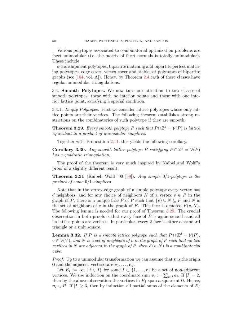
50 HAASE, PAFFENHOLZ, PIECHNIK, AND SANTOS

Various polytopes associated to combinatorial optimization problems arefacet unimodular (i.e. the matrix of facet normals is totally unimodular).These include

b-transhipment polytopes, bipartite matching and bipartite perfect match-ing polytopes, edge cover, vertex cover and stable set polytopes of bipartitegraphs (see [104, vol. A]). Hence, by Theorem 2.4 each of these classes haveregular unimodular triangulations.

3.4. Smooth Polytopes. We now turn our attention to two classes ofsmooth polytopes, those with no interior points and those with one inte-rior lattice point, satisfying a special condition.

3.4.1. Empty Polytopes. First we consider lattice polytopes whose only lat-tice points are their vertices. The following theorem establishes strong re-strictions on the combinatorics of such polytope if they are smooth.

Theorem 3.29. Every smooth polytope P such that P ∩Zd = V(P ) is latticeequivalent to a product of unimodular simplices.

Together with Proposition 2.11, this yields the following corollary.

Corollary 3.30. Any smooth lattice polytope P satisfying P ∩ Zd = V(P )has a quadratic triangulation.

The proof of the theorem is very much inspired by Kaibel and Wolff’sproof of a slightly different result.

Theorem 3.31 (Kaibel, Wolff ’00 [59]). Any simple 0/1-polytope is theproduct of some 0/1-simplices.

Note that in the vertex-edge graph of a simple polytope every vertex hasd neighbors, and for any choice of neighbors N of a vertex v ∈ P in thegraph of P , there is a unique face F of P such that {v} ∪N ⊆ F and N isthe set of neighbors of v in the graph of F . This face is denoted F (v,N).The following lemma is needed for our proof of Theorem 3.29. The crucialobservation in both proofs is that every face of P is again smooth and allits lattice points are vertices. In particular, every 2-face is either a standardtriangle or a unit square.

Lemma 3.32. If P is a smooth lattice polytope such that P ∩ Zd = V(P ),v ∈ V(V ), and N is a set of neighbors of v in the graph of P such that no twovertices in N are adjacent in the graph of P , then F (v,N) is a combinatorialcube.

Proof. Up to a unimodular transformation we can assume that v is the origin0 and the adjacent vertices are e1, . . . ,ed.

Let EI := {ei | i ∈ I} for some I ⊂ {1, . . . , r} be a set of non-adjacentvertices. We use induction on the coordinate sum vI :=

∑i∈I ei. If |I| = 2,

then by the above observation the vertices in EI span a square at 0. Hence,vI ∈ P . If |I| ≥ 3, then by induction all partial sums of the elements of EI

UNIMODULAR TRIANGULATIONS 51

are contained in P . Hence, they span a face that differs from the cube byat most the vertex vI . But in dimensions ≥ 3 the cube minus a vertex isnot a smooth polytope, so vI ∈ P . �

Proof of Theorem 3.29. We can again assume that 0 is a vertex with neigh-bors ei (1 ≤ i ≤ d). So the incident facet inequalities are xi ≥ 0 (1 ≤ i ≤ d).Since P is a simple polytope, any k of the ei define a k-dimensional face.

The first step is to show that “being adjacent” is an equivalence relationamong the vertices ei. That is, if for pairwise distinct 1 ≤ i, j, k ≤ d, ei isadjacent to ej , and ej is adjacent to ek, then all three are contained in acommon two-dimensional face. Suppose ei and ek were not adjacent, thenei − ej + ek would be a forth vertex in this face. But this violates theinequality xj ≥ 0. So, ei and ek are adjacent, and the three vertices are ina common two dimensional face.

If C0, . . . , Cr are the equivalence classes of this relation, then for 1 ≤ j ≤ r,Cj ∪ {0} spans a unimodular simplex ∆j . Letting Q := ∆1 × · · · × ∆r bethe product of these simplices, we aim to show that P = Q.

By the previous lemma all vertices of Q are contained in P . It remainsto show that all edges of Q are edges of P . Before proving this we showthat this will finish the proof. The graph of P is connected, so if there wasa vertex v of P that was not a vertex of Q, then at least one of the verticesof P that was in Q would have a neighbor in P that was not a neighbor inQ, so P would not be simple.

We now show that all edges of Q are edges of P . By the previous lemma, ifEI is a set of pairwise non-adjacent neighbors of 0, then all edges of the cubeF (0, EI) are in P . It remains to argue that if e1 and e2 are adjacent and{1}⊔I indexes pair-wise non-adjacent vertices of P , then e1+eI and e2+eIare adjacent. Assume they are not adjacent. The faces F (0, {e1} ∪EI) andF (0, {e2}∪EI) are cubes. So as neighbors of the vertex vI , vertices e1+vI ,e2 + vI , and vI − ei are pair-wise non-adjacent, for i ∈ I. Hence, they spana cube at vI , contradicting the adjacency of e1 and e2. �

3.4.2. Reflexive Polytopes. In this section we report on a class of polytopeswhere a computational approach implementing pull-back and push-forwardsubdivisions has been quite successful.

A lattice polytope P is called reflexive, if it contains a unique interiorlattice point and all facets are lattice distance one from this point. Withoutlose of generality it can be assumed that the interior point is the origin. Thepolar of a polytope P ⊆ Rd with 0 ∈ int(P ) is

P∨ := {u ∈ Rd | 〈x,u〉 ≥ −1 ∀x ∈ P} .

If P is reflexive then P∨ is again a lattice polytope. P is smooth if P issimple and the primitive generators of every vertex cone span the lattice.

Theorem 3.33. For d ≤ 3, every reflexive d-dimensional lattice polytopehas a regular unimodular triangulation.

52 HAASE, PAFFENHOLZ, PIECHNIK, AND SANTOS

dim. #polytopes RUT quadratic facet uni- projects to opentriangulation modular dimension 1

2 2 2 2 2 2 03 18 18 18 16 18 04 124 124 124 96 124 05 866 866 866 554 866 06 7622 7622 7620 4097 7620 07 72256 72255 72241 31881 72240 1

Table 3.1. Triangulations of smooth reflexive polytopes. There is one opencase in dimension seven.

Proof. The origin is the unique interior lattice point of P . Any pullingtriangulation in which the origin is pulled first will be regular and unimod-ular. For d = 3 we use the fact that any full triangulation of a polygon isunimodular. �

Øbro [76] has computed explicit representations of all d-dimensional sim-plicial reflexive polytopes for d ≤ 8 (up to lattice equivalence). Thereare 5, 18, 124, 866, 7622, 72256, 749892, and 8229721 such polytopes in di-mensions 2, 3, 4, 5, 6, 7, 8 and 9 respectively. The smooth reflexive poly-topes for dimensions 3 to 8 can be obtained from the polymake database

(www.polymake.org/doku.php/data), for the 9-dimensional see [70]. Weused two approaches to establish regular unimodular triangulations of thepolars of these polytopes up to dimension 7 (checking dimensions 8 and 9 isin progress):

(1) We checked whether the facet normals define a unimodular system(then the existence of a triangulation follows from Theorem 2.4).

(2) We searched for a sequence of projections along coordinate directionssatisfying the conditions for push-forward and pull-back subdivisionsgiven in Section 2.2. If such a sequence projects the polytope downto dimension 2, the polytope has a regular unimodular triangulation(as all 2-dimensional lattice polytopes have regular unimodular tri-angulations). If there is such a sequence projecting the polytope todimension 1, we know that the polytope has a quadratic triangula-tion.

For those polytopes for which a 2 dimensional, but no 1 dimen-sional projections were found, individual inspection confirmed a qua-dratic triangulation for some of them.

Both checks were done with software system polymake [58, 94] using anextension for projections of polytopal subdivisions [89]. The detailed resultsare listed in Table 3.1, and are summarized in the next theorem.

Theorem 3.34 (Haase, Paffenholz ’09 [50]).• All smooth reflexive d-polytopes for d ≤ 8 are integrally closed.

UNIMODULAR TRIANGULATIONS 53

• All smooth reflexive polytopes in dimensions d ≤ 6 admit a quadratictriangulation.• All but at most one (out of 72256) of the 7-dimensional smooth re-flexive polytopes have a quadratic triangulation.

The one remaining smooth Fano polytope in dimension seven may stillhave a regular unimodular triangulation, but we were not able to constructsuch a triangulation with our approach. We checked whether the polytopesare integrally closed using the polymake-interface to Normaliz [23]. Previ-ously it was shown by Piechnik that all smooth reflexive d-polytopes have aregular unimodular triangulation for d ≤ 4. Computations in dimensions 8and 9 are currently work in progress.

3.5. The Grobner fan and the toric Hilbert scheme.

3.5.1. The Grobner fan and the secondary fan. Here we examine the relationbetween Grobner bases and subdivisions, mentioned in section 2.4.

As in section 2.4,2 we let A := (P × {1}) ∩ Zd+1 be the homogenized setof lattice points in a polytope P ∈ Rd, take the polynomial ring S := k[xa :a ∈ A] with one variable for each lattice point in P , and consider the toricideal of P , i.e., the binomial ideal generated by linear dependences amongthe lattice points:

IP =

⟨xm − xn : m,n ∈ ZA

≥0 ,∑

a∈A

maa =∑

a∈A

naa

⟩.

Recall, each choice of weights ω ∈ RA induces a regular subdivision Tω of P ,on the lattice polytope side, and an initial ideal inω IP := 〈inω f : f ∈ I〉,on the toric algebra side.

However, if ω is not generic, the subdivision Tω may not be a triangula-tion, and the ideal inω IP may not be a monomial. This means a polynomialf may have several monomials of highest weight with respect to ω, and allthose monomials form the leading part of f , which we also denote in f . Forexample, if ωa is the same constant for every a then:

• Tvω is the trivial subdivision (P itself is its only full-dimensionalcell) and• inω IP = IP , since IP is homogeneous and for a homogeneous f , andin f = f .

We state without proof two properties relating the initial ideals inω IP

and the corresponding regular subdivisions Tω. (See [115, Chapter 10] fordetails.)

Theorem 3.35 (Sturmfels 96 [115]). If inω1 IP = inω(inω2 IP ) for someω1, ω2 and ω (that is, if inω1 IP is an initial ideal of inω2 IP ) then thesubdivision Tω1 refines the subdivision Tω2 .

2Everything we say in this section can be extended to the more general case where A

is any finite and homogeneous set of lattice vectors in Zd+1

54 HAASE, PAFFENHOLZ, PIECHNIK, AND SANTOS

Corollary 3.36. If inω1 IP = inω2 IP for different ω1 and ω2, then Tω1 =Tω2 . This follows from the previous property by letting ω = ω1 (and thenswitching the roles of ω1 and ω2).

These properties mean that there is an order-preserving map from theposet of all initial ideals of IP to the poset of all regular subdivisions ofA, where the latter are partially ordered by refinement and the former areordered by I1 < I2 if I1 is an initial ideal of I2. This was proved by Sturmfelsin [113].

Put another way, the regular subdivision and the initial ideal constructionprovide two stratifications of the vector space RA. The first is based setsof ω’s which give the same regular subdivisions and the second is basedon which ω’s give the same initial ideals. Both stratifications are completerational polyhedral fans, and they are called , respectively, the secondaryfan and the Grobner fan of A.

Theorem 3.37 (Sturmfels 91, [113]). The Grobner fan of A refines thesecondary fan of A.

Observe that for the secondary fan to be well defined, the subdivisions ofA need to be considered as subdivisions of point configurations, as when wedefined weak pulling in Section 2.1.1.

Theorem 3.37 implies that Tω can be clearly determined from inω IP .

3.5.2. The toric Hilbert scheme. We now look at a property that is sharedby all initial ideals of IP and the toric ideal IP itself.

As detailed in [115, Chapter 10], A defines a d-dimensional multi-gradingon the polynomial ring k[xa : a ∈ A], assigning multi-degree ai to thevariable xi. Ideals I ⊂ k[xa :a ∈ A] that are homogeneous with respect tothis grading have well-defined Hilbert functions

Z≥0A −→ Z≥0

b 7−→ dimk Ibwhere Z≥0 is the set of non-negative integers, Z≥0A is the semigroup ofnon-negative integer combinations of A, and for each b ∈ Z≥0A, Ib is thedegree b part of I.

The most natural A-homogeneous ideal is the toric ideal IP , generatedby the binomials

{ xm − xn : m,n ∈ ZA

≥0 ,∑

a∈A

maa =∑

a∈A

naa },

because every b ∈ Z≥0A, (IP )b has codimension one in (k[xa : a ∈ A])b.This characterizes the Hilbert function of Ib.

An A-homogeneous ideal I ⊂ k[xa :a ∈ A] is called A-graded if it has thesame Hilbert function as the toric ideal IP . A-graded ideals include all theinitial ideals of IP , but can include other ideals as well. The toric Hilbertscheme, as introduced by Peeva and Stillman [92], is the set of all A-gradedideals with a suitable algebraic structure defined by some determinantal

UNIMODULAR TRIANGULATIONS 55

equations. An equivalent description via binomial equations appeared in[114, §6]. (See also [72,112].)

Surprisingly, the A-graded ideals that are not initial are still related tosubdivisions of A. Sturmfels [115, Theorem 10.10] proved that the order-preserving map implied in Theorem 3.37 extends to an order preserving mapfrom the poset of all A-graded ideals, where the partial ordered is given byby “toric deformation” (a generalization of the property of being an initialideal), to the poset of all subdivisions, still ordered by refinement.

That is to say, every A-graded ideal I has a canonically associated polyhe-dral subdivision TI of A. If I is monomial, then TI is a triangulation, whosesimplices are spanned by the standard monomials in k[xa :a ∈ A]/Rad(I).

Santos [100] used this map to show the existence of non-connected toricHilbert schemes, elaborating on work of Maclagan and Thomas [72]. Hereare the main ideas. There is a natural and well-known adjacency relationbetween triangulations of the same configuration. It can be defined as anoperation that takes out certain simplices and inserts others, but it is equiv-alent to the following [34, Section 2.4]: two triangulations T1 and T2 of Aare related by a geometric bistellar flip (or just flip, for short) if there is apolyhedral subdivision T of A whose only refinements are T1 and T2. Macla-gan and Thomas defined an analogous adjacency relation between A-gradedmonomial ideals (mono-A-GIs for short), which they also called flip. Theirrelation has the following properties.

Proposition 3.38 (MacLagan & Thomas 02, [72]). (1) A toric Hilbertscheme is connected if and only if the graph of mono-A-GIs is con-nected.

(2) Triangulations of A corresponding to neighboring mono-A-GIs eithercoincide or differ by a geometric bistellar flip.

Lattice point configurations with non-connected graphs of flips are rare,but they were shown to exist in 2000 [99]. Still, this does not necessarilyimply the corresponding toric Hilbert scheme is non-connected, because theSturmfels map going from A-graded ideals to subdivisions of A is in generalnot surjective [115, Example 10.13], [92]. However, Maclagan and Thomasalso observed, based on [115, Theorem 10.14], that the image of the mapalways contains all the unimodular triangulations of A.

Corollary 3.39. The toric Hilbert scheme of A has at least as many con-nected components as there are connected components in the graph of trian-gulations of A that contain unimodular triangulations.

Santos’ non-connected toric Hilbert scheme is based on the constructionof a polytope P for which the corresponding configuration A has unimodulartriangulations in different components of the graph of flips. Let Q ∈ R4 bethe 24-cell. The 24-cell is one of the six regular 4-dimensional polytopes, andcan be realized as the convex hull of the root system of typeD4. We considerit as a lattice polytope in the lattice it generates, D4 := {(a1, a2, a3, a4) ∈

56 HAASE, PAFFENHOLZ, PIECHNIK, AND SANTOS

Figure 3.3. A locally acyclic orientation of the graph of a 24-cell.

Z4 :∑

ai ∈ 2Z}. Its only lattice points are the origin and the 24 roots

±ei ± ej, with (i, j) ∈([4]2

). Q has 24-facets, all regular octahedra, and 96

2-faces, all regular triangles.

Theorem 3.40 (Santos 05, [100], see also [34, Section 7.3]). If P = Q×[0, 1]is a lattice polytope in D4 ×Z, such that A has 50 points: the 48 vertices ofP plus the centers of Q× {0} and Q× {1}, then:

(1) The graph of triangulations of A has at least 13 connected compo-nents, each containing at least 348 unimodular triangulations.

(2) The toric Hilbert scheme of A has at least 13 connected componentseach containing at least 348 monomial ideals, and they all have di-mension at least 96.

Proof. The proof uses the idea of staircase refinements introduced in Sec-tion 2.3. We sketch it here, and refer to [34, Section 7.3] or [100] for details.The crucial tool is an orientation of the graph of the 2-cell with the followingproperties:

• It is locally acyclic, but no edge can be reversed in it without creatinga cycle in one of the 96 triangular faces of D4

• In each of the 24 octahedral facets of Q, one (and only one) of the4-cycles of edges is a directed cycle.

Figure 3.3 depicts this orientation, in several pieces. To understand thefigure, observe that that 24 vertices of Q are the union of the 16 vertices ofa 4-cube plus the eight points ±2ei. Moreover, the graph of Q is the graph

UNIMODULAR TRIANGULATIONS 57

of the 4-cube plus the edges joining each of the eight 3-cube facets of it tothe corresponding ei or −ei. The figure shows stereographic projections ofthe eight 3-cube facets of the 4-cube, each with the orientation of its edges.The projection makes two of the facets regular cubes, so that one of theextra points is sent to infinity. We leave it to the reader to check that theorientation displayed has the two claimed properties (thanks to symmetrythis task is not as hard as it might seem).

We triangulate P as follows. First triangulate each octahedral facet ofQ in the unique way that does not create a local cycle. That is, in eachoctahedron use the diagonal that is orthogonal to the quadrilateral cycleof that octahedron. Also, by the properties of the triangulation, this newdiagonal can only be given one of its two orientations without creating alocal cycle. Cone this triangulation of the boundary of Q to the origin, andorient every new edge away from the origin. This produces a triangulationT of Q with a locally acyclic orientation. Further, this triangulation andorientation is unimodular, and it has no reversible edge. That is, reversalof any individual edge creates a directed cycle. For the 96 original edges ofthe 24-cell, this is part of what we claimed before. It is also true and easyto check for the new 24 diagonals of the octahedra and 24 edges from thecenter.

We triangulate P using the staircase refinement of T and the edge [0, 1](we give to [0, 1] either of its two orientations). It turns out that the factthat no edge can be reversed in the locally acyclic orientation implies thatthis triangulation cannot be connected by flips to any triangulation con-structed in the same way using a different initial orientation of the edgesof the 24-cell. This proves that the graph of triangulations contains uni-modular triangulations in different components. There are at least 13 suchcomponents because symmetries of the 24-cell produce 12 different ways ofconstructing the initial locally acyclic orientation, plus another componentthat will contain all the globally acyclic orientations. The 348 triangulationsin each component and the 96 in the dimension of the toric Hilbert schemeare by-products of the many symmetries of the construction. �

4. Dilations and the KMW Theorem

Dilating a lattice polytope by a positive integer is a natural operation.One of the first theorems about unimodular triangulations was proved in

the early days of toric geometry by Knudsen, Mumford, and Waterman3 [66],who were interested in semi-stable reduction of families over curves.

Theorem 4.1 ( [66]). Given a polytope P , there is a factor c = c(P ) ∈ Z>0

such that the dilation c · P admits a regular unimodular triangulation.

3We call this the Knudsen-Mumford-Waterman Theorem, or KMW, since Knudsensays:“One of the key steps is due to Alan Waterman. The rest is a truly joint effort byMumford and me” [66, p. 109].

58 HAASE, PAFFENHOLZ, PIECHNIK, AND SANTOS

We say that c is a KMW-number of P if cP has a unimodular triangula-tion. This KMW-theorem has raised more questions than it has answered,including:

• What is the minimum c(P ) for a given polytope P? Is there a c(d)that is a KMW-number for every polytope of dimension d?• What is the structure of the set of KMW-numbers of a given P? Isit a monoid? Theorem 4.7 implies it is closed under taking multiplesof an element. It is not clear whether it is closed under taking sums.• To our knowledge, Example 4.12 below is the first class of polytopesP and integers c in the literature such that c is a KMW-number forP but c+ 1 is not.

The two following theorems by Bruns, Gubeladze, and Trung; and Eisen-bud, Reeves, and Totaro, respectively, show that we cannot expect algebraicobstructions to these questions.

Theorem 4.2 ( [20]). c ·P is integrally closed for c ≥ d− 1, and Koszul forc ≥ d.

Theorem 4.3 ( [37]). After a linear change of coordinates, IcP has a qua-dratic Grobner basis for c ≥ reg(IP )/2.

The second half of this section is dedicated to a proof of Theorem 4.1.Our proof differs from the original one (and the reworking of it in [18]) intwo ways. First, a more careful application of the elementary reduction stepenables us to avoid using “local lattices” [18] or “rational structures” [66]and yields a cleaner proof of regularity.4 Secondly, we set up a book-keepingmethod that allows us to obtain the bound stated in Theorem 4.4 below.Determining a bound based upon the original proof would be difficult andinvolve a tower of exponentials whose minimal length would be the maximumvolume among the simplices in the triangulation of P being used for theconstruction (see Remark 4.18). In our proof the bound is “merely” a doubleexponential.

Theorem 4.4. If P is a lattice polytope of dimension d and (lattice) volumevol(P ), then the dilation

d!vol(P )!dd2 vol(P )

P

has a regular unimodular triangulation.More precisely, if P has a triangulation into N d-simplices, of volumes

V1, . . . , VN , then the dilation

d!∑

N

i=1 Vi!((d+1)!(d!)d)Vi−1

T

has a regular unimodular refinement.

4 Bruns and Gubeladze [18] omit regularity, and the proof of regularity in [66] (Theorem2.22, pp. 147–151) is quite intricate.

UNIMODULAR TRIANGULATIONS 59

Before going into the KMW Theorem we deal with two questions thatare, in a sense, special cases of it. In Section 4.1 we review what is knownabout KMW-numbers of three-dimensional lattice polytopes, summing upresults from [60] and [101].

In Section 4.2 we give two proofs that if a polytope P has a unimodulartriangulation every dilation cP (c ∈ N) of it has one, and that regularityand flagness of the triangulation can also be preserved in the process. Thisis equivalent to saying (as noted above) that the set of KMW-numbers ofany polytope P is closed under taking products.

Section 4.3 is a preparation for the proof of Theorem 4.1. It shows that ifP is a lattice simplex of volume V then cP can be triangulated into simplicesof volume strictly smaller than V , for some c ∈ {1, . . . , d+1}. In Section 4.4this reduction is applied iteratively to yield Theorem 4.1. However, theeffective version stated as Theorem 4.4 requires a careful analysis of how todo this reduction in many simplices at the same time, and how to controlthe number (and type) of new simplices obtained in each step. This is donein our final Section 4.5.

4.1. KMW numbers in dmension Three. If P is a segment or a latticepolygon, then P has a regular unimodular triangulation, so for the 1 and 2dimensional cases, P has KMW-number c(P ) = 1.

For 3-dimensional polytopes the following is known:(1) 1 and 2 are not KMW-numbers of every 3-polytope. In fact, there

are non-unimodular simplices whose second dilation does not have aunimodular triangulation (Ziegler 1997, unpublished).

(2) It is not known whether 3 and 5 are KMW-numbers of every 3-polytope.

(3) Every other integer is a KMW-number of every 3-polytope (Kantorand Sarkaria [60] for the integer 4, Santos and Ziegler [101] for everyother integer).

These results all emanate from the fact that every full triangulation ofP gives a subdivision of cP into dilations of empty simplices. This meansthat in order to prove that cP can be unimodularly triangulated for everyP , we can restrict our attention to the case where P is an empty simplex,as long as we manage to make sure that the triangulations of the individualdilated simplices agree on their common faces. So, let us look at what emptysimplices in dimension three look like.

According to White’s Theorem [75, 102, 119], every empty tetrahedronin R3 has width one with respect to some lattice direction (not necessarilywith respect to a facet normal). That is, it fits between two adjacent latticehyperplanes. Consequently, it is either unimodular (if it has three verticesin one of the two lattice hyperplanes) or lattice equivalent to

S(p, q) := conv[ 0 0 1 p0 0 0 q0 1 0 1

]

60 HAASE, PAFFENHOLZ, PIECHNIK, AND SANTOS

for some integers 0 ≤ p ≤ q with gcd(p, q) = 1. Observe that S(p, q) ∼S(q − p, q) ∼ S(p−1, q) ∼ S(q − p−1, q), where inverses are taken modulo p.It can be shown that these are the only cases that give equivalent simplices.The parameter q is the volume of S(p, q), while p carries information of morearithmetic nature.

In the c-th dilation cS(p, q), all the lattice simplices lie in either thebottom edge, the top edge, or the c − 1 intermediate horizontal latticeplanes. The latter can be tiled by lattice translations of the paralellogramC(p, q) := 2S(p, q) ∩ {z = 1} = conv{(0, 0, 1), (1, 0, 1), (p, q, 1), (p + 1, q, 1)}.So, in order to understand the structure of lattice points in cS(p, q) we onlyneed to look at those in C(p, q). These are its four vertices plus q−1 interiorpoints with the following properties: (a) there is exactly one of them in eachof the c− 1 lattice lines of direction (1, 0, 0) and intersecting C(p, q) and (b)there is exactly one in each of the c − 1 lattice lines of direction (0, p, q).This induces two distinct orderings of these interior q − 1 points which wecall the Y -order and the X-order.

All the results about unimodular triangulations of a dilated tetrahedronS(p, q) use, in one way or another, the following decomposition of cS(p, q).We only sketch the descriptions, relying on Figure 4.1 for some of the mean-ing (more details can be found in [101]).

• First slice cS(p, q) into c layers by the c − 1 horizontal planes atinteger heights (Figure 4.1.a).• Then divide each layer into a number of triangular prisms in one oftwo ways: the k-th layer can be divided into either 2k − 1 prismswith axis in the X-direction or 2(c − k) − 1 prisms with axis in theY -direction (Figure 4.1.b). These prisms have a rectangular facet inone of the horizontal lattice planes and a single edge in the other.We call this edge the tip of the prism.• Each such prism can be unimodularly triangulated using joins of theprimitive segments in the tip and monotone lattice paths of length qin the opposite facet (Figure 4.1.c). These paths have to be chosencompatible to one another (they can all be the same one) and apartof these joins the triangulation of the prism only contains pyramids,with vertices at the tip, over unimodular triangles in the oppositefacet.

With this technique we see that:

Corollary 4.5 ( [101, Cor. 4.2]). For every lattice 3-polytope P and everydilation factor c ≥ 2, cP can be dissected into unimodular simplices withdisjoint interiors.

Proof. Consider any full triangulation T of P , and its dilation cT into dilatedempty simplices. Divide every dilated simplex in layers, then prisms, thensimplices, as explained above. �

UNIMODULAR TRIANGULATIONS 61

(a)

(b)

(c)

Figure 4.1. ddd

So, the only thing to take care of is how to make all these dissections agreeon the common boundary facets of adjacent dilated simplices, adjacent layerswithin a dilated simplex, and adjacent prisms within a layer. One way totry to address this issue is to triangulate each dilated simplex c∆ so that itsboundary receives the standard triangulation, the one obtained slicing theboundary by all the lattice lines parallel to edges of c∆ (see Figure 4.2). Withthis in mind, the following statements on dilated simplices guarantee we canfind such desired triangulations of the adjacent components as describedabove.

Theorem 4.6. If ∆(p, q) is an empty 3-simplex, then:(1) 2∆(p, q) has a unimodular triangulation if and only if p = ±1 (mod q).

In this case, the triangulation can be made unimodular and with stan-dard boundary [101, Cor. 3.5, Prop. 3.6]

(2) For every c ≥ 4, c∆ has a unimodular triangulation ( [101, Cor. 4.5]).(3) For every c that can be written as a sum of composite numbers (that

is, every c ≥ 4, other than c = 5, 7, 11), c∆ has a unimodular tri-angulation with standard boundary ( [60] for c = 4, [101, Thm. 5.1]for the rest).

(4) For every c ≥ 7, c∆ has a unimodular triangulation in which theboundary is triangulated with the “quasi-standard” triangulation ob-tained from the standard one by flipping the diagonals incident toedges of c∆ and at lattice distance 3 from the vertices (see Fig-ure 4.2 [101]).

4.2. Canonical triangulation of a dilated simplex. In this section weshow that given a unimodular triangulation T of a polytope P another

62 HAASE, PAFFENHOLZ, PIECHNIK, AND SANTOS

Figure 4.2. The standard triangulation of a dilated triangle (left) and thequasi-standard one used for the case c = 7.

unimodular triangulation of cP can be derived, preserving regularity (The-orem 4.7) and flagness (Corollary 4.11). The first result can by now beconsidered “folklore” (it is sometimes attributed to Santos, 1996, unpub-lished). The second result is new.

The proofs of both theorems start by noting that dilating every simplexin T yields a triangulation cT of cP into dilations of unimodular simplices,and then use the canonical subdivisions of dilated unimodular simplices,as discussed in section 2.1.3. That is, the dilated standard simplex c∆d isrealized as {x ∈ Rd+1

≥0 :∑

xi = c}, and sliced along the hyperplanes parallelto the facets: xi = k for i = 1, . . . , d+1 and k = 1, . . . c−1. The cells of thissubdivision are hypersimplices. The canonical weights ωm :=

∑m2

i showthat this subdivision is regular, and the weights restrict to faces as well.

The naturality of this subdivision and its weights allows one to patch sim-plices together. That is, if we subdivide each of the cells of cT canonically,they agree along their boundaries, and we get a subdivision of P which isregular if T was regular.

Theorem 4.7. If P has a (regular) unimodular triangulation T then, forevery positive integer c, its dilation cP has one too.

Proof. As in Theorem 2.4, all cells (hypersimplices) of the canonical subdivi-sion of cT are compressed. Hence, pulling all the lattice points of cP in anyorder yields a unimodular triangulation T ′. This triangulation is a regularrefinement. Hence, regularity of T implies regularity of T ′ (cf. [34, Lem-mas Lemma 2.3.16 and 4.3.12], or see more details in the proof of Corol-lary 4.11). �

To guarantee flagness, instead of using pulling refinements we dice withrespect to a larger set of hyperplanes, namely those based on the root systemof type A. Remember that if P is a lattice polytope of type A then dicing

UNIMODULAR TRIANGULATIONS 63

P according to all lattice hyperplanes with normals in the root system givesa quadratic triangulation of P (Theorem 3.3).

To apply this to an arbitrary simplex ∆ we first need to show a way tomap a d-simplex to a simplex of type A. This is canonical, once an orderingof ∆’s vertices is prescribed. Thus we introduce the concept of an orderedsimplex, and the canonical triangulation of its dilation. These concepts willbe crucial in the proof of the KMW Theorem (and were used in the previousproofs of it, see [18, Section 3.A]).

Definition 4.8. An ordered simplex is a simplex, ∆ = conv{a0, . . . ,ad}that comes with an ordering of its vertices, a0, . . . ,ad.

Let ∆ be an ordered d-simplex and consider the affine isomorphism send-ing ∆ to the standard simplex ∆d

Aof type A via

ai 7→

i+1∑

j=1

ej ∈ Rd+1.

The A-canonical triangulation of c∆ is the pull back under this map of thetype A dicing triangulation of c∆d

A.

Observe that since the A-dicing is unimodular, all the simplices in thecanonical triangulation of c∆ have the same volume as ∆.

The following lemma makes what the canonical triangulation is moreexplicit (as a dicing triangulation) by expressing it in barycentric coordinateswith respect to ∆. Recall that the barycentric coordinates of a point x ∈ ∆with respect to the vertices a0, . . . ,ad of a simplex ∆ are the unique vector(x0, . . . , xd) with

∑xi = 1 such that

x =

d∑

i=0

xiai.

In particular, for each subset I ⊆ {0, . . . , d} the hyperplanes defined bysetting

∑i∈I xi equal to a constant are parallel to the following two comple-

mentary faces of ∆:

conv{ai : i ∈ I}, and conv{ai : i 6∈ I}.

Lemma 4.9. Let ∆ = conv{v0, . . . ,vd} be an ordered simplex and c apositive integer. Then the canonical triangulation of ∆ is the dicing trian-gulation with respect to the families of lattice hyperplanes defined by makingany sum xi + · · ·+ xj of consecutive barycentric coordinates constant.

Proof. Since an affine isomorphism from one simplex to another preservesbarycentric coordinates, there is no loss of generality in assuming that ∆is the standard simplex ∆d

A. We only need to show that the hyperplanes

orthogonal to the roots are indeed defined by making a sum of consecutivebarycentric coordinates constant. For this, observe that if (x0, . . . , xd) arethe barycentric coordinates of x with respect to ∆d

Athen

64 HAASE, PAFFENHOLZ, PIECHNIK, AND SANTOS

x =

d∑

j=1

xj

(j+1∑

i=1

ei

)=

d+1∑

i=1

ei

d∑

j=i−1

xj

,

so that

〈x,ej − ei〉 =

j−2∑

k=i−1

xk, ∀1 ≤ i < j ≤ d+ 1.

�

With this we can conclude the following.

Theorem 4.10. Let T be a lattice triangulation of a polytope P , let c be apositive integer, and let cT denote the dilation of T , that is, the followingtriangulation of cP :

cT := {c∆ : ∆ ∈ T .

Consider a total order in the vertices of T , such that every ∆ ∈ T isregarded as an ordered simplex. Call T ′ the triangulation of cP obtainedrefining each c∆ to its canonical triangulation. Then:

(1) T ′ is indeed a triangulation. That is, common faces of differentsimplices in cT get the same refinement.

(2) If T his unimodular, then T ′ is unimodular.(3) If T is regular, then T ′ is regular.(4) If T is flag, then T ′ is flag.

Proof. The canonical triangulations agree on common faces of simplices ofcT since they only depend on the ordering of the vertices in those faces.Therefore, this procedure indeed gives a lattice triangulation T ′ of cP . Sincethe canonical triangulation preserves volumes, it preserves unimodularity.We will show that regularity and flagness are also preserved.

For regularity we use the idea of regular refinements [34, Lemma 2.3.16].If T0 is a regular subdivision, given by the weight vector ω0, of a pointconfiguration A and each cell of T0 is refined using a common weight vectorω ∈ RA, then the refinements of all cells agree on their intersections. Thismeans we get a subdivision of A. Moreover, this subdivision is regular, andcould have been obtained directly using the weight vector ω0 + ǫω, for asufficiently small ǫ > 0.

We apply this procedure(n+1

2

)times to the subdivision cT , where n is the

number of vertices of T , as follows. Let a1, . . . ,an be the ordered sequenceof vertices of T . For each interval [i, j] ⊆ [1, n] (including the case i = j),let φi,j be the function that is 0 on cak if k ∈ [i, j], 1 on cak if k /∈ [i, j], and

linear on each simplex of cT . Consider the weight function ωi,j ∈ RcP∩Zd

that restricts φ2i,j to all lattice points in cP . Clearly, the regular refinement

of cT via this weight function dices each simplex c(conv{ai : i ∈ S}) bythe lattice hyperplanes parallel to conv{ai : i ∈ S ∩ [i, j]} and conv{ai :i ∈ S \ [i, j]}. In each simplex of cT this is one of the hyperplanes we want

UNIMODULAR TRIANGULATIONS 65

to use for the canonical triangulation of that simplex. Performing theseregular refinements on cT for each such weight function ωi,j, in any order,gives a dicing of each simplex by more and more families of hyperplanes,eventually all hyperplanes in Lemma 4.9. Hence, the resulting triangulationis T ′, proving that T ′ is regular.

Flagness of T ′ is based solely on the fact that T is flag and that T ′’srefinements of each simplex of cT are also flag (by Theorem 3.3). Let N ⊂cP ∩ Zd and suppose that every pair of points in N defines an edge of T ′.We want to show that N is contained in some simplex cF of cT , since cTis a flag refinement of cP , and conclude that N is a face of T ′.

To each point n ∈ N associate its carrier simplex cF (n) ∈ cT . Let S bethe union of all vertices of all the carriers F (n). Every two points in S forman edge of T because either they lie in the same F (n), which is a simplex,

or they lie in F (n1) and F (n2) for two points of N , hence their dilationslie in the minimal face of cT containing the edge n1n2 of T ′. Since T isflag, S is a face of T , which implies that all the carriers cF (n), hence all thepoints n, lie in the face cS of cT . �

Corollary 4.11. If P has a quadratic triangulation T , then so does itsdilation cP for every positive integer c.

With the canonical triangulations at our disposal, we can now discuss theexample advertised at the beginning of the section. This example is inspiredby [Mustata-Payne] and appears in [Cox-Haase-Hibi-Higashitani].

Example 4.12. Let h and k be positive integers and set d := hk − 1. InRd+1 consider the vector v := 1

k (1, . . . , 1), the lattice Λ := Zd+1+Zv and thed-polytope ∆ := conv{e0, . . . , ed}. Then h∆ has a quadratic triangulationjoining v to the canonical triangulation of h∂∆.

We claim that certain higher multiples of ∆ are not normal and thus donot admit unimodular triangulations. To see this, consider the homomor-phism φ : Λ → Z/k given by x 7→ kx0. If a and b are positive integers withb < h, then the Λ-points in (ah + b)∆ map to {0, 1, . . . , a}. Therefore, wecan only obtain {0, 1, . . . , 2a} from the sum of two such points. On the otherhand, if 2b ≥ h, then 2(ah+ b)∆ contains a Λ-point with image 2a+ 1, wit-nessing non-normality if 2a + 1 < k. The parameters k = 4, h = 2 yield a7-simplex so that 2∆ has a quadratic triangulation but 3∆ is not normal.

4.3. Reducing the volume of simplices in the dilation. The canonicaltriangulation divides c∆ into simplices of the same volume as ∆. We nowwant to improve this, and triangulate c∆ into simplices of volume strictlysmaller than ∆ (assuming ∆ is not unimodular). This cannot be done forevery c, but we prove here that it can always be done for some c ≤ d andall its multiples.

For this we introduce the concept of box points.We start with a seemingly unrelated lemma about the Cayley sum of

two dilated polytopes of type A. Remember that if P1 and P2 are lattice

66 HAASE, PAFFENHOLZ, PIECHNIK, AND SANTOS

polytopes in a lattice Λ ⊂ Rd then the Cayley sum of P1 and P2 is the latticepolytope conv(P1 × {0} ∪ P2 × {1}) in the lattice Λ× Z ⊂ Rd+1.

As usual, the canonical triangulation of a polytope of type A is the oneobtained by slicing by all the lattice hyperplanes normal to the roots. Re-member that this triangulation is regular and unimodular (Theorem 3.3).

Lemma 4.13. If P1 and P2 are lattice polytopes of type A, with canonicaltriangulations T1 and T2, then:

(1) There is a regular triangulation of the Cayley sum conv(P1 × {0} ∪P2 × {1}) that restricts to T1 and T2 on P1 and P2.

(2) Any such triangulation (regular or not) is unimodular.

Proof. The canonical triangulation of a type-A polytope is regular, so letω1 and ω2 be weight vectors producing T1 and T2 in P1 and P2, respectively.Since P1 × {0} and P2 × {1} are faces of the Cayley sum, using the sameweight vectors (that is, using ω1 in P1 × {0} and ω2 in P2 × {1}) yieldsa regular subdivision that restricts to T1 and T2 on P1 and P2. If thatsubdivision is not a triangulation, we do pulling refinements, which preserveregularity.

For part (2), observe that every cell in such a triangulation T will bea join of a face F1 of T1 and a face F2 of T2. It is convenient to think ofthe root system Ad as consisting of the standard basis vectors ±ei plus thedifferences ±(ei − ej). This is done by forgetting the coordinate d + 1 in

the usual definition of Ad as embedded in Rd+1. In this description, the Ad

dicing of Rd refines the tiling by translations of the unit cube, triangulatingevery lattice unit cube by (translations of) the order triangulation of [0, 1]d.

In particular, if k and l are the dimensions of F1 and F2 there is no lossof generality in assuming that

F1 = conv{a0,a1 . . . ,ak} × {0}, F2 = conv{b0, b1 . . . , bl} × {1},

where the ai’s and the bj’s are sequences of 0/1 vectors in Rd with increasingsupports. Moreover, by subtracting a0 from every ai and b0 from every bjwe can assume a0 = b0 = 0. Observe that the ai and bi are in transversalspaces. Then, the volume of the join of F1 and F2 equals the volume ofF := conv{0 = a0 = b0,a1 . . . ,ak, b1 . . . , bl} ⊂ Rd. We are going to showthat this volume is always one (or zero). Without loss of generality weassume F to be full-dimensional. If it is not, we extend the sequence of ai’suntil it is.

We use induction on the dimension d. In particular, we assume that noai and ai+1 differ in a single coordinate, because otherwise we can projectalong that coordinate and get the result by inductive hypothesis. The samehappens if some bj and bj+1 differ by a single coordinate. That implies thatboth k and l are at most d/2, hence they are both equal to d/2 becausek + l = d. But then we must have ak = bl = (1, . . . , 1), which implies thatthe volume of F is zero (except, of course, in the base case for the induction,which is k = l = 0 and produces volume 1). �

UNIMODULAR TRIANGULATIONS 67

It is worth mentioning that Lemma 4.13 is not true for the Cayley sum ofthree or more type-A polytopes, even in dimension three. Indeed, the edgesparallel to the vectors (1, 1, 0), (1, 0, 1) and (0, 1, 1) are type-A polytopesand their Cayley sum, which equals their join, is a non-unimodular simplex.

Our method for refining dilations will be based on combining Lemma 4.13with the concept of anA-canonical triangulation of a dilated ordered simplex(Definition 4.8). Let us explain how.

Let ∆ = conv(b0, . . . , bd) be a non-unimodular lattice simplex, of volumeV with respect to a lattice Λ. Let L∆ be the lattice spanned by the vertices

of ∆. We take ~L∆ := L∆ to denote the linear lattice parallel to L∆, so

Λ : ~L∆ = V . 5 We use barycentric coordinates with respect to ∆, anddilated barycentric coordinates for a dilation c∆. In the latter, points in c∆are written as convex combinations of cv0, . . . , cvd.

A box point for ∆ is simply an element of the quotient Λ/~L∆, where ~L∆

is the linear lattice parallel to L∆. We normally represent a box pointin the ∆-barycentric coordinates of any of its representatives, as m =

(m0, . . . ,md). Quotienting by ~L∆ then means that we are interested onlyin ({m0}, . . . , {md}), where {x} := x− ⌊x⌋ denotes the fractional part of areal number x. The height h(m) of a box point m is the number

∑i{mi}.

It is an integer between 1 and V − 1 and coincides with the smallest integerh for which h∆ contains a point of m+ Λ.

These concepts extend to lower dimensional faces. For a face F LF de-notes the lattice spanned by the vertices of F and ΛF is the intersectionof Λ with the linear space parallel to F . A box point for F is then an

element of ΛF /~LF , and is represented by an m in barycentric coordinateswith respect to F . Observe that if F is a face of ∆ then there is a naturalinclusion ΛF /~LF ≤ Λ/(~L∆) so that a box point for F is also a box point for∆. Coordinates for m are extended from F to ∆ by putting zeroes in thecoordinates of the vertices in ∆ \ F . Conversely, a box point of ∆ is a boxpoint for F if and only if those particular coordinates are zero.

We call carrier of a box point m of ∆ the (unique) minimal face F of ∆for which m is a box point. A box point of ∆ is non-degenerate if its carrieris ∆ itself. That is, if none of its ∆-barycentric coordinates is integral.

Given a box point m of a simplex ∆ and a certain positive integer c, weaim to triangulate c∆ into simplices of volume strictly smaller than that of∆, using only the points of L∆ ∪ (m+ L∆). Of course, this is impossible ifc < h(m). Although it can be done for every c ≥ h(m)

We offer two versions of this procedure. The first works for every c ≥ c0but is less symmetric and complicates the proof of regularity. The secondone is somehow simpler but requires c to be a multiple of (d+1)! (or, rather,

5 To simplify the exposition, in the rest of the paper we assume (w. l. o. g.) that Λcontains the origin, so that all the dilations c∆ are lattice polytopes with respect to thesame lattice Λ. We do not require, however, the affine lattice L∆ to contain the origin.

68 HAASE, PAFFENHOLZ, PIECHNIK, AND SANTOS

Figure 4.3. The points in c∆ ∩ (m+ L∆). Here c = 5 and c0 = 2

a multiple of the number of non-zero coordinates in m. However, since wewill later apply the procedure to several box points at the same time, havingc be a multiple of (d+ 1)! is convenient).

The structure of c∆ ∩ (m+ L∆) is straightforward: it is a translation ofthe points of L∆ in (c− c0)∆ (see Figure 4.3).

Assuming ∆ is an ordered simplex allows us to speak of the canonicaltriangulation of c∆, and of cF for every face F of ∆.

Let F be a face in a triangulation T and let m be a box point of F . Wesay that m is non-degenerate for F if it is not a box point of a proper faceof F . Equivalently, m is non-degenerate if all the F -coordinates of m arefractional. Then, the full-dimensional simplices of T for which m is a boxpoint are precisely the star of F . Recall that the (closed) star of a face Fin a simplicial complex T is the set star(F ;T ) of all simplices of T thatcontain F , together with all their faces. Equivalently:

star(F ;T ) := {F ′ ∈ T : F ∪ F ′ ∈ T }.

By ∂ star(F ;T ) we mean the faces of star(F ;T ) that do not contain F . If Tis a triangulation of a polytope and F is not contained in the boundary ofP then ∂ star(F ;T ) coincides with the topological boundary of star(F ;T ).

As before, a global ordering is assumed on the vertices of T , so that wecan speak of the canonical triangulation of each dilated face in cT .

Lemma 4.14. If T is a lattice triangulation on an ordered set of verticeslying in a lattice Λ, and F = {v0, . . . ,vk} is a non-unimodular face witha non-degenerate box point m = (m0, . . . ,mk) ∈ LF \ ΛF , then for everyinteger c ∈ kN, c · star(F ;T ) has a refinement Tm such that:

(1) The volume of every full-dimensional simplex ∆′ in Tm is strictlyless than the volume of simplex ∆ for which ∆′ ⊂ c∆.

(2) Tm induces the canonical triangulation on the boundary c·∂ star(F ;T ).

UNIMODULAR TRIANGULATIONS 69

(3) Tm is a regular refinement of T , so if T is regular then Tm is regular.In particular, any choice of weights inducing the canonical triangu-lation on Λ ∩ c · ∂ star(F ;T ) has an extension to Λ ∩ c · star(F ;T )that induces Tm as a regular refinement of T .

Proof. The idea is to first subdivide each c∆, ∆ ∈ T by concentric copies ofsmaller and smaller dilations of ∆ and then use Lemma 4.13 to refine thosesubdivisions. But let us explain it in a way that demonstrates the regularityproperties.

We start by describing the structure of lattice points in c · star(F ;T ).(Note: these are not all the lattice points; we are not claiming our triangu-lation Tm to be full.) Observe that requiring c to be a multiple of k impliesthat the barycenter of cF is in LF . Around it, we have concentric copiesk∂ star(F ;T ), 2k∂ star(F ;T ), . . . , c ·∂ star(F ;T ), which contain all the lat-tice points of each c∆ that lie in L∆, for each ∆ ∈ star(F ;T ). Between eachpair of consecutive copies of multiples of k∂ star(F ;T ), we have translatedcopies of (k−c0)∂ star(F ;T ), (2k−c0)∂ star(F ;T ), . . . , (c−c0)∂ star(F ;T ),and those complexes contain the lattice points in the distinct m+L∆. Thelatter are not concentric to the barycenter, but concentric to one anotherand displaced by the vector m. For each two consecutive dilated copies of∂ star(F ;T ), corresponding faces form a Cayley polytope and these Cay-ley polytopes form a polyhedral subdivision of c · star(F ;T ) (the innermostcopy (c−c0)star(F ;T ) is stellarly subdivided from the origin into pyramids,which are nothing but degenerate cases of Cayley polytopes).

We claim that this polyhedral subdivision S is the regular refinement ofc · star(F ;T ) obtained by the following choice of weights. Choose numbersα0 = 0 < α1 < α2 < · · · < α2c/k, each much bigger than the previous one,and give height αi to the points in the i-th concentric copy.

We then refine S into Tm via any second choice of weights ω. Any suchrefinement will satisfy the first claimed property. If ω is chosen to induce thecanonical triangulation on c · ∂ star(F ;T ), then Tm also satisfies properties(2) and (3). For (3), observe that our first choice of weights (the α’s) wereconstant on c · ∂ star(F ;T ). Hence, the restriction of Tm to c · ∂ star(F ;T )is only governed by ω. �

Let us look at how much the number of simplices in a triangulation growswith each iteration of Lemma 4.14. One crude bound is that the number ofsimplices produced in the refinement of each individual dilated simplex c∆is at most the total number of simplices in the refinement.

Lemma 4.15. In the triangulations constructed in Lemma 4.14 and Corol-lary 4.16, each dilated simplex c∆, ∆ ∈ T , is refined into at most (d+ 1)cd

full-dimensional simplices.

Proof. Observe that the combinatorial type, hence the number of simplices,of Tm depends only on two parameters (apart of d and c): how many of the{mi}’s are not zero (call this number d0), and the value of c0 =

∑i{mi}. In

70 HAASE, PAFFENHOLZ, PIECHNIK, AND SANTOS

Figure 4.4. star(F ;T ) (left) and the subdivision of c · star(F ;T ) intoCayley polytopes via concentric dilated copies of ∂ star(F ;T )(right)

particular, to compute the number of simplices there is no loss of generalityin assuming that all the non-zero {mi}’s are equal to one another, henceequal to c0/d0. In this case, all the simplices in Tm have volume exactlyc0/d0 times the volume of ∆, so the number of them needed to fill c∆ equals

d0cd

c0≤ (d+ 1)cd.

In the last inequality we use that d0 ≤ d+ 1 and c0 ≥ 1. �

4.4. A proof of the KMW Theorem. Lemma 4.14 can be applied simul-taneously to several faces F1, . . . , FN each with a non-degenerate box pointm1, . . . ,mN , as long as the stars of the Fi’s intersect only on their bound-aries. Equivalently, as long as there is not an i, j pair for which conv(Fi∪Fj)is a simplex, or as long as the open stars of the Fi’s are disjoint. Here theopen star of a face in a simplicial complex is defined as:

star(F ;T ) = {F ′ ∈ T : F ⊂ F ′}.

(Observe that open stars are not simplicial complexes.)In the following statement, we assume that c is a multiple of d! to guar-

antee that it is a multiple of the dimension of every Fi.

Corollary 4.16. Let T be a lattice triangulation (with an ordering of itsvertices). Suppose there is a family F1, . . . , FN of faces of T with respectivenon-degenerate box points m1, . . . ,mN such that conv(Fi ∪ Fj) 6∈ T , forevery pair i, j ∈ [N ].

Then, for every integer c ∈ d!N, the dilation cT can be refined into atriangulation T ′ with the following properties:

UNIMODULAR TRIANGULATIONS 71

(1) T ′ is the canonical refinement of cT away from ∪istar(Fi;T ). In par-ticular, for every full-dimensional simplex ∆′ ∈ T ′ not in ∪istar(Fi;T ),L∆′ = L∆, where ∆ ∈ T is such that ∆′ ⊂ c∆.

(2) For each full-dimensional simplex ∆′ of T ′ contained in ∪istar(Fi;T ),vol(∆′) = vol(∆) for ∆ ∈ T is such that ∆′ ⊂ c∆.

(3) T ′ is a regular refinement of T .

Proof. The condition conv(Fi ∪ Fj) 6∈ T is equivalent to saying that theclosed stars star(Fi;T ) and star(Fj ;T ) intersect only on their boundaries.So, Lemma 4.14 can be applied simultaneously with respect to all box pointsand stars, since it gives the canonical triangulation on the boundary.

We know the components match up to form a regular refinement sincerefining every simplex of cT to its canonical triangulation is clearly a regularrefinement. By part (3) of Lemma 4.14, if we keep the weights that givethe canonical triangulations outside the stars of the Fi’s (including theirboundaries) we can extend that to give our desired refinement inside thestars. �

With this we can conclude the following statement, which implies Theo-rem 4.1 by induction on V .

Theorem 4.17. Let T be a triangulation of P , and V be the maximalvolume among its simplices. If ∆1, . . . ,∆N is the full-dimensional simplicesof volume V , then applying Corollary 4.16 N times with any c ∈ d!N yields aregular refinement of cNT into a triangulation with maximal volume strictlyless than V .

Proof. Our goal is to apply apply Corollary 4.16 once (at most) for each ofthe N simplices of volume V . The only difficulty is that with each appli-cation the number of simplices of volume V grows. Indeed, for each suchsimplex ∆ not lying in the star of one of the Fi’s that we use in a particularstep, c∆ is refined into its canonical triangulation, which consists of a (huge)number of simplices of the same volume V . Our proof takes advantage ofthe fact that all these simplcies form a canonical triangulation, to refine(dilations of) all of them simultaneously into simplices of volume strictlysmaller than V .

Suppose that a triangulation T contains the canonical triangulation Tk∆of a dilated simplex k∆, for some k. Choose a box point m0 of one of thesimplices ∆0 ∈ Tk∆. Since all the simplices of the canonical triangulationdefine the same lattice, m0 can also be considered a box point in every othersimplex of Tk∆. So, let F1, . . . , FM (M ≤ kd) be the list of minimal faces ofTk∆ for which m0 is a box point. We claim that the stars of the Fi’s aredisjoint and that they cover Tk∆. (The second claim is obvious; the first isalso not hard, and a proof of it in a more general context is in Lemma 4.23below.) Hence, we can get rid off all the simplices of Tk∆ in a single step.

So, our algorithm for refining cNT in N steps is: In the first step, wechoose a box point m1 for ∆1, and apply Corollary 4.16 to that box point

72 HAASE, PAFFENHOLZ, PIECHNIK, AND SANTOS

alone, to get a triangulation T1 in which all the simplices of volume V belongto the canonical triangulations of c∆2, c∆3, . . . , c∆N .

After the i-th step, we have a triangulation Ti in which all the simplices ofvolume V belong to the canonical triangulations of ci∆i+1, . . . , c

i∆N . Wechoose a box point mi+1 for one simplex in ci∆i+1 and apply Corollary 4.16simultaneously to the stars of all the minimal faces of ci∆i+1 having mi+1

as a box point. �

Remark 4.18. As pointed out by Bruns and Gubeladze [18, Remark 3.20],“One could try to give an effective upper bound for the number c in The-orem 4.1 by tracing its proof”. However, neither Knudsen et al. nor Brunsand Gubeladze do this. Part of the reason is that the bound obtained “bytracing the proof” would certainly be a tower of exponentials of length atleast the initial maximal volume V .

This is because applying the result for a given initial maximal volumeV yields a triangulation with maximal volume at most V − 1, but we donot have easy control on the new number N ′ of simplices of volume V − 1.Using Lemma 4.15 for this would give N ′ = cNd vol(P ). Then, in the secondstep we then get that our bound for the number of cells of volume V − 2 is

ccNd vol(P )d vol(P ), in the third step we get cc

cNd vol(P )d vol(P )d vol(P ), and so

on.

Before proving our effective version of Theorem 4.1 in the next section,let us argue that the tower of exponentials in the previous proof could easilybe avoided “if every integer was a prime”.

More specifically, if T contained box points whose carriers had disjointstars for all the simplices of volume V , then the dilation constant in The-orem 4.17 could be taken to be c instead of cN . Further, if this propertycould be preserved inductively, the global dilation needed to unimodularlytriangulate a polytope P would be cV , where V is the maximal volume inan initial triangulation of P .

Unfortunately, the hypothesis that stars are disjoint is not always satis-fied. However, this can be guaranteed when V is a prime.

Lemma 4.19. If ∆ is a lattice simplex of volume V with respect to a certainlattice Λ, then:

(1) ∆ has a unique minimal face F0 of volume V .(2) If V is prime, then every (non-zero) box point of F0 is non-degenerate.

Proof. Let F1 and F2 be two faces of volume V of ∆. F1 and F2 cannot bedisjoint, because the volume of a join is at least the product of the volumes.So, let F3 = F1 ∩ F2. Then either F3 also has volume V or ∆ has volumegreater than V . More precisely, let Λi, i = 1, 2, 3, be the sublattice of Λ inthe affine span of Fi. Then, the volume of ∆ in the sublattice Λ1+Λ2 timesthe volume of F3 in Λ3 equals the volume of F1 in Λ1 times that of F2 inΛ2. This proves part (1).

UNIMODULAR TRIANGULATIONS 73

For part (2), observe that V being prime implies that F0 is the intersectionof all the faces of ∆ that are not unimodular. In particular, all proper facesof F0 are unimodular and every box point of F0 is non-degenerate. �

Corollary 4.20. If T is a lattice simplicial complex in which no simplexhas volume larger than V , then the minimal faces of volume V in T havedisjoint stars. Further, if V is prime, these minimal faces of volume V havenon-degenerate box points. �

Theorem 4.21. Let T be a lattice triangulation with all its faces of volumeat most V , for a prime V . Then, for every c ∈ d!N, the dilation cT has aregular refinement in which every cell has volume less than V .

Proof. Let F1, . . . , FN be the list of minimal faces of volume V in T . ByCorollary 4.20, they have disjoint stars and possess non-degenerate boxpoints m1, . . . ,mN . We then satisfy the conditions of Corollary 4.16, withthe added feature that every simplex of volume V is in one of the stars ofthe Fi’s. �

4.5. An effective version of the KMW-Theorem. Our proof of Theo-rem 4.17 (from which Theorem 4.1 follows) already departs from the previousproofs in that we use the “canonical triangulation” structure of the piecesafter each refinement in order to control the number of iterations needed todecrease the maximum volume of simplices. This avoids us the use of “locallattices” [18] or “rational structures” [66], and it gives a cleaner proof ofregularity.

Here we push this idea further and relate by an “A-structure” simplicesthat do not come from the canonical triangulation of the same dilated sim-plex. As usual, we let L∆ denote the (affine) lattice generated by the ver-tices of a simplex ∆, and say that two full-dimensional ordered lattice sim-plices ∆ = conv{a0, . . . ,ad} and ∆′ = conv{b0, . . . , bd} are A-equivalent ifL∆ = L∆′ and

{ai − ai−1 : i ∈ [d]} = {bi − bi−1 : i ∈ [d]}.

Lemma 4.22 offers ties between the canonical triangulation of c∆ andA-equivalence.

Lemma 4.22. (1) All the simplices in the canonical triangulation of c∆are A-equivalent to ∆.

(2) If two simplices ∆ and ∆′ are A-equivalent then the A-dicing defined

by ∆ and by ∆′ are the same, modulo a translation in ~L∆. �

The second part of Lemma 4.22 allows us to understand a box point m

for a simplex ∆ as a box point for any A-equivalent simplex ∆′. Specifically,let m′ be the translation of m obtained by sending the A-dicing of ∆ to

that of ∆′. This translation is unique, modulo the linear lattice ~L∆. Thekey property of A-equivalence that we need is the following:

74 HAASE, PAFFENHOLZ, PIECHNIK, AND SANTOS

Lemma 4.23. Let ∆ and ∆′ be two A-equivalent full-dimensional simplicesin a triangulation T , and m be a box point for ∆ and m′ the correspondingbox point for ∆′. If F and F ′ be the carrier faces of m and m′ in ∆ and∆′ (that is, F and F ′ are the faces for which m and m′ are non-degeneratebox points), then either F = F ′ or conv(F ∪ F ′) is not a simplex in T .

Proof. Although we defined box points as equivalent classes, let us now thinkof m and m′ as representatives for theie classes. That is, m and m′ aretwo lattice points in the ambient lattice Λ.

Let F0 be the minimal face of the A-dicing of ∆ containing m. F0 mightnot be equal to F , since F0 may not be a face of ∆, but without loss of gen-erality (by changing the representative for m if needed) we can assume thataff(F0) ⊂ aff(F ). (This is because the flat spanned by F contains represen-tatives for m, and the A-dicing induced by ∆ is a hyperplane arrangementrefining the flat spanned by every face of ∆). For the same reason, we as-sume that the minimal face F ′

0, of the A-dicing of ∆′ containing m′, satisfiesaff(F ′

0) ⊂ aff(F ′).Suppose now that conv(F ∪ F ′) is a simplex in T . Since aff(F0) and

aff(F ′0) are parallel flats contained in respective faces of conv(F ∪ F ′), we

must have aff(F0) = aff(F ′0), so F ∩ F ′ is not empty. In particular, the

A-dicings of ∆ and ∆′ are not only translations of one another, but actually

equal. Hence, m = m′, modulo the (linear) lattice ~L∆ = ~L′∆.

By Lemma 4.19, there is a unique face of conv(F ∪F ′) for which m = m′

is a non-degenerate box point. That face must be F = F ′. �

Hence, if we choose an A-class of simplices of a triangulation T , Corol-lary 4.16 can be applied simultaneously to faces whose stars contain all thesimplices in that class.

Corollary 4.24. Let T be a triangulation with a total order in its ver-tices. If ∆1, . . . ,∆N are representatives for all the A-equivalence classesof full-dimensional simplices in T , and V1, . . . , VN are their respective vol-umes, then the total number of A-equivalence classes of simplices used toobtain a unimodular triangulation by iterative applications of Theorem 4.17is bounded above by:

N∑

i=1

Vi!((d+ 1)!cd

)Vi−1

Proof. The statement follows from the claim that the number ofA-equivalenceclasses that arise in the refinements of all the dilations of simplices of a par-ticular A-equivalence class of volume V is bounded above by

V !((d+ 1)!cd

)V−1.

We prove this claim via induction on V , starting with the case V = 1. Inthis case the number of classes is 1. Now consider the case where V > 1, andtake a particular ∆ in a certain A-equivalence class. Once its box point m

UNIMODULAR TRIANGULATIONS 75

is chosen, c∆ gets refined, by Lemma 4.15, into at most (d+ 1)cd simplicesof volume at most V − 1.

By inductive hypothesis each of them will produce at most

(V − 1)!((d+ 1)!cd

)V−2

A-classes when further and further refined. So, the total number of newclasses produced by refining ∆ is bounded by

(d+ 1)cd(V − 1)!((d+ 1)!cd

)V−2

=V !((d+ 1)!cd

)V−1

V d!.

Now, it is not true that all choices of ∆ in the same A-class will producethe same A-classes when refined. On the one hand, we must take intoaccount that there are d! translation classes within each A-class. On theother hand, simplices ∆ and ∆′ that are translations of one another mayget different refinements, because the refinement depends on the choice ofthe box point m. But these two (translation class and box point) are theonly things that can make the dilations of two A-equivalent simplices havecanonical refinements that are not A-equivalent to one another.

Since there are V − 1 choices for m, the total number of classes producedfrom an individual class of volume V (including the initial class itself) isbounded above by

1 + d!(V − 1)V !((d+ 1)!cd

)V−1

V d!

< V !((d+ 1)!cd

)V−1.

�

This implies the following, which in turn proves Theorem 4.4:

Theorem 4.25. Let T be a triangulation of a lattice polytope P . In thenotation of Corollary 4.24, for every c ∈ (d + 1)!N and for every M ≥∑N

i=1 Vi!((d+ 1)!cd

)Vi−1, the dilation cMT has a regular unimodular refine-

ment.

Proof. Apply Corollary 4.16 to each A-class of simplices in T (and the newones created in the process) starting with those of higher volume. At eachiteration, consider box points and faces whose stars completely cover oneA-class of maximal volume, which can be done by Lemma 4.23. Since thatclass will not appear in future steps (because only classes of strictly smallervolume can appear), the total number of iterations is bounded above by thetotal number of A-classes that can arise in the process, which is boundedby M according to Corollary 4.24. �

76 HAASE, PAFFENHOLZ, PIECHNIK, AND SANTOS

Remark 4.26. This proof does not claim that all the simplices of a par-ticular class that appear anywhere in the process are refined in the samestep. Some may get refined “before their turn” if they are in the stars of thefaces Fi used to refine other classes. But this does not invalidate the proof.We devote one iteration to addressing whatever is left from each particularclass, so the number of iterations is at most the number of classes.

References

[1] Mini-workshop: Ehrhart Quasipolynomials: Algebra, Combinatorics, and Geom-etry. Oberwolfach Rep., 1(3):2071–2101, 2004. Abstracts from the mini-workshopheld August 15–21, 2004, Organized by Jesus A. De Loera and Christian Haase,Oberwolfach Reports. Vol. 1, no. 3. [Cited on page 9]

[2] Mini-workshop: Projective normality of smooth toric varieties. Oberwolfach Rep.,4(39/2007), 2007. Abstracts from the mini-workshop held August 12–18, 2007. Or-ganized by Christian Haase, Takayuki Hibi and Diane MacLagan. [Cited on pages 9and 11]

[3] 4ti2 team. 4ti2 — a software package for algebraic, geometric and combinatorialproblems on linear spaces. Available at http://www.4ti2.de. [Cited on page 11]

[4] Karen Aardal, Robert Weismantel, and Laurence A. Wolsey. Non-standard ap-proaches to integer programming. Discrete Appl. Math., 123(1-3):5–74, 2002. Work-shop on Discrete Optimization, DO’99 (Piscataway, NJ). [Cited on page 7]

[5] Satoshi Aoki, Takayuki Hibi, Hidefumi Ohsugi, and Akimichi Takemura. Grobnerbases of nested configurations. Journal of Algebra, 320:2583–2593, 2008. [Cited onpage 25]

[6] Christos A. Athanasiadis. Ehrhart polynomials, simplicial polytopes, magic squaresand a conjecture of Stanley. Journal fur die Reine und Angewandte Mathematik,2005. [Cited on page 14]

[7] Alexander Barvinok. A course in convexity, volume 54 of Graduate Studies in Math-ematics. American Mathematical Society, Providence, RI, 2002. [Cited on page 3]

[8] Victor V. Batyrev. Non–Archimedian integrals and stringy Euler numbers of log–terminal pairs. J. European Math. Soc., 1:5–33, 1999. [Cited on page 8]

[9] Victor V. Batyrev and Dimitrios I. Dais. Strong McKay correspondence, string–theoretic Hodge numbers and mirror symmetry. Topology, 35:901–929, 1996. [Citedon page 8]

[10] Matthias Beck, Beifang Chen, Lenny Fukshansky, Christian Haase, Allen Knutson,Bruce Reznick, Sinai Robins, and Achill Schurmann. Problems from the CottonwoodRoom. In Matthias Beck and Christian Haase, editors, Integer points in polyhedra—geometry, number theory, algebra, optimization, volume 374 of Contemp. Math.,pages 179–191, Providence, RI, 2005. Amer. Math. Soc. [Cited on page 9]

[11] Matthias Beck and Sinai Robins. Computing the continuous discretely. Integer-pointenumeration in polyhedra. Undergraduate Texts in Mathematics. New York, NY:Springer. xviii, 226 p., 2007. [Cited on page 5]

[12] Matthias Beck and Thomas Zaslavsky. Inside-out polytopes. Adv. Math., 205(1):134–162, 2006. [Cited on page 6]

[13] Arkady D. Berenstein and Andrei V. Zelevinsky. Tensor product multiplicities andconvex polytopes in partition space. J. Geom. Phys., 5(3):453–472, 1988. [Cited onpage 6]

[14] Arkady D. Berenstein and Andrei V. Zelevinsky. Tensor product multiplicities,canonical bases and totally positive varieties. Invent. Math., 143(1):77–128, 2001.[Cited on page 6]

UNIMODULAR TRIANGULATIONS 77

[15] Ulrich Betke and Peter McMullen. Lattice points in lattice polytopes. Monatsh.Math., 99:253–265, 1985. [Cited on page 6]

[16] Felix Breuer and Aaron Dall. Bounds on the coefficients of tension and flow polyno-mials. J. Algebraic Combin., 33(3):465–482, 2011. [Cited on page 6]

[17] Felix Breuer and Raman Sanyal. Ehrhart theory, modular flow reciprocity, and theTutte polynomial. Math. Z., 270(1-2):1–18, 2012. [Cited on page 6]

[18] Winfried Bruns and Joseph Gubeladze. Normality and covering properties of affinesemigroups. J. Reine Angew. Math., 510:161–178, 1999. [Cited on pages 9, 58, 63,72, and 73]

[19] Winfried Bruns and Joseph Gubeladze. Polytopes, Rings, and K-Theory. Mono-graphs in Mathematics. Springer-Verlag, 2009. XIV, 461 p. 52 illus. [Cited on page8]

[20] Winfried Bruns, Joseph Gubeladze, and Ngo Viet Trung. Normal polytopes, trian-gulations and Koszul algebras. J. Reine Angew. Math., 485:123–160, 1997. [Citedon pages 32 and 58]

[21] Winfried Bruns, Joseph Gubeladze, and Ngo Viet Trung. Problems and algorithmsfor affine semigroups. Semigroup Forum, 64(2):180–212, 2002. [Cited on page 33]

[22] Winfried Bruns, Jurgen Herzog, and Udo Vetter. Syzygies and walks. In Commuta-tive algebra (Trieste, 1992), pages 36–57. World Sci. Publ., River Edge, NJ, 1994.[Cited on page 8]

[23] Winfried Bruns, Bogdan Ichim, and Christof Soger. Normaliz 2.8, 2012.http://www.math.uos.de/normaliz. [Cited on pages 11 and 53]

[24] Winfried Bruns and Tim Romer. h-vectors of Gorenstein polytopes. J. Comb. The-ory, Ser. A, 114(1):65–76, 2007. [Cited on page 14]

[25] Winfried Bruns and Christof Soger. The computation of generalized ehrhart seriesin normaliz. November 2012. [Cited on page 11]

[26] Anders Skovsted Buch. The saturation conjecture (after A. Knutson and T. Tao).Enseign. Math. (2), 46(1-2):43–60, 2000. With an appendix by William Fulton.[Cited on page 6]

[27] Weronika Buczynska and Jaros law A. Wisniewski. On geometry of binary symmetricmodels of phylogenetic trees. J. Eur. Math. Soc. (JEMS), 9(3):609–635, 2007. [Citedon page 23]

[28] Soojin Cho. Polytopes of roots of type An. Bull. Aust. Math. Soc., 59(3):391–402,1999. [Cited on page 39]

[29] Vaclav Chvatal. On certain polytopes associated with graphs. J. Comb. Theory,Ser. B, 18:138–154, 1975. [Cited on page 49]

[30] CoCoATeam. CoCoA: a system for doing Computations in Commutative Algebra.Available at http://cocoa.dima.unige.it. [Cited on page 11]

[31] Jesus A. De Loera. The many aspects of counting lattice points in polytopes. Math.Semesterber., 52(2):175–195, 2005. [Cited on page 5]

[32] Jesus A. De Loera, Raymond Hemmecke, and Matthias Koppe. Algebraic and geo-metric ideas in the theory of discrete optimization, volume 14 of MOS-SIAM Serieson Optimization. Society for Industrial and Applied Mathematics (SIAM), Philadel-phia, PA, 2013. [Cited on page 7]

[33] Jesus A. De Loera and Tyrrell B. McAllister. On the computation of Clebsch-Gordancoefficients and the dilation effect. Exp. Math., 15(1):7–19, 2006. [Cited on page 6]

[34] Jesus A. De Loera, Jorg Rambau, and Francisco Santos. Triangulations: Structuresfor Algorithms and Applications. Springer, 2010. [Cited on pages 4, 13, 16, 21, 22,55, 56, 62, and 64]

[35] Wolfram Decker, Gert-Martin Greuel, Gunter Pfister, and Hans Schonemann.Singular 3.1.6 — A computer algebra system for polynomial computations.www.singular.uni-kl.de, 2012. [Cited on page 11]

78 HAASE, PAFFENHOLZ, PIECHNIK, AND SANTOS

[36] Eugene Ehrhart. Sur un probleme de geometrie diophantienne lineaire. II. Systemesdiophantiens lineaires. J. Reine Angew. Math., 227:25–49, 1967. [Cited on page 5]

[37] David Eisenbud, Alyson Reeves, and Burt Totaro. Initial ideals, Veronese subrings,and rates of algebras. Adv. Math., 109(2):168–187, 1994. [Cited on pages 8 and 58]

[38] Robert M. Erdahl and Sergej S. Ryshkov. On lattice dicing. Eur. J. Comb.,15(5):459–481, 1994. [Cited on page 15]

[39] Gunter Ewald. Combinatorial Convexity and Algebraic Geometry, volume 168 ofGTM. Springer–Verlag, 1996. [Cited on page 8]

[40] Robert T. Firla and Gunter M. Ziegler. Hilbert bases, unimodular triangulations,and binary coverings of rational polyhedral cones. Disc. Comp. Geom., 21:205–216,1999. [Cited on page 9]

[41] R.T. Firla and G.M. Ziegler. Hilbert bases, unimodular triangulations, and binarycovers of rational polyhedral cones. Discrete Comput. Geom., 21(2):205–216, 1999.[Cited on page 46]

[42] Dominique Foata. Distributions euleriennes et mahoniennes sur le groupe des permu-tations. In Higher combinatorics (Proc. NATO Advanced Study Inst., Berlin, 1976),volume 31 of NATO Adv. Study Inst. Ser., Ser. C: Math. Phys. Sci., pages 27–49.Reidel, Dordrecht, 1977. With a comment by Richard P. Stanley. [Cited on page 81]

[43] William Fulton. Introduction to Toric Varieties, volume 131 of Annals of Mathe-matics Studies. Princeton University Press, Princeton, NJ, 1993. The William H.Roever Lectures in Geometry. [Cited on page 8]

[44] Ewgenij Gawrilow and Michael Joswig. polymake: a framework for analyzing convexpolytopes. In Gil Kalai and Gunter M. Ziegler, editors, Polytopes — Combinatoricsand Computation, volume 29 of DMV Seminar, pages 43–74. Birkhauser, Basel,2000. [Cited on page 11]

[45] Israel M. Gelfand, Mark I. Graev, and Alexander Postnikov. Combinatorics of hy-pergeometric functions associated with positive roots. Arnold, V. I. (ed.) et al., TheArnold-Gelfand mathematical seminars: geometry and singularity theory. Boston,MA: Birkhauser. 205-221 (1997)., 1997. [Cited on pages 39 and 40]

[46] Israel M. Gelfand, Mikhail M. Kapranov, and Andrei V. Zelevinsky. Discriminants,Resultants, and Multidimensional Determinants. Mathematics: Theory & Applica-tions. Birkhauser, 1994. [Cited on pages 13 and 24]

[47] Daniel R. Grayson and Michael E. Stillman. Macaulay2, a software system for re-search in algebraic geometry. Available at http://www.math.uiuc.edu/Macaulay2/.[Cited on page 11]

[48] Joseph Gubeladze. Convex normality of rational polytopes with long edges.Adv. Math., 230:371–389, 2012. [Cited on page 11]

[49] Christian Haase, Benjamin Lorenz, and Andreas Paffenholz. Generating smoothlattice polytopes. In ICMS, pages 315–328, 2010. [Cited on page 11]

[50] Christian Haase and Andreas Paffenholz. On Fanos and chimneys. Oberwolfach Rep.,4(3):2303–2306, 2007. [Cited on pages 10, 17, and 52]

[51] Christian Haase and Andreas Paffenholz. Quadratic Grobner bases for smooth 3 ×

3 transportation polytopes. J. Algebraic Combin., 30(4):477–489, 2009. [Cited onpages 10, 11, and 48]

[52] Martin Henk and Robert Weismantel. The height of minimal Hilbert bases. ResultsMath., 32(3-4):298–303, 1997. [Cited on page 7]

[53] Patricia Hersh and Ed Swartz. Coloring complexes and arrangements. J. AlgebraicComb., 27(2):205–214, April 2008. [Cited on page 6]

[54] Jurgen Herzog, Takayuki Hibi, and Hidefumi Ohsugi. Unmixed bipartite graphs andsublattices of the Boolean lattices. Journal of Algebraic Combinatorics, 2009. [Citedon page 49]

UNIMODULAR TRIANGULATIONS 79

[55] James E. Humphreys. Reflection groups and Coxeter groups, volume 29 of CambridgeStudies in Advanced Mathematics. Cambridge University Press, 1992. [Cited on page34]

[56] Yukari Ito and Miles Reid. The McKay correspondence for finite subgroups ofSL(3,C). In Marco Andreatta and Thomas Peternell, editors, Higher DimensionalComplex Varieties, Proc. Int. Conf. Trento, Italy, pages 221–240. de Gruyter (1996),June 1994. [Cited on page 8]

[57] Michael Joswig. Essentials of Tropical Combinatorics. Springer, Berlin, 2014. [Citedon page 11]

[58] Michael Joswig, Benjamin Lorenz, and Andreas Paffenholz. Polymake and latticepolytopes. February 2009. [Cited on page 52]

[59] Volker Kaibel and Martin Wolff. Simple 0/1-polytopes. Eur. J. Comb., 21(1):139–144, 2000. [Cited on page 50]

[60] Jean-Michel Kantor and Karanbir S. Sarkaria. On primitive subdivisions of an el-ementary tetrahedron. Pacific J. Math., 211(1):123–155, 2003. [Cited on pages 59and 61]

[61] Mikhael M. Kapranov, Bernd Sturmfels, and Andrei V. Zelevinsky. Chow polytopesand general resultants. Duke Math. J., 67(1):189–218, 1992. [Cited on page 31]

[62] Lars Kastner, Benjamin Lorenz, Andreas Paffenholz, and Anna-Lena Winz. poly-make toric (extension to polymake), mar 2013. software. [Cited on page 11]

[63] Lars Kastner, Benjamin Lorenz, and Anna-Lena Winz. polymake algebra (exten-sion to polymake), mar 2013. [Cited on page 11]

[64] George R. Kempf, Finn F. Knudsen, David Mumford, and Bernard Saint-Donat.Toroidal Embeddings I, volume 339 of Lecture Notes in Mathematics. Springer–Verlag, 1973. [Cited on pages 8 and 79]

[65] Tomonori Kitamura. Grobner bases associated with positive roots and Catalan num-bers. Osaka J. Math., 42(2):421–433, 2005. [Cited on page 40]

[66] Finn F. Knudsen. Construction of nice polyhedral subdivisions. In Toroidal Em-beddings I, volume 339 of Lecture Notes in Mathematics, pages 109–164. Springer-Verlag, 1973. Chapter 3 of [64]. [Cited on pages 8, 34, 57, 58, and 73]

[67] Allen Knutson and Terence Tao. The honeycomb model of GLn(C) tensor products.I. Proof of the saturation conjecture. J. Amer. Math. Soc., 12(4):1055–1090, 1999.[Cited on page 6]

[68] Carl W. Lee. Subdivisions and triangulations of polytopes. In Jacob E. Goodmanand Joseph O’Rourke, editors, Handbook of Discrete and Computational Geometry,pages 271–290. CRC-Press, New York, 1997. [Cited on pages 4 and 21]

[69] Matthias Lenz. Torische ideale von flusspolytopen. Master’s thesis, FU Berlin, No-vember 2007. arXiv:0709.3570. [Cited on pages 11 and 48]

[70] Benjamin Lorenz and Andreas Paffenholz. Smooth reflexive polytopes up to dimen-sion 9, 2008. [Cited on page 52]

[71] Anders Lundman. A classification of smooth convex 3-polytopes with at most 16lattice points. J. Algebraic Combin., 37(1):139–165, 2013. [Cited on page 11]

[72] Diane Maclagan and Rekha R. Thomas. Combinatorics of the toric Hilbert scheme.Discrete Comput. Geom., 27(2):249–272, 2002. [Cited on page 55]

[73] Karola Meszaros. Root polytopes, triangulations, and the subdivision algebra, i.Trans. Amer. Math. Soc., 363(8):4359–4382, 2011. [Cited on page 39]

[74] Karola Meszaros. Root polytopes, triangulations, and the subdivision algebra, ii.Trans. Amer. Math. Soc., 363(11):6111–6141, 2011. [Cited on page 39]

[75] David R. Morrison and Glenn Stevens. Terminal quotient singularities in dimension3 and 4. Proc. A.M.S., 90:15–20, 1984. [Cited on page 59]

[76] Mikkel Øbro. An algorithm for the classification of smooth fano polytopes. preprint,arXiv:0704.0049, 2007. [Cited on page 52]

80 HAASE, PAFFENHOLZ, PIECHNIK, AND SANTOS

[77] Tadao Oda. Convex Bodies and Algebraic Geometry. An Introduction to the Theoryof Toric Varieties, volume 15 of Ergebnisse der Mathematik und ihrer Grenzgebiete.Springer-Verlag, 1988. [Cited on page 8]

[78] Hidefumi Ohsugi. Unimodular regular triangulations of (0,1)-polytopes associatedwith finite graphs. Nehaniv, Chrystopher L. (ed.) et al., Algebraic engineering. Pro-ceedings of the international workshop on formal languages and computer systems,Kyoto, Japan, March 18-21, 1997 and proceedings of the first international confer-ence on semigroups and algebraic engineering held in Aizu, Japan, March 24-28,1997. Singapore: World Scientific. 159-171 (1999)., 1999. [Cited on pages 46 and 47]

[79] Hidefumi Ohsugi. Toric ideals and an infinite family of normal (0, 1)-polytopeswithout unimodular regular triangulations. Discrete Comput. Geom., 27(4):551–565,2002. [Cited on page 46]

[80] Hidefumi Ohsugi and Takayuki Hibi. Normal polytopes arising from finite graphs.Jornal of Algebra, 207:409–426, 1998. [Cited on page 44]

[81] Hidefumi Ohsugi and Takayuki Hibi. A normal (0, 1)-polytope none of whose regulartriangulation is unimodular. Discrete Comput. Geom., 21(2):201–204, 1999. [Citedon page 45]

[82] Hidefumi Ohsugi and Takayuki Hibi. Koszul bipartite graphs. Adv. Appl. Math.,22(1):25–28, 1999. [Cited on page 46]

[83] Hidefumi Ohsugi and Takayuki Hibi. Toric ideals generated by quadratic binomials.Jornal of Algebra, 218:509–527, 1999. [Cited on page 44]

[84] Hidefumi Ohsugi and Takayuki Hibi. Convex polytopes all of whose reverse lexico-graphic initial ideals are squarefree. Proc. Am. Math. Soc., 129(9):2541–2546, 2001.[Cited on page 14]

[85] Hidefumi Ohsugi and Takayuki Hibi. Unimodular triangulations and coverings ofconfigurations arising from root systems. J. Algebr. Comb., 14(3):199–219, 2001.[Cited on pages 39, 41, and 42]

[86] Hidefumi Ohsugi and Takayuki Hibi. Quadratic initial ideals of root systems. Proc.Am. Math. Soc., 130(7):1913–1922, 2002. [Cited on pages 39, 41, and 42]

[87] Hidefumi Ohsugi and Takayuki Hibi. Simple polytopes arising from finite graphs.April 2008. [Cited on page 46]

[88] Hidefumi Ohsugi and Takayuki Hibi. Toric rings and ideals of nested configurations.J. Commut. Algebra, 2(2):139–244, 2010. [Cited on pages 10, 25, and 48]

[89] Andreas Paffenholz. Projections of subdivisions, an extension for polymake. availableat github:apaffenholz/polymake projectionWithSubdivision, March 2012. [Cited onpages 20 and 52]

[90] Igor Pak. Hook length formula and geometric combinatorics. Sem. Lothar. Combin.,46:Art. B46f, 13 pp. (electronic), 2001/02. [Cited on page 6]

[91] Sam Payne. Frobenius splittings of toric varieties. Algebra Number Theory, 3(1):107–119, 2009. [Cited on pages 34, 37, and 38]

[92] Irena Peeva and Mike Stillman. Toric Hilbert schemes. Duke Math. J., 111(3):419–449, 2002. [Cited on pages 54 and 55]

[93] Georg Alexander Pick. Geometrisches zur Zahlenlehre. Sitzenber. Lotos (Prague),19:311–319, 1899. [Cited on page 4]

[94] polymake team. polymake version 2.12. available at http://www.polymake.org,March 2012. [Cited on pages 11 and 52]

[95] Alexander Postnikov. Permutohedra, associahedra, and beyond. Int. Math. Res.Not., 2009(6):1026–1106, 2009. [Cited on page 41]

[96] Jorg Rambau. TOPCOM: Triangulations of point configurations and oriented ma-troids. In Arjeh M. Cohen, Xiao-Shan Gao, and Nobuki Takayama, editors, Math-ematical Software — ICMS 2002, pages 330–340. World Scientific, 2002. [Cited onpage 11]

UNIMODULAR TRIANGULATIONS 81

[97] John E. Reeve. On the volume of lattice polyhedra. Proc. London Math. Soc., 7:378–395, 1957. [Cited on page 4]

[98] Miles Reid. McKay correspondence. In Proc. of algebraic geometry symposium (Ki-nosaki, Nov 1996), pages 14–41. 1997. Preprint math.AG/9702016. [Cited on page8]

[99] Francisco Santos. A point configuration whose space of triangulations is discon-nected. J. Amer. Math. Soc., 13(3):611–637, 2000. [Cited on pages 22 and 55]

[100] Francisco Santos. Non-connected toric Hilbert schemes. Math. Annalen, 332:645–665, 2005. [Cited on pages 22, 55, and 56]

[101] Francisco Santos and Gunter M. Ziegler. Unimodular triangulations of dilated 3-polytopes. Trans. Moscow Math. Soc., 74:293–311, 2013. [Cited on pages 59, 60,and 61]

[102] Herbert E. Scarf. Integral polyhedra in three space. Math. Oper. Res., 10:403–438,1985. [Cited on page 59]

[103] Alexander Schrijver. Theory of Linear and Integer Programming. Wiley, Chichester,NY, 1986. [Cited on pages 7 and 47]

[104] Alexander Schrijver. Combinatorial optimization. Polyhedra and efficiency. Vol. A,volume 24 of Algorithms and Combinatorics. Springer-Verlag, Berlin, 2003. Paths,flows, matchings, Chapters 1–38. [Cited on pages 49 and 50]

[105] Andras Sebo. Hilbert bases, Caratheodory’s theorem and combinatorial optimiza-tion. In Ravindran Kannan and William R. Pulleyblank, editors, Integer Program-ming and Combinatorial Optimization, pages 431–456. Math. Prog. Soc., Univ. Wa-terloo Press, 1990. [Cited on page 7]

[106] Aron Simis, Wolmer V. Vasconcelos, and Rafael H. Villarreal. On the ideal theoryof graphs. J. Algebra, 167(2):389–416, 1994. [Cited on page 44]

[107] Aron Simis, Wolmer V. Vasconcelos, and Rafael H. Villarreal. The integral closureof subrings associated to graphs. J. Algebra, 199(1):281–289, 1998. [Cited on page44]

[108] Richard P. Stanley. Eulerian partitions of a unit hypercube. Appendix to [42]. [Citedon page 6]

[109] Richard P. Stanley. Decompositions of rational convex polytopes. Ann. DiscreteMath., 6:333–342, 1980. [Cited on pages 14 and 39]

[110] R.P. Stanley. Two poset polytopes. Discrete Comput. Geom., 1:9–23, 1986. [Citedon page 35]

[111] Einar Steingrımsson. The coloring ideal and coloring complex of a graph. J. Algebr.Comb., 14(1):73–84, 2001. [Cited on page 6]

[112] Michael Stillman, Bernd Sturmfels, and Rekha Thomas. Algorithms for the toricHilbert scheme. In Computations in algebraic geometry with Macaulay 2, volume 8of Algorithms Comput. Math., pages 179–214. Springer, Berlin, 2002. [Cited on page55]

[113] Bernd Sturmfels. Grobner bases of toric varieties. Tohoku Math. J., 43:249–261,1991. [Cited on page 54]

[114] Bernd Sturmfels. The geometry of A-graded algebras. arXiv:math.AG/9410032,1994. [Cited on page 55]

[115] Bernd Sturmfels. Grobner Bases and Convex Polytopes, volume 8 of University Lec-ture Series. American Mathematical Society, Providence, RI, 1996. [Cited on pages21, 29, 31, 53, 54, and 55]

[116] Bernd Sturmfels and Seth Sullivant. Toric geometry of cuts and splits. MichiganMath. J., 57:689–709, 2008. Special volume in honor of Melvin Hochster. [Cited onpage 49]

[117] Seth Sullivant. Compressed polytopes and statistical disclosure limitation. TohokuMath. J., 58(3):303–459, 2006. [Cited on pages 14 and 49]

82 HAASE, PAFFENHOLZ, PIECHNIK, AND SANTOS

[118] Seth Sullivant. Toric fiber products. J. Algebra, 316(2):560–577, 2007. [Cited onpages 10, 23, and 24]

[119] George K. White. Lattice tetrahedra. Canadian J. Math., 16:389–396, 1964. [Citedon page 59]

Christian Haase, Goethe Universitat Frankfurt, Germany

E-mail address: haase@math.uni-frankfurt.de

Andreas Paffenholz, Technische Universitat Darmstadt, Germany

E-mail address: paffenholz@mathematik.tu-darmstadt.de

Lindsay C. Piechnik, High Point University, NC, USA

E-mail address: lpiechni@highpoint.edu

Francisco Santos, Universidad de Cantabria, Spain

E-mail address: santosf@unican.es