exchange rates and fundamentals: co-movement, long-run relationships and short-run dynamics

DEPARTMENT OF ECONOMICS

EUI Working Papers

ECO 2011/21DEPARTMENT OF ECONOMICS

EXCHANGE RATES AND FUNDAMENTALS: CO-MOVEMENT,

LONG-RUN RELATIONSHIPS AND SHORT-RUN DYNAMICS

Stelios Bekiros

EUROPEAN UNIVERSITY INSTITUTE, FLORENCE DEPARTMENT OF ECONOMICS

Exchange Rates and Fundamentals: Co-Movement, Long-Run Relationships and Short-Run Dynamics

STELIOS BEKIROS

EUI Working Paper ECO 2011/21

This text may be downloaded for personal research purposes only. Any additional reproduction for

other purposes, whether in hard copy or electronically, requires the consent of the author(s), editor(s). If cited or quoted, reference should be made to the full name of the author(s), editor(s), the title, the

working paper or other series, the year, and the publisher.

ISSN 1725-6704

© 2011 Stelios Bekiros

Printed in Italy European University Institute

Badia Fiesolana I – 50014 San Domenico di Fiesole (FI)

Italy www.eui.eu

cadmus.eui.eu

http://www.eui.eu/

http://www.eui.eu/

1

EXCHANGE RATES AND FUNDAMENTALS: CO-MOVEMENT, LONG-RUN

RELATIONSHIPS AND SHORT-RUN DYNAMICS

Stelios Bekiros *

European University Institute, Department of Economics,

Via della Piazzuola 43, I-50133 Florence, Italy

ABSTRACT

The present study builds upon the seminal work of Engel and West [2005, Journal of Political Economy 113,

485-517] and in particular on the relationship between exchange rates and fundamentals. The paper

discusses the well-known puzzle that fundamental variables such as money supplies, interest rates, outputs

etc. provide help in predicting changes in floating exchange rates. It also tests the theoretical result of Engel

and West (2005) that in a rational expectations present-value model, the asset price manifests near–random

walk behaviour if the fundamentals are I(1) and the factor for discounting future fundamentals is near one.

The study explores the direction and nature of causal interdependencies and cross-correlations among the

most widely traded currencies in the world, their country-specific fundamentals and their US-differentials.

A new VAR/VECM-GARCH multivariate filtering approach is implemented, whilst linear and nonlinear

non-causality is tested on the time series. In addition to pairwise causality testing, several different

groupings of variables are explored. The methodology is extensively tested and validated on simulated and

empirical data. The implication is that although exchange rates and fundamentals appear to be linked in a

way that is broadly consistent with asset-pricing models, there is no indication of a prevailing causal

behaviour from fundamentals to exchange rates or vice-versa. When nonlinear effects are accounted for, the

evidence implies that the pattern of leads and lags changes over time. These results may influence the

greater predictability of currency markets. Overall, fundamentals may be important determinants of FX

rates, however there may be some other unobservable variables driving the currency rates that current asset-

pricing models have not yet captured.

Keywords: simulation-based inference; causality; random walk; filtering; nonlinearity; asset-pricing

JEL classification: F31; F37; C52; C53

* I am grateful to Massimiliano Marcellino for helpful comments and discussions. This research is supported by the Marie Curie Intra

European Fellowship (FP7-PEOPLE-2009-IEF, N° 251877) under the 7th European Community Framework Programme. The usual

disclaimers apply.

Tel.: +39 055 4685916; Fax: +39 055 4685 902; E-mail address: [email protected]

2

1. INTRODUCTION

In their seminal work Engel and West (2005) deal with the long-standing puzzle in

international economics, i.e., the difficulty of linking floating exchange rates to macroeconomic

fundamentals. It might well be that the exchange rate is determined by such fundamental

variables, but in many occasions FX rates are in fact well approximated as random walks. Meese

and Rogoff (1983a, 1983b) first established the result that fundamental variables do not help

predict future changes in exchange rates. They evaluated the out-of-sample behaviour of several

models of exchange rates, using data from the 1970s. They found that forecast accuracy generally

increased when the assumption of unchanged exchange rate was employed, compared to the

predictions from the exchange rate models. While a large number of studies have subsequently

claimed to find success for various versions of fundamentals-based models, sometimes at longer

horizons and over different time periods, the success of these models has not proved to be robust.

Cheung et al. (2002) show that no particular model/specification is very successful and conclude

that it may be that one model will do well for one exchange rate, and not for another. Engel and

West (2005) show analytically that in a rational expectations present-value model, an asset price

manifests near–random walk behaviour if fundamentals are ( )I 1 and the factor for discounting

future fundamentals is near one. They also argue that the data do exhibit a related link suggested

by standard models and that the exchange rates help predict fundamentals. The implication is that

exchange rates and fundamentals are linked in a way that is broadly consistent with asset-pricing

models of the exchange rate.

The present study builds upon the seminal work of Engel and West (2005), and in

particular on the relationship between exchange rates and fundamentals. In this paper a new line

of attack is taken on the question of linear and nonlinear causality and co-movement between FX

rates and fundamentals. The conventional class of asset-pricing models of Engel and West (2005) is

utilized, in which the exchange rate is the expected present discounted value of a linear

combination of observable fundamentals and unobservable shocks. Linear driving processes are

posited for fundamentals and shocks. In their work Engel and West (2005) present a theorem

concerning the behaviour of an asset price determined in a present-value model. They show that

in the class of present-value models, asset prices will follow a process arbitrarily close to a random

3

walk if at least one forcing variable has a unit autoregressive root and the discount factor is near

unity. So, in the limit, as the discount factor approaches unity, the change of the asset price in time

t will be uncorrelated with information known at time t-1. Hence, as the discount factor

approaches unity the model puts relatively more weight on fundamentals far into the future in

order to estimate the asset price. Transitory shocks in the fundamentals become less important

than the permanent components. As the discount factor approaches one, the variance of the

change of the discounted sum of the random walk component approaches infinity, whereas the

variance of the change of the stationary component approaches a constant. Whether a discount

factor of 0.9 or 0.99 is required to deliver a process statistically indistinguishable from a random

walk depends on the sample size used to test for random walk behaviour and the entire set of

model parameters. Engel and West (2005) present some correlations calculated analytically in a

simple stylized model. This study begins by presenting correlations estimated from simulations

based on the simple stylized model of Engel and West (2005). A simple univariate process for

fundamentals is assumed, with parameters chosen to reflect data from recent floating periods and

discount factors from 0.5 to 0.95, the latter of which suffice to yield near-zero correlations between

the period t and t-1. An attempt is made to verify the theoretical conclusion of Engel and West

(2005) that large discount factors account for random walk behaviour in exchange rates.

Moreover, the important question of model validation arises from the FX rate

unpredictability implied by the random walk behaviour of the present-value models. Surely much

of the short-term fluctuation in FX rates is driven by changes in expectations about the future.

Assuming that the models are good approximations and that expectations reflect information

about future fundamentals, the exchange rate changes will be useful in forecasting these

fundamentals. In other words, exchange rates Granger-cause the fundamentals. Engel and West

(2005) find a unidirectional Granger causality from exchange rates to fundamentals and a far

weaker causality from fundamentals to exchange rates. Overall, the statistical significance of the

predictability is not uniform and suggests a link between exchange rates and fundamentals that

perhaps is modest in comparison with the links among other economic variables. In this study the

validity of Engel and West (2005) results is investigated as well as implications are discussed of a

possible unidirectional causality running from exchange rate to fundamentals and vice-versa, or of

4

a dynamic bi-directional causality. The plausibility of their conclusions is explored also in terms of

cointegration detection and application of nonlinear forecasting models (Taylor et al., 2001; Kilian

and Taylor 2003). Evidence is provided in the literature of forecasting changes in exchange rates at

longer horizons using nonlinear methods. MacDonald and Taylor (1994), Chinn and Meese (1995)

and Mark (1995) have all reported success in forecasting FX rates at longer horizons imposing

long-run restrictions from monetary models. Groen (2000) and Mark and Sul (2001) find greater

success using panel methods. Kilian and Taylor (2003) suggest that models which incorporate

nonlinear mean reversion can improve the forecasting accuracy of fundamentals models, though it

proved difficult to detect the improvement in out-of-sample forecasting exercises. Thus, it seems

natural to pursue the question of whether exchange rates can forecast fundamentals. This paper

investigates the validity of the results in Engel and West (2005) also in the direction of possible

forecasting applications.

In regard to causality detection, the Granger test (Granger, 1969) is used as a benchmark in

the literature. Basically, it assumes a parametric linear, time series model for the conditional mean.

However, this test is sensitive only to causality in the conditional mean while covariables may

influence the conditional distribution of the time series in nonlinear ways. Baek and Brock (1992)

noted that parametric linear Granger causality tests have low power against certain nonlinear

alternatives. In view of this, nonparametric techniques have been applied with success because

they place direct emphasis on prediction without imposing a linear functional form. The test by

Hiemstra and Jones (1994) which is a modified version of the Baek and Brock (1992) test is

regarded as a test for a nonlinear dynamic causal relationship. This test is employed in the present

project in order to detect the direction and nature of causalities between exchange rates and

fundamentals.

The research methodology in this paper incorporates theoretical implications, extensive

simulations and empirical applications. Based on the simple stylized model of Engel and West

(2005) and via Monte Carlo simulations, the correlation structure between fundamentals and

exchange rates for various discount factors is revealed. First, an attempt is made to confirm the

theoretical conclusion of Engel and West (2005) that large discount factors lead to random walk

behaviour in exchange rates. Then, the direction and nature of causalities (linear or nonlinear)

5

among the different exchange rates is investigated using levels, returns and a second-moments

measure (conditional volatility), both on the simulation-driven and empirical time series. The

empirical study examines the most liquid and widely traded currencies in the world (also known

as “FX majors”) as well as the outdated German mark. Many country-specific fundamental drivers

are explored including money, consumer price index, interest rate, industrial production etc., as

well as their differentials with the US.

The rest of the paper is organized as follows. Section 2 briefly reviews the linear Granger

causality framework and provides a description of the nonparametric test for nonlinear causality.

Section 3 presents a new multivariate VAR/VECM-GARCH filtering approach for causality

detection. In section 4, extensive Monte Carlo simulations are presented based on the stylized

model of Engel and West (2005). Section 5 describes the data and section 6 presents the empirical

results. Finally, section 7 summarizes and concludes.

2. CAUSALITY TESTING

In this study linear and nonlinear causality detection is performed via the Granger test and

the modified Baek-Brock (1992) test, respectively. The conventional approach of causality testing is

based on the Granger test (Granger, 1969), which assumes a parametric, linear model for the

conditional mean. This specification is simple and appealing as the test is reduced to determining

whether the lags of one examined variable enter into the equation of the other, albeit it requires

the linearity assumption. In this setup, vector autoregressive residuals are sensitive only to

causality in the conditional mean while co-variables may affect the conditional distribution in

nonlinear patterns. Baek and Brock (1992) noted that the parametric linear Granger causality test

has low power against certain nonlinear alternatives or higher moments. As a result,

nonparametric causality tests have been proposed in the literature directly emphasizing on

prediction without imposing a linear functional form. Hiemstra and Jones (1994) proposed a

modified Baek-Brock test. It is a causality-in-probability test for nonlinear dynamic relationship

which is applied to the residuals of vector autoregressions and it is based on the conditional

correlation integrals of lead–lag vectors of the variables. This test relaxes Baek and Brock’s

assumption of i.i.d time series and instead allows each series to display weak (or short-term)

temporal dependence. It can detect the nonlinear causal relationship between variables by testing

6

whether past values influence present and future values. In what follows, the two causality tests

are formally described.

2.1 Granger causality test

The linear Granger causality test (Granger, 1969) is based on a reduced-form vector

autoregression (VAR) model. If 1,...,

t t ty y =

yℓ

is the vector of endogenous variables and ℓ the

number of lags, the VAR( ℓ ) model is given by

1t s t s t

s

ε−

=

= Φ +∑y yℓ

(1)

where s

Φ is the ×ℓ ℓ parameter matrix and tε the residual vector, for which ( )

tE ε = 0 and

' ( )

t s

t sE

t sεε

ε ε = = ≠ 0

. In case of the stationary time series tx , ty the bivariate VAR is

,

,

( ) ( ) 1,2,...,

( ) ( )t t t x t

t t t y t

x x yt N

y x y

ε

ε

= Φ + Χ +=

= Ψ + Ω +

ℓ ℓ

ℓ ℓ (2)

where ( ), ( ), ( )Φ Χ Ψℓ ℓ ℓ and ( )Ω ℓ are lag polynomials with roots outside the unit circle and the error

terms are i.i.d. processes with zero mean and constant variance. The test whether y strictly

Granger causes x is simply a test of the joint restriction that all coefficients of the lag polynomial

( )Χ ℓ are zero, whilst a test of whether x strictly Granger causes y is a test regarding ( )Ψ ℓ . In the

unidirectional case the null hypothesis of no Granger causality is rejected if the exclusion

restriction is rejected, whereas if both ( )Χ ℓ and ( )Ψ ℓ joint tests for significance are different from

zero the series are bi-causally related. However, in order to explore possible effects of

cointegration a vector autoregression model in error correction form (Vector Error Correction

Model-VECM) is estimated using the methodology developed by Engle and Granger (1987) and

expanded by Johansen (1988) and Johansen and Juselius (1990). The bivariate VECM model has

the following form

1 1 1 ,

2 1 1 ,

1 ( ) ( ) 1, 2, ...,

1 ( ) ( )

T

t t t t t x t

T

t t t t t y t

x p y x x y

t N

y p y x x y

λ ε

λ ε

− − ∆

− − ∆

∆ = − − ⋅ + Φ ∆ + Χ ∆ + =

∆ = − − ⋅ + Ψ ∆ + Ω ∆ +

ℓ ℓ

ℓ ℓ

(3)

7

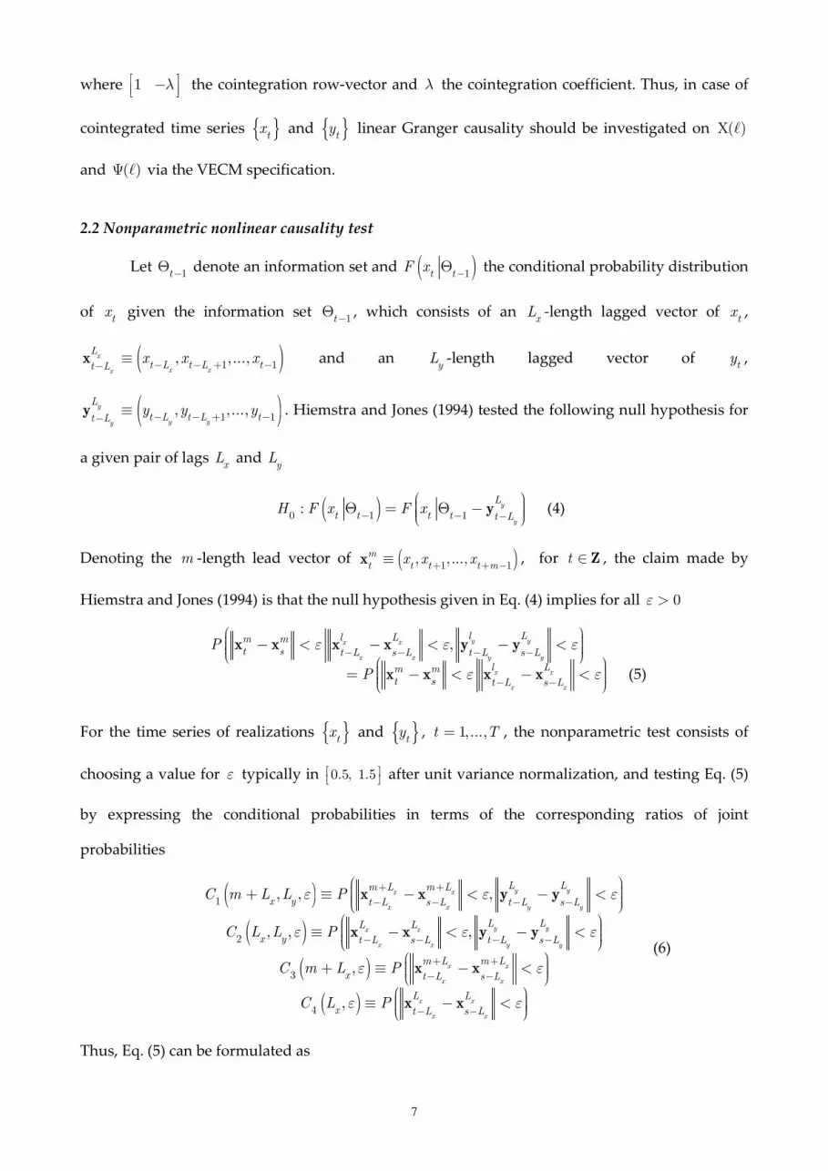
where 1 λ − the cointegration row-vector and λ the cointegration coefficient. Thus, in case of

cointegrated time series tx and ty linear Granger causality should be investigated on ( )Χ ℓ

and ( )Ψ ℓ via the VECM specification.

2.2 Nonparametric nonlinear causality test

Let 1t−

Θ denote an information set and ( )1t tF x

−Θ the conditional probability distribution

of tx given the information set

1t−Θ , which consists of an

xL -length lagged vector of

tx ,

( )1 1, ,...,x

x xx

L

t L t L tt Lx x x

− − + −−≡x and an

yL -length lagged vector of

ty ,

( )1 1, ,...,y

y yy

L

t L t L tt Ly y y

− − + −−≡y . Hiemstra and Jones (1994) tested the following null hypothesis for

a given pair of lags xL and

yL

( )0 1 1: y

y

L

t t t t t LH F x F x

− − −

Θ = Θ − y (4)

Denoting the m -length lead vector of ( )1 1, , ...,m

t t t t mx x x

+ + −≡x , for t ∈ Z , the claim made by

Hiemstra and Jones (1994) is that the null hypothesis given in Eq. (4) implies for all 0ε >

,

y yx x

x x y y

x x

x x

l Ll Lm m

t s t L s L t L s L

l Lm m

t s t L s L

P

P

ε ε ε

ε ε

− − − −

− −

− < − < − < = − < − <

x x x x y y

x x x x (5)

For the time series of realizations tx and ty , 1,...,t T= , the nonparametric test consists of

choosing a value for ε typically in 0.5, 1.5 after unit variance normalization, and testing Eq. (5)

by expressing the conditional probabilities in terms of the corresponding ratios of joint

probabilities

( )

( )

( )

( )

1

2

3

4

, , ,

, , ,

,

,

y yx x

x x y y

y yx x

x x y y

x x

x x

x x

x x

L Lm L m L

x y t L s L t L s L

L LL L

x y t L s L t L s L

m L m L

x t L s L

L L

x t L s L

C m L L P

C L L P

C m L P

C L P

ε ε ε

ε ε ε

ε ε

ε ε

+ +

− − − −

− − − −

+ +

− −

− −

+ ≡ − < − < ≡ − < − <

+ ≡ − < ≡ − <

x x y y

x x y y

x x

x x

(6)

Thus, Eq. (5) can be formulated as

8

( )

( )( )

( )1 3

42

, , ,

,, ,

x y x

xx y

C m L L C m L

C LC L L

ε ε

εε

+ += (7)

Using correlation-integral estimators and under the assumptions that tx and ty are strictly

stationary, weakly dependent and satisfy the mixing conditions of Denker and Keller (1983),

Hiemstra and Jones (1994) showed that

( )

( )( )

( )( )( )1 3 2

42

, , , , ,0, , , ,

, ,, , ,

x y x

x y

xx y

C m L L n C m L nn N m L L

C L nC L L n

ε εσ ε

εε

+ + −

∼ (8)

with ( )2 , , ,x y

m L Lσ ε as given in an appendix. One-sided critical values are used based on this

asymptotic result, rejecting when the observed value of the test statistic in Eq. (8) is too large.

3. VAR/VECM-GARCH FILTERING

This study presents a multi-step methodology for examining dynamic relationships

between exchange rates and fundamentals as well as among exchange rates. Initially, the

nonlinear and linear dynamic linkages are explored through the application of the nonparametric

nonlinear test, and the Granger causality test after controlling for cointegration. Then, after

filtering the series using the properly specified VAR or VECM model, the residuals are examined

by the modified Baek-Brock test. In addition to applying the usual bivariate VAR or VECM model

to each pair of time series, residuals of a full-variate model are also considered to account for the

possible effects of the other variables. In this way any remaining causality is strictly nonlinear in

nature, as the VAR or VECM model has already purged the residuals of linear dependence.

Finally, in the last step, the null hypothesis of nonlinear non-causality is investigated after

controlling for conditional heteroskedasticity in the data using a multivariate GARCH-BEKK

model again both in a bivariate and in a full model representation. Thus, the short-run movements

are accounted for and the volatility persistence mechanism is captured.

The use of the nonlinear test on filtered data with a multivariate GARCH model enables to

determine whether the utilized model is sufficient to describe the relationship among the series.

Consequently, the statistical evidence of nonlinear Granger causality would be strongly reduced

when the appropriate multivariate GARCH model is fitted to the raw or linearly filtered data.

However, failure to accept the no-causality hypothesis may also constitute evidence that the

9

selected multivariate GARCH model is mispecified1. In general, many GARCH models can be

used for second-moment filtering. The present study employs the GARCH-BEKK model.

Considering ty to be a vector stochastic return process of dimension 1Ν× and ω a finite vector

of parameters, let ( )t t ty µ ω ε= + where ( )t

µ θ is the conditional mean vector and ( )1 2

t t tH zε ω=

where ( )1 2

tH ω is a N N× positive definite matrix. The random vector

tz has ( ) 0

tE z = and

( )t NVar z I= as the first two moments where

NI is the identity matrix. Hence,

tH is the

conditional variance matrix of ty . It is difficult to guarantee the positivity of

tH in the VEC-

GARCH representation of Bollerslev et al. (1988) without imposing strong restrictions on the

parameters. Engle and Kroner (1995) proposed a new parametrization of tH that imposes its

positivity, namely the Baba-Engle-Kraft-Kroner (BEKK) model. The full BEKK(1, 1, K) model is

defined as:

1 1 1

1 1

K K

t k t t k k t kk k

H A A B B C H Cε ε∗ ∗ ∗ ∗ ∗ ∗− − −

= =

′ ′ ′′= + +∑ ∑ (9)

where ,k

A B∗ ∗ and kC ∗ are N N× matrices but A∗ is upper triangular. The summation limit K

determines the generality of the process and the sufficient conditions to identify BEKK models are

that ,11 ,11,

k kB C∗ ∗ and the diagonal elements of A∗ are restricted to be positive. To reduce the

number of parameters in the BEKK(1,1,1) model and consequently to reduce the generality, a

diagonal BEKK model can be imposed, i.e. kB∗ and

kC ∗ in (8) are diagonal matrices. The maximum

likelihood method is used to estimate the BEKK model.

4. MONTE CARLO SIMULATIONS

Let ts be the asset price expressed as a discounted sum of current and expected future

fundamentals. The examined asset-pricing model is of the form

( ) ( ) ( )1 20 0

1 , 0 1j j

t t t j t t jj j

s b b E a x b b E a x b∞ ∞

+ += =

′ ′= − + < <∑ ∑ (10)

1 This line of analysis is similar to the use of the univariate BDS test on raw data and on GARCH models (Brock et al., 1996; Brooks,

1996; Hsieh, 1989)

10

where tx is the 1n× vector of fundamentals, b is a discount factor, and

1a and

2a are 1n×

vectors. Campbell and Shiller (1987) and West (1988) consider this model for stock prices where ts

is the level of the stock price, tx the dividend (a scalar),

10a = and

21a = . The log-linearized

model of Campbell and Shiller (1988) also has this form, where ts is the log of the stock price,

tx is

the log of the dividend and 11a = ,

20a = . In this study

ts is the log of the exchange rate and

tx

contains such variables as interest rates and logs of prices, money supplies etc. Assume that at

least one element of the vector tx is an ( )1Ι process, with the Wold innovation being a 1n×

vector tε . Engel and West (2005) require that either (1) ( )1

1t

a x′ Ι∼ and 20a = or (2) ( )2

1t

a x′ Ι∼ ,

with the order of integration of 1 ta x′ essentially unrestricted ( ( )0Ι , ( )1Ι , or identically zero). In

either case, for b near one, ts∆ is well approximated by a linear combination of the elements of

the unpredictable innovation tε . Moreover, as suggested by Engel and West (2005) there is

continuity in the autocorrelations in the sense that for b near one the autocorrelations of ts∆ will

be near zero if the condition that certain variables are ( )1Ι , is replaced with the condition that

those variables are ( )0Ι but with an autoregressive root very near one.

In this study the correlation structure of exchange rates and fundamentals is estimated

from simulations based on the simple stylized model of Engel and West (2005). A simple

univariate process for fundamentals is assumed, with parameters chosen to reflect data from

recent floating periods and discount factors from 0.5 to 0.95, the latter of which suffice to yield

near-zero correlations between the periods t-1 and t. Overall, an attempt is made to simulatively

verify the theoretical conclusion of Engel and West (2005) that large discount factors account for

random walk behaviour in exchange rates. The results of simulations are depicted in Tables 1-3.

The model used is a simplified version of Eq. (10), i.e., ( )0

1 j

t t t jjs b b E x

∞

+== − ∑ or

0

j

t t t jjs b b E x

∞

+== ∑ . The fundamentals variable

tx follows an AR(2) process with autoregressive

roots 1ϕ and ϕ . When

11.0ϕ = ,

tx∆ ∼AR(1) with parameter ϕ and in the limit, as 1b → , each

of the correlations approaches zero. The setup of the simulations is the following: tx =1500

11

observations are simulated with j =5000 forward steps to the future. Thus, in total a path of 6500

observations is produced. Next, the first burn-out 500 points are discarded. The final examined

processes for tx (fundamental),

ts (FX series) and

tz (another FX series) include 1000

observations. Then correlations are computed, the paths are replicated 2000 times and the mean,

median and mode of the correlations are produced. Columns 4-9 present correlations of ts∆ with

time t-1 information when tx follows a scalar univariate AR(2). Either

10a = and

21a = or

11a = and

20a = can be assumed. These two possibilities can be considered interchangeably as

for given 1b < , the autocorrelations of ts∆ are not affected by whether or not a factor of 1 b−

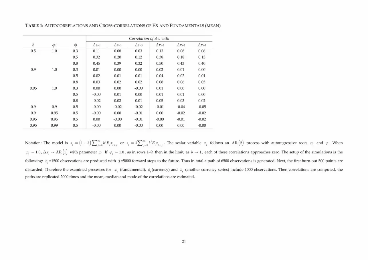
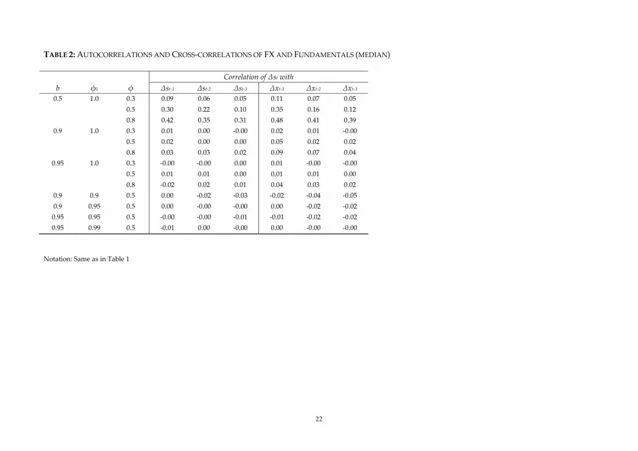
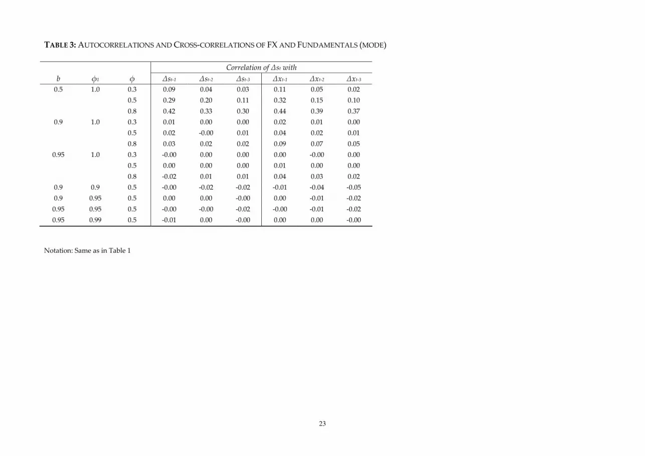
multiplies the present value of fundamentals. Rows 1–9 in Tables 1-3 assume that ( )1tx Ι∼ ,

specifically tx∆ ∼AR(1) with parameterϕ . For 0.5b = the autocorrelations in columns 4–6 and

the cross correlations in columns 7–9 are significant, whereas for 0.9b = , they are dramatically

smaller. Finally, from rows 10–13 it can be inferred that if the unit root in tx is replaced by an

autoregressive root of 0.9 or higher, the autocorrelations and cross-correlations of ts∆ are not

much changed. Overall, Tables 1-3 provide very similar results to the ones produced analytically

by Engel and West (2005).

Next, results from an extensive cross-correlation and causality exercise are presented with

the use of stepwise multivariate filtering, on the simulated series that correspond to rows 1-3 and

7-9 of Tables 1-3 (i.e., with 0.5b = and 0.95b = ). The causality analysis is conducted at the 5%

and 1% significance level and it involves the utilization of three paradigms, namely between the

simulated currency and fundamentals series, between two different currency series as well as two

different FX series with the same fundamentals driver. The case of cointegration is also

investigated via the Johansen trace statistic in order to use the right specification for the Granger

causality testing, i.e., VAR or VECM. Also, the second-moment filtering is conducted via a

GARCH-BEKK model. The results are presented in Tables 4-6. The mode, mean and median of the

correlations are presented. In all cases the GARCH filtering on the VAR/VECM residuals purges

all linkages between the examined series. The numbers presented for causality results are the

percentages of the Granger-caused series detected. It appears that cointegration results vary

12

among the investigated paradigms. The case of two different FX series presents the lowest

percentages, whereas the Granger-causality investigation reveals a unidirectional causality link

from fundamentals to FX series. This corroborates with the theoretical and empirical result of

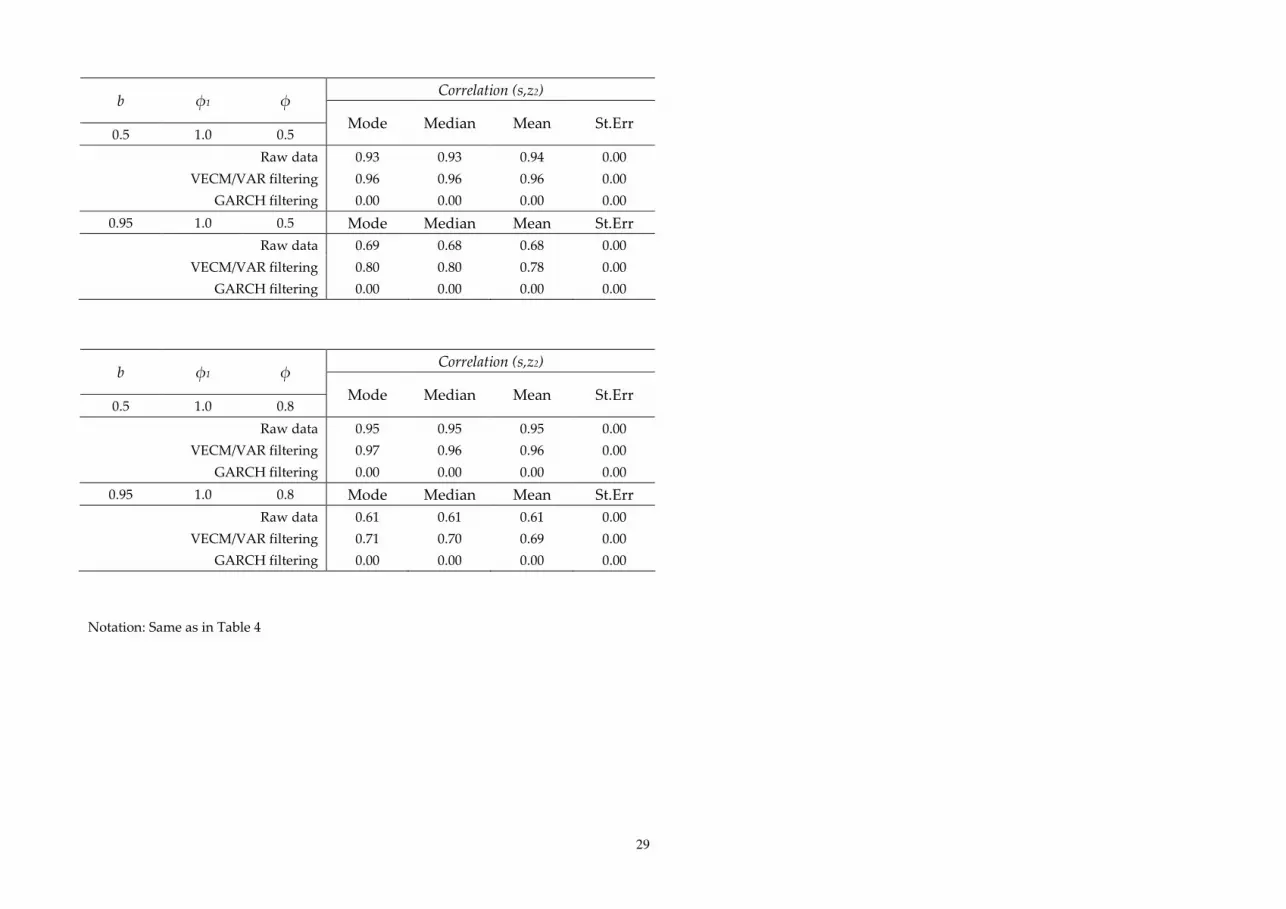
Engel and West (2005). In the other two cases the causality results are qualitatively similar for both

directions, while the percentage detected is higher in case of the two different FX series with the

same fundamentals driver. These results on the simulated series will be juxtaposed with the

empirical results in section 6.

Finally, a forecasting exercise is conducted with various asset-pricing autoregressive

models using the data generating processes produced by the simulations (Table 7). The three-step

filtering methodology for examining dynamic relationships is implemented in each step of the

causality estimation via a rolling window for the out-of-sample forecasting exercise. Specifically,

four AR(1) specifications are used with the lagged variable being the FX series ( β ε−

= +1t t t

s s ), the

fundamentals series ( γ ε−

= +1t t t

s x ) and the FX series with the same and different fundamental

driver ( ζ ε−

= +1t t t

s z and δ ε−

= +1t t t

s z ). In addition, two AR(1) specifications employing both a

lagged fundamental and an FX series with the same and different fundamental driver

( γ γ ε− −

= + +1 11 2t t t t

s x z and β β ε− −

= + +1 11 2t t t t

s x z ) are used. The out-of-sample measure is the

RMSE and in particular the RMSE ratios are reported against the first AR(1) specification which is

used as a benchmark. The simulated series again correspond to rows 1-3 and 7-9 of Tables 1-3, that

is with 0.5b = and 0.95b = . Also, the mode, mean and median is reported. The best out-of-

sample performance is indicated for the AR(1) specification employing a lagged fundamental and

an FX series with the same fundamental driver. The worst was observed for the AR(1)

specification with the lagged variable being the fundamental series, while the other models yield

similar results with their predictability being close to the one of the benchmark.

5. DATA

The data comprises monthly foreign exchange rates denoted relative to United States

dollar (USD), namely Euro (EUR), Great Britain Pound (GBP), Japanese Yen (JPY), Swiss Frank

(CHF), Australian Dollar (AUD), Canadian Dollar (CAD) and German mark (DM). The exact

ratios represent EUR/USD, GBP/USD, USD/JPY, USD/CHF, AUD/USD, USD/CAD and DM/USD

13

respectively. These are the most liquid and widely traded currency pairs in the world and make

up about 90% of total Forex trading worldwide. The data covers the Great Moderation period, the

dot-com bubble, and the period just before the outbreak of the 2007-2010 financial crisis, which

was triggered by a liquidity shortfall in the US banking system. The country-specific fundamentals

are the seasonally adjusted money supply m , the industrial production y (used as a proxy for the

real, seasonally adjusted gross domestic product), the consumer price index (CPI) p , the three-

month rate i , while the m y− (=Money-IP) variable is also considered. Datastream is the source of

the data. All data but interest rates is converted by taking logs and multiplying by 100. The Chow-

Lin method (1971) was used to interpolate the AUDCPI, AUDIP, CHFIP and backdate the JPYi.

Additionally, an asterisk used as superscript denotes the corresponding measure of fundamentals

in the United States relative to the country-specific, i.e., the symbol (*) denotes the non-US value in

the differentials. The differentials are ( )m m∗− , ( )p p∗− , ( )i i∗− , ( )y y∗− , ( )m y m y∗ ∗ − − −

.

Correlations and causalities are investigated on the ∆ (differentials). Overall, the examined period

is in levels 4/1986–7/2008, while for the Euro it spans 1/1999–7/2008.

6. EMPIRICAL RESULTS

In this section, the implications of the asset-pricing models of Engel and West (2005) are

empirically investigated, as well as the hypothesis that asset price might help to predict the

fundamentals or vice-versa is tested. The causal relationships between the FX rates and the five

measures of fundamentals are investigated. As in Engel and West (2005), many autoregressive

specifications are utilized, e.g., pairwise, tri-variate, four-variate as well as the full systems of

variables (5x5). Additionally, the empirical results are juxtaposed with the Monte Carlo

simulations. The statistical significance is presented at the 5% (*) and 1% (**) levels. The lag

lengths of VECM/VAR specification are investigated and set using the SIC and Wald exclusion

criterion and the cointegrating vectors using the Johansen trace statistic (Johansen, 1991). In their

work Engel and West (2005) concluded that it will probably not do great violence to assume lack

of cointegration and so they used for all VAR models four lags2. Instead, in this paper

2 They consider lack of cointegration to be evidence that unobserved variables such as real demand shocks, real money demand shocks,

or possibly even interest parity deviations have a permanent component, or at least are very persistent. Yet, it may be that the data they

used to measure the economic fundamentals have some errors with permanent or very persistent components. For example, it may be

14

cointegration tests were conducted between the exchange rate and each of the fundamentals

differentials in all specifications. The number of lags identified and the cointegrating vectors are

presented in parenthesis as (lags, coint. vectors). For testing reasons linear Granger causality was

further investigated on the VAR/VECM and GARCH residuals, but it was no longer detected. The

nonlinear causality is investigated with the modified Baek-Brock test and the number of lags used

are 1==YXℓℓ . The second moment filtering is performed with a GARCH-BEKK (1,1) model.

The results for all examined multivariate specifications are depicted in Tables 8-21. For the

pairwise investigation, the variables included in the VAR/VECM model are

( ) ( ) ( ) ( ) ( ) ( ) ( ) , , , , , , s m m p p i i i i y y m m y y∗ ∗ ∗ ∗ ∗ ∗ ∗ ∆ ∆ − ∆ − − ∆ − ∆ − ∆ − −∆ −

. In this

case VAR(1,0) is identified except VAR(2,0) in GBP ( )s m m∗

∆ − ∆ − , GBP ( )s m m∗

∆ − ∆ − and

DM ( )s i i∗

∆ − − . VECM (2,1) is identified in all cointegrated pairs except AUD ( )s i i∗

∆ − ∆ − , which

is VECM(1,1). Based on the results there is no consistent evidence that exchange rates predict

fundamentals after examining linear and nonlinear causal interdependencies. Some bidirectional

links also appear but for different fundamentals each time. Overall, the evidence is modest that

there exists a prevailing direction in the examined causalities, i.e., that either exchange rates help

to predict fundamentals, or the ability of fundamentals to predict exchange rates is stronger. This

result is not in full accordance with Engel and West (2005) who observe a stronger unidirectional

linkage in favour of exchange rate predictability. Of course there were some major economic and

non-economic developments during the sample that might perturb any consistent relationships.

Several of the European countries’ exchange rates and monetary policies became more tightly

linked in the 1990s because of the evolution of the European Monetary Union, Germany’s

economy was transformed dramatically in 1990 because of reunification, the dot-com bubble hit

the global economies in the mid-90s, while the Asian crisis of 1997 caused a turmoil in the

international FX markets. Interestingly, two consistent results emerge from the investigation,

namely that (1) linear and nonlinear links differ significantly in all examined specifications and

that (2) after multivariate GARCH filtering most of the nonlinear interdependencies are purged.

This indicates that the nonlinear causality is largely due to simple volatility effects. Some

that the appropriate measure of the money supply has permanently changed because of numerous financial innovations over the

sample, so that the money supply series varies from the “true” money supply by some I(1) errors.

15

remaining nonlinear causalities imply that FX rates may exhibit statistically significant higher-

order moments or that other multivariate GARCH models could capture the transmission

mechanism of the volatility shocks more efficiently.

In addition to causality testing for the bivariate VAR/VECMs, cointegration and causality

tests based on other VAR/VECM specifications are performed. Several different combinations of

variables are included in the VAR/VECM models. Six groupings were tested:

1. ( ) ( ) ( ) ( ) , , , , s m m p p i i y y∗ ∗ ∗ ∗∆ ∆ − ∆ − ∆ − ∆ −

2. ( ) ( ) ( ) , , , s p p i i y y∗ ∗ ∗∆ ∆ − ∆ − ∆ −

3. ( ) ( ) ( ) , , , s m m p p y y∗ ∗ ∗∆ ∆ − ∆ − ∆ −

4. ( ) ( ) ( ) , , , s p p i i y y∗ ∗ ∗∆ ∆ − ∆ − ∆ −

5. ( ) ( ) , , s p p y y∗ ∗∆ ∆ − ∆ − and

6. ( ) ( ) , , s m m y y∗ ∗∆ ∆ − ∆ −

For the first grouping the number of lags identified and the cointegrating vectors presented as

(lags, coint. vectors) are GBP(5,1), JPY(4,1), CHF(8,1), AUD(3,1), CAD(4,1), DM(2,2), EUR(1,0). In

case of the second the number of lags and the cointegrating vectors are GBP(1,0), JPY(1,0),

CHF(5,1), AUD(1,0), CAD(1,0), DM(2,2), EUR(2,1) while for the third they are GBP(5,2), JPY(4,1),

CHF(2,1), AUD(2,0), CAD(4,1), DM(2,1), EUR(1,0). For the fourth these are GBP(1,0), JPY(1,0),

CHF(1,0), AUD(1,0), CAD(1,0), DM(1,0), EUR(2,0), while for the last two specifications they are

GBP(2,1), JPY(1,0), CHF(1,0), AUD(1,0), CAD(1,0), DM(2,1), EUR(1,0) and GBP(1,0), JPY(2,1),

CHF(2,1), AUD(1,0), CAD(1,0), DM(1,0), EUR(2,1) respectively. Linear and nonlinear causality

tests were conducted for the null that Δs does not Granger-cause each of the fundamentals or the

fundamentals as a group, and conversely. The results are similar to those from the bivariate

VAR/VECMs. There is no consistent evidence that causality runs from the fundamentals to the

exchange rates. In total, the evidence is not conclusive that there exists a prevailing direction in the

examined causalities. Again, linear and nonlinear links differ significantly whilst multivariate

GARCH filtering purged most of the nonlinear interdependencies. The evidence is far from

16

overwhelming, but overall there does not appear to be a link from FX rates to fundamentals going

in the direction that FX rates help forecast fundamentals, as advocated by Engel and West (2005).

7. CONCLUSIONS

Engel and West (2005) argued that when standard exchange rate models are plausibly

calibrated, they have the property that the FX rates should nearly follow a random walk. Evidence

that the exchange rate change is not predictable is an implication of the models, albeit observing

that FX rates follow random walks is not a very complete validation of the models. Another

possible explanation of the random walk behaviour of exchange rates could be that they are

dominated by unobservable shocks which are well approximated by random walks. The

fundamentals may not be important determinants of FX rates, and instead there may be some

other variable that models have not captured or that is unobserved that drives the currency rates.

Campbell and Shiller (1987) observe that when a currency variable is the present value of a

fundamentals variable, then either (1) FX rate Granger-causes fundamentals relative to the

bivariate information set consisting of their lags or (2) FX rate is an exact distributed lag of current

and past values of the fundamental variable. Nonetheless, exchange rate models must allow for

unobservable fundamentals. Failure to find Granger causality from the FX rate to the observable

variables no longer implies an obviously restriction that the FX rate is an exact distributed lag of

observables. It is clear, that a finding of Granger causality is supportive of a view that FX rates are

determined as a present value that depends in part on observable fundamentals.

The results of this paper provide some counterbalance to the suitability - especially in the

short run - of rational expectations present-value models of currency rates that became

predominant since Meese and Rogoff (1983a, 1983b). Extensive Monte Carlo simulations in this

work provide evidence that FX rates may incorporate information about future fundamentals. It

was shown that under some assumptions the inability to forecast exchange rates is a natural

implication of the models, which suggests that innovations in the FX rates ought to be highly

correlated with news about future fundamentals. This relationship was also reported in the study

of Andersen et al. (2003), who found strong evidence of exchange rate reaction to news in intraday

data and in a direction consistent with standard models. The analytical results of Engel and West

17

(2005) have been corroborated, in that if discount factors are large (and fundamentals are ( )I 1 ),

then it may not be surprising that present-value models cannot out-perform in terms of

forecastability the random walk model of exchange rates.

Yet, a conclusive support for the link between fundamentals and the exchange rate in the

direction that exchange rates can help forecast the fundamentals was not found, as in Engel and

West (2005). Whilst in some cases and under certain vector autoregressive modelling there was

evidence of this directional predictability, a generic result cannot be drawn. It might be that

exchange rates and fundamentals are linked in a way that is broadly consistent with asset pricing

models of the exchange rate, but no evidence was found of a prevailing direction in the examined

causalities, i.e., that either exchange rates help to predict fundamentals, or the ability of

fundamentals to predict exchange rates is stronger. Specifically, the empirical findings in this

study do not fully accord with the results of Engel and West (2005) on the weak causality from

exchange rates to fundamentals. Indeed there are several caveats. First, while the results from

simulations are consistent with the implications of the present-value models - that exchange rates

should be useful in forecasting future economic variables - there might be other possible

explanations for the discrepancy in the empirical findings. It may be, for example, that currencies

might Granger-cause money supplies because monetary policy makers react to the exchange rate

in setting the money supply. Thus, the present-value models are not the only models that imply

Granger causality from exchange rates to other economic variables. In general the results from

simulations provided evidence on the correlation of exchange rate changes with the change in the

expected discounted fundamentals, as well as that the Granger causality results are generated by

the present-value models.

Moreover, the empirical results are not uniformly strong and overall the evidence is

inconclusive that there exists a prevailing direction in the examined causalities. Additionally,

linear and nonlinear links differ significantly and multivariate GARCH filtering purged most of

the nonlinear interdependencies. This indicates that the nonlinear causality is largely due to

simple volatility effects. Some remaining nonlinear causalities imply that FX rates may exhibit

statistically significant higher-order moments or other multivariate GARCH models could capture

the transmission mechanism of the volatility shocks more efficiently. As opposed to Engel and

18

West (2005) cointegration was detected between exchange rates and fundamentals. In accordance

with the exchange rate literature, there was not much evidence that the exchange rate is explained

only by the “observable” fundamentals. However, observables do not obviously dominate

exchange rate changes and it is perhaps unrealistic to believe that only observable fundamentals

affect currency rates.

Finally, the results of this study may also help explain the near-random walk behaviour

and the causality structure of other asset prices and their markets (equities, bonds etc.)

Theoretically, asset prices follow random walks only under very special circumstances. An

empirical investigation of the causal behaviour of a variety of asset prices could be an interesting

line of future research.

19

REFERENCES

Andersen, T., G., Bollerslev, T., Diebold, F. and Vega, C., 2003. Micro Effects of Macro

Announcements: Real-Time Price Discovery in Foreign Exchange. American Economic Review 93, 38–62.

Baek, E. and Brock, W., 1992. A general test for non-linear Granger causality: bivariate model.

Working paper, Iowa State University and University of Wisconsin, Madison, WI.

Bollerslev, T., Engle, R.F. and Wooldridge, J.M., 1988. A capital asset pricing model with time

varying covariances. Journal of Political Economy 96, 116–131.

Brock, W.A., Dechert, W.D., Scheinkman, J.A. and LeBaron, B., 1996. A test for independence based

on the correlation dimension. Econometric Reviews 15(3), 197-235.

Brooks, C., 1996. Testing for nonlinearities in daily pound exchange rates. Applied Financial

Economics 6, 307-317.

Campbell, J.Y. and Shiller, R.J., 1987. Cointegration and Tests of Present Value Models. Journal of

Political Economy 95, 1062–1088.

Campbell, J.Y., and Shiller, R..J., 1988. Stock Prices, Earnings, and Expected Dividends. Journal of

Finance 43, 661–676.

Cheung, Y.-W., Chinn, M.D. and Pascual, A.G., 2002. Empirical Exchange Rate Models of the

Nineties: Are Any Fit to Survive?. Working Paper no. 9393, NBER, Cambridge, MA.

Chinn, M.D., and Meese, R.A., 1995. Banking on Currency Forecasts: How Predictable Is Change in

Money?. Journal of International Economics 38, 161– 178.

Chow, G. and Lin, A.L., 1971. Best linear unbiased distribution and extrapolation of economic time

series by related series. Review of Economic and Statistics 53(4), 372-375.

Denker, M., and Keller, G., 1983. On U-statistics and von-Mises statistics for weakly dependent

processes. Zeitschrift fur Wahrscheinlichkeitstheorie und Verwandte Gebiete 64, 505-522.

Engel, C., and West, K.D., 2005. Exchange Rates and Fundamentals. Journal of Political Economy 113,

485-517.

Engle, R.F. and Granger, C.W.J., 1987. Co-integration and error correction: representation,

estimation, and testing. Econometrica 55(2), 251–276.

Engle, R.F. and Kroner, F.K., 1995. Multivariate simultaneous generalized ARCH. Econometric

Theory, 11, 122-150.

Granger, C.W.J., 1969, Investigating causal relations by econometric models and cross-spectral

methods. Econometrica 37(3), 424-438.

Groen, J.J., 2000. The Monetary Exchange Rate Model as a Long-Run Phenomenon. Journal of

International Economics 52, 299–319.

Hiemstra, C. and Jones, J.D., 1994. Testing for linear and nonlinear Granger causality in the stock

price-volume relation. Journal of Finance 49(5), 1639-1664.

Johansen, S., 1988. Statistical analysis of cointegration vectors. Journal of Economic Dynamics and

Control 12(2-3), 231–254.

Johansen, S. and Juselius, K., 1990. Maximum likelihood estimation and inference on cointegration

with application to the demand for money. Oxford Bulletin of Economics and Statistics 52, 169–209.

Johansen, S., 1991. Estimation and Hypothesis Testing of Cointegration Vectors in Gaussian Vector

Autoregressive Models. Econometrica 59, 1551–1580.

Hsieh, D., 1989. Modeling heteroscedasticity in daily foreign exchange rates. Journal of Business and

Economic Statistics 7, 307–317.

Kilian, L. and Taylor, M.P., 2003. Why Is It So Difficult to Beat the Random Walk Forecast of

Exchange Rates?. Journal of International Economics 60, 85–107.

MacDonald, R. and Taylor, M.P., 1994. The Monetary Model of the Exchange Rate: Long-Run

Relationships, Short-Run Dynamics and How to Beat a Random Walk. Journal of International Money and

Finance 13 276–290.

Mark, N.C. 1995. Exchange Rates and Fundamentals: Evidence on Long- Horizon Predictability.

American Economic Review 85, 201–218.

Mark, N.C., and Sul, D., 2001. Nominal Exchange Rates and Monetary Fundamentals: Evidence

from a Small Post–Bretton Woods Sample. Journal of International Economics 53, 29–52.

20

Meese, R.A. and Rogoff, K.S., 1983a. Empirical Exchange Rate Models of the Seventies: Do They Fit

Out of Sample?. Journal of International Economics 14, 3–24.

Meese, R.A. and Rogoff, K.S., 1983b. The Out of Sample Failure of Empirical Exchange Models. In:

Exchange Rates and International Macroeconomics, (Eds) J. A. Frenkel. Chicago: Univ. Chicago Press.

Taylor, M.P., Peel, D.A. and Sarno, L., 2001. Nonlinear Mean-Reversion in Real Exchange Rates:

Toward a Solution to the Purchasing Power Parity Puzzles. International Economic Review 42, 1015–1042.

West, K.D., 1988. Dividend Innovations and Stock Price Volatility. Econometrica 56, 37–61.

21

TABLE 1: AUTOCORRELATIONS AND CROSS-CORRELATIONS OF FX AND FUNDAMENTALS (MEAN)

Notation: The model is ( )0

1j

t t t jjs b b E x

∞

+== − ∑ or

0

j

t t t jjs b b E x

∞

+== ∑ . The scalar variable

tx follows an ( )AR 2 process with autoregressive roots

1ϕ and ϕ . When

11.0ϕ = , ( )AR 1

tx∆ ∼ with parameter ϕ . If

11.0ϕ = , as in rows 1–9, then in the limit, as 1b → , each of these correlations approaches zero. The setup of the simulations is the

following: tx =1500 observations are produced with j =5000 forward steps to the future. Thus in total a path of 6500 observations is generated. Next, the first burn-out 500 points are

discarded. Therefore the examined processes for tx (fundamental),

ts (currency) and

tz (another currency series) include 1000 observations. Then correlations are computed, the

paths are replicated 2000 times and the mean, median and mode of the correlations are estimated.

Correlation of Δst with

b φ1 φ Δst-1 Δst-2 Δst-3 Δxt-1 Δxt-2 Δxt-3

0.5 1.0 0.3 0.11 0.08 0.03 0.13 0.08 0.06

0.5 0.32 0.20 0.12 0.38 0.18 0.13

0.8 0.45 0.39 0.32 0.50 0.43 0.40

0.9 1.0 0.3 0.01 0.00 0.00 0.02 0.01 0.00

0.5 0.02 0.01 0.01 0.04 0.02 0.01

0.8 0.03 0.02 0.02 0.08 0.06 0.05

0.95 1.0 0.3 0.00 0.00 -0.00 0.01 0.00 0.00

0.5 -0.00 0.01 0.00 0.01 0.01 0.00

0.8 -0.02 0.02 0.01 0.05 0.03 0.02

0.9 0.9 0.5 -0.00 -0.02 -0.02 -0.01 -0.04 -0.05

0.9 0.95 0.5 -0.00 0.00 -0.01 0.00 -0.02 -0.02

0.95 0.95 0.5 0.00 -0.00 -0.01 -0.00 -0.01 -0.02

0.95 0.99 0.5 -0.00 0.00 -0.00 0.00 0.00 -0.00

22

TABLE 2: AUTOCORRELATIONS AND CROSS-CORRELATIONS OF FX AND FUNDAMENTALS (MEDIAN)

Notation: Same as in Table 1



0.5 1.0 0.3 0.09 0.06 0.05 0.11 0.07 0.05

0.5 0.30 0.22 0.10 0.35 0.16 0.12

0.8 0.42 0.35 0.31 0.48 0.41 0.39

0.9 1.0 0.3 0.01 0.00 -0.00 0.02 0.01 -0.00

0.5 0.02 0.00 0.00 0.05 0.02 0.02

0.8 0.03 0.03 0.02 0.09 0.07 0.04

0.95 1.0 0.3 -0.00 -0.00 0.00 0.01 -0.00 -0.00

0.5 0.01 0.01 0.00 0.01 0.01 0.00

0.8 -0.02 0.02 0.01 0.04 0.03 0.02

0.9 0.9 0.5 0.00 -0.02 -0.03 -0.02 -0.04 -0.05

0.9 0.95 0.5 0.00 -0.00 -0.00 0.00 -0.02 -0.02

0.95 0.95 0.5 -0.00 -0.00 -0.01 -0.01 -0.02 -0.02

0.95 0.99 0.5 -0.01 0.00 -0.00 0.00 -0.00 -0.00

23

TABLE 3: AUTOCORRELATIONS AND CROSS-CORRELATIONS OF FX AND FUNDAMENTALS (MODE)




0.5 1.0 0.3 0.09 0.04 0.03 0.11 0.05 0.02

0.5 0.29 0.20 0.11 0.32 0.15 0.10

0.8 0.42 0.33 0.30 0.44 0.39 0.37

0.9 1.0 0.3 0.01 0.00 0.00 0.02 0.01 0.00

0.5 0.02 -0.00 0.01 0.04 0.02 0.01

0.8 0.03 0.02 0.02 0.09 0.07 0.05

0.95 1.0 0.3 -0.00 0.00 0.00 0.00 -0.00 0.00

0.5 0.00 0.00 0.00 0.01 0.00 0.00

0.8 -0.02 0.01 0.01 0.04 0.03 0.02

0.9 0.9 0.5 -0.00 -0.02 -0.02 -0.01 -0.04 -0.05

0.9 0.95 0.5 0.00 0.00 -0.00 0.00 -0.01 -0.02

0.95 0.95 0.5 -0.00 -0.00 -0.02 -0.00 -0.01 -0.02

0.95 0.99 0.5 -0.01 0.00 -0.00 0.00 0.00 -0.00

24

TABLE 4: CAUSALITY AND CROSS-CORRELATION OF THE SIMULATED FX AND FUNDAMENTALS SERIES

Granger-causality on the Raw series

Correlation on the Filtered series

GC: s->x GC: x->s b φ1 φ

0.95 0.99 0.95 0.99 CI (s,x)

0.5 1.0 0.3 5.9% 1.75% 62.2% 40.5% 100%

0.5 4.8% 1.1% 68% 57% 100%

0.8 5.3% 1.1% 88.7% 77.8% 100%

0.95 1.0 0.3 4.75% 1.2% 18% 12.2% 98.5%

0.5 3.8% 1% 29% 23% 97.1%

0.8 4.8% 0.95% 38.8% 28.7% 97.2%

Correlation (s,x) b φ1 φ

0.5 1.0 0.3 Mode Median Mean St.Err

Raw data 0.93 0.93 0.93 0.00

VECM/VAR filtering 0.96 0.96 0.96 0.00

GARCH filtering 0.00 0.00 0.00 0.00


Raw data 0.84 0.84 0.84 0.00



25

Notation: The model is ( )0

1j

t t t jjs b b E x

∞

+== − ∑ or

0

j

t t t jjs b b E x

∞

+== ∑ . The scalar variable

tx follows an ( )AR 2 process with autoregressive roots

1ϕ and ϕ . When

11.0ϕ = , ( )AR 1

tx∆ ∼ with parameter ϕ . If

11.0ϕ = , as in rows 1–9, then in the limit, as 1b → , each of these correlations approaches zero. The setup of the simulations is the

following: tx =1500 observations are produced with j =5000 forward steps to the future. Thus in total a path of 6500 observations is generated. Next, the first burn-out 500 points are

discarded. Therefore the examined processes for tx (fundamental),

ts (currency) and

tz (another currency series) include 1000 observations. Then correlations are computed, the

paths are replicated 2000 times and the mean, median and mode of the correlations are estimated. Granger causality (GC) is investigated via a VAR or VECM representation

depending on the whether the Johansen trace statistic rejects the null of no cointegration (CI) or not for each pair of the examined simulated paths. The numbers presented for GC are

the percentages of the Granger-caused series detected. Next, the GARCH-BEKK is applied for second-moment filtering.



Raw data 0.90 0.89 0.88 0.00




Raw data 0.72 0.72 0.72 0.00





Raw data 0.83 0.83 0.83 0.00




Raw data 0.45 0.46 0.46 0.00



26

TABLE 5: CAUSALITY AND CROSS-CORRELATION OF TWO DIFFERENT SIMULATED FX SERIES



GC: s->z GC: z->s b φ1 φ

0.95 0.99 0.95 0.99 CI (s,z)

0.5 1.0 0.3 8.5% 2.2% 9.95% 2.4% 20%

0.5 8.3% 1.4% 9.7% 2.1% 14.3%

0.8 9.7% 2.5% 9.8% 2.4% 22.3%

0.95 1.0 0.3 7.95% 1.65% 7.6% 1.35% 18.2%

0.5 9.5% 2.2% 7.75% 2.1% 13.5%

0.8 9.4% 2.35% 9.85% 2.45% 25.15%

Correlation (s,z) b φ1 φ


Raw data 0.00 -0.00 -0.00 0.00

VECM/VAR filtering 0.00 -0.00 -0.00 0.00



Raw data -0.00 -0.00 -0.00 0.00

VECM/VAR filtering -0.00 -0.00 -0.00 0.00


27




Raw data -0.00 -0.00 0.00 0.00

VECM/VAR filtering -0.00 0.00 -0.00 0.00

GARCH filtering 0.00 -0.00 0.00 0.00


Raw data 0.00 0.00 0.00 0.00





Raw data 0.00 0.00 0.00 0.00




Raw data 0.00 0.00 0.00 0.00



28

TABLE 6: CAUSALITY AND CROSS-CORRELATION OF TWO DIFFERENT SIMULATED FX SERIES WITH THE SAME FUNDAMENTALS DRIVER



GC: s->z2 GC: z2->s b φ1 φ

0.95 0.99 0.95 0.99 CI (s,z2)

0.5 1.0 0.3 23.25% 15.25% 25.35% 15.05% 100%

0.5 24.4% 26.5% 23% 25.1% 100%

0.8 26.4% 19.3% 26.1% 18.8% 100%

0.95 1.0 0.3 12.05% 6.3% 11.5% 7.2% 100%

0.5 8.9% 3.7% 8.25% 3.6% 100%

0.8 9.3% 7.21% 12.8% 7.3% 100%

Correlation (s,z2) b φ1 φ


Raw data 0.93 0.93 0.93 0.00




Raw data 0.78 0.78 0.78 0.00



29




Raw data 0.93 0.93 0.94 0.00




Raw data 0.69 0.68 0.68 0.00





Raw data 0.95 0.95 0.95 0.00




Raw data 0.61 0.61 0.61 0.00



30

TABLE 7: PREDICTABILITY OF DIFFERENT FX AND FUNDAMENTALS DATA GENERATING PROCESSES

b φ1 φ Mode Median Mean St.Err Mode Median Mean St.Err Mode Median Mean St.Err

R1 (RMSE1/RMSE2) R2 (RMSE1/RMSE3) R3 (RMSE1/RMSE4)

0.5 1.0 0.3 0.98 0.98 0.97 0.00 0.10 0.09 0.14 0.00 0.99 0.99 1.00 0.00

0.5 0.98 0.97 0.96 0.00 0.11 0.09 0.15 0.00 1.00 1.00 0.99 0.00

0.8 0.99 0.99 0.98 0.00 0.11 0.10 0.16 0.00 1.00 1.00 1.00 0.00

0.95 1.0 0.3 0.99 0.99 0.98 0.00 0.19 0.15 0.15 0.00 0.99 0.99 1.00 0.00

0.5 0.99 0.99 0.98 0.00 0.21 0.15 0.15 0.00 1.00 1.00 1.00 0.00

0.8 0.99 1.00 0.99 0.00 0.21 0.19 0.16 0.00 1.00 1.00 1.01 0.00

b φ1 φ Mode Median Mean St.Err Mode Median Mean St.Err

R4 (RMSE1/RMSE5) R5 (RMSE1/RMSE6)

0.5 1.0 0.3 0.96 0.97 0.97 0.00 0.99 1.00 1.00 0.00

0.5 0.97 0.97 0.97 0.00 1.00 1.00 1.00 0.00

0.8 0.98 0.97 0.97 0.00 1.06 1.06 1.07 0.00

0.95 1.0 0.3 0.98 0.99 1.00 0.00 1.01 1.01 1.01 0.00

0.5 0.98 0.98 1.00 0.00 1.02 1.02 1.02 0.00

0.8 0.98 0.98 0.99 0.00 1.02 1.02 1.03 0.00

Notation: Various data generating processes are produced by the simulations. Specifically, four ( )AR 1 specifications are used with the lagged variable being the FX series, the

fundamentals series, the FX series with the same and different fundamental driver, i.e., (1) β ε−

= +1t t t

s s , (2) γ ε−

= +1t t t

s x , (3) δ ε−

= +1t t t

s z (with different fundamentals driver),

(4) ζ ε−

= +1t t t

s z (with same fundamentals driver). Also two ( )AR 1 specifications are used employing both a lagged fundamental and an FX series with the same and different

fundamental driver, i.e., (5) β β ε− −

= + +1 11 2t t t t

s x z (with different fundamentals driver) and (6) γ γ ε− −

= + +1 11 2t t t t

s x z (with same fundamentals driver). The out-of-sample

measure is the RMSE and in particular the RMSE ratios are reported against the first ( )AR 1 model which is used as a benchmark. The simulated series again correspond to rows 1-3

and 7-9 of Tables 1-3, that is with 0.5b = and 0.95b = . Also, the mode, mean and median is reported.

31

TABLE 8: LINEAR CAUSALITY (PAIRWISE)

Variable Panel A: Linear Granger Causality

Raw data VAR / VECM residuals GARCH-BEKK residuals

X→Y Y→X X→Y Y→X X→Y Y→X X Y

GB

P

JP

Y

CH

F

AU

D

CA

D

DM

EU

R

GB

P

JP

Y

CH

F

AU

D

CA

D

DM

EU

R

GB

P

JP

Y

CH

F

AU

D

CA

D

DM

EU

R

GB

P

JP

Y

CH

F

AU

D

CA

D

DM

EU

R

GB

P

JP

Y

CH

F

AU

D

CA

D

DM

EU

R

GB

P

JP

Y

CH

F

AU

D

CA

D

DM

EU

R

∆s ∆(m-m*) * * *

∆s ∆(p-p*)

∆s i-i* * *

∆s ∆(i-i*) *

∆s ∆(y-y*) * ** *

∆s ∆(m-m*)

- ∆(y-y*) ** * **

X→Y: rX does not Granger Cause r Y. Statistical significance 5% (*), 1% (**).The foreign exchange rates are Euro (EUR), Great Britain Pound (GBP), Japanese Yen (JPY), Swiss Frank (CHF), Australian Dollar

(AUD), Canadian Dollar (CAD) and German mark (DM) are denoted relative to United States dollar (USD). The exact ratios represent EUR/USD, GBP/USD, USD/JPY, USD/CHF, AUD/USD, USD/CAD and

DM/USD respectively. The FX rates are denoted as s and fundamentals as: m=Money, p=CPI, i=Interest rate, y=IP, m-y=Money- IP. In differentials (*) denotes non-US value. Causalities are investigated on

Δ(differentials). All data but interest rates are converted by taking logs and multiplying by 100. The Chow-Lin method was used to interpolate AUDCPI, AUDIP, CHFIP and backdate JPYi. Total period (levels):

4/1986 – 7/2008. EURO period (levels): 1/1999 – 7/2008.

Panel A: Linear Granger Causality All data (levels) were investigated with a VECM specification and the null of no cointegration was not rejected for all except DM: Δs-Δ(p-p*), AUD: Δs-Δ(i-i*), JPY: Δs-Δ(i-i*), EUR: Δs-Δ(i-i*). The lag lengths

of VECM/VAR specification are investigated and set using the SIC and Wald exclusion criterion and the cointegrating vectors using the Johansen trace statistic. The number of lags identified and the

cointegrating vectors are presented in parenthesis as (lags, coint. vectors). VAR(1,0) is identified except VAR(2,0) in GBP: Δs-Δ(m-m*), GBP: Δs-Δ(m-m*), DM: Δs-(i-i*). VECM (2,1) is identified in all

cointegrated pairs except AUD: Δs-Δ(i-i*), which is VECM(1,1). For testing reasons Linear Granger causality was further investigated in the VAR/VECM or GARCH residuals, but not detected.

32

TABLE 9: NONLINEAR CAUSALITY (PAIRWISE)

Variable Panel B: NonLinear Causality



GB

P

JP

Y

CH

F

AU

D

CA

D

DM

EU

R

GB

P

JP

Y

CH

F

AU

D

CA

D

DM

EU

R

GB

P

JP

Y

CH

F

AU

D

CA

D

DM

EU

R

GB

P

JP

Y

CH

F

AU

D

CA

D

DM

EU

R

GB

P

JP

Y

CH

F

AU

D

CA

D

DM

EU

R

GB

P

JP

Y

CH

F

AU

D

CA

D

DM

EU

R

∆s ∆(m-m*) * * *

∆s ∆(p-p*)

∆s i-i* * * ** * * * *

∆s ∆(i-i*) * * * * * * * *

∆s ∆(y-y*) * * * *

∆s ∆(m-m*)

- ∆(y-y*)

Panel B: Non-Linear Causality The number of lags used for the nonlinear causality test are 1==

YXℓℓ . The data used are log-returns. The nonlinear causality was investigated on the VAR/VECM residuals based on Panel A

identification. The number of lags and cointegrating vectors are reported in Panel A. The second moment filtering was performed with a GARCH-BEKK (1,1) model. The Chow-Lin method was used to

interpolate AUDCPI, AUDIP, CHFIP and backdate JPYi. Total period (levels): 4/1986 – 7/2008. EURO period (levels): 1/1999 – 7/2008.

33

TABLE 10: LINEAR CAUSALITY (5X5)




GB

P

JP

Y

CH

F

AU

D

CA

D

DM

EU

R

GB

P

JP

Y

CH

F

AU

D

CA

D

DM

EU

R

GB

P

JP

Y

CH

F

AU

D

CA

D

DM

EU

R

GB

P

JP

Y

CH

F

AU

D

CA

D

DM

EU

R

GB

P

JP

Y

CH

F

AU

D

CA

D

DM

EU

R

GB

P

JP

Y

CH

F

AU

D

CA

D

DM

EU

R

∆s ∆(m-m*) * * *

∆s ∆(p-p*) **

∆s ∆(i-i*)

∆s ∆(y-y*) ** * * *






Panel A: Linear Granger Causality The 5x5 system of the data (levels) for each FX was investigated with a VECM specification and the null of no cointegration was rejected for all except EUR. The lag lengths of VECM/VAR specification are

investigated and set using the SIC and Wald exclusion criterion and the cointegrating vectors using the Johansen trace statistic. The number of lags identified and the cointegrating vectors are presented in

parenthesis as (lags, coint. vectors): GBP(5,1), JPY(4,1), CHF(8,1), AUD(3,1), CAD(4,1), DM(2,2), EUR(1,0). For testing reasons Linear Granger causality was further investigated in the VAR/VECM or GARCH

residuals, but not detected.

34

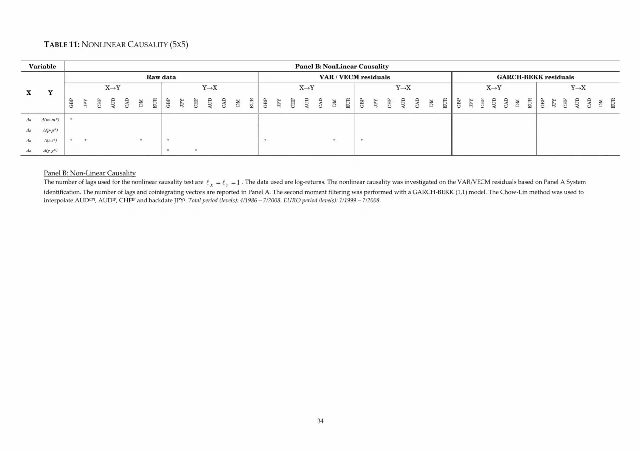
TABLE 11: NONLINEAR CAUSALITY (5X5)




GB

P

JP

Y

CH

F

AU

D

CA

D

DM

EU

R

GB

P

JP

Y

CH

F

AU

D

CA

D

DM

EU

R

GB

P

JP

Y

CH

F

AU

D

CA

D

DM

EU

R

GB

P

JP

Y

CH

F

AU

D

CA

D

DM

EU

R

GB

P

JP

Y

CH

F

AU

D

CA

D

DM

EU

R

GB

P

JP

Y

CH

F

AU

D

CA

D

DM

EU

R

∆s ∆(m-m*) *

∆s ∆(p-p*)

∆s ∆(i-i*) * * * * * * *

∆s ∆(y-y*) * *


YXℓℓ . The data used are log-returns. The nonlinear causality was investigated on the VAR/VECM residuals based on Panel A System



35





GB

P

JP

Y

CH

F

AU

D

CA

D

DM

EU

R

GB

P

JP

Y

CH

F

AU

D

CA

D

DM

EU

R

GB

P

JP

Y

CH

F

AU

D

CA

D

DM

EU

R

GB

P

JP

Y

CH

F

AU

D

CA

D

DM

EU

R

GB

P

JP

Y

CH

F

AU

D

CA

D

DM

EU

R

GB

P

JP

Y

CH

F

AU

D

CA

D

DM

EU

R

∆s ∆(p-p*)

∆s ∆(i-i*) *

∆s ∆(y-y*) ** *






Panel A: Linear Granger Causality The 4x4 system of the data (levels) for each FX was investigated with a VECM specification and the null of no cointegration was rejected for all except GBP, JPY, AUD and CAD. The lag lengths of

VECM/VAR specification are investigated and set using the SIC and Wald exclusion criterion and the cointegrating vectors using the Johansen trace statistic. The number of lags identified and the

cointegrating vectors are presented in parenthesis as (lags, coint. vectors): GBP(1,0), JPY(1,0), CHF(5,1), AUD(1,0), CAD(1,0), DM(2,2), EUR(2,1). For testing reasons Linear Granger causality was further

investigated in the VAR/VECM or GARCH residuals, but not detected.

36




X→Y Y→X X→Y Y→X X→Y Y→X

X Y

GB

P

JP

Y

CH

F

AU

D

CA

D

DM

EU

R

GB

P

JP

Y

CH

F

AU

D

CA

D

DM

EU

R

GB

P

JP

Y

CH

F

AU

D

CA

D

DM

EU

R

GB

P

JP

Y

CH

F

AU

D

CA

D

DM

EU

R

GB

P

JP

Y

CH

F

AU

D

CA

D

DM

EU

R

GB

P

JP

Y

CH

F

AU

D

CA

D

DM

EU

R

∆s ∆(p-p*)

∆s ∆(i-i*) * * * * * * * * *

∆s ∆(y-y*) * *





37





X Y

GB

P

JP

Y

CH

F

AU

D

CA

D

DM

EU

R

GB

P

JP

Y

CH

F

AU

D

CA

D

DM

EU

R

GB

P

JP

Y

CH

F

AU

D

CA

D

DM

EU

R

GB

P

JP

Y

CH

F

AU

D

CA

D

DM

EU

R

GB

P

JP

Y

CH

F

AU

D

CA

D

DM

EU

R

GB

P

JP

Y

CH

F

AU

D

CA

D

DM

EU

R

∆s ∆(m-m*)

∆s ∆(p-p*)

∆s ∆(y-y*) ** * *






Panel A: Linear Granger Causality The 4x4 system of the data (levels) for each FX was investigated with a VECM specification and the null of no cointegration was rejected for all except AUD and EUR. The lag lengths of VECM/VAR

specification are investigated and set using the SIC and Wald exclusion criterion and the cointegrating vectors using the Johansen trace statistic. The number of lags identified and the cointegrating vectors

are presented in parenthesis as (lags, coint. vectors): GBP(5,2), JPY(4,1), CHF(2,1), AUD(2,0), CAD(4,1), DM(2,1), EUR(1,0). For testing reasons Linear Granger causality was further investigated in the

VAR/VECM or GARCH residuals, but not detected.

38





GB

P

JP

Y

CH

F

AU

D

CA

D

DM

EU

R

GB

P

JP

Y

CH

F

AU

D

CA

D

DM

EU

R

GB

P

JP

Y

CH

F

AU

D

CA

D

DM

EU

R

GB

P

JP

Y

CH

F

AU

D

CA

D

DM

EU

R

GB

P

JP

Y

CH

F

AU

D

CA

D

DM

EU

R

GB

P

JP

Y

CH

F

AU

D

CA

D

DM

EU

R

∆s ∆(m-m*) *

∆s ∆(p-p*)

∆s ∆(y-y*) * * * *





39



Raw data VAR residuals GARCH-BEKK residuals


GB

P

JP

Y

CH

F

AU

D

CA

D

DM

EU

R

GB

P

JP

Y

CH

F

AU

D

CA

D

DM

EU

R

GB

P

JP

Y

CH

F

AU

D

CA

D

DM

EU

R

GB

P

JP

Y

CH

F

AU

D

CA

D

DM

EU

R

GB

P

JP

Y

CH

F

AU

D

CA

D

DM

EU

R

GB

P

JP

Y

CH

F

AU

D

CA

D

DM

EU

R

∆s ∆(p-p*)

∆s i-i* *

∆s ∆(y-y*) ** *






Panel A: Linear Granger Causality The 4x4 system of the data (levels) for each FX was investigated with a VECM specification and the null of no cointegration was rejected for all. The lag lengths of VAR specification are investigated and set

using the SIC and Wald exclusion criterion. The number of lags identified and the cointegrating vectors are presented in parenthesis as (lags, coint. vectors): GBP(1,0), JPY(1,0), CHF(1,0), AUD(1,0), CAD(1,0),

DM(1,0), EUR(2,0). For testing reasons Linear Granger causality was further investigated in the VAR or GARCH residuals, but not detected.

40





X Y

GB

P

JP

Y

CH

F

AU

D

CA

D

DM

EU

R

GB

P

JP

Y

CH

F

AU

D

CA

D

DM

EU

R

GB

P

JP

Y

CH

F

AU

D

CA

D

DM

EU

R

GB

P

JP

Y

CH

F

AU

D

CA

D

DM

EU

R

GB

P

JP

Y

CH

F

AU

D

CA

D

DM

EU

R

GB

P

JP

Y

CH

F

AU

D

CA

D

DM

EU

R

∆s ∆(p-p*)

∆s i-i* * * * * * * *

∆s ∆(y-y*)


YXℓℓ . The data used are log-returns. The nonlinear causality was investigated on the VAR residuals based on Panel A System



41





GB

P

JP

Y

CH

F

AU

D

CA

D

DM

EU

R

GB

P

JP

Y

CH

F

AU

D

CA

D

DM

EU

R

GB

P

JP

Y

CH

F

AU

D

CA

D

DM

EU

R

GB

P

JP

Y

CH

F

AU

D

CA

D

DM

EU

R

GB

P

JP

Y

CH

F

AU

D

CA

D

DM

EU

R

GB

P

JP

Y

CH

F

AU

D

CA

D

DM

EU

R

∆s ∆(p-p*)

∆s ∆(y-y*) ** ** *






Panel A: Linear Granger Causality The 3x3 system of the data (levels) for each FX was investigated with a VECM specification and the null of no cointegration was rejected for all except JPY, CHF, AUD, CAD, EUR. The lag lengths of

VECM/VAR specification are investigated and set using the SIC and Wald exclusion criterion and the cointegrating vectors using the Johansen trace statistic. The number of lags identified and the

cointegrating vectors are presented in parenthesis as (lags, coint. vectors): GBP(2,1), JPY(1,0), CHF(1,0), AUD(1,0), CAD(1,0), DM(2,1), EUR(1,0). For testing reasons Linear Granger causality was further

investigated in the VAR/VECM or GARCH residuals, but not detected.

42





X Y

GB

P

JP

Y

CH

F

AU

D

CA

D

DM

EU

R

GB

P

JP

Y

CH

F

AU

D

CA

D

DM

EU

R

GB

P

JP

Y

CH

F

AU

D

CA

D

DM

EU

R

GB

P

JP

Y

CH

F

AU

D

CA

D

DM

EU

R

GB

P

JP

Y

CH

F

AU

D

CA

D

DM

EU

R

GB

P

JP

Y

CH

F

AU

D

CA

D

DM

EU

R

∆s ∆(p-p*)

∆s ∆(y-y*) * * *





43





GB

P

JP

Y

CH

F

AU

D

CA

D

DM

EU

R

GB

P

JP

Y

CH

F

AU

D

CA

D

DM

EU

R

GB

P

JP

Y

CH

F

AU

D

CA

D

DM

EU

R

GB

P

JP

Y

CH

F

AU

D

CA

D

DM

EU

R

GB

P

JP

Y

CH

F

AU

D

CA

D

DM

EU

R

GB

P

JP

Y

CH

F

AU

D

CA

D

DM

EU

R

∆s ∆(m-m*) *

∆s ∆(y-y*) ** *






Panel A: Linear Granger Causality The 3x3 system of the data (levels) for each FX was investigated with a VECM specification and the null of no cointegration was rejected for all except GBP, AUD, CAD, DM. The lag lengths of VECM/VAR

specification are investigated and set using the SIC and Wald exclusion criterion and the cointegrating vectors using the Johansen trace statistic. The number of lags identified and the cointegrating vectors

are presented in parenthesis as (lags, coint. vectors): GBP(1,0), JPY(2,1), CHF(2,1), AUD(1,0), CAD(1,0), DM(1,0), EUR(2,1). For testing reasons Linear Granger causality was further investigated in the

VAR/VECM or GARCH residuals, but not detected.

44





GB

P

JP

Y

CH

F

AU

D

CA

D

DM

EU

R

GB

P

JP

Y

CH

F

AU

D

CA

D

DM

EU

R

GB

P

JP

Y

CH

F

AU

D

CA

D

DM

EU

R

GB

P

JP

Y

CH

F

AU

D

CA

D

DM

EU

R

GB

P

JP

Y

CH

F

AU

D

CA

D

DM

EU

R

GB

P

JP

Y

CH

F

AU

D

CA

D

DM

EU

R

∆s ∆(m-m*) *

∆s ∆(y-y*) * * * *





exchange rates and fundamentals: co-movement, long-run relationships and short-run dynamics

Documents