evaporator calorimeter: the study of overall heat transfer performance
TRANSCRIPT
Evaporator Calorimeter: The Study of Overall Heat Transfer Performance
M. A. Davis, A. M. Jacobi, and P. S. Hmjak
ACRCTR-107
For additional information:
Air Conditioning and Refrigeration Center University of Illinois Mechanical & Industrial Engineering Dept. 1206 West Green Street Urbana, IL 61801
(217) 333-3115
September 1996
Prepared as part of ACRC Project 47 Evaporator Calorimeter: Studies
of Overall Heat Exchanger Performance A. M. Jacobi and P. S. Hmjak, Principal Investigators

The Air Conditioning and Refrigeration Center was founded in 1988 with a grant from the estate of Richard W. Kritzer, the founder of Peerless of America Inc. A State of Illinois Technology Challenge Grant helped build the laboratory facilities. The ACRC receives continuing support from the Richard W. Kritzer Endowment and the National Science Foundation. The following organizations have also become sponsors of the Center.
Amana Refrigeration, Inc. Brazeway, Inc. Carrier Corporation Caterpillar, Inc. Copeland Corporation Dayton Thermal Products Delphi Harrison Thermal Systems Eaton Corporation Ford Motor Company Frigidaire Company General Electric Company Lennox International, Inc. Modine Manufacturing Co. Peerless of America, Inc. Redwood Microsystems, Inc. The Trane Company U. S. Army CERL Whirlpool Corporation
For additional information:
Air Conditioning & Refrigeration Center Mechanical & Industrial Engineering Dept. University of Illinois 1206 West Green Street Urbana IL 61801
2173333115
Abstract
The objective of this study was to develop a flexible facility for evaluating the to-scale
thermal perfonnance of heat exchangers. During this phase of the project, exchanger testing was
completed on three refrigerator evaporators: an as-manufactured plain-fin heat exchanger, a
geometrically identical heat exchanger with brazed fin-tube contacts, and a spine-fin heat
exchanger. These exchangers were selected because they are used in residential refrigeration,
they are relatively simple, and because they provide a useful comparative study.
The evaporator calorimeter was constructed with several air-side sections. Temperature
and humidity control are provided in the thennal-conditioning section, and the flow-conditioning
section provides thennal mixing, flow profile and turbulence control. In the test section, air
temperature, velocity, pressure and humidity are measured. The tube-side flow is supplied and
conditioned by a chiller; temperature and mass flow rate of the coolant are measured. The
apparatus provides air mass flow rates up to about 725 kg/hr (1600 lb/hr); approach temperatures
from -23°C to 49°C (-10 to 120°F); and relative humidity from about 30% to 90%. The coolant
mass flow rate can reach about 500 kg/hr (1100 lb/hr) at temperatures as low as -23°C (-10 OF).
With this apparatus, air-side and tube-side energy balances within ±3% are typically
obtained, with worst-case energy errors less than ±7%. The overall heat exchanger conductance,
UAT, was found to be highest for the spine-fin geometry. The overall conductance for the plain
fin exchangers was roughly half that of the spine-fin geometry for Reynolds numbers from 500
to 3000 based on hydraulic diameter. Interestingly, when air-side area and tube-side resistance
effects were considered, the plain-fin geometry had an air-side heat transfer coefficient roughly
equal to that of the spine-fin geometry. Under dry-surface conditions, the plain-fin exchanger
with brazed fin-tube junctions had an air-side c.onductance about 20% higher than that of the
unbrazed exchanger. This result is probably due to fin-tube contact resistance in the as
manufactured plain-fin exchanger; unfortunately, it is unclear whether contact-resistance is
important under frosting conditions.
iii

Table of Contents
List of Figures .............................................................................................................. vii
Nomenclature ................ ; ........................................................................................... '" IX
Chapter 1 - Introduction ...................................................................................................... 1
1.1 Background ............................................................................................. 1
1.2 Literature Review ................................................................................... 2
1.2.1 Plain-Fin Heat Exchanger ..................................................... 3
1.2.2 Spine-Fin Heat Exchanger .................................................... 5
1.3 Project Objectives ................................................................................... 6
Chapter 2 - Wind Tunnel Design ........................................................................................ 7
2.1 Thermal Conditioning Section ................................................................ 7
2.2 Flow Conditioning Section ..................................................................... 9
2.3 Test Section .......................................................................................... 10
2.4 Heat Exchanger Test Specimens .......................................................... 13
2.5 Air Flow Measurement ......................................................................... 16
2.6 Tube Side .............................................................................................. 17
Chapter 3 - Procedure and Data Interpretation ................................................................. 19
3.1 Data Collection ..................................................................................... 19
3.1.1 Condensate Removal ........................................................... 19
3.2 Energy Balances ................................................................................... 20 3.3 e-NTU and Overall Heat Transfer Performance ................................... 20
3.4 Wilson Plot ........................................................................................... 26
3.5 Contact Resistance ................................................................................ 29
Chapter 4 - Results and Discussion ................................................................................... 30
4.1 Data Fidelity ......................................................................................... 30
4.2 Heat Transfer Performance Comparisons ............................................. 30
4.3 Frost Formation ...................................................................................... 36
Chapter 5 - Conclusions and Recommendations .............................................................. 40
5.1 Summary and Conclusions ................................................................... 40
5.2 Recommendations and Future Work .................................................... 41
v

Appendix A - Heat Exchanger Dimensions ...................................................................... 43
A.I Plate-Fin Heat Exchanger ..................................................................... 43
A.2 Spine-Fin Heat Exchanger .................................................................... 43
Appendix B - Area Analysis ............................................................................................. 44
B.I Plate-Fin Heat Exchanger Area ............................................................ 44
B.1.1 Minimum Free Flow Area .................................................. 44
B.I.2 Heat Transfer Area ............................................................. 44
B.2 Spine-Fin Heat Exchanger Area ........................................................... 45
Appendix C - Reynolds Number Analysis ........................................................................ 47
C.I Reynolds Number for the Plain-Fin Geometry ..................................... 47
C.2 Reynolds Number for the Spine-Fin Geometry .................................... 48
Appendix D - DOWTIIERM 4000 Properties .................................................................. 49
Appendix E - Uncertainty Analysis .................................................................................. 52
E.I Uncertainty in Measurements ............................................................... 52
E.2 Uncertainty in Experimental Data ....................................................... 54
E.2.1 Energy Balance Uncertainties ............................................ 54
E.2.2 Wilson Plot Uncertainties ................................................... 55
Appendix F - Test Data ..................................................................................................... 56
References ......................................................................................................................... 62
vi

List of Figures
Figure 2.1 - Schematic of the calorimetric wind tunnel apparatus used to test heat exchangers ................................................................................................... 8
Figure 2.2 - Photograph showing the flow conditioning section in the wind tunnel. This section was used to provide a uniform flow to the test section .......... 9
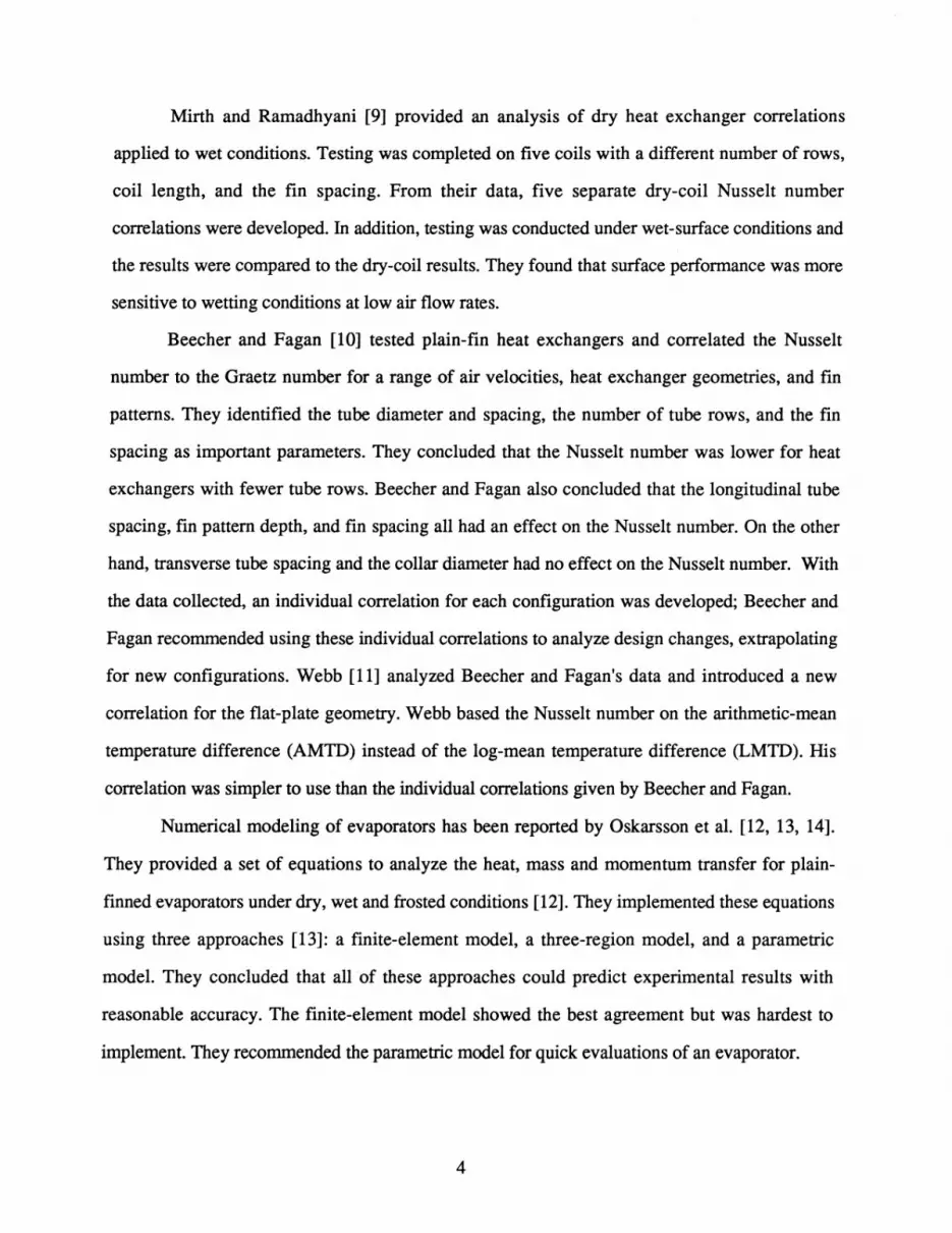
Figure 2.3 - A typical air approach temperature profile ............................................... 12
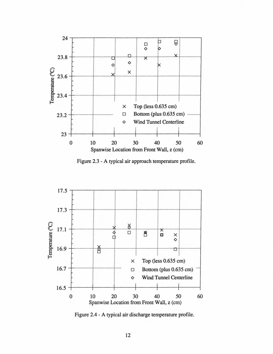
Figure 2.4 - A typical air discharge temperature profile ............................................... 12
Figure 2.5 - Velocity profiles recorded in the approach air flow ................................. 13
Figure 2.6 - Photograph showing the tested plate-fin heat exchanger with 2 tube columns and 16 total tube passes. Air flow is from the bottom of this page; the tube-side flow entered and exited at the air discharge position .......... 14
Figure 2.7 - Schematic of the plate-fin heat exchangers (both brazed and un-brazed) ....................................................................................................... 14
Figure 2.8 - Fin geometry for the plain-fin heat exchanger. The long and short fins were placed on the exchanger in an alternating arrangement (See Figure 2.7.) .......................................................................................................... 15
Figure 2.9- Photograph showing the spine-fin heat exchanger. Air flow is from the bottom of the page. This spine fin heat exchanger has 24 tube passes ........................................................................................................ 16
Figure 2.10 - Schematic showing the spine-fin heat exchanger geometry ..................... 17
Figure 3.1- Heat exchanger configuration for the e-NTU method of heat transfer analysis ...................................................................................................... 21
Figure 3.2 - General thermal resistance network for a heat exchanger ........................ 26
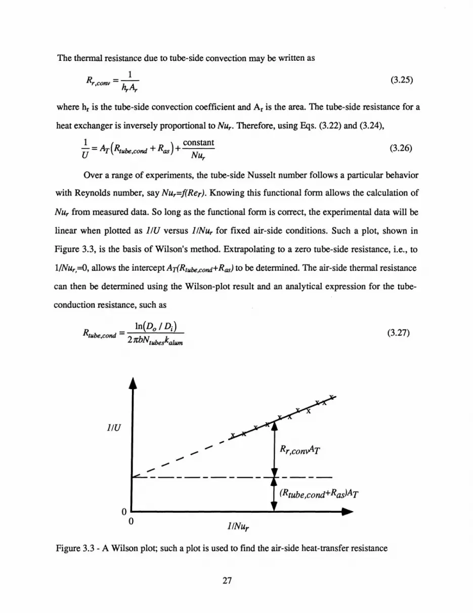
Figure 3.3 - A Wilson plot; such a plot is used to fmd the air-side heat-transfer resistance ................................................................................................... 27
Figure 4.1 - Energy balances for the unbrazed plate-fin heat exchanger, the brazed plate-fin heat exchanger, and the spine-fin heat exchanger ...................... 31
Figure 4.2 - Overall heat transfer performance with a coolant mass flow rate of 0.063 kg/s .................................................................................................. 31
Figure 4.3 - A modified Wilson plot for the unbrazed plate-fm heat exchanger .......... 33
Figure 4.4 - A modified Wilson plot for the brazed plate-fm heat exchanger ............. 33
Figure 4.5 - A modified Wilson plot for the spine-fin heat exchanger ......................... 34
vii

Figure 4.6 - Wilson plot for the unbrazed coil revealing the effects of a common slope on the air-side thennal resistances ................................................... 35
Figure 4.7 - Heat exchanger comparison on the basis of overall air-side heat transfer coefficient .................................................................................................. 36
Figure 4.8 - Frost formation on the brazed plain-fin heat exchanger ........................... 37
Figure 4.9 - Frost formation on the spine-fin heat exchanger ...................................... 38
Figure 4.10 - A close-up of frost fonnation at the air inlet to the spine-fin heat exchanger .................................................................................................. 39
Figure D.l - Volume percent Ethylene Glycol versus Specific Gravity for DOWTIffiRM 4000 at 7()OF ..................................................................... 49
Figure D.2 - Specific Heat for DOWTIffiRM 4000 at different Temperatures and Percentages of Ethylene Glycol. ............................................................... 50
Figure D.3 - Density for different Ethylene Glycol mixtures versus temperature ........ 50
Figure DA - Viscosity of Ethylene Glycol at different percentages of the mixture versus temperature .................................................................................... 51
Figure D.5 - Thennal Conductivity of Ethylene Glycol with different percentages and temperatures .............................................................................................. 51
viii

Nomenclature
Roman Symbols:
}\ area
a fInned length of heat exchanger tubes (see Figures 2.7 and 2.10)
b total width of heat exchanger (see Figures 2.7 and 2.10)
C heat-rate capacity, mcp
c test section height (see Figures 2.7 and 2.10)
Cp constant-pressure specifIc heat
Df outside diameter of the spine fIn (see Figure 2.10)
Dh hydraulic diameter, 4Ami,J.JAT
Do outside diameter of the tube
f Fanning friction factor, (2L\p/PaV2max)(DW4L)
G an NTU function, defined in Equations 3.11 and 3.14
h heat transfer coeffIcient
j Colburn j factor, Nu/Red1J71/3
k thermal conductivity
L effective air-side flow length, taken from air inlet to outlet (see Table 2.1)
I length of spine fin (see Figure 2.10)
M dimensionless fin parameter, U}\TST/krmAc
m mass flow rate
N number
NTU number of transfer units, UATICmin
NUr tube-side Nusselt number, hrD olkr
n number of tube passes per tube column, equal to number of tube rows
Pr Prandtl number, cpJ.1/k
L\p air-side pressure drop across heat exchanger
ix

p fin pitch
q rate of heat transfer
R thennal resistance (see Figure 3.2)
Rc ratio of minimum-to-maximum heat-rate capacity, CalCr
Re Reynolds number, VD/V
t thickness
s fm spacing
Srnin minimum pipe spacing
SI tube pitch, longitudinal (in the air flow direction)
St tube pitch, transverse
T temperature
UAT overall thermal conductance, based on total air-side area
U overall heat-transfer coefficient, based on air-side heat transfer area
Uas overall heat transfer coefficient of only the air side, i.e., J/RTAT
V max air velocity based on the minimum free-flow area, mal PaAmin
w width of the spine (see Figure 2.10)
x distance from contraction inlet measure in the flow direction
y vertical distance from the center of the wind tunnel
z spanwise distance from the front wall of the wind tunnel
Greek Symbols:
E
e
Jl
p
v
heat exchanger effectiveness, q/qmLlX
dimensionless fin temperature, (T-T ao)/(Tri-Tro}
dynamic viscosity
density
kinematic viscosity
dimensionless position on fin (See Equation 3.19).
x
Subscripts;
1,2, ...
a
al,a2
ai, ao
alum
as
B
c
contact
db
fm
i
L
max
min
o
p
r
r,conv
ri, ro
rm
s
T
tube
tube,cond
heat exchanger partition or tube pass number
of the air stream
air stream in partition 1 or partition 2 (see Figure 3.1)
air at the exchanger inlet and air outlet
for aluminum
air-side (total minus tube-side and conduction contributions)
at the fin base
for conduction through the fins, with all fins treated as one
for fin-to-tube contact
based on the hydraulic diameter
of the fin or fm material
tube inner surface
longitudinal or at the fm tip (adiabat)
maximum
minimum
tube outer surface, or of the adiabat where the heat exchanger is partitioned
for a tube pass
for the coolant flow
tube-side convective
tube-side (coolant) flow into and out of the heat exchanger
for the coolant between partitions (see Figure 3.1)
spine-fm or evaluated at the surface temperature
total area on the air-side or transverse
for the tube
for conduction through the tube
xi


Chapter 1 - Introduction
1.1 Background
The heat exchanger is a critical component in refrigeration and air conditioning systems.
Heat exchanger design is driven by material cost, manufacturability concerns, space constraints
and thermal requirements for dry, wet and frosted surfaces. In the refrigeration industry,
government energy standards and industry competitiveness make material selection and surface
geometry especially important to heat transfer surface design.
A few decades ago, copper was commonly used for both the fin and tube construction in
refrigerator evaporators. Copper was used because the required manufacturing methods were
well developed, it has a high thermal conductivity, and it was relatively inexpensive. With rising
copper costs, the industry widely adopted aluminum fins. The degradation in thermal
performance, due to the lower thermal conductivity of aluminum, was offset by using more of a
less-expensive material. Currently, few evaporators are made from copper alone-most use
copper or aluminum tubes and aluminum fins.
There have been advances in manufacturing techniques, and these advances offer new
opportunities for surface designers. Aluminum tubes of almost any cross-sectional geometry can
be extruded with a wide range of passage sizes. Tube expansion methods now provide good fin
tube thermal contact for a wide range of fin materials and thicknesses. Fin-making advances
allow the use of very thin fins and the generation of an almost endless range of geometrical
features-limited only by the imagination of the engineer. In spite of these advances, most
refrigerator evaporators currently rely on round-tube designs with either plain fins (flat plates) or
spine fins (pins or shredded fins). New surface geometries that exploit recent manufacturing
advances might meet the design constraints using less material than the plain-fin or spine-fin
designs; a related opportunity is the exploitation of new geometries to improve the energy
performance of the system.
1

Early refrigerator evaporators were not compact, they were commonly made from copper,
and they often used free convection rather than a forced air flow. In 1927, for example, General
Electric used a free-convection evaporator called the "Monitor-Top" for residential refrigeration.
Material costs, space considerations and increasing thermal performance demands-along with
aesthetics-drove an evolution to aluminum plain-fin and spine-fin evaporators relying on
forced-convection and fewer tube rows. This evolution is ongoing, and it appears that recent
manufacturing advances offer an opportunity for a new generation of evaporator surface designs.
The focus of the current study is on the development of a flexible, accurate facility for
studying overall heat exchanger performance. Such a facility is needed to evaluate candidate
surface designs. While the initial motivation for this project was based on refrigeration
applications, the facility has been developed to be flexible, allowing the study of heat exchangers
for a range of air-conditioning and refrigeration applications. To validate the facility and provide
useful baseline data, experiments were conducted with several heat exchangers. The data
acquisition and interpretation methods developed during this research also can be extended to
other applications.
1.2 Literature Review
Prior to the 1960s, air-conditioner and refrigerator applications almost exclusively used
plain-fin evaporators. During the 1960s, some companies decided to improve the plain-fin
evaporator, and others decided to completely redesign the exchanger. In 1966, GE introduced the
"shredded-fin" evaporator-an early spine-fin-type design. This technology had "an overall heat
transfer coefficient 4 times greater than the plate-fin tubing"[l]. The main problem with the
shredded-fin design was that it required a greater volume than a plain-fm evaporator for the same
thermal performance. The shredded-fin led to the spine-fin design currently in use. The evolution
of compact heat exchanger designs is discussed by London[2], Mori and Nakayama [3], and
Abbott et al. [1]. The literature review presented below has two sections, one focused on plain
fins and one on spine fins.
2

1.2.1 Plain-Fin Heat Exchanger
There has been a tremendous volume of research reported on heat exchangers; in this
section, the focus will be on relatively recent work that is closely related to the plain-fin
geometry used in residential refrigeration applications.
In 1973, Rich [4] studied plain-fin-and-tube heat exchangers. His testing focused on the
effects of fin spacing on a 4-row, 40-tube heat exchanger. Multiple Wilson Plots were used for
air velocities between 1 mls (200 ft/min) and 9 mls (1800 ft/min) with water (coolant) velocities
from 0.2 mls (0.7 ft/sec) to 2.1 mls (7 ft/sec). Rich concluded that, for a fixed air-side Reynolds
number, the heat transfer coefficient and the friction factor were independent of the fin spacing
between 1.2 and 5.5 fins per cm (3 and 14 fins per inch). In 1975, Rich [5] presented a study of
the effect of the number of tube rows on the heat transfer performance of a plain-fin heat
exchanger. The air-side heat transfer coefficients were calculated using a Wilson plot. He found
that the average heat transfer coefficient depended on the Reynolds number, but at different
Reynolds numbers an increase in the number of rows did not always increase the heat transfer
coefficient. Rich concluded that stable vortex patterns associated with the tubes caused high heat
transfer at low Reynolds numbers with a small number of tube rows. A more detailed study of
these vortices was presented by Saboya and Sparrow [6]; they studied a three-row plain-fin-and
tube heat exchanger using the naphthalene sublimation technique to examine local convective
effects and found a pronounced heat transfer effect due to the horseshoe vortex system.
Rich's early studies [4,5] indicated that there was a need for new and better performance
correlations. McQuiston [7] expanded on the data of Rich by testing five plain-fin-and-tube heat
exchangers under dry and wet conditions with filmwise and dropwise condensation. McQuiston
[8] used these data to develop performance correlations that included the influences of tube
diameter and configuration, fin spacing and thickness, the number of tube rows, and the surface
wetting conditions. McQuiston reported uncertainties of ±10% in j and ±35% in f for face
velocities from 1 to 4 mls (200 to 800 ft/min).
3
Mirth and Ramadhyani [9] provided an analysis of dry heat exchanger correlations
applied to wet conditions. Testing was completed on five coils with a different number of rows,
coil length, and the fin spacing. From their data, five separate dry-coil Nusselt number
correlations were developed. In addition, testing was conducted under wet-surface conditions and
the results were compared to the dry-coil results. They found that surface performance was more
sensitive to wetting conditions at low air flow rates.
Beecher and Fagan [10] tested plain-fin heat exchangers and correlated the Nusselt
number to the Graetz number for a range of air velocities, heat exchanger geometries, and fin
patterns. They identified the tube diameter and spacing, the number of tube rows, and the fin
spacing as important parameters. They concluded that the Nusselt number was lower for heat
exchangers with fewer tube rows. Beecher and Fagan also concluded that the longitudinal tube
spacing, fm pattern depth, and fin spacing all had an effect on the Nusselt number. On the other
hand, transverse tube spacing and the collar diameter had no effect on the Nusselt number. With
the data collected, an individual correlation for each configuration was developed; Beecher and
Fagan recommended using these individual correlations to analyze design changes, extrapolating
for new configurations. Webb [11] analyzed Beecher and Fagan's data and introduced a new
correlation for the flat-plate geometry. Webb based the Nusselt number on the arithmetic-mean
temperature difference (AMID) instead of the log-mean temperature difference (LMID). His
correlation was simpler to use than the individual correlations given by Beecher and Fagan.
Numerical modeling of evaporators has been reported by Oskarsson et al. [12, 13, 14].
They provided a set of equations to analyze the heat, mass and momentum transfer for plain
finned evaporators under dry, wet and frosted conditions [12]. They implemented these equations
using three approaches [13]: a fmite-element model, a three-region model, and a parametric
model. They concluded that all of these approaches could predict experimental results with
reasonable accuracy. The finite-element model showed the best agreement but was hardest to
implement. They recommended the parametric model for quick evaluations of an evaporator.
4

Other factors can influence the perfonnance of a heat exchanger, including contact
resistance, flow maldistribution, and fouling. In an interesting study, Sheffield et al. [14]
analyzed the effect of rm-tube contact resistance. Eight fin-tube heat exchangers, constructed by
expanding the tubes, were analyzed. One coil was tested unexpanded for comparison purposes.
The other coils differed by fin contact area, and the number and thickness of the fins. The final
result was a mathematical model that can be used to calculate the contact resistance. Timoney
and Foley [15] perfonned an analysis to explore the effects of velocity non-uniformity. They
found a small increase in capacity with flow non-unifonnity; however, this study was limited
because the heat exchangers were only tested at two air flow rates. Barrow and Sherwin [16]
analyzed the effects of fouling. Their analysis revealed that as a heat exchanger fouls, its
perfonnance can improve at first, but after some period the perfonnance will decrease. This
result might imply that fouling decreased the contact resistance.
1.2.2 Spine-Fin Heat Exchanger
Spine-fin tubing has been used in refrigeration applications since the 1960s, but little
research on this geometry has been reported in the open literature. Holtzapple and Carranza [17]
provided an analysis of the pressure drop across spine-finned tubing. In their analysis, a
correlation for the pressure drop was developed which depended on the velocity and the number
of tube rows. In a second paper, Holtzapple et al. [18] presented heat transfer results for the
spine-fin tube. Heat exchangers with two different sizes of pipe were studied for three different
configurations. Their results indicated that the fin efficiency of the spines was approximately
70% instead of the 100% that was normally assumed. Holtzapple and Carranza [19] compared
spine-fin perfonnance to other geometries, including bare tubes, helical finned tubes, and plate
fins. The comparisons were presented for heat transfer versus blower power, heat transfer versus
unit frontal area, and heat transfer versus unit weight. No single heat exchanger was found to be
superior for all applications-the blower power, frontal area, and weight all must be considered
as design parameters.
5

Very recently, Assis et al. [20] perfonned a study of spines in free convection. They used
liquid crystals for visualization and thennocouples for quantitative measurements. In addition,
they developed and verified a transient model of spine-fin heat exchangers. Yeh [21] also
analyzed the effects of natural convection in optimizing spine fins. The optimal spine design was
found to depend on fin volume, heat transfer coefficient at the base of the fin, and thennal
conductivity.
1.3 Project Objectives
The objective of this study was to develop a flexible facility for evaluating the thennal
perfonnance of evaporators-a so-called evaporator calorimeter. A particular focus was directed
at refrigerator evaporators; however, the apparatus and methods developed should be applicable
to other heat exchangers. The evaporator calorimeter provides a range of test temperatures,
humidity ratios and air velocities, and it accommodates a variety of heat exchanger
configurations. To validate the calorimeter perfonnance, three heat exchangers were tested: an
as-manufactured plain-fin heat exchanger, an identical heat exchanger with brazed fin-tube
contacts, and a spine-fin heat exchanger. These geometries are typical to those commonly used in
residential refrigeration. By comparing the as-manufactured and brazed heat exchanger
performance, contact resistance effects were explored. Furthermore, preliminary studies of
systemic frost deposition were conducted.
Data interpretation techniques include an assessment of the energy balance for each
experimental condition. The e-NTU method was utilized to calculate an accurate overall thennal
conductance, and a Modified Wilson Plot was used to infer the air-side thennal resistance.
Testing was perfonned with coolant mass flow rates from 227 to 385 kg/hr (500 to 850 lb/hr) and
temperatures from 5 to 15"C (40 to 58·F). The air-side flow rates were from 60 to 360 kg/hr (132
to 794 lb/hr), and the approach temperatures ranged from 4 to 35"C (39 to 95·F).
6

Chapter 2 . Wind Tunnel Design
The wind tunnel apparatus was divided into four air-side sections: the thermal conditioning
chamber, the flow conditioning section, the test section, and the flow measuring station (See
Figure 2.1.). The tube side used a water and ethylene-glycol mixture supplied by a chiller and
pump. The apparatus design, instrumentation, and wind tunnel performance data are described in
this chapter, along with the test heat exchanger configurations.
2.1 Thermal Conditioning Section
The thermal conditioning section provided temperature and humidity control of the air
flow. This section, like the rest of the wind tunnel, was constructed using O.64-cm thick (0.25 in)
acrylic and was insulated with 1.3 to 5.1 cm (0.5 to 2.0 in) of Celotex Tuff-R insulation. The
chamber was 46 by 61 by 122 cm (18 by 24 by 48 in) and was fitted with an access panel in the
chamber wall. The panel was well sealed from air leaks using a gasket system and duct tape.
Air temperatures from -23 to 49°C (-10 to 120°F) could be achieved in the conditioning
section; however, dry-surface data were obtained with approach air temperatures from 4 to 35°C
(39 to 95°F). Temperature control was possible through a combination of preheaters, cooling
coils, and after heaters. The preheaters consisted of 4 electric resistance heaters, each supplying
up to 500 W; these heaters were 45 cm (18 in) long and were placed at the chamber entrance.
The walls of the chamber were protected from the heaters using aluminum foil as a radiation
shield. The cooling coils consisted of four chiller-supplied heat exchangers and were located
downstream of the heaters. Two electrically powered after heaters were located downstream of
the cooling coils and upstream of the blower inlet. All heaters were controlled manually using
variable transformers. The chamber was .equipped with.a drain for water removal. Although heat
exchanger testing was performed with dry surfaces, a humidifier provided a relative humidity
from 30% to 90% for a preliminary study of frost formation. A 3-HP blower, mounted on
vibration isolators, delivered air from the thermal to the flow conditioning sections.
7

00
After
Humidifier1
Q) ®
Flow Conditionin& Centrifugal Mixer Mixing Fans Honeycomb Straightener Screens Contraction
Tube-Side II ' ,Sunnly
Figure 2.1 - Schematic of the calorimetric wind tunnel apparatus used to test heat exchangers.

2.2 Flow Conditioning Section
The flow conditioning section provided thermal mixing and flow straightening to ensure
a uniform temperature and velocity distribution. The 60 by 61 by 61 cm (23.5 x 24 x 24 in) flow
conditioning section was constructed using material and methods typical to those used for the
thermal conditioning chamber. Temperature uniformity was obtained using a centrifugal mixer
and fans, as shown in Figure 2.2. The centrifugal mixer was constructed using a curved plastic
vane, 19.0-cm wide (7.5 in), to introduce a swirl flow. The small fans (nominal 65 cfm) were
added to aid in thermal mixing at low air flow rates. The velocity field was conditioned using
honeycomb and screens as recommended by NASA [22,23] to obtain a steady laminar flow.
The 0.32-cm-cell (0.125 in) honeycomb was placed 12.7 cm (5 in) upstream of the screens.
Following the NASA recommendations [22], the screen was 70.4% open, and the frame
thickness allowed for at least 75 screen-mesh sizes between the screens. Care was taken to ensure
that the wind tunnel walls were smooth and uninterrupted downstream of the honeycomb.
Figure 2.2 - Photograph showing the flow conditioning section in the wind tunnel. This section was used to provide a . uniform flow to the test section.
9

2.3 Test Section
The contraction was designed to allow for a smooth transition into the test section and to
reduce turbulence. The 12-to-l cubic contraction was designed in accordance with the
recommendations of Morel [24] to maintain flow uniformity and to avoid flow separation. The
contraction shape conformed to the following relation between the distance from the centerline
of the flow, y, and the axial distance from the contraction inlet, x (both y and x are in inches).
y = 11.29-0.113x-0.0764x2 +0.OO2997x3 (2.1)
The pattern specified by Eq. (2.1) was transferred onto the side-wall construction
material. These pieces were cut and attached to a wooden frame for stability. With the frame
complete, 0.32-cm thick (0.125 in) pieces of acrylic were heated and bent to form the top and
bottom of the wind tunnel. This contraction allowed for flow from the 61 cm (24 in) flow
conditioning section to the 5.1 cm (2 in) test section. In order to eliminate the effects of the tube
bends on the heat transfer performance, a second interior contraction was used to avoid any by
pass flow. The air flow only passed through the finned heat exchanger volume. The interior
contraction reduced the wind-tunnel span to 52.7 cm (20.75 in) for the plain-fin heat exchanger,
45.1 cm (17.75 in) for the brazed plain-fin heat exchanger, and 50.0 cm (19.69 in) for the spine
fin heat exchanger. Furthermore, the tube bends were carefully insulated and sealed. A smooth
contraction into the test section, through careful construction, ensured that the boundary layer
was not tripped.
Upstream and downstream of the test section, the temperature distribution was measured
using thermocouple rakes consisting of six thermocouples on each rake. These thermocouple
rakes allowed for any temperature maldistribution to be observed. The thermocouples on the inlet
rake were located at spanwise locations from the front wind tunnel wall of 12.1, 19.1,26.7,34.3,
40.6 and 48.3 cm (4.75, 7.5, 10.5, 13.5, 16, 19 in, respectively). The thermocouples of the outlet
rake were at spanwise locations of 12.7, 19.7,26.7,34.3,41.9 and 48.3 cm from the wind tunnel
front wall (5, 7.75, 10.5, 13.5, 16.5, 19 in, respectively). To verify that proper thermal mixing of
10

the air was achieved, temperature profiles were measured at three vertical locations for each
spanwise location; these vertical positions were 0.64 cm (0.25 in) from the wind tunnel bottom,
along the center line, and 0.64 cm (0.25 in) from the wind tunnel top wall. Thus, the air approach
and discharge flows were each measured at 18 positions; example results are provided in Figures
2.3 and 2.4. The temperature profiles shown in the figures were recorded at an air flow rate
representative of the lowest in the experimental regimen; thus these data represent a worst case
for thermal mixing. The temperature profiles were found to be flat to within ±O.1 °C (0.2°F);
therefore, heat exchanger data were analyzed with the thermocouple rake centered in the wind
tunnel.
Care was taken to ensure that the ice bath was uniform and to mitigate thermocouple
conduction errors. The ice bath was stirred often, and reference thermocouples were positioned at
several locations in the ice slurry. To check the ice bath, thermocouples in a typical ice bath were
compared to an electronic ice point. This comparison confirmed that the experimental procedure
provided accurate reference temperatures. Precautions to reduce conduction errors included
thermally isolating the thermocouple bead from its mounting on the rake and insulating the wires
with at least 2.5 cm (1 in) of fiberglass where the rakes exited the wind tunnel. Auxiliary tests,
undertaken by changing the thermocouple exit condition (heating the wire where it exited the
wind tunnel), indicated that the exit condition had no discernible influence on the temperature
indicated by the thermocouple. Therefore, conduction errors were considered negligible.
Radiation errors in thermometry were neglected since the internal wind tunnel temperature
(except for the heat exchanger) was equal to the air temperature at steady state. A typical
approach air velocity profile is shown in Figure 2.5. These velocity data were collected using a
hot-wire anemometer. In the worst case, the velocity profile was found to exhibit variations of
±3.4%. The air mass flow rate obtained by integrating these velocity distributions agreed with the
orifice plate results to within the uncertainty of the measurements. During normal heat exchanger
testing, the air mass flow rate was determined using the orifice plate (See section 2.5.).
11
24~-----'----~------~----~-----'----~
~ 91 o <>
I x Top (less 0.635 em)
23.2 +---r ~ ~=;,<::: ~~!: -iii i i
23~-----+'----~1------r-'----'1------r-,--~
o 10 20 30 40 50 60 Spanwise Location from Front Wall, z (em)
Figure 2.3 - A typical air approach temperature profile.
17.5 ~-----.---------,------~----~-----.----~
17.3 -~--111r--1--
E 17.1 -t--·····················I·····················~········ ..... a······I························I·x··················1························ ~ i 0, 0 i ~ iC xi ~ 1 9 1 i <> 1 ! 16.9 ---jaj---jj---ni-
16.7 -t--····················· .. i:.I.i:.!- : ' ~::~~~~3:.:~) cm)-
<> ·Wind Tunnel Centerline I Iii i 16.54------+1----~1------~1----'1------~1--~
o 10 20 30 40 50 60 Spanwise Location from Front Wall, z (cm)
Figure 2.4 - A typical air discharge temperature profile.
12

3.-----~----~------~----~----~-----.
! 2.5 -r~~gh8+i+---+ ~ ~i~~~r~~~~~~~F§~~r
1 2 +--rll-- 1-=:: ~ 1.5 ---111 : Bottom
I I I I I 1~-----+-1----~1------+-,----41------+-'--~
o 0.1 0.2 0.3 0.4 0.5 0.6 Spanwise Location from Front Wall, z (m)
Figure 2.5 - Velocity profiles recorded in the approach air flow.
2.4 Heat Exchanger Test Specimens
Three evaporators were tested in the wind tunnel: an as-manufactured plain-fin heat
exchanger, a plain-fin exchanger with brazed fin-tube contacts, and a spine-fin heat exchanger. A
photograph of the plain-fin exchanger is given in Figure 2.6, and a schematic is provided in
Figure 2.7. The plain-fin heat exchanger was finned with alternating short and long fins to allow
for greater fin spacing at the leading edge (See figure 2.8.). The dimensions of the heat
exchangers are given in Table 2.1 and Appendix A.I. The brazed and unbrazed plain-fin heat
exchangers were geometrically identical, except that they differed in the total heat transfer area
because they had differing spanwise lengths. A photograph and schematic of the spine-fin heat
exchanger are given in Figures 2.9 and 2.10, respectively. While a direct comparison of the
thermal performances of the plain-fin geometries was possible, comparisons to the spine-fin
results are complicated by geometrical differences. In addition to overall area differences, the
spine-fin heat exchanger had three 3 tube columns whereas the plain-fin geometry had 2 tube
columns (cf. Figures 2.7 and 2.10).
13

111111 ~IIIIII Figure 2.6 - Photograph showing the tested plate-fin heat exchanger with 2 tube columns and t 6
total tube passes. Air flow is from the bottom of this page; the tube-side flow entered and exited at the air discharge position.
t S! • Refrigerant in c. ~~8-'----"" ---t.~ Refrigerant out
Long Fins
Short Fins
r ~ ,r;::"' ~ ,.. r ,... ~
-- I"'" ~~
a
~r
~ ...... ~ ~ .... ....
Figure 2.7 - Schematic of the plate-fin heat exchangers (both brazed and unbrazed).
14
j~
b
"

9.52 17.46 7.94 7.94
ir--,rir-1r-. L 50.8
12.7 --*-T ..... �.1---203.2----I~~1
Long Fin
17.46 7.94
184.2 Short Fin
(all dimensions in mm)
Figure 2.8 - Fin geometry for the plain-fin heat exchanger. The long and short fms were placed on the exchanger in an alternating arrangement (See Figure 2.7.).
Table 2.1 Geometrical Parameters for the Test Heat Exchangers
Type Unbrazed Plain Fin Brazed Plain Fin Spine Fin
Number of Tube Rows (NR) 8 8 8
Number of Tube Passes 16 16 24
Column #1 Configuration overall counterflow overall counterflow overall counterflow
Column #2 Configuration overall parallel flow overall parallel flow overall parallel flow
Column #3 Configuration N/A N/A overall counterflow
Tube diameter (Do) 0.952 cm (0.375 in) 0.952 cm (0.375 in) 0.952 cm (0.375 in)
Tube thickness (ttube) 0.076 cm (0.030 in) 0.076 cm (0.030 in) 0.076 cm (0.030 in)
L, Fin Length (Long) 20.32 cm (8 in) 20.32 cm (8 in) 20.32 cm (8 in)
Fin Length (Short) 18.42 cm (7.25 in) 18.42 cm (7.25 in) N/A
Number of Fins 106 92 Helical wrap
Fin Thickness (truJ 0.0127 cm (0.005 in) 0.0127 cm (0.005 in) 0.0229 cm (0.009 in)
Fin pitch (p) 2 fins/cm (5 fpi) 2fins/cm (5 fpi) 3.15 fins/cm (8 fpi)
Testing Length (a) 50.70 cm (20.75 in) 45.08 cm (17.75 in) 50.01 cm (19.69 in)
Total Length (b) 59.69 cm (23.50 in) 51.75 cm (20.38 in) 54.61 cm (21.50 in)
Total Height (c) 5.08 cm (2 in) 5.08 cm (2 in) 7.62 cm (3 in)
15
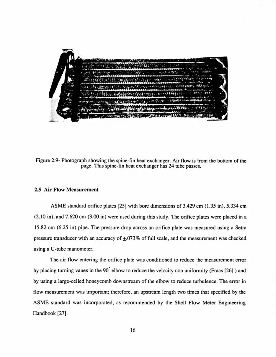
Figure 2.9- Photograph showing the spine-fin heat exchanger. Air flow is :from the bottom of the page. This spine-fin heat exchanger has 24 tube passes.
2.5 Air Flow Measurement
ASME standard orifice plates [25] with bore dimensions of 3.429 cm (1.35 in), 5.334 cm
(2.10 in), and 7.620 cm (3.00 in) were used during this study. The orifice plates were placed in a
15.82 cm (6.25 in) pipe. The pressure drop across an orifice plate was measured using a Setra
pressure transducer with an accuracy of ±.073 % of full scale, and the measurement was checked
using a U-tube manometer.
The air flow entering the orifice plate was conditioned to reduce ~he measurement error
by placing turning vanes in the 90· elbow to reduce the velocity non unifonnity (Fraas [26] ) and
by using a large-celled honeycomb downstream of the elbow to reduce turbulence. The error in
flow measurement was important; therefore, an upstream length two times that specified by the
ASME standard was incorporated, as recommended by the Shell Flow Meter Engineering
Handbook [27].
16

· .l-r 4:,r r· ~~I~~~OW c,- ~ ~ ~ ~ ~ " ----,:--
Airflow
a b
l' ri l ~ A-A
~~~~
I
SECTION A-A
Figure 2.10 - Schematic showing the spine-fin heat exchanger geometry.
2.6 Tube Side
The tube-side loop included a chiller, 18.3 m (60 ft) of insulated copper tubing, two
pumps, control valves, and a flow meter. The chiller circulated a single-phase ethylene glycol
mixture (DOWTHERM 4000) to allow for a wide temperature range on the tube side and to
make property calculations easy. The properties of the ethylene glycol mixture were calculated
17

from the specific gravity and company-supplied data (See Appendix D.). DOWTHERM 4000
consists of 92.4% ethylene glycol and 7.6% inhibitors and water as specified by Dow [28]; it was
mixed with additional water to produce a mixture that was 56.92% ethylene glycol by weight.
The specific gravity of the mixed fluid was periodically measured to ensure that properties could
be accurately determined.
Two pumps and multiple valves were used to deliver and control the tube-side flow rate.
The first pump, which was part of the chiller, only provided a 3.33 kg/hr (8Iblhr) flow to the test
section. An auxiliary pump--a rotary gear pump with a 1/2 HP (nominal) motor-was added so
that tube-side flow rates of the ethylene glycol mixture greater than 454 kg/hr (1000 lblhr) were
obtained. The tube-side temperature was set using the chiller and trim heaters. The chiller
supplied a flow at temperatures from -13 to 32°C (8 to 89°P) to the heat exchanger under test.
The chiller also supplied the cooling/dehumidifying coils in the thermal conditioning section (as
described earlier). The control valves were manually set to achieve the desired flow rates, and the
tube-side mass flow rate to the heat exchanger under test was measured using a Coriolis-effect
mass flow meter (±O.15%) placed immediately downstream from the heat exchanger.
Temperature measurements on the tube side were conducted using mixing cups at the
heat exchanger inlet and discharge. These mixing cups consisted of a copper-tube expansion cup
and a helical copper insert to ensure mixing of the fluid. Exposed-junction, type-T thermocouples
were inserted into the middle of the mixing cups, and the entire assembly was carefully insulated.
A tubing length of approximately 0.6 m (2 ft) was maintained between the mixing cups and the
closest trim heater.
18

Chapter 3 - Procedure and Data Interpretation
3.1 Data Collection
Air temperatures were recorded at 6 locations upstream of the heat exchanger, 6 locations
downstream of the heat exchanger, and 1 location downstream of the orifice plates. Coolant
temperatures were recorded at 1 location in the inlet flow and 1 in the outlet; 3 thermocouples
were placed in the reference ice bath. In total, 18 thermocouples were used to record temperature
data. The pressure drop across the orifice plate, the relative humidity, and the mass flow rate on
the refrigerant side were also measured. All data were recorded at steady state and averaged over
4 minutes (approximately 70 samples per channel). Steady-state conditions were assumed to
prevail when the averaged inlet air temperature to the heat exchanger remained constant to within
±O.loC for 15 minutes. The tube-side flow was provided by the chiller, and the inlet refrigerant
temperatures stayed nearly constant throughout a set of experiments. Recording a typical set of
data for one experimental point required about 15 minutes; however, several hours were
sometimes required to reach steady state.
3.1.1 Condensate Removal
Because data interpretation was based on dry-coil equations, steps were taken to ensure
that the heat exchanger surface was free of condensate. Prior to a test, moisture was removed
from the wind tunnel by maintaining a high mass flow rate and low temperature supply to the
cooling/dehumidifying coils in the thermal conditioning section. Condensate that collected in the
thermal conditioning section was removed by hand. Since the cooling coils and test heat
exchanger were supplied by the same chiller, an electrical resistance heater (416 W) was used to
preheat the inlet liquid flow to the test heat exchanger. This trim heater-controlled manually
using a variable transformer-maintained the test heat exchanger surface at a temperature
slightly above the dew point of the flowing air stream.
19

3.2 Energy Balances
An energy balance was used to identify potential problems and verify proper operation of
the calorimeter. In evaluating the energy balance, special care was taken to properly calculate
thermophysical properties (as explained earlier and in Appendix D). Assuming no heat leaks to
the calorimeter environment, the rate of energy transfer from the air stream must equal the rate of
transfer to the flowing coolant at steady state. These rates may be determined using the First Law
of thermodynamics, which can be written in rate form for both streams:
(3.1)
(3.2)
Once an acceptable energy balance was achieved, the E-NTU method was used to determine the
overall heat-transfer performance.
3.3 E-NTU and Overall Heat Transfer Performance
Rohsenow, Hartnett, and Ganic [29] discuss four different methods for evaluating heat
exchanger performance: E-NTU, P-NTU, LMTD, and ,!,-P. While each of these methods can
have advantages, the configuration correlations needed to apply the P-NTU and ,!,-P methods to
the current geometries are difficult to find in the literature. Likewise, an appropriate crossflow
correction factor is difficult to find for the LMTD approach. Since E-NTU relations are readily
available in the literature (e.g., see Kays and London [30]), this approach was adopted.
Using the E-NTU method and relations from Rohsenow et al. [29] and Incropera and
DeWitt [31], the plain-fin heat exchangers were analyzed as consisting of two heat exchanger
partitions. The frrstpartitionwas considered as eight crossflow.passes in an overall counterflow
arrangement, and the second partition was analyzed as eight crossflow passes in an overall
parallel-flow arrangement. This scheme is illustrated in Figure 3.1. The spine-fin heat exchanger
was treated the same way, except that a third overall counterflow partition was added.
20

T· aJ.
~ ~ ~
~ ~ ~
0 Trm
~ 0
Partition 1
0 0 0
0 0 0 Partition 2
T· n
r ~
0 0 ~ ~
~
0 0 ~ ~
'rrro
Figure 3.1- Heat exchanger configuration for the e-NTU method of heat transfer analysis
If it is assumed that heat transfer from one partition to another is negligible, then the rate
of heat transfer to each partition may be written using the following simple First-Law analysis:
ql = Ca1 (T ai -Tool) (3.3)
ql = Cr(Trm - Tri ) (3.4)
q2 = Ca2 (T ai - T 002) (3.5)
q2 = Cr(Tro - Trm) (3.6)
In Eqs. (3.3)-(3.6), Cal and Ca2 represent the air-stream heat rate capacities for each
partition-the heat-rate capacity is the mass-flow-rate-specific-heat product for the flowing
stream. In this analysis, it is assumed that Cal and Ca2 are equal, and that their sum is the total for
the air stream, i.e., Ca=Cal+Ca2. The heat rate capacity for the coolant stream is Cr; it is the
same for every pass in both partitions. These assumptions will be evaluated and discussed later.
Since for the data collected, Ca < Cr the First Law can also be written on a rate basis ,
using the definition of heat exchanger effectiveness [31]. Thus, for each partition:
21

(3.7)
(3.8)
Each heat exchanger partition can be considered a multi-pass heat exchanger, and the
efficiency of each row pass in a partition can be determined separately. Assuming that each pass
has the same area and overall heat transfer coefficient, the efficiencies of individual passes
within a partition are equal. It should be noted that for the data presented later, the air stream had
a heat-rate capacity less than the coolant stream; Ca < Cr. Furthermore, the air stream was
unmixed in a pass due to finning, but the coolant stream was mixed because there was no tube
side finning. On this basis, the efficiency of Partition 1, El, and the efficiency of each pass in that
partition, Epl, were calculated using the following relationships for an overall counterflow
exchanger (Rohsenow et al. [29] and Incropera and DeWitt [31]):
(3.9)
(3.10)
where,
(3.11)
In these equations, nl represents the number of passes in the partition; for this study, there were
always 8 passes per partition (nl =n2=n3=8). The ratio of heat rate capacities, RC1, represents the
ratio of minimum-to-maximum heat rate capacity for the flowing streams (CmmlCmax). For the
data to be presented, RCi=Cai/Cr.
For heat exchanger Partition 2, with an overall parallel-flow arrangement, the following
relations were used to fmd NTU (Rohsenow et al. [29] and Incropera and DeWitt [31]).
22

(3.12)
(3.13)
where,
(3.14)
Taking the refrigerant temperatures Tri and Tro as known, along with the known air and
refrigerant mass flow rates and specific heats, the 12 equations given in Eqs. (3.3)-(3.14) have
the following 13 unknowns: ql, q2, Tao1. Tao2, Trm, El, E2, Elp, E2p, 01. 02, NTUpl, and NTUp2.
Since the passes represent equal air-side heat transfer areas with equal convective heat transfer
coefficients, this system of equations is closed by imposing the following condition:
(3.15)
Furthermore, by definition,
NTU =(UAp) pI C
al
(3.16)
and
(3.17)
Finally, for the reasons outlined above, the Number of Transfer Units for each heat exchanger
partition are equal, and the overall thermal conductance of the heat exchanger can be found using
N
UAr =UAp Lni i=1
(3.18)
where the summation represents the total number of tube passes (for the plain-fin configurations
the summation equals 16; for the spine-fin configuration it is equal to 24).
23

It is important to consider the validity of several key assumptions adopted in the analysis.
The heat-rate capacities for each partition were assumed to be equal. Since the approach air
velocity profile is highly uniform, and since the heat exchanger partitions are identical
presenting identical flow resistance-the flow rates through each of the partitions must be very
nearly identical. Furthermore, the thermophysical properties of the air streams in each partition
are nearly identical because their temperatures are within a few degrees of each other. Therefore,
the assumption of identical air-side heat rate capacities for each partition is justified.
It was assumed that NTUpl=NTUp2. Each heat exchanger pass represents the same area
and each has the same minimum-heat-rate capacity (refer to Eqs. 3.16 and 3.17). Although the
local convective heat transfer behavior is complex and may give rise to variations in local
convection coefficients, no information on this behavior is available from standard calorimetric
data. Furthermore, the current intent is to identify an effective average overall convection
coefficient for the surface. Therefore, it is reasonable to neglect local surface variations and
assume a uniform conductance. With a uniform conductance, the NTU for each pass is a
constant.
Finally, it was assumed that no heat transfer occurred between the heat exchanger
Partitions 1 and 2. This assumption implies that the line of symmetry between the partitions
represents an adiabat. If the assumption is violated, the area distribution between the partitions is
no longer equal. To estimate the potential impact of this assumption, consider the heat equation
for a fin with a constant cross-sectional area, Ac, and a length equal to the transverse tube pitch,
ST, (measured as x goes from Partition 1 to 2).
where
x , c= ST
(3.19)
24

Solving Eq. (3.19) subject to the fin base condition e(~=O)=eB=(Twi-Tao)l(Twi-Two) and the tip
condition e(~=I)=eL=(Tp2-T~/(Tpl-Tp2)' yields the following temperature distribution within the
fin:
8 = 8L sinh{M,} + 8B sinh{M(I- O} sinh{M}
(3.20)
Setting the derivative of Eq. (3.20) to zero provides an expression for finding the location of the
adiabat, ~o:
0= 8LM cosh{M'o} - M8B cosh{M(l- 'a)} sinh{M}
(3.21)
Recognizing that physical situation imposes symmetry at the air inlet, Eq. (3.21) is used
to evaluate the departure from symmetry at the air outlet. Using typical "poor" operating
conditions, M::: 2.42, 8B ::: 4, and 8L ::: 3. Solving Eq. (3.21), the location of the adiabat at the
air outlet is found to be ~o=0.57. Since symmetry at the inlet is imposed, the overall error in
assigning areas to the heat exchanger partitions is about 7%. Such an error, although relatively
small, is further reduced by forcing the NTU's for each partition to be equal (see Eq. 3.15). Since
the UAT determined using Eqs. (3.3) to (3.18) represents the average for the two partitions, an
error due to adiabat asymmetry is approximately halved when the partitions are averaged. Thus,
the error in calculating UAT due to neglecting inter-partition conduction is limited to about 3.5%
(with UAp for one partition slightly over estimated and U Ap for the other slightly under
estimated). When a contact resistance is present, the fin temperature near the tubes approaches
the air temperature; as 8B ~ 8L ~ 1, heat exchanger symmetry improves. Therefore, the UAT
error is smaller when realistic conditions are tested. For these reasons, neglecting inter-partition
conduction is justified.
25

3.4 Wilson Plot
A Wilson Plot was developed for each heat exchanger to obtain the air-side heat transfer
resistance from the overall conductance, UAT. Data were obtained over a range of coolant flow
rates with a fixed air flow rate. Increasing the coolant flow rate, decreases the tube-side thermal
resistance. The Wilson plot allows extrapolation to a negligible tube-side resistance, isolating the
air-side thermal resistance for specified air-side conditions. This approach is easy to understand
by considering the total thermal resistance given in Eqs. (3.22) and (3.23), based on the network
shown in Figure 3.2.
RT = R"conv + R'ube,cond + Ras (3.22)
where,
R =(_1 +_1 )-1 as Rtube R fm + Rcontact
(3.23)
The total thermal resistance of the heat exchanger is related to the overall conductance through
the following expression:
1 RT =--
UAr
Rr, conv
Ts,ti
Rtube, conti
Ras
p " ----------, I Rfin Rcontact I
: I Ts,to I ITa
I I I I I Rtube I __________ J
Figure 3.2 - General thermal resistance network for a heat exchanger.
26
(3.24)
The thermal resistance due to tube-side convection may be written as
1 R =, ,conv h,.A,. (3.25)
where hr is the tube-side convection coefficient and Ar is the area. The tube-side resistance for a
heat exchanger is inversely proportional to Nu,. Therefore, using Eqs. (3.22) and (3.24),
1 ( ) constant - = AT Rtube cond + Ras + ---U ' Nu , (3.26)
Over a range of experiments, the tube-side Nusselt number follows a particular behavior
with Reynolds number, say Nu,=/(RerJ. Knowing this functional form allows the calculation of
Nu, from measured data. So long as the functional form is correct, the experimental data will be
linear when plotted as llU versus llNu, for fixed air-side conditions. Such a plot, shown in
Figure 3.3, is the basis of Wilson's method. Extrapolating to a zero tube-side resistance, i.e., to
lINu,,=O, allows the intercept Ar(Rtube,cond+RasJ to be determined. The air-side thermal resistance
can then be determined using the Wilson-plot result and an analytical expression for the tube-
conduction resistance, such as
(3.27)
l/U
o~--------------------------------~~ o llNur
Figure 3.3 - A Wilson plot; such a plot is used to find the air-side heat-transfer resistance
27

For the present study, the data obeyed 0.48 < Pr < 16700; 0.0044 < (J.l/J-ls) < 9.75; and
[RetPr/(L/D)]1!3(J.l/J-ls)0.14] ~ 2. Therefore, the tube-side Nusselt number behavior was based on
the following correlation due to Whitaker [32]:
Nu, = 1.86 Ret Pr .1!:.... ( )1/3( )0.14
£, / Dt Ils (3.28)
The Reynolds number in Eq. 3.28 is based on the inside tube diameter, average tube-side
velocity and thermophysical properties evaluated at the mean temperature (except J..1s which is
evaluated at the tube-wall temperature). The tube-side flow length, Lt, was taken as the total
length less the length required for the tube bends, as the tube bends were well insulated.
Once the Wilson plot was constructed for several air flow rates, a linear least-squared
error fit was developed for the data at each air flow rate. Such fits will be referred to as
individual fits. Since the tube-side Nusselt number behavior should be nearly independent of the
air-side conditions, the "constant" appearing in Eq. (3.26) should be independent of the air flow
rate. Therefore, the Wilson-plot slopes of the individual fits for different air flow rates were
averaged, and this common slope was used to develop new least-squared-error fits to the data.
This approach to data reduction is further discussed with the results.
During the data reduction, it was found that the tube conduction resistance was very small
(about 6(10-6) KIW); nevertheless, this resistance was taken into account. In representing the air
side behavior, the air.,side Reynolds number is calculated using the conventional approach [30].
R - VmaxDh edh - --..:::=-= V
(3.29)
(3.30)
Formulae for calculating the hydraulic diameter, Dh. and minimum free-flow area are provided in
Appendix B.
28

3.5 Contact Resistance
To evaluate the contact resistance, the brazed and unbrazed plain-fin coils were
compared. Since the brazed joint provided a perfect thermal contact, it was assumed that no fin
tube contact resistance existed in the brazed coil. Under this condition, Ras was determined using
the methods detailed earlier. Since the brazed and unbrazed coil are geometrically identical with
respect to convective heat transfer, the overall heat transfer coefficients for each of these coils are
equal. Therefore (RtuooAThazed=(RtubeATAmbrazed and (RfinAThazed= (RtmATAmbrazed. Using data
from the brazed coil to determine U, and performance data for the unbrazed coil to find
(Rashmbrazed, the contact resistance was inferred.
29

Chapter 4 - Results and Discussion
The results are presented in three sections. The first section deals with the accuracy and
dependability of the data. The second section presents heat transfer performance comparisons
obtained through the methods detailed in Chapter 3. In the third section, preliminary results from
a study of frost behavior are given.
4.1 Data Fidelity
By comparing the measured rate at which energy leaves the air stream to the rate at which
energy enters the coolant stream, it is possible to check for heat leaks in the calorimeter and to
verify proper operation of the instruments. Such an energy balance is shown over the entire
operating range for three different heat exchangers in Figure 4.1. The error bars were determined
using standard propagation-of-error methods. The uncertainty in heat transferred from the air (qJ
was less than ±5%. For some cases, the estimated uncertainty in heat transferred to the coolant
(qr) reached ±30%; these uncertainties were caused by a small coolant temperature rise (recall
that Ca <Cr). A sometimes large estimated uncertainty in qr notwithstanding, the energy balances
were within ±7%, and for all data the energy balance was within the estimated uncertainty of the
measurement (See Figure 4.1.). The energy balance exhibits a systematic over prediction of qr (or
under prediction of qJ. This systematic behavior indicates that further improvements in the data
interpretation may reduce the experimental uncertainty. However, taking q=(qa+qr)/2 results in
an estimated uncertainty less than ±5%, and this accuracy is acceptable.
4.2 Heat Transfer Performance Comparisons
The overall heat transferconductance, UAT, was .. determined for each test heat exchanger
using the E-NTU method as detailed in Chapter 3. In Figure 4.2, UAT is plotted as a function of
air-side Reynolds number, Redh, for a fixed coolant mass flow rate. For these heat exchangers,
with identical tube-side geometries, and thus identical tube-side heat transfer coefficients, the
30

1200
1000
800
~ 600 r:;r"'
400
200
0 0
x Unbrazed Plain-Fin Heat Exchanger
+ Brazed Plain-Fin Heat Exchanger
o Spine-Fin Heat Exchanger
200 400 600 800
<Ir(W) 1000 1200
Figure 4.1 - Energy balances for the unbrazed plate-fm heat exchanger, the brazed plate-fin heat exchanger, and the spine-fin heat exchanger.
90~----~----~----~------------~----'
!/¢ ..................... j ........................ j ....... ·······07-j······ i i / i )( Unbrazed Plain-Fin
.................... L ...................... L,t.' .................. L.... --B - Brazed Plain-Fin ! <Y! ! - ~ -Spine-Fin
····················-1-·········/.········-1-······················-1-······················-1························I···········:;:P······ p/ iii .-f-
-?~II---?~I:::::-l
80
70
40 , ,----, : ,
••••••••••••••••••••• ~ ••• n ..................... ~.D. .................. j........... -_ ...... 1 ........................ 1 ....................... .. ~ ~ ~ j ~: ! i
30 ....................... : .......................... : ......................... : ....................... --! ...................... -•••
1 1 1 1 I 20~-----+----~~----+-----~-----+----~
500 1000 1500 2000 Redh
2500 3000 3500
Figure 4.2 - Overall heat transfer perfonnance with a coolant mass flow rate of 0.063 kg/so
31

figure provides a reasonable method for a "first-cut" comparison of heat transfer performance.
The results show that the spine-fin geometry has the highest overall heat transfer conductance.
The brazed and unbrazed plain-fm evaporators have overall conductances less than that of the
spine fin, with the brazed heat exchanger conductance consistently higher than the unbrazed
conductance by roughly 20%. This result is likely due to the absence of contact resistance in the
brazed coil. Unfortunately, comparisons of UAT cloud the physical mechanisms associated with
heat transfer because the heat exchanger areas are unequal. Furthermore, overall thermal
conductance is influenced by tube-side behavior, and the current focus is on the air-side.
A modified Wilson plot was developed for each heat exchanger. As discussed in
Chapter 3, the modified Wilson Plot was based on plotting ATRT (or l/U) versus 1/N\lr, where
NUr was determined using an appropriate correlation from the literature. Extrapolating to the
zero-tube-side-resistance limit (1/ NUT ~ 0) provides the air-side thermal resistance. The
modified Wilson Plot data are shown in Figures 4.3 through 4.5. The trends in the Wilson Plots
are consistent with the physics: higher air-side Reynolds numbers have higher air-side thermal
conductances, and the differences in slope from plot to plot are due to the differing tube-side
areas of the exchangers. In the plots, lower values of l/Nur correspond to higher tube-side
Reynolds numbers, and the data suggest a consistent fall-off in l/U for high tube-side Reynolds
numbers. This behavior may be due to uncertainty in the NUr correlation at the highest tube-side
Reynolds numbers. If the tube-side Nusselt number is under predicted by the correlation at high
Reynolds numbers (due to turbulence for example), the modified Wilson Plot will exhibit a fall
off in l/U at low l/Nur. One approach to address uncertainties in the NUr correlation is to force a
common slope on the modified Wilson Plot data for a particular heat exchanger.
In the 1/ NUT ~ 0 extrapolation of the modified Wilson Plot data of Figures 4.3 to 4.5, at
least two approaches are possible: (1) linear fits to the data for each air-side· Reynolds number
can be developed with a unique slope for each Reynolds number; or (2) linear fits to the data for
each air-side Reynolds number can be developed with a common slope for all data from a
particular heat exchanger. The second approach is superior. Since the tube-side Nusselt number
32

0.07
0.06 ~ --~ 0.05 ~
~ --~ 0.04
0.03
0.02 -t----+------j-----t-----t----i
0.1 0.11 0.12 0.13 0.14 0.15 1INu
r
Figure 4.3 - A modified Wilson plot for the unbrazed plate-fin heat exchanger.
0.08 -r----.----~r-------r------:------,
n .............................. ~ •••••••••• _ ••••••• u ............ ~ ........... _ •••••••••••• __ ........ ~ .............. _ ........ _0. -_ ...... i-.. o ••• _ ••••••••••••••• _eo •• _
I I I Redh I 0.07
j l 0 3340 ...................... .
=:::r::::=~-:: --: : ~:-. . - -x - - 1570
~:J~==x1::-~t---i-xX i <>. l..¢ i i
......... O"'"·o-4 .. :::9. .. :::: ... = ... .J:,...D .................. j ............................. ~ ........................... · 0 ~D~ ~ [ i
0.06
~ --~ 0.05 -~ --~ 0.04
0.03
iii : : :
0.02 -t----+------j-----t-----t----i
0.1 0.11 0.12 0.13 0.14 0.15 llNu
r
Figure 4.4 - A modified Wilson plot for the brazed plate-fin heat exchanger.
33

0.08 -r-----,-----,-----,-----,------,
! II II ......... -....... -.. -.... ~ ........................... -.~ ..... -......................... ~ ........... : .......... ':' ... : ... :.L ...... : ..................... .
Redh I -. Li r:~· I x
o 2170 -t-~'~f~--
0.07
0.06
~ -- -a -1830 ! x ! 0- _oi-........ j .................. --o .. ~ ................... ~ ........................... .
- ~ - 1370 i 0 i i
--X--l020I~_ ~ 0.05 -::::, --~ 0.04
- . 8 - . 720 1 1 1 .......................... 1 ................................. J ....... _ ......................... t .................... u ••••••• 1-.......................... .
I I I I 0.03
i ~ i ~ 0.02 -+-----+-----+-----+-----+-----1
0.1 0.11 0.12 0.13 0.14 0.15 J/Nu
T
Figure 4.5 - A modified Wilson plot for the spine-fm heat exchanger.
behavior of a particular heat exchanger is very nearly independent of its air-side environment, the
slope of the Wilson Plot data should be independent of air-side Reynolds number. Therefore,
using all the data for a heat exchanger to determine this slope reduces the effect of uncertainties
in the NUr correlation. The superiority of the common-slope approach is demonstrated in Figure
4.6 where U as (l/RasAtotal) data, as determined by both methods, are plotted as a function of the
air-side Reynolds number. Clearly, forcing a common slope on the Wilson plot produces more
consistent predictions of the air-side thermal performance.
The intercept determined from the Wilson Plot is equal to Atotal(Rt,cond+Ras). The air-side
resistance is then determined using the calculated tube-conduction resistance (for the unbrazed
plain-fin coil, Rtube.cond=5.86(lQ-6) K/W; for the brazed plain-fin coil, Rtube,contL=6.76(1Q-6) K/W;
and for the spine-fin coil, Rtube,cona-4.27(lQ-6) K/W). The conduction resistance varies because
the total length of tubing varies.
34

loo~------~----~------~------~----~
x Individual Curve Fits ! x
80 -r· o Common-Slope Curve Fit ........................ [ .... e ................... . x ! o 1
~ 60 - _ ......................... + ............................. ~ ............................. ~ ............................. } ............................ . ~ iii i ~ !! o! !
~ ~ ! ! iii i
O~-------r-J------+J------~l--------r-J----~
° 500 1000 1500 2000 2500 Redh
Figure 4.6 - Wilson plot for the unbrazed coil revealing the effects of a common slope on the airside thermal resistances.
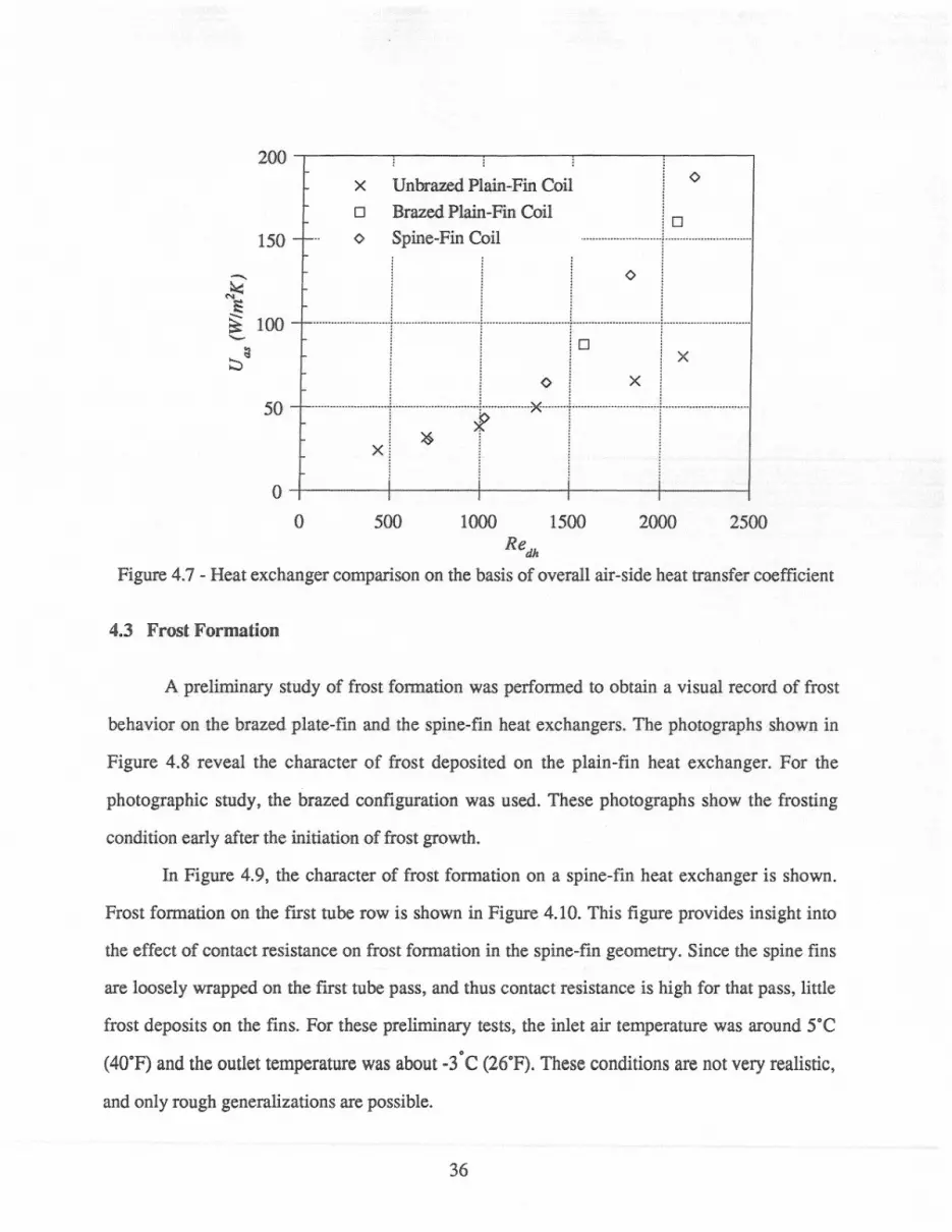
In Figure 4.7, Uas (i.e., l/RasAtotal) is presented as a function of air-side Reynolds number
for each of the heat exchangers. When area changes and tube-side resistance are considered, the
brazed plain-fin heat exchanger performs better than the unbrazed heat exchanger. Contact
resistance in the unbrazed configuration is believed to be responsible for this difference;
however, it is unclear why the effect appears to depend on Reynolds number. This behavior may
be due to temperature effects on thermal contact pressure. Interestingly, with area and tube-side
resistance effects included, the spine-fin and plain-fin coils have a comparable Uas• However, the
spine-fin geometry has more heat transfer area (See Figure 4.2). Least-squared-error fits to the
as-manufactured plain-fin and spine-fm 'performance·resultsare,.given in Eqs. 4.1 and 4.2.
U asAT = 19. 27exp{0. 0006784Redh} (as-manufactured plain-fin) (4.1)
(as-manufactured spine-fin) (4.2)
35
200~------~------------~------~----~
x Unbrazed Plain-Fin Coil o
o Brazed Plain-Fin Coil !D N~ 150 - _.. 0 Spine-Fin Coil-··········:····l···············_··
~~ 100 -~-111~--j-=---I I 0 I x I
50 +--j-~-l-*-r--t---
I iii O~-------+-I------~I------~I--------+-I----~
o 500 1000 1500 2000 2500 Redh
Figure 4.7 - Heat exchanger comparison on the basis of overall air-side heat transfer coefficient
4.3 Frost Formation
A preliminary study of frost formation was performed to obtain a visual record of frost
behavior on the brazed plate-fin and the spine-fin heat exchangers. The photographs shown in
Figure 4.8 reveal the character of frost deposited on the plain-fin heat exchanger. For the
photographic study, the brazed configuration was used. These photographs show the frosting
condition early after the initiation of frost growth.
In Figure 4.9, the character of frost formation on a spine-fin heat exchanger is shown.
Frost formation on the first tube row is shown in Figure 4.10. This figure provides insight into
the effect of contact resistance on frost formation in the spine-fin geometry. Since the spine fins
are loosely wrapped on the first tube pass, and thus contact resistance is high for that pass, little
frost deposits on the fins. For these preliminary tests, the inlet air temperature was around 5°C
(40"F) and the outlet temperature was about -3·C (26°F). These conditions are not very realistic,
and only rough generalizations are possible.
36
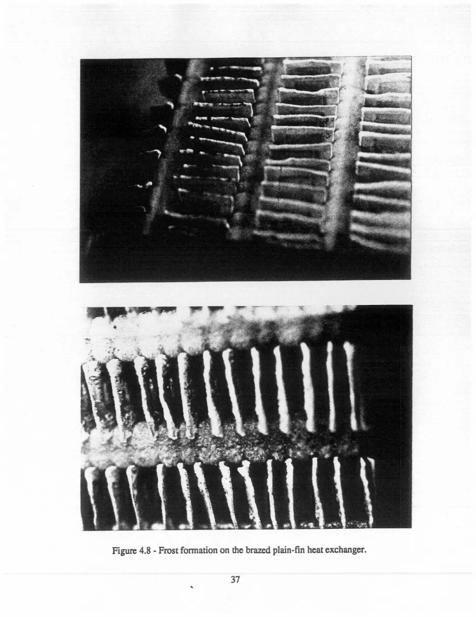
Figure 4.8 - Frost formation on the brazed plain-fin heat exchanger.
37

Figure 4.9 • Frost fmmation on the spine-fin heat exchanger
38
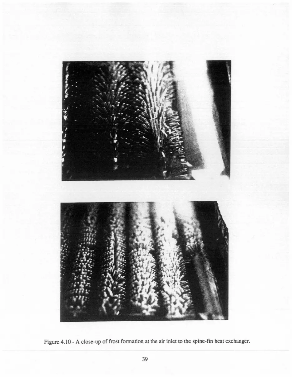
Figure 4.10 • A close-up of frost formation at the air inlet to the spine-fin heat exchanger.
39
Chapter 5 - Conclusions and Recommendations
5.1 Summary and Conclusions
This main objective of this research was to design, build and validate a calorimetric wind
tunnel suitable for testing heat exchangers used in air-conditioning and refrigeration applications.
A secondary objective was to explore the thermal performance of particular plain-fin and spine
fin evaporators used in residential refrigerator applications, with attention directed toward
contact resistance in the plain-fm geometry. A third objective was to present a preliminary study
of frost deposition patterns on these heat exchangers. These objectives were fulfilled through the
following progress:
• A wind tunnel was designed and built to provide
-air mass flow rates up to about 725 kg/hr (1600 lb/hr)
-approach air temperatures from -23 to 49DC (-10 to 120DF)
-air relative humidity from about 30% to 90%
-coolant mass flow rates up to about 500 kg/hr (1100 lb/hr)
-heat transfer surface temperatures down to about -23DC (_lODF)
• The calorimetric wind tunnel performance is as follows:
-approach velocity profiles are flat to within 3.4% over the entire test range
-approach temperature profiles are flat to within ±0.1 DC (0.2DF)
-energy transfer rates may be determined to within ±5%
-overall energy balances are typically within ±3% (7% worst case)
• Data reduction techniques, based on an £-NTU and modified Wilson Plot approach,
were developed to determine the air-side performance of complex heat exchanger
geometries. These methods account thermal resistances due to in-tube convection,
conduction through the tube, fin-tube contact, and conduction and convection within
the fins. Data fidelity was improved by forcing a common slope on the Wilson Plot data
for each particular heat exchanger. The following results were obtained:
40

- The overall heat exchanger conductance, U AT, is highest for the spine fin heat
exchanger (about twice that of the plain-fm) for air-side Reynolds numbers from
500 to 3000 based on hydraulic diameter.
- Under dry-surface conditions, the brazed plain-fin exchanger performs with a UAT
about 20% higher than an identical as-manufactured (unbrazed) heat exchanger. The
difference between brazed and unbrazed performance is probably due to contact
resistance; unfortunately, no experiments were conducted to explore the effects of
frost or water retention on contact resistance. It is therefore unclear whether contact
resistance is important under normal operating conditions.
- When variations in total area and tube-side performance are included, the plain-fm
exchanger has an overall air-side heat transfer coefficient, Uas, roughly equal to that
of the spine-fin geometry.
• Limited visual studies of frost deposition show that contact resistance influences the
growth of frost. At locations where poor fin-tube contact existed, frost was not
deposited on the fins. Frost deposition depends on the surface temperature distribution,
and these visualization studies were limited to cases in which the entire exchanger was
not below the frost point.
S.2 Recommendations and Future Work
With the experimental facility complete and the data acquisition and reduction methods
developed, future research directed toward characterizing heat exchanger performance is
possible. Further work with the plain-fm and spine-fm designs might be fruitful. For example,
experiments with the should be conducted at lower Reynolds numbers and under frosted
conditions to determine whether contact resistance effects are important under realistic operating
conditions. In order to explore manufacturing effects and variability, specimens that were
prepared using different manufacturing techniques should be tested.
A few minor improvements to the apparatus may help in future testing. In particular, the
tube-side fluid or the mass flow meter should be changed to obtain data at higher tube-side flow
41

rates. This change would improve the Wilson Plot results by allowing a wider range of NUr to be
recorded. It may also be useful to add redundant thermocouples in the tube-side flow. This
change might reduce the uncertainty in (Jr. Finally, data interpretation methods should be
explored with the goal of removing the systematic energy-balance bias discussed in Chapter 4.
As research in air-side heat transfer enhancements continues, it is important to take the
model results from detailed convection studies to the evaporator calorimeter for to-scale testing.
Heat exchanger scaling is complex, and full-scale testing is required to assess the true merit of
candidate surface designs. Through this approach, the goal of developing new heat exchanger
surfaces, exploiting manufacturing capabilities, can be realized.
42

Appendix A - Heat Exchanger Dimensions
Heat exchanger dimensions, which may be inferred from Chapter 2, are presented in this
Appendix.
A.I Plain-Fin Heat Exchanger
ST=25.4 mm (1 in)
ST=25.4 mm (1 in)
A.2 Spine-Fin Heat Exchanger
approximate collar width is 4 mm (0.16 in)
fin-tip to fm-tip height is approximately 70 mm (2.75 in), but c=76.2 mm (3 in).
Df = 25.4 mm (1 in)
1=9.09 mm (0.358 in)
L =203.2 mm (8 in)
p = 3.15 fins/em (8 fins/inch)
Smin =16.7 mm (0.657 in) (minumum distance outer tube surface to outer tube surface)
SL= 25.0 mm (0.986 in)
ST = 22.2 mm (0.875 in)
w = 0.76 mm (0.03 in)
43
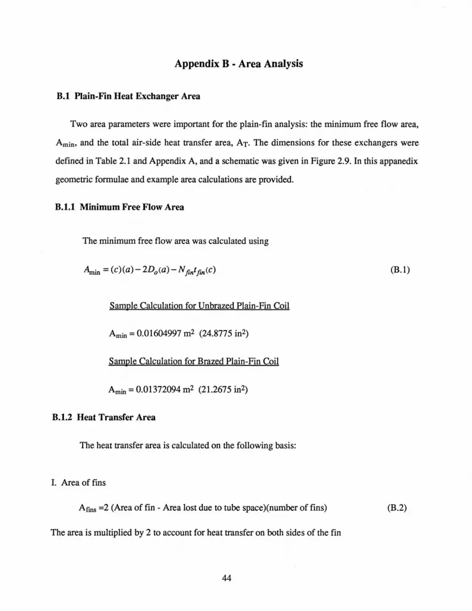
Appendix B - Area Analysis
B.I Plain-Fin Heat Exchanger Area
Two area parameters were important for the plain-fin analysis: the minimum free flow area,
Amin, and the total air-side heat transfer area, AT. The dimensions for these exchangers were
defined in Table 2.1 and Appendix A, and a schematic was given in Figure 2.9. In this appanedix
geometric formulae and example area calculations are provided.
B.I.I Minimum Free Flow Area
The minimum free flow area was calculated using
Sample Calculation for Unbrazed Plain-Fin Coil
Amin = 0.01604997 m2 (24.8775 in2)
Sample Calculation for Brazed Plain-Fin Coil
Amin = 0.01372094 m2 (21.2675 in2)
B.I.2 Heat Transfer Area
The heat transfer area is calculated on the following basis:
I. Area of fms
A fms =2 (Area of fin - Area lost due to tube space )(number of fins)
The area is multiplied by 2 to account for heat transfer on both sides of the fin
44
(B.l)
(B.2)

AT,fin = (area of short fins) + (area of long fins)
II. Area of tubes
ill. Total Heat Transfer Area
Sample Calculation for Unbrazed Plain-Fin Coil
I. Area of fms
Area of short fins = (1240.817344 in2)
Area of long fins = (1399.817344 in2)
AT,fin = 1.703632 m2 (2640.634688 in2)
II. Area of tubes
Atubes =0.25234 m2 (391.128 in2)
lIT. Total Heat Transfer Area
AT = 1.95597 m2 (3031.763 in2)
Sample Calculation for Brazed Plain-Fin Coil
AT= 1.64226 m2 (2545.511 in2)
B.2 Spine-Fin Heat Exchanger Area
(B.3)
(B.4)
(B.5)
Area calculations are more complex for the spine-fin coil. Coil dimensions are given in
Table 2.1, Appendix A and Figure 2.10. Using these measurements,
A =lw s
Afr = (c)(a)
45
(B.6)
(B.7)
(B.8)

~ = (c) (a) - 3Doa - 3(p)(a)(tfm)(Dt - Do)
Ar = 48( n-( Dl-D;) / 4 )p(a) + 247dJoa
(B.9)
(B.1O)
(B.11)
(B.12)
In equation B.12. the number of fin-goufins per tube is (p)(a). While B.12 is approximate, this
method was adopted because a more careful formulation was vitiated by nonuniformities in the
spine fins and the overall coil construction.
Sample Calculation for Spine-Fin Coil
As = 6.92902(10-6) m2 (0.01074 in2)
Amin =0.00834494 m2 (12.93468 in2)
Afr = 0.0113679 m2 (17.6203 in2)
V = 0.0289882 m3 (44.9318 in3)
A = 0.0299274 m2 (46.3876 in2)
Amin=0.02210076 m2 (34.25625 in2)
AT = 3.65 m2 (5659.28 in2)
46
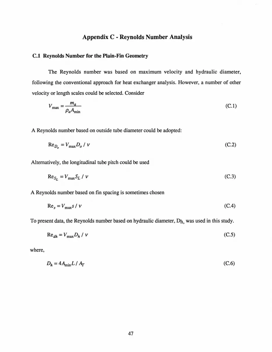
Appendix C - Reynolds Number Analysis
C.I Reynolds Number for the Plain-Fin Geometry
The Reynolds number was based on maximum velocity and hydraulic diameter,
following the conventional approach for heat exchanger analysis. However, a number of other
velocity or length scales could be selected. Consider
v = rna max Pa~
A Reynolds number based on outside tube diameter could be adopted:
Alternatively, the longitudinal tube pitch could be used
A Reynolds number based on fin spacing is sometimes chosen
(C.l)
(C.2)
(C.3)
(C.4)
To present data, the Reynolds number based on hydraulic diameter, Dh, was used in this study.
(C.5)
where,
(C.6)
47

C.2 Reynolds Number for the Spine-Fin Geometry
The spine-fm coil was analyzed following the approach of Holtzapple and Carranza [17].
(C.7)
where,
(C.8)
(J = _Amm_"_ = --'STO---_D..,.o_-_2_1w-'f'--s Afr ST
(C.9)
A 1CDo + p(As - wt) a = - = -""--":"""':'-':<---:;"
V SLSr (C.lO)
48

Appendix D - DOWTHERM 4000 Properties
DOWTHERM 4000 is a product that was made by Dow [28] which is 92.4% ethylene
glycol, and 7.6% inhibitors and water. During the experiments, DOWTHERM 4000 was mixed
with water. The specific gravity of the mixture was determined using a precision hydrometer.
These data were used with the manufacturer's data shown in Figure D.1 to determine the mixture
composition. During experiments, the specific gravity of the mixture used was 1.0960 which
corresponds to a 56.92% ethylene glycol based on volume-the mixture composition was
constant during this study. Using this composition, the other relevant thermophysical properties
were determined using the manufacturer's data (See Figures D.2 - D.5).
85 .............................. : ................................ : ................................ : .................. u··········· .. r························ .. ··· .. :
iii i i 80 ......... -........ --......... -~ ... -.-............... --......... i ................................ J ..... --......................... ! ........... --.... ----- -.... -.. ~
! ~ iii ! ~ i ~ i
75 ! 1 ! i ! .............. --•••••••••••••• .:. ••••••••••••••••••••••••••••.•.• ; ••••• ---•••••••••••.•••••••••••• .:. •••••••••.••••••••• --••.••• -•••• ; ..................................... -c : :: : -0
~ 70 0 0
5 65 -i»
~ ~ 60 0
] 55 0 >
50
i !! ! : :: : ! ~ ! . ! ····· .. ···· .. · .. ··· .. ·· .. · .. ·······r················ .. ···············!·· .. ·· .. ·························r··········· ·· .. ················t·······························1
II! 1 1
=:t:=J:~==--=.:l==1 =~=:==r:=~:=j:~=:I=::::1
1 l l l 1 45 4--------1--------4--------4--------+-------~
1.08 1.09 1.1 1.11 1.12 1.13 Specific Gravity
Figure D.1 - Volume percent Ethylene Glycol versus Specific Gravity for DOWTIIERM 4000 at 70°F.
49

0.8
0.76
--.. t 0.72 :9 ~ ..... IXI '-' J>.68 u
0.64
_ 0--
------------------------------i--------------------------------+--------------------------------i-------------------~--------------------------------i
1 I ; 1 -*-70~ 1 1 -a- 60% T-r"---r----r =-:~;~: %
0.6 ~--------r_------_+--------+_------~--------~
o 20 40 60 Temperature tF)
80 100
Figure D.2 - Specific Heat for DOWTHERM 4000 at different Temperatures and Percentages of Ethylene Glycol.
71 .~n ••••••• _ ••••• _ •••••••••••••• n ••••••••••••• _._ •••••••••••••••••••••••••••••••••••••••••••••••••••••••••••••••••••••••• __ ._ •••••••••••••••• ___ •••••••••••• u ••••• . . . . . . . . . .
I I I I I 70.5
70 --..
<"l
~ 69.5 -....... » ..... .... rI.l 69 5 0
68.5
68
-~ i i .............. o i . i -~--::··=~·------.:.--~..:::--··---.. ·-·--------------T------------···---~-~·---------------------.. -···---r-----·-.... ·--------·----------1
'_ 1 -0_ 1 1 .............. 1 . ''f--,-~ i 0 i ~-70%
----------------------·-------1---------:-:--'*.::------------j--::::..--------------------------t--------------------~- .. --i - - ~ --0 _ i 1 -a- 60% i i'-,~ ~_ i
-------.----------------------!-------------.. -.. -.------------j-----------.-------:::-::::---.J,----------~--~-------~-.---- - <>- 56.92% : : '!'- ~
! ! ! "~ , ; - ~- -50% : : : ..... : : : : -:
67.5
0 20 40 60 80 100 Temperature tF)
Figure D.3 - Density for different Ethylene Glycol mixtures versus temperature.
50

100
120
~:[~~::I:l=C · . . . · . . . · . . . · . . . : : : : : : : : -B- 60%
,.-.. 80 ¢:: ------------------------1------------ ------------1---------------------------1---------------------------1--------- - <>- 56.92%
* 1-< e :0-
60 -'-' ;;>. .... ..... {Il
0 u
~; iii - ~- -50% · . . . ~
. : : : . . . . . , . . · . . . . -----------------------l--~-~---------------j--------------------------I--------------------------l--------------------------I--------------------------
· . . . , · . . . . · . . . . 'K ~ iii i
{Il 40 ..... >
20
0
-20 o 20 40 60 80 100 Temperature (OP)
Figure D.4 - Viscosity of Ethylene Glycol at different percentages of the mixture versus temperature.
0.23
0.22
,.-.. 0.21 ~ o
* ¢::
* 13 0.2
~ iX-l '-' ~ 0.19
0.18
0.17
o
•••••••• -- ••••••••••••••••• --y •••••• ---.--------•••••• - ••••••• , •••••••••• - ••• ----•••• ---....... -~ •••••••••••••••••••• _---•••••••• , ••••• _-••••• __ ••••••••••••••• --••• · . . . . · . . , . · . . . . · . . . , · . . . . · . . . . · . . . , · . . . . · . . . . iii _ -* j
-----------------------------t-------------------------------t---------------------------~--~--:::--;.:--""-*---::----------1---------------------------------1
; ; x-; ; ; i -.J-:- - iii
~~~~~;~~~~~-~~~~-~:I __ 0' Jr--- iii i
------------~----f--------------------------------j---------------------------------r-----------------------------j------· .. ----x----- 70%
: j -~j -a- 60%
------------------------~~~~~~=-----------t--------------------------------I------- ---0-- 56.92% ___ --x--- ! ! ! ! _ ~ __ 50%
20 40 60 80 100 Temperature (OP)
Figure D.5 - Thennal Conductivity of Ethylene Glycol with different percentages and temperatures.
51

Appendix E - Uncertainty Analysis
E.I Uncertainty in Measurements
In order to calculate the uncertainty in the overall heat transfer, it is necessary to know
the uncertainty of the individual measurements. In this study, the following information was
recorded by the data acquisition system: 18 temperatures, pressure drop across the orifice plate,
relative humidity, and refrigerant mass flow rate. In addition, correlations had to be used for
thermal physical properties. In Table E.1, the relevant experimental parameters and properties
are listed with estimated uncertainties.
During this study the thermocouples were calibrated to increase the accuracy of their
readings. In this calibration, an isothermal bath was used to calibrate the thermocouples,
however, a uniform curve fit was desirable for the ease in implementation. The curve fit as
prescribed by Omega [33] which was based on the National Bureau of Standards was used. It
was found that the individual curve fits were inaccurate due to the stratification in the isothermal
bath and the placement of the thermal couple rakes in the bath. The rakes were not
disassembled, and therefore, they could not have been placed at a centralized location. As a
result, the generalized curve fit was used and checked three times at room temperature in an
isothermal insulated box. It was concluded that using this correlation, the thermocouples were
within 0.1 0C of each other and an ASTM certified thermometer.
The pressure readings were checked and verified during each test run. The pressure
transducer was calibrated with a special limits of error. The calibration states that the best
straight line method that was used had a ± .073% uncertainty over the full scale. In addition,
during each test run, a manometer was used to verify the reading.of the pressure transducer. This
manometer had a range from 0 to 10 inches of H20 with increments of .01 for 1 in of H20 or
less, and .1 for 1 in of H20 and larger. During each run, the manometer and the pressure
differential would have the same reading.
52

Table E.l - Variables resolution and their uncertainties.
Variable (measurement) Change in variable (d(x» Uncertainty (%) (d(x)/x)
a (Coil #1) (20.75") .0625 " .30
a (Coil #2) (17.75") .0625 " .35
a (Coil #3) (19.6875") .0625 " .32
b (Coil #1) (23.5") .0625 " .27
b (Coil #2) (20.375") .0625 " .31
b (Coil #3) (21.5") .0625 " .29
c (Coil #1 & 2) (2") .0625 " 3.1
c (Coil #3) (3") .0625 " 2.1
~ (plate with d=1.35) .014
~ (plate with d=2.10) .014
~ (plate with d=3.00) .014
Cpa 10.5
Cpr 10
c (plate with d=1.35) .816 (.6 +~)
c (Plate with d=2.1O) .936 (.6 +~)
c (plate with d=3.00) 1.08 (.6 +~)
d (plate with d=1.35) .001" .07
d (plate with d=2.10) .001" .05
d (plate with d=3.00) .001" .03
D .0625 " 1
DO* .01 inch 2.6
e .1 (4M>/P)
mfr .15
53

AI> .146
Relative Humidity 4
tfm .001 in. 20
ttube .001 in. 3.33
S.O. .0005 .05
ATa.r .2oC
Pa 1.13
Pr
* Do had a variation in diameter due to the expansion of the tube.
E.2 Uncertainty in Experimental Data
The uncertainty will be divided up into two sections: an energy balance, and a modified
Wilson plot section. In the uncertainty analysis, the Pythagorean summation of the discrete
uncertainties [34] was utilized.
E.2.1 Energy Balance Uncertainties
The error in uncertainty in the energy balance also includes the uncertainty of the air flow
rate and water flow rate. To fmd the energy balance, the values for qa and qr were calculated
from Equations 3.1 and 3.2. The uncertainty in the energy balances were computed using
equations E.1, E.2, and E.3.
(::'f = (2:ddf +(~f +(~f {5:~pf {5:dpf +(2:~~:d~r (E.1)
[ dQ~] 2 = [dmfa] 2 + [ dCpa ] 2 + [ ddeltaTa ] 2 Qair mfa Cpa. 1000 T ai - Tao
(E.2)
54

[ dQref] 2 = [dmfr] 2 + [ dCpr ] 2 + [ ddeltaTr ] 2
Qref mfr Cpref. 1000 T ro - T ri (E.3)
E.2.2 Wilson Plot Uncertainties
In the modified Wilson plot the variables that were used were Ua, and NurDh. From
Whitaker [35], the "error in the experimentally determined Nusselt numbers is on the order of
±25%". This was the only reference that is made to the error of using this specified Nusselt
number correlation. The error on Ua was developed in equations E.4 through E.6.
dUA =( BUA J*dNTU +(BUA)*dC BNTU p p BCal al
(E.4)
( dUA)2 = (dNTUp J2 +(dCal)2 UA NTUp Cal
(E.5)
( dCal)2 = (dmfa)2 +(dCpa)2 Cal mfa CPa
(E.6)
55

Appendix F - Test Data
Table F.l - Raw data for the unbrazed plain-fin heat exchanger Test mfa(kg/s) mfr(kg/s) Tai(C) Tao(C) Tri (C) Tro(C) Relative
Humiditv 1.01 0.04306 0.04554 17.833 12.583 6.464 8.222 0.74 1.02 0.07961 0.06611 18.315 14.051 6.79 8.59 0.39 1.03 0.07967 0.07597 18.135 13.885 6.87 8.453 0.41 1.04 0.07962 0.08112 17.978 13.772 6.95 8.406 0.41 1.05 0.09239 0.06277 19.525 15.275 7.119 9.274 0.38 1.06 0.09241 0.06959 19.247 14.974 6.895 8.889 0.42 1.07 0.0922 0.07498 19.27 14.982 7.044 8.896 0.47 1.08 0.09201 0.08099 19.073 14.809 7.073 8.784 0.49 1.09 0.09224 0.08318 19.019 14.792 7.138 8.784 0.5 1.1 0.04311 0.04139 17.939 12.791 6.714 8.636 0.49
1.11 0.04317 0.05198 17.181 12.229 6.689 8.167 0.56 1.12 0.04301 0.0579 17.322 12.094 6.801 8.189 0.8 1.13 0.04294 0.06205 17.327 12.056 6.823 8.113 0.81 1.14 0.05669 0.06143 22.469 17.01 10.001 11.716 0.39 1.15 0.05662 0.06716 22.695 17.089 10.026 11.637 0.43 1.16 0.05655 0.07372 22.74 17.071 10.051 11.569 0.43 1.17 0.04222 0.0627 23.863 17.515 11.132 12.621 0.66 1.18 0.04227 0.07614 23.898 16.996 10.202 11.548 0.66 1.19 0.04225 0.08789 24.258 17.439 10.888 12.056 0.64 1.2 0.04223 0.1023 24.739 17.576 10.924 11.999 0.61
1.21 0.05535 0.07543 30.756 22.11 11.909 14.113 0.34 1.22 0.05532 0.08791 30.62 21.884 11.909 13.849 0.33 1.23 0.05704 0.10111 19.313 15.68 11.429 12.178 0.51 1.24 0.05707 0.11185 19.493 15.777 11.526 12.246 0.5 1.25 0.0184 0.06326 23.816 14.163 9.364 10.411 0.65 1.26 0.0184 0.07487 23.982 14.161 9.422 10.306 0.7 1.27 0.01845 0.08309 24.042 14.108 9.361 10.188 0.71 1.28 0.01841 0.08828 24.1 14.113 9.335 10.127 0.71 1.29 0.01838 0.10048 24.153 14.081 9.393 10.094 0.72 1.3 0.03041 0.06273 21.341 15.72 11.261 12.246 0.79
1.31 0.02995 0.0652 24.68 18.883 14.373 15.338 0.7 1.32 0.02995 0.07449 24.677 18.774 14.313 15.17 0.67 1.33 0.02993 0.08182 24.699 18.766 14.405 15.195 0.64 1.34 0.03023 0.08841 23.22 16.563 11.508 12.357 0.71 1.35 0.03023 0.102 23.037 16.43 11.594 12.346 0.72 1.36 0.0302 0.11081 23.136 16.355 11.53 12.257 0.73 1.37 0.07968 0.06143 15.677 13.68 10.188 11.075 0.75 1.38 0.07978 0.07507 15.657 13.624 10.163 10.913 0.78 1.39 0.0796 0.08189 15.716 13.586 10.13 10.849 0.78 1.4 0.07848 0.08799 20.594 16.597 10.457 11.702 0.65
1.41 0.07837 0.09887 21.435 17.034 10.504 11.738 0.61 1.42 0.09014 0.07559 25.173 19.447 9.191 11.558 0.5 1.43 0.09098 0.07574 23.317 17.148 6.178 8.784 0.59 1.44 0.09022 0.08335 25.205 19.359 9.191 11.379 0.52 1.45 0.09027 0.08782 25.326 19.403 9.213 11.329 0.54 1.46 0.09003 0.10067 25.471 19.36 9.26 11.182 0.57 1.47 0.08962 0.10987 26.275 20.308 10.852 12.636 0.57
56

Table F.2 .:. Important variables calculated for the unbrazed plain-rm heat exchanger Test UA(W/K) Qair(W) Qref(W) ReD Res ReretD NuDref
1.01 32.988 229.749 242.633 1447.814 741.281 832.125 6.969 1.02 44.233 343.24 360.778 2653.953 1358.824 1224.636 7.89 1.03 45.704 342.373 364.688 2657.787 1360.787 1405.631 8.265 1.04 45.645 338.667 358.363 2656.913 1360.34 1502.069 8.448 1.05 46.01 397.128 410.407 3071.207 1572.458 1186.382 7.754 1.06 47.346 399.689 420.851 3075.979 1574.901 1299.551 8.026 1.07 47.726 400.486 421.412 3071.455 1572.585 1404.474 8.228 1.08 48.487 397.514 420.624 3067.301 1570.458 1514.502 8.442 1.09 48.175 395.171 415.634 3075.569 1574.691 1557.581 8.518 1.1 33.898 224.667 241.29 1443.684 739.166 766.314 6.75
1.11 34.658 216.569 233.081 1448.754 741.762 952.959 7.283 1.12 36.67 228.678 243.746 1448.786 741.778 1064.262 7.55 1.13 36.299 230.232 242.892 1446.828 740.776 1139.412 7.727 1.14 37.811 313.314 321.081 1877.653 961.358 1288.401 7.696 1.15 38.062 321.742 329.731 1876.519 960.778 1406.976 7.928 1.16 39.63 324.918 341.011 1874.233 959.607 1543.135 8.178 1.17 34.63 273.073 285.037 1404.171 718.936 1367.632 7.747 1.18 35.034 297.095 312.262 1407.162 720.467 1597.786 8.267 1.19 36.227 293.435 313.28 1405.06 719.391 1887.513 8.672 1.2 38.066 307.923 335.565 1403.097 718.385 2195.934 9.122
1.21 40.06 485.351 507.941 1811.429 927.452 1718.517 '8.237 1.22 41.61 489.924 521.095 1810.743 927.1 1992.646 8.669 1.23 43.935 210.202 231.065 1898.835 972.204 2199.27 9.087 1.24 47.319 215.066 245.819 1899.076 972.327 2440.634 9.398 1.25 27.667 180.487 201.51 615.964 315.374 1277.566 7.774 1.26 26.84 183.736 201.658 616.262 315.526 1510.806 8.223 1.27 28.395 186.353 209.258 618.047 316.44 1670.762 8.514 1.28 29.073 187.04 212.66 616.976 315.892 1772.021 8.688 1.29 29.567 188.315 214.566 616.014 315.399 2018.004 9.071 1.3 31.168 174.347 188.585 1017.117 520.764 1361.708 7.749
1.31 31.341 177.322 192.77 994.548 509.209 1593.483 7.846 1.32 31.617 180.414 195.875 994.119 508.989 1812.594 8.203 1.33 32.527 181.046 198.186 992.78 508.303 1995.361 8.463 1.34 33.057 205.101 229.068 1008.117 516.156 1932.549 8.689 1.35 35.685 203.567 234.183 1008.545 516.375 2232.848 9.113 1.36 38.066 208.738 245.948 1007.935 516.063 2418.544 9.368 1.37 42.344 161.893 166.02 2673.73 1368.95 1276.96 7.697 1.38 43.366 165.083 171.703 2678.562 1371.424 1554.901 8.23 1.39 44.674 172.621 179.241 2672.699 1368.422 1692.916 8.472 1.4 46.277 319.344 333.889 2614.453 1338.6 1861.099 8.675
1.41 48.04 350.972 371.93 2606.378 1334.465 2094.597 9.019 1.42 47.154 524.825 544.606 2977.333 1524.395 1555.874 8.246 1.43 48.655 570.847 598.198 3024.117 1548.348 1391.51 8.255 1.44 47.789 536.454 555.072 2981.647 1526.603 1709.683 8.519 1.45 48.382 544.151 565;658 2984.489 1528.058 1800.336 8.669 1.46 50.188 560.315 589.038 2978.8 1525.146 2059.605 9.073 1.47 54.712 545.196 597.863 2960.16 1515.602 2384.341 9.34
57

Table F.3 - Raw data for the brazed plain-fin heat exchanger
Test mfa(kg/s) ffifr (kgls) Tai (C) Tao{C) Tri (C) Tro(C) Relative Humidity
2.01 0.01768 0.09444 33.983 19.57 14.516 15.618 0.75 2.02 0.04072 0.08882 33.671 23.32 15.838 17.565 0.61 2.03 0.04099 0.07526 3l.726 2l.618 13.796 15.778 0.67 2.04 0.04073 0.08254 33.438 23.313 15.792 17.618 0.63 2.05 0.04085 0.06355 32.269 22.763 15.082 17.246 0.63 2.06 0.0408 0.0948 33.454 23.26 15.856 17.515 0.6 2.07 0.04083 0.10087 33.461 23.126 15.849 17.427 0.6 2.08 0.05411 0.09417 32.741 23.764 15.97 17.89 0.59 2.09 0.0542 0.10856 33.046 23.418 15.49 17.303 0.61 2.1 0.05401 0.06281 32.851 24.762 17.03 19.471 0.54 2.11 0.05422 0.08905 32.38 23.624 15.917 17.862 0.59 2.12 0.05425 0.08274 32.068 23.577 15.87 17.897 0.58 2.13 0.0543 0.07503 32.055 23.65 15.892 18.06 0.56 2.14 0.05424 0.10126 32.822 23.67 15.977 17.791 0.6 2.15 0.07487 0.10908 3l.793 24.078 16.325 18.261 0.66 2.16 0.07638 0.10051 28.18 2l.016 12.986 14.986 0.66 2.17 0.07645 0.08805 28.217 21.179 12.957 15.153 0.65 2.18 0.07645 0.08171 28.211 21.262 12.929 15.252 0.67 2.19 0.07644 0.07689 28.245 21.353 12.879 15.338 0.67 2.2 0.07637 0.06311 29.321 22.216 12.679 15.707 0.59 2.21 0.0873 0.10134 3l.976 24.739 16.378 18.618 0.59 2.22 0.08692 0.06341 32.613 25.89 16.566 19.781 0.57 2.23 0.08738 0.10619 31.875 24.618 16.371 18.529 0.59 2.24 0.08725 0.08107 32.284 25.295 16.463 19.101 0.57 2.25 0.08719 0.07546 32.359 25.451 16.516 19.313 0.57 2.26 0.08733 0.08828 32.229 25.145 16.484 18.974 0.57 2.27 0.10088 22.706 14.062 10.586 11.311 0.79
58

Table F.4 - Important variables calculated for the brazed plain-fin heat exchanger Test UA(WfK) Qair(W) Qref(W) ReD Res ReretD NuDref 2.01 46.891 260.799 319.184 686.85 351.667 2279.116 9.31 2.02 45.561 431.53 471.331 1567.098 802.354 2253.444 9.117 2.03 43.083 424.189 457.009 1584.449 811.238 1800.755 8.63 2.04 45.238 422.533 463.084 1568.593 803.119 2094.34 8.897 2.05 41.136 397.557 422.112 1574.321 806.053 1585.941 8.154 2.06 48.719 425.616 483.269 1569.736 803.705 2403.978 9.318 2.07 49.489 431.839 489.101 1571.527 804.622 2554.168 9.513 2.08 55.635 497.225 555.672 2079.694 1064.803 2406.068 9.296 2.09 58.74 534.342 604.47 2085.623 1067.839 2728.574 9.748 2.1 48.628 446.99 471.907 2069.651 1059.662 1672.541 8.12 2.11 53.489 485.932 532.262 2084.546 1067.288 2272.408 9.125 2.12 52.419 471.333 515.361 2085.361 1067.705 2110.996 8.904 2.13 50.449 466.689 499.862 2085.685 1067.871 1919.762 8.618 2.14 56.258 508.252 564.526 2085.622 1067.839 2583.548 9.524 2.15 67.105 592.933 649.344 2882.491 1475.835 2818.537 9.762 2.16 63.236 559.575 615.167 2954.011 1512.454 2346.452 9.504 2.17 59.824 550.221 591.694 2955.418 1513.174 2059.947 9.094 2.18 58.449 543.607 580.822 2956.433 1513.694 1913.715 8.87 2.19 58.035 539.098 578.516 2955.423 1513.176 1801.826 8.691 2.2 53.505 554.533 584.544 2942.77 1506.698 1482.761 8.136 2.21 69.306 647.514 698.049 3350.644 1715.53 2635.313 9.525 2.22 59.78 599.324 627.064 3328.348 1704.114 1684.388 8.144 2.23 70.654 649.778 704.673 3354.184 1717.342 2757.304 9.675 2.24 63.412 624.928 657.725 3343.778 1712.014 2127.03 8.841 2.25 62.626 617.401 649.16 3340.845 1710.513 1988.115 8.631 2.26 65.975 633.903 676.059 3347.664 1714.004 2312.347 9.096
59

Table F.5 - Raw data for the spine-fin heat exchanger Test mfa{kg/s) mfr(kg/s) Tai (C) Tao(C) Tri (C) Tro(C) Relative
Humidity 3.01 0.02959 0.07564 27.356 17.988 13.057 14.502 0.74 3.02 0.02959 0.08168 27.385 18.034 13.1 14.469 0.74 3.03 0.0296 0.09408 27.645 18.072 13 14.266 0.71 3.04 0.02958 0.06935 27.311 18.355 13.81 15.22 0.72 3.05 0.02965 0.08831 27.526 17.912 12.968 14.274 0.74 3.06 0.02961 0.06334 27.279 18.263 13.297 14.943 0.75 3.07 0.04224 0.09425 22.997 15.751 11.333 12.636 0.62 3.08 0.04235 0.08212 22.879 15.656 11.286 12.714 0.59 3.09 0.04237 0.07027 22.605 15.576 11.225 12.811 0.59 3.1 0.04236 0.07601 22.773 15.604 11.282 12.786 0.59
3.11 0.04236 0.08804 22.945 15.721 11.275 12.636 0.58 3.12 0.04236 0.06278 22.521 16.102 11.308 13.029 0.59 3.13 0.05644 0.09204 20.967 15.379 11.451 12.775 0.62 3.14 0.05642 0.08878 21.019 15.405 11.44 12.807 0.63 3.15 0.05641 0.06905 21.02 15.623 11.437 13.079 0.64 3.16 0.05644 0.08211 21.037 15.486 11.429 12.875 0.64 3.17 0.05642 0.06308 21.021 15.663 11.487 13.243 0.64 3.18 0.05645 0.07573 21.096 15.548 11.397 12.943 0.64 3.19 0.07544 0.08818 30.988 18.448 9.515 13.247 0.71 3.2 0.07554 0.09425 30.852 18.399 9.648 13.136 0.73
3.21 0.07565 0.08212 30.355 18.187 9.443 13.311 0.72 3.22 0.07571 0.07508 29.821 18.055 9.22 13.364 0.72 3.23 0.07571 0.0701 30.3 18.314 9.321 13.728 0.71 3.24 0.0757 0.06399 30.302 18.424 9.245 14.01 0.72 3.25 0.08986 0.09453 23.53 17.571 12.128 14.213 0.62 3.26 0.08995 0.08806 23.467 17.551 12.06 14.252 0.62 3.27 0.09013 0.07552 23.231 17.46 11.906 14.345 0.6 3.28 0.09017 0.08272 23.331 17.494 11.995 14.266 0.61 3.29 0.09012 0.06202 23.332 17.753 11.956 14.811 0.62 3.3 0.09026 0.06914 23.249 17.529 11.856 14.48 0.6
60

Table F.6 .,; Important variables calculated for the spine-fm heat exchanger Test UA(WIK)- Qair(W) Qref(W) ReD RerefD NuDref
3.01 50.255 283.127 334.352 715.36 1754.679 7.419 3.02 53.213 282.628 342.325 715.24 1894.988 7.612 3.03 58.559 289.261 364.585 715.082 2172.476 7.979 3.04 44.586 270.508 299.6 714.283 1645.621 7.207 3.05 54.218 291.093 352.817 716.843 2038.419 7.813 3.06 48.325 272.81 319.267 715.584 1484.86 6.993 3.07 66.974 311.187 374.94 1023.033 2066.252 7.986 3.08 61.825 310.72 358.026 1025.206 1801.078 7.627 3.09 58.67 302.503 340.14 1025.804 1542.222 7.241 3.1 60.059 308.534 348.832 1025.688 1669.032 7.433
3.11 63.334 310.816 365.601 1025.093 1928.217 7.807 3.12 57.654 276.327 329.862 1024.659 1384.386 6.974 3.13 75.269 320.477 372.122 1367.741 2026.036 7.923 3.14 73.933 321.974 370.579 1367.537 1955 7.828 3.15 66.72 309.569 346.213 1366.976 1527.021 7.199 3.16 70.849 318.599 362.423 1368.16 1809.647 7.627 3.17 65.377 307.451 338.288 1367.206 1399.818 6.985 3.18 68.349 318.464 357.406 1368.208 1670.019 7.424 3.19 83.251 966.027 1001.864 1821.216 1895.686 7.807 3.2 84.111 961.01 1001.068 1824.567 2026.964 7.983
3.21 82.698 940.017 966.958 1827.566 1765.149 7.624 3.22 83.191 909.461 947.006 1829.394 1609.329 7.399 3.23 80.323 926.494 940.483 1828.091 1514.057 7.231 3.24 79.279 918.362 928.052 1827.921 1386.798 7.014 3.25 92.159 545.185 602.478 2168.729 2151.64 7.991 3.26 89.649 541.734 590.04 2170.821 2003.493 7.804 3.27 85.689 529.259 562.756 2174.827 1716.425 7.414 3.28 87.105 535.645 574.096 2175.898 1880.52 7.643 3.29 82.619 511.982 541.119 2174.178 1421.136 6.942 3.3 83.942 525.372 554.37 2177.489 1573.575 7.199
61

References
[1] Abott, R.W., Norris, R.H., and Spofford, W.A., 1980, "Compact Heat Exchangers in General Electric Products - Sixty Years of Advances in Design and in Manufacturing Technologies," Compact Heat Exchangers- History, Technological Advancement and Mechanical Design Problems, Vol. 10, pp. 37-55.
[2] London, A.L., 1980, "A Brief History of Compact Heat Exchanger Technology," Compact Heat Exchangers- History, Technological Advancement and Mechanical Design Problems, Vol. 10, pp. 1-4.
[3] Mori, Y. , and Nakayama, W., 1980, "Recent Advance in Compact Heat Exchangers in Japan," Compact Heat Exchangers- History, Technological Advancement and Mechanical Design Problems, Vol. 10, pp. 5-16.
[4] Rich, D., 1973, "The Effect of Fin Spacing on the Heat Transfer and Friction Performance of Multi-row, Smooth Plate Fin-and-Tube Heat Exchangers," ASHRAE Transactions, Vol. 79 (2), pp. 137-145.
[5] Rich, D., 1975, "The Effect of the Number of Tube Rows on Heat Transfer Performance of Smooth Plate Fin-and-Tube Heat Exchangers," ASHRAE Transactions, Vol. 81 (1), pp. 307-318.
[6] Saboya, F.E.M., and Sparrow, E.M., 1976, "Experiments on a Three-Row Fin and Tube HeatExchanger," Journal of Heat Transfer, Vol. 98, pp. 520-521.
[7] McQuiston, F.C., 1978, "Heat, Mass, and Momentum Transfer Data for Five Plate-FinTube Heat Transfer Surfaces ," ASH RAE Transactions, Vol. 84 (1), pp. 266-293.
[8] McQuiston, F.C., 1978, "Correlation of Heat, Mass, and Momentum Transport Coefficients for Plate-Fin-Tube Heat Transfer Surfaces with Staggered Tubes," ASHRAE Transactions, Vol. 84 (1), pp. 294-309.
[9] Mirth, D.R., and Ramadhyani, S., 1993, "Prediction of cooling-coil performance under condensing conditions," International Journal of Heat and Fluid Flow, Vol. 14 (4), pp. 391-400.
[10] Beecher, D.T., and Fagan, T.J., 1987, "Effects of Fin Pattern on the Air-Side Heat Transfer Coefficient in Plate Finned-Tube Heat Exchangers," ASHRAE Transactions, Vol. 93, pp. 1961-1984.
[11] Webb, R.L., 1990, "Air-Side Heat Transfer Correlations for Flat and Wavy Plate Fin-andTube Geometries," ASHRAE Transactions, Vol. 96 (2), pp. 445-449.
[12] Oskarsson, S.P., Krakow, K.I.. and Lin., S., 1990, "Evaporator Models for Operation with Dry, Wet, and Frosted Finned Surfaces Part I: Heat Transfer and Fluid Flow Theory," ASH RAE Transactions, Vol. 96 (1), pp. 373-381.
[13] Oskarsson, S.P., Krakow, K.I., and Lin, S., 1990, "Evaporator Models for Operation with Dry, Wet, and Frosted Finned Surfaces Part II: Evaporator Models and Verification," ASH RAE Transactions, Vol. 96 (1), pp. 381-392.
62

[14] Sheffield, I.W., Abu-Ebid, M., and Sauer, H.I., 1995, "Finned Tube Contact Conductance: Empirical Correlation of Thermal Conductance," ASHRAETransactions, Vol. 97 (2a), pp. 100-117.
[15 Timoney, 0.1., and Foley, P.I., 1994, "Some Effects of Air Flow Maldistribution on PeIformance of a Compact Evaporator with RI34a," Heat Recovery Systems & CHP, Vol. 14 (5), pp. 517-523.
[16] Barrow, H., and Sherwin, K., 1994, "Theoretical Investigation of the Effect of Fouling on the PeIformance of a Tube and Plate Fin Heat Exchanger," Heat Recovery Systems & CHP, Vol. 14 (1), pp. 1-5.
[17] Holtzapple, M.T., and Carranza, R.O., 1990, "Heat Transfer and Pressure Drop of Spined Pipe in Cross Flow-Part I: Pressure Drop Studies," ASHRAE Transactions, Vol. 96(2), pp. 122-129.
[18] Holtzapple, M.T., Allen, A.L., and Lin, K.,1990, "Heat Transfer and Pressure Drop of Spined Pipe in Cross Flow-Part II: Heat Transfer Studies," ASHRAE Transactions, Vol. 96(2), pp. 130-135.
[19] Holtzapple, M.T., and Carranza, R.O., 1990, "Heat Transfer and Pressure Drop of Spined Pipe in Cross Flow-Part ill: Air Side PeIformance Comparison to Other Heat Exchangers," ASHRAE Transactions, Vol. 96(2), pp. 136-141.
[20] Assis, E., Laor, K., and Kalman, H., 1994, "Experimental and Theoretical Investigation of the Transient Temperature Response of Spines in Free Convection," Experimental Thermal and Fluid Science, Vol. 9, pp.289-298.
[21] Yeh, Rong-Hua, 1995, "On Optimum Spines," Journal of Thermophysics and Heat Transfer, Vol.9 (2), pp. 359-362.
[22] Scheiman, S., 1981, "Considerations for the Installation of Honeycomb and Screens To Reduce Wind-Tunnel Turbulence," NASA Technical Memorandum 81868, pp.I-50.
[23] Scheiman, S., 1981, "Comparison of Experimental and Theoretical Turbulence Reduction Characteristics for Screens, Honeycomb, and Honeycomb-Screen Combinations," NASA Technical Paper 1958 pp.I-52.
[24] Morel, T., 1995, "Comprehensive Design of Axisymmetric Wind Tunnel Contractions", Journal of Fluids Engineering, pp. 225-232.
[25] "Measurement of Fluid Flow in Pipes Using Orifice, Nozzle, and Venturi," ASME MFC-3M-1989, The American Society of Mechanical Engineers, New York.
[26] Fraas, Arthur P., 1989, Heat Exchanger Design Second Edition, John Wiley & Sons, New York, pp. 151-170.
[27] Danen, O.W.A., 1985, Shell Flow Meter Engineering Handbook, McGraw-Hill, New York.
[28] Engineering and Operating Guide DOWFHERM, Dow.
[29] Rohsenow, W.M., Hartnett, I.P., and Oani'c, E.N., 1985, Handbook of Heat Transfer Applications, McGraw-Hill, New York.
63

[30] Kays, W.M, and London, A.L., 1984, Compact Heat Exchangers, McGraw-Hill, New York.
[31] Incropera, F.P., and DeWitt, D.P., 1985, Introduction to Heat Transfer - Second Edition, John Wiley & Sons.
[32] Stoecker, W.P., and Jones, J.W., 1982, Refrigeration and Air Conditioning - Second Edition, Mc-Graw-Hill, Inc.
[33] OMEGA Temperature Handbook, OMEGA, Vol. 28, pp. Zll-Z32.
[34] Beckwith, T.G., and Marangoni, R.D., 1990, Mechanical Measurements - Fourth Edition, Addison-Wesley Publishing Company, pp.37-45.
[35] Whitaker, S., March 1972, "Forced Convection Heat Transfer Correlations for Flow in Pipes, Past Flat Plates, Single Spheres, and for Flow in Packed Beds and Tube Bundles," AIChE Journal, Vol. 18 (2), pp. 361-371.
[36] Hrnjak, P.S., and Sheffield, J.W., 1990, "Contact Resistance in Plate Finned Tubes Heat Exchangers," Heat Transfer 1990 Proceeding of The Ninth International Heat Transfer Conference, IHTC 1990.
[37] Schmidt, T.E., 1949, "Heat Transfer Calculations for Extended Surfaces," Refrigerating Engineering, Vol. 57, pp. 351-357.
64